2508.19982v3

# Diffusion Language Models Know the Answer Before Decoding **Authors**: - Soroush Vosoughi, Shiwei Liu (The Hong Kong Polytechnic University  Dartmouth College  University of Surrey  Sun Yat-sen University) Abstract Diffusion language models (DLMs) have recently emerged as an alternative to autoregressive approaches, offering parallel sequence generation and flexible token orders. However, their inference remains slower than that of autoregressive models, primarily due to the cost of bidirectional attention and the large number of refinement steps required for high-quality outputs. In this work, we highlight and leverage an overlooked property of DLMs— early answer convergence: in many cases, the correct answer can be internally identified by half steps before the final decoding step, both under semi-autoregressive and random re-masking schedules. For example, on GSM8K and MMLU, up to 97% and 99% of instances, respectively, can be decoded correctly using only half of the refinement steps. Building on this observation, we introduce Prophet, a training-free fast decoding paradigm that enables early commit decoding. Specifically, Prophet dynamically decides whether to continue refinement or to go “all-in” (i.e., decode all remaining tokens in one step), using the confidence gap between the top-2 prediction candidates as the criterion. It integrates seamlessly into existing DLM implementations, incurs negligible overhead, and requires no additional training. Empirical evaluations of LLaDA-8B and Dream-7B across multiple tasks show that Prophet reduces the number of decoding steps by up to 3.4 $×$ while preserving high generation quality. These results recast DLM decoding as a problem of when to stop sampling, and demonstrate that early decode convergence provides a simple yet powerful mechanism for accelerating DLM inference, complementary to existing speedup techniques. Our code is available at https://github.com/pixeli99/Prophet. 1 Introduction Along with the rapid evolution of diffusion models in various domains (Ho et al., 2020; Nichol & Dhariwal, 2021; Ramesh et al., 2021; Saharia et al., 2022; Jing et al., 2022), Diffusion language models (DLMs) have emerged as a compelling and competitively efficient alternative to autoregressive (AR) models for sequence generation (Austin et al., 2021a; Lou et al., 2023; Shi et al., 2024; Sahoo et al., 2024; Nie et al., 2025; Gong et al., 2024; Ye et al., 2025). Primary strengths of DLMs over AR models include, but are not limited to, efficient parallel decoding and flexible generation orders. More specifically, DLMs decode all tokens in parallel through iterative denoising and remasking steps. The remaining tokens are typically refined with low-confidence predictions over successive rounds (Nie et al., 2025). Despite the speed-up potential of DLMs, the inference speed of DLMs is slower than AR models in practice, due to the lack of KV-cache mechanisms and the significant performance degradation associated with fast parallel decoding (Israel et al., 2025a). Recent endeavors have proposed excellent algorithms to enable KV-cache (Ma et al., 2025a; Liu et al., 2025a; Wu et al., 2025a) and improve the performance of parallel decoding (Wu et al., 2025a; Wei et al., 2025a; Hu et al., 2025). In this paper, we aim to accelerate the inference of DLMs from a different perspective, motivated by an overlooked yet powerful phenomenon of DLMs— early answer convergence. Through extensive analysis, we observed that: a strikingly high proportion of samples can be correctly decoded during the early phase of decoding for both semi-autoregressive remasking and random remasking. This trend becomes more significant for random remasking. For example, on GSM8K and MMLU, up to 97% and 99% of instances, respectively, can be decoded correctly using only half of the refinement steps. Motivated by this finding, we introduce Prophet, a training-free fast decoding strategy designed to capitalize on early answer convergence. Prophet continuously monitors the confidence gap between the top-2 answer candidates throughout the decoding trajectory, and opportunistically decides whether it is safe to decode all remaining tokens at once. By doing so, Prophet achieves substantial inference speed-up (up to 3.4 $×$ ) while maintaining high generation quality. Our contributions are threefold: - Empirical observations of early answer convergence: We demonstrate that a strikingly high proportion of samples (up to 99%) can be correctly decoded during the early phase of decoding for both semi-autoregressive remasking and random remasking. This underscores a fundamental redundancy in conventional full-length slow decoding. - A fast decoding paradigm enabling early commit decoding: We propose Prophet, which evaluates at each step whether the remaining answer is accurate enough to be finalized immediately, which we call Early Commit Decoding. We find that the confidence gap between the top-2 answer candidates serves as an effective metric to determine the right time of early commit decoding. Leveraging this metric, Prophet dynamically decides between continued refinement and immediate answer emission. - Substantial speed-up gains with high-quality generation: Experiments across diverse benchmarks reveal that Prophet delivers up to 3.4 $×$ reduction in decoding steps. Crucially, this acceleration incurs negligible degradation in accuracy-affirming that early commit decoding is not just computationally efficient but also semantically reliable for DLMs. 2 Related Work 2.1 Diffusion Large Language Model The idea of adapting diffusion processes to discrete domains traces back to the pioneering works of Sohl-Dickstein et al. (2015); Hoogeboom et al. (2021). A general probabilistic framework was later developed in D3PM (Austin et al., 2021a), which modeled the forward process as a discrete-state Markov chain progressively adding noise to the clean input sequence over time steps. The reverse process is parameterized to predict the clean text sequence based on the current noisy input by maximizing the Evidence Lower Bound (ELBO). This perspective was subsequently extended to the continuous-time setting. Campbell et al. (2022) reinterpreted the discrete chain within a continuous-time Markov chain (CTMC) formulation. An alternative line of work, SEDD (Lou et al., 2023), focused on directly estimating likelihood ratios and introduced a denoising score entropy criterion for training. Recent analyses in MDLM (Shi et al., 2024; Sahoo et al., 2024; Zheng et al., 2024) and RADD (Ou et al., 2024) demonstrate that multiple parameterizations of MDMs are in fact equivalent. Motivated by these groundbreaking breakthroughs, practitioners have successfully built product-level DLMs. Notable examples include commercial releases such as Mercury (Labs et al., 2025), Gemini Diffusion (DeepMind, 2025), and Seed Diffusion (Song et al., 2025b), as well as open-source implementations including LLaDA (Nie et al., 2025) and Dream (Ye et al., 2025). However, DLMs face an efficiency-accuracy tradeoff that limits their practical advantages. While DLMs can theoretically decode multiple tokens per denoising step, increasing the number of simultaneously decoded tokens results in degraded quality. Conversely, decoding a limited number of tokens per denoising step leads to high inference latency compared to AR models, as DLMs cannot naively leverage key-value (KV) caching or other advanced optimization techniques due to their bidirectional nature. 2.2 Acceleration Methods for Diffusion Language Models To enhance the inference speed of DLMs while maintaining quality, recent optimization efforts can be broadly categorized into three complementary directions. One strategy leverages the empirical observation that hidden states exhibit high similarity across consecutive denoising steps, enabling approximate caching (Ma et al., 2025b; Liu et al., 2025b; Hu et al., 2025). The alternative strategy restructures the denoising process in a semi-autoregressive or block-autoregressive manner, allowing the system to cache states from previous context or blocks. These methods may optionally incorporate cache refreshing that update stored cache at regular intervals (Wu et al., 2025b; Arriola et al., 2025; Wang et al., 2025b; Song et al., 2025a). The second direction reduces attention cost by pruning redundant tokens. For example, DPad (Chen et al., 2025) is a training-free method that treats future (suffix) tokens as a computational ”scratchpad” and prunes distant ones before computation. The third direction focuses on optimizing sampling methods or reducing the total denoising steps through reinforcement learning (Song et al., 2025b). Sampling optimization methods aim to increase the number of tokens decoded at each denoising step through different selection strategies. These approaches employ various statistical measures—such as confidence scores or entropy—as thresholds for determining the number of tokens to decode simultaneously. The token count can also be dynamically adjusted based on denoising dynamics (Wei et al., 2025b; Huang & Tang, 2025), through alignment with small off-the-shelf AR models (Israel et al., 2025b) or use the DLM itself as a draft model for speculative decoding (Agrawal et al., 2025). Different from the above optimization methods, our approach stems from the observation that DLMs can correctly predict the final answer at intermediate steps, enabling early commit decoding to reduce inference time. Note that the early answer convergence has also been discovered by an excellent concurrent work (Wang et al., 2025a), where they focus on averaging predictions across time steps for improved accuracy, whereas we develop an early commit decoding method that reduces computational steps while maintaining quality. 3 Preliminary 3.1 Background on Diffusion Language Models Concretely, let $x_{0}\sim p_{\text{data}}(x_{0})$ be a clean input sequence. At an intermediate noise level $t∈[0,T]$ , we denote by $x_{t}$ the corrupted version obtained after applying a masking procedure to a subset of its tokens. Forward process. The corruption mechanism can be expressed as a Markov chain $$ \displaystyle q(x_{1:T}\mid x_{0})\;=\;\prod_{t=1}^{T}q(x_{t}\mid x_{t-1}), \tag{1} $$ which gradually transforms the original sample $x_{0}$ into a maximally degraded representation $x_{T}$ . At each step, additional noise is injected, so that the sequence becomes progressively more masked as $t$ increases. While the forward process in Eq.(1) is straightforward, its exact reversal is typically inefficient because it unmasks only one position per step (Campbell et al., 2022; Lou et al., 2023). To accelerate generation, a common remedy is to use the $\tau$ -leaping approximation (Gillespie, 2001), which enables multiple masked positions to be recovered simultaneously. Concretely, transitioning from corruption level $t$ to an earlier level $s<t$ can be approximated as $$ \displaystyle q_{s|t} \displaystyle=\prod_{i=1}^{n}q_{s|t}({x}_{s}^{i}\mid{x}_{t}),\quad q_{s|t}({x}_{s}^{i}\mid{x}_{t})=\begin{cases}1,&{x}_{t}^{i}\neq[\text{MASK}],~{x}_{s}^{i}={x}_{t}^{i},\\[4.0pt] \frac{s}{t},&{x}_{t}^{i}=[\text{MASK}],~{x}_{s}^{i}=[\text{MASK}],\\[4.0pt] \frac{t-s}{t}\,q_{0|t}({x}_{s}^{i}\mid{x}_{t}),&{x}_{t}^{i}=[\text{MASK}],~{x}_{s}^{i}\neq[\text{MASK}].\end{cases} \tag{2} $$ Here, $q_{0|t}({x}_{s}^{i}\mid{x}_{t})$ is a predictive distribution over the vocabulary, supplied by the model itself, whenever a masked location is to be unmasked. In conditional generation (e.g., producing a response ${x}_{0}$ given a prompt $p$ ), this predictive distribution additionally depends on $p$ , i.e., $q_{0|t}({x}_{s}^{i}\mid{x}_{t},p)$ . Reverse generation. To synthesize text, one needs to approximate the reverse dynamics. The generative model is parameterized as This reverse process naturally decomposes into two complementary components. i. Prediction step. The model $p_{\theta}(x_{0}\mid x_{t})$ attempts to reconstruct a clean sequence from the corrupted input at level $t$ . We denote the predicted sequence after this step by $x_{0}^{t}$ , i.e. $x_{0}^{t}=p_{\theta}(x_{0}\mid x_{t})$ . (2) ii. Re-masking step. Once a candidate reconstruction $x_{0}^{t}$ is obtained, the forward noising mechanism is reapplied in order to produce a partially corrupted sequence $x_{t-1}$ that is less noisy than $x_{t}$ . This “re-masking” can be implemented in various ways, such as masking tokens uniformly at random or selectively masking low-confidence positions (Nie et al., 2025). Through the interplay of these two steps—prediction and re-masking—the model iteratively refines an initially noisy sequence into a coherent text output. 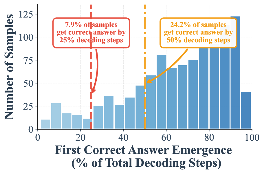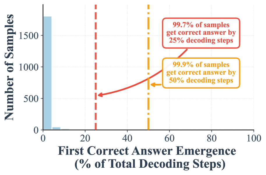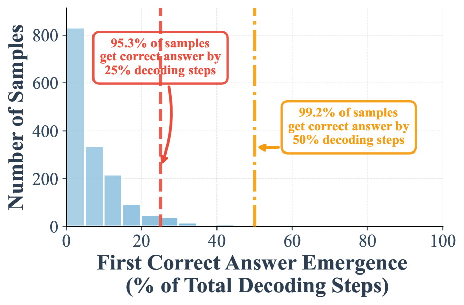3.2 Early Answer Convergency In this section, we investigate the early emergence of correct answers in DLMs. We conduct a comprehensive analysis using LLaDA-8B (Nie et al., 2025) on two widely used benchmarks: GSM8K (Cobbe et al., 2021) and MMLU (Hendrycks et al., 2021). Specifically, we examine the decoding dynamics, that is, how the top 1 predicted token evolves across positions at each decoding step, and report the percentage of the full decoding process at which the top 1 predicted tokens first match the ground truth answer tokens. In this study, we only consider samples where the final output contains the ground truth answer. For low confidence remasking, we set Answer length at 256 and Block length at 32 for GSM8K, and Answer length at 128 and Block length to 128 for MMLU. For random remasking, we set Answer length at 256 and Block length at 256 for GSM8K, and Answer length at 128 and Block length at 128 for MMLU. <details> <summary>x1.png Details</summary>  ### Visual Description ## Bar Chart: First Correct Answer Emergence ### Overview The image is a bar chart illustrating the distribution of the "First Correct Answer Emergence" as a percentage of total decoding steps. The chart shows the number of samples that achieve a correct answer at different percentages of decoding steps. Two vertical lines highlight specific points: 25% and 50% decoding steps, with annotations indicating the percentage of samples that get the correct answer at or before these points. ### Components/Axes * **Y-axis:** "Number of Samples", ranging from 0 to 125 in increments of 25. * **X-axis:** "First Correct Answer Emergence (% of Total Decoding Steps)", ranging from 0 to 100 in increments of 20. * **Bars:** Blue bars representing the number of samples for each percentage range of decoding steps. The bars are lighter blue on the left side of the chart and transition to a darker blue on the right side. * **Vertical Lines:** * A red dashed vertical line at 25% decoding steps. * An orange dashed vertical line at 50% decoding steps. * **Annotations:** * A red box with text: "7.9% of samples get correct answer by 25% decoding steps". An arrow points from the box to the red vertical line. * An orange box with text: "24.2% of samples get correct answer by 50% decoding steps". An arrow points from the box to the orange vertical line. ### Detailed Analysis The bar chart shows the distribution of the first correct answer emergence. The x-axis represents the percentage of total decoding steps, and the y-axis represents the number of samples. Here's a breakdown of the approximate bar heights at different percentage ranges: * **0-10%:** Approximately 12 samples * **10-20%:** Approximately 22 samples * **20-30%:** Approximately 30 samples * **30-40%:** Approximately 20 samples * **40-50%:** Approximately 35 samples * **50-60%:** Approximately 55 samples * **60-70%:** Approximately 65 samples * **70-80%:** Approximately 85 samples * **80-90%:** Approximately 80 samples * **90-100%:** Approximately 40 samples The annotations indicate that 7.9% of samples get the correct answer by 25% decoding steps, and 24.2% of samples get the correct answer by 50% decoding steps. ### Key Observations * The number of samples getting the correct answer increases as the percentage of decoding steps increases, peaking between 70% and 80%. * A significant portion of samples (24.2%) get the correct answer by 50% decoding steps. * The distribution is skewed towards the right, indicating that most samples require a larger percentage of decoding steps to arrive at the correct answer. ### Interpretation The data suggests that the model or system being analyzed typically requires a significant portion of the total decoding steps to produce the correct answer. While a small percentage of samples achieve the correct answer early on (7.9% by 25% decoding steps), the majority require more steps. The peak between 70% and 80% indicates that this range is where the highest number of samples first achieve the correct answer. The fact that 24.2% of samples are correct by 50% decoding steps suggests that there's a notable group that finds the solution relatively early, but the overall distribution indicates a general need for more decoding steps. This could be due to the complexity of the problem, the nature of the decoding algorithm, or the characteristics of the samples themselves. </details> (a) w/o suffix prompt (low-confidence remasking) <details> <summary>x2.png Details</summary>  ### Visual Description ## Histogram: First Correct Answer Emergence ### Overview The image is a histogram showing the distribution of the "First Correct Answer Emergence" as a percentage of total decoding steps. The y-axis represents the number of samples, and the x-axis represents the percentage of total decoding steps. Two vertical dashed lines, one red and one orange, indicate specific percentages of decoding steps (25% and 50%, respectively) and are annotated with the percentage of samples that achieve a correct answer by those points. ### Components/Axes * **Y-axis:** "Number of Samples", ranging from 0 to 500 in increments of 100. * **X-axis:** "First Correct Answer Emergence (% of Total Decoding Steps)", ranging from 0 to 100. The x-axis appears to be divided into bins of approximately 5 units each. * **Bars:** The histogram consists of blue bars of varying heights, representing the number of samples for each bin of "First Correct Answer Emergence". * **Red Dashed Line:** Located at approximately 25% on the x-axis. * **Orange Dashed Line:** Located at approximately 50% on the x-axis. * **Annotations:** * A red box states: "59.7% of samples get correct answer by 25% decoding steps". An arrow points from the box to the red dashed line. * An orange box states: "75.8% of samples get correct answer by 50% decoding steps". An arrow points from the box to the orange dashed line. ### Detailed Analysis * **Bar Heights:** * The bar at 0% has a height of approximately 480. * The bar at 95-100% has a height of approximately 75. * The bars between 5% and 95% are significantly lower, generally below 40. * **Red Dashed Line:** * Located at 25% on the x-axis. * The annotation indicates that 59.7% of samples get the correct answer by this point. * **Orange Dashed Line:** * Located at 50% on the x-axis. * The annotation indicates that 75.8% of samples get the correct answer by this point. ### Key Observations * A large number of samples (approximately 480) achieve the correct answer very early in the decoding process (0% decoding steps). * The number of samples achieving the correct answer decreases significantly after 0% and remains low until the end. * There is a slight increase in the number of samples achieving the correct answer towards the end of the decoding process (95-100%). * 59.7% of samples get the correct answer by 25% of the decoding steps. * 75.8% of samples get the correct answer by 50% of the decoding steps. ### Interpretation The histogram suggests that for a significant portion of the samples, the correct answer emerges very early in the decoding process. This is indicated by the high bar at 0%. The relatively flat distribution between 5% and 95% suggests that for the remaining samples, the correct answer emerges more uniformly across this range. The annotations highlight that a substantial percentage of samples achieve the correct answer by 25% and 50% of the decoding steps, indicating the efficiency of the decoding process for a majority of the samples. The slight increase at the end suggests that some samples require nearly the entire decoding process to arrive at the correct answer. </details> (b) w/ suffix prompt (low-confidence remasking) <details> <summary>x3.png Details</summary>  ### Visual Description ## Histogram: First Correct Answer Emergence ### Overview The image is a histogram showing the distribution of the "First Correct Answer Emergence" as a percentage of total decoding steps. The x-axis represents the percentage of total decoding steps, and the y-axis represents the number of samples. Two vertical lines are overlaid on the histogram, indicating the percentage of samples that achieve a correct answer by 25% and 50% of the decoding steps, respectively. ### Components/Axes * **X-axis:** "First Correct Answer Emergence (% of Total Decoding Steps)". The axis ranges from 0 to 100, with tick marks at intervals of 20 (0, 20, 40, 60, 80, 100). * **Y-axis:** "Number of Samples". The axis ranges from 0 to 150, with tick marks at intervals of 50 (0, 50, 100, 150). * **Bars:** Light blue bars represent the frequency of samples for each percentage range of decoding steps. * **Vertical Lines:** * A dashed red vertical line is positioned at approximately 25% of total decoding steps. A red box indicates that 88.5% of samples get the correct answer by 25% decoding steps. * A dashed-dotted orange vertical line is positioned at approximately 50% of total decoding steps. An orange box indicates that 97.2% of samples get the correct answer by 50% decoding steps. ### Detailed Analysis The histogram shows a right-skewed distribution. The majority of samples achieve a correct answer within the first 25% of decoding steps. The frequency of samples decreases as the percentage of decoding steps increases. * **0-20%:** The number of samples in this range is high, with the first bar (0%) reaching approximately 85 samples, and the bar at 20% reaching approximately 55 samples. * **20-40%:** The number of samples decreases significantly in this range. The bar at 30% reaches approximately 10 samples. * **40-100%:** The number of samples is very low in this range, with only a single bar at 100% reaching approximately 10 samples. ### Key Observations * A large proportion of samples (88.5%) achieve a correct answer within the first 25% of decoding steps. * An even larger proportion of samples (97.2%) achieve a correct answer within the first 50% of decoding steps. * The distribution is heavily skewed towards the left, indicating that most samples converge to a correct answer relatively quickly. ### Interpretation The data suggests that the decoding process is efficient, with the majority of samples converging to a correct answer within the first half of the decoding steps. The high percentages of samples achieving correct answers by 25% and 50% of decoding steps indicate that the model or algorithm being evaluated is performing well. The right-skewed distribution suggests that while most samples converge quickly, there are some outliers that require a significantly larger number of decoding steps to reach a correct answer. This could be due to the complexity of the input data or the presence of noise. </details> (c) w/o suffix prompt (random remasking) <details> <summary>x4.png Details</summary>  ### Visual Description ## Histogram: First Correct Answer Emergence ### Overview The image is a histogram showing the distribution of the "First Correct Answer Emergence" as a percentage of total decoding steps. It also highlights the percentage of samples that achieve a correct answer by 25% and 50% of the decoding steps. ### Components/Axes * **X-axis:** "First Correct Answer Emergence (% of Total Decoding Steps)". The scale ranges from 0 to 100, with tick marks at 0, 20, 40, 60, 80, and 100. * **Y-axis:** "Number of Samples". The scale ranges from 0 to 500, with tick marks at 0, 100, 200, 300, 400, and 500. * **Bars:** Light blue bars represent the frequency of samples for each percentage range of decoding steps. * **Vertical Lines:** * A dashed red vertical line is positioned at approximately 25% on the x-axis. * A dashed orange vertical line is positioned at approximately 50% on the x-axis. * **Annotations:** * A red box states: "94.6% of samples get correct answer by 25% decoding steps". An arrow points from the box to the red vertical line. * An orange box states: "97.3% of samples get correct answer by 50% decoding steps". An arrow points from the box to the orange vertical line. ### Detailed Analysis * **Bar at 0%:** The tallest bar is at 0%, indicating that a large number of samples get the correct answer almost immediately. The height of this bar is approximately 500. * **Bars between 0% and 20%:** The frequency of samples decreases rapidly between 0% and 20%. The bar at 10% is approximately 80. * **Bars between 20% and 40%:** The frequency of samples continues to decrease, with very few samples getting the correct answer in this range. The bar at 30% is approximately 10. * **Bars between 40% and 100%:** The frequency of samples remains very low, with a slight increase at 100%. The bar at 100% is approximately 20. * **Red Vertical Line (25%):** The red dashed line at 25% indicates that 94.6% of samples have found the correct answer by this point. * **Orange Vertical Line (50%):** The orange dashed line at 50% indicates that 97.3% of samples have found the correct answer by this point. ### Key Observations * A significant portion of samples (approximately 500) achieve the correct answer almost immediately (0% decoding steps). * The number of samples that find the correct answer decreases rapidly as the percentage of decoding steps increases. * By 25% of the decoding steps, the vast majority (94.6%) of samples have found the correct answer. * By 50% of the decoding steps, an even larger majority (97.3%) of samples have found the correct answer. ### Interpretation The histogram suggests that the decoding process is highly efficient for most samples. A large number of samples find the correct answer very early in the process. The annotations highlight that the vast majority of samples converge to the correct answer within the first 25% of the decoding steps, with only a small fraction requiring up to 50% of the steps. This indicates that the model or algorithm being analyzed is generally very effective at quickly identifying the correct solution. The rapid decline in the number of samples finding the correct answer after 0% suggests that while many samples are easily decoded, there is a subset that requires more processing, but even these typically converge within a relatively small number of steps. 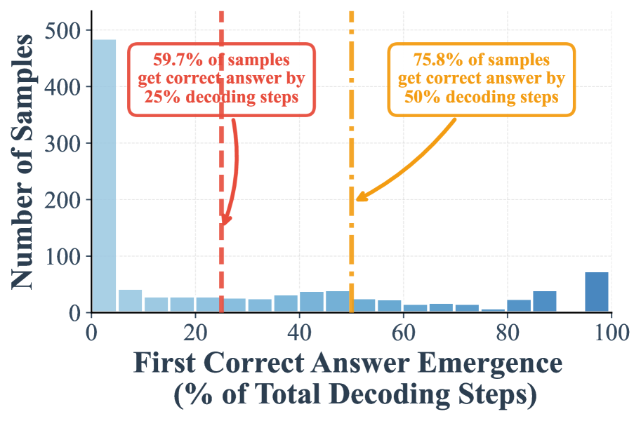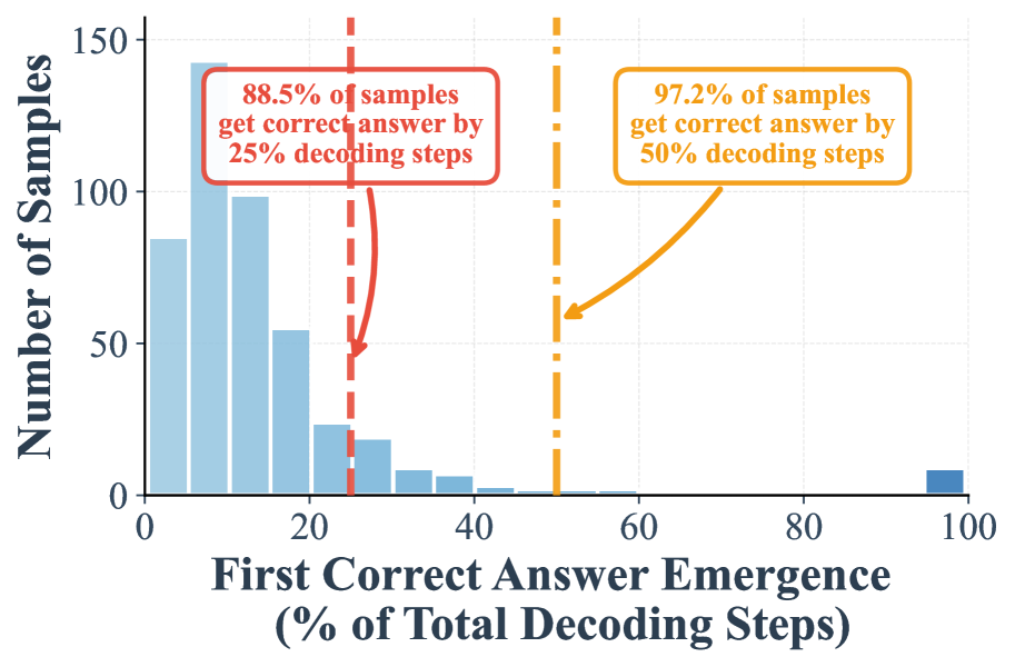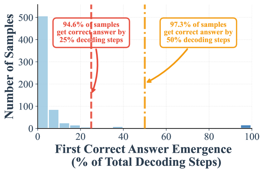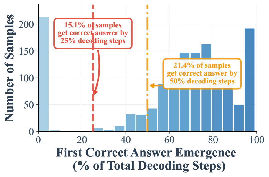</details> (d) w/ suffix prompt (random remasking) Figure 1: Distribution of early correct answer detection during decoding process.. Histograms show when correct answers first emerge during diffusion decoding, measured as percentage of total decoding steps, using LLaDA 8B on GSM8K. Red and orange dashed lines indicate 50% and 70% completion thresholds, with corresponding statistics showing substantial early convergence. Suffix prompting (b,d) dramatically accelerates convergence compared to standard prompting (a,c). This early convergence pattern demonstrates that correct answer tokens stabilize as top-1 candidates well before full decoding. I. A high proportion of samples can be correctly decoded during the early phase of decoding. Figure 1 (a) demonstrates that when remasking with the low-confidence strategy, 24.2% samples are already correctly predicted in the first half steps, and 7.9% samples can be correctly decoded in the first 25% steps. These two numbers will be further largely boosted to 97.2% and 88.5%, when shifted to random remasking as shown in Figure 1 -(c). II. Our suffix prompt further amplifies the early emergence of correct answers. Adding the suffix prompt “Answer:” significantly improves early decoding. With low confidence remasking, the proportion of correct samples emerging by the 25% step rises from 7.9% to 59.7%, and by the 50% step from 24.2% to 75.8% (Figure 1 -(b)). Similarly, under random remasking, the 25% step proportion increases from 88.5% to 94.6%. 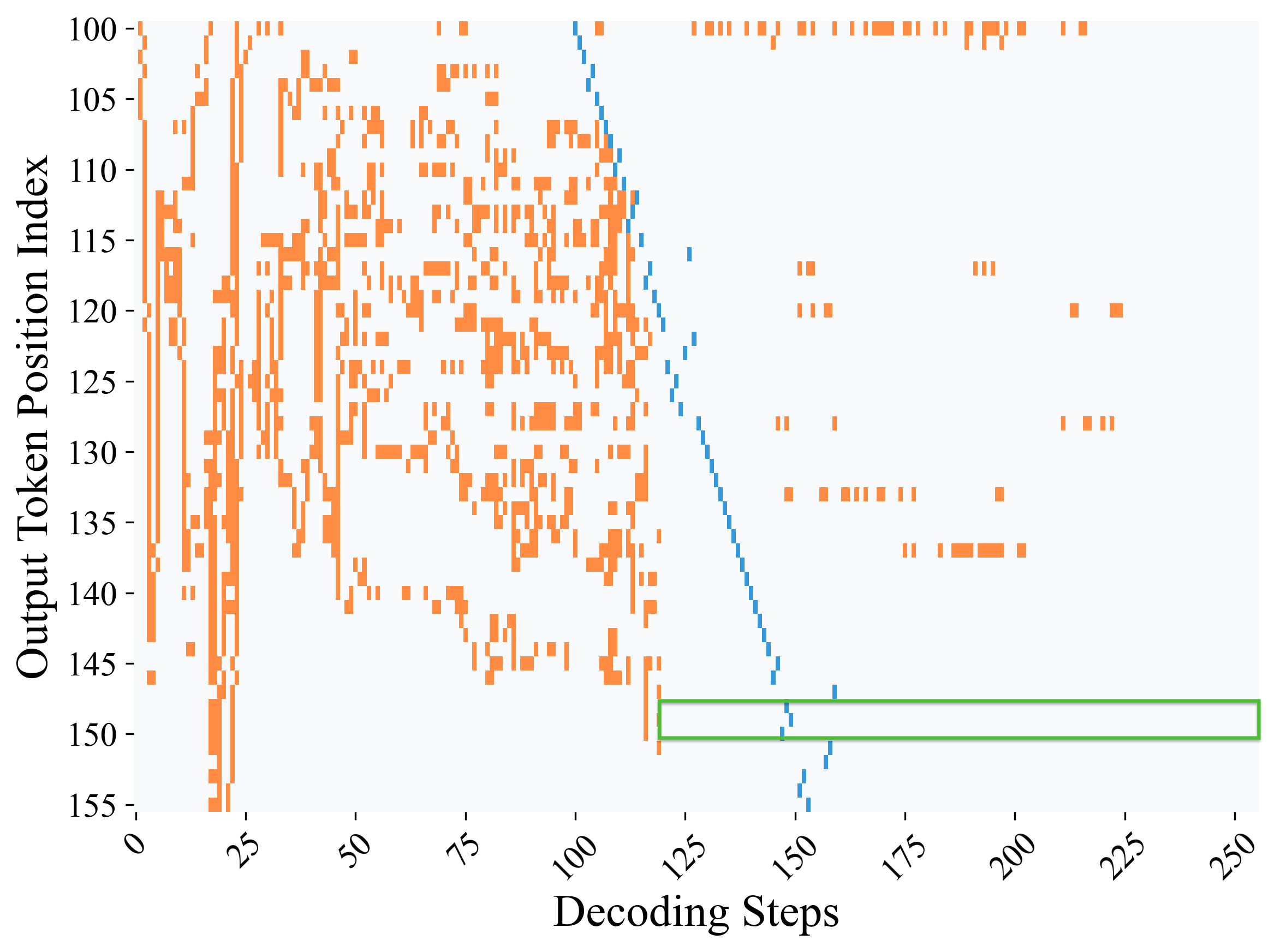III. Decoding dynamics of chain-of-thought tokens. We further examine the decoding dynamics of chain-of-thought tokens in addition to answer tokens, as shown in Figure 2. First, most non-answer tokens fluctuate frequently before being finalized. Second, answer tokens change far less often and tend to stabilize earlier, remaining unchanged for the rest of the decoding process. <details> <summary>x5.png Details</summary>  ### Visual Description ## Legend: Token Status ### Overview The image is a legend defining the color codes used to represent different token statuses. The legend consists of four color-coded boxes, each associated with a specific token status. ### Components/Axes The legend includes the following components: * **White Box:** Labeled "No Change" * **Orange Box:** Labeled "Token Change" * **Blue Box:** Labeled "Token Decoded" * **Green Box:** Labeled "Correct Answer Token" ### Detailed Analysis or ### Content Details The legend provides a visual key for interpreting token status based on color: * **No Change:** Represented by a white box. * **Token Change:** Represented by an orange box. * **Token Decoded:** Represented by a blue box. * **Correct Answer Token:** Represented by a green box. ### Key Observations The legend clearly defines the color-coding scheme for token statuses, allowing for easy interpretation of visualizations that use these colors. ### Interpretation The legend is a key component for understanding visualizations that represent token changes, decoding, and correctness. The color-coding allows for quick identification of token status within a given context. </details> <details> <summary>figures/position_change_heatmap_low_conf_non_qi_700_step256_blocklen32_box.png Details</summary>  ### Visual Description ## Heatmap: Output Token Position Index vs. Decoding Steps ### Overview The image is a heatmap visualizing the relationship between the output token position index and decoding steps. The x-axis represents decoding steps, ranging from 0 to 250. The y-axis represents the output token position index, ranging from 100 to 155. Orange blocks indicate the presence of a token at a specific position index during a particular decoding step. A blue line indicates a specific event or transition during the decoding process. A green rectangle highlights a region of interest. ### Components/Axes * **X-axis:** Decoding Steps, ranging from 0 to 250 in increments of 25. * **Y-axis:** Output Token Position Index, ranging from 100 to 155 in increments of 5. * **Orange Blocks:** Indicate the presence of a token at a specific position index during a particular decoding step. * **Blue Line:** A diagonal line starting at approximately (100, 100) and ending at approximately (155, 155). * **Green Rectangle:** A rectangle spanning from approximately (120, 148) to (250, 152). ### Detailed Analysis or ### Content Details * **Orange Blocks:** * From decoding steps 0 to approximately 120, there is a high density of orange blocks, indicating frequent token presence across various position indices. * After decoding step 120, the density of orange blocks decreases significantly, suggesting fewer tokens are present at different position indices. * The orange blocks are scattered and less concentrated as the decoding steps increase beyond 120. * **Blue Line:** * The blue line starts at approximately decoding step 100 and position index 100. * It progresses diagonally downwards to approximately decoding step 155 and position index 155. * The line appears to be relatively linear. * **Green Rectangle:** * The green rectangle spans from approximately decoding step 120 to 250. * It covers the position index range of approximately 148 to 152. ### Key Observations * The density of tokens is significantly higher in the initial decoding steps (0-120) compared to later steps (120-250). * The blue line represents a clear transition or event during the decoding process. * The green rectangle highlights a specific region of interest in the later decoding steps. ### Interpretation The heatmap visualizes the token generation process during decoding. The high density of orange blocks in the initial steps suggests that the model is actively exploring and generating tokens across a wide range of positions. The blue line likely indicates a shift or convergence in the decoding process, possibly representing the model focusing on specific tokens or positions. The green rectangle might highlight a region where the model is refining or finalizing the output sequence. The sparse orange blocks after decoding step 120 suggest that the model has largely determined the output sequence and is making minor adjustments or completing the process. </details> (a) w/o suffix prompt <details> <summary>figures/position_change_heatmap_low_conf_constraint_qi_700_step256_blocklen32_box.png Details</summary>  ### Visual Description ## Heatmap: Output Token Position Index vs. Decoding Steps ### Overview The image is a heatmap that visualizes the relationship between the output token position index and the decoding steps. The x-axis represents the decoding steps, ranging from 0 to 250. The y-axis represents the output token position index, ranging from 180 to 235. Orange blocks indicate the presence of a token at a specific position index during a specific decoding step. A blue line indicates a different type of event or state during decoding. A green rectangle highlights a specific region of interest. ### Components/Axes * **X-axis:** Decoding Steps, ranging from 0 to 250, with markers at 0, 25, 50, 75, 100, 125, 150, 175, 200, 225, and 250. * **Y-axis:** Output Token Position Index, ranging from 180 to 235, with markers at 180, 185, 190, 195, 200, 205, 210, 215, 220, 225, 230, and 235. * **Data Points:** * Orange blocks: Indicate the presence of a token at a specific position index during a specific decoding step. * Blue line: A diagonal line starting from approximately (185, 180) and extending to approximately (250, 235). * **Green Rectangle:** A rectangle spanning approximately from decoding steps 90 to 250 and output token position index 222 to 227. ### Detailed Analysis or ### Content Details * **Orange Blocks:** * The orange blocks are scattered throughout the heatmap, primarily concentrated in the upper-left region (decoding steps 0-175, output token position index 180-225). * The density of orange blocks decreases as the decoding steps increase beyond 175. * There are relatively few orange blocks below the output token position index of 225. * **Blue Line:** * The blue line starts at approximately decoding step 185 and output token position index 180. * The blue line slopes downward and to the right, reaching approximately decoding step 250 and output token position index 235. * The blue line appears to be composed of individual vertical blue lines. * **Green Rectangle:** * The green rectangle spans from approximately decoding step 90 to 250 and output token position index 222 to 227. * The green rectangle highlights a specific region of interest, potentially indicating a particular state or event during decoding. ### Key Observations * The orange blocks are more concentrated in the earlier decoding steps (0-175), suggesting that tokens are primarily generated during this phase. * The blue line indicates a distinct event or state that occurs later in the decoding process (decoding steps 185-250). * The green rectangle highlights a specific region of interest, potentially indicating a particular state or event during decoding. ### Interpretation The heatmap visualizes the decoding process, showing the relationship between the output token position index and the decoding steps. The orange blocks represent the generation of tokens, which are more frequent in the earlier decoding steps. The blue line may represent a transition or completion phase of the decoding process. The green rectangle highlights a specific region of interest, potentially indicating a particular state or event during decoding, such as a stabilization or convergence point in the decoding process. The data suggests that the decoding process involves an initial phase of token generation followed by a transition or completion phase. 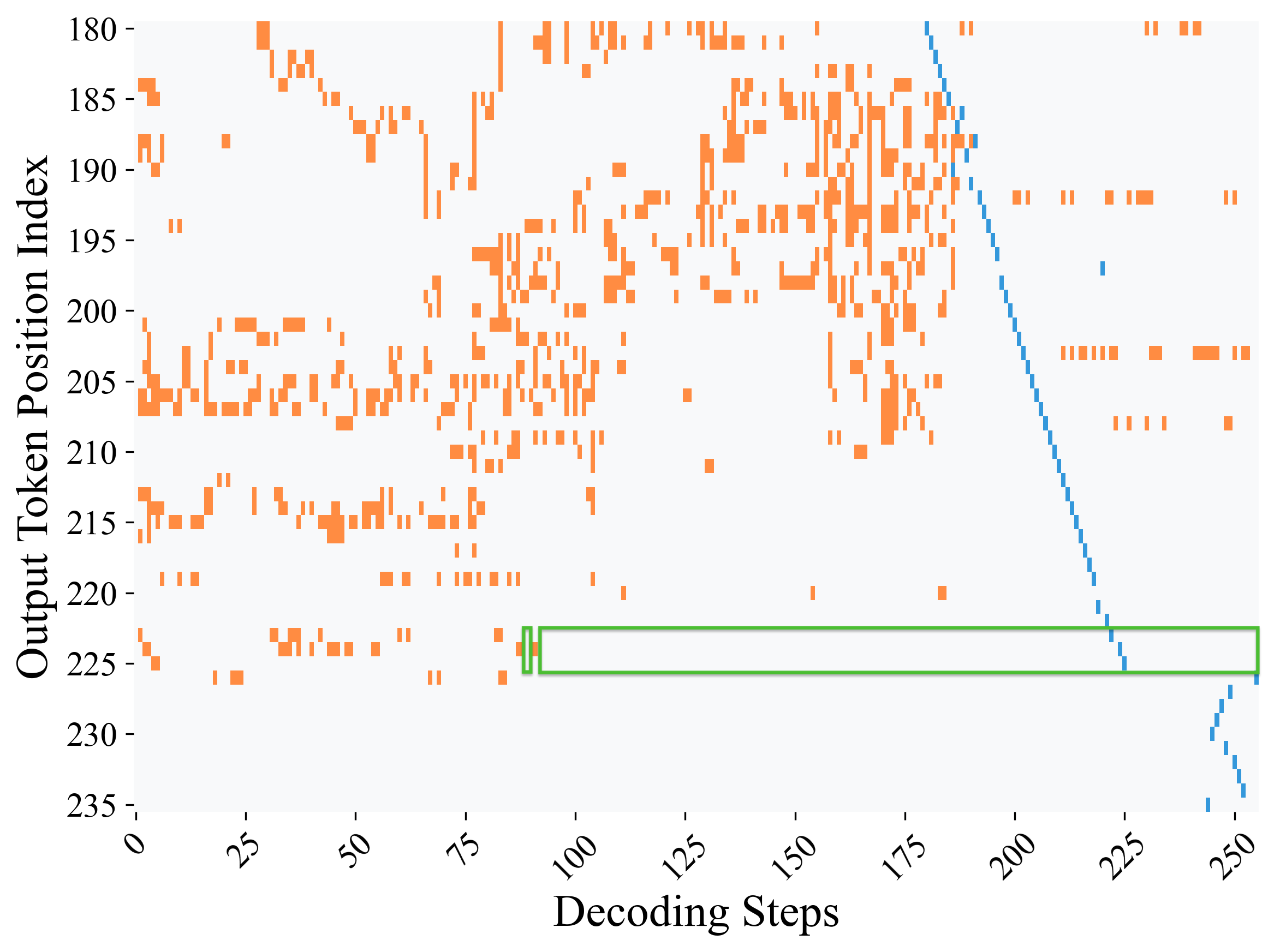</details> (b) w/ suffix prompt Figure 2: Decoding dynamics across all positions based on maximum-probability predictions. Heatmaps track how the top-1 token changes at each position, if it is decoded at the current step, over the course of decoding. (a) Without our suffix prompts, correct answer tokens reach maximum probability at step 119. (b) With our suffix prompts, this occurs earlier at step 88, showing that the model internally identifies correct answers well before the final output. Results are shown for LLaDA 8B solving problem index 700 from GSM8K under low-confidence decoding. Gray indicates positions where the top-1 prediction remains unchanged, orange marks positions where the prediction changes to a different token, blue denotes the step at which the corresponding y-axis position is actually decoded, and green box highlights the answer region where the correct answer remains stable as the top-1 token and can be safely decoded without further changes as the decoding process progresses. 4 Methodology <details> <summary>x6.png Details</summary>  ### Visual Description ## Diagram: Decoding Methods Comparison ### Overview The image presents two diagrams comparing different decoding methods: (a) Standard Full-Step Decoding and (b) Prophet with Early Commit Decoding. Both diagrams illustrate the steps involved in generating an output, but the second method aims to save steps by committing early based on a confidence gap. ### Components/Axes **Diagram (a): Standard Full-Step Decoding** * **Title:** (a) Standard Full-Step Decoding * **Chain-of-Thought:** This label indicates the type of reasoning process. * **Time Axis:** A horizontal line represents the progression of steps, labeled with time points t=0, t=2, t=4, t=6, and t=10. * **Answer Tokens:** This label indicates the values generated at each step. * **Steps:** * \[MASK] \[MASK] \[MASK] (at the beginning) * 3 sprints \[MASK] * 3x3=9, 9x60=\[MASK] * 3x3=9, 9x60=540 * **Values:** 3 (at t=0), 60 (at t=2), 5400 (at t=4), 540 (at t=6), Output: 540 (at the end) * **Redundant Steps:** A dashed red box highlights steps between t=6 and t=10 as "Redundant Steps." **Diagram (b): Prophet with Early Commit Decoding** * **Title:** (b) Prophet with Early Commit Decoding * **Steps Saved:** "~55% Steps Saved" is indicated at the top right. * **Chain-of-Thought:** This label indicates the type of reasoning process. * **Time Axis:** A horizontal line represents the progression of steps. * **Steps:** * \[MASK] \[MASK] \[MASK] (at the beginning) * 3 sprints \[MASK] * 3x3=9, 9x60=\[MASK] * 3x3=9, 9x60=540 * **Values:** 540 (below the green node), Output: 540 (at the end) * **Confidence Gap:** A green bar labeled "Confidence Gap > τ" spans from the beginning to a point before the final step. * **Early Commit Decoding:** A yellow arrow indicates "Early Commit Decoding" leading to the output. ### Detailed Analysis or Content Details **Diagram (a): Standard Full-Step Decoding** * At t=0, the value is 3. * At t=2, the value is 60. * At t=4, the value is 5400. * At t=6, the value is 540. * The process continues until t=10, but these steps are marked as redundant. * The final output is 540. **Diagram (b): Prophet with Early Commit Decoding** * The process starts similarly to the standard decoding. * The "Confidence Gap > τ" condition is met, triggering early commit decoding. * The early commit decoding leads directly to the output of 540. * The diagram indicates a saving of approximately 55% of steps. ### Key Observations * The standard decoding method involves more steps, including redundant ones. * The prophet method aims to reduce steps by committing early based on a confidence measure. * Both methods arrive at the same output (540). ### Interpretation The diagrams illustrate the difference between standard full-step decoding and a more efficient "prophet" decoding method. The prophet method leverages a confidence measure to identify when it's safe to commit to an answer early, thus saving computational steps. The "Redundant Steps" in the standard method highlight the inefficiency that the prophet method addresses. The "~55% Steps Saved" suggests a significant performance improvement can be achieved using the prophet method. The "Confidence Gap > τ" condition implies a threshold-based decision for early commitment. 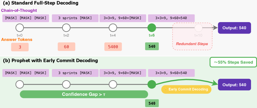</details> Figure 3: An illustration of the Prophet’s early-commit-decoding mechanism. (a) Standard full-step decoding completes all predefined steps (e.g., 10 steps), incurring redundant computations after the answer has stabilized (at t=6). (b) Prophet dynamically monitors the model’s confidence (the “Confidence Gap”). It triggers an early commit decoding as soon as the answer converges, saving a significant portion of the decoding steps (in this case, 55%) without compromising the output quality. Built upon the above findings, we introduce Prophet, a training-free fast decoding algorithm designed to accelerate the generation phase of DLMs. Prophet by committing to all remaining tokens in one shot and predicting answers as soon as the model’s predictions have stabilized, which we call Early Commit Decoding. Unlike conventional fixed-step decoding, Prophet actively monitors the model’s certainty at each step to make an informed, on-the-fly decision about when to finalize the generation. Confidence Gap as a Convergence Metric. The core mechanism of Prophet is the Confidence Gap, a simple yet effective metric for quantifying the model’s conviction for a given token. At any decoding step $t$ , the DLM produces a logit matrix $\mathbf{L}_{t}∈\mathbb{R}^{N×|\mathcal{V}|}$ , where $N$ is the sequence length and $|\mathcal{V}|$ is the vocabulary size. For each position $i$ , we identify the highest logit value, $L_{t,i}^{(1)}$ , and the second-highest, $L_{t,i}^{(2)}$ . The confidence gap $g_{t,i}$ is defined as their difference: $$ g_{t,i}=L_{t,i}^{(1)}-L_{t,i}^{(2)}. \tag{1} $$ This value serves as a robust indicator of predictive certainty. A large probability gap signals that the prediction has likely converged, with the top-ranked token clearly outweighing all others. Early Commit Decoding. The decision of when to terminate the decoding loop can be framed as an optimal stopping problem. At each step, we must balance two competing costs: the computational cost of performing additional refinement iterations versus the risk of error from a premature and potentially incorrect decision. The computational cost is a function of the remaining steps, while the risk of error is inversely correlated with the model’s predictive certainty, for which the Confidence Gap serves as a robust proxy. Prophet addresses this trade-off with an adaptive strategy that embodies a principle of time-varying risk aversion. Let denote $p=(T_{\text{max}}-t)/T_{\text{max}}$ as the decoding progress, where $T_{\text{max}}$ is the total number of decoding steps, and $\tau(p)$ is the threshold for early commit decoding. In the early, noisy stages of decoding (when progress $p$ is small), the potential for significant prediction improvement is high. Committing to an answer at this stage carries a high risk. Therefore, Prophet acts in a risk-averse manner, demanding an exceptionally high threshold ( $\tau_{\text{high}}$ ) to justify an early commit decoding, ensuring such a decision is unequivocally safe. As the decoding process matures (as $p$ increases), two things happen: the model’s predictions stabilize, and the potential computational savings from stopping early diminish. Consequently, the cost of performing one more step becomes negligible compared to the benefit of finalizing the answer. Prophet thus becomes more risk-tolerant, requiring a progressively smaller threshold ( $\tau_{\text{low}}$ ) to confirm convergence. This dynamic risk-aversion policy is instantiated through our staged threshold function, which maps the abstract trade-off between inference speed and generation certainty onto a concrete decision rule: $$ \bar{g}_{t}\geq\tau(p),\quad\text{where}\quad\tau(p)=\begin{cases}\tau_{\text{high}}&\text{if }p<0.33\\ \tau_{\text{mid}}&\text{if }0.33\leq p<0.67\\ \tau_{\text{low}}&\text{if }p\geq 0.67\end{cases} \tag{5} $$ Once the exit condition is satisfied at step $t^{*}$ , the iterative loop is terminated. The final output is then constructed in a single parallel operation by filling any remaining [MASK] tokens with the argmax of the current logits $\mathbf{L}_{t^{*}}$ . Algorithm Summary. The complete Prophet decoding procedure is outlined in Algorithm 1. The integration of the confidence gap check adds negligible computational overhead to the standard DLM decoding loop. Prophet is model-agnostic, requires no retraining, and can be readily implemented as a wrapper around existing DLM inference code. Algorithm 1 Prophet: Early Commit Decoding for Diffusion Language Models 1: Input: Model $M_{\theta}$ , prompt $\mathbf{x}_{\text{prompt}}$ , max steps $T_{\text{max}}$ , generation length $N_{\text{gen}}$ 2: Input: Threshold function $\tau(·)$ , answer region positions $\mathcal{A}$ 3: Initialize sequence $\mathbf{x}_{T}←\text{concat}(\mathbf{x}_{\text{prompt}},\text{[MASK]}^{N_{\text{gen}}})$ 4: Let $\mathcal{M}_{t}$ be the set of masked positions at step $t$ . 5: for $t=T_{\text{max}},T_{\text{max}}-1,...,1$ do 6: Compute logits: $\mathbf{L}_{t}=M_{\theta}(\mathbf{x}_{t})$ 7: $\triangleright$ Prophet’s Early-Commit-Decoding Check 8: Calculate average confidence gap $\bar{g}_{t}$ over positions $\mathcal{A}$ using Eq. 4. 9: Calculate progress: $p←(T_{\text{max}}-t)/T_{\text{max}}$ 10: if $\bar{g}_{t}≥\tau(p)$ then $\triangleright$ Check condition from Eq. 5 11: $\mathbf{\hat{x}}_{0}←\text{argmax}(\mathbf{L}_{t},\text{dim}=-1)$ 12: $\mathbf{x}_{0}←\mathbf{x}_{t}$ . Fill positions in $\mathcal{M}_{t}$ with tokens from $\mathbf{\hat{x}}_{0}$ . 13: Return $\mathbf{x}_{0}$ $\triangleright$ Terminate and finalize 14: end if 15: $\triangleright$ Standard DLM Refinement Step 16: Determine tokens to unmask $\mathcal{U}_{t}⊂eq\mathcal{M}_{t}$ via a re-masking strategy. 17: $\mathbf{\hat{x}}_{0}←\text{argmax}(\mathbf{L}_{t},\text{dim}=-1)$ 18: Update $\mathbf{x}_{t-1}←\mathbf{x}_{t}$ , replacing tokens at positions $\mathcal{U}_{t}$ with those from $\mathbf{\hat{x}}_{0}$ . 19: end for 20: Return $\mathbf{x}_{0}$ $\triangleright$ Return result after full iterations if no early commit decoding 5 Experiments We evaluate Prophet on diffusion language models (DLMs) to validate two key hypotheses: first, that Prophet can preserve the performance of full-budget decoding while using substantially fewer denoising steps; second, that our adaptive approach provides more reliable acceleration than naive static baselines. We demonstrate that Prophet achieves notable computational savings with negligible quality degradation through comprehensive experiments across diverse benchmarks. 5.1 Experimental Setup We conduct experiments on two state-of-the-art diffusion language models: LLaDA-8B (Nie et al., 2025) and Dream-7B (Ye et al., 2025). For each model, we compare three decoding strategies: Full uses the standard diffusion decoding with the complete step budget of $T_{\max}$ and Prophet employs early commit decoding with dynamic threshold scheduling. The threshold parameters are set to $\tau_{\text{high}}=7.5$ , $\tau_{\text{mid}}=5.0$ , and $\tau_{\text{low}}=2.5$ , with transitions occurring at 33% and 67% of the decoding progress. These hyperparameters were selected through preliminary validation experiments. Our evaluation spans four capability domains to comprehensively assess Prophet’s effectiveness. For general reasoning, we use MMLU (Hendrycks et al., 2021), ARC-Challenge (Clark et al., 2018), HellaSwag (Zellers et al., 2019), TruthfulQA (Lin et al., 2021), WinoGrande (Sakaguchi et al., 2021), and PIQA (Bisk et al., 2020). Mathematical and scientific reasoning are evaluated through GSM8K (Cobbe et al., 2021) and GPQA (Rein et al., 2023). For code generation, we employ HumanEval (Chen et al., 2021) and MBPP (Austin et al., 2021b). Finally, planning capabilities are assessed using Countdown and Sudoku tasks (Gong et al., 2024). We follow the prompt in simple-evals for LLaDA and Dream, making the model reason step by step. Concretely, we set the generation length $L$ to 128 for general tasks, to 256 for GSM8K and GPQA, and to 512 for the code benchmarks. Unless otherwise noted, all baselines use a number of iterative steps equal to the specified generation length. All experiments employ greedy decoding to ensure deterministic and reproducible results. 5.2 Main Results and Analysis The results of our experiments are summarized in Table 1. Across the general reasoning tasks, Prophet demonstrates its ability to match or even exceed the performance of the full baseline. For example, using LLaDA-8B, Prophet achieves 54.0% on MMLU and 83.5% on ARC-C, both of which are statistically on par with the full step decoding. Interestingly, on HellaSwag, Prophet (70.9%) not only improves upon the full baseline (68.7%) but also the half baseline (70.5%), suggesting that early commit decoding can prevent the model from corrupting an already correct prediction in later, noisy refinement steps. Similarly, Dream-7B maintains competitive performance across benchmarks, with Prophet achieving 66.1% on MMLU compared to the full model’s 67.6%—a minimal drop of 1.5% while delivering 2.47× speedup. Prophet continues to prove its reliability in more complex reasoning tasks, including mathematics, science, and code generation. For the GSM8K dataset, Prophet with LLaDA-8B obtains an accuracy of 77.9%, outperforming the baseline’s 77.1%. This reliability also extends to code generation benchmarks. For instance, on HumanEval, Prophet perfectly matches the full baseline’s score with LLaDA-8B (30.5%) and even slightly improves it with Dream-7B (55.5% vs. 54.9%). Notably, the acceleration on these intricate tasks (e.g., 1.20× on HumanEval) is more conservative compared to general reasoning. This demonstrates Prophet’s adaptive nature: it dynamically allocates more denoising steps when a task demands further refinement, thereby preserving accuracy on complex problems. This reinforces Prophet’s role as a ”safe” acceleration method that avoids the pitfalls of premature, static termination. In summary, our empirical results strongly support the central hypothesis of this work: DLMs often determine the correct answer long before the final decoding step. Prophet successfully capitalizes on this phenomenon by dynamically monitoring the model’s predictive confidence. It terminates the iterative refinement process as soon as the answer has stabilized, thereby achieving significant computational savings with negligible, and in some cases even positive, impact on task performance. This stands in stark contrast to static truncation methods, which risk cutting off the decoding process prematurely and harming accuracy. Prophet thus provides a robust and model-agnostic solution to accelerate DLM inference, enhancing its practicality for real-world deployment. Table 1: Benchmark results on LLaDA-8B-Instruct and Dream-7B-Instruct. Sudoku and Countdown are evaluated using 8-shot setting; all other benchmarks use zero-shot evaluation. Detailed configuration is listed in the Appendix. | Benchmark General Tasks MMLU | LLaDA 8B 54.1 | LLaDA 8B (Ours) 54.0 (2.34×) | Gain ( $\Delta$ ) -0.1 | Dream-7B 67.6 | Dream-7B (Ours) 66.1 (2.47×) | Gain ( $\Delta$ ) -1.5 | | --- | --- | --- | --- | --- | --- | --- | | ARC-C | 83.2 | 83.5 (1.88×) | +0.3 | 88.1 | 87.9 (2.61×) | -0.2 | | Hellaswag | 68.7 | 70.9 (2.14×) | +2.2 | 81.2 | 81.9 (2.55×) | +0.7 | | TruthfulQA | 34.4 | 46.1 (2.31×) | +11.7 | 55.6 | 53.2 (1.83×) | -2.4 | | WinoGrande | 73.8 | 70.5 (1.71×) | -3.3 | 62.5 | 62.0 (1.45×) | -0.5 | | PIQA | 80.9 | 81.9 (1.98×) | +1.0 | 86.1 | 86.6 (2.29×) | +0.5 | | Mathematics & Scientific | | | | | | | | GSM8K | 77.1 | 77.9 (1.63×) | +0.8 | 75.3 | 75.2 (1.71×) | -0.1 | | GPQA | 25.2 | 25.7 (1.82×) | +0.5 | 27.0 | 26.6 (1.66×) | -0.4 | | Code | | | | | | | | HumanEval | 30.5 | 30.5 (1.20×) | 0.0 | 54.9 | 55.5 (1.44×) | +0.6 | | MBPP | 37.6 | 37.4 (1.35×) | -0.2 | 54.0 | 54.6 (1.33×) | +0.6 | | Planning Tasks | | | | | | | | Countdown | 15.3 | 15.3 (2.67×) | 0.0 | 14.6 | 14.6 (2.37×) | 0.0 | | Sudoku | 35.0 | 38.0 (2.46×) | +3.0 | 89.0 | 89.0 (3.40×) | 0.0 | 5.3 Ablation Studies Beyond the coarse step–budget ablation above, we further dissect why Prophet outperforms static truncation by examining (i) sensitivity to the generation length $L$ and available step budget, (ii) robustness to the granularity of semi-autoregressive block updates, and (iii) compatibility with different re-masking heuristics. Together, these studies consistently show that Prophet’s adaptive early-commit rule improves the compute–quality Pareto frontier, whereas static schedules either under-compute (hurting accuracy) or over-compute (wasting steps). Accuracy vs. step budget under different $L$ . Table 2 (Panel A) summarizes GSM8K accuracy as we vary the number of refinement steps under two generation lengths ( $L\!=\!256$ and $L\!=\!128$ ). Accuracy under a static step cap rises monotonically with more steps (e.g., $7.7\%\!→\!22.5\%\!→\!58.8\%\!→\!76.2\%$ for 16/32/64/128 at $L\!=\!256$ ), but still underperforms either the full-budget decoding or Prophet. In contrast, Prophet stops adaptively at $≈ 160$ steps for $L\!=\!256$ (saving $≈ 38\%$ steps; $256/160\!≈\!1.63×$ ) and yields a higher score than the 256-step baseline (77.9% vs. 77.1%). When the target length is shorter ( $L\!=\!128$ ), Prophet again surpasses the 128-step baseline (72.7% vs. 71.3%) while using only $≈ 74$ steps (saving $≈ 42\%$ ; $128/74\!≈\!1.73×$ ). These results reaffirm that the gains are not a byproduct of simply using fewer steps: Prophet avoids late-stage over-refinement when the answer has already stabilized, while still allocating extra iterations when needed. Granularity of semi-autoregressive refinement (block length). Table 3 shows that static block schedules are brittle: accuracy peaks around moderate blocks and collapses for large blocks (e.g., 59.9 at 64 and 33.1 at 128). Prophet markedly attenuates this brittleness, delivering consistent gains across the entire range, and especially at large blocks where over-aggressive parallel updates inject more noise. For instance, at block length 64 and 128, Prophet improves accuracy by $+9.9$ and $+19.1$ points, respectively. This robustness is a direct consequence of Prophet’s time-varying risk-aversion: when coarse-grained updates raise uncertainty, the threshold schedule defers early commit; once predictions settle, Prophet exits promptly to avoid additional noisy revisions. Re-masking strategy compatibility. Table 2 (Panel B) evaluates three off-the-shelf re-masking heuristics (random, low-confidence, top- $k$ margin). Prophet consistently outperforms their static counterparts, with the largest gain under random re-masking (+2.8 points), aligning with our earlier observation that random schedules accentuate early answer convergence. The improvement persists under more informed heuristics (low-confidence: +1.4; top- $k$ margin: +0.7), indicating that Prophet’s stopping rule complements, rather than replaces, token-selection policies. Table 2: GSM8K ablations. (a) Accuracy vs. step budget under two generation lengths $L$ . Prophet stops early (average steps in parentheses) yet matches/exceeds the full-budget baseline. (b) Accuracy under different re-masking strategies; Prophet complements token-selection policies. (a) Accuracy vs. step budget and generation length | 256 | 7.7 | 22.5 | 58.8 | 76.2 | 77.9 ( $≈$ 160; 1.63 $×$ ) | 77.1 | | --- | --- | --- | --- | --- | --- | --- | | 128 | 21.8 | 50.3 | 67.9 | 71.3 | 72.7 ( $≈$ 74; 1.73 $×$ ) | 71.3 | (b) Re-masking strategy | Random Low-confidence Top- $k$ margin | 63.8 71.3 72.4 | 66.6 72.7 73.1 | | --- | --- | --- | Table 3: Sensitivity to block length on GSM8K (semi-autoregressive updates). Prophet is less brittle to coarse-grained updates and yields larger gains as block length increases. | Baseline Ours (Prophet) $\Delta$ (Abs.) | 67.1 72.8 +5.7 | 68.7 73.3 +4.6 | 71.3 72.7 +1.4 | 59.9 69.8 +9.9 | 33.1 52.2 +19.1 | | --- | --- | --- | --- | --- | --- | 6 Conclusion In this work, we identified and leveraged a fundamental yet overlooked property of diffusion language models: early answer convergence. Our analysis revealed that up to 99% of instances can be correctly decoded using only half the refinement steps, challenging the necessity of conventional full-length decoding. Building on this observation, we introduced Prophet, a training-free early commit decoding paradigm that dynamically monitors confidence gaps to determine optimal termination points. Experiments on LLaDA-8B and Dream-7B demonstrate that Prophet achieves up to 3.4× reduction in decoding steps while maintaining generation quality. By recasting DLM decoding as an optimal stopping problem rather than a fixed-budget iteration, our work opens new avenues for efficient DLM inference and suggests that early convergence is a core characteristic of how these models internally resolve uncertainty, across diverse tasks and settings. References - Agrawal et al. (2025) Sudhanshu Agrawal, Risheek Garrepalli, Raghavv Goel, Mingu Lee, Christopher Lott, and Fatih Porikli. Spiffy: Multiplying diffusion llm acceleration via lossless speculative decoding, 2025. URL https://arxiv.org/abs/2509.18085. - Arriola et al. (2025) Marianne Arriola, Aaron Gokaslan, Justin T. Chiu, Zhihan Yang, Zhixuan Qi, Jiaqi Han, Subham Sekhar Sahoo, and Volodymyr Kuleshov. Block diffusion: Interpolating between autoregressive and diffusion language models, 2025. URL https://arxiv.org/abs/2503.09573. - Austin et al. (2021a) Jacob Austin, Daniel D Johnson, Jonathan Ho, Daniel Tarlow, and Rianne Van Den Berg. Structured denoising diffusion models in discrete state-spaces. Advances in neural information processing systems, 34:17981–17993, 2021a. - Austin et al. (2021b) Jacob Austin, Augustus Odena, Maxwell Nye, Maarten Bosma, Henryk Michalewski, David Dohan, Ellen Jiang, Carrie Cai, Michael Terry, Quoc Le, et al. Program synthesis with large language models. arXiv preprint arXiv:2108.07732, 2021b. - Bisk et al. (2020) Yonatan Bisk, Rowan Zellers, Jianfeng Gao, Yejin Choi, et al. Piqa: Reasoning about physical commonsense in natural language. In Proceedings of the AAAI conference on artificial intelligence, 2020. - Campbell et al. (2022) Andrew Campbell, Joe Benton, Valentin De Bortoli, Thomas Rainforth, George Deligiannidis, and Arnaud Doucet. A continuous time framework for discrete denoising models. Advances in Neural Information Processing Systems, 35:28266–28279, 2022. - Chen et al. (2021) Mark Chen, Jerry Tworek, Heewoo Jun, Qiming Yuan, Henrique Ponde De Oliveira Pinto, Jared Kaplan, Harri Edwards, Yuri Burda, Nicholas Joseph, Greg Brockman, et al. Evaluating large language models trained on code. arXiv preprint arXiv:2107.03374, 2021. - Chen et al. (2025) Xinhua Chen, Sitao Huang, Cong Guo, Chiyue Wei, Yintao He, Jianyi Zhang, Hai Li, Yiran Chen, et al. Dpad: Efficient diffusion language models with suffix dropout. arXiv preprint arXiv:2508.14148, 2025. - Clark et al. (2018) Peter Clark, Isaac Cowhey, Oren Etzioni, Tushar Khot, Ashish Sabharwal, Carissa Schoenick, and Oyvind Tafjord. Think you have solved question answering? try arc, the ai2 reasoning challenge. arXiv:1803.05457v1, 2018. - Cobbe et al. (2021) Karl Cobbe, Vineet Kosaraju, Mohammad Bavarian, Mark Chen, Heewoo Jun, Lukasz Kaiser, Matthias Plappert, Jerry Tworek, Jacob Hilton, Reiichiro Nakano, et al. Training verifiers to solve math word problems. arXiv preprint arXiv:2110.14168, 2021. - DeepMind (2025) Google DeepMind. Gemini-diffusion, 2025. URL https://blog.google/technology/google-deepmind/gemini-diffusion/. - Gillespie (2001) Daniel T Gillespie. Approximate accelerated stochastic simulation of chemically reacting systems. The Journal of chemical physics, 115(4):1716–1733, 2001. - Gong et al. (2024) Shansan Gong, Shivam Agarwal, Yizhe Zhang, Jiacheng Ye, Lin Zheng, Mukai Li, Chenxin An, Peilin Zhao, Wei Bi, Jiawei Han, et al. Scaling diffusion language models via adaptation from autoregressive models. arXiv preprint arXiv:2410.17891, 2024. - Hendrycks et al. (2021) Dan Hendrycks, Collin Burns, Saurav Kadavath, Akul Arora, Steven Basart, Eric Tang, Dawn Song, and Jacob Steinhardt. Measuring mathematical problem solving with the math dataset. arXiv preprint arXiv:2103.03874, 2021. - Ho et al. (2020) Jonathan Ho, Ajay Jain, and Pieter Abbeel. Denoising diffusion probabilistic models. Advances in neural information processing systems, 33:6840–6851, 2020. - Hoogeboom et al. (2021) Emiel Hoogeboom, Didrik Nielsen, Priyank Jaini, Patrick Forré, and Max Welling. Argmax flows and multinomial diffusion: Learning categorical distributions. Advances in Neural Information Processing Systems, 34:12454–12465, 2021. - Hu et al. (2025) Zhanqiu Hu, Jian Meng, Yash Akhauri, Mohamed S Abdelfattah, Jae-sun Seo, Zhiru Zhang, and Udit Gupta. Accelerating diffusion language model inference via efficient kv caching and guided diffusion. arXiv preprint arXiv:2505.21467, 2025. - Huang & Tang (2025) Chihan Huang and Hao Tang. Ctrldiff: Boosting large diffusion language models with dynamic block prediction and controllable generation. arXiv preprint arXiv:2505.14455, 2025. - Israel et al. (2025a) Daniel Israel, Guy Van den Broeck, and Aditya Grover. Accelerating diffusion llms via adaptive parallel decoding. arXiv preprint arXiv:2506.00413, 2025a. - Israel et al. (2025b) Daniel Israel, Guy Van den Broeck, and Aditya Grover. Accelerating diffusion llms via adaptive parallel decoding, 2025b. URL https://arxiv.org/abs/2506.00413. - Jing et al. (2022) Bowen Jing, Gabriele Corso, Jeffrey Chang, Regina Barzilay, and Tommi Jaakkola. Torsional diffusion for molecular conformer generation. Advances in neural information processing systems, 35:24240–24253, 2022. - Labs et al. (2025) Inception Labs, Samar Khanna, Siddhant Kharbanda, Shufan Li, Harshit Varma, Eric Wang, Sawyer Birnbaum, Ziyang Luo, Yanis Miraoui, Akash Palrecha, Stefano Ermon, Aditya Grover, and Volodymyr Kuleshov. Mercury: Ultra-fast language models based on diffusion, 2025. URL https://arxiv.org/abs/2506.17298. - Lin et al. (2021) Stephanie Lin, Jacob Hilton, and Owain Evans. Truthfulqa: Measuring how models mimic human falsehoods. arXiv preprint arXiv:2109.07958, 2021. - Liu et al. (2025a) Zhiyuan Liu, Yicun Yang, Yaojie Zhang, Junjie Chen, Chang Zou, Qingyuan Wei, Shaobo Wang, and Linfeng Zhang. dllm-cache: Accelerating diffusion large language models with adaptive caching. arXiv preprint arXiv:2506.06295, 2025a. - Liu et al. (2025b) Zhiyuan Liu, Yicun Yang, Yaojie Zhang, Junjie Chen, Chang Zou, Qingyuan Wei, Shaobo Wang, and Linfeng Zhang. dllm-cache: Accelerating diffusion large language models with adaptive caching, 2025b. URL https://arxiv.org/abs/2506.06295. - Lou et al. (2023) Aaron Lou, Chenlin Meng, and Stefano Ermon. Discrete diffusion language modeling by estimating the ratios of the data distribution. arXiv preprint arXiv:2310.16834, 2023. - Ma et al. (2025a) Xinyin Ma, Runpeng Yu, Gongfan Fang, and Xinchao Wang. dkv-cache: The cache for diffusion language models. arXiv preprint arXiv:2505.15781, 2025a. - Ma et al. (2025b) Xinyin Ma, Runpeng Yu, Gongfan Fang, and Xinchao Wang. dkv-cache: The cache for diffusion language models, 2025b. URL https://arxiv.org/abs/2505.15781. - Nichol & Dhariwal (2021) Alexander Quinn Nichol and Prafulla Dhariwal. Improved denoising diffusion probabilistic models. In International conference on machine learning, pp. 8162–8171. PMLR, 2021. - Nie et al. (2025) Shen Nie, Fengqi Zhu, Zebin You, Xiaolu Zhang, Jingyang Ou, Jun Hu, Jun Zhou, Yankai Lin, Ji-Rong Wen, and Chongxuan Li. Large language diffusion models. arXiv preprint arXiv:2502.09992, 2025. - Ou et al. (2024) Jingyang Ou, Shen Nie, Kaiwen Xue, Fengqi Zhu, Jiacheng Sun, Zhenguo Li, and Chongxuan Li. Your absorbing discrete diffusion secretly models the conditional distributions of clean data. arXiv preprint arXiv:2406.03736, 2024. - Ramesh et al. (2021) Aditya Ramesh, Mikhail Pavlov, Gabriel Goh, Scott Gray, Chelsea Voss, Alec Radford, Mark Chen, and Ilya Sutskever. Zero-shot text-to-image generation. In International conference on machine learning, pp. 8821–8831. Pmlr, 2021. - Rein et al. (2023) David Rein, Betty Li Hou, Asa Cooper Stickland, Jackson Petty, Richard Yuanzhe Pang, Julien Dirani, Julian Michael, and Samuel R Bowman. Gpqa: A graduate-level google-proof q&a benchmark. arXiv preprint arXiv:2311.12022, 2023. - Saharia et al. (2022) Chitwan Saharia, Jonathan Ho, William Chan, Tim Salimans, David J Fleet, and Mohammad Norouzi. Image super-resolution via iterative refinement. IEEE transactions on pattern analysis and machine intelligence, 45(4):4713–4726, 2022. - Sahoo et al. (2024) Subham Sahoo, Marianne Arriola, Yair Schiff, Aaron Gokaslan, Edgar Marroquin, Justin Chiu, Alexander Rush, and Volodymyr Kuleshov. Simple and effective masked diffusion language models. Advances in Neural Information Processing Systems, 37:130136–130184, 2024. - Sakaguchi et al. (2021) Keisuke Sakaguchi, Ronan Le Bras, Chandra Bhagavatula, and Yejin Choi. Winogrande: An adversarial winograd schema challenge at scale. Communications of the ACM, 64(9):99–106, 2021. - Shi et al. (2024) Jiaxin Shi, Kehang Han, Zhe Wang, Arnaud Doucet, and Michalis K Titsias. Simplified and generalized masked diffusion for discrete data. arXiv preprint arXiv:2406.04329, 2024. - Sohl-Dickstein et al. (2015) Jascha Sohl-Dickstein, Eric Weiss, Niru Maheswaranathan, and Surya Ganguli. Deep unsupervised learning using nonequilibrium thermodynamics. In International conference on machine learning, pp. 2256–2265. PMLR, 2015. - Song et al. (2025a) Yuerong Song, Xiaoran Liu, Ruixiao Li, Zhigeng Liu, Zengfeng Huang, Qipeng Guo, Ziwei He, and Xipeng Qiu. Sparse-dllm: Accelerating diffusion llms with dynamic cache eviction, 2025a. URL https://arxiv.org/abs/2508.02558. - Song et al. (2025b) Yuxuan Song, Zheng Zhang, Cheng Luo, Pengyang Gao, Fan Xia, Hao Luo, Zheng Li, Yuehang Yang, Hongli Yu, Xingwei Qu, Yuwei Fu, Jing Su, Ge Zhang, Wenhao Huang, Mingxuan Wang, Lin Yan, Xiaoying Jia, Jingjing Liu, Wei-Ying Ma, Ya-Qin Zhang, Yonghui Wu, and Hao Zhou. Seed diffusion: A large-scale diffusion language model with high-speed inference, 2025b. URL https://arxiv.org/abs/2508.02193. - Wang et al. (2025a) Wen Wang, Bozhen Fang, Chenchen Jing, Yongliang Shen, Yangyi Shen, Qiuyu Wang, Hao Ouyang, Hao Chen, and Chunhua Shen. Time is a feature: Exploiting temporal dynamics in diffusion language models, 2025a. URL https://arxiv.org/abs/2508.09138. - Wang et al. (2025b) Xu Wang, Chenkai Xu, Yijie Jin, Jiachun Jin, Hao Zhang, and Zhijie Deng. Diffusion llms can do faster-than-ar inference via discrete diffusion forcing, aug 2025b. URL https://arxiv.org/abs/2508.09192. arXiv:2508.09192. - Wei et al. (2025a) Qingyan Wei, Yaojie Zhang, Zhiyuan Liu, Dongrui Liu, and Linfeng Zhang. Accelerating diffusion large language models with slowfast: The three golden principles. arXiv preprint arXiv:2506.10848, 2025a. - Wei et al. (2025b) Qingyan Wei, Yaojie Zhang, Zhiyuan Liu, Dongrui Liu, and Linfeng Zhang. Accelerating diffusion large language models with slowfast sampling: The three golden principles, 2025b. URL https://arxiv.org/abs/2506.10848. - Wu et al. (2025a) Chengyue Wu, Hao Zhang, Shuchen Xue, Zhijian Liu, Shizhe Diao, Ligeng Zhu, Ping Luo, Song Han, and Enze Xie. Fast-dllm: Training-free acceleration of diffusion llm by enabling kv cache and parallel decoding. arXiv preprint arXiv:2505.22618, 2025a. - Wu et al. (2025b) Chengyue Wu, Hao Zhang, Shuchen Xue, Zhijian Liu, Shizhe Diao, Ligeng Zhu, Ping Luo, Song Han, and Enze Xie. Fast-dllm: Training-free acceleration of diffusion llm by enabling kv cache and parallel decoding, 2025b. URL https://arxiv.org/abs/2505.22618. - Ye et al. (2025) Jiacheng Ye, Zhihui Xie, Lin Zheng, Jiahui Gao, Zirui Wu, Xin Jiang, Zhenguo Li, and Lingpeng Kong. Dream 7b: Diffusion large language models. arXiv preprint arXiv:2508.15487, 2025. - Zellers et al. (2019) Rowan Zellers, Ari Holtzman, Yonatan Bisk, Ali Farhadi, and Yejin Choi. Hellaswag: Can a machine really finish your sentence? arXiv preprint arXiv:1905.07830, 2019. - Zheng et al. (2024) Kaiwen Zheng, Yongxin Chen, Hanzi Mao, Ming-Yu Liu, Jun Zhu, and Qinsheng Zhang. Masked diffusion models are secretly time-agnostic masked models and exploit inaccurate categorical sampling. arXiv preprint arXiv:2409.02908, 2024. Appendix Appendix A Additional results <details> <summary>x7.png Details</summary>  ### Visual Description ## Histogram: First Correct Answer Emergence ### Overview The image is a histogram showing the distribution of the "First Correct Answer Emergence" as a percentage of total decoding steps. The y-axis represents the number of samples, and the x-axis represents the percentage of total decoding steps at which the first correct answer emerges. There are two vertical lines indicating specific percentages of decoding steps (25% and 50%), with annotations indicating the percentage of samples that achieve a correct answer by those points. ### Components/Axes * **Y-axis:** "Number of Samples", ranging from 0 to 200 in increments of 50. * **X-axis:** "First Correct Answer Emergence (% of Total Decoding Steps)", ranging from 0 to 100 in increments of 20. * **Vertical Dashed Red Line:** Located at approximately 25% on the x-axis. * **Vertical Dash-Dot Orange Line:** Located at approximately 50% on the x-axis. * **Annotation 1 (Red):** "15.1% of samples get correct answer by 25% decoding steps". An arrow points from the text box to the red dashed line. * **Annotation 2 (Orange):** "21.4% of samples get correct answer by 50% decoding steps". An arrow points from the text box to the orange dash-dot line. * **Histogram Bars:** The bars are light blue to blue, with the first bar being the lightest and the bars generally getting darker as the x-axis value increases. ### Detailed Analysis * **Bar at 0%:** The first bar, representing 0% decoding steps, is the tallest, reaching approximately 215 samples. * **Bars between 20% and 40%:** The bars in this range are very short, with values less than 10 samples. * **Bars between 40% and 100%:** The bars generally increase in height as the percentage of decoding steps increases, with some fluctuations. The bar at 100% is the second tallest, reaching approximately 195 samples. * **Red Dashed Line (25%):** The annotation indicates that 15.1% of samples get the correct answer by 25% of the decoding steps. * **Orange Dash-Dot Line (50%):** The annotation indicates that 21.4% of samples get the correct answer by 50% of the decoding steps. ### Key Observations * A significant number of samples (approximately 215) achieve the correct answer very early in the decoding process (0% of steps). * The number of samples achieving the correct answer is relatively low between 20% and 40% of decoding steps. * The number of samples achieving the correct answer generally increases as the percentage of decoding steps increases from 40% to 100%. * A large number of samples (approximately 195) achieve the correct answer only at or near the end of the decoding process (100% of steps). ### Interpretation The histogram suggests a bimodal distribution of "First Correct Answer Emergence." A substantial portion of samples gets the correct answer either very early (0% decoding steps) or very late (near 100% decoding steps). This could indicate two distinct strategies or behaviors in the decoding process. The annotations highlight that a relatively small percentage of samples achieve the correct answer at the 25% and 50% decoding step milestones. This suggests that for many samples, the correct answer emerges either very quickly or requires a significant portion of the decoding process. </details> (a) MMLU w/o suffix prompt (low confidence) <details> <summary>x8.png Details</summary>  ### Visual Description ## Histogram: First Correct Answer Emergence ### Overview The image is a histogram showing the distribution of the "First Correct Answer Emergence" as a percentage of total decoding steps. It also includes annotations indicating the percentage of samples that achieve a correct answer within 25% and 50% of the decoding steps. ### Components/Axes * **X-axis:** "First Correct Answer Emergence (% of Total Decoding Steps)". The scale ranges from 0 to 100, with tick marks at intervals of 20. * **Y-axis:** "Number of Samples". The scale ranges from 0 to 1500, with tick marks at intervals of 500. * **Bars:** Light blue bars represent the frequency of samples for each percentage range of "First Correct Answer Emergence". * **Vertical Dashed Lines:** A red dashed vertical line is positioned at approximately 25 on the x-axis. An orange dashed-dotted vertical line is positioned at approximately 50 on the x-axis. * **Annotations:** * A red rounded rectangle contains the text "99.7% of samples get correct answer by 25% decoding steps". An arrow points from the rectangle to the red dashed line. * An orange rounded rectangle contains the text "99.9% of samples get correct answer by 50% decoding steps". An arrow points from the rectangle to the orange dashed-dotted line. ### Detailed Analysis * **Bar Distribution:** The majority of samples have their first correct answer emerge very early in the decoding process. The tallest bar is at the beginning of the x-axis, indicating that a large number of samples achieve a correct answer within a small percentage of the total decoding steps. The height of this bar is approximately 1750. The other bars are significantly smaller, indicating fewer samples with later correct answer emergence. * **Red Dashed Line:** This line is positioned at approximately 25% of total decoding steps. The annotation indicates that 99.7% of samples get the correct answer by this point. * **Orange Dashed-Dotted Line:** This line is positioned at approximately 50% of total decoding steps. The annotation indicates that 99.9% of samples get the correct answer by this point. ### Key Observations * The distribution is heavily skewed towards the left, indicating that most samples achieve a correct answer early in the decoding process. * A very high percentage of samples (99.7%) achieve a correct answer within the first 25% of decoding steps. * An even higher percentage of samples (99.9%) achieve a correct answer within the first 50% of decoding steps. ### Interpretation The data suggests that the decoding process is highly efficient, with the vast majority of samples achieving a correct answer very early on. The fact that 99.7% of samples get the correct answer by 25% decoding steps and 99.9% by 50% decoding steps indicates that the model or algorithm being evaluated is performing well. The rapid convergence to a correct answer suggests that the model is robust and efficient in its decoding process. The difference between 99.7% and 99.9% suggests that there are diminishing returns in continuing the decoding process beyond 25% of the total steps. </details> (b) MMLU w/ suffix prompt (low confidence) <details> <summary>x9.png Details</summary>  ### Visual Description ## Histogram: First Correct Answer Emergence ### Overview The image is a histogram showing the distribution of the "First Correct Answer Emergence" as a percentage of total decoding steps. It also includes annotations indicating the percentage of samples that achieve a correct answer by 25% and 50% of the decoding steps. ### Components/Axes * **Y-axis:** "Number of Samples", ranging from 0 to 800 in increments of 200. * **X-axis:** "First Correct Answer Emergence (% of Total Decoding Steps)", ranging from 0 to 100. * **Bars:** Light blue bars representing the frequency of samples for each range of "First Correct Answer Emergence". * **Vertical Dashed Red Line:** Located at approximately 25% on the x-axis. * **Vertical Dashed Orange Line:** Located at approximately 50% on the x-axis. * **Annotations:** * Red box: "95.3% of samples get correct answer by 25% decoding steps" with an arrow pointing to the red dashed line. * Orange box: "99.2% of samples get correct answer by 50% decoding steps" with an arrow pointing to the orange dashed line. ### Detailed Analysis * **Bar Heights (Approximate):** * 0-5%: ~820 * 5-10%: ~320 * 10-15%: ~210 * 15-20%: ~90 * 20-25%: ~40 * 25-30%: ~15 * 30-35%: ~5 * 35-40%: ~2 * 40-45%: ~1 * **Trend:** The number of samples decreases as the percentage of total decoding steps increases. The distribution is heavily skewed to the left, indicating that most samples achieve a correct answer early in the decoding process. * **95.3% Threshold:** A red dashed vertical line is placed at 25% of total decoding steps. An annotation indicates that 95.3% of samples get the correct answer by this point. * **99.2% Threshold:** An orange dashed vertical line is placed at 50% of total decoding steps. An annotation indicates that 99.2% of samples get the correct answer by this point. ### Key Observations * The vast majority of samples achieve a correct answer within the first 25% of decoding steps. * The number of samples achieving a correct answer decreases rapidly after 10-15% of decoding steps. * Only a small fraction of samples require more than 50% of decoding steps to achieve a correct answer. ### Interpretation The histogram demonstrates that the decoding process is highly efficient for the majority of samples. The fact that 95.3% of samples achieve a correct answer within 25% of the decoding steps suggests that the underlying model or algorithm converges quickly. The remaining 4.7% of samples that require more than 25% of decoding steps may represent more complex or ambiguous cases. The fact that 99.2% of samples achieve a correct answer by 50% of the decoding steps indicates that the model is robust and can eventually handle even the most challenging cases. The rapid decrease in the number of samples achieving a correct answer after 10-15% of decoding steps suggests that there may be diminishing returns to further decoding steps for many samples. 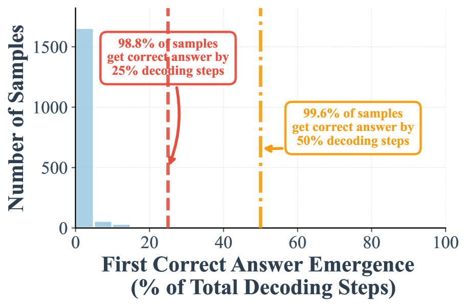</details> (c) MMLU w/o suffix prompt (random) <details> <summary>x10.png Details</summary>  ### Visual Description ## Histogram: First Correct Answer Emergence ### Overview The image is a histogram showing the distribution of the "First Correct Answer Emergence" as a percentage of total decoding steps. The x-axis represents the percentage of total decoding steps, and the y-axis represents the number of samples. The histogram shows that a large number of samples get the correct answer very early in the decoding process. Two vertical lines indicate the percentage of samples that get the correct answer by 25% and 50% of the decoding steps. ### Components/Axes * **X-axis:** "First Correct Answer Emergence (% of Total Decoding Steps)". The axis ranges from 0 to 100 with tick marks at intervals of 20 (0, 20, 40, 60, 80, 100). * **Y-axis:** "Number of Samples". The axis ranges from 0 to 1500 with tick marks at intervals of 500 (0, 500, 1000, 1500). * **Bars:** Light blue bars represent the number of samples for each percentage range of the first correct answer emergence. * **Vertical Lines:** * Red dashed line at approximately x=25, indicating that 98.8% of samples get the correct answer by 25% decoding steps. * Orange dashed-dotted line at approximately x=50, indicating that 99.6% of samples get the correct answer by 50% decoding steps. ### Detailed Analysis * The histogram is heavily skewed to the left, with the vast majority of samples (approximately 1600) achieving the first correct answer emergence within the first 0-5% of total decoding steps. * The number of samples decreases rapidly as the percentage of decoding steps increases. * At 25% of decoding steps, 98.8% of samples have already achieved the correct answer. This is indicated by a red dashed vertical line and a text annotation. * At 50% of decoding steps, 99.6% of samples have achieved the correct answer. This is indicated by an orange dashed-dotted vertical line and a text annotation. ### Key Observations * The model achieves a high percentage of correct answers very early in the decoding process. * The marginal gain in correct answers from 25% to 50% decoding steps is relatively small (98.8% to 99.6%). ### Interpretation The data suggests that the model is highly efficient in finding the correct answer. A large majority of samples converge to the correct answer within a small fraction of the total decoding steps. The fact that 98.8% of samples get the correct answer by 25% decoding steps indicates that the model quickly identifies the relevant information and converges to the solution. The additional 0.8% of samples that get the correct answer between 25% and 50% decoding steps may represent more complex or ambiguous cases that require more processing. Overall, the histogram demonstrates the model's ability to efficiently and accurately decode information. </details> (d) MMLU w/ suffix prompt (random) Figure 4: Distribution of early correct answer detection during decoding process. Histograms show when correct answers first emerge during diffusion decoding, measured as percentage of total decoding steps, using LLaDA 8B on MMLU. Red and orange dashed lines indicate 50% and 70% completion thresholds, with corresponding statistics showing substantial early convergence. Suffix prompting (b,d) dramatically accelerates convergence compared to standard prompting (a,c). This early convergence pattern demonstrates that correct answer tokens stabilize as top-1 candidates well before full decoding. Table 4: Configurations used in our runs. We keep only parameters relevant to our method: base budget $(L,T,B)$ and Prophet ’s confidence schedule. | MMLU | $L{=}64,\ T{=}64,\ B{=}16$ | $(7.5,\;5.0,\;2.5)$ | 33%, 67% | | --- | --- | --- | --- | | ARC-C | $L{=}64,\ T{=}64,\ B{=}16$ | $(7.5,\;5.0,\;2.5)$ | 33%, 67% | | Hellaswag | $L{=}64,\ T{=}64,\ B{=}16$ | $(7.5,\;5.0,\;2.5)$ | 33%, 67% | | TruthfulQA | $L{=}64,\ T{=}64,\ B{=}16$ | $(7.5,\;5.0,\;2.5)$ | 33%, 67% | | WinoGrande | $L{=}64,\ T{=}64,\ B{=}16$ | $(7.5,\;5.0,\;2.5)$ | 33%, 67% | | PIQA | $L{=}64,\ T{=}64,\ B{=}16$ | $(7.5,\;5.0,\;2.5)$ | 33%, 67% | | GSM8K | $L{=}256,\ T{=}256,\ B{=}32$ | $(8.0,\;5.0,\;3.5)$ | 33%, 67% | | GPQA | $L{=}256,\ T{=}256,\ B{=}32$ | $(8.0,\;5.0,\;3.5)$ | 33%, 67% | | HumanEval | $L{=}512,\ T{=}512,\ B{=}32$ | $(7.5,\;5.0,\;4.5)$ | 33%, 67% | | MBPP | $L{=}512,\ T{=}512,\ B{=}32$ | $(7.5,\;5.0,\;4.5)$ | 33%, 67% | | Sudoku | $L{=}24,\ T{=}24,\ B{=}24$ | $(7.5,\;5.0,\;2.5)$ | 33%, 67% | | Countdown | $L{=}32,\ T{=}32,\ B{=}32$ | $(7.5,\;5.0,\;2.5)$ | 33%, 67% | Appendix B Evaluation Details We re-implemented the evaluation of LLaDA and Dream on those reported datasets. We generate and extract the final answer instead of comparing the log probability in the multiple-choice setting, which can lower the reported scores on some datasets because the model sometimes fails to produce an answer in the given format. The configuration of each experiment is summarized in Table 4.