2509.03047

# FlashRecovery: Fast and Low-Cost Recovery from Failures for Large-Scale Training of LLMs > 1iFLYTEK AI Engineering Institute, Hefei 230088, China2University of Science and Technology of China, Hefei 230026, China3Huawei Technologies Co., Ltd, Shenzhen 518129, China Abstract Large language models (LLMs) have made a profound impact across various fields due to their advanced capabilities. However, training these models at unprecedented scales requires extensive AI accelerator clusters and sophisticated parallelism strategies, which pose significant challenges in maintaining system reliability over prolonged training periods. A major concern is the substantial loss of training time caused by inevitable hardware and software failures. To address these challenges, we present FlashRecovery, a fast and low-cost failure recovery system comprising three core modules: (1) Active and real-time failure detection. This module performs continuous training state monitoring, enabling immediate identification of hardware and software failures within seconds, thus ensuring rapid incident response; (2) Scale-independent task restart. By employing different recovery strategies for normal and faulty nodes, combined with an optimized communication group reconstruction protocol, our approach ensures that the recovery time remains nearly constant, regardless of cluster scale; (3) Checkpoint-free recovery within one step. Our novel recovery mechanism enables single-step restoration, completely eliminating dependence on traditional checkpointing methods and their associated overhead. Collectively, these innovations enable FlashRecovery to achieve optimal Recovery Time Objective (RTO) and Recovery Point Objective (RPO), substantially improving the reliability and efficiency of long-duration LLM training. Experimental results demonstrate that FlashRecovery system can achieve training restoration on training cluster with 4, 800 devices in 150 seconds. We also verify that the time required for failure recovery is nearly consistent for different scales of training tasks. Index Terms: failure recovery, large language models, checkpoint, data parallelism. I Introduction Large language models (LLMs) have emerged as a focal point in artificial intelligence (AI) research due to their exceptional capabilities across a range of tasks and applications, including text generation, code assistance, and scientific discovery [1, 2, 3]. The superior performance of these models is fundamentally governed by scaling laws, with empirical studies consistently demonstrating that their capabilities improve as model parameters and training data increase [4]. However, this growth in model scale necessitates the use of increasingly large clusters of GPUs or specialized AI accelerators, along with extended training duration. Consequently, maintaining reliable LLM training in large-scale accelerator clusters over extended periods presents a critical yet formidable challenge. The increasing scale of LLMs has been enabled by advances in parallelism techniques, including data parallelism, model parallelism, pipeline parallelism, and hybrid three-dimensional parallelism [5, 6, 7]. While these methods facilitate large-scale model training, they also introduce significant vulnerability to errors due to their inherently synchronous nature. In such frameworks, even a single node failure can disrupt the entire training process, necessitating a full cluster halt and costly re-computation during recovery. For instance, in data parallelism, the training data is partitioned across clusters along the batch dimension, with each accelerator independently processing its assigned data segment through forward and backward passes. Then a synchronous collective communication is performed to aggregate gradients globally before updating model parameters. Similarly, pipeline parallelism divides the model into sequential stages, requiring intermediate tensor exchanges at predetermined pipeline boundaries, while tensor parallelism distributes layer parameters across multiple dimensions, necessitating continuous communication of activation tensors. Although these strategies enable efficient distributed training, their dependence on strict synchronization exacerbates the cost of failures. A single node failure can cascade into system-wide downtime, highlighting the critical need for resilient fault tolerance mechanisms to maintain training efficiency. AI accelerators and network devices frequently encounter errors, including hardware failures, software bugs, and communication timeouts. Critically, failure frequency exhibits a strong positive correlation with cluster size. For instance, training of the Bloom model experiences 1-2 GPU failures per week on a cluster of 384 GPUs [8], while the OPT-175B model encountered approximately 110 failures over a two-month period on a cluster of 992 GPUs [9]. Additionally, pretraining of Meta’s LLaMA3 experienced 466 job interruptions during a 54-day period on a cluster of 16, 384 GPUs [10]. As AI clusters grow to accommodate larger models, the probability of failures increases proportionally. This trend underscores the imperative for robust error detection and recovery mechanisms to maintain training continuity and operational efficiency. The most conventional approach to anomaly recovery systems is periodic checkpointing, wherein model states are saved to persistent storage at fixed intervals and restored after failures. However, this method suffers from two critical limitations: (1) The substantial I/O overhead incurred during checkpoint saving and loading grows proportionally with model size, creating a significant bottleneck as modern LLMs scale to hundreds of gigabytes or terabytes. This I/O burden dramatically slows overall training progress; (2) When a failure occurs, recovery requires all clusters to revert to the last checkpoint, discarding all intermediate computations since the last checkpoint. Statistically, this results in approximately half of the work between checkpoints being redundantly recomputed per failure. These limitations create an inherent tension in system design: increasing checkpoint frequency reduces recovery time but exacerbate I/O overhead, while decreasing frequency minimizes checkpointing costs at the expense of longer recovery periods. This fundamental trade-off poses a major obstacle to achieving reliable large-scale training, motivating the development of more efficient fault-tolerance paradigms for large-scale LLM training. Recovery Point Objective (RPO) and Recovery Time Objective (RTO) are critical metrics in disaster recovery planning [11]. Both metrics are also suitable for evaluating the efficacy of fault recovery systems in LLM training. RPO defines the maximum tolerable data loss, measured from the most recent backup to the point of system failure. In the context of LLM training, RPO corresponds to the potential loss of training progress between the latest checkpoint and the failure point. RTO, on the other hand, refers to the maximum acceptable duration for restoring system after an disaster. For LLM training, RTO is determined by the time required to restart the training process following a failure. While RPO aims to minimize data loss, RTO focuses on reducing downtime. An effective fault recovery system for LLM training must strike an optimal balance between these two objectives, ensuring efficient recovery with minimal disruption to training job. In this paper, we propose FlashRecovery, a fast and low-cost LLM training fault recovery system. Its key features and innovations include: - Fast recovery with optimal RTO. Our system actively detects hardware and software failures within seconds, enabling immediate response. And the recovery time is nearly scalability-agnostic, ensuring consistent performance regardless of training cluster size. - Low-cost recovery with optimal RPO. The system restricts computation lost due to a failure recovery to a single training step and eliminates the need for periodic checkpointing. The main contributions of this paper are as follows: - A theoretical quantification is done to analyze the recovery overhead. - RPO and RTO are introduced to evaluate the performance of fault recovery systems. - A fast and low-cost recovery solution is devised and implemented for large-scale LLMs training. - Our solution, FlashRecovery, is validated on a large computing cluster with 10, 000 devices. II Recovery Overhead Analysis <details> <summary>x1.png Details</summary>  ### Visual Description # Technical Document Extraction: Training and Checkpointing Timeline ## 1. Document Overview This image is a technical diagram illustrating a multi-stage machine learning training process with a two-tier checkpointing strategy. It uses a horizontal timeline to represent the flow of operations, distinguishing between active training, memory-based checkpointing, and persistent storage checkpointing. ## 2. Component Isolation ### Region A: Main Timeline (Horizontal Axis) The timeline is composed of several colored blocks and markers: * **Blue Blocks (Training):** Represent the active training phase. These blocks feature a chevron-style indentation on the right and a corresponding point on the left, suggesting a continuous, repeating process. * **Green Block (Memory Checkpoint):** A distinct segment occurring immediately after a training interval. * **Vertical Blue Lines:** Act as temporal delimiters between major phases. ### Region B: Checkpointing Operations (Upper Layer) * **Orange Block:** Positioned above the main timeline, representing an asynchronous or secondary storage operation. * **Orange L-shaped Arrow:** Originates at the end of the green block and points to the start of the orange block, indicating a causal or sequential relationship. ## 3. Textual Transcription and Labels | Label | Transcription | Context/Meaning | | :--- | :--- | :--- | | **Lower Label 1** | `Training for t steps` | Defines the duration of the first blue training segment. | | **Lower Label 2** | `Training for t steps` | Defines the duration of the second blue training segment. | | **Upper Label 1** | `checkpoint → memory k₀` | Describes the green block; saving state to volatile memory. | | **Upper Label 2** | `checkpoint → persistent storage k₁` | Describes the orange block; saving state to non-volatile storage. | | **Symbol** | `...` | Ellipses indicate that the training blocks represent a longer, ongoing sequence of steps. | ## 4. Process Flow and Logic Analysis ### Step-by-Step Execution: 1. **Training Phase ($t$ steps):** The system undergoes training for a duration defined as $t$. This is represented by the first set of blue blocks. 2. **Memory Checkpoint ($k_0$):** Immediately following the training interval, the system performs a checkpoint to memory. This is represented by the **Green Block**. The duration of this task is $k_0$. 3. **Persistent Storage Checkpoint ($k_1$):** * As soon as the memory checkpoint ($k_0$) is complete, an orange arrow indicates the start of a transfer to persistent storage. * This is represented by the **Orange Block** with duration $k_1$. * **Crucial Observation:** The orange block sits *above* the next training block. This indicates that while the state is being written to persistent storage ($k_1$), the next round of training begins immediately in parallel. 4. **Resumed Training ($t$ steps):** The second blue block begins exactly when the green block ends, showing that training is not blocked by the persistent storage write ($k_1$), only by the memory write ($k_0$). ## 5. Technical Summary of Data Points * **Primary Task:** Training (Blue). * **Synchronous Overhead:** Memory Checkpointing (Green, $k_0$). Training stops during this period. * **Asynchronous Task:** Persistent Storage Checkpointing (Orange, $k_1$). Training continues while this task runs in the background. * **Temporal Variables:** * $t$: Duration of training intervals. * $k_0$: Time taken to checkpoint to memory (blocking). * $k_1$: Time taken to checkpoint to persistent storage (non-blocking/asynchronous). 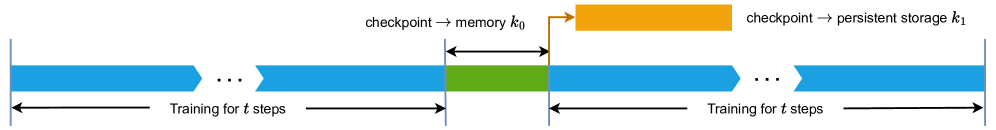</details> Figure 1: Alternative procedures (training and checkpointing) of normal training tasks. There are two procedures in common tasks of training deep learning models, which are alternatively executed by training processes (Fig. 1): 1. Training. Each training process does forward, backward and optimizer step to fit weights of a model. 1. Checkpointing. Model parameters, optimizer states and other necessary information are stashed periodically (every $t$ steps) in case of possible failures. Usually checkpoints can be dumped to hosts’ memory (procedure $k_{0}$ in Fig 1) and then to persistent storage (procedure $k_{1}$ in Fig 1). 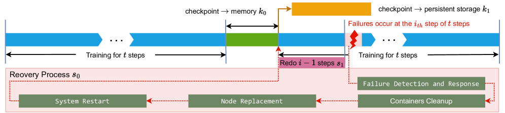Conventional Failure Recovery Protocol When a failure occurs, a standard strategy for recovery typically involves the following steps (Fig. 2): 1. Failure Detection and Response. The monitoring system identifies the failure and triggers recovery protocols. This phase inevitably incurs some latency between fault occurrence and system response due to detection overhead. 1. Container Modern clusters for deep learning generally use Docker to isolate physical environments and thus training processes run in containers. Cleanup. The training process is halted and all containers on normal nodes are terminated. 1. Node Replacement. The faulty node is decommissioned and replaced with a new healthy one, which then rejoins the training cluster. 1. System Restart. All containers are restarted across nodes, and the communication group is re-established. 1. Traning Resumption. The system loads the latest checkpoint and resumes the training process. While this recovery procedure successfully restores the training state after failures, it introduces significant inefficiencies. The most notable drawback is the waste of computational work. Since the system must revert to the last saved checkpoint, all training progress between the latest checkpoint and the failure point is discarded. <details> <summary>x2.png Details</summary>  ### Visual Description # Technical Document Extraction: Machine Learning Training Recovery Process This document provides a detailed technical breakdown of the provided diagram, which illustrates a checkpointing and recovery workflow for a machine learning training process. ## 1. Component Isolation The image is divided into two primary horizontal regions: * **Upper Region (Timeline):** A linear progression of training steps, checkpointing events, and failure occurrences. * **Lower Region (Recovery Process $s_0$):** A detailed sub-process triggered by a system failure, contained within a light pink shaded box. --- ## 2. Timeline and Training Flow (Upper Region) The timeline progresses from left to right, representing the sequential execution of training steps. ### Training Phases * **Initial Training:** Represented by blue chevron bars. * **Label:** "Training for $t$ steps" * **Visual Note:** Includes an ellipsis (`...`) indicating a continuous sequence of steps. * **Checkpointing to Memory ($k_0$):** * **Color:** Green block. * **Label:** "checkpoint $\rightarrow$ memory $k_0$" * **Duration:** Indicated by a double-headed black arrow above the green block. * **Checkpointing to Persistent Storage ($k_1$):** * **Color:** Orange block (positioned above the main timeline). * **Label:** "checkpoint $\rightarrow$ persistent storage $k_1$" * **Flow:** An orange arrow points from the end of the memory checkpoint ($k_0$) to the start of the persistent storage checkpoint ($k_1$). * **Post-Checkpoint Training:** Training resumes (blue bar) until a failure occurs. * **Failure Event:** * **Visual:** A red jagged "lightning bolt" icon. * **Label (Red Text):** "Failures occur at the $i_{th}$ step of $t$ steps" * **Redo Phase:** * **Color:** Pink block below the blue training bar. * **Label:** "Redo $i - 1$ steps $s_1$" * **Logic:** Following a failure at step $i$, the system must re-execute the preceding $i-1$ steps from the last valid checkpoint. * **Resumed Training:** * **Label:** "Training for $t$ steps" (following the redo phase). --- ## 3. Recovery Process $s_0$ (Lower Region) When a failure occurs, the system enters a recovery cycle. This is depicted inside a light pink box labeled **"Recovery Process $s_0$"**. ### Workflow Components The recovery process consists of four sequential stages, represented by dark green rectangular blocks with white monospaced text. The flow is indicated by red dotted arrows moving from right to left. 1. **Failure Detection and Response:** * Triggered directly by the failure event (indicated by a red dotted line from the failure icon). 2. **Containers Cleanup:** * The next step after detection, ensuring the environment is cleared of stale processes. 3. **Node Replacement:** * The process of replacing faulty hardware or virtual instances. 4. **System Restart:** * The final stage of the recovery process. * **Flow Completion:** A red dotted line leads from "System Restart" back up to the start of the "Redo $i - 1$ steps $s_1$" phase in the timeline. --- ## 4. Summary of Variables and Symbols | Symbol | Description | | :--- | :--- | | $t$ | Total number of steps in a training interval. | | $k_0$ | Time/cost associated with checkpointing to volatile memory. | | $k_1$ | Time/cost associated with checkpointing to persistent storage. | | $i$ | The specific step index where a failure occurs. | | $s_0$ | The total time/process for system recovery (Detection $\rightarrow$ Restart). | | $s_1$ | The time/process for re-executing steps lost due to failure. | ## 5. Technical Logic Summary The diagram describes a fault-tolerant training system. Training proceeds in blocks of $t$ steps. At the end of a block, a two-stage checkpoint is performed: first to fast memory ($k_0$), then to durable persistent storage ($k_1$). If a failure occurs at step $i$, the system must undergo a multi-stage recovery process ($s_0$) involving cleanup and hardware replacement, followed by a re-computation phase ($s_1$) to return to the state exactly before the failure occurred. </details> Figure 2: The standard recovery process from failures. Recovery Overhead Modeling Ideally, users can adjust $t$ to change the frequency of checkpointing. A large $t$ results in a lower checkpointing frequency and minimize the training overhead. However, infrequent checkpointing may incur significant costs in the event of a failure, as all devices will need to redo a substantial amount of work from a long-ago checkpoint [12]. Thus, a careful trade-off must be made between recovery costs and training overhead. To address this issue, we model the recovery process from failures and analyze the overhead of a recovery quantitatively, i.e., the elapsed time of recovery from failures. Suppose that: - $d$ . A fixed training time period. - $t$ . The number of steps between two consecutive checkpoints, referred to as the checkpointing interval. $\frac{d}{t}$ is the times of checkpointing during $d$ . - $m$ . The number of failures occurring in the cluster during time period $d$ . - $s_{0}$ . The recovery overhead, encompassing failure detection, failure response, container cleanup, node replacement, system restart and training resumption. This term is associated with the Recovery Time Objective (RTO). - $s_{1}$ . The recomputation cost, representing the training time overhead due to rollback. Under the assumption that failures occur uniformly at random, this cost can be approximated as $\frac{t}{2}$ , corresponding to the Recovery Point Objective (RPO). - $k_{0}$ . The time taken to dump checkpoints from AI clusters to host memory (non-overlapping with other operations). - $k_{1}$ . The time taken to dump checkpoints from host memory to persistent storage (may overlap with training). In the traditional periodic checkpointing approach, the parameters $m$ , $s_{0}$ , $k_{0}$ can be treated as constants, $k_{1}$ is negligible as it overlaps with training, while the checkpointing interval $t$ and the recomputation cost $s_{1}≈\frac{t}{2}$ is tunable. The total failure recovery time $\mathcal{F}(t)$ can thus be expressed as a function of $t$ : $$ \mathcal{F}(t)=m*(s_{0}+s_{1})+\frac{d}{t}*k_{0}=m*(s_{0}+\frac{t}{2})+\frac{d}{t}*k_{0} \tag{1} $$ where $m*(s_{0}+\frac{t}{2})$ represents failure recovery costs and $\frac{d}{t}*k_{0}$ denotes checkpointing overhead. By optimizing $\mathcal{F}(t)$ with respect to $t$ , we derive the optimal checkpointimg interval $t^{*}$ that minimizes total recovery time. This is obtained by solving: $$ \mathcal{F}^{\prime}(t)=\frac{m}{2}-\frac{d*k_{0}}{t^{2}}=0 \tag{2} $$ $$ t^{*}=\sqrt{\frac{2d*k_{0}}{m}} \tag{3} $$ The corresponding minimized recovery time is: $$ \mathcal{F}_{min}=m*s_{0}+\sqrt{2d*k_{0}*m} \tag{4} $$ The equation (3) reveals two critical observations: 1. A higher failure rate (i.e., larger $m$ ) necessitates more frequent checkpointing (i.e., smaller $t$ ) to achieve the minimized recovery time $\mathcal{F}_{min}$ . 1. Conversely, a larger checkpointing overhead $k_{0}$ demands a larger checkpoint interval $t$ to achieve $\mathcal{F}_{min}$ . And equation (4) further identifies three primary directions for minimizing $\mathcal{F}_{min}$ : 1. Enhancing the stability of equipments, i.e., decrease $m$ , which usually is hard to achieve and does not work when more devices are deployed. For example, when fault rate of a device is $0.001$ , the probability that 100 devices work correctly is $(1-0.001)^{100}=0.90479$ . While when we decrease the fault rate of a device to $0.0001$ (a tenth of $0.001$ ), the probability that 1000 devices work correctly is $(1-0.0001)^{1000}=0.90483$ . It can be concluded that the improvements on stability of devices are mostly liked to be canceled out due to a larger scale of devices. 1. Decreasing recovery overhead ( $s_{0}$ ). $s_{0}$ typically grows with cluster size due to distributed coordination overhead. Decoupling $s_{0}$ from cluster scale, thus making $s_{0}$ become a cluster-size-agnostic constant, is a possible optimization goal. 1. Reducing checkpoint overhead ( $k_{0}$ ). A variety of checkpoint performance optimization methods have been developed to minimize $k_{0}$ . However, checkpoint-free recovery mechanism could achieve $k_{0}=0$ , eliminating checkpointing overhead entirely. Furthermore, checkpoint-free approach naturally separates the recomputation cost ( $s_{1}$ ) from the checkpoint interval( $t$ ), as the latter is not exist in a checkpoint-free system. <details> <summary>x3.png Details</summary>  ### Visual Description # Technical Document Extraction: Distributed Computing Architecture Diagram This image is a technical schematic illustrating a complex parallel processing strategy for machine learning or large-scale data processing. It visualizes the intersection of **Pipeline Parallelism (PP)**, **Tensor Parallelism (TP)**, and **Data Parallelism (DP)** across 16 devices. ## 1. Component Isolation and Hierarchy The diagram is organized into a grid structure defined by three primary axes of parallelism: ### Vertical Axis: Pipeline Parallelism (PP) The image is divided into two horizontal rows: * **PP 1 (Top Row):** Contains Devices 1 through 8. * **PP 2 (Bottom Row):** Contains Devices 9 through 16. ### Horizontal Axis: Data Parallelism (DP) The image is divided into four main vertical sections representing data shards: * **DP 1:** Encompasses Devices 1, 2, 9, and 10. * **DP 2:** Encompasses Devices 3, 4, 11, and 12. * **DP 3:** Encompasses Devices 5, 6, 13, and 14. * **DP 4:** Encompasses Devices 7, 8, 15, and 16. ### Sub-Horizontal Axis: Tensor Parallelism (TP) Within each DP group, devices are paired to handle tensor shards: * **TP 1:** Devices 1, 3, 5, 7 (Top) and 9, 11, 13, 15 (Bottom). * **TP 2:** Devices 2, 4, 6, 8 (Top) and 10, 12, 14, 16 (Bottom). --- ## 2. Device and Shard Mapping Each device contains a block representing memory or processing units, subdivided into four segments. Specific segments are highlighted (darker green) and labeled to show how model weights or data shards are distributed. ### DP Group 1 & 2 (Left Half - Darker Green Theme) | Device | PP Level | TP Level | Shard Label | Highlighted Segment Position | | :--- | :--- | :--- | :--- | :--- | | **Device 1** | PP 1 | TP 1 | **1a** | 1st (Leftmost) - *Red Border* | | **Device 2** | PP 1 | TP 2 | **1c** | 3rd | | **Device 3** | PP 1 | TP 1 | **1b** | 2nd | | **Device 4** | PP 1 | TP 2 | **1d** | 4th (Rightmost) | | **Device 9** | PP 2 | TP 1 | **2a** | 1st (Leftmost) | | **Device 10** | PP 2 | TP 2 | **2c** | 3rd | | **Device 11** | PP 2 | TP 1 | **2b** | 2nd | | **Device 12** | PP 2 | TP 2 | **2d** | 4th (Rightmost) | ### DP Group 3 & 4 (Right Half - Lighter Green Theme) *Note: This section mirrors the left half, representing a replication of the model across different data batches.* | Device | PP Level | TP Level | Shard Label | Highlighted Segment Position | | :--- | :--- | :--- | :--- | :--- | | **Device 13** | PP 1 | TP 1 | **1a** | 1st (Leftmost) - *Red Border* | | **Device 14** | PP 1 | TP 2 | **1c** | 3rd | | **Device 15** | PP 1 | TP 1 | **1b** | 2nd | | **Device 16** | PP 1 | TP 2 | **1d** | 4th (Rightmost) | | **Device 5** | PP 2 | TP 1 | **2a** | 1st (Leftmost) | | **Device 6** | PP 2 | TP 2 | **2c** | 3rd | | **Device 7** | PP 2 | TP 1 | **2b** | 2nd | | **Device 8** | PP 2 | TP 2 | **2d** | 4th (Rightmost) | --- ## 3. Data Flow and Sharding Logic ### Shard Grouping (Arrows) The diagram uses black arrows to indicate how individual tensor shards (1a, 1b, 1c, 1d) are logically grouped into "Shard 1" and "Shard 2": * **Shard 1:** Comprised of segments from **TP 1** (Device 1/5) and **TP 2** (Device 2/6). Specifically, labels **1a** and **1c** point to "Shard 1". * **Shard 2:** Comprised of segments from **TP 1** (Device 3/7) and **TP 2** (Device 4/8). Specifically, labels **1b** and **1d** point to "Shard 2". ### Visual Indicators * **Red Outlines:** Highlighted on the "1a" segments in Device 1 and Device 5. This likely indicates the entry point of a specific data operation or a primary reference point for the documentation. * **Color Coding:** * **DP 1 & 2** use a darker olive green for highlighted shards. * **DP 3 & 4** use a brighter lime green for highlighted shards. * This distinction emphasizes that while the model structure (PP and TP) is identical, the data being processed (DP) is different. ## 4. Summary of Architecture * **Total Devices:** 16 * **Pipeline Stages:** 2 (PP 1, PP 2) * **Tensor Parallelism Degree:** 2 (TP 1, TP 2) * **Data Parallelism Degree:** 4 (DP 1, DP 2, DP 3, DP 4) * **Total Sharding:** The model is split into 4 logical shards (a, b, c, d) per pipeline stage, distributed across the TP and DP groups. 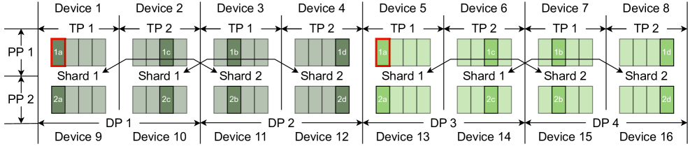</details> Figure 3: A combination of data parallelism, tensor parallelism, pipeline parallelism and ZeRO / FSDP parallelism. A frame represents a shard of parameters and the ones with the same id denotes the replicated parameters (e.g., the red frames are replicas of each other). In the following section, we elaborate on the key ideas of our recovery mechanism and its implementation. The quantitative analysis of our recovery mechanism and the system’s limitations are also presented. III Methodology III-A Motivation The scale of training datasets and the size of models in the state-of-the-art LLMs have grown at a exponential rate [13]. There is no chance to fit the parameters of LLMs in the main memory of even the largest AI accelerator [14, 5, 13, 15]. And vast amounts of data also require a lot of operations leading to a unbearably long training time on single device. Thus various model parallelism techniques have been proposed to address these challenges, such as: - Data parallelism (DP). Each process has a copy of the full model and aggregates the gradients periodically to ensure the consistency between model copies. - Pipeline parallelism (PP). The layers of a model are sharded across multiple devices. A batch is split into multiple micro-batches, which are then pipelined across different pipeline stages. There are several possible ways of scheduling forward and backward of micro-batches, e.g., PipeDream-1F1B [14], 1F1B-interleave [13], etc. - Tensor parallelism (TP). Tensors in the two-layer multi-layer perceptron (MLP) and the attention module can be split along columns, rows or heads and matrix multiplications (GEMM) are then performed in these partitioned tensors, which reduces the memory footprint [13]. - Zero redundancy Optimizer (ZeRO) / Fully Shared Data Parallel (FSDP). Unlike basic data parallelism where model states are replicated across processes, ZeRO / FSDP partitions model states in stead, to scale the model size linearly with the number of devices [5]. ZeRO / FSDP is a special data parallelism with sharded model states. A combination of different parallelism techniques can be deployed simultaneously, which is demonstrated in Fig 3. To process datasets more efficiently, data parallelism is often deployed with other parallelism techniques. With the deployment of data parallelism, we can confirm that there must be at least one replica of a model state for each process. Suppose the degree of data parallelism is $N$ , then the number of replicas of a model state on single device is $N-1$ . Given a fault rate $0.001$ of a device and $N=4$ , the probability that none of those $N$ devices in a data parallelism group work correctly is $0.001^{N}=1e^{-12}$ , which is extremely small and means that it is not likely to lose all of copies of a model state. Based on the quantitative analysis, we can conclude that it is a robust way to recovery from failures based on the replicas in a data parallelism group. The bigger the degree of data parallelism is, the more robust the recovery mechanism is. III-B Overview of the System Architecture In response to the challenges mentioned above, we propose FlashRecovery —- a fast and low-cost recovery mechanism comprising three key modules: 1. Active and real-time failure detection. This module employs a heartbeat mechanism coupled with device plugins to continuously monitor node performance and operational status. It detects failures within seconds and immediately broadcasts system-wide notifications. Compared to conventional timeout-based approaches, our method significantly reduces monitoring overhead. 1. Scale-independent task restart. This module handles failures and restarts training jobs. Unlike conventional approaches that indiscriminately terminate and restart all training processes, our system localizes the impact of failures by selectively substituting the faulty node with a healthy one. By limiting the number of nodes requiring restart, our approach decouples task restart time from cluster scale. We further accelerate recovery process through parallelized TCP Store initialization and by eliminating ranktable negotiations between devices, ensuring communication group setup remains independent of cluster size. 1. Checkpoint-free recovery within one step. This module takes a replica of the model state from other normal devices in the data parallelism group to restore failed processes. By leveraging data parallel redundancy, it eliminates checkpointing requirements while guaranteeing that at most one training step’s progress is lost. The details of design and implementation of our system are described in the subsequent sections. <details> <summary>x4.png Details</summary>  ### Visual Description # Technical Document Extraction: System Architecture Diagram ## 1. Overview This image is a technical system architecture diagram illustrating a distributed computing or machine learning training environment. It depicts the flow of monitoring data (Heartbeat and Statistical Information) from multiple "Work Nodes" to a central "Controller." The diagram specifically highlights a failure state in one of the training processes. --- ## 2. Component Isolation ### Region A: Control Layer (Header/Top) This region contains the central management components and the types of data they receive. * **Controller:** A central red oval representing the primary management entity. * **Heartbeat Information (Left Block):** A light blue rectangular container feeding into the Controller. It contains: * **Step Info** (Pink box) * **Process Status** (Pink box) * **Statistical Information (Right Block):** A light blue rectangular container feeding into the Controller. It contains: * **Chip Info** (Pink box) * **Health Status** (Pink box) * **Network Status** (Pink box) ### Region B: Execution Layer (Main Body/Bottom) This region contains two primary "Work Nodes" where the actual processing occurs. #### Work Node 1 (Left Green Block) * **Sub-components:** Contains two identical vertical stacks. * **Stack 1 & 2:** Each consists of a **Monitoring Process** (Pink box) pointing down to a **Training Process** (Green box). * **Hardware Layer:** * **Device Plugin** (Brown horizontal bar) spanning across the bottom. * **Device 1** and **Device 2** labels at the base. #### Work Node 2 (Right Green Block) * **Sub-components:** Contains two vertical stacks, one of which is in a failure state. * **Stack 3 (Left side of Node 2):** Consists of a **Monitoring Process** (Pink box) pointing down to a **Training Process** (Green box). * *Critical Detail:* The arrow between these two is **Red**, and a red lightning bolt icon with the text "**Failure**" is placed next to the Training Process. * **Stack 4 (Right side of Node 2):** Consists of a **Monitoring Process** (Pink box) pointing down to a **Training Process** (Green box). * **Hardware Layer:** * **Device Plugin** (Brown horizontal bar). * **Device 3** and **Device 4** labels at the base. --- ## 3. Data Flow and Logic Verification ### Flow 1: Heartbeat Reporting * **Source:** The "Monitoring Process" blocks in both Work Node 1 and Work Node 2. * **Path:** Black lines originate from the Monitoring Processes, merge into a single line, and point upward into the **Heartbeat Information** block, which then points to the **Controller**. * **Trend:** This represents an upward status reporting flow. ### Flow 2: Statistical Reporting * **Source:** The "Device Plugin" / Hardware layer at the bottom of both Work Nodes. * **Path:** Black lines originate from the base of the devices (Device 1, 2, 3, and 4), merge, and point upward into the **Statistical Information** block on the far right, which then points to the **Controller**. * **Trend:** This represents hardware-level telemetry being sent to the central controller. ### Flow 3: Internal Node Control * **Source:** The Controller. * **Path:** A line descends from the Controller and branches out to the **Monitoring Process** blocks in all nodes. * **Trend:** This represents command-and-control signals sent from the Controller to the individual monitoring agents. --- ## 4. Textual Transcription | Category | Exact Text | | :--- | :--- | | **Central Entity** | Controller | | **Data Categories** | Heartbeat Information, Statistical Information | | **Data Sub-types** | Step Info, Process Status, Chip Info, Health Status, Network Status | | **Node Labels** | Work Node 1, Work Node 2 | | **Process Labels** | Monitoring Process, Training Process | | **Hardware Labels** | Device Plugin, Device 1, Device 2, Device 3, Device 4 | | **Status Indicator** | Failure | --- ## 5. Critical Observations * **Failure State:** The diagram explicitly identifies a "Failure" in the Training Process associated with Device 3 in Work Node 2. This is visually emphasized by a red arrow and a red lightning bolt. * **Symmetry:** The architecture is symmetrical, suggesting a scalable design where multiple Work Nodes report to a single Controller. * **Separation of Concerns:** The system distinguishes between "Heartbeat" (process-level liveness) and "Statistical" (hardware/network-level performance) data streams. 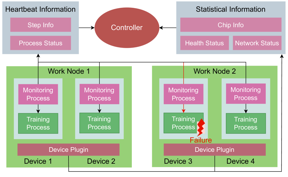</details> Figure 4: The architecture of the system and the workflow of the failure detection. III-C Active Real-time Failure Detection In the absence of an additional failure detection module, training processes traditionally identify occurrences of failures from other devices by a hang during collective communication, which can last up to 30 minutes in PyTorch. To address the inefficiency of the passive manner of sensing failures, we propose a novel failure detection mechanism which detects failures actively and achieve fast failure identification. The workflow of the mechanism is illustrated in Fig. 4 and it consists of three components: 1. Controller. A controller is a global service, which collects failure report from device plugins and monitoring processes. It also decides strategies to handle failures that occur at different stages and reschedules all processes after failures. 1. Monitoring Processes. Monitoring Processes are created and run with every training process. They are able to monitor the health status of the associated training process and collect other necessary information (e.g. current step number) for recovery, which are reported to the controller periodically. 1. Device Plugins. Device plugin is a component that is installed on every node and is able to report various statistical information of devices on a node, including chip info, health and network status. The information helps to determine the status of a device. Both heartbeat mechanism and device plugins provide a active ability to detect failures, which helps to detect a failure in seconds. When a failure occurs and the faulty device is confirmed, the controller decides the recovery strategy for every nodes and reschedules all training processes. Subsequently, our system restarts and recoveries the training task, which is to be introduced in the next two sections. III-D Scale-Independent Task Restart Traditional system restart methods often exhibit a linear increase in time consumption as cluster scale grows, primarily due to three factors: - Inefficient Container Management. These approaches destroy and recreate all containers indiscriminately, even when the training environment remains intact on normal nodes. This forces the system to wait for the slowest container initialization, creating a performance bottleneck. Since container startup times follow a normal distribution, larger clusters inevitably encounter longer tail latencies, leading to linear growth in total reconstruction time. - Scale-dependent Communication Group Establishment. The restart of all containers is accompanied by the creation of a new global communication group. This procedure entails the establishment of multiple communication links, followed by the execution of data exchange operations across these newly formed connections. Notably, as the cluster size increases, both the volume of data exchanged and the number of required communication links grow proportionally. In the unoptimized implementation, these tasks are executed serially within a single process, leading to a linear increase in time complexity relative to the number of nodes. - I/O Overhead During Training Process Initialization. The training process initialization phase requires loading both the python environment (which may consist of tens of thousands of small files) and checkpoint (which can scale up to hundreds of gigabytes or terabytes). When thousands of containers restart simultaneously, massive parallel access to shared storage resources leads to severe I/O pressure. This bottleneck severely degrades initialization performance and further increases reconstruction latency. These factors collectively constrain the scalability of traditional recovery mechanisms, motivating the need for a more efficient approach. In FlashRecovery, as illustrated in Fig 5, normal nodes, abnormal nodes, and the controller exhibit distinct behavioral patterns during the task restart process. We optimize the restart process, which can be systematically divided into three stages: 1. Node Rescheduling with Limited Recreation. Upon detecting a fault, the controller initiates a concurrent recovery protocol for different nodes. First, it dispatches termination signals to every normal nodes, instructing them to suspend their training processes. These nodes then transition to a standby state, awaiting for another continue signal from the controller to restart their training processes. Simultaneously, the controller executes node rescheduling, substituting faulty nodes with healthy ones. The newly allocated nodes execute the training script, initialize communication, and notify the controller to update the ranktable accordingly. The restart procedure for new joined nodes and the suspension of training on normal nodes are executed concurrently. Through applying different strategies for normal and faulty nodes respectively, we restrict the number of recreated nodes to only those encountering errors and reduce the unnecessary container recreation, which make the restart process independent of the scale of the training cluster and faster. <details> <summary>x5.png Details</summary>  ### Visual Description # Technical Document Extraction: Node Rescheduling and Training Recovery Workflow This document provides a comprehensive extraction of the technical flowchart illustrating the process of node replacement and training recovery in a distributed computing environment. ## 1. System Architecture Overview The diagram is organized into three vertical columns representing the primary actors/components and three horizontal phases representing the logical stages of the process. ### Vertical Columns (Actors) * **Normal Nodes (Left, Green Background):** Existing healthy nodes in the cluster. * **Controller (Center, Blue Background):** The management entity coordinating the recovery. * **New Nodes (Right, Yellow Background):** Replacement nodes introduced to the cluster. ### Horizontal Phases (Process Stages) * **Node Reschedule (Top):** Handling the failure and provisioning new resources. * **Communication Group Restore (Middle):** Re-establishing the network and rank configuration. * **Training Recovery (Bottom):** Synchronizing state and resuming the workload. --- ## 2. Detailed Component and Flow Analysis ### Phase 1: Node Reschedule This phase initiates when a node failure is detected. 1. **Controller Actions:** * Sends a **Termination Signal** to **Normal Nodes**. * Executes **Replace Faulty Node**, which triggers the creation of a replacement. * Sends a **Continue Signal** to **Normal Nodes** once the replacement is ready. * Performs **Generate & Update Ranktable** (internal process). 2. **Normal Nodes Actions:** * Receive Termination Signal $\rightarrow$ **Stop Training**. * Receive Continue Signal $\rightarrow$ **Restart Training**. 3. **New Nodes Actions:** * Triggered by Controller $\rightarrow$ **Create Container**. * Followed by **Init Training**. ### Phase 2: Communication Group Restore This phase involves all nodes (Normal and New) and is represented by wide blocks spanning across the columns. The flow is strictly sequential: 1. **Torch Agent Establishment:** Initializing the distributed agents. 2. **TCP Store Establishment:** Setting up the key-value store for distributed coordination. 3. **Updated Ranktable Loading:** Loading the new cluster configuration generated by the Controller in Phase 1. 4. **Inter-Device Communication Establishment:** Finalizing the network layer for data exchange between nodes. ### Phase 3: Training Recovery This phase focuses on data synchronization and resuming the computational task. 1. **Recovery Strategy (Controller/Global):** The central logic determining how to resume. 2. **Normal Nodes Path:** * **Send Training State:** Transmits the last known good checkpoint/state to the new nodes. * **Rollback Dataset:** Reverts the data iterator to the correct position. 3. **New Nodes Path:** * **Receive Training State:** Accepts the state from Normal Nodes. * **Load Dataset:** Initializes the data stream. 4. **Final Step (Unified):** * **Continue Training:** All nodes resume the training process in synchronization. --- ## 3. Textual Transcription | Category | Transcribed Text | | :--- | :--- | | **Headers** | Normal Nodes, Controller, New Nodes | | **Phase Labels (Purple)** | Node Reschedule, Communication Group Restore, Training Recovery | | **Process Blocks** | Stop Training, Restart Training, Termination Signal, Replace Faulty Node, Continue Signal, Generate & Update Ranktable, Create Container, Init Training, Torch Agent Establishment, TCP Store Establishment, Updated Ranktable Loading, Inter-Device Communication Establishment, Recovery Strategy, Send Training State, Rollback Dataset, Receive Training State, Load Dataset, Continue Training | --- ## 4. Technical Summary of Logic The system employs a **Stop-and-Restart** recovery mechanism. The **Controller** acts as the orchestrator, managing the lifecycle of the **New Nodes** and updating the **Ranktable** (the map of node identities). The **Communication Group Restore** phase acts as a synchronization barrier where all nodes must re-initialize their distributed environment (Torch Agent, TCP Store) before the **Training Recovery** phase can synchronize the model state and dataset offsets to ensure training continuity without data corruption or loss of progress. </details> Figure 5: The task restart process in FlashRecovery. 1. Optimized Communication Group Establishment. The communication group establishment process is a critical step in the recovery process, as it involves the establishment of multiple communication links and data exchange operations across devices. Some procedures in this process are typically executed serially within a single process, leading to a time complexity relative to the number of nodes, i.e., $O(n)$ . The process of establishing communication group usually can be decomposed into four procedures: - Torch Agent establishment. This procedure involves communication initialization and making connection with master node, which usually exhibits a relatively fixed time consumption. - TCP Store establishment. In contrast to Torch Agent establishment, TCP Store generally establishes in a serialized way, resulting in a linear time consumption dependent on cluster size. To improve efficiency, we apply a optimized strategy and parallelize the establishment of TCP Store, which reduces the time complexity from $O(n)$ to $O(\frac{n}{p})$ ( $n$ is the scale of a cluster and $p$ is the degree of parallelization). - Updated ranktable loading. The ranktable records the resource information of the entire cluster for inter-device communication establishment. Originally, master node collects information from every node and then generates a global ranktable, which is sent to every node later. The generation and distribution of ranktable is executed serially and thus the time complexity is $O(n)$ . In contrast, the controller in our system maintains a global ranktable in a shared file across nodes. Every device is able to load the latest ranktable from the file directly without any collection and distribution of ranktable, reducing the time complexity to $O(1)$ . - Inter-device communication establishment. The inter-device link establishment also adopts highly parallelized measures and the time is primarily dependent on the number of communication neighbors of the communication operators rather than the cluster size. 1. Training State Recovery. The controller employs distinct recovery strategies for normal nodes and faulty nodes. It also determines the device on normal nodes whose model state will be used to restore the training on newly scheduled nodes. A comprehensive analysis of this approach will be presented in the following section. III-E Checkpoint-Free Recovery within One Step In general, model states of a specific step can be recovered totally from the last checkpoint, which requires extra training from the step of the checkpoint to the step with failures. 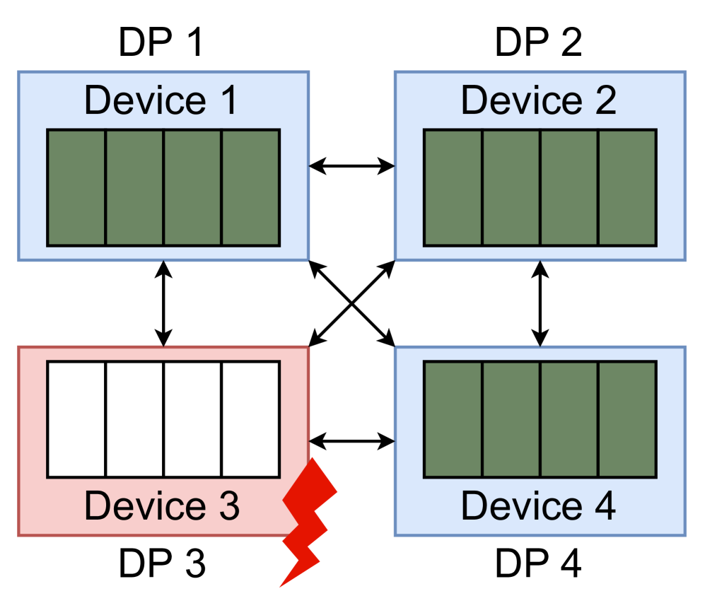To reduce the overhead resulting from the redone training, we propose a checkpoint-free recovery approach as follows: 1. Restoration. We use data parallelism replicas to restore consistent model states of the restarted processes rather than a checkpoint. In this way, training processes hold model states of the $i_{\mathrm{th}}$ or $(i+1)_{\mathrm{th}}$ step. The specific step is depended on the phase where a failure occurs. We will describe the details of model state restoration and step determination in the following. 1. Rollback. The iterator of dataset is rolled back to the step aligned with the model state ( $i_{\mathrm{th}}$ or $(i+1)_{\mathrm{th}}$ step). 1. Continue Training. The training process is totally recovered after restoration and rollback, and the training loop continues for a new batch. 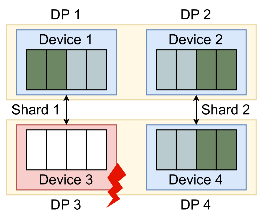Model states Restoration As described in III-A, we can restore the model states of recreated processes from data parallelism replicas. In this case, any checkpoints is not required and model states in recreated processes can be restored with collective communication. Because the controller has the global failure information, we can easily determine if we have a model state replica for the faulty process. Actually, if there is at least one training process of the same DP group on the normal node, we can restore the model states of other processes on the faulty node. We support model states restoration from two kinds of data parallelism: (1) vanilla data parallelism, and (2) data parallelism with ZeRO / FSDP. The model states restoration for these two parallelisms are illustrated in Fig. 6. Furthermore, our system also supports model states restoration from a combination of various data and model parallelism, which is demonstrated in Fig. 3. <details> <summary>x6.png Details</summary>  ### Visual Description # Technical Document Extraction: Network Device Topology and Fault State ## 1. Document Overview This image is a technical diagram illustrating a four-node network or system topology. It depicts the connectivity between four distinct devices (labeled Device 1 through Device 4) and highlights a failure state associated with one of the nodes. --- ## 2. Component Isolation ### Region A: Upper Nodes (Healthy State) * **DP 1 / Device 1 (Top-Left):** * **Container:** Light blue rectangular box. * **Internal State:** Contains four vertical green rectangles, indicating active or healthy internal modules/sub-components. * **DP 2 / Device 2 (Top-Right):** * **Container:** Light blue rectangular box. * **Internal State:** Contains four vertical green rectangles, indicating active or healthy internal modules/sub-components. ### Region B: Lower Nodes (Mixed State) * **DP 3 / Device 3 (Bottom-Left):** * **Container:** Light red rectangular box, indicating a fault or error state. * **Internal State:** Contains four vertical white (empty) rectangles, indicating that the internal modules/sub-components are inactive or have failed. * **Visual Indicator:** A large red lightning bolt icon is positioned at the bottom right corner of this device block, signifying a critical failure or electrical fault. * **DP 4 / Device 4 (Bottom-Right):** * **Container:** Light blue rectangular box. * **Internal State:** Contains four vertical green rectangles, indicating active or healthy internal modules/sub-components. --- ## 3. Connectivity and Flow (Full Mesh Topology) The diagram utilizes double-headed black arrows to represent bidirectional communication or power paths between the devices. The arrangement constitutes a **Full Mesh Topology**, where every node is connected to every other node. | Connection Path | Description | | :--- | :--- | | **Horizontal (Top)** | Device 1 $\leftrightarrow$ Device 2 | | **Horizontal (Bottom)** | Device 3 $\leftrightarrow$ Device 4 | | **Vertical (Left)** | Device 1 $\leftrightarrow$ Device 3 | | **Vertical (Right)** | Device 2 $\leftrightarrow$ Device 4 | | **Diagonal (Backslash)** | Device 1 $\leftrightarrow$ Device 4 | | **Diagonal (Forward slash)** | Device 2 $\leftrightarrow$ Device 3 | --- ## 4. Textual Data Extraction | Label Type | Extracted Text | | :--- | :--- | | **Primary Headers** | DP 1, DP 2, DP 3, DP 4 | | **Secondary Labels** | Device 1, Device 2, Device 3, Device 4 | --- ## 5. Technical Summary of Trends and Data * **Operational Status:** 75% of the system (Devices 1, 2, and 4) is operational, indicated by the blue housing and green internal status bars. * **Failure Point:** 25% of the system (Device 3) is in a failed state, indicated by the red housing, empty (white) status bars, and the red lightning bolt symbol. * **Redundancy:** Despite the failure of Device 3 (DP 3), the mesh connectivity suggests that paths still exist between the remaining healthy nodes (1, 2, and 4), though any data or processes dependent on Device 3 are currently compromised. </details> (a) Vanilla DP restoration. <details> <summary>x7.png Details</summary>  ### Visual Description # Technical Document Extraction: Distributed System Sharding Diagram ## 1. Overview This image is a technical architectural diagram illustrating a distributed computing or storage system utilizing sharding and data parallelism (DP). It depicts four Data Parallel (DP) units, each containing a device, and shows the distribution of data shards across these devices. The diagram specifically highlights a failure state in one of the devices. ## 2. Component Isolation ### Region A: Top Row (Active/Healthy) * **DP 1 (Top Left):** Contains **Device 1**. * **Internal State:** Contains four data slots. The first two slots (left) are filled with dark green blocks. The last two slots (right) are filled with light grey blocks. * **DP 2 (Top Right):** Contains **Device 2**. * **Internal State:** Contains four data slots. The first two slots (left) are filled with light grey blocks. The last two slots (right) are filled with dark green blocks. ### Region B: Bottom Row (Mixed State) * **DP 3 (Bottom Left):** Contains **Device 3**. * **Internal State:** This device is highlighted with a **red border and light red background**. It contains four data slots, all of which are **empty (white)**. * **Status Indicator:** A red lightning bolt icon is positioned at the bottom right corner of Device 3, indicating a hardware or software failure. * **DP 4 (Bottom Right):** Contains **Device 4**. * **Internal State:** Contains four data slots. The first two slots (left) are filled with light grey blocks. The last two slots (right) are filled with dark green blocks. ### Region C: Interconnects and Sharding Labels * **Shard 1:** Indicated by a vertical double-headed black arrow connecting the DP 1/Device 1 block to the DP 3/Device 3 block. * **Shard 2:** Indicated by a vertical double-headed black arrow connecting the DP 2/Device 2 block to the DP 4/Device 4 block. --- ## 3. Data and Shard Mapping The diagram uses color coding to represent data distribution across the shards. | Component | Shard Association | Slot 1 | Slot 2 | Slot 3 | Slot 4 | Status | | :--- | :--- | :--- | :--- | :--- | :--- | :--- | | **Device 1** | Shard 1 | Dark Green | Dark Green | Light Grey | Light Grey | Healthy | | **Device 2** | Shard 2 | Light Grey | Light Grey | Dark Green | Dark Green | Healthy | | **Device 3** | Shard 1 | Empty | Empty | Empty | Empty | **FAILED** | | **Device 4** | Shard 2 | Light Grey | Light Grey | Dark Green | Dark Green | Healthy | --- ## 4. Technical Analysis and Flow * **Sharding Logic:** The system is divided into at least two shards. Shard 1 encompasses DP 1 and DP 3. Shard 2 encompasses DP 2 and DP 4. * **Data Redundancy/Parallelism:** * In Shard 2, Device 2 and Device 4 contain identical data patterns (Light Grey in slots 1-2, Dark Green in slots 3-4), suggesting a mirrored or replicated state. * In Shard 1, Device 1 holds data, but Device 3 is empty and marked with a failure symbol. This implies that the data intended for DP 3 is lost, inaccessible, or failed to load due to the device fault. * **Visual Trends:** * **Healthy Devices (1, 2, 4):** Represented with blue borders and light blue backgrounds. * **Failed Device (3):** Represented with a red border/background and a lightning bolt, signifying a critical error in the Shard 1 pipeline. ## 5. Textual Transcription The following text strings are present in the image: * **DP 1** * **DP 2** * **DP 3** * **DP 4** * **Device 1** * **Device 2** * **Device 3** * **Device 4** * **Shard 1** * **Shard 2** </details> (b) ZeRO/FSDP restoration. Figure 6: Model states restoration with different parallelism. Step $i$ or step $i+1$ to resume? Suppose that a failure occurs at the $i_{\mathrm{th}}$ step, the phase where a failure occurs determines where to resume the training, which can be divided into two cases: - Failures occur during forward and backward. In this case, the parameters of the model have not been updated for the next step and the training process can be resumed from the $i_{\mathrm{th}}$ step. - Failures occur during optimizer step. In this case, despite it is difficult to determine which parameters on a device have been updated, it can be confirmed that the parameters of a normal device will be updated. Therefore, the parameters from recreated processes is able to be restored from those updated parameters on normal devices. Then the training should be resumed from the $(i+1)_{\mathrm{th}}$ step. <details> <summary>x8.png Details</summary>  ### Visual Description # Technical Diagram Analysis: Distributed Training Synchronization and Failure Points ## 1. Overview This image is a technical timeline diagram illustrating a synchronized training iteration across two computational devices (Device 1 and Device 2). It highlights the phases of a machine learning training step, the synchronization barriers, and potential failure points during the process. ## 2. Component Isolation ### A. Header / Global Annotations * **Gradient Synchronization Barrier:** A red vertical line intersects the timeline. Above this line, a light red text box contains the labels: * **Gradient Synchronization** (Left of the barrier) * **Barrier** (Right of the barrier) * **Parameter State (Center Lane):** A light blue/grey horizontal band between Device 1 and Device 2 tracks the state of the model parameters: * **Consistent Parameters:** Spans the "Forward" and "Backward" phases. * **Update Parameters:** Spans the "Optimizer Step" phase. ### B. Main Timeline (Device 1) Device 1 represents a successful, uninterrupted execution of a training step. * **Phase 1 (Blue):** "Forward" pass. * **Phase 2 (Green):** "Backward" pass. * **Phase 3 (Orange):** "Optimizer Step" (Occurs after the synchronization barrier). ### C. Main Timeline (Device 2) Device 2 represents an execution path prone to interruptions, marked by red lightning bolt icons labeled **"Failure"**. * **Phase 1 (Blue):** "Forward" pass. Interrupted by a **Failure** near the end of the phase. * **Phase 2 (Green):** "Backward" pass. Interrupted by a **Failure** at the beginning of the phase. * **Phase 3 (Orange):** "Optimizer Step". Interrupted by a **Failure** at the very end of the step. --- ## 3. Data Extraction and Flow Logic ### Process Flow Table | Phase | Color Code | Device 1 Status | Device 2 Status | Parameter State | | :--- | :--- | :--- | :--- | :--- | | **Forward** | Blue | Continuous | Interrupted by Failure | Consistent | | **Backward** | Green | Continuous | Interrupted by Failure | Consistent | | **Sync Barrier** | Red Line | Reached | Reached | Transition | | **Optimizer Step** | Orange | Continuous | Interrupted by Failure | Update Parameters | ### Key Trends and Observations 1. **Synchronization Dependency:** The "Optimizer Step" (Orange) for both devices only begins after the "Backward" pass (Green) is completed and the "Gradient Synchronization" barrier is crossed. 2. **Temporal Alignment:** Device 1 and Device 2 are horizontally aligned, indicating they are operating in parallel. 3. **Failure Distribution:** The diagram identifies that failures can occur at any stage of the pipeline: * During computation (Forward/Backward). * During the state update (Optimizer Step). 4. **Parameter Consistency:** Parameters remain "Consistent" across devices during the computation of gradients (Forward/Backward) and are only modified ("Update Parameters") during the Optimizer Step following the synchronization barrier. ## 4. Text Transcription The following text is extracted exactly as it appears in the image: * **Top Labels:** Gradient Synchronization | Barrier * **Y-Axis Labels:** Device 1, Device 2 * **Phase Labels (Internal):** Forward, Backward, Optimizer Step * **Status Labels (Center):** Consistent Parameters, Update Parameters * **Error Labels:** Failure, Failure, Failure (associated with red lightning bolt icons on Device 2) --- **Language Declaration:** All text in this image is in **English**. </details> Figure 7: Training processes with data parallelism and barrier before optimizer step. 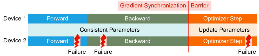Since devices execute asynchronously, we can not guarantee that all devices in the phase of forward and backward or the phase of optimizer step, which means above step determination strategy fails to be applied in practice. Fortunately, we can solve this problem with a easy barrier mechanism as demonstrated in Fig. 7. A barrier operation is added just in the beginning of the optimizer step, which achieves: - When a failure occurs during forward and backward, other normal processes must be hung before optimizer step due to the barrier operation, which ensures that all processes must be in the phase of forward and backward. - When a failure occurs in a process during optimizer step, the barrier operation indicates that the process must have synchronized with other processes. In other words, all processes have entered the phase of optimizer step. A synchronous barrier operation almost does not introduce any extra latency since we can merge the barrier operation and the last synchronization —- gradient synchronization (by all-reduce). 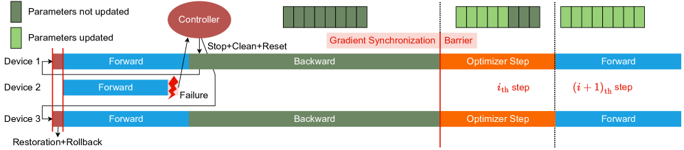The moment to stop, clean and reset When we do restarting, the controller stops and cleans the kernels of the task-queue of every device and resets all devices on normal nodes, which destroys the running state of a process. When a failure occurs during forward and backward, it makes no sense to continue the execution of kernels because the model states of $i_{\mathrm{th}}$ step have not been updated. But when a failure occurs during optimizer step, the execution of kernels can be continued and we can restore the model states on the faulty node with the updated parameters (from the $(i+1)_{\mathrm{th}}$ step). We design a mechanism to determine when to issue ”stop”, ”clean” and ”reset” instructions from the controller to devices on normal nodes. The mechanism is implemented with step tags and includes the following steps: 1. Set $\mathrm{step}=i$ for every training processes at the beginning of forward phase. 1. The controller receives step tags from every device by the heartbeat mechanism. 1. When a failure occurs during forward and backward, the controller receives $\mathrm{step}=i$ from all normal devices except those on the faulty node, we can confirm that all normal processes are in the phase of forward or backward and is able to issue ”stop”, ”clean” and ”reset” immediately without any side effect. 1. Set $\mathrm{step}=-1$ for every training processes at the beginning of optimizer step. 1. Set $\mathrm{step}=i+1$ when a normal training process completes the optimizer step, 1. When a failure occurs during optimizer step, the controller receives $\mathrm{step}=i+1$ from all normal devices except those on faulty node, we can confirm the end of optimizer step of all processes on normal nodes. At this moment, the ”stop”, ”clean” and ”reset” instructions can be issued without any side effect and model states of training processes on the faulty node can be restored from the updated parameters at $\mathrm{step}=i+1$ . 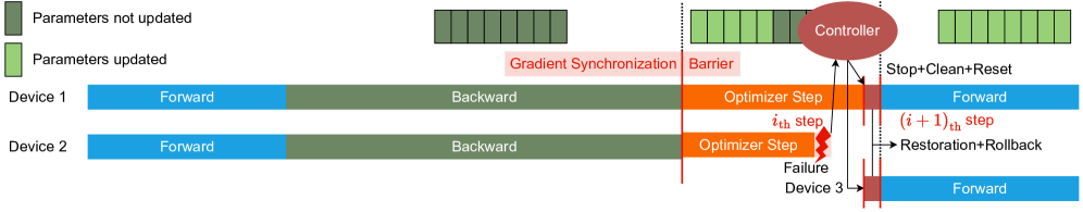Finally, detailed recovery process of our system is illustrated in Fig. 8. The recovery process for failures in the phase of forward and backward is shown in Fig. 8(a) and the recovery process for failures in the phase of optimizer step is demonstrated in Fig. 8(b). <details> <summary>x9.png Details</summary>  ### Visual Description # Technical Document Extraction: Distributed Training Failure Recovery Diagram ## 1. Document Overview This image is a technical timing diagram illustrating a fault-tolerance mechanism in a distributed machine learning environment across multiple devices. It details the interaction between a central controller and three computing devices during a failure event, recovery, and subsequent synchronization. --- ## 2. Component Isolation ### A. Legend (Top Left) * **Location:** [x: 0-200, y: 0-150] * **Dark Green Square:** "Parameters not updated" * **Light Green Square:** "Parameters updated" ### B. Header / Global State (Top Center/Right) * **Controller:** A red oval representing the central management unit. * **Parameter State Bars:** Horizontal segmented bars showing the status of model parameters. * **Initial State:** All segments are Dark Green (Not updated). * **Post-Barrier State:** Most segments are Light Green, some remain Dark Green. * **Final State:** All segments are Light Green (Updated). * **Text Labels:** * "Gradient Synchronization Barrier" (Red text, split by a vertical red line). ### C. Main Timeline (Center) * **Y-Axis (Devices):** Device 1, Device 2, Device 3. * **X-Axis (Process Flow):** * **Forward Pass (Blue):** Active on all devices initially. * **Backward Pass (Muted Green):** Active on Device 1 and Device 3. * **Optimizer Step (Orange):** Active on Device 1 and Device 3 after the barrier. * **Step Indicators (Red Text):** * $i_{th}$ step * $(i + 1)_{th}$ step ### D. Footer / Control Signals (Bottom Left) * **Text:** "Restoration+Rollback" with arrows pointing to the start of the timeline. --- ## 3. Process Flow and Logic Analysis ### Phase 1: Failure and Detection 1. **Execution:** Devices 1, 2, and 3 begin the **Forward** pass (Blue bars). 2. **Event:** A red lightning bolt icon labeled **"Failure"** occurs on **Device 2** during its Forward pass. 3. **Communication:** An arrow points from the failure point on Device 2 to the **Controller**. ### Phase 2: Controller Intervention 1. **Command:** The Controller issues a **"Stop+Clean+Reset"** signal (indicated by downward arrows) to the other active devices. 2. **Rollback:** A vertical red shaded region at the start of the timeline is labeled **"Restoration+Rollback"**. Arrows indicate that the system resets to the beginning of the current step. ### Phase 3: Resilient Execution (The $i_{th}$ step) 1. **Forward/Backward:** Device 1 and Device 3 proceed through the **Forward** (Blue) and **Backward** (Muted Green) passes. Note that Device 2 remains inactive/absent during this phase. 2. **Synchronization:** A vertical red line marks the **"Gradient Synchronization Barrier"**. 3. **Optimization:** After the barrier, Device 1 and Device 3 perform the **Optimizer Step** (Orange). 4. **Parameter Update:** Above this section, the parameter bar changes from all Dark Green to mostly Light Green, indicating the model is being updated despite the missing device. ### Phase 4: Transition to $(i + 1)_{th}$ step 1. **Boundary:** A vertical dotted black line separates the $i_{th}$ step from the $(i + 1)_{th}$ step. 2. **Completion:** The parameter bar at the top right is now entirely Light Green ("Parameters updated"). 3. **Next Iteration:** Device 1 and Device 3 begin the next **Forward** pass. --- ## 4. Summary of Textual Data | Category | Exact Transcription | | :--- | :--- | | **Legend** | Parameters not updated, Parameters updated | | **Components** | Controller, Device 1, Device 2, Device 3 | | **Actions/States** | Forward, Backward, Optimizer Step, Failure, Restoration+Rollback, Stop+Clean+Reset | | **Synchronization** | Gradient Synchronization Barrier | | **Iteration Markers** | $i_{th}$ step, $(i + 1)_{th}$ step | --- ## 5. Technical Observations * **Fault Tolerance:** The diagram depicts a "subset" update strategy. When Device 2 fails, the Controller resets the remaining devices (1 and 3), which then complete the $i_{th}$ iteration and update the parameters without waiting for Device 2 to recover. * **Color Coding Consistency:** * **Blue** always represents the Forward pass. * **Muted Green** always represents the Backward pass. * **Orange** always represents the Optimizer Step. * **Red** is reserved for control signals, failures, and synchronization barriers. </details> (a) The recovery process from the $i_{\mathrm{th}}$ step when failures occur during forward and backward. <details> <summary>x10.png Details</summary>  ### Visual Description # Technical Document Extraction: Distributed Training Failure Recovery Diagram ## 1. Document Overview This image is a technical timing diagram illustrating a distributed machine learning training process across multiple devices, specifically focusing on a failure event during the optimizer step and the subsequent recovery mechanism managed by a central controller. --- ## 2. Component Isolation ### A. Legend (Top-Left) * **Dark Green Square:** "Parameters not updated" * **Light Green Square:** "Parameters updated" ### B. Main Timeline (Center) The diagram tracks the operations of two primary devices over time, moving from left to right. * **Y-Axis Labels:** `Device 1`, `Device 2`. * **X-Axis Phases (Sequential):** 1. **Forward Pass (Blue):** Labeled "Forward". 2. **Backward Pass (Dark Green):** Labeled "Backward". 3. **Optimizer Step (Orange):** Labeled "Optimizer Step". 4. **Recovery/Next Step (Blue):** Labeled "Forward". ### C. Control and Status Overlays (Top and Right) * **Parameter State Blocks:** Horizontal arrays of squares indicating the update status of model parameters. * **Gradient Synchronization Barrier:** A red vertical line separating the Backward pass from the Optimizer Step, labeled "Gradient Synchronization Barrier" (text in red). * **Controller:** A red oval labeled "Controller" positioned above the timeline, interacting with the devices via arrows. * **Failure Event:** A red lightning bolt icon located at the end of the Optimizer Step for Device 2, labeled "Failure". --- ## 3. Process Flow and Logic Analysis ### Phase 1: Standard Iteration ($i_{th}$ step) 1. **Forward/Backward:** Both Device 1 and Device 2 execute the Forward pass (blue) followed by the Backward pass (dark green). 2. **Synchronization:** A "Gradient Synchronization Barrier" occurs. Above this, a block of 10 dark green squares indicates that parameters are currently "not updated." 3. **Optimizer Step:** Both devices begin the "Optimizer Step" (orange). During this phase, the parameter blocks above transition from dark green to light green, indicating "Parameters updated." ### Phase 2: Failure and Detection 1. **The Event:** At the end of the $i_{th}$ step, a "Failure" occurs on Device 2 (indicated by the lightning bolt). 2. **Controller Intervention:** * An arrow points from the failure point to the **Controller**. * The Controller sends signals back to the system. * A vertical dashed line marks the boundary where the failure is processed. ### Phase 3: Recovery and Rollback ($(i+1)_{th}$ step) 1. **Device 1 Action:** Labeled "Stop+Clean+Reset". Device 1 is interrupted (indicated by a small red block) before starting the next "Forward" pass. 2. **Device 2/3 Transition:** The diagram shows a transition from the failed Device 2 to a new **Device 3**. 3. **Restoration:** An arrow labeled "Restoration+Rollback" points to the start of the next phase for Device 3. 4. **Resumption:** Both Device 1 and the new Device 3 begin the $(i+1)_{th}$ step with a "Forward" pass (blue). The parameter blocks above this phase are all light green, indicating the system has recovered to a state where parameters are ready for the next iteration. --- ## 4. Textual Transcriptions | Category | Exact Text | | :--- | :--- | | **Legend** | Parameters not updated, Parameters updated | | **Device Labels** | Device 1, Device 2, Device 3 | | **Process Steps** | Forward, Backward, Optimizer Step | | **Synchronization** | Gradient Synchronization Barrier | | **Iteration Markers** | $i_{th}$ step, $(i+1)_{th}$ step | | **Failure/Recovery** | Failure, Controller, Stop+Clean+Reset, Restoration+Rollback | --- ## 5. Technical Summary of Trends * **Temporal Consistency:** Device 1 and Device 2 operate in parallel and are synchronized by the Gradient Synchronization Barrier. * **State Transition:** The transition from "Parameters not updated" to "Parameters updated" occurs strictly during the "Optimizer Step" phase. * **Fault Tolerance:** The system demonstrates a "Rollback" mechanism where a failure in one device (Device 2) triggers a controller-led reset of healthy devices (Device 1) and the introduction of a replacement resource (Device 3) to ensure the $(i+1)_{th}$ step can proceed. </details> (b) The recovery process from the $(i+1)_{\mathrm{th}}$ step when failures occur during optimizer step. Figure 8: The recovery processes for failures in different phases of a training step. III-F Recovery Overhead Analysis of Our Method Above all, our approach can recover training task with DP replicas and remove the extra redone training from checkpointing. The recovery time due to extra redone training ( $s_{1}$ ) becomes a constant (approximately a bit longer than the running time of one training step). Moreover, the active failure detection mechanism can reduce the time of detecting a failure. And the scale-independent task restarting only restarts processes on faulty nodes, which is independent of the scale of a training task and further reduces the restarting overhead. Both of them reduce the recovery time $s_{0}$ . Checkpoint-free recovery from DP replicas also removes the checkpointing overhead $\frac{d}{t}*k_{0}$ . To sum up, the equation 1 becomes: $$ \mathcal{F}=m*(s_{0}^{\prime}+s_{1}^{\prime}) \tag{5} $$ where $s^{\prime}_{0}$ represents the optimized recovery overhead regardless of cluster size, and $s^{\prime}_{1}$ denotes the optimized recomputation cost, which is limited to only one step. III-G Limitations of Our Method Although our method substantially reduces recovery overhead, it still has some limitations: 1. The method still cannot fully eliminate checkpointing in practice because there remains a small chance that all devices in the same DP group fails simultaneously, leaving no replica to restore the training processes on the faulty node. In such case, checkpointing overhead is still unavoidable. While the probability of this scenario is extremely low (allowing reduced checkpointing frequency), our method still incurs significantly lower overhead than the vanilla approach. 1. The solution requires tight coordination among devices, the training framework, and the global controller. This architectural complexity complicates integration and deployment. Future work should prioritize standardizing interfaces to improve usability. 1. Current failure detection relies on active heartbeats and may not promptly identify processes stalled during computation or communication. Additionally, our failure categorization does not cover all possible error scenarios. IV Experiments and Evaluations Our system is implemented on a computing cluster equipped with Huawei Ascend NPU and Kunpeng CPU Ascend: https://www.hiascend.com/, Kunpeng: https://www.hikunpeng.com/, which deploys more than 10, 000 NPUs. IV-A Failure Types And Ratios We performed a comprehensive statistical analysis of failure occurrences in our training cluster Fig. 9. The types of failures can be broadly categorized into two types: hardware failures and software failures. Our findings indicate that hardware failures constituted the majority, accounting for 59.6% of all failures, while software failures represented 40.4%. Within hardware failures, network anomalies are the most prevalent, contributing to 57% of cases, followed by Device Memory issues at 20%. The remaining hardware failures included AICore failures, timeout errors, and driver-related problems. Additionally, 11% of the observed failures could not be classified within our existing taxonomy. Among software failures, segmentation faults are the most frequent, comprising 34% of cases. Other notable software-related issues includes resource errors, torch initialization failed, configuration anomalies, and out-of-memory (OOM) errors. A small proportion (9%) of software faults remains unclassified. 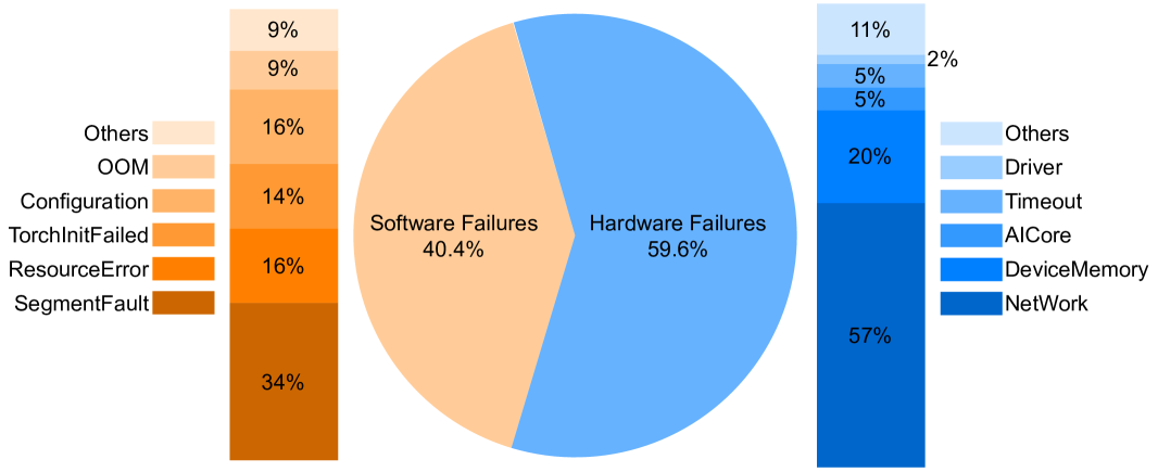<details> <summary>x11.png Details</summary>  ### Visual Description # Technical Data Extraction: Failure Analysis Breakdown This document provides a comprehensive extraction of data from the provided infographic, which illustrates the distribution and sub-categorization of system failures. ## 1. Overview (Main Chart) The central component is a pie chart dividing total failures into two primary categories. | Category | Percentage | Color Code | | :--- | :--- | :--- | | **Hardware Failures** | 59.6% | Blue | | **Software Failures** | 40.4% | Orange/Peach | --- ## 2. Software Failures Breakdown (Left Segment) The software failures (40.4% of total) are further decomposed into six sub-categories via a stacked bar chart and a corresponding legend. ### Legend and Spatial Grounding The legend is located on the far left. The bar chart is positioned between the legend and the central pie chart. The color gradient transitions from dark orange (bottom) to light peach (top). ### Data Table: Software Sub-categories | Sub-category | Percentage (of Software Failures) | Color Description | | :--- | :--- | :--- | | **SegmentFault** | 34% | Dark Brownish-Orange | | **ResourceError** | 16% | Deep Orange | | **TorchInitFailed** | 14% | Vibrant Orange | | **Configuration** | 16% | Medium Orange | | **OOM** (Out of Memory) | 9% | Light Orange | | **Others** | 9% | Pale Peach | **Trend Analysis:** "SegmentFault" is the dominant software failure mode, accounting for over one-third of software issues. "ResourceError," "TorchInitFailed," and "Configuration" represent a middle tier of frequency (14-16% each), while "OOM" and "Others" are the least frequent. --- ## 3. Hardware Failures Breakdown (Right Segment) The hardware failures (59.6% of total) are decomposed into six sub-categories via a stacked bar chart and a corresponding legend. ### Legend and Spatial Grounding The legend is located on the far right. The bar chart is positioned between the central pie chart and the legend. The color gradient transitions from dark blue (bottom) to very light blue (top). ### Data Table: Hardware Sub-categories | Sub-category | Percentage (of Hardware Failures) | Color Description | | :--- | :--- | :--- | | **NetWork** | 57% | Dark Navy Blue | | **DeviceMemory** | 20% | Bright Blue | | **AICore** | 5% | Medium Blue | | **Timeout** | 5% | Sky Blue | | **Driver** | 2% | Light Blue | | **Others** | 11% | Pale Blue | **Trend Analysis:** The hardware failure distribution is highly skewed. "NetWork" issues constitute the vast majority (57%) of hardware-related failures. "DeviceMemory" is the second most significant factor at 20%. All other specific categories (AICore, Timeout, Driver) are relatively minor, though the "Others" category is notable at 11%. --- ## 4. Summary of Findings * **Primary Driver:** Hardware failures are the more frequent cause of system issues (59.6%). * **Critical Hardware Point:** Network issues are the single largest specific failure point across the entire dataset (57% of the 59.6% hardware share). * **Critical Software Point:** SegmentFault is the leading software issue (34% of the 40.4% software share). * **Terminology Note:** * **OOM:** Likely refers to "Out of Memory." * **TorchInitFailed:** Likely refers to initialization failures in the PyTorch machine learning framework. * **AICore:** Refers to failures in specialized AI processing units. </details> Figure 9: The types and frequencies of observed failures. IV-B Evaluation of Communication Group Establishment This study implements a parallelized strategy for TCP Store establishment and an optimized ranktable update that eliminates any negotiation with the master node. First, we analyze the time required for TCP Store establishment under two approaches: (1) the serialized procedure, and (2) the parallelized procedure across varying scales of training clusters. Experimental results indicate that the original serialized link establishment method (green line in Fig. 10) exhibits near-linear time complexity with respect to cluster scale. In contrast, our system uses the parallelized approach (red line in Fig. 10) that significantly reduces the scaling coefficient and effectively decouples establishment overhead from cluster scale. Secondly, we evaluate the time cost of ranktable updates before and after the introduction of a global ranktable. The default way for updating a ranktable requires message collection and distribution between every device and the master node, with a time cost proportional to the scale of the training cluster (i.e., $O(n)$ ). This relationship is confirmed by observations in the first row of Tab. I. In contrast, FlashRecovery’s controller maintains an up-to-date global ranktable, which can be loaded via a shared file. This eliminates communication overhead for ranktable updates and accelerates the process. Experimental results demonstrate that the time cost of updating the ranktable via a shared file (bottom row of Tab. I) is optimized to a constant (i.e., $O(1)$ ), significantly improving efficiency. TABLE I: The time of ranktable updating (in seconds). | Num. of Devices | 1, 000 | 4, 000 | 8, 000 | 16, 000 | 18, 000 | | --- | --- | --- | --- | --- | --- | | Original ranktable updating | 8 | 31 | 60 | 176 | 249 | | Loading ranktable directly | 0.1 | 0.1 | $<0.5$ | $<0.5$ | $<0.5$ | IV-C Assessment of Overall Failure Recovery Time We first evaluate the recovery time ( $s_{0}$ in equation 1) of a vanilla method for different task scales, details of which are provided in Tab. II. We use the default configuration of PyTorch. A failure is reported when a communication hang lasts 1, 800 seconds. The task restarting time increases linearly with the task scale, as illustrated in the last column of Tab. II. Since a failure occur randomly between two consecutive checkpoints, we do not include the recomputation cost ( $s_{1}$ in equation 1, i.e., the wasted work from the last checkpoint to the step that a failure occurs). 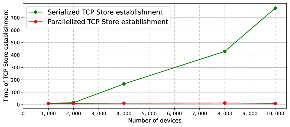<details> <summary>x12.png Details</summary>  ### Visual Description # Technical Data Extraction: TCP Store Establishment Performance ## 1. Component Isolation * **Header/Legend:** Located in the top-left quadrant of the chart area. * **Main Chart Area:** A line graph with a light gray background and a dashed grid. * **X-Axis (Horizontal):** Represents the independent variable "Number of devices". * **Y-Axis (Vertical):** Represents the dependent variable "Time of TCP Store establishment". ## 2. Axis and Legend Information * **Y-Axis Title:** Time of TCP Store establishment (Units not explicitly stated, likely milliseconds or seconds based on scale). * **Y-Axis Markers:** 0, 100, 200, 300, 400, 500, 600, 700. * **X-Axis Title:** Number of devices. * **X-Axis Markers:** 0, 1,000, 2,000, 3,000, 4,000, 5,000, 6,000, 7,000, 8,000, 9,000, 10,000. * **Legend [Top-Left]:** * **Green Line with Circle Markers:** Serialized TCP Store establishment. * **Red Line with Circle Markers:** Parallelized TCP Store establishment. ## 3. Trend Verification and Data Extraction ### Series 1: Serialized TCP Store establishment (Green Line) * **Visual Trend:** This line slopes upward significantly. The slope is relatively shallow between 1,000 and 2,000 devices, becomes steeper and linear between 2,000 and 8,000, and shows a further increase in steepness between 8,000 and 10,000 devices. This indicates that as the number of devices increases, the time required grows at an accelerating rate (super-linear). * **Data Points (Approximate):** * 1,000 devices: ~10 * 2,000 devices: ~20 * 4,000 devices: ~170 * 8,000 devices: ~430 * 10,000 devices: ~780 ### Series 2: Parallelized TCP Store establishment (Red Line) * **Visual Trend:** This line is nearly horizontal (flat). It shows almost no visible increase in time as the number of devices scales from 1,000 to 10,000. This indicates high efficiency and scalability, where the establishment time is independent of the device count within this range. * **Data Points (Approximate):** * 1,000 devices: ~10 * 2,000 devices: ~10 * 4,000 devices: ~10 * 8,000 devices: ~10 * 10,000 devices: ~10 ## 4. Data Table Reconstruction | Number of Devices | Serialized Time (Green) | Parallelized Time (Red) | | :--- | :--- | :--- | | 1,000 | ~10 | ~10 | | 2,000 | ~20 | ~10 | | 4,000 | ~170 | ~10 | | 8,000 | ~430 | ~10 | | 10,000 | ~780 | ~10 | ## 5. Summary of Findings The chart demonstrates a critical performance difference between serialized and parallelized methods for TCP Store establishment. While both methods perform similarly at a low scale (1,000 devices), the **Serialized** method experiences a massive performance degradation as the network grows, reaching nearly 800 units of time at 10,000 devices. In contrast, the **Parallelized** method maintains a constant, low establishment time (approximately 10 units) regardless of the number of devices, showcasing superior scalability. </details> Figure 10: The time cost of TCP Store establishment under different approaches (in seconds). To assess the efficacy of FlashRecovery, we artificially inject faults during the standard training process and record the time taken for each stage in the recovery. From the 3rd column of Tab. III, our system is able to sense a failure within 10 seconds. And from the 4th column of Tab. III, the restart time in our system is almost invariable and becomes independent of the scale of a training cluster. In addition, according to the assumption about $s_{1}$ , we use the average time of one step to estimate the time of redone training, i.e., half of the redone step (shown in the 6th column in Tab. III). The variation on the scale of training clusters has much less impact on the total recovery time. Although we increase the number of devices from 32 to 4, 800, the total recovery time is still able to remains in 150 seconds, which increase about 52% and is much less than the rising on the number of devices (150 $×$ ). In short, the results in Tab. III show that the time required for failure recovery by our system is nearly scalability-agnostic. TABLE II: The recovery time of vanilla recovery method at different task scales (in seconds). | Num. of Parameters | Num. of Devices | Failure Detection Time | Task Restarting Time | | --- | --- | --- | --- | | 175B | 1, 824 | 1, 800 | 231 | | 175B | 3, 936 | 1, 800 | 801 | | 175B | 5, 472 | 1, 800 | 1, 115 | TABLE III: Recovery time of our method for different task scales and model sizes (in seconds). | Num. of Parameters | Num. of Devices | Failure Detection Time | Task Restarting Time | Redone Training | Total Time | | | --- | --- | --- | --- | --- | --- | --- | | step | step/2 | | | | | | | 7B | 32 | 6 | 88 | 6 | 3 | 97 | | 7B | 960 | 6 | 92 | 6 | 3 | 101 | | 70B | 80 | 4 | 84 | 4 | 2 | 90 | | 70B | 800 | 9 | 92 | 20 | 10 | 111 | | 70B | 960 | 8 | 78 | 24 | 12 | 98 | | 70B | 2, 880 | 11 | 90 | 39 | 19.5 | 120.5 | | 175B | 2, 880 | 10 | 90 | 79 | 39.5 | 139.5 | | 175B | 4, 800 | 7 | 116 | 49 | 24.5 | 147.5 | V Related Work V-A Comprehensive Failure Recovery System A variety of comprehensive failure recovery systems have been proposed, mainly encompassing failure detection, task rescheduling, and/or training restart mechanisms. TRANSOM [16] is a fault-tolerant system for large-scale model training, which integrates an automatic fault tolerance and recovery mechanism, an automatic anomaly detection system and the asynchronous checkpoint saving technology. Unicron [17] is a workload manager designed for self-healing in LLM training, demonstrating up to a 1.9 $×$ improvement in training efficiency. Its key features include in-band error detection for real-time error identification, a dynamic cost aware plan generation mechanism for optimal reconfiguration, and a transition strategy to reduce downtime during state changes. MegaScale [18] has developed a set of diagnostic tools designed to monitor system components and events. These tools focus on identifying root causes of issues and deriving effective techniques to achieve fault tolerance and mitigate stragglers. As a result, MegaScale improves Model FLOPs Utilization (MFU) by 1.34 $×$ compared to Megatron-LM. MoC-System [19] is a fault tolerance system specifically designed for the sparse Mixture-of-Experts model. It incorporates 1) partial experts checkpointing mechanism, 2) fully sharded checkpointing strategies, and 3) a two-level checkpointing management method to enhance reliability and efficiency. However, these systems are often customized for specific scenarios, making it difficult to achieve claimed performance in different training environments and configurations. Diversity in hardware, network architecture, and workload characteristics may complicate the implementation of these fault recovery systems. V-B Checkpointing Performance Optimization Checkpointing is a common practice for failure recovery in LLM training. Due to the substantial sizes of LLMs, a straightforward checkpointing solution that directly dumps model states to persistent storage incurs significant I/O overhead. To address this challenge, a range of checkpoint performance optimization methods has been developed to minimize the associated overheads. Checkpionting Speed Up Checkpointing typically consists of two phases [20]: (1) snapshot phase ( $k_{0}$ in Fig. 2), (2) persist phase ( $k_{1}$ in Fig. 2). To address the time cost associated with checkpointing, several approaches have been developed to decouple these two phases, which allow training to stall for only a few seconds during the snapshot phase while asynchronously persisting snapshots using dedicated background CPU processes. DataStates-LLM [21] introduces a lazy asynchronous multi-level approach that overlaps checkpoint I/O with the immutable phases of forward and backward passes during training and speeds up checkpointing by a factor of 3× to 4.2×. CheckFreq [22] features a resumable data iterator and a pipelined two-phase checkpointing mechanism, by which a consistent and low-cost checkpointing at the iteration level is achieved. LightCheck [23] implements a fine-grained checkpointing scheme and a persistent memory (PM) manager. The checkpointing scheme pipelines checkpointing with computation and communication in a layer-wise manner. Additionally, the persistent memory is mapped into GPU virtual memory space and separates the storage of metadata and data of tensors in PM. Some other approaches aim to reduce I/O overhead during checkpointing. Check-N-Run [24] takes advantage of the fact that only a fraction of the recommendation model is updated in each iteration and proposes an incremental checkpointing strategy, which is primarily limited to recommendation models. DeepFreeze [25] combines lightweight serialization, sharding checkpointing across data-parallel GPUs, and the augmentation of the execution graph to asynchronously mask the overhead of capturing weights from tensors. Universal checkpointing [26] decouples distributed checkpoint storage from parallelism methods, providing the flexibility to resume operations using various parallelism strategies and hardware configurations. ByteCheckpoint [27] advocates for a parallelism-agnostic checkpoint representation and a generic workflow for saving and loading checkpoints. Although the methods mentioned above can significantly reduce periodic checkpointing time costs, the enlarged checkpointing duration cannot be fully overlapped with the training process, a trade-off remains between checkpointing frequency and the time lost during recovery from failures. Just-In-Time Checkpointing Several approaches aim to avoid checkpointing until an error occurs, which can reduce the steady-state overhead associated with periodic checkpointing while minimizing wasted work during recovery. Just-In-Time Checkpointing [12] introduces user-level recovery solutions and transparent error recovery mechanisms. It captures just-in-time checkpoints immediately after failures occur, allowing training to resume seamlessly from these JIT checkpoints. The Update-Undo Mechanism, proposed by Swift [28], enables failure recovery with replicas of a model state in data parallelism. Additionally, Swift advocates for employing asynchronous logging methods to expedite failure recovery in pipeline parallelism. While both Just-In-Time Checkpointing and Swift offer improvements in reducing steady-state overhead, they still require checkpoints when failures occur, which can stall the recovery process and lead to delays in resuming training. Parcae [29] further eliminates the need to restart and roll back to previous checkpoints when failures occur. Instead, it transfers valid model states from the remaining healthy instances to reconfigured nodes. However, Parcae is specifically designed for LLM training on preemptible instances and requires adjustments to the parallelization strategy. VI Conclusions This paper presents the design and implementation of FlashRecovery, a fast and low-cost failure recovery system for large-scale training of LLMs. By incorporating a novel active and real-time failure detection mechanism, along with a scale-independent task restart mechanism and checkpoint-free recovery within one step, FlashRecovery can reduce the failure recovery time overhead of a training cluster with thousands of devices to less than 150 seconds and almost achieve the optimal RPO and RTO. In the future, we will focus on standardizing the system’s interfaces to improve usability, optimizing the recovery process and further reducing the total recovery time to 30 seconds for clusters with more than 10, 000 devices. References - [1] J. Achiam, S. Adler, S. Agarwal, L. Ahmad, I. Akkaya, F. L. Aleman, D. Almeida, J. Altenschmidt, S. Altman, S. Anadkat et al., “Gpt-4 technical report,” arXiv preprint arXiv:2303.08774, 2023. - [2] J. Liu, C. S. Xia, Y. Wang, and L. Zhang, “Is your code generated by chatgpt really correct? rigorous evaluation of large language models for code generation,” Advances in Neural Information Processing Systems, vol. 36, pp. 21 558–21 572, 2023. - [3] S. L. Song, B. Kruft, M. Zhang, C. Li, S. Chen, C. Zhang, M. Tanaka, X. Wu, J. Rasley, A. A. Awan et al., “Deepspeed4science initiative: Enabling large-scale scientific discovery through sophisticated ai system technologies,” arXiv preprint arXiv:2310.04610, 2023. - [4] J. Kaplan, S. McCandlish, T. Henighan, T. B. Brown, B. Chess, R. Child, S. Gray, A. Radford, J. Wu, and D. Amodei, “Scaling laws for neural language models,” arXiv preprint arXiv:2001.08361, 2020. - [5] S. Rajbhandari, J. Rasley, O. Ruwase, and Y. He, “Zero: Memory optimizations toward training trillion parameter models,” in SC20: International Conference for High Performance Computing, Networking, Storage and Analysis. IEEE, 2020, pp. 1–16. - [6] S. Li, H. Liu, Z. Bian, J. Fang, H. Huang, Y. Liu, B. Wang, and Y. You, “Colossal-ai: A unified deep learning system for large-scale parallel training,” in Proceedings of the 52nd International Conference on Parallel Processing, 2023, pp. 766–775. - [7] M. Shoeybi, M. Patwary, R. Puri, P. LeGresley, J. Casper, and B. Catanzaro, “Megatron-lm: Training multi-billion parameter language models using model parallelism,” arXiv preprint arXiv:1909.08053, 2019. - [8] T. Le Scao, A. Fan, C. Akiki, E. Pavlick, S. Ilić, D. Hesslow, R. Castagné, A. S. Luccioni, F. Yvon, M. Gallé et al., “Bloom: A 176b-parameter open-access multilingual language model,” 2023. - [9] “Metaseq: Opt-175 logbook,” https://github.com/facebookresearch/metaseq/blob/main/projects/OPT/chronicles/OPT175B_Logbook.pdf, accessed: 2024-03-07. - [10] A. Dubey, A. Jauhri, A. Pandey, A. Kadian, A. Al-Dahle, A. Letman, A. Mathur, A. Schelten, A. Yang, A. Fan et al., “The llama 3 herd of models,” arXiv preprint arXiv:2407.21783, 2024. - [11] O. H. Alhazmi and Y. K. Malaiya, “Evaluating disaster recovery plans using the cloud,” in 2013 Proceedings Annual Reliability and Maintainability Symposium (RAMS), 2013, pp. 1–6. - [12] T. Gupta, S. Krishnan, R. Kumar, A. Vijeev, B. Gulavani, N. Kwatra, R. Ramjee, and M. Sivathanu, “Just-in-time checkpointing: Low cost error recovery from deep learning training failures,” in Proceedings of the Nineteenth European Conference on Computer Systems, 2024, pp. 1110–1125. - [13] D. Narayanan, M. Shoeybi, J. Casper, P. LeGresley, M. Patwary, V. Korthikanti, D. Vainbrand, P. Kashinkunti, J. Bernauer, B. Catanzaro et al., “Efficient large-scale language model training on gpu clusters using megatron-lm,” in Proceedings of the international conference for high performance computing, networking, storage and analysis, 2021, pp. 1–15. - [14] Y. Huang, Y. Cheng, A. Bapna, O. Firat, D. Chen, M. Chen, H. Lee, J. Ngiam, Q. V. Le, Y. Wu et al., “Gpipe: Efficient training of giant neural networks using pipeline parallelism,” Advances in neural information processing systems, vol. 32, 2019. - [15] V. A. Korthikanti, J. Casper, S. Lym, L. McAfee, M. Andersch, M. Shoeybi, and B. Catanzaro, “Reducing activation recomputation in large transformer models,” Proceedings of Machine Learning and Systems, vol. 5, pp. 341–353, 2023. - [16] B. Wu, L. Xia, Q. Li, K. Li, X. Chen, Y. Guo, T. Xiang, Y. Chen, and S. Li, “Transom: an efficient fault-tolerant system for training llms,” arXiv preprint arXiv:2310.10046, 2023. - [17] T. He, X. Li, Z. Wang, K. Qian, J. Xu, W. Yu, and J. Zhou, “Unicron: Economizing self-healing llm training at scale,” arXiv preprint arXiv:2401.00134, 2023. - [18] Z. Jiang, H. Lin, Y. Zhong, Q. Huang, Y. Chen, Z. Zhang, Y. Peng, X. Li, C. Xie, S. Nong et al., “Megascale: Scaling large language model training to more than 10,000 gpus,” in 21st USENIX Symposium on Networked Systems Design and Implementation (NSDI 24), 2024, pp. 745–760. - [19] W. Cai, L. Qin, and J. Huang, “Moc-system: Efficient fault tolerance for sparse mixture-of-experts model training,” arXiv preprint arXiv:2408.04307, 2024. - [20] J. Duan, S. Zhang, Z. Wang, L. Jiang, W. Qu, Q. Hu, G. Wang, Q. Weng, H. Yan, X. Zhang et al., “Efficient training of large language models on distributed infrastructures: a survey,” arXiv preprint arXiv:2407.20018, 2024. - [21] A. Maurya, R. Underwood, M. M. Rafique, F. Cappello, and B. Nicolae, “Datastates-llm: Lazy asynchronous checkpointing for large language models,” in Proceedings of the 33rd International Symposium on High-Performance Parallel and Distributed Computing, 2024, pp. 227–239. - [22] J. Mohan, A. Phanishayee, and V. Chidambaram, “Checkfreq: Frequent, fine-grained dnn checkpointing,” in 19th USENIX Conference on File and Storage Technologies (FAST 21), 2021, pp. 203–216. - [23] M. Chen, Y. Hua, R. Bai, and J. Huang, “A cost-efficient failure-tolerant scheme for distributed dnn training,” in 2023 IEEE 41st International Conference on Computer Design (ICCD). IEEE, 2023, pp. 150–157. - [24] A. Eisenman, K. K. Matam, S. Ingram, D. Mudigere, R. Krishnamoorthi, K. Nair, M. Smelyanskiy, and M. Annavaram, “Check-n-run: A checkpointing system for training deep learning recommendation models,” in 19th USENIX Symposium on Networked Systems Design and Implementation (NSDI 22), 2022, pp. 929–943. - [25] B. Nicolae, J. Li, J. M. Wozniak, G. Bosilca, M. Dorier, and F. Cappello, “Deepfreeze: Towards scalable asynchronous checkpointing of deep learning models,” in 2020 20th IEEE/ACM International Symposium on Cluster, Cloud and Internet Computing (CCGRID). IEEE, 2020, pp. 172–181. - [26] X. Lian, S. A. Jacobs, L. Kurilenko, M. Tanaka, S. Bekman, O. Ruwase, and M. Zhang, “Universal checkpointing: Efficient and flexible checkpointing for large scale distributed training,” arXiv preprint arXiv:2406.18820, 2024. - [27] B. Wan, M. Han, Y. Sheng, Y. Peng, H. Lin, M. Zhang, Z. Lai, M. Yu, J. Zhang, Z. Song et al., “Bytecheckpoint: A unified checkpointing system for large foundation model development,” arXiv preprint arXiv:2407.20143, 2024. - [28] Y. Zhong, G. Sheng, J. Liu, J. Yuan, and C. Wu, “Swift: Expedited failure recovery for large-scale dnn training,” in Proceedings of the 28th ACM SIGPLAN Annual Symposium on Principles and Practice of Parallel Programming, 2023, pp. 447–449. - [29] J. Duan, Z. Song, X. Miao, X. Xi, D. Lin, H. Xu, M. Zhang, and Z. Jia, “Parcae: Proactive,liveput-optimized dnn training on preemptible instances,” in 21st USENIX Symposium on Networked Systems Design and Implementation (NSDI 24), 2024, pp. 1121–1139.