# The Illusion of Diminishing Returns: Measuring Long Horizon Execution in LLMs
**Authors**:
- Steffen Staab Jonas Geiping (University of Cambridge Institute for AI, University of Stuttgart)
Abstract
Does continued scaling of large language models (LLMs) yield diminishing returns? In this work, we show that short-task benchmarks may give an illusion of slowing progress, as even marginal gains in single-step accuracy can compound into exponential improvements in the length of tasks a model can successfully complete. Then, we argue that failures of LLMs when simple tasks are made longer arise from mistakes in execution, rather than an inability to reason. So, we propose isolating execution capability, by explicitly providing the knowledge and plan needed to solve a long-horizon task. First, we find that larger models can correctly execute significantly more turns even when small models have near-perfect single-turn accuracy. We then observe that the per-step accuracy of models degrades as the number of steps increases. This is not just due to long-context limitations—curiously, we observe a self-conditioning effect—models become more likely to make mistakes when the context contains their errors from prior turns. Self-conditioning does not reduce by just scaling the model size. But, we find that thinking mitigates self-conditioning, and also enables execution of much longer tasks in a single turn. We conclude by benchmarking frontier thinking models on the length of tasks they can execute in a single turn. Overall, by focusing on the ability to execute, we hope to reconcile debates on how LLMs can solve complex reasoning problems yet fail at simple tasks when made longer, and highlight the massive benefits of scaling model size and sequential test-time compute for long-horizon tasks.
Code ? Dataset
1 Introduction
Is continued scaling of compute for Large Language Models (LLMs) economically justified given diminishing marginal gains? This question lies at the heart of the ongoing debate on the viability of continued massive investments in LLMs. While scaling laws show diminishing returns on metrics like test loss, the true economic potential of LLMs might arise from automating long, multi-step tasks (METR, 2025). However, long-horizon tasks have been the Achilles’ heel of Deep Learning. We see recent vision models generating impressive images, yet consistency over long videos remains an unsolved challenge. As the industry races to build agents that tackle entire projects, not just isolated questions, a fundamental question arises:
How can we measure the number of steps an LLM can reliably execute?
<details>
<summary>x1.png Details</summary>
### Visual Description
# Technical Document Extraction: AI Model Performance and Scaling Analysis
This document provides a comprehensive extraction of data and conceptual diagrams from the provided image, which analyzes the relationship between model accuracy, task length, scaling, and self-conditioning in Large Language Models (LLMs).
---
## 1. Top Left Panel: Diminishing Gains vs. Exponential Gains
**Header:** Diminishing Gains On A Single Step Can Lead To Exponential Gains Over Long Horizon
**Sub-caption:** *assuming step accuracy is constant across all steps of the task*
### Chart A: Step Accuracy vs. Model Release Date
* **Y-Axis:** Step Accuracy (Range: 0.92 to 1.00)
* **X-Axis:** Model Release Date (Time progression)
* **Trend:** A red logarithmic curve showing rapid initial improvement that plateaus as it approaches 1.00 (100% accuracy).
* **Data Points (Color-coded markers):**
* **Pink:** ~0.987 accuracy.
* **Green:** ~0.998 accuracy.
* **Yellow:** ~0.999 accuracy.
* **Light Blue:** ~1.000 accuracy.
### Chart B: Task Length vs. Model Release Date
* **Y-Axis:** Task Length (Linear scale: 0k to 20k)
* **X-Axis:** Model Release Date
* **Trend:** A blue exponential curve. While step accuracy (Chart A) shows diminishing returns, the resulting maximum task length achievable grows exponentially.
* **Data Points (Mapped from Chart A):**
* **Pink:** ~0.5k task length.
* **Green:** ~1.5k task length.
* **Yellow:** ~7.5k task length.
* **Light Blue:** ~17.5k task length.
---
## 2. Top Right Panel: Self-Conditioning and Error Propagation
**Header:** Models Self-Condition On Their Errors, Taking Worse Steps
### Conceptual Chart: Step Accuracy vs. Task Length
* **Y-Axis:** Step Accuracy
* **X-Axis:** Task Length
* **Series 1 (Green Line):** "Expected" - A horizontal line representing constant accuracy.
* **Series 2 (Red Line):** "Observed" - A downward sloping curve showing that as task length increases, step accuracy degrades.
### Diagram: Execution History Comparison
* **Left Scenario (Success):**
* **Execution History:** Five green checkmarks.
* **Input:** User icon + "Add 56 and -92".
* **Model State:** Smiling robot icon.
* **Output:** `56 + -92 = -36` [Green Checkmark].
* **Right Scenario (Failure due to Self-Conditioning):**
* **Execution History:** Two green checkmarks followed by three red "X" marks.
* **Input:** User icon + "Add 56 and -92".
* **Model State:** Sad/Confused robot icon.
* **Output:** `56 + -92 = -24` [Red X].
* **Logic:** The diagram illustrates that previous errors in the history cause the model to perform worse on subsequent steps.
---
## 3. Bottom Left Panel: Scaling and Task Length
**Header:** Scaling Model Size Enables Execution of Longer Tasks
| Model Family | Parameter Count (Billion) | Task Length (Approx.) |
| :--- | :--- | :--- |
| Gemma3 (Red) | 2 | 3 |
| Gemma3 (Red) | 12 | 4 |
| Gemma3 (Red) | 27 | 9 |
| Qwen3 (Blue) | 8 | 4 |
| Qwen3 (Blue) | 14 | 5 |
| Qwen3 (Blue) | 32 | 12 |
* **Trends:** Both model families show a positive linear correlation between parameter count and task length.
---
## 4. Bottom Middle Panel: Thinking and Long Tasks
**Header:** Thinking Enables Execution of Long Tasks In A Single Turn
* **Y-Axis:** Task Length (Single Turn) - Logarithmic Scale ($2^6$ to $2^{12}$)
* **Legend:**
* **Solid Grey:** Thinking
* **Hatched Grey:** Chain-of-Thought
| Model | Task Length (Log Scale) | Visual Style |
| :--- | :--- | :--- |
| Kimi-K2 | ~$2^{6.2}$ | Solid Grey |
| Deepseek V3 | ~$2^{6.8}$ | Hatched Blue |
| Gemini-2.5-Pro | ~$2^{6.9}$ | Solid Light Blue |
| Deepseek-R1 | ~$2^{6.9}$ | Solid Blue |
| Grok-4 | ~$2^{8.5}$ | Solid Grey |
| Claude-4-Sonnet | ~$2^{8.8}$ | Solid Orange |
| GPT-5 | ~$2^{11.1}$ | Solid Dark Grey |
---
## 5. Bottom Right Panel: Self-Conditioning Sensitivity
**Header:** Larger Models Are More Prone To Self-Conditioning
* **Y-Axis:** Turn 100 Accuracy (Scale: 0.0 to 1.0)
* **X-Axis:** Induced Error Rate (Scale: 0.00 to 1.00)
* **Trend Verification:** All lines slope downward. As the induced error rate increases, the accuracy at turn 100 drops.
* **Key Observation:** The largest model (Qwen3-32b) starts with the highest accuracy at 0.00 error rate (~0.85) but has the steepest decline, indicating higher sensitivity to previous errors.
| Model | Accuracy at 0.00 Induced Error | Accuracy at 1.00 Induced Error |
| :--- | :--- | :--- |
| Qwen3-32b (Darkest Blue) | 0.85 | 0.20 |
| Qwen3-14b (Medium Blue) | 0.80 | 0.25 |
| Qwen3-8b (Light Blue) | 0.50 | 0.10 |
| Qwen3-4b (Lightest Blue) | 0.25 | 0.05 |
</details>
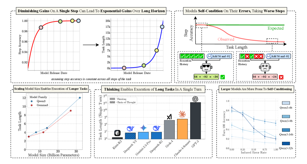
Figure 1: A summary of our contributions. Our work measures long-horizon execution, finding large benefits from scaling model size and sequential test-time compute. We identify a failure mode where models self-condition on their own errors, degrading future performance.
LLM failures on simple, but long tasks have been considered a fundamental inability to reason (Mirzadeh et al., 2024). Despite massive improvements on complex reasoning benchmarks, Shojaee et al. (2025) claim thinking models (Guo et al., 2025) only give an “illusion of thinking”, as they eventually fail when the task is made longer. These results have sparked much debate in the community, which we think can be resolved by decoupling the need for planning and execution in reasoning or agentic tasks. Planning involves deciding what information to retrieve or tools to use and in which order, while execution involves carrying out the plan. In Shojaee et al. (2025) setup, the LLMs know the correct plan, as they initially follow it correctly for many steps. We posit that the eventual failures are in execution—as the task gets longer, the model is more likely to make a mistake in executing the plan. Although much attention has been paid to LLM planning abilities (Kambhampati et al., 2024), execution remains an understudied challenge, despite being increasingly important as LLMs begin to be used for long reasoning and agentic tasks.
In this work, we measure long-horizon execution capabilities of LLMs in a controlled setting. We isolate the execution capability of LLMs by explicitly providing them the knowledge and plan needed. By controlling the number of turns, and the number of steps per turn, which together contribute to task length, we reveal insights about long-horizon execution in LLMs:
Does Scaling have Diminishing Returns? We observe that diminishing improvements in single-step accuracy can compound, leading to exponential growth in the length of task a model can complete. Traditionally, scaling model size is assumed to increase capacity to store parametric knowledge or search for plans. Yet, even when the required knowledge and plan are explicitly provided, we find that scaling model size leads to large improvements in the number of turns a model can execute successfully.
The Self-Conditioning Effect. One might assume that failures on long tasks are simply due to the compounding of a small, constant per-step error rate and context length issues. However, we find that the per-step error rate itself rises as the task progresses. This is in contrast to humans, who typically improve at executing a task with practice. We hypothesize that, as a significant fraction of model training is to predict the most likely next token given its context, conditioning models on their own error-prone history increases the likelihood of future errors. We test this by controlling the error rate in the history provided to the model. As the error rate in the history is increased, we observe a sharp degradation in subsequent step accuracy, validating that models self-condition. We show how self-conditioning leads to degradation in model performance in long-horizon tasks beyond previously identified long-context issues, and unlike the latter, is not mitigated by scaling model size.
The Impact of Thinking. We find that recent thinking models are not affected by prior mistakes, fixing the self-conditioning effect. Further, sequential test time compute also significantly improves the length of task a model can complete in a single turn. Where, without chain-of-thought prompting, even frontier LLMs like DeepSeek-V3 fail at performing even four steps of execution, and its thinking version R1 can execute over 100 steps, highlighting the importance of reasoning before acting (Yao et al., 2023). We benchmark frontier thinking models, and find GPT-5 thinking (codenamed “Horizon”) can execute over 2100 steps, far ahead of the next best competitor, Claude-4 Sonnet at 432.
The “jagged frontier” (Dell’Acqua et al., 2023) of LLM capabilities remains fascinating yet confusing. Unlike traditional machines, LLMs are more susceptible to failure when used for executing repetitive tasks. Thus, we argue that execution failures in long tasks should not be misinterpreted as the inability to reason. We show that long-horizon execution improves dramatically by scaling model size and sequential test time compute. If the length of tasks a model can complete indicates its economic value, continued investment in scaling compute might be worth the cost, even if short-task benchmarks give the illusion of slowing progress.
2 Formulation
First, we define key capabilities involved in an agentic or reasoning task. As a motivating example, consider an agent for the task of booking flights. Upon receiving a search result, the agent must reason to choose a flight that aligns with user preferences. One plan for this reasoning task could be:
For each flight, verify the flight timings, baggage allowance, and airline reviews. Then apply any available discounts or reward programs, and finally select a flight based on cost and travel time.
Each of these individual steps requires two operations: retrieving some information, and composing it with the existing information state, until the goal of choosing the final flight is reached. Both these operations require knowledge, potentially tacit, about how to perform them. Execution is carrying out this plan, a sequence of retrieve-then-compose steps, until a final booking is made. We formalize these terms for our work as follows:
Key Terms
Planning.
Deciding what steps to take, and in what sequence. Execution.
Carrying out the steps decided in the plan. Knowledge.
Information about different types of steps, and how to compose them. A reasoning task.
Requires planning the steps needed to solve it, and then executing them. An agentic task.
Requires planning what actions to take, and then executing them.
In this work, we focus on execution, as we argue that it is a critical component of long-horizon capabilities. Execution has traditionally received less attention (Stechly et al., 2024) than capabilities such as reasoning, planning, and world knowledge, which have been the primary focus of LLM capability discussions. In fact, failures in execution have been misattributed to limitations in reasoning or planning capabilities (Shojaee et al., 2025; Khan et al., 2025). This perception may stem from the view that execution is straightforward or mundane. For example, once we as humans learn how to do a task, we are quite reliable at executing it, even improving with practice. However, as LLMs do not come with correctness guarantees, we posit that just execution over a long horizon can surprisingly be a challenge. We hypothesize that:
Even if planning and world knowledge are perfected, LLMs will still make mistakes in execution over a long-horizon.
In an agentic or reasoning task, the model begins in an initial state (based on the first input) and has to perform a sequence of steps to reach the final goal. A long-horizon task requires a large number of steps, with the task length being the number of steps needed to complete it. We define the following metrics to evaluate performance:
Evaluation Metrics
Step Accuracy.
Measures the fraction of samples where the state update from step $i-1$ to step $i$ is correct, regardless of the correctness of the model’s state at step $i-1$ . Turn Accuracy.
A turn is a single interaction with the model, which may require executing multiple steps. Turn Accuracy measures the fraction of samples where the state update from turn $t-1$ to turn $t$ is correct, regardless of the correctness of the model’s state at turn $t-1$ . Turn Complexity ( $K$ ).
Defined as the number of steps the model has to execute per turn. Task Accuracy.
Measures the fraction of samples in which the model can complete a task of $i$ steps without making any mistakes in the process. Horizon Length ( $H_{s}$ ).
Given a success rate threshold $0≤ s≤ 1$ , the horizon length is the first step $i$ where the model’s mean task accuracy across samples drops below $s$ . It can be interpreted as: the model can perform a task of length $H_{s}$ without making mistakes, with probability $s$ . We use $s=0.5$ unless otherwise specified, like Kwa et al. (2025).
2.1 Diminishing Returns in Step Accuracy Compound Over a Long Horizon
We begin by analyzing the relationship between a model’s single-step accuracy and its horizon length. Note that this analysis applies not just to execution, but rather to any general long-horizon task. To obtain a mathematical relation, we make two simplifying assumptions similar to LeCun (2023). First, we assume a model’s step accuracy remains constant over the task. Second, we assume a model does not self-correct, meaning any single error leads to task failure. We assume this only for the analysis here, which is illustrative and provides useful intuition. Our subsequent empirical analysis goes beyond this, investigating how LLMs, in fact, do not exhibit constant step accuracy for long-horizon execution, and may also correct their mistakes.
<details>
<summary>figs/math_plot.png Details</summary>
### Visual Description
# Technical Document Extraction: Horizon Length vs. Step Accuracy
## 1. Image Overview
This image is a technical line chart illustrating the relationship between **Step Accuracy ($p$)** and **Horizon Length**. It features five distinct data series, each representing a different threshold or parameter denoted as $H_{\text{value}}$. The chart uses a logarithmic-like growth pattern where the Horizon Length increases exponentially as Step Accuracy approaches 1.
---
## 2. Component Isolation
### A. Header / Legend
* **Location:** Top-left quadrant of the chart area.
* **Content:** A white box with a light gray border containing five entries.
* **Legend Items (Color-Coded):**
1. **Yellow Line:** $H_{0.10}$
2. **Orange Line:** $H_{0.25}$
3. **Pink/Magenta Line:** $H_{0.50}$
4. **Purple Line:** $H_{0.75}$
5. **Dark Indigo/Violet Line:** $H_{0.90}$
### B. Main Chart Area (Axes and Grid)
* **Y-Axis (Vertical):**
* **Label:** "Horizon Length"
* **Scale:** Linear, ranging from 0 to 100.
* **Major Markers:** 20, 40, 60, 80, 100.
* **X-Axis (Horizontal):**
* **Label:** "Step Accuracy (p)"
* **Scale:** Linear, ranging from 0.8 to 1.
* **Major Markers:** 0.8, 0.85, 0.9, 0.95, 1.
* **Grid:** Dashed gray lines corresponding to the major markers on both axes.
---
## 3. Data Series Analysis and Trend Verification
All five series exhibit a **positive exponential growth trend**. As Step Accuracy ($p$) moves from 0.8 toward 1.0, the Horizon Length increases. The rate of increase is highest for the $H_{0.10}$ series and lowest for the $H_{0.90}$ series at any given point on the x-axis.
### Detailed Series Extraction
| Series Label | Color | Visual Trend Description | Approx. Value at $p=0.8$ | Approx. Value at $p=0.9$ | Vertical Asymptote Behavior |
| :--- | :--- | :--- | :--- | :--- | :--- |
| **$H_{0.10}$** | Yellow | Steepest upward curve; reaches the y-limit (100) earliest. | ~11 | ~22 | Crosses $y=100$ at $p \approx 0.975$ |
| **$H_{0.25}$** | Orange | Moderate-steep upward curve. | ~7 | ~13 | Crosses $y=100$ at $p \approx 0.985$ |
| **$H_{0.50}$** | Pink | Moderate upward curve. | ~3 | ~6 | Crosses $y=100$ at $p \approx 0.993$ |
| **$H_{0.75}$** | Purple | Shallow curve until $p > 0.95$, then sharp rise. | ~2 | ~3 | Crosses $y=100$ at $p \approx 0.998$ |
| **$H_{0.90}$** | Indigo | Shallowest curve; remains near $y=0$ until $p > 0.98$. | ~1 | ~1.5 | Crosses $y=100$ at $p \approx 0.999$ |
---
## 4. Key Observations and Data Patterns
1. **Inverse Relationship of Subscripts:** There is an inverse relationship between the subscript value in $H$ and the Horizon Length. For a fixed Step Accuracy (e.g., $p=0.9$), $H_{0.10}$ has the highest value (~22) while $H_{0.90}$ has the lowest (~1.5).
2. **Convergence at $p=1$:** All lines appear to be asymptotic to the vertical line $p=1$. As accuracy reaches perfection (1.0), the Horizon Length theoretically approaches infinity for all series.
3. **Sensitivity:** The "Horizon Length" is extremely sensitive to small changes in "Step Accuracy" once $p$ exceeds 0.95. For example, in the $H_{0.10}$ (yellow) series, the length doubles from ~20 to ~40 between $p=0.88$ and $p=0.94$, but then jumps from 40 to 100 between $p=0.94$ and $p=0.975$.
---
## 5. Text Transcription
* **Y-Axis Label:** Horizon Length
* **X-Axis Label:** Step Accuracy (p)
* **Legend Text:**
* $H_{0.10}$
* $H_{0.25}$
* $H_{0.50}$
* $H_{0.75}$
* $H_{0.90}$
* **Numerical Markers (Y):** 20, 40, 60, 80, 100
* **Numerical Markers (X):** 0.8, 0.85, 0.9, 0.95, 1
</details>
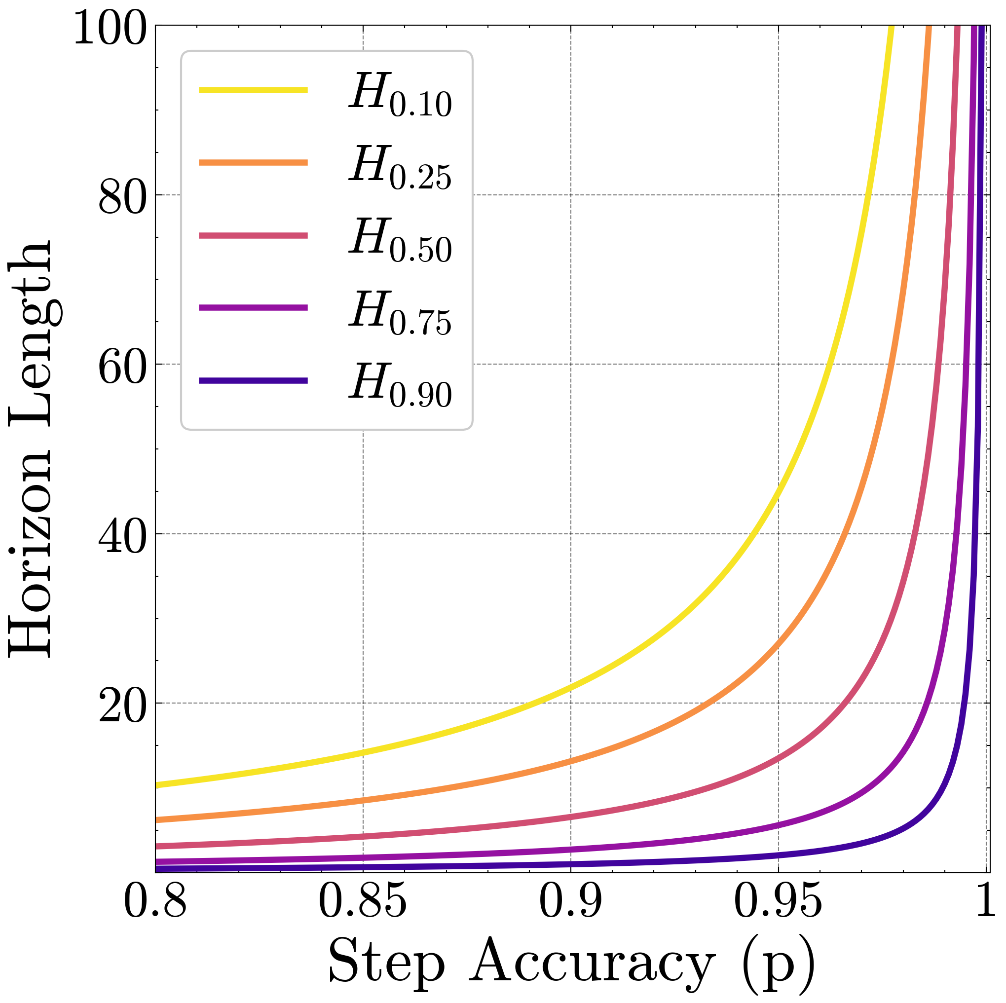
Figure 2: Growth of Horizon Length. The length of task a model can perform grows hyperbolically in the high accuracy regime.
**Proposition 1**
*Assuming a constant step accuracy $p$ and no self-correction, the task-length $H$ at which a model achieves a success rate $s$ is given by:
$$
\hskip-56.9055ptH_{s}(p)=\left\lceil\frac{\ln(s)}{\ln(p)}\right\rceil\ \approx\frac{\ln(s)}{\ln(p)}
$$
(The derivation is provided in Appendix ˜ H.)*
This shows that the horizon length grows hyperbolically with the step accuracy. We illustrate this growth in Figure ˜ 2 across different values for the success rate $s$ . Notice the sharp growth in horizon length beyond 80% single-step accuracy, performance that frontier models now achieve on many question-answering benchmarks (Vendrow et al., 2025), which can be considered short tasks.
We note that human labor is often compensated for its time. If the economic value of an agent also arises from the length of tasks it can complete, single-turn or short task benchmarks may be misleading for evaluating the benefits of further investment in LLM compute. While these benchmarks reveal genuine diminishing returns at the step level, they understate the compounding benefits that emerge over long-horizons. Beyond a threshold, small improvements in step accuracy can translate into success at rapidly increasing task lengths, which may provide a more faithful indicator of economic value.
For example, in METR’s horizon length plot on software engineering tasks (Kwa et al., 2025), it was empirically observed that the horizon length at $s=0.5$ of frontier models is growing exponentially, doubling every 7 months. Using our result above, in Figure ˜ 1 we show that such exponential growth in horizon length occurs even in a regime of diminishing returns on step accuracy. If we set $s=0.5$ , we obtain $H_{0.5}=-\frac{\ln(2)}{\ln(p)}$ . As such, the step-accuracy $p$ required to sustain exponential growth in $H_{0.5}$ over time ( $t$ ) is $2^{\frac{-1}{2^{t}}}$ , which is indeed a diminishing function.
2.2 Isolating execution by decoupling planning and knowledge
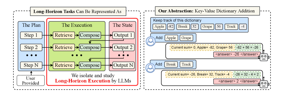
We now describe how we measure long-horizon execution empirically. We isolate execution failures by explicitly providing the requisite knowledge and plan. We study the chaining of the retrieve-then-compose step motivated in the flight-selection agent example earlier. Each step involves retrieving relevant information or a tool specified by the plan and then composing its output to update the current state. The plan is deciding what to retrieve and how to compose it, whereas execution is actually performing those operations. This fits a natural abstraction—a key-value dictionary. The key serves as one step of a plan specifying what knowledge to retrieve, or tool to call, while the value represents the knowledge or tool output, which then has to be composed with the current state. In our study, we provide the plan as the keys in each query, eliminating the need for planning abilities from the LLM. We also provide the key-value dictionary in context, removing any dependency on the model’s parametric knowledge. With this design, we directly control two important axes that multiply to obtain the task length (number of retrieve-then-compose steps): the number of turns, and the turn complexity ( $K$ ). The turn complexity can be varied by changing the number of keys queried per turn.
<details>
<summary>x2.png Details</summary>
### Visual Description
# Technical Document Extraction: Long-Horizon Task Abstraction
This image contains two primary panels enclosed in dashed borders, illustrating a conceptual framework for representing long-horizon tasks and a specific mathematical abstraction used to study them.
---
## Panel 1: Conceptual Framework
**Header:** Long-Horizon Tasks Can Be Represented As
### Component Isolation
This panel is divided into three vertical segments representing the flow of a task.
#### 1. The Plan (Blue Segment)
* **Input Source:** A dashed box at the bottom labeled "User Provided" points upward to this segment.
* **Components:**
* **Step 1**: Top-level task instruction.
* **Step 2**: Intermediate task instruction.
* **...**: Ellipsis indicating multiple intermediate steps.
* **Step N**: Final task instruction.
* **Flow:** Each step in "The Plan" points horizontally to a corresponding "Retrieve" block in the next segment.
#### 2. The Execution (Green Segment)
* **Context:** This segment is enclosed in a thick red border with the caption: "We isolate and study **Long-Horizon Execution** by LLMs".
* **Internal Logic (Repeated for Steps 1 through N):**
* **Retrieve**: Receives input from "The Plan".
* **Compose**: Receives input from "Retrieve".
* **Inter-step Flow:** A downward arrow connects the "Compose" block of one step to the "Compose" block of the subsequent step, indicating state or context carry-over.
#### 3. The State (Red Segment)
* **Components:**
* **Output 1**: Result of Step 1 execution.
* **Output 2**: Result of Step 2 execution.
* **...**: Ellipsis indicating intermediate outputs.
* **Output N**: Final result.
* **Flow:** Each "Compose" block in the Execution segment points horizontally to its corresponding "Output" block.
---
## Panel 2: Mathematical Abstraction
**Header:** Our Abstraction: Key-Value Dictionary Addition
This panel illustrates a specific task designed to test the execution logic described in Panel 1.
### Data Table: The Dictionary
A blue box at the top contains a key-value dictionary that the system must "Keep track of":
| Key | Value | Key | Value | Key | Value | Key | Value |
| :--- | :--- | :--- | :--- | :--- | :--- | :--- | :--- |
| Apple | -82 | Break | 32 | Grape | 56 | Track | -4 |
### Interaction Flow (User and AI Agent)
#### Interaction 1:
* **User Input (User Icon):** "Add Apple Grape"
* **AI Reasoning (Robot Icon):**
* **Retrieval/State Check (Yellow dashed box):** "Current sum= 0, Apple= -82, Grape= 56"
* **Computation (Green dashed box):** "-82 + 56 = -26"
* **Final Output (Pink box):** `<answer> -26 </answer>`
#### Interaction 2:
* **User Input (User Icon):** "Add Break Track"
* **AI Reasoning (Robot Icon):**
* **Retrieval/State Check (Yellow dashed box):** "Current sum= -26, Break= 32, Track= -4" (Note: The current sum is carried over from the previous interaction).
* **Computation (Green dashed box):** "-26 + 32 - 4 = 2"
* **Final Output (Pink box):** `<answer> 2 </answer>`
---
## Summary of Technical Information
* **Primary Objective:** To isolate and study how Large Language Models (LLMs) execute long-horizon tasks by maintaining state across multiple steps.
* **Task Logic:** The task involves a "Key-Value Dictionary Addition" where the model must retrieve values for specific keys and maintain a running sum across sequential user prompts.
* **Key Data Points:**
* Initial State: Sum = 0.
* Step 1: Apple (-82) + Grape (56) = -26.
* Step 2: Previous Sum (-26) + Break (32) + Track (-4) = 2.
</details>
Figure 3: Overview of our framework. (Left) Our framework models long-horizon tasks as a sequence of retrieve-then-compose steps. (Right) We design a simple task that decouples planning from execution: in each turn, we provide the model the plan as key(s), asking it to retrieve their value(s), and compose them to maintain a running sum. We control the number of turns and turn complexity (keys per query).
3 Experiments
We design a simple task where even language models with 4 billion parameters can achieve high accuracy, to isolate the capability of long-horizon execution.
Setup. As illustrated in Figure ˜ 3, we provide the model with the needed knowledge, a fixed, in-context dictionary $\mathcal{D}:\mathcal{V}→\mathbb{Z}$ , where $\mathcal{V}$ is a vocabulary of common five-letter English words and values are integers sampled uniformly from $[-99,99]$ . The initial state is $S_{0}=0$ . In turn $t∈\{1,...,T\}$ , the model receives an explicit plan $P_{t}=\{k_{t,1},...,k_{t,K}\}$ , which is a set of $K$ keys sampled from $\mathcal{V}$ . For each turn $t$ , the model must execute this plan, which requires updating the state, $S_{t}$ , to maintain a running sum of values for all past queried keys. This requires the retrieve-then-compose steps:
1. Retrieval: Look up the integer value $\mathcal{D}[k]$ for each key $k∈ P_{t}$
1. Composition: Sum these values and add them to the previous state, $S_{t}=S_{t-1}+\sum_{i=1}^{K}\mathcal{D}[k_{t,i}]$
We choose short English words and two-digit integers to minimize errors arising from tokenization. We provide few-shot examples to clarify the task. More details, including the exact prompt, are provided in Appendix ˜ E. We also disentangle performance on the individual retrieval and composition operations, finding that models have much higher accuracies on each of them alone (Appendix ˜ D).
3.1 Effect of increasing the number of turns
We first test our hypothesis that long-horizon execution can be challenging even when a model has the required knowledge and planning ability, and then study the benefits of scaling model size.
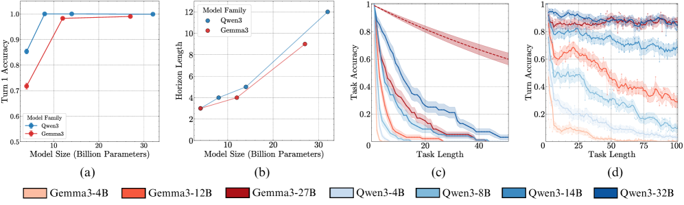
Setup. We evaluate the Qwen3 (Yang et al., 2025) and Gemma3 (Gemma-Team et al., 2025) model families, as they offer a range of sizes: [4, 8, 14, 32]B and [4, 12, 27]B parameters, respectively. For this experiment, we set the turn complexity to its simplest form ( $K=1$ ), providing a single key per turn, and vary the number of turns. Models are instructed to output the final answer directly, without intermediate thinking tokens, with the format enforced via few-shot examples. We verify that format-following errors are not the primary failure mode (Appendix ˜ F). We also show that the results below hold with chain-of-thought (CoT) prompting, and thinking models (Appendix Figure ˜ 12), and the trends are not affected by the temperature used (Appendix Figure ˜ 13).
Result 1: Execution alone is challenging. As seen in Figure ˜ 4 (a), all models except Gemma3-4B and Qwen3-4B achieve near-perfect accuracy on the first step, confirming they have the knowledge required to perfectly do a single step of our task. Yet, task accuracy falls rapidly over subsequent turns (Figure ˜ 4 (c)). Even the best-performing model (Qwen3-32B) sees its accuracy fall below 50% within 15 turns. This confirms our hypothesis that long-horizon execution can be challenging for LLMs, even if they have the needed knowledge and plan.
Result 2: Non-diminishing benefits of scaling model size. As shown in Figure ˜ 4 (c), larger models sustain higher task accuracy for significantly more turns, resulting in a clear scaling trend for horizon length (Figure ˜ 4 (b)). We abstain from deriving a “scaling law” since we can only obtain at most four model sizes from the same family, but the improvements do not seem diminishing. This observation is non-trivial. While the benefits of increasing model size are often attributed to improved capacity for knowledge, our task is not knowledge-constrained, as models achieve near-perfect first step accuracy (Figure ˜ 4 (a)), nor is the task more complex so that a larger model would be required. Yet, larger models are clearly more reliable at executing the task for longer. A possible explanation is the redundancy of internal circuits in larger models, which ensembles to reduce error (Lindsey et al., 2025). However, we find that simulating this redundancy with output-level aggregation of parallel compute does not replicate the gains observed from scaling model size (Appendix ˜ B).
<details>
<summary>x3.png Details</summary>
### Visual Description
# Technical Data Extraction: Model Performance Analysis
This document contains a detailed extraction of data from four technical charts (labeled a, b, c, and d) comparing the performance of two model families: **Qwen3** (represented by blue tones) and **Gemma3** (represented by red tones).
---
## Global Legend (Footer)
The following models are identified across the subplots, categorized by color and parameter count:
| Model Family | Color Code | Specific Model Variants |
| :--- | :--- | :--- |
| **Gemma3** | Red/Orange Tones | Gemma3-4B (Light), Gemma3-12B (Medium), Gemma3-27B (Dark) |
| **Qwen3** | Blue Tones | Qwen3-4B (Lightest), Qwen3-8B (Light), Qwen3-14B (Medium), Qwen3-32B (Darkest) |
---
## Chart (a): Scaling of Initial Accuracy
**Type:** Line graph with markers and error bars.
**Spatial Grounding:** Legend located at bottom-left [x: low, y: low].
### Axis Labels
* **Y-Axis:** Turn 1 Accuracy (Scale: 0.5 to 1.0)
* **X-Axis:** Model Size (Billion Parameters) (Scale: 0 to 30+)
### Data Trends and Points
* **Qwen3 (Blue Line):** Shows a rapid upward slope from 4B to 8B, then plateaus at near-perfect accuracy.
* ~4B: ~0.85 accuracy
* ~8B: ~1.0 accuracy
* ~14B: ~1.0 accuracy
* ~32B: ~1.0 accuracy
* **Gemma3 (Red Line):** Shows a steep upward slope from 4B to 12B, then plateaus slightly below Qwen3.
* ~4B: ~0.72 accuracy
* ~12B: ~0.98 accuracy
* ~27B: ~0.99 accuracy
---
## Chart (b): Scaling of Horizon Length
**Type:** Line graph with markers.
**Spatial Grounding:** Legend located at top-left [x: low, y: high].
### Axis Labels
* **Y-Axis:** Horizon Length (Scale: 0 to 12)
* **X-Axis:** Model Size (Billion Parameters) (Scale: 0 to 30+)
### Data Trends and Points
Both families show a positive linear-to-exponential correlation between model size and horizon length.
* **Qwen3 (Blue Line):** Consistently maintains a higher horizon length than Gemma3 for equivalent sizes.
* 4B: ~3.0
* 8B: ~4.0
* 14B: ~5.0
* 32B: ~12.0
* **Gemma3 (Red Line):**
* 4B: ~3.0
* 12B: ~4.0
* 27B: ~9.0
---
## Chart (c): Task Accuracy vs. Task Length
**Type:** Decay curves with shaded confidence intervals.
**Spatial Grounding:** Uses the global footer legend.
### Axis Labels
* **Y-Axis:** Task Accuracy (Scale: 0 to 1.0)
* **X-Axis:** Task Length (Scale: 0 to 50)
### Data Trends
All models exhibit performance decay as task length increases.
* **Top Performer:** **Gemma3-27B** (Dark Red dashed line) shows the most resilience, maintaining ~0.6 accuracy at length 50.
* **Qwen3 Series:** The darkest blue (Qwen3-32B) performs best within its family but drops to near 0 accuracy by length 50.
* **Small Models:** Gemma3-4B (lightest orange) and Qwen3-4B (lightest blue) decay the fastest, hitting near 0 accuracy before length 10.
---
## Chart (d): Turn Accuracy vs. Task Length
**Type:** Noisy line plots with shaded variance.
**Spatial Grounding:** Uses the global footer legend.
### Axis Labels
* **Y-Axis:** Turn Accuracy (Scale: 0 to 1.0)
* **X-Axis:** Task Length (Scale: 0 to 100)
### Data Trends
* **High Stability Group:** **Gemma3-27B** (Dark Red) and **Qwen3-32B** (Dark Blue) maintain high accuracy (~0.8 to 0.9) even out to 100 turns.
* **Mid-Tier Decay:** **Qwen3-14B** (Medium Blue) and **Gemma3-12B** (Orange) show a gradual decline. Gemma3-12B starts at ~0.8 and drops to ~0.3 by turn 100. Qwen3-14B starts at ~0.9 and drops to ~0.7.
* **Low-Tier:** Smaller models (4B variants) start with lower initial accuracy and show significant volatility/noise, trending toward 0.1-0.2 accuracy at long task lengths.
</details>
Figure 4: Scaling model size has non-diminishing improvements in the number of turns it can execute. The first-step accuracy for our task is near-perfect for all except the smallest models (a). Yet, as the model size is scaled, the horizon length increases significantly (b). We also see the effect of scaling in widening the gap between small and large models in task accuracy (c) and turn accuracy (d) as the number of turns increases. The shaded region is the mean $±$ one standard deviation over 100 samples; the solid line is the moving average over 5 turns; the dotted line is a hypothetical baseline model with constant step-accuracy of 0.99.
3.2 Why Does Turn Accuracy Degrade? The Self-Conditioning Effect
One might expect a model’s turn accuracy to remain constant. Yet, Figure ˜ 4 (d) shows the accuracy of individual turns degrading as the number of turns increases. We investigate two competing hypotheses:
1. Degradation as the context length increases. The model’s performance degrades simply due to increasing context length (Zhou et al., 2025a), irrespective of its content.
2. Self-conditioning. The model conditions on its own past mistakes. It becomes more likely to make a mistake after observing its own past errors in previous turns.
Setup. To disentangle these factors, we conduct a counterfactual experiment by manipulating the model’s chat history. We control the error rate by injecting artificial output histories with a chosen error rate in the same format. If we fully heal the history, with a $0\%$ error rate, degradation in the model’s turn accuracy between turn 1 and a later turn can be attributed to long-context issues. If a model’s accuracy for a fixed later turn consistently worsens with increasing error rate in prior turns, this would support our self-conditioning hypothesis.
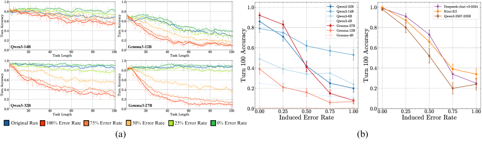
Result 3: Self-conditioning causes degradation in turn accuracy beyond long-context. Our results in Figure ˜ 5 (a) show evidence for degradation due to both long-context and self-conditioning. When conditioned on an error-free history (Induced Error Rate = 0.00), model turn accuracy at turn 100 is below its initial value, consistent with prior observations of long-context degradation (Zhou et al., 2025a). More interestingly, as we increase the rate of injected errors into the context, accuracy at turn 100 consistently degrades further. This demonstrates the self-conditioning effect—as models make mistakes, they become more likely to make more mistakes, leading to a continuous degradation in per-turn accuracy throughout the output trajectory as shown in Figure ˜ 5 (b).
Result 4: Unlike long-context, scaling model size does not mitigate self-conditioning. At the error rate of 0%, notice that the accuracy at turn 100 consistently improves as you scale model size. As shown in Figure ˜ 5 (b), scaling to frontier (200B+ parameter) models like Kimi-K2 (Kimi-Team et al., 2025), DeepSeek-V3 (DeepSeek-AI et al., 2025), and Qwen3-235B-Instruct-2507 (Yang et al., 2025) largely solves long-context degradation for up to 100 turns, achieving near-perfect accuracy on a healed history. However, even these large models remain susceptible to self-conditioning, as their performance consistently degrades as the induced error rate in their history increases. This may be akin to recent results showing larger models shift in personality during multi-turn conversations (Choi et al., 2024; Becker et al., 2025), where in our case, the drift is toward a personality that makes errors.
<details>
<summary>x4.png Details</summary>
### Visual Description
# Technical Data Extraction: Performance Analysis of LLMs under Induced Error
This document provides a comprehensive extraction of data from a technical figure containing multiple line charts. The figure is divided into two primary sections: **(a)**, which shows accuracy over task length for specific models, and **(b)**, which shows accuracy at a specific turn (Turn 100) relative to induced error rates.
---
## Section (a): Turn Accuracy vs. Task Length
This section consists of four sub-plots, each representing a different Large Language Model (LLM).
### Common Axis and Legend Information
* **Y-Axis:** "Turn Accuracy" (Scale: 0.0 to 1.0).
* **X-Axis:** "Task Length" (Scale: 0 to 100).
* **Legend (Bottom Left):**
* **Dark Blue Square:** Original Run
* **Red Square:** 100% Error Rate
* **Orange Square:** 75% Error Rate
* **Yellow Square:** 50% Error Rate
* **Light Green Square:** 25% Error Rate
* **Dark Green Square:** 0% Error Rate
### Sub-plot 1: Qwen3-14B
* **Trend:** Performance is relatively stable for low error rates (0%, 25%, Original). As the error rate increases (50% to 100%), accuracy degrades significantly as task length increases.
* **Data Points (Approximate at Task Length 100):**
* 0% Error Rate (Dark Green): ~0.8
* 25% Error Rate (Light Green): ~0.75
* Original Run (Dark Blue): ~0.7
* 50% Error Rate (Yellow): ~0.65
* 75% Error Rate (Orange): ~0.55
* 100% Error Rate (Red): ~0.5
### Sub-plot 2: Gemma3-12B
* **Trend:** Shows a much steeper decline in accuracy compared to Qwen3-14B. Even at low error rates, accuracy drops below 0.4 by task length 100.
* **Data Points (Approximate at Task Length 100):**
* 0% Error Rate (Dark Green): ~0.4
* 25% Error Rate (Light Green): ~0.3
* Original Run (Dark Blue): ~0.3
* 50% Error Rate (Yellow): ~0.2
* 75% Error Rate (Orange): ~0.15
* 100% Error Rate (Red): ~0.1
### Sub-plot 3: Qwen3-32B
* **Trend:** High resilience. The 0%, 25%, and Original runs maintain accuracy above 0.8 throughout the task. Higher error rates (75%, 100%) show a steady decline but remain higher than the Gemma models.
* **Data Points (Approximate at Task Length 100):**
* 0%/25%/Original: ~0.85 - 0.9
* 50% Error Rate (Yellow): ~0.6
* 75% Error Rate (Orange): ~0.35
* 100% Error Rate (Red): ~0.3
### Sub-plot 4: Gemma3-27B
* **Trend:** Similar to the 12B version, it shows a rapid collapse in accuracy for high error rates, though the 0% and 25% rates stay higher (~0.8) than the 12B model.
* **Data Points (Approximate at Task Length 100):**
* 0%/25% Error Rate: ~0.8 - 0.85
* 50% Error Rate (Yellow): ~0.4
* 75% Error Rate (Orange): ~0.15
* 100% Error Rate (Red): ~0.1
---
## Section (b): Turn 100 Accuracy vs. Induced Error Rate
This section contains two charts comparing different model families.
### Common Axis Information
* **Y-Axis:** "Turn 100 Accuracy" (Scale: 0.0 to 1.0).
* **X-Axis:** "Induced Error Rate" (Markers: 0.00, 0.25, 0.50, 0.75, 1.00).
### Left Chart (Qwen vs. Gemma)
**Legend (Top Right):**
* **Blue Tones (Qwen):** Qwen3-32B (Darkest), Qwen3-14B, Qwen3-8B, Qwen3-4B (Lightest).
* **Red/Orange Tones (Gemma):** Gemma-27B (Darkest), Gemma-12B, Gemma-4B (Lightest).
**Key Trends:**
* **Qwen Series:** Generally more robust. Qwen3-32B starts at ~0.85 and ends at ~0.55.
* **Gemma Series:** Starts higher (Gemma-27B at ~0.92) but drops precipitously to near 0.1 accuracy as error rate reaches 1.00.
### Right Chart (Competitive Models)
**Legend (Top Right):**
* **Purple Line:** Deepseek-chat-v3-0324
* **Yellow Line:** Kimi-k2
* **Brown Line:** Qwen3-2507-235B
**Data Extraction (Approximate Values):**
| Induced Error Rate | Deepseek-chat-v3 | Kimi-k2 | Qwen3-2507-235B |
| :--- | :--- | :--- | :--- |
| **0.00** | 1.0 | 1.0 | 0.98 |
| **0.25** | 0.91 | 0.87 | 0.80 |
| **0.50** | 0.73 | 0.66 | 0.52 |
| **0.75** | 0.34 | 0.39 | 0.20 |
| **1.00** | 0.25 | 0.34 | 0.24 |
**Trend Observation:** All three high-parameter models show a sharp, non-linear decline in accuracy as the induced error rate increases. Deepseek maintains the highest accuracy until the 0.75 mark, where Kimi-k2 becomes slightly more resilient.
</details>
Figure 5: Models self-condition on their previous mistakes, leading to more mistakes in subsequent turns. By manipulating the chat history, we counterfactually vary the fraction of errors in previous turns. We find this increases the likelihood of errors in future turns (left). This shows a source of degradation in turn-wise model accuracy beyond long-context, as in the turn 100 slice (right) model accuracies are much higher when we provide a fully correct history. Scaling model size increases self-conditioning, even for frontier non-thinking models.
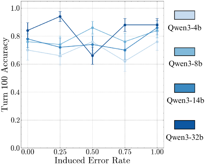
In Appendix ˜ G, we try the above setup of output manipulations with CoT prompting, finding that accuracy still deteriorates as the induced error rate increases. A potential confounder is that the manipulated outputs deviate from the CoT. We try to mitigate this issue with programmatically generated CoT traces, but still observe self-conditioning. We also try removing CoT traces from previous turns from history, which causes the model to stop using CoT completely. So, we now present results for the Qwen3 thinking models, which are trained with reinforcement learning (RL) to think even when previous turn traces are not presented. As before, we observe their turn 100 accuracy while controlling the error rate in prior turns.
<details>
<summary>x5.png Details</summary>
### Visual Description
# Technical Data Extraction: Performance Analysis of Qwen3 Models
## 1. Document Overview
This image is a line graph illustrating the relationship between an "Induced Error Rate" and "Turn 100 Accuracy" for four different versions of the "Qwen3" model family. The chart includes error bars for each data point, indicating variability or confidence intervals.
## 2. Component Isolation
### A. Header/Axes
* **Y-Axis Label:** `Turn 100 Accuracy`
* **Y-Axis Scale:** Linear, ranging from `0.0` to `1.0` with major tick marks every `0.2`.
* **X-Axis Label:** `Induced Error Rate`
* **X-Axis Scale:** Linear, ranging from `0.00` to `1.00` with major tick marks at `0.00`, `0.25`, `0.50`, `0.75`, and `1.00`.
### B. Legend (Spatial Grounding: Right Margin)
The legend is located on the right side of the plot area. It uses a color-coded gradient of blue to distinguish between model sizes.
* **Lightest Blue:** `Qwen3-4b`
* **Light-Medium Blue:** `Qwen3-8b`
* **Medium-Dark Blue:** `Qwen3-14b`
* **Darkest Blue:** `Qwen3-32b`
## 3. Data Series Analysis and Trend Verification
### Series 1: Qwen3-4b (Lightest Blue)
* **Visual Trend:** This series generally maintains the lowest accuracy relative to the others. It shows a slight decline from 0.00 to 0.25, stays relatively flat to 0.50, dips at 0.75, and recovers at 1.00.
* **Data Points (Approximate):**
* 0.00: ~0.70
* 0.25: ~0.66
* 0.50: ~0.76
* 0.75: ~0.62
* 1.00: ~0.76
### Series 2: Qwen3-8b (Light-Medium Blue)
* **Visual Trend:** Shows moderate volatility. It starts mid-range, dips slightly at 0.25, peaks significantly at 0.50, drops at 0.75, and rises again at 1.00.
* **Data Points (Approximate):**
* 0.00: ~0.76
* 0.25: ~0.74
* 0.50: ~0.86
* 0.75: ~0.76
* 1.00: ~0.84
### Series 3: Qwen3-14b (Medium-Dark Blue)
* **Visual Trend:** Relatively stable compared to the others. It starts at a similar level to the 8b model, experiences a slight downward trend until 0.75, and then sharpens upward at 1.00.
* **Data Points (Approximate):**
* 0.00: ~0.78
* 0.25: ~0.72
* 0.50: ~0.74
* 0.75: ~0.70
* 1.00: ~0.86
### Series 4: Qwen3-32b (Darkest Blue)
* **Visual Trend:** Highly volatile. It starts with high accuracy, peaks at 0.25, suffers a major drop at 0.50 (becoming the lowest performer at that specific point), and then recovers to a high plateau for 0.75 and 1.00.
* **Data Points (Approximate):**
* 0.00: ~0.84
* 0.25: ~0.94
* 0.50: ~0.66
* 0.75: ~0.88
* 1.00: ~0.88
## 4. Reconstructed Data Table (Estimated Values)
| Induced Error Rate | Qwen3-4b (Acc) | Qwen3-8b (Acc) | Qwen3-14b (Acc) | Qwen3-32b (Acc) |
| :--- | :--- | :--- | :--- | :--- |
| **0.00** | 0.70 | 0.76 | 0.78 | 0.84 |
| **0.25** | 0.66 | 0.74 | 0.72 | 0.94 |
| **0.50** | 0.76 | 0.86 | 0.74 | 0.66 |
| **0.75** | 0.62 | 0.76 | 0.70 | 0.88 |
| **1.00** | 0.76 | 0.84 | 0.86 | 0.88 |
## 5. Key Observations
* **Non-Linear Correlation:** There is no simple linear correlation between the Induced Error Rate and Accuracy across the models. Performance fluctuates significantly as the error rate increases.
* **Model Scaling:** Generally, the larger models (32b and 14b) perform better than the smaller models (4b), but this is inconsistent. For example, at an Error Rate of 0.50, the 8b model outperforms all others, while the 32b model performs significantly worse than its own baseline.
* **Error Bars:** All data points include vertical error bars extending approximately ±0.05 to ±0.10 from the mean, suggesting a notable margin of error or variance in the testing results.
</details>
Figure 6: Thinking fixes self-conditioning. Qwen3 models with thinking enabled no longer self-condition, even when the entire prior history has wrong answers, in contrast to non-thinking results.
Result 5: Thinking fixes self-conditioning. In Figure ˜ 6, we observe that the Qwen3 thinking models do not self-condition—the accuracy of the models at turn 100 remains stable, regardless of the error rate in its context. This could arise from two reasons. First, RL training can reduce the most likely next token prediction behaviour of language models, making them oriented towards task success rather than continuing the context. Second, the removal of thinking traces from prior turns could reduce the influence of prior turns on the model’s output, as it thinks about the new turn independently. By inspecting the models’ thinking traces, we observe that they do not refer back to their answers in prior turns, which could be a potential reason why they do not self-condition. Inspired by this, for non-thinking models, we experiment with context engineering by explicitly removing prior history and find that it indeed mitigates self-conditioning (Section ˜ A.2). We also find that just prompting models to self-verify their answers does not solve self-conditioning completely (Section ˜ A.1).
3.3 What is the length of tasks models can complete in a single turn?
In the previous sections, we measured how many turns models can successfully execute a single retrieve-then-compose step. However, most real-world tasks require more complex processing every turn. In fact, in Appendix ˜ C we show that the horizon length of different models can vary significantly at different turn complexities. The total task length a model can handle is a function of both the number of turns and the number of steps to execute per turn. We now measure the latter dimension: the maximum number of steps a model can execute per turn.
<details>
<summary>x6.png Details</summary>
### Visual Description
# Technical Data Extraction: Task Length Comparison (Single Turn)
This document contains a detailed extraction of data from two bar charts, labeled **(a)** and **(b)**, comparing the task lengths of various Large Language Models (LLMs) in a single-turn context.
---
## Chart (a): Without Chain-of-Thought (CoT)
### Metadata and Layout
- **Header/Label:** A text box in the top-left corner contains the text "Without CoT".
- **Y-Axis Title:** "Task Length (Single Turn)"
- **Y-Axis Scale:** Linear, ranging from 0 to 6.
- **X-Axis Labels:** Model names oriented at a 45-degree angle.
- **Trend:** The chart shows a step-wise increase in task length capacity across the four listed models, starting at 2 and peaking at 6.
### Data Table (Reconstructed)
| Model Name | Bar Color | Task Length Value |
| :--- | :--- | :--- |
| Qwen3-32B | Dark Blue/Teal | 2 |
| Gemma3-27B | Red | 2 |
| Deepseek-V3 | Blue | 4 |
| Kimi-K2 | Dark Grey/Black | 6 |
---
## Chart (b): Thinking vs. Chain-of-Thought
### Metadata and Layout
- **Legend [Top-Left]:**
- Solid Grey Square: "Thinking"
- Hatched/Diagonal Striped Grey Square: "Chain-of-Thought"
- **Y-Axis Title:** "Task Length (Single Turn)"
- **Y-Axis Scale:** Logarithmic (Base 2), ranging from $2^6$ (64) to $2^{11}$ (2048).
- **X-Axis Labels:** Model names oriented at a 45-degree angle.
- **Trend:** The chart displays an exponential growth trend. While the first four models (Kimi-K2 through Gemini-2.5-Pro) show relatively similar capacities (72 to 120), there is a significant jump in capacity for Grok-4, Claude-4-Sonnet, and a massive outlier in GPT-5.
### Component Isolation: Bar Styles
- **Hatched Bar:** Only **Deepseek-V3** uses a diagonal hatched pattern, which according to the legend signifies "Chain-of-Thought".
- **Solid Bars:** All other models use solid colors, signifying "Thinking" processes.
### Data Table (Reconstructed)
| Model Name | Bar Color/Style | Task Length Value |
| :--- | :--- | :--- |
| Kimi-K2 | Dark Grey (Solid) | 72 |
| Deepseek-V3 | Blue (Hatched) | 112 |
| Deepseek-R1 | Blue (Solid) | 120 |
| Gemini-2.5-Pro | Light Blue (Solid) | 120 |
| Grok-4 | Medium Grey (Solid) | 384 |
| Claude-4-Sonnet | Orange (Solid) | 432 |
| GPT-5 | Dark Grey/Black (Solid) | 2176 |
---
## Comparative Analysis Summary
- **Scale Difference:** Chart (a) uses a small linear scale (0-6) for non-CoT tasks. Chart (b) uses a logarithmic scale to accommodate values ranging from 72 to over 2000.
- **Top Performer:** In both charts, the dark grey/black bar represents the highest value. In chart (a) this is **Kimi-K2** (Value: 6), and in chart (b) this is **GPT-5** (Value: 2176).
- **Methodology Note:** Deepseek-V3 is the only model explicitly highlighted as using "Chain-of-Thought" (hatched pattern) in the second chart, whereas others are categorized under "Thinking".
</details>
Figure 7: Benchmarking the length of task models can execute in a single turn. Without CoT or thinking, even the biggest models fail to execute more than a few steps (a). Sequential test time compute (thinking tokens) significantly improves this, especially when trained with RL (b), where GPT-5 is far ahead of the rest.
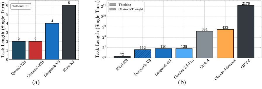
Setup. To quantify the length of task models can complete in one go, without user input, we run a binary search (Lehmer, 1960) to find the highest turn complexity ( $K$ , the number of keys) the model can provide the correct sum for with accuracy $≥ 80\%$ . We evaluate a suite of frontier models like GPT-5 (OpenAI, 2025), Claude-4 Sonnet (Anthropic, 2025), Grok 4 (xAI, 2025), Gemini 2.5 Pro (Gemini Team, 2025), Kimi K2 (Kimi-Team et al., 2025), and DeepSeek-R1 (Guo et al., 2025). An advantage of our benchmark is that it is contamination-free, as new examples can be generated programmatically.
Result 6: Without CoT, non-thinking models struggle to chain more than a few steps per turn. In Figure ˜ 7 (left), we first find that when prompted to answer directly, without chain-of-thought, the larger Qwen3 32B, Gemma3 27B, as well as frontier non-thinking models like DeepSeek-V3 (670B), and Kimi K2 (1026B), fail to execute even a turn complexity of more than six. This is consistent with prior work showing the necessity of thinking tokens for transformers to perform sequential tasks (Weiss et al., 2021; Merrill and Sabharwal, 2023). We see that the number of steps the model can execute in a single turn improves significantly with chain-of-thought. This reinforces the importance of reasoning before acting (ReAct (Yao et al., 2023)) for agents, even if this costs more and fills up the context window. We show preliminary evidence that parallel test time compute is not as helpful, with majority voting leading to only marginal improvements in execution length (Appendix ˜ B).
Result 7: Benchmarking frontier models. In Figure ˜ 7 (right), we benchmark frontier models on the length of task they can execute in a single turn. We find a surprisingly large gap between GPT-5 (codenamed Horizon) with 2176 steps and others like Claude-4 Sonnet (432 steps), Grok 4 (384 steps), and Gemini 2.5 Pro (120 steps). Overall, even our simple task can separate frontier models in their long-horizon execution capability, and presents a clear opportunity to improve current open-weight models.
4 Related Work
Increasing Task Length. Multiple works have recently shown how models worsen as problem complexity increases (Zhou et al., 2025b), often attributed to failures of reasoning (Cheng, 2025; Shojaee et al., 2025). Recently, multiple real-world long-horizon agentic benchmarks have been proposed (Backlund and Petersson, 2025; Xie et al., 2024; Shen et al., 2025), where prior work has studied planning failures (Chen et al., 2024b). By designing a task where no reasoning is required, given that we provide the model the requisite plan and knowledge, we show that execution alone can be a challenge, degrading model accuracy on longer tasks. Our observations on scaling could hold for the related problem of length-generalization—training models to succeed on tasks longer than those seen during training (Fan et al., 2024; Cai et al., 2025).
Long Context. Much of prior work has focused on improving the maximum context length that can be provided in the input to a language model (Su et al., 2021), and evaluating whether (Tay et al., 2020) and how (Olsson et al., 2022; Li et al., 2023) models maintain performance as the context gets longer (Tay et al., 2020). Closest is the recent RULER (Hsieh et al., 2024) and GSM-Infinite (Zhou et al., 2025b), which also use synthetic data to systematically evaluate long-context abilities. While long-context will help models execute for longer, it is a different capability compared to long-horizon execution (Zhou et al., 2023; Chen et al., 2024a), as it focuses on performance as a function of input, not output length. We identified one such difference, the self-conditioning effect—where past errors in model output increase the chance of future mistakes, and disentangle this effect from long-context degradation in Section ˜ 3.2. Motivated by a similar effect at the token level, termed exposure bias, Ranzato et al. (2015) proposed training language models with RL.
Scaling LLMs and RL. Scaling laws for language models show diminishing returns on the loss for the single step of predicting the next token (Kaplan et al., 2020; Hoffmann et al., 2022). When models competed in simple knowledge-based question-answering tasks such as MMLU (Hendrycks et al., 2020), such single-step measurements could inform us about the rate of progress. This has changed in the last year. Where earlier we could only post-train on human demonstrations (Mishra et al., 2021), language models can now be trained with just rewards (Shao et al., 2024), enabling sophisticated reasoning (Guo et al., 2025; Jain et al., 2024) and agents (Kimi Team et al., 2025). This opens up the opportunity to solve much longer tasks where earlier human supervision would be too expensive to scale. Our work shows how diminishing returns on single-step performance can compound to provide large benefits in the length of tasks a model can solve. This motivates the need to study empirical scaling laws for horizon length in agents (Hilton et al., 2023).
Tool Use. In symbolic AI, once tasks are formalized, for example, into STRIPS plans (Fikes and Nilsson, 1971), they can be executed without issues. Prior work (Chen et al., 2024b; Valmeekam et al., 2024) has shown LLMs struggle to match symbolic algorithms for automated planning. In contrast, we show LLMs can fail on straightforward execution (Zhu et al., 2025; Sun et al., 2025; Stechly et al., 2024) over a long horizon even when the plan is provided. Teaching LLMs to use tools offers one way to shift the burden of execution from probabilistic models to reliable programs (Schick et al., 2023). However, reasoning is often fuzzy and not always easy to implement as a tool, requiring the model to execute some steps by itself. Even calling the right tools requires reliable execution from the model (Patil et al., 2025).
Reliability. While there has been recent interest in evaluations for LLM reliability (Vendrow et al., 2025; Yao et al., 2024), it does not focus on long-horizon outputs, where the context differs every step. For example, Yao et al. (2024) focus on the $pass^{k}$ metric, which checks if the model makes a mistake when we sample $k$ generations. However, this keeps the input fixed, and at 0 temperature (deterministic sampling), becomes equivalent to $pass@1$ . In long-horizon tasks, error compounds irrespective of temperature, as shown in Appendix Figure ˜ 13.
5 Conclusion
In this work, we show how short-task benchmarks may give the illusion of slowing progress for modern language models. We show that scaling model size increases the number of turns a model can execute, while sequential test-time compute increases the length of tasks a model can perform on a single turn. Together, these contribute to dramatically increasing horizon lengths for LLMs.
Limitations. As with any “synthetic” task (Allen-Zhu, 2024; Poli et al., 2024; Chollet et al., 2024) used for a controlled study of LLM capabilities, there are a few limitations of our setup. It does not reflect complexities and sources of error arising in real agentic tasks with a large number of possible actions. In such settings, the number of actions and the accuracy of each action can both vary based on the plan, requiring more careful consideration. It would be interesting future work to study the self-conditioning effect when doing diverse actions instead of repeating the same ones. Our results are observations about pretrained LLMs, and not inherent properties of transformers, so they might change with task-specific finetuning. Improvement on our task is necessary, but not sufficient for long-horizon execution on real-world tasks. Finally, our current task accuracy metric does not account for self-correction. In tasks where mistakes are acceptable and easy to undo, self-correction is a promising direction to improve long-horizon execution.
Outlook. Scaling up the length of tasks a model can complete would be a major step towards realizing the true potential of general, open-ended agents (Raad et al., 2024). If they are trained in simulated environments created with generative models (Bruce et al., 2024), maintaining accuracy over a long-horizon becomes doubly important. By showing long-horizon execution can be studied on simple tasks, we hope to inspire more research on this capability, as it is an increasingly important capability in the era of experience (Silver and Sutton, 2025).
Acknowledgements
We thank Maksym Andriushchenko, Nikhil Chandak, Paras Chopra, Dulhan Jayalath, Abhinav Menon, Sumeet Motwani, Mathias Niepert, Lluís Pastor Pérez, Ameya Prabhu, Tim Schneider, Shashwat Singh, and Timon Willi for helpful feedback. AA was funded by the CHIPS Joint Undertaking (JU) under grant agreement No. 101140087 (SMARTY), and by the German Federal Ministry of Education and Research (BMBF) under the sub-project with the funding number 16MEE0444. AA thanks the International Max Planck Research School for Intelligent Systems (IMPRS-IS) and the ELLIS PhD programs for support. The authors gratefully acknowledge compute time on the Artificial Intelligence Software Academy (AISA) cluster funded by the Ministry of Science, Research and Arts of Baden-Württemberg.
Author Contributions
SG conceived the project. AS led the execution of the experiments with the help of AA, while SG led their planning with the help of AA, AS, and JG. SG and AA wrote the paper, while AS worked on the figures. JG and SS advised the project, providing valuable feedback throughout.
References
- Allen-Zhu [2024] Zeyuan Allen-Zhu. ICML 2024 Tutorial: Physics of Language Models, July 2024. Project page: https://physics.allen-zhu.com/.
- Anthropic [2025] Anthropic. System card: Claude Opus 4 & Claude Sonnet 4, May 2025. URL https://www.anthropic.com/claude-4-system-card. Covers Claude Sonnet 4 and Opus 4.
- Backlund and Petersson [2025] Axel Backlund and Lukas Petersson. Vending-Bench: A Benchmark for Long-Term Coherence of Autonomous Agents. arxiv:2502.15840[cs], February 2025. doi: 10.48550/arXiv.2502.15840. URL http://arxiv.org/abs/2502.15840.
- Becker et al. [2025] Jonas Becker, Lars Benedikt Kaesberg, Andreas Stephan, Jan Philip Wahle, Terry Ruas, and Bela Gipp. Stay Focused: Problem Drift in Multi-Agent Debate. arxiv:2502.19559[cs], May 2025. doi: 10.48550/arXiv.2502.19559. URL http://arxiv.org/abs/2502.19559.
- Bruce et al. [2024] Jake Bruce, Michael D Dennis, Ashley Edwards, Jack Parker-Holder, Yuge Shi, Edward Hughes, Matthew Lai, Aditi Mavalankar, Richie Steigerwald, Chris Apps, et al. Genie: Generative interactive environments. In Forty-first International Conference on Machine Learning, 2024.
- Cai et al. [2025] Ziyang Cai, Nayoung Lee, Avi Schwarzschild, Samet Oymak, and Dimitris Papailiopoulos. Extrapolation by Association: Length Generalization Transfer in Transformers. arxiv:2506.09251[cs], August 2025. doi: 10.48550/arXiv.2506.09251. URL http://arxiv.org/abs/2506.09251.
- Chen et al. [2024a] Siwei Chen, Anxing Xiao, and David Hsu. LLM-State: Open World State Representation for Long-horizon Task Planning with Large Language Model. arxiv:2311.17406[cs], April 2024a. doi: 10.48550/arXiv.2311.17406. URL http://arxiv.org/abs/2311.17406.
- Chen et al. [2024b] Yanan Chen, Ali Pesaranghader, Tanmana Sadhu, and Dong Hoon Yi. Can We Rely on LLM Agents to Draft Long-Horizon Plans? Let’s Take TravelPlanner as an Example. arxiv:2408.06318[cs], August 2024b. doi: 10.48550/arXiv.2408.06318. URL http://arxiv.org/abs/2408.06318.
- Cheng [2025] Jingde Cheng. Why cannot large language models ever make true correct reasoning?, 2025. URL https://arxiv.org/abs/2508.10265.
- Choi et al. [2024] Junhyuk Choi, Yeseon Hong, Minju Kim, and Bugeun Kim. Examining identity drift in conversations of llm agents. arXiv preprint arXiv:2412.00804, 2024.
- Chollet et al. [2024] Francois Chollet, Mike Knoop, Gregory Kamradt, and Bryan Landers. Arc prize 2024: Technical report. arXiv preprint arXiv:2412.04604, 2024.
- DeepSeek-AI et al. [2025] DeepSeek-AI, Aixin Liu, Bei Feng, et al. Deepseek-v3 technical report, 2025. URL https://arxiv.org/abs/2412.19437.
- Dell’Acqua et al. [2023] Fabrizio Dell’Acqua, Edward McFowland III, Ethan R. Mollick, Hila Lifshitz-Assaf, Katherine C. Kellogg, Saran Rajendran, Lisa Krayer, François Candelon, and Karim R. Lakhani. Navigating the jagged technological frontier: Field experimental evidence of the effects of AI on knowledge worker productivity and quality. Working paper, Harvard Business School Technology & Operations Management Unit, 2023. URL https://ssrn.com/abstract=4573321. Also circulated as The Wharton School Research Paper; last revised 2023-09-27.
- Fan et al. [2024] Ying Fan, Yilun Du, Kannan Ramchandran, and Kangwook Lee. Looped Transformers for Length Generalization. In The Thirteenth International Conference on Learning Representations, October 2024. URL https://openreview.net/forum?id=2edigk8yoU.
- Fikes and Nilsson [1971] Richard E. Fikes and Nils J. Nilsson. Strips: A new approach to the application of theorem proving to problem solving. Artificial Intelligence, 2(3):189–208, December 1971. ISSN 0004-3702. doi: 10.1016/0004-3702(71)90010-5. URL https://www.sciencedirect.com/science/article/pii/0004370271900105.
- Gemini Team [2025] Gemini Team. Gemini 2.5: Pushing the frontier with advanced reasoning, multimodality, long context, and next generation agentic capabilities. Technical report, Google DeepMind, June 2025. URL https://storage.googleapis.com/deepmind-media/gemini/gemini_v2_5_report.pdf.
- Gemma-Team et al. [2025] Gemma-Team, Aishwarya Kamath, Johan Ferret, et al. Gemma 3 technical report, 2025. URL https://arxiv.org/abs/2503.19786.
- Guo et al. [2025] Daya Guo, Dejian Yang, Haowei Zhang, Junxiao Song, Ruoyu Zhang, Runxin Xu, Qihao Zhu, Shirong Ma, Peiyi Wang, Xiao Bi, et al. Deepseek-r1: Incentivizing reasoning capability in llms via reinforcement learning. arXiv preprint arXiv:2501.12948, 2025.
- Hendrycks et al. [2020] Dan Hendrycks, Collin Burns, Steven Basart, Andy Zou, Mantas Mazeika, Dawn Song, and Jacob Steinhardt. Measuring massive multitask language understanding. arXiv preprint arXiv:2009.03300, 2020.
- Hilton et al. [2023] Jacob Hilton, Jie Tang, and John Schulman. Scaling laws for single-agent reinforcement learning. arXiv preprint arXiv:2301.13442, 2023.
- Hoffmann et al. [2022] Jordan Hoffmann, Sebastian Borgeaud, Arthur Mensch, Elena Buchatskaya, Trevor Cai, Eliza Rutherford, Diego de Las Casas, Lisa Anne Hendricks, Johannes Welbl, Aidan Clark, et al. Training compute-optimal large language models. arXiv preprint arXiv:2203.15556, 2022.
- Hsieh et al. [2024] Cheng-Ping Hsieh, Simeng Sun, Samuel Kriman, Shantanu Acharya, Dima Rekesh, Fei Jia, and Boris Ginsburg. RULER: What’s the Real Context Size of Your Long-Context Language Models? In First Conference on Language Modeling, August 2024. URL https://openreview.net/forum?id=kIoBbc76Sy.
- Jain et al. [2024] Naman Jain, King Han, Alex Gu, Wen-Ding Li, Fanjia Yan, Tianjun Zhang, Sida Wang, Armando Solar-Lezama, Koushik Sen, and Ion Stoica. Livecodebench: Holistic and contamination free evaluation of large language models for code. arXiv preprint arXiv:2403.07974, 2024.
- Kambhampati et al. [2024] Subbarao Kambhampati, Karthik Valmeekam, Lin Guan, Mudit Verma, Kaya Stechly, Siddhant Bhambri, Lucas Saldyt, and Anil Murthy. Llms can’t plan, but can help planning in llm-modulo frameworks. arXiv preprint arXiv:2402.01817, 2024.
- Kaplan et al. [2020] Jared Kaplan, Sam McCandlish, Tom Henighan, Tom B. Brown, Benjamin Chess, Rewon Child, Scott Gray, Alec Radford, Jeffrey Wu, and Dario Amodei. Scaling laws for neural language models, 2020. URL https://arxiv.org/abs/2001.08361.
- Khan et al. [2025] Sheraz Khan, Subha Madhavan, and Kannan Natarajan. A comment on" the illusion of thinking": Reframing the reasoning cliff as an agentic gap. arXiv preprint arXiv:2506.18957, 2025.
- Kimi Team et al. [2025] Kimi Team, Yifan Bai, Yiping Bao, Guanduo Chen, Jiahao Chen, Ningxin Chen, Ruijue Chen, Yanru Chen, Yuankun Chen, Yutian Chen, et al. Kimi k2: Open agentic intelligence. arXiv preprint arXiv:2507.20534, 2025.
- Kimi-Team et al. [2025] Kimi-Team, Yifan Bai, Yiping Bao, et al. Kimi k2: Open agentic intelligence, 2025. URL https://arxiv.org/abs/2507.20534.
- Kwa et al. [2025] Thomas Kwa, Ben West, Joel Becker, Amy Deng, Katharyn Garcia, Max Hasin, Sami Jawhar, Megan Kinniment, Nate Rush, Sydney Von Arx, et al. Measuring ai ability to complete long tasks. arXiv preprint arXiv:2503.14499, 2025.
- LeCun [2023] Yann LeCun. Do large language models need sensory grounding for meaning and understanding? Slide deck, NYU Philosophy of Deep Learning debate, March 2023. URL https://drive.google.com/file/d/1BU5bV3X5w65DwSMapKcsr0ZvrMRU_Nbi/view. Includes slide “Autoregressive LLMs are Doomed.”.
- Lehmer [1960] Derrick H Lehmer. Teaching combinatorial tricks to a computer. In Proceedings of Symposia in Applied Mathematics, pages 179–193. American Mathematical Society, 1960.
- Li et al. [2023] Yingcong Li, Muhammed Emrullah Ildiz, Dimitris Papailiopoulos, and Samet Oymak. Transformers as Algorithms: Generalization and Stability in In-context Learning. In Proceedings of the 40th International Conference on Machine Learning, pages 19565–19594. PMLR, July 2023. URL https://proceedings.mlr.press/v202/li23l.html.
- Lindsey et al. [2025] Jack Lindsey, Wes Gurnee, Emmanuel Ameisen, Brian Chen, Adam Pearce, Nicholas L. Turner, Craig Citro, David Abrahams, Shan Carter, Basil Hosmer, Jonathan Marcus, Michael Sklar, Adly Templeton, Trenton Bricken, Callum McDougall, Hoagy Cunningham, Thomas Henighan, Adam Jermyn, Andy Jones, Andrew Persic, Zhenyi Qi, T. Ben Thompson, Sam Zimmerman, Kelley Rivoire, Thomas Conerly, Chris Olah, and Joshua Batson. On the biology of a large language model. Transformer Circuits Thread, 2025. URL https://transformer-circuits.pub/2025/attribution-graphs/biology.html.
- Merrill and Sabharwal [2023] William Merrill and Ashish Sabharwal. The expressive power of transformers with chain of thought. arXiv preprint arXiv:2310.07923, 2023.
- METR [2025] METR. Measuring ai ability to complete long tasks, March 2025. URL https://metr.org/blog/2025-03-19-measuring-ai-ability-to-complete-long-tasks/.
- Mirzadeh et al. [2024] Iman Mirzadeh, Keivan Alizadeh, Hooman Shahrokhi, Oncel Tuzel, Samy Bengio, and Mehrdad Farajtabar. Gsm-symbolic: Understanding the limitations of mathematical reasoning in large language models. arXiv preprint arXiv:2410.05229, 2024.
- Mishra et al. [2021] Swaroop Mishra, Daniel Khashabi, Chitta Baral, and Hannaneh Hajishirzi. Cross-task generalization via natural language crowdsourcing instructions. arXiv preprint arXiv:2104.08773, 2021.
- Olsson et al. [2022] Catherine Olsson, Nelson Elhage, Neel Nanda, Nicholas Joseph, Nova DasSarma, Tom Henighan, Ben Mann, Amanda Askell, Yuntao Bai, Anna Chen, Tom Conerly, Dawn Drain, Deep Ganguli, Zac Hatfield-Dodds, Danny Hernandez, Scott Johnston, Andy Jones, Jackson Kernion, Liane Lovitt, Kamal Ndousse, Dario Amodei, Tom Brown, Jack Clark, Jared Kaplan, Sam McCandlish, and Chris Olah. In-context Learning and Induction Heads. CoRR, January 2022. URL https://openreview.net/forum?id=nJ10GgImU0.
- OpenAI [2025] OpenAI. Gpt-5 system card, August 2025. URL https://cdn.openai.com/gpt-5-system-card.pdf. Canonical system card PDF.
- Patil et al. [2025] Shishir G Patil, Huanzhi Mao, Fanjia Yan, Charlie Cheng-Jie Ji, Vishnu Suresh, Ion Stoica, and Joseph E Gonzalez. The berkeley function calling leaderboard (bfcl): From tool use to agentic evaluation of large language models. In Forty-second International Conference on Machine Learning, 2025.
- Poli et al. [2024] Michael Poli, Armin W. Thomas, Eric Nguyen, Pragaash Ponnusamy, Björn Deiseroth, Kristian Kersting, Taiji Suzuki, Brian Hie, Stefano Ermon, Christopher Re, Ce Zhang, and Stefano Massaroli. Mechanistic Design and Scaling of Hybrid Architectures. In Forty-First International Conference on Machine Learning, June 2024. URL https://openreview.net/forum?id=GDp7Gyd9nf.
- Raad et al. [2024] Maria Abi Raad, Arun Ahuja, Catarina Barros, Frederic Besse, Andrew Bolt, Adrian Bolton, Bethanie Brownfield, Gavin Buttimore, Max Cant, Sarah Chakera, et al. Scaling instructable agents across many simulated worlds. arXiv preprint arXiv:2404.10179, 2024.
- Ranzato et al. [2015] Marc’Aurelio Ranzato, Sumit Chopra, Michael Auli, and Wojciech Zaremba. Sequence level training with recurrent neural networks. arXiv preprint arXiv:1511.06732, 2015.
- Schick et al. [2023] Timo Schick, Jane Dwivedi-Yu, Roberto Dessì, Roberta Raileanu, Maria Lomeli, Eric Hambro, Luke Zettlemoyer, Nicola Cancedda, and Thomas Scialom. Toolformer: Language models can teach themselves to use tools. Advances in Neural Information Processing Systems, 36:68539–68551, 2023.
- Shao et al. [2024] Zhihong Shao, Peiyi Wang, Qihao Zhu, Runxin Xu, Junxiao Song, Xiao Bi, Haowei Zhang, Mingchuan Zhang, YK Li, Yang Wu, et al. Deepseekmath: Pushing the limits of mathematical reasoning in open language models. arXiv preprint arXiv:2402.03300, 2024.
- Shen et al. [2025] Yongliang Shen, Kaitao Song, Xu Tan, Wenqi Zhang, Kan Ren, Siyu Yuan, Weiming Lu, Dongsheng Li, and Yueting Zhuang. TaskBench: Benchmarking large language models for task automation. In Proceedings of the 38th International Conference on Neural Information Processing Systems, volume 37 of NIPS ’24, pages 4540–4574, Red Hook, NY, USA, June 2025. Curran Associates Inc. ISBN 979-8-3313-1438-5.
- Shojaee et al. [2025] Parshin Shojaee, Iman Mirzadeh, Keivan Alizadeh, Maxwell Horton, Samy Bengio, and Mehrdad Farajtabar. The illusion of thinking: Understanding the strengths and limitations of reasoning models via the lens of problem complexity, 2025. URL https://arxiv.org/abs/2506.06941.
- Silver and Sutton [2025] David Silver and Richard S Sutton. Welcome to the era of experience. Google AI, 1, 2025.
- Snell et al. [2024] Charlie Snell, Jaehoon Lee, Kelvin Xu, and Aviral Kumar. Scaling llm test-time compute optimally can be more effective than scaling model parameters. arXiv preprint arXiv:2408.03314, 2024.
- Stechly et al. [2024] Kaya Stechly, Karthik Valmeekam, and Subbarao Kambhampati. Chain of thoughtlessness? an analysis of cot in planning. Advances in Neural Information Processing Systems, 37:29106–29141, 2024.
- Su et al. [2021] Jianlin Su, Yu Lu, Shengfeng Pan, Bo Wen, and Yunfeng Liu. Roformer: Enhanced transformer with rotary position embedding, 2021.
- Sun et al. [2025] Simeng Sun, Cheng-Ping Hsieh, Faisal Ladhak, Erik Arakelyan, Santiago Akle Serano, and Boris Ginsburg. L0-Reasoning Bench: Evaluating Procedural Correctness in Language Models via Simple Program Execution. arxiv:2503.22832[cs], April 2025. doi: 10.48550/arXiv.2503.22832. URL http://arxiv.org/abs/2503.22832.
- Tay et al. [2020] Yi Tay, Mostafa Dehghani, Samira Abnar, Yikang Shen, Dara Bahri, Philip Pham, Jinfeng Rao, Liu Yang, Sebastian Ruder, and Donald Metzler. Long Range Arena : A Benchmark for Efficient Transformers. In International Conference on Learning Representations, October 2020. URL https://openreview.net/forum?id=qVyeW-grC2k.
- Valmeekam et al. [2024] Karthik Valmeekam, Kaya Stechly, Atharva Gundawar, and Subbarao Kambhampati. A Systematic Evaluation of the Planning and Scheduling Abilities of the Reasoning Model o1. Transactions on Machine Learning Research, December 2024. ISSN 2835-8856. URL https://openreview.net/forum?id=FkKBxp0FhR.
- Vendrow et al. [2025] Joshua Vendrow, Edward Vendrow, Sara Beery, and Aleksander Madry. Do large language model benchmarks test reliability? arXiv preprint arXiv:2502.03461, 2025.
- Weiss et al. [2021] Gail Weiss, Yoav Goldberg, and Eran Yahav. Thinking like transformers. In International Conference on Machine Learning, pages 11080–11090. PMLR, 2021.
- xAI [2025] xAI. Grok 4 model card, August 2025. URL https://data.x.ai/2025-08-20-grok-4-model-card.pdf.
- Xie et al. [2024] Jian Xie, Kai Zhang, Jiangjie Chen, Tinghui Zhu, Renze Lou, Yuandong Tian, Yanghua Xiao, and Yu Su. Travelplanner: A benchmark for real-world planning with language agents, 2024. URL https://arxiv.org/abs/2402.01622.
- Yang et al. [2025] An Yang, Anfeng Li, Baosong Yang, et al. Qwen3 technical report, 2025. URL https://arxiv.org/abs/2505.09388.
- Yao et al. [2023] Shunyu Yao, Jeffrey Zhao, Dian Yu, Nan Du, Izhak Shafran, Karthik Narasimhan, and Yuan Cao. React: Synergizing reasoning and acting in language models. In International Conference on Learning Representations (ICLR), 2023.
- Yao et al. [2024] Shunyu Yao, Noah Shinn, Pedram Razavi, and Karthik Narasimhan. tau-bench: A benchmark for tool-agent-user interaction in real-world domains. arXiv preprint arXiv:2406.12045, 2024.
- Zhou et al. [2023] Haoyu Zhou, Mingyu Ding, Weikun Peng, Masayoshi Tomizuka, Lin Shao, and Chuang Gan. Generalizable Long-Horizon Manipulations with Large Language Models. arxiv:2310.02264[cs], October 2023. doi: 10.48550/arXiv.2310.02264. URL http://arxiv.org/abs/2310.02264.
- Zhou et al. [2025a] Yang Zhou, Hongyi Liu, Zhuoming Chen, Yuandong Tian, and Beidi Chen. Gsm-infinite: How do your llms behave over infinitely increasing context length and reasoning complexity? arXiv preprint arXiv:2502.05252, 2025a.
- Zhou et al. [2025b] Yang Zhou, Hongyi Liu, Zhuoming Chen, Yuandong Tian, and Beidi Chen. GSM-$\infty$: How Do your LLMs Behave over Infinitely Increasing Reasoning Complexity and Context Length? In Forty-Second International Conference on Machine Learning, June 2025b. URL https://openreview.net/forum?id=n52yyvEwPa.
- Zhu et al. [2025] Minjun Zhu, Qiujie Xie, Yixuan Weng, Jian Wu, Zhen Lin, Linyi Yang, and Yue Zhang. AI Scientists Fail Without Strong Implementation Capability. arxiv:2506.01372[cs], June 2025. doi: 10.48550/arXiv.2506.01372. URL http://arxiv.org/abs/2506.01372.
Appendix
Appendix A Investigating Potential Fixes for Self-conditioning
A.1 Turn-wise Self-Verification Prompting
We investigate whether the self-conditioning effect can be mitigated by explicitly prompting the model to perform active self-correction. At each turn, we instruct the model to first re-validate its previously reported state and, if required, recalculate the full historical sum before processing the current turn’s keys.
The results, shown in Figure 8, are mixed. For the Gemma3 family with CoT, this setup provides an initial boost in accuracy, successfully breaking the self-conditioning loop in early turns. However, the self-verification process significantly increases the number of tokens generated per turn, causing the model to exhaust its context window much sooner, which leads to a sharper performance collapse in later stages. In contrast, the Qwen3 thinking models show negligible improvement. Manually inspecting their reasoning traces, we find that these models, likely due to their fine-tuning, overthink and frequently fail at the verification step itself, sometimes making arithmetic errors even during their re-calculation process.
These findings suggest that prompting self-correction may not be a viable solution. It is computationally expensive, incurring a context-length penalty, and is itself a complex, error-prone execution task that models may not be able to perform reliably.
<details>
<summary>x7.png Details</summary>
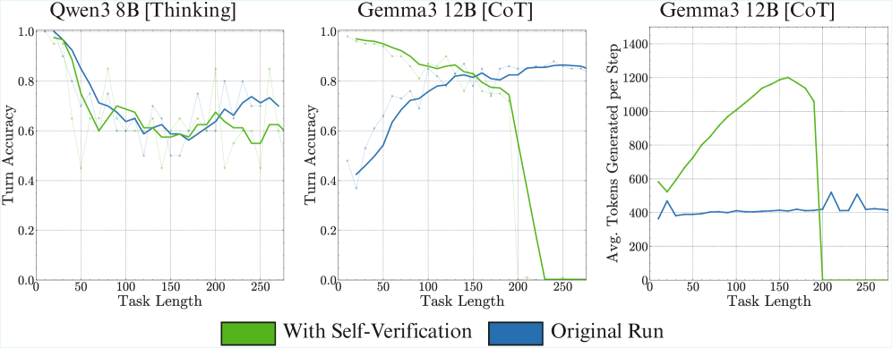
### Visual Description
# Technical Data Extraction: Performance Analysis of Qwen3 and Gemma3 Models
This document provides a comprehensive extraction of data and trends from the provided image, which contains three line charts comparing model performance with and without "Self-Verification."
## 1. Global Metadata and Legend
* **Language:** English
* **Legend Location:** Bottom center of the image.
* **Legend Categories:**
* **Green Box/Line:** "With Self-Verification"
* **Blue Box/Line:** "Original Run"
* **Common X-Axis:** "Task Length" (Scale: 0 to ~275)
* **Common Visual Elements:** Solid lines represent smoothed averages; faint dotted lines with markers represent raw data points.
---
## 2. Component Analysis
### Chart 1: Qwen3 8B [Thinking]
* **Y-Axis:** Turn Accuracy (Scale: 0.0 to 1.0)
* **Trend Analysis:**
* **Original Run (Blue):** Starts at 1.0 accuracy for short tasks. Shows a steep decline until Task Length ~75, then stabilizes into a fluctuating plateau between 0.6 and 0.75.
* **With Self-Verification (Green):** Also starts at 1.0. Follows a similar downward trajectory but generally stays slightly below or equal to the Original Run after Task Length 100.
* **Key Data Observations:**
* Both methods converge toward a similar accuracy range (0.6 - 0.7) as task length increases.
* Self-verification does not appear to provide a significant accuracy boost for this specific model configuration across longer tasks.
### Chart 2: Gemma3 12B [CoT]
* **Y-Axis:** Turn Accuracy (Scale: 0.0 to 1.0)
* **Trend Analysis:**
* **Original Run (Blue):** Shows a strong upward trend. Starts low (~0.4 accuracy) for short tasks and steadily improves as Task Length increases, peaking and stabilizing around 0.85 after Task Length 200.
* **With Self-Verification (Green):** Starts very high (~0.95 accuracy) for short tasks. It maintains high accuracy until Task Length ~180, after which it suffers a catastrophic failure, dropping sharply to 0.0 accuracy by Task Length 230.
* **Key Data Observations:**
* **Crossover Point:** At Task Length ~160, the Original Run surpasses the Self-Verification run.
* **Failure State:** The green line indicates that for very long tasks (>200), the self-verification mechanism causes the model to fail completely (0% accuracy).
### Chart 3: Gemma3 12B [CoT] (Token Generation)
* **Y-Axis:** Avg. Tokens Generated per Step (Scale: 0 to 1400)
* **Trend Analysis:**
* **Original Run (Blue):** Remains extremely stable. Regardless of Task Length, the model generates a consistent average of approximately 400 tokens per step.
* **With Self-Verification (Green):** Shows a significant, linear increase in token generation as Task Length increases. It starts at ~550 tokens and peaks at ~1200 tokens at Task Length 160. Following this peak, it drops slightly and then crashes to 0 tokens at Task Length 200.
* **Key Data Observations:**
* The "Self-Verification" process is computationally more expensive, requiring significantly more tokens as tasks get longer.
* The crash to 0 tokens in Chart 3 correlates exactly with the 0.0 accuracy seen in Chart 2, suggesting a context window limit or a processing error that halts generation entirely for long tasks when self-verification is active.
---
## 3. Summary of Findings
| Metric | Qwen3 8B [Thinking] | Gemma3 12B [CoT] |
| :--- | :--- | :--- |
| **Accuracy Trend** | Decreases then plateaus. | Original improves; Self-Verification crashes. |
| **Self-Verification Impact** | Minimal/Neutral. | High benefit for short tasks; Catastrophic for long tasks. |
| **Token Cost** | N/A (Not charted) | Self-Verification increases token usage by up to 3x before failing. |
**Conclusion:** While "Self-Verification" improves accuracy for Gemma3 12B on shorter tasks, it introduces a scaling overhead in token generation that leads to a total system failure once a certain task length threshold (approx. 200) is reached. Qwen3 8B appears more robust to task length but does not benefit significantly from the self-verification logic shown.
</details>
Figure 8: Self-verification does not fix self-conditioning. Prompting to self-verify does not suffice to fix the self-conditioning effect completely. It leads to overthinking in thinking models and increases the amount of tokens required per turn, leading to faster context consumption in CoT models.
A.2 Context Engineering
Another natural mitigation strategy is to limit the model’s exposure to its own past errors in its history. We operationalize this using a simple sliding context window, which is particularly well-suited for Markovian tasks like ours. This approach maintains only the $N$ most recent turns in the model’s context. The rationale is that a smaller context window reduces the probability of the model observing a lot of its own past failures, thereby breaking the negative feedback loop of self-conditioning.
As shown in Figure ˜ 9 (a), performance improves significantly as the context window size is reduced, allowing models to sustain execution for longer horizons. While a fixed sliding window is only applicable to tasks without long-range dependencies, this result validates a more general principle: active context management designed to minimize the accumulation of errors in the context is a promising direction for improving long-horizon reliability in LLM agents.
<details>
<summary>x8.png Details</summary>
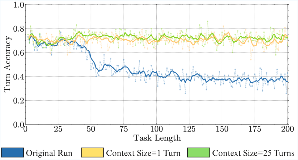
### Visual Description
# Technical Document Extraction: Turn Accuracy vs. Task Length
## 1. Component Isolation
* **Header:** None present.
* **Main Chart Area:** A line graph plotted on a Cartesian coordinate system with a grid. It features three distinct data series, each represented by a solid trend line (moving average) and a faint, dashed line with individual data points.
* **Footer (Legend):** Located at the bottom of the image, centered horizontally.
---
## 2. Axis and Label Extraction
* **Y-Axis Label:** "Turn Accuracy" (Vertical, left-aligned).
* **Y-Axis Scale:** Ranges from `0.0` to `1.0` with major tick marks and labels every `0.2` units. Minor tick marks are present at `0.1` intervals.
* **X-Axis Label:** "Task Length" (Horizontal, bottom-centered).
* **X-Axis Scale:** Ranges from approximately `0` to `200`. Major tick marks and labels are placed at `25, 50, 75, 100, 125, 150, 175, 200`.
---
## 3. Legend and Data Series Identification
The legend is located at the bottom of the chart.
| Color | Label | Visual Trend Description |
| :--- | :--- | :--- |
| **Blue** | `Original Run` | Starts high (~0.75), remains stable until Task Length 50, then drops sharply to ~0.4 and fluctuates around that level for the remainder of the task. |
| **Yellow/Gold** | `Context Size=1 Turn` | Starts at ~0.75, shows high variance but maintains a relatively flat horizontal trend between 0.65 and 0.75 throughout the entire task length. |
| **Green** | `Context Size=25 Turns` | Starts at ~0.75, maintains a stable horizontal trend with moderate variance, generally staying between 0.7 and 0.8 throughout the task length. |
---
## 4. Detailed Data Analysis and Key Trends
### Series 1: Original Run (Blue)
* **Initial Phase (0-50):** Accuracy begins at approximately 0.75. It fluctuates slightly but maintains a mean above 0.65.
* **Degradation Phase (50-60):** A significant and rapid decline occurs. Accuracy drops from ~0.6 to ~0.45 within 10 units of Task Length.
* **Stable Low Phase (60-200):** The accuracy plateaus. While there is significant "noise" (individual points ranging from 0.25 to 0.55), the smoothed trend line remains consistently near the 0.4 mark.
### Series 2: Context Size=1 Turn (Yellow/Gold)
* **Overall Trend:** This series exhibits the highest degree of point-to-point volatility (noise).
* **Performance:** Despite the noise, the performance does not decay over time. It maintains an average accuracy of approximately 0.70 across the entire x-axis.
* **Comparison:** It significantly outperforms the "Original Run" after Task Length 50.
### Series 3: Context Size=25 Turns (Green)
* **Overall Trend:** This is the highest-performing series. It shows a very slight upward trend or stabilization after the initial 50 turns.
* **Performance:** The trend line stays consistently between 0.7 and 0.8. It appears more stable (less variance in the dashed line) than the "Context Size=1 Turn" series.
* **Comparison:** This configuration provides the most reliable and highest accuracy for long-duration tasks.
---
## 5. Summary of Findings
The chart demonstrates a "long-context" or "long-task" performance issue in the **Original Run**, where accuracy collapses after 50 turns. Implementing a fixed context window (either 1 turn or 25 turns) effectively mitigates this collapse, maintaining accuracy levels above 0.7 for the duration of a 200-turn task. The **Context Size=25 Turns** (Green) provides the most stable and highest overall accuracy.
</details>
(a) Context Engineering
<details>
<summary>x9.png Details</summary>
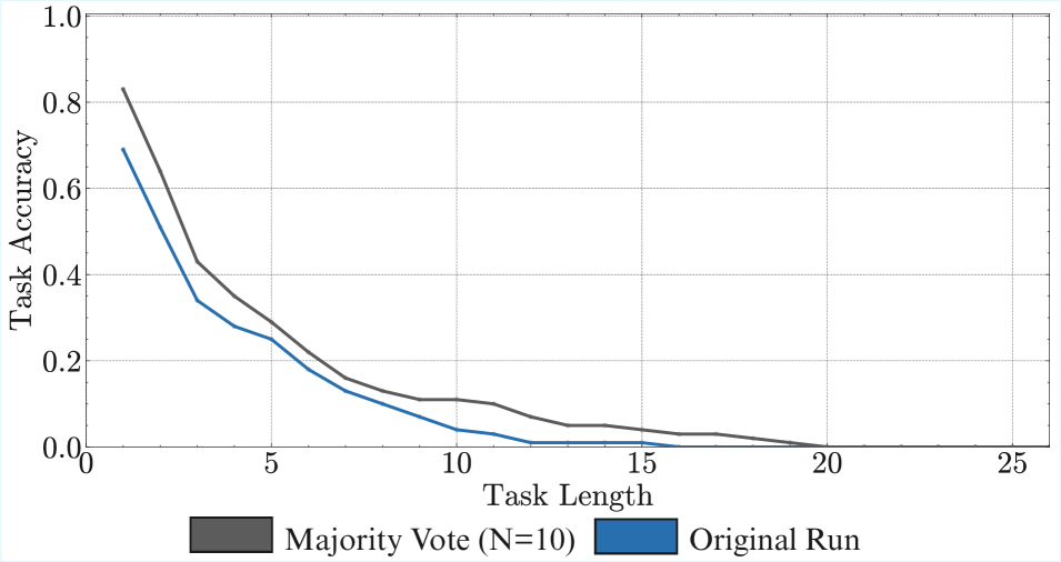
### Visual Description
# Technical Data Extraction: Task Accuracy vs. Task Length
## 1. Image Overview
This image is a line graph illustrating the relationship between "Task Length" and "Task Accuracy." It compares two different methodologies: an "Original Run" and a "Majority Vote (N=10)" approach.
## 2. Component Isolation
### A. Header / Title
* **Text:** None explicitly provided as a header; the information is contained within the axis labels and legend.
### B. Main Chart Area (Axes and Grid)
* **Y-Axis Label:** Task Accuracy
* **Y-Axis Scale:** 0.0 to 1.0, with major tick marks and grid lines every 0.2 units.
* **X-Axis Label:** Task Length
* **X-Axis Scale:** 0 to 25, with major tick marks and grid lines every 5 units. Minor tick marks are visible every 1 unit.
* **Grid:** A dashed light-gray grid is present for both horizontal and vertical major increments.
### C. Legend (Footer Region)
* **Location:** Centered at the bottom of the image, below the X-axis.
* **Series 1:** Dark Gray Box — **Majority Vote (N=10)**
* **Series 2:** Blue Box — **Original Run**
---
## 3. Trend Verification and Data Extraction
### Series 1: Majority Vote (N=10)
* **Color:** Dark Gray
* **Visual Trend:** The line starts at its highest point (approx. 0.83) at Task Length 1. It exhibits a steep exponential decay as Task Length increases. It consistently maintains a higher accuracy than the "Original Run" across all task lengths until both converge near zero at Task Length 20.
* **Estimated Data Points:**
| Task Length | Estimated Accuracy |
| :--- | :--- |
| 1 | ~0.83 |
| 3 | ~0.43 |
| 5 | ~0.29 |
| 10 | ~0.11 |
| 15 | ~0.04 |
| 20 | ~0.00 |
### Series 2: Original Run
* **Color:** Blue
* **Visual Trend:** The line starts at approximately 0.69 at Task Length 1. Like the gray line, it follows a steep downward curve. It remains below the "Majority Vote" line throughout the entire duration. The accuracy drops to near-zero faster than the majority vote, hitting a floor around Task Length 12-13.
* **Estimated Data Points:**
| Task Length | Estimated Accuracy |
| :--- | :--- |
| 1 | ~0.69 |
| 3 | ~0.34 |
| 5 | ~0.25 |
| 10 | ~0.04 |
| 12 | ~0.01 |
| 15+ | ~0.01 to 0.00 |
---
## 4. Key Findings and Observations
* **Inverse Correlation:** There is a strong inverse relationship between Task Length and Task Accuracy. As the complexity or length of the task increases, the ability of the system to maintain accuracy diminishes significantly.
* **Performance Enhancement:** The "Majority Vote (N=10)" method provides a consistent performance buffer over the "Original Run." At Task Length 1, the majority vote improves accuracy by roughly 14 percentage points.
* **Failure Threshold:** For both methods, accuracy becomes negligible (less than 10%) once the Task Length exceeds 10. By Task Length 20, accuracy is effectively 0 for both methods.
* **Language:** All text in this document is in English.
</details>
(b) Majority Voting
Figure 9: Context engineering and majority voting on Gemma3 12B. Controlling context size reduces the self-conditioning effect, but relies on the Markovian nature of our task. Majority voting at K=1 provides only minimal improvements over the baseline.
Appendix B Can Parallel Test-time Compute Scaling Match Thinking?
<details>
<summary>x10.png Details</summary>
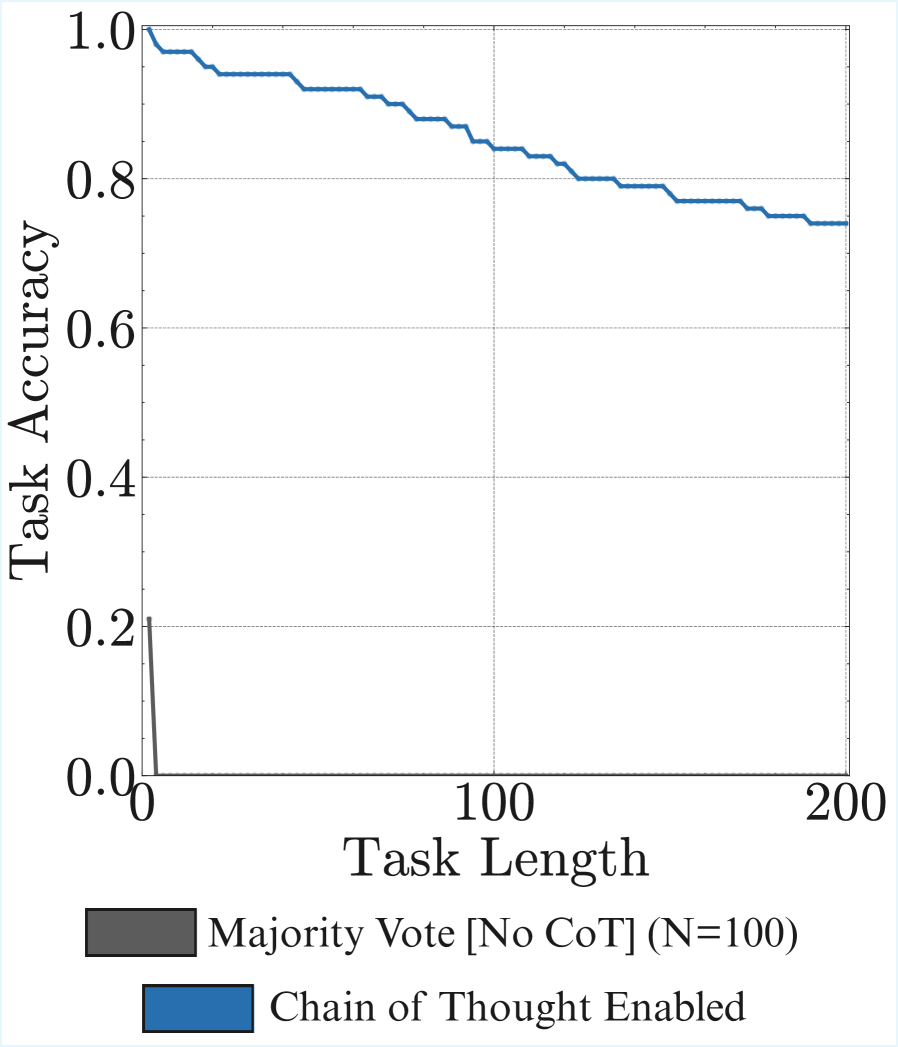
### Visual Description
# Technical Data Extraction: Task Accuracy vs. Task Length
## 1. Component Isolation
* **Header:** None present.
* **Main Chart:** A 2D line graph plotting "Task Accuracy" against "Task Length". It features a grid with dashed lines and two distinct data series.
* **Footer (Legend):** Located at the bottom of the image, containing two labeled color swatches.
---
## 2. Axis and Metadata Extraction
* **Y-Axis Label:** Task Accuracy
* **Y-Axis Scale:** 0.0 to 1.0 (increments of 0.2 marked, with minor ticks every 0.1).
* **X-Axis Label:** Task Length
* **X-Axis Scale:** 0 to 200 (increments of 100 marked, with minor ticks every 50).
* **Grid:** Horizontal and vertical dashed lines at major intervals (0.2, 0.4, 0.6, 0.8 on Y; 100 on X).
---
## 3. Legend and Series Identification
The legend is located at the bottom of the frame.
| Color | Label | Spatial Grounding [x, y] |
| :--- | :--- | :--- |
| **Dark Grey** | Majority Vote [No CoT] (N=100) | Bottom Left |
| **Blue** | Chain of Thought Enabled | Bottom Right |
---
## 4. Trend Verification and Data Extraction
### Series 1: Majority Vote [No CoT] (N=100)
* **Visual Trend:** The line starts at a low accuracy (approx. 0.2) and immediately drops sharply to 0.0 within a very short task length (less than 10).
* **Key Data Points:**
* **Length 0:** ~0.21 Accuracy
* **Length ~5:** 0.0 Accuracy
* **Observation:** This method fails almost immediately as task complexity/length increases.
### Series 2: Chain of Thought Enabled
* **Visual Trend:** The line starts at perfect accuracy (1.0) and exhibits a gradual, "stair-step" downward slope as task length increases. It maintains high performance throughout the entire range shown.
* **Key Data Points (Approximate):**
* **Length 0:** 1.0 Accuracy
* **Length 50:** ~0.92 Accuracy
* **Length 100:** ~0.84 Accuracy
* **Length 150:** ~0.78 Accuracy
* **Length 200:** ~0.74 Accuracy
* **Observation:** Accuracy remains above 70% even at the maximum task length of 200, demonstrating significant robustness compared to the "No CoT" baseline.
---
## 5. Summary of Findings
The chart illustrates a significant performance gap between two reasoning methods. The **Majority Vote [No CoT]** approach is unable to handle tasks beyond a negligible length, dropping to zero accuracy almost instantly. In contrast, the **Chain of Thought Enabled** approach shows a high degree of resilience; while accuracy does degrade as the task length increases, it follows a slow, linear-like decay, retaining roughly 74% accuracy at a task length of 200.
</details>
Figure 10: Parallel test time scaling on Gemma3 12B at K=2. Majority voting with the same amount of tokens as CoT traces does not match the performance of CoT.
We also experiment to validate if parallel scaling in test-time compute can achieve the same improvements as thinking. We verify this by testing if parallel majority voting can replicate the gains from either model scale or sequential computation (thinking). To create a fair comparison, we sample multiple outputs from a non-thinking Gemma3 model at each turn, with the number of samples set to match the average token count of its CoT counterpart. The final answer is determined by a majority vote over these parallel generations. From the results in Figure ˜ 10 and 9 (b), we see that while majority voting yields a marginal performance improvement over the base model, it is insufficient to match the reliability of a larger, non-thinking model, let alone the substantial gains from using CoT reasoning. This suggests that for long-horizon execution, sequential computation provides an advantage that parallel test time scaling cannot match. This contrasts with findings in other domains, such as math or common-sense reasoning, where parallel sampling with self-consistency has been shown to be highly competitive (Snell et al., 2024).
Appendix C Number of Turns vs Turn Complexity
In our experiments, we show that we can increase the length of the task needed to be performed by either (1) increasing the number of turns or (2) increasing the turn complexity, i.e, providing more inputs in the same turn. To investigate the relationship between these two axes, we perform an experiment where a model has to perform a fixed number of operations while varying the turn complexity. With a higher turn complexity, the model requires fewer turns to reach the fixed number of operations. Results in Figure ˜ 11 (a) indicate there is no strict turn complexity that is consistently the best across model families. Rather, we found that different models behave quite differently for the same turn complexities. Qwen3 32B seems to show poorer performance at lower turn complexities, indicating that it is unable to perform well over a large number of turns, even if the turns are simple themselves. Gemma3 12B shows a different trend. It reaches accuracy peaks at either extreme of the turn complexity spectrum, failing badly at mid-level turn complexities. This indicates it suffers when the turn complexity and the number of turns are both sufficiently high.
Another axis of evaluating the number of turns vs turn complexity trade-off is the test-time compute used. From a cost perspective, increasing the number of turns increases the overall cost of inference. We can lower the number of turns by increasing the turn complexity, but that would result in an increase in the per-turn inference cost, as a result of the added complexity. For the same experiment above, we track the number of output tokens used for computation (including thinking tokens) per sample, and again find diverging results for each family in Figure ˜ 11 (b).
<details>
<summary>x11.png Details</summary>
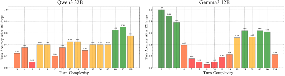
### Visual Description
# Technical Data Extraction: Model Performance Comparison
This document contains a detailed extraction of data from two bar charts comparing the performance of two Large Language Models (LLMs), **Qwen3 32B** and **Gemma3 12B**, based on task accuracy relative to "Turn Complexity."
---
## 1. Chart Overview and Global Metadata
The image consists of two side-by-side bar charts. Both charts share a similar structure:
* **Y-Axis:** "Task Accuracy After [N] Steps" (Scale: 0.0 to 1.0).
* **X-Axis:** "Turn Complexity" (Categorical values representing steps or complexity levels).
* **Color Coding (Performance Tiers):**
* **Green:** High Accuracy (typically $\ge 0.60$).
* **Yellow/Orange:** Medium Accuracy (typically $0.40$ to $0.59$).
* **Red/Coral:** Low Accuracy (typically $< 0.40$).
---
## 2. Left Chart: Qwen3 32B
**Header:** Qwen3 32B
**Y-Axis Label:** Task Accuracy After 180 Steps
**Trend Analysis:** The model shows inconsistent performance at low complexity (3-12), stabilizes at a moderate level for mid-range complexity (15-45), and peaks at high complexity (60-90) before dropping slightly at the maximum complexity of 180.
### Data Table: Qwen3 32B
| Turn Complexity (X) | Task Accuracy (Y) | Color Category |
| :--- | :--- | :--- |
| 3 | 0.250 | Red/Coral |
| 4 | 0.350 | Red/Coral |
| 5 | 0.100 | Red |
| 6 | 0.400 | Yellow |
| 9 | 0.400 | Yellow |
| 10 | 0.200 | Red/Coral |
| 12 | 0.350 | Red/Coral |
| 15 | 0.450 | Yellow |
| 18 | 0.450 | Yellow |
| 20 | 0.300 | Red/Coral |
| 30 | 0.400 | Yellow |
| 36 | 0.400 | Yellow |
| 45 | 0.400 | Yellow |
| 60 | 0.650 | Green |
| 90 | 0.700 | Green |
| 180 | 0.550 | Yellow |
---
## 3. Right Chart: Gemma3 12B
**Header:** Gemma3 12B
**Y-Axis Label:** Task Accuracy After 120 Steps
**Trend Analysis:** This model exhibits a "U-shaped" or "Bimodal" distribution. It starts with perfect/near-perfect accuracy at very low complexity (1-3), suffers a significant "trough" or performance collapse in the mid-range (5-12), recovers significantly at higher complexities (24-60), and then drops sharply at the final complexity level (120).
### Data Table: Gemma3 12B
| Turn Complexity (X) | Task Accuracy (Y) | Color Category |
| :--- | :--- | :--- |
| 1 | 1.000 | Green |
| 2 | 0.890 | Green |
| 3 | 0.780 | Green |
| 4 | 0.390 | Red/Coral |
| 5 | 0.160 | Red |
| 6 | 0.100 | Red |
| 8 | 0.060 | Red |
| 10 | 0.100 | Red |
| 12 | 0.180 | Red |
| 15 | 0.230 | Red/Coral |
| 20 | 0.520 | Yellow |
| 24 | 0.640 | Green |
| 30 | 0.530 | Yellow |
| 40 | 0.640 | Green |
| 60 | 0.620 | Green |
| 120 | 0.230 | Red/Coral |
---
## 4. Comparative Summary
* **Peak Performance:** Gemma3 12B achieves a higher absolute peak (1.000 at complexity 1) compared to Qwen3 32B (0.700 at complexity 90).
* **Stability:** Qwen3 32B maintains a more consistent, albeit lower, baseline across the mid-range complexities.
* **Failure Points:** Gemma3 12B shows a critical failure zone between complexity 5 and 12, where accuracy drops below 0.200. Qwen3 32B's lowest point is 0.100 at complexity 5, but it recovers much faster.
* **High Complexity Handling:** Both models show a performance decline at their respective maximum complexity limits (180 for Qwen3, 120 for Gemma3).
</details>
(a) For the same number of total steps, different turn complexities lead to different outcomes. We find no trend across families.
<details>
<summary>x12.png Details</summary>
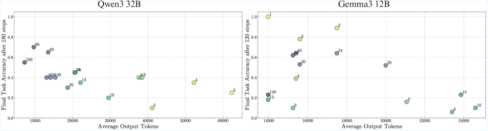
### Visual Description
# Technical Data Extraction: Model Performance Comparison
This document provides a detailed extraction of data from two side-by-side scatter plots comparing the performance of two Large Language Models: **Qwen3 32B** and **Gemma3 12B**.
## 1. Document Structure and Global Metadata
The image consists of two distinct panels arranged horizontally.
* **Language:** English.
* **Common X-Axis:** Average Output Tokens.
* **Common Y-Axis:** Final Task Accuracy after [N] steps.
* **Data Representation:** Scatter plot with colored circular markers. Each marker is labeled with a numerical value representing a specific parameter (likely a hyperparameter or configuration setting).
* **Color Gradient:** Both charts use a consistent color mapping where purple/dark blue represents higher numerical labels and yellow/light green represents lower numerical labels.
---
## 2. Panel 1: Qwen3 32B
**Header:** Qwen3 32B
**Y-Axis Label:** Final Task Accuracy after 180 steps
**X-Axis Label:** Average Output Tokens
### Trend Analysis
The data for Qwen3 32B shows a generally **inverse relationship** between average output tokens and accuracy. As the output length increases (moving right on the x-axis), the accuracy tends to decrease. The highest accuracy is achieved at lower token counts (approx. 10,000 tokens).
### Data Point Extraction
| Label (Value) | Approx. X (Tokens) | Approx. Y (Accuracy) | Color Note |
| :--- | :--- | :--- | :--- |
| 180 | 7,000 | 0.55 | Dark Purple |
| 90 | 10,000 | 0.70 | Purple |
| 60 | 14,000 | 0.65 | Purple-Blue |
| 45 | 13,500 | 0.40 | Blue |
| 36 | 14,500 | 0.40 | Blue |
| 30 | 15,500 | 0.40 | Blue |
| 20 | 19,000 | 0.30 | Teal |
| 18 | 21,000 | 0.45 | Teal |
| 15 | 21,000 | 0.45 | Teal |
| 12 | 22,000 | 0.35 | Light Teal |
| 10 | 29,500 | 0.20 | Green |
| 9 | 37,500 | 0.40 | Light Green |
| 6 | 38,500 | 0.40 | Light Green |
| 5 | 41,000 | 0.10 | Yellow-Green |
| 4 | 52,500 | 0.35 | Yellow |
| 3 | 62,500 | 0.25 | Yellow |
---
## 3. Panel 2: Gemma3 12B
**Header:** Gemma3 12B
**Y-Axis Label:** Final Task Accuracy after 120 steps
**X-Axis Label:** Average Output Tokens
### Trend Analysis
The data for Gemma3 12B is more **dispersed** and does not follow a simple linear trend. There is a cluster of high-accuracy points at lower token counts (14,000 - 18,000), but accuracy drops significantly as token counts exceed 20,000. Notably, the labels on this chart appear to be inverted compared to the first chart (lower numerical labels correspond to higher accuracy/lower tokens).
### Data Point Extraction
| Label (Value) | Approx. X (Tokens) | Approx. Y (Accuracy) | Color Note |
| :--- | :--- | :--- | :--- |
| 1 | 14,000 | 1.00 | Yellow |
| 2 | 17,500 | 0.89 | Yellow |
| 3 | 15,500 | 0.78 | Light Green |
| 4 | 15,300 | 0.39 | Light Green |
| 5 | 21,000 | 0.16 | Green |
| 6 | 15,100 | 0.10 | Green |
| 8 | 23,400 | 0.06 | Teal |
| 10 | 24,600 | 0.10 | Teal |
| 12 | 14,000 | 0.18 | Teal |
| 15 | 23,800 | 0.23 | Blue-Teal |
| 20 | 20,000 | 0.52 | Blue |
| 24 | 17,500 | 0.64 | Blue |
| 30 | 15,600 | 0.53 | Purple-Blue |
| 40 | 15,400 | 0.64 | Purple |
| 60 | 15,300 | 0.63 | Purple |
| 120 | 14,000 | 0.23 | Dark Purple |
---
## 4. Comparative Summary
* **Scale:** Qwen3 32B operates across a much wider range of output tokens (up to 60,000+), whereas Gemma3 12B is concentrated between 14,000 and 25,000 tokens.
* **Accuracy:** Gemma3 12B achieves a higher peak accuracy (1.0 at label 1) compared to Qwen3 32B (approx 0.7 at label 90), though it is measured at fewer steps (120 vs 180).
* **Efficiency:** Qwen3 shows a more stable, predictable decay in performance as output length increases, while Gemma3 shows high volatility in the 14k-16k token range.
</details>
(b) Average output tokens used to complete the execution vs final accuracy. We see that for Qwen3 32B, more turns lead to more token usage, even at lower turn complexities, pointing to overthinking. Gemma3 12B, on the other hand, uses fewer tokens for very low turn complexity or very high turn complexity.
Figure 11: Relation between the turn complexity and the number of turns.
<details>
<summary>x13.png Details</summary>
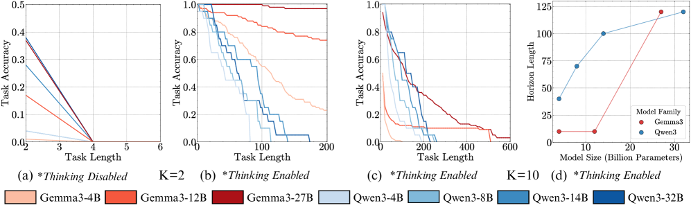
### Visual Description
# Technical Data Extraction: Model Performance Analysis
This document provides a comprehensive extraction of data and trends from the provided image, which consists of four technical charts (labeled a, b, c, and d) comparing the performance of two model families, **Gemma3** and **Qwen3**, across various task lengths and model sizes.
---
## 1. Global Legend and Metadata
The following models are represented across the charts, distinguished by color:
| Model Family | Color Code | Model Name |
| :--- | :--- | :--- |
| **Gemma3** | Light Orange | Gemma3-4B |
| | Medium Orange | Gemma3-12B |
| | Dark Red | Gemma3-27B |
| **Qwen3** | Very Light Blue | Qwen3-4B |
| | Light Blue | Qwen3-8B |
| | Medium Blue | Qwen3-14B |
| | Dark Blue | Qwen3-32B |
---
## 2. Chart (a): *Thinking Disabled*, K=2
* **Y-Axis:** Task Accuracy (Scale: 0.0 to 0.5)
* **X-Axis:** Task Length (Scale: 2 to 6)
* **Trend Analysis:** All models exhibit a sharp, linear decline in accuracy as task length increases.
* **Data Points:**
* At **Task Length 2**, accuracies range from ~0.01 (Qwen3-4B) to ~0.38 (Qwen3-32B and Gemma3-27B).
* By **Task Length 4**, the accuracy for **all models** drops to 0.0.
* **Conclusion:** Without "Thinking" enabled, no model can handle tasks longer than length 3.
---
## 3. Chart (b): *Thinking Enabled*, K=2
* **Y-Axis:** Task Accuracy (Scale: 0.0 to 1.0)
* **X-Axis:** Task Length (Scale: 0 to 200)
* **Trend Analysis:** Enabling "Thinking" significantly extends the horizon. Performance degrades as task length increases, but larger models maintain high accuracy for much longer.
* **Key Observations:**
* **Gemma3-27B (Dark Red):** Maintains near 1.0 accuracy across the entire range (0-200).
* **Gemma3-12B (Medium Orange):** Slopes downward gradually, ending at ~0.75 accuracy at length 200.
* **Qwen3-32B (Dark Blue):** Drops sharply after length 50, reaching 0.0 accuracy around length 175.
* **Small Models (4B variants):** Accuracy drops to 0.0 before task length 100.
---
## 4. Chart (c): *Thinking Enabled*, K=10
* **Y-Axis:** Task Accuracy (Scale: 0.0 to 1.0)
* **X-Axis:** Task Length (Scale: 0 to 600)
* **Trend Analysis:** Increasing K to 10 further extends the operational range. All models eventually decay to zero accuracy, but the decay is more gradual than in Chart (b).
* **Key Observations:**
* **Gemma3-27B (Dark Red):** The most resilient; accuracy stays above 0.5 until length ~200, then decays to near 0.0 by length 600.
* **Qwen3-32B (Dark Blue):** Accuracy drops below 0.5 at length ~150 and reaches 0.0 by length ~250.
* **Gemma3-4B (Light Orange):** Shows a very rapid decline, hitting near 0.0 before length 100.
---
## 5. Chart (d): Horizon Length vs. Model Size
* **Y-Axis:** Horizon Length (Scale: 0 to 125)
* **X-Axis:** Model Size (Billion Parameters) (Scale: 0 to 30+)
* **Legend [x, y]:** Located at the bottom right of the chart.
* **Trend Analysis:**
* **Qwen3 (Blue Line):** Shows a logarithmic-style growth. Horizon length increases significantly from 4B to 14B parameters, then plateaus/slows toward 32B.
* **Gemma3 (Red Line):** Shows a "step-function" or exponential growth. Horizon length remains low and flat for 4B and 12B models, then shoots up vertically for the 27B model.
* **Extracted Data Points (Approximate):**
| Model Family | Model Size (B) | Horizon Length |
| :--- | :--- | :--- |
| **Qwen3** | ~4B | ~40 |
| **Qwen3** | ~8B | ~70 |
| **Qwen3** | ~14B | ~100 |
| **Qwen3** | ~32B | ~120 |
| **Gemma3** | ~4B | ~10 |
| **Gemma3** | ~12B | ~10 |
| **Gemma3** | ~27B | ~120 |
---
## Summary of Findings
1. **Thinking Capability:** Enabling "Thinking" is the primary driver for handling longer task lengths. Without it, all models fail by task length 4.
2. **Scaling:** Larger models consistently outperform smaller models in "Horizon Length" (the ability to maintain accuracy over longer tasks).
3. **Family Comparison:** Qwen3 models show better "Horizon" performance at smaller parameter counts (4B-14B), while Gemma3 requires a larger parameter count (27B) to achieve its maximum horizon, at which point it matches or slightly exceeds the largest Qwen3 model.
</details>
Figure 12: Scaling trends hold even after enabling Sequential Test Time compute. We compare model performance with thinking disabled (a) against thinking enabled (b, c) at varying turn complexities. (a) Without thinking, all models fail to execute even two steps ( $K=2$ ) in a single turn. (b) In contrast, enabling thinking prevents this performance collapse, with all models successfully handling $K=2$ . (c) When the turn complexity is further increased to $K=10$ , performance degrades, but a clear scaling trend emerges. (d) This trend is explicitly shown, illustrating that for complex turns, the horizon length increases consistently with model size, reinforcing the benefits of scaling model size even when thinking is enabled.
<details>
<summary>x14.png Details</summary>
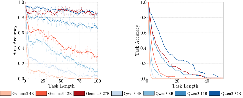
### Visual Description
# Technical Data Extraction: Model Performance Comparison
This document contains a detailed extraction of data from two line charts comparing the performance of **Gemma3** and **Qwen3** model families across varying task lengths.
## 1. Metadata and Global Legend
The image consists of two side-by-side line graphs sharing a common legend located at the bottom of the image.
**Legend (Spatial Placement: Bottom Center [x, y])**
The legend identifies seven distinct models categorized by color family:
* **Gemma3 Family (Red/Orange Tones):**
* **Gemma3-4B**: Light Peach/Orange
* **Gemma3-12B**: Bright Orange-Red
* **Gemma3-27B**: Dark Maroon/Red
* **Qwen3 Family (Blue Tones):**
* **Qwen3-4B**: Very Light Blue
* **Qwen3-8B**: Medium Light Blue
* **Qwen3-14B**: Medium Blue
* **Qwen3-32B**: Dark Navy Blue
---
## 2. Left Chart: Step Accuracy vs. Task Length
### Axis Information
* **Y-Axis:** "Step Accuracy" (Scale: 0.0 to 1.0, increments of 0.2)
* **X-Axis:** "Task Length" (Scale: 0 to 100, markers at 0, 25, 50, 75, 100)
### Component Analysis & Trends
This chart displays raw data points (faint dots) and a smoothed trend line for each model.
| Model | Color | Visual Trend Description | Performance Summary |
| :--- | :--- | :--- | :--- |
| **Qwen3-32B** | Dark Navy | High stability; slight downward slope. | Starts ~0.95, ends ~0.85. |
| **Gemma3-27B** | Dark Red | High stability; fluctuates around a horizontal mean. | Maintains ~0.85 to 0.90 throughout. |
| **Qwen3-14B** | Medium Blue | Moderate decline. | Starts ~0.85, drops to ~0.65 by length 100. |
| **Gemma3-12B** | Orange-Red | Significant steady decline. | Starts ~0.80, drops to ~0.30 by length 100. |
| **Qwen3-8B** | Light Blue | Sharp initial drop, then steady decline. | Starts ~0.80, drops to ~0.10 by length 100. |
| **Qwen3-4B** | V. Light Blue | Very sharp drop; stabilizes near zero. | Drops below 0.2 by length 25; ends near 0.05. |
| **Gemma3-4B** | Peach | Immediate collapse to baseline. | Drops to ~0.05 by length 10; remains near 0. |
---
## 3. Right Chart: Task Accuracy vs. Task Length
### Axis Information
* **Y-Axis:** "Task Accuracy" (Scale: 0.0 to 1.0, increments of 0.2)
* **X-Axis:** "Task Length" (Scale: 0 to 50+, markers at 0, 20, 40)
### Component Analysis & Trends
This chart measures the success of the entire task. Accuracy for all models begins at 1.0 for length 0 and decays exponentially as task length increases.
| Model | Color | Visual Trend Description | Performance Summary |
| :--- | :--- | :--- | :--- |
| **Qwen3-32B** | Dark Navy | Slowest decay; most resilient. | Hits 0.2 accuracy at length ~30; reaches ~0.02 at length 50. |
| **Gemma3-27B** | Dark Red | Moderate decay; second best. | Hits 0.2 accuracy at length ~15; reaches ~0.01 at length 40. |
| **Qwen3-14B** | Medium Blue | Moderate decay; follows Gemma3-27B closely. | Hits 0.2 accuracy at length ~15; reaches 0 at length 35. |
| **Gemma3-12B** | Orange-Red | Rapid decay. | Hits 0.2 accuracy at length ~8; reaches 0 at length 25. |
| **Qwen3-8B** | Light Blue | Very rapid decay. | Hits 0.2 accuracy at length ~5; reaches 0 at length 15. |
| **Qwen3-4B** | V. Light Blue | Near-instant decay. | Hits 0.2 accuracy at length ~2; reaches 0 at length 10. |
| **Gemma3-4B** | Peach | Instant decay. | Hits 0 accuracy by length ~3. |
---
## 4. Key Observations and Data Synthesis
1. **Scaling Law Correlation:** In both charts, there is a direct correlation between parameter count (B) and performance. Larger models (32B, 27B) maintain significantly higher accuracy as task complexity (length) increases.
2. **Step vs. Task Accuracy:** While the largest models maintain high *Step Accuracy* (above 80%) even at length 100, their *Task Accuracy* (the probability of completing every step correctly) drops toward zero much earlier (around length 50). This indicates that even small errors per step compound over time.
3. **Cross-Family Comparison:** The **Qwen3-32B** (Dark Navy) is the top performer across both metrics, followed by **Gemma3-27B** (Dark Red). The **Qwen3-14B** (Medium Blue) performs comparably to the **Gemma3-27B** in Task Accuracy despite having fewer parameters.
</details>
Figure 13: Temperature does not impact the trends observed. We reproduce the same trends in Figure ˜ 4, when running with temperature 0.
Appendix D Deconstructing Errors in Retrieve-then-compose Steps
To further isolate the source of execution errors, we decompose our task into its two constituent operations–retrieval and addition–and evaluate models on them individually:
- Retrieval-Only Task. A stateless task where, at each turn, the model is given a key and must simply return the corresponding integer value from the dictionary. No running sum is maintained. This isolates the retrieval component.
- Addition-Only Task. A stateless task where, at each turn, the model is given two random integers to add. No running sum is maintained. This isolates the arithmetic component.
- Prefix-sum Task. A stateful task where, at each turn, the model is given an integer directly and must add it to its previously reported running sum. This isolates the combination of arithmetic and state-tracking components.
From Figure ˜ 14, we can observe that models achieve near-perfect performance on the stateless retrieval and addition task, indicating that neither simple dictionary lookup nor addition is a significant source of error. In contrast, the prefix sum task, while significantly better than our task, still exhibits a slow degradation over time.
This leads to two key insights. First, the difficulty lies not in the atomic operations themselves, which models perform with high accuracy in isolation over long horizons. Second, this suggests that the primary source of degradation is the state-management component of the task. While stateless retrieval and addition are trivial, the requirement to reliably maintain and update a running sum introduces higher chances of error. This suggests that the models struggle with the requirement to concurrently manage information lookup and state updates.
<details>
<summary>x15.png Details</summary>
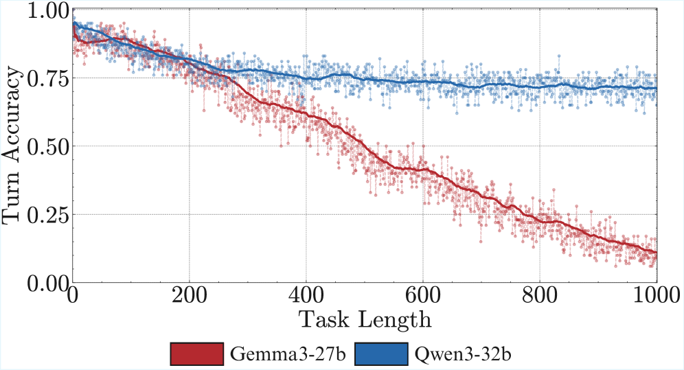
### Visual Description
# Technical Document Extraction: Model Performance Comparison
## 1. Image Overview
This image is a line graph comparing the performance of two Large Language Models (LLMs) across increasing task lengths. It plots "Turn Accuracy" against "Task Length."
## 2. Component Isolation
### Header / Metadata
* **Language:** English
* **Content:** None (The image starts directly with the chart area).
### Main Chart Area
* **Y-Axis Label:** Turn Accuracy
* **Y-Axis Scale:** 0.00 to 1.00 (increments of 0.25 marked, with grid lines every 0.25).
* **X-Axis Label:** Task Length
* **X-Axis Scale:** 0 to 1000 (increments of 200 marked).
* **Grid:** A light gray dashed grid is present for both axes.
* **Data Representation:** Each model is represented by a solid trend line (likely a moving average) and a scatter plot of semi-transparent points connected by thin dashed lines representing raw data variance.
### Footer / Legend
* **Spatial Placement:** Centered at the bottom of the image.
* **Legend Items:**
* **Red Box:** Gemma3-27b
* **Blue Box:** Qwen3-32b
---
## 3. Data Series Analysis and Trend Verification
### Series 1: Qwen3-32b (Blue)
* **Visual Trend:** The line starts at a high accuracy (~0.95). It shows a very gradual, slight downward slope as task length increases, but remains remarkably stable. It plateaus and maintains a high level of performance even at the maximum task length.
* **Key Data Points:**
* **Start (Length 0):** ~0.95 Accuracy.
* **Midpoint (Length 500):** ~0.75 Accuracy.
* **End (Length 1000):** ~0.70 Accuracy.
* **Variance:** The raw data points (light blue) show moderate fluctuation around the trend line, staying mostly between 0.65 and 0.85 after the initial drop.
### Series 2: Gemma3-27b (Red)
* **Visual Trend:** The line starts at a high accuracy (~0.90), similar to Qwen. However, it exhibits a significant and consistent downward slope (negative correlation) as task length increases. The performance degrades much more rapidly than the blue series.
* **Key Data Points:**
* **Start (Length 0):** ~0.90 Accuracy.
* **Intersection Point:** At approximately Task Length 200, both models have an accuracy of ~0.80.
* **Midpoint (Length 500):** ~0.50 Accuracy.
* **End (Length 1000):** ~0.10 Accuracy.
* **Variance:** The raw data points (light red) show high fluctuation, with some points dropping toward 0.00 and others reaching up to 0.25 near the end of the task length.
---
## 4. Comparative Summary
The chart demonstrates a clear performance gap between the two models as task complexity or duration (Task Length) increases.
| Metric | Qwen3-32b (Blue) | Gemma3-27b (Red) |
| :--- | :--- | :--- |
| **Initial Accuracy** | High (~0.95) | High (~0.90) |
| **Stability** | High; maintains >0.70 accuracy | Low; drops to ~0.10 accuracy |
| **Degradation Rate** | Minimal/Gradual | Significant/Linear |
| **Performance at Length 1000** | ~0.70 | ~0.10 |
**Conclusion:** Qwen3-32b is significantly more robust to long-form tasks than Gemma3-27b, which suffers from a near-total loss of accuracy as the task length approaches 1000.
</details>
<details>
<summary>x16.png Details</summary>
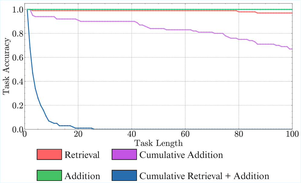
### Visual Description
# Technical Document Extraction: Task Accuracy vs. Task Length
## 1. Component Isolation
* **Header/Title:** None present in the image.
* **Main Chart Area:** A line graph plotted on a Cartesian coordinate system with a grid.
* **Axes:**
* **Y-Axis (Vertical):** Labeled "Task Accuracy". Scale ranges from 0.0 to 1.0 with major ticks every 0.2.
* **X-Axis (Horizontal):** Labeled "Task Length". Scale ranges from 0 to 100 with major ticks every 20.
* **Footer/Legend:** Located at the bottom of the image, below the X-axis label. It contains four color-coded categories.
---
## 2. Legend and Data Series Identification
The legend is positioned at the bottom center of the image.
| Color | Label | Visual Trend Description |
| :--- | :--- | :--- |
| **Red** | **Retrieval** | Maintains a constant accuracy of 1.0 until approximately Task Length 80, where it drops slightly to ~0.98 and remains flat. |
| **Green** | **Addition** | Maintains a perfectly flat, constant accuracy of 1.0 across the entire range (0 to 100). |
| **Purple** | **Cumulative Addition** | Shows a "staircase" downward trend. Starts at 1.0, drops to ~0.95 early, stays flat, drops to ~0.90 at length 20, ~0.83 at length 50, and continues a staggered decline to ~0.68 at length 100. |
| **Blue** | **Cumulative Retrieval + Addition** | Shows a sharp exponential decay. Starts at 1.0 at length 0 and crashes to near 0.0 by Task Length 25, remaining at 0.0 for the rest of the chart. |
---
## 3. Data Extraction and Key Trends
### Axis Markers
* **Y-Axis:** 0.0, 0.2, 0.4, 0.6, 0.8, 1.0
* **X-Axis:** 0, 20, 40, 60, 80, 100
### Detailed Data Points (Estimated from Grid)
| Task Length | Retrieval (Red) | Addition (Green) | Cumulative Addition (Purple) | Cumulative Retrieval + Addition (Blue) |
| :--- | :--- | :--- | :--- | :--- |
| **0** | 1.0 | 1.0 | 1.0 | 1.0 |
| **10** | 1.0 | 1.0 | 0.94 | 0.08 |
| **20** | 1.0 | 1.0 | 0.90 | 0.01 |
| **40** | 1.0 | 1.0 | 0.90 | 0.00 |
| **60** | 1.0 | 1.0 | 0.83 | 0.00 |
| **80** | 0.98 | 1.0 | 0.75 | 0.00 |
| **100** | 0.98 | 1.0 | 0.68 | 0.00 |
---
## 4. Technical Analysis of Trends
1. **Stability of Simple Tasks:** Both "Addition" (Green) and "Retrieval" (Red) demonstrate high resilience to task length, maintaining near-perfect accuracy (1.0) throughout the sequence.
2. **Complexity Penalty:** The "Cumulative Addition" (Purple) task shows that as the length of the sequence increases, the accuracy degrades in a step-wise fashion, suggesting a cumulative error or memory strain that increases every 10-20 units of task length.
3. **Critical Failure Point:** The "Cumulative Retrieval + Addition" (Blue) task represents a catastrophic failure mode. The system's ability to perform this combined task effectively vanishes once the task length exceeds 20 units. The most significant drop occurs between length 0 and 10, where accuracy falls by over 90%.
## 5. Language Declaration
The text in this image is entirely in **English**. No other languages were detected.
</details>
Figure 14: Analysis of execution failures. (a) Self-conditioning effect emerges as tasks get longer. Even for models that ace the task at a task length of 100, the Turn Accuracy drops constantly as we further increase the turns. (b) Models are good at the tasks individually, but not on their composition. State tracking introduces additional difficulty.
Appendix E Experimental Setup
E.1 Task Details
We create a dictionary where keys consist of common five-letter English words, and the values consist of integers uniformly sampled from $-99$ to $99$ . The range of values is deliberately kept large to minimize the chance of an assistant being wrong in an earlier turn correcting its response by pure accident. For our experiment, we first create a fixed set of $100$ keys. Then, we create multiple rollouts (samples) of $50,000$ steps. For each rollout, we uniformly sample a separate set of values to be assigned to each key, in order to increase experimental breadth. Next, at each step, we uniformly sample a key to be provided at that step with replacement. This gives us a list of keys to be processed in order, which is exactly the plan to be executed by the agent.
To account for the turn complexity ( $K$ ), we group $K$ consecutive keys together and represent them as one turn. Thus, we can fully specify our intended evaluation by (1) specifying the number of samples (rollouts) needed, (2) the turn complexity, $K$ , and (3) the number of turns required. This gives us a superset of data from which we sample rollouts to use in our experiments. For the Qwen3 and Gemma3 families, we sample 100 rollouts. For frontier models, due to cost limitations, we sample 20-50 rollouts. To ensure consistency in evaluation, we provide the same rollouts to each model.
E.2 Prompting
Each LLM is provided a standardized prompt describing the task at the start of the conversation. This prompt specifies the dictionary containing the five-letter word keys and their corresponding values. Further, the prompt specifies the number of keys that will be provided to the LLM at each subsequent turn. To ensure format following, the prompt also contains few-shot examples with different turn complexities. Finally, the LLM is asked to provide the running sum after each turn in <answer> tags. An example conversation is shown below.
E.3 Prompting for Thinking Models
To enable models to use chain-of-thought prompting, we add the line ‘‘Think step by step before answering.’’ to the prompt and also add CoT traces to the few-shot examples. We find that models stop performing CoT reasoning after a few turns, as it starts conditioning on the answer format in its history. Thus, we end up including the chain-of-thought trace in the conversation history, to ensure the model does not forget the CoT instruction. This is a trade-off we had to make as it increases the input context of the LLM, however, it was essential to ensure instruction following. Thinking models provided their reasoning in <think> tags, which were removed from the conversation history. No other changes were needed to make the thinking models follow instructions.
E.4 Model Specifications
For chain-of-thought prompting, we set the per-turn output token limit to $10,000$ tokens, and for thinking models, the token limit is set to $32,000$ tokens, consistent with token limits provided by OpenRouter. We ensure that these token limits are sufficient to complete the required computations.
We use a temperature of $0.6$ and a top-p value of $0.95$ for all Gemma models. For Qwen, we use a temperature of $0.6$ and a top-p value of $0.95$ for thinking mode and a temperature of $0.7$ and a top-p value of $0.8$ for non-thinking as recommended in their documentation. https://huggingface.co/Qwen/Qwen3-32B We find in Figure ˜ 13 that temperature does not affect the observed trends by much.
E.5 Compute Details
All experiments were conducted on machines equipped with 4x NVIDIA A100 GPUs with 40/80GB memory. Frontier model evaluations were performed using OpenRouter.
Starting Prompt: You are an AI assistant. I will provide you with a dictionary and then give you keys in groups of 2. Your task is to keep a running total (starting from 0) by adding the values associated with the keys I provide. In each turn, I’ll provide 2 keys (comma-separated). Respond with the current running sum, enclosed in <answer> tags. Examples: Dictionary to maintain: ‘apple’: 5, ‘banana’: 0, ‘cherry’: 7, ‘grape’: -4, ‘kiwi’: 2, ‘mango’: -1 Example 1: keys in groups of 2 User: apple, banana Assistant: <answer>5</answer> User: cherry, grape Assistant: <answer>8</answer> User: kiwi, mango Assistant: <answer>9</answer> Example 2: keys in groups of 3 User: apple, banana, cherry Assistant: <answer>12</answer> User: grape, kiwi, mango Assistant: <answer>9</answer> Example 3: keys in groups of 6 User: apple, banana, cherry, grape, kiwi, mango Assistant: <answer>9</answer> Now, here is the actual task: Dictionary to maintain: ’doubt’: -64, ‘alone’: 46, ‘adult’: 84, ‘fault’: -19, ‘brain’: -45, ‘blind’: 68, ... ‘coach’: -31, ‘alarm’: 88, ‘could’: 25, ‘cable’: -32 Ready to start! IMPORTANT: DO NOT OUTPUT ANY OTHER TEXT OUTSIDE ANSWER TAGS. Only provide the final running sum OF ALL TURNS in <answer> tags. User: alarm,coach Assistant: <answer>57</answer> User: doubt,cable Assistant: <answer>-39</answer>
Appendix F Format Following Failures
In any LLM evaluation, format following failures are a common source of error that is often neglected. In our experiments, any model can have 2 types of format following failures: (1) They do not provide <answer> tags in their answer, and (2) They do not provide a valid integer within <answer> tags. To minimize format following failures, we ensure clarity in the starting prompt with clear format instructions, as well as few-shot examples. To empirically verify that model errors on our task are actually execution errors and not just format following errors in disguise, for each experiment, we also track the format failure fraction: the fraction of samples that do not correctly follow the format, with the failure being either (1) or (2). It is important to note that while we try to minimize any such error to the best of our abilities, we still count format following as a limitation of the model and hence a source of error.
Our results for format following failures are presented in Figure ˜ 15 for the experiments presented in Section ˜ 3. We observe that smaller models are more susceptible to format failures, with the Qwen3 family in particular being worse at following format instructions. Overall, the fraction for format following errors is low (around 0.1), with the Qwen3-8B being an exception. We find that the error here actually comes from the model trying to cheat, and do the entire summation inside the <answer> tags (For example, <answer>39 + 51 = 90</answer>). This is explicitly forbidden as we do not allow chain-of-thought or thinking in this experiment, and thus we count this as an error. Gemma3 4B fails at later turns due to context length limitations; however, that does not affect any results, as its accuracies drop much earlier.
<details>
<summary>x17.png Details</summary>
### Visual Description
# Technical Data Extraction: Format Failure Fraction Analysis
This document provides a comprehensive extraction of data and trends from the provided image, which consists of four line charts comparing the "Format Failure Fraction" of various Large Language Models (Gemma3 and Qwen3 series) across different task lengths and configurations.
## 1. Global Metadata and Legend
The image is segmented into four sub-plots (a through d) and a shared legend at the bottom.
### Legend Identification [Spatial Grounding: Bottom Center]
The legend maps specific colors to model names and parameter sizes.
* **Gemma3 Series (Red/Orange Tones):**
* **Gemma3-4B:** Light Peach/Orange
* **Gemma3-12B:** Bright Red-Orange
* **Gemma3-27B:** Dark Maroon/Burgundy
* **Qwen3 Series (Blue Tones):**
* **Qwen3-4B:** Very Light Blue
* **Qwen3-8B:** Medium Light Blue
* **Qwen3-14B:** Medium Blue
* **Qwen3-32B:** Dark Blue
---
## 2. Sub-plot Analysis
### (a) K=1
* **X-axis:** Task Length (0 to 200)
* **Y-axis:** Format Failure Fraction (0.0 to 1.0)
* **Trends:**
* **Qwen3-4B (Lightest Blue):** Shows the highest failure rate, fluctuating significantly between 0.2 and 0.4 across the task length.
* **Gemma3-4B (Peach):** Maintains a steady failure rate around 0.1 until Task Length ~150, where it suddenly spikes to 1.0 (total failure).
* **Other Models (Qwen3-8B, 14B, 32B and Gemma3-12B, 27B):** Generally cluster at the bottom, maintaining low failure rates between 0.0 and 0.15.
### (b) K=2, Thinking Disabled
* **X-axis:** Task Length (0 to 200)
* **Y-axis:** Format Failure Fraction (0.0 to 1.0)
* **Trends:**
* **Qwen3-8B (Medium Light Blue):** Highest failure rate, stabilizing quickly at approximately 0.7.
* **Qwen3-4B (Lightest Blue):** Second highest, stabilizing around 0.6 with some noise.
* **Qwen3-14B (Medium Blue):** Stabilizes at a lower tier, approximately 0.2.
* **Gemma3 Series:** All Gemma models (4B, 12B, 27B) remain very low, near 0.0 to 0.05.
### (c) K=2, Thinking Enabled
* **X-axis:** Task Length (0 to 200)
* **Y-axis:** Format Failure Fraction (0.0 to 1.0)
* **Trends:**
* **Significant Improvement:** Compared to plot (b), enabling "Thinking" causes a massive drop in failure rates for all models.
* **All Models:** Most data points are at or very near 0.0. There are minor "spikes" of failure (noise) for Qwen3-4B and Qwen3-8B reaching up to 0.1, but they do not sustain a high failure rate.
### (d) K=10, Thinking Enabled
* **X-axis:** Task Length (0 to 800) - *Note the expanded scale.*
* **Y-axis:** Format Failure Fraction (0.0 to 1.0)
* **Trends:**
* **Gemma3-4B (Peach):** Maintains near-zero failure until Task Length ~500, where it abruptly spikes to 1.0.
* **Gemma3-27B (Dark Maroon):** Shows a small uptick in failure at the very end of the scale (Task Length ~750).
* **Qwen3 Series:** Show occasional minor spikes (under 0.1) around Task Length 200, but otherwise remain stable near 0.0.
---
## 3. Component Summary Table
| Feature | Plot (a) | Plot (b) | Plot (c) | Plot (d) |
| :--- | :--- | :--- | :--- | :--- |
| **Configuration** | K=1 | K=2, Thinking Disabled | K=2, Thinking Enabled | K=10, Thinking Enabled |
| **Max X-Axis** | 200 | 200 | 200 | 800 |
| **Highest Failure Model** | Qwen3-4B (~0.3) | Qwen3-8B (~0.7) | None (All < 0.1) | Gemma3-4B (Spike to 1.0) |
| **Key Observation** | Gemma3-4B fails at L=150 | High failure for Qwen series | "Thinking" eliminates most failures | Failure occurs at much higher lengths |
---
## 4. Technical Conclusions
1. **Thinking Benefit:** Comparing (b) and (c) demonstrates that "Thinking Enabled" drastically reduces format failure fractions for the Qwen3 models.
2. **Scaling Limits:** Gemma3-4B exhibits a "cliff" behavior where it functions perfectly until a specific task length (150 in K=1, 500 in K=10), at which point it fails completely.
3. **Model Robustness:** Larger models (Gemma3-27B, Qwen3-32B) consistently show lower format failure fractions across all tested task lengths compared to their smaller counterparts.
</details>
Figure 15: Format following is not the primary mode of failure. We analyze the fraction of errors attributed to incorrect format following for the experiments presented in Section ˜ 3. Overall, format adherence is high and not the primary source of execution errors.
For the experiments presented in Figure ˜ 15, we find the Qwen3 family to be prone to format following errors in the case where we have thinking disabled for $K=2$ . We again find this to be the consequence of models trying to cheat and use extra tokens for computation inside the answer tags. This is fixed by enabling thinking. Following this, the errors in format become negligible. At $K=10$ , we see Gemma3 12B sharply rise to a format failure fraction of 1.0, again due to a full context window.
Appendix G Chain-of-Thought Self-Conditioning
While our self-conditioning analysis provides clear insights for thinking models, extending this to models using Chain-of-Thought (CoT) presents some significant methodological challenges.
First, a fundamental prerequisite for reliable CoT reasoning is the inclusion of prior CoT traces in the context history. As we observed with the Gemma3 models, they often condition on the format of the context; if prior turns lack CoT traces, the models cease to generate them, even when explicitly instructed to do so. Consequently, this experiment for CoT must include the full reasoning trace for every preceding turn. This requirement immediately makes the setup practically infeasible, as the verbose nature of CoT traces would rapidly exhaust the context window limits of even frontier models.
Second, even if context length were not a constraint, the process of injecting controlled errors into CoT histories is not straightforward. A naive approach of only altering the final answer while preserving the original, correct CoT trace creates an unfaithful history. When conditioned on a history where reasoning and conclusions are contradictory, the model is no longer being tested on its execution reliability but on how it resolves inconsistency—it might learn to distrust its own reasoning, introducing a confounding variable.
<details>
<summary>x18.png Details</summary>
### Visual Description
# Technical Document Extraction: Gemma-3-12B CoT Performance Analysis
This document contains a detailed extraction of data from two line charts analyzing the performance of the **Gemma-3-12B CoT** model across varying task lengths and error rates.
---
## 1. Global Legend and Metadata
The following legend applies to both charts and is located at the bottom of the image.
| Color | Label | Description |
| :--- | :--- | :--- |
| **Blue** | Original Run | Baseline performance without injected errors. |
| **Red** | 100% Error Rate | Performance with a 100% error injection rate. |
| **Orange** | 75% Error Rate | Performance with a 75% error injection rate. |
| **Yellow/Gold** | 50% Error Rate | Performance with a 50% error injection rate. |
| **Light Green** | 25% Error Rate | Performance with a 25% error injection rate. |
| **Dark Green** | 0% Error Rate | Performance with a 0% error injection rate (control). |
| **Purple** | (Unlabeled) | Appears in charts, likely representing a specific high-error or baseline condition. |
---
## 2. Left Chart: Turn Accuracy vs. Task Length
**Title:** Gemma-3-12B CoT
### Axis Definitions
* **Y-Axis:** Turn Accuracy (Scale: 0 to 0.4, increments of 0.05)
* **X-Axis:** Task Length (Scale: 0 to 80, increments of 20)
### Trend Analysis and Data Extraction
This chart shows a general downward trend in accuracy as task length increases for all series.
* **Original Run (Blue):**
* **Trend:** Starts highest (~0.28) and maintains the highest accuracy throughout, though it steadily declines.
* **Key Points:** Drops to ~0.20 at length 20, ~0.15 at length 40, and falls sharply toward 0 after length 60.
* **75% Error Rate (Orange):**
* **Trend:** Starts at ~0.21. Follows the blue line's downward trajectory but at a lower offset.
* **Key Points:** Drops to ~0.10 at length 20 and fluctuates around 0.05-0.10 until length 55.
* **100% Error Rate (Red):**
* **Trend:** Starts at ~0.19. Rapid initial decline.
* **Key Points:** Drops below 0.05 by length 15, with minor spikes around length 45 before hitting 0.
* **0% Error Rate (Dark Green):**
* **Trend:** Starts at ~0.20. Sharp decline.
* **Key Points:** Hits near-zero accuracy by length 15, with a small late-stage bump around length 55-60.
* **Purple Series:**
* **Trend:** Lowest starting accuracy (~0.13).
* **Key Points:** Drops to near 0 almost immediately (by length 10).
---
## 3. Right Chart: Format Failure Fraction vs. Task Length
### Axis Definitions
* **Y-Axis:** Format Failure Fraction (Scale: 0 to 1, increments of 0.2)
* **X-Axis:** Task Length (Scale: 0 to 1000, increments of 200)
### Trend Analysis and Data Extraction
This chart measures the point at which the model's output format breaks down completely (failure fraction = 1). All series show a "step function" behavior where they stay at 0 and then suddenly jump to 1.
* **50% Error Rate (Yellow/Gold):**
* **Trend:** Stable at 0 until a critical threshold.
* **Failure Point:** Sharp vertical jump to 1.0 at **Task Length ≈ 520**.
* **100% Error Rate (Red):**
* **Trend:** Stable at 0 until a critical threshold.
* **Failure Point:** Sharp vertical jump to 1.0 at **Task Length ≈ 610**.
* **Purple Series:**
* **Trend:** Stable at 0 until a critical threshold.
* **Failure Point:** Sharp vertical jump to 1.0 at **Task Length ≈ 720**.
* **Baseline (Blue/Green/Orange):**
* These lines remain at 0 for the duration of the visible X-axis (up to 1000), indicating no format failure within this range.
---
## 4. Summary of Observations
1. **Accuracy Degradation:** The model's accuracy (Left Chart) is highly sensitive to task length, even in the "Original Run." Accuracy effectively hits zero for all configurations once task length exceeds 70.
2. **Format Robustness:** While accuracy drops early, the model maintains correct formatting (Right Chart) for much longer. However, once a specific task length is reached (between 500 and 750 depending on error rate), the format fails catastrophically and completely.
3. **Inverse Correlation:** Higher error rates generally correlate with earlier format failure and lower initial accuracy.
</details>
Figure 16: CoT does not fix self-conditioning. We observe that even with programmatically generated CoT history, the Gemma3 models cannot mitigate self-conditioning.
The alternative is to programmatically generate flawed CoT traces. We implemented and experimented with this, and as seen in Figure ˜ 16, CoT does not mitigate the self-conditioning effect. However, this setup also introduces its own complexities. For our simple task, there are multiple distinct points of failure within a single trace: an error in the retrieval step (looking up an incorrect value) or an error in the composition step (an arithmetic mistake). A controlled experiment would need to systematically manage the type, frequency, and location of these injected errors, making the setup intractable. Even establishing a “perfectly correct” (Induced Error Rate = 0.00) baseline history is problematic. A model might have a CoT trace with flawed reasoning (e.g., a minor calculation error that cancels out), which we then replace with the correct final answer. Such a history is also unfaithful.
Given these challenges—the practical infeasibility due to context length and the difficulty of designing a faithful error injection mechanism, we limit our self-conditioning analysis to non-thinking and thinking models.
Appendix H Proof and Analysis of Proposition 1
**Proposition 1**
*Assuming a constant per-step accuracy $p$ and no self-correction, the horizon-length $H$ at which a model can achieve a success rate $s$ is given by:
$$
H_{s}(p)=\frac{\ln(s)}{\ln(p)}
$$*
* Proof*
Let $p$ be the constant probability of successfully executing a single step. Under the assumption of no self-correction, a task of length $H$ is successful only if all $H$ independent steps are executed correctly. The probability of this joint event, $P(\text{success},H)$ , is the product of the individual step probabilities:
$$
P(\text{success},H)=\underbrace{p\times p\times\cdots\times p}_{H\text{ times}}=p^{H}
$$
This is equivalent to the Task Accuracy at turn $H$ , i.e., $\text{TA}(H)=p^{H}$ . We define the horizon-length $H$ as the number of turns at which the probability of success equals a desired rate $s$ . Therefore, we set our expression for the success probability equal to $s$ :
$$
p^{H}=s
$$ Solving for $H$ ,
$$
\ln(p^{H})=\ln(s)\Rightarrow H\cdot\ln(p)=\ln(s)
$$
$$
H_{s}(p)=\left\lceil\frac{\ln(s)}{\ln(p)}\right\rceil\approx\frac{\ln(s)}{\ln p}
$$
This completes the proof. ∎
H.1 Implications for Horizon Length ( $H_{0.5}$ )
We can apply this general result to our specific metric, the Horizon Length ( $H_{0.5}$ ), which is defined as the number of turns at which Task Accuracy drops to $s=0.5$ ,
$$
H_{0.5}(p)=\left\lceil\frac{\ln(0.5)}{\ln p}\right\rceil=\left\lceil-\frac{\ln(2)}{\ln p}\right\rceil \tag{2}
$$
For analysis, we use the continuous approximation:
$$
H_{0.5}(p)\approx-\frac{\ln(2)}{\ln p} \tag{2}
$$
Sensitivity to Small Changes in Step Accuracy.
This formulation allows us to analyze the sensitivity of the horizon length to small improvements in per-step accuracy by taking the derivative with respect to $p$ ,
$$
\frac{dH_{0.5}}{dp}=-\ln(2)\cdot\left(-\frac{1}{(\ln p)^{2}}\cdot\frac{1}{p}\right)=\frac{\ln 2}{p(\ln p)^{2}} \tag{2}
$$
This implies that a small change in accuracy $\Delta p$ results in a change in horizon length $\Delta H_{0.5}$ of,
$$
\Delta H_{0.5}\approx\frac{\ln 2}{p(\ln p)^{2}}\,\Delta p
$$
Near-Perfect Accuracy Regime.
The effect is most dramatic when accuracy is already high. For near-perfect accuracy, let $p=1-\varepsilon$ where $\varepsilon\ll 1$ . Using the Taylor approximation $\ln(1-\varepsilon)≈-\varepsilon$ , we can simplify the expression for $H_{0.5}$ ,
$$
H_{0.5}\approx-\frac{\ln(2)}{\ln(1-\varepsilon)}\approx-\frac{\ln(2)}{-\varepsilon}=\frac{\ln 2}{\varepsilon}=\frac{\ln 2}{1-p} \tag{2}
$$
The sensitivity in this regime becomes,
$$
\frac{dH_{0.5}}{dp}\approx\frac{\ln 2}{(1-p)^{2}}\quad\Rightarrow\quad\Delta H_{0.5}\approx\frac{\ln 2}{(1-p)^{2}}\,\Delta p
$$
This demonstrates that as $p→ 1$ , the improvement in horizon length for a fixed gain in step accuracy grows quadratically, highlighting the compounding benefits of scale.