# Language Modeling with Learned Meta-Tokens
**Authors**: Denotes equal contribution
## Abstract
While modern Transformer-based language models (LMs) have achieved major success in multi-task generalization, they often struggle to capture long-range dependencies within their context window. This work introduces a novel approach using meta-tokens, special tokens injected during pre-training, along with a dedicated meta-attention mechanism to guide LMs to use these tokens. We pre-train a language model with a modified GPT-2 architecture equipped with meta-attention in addition to causal multi-head attention, and study the impact of these tokens on a suite of synthetic tasks. We find that data-efficient language model pre-training on fewer than 100B tokens utilizing meta-tokens and our meta-attention mechanism achieves strong performance on these tasks after fine-tuning. We suggest that these gains arise due to the meta-tokens sharpening the positional encoding. This enables them to operate as trainable, content-based landmarks, implicitly compressing preceding context and "caching" it in the meta-token. At inference-time, the meta-token points to relevant context, facilitating length generalization up to 2 $\times$ its context window, even after extension with YaRN. We provide further evidence of these behaviors by visualizing model internals to study the residual stream, and assessing the compression quality by information-theoretic analysis on the rate-distortion tradeoff. Our findings suggest that pre-training LMs with meta-tokens offers a simple, data-efficient method to enhance long-context language modeling performance, while introducing new insights into the nature of their behavior towards length generalization.
## 1 Introduction
Transformer-based language models (LMs) have showcased remarkable capabilities across diverse language tasks (Brown et al., 2020b; Chowdhery et al., 2022; OpenAI, 2023). Nevertheless, such models suffer from an inability to capture dependencies spanning over their entire context window. With growing adoption and ever-expanding demands on the context over which the model can process and reason, it is vital to develop methods that facilitate long-context adaptation and length generalization. Despite numerous architectural remedies, including sparse attention (Beltagy et al., 2020; Zaheer et al., 2020), recurrent blocks (Hutchins et al., 2022), and modified positional encoding (Press et al., 2021; Su et al., 2021; Chen et al., 2023), the fundamental challenge still remains: how can models reliably access and summarize distant context in a concise, cheap, yet expressive manner?
We propose a simple solution, by way of meta-tokens, learned tokens periodically injected into the input sequence during pretraining, and cleverly placed during fine-tuning. Unlike conventional dummy tokens (Goyal et al., 2024), meta-tokens are explicitly trained via a dedicated sparse attention layer, guiding the model to condense and "cache" contextual information as an in-line storage mechanism. As a result, these tokens act as adaptive landmarks (Mohtashami and Jaggi, 2023), summarizing preceding context segments into compact representations. At inference time, meta-tokens provide implicit pathways to distant information, enabling models to generalize effectively across sequences longer than those encountered during training.
We demonstrate the empirical efficacy of this approach by pre-training a 152M parameter modified GPT-2 model with meta-tokens and a sparsely activated meta-attention mechanism. Our approach not only excels on recall-oriented synthetic tasks but also generalizes up to 2x the pretraining context window (via YaRN) — a rare feat for decoder-only architectures trained on 100B tokens or less. We trace these gains to a subtle mechanism: meta-tokens provably induce a sharpening effect on positional encoding, enabling the meta-token to locate its position based on the content it stores and reducing the entropy of the attention distribution. We present evidence that this sharpening is responsible for an anchoring effect on relevant distant tokens, facilitating robust length generalization. Furthermore, by analyzing internal model activations and studying the rate-distortion tradeoff, we validate that meta-tokens function as compressed representations of context.
Our contributions can be summarized as follows:
1. We introduce a simple language model pre-training scheme using meta-tokens and a meta-attention mechanism to improve performance on a wide range of synthetic tasks.
1. We show that meta-tokens sharpen the positional encoding, enabling precise long-range attention; we further show that length generalization improves without positional encoding.
1. The sharpening hypothesis and implicit compression behavior are supported by visualizations of model internals and information-theoretic analysis into the rate-distortion tradeoff.
## 2 Preliminaries
Causal Multi-Head Attention.
Let $\mathbf{x}=\{x_{1},x_{2},\dots,x_{T}\}$ denote an input sequence of tokens of length $T$ , $\mathcal{V}$ denote the vocabulary size of V, and $E:\mathcal{V}\rightarrow\mathbb{R}^{d}$ represent the the token embedding function mapping each token to a $d$ -dimensional vector. Each $x_{t}$ is embedded into some continuous representation where $\mathbf{e}_{t}=E(x_{t})+\mathbf{p}_{t}$ , such that $\mathbf{p}_{t}$ is the positional encoding for $t$ .
In decoder-only architecture, we utilize causal self-attention to ensure that predictions for a given token are only based on preceding tokens. The causal self-attention mechanism modifies the attention computation by masking future positions in the attention weights. Formally:
$$
\text{Causal Attention}(Q,K,V)=\text{softmax}\left(\frac{QK^{\top}}{\sqrt{d_{k}}}+M\right)
$$
where $M$ masks future tokens, ensuring that the model can only attend to current and past tokens. If $A$ is the matrix of attentions scores, then
$$
A_{ij}=\begin{cases}\text{softmax}(A_{ij})&\text{if }i\geq j\\
0&\text{if }i<j\end{cases}
$$
This masking zeros attention scores for future tokens, allowing only the relevant past tokens to influence the current token’s representation.
Positional Encoding.
Positional encoding was introduced in Transformer pre-training to provide models with information about the ordering of tokens. With absolute positional embeddings (APE; Vaswani et al. (2017)), each position $t$ in the sequence receives a vector $p_{t}$ , independent of its content, so tokens are distinguished in an index-by-index manner. Given learned token-embedding lookup table $E:V\rightarrow\mathbb{R}^{d}$ for vocabulary $V$ and hidden dimension $d$ , and positional embedding $p_{t}=\text{Emb}_{pos}(t)$ for $t\in[0,T-1]$ and $\text{Emb}_{pos}\in\mathbb{R}^{T\times d}$ . Each token embedding is then defined as $e_{t}=E(x_{t})+p_{t}$ ; this method was used in GPT-2 and GPT-3 (Radford et al., 2019; Brown et al., 2020a).
By contrast, Rotary Position Embedding (RoPE; Su et al. (2023)) rotates each pair of embedding dimensions by an angle proportional to position, rather than adding a separate vector per position. This makes the difference in attention scores directly encode relative distance between embeddings. The hidden vector $h$ is split into $\frac{d}{2}$ contiguous 2-D slices, and the angle for a position $t$ is defined as $\theta_{t,i}=\frac{t}{10000^{2i/d}}$ . The 2-D rotation matrix is taken as $R(\theta)=\begin{pmatrix}\cos\theta&-\sin\theta\\ \sin\theta&\cos\theta\end{pmatrix}$ . Then, $\text{RoPE}(h)_{t}^{(2i:2i+1)}=R(\theta_{t,i})h^{(2i:2i+1)}$ . This has proven successful in the Llama models (Grattafiori et al., 2024). It can be observed that RoPE reflects the relative offset $i-j$ , with the dot product $\langle Q_{i},K_{j}\rangle$ introducing a new factor of $\cos{(\frac{i-j}{10000^{2i/d}})}$ . This is reflected in works using relative bias (Shaw et al., 2018), which introduces a bias term as a learned function over the $i-j$ distance. T5 (Raffel et al., 2020) then adds this bias to $\langle Q_{i},K_{j}\rangle$ .
## 3 Training Language Models with Meta-Attention
We introduce a set of $M$ meta-tokens (denoted as $m$ ); given a context length or block size of the model, $n$ , we take $M=kn$ for some constant fraction $k\in[0,1]$ We take $k=0.1$ in practice; balancing next-token prediction over the standard vocabulary while injecting a non-trivial number of meta-tokens.. The aim of introducing these meta-tokens is to capture or store contextual information to enhance the model’s retrieval and reasoning capabilities; attending to a meta-token should enable implicit retrieval of the context that it stores, guiding shortcut paths over the context window. In practice, these may be treated akin to adding a filler token to the model’s vocabulary.
The $M$ tokens are injected into the input sequences during pre-training uniformly at random, which was informed by two key premises. While we desire interpretability and control in applying these tokens, and as a result, prefer distinguishability at the task level, this is challenging to do without explicitly fixing a downstream task, impeding generality. The second consideration was in how they specifically they should be injected. While Zelikman et al. (2024) introduced <|startofthought|> and <|endofthought|> tokens interleaved between reasoning steps near punctuation (serving as natural break), the introduction of a rough periodicity between tokens during pre-training could result in being trapped into local minima in the optimization landscape. We instead chose to follow the random injection scheme, supported by the meta-token pre-training approach outlined in Goyal et al. (2024).
We ensure that the trained model incurs no loss for predicting meta-tokens, unlike a standard token in the vocabulary – the meta-tokens’ indices are simply shifted and removed when computing the binary cross-entropy (BCE) loss.
Meta-Attention Mechanism.
We augment our transformer $H$ to take $P$ which contains the positions of the meta-tokens. We introduce a sparse attention mechanism, called meta-attention, which selectively modifies attention scores for the specially marked "meta-tokens" within a sequence. This allows the model to simulate selective attention, influencing the final behavior by focusing on these meta-tokens. The underlying principles of the desired behavior is influenced by dual cross-attention (Jiang et al., 2024), such that operations are performed higher on the abstraction hierarchy than the feature space alone. This induces a meta-learning-like setup over which attention on the meta-tokens is learned.
Let the indices of special "meta-tokens" be denoted by $\text{positions}\in\mathbb{R}^{B\times T^{\prime}}$ , where $T^{\prime}$ is the number of meta tokens in a batch. We construct a meta mask $P\in\mathbb{R}^{B\times T\times T}$ to influence the attention mechanism. For each batch element $b$ and token positions $i$ , $j$ :
$$
P[b,i,j]=\begin{cases}0&\text{if both }i\text{ and }j\text{ are meta tokens (i.e., }i,j\in\text{positions}[b,:])\\
-\infty&\text{otherwise}\end{cases}
$$
The meta-attention operation is defined as:
$$
\text{MetaAttention}(Q,K,V)=\text{softmax}\left(\left(\frac{QK^{\top}}{\sqrt{d_{k}}}+M\right)+P\right)V
$$
Where M is the same causal mask as before. Here, the meta mask $P$ allows attention to flow only among the meta tokens in the sequence, introducing a distinct interaction compared to regular attention. This meta-attention layer selectively modifies the attention by influencing the flow of information to and from these meta tokens, distinguishing itself from the standard causal attention.
In particular, if $A$ is the matrix of attentions scores then
$$
A_{ij}=\begin{cases}\text{softmax}(A_{ij})&\text{if i and j are meta tokens}\\
-\infty&\text{otherwise}\end{cases}
$$
To assemble the architecture used for our model, we insert the meta-attention mechanism after the causal masked self-attention computation, to specifically attend to the injected meta tokens, as defined above. We provide a complete breakdown of the architecture in Appendix A.
## 4 Results
### 4.1 Model Training and Architecture
All experiments were performed with 4 NVIDIA A100 GPUs, training the meta attention transformer for 200,000 iterations or 98B tokens using Distributed Data Parallel (DDP) on the Colossal Cleaned Crawl Corpus (C4) (Raffel et al., 2020). The configuration and hyperparameters used in our pre-training are included in Appendix A and B. As a baseline, we also pre-train GPT-2 (124M) on C4, with identical hyperparameters. The primary change we make from a standard GPT-2 architecture is the addition of RoPE to enable better generalization to longer contexts and improve stability in next-token prediction tasks.
We extend our transformer model’s context window from 1024 tokens to longer sequences by training two distinct models with context lengths of 4096 and 8192 tokens, respectively. This extension is implemented using the YaRN method (Peng et al., 2023), which dynamically scales Rotary Positional Embeddings (RoPE) to effectively process significantly longer sequences without compromising performance or computational efficiency. The key parameters are detailed in Appendix C
### 4.2 Experimental Setup and Tasks
We design four synthetic tasks to evaluate the recall capabilities of models trained with meta-tokens. The tasks are List Recall, Segment Counting, Parity, and Copying. For each task, we define three difficulty levels by varying the maximum sequence length. In all tasks, we insert a designated _PAUSE_ meta-token at task-specific positions to indicate where the model should focus its meta-attention. We fine-tune on synthetic data that we generate for each task (binned by instance length) and report the validation score on a held-out test set. Detailed examples for each task are provided in Appendix H.
- List Recall: Given $N$ named lists of length $k$ , the model is prompted to recall a specific item from a specified list. We insert a _PAUSE_ meta-token immediately following the list containing the queried item, as well as before the final question. The expected answer is the corresponding item. Task difficulty is scaled by varying the list length $k$ and number of lists $N$ .
- Segment Counting: The model is presented with several named lists, with a segment in these lists wrapped by by _PAUSE_ meta-tokens. The prompt then asks how many times a specified item appears between the two meta-tokens. The task difficulty changes based on the number and size of the named lists.
- Parity: In this task, the input consists of a sequence of bits, with a _PAUSE_ meta-token indicating a specific position in the sequence. The model is prompted to compute the XOR of all bits appearing before the meta-token. The task difficulty changes based on the number of bits it has to XOR.
- Copying The model is given with a segment of text containing a bracketed spans marked by _PAUSE_ meta-tokens. The model is prompted to reproduce the exact content found between the meta-token-marked boundaries. The task is designed to assess the model’s ability to extract and copy arbitrary spans of text from a context, with difficulty varying according to the length and complexity of the bracketed span. We report the sequence accuracy.
Within these four tasks, we investigate length generalization by fine-tuning our model in multiple phases. At each phase, we assess the model’s performance on sequence lengths exceeding those seen during that phase’s training, enabling us to evaluate its generalization to longer contexts. In addition, Appendix D reports the performance of our models on a context length of 2048 tokens, which is twice the length seen during pretraining (1024 tokens).
Baselines.
For a controlled comparison, we also pre-train a GPT-2 model (NanoGPT, 124M; Karpathy (2023)) on C4, with identical hyperparameters as the meta-tokens model. Additionally, we use Eleuther AI’s GPT-Neo-125M (Black et al., 2021) as another baseline.
### 4.3 Meta-Tokens Improve Performance on Synthetic Recall-Oriented Tasks.
As seen in Figure 1, we find that the models trained on meta-tokens substantially outperform our pre-trained GPT-2 and GPT-Neo-125M baselines, across all tasks and all train lengths. The complete tables for these results are included in Appendix F. We observe the GPT-2 model trained with APE to generally perform poorly; however, it does achieve reasonable performance in the segment counting and parity tasks, albeit much further behind the models with meta-attention. This suggests that training on further data could improve its performance; this also highlights the data-efficiency of our meta-tokens models. The models also gain in performance much more quickly with fine-tuning when increasing the train length – a phenomenon not observed with the GPT-2 models. Our models also outperform the GPT-Neo-125M model by a substantial margin; given that GPT-Neo was pre-trained on 300B tokens, nearly three times the volume of data on which our meta-attention models were trained (albeit from a different corpus).
To study the effect of positional encoding on our results, we ablate by zeroing out the positional encoding, zeroing out the text embedding, and performing both operations – all just at the meta-token indices. Curiously, we observe in Tables 11 - 14 that the score without positional encoding nearly matches or exceeds the accuracy of the model with the positional encoding as is. The lone exception is the segment counting task, where there is a gap for all settings except the model trained with APE at a length of 256, which achieves a $+4.8\$ improvement over the "Full" model. By contrast, zeroing out the token embedding hurts performance substantially in nearly every setting on List Recall, Segment Counting, and Copying; on Parity, this generally matches the performance of zeroing out the positional encoding. Thus, we find that 1. pre-training with meta-tokens and meta-attention boosts performance, and 2. zeroing out the positional encoding at just the meta-tokens can match or improve performance at inference time.
<details>
<summary>Figures/Accuracy_at_Eval_Length_=_512_on_List_Recall.png Details</summary>

### Visual Description
## Bar Chart: Accuracy at Eval Length = 512 on List Recall
### Overview
This is a grouped bar chart comparing the performance of four different models or methods on a "List Recall" task. The performance metric is accuracy percentage, measured at a fixed evaluation sequence length of 512 tokens. The chart compares performance across three different training sequence lengths for each model.
### Components/Axes
* **Chart Title:** "Accuracy at Eval Length = 512 on List Recall"
* **Y-Axis:**
* **Label:** "Accuracy (%) at Eval Length = 512"
* **Scale:** Linear scale from 0 to 100, with major tick marks every 20 units (0, 20, 40, 60, 80, 100).
* **X-Axis:**
* **Categories (Models/Methods):** Four distinct groups are labeled from left to right:
1. "GPT-2 APE"
2. "Meta + APE"
3. "Meta + RoPE"
4. "GPT-Neo-125M"
* **Legend:**
* **Title:** "Train Length"
* **Location:** Top-left corner of the plot area.
* **Categories & Colors:**
* **Red Square:** 128
* **Orange Square:** 256
* **Blue Square:** 512
* **Data Labels:** Numerical accuracy values are printed directly above each bar.
### Detailed Analysis
The chart presents accuracy data for each model across the three training lengths (128, 256, 512). The bars are grouped by model.
1. **GPT-2 APE:**
* **Train Length 128 (Red):** Accuracy = 0.0%
* **Train Length 256 (Orange):** Accuracy = 0.0%
* **Train Length 512 (Blue):** Accuracy = 3.6%
* **Trend:** Performance is near zero for shorter training lengths, with a very slight improvement at the longest training length.
2. **Meta + APE:**
* **Train Length 128 (Red):** Accuracy = 12.0%
* **Train Length 256 (Orange):** Accuracy = 42.6%
* **Train Length 512 (Blue):** Accuracy = 98.7%
* **Trend:** Shows a strong, consistent upward trend. Accuracy increases dramatically with each increase in training sequence length.
3. **Meta + RoPE:**
* **Train Length 128 (Red):** Accuracy = 5.9%
* **Train Length 256 (Orange):** Accuracy = 48.6%
* **Train Length 512 (Blue):** Accuracy = 99.3%
* **Trend:** Similar strong upward trend as "Meta + APE". It starts lower than "Meta + APE" at train length 128 but surpasses it at lengths 256 and 512.
4. **GPT-Neo-125M:**
* **Train Length 128 (Red):** No bar present (implying 0.0% or not measured).
* **Train Length 256 (Orange):** No bar present (implying 0.0% or not measured).
* **Train Length 512 (Blue):** Accuracy = 81.2%
* **Trend:** Only data for the longest training length is shown, indicating a high accuracy of 81.2%.
### Key Observations
* **Dominant Trend:** For the models where data is available across all training lengths ("Meta + APE" and "Meta + RoPE"), accuracy improves substantially as the training sequence length increases from 128 to 512 tokens.
* **Performance Ceiling:** Both "Meta" variants achieve near-perfect accuracy (~99%) when trained on sequences of length 512.
* **Model Comparison:** At the longest training length (512), the performance hierarchy is: Meta + RoPE (99.3%) > Meta + APE (98.7%) > GPT-Neo-125M (81.2%) > GPT-2 APE (3.6%).
* **Baseline Performance:** "GPT-2 APE" performs very poorly on this task, achieving only 3.6% accuracy even with the longest training.
* **Missing Data:** "GPT-Neo-125M" lacks reported accuracy for training lengths of 128 and 256.
### Interpretation
The data strongly suggests that for the "List Recall" task at an evaluation length of 512 tokens, **training sequence length is a critical factor for model performance**. Models trained on longer sequences (512) dramatically outperform those trained on shorter sequences (128, 256).
The "Meta" architecture (likely referring to models using a specific meta-learning or memory-augmented approach) combined with either APE (Absolute Positional Encoding) or RoPE (Rotary Positional Embedding) is highly effective for this task, reaching near-perfect accuracy when given sufficient training context. The slight edge of RoPE over APE at the longest training length (99.3% vs. 98.7%) may indicate a minor advantage for rotary embeddings in capturing long-range dependencies necessary for recall.
The poor performance of "GPT-2 APE" indicates that the base GPT-2 architecture, even with APE, struggles significantly with this specific recall task at this scale. "GPT-Neo-125M" shows respectable performance (81.2%) but does not match the Meta variants, suggesting its architecture or training is less optimized for this particular challenge. The absence of data for GPT-Neo at shorter training lengths prevents analysis of its scaling trend.
**In summary, the chart demonstrates that solving the List Recall task at length 512 requires both an appropriate model architecture (like the Meta variants) and, crucially, training on sequences that match the evaluation length.**
</details>
<details>
<summary>Figures/Accuracy_at_Eval_Length_=_512_on_Segment_Counting.png Details</summary>
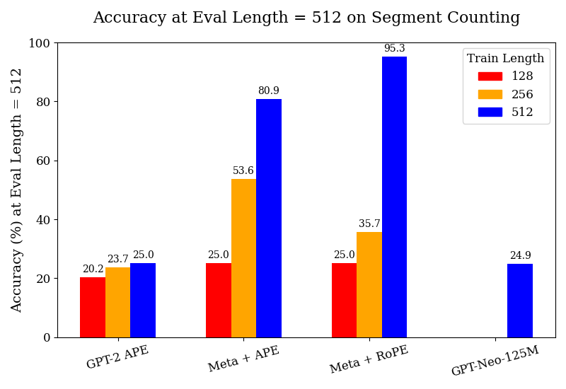
### Visual Description
\n
## Bar Chart: Accuracy at Eval Length = 512 on Segment Counting
### Overview
This is a grouped bar chart comparing the accuracy of four different language models or model configurations on a "Segment Counting" task. The evaluation is performed at a fixed sequence length of 512 tokens. The chart measures how model accuracy changes when trained on sequences of different lengths (128, 256, and 512 tokens).
### Components/Axes
* **Chart Title:** "Accuracy at Eval Length = 512 on Segment Counting"
* **Y-Axis:**
* **Label:** "Accuracy (%) at Eval Length = 512"
* **Scale:** Linear, from 0 to 100 in increments of 20.
* **X-Axis:** Lists four model configurations:
1. GPT-2 APE
2. Meta + APE
3. Meta + RoPE
4. GPT-Neo-125M
* **Legend:** Located in the top-right corner. It defines the "Train Length" for the colored bars:
* **Red Bar:** Train Length = 128
* **Orange Bar:** Train Length = 256
* **Blue Bar:** Train Length = 512
### Detailed Analysis
The chart presents accuracy percentages for each model across available training lengths. The data points, extracted by matching bar color to the legend, are as follows:
**1. GPT-2 APE**
* **Trend:** Shows a slight, monotonic increase in accuracy as training length increases.
* **Data Points:**
* Train Length 128 (Red): **20.2%**
* Train Length 256 (Orange): **23.7%**
* Train Length 512 (Blue): **25.0%**
**2. Meta + APE**
* **Trend:** Shows a strong, monotonic increase in accuracy with longer training lengths. The jump from 256 to 512 is substantial.
* **Data Points:**
* Train Length 128 (Red): **25.0%**
* Train Length 256 (Orange): **53.6%**
* Train Length 512 (Blue): **80.9%**
**3. Meta + RoPE**
* **Trend:** Shows the most dramatic increase. Accuracy is flat between train lengths 128 and 256, then surges dramatically at 512.
* **Data Points:**
* Train Length 128 (Red): **25.0%**
* Train Length 256 (Orange): **35.7%**
* Train Length 512 (Blue): **95.3%**
**4. GPT-Neo-125M**
* **Trend:** Only one data point is provided. No trend can be established.
* **Data Point:**
* Train Length 512 (Blue): **24.9%**
### Key Observations
1. **Scaling with Training Length:** For the "Meta" architectures (both APE and RoPE), training on longer sequences (512) yields dramatically higher accuracy on the 512-length evaluation task compared to training on shorter sequences (128 or 256). This effect is much less pronounced for GPT-2 APE.
2. **Architecture Performance:** At the matched train/eval length of 512, the "Meta + RoPE" configuration achieves the highest accuracy by a significant margin (95.3%), followed by "Meta + APE" (80.9%). GPT-2 APE and GPT-Neo-125M perform similarly poorly at this length (~25%).
3. **Baseline Performance:** When trained on the shortest length (128), all three models with available data (GPT-2 APE, Meta + APE, Meta + RoPE) cluster around 20-25% accuracy, suggesting a common baseline difficulty for the task with limited training context.
4. **Missing Data:** GPT-Neo-125M lacks data for train lengths 128 and 256, preventing a full comparison of its scaling behavior.
### Interpretation
The data strongly suggests that the "Meta" model architectures possess a superior ability to leverage longer training sequences to solve the segment counting task, especially when evaluated at that same length. The near-perfect accuracy (95.3%) of "Meta + RoPE" at train length 512 indicates that this combination (Meta architecture with Rotary Position Embeddings) is highly effective for this specific length-generalization challenge.
The stark contrast between the Meta models and the baselines (GPT-2, GPT-Neo) implies that architectural innovations beyond the base transformer are critical for tasks requiring precise reasoning over long contexts. The minimal improvement of GPT-2 APE with longer training suggests it may hit a performance ceiling or lack the mechanisms to effectively use the additional context. The single, low data point for GPT-Neo-125M positions it as a weaker baseline for this task at the 512-length scale.
In summary, the chart demonstrates that for segment counting at length 512, **model architecture and the alignment of training length with evaluation length are the dominant factors determining success**, with the Meta + RoPE configuration being the clear winner.
</details>
<details>
<summary>Figures/Accuracy_at_Eval_Length_=_512_on_Parity.png Details</summary>
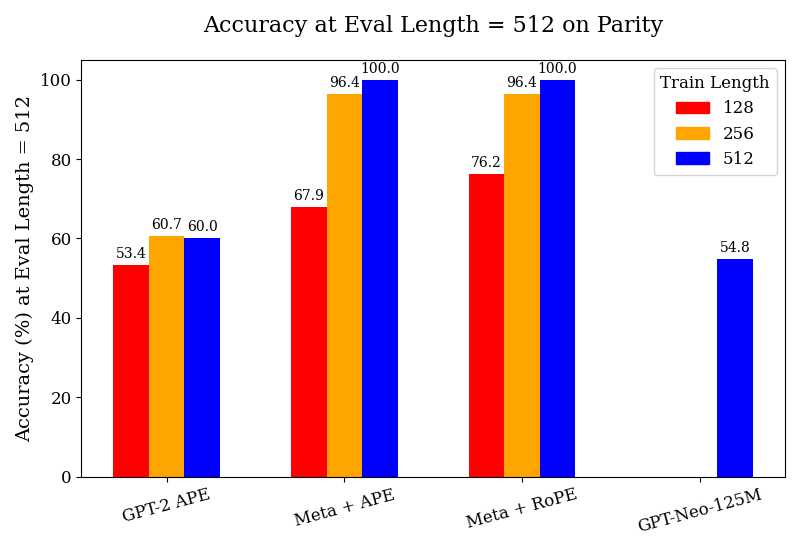
### Visual Description
\n
## Grouped Bar Chart: Accuracy at Eval Length = 512 on Parity
### Overview
This is a grouped bar chart comparing the accuracy (in percentage) of four different language model configurations when evaluated on a sequence length of 512 tokens. The performance is measured across three different training sequence lengths (128, 256, and 512 tokens). The chart demonstrates how model architecture and training length affect evaluation accuracy on a "Parity" task.
### Components/Axes
* **Chart Title:** "Accuracy at Eval Length = 512 on Parity"
* **Y-Axis:**
* **Label:** "Accuracy (%) at Eval Length = 512"
* **Scale:** Linear scale from 0 to 100, with major tick marks at intervals of 20 (0, 20, 40, 60, 80, 100).
* **X-Axis:**
* **Categories (Model Configurations):** Four distinct groups are labeled from left to right:
1. "GPT-2 APE"
2. "Meta + APE"
3. "Meta + RoPE"
4. "GPT-Neo-125M"
* **Legend:**
* **Title:** "Train Length"
* **Placement:** Top-right corner of the chart area.
* **Items:**
* Red square: "128"
* Orange square: "256"
* Blue square: "512"
* **Data Series:** Three bars per model group (except the last), colored according to the legend. Each bar has its exact numerical value annotated above it.
### Detailed Analysis
The chart presents the following data points for each model configuration and training length:
1. **GPT-2 APE:**
* Train Length 128 (Red): **53.4%**
* Train Length 256 (Orange): **60.7%**
* Train Length 512 (Blue): **60.0%**
* *Trend:* Accuracy increases from train length 128 to 256, then plateaus or slightly decreases at 512.
2. **Meta + APE:**
* Train Length 128 (Red): **67.9%**
* Train Length 256 (Orange): **96.4%**
* Train Length 512 (Blue): **100.0%**
* *Trend:* A strong, consistent upward trend. Accuracy improves dramatically with longer training, reaching perfect accuracy at train length 512.
3. **Meta + RoPE:**
* Train Length 128 (Red): **76.2%**
* Train Length 256 (Orange): **96.4%**
* Train Length 512 (Blue): **100.0%**
* *Trend:* Similar strong upward trend as "Meta + APE". It starts at a higher baseline (76.2% vs 67.9%) for train length 128 and also reaches perfect accuracy at train length 512.
4. **GPT-Neo-125M:**
* Train Length 128 (Red): **No bar present.**
* Train Length 256 (Orange): **No bar present.**
* Train Length 512 (Blue): **54.8%**
* *Trend:* Only data for train length 512 is provided. Its performance (54.8%) is comparable to the lowest-performing configuration (GPT-2 APE at train length 128).
### Key Observations
* **Performance Ceiling:** Both "Meta" configurations (with APE and RoPE) achieve **100.0% accuracy** when trained on sequences of length 512.
* **Training Length Impact:** For the "Meta" models, increasing the training sequence length from 128 to 512 tokens yields a massive performance gain of over 30 percentage points.
* **Model Comparison:** The "Meta" architectures significantly outperform the baseline GPT-2 and GPT-Neo models on this task, especially with longer training.
* **Missing Data:** The GPT-Neo-125M model only has a result for the longest training length (512), suggesting it may not have been evaluated or trained on shorter sequences for this experiment.
* **APE vs. RoPE:** At the shortest training length (128), "Meta + RoPE" (76.2%) shows a clear advantage over "Meta + APE" (67.9%). This gap closes at longer training lengths where both reach the same high accuracy.
### Interpretation
This chart provides a clear technical comparison relevant to research on transformer model architectures and positional encoding schemes. The data suggests several key findings:
1. **Superiority of Meta Architectures:** The models labeled "Meta" (likely referring to architectures from Meta AI Research) demonstrate a much higher capacity to learn the "Parity" task, especially when given sufficient training data (longer sequences). Their ability to reach perfect accuracy indicates the task is fully solvable by these models under the right conditions.
2. **Critical Role of Training Context Length:** The most significant factor for success appears to be matching the training sequence length to the evaluation length. All models show their best performance at train length 512, which matches the eval length. The "Meta" models show an especially strong dependence on this, with performance skyrocketing as training length increases.
3. **Architectural Efficiency:** "Meta + RoPE" shows better sample efficiency at the shortest training length (128) compared to "Meta + APE," suggesting that Rotary Positional Embeddings (RoPE) may provide a better inductive bias for learning positional relationships with limited data. However, with enough data (train length 512), both positional encoding methods (APE and RoPE) enable perfect task mastery.
4. **Baseline Model Limitations:** The GPT-2 and GPT-Neo-125M models plateau at around 54-60% accuracy, indicating they may lack the architectural capacity or appropriate inductive biases to fully solve this specific parity task, even with extended training. Their performance is essentially at a guessing or shallow pattern-matching level for this problem.
In summary, the chart is an empirical demonstration that for certain algorithmic tasks like parity, model architecture (specifically the "Meta" designs) and the alignment of training and evaluation context lengths are paramount for achieving high performance.
</details>
<details>
<summary>Figures/Accuracy_at_Eval_Length_=_512_on_Copying.png Details</summary>
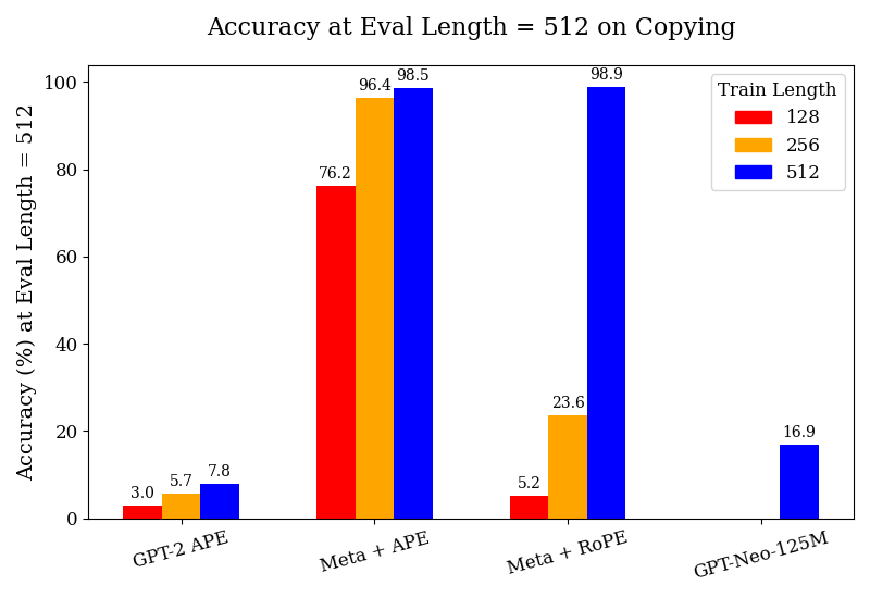
### Visual Description
\n
## Bar Chart: Accuracy at Eval Length = 512 on Copying
### Overview
This is a grouped bar chart comparing the accuracy (in percentage) of four different language models or model configurations on a "copying" task, evaluated at a sequence length of 512. The performance is broken down by three different training sequence lengths (128, 256, and 512 tokens).
### Components/Axes
* **Title:** "Accuracy at Eval Length = 512 on Copying"
* **Y-Axis:** Label: "Accuracy (%) at Eval Length = 512". Scale: 0 to 100, with major ticks at intervals of 20.
* **X-Axis:** Lists four model configurations:
1. GPT-2 APE
2. Meta + APE
3. Meta + RoPE
4. GPT-Neo-125M
* **Legend:** Located in the top-right corner, titled "Train Length". It defines three color-coded categories:
* Red square: 128
* Orange square: 256
* Blue square: 512
### Detailed Analysis
The chart presents accuracy data for each model across the three training lengths. Values are annotated on top of each bar.
**1. GPT-2 APE:**
* **Trend:** Accuracy increases slightly with longer training length.
* **Data Points:**
* Train Length 128 (Red): ~3.0%
* Train Length 256 (Orange): ~5.7%
* Train Length 512 (Blue): ~7.8%
**2. Meta + APE:**
* **Trend:** Shows a strong, positive correlation between training length and accuracy. This group has the highest overall performance.
* **Data Points:**
* Train Length 128 (Red): ~76.2%
* Train Length 256 (Orange): ~96.4%
* Train Length 512 (Blue): ~98.5%
**3. Meta + RoPE:**
* **Trend:** Shows a very strong positive correlation. Performance is low for shorter training lengths but jumps dramatically for the longest training length.
* **Data Points:**
* Train Length 128 (Red): ~5.2%
* Train Length 256 (Orange): ~23.6%
* Train Length 512 (Blue): ~98.9%
**4. GPT-Neo-125M:**
* **Trend:** Only one data point is present.
* **Data Point:**
* Train Length 512 (Blue): ~16.9%
* (No bars are present for Train Lengths 128 or 256).
### Key Observations
1. **Dominant Performance:** The "Meta + APE" configuration achieves the highest accuracy across all training lengths, reaching near-perfect performance (~98.5%) when trained on sequences of length 512.
2. **Critical Training Length for Meta + RoPE:** The "Meta + RoPE" model shows a massive performance leap (from ~23.6% to ~98.9%) when the training length is increased from 256 to 512, matching the top performance of Meta + APE at that length.
3. **Baseline Performance:** "GPT-2 APE" shows consistently low accuracy (<8%), indicating poor performance on this copying task regardless of training length within the tested range.
4. **Missing Data:** "GPT-Neo-125M" only has a result for the 512 training length, which is modest (~16.9%). Its performance at shorter training lengths is not reported.
5. **General Trend:** For the three models with complete data, accuracy improves as the training sequence length increases.
### Interpretation
This chart demonstrates the critical importance of matching training sequence length to evaluation sequence length for certain model architectures on a copying task.
* **Architectural Efficacy:** The "Meta" architectures (likely referring to models using techniques from Meta AI) combined with either APE (Absolute Positional Encoding) or RoPE (Rotary Positional Embedding) significantly outperform the baseline GPT-2 APE model. This suggests the underlying "Meta" architecture or training method is superior for this specific task.
* **Positional Encoding Comparison:** At the longest training length (512), both APE and RoPE enable near-perfect copying (~98.5% vs. ~98.9%). However, their behavior differs at shorter training lengths. Meta + APE maintains relatively high accuracy even when trained on shorter sequences (76.2% at 128), while Meta + RoPE performs poorly until trained on sequences of the same length as the evaluation (5.2% at 128, jumping to 98.9% at 512). This implies RoPE may be more sensitive to the disparity between training and evaluation lengths.
* **Task Nature:** The "copying" task is a fundamental test of a model's ability to recall and reproduce input sequences. The near-perfect scores at 512 for the Meta models indicate they have successfully learned this pattern when provided with sufficient training context. The low scores for GPT-2 APE suggest it struggles with this form of long-range dependency or exact replication.
* **Implication:** For tasks requiring precise recall of long contexts, using a model architecture like the "Meta" variants and ensuring the training data includes sequences at least as long as the expected evaluation length is crucial for high performance.
</details>
Figure 1: We study the performance of the pre-trained GPT-2 w/ APE, Meta-attention w/ APE, and Meta-attention w/ RoPE, as well as GPT-Neo-125M, all fine-tuned on synthetic data for their respective tasks at the maximum train lengths indicated in the legends. All experiments are performed on a test set of prompt lengths up to 512 tokens.
Table 1: Token Accuracy (%) on List Recall and Segment Counting across long contexts.
| List 4k / 4k 8k / 4k | 4k / 2k 85.0 85.0 | 19.5 88.2 95.8 | 16.0 90.2 91.2 | 13.7 20.5 97.4 | 0.9 1.8 98.2 | 0.0 1.0 96.2 | 0.0 3.5 93.9 | 0.9 4.4 31.9 | 1.1 1.1 0.0 | 0.0 2.1 2.1 | 2.1 2.1 2.1 | 1.1 |
| --- | --- | --- | --- | --- | --- | --- | --- | --- | --- | --- | --- | --- |
| 8k / 8k | 92.9 | 98.3 | 97.1 | 100.0 | 98.2 | 100.0 | 100.0 | 89.0 | 26.1 | 10.4 | 9.6 | |
| Count | 4k / 2k | 19.1 | 23.8 | 19.2 | 14.6 | 25.2 | 14.1 | 14.0 | 12.0 | 16.0 | 8.0 | 6.0 |
| 4k / 4k | 17.5 | 23.8 | 31.8 | 20.3 | 30.4 | 19.3 | 19.1 | 14.0 | 26.0 | 12.0 | 16.0 | |
| 8k / 4k | 19.1 | 23.8 | 14.3 | 11.1 | 20.6 | 12.7 | 12.7 | 14.0 | 16.0 | 14.0 | 12.0 | |
| 8k / 8k | 27.0 | 33.3 | 15.9 | 19.1 | 27.0 | 19.1 | 23.8 | 22.0 | 18.0 | 18.0 | 18.0 | |
Meta-Tokens Aid in Length Generalization.
In Figure 1 and Appendix F, we find that the model trained on meta-tokens length generalizes well on the parity and copying tasks with APE, and performs somewhat well (much better than the baselines) on list recall and segment counting at a train length of 256. For instance, despite relatively similar performance at the 128 train length on the segment counting task, the performance on the test set of up to a length of 512 dramatically increases when training at the 256 length, by $+28.6\$ with APE and $+10.7\$ with RoPE, compared to $+3.5\$ for GPT-2 with APE. Table 1 exhibits a similar trend for the YaRN models, achieving strong performance across its respective context windows, and even achieves non-trivial accuracy beyond the window. Fine-tuning the 8k YaRN model on examples of up to a length of 4k can generalize very well up to 8k. These findings underscore the substantial advantages of training with meta-tokens and the nuanced role positional encoding plays in task-specific and length-generalization contexts.
Moreover, when looking at the results on Meta + RoPe on test set lengths of prompts up to 1024 tokens (denoted extra-hard in Table 2), we find that zeroing out the positional encoding also plays a sizable role in improving length generalization, especially in the List Recall task. While the model originally achieves performances of $11.1\$ , $0\$ and $44.4\$ when fine-tuned on train lengths of 512 (APE), 256 and 512 (RoPE), respectively, the scores improve by $+38.9\$ , $+22.2\$ and $+11.2\$ , by simply zeroing out the positional encoding at the meta-tokens.
### 4.4 Examination of Positional Encoding through Internal Representations.
Table 2: The configurations where zeroing the positional encoding at inference time results in accuracy improvements on the List Pointer task, denoted by the $\Delta$ (pp) percentage points column.
| Meta + APE (medium, 128) | 77.8% | 88.9% | +11.1 |
| --- | --- | --- | --- |
| Meta + APE (hard, 128) | 11.1% | 22.2% | +11.1 |
| Meta + APE (extra-hard, 512) | 11.1% | 50.0% | +38.9 |
| Meta + RoPE (medium, 128) | 44.4% | 55.6% | +11.1 |
| Meta + RoPE (hard, 256) | 33.3% | 66.7% | +33.3 |
| Meta + RoPE (extra-hard, 256) | 0.0% | 22.2% | +22.2 |
| Meta + RoPE (extra-hard, 512) | 44.4% | 55.6% | +11.1 |
As discussed above, the results in Tables 11 - 14 suggest that the positional encoding of the meta-token can potentially be holding back the downstream performance of the meta-attention models. We posit that the model is instead relying on its content – cached context stored within the meta-token – to sharpen its sense of its position in the sequence.
Next, we aim to formally define this notion of sharpness in the context of positional encoding, and its relationship to the model’s logits. Let $\alpha_{i\rightarrow k}=\text{softmax}_{k}(Q_{i}K_{j}^{T}+b_{i-j})$ be the attention distribution for query $i$ over keys $j$ , with relative bias term $b_{i-j}$ . We define the sharpness of the positional encoding by the entropy:
$$
H(\alpha_{i})=-\sum_{j}\alpha_{i\rightarrow j}\log\alpha_{i\rightarrow j}
$$
Intuitively, when a meta-token is present at position $t$ , the model’s attention becomes peaked around a small set of keys; this "honing in" behavior reduces $H(\alpha)$ compared to APE or RoPE without meta-tokens. In this manner, meta-tokens behave as content-driven landmarks – they serve as a low-entropy channel that serves as a pointer to relevant context. As noted prior, the data efficiency observation suggests that the meta-token helps to accelerate next-token prediction behavior while introducing a stabilizing effect in the midst of noisy positional encoding.
**Theorem 4.1**
*Consider a Transformer head at query position $i$ over keys $1,\dots,N$ . Let $\alpha_{i}^{\text{abs}}(j)\propto\exp(Q_{i}K_{j}^{T})$ be the attention under absolute positional encoding and let $\alpha_{i}^{\text{meta}}\propto\exp(Q_{i}K_{j}^{T}+\delta_{j,j^{*}}\Delta)$ when a meta-token at position $j^{*}$ introduces an additive logit boost of $\Delta>0$ . Then, for some function $\kappa(\Delta)>0$ :
$$
\displaystyle H(\alpha_{i}^{\text{meta}})\leq H(\alpha_{i}^{\text{abs}})-\kappa(\Delta) \tag{1}
$$*
* Proof Sketch*
Parametrize the path by $t\in[0,\Delta]$ , and define logits $\ell_{j}^{(t)}$ and their softmax $\alpha^{(t)}$ respectively. Since boosting the true index tightens the margin, the derivative of $H(\alpha^{(t)}$ is strictly negative. Therefore, over the path, $H(\alpha^{(\Delta)})<H(\alpha^{(0)})$ , so $H(\alpha^{\text{meta}})<H(\alpha^{\text{abs}})$ , where their difference must be a function of $\Delta$ . The full proof is included in Appendix G. ∎
We note that this theorem also applies to RoPE, using $\alpha_{i}^{\text{RoPE}}(j)\propto\exp{Q_{i}(\text{RoPE}(K_{j}))^{T}}$ . A natural consequence of Theorem 4.1 is that the meta-token operates as an "anchor" from a logits standpoint by creating a margin $\Delta$ that concentrates the softmax. Concretely, we can specify that for meta-token $m_{t}$ at position $t$ and embedding $e_{t}\in\mathbb{R}^{d}$ , and query at position $i$ with vector $Q_{i}$ , has contribution to the $(i,j)$ logit of $\Delta_{i,j}^{(t)}=Q_{i}\cdot We_{t}\times\textbf{1}_{j=t}$ for learned linear head $W$ . Summing over $t$ yields the bias matrix $B\in\mathcal{B}_{\text{meta}}$ , the set of all realizable bias matrices under the meta-token embeddings. Thus, any learned meta-token embedding – provided that it adds to the logits at the summary position $j^{*}$ – guarantees sharper attention by reducing that attention head’s entropy.
<details>
<summary>Figures/logit-boost.png Details</summary>
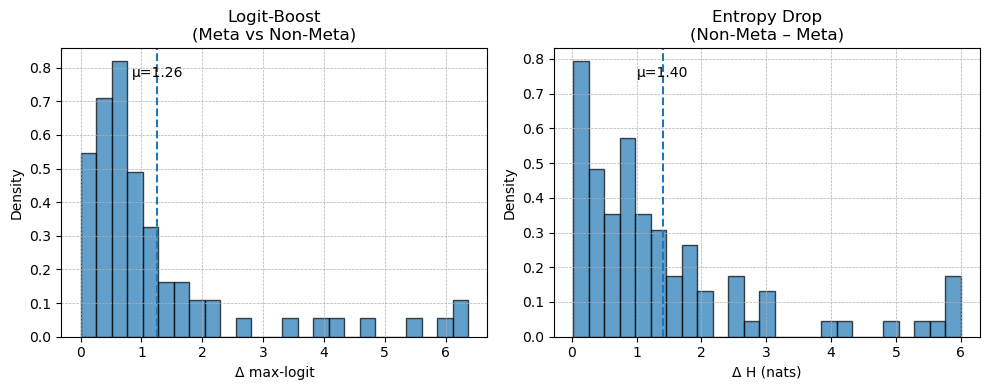
### Visual Description
## Comparative Histograms: Logit-Boost and Entropy Drop Distributions
### Overview
The image displays two side-by-side histograms comparing statistical distributions related to a "Meta" versus "Non-Meta" analysis. The left histogram visualizes the distribution of "Logit-Boost," while the right histogram visualizes the distribution of "Entropy Drop." Both charts share a similar visual style, using blue bars on a white background with grid lines, and each includes a vertical dashed line indicating the mean (μ) of the distribution.
### Components/Axes
**Left Histogram:**
* **Title:** `Logit-Boost (Meta vs Non-Meta)`
* **X-axis Label:** `Δ max-logit`
* **Y-axis Label:** `Density`
* **X-axis Scale:** Linear scale from 0 to 6, with major tick marks at every integer (0, 1, 2, 3, 4, 5, 6).
* **Y-axis Scale:** Linear scale from 0.0 to 0.8, with major tick marks at 0.0, 0.1, 0.2, 0.3, 0.4, 0.5, 0.6, 0.7, 0.8.
* **Annotation:** A vertical, dashed blue line is positioned at approximately x = 1.26. The text `μ=1.26` is placed to the right of this line, near the top of the chart.
**Right Histogram:**
* **Title:** `Entropy Drop (Non-Meta – Meta)`
* **X-axis Label:** `Δ H (nats)`
* **Y-axis Label:** `Density`
* **X-axis Scale:** Linear scale from 0 to 6, with major tick marks at every integer (0, 1, 2, 3, 4, 5, 6).
* **Y-axis Scale:** Linear scale from 0.0 to 0.8, with major tick marks at 0.0, 0.1, 0.2, 0.3, 0.4, 0.5, 0.6, 0.7, 0.8.
* **Annotation:** A vertical, dashed blue line is positioned at approximately x = 1.40. The text `μ=1.40` is placed to the right of this line, near the top of the chart.
### Detailed Analysis
**Left Histogram (Logit-Boost):**
* **Trend Verification:** The distribution is strongly right-skewed (positively skewed). The highest density of data points is concentrated on the left side (low Δ max-logit values), with a long tail extending to the right towards higher values.
* **Data Points (Approximate Bar Heights):**
* Bin 0.0-0.5: Density ≈ 0.55
* Bin 0.5-1.0: Density ≈ 0.71
* Bin 1.0-1.5: Density ≈ 0.82 (This is the peak of the distribution)
* Bin 1.5-2.0: Density ≈ 0.49
* Bin 2.0-2.5: Density ≈ 0.32
* Bin 2.5-3.0: Density ≈ 0.16
* Bin 3.0-3.5: Density ≈ 0.11
* Bin 3.5-4.0: Density ≈ 0.05
* Bin 4.0-4.5: Density ≈ 0.05
* Bin 4.5-5.0: Density ≈ 0.05
* Bin 5.0-5.5: Density ≈ 0.05
* Bin 5.5-6.0: Density ≈ 0.05
* Bin 6.0-6.5: Density ≈ 0.11
* **Mean (μ):** 1.26. The mean is located to the right of the distribution's peak (mode), which is characteristic of a right-skewed distribution.
**Right Histogram (Entropy Drop):**
* **Trend Verification:** This distribution is also right-skewed, with the highest density at the lowest values and a tail extending to the right.
* **Data Points (Approximate Bar Heights):**
* Bin 0.0-0.5: Density ≈ 0.79 (This is the peak of the distribution)
* Bin 0.5-1.0: Density ≈ 0.48
* Bin 1.0-1.5: Density ≈ 0.35
* Bin 1.5-2.0: Density ≈ 0.57
* Bin 2.0-2.5: Density ≈ 0.35
* Bin 2.5-3.0: Density ≈ 0.30
* Bin 3.0-3.5: Density ≈ 0.17
* Bin 3.5-4.0: Density ≈ 0.26
* Bin 4.0-4.5: Density ≈ 0.13
* Bin 4.5-5.0: Density ≈ 0.05
* Bin 5.0-5.5: Density ≈ 0.05
* Bin 5.5-6.0: Density ≈ 0.05
* Bin 6.0-6.5: Density ≈ 0.17
* **Mean (μ):** 1.40. Similar to the left chart, the mean is to the right of the peak.
### Key Observations
1. **Skewness:** Both distributions are right-skewed, indicating that for most observations, the difference (`Δ`) between Meta and Non-Meta conditions is relatively small. However, there is a subset of observations where the difference is considerably larger.
2. **Peak Location:** The peak density for Logit-Boost occurs in the 1.0-1.5 bin, while for Entropy Drop, it occurs in the 0.0-0.5 bin. This suggests the most common magnitude of change is slightly different between the two metrics.
3. **Mean vs. Peak:** In both charts, the mean (μ) is greater than the value at the peak density (mode), confirming the right skew.
4. **Range:** Both metrics show differences spanning the full observed range from 0 to over 6 units.
5. **Visual Similarity:** The overall shape and spread of the two distributions are visually similar, suggesting a potential correlation in how these two metrics (logit boost and entropy drop) respond to the Meta vs. Non-Meta comparison.
### Interpretation
These histograms provide a comparative statistical view of two performance or behavioral metrics—Logit-Boost and Entropy Drop—in a "Meta" learning or modeling context versus a "Non-Meta" baseline.
* **What the data suggests:** The right-skewed distributions imply that the "Meta" approach typically yields a modest improvement (or change) over the "Non-Meta" approach for the majority of cases. The long tail to the right indicates that for a smaller number of instances, the Meta approach leads to a substantially larger boost in logit scores or a larger drop in entropy.
* **Relationship between elements:** The side-by-side presentation invites direct comparison. The fact that both metrics show similar distributional shapes (right-skewed, similar range) suggests they may be capturing related aspects of the Meta method's effect. A larger `Δ max-logit` (left chart) likely corresponds to a more confident prediction from the Meta model. A larger `Δ H` (right chart) indicates a greater reduction in uncertainty (entropy) by the Meta model compared to the Non-Meta model.
* **Notable patterns/anomalies:** The presence of data points at the far right of both histograms (Δ > 6) is notable. These represent outlier cases where the Meta method had an exceptionally strong effect. The slight difference in peak location (1.0-1.5 for Logit-Boost vs. 0.0-0.5 for Entropy Drop) might indicate that while entropy often drops by a very small amount, the corresponding logit boost is slightly more distributed. The analysis would benefit from knowing the sample size and the specific context of "Meta" (e.g., meta-learning, metadata) to draw more concrete conclusions about the practical significance of these distributions.
</details>
<details>
<summary>Figures/Meta2_past_heatmap_padded.png Details</summary>
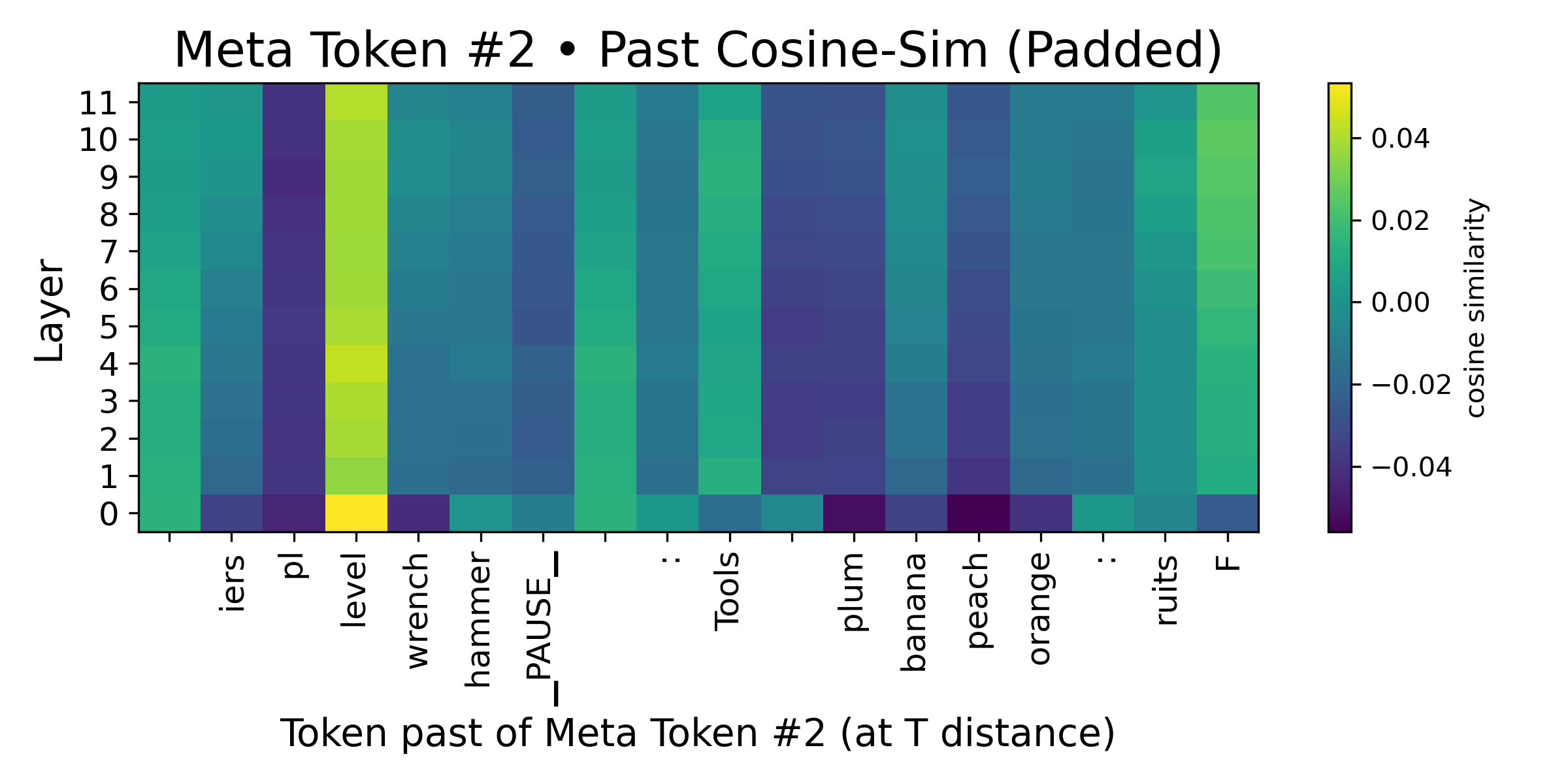
### Visual Description
## Heatmap: Meta Token #2 • Past Cosine-Sim (Padded)
### Overview
This image is a heatmap visualizing the cosine similarity between a specific "Meta Token #2" and a sequence of past tokens, measured across different layers of a neural network model. The title indicates the data is "Padded," suggesting the sequence may have been extended to a fixed length. The visualization uses a color gradient to represent the similarity values.
### Components/Axes
* **Title:** "Meta Token #2 • Past Cosine-Sim (Padded)" (Top center).
* **Y-Axis (Vertical):** Labeled "Layer". It represents the layer index within the model, numbered from 0 at the bottom to 11 at the top.
* **X-Axis (Horizontal):** Labeled "Token past of Meta Token #2 (at T distance)". It lists a sequence of tokens that occurred prior to Meta Token #2. The tokens are, from left to right:
1. `iers`
2. `pl`
3. `level`
4. `wrench`
5. `hammer`
6. `PAUSE`
7. `..` (ellipsis)
8. `Tools`
9. `..` (ellipsis)
10. `plum`
11. `banana`
12. `peach`
13. `orange`
14. `..` (ellipsis)
15. `ruits`
16. `F`
* **Color Bar/Legend (Right side):** A vertical bar labeled "cosine similarity". It maps colors to numerical values, ranging from dark purple at the bottom (approximately -0.04) to bright yellow at the top (approximately +0.04). The scale includes tick marks at -0.04, -0.02, 0.00, 0.02, and 0.04.
### Detailed Analysis
The heatmap is a grid where each cell's color corresponds to the cosine similarity between Meta Token #2 and the token at a specific past position (X-axis), as computed in a specific model layer (Y-axis).
**Color-to-Value Mapping (Approximate):**
* **Bright Yellow:** ~ +0.04 (Highest positive similarity)
* **Light Green/Yellow-Green:** ~ +0.02
* **Teal/Green-Blue:** ~ 0.00 (Neutral similarity)
* **Blue/Indigo:** ~ -0.02
* **Dark Purple:** ~ -0.04 (Highest negative similarity)
**Spatial Patterns and Trends:**
* **Column "level":** This column is predominantly bright yellow to light green across most layers (0-11), indicating a consistently high positive cosine similarity between Meta Token #2 and the token "level" throughout the network's depth. The similarity appears strongest in the lower layers (0-2).
* **Column "pl":** This column is consistently dark purple/blue across all layers, indicating a consistently negative cosine similarity.
* **Column "peach":** This column is very dark purple, especially in the lower layers (0-4), suggesting a strong negative similarity.
* **Columns "iers", "wrench", "hammer", "PAUSE", "Tools", "plum", "banana", "orange", "ruits", "F":** These columns show a mix of teal, blue, and green shades. The similarity values for these tokens appear to be closer to zero (neutral) or slightly positive/negative, with no single strong trend across all layers.
* **Ellipsis Columns (`..`):** These columns also show mixed, near-neutral values.
* **Layer 0 (Bottom Row):** This row shows more extreme colors (both bright yellow for "level" and dark purple for "peach") compared to higher layers, suggesting that similarity relationships might be more pronounced or specialized in the initial embedding or first processing layer.
* **General Trend with Layer Depth:** For many tokens (e.g., "iers", "wrench", "Tools"), the color becomes slightly more teal/green (closer to zero) in the middle layers (4-8) compared to the very bottom or top layers, indicating a potential normalization or attenuation of the similarity signal in the network's mid-section.
### Key Observations
1. **Strong Positive Anchor:** The token "level" has a uniquely strong and persistent positive association with Meta Token #2 across all model layers.
2. **Strong Negative Associations:** The tokens "pl" and "peach" show consistently negative similarity, with "peach" being particularly strong in early layers.
3. **Contextual Grouping:** The tokens appear to be from two semantic groups: tools ("wrench", "hammer", "Tools") and fruits ("plum", "banana", "peach", "orange", "ruits"). However, the heatmap does not show a uniform similarity pattern within these groups. For example, "peach" is strongly negative while "banana" is near-neutral.
4. **Layer-Dependent Variation:** The strength and sign of the similarity for most tokens (except "level" and "pl") are not constant but vary with the layer index, suggesting the relationship between Meta Token #2 and past tokens is processed and transformed at different stages of the network.
### Interpretation
This heatmap provides a diagnostic view into the internal state of a transformer-like model. It reveals how a special "meta token" attends to or aligns with specific past tokens in its context window.
* **What the data suggests:** The high positive similarity for "level" implies that Meta Token #2's representation is highly aligned with the concept or function of "level" within the model's processing. This could mean the meta token is acting as a placeholder or carrier for information related to "level". Conversely, the negative similarities for "pl" and "peach" suggest an inhibitory or contrasting relationship.
* **How elements relate:** The variation across layers shows that these relationships are not static. The model builds and refines the meta token's association with past context as information flows through its layers. The pronounced values in Layer 0 may reflect direct embedding similarities, while patterns in higher layers reflect more abstract, processed relationships.
* **Notable anomalies:** The stark contrast between "level" (strong positive) and "pl"/"peach" (strong negative) is the most significant anomaly. This could indicate that the meta token is being used to track or differentiate between specific types of information (e.g., perhaps "level" is a key parameter, while "pl" and "peach" are part of a different, unrelated context). The lack of a clear pattern within the obvious semantic groups (tools vs. fruits) suggests the meta token's role is not simply categorical but tied to more specific, possibly syntactic or functional, roles in the sequence it was trained on.
</details>
Figure 2: (Left) We analyze the change in logits at the meta-token position, and observe that the meta-tokens do indeed induce a sizable boost in logits compare to zeroing its token embedding. (Middle) We find the boost in logits to correspond with a meaningful reduction in Shannon entropy over the softmax of the logits between the zeroed meta-token sequence and the sequence with the meta-token as is. This corroborates with our assumptions and claims in Theorem 4.1. (Right) We study the implicit "caching" ability of the meta-token by studying the cosine similarity over the token embeddings. We observe high spikes (the yellow column), diminishing as we move further away. This substantiates our claims of the presence of an implicit compression and "caching" mechanism.
In Figure 2, we analyze the logits, comparing two settings: (1.) the current meta-token and (2.) the meta-token with its token embedding zeroed out. We find that the former gains a sizable amount over the latter, reinforcing the assumption made in Theorem 4.1 that the meta-token introduces an additive logit boost of $\Delta>0$ . Our empirical results show that the entropy over the softmax distribution of the logits decreases (the difference between "non-meta-token" and "meta-token" is positive), thus corroborating our central claim in Theorem 4.1.
### 4.5 Inference Efficiency
Meta-tokens are generated at inference. The additional computation is sparse—each attention head only considers a small number of meta positions rather than the full attention matrix. In our current PyTorch implementation, which materializes the sparse mask as a dense tensor, we observe a throughput drop from 130.82 to 117.86 tokens/sec and a TTFT increase from 7.44ms to 7.57ms, i.e., a 1.11× slowdown. We expect optimized sparse attention implementations to reduce or eliminate this overhead.
Table 3: Inference speed comparison with and without meta/pause tokens.
| TPS (tokens/sec) TTFT (ms) Slowdown factor | 130.82 7.44 1.00 | 117.86 7.57 1.11 |
| --- | --- | --- |
## 5 Examining Context Compression with Rate-Distortion Theory
Given that these results provide evidence that meta-tokens can compress context in their representation, we develop mathematical formalizations to analyze this behavior. In particular, we turn to information-theoretic tools – specifically, an information bottleneck view.
For a meta-token at $x_{m}$ succeeding a sequence of tokens $X=x_{i:m-1}$ from indices $i$ to $m-1$ , we consider a compression function $\zeta(\cdot)$ which transforms the subsequence $X$ into $x_{m}$ . As such, we define $\hat{X}=\zeta(X)=\zeta(x_{i:{m-1}})$ to be the compressed representation stored in $x_{m}$ . This can be generalized to the full set of $M$ meta-tokens:
$$
\hat{X}_{1:M}=[\zeta_{1}(X_{1:m_{1}-1}),\zeta_{2}(X_{m_{1}+1:m_{2}-1}),\dots\zeta_{M}({m_{M+1}:m_{n}})]
$$
For practicality, we consider the variational information bottleneck (Alemi et al., 2017). This introduces an encoder $q_{\phi}(\hat{x}\mid x)$ and decoder $q_{\theta}(y\mid\hat{x})$ , along with a simple prior $r(z)$ (e.g. $N(0,1)$ ), yielding the following form to solve for these variational distributions:
$$
\min_{q_{\phi},q_{\theta}}\mathop{\mathbb{E}}_{p(x,y)}[\mathop{\mathbb{E}}_{q_{\phi}(\hat{x}\mid x)}[-\log q_{\theta}(y\mid\hat{x}]]+\beta\cdot\mathop{\mathbb{E}}_{p(x)}[KL(q_{\phi}(\hat{x}\mid x)||r(x))]
$$
This form admits an equivalent perspective in rate-distortion theory. Specifically, the first term measures the quality in predicting the downstream target given a lossy compression $\hat{X}$ ("distortion"). The second term measures the average number of bits required to encode $\hat{X}$ , relative to some simple reference code $r(z)$ ("rate"). As such, analyzing rate-distortion curves – sweeping over values of $\beta$ – can provide valuable insights into the quality of the "compression" behavior and its informativeness when the meta-token is attended to.
**Theorem 5.1**
*Let $D_{\text{abs}}(R)$ be the minimum distortion achievable at rate $R$ under the VIB objective only using absolute positional encoding (no meta-tokens), and let $D_{\text{meta}}(R)$ be the minimum distortion achievable at rate $R$ with meta-tokens. Then, for every $R\geq 0$ ,
$$
\displaystyle D_{\text{meta}}(R)\leq D_{\text{abs}}(R) \tag{2}
$$*
Intuitively, meta-tokens expand the feasible set of encoders and decoders, which will either match or lower distortion for a given rate. Thus, the quality of compression with respect to its informativeness in predicting the target can only improve.
<details>
<summary>Figures/attention_heatmap.png Details</summary>
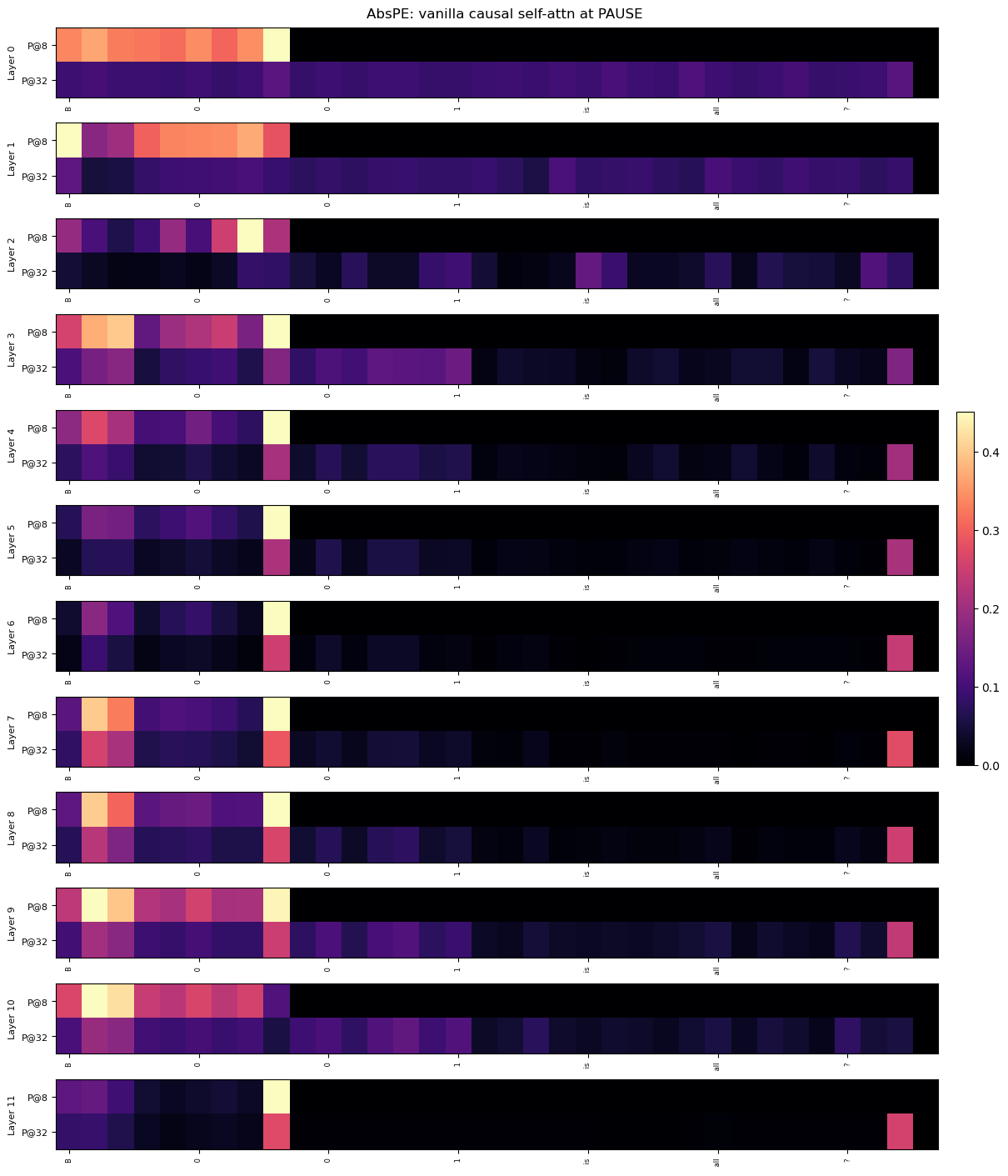
### Visual Description
## Heatmap: AbsPE: vanilla causal self-attn at PAUSE
### Overview
This image is a vertical stack of 12 horizontal heatmaps, each representing a different layer (Layer 0 to Layer 11) of a neural network model. The visualization appears to analyze attention patterns or activation values at a specific token or position labeled "PAUSE" within a "vanilla causal self-attention" mechanism using "AbsPE" (likely Absolute Positional Encoding). Each layer's heatmap is subdivided into two rows, labeled "P@8" and "P@32", which likely represent two different positional contexts or sequence lengths (e.g., attention at position 8 vs. position 32). A color bar on the right provides the scale for the heatmap values.
### Components/Axes
* **Title:** "AbsPE: vanilla causal self-attn at PAUSE" (centered at the top).
* **Vertical Axis (Left Side):** Labels for each of the 12 layers, from "Layer 0" (top) to "Layer 11" (bottom).
* **Sub-Row Labels (Within each layer):** Each layer's heatmap contains two rows. The top row is labeled "P@8" and the bottom row is labeled "P@32". These labels are positioned to the left of their respective rows.
* **Horizontal Axis (Bottom of each heatmap):** A set of seven numerical labels appears below each individual heatmap. The sequence is consistent across all layers: `8`, `0`, `0`, `1`, `15`, `16`, `7`. These likely represent specific token indices or positions in a sequence.
* **Color Bar (Right Side):** A vertical gradient bar mapping colors to numerical values. The scale runs from `0.0` (bottom, dark purple/black) to `0.4` (top, bright yellow). Intermediate ticks are at `0.1`, `0.2`, and `0.3`.
* **Heatmap Grid:** Each of the 12 layers contains a grid of colored cells. The grid appears to have 7 columns (corresponding to the x-axis labels) and 2 rows (P@8 and P@32).
### Detailed Analysis
**Trend Verification & Data Point Extraction:**
The heatmaps show the distribution of values (likely attention weights or activation strengths) across 7 positions (x-axis) for two conditions (P@8, P@32) across 12 network layers.
* **General Pattern (P@8 vs. P@32):** Across most layers, the "P@8" row exhibits higher values (warmer colors: orange, yellow) concentrated in the leftmost columns (positions `8`, `0`, `0`). The "P@32" row generally shows lower values (cooler colors: dark purple, black) across the board, with occasional isolated spots of moderate value (pink/purple) in the rightmost columns (positions `16`, `7`).
* **Layer-by-Layer Analysis:**
* **Layer 0:** P@8: High values (~0.3-0.4) at positions `8`, `0`, `0`. P@32: Very low values (<0.1) across all positions.
* **Layer 1:** P@8: High values at `8`, `0`, `0`. P@32: Low values, with a slight increase at position `16`.
* **Layer 2:** P@8: A distinct, very high-value (yellow, ~0.4) cell at the 4th position (label `1`). P@32: Mostly low, with a faint purple spot at position `15`.
* **Layer 3:** P@8: High values at `8`, `0`, `0`. P@32: A band of moderate value (~0.1-0.2) across positions `8` to `1`.
* **Layer 4:** P@8: High values at `8`, `0`, `0`. P@32: Low, with a pink spot (~0.2) at position `7`.
* **Layer 5:** P@8: High values at `8`, `0`, `0`. P@32: Low, with a pink spot at position `7`.
* **Layer 6:** P@8: High values at `8`, `0`, `0`. P@32: Low, with a pink spot at position `7`.
* **Layer 7:** P@8: High values at `8`, `0`, `0`. P@32: Moderate values (~0.2-0.3) at positions `8`, `0`, and a pink spot at `7`.
* **Layer 8:** P@8: High values at `8`, `0`, `0`. P@32: Moderate values at `8`, `0`, and a pink spot at `7`.
* **Layer 9:** P@8: High values at `8`, `0`, `0`. P@32: Moderate values at `8`, `0`, and a pink spot at `7`.
* **Layer 10:** P@8: High values at `8`, `0`, `0`. P@32: A band of low-to-moderate values across the left half.
* **Layer 11:** P@8: Moderate values at `8`, `0`, `0`. P@32: A single, isolated pink spot (~0.25) at the far right position `7`.
### Key Observations
1. **Positional Bias in P@8:** The "P@8" condition shows a strong and consistent bias toward the first three positions (`8`, `0`, `0`) across nearly all layers. This suggests that when the model attends from or to position 8, it focuses heavily on these early tokens.
2. **Sparse Activation in P@32:** The "P@32" condition is characterized by generally low activation, with notable exceptions. The most common exception is a recurring spot of moderate value at the final position (`7`) in layers 4-9 and 11.
3. **Layer 2 Anomaly:** Layer 2, P@8 contains the single highest-value cell in the entire visualization (bright yellow at position `1`), indicating a unique, strong activation at this specific layer and position.
4. **Evolution Through Layers:** The pattern is not static. While the left-side bias in P@8 is constant, the specific distribution of values within those first three cells changes slightly per layer. The P@32 pattern becomes more active in the middle layers (3-9) before simplifying again in the final layers.
### Interpretation
This heatmap provides a diagnostic view of how a causal self-attention model processes information at a "PAUSE" token under two different positional contexts (P@8 and P@32). The data suggests:
* **Context-Dependent Attention:** The model's attention mechanism behaves fundamentally differently depending on the positional context. The "P@8" context triggers a strong, localized focus on a small set of early tokens, which could be crucial for resolving dependencies or maintaining state near the pause point.
* **Role of the "PAUSE" Token:** The consistent high values at positions labeled `0` (which appears twice) might indicate that the model treats the token at index 0 as particularly important when encountering a PAUSE, possibly as a anchor or reset point.
* **Functional Specialization Across Layers:** The anomaly in Layer 2 suggests that specific layers may be specialized for detecting or processing particular positional relationships. The recurring activation at position `7` in the P@32 condition for mid-to-late layers might indicate a learned pattern for handling longer-range dependencies or sequence endings.
* **Implication for Model Design:** The stark contrast between P@8 and P@32 patterns highlights the significant impact of absolute positional encoding on attention. This could inform architectural choices, suggesting that different positional schemes might be needed for different parts of a sequence or different tasks. The visualization acts as a "fMRI" for the model's attention, revealing where it "looks" and how that gaze changes with depth and context.
</details>
<details>
<summary>Figures/rate-distortion.png Details</summary>
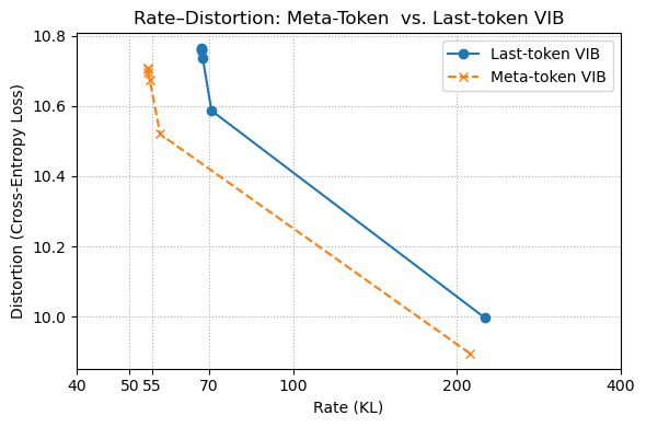
### Visual Description
## Line Chart: Rate-Distortion: Meta-Token vs. Last-token VIB
### Overview
This is a 2D line chart comparing the performance of two methods—"Last-token VIB" and "Meta-token VIB"—on a rate-distortion trade-off. The chart plots Distortion (measured as Cross-Entropy Loss) against Rate (measured in KL divergence). The visual data suggests a trade-off where increasing the Rate (KL) leads to a decrease in Distortion (Loss) for both methods, with the Meta-token VIB method consistently achieving lower distortion at comparable or higher rates.
### Components/Axes
* **Chart Title:** "Rate-Distortion: Meta-Token vs. Last-token VIB"
* **Y-Axis (Vertical):**
* **Label:** "Distortion (Cross-Entropy Loss)"
* **Scale:** Linear scale.
* **Range:** Approximately 10.0 to 10.8.
* **Major Ticks:** 10.0, 10.2, 10.4, 10.6, 10.8.
* **X-Axis (Horizontal):**
* **Label:** "Rate (KL)"
* **Scale:** Logarithmic scale (based on uneven spacing of tick labels).
* **Range:** Approximately 40 to 400.
* **Major Ticks:** 40, 50, 55, 70, 100, 200, 400.
* **Legend:** Located in the top-right corner of the plot area.
* **Series 1:** "Last-token VIB" - Represented by a solid blue line with circular markers (`o`).
* **Series 2:** "Meta-token VIB" - Represented by a dashed orange line with 'x' markers (`x`).
### Detailed Analysis
**Data Series: Last-token VIB (Blue, Solid Line, Circle Markers)**
* **Trend:** The line shows a steep negative slope, indicating a strong inverse relationship between Rate and Distortion. Distortion decreases rapidly as Rate increases.
* **Approximate Data Points (Rate KL, Distortion Loss):**
1. (~70, ~10.75) - Highest distortion point for this series.
2. (~70, ~10.70)
3. (~70, ~10.60)
4. (~200, ~10.00) - Lowest distortion point for this series, at the highest rate shown.
**Data Series: Meta-token VIB (Orange, Dashed Line, 'x' Markers)**
* **Trend:** The line also shows a negative slope, but it is less steep than the Last-token VIB line. Distortion decreases as Rate increases, but at a more gradual rate.
* **Approximate Data Points (Rate KL, Distortion Loss):**
1. (~55, ~10.70) - Highest distortion point for this series.
2. (~55, ~10.68)
3. (~55, ~10.52)
4. (~200, ~9.90) - Lowest distortion point for this series, at the highest rate shown.
**Spatial Grounding & Cross-Reference:**
* The blue circle markers for "Last-token VIB" are clustered at a Rate of approximately 70 for the first three points, then a single point at Rate ~200.
* The orange 'x' markers for "Meta-token VIB" are clustered at a Rate of approximately 55 for the first three points, then a single point at Rate ~200.
* At the highest rate point (~200), the Meta-token VIB (orange 'x') is positioned below the Last-token VIB (blue circle), confirming it achieves lower distortion at that rate.
### Key Observations
1. **Performance Crossover:** The Meta-token VIB line is consistently below the Last-token VIB line across the entire plotted range. This indicates that for any given Rate (KL) shown, the Meta-token VIB method results in lower Distortion (Cross-Entropy Loss).
2. **Rate Efficiency:** The Meta-token VIB achieves comparable or lower distortion at significantly lower rates. For example, its distortion at Rate ~55 (~10.52) is already lower than the Last-token VIB's distortion at Rate ~70 (~10.60).
3. **Diminishing Returns:** Both curves show a flattening trend as Rate increases, suggesting diminishing returns in distortion reduction for additional increases in rate, especially beyond Rate=100.
4. **Data Clustering:** Both series have three data points clustered at a specific low rate (70 for Last-token, 55 for Meta-token) before a single point at a much higher rate (~200). This may indicate specific experimental configurations or hyperparameter settings.
### Interpretation
This chart demonstrates a classic rate-distortion trade-off in the context of Variational Information Bottleneck (VIB) methods applied to language models. The "Rate" (KL divergence) measures the compression or information bottleneck constraint, while "Distortion" (Cross-Entropy Loss) measures the reconstruction or prediction error.
The key finding is the **superior performance of the Meta-token VIB method**. It defines a more efficient Pareto frontier, achieving better (lower) distortion for the same rate, or equivalently, requiring a lower rate to achieve the same level of distortion. This suggests that using a "meta-token" as the information bottleneck is a more effective strategy for compressing model representations than using the "last-token," leading to better preservation of task-relevant information under a compression constraint. The steep initial drop in both curves highlights that even a modest increase in the allowed rate (KL) can yield significant gains in reducing model loss.
</details>
Figure 3: (Left) This plot visualizes the residual stream after each layer, to analyze the meta-token within causal attention. The colors before the meta-token (the colored band across the layers) denote the context which the meta-token attends to and implicitly stores, and the final, rightmost colored line represents the final meta-token in the sequence, which attends to the previous one at the aforementioned band. (Right) We analyze the variational information bottleneck (VIB) objective and its decomposition into its rate and distortion components. Supporting the findings of Theorem 5.1, for a given rate $R$ , the distortion $D$ is strictly lower for the meta-token compared to the last non-meta-token element in the sequence.
### 5.1 Rate-Distortion Informs the Quality of Context Caching
To obtain empirical rate–distortion curves for our meta‐token bottleneck in Figure 3, we freeze the pre-trained meta-token model and fix a small variational bottleneck head to the last meta-token hidden state. Concretely, let $h_{m}\in\mathbb{R}^{D}$ be the output of the final Transformer layer at the last meta-token position. We introduce
$$
q_{\phi}(z\mid h_{m})=\mathcal{N}\bigl(\mu_{\phi}(h_{m}),\,\mathrm{diag}(\sigma^{2}_{\phi}(h_{m}))\bigr),\quad q_{\theta}(y\mid z)=\mathrm{softmax}(Wz+b),
$$
with $\mu_{\phi},\sigma_{\phi}:\mathbb{R}^{D}\to\mathbb{R}^{L}$ and $W\in\mathbb{R}^{|\mathcal{V}|\times L}$ . We then optimize the ELBO:
$$
\min_{\phi,\theta}\;\mathbb{E}_{h_{m},y}\bigl[-\log q_{\theta}(y\mid z)\bigr]\;+\;\beta\;\mathbb{E}_{h_{m}}\bigl[\mathrm{KL}\bigl(q_{\phi}(z\mid h_{m})\,\|\,\mathcal{N}(0,I)\bigr)\bigr].
$$
Training is performed on the small List-Pointer D.1.1 split (50 examples, batch size 1), for 5 epochs at each $\beta\in\{0.01,\,0.02,\,0.05,\,0.1,\,0.2,\,0.5,\,1.0\}$ . After each run, we record the average cross-entropy loss (“distortion”) and KL (“rate”) on the same 50 examples. Finally, we plot the resulting rate–distortion curves on a symlog x-axis (linear below 20 nats, logarithmic above) so that both the low-rate “knee” and the long tail are visible (see Figure 3).
### 5.2 Positional Encoding as a Source of Bottleneck Distortion
The consistent improvements in recall fidelity and length generalization from zeroing positional encodings at meta-token positions 2 are well-explained through through our rate-distortion analysis.
Prior work (e.g., NoPE; Kazemnejad et al., 2023) shows that Transformers can infer token order from the causal mask alone, often generalizing better when explicit positional embeddings (PEs) are removed. Our results extend this insight: in Theorem 5.1, we formalize meta-tokens as learned compression bottlenecks.
If a meta-token retains its PE (absolute or rotary), a portion of its representational capacity is spent encoding position rather than semantic content. This index-dependent signal introduces unnecessary variance, increasing the distortion of the compressed summary. By contrast, zeroing out the PE forces the full embedding capacity to encode task-relevant information. As a result, we observe lower distortion (higher retrieval accuracy) at a given rate—both theoretically and empirically—across all four synthetic tasks.
## 6 Related Work
Pause and Memory Tokens
As detailed in our work, recent studies on Transformer-based models have explored the introduction of special tokens, beyond ordinary vocabulary symbols. Pause or dummy tokens as introduced in Goyal et al. (2024) enhance computational width, allowing models to perform additional internal computation by effectively delaying their outputs. This yields empirical gains on question answering and reasoning-intensive tasks. Similarly, Pfau et al. (2024) explore using filler tokens – sequences of seemingly meaningless symbols – as a stand-in for chain-of-thought. These special tokens may also delineate phases of reasoning, as in Quiet-STaR Zelikman et al. (2024). Quiet-STaR uses a begin-of-thought token and an end-of-thought token, generating a silent rationale sequence for each step before emitting the next word, showing that this helps zero-shot reasoning.
Works such as Memory Transformer (Burtsev et al., 2021) and Landmark Attention (Mohtashami and Jaggi, 2023) introduce memory tokens; the former prepends them, while the latter uses them as learnable keys for retrieval over blocks of context. Our work is most closely related to the latter, while performing this retrieval in a purely implicit manner via the observed "pointer" mechanism. For vision transformers (ViTs), LeMeVit (Jiang et al., 2024) introduces a similar meta-tokens notion as our work by adding learnable sparse tokens and an attention mechanism between standard tokens and their meta tokens, improving performance and reducing spatial redundancy. Darcet et al. (2024) uses specialized "register" tokens applies to patches to denoise images by extracting the high-norm, outlier tokens, smoothening the feature and attention maps. These works suggest that special tokens, even devoid of semantic content, can influence a model’s internal reasoning and memory mechanisms.
Positional Encoding
We have already described absolute positional embeddings (APE), rotary positional embeddings (RoPE) and relative bias in Section 2. In addition to these methods, ALiBi (Press et al., 2022) adds a fixed linear penalty to attention scores based on the distance between query and key positions, favoring nearer tokens and generalizing to longer contexts with minimal loss in perplexity. Recent work has suggested that Transformers without any added position embeddings can still learn order information and, in some cases, generalize to longer sequences better than models with standard positional encoding. NoPE (Kazemnejad et al., 2023) showed that models trained without positional embeddings can achieve strong length extrapolation in comparison to models trained with positional encoding. They can internally represent both absolute and relative PEs without any explicit positional signal, suggesting these may emerge implicitly via training dynamics or over the data distribution. NoPos (Haviv et al., 2022) also found a similar result, suggesting that models trained without PE can infer their absolute position due to causal attention masks. These findings are highly relevant to our work, given our evidence on length generalization behavior whiling zeroing the positional encoding at the meta-tokens.
## 7 Discussion and Limitations
Our findings suggest that decoder-only language models trained with meta-tokens and meta-attention achieve strong performance on recall-oriented tasks. Furthermore, they are able to length generalize, with performance improvements when removing the effect of positional encoding at the meta-tokens. Given the prior findings of NoPos, we believe the introduction of the meta-attention mechanism and a second causal mask (the "meta mask") could be responsible for this behavior, provided that this behavior is specific to the meta-tokens. We suggest that hybrid attention methods such as RNoPE (Yang et al., 2025) could be suitable for facilitating long-context modeling with meta-tokens.
Given the findings that the meta-tokens operate like anchors within the context, it would be valuable to explore the impact of our proposed mechanism in pre-training larger models over longer context windows, under greater computational resources. We employ synthetic tasks that are well-aligned to recall abilities, and design experiments to test length generalization, with the aim of strong synergy with long-context modeling capabilities. Nonetheless, training larger models would indicate the viability of our approach for real-world deployment.
Notably, our method requires little overhead – the addition of meta-tokens is a simple data augmentation strategy, and the meta-attention layer is added after standard causal masked self-attention, as described in Appendix A. It would also be informative to study larger-scale corpora – given the data-efficient nature of the meta-tokens approach in vastly outperforming the vanilla GPT-2 model at the $\approx 100B$ tokens scale, how rapidly does each model saturate our designed synthetic tasks?
## 8 Conclusion
We introduce meta-tokens in language model pre-training, in addition to a dedicated meta-attention mechanism which learns the relationship between standard tokens and meta-tokens. We find that this improves performance on a suite of synthetic recall tasks, and enables length generalization behavior when removing the positional encoding at each meta-token. We provide evidence to suggest that the meta-tokens sharpen the positional encoding, enabling them to operate as content-based landmarks in the context; we further show that they implicitly compress preceding context, demonstrated by similar token embeddings. These interesting phenomena demonstrate the promise of long-context language modeling enabled via data-efficient pre-training using meta-tokens.
## References
- Alemi et al. (2017) A. A. Alemi, I. Fischer, J. V. Dillon, and K. Murphy. Deep variational information bottleneck. In International Conference on Learning Representations, 2017. URL https://openreview.net/forum?id=HyxQzBceg.
- Beltagy et al. (2020) I. Beltagy, M. E. Peters, and A. Cohan. Longformer: The long-document transformer. arXiv preprint arXiv:2004.05150, 2020.
- Black et al. (2021) S. Black, G. Leo, P. Wang, C. Leahy, and S. Biderman. GPT-Neo: Large Scale Autoregressive Language Modeling with Mesh-Tensorflow, Mar. 2021. URL https://doi.org/10.5281/zenodo.5297715. If you use this software, please cite it using these metadata.
- Brown et al. (2020a) T. Brown, B. Mann, N. Ryder, M. Subbiah, J. D. Kaplan, P. Dhariwal, A. Neelakantan, P. Shyam, G. Sastry, A. Askell, S. Agarwal, A. Herbert-Voss, G. Krueger, T. Henighan, R. Child, A. Ramesh, D. Ziegler, J. Wu, C. Winter, C. Hesse, M. Chen, E. Sigler, M. Litwin, S. Gray, B. Chess, J. Clark, C. Berner, S. McCandlish, A. Radford, I. Sutskever, and D. Amodei. Language models are few-shot learners. In H. Larochelle, M. Ranzato, R. Hadsell, M. Balcan, and H. Lin, editors, Advances in Neural Information Processing Systems, volume 33, pages 1877–1901. Curran Associates, Inc., 2020a. URL https://proceedings.neurips.cc/paper_files/paper/2020/file/1457c0d6bfcb4967418bfb8ac142f64a-Paper.pdf.
- Brown et al. (2020b) T. B. Brown, B. Mann, N. Ryder, et al. Language models are few-shot learners. NeurIPS, 2020b.
- Burtsev et al. (2021) M. S. Burtsev, Y. Kuratov, A. Peganov, and G. V. Sapunov. Memory transformer, 2021. URL https://arxiv.org/abs/2006.11527.
- Chen et al. (2023) T. D. Chen et al. Flashattention-2: Faster attention with better parallelism and work partitioning. arXiv preprint arXiv:2307.08691, 2023.
- Chowdhery et al. (2022) A. Chowdhery, S. Narang, J. Devlin, et al. Palm: Scaling language modeling with pathways. arXiv preprint arXiv:2204.02311, 2022.
- Cover and Thomas (2006) T. M. Cover and J. A. Thomas. Elements of Information Theory (Wiley Series in Telecommunications and Signal Processing). Wiley-Interscience, USA, 2006. ISBN 0471241954.
- Darcet et al. (2024) T. Darcet, M. Oquab, J. Mairal, and P. Bojanowski. Vision transformers need registers. In The Twelfth International Conference on Learning Representations, 2024. URL https://openreview.net/forum?id=2dnO3LLiJ1.
- Goyal et al. (2024) S. Goyal, Z. Ji, A. S. Rawat, et al. Think before you speak: Training language models with pause tokens. In ICLR, 2024.
- Grattafiori et al. (2024) A. Grattafiori et al. The llama 3 herd of models, 2024. URL https://arxiv.org/abs/2407.21783.
- Haviv et al. (2022) A. Haviv, O. Ram, O. Press, P. Izsak, and O. Levy. Transformer language models without positional encodings still learn positional information. In Y. Goldberg, Z. Kozareva, and Y. Zhang, editors, Findings of the Association for Computational Linguistics: EMNLP 2022, pages 1382–1390, Abu Dhabi, United Arab Emirates, Dec. 2022. Association for Computational Linguistics. doi: 10.18653/v1/2022.findings-emnlp.99. URL https://aclanthology.org/2022.findings-emnlp.99/.
- Hutchins et al. (2022) D. Hutchins et al. Block-recurrent transformers. In NeurIPS, 2022.
- Jiang et al. (2024) W. Jiang, J. Zhang, D. Wang, Q. Zhang, Z. Wang, and B. Du. Lemevit: Efficient vision transformer with learnable meta tokens for remote sensing image interpretation. In K. Larson, editor, Proceedings of the Thirty-Third International Joint Conference on Artificial Intelligence, IJCAI-24, pages 929–937. International Joint Conferences on Artificial Intelligence Organization, 8 2024. doi: 10.24963/ijcai.2024/103. URL https://doi.org/10.24963/ijcai.2024/103. Main Track.
- Karpathy (2023) A. Karpathy. nanoGPT. https://github.com/karpathy/nanoGPT, 2023. Accessed: 2025-05-16.
- Kazemnejad et al. (2023) A. Kazemnejad, I. Padhi, K. Natesan, P. Das, and S. Reddy. The impact of positional encoding on length generalization in transformers. In Thirty-seventh Conference on Neural Information Processing Systems, 2023. URL https://openreview.net/forum?id=Drrl2gcjzl.
- Marshall et al. (2011) A. W. Marshall, I. Olkin, and B. C. Arnold. Inequalities: Theory of Majorization and Its Applications. Springer Series in Statistics. Springer New York, New York, NY, 2 edition, 2011. ISBN 978-0-387-68276-1. doi: 10.1007/978-0-387-68276-1.
- Mohtashami and Jaggi (2023) A. Mohtashami and M. Jaggi. Random-access infinite context length for transformers. In Thirty-seventh Conference on Neural Information Processing Systems, 2023. URL https://openreview.net/forum?id=7eHn64wOVy.
- OpenAI (2023) OpenAI. Gpt-4 technical report. https://openai.com/research/gpt-4, 2023.
- Peng et al. (2023) B. Peng, J. Quesnelle, H. Fan, and E. Shippole. Yarn: Efficient context window extension of large language models, 2023. URL https://arxiv.org/abs/2309.00071.
- Pfau et al. (2024) J. Pfau, W. Merrill, and S. R. Bowman. Let’s think dot by dot: Hidden computation in transformer language models. In First Conference on Language Modeling, 2024. URL https://openreview.net/forum?id=NikbrdtYvG.
- Press et al. (2021) O. Press, N. A. Smith, and O. Levy. Alibi: Trainable linear biases for transformers. arXiv preprint arXiv:2108.12409, 2021.
- Press et al. (2022) O. Press, N. A. Smith, and M. Lewis. Train short, test long: Attention with linear biases enables input length extrapolation, 2022. URL https://arxiv.org/abs/2108.12409.
- Radford et al. (2019) A. Radford, J. Wu, R. Child, D. Luan, D. Amodei, and I. Sutskever. Language models are unsupervised multitask learners. OpenAI Technical Report, 2019. URL https://cdn.openai.com/better-language-models/language_models_are_unsupervised_multitask_learners.pdf. Accessed: 2025-05-15.
- Raffel et al. (2020) C. Raffel, N. Shazeer, A. Roberts, K. Lee, S. Narang, M. Matena, Y. Zhou, W. Li, and P. J. Liu. Exploring the limits of transfer learning with a unified text-to-text transformer. J. Mach. Learn. Res., 21(1), Jan. 2020. ISSN 1532-4435.
- Shaw et al. (2018) P. Shaw, J. Uszkoreit, and A. Vaswani. Self-attention with relative position representations. In M. Walker, H. Ji, and A. Stent, editors, Proceedings of the 2018 Conference of the North American Chapter of the Association for Computational Linguistics: Human Language Technologies, Volume 2 (Short Papers), pages 464–468, New Orleans, Louisiana, June 2018. Association for Computational Linguistics. doi: 10.18653/v1/N18-2074. URL https://aclanthology.org/N18-2074/.
- Su et al. (2021) J. Su, Y. Lu, S. Pan, et al. Roformer: Enhanced transformer with rotary position embedding. In ACL, 2021.
- Su et al. (2023) J. Su, Y. Lu, S. Pan, A. Murtadha, B. Wen, and Y. Liu. Roformer: Enhanced transformer with rotary position embedding, 2023. URL https://arxiv.org/abs/2104.09864.
- Vaswani et al. (2017) A. Vaswani, N. Shazeer, N. Parmar, J. Uszkoreit, L. Jones, A. N. Gomez, L. u. Kaiser, and I. Polosukhin. Attention is all you need. In I. Guyon, U. V. Luxburg, S. Bengio, H. Wallach, R. Fergus, S. Vishwanathan, and R. Garnett, editors, Advances in Neural Information Processing Systems, volume 30. Curran Associates, Inc., 2017. URL https://proceedings.neurips.cc/paper_files/paper/2017/file/3f5ee243547dee91fbd053c1c4a845aa-Paper.pdf.
- Yang et al. (2025) B. Yang, B. Venkitesh, D. Talupuru, H. Lin, D. Cairuz, P. Blunsom, and A. Locatelli. Rope to nope and back again: A new hybrid attention strategy, 2025. URL https://arxiv.org/abs/2501.18795.
- Zaheer et al. (2020) M. Zaheer, G. Guruganesh, A. Dubey, et al. Big bird: Transformers for longer sequences. In NeurIPS, 2020.
- Zelikman et al. (2024) E. Zelikman, G. R. Harik, Y. Shao, V. Jayasiri, N. Haber, and N. Goodman. Quiet-STar: Language models can teach themselves to think before speaking. In First Conference on Language Modeling, 2024. URL https://openreview.net/forum?id=oRXPiSOGH9.
## Appendix A Full Architecture Details
We provide a full outline of the architecture design out method uses. Our architecture is equivalent to the NanoGPT (GPT-2) architecture, while introducing the meta-attention block after the initial causal masked attention and layer normalization computation.
1. Input Layer: Given an input sequence of tokens $\mathbf{x}=\{x_{1},x_{2},\dots,x_{T}\}$ , we first embed each token into a continuous representation. Instead of absolute positional encodings, we apply Rotary Position Embeddings (RoPE) Su et al. (2023) to inject positional information. For each token, the embedded representation is:
$$
\mathbf{e}_{t}=\text{RoPE}(E(x_{t}),t),
$$
where $\text{RoPE}(\cdot,t)$ denotes the rotary positional embedding applied to the $t^{\text{th}}$ position, with a base $\theta=10000.0$ .
1. Causal Masked Self-Attention: The first layer consists of the causal masked self-attention mechanism. For each head $h$ , the attention operation is computed as:
$$
\text{CausalAttention}_{h}(Q,K,V)=\text{softmax}\left(\frac{QK_{h}^{\top}}{\sqrt{d_{k}}}+M\right)V_{h},
$$
where $Q,K,V$ are the query, key, and value matrices derived from the input embeddings $\mathbf{E}$ , and $M$ is the mask matrix.
1. Meta Attention Layer: After the causal masked self-attention, we integrate the meta-attention mechanism to specifically attend to the injected meta tokens. This operation is defined as:
$$
\text{MetaAttention}(Q,K,V,P)=\text{softmax}\left(\frac{QK^{\top}}{\sqrt{d_{k}}}+M_{\text{causal}}+P\right)V,
$$
where $P$ is the meta mask constructed from the indices of the meta tokens.
1. Feedforward Layer: Following the attention layers, we pass the output through a feedforward neural network defined by:
$$
\text{FFN}(x)=\text{ReLU}(xW_{1}+b_{1})W_{2}+b_{2},
$$
where $W_{1},W_{2}$ are weight matrices, and $b_{1},b_{2}$ are bias vectors.
1. Layer Normalization: After both the causal self-attention and meta-attention operations, we apply layer normalization:
$$
\text{LayerNorm}(x)=\frac{x-\mu}{\sigma+\epsilon},
$$
where $\mu$ and $\sigma$ are the mean and standard deviation of the features, and $\epsilon$ is a small constant for numerical stability.
1. Final Output Layer: The final layer projects the output of the last feedforward layer back to the vocabulary size to produce the s for the next token prediction:
$$
\text{s}=\text{softmax}(xW_{\text{out}}+b_{\text{out}}),
$$
where $W_{\text{out}}$ and $b_{\text{out}}$ are the output weight matrix and bias vector, respectively.
## Appendix B Pre-training Hyperparameters and Model Details
Our decoder-only modified GPT-2 model was pre-trained on the C4 dataset with the following configuration and hyperparameters:
Table 4: Pretraining Configuration Parameters
| Batch Size Gradient Accumulation Steps Block Size | 12 40 1024 |
| --- | --- |
| Number of Layers | 12 |
| Number of Heads | 12 |
| Embedding Size | 768 |
| Learning Rate | 6e-4 |
| Weight Decay | 1e-1 |
| Max Iterations | 600,000 |
| Warmup Iterations | 2,000 |
| Minimum Learning Rate | 6e-5 |
| Dropout Rate | 0.0 |
| RoPE Theta | 10000.0 |
| Initial Model | Resume |
| Optimizer | AdamW |
| AdamW Beta1 | 0.90 |
| AdamW Beta2 | 0.95 |
| Gradient Clipping | 1.0 |
| Tokenizer | tiktoken |
## Appendix C YaRN Hyperparameters
| yarn_extrapolation_factor yarn_attn_factor yarn_beta_fast | 1.0 1.0 32.0 |
| --- | --- |
| yarn_beta_slow | 1.0 |
Table 5: YaRN parameter configurations for extended context models.
## Appendix D Additional Experimental Details
### D.1 Synthetic Data Generation
We generate 90,000 train examples and held-out test set of 10,000 examples for each task.
#### D.1.1 List Recall
We generate a suite of “list-pointer” examples by sampling random categories and list items, inserting a special meta token as a marker, and asking the model to recover the item immediately following the meta-token. Each example consists of:
1. m categories drawn without replacement from a fixed set of 20.
1. n items per category, sampled with replacement from the category’s 10–item inventory
1. One “target” category in which we inject a single meta token after the jth item ( $j\in[n]$ ) and then append the remaining items
1. A question line “Q: What is item j of <target>? _META_”
This pipeline yields curriculum‐structured data that systematically probes the model’s ability to attend to and copy items in long, multi‐list contexts.
| 1 2 3 | Uniform $3\text{--}8$ Uniform $8\text{--}12$ Uniform $12\text{--}19$ | Uniform $3\text{--}10$ Uniform $3\text{--}16$ (bimodal) Mixture $\{3\text{--}8,9\text{--}16,17\text{--}25\}$ | Short ( $\approx 100\text{--}200$ tokens) Mid‐range ( $\approx 200\text{--}300$ tokens) Full‐range ( $\approx 500\text{--}700$ tokens) |
| --- | --- | --- | --- |
| 4 | Uniform $15\text{--}20$ | Uniform $40\text{--}60$ | “Extra‐hard” $\leq 1024$ tokens |
| 5 | Uniform $15\text{--}20$ | Uniform $90\text{--}110$ | “Long” $\leq 2048$ tokens |
Table 6: Curriculum schedule for synthetic data.
#### D.1.2 Segment Counting
Similar to List-pointer, except the model must count occurrences of a target token within a meta-token bracketed list segment. Uses the schedule dictated by Table 6. Asks the question: "Q: How many times does <token> appear between the pauses around <Category>? _META_".
#### D.1.3 Parity
Generates examples where the model computes the XOR (parity) of a bit‐string segment up to the first L characters where L is drawn phase-dependently. the same scheduling dictated by Table 6. Asks the question: "Q: What is the XOR of all bits before this pause? _META_ "
#### D.1.4 Copying
Generates examples where the model must copy a bracketed span from a text. Uses schedule dictated by Table 6 and samples an additional copy length $C$ and distance length $D$ depending on the phase
## Appendix E Licenses
### nanoGPT
Our implementation of the vanilla GPT-2 is based on the nanoGPT repository (https://github.com/karpathy/nanoGPT), which is licensed under the MIT License.
### EleutherAI GPT-Neo-125M
We directly use the EleutherAI GPT-Neo 125M model checkpoint and weights, available via the Hugging Face Model Hub at https://huggingface.co/EleutherAI/gpt-neo-125m. This model is released under the MIT License.
### C4 Dataset
Our model was trained on the C4 dataset (https://huggingface.co/datasets/allenai/c4), which is provided under the Open Data Commons Attribution License (ODC-BY).
### tiktoken
We use the tiktoken library from OpenAI for tokenization (https://github.com/openai/tiktoken), which is released under the MIT License.
## Appendix F Complete Experimental Results
### F.1 Synthetic Task Accuracies Across Test Lengths
We stress test RoPE models at a sequence length of 2048—twice the pretraining block size of 1024—as relative position embeddings naturally support extrapolation beyond the training context window. In contrast, absolute positional encodings (APE) cannot generalize to sequences longer than those seen during pretraining.
Table 7: Accuracy (%) across evaluation lengths for each model train on List Recall
Table 8: Accuracy (%) across evaluation lengths for each model trained on Segment Counting. Each model is evaluated on longer contexts than seen during training.
Table 9: Accuracy (%) across evaluation lengths for each model train on Parity
Table 10: Accuracy (%) across evaluation lengths for each model trained on Copying
### F.2 Ablations on Positional Encoding and Token Embedding
Table 11: Accuracy (%) on the List-Recall task under different ablations: zeroing the positional encoding (No Pos), zeroing the text embeddings (No Embed), or zeroing both of the meta-tokens.
Table 12: Accuracy (%) on the Segment Counting task under different ablations: zeroing the positional encoding (No Pos), text embeddings (No Embed), or both, only on the meta-token.
Table 13: Accuracy (%) on the Parity task under different ablations: zeroing the positional encoding (No Pos), text embeddings (No Embed), or both, only on the meta-token.
Table 14: Accuracy (%) on the Copying task under different ablations: zeroing the positional encoding (No Pos), text embeddings (No Embed), or both, only on the meta-token.
### F.3 Positional Encoding Robustness Ablations
Table 15: Accuracy (%) on the List Pointer task with Gaussian noise added to positional encoding.
Table 16: Accuracy (%) on the Copying task with Gaussian noise added to positional encoding.
### F.4 Length Generalization Ability under No Positional Encoding Ablation
Table 17: List-Recall: “No Pos” vs. Full accuracy for Meta-attention with APE and Meta-attention with RoPE.
$$
\Delta \tag{128}
$$
## Appendix G Theoretical Analysis
### G.1 Proof of Theorem 4.1
**Lemma G.1**
*Let $\ell_{1},\ell_{2},\dots,\ell_{N}$ be logits and define softmax distribution $\alpha_{j}=\frac{\exp(\ell_{j})}{\sum_{k=1}^{N}\exp(\ell_{k})}$ . Suppose that for some "correct" index $j^{*}$ we have $\ell_{j^{*}}=L$ , and for all other indices $j\neq j^{*}$ , $\ell_{j}\leq L-\Delta$ for some $\Delta>0$ . Then, entropy $H(\alpha)$ is strictly decreasing in $\Delta$ .*
* Proof*
First, we can group the other logits (i.e. $j\neq j^{*}$ , such that $S=\sum\limits_{j\neq j^{*}}e^{\ell_{j}}$ . Then, since each $\ell_{j}$ carries the property that $e^{\ell_{j}}\leq e^{L-\Delta}$ given $\ell_{j^{*}}=L$ , we have that $S\leq(N-1)e^{L-\Delta}$ since there are $N-1$ terms. Revisiting the softmax $\alpha$ , we have that $\alpha_{j^{*}}=\frac{e^{L}}{e^{L}+S}\geq\frac{e^{L}}{e^{L}+(N-1)e^{L-\Delta}}=\frac{1}{1+(N-1)e^{-\Delta}}$ . We will denote this quantity as $p$ henceforth. Next, each other softmax $\alpha_{j}$ for $j\neq j^{*}$ must have the property that $\alpha_{j}=\frac{e^{\ell}}{e^{L}+S}\leq\frac{e^{L-\Delta}}{e^{L}(1+(N-1)e^{-\Delta})}=\frac{e^{-\Delta}}{1+(N-1)e^{-\Delta}}=\frac{1-p}{N-1}$ . As a result, we have the following entropy maximization problem:
| | | $\displaystyle\underset{\alpha_{1},\dots,\alpha_{N}}{\text{maximize}}$ | | $\displaystyle-\sum_{j=1}^{N}\alpha_{j}\,\log\alpha_{j}$ | |
| --- | --- | --- | --- | --- | --- | Observe that the entropy (objective) function is Schur-concave in $\alpha$ , so it is maximized when $\alpha_{j^{*}}=p$ and the remaining softmax mass is split uniformly over the $N-1$ elements, i.e. $\alpha_{j}=\frac{1-p}{N-1}\hskip 1.42262pt\forall\hskip 1.42262ptj\neq j^{*}$ . Plugging this in for $H(\alpha)$ yields:
$$
\displaystyle H(\alpha)\leq-p\log p-(1-p)\log(1-p)+(1-p)\log(N-1) \tag{3}
$$ Next, we aim to study the relationship between $H$ and $\Delta$ . By the chain rule, $\frac{dH}{d\Delta}=\frac{dH}{dp}\cdot\frac{dp}{d\Delta}$ . $\frac{dH}{dp}=-(1+\log p)+\log\frac{1-p}{N-1}+1=\log\frac{1-p}{(N-1)p}$ . Substituting $\frac{1-p}{p}=(N-1)e^{-\Delta}$ , we get $\frac{dH}{dp}=-\Delta$ and since $\Delta>0$ , $\frac{dH}{dp}<0$ . We then turn to $\frac{dp}{d\Delta}=\frac{(N-1)e^{-\Delta}}{[1+(N-1)e^{-\Delta}]^{2}}>0$ since both numerator and denominator must be $>0$ . Therefore, $\frac{dH}{d\Delta}=-\Delta\frac{(N-1)e^{-\Delta}}{[1+(N-1)e^{-\Delta}]^{2}}<0$ , meaning that $H(\alpha)$ is strictly decreasing in the margin $\Delta$ . ∎
We will now use Lemma G.1 to prove Theorem 4.1.
* Proof of Theorem 4.1*
Consider a parametrized path by variable $t\in[0,\Delta]$ ; define $\ell_{j}^{(t)}=\ell_{j}+\delta_{j,j^{*}}t$ , and $\alpha_{j}^{(t)}=\frac{e^{\ell_{j}^{(t)}}}{\sum\limits_{k=1}^{N}e^{\ell_{k}^{(t)}}}=\frac{e^{(\ell_{j}+\delta_{j,j^{*}}t)}}{\sum\limits_{k=1}^{N}e^{(\ell_{k}+\delta_{k,j^{*}}t)}}$ . Define $\ell_{j}^{{}^{\prime}(t)}=\frac{d}{dt}\ell_{j}^{(t)}$ and $\alpha_{j}^{{}^{\prime}(t)}=\frac{d}{dt}\alpha_{j}^{(t)}$ . Next, we differentiate the entropy $H(\alpha)$ with respect to $t$ :
| | $\displaystyle\frac{d}{dt}H(\alpha)=-\sum_{j=1}^{N}[\alpha_{j}^{\prime}\ln\alpha_{j}+\alpha_{j}\frac{\alpha_{j}^{\prime}}{\alpha_{j}}]=-\sum\limits_{j=1}^{N}\alpha_{j}^{\prime}(1+\ln\alpha_{j})=-\sum_{j=1}^{N}\alpha_{j}^{\prime}+\alpha_{j}^{\prime}\ln\alpha_{j}$ | |
| --- | --- | --- | Since $\sum{\alpha_{j}^{\prime}}=0$ due to $\sum\alpha_{j}=1$ , this simply reduces to $\frac{d}{dt}H(\alpha)=-\sum_{j=1}^{N}\alpha_{j}^{\prime}\ln\alpha_{j}$ . From Cover and Thomas (2006), we have that $\alpha_{j}^{\prime}=\alpha_{j}(\ell_{j}-\mathop{\mathbb{E}}_{\alpha}[\ell^{\prime}])$ , where $\mathop{\mathbb{E}}_{\alpha}[\ell^{\prime}]=\sum\limits_{k=1}^{N}\alpha_{k}\ell_{k}^{\prime}$ . Plugging this into the expression for the derivative of entropy with respect to $t$ :
| | $\displaystyle\frac{d}{dt}H(\alpha)=-\sum_{j}\alpha_{j}(\ell_{j}^{\prime}-\mathop{\mathbb{E}_{\alpha}[\ell^{\prime}]})\ln\alpha_{j}=-(\sum_{j}a_{j}\ell_{j}^{\prime}\ln\alpha_{j}-\mathop{\mathbb{E}_{\alpha}[\ell^{\prime}]}\sum_{j}\alpha_{j}\ln\alpha_{j})$ | |
| --- | --- | --- | Observe that $\sum_{j}\alpha_{j}\ln\alpha_{j}=\mathop{\mathbb{E}_{\alpha}}[\ln\alpha]$ so this simply reduces as:
$$
\displaystyle\frac{d}{dt}H(\alpha)=-(\mathop{\mathbb{E}_{\alpha}}[\ell^{\prime}\ln\alpha]-\mathop{\mathbb{E}_{\alpha}}[\ell^{\prime}]\mathop{\mathbb{E}_{\alpha}}[\ln\alpha])=-\text{Cov}_{\alpha}(\ell^{\prime},\ln\alpha) \tag{4}
$$ Revisiting the meta-token setup where only the "correct" logit at $j^{*}$ is boosted, this suggests that $\ell_{j}^{\prime}=\textbf{1}(j=j^{*})$ . Therefore, $\mathop{\mathbb{E}_{\alpha}}[\ell^{\prime}]=\alpha_{j^{*}}$ and $\mathop{\mathbb{E}_{\alpha}}[\ell^{\prime}\ln\alpha]=\alpha_{j^{*}}\ln\alpha_{j^{*}}$ . This can be substituted into the covariance term above:
$$
\frac{d}{dt}H(\alpha)=-\text{Cov}_{\alpha}(\ell^{\prime},\ln\alpha)=-(\alpha_{j^{*}}\ln\alpha_{j^{*}}-\alpha_{j^{*}}\mathop{\mathbb{E}_{\alpha}}[\ln\alpha])=-\alpha_{j^{*}}(\ln\alpha_{j^{*}}-\mathop{\mathbb{E}_{\alpha}}[\ln\alpha])
$$ Due to the Schur-concavity of $H(\alpha)$ (Marshall et al., 2011), $\ln\alpha_{j^{*}}=\max_{j}\ln\alpha_{j}$ and $\ln\alpha_{j^{*}}>\mathop{\mathbb{E}_{\alpha}}[\ln\alpha]$ . As such, given $\alpha_{j^{*}}>0$ and $\ln\alpha_{j^{*}}-\mathop{\mathbb{E}_{\alpha}}[\ln\alpha]>0$ , this suggests that $\text{Cov}_{\alpha}(\ell^{\prime},\ln\alpha)>0$ and thus, $\frac{d}{dt}H(\alpha)<0$ . Therefore, we conclude that adding a positive logit boost at the meta-token index ("correct" logit) strictly decreases entropy, supporting the proposed "anchoring" effect notion. ∎
### G.2 Proof of Theorem 5.1
* Proof of Theorem 5.1*
The meta-tokens are simply a new (latent) channel that may be utilized to search for candidate distributions. However, this latent can be ignored, yielding the original search space; that is, any encoder $q_{\phi}(\hat{x}\mid x)$ that does not use meta-tokens can be implemented in the meta-token model by zeroing out all meta-token contributions. Therefore, $\mathcal{Q}_{\rm abs}\subseteq\mathcal{Q}_{\rm meta}$ , where $q=(q_{\phi},q_{\theta})$ over the feasible combinations of encoder and decoder. Naturally, minimizing a function over a larger feasible set cannot increase its minimum. Thus, for a fixed rate $R$ ,
$$
D_{\rm meta}(R)=\min_{q\in\mathcal{Q}_{\rm meta}\,\colon\,I(X;\hat{X})=R}D(q)\;\leq\;\min_{q\in\mathcal{Q}_{\rm abs}\,\colon\,I(X;\hat{X})=R}D(q)=D_{\rm abs}(R).
$$ Note that the same result holds for RoPE in place of APE (i.e. $D_{\text{RoPE}}$ in place of $D_{\text{abs}}$ ), as well. ∎
### G.3 Theorem C.2
**Theorem G.2**
*Consider functions $p:\{0,\dots,T-1\}\rightarrow\mathbb{R}$ and $b:\{-(T-1),\dots,T-1\}\rightarrow\mathbb{R}$ for absolute postional biases and relative biases, respectively. Let $\mathcal{B}_{\text{abs}}$ to be the set of all fixed absolute positional bias matrices $B_{i,j}^{\text{abs}}=p(j)$ and $\mathcal{B}_{\text{rel}}$ to be the set of all fixed relative biases $B_{i,j}^{\text{rel}}=b(i-j)$ . Let $\mathcal{B}_{\text{meta}}$ be the set of bias matrices implementable by the Transformer augmented with meta-token embeddings $\{m_{t}\}$ which emit a content-dependent logit boost at their respective indices. Then,
$$
\displaystyle\mathcal{B}_{\text{abs}}\cup\mathcal{B}_{\text{rel}}\subsetneq\mathcal{B}_{\text{meta}} \tag{5}
$$*
* Proof*
We break this argument down into two parts $\rightarrow$ (i.) the forward direction, where we show that all absolute and relative biases without meta-tokens can be modeled by the meta-token model.
(i) $\mathcal{B}_{\rm abs}\cup\mathcal{B}_{\rm rel}\subseteq\mathcal{B}_{\rm meta}$ .
Every $B\in\mathcal{B}_{\rm meta}$ is obtained by choosing meta‐token embeddings $e_{t}\in\mathbb{R}^{d}$ at each position $t$ and a linear head $W$ , so that the total bias at $(i,j)$ is $B_{i,j}=\sum_{t}\;Q_{i}^{\top}W\,e_{t}\;\mathbf{1}_{j=t}$ .
- Absolute case. Given $p(j)$ , set $W\in\mathbb{R}^{1\times d}$ and choose each $e_{j}$ so that $Q_{i}^{\top}W\,e_{j}=p(j)\hskip 2.84526pt\forall\hskip 2.84526pti.$ All other $e_{t\neq j}$ are zero. Then $B_{i,j}=p(j)$ .
- Relative case. Given $b(i-j)$ , place a meta‐token at every position $j$ . Choose $W$ and embeddings $e_{j}$ so that $Q_{i}^{\top}W\,e_{j}=b(i-j)\hskip 2.84526pt\forall\hskip 2.84526pti,j.$
For instance, if we let $W=\mathrm{I}d$ and arrange that $e_{j}$ encodes the vector $\bigl(b(1-j),b(2-j),\dots,b(T-j)\bigr)$ , then $Q_{i}^{\top}e_{j}=b(i-j)$ when $Q_{i}$ is the $i$ -th standard basis vector.
Therefore, every absolute or relative bias (in $\mathcal{B}_{\rm abs}$ and $\mathcal{B}_{\rm rel}$ ) lies in $\mathcal{B}_{\rm meta}$ .
(ii) There exists a bias $B^{*}\in\mathcal{B}_{\rm meta}$ such that $B^{*}\notin\mathcal{B}_{\rm abs}\cup\mathcal{B}_{\rm rel}$ .
Define a content‐dependent bias $B^{*}_{i,j}=f\bigl(C_{j}\bigr)$ where $C_{j}$ is the full token context preceding position $j$ and $f$ is any non‐constant function. Such a $B^{*}$ arises by setting each meta-token embedding $e_{j}=f(C_{j})$ and $W=\mathrm{I}d$ , so $B^{*}\in\mathcal{B}_{\rm meta}$ .
However, if there was $B^{*}\in\mathcal{B}_{\rm abs}$ , then there is $p(j)$ with $p(j)=f(C_{j})$ for all $j$ and all possible $C_{j}$ , which is impossible since $C_{j}$ varies. Furthermore, if $B^{*}\in\mathcal{B}_{\rm rel}$ , then there is $b(i-j)$ with $b(i-j)=f(C_{j})$ independent of $i$ ; again, this condition is impossible to be satisfied. Therefore $B^{*}\notin\mathcal{B}_{\rm abs}\cup\mathcal{B}_{\rm rel}$ .
As a result, we conclude that the biases represented by $\mathcal{B}_{\rm meta}$ contain the set of both absolute and relative biases without meta-tokens, and represent additional biases that cannot be represented without meta-tokens. ∎
The result of Theorem G.2 is that the introduction of meta-tokens strictly grows the expressivity of biases that may be represented, while still being entirely inclusive of the fixed realizable absolute and relative encoding biases. As a result, we do not "lose" anything representationally by introducing meta-tokens, from a positional biases standpoint. This enhanced expressive power also plays a role in enabling the model to learn to focus attention on relevant context spans, reinforcing the aforementioned sharpening effect.
## Appendix H Example Prompts for Synthetic Tasks
We provide example prompts and target completions for each synthetic task used in our experiments. Each example illustrates the input format, the placement of _PAUSE_ meta-tokens, and the expected model output.
List Recall
Prompt: Fruits: orange peach banana plum Tools: hammer wrench level pliers Sports: boxing baseball boxing golf Spices: turmeric cardamom cumin cinnamon Animals: cat tiger wolf fox Professions: teacher nurse lawyer architect Vegetables: onion cucumber broccoli cucumber Instruments: piano clarinet violin piano Professions: teacher nurse lawyer _PAUSE_ architect Q: What is item 3 of Professions? _PAUSE_
Completion: lawyer
Segment Counting
Prompt: Fruits: orange peach banana plum Tools: _PAUSE_ hammer wrench level pliers _PAUSE_ Sports: boxing baseball boxing golf Spices: turmeric cardamom cumin cinnamon Q: How many times does wrench appear between the pauses around Tools? _PAUSE_
Completion: 1
Parity
Prompt: Bits: 0 _PAUSE_ 1 0 0 Q: What is the XOR of all bits before this pause? _PAUSE_
Completion: 0
Copying
Prompt: ...as ever Mr _PAUSE_ . Darcy had been, was much relieved by discerning such different feelings. They had not been long together before Darcy told her that Bingley was also coming to wait on her; and she had barely time to express her satisfaction, and prepare for such a visitor, when Bingleys quick step was heard on the stairs, and in a moment he entered the room. All Elizabeths anger against him had been long done away; but had she still felt any, it could hardly have stood its ground against the unaffected cordiality with which he expressed himself on seeing her again. He inquired in a friendly, though general, way, after her family, and looked and spoke with the same _PAUSE_ good-humoured ease that he had ever done. Q: Copy the bracketed text. _PAUSE_
Completion: . Darcy had been, was much relieved by discerning such different feelings. They had not been long together before Darcy told her that Bingley was also coming to wait on her; and she had barely time to express her satisfaction, and prepare for such a visitor, when Bingleys quick step was heard on the stairs, and in a moment he entered the room. All Elizabeths anger against him had been long done away; but had she still felt any, it could hardly have stood its ground against the unaffected cordiality with which he expressed himself on seeing her again. He inquired in a friendly, though general, way, after her family, and looked and spoke with the same.
## Appendix I Broader Impacts Statement
Our work on learned meta-tokens and meta-attention offers a lightweight, data-efficient way to pre-train language models while demonstrating strong performance when fine-tuned for recall tasks. This suggests a path toward more capable, leaner language models that could be used to handle contexts such as like long legal or medical documents, extended multi-turn dialogues, or large codebases without resorting to prohibitively large architectures or expensive fine-tuning runs. Such models could bring real benefits to areas such as conversational agents for education or healthcare. Building off of prior literature that performs a more explicit learned retrieval from the context (Mohtashami and Jaggi, 2023), this could induce improved and efficient in-line retrieval over vast corpora.
Our work relates strongly to the recent debates in the language modeling community on the impact of positional encoding, particularly around works such as NoPE (Kazemnejad et al., 2023). We provide strong evidence that zeroing the positional encoding can improve performance, providing motivation for hybrid attention mechanisms such as RNoPE (Yang et al., 2025), and other, more efficient ways to pre-train language models with long-context modeling settings in mind. We note that advances in long-context modeling could introduce risks around misuse and unintended harm. More powerful context understanding over long ranges can fuel phishing text and distracted models, especially in the phase of noisy context. However, models trained on corpora without data pre-processing a priori may be subject to harmful behavior such as profane generations. In the context of our work, which uses standard, pre-filtered corpora, this issue is avoided; we encourage users to audit the data used for pre-training first.