# EG-MLA: Embedding-Gated Multi-head Latent Attention for Scalable and Efficient LLMs
**Authors**: Zhengge CaiHaowen Hou
## Abstract
Reducing the key-value (KV) cache size is a crucial step toward enabling efficient inference in large language models (LLMs), especially under latency and memory constraints. While Multi-Head Attention (MHA) offers strong representational power, it incurs significant memory overhead. Recent work on Multi-head Latent Attention (MLA) mitigates this by compressing KV representations into a shared latent space, achieving a better trade-off between performance and cache efficiency. While MLA already achieves significant KV cache reduction, the scope for further compression remains limited without performance loss. In this paper, we propose Embedding-Gated Multi-head Latent Attention (EG-MLA), a novel extension of MLA that further reduces KV cache size while enhancing representational expressiveness. EG-MLA introduces a token-specific embedding gating mechanism applied in the latent space, enabling fine-grained modulation of compressed KV vectors with minimal additional computation. Compared to MHA, EG-MLA achieves over 91.6% reduction in KV cache size with negligible performance degradation. Relative to MLA, EG-MLA consistently improves task accuracy across diverse reasoning benchmarks while achieving up to 59.9% additional memory savings. Our theoretical analysis highlights how embedding gating induces implicit high-order interactions, and empirical evaluations demonstrate robust generalization across model scales and compression regimes. Notably, we successfully scale EG-MLA to over 1 billion parameters, demonstrating its practical viability for large-scale LLM deployment. These results establish EG-MLA as a memory- and compute-efficient attention mechanism that enables scalable, high-performance inference in modern LLMs.
## Introduction
<details>
<summary>x1.png Details</summary>
### Visual Description
This document provides a technical analysis of the four sub-figures (a, b, c, and d) presented in the image, which evaluate the performance and efficiency of different model architectures (MLA and EG-MLA variants).
## Chart/Diagram Type: Performance and Efficiency Metrics for MLA and EG-MLA Models
### Overview
The image contains four sub-figures illustrating the performance trade-offs of "EG-MLA" (likely "Extended Grouped Multi-Head Latent Attention") compared to standard "MLA" (Multi-Head Latent Attention) and "MHA" (Multi-Head Attention).
* **(a)** shows accuracy scaling with training tokens.
* **(b)** shows loss reduction relative to embedding size.
* **(c)** compares KV cache size requirements.
* **(d)** compares decoding latency.
---
### Components/Axes
#### Sub-figure (a): Avg. Accuracy vs. Training Tokens
* **X-Axis:** Training Tokens (10B, 20B, 30B, 40B, 50B).
* **Y-Axis:** Avg. Accuracy (41.00% to 45.00%).
* **Legend (Bottom-Right):**
* `MLA-kv256` (Green, dashed line)
* `EG-MLA-emb64` (Blue, circle marker)
* `EG-MLA-emb128` (Orange, triangle marker)
* `EG-MLA-emb256` (Teal, square marker)
* `EG-MLA-emb512` (Purple, diamond marker)
* `EG-MLA-emb1024` (Red, inverted triangle marker)
* `EG-MLA-emb2048` (Pink, circle marker)
#### Sub-figure (b): Loss vs. Embed Size
* **X-Axis:** Embed Size (38M, 77M, 10^8, 154M, 309M, 618M, 10^9, 1236M).
* **Y-Axis:** Loss (3.05 to 3.30).
* **Annotations:** A horizontal red dashed line labeled "MLA-Base" at ~3.295. An arrow points from the label "EG-MLA-Base" to the blue line curve.
#### Sub-figure (c): KV Cache (K/Token #Elem)
* **Y-Axis (Categories):** MHA, MLA-Base, EG-MLA-Base.
* **X-Axis:** KV Cache (K/Token #Elem) (0 to 15+).
* **Annotations:**
* Double-headed arrow between MLA-Base and EG-MLA-Base: "59.9% reduction compared to MLA".
* Double-headed arrow between MHA and EG-MLA-Base: "91.6% reduction compared to MHA".
#### Sub-figure (d): Decoding latency (ms/Token)
* **Y-Axis (Categories):** MLA-Base, EG-MLA-Base.
* **X-Axis:** Decoding latency (ms/Token) (0 to 25+).
---
### Detailed Analysis
#### (a) Accuracy Scaling
* **Trend:** All models exhibit a positive correlation between training tokens and accuracy.
* **Data Points (Approximate):**
* **10B Tokens:** Accuracy ranges from ~41.0% (EG-MLA-emb64) to ~42.6% (EG-MLA-emb1024).
* **50B Tokens:** Accuracy ranges from ~43.3% (EG-MLA-emb64) to ~45.2% (EG-MLA-emb2048).
* **Observation:** Higher embedding sizes (emb1024, emb2048) consistently outperform lower embedding sizes across all token counts.
#### (b) Loss vs. Embed Size
* **Trend:** The loss curve for EG-MLA-Base slopes downward sharply as the embedding size increases from 38M to 309M, after which the rate of improvement slows significantly (plateauing).
* **Data Points:**
* Starts at ~3.32 (38M).
* Drops to ~3.02 (309M).
* Slight fluctuation/increase at 618M (~3.05), then drops again at 1236M (~3.02).
* **Comparison:** The EG-MLA-Base curve crosses below the MLA-Base baseline (red dashed line) between 77M and 10^8 embed size.
#### (c) KV Cache Reduction
* **MHA:** ~18 units.
* **MLA-Base:** ~4 units.
* **EG-MLA-Base:** ~1.5 units.
* **Efficiency:** The EG-MLA-Base architecture achieves a massive reduction in KV cache memory footprint compared to both MHA and standard MLA.
#### (d) Decoding Latency
* **MLA-Base:** ~26 ms/Token.
* **EG-MLA-Base:** ~28 ms/Token.
* **Observation:** EG-MLA-Base incurs a slight latency penalty (approx. 2ms) compared to the MLA-Base model.
---
### Key Observations
1. **Efficiency Trade-off:** Sub-figures (c) and (d) demonstrate a clear trade-off: EG-MLA-Base provides a significant reduction in KV cache memory usage (91.6% vs MHA) at the cost of a minor increase in decoding latency.
2. **Scaling:** Sub-figure (a) confirms that increasing the embedding size in the EG-MLA architecture leads to better accuracy, with the 2048-embedding model performing best at 50B tokens.
3. **Diminishing Returns:** Sub-figure (b) shows that increasing embedding size beyond 309M yields diminishing returns in loss reduction.
---
### Interpretation
The data suggests that **EG-MLA** is an optimization strategy focused on memory efficiency. By significantly reducing the KV cache size (as shown in chart c), the model becomes much more lightweight in terms of memory footprint. While this comes with a slight latency penalty (chart d), the accuracy scaling (chart a) remains competitive and improves with larger embedding sizes. This architecture is likely intended for deployment scenarios where memory constraints (KV cache size) are more critical than raw decoding speed, or where the memory savings allow for larger batch sizes that could offset the latency penalty.
</details>
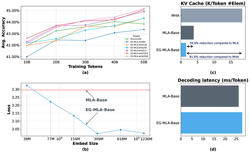
Figure 1: (a) Average accuracy versus training tokens. (b) Validation loss with respect to embedding size used in embedding gating. (c) KV cache elements per token. EG-MLA significantly reduces cache size compared to MHA and MLA. (d) Decoding efficiency of EG-MLA.
Autoregressive decoding remains a critical bottleneck in the deployment of Transformer-based large language models (LLMs), particularly in real-time or resource-constrained scenarios. A major contributor to this inefficiency is the large memory footprint required to store key-value (KV) pairs during inference. In standard Multi-Head Attention (MHA) (Vaswani et al. 2017), each attention head maintains its own set of key and value vectors, leading to quadratic memory scaling with respect to sequence length and model size. While effective in capturing complex dependencies, this design is increasingly impractical for latency-sensitive applications or deployment on edge devices.
To mitigate this challenge, a series of efficient attention mechanisms have been proposed to reduce KV cache requirements while preserving model performance. Notably, Multi-Query Attention (MQA) (Shazeer 2019) and Grouped-Query Attention (GQA) (Ainslie et al. 2023) compress the KV cache by sharing key and value representations across attention heads or head groups. More recently, Multi-head Latent Attention (MLA) (Liu et al. 2024) introduces a shared latent projection space that significantly reduces memory usage while maintaining strong expressiveness, striking a better balance between performance and efficiency.
Building on this line of work, we introduce Embedding-Gated Multi-head Latent Attention (EG-MLA), a novel extension to MLA that further enhances memory efficiency without sacrificing model quality. EG-MLA augments the latent attention mechanism with a token-specific embedding gating module that modulates compressed KV representations in a fine-grained manner. This lightweight gating design introduces minimal additional computation and parameter overhead, yet substantially improves the expressive capacity of the compressed latent space.
Compared to MHA, EG-MLA achieves over 91.6% reduction in KV cache size, and compared to MLA, it provides up to 59.9% additional memory savings while achieving equal or better performance across multiple reasoning benchmarks. Our theoretical analysis reveals that embedding gating implicitly induces a second-order feature space, which enhances token-specific representation capacity. Empirically, we demonstrate that EG-MLA is robust across varying compression ratios, embedding dimensions, and model scales.
Notably, we successfully scale EG-MLA to over 1 billion parameters, confirming its effectiveness not only in compact models but also in large-scale LLMs. Despite aggressive compression, our 1.2B EG-MLA model maintains competitive performance with its MLA counterpart, while using only 40% of the KV cache.
Our contributions can be summarized as follows:
- We propose EG-MLA, an embedding-gated extension to latent attention that enables token-specific modulation of compressed KV representations.
- We demonstrate that EG-MLA achieves superior performance-to-memory trade-offs compared to both MHA and MLA, across diverse tasks and model scales.
- We provide theoretical insights into the gating mechanism and show through comprehensive experiments that EG-MLA supports efficient inference at scale, including in 1B+ parameter regimes.
- We identify that further reducing the KV cache in MLA is inherently difficult, as its latent space is already highly compressed and empirically optimized. To overcome this limitation without degrading model performance, we introduce a novel architectural dimension—embedding gating—which adds token-specific parameters that compensate for the loss of latent capacity. This design preserves model expressiveness and inference efficiency, enabling deeper KV compression with minimal decoding overhead.
Overall, EG-MLA advances the frontier of efficient Transformer architectures, offering a promising path toward scalable, high-performance, and resource-efficient language model deployment.
## Related Works
### KV Cache Compression in Attention Mechanisms
Reducing the key-value (KV) cache size during inference is a fundamental challenge in scaling large language models (LLMs). Traditional multi-head attention (MHA) (Vaswani et al. 2017) stores separate key and value vectors for each attention head, resulting in substantial memory usage. To alleviate this, multi-query attention (MQA) (Shazeer 2019) and grouped-query attention (GQA) (Ainslie et al. 2023) share KV representations across heads or groups, achieving cache reduction with minimal performance degradation.
Multi-head latent attention (MLA) (Liu et al. 2024; Ji et al. 2025) extends this direction by introducing shared latent projections that significantly reduce KV cache size while retaining model expressiveness. Ji et al. (Ji et al. 2025) further adapt MLA to arbitrary Transformer-based LLMs, highlighting its applicability for broad deployment. However, MLA’s reliance on fixed latent projections may limit its adaptability, especially under aggressive compression.
Several recent studies further advance this paradigm. TransMLA (Meng et al. 2025) systematizes the latent attention design for efficient inference, though it does not incorporate token-level adaptability. Deng and Woodland (Deng and Woodland 2025) propose a temporal latent attention mechanism, exploring compression along different axes, which is conceptually related to our gating strategy. Mehta et al. (Mehta et al. 2025) investigate latent attention specifically for small language models, offering evidence that such approaches can maintain quality under limited resource budgets—an area in which EG-MLA also excels.
### Gating Mechanisms in Transformer Architectures
Gating mechanisms have been widely studied to enhance Transformer expressiveness. For example, the Highway Transformer (Chai, Jin, and Hou 2020) employs self-gating to modulate internal information flow, showing that adaptive gating can improve model capacity. However, these approaches typically operate over the full attention space and introduce non-negligible computational overhead.
Our proposed EG-MLA differs by introducing a lightweight embedding gating mechanism that operates in the compressed latent space. This enables token-specific modulation of KV representations with minimal computational and memory cost, effectively enhancing expressiveness without sacrificing efficiency.
### Other Attention Variants
Other attention variants such as Performer (Choromanski et al. 2020), Linformer (Wang et al. 2020), and Longformer (Beltagy, Peters, and Cohan 2020) aim to improve efficiency by approximating the softmax attention kernel. However, these methods primarily target encoder-based architectures or long-context processing, and do not directly address the memory overhead from KV caching during decoder-side autoregressive inference. In contrast, EG-MLA maintains the original attention structure while focusing on minimizing the KV cache footprint during generation. Thus, we consider our comparisons with MLA, MQA, and GQA to be more directly aligned.
### Summary
EG-MLA integrates latent compression and token-specific modulation into a unified architecture. By building on and extending prior work in both KV cache reduction and attention gating, it achieves improved trade-offs between memory usage and model quality. This positions EG-MLA as a practical and scalable solution for efficient LLM inference across a wide range of deployment scenarios.
## Embedding Gated MLA
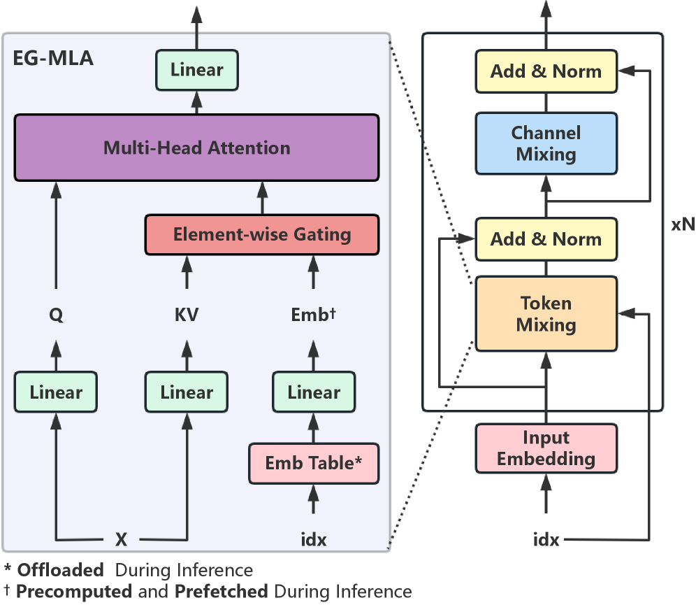
Simplified Architecture of EG-MLA is shown in Figure 2.
<details>
<summary>x2.png Details</summary>
### Visual Description
## Diagram: EG-MLA Architecture
### Overview
The image is a technical architecture diagram illustrating a neural network module labeled "EG-MLA" (left) and its integration into a standard transformer-style block (right). The diagram highlights data flow, specific processing layers, and optimization strategies (offloading and prefetching) used during inference.
### Components/Axes
**Left Region (EG-MLA Module):**
* **Inputs:** "X" and "idx".
* **Processing Blocks:**
* Three "Linear" layers (light green).
* "Emb Table*" (light pink).
* "Element-wise Gating" (light red).
* "Multi-Head Attention" (purple).
* **Intermediate Variables:** "Q", "KV", "Embt" (light blue/text).
**Right Region (Transformer Block):**
* **Inputs:** "idx".
* **Processing Blocks:**
* "Input Embedding" (light pink).
* "Token Mixing" (light orange).
* "Add & Norm" (light yellow, appears twice).
* "Channel Mixing" (light blue).
* **Structure:** The entire block is enclosed in a box labeled "xN" on the right, indicating this block is repeated N times.
**Footer (Legend):**
* `*`: "Offloaded During Inference"
* `†`: "Precomputed and Prefetched During Inference"
### Detailed Analysis
**1. EG-MLA Module (Left):**
* **Input Processing:**
* Input "X" splits into two paths, each passing through a "Linear" layer to produce "Q" and "KV".
* Input "idx" passes through "Emb Table*" (marked with `*`) and then a "Linear" layer to produce "Embt" (marked with `†`).
* **Gating and Attention:**
* "KV" and "Embt" serve as inputs to the "Element-wise Gating" layer.
* The output of "Element-wise Gating" and the "Q" variable are fed into the "Multi-Head Attention" layer.
* The output of "Multi-Head Attention" passes through a final "Linear" layer.
**2. Transformer Block (Right):**
* **Flow:**
* Input "idx" enters "Input Embedding".
* The output flows into "Token Mixing".
* A dotted line connects the "EG-MLA" block on the left to the "Token Mixing" block on the right, indicating that EG-MLA is the specific implementation or replacement for this component.
* The output of "Token Mixing" flows into an "Add & Norm" layer.
* The output of "Add & Norm" flows into "Channel Mixing".
* The output of "Channel Mixing" flows into a second "Add & Norm" layer.
* **Residual Connections:** Arrows loop back from the output of the first "Add & Norm" to the input of "Token Mixing", and from the output of the second "Add & Norm" to the input of "Channel Mixing".
### Key Observations
* **Optimization Strategy:** The diagram explicitly marks components for inference optimization. The "Emb Table" is offloaded, and the "Embt" (embedding) values are precomputed and prefetched.
* **Integration:** The dotted line indicates that the EG-MLA module is a specialized version of the "Token Mixing" component found in the standard transformer block.
* **Data Flow:** The architecture separates the query (Q) and key-value (KV) generation, with the KV path being augmented by precomputed embeddings ("Embt") via element-wise gating before entering the attention mechanism.
### Interpretation
This diagram illustrates an optimized attention mechanism designed to reduce computational overhead during inference.
By offloading the embedding table and precomputing/prefetching the embeddings ("Embt"), the system avoids performing these operations in real-time. The "Element-wise Gating" layer suggests that the model dynamically modulates the Key-Value (KV) information using these precomputed embeddings before the attention calculation. This architecture likely aims to reduce latency or memory bandwidth requirements in large language models by replacing standard token mixing with this gated, precomputed approach. The "xN" notation confirms this is a modular component within a larger, repeating transformer stack.
</details>
Figure 2: Simplified Architecture of the Embedding Gated Multi-Head Latent Attention (EG-MLA).
### Core Formulas
#### Low-Rank Key-Value Joint Compression
We begin by inheriting the core principle of MLA, namely the low-rank joint compression of keys and values, which serves to reduce the memory footprint of the KV cache:
$$
\displaystylec_t^KV \displaystyle=W^DKVx_t, \displaystylekv_t^C \displaystyle=W^UKVc_t^KV, \tag{1}
$$
where $c_t^KV∈ℝ^d_c$ is the compressed latent vector for keys and values; $W^UKV$ is up-projection matrix for joint keys and values.
#### Embedding Gating
Given the token index $i_t$ , we retrieve its per-layer embedding $e_t$ from a learnable lookup table. This embedding is then passed through an up-projection matrix $W^UE$ to obtain a gating signal $g_t$ , representing a token-specific modulation vector. We apply element-wise modulation to the compressed key-value representation $kv_t^C$ via the Hadamard product with $g_t$ . Finally, a layer normalization is applied to the result, producing the final key and value representation $\widetilde{kv}_t^C$ .
$$
\displaystylee_t \displaystyle=Emb(i_t), \displaystyleg_t \displaystyle=W^UEe_t, \displaystyle\widetilde{kv}_t^C \displaystyle=LN≤ft(kv_t^C\odotg_t\right), \tag{3}
$$
The subsequent computation follows the same procedure as MLA. To provide a comprehensive view of the EG-MLA mechanism, we present the complete set of formulas along with a detailed architectural diagram in Appendix C.
### Rationale behind Embedding Gating
We analyze the embedding gating mechanism by reformulating its core expression, in order to highlight its ability to project inputs into a high-dimensional nonlinear feature space.
In a single layer of EG-MLA, the embedding gating operation can be written as $(W^UKV c_t^KV)\odot(W^UE e_t)$ , which denotes the element-wise multiplication of two linearly projected features.
For ease of analysis, this operation can be abstracted as $(W_1x_1)\odot(W_2x_2)$ , where $x_1∈ℝ^d_1$ and $x_2∈ℝ^d_2$ are two distinct input vectors, and $W_1∈ℝ^d_1× d$ , $W_2∈ℝ^d_2× d$ are their corresponding projection matrices into a shared $d$ -dimensional space.
Focusing on the case of a single output channel, the embedding gating can be further expressed as:
$$
\displaystyle w_1^Tx_1\odot w_2^Tx_2 \displaystyle=≤ft(∑_i=1^d_1w_1^(i)x_1^(i)\right)\odot≤ft(∑_j=1^d_2w_2^(j)x_2^(j)\right) \displaystyle=∑_i=1^d_1∑_j=1^d_2w_1^(i)w_2^(j)x_1^(i)x_2^(j) \tag{6}
$$
As shown in Eq. 8, this formulation expands into $d_1× d_2$ distinct second-order interaction terms between $x_1$ and $x_2$ . Therefore, a single-layer embedding gating operation implicitly maps the input into a nonlinear feature space of dimensionality $d_1× d_2$ , significantly enhancing the representational capacity without introducing any additional computational overhead. This formulation forms the fundamental rationale behind our design choice to incorporate embedding gating. By leveraging its ability to construct an implicit high-dimensional representation, we enable an architecture with a more compact latent space without compromising expressiveness.
## Performance Evaluation
### Experimental Settings
#### Data
We use ClimbMix (Diao et al. 2025) as the training dataset, which consists of 400 billion tokens in total. For evaluation, we adopt several reasoning benchmarks: PIQA (Bisk et al. 2020), ARC-C, ARC-E (Clark et al. 2018), HellaSwag (Zellers et al. 2019), WinoGrande (Sakaguchi et al. 2019), and SIQA (Sap et al. 2019). We optimize the data mixture using the validation sets of PIQA, ARC-E, and HellaSwag, and then evaluate on their respective test sets. All evaluations are performed using the LM-Evaluation Harness (Gao et al. 2024), under the 0-shot setting for all tasks except MMLU, which uses a 5-shot setting (Allal et al. 2025; Cosmopedia Team 2024).
#### Model
We train a series of Transformer decoder-only models using the EG-MLA architecture with next-token prediction as the training objective. The training data consists of 50 billion tokens.
#### Baselines
We compare the proposed EG-MLA architecture against MLA models with equivalent activation parameter counts. More detailed experimental settings and training hyper-parameters can be found in Appendix A.
### Towards Compact KV Cache
Table 1 reveals several noteworthy patterns regarding the impact of embedding gating and KV cache size on model performance. First, the introduction of embedding gating consistently enhances performance across nearly all tasks compared to the baseline MLA model with the same KV cache size, indicating that the proposed mechanism effectively enriches representational capacity without increasing computational burden. Second, EG-MLA models demonstrate strong robustness to aggressive KV compression: even when the KV cache size is reduced from 256 to as low as 64 or 16, the average accuracy remains stable, with only marginal fluctuations across most benchmarks. This suggests that embedding gating allows the model to retain crucial information in a more compact latent space.
| Model Name | Size | piqa | arc-c | arc-e | hella | winog | siqa | mmlu | obqa | boolq | race | truth | lmb.o | Avg. |
| --- | --- | --- | --- | --- | --- | --- | --- | --- | --- | --- | --- | --- | --- | --- |
| MLA-Base-kv256 | 120M | 69.48 | 26.45 | 61.36 | 34.11 | 52.33 | 85.40 | 25.12 | 21.40 | 58.10 | 30.91 | 29.82 | 31.63 | 43.84 |
| EG-MLA-Base-kv256 | 125M | 70.29 | 29.27 | 62.80 | 35.82 | 50.67 | 86.40 | 25.22 | 24.40 | 55.26 | 30.62 | 29.20 | 33.63 | 44.46 |
| EG-MLA-Base-kv128 | 122M | 71.49 | 29.18 | 62.75 | 35.57 | 53.43 | 87.80 | 26.71 | 22.20 | 47.74 | 30.24 | 29.09 | 33.48 | 44.14 |
| EG-MLA-Base-kv64 | 120M | 71.60 | 29.61 | 63.89 | 35.31 | 51.14 | 86.20 | 24.19 | 23.00 | 55.05 | 30.43 | 29.21 | 32.35 | 44.33 |
| EG-MLA-Base-kv16 | 119M | 71.16 | 28.50 | 62.08 | 34.48 | 50.75 | 84.70 | 26.21 | 21.40 | 57.13 | 31.29 | 30.58 | 30.95 | 44.10 |
Table 1: Accuracy of different models across 12 benchmark tasks under varying KV cache sizes. All models use a fixed embedding dimension of 256. ”Size” denotes the number of activated parameters. Task abbreviations: LAMBADA (lmb.o), HellaSwag (hella), Winogrande (winog), TruthfulQA (truth).
We also assess EG-MLA on standard language modeling datasets such as WikiText103 (Merity, Keskar, and Socher 2018), LAMBADA (Paperno et al. 2016), and ClimbMix (Diao et al. 2025). As reported in Appendix D, EG-MLA consistently outperforms MLA in perplexity or validation loss under equivalent compression settings. This suggests that embedding gating provides benefits beyond reasoning and applies broadly to language modeling scenarios. These results demonstrate that EG-MLA remains robust even under aggressive compression settings. It is important to emphasize, however, that MLA itself is already near the limit of feasible compression.
### Scaling Law for Embedding Size
Table 2 highlights several key trends as the embedding dimension increases. Most notably, performance consistently improves when moving from extremely small embeddings (e.g., 64) to moderate sizes (e.g., 512), suggesting that larger embedding vectors enable more expressive token-specific modulation through the gating mechanism. However, beyond a certain point—particularly past 1024 dimensions—the performance gains begin to saturate and even exhibit some inconsistency across tasks. For instance, while some benchmarks such as ARC-E and LAMBADA continue to improve steadily, others like MMLU and WinoGrande fluctuate or plateau. This indicates diminishing returns from simply scaling up the embedding size, likely due to a combination of overparameterization and limited benefit from increased modulation granularity. Interestingly, even relatively compact models with 128–256 embedding dimensions already capture most of the benefit, striking a favorable balance between performance and efficiency. These findings suggest that embedding size should be carefully tuned rather than blindly scaled, and that EG-MLA achieves strong performance even under strict parameter budgets.
Notably, performance does not increase monotonically as shown in Figure 1. Beyond the point where the embedding size exceeds the total dimensionality of the key and value vectors, we observe saturation or even slight regressions on some tasks. This suggests that overparameterization beyond the combined key-value capacity yields limited benefits, revealing a current scaling limitation of our method. Exploring architectures that scale more gracefully with increased embedding capacity is an important direction for future work.More comprehensive scaling experiments are provided in Appendix G.
| Model Name | Embed Size | piqa | arc-c | arc-e | hella | winog | siqa | mmlu | obqa | boolq | race | truth | lmb.o | Avg. |
| --- | --- | --- | --- | --- | --- | --- | --- | --- | --- | --- | --- | --- | --- | --- |
| EG-MLA-Base-emb64 | 38M | 69.37 | 27.47 | 60.82 | 33.96 | 51.22 | 83.90 | 27.73 | 21.00 | 55.17 | 28.71 | 29.81 | 31.13 | 43.36 |
| EG-MLA-Base-emb128 | 77M | 70.62 | 29.44 | 63.22 | 34.72 | 54.22 | 86.60 | 25.48 | 22.60 | 54.68 | 28.80 | 30.54 | 31.07 | 44.33 |
| EG-MLA-Base-emb256 | 154M | 71.60 | 29.61 | 63.89 | 35.31 | 51.14 | 86.20 | 24.19 | 23.00 | 55.05 | 30.43 | 29.21 | 32.35 | 44.33 |
| EG-MLA-Base-emb512 | 309M | 71.93 | 30.12 | 63.89 | 35.86 | 52.01 | 87.10 | 26.27 | 22.20 | 56.12 | 30.05 | 29.50 | 33.86 | 44.91 |
| EG-MLA-Base-emb1024 | 618M | 71.98 | 31.83 | 64.69 | 36.24 | 50.21 | 86.10 | 26.63 | 23.80 | 58.81 | 29.28 | 28.22 | 32.91 | 45.06 |
| EG-MLA-Base-emb2048 | 1236M | 72.69 | 30.89 | 66.37 | 36.44 | 54.07 | 85.40 | 25.43 | 22.80 | 53.61 | 28.90 | 30.78 | 34.70 | 45.17 |
Table 2: Accuracy results of EG-MLA models across 12 benchmark tasks with varying embedding dimensions. The KV cache dimension is fixed at 64. Task abbreviations: LAMBADA (lmb.o), HellaSwag (hella), WinoGrande (winog), TruthfulQA (truth).
### Ablation on Embedding Gating
The ablation study in Table 3 reveals two critical observations about the design of the embedding gating mechanism.
#### The Critical Role of Layer Normalization
First, the presence of LayerNorm after the gating operation is essential. Its removal leads to a clear degradation in performance, suggesting that normalization is crucial for stabilizing the gated feature distribution and ensuring effective downstream attention computation.
#### Effectiveness of element-wise multiplication
Second, replacing the element-wise multiplication with simple addition results in a noticeable loss increase, although not as severe as removing LayerNorm. This indicates that the element-wise multiplicative interaction plays a more effective role in modulating key-value representations, likely because it enables fine-grained, dimension-wise control over the information flow.
Overall, these findings reinforce the importance of both architectural choices—the normalization step and multiplicative gating—in maximizing the benefits of the embedding-guided modulation.
| Model Name | Size | Tokens | Loss (val) |
| --- | --- | --- | --- |
| MLA-Base-kv256 | 120M | 10B | 3.2156 |
| EG-MLA-Base-kv256 | 125M | 10B | 3.1609 |
| - remove LayerNorm | 125M | 10B | 3.2573 |
| - replace $\odot$ with addition | 125M | 10B | 3.1901 |
Table 3: Ablation on Embedding Gating. ”Size” refers to Activated Parameters
### Scaling to 1B Language Model
To probe into the impact of scaling model size and training data, we train two models, namely MLA-1.2B and EG-MLA-1.2B (with 1.2 billion activated parameters and 600 million offloaded parameters). Both models are trained on 50 billion tokens from the ClimbMix dataset (Diao et al. 2025). MLA-1.2B is built on the Deepseek framework (Liu et al. 2024). EG-MLA-1.2B, which is designed for efficiency, utilizes merely 40.1% of the cache size of MLA-1.2B while still achieving competitive performance.
| Model Name | Size | Embed Size | piqa | arc-c | arc-e | hella | winog | siqa | mmlu | obqa | boolq | race | truth | lmb.o | Avg. |
| --- | --- | --- | --- | --- | --- | --- | --- | --- | --- | --- | --- | --- | --- | --- | --- |
| MLA-1.2B | 1188M | 0M | 75.52 | 38.82 | 73.02 | 44.15 | 56.83 | 92.20 | 28.42 | 27.20 | 53.15 | 34.26 | 33.76 | 38.02 | 49.61 |
| EG-MLA-1.2B | 1182M | 618M | 75.41 | 38.74 | 72.85 | 44.88 | 56.83 | 91.00 | 26.92 | 27.80 | 59.45 | 33.97 | 31.27 | 40.25 | 49.95 |
Table 4: Accuracy results of additional models across 12 benchmark tasks for EG-MLA with over 1B parameters. ”Size” denotes the number of activated parameters.
Table 4 demonstrates that EG-MLA-1.2B attains performance on par with MLA-1.2B across a wide array of benchmarks, featuring a remarkable enhancement in average accuracy. This competitive performance, in conjunction with the reduced cache size of EG-MLA-1.2B, emphasizes its capability to generalize proficiently under resource limitations.
In conclusion, EG-MLA-1.2B matches the performance of MLA-1.2B in both base and fine-tuned scenarios, while utilizing merely 40% of the KV cache size of MLA-1.2B. These findings highlight the potential of memory- and compute-efficient architectures for the expansion of large language models, facilitating sustainable and resource-efficient AI development.
## Efficiency Evaluation
### Analytical Comparison of KV Cache Costs
Table 5 presents a theoretical comparison of the KV cache cost per token across different attention mechanisms, including our proposed EG-MLA. Traditional methods such as Multi-Head Attention (MHA) and Grouped-Query Attention (GQA) store separate key and value vectors for each head or group, leading to a cache size that scales with the number of heads $n_h$ or groups $n_g$ . Multi-Query Attention (MQA), while more efficient, sacrifices representational capacity by sharing keys and values across all heads.
In comparison, MLA introduces a shared latent vector to compress key-value representations, significantly reducing the cache size while maintaining reasonable performance. However, EG-MLA further improves this design by applying a token-specific embedding gating mechanism, enabling more expressive modulation of the shared latent without increasing cache overhead. Specifically, EG-MLA stores only a compressed latent vector of dimension $d_c/r$ per token, resulting in a leaner cache footprint than MLA. Despite the more aggressive compression, EG-MLA retains strong representational power thanks to the multiplicative interaction with token embeddings. This analytical comparison highlights EG-MLA’s advantage in offering both compact memory usage and enhanced modeling capacity.
The actual KV cache savings can be found in Appendix F, where we provide a concrete example. In this case, EG-MLA achieves a 59.9% reduction in KV cache compared to MLA, and a substantial 91.6% reduction compared to MHA.
| Attention Mechanism | KV Cache / Token (#Elem) | Capability |
| --- | --- | --- |
| Multi-Head Attention (MHA) | $2n_hd_hl$ | Strong |
| Grouped-Query Attention (GQA) | $2n_gd_hl$ | Moderate |
| Multi-Query Attention (MQA) | $2d_hl$ | Weak |
| Multi-Head Latent Attention (MLA) | $(d_c+d_h^R)l$ | Strong |
| EG-MLA (Ours) | $(d_c/r+d_h^R)l$ | Stronger |
Table 5: Comparison of the number of KV cache elements per token across different attention mechanisms. $n_h$ denotes the number of attention heads, $d_h$ the dimension per attention head, $l$ the number of layers, $n_g$ the number of groups in GQA, and $d_c$ and $d_h^R$ represent the latent space dimension and the KV cache dimension used for RoPE in MLA, respectively. For EG-MLA, a compressed latent vector of dimension $d_c/r$ is stored per token, where $r$ is the compression factor applied to the latent representation. This results in a significantly smaller KV cache while preserving strong representational capacity through embedding gating.
<details>
<summary>x3.png Details</summary>
### Visual Description
## Diagram: Apply Embedding to kv
### Overview
The image is a schematic block diagram illustrating a data processing pipeline, titled "Apply Embedding to kv". The diagram depicts a sequential process that begins with an embedding layer, splits into two parallel processing branches, converges into a concatenation operation, and concludes with a normalization step. The entire process is enclosed within a dashed-line rectangular border.
### Components/Axes
The diagram flows from left to right. The components are color-coded and arranged as follows:
* **Header:** "Apply Embedding to kv" (centered above the diagram).
* **Input Stage (Far Left):**
* **"Emb"**: A yellow rectangular block. An arrow enters from the left.
* **Parallel Processing Branches (Middle):**
* **Top Branch**:
* **"e1"**: A light green rectangular block.
* **"W"**: A light orange rectangular block.
* **Bottom Branch**:
* **"e2"**: A light green rectangular block.
* **"W"**: A light orange rectangular block.
* **Convergence Stage (Middle-Right):**
* **"Gather&Cat"**: A light blue vertical rectangular block. Both parallel branches feed into this block.
* **Output Stage (Far Right):**
* **"Norm"**: A light pink vertical rectangular block. An arrow exits to the right.
### Detailed Analysis
The flow of data through the diagram is as follows:
1. **Initial Embedding**: Data enters the system via an arrow pointing into the **"Emb"** (yellow) block.
2. **Branching**: The output of the "Emb" block splits into two identical parallel paths.
* **Top Path**: The signal flows from "Emb" to **"e1"** (light green), then to **"W"** (light orange), and finally into the **"Gather&Cat"** (light blue) block.
* **Bottom Path**: The signal flows from "Emb" to **"e2"** (light green), then to **"W"** (light orange), and finally into the **"Gather&Cat"** (light blue) block.
3. **Aggregation**: The **"Gather&Cat"** block acts as a junction, receiving inputs from both the top and bottom "W" blocks.
4. **Normalization**: The output of the "Gather&Cat" block flows into the **"Norm"** (light pink) block.
5. **Final Output**: The processed data exits the "Norm" block via an arrow pointing to the right.
### Key Observations
* **Symmetry**: The diagram exhibits strong vertical symmetry. The top and bottom branches are identical in structure ("e" -> "W"), suggesting that the system processes two distinct components (e1 and e2) in parallel using similar transformation weights (W).
* **Color Coding**: The color scheme is consistent across functional groups:
* Yellow: Initial embedding.
* Light Green: Intermediate feature/embedding vectors.
* Light Orange: Transformation/Weight matrices.
* Light Blue: Aggregation/Concatenation operation.
* Light Pink: Normalization layer.
* **Flow**: The diagram clearly delineates a "split-transform-merge" architecture.
### Interpretation
This diagram represents a specific architectural pattern often found in neural networks, particularly those involving attention mechanisms or multi-modal data processing.
* **"kv" Context**: The title "Apply Embedding to kv" strongly suggests this is a mechanism for generating Key (k) and Value (v) vectors used in Transformer-based architectures.
* **Functional Logic**:
* The "Emb" block likely creates a shared representation of the input.
* The split into "e1" and "e2" suggests the generation of two distinct feature sets (e.g., one for keys, one for values, or two different attention heads).
* The "W" blocks represent learned linear projections (weights) applied to these features.
* "Gather&Cat" implies that these transformed features are collected and concatenated into a single tensor.
* "Norm" (likely Layer Normalization) is applied at the end to stabilize the output before it is passed to subsequent layers in the network.
* **Significance**: This architecture allows the model to derive multiple, distinct representations from a single input source simultaneously, which is a fundamental requirement for complex sequence modeling.
</details>
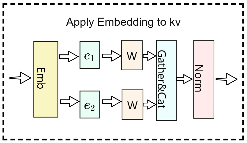
Figure 3: Dimension-wise sharding pipeline.
### Empirical Comparison of Efficiency
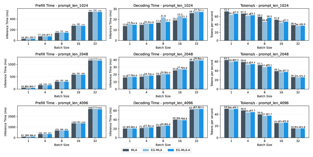
We evaluate the inference efficiency of EG-MLA on a single NVIDIA A800 80 GB GPU. As shown in Figure 4, we report Prefill latency, Decoding latency and tokens-per-second under varying prompt lengths and batch sizes. The MLA model contains 120M parameters in total, whereas EG-MLA contains 274M, of which 154M are embed parameters.EG-MLA-A is an inference-optimized variant of EG-MLA in which the projection matrices are pre-computed offline during model loading; during inference, matrix multiplication is thus eliminated and only a table lookup is performed, further reducing inference latency.Despite the extra embed parameters introduced, EG-MLA maintains inference performance comparable to or better than that of MLA. Concretely, when the batch size exceeds 8, EG-MLA reduces the average pre-fill latency by 5.6 ms compared with MLA while adding only 0.91 ms to the average decoding latency. When the batch size reaches 32, EG-MLA-A narrows the average decoding latency gap with MLA to merely 1 ms, underscoring the efficiency of our approach for large-scale parallel workloads.
<details>
<summary>x4.png Details</summary>
### Visual Description
## Bar Chart Grid: Performance Comparison of MLA, EG-MLA, and EG-MLA-A
### Overview
This image presents a 3x3 grid of bar charts comparing the performance of three different methods—**MLA** (dark grey), **EG-MLA** (light blue), and **EG-MLA-A** (medium blue)—across varying batch sizes (1, 4, 8, 16, 32) and prompt lengths (1024, 2048, 4096). The metrics evaluated are **Prefill Time (ms)**, **Decoding Time (ms)**, and **Tokens/s**.
### Components/Axes
* **Legend (Bottom Center):**
* **MLA:** Dark Grey bar
* **EG-MLA:** Light Blue bar
* **EG-MLA-A:** Medium Blue bar
* **Grid Structure:**
* **Rows (Top to Bottom):** Prompt Length 1024, Prompt Length 2048, Prompt Length 4096.
* **Columns (Left to Right):** Prefill Time (ms), Decoding Time (ms), Tokens/s.
* **Axes:**
* **X-Axis:** Batch Size (1, 4, 8, 16, 32).
* **Y-Axis:** Varies by column (Inference Time in milliseconds or Tokens per second).
---
### Detailed Analysis
#### Row 1: Prompt Length 1024
* **Prefill Time (ms):** Values increase with batch size. MLA is consistently the fastest (lowest time).
* Batch 1: MLA 29.5, EG-MLA 31
</details>
Figure 4: Prefill and Decoding times and Tokens per seconds for MLA, EG-MLA and EG-MLA-A across configurations on an NVIDIA A800 80GB GPU. EG-MLA-A is an inference-optimized variant of EG-MLA that pre-computes all embeddings at model-loading time and pre-fetch during inference.
| Method | Node | Peak Mem. | Throughput | Avg. Step Time | Comm. Time |
| --- | --- | --- | --- | --- | --- |
| vanilla | 2 | 13950 | 42528 | 385.25 | – |
| dimension-wise | 2 | 12233 | 86743 | 188.88 | 16.25 |
| vanilla | 4 | 13950 | 80114 | 409.02 | – |
| dimension-wise | 4 | 11759 | 175031 | 187.21 | 24.38 |
Table 6: Performance comparison between vanilla and dimension-wise parallelism under varying node counts. Memory is reported in megabytes (MB) and throughput in tokens per second (tokens/s), and all timing metrics in milliseconds (ms).
### Embedding Parallelism
Embedding gating introduces additional parameters into each attention layer, significantly increasing GPU memory usage during training. To mitigate peak memory footprint on individual devices, we adopt a dimension-wise sharding strategy (Shoeybi et al. 2020), which partitions the key–value embedding uniformly along the embedding dimension across $W$ parallel workers. The per-rank embedding dimension is given by:
$$
\displaystyled_local \displaystyle=\frac{d_kv}{W}, \tag{9}
$$
where $d_kv$ is the original KV embedding dimension.
Each worker independently computes its local embedding and corresponding projection:
$$
\displaystylee_i \displaystyle=Emb(i_t), \displaystyleg_t^(i) \displaystyle=W_i^UEe_i, \tag{10}
$$
and the final gating vector is reconstructed via concatenation.
This approach yields near-linear memory scaling. Embedding lookups and projections are fully parallelized across workers, with only a single all-gather operation needed during final aggregation, incurring minimal communication overhead. A simplified pipeline is illustrated in Figure 3.
As shown in Table 6, dimension-wise parallelism with two nodes reduces peak memory by 12.3%, shortens per-step time by 51%, and increases throughput by 104% relative to the baseline. Scaling to four nodes yields further reductions in both peak memory and per-step time, together with an additional throughput gain.
Why Dimension-wise Sharding?
Tensor parallelism distributes matrix computations across multiple GPUs to reduce memory usage and accelerate training, but introduces inter-device communication. Compared to alternatives like layer-wise sharding, we choose dimension-wise partitioning for the following reasons:
- Load Balancing: Evenly splits the embedding matrix, ensuring uniform computational load across devices.
- No Serial Dependencies: Enables full parallelism by avoiding sequential computation across layers.
- Memory Efficiency: Embedding layers are memory-intensive; partitioning them maximizes GPU memory bandwidth and cache utilization.
<details>
<summary>x5.png Details</summary>
### Visual Description
## Line Charts: PPL vs Embedding Dimension and PPL vs Layer Group Size
### Overview
The image displays two line charts, labeled (a) and (b), which evaluate the performance of different model configurations by measuring "Avg. PPL" (Average Perplexity). Lower perplexity values generally indicate better model performance. Chart (a) examines the impact of varying the "Embedding Dimension," while Chart (b) examines the impact of varying the "Layer Group Size." Both charts include a baseline comparison represented by a horizontal dashed red line.
---
### Components/Axes
#### Chart (a): PPL vs Embedding Dimension
* **Positioning:** Located on the left side of the image.
* **X-Axis:** "Embedding Dimension" with discrete markers at 64, 128, 256, 512, 1024, and 2048.
* **Y-Axis:** "Avg. PPL" ranging from 21 to 28.
* **Legend (Top-Right):**
* **EG-MLA-emb:** Represented by a solid blue line with circular data points.
* **MLA-kv256:** Represented by a horizontal dashed red line.
#### Chart (b): PPL vs Layer Group Size
* **Positioning:** Located on the right side of the image.
* **X-Axis:** "Layer Group Size" with discrete markers at 0, 2, 4, and 6.
* **Y-Axis:** "Avg. PPL" ranging from 11.50 to 13.50.
* **Legend (Top-Left):**
* **EG-MLA-Large-ctx2048-kv256emb512:** Represented by a solid green line with circular data points.
* **MLA-Large-ctx2048-kv512:** Represented by a horizontal dashed red line.
---
### Detailed Analysis
#### Chart (a) Analysis
* **Trend Verification:** The blue line ("EG-MLA-emb") shows a sharp downward trend (improvement in PPL) as the embedding dimension increases from 64 to 512. After 512, the trend flattens and shows a slight, negligible increase at 1024 before stabilizing. The red dashed line remains constant.
* **Data Points (Approximate):**
* **64:** ~27.8
* **128:** ~25.0
* **256:** ~22.9
* **512:** ~20.5 (Minimum point)
* **1024:** ~21.0
* **2048:** ~20.6
* **Red Baseline:** Constant at ~27.0
#### Chart (b) Analysis
* **Trend Verification:** The green line ("EG-MLA-Large...") shows a steady upward trend (degradation in PPL) as the Layer Group Size increases from 0 to 6. The red dashed line remains constant.
* **Data Points (Approximate):**
* **0:** ~11.55
* **2:** ~11.90
* **4:** ~12.55
* **6:** ~13.50
* **Red Baseline:** Constant at ~12.10
---
### Key Observations
* **Chart (a) Efficiency:** The "EG-MLA-emb" model significantly outperforms the "MLA-kv256" baseline once the embedding dimension exceeds 128. The performance gains saturate at an embedding dimension of 512; increasing the dimension further provides no additional benefit to perplexity.
* **Chart (b) Trade-off:** Increasing the "Layer Group Size" consistently degrades model performance. The "EG-MLA-Large" model is superior to the baseline only at lower group sizes (0 and 2). At a group size of approximately 2.5, the performance crosses the baseline, and at higher group sizes (4 and 6), the model performs worse than the baseline.
---
### Interpretation
These charts illustrate hyperparameter optimization for a specific model architecture, likely a variant of Multi-Head Latent Attention (MLA) in a Large Language Model (LLM) context.
* **Embedding Dimension (Chart a):** The data suggests that 512 is the "sweet spot" for the embedding dimension. Increasing the dimension beyond this point likely introduces unnecessary complexity or parameters without improving the model's predictive capability (perplexity), indicating a point of diminishing returns.
* **Layer Group Size (Chart b):** This chart demonstrates a clear negative correlation between "Layer Group Size" and model performance. While grouping layers is often done to reduce memory usage or increase inference speed, this data quantifies the "cost" of that optimization in terms of perplexity. The crossover point (where the model becomes worse than the baseline) indicates the maximum allowable grouping size before the architectural trade-off becomes detrimental to the model's accuracy.
</details>
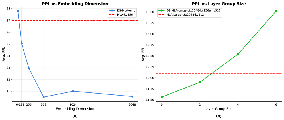
Figure 5: (a) Average Perplexity(PPL) versus Embedding Dimension. (b) Average Perplexity(PPL) versus Layer Group Size in Inter. The PPL reported in both (a) and (b) are averaged over the ClimbMix-val, Wiki, and LAMBADA benchmarks.
### Toward Greater Efficiency
To compress model parameters further while preserving performance, we explore two orthogonal directions. First, as shown in Table 5, the proposed embedding-gating mechanism yields a significantly smaller KV-cache than competing techniques. Second, we investigate inter-layer parameter sharing: the first half of the KV-projection matrices is reused across neighboring layers, with a single hyper-parameter that controls the width of the sharing window. Setting this hyper-parameter to 2, for example, theoretically halves the parameter count of the first half of the KV projections and simultaneously reuses the associated intermediate activations, cutting both memory footprint and computation. Detailed ablations are provided in Appendix H.
Figure 5 reveals that perplexity decreases monotonically with embedding dimension (emb) until it plateaus beyond emb = 512, indicating the current capacity limit of our embedding gating mechanism; surpassing this limit will be the focus of future work. Figure 3(b) shows that a layer group size of 2 or 3 strikes the best trade-off. Consequently, we recommend emb = 512 and layer group size = 2 for an optimal balance between performance and storage.
## Conclusion
In this work, we introduced Embedding-Gated Multi-head Latent Attention (EG-MLA), a novel extension of MLA designed to achieve more compact and expressive key-value (KV) representations. By integrating a lightweight embedding gating mechanism, EG-MLA effectively compresses the KV cache without sacrificing model performance. Through extensive experiments across multiple reasoning benchmarks, we demonstrated that EG-MLA consistently matches or surpasses MLA while significantly reducing memory usage, achieving up to a 59.9% reduction in KV cache compared to MLA and over 91.6% relative to MHA. We further analyzed the impact of embedding size, layer normalization, and multiplicative gating, highlighting the critical design choices that underpin EG-MLA’s effectiveness. Although MLA already represents a compact and efficient KV caching solution, our work highlights that meaningful further compression is only achievable by innovating along other architectural axes. EG-MLA achieves this by introducing a new token-specific embedding gating dimension that improves expressiveness with minimal impact on decoding latency, thereby enabling deeper compression without performance degradation. Scaling experiments on 1B-parameter models confirmed that EG-MLA retains competitive accuracy under stringent resource constraints, making it a promising candidate for efficient large language model deployment. Additionally, our theoretical and empirical efficiency analyses reveal that embedding gating enables a favorable trade-off between expressiveness and memory footprint. Future work will explore adaptive gating strategies, integration with sparsity-based attention mechanisms, and broader applications of EG-MLA in multi-modal and instruction-tuned models. We believe EG-MLA provides a foundation for advancing memory-efficient and high-performance language model architectures.
## References
- Ainslie et al. (2023) Ainslie, J.; Lee-Thorp, J.; De Jong, M.; Zemlyanskiy, Y.; Lebrón, F.; and Sanghai, S. 2023. Gqa: Training generalized multi-query transformer models from multi-head checkpoints. arXiv preprint arXiv:2305.13245.
- Allal et al. (2025) Allal, L. B.; Lozhkov, A.; Bakouch, E.; Bl’azquez, G. M.; Penedo, G.; Tunstall, L.; Marafioti, A.; Kydl’ivcek, H.; Lajar’in, A. P.; Srivastav, V.; Lochner, J.; Fahlgren, C.; Nguyen, X.-S.; Fourrier, C.; Burtenshaw, B.; Larcher, H.; Zhao, H.; Zakka, C.; Morlon, M.; Raffel, C.; von Werra, L.; and Wolf, T. 2025. SmolLM2: When Smol Goes Big - Data-Centric Training of a Small Language Model. ArXiv, abs/2502.02737.
- Beltagy, Peters, and Cohan (2020) Beltagy, I.; Peters, M. E.; and Cohan, A. 2020. Longformer: The long-document transformer. arXiv preprint arXiv:2004.05150.
- Bisk et al. (2020) Bisk, Y.; Zellers, R.; Gao, J.; and Choi, Y. 2020. PIQA: Reasoning about Physical Commonsense in Natural Language. In Proceedings of the AAAI Conference on Artificial Intelligence, volume 34, 7432–7439.
- Chai, Jin, and Hou (2020) Chai, Y.; Jin, S.; and Hou, X. 2020. Highway transformer: Self-gating enhanced self-attentive networks. arXiv preprint arXiv:2004.08178.
- Choromanski et al. (2020) Choromanski, K.; Likhosherstov, V.; Dohan, D.; Song, X.; Gane, A.; Sarlos, T.; Hawkins, P.; Davis, J.; Mohiuddin, A.; Kaiser, L.; et al. 2020. Rethinking attention with performers. arXiv preprint arXiv:2009.14794.
- Clark et al. (2018) Clark, P.; Cowhey, I.; Etzioni, O.; Khot, T.; Sabharwal, A.; Schoenick, C.; and Tafjord, O. 2018. Think you have Solved Question Answering? Try ARC, the AI2 Reasoning Challenge. ArXiv, abs/1803.05457.
- Cosmopedia Team (2024) Cosmopedia Team. 2024. Cosmopedia/evaluation at main · huggingface/cosmopedia. https://huggingface.co/Cosmopedia/evaluation.
- Deng and Woodland (2025) Deng, K.; and Woodland, P. C. 2025. Multi-head Temporal Latent Attention. arXiv preprint arXiv:2505.13544.
- Diao et al. (2025) Diao, S.; Yang, Y.; Fu, Y.; Dong, X.; Su, D.; Kliegl, M.; Chen, Z.; Belcák, P.; Suhara, Y.; Yin, H.; Patwary, M.; Lin, Y. C.; Kautz, J.; and Molchanov, P. 2025. CLIMB: CLustering-based Iterative Data Mixture Bootstrapping for Language Model Pre-training. ArXiv, abs/2504.13161.
- Gao et al. (2024) Gao, L.; Tow, J.; Abbasi, B.; Biderman, S.; Black, S.; DiPofi, A.; Foster, C.; Golding, L.; Hsu, J.; Le Noac’h, A.; Li, H.; McDonell, K.; Muennighoff, N.; Ociepa, C.; Phang, J.; Reynolds, L.; Schoelkopf, H.; Skowron, A.; Sutawika, L.; Tang, E.; Thite, A.; Wang, B.; Wang, K.; and Zou, A. 2024. The Language Model Evaluation Harness.
- Ji et al. (2025) Ji, T.; Guo, B.; Wu, Y.; Guo, Q.; Shen, L.; Chen, Z.; Qiu, X.; Zhang, Q.; and Gui, T. 2025. Towards Economical Inference: Enabling DeepSeek’s Multi-Head Latent Attention in Any Transformer-based LLMs. arXiv preprint arXiv:2502.14837.
- Liu et al. (2024) Liu, A.; Feng, B.; Wang, B.; Wang, B.; Liu, B.; Zhao, C.; Dengr, C.; Ruan, C.; Dai, D.; Guo, D.; et al. 2024. Deepseek-v2: A strong, economical, and efficient mixture-of-experts language model. arXiv preprint arXiv:2405.04434.
- Mehta et al. (2025) Mehta, S.; Dandekar, R.; Dandekar, R.; and Panat, S. 2025. Latent Multi-Head Attention for Small Language Models. arXiv preprint arXiv:2506.09342.
- Meng et al. (2025) Meng, F.; Tang, P.; Tang, X.; Yao, Z.; Sun, X.; and Zhang, M. 2025. Transmla: Multi-head latent attention is all you need. arXiv preprint arXiv:2502.07864.
- Merity, Keskar, and Socher (2018) Merity, S.; Keskar, N. S.; and Socher, R. 2018. An analysis of neural language modeling at multiple scales. arXiv preprint arXiv:1803.08240.
- Paperno et al. (2016) Paperno, D.; Kruszewski, G.; Lazaridou, A.; Pham, Q. N.; Bernardi, R.; Pezzelle, S.; Baroni, M.; Boleda, G.; and Fernández, R. 2016. The LAMBADA dataset: Word prediction requiring a broad discourse context. arXiv preprint arXiv:1606.06031.
- Sakaguchi et al. (2019) Sakaguchi, K.; Bras, R. L.; Bhagavatula, C.; and Choi, Y. 2019. WinoGrande. Communications of the ACM, 64: 99 – 106.
- Sap et al. (2019) Sap, M.; Rashkin, H.; Chen, D.; Le Bras, R.; and Choi, Y. 2019. Social IQa: Commonsense Reasoning about Social Interactions. In Inui, K.; Jiang, J.; Ng, V.; and Wan, X., eds., Proceedings of the 2019 Conference on Empirical Methods in Natural Language Processing and the 9th International Joint Conference on Natural Language Processing (EMNLP-IJCNLP), 4463–4473. Hong Kong, China: Association for Computational Linguistics.
- Shazeer (2019) Shazeer, N. 2019. Fast transformer decoding: One write-head is all you need. arXiv preprint arXiv:1911.02150.
- Shoeybi et al. (2020) Shoeybi, M.; Patwary, M.; Puri, R.; LeGresley, P.; Casper, J.; and Catanzaro, B. 2020. Megatron-LM: Training Multi-Billion Parameter Language Models Using Model Parallelism. arXiv:1909.08053.
- Vaswani et al. (2017) Vaswani, A.; Shazeer, N.; Parmar, N.; Uszkoreit, J.; Jones, L.; Gomez, A. N.; Kaiser, Ł.; and Polosukhin, I. 2017. Attention is all you need. Advances in neural information processing systems, 30.
- Wang et al. (2020) Wang, S.; Li, B. Z.; Khabsa, M.; Fang, H.; and Ma, H. 2020. Linformer: Self-attention with linear complexity. arXiv preprint arXiv:2006.04768.
- Zellers et al. (2019) Zellers, R.; Holtzman, A.; Bisk, Y.; Farhadi, A.; and Choi, Y. 2019. HellaSwag: Can a Machine Really Finish Your Sentence? In Annual Meeting of the Association for Computational Linguistics.
## A. Hyper-parameters
| Model Name | Model Size | Embed Size | n_layer / n_emb / kv_emb_dim | q_lora_rank / kv_lora_rank | qk_head_dim / v_head_dim | Batch Size | Learning Rate |
| --- | --- | --- | --- | --- | --- | --- | --- |
| MLA-Base-kv256 | 120M | 0M | 12/768/0 | 0/256 | 64+64 / 64 | 0.39M | $6.0× 10^-4$ |
| MLA-Large-kv512 | 645M | 0M | 12/2048/0 | 0/512 | 128+64 / 128 | 0.39M | $2.5× 10^-4$ |
| MLA-XLarge-kv512 | 1188M | 0M | 24/2048/0 | 0/512 | 128+64 / 128 | 0.39M | $2.0× 10^-4$ |
| EG-MLA-Base-kv256 | 279M | 154M | 12/768/256 | 0/256 | 64+64 / 64 | 0.39M | $6.0× 10^-4$ |
| EG-MLA-Base-kv128 | 276M | 154M | 12/768/256 | 0/128 | 64+64 / 64 | 0.39M | $6.0× 10^-4$ |
| EG-MLA-Base-kv64 | 274M | 154M | 12/768/256 | 0/64 | 64+64 / 64 | 0.39M | $6.0× 10^-4$ |
| EG-MLA-Base-kv16 | 273M | 154M | 12/768/256 | 0/16 | 64+64 / 64 | 0.39M | $6.0× 10^-4$ |
| EG-MLA-Base-emb64 | 155M | 38M | 12/768/64 | 0/64 | 64+64 / 64 | 0.39M | $6.0× 10^-4$ |
| EG-MLA-Base-emb128 | 195M | 77M | 12/768/128 | 0/64 | 64+64 / 64 | 0.39M | $6.0× 10^-4$ |
| EG-MLA-Base-emb256 | 274M | 154M | 12/768/256 | 0/64 | 64+64 / 64 | 0.39M | $6.0× 10^-4$ |
| EG-MLA-Base-emb512 | 433M | 309M | 12/768/512 | 0/64 | 64+64 / 64 | 0.39M | $6.0× 10^-4$ |
| EG-MLA-Base-emb1024 | 752M | 618M | 12/768/1024 | 0/64 | 64+64 / 64 | 0.39M | $6.0× 10^-4$ |
| EG-MLA-Base-emb2048 | 1389M | 1236M | 12/768/2048 | 0/64 | 64+64 / 64 | 0.39M | $6.0× 10^-4$ |
| EG-MLA-XLarge-kv128emb512 | 1800M | 618M | 24/2048/512 | 0/128 | 128+64 / 128 | 0.39M | $2.0× 10^-4$ |
| EG-MLA-Large-kv128emb512 | 274M | 154M | 12/2048/512 | 0/128 | 128+64 / 128 | 0.39M | $2.5× 10^-4$ |
| EG-MLA-Large-kv256emb512 | 274M | 154M | 12/768/512 | 0/256 | 64+64 / 64 | 0.39M | $2.5× 10^-4$ |
Table 7: Sizes, architectures, and learning hyper-parameters (batch size in tokens and learning rate) of the models which we trained. All models were trained for a total of 50 billion tokens.
## B. Why Reducing KV Cache Size Matters
### Why is it so important to reduce the size of the KV cache?
It is well known that inference for large language models (LLMs) is typically performed on GPUs, where memory is a scarce and valuable resource. On a single GPU, memory is primarily consumed by two components: (1) model parameters and activation values required for forward computation, which are relatively fixed once the model size is determined; and (2) the KV cache, which stores intermediate key and value tensors for autoregressive decoding. Unlike the model parameters, the KV cache grows dynamically with the input context length and can dominate total memory usage as the sequence becomes longer. In extreme cases, the KV cache alone can exceed the memory capacity of a single GPU or even an entire 8-GPU server.
A fundamental principle of LLM deployment is: if the model can run on a single GPU, do not use multiple GPUs; if it can run on a single server, do not distribute it across machines. This is due to the hardware hierarchy: intra-GPU communication bandwidth is much higher than inter-GPU, which in turn is much higher than inter-node bandwidth. As a result, the more devices involved in inference, the more likely it is to suffer from communication bottlenecks—a classic manifestation of the bottleneck effect. In fact, even the H100 GPU, with up to 3 TB/s of internal SRAM-to-HBM bandwidth, can still experience bandwidth constraints for short-context inference. These issues are exacerbated when spanning multiple GPUs or nodes with slower interconnects.
Therefore, reducing KV cache size enables inference over longer contexts using fewer devices, or allows larger batch sizes under the same memory budget. This results in either faster inference or higher overall throughput. Ultimately, all of these benefits translate to lower inference cost, which is a key concern in the practical deployment of LLMs.
## C. Detailed Architecture and Full Formulas
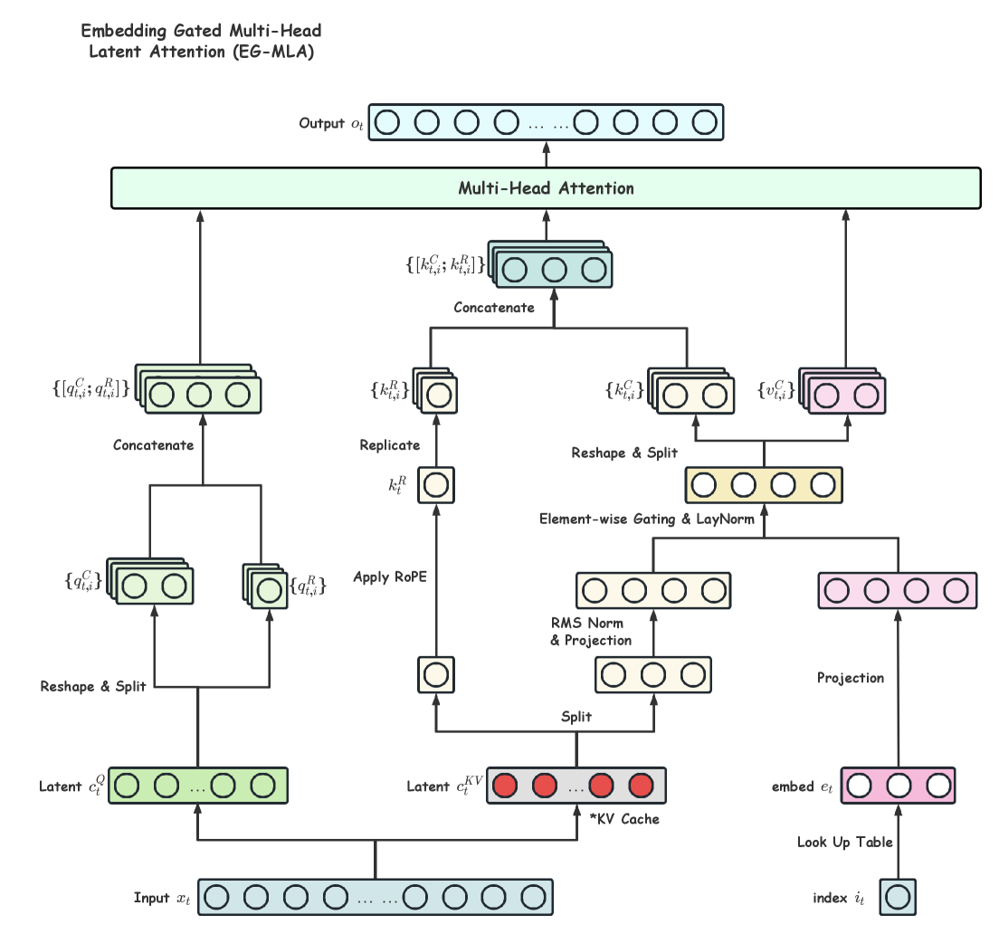
Detailed Architecture is shown in Figure 6.
The full computation pipeline begins by projecting the input into a low-rank latent space, followed by an up-projection to the original dimensionality. Embedding gating is then applied to produce the key and value representations for attention. These representations are subsequently split, with Partial RoPE individually applied to the keys and values, before being fed into a multi-head attention (MHA) module for final computation. Full formulas are shown as follows:
$$
\displaystylec_t^KV \displaystyle=W^DKVx_t, \displaystylekv_t^C \displaystyle=W^UKVc_t^KV, \displaystylee_t \displaystyle=Emb(i_t), \displaystyleg_t \displaystyle=W^UEe_t, \displaystyle\widetilde{kv}_t^C \displaystyle=LN≤ft(kv_t^C\odotg_t\right), \displaystylek_t^C,v_t^C \displaystyle=split(\widetilde{kv}_t^C) \displaystylec_t^Q \displaystyle=W^DQx_t, \displaystyleq_t^C \displaystyle=W^UQc_t^Q, \displaystyleq_t^R \displaystyle=({W^QR}c_t^Q), \displaystylek_t^R \displaystyle=({W^KR}x_t), \displaystyleq_t,i \displaystyle=[q_t,i^C;q_t,i^R], \displaystylek_t,i \displaystyle=[k_t,i^C;k_t^R], \displaystyleu_t,i \displaystyle=∑_j=1^t_j(\frac{q_t,i^Tk_j,i}{√{d_h+d_h^R}})v_j,i^C, \displaystyleo_t \displaystyle=W^O[u_t,1;u_t,2;...;u_t,n_{h}], \tag{1}
$$
<details>
<summary>x6.png Details</summary>
### Visual Description
## Diagram: Embedding Gated Multi-Head Latent Attention (EG-MLA)
### Overview
The image is a technical architecture diagram illustrating the "Embedding Gated Multi-Head Latent Attention (EG-MLA)" mechanism. The diagram depicts a neural network flow where input data ($x_t$ and index $i_t$) is processed through three distinct parallel branches—Query, Key, and Value/Gating—before converging into a Multi-Head Attention block to produce an output ($o_t$).
### Components/Axes
The diagram is organized into a hierarchical flow from bottom to top, with three primary processing branches:
* **Bottom Level (Inputs):**
* **Input $x_t$:** A blue box containing a sequence of circles.
* **index $i_t$:** A blue box containing a single circle, feeding into a "Look Up Table".
* **Left Branch (Query Path - Green):**
* **Latent $c_t^Q$:** Green box.
* **Reshape & Split:** Operation block.
* **$\{q_{t,i}^C\}$ and $\{q_{t,i}^R\}$:** Intermediate green boxes.
* **Concatenate:** Operation block.
* **$\{ [q_{t,i}^C; q_{t,i}^R] \}$:** Final green box.
* **Center Branch (Key Path - Red/Cyan):**
* **Latent $c_t^{KV}$:** Red box (labeled "*KV Cache").
* **Split:** Operation block.
* **RMS Norm & Projection:** Operation block.
* **Apply RoPE:** Operation block.
* **$k_t^R$:** Intermediate box.
* **Replicate:** Operation block.
* **$\{k_{t,i}^R\}$ and $\{k_{t,i}^C\}$:** Intermediate cyan boxes.
* **Concatenate:** Operation block.
* **$\{ [k_{t,i}^C; k_{t,i}^R] \}$:** Final cyan box.
* **Right Branch (Value/Gating Path - Pink):**
* **Look Up Table:** Operation block.
* **embed $e_t$:** Pink box.
* **Projection:** Operation block.
* **Element-wise Gating & LayNorm:** Operation block.
* **$\{v_{t,i}^C\}$:** Final pink box.
* **Top Level (Output):**
* **Multi-Head Attention:** Large light green horizontal bar.
* **Output $o_t$:** Blue box containing a sequence of circles.
### Detailed Analysis
#### 1. Query Branch (Left)
* **Flow:** Input $x_t$ feeds into Latent $c_t^Q$.
* **Transformation:** The latent vector undergoes "Reshape & Split" to create two components: $\{q_{t,i}^C\}$ (likely Content) and $\{q_{t,i}^R\}$ (likely Rotary/Positional).
* **Result:** These are concatenated to form the final Query vector $\{ [q_{t,i}^C; q_{t,i}^R] \}$, which is passed to the Multi-Head Attention block.
#### 2. Key Branch (Center)
* **Flow:** Input $x_t$ feeds into Latent $c_t^{KV}$ (marked as *KV Cache).
* **Transformation:** The latent vector is split.
* **Path A:** Passes through "RMS Norm & Projection" and then feeds into the "Element-wise Gating & LayNorm" block in the right branch.
* **Path B:** Passes through "Apply RoPE" (Rotary Positional Embedding), resulting in $k_t^R$, which is then "Replicated" to form $\{k_{t,i}^R\}$.
* **Result:** $\{k_{t,i}^C\}$ (derived from the RMS Norm path) and $\{k_{t,i}^R\}$ are concatenated to form the final Key vector $\{ [k_{t,i}^C; k_{t,i}^R] \}$, which is passed to the Multi-Head Attention block.
#### 3. Value/Gating Branch (Right)
* **Flow:** Index $i_t$ is processed via a "Look Up Table" to produce embedding $e_t$.
* **Transformation:** $e_t$ undergoes "Projection".
* **Gating:** The output of this projection and the output from the "RMS Norm & Projection" (from the Key branch) are combined in the "Element-wise Gating & LayNorm" block.
* **Result:** This produces the final Value vector $\{v_{t,i}^C\}$, which is passed to the Multi-Head Attention block.
### Key Observations
* **Hybrid Latent/Embedding Approach:** The architecture explicitly separates content (Latent $c_t$) from positional/index-based information (RoPE and Look Up Table embeddings).
* **Gating Mechanism:** The "Element-wise Gating & LayNorm" is a critical junction where the KV cache information is modulated by the embedding $e_t$ before becoming the Value vector.
* **KV Cache Efficiency:** The use of a shared Latent $c_t^{KV}$ for both Key and Value generation suggests an optimization to reduce memory footprint, common in modern LLM architectures.
* **Color Coding:** The diagram uses distinct color palettes to separate the three attention components: Green (Query), Cyan (Key), and Pink (Value/Embedding).
### Interpretation
This diagram represents a sophisticated attention mechanism designed to optimize the trade-off between model capacity and computational efficiency.
1. **Latent Compression:** By using Latent $c_t^Q$ and $c_t^{KV}$ instead of projecting the full input $x_t$ directly into Query, Key, and Value spaces, the model likely reduces the memory overhead of the KV cache.
2. **Dynamic Gating:** The "Embedding Gated" aspect implies that the Value vector is not static; it is dynamically adjusted based on the input index $i_t$. This allows the model to inject token-specific or position-specific information into the attention mechanism via the embedding $e_t$ without increasing the size of the latent cache.
3. **Positional Encoding:** The explicit "Apply RoPE" step in the Key branch indicates that positional information is injected specifically into the Key vectors, a standard practice in modern Transformers (like Llama) to maintain relative positional awareness.
4. **Peircean Investigative Note:** The architecture suggests a "compressed-then-expanded" logic. The model compresses input into a latent space, performs operations (RoPE, Gating), and then expands/concatenates these components back into a format suitable for standard Multi-Head Attention. This is likely an architecture designed for high-throughput inference where KV cache size is the primary bottleneck.
</details>
Figure 6: Detailed Architecture of the Embedding Gated Multi-Head Latent Attention (EG-MLA).
## D. More Experimental Results
Here we present more experimental data, covering additional dimensions, a broader range of metrics, and more test datasets.
### Scaling Embedding Size
| Model Name | Embed Size | Tokens | ClimbMix-val | wiki | lambada | Avg. |
| --- | --- | --- | --- | --- | --- | --- |
| EG-MLA-emb64 | 38M | 50B | 15.47 | 15.49 | 50.38 | 27.78 |
| EG-MLA-emb128 | 77M | 50B | 15.04 | 15.04 | 45.11 | 25.06 |
| EG-MLA-emb256 | 154M | 50B | 15.32 | 14.58 | 38.94 | 22.95 |
| EG-MLA-emb512 | 309M | 50B | 14.61 | 14.02 | 32.89 | 20.51 |
| EG-MLA-emb1024 | 618M | 50B | 13.91 | 13.72 | 35.41 | 21.01 |
| EG-MLA-emb2048 | 1236M | 50B | 13.81 | 13.62 | 34.25 | 20.56 |
Table 8: Perplexity results of EG-MLA models with scaling embedding size. The KV cache is fixed at 64.
### Scaling KV Cache
| Model Name | Size | Tokens | ClimbMix-val | wiki | lambada | Avg. |
| --- | --- | --- | --- | --- | --- | --- |
| MLA-kv256 | 120M | 50B | 15.45 | 15.63 | 49.88 | 26.99 |
| EG-MLA-kv256 | 125M | 50B | 14.32 | 14.26 | 37.12 | 21.90 |
| EG-MLA-kv128 | 122M | 50B | 14.49 | 14.34 | 35.73 | 21.52 |
| EG-MLA-kv64 | 120M | 50B | 15.32 | 14.58 | 38.94 | 22.95 |
| EG-MLA-kv16 | 119M | 50B | 15.13 | 15.08 | 43.76 | 24.66 |
Table 9: Perplexity results of EG-MLA models across 12 tasks with scaling KV cache. The embedding size is fixed at 256. ”Size” denotes the number of activated parameters.
## E. PyTorch Code
We provide the PyTorch code here to facilitate readers’ understanding of our method.
⬇
1 class EmbeddingGatedMLA (nn. Module):
2 def __init__ (self, config):
3 super (). __init__ ()
4 self. n_embd = config. n_embd
5 self. n_head = config. n_head
6 self. qk_nope_head_dim = config. qk_nope_head_dim
7 self. qk_rope_head_dim = config. qk_rope_head_dim
8 self. qk_head_dim = config. qk_nope_head_dim + config. qk_rope_head_dim
9 self. v_head_dim = config. v_head_dim
10 self. q_lora_rank = config. q_lora_rank
11 self. kv_lora_rank = config. kv_lora_rank
12 assert config. n_embd % config. n_head == 0
13
14 if self. q_lora_rank == 0:
15 self. wq = nn. Linear (config. n_embd, config. n_head * self. qk_head_dim, bias = False)
16 else:
17 self. wq_a = nn. Linear (config. n_embd, config. q_lora_rank, bias = False)
18 self. q_norm = nn. RMSNorm (config. q_lora_rank)
19 self. wq_b = nn. Linear (config. q_lora_rank, config. n_head * self. qk_head_dim, bias = False)
20
21 self. wkv_a = nn. Linear (config. n_embd, config. kv_lora_rank + config. qk_rope_head_dim, bias = False)
22 self. kv_norm = nn. RMSNorm (config. kv_lora_rank)
23 self. wkv_b = nn. Linear (config. kv_lora_rank, config. n_head * (config. qk_nope_head_dim + config. v_head_dim), bias = False)
24 self. kv_emb = nn. Embedding (config. vocab_size, config. kv_emb_dim)
25 self. kv_up = nn. Linear (config. kv_emb_dim, config. n_head * (config. qk_nope_head_dim + config. v_head_dim), bias = False)
26 self. ln_emb = nn. LayerNorm (config. n_head * (config. qk_nope_head_dim + config. v_head_dim))
27 self. c_proj = nn. Linear (config. n_head * config. v_head_dim, config. n_embd, bias = False)
28
29 def forward (self, x, idx, freqs_cis):
30 B, T, _ = x. size ()
31 if self. q_lora_rank == 0:
32 q = self. wq (x)
33 else:
34 q = self. wq_b (self. q_norm (self. wq_a (x)))
35
36 q = q. view (B, T, self. n_head, self. qk_head_dim)
37 q_nope, q_pe = torch. split (q, [self. qk_nope_head_dim, self. qk_rope_head_dim], dim =-1)
38 q_pe = apply_rotary_emb (q_pe, freqs_cis)
39
40 kv = self. wkv_a (x)
41 kv, k_pe = torch. split (kv, [self. kv_lora_rank, self. qk_rope_head_dim], dim =-1)
42 k_pe = apply_rotary_emb (k_pe. unsqueeze (2), freqs_cis)
43
44 q = torch. cat ([q_nope, q_pe], dim =-1)
45 kv = self. wkv_b (self. kv_norm (kv))
46 kv = self. ln_emb (kv * self. kv_up (self. kv_emb (idx)))
47 kv = kv. view (B, T, self. n_head, self. qk_nope_head_dim + self. v_head_dim)
48 k_nope, v = torch. split (kv, [self. qk_nope_head_dim, self. v_head_dim], dim =-1)
49 k = torch. cat ([k_nope, k_pe. expand (-1, -1, self. n_head, -1)], dim =-1)
50
51 k = k. view (B, T, self. n_head, -1). transpose (1, 2)
52 q = q. view (B, T, self. n_head, -1). transpose (1, 2)
53 v = v. view (B, T, self. n_head, -1). transpose (1, 2)
54
55 y = F. scaled_dot_product_attention (q, k, v, attn_mask = None, is_causal = True)
56 y = y. transpose (1, 2). contiguous (). view (B, T, -1)
57
58 y = self. c_proj (y)
59 return y
Listing 1: Implementation of Embedding Gated MLA in pseudo PyTorch style.
## F. Comparison Between Attention Mechanisms
### Comparison of Actual KV Cache Among MHA, MLA, and EG-MLA
To ensure a fair evaluation of attention mechanism efficiency, all comparisons are conducted across models with comparable overall sizes and core architectural hyperparameters—namely, the same number of layers, model hidden dimension, and attention head configuration.
Table 10 highlights the dramatic reduction in KV cache size achieved by EG-MLA compared to standard Multi-Head Attention (MHA). While MHA stores separate key and value vectors for each attention head, resulting in 18.43K elements per token, EG-MLA reduces this number by up to 94.8%, requiring as few as 0.96K elements per token in the most compressed configuration.
Among the EG-MLA variants, EG-MLA-kv64 offers a particularly favorable trade-off between performance and memory efficiency. It reduces the KV cache per token to only 1.54K elements, which constitutes a 91.6% reduction compared to standard Multi-Head Attention (MHA), and a 59.9% reduction relative to MLA. This substantial saving is achieved without altering the number of attention heads or compromising activated model parameters.
| Model Name | Total Params | Activated Params | Embed Params | n_layer / n_emb / kv_emb_dim | q_lora_rank / kv_lora_rank | qk_head_dim / v_head_dim | KV Cache / Token (#Element) |
| --- | --- | --- | --- | --- | --- | --- | --- |
| MHA-Base | 124M | 124M | 0M | 12/768/- | - | 64 | 18.43K |
| MLA-Base | 120M | 120M | 0M | 12/768/256 | 0/256 | 64+64 / 64 | 3.84K |
| EG-MLA-Base-kv256 | 279M | 125M | 154M | 12/768/256 | 0/256 | 64+64 / 64 | 3.84K |
| EG-MLA-Base-kv128 | 276M | 122M | 154M | 12/768/256 | 0/128 | 64+64 / 64 | 2.30K |
| EG-MLA-Base-kv64 | 274M | 120M | 154M | 12/768/256 | 0/64 | 64+64 / 64 | 1.54K |
| EG-MLA-Base-kv16 | 273M | 119M | 154M | 12/768/256 | 0/16 | 64+64 / 64 | 0.96K |
Table 10: Comparison of actual KV cache usage among Multi-Head Attention (MHA), Multi-Head Latent Attention (MLA), and our proposed Embedding Gated MLA (EG-MLA). EG-MLA achieves comparable or stronger performance while significantly reducing the KV cache per token, thanks to its compressed latent representation and token-specific gating.
## G. More Scaling Experiment
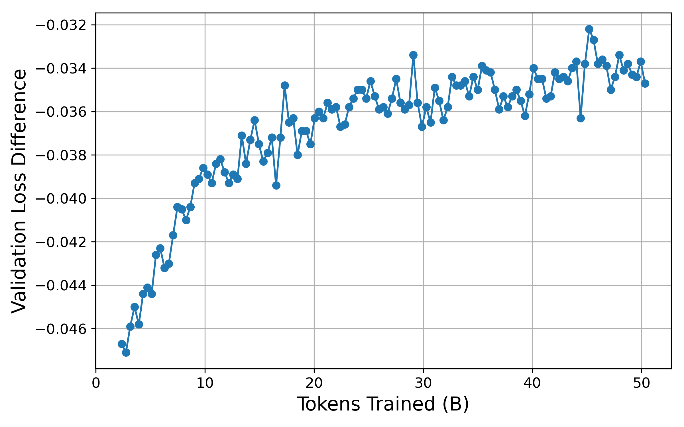
Figure 7 shows the difference in validation loss between the EG-MLA-1.2B model and the baseline MLA-1.2B model over the course of training. The x-axis represents the number of tokens processed (in billions), while the y-axis indicates the validation loss difference. A negative value implies that EG-MLA-1.2B performs better (i.e., lower validation loss) than the baseline at that point in training. The trend highlights how the enhancements in EG-MLA-1.2B translate into improved generalization throughout the training trajectory.
<details>
<summary>figures/EG-MLA-1.2B_vs_MLA-1.2B_val_loss_diff.png Details</summary>
### Visual Description
## Line Chart: Validation Loss Difference vs. Tokens Trained
### Overview
The image displays a line chart illustrating the relationship between the number of tokens trained (in billions) and the "Validation Loss Difference." The chart shows a single data series represented by a blue line with circular markers, indicating a clear upward trend (moving from more negative to less negative values) as the number of tokens increases.
### Components/Axes
* **X-Axis:** Labeled "Tokens Trained (B)". The scale ranges from 0 to 50, with major grid lines at intervals of 10.
* **Y-Axis:** Labeled "Validation Loss Difference". The scale ranges from -0.046 to -0.032, with major grid lines at intervals of 0.002.
* **Data Series:** A single blue line connecting circular data points, representing the performance metric over the training duration.
* **Grid:** A light gray grid is overlaid on the plot area to facilitate reading values.
### Detailed Analysis
The data series exhibits a distinct logarithmic-style growth curve, characterized by rapid initial improvement followed by a plateau.
* **Trend Verification:**
* **0B to 15B Tokens:** The curve shows a steep, consistent upward slope. The value rises from approximately -0.047 to -0.037.
* **15B to 50B Tokens:** The slope flattens significantly, indicating diminishing returns. The values oscillate within a tighter band, generally between -0.037 and -0.034.
* **Data Point Approximations:**
* **Start (~2B):** The series begins at approximately -0.047.
* **10B:** The value is approximately -0.039.
* **20B:** The value is approximately -0.037.
* **30B:** The value is approximately -0.036.
* **40B:** The value is approximately -0.035.
* **50B:** The value is approximately -0.035.
### Key Observations
* **Diminishing Returns:** The most significant gains in the "Validation Loss Difference" occur within the first 15 billion tokens. After this point, the rate of improvement slows drastically.
* **Stochastic Noise:** The line is not smooth; it exhibits frequent, high-frequency fluctuations (jitter) throughout the entire training process. This is typical of stochastic gradient descent or batch-level training metrics.
* **Notable Outliers:**
* There is a distinct upward spike around 29B tokens, where the value briefly reaches approximately -0.033.
* There is a notable dip around 45B tokens, where the value drops to approximately -0.036.
### Interpretation
* **Performance Metric:** The data represents a learning curve for a machine learning model. Assuming "Validation Loss Difference" is calculated as `(Baseline Loss - Current Model Loss)` or a similar comparative metric, the upward trend indicates that the model is improving as it consumes more training data.
* **Training Dynamics:** The transition from a steep slope to a plateau suggests that the model has reached a point of saturation where additional training tokens provide marginal improvements.
* **Stability:** The persistent "jitter" in the line suggests that the training process is noisy. This could be due to the batch size, the learning rate, or the inherent variance in the validation dataset.
* **Conclusion:** The model benefits significantly from the first 15B tokens of training. Beyond 20B tokens, the training process enters a phase of refinement where the gains are incremental and subject to higher volatility.
</details>
Figure 7: Difference in validation loss between EG-MLA-1.2B and MLA-1.2B models as a function of tokens trained.
| Model Name | Model Size | Embed Size | piqa | arc-c | arc-e | hella | winog | siqa | mmlu | obqa | boolq | race | truth | lmb.o | Avg. |
| --- | --- | --- | --- | --- | --- | --- | --- | --- | --- | --- | --- | --- | --- | --- | --- |
| EG-MLA-Large-ctx2048-kv128emb512 | 951M | 309M | 75.35 | 37.20 | 70.33 | 42.50 | 53.83 | 90.80 | 27.22 | 26.80 | 57.55 | 33.01 | 29.61 | 39.72 | 48.66 |
| MLA-Large-ctx2048-kv512 | 645M | 0M | 74.54 | 37.88 | 69.70 | 42.16 | 55.01 | 90.40 | 27.34 | 27.20 | 62.97 | 34.83 | 31.12 | 41.24 | 49.53 |
| EGA-XLarge-ctx4096-kv128emb512 | 1800M | 618M | 75.41 | 38.74 | 72.85 | 44.88 | 56.83 | 91.00 | 26.92 | 27.80 | 59.45 | 33.97 | 31.27 | 40.25 | 49.95 |
| MLA-XLarge-ctx4096-kv512 | 1188M | 0M | 75.52 | 38.82 | 73.02 | 44.15 | 56.83 | 92.20 | 28.42 | 27.20 | 53.15 | 34.26 | 33.76 | 38.02 | 49.61 |
| EG-MLA-Large-ctx2048-kv256emb512 | 961M | 309M | 74.92 | 37.12 | 71.55 | 42.79 | 54.38 | 90.70 | 25.93 | 23.80 | 58.96 | 33.21 | 29.24 | 41.98 | 48.71 |
Table 11: Accuracy results of more models across 12 benchmark tasks. kv refers to KV cache dimension and emb refers to embedding dimension.All models were trained for a total of 50 billion tokens.
| Model Name | Model Size | Embed Size | ClimbMix-val | wiki | lambada | Avg. |
| --- | --- | --- | --- | --- | --- | --- |
| EG-MLA-Large-ctx2048-kv128emb512 | 951M | 309M | 10.79 | 6.17 | 19.57 | 12.18 |
| MLA-Large-ctx2048-kv512 | 645M | 0M | 11.02 | 6.31 | 18.95 | 12.09 |
| EGA-XLarge-ctx4096-kv128emb512 | 1800M | 618M | 10.35 | 2.94 | 19.01 | 10.77 |
| MLA-XLarge-ctx4096-kv512 | 1188M | 0M | 10.71 | 3.00 | 22.99 | 12.23 |
| EG-MLA-Large-ctx2048-kv256emb512 | 961M | 309M | 10.58 | 6.14 | 17.95 | 11.56 |
Table 12: Perplexity results of more models across 12 benchmark tasks. kv refers to KV cache dimension and emb refers to embedding dimension.All models were trained for a total of 50 billion tokens.
## H. Compression through Layer Grouping
To push the optimization frontier and further curtail computational and memory costs, we explore the reuse of both the KV-projection parameters and their intermediate activations across transformer layers. Specifically, we introduce a hyper-parameter $layergroupsize(lgz)$ that dictates how many consecutive transformer layers share a single parameter set rather than maintaining independent parameters for each layer. During the forward pass, all layers within the same group directly reuse the shared parameters and cached intermediate results, eliminating redundant computation and improving training and inference efficiency.
Empirical results show that when $lgz$ = 2, the performance of model remains comparable to the baseline. However, once $lgz$ exceeds 4, a significant performance degradation is observed. Therefore, $lgz$ = 4 represents the compression limit under current settings, and we recommend $lgz$ = 3 as a balanced trade-off between efficiency gains and accuracy loss.
| Model Name | piqa | arc-c | arc-e | hella | winog | siqa | mmlu | obqa | boolq | race | truth | lmb.o | Avg. | Diff (%) |
| --- | --- | --- | --- | --- | --- | --- | --- | --- | --- | --- | --- | --- | --- | --- |
| MLA-Large-ctx2048-kv512 | 74.54 | 37.88 | 69.70 | 42.16 | 55.01 | 90.40 | 27.34 | 27.20 | 62.97 | 34.83 | 31.12 | 41.24 | 49.53 | — |
| EG-MLA-Large-ctx2048-kv256emb512 | 74.92 | 37.12 | 71.55 | 42.79 | 54.38 | 90.70 | 25.93 | 23.80 | 58.96 | 33.21 | 29.24 | 41.98 | 48.71 | — |
| EG-MLA-Large-ctx2048-kv256emb512lgz2 | 74.76 | 37.03 | 69.57 | 42.56 | 52.33 | 90.50 | 25.65 | 27.80 | 59.79 | 31.87 | 30.59 | 39.90 | 48.53 | -0.37 |
| EG-MLA-Large-ctx2048-kv256emb512lgz4 | 75.03 | 36.18 | 69.32 | 41.61 | 52.25 | 91.60 | 27.70 | 26.40 | 55.69 | 32.25 | 29.27 | 40.50 | 48.15 | -1.15 |
| EG-MLA-Large-ctx2048-kv256emb512lgz6 | 74.48 | 36.35 | 70.58 | 40.69 | 52.80 | 90.10 | 26.98 | 24.60 | 58.10 | 31.20 | 29.20 | 38.48 | 47.80 | -1.87 |
Table 13: Accuracy results across 12 benchmark tasks under different layer group sizes (lgz). Diff is the relative change (%) compared to EG-MLA-Large-ctx2048-kv256emb512.
| Model Name | ClimbMix-val | wiki | lambada | Avg. | Diff (%) |
| --- | --- | --- | --- | --- | --- |
| MLA-Large-ctx2048-kv512 | 11.02 | 6.31 | 18.95 | 12.09 | — |
| EG-MLA-Large-ctx2048-kv256emb512 | 10.58 | 6.14 | 17.95 | 11.56 | — |
| EG-MLA-Large-ctx2048-kv256emb512lgz2 | 10.78 | 6.23 | 18.69 | 11.90 | -2.94 |
| EG-MLA-Large-ctx2048-kv256emb512lgz4 | 11.05 | 6.38 | 20.19 | 12.54 | -8.47 |
| EG-MLA-Large-ctx2048-kv256emb512lgz6 | 11.27 | 6.51 | 22.77 | 13.52 | -16.98 |
Table 14: Perplexity results across 12 benchmark tasks under different layer group sizes (lgz). Diff is the relative change (%) compared to EG-MLA-Large-ctx2048-kv256emb512.