2509.16866v1

# seqBench: A Tunable Benchmark to Quantify Sequential Reasoning Limits of LLMs **Authors**: - M.R. Ramezanali - Salesforce AI - Palo Alto, CA - &M. Vazifeh (Capital One, MIT) - Cambridge, MA - &P. Santi (MIT) - Cambridge, MA > ⋆ \star denotes equal contribution. ## Abstract We introduce seqBench, a parametrized benchmark for probing sequential reasoning limits in Large Language Models (LLMs) through precise, multi-dimensional control over several key complexity dimensions. seqBench allows systematic variation of (1) the logical depth, defined as the number of sequential actions required to solve the task; (2) the number of backtracking steps along the optimal path, quantifying how often the agent must revisit prior states to satisfy deferred preconditions (e.g., retrieving a key after encountering a locked door); and (3) the noise ratio, defined as the ratio between supporting and distracting facts about the environment. Our evaluations on state-of-the-art LLMs reveal a universal failure pattern: accuracy collapses exponentially beyond a model-specific logical depth. Unlike existing benchmarks, seqBench ’s fine-grained control facilitates targeted analyses of these reasoning failures, illuminating universal scaling laws and statistical limits, as detailed in this paper alongside its generation methodology and evaluation metrics. We find that even top-performing models systematically fail on seqBench ’s structured reasoning tasks despite minimal search complexity, underscoring key limitations in their commonsense reasoning capabilities. Designed for future evolution to keep pace with advancing models, the seqBench datasets are publicly released to spur deeper scientific inquiry into LLM reasoning, aiming to establish a clearer understanding of their true potential and current boundaries for robust real-world application. seqBench: A Tunable Benchmark to Quantify Sequential Reasoning Limits of LLMs M.R. Ramezanali thanks: $\star$ denotes equal contribution. Salesforce AI Palo Alto, CA 94301 mramezanali@salesforce.com M. Vazifeh footnotemark: Capital One, MIT Cambridge, MA 02143 mvazifeh@mit.edu P. Santi MIT Cambridge, MA 02143 psanti@mit.edu Large Language Models (LLMs) have shown remarkable performance (Vaswani et al., 2017; Brown et al., 2020; Lieber et al., 2021; Rae et al., 2021; Smith et al., 2022; Thoppilan et al., 2022; Hoffmann et al., 2022; Du et al., 2021; Fedus et al., 2022; Zoph et al., 2022) on a wide range of tasks and benchmarks spanning diverse human-like capabilities; however, these successes can obscure fundamental limitations in sequential reasoning that still persist. Arguably, reasoning captures a more pure form of intelligence, going beyond mere pattern matching or fact memorization, and is thus a critical capability to understand and enhance in AI systems. Recent studies show that state-of-the-art LLMs (OpenAI, 2025; Google DeepMind, 2025; Meta AI, 2025; Mistral AI, 2024; Anthropic, 2025) excel at complex benchmarks, yet stumble upon simple common-sense inferences trivial for an adult human (Nezhurina et al., 2025; Han et al., 2024; Sharma, 2024; Berglund et al., 2024; Yang et al., 2019). Most existing benchmarks saturate quickly, leaving little room for fine-grained attribution studies to perform systemic probes of LLM failure modes. Consequently, a robust understanding of why and under what circumstances these models fail, especially on problems requiring sequential reasoning, remains elusive. This gap, we argue, stems from the lack of evaluation benchmarks allowing systematic, multi-dimensional control over key independent factors that influence a task’s overall reasoning difficulty. Most benchmarks (Cobbe et al., 2021; Hendrycks et al., 2021; Srivastava et al., 2023; Weston et al., 2015; Clark et al., 2018; Dua et al., 2019; Rein et al., 2023), despite their evaluation merits, often do not support a systematic variation of crucial complexity dimensions. This makes it difficult to isolate the specific conditions under which reasoning in LLMs falter. For instance, discerning whether a failure is due to the length of the required reasoning chain, the necessity to revise intermediate conclusions, or the density of distracting information is often not quantitatively possible. While prompting strategies like chain-of-thought (CoT) and model scaling have boosted aggregate performance, they often obscure sharp performance cliffs that can emerge when these underlying complexity dimensions are varied independently (Wei et al., 2023; Kojima et al., 2022). Without such systematic control, disentangling inherent architectural limitations from those addressable via scaling (model size, data, or compute), fine-tuning, or prompting techniques is challenging. A fine-grained understanding of these performance boundaries is crucial for developing more robust and reliable reasoning systems. 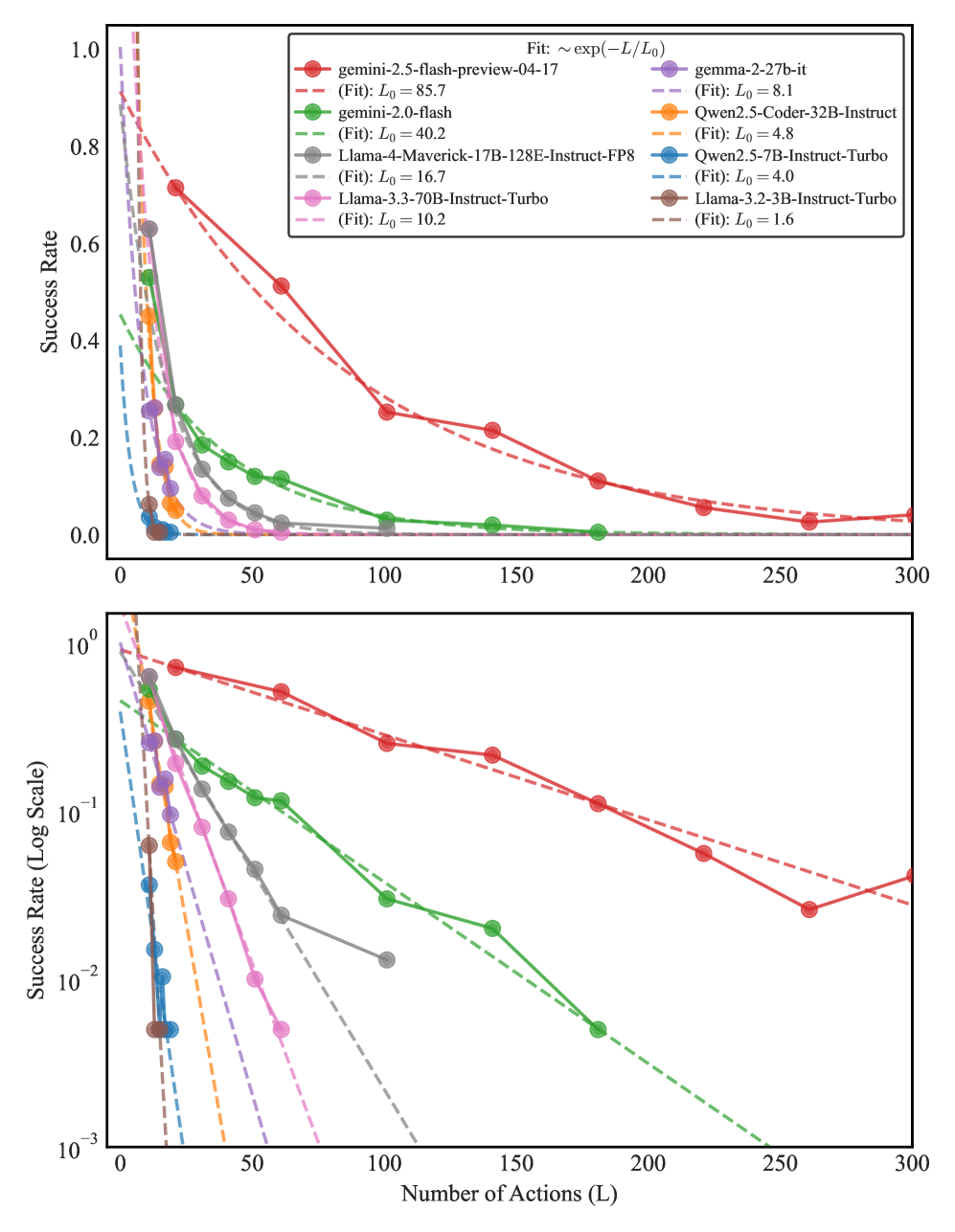To complement recent efforts (Sprague et al., 2024; Tyagi et al., 2024; Kuratov et al., 2024; Tang and Kejriwal, 2025; Mirzaee et al., 2021; Tikhonov, 2024; Mirzaee and Kordjamshidi, 2022; Shi et al., 2022) in evaluating reasoning, and to address the need for more controlled analysis, we introduce seqBench, a tunable benchmark designed explicitly to probe and analyze sequential reasoning capabilities in language models. The dataset comprises synthetic yet linguistically grounded pathfinding task configurations on two-dimensional grids. Solving each problem requires sequential inference over relevant and distracting structured facts. Each instance is automatically verifiable and parameterized by controllable factors that directly address the previously identified gaps: (1) logical depth (total number of actions in the ground-truth solution, reflecting the length of the reasoning chain); (2) backtracking count (number of locked-door detours on the optimal path, requiring revision of tentative solution paths); and (3) noise ratio (proportion of distracting vs. supporting facts, testing robustness to irrelevant information). Performance against these dimensions can be quantified with fine-grained metrics (e.g., via progress ratio as we define here). We observe that beyond a certain logical depth, Pass@1 success collapses to near zero for all models (see Figure 1). These features enable precise attribution studies of model failure modes, offering insights into the brittle boundaries of current LLM generalization. <details> <summary>x1.png Details</summary>  ### Visual Description ## Dual-Panel Line Chart: Success Rate vs. Number of Actions (L) ### Overview The image displays two line charts comparing the performance of eight different Large Language Models (LLMs) across varying task lengths, defined as "Number of Actions (L)." The top chart uses a linear y-axis, while the bottom chart uses a logarithmic y-axis to better visualize the rapid performance decay of lower-performing models. The data is modeled using an exponential decay function: $\text{Success Rate} \approx \exp(-L/L_0)$, where $L_0$ represents the characteristic length scale of the model's capability. ### Components/Axes * **Legend (Top Center):** Lists the eight models, their associated line colors, and their fitted $L_0$ values. * **X-Axis (Shared):** "Number of Actions (L)". Ranges from 0 to 300. * **Y-Axis (Top Chart):** "Success Rate". Linear scale ranging from 0.0 to 1.0. * **Y-Axis (Bottom Chart):** "Success Rate (Log Scale)". Logarithmic scale ranging from $10^{-3}$ to $10^0$. * **Data Series:** Each model is represented by a solid line with circular markers (data points) and a dashed line representing the exponential fit. ### Detailed Analysis #### Legend and Model Parameters The models are ordered by their $L_0$ value (characteristic length), which correlates with their ability to maintain success over longer action sequences. | Model | Color | Fitted $L_0$ | | :--- | :--- | :--- | | **gemini-2.5-flash-preview-04-17** | Red | 85.7 | | **gemini-2.0-flash** | Green | 40.2 | | **Llama-4-Maverick-17B-128E-Instruct-FP8** | Grey | 16.7 | | **Llama-3.3-70B-Instruct-Turbo** | Pink | 10.2 | | **gemma-2-27b-it** | Purple | 8.1 | | **Qwen2.5-Coder-32B-Instruct** | Orange | 4.8 | | **Qwen2.5-7B-Instruct-Turbo** | Blue | 4.0 | | **Llama-3.2-3B-Instruct-Turbo** | Brown | 1.6 | #### Visual Trends * **General Trend:** All models exhibit an exponential decay in success rate as the number of actions ($L$) increases. * **Top-Performing Models (Red/Green):** The `gemini-2.5-flash-preview-04-17` (Red) and `gemini-2.0-flash` (Green) lines show the shallowest slopes. The Red line remains above a 0.05 success rate even at $L=300$. * **Mid-Tier Models (Grey/Pink/Purple):** These models show a moderate decay. The Grey line (`Llama-4-Maverick`) is the most robust of this group, extending to $L \approx 100$ before dropping near the baseline. * **Low-Tier Models (Orange/Blue/Brown):** These models exhibit extremely rapid decay. Their success rates collapse toward zero almost immediately (between $L=10$ and $L=25$). ### Key Observations * **The $L_0$ Metric:** The $L_0$ value acts as a "half-life" equivalent for model performance. A higher $L_0$ indicates a model that is significantly more capable of handling long-horizon tasks. * **Logarithmic Clarity:** The bottom chart is essential for distinguishing the performance of the lower-tier models. On the linear chart, the Orange, Blue, and Brown lines appear to hit zero almost instantly. On the log chart, we can see they maintain non-zero success rates at very low $L$ values before plummeting. * **Outlier Performance:** The `gemini-2.5-flash-preview-04-17` (Red) is a significant outlier, with an $L_0$ (85.7) more than double that of the next best model (`gemini-2.0-flash`, 40.2), indicating a substantial leap in long-context reasoning capability. ### Interpretation This data demonstrates the "contextual endurance" of various LLMs. In the context of agentic workflows or multi-step reasoning, the "Number of Actions" represents the depth of the reasoning chain. * **Peircean Investigative View:** The $L_0$ value is the *interpretant* of the model's architecture. It serves as a proxy for the model's ability to maintain coherence over time. The exponential decay suggests that these models suffer from a cumulative error rate; each additional action introduces a probability of failure, and the models with lower $L_0$ values accumulate these errors much faster. * **Practical Implication:** If a task requires a sequence of 50 actions, only the Red, Green, and potentially the Grey models are viable candidates. The other models would likely fail with near-certainty, as their success rates at $L=50$ are negligible on the logarithmic scale. The data suggests that model size (e.g., 70B vs 3B) is not the only factor; architecture and training (as seen by the Gemini models' dominance) are the primary drivers of long-horizon success. </details> Figure 1: Performance collapse of various models with increasing logical depth $L$ for a pathfinding task ( $N,M=40,\mathcal{B}=2$ keys, Noise Ratio $\mathcal{N}=0.0$ ). Success rates (Pass@1) are shown on linear (top panel) and logarithmic (bottom panel) y-axes, averaged from 5 runs/problem across 40 problems per unit $L$ -bin. All evaluations used Temperature=1.0 and top-p=0.95 (Gemini-2.5-flash: ’auto’ thinking). The displayed fits employ a Weighted Least Squares (WLS) Carroll and Ruppert (2017) method on log-success rates. Weights are derived from inverse squared residuals of a preliminary Ordinary Least Squares (OLS) fit. (In the supplementary section, we have added Figure 16 to show a similar pattern is observed in recently released OpenAI models.) Furthermore, the seqBench benchmark is built upon a scalable data generation framework, allowing it to evolve alongside increasingly capable models to help with both model training and evaluation. Through evaluations on popular LLMs, we reveal that top-performing LLMs exhibit steep universal declines as either of the three complexity dimensions increases, while remaining comparatively robust to fact shuffle, despite the underlying logical structure being unchanged. #### Contributions. Our main contributions are: 1. seqBench: A Tunable Benchmark for Sequential Reasoning. We introduce an open-source framework for generating pathfinding tasks with fine-grained, orthogonal control over logical depth, backtracking steps, and noise ratio. We also evaluate secondary factors like fact ordering (shuffle ratio; See supplementary material for details). 1. Comprehensive LLM Attribution Study. Using seqBench, we demonstrate the significant impact of these controlled complexities on LLM performance, revealing sharp performance cliffs in state-of-the-art models even when search complexity is minimal. The seqBench dataset is publicly available https://huggingface.co/datasets/emnlp-submission/seqBench under the CC BY 4.0 license to facilitate benchmarking. <details> <summary>figs/llama4_deepdive.png Details</summary>  ### Visual Description ## Line Charts: Performance Metrics vs. Number of Actions ### Overview This image contains two stacked line charts illustrating the performance of an AI model (Llama-4-Maverick-17B-128E-Instruct-FP8) as the "Number of actions" increases. * **Top Chart:** Displays the "Success rate" decay, modeled against an exponential function. * **Bottom Chart:** Displays three distinct metrics—Precision, Recall, and Progress ratio—with associated error bars, showing how these metrics evolve as the number of actions increases. --- ### Components/Axes #### Top Chart * **Y-Axis:** Labeled "Success rate". Scale ranges from 0 to 0.6+. * **X-Axis:** Labeled "Number of actions". Scale ranges from 0 to 300. * **Legend (Top-Right):** * Blue solid line with circular markers: "Llama-4-Maverick-17B-128E-Instruct-FP8" * Orange dashed line: "$\propto \exp(-L/L_0), L_0 = 16.7$" (This indicates an exponential decay function where $L$ is the number of actions and $L_0$ is the decay constant). #### Bottom Chart * **Y-Axis:** Unlabeled (implied range 0.0 to 1.0). * **X-Axis:** Labeled "Number of actions". Scale ranges from 0 to 400. * **Legend (Top-Right):** * Blue line with circular markers: "Precision" * Orange line with circular markers: "Recall" * Green line with circular markers: "Progress ratio" --- ### Detailed Analysis #### Top Chart: Success Rate Decay * **Trend:** The success rate exhibits a sharp exponential decay. It starts at its peak and drops precipitously within the first 50 actions, then plateaus near zero. * **Data Points (Approximate):** * At ~10 actions: Success rate is ~0.65. * At ~20 actions: Success rate drops to ~0.27. * At ~30 actions: Success rate is ~0.14. * At ~40 actions: Success rate is ~0.08. * At ~50 actions: Success rate is ~0.05. * At ~100 actions: Success rate is ~0.03. * At ~150–300 actions: Success rate remains consistently low, near 0.01. #### Bottom Chart: Metric Performance * **Precision (Blue):** * **Trend:** Relatively stable. It starts at ~0.9 and maintains a high level throughout the range (0 to 300 actions), ending at ~0.88. * **Uncertainty:** Large error bars are present, particularly as the number of actions increases, indicating high variance in the precision measurements. * **Recall (Orange):** * **Trend:** Gradual downward slope. It starts at ~0.78 and declines steadily to ~0.28 by 300 actions. * **Uncertainty:** Significant error bars that widen as the number of actions increases. * **Progress ratio (Green):** * **Trend:** Sharp downward slope. It starts at ~0.75 and drops rapidly, reaching ~0.1 by 100 actions, and continues to decline to ~0.05 by 300 actions. * **Uncertainty:** Large error bars, especially in the early stages (0–100 actions). --- ### Key Observations 1. **Exponential Decay:** The top chart confirms that the model's success rate is highly sensitive to the number of actions, following a mathematical decay curve ($L_0 = 16.7$). 2. **Precision vs. Recall Trade-off:** While the model maintains high "Precision" (it is accurate when it acts), its "Recall" and "Progress ratio" degrade significantly as the number of actions increases. This suggests the model is capable of performing correct individual steps but struggles to complete longer, multi-step sequences. 3. **High Variance:** The large error bars in the bottom chart suggest that the model's performance is inconsistent, particularly for longer sequences of actions. --- ### Interpretation The data demonstrates a classic "context window" or "sequence length" limitation in the Llama-4-Maverick model. * **The "Success" Problem:** The top chart shows that the probability of a successful outcome drops exponentially as the task length increases. The model is effectively "forgetting" or losing coherence after a relatively small number of actions ($L_0 = 16.7$). * **The Nature of Failure:** The bottom chart provides the diagnostic: the model does not necessarily become "wrong" (Precision remains high), but it becomes "incomplete" (Recall and Progress ratio drop). * **Peircean Investigative Insight:** If we read between the lines, this model is likely a "greedy" agent. It is precise in its immediate actions, but it lacks the long-term planning or state-maintenance required to sustain progress over longer sequences. The high variance (error bars) suggests that for any given task length, the model's performance is highly dependent on the specific nature of the task, rather than just the length itself. 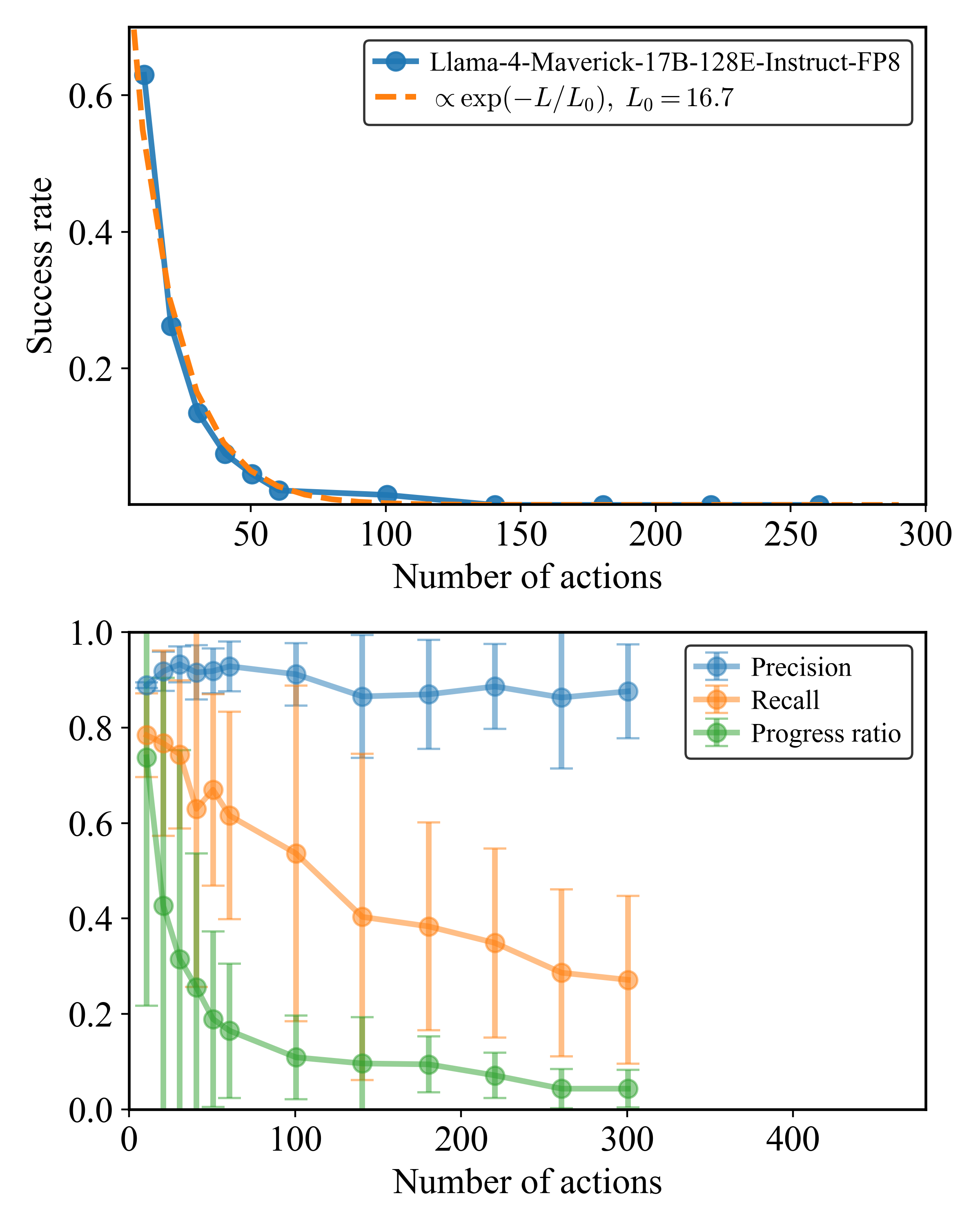</details> Figure 2: On the left: Llama-4 Maverick-17B-128E-Instruct Model’s performance (pass@1 success rate) versus number of actions in the ground truth path of the pathfinding problems ( $N,M=40,\mathcal{B}=2$ keys, Noise Ratio $\mathcal{N}=0.0$ ) is shown. This Pass@1 success rate across 5 runs per problem is averaged over the problem instances sampled from different actions count bins of width equal to 1. On the right: The mean of progress ratio across all problems as well as mean of precision and recall is shown to highlight models gradually increasing struggle in completing the path. The Temperature is set to 1.0 and the top-p is set to 0.95 in all runs. ## 1 Methods ### 1.1 Dataset Generation The seqBench dataset consists of spatial pathfinding tasks. Task instance generation, detailed below (Algorithm 1; See Appendix A for details), is predicated on the precise independent control of the three key complexity dimensions introduced earlier: Logical Depth ( $L$ ), Backtracking Count ( $\mathcal{B}$ ), and Noise Ratio ( $\mathcal{N}$ ). This allows the creation of instances with specific values for these parameters, enabling targeted studies of their impact on LLM reasoning. Task instances are produced in a multi-stage process. Initially, primary generation parameters—maze dimensions ( $N,M$ ), target backtracks ( $\mathcal{B}_{\text{target}}$ ), and target noise ratio ( $\mathcal{N}_{\text{target}}$ )—are specified. An acyclic maze graph ( $M_{g}$ ) is formed on an $N\times M$ grid using Kruskal’s algorithm (Kleinberg and Tardos, 2006). Our "Rewind Construction" method (Algorithm 1) then embeds $\mathcal{B}_{\text{target}}$ backtracking maneuvers by working backward from a goal to strategically place keys and locked doors, yielding the instance’s actual backtracking count $\mathcal{B}$ . Finally, a natural language fact list ( $\mathcal{F}$ ) is derived from the maze, and distracting facts are added according to $\mathcal{N}_{\text{target}}$ to achieve the final noise ratio $\mathcal{N}$ . The logical depth $L$ (optimal path length) emerges from these generative steps, influenced by $N,M,\mathcal{B}_{\text{target}}$ , and construction stochasticity. While $L$ is not a direct input to the generation algorithm, the process is designed to yield a wide spectrum of logical depths. Each generated instance is then precisely annotated with its emergent $L$ value, alongside its effective $\mathcal{B}$ and $\mathcal{N}$ values. This annotation effectively makes $L$ a key, selectable parameter for users of the seqBench dataset, enabling them to choose or filter tasks by their desired logical depth. Our rewind construction method guarantees task solvability. The full seqBench benchmark is constructed by systematically applying this instance generation process (detailed in Algorithm 1) across a wide range of initial parameters. This includes varied grid sizes (e.g., $N\in\{5..50\},M\approx N$ ) and target backtracks ( $\mathcal{B}_{\text{target}}\in\{0..7\}$ ), yielding a large and diverse data pool. For each $(N,M,\mathcal{B}_{\text{target}})$ configuration, multiple unique base mazes are generated, to which different noise ratios (e.g., $\mathcal{N}_{\text{target}}\in\{0..1\}$ ) are subsequently applied. It is important to note that the algorithm constrains backtracking complexity to a simple dependency chain. In this setting, retrieving the key for each locked door involves at most one backtracking step to pick up its corresponding key, without requiring the unlocking of additional doors along the optimal path. Combined with the uniform random placement of keys, this design ensures a well-balanced distribution of backtracking difficulty across the generated instances for each logical depth $L$ . Nevertheless, the same backward-in-time construction can be extended to generate tasks with higher backtracking complexity—for example, doors that require multiple keys, or intermediate doors that must be unlocked en route to other keys. Such extensions would introduce richer tree-structured dependency graphs and allow seqBench to probe model performance under more complex long-horizon reasoning regimes. The creation of this comprehensive data pool was computationally efficient, requiring approximately an hour of computation on a standard laptop while using minimal memory. The publicly released benchmark comprises a substantial collection of these generated instances, each annotated with its specific emergent logical depth $L$ , effective backtracking count $\mathcal{B}$ , and noise ratio $\mathcal{N}$ . This rich annotation is key, enabling researchers to readily select or filter task subsets by these dimensions for targeted studies (e.g., as done for Figure 1, where instances were sampled into $L$ -bins with other parameters fixed). For the experiments presented in this paper, specific subsets were drawn from this benchmark pool, often involving further filtering or parameter adjustments tailored to the objectives of each study; precise details for each experiment are provided in the relevant sections and figure captions. Full details on path derivation, fact compilation, and overall dataset generation parameters are provided in the Appendix A. Input : Grid $N\times M$ , Target backtracks $\mathcal{B}$ Output : Maze graph $M_{g}$ , Locked doors $\mathcal{D}_{L}$ , Key info $\mathcal{K}_{I}$ , Path skeleton $\Pi_{S}$ 1 2 $M_{g}\leftarrow$ Acyclic graph on grid (Kruskal’s); 3 $x\leftarrow C_{goal}\leftarrow$ Random goal cell in $M_{g}$ ; 4 $\mathcal{D}_{L},\mathcal{K}_{I}\leftarrow\emptyset,\emptyset$ ; $b\leftarrow 0$ ; 5 $\Pi_{S}\leftarrow[(C_{goal},\text{GOAL})]$ ; 6 7 while $b<\mathcal{B}$ do 8 $c_{key}\leftarrow$ Random cell in $M_{g}$ accessible from $x$ (path avoids $\mathcal{D}_{L}$ for this step); 9 $\pi_{seg}\leftarrow$ Unique path in $M_{g}$ from $x$ to $c_{key}$ ; 10 if $\exists e\in\pi_{seg}$ such that $e\notin\mathcal{D}_{L}$ then 11 $d\leftarrow$ Randomly select such an edge $e$ ; 12 $\mathcal{D}_{L}\leftarrow\mathcal{D}_{L}\cup\{d\}$ ; 13 $K_{id}\leftarrow$ New unique key ID; 14 $\mathcal{K}_{I}[K_{id}]\leftarrow\{\text{opens}:d,\text{loc}:c_{key}\}$ ; 15 $\Pi_{S}$ .prepend( $(c_{key},\text{PICKUP }K_{id})$ , $(d,\text{UNLOCK }K_{id})$ , $(\pi_{seg},\text{MOVE})$ ); 16 $x\leftarrow c_{key}$ ; $b\leftarrow b+1$ ; 17 18 end if 19 else 20 Break 21 end if 22 23 end while 24 $\Pi_{S}$ .prepend( $(x,\text{START}))$ ; 25 return $M_{g},\mathcal{D}_{L},\mathcal{K}_{I},\Pi_{S}$ ; Algorithm 1 Rewind Construction of Path Skeleton ### 1.2 Prompt Construction and Model Configuration 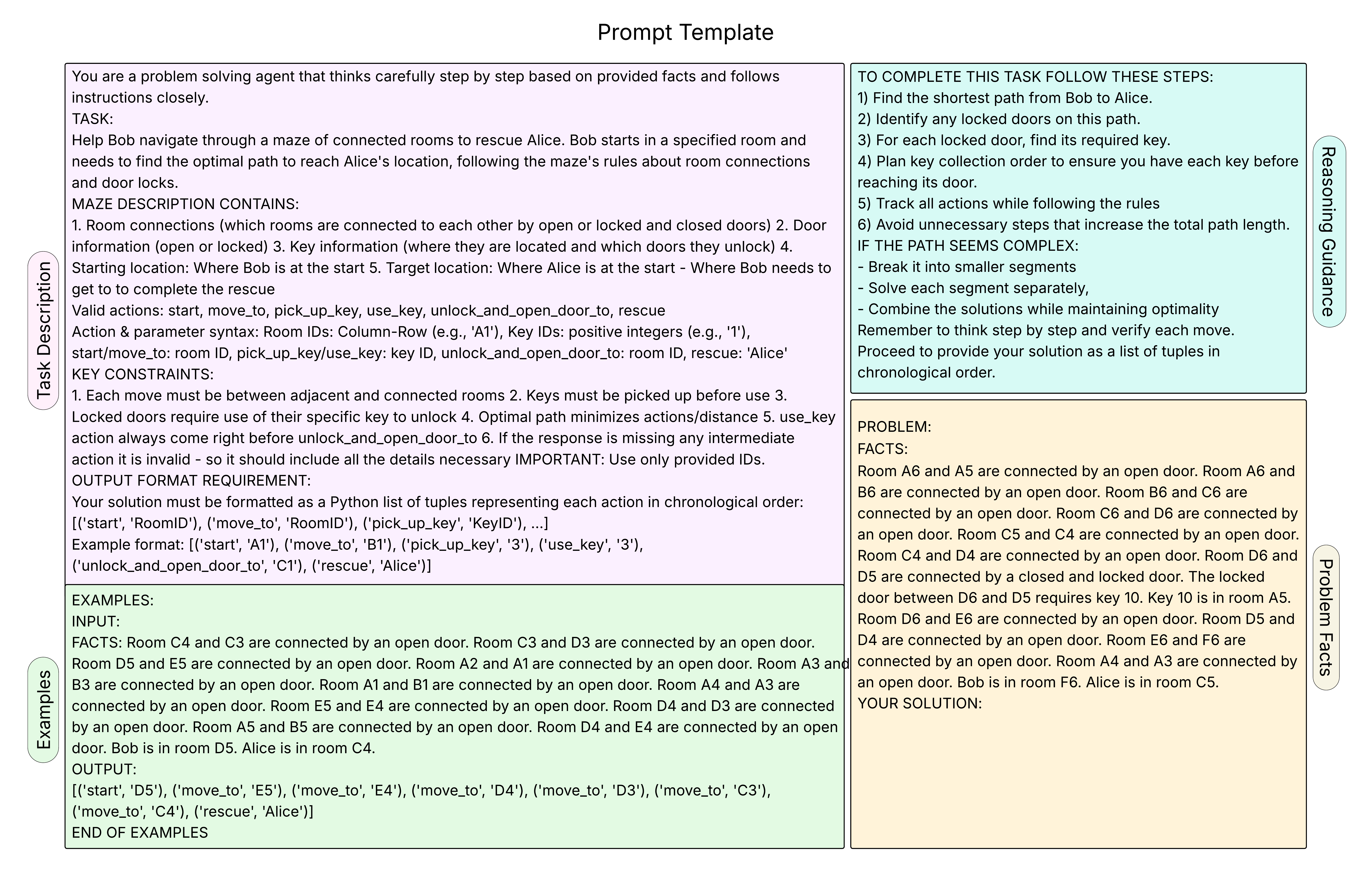Our evaluation uses a standardized prompt template with four components: (i) task instructions and action schema, (ii) three few-shot examples of increasing complexity (simple navigation, single-key, and multi-key backtracking), (iii) optional reasoning guidance, and (iv) the problem’s natural-language facts. All models are queried using temperature $T{=}1.0$ , nucleus sampling $p{=}0.95$ , and maximum allowed setting in terms of output token limits on a per model basis. For each instance, we compute 5 independent runs to establish robust performance statistics. The complete prompt structure, shown in Figure 6, is provided in the Appendix B. ### 1.3 Evaluation Metrics To analyze not just success but also how models fail, we employ several complementary metrics. Success Rate (Pass@1) measures the proportion of runs where the predicted action sequence exactly matches the ground truth. The Progress Ratio (Tyagi et al., 2024), calculated as $k/n$ (where $n$ is the total ground-truth actions and $k$ is the number correctly executed before the first error), pinpoints the breakdown position in reasoning. We also use Precision and Recall. Precision is the proportion of predicted actions that are correct, while Recall is the proportion of ground-truth actions that were correctly predicted. Low precision indicates hallucinated actions, while low recall signifies missed necessary actions. Additionally, we visualize error locations via a Violation Map. This multi-faceted approach reveals each model’s effective "reasoning horizon"—the maximum sequence length it can reliably traverse. Further details on all metrics and visualizations are provided in the supplementary material. ## 2 Benchmarking Results <details> <summary>figs/fig_vs_backtracking_fixed_L_shuffle1.0_noise0.0.png Details</summary>  ### Visual Description ## Line Charts: Performance Metrics vs. Number of Backtracking Steps ### Overview This image displays three side-by-side line charts comparing the performance of five different Large Language Models (LLMs) across three metrics: "Progress ratio mean," "Success rate," and "Number of tokens." The x-axis for all three charts represents the "Number of backtracking steps," ranging from 0 to 5. ### Components/Axes * **Shared X-Axis:** "Number of backtracking steps" (0, 1, 2, 3, 4, 5). * **Legend (Located in the top-left chart):** * **Blue:** Llama-4-maverick-17b-128e-instruct-fp8 * **Orange:** Qwen2.5-coder-32b-instruct * **Green:** Llama-3.1-nemotron-70b-instruct-hf * **Red:** Gemini-2.0-flash * **Purple:** Gemini-2.5-flash-preview-04-17 * **Chart 1 (Left):** Y-axis "Progress ratio mean" (Scale: 0.0 to 1.0). * **Chart 2 (Center):** Y-axis "Success rate" (Scale: 0.0 to 1.0). * **Chart 3 (Right):** Y-axis "Number of tokens" (Scale: 250 to 1750). --- ### Detailed Analysis #### 1. Progress Ratio Mean (Left Chart) * **Trend:** All models show a downward trend as backtracking steps increase. * **Data Points (Approximate):** * **Purple (Gemini-2.5):** Starts at ~0.95, dips to ~0.72 at step 2, recovers slightly to ~0.78 at step 3, then trends down to ~0.70 at step 5. * **Red (Gemini-2.0):** Starts at ~0.75, drops consistently to ~0.12 at step 5. * **Blue (Llama-4):** Starts at ~0.50, drops to ~0.18 at step 5. * **Green (Llama-3.1):** Starts at ~0.38, drops to ~0.13 at step 5. * **Orange (Qwen2.5):** Starts at ~0.28, drops to ~0.05 at step 5. #### 2. Success Rate (Center Chart) * **Trend:** Most models show a sharp decline in success rate as backtracking steps increase, with the exception of the Purple line, which remains significantly higher than the others. * **Data Points (Approximate):** * **Purple (Gemini-2.5):** Starts at ~0.90, drops to ~0.63 at step 2, fluctuates slightly, ending at ~0.63 at step 5. * **Red (Gemini-2.0):** Starts at ~0.55, drops sharply to ~0.25 at step 1, and continues to near 0.0 by step 5. * **Blue (Llama-4):** Starts at ~0.25, drops to near 0.0 by step 1. * **Green (Llama-3.1):** Starts near 0.03, remains very low throughout, ending near 0.0. * **Orange (Qwen2.5):** Remains at ~0.0 throughout all steps. #### 3. Number of Tokens (Right Chart) * **Trend:** All models show an upward trend or stability in token usage as backtracking steps increase, indicating higher computational cost. * **Data Points (Approximate):** * **Blue (Llama-4):** Highest usage, starting at ~1580, rising to ~1800 at step 5. * **Orange (Qwen2.5):** Starts at ~900, rises to ~1100 at step 5. * **Green (Llama-3.1):** Starts at ~630, rises to ~870 at step 5. * **Red (Gemini-2.0):** Starts at ~330, rises to ~410 at step 5. * **Purple (Gemini-2.5):** Lowest usage, starting at ~280, rising to ~410 at step 5. --- ### Key Observations * **Performance Outlier:** The **Gemini-2.5-flash-preview-04-17 (Purple)** model is the clear outlier, maintaining a significantly higher "Progress ratio mean" and "Success rate" compared to all other models, despite having the lowest token usage. * **Inverse Correlation:** There is a general inverse correlation between "Number of backtracking steps" and performance metrics (Progress/Success). As the models are forced to backtrack more, their success and progress rates decline. * **Cost Inefficiency:** The "Number of tokens" chart shows that increasing backtracking steps increases the computational cost (tokens) for all models, yet the performance metrics (Progress/Success) decrease. This suggests that for these models, the backtracking mechanism is inefficient. * **Model Failure:** The **Qwen2.5-coder-32b-instruct (Orange)** model shows a near-zero success rate across all backtracking steps, suggesting it is not suited for this specific task or backtracking configuration. ### Interpretation The data demonstrates that increasing the number of backtracking steps is generally detrimental to the performance of these LLMs in the tested task. Despite the increased computational cost (evidenced by the rising number of tokens), the models fail to achieve higher success rates or progress ratios. The **Gemini-2.5-flash-preview-04-17** model demonstrates superior robustness, maintaining high performance even as backtracking steps increase, whereas other models see their success rates collapse almost immediately (e.g., Llama-4 and Gemini-2.0). This suggests that the backtracking mechanism implemented here may be causing "hallucination loops" or confusion in the models, where they spend more tokens to achieve worse results, with the exception of the Gemini-2.5 model which handles the process more effectively. 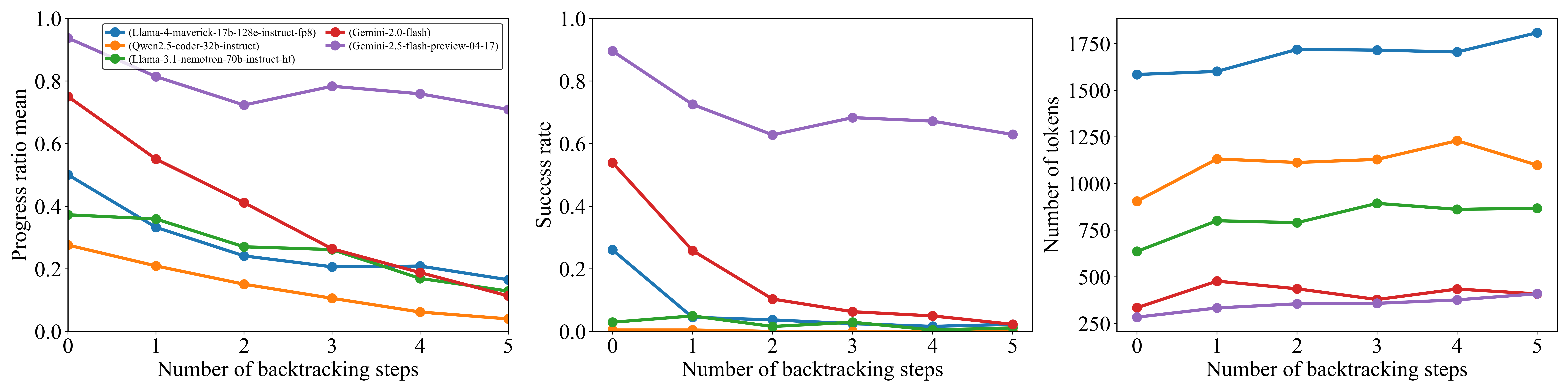</details> Figure 3: Performance as a function of the number of required backtracking steps, operationalized via the number of locked doors with distributed keys along the optimal path. Holding all other complexity factors constant, all models exhibit a clear decline in both progress ratio and success rate as backtracking demands increase. Additionally, we report the corresponding rise in output token counts per model, highlighting the increased reasoning burden associated with longer dependency chains. Fixed experimental parameters in this figure are the same as those in Figure 1. (for each point 100 problems sampled from $L=[40,60]$ ) ### 2.1 Evaluated Models We evaluate a diverse set of transformer-based LLMs across different model families and parameter scales. Our analysis includes Gemini models (2.5-flash-preview, 2.0-flash), Meta’s Llama family (4-Maverick-17B, 3.3-70B, 3.2-3B), Google’s Gemma-2-27b, and Alibaba’s Qwen models (2.5-Coder-32B, 2.5-7B). [Note: GPT-5 was released during the preparation of this paper’s final version. Our analysis shows that this model exhibits the same performance degradation, as shown in Figure 16]. Access to some open-weight models and benchmarking infrastructure was facilitated by platforms such as Together AI https://www.together.ai/ and Google AI Studio https://aistudio.google.com/. Problem instances for varying logical depths ( $L$ ) were generated by sampling 40 problems for each $L$ , using a fixed maze size of $40\times 40$ and 2 keys, unless otherwise specified for specific experiments (e.g., when varying the number of keys for backtracking analysis). All models were evaluated using the standardized prompt template (see Figure 6), the inference settings detailed in Section 1.2, and a common response parsing methodology. For each task instance, we perform 5 independent runs to establish robust performance statistics, primarily analyzing Pass@1 success rates. ### 2.2 Universal Performance Collapse with Increasing Logical Depth A central finding of our study is the universal collapse in reasoning performance observed across all evaluated LLMs when confronted with tasks requiring increasing sequential inference steps. As illustrated in Figure 1, Pass@1 success rates exhibit a consistent and sharp exponential decay as the ground-truth path length ( $L$ ) increases. Performance rapidly approaches near-zero past a model-specific point in this decay. To quantify and compare this exponential decay, we fit an exponential decay curve $P(L)=\exp(-L/L_{0})$ to the success rates, deriving a characteristic path length $L_{0}$ . This $L_{0}$ value, representing the path length at which performance drops by a factor of $e^{-1}$ , serves as a robust metric for each model’s sequential reasoning horizon. Plotting success rates on a semi-logarithmic (log-y) scale against $L$ reveals an approximately linear decay trend across the evaluated regime. This log-linear relationship suggests that errors may accumulate with a degree of independence at each reasoning step, eventually overwhelming the model’s capacity for coherent inference. The observed $L_{0}$ values vary significantly, from 85.7 for Gemini-2.5-Flash down to 1.6 for Llama-3.2-3B (Figure 1), underscoring a fundamental bottleneck in current transformer architectures for extended multi-step reasoning. ### 2.3 Impact of Independently Controlled Complexity Dimensions Beyond the universal impact of logical depth ( $L$ ) discussed in Section 2.2, our benchmark’s ability to independently vary key complexity dimensions allows for targeted analysis of their distinct impacts on LLM reasoning performance. We highlight the effects of noise, backtracking, and fact ordering, primarily focusing on Pass@1 success rates, mean progress ratios, and response token counts. <details> <summary>figs/fig_vary_noise_fixed_L_keys2_shuffle1.0.png Details</summary>  ### Visual Description ## Line Charts: Performance Metrics vs. Noise Ratio ### Overview This image displays three side-by-side line charts illustrating the performance and token usage of two AI models—**Llama-4-maverick-17b-128e-instruct-fp8** (represented by the blue line) and **Gemini-2.5-flash-preview-04-17** (represented by the orange line)—across varying levels of "Noise ratio" (from 0.00 to 1.00). The charts measure "Mean progress ratio," "Mean success rate (pass@1)," and "Cot tokens" respectively. ### Components/Axes * **Legend:** Located in the top-left corner of the first chart. * Blue circle marker: (Llama-4-maverick-17b-128e-instruct-fp8) * Orange circle marker: (Gemini-2.5-flash-preview-04-17) * **X-Axis (Common to all three charts):** Labeled "Noise ratio," with a scale from 0.00 to 1.00, marked at 0.00, 0.25, 0.50, 0.75, and 1.00. * **Y-Axes:** * **Left Chart:** "Mean progress ratio" (Scale: 0.0 to 1.0). * **Center Chart:** "Mean success rate (pass@1)" (Scale: 0.0 to 1.0). * **Right Chart:** "Cot tokens" (Scale: 500 to 1750). --- ### Detailed Analysis #### 1. Mean Progress Ratio (Left Chart) * **Trend:** Both models exhibit a downward trend as the noise ratio increases. * **Data Points (Approximate):** * **Blue (Llama):** Starts at ~0.24 (0.00 noise), declines steadily to ~0.18 (0.25 noise), ~0.16 (0.50 noise), ~0.13 (0.75 noise), and ends at ~0.11 (1.00 noise). * **Orange (Gemini):** Starts at ~0.72 (0.00 noise), declines to ~0.66 (0.25 noise), ~0.54 (0.50 noise), ~0.38 (0.75 noise), and ends at ~0.24 (1.00 noise). #### 2. Mean Success Rate (pass@1) (Center Chart) * **Trend:** Both models show a significant downward trend. The blue line (Llama) drops to near-zero very quickly. * **Data Points (Approximate):** * **Blue (Llama):** Starts at ~0.04 (0.00 noise), drops to ~0.02 (0.25 noise), and effectively hits 0.00 from 0.50 noise onwards. * **Orange (Gemini):** Starts at ~0.63 (0.00 noise), drops to ~0.50 (0.25 noise), ~0.34 (0.50 noise), ~0.20 (0.75 noise), and ends at ~0.04 (1.00 noise). #### 3. Cot Tokens (Right Chart) * **Trend:** The blue line (Llama) shows a downward trend, while the orange line (Gemini) remains relatively flat with a slight increase at the end. * **Data Points (Approximate):** * **Blue (Llama):** Starts at ~1725 (0.00 noise), declines to ~1650 (0.25 noise), ~1625 (0.50 noise), ~1500 (0.75 noise), and ends at ~1450 (1.00 noise). * **Orange (Gemini):** Remains consistently low, starting at ~350 (0.00 noise), staying flat at ~350 through 0.75 noise, and rising slightly to ~375 at 1.00 noise. --- ### Key Observations * **Performance Gap:** Gemini-2.5-flash-preview-04-17 significantly outperforms Llama-4-maverick-17b-128e-instruct-fp8 in both "Mean progress ratio" and "Mean success rate" across all noise levels. * **Efficiency Gap:** Llama uses a much higher number of Chain-of-Thought (Cot) tokens (1450–1725 range) compared to Gemini (consistently ~350–375), despite having lower performance metrics. * **Noise Sensitivity:** Both models are sensitive to noise, as evidenced by the degradation in progress and success rates. However, Gemini maintains a non-zero success rate even at high noise levels, whereas Llama's success rate collapses to zero at 0.50 noise. * **Token Usage Behavior:** As noise increases, Llama's CoT token usage decreases, suggesting the model may be truncating its reasoning process or failing to generate long chains when the input is highly noisy. ### Interpretation The data suggests that **Gemini-2.5-flash-preview-04-17 is significantly more robust and efficient** than the Llama-4-maverick variant tested. The "Mean progress ratio" and "Mean success rate" charts demonstrate that the Llama model struggles to maintain coherence or accuracy as input noise increases. The "Cot tokens" chart provides a critical insight: Llama is "thinking" (generating tokens) much more than Gemini, yet achieving worse results. The fact that Llama's token count drops as noise increases—while its success rate is already near zero—implies that the model's reasoning capabilities are severely degraded by the noise, potentially causing it to output shorter, less coherent, or "failed" responses rather than attempting a full reasoning chain. Gemini, conversely, maintains a stable, low-token reasoning strategy that remains effective even as noise increases. 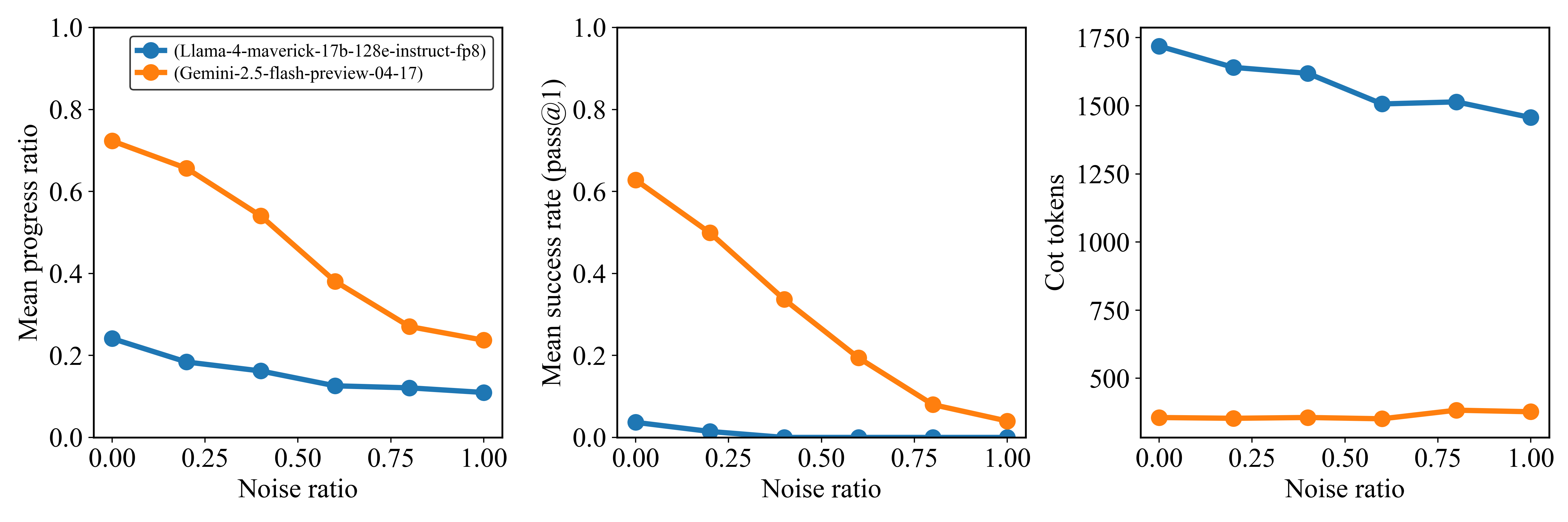</details> Figure 4: Performance as a function of contextual noise for Gemini 2.5 flash and Llama-4 Maverick-17B-128E-Instruct models. As noise increases through the inclusion of distracting or irrelevant facts, both models exhibit a clear and consistent decline in performance. Fixed experimental parameters in this figure are the same as those in Figure 1 (for each point 100 problems sampled from $L=[40,60]$ and number of keys is equal to 2). #### Impact of Backtracking Requirements. Increasing the number of required backtracking steps—operationalized via key-door mechanisms—also leads to a clear and significant decline in Pass@1 success rates and mean progress ratios across all evaluated models as shown in Figure 3. Gemini 2.5 Flash-preview maintains the highest performance but still exhibits a notable drop as backtracking count increases from 0 to 5. This decline in reasoning accuracy is generally accompanied by an increase or sustained high level in the mean number of response tokens (Figure 3, right panel). For example, models like Llama-4 Maverick and Gemini 2.5 Flash-preview show a clear upward trend or maintain high token counts as backtracking complexity rises, reflecting the increased reasoning effort or path length articulated by the models when managing more complex sequential dependencies. #### Sensitivity to Noise Ratio. Model performance is highly sensitive to the noise ratio—the proportion of distracting versus supporting facts. As demonstrated in Figure 4 for Gemini 2.5 Flash and Llama-4 Maverick, increasing the proportion of irrelevant facts consistently and significantly degrades both Pass@1 success rates and mean progress ratios. For instance, Gemini 2.5 Flash’s Pass@1 success rate drops from over 0.7 at zero noise to approximately 0.2 at a noise ratio of 1.0. Llama-4 Maverick, starting with lower performance, also shows a consistent decline. Interestingly, for these two models, the number of CoT (output) tokens remains relatively stable despite the increasing noise and degrading performance (Figure 4, right panel), suggesting that models do not necessarily "work harder" (in terms of output length) when faced with more distractors, but their accuracy suffers. #### Fact Ordering (Shuffle Ratio). In contrast to the strong effects of noise and backtracking, shuffle ratio (entropy of fact presentation order) within the prompt appears to play a secondary role when varied in isolation. Our experiments, exemplified by the performance of Gemini 2.5 Flash and Llama-4 Maverick (see Appendix C Figure 14 for details), show that complete shuffling of facts (randomizing their presentation order without adding or removing any information) has a minimal impact on Pass@1 success rates and mean progress ratios. Output token counts also remain stable. This suggests a relative robustness to presentation order as long as all necessary information is present and distinguishable. However, as details provided in supplementary material, when high noise and high shuffle co-occur, the combined effect can be more detrimental than either factor alone, though noise remains the dominant degrading factor. ### 2.4 Characterizing Key Failure Modes and Error Patterns #### A Key Failure Mode: Omission of Critical Steps. Beyond simply taking illegal shortcuts, detailed analysis reveals that LLMs often fail by omitting critical sub-goals necessary for task completion. Figure 2 (bottom panel) provides a quantitative view for Llama-4 Maverick (Meta AI, 2025), showing that while precision generally remains high (models infrequently hallucinate non-existent rooms or facts), recall and progress ratio plummet with increasing path length ( $L$ ). This indicates that models predominantly fail by missing necessary actions or entire crucial sub-sequences. For a qualitative example, even capable models like Gemini-2.5-Flash can neglect essential detours, such as collecting a required key, thereby violating sequential dependencies and rendering the task unsolvable (illustrative examples are provided in the Appendix B.4; see Figures 8 and 9). This pattern highlights a fundamental breakdown in robust multi-step planning and execution. #### Path-Length Dependent First Errors: The Burden of Anticipated Complexity. The propensity for models to make critical errors is not uniformly distributed across the reasoning process, nor is it solely a feature of late-stage reasoning fatigue. Examining the distribution of steps at which the first constraint violations occur reveals a counterintuitive pattern: as the total required path length ( $L$ ) of a problem increases, models tend to fail more frequently even at the earliest steps of the reasoning chain. This leftward shift in the first-error distribution also observed under increasing noise, (Appendix B.4; Figures 10 and 11) contradicts a simple cumulative error model where each step carries a fixed, independent failure probability. Instead, an error at an early step (e.g., step 5) becomes substantially more likely when the model is attempting to solve an 80-step problem versus a 20-step problem. This suggests that the overall anticipated complexity of the full problem influences reasoning quality from the very outset, indicating a struggle with global planning or maintaining coherence over longer horizons, rather than just an accumulation of local errors. This phenomenon may help explain why prompting techniques that decompose long problems into smaller, manageable sub-problems often succeed. ### 2.5 Disparity: Information Retention vs. Reasoning Capacity On seqBench tasks, this disparity is quantitatively striking. While modern LLMs boast million-token contexts, their effective sequential reasoning depth typically remains on the order of hundreds of actions (Figure 1). This functional limit, even at several hundred actions (e.g., 300 actions, with each like (’move_to’, ’A12’) being 5-7 tokens, totaling 1.5k-2.1k tokens), still consumes a minute fraction of their nominal context. Consequently, the ratio of context capacity to reasoning tokens often spans from several hundred-fold (e.g., 500:1 for 300 actions consuming 2k tokens within a 1M context) to potentially higher values given fewer limiting actions or larger model contexts. This striking gap suggests that while transformers can store and retrieve vast information, their ability to reliably chain it for coherent, multi-step inference appears surprisingly constrained. ### 2.6 Challenging the Conventional Performance Hierarchy While metrics like average $L_{0}$ provide a general ranking of model capabilities, our fine-grained analysis reveals instances that challenge a simple linear performance hierarchy. Scatter plots of progress ratios across different models on identical tasks (see Appendix C Figure 13) show intriguing cases where models with lower overall $L_{0}$ values (i.e., typically weaker models) occasionally solve specific complex problems perfectly, while models with higher average $L_{0}$ values fail on those same instances. These performance inversions suggest that sequential reasoning failures may not solely stem from insufficient scale (parameters or general training) but could also arise from more nuanced reasoning limitations. ## 3 Related Work Recent advancements in benchmarks evaluating sequential reasoning capabilities of LLMs have illuminated various strengths and limitations across different dimensions of complexity. These benchmarks typically differ in how they isolate and quantify reasoning challenges, such as logical deduction, retrieval difficulty, combinatorial complexity, and sensitivity to irrelevant information. ZebraLogic (Lin et al., 2025), for instance, targets formal deductive inference through logic-grid puzzles framed as constraint-satisfaction problems (csp, 2008). While valuable for probing deduction, its core methodology leads to a search space that grows factorially with puzzle size (Sempolinski, 2009). This makes it challenging to disentangle intrinsic reasoning failures from the sheer combinatorial complexity of the search. As the ZebraLogic authors themselves acknowledge: “ solving ZebraLogic puzzles for large instances may become intractable… the required number of reasoning tokens may increase exponentially with the size of the puzzle. ” This inherent characteristic means that for larger puzzles, performance is primarily dictated by the manageability of the search space rather than the limits of sequential reasoning depth. GridPuzzle (Tyagi et al., 2024) complements this by providing a detailed error taxonomy for grid puzzles, focusing on what kinds of reasoning mistakes LLMs make. However, like ZebraLogic, it doesn’t offer independent control over key complexity dimensions such as logical depth, backtracking needs, or noise, separate from the puzzle’s inherent search complexity. Other benchmarks conflate reasoning with different cognitive demands. BABILong (Kuratov et al., 2024) tests models on extremely long contexts (up to 50M tokens), primarily assessing the ability to retrieve "needles" (facts) from a "haystack" (distracting text that does not contribute to solving the task). While valuable for evaluating long-context processing, this design makes it hard to disentangle retrieval failures from reasoning breakdowns, as performance is often dictated by finding the relevant information rather than reasoning over it. MuSR (Sprague et al., 2024) embeds reasoning tasks within lengthy narratives (e.g., murder mysteries), mixing information extraction challenges with complex, domain-specific reasoning structures. This realism obscures which specific aspect—extraction or reasoning depth—causes model failures. Dyna-bAbI (Tamari et al., 2021) offers a dynamic framework for compositional generalization but focuses on qualitative combinations rather than systematically varying quantitative complexity metrics needed to find precise failure points. Spatial reasoning benchmarks, while relevant, also target different aspects. GRASP (Tang and Kejriwal, 2025) assesses practical spatial planning efficiency (like obstacle avoidance) in 2D grids, a different skill than the abstract sequential reasoning seqBench isolates. SPARTQA (Mirzaee et al., 2021) focuses on specialized spatial relational complexity (transitivity, symmetry) using coupled dimensions, preventing independent analysis of factors like path length. SpaRTUN (Mirzaee and Kordjamshidi, 2022) uses synthetic data primarily for transfer learning in Spatial Question Answering (SQA), aiming to improve model performance rather than serve as a diagnostic tool with controllable complexity. Similarly, StepGame (Shi et al., 2022) demonstrates performance decay with more reasoning steps in SQA but lacks the fine-grained, orthogonal controls over distinct complexity factors provided by seqBench. In contrast, seqBench takes a targeted diagnostic approach. By deliberately simplifying the spatial environment to minimize search complexity, it isolates sequential reasoning. Its core contribution lies in the independent, fine-grained control over (1) logical depth (the number of sequential actions required to solve the task), (2) backtracking count (the number of backtracking steps along the optimal path), and (3) noise ratio (the ratio of supporting to distracting facts). This orthogonal parameterization allows us to precisely pinpoint when and why sequential reasoning capabilities degrade, revealing fundamental performance cliffs even when search and retrieval demands are trivial. seqBench thus offers a complementary tool for understanding the specific limitations of sequential inference in LLMs. ## 4 Limitations While seqBench offers precise control over key reasoning complexities, our study has limitations that open avenues for future research: 1. Generalizability and Task Design Fidelity: Our current findings are rooted in synthetic spatial pathfinding tasks. While this allows for controlled experimentation, future work must extend seqBench ’s methodology to more diverse reasoning domains (e.g., mathematical proofs) and incorporate greater linguistic diversity (e.g., ambiguity) to assess the broader applicability of the observed phenomena of performance collapse (quantified by $L_{0}$ ) and failure patterns. Moreover, this work did not investigate whether similar failure modes arise when the problem is also presented visually (e.g., as maze images). Multimodal capabilities could influence spatial reasoning outcomes, and we have already extended the benchmark by releasing maze image generation code alongside the HuggingFace dataset. This dataset can also be used to help train multimodal reasoning models. 1. Model Scope and Understanding Deeper Failure Dynamics: Our current evaluation, while covering diverse public models, should be expanded to a wider array of LLMs—including recent proprietary and newer open-source variants (e.g., GPT, Claude, DeepSeek series)—to rigorously assess the universality of our findings on the characteristic length $L_{0}$ and failure patterns. Furthermore, while seqBench effectively characterizes how reasoning performance degrades with logical depth (i.e., by determining $L_{0}$ ), two complementary research thrusts are crucial for understanding why. First, systematic investigation is needed to disentangle how $L_{0}$ is influenced by factors such as model architecture, scale (parameters, training data, compute), fine-tuning strategies, and inference-time computation (e.g., chain-of-thought depth). Second, deeper analysis is required to explain the precise mechanisms underlying the observed exponential performance collapse characterized by $L_{0}$ and to account for other non-trivial error patterns, such as path-length dependent first errors. Additionally, the evaluation presented here does not consider how agentic systems capable of tool use perform as the reasoning complexity is tuned across various dimensions. Exploring such setups, where the LLM can externalize sub-problems, invoke tools, or backtrack programmatically, could provide valuable insights into whether the same exponential failure modes persist. In particular, one can define sequential problems where the degree of backtracking or sequential tool use can be systematically varied, and to test whether similar performance drop emerge as the dependency chain grows. We highlight this as a promising direction for future research. 1. Impact of Prompting: Our current study employed standardized prompts and inference settings. A crucial next step is a robust sensitivity analysis to determine overall decay behavior are influenced by different prompting strategies (e.g., zero-shot vs. few-shot, decomposition techniques), varied decoding parameters (temperature, top-p), and interactive mechanisms such as self-verification or self-correction. Investigating the potential of these techniques to mitigate the observed sequential inference failures, particularly given seqBench ’s minimal search complexity, remains a key avenue for future research. Addressing these points by leveraging frameworks like seqBench will be vital for developing LLMs with more robust and generalizable sequential reasoning capabilities, and for understanding their fundamental performance limits. ## 5 Conclusion We introduced seqBench, a novel benchmark framework designed for the precise attribution of sequential reasoning failures in Large Language Models. seqBench ’s core strength lies in its unique capability for fine-grained, independent control over fundamental complexity dimensions; most notably, logical depth ( $L$ ), backtracking requirements, and noise ratio, its provision of automatically verifiable solutions, and critically minimizing confounding factors like search complexity. This design allows seqBench to isolate and rigorously evaluate the sequential inference capabilities of LLMs, enabling the automatic quantification of fine-grained performance metrics (such as progress ratio) and providing a clear lens into mechanisms often obscured in most other benchmarks. The framework’s inherent scalability and open-source nature position it as a durable tool for assessing and driving progress in current and future generations of models, ultimately aiming to enhance their utility for complex, real-world problems that often span multiple domains. Our comprehensive evaluations using seqBench reveal that reasoning accuracy consistently collapses exponentially with increasing logical depth across a diverse range of state-of-the-art LLMs. This collapse is characterized by a model-specific parameter $L_{0}$ (Section 2.2), indicating an inherent architectural bottleneck in maintaining coherent multi-step inference. In alignment with the goal of advancing NLP’s reach and fostering its responsible application in other fields by offering this precise analysis, seqBench provides a valuable resource. It encourages a shift beyond aggregate benchmark scores towards a more nuanced understanding of model capabilities, an essential step for rigorously assessing the true impact and potential risks of applying LLMs in new domains. The insights gleaned from seqBench can inform both NLP developers in building more robust models, and experts in other disciplines in setting realistic expectations and co-designing NLP solutions that are genuinely fit for purpose. Targeted improvements, guided by such fundamental understanding, are key to enhancing the robustness of sequential reasoning, making LLMs more reliable partners in interdisciplinary endeavors. Future work should leverage these insights to develop models that can overcome the observed performance cliffs and extend their effective reasoning horizons, thereby unlocking their transformative potential in diverse interdisciplinary applications—such as navigating complex scientific literature, supporting intricate legal analysis, or enabling robust multi-step planning in critical autonomous systems. Focusing on commonsense reasoning is paramount for NLP to achieve transformative societal impact, moving beyond incremental improvements to genuine breakthroughs. ## References - csp (2008) 2008. Rina dechter , constraint processing, morgan kaufmann publisher (2003) isbn 1-55860-890-7, francesca rossi, peter van beek and toby walsh, editors, handbook of constraint programming, elsevier (2006) isbn 978-0-444-52726-4. Computer Science Review, 2:123–130. - Anthropic (2025) Anthropic. 2025. Claude 3.7 sonnet. https://www.anthropic.com/news/claude-3-7-sonnet. - Berglund et al. (2024) Lukas Berglund, Meg Tong, Max Kaufmann, Mikita Balesni, Asa Cooper Stickland, Tomasz Korbak, and Owain Evans. 2024. The reversal curse: Llms trained on "a is b" fail to learn "b is a". Preprint, arXiv:2309.12288. - Brown et al. (2020) Tom Brown, Benjamin Mann, Nick Ryder, Melanie Subbiah, Jared D Kaplan, Prafulla Dhariwal, Arvind Neelakantan, Pranav Shyam, Girish Sastry, Amanda Askell, and 1 others. 2020. Language models are few-shot learners. Advances in neural information processing systems, 33:1877–1901. - Carroll and Ruppert (2017) Raymond J Carroll and David Ruppert. 2017. Transformation and weighting in regression. Chapman and Hall/CRC. - Clark et al. (2018) Peter Clark, Isaac Cowhey, Oren Etzioni, Tushar Khot, Ashish Sabharwal, Carissa Schoenick, and Oyvind Tafjord. 2018. Think you have solved question answering? try arc, the ai2 reasoning challenge. Preprint, arXiv:1803.05457. - Cobbe et al. (2021) Karl Cobbe, Vineet Kosaraju, Mohammad Bavarian, Mark Chen, Heewoo Jun, Lukasz Kaiser, Matthias Plappert, Jerry Tworek, Jacob Hilton, Reiichiro Nakano, Christopher Hesse, and John Schulman. 2021. Training verifiers to solve math word problems. Preprint, arXiv:2110.14168. - Du et al. (2021) Nan Du, Yanping Huang, Andrew M. Dai, Simon Tong, Dmitry Lepikhin, Yuanzhong Xu, Maxim Krikun, Yanqi Zhou, Adams Wei Yu, Orhan Firat, Barret Zoph, Liam Fedus, Maarten Bosma, Zongwei Zhou, Tao Wang, Yu Emma Wang, Kellie Webster, Marie Pellat, Kevin Robinson, and 8 others. 2021. Glam: Efficient scaling of language models with mixture-of-experts. In International Conference on Machine Learning. - Dua et al. (2019) Dheeru Dua, Yizhong Wang, Pradeep Dasigi, Gabriel Stanovsky, Sameer Singh, and Matt Gardner. 2019. Drop: A reading comprehension benchmark requiring discrete reasoning over paragraphs. Preprint, arXiv:1903.00161. - Fedus et al. (2022) William Fedus, Barret Zoph, and Noam Shazeer. 2022. Switch transformers: Scaling to trillion parameter models with simple and efficient sparsity. Journal of Machine Learning Research, 23(120):1–39. - Google DeepMind (2025) Google DeepMind. 2025. Gemini 2.5 pro experimental. https://blog.google/technology/google-deepmind/gemini-model-thinking-updates-march-2025/. - Han et al. (2024) Pengrui Han, Peiyang Song, Haofei Yu, and Jiaxuan You. 2024. In-context learning may not elicit trustworthy reasoning: A-not-b errors in pretrained language models. Preprint, arXiv:2409.15454. - Hendrycks et al. (2021) Dan Hendrycks, Collin Burns, Steven Basart, Andy Zou, Mantas Mazeika, Dawn Song, and Jacob Steinhardt. 2021. Measuring massive multitask language understanding. Preprint, arXiv:2009.03300. - Hoffmann et al. (2022) Jordan Hoffmann, Sebastian Borgeaud, Arthur Mensch, Elena Buchatskaya, Trevor Cai, Eliza Rutherford, Diego de Las Casas, Lisa Anne Hendricks, Johannes Welbl, Aidan Clark, Tom Hennigan, Eric Noland, Katie Millican, George van den Driessche, Bogdan Damoc, Aurelia Guy, Simon Osindero, Karen Simonyan, Erich Elsen, and 3 others. 2022. Training compute-optimal large language models. Preprint, arXiv:2203.15556. - Kleinberg and Tardos (2006) Jon Kleinberg and Eva Tardos. 2006. Algorithm Design. Pearson/Addison-Wesley, Boston. - Kojima et al. (2022) Takeshi Kojima, Shixiang (Shane) Gu, Machel Reid, Yutaka Matsuo, and Yusuke Iwasawa. 2022. Large language models are zero-shot reasoners. In Advances in Neural Information Processing Systems, volume 35, pages 22199–22213. Curran Associates, Inc. - Kuratov et al. (2024) Yury Kuratov, Aydar Bulatov, Petr Anokhin, Ivan Rodkin, Dmitry Sorokin, Artyom Sorokin, and Mikhail Burtsev. 2024. Babilong: Testing the limits of llms with long context reasoning-in-a-haystack. Advances in Neural Information Processing Systems, 37:106519–106554. - Lieber et al. (2021) Opher Lieber, Or Sharir, Barak Lenz, and Yoav Shoham. 2021. Jurassic-1: Technical details and evaluation. https://www.ai21.com/blog/jurassic-1-technical-details-and-evaluation. White Paper. - Lin et al. (2025) Bill Yuchen Lin, Ronan Le Bras, Kyle Richardson, Ashish Sabharwal, Radha Poovendran, Peter Clark, and Yejin Choi. 2025. Zebralogic: On the scaling limits of llms for logical reasoning. Preprint, arXiv:2502.01100. - Meta AI (2025) Meta AI. 2025. Llama 4: Open and efficient multimodal language models. https://github.com/meta-llama/llama-models. - Mirzaee et al. (2021) Roshanak Mirzaee, Hossein Rajaby Faghihi, Qiang Ning, and Parisa Kordjmashidi. 2021. Spartqa: : A textual question answering benchmark for spatial reasoning. Preprint, arXiv:2104.05832. - Mirzaee and Kordjamshidi (2022) Roshanak Mirzaee and Parisa Kordjamshidi. 2022. Transfer learning with synthetic corpora for spatial role labeling and reasoning. Preprint, arXiv:2210.16952. - Mistral AI (2024) Mistral AI. 2024. Mistral large 2. https://mistral.ai/news/mistral-large-2407. - Nezhurina et al. (2025) Marianna Nezhurina, Lucia Cipolina-Kun, Mehdi Cherti, and Jenia Jitsev. 2025. Alice in wonderland: Simple tasks showing complete reasoning breakdown in state-of-the-art large language models. Preprint, arXiv:2406.02061. - OpenAI (2025) OpenAI. 2025. Openai gpt-5, o3 and o4-mini. https://openai.com/index/introducing-o3-and-o4-mini/, https://openai.com/index/introducing-gpt-5/. Paper’s supplementary material (appendix) was revised, after GPT-5 release, with a new figure, to reflect that GPT-5 also suffers from the same failure pattern we have observed in this paper. - Rae et al. (2021) Jack W. Rae, Sebastian Borgeaud, Trevor Cai, Katie Millican, Jordan Hoffmann, Francis Song, John Aslanides, Sarah Henderson, Roman Ring, Susannah Young, Eliza Rutherford, Tom Hennigan, Jacob Menick, Albin Cassirer, Richard Powell, George van den Driessche, Lisa Anne Hendricks, Matthias Rauh, Po-Sen Huang, and 58 others. 2021. Scaling language models: Methods, analysis & insights from training Gopher. Preprint, arXiv:2112.11446. - Rein et al. (2023) David Rein, Betty Li Hou, Asa Cooper Stickland, Jackson Petty, Richard Yuanzhe Pang, Julien Dirani, Julian Michael, and Samuel R. Bowman. 2023. Gpqa: A graduate-level google-proof q&a benchmark. Preprint, arXiv:2311.12022. - Sempolinski (2009) Peter Sempolinski. 2009. Automatic solutions of logic puzzles. - Sharma (2024) Manasi Sharma. 2024. Exploring and improving the spatial reasoning abilities of large language models. In I Can’t Believe It’s Not Better Workshop: Failure Modes in the Age of Foundation Models. - Shi et al. (2022) Zhengxiang Shi, Qiang Zhang, and Aldo Lipani. 2022. Stepgame: A new benchmark for robust multi-hop spatial reasoning in texts. In Proceedings of the AAAI conference on artificial intelligence, volume 36, pages 11321–11329. - Smith et al. (2022) Samuel Smith, Mostofa Patwary, Brian Norick, Patrick LeGresley, Samyam Rajbhandari, Jared Casper, Zhenhao Liu, Shrimai Prabhumoye, Georgios Zerveas, Vikas Korthikanti, Eric Zhang, Rewon Child, Reza Yazdani Aminabadi, Jared Bernauer, Xia Song Song, Mohammad Shoeybi, Yuxin He, Michael Houston, Shishir Tiwary, and Bryan Catanzaro. 2022. Using deepspeed and megatron to train megatron-turing nlg 530b, a large-scale generative language model. Preprint, arXiv:2201.11990. - Sprague et al. (2024) Zayne Sprague, Xi Ye, Kaj Bostrom, Swarat Chaudhuri, and Greg Durrett. 2024. Musr: Testing the limits of chain-of-thought with multistep soft reasoning. Preprint, arXiv:2310.16049. - Srivastava et al. (2023) Aarohi Srivastava, Abhinav Rastogi, Abhishek Rao, Abu Awal Md Shoeb, Abubakar Abid, Adam Fisch, Adam R. Brown, Adam Santoro, Aditya Gupta, Adrià Garriga-Alonso, Agnieszka Kluska, Aitor Lewkowycz, Akshat Agarwal, Alethea Power, Alex Ray, Alex Warstadt, Alexander W. Kocurek, Ali Safaya, Ali Tazarv, and 432 others. 2023. Beyond the imitation game: Quantifying and extrapolating the capabilities of language models. Preprint, arXiv:2206.04615. - Tamari et al. (2021) Ronen Tamari, Kyle Richardson, Aviad Sar-Shalom, Noam Kahlon, Nelson Liu, Reut Tsarfaty, and Dafna Shahaf. 2021. Dyna-babi: unlocking babi’s potential with dynamic synthetic benchmarking. Preprint, arXiv:2112.00086. - Tang and Kejriwal (2025) Zhisheng Tang and Mayank Kejriwal. 2025. Grasp: A grid-based benchmark for evaluating commonsense spatial reasoning. Preprint, arXiv:2407.01892. - Thoppilan et al. (2022) Rami Thoppilan, Daniel De Freitas, Jamie Hall, Noam Shazeer, Apoorv Kulshreshtha, Heng-Tze Cheng, Alicia Jin, Taylor Bos, Leslie Baker, Yi Du, Yanping Li, Hongrae Lee, Huaixiu Steven Zheng, Amin Ghafouri, Marcelo Menegali, Yanping Huang, Max Krikun, Dmitry Lepikhin, James Qin, and 38 others. 2022. Lamda: Language models for dialog applications. arXiv preprint. Technical report, Google Research. - Tikhonov (2024) Alexey Tikhonov. 2024. Plugh: A benchmark for spatial understanding and reasoning in large language models. Preprint, arXiv:2408.04648. - Tyagi et al. (2024) Nemika Tyagi, Mihir Parmar, Mohith Kulkarni, Aswin RRV, Nisarg Patel, Mutsumi Nakamura, Arindam Mitra, and Chitta Baral. 2024. Step-by-step reasoning to solve grid puzzles: Where do llms falter? Preprint, arXiv:2407.14790. - Vaswani et al. (2017) Ashish Vaswani, Noam Shazeer, Niki Parmar, Jakob Uszkoreit, Llion Jones, Aidan N Gomez, Ł ukasz Kaiser, and Illia Polosukhin. 2017. Attention is all you need. In Advances in Neural Information Processing Systems, volume 30. Curran Associates, Inc. - Wei et al. (2023) Jason Wei, Xuezhi Wang, Dale Schuurmans, Maarten Bosma, Brian Ichter, Fei Xia, Ed Chi, Quoc Le, and Denny Zhou. 2023. Chain-of-thought prompting elicits reasoning in large language models. Preprint, arXiv:2201.11903. - Weston et al. (2015) Jason Weston, Antoine Bordes, Sumit Chopra, Alexander M. Rush, Bart van Merriënboer, Armand Joulin, and Tomas Mikolov. 2015. Towards ai-complete question answering: A set of prerequisite toy tasks. Preprint, arXiv:1502.05698. - Yang et al. (2019) Kaiyu Yang, Olga Russakovsky, and Jia Deng. 2019. SpatialSense: An adversarially crowdsourced benchmark for spatial relation recognition. In International Conference on Computer Vision (ICCV). - Zoph et al. (2022) Barret Zoph, Irwan Bello, Sameer Kumar, Nan Du, Yanping Huang, Jeff Dean, Noam Shazeer, and William Fedus. 2022. St-moe: Designing stable and transferable sparse expert models. Preprint, arXiv:2202.08906. ## Appendices ## Appendix A Dataset Generation Details The seqBench benchmark generates pathfinding tasks by systematically controlling several complexity dimensions. As described in Section 1 (main paper), Algorithm 1 is central to this process. This appendix provides further details on the generation phases, natural language encoding of tasks, and specific dataset parameters. 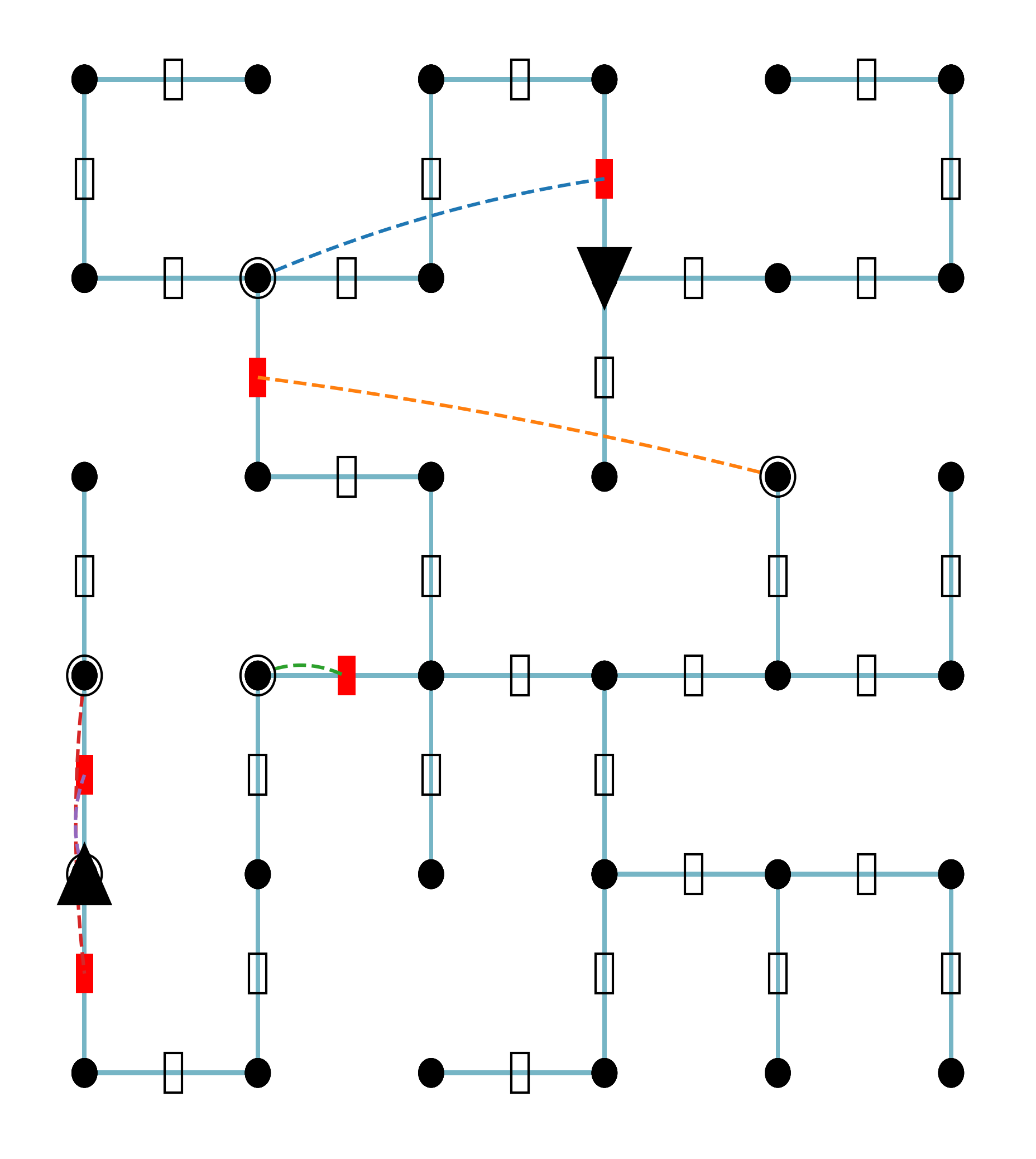### A.1 Generation Phases The generation process, guided by Algorithm 1, involves three main phases: 1. Base Maze Construction: An initial $N\times M$ grid is populated, and an acyclic maze graph ( $M_{g}$ ) is formed using Kruskal’s algorithm (Kleinberg and Tardos, 2006). This ensures a simply connected environment where a unique path exists between any two cells if all internal "walls" (potential door locations) were open. The overall process results in maze instances like the one visualized in Figure 5. 1. Rewind Construction for Path Skeleton and Key/Door Placement: This phase implements the "Rewind Construction" (Algorithm 1 in the main paper). Starting from a randomly selected goal cell ( $C_{goal}$ ), the algorithm works backward to define a solvable path skeleton ( $\Pi_{S}$ ). It iteratively: 1. Selects a cell $c_{key}$ that would be a preceding point on a path towards the current cell $x$ (initially $C_{goal}$ ). 1. Identifies the unique path segment $\pi_{seg}$ in $M_{g}$ from $x$ to $c_{key}$ . 1. Randomly selects an edge $d$ on this segment $\pi_{seg}$ to become a locked door. This edge $d$ is added to the set of locked doors $\mathcal{D}_{L}$ . 1. A new unique key $K_{id}$ is conceptually placed at $c_{key}$ , and its information (which door it opens, its location) is stored in $\mathcal{K}_{I}$ . 1. The conceptual steps (moving along $\pi_{seg}$ , unlocking door $d$ with $K_{id}$ , picking up $K_{id}$ at $c_{key}$ ) are prepended (in reverse logical order) to the path skeleton $\Pi_{S}$ . 1. The current cell $x$ is updated to $c_{key}$ , and the process repeats until the target number of backtracks ( $\mathcal{B}$ ) is achieved or no valid placements remain. This backward construction ensures solvability and controlled backtracking complexity. The final agent starting position is the cell $x$ at the end of this phase. 1. Fact Compilation and Noise Injection: Based on the final maze structure ( $M_{g},\mathcal{D}_{L},\mathcal{K}_{I}$ ), a set of natural language facts $\mathcal{F}$ is compiled. This includes facts describing room connections, key locations, and door states. Distracting facts are then introduced based on the target noise ratio $\mathcal{N}$ . These distractors might describe non-existent connections, spurious keys, or misleading adjacencies, chosen to be plausible yet incorrect. <details> <summary>figs/compath_viz.png Details</summary>  ### Visual Description ## Diagram: Network Topology and Flow Logic ### Overview The image displays a 5x5 grid-based network diagram. It consists of nodes connected by solid light-blue lines and dashed colored lines. The diagram appears to represent a flow network, circuit, or routing puzzle where specific nodes act as hubs or directional gates, and dashed lines represent non-standard or "jump" connections between nodes. ### Components/Axes * **Grid Structure:** A 5x5 matrix of nodes. * **Nodes:** * **Standard Nodes:** Solid black circles. * **Hub Nodes:** Double-ringed black circles (located at (2,2), (3,5), (4,1), (4,2)). * **Directional Nodes:** Black triangles (pointing down at (2,4), pointing up at (5,1)). * **Edges:** * **Standard Edges:** Solid light-blue lines connecting adjacent nodes horizontally and vertically. Each segment contains a small white rectangle (likely representing a resistor, gate, or standard path segment). * **Special Edges:** Dashed lines connecting non-adjacent nodes. Each dashed line features a red rectangle (likely representing a switch, override, or high-cost path). * **Coordinate System (for reference):** * Rows 1-5 (top to bottom). * Columns 1-5 (left to right). ### Detailed Analysis The diagram features four distinct "special" connections. </details> Figure 5: Example visualization of a $6\times 6$ seqBench maze instance. Red rectangles denote locked doors, dashed lines indicate the locations of keys corresponding to those doors, and triangles mark the start (upward-pointing) and goal (downward-pointing) positions. This illustrates the spatial nature of the tasks. ### A.2 Natural Language Encoding Each task instance is translated into a set of atomic natural language facts. We use a consistent templating approach: - Room Connections: "Room A1 and B1 are connected by an open door." - Locked Connections: "Room C3 and D3 are connected by a closed and locked door." - Key Requirements: "The locked door between C3 and D3 requires key 5." (Key IDs are simple integers). - Key Placements: "Key 5 is in room E4." (Room IDs use spreadsheet-like notation, e.g., A1, B2). - Starting Position: "Bob is in room A2." - Goal Position: "Alice is in room D5." The full set of facts for a given problem constitutes its description. ### A.3 Dataset Parameters and Scope The seqBench dataset was generated using the following parameter ranges based on the generation configuration: - Grid Sizes ( $N\times M$ ): $N\times M$ where $N$ and $M$ range from 5 to 50 (e.g., [5,5], [6,6], …, [50,50]), with $M=N$ for all configurations. - Target Backtracking Steps ( $\mathcal{B}$ ): Values from 0 to 7. This controls the number of key-door mechanisms deliberately placed on the optimal path. - Noise Ratio ( $\mathcal{N}$ ): Values from $0.0$ (no distracting facts) to $1.0$ (equal number of supporting and distracting facts), typically in increments of $0.2$ . - Instances per Configuration: For each primary configuration, defined by a specific grid size ( $N,M$ ) and a specific target backtracking step count ( $\mathcal{B}\in\{0..7\}$ ), 400 unique base maze instances were generated. - Logical Depth ( $L$ ): As an emergent property, $L$ varies. Experiments typically select problems from these generated instances that fall into specific $L$ bins (e.g., $L\in[10,11),[11,12),\ldots$ ). This generation pipeline, leveraging the described parameter ranges and variations, can produce a vast and diverse set of problem instances. The publicly released seqBench dataset, used for the analyses in this paper (see main paper for access link), comprises 7,079 such curated instances. This collection offers a rich resource for studying the combined effects of the controlled complexity dimensions. ## Appendix B Prompt Design and Model Configuration Details This appendix provides the complete details of the prompt structure and model configurations used for evaluating LLMs on the seqBench benchmark. The overall prompt, illustrated in Figure 6, concatenates four main components which are detailed below. <details> <summary>figs/prompt_template.png Details</summary>  ### Visual Description ## Diagram: Prompt Template ### Overview The image displays a structured "Prompt Template" designed to guide an AI agent through a specific logic-based pathfinding task. The layout is divided into three distinct functional regions: a large "Task Description" panel on the left, a "Reasoning Guidance" panel in the top-right, and a "Problem Facts" panel in the bottom-right. The template is designed to enforce strict constraints, specific output formatting, and a chain-of-thought reasoning process. ### Components/Axes * **Header**: "Prompt Template" (Centered at the top). * **Left Panel (Task Description)**: Contains the core instructions, constraints, valid actions, and an example. * **Top-Right Panel (Reasoning Guidance)**: Contains a step-by-step heuristic for the AI to follow. * **Bottom-Right Panel (Problem Facts)**: Contains the specific maze configuration and current state for the current instance of the problem. ### Detailed Analysis #### 1. Task Description (Left Panel) * **Role**: Problem-solving agent that thinks step-by-step. * **Task**: Help Bob navigate a maze to rescue Alice. * **Maze Description**: Includes room connections, door status (open/locked), key locations, and start/target locations. * **Valid Actions**: `start`, `move_to`, `pick_up_key`, `use_key`, `unlock_and_open_door_to`, `rescue`. * **Syntax**: * Room IDs: Column-Row (e.g., 'A1'). * Key IDs: Positive integers (e.g., '1'). * **Key Constraints**: 1. Must be between adjacent/connected rooms. 2. Keys must be picked up before use. 3. Locked doors require specific keys. 4. Minimize actions/distance. 5. `use_key` must occur immediately before `unlock_and_open_door_to`. * **Output Format**: Python list of tuples: `[('start', 'RoomID'), ('move_to', 'RoomID'), ...]` * **Example**: Provided input/output block demonstrating the required syntax. #### 2. Reasoning Guidance (Top-Right Panel) * **Steps**: 1. Find shortest path from Bob to Alice. 2. Identify locked doors. 3. Find required keys. 4. Plan key collection order. 5. Track actions. 6. Avoid unnecessary steps. * **Complex Path Handling**: Break into segments, solve separately, combine while maintaining optimality. #### 3. Problem Facts (Bottom-Right Panel) * **Connections**: * A6 ↔ A5 (Open) * A6 ↔ B6 (Open) * B6 ↔ C6 (Open) * C6 ↔ D6 (Open) * C5 ↔ C4 (Open) * C4 ↔ D4 (Open) * D6 ↔ D5 (Closed/Locked, requires Key 10) * D6 ↔ E6 (Open) * D5 ↔ D4 (Open) * E6 ↔ F6 (Open) * A4 ↔ A3 (Open) * A1 ↔ B1 (Open) * **Key Location**: Key 10 is in Room A5. * **Positions**: Bob is in F6; Alice is in C5. ### Key Observations * **Constraint Enforcement**: The prompt explicitly mandates the order of operations (e.g., `use_key` must precede `unlock_and_open_door_to`), which is a common technique to prevent LLMs from hallucinating invalid sequences. * **Modularity**: The separation of "Task Description" (static instructions) from "Problem Facts" (dynamic data) suggests this template is intended to be reused with different maze configurations. * **Chain-of-Thought**: The "Reasoning Guidance" section forces the model to perform internal planning before generating the final output, increasing the likelihood of finding the optimal path. ### Interpretation This document is a highly engineered prompt designed to minimize errors in an automated pathfinding task. By defining a strict Python-like syntax for the output, the creator ensures that the AI's response can be parsed programmatically by a downstream system (e.g., a game engine or a simulator). The inclusion of "Reasoning Guidance" is a classic "Chain-of-Thought" prompting strategy, which significantly improves performance on multi-step logic problems by forcing the model to decompose the problem into smaller, manageable segments before committing to a final sequence of actions. The specific constraints (e.g., "use_key" immediately before "unlock") suggest the underlying system is sensitive to the order of operations, likely requiring a specific state-change sequence to function correctly. </details> Figure 6: The complete prompt structure passed to the LLMs. This includes: Component 1 (System Instructions and Task Definition), one of the three Few-Shot Examples (Component 2, specifically a simple navigation task), Component 3 (Reasoning Guidance), and an illustration of where the Problem Instance Facts (Component 4) are inserted. For clarity and completeness, the full verbatim text for all three few-shot examples (Component 2) is provided in 7. ### B.1 Overall Prompt Components The prompt presented to the LLMs consists of the following components: 1. System Instructions and Task Definition (Component 1): Outlines the agent’s task, the structure of the maze description, valid actions and their syntax, key operational constraints, and the required output format. 1. Few-Shot Examples (Component 2): Three examples are provided to illustrate the task, ranging in complexity. One of these examples (a simple navigation task) is detailed in Figure 6. The verbatim text for all three examples is provided in Figure 7 for completeness. 1. Reasoning Guidance and Self-Assessment (Component 3): Offers step-by-step algorithmic tips for solving the task and requests the model to provide a self-assessment of its confidence and the perceived difficulty of the instance. 1. Problem Instance Facts (Component 4): The specific natural language facts describing the current maze configuration for the task instance. As illustrated in Figure 6, these facts are appended after the preceding components and are followed by the line "YOUR SOLUTION:" to prompt the model. These facts are generated using the templates described in Appendix A. 1. Example 1 (Simple Navigation): This example, as shown in Figure 6, involves navigating a maze with only open doors. ⬇ EXAMPLE: INPUT: Maze Structure: Room C4 and C3 are connected by an open door. Room C3 and D3 are connected by an open door. Room D5 and E5 are connected by an open door. Room A2 and A1 are connected by an open door. Room A3 and B3 are connected by an open door. Room A1 and B1 are connected by an open door. Room A4 and A3 are connected by an open door. Room E5 and E4 are connected by an open door. Room D4 and D3 are connected by an open door. Room A5 and B5 are connected by an open door. Room D4 and E4 are connected by an open door. Bob is in room D5. Alice is in room C4. OUTPUT: Solution: [(’ start ’, ’ D5 ’), (’ move_to ’, ’ E5 ’), (’ move_to ’, ’ E4 ’), (’ move_to ’, ’ D4 ’), (’ move_to ’, ’ D3 ’), (’ move_to ’, ’ C3 ’), (’ move_to ’, ’ C4 ’), (’ rescue ’, ’ Alice ’)] 1. Example 2 (Single-Key Backtracking): This example introduces a single locked door and a corresponding key. ⬇ EXAMPLE: INPUT: Maze Structure: Room A1 and A2 are connected by an open door. Room A2 and B2 are connected by an open door. Room B1 and B2 are connected by an open door. Room B1 and C1 are connected by an open door. Room C1 and C2 are connected by a closed and locked door. Door between C1 and C2 requires key 1. Key 1 is in room A2. Bob is in room A1. Alice is in room C2. OUTPUT: Solution: [(’ start ’, ’ A1 ’), (’ move_to ’, ’ A2 ’), (’ pick_up_key ’, ’1’), (’ move_to ’, ’ B2 ’), (’ move_to ’, ’ B1 ’), (’ move_to ’, ’ C1 ’), (’ use_key ’, ’1’), (’ unlock_and_open_door_to ’, ’ C2 ’), (’ move_to ’, ’ C2 ’), (’ rescue ’, ’ Alice ’)] 1. Example 3 (Multi-Key Backtracking): This example presents a more complex scenario with multiple locked doors and keys, requiring more extensive backtracking. ⬇ EXAMPLE: INPUT: Maze Structure: Room B5 and B4 are connected by a closed and locked door. The locked door between B5 and B4 requires key 3. Key 3 is in room B5. Room B5 and C5 are connected by a closed and locked door. The locked door between B5 and C5 requires key 16. Key 16 is in room C5. Room B4 and C4 are connected by an open door. Room C4 and C3 are connected by an open door. Room C3 and D3 are connected by a closed and locked door. The locked door between C3 and D3 requires key 10. Key 10 is in room C4. Room D5 and D4 are connected by an open door. Room D4 and D3 are connected by an open door. Room A5 and B5 are connected by an open door. Bob is in room C5. Alice is in room D5. OUTPUT: Solution: [(’ start ’, ’ C5 ’), (’ pick_up_key ’, ’16’), (’ use_key ’, ’16’), (’ unlock_and_open_door_to ’, ’ B5 ’), (’ move_to ’, ’ B5 ’), (’ pick_up_key ’, ’3’), (’ use_key ’, ’3’), (’ unlock_and_open_door_to ’, ’ B4 ’), (’ move_to ’, ’ B4 ’), (’ move_to ’, ’ C4 ’), (’ pick_up_key ’, ’10’), (’ move_to ’, ’ C3 ’), (’ use_key ’, ’10’), (’ unlock_and_open_door_to ’, ’ D3 ’), (’ move_to ’, ’ D3 ’), (’ move_to ’, ’ D4 ’), (’ move_to ’, ’ D5 ’), (’ rescue ’, ’ Alice ’)] Figure 7: Few-shot examples provided to guide the LLMs in the maze-solving task. These examples demonstrate simple navigation, single-key backtracking, and multi-key backtracking scenarios. The three examples illustrate increasing levels of complexity. ### B.2 Evaluation Metrics and Error Analysis Details This section provides further details on specific aspects of our evaluation metrics and observed error categories, complementing the overview of metrics in Section 1 of the main paper and the discussion of failure modes in Section 2 of the main paper. #### Observed Violation Categories. Failures in model solutions on seqBench tasks can be categorized into several types. Understanding these categories is crucial for interpreting model performance and failure modes. Key types of violations observed include: - Adjacency errors (e.g., attempting to move between unconnected rooms). - Locked door errors (e.g., navigating through locked doors without the correct key or without unlocking them). - Key usage errors (e.g., attempting to use keys not yet collected, or using the wrong key for a door). - Path inefficiency (e.g., taking unnecessary detours or redundant actions; while not always a hard violation that stops progress, this contributes to solutions not matching the optimal path and thus failing Pass@1). - Missed critical actions (e.g., failing to pick up a necessary key or unlock a required door). This is a key failure mode discussed in the main paper (Section 2.4) and is often reflected in metrics like low recall or a low progress ratio if the omission occurs early and prevents further correct steps. Identifying these distinct categories of errors provides a more granular understanding of why models fail on sequential reasoning tasks and helps in the interpretation of aggregate performance metrics reported in the main paper. ### B.3 Violation Map: Qualitative Examples of Model Failures This section provides qualitative examples of characteristic model failures to illustrate common error types. These examples visually support the discussion of failure modes in the main paper (Section 2.4, "A Key Failure Mode: Omission of Critical Steps"). Figure 8 illustrates a significant error by Gemini-2.5-Flash on a complex task, where the model generates an illegal path, bypassing necessary steps and locked doors. This exemplifies a breakdown in multi-step planning. Additionally, Figure 9 shows another common ’adjacency error,’ where a model attempts to jump between unconnected rooms. This type of error reveals a critical lapse in grounding its generated actions within the spatial adjacencies explicitly stated by the task’s input facts. 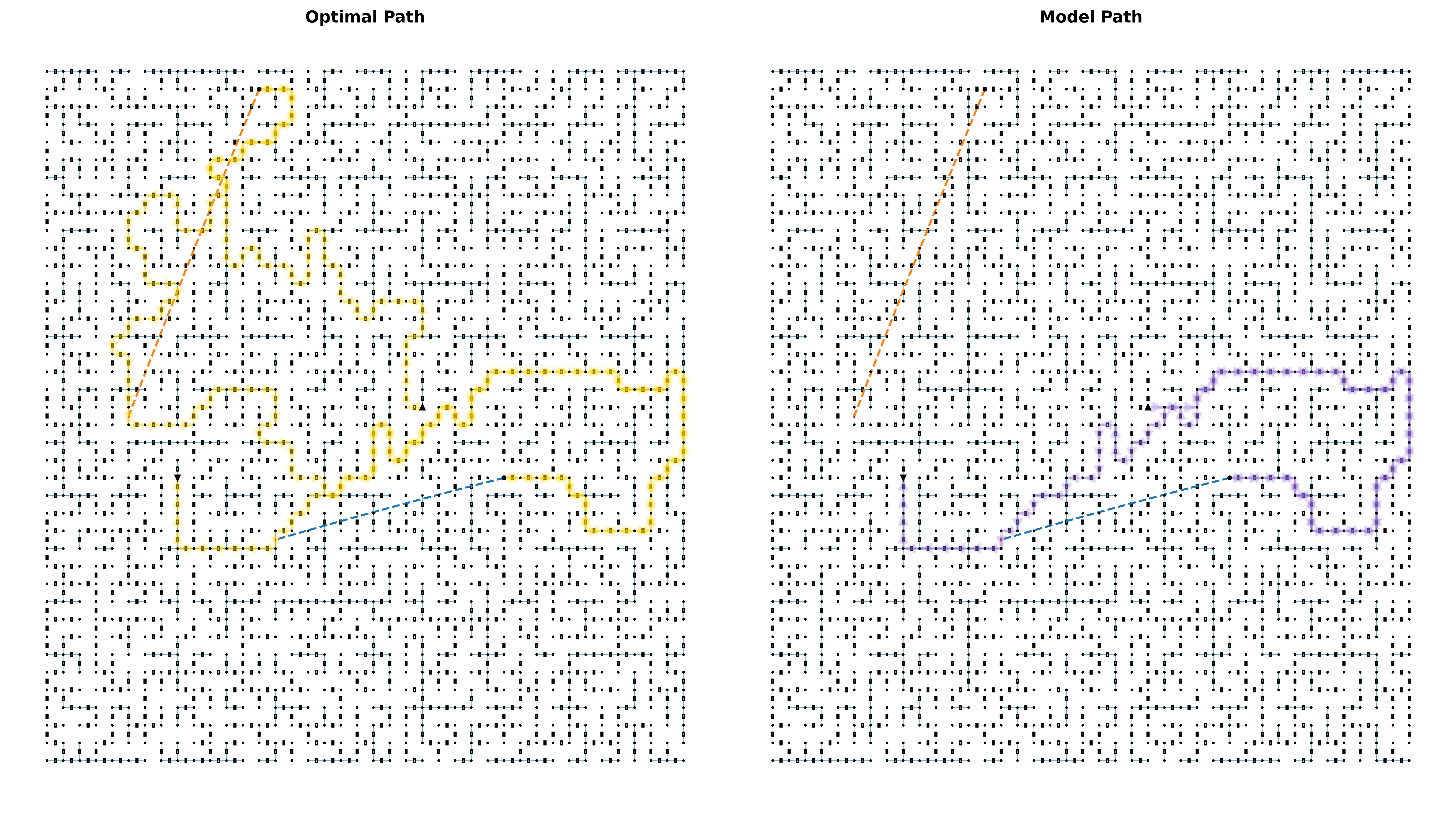<details> <summary>figs/goodexample4040.png Details</summary>  ### Visual Description ## Diagram: Comparison of Optimal Path vs. Model Path ### Overview The image presents two side-by-side visualizations of a maze navigation task. The left panel, titled "Optimal Path," displays a complex, winding route in yellow. The right panel, titled "Model Path," displays a more direct, shorter route in purple. Both diagrams utilize the same underlying maze structure, start/end points, and reference vectors (dashed lines). This comparison is characteristic of machine learning or pathfinding algorithm evaluation, where a "ground truth" or optimal solution is compared against an agent's learned behavior. ### Components/Axes * **Grid Structure:** A uniform rectangular grid of nodes (dots) connected by vertical and horizontal segments (walls/paths). * **Start/End Markers:** * **Start:** A black triangle pointing downward, located in the middle-left region of the maze. * **End:** A black triangle pointing upward, located in the middle-right region of the maze. * **Reference Vectors (Dashed Lines):** * **Orange Dashed Line:** Located in the upper-left quadrant, connecting a point in the top-left to a point near the top-center. * **Blue Dashed Line:** Located in the lower-middle region, connecting a point in the bottom-middle to a point near the middle-right. * **Paths:** * **Yellow Path (Left Panel):** Represents the "Optimal Path." * **Purple Path (Right Panel):** Represents the "Model Path." ### Detailed Analysis #### 1. Optimal Path (Left Panel) * **Trend:** The path is highly convoluted and non-linear. It exhibits significant "exploration" behavior. * **Trajectory:** * Starts at the downward triangle. * Moves upward and left, traversing a large, looping section in the upper-left quadrant. * It appears to pass near the orange dashed line but does not follow it strictly. * The path winds through the center of the maze, moving rightward. * It follows a jagged, step-like progression toward the end point. * Ends at the upward triangle. * **Characteristics:** The path covers a large surface area of the maze, suggesting the "Optimal" criteria may involve visiting specific nodes, maximizing path length, or navigating a complex constraint set. #### 2. Model Path (Right Panel) * **Trend:** The path is significantly more direct and efficient than the Optimal Path. * **Trajectory:** * Starts at the downward triangle. * Moves downward, then shifts rightward. * It follows a path that aligns closely with the blue dashed line segment. * It avoids the large, looping exploration seen in the Optimal Path. * Ends at the upward triangle. * **Characteristics:** The path is much shorter in total distance, suggesting the model is optimized for "shortest path" or "time-to-goal" rather than the specific, complex route defined as "Optimal." ### Key Observations * **Divergence:** The "Model Path" fails to replicate the "Optimal Path." The model takes a direct route, whereas the optimal path takes a circuitous route. * **Reference Vectors:** The orange and blue dashed lines are identical in both images. They appear to be "straight-line" projections or heuristic guides. The Model Path seems to utilize the blue dashed line as a guide, whereas the Optimal Path ignores these straight-line projections in favor of a more complex route. * **Start/End Consistency:** The start and end points are identical in both diagrams, confirming that the task is the same for both paths. ### Interpretation This visualization demonstrates a classic discrepancy in reinforcement learning or pathfinding: **Objective Mismatch.** * **The "Optimal" Path:** The complexity of the yellow path suggests that the "Optimal" definition is not simply "shortest distance." It may be a path that requires visiting specific waypoints, avoiding certain "danger" zones, or satisfying a complex reward function that encourages exploration. * **The "Model" Path:** The purple path suggests the model has learned a "greedy" strategy—minimizing distance to the goal. It ignores the complex, winding requirements of the Optimal Path. * **Conclusion:** The model is likely failing to learn the specific constraints of the environment (the "Optimal" behavior) and is instead defaulting to a simpler, distance-minimizing heuristic. The dashed lines likely represent the "straight-line" distance, which the model is successfully approximating, while the "Optimal" path is constrained by the maze walls in a way the model has not yet internalized. </details> Figure 8: Illustrative failure case for Gemini-2.5-Flash on a 40x40 task with 2 locked doors on the optimal path. Left: Optimal path (yellow). Right: Model’s generated path showing an illegal adjacency jump (red arrow), bypassing multiple rooms and a locked door, despite only supporting facts being provided. This highlights a breakdown in multi-step planning. 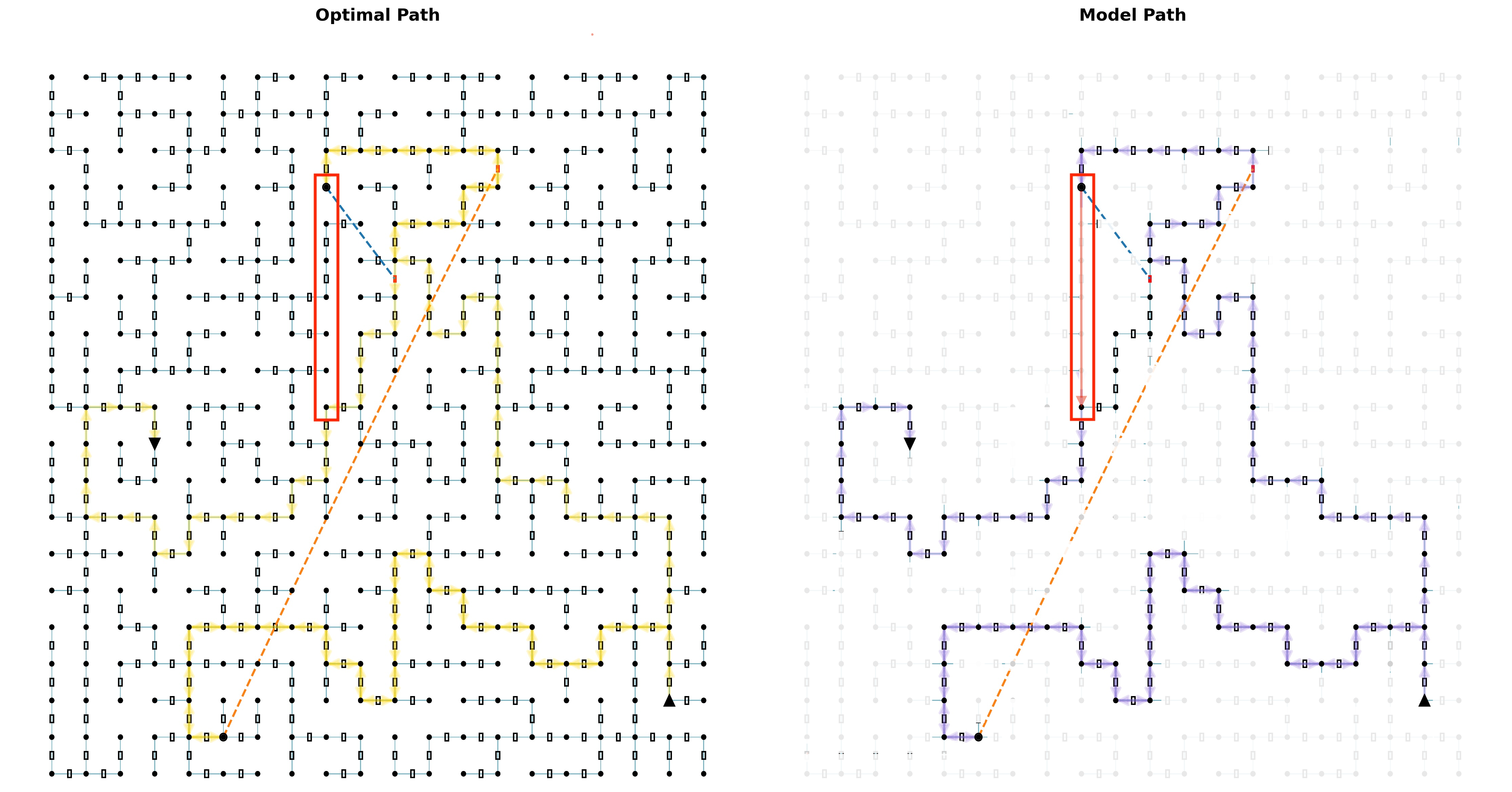<details> <summary>figs/mistakev2.png Details</summary>  ### Visual Description ## Diagram: Comparison of Optimal Path vs. Model Path ### Overview The image presents two side-by-side grid-based network diagrams, each visualizing a pathfinding solution. The left diagram is labeled "Optimal Path" and highlights a route in yellow. The right diagram is labeled "Model Path" and highlights a route in purple. Both diagrams share an identical underlying grid structure, a dashed orange diagonal reference line, and a red-boxed vertical segment. ### Components/Axes * **Grid Structure:** A uniform lattice of black nodes (dots) connected by thin lines (edges). Some edges contain small rectangular markers, likely representing obstacles or gates. * **Labels:** * "Optimal Path" (Top-center of the left grid). * "Model Path" (Top-center of the right grid). * **Markers:** * **Black Circle:** Located in the bottom-left quadrant of both grids; serves as the starting point. * **Black Triangle:** Located in the bottom-right corner of both grids; serves as the destination point. * **Red Rectangle:** Positioned in the upper-middle section of both grids, highlighting a specific vertical path segment. * **Dashed Orange Line:** A diagonal line extending from the bottom-left (near the black circle) to the top-right of the grid. * **Path Indicators:** * **Yellow Path (Left):** A highlighted route connecting the start and end points. * **Purple Path (Right):** A highlighted route connecting the start and end points, featuring directional arrows on the segments. ### Detailed Analysis #### Left Grid: Optimal Path * **Trend:** The path follows a relatively direct trajectory from the bottom-left start point toward the top-right, then descends toward the bottom-right destination. * **Pathing:** The path originates at the black circle, moves right and upward, enters the red-boxed region from the top, traverses it vertically downward, and then exits the box to navigate toward the bottom-right black triangle. The yellow highlighting is continuous. #### Right Grid: Model Path * **Trend:** The path is significantly more complex and winding compared to the Optimal Path. It exhibits "suboptimal" behavior, characterized by frequent turns and backtracking. * **Pathing:** The path originates at the black circle, moves in a complex, jagged pattern through the left and bottom sections of the grid. Like the Optimal Path, it enters the red-boxed region from the top and traverses it vertically downward. After exiting the red box, it continues to navigate a winding route through the bottom-right quadrant before reaching the black triangle. * **Directionality:** Unlike the Optimal Path, the purple path includes explicit directional arrows on the segments, indicating the flow of movement. ### Key Observations * **The "Bottleneck" (Red Box):** Both the Optimal and Model paths traverse the exact same vertical segment within the red rectangle. This suggests that this specific segment is a mandatory waypoint or a constrained passage that both the optimal algorithm and the model successfully identified. * **Path Efficiency:** The "Model Path" (purple) is visibly longer and more convoluted than the "Optimal Path" (yellow). The model appears to struggle with efficient navigation in the open grid areas, whereas the optimal path is much straighter. * **Reference Line:** The dashed orange diagonal line appears to act as a Euclidean distance reference or a heuristic constraint. The Optimal Path stays closer to this line in its general trajectory, whereas the Model Path deviates significantly. ### Interpretation This image is a visualization of a pathfinding algorithm's performance, likely from a Reinforcement Learning (RL) or path-planning context. * **What the data demonstrates:** The "Optimal Path" represents the ground truth or the most efficient solution (shortest path). The "Model Path" represents the output of an AI agent or algorithm that has not yet fully converged or learned the optimal policy. * **Why it matters:** The discrepancy between the two paths highlights the "suboptimality" of the model. While the model has learned to navigate the critical "bottleneck" (the red box), it lacks the efficiency to navigate the rest of the grid optimally, resulting in unnecessary, winding movements. * **Peircean Investigative Reading:** The presence of the red box suggests that the model is capable of learning specific constraints or high-value waypoints, but the surrounding "noise" in the purple path indicates that the model's exploration or exploitation strategy is currently inefficient. The model is "getting there," but it is taking a much longer route than necessary. </details> Figure 9: Illustrative failure case of an ’adjacency error’ in model-generated pathfinding on a 20x20 task with 2 locked doors on the optimal path. The left panel displays the optimal path (yellow) to the target (triangle). The right panel shows a suboptimal path (purple) generated by the model. This example highlights a common error where, after a sequence of actions (in this scenario, following a key acquisition), the model fails to navigate through valid connections. Instead, it attempts to ’jump’ directly between two unconnected rooms. This violation of room adjacency constraints is a key challenge in model performance. ### B.4 Quantitative Analysis of Error Patterns To understand how and when models begin to fail within a reasoning sequence, we analyze the distribution of the first violation step. We record the time step at which the initial violation occurs in a model’s generated path. Aggregating this step-indexed data across multiple instances allows us to create temporal distributions of errors. These distributions help determine whether errors tend to cluster early in the reasoning process (potentially indicating issues with initial planning or understanding of the overall problem complexity) or accumulate later (suggesting difficulties in maintaining long chains of inference or context). This analysis complements the discussion in the main paper (Section 2.4, "Path-Length Dependent First Errors: The Burden of Anticipated Complexity"). Figure 10 shows how the distribution of these first-error positions shifts with the overall problem complexity, represented by logical depth ( $L$ ). As detailed in the main paper, an increase in $L$ tends to cause errors to occur earlier in the reasoning chain. 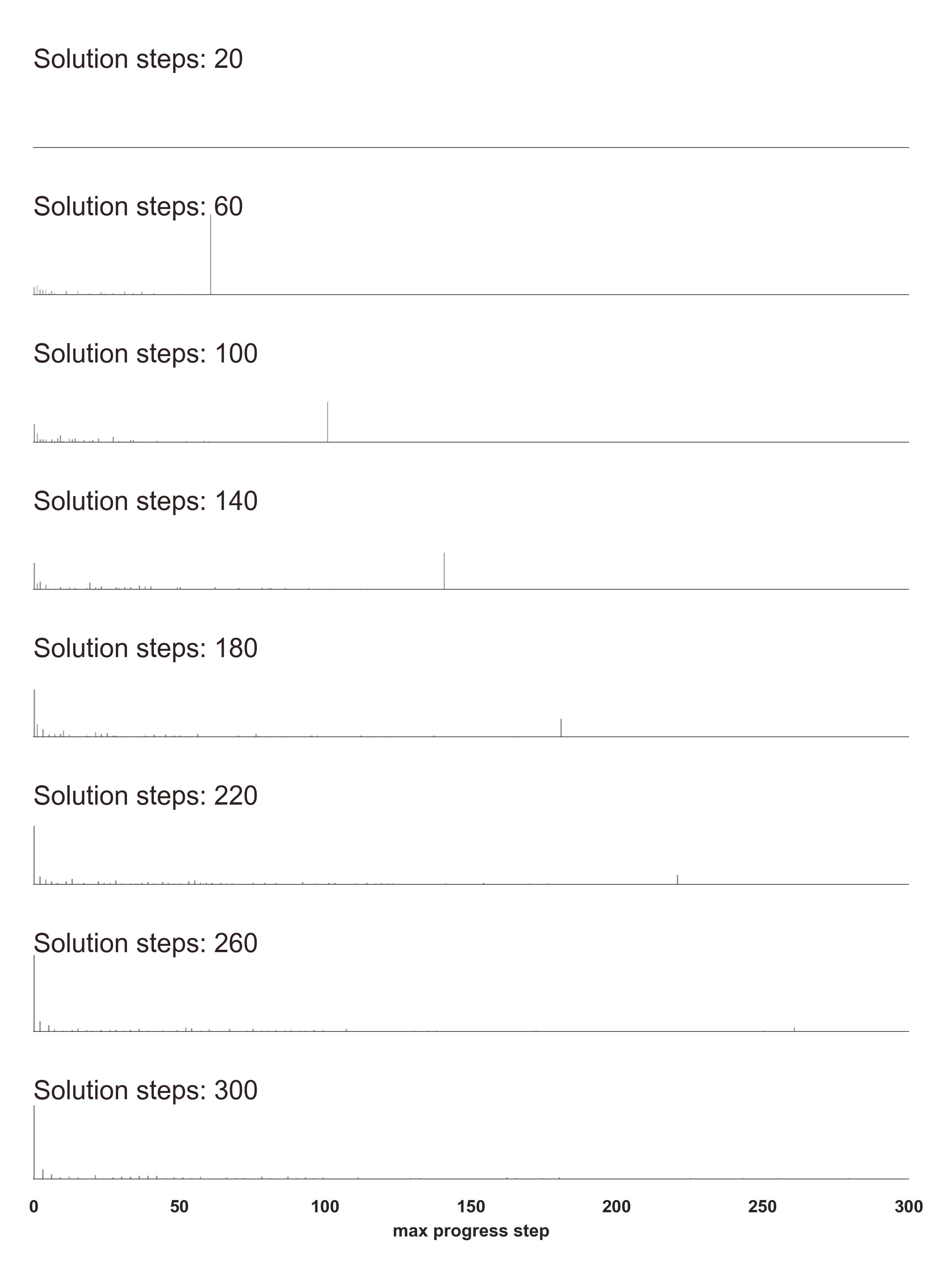<details> <summary>figs/failure_step_dist_vs_L.png Details</summary>  ### Visual Description ## Histogram Series: Distribution of Max Progress Steps by Solution Steps ### Overview The image displays a series of eight stacked histograms, each representing the distribution of "max progress step" achieved for a specific number of "Solution steps." The charts are aligned vertically, sharing a common x-axis at the bottom. Each histogram is dominated by a single, prominent vertical bar that shifts progressively to the right as the "Solution steps" value increases. ### Components/Axes * **Vertical Labels:** Located on the left of each histogram row, indicating the "Solution steps" parameter. The values are: 20, 60, 100, 140, 180, 220, 260, and 300. * **X-Axis:** Located at the bottom of the entire figure, labeled "max progress step." The scale ranges from 0 to 300, with major tick marks at intervals of 50 (0, 50, 100, 150, 200, 250, 300). * **Y-Axis:** Implicit frequency/count for each histogram. The height of the bars represents the density or count of occurrences at that specific "max progress step." ### Detailed Analysis Each row represents a distinct dataset. Below is the approximate position of the primary peak (tallest bar) for each "Solution steps" category: | Solution steps | Primary Peak Position (approx. max progress step) | | :--- | :--- | | 20 | ~20 | | 60 | ~60 | | 100 | ~100 | | 140 | ~140 | | 180 | ~180 | | 220 | ~220 | | 260 | ~260 | | 300 | ~300 | **Trend Verification:** * **Primary Trend:** There is a strong, linear positive correlation between the "Solution steps" label and the position of the primary peak on the x-axis. As the label increases, the peak shifts rightward by an equivalent amount. * **Secondary Trend:** In every row, there is a consistent, smaller cluster of activity located near the 0 mark on the x-axis. This suggests a baseline or "failure" state where the progress step remained near zero regardless of the target solution steps. ### Key Observations * **High Precision:** The primary peak in every row aligns almost perfectly with the numerical value of the "Solution steps" label. * **Bimodal Distribution:** Each histogram exhibits a bimodal-like distribution: a very tall, thin spike at the target value, and a small, low-frequency cluster of bars near 0. * **Consistency:** The height of the primary peak appears relatively consistent across all rows, suggesting that the system successfully reaches the target "Solution steps" with high reliability in the majority of cases. ### Interpretation This visualization likely represents the performance of an algorithm, agent, or simulation (such as a reinforcement learning agent or a pathfinding process) tasked with reaching a specific progress goal. * **The "Solution steps" label** acts as the target or constraint for the system. * **The primary peak** represents the system successfully completing the task and reaching the target progress step. The fact that this peak aligns with the label suggests the system is highly accurate and deterministic in achieving its target. * **The small cluster near 0** likely represents "failures" or "initial states"—instances where the system failed to make progress or was terminated immediately. * **Conclusion:** The data demonstrates a highly effective system that consistently achieves the target progress step, with a negligible error rate (represented by the small bars near 0). The system's performance is tightly coupled to the input parameter "Solution steps." </details> Figure 10: Distribution of first-violation steps for Gemini-2.5-Flash across varying logical depths ( $L$ ). As $L$ (total required path length) increases, the distribution of first errors tends to shift leftward, indicating that models are more likely to fail at earlier steps in longer problems. This suggests that anticipated global complexity impacts reasoning from the outset. Experimental parameters in this figure are the same as those in Figure 1. Similarly, Figure 11 illustrates how the introduction of contextual noise (distracting facts) affects the point of failure. Increased noise also tends to precipitate earlier errors in the reasoning sequence, as discussed in the main paper in relation to sensitivity to noise (Section 2.3) and its impact on error patterns (Section 2.4). 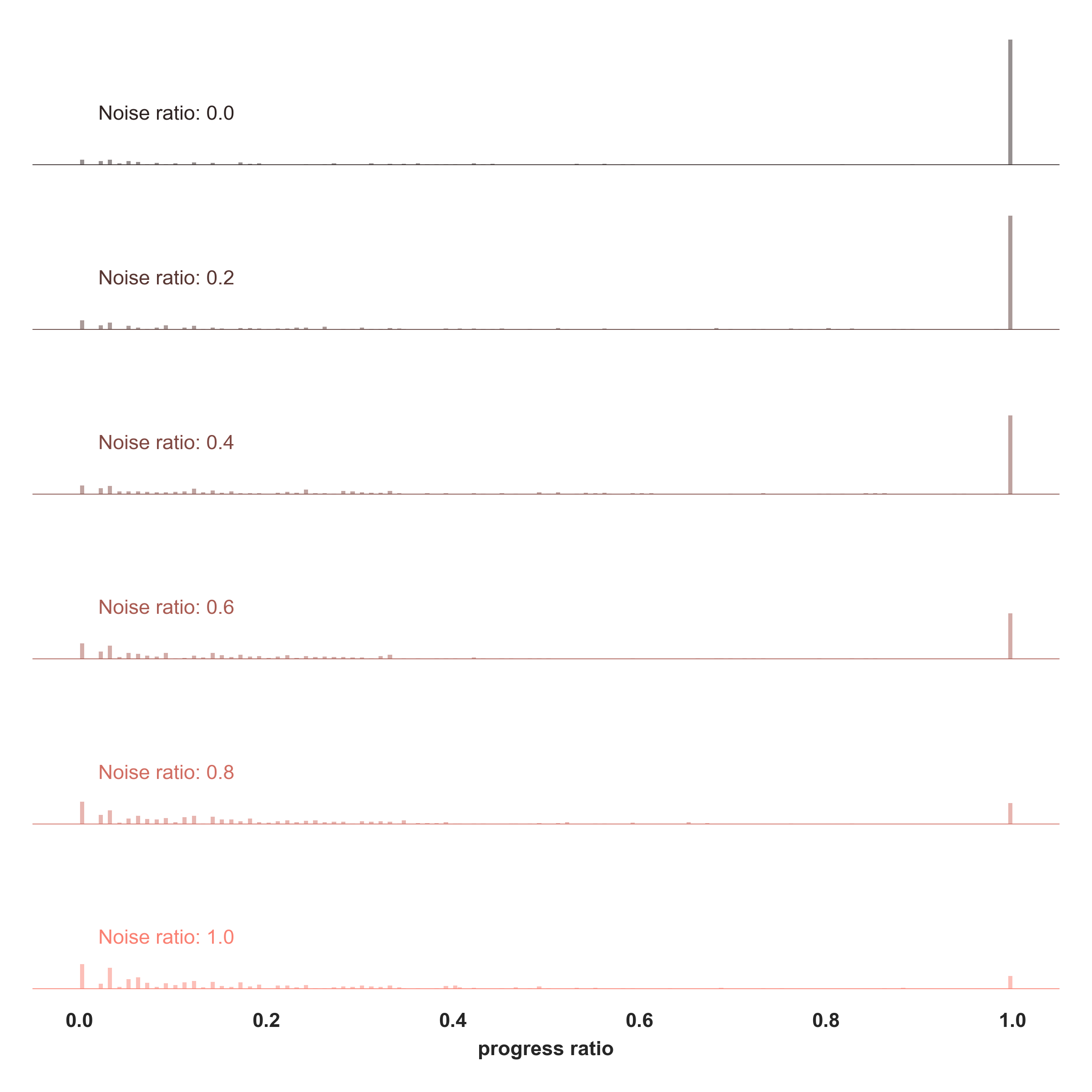<details> <summary>figs/gemini-progress-ratio-vs-noise.png Details</summary>  ### Visual Description ## Multi-Panel Histogram: Distribution of Progress Ratio by Noise Ratio ### Overview The image displays a series of six stacked histograms, each representing the distribution of a "progress ratio" (ranging from 0.0 to 1.0) under different levels of "Noise ratio" (ranging from 0.0 to 1.0). The chart illustrates how increasing noise levels negatively impact the "progress ratio," shifting the distribution away from completion (1.0) toward lower values. ### Components/Axes * **X-Axis:** Labeled "progress ratio" at the bottom center. The scale is linear, with major tick marks at 0.0, 0.2, 0.4, 0.6, 0.8, and 1.0. * **Y-Axis (Implicit):** Each of the six horizontal rows represents a frequency or probability density for a specific "Noise ratio." There are no numerical values on the vertical axis, but the height of the bars indicates relative frequency. * **Rows (Independent Variables):** * **Top Row:** "Noise ratio: 0.0" (Color: Dark Grey) * **Second Row:** "Noise ratio: 0.2" (Color: Grey-Brown) * **Third Row:** "Noise ratio: 0.4" (Color: Light Brown) * **Fourth Row:** "Noise ratio: 0.6" (Color: Muted Orange) * **Fifth Row:** "Noise ratio: 0.8" (Color: Light Orange) * **Bottom Row:** "Noise ratio: 1.0" (Color: Pale Orange) ### Detailed Analysis The data shows a consistent bimodal distribution across all noise levels, with a primary mode at 1.0 and a secondary, lower-frequency distribution clustered between 0.0 and 0.3. * **Noise ratio 0.0 (Top):** The distribution is almost entirely concentrated at 1.0. There is virtually no activity in the 0.0–0.9 range. * **Noise ratio 0.2:** The dominant spike remains at 1.0. There is a negligible amount of activity appearing in the 0.0–0.1 range. * **Noise ratio 0.4:** The spike at 1.0 remains dominant, but the activity in the 0.0–0.15 range becomes slightly more visible and frequent. * **Noise ratio 0.6:** The spike at 1.0 begins to decrease in relative height. The distribution in the 0.0–0.3 range becomes more pronounced and spread out. * **Noise ratio 0.8:** The spike at 1.0 is noticeably lower than in previous rows. The activity in the 0.0–0.3 range is significant, showing a wider spread of values. * **Noise ratio 1.0 (Bottom):** The spike at 1.0 is at its lowest point. The distribution in the 0.0–0.3 range is the most dense and widespread, indicating that a large portion of the data has failed to reach the 1.0 progress mark. ### Key Observations * **Inverse Correlation:** There is a clear inverse relationship between "Noise ratio" and the frequency of reaching a "progress ratio" of 1.0. As noise increases, the probability of reaching full progress decreases. * **Distribution Shift:** As the noise ratio increases, the data mass shifts from the right side of the chart (1.0) to the left side (0.0–0.3). * **Visual Encoding:** The color gradient (from dark grey at 0.0 noise to pale orange at 1.0 noise) acts as a visual cue for the increasing severity of the noise. ### Interpretation This chart likely represents the performance of an iterative process, such as a machine learning model training, a diffusion process, or a task completion algorithm, where "progress ratio" measures the degree of completion. * **The "Success" State:** The spike at 1.0 represents the successful completion of the task. At low noise levels (0.0–0.2), the system is highly reliable, almost always reaching completion. * **The "Failure" State:** The cluster of bars on the left (0.0–0.3) represents processes that failed to complete or were interrupted. * **The Impact of Noise:** The data demonstrates that "Noise ratio" acts as a degradation factor. As noise increases, the system's ability to reach 1.0 is compromised, causing the distribution to "leak" into the lower progress ratios. The transition from 0.6 to 1.0 noise appears to be the most critical phase where the reliability of reaching 1.0 drops significantly. </details> Figure 11: Impact of increasing noise ratio on the distribution of failure steps for Gemini 2.5 Flash. As noise (proportion of distracting facts) increases, failures tend to occur earlier in the reasoning chain. This reflects increased difficulty in isolating relevant information and maintaining focus. Fixed experimental parameters in this figure are the same as those in Figure 1. ## Appendix C Supplementary Figures This appendix provides supplementary figures that offer further visual support for analyses presented in the main paper. These figures illustrate the impact of various complexity dimensions and provide comparative views of model performance, elaborating on points made throughout Section 2 (Benchmarking Results) of the main paper. Figure 12 details the performance of Llama-4 Maverick-17B-128E-Instruct under varying levels of noise and fact shuffling. This supports the discussion in the main paper (Section 2.3, on how these factors, especially in combination, affect success rates, with noise being a dominant factor. 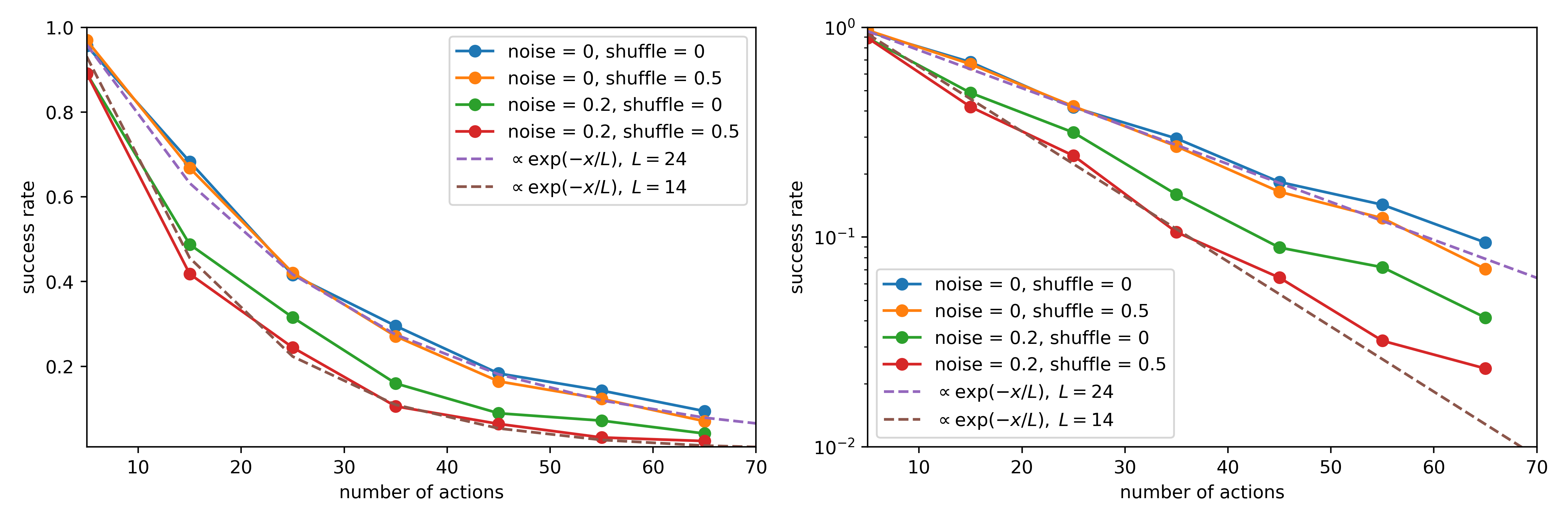<details> <summary>figs/single_model_vs_steps_count_varied_noise_shuffle_Llama-4-Maverick-17B-128E-Instruct-FP8.png Details</summary>  ### Visual Description ## Line Charts: Success Rate vs. Number of Actions ### Overview This image displays two side-by-side line charts illustrating the decay of "success rate" as the "number of actions" increases. The left chart utilizes a linear y-axis scale, while the right chart utilizes a logarithmic y-axis scale. Both charts compare four experimental conditions (varying noise and shuffle parameters) against two theoretical exponential decay reference curves. ### Components/Axes * **Common Axes:** * **X-axis:** "number of actions", ranging from 5 to 70, with major ticks at 10, 20, 30, 40, 50, 60, 70. * **Y-axis:** "success rate". * **Left Chart Y-axis:** Linear scale from 0.0 to 1.0. * **Right Chart Y-axis:** Logarithmic scale from $10^{-2}$ to $10^0$. * **Legend (Located in the top-right of the left chart and center-left of the right chart):** * **Blue solid line/dot:** `noise = 0, shuffle = 0` * **Orange solid line/dot:** `noise = 0, shuffle = 0.5` * **Green solid line/dot:** `noise = 0.2, shuffle = 0` * **Red solid line/dot:** `noise = 0.2, shuffle = 0.5` * **Purple dashed line:** `∝ exp(-x/L), L = 24` * **Brown dashed line:** `∝ exp(-x/L), L = 14` ### Detailed Analysis The data series are plotted at x-values of 5, 15, 25, 35, 45, 55, and 65. **Trend Verification:** All four experimental data series exhibit a monotonic downward trend (decay) as the number of actions increases. The logarithmic plot (right) confirms that this decay is exponential, as the lines appear roughly linear on the log-y scale. **Data Point Extraction (Approximate):** | Number of Actions | Blue (0,0) | Orange (0, 0.5) | Green (0.2, 0) | Red (0.2, 0.5) | | :--- | :--- | :--- | :--- | :--- | | **5** | ~0.98 | ~0.98 | ~0.90 | ~0.89 | | **15** | ~0.68 | ~0.66 | ~0.49 | ~0.42 | | **25** | ~0.41 | ~0.42 | ~0.31 | ~0.25 | | **35** | ~0.30 | ~0.27 | ~0.16 | ~0.11 | | **45** | ~0.19 | ~0.17 | ~0.09 | ~0.07 | | **55** | ~0.15 | ~0.13 | ~0.08 | ~0.05 | | **65** | ~0.10 | ~0.08 | ~0.05 | ~0.03 | * **Reference Curves:** * The **Purple dashed line ($L=24$)** closely tracks the Blue and Orange data series. * The **Brown dashed line ($L=14$)** closely tracks the Red data series. ### Key Observations * **Noise Impact:** The "noise" parameter is the primary driver of performance degradation. Conditions with `noise = 0` (Blue/Orange) maintain significantly higher success rates than conditions with `noise = 0.2` (Green/Red). * **Shuffle Impact:** The "shuffle" parameter has a secondary effect. Within the same noise level, the `shuffle = 0.5` condition generally results in a slightly lower success rate compared to `shuffle = 0`. </details> Figure 12: Pass@1 success rate for Llama-4 Maverick-17B-128E-Instruct versus solution length ( $L$ ) under different noise and shuffle ratios. Left: Linear scale. Right: Log-linear scale. Performance degrades with increased noise but is less affected by shuffle ratios. Fixed experimental parameters in this figure are the same as those in Figure 1. To illustrate the performance consistency and disparities across different models, as detailed in Section 2.6, Figure 13 presents scatter and density plots of mean progress ratios. These plots clearly demonstrate that model performance hierarchies are not strictly linear. They reveal ’performance inversions’—instances, also noted in Section 2.6, where models with typically lower overall performance (e.g., lower average $L_{0}$ ) occasionally solve specific complex problems that models with higher average $L_{0}$ values fail on. 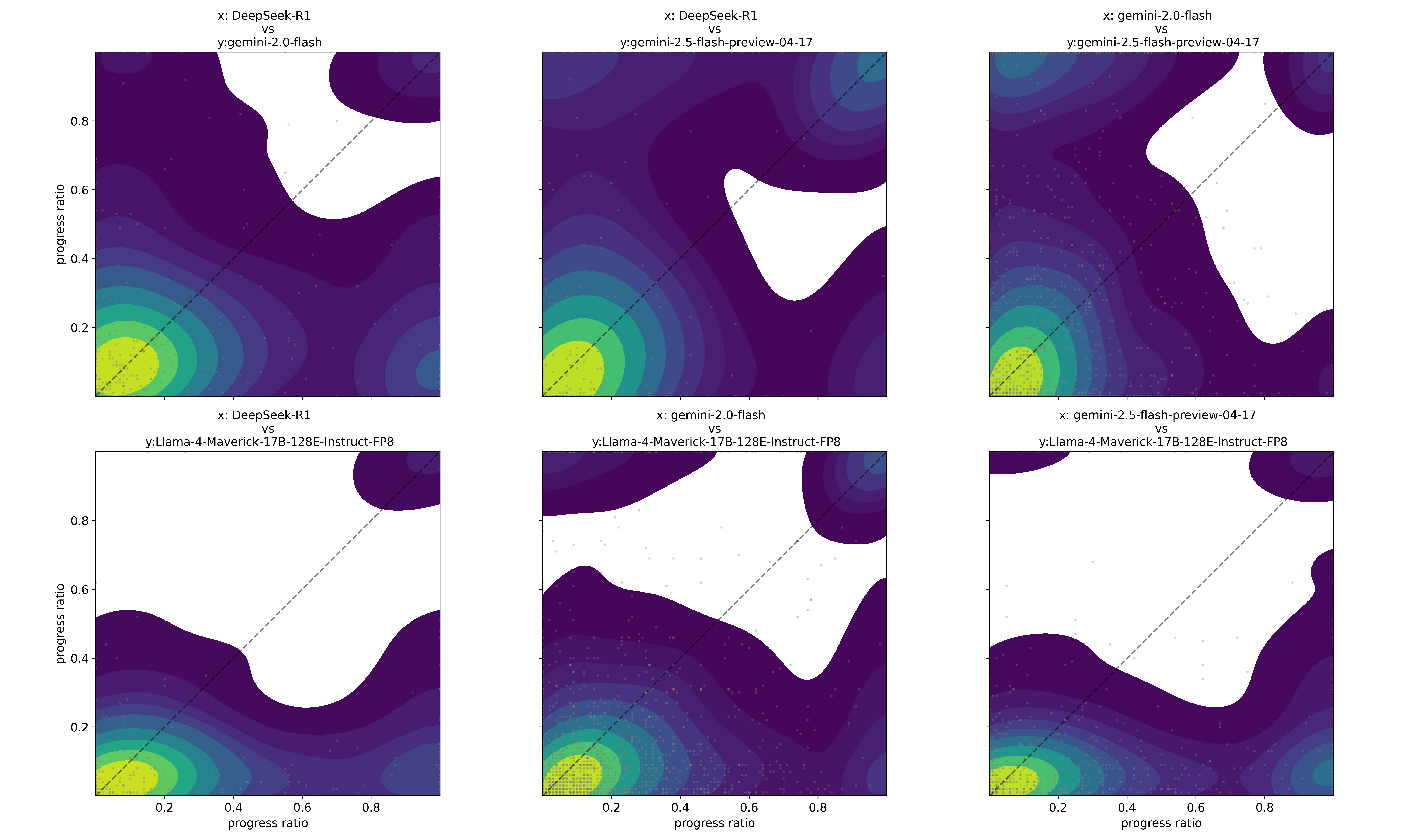<details> <summary>figs/progress_vs_progress.png Details</summary>  ### Visual Description ## Heatmap Matrix: AI Model Progress Ratio Comparison ### Overview This image displays a 2x3 grid of density heatmaps comparing the "progress ratio" of various AI models against one another. Each plot visualizes the correlation of performance between two specific models. The density of data points is represented by a color gradient, ranging from dark purple (low density) to yellow/green (high density). A dashed diagonal line (y=x) is present in each plot to indicate parity; points above the line indicate the model on the Y-axis performed better, while points below the line indicate the model on the X-axis performed better. ### Components/Axes * **Grid Layout:** 2 rows by 3 columns. * **Axes:** Both X and Y axes represent "progress ratio," scaled from 0.0 to 0.8 (with tick marks at 0.2, 0.4, 0.6, 0.8). * **Data Representation:** * **Scatter:** Light grey dots represent individual data points. * **Density:** Overlaid color gradient (Purple to Yellow/Green) indicates the concentration of data points. * **Reference:** A dashed diagonal line represents the line of equality (where both models have the same progress ratio). ### Detailed Analysis #### Row 1 * **Top-Left (x: DeepSeek-R1 vs y: gemini-2.0-flash):** * **Trend:** High density at the origin (0,0). A significant portion of the density cloud lies above the diagonal line, indicating that *gemini-2.0-flash* generally achieves a higher progress ratio than *DeepSeek-R1*. * **Top-Center (x: DeepSeek-R1 vs y: gemini-2.5-flash-preview-04-17):** * **Trend:** High density at the origin. The density cloud is heavily skewed above the diagonal, indicating *gemini-2.5-flash-preview-04-17* consistently outperforms *DeepSeek-R1*. * **Top-Right (x: gemini-2.0-flash vs y: gemini-2.5-flash-preview-04-17):** * **Trend:** High density at the origin. The distribution is tightly clustered along the diagonal, but with a noticeable bias above the diagonal, suggesting *gemini-2.5-flash-preview-04-17* is slightly superior to *gemini-2.0-flash*. #### Row 2 * **Bottom-Left (x: DeepSeek-R1 vs y: Llama-4-Maverick-17B-128E-Instruct-FP8):** * **Trend:** High density at the origin. The density cloud is heavily skewed *below* the diagonal, indicating *DeepSeek-R1* significantly outperforms *Llama-4-Maverick-17B-128E-Instruct-FP8*. * **Bottom-Center (x: gemini-2.0-flash vs y: Llama-4-Maverick-17B-128E-Instruct-FP8):** * **Trend:** High density at the origin. The density cloud is heavily skewed *below* the diagonal, indicating *gemini-2.0-flash* significantly outperforms *Llama-4-Maverick-17B-128E-Instruct-FP8*. * **Bottom-Right (x: gemini-2.5-flash-preview-04-17 vs y: Llama-4-Maverick-17B-128E-Instruct-FP8):** * **Trend:** High density at the origin. The density cloud is heavily skewed *below* the diagonal, indicating *gemini-2.5-flash-preview-04-17* significantly outperforms *Llama-4-Maverick-17B-128E-Instruct-FP8*. ### Key Observations * **Universal Origin Cluster:** In all six plots, there is a very high density of points at the (0,0) coordinate. This suggests that for a large number of tasks, all models either fail immediately or make very little progress. * **Performance Hierarchy:** 1. *gemini-2.5-flash-preview-04-17* appears to be the strongest model in this set. 2. *gemini-2.0-flash* and *DeepSeek-R1* are competitive with each other, though *gemini-2.0-flash* shows a slight edge. 3. *Llama-4-Maverick-17B-128E-Instruct-FP8* is the weakest performer, consistently falling below the diagonal when compared to the other three models. ### Interpretation This matrix provides a comparative performance analysis of four AI models based on a "progress ratio" metric, which likely quantifies how far a model gets through a multi-step reasoning or generation task. * **The "Llama" Gap:** The bottom row clearly demonstrates that *Llama-4-Maverick* struggles to keep pace with the Gemini and DeepSeek models. The density is consistently pushed below the diagonal, meaning the X-axis models (the Gemini/DeepSeek variants) are reaching higher progress ratios than the Llama model. * **Gemini Evolution:** The top-right plot (Gemini 2.0 vs 2.5) shows that while the models are very similar, the 2.5-flash-preview version has a distinct advantage, as the density is shifted above the parity line. * **Task Difficulty:** The heavy clustering at (0,0) across all charts suggests that the dataset contains a significant number of "hard" or "impossible" tasks where none of the models are able to make meaningful progress. The models are differentiated primarily by their ability to handle the tasks that *do* allow for progress (the spread away from the origin). </details> Figure 13: Scatter and density plots of progress ratios per task instance, comparing model pairs on the tasks. These plots illustrate performance agreement and disparities on the same instances of pathfinding tasks. Notably, Gemini-2.5-Flash (example) often succeeds on instances where other models achieve near-zero progress. Data from experiments in Figure 1 (main paper). Figure 14 isolates the impact of shuffle ratio on model performance when other factors like noise are controlled. This visualization corresponds to the findings discussed in the main paper (Section 2.3, "Fact Ordering (Shuffle Ratio)") that simple reordering of facts has a minimal impact on the performance of the evaluated models under low-noise conditions. Figure 15 isolates the impact of adding more examples in the instruction prompt, showing a clear improvement once more than a single example is included compared to using none or only one. Figure 16 is added in this revised version of the supplementary section to reflect that even the most recent SOTA models released by OpenAI suffer from the same performance drop observed in the main paper. 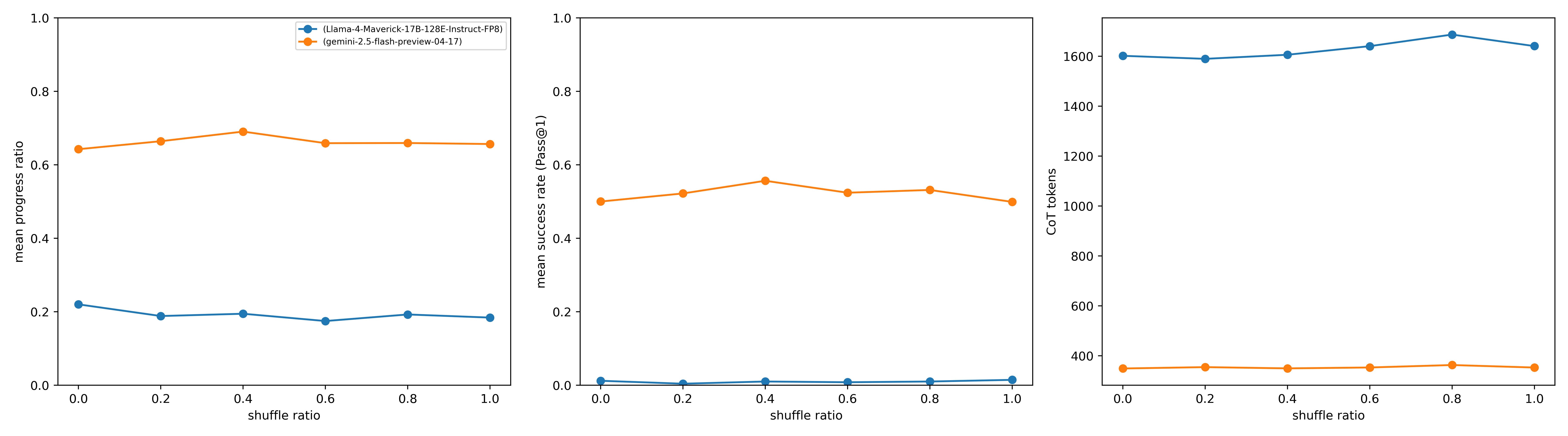<details> <summary>figs/fig_vs_shuffle_fixed_L_keys2_noise0.2.png Details</summary>  ### Visual Description ## Line Charts: Performance Metrics vs. Shuffle Ratio ### Overview This image displays three side-by-side line charts comparing the performance of two AI models: **Llama-4-Maverick-17B-128E-Instruct-FP8** (represented by the blue line) and **gemini-2.5-flash-preview-04-17** (represented by the orange line). The charts evaluate these models across a "shuffle ratio" ranging from 0.0 to 1.0. The three metrics being measured are "mean progress ratio," "mean success rate (Pass@1)," and "CoT tokens." ### Components/Axes * **Shared X-Axis:** "shuffle ratio" ranging from 0.0 to 1.0 in increments of 0.2. * **Legend:** Located in the top-left chart. * **Blue Line:** Llama-4-Maverick-17B-128E-Instruct-FP8 * **Orange Line:** gemini-2.5-flash-preview-04-17 * **Chart 1 (Left) Y-Axis:** "mean progress ratio" (Scale: 0.0 to 1.0). * **Chart 2 (Center) Y-Axis:** "mean success rate (Pass@1)" (Scale: 0.0 to 1.0). * **Chart 3 (Right) Y-Axis:** "CoT tokens" (Scale: 400 to 1600). --- ### Detailed Analysis #### Chart 1: Mean Progress Ratio * **Blue Line (Llama):** Starts at ~0.22 at 0.0 shuffle ratio. It exhibits a slight downward trend, fluctuating between 0.18 and 0.20 for the remainder of the ratios. * **Orange Line (Gemini):** Starts at ~0.64 at 0.0 shuffle ratio. It rises to a peak of ~0.69 at 0.4, then stabilizes around 0.66 for the remaining ratios (0.6 to 1.0). * **Trend:** The Gemini model consistently maintains a significantly higher mean progress ratio than the Llama model. #### Chart 2: Mean Success Rate (Pass@1) * **Blue Line (Llama):** Remains consistently near 0.0 across all shuffle ratios, indicating very low success rates for this specific metric. * **Orange Line (Gemini):** Starts at ~0.50 at 0.0 shuffle ratio. It shows a slight upward trend to ~0.56 at 0.4, then dips back down to ~0.50 at 1.0. * **Trend:** The Gemini model shows moderate success, while the Llama model shows negligible success on this metric. #### Chart 3: CoT (Chain of Thought) Tokens * **Blue Line (Llama):** Starts at ~1600 tokens at 0.0 shuffle ratio. It shows a slight, gradual upward trend, reaching a peak of ~1680 at 0.8, before dipping slightly to ~1640 at 1.0. * **Orange Line (Gemini):** Starts at ~350 tokens at 0.0 shuffle ratio. It remains extremely stable, hovering consistently between 350 and 360 tokens across all shuffle ratios. * **Trend:** The Llama model utilizes significantly more CoT tokens (roughly 4.5x more) than the Gemini model. --- ### Key Observations * **Performance Gap:** Gemini-2.5-flash-preview-04-17 significantly outperforms Llama-4-Maverick-17B-128E-Instruct-FP8 in both "mean progress ratio" and "mean success rate." * **Efficiency Gap:** There is a massive disparity in "CoT tokens" usage. Llama uses ~1600 tokens per task, whereas Gemini uses ~350. Despite using fewer tokens, Gemini achieves higher success rates. * **Robustness:** Both models appear robust to the "shuffle ratio." The performance metrics do not fluctuate wildly as the shuffle ratio increases, suggesting that the order of input data has a negligible impact on the reasoning capabilities of either model. ### Interpretation The data suggests a fundamental difference in the reasoning efficiency and capability between the two models. 1. **Efficiency vs. Verbosity:** The Llama model is generating significantly longer Chain-of-Thought (CoT) sequences (higher token count) but is failing to convert that "thinking" into successful outcomes (low Pass@1). This could indicate that the Llama model is either "hallucinating" or getting lost in its own reasoning process, or that its CoT generation is inherently verbose without adding value. 2. **Model Capability:** Gemini-2.5-flash appears to be a much more efficient and capable model in this specific testing context, achieving higher success rates with a much smaller computational footprint (fewer tokens). 3. **Robustness:** The "shuffle ratio" variable seems to be a test of input sensitivity. The flatness of the lines indicates that both models are invariant to the order of the input, which is a positive trait for general-purpose reasoning models. </details> Figure 14: Impact of shuffle ratio on Pass@1 success rate. Varying the degree of mixing (shuffle) between supporting and distracting facts shows minimal impact on performance for Gemini 2.5 Flash and Llama-4 Maverick, suggesting robustness to fact order when noise is controlled. The generation and sampling of maze instances for these tasks follow the same methodology detailed for experiments in the main paper (Figures 3 and 4). 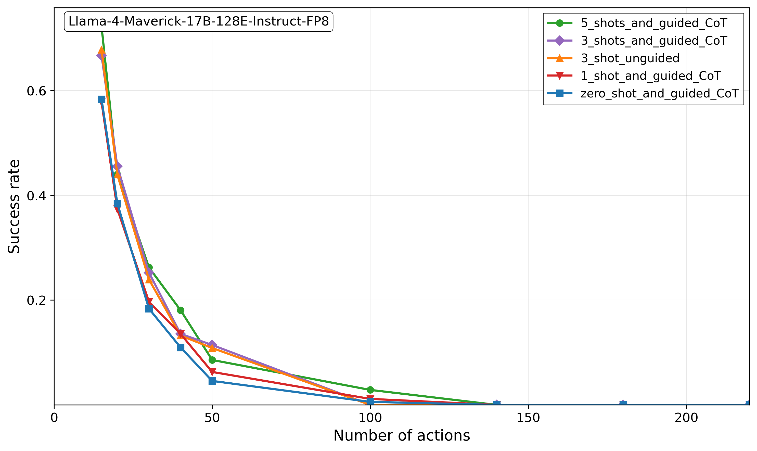<details> <summary>figs/maze_ablation_analysis.png Details</summary>  ### Visual Description ## Line Chart: Success Rate vs. Number of Actions for Llama-4-Maverick-17B-128E-Instruct-FP8 ### Overview This chart illustrates the performance degradation of the "Llama-4-Maverick-17B-128E-Instruct-FP8" model as the complexity of a task—measured by the "Number of actions"—increases. The chart compares five different prompting strategies, ranging from zero-shot to 5-shot with Chain-of-Thought (CoT) guidance. All strategies exhibit a sharp, exponential-like decay in success rate as the number of actions increases. ### Components/Axes * **Header**: "Llama-4-Maverick-17B-128E-Instruct-FP8" (Top-left). * **X-Axis**: "Number of actions". Linear scale, marked at 0, 50, 100, 150, 200. * **Y-Axis**: "Success rate". Linear scale, marked at 0, 0.2, 0.4, 0.6. * **Legend**: Located in the top-right corner. * **Green circle**: `5_shots_and_guided_CoT` * **Purple diamond**: `3_shots_and_guided_CoT` * **Orange triangle (up)**: `3_shot_unguided` * **Red triangle (down)**: `1_shot_and_guided_CoT` * **Blue square**: `zero_shot_and_guided_CoT` ### Detailed Analysis The chart displays five data series, all showing a steep downward trend. The data points are clustered at specific intervals along the X-axis (approximately 15, 20, 30, 40, 50, 100, 140, 180, 220). **Trend Verification:** All five series start at a high success rate (approx. 0.65–0.70) at the lowest action count (~15) and drop precipitously to near-zero success rates as the number of actions exceeds 100. **Data Point Estimates (Approximate):** | Number of Actions | 5-shots (Green) | 3-shots CoT (Purple) | 3-shot Unguided (Orange) | 1-shot CoT (Red) | Zero-shot CoT (Blue) | | :--- | :--- | :--- | :--- | :--- | :--- | | **~15** | ~0.70 | ~0.68 | ~0.69 | ~0.67 | ~0.58 | | **~20** | ~0.45 | ~0.46 | ~0.44 | ~0.38 | ~0.38 | | **~30** | ~0.27 | ~0.25 | ~0.24 | ~0.20 | ~0.18 | | **~40** | ~0.18 | ~0.14 | ~0.14 | ~0.14 | ~0.11 | | **~50** | ~0.09 | ~0.12 | ~0.11 | ~0.07 | ~0.05 | | **~100** | ~0.04 | ~0.02 | ~0.02 | ~0.01 | ~0.01 | *Note: Beyond 100 actions, all series converge toward a success rate of 0.* ### Key Observations * **Performance Convergence**: While there is a noticeable spread in success rates at lower action counts (15–50), the performance gap between the different prompting strategies narrows significantly as the number of actions increases. By 100 actions, all strategies perform poorly (success rate < 0.05). * **Initial Performance**: At the lowest action count (~15), the `5_shots_and_guided_CoT` (Green) and `3_shot_unguided` (Orange) strategies appear to have the highest success rates. * **Mid-Range Divergence**: At 50 actions, the `3_shots_and_guided_CoT` (Purple) and `3_shot_unguided` (Orange) strategies maintain a slightly higher success rate compared to the `5_shots_and_guided_CoT` (Green), which drops more sharply between 40 and 50 actions. * **Zero-Shot Baseline**: The `zero_shot_and_guided_CoT` (Blue) consistently performs at or near the bottom of the group across all action counts, indicating that providing examples (shots) generally improves performance for this model. ### Interpretation The data demonstrates that the Llama-4-Maverick-17B-128E-Instruct-FP8 model suffers from a severe "context length" or "task complexity" penalty. Regardless of the prompting strategy used (CoT, few-shot, or unguided), the model's ability to successfully complete tasks drops off exponentially as the number of required actions increases. The prompting strategies provide a "cushion" at low action counts, but they fail to mitigate the fundamental degradation of the model's reasoning capabilities as the task length grows. The fact that all lines converge to near-zero success rates suggests that the model's failure is likely due to an inherent limitation in handling long-horizon planning or extended action sequences, rather than a limitation of the prompting technique itself. </details> Figure 15: The impact of including different number of reference examples in the prompt as part of in-context learning. Increasing the number of examples leads to slight improvements in performance. The experimental parameters used here are the same as ones in Figure 1. 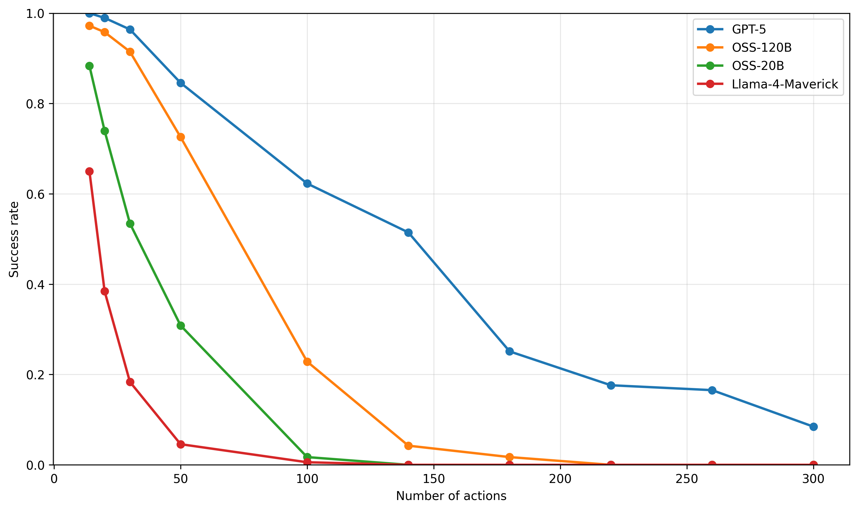<details> <summary>figs/model_comparison_openai.png Details</summary>  ### Visual Description ## Line Chart: Success Rate vs. Number of Actions ### Overview This image is a line chart illustrating the performance degradation of four distinct AI models (GPT-5, OSS-120B, OSS-20B, and Llama-4-Maverick) as the complexity or length of a task increases. The chart plots "Success rate" (y-axis) against the "Number of actions" (x-axis). All four models exhibit a negative correlation, where success rates decline as the number of actions increases, demonstrating a compounding error effect common in multi-step reasoning or agentic tasks. ### Components/Axes * **X-Axis:** Labeled "Number of actions". The scale ranges from 0 to 300, with major grid lines at intervals of 50. * **Y-Axis:** Labeled "Success rate". The scale ranges from 0.0 to 1.0, with major grid lines at intervals of 0.2. * **Legend:** Located in the top-right corner. It maps the following colors to model names: * **Blue:** GPT-5 * **Orange:** OSS-120B * **Green:** OSS-20B * **Red:** Llama-4-Maverick * **Grid:** A light gray grid is overlaid to assist in reading values. ### Detailed Analysis The data points are plotted at specific intervals along the x-axis (approximately 15, 25, 35, 50, 100, 140, 180, 220, 260, and 300). **1. GPT-5 (Blue Line)** * **Trend:** The most resilient model. It maintains a high success rate for the longest duration before experiencing a significant drop-off after 140 actions. * **Data Points (Approximate):** * x=15: ~1.0 * x=50: ~0.85 * x=100: ~0.62 * x=140: ~0.52 * x=180: ~0.25 * x=300: ~0.09 **2. OSS-120B (Orange Line)** * **Trend:** Shows strong initial performance but experiences a sharp decline between 50 and 100 actions. * **Data Points (Approximate):** * x=15: ~0.98 * x=50: ~0.73 * x=100: ~0.23 * x=140: ~0.05 * x=180+: ~0.00 **3. OSS-20B (Green Line)** * **Trend:** Significant performance drop-off occurs earlier than the larger models, specifically between 25 and 50 actions. * **Data Points (Approximate):** * x=15: ~0.88 * x=35: ~0.54 * x=50: ~0.31 * x=100: ~0.02 * x=140+: ~0.00 **4. Llama-4-Maverick (Red Line)** * **Trend:** The least resilient model. It experiences a rapid "cliff" drop-off almost immediately after the first few data points. * **Data Points (Approximate):** * x=15: ~0.65 * x=25: ~0.38 * x=35: ~0.18 * x=50: ~0.05 * x=100+: ~0.00 ### Key Observations * **Performance Hierarchy:** There is a clear correlation between model size/capability and task length resilience. The order of performance is consistently GPT-5 > OSS-120B > OSS-20B > Llama-4-Maverick. * **The "Cliff" Effect:** All models exhibit a non-linear decay. They maintain a relatively high success rate for a short window before hitting a "cliff" where the success rate drops precipitously toward zero. * **Compounding Errors:** The steepness of the curves suggests that as the number of actions increases, the probability of a single error occurring—which likely invalidates the entire task—increases exponentially. ### Interpretation This chart demonstrates the "long-horizon" capability of these AI models. In agentic workflows, where an AI must perform a sequence of actions to achieve a goal, the probability of success is the product of the probability of success for each individual step. * **Why it matters:** The data suggests that for complex tasks requiring long sequences of actions (e.g., >100 steps), even the most capable model (GPT-5) struggles, with a success rate dropping below 60%. * **Peircean Investigative Insight:** The visual clustering of the "cliff" points suggests that these models have a "context window" or "reasoning horizon" limit. Once the task length exceeds the model's effective planning horizon, the success rate collapses. The smaller models (Llama-4-Maverick and OSS-20B) have very short horizons, rendering them ineffective for tasks requiring more than ~50 actions, whereas GPT-5 extends this utility significantly further. </details> Figure 16: This figure is added to reflect that the recent closed (GPT-5) and open sourced models (OSS-20B/120B) released by OpenAI also follow the same universal failure patterns highlighted in this paper. The data used here as well as experimental settings is the same as the one used in Figure 1 of the main paper. We include Llama-4-Maverick which is also used in Figure 1 as the benchmark reference.