# Breaking Token Into Concepts: Exploring Extreme Compression in Token Representation Via Compositional Shared Semantics
**Authors**:
- Kavin R V (Indian Institute of Technology)
- Kharagpur, WB, India
- &Pawan Goyal (Indian Institute of Technology)
- Kharagpur, WB, India
Abstract
Standard language models employ unique, monolithic embeddings for each token, potentially limiting their ability to capture the multifaceted nature of word meanings. We investigate whether tokens can be more effectively represented through a compositional structure that accumulates diverse semantic facets. To explore this, we propose Aggregate Semantic Grouping (ASG), a novel approach leveraging Product Quantization (PQ). We apply ASG to standard transformer architectures (mBERT, XLM-R, mT5) and evaluate this representational scheme across diverse tasks (NLI, NER, QA), as well as a biomedical domain-specific benchmark (BC5CDR) using BioBERT. Our findings demonstrate that representing tokens compositionally via ASG achieves extreme compression in embedding parameters (0.4–0.5%) while maintaining $>$ 95% task performance relative to the base model, even in generative tasks and extends to both cross lingual transfer and domain-specific settings. These results validate the principle that tokens can be effectively modeled as combinations of shared semantic building blocks. ASG offers a simple yet concrete method for achieving this, showcasing how compositional representations can capture linguistic richness while enabling compact yet semantically rich models.
Breaking Token Into Concepts: Exploring Extreme Compression in Token Representation Via Compositional Shared Semantics
Kavin R V Indian Institute of Technology Kharagpur, WB, India kavinrv13@gmail.com Pawan Goyal Indian Institute of Technology Kharagpur, WB, India pawang@cse.iitkgp.ac.in
1 Introduction
In modern language models, each token is typically represented by an individual, unique embedding. However, this approach may not be optimal, as semantically similar tokens (e.g., "mother," "mom," and their respective translations in different languages) can be assigned entirely distinct representations, potentially overlooking shared conceptual underpinnings. Recent works (Park et al., 2023, 2024; Shani et al., 2025) suggests that token representations in LLMs implicitly encode higher-level semantic regularities, often described as concepts, which may be shared across words or subwords. While these studies analyze such concepts as emergent semantic categories or directions in representation space, our work explores an explicit, compositional formulation where tokens are represented as sequences of shared Concept Vectors. In parallel, Zhang et al. (2024) proposed concept-level representations, grouping semantically similar tokens, using k-means. While this method achieved significant vocabulary compression with retained performance, it struggles with polysemy (e.g., "father" as family vs. religious figure) and is limited to encoder-only models, hindered by not explicitly predicting subword in autoregressive decoding.
<details>
<summary>images/main.png Details</summary>
### Visual Description
## Diagram: Word Embedding Transformation
### Overview
The image illustrates a transformation process of word embeddings into new embeddings based on concept vectors. It shows how initial word embeddings are segmented, clustered into concept groups, and then used to create new input embeddings for tokens.
### Components/Axes
* **Word Embeddings:** A grid representing word embeddings, with rows labeled W1 to W10. The grid is divided into three segments: Segment 1, Segment 2, and Segment 3.
* **Clustering Plots:** Three scatter plots showing clustering of concepts (c1-c12). Each plot has an x and y axis, but no labels are provided.
* **New Embedding (Concept Vectors):** Three stacked bar charts, each corresponding to one of the clustering plots. The bars are labeled c1-c4, c5-c8, and c9-c12.
* **Old Input embedding for token w6:** A horizontal bar representing the old input embedding for token w6.
* **New Input embedding for token w6 (c2, c8, c10):** A horizontal bar representing the new input embedding for token w6, composed of concepts c2, c8, and c10.
### Detailed Analysis
1. **Word Embeddings Grid:**
* The grid has 10 rows labeled W1 to W10.
* Segment 1 is outlined in blue, Segment 2 in red, and Segment 3 in green.
* Each row in the grid has a distinct color, representing the embedding vector for that word.
* The colors of the rows are approximately:
* W1: Light Blue
* W2: Red
* W3: Pink
* W4: Green
* W5: Light Green
* W6: Light Red
* W7: Blue
* W8: Yellow
* W9: Light Yellow
* W10: Light Blue
2. **Clustering Plots:**
* **Top Plot:** Clusters c1, c2, c3, and c4.
* c1: Contains two green and one brown data points.
* c2: Contains two red and one brown data points.
* c3: Contains two blue and one brown data points.
* c4: Contains two blue and one brown data points.
* **Middle Plot:** Clusters c5, c6, c7, and c8.
* c5: Contains two green and one brown data points.
* c6: Contains two pink data points.
* c7: Contains two blue and one brown data points.
* c8: Contains two brown and one red data points.
* **Bottom Plot:** Clusters c9, c10, c11, and c12.
* c9: Contains two yellow and one brown data points.
* c10: Contains two red and one brown data points.
* c11: Contains two purple and one brown data points.
* c12: Contains two blue and one green data points.
3. **New Embedding (Concept Vectors):**
* Each stacked bar chart corresponds to a clustering plot.
* The colors of the bars match the colors of the clusters in the corresponding plot.
* Top Chart: c1 (light green), c2 (red), c3 (purple), c4 (blue).
* Middle Chart: c5 (light green), c6 (pink), c7 (light blue), c8 (light brown).
* Bottom Chart: c9 (light green), c10 (red), c11 (pink), c12 (light green).
4. **Old and New Input Embeddings for Token w6:**
* The "Old Input embedding for token w6" is a single bar with a light red color.
* The "New Input embedding for token w6 (c2, c8, c10)" is a bar composed of three segments: c2 (red), c8 (light brown), and c10 (dark red).
### Key Observations
* The word embeddings are segmented and then clustered into concept groups.
* The new embeddings are created by combining the concept vectors from the clustering plots.
* The example shows how the old embedding for token w6 is transformed into a new embedding based on concepts c2, c8, and c10.
### Interpretation
The diagram illustrates a method for transforming word embeddings by clustering them into concept groups and then creating new embeddings based on these concepts. This approach allows for a more nuanced representation of words, capturing different aspects or meanings based on the context. The example of token w6 shows how the original embedding is replaced by a combination of concept vectors, potentially leading to improved performance in downstream tasks. The segmentation of the initial word embeddings suggests that different segments may contribute to different concept clusters.
</details>
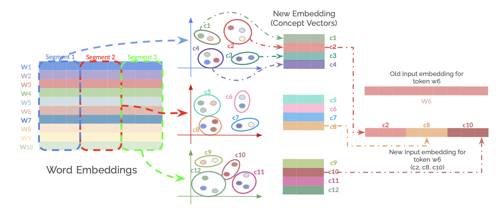
Figure 1: Overview of the Aggregate Semantic Grouping (ASG) method for creating compositional token embeddings. Product Quantization is applied to the original word embedding layer. Embeddings are segmented into $m$ sub-vectors. For each of the $m$ segment positions, k-means clustering is performed on the corresponding sub-vectors from all tokens to learn a codebook of $k$ Concept Vectors (centroids). The new ASG embedding layer containing these learned Concept Vectors is initialized as the embedding layer. Instead of using the original input embedding for a token ‘w’, a sequence of $m$ ConceptIDs used to get their respective Concept Vectors from the ASG layer, these are then concatenated to form the new representation for token ‘w’.
To address these limitations, we introduce Aggregate Semantic Grouping (ASG). ASG maintains concept-level sharing but represents tokens as sequences of ‘conceptIDs’, thereby accumulating multiple semantic facets. This sequence-based representation is inspired by successful applications in information and generative retrieval Wang et al. (2022); Tay et al. (2022); Zhou et al. (2022). We employ Product Quantization (PQ) (Jégou et al., 2011) to transform tokens into these conceptID sequences, aiming to preserve token’s uniqueness and nuances while benefiting from shared semantics.
Our primary contribution is the introduction of Aggregate Semantic Grouping (ASG), a novel method leveraging Product Quantization to represent tokens as sequences of shared ConceptIDs, thereby capturing multiple semantic facets while significantly compressing embedding layer parameters. We provide a detailed methodology for applying ASG to both encoder and encoder–decoder transformer models. Conducting experiments across diverse tasks (NLI, NER, QA) and models (mBERT, XLM-R, mT5), we demonstrate that even with extreme compression on embeddings (down to 0.4–0.5% of the original embedding parameters), ASG maintains high performance (often $>$ 95% relative to baseline) and outperforms the prior semantic grouping method (Zhang et al., 2024), including in zero-shot cross-lingual transfer scenarios. Furthermore, we extend our evaluation to a domain-specific benchmark (BC5CDR; Li et al., 2016) and a domain-specialized model (BioBERT; Lee et al., 2020), where ASG achieves similar robustness, confirming its applicability beyond general-domain tasks. The code will be available at https://github.com/KavinRV/Aggregate-Semantic-Grouping.
2 Aggregate Semantic Grouping (ASG)
Our approach, Aggregate Semantic Grouping, reframes token representation by learning compositional embeddings from pre-trained models.
2.1 Learning Concept Vectors via Product Quantization
We begin with a pre-trained word embedding matrix $E$ , where each row is a $D$ -dimensional vector for a token in a vocabulary of size $V$ . Using Product Quantization (PQ), each $D$ -dimensional embedding is first divided into $m$ distinct segments (sub-vectors), each of dimension $D/m$ . For each of these $m$ segment positions, we apply k-means clustering to the collection of all corresponding segments from every token in the vocabulary. This process yields $m$ distinct codebooks; each codebook $C_{i}$ (for $i=0,...,m-1$ ) contains $k$ centroids, termed Concept Vectors, specific to that segment position. Each Concept Vector is of dimension $D/m$ .
2.2 ASG Embedding Layer Initialization
The $m$ distinct codebooks ( $C_{0},C_{1},...,C_{m-1}$ ), where each codebook $C_{i}$ contains $k$ Concept Vectors of dimension $D/m$ , are concatenated to form a single, new embedding matrix $E^{\prime}$ . This matrix $E^{\prime}$ has dimensions $(m× k)×(D/m)$ and stores all unique Concept Vectors. Specifically, the $j$ -th Concept Vector (where $j∈[0,k-1]$ ) from the $i$ -th codebook $C_{i}$ is located at row $i× k+j$ within $E^{\prime}$ .
Each token is then mapped to a sequence of $m$ ConceptIDs. For each of its $m$ embedding segments, the corresponding ConceptID is the specific row index in $E^{\prime}$ that stores the chosen Concept Vector for that segment. This row index is determined as $i× k+s_{i}$ , where $i$ is the segment index (from $0$ to $m-1$ ) and $s_{i}$ is the index (from $0$ to $k-1$ ) of the selected centroid from the $i$ -th segment’s codebook. This sequence of $m$ row indices (ConceptIDs) thus identifies the set of Concept Vectors representing the token.
Table 1: Evaluation results across cluster granularities for mBert and XLM-R on multilingual benchmarks. Scores include F1, Accuracy, and relative performance (%Base). For XNLI %Base is for the accuracy relative to the base model. 40% SG: Semantic Grouping as mentioned in Zhang et al. (2024). In the Zero-Shot setting the models were trained on english dataset and have been tested on all the languages.
| mBERT | 100.00 | 100.00 | 75.46 | 74.79 | 100.00 | 89.74 | 100.00 | 64.86 | 100.00 | 58.58 | 100.00 |
| --- | --- | --- | --- | --- | --- | --- | --- | --- | --- | --- | --- |
| -40% SG | 40.00 | 68.95 | 72.43 | 71.88 | 95.99 | 86.69 | 96.61 | 60.64 | 93.49 | 52.35 | 89.37 |
| -ASG( $k$ =512, $m$ =48) | 0.50 | 48.65 | 73.51 | 72.84 | 97.42 | 88.11 | 98.19 | 61.30 | 94.51 | 55.71 | 95.10 |
| XLM-R | 100.00 | 100.00 | 77.98 | 77.28 | 100.00 | 88.37 | 100.000 | 71.94 | 100.00 | 58.74 | 100.00 |
| -40% SG | 40.00 | 58.48 | 74.56 | 73.96 | 95.61 | 84.57 | 95.70 | 65.83 | 91.51 | 51.48 | 87.65 |
| -ASG( $k$ =1024, $m$ =48) | 0.40 | 31.08 | 77.06 | 76.39 | 98.81 | 86.53 | 97.92 | 68.05 | 67.39 | 54.46 | 92.72 |
2.3 Token Representation with ASG
When a token is processed, its pre-computed sequence of $m$ ConceptIDs is used to retrieve the corresponding $m$ Concept Vectors from their respective codebooks within $E^{\prime}$ . Let these retrieved Concept Vectors be $v_{0},v_{1},...,v_{m-1}$ , where each $v_{i}$ has dimension $D/m$ . The final ASG representation for the token, $e^{\prime}∈\mathbb{R}^{D}$ , is obtained by concatenating these $m$ Concept Vectors:
$$
e^{\prime}=\text{concat}(v_{0},v_{1},\dots,v_{m-1}) \tag{1}
$$
This vector $e^{\prime}$ serves as the input to subsequent layers of the model.
2.4 Application to Generative Models
For model with decoder, which have separate input and output embedding layers (the latter often serving as token classifier weights), we apply the ASG process to both. This results in two distinct ASG embedding structures: one for input token representations ( $E^{\prime}$ ) and another for the output layer ( $OE^{\prime}$ ), each derived from their respective original embedding matrices.
Table 2: Evaluation results for Generative models across cluster granularities for mT5 on TyDiQA and WikiANN. Seperate: 1 codebook per segment, Shared: codebooks shared across all segments, In the Zero-Shot setting the models were trained on English dataset and have been tested on all the languages.
| Model | Parameter Reduced to (%) | TyDIQA | WikiANN | WikiANN (Zero-Shot) | | | | | | |
| --- | --- | --- | --- | --- | --- | --- | --- | --- | --- | --- |
| Embedding | Model | F1 | EM | %Base | F1 | %Base | F1 | %Base | | |
| mT5 | 100.00 | 100.00 | 70.74 | 56.20 | 100.00 | 84.21 | 100.00 | 50.75 | 100.00 | |
| ASG Separate | -( $k=1024,m=32$ ) | 0.45 | 15.06 | 60.67 | 46.15 | 85.76 | 79.85 | 94.82 | 25.84 | 50.91 |
| -( $k=2048,m=32$ ) | 0.85 | 15.41 | 63.81 | 49.06 | 90.19 | 80.93 | 96.11 | 29.85 | 58.82 | |
| -( $k=8192,m=32$ ) | 3.32 | 17.51 | 66.22 | 51.71 | 93.61 | 82.19 | 97.60 | 33.51 | 66.03 | |
| -( $k=1024,m=64$ ) | 0.45 | 15.06 | 69.96 | 55.53 | 98.89 | 83.18 | 98.78 | 44.02 | 86.74 | |
| ASG Shared | -( $k=16384,m=32$ ) | 0.25 | 14.89 | 66.50 | 51.90 | 93.99 | 81.65 | 96.96 | 34.01 | 67.02 |
| -( $k=32768,m=32$ ) | 0.45 | 15.06 | 67.00 | 53.06 | 94.71 | 82.04 | 97.42 | 37.01 | 72.92 | |
| -( $k=32768,m=64$ ) | 0.25 | 14.89 | 70.81 | 56.51 | 100.09 | 84.19 | 99.97 | 47.23 | 93.06 | |
Output Logit Calculation: To compute the logit $l_{t}$ for a target token $t$ , the final hidden state $H∈\mathbb{R}^{D}$ from the model is first segmented into $m$ parts: $H=[H_{0},H_{1},...,H_{m-1}]$ , where each $H_{i}∈\mathbb{R}^{D/m}$ . Let the sequence of Concept Vectors for token $t$ be $u_{t,0},u_{t,1},...,u_{t,m-1}∈ OE^{\prime}$ . The logit is calculated as:
$$
l_{t}=\sum_{i=0}^{m-1}H_{i}\cdot u_{t,i} \tag{2}
$$
3 Experiments and Results
3.1 Datasets
We evaluate our proposed ASG method on diverse cross-lingual benchmarks for natural language inference (NLI), question answering (QA), and named entity recognition (NER). These include: XNLI (Conneau et al., 2018), a 15-language sentence understanding benchmark; the Gold Passage (GoldP) task of TyDi QA (Clark et al., 2020), an 11-language QA dataset where gold context is provided; and the XTREME benchmark version (Hu et al., 2020) of WikiANN (Pan et al., 2017), a 40-language NER dataset.
3.2 Settings
For $k$ , values were generally chosen as powers of two. This allowed us to systematically target specific levels of embedding parameter compression, aiming for reductions that brought the ASG embedding layer size to approximately 0.5%, 1%, and 4% of the original embedding parameters. Regarding the number of subspaces $m$ , our explorations indicated that too few subspaces (e.g., $m=16$ ) resulted in a significant degradation of model performance. Conversely, using very high values for $m$ (e.g., 128, 256, or 512), would lead to extremely small dimensions for each segment ( $D/m$ , potentially as low as 4, 2, or 1 for common embedding sizes $D$ ) and would consequently require very long sequences of ConceptIDs (length $m$ ) to represent each token. These considerations led us to focus on $m$ values within a moderate range for the experiments detailed below.
3.3 Fine-tuning Performance
We evaluated ASG on encoder-only mBERT (Devlin et al., 2019) and XLM-R (Conneau et al., 2019) models using the XNLI and WikiANN datasets, mainly to compare it’s effectiveness against the Semantic grouping as mention in Zhang et al. (2024). As demonstrated in Table 1, ASG achieves significant embedding compression while maintaining over 97% of baseline performance and notably outperforms Semantic Grouping (SG) method, even with a low $k$ value.
To assess ASG for generative tasks, we then evaluated the mT5 model (Xue et al., 2020) on the TyDiQA and WikiANN datasets, applying ASG to both its input and output embeddings. Table 2, detailing results for various cluster ( $k$ ) and subspace ( $m$ ) configurations, shows ASG consistently achieved over 85% of baseline mT5 performance. Specifically, with $k≥ 2048$ , relative performance on TyDiQA surpassed 90%, while on WikiANN, ASG configurations generally exceeded 95% of the baseline.
Furthermore, for mT5, we investigated a variant employing a single shared codebook across all $m$ subspaces. To achieve this, the $m$ segments from all token embeddings in the vocabulary are pooled together before applying k-means clustering. This yields one global codebook of Concept Vectors. Each of the $m$ ConceptIDs for a token then selects a Concept Vector from this single shared codebook to represent its corresponding segment. This shared codebook is then used across all $m$ positions for constructing the token representation. This approach, despite reducing the diversity of available Concept Vectors, impressively maintained over 95% relative performance across both TyDiQA and WikiANN. This suggests that a highly restricted set of output Concept Vectors can still be effective for generative tasks.
3.4 Domain-Specific Evaluation (BC5CDR)
| BERT-base -40% SG -ASG ( $k{=}128$ , $m{=}48$ ) | 100 40 0.81 | 100.00 87.64 79.50 | 85.58 81.57 83.90 | 100.00 95.32 98.03 |
| --- | --- | --- | --- | --- |
| -ASG ( $k{=}512$ , $m{=}48$ ) | 2.13 | 79.77 | 85.24 | 99.60 |
Table 3: BERT-base fine-tuned on BC5CDR.
To further validate ASG in specialized settings, we evaluate on the BC5CDR Named Entity Recognition task Li et al. (2016), a biomedical benchmark focused on identifying chemical and disease entities. This task poses strong vocabulary-specific requirements, making it a challenging testbed for compressed embeddings.
We compare BioBERT Lee et al. (2020) and BERT-base with standard embeddings, Semantic Grouping (SG), and ASG under varying compression levels. Results are reported in F1 score and relative performance (%Base).
| BioBERT -40% SG -ASG( $k{=}128$ , $m{=}48$ ) | 100 40 0.81 | 100.00 87.64 79.50 | 89.48 86.71 87.78 | 100.00 96.90 98.10 |
| --- | --- | --- | --- | --- |
| -ASG( $k{=}512$ , $m{=}48$ ) | 2.13 | 79.77 | 88.93 | 99.39 |
Table 4: BioBERT fine-tuned on BC5CDR.
Across both backbones, ASG preserves high task performance under strong embedding compression. Even at $<1\%$ of the original embedding size, ASG recovers over 98% of the base model performance. These results demonstrate that ASG generalizes beyond general-domain benchmarks to biomedical NER.
3.5 Cross-Lingual Transfer (Zero-Shot)
For zero-shot cross-lingual transfer, we followed the experimental setup of Zhang et al. (2024). Models were trained solely on the English XNLI and WikiANN training sets and then evaluated on the multilingual test sets of these datasets. In this setting, ASG-enhanced models outperformed the Semantic Grouping method. While generative models using ASG with lower $k$ (clusters per segment) and $m$ (segments) values showed reduced performance in cross-lingual transfer (Table 2), configurations with $m=64$ segments nonetheless achieved at least 86% relative to baseline model performance. Using shared codebook, the performance further improved upto 93% relative to the baseline model, with just 0.25% of the embedding parameters.
3.6 Qualitative Analysis
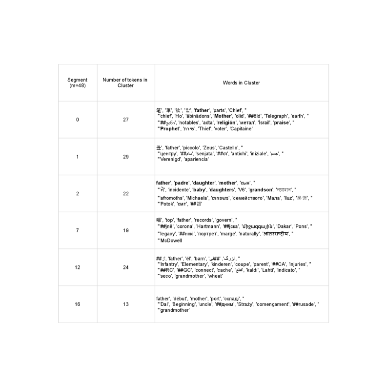
Figure 2 illustrates how Aggregate Semantic Grouping (ASG) captures varied semantic facets of the token "father" through its clustering across selected segments:
- Familial Context: "father" clusters with kinship terms such as "padre" (father), "mother", and "daughter" (Segment 2), or "barn" (child), "parent", and "grandmother" (Segment 12; also Segment 16), reflecting its primary familial sense.
- Authority/Religious Context: In Segment 0, "father" groups with "Chief", "Prophet", "notables", and "religión", indicating connotations of leadership or religious reverence.
- Figurative/Abstract Contexts: Other segments link "father" to broader concepts, such as "Zeus" (mythological father figure), or with terms like "records", "govern", and "legacy" (Segment 7), potentially reflecting historical origin, or the act of establishing something significant.
4 Conclusion
This work investigated equipping language models with shared, compositional token representations as an alternative to traditional monolithic embeddings. We explored this through Aggregate Semantic Grouping (ASG), where Product Quantization transforms embeddings into sequences of ConceptIDs that map to shared, learned Concept Vectors, enabling multifaceted semantic capture alongside significant compression. Extensive experiments on diverse models (including mBERT, XLM-R, and mT5) and NLU tasks (such as NLI, NER, and QA) found ASG maintains high performance (often >95% relative to baseline) despite extreme parameter reduction (to <1% of original size). ASG also outperformed prior semantic grouping methods, and proved effective for generative architectures. These findings confirm that ASG’s decomposition of tokens into shared components offers an efficient, semantically rich, and promising direction for language modeling; future work may explore dynamic or adaptive quantization techniques.
5 Limitations
ASG was applied directly to word embeddings from pre-trained models without an explicit cross-lingual alignment step, which could refine Concept Vector clustering. This may partly explain the observed performance degradation in generative tasks within cross-lingual settings, such as on WikiANN, where better nuance preservation through alignment-optimized clustering could be beneficial. Furthermore, we did not undertake continual pre-training of the models with the ASG embeddings; such a phase could allow models to more effectively adapt to the compositional representations and potentially enhance overall performance. Complementary to this, methods similar GraphMerge Wu and Monz (2023), could potentially be combined with ASG to pre-align embeddings before clustering, leading to more coherent ConceptID assignments.
References
- Clark et al. (2020) Jonathan H Clark, Eunsol Choi, Michael Collins, Dan Garrette, Tom Kwiatkowski, Vitaly Nikolaev, and Jennimaria Palomaki. 2020. Tydi qa: A benchmark for information-seeking question answering in ty pologically di verse languages. Transactions of the Association for Computational Linguistics, 8:454–470.
- Conneau et al. (2019) Alexis Conneau, Kartikay Khandelwal, Naman Goyal, Vishrav Chaudhary, Guillaume Wenzek, Francisco Guzmán, Edouard Grave, Myle Ott, Luke Zettlemoyer, and Veselin Stoyanov. 2019. Unsupervised cross-lingual representation learning at scale. arXiv preprint arXiv:1911.02116.
- Conneau et al. (2018) Alexis Conneau, Guillaume Lample, Ruty Rinott, Adina Williams, Samuel R Bowman, Holger Schwenk, and Veselin Stoyanov. 2018. Xnli: Evaluating cross-lingual sentence representations. arXiv preprint arXiv:1809.05053.
- Devlin et al. (2019) Jacob Devlin, Ming-Wei Chang, Kenton Lee, and Kristina Toutanova. 2019. Bert: Pre-training of deep bidirectional transformers for language understanding. In Proceedings of the 2019 conference of the North American chapter of the association for computational linguistics: human language technologies, volume 1 (long and short papers), pages 4171–4186.
- Hu et al. (2020) Junjie Hu, Sebastian Ruder, Aditya Siddhant, Graham Neubig, Orhan Firat, and Melvin Johnson. 2020. Xtreme: A massively multilingual multi-task benchmark for evaluating cross-lingual generalisation. In International conference on machine learning, pages 4411–4421. PMLR.
- Jégou et al. (2011) Herve Jégou, Matthijs Douze, and Cordelia Schmid. 2011. Product quantization for nearest neighbor search. IEEE Transactions on Pattern Analysis and Machine Intelligence, 33(1):117–128.
- Lee et al. (2020) Jinhyuk Lee, Wonjin Yoon, Sungdong Kim, Donghyeon Kim, Sunkyu Kim, Chan Ho So, and Jaewoo Kang. 2020. Biobert: a pre-trained biomedical language representation model for biomedical text mining. Bioinformatics, 36(4):1234–1240.
- Li et al. (2016) Jiao Li, Yueping Sun, Robin J. Johnson, Daniela Sciaky, Chih-Hsuan Wei, Robert Leaman, Allan Peter Davis, Carolyn J. Mattingly, Thomas C. Wiegers, and Zhiyong Lu. 2016. Biocreative V CDR task corpus: a resource for chemical disease relation extraction. Database J. Biol. Databases Curation, 2016.
- Pan et al. (2017) Xiaoman Pan, Boliang Zhang, Jonathan May, Joel Nothman, Kevin Knight, and Heng Ji. 2017. Cross-lingual name tagging and linking for 282 languages. In Proceedings of the 55th Annual Meeting of the Association for Computational Linguistics (Volume 1: Long Papers), pages 1946–1958, Vancouver, Canada. Association for Computational Linguistics.
- Park et al. (2024) Kiho Park, Yo Joong Choe, Yibo Jiang, and Victor Veitch. 2024. The geometry of categorical and hierarchical concepts in large language models. arXiv preprint arXiv:2406.01506.
- Park et al. (2023) Kiho Park, Yo Joong Choe, and Victor Veitch. 2023. The linear representation hypothesis and the geometry of large language models. arXiv preprint arXiv:2311.03658.
- Shani et al. (2025) Chen Shani, Dan Jurafsky, Yann LeCun, and Ravid Shwartz-Ziv. 2025. From tokens to thoughts: How llms and humans trade compression for meaning. arXiv preprint arXiv:2505.17117.
- Tay et al. (2022) Yi Tay, Vinh Tran, Mostafa Dehghani, Jianmo Ni, Dara Bahri, Harsh Mehta, Zhen Qin, Kai Hui, Zhe Zhao, Jai Gupta, and 1 others. 2022. Transformer memory as a differentiable search index. Advances in Neural Information Processing Systems, 35:21831–21843.
- Wang et al. (2022) Yujing Wang, Yingyan Hou, Haonan Wang, Ziming Miao, Shibin Wu, Qi Chen, Yuqing Xia, Chengmin Chi, Guoshuai Zhao, Zheng Liu, and 1 others. 2022. A neural corpus indexer for document retrieval. Advances in Neural Information Processing Systems, 35:25600–25614.
- Wu and Monz (2023) Di Wu and Christof Monz. 2023. Beyond shared vocabulary: Increasing representational word similarities across languages for multilingual machine translation. In Proceedings of the 2023 Conference on Empirical Methods in Natural Language Processing, pages 9749–9764, Singapore. Association for Computational Linguistics.
- Xue et al. (2020) Linting Xue, Noah Constant, Adam Roberts, Mihir Kale, Rami Al-Rfou, Aditya Siddhant, Aditya Barua, and Colin Raffel. 2020. mt5: A massively multilingual pre-trained text-to-text transformer. arXiv preprint arXiv:2010.11934.
- Zhang et al. (2024) Xinyu Zhang, Jing Lu, Vinh Q Tran, Tal Schuster, Donald Metzler, and Jimmy Lin. 2024. Tomato, tomahto, tomate: Measuring the role of shared semantics among subwords in multilingual language models. arXiv preprint arXiv:2411.04530.
- Zhou et al. (2022) Yujia Zhou, Jing Yao, Zhicheng Dou, Ledell Wu, Peitian Zhang, and Ji-Rong Wen. 2022. Ultron: An ultimate retriever on corpus with a model-based indexer. arXiv preprint arXiv:2208.09257.
Table 5: Model Configurations and Embedding Parameters for ASG, Underlined uses a shared codebook
| Model | k | m | Parameters | Embedding Shape (Dim) |
| --- | --- | --- | --- | --- |
| mBERT | N/A | N/A | 177M | [ 120k, 768] |
| 512 | 48 | 86M | [ 30k, 16] | |
| XLM-R | N/A | N/A | 277M | [ 250k, 768] |
| 1024 | 48 | 86M | [ 49k, 16] | |
| mT5 | N/A | N/A | 300M | [ 256k, 512] |
| 1024 | 32 | 45M | [ 36k, 16] | |
| 2048 | 32 | 46M | [ 68k, 16] | |
| 8192 | 32 | 53M | [ 265k, 16] | |
| 16384 | 32 | 44M | [ 20k, 16] | |
| 32768 | 32 | 45M | [ 36k, 16] | |
| 32768 | 64 | 44M | [ 39k, 8] | |
| 1024 | 64 | 45M | [ 72k, 8] | |
Appendix A Experimental Setup
All our experiments are conducted using the smallest available checkpoint for each respective pre-trained model. Training is performed with a batch size of 128, and all experiments were run on a single Nvidia L40 GPU.
For the encoder models (mBERT and XLM-R), we set a weight decay of $0.01$ . The learning rate was $5× 10^{-6}$ for XNLI experiments and $5× 10^{-5}$ for WikiANN experiments. These models were trained for 2 epochs; for cross-lingual transfer settings, training was extended to 5 epochs. The mT5 model was trained with a learning rate of $1× 10^{-3}$ .
Product Quantization is implemented using the nanopq library https://github.com/matsui528/nanopq. For the k-means clustering within nanopq we use the faiss library https://faiss.ai/.
Appendix B Parameter Reduction Calculation
In a standard model, the token embedding table has shape $(V,D)$ , where $V$ is the vocabulary size and $D$ is the embedding dimension.
With ASG, the embedding layer is replaced by $m$ codebooks, each with $k$ Concept Vectors of size $D/m$ . The ASG embedding matrix thus has shape:
$$
(k\cdot m,\tfrac{D}{m})
$$
The number of parameters becomes:
$$
k\cdot m\cdot\tfrac{D}{m}=k\cdot D
$$
So the ratio of ASG to original embedding parameters is:
$$
\frac{k\cdot D}{V\cdot D}=\frac{k}{V}
$$
For example, in XLM-R with $V=250{,}000$ , $k=1024$ , and $m=48$ , the ASG matrix has shape $(49{,}000,16)$ , and the compression ratio is:
$$
\frac{49{,}000\cdot 16}{250{,}000\cdot 768}\approx 0.0040\,(=0.4\%).
$$
Appendix C Token-to-ConceptID Mapping Matrix.
Each token is mapped to a sequence of $m$ ConceptIDs (integers in $[0,k)$ ), forming a matrix of shape $(V,m)$ . This mapping is:
- Not a parameter: it is precomputed, fixed, and non-trainable.
- Stored externally and could be used during tokenization.
- Extremely compact, as it contains only small integers.
For $V=250$ k and $m=48$ , this mapping can be stored with an overhead of $\sim 2\%$ ( $15$ MB) or $\sim 2.15\%$ ( $16.5$ MB) of the memory required for the original embedding matrix, when $k=1024$ or $k=2048$ respectively.
Appendix D ASG Configuration and Embedding Parameters
Table 5 provides a summary of the configurations used for Aggregate Semantic Grouping (ASG) across different models, alongside details for the original base models. The table specifies the choices for $k$ (number of centroids per subspace) and $m$ (number of subspaces) for each ASG setup. It also lists the resulting total number of parameters in the model and the shape of the embbeding layer.
<details>
<summary>x1.png Details</summary>
### Visual Description
## Table: Word Clusters by Segment
### Overview
The image presents a table that categorizes words into clusters based on segments. The table has three columns: "Segment (m=48)", "Number of tokens in Cluster", and "Words in Cluster". Each row represents a different segment and lists the number of tokens (words) belonging to that segment's cluster, along with the words themselves.
### Components/Axes
* **Columns:**
* **Segment (m=48):** Identifies the segment number. The total number of segments is indicated as m=48.
* **Number of tokens in Cluster:** Indicates the number of words (tokens) that belong to the cluster for that segment.
* **Words in Cluster:** Lists the words that belong to the cluster for that segment. The words are enclosed in single quotes and separated by commas.
* **Rows:** Each row represents a different segment, with the segment number, the number of tokens in its cluster, and the words in the cluster.
### Detailed Analysis
Here's a breakdown of the table's content, row by row:
* **Segment 0:**
* Number of tokens: 27
* Words: '笔', '筆', '钦', '', 'father', 'parts', 'Chief', 'chief', 'Ho', 'äbinädons', 'Mother', 'olid', '##öld', 'Telegraph', 'earth', '##360', 'notables', 'adta', 'religión', 'метал', 'Israil', 'praise', 'Prophet', 'שרת', 'Thief', 'voter', 'Capitaine'
* Languages: Chinese, English, German, Spanish, Russian, Hebrew, French
* **Segment 1:**
* Number of tokens: 29
* Words: '丑', 'father', 'piccolo', 'Zeus', 'Castello', 'центру', '##سام', 'senjata', '##', 'antichi', 'iniziale', 'جسم', 'Verenigd', 'apariencia'
* Languages: Chinese, English, Italian, Russian, Arabic, Dutch, Spanish
* **Segment 2:**
* Number of tokens: 22
* Words: 'father', 'padre', 'daughter', 'mother', 'сын', 'ते', 'incidente', 'baby', 'daughters', 'V6', 'grandson', 'লয়াহান', 'afromoths', 'Michaela', 'משפחתו', 'семейството', 'Мала', 'Iluz', '운영', 'Potok', 'смт', '##캡'
* Languages: English, Spanish, Russian, Hindi, Bengali, Hebrew, Bulgarian, Ukrainian, Korean
* **Segment 7:**
* Number of tokens: 19
* Words: '떼', 'top', 'father', 'records', 'govern', '##jnë', 'corona', 'Hartmann', '##jска', 'Uհqսqqային', 'Dakar', 'Pons', 'legacy', '##нскі', 'портрет', 'marge', 'naturally', 'आंतरराष्ट्रीय', 'McDowell'
* Languages: Korean, English, Albanian, Russian, Armenian, Marathi
* **Segment 12:**
* Number of tokens: 24
* Words: '##', 'father', 'el', 'barn', '## بزرگ', 'Infantry', 'Elementary', 'kinderen', 'coupe', 'parent', '##CA', 'injuries', '##RC', '##GC', 'connect', 'cache', 'قطع', 'kaldı', 'Lahti', 'indicato', 'seco', 'grandmother', 'wheat'
* Languages: English, Spanish, Dutch, French, Arabic, Turkish, Finnish, Italian
* **Segment 16:**
* Number of tokens: 13
* Words: 'father', 'début', 'mother', 'port', 'складі', 'Dal', 'Beginning', 'uncle', '##дним', 'Straży', 'començament', '##rusade', 'grandmother'
* Languages: English, French, Ukrainian, Polish, Portuguese
### Key Observations
* The segments contain a mix of words from different languages.
* Some words are preceded by '##', which might indicate a specific encoding or tagging.
* The number of tokens in each cluster varies, ranging from 13 to 29.
* The word "father" appears in most of the clusters.
### Interpretation
The table appears to be the result of a text analysis process where words have been grouped into clusters based on some criteria, possibly semantic similarity or co-occurrence. The presence of multiple languages suggests that the analysis was performed on a multilingual corpus. The '##' prefix might indicate that these are special tokens or that the words have been processed in some way (e.g., stemming or lemmatization). The consistent presence of "father" across multiple clusters could indicate its central role in the dataset or a bias in the clustering algorithm. The varying number of tokens per cluster suggests different levels of coherence or specificity within each segment.
</details>
Figure 2: Grouping of the token "father" at a few selected subspaces