2509.21154v2

# GRPO is Secretly a Process Reward Model **Authors**: - Michael Sullivan (Department of Language Science and Technology) - Saarland Informatics Campus (Saarland University, Saarbrücken, Germany) Abstract We prove theoretically that the GRPO RL algorithm induces a non-trivial process reward model (PRM), under certain assumptions regarding within-group overlap of token sequences across completions. We then show empirically that these assumptions are met under real-world conditions: GRPO does in fact induce a non-trivial PRM. Leveraging the framework of GRPO-as-a-PRM, we identify a flaw in the GRPO objective: non-uniformly distributed process steps hinder both exploration and exploitation (under different conditions). We propose a simple modification to the algorithm to mitigate this defect ( $\lambda$ -GRPO), and show that LLMs trained with $\lambda$ -GRPO achieve higher validation accuracy and performance on downstream reasoning tasks—and reach peak performance more rapidly—than LLMs trained with standard GRPO. Our results call into question the advantage of costly, explicitly-defined PRMs for GRPO: we show that it is possible to instead leverage the hidden, built-in PRM structure within the vanilla GRPO algorithm to boost model performance with a negligible impact on training time and cost. 1 Introduction Process reward models (PRMs)—models that assign reward to intermediate steps (see Section 2.2)—allow for finer-grained reward assignment than outcome-level signals, thereby yielding improved multi-step reasoning performance (Lightman et al., 2024). PRMs are therefore particularly applicable to RL training for step-by-step processes such as mathematical reasoning. However, training neural PRMs requires costly, step-level human annotation (Zhang et al., 2025), and such models are particularly susceptible to reward hacking (Cui et al., 2025). These shortcomings have resulted in the limited adoption of learned PRMs for RL training Setlur et al. (2025), leading to the development of Monte-Carlo-based and other heuristic, non-neural PRMs (e.g. Wang et al., 2024; Kazemnejad et al., 2025; Hou et al., 2025). PRMs are typically employed with RL algorithms such as Proximal Policy Optimization (PPO; Schulman et al., 2017) that employ a critic model and/or generalized advantage estimation (GAE). Although Group Relative Policy Optimization (GRPO; Shao et al., 2024) greatly simplifies and reduces the memory consumption of RL training, leading to its adoption for a wide range of applications—e.g. tool use (Qian et al., 2025; Sullivan et al., 2025), RLHF (Yang et al., 2025b), and, in particular, mathematical reasoning (Shao et al., 2024; DeepSeek-AI, 2025) —it does so by eliminating the critic model and GAE of PPO (see Section 2.1). GRPO has therefore not been widely used with PRMs: to the best of our knowledge, Shao et al. (2024), Yang et al. (2025a), and Feng et al. (2025) are the only instances in which GRPO is employed with step-level rewards—and these approaches necessitate the modification of the algorithm to accommodate finer-grained reward signals. In this paper, we show that—under certain mild assumptions—GRPO induces a Monte-Carlo-based PRM (Section 3). Specifically, we prove theoretically that GRPO assigns rewards (and advantages) derived from outcome-level rewards and Monte-Carlo-sampled completions to sub-trajectories, whenever subsets of trajectories within each group share identical prefixes. We then show empirically that this identical-prefix condition is almost always met under real-world conditions, yielding rich step-level process reward structures. These two findings definitively demonstrate that the GRPO objective covertly assigns and optimizes for complex, structured step-level rewards and advantages. An investigation of the properties of GRPO’s hidden PRM reveals a defect in the objective function that hinders both exploration and exploitation (under different conditions) during RL training (Section 4): namely, a vulnerability to non-uniformly-distributed process steps within a group. To mitigate this shortcoming, we propose including a PRM-aware normalization factor into the GRPO loss function ( $\lambda$ -GRPO). We show that $\lambda$ -GRPO results in higher validation accuracy and a $\sim$ 2x training speedup over standard GRPO (Section 5). On downstream reasoning benchmarks, $\lambda$ -GRPO consistently improves over standard GRPO, demonstrating the superiority of our method. Our findings call into question the utility of dedicated PRMs for GRPO, and suggest that future work may benefit instead from exploiting the step-level reward signal already available to the GRPO algorithm. 2 Background 2.1 GRPO GRPO is a variant of PPO that discards the critic model and GAE of the latter. Instead, for each query $q$ in the training set, GRPO nondeterministically samples a group ${\mathbb{G}}$ of $k$ trajectories (completions to $q$ ) and computes the advantage ${a}_{i}$ for the completion $g^{(i)}∈{\mathbb{G}}$ relative to the mean (outcome) reward of ${\mathbb{G}}$ , as in Equation 1 (where ${r}_{i}$ is the reward for $g^{(i)}$ ). $$ {a}_{i}=\frac{{r}_{i}-r_{\text{{mean}}}({\mathbb{G}})}{r_{\text{{std}}}({\mathbb{G}})} \tag{1} $$ In our theoretical analysis in Section 3, we make two key assumptions: first, we assume the use of the DAPO token-level policy gradient objective (Yu et al., 2025), rather than sample-level loss. Although it differs from the original GRPO formulation laid out in Shao et al. (2024), Yu et al. (2025) show that this objective leads to more stable training, and it is the standard GRPO loss function employed in commonly-used RL packages (e.g. the TRL GRPO trainer https://huggingface.co/docs/trl/main/en/grpo_trainer). Second, we assume that the number of update iterations per batch ( $\mu$ ) is set to $\mu=1$ . Under this assumption, the ratio ${P}_{i,t}$ is fixed at $1.0$ (see Equation 2b), allowing us to ignore the clipping factor of the GRPO loss function in our theoretical analysis. Under these two assumptions, the per-group GRPO loss $L_{\text{GRPO}}({\mathbb{G}})$ reduces to that in Equation 2. $$ \displaystyle L_{\text{GRPO}}({\mathbb{G}})=\frac{1}{\sum_{g^{(i)}\in{\mathbb{G}}}\textit{len}(g^{(i)})}\sum_{g^{(i)}\in{\mathbb{G}}}\sum_{t=0}^{\textit{len}(g^{(i)})-1}({P}_{i,t}\cdot{a}_{i})-{D}_{i,t} $$ $$ {P}_{i,t}=\frac{\pi_{\theta}(g^{(i)}_{t}\hskip 2.84526pt|\hskip 2.84526ptq,g^{(i)}_{:t})}{\pi_{\theta_{\textit{old}}}(g^{(i)}_{t}\hskip 2.84526pt|\hskip 2.84526ptq,g^{(i)}_{:t})} $$ $$ {D}_{i,t}=\beta\cdot\left(\frac{\pi_{\theta_{\textit{ref}}}(g^{(i)}_{t}\hskip 2.84526pt|\hskip 2.84526ptq,g^{(i)}_{:t})}{\pi_{\theta}(g^{(i)}_{t}\hskip 2.84526pt|\hskip 2.84526ptq,g^{(i)}_{:t})}-\textit{ln}\frac{\pi_{\theta_{\textit{ref}}}(g^{(i)}_{t}\hskip 2.84526pt|\hskip 2.84526ptq,g^{(i)}_{:t})}{\pi_{\theta}(g^{(i)}_{t}\hskip 2.84526pt|\hskip 2.84526ptq,g^{(i)}_{:t})}-1\right) $$ 2.2 Process Reward Models (PRMs) Given an alphabet $\Sigma$ (i.e. set of tokens), we formally define a PRM as a function $f_{\phi}\colon\Sigma^{*}→(\Sigma^{*}×\mathbb{R})^{*}$ parameterized by $\phi$ that maps a trajectory $y∈\Sigma^{*}$ to the sequence $f_{\phi}(y)=((y_{:i_{1}},r^{(y)}_{0}),(y_{i_{1}:i_{2}},r^{(y)}_{1}),...,(y_{i_{n-1}:},r^{(y)}_{n-1}))$ of pairs of process steps (sub-trajectories) $y_{i_{k}:i_{k+1}}$ and step-level rewards $r^{(y)}_{k}$ . While PRMs are typically contrasted with outcome reward models (ORMs)—which assign a single reward to the entire trajectory—under the above definition, an ORM $f_{\phi^{\prime}}^{\prime}$ is simply a trivial PRM: i.e. $f_{\phi^{\prime}}^{\prime}(y)=((y,r^{(y)}_{0}))$ . Both the division of the trajectory $y$ into steps and the assignment of rewards to those steps are dependent upon the PRM in question. When trajectories are clearly delineated into individual steps—e.g. via ReACT-style prompting Yao et al. (2023) or instructing the model to divide its reasoning into demarcated steps—the PRM can simply be directed to assign a reward to each pre-defined step (e.g. Li & Li, 2025). In other cases, trajectories are heuristically split into steps—for example, at high-entropy tokens (e.g. Hou et al., 2025). Although the assignment of step-level reward can be performed by a model with learned parameters $\phi$ (e.g. Uesato et al., 2022), Kazemnejad et al. (2025) and Hou et al. (2025) combine Monte Carlo estimation with outcome-level rewards to yield heuristic PRMs that do not require the labor-intensive annotation of—and are less susceptible to reward-hacking than—their learned counterparts. In cases such as these in which the PRM $f_{\phi}$ is not learned, we simply consider $\phi$ to be fixed/trivial. 3 The PRM in the Machine <details> <summary>x1.png Details</summary>  ### Visual Description ## Hierarchical Diagram with Segmented Bars: Group Composition and Relationships ### Overview The image consists of two primary components: 1. **Left Side**: Six horizontal bars labeled `g^(1)` to `g^(6)`, each divided into colored segments with numerical labels (0-8). 2. **Right Side**: A hierarchical tree diagram (`G`) showing relationships between the `g^(i)` sets, with color-coded groupings and arrows indicating connections. --- ### Components/Axes #### Left Side (Segmented Bars) - **Labels**: `g^(1)` to `g^(6)` (top to bottom). - **Segments**: - Each bar is divided into colored segments with numerical labels (0-8). - Colors vary per bar, with no explicit legend provided for segment meanings. - **Example**: - `g^(1)`: Blue (0-1), Pink (2-4), Light Pink (5). - `g^(2)`: Orange (0-8). - `g^(3)`: Red (0-3), Green (4-6). - `g^(4)`: Red (0-3), Purple (4-5), Pink (6-8). - `g^(5)`: Red (0-3), Purple (4-5), Yellow (6-7). - `g^(6)`: Teal (0-4). #### Right Side (Hierarchical Diagram) - **Root Node**: `G = {g^(1), g^(2), g^(3), g^(4), g^(5), g^(6)}`. - **Branches**: - **First Level**: - Left: `{g^(1), g^(2)}` (Blue + Orange). - Center: `{g^(3), g^(4), g^(5)}` (Red + Green + Purple). - Right: `{g^(6)}` (Teal). - **Second Level**: - `{g^(1), g^(2)}` splits into `{g^(1)}` (Blue) and `{g^(2)}` (Orange). - `{g^(3), g^(4), g^(5)}` splits into `{g^(3)}` (Red), `{g^(4), g^(5)}` (Green + Purple). - `{g^(4), g^(5)}` splits into `{g^(4)}` (Green) and `{g^(5)}` (Purple). - **Legend**: Colors correspond to groupings (e.g., Blue = `{g^(1), g^(2)}`, Red = `{g^(3)}`). --- ### Detailed Analysis #### Left Side (Segmented Bars) - **g^(1)**: 6 segments (0-5). Colors: Blue (0-1), Pink (2-4), Light Pink (5). - **g^(2)**: 9 segments (0-8). Uniform Orange. - **g^(3)**: 7 segments (0-6). Colors: Red (0-3), Green (4-6). - **g^(4)**: 9 segments (0-8). Colors: Red (0-3), Purple (4-5), Pink (6-8). - **g^(5)**: 8 segments (0-7). Colors: Red (0-3), Purple (4-5), Yellow (6-7). - **g^(6)**: 5 segments (0-4). Uniform Teal. #### Right Side (Hierarchical Diagram) - **Root to Leaves Flow**: - `G` branches into three main groups, which further subdivide into individual `g^(i)` elements. - Colors in the diagram match the dominant colors of the corresponding `g^(i)` bars (e.g., `g^(3)` is Red in both the bar and diagram). --- ### Key Observations 1. **Color Consistency**: - Colors in the diagram (e.g., Blue for `{g^(1), g^(2)}`) align with the dominant colors in the left-side bars. - Example: `g^(3)` uses Red in both the bar and diagram. 2. **Segment Lengths**: - Bars vary in length: `g^(2)` and `g^(4)` are longest (9 segments), while `g^(6)` is shortest (5 segments). 3. **Hierarchical Grouping**: - The diagram suggests a taxonomy where `G` is the universal set, partitioned into subsets (e.g., `{g^(1), g^(2)}`, `{g^(3), g^(4), g^(5)}`, `{g^(6)}`). 4. **Numerical Labels**: - Numbers in segments (0-8) may represent identifiers, counts, or ordinal positions, but their semantic meaning is unclear without additional context. --- ### Interpretation - **Purpose of the Diagram**: - The hierarchical tree (`G`) likely represents a classification or dependency structure among the `g^(i)` elements. For example, `{g^(1), g^(2)}` could denote a shared category or relationship between these groups. - **Relationship Between Components**: - The left-side bars show the internal composition of each `g^(i)` (via colored segments), while the right-side diagram illustrates how these groups interrelate at higher levels. - **Notable Patterns**: - `g^(2)` and `g^(4)` have uniform colors (Orange and Pink/Purple, respectively), suggesting homogeneity within these groups. - `g^(3)` and `g^(5)` exhibit mixed colors, indicating potential subcategories or transitions. - **Uncertainties**: - The exact meaning of numerical labels (0-8) and segment colors remains ambiguous without domain-specific context. - The hierarchical diagram’s grouping logic (e.g., why `{g^(3), g^(4), g^(5)}` are grouped together) is not explicitly explained. --- ### Conclusion The image combines segmented bars (showing detailed compositions of `g^(i)`) with a hierarchical diagram (showing relationships between groups). While the visual structure is clear, the semantic interpretation of colors, numbers, and groupings requires additional context to fully resolve. 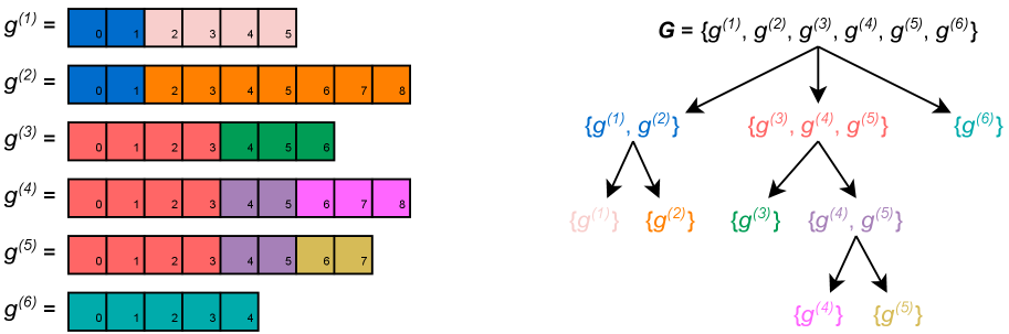</details> Figure 1: Toy example of a group ${\mathbb{G}}=\{g^{(1)},...,g^{(6)}\}$ (left) and its corresponding ${\mathcal{B}}({\mathbb{G}})$ tree (right). Tokens (boxes) are numbered for readability—subscripted numbers within boxes only indicate position. Each process set (node in the ${\mathcal{B}}({\mathbb{G}})$ tree) is a set of trajectories that share a common prefix, and corresponds to a process step (subtrajectory) spanning those shared tokens: in this figure, colored nodes in ${\mathcal{B}}({\mathbb{G}})$ correspond to those subsequences in ${\mathbb{G}}$ that span tokens/boxes of the same color Same-colored boxes in ${\mathbb{G}}$ indicate identical sequences of tokens across trajectories only: for example, $g^{(3)}_{:4}=g^{(4)}_{:4}$ and $g^{(4)}_{4:6}=g^{(5)}_{4:6}$ , but it is not necessarily the case that e.g. $g^{(3)}_{0}=g^{(3)}_{1}$ .. GRPO implicitly assigns a step-level reward and advantage to the tokens of each process step, which are computed as functions of the mean outcome-level reward of each trajectory in the corresponding process set. In Section 3.1, we prove that GRPO theoretically induces a PRM (given the assumptions of Section 2.1) as defined in Section 2.2. However, this PRM is only non-trivial—i.e. not equivalent to an ORM—if subsets of trajectories within each group share identical initial sub-trajectories. In Section 3.2, we empirically demonstrate that such rich, overlapping prefix structures arise very frequently under real-world conditions: this shows that GRPO is “secretly” a non-trivial PRM. 3.1 Theoretical Analysis Let ${\mathcal{B}}({\mathbb{G}})=\{\lambda⊂eq{\mathbb{G}}\hskip 2.84526pt|\hskip 2.84526pt∃ n≥ 0∀ g^{(i)},g^{(k)}∈\lambda\colon g^{(i)}_{:n}=g^{(k)}_{:n}\}$ be the set of all process sets: sets $\lambda⊂eq{\mathbb{G}}$ of completions such that all $g^{(i)}∈\lambda$ are identical up to the $n^{th}$ token, for some $n≥ 0$ (see Figure 2). Note that there is a natural tree structure on ${\mathcal{B}}({\mathbb{G}})$ , which is induced by the $⊃eq$ relation. Each $\lambda∈{\mathcal{B}}({\mathbb{G}})$ defines a process step within each $g^{(i)}∈\lambda$ , spanning the subsequence $g^{(i)}_{s(\lambda):e(\lambda)}$ from the $s(\lambda)^{th}$ to the $e(\lambda)^{th}$ tokens of $g^{(i)}$ . The endpoint $e(\lambda)$ is defined as the largest $n$ such that $g^{(i)}_{:n}=g^{(k)}_{:n}$ for all $g^{(i)},g^{(k)}∈\lambda$ , and $s(\lambda)$ is defined as the endpoint of the immediate parent $Pa_{{\mathcal{B}}({\mathbb{G}})}(\lambda)$ of $\lambda$ in the tree structure induced on ${\mathcal{B}}({\mathbb{G}})$ . $$ \begin{split}&e(\lambda)=\textit{max}\{n\geq 0\hskip 2.84526pt|\hskip 2.84526pt\forall g^{(i)},g^{(k)}\in\lambda:g^{(i)}_{:n}=g^{(k)}_{:n}\}\\ &s(\lambda)=\begin{cases}0&\text{if }\lambda=\textit{root}(\mathcal{B}(G))\\ e(Pa_{{\mathcal{B}}({\mathbb{G}})}(\lambda))&\text{otherwise}\end{cases}\end{split} $$ For example, $s(\{g^{(4)},g^{(5)}\})=e(\{g^{(3)},g^{(4)},g^{(5)}\})=4$ in Figure 2, and $e(\{g^{(4)},g^{(5)}\})=6$ : the process step corresponding to $\{g^{(4)},g^{(5)}\}$ spans $g^{(4)}_{4:6}$ and $g^{(5)}_{4:6}$ . For each $g^{(i)}∈{\mathbb{G}}$ and each $0≤ t<\textit{len}(g^{(i)})$ , let $\lambda^{(i,t)}∈{\mathcal{B}}({\mathbb{G}})$ denote the unique process set such that $g^{(i)}∈\lambda^{(i,t)}$ and $s(\lambda^{(i,t)})≤ t<e(\lambda^{(i,t)})$ . In other words, $\lambda^{(i,t)}$ is the process step to which the token $g^{(i)}_{t}$ belongs. In Figure 2, $\lambda^{(i,t)}$ corresponds to the set whose color matches that of $g^{(i)}_{t}$ : $\lambda^{(1,0)}=\{g^{(1)},g^{(2)}\}$ , $\lambda^{(1,3)}=\{g^{(1)}\}$ , $\lambda^{(5,5)}=\{g^{(4)},g^{(5)}\}$ , etc. Now, for each process step defined by some $\lambda∈{\mathcal{B}}({\mathbb{G}})$ , we define the step-level reward $\hat{R}(\lambda)$ via Monte Carlo estimation (Equation 3): $\hat{R}(\lambda)$ is the mean outcome-level reward of each trajectory in $\lambda$ . In other words, $\hat{R}(\lambda)$ is the mean reward of each leaf node dominated by $\lambda$ in the tree structure induced on ${\mathcal{B}}({\mathbb{G}})$ —i.e. of each sampled completion to the process step defined by $\lambda$ . $$ \hat{R}(\lambda)=\frac{\sum_{g^{(i)}\in\lambda}{r}_{i}}{|\lambda|} \tag{3} $$ For each trajectory $g^{(i)}∈{\mathbb{G}}$ and each $0≤ t<\textit{len}(g^{(i)})$ define the reward ${R}_{i,t}$ for the token $g^{(i)}_{t}$ as the reward of the process step to which $g^{(i)}_{t}$ belongs: ${R}_{i,t}=\hat{R}(\lambda^{(i,t)})$ . For example, in Figure 2, the step-level reward for the sub-trajectories $g^{(3)}_{:4}$ , $g^{(4)}_{:4}$ , $g^{(5)}_{:4}$ is the mean of the outcome-level rewards for $g^{(3)}$ , $g^{(4)}$ , and $g^{(5)}$ : ${R}_{3,0}=...={R}_{5,3}=\textit{mean}(\{{r}_{3},{r}_{4},{r}_{5}\})$ . By the definition given in Section 2.2, ${R}_{i,t}$ and ${\mathcal{B}}({\mathbb{G}})$ clearly define a PRM: each $g^{(i)}∈{\mathbb{G}}$ is mapped to the sequence $(g^{(i)}_{:s(\lambda_{1})},{R}_{i,0}),(g^{(i)}_{s(\lambda_{1}):s(\lambda_{2})},{R}_{i,s(\lambda_{1})}),...,(g^{(i)}_{s(\lambda_{n}):},{R}_{i,s(\lambda_{n})})$ , where $(\lambda_{0}={\mathbb{G}})→...→(\lambda_{n}=\{g^{(i)}\})$ is the unique path in the tree structure induced on ${\mathcal{B}}({\mathbb{G}})$ from the root ${\mathbb{G}}$ to the node $\{g^{(i)}\}$ . Now, define the step-level advantage ${A}_{i,t}$ for the token $g^{(i)}_{t}$ in an analogous manner to the original GRPO definition in Equation 1 —i.e. as the normalized difference between the step-level reward ${R}_{i,t}$ for $g^{(i)}_{t}$ and the mean reward of ${\mathbb{G}}$ : ${A}_{i,t}=({R}_{i,t}-r_{\textit{mean}}({\mathbb{G}}))/r_{\textit{std}}({\mathbb{G}})$ . Replacing the term ${a}_{i}$ with ${A}_{i,t}$ in Equation 2a yields a PRM-aware RL objective (Equation 4). $$ L_{\text{PRM}}({\mathbb{G}})=\frac{1}{\sum_{g^{(i)}\in{\mathbb{G}}}\textit{len}(g^{(i)})}\sum_{g^{(i)}\in{\mathbb{G}}}\sum_{t=0}^{\textit{len}(g^{(i)})-1}({P}_{i,t}\cdot\hbox{\pagecolor{yellow}$\displaystyle{A}_{i,t}$})-{D}_{i,t} \tag{4} $$ We now show that the standard GRPO objective defined in Equation 2a with outcome-level rewards ( $L_{\text{GRPO}}$ ) is equivalent to the PRM defined in Equations 3 - 4 ( $L_{\text{PRM}}$ ). **Theorem 1** *For any query $q$ , policy $\pi_{\theta}$ , and group ${\mathbb{G}}\sim\pi_{\theta}(\text{\textendash}\hskip 2.84526pt|\hskip 2.84526ptq)$ with outcome-level rewards $\{r_{i}\}_{g^{(i)}∈{\mathbb{G}}}$ : $L_{\text{GRPO}}({\mathbb{G}})=L_{\text{PRM}}({\mathbb{G}})$ .* * Proof* Let $\lambda$ be any process set in ${\mathcal{B}}({\mathbb{G}})$ , and let $t$ be any integer such that $s(\lambda)≤ t<e(\lambda)$ . We first prove that the sum of the PRM loss terms ${P}_{i,t}·{A}_{i,t}-{D}_{i,t}$ for each trajectory $g^{(i)}∈\lambda$ at the token $t$ is equivalent to the sum of the standard GRPO loss terms ${P}_{i,t}·{a}_{i}-{D}_{i,t}$ (Equation 5). Recall that for any $g^{(i)},g^{(k)}∈\lambda$ , $g^{(i)}_{:t+1}=g^{(k)}_{:t+1}$ by definition: therefore, ${P}_{i,t}={P}_{k,t}$ and ${D}_{i,t}={D}_{k,t}$ (Equations 2b - 2c). Again by definition, $g^{(i)},g^{(k)}∈\lambda$ implies that ${R}_{i,t}={R}_{k,t}=\hat{R}(\lambda)$ (Equation 3), and so ${A}_{i,t}={A}_{k,t}$ . As such, we may define $\hat{P}_{t}(\lambda)={P}_{k,t}$ , $\hat{D}_{t}(\lambda)={D}_{k,t}$ , and $\hat{A}(\lambda)={A}_{k,t}$ in Equation 5, choosing any arbitrary $g^{(k)}∈\lambda$ . $$ \begin{split}&\sum_{g^{(i)}\in\lambda}({P}_{i,t}\cdot{A}_{i,t})-{D}_{i,t}=|\lambda|\cdot((\hat{P}_{t}(\lambda)\cdot\hat{A}(\lambda))-\hat{D}_{t}(\lambda))\\ &=|\lambda|\cdot\left(\left(\hat{P}_{t}(\lambda)\cdot\frac{\hat{R}(\lambda)-r_{\textit{mean}}({\mathbb{G}})}{r_{\textit{std}}({\mathbb{G}})}\right)-\hat{D}_{t}(\lambda)\right)=|\lambda|\cdot\left(\left(\hat{P}_{t}(\lambda)\cdot\frac{\sum_{g^{(i)}\in\lambda}\frac{{r}_{i}}{|\lambda|}-r_{\textit{mean}}({\mathbb{G}})}{r_{\textit{std}}({\mathbb{G}})}\right)-\hat{D}_{t}(\lambda)\right)\\ &=\left(\hat{P}_{t}(\lambda)\frac{|\lambda|(\sum_{g^{(i)}\in\lambda}\frac{{r}_{i}}{|\lambda|}-r_{\textit{mean}}({\mathbb{G}}))}{r_{\textit{std}}({\mathbb{G}})}\right)-|\lambda|\hat{D}_{t}(\lambda)=\left(\hat{P}_{t}(\lambda)\frac{\sum_{g^{(i)}\in\lambda}{r}_{i}-\sum_{g^{(i)}\in\lambda}r_{\textit{mean}}({\mathbb{G}})}{r_{\textit{std}}({\mathbb{G}})}\right)-|\lambda|\hat{D}_{t}(\lambda)\\ &=\left(\sum_{g^{(i)}\in\lambda}{P}_{i,t}\frac{{r}_{i}-r_{\textit{mean}}({\mathbb{G}})}{r_{\textit{std}}({\mathbb{G}})}\right)-\sum_{g^{(i)}\in\lambda}{D}_{i,t}=\sum_{g^{(i)}\in\lambda}({P}_{i,t}\cdot{a}_{i})-{D}_{i,t}\end{split} \tag{5} $$ Now, letting $t_{\textit{max}}=\textit{max}_{g^{(i)}∈{\mathbb{G}}}\hskip 2.84526pt\textit{len}(g^{(i)})$ , for each $0≤ t<t_{\textit{max}}$ we can define a partition ${\mathbb{X}}_{t}⊂eq{\mathcal{B}}({\mathbb{G}})$ of $\{g^{(i)}∈{\mathbb{G}}\hskip 2.84526pt|\hskip 2.84526pt\textit{len}(g^{(i)})≤ t\}$ such that ${\mathbb{X}}_{t}=\{\lambda∈{\mathcal{B}}({\mathbb{G}})\hskip 2.84526pt|\hskip 2.84526pts(\lambda)≤ t<e(\lambda)\}$ is the set of all process sets corresponding to a token span containing the index $t$ . The GRPO loss term $L_{\text{GRPO}}({\mathbb{G}})$ (Equation 2a) can be equivalently expressed as in Equation 6 (and analogously for $L_{\text{PRM}}({\mathbb{G}})$ of Equation 4). $$ L_{\text{GRPO}}({\mathbb{G}})=\frac{1}{\sum_{g^{(i)}\in{\mathbb{G}}}\textit{len}(g^{(i)})}\cdot\sum_{t=0}^{t_{\textit{max}}-1}\sum_{\lambda\in{\mathbb{X}}_{t}}\sum_{g_{i}\in\lambda}({P}_{i,t}\cdot{a}_{i})-{D}_{i,t} \tag{6} $$ We then have the following equalities by Equations 5 and 6: $$ \begin{split}L_{\text{GRPO}}({\mathbb{G}})&=\frac{1}{\sum_{g^{(i)}\in{\mathbb{G}}}\textit{len}(g^{(i)})}\cdot\sum_{g^{(i)}\in{\mathbb{G}}}\sum_{t=0}^{\textit{len}(g^{(i)})-1}({P}_{i,t}\cdot{a}_{i})-{D}_{i,t}=\\ \frac{1}{\sum_{g^{(i)}\in{\mathbb{G}}}\textit{len}(g^{(i)})}\cdot\sum_{t=0}^{t_{\textit{max}}-1}&\sum_{\lambda\in{\mathbb{X}}_{t}}\sum_{g^{(i)}\in\lambda}({P}_{i,t}\cdot{a}_{i})-{D}_{i,t}=\frac{1}{\sum_{g^{(i)}\in{\mathbb{G}}}\textit{len}(g^{(i)})}\cdot\sum_{t=0}^{t_{\textit{max}}-1}\sum_{\lambda\in{\mathbb{X}}_{t}}\sum_{g^{(i)}\in\lambda}({P}_{i,t}\cdot{A}_{i,t})-{D}_{i,t}\\ &=\frac{1}{\sum_{g^{(i)}\in{\mathbb{G}}}\textit{len}(g^{(i)})}\cdot\sum_{g^{(i)}\in{\mathbb{G}}}\sum_{t=0}^{\textit{len}(g^{(i)})-1}({P}_{i,t}\cdot{A}_{i,t})-{D}_{i,t}=L_{\text{PRM}}({\mathbb{G}})\end{split} $$ ∎ In other words, the standard GRPO objective defined in Equation 2a automatically induces the PRM and PRM-aware objective defined in Equations 3 - 4. 3.2 Empirical Analysis The theoretical analysis in Section 3.1 shows that the GRPO objective induces a PRM: it remains to be shown, however, that this induced PRM is non-trivial. We refer to the set ${\mathcal{B}}({\mathbb{G}})$ of process sets as trivial if it contains only singleton sets And, by definition, ${\mathbb{G}}$ itself, with $s({\mathbb{G}})=e({\mathbb{G}})=0$ . —i.e. ${\mathcal{B}}({\mathbb{G}})=\{{\mathbb{G}}\}\cup\{\{g^{(i)}\}\hskip 2.84526pt|\hskip 2.84526ptg^{(i)}∈{\mathbb{G}}\}$ . If ${\mathcal{B}}({\mathbb{G}})$ is trivial, then there are no meaningful process steps within each trajectory, and only the outcome reward has an effect on learning. On the other hand, if ${\mathcal{B}}({\mathbb{G}})$ is not trivial, then Theorem 1 entails that the standard GRPO objective of Equation 2a induces a non-trivial PRM. To analyze the complexity of real-world, GRPO-derived step-level rewards, we empirically evaluated ${\mathcal{B}}({\mathbb{G}})$ structures generated during standard GRPO training: for each group ${\mathbb{G}}$ , we computed its ${\mathcal{B}}({\mathbb{G}})$ tree, and measured the number of intermediate nodes between the root ${\mathbb{G}}$ and each terminal node $\{g^{(i)}\}$ (path depth), as a proxy for the complexity of the ${\mathcal{B}}({\mathbb{G}})$ structure. In addition, for each completion $g^{(i)}∈{\mathbb{G}}$ , we counted the number of tokens $n^{(i)}_{\textit{term}}=e(\{g^{(i)}\})-s(\{g^{(i)}\})$ contained in the process step corresponding to the terminal node $\{g^{(i)}\}$ —i.e. the number of tokens unique to $g^{(i)}$ —and calculated the intermediate proportion ${p}_{i}$ of $g^{(i)}$ : ${p}_{i}=(\textit{len}(g^{(i)})-n^{(i)}_{\textit{term}})/\textit{len}(g^{(i)})$ . Higher values of ${p}_{i}$ indicate that a greater proportion of the trajectory $g^{(i)}$ belongs to intermediate process steps and is therefore assigned non-trivial step-level reward. <details> <summary>x2.png Details</summary>  ### Visual Description ## Line Charts: Performance Metrics Across Group Sizes (36 and 6) ### Overview The image contains six line charts organized in a 2x3 grid, comparing three performance metrics (Validation Reward, Path Depth, Intermediate Proportion) across two group sizes (36 and 6). Each chart includes mean (solid blue) and median (dashed orange) trend lines, with x-axis labeled "STEP" and y-axis labeled with metric-specific values. ### Components/Axes 1. **X-Axis (STEP)**: - Group Size 36: 0–250 steps (intervals of 50) - Group Size 6: 0–1600 steps (intervals of 200) 2. **Y-Axes**: - Validation Reward: 0.20–0.375 (Group 36) / 0.20–0.375 (Group 6) - Path Depth: 4–12 (Group 36) / 1–4 (Group 6) - Intermediate Proportion: 0–1 (both groups) 3. **Legends**: - Top-right corner of each subplot - Blue = Mean, Orange = Median - Positioned consistently across all charts ### Detailed Analysis #### Group Size 36 1. **Validation Reward**: - Starts at ~0.20, fluctuates between 0.22–0.32, then rises sharply to ~0.34 by step 250. - Key peaks: ~0.28 (step 50), ~0.32 (step 150), ~0.34 (step 250). 2. **Path Depth**: - Gradual increase from 4 to 12, with minor plateaus. - Mean (blue) and Median (orange) lines nearly overlap. 3. **Intermediate Proportion**: - Slow initial growth (0.01–0.2 by step 150), then exponential rise to 1.0 by step 250. #### Group Size 6 1. **Validation Reward**: - High volatility: sharp peaks (~0.375 at step 200) and troughs (~0.22 at step 1000). - Ends at ~0.35 after 1600 steps. 2. **Path Depth**: - Stepwise increases: 1→2 (step 200), 2→3 (step 600), 3→4 (step 1200). - Mean and Median lines diverge slightly at later steps. 3. **Intermediate Proportion**: - Slow growth (0.01–0.4 by step 1200), then rapid rise to 0.8 by step 1600. ### Key Observations 1. **Group Size Impact**: - Larger groups (36) show smoother, more stable trends. - Smaller groups (6) exhibit higher volatility in Validation Reward and stepwise Path Depth changes. 2. **Metric Correlations**: - Validation Reward and Intermediate Proportion trends align positively in both groups. - Path Depth increases correlate with Validation Reward improvements. 3. **Mean vs. Median**: - Lines are closely aligned in Group 36, suggesting symmetric distributions. - Divergence in Group 6 (Path Depth) indicates potential outliers in smaller datasets. ### Interpretation The data suggests that larger group sizes (36) yield more stable and predictable performance metrics, while smaller groups (6) experience greater variability. The Validation Reward metric improves with training steps in both cases, but the smaller group requires significantly more steps (1600 vs. 250) to reach comparable performance levels. The Intermediate Proportion's exponential growth in Group 36 implies a critical threshold effect absent in the smaller group, which plateaus at 0.8. The Path Depth's stepwise behavior in Group 6 may reflect discrete decision-making stages, whereas the smoother progression in Group 36 suggests continuous optimization. These patterns highlight the importance of group size in balancing exploration (Path Depth) and exploitation (Validation Reward) in algorithmic training. 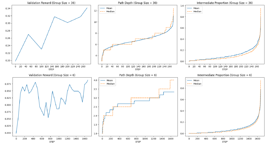</details> Figure 2: Validation reward (exact-match accuracy; left), ${\mathcal{B}}({\mathbb{G}})$ root-to-terminal path depth (center), and proportions of trajectories spanned by intermediate (non-terminal) process steps (right) for GRPO runs with group sizes of 36 (top) and 6 (bottom). Experimental Setup. We trained two DeepSeek-R1-Distill-Qwen-1.5B models (DeepSeek-AI, 2025) on the OpenRS (Dang & Ngo, 2025) dataset using the standard GRPO algorithm and objective of Equation 2. We selected 125 OpenRS examples at random to serve as a validation set. The first model trained for 1675 steps with a group size of six and a learn rate of $6× 10^{-6}$ . The second was trained with a group size of 36 and a learn rate of $10^{-6}$ for 275 steps (due to the larger group size). Both models were trained with a maximum new token limit of 4096, a batch size of four, and a temperature of 0.75. Additional training details are located in Appendix B. Results. Figure 2 shows that both path depth and intermediate proportion increase drastically as validation reward saturates, for group sizes of six and 36. These results are supported by Yu et al. (2025), who find that entropy decreases sharply as GRPO training progresses: this indicates that increasingly rich PRM-inducing structures arise as the model converges on a locally optimal policy. In addition, found that only twelve of 6,700 ${\mathcal{B}}({\mathbb{G}})$ structures were trivial with a group size of six ( $\sim$ 0.2%). With a group size of 36, zero trivial ${\mathcal{B}}({\mathbb{G}})$ structures arose out of the 1,100 generated groups. Examples of non-trivial ${\mathcal{B}}({\mathbb{G}})$ structures from this experiment are given in Appendix C. In conjunction with the theoretical analysis of Section 3.1, the results of this experiment demonstrate that GRPO induces a non-trivial PRM under real-world conditions. In Section 4, we show that this induced PRM carries a serious flaw that is detrimental to RL training, and propose a minor modification to the GRPO algorithm to mitigate this shortcoming. 4 Proposed Approach: $\lambda$ -GRPO Viewing the GRPO objective in terms of process set partitions ${\mathbb{X}}_{t}$ (see Equation 6), we note that the contribution of each trajectory $g^{(i)}∈{\mathbb{G}}$ to the loss at index $t$ is identical to that of all other trajectories in the process set $\lambda^{(i,t)}$ (where $\hat{P}_{t}(\lambda)$ , $\hat{D}_{t}(\lambda)$ , and $\hat{A}(\lambda)$ are defined as in Equation 5): $$ \begin{split}\frac{1}{\sum_{g^{(i)}\in{\mathbb{G}}}\textit{len}(g^{(i)})}\cdot\sum_{g^{(i)}\in{\mathbb{G}}}&\sum_{t=0}^{\textit{len}(g^{(i)})-1}({P}_{i,t}\cdot{a}_{i})-{D}_{i,t}=\frac{1}{\sum_{g^{(i)}\in{\mathbb{G}}}\textit{len}(g^{(i)})}\cdot\sum_{t=0}^{t_{\textit{max}}-1}\sum_{\lambda\in{\mathbb{X}}_{t}}\sum_{g^{(i)}\in\lambda}({P}_{i,t}\cdot{A}_{i,t})-{D}_{i,t}\\ =&\frac{1}{\sum_{g^{(i)}\in{\mathbb{G}}}\textit{len}(g^{(i)})}\cdot\sum_{t=0}^{t_{\textit{max}}-1}\sum_{\lambda\in{\mathbb{X}}_{t}}|\lambda|\cdot((\hat{P}_{t}(\lambda)\cdot\hat{A}(\lambda))-\hat{D}_{t}(\lambda))\end{split} \tag{7} $$ The contribution of each process set $\lambda∈{\mathcal{B}}({\mathbb{G}})$ to the overall loss, $\hat{P}_{t}(\lambda)·\hat{A}(\lambda)-\hat{D}_{t}(\lambda)$ , is scaled by $|\lambda|$ : this carries the danger of harming exploration (for $\hat{A}(\lambda)<0$ ) and exploitation (for $\hat{A}(\lambda)>0$ ). Consider some process set $\lambda$ with $|\lambda|\gg 1$ . If $\hat{A}(\lambda)>0$ , then the increase in probability assigned to the process step corresponding to $\lambda$ by $\pi_{\theta}$ under GRPO is compounded by a factor of $|\lambda|$ , decreasing the likelihood of exploring process steps that are dissimilar from $\lambda$ in subsequent training episodes. Conversely, if $\hat{A}(\lambda)<0$ , then the decrease in probability assigned to $\lambda$ under GRPO is compounded by a factor of $|\lambda|$ , decreasing the likelihood of exploiting high-reward trajectories in $\lambda$ . To illustrate, consider the group ${\mathbb{G}}$ in Figure 2, assume ${r}_{1}={r}_{2}={r}_{6}=0.5$ , ${r}_{4}={r}_{5}=0$ , ${r}_{3}=1$ , and let $\lambda=\{g^{(3)},g^{(4)},g^{(5)}\}$ . Then $\hat{A}(\lambda)=-0.22$ : despite the fact that $g^{(3)}$ has the highest reward, the probability of the sub-trajectory $g^{(3)}_{:4}$ is decreased under the GRPO objective, thereby decreasing the overall likelihood of generating the completion $g^{(3)}$ . The term $|\lambda|$ in Equation 7 then scales this decrease in probability by a factor of three. We propose scaling the token-level loss for $g^{(i)}_{t}$ by $|\lambda^{(i,t)}|^{-1}$ ( $\lambda$ -GRPO; Equation 8): this has the effect of canceling out the term $|\lambda|$ in Equation 7, so that each process set contributes equally to the loss at index $t$ . $$ \begin{split}L_{\lambda\text{-GRPO}}({\mathbb{G}})&=\frac{1}{\sum_{g^{(i)}\in{\mathbb{G}}}\textit{len}(g^{(i)})}\cdot\sum_{g^{(i)}\in{\mathbb{G}}}\sum_{t=0}^{\textit{len}(g^{(i)})-1}\frac{({P}_{i,t}\cdot{a}_{i})-{D}_{i,t}}{|\lambda^{(i,t)}|}\\ &=\frac{1}{\sum_{g^{(i)}\in{\mathbb{G}}}\textit{len}(g^{(i)})}\cdot\sum_{t=0}^{t_{\textit{max}}-1}\sum_{\lambda\in{\mathbb{X}}_{t}}(\hat{P}_{t}(\lambda)\cdot\hat{A}(\lambda))-\hat{D}_{t}(\lambda)\end{split} \tag{8} $$ 5 Experiments To evaluate our proposed approach, we trained DeepSeek-R1-Distill-Qwen-1.5B and Llama-3.2-1B-Instruct https://huggingface.co/meta-llama/Llama-3.2-1B-Instruct with the $\lambda$ -GRPO (Equation 8) objective on the OpenRS dataset of Section 3.2, and compared them to standard GRPO (Equation 2a) models trained with an identical setup. All models were evaluated on an OpenRS validation set and five downstream reasoning benchmarks (see Section 5.1). 5.1 Experimental Setup All models were trained for 1,000 steps with a group size of six, a batch size of four, a maximum of 4,096 new tokens, and a temperature of 0.75. We conducted two sets of trials across the two models (for a total of four trials): in the first, we set the KL coefficient $\beta=0.0$ , and in the second $\beta=0.04$ . The Qwen models were trained with a learn rate of $10^{-6}$ ; the Llama models were trained with a learn rate of $5× 10^{-7}$ for the $\beta=0.0$ trial and $10^{-7}$ for $\beta=0.04$ (as training was highly unstable with higher learn rates for Llama). Additional training details are located in Appendix B. We evaluated the models on the AIME24 https://huggingface.co/datasets/AI-MO/aimo-validation-aime, MATH-500 (Hendrycks et al., 2021; Lightman et al., 2024), AMC23 https://huggingface.co/datasets/AI-MO/aimo-validation-amc, Minerva (Lewkowycz et al., 2022), and OlympiadBench (He et al., 2024) benchmarks, using the LightEval framework Habib et al. (2023); Dang & Ngo (2025). All models were evaluated at the checkpoint corresponding to the step at which they achieved maximum validation accuracy. As in the experiment in Section 3.2, we withheld 125 examples as a validation set. 5.2 Results and Discussion <details> <summary>x3.png Details</summary>  ### Visual Description ## Line Graphs: Comparison of GRPO and Λ-GRPO Algorithms Across Datasets ### Overview The image contains four line graphs comparing the validation rewards of two algorithms, **GRPO** (cyan) and **Λ-GRPO** (purple), across different datasets and hyperparameter settings (β values). Each graph represents a distinct dataset and β value, with the x-axis showing training steps (0–800) and the y-axis showing validation reward. Peaks in performance are annotated with coordinates, and legends are positioned in the bottom-right corner of each graph. --- ### Components/Axes - **X-axis**: Labeled "STEP," ranging from 0 to 800 (steps). - **Y-axis**: Labeled "VALIDATION REWARD," with scales varying by graph (e.g., 0.20–0.40 for Qwen, 0.06–0.14 for Llama). - **Legends**: Located in the bottom-right of each graph, with cyan representing **GRPO** and purple representing **Λ-GRPO**. - **Graph Titles**: - Top-left: "Qwen (β=0.0)" - Top-right: "Qwen (β=0.04)" - Bottom-left: "Llama (β=0.0)" - Bottom-right: "Llama (β=0.04)" --- ### Detailed Analysis #### Qwen (β=0.0) - **GRPO** (cyan): Peaks at **(1900, 0.373)**. The line shows significant fluctuations, with a sharp rise to the peak followed by a decline. - **Λ-GRPO** (purple): Peaks at **(325, 0.429)**. The line exhibits earlier and sharper peaks compared to GRPO, with higher validation rewards. #### Qwen (β=0.04) - **GRPO** (cyan): Peaks at **(600, 0.373)**. The line shows moderate fluctuations, with a peak near the midpoint of the x-axis. - **Λ-GRPO** (purple): Peaks at **(400, 0.381)**. Slightly higher reward than GRPO, with a peak slightly later than GRPO. #### Llama (β=0.0) - **GRPO** (cyan): Peaks at **(350, 0.159)**. The line shows moderate fluctuations, with a peak near the midpoint. - **Λ-GRPO** (purple): Peaks at **(325, 0.143)**. Slightly lower reward than GRPO, with a peak slightly earlier. #### Llama (β=0.04) - **GRPO** (cyan): Peaks at **(700, 0.135)**. The line shows late-stage fluctuations, with a peak near the end of the x-axis. - **Λ-GRPO** (purple): Peaks at **(325, 0.143)**. Slightly higher reward than GRPO, with a peak earlier in training. --- ### Key Observations 1. **Peak Timing**: - Λ-GRPO often peaks earlier than GRPO (e.g., Qwen β=0.0: 325 vs. 1900 steps). - GRPO sometimes achieves higher rewards later in training (e.g., Qwen β=0.04: 600 steps vs. Λ-GRPO’s 400 steps). 2. **Reward Magnitude**: - Λ-GRPO outperforms GRPO in Qwen β=0.0 (0.429 vs. 0.373). - GRPO matches or exceeds Λ-GRPO in other cases (e.g., Qwen β=0.04: 0.373 vs. 0.381). 3. **Fluctuations**: Both algorithms exhibit high volatility in validation rewards, suggesting sensitivity to hyperparameters or training dynamics. --- ### Interpretation The data suggests that the choice between GRPO and Λ-GRPO depends on the dataset and β value: - **Λ-GRPO** excels in Qwen β=0.0, achieving higher rewards earlier, but underperforms in Qwen β=0.04. - **GRPO** shows better late-stage performance in Qwen β=0.04 and Llama β=0.04, indicating potential robustness in later training phases. - The β parameter (likely a regularization or learning rate factor) significantly influences algorithm effectiveness, with Λ-GRPO favoring lower β values (e.g., Qwen β=0.0) and GRPO performing better at higher β (e.g., Llama β=0.04). The annotations and peak coordinates highlight critical inflection points, emphasizing the need for careful hyperparameter tuning. The visual trends align with the numerical data, confirming that Λ-GRPO’s early peaks and GRPO’s late-stage gains are consistent across datasets. 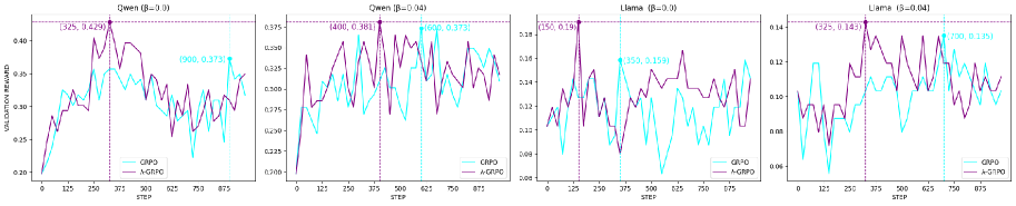</details> Figure 3: Models’ validation accuracy across training steps. Peak accuracy is highlighted by vertical, dashed lines. | Model Qwen | $\beta$ — | Version Base | AIME24 0.2000 ±0.0743 | MATH-500 0.8300 ±0.0168 | AMC23 0.7500 ±0.0693 | Minerva 0.2978 ±0.0278 | OB 0.5096 ±0.0193 | Avg. 0.5175 | | --- | --- | --- | --- | --- | --- | --- | --- | --- | | 0.0 | GRPO | 0.3333 ±0.0875 | 0.7660 ±0.0190 | 0.6250 ±0.0775 | 0.2500 ±0.0263 | 0.4444 ±0.0191 | 0.4837 | | | $\lambda$ -GRPO (ours) | 0.3667 ±0.0895 | 0.8460 ±0.0162 | 0.7500 ±0.0693 | 0.2904 ±0.0276 | 0.5348 ±0.0192 | 0.5576 | | | | 0.04 | GRPO | 0.3000 ±0.0851 | 0.8660 ±0.0152 | 0.7500 ±0.0693 | 0.2610 ±0.0267 | 0.5200 ±0.0192 | 0.5394 | | | $\lambda$ -GRPO (ours) | 0.4000 ±0.0910 | 0.8340 ±0.0167 | 0.8000 ±0.0641 | 0.2978 ±0.0278 | 0.5378 ±0.0192 | 0.5739 | | | | Llama | — | Base | 0.0000 ±0.0000 | 0.2280 ±0.0188 | 0.0750 ±0.0422 | 0.0478 ±0.0130 | 0.0563 ±0.0089 | 0.0814 | | 0.0 | GRPO | 0.0000 ±0.0000 | 0.2300 ±0.0188 | 0.0750 ±0.0422 | 0.0551 ±0.0130 | 0.0607 ±0.0089 | 0.0842 | | | $\lambda$ -GRPO (ours) | 0.0000 ±0.0000 | 0.2620 ±0.0197 | 0.1250 ±0.0530 | 0.0515 ±0.0134 | 0.0622 ±0.0092 | 0.1001 | | | | 0.04 | GRPO | 0.0000 ±0.0000 | 0.2180 ±0.0185 | 0.1750 ±0.0608 | 0.0515 ±0.0134 | 0.0533 ±0.0087 | 0.0996 | | | $\lambda$ -GRPO (ours) | 0.0333 ±0.0333 | 0.2560 ±0.0195 | 0.0750 ±0.0422 | 0.0735 ±0.0159 | 0.0489 ±0.0083 | 0.0973 | | | Table 1: Exact-match accuracy for the base and GRPO-/ $\lambda$ -GRPO-trained Llama and Qwen models on downstream reasoning datasets ( $\text{OB}=\text{OlympiadBench}$ ). The best results in each column are indicated in bold, and the best results within each model type (i.e. Llama or Qwen) are underlined. Confidence intervals are subscripted. For each $\lambda$ -GRPO-trained model, results are given in green if it outperforms its GRPO-trained counterpart and the base model; yellow if it outperforms only its GRPO-trained counterpart; orange if it only improves over the base model; and red if it fails to outperform either model (see Table 2 in the Appendix for exact differences). All four $\lambda$ -GRPO models reach a higher validation accuracy in fewer steps than their GRPO counterparts (see Figure 3): on average, $\lambda$ -GRPO represents a more than 10% increase over the standard GRPO validation accuracy—in less than half of the number of training steps. This increase in validation accuracy corresponds to improved performance on downstream reasoning tasks (see Table 1). In total, the $\lambda$ -GRPO models outperform standard GRPO on 15/20 cells (excluding average performance) in Table 1, and they improve over the base Llama/Qwen models on 14/20 cells. Only the Llama $\lambda$ -GRPO model with $\beta=0.04$ failed to outperform its GRPO counterpart on average downstream performance—this model still outperformed standard GRPO on a majority (3/5) of the tasks. In addition, these performance gains result in effectively zero training slowdown: as we are merely detecting ${\mathcal{B}}({\mathbb{G}})$ structures that occur during training—rather than generating them (e.g. Kazemnejad et al., 2025; Hou et al., 2025; Yang et al., 2025a) —the added computational cost from $\lambda$ -GRPO (vs. standard GRPO) is negligible. 6 Related Work Monte Carlo Sampling for Finer-Grained Rewards. As discussed in Section 2.2, the labor-intensive human annotation required to obtain step-level rewards for PRM training has driven the development of heuristic methods for PRMs and PRM-like finer-grained reward signals, in particular those based on Monte Carlo estimation. Kazemnejad et al. (2025) replace the critic model in PPO with Monte Carlo estimation: multiple completions are sampled for each step, and the value for that step is derived from their mean outcome reward. On the other hand, Wang et al. (2024) train a neural PRM, using Monte Carlo estimation in a similar manner to Kazemnejad et al. (2025) in order to obtain step-level training rewards, and thereby avoid the need for costly human annotation. Xie et al. (2024) generate step-level preference data for Direct Preference Optimization (DPO; Rafailov et al., 2023) training via Monte Carlo Tree Search and outcome-level rewards: sequences of overlapping trajectories are obtained by forking trajectories at defined split points to construct tree structures similar to the $\mathcal{B}(G)$ trees introduced in Section 3.1. The daughter nodes with the highest and lowest mean reward are then selected as the preferred and dispreferred (respectively) sequences for step-level DPO. Similarly, Hou et al. (2025) construct $\mathcal{B}(G)$ -like trees by splitting generated trajectories at high-entropy tokens to create multiple completions to the same initial trajectory prefix. Subtrajectory rewards are then derived from the mean reward of the corresponding node’s daughters in the tree structure. Yang et al. (2025a) employ an analogous approach to generate step-level rewards for GRPO training. Unlike standard GRPO, however, the advantages for each node (step) are computed relative to the rewards of node’s sisters in the tree structure, rather than the entire group. These methods are orthogonal to our approach: they apply Monte Carlo estimation to explicitly construct step-level reward signals from outcome-level rewards, while we leverage the implicit step-level rewards already present in standard GRPO. PRMs with GRPO. Aside from Yang et al. (2025a), GRPO has been employed with PRMs in Shao et al. (2024) and Feng et al. (2025). Shao et al. (2024) modify the advantage computation of GRPO to account for step-level rewards: normalized rewards are computed relative to all step-level rewards of all trajectories in the group, and the advantage for each step is the sum of the normalized reward of each subsequent step in its trajectory. Feng et al. (2025) construct a two-level variant of GRPO, in which standard, trajectory-level GRPO advantage is combined with a step-level GRPO advantage, and step-level groups are dynamically computed according to the similarity of steps across trajectories. Our results in Sections 3 and 5 call into question the necessity of adapting GRPO to step-level rewards, given the rich step-level reward signal already present in the outcome-level variant of the algorithm. 7 Conclusion In this paper, we demonstrated both theoretically and empirically that the standard GRPO algorithm induces a PRM that derives step-level rewards via Monte Carlo estimation. We then showed that this hidden PRM is faulty, and as a result is potentially detrimental to exploration and exploitation. To mitigate this flaw, we introduced a process-step-aware scaling factor to GRPO to derive the $\lambda$ -GRPO objective. Models trained with $\lambda$ -GRPO reach higher validation accuracy faster than with standard GRPO, and achieve improved performance on downstream reasoning tasks. Our results indicate that it is possible to leverage the existing PRM structure inherent in the outcome-based GRPO algorithm, rather than employing costly, explicitly-defined PRMs. The limitations of this work are discussed in Appendix A. Reproducibility Statement We provide the complete proof of Theorem 1 in the main body of the paper. All settings and hyperparameters for the experiments conducted in this work are given in Sections 3.2 / 5.1 and Appendix B. All code is available on GitHub: https://github.com/coli-saar/grpo-prm/. References - Cui et al. (2025) Ganqu Cui, Lifan Yuan, Zefan Wang, Hanbin Wang, Wendi Li, Bingxiang He, Yuchen Fan, Tianyu Yu, Qixin Xu, Weize Chen, Jiarui Yuan, Huayu Chen, Kaiyan Zhang, Xingtai Lv, Shuo Wang, Yuan Yao, Xu Han, Hao Peng, Yu Cheng, Zhiyuan Liu, Maosong Sun, Bowen Zhou, and Ning Ding. Process reinforcement through implicit rewards. arXiv preprint arXiv:2502.01456, 2025. - Dang & Ngo (2025) Quy-Anh Dang and Chris Ngo. Reinforcement learning for reasoning in small llms: What works and what doesn’t. arXiv preprint arXiv:2503.16219, 2025. - DeepSeek-AI (2025) DeepSeek-AI. Deepseek-r1: Incentivizing reasoning capability in llms via reinforcement learning. arXiv preprint arXiv:2501.12948, 2025. - Feng et al. (2025) Lang Feng, Zhenghai Xue, Tingcong Liu, and Bo An. Group-in-group policy optimization for llm agent training. arXiv preprint arXiv:2505.10978, 2025. - Habib et al. (2023) Nathan Habib, Clémentine Fourrier, Hynek Kydlíček, Thomas Wolf, and Lewis Tunstall. Lighteval: A lightweight framework for llm evaluation, 2023. URL https://github.com/huggingface/lighteval. - He et al. (2024) Chaoqun He, Renjie Luo, Yuzhuo Bai, Shengding Hu, Zhen Thai, Junhao Shen, Jinyi Hu, Xu Han, Yujie Huang, Yuxiang Zhang, Jie Liu, Lei Qi, Zhiyuan Liu, and Maosong Sun. OlympiadBench: A challenging benchmark for promoting AGI with olympiad-level bilingual multimodal scientific problems. In Proceedings of the 62nd Annual Meeting of the Association for Computational Linguistics (Volume 1: Long Papers), pp. 3828–3850, 2024. - Hendrycks et al. (2021) Dan Hendrycks, Collin Burns, Saurav Kadavath, Akul Arora, Steven Basart, Eric Tang, Dawn Song, and Jacob Steinhardt. Measuring mathematical problem solving with the MATH dataset. In Thirty-fifth Conference on Neural Information Processing Systems Datasets and Benchmarks Track (Round 2), 2021. - Hou et al. (2025) Zhenyu Hou, Ziniu Hu, Yujiang Li, Rui Lu, Jie Tang, and Yuxiao Dong. TreeRL: LLM reinforcement learning with on-policy tree search. In Proceedings of the 63rd Annual Meeting of the Association for Computational Linguistics (Volume 1: Long Papers), pp. 12355–12369, 2025. - Kazemnejad et al. (2025) Amirhossein Kazemnejad, Milad Aghajohari, Eva Portelance, Alessandro Sordoni, Siva Reddy, Aaron Courville, and Nicolas Le Roux. VinePPO: Refining credit assignment in RL training of LLMs. In Forty-second International Conference on Machine Learning, 2025. - Lewkowycz et al. (2022) Aitor Lewkowycz, Anders Andreassen, David Dohan, Ethan Dyer, Henryk Michalewski, Vinay Ramasesh, Ambrose Slone, Cem Anil, Imanol Schlag, Theo Gutman-Solo, Yuhuai Wu, Behnam Neyshabur, Guy Gur-Ari, and Vedant Misra. Solving quantitative reasoning problems with language models. Advances in Neural Information Processing Systems, 35:3843–3857, 2022. - Li & Li (2025) Wendi Li and Yixuan Li. Process reward model with q-value rankings. In The Thirteenth International Conference on Learning Representations, 2025. - Lightman et al. (2024) Hunter Lightman, Vineet Kosaraju, Yuri Burda, Harrison Edwards, Bowen Baker, Teddy Lee, Jan Leike, John Schulman, Ilya Sutskever, and Karl Cobbe. Let’s verify step by step. In The Twelfth International Conference on Learning Representations, 2024. - Luo et al. (2025) Michael Luo, Sijun Tan, Justin Wong, Xiaoxiang Shi, William Y. Tang, Manan Roongta, Colin Cai, Jeffrey Luo, Li Erran Li, Raluca Ada Popa, and Ion Stoica. Deepscaler: Surpassing o1-preview with a 1.5b model by scaling rl. https://pretty-radio-b75.notion.site/DeepScaleR-Surpassing-O1-Preview-with-a-1-5B-Model-by-Scaling-RL-19681902c1468005bed8ca303013a4e2, 2025. Notion Blog. - Muennighoff et al. (2025) Niklas Muennighoff, Zitong Yang, Weijia Shi, Xiang Lisa Li, Li Fei-Fei, Hannaneh Hajishirzi, Luke Zettlemoyer, Percy Liang, Emmanuel Candès, and Tatsunori Hashimoto. s1: Simple test-time scaling. arXiv preprint arXiv:2501.19393, 2025. - Qian et al. (2025) Cheng Qian, Emre Can Acikgoz, Qi He, Hongru Wang, Xiusi Chen, Dilek Hakkani-Tür, Gokhan Tur, and Heng Ji. Toolrl: Reward is all tool learning needs. arXiv preprint arXiv:2504.13958, 2025. - Rafailov et al. (2023) Rafael Rafailov, Archit Sharma, Eric Mitchell, Stefano Ermon, Christopher D Manning, and Chelsea Finn. Direct preference optimization: Your language model is secretly a reward model. In Proceedings of the 37th International Conference on Neural Information Processing Systems, pp. 53728–53741, 2023. - Schulman et al. (2017) John Schulman, Filip Wolski, Prafulla Dhariwal, Alec Radford, and Oleg Klimov. Proximal policy optimization algorithms. arXiv preprint arXiv:1707.06347, 2017. - Setlur et al. (2025) Amrith Setlur, Chirag Nagpal, Adam Fisch, Xinyang Geng, Jacob Eisenstein, Rishabh Agarwal, Alekh Agarwal, Jonathan Berant, and Aviral Kumar. Rewarding progress: Scaling automated process verifiers for LLM reasoning. In The Thirteenth International Conference on Learning Representations, 2025. - Shao et al. (2024) Zhihong Shao, Peiyi Wang, Qihao Zhu, Runxin Xu, Junxiao Song, Xiao Bi, Haowei Zhang, Mingchuan Zhang, YK Li, Yang Wu, and Daya Guo. Deepseekmath: Pushing the limits of mathematical reasoning in open language models. arXiv preprint arXiv:2402.03300, 2024. - Sullivan et al. (2025) Michael Sullivan, Mareike Hartmann, and Alexander Koller. Procedural environment generation for tool-use agents. arXiv preprint arXiv:2506.11045, 2025. - Uesato et al. (2022) Jonathan Uesato, Nate Kushman, Ramana Kumar, Francis Song, Noah Siegel, Lisa Wang, Antonia Creswell, Geoffrey Irving, and Irina Higgins. Solving math word problems with process- and outcome-based feedback. arXiv preprint arXiv:2211.14275, 2022. - Wang et al. (2024) Peiyi Wang, Lei Li, Zhihong Shao, Runxin Xu, Damai Dai, Yifei Li, Deli Chen, Yu Wu, and Zhifang Sui. Math-shepherd: Verify and reinforce LLMs step-by-step without human annotations. In Proceedings of the 62nd Annual Meeting of the Association for Computational Linguistics (Volume 1: Long Papers), pp. 9426–9439, 2024. - Xie et al. (2024) Yuxi Xie, Anirudh Goyal, Wenyue Zheng, Min-Yen Kan, Timothy P Lillicrap, Kenji Kawaguchi, and Michael Shieh. Monte carlo tree search boosts reasoning via iterative preference learning. In The First Workshop on System-2 Reasoning at Scale, NeurIPS’24, 2024. - Yang et al. (2025a) Zhicheng Yang, Zhijiang Guo, Yinya Huang, Xiaodan Liang, Yiwei Wang, and Jing Tang. Treerpo: Tree relative policy optimization. arXiv preprint arXiv:2506.05183, 2025a. - Yang et al. (2025b) Zonglin Yang, Zhexuan Gu, Houduo Qi, and Yancheng Yuan. Accelerating rlhf training with reward variance increase. arXiv preprint arXiv:2505.23247, 2025b. - Yao et al. (2023) Shunyu Yao, Jeffrey Zhao, Dian Yu, Nan Du, Izhak Shafran, Karthik Narasimhan, and Yuan Cao. React: Synergizing reasoning and acting in language models. In The Eleventh International Conference on Learning Representations, 2023. - Yu et al. (2025) Qiying Yu, Zheng Zhang, Ruofei Zhu, Yufeng Yuan, Xiaochen Zuo, Yu Yue, Weinan Dai, Tiantian Fan, Gaohong Liu, Lingjun Liu, et al. Dapo: An open-source llm reinforcement learning system at scale. arXiv preprint arXiv:2503.14476, 2025. - Zhang et al. (2025) Zhenru Zhang, Chujie Zheng, Yangzhen Wu, Beichen Zhang, Runji Lin, Bowen Yu, Dayiheng Liu, Jingren Zhou, and Junyang Lin. The lessons of developing process reward models in mathematical reasoning. arXiv preprint arXiv:2501.07301, 2025. | Model Qwen | $\beta$ 0.0 | Version Base | AIME24 +0.1667 | MATH-500 +0.0160 | AMC23 0.0000 | Minerva -0.0074 | OB +0.0252 | Avg. +0.0401 | | --- | --- | --- | --- | --- | --- | --- | --- | --- | | GRPO | +0.0334 | +0.0800 | +0.1250 | +0.0404 | +0.0904 | +0.0738 | | | | 0.04 | Base | +0.2000 | +0.0040 | +0.0500 | 0.0000 | +0.0282 | +0.0564 | | | GRPO | +0.1000 | -0.0320 | +0.0500 | +0.0368 | +0.0178 | +0.0345 | | | | Llama | 0.0 | Base | 0.0000 | +0.0340 | +0.0500 | +0.0037 | +0.0059 | +0.0187 | | GRPO | 0.0000 | +0.0320 | +0.0500 | -0.0036 | +0.0015 | +0.0160 | | | | 0.04 | Base | +0.0333 | +0.0280 | 0.0000 | +0.0257 | -0.0074 | +0.0159 | | | GRPO | +0.0333 | +0.0380 | -0.1000 | +0.0220 | -0.0044 | -0.0022 | | | Table 2: Difference in accuracy between the $\lambda$ -GRPO-trained models, and their corresponding base models and standard-GRPO-trained counterparts. Positive differences (i.e. $\lambda$ -GRPO outperforms the comparison model) are highlighted in green; negative differences (i.e. the comparison model outperforms $\lambda$ -GRPO) are highlighted in red. For example, the top-most entry in the AIME24 column indicates that the $\lambda$ -GRPO Qwen model with $\beta=0.0$ outperformed the base DeepSeek-R1-Distill-Qwen-1.5B by 0.1667 on the AIME24 benchmark. Appendix A Limitations Due to computational resource constraints, we were only able to conduct the experiments in Sections 3.2 and 5 with relatively small models: 1.5 billion (Qwen) and 1 billion (Llama) parameters. Similarly, we only use one dataset for RL training in both experiments—although OpenRS is a combination of the s1 (Muennighoff et al., 2025) and DeepScaleR Luo et al. (2025) datasets. Future work should extend our findings regarding the non-triviality of the GRPO-induced PRM and the effectiveness of $\lambda$ -GRPO to larger models and more diverse (training) datasets. Finally, the objective of this work is to expose the PRM induced by the GRPO algorithm, and to highlight the deficiencies of that PRM as described in Section 4. To that end, our proposed $\lambda$ -GRPO method does not actually remedy the anti-exploitation effect of the GRPO-induced PRM—it merely lessens its impact. In future work, we intend to investigate more extensive modifications to the GRPO algorithm, with the goal of entirely solving the problems laid out in Section 4. Appendix B Experimental Setup All experiments were conducted on a single NVIDIA H100 GPU. We trained all models with 24 gradient accumulation steps per step and a generation batch size of 6. The models were evaluated on the validation split every 25 training steps. We additionally hard-coded the generation procedure to halt after “\boxed{…}” was detected: this was to prevent the model from generating multiple boxed answers for a single prompt. 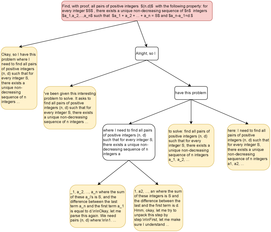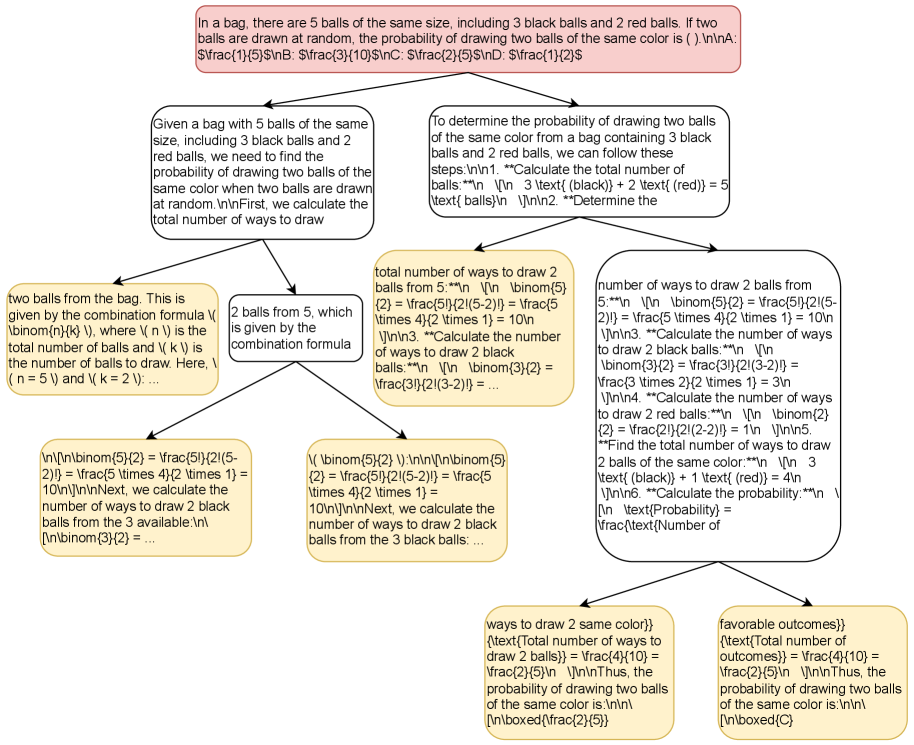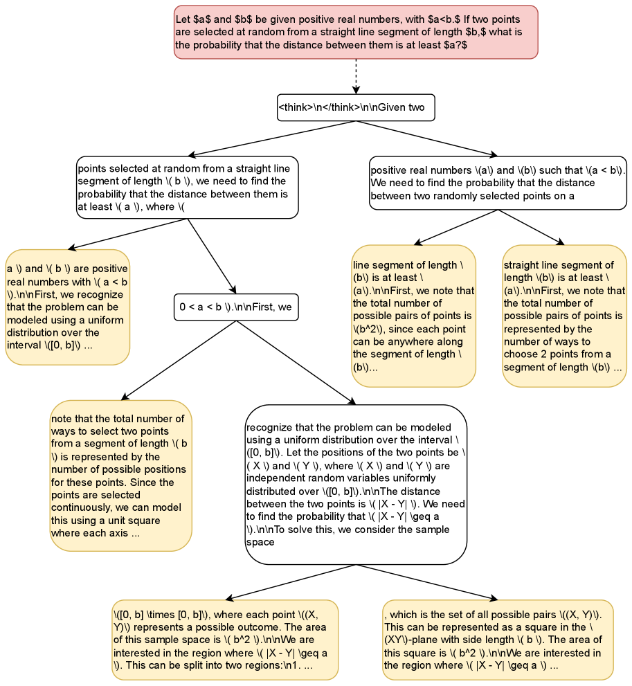Appendix C ${\mathcal{B}}({\mathbb{G}})$ Structure Examples The following (Figures 4, 5, 6) represent ${\mathcal{B}}({\mathbb{G}})$ structures on groups generated during the group size 6 trial of the experiment in Section 3.2. A full trajectory is reconstructed by tracing the unique path from the root to a terminal node. The root ( red) corresponds to the prompt/query $q$ . Terminal nodes ( yellow) denote singleton process steps $\{g^{(i)}\}$ ; each non-terminal node $\lambda$ (white; including the root) denotes the process step corresponding to the set of all terminal nodes dominated by $\lambda$ . For the sake of presentation, overlong terminal steps are truncated with “…”. <details> <summary>x4.png Details</summary>  ### Visual Description ## Flowchart: Problem Decomposition for Integer Sequence Pairs ### Overview The image depicts a flowchart representing a recursive or iterative problem-solving process for finding pairs of positive integers (n, d) that satisfy specific mathematical conditions. The central node contains the core problem statement, with branching paths leading to progressively detailed explanations, restatements, and component breakdowns. The flowchart appears to map out a logical decomposition of a complex mathematical problem, likely related to number theory or combinatorial sequences. ### Components/Axes - **Central Node**: Contains the primary problem statement in LaTeX-style mathematical notation - **Branching Arrows**: Connect the central node to 6 peripheral nodes containing: 1. Simplified problem restatement 2. Problem clarification 3. Component breakdown (sequence definition) 4. Problem restatement with variables 5. Component breakdown (sum/difference conditions) 6. Problem restatement with sequence notation ### Detailed Analysis #### Central Node Text "Find, with proof, all pairs (n,d) with the following property: for every integer S$, there exists a unique non-decreasing sequence of n$ integers a_1,a_2,...,a_n$ such that a_1 + a_2 + ... + a_n = S$ and a_n - a_1 = d$" #### Peripheral Nodes 1. **Simplified Restatement**: "Okay, so I have this problem where I need to find all pairs of positive integers (n, d) such that for every integer S, there exists a unique non-decreasing sequence of n integers ..." 2. **Problem Clarification**: "Alright, so I have this problem. It asks to find all pairs of positive integers (n, d) such that for every integer S, there exists a unique non-decreasing sequence of n integers ..." 3. **Component Breakdown (Sequence Definition)**: "where I need to find all pairs of positive integers (n, d) such that for every integer S, there exists a unique non-decreasing sequence of n integers a_1, a_2, ..." 4. **Variable-Restated Problem**: "to solve: find all pairs of positive integers (n, d) such that for every integer S, there exists a unique non-decreasing sequence of n integers a_1, a_2, ..." 5. **Sum/Difference Conditions**: "1, a_2, ..., a_n where the sum of these a_i's is S, and the difference between the last term a_n and the first term a_1 is equal to d" 6. **Confusion Node**: "Hmm, okay, let me try to unpack this step by step. First, let me make sure I understand ..." ### Key Observations - The problem requires finding integer pairs (n,d) that work universally for all integers S - The solution must guarantee both existence and uniqueness of sequences - The sequences must be non-decreasing and satisfy two constraints: 1. Sum equals S 2. Difference between maximum and minimum terms equals d - Multiple nodes show recursive restatements, suggesting iterative refinement of understanding - One node explicitly shows confusion about parsing the problem, indicating potential complexity ### Interpretation This flowchart represents a systematic approach to solving a non-trivial mathematical problem, likely related to: 1. **Integer Partition Theory**: Finding ways to represent integers as sums of sequences 2. **Combinatorial Design**: Creating sequences with specific structural properties 3. **Algorithmic Proof Construction**: Developing a method to verify the existence and uniqueness of solutions The recursive nature of the flowchart suggests the problem may require: - Mathematical induction - Recursive sequence construction - Case analysis based on n and d values The presence of confusion in one node indicates that: - The problem may have non-obvious constraints - The solution space might be complex or counterintuitive - Multiple verification steps are needed to ensure correctness The use of LaTeX-style notation and mathematical rigor in the problem statement implies this is likely: - A theoretical computer science problem - A mathematical competition question - A research-level number theory challenge The flowchart's structure demonstrates an effective problem-solving strategy of: 1. Restating the problem in multiple ways 2. Breaking down complex conditions 3. Verifying understanding through iterative explanation 4. Identifying knowledge gaps through self-questioning </details> Figure 4: ${\mathcal{B}}({\mathbb{G}})$ structure from step 1 (see the beginning of Appendix C for additional details). <details> <summary>x5.png Details</summary>  ### Visual Description ## Flowchart: Probability Calculation for Drawing Two Balls of the Same Color ### Overview The flowchart illustrates a step-by-step probability calculation to determine the likelihood of drawing two balls of the same color from a bag containing 3 black balls and 2 red balls. It uses combinatorial mathematics (binomial coefficients and factorials) to compute favorable outcomes and total outcomes. ### Components/Axes - **Main Title**: "In a bag, there are 5 balls of the same size, including 3 black balls and 2 red balls. If two balls are drawn at random, the probability of drawing two balls of the same color is..." - **Key Text Boxes**: 1. **Problem Statement**: Defines the scenario (5 balls: 3 black, 2 red). 2. **Total Outcomes Calculation**: - Formula: `binom(5, 2) = frac(5!){2!(5-2)!} = 10` - Explanation: Total ways to draw 2 balls from 5. 3. **Favorable Outcomes for Black Balls**: - Formula: `binom(3, 2) = frac(3!){2!(3-2)!} = 3` - Explanation: Ways to draw 2 black balls from 3. 4. **Favorable Outcomes for Red Balls**: - Formula: `binom(2, 2) = frac(2!){2!(2-2)!} = 1` - Explanation: Ways to draw 2 red balls from 2. 5. **Total Favorable Outcomes**: - Sum: `3 (black) + 1 (red) = 4` 6. **Probability Calculation**: - Formula: `frac(4){10} = 0.4` (or 40%) ### Detailed Analysis - **Combinatorial Logic**: - Total outcomes: `C(5, 2) = 10` (all possible pairs). - Favorable outcomes: `C(3, 2) + C(2, 2) = 3 + 1 = 4` (same-color pairs). - **Code Snippets**: - Python-like pseudocode for factorial (`frac`) and combination (`binom`) functions. - Example: `frac(5!){2!(5-2)!} = 10` (total outcomes). ### Key Observations - The probability of drawing two balls of the same color is **40%**. - The calculation relies on combinatorial principles: `P = (favorable outcomes) / (total outcomes)`. - No outliers or anomalies; the logic is deterministic. ### Interpretation The flowchart demonstrates how combinatorial mathematics quantifies probability. By isolating favorable outcomes (same-color pairs) and dividing by total possible outcomes, it provides a clear, formulaic approach to solving probability problems. The use of `binom(n, k)` and `frac` functions simplifies complex calculations, making the process reproducible and verifiable. This method is foundational in probability theory and applicable to real-world scenarios like quality control or statistical sampling. </details> Figure 5: ${\mathcal{B}}({\mathbb{G}})$ structure from step 1001 (see the beginning of Appendix C for additional details). <details> <summary>x6.png Details</summary>  ### Visual Description ```markdown ## Flowchart: Probability of Distance Between Two Random Points on a Line Segment ### Overview The flowchart illustrates a step-by-step logical breakdown of solving a probability problem: determining the likelihood that two randomly selected points on a straight line segment of length `b` are at least a distance `a` apart. The problem is decomposed into cases based on the relationship between `a` and `b`, with geometric probability methods used to calculate the result. --- ### Components/Axes 1. **Title Node**: - Text: *"Let $a$ and $b$ be given positive real numbers, with $a < b$. If two points are selected at random from a straight line segment of length $b$, what is the probability that the distance between them is at least $a$?"* - Position: Top-center. 2. **Main Decision Node**: - Text: `think>>>>>>>>>>>think>>>> </details> Figure 6: ${\mathcal{B}}({\mathbb{G}})$ structure from step 1673 (see the beginning of Appendix C for additional details).