# Group-Relative REINFORCE Is Secretly an Off-Policy Algorithm: Demystifying Some Myths About GRPO and Its Friends
## Abstract
Off-policy reinforcement learning (RL) for large language models (LLMs) is attracting growing interest, driven by practical constraints in real-world applications, the complexity of LLM-RL infrastructure, and the need for further innovations of RL methodologies. While classic REINFORCE and its modern variants like Group Relative Policy Optimization (GRPO) are typically regarded as on-policy algorithms with limited tolerance of off-policyness, we present in this work a first-principles derivation for group-relative REINFORCE without assuming a specific training data distribution, showing that it admits a native off-policy interpretation. This perspective yields two general principles for adapting REINFORCE to off-policy settings: regularizing policy updates, and actively shaping the data distribution. Our analysis demystifies some myths about the roles of importance sampling and clipping in GRPO, unifies and reinterprets two recent algorithms — Online Policy Mirror Descent (OPMD) and Asymmetric REINFORCE (AsymRE) — as regularized forms of the REINFORCE loss, and offers theoretical justification for seemingly heuristic data-weighting strategies. Our findings lead to actionable insights that are validated with extensive empirical studies, and open up new opportunities for principled algorithm design in off-policy RL for LLMs. Source code for this work is available at https://github.com/modelscope/Trinity-RFT/tree/main/examples/rec_gsm8k.
footnotetext: Equal contribution. Contact: chaorui@ucla.edu, chenyanxi.cyx@alibaba-inc.com footnotetext: UCLA. Work done during an internship at Alibaba Group. footnotetext: Alibaba Group.
## 1 Introduction
The past few years have witnessed rapid progress in reinforcement learning (RL) for large language models (LLMs). This began with reinforcement learning from human feedback (RLHF) (Bai et al., 2022; Ouyang et al., 2022) that aligns pre-trained LLMs with human preferences, followed by reasoning-oriented RL that enables LLMs to produce long chains of thought (OpenAI, 2024; DeepSeek-AI, 2025; Kimi-Team, 2025b; Zhang et al., 2025b). More recently, agentic RL (Kimi-Team, 2025a; Gao et al., 2025; Zhang et al., 2025a) aims to train LLMs for agentic capabilities such as tool use, long-horizon planning, and multi-step task execution in dynamic environments.
Alongside these developments, off-policy RL has been attracting growing interest. In the “era of experience” (Silver and Sutton, 2025), LLM-powered agents need to be continually updated through interaction with the environment. Practical constraints in real-world deployment and the complexity of LLM-RL infrastructure often render on-policy training impractical (Noukhovitch et al., 2025): rollout generation and model training can proceed at mismatched speeds, data might be collected from different policies, reward feedback might be irregular or delayed, and the environment may be too costly or unstable to query for fresh trajectories. Moreover, in pursuit of higher sample efficiency and model performance, it is desirable to go beyond the standard paradigm of independent rollout sampling, e.g., via replaying past experiences (Schaul et al., 2016; Rolnick et al., 2019; An et al., 2025), synthesizing higher-quality experiences based on auxiliary information (Da et al., 2025; Liang et al., 2025; Guo et al., 2025), or incorporating expert demonstrations into online RL (Yan et al., 2025; Zhang et al., 2025c) — all of which incur off-policyness.
However, the prominent algorithms in LLM-RL — Proximal Policy Optimization (PPO) (Schulman et al., 2017) and Group Relative Policy Optimization (GRPO) (Shao et al., 2024) — are essentially on-policy methods: as modern variants of REINFORCE (Williams, 1992), their fundamental rationale is to produce unbiased estimates of the policy gradient, which requires fresh data sampled from the current policy. PPO and GRPO can handle a limited degree of off-policyness via importance sampling, but require that the current policy remains sufficiently close to the behavior policy. Truly off-policy LLM-RL often demands ad-hoc analysis and algorithm design; worse still, as existing RL infrastructure (Sheng et al., 2024; Hu et al., 2024; von Werra et al., 2020; Wang et al., 2025; Pan et al., 2025; Fu et al., 2025a) is typically optimized for REINFORCE-style algorithms, their support for specialized off-policy RL algorithms could be limited. All these have motivated our investigation into principled and infrastructure-friendly algorithm design for off-policy RL.
#### Core finding: a native off-policy interpretation for group-relative REINFORCE.
Consider a one-step RL setting and a group-relative variant of REINFORCE that, like in GRPO, assumes access to multiple responses $\{y_1,\dots,y_K\}$ for the same prompt $x$ and use the group mean reward $\overline{r}$ as the baseline in advantage calculation. Each response is a sequence of tokens $y_i=(y^1_i,y^2_i,\dots)$ , and receives a response-level reward $r_i=r(x,y_i)$ . Let $π_\bm{θ}(·|x)$ denote an autoregressive policy parameterized by $\bm{θ}$ . The update rule for each iteration of group-relative REINFORCE is $\bm{θ}^\prime=\bm{θ}+η\bm{g}$ , where $η$ is the learning rate, and $\bm{g}$ is the sum of updates from multiple prompts and their corresponding responses. For a specific prompt $x$ , the update would be For notational simplicity and consistency, we use the same normalization factor $1/K$ for both response-wise and token-wise formulas in Eq. (1a) and (1b). For practical implementation, the gradient is calculated with samples from a mini-batch, and typically normalized by the total number of response tokens. This mismatch does not affect our theoretical studies in this work. Interestingly, our analysis of REINFORCE in this work provides certain justifications for calculating the token-mean loss within a mini-batch, instead of first taking the token-mean loss within each sequence and then taking the average across sequences (Shao et al., 2024); our perspective is complementary to the rationales explained in prior works like DAPO (Yu et al., 2025), although a deeper understanding of this aspect is beyond our current focus.
$$
\displaystyle\bm{g}\big(\bm{θ};x,\{y_i,r_i\}_1≤ i≤ K\big) \displaystyle=\frac{1}{K}∑_1≤ i≤ K(r_i-\overline{r})∇_\bm{θ}\logπ_\bm{θ}(y_i | x) (response-wise) \displaystyle=\frac{1}{K}∑_1≤ i≤ K∑_1≤ t≤|y_{i|}(r_i-\overline{r})∇_\bm{θ}\logπ_\bm{θ}(y_i^t | x,y_i^<t) (token-wise).
$$
Here, the response-wise and token-wise formulas are linked by the elementary decomposition $\logπ_\bm{θ}(y_i | x)=∑_t\logπ_\bm{θ}(y_i^t | x,y_i^<t)$ , where $y^<t_i$ denotes the first $t-1$ tokens of $y_i$ .
A major finding of this work is that group-relative REINFORCE admits a native off-policy interpretation. We establish this in Section 2 via a novel, first-principles derivation that makes no explicit assumption about the sampling distribution of the responses $\{y_i\}$ , in contrast to the standard policy gradient theory. Our derivation provides a new perspective for understanding how REINFORCE makes its way towards the optimal policy by constructing a series of surrogate objectives and taking gradient steps for the corresponding surrogate losses. Such analysis can be extended to multi-step RL settings as well, with details deferred to Appendix A.
#### Implications: principles and concrete methods for augmenting REINFORCE.
While the proposed off-policy interpretation does not imply that vanilla REINFORCE should converge to the optimal policy when given arbitrary training data (which is too good to be true), our analysis in Section 3 identifies two general principles for augmenting REINFORCE in off-policy settings: (1) regularize the policy update step to stabilize learning, and (2) actively shape the training data distribution to steer the policy update direction. As we will see in Section 4, this unified framework demystifies common myths about the rationales behind many recent RL algorithms: (1) It reveals that in GRPO, clipping (as a form of regularization) plays a much more essential role than importance sampling, and it is often viable to enlarge the clipping range far beyond conventional choices for accelerated convergence without sacrificing stability. (2) Two recent algorithms — Kimi’s Online Policy Mirror Descent (OPMD) (Kimi-Team, 2025b) and Meta’s Asymmetric REINFORCE (AsymRE) (Arnal et al., 2025) — can be reinterpreted as adding a regularization loss to the standard REINFORCE loss, which differs substantially from the rationales explained in their original papers. (3) Our framework justifies heuristic data-weighting strategies like discarding certain low-reward samples or up-weighting high-reward ones, even though they violate assumptions in policy gradient theory and often require ad-hoc analysis in prior works.
Extensive empirical studies in Section 4 and Appendix B validate these insights and demonstrate the efficacy and/or limitations of various algorithms under investigation. By revealing the off-policy nature of group-relative REINFORCE, our work opens up new opportunities for principled, infrastructure-friendly algorithm design in off-policy LLM-RL with solid theoretical foundation.
## 2 Two interpretations for REINFORCE
Consider the standard reward-maximization objective in reinforcement learning:
$$
\max_\bm{θ} J(\bm{θ})\coloneqq{E}_x∼ D J(\bm{θ};x), where J(\bm{θ};x)\coloneqq{E}_y∼π_{\bm{θ}(·|x)} r(x,y), \tag{2}
$$
where $D$ is a distribution over the prompts $x$ .
We first recall the standard on-policy interpretation of REINFORCE in Section 2.1, and then present our proposed off-policy interpretation in Section 2.2.
### 2.1 Recap: on-policy interpretation via policy gradient theory
In the classical on-policy view, REINFORCE updates policy parameters $\bm{θ}$ using samples that are drawn directly from $π_\bm{θ}$ . The policy gradient theorem (Sutton et al., 1998) tells us that
$$
∇_\bm{θ}J(\bm{θ};x)=∇_\bm{θ} {E}_y∼π_{\bm{θ}(·|x)} r(x,y)={E}_y∼π_{\bm{θ}(·|x)}\Big[\big(r(x,y)-b(x)\big) ∇_\bm{θ}\logπ_\bm{θ}(y|x)\Big],
$$
where $b(x)$ is a baseline for reducing variance when $∇_\bm{θ}J(\bm{θ};x)$ is estimated with finite samples. If samples are drawn from a different behavior policy $π_\textsf{b}$ instead, the gradient can be rewritten as
| | $\displaystyle∇_\bm{θ}J(\bm{θ};x)$ | $\displaystyle={E}_y∼π_{\textsf{b}(·|x)}\bigg[\big(r(x,y)-b(x)\big) \frac{π_\bm{θ}(y\mid x)}{π_\textsf{b}(y\mid x)} ∇_\bm{θ}\logπ_\bm{θ}(y\mid x)\bigg].$ | |
| --- | --- | --- | --- |
While the raw importance-sampling weight ${π_\bm{θ}(y|x)}/{π_b(y|x)}$ facilitates unbiased policy gradient estimate, it may be unstable when $π_\bm{θ}$ and $π_\textsf{b}$ diverge. Modern variants of REINFORCE address this by modifying the probability ratios (e.g., via clipping or normalization), which achieves better bias-variance trade-off in the policy gradient estimate and leads to a stable learning process.
In the LLM context, we have $∇_\bm{θ}\logπ_\bm{θ}(y | x)=∑_t∇_\bm{θ}\logπ_\bm{θ}(y^t | x,y^<t)$ , but the response-wise probability ratio $π_\bm{θ}(y|x)/π_\textsf{b}(y|x)$ can blow up or shrink exponentially with the sequence length. Practical implementations typically adopt token-wise probability ratio instead:
| | $\displaystyle\widetilde{g}(\bm{θ};x)$ | $\displaystyle={E}_y∼π_{\textsf{b}(·|x)}\bigg[\big(r(x,y)-b(x)\big) ∑_1≤ t≤|y|\frac{π_\bm{θ}(y^t | x,y^<t)}{π_\textsf{b}(y^t | x,y^<t)} ∇_\bm{θ}\logπ_\bm{θ}(y^t | x,y^<t)\bigg].$ | |
| --- | --- | --- | --- |
Although this becomes a biased approximation of $∇_\bm{θ}J(\bm{θ};x)$ , classical RL theory still offers policy improvement guarantees if $π_\bm{θ}$ is sufficiently close to $π_\textsf{b}$ (Kakade and Langford, 2002; Fragkiadaki, 2018; Schulman et al., 2015, 2017; Achiam et al., 2017).
### 2.2 A new interpretation: REINFORCE is inherently off-policy
We now provide an alternative off-policy interpretation for group-relative REINFORCE. Let us think of policy optimization as an iterative process $\bm{θ}_1,\bm{θ}_2,\dots$ , and focus on the $t$ -th iteration that updates the policy model parameters from $\bm{θ}_t$ to $\bm{θ}_t+1$ . Our derivation consists of three steps: (1) define a KL-regularized surrogate objective, and show that its optimal solution must satisfy certain consistency conditions; (2) define a surrogate loss (with finite samples) that enforces such consistency conditions; and (3) take one gradient step of the surrogate loss, which turns out to be equivalently the group-relative REINFORCE method.
#### Step 1: surrogate objective and consistency condition.
Consider the following KL-regularized surrogate objective that incentivizes the policy to make a stable improvement over $π_\bm{θ_t}$ :
$$
\max_\bm{θ} J(\bm{θ};π_\bm{θ_t})\coloneqq{E}_x∼ D\Big[{E}_y∼π_{\bm{θ}(·|x)}[r(x,y)]-τ· D_\textsf{KL}\big(π_\bm{θ}(·|x) \| π_\bm{θ_t}(·|x)\big)\Big], \tag{3}
$$
where $τ$ is a regularization coefficient. It is a well-known fact that the optimal policy $π$ for this surrogate objective satisfies the following (Nachum et al., 2017; Korbak et al., 2022; Rafailov et al., 2023; Richemond et al., 2024; Kimi-Team, 2025b): for any prompt $x$ and response $y$ ,
$$
\displaystyleπ(y|x)=\frac{π_\bm{θ_t}(y|x)e^r(x,y)/τ}{Z(x,π_\bm{θ_t})}, where Z(x,π_\bm{θ_t})\coloneqq∫π_\bm{θ_t}(y^\prime|x)e^r(x,y^{\prime)/τ}\mathop{}dy^\prime. \tag{4}
$$
Note that Eq. (4) is equivalent to the following: for any pair of responses $y_1$ and $y_2$ ,
| | $\displaystyle\frac{π(y_1|x)}{π(y_2|x)}=\frac{π_\bm{θ_t}(y_1|x)}{π_\bm{θ_t}(y_2|x)}\exp\bigg(\frac{r(x,y_1)-r(x,y_2)}{τ}\bigg).$ | |
| --- | --- | --- |
Taking logarithm of both sides, we have this pairwise consistency condition:
$$
\displaystyle r_1-τ·\big(\logπ(y_1|x)-\logπ_\bm{θ_t}(y_1|x)\big)=r_2-τ·\big(\logπ(y_2|x)-\logπ_\bm{θ_t}(y_2|x)\big). \tag{5}
$$
#### Step 2: surrogate loss with finite samples.
Given a prompt $x$ and $K$ responses $y_1,\dots,y_K$ , we define the following mean-squared surrogate loss that enforces the consistency condition:
$$
\widehat{L}({\bm{θ}};x,π_\bm{θ_t})\coloneqq\frac{1}{K^2}∑_1≤ i<j≤ K\frac{(a_i-a_j)^2}{(1+τ)^2}, where a_i\coloneqq r_i-τ\Big(\logπ_\bm{θ}(y_i|x)-\logπ_\bm{θ_t}(y_i|x)\Big). \tag{6}
$$
Here, we normalize $a_i-a_j$ by $1+τ$ to account for the loss scale. In theory, if this surrogate loss is defined by infinite samples with sufficient coverage of the action space, then its minimizer is the same as the optimal policy for the surrogate objective in Eq. (3).
#### Step 3: one gradient step of the surrogate loss.
Let us conduct further analysis for $(a_i-a_j)^2$ . The trick here is that, if we take only one gradient step of this loss at $\bm{θ}=\bm{θ}_t$ , then the values of $\logπ_\bm{θ}(y_i|x)-\logπ_\bm{θ_t}(y_i|x)$ and $\logπ_\bm{θ}(y_j|x)-\logπ_\bm{θ_t}(y_j|x)$ are simply zero. As a result,
| | $\displaystyle∇_\bm{θ}{(a_i-a_j)^2}\big|_\bm{θ_t}={-2τ} (r_i-r_j)\Big(∇_\bm{θ}\logπ_\bm{θ}(y_i|x)\big|_\bm{θ_t}-∇_\bm{θ}\logπ_\bm{θ}(y_j|x)\big|_\bm{θ_t}\Big) ⇒$ | |
| --- | --- | --- |
Putting these back to the surrogate loss defined in Eq. (6), we end up with this policy update step:
$$
\bm{g}\big(\bm{θ};x,\{y_i,r_i\}_1≤ i≤ K\big)=\frac{2τ}{(1+τ)^2}·\frac{1}{K}∑_1≤ i≤ K\big(r_i-\overline{r}\big) ∇_\bm{θ}\logπ_\bm{θ}(y_i | x). \tag{7}
$$
That’s it! We have just derived the group-relative REINFORCE method, but without any on-policy assumption about the distribution of training data $\{x,\{y_i,r_i\}_1≤ i≤ K\}$ . The regularization coefficient $τ>0$ controls the update step size; a larger $τ$ effectively corresponds to a smaller learning rate.
#### Summary and remarks.
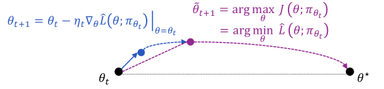
Figure 1 visualizes the proposed interpretation of what REINFORCE is actually doing. The curve going through $\bm{θ}_t→\bm{θ}_t+1→\widetilde{\bm{θ}}_t+1→\bm{θ}^⋆$ stands for the ideal optimization trajectory from $\bm{θ}_t$ to the optimal policy model parametrized by $\bm{θ}^⋆$ , if the algorithm solves each intermediate surrogate objective $J(\bm{θ};π_\bm{θ_t})$ / surrogate loss $\widehat{L}(\bm{θ};π_\bm{θ_t})$ exactly at each iteration $t$ . In comparison, REINFORCE is effectively taking a single gradient step of the surrogate loss and immediately moving on to the next iteration $\bm{θ}_t+1$ with a new surrogate objective.
Two remarks are in place. (1) Our derivation of group-relative REINFORCE can be generalized to multi-step RL settings, by replacing a response $y$ in the previous analysis with a full trajectory consisting of multiple turns of agent-environment interaction. For example, regarding the surrogate objective in Eq. (3), we need to replace the response-level reward and KL divergence with their trajectory-level counterparts. Interested readers might refer to Appendix A for the full analysis. (2) The above analysis suggests that we might interpret group-relative REINFORCE from a pointwise or pairwise perspective. While the policy update in Eq. (7) is stated in a pointwise manner, we have also seen that, at each iteration, REINFORCE is implicitly enforcing the pairwise consistency condition in Eq. (5) among multiple responses. This allows us the flexibility to choose whichever perspective that offers more intuition for our analysis later in this work.
<details>
<summary>x1.png Details</summary>
### Visual Description
## Diagram: Optimization Process Flow
### Overview
The image is a technical diagram illustrating two different optimization update rules in machine learning, visually comparing their trajectories from an initial parameter state (θ_t) toward an optimal state (θ*). It combines mathematical equations with a graphical representation of parameter space movement.
### Components/Axes
**Top Section (Equations):**
1. **Left Equation (Blue Text):**
`θ_{t+1} = θ_t - η_t ∇_θ L̂(θ; π_{θ_t}) |_{θ=θ_t}`
* This is a standard gradient descent update rule.
* **Components:** `θ_{t+1}` (updated parameters), `θ_t` (current parameters), `η_t` (learning rate), `∇_θ` (gradient operator), `L̂` (estimated loss function), `π_{θ_t}` (policy parameterized by `θ_t`).
2. **Right Equation (Purple Text):**
`θ̃_{t+1} = arg max_θ J(θ; π_{θ_t})`
`= arg min_θ L̂(θ; π_{θ_t})`
* This defines an alternative update rule that seeks the parameters maximizing an objective `J` (or equivalently, minimizing the estimated loss `L̂`) directly, given the current policy `π_{θ_t}`.
* **Components:** `θ̃_{t+1}` (updated parameters via this rule), `arg max_θ`/`arg min_θ` (argument of the maximum/minimum), `J` (objective function).
**Bottom Section (Visual Diagram):**
* **Points:**
* `θ_t`: Black dot, positioned at the bottom-left. Represents the starting parameter state at time `t`.
* `θ_{t+1}`: Blue dot, positioned to the right and slightly above `θ_t`. Represents the parameter state after one step of the gradient descent update (left equation).
* `θ̃_{t+1}`: Purple dot, positioned further right and higher than `θ_{t+1}`. Represents the parameter state after one step of the `arg max`/`arg min` update (right equation).
* `θ*`: Black dot, positioned at the bottom-right. Represents the optimal parameter state.
* **Arrows/Paths:**
* **Solid Blue Arrow:** Connects `θ_t` to `θ_{t+1}`. Corresponds to the gradient descent update (left equation).
* **Dashed Purple Arrow:** Connects `θ_t` to `θ̃_{t+1}`. Corresponds to the `arg max`/`arg min` update (right equation).
* **Dotted Black Line:** Connects `θ_t` directly to `θ*`. Represents a hypothetical direct path to the optimum.
* **Dashed Purple Arc:** Connects `θ̃_{t+1}` to `θ*`. Suggests a subsequent path from the intermediate point to the optimum.
### Detailed Analysis
* **Spatial Grounding & Color Correspondence:**
* The **blue** text of the left equation corresponds to the **blue** dot (`θ_{t+1}`) and the **solid blue arrow**.
* The **purple** text of the right equation corresponds to the **purple** dot (`θ̃_{t+1}`) and the **dashed purple arrow** and arc.
* The **black** dots (`θ_t`, `θ*`) and the **dotted black line** are neutral, representing start and end points.
* **Trend Verification:**
* The **gradient descent path (blue)** shows a small, incremental step from `θ_t` toward the general direction of `θ*`, but it lands at `θ_{t+1}`, which is not on the direct line to `θ*`.
* The **`arg max`/`arg min` path (purple dashed)** shows a larger, more direct leap from `θ_t` to `θ̃_{t+1}`, which is positioned closer to the vertical level of `θ*` and further along the horizontal axis.
* The **dotted black line** shows the ideal, straight-line path from start to optimum.
### Key Observations
1. The diagram visually contrasts a local, gradient-based step (blue) with a more global, objective-based step (purple).
2. The point `θ̃_{t+1}` is depicted as being "higher" (potentially indicating a higher objective value `J`) and further along the path to `θ*` than `θ_{t+1}` after a single update.
3. The dashed purple arc from `θ̃_{t+1}` to `θ*` implies that the `arg max` update places the parameters on a more favorable trajectory for reaching the optimum, possibly requiring fewer subsequent steps.
### Interpretation
This diagram is likely from a reinforcement learning or optimization theory context. It illustrates a conceptual comparison between two fundamental update strategies:
* **Gradient Descent (Blue):** A first-order method that follows the local slope of the loss landscape. It's computationally efficient but can be slow, myopic, and prone to getting stuck in local minima or taking a circuitous path.
* **Direct Objective Optimization (Purple):** A method that, at each step, seeks the parameters that would be optimal *if the current policy (π_{θ_t}) were fixed*. This is a more aggressive, "look-ahead" or "policy improvement" step. In algorithms like Trust Region Policy Optimization (TRPO) or Proximal Policy Optimization (PPO), such steps are constrained to ensure stability.
The visual metaphor suggests that while the gradient step makes safe, small progress, the direct optimization step makes a more significant leap toward regions of higher reward (or lower loss), potentially leading to faster overall convergence to the optimum `θ*`. The diagram argues for the potential efficiency of the latter approach by showing its intermediate point (`θ̃_{t+1}`) as being qualitatively closer to the goal.
</details>
Figure 1: A visualization of our off-policy interpretation for group-relative REINFORCE. Here $\widehat{L}(\bm{θ};π_\bm{θ_t})={E}_x∼\widehat{D}[\widehat{L}(\bm{θ};x,π_\bm{θ_t})]$ , where $\widehat{D}$ is the sampling distribution for prompts, and $\widehat{L}(\bm{θ};x,π_\bm{θ_t})$ is the surrogate loss defined in Eq. (6) for a specific prompt $x$ .
## 3 Pitfalls and augmentations
Although we have provided a native off-policy interpretation for REINFORCE, it certainly does not guarantee convergence to the optimal policy when given arbitrary training data. This section identifies pitfalls that could undermine vanilla REINFORCE, which motivate two principles for augmentations in off-policy settings.
#### Pitfalls of vanilla REINFORCE.
In Figure 1, we might expect that ideally, (1) $\widetilde{\bm{θ}}_t+1-\bm{θ}_t$ aligns with the direction of $\bm{θ}^⋆-\bm{θ}_t$ ; and (2) $\bm{θ}_t+1-\bm{θ}_t$ aligns with the direction of $\widetilde{\bm{θ}}_t+1-\bm{θ}_t$ . One pitfall, however, is that even if both conditions hold, they do not necessarily imply that $\bm{θ}_t+1-\bm{θ}_t$ should align well with $\bm{θ}^⋆-\bm{θ}_t$ . That is, $⟨\widetilde{\bm{θ}}_t+1-\bm{θ}_t,\bm{θ}^⋆-\bm{θ}_t⟩>0$ and $⟨\bm{θ}_t+1-\bm{θ}_t,\widetilde{\bm{θ}}_t+1-\bm{θ}_t⟩>0$ do not imply $⟨\bm{θ}_t+1-\bm{θ}_t,\bm{θ}^⋆-\bm{θ}_t⟩>0$ . Moreover, it is possible that $\bm{θ}_t+1-\bm{θ}_t$ might not align well with $\widetilde{\bm{θ}}_t+1-\bm{θ}_t$ . Recall from Eq. (7) that, from $\bm{θ}_t$ to $\bm{θ}_t+1$ , we take one gradient step for a surrogate loss that enforces the pairwise consistency condition among a finite number of samples. Given the enormous action space of an LLM, some implicit assumptions about the training data (e.g., balancedness and coverage) would be needed to ensure that the gradient aligns well with the direction towards the optimum of the surrogate objective, namely $\widetilde{\bm{θ}}_t+1-\bm{θ}_t$ .
In fact, without a mechanism that ensures boundedness of policy update under a sub-optimal data distribution, vanilla REINFORCE could eventually converge to a sub-optimal policy. Let us show this with a minimal example in a didactic 3-arm bandit setting. Suppose that there are three actions $\{a_j\}_1≤ j≤ 3$ with rewards $\{r(a_j)\}$ . Consider $K$ training samples $\{y_i\}_1≤ i≤ K$ , where $y_i∈\{a_j\}_1≤ j≤ 3$ is sampled from some behavior policy $π_\textsf{b}$ . Denote by $μ_r\coloneqq∑_1≤ j≤ 3π_\textsf{b}(a_j)r(a_j)$ the expected reward under $π_\textsf{b}$ , and $\overline{r}\coloneqq∑_ir(y_i)/K$ the average reward of training samples. We consider the softmax parameterization, i.e., $π_\bm{θ}(a_j)=e^θ_j/∑_\elle^θ_\ell$ for a policy parameterized by $\bm{θ}∈{ℝ}^3$ . A standard fact is that $∇_\bm{θ}\logπ_\bm{θ}(a_j)=\bm{e}_j-π_\bm{θ}$ , where $\bm{e}_j∈{ℝ}^3$ is a one-hot vector with value 1 at entry $j$ . Now we examine the policy update direction of REINFORCE, as $K→∞$ :
| | $\displaystyle\bm{g}$ | $\displaystyle=\frac{1}{K}∑_1≤ i≤ K(r(y_i)-\overline{r})∇_\bm{θ}\logπ_\bm{θ}(y_i)→∑_1≤ j≤ 3π_\textsf{b}(a_j)(r(a_j)-μ_r)∇_\bm{θ}\logπ_\bm{θ}(a_j)$ | |
| --- | --- | --- | --- |
For example, if $\bm{r}=[r(a_j)]_1≤ j≤ 3=[0,0.8,1]$ and $π_\textsf{b}=[0.3,0.6,0.1]$ , then basic calculation says $μ_r=0.58$ , $\bm{r}-μ_r=[-0.58,0.22,0.42]$ , and finally $g_2=π_\textsf{b}(a_2)(r(a_2)-μ_r)>π_\textsf{b}(a_3)(r(a_3)-μ_r)=g_3$ , which implies that the policy will converge to the sub-optimal action $a_2$ .
#### Two principles for augmenting REINFORCE.
The identified pitfalls of vanilla REINFORCE suggest two general principles for augmenting REINFORCE in off-policy scenarios:
- One is to regularize the policy update step, ensuring that the optimization trajectory remains bounded and reasonably stable when given training data from a sub-optimal distribution;
- The other is to steer the policy update direction, by actively weighting the training samples rather than naively using them as is.
These two principles are not mutually exclusive, and might be integrated within a single algorithm. We will see in the next section that many RL algorithms can be viewed as instantiations of them.
## 4 Rethinking the rationales behind recent RL algorithms
This section revisits various RL algorithms through a unified lens — the native off-policy interpretation of group-relative REINFORCE and its augmentations — and demystifies some common myths about their working mechanisms. Our main findings are summarized as follows:
| ID | Finding | Analysis & Experiments |
| --- | --- | --- |
| F1 | GRPO’s effectiveness in off-policy settings stems from clipping as regularization rather than importance sampling. A wider clipping range than usual often accelerates training without harming stability. | Section 4.1, Figures 3, 4, 6, 9, 10 |
| F2 | Kimi’s OPMD and Meta’s AsymRE can be interpreted as REINFORCE loss + regularization loss, a perspective that is complementary to the rationales in their original papers. | Section 4.2, Figure 11 |
| F3 | Data-oriented heuristics — such as dropping excess negatives or up-weighting high-reward rollouts — fit naturally into our off-policy view and show strong empirical performance. | Section 4.3, Figures 5, 6, 7 |
#### Experimental setup.
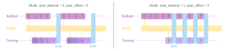
We primarily consider two off-policy settings in our experiments, specified by the sync_interval and sync_offset parameters in the Trinity-RFT framework (Pan et al., 2025). sync_interval specifies the number of generated rollout batches (each corresponding to one gradient step) between two model synchronization operations, while sync_offset specifies the relative lag between the generation and consumption of each batch. These parameters can be deliberately set to large values in practice, for improving training efficiency via pipeline parallelism and reduced frequency of model synchronization. In addition, $\texttt{sync\_offset}>1$ serves to simulate realistic scenarios where environmental feedback could be delayed. We also consider a stress-test setting that only allows access to offline data generated by the initial policy model. See Figure 2 for an illustration of these off-policy settings, and Appendix B.2 for further details.
We conduct experiments on math reasoning tasks like GSM8k (Cobbe et al., 2021), MATH (Hendrycks et al., 2021) and Guru (math subset) (Cheng et al., 2025), as well as tool-use tasks like ToolACE (Liu et al., 2025a). We consider models of different families and scales, including Qwen2.5-1.5B-Instruct, Qwen2.5-7B-Instruct (Qwen-Team, 2025), Llama-3.1-8B-Instruct, and Llama-3.2-3B-Instruct (Dubey et al., 2024). Additional experiment details can be found in Appendix B.
<details>
<summary>x2.png Details</summary>
### Visual Description
## Diagram: Synchronization Modes in a Machine Learning Training Pipeline
### Overview
The image displays two side-by-side diagrams illustrating different synchronization strategies between a "Rollout" process, a shared "Buffer," and a "Training" process. The diagrams compare how data batches flow and synchronize under two distinct parameter sets for `sync_interval` and `sync_offset`.
### Components/Axes
The diagrams are structured with three horizontal layers, from top to bottom:
1. **Rollout**: Represented by a sequence of purple rectangular boxes containing numbers (0, 1, 2, 3, etc.). This likely represents the generation of data batches or experiences.
2. **Buffer**: A continuous, horizontal yellow bar. This represents a shared memory or storage area where rollout data is held.
3. **Training**: Represented by another sequence of purple rectangular boxes, mirroring the Rollout layer. This represents the consumption of data batches for model training.
Vertical light blue bars labeled **"sync"** connect the layers, indicating synchronization points where data is transferred or consistency is enforced.
**Text Labels:**
* **Left Diagram Title:** `Mode: sync_interval = 4, sync_offset = 0`
* **Right Diagram Title:** `Mode: sync_interval = 1, sync_offset = 4`
* **Layer Labels (Left Side):** `Rollout`, `Buffer`, `Training` (written in a purple font).
* **Synchronization Label:** `sync` (written in blue at the base of each vertical blue bar).
### Detailed Analysis
The diagrams visualize the temporal relationship and data flow between the three components based on the synchronization parameters.
**Left Diagram (`sync_interval = 4, sync_offset = 0`):**
* **Rollout Sequence:** Generates batches in two visible groups: `0, 1, 2, 3` and then `4, 5, 6, 7`.
* **Training Sequence:** Consumes batches in identical groups: `0, 1, 2, 3` and then `4, 5, 6, 7`.
* **Synchronization Flow:**
1. Rollout generates batch `0`. An orange arrow points down to the Buffer, indicating data is stored.
2. After Rollout completes batch `3`, a vertical blue "sync" bar appears. A yellow arrow from the Buffer points to Training batch `0`, and a blue arrow from the sync bar points to Training batch `0`. This indicates a synchronized transfer of the first group of data (0-3) from the Buffer to the Training process.
3. The pattern repeats for the next group (batches 4-7).
* **Trend:** Synchronization occurs in **batches of 4** (`sync_interval=4`). Training starts immediately after the first rollout group is complete (`sync_offset=0`).
**Right Diagram (`sync_interval = 1, sync_offset = 4`):**
* **Rollout Sequence:** Generates batches sequentially: `0, 1, 2, 3, 4, 5, 6, 7`.
* **Training Sequence:** Consumes batches sequentially: `0, 1, 2, 3`.
* **Synchronization Flow:**
1. Rollout generates batches `0, 1, 2, 3, 4`. Data from each is stored in the Buffer (orange arrows).
2. **After Rollout completes batch `4`**, the first vertical blue "sync" bar appears. A yellow arrow from the Buffer points to Training batch `0`, and a blue arrow from the sync bar points to Training batch `0`. This indicates training begins only after rollout has produced 5 batches (0 through 4), establishing an offset.
3. Subsequent syncs happen after **every single new rollout batch** (`5`, `6`, `7`). Each sync bar connects the latest rollout batch to the next sequential training batch.
* **Trend:** Synchronization occurs **after every single rollout batch** (`sync_interval=1`). Training is **delayed** until the rollout has produced 5 batches (`sync_offset=4`, meaning training starts at index 0 when rollout is at index 4).
### Key Observations
1. **Parameter Impact:** The `sync_interval` parameter controls the frequency of synchronization (batched vs. continuous). The `sync_offset` parameter controls the delay or lead time between the rollout and training processes.
2. **Visual Metaphor:** The Buffer acts as an intermediary queue. The orange arrows show data being enqueued from Rollout. The yellow arrows show data being dequeued for Training, triggered by the blue sync events.
3. **Spatial Layout:** The Rollout and Training layers are aligned vertically to emphasize their sequential correspondence. The sync bars are placed at the temporal point where the handoff occurs.
### Interpretation
These diagrams illustrate two fundamental strategies for coordinating data generation (rollout) and model update (training) in reinforcement learning or similar iterative learning systems.
* The **left mode (`interval=4, offset=0`)** represents a **batch-synchronous** approach. It waits for a full batch of experiences to be collected before synchronously updating the training process. This can be computationally efficient but may introduce latency, as training is idle while waiting for the rollout batch to complete.
* The **right mode (`interval=1, offset=4`)** represents a **more asynchronous, pipelined** approach. Training starts after an initial warm-up period (the offset) and then continuously processes experiences as soon as they are available (every interval). This can lead to more frequent model updates and potentially faster adaptation, but with higher synchronization overhead and the complexity of managing a constantly shifting data window.
The choice between these modes involves a trade-off between computational throughput, update frequency, and system complexity. The diagrams effectively communicate how the `sync_interval` and `sync_offset` parameters directly govern this trade-off by defining the choreography between the rollout and training workers.
</details>
Figure 2: A visualization of the rollout-training scheduling in sync_interval = 4 (left) or sync_offset = 4 (right) modes. Each block denotes one batch of samples for one gradient step, and the number in it denotes the corresponding batch id. Training blocks are color-coded by data freshness, with lighter color indicating increasing off-policyness.
### 4.1 Demystifying myths about GRPO
Recall that in GRPO, the advantage for each response $y_i$ is defined as $A_i={(r_i-\overline{r})}/{σ_r}$ , where $\overline{r}$ and $σ_r$ denote the within-group mean and standard deviation of the rewards $\{r_i\}_1≤ i≤ K$ respectively. We consider the practical implementation of GRPO with token-wise importance-sampling (IS) weighting and clipping, whose loss function for a specific prompt $x$ and responses $\{y_i\}$ is In our experiments with GRPO, we neglect KL regularization with respect to an extra reference model, or entropy regularization that encourages output diversity. Recent works (Yu et al., 2025; Liu et al., 2025b) have shown that these practical techniques are often unnecessary.
| | $\displaystyle\widehat{L}=\frac{1}{K}∑_1≤ i≤ K∑_1≤ t≤|y_{i|}\min\bigg\{\frac{π_\bm{θ}(y_i^t | x,y_i^<t)}{π_\textsf{old}(y_i^t | x,y_i^<t)}A_i, \Big(\frac{π_\bm{θ}(y_i^t | x,y_i^<t)}{π_\textsf{old}(y_i^t | x,y_i^<t)},1-ε_\textsf{low},1+ε_\textsf{high}\Big)A_i\bigg\},$ | |
| --- | --- | --- |
where $π_\textsf{old}$ denotes the older policy version that generated this group of rollout data. The gradient of this loss can be written as (Schulman et al., 2017)
$$
\bm{g}\big(\bm{θ};x,\{y_i,r_i\}_1≤ i≤ K\big)=\frac{1}{K}∑_1≤ i≤ K∑_1≤ t≤|y_{i|}∇_\bm{θ}\logπ_\bm{θ}(y_i^t | x,y_i^<t)· A_i\frac{π_\bm{θ}(y_i^t | x,y_i^<t)}{π_\textsf{old}(y_i^t | x,y_i^<t)}M_i^t,
$$
where $M_i^t$ denotes a one-side clipping mask:
$$
M_i^t=\mathbbm{1}\bigg(A_i>0, \frac{π_\bm{θ}(y_i^t | x,y_i^<t)}{π_\textsf{old}(y_i^t | x,y_i^<t)}≤ 1+ε_\textsf{high}\bigg)+\mathbbm{1}\bigg(A_i<0, \frac{π_\bm{θ}(y_i^t | x,y_i^<t)}{π_\textsf{old}(y_i^t | x,y_i^<t)}≥ 1-ε_\textsf{low}\bigg). \tag{8}
$$
#### Ablation study with the REC series.
To isolate the roles of importance sampling and clipping, we consider a series of RE INFORCE-with- C lipping (REC) algorithms. Due to space limitation, we defer our studies of more clipping mechanisms to Appendix B.3, and focus on REC with one-side clipping in this section. More specifically, REC-OneSide-IS removes advantage normalization in GRPO (to reduce variability), and REC-OneSide-NoIS further removes IS weighting:
| | $\displaystyle{REC-OneSide-IS:} \bm{g}$ | $\displaystyle=\frac{1}{K}∑_1≤ i≤ K∑_1≤ t≤|y_{i|}∇_\bm{θ}\logπ_\bm{θ}(y_i^t | x,y_i^<t)·(r_i-\overline{r}) \frac{π_\bm{θ}(y_i^t | x,y_i^<t)}{π_\textsf{old}(y_i^t | x,y_i^<t)} M_i^t,$ | |
| --- | --- | --- | --- |
<details>
<summary>x3.png Details</summary>
### Visual Description
\n
## Multi-Panel Line Chart: Comparative Performance of Reinforcement Learning Algorithms
### Overview
The image displays a 2x3 grid of line charts comparing the performance of five different reinforcement learning algorithms across three distinct experimental conditions. The top row tracks "Evaluation Accuracy" over training steps, while the bottom row tracks "Training Reward". The three columns represent different synchronization settings: "sync_interval = 20", "sync_offset = 10", and "offline".
### Components/Axes
* **Main Titles (Column Headers):** "sync_interval = 20", "sync_offset = 10", "offline".
* **Y-Axis Labels (Row Headers):**
* Top Row: "Evaluation Accuracy" (Scale: 0.00 to 0.75, with ticks at 0.00, 0.25, 0.50, 0.75).
* Bottom Row: "Training Reward" (Scale: 0.0 to 1.0, with ticks at 0.0, 0.5, 1.0).
* **X-Axis Label (Common to all plots):** "Training Steps" (Scale: 0 to 150, with ticks at 0, 50, 100, 150).
* **Legend (Bottom Center):** Contains five entries, each with a distinct color and marker:
1. `REINFORCE` - Light blue line with circle markers.
2. `GRPO` - Teal line with square markers.
3. `REC-OneSide-NoIS (0.2)` - Light purple line with diamond markers.
4. `REC-OneSide-IS (0.2)` - Dotted purple line with upward-pointing triangle markers.
5. `REC-OneSide-NoIS (0.6, 2.0)` - Dark purple line with plus (+) markers.
### Detailed Analysis
**Top Row: Evaluation Accuracy**
* **sync_interval = 20 (Top-Left Plot):**
* `REC-OneSide-NoIS (0.6, 2.0)` (Dark purple, +): Shows a strong, steady upward trend from ~0.35 at step 0 to ~0.75 at step 150. It is the top-performing algorithm.
* `GRPO` (Teal, square): Increases steadily from ~0.35 to ~0.65.
* `REC-OneSide-NoIS (0.2)` (Light purple, diamond) & `REC-OneSide-IS (0.2)` (Dotted purple, triangle): Both show similar, moderate upward trends, ending near ~0.65.
* `REINFORCE` (Light blue, circle): Highly unstable. Starts near 0.35, peaks at ~0.65 around step 40, then crashes to near 0.00 by step 75, with a brief recovery spike before falling again.
* **sync_offset = 10 (Top-Middle Plot):**
* `REC-OneSide-NoIS (0.6, 2.0)` (Dark purple, +): Again shows a strong upward trend, reaching ~0.75.
* `GRPO`, `REC-OneSide-NoIS (0.2)`, `REC-OneSide-IS (0.2)`: All cluster together, showing steady improvement to ~0.65-0.70.
* `REINFORCE` (Light blue, circle): Exhibits a sharp dip to ~0.25 around step 60 but recovers to join the cluster near ~0.65 by step 150.
* **offline (Top-Right Plot):**
* `REC-OneSide-NoIS (0.6, 2.0)` (Dark purple, +): Increases to a peak of ~0.60 around step 100, then declines to ~0.25 by step 150.
* `GRPO`, `REC-OneSide-NoIS (0.2)`, `REC-OneSide-IS (0.2)`: All plateau early around ~0.40-0.50 and remain flat.
* `REINFORCE` (Light blue, circle): Peaks early at ~0.60, then plummets to near 0.00 by step 100 and stays there.
**Bottom Row: Training Reward**
* **sync_interval = 20 (Bottom-Left Plot):**
* `REC-OneSide-NoIS (0.6, 2.0)` (Dark purple, +): Shows a noisy but clear upward trend, reaching near 1.0.
* `GRPO`, `REC-OneSide-NoIS (0.2)`, `REC-OneSide-IS (0.2)`: All trend upward with noise, ending between 0.75 and 0.90.
* `REINFORCE` (Light blue, circle): Reward collapses to near 0.00 after step 75, mirroring its accuracy crash.
* **sync_offset = 10 (Bottom-Middle Plot):**
* All algorithms except `REINFORCE` show strong, noisy upward trends, converging near 0.90-1.0 by step 150.
* `REINFORCE` (Light blue, circle): Shows a significant dip around step 60 but recovers to join the others near 0.90.
* **offline (Bottom-Right Plot):**
* All five algorithms show nearly identical, flat performance. The reward hovers around 0.5 with very minor fluctuations throughout all 150 steps. There is no clear upward trend for any method.
### Key Observations
1. **Algorithm Dominance:** `REC-OneSide-NoIS (0.6, 2.0)` is consistently the top or among the top performers in both accuracy and reward for the two synchronized conditions (`sync_interval`, `sync_offset`).
2. **REINFORCE Instability:** The `REINFORCE` algorithm is highly unstable in synchronized settings, suffering catastrophic performance drops. It performs comparably to others only in the `offline` setting for accuracy (until it crashes) and is flat in reward.
3. **Condition Impact:** The "offline" condition severely limits learning for all algorithms. Accuracy plateaus at a lower level (~0.5) or declines, and training reward shows no improvement over time, staying at ~0.5.
4. **Synchronization Benefit:** Both `sync_interval=20` and `sync_offset=10` enable clear learning progress for most algorithms, with `sync_offset=10` appearing to offer slightly more stability for `REINFORCE`.
5. **Performance Clustering:** The three `REC` variants and `GRPO` often perform similarly, forming a cluster below the top-performing `REC-OneSide-NoIS (0.6, 2.0)`.
### Interpretation
This set of charts demonstrates a comparative study of distributed or synchronized reinforcement learning algorithms. The data suggests that the proposed method, `REC-OneSide-NoIS (0.6, 2.0)`, is more robust and achieves higher final performance than the baselines (`REINFORCE`, `GRPO`) and its own ablated variants (`REC-OneSide-NoIS (0.2)`, `REC-OneSide-IS (0.2)`) under conditions with periodic synchronization (`sync_interval`, `sync_offset`).
The catastrophic failure of `REINFORCE` in synchronized settings highlights a known challenge of variance in policy gradient methods, which the `REC` methods appear to mitigate. The complete stagnation in the "offline" condition implies that without any synchronization or online interaction, the learning process for these particular tasks and algorithms fails to make progress, plateauing at a suboptimal reward level. The near-identical flat lines in the bottom-right plot are a strong visual indicator of this failure mode. The study underscores the critical importance of synchronization strategy and algorithmic stability in achieving effective learning.
</details>
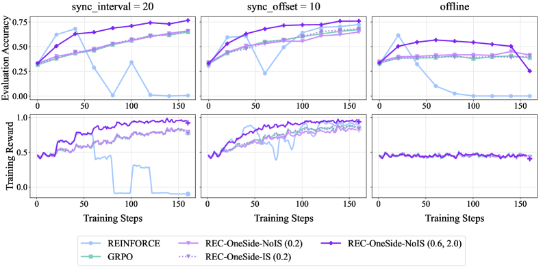
Figure 3: Empirical results for REC algorithms on GSM8k with Qwen2.5-1.5B-Instruct. Training reward curves are smoothed with a running-average window of size 3. Numbers in the legend denote clipping parameters $ε_\textsf{low},ε_\textsf{high}$ .
<details>
<summary>x4.png Details</summary>
### Visual Description
## Dual-Axis Line Chart: Training Reward and Clipping Fraction with sync_interval = 20
### Overview
The image displays two line charts side-by-side, sharing a common x-axis ("Training Steps") and a common legend. The left chart plots "Training Reward" against training steps, while the right chart plots "Clipping Fraction" (on a logarithmic scale) against the same steps. Both charts are titled "sync_interval = 20". A legend at the bottom identifies six different experimental conditions, distinguished by color and line style.
### Components/Axes
* **Chart Titles:** Both subplots are titled "sync_interval = 20".
* **Left Chart (Training Reward):**
* **Y-axis Label:** "Training Reward"
* **Y-axis Scale:** Linear, ranging from 0.25 to 1.00, with major ticks at 0.25, 0.50, 0.75, and 1.00.
* **X-axis Label:** "Training Steps"
* **X-axis Scale:** Linear, ranging from 0 to 400, with major ticks at 0, 100, 200, 300, and 400.
* **Right Chart (Clipping Fraction):**
* **Y-axis Label:** "Clipping Fraction"
* **Y-axis Scale:** Logarithmic (base 10), ranging from 10⁻⁴ to 10⁻¹, with major ticks at 10⁻⁴, 10⁻³, 10⁻², and 10⁻¹.
* **X-axis Label:** "Training Steps"
* **X-axis Scale:** Linear, identical to the left chart (0 to 400).
* **Legend:** Positioned at the bottom center of the figure, spanning both charts. It contains six entries:
1. `REC-OneSide-NoIS (0.2, 0.25)` - Solid purple line.
2. `REC-OneSide-IS (0.2, 0.25)` - Dotted purple line.
3. `REC-Ring-NoIS (0.2, 0.25) & (0.6, 2.0)` - Solid pink/magenta line.
4. `REC-OneSide-NoIS (0.6, 2.0)` - Solid dark purple/indigo line.
5. `REC-TwoSide-NoIS (0.2, 0.25)` - Solid orange/yellow line.
6. `REC-TwoSide-NoIS (0.6, 2.0)` - Dotted orange/yellow line.
### Detailed Analysis
**Left Chart - Training Reward:**
* **Trend Verification:** All six data series show a clear upward trend, starting from a low reward (between ~0.25 and ~0.50) at step 0 and converging towards a high reward (between ~0.90 and ~1.00) by step 400. The rate of increase is steepest in the first ~100 steps.
* **Data Series & Approximate Values:**
* `REC-OneSide-NoIS (0.2, 0.25)` (Solid Purple): Starts ~0.35, rises steadily, ends ~0.98.
* `REC-OneSide-IS (0.2, 0.25)` (Dotted Purple): Follows a nearly identical path to its solid counterpart, ending ~0.98.
* `REC-Ring-NoIS (0.2, 0.25) & (0.6, 2.0)` (Solid Pink): Starts slightly higher (~0.45), rises quickly, and maintains a slight lead for most of the training, ending ~0.99.
* `REC-OneSide-NoIS (0.6, 2.0)` (Solid Dark Purple): Starts the lowest (~0.25), rises more slowly initially but catches up, ending ~0.97.
* `REC-TwoSide-NoIS (0.2, 0.25)` (Solid Orange): Starts ~0.40, rises quickly, and is among the top performers, ending ~0.99.
* `REC-TwoSide-NoIS (0.6, 2.0)` (Dotted Orange): Follows a very similar path to its solid counterpart, ending ~0.99.
* **Convergence:** By step 400, all lines are tightly clustered between approximately 0.95 and 1.00, indicating similar final performance in terms of training reward.
**Right Chart - Clipping Fraction:**
* **Trend Verification:** All series exhibit a distinct, regular oscillatory pattern (sawtooth wave) throughout training. The amplitude and baseline of these oscillations differ between series.
* **Data Series & Approximate Values:**
* `REC-OneSide-NoIS (0.2, 0.25)` (Solid Purple): Oscillates with a baseline around 10⁻³ and peaks near 10⁻².
* `REC-OneSide-IS (0.2, 0.25)` (Dotted Purple): Oscillates with a lower baseline (between 10⁻⁴ and 10⁻³) and lower peaks (around 10⁻³).
* `REC-Ring-NoIS (0.2, 0.25) & (0.6, 2.0)` (Solid Pink): Shows the highest oscillations, with a baseline around 10⁻² and peaks reaching close to 10⁻¹.
* `REC-OneSide-NoIS (0.6, 2.0)` (Solid Dark Purple): Has the lowest overall values, oscillating between 10⁻⁴ and 10⁻³.
* `REC-TwoSide-NoIS (0.2, 0.25)` (Solid Orange): Oscillates with a baseline around 10⁻² and peaks near 5x10⁻².
* `REC-TwoSide-NoIS (0.6, 2.0)` (Dotted Orange): Follows a similar pattern to its solid counterpart but with slightly lower peaks.
* **Pattern:** The oscillations are synchronized across all series, with peaks and troughs occurring at the same training steps (approximately every 20 steps, consistent with `sync_interval = 20`).
### Key Observations
1. **Performance Convergence:** Despite different starting points and clipping behaviors, all methods achieve nearly identical high training rewards (~0.95-1.00) by the end of 400 steps.
2. **Clipping Fraction Hierarchy:** There is a clear hierarchy in clipping fraction magnitude: `REC-Ring-NoIS` > `REC-TwoSide-NoIS` ≈ `REC-OneSide-NoIS (0.2, 0.25)` > `REC-OneSide-IS (0.2, 0.25)` > `REC-OneSide-NoIS (0.6, 2.0)`.
3. **Impact of IS (Importance Sampling?):** The `REC-OneSide-IS` variant (dotted purple) shows significantly lower clipping fractions than its `NoIS` counterpart (solid purple) while achieving similar final reward.
4. **Impact of Parameters (0.2, 0.25) vs (0.6, 2.0):** For the `OneSide-NoIS` method, the (0.6, 2.0) parameter set (dark purple) results in lower initial reward, slower initial learning, and lower clipping fractions compared to the (0.2, 0.25) set (purple).
5. **Synchronized Oscillations:** The perfect synchronization of clipping fraction oscillations across all methods confirms the `sync_interval = 20` setting is actively influencing the training dynamics at a fixed frequency.
### Interpretation
This data suggests an experiment comparing different variants of a "REC" (likely a Reinforcement Learning or optimization algorithm) under a fixed synchronization interval. The primary finding is that **all tested variants are effective at maximizing the training reward**, converging to a similar high performance. The key differences lie in their *training dynamics*, specifically the magnitude of gradient clipping applied.
The `REC-Ring-NoIS` method operates with the highest clipping fractions, suggesting it experiences the largest gradient updates that are frequently clipped. In contrast, the `REC-OneSide-NoIS (0.6, 2.0)` method has the smallest clipping fractions, indicating more conservative updates. The `REC-OneSide-IS` method achieves a middle ground, suggesting importance sampling may help stabilize updates, reducing the need for aggressive clipping.
The synchronized sawtooth pattern in clipping fraction is a direct artifact of the `sync_interval = 20` parameter, likely representing a periodic reset or synchronization event that causes gradients to build up and then be clipped in a regular cycle. The fact that reward converges similarly despite vastly different clipping profiles implies the task may be robust to a range of update magnitudes, or that the clipping mechanism is effectively normalizing the learning process across all variants. The experiment highlights how algorithmic choices (OneSide vs. TwoSide vs. Ring, with or without IS) and hyperparameters (the numeric pairs) primarily affect the *path* (clipping behavior) rather than the *destination* (final reward) in this specific setting.
</details>
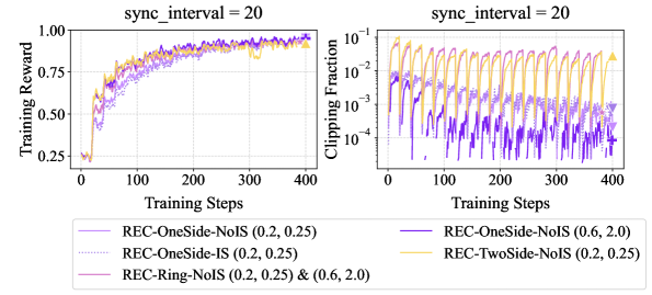
Figure 4: Empirical results for REC on ToolACE with Llama-3.2-3B-Instruct. Training reward curves are smoothed with a running-average window of size 3. Details about REC-TwoSide and REC-Ring are provided in Appendix B.3.
#### Experiments.
Figure 3 presents GSM8k results with Qwen2.5-1.5B-Instruct in various off-policy settings. REC-OneSide-IS / NoIS and GRPO (with the same $ε_\textsf{low}=ε_\textsf{high}=0.2$ ) have nearly identical performance, indicating that importance sampling is non-essential, whereas the collapse of REINFORCE highlights the critical role of clipping. Radically enlarging $(ε_\textsf{low},ε_\textsf{high})$ to $(0.6,2.0)$ accelerates REC-OneSide-NoIS without compromising stability in both sync_interval = 20 and sync_offset = 10 settings. Similar patterns also appear in Figure 4 (ToolAce with Llama-3.2-3B-Instruct) and other results in Appendix B. As for the stress-test (“offline”) setting, Figure 3 reveals an intrinsic trade-off between the speed and stability of policy improvement, motivating future work toward better algorithms that achieve both.
### 4.2 Understanding Kimi’s OPMD and Meta’s AsymRE
Besides clipping, another natural method is to add a regularization loss $R(·)$ to vanilla REINFORCE:
| | $\displaystyle\widehat{L}\big(\bm{θ};x,\{y_i,r_i\}_1≤ i≤ K\big)$ | $\displaystyle=-\frac{1}{K}∑_i∈[K](r_i-\overline{r})\logπ_\bm{θ}(y_i | x)+τ· R\big(\bm{θ};x,\{y_i,r_i\}_1≤ i≤ K\big),$ | |
| --- | --- | --- | --- |
and take $\bm{g}=-∇_\bm{θ}\widehat{L}$ . We show below that Kimi’s OPMD and Meta’s AsymRE are indeed special cases of this unified formula, with empirical validation of their efficacy deferred to Appendix B.5.
#### Kimi’s OPMD.
Kimi-Team (2025b) derives an OPMD variant by taking logarithm of both sides of Eq. (4), which leads to a consistency condition and further motivates the following surrogate loss:
$$
\widetilde{L}=\frac{1}{K}∑_1≤ i≤ K\bigg(r_i-τ\log Z(x,π_\bm{θ_t})-τ \Big(\logπ_\bm{θ}(y_i | x)-\logπ_\bm{θ_t}(y_i|x)\Big)\bigg)^2.
$$
With $K$ responses generated by $π_\textsf{old}=π_\bm{θ_t}$ , the term $τ\log Z(x,π_\bm{θ_t})$ can be approximated by a finite-sample estimate $τ\log(∑_ie^r_i/τ/K)$ , which can be further approximated by the mean reward $\overline{r}=∑_ir_i/K$ if $τ$ is large. With these approximations, the gradient of $\widetilde{L}$ becomes equivalent to that of the following loss (which is the final version of Kimi’s OPMD):
$$
\widehat{L}=-\frac{1}{K}∑_1≤ i≤ K(r_i-\overline{r})\logπ_\bm{θ}(y_i | x)+\frac{τ}{2K}∑_1≤ i≤ K\Big(\logπ_\bm{θ}(y_i | x)-\logπ_\textsf{old}(y_i | x)\Big)^2.
$$
In comparison, our analysis in Sections 2 and 3 suggests that this is in itself a principled loss function for off-policy RL, adding a mean-squared regularization loss to the vanilla REINFORCE loss.
#### Meta’s AsymRE.
AsymRE (Arnal et al., 2025) modifies REINFORCE by tuning down the baseline (from $\overline{r}$ to $\overline{r}-τ$ ) in advantage calculation, which was motivated by the intuition of prioritizing learning from positive samples and justified by multi-arm bandit analysis in the original paper. We offer an alternative interpretation for AsymRE by rewriting its loss function:
| | $\displaystyle\widehat{L}$ | $\displaystyle=-\frac{1}{K}∑_i\Big(r_i-(\overline{r}-τ)\Big)\logπ_\bm{θ}(y_i | x)=-\frac{1}{K}∑_i(r_i-\overline{r})\logπ_\bm{θ}(y_i | x)-\frac{τ}{K}∑_i\logπ_\bm{θ}(y_i | x).$ | |
| --- | --- | --- | --- |
Note that the first term on the right-hand side is the REINFORCE loss, and the second term serves as regularization, enforcing imitation of responses from an older version of the policy model. For the latter, we may also add a term that is independent of $\bm{θ}$ to it and take the limit $K→∞$ :
| | $\displaystyle-\frac{1}{K}∑_1≤ i≤ K\logπ_\bm{θ}(y_i | x)+\frac{1}{K}∑_1≤ i≤ K\logπ_\textsf{old}(y_i | x)=\frac{1}{K}∑_1≤ i≤ K\log\frac{π_\textsf{old}(y_i | x)}{π_\bm{θ}(y_i | x)}$ | |
| --- | --- | --- |
which turns out to be a finite-sample approximation of KL regularization.
### 4.3 Understanding data-weighting methods
We now shift our attention to the second principle for augmenting REINFORCE, i.e., actively shaping the training data distribution.
#### Pairwise weighting.
Recall from Section 2 that we define the surrogate loss in Eq. (6) as an unweighted sum of pairwise mean-squared losses. However, if we have certain knowledge about which pairs are more informative for RL training, we may assign higher weights to them. This motivates generalizing $∑_i<j(a_i-a_j)^2$ to $∑_i<jw_i,j(a_i-a_j)^2$ , where $\{w_i,j\}$ are non-negative weights. Assuming that $w_i,j=w_j,i$ and following the steps in Section 2, we end up with
$$
\bm{g}\big(\bm{θ};x,\{y_i,r_i\}_1≤ i≤ K\big)=\frac{1}{K}∑_1≤ i≤ K\Big(∑_1≤ j≤ Kw_i,j\Big)\bigg(r_i-\frac{∑_jw_i,jr_j}{∑_jw_i,j}\bigg)∇_\bm{θ}\logπ_\bm{θ}(y_i | x).
$$
In the special case where $w_i,j=w_iw_j$ , this becomes
$$
\bm{g}=\Big(∑_jw_j\Big) \frac{1}{K}∑_1≤ i≤ Kw_i\big(r_i-\overline{r}_w\big)∇_\bm{θ}\logπ_\bm{θ}(y_i | x), where \overline{r}_w\coloneqq\frac{∑_jw_jr_j}{∑_jw_j}. \tag{9}
$$
Based on this, we investigate two RE INFORCE-with- d ata-weighting (RED) methods.
#### RED-Drop : sample dropping.
The idea is to use a filtered subset $S⊆[K]$ of responses for training; for example, the Kimi-Researcher technical blog (Kimi-Team, 2025a) proposes to “discard some negative samples strategically”, as negative gradients increase the risk of entropy collapse. This is indeed a special case of Eq. (9), by setting $w_i=√{K}/|S|$ for $i∈S$ and $0$ otherwise:
$$
\bm{g}\big(\bm{θ};x,\{y_i,r_i\}_1≤ i≤ K\big)=\frac{1}{|S|}∑_i∈S(r_i-\overline{r}_S)∇_\bm{θ}\logπ_\bm{θ}(y_i | x), where \overline{r}_S=\frac{1}{|S|}∑_i∈Sr_i. \tag{10}
$$
While this is no longer an unbiased estimate of policy gradient even if all responses are sampled from the current policy, it is still well justified by our off-policy interpretation of REINFORCE.
#### RED-Weight : pointwise loss weighting.
Another approach for prioritizing high-reward responses is to directly up-weight their gradient terms in Eq. (1a). To better understand the working mechanism of this seemingly heuristic method, we rewrite its policy update:
| | $\displaystyle\bm{g}$ | $\displaystyle=∑_1≤ i≤ Kw_i(r_i-\overline{r})∇_\bm{θ}\logπ_\bm{θ}(y_i|x)=∑_1≤ i≤ Kw_i(r_i-\overline{r}_w+\overline{r}_w-\overline{r})∇_\bm{θ}\logπ_\bm{θ}(y_i|x)$ | |
| --- | --- | --- | --- |
This is the pairwise-weighted REINFORCE gradient in Eq. (9), plus a regularization term (weighted by $\overline{r}_w-\overline{r}>0$ ) that resembles the one in AsymRE but prioritizes imitating higher-reward responses, echoing the finding from offline RL literature (Hong et al., 2023a, b) that regularizing against high-reward trajectories can be more effective than conservatively imitating all trajectories in the dataset.
#### Implementation details.
Below are the concrete instantiations adopted in our empirical studies:
- RED-Drop: When the number of negative samples in a group exceeds the number of positive ones, we randomly drop the excess negatives so that positives and negatives are balanced. After this subsampling step, we recompute the advantages using the remaining samples, which are then fed into the loss.
- RED-Weight: Each sample $i$ is weighted by $w_i=\exp({A_i}/{τ})$ , where $A_i$ denotes its advantage estimate and $τ>0$ is a temperature parameter controlling the sharpness of weighting. This scheme amplifies high-advantage samples while down-weighting low-advantage ones. We fix $τ=1$ for all experiments.
<details>
<summary>x5.png Details</summary>
### Visual Description
\n
## Line Charts: Comparative Performance of Reinforcement Learning Algorithms
### Overview
The image displays a 2x2 grid of line charts comparing the performance of four reinforcement learning algorithms across two different training conditions. The top row measures "Evaluation Accuracy," and the bottom row measures "Training Reward" over the course of "Training Steps." The left column represents an "on-policy" condition, while the right column represents a condition with "sync_interval = 20."
### Components/Axes
* **Titles:**
* Top-left chart: "on-policy"
* Top-right chart: "sync_interval = 20"
* **Y-Axis Labels:**
* Top row (both charts): "Evaluation Accuracy" (Scale: 0.0 to 0.8)
* Bottom row (both charts): "Training Reward" (Scale: 0.00 to 1.00)
* **X-Axis Label (All Charts):** "Training Steps" (Scale: 0 to 150, with major ticks at 0, 25, 50, 75, 100, 125, 150)
* **Legend (Bottom Center):**
* **REINFORCE:** Light blue line with circle markers.
* **RED-Weight:** Orange line with diamond markers.
* **RED-Drop:** Red line with square markers.
* **REC-OneSide-NoIS (0.6, 2.0):** Purple line with plus (+) markers.
### Detailed Analysis
**Top-Left Chart: Evaluation Accuracy (on-policy)**
* **Trend:** All four algorithms show a strong, similar upward trend, converging to high accuracy.
* **Data Points (Approximate):**
* All lines start near 0.35 at step 0.
* By step 25, all are clustered around 0.60-0.65.
* By step 75, all are tightly grouped between 0.70-0.75.
* From step 100 to 150, all lines plateau and remain very close, ending near 0.75-0.78.
**Top-Right Chart: Evaluation Accuracy (sync_interval = 20)**
* **Trend:** The REINFORCE algorithm shows a dramatic decline, while the other three maintain high performance.
* **Data Points (Approximate):**
* **REINFORCE (Light Blue):** Starts ~0.45, peaks ~0.55 at step 40, then declines sharply. It falls below 0.20 by step 100 and approaches 0.00 by step 150.
* **RED-Weight (Orange):** Starts ~0.45, rises steadily to ~0.70 by step 100, and plateaus near 0.72.
* **RED-Drop (Red) & REC-OneSide-NoIS (Purple):** Both start ~0.40, follow a very similar upward path, and converge near 0.75-0.78 by step 150, slightly outperforming RED-Weight.
**Bottom-Left Chart: Training Reward (on-policy)**
* **Trend:** All algorithms show rapid initial learning and converge to a high, stable reward.
* **Data Points (Approximate):**
* All lines start near 0.50.
* They rise sharply, reaching ~0.90 by step 50.
* From step 50 to 150, all lines fluctuate in a tight band between approximately 0.90 and 1.00, showing stable convergence.
**Bottom-Right Chart: Training Reward (sync_interval = 20)**
* **Trend:** REINFORCE collapses to near-zero reward, while the other algorithms maintain high reward.
* **Data Points (Approximate):**
* **REINFORCE (Light Blue):** Starts ~0.50, rises to ~0.75 by step 50, then crashes. It drops to near 0.00 by step 80, shows a brief, small recovery around step 100, then falls back to 0.00.
* **RED-Weight (Orange):** Starts ~0.50, rises to ~0.90 by step 75, and remains stable between 0.85-0.95.
* **RED-Drop (Red) & REC-OneSide-NoIS (Purple):** Both follow a nearly identical path, starting ~0.50, rising to ~0.95 by step 75, and maintaining a high reward between 0.90-1.00.
### Key Observations
1. **Algorithm Divergence:** The "sync_interval = 20" condition causes a catastrophic performance collapse for the REINFORCE algorithm in both evaluation accuracy and training reward, while the other three methods (RED-Weight, RED-Drop, REC-OneSide-NoIS) remain robust.
2. **Method Similarity:** RED-Drop and REC-OneSide-NoIS (0.6, 2.0) perform almost identically across all four charts, suggesting similar underlying behavior or effectiveness in these scenarios.
3. **Stability vs. Instability:** The "on-policy" condition leads to stable, convergent learning for all methods. The "sync_interval = 20" condition introduces instability that only REINFORCE succumbs to.
4. **Performance Ceiling:** Under stable conditions (on-policy), all methods appear to reach a similar performance ceiling (~0.75 accuracy, ~0.95 reward).
### Interpretation
This data demonstrates a critical vulnerability in the standard REINFORCE algorithm when training is synchronized at intervals (sync_interval=20), likely due to issues with stale gradients or policy lag. The other three algorithms, which presumably incorporate mechanisms to handle off-policy or delayed updates (implied by names like "RED" and "REC"), show significant robustness to this synchronization delay.
The near-identical performance of RED-Drop and REC-OneSide-NoIS suggests that their specific technical differences may not be consequential for this particular task and set of conditions. The charts effectively argue that for distributed or synchronized training setups, using one of the more robust variants (RED or REC family) is essential to prevent complete training failure, as exhibited by REINFORCE. The "on-policy" results serve as a control, proving all algorithms are capable of learning the task under ideal, low-latency conditions.
</details>
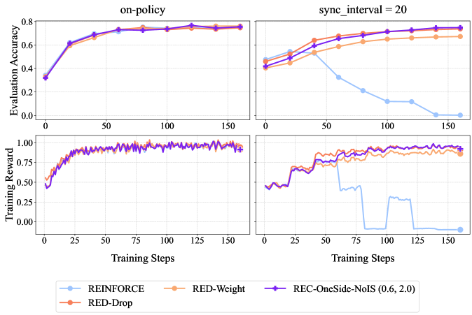
Figure 5: Empirical performance of RED-Drop and RED-Weight on GSM8k with Qwen2.5-1.5B-Instruct, in both on-policy and off-policy settings. Training reward curves are smoothed with a running-average window of size 3.
#### Experiments.
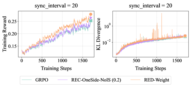
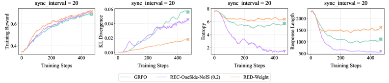
Figure 5 presents GSM8k results with Qwen2.5-1.5B-Instruct, which confirm the efficacy of RED-Drop and RED-Weight in on/off-policy settings, comparable to REC-OneSide-NoIS with enlarged $(ε_\textsf{low},ε_\textsf{high})$ . Figure 6 reports larger-scale experiments on Guru-Math with Qwen2.5-7B-Instruct, where RED-Weight achieves higher rewards than GRPO, with similar KL distance to the initial policy. Figure 7 further validates the efficacy of RED-Weight on MATH with Llama-3.1-8B-Instruct; compared to GRPO and REC-OneSide-NoIS, RED-Weight achieves higher rewards with lower KL divergence, while maintaining more stable entropy and response lengths.
<details>
<summary>x6.png Details</summary>
### Visual Description
\n
## Line Charts: Training Reward and KL Divergence Comparison
### Overview
The image displays two side-by-side line charts comparing the performance of three different methods (GRPO, REC-OneSide-NoIS (0.2), RED-Weight) over the course of training. The left chart tracks "Training Reward," and the right chart tracks "KL Divergence." Both charts share the same x-axis ("Training Steps") and a legend located at the bottom center of the figure. The title "sync_interval = 20" appears above each chart.
### Components/Axes
* **Titles:**
* Left Chart: "Training Reward"
* Right Chart: "KL Divergence"
* Above Both Charts: "sync_interval = 20"
* **X-Axis (Both Charts):**
* Label: "Training Steps"
* Scale: Linear, from 0 to 1500, with major ticks at 0, 500, 1000, 1500.
* **Y-Axis (Left Chart - Training Reward):**
* Label: "Training Reward"
* Scale: Linear, from approximately 0.15 to 0.25, with major ticks at 0.15, 0.20, 0.25.
* **Y-Axis (Right Chart - KL Divergence):**
* Label: "KL Divergence"
* Scale: Logarithmic (base 10), ranging from 10⁻² to 10⁰ (0.01 to 1.0).
* **Legend (Bottom Center):**
* **GRPO:** Teal line.
* **REC-OneSide-NoIS (0.2):** Purple line.
* **RED-Weight:** Orange line.
### Detailed Analysis
**Left Chart: Training Reward**
* **Trend Verification:** All three lines show a clear, consistent upward trend from step 0 to step 1500, indicating that the training reward increases for all methods as training progresses.
* **Data Series & Points:**
* **RED-Weight (Orange):** Starts near 0.15 at step 0. Shows the steepest and most consistent increase. Ends at the highest point, approximately 0.27 at step 1500 (marked with an orange circle).
* **GRPO (Teal):** Starts near 0.15 at step 0. Follows a similar upward trajectory but slightly below RED-Weight. Ends at approximately 0.25 at step 1500 (marked with a teal circle).
* **REC-OneSide-NoIS (0.2) (Purple):** Starts near 0.15 at step 0. Increases at a slightly slower rate than the other two. Ends at approximately 0.23 at step 1500 (marked with a purple circle).
* **Spatial Grounding:** The lines are tightly clustered at the start (step 0) and gradually diverge, with RED-Weight consistently on top, GRPO in the middle, and REC-OneSide-NoIS (0.2) at the bottom from roughly step 500 onward.
**Right Chart: KL Divergence**
* **Trend Verification:** All three lines show an upward trend on the logarithmic scale, meaning the KL Divergence increases exponentially over training steps. The RED-Weight line exhibits significant volatility with sharp spikes.
* **Data Series & Points:**
* **RED-Weight (Orange):** Starts near 10⁻² (0.01) at step 0. Increases steadily but with very prominent, sharp upward spikes, particularly around steps 800, 1000, and 1100. The highest spike exceeds 10⁰ (1.0). Ends at approximately 0.1 at step 1500 (marked with an orange circle).
* **GRPO (Teal):** Starts near 10⁻² (0.01) at step 0. Shows a smoother, more consistent increase compared to RED-Weight, with minor fluctuations. Ends at approximately 0.05 at step 1500 (marked with a teal circle).
* **REC-OneSide-NoIS (0.2) (Purple):** Starts near 10⁻² (0.01) at step 0. Follows a path very similar to GRPO, slightly below it for most of the training. Ends at approximately 0.04 at step 1500 (marked with a purple circle).
* **Spatial Grounding:** The GRPO and REC-OneSide-NoIS (0.2) lines are closely intertwined throughout. The RED-Weight line is generally above them and is distinguished by its large, intermittent spikes that reach far above the other two series.
### Key Observations
1. **Performance Trade-off:** The RED-Weight method achieves the highest final Training Reward but also exhibits the highest and most volatile KL Divergence.
2. **Stability vs. Aggressiveness:** GRPO and REC-OneSide-NoIS (0.2) show more stable and similar behavior in both metrics, with lower final rewards but also lower and smoother KL Divergence.
3. **Volatility Signature:** The KL Divergence chart for RED-Weight contains extreme, short-lived spikes not present in the other methods, suggesting periods of significant policy shift during its training.
4. **Convergence:** All methods show continued improvement (increasing reward, increasing divergence) up to the final step (1500), with no clear plateau.
### Interpretation
The data suggests a fundamental trade-off between reward optimization and policy stability in the context of these training methods. **RED-Weight** appears to be a more aggressive optimization strategy: it pushes the policy further (higher KL Divergence) to achieve greater reward gains, but this comes at the cost of training stability, as evidenced by the dramatic spikes in divergence. These spikes could indicate moments where the policy undergoes rapid, substantial changes.
In contrast, **GRPO** and **REC-OneSide-NoIS (0.2)** represent more conservative approaches. They yield more modest reward improvements but maintain a smoother, more controlled evolution of the policy (lower, stable KL Divergence). The near-identical performance of GRPO and REC-OneSide-NoIS (0.2) suggests their underlying mechanisms may be similar or that the (0.2) parameter in the latter effectively regularizes it to behave like GRPO.
The "sync_interval = 20" parameter is a constant across both charts, implying it is a fixed hyperparameter for this experiment. The charts collectively demonstrate that method selection involves balancing the goal of maximizing reward against the risk of destabilizing the learned policy, with RED-Weight favoring the former and the other two favoring the latter.
</details>
Figure 6: Empirical results on Guru-Math with Qwen2.5-7B-Instruct. Training reward curves are smoothed with a running-average window of size 3.
<details>
<summary>x7.png Details</summary>
### Visual Description
## Multi-Panel Line Chart: Training Metrics Comparison
### Overview
The image displays a set of four line charts arranged horizontally, comparing the performance of three different methods (GRPO, REC-OneSide-NoIS (0.2), and RED-Weight) across four distinct training metrics over 4000 training steps. All charts share the same title, "sync_interval = 20", and a common legend at the bottom.
### Components/Axes
* **Common Title (Top of each chart):** `sync_interval = 20`
* **X-Axis (All charts):** Label: `Training Steps`. Scale: Linear, from 0 to 4000, with major ticks at 0, 2000, and 4000.
* **Legend (Bottom center of the image):** Contains three entries with colored lines and text labels.
* Teal line: `GRPO`
* Purple line: `REC-OneSide-NoIS (0.2)`
* Orange line: `RED-Weight`
* **Chart 1 (Leftmost):**
* **Y-Axis Label:** `Training Reward`
* **Y-Axis Scale:** Linear, from approximately 0.3 to 0.8.
* **Chart 2 (Second from left):**
* **Y-Axis Label:** `KL Divergence`
* **Y-Axis Scale:** Linear, from 0.00 to 0.06.
* **Chart 3 (Third from left):**
* **Y-Axis Label:** `Entropy`
* **Y-Axis Scale:** Linear, from 0 to 8.
* **Chart 4 (Rightmost):**
* **Y-Axis Label:** `Response Length`
* **Y-Axis Scale:** Linear, from 500 to 2000.
### Detailed Analysis
**Chart 1: Training Reward**
* **Trend Verification:** All three lines show a clear, consistent upward trend, indicating increasing reward over training steps.
* **Data Points (Approximate at Step 4000):**
* GRPO (Teal): ~0.75
* REC-OneSide-NoIS (0.2) (Purple): ~0.73
* RED-Weight (Orange): ~0.78 (appears to be the highest)
* **Observation:** The lines are closely grouped, with RED-Weight showing a slight advantage in the later stages.
**Chart 2: KL Divergence**
* **Trend Verification:** GRPO (Teal) and REC-OneSide-NoIS (0.2) (Purple) show a strong upward trend. RED-Weight (Orange) shows a much more gradual, linear increase.
* **Data Points (Approximate at Step 4000):**
* GRPO (Teal): ~0.058
* REC-OneSide-NoIS (0.2) (Purple): ~0.045 (with notable fluctuations)
* RED-Weight (Orange): ~0.020
* **Observation:** There is a significant divergence in behavior. RED-Weight maintains a much lower KL divergence compared to the other two methods.
**Chart 3: Entropy**
* **Trend Verification:** GRPO (Teal) and RED-Weight (Orange) remain relatively stable with a slight downward drift. REC-OneSide-NoIS (0.2) (Purple) shows a dramatic, steep decline.
* **Data Points (Approximate at Step 4000):**
* GRPO (Teal): ~6.5
* REC-OneSide-NoIS (0.2) (Purple): ~1.5
* RED-Weight (Orange): ~6.8
* **Observation:** The REC-OneSide-NoIS (0.2) method experiences a severe collapse in entropy, while the other two methods maintain high entropy.
**Chart 4: Response Length**
* **Trend Verification:** RED-Weight (Orange) is relatively stable. GRPO (Teal) shows a moderate decline. REC-OneSide-NoIS (0.2) (Purple) shows a very steep decline.
* **Data Points (Approximate at Step 4000):**
* GRPO (Teal): ~1000
* REC-OneSide-NoIS (0.2) (Purple): ~500
* RED-Weight (Orange): ~1500
* **Observation:** The response length for REC-OneSide-NoIS (0.2) halves over training, while RED-Weight maintains a consistent, longer length.
### Key Observations
1. **Performance vs. Stability Trade-off:** While all methods improve reward (Chart 1), they exhibit drastically different behaviors in auxiliary metrics (KL, Entropy, Length).
2. **REC-OneSide-NoIS (0.2) Anomaly:** This method shows a distinctive pattern: moderate reward gain coupled with a collapse in entropy and response length, and a high, fluctuating KL divergence. This suggests a potential "mode collapse" or over-optimization phenomenon.
3. **RED-Weight Stability:** The RED-Weight method appears the most stable, achieving the highest final reward while maintaining low KL divergence, high entropy, and stable response length.
4. **GRPO as a Middle Ground:** GRPO's performance generally falls between the other two methods across the stability metrics.
### Interpretation
This set of charts provides a multi-faceted view of reinforcement learning or fine-tuning dynamics for language models. The data suggests that optimizing solely for training reward (Chart 1) can lead to unintended consequences in model behavior, as revealed by the other metrics.
* **The REC-OneSide-NoIS (0.2) method** appears to be aggressively optimizing the reward function at the cost of the model's behavioral diversity (plummeting entropy) and verbosity (shorter responses). The high and volatile KL divergence indicates the model's output distribution is shifting significantly and unstably from its reference. This could lead to repetitive, narrow, or degenerate outputs despite good reward scores.
* **The RED-Weight method** demonstrates a more desirable training profile. It achieves superior reward while preserving the model's entropy (indicating maintained exploratory capacity or output diversity) and keeping its behavior closer to the reference model (low KL divergence). The stable response length suggests it is not achieving reward by simply making responses shorter or longer.
* **The GRPO method** shows a balanced but less optimal profile compared to RED-Weight.
In summary, the charts argue that **RED-Weight is the most robust training method** among the three presented, as it maximizes the primary objective (reward) without sacrificing the secondary characteristics (stability, diversity, and behavioral consistency) that are crucial for a useful and reliable language model. The visualization effectively uses multiple metrics to expose the hidden costs of different optimization strategies.
</details>
<details>
<summary>x8.png Details</summary>

### Visual Description
\n
## Line Chart: Training Steps vs. MATH500 Accuracy (sync_interval = 20)
### Overview
The image is a line chart comparing the performance of three different training methods or algorithms over the course of training steps. The performance metric is accuracy on the MATH500 benchmark. The chart title indicates a specific experimental parameter: `sync_interval = 20`.
### Components/Axes
* **Chart Title:** `sync_interval = 20` (centered at the top).
* **Y-Axis:**
* **Label:** `MATH500 Accuracy` (vertical text on the left).
* **Scale:** Linear scale from 0.40 to 0.50, with major tick marks at 0.40, 0.45, and 0.50.
* **X-Axis:**
* **Label:** `Training Steps` (horizontal text at the bottom).
* **Scale:** Linear scale from 0 to approximately 450, with major tick marks labeled at 0, 200, and 400.
* **Legend:** Located in the bottom-right quadrant of the chart area. It contains three entries, each with a colored line sample and a text label:
1. **Blue Line:** `GRPO`
2. **Purple Line:** `REC-OneSide-NoIS (0.2)`
3. **Orange Line:** `RED-Weight`
### Detailed Analysis
The chart plots three data series, each showing the trajectory of MATH500 accuracy as training progresses.
1. **GRPO (Blue Line):**
* **Trend:** Starts at a moderate accuracy, experiences a slight initial dip, then shows a steady, consistent upward trend throughout the training steps.
* **Approximate Data Points:**
* Step 0: ~0.43
* Step ~50: ~0.42 (slight dip)
* Step ~150: ~0.44
* Step ~250: ~0.46
* Step ~350: ~0.48
* Step ~450: ~0.50
2. **REC-OneSide-NoIS (0.2) (Purple Line):**
* **Trend:** Begins at a higher accuracy than the other two methods. It shows a strong, relatively smooth upward trend, maintaining the highest accuracy for most of the training duration before being closely matched by GRPO at the end.
* **Approximate Data Points:**
* Step 0: ~0.45
* Step ~100: ~0.47
* Step ~200: ~0.48
* Step ~300: ~0.50
* Step ~400: ~0.51 (peak)
* Step ~450: ~0.50
3. **RED-Weight (Orange Line):**
* **Trend:** Starts at the lowest accuracy but exhibits the most rapid initial improvement, jumping significantly within the first ~50 steps. After this initial surge, its performance plateaus and fluctuates within a narrow band (approximately 0.48 to 0.49), showing less continued improvement compared to the other two methods.
* **Approximate Data Points:**
* Step 0: ~0.40
* Step ~50: ~0.48 (sharp increase)
* Step ~150: ~0.485
* Step ~250: ~0.48
* Step ~350: ~0.49
* Step ~450: ~0.485
### Key Observations
* **Initial Performance Hierarchy:** At step 0, the order from highest to lowest accuracy is: REC-OneSide-NoIS (0.2) > GRPO > RED-Weight.
* **Learning Dynamics:** RED-Weight learns fastest initially but saturates quickly. GRPO learns more slowly but steadily. REC-OneSide-NoIS (0.2) starts strong and maintains a consistent learning rate.
* **Convergence:** By the end of the plotted training steps (~450), the performance of GRPO and REC-OneSide-NoIS (0.2) converges to a very similar level (~0.50), while RED-Weight remains slightly below them.
* **Volatility:** The RED-Weight line shows more minor fluctuations (ups and downs) after its initial rise compared to the smoother trajectories of the other two methods.
### Interpretation
This chart demonstrates the comparative learning efficiency and final performance of three algorithms on the MATH500 task under a specific synchronization setting (`sync_interval = 20`).
* **REC-OneSide-NoIS (0.2)** appears to be the most robust method, offering both a strong starting point (possibly due to better initialization or a more effective early-stage update rule) and sustained improvement. Its final performance is among the best.
* **GRPO** shows a classic, steady learning curve. While it starts slower, its consistent improvement suggests it is a reliable method that continues to benefit from extended training, ultimately matching the top performer.
* **RED-Weight** is characterized by extremely rapid early gains, which could be advantageous if training compute is severely limited. However, its early plateau indicates it may get stuck in a local optimum or lack the mechanisms for fine-grained later-stage improvement that the other methods possess.
The key takeaway is that the choice of method involves a trade-off: **RED-Weight** for fast, early results, **GRPO** for steady, predictable improvement, and **REC-OneSide-NoIS (0.2)** for strong performance throughout. The `sync_interval` parameter is a critical experimental condition, and these relative performances might change under different synchronization settings.
</details>
Figure 7: Comparison of RED-Weight, REC-OneSide-NoIS, and GRPO on MATH with Llama-3.1-8B-Instruct. Reported metrics for training include reward, KL distance to the initial model, entropy, and response length. We also report evaluation accuracy on the MATH500 subset.
## 5 Related works
Off-policy RL for LLMs has been studied from various perspectives. Importance sampling has long been considered one foundational mechanism for off-policy RL; besides PPO and GRPO, recent extensions include GSPO (Zheng et al., 2025) and GMPO (Zhao et al., 2025) that work with sequence-wise probability ratios, CISPO (Chen et al., 2025) that clips probability ratios rather than token updates, decoupled PPO (Fu et al., 2025a) that adapts PPO to asynchronous RL, among others. AsymRE (Arnal et al., 2025) offers an alternative baseline-shift approach (with ad-hoc analysis for discrete bandit settings), while OPMD (Kimi-Team, 2025b) partly overlaps with our analysis up to Eq. (4) before diverging, as discussed earlier in Section 4.2. Contrastive Policy Gradient (Flet-Berliac et al., 2024) overlaps with our analysis up to Eq. (6), but it requires paired responses within the same micro-batch (in order to optimize the pairwise surrogate loss), rendering it less infra-friendly than REINFORCE variants. Other perspectives include learning dynamics of DPO and SFT (Ren and Sutherland, 2025), training offline loss functions with negative gradients on on-policy data (Tajwar et al., 2024), or improving generalization of SFT via probability-aware rescaling (Wu et al., 2025). Another line of research integrates expert data into online RL (Yan et al., 2025; Zhang et al., 2025c; Fu et al., 2025b). Our work contributes complementary perspectives to this growing toolkit for off-policy LLM-RL.
## 6 Limitations and future work
While our work offers a new off-policy interpretation for group-relative REINFORCE and shows its broad implications for LLM-RL, several limitations remain. (1) Our current analysis covers single/multi-step RL with response/trajectory-level rewards, and assumes access to multiple rollouts per query. Future work may expand its scope and applicability, e.g., generalizing to settings with step-level rewards or only one rollout per query. (2) Our analysis lacks formal guarantees for policy improvement or convergence. Future work may identify distributional assumptions that yield provable guarantees for REINFORCE variants in off-policy settings. (3) Our experiments focus on settings where training data is generated by older policy versions. Extensions to broader off-policy settings (e.g., advanced experience synthesis or incorporation of expert data) may reveal new insights. Addressing these limitations will further solidify the theoretical foundation and advance principled algorithm design for off-policy LLM-RL.
## References
- Achiam et al. [2017] Joshua Achiam, David Held, Aviv Tamar, and Pieter Abbeel. Constrained policy optimization. In Proceedings of the 34th International Conference on Machine Learning, volume 70 of Proceedings of Machine Learning Research, pages 22–31. PMLR, 2017.
- An et al. [2025] Chenxin An, Zhihui Xie, Xiaonan Li, Lei Li, Jun Zhang, Shansan Gong, Ming Zhong, Jingjing Xu, Xipeng Qiu, Mingxuan Wang, and Lingpeng Kong. POLARIS: A post-training recipe for scaling reinforcement learning on advanced reasoning models, 2025. URL https://hkunlp.github.io/blog/2025/Polaris.
- Arnal et al. [2025] Charles Arnal, GaĂŤtan Narozniak, Vivien Cabannes, Yunhao Tang, Julia Kempe, and Remi Munos. Asymmetric reinforce for off-policy reinforcement learning: Balancing positive and negative rewards. arXiv Preprint arXiv:2506.20520, 2025.
- Bai et al. [2022] Yuntao Bai, Andy Jones, Kamal Ndousse, Amanda Askell, Anna Chen, Nova DasSarma, Dawn Drain, Stanislav Fort, Deep Ganguli, Tom Henighan, et al. Training a helpful and harmless assistant with reinforcement learning from human feedback. arXiv preprint arXiv:2204.05862, 2022.
- Chen et al. [2025] Aili Chen, Aonian Li, Bangwei Gong, Binyang Jiang, Bo Fei, Bo Yang, Boji Shan, Changqing Yu, Chao Wang, Cheng Zhu, et al. MiniMax-M1: Scaling test-time compute efficiently with lightning attention. arXiv preprint arXiv:2506.13585, 2025.
- Cheng et al. [2025] Zhoujun Cheng, Shibo Hao, Tianyang Liu, Fan Zhou, Yutao Xie, Feng Yao, Yuexin Bian, Yonghao Zhuang, Nilabjo Dey, Yuheng Zha, Yi Gu, Kun Zhou, Yuqi Wang, Yuan Li, Richard Fan, Jianshu She, Chengqian Gao, Abulhair Saparov, Haonan Li, Taylor W. Killian, Mikhail Yurochkin, Zhengzhong Liu, Eric P. Xing, and Zhiting Hu. Revisiting reinforcement learning for LLM reasoning from a cross-domain perspective. arXiv preprint arXiv:2506.14965, 2025.
- Cobbe et al. [2021] Karl Cobbe, Vineet Kosaraju, Mohammad Bavarian, Mark Chen, Heewoo Jun, Lukasz Kaiser, Matthias Plappert, Jerry Tworek, Jacob Hilton, Reiichiro Nakano, Christopher Hesse, and John Schulman. Training verifiers to solve math word problems. arXiv, 2021.
- Da et al. [2025] Jeff Da, Clinton Wang, Xiang Deng, Yuntao Ma, Nikhil Barhate, and Sean Hendryx. Agent-RLVR: Training software engineering agents via guidance and environment rewards. arXiv, 2025.
- DeepSeek-AI [2025] DeepSeek-AI. DeepSeek-R1: Incentivizing reasoning capability in LLMs via reinforcement learning. arXiv, 2025.
- Dubey et al. [2024] Abhimanyu Dubey, Abhinav Jauhri, Abhinav Pandey, Abhishek Kadian, Ahmad Al-Dahle, Aiesha Letman, Akhil Mathur, Alan Schelten, Amy Yang, Angela Fan, et al. The Llama 3 herd of models. arXiv, 2024.
- Flet-Berliac et al. [2024] Yannis Flet-Berliac, Nathan Grinsztajn, Florian Strub, Eugene Choi, Bill Wu, Chris Cremer, Arash Ahmadian, Yash Chandak, Mohammad Gheshlaghi Azar, Olivier Pietquin, and Matthieu Geist. Contrastive policy gradient: Aligning LLMs on sequence-level scores in a supervised-friendly fashion. In Proceedings of the 2024 Conference on Empirical Methods in Natural Language Processing, pages 21353–21370, 2024.
- Fragkiadaki [2018] Katerina Fragkiadaki. Natural policy gradients, TRPO, PPO. https://www.andrew.cmu.edu/course/10-703/slides/Lecture_NaturalPolicyGradientsTRPOPPO.pdf, 2018.
- Fu et al. [2025a] Wei Fu, Jiaxuan Gao, Xujie Shen, Chen Zhu, Zhiyu Mei, Chuyi He, Shusheng Xu, Guo Wei, Jun Mei, Jiashu Wang, Tongkai Yang, Binhang Yuan, and Yi Wu. AReaL: A large-scale asynchronous reinforcement learning system for language reasoning. arXiv, 2025a.
- Fu et al. [2025b] Yuqian Fu, Tinghong Chen, Jiajun Chai, Xihuai Wang, Songjun Tu, Guojun Yin, Wei Lin, Qichao Zhang, Yuanheng Zhu, and Dongbin Zhao. SRFT: A single-stage method with supervised and reinforcement fine-tuning for reasoning. arXiv, 2025b.
- Gao et al. [2025] Jiaxuan Gao, Wei Fu, Minyang Xie, Shusheng Xu, Chuyi He, Zhiyu Mei, Banghua Zhu, and Yi Wu. Beyond ten turns: Unlocking long-horizon agentic search with large-scale asynchronous rl. arXiv, 2025.
- Guo et al. [2025] Yongxin Guo, Wenbo Deng, Zhenglin Cheng, and Xiaoying Tang. G 2 RPO-A: Guided group relative policy optimization with adaptive guidance. arXiv, 2025.
- Hendrycks et al. [2021] Dan Hendrycks, Collin Burns, Saurav Kadavath, Akul Arora, Steven Basart, Eric Tang, Dawn Song, and Jacob Steinhardt. Measuring mathematical problem solving with the MATH dataset. NeurIPS, 2021.
- Hong et al. [2023a] Zhang-Wei Hong, Pulkit Agrawal, Remi Tachet des Combes, and Romain Laroche. Harnessing mixed offline reinforcement learning datasets via trajectory weighting. In The Eleventh International Conference on Learning Representations, 2023a.
- Hong et al. [2023b] Zhang-Wei Hong, Aviral Kumar, Sathwik Karnik, Abhishek Bhandwaldar, Akash Srivastava, Joni Pajarinen, Romain Laroche, Abhishek Gupta, and Pulkit Agrawal. Beyond uniform sampling: Offline reinforcement learning with imbalanced datasets. In Thirty-seventh Conference on Neural Information Processing Systems, 2023b.
- Hu et al. [2024] Jian Hu, Xibin Wu, Zilin Zhu, Xianyu, Weixun Wang, Dehao Zhang, and Yu Cao. OpenRLHF: An easy-to-use, scalable and high-performance RLHF framework. arXiv preprint arXiv:2405.11143, 2024.
- Kakade and Langford [2002] Sham M. Kakade and John Langford. Approximately optimal approximate reinforcement learning. In International Conference on Machine Learning, 2002.
- Kimi-Team [2025a] Kimi-Team. Kimi-Researcher. https://moonshotai.github.io/Kimi-Researcher, 2025a.
- Kimi-Team [2025b] Kimi-Team. Kimi k1.5: Scaling reinforcement learning with LLMs. arXiv preprint arXiv:2501.12599, 2025b.
- Korbak et al. [2022] Tomasz Korbak, Ethan Perez, and Christopher L. Buckley. RL with KL penalties is better viewed as bayesian inference. In Conference on Empirical Methods in Natural Language Processing, 2022.
- Liang et al. [2025] Xiao Liang, Zhong-Zhi Li, Yeyun Gong, Yang Wang, Hengyuan Zhang, Yelong Shen, Ying Nian Wu, and Weizhu Chen. SwS: Self-aware weakness-driven problem synthesis in reinforcement learning for LLM reasoning. arXiv Preprint arXiv:2506.08989, 2025.
- Liu et al. [2025a] Weiwen Liu, Xu Huang, Xingshan Zeng, xinlong hao, Shuai Yu, Dexun Li, Shuai Wang, Weinan Gan, Zhengying Liu, Yuanqing Yu, Zezhong WANG, Yuxian Wang, Wu Ning, Yutai Hou, Bin Wang, Chuhan Wu, Wang Xinzhi, Yong Liu, Yasheng Wang, Duyu Tang, Dandan Tu, Lifeng Shang, Xin Jiang, Ruiming Tang, Defu Lian, Qun Liu, and Enhong Chen. ToolACE: Winning the points of LLM function calling. In The Thirteenth International Conference on Learning Representations, 2025a.
- Liu et al. [2025b] Zihe Liu, Jiashun Liu, Yancheng He, Weixun Wang, Jiaheng Liu, Ling Pan, Xinyu Hu, Shaopan Xiong, Ju Huang, Jian Hu, Shengyi Huang, Siran Yang, Jiamang Wang, Wenbo Su, and Bo Zheng. Part I: Tricks or traps? a deep dive into RL for LLM reasoning. arXiv preprint arXiv:2508.08221, 2025b.
- Nachum et al. [2017] Ofir Nachum, Mohammad Norouzi, Kelvin Xu, and Dale Schuurmans. Bridging the gap between value and policy based reinforcement learning. In NIPS, 2017.
- Noukhovitch et al. [2025] Michael Noukhovitch, Shengyi Huang, Sophie Xhonneux, Arian Hosseini, Rishabh Agarwal, and Aaron Courville. Asynchronous RLHF: Faster and more efficient off-policy RL for language models. In The Thirteenth International Conference on Learning Representations, 2025.
- OpenAI [2024] OpenAI. OpenAI o1 system card. arXiv Preprint arXiv:2412.16720, 2024.
- Ouyang et al. [2022] Long Ouyang, Pamela Mishkin, Jeff Wu, C L Mar, Jacob Hilton, Amanda Askell, and Paul Christiano. Training language models to follow instructions with human feedback. arXiv, 2022.
- Pan et al. [2025] Xuchen Pan, Yanxi Chen, Yushuo Chen, Yuchang Sun, Daoyuan Chen, Wenhao Zhang, Yuexiang Xie, Yilun Huang, Yilei Zhang, Dawei Gao, Weijie Shi, Yaliang Li, Bolin Ding, and Jingren Zhou. Trinity-RFT: A general-purpose and unified framework for reinforcement fine-tuning of large language models. arXiv Preprint arXiv:2505.17826, 2025.
- Qwen-Team [2025] Qwen-Team. Qwen2.5 technical report, 2025. URL https://arxiv.org/abs/2412.15115.
- Rafailov et al. [2023] Rafael Rafailov, Archit Sharma, Eric Mitchell, Christopher D Manning, Stefano Ermon, and Chelsea Finn. Direct preference optimization: Your language model is secretly a reward model. In Thirty-seventh Conference on Neural Information Processing Systems, 2023.
- Ren and Sutherland [2025] Yi Ren and Danica J. Sutherland. Learning dynamics of LLM finetuning. In The Thirteenth International Conference on Learning Representations, 2025.
- Richemond et al. [2024] Pierre Harvey Richemond, Yunhao Tang, Daniel Guo, Daniele Calandriello, Mohammad Gheshlaghi Azar, Rafael Rafailov, Bernardo Avila Pires, Eugene Tarassov, Lucas Spangher, Will Ellsworth, Aliaksei Severyn, Jonathan Mallinson, Lior Shani, Gil Shamir, Rishabh Joshi, Tianqi Liu, Remi Munos, and Bilal Piot. Offline regularised reinforcement learning for large language models alignment. arXiv Preprint arXiv:2405.19107, 2024.
- Rolnick et al. [2019] David Rolnick, Arun Ahuja, Jonathan Schwarz, Timothy Lillicrap, and Gregory Wayne. Experience replay for continual learning. In Advances in Neural Information Processing Systems, volume 32, 2019.
- Schaul et al. [2016] Tom Schaul, John Quan, Ioannis Antonoglou, and David Silver. Prioritized experience replay. arXiv Preprint arXiv:1511.05952, 2016.
- Schulman et al. [2015] John Schulman, Sergey Levine, Pieter Abbeel, Michael Jordan, and Philipp Moritz. Trust region policy optimization. In International conference on machine learning, pages 1889–1897. PMLR, 2015.
- Schulman et al. [2017] John Schulman, Filip Wolski, Prafulla Dhariwal, Alec Radford, and Oleg Klimov. Proximal policy optimization algorithms. arXiv preprint arXiv:1707.06347, 2017.
- Shao et al. [2024] Zhihong Shao, Peiyi Wang, Qihao Zhu, Junxiao Song Runxin Xu, Mingchuan Zhang, Y.K. Li, Y. Wu, and Daya Guo. DeepSeekMath: Pushing the limits of mathematical reasoning in open language models. arXiv, 2024.
- Sheng et al. [2024] Guangming Sheng, Chi Zhang, Zilingfeng Ye, Xibin Wu, Wang Zhang, Ru Zhang, Yanghua Peng, Haibin Lin, and Chuan Wu. HybridFlow: A flexible and efficient RLHF framework. arXiv, 2024.
- Silver and Sutton [2025] David Silver and Richard S. Sutton. Welcome to the era of experience. https://storage.googleapis.com/deepmind-media/Era-of-Experience%20/The%20Era%20of%20Experience%20Paper.pdf, 2025.
- Sutton et al. [1998] Richard S Sutton, Andrew G Barto, et al. Reinforcement learning: An introduction. MIT press Cambridge, 1998.
- Tajwar et al. [2024] Fahim Tajwar, Anikait Singh, Archit Sharma, Rafael Rafailov, Jeff Schneider, Tengyang Xie, Stefano Ermon, Chelsea Finn, and Aviral Kumar. Preference fine-tuning of LLMs should leverage suboptimal, on-policy data. In Forty-first International Conference on Machine Learning, 2024.
- Vaswani et al. [2022] Sharan Vaswani, Olivier Bachem, Simone Totaro, Robert Müller, Shivam Garg, Matthieu Geist, Marlos C. Machado, Pablo Samuel Castro, and Nicolas Le Roux. A functional mirror ascent view of policy gradient methods with function approximation. In Proceedings of the 25th International Conference on Artificial Intelligence and Statistics (AISTATS), volume 151, Valencia, Spain, 2022. PMLR.
- von Werra et al. [2020] Leandro von Werra, Younes Belkada, Lewis Tunstall, Edward Beeching, Tristan Thrush, Nathan Lambert, Shengyi Huang, Kashif Rasul, and Quentin Gallouédec. TRL: Transformer reinforcement learning. https://github.com/huggingface/trl, 2020.
- Wang et al. [2025] Weixun Wang, Shaopan Xiong, Gengru Chen, Wei Gao, Sheng Guo, Yancheng He, Ju Huang, Jiaheng Liu, Zhendong Li, Xiaoyang Li, et al. Reinforcement learning optimization for large-scale learning: An efficient and user-friendly scaling library. arXiv preprint arXiv:2506.06122, 2025.
- Williams [1992] Ronald J Williams. Simple statistical gradient-following algorithms for connectionist reinforcement learning. Machine learning, 8(3):229–256, 1992.
- Wu et al. [2025] Yongliang Wu, Yizhou Zhou, Zhou Ziheng, Yingzhe Peng, Xinyu Ye, Xinting Hu, Wenbo Zhu, Lu Qi, Ming-Hsuan Yang, and Xu Yang. On the generalization of SFT: A reinforcement learning perspective with reward rectification. arXiv preprint arXiv:2508.05629, 2025.
- Yan et al. [2025] Jianhao Yan, Yafu Li, Zican Hu, Zhi Wang, Ganqu Cui, Xiaoye Qu, Yu Cheng, and Yue Zhang. Learning to reason under off-policy guidance. arXiv Preprint arXiv:2504.14945, 2025.
- Yao et al. [2025] Feng Yao, Liyuan Liu an Dinghuai Zhang, Chengyu Dong, Jingbo Shang, and Jianfeng Gao. Your efficient RL framework secretly brings you off-policy RL training. https://fengyao.notion.site/off-policy-rl, 2025.
- Yu et al. [2025] Qiying Yu, Zheng Zhang, Ruofei Zhu, Yufeng Yuan, Xiaochen Zuo, Yu Yue, Weinan Dai, Tiantian Fan, Gaohong Liu, Lingjun Liu, Xin Liu, Haibin Lin, Zhiqi Lin, Bole Ma, Guangming Sheng, Yuxuan Tong, Chi Zhang, Mofan Zhang, Wang Zhang, Hang Zhu, Jinhua Zhu, Jiaze Chen, Jiangjie Chen, Chengyi Wang, Hongli Yu, Yuxuan Song, Xiangpeng Wei, Hao Zhou, Jingjing Liu, Wei-Ying Ma, Ya-Qin Zhang, Lin Yan, Mu Qiao, Yonghui Wu, and Mingxuan Wang. DAPO: An open-source LLM reinforcement learning system at scale. arXiv preprint arXiv:2503.14476, 2025.
- Zhang et al. [2025a] Guibin Zhang, Hejia Geng, Xiaohang Yu, Zhenfei Yin, Zaibin Zhang, Zelin Tan, Heng Zhou, Zhongzhi Li, Xiangyuan Xue, Yijiang Li, Yifan Zhou, Yang Chen, Chen Zhang, Yutao Fan, Zihu Wang, Songtao Huang, Yue Liao, Hongru Wang, Mengyue Yang, Heng Ji, Michael Littman, Jun Wang, Shuicheng Yan, Philip Torr, and Lei Bai. The landscape of agentic reinforcement learning for LLMs: A survey, 2025a.
- Zhang et al. [2025b] Kaiyan Zhang, Yuxin Zuo, Bingxiang He, Youbang Sun, Runze Liu, Che Jiang, Yuchen Fan, Kai Tian, Guoli Jia, Pengfei Li, et al. A survey of reinforcement learning for large reasoning models. arXiv preprint arXiv:2509.08827, 2025b.
- Zhang et al. [2025c] Wenhao Zhang, Yuexiang Xie, Yuchang Sun, Yanxi Chen, Guoyin Wang, Yaliang Li, Bolin Ding, and Jingren Zhou. On-policy RL meets off-policy experts: Harmonizing supervised fine-tuning and reinforcement learning via dynamic weighting. arXiv preprint arXiv:2508.11408, 2025c.
- Zhao et al. [2025] Yuzhong Zhao, Yue Liu, Junpeng Liu, Jingye Chen, Xun Wu, Yaru Hao, Tengchao Lv, Shaohan Huang, Lei Cui, Qixiang Ye, Fang Wan, and Furu Wei. Geometric-mean policy optimization. arXiv preprint arXiv:2507.20673, 2025.
- Zheng et al. [2025] Chujie Zheng, Shixuan Liu, Mingze Li, Xiong-Hui Chen, Bowen Yu, Chang Gao, Kai Dang, Yuqiong Liu, Rui Men, An Yang, Jingren Zhou, and Junyang Lin. Group sequence policy optimization. arXiv preprint arXiv:2507.18071, 2025.
## Appendix A Extending Section 2.2 to multi-step RL
This section extends the off-policy interpretation proposed in Section 2.2 to multi-step RL settings. Let us start by introducing some notations. In multi-step RL, the initial prompt $x$ is also regarded as the initial state $s^1=x$ . A rollout trajectory consisting of multiple turns of agent-environment interaction is denoted by
$$
T=(s^1,a^1,s^2,a^2,\dots)=(s^\ell,a^\ell)_1≤\ell≤|T|,
$$
where $s^\ell$ is the state and $a^\ell$ is the action, i.e., an LLM response (akin to $y$ in Section 2.2). Let $c^\ell$ denote the context up to step $\ell$ , so that $a^\ell∼π(·|c^\ell)$ for some policy $π$ . Throughout this section, we consider trajectory-level rewards $r(x,T)$ . Let $ρ_\bm{θ}(·|x)$ denote the trajectory distribution induced by policy $π_\bm{θ}$ at initial state $s^1=x$ .
The following analysis focuses on the $t$ -th iteration, updating the policy model from $\bm{θ}_t$ to $\bm{θ}_t+1$ .
#### Step 1: surrogate objective and consistency condition.
For the $t$ -th iteration of policy optimization, consider the following KL-regularized objective:
$$
\max_\bm{θ} J(\bm{θ};π_\bm{θ_t})\coloneqq{E}_x∼ D\bigg[{E}_T∼ρ_\bm{θ(·|x)}[r(x,T)]-τ· D_\textsf{KL}\big(ρ_\bm{θ}(·|x) \| ρ_\bm{θ_t}(·|x)\big)\bigg]. \tag{11}
$$
The optimal policy $π$ and the induced trajectory distribution $ρ$ satisfies the following: for any trajectory $T$ ,
$$
\displaystyleρ(T|x) \displaystyle=\frac{ρ_\bm{θ_t}(T|x)e^r(x,T)/τ}{Z(x,ρ_\bm{θ_t})}, where \displaystyle Z(x,ρ_\bm{θ_t}) \displaystyle\coloneqq∫ρ_\bm{θ_t}(T^\prime|x)e^r(x,T^\prime)/τ\mathop{}dT^\prime={E}_T^\prime∼ρ_\bm{θ_t(·|x)}[e^r(x,T^\prime)/τ]. \tag{12}
$$
This is equivalent to the following: for any pair of trajectories $T_1$ and $T_2$ ,
| | $\displaystyle\frac{ρ(T_1|x)}{ρ(T_2|x)}=\frac{ρ_\bm{θ_t}(T_1|x)}{π_\bm{θ_t}(T_2|x)}e^\big(r(x,T_1)-r(x,\mathcal{T_2)\big)/τ}.$ | |
| --- | --- | --- |
Taking logarithm of both sides and doing some rearrangement, we have equivalently
$$
\displaystyle r(x,T_1)-τ·\big(\logρ(T_1|x)-\logρ_\bm{θ_t}(T_1|x)\big)=r(x,T_2)-τ·\big(\logρ(T_2|x)-\logρ_\bm{θ_t}(T_2|x)\big). \tag{14}
$$
Note that for a trajectory $T$ , we have
$$
\logρ(T|x)-\logρ_\bm{θ_t}(T|x)=∑_\ell\logπ(a^\ell|c^\ell)-∑_\ell\logπ_\bm{θ_t}(a^\ell|c^\ell)
$$
since the state-transition probability terms in $\logρ(T|x)$ and $\logρ_\bm{θ_t}(T|x)$ cancel out.
#### Step 2: surrogate loss with finite samples.
Given $K$ trajectories from the same initial state $s_1=x$ , we define the following mean-squared surrogate loss that enforces the consistency condition:
$$
\displaystyle\widehat{L}({\bm{θ}};x,π_\bm{θ_t})\coloneqq\frac{1}{K^2}∑_1≤ i<j≤ K\frac{(a_i-a_j)^2}{(1+τ)^2}, \displaystylewhere a_i\coloneqq r(x,T_i)-τ\Big(∑_\ell\logπ_\bm{θ}(a^\ell_i|c^\ell_i)-∑_\ell\logπ_\bm{θ_t}(a^\ell_i|c^\ell_i)\Big). \tag{15}
$$
With infinite samples and sufficient coverage of the action space, the optimum of this surrogate loss would be the same as the optimal policy for the surrogate objective in Eq. (11).
#### Step 3: one gradient step of the surrogate loss.
By the same trick as in Section 2.2, we have
| | $\displaystyle∇_\bm{θ}{(a_i-a_j)^2}\big|_\bm{θ_t}={-2τ} \Big(r(x,T_i)-r(x,T_j)\Big)\Big(∇_\bm{θ}∑_\ell\logπ_\bm{θ}(a^\ell_i|c^\ell_i)\big|_\bm{θ_t}-∇_\bm{θ}∑_\ell\logπ_\bm{θ}(a^\ell_j|c^\ell_j)\big|_\bm{θ_t}\Big),$ | |
| --- | --- | --- |
and
| | $\displaystyle∇_\bm{θ}∑_1≤ i<j≤ K\frac{(a_i-a_j)^2}{(1+τ)^2}\Big|_\bm{θ_t}=\frac{-2τ K}{(1+τ)^2}∑_1≤ i≤ K\big(r(x,T_i)-\overline{r}(x)\big)∇_\bm{θ}∑_\ell\logπ_\bm{θ}(a^\ell_i|c^\ell_i)\Big|_\bm{θ_t},$ | |
| --- | --- | --- |
where $\overline{r}(x)\coloneqq∑_1≤ j≤ Kr(x,T_j)/K$ denotes the group mean reward in the last line.
In sum, the gradient of the surrogate loss in Eq. (16) becomes:
$$
∇_\bm{θ}\widehat{L}(\bm{θ};x,π_\bm{θ_t})\big|_\bm{θ_t}=\frac{-2τ}{(1+τ)^2}·\frac{1}{K}∑_1≤ i≤ K\big(r(x,T_i)-\overline{r}(x)\big) ∇_\bm{θ}∑_\ell\logπ_\bm{θ}(a^\ell_i|c^\ell_i)\Big|_\bm{θ_t}.
$$
This motivates the following policy update step:
$$
g\big(\bm{θ};x,\{T_i,r_i\}_1≤ i≤ K\big)=\frac{2τ}{(1+τ)^2}·\frac{1}{K}∑_1≤ i≤ K\big(r(x,T_i)-\overline{r}(x)\big) ∇_\bm{θ}∑_1≤\ell≤|T_i|\logπ_\bm{θ}(a^\ell_i|c^\ell_i), \tag{17}
$$
which concludes our derivation of group-relative REINFORCE in multi-step RL settings.
## Appendix B Implementation details and additional experiments
We implement all algorithms with the Trinity-RFT framework [Pan et al., 2025], and run experiments on NVIDIA L20, H20, and A800 GPUs. See Tables 1 and 2 for detailed configurations of our experiments.
### B.1 Dataset details
We provide additional descriptions of the datasets used in our experiments:
- GSM8k [Cobbe et al., 2021] is a widely used benchmark with 8.5k grade-school math word problems, designed to test arithmetic reasoning and step-by-step problem solving.
- MATH [Hendrycks et al., 2021] covers algebra, geometry, probability, and number theory, containing 12.5k examples in total (7.5k for training and 5k for testing); it demands advanced symbolic reasoning beyond GSM8k.
- Guru [Cheng et al., 2025] is a multi-domain reasoning dataset with 91.9k examples spanning math, code, science, logic, simulation, and tabular tasks; we use its math subset (around 54k samples), which introduces diverse problem formats for evaluating transfer of reasoning strategies.
- ToolACE [Liu et al., 2025a] is a multilingual benchmark with around 11k synthetic samples designed to evaluate LLMs’ ability to solve tasks by selecting and invoking external tools via strict JSON-formatted function calls; we use a 5k single-turn subset in our experiments.
### B.2 Understanding the synchronization parameters
We parameterize rollout-training scheduling by two configuration parameters in Trinity-RFT: the synchronization interval (sync_interval) and synchronization offset (sync_offset). Their meanings are visualized in Figure 2 and explained in the following.
The parameter sync_interval specifies the number of generated rollout batches (which equals the number of gradient steps for training the policy model) between two consecutive executions of model weight synchronization. When sync_interval $=1$ , the rollout and policy models synchronize after each gradient step with one batch of samples, yielding a strictly on-policy process (if we ignore the issue of precision mismatch between rollout and training engines [Yao et al., 2025]). When sync_interval $>1$ , sync_interval rollout batches are generated with stale model weights before synchronization, which accelerates the overall RL process through pipeline parallelism but incurs off-policyness.
The parameter sync_offset specifies the lag between the generation and consumption of each batch. More specifically, sync_offset batches are generated and saved to the buffer before training is launched, which is also useful for reducing pipeline bubbles and improving hardware utilization [Noukhovitch et al., 2025]. In some of our experiments, we deliberately set sync_offset to a large value, in order to simulate a scenario where reward signals from the environment are lagged.
In general, with $(\texttt{sync\_interval},\texttt{sync\_offset})=(m,n)$ , the off-policyness of a consumed batch with zero-index id $l$ corresponds to its temporal distance from the most recent synchronized policy is $(l\bmod m)+n$ . For example, $(4,0)$ yields off-policyness ${0,1,2,3}$ within each interval, while $(1,4)$ yields a constant off-policyness of $4$ .
Table 1: Default hyperparameters. Deviations from defaults are noted in figure captions.
| | GSM8K (Qwen2.5-1.5B) | ToolACE (Llama-3.2-3B) | Guru (Qwen2.5-7B) | MATH (Llama-3.1-8B) |
| --- | --- | --- | --- | --- |
| Learning rate | $1×10^-6$ | $1×10^-6$ | $1×10^-6$ | $5×10^-7$ |
| Batch size | 96 | 96 | 64 | 64 |
| $K$ | 8 | 8 | 16 | 16 |
| Weight decay | 0.01 | 0.01 | 0.1 | 0.1 |
| Warmup steps | 0 | 0 | 80 | 40 |
| Eval temperature | 1.0 | N/A | N/A | 0.6 |
| Eval top-p | 1.0 | N/A | N/A | 1.0 |
| Figures | 3, 5, 9, 10, 11 | 4 | 6 | 7 |
Table 2: Other shared hyperparameters across all experiments.
| Parameter | Value |
| --- | --- |
| Optimizer | AdamW |
| $(β_1,β_2)$ | (0.9, 0.999) |
| Gradient clipping | 1.0 |
| Warmup style | constant |
| Weight-decay increment style | constant |
| Auxiliary LR decay style | exponential |
| Training inference temperature | 1.0 |
| Training inference top-p | 1.0 |
### B.3 REC with different clipping mechanisms
In addition to one-side clipping investigated in Section 4, here we compare additional clipping mechanisms for the REC series, to understand how the geometry of clipping — asymmetric vs. symmetric bounds and the presence of a zero-gradient band — affects the learning process.
#### REC-TwoSide-IS / NoIS .
We replace the mask $M_i^t$ in REC-OneSide-IS / NoIS in Eq. (8) with a two-side mask It turns out that REC-TwoSide-NoIS resembles the sPPO algorithm proposed by Vaswani et al. [2022], though derived with different rationales. :
$$
\widetilde{M}_i^t=\mathbbm{1}\Big(1-ε_\textsf{low}≤\frac{π_\bm{θ}(y_i^t | x,y_i^<t)}{π_\textsf{old}(y_i^t | x,y_i^<t)}≤ 1+ε_\textsf{high}\Big). \tag{18}
$$
Two-side clipping imposes weaker regularization than one-side clipping does with the same clipping parameter $(ε_\textsf{low},ε_\textsf{high})$ . This can potentially improve training efficiency, but might also be risky when the probability ratio $π_\bm{θ}/π_\textsf{old}$ goes far off. To compensate for this, we design REC-Ring.
#### REC-Ring .
In addition to the inner band $(1-ε_\textsf{low},1+ε_\textsf{high})$ as in Eq. (18), we further specify outer safety margins $ε_\textsf{low}^\prime≥ε_\textsf{low}$ and $ε_\textsf{high}^\prime≥ε_\textsf{high}$ . The REC-Ring mask is:
$$
\displaystyle\widehat{M}_i^t \displaystyle=\mathbbm{1}\Big(1-ε_\textsf{low}≤\frac{π_\bm{θ}(y_i^t | x,y_i^<t)}{π_\textsf{old}(y_i^t | x,y_i^<t)}≤ 1+ε_\textsf{high}\Big) \displaystyle +\mathbbm{1}\Big(A_i>0 and \frac{π_\bm{θ}(y_i^t | x,y_i^<t)}{π_\textsf{old}(y_i^t | x,y_i^<t)}≤ 1-ε_\textsf{low}^\prime\Big) \displaystyle +\mathbbm{1}\Big(A_i<0 and \frac{π_\bm{θ}(y_i^t | x,y_i^<t)}{π_\textsf{old}(y_i^t | x,y_i^<t)}≥ 1+ε_\textsf{high}^\prime\Big). \tag{19}
$$
A comparison of the clipping mechanisms are visualized in Figure 8. Note that REC-OneSide and REC-TwoSide can be regarded as special cases of REC-Ring.
<details>
<summary>x9.png Details</summary>
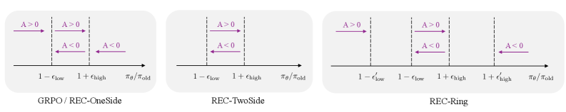
### Visual Description
## Diagram: Comparison of Three Evaluation/Comparison Strategies (GRPO/REC-OneSide, REC-TwoSide, REC-Ring)
### Overview
The image displays three horizontally aligned schematic diagrams, each illustrating a different method or strategy for comparing two probability distributions, denoted as π_θ and π_old. The diagrams use a horizontal axis representing the ratio π_θ/π_old and define regions where a quantity "A" is positive or negative. The three methods are labeled "GRPO / REC-OneSide", "REC-TwoSide", and "REC-Ring".
### Components/Axes
* **Common Axis:** All three diagrams share a horizontal axis labeled **π_θ/π_old**. This axis represents the ratio of a new policy's probability (π_θ) to an old policy's probability (π_old).
* **Key Thresholds:** The axis is marked with specific threshold values:
* `1 - ε_low`
* `1 + ε_high`
* The third diagram (REC-Ring) introduces two additional thresholds: `1 - ε'_low` and `1 + ε'_high`.
* **Condition Labels:** Within defined regions on the axis, the text **A > 0** and **A < 0** is placed, indicating the sign of a quantity "A" (likely an advantage, reward, or gradient signal) in that region.
* **Visual Elements:** Vertical dashed lines mark the threshold points. Horizontal arrows (→ and ←) are used to visually indicate the direction or span of the regions where A is positive or negative.
### Detailed Analysis
**1. GRPO / REC-OneSide (Left Panel)**
* **Axis Markers:** `1 - ε_low`, `1 + ε_high`.
* **Region Analysis:**
* **Left of `1 - ε_low`:** An arrow points right (→) with the label **A > 0**. This indicates that when the ratio π_θ/π_old is significantly less than 1 (the new policy assigns much lower probability), A is positive.
* **Between `1 - ε_low` and `1 + ε_high`:** An arrow points left (←) with the label **A < 0**. This indicates that when the ratio is close to 1 (within a tolerance band), A is negative.
* **Right of `1 + ε_high`:** An arrow points right (→) with the label **A > 0**. This indicates that when the ratio is significantly greater than 1 (the new policy assigns much higher probability), A is positive.
* **Spatial Grounding:** The `A > 0` labels are positioned above the axis in the far-left and far-right segments. The `A < 0` label is positioned above the axis in the central segment.
**2. REC-TwoSide (Center Panel)**
* **Axis Markers:** `1 - ε_low`, `1 + ε_high`.
* **Region Analysis:**
* **Left of `1 - ε_low`:** An arrow points right (→) with the label **A > 0**. Similar to the first diagram, a low ratio yields positive A.
* **Right of `1 + ε_high`:** An arrow points left (←) with the label **A < 0**. This is a key difference from the first diagram. Here, a high ratio yields *negative* A.
* **Between `1 - ε_low` and `1 + ε_high`:** No explicit label is placed in this central region in this diagram.
* **Spatial Grounding:** The `A > 0` label is above the axis on the left. The `A < 0` label is above the axis on the right.
**3. REC-Ring (Right Panel)**
* **Axis Markers:** `1 - ε'_low`, `1 - ε_low`, `1 + ε_high`, `1 + ε'_high`. This creates five distinct regions.
* **Region Analysis (from left to right):**
1. **Left of `1 - ε'_low`:** Arrow points right (→), label **A > 0**.
2. **Between `1 - ε'_low` and `1 - ε_low`:** Arrow points left (←), label **A < 0**.
3. **Between `1 - ε_low` and `1 + ε_high`:** Arrow points right (→), label **A > 0**.
4. **Between `1 + ε_high` and `1 + ε'_high`:** Arrow points left (←), label **A < 0**.
5. **Right of `1 + ε'_high`:** Arrow points left (←), label **A < 0**.
* **Spatial Grounding:** The labels alternate above the axis, corresponding to the five segments defined by the four vertical dashed lines.
### Key Observations
1. **Increasing Complexity:** The diagrams progress from a three-region model (OneSide) to a two-region model (TwoSide) to a five-region model (Ring), suggesting increasing granularity in the evaluation strategy.
2. **Sign Flip on High Ratios:** A critical difference exists between REC-OneSide and REC-TwoSide. In OneSide, both very low and very high ratios yield `A > 0`. In TwoSide, a very high ratio yields `A < 0`.
3. **REC-Ring's Alternating Pattern:** The REC-Ring method introduces a complex, alternating pattern of positive and negative A values as the ratio π_θ/π_old increases, creating a "ring" or oscillating effect around the central value of 1.
4. **Parameter Notation:** The use of `ε_low`/`ε_high` versus `ε'_low`/`ε'_high` in REC-Ring implies two different sets of tolerance parameters, allowing for finer control over the boundaries.
### Interpretation
These diagrams likely represent different **clipping or filtering strategies** used in reinforcement learning from human feedback (RLHF) or policy optimization algorithms like Proximal Policy Optimization (PPO). The quantity "A" is probably the **advantage estimate** used to compute the policy gradient.
* **GRPO / REC-OneSide:** This appears to be a standard approach. It encourages the policy to move away from the old policy in both directions (making unlikely actions more likely and likely actions less likely) when the advantage is positive, but discourages changes when the policy is already close to the old one (where A is negative, acting as a stabilizer).
* **REC-TwoSide:** This is a more conservative or constrained variant. It only encourages moving away from the old policy when the new probability is *lower* (`A > 0` on the left). When the new probability is much higher, it actively discourages that change (`A < 0` on the right), preventing the policy from becoming overconfident too quickly.
* **REC-Ring:** This is the most sophisticated strategy. It creates multiple "safe" and "unsafe" zones. The central region (`1 - ε_low` to `1 + ε_high`) encourages change (`A > 0`), similar to the core of PPO's clipping. The adjacent bands (`1 - ε'_low` to `1 - ε_low` and `1 + ε_high` to `1 + ε'_high`) discourage change (`A < 0`), acting as buffers. The outermost regions then have opposing effects: very low ratios are encouraged (`A > 0`), while very high ratios are strongly discouraged (`A < 0`). This creates a complex, non-monotonic relationship between the probability ratio and the learning signal, potentially offering more nuanced control over policy updates and stability.
**In summary, the image provides a technical schematic comparing three distinct mechanisms for modulating a learning signal (A) based on the divergence between a new and old policy (π_θ/π_old), with REC-Ring presenting the most intricate, multi-zone approach.**
</details>
Figure 8: A visualization of activated gradient for various REC algorithms. Here, $A$ represents the advantage of a specific token, and an arrow pointing to the right and annotated with “ $A>0$ ” means there is activated gradient that incentivizes increasing $π_\bm{θ}$ when the token advantage is positive and the probability ratio $π_\bm{θ}/π_\textsf{old}$ lies in the corresponding interval.
#### Experiments.
We compare the following algorithms: REINFORCE, GRPO, REC-TwoSide-IS, REC-TwoSide-NoIS, and REC-Ring-NoIS. Clipping parameters are set to $(ε_low,ε_high)=(0.2,0.2)$ , and for REC-Ring we additionally set $(ε_\textsf{low}^\prime,ε_\textsf{high}^\prime)=(0.6,2.0)$ .
<details>
<summary>x10.png Details</summary>
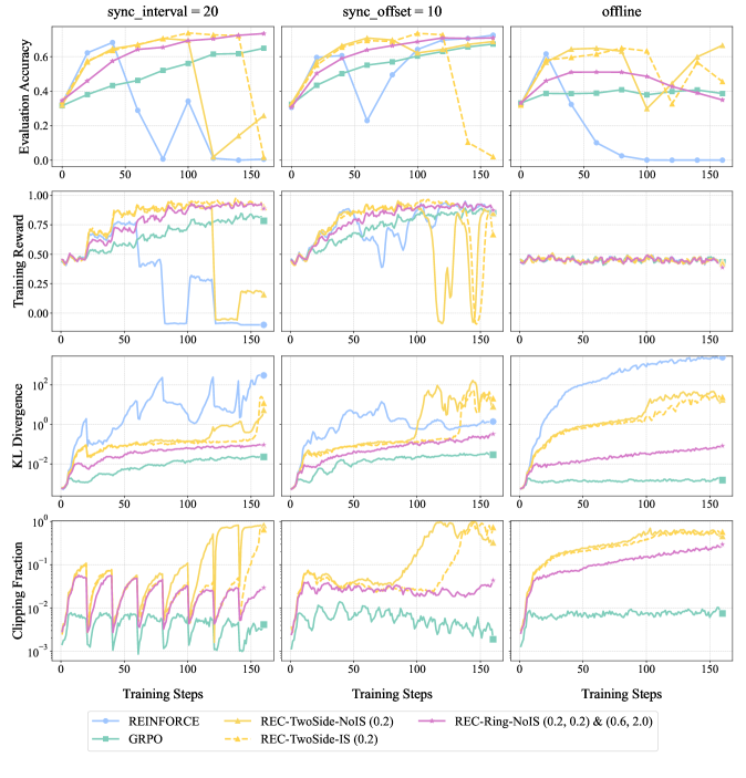
### Visual Description
## Multi-Panel Line Chart: Training Metrics Comparison Across Synchronization Settings
### Overview
The image is a 4x3 grid of line charts comparing the performance of six different reinforcement learning or policy optimization methods across three distinct training synchronization configurations. The charts track four key metrics over 150 training steps. The overall purpose is to visualize and compare the stability, performance, and optimization behavior of the methods under different synchronization regimes.
### Components/Axes
* **Column Headers (Synchronization Settings):**
* Left Column: `sync_interval = 20`
* Middle Column: `sync_offset = 10`
* Right Column: `offline`
* **Row Headers (Metrics):**
* Top Row: `Evaluation Accuracy` (Y-axis scale: 0.0 to ~0.7)
* Second Row: `Training Reward` (Y-axis scale: 0.00 to 1.00)
* Third Row: `KL Divergence` (Y-axis scale: logarithmic, from 10^-3 to 10^1)
* Bottom Row: `Clipping Fraction` (Y-axis scale: logarithmic, from 10^-3 to 10^0)
* **Common X-Axis:** `Training Steps` (Linear scale, marked at 0, 50, 100, 150).
* **Legend (Bottom Center):** Contains six entries, each with a unique color and marker:
1. `REINFORCE` - Light blue line with circle markers.
2. `GRPO` - Teal/green line with square markers.
3. `REC-TwoSide-NoIS (0.2)` - Yellow line with upward-pointing triangle markers.
4. `REC-TwoSide-IS (0.2)` - Yellow dashed line with downward-pointing triangle markers.
5. `REC-Ring-NoIS (0.2, 0.2) & (0.6, 2.0)` - Purple line with plus sign markers.
6. `REC-Ring-NoIS (0.2, 0.2)` - Pink/magenta line with 'x' markers.
### Detailed Analysis
**Column 1: `sync_interval = 20`**
* **Evaluation Accuracy:** Most methods (GRPO, REC variants) show a steady increase from ~0.3 to between 0.6-0.7. `REINFORCE` (blue) increases initially but crashes to near 0.0 after step 50. `REC-TwoSide-NoIS` (yellow triangle) also crashes after step 100.
* **Training Reward:** Mirrors accuracy trends. GRPO and REC variants rise to ~0.8-0.9. `REINFORCE` crashes to 0.0 after step 50. `REC-TwoSide-NoIS` crashes after step 100.
* **KL Divergence:** `REINFORCE` shows the highest and most volatile divergence, peaking above 10^1. Other methods remain lower, with GRPO and the pink `REC-Ring-NoIS` being the most stable (lowest divergence, ~10^-2 to 10^-1).
* **Clipping Fraction:** Shows periodic, sharp oscillations for several methods (notably the pink and purple `REC-Ring-NoIS` variants), suggesting regular policy updates hitting clipping boundaries. `REINFORCE` and `GRPO` have lower, more stable clipping fractions.
**Column 2: `sync_offset = 10`**
* **Evaluation Accuracy:** Similar initial rise for most. `REINFORCE` crashes early (around step 50). `REC-TwoSide-NoIS` (yellow triangle) maintains performance longer but crashes after step 125.
* **Training Reward:** `REINFORCE` crashes to 0.0. `REC-TwoSide-NoIS` shows extreme volatility, dropping to 0.0 multiple times before a final crash. Other methods remain high and stable.
* **KL Divergence:** `REINFORCE` again shows high divergence. `REC-TwoSide-NoIS` shows a late, sharp increase in divergence coinciding with its performance crash.
* **Clipping Fraction:** `REC-TwoSide-NoIS` shows a massive spike to near 1.0 (10^0) after step 125, indicating almost all updates were clipped. Other methods show moderate, stable clipping.
**Column 3: `offline`**
* **Evaluation Accuracy:** `REINFORCE` performance decays steadily to near 0.0. `REC-TwoSide-NoIS` (yellow triangle) is highly volatile, oscillating between ~0.2 and 0.7. The other four methods maintain stable, high accuracy (~0.6-0.7).
* **Training Reward:** `REINFORCE` and the two `REC-TwoSide` methods show flat or declining rewards (~0.4-0.5). The GRPO and `REC-Ring` methods maintain stable, high rewards (~0.8-0.9).
* **KL Divergence:** `REINFORCE` divergence grows monotonically and very high (approaching 10^2). `REC-TwoSide-NoIS` also shows high, growing divergence. The other methods maintain low, stable divergence.
* **Clipping Fraction:** `REC-TwoSide-NoIS` and the purple `REC-Ring-NoIS` show a steady increase in clipping fraction over time, ending near 1.0. `GRPO` remains very low and stable.
### Key Observations
1. **Method Stability Hierarchy:** `GRPO` (teal) and the `REC-Ring-NoIS` variants (purple/pink) are consistently the most stable across all metrics and synchronization settings. `REINFORCE` (blue) is consistently the least stable, often crashing completely.
2. **Sensitivity of REC-TwoSide:** The `REC-TwoSide-NoIS` method (yellow triangle) is highly sensitive to the synchronization setting. It performs well initially in synchronized settings but exhibits catastrophic forgetting or instability later, and is highly volatile in the offline setting.
3. **KL Divergence as a Failure Indicator:** High and growing KL Divergence (especially for `REINFORCE` and `REC-TwoSide-NoIS` in offline mode) strongly correlates with performance collapse (drops in Accuracy and Reward).
4. **Offline Setting is Challenging:** The `offline` configuration appears most difficult, causing performance decay in `REINFORCE` and severe volatility in `REC-TwoSide-NoIS`, while other methods remain robust.
5. **Clipping Correlates with Instability:** Spikes in Clipping Fraction (e.g., `REC-TwoSide-NoIS` in `sync_offset=10`) immediately precede or coincide with performance crashes, suggesting optimization difficulties.
### Interpretation
This data demonstrates a comparative analysis of policy optimization algorithms, likely in a reinforcement learning from human feedback (RLHF) or similar context. The core finding is that **synchronization strategy critically impacts algorithm stability and performance**.
* **Synchronized Training (`sync_interval`, `sync_offset`)** provides a stabilizing effect for most methods, but can delay the onset of instability for sensitive algorithms like `REC-TwoSide-NoIS`, leading to a sudden, catastrophic collapse after many steps of apparent success.
* **Offline Training** removes this stabilizing buffer, exposing inherent weaknesses. Algorithms that rely on frequent, on-policy updates (`REINFORCE`) fail completely. Algorithms with potentially high variance (`REC-TwoSide`) become unusably volatile. The success of `GRPO` and `REC-Ring` variants suggests they have inherent mechanisms (perhaps related to their gradient estimation or trust region methods) that make them robust to distribution shift and stale data, which are key challenges in offline optimization.
* The **strong correlation between rising KL Divergence and falling performance** underscores the importance of monitoring this metric as a health check for the training process. It indicates the policy is drifting too far from its reference model, leading to collapse.
* The **Clipping Fraction** acts as a diagnostic for optimization health. A value approaching 1.0 means the optimizer is constantly fighting against its own update constraints, a sign of impending failure.
In essence, the charts argue for the use of robust algorithms (`GRPO`, `REC-Ring`) and careful consideration of synchronization schemes, especially when moving towards offline or large-interval update paradigms, to ensure stable and reliable training.
</details>
Figure 9: Comparison of REC variants on GSM8K with Qwen2.5-1.5B-Instruct under different off-policy settings. Evaluation accuracy, training reward, KL divergence (with respect to the initial model) and clipping fraction are reported. Training reward curves are smoothed with a running-average window of size 3.
Figure 9 presents the empirical results. We observe that for REC-TwoSide, importance sampling is non-essential in all three settings, akin to the case of REC-OneSide. In addition, REC-TwoSide methods demonstrate fast policy improvement at the beginning but tend to collapse later on, whereas REC-Ring achieves a better balance of convergence speed and stability.
### B.4 Ablation: the impact of learning rates
Recall that in Section 4.1, we have demonstrated empirically the advantages of enlarging the clipping parameters $ε_\textsf{low},ε_\textsf{high}$ for REC-OneSide-NoIS. One might wonder if the relatively weak performance of GRPO or REC-OneSide with conventional $ε_\textsf{low}=ε_\textsf{high}=0.2$ is genuinely rooted in the clipping mechanism itself, or simply due to the choice of a small learning rate.
To answer this, we enhance the experiment of Figure 3 by sweeping learning rates over $\{1×10^-5,2×10^-6,5×10^-6\}$ . The results are illustrated in Figure 10, which confirm that simply increasing the learning rate cannot bridge the performance gap between GRPO with $ε_\textsf{low}=ε_\textsf{high}=0.2$ and REC-OneSide-NoIS with $ε_\textsf{low}=0.6,ε_\textsf{high}=2.0$ . This shows that relaxing the clipping range acts as a genuine improvement of regularization, rather than merely mimicking a larger learning rate.
<details>
<summary>x11.png Details</summary>
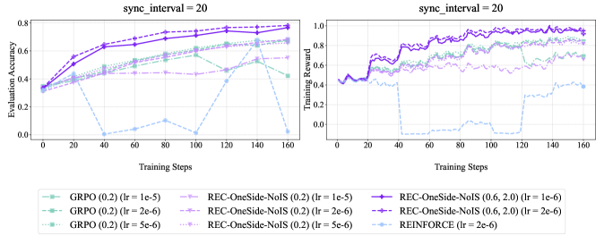
### Visual Description
\n
## Comparison of Reinforcement Learning Algorithms: Evaluation Accuracy and Training Reward over Steps
### Overview
The image displays two line charts side-by-side, sharing a common legend. Both charts plot the performance of several reinforcement learning algorithms over 160 training steps, with a fixed `sync_interval = 20`. The left chart measures "Evaluation Accuracy," and the right chart measures "Training Reward." The charts compare variants of GRPO, REC-OneSide-NoIS, and REINFORCE algorithms with different learning rates (lr).
### Components/Axes
* **Common Title (Top Center):** `sync_interval = 20` (appears above both charts).
* **Left Chart:**
* **Y-Axis Label:** `Evaluation Accuracy`
* **Y-Axis Scale:** Linear, from 0 to 0.8, with major ticks at 0.0, 0.2, 0.4, 0.6, 0.8.
* **X-Axis Label:** `Training Steps`
* **X-Axis Scale:** Linear, from 0 to 160, with major ticks every 20 steps (0, 20, 40, ..., 160).
* **Right Chart:**
* **Y-Axis Label:** `Training Reward`
* **Y-Axis Scale:** Linear, from 0.0 to 1.0, with major ticks at 0.0, 0.2, 0.4, 0.6, 0.8, 1.0.
* **X-Axis Label:** `Training Steps`
* **X-Axis Scale:** Identical to the left chart.
* **Legend (Bottom Center, spanning both charts):** Contains 8 entries, each with a unique color, marker, and label.
1. **Color:** Light teal, **Marker:** Circle, **Label:** `GRPO (0.2) (lr = 1e-5)`
2. **Color:** Medium teal, **Marker:** Square, **Label:** `GRPO (0.2) (lr = 2e-6)`
3. **Color:** Dark teal, **Marker:** Diamond, **Label:** `GRPO (0.2) (lr = 5e-6)`
4. **Color:** Light purple, **Marker:** Circle, **Label:** `REC-OneSide-NoIS (0.2) (lr = 1e-5)`
5. **Color:** Medium purple, **Marker:** Square, **Label:** `REC-OneSide-NoIS (0.2) (lr = 2e-6)`
6. **Color:** Dark purple, **Marker:** Diamond, **Label:** `REC-OneSide-NoIS (0.2) (lr = 5e-6)`
7. **Color:** Deep violet, **Marker:** Circle, **Label:** `REC-OneSide-NoIS (0.6, 2.0) (lr = 1e-6)`
8. **Color:** Light blue, **Marker:** Circle, **Label:** `REINFORCE (lr = 2e-6)`
### Detailed Analysis
**Left Chart: Evaluation Accuracy**
* **Trend Verification:** Most lines show an upward trend, indicating improving accuracy with training. The REINFORCE line (light blue) is a major exception, showing high volatility and a significant drop.
* **Data Series & Approximate Values:**
* **REC-OneSide-NoIS (0.6, 2.0) (lr = 1e-6) [Deep violet, circle]:** The top performer. Starts ~0.35, rises steadily to ~0.78 by step 160.
* **REC-OneSide-NoIS (0.2) variants [Purples]:** Cluster in the middle. The `lr=5e-6` (dark purple, diamond) variant performs best among them, reaching ~0.70. The `lr=1e-5` (light purple, circle) variant is the lowest of this group, ending near ~0.65.
* **GRPO (0.2) variants [Teals]:** Also cluster in the middle, slightly below the REC-OneSide-NoIS (0.2) group. The `lr=5e-6` (dark teal, diamond) variant is the best GRPO, ending near ~0.68. The `lr=1e-5` (light teal, circle) variant ends near ~0.62.
* **REINFORCE (lr = 2e-6) [Light blue, circle]:** Highly anomalous. Starts ~0.35, rises to ~0.45 by step 20, then plummets to near 0.0 by step 40. It shows a partial, volatile recovery between steps 100-140 (peaking ~0.55) before dropping again to near 0.0 at step 160.
**Right Chart: Training Reward**
* **Trend Verification:** Similar to accuracy, most reward lines trend upward. The REINFORCE line again shows a catastrophic drop and poor recovery.
* **Data Series & Approximate Values:**
* **REC-OneSide-NoIS (0.6, 2.0) (lr = 1e-6) [Deep violet, circle]:** Clearly dominant. Starts ~0.45, climbs rapidly to ~0.8 by step 40, and continues to a near-perfect reward of ~0.98 by step 160.
* **REC-OneSide-NoIS (0.2) variants [Purples]:** Form a middle cluster. The `lr=5e-6` (dark purple, diamond) variant leads this subgroup, reaching ~0.90. The `lr=1e-5` (light purple, circle) variant is the lowest, ending near ~0.70.
* **GRPO (0.2) variants [Teals]:** Cluster below the REC (0.2) group. The `lr=5e-6` (dark teal, diamond) variant is the best GRPO, ending near ~0.80. The `lr=1e-5` (light teal, circle) variant ends near ~0.65.
* **REINFORCE (lr = 2e-6) [Light blue, circle]:** Shows a severe failure mode. Starts ~0.45, rises briefly to ~0.65 by step 20, then crashes to 0.0 by step 40. It remains near 0.0 until step 120, after which it shows a weak, noisy recovery to only ~0.40 by step 160.
### Key Observations
1. **Clear Performance Hierarchy:** The `REC-OneSide-NoIS (0.6, 2.0)` algorithm with a low learning rate (`1e-6`) is the unequivocal best performer on both metrics, achieving near-maximum reward and highest accuracy.
2. **Learning Rate Sensitivity:** For both GRPO and REC-OneSide-NoIS (0.2), the intermediate learning rate (`5e-6`) consistently outperforms the higher (`1e-5`) and lower (`2e-6`) rates tested, suggesting an optimal LR exists in that range for these configurations.
3. **Catastrophic Failure of REINFORCE:** The REINFORCE algorithm exhibits a complete collapse in performance early in training (around step 40) on both metrics. Its recovery is minimal and unstable, indicating severe instability with the given hyperparameters (`lr=2e-6`, `sync_interval=20`).
4. **Correlation Between Metrics:** There is a strong positive correlation between Evaluation Accuracy and Training Reward for all stable algorithms. The line shapes in both charts are very similar for each corresponding algorithm/color.
### Interpretation
This data demonstrates a controlled experiment comparing policy gradient methods in reinforcement learning. The key finding is the significant superiority of the `REC-OneSide-NoIS` algorithm, particularly with the `(0.6, 2.0)` parameterization and a very low learning rate. This configuration achieves robust, high-performance learning.
The results highlight two critical factors for successful training in this context:
1. **Algorithm Choice:** The `REC-OneSide-NoIS` approach appears more stable and sample-efficient than both GRPO and the classic REINFORCE under these conditions.
2. **Hyperparameter Tuning:** Learning rate is a crucial hyperparameter. The performance gap between LR variants of the same algorithm is substantial, and the wrong choice (as seen with REINFORCE) can lead to complete training failure.
The `sync_interval=20` parameter is held constant, so its effect is not evaluated here. The catastrophic drop in the REINFORCE line suggests a potential issue with high variance in gradient estimates, which the other algorithms seem to mitigate more effectively. This visualization would be used to justify the selection of `REC-OneSide-NoIS (0.6, 2.0) (lr=1e-6)` for further experiments or deployment, and to caution against using REINFORCE without significant modification or different hyperparameter tuning.
</details>
Figure 10: Comparison of GRPO and REC-OneSide-NoIS on GSM8K with Qwen2.5-1.5B-Instruct. Evaluation accuracy (left) and training reward (right) are reported for varying learning rates.
### B.5 Experiments for OPMD and AsymRE
Figure 11 presents empirical results for OPMD and AsymRE in various off-policy settings. It is worth noting that, while the analysis and experiments in their original papers [Kimi-Team, 2025b, Arnal et al., 2025] focus on a setting that is effectively the same as our $\texttt{sync\_interval}>1$ setting, our analysis and experiments have also validated their efficacy in $\texttt{sync\_offset}>1$ scenarios.
<details>
<summary>x12.png Details</summary>
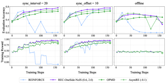
### Visual Description
## [Chart Type]: Multi-Panel Line Chart - Reinforcement Learning Algorithm Performance Comparison
### Overview
The image displays a 2x3 grid of line charts comparing the performance of four reinforcement learning algorithms across three different training conditions. The top row of charts measures "Evaluation Accuracy," while the bottom row measures "Training Reward." The x-axis for all charts is "Training Steps," ranging from 0 to 150. The three columns represent distinct experimental conditions: `sync_interval = 20`, `sync_offset = 10`, and `offline`. A shared legend is positioned at the bottom center of the entire figure.
### Components/Axes
* **Chart Titles (Top Row, Left to Right):** `sync_interval = 20`, `sync_offset = 10`, `offline`.
* **Y-Axis Labels:**
* Top Row: `Evaluation Accuracy` (Scale: 0.0 to 0.8, with increments of 0.2).
* Bottom Row: `Training Reward` (Scale: 0.00 to 1.00, with increments of 0.25).
* **X-Axis Label (Common to all charts):** `Training Steps` (Scale: 0 to 150, with major ticks at 0, 50, 100, 150).
* **Legend (Bottom Center):** Contains four entries, each with a colored line and marker symbol:
1. **REINFORCE:** Light blue line with circular markers.
2. **REC-OneSide-NoIS (0.6, 2.0):** Purple line with plus-sign markers.
3. **OPMD:** Green line with diamond markers.
4. **AsymRE (-0.1):** Light green line with square markers.
### Detailed Analysis
**Top Row: Evaluation Accuracy**
* **sync_interval = 20 (Top-Left Chart):**
* **REC-OneSide-NoIS (Purple):** Shows a strong, steady upward trend from ~0.35 at step 0 to a peak of ~0.8 at step 150. It is the top-performing algorithm for most of the training.
* **OPMD (Green):** Also shows a steady upward trend, starting near ~0.35 and reaching ~0.7 by step 150. It consistently performs below REC-OneSide-NoIS.
* **AsymRE (Light Green):** Follows a similar upward trajectory to OPMD, ending near ~0.65 at step 150.
* **REINFORCE (Light Blue):** Exhibits highly unstable performance. It starts near ~0.35, spikes to ~0.65 around step 25, then crashes to near 0.0 by step 75. It shows a brief recovery to ~0.35 at step 100 before dropping back to near 0.0.
* **sync_offset = 10 (Top-Center Chart):**
* **REC-OneSide-NoIS (Purple):** Again shows a strong upward trend, starting ~0.35 and reaching ~0.8 by step 150.
* **OPMD (Green):** Follows a similar upward path, ending near ~0.7.
* **AsymRE (Light Green):** Trends upward to ~0.65.
* **REINFORCE (Light Blue):** Shows instability. It starts ~0.35, peaks near ~0.6 at step 25, drops sharply to ~0.2 at step 75, recovers to ~0.6 at step 100, then declines to near 0.0 by step 150.
* **offline (Top-Right Chart):**
* **REC-OneSide-NoIS (Purple):** Performance is less stable here. It starts ~0.35, peaks near ~0.6 at step 50, then gradually declines to ~0.2 by step 150.
* **OPMD (Green):** Shows a moderate upward trend to ~0.5 at step 100, then a sharp drop to ~0.1 at step 125, followed by a recovery to ~0.5 at step 150.
* **AsymRE (Light Green):** Trends upward to ~0.5 by step 100, then declines to ~0.3 by step 150.
* **REINFORCE (Light Blue):** Starts ~0.35, peaks near ~0.6 at step 25, then crashes to near 0.0 by step 75 and remains there.
**Bottom Row: Training Reward**
* **sync_interval = 20 (Bottom-Left Chart):**
* **REC-OneSide-NoIS (Purple):** Shows a noisy but clear upward trend from ~0.4 to near 1.0 by step 150.
* **OPMD (Green):** Also trends upward with noise, reaching ~0.9 by step 150.
* **AsymRE (Light Green):** Follows a similar noisy upward path, ending near ~0.85.
* **REINFORCE (Light Blue):** Extremely unstable. It fluctuates between ~0.4 and ~0.7 until step 75, then crashes to near 0.0, with a brief, partial recovery around step 100 before falling back to 0.0.
* **sync_offset = 10 (Bottom-Center Chart):**
* **REC-OneSide-NoIS (Purple):** Strong upward trend with noise, approaching 1.0 by step 150.
* **OPMD (Green):** Upward trend, reaching ~0.9.
* **AsymRE (Light Green):** Upward trend, reaching ~0.85.
* **REINFORCE (Light Blue):** Shows significant volatility. It fluctuates between ~0.5 and ~0.8 until step 100, then drops sharply to near 0.0 by step 125.
* **offline (Bottom-Right Chart):**
* **All Algorithms:** Performance is markedly different and poor in this condition. All four lines (Purple, Green, Light Green, Light Blue) are tightly clustered and nearly flat, hovering around a Training Reward of ~0.4 to ~0.5 for the entire duration of 150 steps. There is minimal improvement or divergence between the algorithms.
### Key Observations
1. **Algorithm Stability:** REC-OneSide-NoIS (Purple) is the most consistent top performer in the `sync_interval` and `sync_offset` conditions for both metrics. REINFORCE (Light Blue) is consistently the most unstable, often suffering catastrophic performance collapses.
2. **Condition Impact:** The `offline` condition severely degrades performance and eliminates the differentiation between algorithms. All methods perform poorly and similarly.
3. **Metric Correlation:** In the first two conditions, trends in Evaluation Accuracy generally correlate with trends in Training Reward for each algorithm.
4. **OPMD Anomaly:** In the `offline` Evaluation Accuracy chart, OPMD (Green) shows a unique, sharp V-shaped dip and recovery between steps 100 and 150, which is not mirrored in its Training Reward for the same condition.
### Interpretation
This data suggests that the synchronization strategy (`sync_interval` vs. `sync_offset`) is critical for the effective training of these algorithms, with `sync_offset=10` yielding slightly more stable high-end performance for the leading algorithm (REC-OneSide-NoIS). The `offline` setting appears to be a fundamentally more difficult or poorly configured learning environment, as it prevents meaningful learning progress for all tested methods.
The REC-OneSide-NoIS algorithm demonstrates superior robustness and learning efficiency in the synchronized settings. In contrast, the classic REINFORCE algorithm shows a high susceptibility to training instability, which may be linked to issues like high variance in gradient estimates. The near-identical, flat performance in the `offline` condition indicates a potential failure mode or a scenario where the problem setup itself (e.g., lack of environment interaction or feedback) is the primary bottleneck, not the choice of algorithm. The outlier dip in OPMD's accuracy in the offline chart, without a corresponding dip in reward, might indicate a temporary misalignment between the agent's policy (which determines reward) and the evaluation metric, or simply noise in the evaluation process.
</details>
Figure 11: Empirical results for OPMD and AsymRE (cf. Section 4.2) on GSM8K with Qwen2.5-1.5B-Instruct under various off-policy settings. The regularization coefficient for OPMD and the baseline shift for AsymRE are both $0.1$ . Training reward curves are smoothed with a running-average window of size 3.
## Appendix C Summary: a unified view of various algorithms
For convenient reference, Table 3 summarizes the algorithms investigated in Section 4.
Table 3: A summary of algorithms investigated in Section 4.
| Augmentation | Algorithm | Gradient / Loss |
| --- | --- | --- |
| Regularize by clipping | GRPO | $\bm{g}=\frac{1}{K}∑_i∑_t∇_\bm{θ}\logπ_\bm{θ}(y_i^t | x,y_i^<t)· A_i\frac{π_\bm{θ}(y_i^t | x,y_i^<t)}{π_\textsf{old}(y_i^t | x,y_i^<t)}M_i^t$ |
| REC-OneSide-IS | $\bm{g}=\frac{1}{K}∑_i∑_t∇_\bm{θ}\logπ_\bm{θ}(y_i^t | x,y_i^<t)·(r_i-\overline{r})\frac{π_\bm{θ}(y_i^t | x,y_i^<t)}{π_\textsf{old}(y_i^t | x,y_i^<t)}M_i^t$ | |
| REC-OneSide-NoIS | $\bm{g}=\frac{1}{K}∑_i∑_t∇_\bm{θ}\logπ_\bm{θ}(y_i^t | x,y_i^<t)·(r_i-\overline{r})M_i^t$ | |
| Add regularization loss | OPMD | $\widehat{L}=-\tfrac{1}{K}∑_i(r_i-\overline{r})\logπ_\bm{θ}(y_i|x)+\tfrac{τ}{2K}∑_i(\logπ_\bm{θ}(y_i|x)-\logπ_\textsf{old}(y_i|x))^2$ |
| AsymRE | $\widehat{L}=-\tfrac{1}{K}∑_i(r_i-\overline{r})\logπ_\bm{θ}(y_i|x)-\tfrac{τ}{K}∑_i\logπ_\bm{θ}(y_i|x)$ | |
| Reweight data | Pairwise-weighted REINFORCE | $\bm{g}=\tfrac{1}{K}∑_i\Big(∑_jw_i,j\Big)\Big(r_i-\tfrac{∑_jw_i,jr_j}{∑_jw_i,j}\Big)∇_\bm{θ}\logπ_\bm{θ}(y_i|x)$ |
| RED-Drop | $\bm{g}=\tfrac{1}{|S|}∑_i∈ S(r_i-\overline{r}_S) ∇_\bm{θ}\logπ_\bm{θ}(y_i|x)$ | |
| RED-Weight | $\bm{g}=∑_iw_i(r_i-\overline{r}) ∇_\bm{θ}\logπ_\bm{θ}(y_i|x), w_i=\exp(A_i/τ)$ | |