# A Formal Comparison Between Chain of Thought and Latent Thought
**Authors**: Kevin Xu, Issei Sato
## Abstract
Chain of thought (CoT) elicits reasoning in large language models by explicitly generating intermediate tokens. In contrast, latent thought reasoning operates directly in the continuous latent space, enabling computation beyond discrete linguistic representations. While both approaches exploit iterative computation, their comparative capabilities remain underexplored. In this work, we present a formal analysis showing that latent thought admits more efficient parallel computation than inherently sequential CoT. In contrast, CoT enables approximate counting and sampling through stochastic decoding. These separations suggest the tasks for which depth-driven recursion is more suitable, thereby offering practical guidance for choosing between reasoning paradigms.
Machine Learning, ICML
## 1 Introduction
Transformer-based large language models (LLMs) (Vaswani et al., 2017) have shown strong performance across diverse tasks and have recently been extended to complex reasoning. Rather than directly predicting final answers, generating intermediate reasoning steps, known as chain of thought (CoT) (Wei et al., 2022), enhances reasoning abilities. This naturally raises the question: why is CoT effective for complex tasks? Recent studies have approached this question by framing reasoning as a computational problem and analyzing its complexity (Feng et al., 2023; Merrill and Sabharwal, 2024; Li et al., 2024; Nowak et al., 2024), showing that CoT improves performance by increasing the model’s effective depth through iterative computation, thereby enabling the solution of problems that would otherwise be infeasible.
As an alternative to CoT, recent work has explored latent thought, which reasons directly in the hidden state space rather than in the discrete token space. This paradigm includes chain of continuous thought (Coconut) (Hao et al., 2025), which replaces next tokens with hidden state, and looped Transformer (looped TF), in which output hidden states are iteratively fed back as inputs (Dehghani et al., 2019). Such iterative architectures have been shown to enhance expressivity: Coconut enables the simultaneous exploration of multiple traces (Zhu et al., 2025a; Gozeten et al., 2025), while looped TF satisfies universality (Giannou et al., 2023; Xu and Sato, 2025). Empirically, looped TF achieves competitive performance with fewer parameters (Csordás et al., 2024; Bae et al., 2025; Zhu et al., 2025b), and improves reasoning performance (Saunshi et al., 2025).
<details>
<summary>x1.png Details</summary>
### Visual Description
## Diagram: Comparison of "Chain of thought" and "Latent thought" Computational Paradigms
### Overview
The image is a conceptual diagram comparing two theoretical approaches or paradigms, labeled "Chain of thought" and "Latent thought." It is structured as a two-column comparison, with "Chain of thought" on the left (light blue background) and "Latent thought" on the right (light orange background). The diagram is divided into two primary horizontal sections, each enclosed in a dashed box, illustrating key theoretical relationships and bounds for each paradigm.
### Components/Axes
The diagram is organized into the following textual and conceptual components:
**Header (Top Row):**
* **Left Column Title:** `Chain of thought`
* **Right Column Title:** `Latent thought`
**First Dashed Box (Upper Section):**
* **Central Title:** `Parallel computation`
* **Left Column (Chain of thought):**
* Text: `Upper bound`
* Text: `Sequentially`
* Reference: `Lem. 3.13` (positioned above the central title)
* **Right Column (Latent thought):**
* Text: `Exact bound`
* Text: `Parallelizability`
* Reference: `Thm. 3.12` (positioned above the central title)
* **Central Symbol:** A "proper subset" symbol (`⊊`) is placed between the left and right columns, indicating a relationship where the left is a strict subset of the right.
* **Bottom Reference:** `Thm. 3.14, 3.15` (spanning the bottom of the box)
**Second Dashed Box (Lower Section):**
* **Central Title:** `Approximate counting`
* **Left Column (Chain of thought):**
* Text: `Lower bound`
* Text: `Stochasticity`
* **Right Column (Latent thought):**
* Text: `Upper bound`
* Text: `Determinism`
* **Central Symbol:** A "not equal to" symbol (`≠`) is placed between the left and right columns, indicating a fundamental difference or inequality.
* **Bottom Reference:** `Lem. 4.3, Thm. 4.4, Thm. 4.5` (spanning the bottom of the box)
### Detailed Analysis
The diagram presents a structured theoretical comparison:
1. **Parallel Computation Section:**
* For **Chain of thought**, the diagram states there is an "Upper bound" related to "Sequentially," referenced by Lemma 3.13.
* For **Latent thought**, it states there is an "Exact bound" related to "Parallelizability," referenced by Theorem 3.12.
* The `⊊` symbol suggests that the sequential capabilities of Chain of thought are strictly contained within or are a proper subset of the parallelizability of Latent thought in this context.
* Theorems 3.14 and 3.15 are cited as supporting this relationship.
2. **Approximate Counting Section:**
* For **Chain of thought**, the diagram indicates a "Lower bound" associated with "Stochasticity."
* For **Latent thought**, it indicates an "Upper bound" associated with "Determinism."
* The `≠` symbol signifies that the stochastic lower bound of Chain of thought is not equal to the deterministic upper bound of Latent thought, highlighting a core distinction in their properties for this task.
* Lemma 4.3 and Theorems 4.4 and 4.5 are cited as the basis for these bounds.
### Key Observations
* **Structural Symmetry:** The diagram uses a mirrored layout for direct comparison, with each paradigm having corresponding "bound" and "property" labels (Upper/Exact, Lower/Upper; Sequentially/Parallelizability, Stochasticity/Determinism).
* **Mathematical Notation:** The use of formal symbols (`⊊`, `≠`) and theorem/lemma references (`Thm.`, `Lem.`) grounds the comparison in a rigorous, academic context, likely from a paper in theoretical computer science or computational complexity.
* **Conceptual Contrast:** The properties are paired as conceptual opposites: Sequential vs. Parallel, Stochasticity vs. Determinism. The diagram visually argues that "Latent thought" is associated with more powerful or definitive properties (Exact bound, Parallelizability, Determinism) compared to "Chain of thought."
### Interpretation
This diagram serves as a high-level summary of theoretical results comparing two computational models. It suggests that the "Latent thought" paradigm possesses superior or more definitive characteristics in the contexts of parallel computation and approximate counting.
* **In Parallel Computation:** The relationship `Chain of thought ⊊ Latent thought` implies that any computation that can be done sequentially (Chain of thought) can also be handled by the parallelizable Latent thought model, but the Latent thought model can solve problems that are not efficiently sequential. It establishes a hierarchy of power.
* **In Approximate Counting:** The relationship `Stochasticity ≠ Determinism` highlights a fundamental methodological difference. Chain of thought relies on or is bounded by randomness (stochasticity), while Latent thought operates within deterministic bounds. This could imply different resource requirements, guarantees, or algorithmic approaches.
* **Overall Purpose:** The diagram is likely used to motivate the study of "Latent thought" by showing its theoretical advantages over the perhaps more intuitive "Chain of thought" approach. It condenses several formal proofs (referenced by the theorem and lemma numbers) into a single, digestible visual argument about computational power and nature.
</details>
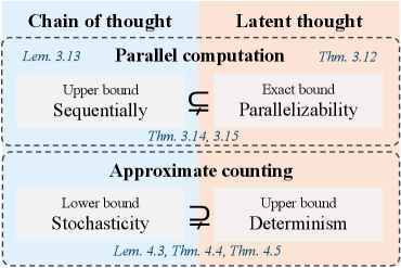
Figure 1: Overview of the formal comparison between chain of thought and latent thought reasoning with respect to parallel computation and approximate counting, providing upper, lower, or exact bounds that highlight their respective characteristics.
These reasoning paradigms share the core idea of iteratively applying Transformers to enhance expressive power, which naturally leads to a fundamental question:
What is the separation between chain of thought and latent thought?
Recent studies characterize how expressivity scales with the number of iterations. Specifically, it has been shown that looped TF subsumes deterministic CoT (Saunshi et al., 2025), and exhibits a strict separation with only a logarithmic number of iterations (Merrill and Sabharwal, 2025a). Nevertheless, fundamental questions remain open:
Does the separation extend beyond the logarithmic regime?
Is latent thought always more expressive than CoT?
### 1.1 Our Contributions
In this work, we address both questions by clarifying the respective strengths and limitations of the two reasoning paradigms through a formal complexity-theoretic analysis of their expressive power. Specifically, we show that latent thought gains efficiency from its parallelizability, yielding separations beyond the polylogarithmic regime. In contrast, CoT benefits from stochasticity, which enables approximate counting. An overview is given in Fig. 1.
Latent thought enables parallel reasoning.
By formalizing decision problems as the evaluation of directed acyclic graphs (DAGs), we reveal the parallel computational capability of latent thought utilizing continuous hidden states. This analysis can be formalized by relating the class of decision problems realizable by the model to Boolean circuits. In particular, Boolean circuits composed of logic gates such as AND, OR, NOT, and Majority, with polylogarithmic depth $\log^{k}n$ for $k\in\mathbb{N}$ and input size $n$ , define the class $\mathsf{TC}^{k}$ , a canonical model of parallel computation. Circuit complexity plays a central role in analyzing the computational power of Transformer models: fixed-depth Transformers without CoT are known to be upper-bounded by $\mathsf{TC}^{0}$ (Merrill and Sabharwal, 2023), and subsequent studies analyze how the expressivity of CoT scales their computational power in terms of Boolean circuit complexity (Li et al., 2024). We show that latent thought with $\log^{k}n$ iterations exactly captures the power of $\mathsf{TC}^{k}$ (Thm. 3.12); in contrast, CoT with $\log^{k}n$ steps cannot realize the full power of $\mathsf{TC}^{k}$ (Thm. 3.13) due to its inherent sequentiality. This yields a strict separation in favor of latent thought in polylogarithmic regime (Thm. 3.15), showing its efficiency in terms of the required number of iterations.
CoT enables approximate counting.
A counting problem is a fundamental task in mathematics and computer science that determines the number of solutions satisfying a given set of constraints, including satisfying assignments of Boolean formulas, graph colorings, and partition functions (Arora and Barak, 2009). While exact counting for the complexity class $\#\mathsf{P}$ is generally computationally intractable, approximation provides a feasible alternative. We show that CoT supports fully polynomial-time randomized approximation schemes ( $\mathsf{FPRAS}$ ), yielding reliable estimates even in cases where exact counting via deterministic latent thought reasoning is intractable (Lemma 4.3). Furthermore, leveraging classical results connecting approximate counting and sampling (Jerrum et al., 1986), we extend this separation to distribution modeling: there exist target distributions that CoT can approximately represent and sample from, but that remain inaccessible to latent thought (Theorem 4.4). To the best of our knowledge, this constitutes the first formal separation in favor of CoT.
## 2 Background
### 2.1 Models of Computation
We define a class of reasoning paradigms in which a Transformer block (Vaswani et al., 2017) is applied iteratively. Informally, CoT generates intermediate reasoning steps explicitly as tokens in an autoregressive manner. Formal definitions and illustrations are given in Appendix A.
**Definition 2.1 (CoT, followingMerrill and Sabharwal (2024))**
*Let ${\mathcal{V}}$ be a vocabulary, and let $\mathrm{TF}_{\mathrm{dec}}:{\mathcal{V}}^{*}\to{\mathcal{V}}$ denote an decoder-only Transformer. Given an input sequence $x=(x_{1},\dots,x_{n})\in{\mathcal{V}}^{n}$ , the outputs of CoT are defined by
$$
f_{\mathrm{cot}}^{0}(x)\coloneq x,\quad f_{\mathrm{cot}}^{k+1}(x)\coloneq f_{\mathrm{cot}}^{k}(x)\cdot\mathrm{TF}_{\mathrm{dec}}(f_{\mathrm{cot}}^{k}(x)),
$$
where $\cdot$ denotes concatenation. We define the output to be the last tokens of $f_{\mathrm{cot}}^{T(n)}(x)\in{\mathcal{V}}^{\,n+T(n)}$ .*
Coconut feeds the final hidden state as the embedding of the next token. Although the original Coconut model (Hao et al., 2025) can generate both language tokens and hidden states, we focus exclusively on hidden state reasoning steps, in order to compare its representational power with that of CoT. Here, $\mathbb{F}$ denotes the set of finite-precision floating-point numbers, and $d\in\mathbb{N}$ denotes the embedding dimension.
**Definition 2.2 (Coconut)**
*Let ${\mathcal{V}}$ be a vocabulary and let $\mathrm{TF}^{\mathrm{Coconut}}_{\mathrm{dec}}:{\mathcal{V}}^{*}\times(\mathbb{F}^{d})^{*}\to\mathbb{F}^{d}$ be a decoder-only Transformer that maps a fixed token prefix together with a hidden state to the next hidden state. Given an input sequence $x=(x_{1},\dots,x_{n})\in{\mathcal{V}}^{n}$ , we define the hidden states recursively by
$$
h^{0}\coloneq\bigl(e(x_{i})\bigr)_{i=1}^{n},\quad h^{k+1}\coloneq\mathrm{TF}^{\mathrm{Coconut}}_{\mathrm{dec}}(x,h^{k}),
$$
where $e:{\mathcal{V}}\to\mathbb{F}^{d}$ denotes an embedding. The output after $T(n)$ steps is obtained by decoding a suffix of the hidden state sequence ending at $h^{T(n)}$ .*
Looped TFs, by contrast, feed the entire model output back into the input without generating explicit tokens, recomputing all hidden states of the sequence at every iteration.
**Definition 2.3 (Looped TF)**
*Let $\mathrm{TF}:\mathbb{F}^{d\times*}\to\mathbb{F}^{d\times*}$ denote a Transformer block. Given an input sequence $x=(x_{1},\dots,x_{n})\in{\mathcal{V}}^{n}$ , the outputs are defined recursively by
$$
f_{\mathrm{loop}}^{0}(x)\coloneq\bigl(e(x_{i})\bigr)_{i=1}^{n},\quad f_{\mathrm{loop}}^{k+1}(x)\coloneq\mathrm{TF}(f_{\mathrm{loop}}^{k}(x)),
$$
where $e:{\mathcal{V}}\to\mathbb{F}^{d}$ denotes an embedding. The output after $T(n)$ loop iterations is the decoded last tokens of $f_{\mathrm{loop}}^{T(n)}(x)$ .*
Here, we assume that the input for looped TF may include sufficient padding so that its length is always at least as large as the output length, as in (Merrill and Sabharwal, 2025b). The definitions of the models describe their core architectures; the specific details may vary depending on the tasks to which they are applied.
Table 1: Comparison between prior theoretical analyses and our work on the computational power of CoT, Coconut, and looped TF.
$$
\mathsf{\mathsf{TC}^{k}} \mathsf{\mathsf{TC}^{k}} \mathsf{\mathsf{TC}^{k}} \tag{2024}
$$
### 2.2 Related Work
To understand the expressive power of Transformers, previous work studies which classes of problems can be solved and with what computational efficiency. These questions can be naturally analyzed within the framework of computational complexity theory. Such studies on CoT and latent thought are summarized below and in Table 1.
Computational power of chain of thought.
The expressivity of Transformers is limited by bounded depth (Merrill and Sabharwal, 2023), whereas CoT enhances their expressiveness by effectively increasing the number of sequential computational steps, enabling the solution of problems that would otherwise be intractable for fixed-depth architectures (Feng et al., 2023). Recent work has investigated how the expressivity of CoT scales with the number of reasoning steps, formalizing CoT for decision problems and computational complexity classes (Merrill and Sabharwal, 2024; Li et al., 2024). Beyond decision problems, CoT has been further formalized in a probabilistic setting for representing probability distributions over strings (Nowak et al., 2024).
Computational power of latent thought.
Latent thought is an alternative paradigm for increasing the number of computational steps without being constrained to the language space, with the potential to enhance model expressivity. In particular, Coconut has been shown to enable the simultaneous exploration of multiple candidate reasoning traces (Zhu et al., 2025a; Gozeten et al., 2025). Looped TFs can simulate iterative algorithms (Yang et al., 2024; de Luca and Fountoulakis, 2024) and, more generally, realize polynomial-time computations (Giannou et al., 2023). Recent results further demonstrate advantages over chain of thought reasoning: looped TFs can subsume the class of deterministic computations realizable by CoT using the same number of iterations (Saunshi et al., 2025), and exhibit a strict separation within the same logarithmic iterations (Merrill and Sabharwal, 2025a). Concurrent work (Merrill and Sabharwal, 2025b) further establishes that looped TFs, when equipped with padding and a polylogarithmic number of loops, are computationally equivalent to uniform $\mathsf{TC}^{k}$ .
## 3 Latent Thought Enables Parallel Reasoning
We formalize the reasoning problem as a graph evaluation problem. Section 3.2 illustrates how each model approaches the same problem differently, providing intuitive insight into their contrasting capabilities. Building on these observations, Section 3.3 characterizes their expressive power and establishes a formal separation between them.
### 3.1 Problem Setting
<details>
<summary>x2.png Details</summary>
### Visual Description
## Diagram: Computation Graph and Simulation Methods
### Overview
The image is a technical diagram composed of three interconnected parts labeled (a), (b), and (c). It illustrates different representations and simulation methods for a computational process, likely related to neural networks or symbolic reasoning. The diagram uses nodes (circles) representing variables or operations, connected by directed edges (arrows) to show data flow or dependencies.
### Components/Axes
The diagram is divided into three distinct panels:
**Panel (a): Computation graph (DAG)**
* **Title:** `(a) Computation graph (DAG)`
* **Set Notation:** `F_n = {+, -, ×, ÷}` (The set of available operations: addition, subtraction, multiplication, division).
* **Parameters:**
* `m = 3` (Number of output nodes, labeled `y1`, `y2`, `y3`).
* `n = 5` (Number of input nodes, labeled `x1`, `x2`, `x3`, `x4`, `x5`).
* `size: 12` (Total number of nodes in the graph).
* `depth: 2` (The maximum number of sequential operations from input to output).
* **Node Labels & Values:**
* **Input Layer (Bottom):** `x1`, `x2`, `x3`, `x4`, `x5`.
* **Hidden Layer (Middle):** Nodes containing operations and values: `+6`, `×2`, `÷8`.
* **Output Layer (Top):** `y1` (with value `+9`), `y2` (with value `+10`), `y3` (with value `-11`), `y4` (with value `÷12`). *Note: The label `y4` is present, but the parameter `m=3` suggests only `y1-y3` are primary outputs; `y4` may be an auxiliary or intermediate output.*
**Panel (b): Latent thought simulates layer-by-layer.**
* **Title:** `(b) Latent thought simulates layer-by-layer.`
* **Structure:** Shows an iterative process (`iter` arrows pointing upwards) simulating the computation graph from (a) in two layers.
* **Iteration 1 (Bottom):** Shows the first layer of computation. Active nodes (solid blue) are `x1`, `x2`, `x3`, `x4`, `x5` and operation nodes `+`, `×`, `÷`. Inactive/latent nodes (faded blue) are `x2`, `x4`, `x5` in the operation layer and `y1`, `y2`, `y3`, `y4` in the output layer.
* **Iteration 2 (Top):** Shows the second layer. Active nodes are now the output nodes `y1`, `y2`, `y3`, `y4` with their operations (`+`, `+`, `-`, `×`). The previous operation nodes are now faded.
**Panel (c): Chain-of-Thought can simulate node by node.**
* **Title:** `(c) Chain-of-Thought can simulate node by node.`
* **Structure:** A linear sequence of steps, enclosed in an oval, representing a step-by-step execution.
* **Sequence:** `x1` → `x2` → `x3` → `x4` → `x5` → `step` → `+` → `step` → `×` → `step` → `÷` → `step` → `y1` → `step` → `y2` → `step` → `y3` → `step` → `y4`.
* **Visual Emphasis:** The nodes `y1`, `y2`, `y3`, `y4` have a darker, thicker border compared to the input and operation nodes.
### Detailed Analysis
**Panel (a) - Graph Topology:**
* **Input to Hidden Connections:**
* `x1`, `x2` → `+6` node.
* `x2`, `x3` → `×2` node.
* `x3`, `x4`, `x5` → `÷8` node.
* **Hidden to Output Connections:**
* `+6` node → `y1 (+9)` and `y2 (+10)`.
* `×2` node → `y2 (+10)` and `y3 (-11)`.
* `÷8` node → `y3 (-11)` and `y4 (÷12)`.
* **Trend/Flow:** The graph shows a feed-forward flow from inputs (`x`) through a single hidden layer of operations to produce outputs (`y`). Each output is a function of multiple hidden nodes, and each hidden node feeds multiple outputs, creating a densely connected bipartite structure between layers.
**Panel (b) - Layer-wise Simulation:**
* **Trend:** The simulation progresses from the bottom layer (inputs and first operations) to the top layer (final outputs). The "iter" arrows indicate a clear bottom-up, layer-by-layer activation sequence, mimicking the forward pass of a neural network.
**Panel (c) - Sequential Simulation:**
* **Trend:** The simulation follows a strict left-to-right, sequential order. It first processes all inputs (`x1` to `x5`), then all operations (`+`, `×`, `÷`), and finally all outputs (`y1` to `y4`). This represents a token-by-token or step-by-step generation process, akin to a Chain-of-Thought reasoning trace.
### Key Observations
1. **Discrepancy in Output Count:** Panel (a) defines `m=3` (outputs `y1, y2, y3`) but clearly draws and labels a fourth output node, `y4`. This suggests `y4` might be an extra or auxiliary output not counted in the primary parameter `m`.
2. **Operation Set vs. Usage:** The defined operation set `F_n` includes subtraction (`-`), which is used in node `y3 (-11)`. However, the hidden layer only uses `+`, `×`, and `÷`. Subtraction appears only at the output stage.
3. **Simulation Paradigms:** The diagram contrasts two distinct simulation methods: (b) parallel/layer-wise (like a standard neural network forward pass) and (c) sequential/node-by-node (like an autoregressive language model generating a reasoning chain).
4. **Visual Coding:** Solid blue circles represent active or computed nodes in the current step of simulation (in b and c). Faded blue circles represent latent, inactive, or previously computed nodes. Nodes with darker borders in (c) highlight the final output sequence.
### Interpretation
This diagram serves as a conceptual bridge between **symbolic computation graphs** and **modern neural network inference paradigms**.
* **What it demonstrates:** It shows how a fixed, structured computation (the DAG in part a) can be executed or "simulated" by different underlying mechanisms. Panel (b) represents a **parallel, layer-parallel** execution model, efficient for hardware like GPUs. Panel (c) represents a **sequential, autoregressive** execution model, characteristic of large language models (LLMs) that generate outputs token-by-token.
* **Relationship between elements:** The computation graph (a) is the ground-truth specification of *what* needs to be computed. Panels (b) and (c) are two different *how* strategies for realizing that computation. The "latent thought" in (b) implies hidden states being updated in layers, while "Chain-of-Thought" in (c) implies an explicit, interpretable sequence of steps.
* **Notable Implication:** The core message is that a **Chain-of-Thought (CoT) process can emulate the execution of a complex, pre-defined computational graph**. This is a foundational idea for research into making LLMs perform reliable, multi-step reasoning by having them generate a step-by-step "program" (the sequence in c) that mirrors the structure of a formal computation (the graph in a). The discrepancy with `y4` might be an intentional minor error to test attention to detail or could indicate the graph supports optional outputs.
</details>
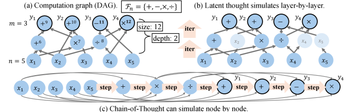
Figure 2: Comparison of reasoning paradigms for evaluating a DAG. (a) A computation graph $G_{n}$ . (b) Latent thought can simulate the computation layer by layer in parallel, using a number of loops equal to the depth of the graph, $\mathrm{depth}(G_{n})$ . (c) CoT can sequentially simulate the computation node by node, using a number of steps proportional to the size of the graph, $O(\mathrm{size}(G_{n}))$ .
Reasoning problems that can be solved by straight-line programs admit representations as directed acyclic graphs (DAGs) (Aho and Ullman, 1972), as illustrated in Fig. 2 (a).
**Definition 3.1 (Computation graph)**
*Let $\Sigma$ be a finite alphabet, and let $\mathcal{F}$ denote a finite set of functions $f:\Sigma^{*}\to\Sigma$ . A computation graph is a directed acyclic graph $G_{n}=(V_{n},E_{n})$ that defines a function $F_{G_{n}}:\Sigma^{n}\to\Sigma^{m(n)}$ , where $m(n)$ denotes the output length. Here $V_{n}$ denotes the set of nodes, consisting of (i) $n$ input nodes with in-degree $0$ , (ii) function nodes labeled by $f\in\mathcal{F}$ , which take as arguments the predecessor nodes specified by their incoming edges in $E_{n}$ , and (iii) $m(n)$ output nodes with out-degree $0$ . The overall function is obtained by evaluating the graph in topological order. The size of the graph is $|V_{n}|$ , denoted by $\mathrm{size}(G_{n})$ , and its depth is the length of the longest path from an input to an output node, denoted by $\mathrm{depth}(G_{n})$ .*
Assumptions on models.
Our goal is to evaluate the computational efficiency of each model via an asymptotic analysis of how the required number of reasoning steps or loops scales with the input size $n$ . Beyond time complexity, we also allow the space complexity of the model to scale with the input size $n$ . In particular, the embedding dimension in Transformer blocks can be viewed as analogous to the number of processors in classical parallel computation models. Accordingly, we adopt a non-uniform computational model, in which a different model is allowed for each input size. This non-uniform setting is standard in the study of circuit complexity and parallel computation (Cook, 1985), and is consistent with prior analyses of Transformers and CoT (Sanford et al., 2024b; Li et al., 2024).
On the fairness of comparing steps and loops.
We analyze expressivity in terms of the number of reasoning steps. Although this may appear unfair in terms of raw computation, it is justified when comparing latency. Specifically, CoT benefits from KV caching, which makes each step computationally inexpensive; however, accessing cached states is typically memory-bound, leaving compute resources underutilized. In contrast, looped TFs recompute over the full sequence at each iteration, incurring higher arithmetic cost but achieving higher arithmetic intensity and better utilization of modern parallel hardware. As a result, the latency of looped TFs is comparable to that of CoT.
### 3.2 CoT Suffices with Size-scaled Steps and Latent Thought Suffices with Depth-scaled Iterations
We show how each model can evaluate DAGs, which provides a lower bound on their expressivity and offers intuition for the distinctions between the models, in terms of sequentiality and parallelizability. Before presenting our main result, we first state the underlying assumptions.
**Definition 3.2 (Merrill and Sabharwal,2023)**
*The model is log-precision, where each scalar is stored with $O(\log n)$ bits and every arithmetic operation is rounded to that precision.*
**Assumption 3.3 (Poly-size graph)**
*$\mathrm{size}(G_{n})\in\mathsf{poly}(n)$ .*
**Assumption 3.4 (Poly-efficient approximation, cf.(Fenget al.,2023))**
*Each node function of $G_{n}$ can be approximated by a log-precision feedforward network whose parameter size is polynomial in the input length and the inverse of the approximation error. We denote by $\mathrm{ff\_param}(G_{n})$ an upper bound such that every $f\in\mathcal{F}$ admits such a network with at most $\mathrm{ff\_param}(G_{n})$ parameters.*
Under these assumptions, we show that CoT can simulate computation by sequentially decoding nodes, where intermediate tokens serve as a scratchpad allowing the evaluation of each node once all its predecessors have been computed.
**Theorem 3.5 (CoT for DAGs)**
*Let $\{G_{n}\}_{n\in\mathbb{N}}$ be a family of computation graphs that satisfy Assumptions 3.3 and 3.4. Then, for each $n\in\mathbb{N}$ , there exists a log-precision CoT with parameter size bounded by $O(\mathrm{ff\_param}(G_{n}))$ , such that for every input $x\in\Sigma^{n}$ , the model outputs $F_{G_{n}}(x)$ with steps proportional to the “size” of the graph, i.e., $O(\mathrm{size}(G_{n}))$ .*
* Proof sketch*
At each step, the attention layer retrieves the outputs of predecessor nodes from previously generated tokens, and a feed-forward layer then computes the node function, whose output is generated as the next token. ∎
In contrast, latent thought can operate in parallel, layer by layer, where all nodes at the same depth are computed simultaneously, provided that the model has sufficient size.
**Theorem 3.6 (Latent thought for DAGs)**
*Let $\{G_{n}\}_{n\in\mathbb{N}}$ be a family of computation graphs that satisfy Assumptions 3.3 and 3.4. Then, for each $n\in\mathbb{N}$ , there exists a log-precision Coconut and looped TF with parameter size $O(\mathrm{ff\_param}(G_{n})\cdot\mathrm{size}(G_{n}))$ , such that for every input $x\in\Sigma^{n}$ , it computes $F_{G_{n}}(x)$ with iterations proportional to the “depth” of the graph $G_{n}$ , i.e., $O(\mathrm{depth}(G_{n}))$ .*
* Proof sketch*
The role assignment of each layer is based on (Li et al., 2024), as shown in Figure 9. An attention layer aggregates its inputs into a single hidden state. Unlike discrete tokens, continuous latent states allow the simultaneous encoding of the outputs of multiple nodes, enabling the feed-forward layer to compute node functions in parallel. ∎
Remark.
Illustrations are provided in Fig. 2, with formal proofs deferred to Appendix B. These results reveal distinct characteristics: CoT can utilize intermediate steps as scratchpad memory and perform computations sequentially, whereas latent thought can leverage structural parallelism to achieve greater efficiency with sufficient resources.
### 3.3 Separation in Polylogarithmic Iterations
In this section, we shift to formal decision problems to precisely characterize the computational power of each reasoning paradigm, clarify what cannot be achieved, and use these limitations to derive rigorous separations. We begin by defining their complexity classes, as in (Li et al., 2024).
**Definition 3.7 (Complexity Classes𝖢𝗈𝖳\mathsf{CoT},𝖢𝖳\mathsf{CT}and𝖫𝗈𝗈𝗉\mathsf{Loop})**
*Let $\mathsf{CoT}[T(n),d(n),s(n)]$ , $\mathsf{CT}[T(n),d(n),s(n)]$ , and $\mathsf{Loop}[T(n),d(n),s(n)]$ denote the sets of languages ${\mathcal{L}}:\{0,1\}^{*}\to\{0,1\}$ for which there exists a deterministic CoT, Coconut, and looped TF, respectively, denoted by $M_{n}$ for each input size $n$ , with embedding size $O(d(n))$ and $O(s(n))$ bits of precision, such that for all $x\in\{0,1\}^{n}$ , the final output token after $O(T(n))$ iterations equals ${\mathcal{L}}(x)$ .*
Boolean circuits serve as a standard formal model of computation, where processes are defined by the evaluation of DAGs with well-established complexity measures.
**Definition 3.8 (Informal)**
*A Boolean circuit is a DAG over the alphabet $\Sigma=\{0,1\}$ , where each internal node (gate) computes a Boolean function such as AND, OR, or NOT. $\mathsf{SIZE}[s(n)]$ and $\mathsf{DEPTH}[d(n)]$ denote the class of languages decidable by a non-uniform circuit family $\{C_{n}\}$ with size $O(s(n))$ and depth $O(d(n))$ , respectively.*
First, we formalize the results of the previous section to show that latent thought iterations can represent circuit depth, whereas CoT corresponds to circuit size.
**Theorem 3.9 (Liet al.,2024)**
*$\forall T(n)\in\mathrm{poly}(n),$
$$
\mathsf{SIZE}[T(n)]\subseteq\mathsf{CoT}[T(n),\log{n},1].
$$*
**Theorem 3.10**
*For any function $T(n)\in\mathrm{poly}(n)$ and any non-uniform circuit family $\{C_{n}\}$ , it holds that
| | $\displaystyle\mathsf{DEPTH}[T(n)]$ | $\displaystyle\subseteq\mathsf{Loop}[T(n),\mathrm{size}(C_{n}),1],$ | |
| --- | --- | --- | --- |*
Boolean circuits serve as a formal model of parallel computations that run in polylogarithmic time using a polynomial number of processors (Stockmeyer and Vishkin, 1984).
**Definition 3.11**
*For each $k\in\mathbb{N}$ , the classes $\mathsf{NC}^{k}$ , $\mathsf{AC}^{k}$ , and $\mathsf{TC}^{k}$ consist of languages decidable by non-uniform circuit families of size $\mathsf{poly}(n)$ and depth $O(\log^{k}n)$ , using bounded-fanin Boolean gates, unbounded-fanin $\mathsf{AND}$ / $\mathsf{OR}$ gates, and threshold gates, respectively.*
We then characterize the exact computational power of latent thought in the parallel computation regime.
**Theorem 3.12**
*For each $k\in\mathbb{N},$ it holds that
| | | $\displaystyle\mathsf{Loop}[\log^{k}n,\,\mathsf{poly}(n),1\ \textup{(resp.\ }\log n)]$ | |
| --- | --- | --- | --- |*
* Proof sketch*
The inclusion from circuits to latent thought follows from Theorem 3.10. For the converse inclusion, we build on the arguments of prior work (Merrill and Sabharwal, 2023; Li et al., 2024), which show that a fixed-depth Transformer block under finite precision is contained in $\mathsf{AC}^{0}$ (or $\mathsf{TC}^{0}$ under logarithmic precision). We extend their analysis to the looped setting, which can be unrolled into a $\mathsf{TC}^{k}$ circuit by composing a $\mathsf{TC}^{0}$ block for $\log^{k}n$ iterations. ∎
Moreover, we establish an upper bound on the power of CoT in the parallel computation regime. This limitation arises from the inherently sequential nature of CoT.
**Lemma 3.13**
*For each $k\in\mathbb{N},$ it holds that
$$
\mathsf{CoT}[\log^{k}{n},\mathsf{poly}(n),\log{n}]\subseteq\mathsf{TC}^{k-1}.
$$*
* Proof*
The total $\log^{k}n$ steps can be divided into $\log^{k-1}n$ blocks, each consisting of $\log n$ steps. Since $\mathsf{CoT}[\log n,\mathsf{poly}(n),\log n]\subseteq\mathsf{TC}^{0}$ (Li et al., 2024), each block with the previous block’s outputs fed as inputs to the next block can be simulated in $\mathsf{TC}^{0}$ ; iterating this over $\log^{k-1}n$ layers yields a circuit in $\mathsf{TC}^{k-1}$ . ∎
<details>
<summary>x3.png Details</summary>
### Visual Description
## Diagram: Computational Complexity Hierarchy
### Overview
The image displays a nested diagram illustrating relationships between different computational complexity classes, specifically involving "CT/Loop" and "CoT" models with logarithmic depth constraints, and their containment within or equality to "TC" (Threshold Circuit) classes of specific depths. The diagram uses a layered, box-in-box visual structure with color-coded backgrounds to denote hierarchy.
### Components/Axes
The diagram consists of three nested rectangular boxes, each containing a mathematical expression. There are no traditional chart axes, legends, or data points. The components are purely textual and symbolic.
1. **Outermost Box (Light Peach Background):**
* **Text:** `CT / Loop[log^k(n)] = TC^k`
* **Position:** This is the largest, containing box. It forms the outer boundary of the diagram.
2. **Middle Box (White Background, Black Border):**
* **Text:** `CT / Loop[log^{k-1}(n)] = TC^{k-1}`
* **Position:** Centered within the outermost box. It is fully contained by the peach box.
3. **Innermost Box (Light Blue Background):**
* **Text:** `CoT[log^k(n)] ⊆ TC^{k-1}`
* **Position:** Centered within the middle box. It is fully contained by the white box.
### Detailed Analysis
The diagram presents three formal statements about computational models:
1. **Statement 1 (Outer):** The model or class denoted `CT / Loop` with a resource bound of `log^k(n)` (logarithmic depth to the power *k*) is **equal** to the Threshold Circuit class of depth *k* (`TC^k`).
2. **Statement 2 (Middle):** The same `CT / Loop` model with a stricter resource bound of `log^{k-1}(n)` is **equal** to the Threshold Circuit class of depth *k-1* (`TC^{k-1}`).
3. **Statement 3 (Inner):** The model or class denoted `CoT` with a resource bound of `log^k(n)` is **contained within** (a subset of, `⊆`) the Threshold Circuit class of depth *k-1* (`TC^{k-1}`).
**Key Symbolic Elements:**
* `CT / Loop`: Likely represents a class of circuits or programs (e.g., Circuit Trees, Loop programs).
* `CoT`: Likely represents a different, possibly more constrained, class (e.g., Circuits of Trees).
* `log^m(n)`: Denotes a logarithmic depth or iteration bound raised to the power *m*.
* `TC^m`: Denotes the class of problems solvable by Threshold Circuits of depth *m*.
* `=`: Denotes equality between complexity classes.
* `⊆`: Denotes subset inclusion (the left class is contained within the right class).
### Key Observations
1. **Nested Hierarchy:** The visual nesting directly mirrors the logical relationship. The statement about `CoT` (innermost) is a more specific or constrained result contained within the broader framework defined by the `CT/Loop` equalities.
2. **Parameter Shift:** Moving from the outer to the middle box, the parameter *k* decreases to *k-1* in both the resource bound (`log^k` to `log^{k-1}`) and the resulting TC class (`TC^k` to `TC^{k-1}`), maintaining the equality.
3. **Critical Inclusion:** The innermost statement is the only one using `⊆` instead of `=`. It shows that `CoT` with a `log^k` bound is no more powerful than `TC^{k-1}`, which is a *lower* depth class than the `TC^k` that `CT/Loop[log^k]` achieves. This suggests `CoT` is a strictly weaker model than `CT/Loop` under the same `log^k` resource constraint.
4. **Color Coding:** The light blue highlight on the innermost box draws attention to this inclusion result, suggesting it may be the primary theorem or key insight being illustrated.
### Interpretation
This diagram summarizes a theoretical result in circuit complexity or computational models. It establishes a precise hierarchy:
* **Power of CT/Loop:** The `CT/Loop` model is perfectly characterized by threshold circuits; its power scales exactly with the allowed logarithmic depth (`log^k` gives `TC^k`).
* **Power of CoT:** The `CoT` model is strictly weaker. Even with the same `log^k` depth allowance, it cannot exceed the power of a `TC^{k-1}` circuit. This implies that the structural constraints of `CoT` limit its computational power relative to `CT/Loop`.
* **Implication:** The nesting visually argues that understanding the `CT/Loop` model at level *k* inherently involves understanding its behavior at level *k-1*, and that the `CoT` model sits entirely within that lower-level understanding. This could be used to prove separations between complexity classes or to classify the power of different programming/circuit paradigms.
**Language Note:** The text in the image is entirely mathematical notation, which is language-agnostic. The symbols and structure are standard in theoretical computer science.
</details>
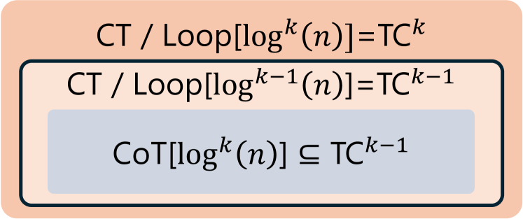
Figure 3: The separation between latent thought and CoT for decision problems, under polylogarithmic iterations.
These results lead to a separation in expressive power under standard complexity assumptions, as illustrated in Figure 3.
**Theorem 3.14**
*For each $k\in\mathbb{N}$ , if $\mathsf{TC}^{k-1}\subsetneq\mathsf{NC}^{k}$ , then
| | $\displaystyle\mathsf{CoT}[\log^{k}n,\mathsf{poly}(n),\log{n}]$ | $\displaystyle\subsetneq\mathsf{Loop}[\log^{k}n,\mathsf{poly}(n),1],$ | |
| --- | --- | --- | --- |*
**Theorem 3.15**
*For each $k\in\mathbb{N}$ , if $\mathsf{TC}^{k-1}\subsetneq\mathsf{TC}^{k}$ , then
| | $\displaystyle\mathsf{CoT}[\log^{k}n,\mathsf{poly}(n),\log n]$ | $\displaystyle\subsetneq\mathsf{Loop}[\log^{k}n,\mathsf{poly}(n),\log n],$ | |
| --- | --- | --- | --- |*
Remark.
The claims follow directly from Theorem 3.12 and Lemma 3.13. The established separations of the complexity classes, as summarized in Fig. 3, show that latent thought reasoning enables efficient parallel solutions more effectively than CoT, which is inherently sequential.
## 4 CoT Enables Approximate Counting
In the previous section, we showed that for decision problems, latent thought can yield more efficient solutions than CoT. This naturally raises the question of whether latent thought is universally more powerful than CoT. While prior work has shown that CoT can be simulated by looped Transformer models for deterministic decision problems under deterministic decoding (Saunshi et al., 2025), we found that this result does not directly extend to probabilistic settings with stochastic decoding. Accordingly, we shift our focus from efficiency in terms of the number of reasoning steps to expressive capability under polynomially many iterations.
### 4.1 Preliminaries
Approximate counting.
Formally, let $\Sigma$ be a finite alphabet and let $R\subseteq\Sigma^{*}\times\Sigma^{*}$ be a relation. For an input $x\in\Sigma^{*}$ , define $R(x):=\{\,y\in\Sigma^{*}\mid(x,y)\in R\,\},$ and the counting problem is to determine $|R(x)|$ . A wide class of natural relations admits a recursive structure, which allows solutions to be constructed from smaller subproblems.
**Definition 4.1 (Informal: Self-reducibility(Schnorr,1976))**
*A relation $R$ is self-reducible if there exists a polynomial-time procedure that, given any input $x$ and prefix $y_{1:k}$ (with respect to a fixed output order), produces a sub-instance $\psi(x,y_{1:k})$ such that every solution $z$ of $\psi(x,y_{1:k})$ extends $y_{1:k}$ to a solution of $R(x)$ (and conversely), i.e., $R\bigl(\psi(x,y_{1:k})\bigr)=\{z\mid\ \mathrm{concat}(y_{1:k},z)\in R(x)\,\}.$*
While exact counting is intractable, there exist efficient randomized approximation algorithms (Karp and Luby, 1983).
**Definition 4.2 (FPRAS)**
*An algorithm is called a fully polynomial-time randomized approximation scheme (FPRAS) for a function $f$ if, for any $\varepsilon>0$ and $\delta>0$ , it outputs an estimate $\hat{f}(x)$ such that
$$
\Pr\!\left[(1-\varepsilon)f(x)\leq\hat{f}(x)\leq(1+\varepsilon)f(x)\right]\geq 1-\delta,
$$
and runs in time polynomial in $|x|$ , $1/\varepsilon$ , and $\log(1/\delta)$ .*
The class of counting problems that admit an FPRAS is denoted by $\mathsf{FPRAS}$ . Although randomized algorithms provide only probabilistic guarantees, they are often both more efficient and simpler than their deterministic counterparts, denoted by $\mathsf{FPTAS}$ (Definition C.11). For example, counting the number of satisfying assignments of a DNF formula admits an FPRAS based on Monte Carlo methods (Karp et al., 1989), whereas no FPTAS is known for this problem. Moreover, probabilistic analysis enables us to capture algorithmic behavior on typical instances arising in real-world applications (Mitzenmacher and Upfal, 2017).
Probabilistic models of computation.
In contrast to the deterministic models considered in the previous section, we now study probabilistic models that define a conditional distribution over output strings $y=(y_{1},\ldots,y_{m})\in\Sigma^{*}$ . We consider autoregressive next-token prediction of the form
$$
p(y\mid x)=\prod_{i=1}^{m}p(y_{i}\mid x,y_{<i}),
$$
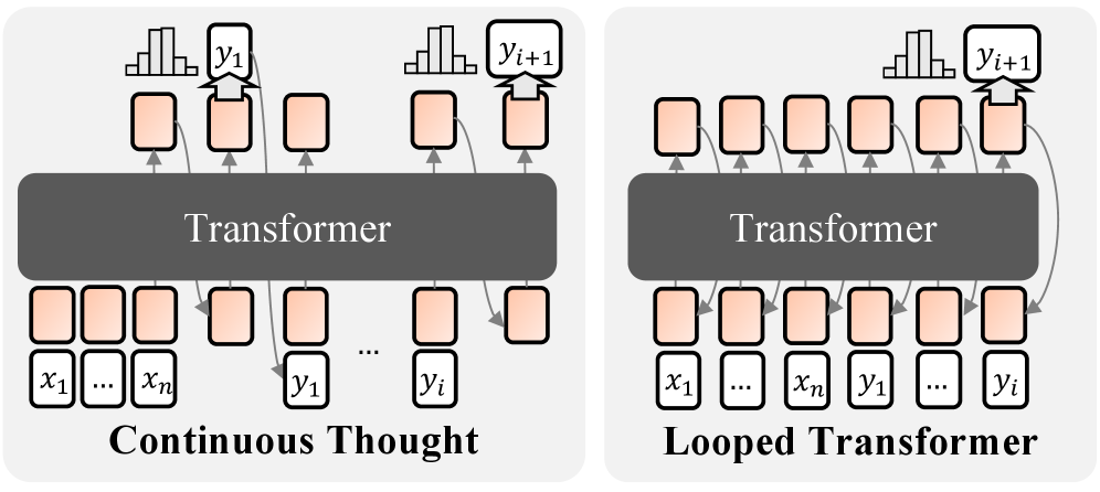
where the model is allowed to perform additional reasoning steps before producing each output token $y_{i}$ . This formulation was first used to formalize CoT for language modeling by Nowak et al. (2024). For latent thought, reasoning iterations are performed entirely in hidden space; no linguistic tokens are sampled except for the output token $y_{i}$ , as illustrated in Fig. 4. This definition is consistent with practical implementations (Csordás et al., 2024; Bae et al., 2025). Within this framework, we define complexity classes of probabilistic models, denoted by $\mathsf{pCoT}$ , $\mathsf{pCT}$ , and $\mathsf{pLoop}$ , respectively. Formal definitions are in Section C.1.
<details>
<summary>x4.png Details</summary>
### Visual Description
## Diagram: Transformer Architecture Comparison
### Overview
The image displays two side-by-side technical diagrams illustrating different architectural approaches for processing sequences with a Transformer model. The left diagram is labeled "Continuous Thought" and the right is labeled "Looped Transformer." Both diagrams use a consistent visual language: a central dark gray block representing the "Transformer," with sequences of light orange rounded rectangles representing data tokens or hidden states, and arrows indicating data flow.
### Components/Axes
**Common Elements:**
* **Central Block:** A dark gray, horizontally oriented rectangle labeled "Transformer" in white text. This is the core processing unit in both diagrams.
* **Data Tokens:** Light orange, rounded rectangles. These represent input tokens, output tokens, or intermediate hidden states.
* **Arrows:** Gray lines with arrowheads indicating the direction of data flow between tokens and the Transformer block.
* **Probability Distributions:** Small bar chart icons placed above certain output tokens, indicating a predicted probability distribution over a vocabulary.
**Left Diagram: "Continuous Thought"**
* **Title:** "Continuous Thought" in bold, black text at the bottom.
* **Input Sequence (Bottom Row):** A sequence of tokens labeled `x₁`, `...`, `xₙ`, followed by `y₁`, `...`, `yᵢ`. The ellipsis (`...`) indicates a variable-length sequence.
* **Output Sequence (Top Row):** A sequence of tokens. The first token has a probability distribution icon above it and is labeled `y₁`. The last token has a probability distribution icon above it and is labeled `yᵢ₊₁`.
* **Data Flow:**
1. The initial input sequence (`x₁...xₙ`) is fed into the Transformer.
2. The Transformer produces an output sequence. The first output token is `y₁`.
3. A critical feedback loop is shown: the output token `y₁` is fed back into the Transformer as part of the input for the next step.
4. This process continues iteratively. The diagram shows the token `yᵢ` being fed back to help produce the next output, `yᵢ₊₁`.
5. The final output shown is `yᵢ₊₁`.
**Right Diagram: "Looped Transformer"**
* **Title:** "Looped Transformer" in bold, black text at the bottom.
* **Input Sequence (Bottom Row):** A single, combined sequence of tokens labeled `x₁`, `...`, `xₙ`, `y₁`, `...`, `yᵢ`.
* **Output Sequence (Top Row):** A sequence of tokens. The final token has a probability distribution icon above it and is labeled `yᵢ₊₁`.
* **Data Flow:**
1. The entire combined sequence (`x₁...xₙ y₁...yᵢ`) is presented as input to the Transformer in a single pass.
2. The Transformer processes this entire sequence.
3. The diagram shows multiple arrows originating from the Transformer block and pointing to various positions within the input sequence row, suggesting internal recurrence or iterative refinement within the model's processing.
4. The final output token `yᵢ₊₁` is generated from the end of the processed sequence.
### Detailed Analysis
**Spatial Grounding & Component Isolation:**
* **Header Region (Top):** Contains the output tokens and their associated probability distribution icons. In the "Continuous Thought" diagram, outputs are generated sequentially (`y₁` then later `yᵢ₊₁`). In the "Looped Transformer," only the final output `yᵢ₊₁` is explicitly shown.
* **Main Chart Region (Center):** Dominated by the "Transformer" block. The density of connecting arrows differs significantly. The "Continuous Thought" diagram has a clear, sequential loop on the right side. The "Looped Transformer" has a denser web of arrows connecting the Transformer to multiple points in the input sequence.
* **Footer Region (Bottom):** Contains the input sequences and the diagram titles. The "Continuous Thought" input is split into an initial context (`x`) and a growing sequence of generated thoughts (`y`). The "Looped Transformer" input is a single concatenated sequence.
**Flow Comparison:**
* **Continuous Thought Flow:** `x₁...xₙ` → Transformer → `y₁` → (feed `y₁` back) → Transformer → ... → `yᵢ` → (feed `yᵢ` back) → Transformer → `yᵢ₊₁`. This is an **autoregressive, sequential generation** process where each new output depends on all previous outputs.
* **Looped Transformer Flow:** `[x₁...xₙ, y₁...yᵢ]` → Transformer (with internal loops/recurrence) → `yᵢ₊₁`. This suggests a **parallel or iterative refinement** process where the model can revisit and update its internal states for all tokens in the sequence before producing the final output.
### Key Observations
1. **Architectural Distinction:** The core difference is the processing paradigm. "Continuous Thought" is strictly sequential and autoregressive. "Looped Transformer" implies a mechanism for parallel computation or recurrent processing within a fixed forward pass.
2. **Input Representation:** The "Continuous Thought" model treats generated tokens (`y`) as part of the input stream for subsequent steps. The "Looped Transformer" model treats the entire history (both original input `x` and generated tokens `y`) as a single, static input block.
3. **Output Granularity:** The "Continuous Thought" diagram explicitly shows intermediate outputs (`y₁`). The "Looped Transformer" diagram only highlights the final output (`yᵢ₊₁`), emphasizing its end-to-end nature.
4. **Visual Complexity:** The "Looped Transformer" diagram has a more complex arrow pattern, visually representing its more intricate internal connectivity compared to the straightforward loop of the "Continuous Thought" model.
### Interpretation
This diagram contrasts two fundamental approaches to sequence modeling and generation with Transformers.
The **"Continuous Thought"** architecture represents the standard **autoregressive decoding** paradigm used in models like GPT. It generates tokens one-by-one, with each new token conditioned on all previous tokens. This is simple and effective but can be slow for long sequences as it requires `O(n)` sequential steps.
The **"Looped Transformer"** architecture suggests a more advanced, potentially **recurrent or iterative** design. It aims to overcome the sequential bottleneck by allowing the model to process the entire sequence (including partially generated outputs) in parallel, using internal loops to refine its understanding over multiple "virtual" steps within a single forward pass. This could lead to faster inference and the ability to model more complex, non-causal dependencies.
The key implication is a trade-off between simplicity/serial dependency ("Continuous Thought") and potential parallelism/computational efficiency ("Looped Transformer"). The "Looped Transformer" concept aligns with research into models like Universal Transformers or architectures that incorporate recurrence to improve reasoning and generalization beyond standard feed-forward processing.
</details>
Figure 4: Probabilistic models of computation with latent thought. Each output token $y_{i}$ is generated autoregressively, with computation permitted in a continuous latent space prior to each token.
### 4.2 Separation in Approximate Counting
We first analyze the expressivity of the token-level conditional prediction at each step, $p(y_{i}\mid x,y_{<i})$ , and show that CoT is strictly more expressive than latent thought in this setting. The key distinction is whether intermediate computation permits sampling. CoT explicitly samples intermediate reasoning tokens, inducing stochastic computation and enabling the emulation of randomized algorithms. In contrast, latent thought performs only deterministic transformations in latent space, resulting in deterministic computation.
**Lemma 4.3 (Informal)**
*Assume that $\mathsf{FPTAS}\subsetneq\mathsf{FPRAS}$ for self-reducible relations. There exists a self-reducible relation $R$ and an associated function $f:\Sigma^{*}\times\Sigma^{*}\to\mathbb{N}$ defined by $f(x,y_{<i})\coloneqq|\{\,z\in\Sigma^{*}:(x,y_{<i}z)\in R\,\}|$ such that CoT with polynomially many steps admits an FPRAS for $f$ . Whereas, no latent thought with polynomially many iterations admits the same approximation guarantee.*
* Proof sketch*
For self-reducible relations, approximating the counting function $f$ on subproblems is polynomial-time inter-reducible with approximating $|R(x)|$ (Jerrum et al., 1986). If latent thought with polynomially many iterations admitted an FPTAS for $f$ , then it would induce a deterministic FPTAS for $|R(x)|$ , contradicting the assumption.∎
### 4.3 Separation in Approximate Sampling
We then move from token-level conditional distributions $p(y_{i}\mid x,y_{<i})$ to the full sequence-level distribution $p(y\mid x)$ . Beyond approximate counting, we establish a separation for approximate sampling problems. Specifically, we construct target distributions for which the complexity of each conditional can be reduced to approximate counting.
**Theorem 4.4**
*Assume that $\mathsf{FPTAS}\subsetneq\mathsf{FPRAS}$ for self-reducible relations. There exists a distribution $p(y\mid x)$ over $y\in\Sigma^{*}$ and $x\in\Sigma^{n}$ such that a CoT with a polynomial number of steps, whose induced output conditionals are denoted by $q(y_{i}\mid x,y_{<i})$ , admits an FPRAS for approximating the conditional probabilities $p(y_{i}\mid x,y_{<i})$ for all $x\in\Sigma^{n}$ , indices $i\geq 1$ , and prefixes $y_{<i}\coloneq(y_{1},\ldots,y_{i-1})$ . In contrast, no latent thought with polynomially many iterations admits the same approximation guarantee.*
* Proof sketch*
Define the target distribution $p$ to be the uniform distribution supported on the solution set $R(x)$ . We rely on the classical result that approximate sampling from the uniform distribution over solutions, captured by the class $\mathsf{FPAUS}$ , is polynomial-time inter-reducible with approximate counting for self-reducible relations (Jerrum et al., 1986). Let $U(\cdot\mid x)$ denote the uniform distribution over solutions of a self-reducible relation $R(x)$ . This distribution admits an autoregressive factorization $U(y\mid x)\;=\;\prod_{i=1}^{m}p(y_{i}\mid x,y_{<i}),$ where each conditional probability is given by $p(y_{i}\mid x,y_{<i})=\frac{\bigl|\{\,z\in\Sigma^{*}:(x,y_{1:i+1}z)\in R\,\}\bigr|}{\bigl|\{\,z\in\Sigma^{*}:(x,y_{1:i}z)\in R\,\}\bigr|}.$ We show that each conditional probability, expressed as a ratio of subproblem counts, reduces to approximate counting. Then, applying Lemma 4.3 to these conditionals yields the desired separation for approximate sampling. ∎
<details>
<summary>x5.png Details</summary>
### Visual Description
## Diagram: Nested Complexity Class Relationships
### Overview
The image is a conceptual diagram illustrating the hierarchical and subset relationships between several computational complexity classes or algorithmic concepts. It uses nested, colored boxes to represent containment, with text labels identifying each class. The diagram appears to be from a theoretical computer science or algorithm analysis context.
### Components/Axes
The diagram consists of three primary visual components:
1. **Outer Container (Light Blue Box):**
* **Label:** `pCoT[poly(n)]`
* **Position:** Forms the background and outermost boundary of the diagram.
* **Meaning:** Represents a broad complexity class or problem family parameterized by a polynomial function `poly(n)`.
2. **Left Inner Box (Gray):**
* **Labels:**
* `FPRAS`
* `FPAUS`
* `(self-reducibility)`
* **Position:** Located in the left portion of the outer container. It is partially overlapped by the right inner box.
* **Meaning:** Represents a set of concepts or classes (FPRAS, FPAUS) characterized by the property of "self-reducibility."
3. **Right Inner Box (Peach with Black Border):**
* **Label:** `pCT / pLoop [poly(n)]`
* **Position:** Located in the right portion of the outer container, overlapping the right side of the gray box. It has a distinct, thick black border.
* **Meaning:** Represents another class or set of techniques (pCT, pLoop), also parameterized by `poly(n)`. The black border and overlapping placement suggest it is a specific, emphasized subset within the broader `pCoT[poly(n)]` class and has a relationship with the concepts in the gray box.
### Detailed Analysis
* **Text Transcription:** All text is in English, using standard technical abbreviations.
* `pCoT[poly(n)]`
* `FPRAS`
* `FPAUS`
* `(self-reducibility)`
* `pCT / pLoop [poly(n)]`
* **Spatial Relationships:**
* The diagram establishes a clear hierarchy: `pCT/pLoop [poly(n)]` and the `FPRAS/FPAUS` set are both contained within `pCoT[poly(n)]`.
* The overlap between the gray and peach boxes indicates an intersection or a specific relationship between the `FPRAS/FPAUS` concepts (with self-reducibility) and the `pCT/pLoop` class. This could mean that problems in `pCT/pLoop` may exhibit self-reducibility, or that techniques from one area apply to the other.
* The black border around the peach box highlights it as a focal point or a distinct, important subclass.
### Key Observations
1. **Parameterization:** Both the outer class (`pCoT`) and the inner class (`pCT/pLoop`) are explicitly parameterized by `[poly(n)]`, indicating their complexity or runtime scales polynomially with the input size `n`.
2. **Self-Reducibility:** The term `(self-reducibility)` is explicitly associated with the `FPRAS` and `FPAUS` concepts, defining a key algorithmic property for that group.
3. **Visual Emphasis:** The `pCT / pLoop [poly(n)]` box is visually emphasized with a black border and a distinct color, suggesting it is the primary subject of interest or a newly introduced class within the broader `pCoT` framework.
4. **Subset Implication:** The containment within the light blue box implies that `FPRAS`, `FPAUS`, `pCT`, and `pLoop` are all, in some form, subclasses or instances of `pCoT[poly(n)]`.
### Interpretation
This diagram visually summarizes a theoretical framework in computational complexity or randomized algorithms.
* **What it suggests:** It proposes a structural relationship where `pCoT[poly(n)]` is a unifying class encompassing both established concepts like FPRAS (Fully Polynomial Randomized Approximation Scheme) and FPAUS (likely a related approximation or sampling class), as well as a specific subclass `pCT/pLoop`. The property of "self-reducibility" is highlighted as a defining characteristic of the FPRAS/FPAUS group.
* **How elements relate:** The overlap is the most critical relational element. It suggests that the `pCT/pLoop` class is not entirely separate but intersects with the world of self-reducible approximation schemes. This could imply that `pCT/pLoop` algorithms can be applied to self-reducible problems, or that problems in this intersection have specific, advantageous properties.
* **Notable emphasis:** The black border around `pCT/pLoop` draws the viewer's attention, indicating that this is likely the novel contribution, the specific focus of the accompanying research, or a class with particularly interesting properties that warrant distinction from the broader `pCoT` family. The diagram efficiently communicates that understanding `pCT/pLoop` requires understanding its place within `pCoT` and its connection to self-reducibility.
</details>
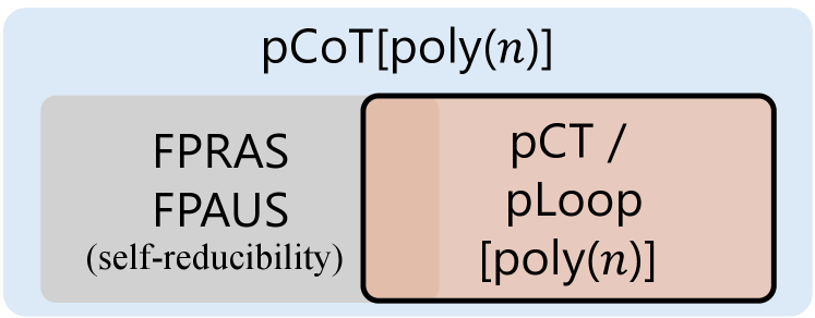
Figure 5: The separation for approximate counting (sampling).
Consequently, we obtain the following separations in favor of CoT, as also shown in Fig. 5.
**Theorem 4.5**
*Assuming $\mathsf{FPTAS}\subsetneq\mathsf{FPRAS}$ for self-reducible relations, it holds that
$$
\forall\,\mathcal{M}\in\{\mathsf{pCT},\mathsf{pLoop}\},\quad\mathcal{M}[\mathsf{poly}(n)]\subsetneq\mathsf{pCoT}[\mathsf{poly}(n)].
$$*
## 5 Experiments
In this section, we provide empirical validation of our theoretical results on tasks with well-characterized complexity. Specifically, we study parallelizable tasks to empirically validate the efficiency of latent thought predicted in Section 3, and approximate counting and sampling tasks to demonstrate the effectiveness of CoT as shown in Section 4.
### 5.1 Experimental Setting
Fundamental algorithmic reasoning tasks.
We use four problems. (1) Word problems for finite non-solvable groups: given a sequence of generators, the task is to evaluate their composition, which is $\mathsf{NC}^{1}$ -complete (Barrington, 1986), also studied for Looped TF (Merrill and Sabharwal, 2025a). (2) $s$ – $t$ connectivity (STCON): given a directed graph $G=(V,E)$ and two vertices $s,t\in V$ , the task is to decide whether $t$ is reachable from $s$ , which belongs to $\mathsf{TC}^{1}$ (Gibbons and Rytter, 1989). (3) Arithmetic expression evaluation: given a formula consisting of $+,\times,-,/$ operations on integers, the task is to evaluate it. This problem is $\mathsf{TC}^{0}$ -reducible to Boolean formula evaluation (Feng et al., 2023), which is $\mathsf{NC}^{1}$ -complete (Buss, 1987). (4) Edit distance: given two strings $x$ and $y$ , the task is to compute the minimum cost to transform $x$ into $y$ . By reducing the dynamic programming formulation to shortest paths, this problem is in $\mathsf{TC}^{1}$ (Apostolico et al., 1990).
Approximate counting tasks.
We consider DNF counting and uniform sampling of graph colorings, both of which admit fully polynomial randomized approximation schemes for counting and sampling (FPRAS and FPAUS). Specifically, DNF counting admits an FPRAS via Monte Carlo sampling (Karp et al., 1989), while approximate counting and sampling of graph colorings admit an FPAUS based on rapidly mixing Markov chain Monte Carlo under suitable degree and color constraints (Jerrum, 1995).
Training strategy.
Since our primary objective is to study expressive power, we allow flexibility in optimization and training strategies. For CoT models, training is performed with supervision from explicit sequential algorithms. For fewer CoT steps, we compare two strategies: uniformly selecting steps from the indices of the complete trajectory (Bavandpour et al., 2025), and stepwise internalization (distillation) methods (Deng et al., 2024). For latent thought, we observe that looped TF is easier to train than Coconut, and therefore adopt looped TF as our instantiation of latent thought, with curriculum learning applied to certain tasks.
Table 2: Accuracy (%) of CoT and looped TF on parallelizable tasks across different numbers of iterations. Here, $n$ denotes the problem size. For CoT, we report the best accuracy achieved across the two training strategies.
| Word Problem Graph Connectivity Arithmetic Evaluation | 64 32 32/16 | 0.8 80.8 43.7 | 0.8 95.8 99.4 | 100.0 99.0 99.5 | 100.0 99.0 99.7 | 0.8 81.0 47.3 | 0.8 81.4 47.6 | 100.0 88.2 48.2 | 100.0 100.0 82.5 |
| --- | --- | --- | --- | --- | --- | --- | --- | --- | --- |
| Edit Distance | 32/16 | 57.3 | 72.9 | 86.2 | 90.7 | 76.5 | 80.9 | 87.5 | 94.8 |
### 5.2 Results
Table 2 reports results on parallelizable tasks, comparing latent thought and CoT under varying numbers of iterations. Latent thought solves the problems with fewer iterations than CoT requires to reach comparable performance. These empirical results are consistent with our theoretical analysis: latent thought supports efficient parallel reasoning, in contrast to the inherently sequential nature of CoT.
<details>
<summary>x6.png Details</summary>
### Visual Description
## Line Chart: Accuracy vs. Input Size for Different Rank Values
### Overview
The image is a line chart plotting model accuracy (as a percentage) against input size for four different rank values (r). The chart demonstrates how the performance of models with different rank capacities degrades as the input size increases.
### Components/Axes
* **Y-Axis:** Labeled "Accuracy (%)". The scale is linear, with major tick marks labeled at 33, 66, and 100.
* **X-Axis:** Labeled "Input size". The scale is logarithmic (base 2), with major tick marks labeled at 8, 16, 32, and 64.
* **Legend:** Positioned in the top-right quadrant of the chart area. It contains four entries, each associating a colored line with a rank value:
* Teal line with circle markers: `r = 5`
* Orange line with circle markers: `r = 4`
* Purple line with circle markers: `r = 3`
* Pink line with circle markers: `r = 2`
### Detailed Analysis
The chart displays four data series, each showing a distinct trend. All series begin at approximately 100% accuracy for an input size of 8.
1. **r = 5 (Teal Line):**
* **Trend:** The line is nearly horizontal, showing a very slight, almost negligible downward slope.
* **Data Points (Approximate):**
* Input Size 8: ~100%
* Input Size 16: ~100%
* Input Size 32: ~99%
* Input Size 64: ~98%
2. **r = 4 (Orange Line):**
* **Trend:** The line shows a gentle, steady downward slope.
* **Data Points (Approximate):**
* Input Size 8: ~100%
* Input Size 16: ~99%
* Input Size 32: ~97%
* Input Size 64: ~93%
3. **r = 3 (Purple Line):**
* **Trend:** The line shows a pronounced, steady downward slope, significantly steeper than the r=4 line.
* **Data Points (Approximate):**
* Input Size 8: ~100%
* Input Size 16: ~97%
* Input Size 32: ~64%
* Input Size 64: ~45%
4. **r = 2 (Pink Line):**
* **Trend:** The line exhibits a very sharp, steep decline between input sizes 8 and 16, followed by a much shallower, nearly flat decline from 16 to 64.
* **Data Points (Approximate):**
* Input Size 8: ~99%
* Input Size 16: ~55%
* Input Size 32: ~40%
* Input Size 64: ~38%
### Key Observations
* **Inverse Relationship:** There is a clear inverse relationship between the rank value (`r`) and the sensitivity of accuracy to increasing input size. Lower rank models (r=2, r=3) experience dramatic performance degradation, while higher rank models (r=4, r=5) are much more robust.
* **Convergence at Small Input:** All models, regardless of rank, achieve near-perfect accuracy (~100%) on the smallest input size (8).
* **Divergence with Scale:** As input size increases, the performance of the models diverges significantly. The gap in accuracy between the highest (r=5) and lowest (r=2) rank models grows from ~1% at input size 8 to ~60% at input size 64.
* **Critical Threshold for r=2:** The model with r=2 shows a critical failure mode, losing nearly half its accuracy with just a doubling of input size from 8 to 16.
### Interpretation
This chart illustrates a fundamental trade-off in model capacity (represented by rank `r`) and its ability to generalize to larger, more complex inputs.
* **What the data suggests:** Higher-rank models possess a more expressive or robust internal representation, allowing them to maintain high accuracy even as the problem scale (input size) increases. Lower-rank models appear to be "under-parameterized" for larger tasks; their limited capacity is quickly overwhelmed, leading to a sharp drop in performance.
* **How elements relate:** The x-axis (Input size) represents the scaling challenge. The y-axis (Accuracy) is the performance metric. The different colored lines (r values) represent different model architectures or configurations being tested against this scaling challenge. The legend is essential for mapping the visual trend (line color/slope) to the specific model parameter being varied.
* **Notable implications:** The data implies that for tasks involving large input sizes, selecting a model with a sufficiently high rank is critical for maintaining performance. The r=2 model is effectively unusable for input sizes beyond 16. The near-flat line for r=5 suggests it may have capacity to spare for the tested range, while r=4 is beginning to show strain at the largest input size. This visualization would be crucial for guiding model selection and understanding the scaling limits of different architectural choices.
</details>
<details>
<summary>x7.png Details</summary>
### Visual Description
## Line Chart: Accuracy vs. Input Size for Different 'r' Values
### Overview
The image is a line chart displaying the relationship between "Input size" (x-axis) and "Accuracy (%)" (y-axis) for four different series, each corresponding to a distinct value of a parameter labeled 'r'. The chart demonstrates how accuracy changes as input size increases, with the rate of change dependent on the 'r' value.
### Components/Axes
* **X-Axis:** Labeled "Input size". Major tick marks are present at values 10, 15, 20, 25, and 30. The axis spans from approximately 8 to 32.
* **Y-Axis:** Labeled "Accuracy (%)". Major tick marks are present at values 80, 90, and 100. The axis spans from 80 to 100.
* **Legend:** Positioned in the top-left quadrant of the chart area. It contains four entries, each with a colored line segment and a label:
* Green line with circle markers: `r = 5`
* Orange line with circle markers: `r = 4`
* Purple line with circle markers: `r = 3`
* Pink line with circle markers: `r = 2`
### Detailed Analysis
The chart contains four data series, each plotted as a line with circular markers at data points. The general trend for all series is a decrease in accuracy as input size increases, but the severity of the decline varies significantly with 'r'.
**1. Series: r = 5 (Green Line)**
* **Trend:** The line is nearly horizontal, showing a very slight downward slope. It represents the highest and most stable accuracy across all input sizes.
* **Approximate Data Points:**
* Input Size ~8: Accuracy ~100%
* Input Size ~12: Accuracy ~100%
* Input Size ~16: Accuracy ~100%
* Input Size ~20: Accuracy ~100%
* Input Size ~24: Accuracy ~99.5%
* Input Size ~28: Accuracy ~99.5%
* Input Size ~32: Accuracy ~99%
**2. Series: r = 4 (Orange Line)**
* **Trend:** The line shows a moderate, steady downward slope. Accuracy decreases gradually with larger input sizes.
* **Approximate Data Points:**
* Input Size ~8: Accuracy ~100%
* Input Size ~12: Accuracy ~100%
* Input Size ~16: Accuracy ~99%
* Input Size ~20: Accuracy ~97.5%
* Input Size ~24: Accuracy ~96.5%
* Input Size ~28: Accuracy ~96%
* Input Size ~32: Accuracy ~95.5%
**3. Series: r = 3 (Purple Line)**
* **Trend:** The line shows a pronounced downward slope, steeper than the r=4 series. Accuracy drops significantly as input size grows.
* **Approximate Data Points:**
* Input Size ~8: Accuracy ~100%
* Input Size ~12: Accuracy ~100%
* Input Size ~16: Accuracy ~95%
* Input Size ~20: Accuracy ~93%
* Input Size ~24: Accuracy ~89.5%
* Input Size ~28: Accuracy ~87.5%
* Input Size ~32: Accuracy ~86%
**4. Series: r = 2 (Pink Line)**
* **Trend:** The line shows the steepest downward slope of all series. Accuracy degrades rapidly with increasing input size.
* **Approximate Data Points:**
* Input Size ~8: Accuracy ~100%
* Input Size ~12: Accuracy ~95.5%
* Input Size ~16: Accuracy ~91%
* Input Size ~20: Accuracy ~87.5%
* Input Size ~24: Accuracy ~84%
* Input Size ~28: Accuracy ~82%
* Input Size ~32: Accuracy ~81%
### Key Observations
1. **Inverse Relationship:** For all series, accuracy is inversely related to input size. As input size increases, accuracy decreases.
2. **Parameter 'r' as a Stabilizer:** The value of 'r' has a strong positive correlation with performance stability. Higher 'r' values (5, 4) result in much flatter curves and higher final accuracy at large input sizes compared to lower 'r' values (3, 2).
3. **Convergence at Small Inputs:** All four series converge at or near 100% accuracy for the smallest input sizes (around 8-12). The divergence in performance becomes pronounced only as input size increases beyond ~12.
4. **Performance Hierarchy:** The order of performance (from highest to lowest accuracy) is strictly maintained across all input sizes: r=5 > r=4 > r=3 > r=2. The lines do not cross.
### Interpretation
This chart likely illustrates the performance of a computational model or algorithm where 'r' represents a key hyperparameter, such as model rank, capacity, or complexity. The data suggests that:
* **Model Robustness:** Models with higher 'r' values are more robust to increases in input size. They maintain near-perfect accuracy even as the problem scale grows.
* **Capacity Limitation:** Models with lower 'r' values (r=2, r=3) appear to have a limited capacity. Their performance degrades sharply when faced with larger, presumably more complex, inputs, indicating they may be underfitting or lack the necessary parameters to capture the patterns in larger datasets.
* **Practical Implication:** There is a clear trade-off. If computational resources allow, using a higher 'r' value is preferable for ensuring consistent accuracy across varying input sizes. However, if 'r' correlates with cost (e.g., memory, time), a designer must choose the minimum 'r' that meets the accuracy requirements for the expected range of input sizes. The chart provides the empirical data needed to make that engineering decision.
* **Underlying Phenomenon:** The consistent, non-intersecting fan-out pattern from a common starting point is characteristic of a system where a single parameter ('r') controls the system's ability to generalize or scale. The investigation would next focus on what 'r' physically represents and why it has this specific scaling effect.
</details>
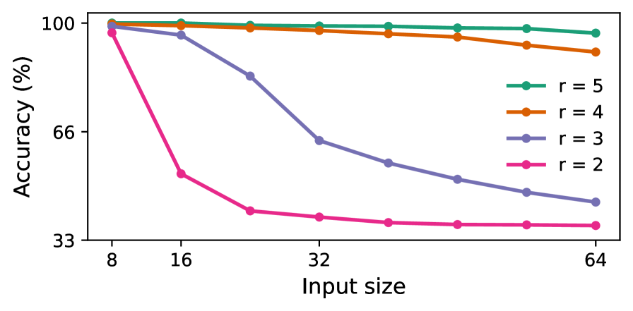
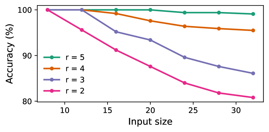
Figure 6: Accuracy of looped TFs on the arithmetic evaluation (top) and the connectivity (bottom). Each curve shows the performance for a fixed loop count $r$ as the input size $n$ increases.
We also evaluate the relationship between performance, input size, and the number of iterations, as in prior studies (Sanford et al., 2024b; Merrill and Sabharwal, 2025a). Figure 6 presents our results for looped TFs, illustrating that as the input size $n$ increases, the number of loops required to maintain high accuracy grows only logarithmically, supporting our theoretical claim in the (poly-)logarithmic regime.
<details>
<summary>x8.png Details</summary>
### Visual Description
## Line Chart: Relative Error vs. Computational Effort (Iterations × Trials)
### Overview
The image is a line chart comparing the performance of two methods, "Looped" and "CoT," as a function of increasing computational effort. The performance metric is "Relative error," where a lower value indicates better performance. The chart demonstrates how the error rates for the two methods change as the product of iterations and trials increases on a logarithmic scale.
### Components/Axes
* **Y-Axis (Vertical):**
* **Label:** `Relative error (↓)`
* **Scale:** Linear, ranging from approximately 0.25 to 0.5.
* **Markers:** Major ticks are visible at 0.3 and 0.4.
* **Note:** The downward arrow `(↓)` explicitly indicates that lower values are desirable.
* **X-Axis (Horizontal):**
* **Label:** `iterations × trials`
* **Scale:** Logarithmic (base 10).
* **Markers:** Major ticks at `10`, `100`, and `1000`.
* **Legend:**
* **Position:** Top-left corner of the chart area.
* **Series 1:** `Looped` - Represented by a teal/green line with circular markers.
* **Series 2:** `CoT` - Represented by an orange line with circular markers.
### Detailed Analysis
**Data Series: Looped (Teal/Green Line)**
* **Trend:** The line is perfectly horizontal, indicating no change in relative error as computational effort increases.
* **Data Points (Approximate):**
* At `iterations × trials = 10`: Relative error ≈ 0.36
* At `iterations × trials = 100`: Relative error ≈ 0.36
* At `iterations × trials = 1000`: Relative error ≈ 0.36
**Data Series: CoT (Orange Line)**
* **Trend:** The line slopes steeply downward, indicating a significant reduction in relative error as computational effort increases.
* **Data Points (Approximate):**
* At `iterations × trials ≈ 100`: Relative error ≈ 0.48 (This is the highest error point on the chart).
* At `iterations × trials ≈ 300`: Relative error ≈ 0.39.
* At `iterations × trials = 1000`: Relative error ≈ 0.26 (This is the lowest error point on the chart).
### Key Observations
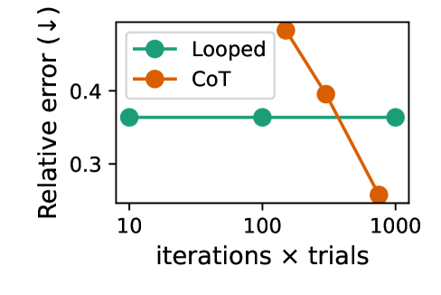
1. **Performance Crossover:** The CoT method starts with a higher error than Looped at lower computational budgets (around 100 iterations×trials) but surpasses it (achieves lower error) at a higher budget (around 1000 iterations×trials).
2. **Scalability:** The Looped method shows zero scalability with respect to the `iterations × trials` metric; its performance is static. In contrast, the CoT method demonstrates strong, positive scalability.
3. **Magnitude of Change:** The CoT method's error reduces by nearly half (from ~0.48 to ~0.26) as the computational budget increases from ~100 to 1000 on the log scale.
### Interpretation
This chart illustrates a classic trade-off between a method with fixed performance ("Looped") and a method whose performance improves with more resources ("CoT").
* **What the data suggests:** The "CoT" (likely "Chain-of-Thought") method benefits substantially from increased computational investment. The "Looped" method appears to be a baseline or a method that has reached its performance ceiling and cannot leverage additional iterations or trials for improvement.
* **How elements relate:** The logarithmic x-axis is crucial. It shows that achieving the performance gain from CoT requires an *order-of-magnitude* increase in computational effort (from 100 to 1000). The crossover point suggests there is a minimum resource threshold required for CoT to become the superior choice.
* **Notable implications:** For resource-constrained scenarios (low `iterations × trials`), the simpler "Looped" method may be preferable. For scenarios where high accuracy is critical and computational resources are abundant, "CoT" is the clearly superior approach. The chart argues that the investment in CoT's computational cost pays off in reduced error.
</details>
<details>
<summary>x9.png Details</summary>
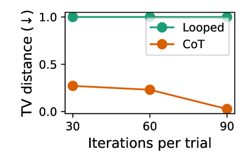
### Visual Description
## Line Chart: TV Distance vs. Iterations per Trial for Two Methods
### Overview
The image is a line chart comparing the performance of two methods, "Looped" and "CoT," based on a metric called "TV distance." The chart plots this distance against the number of "Iterations per trial." The y-axis includes a downward arrow (↓), indicating that a lower TV distance value is better or more desirable.
### Components/Axes
* **Chart Type:** Line chart with markers.
* **X-Axis:**
* **Label:** "Iterations per trial"
* **Scale/Major Ticks:** 30, 60, 90.
* **Y-Axis:**
* **Label:** "TV distance (↓)"
* **Scale/Major Ticks:** 0.0, 0.5, 1.0.
* **Legend:** Located in the top-right corner of the plot area.
* **Looped:** Represented by a teal/green line with solid circle markers.
* **CoT:** Represented by an orange line with solid circle markers.
### Detailed Analysis
**Data Series 1: Looped (Teal/Green Line)**
* **Trend Verification:** The line is perfectly horizontal, indicating no change in the measured value across the tested iterations.
* **Data Points:**
* At 30 iterations: TV distance ≈ 1.0
* At 60 iterations: TV distance ≈ 1.0
* At 90 iterations: TV distance ≈ 1.0
**Data Series 2: CoT (Orange Line)**
* **Trend Verification:** The line shows a clear downward slope, indicating improvement (reduction in TV distance) as iterations increase. The rate of decrease accelerates between 60 and 90 iterations.
* **Data Points:**
* At 30 iterations: TV distance ≈ 0.3
* At 60 iterations: TV distance ≈ 0.25
* At 90 iterations: TV distance ≈ 0.05 (very close to 0.0)
### Key Observations
1. **Performance Gap:** There is a significant and consistent performance gap between the two methods. The "Looped" method performs poorly (high TV distance) compared to "CoT" at all measured points.
2. **CoT Improvement:** The "CoT" method shows a clear benefit from increased computation (more iterations per trial), with its best performance at 90 iterations.
3. **Looped Stagnation:** The "Looped" method shows no sensitivity to the number of iterations within the tested range (30-90), maintaining a constant, high TV distance.
4. **Convergence:** The "CoT" method appears to be converging towards a TV distance of 0.0 as iterations increase.
### Interpretation
This chart demonstrates a comparative evaluation of two algorithmic approaches ("Looped" vs. "CoT") on a task measured by Total Variation (TV) distance, where lower values indicate better alignment or fidelity.
* **What the data suggests:** The "CoT" (likely "Chain-of-Thought") method is substantially more effective than the "Looped" method for this specific task. Its effectiveness scales with computational budget (iterations), suggesting an iterative refinement process that successfully reduces error or divergence. In contrast, the "Looped" method appears to be stuck in a suboptimal state, unable to improve regardless of additional iterations.
* **How elements relate:** The x-axis (Iterations per trial) represents the computational effort allowed per attempt. The y-axis (TV distance) is the outcome metric. The diverging trends of the two lines highlight a fundamental difference in how the two methods utilize additional computation. The downward arrow on the y-axis label explicitly frames the goal: minimize TV distance.
* **Notable anomalies/implications:** The most striking feature is the flat line for "Looped." This could indicate a method that is either fundamentally incapable of improvement on this metric, has already reached its performance ceiling at 30 iterations, or is not designed to leverage iterative refinement in the same way "CoT" is. The chart strongly argues for the superiority of the "CoT" approach in this context, especially when more iterations are feasible.
</details>
<details>
<summary>x10.png Details</summary>
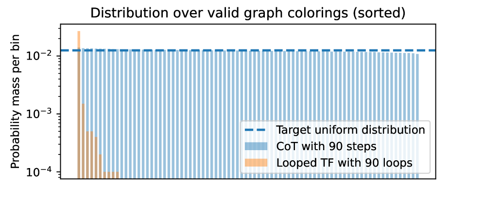
### Visual Description
## Bar Chart: Distribution over valid graph colorings (sorted)
### Overview
The image is a bar chart comparing the probability distributions of two methods for generating valid graph colorings against a target uniform distribution. The chart uses a logarithmic scale on the y-axis to display probability mass per bin. The data is sorted, and the two methods are "CoT with 90 steps" and "Looped TF with 90 loops."
### Components/Axes
* **Title:** "Distribution over valid graph colorings (sorted)"
* **Y-Axis:**
* **Label:** "Probability mass per bin"
* **Scale:** Logarithmic, with major tick marks at 10⁻⁴, 10⁻³, and 10⁻².
* **X-Axis:** Not explicitly labeled. Represents discrete bins for the sorted graph colorings. The axis is categorical, with each bar representing a unique coloring or a group of colorings.
* **Legend:** Located in the bottom-right quadrant of the chart area.
* **Item 1:** A dashed blue line labeled "Target uniform distribution."
* **Item 2:** A light blue bar labeled "CoT with 90 steps."
* **Item 3:** An orange bar labeled "Looped TF with 90 loops."
### Detailed Analysis
The chart displays two distinct data series as vertical bars, plotted against the same set of bins on the x-axis.
1. **Target Uniform Distribution (Dashed Blue Line):**
* **Trend:** A perfectly horizontal line.
* **Value:** Positioned at approximately 1.2 x 10⁻² on the y-axis. This represents the ideal probability mass if every valid graph coloring were equally likely.
2. **CoT with 90 steps (Light Blue Bars):**
* **Trend:** The bars are of nearly uniform height across the entire x-axis. There is very slight variation, but no strong upward or downward slope is visible.
* **Values:** The height of the vast majority of blue bars is very close to the "Target uniform distribution" line, clustering around 10⁻². A few bars on the far right may be marginally shorter, but they remain within the same order of magnitude.
3. **Looped TF with 90 loops (Orange Bars):**
* **Trend:** A sharply decreasing trend from left to right. The distribution is highly skewed.
* **Values:**
* The first (leftmost) orange bar is the tallest, reaching approximately 3 x 10⁻², which is significantly *above* the target uniform line.
* The second bar drops to roughly 1.5 x 10⁻³.
* The third bar is near 5 x 10⁻⁴.
* The fourth and fifth bars are at or below 10⁻⁴.
* No orange bars are visible beyond the fifth bin, indicating their probability mass is negligible (< 10⁻⁴).
### Key Observations
* **Spatial Grounding:** The legend is placed in the bottom-right, overlapping the area where the orange bars diminish to zero. The blue bars span the entire width of the chart, while the orange bars are confined to the first five bins on the far left.
* **Contrast in Performance:** There is a stark contrast between the two methods. "CoT with 90 steps" produces a distribution that closely approximates the target uniform distribution. "Looped TF with 90 loops" produces a highly non-uniform, peaked distribution.
* **Outlier:** The first orange bar is a significant outlier, being the only data point (from either series) that clearly exceeds the target uniform probability.
* **Scale:** The use of a logarithmic y-axis is crucial, as it allows the visualization of the orange series' rapid decay across multiple orders of magnitude, which would be impossible on a linear scale.
### Interpretation
This chart demonstrates a comparative evaluation of two algorithmic approaches—likely "Chain-of-Thought" (CoT) and a "Looped TensorFlow" (TF) method—for the task of sampling valid graph colorings.
* **What the data suggests:** The "CoT with 90 steps" method is highly effective at generating a diverse and uniform set of solutions. Its output distribution is nearly indistinguishable from the ideal uniform distribution, meaning it explores the space of valid colorings evenly. In contrast, the "Looped TF with 90 loops" method is biased. It overwhelmingly favors a very small subset of possible colorings (the first few bins) and fails to explore the vast majority of the solution space.
* **How elements relate:** The dashed "Target" line serves as the benchmark. The proximity of the blue bars to this line indicates success. The deviation of the orange bars, especially the first one overshooting the target and the subsequent rapid drop-off, indicates failure to achieve uniform sampling.
* **Underlying Implication:** For applications requiring exploration of a combinatorial space (like graph colorings), the CoT approach appears superior. The Looped TF method, as configured here, suffers from a mode collapse or a strong prior that prevents it from sampling uniformly. The "sorted" nature of the x-axis likely orders colorings by some metric (e.g., lexicographical order), making the skewed distribution of the Looped TF method even more apparent.
</details>
Figure 7: Performance of Looped TF and CoT. Top: Relative error for counting (left) and sampling (right). Bottom: Empirical distributions for approximate sampling of graph colorings.
Figure 7 shows the results on the approximate counting and approximate sampling tasks. For approximate counting, CoT performs Monte Carlo estimation: the effective number of samples is given by the product of the number of reasoning steps per trial and the number of independent trials. Accordingly, increasing the iteration count corresponds to increasing this total sample budget. For approximate sampling, CoT emulates Markov chain Monte Carlo, where the iteration axis represents the number of Markov chain steps per trial. In contrast, for looped TF on both tasks, the iteration count simply corresponds to the number of loop iterations applied within a single trial. These results support the separation advantages of CoT with stochastic decoding.
## 6 Conclusion
We formally analyze the computational capabilities of chain-of-thought and latent thought reasoning, providing a rigorous comparison that reveals their respective strengths and limitations. Specifically, we show that latent thought enables efficient parallel computation, whereas CoT enables randomized approximate counting. Our theoretical results are further supported by experiments. These insights offer practical guidance for reasoning model design. For future work, an important direction is to investigate whether techniques such as distillation can reduce the number of iterations without compromising computational power. Another promising avenue is to extend our analysis to diffusion language models, which possess both parallelizability and stochasticity. Moreover, extending the analysis to realistic downstream tasks remains an important direction.
## Impact Statement
This paper presents work whose goal is to advance the field of Machine Learning. There are many potential societal consequences of our work, none which we feel must be specifically highlighted here.
## References
- A. V. Aho and J. D. Ullman (1972) Optimization of straight line programs. SIAM Journal on Computing 1 (1), pp. 1–19. Cited by: §3.1.
- A. Apostolico, M. J. Atallah, L. L. Larmore, and S. McFaddin (1990) Efficient parallel algorithms for string editing and related problems. SIAM Journal on Computing. Cited by: §5.1.
- S. Arora and B. Barak (2009) Computational complexity: a modern approach. Cambridge University Press. Cited by: §1.1.
- S. Bae, Y. Kim, R. Bayat, S. Kim, J. Ha, T. Schuster, A. Fisch, H. Harutyunyan, Z. Ji, A. Courville, et al. (2025) Mixture-of-recursions: learning dynamic recursive depths for adaptive token-level computation. arXiv preprint arXiv:2507.10524. Cited by: §1, §4.1.
- D. A. Barrington (1986) Bounded-width polynomial-size branching programs recognize exactly those languages in nc. In ACM symposium on Theory of computing, Cited by: §5.1.
- A. A. Bavandpour, X. Huang, M. Rofin, and M. Hahn (2025) Lower bounds for chain-of-thought reasoning in hard-attention transformers. In Forty-second International Conference on Machine Learning, External Links: Link Cited by: §D.1.2, §D.1.2, §5.1.
- S. R. Buss (1987) The boolean formula value problem is in alogtime. In Proceedings of the nineteenth annual ACM symposium on Theory of computing, pp. 123–131. Cited by: §5.1.
- S. A. Cook (1985) A taxonomy of problems with fast parallel algorithms. Information and control 64 (1-3), pp. 2–22. Cited by: §3.1.
- R. Csordás, K. Irie, J. Schmidhuber, C. Potts, and C. D. Manning (2024) MoEUT: mixture-of-experts universal transformers. In The Thirty-eighth Annual Conference on Neural Information Processing Systems, External Links: Link Cited by: §1, §4.1.
- A. B. de Luca and K. Fountoulakis (2024) Simulation of graph algorithms with looped transformers. In Forty-first International Conference on Machine Learning, External Links: Link Cited by: §2.2.
- M. Dehghani, S. Gouws, O. Vinyals, J. Uszkoreit, and L. Kaiser (2019) Universal transformers. In International Conference on Learning Representations, External Links: Link Cited by: §1.
- Y. Deng, Y. Choi, and S. Shieber (2024) From explicit cot to implicit cot: learning to internalize cot step by step. arXiv preprint arXiv:2405.14838. Cited by: §D.1.2, §5.1.
- P. Erdos and A. Renyi (1959) On random graphs i. Publ. math. debrecen 6 (290-297), pp. 18. Cited by: §D.1.1.
- G. Feng, B. Zhang, Y. Gu, H. Ye, D. He, and L. Wang (2023) Towards revealing the mystery behind chain of thought: a theoretical perspective. Advances in Neural Information Processing Systems 36, pp. 70757–70798. Cited by: §B.2, §D.1.1, §D.1.1, §D.1.2, §1, §2.2, Assumption 3.4, §5.1.
- A. Giannou, S. Rajput, J. Sohn, K. Lee, J. D. Lee, and D. Papailiopoulos (2023) Looped transformers as programmable computers. In International Conference on Machine Learning, pp. 11398–11442. Cited by: §1, §2.2.
- A. Gibbons and W. Rytter (1989) Efficient parallel algorithms. Cambridge University Press. Cited by: §5.1.
- H. A. Gozeten, M. E. Ildiz, X. Zhang, H. Harutyunyan, A. S. Rawat, and S. Oymak (2025) Continuous chain of thought enables parallel exploration and reasoning. arXiv preprint arXiv:2505.23648. Cited by: §1, §2.2, Table 1.
- S. Hao, S. Sukhbaatar, D. Su, X. Li, Z. Hu, J. E. Weston, and Y. Tian (2025) Training large language models to reason in a continuous latent space. In Second Conference on Language Modeling, External Links: Link Cited by: §1, §2.1.
- M. R. Jerrum, L. G. Valiant, and V. V. Vazirani (1986) Random generation of combinatorial structures from a uniform distribution. Theoretical computer science 43, pp. 169–188. Cited by: Proposition C.13, Proposition C.16, Theorem C.19, §1.1, §4.2, §4.3.
- M. Jerrum (1995) A very simple algorithm for estimating the number of k-colorings of a low-degree graph. Random Structures & Algorithms 7 (2), pp. 157–165. Cited by: §D.2.2, §5.1.
- R. M. Karp, M. Luby, and N. Madras (1989) Monte-carlo approximation algorithms for enumeration problems. Journal of algorithms 10 (3), pp. 429–448. Cited by: §4.1, §5.1.
- R. M. Karp and M. Luby (1983) Monte-carlo algorithms for enumeration and reliability problems. In 24th Annual Symposium on Foundations of Computer Science, pp. 56–64. Cited by: §D.2.1, §4.1.
- Z. Li, H. Liu, D. Zhou, and T. Ma (2024) Chain of thought empowers transformers to solve inherently serial problems. In The Twelfth International Conference on Learning Representations, External Links: Link Cited by: §B.1, §B.3.1, §B.7, Definition B.1, Lemma B.10, Definition B.2, Definition B.3, Lemma B.5, Theorem B.9, §1.1, §1, §2.2, Table 1, §3.1, §3.2, §3.3, §3.3, §3.3, Theorem 3.9.
- Y. Liang, Z. Sha, Z. Shi, Z. Song, and Y. Zhou (2024) Looped relu mlps may be all you need as practical programmable computers. arXiv preprint arXiv:2410.09375. Cited by: §B.5.
- W. Merrill, A. Sabharwal, and N. A. Smith (2022) Saturated transformers are constant-depth threshold circuits. Transactions of the Association for Computational Linguistics. Cited by: item 3, §C.1.
- W. Merrill and A. Sabharwal (2023) The parallelism tradeoff: limitations of log-precision transformers. Transactions of the Association for Computational Linguistics 11, pp. 531–545. Cited by: §1.1, §2.2, §3.3, Definition 3.2.
- W. Merrill and A. Sabharwal (2024) The expressive power of transformers with chain of thought. In The Twelfth International Conference on Learning Representations, External Links: Link Cited by: §C.1, §1, §2.2, Definition 2.1.
- W. Merrill and A. Sabharwal (2025a) A little depth goes a long way: the expressive power of log-depth transformers. arXiv preprint arXiv:2503.03961. Cited by: §A.2, §1, §2.2, §5.1, §5.2.
- W. Merrill and A. Sabharwal (2025b) Exact expressive power of transformers with padding. arXiv preprint arXiv:2505.18948. Cited by: §D.1.1, §2.1, §2.2, Table 1.
- M. Mitzenmacher and E. Upfal (2017) Probability and computing: randomization and probabilistic techniques in algorithms and data analysis. Cambridge university press. Cited by: §4.1.
- F. Nowak, A. Svete, A. Butoi, and R. Cotterell (2024) On the representational capacity of neural language models with chain-of-thought reasoning. In Association for Computational Linguistics, External Links: Link Cited by: §C.1, Lemma C.6, §1, §2.2, Table 1, §4.1.
- C. Sanford, B. Fatemi, E. Hall, A. Tsitsulin, M. Kazemi, J. Halcrow, B. Perozzi, and V. Mirrokni (2024a) Understanding transformer reasoning capabilities via graph algorithms. In The Thirty-eighth Annual Conference on Neural Information Processing Systems, External Links: Link Cited by: §D.1.1.
- C. Sanford, D. Hsu, and M. Telgarsky (2024b) Transformers, parallel computation, and logarithmic depth. In Forty-first International Conference on Machine Learning, External Links: Link Cited by: §B.5, §3.1, §5.2.
- N. Saunshi, N. Dikkala, Z. Li, S. Kumar, and S. J. Reddi (2025) Reasoning with latent thoughts: on the power of looped transformers. In The Thirteenth International Conference on Learning Representations, External Links: Link Cited by: §1, §1, §2.2, Table 1, §4.
- C. Schnorr (1976) Optimal algorithms for self-reducible problems. In Proceedings of the Third International Colloquium on Automata, Languages and Programming, Cited by: Definition C.15, Definition 4.1.
- L. Stockmeyer and U. Vishkin (1984) Simulation of parallel random access machines by circuits. SIAM Journal on Computing 13 (2), pp. 409–422. Cited by: §3.3.
- A. Svete and A. Sabharwal (2025) On the reasoning abilities of masked diffusion language models. arXiv preprint arXiv:2510.13117. Cited by: Table 1.
- L. G. Valiant (1979) The complexity of enumeration and reliability problems. siam Journal on Computing 8 (3), pp. 410–421. Cited by: §C.3.
- A. Vaswani, N. Shazeer, N. Parmar, J. Uszkoreit, L. Jones, A. N. Gomez, Ł. Kaiser, and I. Polosukhin (2017) Attention is all you need. Advances in neural information processing systems 30. Cited by: §1, §2.1.
- J. Wei, X. Wang, D. Schuurmans, M. Bosma, F. Xia, E. Chi, Q. V. Le, D. Zhou, et al. (2022) Chain-of-thought prompting elicits reasoning in large language models. Advances in neural information processing systems 35, pp. 24824–24837. Cited by: §1.
- K. Xu and I. Sato (2025) On expressive power of looped transformers: theoretical analysis and enhancement via timestep encoding. In Forty-second International Conference on Machine Learning, External Links: Link Cited by: §D.1.2, §1.
- L. Yang, K. Lee, R. D. Nowak, and D. Papailiopoulos (2024) Looped transformers are better at learning learning algorithms. In The Twelfth International Conference on Learning Representations, External Links: Link Cited by: §2.2.
- H. Zhu, S. Hao, Z. Hu, J. Jiao, S. Russell, and Y. Tian (2025a) Reasoning by superposition: a theoretical perspective on chain of continuous thought. In The Thirty-ninth Annual Conference on Neural Information Processing Systems, External Links: Link Cited by: §1, §2.2, Table 1.
- R. Zhu, Z. Wang, K. Hua, T. Zhang, Z. Li, H. Que, B. Wei, Z. Wen, F. Yin, H. Xing, et al. (2025b) Scaling latent reasoning via looped language models. arXiv preprint arXiv:2510.25741. Cited by: §1.
## Appendix A Formal Definitions
### A.1 Notation
Vectors are written in lowercase bold letters (e.g., ${\bm{x}}$ ) and matrices in uppercase bold letters (e.g., ${\bm{W}}$ ). The $i$ -th entry of a vector ${\bm{x}}$ is ${\bm{x}}_{i}$ , the vector from the $i$ -th to the $j$ -th entry is denoted by ${\bm{x}}_{i:j}$ , and the $(i,j)$ -th entry of a matrix ${\bm{W}}$ is ${\bm{W}}_{i,j}$ . We use the symbol $*$ to denote a “don’t care” value (or block of values). For $n\in\mathbb{N}^{+}$ , let $[n]\coloneq\{1,2,\ldots,n\}$ . We sometimes write column vectors horizontally, e.g., ${\bm{x}}=(x_{1},\ldots,x_{n})$ , for brevity. The Hadamard (element-wise) product is $\odot$ . ${\bm{e}}_{i}\in\{0,1\}^{d}$ is the $i$ -th standard basis vector, ${\bm{1}}_{d}\in\mathbb{R}^{d}$ (or $1_{d}$ ) the all-ones vector, and ${\bm{0}}_{d}\in\mathbb{R}^{d}$ the zero vector. ${\bm{I}}_{d}\in\mathbb{R}^{d\times d}$ denotes the $d\times d$ identity matrix, and $\mathbf{0}_{m\times n}\in\mathbb{R}^{m\times n}$ the $m\times n$ zero matrix. The indicator function is ${\bm{1}}[\cdot]$ , and $\bigoplus$ denotes block-diagonal concatenation. Functions on scalars or vectors are written in upright letters (e.g., $\mathrm{FFN}$ ), while functions on matrices are boldface (e.g., $\mathbf{ATTN}$ ). Boldface is also used when scalar- or vector-level functions are extended to sequence level and applied independently to each token (e.g., $\mathbf{FFN}$ ). Finally, $\mathsf{poly}(n)$ denotes the set of functions growing at most polynomially: $\mathsf{poly}(n)\coloneq\left\{f:\mathbb{N}\to\mathbb{N}\;\middle|\;\exists k\in\mathbb{N},\;\exists c>0,\;\forall n\in\mathbb{N},\;f(n)\leq c\cdot n^{k}\right\}.$
### A.2 Transformer Block
We define the computational components of a Transformer block using the notation of (Merrill and Sabharwal, 2025a). Let $\mathbb{F}_{s}$ denote the set of $s$ -bit floating-point numbers with truncated arithmetic (Definition B.1).
**Definition A.1 (Transformer)**
*A Transformer consists of the following components:
1. A word embedding function $\mathrm{WE}:{\mathcal{V}}\to\mathbb{F}_{s}^{m}$ , where ${\mathcal{V}}$ denotes the vocabulary set.
1. A positional embedding function $\mathrm{PE}:\mathbb{N}\to\mathbb{F}_{s}^{m}$ .
1. A multi-head self-attention layer $\mathbf{SA}:\mathbb{F}_{s}^{m\times N}\to\mathbb{F}_{s}^{m\times N}$ for arbitrary sequence length $N$ , parameterized by a matrix ${\bm{O}}:\mathbb{F}_{s}^{s\times H}\to\mathbb{F}_{s}^{m}$ and, for each head $h\in[H]$ with head size $s$ , matrices ${\bm{Q}}_{h},{\bm{K}}_{h},{\bm{V}}_{h}:\mathbb{F}_{s}^{m}\to\mathbb{F}_{s}^{s}$ . Given an input ${\bm{x}}_{i}\in\mathbb{F}_{s}^{m}$ for each position $i\in[N]$ , it computes the query $\mathbf{q}_{i,h}={\bm{Q}}_{h}{\bm{x}}_{i}$ , key ${\bm{k}}_{i,h}={\bm{K}}_{h}{\bm{x}}_{i}$ , and value $\mathbf{v}_{i,h}={\bm{V}}_{h}{\bm{x}}_{i}$ , and outputs ${\bm{O}}\cdot({\bm{a}}_{i,1},\ldots,{\bm{a}}_{i,H}),$ where each attention output ${\bm{a}}_{i,h}$ is defined, for softmax function, as:
$$
{\bm{a}}_{i,h}=\sum_{j=1}^{c(i)}\frac{\exp(\mathbf{q}_{i,h}^{\top}{\bm{k}}_{j,h})}{Z_{i,h}}\cdot\mathbf{v}_{j,h},\quad Z_{i,h}=\sum_{j=1}^{c(i)}\exp(\mathbf{q}_{i,h}^{\top}{\bm{k}}_{j,h}), \tag{1}
$$
with $c(i)=i$ for causal attention and $c(i)=N$ for full attention. For the saturated hardmax attention (Merrill et al., 2022), each attention output ${\bm{a}}_{i,h}$ is defined as:
$$
{\bm{a}}_{i,h}=\sum_{j\in M_{i,h}}\frac{1}{|M_{i,h}|}\,\mathbf{v}_{j,h},\quad M_{i,h}=\left\{j\in[c(i)]\;\middle|\;\mathbf{q}_{i,h}^{\top}{\bm{k}}_{j,h}=\max_{j^{\prime}}\mathbf{q}_{i,h}^{\top}{\bm{k}}_{j^{\prime},h}\right\}. \tag{2}
$$
1. A feedforward layer $\mathrm{FF}:\mathbb{F}_{s}^{m}\to\mathbb{F}_{s}^{m}$ with parameter ${\bm{W}}_{1}:\mathbb{F}_{s}^{m}\to\mathbb{F}_{s}^{w}$ , ${\bm{W}}_{2}:\mathbb{F}_{s}^{w}\to\mathbb{F}_{s}^{m}$ , and ${\bm{b}}\in\mathbb{F}_{s}^{m}$ , where $w$ is the hidden dimension. Given an input ${\bm{x}}_{i}\in\mathbb{F}_{s}^{m}$ , it outputs ${\bm{W}}_{2}\mathrm{ReLU}({\bm{W}}_{1}{\bm{x}}_{i}+{\bm{b}})$ , where $\mathrm{ReLU}({\bm{x}})=(\max\{0,{\bm{x}}_{1}\},\ldots,\max\{0,{\bm{x}}_{m}\})^{\top}$ .
1. An output function $\mathbf{OUT}:\mathbb{F}_{s}^{m}\to\mathbb{F}_{s}^{|{\mathcal{V}}|}$ , parameterized as a linear transformation.*
### A.3 Chain of Thought
**Definition A.2 (CoT)**
*Let the Transformer be defined as the composition:
$$
\mathrm{TF}_{\mathrm{dec}}\coloneq\mathbf{OUT}\circ(\operatorname{id}+\mathbf{FF}_{L})\circ(\operatorname{id}+\mathbf{SA}_{L})\circ\cdots\circ(\operatorname{id}+\mathbf{FF}_{1})\circ(\operatorname{id}+\mathbf{SA}_{1})\circ(\mathbf{WE}+\mathbf{PE}), \tag{3}
$$
where $\mathbf{SA}_{\ell}$ and $\mathbf{FF}_{\ell}$ denote the causal attention and the feedforward layers at depth $\ell\in[L]$ , respectively, and $\operatorname{id}$ denotes the identity function. The input tokens are first embedded via the word embedding function $\mathbf{WE}$ and the positional encoding $\mathbf{PE}$ , and the final output is produced by a linear projection $\mathbf{OUT}$ . Given an input sequence $x=(x_{1},\dots,x_{n})\in{\mathcal{V}}^{n}$ , we define the initial sequence as: $f_{\mathrm{cot}}^{0}(x)\coloneq x.$ Then, the CoT computes recursively as:
$$
f_{\mathrm{cot}}^{k+1}(x)\coloneq f_{\mathrm{cot}}^{k}(x)\cdot\mathrm{Dec}\,(\mathrm{TF}_{\mathrm{dec}}(f_{\mathrm{cot}}^{k}(x))), \tag{4}
$$
where $\cdot$ denotes concatenation, and $\mathrm{Dec}(\cdot)$ is a decoding function that maps the output logits to a token in ${\mathcal{V}}$ : in the deterministic model, $\mathrm{Dec}(z)\coloneq\arg\max_{i\in[|{\mathcal{V}}|]}z_{i}$ ; in the stochastic model, $\mathrm{Dec}(z)\sim\mathrm{Multinomial}({z_{i}}/{\sum_{j}z_{j}})$ , assuming $z_{i}>0$ for all $i$ . The final output of the CoT model after $T(n)$ steps is defined as the last output length $m$ tokens of $f_{\mathrm{cot}}^{T(n)}(x)$ .*
### A.4 Continuous Thought
**Definition A.3 (Coconut)**
*Let the Transformer block be defined as the composition:
$$
\mathrm{TF}_{\mathrm{dec}}\coloneq(\operatorname{id}+\mathbf{FF}_{L})\circ(\operatorname{id}+\mathbf{SA}_{L})\circ\cdots\circ(\operatorname{id}+\mathbf{FF}_{1})\circ(\operatorname{id}+\mathbf{SA}_{1}), \tag{5}
$$
where $\mathbf{SA}_{\ell}$ and $\mathbf{FF}_{\ell}$ denote the causal attention and the feedforward layers at depth $\ell\in[L]$ , respectively, and $\operatorname{id}$ denotes the identity function. Given an input sequence $x=(x_{1},\dots,x_{n})\in{\mathcal{V}}^{n}$ , we define the initial sequence as: $f_{\mathrm{cot}}^{0}(x)\coloneq\mathbf{WE}(x)+\mathbf{PE}([n]),$ where the input tokens are first embedded via the word embedding function $\mathbf{WE}$ and the positional encoding $\mathbf{PE}$ Then, the continuous thought (Coconut) computes recursively as:
$$
f_{\mathrm{ct}}^{k+1}(x)\coloneq f_{\mathrm{ct}}^{k}(x)\cdot(\mathrm{TF}_{\mathrm{dec}}(f_{\mathrm{cot}}^{k}(x)+\mathbf{PE}(k))), \tag{6}
$$
where $\cdot$ denotes concatenation. The final output of the model after $T(n)$ steps is defined as the last output length $m$ tokens of $\mathrm{Dec}\,\left(\mathbf{OUT}\,\left(f_{\mathrm{ct}}^{T(n)}(x))\right)\right),$ where the final output is produced by a linear projection $\mathbf{OUT}$ and $\mathrm{Dec}(\cdot)$ is a decoding function that maps the output logits to a token in ${\mathcal{V}}$ : in the deterministic model, $\mathrm{Dec}(z)\coloneq\arg\max_{i\in[|{\mathcal{V}}|]}z_{i}$ ; in the stochastic model, $\mathrm{Dec}(z)\sim\mathrm{Multinomial}({z_{i}}/{\sum_{j}z_{j}})$ , assuming $z_{i}>0$ for all $i$ .*
### A.5 Looped Transformer
**Definition A.4 (Looped TF)**
*Let the Transformer block be defined as the composition:
$$
\mathrm{TF}\coloneq(\operatorname{id}+\mathbf{FF}_{L})\circ(\operatorname{id}+\mathbf{SA}_{L})\circ\cdots\circ(\operatorname{id}+\mathbf{FF}_{1})\circ(\operatorname{id}+\mathbf{SA}_{1}), \tag{7}
$$
where $\mathbf{SA}_{\ell}$ and $\mathbf{FF}_{\ell}$ denote the (non-causal) self-attention and feedforward layers at depth $\ell\in[L]$ . Given an input token sequence $x=(x_{1},\dots,x_{n})\in{\mathcal{V}}^{n}$ , the initial hidden state is: $f_{\mathrm{loop}}^{0}(x)\coloneq\mathbf{WE}(x).$ At each loop iteration $k$ , the hidden state is updated by:
$$
f_{\mathrm{loop}}^{k+1}(x)\coloneq\mathrm{TF}\left(f_{\mathrm{loop}}^{k}(x)\right). \tag{8}
$$
The final outputs after $T(n)$ loop iterations are decoded as $\mathrm{Dec}\circ\mathbf{OUT}\circ f_{\mathrm{loop}}^{T(n)}(x),$ and the model’s prediction is defined as the last output length $m\leq n$ tokens of this projected sequence.*
<details>
<summary>x11.png Details</summary>
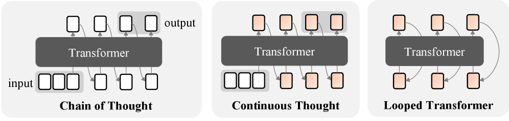
### Visual Description
## Diagram: Transformer Architecture Variants
### Overview
The image displays three schematic diagrams illustrating different architectural approaches for processing sequences with a Transformer model. Each diagram is presented in a separate panel with a light gray background, arranged horizontally from left to right. The diagrams compare "Chain of Thought," "Continuous Thought," and "Looped Transformer" methods.
### Components/Axes
* **Common Elements:** Each panel contains a central dark gray rectangular block labeled "Transformer" in white text. Below this block is a sequence of squares representing the "input," and above it is a sequence representing the "output." Arrows indicate the flow of information.
* **Color Coding:** Squares are either white or a light orange/peach color. The color appears to denote the state or type of token (e.g., initial input vs. generated or continuous thought).
* **Panel-Specific Labels:** The title for each architecture is printed in bold black text below its respective diagram.
### Detailed Analysis
**1. Left Panel: Chain of Thought**
* **Title:** "Chain of Thought"
* **Input Sequence:** Four white squares in a row, labeled "input" to the left.
* **Transformer Block:** Central dark gray rectangle.
* **Output Sequence:** Four white squares in a row, labeled "output" to the right.
* **Flow/Connections:**
* Arrows point from each input square up into the Transformer block.
* Arrows point from the Transformer block down to each output square.
* **Key Feature:** Curved arrows connect each output square to the next one in the sequence (output token `n` points to output token `n+1`), indicating a sequential, step-by-step reasoning process where each thought depends on the previous one.
**2. Middle Panel: Continuous Thought**
* **Title:** "Continuous Thought"
* **Input Sequence:** A mixed sequence of three white squares followed by three light orange squares.
* **Transformer Block:** Central dark gray rectangle.
* **Output Sequence:** A row of four light orange squares.
* **Flow/Connections:**
* Arrows point from all input squares (both white and orange) up into the Transformer block.
* Arrows point from the Transformer block down to all output squares.
* **Key Feature:** Curved arrows connect each output square back to the *input* sequence, specifically to the light orange squares within it. This suggests a process where generated "thoughts" (orange) are fed back into the input stream for continuous refinement, blending input and generated content.
**3. Right Panel: Looped Transformer**
* **Title:** "Looped Transformer"
* **Input Sequence:** Three light orange squares.
* **Transformer Block:** Central dark gray rectangle.
* **Output Sequence:** Three light orange squares.
* **Flow/Connections:**
* Arrows point from each input square up into the Transformer block.
* Arrows point from the Transformer block down to each output square.
* **Key Feature:** A large, prominent curved arrow connects the entire output sequence back to the entire input sequence. This represents a recurrent or iterative loop where the model's output is fed back as its input for multiple processing passes, allowing for deep, recursive computation on the same set of tokens.
### Key Observations
1. **Progression of Complexity:** The diagrams show an evolution from a simple, feed-forward sequential process (Chain of Thought) to more complex, recurrent architectures (Continuous Thought, Looped Transformer).
2. **Color Semantics:** White squares likely represent original, discrete input tokens. Light orange squares represent generated tokens, "thoughts," or a continuous representation that is fed back into the system.
3. **Information Flow:** The primary differentiator between the models is the feedback mechanism:
* **Chain of Thought:** Output-to-output (sequential dependency).
* **Continuous Thought:** Output-to-input (integration of generated thoughts with the input stream).
* **Looped Transformer:** Output-to-input as a full loop (iterative refinement of the entire state).
4. **Absence of Numerical Data:** This is a conceptual diagram illustrating architectural patterns, not a chart with quantitative data points or trends.
### Interpretation
This diagram visually contrasts three paradigms for enabling complex reasoning in Transformer models.
* **Chain of Thought** mimics human step-by-step reasoning, where each conclusion builds linearly on the last. It's effective for tasks with a clear procedural logic.
* **Continuous Thought** suggests a more fluid cognitive process, where generated ideas are immediately mixed with incoming information, allowing for dynamic context updating and potentially more flexible reasoning.
* **Looped Transformer** represents a powerful but computationally intensive approach, akin to "thinking deeply" or repeatedly deliberating on the same problem. This could allow the model to converge on a solution through iterative refinement, useful for tasks requiring search, optimization, or profound analysis.
The progression implies a research direction aimed at moving beyond single-pass inference. The architectures seek to imbue models with internal states that evolve over multiple steps (temporal depth), either sequentially, continuously, or recursively, to solve problems that require more than immediate pattern recognition. The choice of architecture involves a trade-off between computational cost, reasoning depth, and the nature of the task (procedural vs. deliberative).
</details>
Figure 8: The models of reasoning paradigms based on iterative use of Transformer models.
## Appendix B Deferred Proofs for Section 3
### B.1 Precision Modeling
We focus on signed floating-point numbers, following (Li et al., 2024), but omit exponents for simplicity.
**Definition B.1 (Floating-point Representation, cf.(Liet al.,2024))**
*Consider floating-point numbers with a mantissa part of $s$ bits and a sign bit of 1, totaling $(s+1)$ bits. We denote the set of such floating-point numbers by $\mathbb{F}_{s}$ , and define $B_{s}\triangleq\max\mathbb{F}_{s}.$*
**Definition B.2 (Correct Rounding, cf.(Liet al.,2024))**
*For any $x\in\mathbb{R}$ and any closed subset $\mathbb{F}\subset\mathbb{R}$ containing $0$ , we define the correct rounding $\operatorname{round}(x,\mathbb{F})$ as the number in $\mathbb{F}$ closest to $x$ . In particular, rounding to a floating-point number with mantissa part $s$ bits is denoted by $[\cdot]_{s}$ . Rounding applied to vectors is to be operated coordinate-wise.*
They also define primitive arithmetic under finite precision by applying rounding after each basic operation. In particular, for multi-operand operations, rounding is applied after each binary operation. Finite-precision summation over more than two numbers is thus defined as follows.
**Definition B.3 (Summation with Iterative Rounding(Liet al.,2024))**
*For any $s,n\in\mathbb{N}^{+}$ and vector ${\bm{x}}\in\mathbb{R}^{n}$ , define the summation with iterative rounding to $s$ -bit precision
$$
\mathrm{sum}_{s}:\ \bigcup_{n\in\mathbb{N}^{+}}(\mathbb{F}_{s})^{n}\to\mathbb{F}_{s}, \tag{9}
$$
where, for any $n\in\mathbb{N}^{+}$ and ${\bm{x}}=(x_{1},\dots,x_{n})\in\mathbb{R}^{n}$ ,
$$
\mathrm{sum}_{s}(x)\coloneqq\Bigl[\;\Bigl[\;\cdots\Bigl[\,[x_{1}+x_{2}]_{s}+x_{3}\Bigr]_{s}+\cdots+x_{n-1}\Bigr]_{s}+x_{n}\;\Bigr]_{s}. \tag{10}
$$*
Based on this definition, all computations in the Transformer block of Definition A.1 can be represented in finite precision. The inner product and the matrix product are defined as
$$
{\bm{x}}^{\top}{\bm{y}}\coloneqq\operatorname{sum}_{s}({\bm{x}}\odot{\bm{y}}),\qquad({\bm{A}}{\bm{B}})_{i,j}\coloneqq{\bm{A}}_{i,:}^{\top}{\bm{B}}_{:,j}. \tag{11}
$$
Throughout this section, we interpret all operations as finite-precision computations as defined above.
### B.2 Definition of Assumption 3.4
Our definition of polynomially efficient approximation follows that of Feng et al. (2023), but differs in scope: while their framework targets real-valued functions, ours applies to symbolic functions.
**Definition B.4 (Polynomially-efficient approximation)**
*We say that a function $f_{n}:\Sigma^{\ell(n)}\to\Sigma$ admits a polynomially efficient approximation if, for a sufficiently small error tolerance $0<\delta\leq\tfrac{1}{3}$ , there exists a feedforward network $\mathrm{FF}:\mathbb{F}_{s(n)}^{\ell(n)\cdot|\Sigma|}\to\mathbb{F}_{s(n)}^{|\Sigma|},\ s(n)=O(\log n),$ such that the following holds: for every input ${\bm{x}}=(x_{1},\ldots,x_{\ell(n)})\in\Sigma^{\ell(n)}$ ,
$$
\mathrm{FF}(\bm{e}(x_{1}),\ldots,\bm{e}(x_{\ell(n)}))_{i}\;=\;\begin{cases}\;\geq 1-\delta&\text{if}\quad\bm{e}(f_{n}({\bm{x}}))={\bm{e}}_{i},\\
\;\leq\delta&\text{else },\end{cases} \tag{12}
$$
where $\bm{e}:\Sigma\to\{0,1\}^{|\Sigma|}$ denote the one-hot encoding. Moreover, the number of parameters of the feedforward network is bounded by a polynomial in $\ell(n)$ and $1/\delta$ .*
### B.3 Technical lemmas
In this section, we provide the key components for our constructive proofs.
#### B.3.1 Orthogonal Vectors
We follow the notation of (Li et al., 2024). For any positive integer $s\in\mathbb{N}^{+}$ and $x\in\{0,1,\dots,2^{s}-1\}$ , we denote by $\mathsf{bin}_{s}(x)\in\{0,1\}^{s}$ the standard binary representation of $x$ using $s$ bits, defined such that $x=\sum_{i=1}^{s}2^{i}\cdot(\mathsf{bin}_{s}(x))_{i}.$ We further define the signed binary encoding of $x$ , denoted by $\mathsf{sbin}_{s}(x)\in\{-1,1\}^{s}$ , as $\mathsf{sbin}_{s}(x)=2\cdot\mathsf{bin}_{s}(x)-(1,\ldots,1).$ Let ${\bm{x}},{\bm{y}}\in\mathbb{R}^{s}$ be two vectors of the same length. We define their interleaving, denoted by ${{\bm{x}}}^{\frown}{{\bm{y}}}\in\mathbb{R}^{2s}$ , as follows: $({{\bm{x}}}^{\frown}{{\bm{y}}})_{2i-1}=x_{i},({{\bm{x}}}^{\frown}{{\bm{y}}})_{2i}={\bm{y}}_{i}$ for all $i\in[s].$ The orthogonal vectors under finite-precision arithmetic can be:
**Lemma B.5 (Liet al.,2024)**
*For any $s\in\mathbb{N}^{+}$ , let ${\bm{q}}_{i}={\mathsf{sbin}_{s}(i)}^{\frown}{1_{s}}$ and ${\bm{k}}_{i}=2^{s+1}\cdot({\mathsf{sbin}_{s}(i)}^{\frown}{(-1_{s})})$ for all $i\in[2^{s}-1]$ , it holds that $\left\langle{\bm{q}}_{i},{\bm{k}}_{j}\right\rangle_{s}=-B_{s}$ if $i\neq j$ and $\left\langle{\bm{q}}_{i},{\bm{k}}_{j}\right\rangle_{s}=0$ if $i=j$ . Since $\bigl[\exp(-B_{s})\bigr]_{s}\leq\bigl[2^{-s-1}]_{s}=0$ , it follows that $\left[\exp(\left\langle{\bm{q}}_{i},{\bm{k}}_{j}\right\rangle_{s})\right]_{s}=\mathbf{1}[i=j]$ for all $i,j\in[2^{s}-1]$ .*
#### B.3.2 Position Selector
**Lemma B.6**
*For any $m\in\mathbb{N}^{+}$ and ${\bm{x}}\in\mathbb{F}_{s}^{m}$ with $x_{i}>0$ for all $i\in[m]$ , there exists a feedforward layer $\mathrm{FF}:\mathbb{F}_{s}^{2m}\to\mathbb{F}_{s}^{2m}$ , for any $i\in[m]$ , such that
$$
(\operatorname{id}+\mathrm{FF})(({\bm{x}},{\bm{e}}_{i}))=({\bm{x}}\odot{\bm{e}}_{i},{\bm{e}}_{i})\,. \tag{13}
$$*
* Proof*
Let the input be ${\bm{z}}=({\bm{x}},{\bm{e}}_{i})\in\mathbb{F}_{s}^{2m}$ . Set the weight ${\bm{W}}_{1}\in\mathbb{F}_{s}^{m\times 2m}$ and bias ${\bm{b}}\in\\ mathbb{F}_{s}^{m}$ by
$$
{\bm{W}}_{1}=\bigl[\,{\bm{I}}_{m}\;\;\;-B_{s}{\bm{I}}_{m}\,\bigr],\qquad{\bm{b}}={\bm{0}}, \tag{14}
$$
to have ${\bm{W}}_{1}{\bm{z}}+{\bm{b}}={\bm{x}}-B_{s}{\bm{e}}_{i}.$ Applying the ReLU activation coordinate-wise gives
$$
\mathrm{ReLU}({\bm{x}}-B_{s}{\bm{e}}_{i})_{j}=\begin{cases}0,&j=i,\\
x_{j},&j\neq i.\end{cases} \tag{15}
$$
Hence,
$$
{\bm{h}}\coloneqq\mathrm{ReLU}({\bm{W}}_{1}{\bm{z}}+{\bm{b}})={\bm{x}}\odot({\bm{1}}-{\bm{e}}_{i}). \tag{16}
$$ Next, set the second linear layer ${\bm{W}}_{2}\in\mathbb{F}_{s}^{2m\times m}$ by
$$
{\bm{W}}_{2}=\begin{bmatrix}-{\bm{I}}_{m}\\
\mathbf{0}_{m\times m}\end{bmatrix}. \tag{17}
$$
Thus we have
$$
{\bm{z}}+{\bm{W}}_{2}{\bm{h}}=\begin{bmatrix}{\bm{x}}\\
{\bm{e}}_{i}\end{bmatrix}+\begin{bmatrix}-{\bm{h}}\\
{\bm{0}}\end{bmatrix}=\begin{bmatrix}{\bm{x}}\\
{\bm{e}}_{i}\end{bmatrix}+\begin{bmatrix}-{\bm{x}}\odot({\bm{1}}-{\bm{e}}_{i})\\
{\bm{0}}\end{bmatrix}=\begin{bmatrix}{\bm{x}}\odot{\bm{e}}_{i}\\
{\bm{e}}_{i}\end{bmatrix}. \tag{18}
$$
∎
#### B.3.3 Feedforward layers
**Lemma B.7**
*Let $N\in\mathbb{N}^{+}$ . For each $i\in[N]$ , let $f_{i}:\Sigma^{\ell_{i}}\to\Sigma$ admit polynomially-efficient approximation by $\mathrm{FF}_{i}$ . Then there exists a feedforward layer $\mathrm{FF}:\ \mathbb{F}_{s}^{\sum_{i=1}^{N}\ell_{i}|\Sigma|}\to\mathbb{F}_{s}^{N|\Sigma|}$ such that for every input tuple ${\bm{x}}_{i}=(x^{(i)}_{1},\ldots,x^{(i)}_{\ell_{i}})\in\Sigma^{\ell_{i}}$ ,
$$
\mathrm{FF}\!\left(\big\|_{i=1}^{N}\,(\bm{e}(x^{(i)}_{1}),\ldots,\bm{e}(x^{(i)}_{\ell_{i}}))\right)\;=\;\big\|_{i=1}^{N}\,\mathrm{FF}_{i}({\bm{x}}_{i}), \tag{19}
$$
where $\|$ denotes concatenation.*
* Proof*
For each $i\in[N]$ , by Definition B.4, there exist width $w_{i}\in\mathbb{N}$ and parameters
$$
{\bm{W}}^{(i)}_{1}\in\mathbb{F}_{s}^{w_{i}\times\ell_{i}|\Sigma|},\quad{\bm{W}}^{(i)}_{2}\in\mathbb{F}_{s}^{|\Sigma|\times w_{i}},\quad{\bm{b}}^{(i)}\in\mathbb{F}_{s}^{w_{i}} \tag{20}
$$
such that $\mathrm{FF}_{i}({\bm{x}}_{i})={\bm{W}}^{(i)}_{2}\mathrm{ReLU}({\bm{W}}^{(i)}_{1}\,\bm{e}({\bm{x}}_{i})+{\bm{b}}^{(i)}).$ Now, define block-diagonal matrices
$$
{\bm{W}}_{1}\coloneqq\bigoplus_{i=1}^{N}{\bm{W}}^{(i)}_{1},\qquad{\bm{W}}_{2}\coloneqq\bigoplus_{i=1}^{N}{\bm{W}}^{(i)}_{2},\qquad{\bm{b}}\coloneqq\bigoplus_{i=1}^{N}{\bm{b}}^{(i)}. \tag{21}
$$
Then the single feedforward layer
$$
\mathrm{FF}({\bm{x}})\coloneqq{\bm{W}}_{2}\mathrm{ReLU}({\bm{W}}_{1}{\bm{x}}+{\bm{b}}) \tag{22}
$$
applies each block independently to its corresponding input, yielding exactly $\mathrm{FF}({\bm{x}})=\big\|_{i=1}^{N}\mathrm{FF}_{i}({\bm{x}}_{i}).$ ∎
**Lemma B.8**
*Let $f:\Sigma^{\ell}\to\Sigma$ be a function that admits polynomially-efficient approximation (Definition B.4). Then, there exist two feedforward layers
$$
\mathrm{FF}_{1}:\mathbb{F}_{s}^{(1+\ell)|\Sigma|+1}\to\mathbb{F}_{s}^{(1+\ell)|\Sigma|+1},\quad\mathrm{FF}_{2}:\mathbb{F}_{s}^{(1+\ell)|\Sigma|+1}\to\mathbb{F}_{s}^{(1+\ell)|\Sigma|+1}, \tag{23}
$$
such that, for every ${\bm{x}}=(x_{1},\ldots,x_{\ell})\in\Sigma^{\ell}$ and $t\in\{0,1\}$ ,
$$
(\operatorname{id}+\mathrm{FF}_{2})\circ(\operatorname{id}+\mathrm{FF}_{1})\big({\bm{0}},\ \bm{e}(x_{1}),\ldots,\bm{e}(x_{\ell}),\ t\big)\;=\;(t\cdot\bm{e}(f({\bm{x}})),\ \bm{e}(x_{1}),\ldots,\bm{e}(x_{\ell}),\ t). \tag{24}
$$*
* Proof*
Let $n\coloneqq|\Sigma|$ and $L\coloneqq\ell n$ . Write ${\bm{u}}=(\bm{e}(x_{1}),\ldots,\bm{e}(x_{\ell}))\in\{0,1\}^{L}$ . By Definition B.4, there exist $w_{f}\in\mathbb{N}$ , matrices ${\bm{W}}^{(f)}_{1}\in\mathbb{F}_{s}^{w_{f}\times L}$ , ${\bm{W}}^{(f)}_{2}\in\mathbb{F}_{s}^{n\times w_{f}}$ , and bias ${\bm{b}}^{(f)}\in\mathbb{F}_{s}^{w_{f}}$ such that
$$
\mathrm{FF}_{f}({\bm{u}})\coloneqq{\bm{W}}^{(f)}_{2}\,\mathrm{ReLU}({\bm{W}}^{(f)}_{1}{\bm{u}}+{\bm{b}}^{(f)}),\quad\mathrm{FF}_{f}({\bm{u}})_{i}=\begin{cases}\geq 1-\delta&\text{if }\ \bm{e}(f({\bm{x}}))={\bm{e}}_{i},\\
\leq\delta&\text{otherwise}.\end{cases} \tag{25}
$$ Set the first layer as
$$
{\bm{W}}^{(1)}_{1}=\begin{bmatrix}{\bm{0}}&{\bm{W}}^{(f)}_{1}&\mathbf{0}_{\,w_{f}\times 1}\\
{\bm{0}}&{\bm{I}}_{L}&\mathbf{0}_{\,L\times 1}\end{bmatrix},\quad{\bm{b}}^{(1)}=\begin{bmatrix}{\bm{b}}^{(f)}\\
{\bm{0}}_{L}\end{bmatrix},\quad{\bm{W}}^{(1)}_{2}=\begin{bmatrix}{\bm{W}}^{(f)}_{2}&\,{\bm{0}}\\
\mathbf{0}_{\,L\times w_{f}}&\,{\bm{0}}\\
\mathbf{0}_{\,1\times w_{f}}&{\bm{0}}\end{bmatrix}, \tag{1}
$$
and define $\mathrm{FF}_{1}({\bm{0}},{\bm{u}},t)\coloneqq{\bm{W}}^{(1)}_{2}\,\mathrm{ReLU}\big({\bm{W}}^{(1)}_{1}({\bm{0}},{\bm{u}},t)+{\bm{b}}^{(1)}\big)$ . Then, it holds that
$$
\displaystyle\mathrm{FF}_{1}({\bm{0}},{\bm{u}},t) \displaystyle={\bm{W}}^{(1)}_{2}\,\mathrm{ReLU}\left(\begin{bmatrix}{\bm{W}}^{(f)}_{1}{\bm{u}}+{\bm{b}}^{(f)}\\
{\bm{u}}\end{bmatrix}\right) \displaystyle=\begin{bmatrix}{\bm{W}}^{(f)}_{2}\mathrm{ReLU}({\bm{W}}^{(f)}_{1}{\bm{u}}+{\bm{b}}^{(f)})\\
{\bm{0}}\end{bmatrix} \displaystyle=\begin{bmatrix}\mathrm{FF}_{f}({\bm{u}})\\
{\bm{0}}\end{bmatrix}. \tag{1}
$$
Thus we have $(\operatorname{id}+\mathrm{FF}_{1})({\bm{0}},{\bm{u}},t)=\bigl(\mathrm{FF}_{f}({\bm{u}}),\,{\bm{u}},\,t\bigr).$ For the second layer, choose $\delta\leq\tfrac{1}{3}$ and $M\geq 1$ and set
$$
{\bm{W}}^{(2)}_{1}=\begin{bmatrix}2{\bm{I}}_{n}&\mathbf{0}_{n\times L}&M{\bm{1}}_{n}\\
2{\bm{I}}_{n}&\mathbf{0}_{n\times L}&M{\bm{1}}_{n}\\
{\bm{I}}_{n}&\mathbf{0}_{n\times L}&\mathbf{0}_{n\times 1}\\
-{\bm{I}}_{n}&\mathbf{0}_{n\times L}&\mathbf{0}_{n\times 1}\end{bmatrix},\ {\bm{b}}^{(2)}=\begin{bmatrix}-M{\bm{1}}_{n}\\
(1-M){\bm{1}}_{n}\\
{\bm{0}}_{n}\\
{\bm{0}}_{n}\end{bmatrix},\ {\bm{W}}^{(2)}_{2}=\begin{bmatrix}\ {\bm{I}}_{n}&-{\bm{I}}_{n}&-{\bm{I}}_{n}&\ {\bm{I}}_{n}\ \\
\ \mathbf{0}_{\,L\times n}&\mathbf{0}_{\,L\times n}&\mathbf{0}_{\,L\times n}&\mathbf{0}_{\,L\times n}\\
\ \mathbf{0}_{\,1\times n}&\mathbf{0}_{\,1\times n}&\mathbf{0}_{\,1\times n}&\mathbf{0}_{\,1\times n}\end{bmatrix}. \tag{2}
$$
and define $\mathrm{FF}_{2}({\bm{y}})\coloneqq{\bm{W}}^{(2)}_{2}\,\mathrm{ReLU}\big({\bm{W}}^{(2)}_{1}{\bm{y}}+{\bm{b}}^{(2)}\big)$ . Then it holds that, for ${\bm{z}}\coloneqq\mathrm{FF}_{f}({\bm{u}})$ ,
$$
\displaystyle\mathrm{FF}_{2}({\bm{z}},{\bm{u}},t) \displaystyle={\bm{W}}^{(2)}_{2}\,\begin{bmatrix}\mathrm{ReLU}\bigl(2{\bm{z}}+Mt{\bm{1}}_{n}-M{\bm{1}}_{n}\bigr)\\
\mathrm{ReLU}\bigl(2{\bm{z}}+Mt{\bm{1}}_{n}+(1-M){\bm{1}}_{n}\bigr)\\
\mathrm{ReLU}({\bm{z}})\\
\mathrm{ReLU}(-{\bm{z}})\end{bmatrix} \displaystyle={\bm{W}}^{(2)}_{2}\,\begin{bmatrix}\mathrm{ReLU}\bigl(2{\bm{z}}+M(t-1){\bm{1}}_{n}\bigr)\\
\mathrm{ReLU}\bigl(2{\bm{z}}+1+M(t-1){\bm{1}}_{n}\bigr)\\
{\bm{z}}\\
{\bm{0}}\end{bmatrix} \displaystyle=\begin{bmatrix}\mathrm{ReLU}\bigl({\bm{z}}-\delta+M(t-1)\bigr)-\mathrm{ReLU}\bigl({\bm{z}}-1+M(t-1)\bigr)-{\bm{z}}\\
\mathbf{0}\\
0\end{bmatrix}, \tag{2}
$$
where it satisfies that
$$
\mathrm{ReLU}\bigl({\bm{z}}-\delta+M(t-1)\bigr)-\mathrm{ReLU}\bigl({\bm{z}}-\delta-1+M(t-1)\bigr)\;=\;\begin{cases}\;\bm{e}(f({\bm{x}}))&\text{if}\quad t=1,\\
\;{\bm{0}}&\text{if}\quad t=0.\end{cases} \tag{34}
$$ Therefore, the composition satisfies $(\operatorname{id}+\mathrm{FF}_{2})\circ(\operatorname{id}+\mathrm{FF}_{1})\bigl({\bm{0}},{\bm{u}},t\bigr)=(t\cdot\bm{e}(f({\bm{x}})),\ {\bm{u}},\ t).$ ∎
### B.4 Proof for Theorem 3.5
* Proof*
Let $G_{n}=(V_{n},E_{n})$ be a computation graph, where $\mathcal{F}=\{f_{1},f_{2},\dots,f_{|\mathcal{F}|}\}$ . Each node $v\in V_{n}$ is labeled by a one-hot vector $\bm{e}(v)\in\{0,1\}^{|\mathcal{F}|}$ indicating the function assigned to $v$ from the finite set $\mathcal{F}$ . Let $v_{1},v_{2},\dots,v_{|V_{n}|}$ denote a fixed topological ordering of $V_{n}$ , with inputs appearing first and outputs last. For each function $f_{i}\in\mathcal{F}$ , let $C_{f_{i}}(n)\coloneqq\max\{\,|\mathrm{pred}(v)|:v\in V_{n},\;\bm{e}(v)={\bm{e}}_{i}\,\}.$ and define $C_{\mathrm{sum}}(n)\coloneqq\sum_{f\in\mathcal{F}}C_{f}(n),\ C_{\mathrm{max}}(n)\coloneqq\max_{f\in\mathcal{F}}C_{f}(n).$ Let the precision be $s(n)=C\cdot\lceil\log_{2}n\rceil$ where $C\in\mathbb{N}$ is a sufficiently large integer such that $2^{s(n)}\;\geq\;n^{C}$ exceeds the maximum polynomial step bound under consideration. We denote by $\mathrm{pred}(v_{i})\in\mathbb{F}_{s(n)}^{C_{\max}(n)}$ the vector of predecessor indices of node $v_{i}$ ; that is, if $v_{i}$ has $d\leq C_{\max}(n)$ incoming edges from nodes $v_{j_{1}},\dots,v_{j_{d}}$ , then $\mathrm{pred}(v_{i})=(j_{1},\dots,j_{d},{\bm{0}})$ , where zeros are used for padding so that the length is exactly $C_{\max}(n)$ . Let the vocabulary be ${\mathcal{V}}=\Sigma$ . At decoding step $k$ , the model has access to the concatenated sequence
$$
(x_{1},x_{2},\ldots,x_{n},\,y_{1},y_{2},\ldots,y_{k})\in\Sigma^{n+k}, \tag{35}
$$
where $x=(x_{1},\ldots,x_{n})\in\Sigma^{n}$ denotes the input, and $y_{i}$ is the token generated at the $i$ -th CoT step. For each node $v_{j}$ , let $v_{j}(x)$ denote its value on input $x$ . We assume that every intermediate output satisfies $y_{i}=v_{n+i}(x).$ Under this assumption, we prove by induction that the model generates the next token correctly, i.e., $y_{k+1}=v_{n+k+1}(x).$
Embedding
The embedding at position $i\in[n+k]$ , denoted by ${\bm{h}}^{(0)}_{i}\in\mathbb{F}_{s(n)}^{m}$ , where $m\coloneq|\Sigma|+|\mathcal{F}|+(1+C_{\mathrm{max}}(n))s(n)+|\Sigma|C_{\mathrm{sum}}(n)$ is defined as
$$
{\bm{h}}^{(0)}_{i}=\left(\bm{e}(v_{i}(x)),\,\bm{e}(v_{i+1}),\,\mathsf{sbin}_{s(n)}(i),\,\bm{\mathrm{sbinpred}}_{s(n)}(v_{i+1}),\,{\bm{0}}_{|\Sigma|C_{\mathrm{sum}}(n)}\right), \tag{0}
$$
where $\bm{e}\colon\Sigma\to\{0,1\}^{|\Sigma|}$ denote the one-hot encoding of the symbol and, $\bm{\mathrm{sbinpred}}_{s(n)}(v)\in\mathbb{F}^{C_{\mathrm{max}}(n)\cdot s(n)}_{s(n)}$ encodes the binary representations of the predecessor indices:
$$
\bm{\mathrm{sbinpred}}_{s(n)}(v_{i})\coloneq\left(\mathsf{sbin}_{s(n)}(\mathrm{pred}(v_{i})_{0}),\,\ldots,\,\mathsf{sbin}_{s(n)}(\mathrm{pred}(v_{i})_{C_{\mathrm{max}}(n)})\right). \tag{37}
$$
This embedding is constructed, for $z\in\Sigma$ , as
$$
\mathbf{WE}(z)=\left(\bm{e}(z),\,{\bm{0}}\right),\quad\mathbf{PE}(i)=\left({\bm{0}},\,\bm{e}(v_{i+1}),\,\mathsf{sbin}_{s(n)}(i),\,\bm{\mathrm{sbinpred}}_{s(n)}(v_{i+1}),\,\mathbf{0}\right). \tag{38}
$$
Attention layer
The first attention layer consists of $C_{\mathrm{max}(n)}$ heads. The $h$ -th head is configured to attend to the position corresponding to the $h$ -th predecessor. Specifically, for each position $i$ and head $h\in[C_{\mathrm{max}(n)}]$ , the attention vectors are defined as:
$$
\displaystyle{\bm{q}}_{i,h} \displaystyle={\mathsf{sbin}_{s(n)}(\mathrm{pred}(v_{i+1})_{h})}^{\frown}{1_{s(n)}}, \displaystyle{\bm{k}}_{i,h} \displaystyle=2^{s(n)+1}\cdot{\mathsf{sbin}_{s(n)}(i)}^{\frown}{(-1_{s(n)})}, \displaystyle\mathbf{v}_{i,h} \displaystyle=\bm{e}(v_{i}(x)), \tag{39}
$$
where vectors of different lengths are zero-padded to match the dimension. By Lemma B.5, each attention head of the last position $i=n+k$ retrieves the predecessor’s value of $v_{n+k}$
$$
{\bm{a}}_{n+k,h}=\bm{e}\bigl(v_{\mathrm{pred}(v_{n+k+1})_{h}}(x)\bigr) \tag{42}
$$
With an appropriate output projection ${\bm{O}}$ such that
$$
{\bm{O}}({\bm{a}}_{i,1},\ldots,{\bm{a}}_{i,H})=({\bm{0}},\,\bm{e}(v_{\mathrm{pred}(v_{n+k+1})_{0}}(x)),\,\ldots,\,\bm{e}(v_{\mathrm{pred}(v_{n+k+1})_{C_{\mathrm{max}(n)}}}(x)),\,{\bm{0}}), \tag{43}
$$
the hidden state at position $n+k$ after the attention layer is given by
$$
\displaystyle{\bm{h}}^{(0.5)}_{n+k}=\Big(\bm{e}(v_{n+k}(x)),\,\bm{e}(v_{n+k+1}),\,\mathsf{sbin}_{s(n)}(n+k),\,\bm{\mathrm{sbinpred}}_{s(n)}(v_{n+k+1}),\, \displaystyle\underbrace{\bm{e}(v_{\mathrm{pred}(v_{n+k+1})_{0}}(x)),\,\ldots,\,\bm{e}(v_{\mathrm{pred}(v_{n+k+1})_{C_{\mathrm{max}(n)}}}(x))}_{\text{updated}}\,,{\bm{0}}_{C_{\mathrm{sum}}(n)|\Sigma|}\Big). \tag{44}
$$
The second and third attention layers are disabled (i.e., all attention weights are set to zero).
Feed-forward layer
By Lemma B.7, a single feed-forward layer can approximate multiple functions by partitioning the input into blocks. The first feed-forward layer then places the arguments, gathered by attention, into the correct positions. By Lemma B.6, where the vector ${\bm{e}}_{i}$ therein corresponds to ${\bm{1}}_{|\Sigma|}$ here, the hidden state at the last position, denoted by ${\bm{h}}^{(1)}_{n+k}$ , becomes
$$
\displaystyle\Big(({\bm{h}}^{(0.5)}_{n+k})_{1:r},\big\|_{j=1}^{|\mathcal{F}|}\,\big(\bm{e}(v_{\mathrm{pred}(v_{n+k+1})_{1}}(x))\cdot 1,\ldots,\bm{e}(v_{\mathrm{pred}(v_{n+k+1})_{C_{j}(n)}}(x))\cdot 1\Big), \tag{46}
$$
where $r=|\Sigma|+|\mathcal{F}|+(1+C_{\mathrm{max}})(n)s(n)$ .
By Assumption 3.4 and Lemmas B.8 and B.7, there exist feed-forward layers $\mathrm{FF}_{2},\mathrm{FF}_{3}:\mathbb{F}_{s(n)}^{m}\to\mathbb{F}_{s(n)}^{m}$ such that, for every input tuple ${\bm{x}}_{j}\coloneq(x^{(j)}_{1},\ldots,x^{(j)}_{C_{j}(n)})\in\Sigma^{C_{j}(n)}$ for $j\in[|\mathcal{F}|]$ and every ${\bm{t}}\in\{0,1\}^{|\mathcal{F}|}$ , the composition $\mathcal{FF}\coloneq(\operatorname{id}+\mathrm{FF}_{3})\circ(\operatorname{id}+\mathrm{FF}_{2})$ satisfies
$$
\mathcal{FF}\left(*,\,{\bm{t}},\,*,\,\big\|_{j=1}^{|\mathcal{F}|}\,(\bm{e}(x^{(j)}_{1}),\ldots,\bm{e}(x^{(j)}_{C_{j}(n)}))\right)\;=\;\left(\sum^{|\mathcal{F}|}_{j}{\bm{t}}_{j}\cdot\bm{e}(f_{j}({\bm{x}}_{j})),*\right), \tag{47}
$$
zwhere $*$ denotes an unspecified vector. Since the second and third attention layers are disabled, after the third layer, applying the second and third feed-forward layers $\mathrm{FF}_{2},\mathrm{FF}_{3}$ , the hidden state becomes
$$
\displaystyle{\bm{h}}^{(3)}_{n+k} \displaystyle=\mathcal{FF}\left({\bm{h}}^{(1)}_{n+k}\right) \displaystyle=\mathcal{FF}\left(*,\,\bm{e}(v_{n+k+1}),\,*,\,\bigg\|_{j=1}^{|\mathcal{F}|}\,\big(\bm{e}(v_{\mathrm{pred}(v_{n+k+1})_{1}}(x)),\ldots,\bm{e}(v_{\mathrm{pred}(v_{n+k+1})_{C_{j}(n)}}(x))\big)\right) \displaystyle=\Biggl(\sum_{j=1}^{|\mathcal{F}|}\bm{e}(v_{n+k+1})_{j}\cdot\bm{e}\Big(f_{j}\big(\bm{e}(v_{\mathrm{pred}(v_{n+k+1})_{1}}(x)),\ldots,\bm{e}(v_{\mathrm{pred}(v_{n+k+1})_{C_{j}(n)}}(x))\big)\Big),\;*\Biggr) \displaystyle=\Biggl(\bm{e}\Big(f_{l}\big(\bm{e}(v_{\mathrm{pred}(v_{n+k+1})_{1}}(x)),\ldots,\bm{e}(v_{\mathrm{pred}(v_{n+k+1})_{C_{l}(n)}}(x))\big)\Big),\;*\Biggr),\,\text{where}\quad\bm{e}(v_{n+k+1})={\bm{e}}_{l} \displaystyle=\Big(\bm{e}\big(v_{n+k+1}(x)\big),\;*\Big). \tag{3}
$$
Output layer
The final output is given by
$$
{\bm{h}}_{n+k}=\mathbf{OUT}({\bm{h}}^{(3)}_{n+k})=\begin{bmatrix}{\bm{I}}_{|\Sigma|}&\mathbf{0}\end{bmatrix}{\bm{h}}^{(3)}_{n+k}=\bm{e}\!\left(v_{n+k+1}(x)\right). \tag{3}
$$
The decoding function then outputs the symbol corresponding to the maximum score,
$$
y_{n+k+1}=\mathrm{Dec}({\bm{h}}_{n+k})=\arg\max_{j\in[|\Sigma|]}\bm{e}(v_{n+k+1}(x))=v_{n+k+1}(x). \tag{54}
$$
By induction on $k$ , the model computes the values at all nodes in topological order. The parameter size of the model is determined by the requirements of the feedforward layers, $O(\mathrm{ff\_param}(G_{n}))\,.$ While the dimensions and heads of the attention layers depend on $C_{\max}(n)$ , which is precisely what is already required for the feedforward layers to approximate the target functions. ∎
### B.5 Proof of Theorem 3.6 for Looped Transformer
<details>
<summary>x12.png Details</summary>
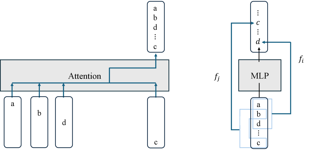
### Visual Description
## Diagram: Attention and MLP Component Flow
### Overview
The image is a technical diagram illustrating two fundamental components of a neural network architecture, likely a transformer or similar model. It is divided into two distinct sections: a left panel depicting an **Attention** mechanism and a right panel depicting a **Multi-Layer Perceptron (MLP)** block. The diagram uses a consistent visual language of gray blocks, blue arrows, and labeled rectangular nodes to represent data flow and transformations.
### Components/Axes
The diagram contains no traditional chart axes. Its components are:
**Left Panel (Attention Mechanism):**
* **Central Block:** A wide, horizontal gray rectangle labeled **"Attention"** in its center.
* **Input Nodes (Bottom):** Four vertically oriented, rounded rectangles positioned below the Attention block.
* Three are grouped on the left, labeled **"a"**, **"b"**, and **"d"** from left to right.
* One is isolated on the right, labeled **"c"**.
* **Output Node (Top):** A single, vertically oriented, rounded rectangle positioned above the Attention block, slightly to the right of center. It contains a vertical list of labels: **"a"**, **"b"**, **"d"**, **"..."** (ellipsis), and **"c"**.
* **Data Flow (Arrows):**
* Blue arrows point upward from each of the four input nodes ("a", "b", "d", "c") into the bottom of the Attention block.
* A blue arrow originates from the top of the Attention block and points to the output node.
* A specific blue arrow path is highlighted: it originates from the input node **"c"**, travels horizontally left within the Attention block, then turns upward to connect to the **"c"** in the output node's list.
**Right Panel (MLP Block):**
* **Central Block:** A square gray block labeled **"MLP"** in its center.
* **Input Node (Bottom):** A vertically oriented, rounded rectangle positioned below the MLP block. It contains a vertical list of labels: **"a"**, **"b"**, **"d"**, **"..."** (ellipsis), and **"c"**. This list is visually identical to the output node from the left panel.
* **Output Node (Top):** A vertically oriented, rounded rectangle positioned above the MLP block. It contains a vertical list of labels: **"..."** (ellipsis) at the top, followed by **"c"**, another **"..."** (ellipsis), and **"d"** at the bottom.
* **Data Flow (Arrows & Functions):**
* A blue arrow points upward from the center of the bottom input node into the MLP block.
* A blue arrow points upward from the top of the MLP block into the center of the top output node.
* **Bypass/Skip Connections:** Two curved blue arrows create direct connections from the bottom input node to the top output node, bypassing the MLP.
* One arrow originates from the label **"a"** in the bottom node and points to the label **"c"** in the top node. This connection is labeled **`f_i`**.
* Another arrow originates from the label **"b"** in the bottom node and points to the label **"d"** in the top node. This connection is labeled **`f_j`**.
* A faint, light-blue rectangular outline surrounds the bottom input node, possibly indicating it is a single tensor or grouped data structure.
### Detailed Analysis
The diagram explicitly maps the transformation of a set of elements {a, b, c, d}.
1. **Attention Stage (Left):**
* **Input:** Four separate elements: `a`, `b`, `d`, `c`.
* **Process:** The Attention mechanism processes these inputs. The highlighted path for element `c` suggests it is being attended to or re-weighted.
* **Output:** The elements are reordered into a sequence: `a`, `b`, `d`, `...`, `c`. The ellipsis (`...`) implies there may be additional, unspecified elements in the sequence between `d` and `c`. The output is a single, ordered representation.
2. **MLP Stage (Right):**
* **Input:** The ordered sequence from the Attention output: `[a, b, d, ..., c]`.
* **Process:** This sequence is processed in two parallel ways:
* **Through the MLP:** The entire sequence is passed through the MLP block for nonlinear transformation.
* **Via Direct Mapping:** Specific elements are mapped directly to the output via functions `f_i` and `f_j`. Element `a` is transformed by `f_i` to become `c` in the output. Element `b` is transformed by `f_j` to become `d` in the output.
* **Output:** A new sequence: `[..., c, ..., d]`. The ellipses indicate a sequence of unspecified length and content, with the known transformed elements `c` and `d` placed at specific positions.
### Key Observations
* **Consistent Element Set:** The core elements `a`, `b`, `c`, and `d` are tracked through both stages.
* **Role of Ellipses (`...`):** The ellipses are critical. They indicate that the sequences contain more elements than are explicitly labeled, making this a generalized diagram rather than a specific example with four items.
* **Dual-Path Processing in MLP:** The MLP block does not solely process the input sequence. It works in conjunction with direct, element-wise functional mappings (`f_i`, `f_j`), suggesting a hybrid transformation.
* **Spatial Grounding:** The legend/labels (`f_i`, `f_j`) are placed directly next to their corresponding bypass arrows. The input to the MLP is spatially aligned with the output from the Attention block, confirming data flow between the two components.
### Interpretation
This diagram illustrates a common pattern in advanced neural network architectures, particularly transformers.
* **Attention's Role:** The left panel shows the **Attention mechanism's core function: reordering and contextualizing input elements.** It takes a set of tokens (a, b, d, c) and produces an ordered sequence where the position of `c` is specifically highlighted, likely indicating it has been given contextual importance relative to the others. The output is a context-aware representation.
* **MLP's Role:** The right panel shows the **MLP's role in feature transformation and refinement.** It takes the context-aware sequence and applies two types of operations:
1. A **global, nonlinear transformation** via the MLP block itself, which likely mixes information across all positions.
2. **Specific, element-wise transformations** (`f_i`, `f_j`) that map certain input features directly to different output features (e.g., `a -> c`, `b -> d`). This could represent operations like position-wise feed-forward networks or specific feature projections.
* **Architectural Insight:** The diagram emphasizes that the output of one major component (Attention) becomes the direct input to the next (MLP), forming a pipeline. The bypass connections (`f_i`, `f_j`) suggest that not all information is processed through the same pathway; some transformations are direct and specific, while others are global and contextual. This is a visual representation of how information flows and is transformed in a layer of a deep learning model, balancing contextual mixing with targeted feature update.
</details>
Figure 9: Illustration of the role of the attention and feedforward layers in looped TFs for evaluating DAGs: the attention layer uniformly attends to and aggregates all inputs at each position, while the feedforward layer simultaneously simulates the functions of the nodes.
* Proof*
In the proof, we assume that the computation graph contains at most $n$ output nodes. This assumption is without loss of generality: if the number of output nodes exceeds the number of input nodes, we can simply pad the input with dummy nodes (e.g., fixed zeros), thereby reducing the setting to the same case. We construct a model in which (1) the attention layer aggregates the inputs, and (2) the looped feed-forward layer performs the computation of all nodes in parallel, as illustrated in Figure 9. We first show that a feedforward layer followed by an attention layer can copy all input tokens to each position. Assume, given an input sequence $x=(x_{1},x_{2},\ldots,x_{n})\in\Sigma^{n}$ and one-hot encoding $\bm{e}:\Sigma\to\{0,1\}^{|\Sigma|}$ . Assume each input at position $i\in[n]$ is embedded as
$$
{\bm{h}}_{i}=\bigl(\,{\bm{0}},\;\bm{e}(x_{i}),\;{\bm{e}}_{i}\,\bigr)\in\{0,1\}^{n|\Sigma|+|\Sigma|+n}, \tag{55}
$$
where ${\bm{e}}_{i}\in\{0,1\}^{n}$ . By Lemma B.6, when substituting ${\bm{x}}=(\bm{e}(x_{1}),\ldots,\bm{e}(x_{n}))$ into the lemma, there exists a feed-forward layer $\mathrm{FF}_{1}$ such that
$$
(\operatorname{id}+\mathrm{FF}_{1})({\bm{h}}_{i})=\bigl(\,({\bm{e}}_{i})_{1}\cdot\bm{e}(x_{i}),\;({\bm{e}}_{i})_{2}\cdot\bm{e}(x_{i}),\;\ldots,\;({\bm{e}}_{i})_{n}\cdot\bm{e}(x_{i}),\;\bm{e}(x_{i}),\;{\bm{e}}_{i}\,\bigr). \tag{56}
$$
To aggregate all positions via uniform attention, we use a single-head attention layer with:
$$
\mathbf{q}_{i}={\bm{k}}_{i}=\mathbf{1}_{n|\Sigma|},\quad\mathbf{v}_{i}=n\big(({\bm{e}}_{i})_{1}\cdot\bm{e}(x_{i}),\;({\bm{e}}_{i})_{2}\cdot\bm{e}(x_{i}),\;\ldots,\;({\bm{e}}_{i})_{n}\cdot\bm{e}(x_{i})\big)\quad\text{for all }i\in[n], \tag{57}
$$
with an appropriate output projection, the output of the attention layer, at position $i$ , becomes
$$
\displaystyle\frac{1}{n}\sum^{n}_{j=1}1\cdot n{\bm{h}}_{j} \displaystyle\;=\;\Bigl(\sum_{j=1}^{n}({\bm{e}}_{j})_{1}\,\bm{e}(x_{j}),\;\;\sum_{j=1}^{n}({\bm{e}}_{j})_{2}\,\bm{e}(x_{j}),\;\;\ldots,\;\;\sum_{j=1}^{n}({\bm{e}}_{j})_{n}\,\bm{e}(x_{j})\Bigr) \displaystyle\;=\;\bigl(\,\bm{e}(x_{1}),\;\bm{e}(x_{2}),\;\ldots,\;\bm{e}(x_{n})\,\bigr). \tag{58}
$$ Then, we show that the feed-forward layer can encode the entire computation graph into its weights and simulate all nodes simultaneously. Let the flag vector for each node be $(t_{1},\ldots,t_{N})\in\{0,1\}^{N}$ , where $N\coloneqq|V_{n}|=\mathrm{size}(G_{n})$ . By Lemmas B.7 and B.8, there exist feed-forward layers $\mathrm{FF}_{2},\mathrm{FF}_{3}:\mathbb{F}_{s}^{N(|\Sigma|+1)}\to\mathbb{F}_{s}^{N(|\Sigma|+1)}$ such that, for the input vector $(z_{1},\ldots,z_{N})\in\Sigma^{N}.$ ,
$$
\displaystyle\mathcal{FF}\Bigl(\,\bm{e}(z_{1}),t_{1},\ldots,\bm{e}(z_{N}(x)),t_{N}\Bigr) \displaystyle=\big\|_{i=1}^{N}\,\Bigl(t_{i}\cdot\bm{e}\bigl(f_{v_{i}}({\bm{z}}^{(i)})\bigr),\;\frac{1}{m_{i}}\sum_{j=1}^{m_{i}}t_{p_{i,j}}\Bigr), \tag{60}
$$
where $\mathcal{FF}\coloneq(\operatorname{id}+\mathrm{FF}_{3})\circ(\operatorname{id}+\mathrm{FF}_{2})$ . Here, $f_{v_{i}}$ denotes the function associated with node $v_{i}$ , and $p_{i,1},\ldots,p_{i,m_{i}}$ denote the indices of the predecessor nodes of $v_{i}$ , and ${\bm{z}}^{(i)}=(z_{p_{i,1}},\ldots,z_{p_{i,m_{i}}})$ denotes their values. The last term $\frac{1}{m_{i}}\sum_{j=1}^{m_{i}}t_{p_{i,j}}$ can be obtained using a linear layer. For the $k$ -th loop, assume by induction that the hidden state is
$$
{\bm{h}}(k)\coloneq\bigl(t_{1,k-1}\cdot\bm{e}(v_{1}(x)),\,t_{1,k},\,t_{2,k-1}\cdot\bm{e}(v_{2}(x)),\,t_{2,k},\,\ldots,\,t_{N,k-1}\cdot\bm{e}(v_{N}(x)),\,t_{N,k}\bigr), \tag{61}
$$
where $v_{i}(x)\in\Sigma$ denotes the value computed by node $v_{i}$ given the input $x$ , and $t_{i,k}\in\{0,1\}$ indicates whether node $v_{i}$ lies within depth at most $k$ . Under this assumption, it holds that
$$
\displaystyle\mathcal{FF}({\bm{h}}(k)) \displaystyle\;=\;\big\|_{i=1}^{N}\,\Bigl(t_{i,k}\cdot\bm{e}\bigl(f_{v_{i}}(v_{p_{i,1}}(x),v_{p_{i,2}}(x),\ldots,v_{p_{i,m_{i}}}(x))\bigr),\;\frac{1}{m_{i}}\sum_{j=1}^{m_{i}}t_{(p_{i,j},k)}\Bigr), \displaystyle\;=\;\big\|_{i=1}^{N}\,\Bigl(t_{i,k}\cdot\bm{e}\bigl(v_{i}(x))\bigr),\;t_{i,k+1}\Bigr)\;=\;{\bm{h}}(k+1). \tag{62}
$$ To extract the output node corresponding to each position denoted by $o_{i}$ , in the final loop iteration, by Lemma B.6, there exists a feedforward layer $\mathrm{FF}_{4}$ such that
$$
(\operatorname{id}+\mathrm{FF}_{4})({\bm{h}}(k),{\bm{e}}_{o_{i}})=\bigl(t_{o_{i},k}\cdot\bm{e}(v_{o_{i}}(x)),\;*\bigr)\,. \tag{64}
$$
Summary
We construct the looped model as follows. Each input token $x_{i}\in\Sigma$ at position $i\in[n]$ is embedded as
$$
{\bm{h}}^{(0)}_{i}=\bigl(\,{\bm{e}}_{i},\;{\bm{e}}_{o_{i}},\;\bm{e}(x_{i}),\;0,\;\bm{e}(x_{i}),\;0,\;\ldots,\;\bm{e}(x_{i}),\;0,\;{\bm{0}}_{(1+|\Sigma|)(N-n)+|\Sigma|}\bigr)\in\{0,1\}^{2n+(1+|\Sigma|)N+|\Sigma|}. \tag{0}
$$
The first attention layer is an identity map, while the first feedforward layers compute
$$
{\bm{h}}^{(1)}_{i}\;=\;\bigl(\,{\bm{e}}_{i},\;{\bm{e}}_{o_{i}},\;({\bm{e}}_{i})_{1}\cdot\bm{e}(x_{i}),\;0,\;({\bm{e}}_{i})_{2}\cdot\bm{e}(x_{i}),\;0,\;\ldots,\;({\bm{e}}_{i})_{n}\cdot\bm{e}(x_{i}),\;0,\;{\bm{0}}_{(1+|\Sigma|)(N-n)+|\Sigma|}\,\bigr). \tag{1}
$$
The second attention layer uniformly gathers all positions and appends a constant $1$ to each block:
$$
\displaystyle{\bm{h}}^{(1.5)}_{i} \displaystyle\;=\;\bigl(\,{\bm{e}}_{i},\;{\bm{e}}_{o_{i}},\;\bm{e}(x_{1}),\;1,\;\bm{e}(x_{2}),\;1,\;\ldots,\;\bm{e}(x_{n}),\;1,\;{\bm{0}}_{(1+|\Sigma|)(N-n)+|\Sigma|}\,\bigr) \displaystyle\;=\;\bigl(\,{\bm{e}}_{i},\;{\bm{e}}_{o_{i}},\;{\bm{h}}(0),\;{\bm{0}}_{|\Sigma|}\,\bigr). \tag{67}
$$
We now proceed by induction. Assume that at the $k$ -th iteration, the output after the second attention layer at position $i$ is
$$
{\bm{h}}^{(1.5)}_{k,i}\;=\;\bigl(\,{\bm{e}}_{i},\;{\bm{e}}_{o_{i}},\;{\bm{h}}(k),\;t_{o_{i},k-1}\cdot\bm{e}(v_{o_{i}}(x))\bigr), \tag{69}
$$
where $t_{o_{i},k-1}\coloneq\bigl({\bm{h}}^{(1.5)}_{k-1,i}\bigr)_{\,2n+(1+|\Sigma|)(o_{i}-1)}$ denotes the indicator flag showing whether the $o_{i}$ -th node has been reached, i.e., whether it lies at depth $k-1$ .
After passing through the second feedforward layer, the third attention layer with all weights set to zero, and the third feedforward layer, the hidden state updates to
$$
{\bm{h}}^{(3)}_{k,i}\;=\;\bigl(\,{\bm{e}}_{i},\;{\bm{e}}_{o_{i}},\;{\bm{h}}(k+1),\;t_{o_{i},k-1}\cdot\bm{e}(v_{o_{i}}(x))\,\bigr). \tag{3}
$$
After the fourth feedforward layer, the hidden state becomes
$$
{\bm{h}}^{(4)}_{k,i}\;=\;\bigl(\,{\bm{e}}_{i},\;{\bm{e}}_{o_{i}},\;{\bm{h}}(k+1),\;t_{o_{i},k}\cdot\bm{e}(v_{o_{i}}(x))\bigr). \tag{4}
$$
By induction, after the final iteration of depth $\mathrm{depth}(G_{n})$ of the computation graph $G_{n}$ , we obtain
$$
{\bm{h}}^{(4)}_{\mathrm{depth}(G_{n}),i}\;=\;\bigl(\,*,\;t_{o_{i},\mathrm{depth}(G_{n})}\cdot\bm{e}(v_{o_{i}}(x))\bigr)\;=\;\bigl(\,*,\;\bm{e}(v_{o_{i}}(x))\bigr). \tag{4}
$$
The final output is given by
$$
z_{i}=\mathbf{OUT}({\bm{h}}^{(4)}_{\mathrm{depth}(G_{n}),i})=\begin{bmatrix}{\bm{0}}&{\bm{I}}_{|\Sigma|}\end{bmatrix}({\bm{h}}^{(4)}_{\mathrm{depth}(G_{n}),i})=\bm{e}(v_{o_{i}}(x)). \tag{4}
$$
The decoding function then selects the symbol corresponding to the maximum score:
$$
y_{i}\;=\;\mathrm{Dec}(z_{i})=\arg\max_{j\in[|\Sigma|]}\,\bigl(\bm{e}(v_{o_{i}}(x))\bigr)_{j}=v_{o_{i}}(x). \tag{74}
$$
The parameter size grows proportionally with the input dimension $\mathrm{size}(G_{n})$ , since the function must be approximated along each dimension. Therefore, it can be bounded by $O\!\left(\mathrm{ff\_param}(G_{n})\cdot\mathrm{size}(G_{n})\right).$ ∎
Discussion: Our proof compresses the entire input into a single position before applying an arbitrary feed-forward computation, which may appear to deviate from the standard Transformer architecture. An alternative approach is to distribute computation across multiple positions, as shown by (Sanford et al., 2024b), which can reduce the required embedding dimension. We nevertheless adopt the single-position construction to isolate the core characteristics of looped models: attention is used purely as an information aggregation mechanism, a single Transformer layer suffices, and all computation is carried out by the feed-forward network in latent space. This latent-space computation is strictly more expressive than computation in the language space. This is supported by recent work for looped ReLUs (Liang et al., 2024).
### B.6 Proof of Theorem 3.6 for Continuous Thought
* Proof*
The proofs are based on the construction for CoT and looped TF. Let the vocabulary be ${\mathcal{V}}=\Sigma$ and each node $v\in V_{n}$ is labeled by a one-hot vector $\bm{e}(v)\in\{0,1\}^{|\mathcal{F}|}$ . At decoding step $k$ , the model has access to the concatenated sequence
$$
(x_{1},x_{2},\ldots,x_{n},\,h_{1},h_{2},\ldots,h_{k}) \tag{75}
$$
where $x=(x_{1},\ldots,x_{n})\in\Sigma^{n}$ denotes the input, and $h_{i}\in\mathbb{F}_{s}^{m}$ is the hidden state generated at the $i$ -th Coconut step. For each node $v_{j}$ , let $v_{j}(x)$ denote its value on input $x$ . We assume that
$$
h_{k}\coloneq\bigl(t_{1,k-1}\cdot\bm{e}(v_{1}(x)),\,t_{1,k},\,t_{2,k-1}\cdot\bm{e}(v_{2}(x)),\,t_{2,k},\,\ldots,\,t_{N,k-1}\cdot\bm{e}(v_{N}(x)),\,t_{N,k},\,{\bm{e}}^{\prime}_{k},\,{\bm{0}}_{|\Sigma|}\bigr),
$$
where $N\coloneqq\mathrm{size}(G_{n})$ , $t_{i,k}\in\{0,1\}$ indicates whether node $v_{i}$ lies within depth at most $k$ , and $\bm{e}:\Sigma\to\{0,1\}^{|\Sigma|}$ denotes one-hot encoding, and the vector ${\bm{e}}^{\prime}_{k}\in\{0,1\}^{N}$ is defined by
$$
{\bm{e}}^{\prime}_{k}=\begin{cases}\mathbf{0}&k<\mathrm{depth}(G_{n}),\\[4.0pt]
\bm{e}(v_{o_{i}})&k=\mathrm{depth}(G_{n})+i,\end{cases} \tag{76}
$$
where $v_{o_{i}}$ denotes the $i$ -th output node, and ${\bm{e}}^{\prime}_{k}$ can be encoded by positional embeddings. Under this assumption, we prove by induction that the model generates $h_{k+1}(x)$ . We first consider the base case $k=1$ , in which the model receives only ${\bm{x}}$ . We focus on the final token. Using the same construction as in the looped TF, we can show that a single feed-forward layer followed by an attention layer suffices to copy all input tokens to every position. Specifically, the hidden representation at the last position becomes
$$
h_{1}=\bigl(\bm{e}(v_{1}(x)),\,1,\,\ldots,\,\bm{e}(v_{n}(x)),\,1,\,{\bm{0}},\ 1,\,{\bm{0}},\,{\bm{e}}^{\prime}_{0},\,{\bm{0}}\bigl), \tag{77}
$$
where $v_{i}(x)=x_{i}$ for all $i\in[n]$ , corresponding to the input nodes. In what follows, we consider the case $k>1$ . By the same argument as for Looped TF, based on Equation 62, we show that the feed-forward layers can encode the entire computation graph into their weights and simulate all nodes simultaneously. That is, there exist two feed-forward layers whose composition, denoted by $\mathcal{FF}$ , satisfies $\mathcal{FF}(h_{k})=h_{k+1}.$ Consider the last feed-forward layer applied after the zero-weight attention layer. By substituting ${\bm{e}}_{i}={\bm{e}}_{k}^{\prime}$ and ${\bm{x}}={(h_{k})}_{1:m-|\Sigma|}$ into Lemma B.6, there exists a feed-forward network $\mathrm{FF}$ such that
$$
(\operatorname{id}+\mathrm{FF})(h_{k})=\begin{cases}h_{k+1},&\text{if }k<\mathrm{depth}(G_{n}),\\[6.0pt]
\Bigl({(h_{k+1})}_{1:m-|\Sigma|},\,\bm{e}(v_{o_{i}}(x))\Bigr),&\text{if }k=\mathrm{depth}(G_{n})+i.\end{cases} \tag{78}
$$
In particular, for all $k<\mathrm{depth}(G_{n})$ , the output of the last token, for the input $(x_{1},x_{2},\ldots,x_{n},\;h_{1},h_{2},\ldots,h_{k})$ is $h_{k+1}$ . For the final positions corresponding to output nodes, namely $k=\mathrm{depth}(G_{n})+i$ , the hidden state ${\bm{h}}_{k}$ contains the embedding of the output symbol $v_{o_{i}}(x)$ . Applying the output projection yields
$$
\mathbf{OUT}({\bm{h}}_{k})=\begin{bmatrix}\mathbf{0}&{\bm{I}}_{|\Sigma|}\end{bmatrix}{\bm{h}}_{k}=\bm{e}\!\left(v_{o_{i}}(x)\right). \tag{79}
$$ Finally, the decoding function outputs the symbol in $\Sigma$ corresponding to the maximum coordinate of $\mathbf{OUT}({\bm{h}}_{k})$ . ∎
### B.7 Proof for Theorem 3.12
For the upper bound $\mathsf{Loop}[\log^{k}n,\,\mathsf{poly}(n),\,1\ \textup{(resp.\ }\log n)]\subseteq\mathsf{AC}^{k}\ \textup{(resp.\ }\mathsf{TC}^{k}),$ we follow the argument of (Li et al., 2024). Their key observation is that a restricted form of automaton can model iterative computation under constant precision: the rounding operation preserves monotonicity, and constant precision yields counter-free, restricted state spaces, which are therefore computable by $\mathsf{AC}^{0}$ circuits. In the case of polynomial precision, prefix summation can be simulated by $\mathsf{TC}^{0}$ , which also allows the detection and correction of rounding in floating-point arithmetic.
**Theorem B.9 (Liet al.,2024)**
*For $s(n)\in\mathsf{poly}(n)$ , $\mathrm{sum}_{s(n)}:(\mathbb{F}_{s(n)})^{n}\to\mathbb{F}_{s(n)}$ is computable by $\mathsf{TC}^{0}$ circuits, and by $\mathsf{AC}^{0}$ circuits when $s(n)$ is constant.*
It has also been shown that gates can be efficiently simulated by feedforward layers.
**Lemma B.10 (Liet al.,2024)**
*Unbounded-fanin $\and,\mathsf{OR}$ (resp. $\mathsf{MAJORITY}):\{0,1\}^{n}\to\{0,1\}$ can be simulated by a two-layer feedforward ReLU network with constant (resp. $\log{n}$ ) bits of precision constant hidden dimension and additional $n$ constant inputs of value $1$ .*
* Proof forTheorem3.12*
$\mathsf{Loop}[\log^{k}n,\,\mathsf{poly}(n),\,1\ \textup{(resp.\ }\log n)]\subseteq\mathsf{AC}^{k}\ \textup{(resp.\ }\mathsf{TC}^{k}):$ In Transformers, constant-depth computation is defined by Summation with Iterative Rounding (see Definition B.3), which by Theorem B.9 can be simulated in $\mathsf{AC}^{0}$ (resp. $\mathsf{TC}^{0}$ ). A looped TF simply stacks these computations vertically through iteration, and thus the result follows. $\mathsf{AC}^{k}\ \textup{(resp.\ }\mathsf{TC}^{k})\subseteq\mathsf{Loop}[\log^{k}n,\,\mathsf{poly}(n),\,1\ \textup{(resp.\ }\log n)]:$ Since Boolean circuits are DAGs, the claim follows directly from Theorem 3.10 together with Lemma B.10. ∎
## Appendix C Deferred Proofs for Section 4
### C.1 Definition for Models of Computation
We model a language model as a probabilistic process that, given an input and a generated prefix, produces either an internal reasoning state or an output token. This process induces a probability distribution over final outputs. We first formalize CoT under this setting. We focus on the saturated hardmax attention as in (Merrill et al., 2022; Nowak et al., 2024).
**Definition C.1 (Language model with CoT)**
*Let ${\mathcal{V}}$ be a vocabulary. Given an input $x\in{\mathcal{V}}^{*}$ , a language model with CoT stochastically generates a sequence of output blocks of the form
$$
\Big(r_{1},\,e,\,y_{1},\,e^{\prime},\;r_{2},\,e,\,y_{2},\,e^{\prime},\;\cdots\;r_{m},\,e,\,y_{m},\,e^{\prime}\Big), \tag{80}
$$
where each $r_{i}\in{\mathcal{V}}^{*}$ represents an explicit reasoning trace, $y_{i}\in{\mathcal{V}}$ is an output token, and $e,e^{\prime}\in{\mathcal{V}}$ are special delimiter tokens. The final output is the string $y_{1}\cdots y_{m}$ . Generation proceeds autoregressively: at iteration $i$ , the model generates a reasoning segment $r_{i}$ followed by an output token $y_{i}$ , conditioned on the input $x$ , the previously generated outputs $y_{<i}$ , and prior reasoning segments $r_{<i}$ . We denote by $p(y\mid x)$ the resulting distribution over final outputs.*
Then we define the language models with latent thought reasoning: Coconut and looped TF.
**Definition C.2 (Language model with Coconut)**
*Let ${\mathcal{V}}$ be a vocabulary. Given an input $x\in{\mathcal{V}}^{*}$ , a language model with Coconut generates a sequence of blocks
$$
\Big(r_{1},\,y_{1},\,r_{2},\,y_{2},\,\ldots,\,r_{m},\,y_{m}\Big), \tag{81}
$$
where each $r_{i}\in{\mathbb{F}^{d}}^{*}$ represents an internal continuous reasoning state, and each $y_{i}\in{\mathcal{V}}$ is an output token. Generation proceeds autoregressively. At each iteration, the internal continuous reasoning state $r_{i}$ is generated deterministically as a function of the input $x$ , the previously generated outputs $y_{<i}$ , and the prior internal states $r_{<i}$ , while the output token $y_{i}$ is generated stochastically. The decision of when to emit an output token is determined internally by the model.*
For looped TF models, the computation proceeds through internally repeated iterations before producing any output tokens. The number of iterations is determined by the model as a function of the input.
**Definition C.3 (Language model with looped TF)**
*Given an input $x\in{\mathcal{V}}^{*}$ , a looped TF produces an output sequence autoregressively. At each iteration $i\in[m]$ , the model internally performs a number of repeated transformation steps before emitting an output token $y_{i}$ , conditioned on the input $x$ and the previously generated outputs $y_{<i}$ . The number of internal loop iterations required to generate each output token is determined internally by the model as a function of the input $x$ and the generated prefix $y_{<i}$ .*
We define complexity classes corresponding to language models under different reasoning paradigms. In contrast to the non-uniform models typically used in parallel computation analysis, we adopt a uniform setting analogous to Turing machines: a single model with a fixed set of parameters is applied to all input lengths, while the number of reasoning steps is allowed to grow as a function of the input size $n$ . Following the convention in (Merrill and Sabharwal, 2024), we allow $O(\log n)$ bits of numerical precision to represent positional embeddings and internal activations. Furthermore, we extend the output space beyond simple binary decisions. Specifically, the model’s output is not restricted to $\Sigma^{k}$ , but can be an arbitrary finite binary string in $\Sigma^{*}$ . This extension enables the model to represent functions of the form $f:\Sigma^{*}\to\mathbb{R}$ , thereby capturing counting, probabilistic modeling, and approximation tasks.
**Definition C.4 (Complexity Classes𝗉𝖢𝗈𝖳\mathsf{pCoT},𝗉𝖢𝖳\mathsf{pCT}, and𝗉𝖫𝖮𝖮𝖯\mathsf{pLOOP})**
*Let $\mathsf{pCoT}[T(n)]$ , $\mathsf{pCT}[T(n)]$ , and $\mathsf{pLOOP}[T(n)]$ denote the classes of probabilistic computations that define an output distribution $p:\Sigma^{*}\times\Sigma^{*}\to[0,1]$ . A function $f$ belongs to such a class if there exists a language model $\mathcal{M}$ , employing CoT, Coconut, or looped TF, respectively, such that for any input $x\in\Sigma^{n}$ , the model induces the distribution $p(x,\cdot)$ within $O(T(n))$ steps using $O(\log n)$ bits of numerical precision.*
### C.2 Lemma: Universality of Chain of Thought
**Definition C.5**
*A probabilistic Turing machine $M=(Q,\Sigma,\Gamma,q_{0},q_{1},\delta_{1},\delta_{2})$ is defined as:
- $Q$ is a finite set of states,
- $\Sigma$ is the input/output alphabet,
- $\Gamma$ is the tape alphabet, with $\Sigma\subseteq\Gamma$ and a distinguished blank symbol $\sqcup\in\Gamma$ ,
- $q_{0}\in Q$ denotes the initial state, and $q_{1}\in Q$ denotes the final state,
- $\delta_{1},\delta_{2}:Q\times\Gamma\to Q\times\Gamma\times(\Sigma\cup\{\varepsilon\})\times\{L,S,R\}$ are two transition functions.
At each step, $M$ chooses uniformly at random between $\delta_{1}$ and $\delta_{2}$ . Each transition $\delta_{i}(q,a)=(q^{\prime},b,\sigma,D)$ is interpreted as: writing $b\in\Gamma$ on the work tape, writing $\sigma\in\Sigma$ on the output tape, where $\varepsilon$ means that nothing is written, and moving the tape head in direction $D\in\{L,S,R\}$ , where $L$ = left, $R$ = right, and $S$ = stay. The output of $M$ is defined to be the string remaining on the output tape when the machine halts.*
Prior work has shown that probabilistic CoT can simulate any such PTM, thereby demonstrating its universality.
**Lemma C.6 (Nowaket al.,2024)**
*Let $M$ be a PTM with input and output alphabet $\Sigma$ , and running time bounded by $T(n)$ on inputs of length $n$ . Then there exists a log-precision CoT model with stochastic decoding, denoted $\mathsf{CoT}_{M}$ , such that the induced output distribution of $\mathsf{CoT}_{M}$ coincides exactly with that of $M$ . Formally, for every input string $x\in\Sigma^{*}$ and output string $y\in\Sigma^{*}$ ,
$$
\Pr\bigl[\mathsf{CoT}_{M}(x)=y\bigr]\;=\;\Pr\bigl[M(x)=y\bigr]. \tag{82}
$$
Moreover, the number of reasoning steps of $\mathsf{CoT}_{M}$ is bounded by $\mathsf{poly}(|x|)$ .*
### C.3 Self-Reducibility and Complexity of Approximate Counting
Here, we provide the definitions of relation and associated counting problems.
**Definition C.7 (Relation)**
*A relation over an alphabet $\Sigma$ is a subset $R\subseteq\Sigma^{*}\times\Sigma^{*}.$ For an input $x\in\Sigma^{*}$ , we denote
$$
R(x):=\{\,y\in\Sigma^{*}:(x,y)\in R\,\}.
$$*
**Definition C.8 (Counting)**
*Given a relation $R$ , the associated counting function is defined as
$$
N_{R}:\Sigma^{*}\to\mathbb{N},\qquad N_{R}(x):=|R(x)|.
$$*
**Definition C.9 (pp-relation)**
*A relation $R\subseteq\Sigma^{*}\times\Sigma^{*}$ is called a $p$ -relation if
- the membership $(x,y)\in R$ can be decided in time polynomial in $|x|$ , and
- there exists a polynomial $p$ such that for all $(x,y)\in R$ , we have $|y|\leq p(|x|)$ .*
**Definition C.10**
*The extension counting function associated with a relation $R\subseteq\Sigma^{*}\times\Sigma^{*}$ is
$$
\operatorname{EXT}_{R}:\Sigma^{*}\times\Sigma^{*}\to\mathbb{N},\qquad\operatorname{EXT}_{R}(x,w):=\bigl|\{\,z\in\Sigma^{*}:(x,wz)\in R\,\}\bigr|.
$$*
The complexity class $\#\mathsf{P}$ consists of counting problems associated with $p$ -relations (Valiant, 1979). Then, we provide definitions of schemes for approximate counting. In the remainder of this paper, we say that an algorithm produces an output approximating $f(x)$ within ratio $1+\varepsilon$ if its output $\hat{f}(x)$ satisfies
$$
(1-\varepsilon)f(x)\leq\hat{f}(x)\leq(1+\varepsilon)f(x),
$$
**Definition C.11 (FPTAS)**
*An algorithm is called a fully polynomial-time approximation scheme (FPTAS) for a function $f$ if, for any input $x$ and any $\varepsilon>0$ , it produces an output approximating $f(x)$ within ratio $1+\varepsilon$ , and runs in time polynomial in $|x|$ and $1/\varepsilon$ .*
**Definition C.12 (FPRAS)**
*An algorithm is a fully polynomial-time randomized approximation scheme (FPRAS) for a function $f$ if, for any input $x$ and any $\varepsilon>0$ and $\delta>0$ , it produces an output approximating $f(x)$ within ratio $1+\varepsilon$ with probability at least $1-\delta$ , and runs in time polynomial in $|x|$ , $1/\varepsilon$ , and $\log(1/\delta)$ .*
The following proposition formalizes the relationship between approximate counting and the extension counting function.
**Proposition C.13 (Jerrumet al.,1986)**
*Let $R$ be a $p$ -relation and let $x\in\Sigma^{n}$ . Let $m=p(n)$ and define $r=1+\frac{\varepsilon}{2m}$ . If there exists a FPRAS that approximates $\mathrm{Ext}_{R}(x,w)$ within ratio $r$ for all prefixes $w$ with probability at least $1-\delta/m$ , then there exists an FPRAS that approximates $N_{R}(x)$ within ratio $1+\varepsilon$ with probability at least $1-\delta$ .*
This reduction transforms the global counting problem into a sequence of local estimation steps.
**Proposition C.14**
*For any $0<\varepsilon\leq 1$ and any integer $m\geq 1$ , it holds that
$$
\left(1+\frac{\varepsilon}{2m}\right)^{m}<1+\varepsilon. \tag{83}
$$*
* Proof*
We use the standard inequality $1+x\leq e^{x}$ , which holds for all $x\in\mathbb{R}$ . Substituting $x=\frac{\varepsilon}{2m}$ , we have:
$$
\left(1+\frac{\varepsilon}{2m}\right)^{m}\leq\left(\exp\left(\frac{\varepsilon}{2m}\right)\right)^{m}=e^{\varepsilon/2}. \tag{84}
$$
For $0<\varepsilon\leq 1$ , we show that $e^{\varepsilon/2}<1+\varepsilon$ . Let $f(\varepsilon)=1+\varepsilon-e^{\varepsilon/2}$ . Then $f(0)=0$ and $f^{\prime}(\varepsilon)=1-\frac{1}{2}e^{\varepsilon/2}$ . Since $e^{\varepsilon/2}\leq e^{1/2}<2$ for all $\varepsilon\in[0,1]$ , it follows that $f^{\prime}(\varepsilon)>0$ . Thus, $f$ is strictly increasing on $[0,1]$ , implying $f(\varepsilon)>f(0)=0$ , or equivalently $e^{\varepsilon/2}<1+\varepsilon$ . ∎
* Proof forPropositionC.13*
Let $x\in\Sigma^{n}$ and $m=p(n)$ . We express $N_{R}(x)$ as a product of $m$ ratios. Let $w=y_{1}y_{2}\dots y_{m}$ be a witness, and let $w^{(i)}$ denote its prefix of length $i$ . We can write:
$$
N_{R}(x)=\mathrm{Ext}_{R}(x,\lambda)=\prod_{i=1}^{m}\frac{\mathrm{Ext}_{R}(x,w^{(i-1)})}{\mathrm{Ext}_{R}(x,w^{(i)})}\cdot\mathrm{Ext}_{R}(x,w^{(m)}). \tag{85}
$$
In the standard self-reducibility framework, we estimate each ratio $\rho_{i}=\mathrm{Ext}_{R}(x,w^{(i-1)})/\mathrm{Ext}_{R}(x,w^{(i)})$ using the assumed approximation scheme. Let $A_{i}$ be the estimator for the $i$ -th ratio such that:
$$
\mathbb{P}\left[\frac{1}{r}\leq\frac{A_{i}}{\rho_{i}}\leq r\right]\geq 1-\frac{\delta}{m}. \tag{86}
$$
By the union bound, the probability that at least one of these $m$ estimations fails to stay within the ratio $r$ is at most $m\cdot(\delta/m)=\delta$ . Therefore, with probability at least $1-\delta$ , all $m$ estimations are successful. Under this condition, the final estimate $\hat{N}=\prod_{i=1}^{m}A_{i}$ satisfies:
$$
\frac{1}{r^{m}}\leq\frac{\hat{N}}{N_{R}(x)}\leq r^{m}. \tag{87}
$$
From Proposition C.14, we have $r^{m}=(1+\frac{\varepsilon}{2m})^{m}<1+\varepsilon$ . Furthermore, for $0<\varepsilon\leq 1$ , it holds that $1/r^{m}>(1+\varepsilon)^{-1}\geq 1-\varepsilon$ , ensuring a relative error of at most $\varepsilon$ . Regarding complexity, each of the $m$ calls to the FPRAS for $\mathrm{Ext}_{R}$ runs in time $\mathrm{poly}(n,(r-1)^{-1},\log(m/\delta))$ . Substituting $r-1=\varepsilon/2m$ , the runtime per call is $\mathrm{poly}(n,m/\varepsilon,\log(m/\delta))$ . Since $m=p(n)$ is a polynomial in $n$ , the total running time is $\mathrm{poly}(n,1/\varepsilon,\log(1/\delta))$ , which satisfies the requirements for an FPRAS. ∎
We have shown that approximate counting reduces to approximating the extension counting function. For a general relation $R$ , however, the connection between the extension counting function and the original counting problem for $R$ remains unclear. This gap is bridged by the notion of self-reducibility: for self-reducible relations, the extension counting function can be reduced back to the original counting problem for $R$ .
**Definition C.15 (Schnorr,1976)**
*A relation $R\subseteq\Sigma^{*}\times\Sigma^{*}$ is self-reducible if:
1. There exists a polynomial-time computable function $g\in\Sigma^{*}\to\mathbb{N}$ s.t., $(x,y)\in R\Rightarrow|y|=g(x);$
1. There exists a polynomial-time Turing machine that decides membership in $R$ .
1. There exist polynomial-time computable functions $\psi\in\Sigma^{*}\times\Sigma^{*}\to\Sigma^{*}$ and $\sigma\in\Sigma^{*}\to\mathbb{N}$ s.t.
$$
\displaystyle\sigma(x) \displaystyle=O(\log|x|), \displaystyle g(x)>0 \displaystyle\Rightarrow\sigma(x)>0\quad\forall x\in\Sigma^{*}, \displaystyle|\psi(x,w)| \displaystyle\leq|x|\quad\forall x,w\in\Sigma^{*}, \tag{88}
$$
and such that, for all $x\in\Sigma^{*}$ , $y=y_{1}\dots y_{n}\in\Sigma^{*}$ ,
$$
\langle x,y_{1},\dots,y_{n}\rangle\in R\iff\langle\psi(x,y_{1}\dots y_{\sigma(x)}),y_{\sigma(x)+1},\dots,y_{n}\rangle\in R. \tag{91}
$$*
For example, SAT is self-reducible: by fixing a prefix of variables and applying the reduction map $\psi$ , the problem is simplified to a smaller instance whose solutions extend the chosen prefix. Consider the Boolean formula $F=(x_{1}\vee x_{2})\ \wedge\ (\neg x_{1}\vee x_{3})\ \wedge\ (\neg x_{2}\vee\neg x_{3}),$ and suppose we fix the first variable to $x_{1}=1$ . The residual instance is obtained by applying $\psi(F,(1))$ , which substitutes $x_{1}=1$ and simplifies the formula by deleting satisfied clauses and removing falsified literals: $\psi(F,(1))\;=\;(x_{3})\ \wedge\ (\neg x_{2}\vee\neg x_{3}).$ The unit clause $(x_{3})$ forces $x_{3}=1$ , which in turn simplifies $(\neg x_{2}\vee\neg x_{3})$ to $\neg x_{2}$ , yielding $x_{2}=0$ . Hence the unique residual assignment is $(x_{2},x_{3})=(0,1)$ , and together with the prefix $x_{1}=1$ , we obtain the satisfying assignment $(x_{1},x_{2},x_{3})=(1,0,1).$
For self-reducible relations, the extension counting function is no harder to approximate than the original counting problem.
**Proposition C.16 (Jerrumet al.,1986)**
*Let $R$ be self-reducible. If there exists an FPRAS for $N_{R}$ , then there exists an FPRAS for $\mathrm{Ext}_{R}$ .*
* Proof*
By the definition of self-reducibility, the extension function $\mathrm{Ext}_{R}(x,w)$ , which counts the number of strings $y$ such that $(x,wy)\in R$ , can be mapped to the counting problem of a modified instance. Specifically, for any prefix $w$ where $|w|\leq\sigma(x)$ , there exists a polynomial-time computable mapping $\psi$ such that:
$$
\mathrm{Ext}_{R}(x,w)=|\{y\in\Sigma^{\sigma(x)-|w|}:(x,wy)\in R\}|=N_{R}(\psi(x,w)). \tag{92}
$$
Since $R$ is self-reducible, the instance $x_{w}=\psi(x,w)$ can be constructed in polynomial time relative to $|x|$ . By the hypothesis, there exists an FPRAS for $N_{R}$ , which provides a randomized $(1\pm\epsilon)$ -approximation of $N_{R}(x_{w})$ in time polynomial in $|x_{w}|$ and $1/\epsilon$ . Consequently, this algorithm serves as an FPRAS for $\mathrm{Ext}_{R}(x,w)$ , as it runs in polynomial time and satisfies the required approximation guarantees. ∎
### C.4 Proof for Theorem 4.3
**Lemma C.17 (Formal Statement ofLemma4.3)**
*Assume that $\mathsf{FPTAS}\subsetneq\mathsf{FPRAS}$ for self-reducible relations. There exists a self-reducible relation $R$ and an associated function $\mathrm{Ext}_{R}:\Sigma^{*}\times\Sigma^{*}\to\mathbb{N}$ defined by $\mathrm{Ext}_{R}(x,y_{<i})\coloneqq|\{\,z\in\Sigma^{*}:(x,y_{<i}z)\in R\,\}|$ such that language models with CoT using polynomially many reasoning steps, which output a distribution for a given input $(x,y_{<i})\in\Sigma^{n}\times\Sigma^{*}$ by using a linear head for the last hidden state before emitting the output token, admit an FPRAS for $\mathrm{Ext}_{R}$ , whereas no latent thought with polynomially many iterations admits the same approximation guarantee using a linear head for the last hidden state before emitting the output token.*
* Proof*
By Lemma C.6, CoT can simulate any probabilistic Turing machine running in polynomial time; thus, it can implement an FPRAS for $N_{R}$ . By Proposition C.16, the existence of an FPRAS for $N_{R}$ further implies the existence of an FPRAS for the extension function $\mathrm{Ext}_{R}$ . On the other hand, latent thought consisting of a polynomial number of iterations can always be simulated by a deterministic polynomial-time Turing machine, provided that all state transitions in the latent computation are deterministic. Consequently, if such a latent thought process were to admit an FPRAS for $\mathrm{Ext}_{R}$ , it would effectively yield a deterministic polynomial-time approximation scheme. By Proposition C.16, the existence of such a scheme for $\mathrm{Ext}_{R}$ would imply the existence of an FPTAS for $N_{R}$ . However, under the standard complexity-theoretic assumption that $\mathsf{FPTAS}\subsetneq\mathsf{FPRAS}$ for self-reducible relations, there exists a self-reducible relation $R$ whose counting function admits an FPRAS but no FPTAS. This yields a contradiction. ∎
### C.5 Proof for Theorem 4.4
**Definition C.18 (FPAUS)**
*Uniform generation asks to sample an element $y$ uniformly at random from $R(x)$ . A fully polynomial almost uniform sampler (FPAUS) for $R$ is a randomized algorithm that, given an input $x\in\Sigma^{*}$ and an accuracy parameter $\varepsilon>0$ , runs in time polynomial in $|x|$ and $\log(1/\varepsilon)$ , and outputs a distribution $q(\cdot\mid x)$ such that
$$
\bigl\|q(\cdot\mid x)-U(R(x))\bigr\|_{\mathrm{TV}}\;\leq\;\varepsilon,
$$
where $U(R(x))$ denotes the uniform distribution over the set $R(x)$ , and $\|\cdot\|_{\mathrm{TV}}$ denotes total variation distance.*
For self-reducible relations, the following holds.
**Theorem C.19 (Jerrumet al.,1986)**
*Let $R$ be a self-reducible relation. There exists an FPRAS for approximating $|R(x)|$ if and only if there exists an FPAUS for sampling uniformly from $R(x)$ .*
* Proof ofTheorem4.4*
The target uniform conditional distribution is defined as follows:
$$
p(y_{i}\mid x,y_{<i})\;:=\;\frac{\operatorname{EXT}_{R}(x,y_{<i}y_{i})}{\sum_{u\in\Sigma}\operatorname{EXT}_{R}(x,y_{<i}u)}\qquad(y_{i}\in\Sigma). \tag{93}
$$
Assume an FPRAS $\mathcal{A}(x,\varepsilon,\delta)$ exists for the self-reducible relation $|R(x)|$ . By Proposition C.16, the existence of an FPRAS for $|R(x)|$ implies the existence of an FPRAS for the extension function $\operatorname{EXT}_{R}$ . We construct a CoT that samples $y\in R(x)$ by sequentially approximating these conditional probabilities. For each step $i\in\{1,\dots,m(n)\}$ , the CoT computes $(1\pm\varepsilon)$ -accurate estimates $\widehat{\operatorname{EXT}}_{R}(x,y_{<i}u)$ for all $u\in\Sigma$ using $\mathcal{A}$ , and induces the following distribution:
$$
\pi(y_{i}\mid x,y_{<i})\;:=\;\frac{\widehat{\operatorname{EXT}}_{R}(x,y_{<i}y_{i})}{\sum_{u\in\Sigma}\widehat{\operatorname{EXT}}_{R}(x,y_{<i}u)}. \tag{94}
$$
Conditioned on the event that all estimates in Equation 94 are $(1\pm\varepsilon)$ -accurate, the multiplicative error is bounded by:
$$
\frac{1-\varepsilon}{1+\varepsilon}\leq\frac{\pi(y_{i}\mid x,y_{<i})}{p(y_{i}\mid x,y_{<i})}\leq\frac{1+\varepsilon}{1-\varepsilon}. \tag{95}
$$
To ensure the cumulative approximation error remains within $(1\pm\varepsilon^{\prime})$ , we set the local precision to $\varepsilon\leq\frac{\varepsilon^{\prime}}{2+\varepsilon^{\prime}}$ , which yields $\frac{1+\varepsilon}{1-\varepsilon}\leq 1+\varepsilon^{\prime}$ and $\frac{1-\varepsilon}{1+\varepsilon}\geq 1-\varepsilon^{\prime}$ . To ensure the failure probability is at most $\delta^{\prime}$ , we apply a union bound over the $m(n)$ generation steps and the $|\Sigma|$ calls per step. By setting the local confidence to $\delta\leq\frac{\delta^{\prime}}{m(n)(|\Sigma|+1)}$ , the joint success event holds with probability at least $1-\delta^{\prime}$ . Under this event, the CoT correctly simulates an FPRAS for $p(y_{i}\mid x,y_{<i})$ in total time $\text{poly}(n,1/\varepsilon^{\prime},\log(1/\delta^{\prime}))$ . Finally, since CoT can represent an FPRAS by Lemma 4.3, it satisfies the requirements for the construction. On the other hand, we show that latent thought cannot compute such an approximation. Suppose, for contradiction, that the model could compute the conditional distribution $\pi(y_{i}\mid x,y_{<i})$ to within a $(1\pm\varepsilon)$ relative error in a single step. We define the estimator for the total count $Z(x)=|R(x)|$ as:
$$
\widehat{Z}(x)\;\coloneq\;\Biggl(\prod_{i=1}^{m(n)}\pi(y_{i}\mid x,y_{<i})\Biggr)^{-1}. \tag{96}
$$
Since the true distribution satisfies $p(y\mid x)=1/|R(x)|=\prod_{i}p(y_{i}\mid x,y_{<i})$ , the relative error of $\widehat{Z}(x)$ is governed by the product of local errors:
$$
(1+\varepsilon)^{-m(n)}|R(x)|\leq Z(x)\leq(1-\varepsilon)^{-m(n)}|R(x)|, \tag{97}
$$
By setting $\varepsilon\leq\frac{\varepsilon^{\prime}}{2m(n)}$ , we apply Proposition C.14 and the properties of multiplicative error:
$$
(1+\varepsilon)^{-m(n)}\geq 1-m(n)\varepsilon\geq 1-\varepsilon^{\prime}/2>1-\varepsilon^{\prime}, \tag{98}
$$
and for sufficiently small $\varepsilon$ ,
$$
(1-\varepsilon)^{-m(n)}\leq 1+2m(n)\varepsilon\leq 1+\varepsilon^{\prime}. \tag{99}
$$
Substituting these into Equation 96, we obtain:
$$
(1-\varepsilon^{\prime})|R(x)|\leq\widehat{Z}(x)\leq(1+\varepsilon^{\prime})|R(x)|. \tag{100}
$$
This implies that if the model could compute $\pi$ accurately, $\widehat{Z}(x)$ would constitute an FPTAS for $|R(x)|$ . However, under the standard complexity-theoretic assumption that $\mathsf{FPTAS}\subsetneq\mathsf{FPRAS}$ for self-reducible relations, this yields a contradiction. ∎
## Appendix D Experimental Details
### D.1 Fundamental Algorithmic Reasoning Tasks
#### D.1.1 Task Settings
Word Problem
We define a sequence prediction task based on finite groups such as the symmetric group $S_{5}$ . Given a sequence of group elements of length $k$ , the model is required to output the cumulative products obtained by scanning the sequence from left to right. Formally, for an input sequence $(g_{1},g_{2},\ldots,g_{k})$ , the target sequence is $(g_{1},\;g_{1}g_{2},\;g_{1}g_{2}g_{3},\;\ldots,\;g_{1}g_{2}\cdots g_{k}).$ We follow the setting of (Merrill and Sabharwal, 2025b).
Connectivity
To ensure that the reachability labels are approximately balanced, we generate undirected graphs according to the Erdős–Rényi model (Erdos and Renyi, 1959) $G(n,p)$ , where $n$ is the number of vertices and each possible edge is included independently with probability $p$ . In the supercritical regime ( $pn=c>1$ ), a single “giant” connected component emerges, occupying a fraction $s\in(0,1)$ of the vertices, which satisfies $s=1-e^{-cs}.$ Consequently, the probability that two uniformly random vertices are both in this component—and hence mutually reachable—is approximately $s^{2}$ . To target a reachability probability of $1/2$ , we set $s\approx\sqrt{\tfrac{1}{2}}\approx 0.707,c\approx\tfrac{-\ln(1-s)}{s}\approx 1.74,$ and thus $p=\tfrac{c}{n}\approx\tfrac{1.7}{n}.$ In practice, for each graph of size $n$ we fix $p=1.7/n$ , which empirically yields $\Pr[\text{reachable}]\approx 50\$ for $n\in[50,100]$ . We follow the encoding scheme of Sanford et al. (2024a). The input to the model is serialized as a flat token sequence consisting of three parts: $v_{0}\,v_{1}\,\cdots\,v_{n-1}\;e_{1}\,e_{2}\,\cdots\,e_{m}\;s,t$ where each vertex is denoted by a token $v_{i}$ , each edge is represented as a pair “ u,v ” with $u<v$ , and the final token “ s,t ” specifies the source–target pair for the reachability query.
Arithmetic Expression Evaluation
Following (Feng et al., 2023), we generate expressions over integers modulo $r$ using the four operations ${+,-,\times,\div}$ , where multiplication and division are defined via precomputed modular tables. To guarantee that each expression evaluates to a specific target value, we grow expressions backwards: starting from a sampled number, we iteratively replace it with a binary sub-expression that preserves its value under modular arithmetic. Different from (Feng et al., 2023), we fix the modulus to $r=3$ , as our focus lies in evaluating the reasoning over expressions rather than exploring the properties of each modular arithmetic system.
Edit Distance
The Edit Distance task requires computing the minimum number of edit operations needed to transform one string into another. The allowed operations are insertion, deletion, and replacement of a single character, and the objective is to predict the total edit distance given two input strings. To build the dataset, we follow (Feng et al., 2023). We first generate two strings over a randomly sampled alphabet. The first string has a fixed length, while the second string is produced in two possible ways: with probability $0.4$ , it is drawn as a random string of nearly the same length (within $\pm 3$ characters), and with probability $0.6$ , it is derived from the first string by applying a given number of random edit operations. Each edit operation is chosen uniformly among deletion, replacement, and insertion. To avoid trivial cases, string pairs that are identical or whose lengths differ excessively are rejected and resampled. Finally, the shorter string is always placed first to maintain a consistent input format. An example instance in the format is shown below: s v d h s s e e … v e | s h d s s s s … e s e <sep> 20 Here, the two input strings are separated by the token “ | ”, “ <sep> ” marks the end of the inputs, and the final number “ 20 ” denotes the computed edit distance.
#### D.1.2 Training Configuration
Configuration of chain of thought
For CoT models, training is performed with supervision of step-by-step algorithms. (1) Word problem: for this task, the CoT algorithm proceeds by sequentially scanning the token sequence and producing at each prefix the evaluation result of the expression step by step. Thus, the overall length of the CoT sequence matches the input length. (2) Graph connectivity: Following Bavandpour et al. (2025), the algorithm sequence is simply the trace of a breadth-first search (BFS) starting from the source $s$ . At each step, the model emits the incident edges of the currently expanded node in the order they are visited. The sequence terminates as soon as the target $t$ is discovered. To implement this algorithm, we maintain a list (“scratchpad”) initialized with a dummy marker and the source, $(\texttt{N},s)$ . We iterate through this list from left to right (i.e., queue order). Whenever the current node $u$ is expanded, we append to the end of the list all incident edges $(u,v)$ for neighbors $v$ , followed by a separator token $(u,\texttt{N})$ . (3) Arithmetic expression evaluation: Following (Feng et al., 2023), the CoT takes the fully expanded expression and repeatedly evaluates one innermost subexpression, writing down the simplified expression at each step until only a single numeral remains. For example, $2*(0+1)/2\to 2*1/2\to 2/2\to 1.$ The overall CoT sequence has quadratic length. (4) Edit distance: Following (Feng et al., 2023), the CoT algorithm outputs the DP table entries in the same order they are computed, i.e., row by row from top-left to bottom-right (topological order). This yields a quadratic number of steps in the input length.
Optimization and model details.
We trained all models using the AdamW optimizer with a linear learning rate schedule. The initial learning rate was set to $1\times 10^{-4}$ with a weight decay of $0.01$ , and a batch size of $256$ . Training was continued until the training loss plateaued. For looped TFs, curriculum learning was applied to all tasks except edit distance: the input size was increased by $2$ for the word problem task, and by $4$ for the connectivity and arithmetic evaluation tasks. The model architecture was based on standard Transformers with an embedding dimension of $256$ . We used $4$ attention heads, and varied the number of Transformer layers depending on the task: two layers for word problems, a single layer for connectivity, and time-modulated (Xu and Sato, 2025) model with a single layer for looped TF, to stabilize training, on both arithmetic evaluation and the edit distance task. For CoT, we use the same configuration of the Transformer block.
Uniform selection.
To estimate a lower bound on the number of reasoning steps required by CoT for each task, we first follow the procedure introduced in prior work (Bavandpour et al., 2025). Specifically, given a complete CoT trajectory consisting of $T$ intermediate reasoning steps, we construct shortened trajectories by uniformly selecting $k$ step indices from $\{1,\dots,T\}$ , i.e., by taking a uniformly spaced subsequence of the original trajectory. Only the selected intermediate steps are used, while the remaining steps are removed. We then evaluate task performance as a function of $k$ , as shown in Table 3.
Table 3: Results for CoT on parallelizable tasks trained with uniform selection.
| Word Problem Graph Connectivity Arithmetic Evaluation | 64 32 16 | 0.8 81.0 41.0 | 0.8 81.4 41.5 | 0.8 83.6 41.2 | 100.0 100.0 82.5 |
| --- | --- | --- | --- | --- | --- |
| Edit Distance | 16 | 69.2 | 70.3 | 82.6 | 94.8 |
Stepwise internalization.
We adopt stepwise internalization proposed by (Deng et al., 2024), a curriculum-based training procedure that gradually removes CoT tokens and encourages the model to internalize intermediate reasoning within its hidden states. Starting from a model trained on full CoT trajectories, we progressively truncate intermediate reasoning tokens according to a predefined schedule and finetune the model at each stage. Specifically, when the CoT length is greater than $128$ , we remove $16$ tokens per stage until the remaining CoT length reaches $128$ . We then continue removing $8$ tokens per stage until the CoT length is reduced to $8$ , training the model for $16$ epochs at each stage. The results for each fundamental algorithmic reasoning task are shown in Fig. 10.
<details>
<summary>x13.png Details</summary>
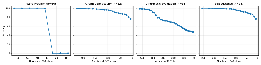
### Visual Description
## Line Charts: Accuracy vs. Number of Chain-of-Thought (CoT) Steps
### Overview
The image displays four separate line charts arranged horizontally. Each chart plots "Accuracy" (y-axis) against the "Number of CoT steps" (x-axis) for a different task or problem type. The x-axis is **reversed**, with values decreasing from left to right. All charts use blue lines with circular markers. The charts appear to be from a technical or research context, likely evaluating the performance of a reasoning model as the number of reasoning steps changes.
### Components/Axes
* **Common Y-Axis (All Charts):** Label: "Accuracy". Scale: 0 to 100, with major tick marks at 0, 20, 40, 60, 80, 100.
* **Common X-Axis (All Charts):** Label: "Number of CoT steps". The scale is reversed and varies per chart.
* **Chart Titles & Sample Sizes (n):**
1. **Leftmost Chart:** "Word Problem (n=64)"
2. **Second Chart:** "Graph Connectivity (n=32)"
3. **Third Chart:** "Arithmetic Evaluation (n=16)"
4. **Rightmost Chart:** "Edit Distance (n=16)"
* **Legend:** No separate legend is present. The task type is indicated by the title above each chart.
* **Spatial Layout:** The four charts are aligned in a single row. Each chart occupies an equal-width panel with a light gray grid in the background.
### Detailed Analysis
**Chart 1: Word Problem (n=64)**
* **X-Axis Range:** Approximately 65 to 5 (decreasing left to right).
* **Trend & Data Points:** The line shows a **sharp, cliff-like drop**. Accuracy is at or near 100% for a high number of CoT steps (from ~65 down to ~30). Between approximately 30 and 20 steps, accuracy plummets to near 0%. It remains at ~0% for step counts below 20 (down to ~5).
* **Key Values (Approximate):** At ~65 steps: 100%. At ~30 steps: 100%. At ~25 steps: ~0%. At ~5 steps: ~0%.
**Chart 2: Graph Connectivity (n=32)**
* **X-Axis Range:** Approximately 225 to 0 (decreasing left to right).
* **Trend & Data Points:** The line shows a **gradual, accelerating decline**. Accuracy starts very high (~98-100%) at the highest step count (~225). It decreases slowly at first, then more rapidly as the number of steps decreases, ending at approximately 75% accuracy at 0 steps.
* **Key Values (Approximate):** At ~225 steps: ~98%. At ~150 steps: ~95%. At ~75 steps: ~85%. At 0 steps: ~75%.
**Chart 3: Arithmetic Evaluation (n=16)**
* **X-Axis Range:** Approximately 550 to 0 (decreasing left to right).
* **Trend & Data Points:** The line shows a **steady, near-linear decline**. Accuracy begins near 100% at ~550 steps and falls consistently as steps decrease, ending at approximately 50% accuracy at 0 steps.
* **Key Values (Approximate):** At ~550 steps: ~98%. At ~400 steps: ~90%. At ~200 steps: ~70%. At 0 steps: ~50%.
**Chart 4: Edit Distance (n=16)**
* **X-Axis Range:** Approximately 250 to 0 (decreasing left to right).
* **Trend & Data Points:** The line shows a **gradual decline that steepens at the end**. Accuracy starts near 100% at ~250 steps, decreases slowly to about 90% at ~100 steps, then drops more sharply to approximately 75% at 0 steps.
* **Key Values (Approximate):** At ~250 steps: ~98%. At ~150 steps: ~92%. At ~50 steps: ~85%. At 0 steps: ~75%.
### Key Observations
1. **Reversed X-Axis:** All charts plot a higher number of CoT steps on the left and a lower number on the right. This visually represents "reducing steps" from left to right.
2. **Universal Negative Correlation:** In all four tasks, accuracy is positively correlated with the number of CoT steps. Fewer steps lead to lower accuracy.
3. **Task-Dependent Sensitivity:** The *rate* and *pattern* of decline vary significantly by task:
* **Word Problems** exhibit a catastrophic failure mode after a critical step threshold (~30 steps).
* **Graph Connectivity** and **Edit Distance** show more graceful degradation.
* **Arithmetic Evaluation** shows the most linear and predictable decline.
4. **Sample Size Variation:** The sample size (n) is largest for Word Problems (64) and smallest for Arithmetic Evaluation and Edit Distance (16 each), which may affect the smoothness and reliability of the curves.
### Interpretation
The data strongly suggests that **Chain-of-Thought (CoT) reasoning is crucial for maintaining high accuracy across these diverse problem types.** The number of reasoning steps acts as a key performance resource.
* **The "Cliff" in Word Problems** indicates a potential **phase transition or minimum complexity threshold**. Below a certain number of steps (~30), the model likely cannot construct a coherent solution path, causing performance to collapse entirely. This is a critical finding for reliability.
* **The Gradual Declines** in the other tasks imply that while more steps are beneficial, the model can still perform reasonably well with suboptimal step counts, albeit with degrading performance. The steeper final drop in Edit Distance might suggest a secondary threshold for that specific task.
* **The Linear Decline in Arithmetic** is noteworthy. It suggests a direct, proportional relationship between the allocated reasoning "budget" (steps) and success rate for this task, making it potentially more predictable.
* **Practical Implication:** For real-world applications, these charts argue for **dynamically allocating or encouraging more reasoning steps**, especially for complex word problems, to avoid catastrophic failure. The optimal number of steps is task-dependent. The reversed axis cleverly visualizes the cost (in accuracy) of *reducing* computational effort (steps).
</details>
Figure 10: Accuracy as a function of the CoT steps during stepwise internalization.
### D.2 Approximate Counting and Approximate Sampling
#### D.2.1 Approximate Counting of DNF Formulas
To generate the dataset, we first construct a DNF formula $F$ by sampling $m$ clauses, each consisting of $w$ distinct literals over $n$ Boolean variables. Each literal is independently assigned to be either positive or negated. The formula is then serialized into a token sequence in which each clause is represented by its index together with variable–value pairs such as “ $2=$ $+1$ ” or “ $4=$ $-1$ ”. For looped TFs, we prepare $100{,}000$ training samples and $1{,}000$ test samples. For CoT models, we instead generate an online dataset with the following structure. To train the CoT models, we simulate a single trial of the randomized counting algorithm of Karp and Luby (1983). The sequence concatenates the serialized formula, the sampled clause, the full assignment, and the verification outcome, separated by <sep> tokens and terminated by <eos>. CoT model is trained in an autoregressive manner, where prediction targets are defined by shifting the token sequence while masking out the formula description. We trained the models using the AdamW optimizer with a linear learning rate schedule. The initial learning rate was set to $1\times 10^{-4}$ , with a weight decay of $0.01$ . We used a batch size of $256$ (reduced to $32$ for the $1000$ -loop setting) and trained for $10{,}000$ iterations. For inference, we count the total number of iterations used for summing output tokens (steps) in CoT across trials, and the number of loop iterations in the looped TF.
#### D.2.2 Approximate Sampling of Graph Colorings
We consider the problem of approximately sampling a proper $k$ -coloring of a graph, also known as almost-uniform generation, a canonical randomized task closely related to $\#\mathsf{P}$ -hard counting problems. Given an undirected graph $G=(V,E)$ with $n=|V|$ vertices and maximum degree $\Delta$ , a proper $k$ -coloring is an assignment of colors from $\{1,\dots,k\}$ to vertices such that no adjacent vertices share the same color. Let $\Omega_{k}(G)$ denote the set of all proper $k$ -colorings of $G$ . We restrict attention to graphs of bounded degree and assume $k\geq 2\Delta+1.$ Under this condition, classical results in approximate counting show that the number of proper $k$ -colorings admits a FPAUS (Jerrum, 1995). The approximation relies on Markov Chain Monte Carlo (MCMC) sampling using Glauber dynamics for graph colorings. Starting from an arbitrary proper coloring, the Markov chain repeatedly selects a vertex uniformly at random and proposes to recolor it with a randomly chosen color, accepting the update only if the resulting coloring remains proper. When $k\geq 2\Delta+1$ , this Markov chain is known to be rapidly mixing, converging to the uniform distribution over $\Omega_{k}(G)$ in polynomial time. For our experiments, we generate an undirected Erdős–Rényi random graph, where each edge is included independently with probability $p=\frac{1.7}{n},$ using a fixed random seed for reproducibility. For simplicity and ease of analysis, we focus on small graphs with $n=3$ and set the number of colors to $k=5$ .
Each sample is generated by running $T$ steps of Glauber dynamics on the space $\Omega_{k}(G)$ of proper $k$ -colorings. Starting from a greedy proper initialization, at each step we uniformly select a vertex and a color; the recoloring is accepted if and only if it preserves properness. The final state of the Markov chain is treated as an approximate sample from the uniform distribution over $\Omega_{k}(G)$ . In addition to the final coloring, we optionally record the entire sequence of proposals and accept/reject outcomes for CoT and use it as supervision, which is not included for latent thought. To train sequence models, we serialize the graph structure, the initial coloring, and either the MCMC history or the final coloring into a single token sequence. We evaluate the distribution of solutions generated by the model rather than only solution accuracy. Given an input $x$ , we draw $N$ independent samples from the model using ancestral decoding. Generation continues until an end-of-sequence (EOS) token is produced, and from each generated sequence we extract the final $n$ tokens immediately preceding the first EOS token, which encode a candidate solution. The resulting samples define an empirical distribution $\hat{P}$ over generated solutions via normalized occurrence counts. For each instance, the task provides an exact enumeration $\mathcal{Y}$ of all valid solutions. We define the reference distribution $P_{\mathrm{true}}$ as the uniform distribution over this solution set, assigning probability $1/|\mathcal{Y}|$ to each $y\in\mathcal{Y}$ and zero otherwise. We quantify the discrepancy between the empirical distribution $\hat{P}$ and the uniform reference distribution using the total variation distance $\frac{1}{2}\sum_{y\in\mathcal{Y}\cup\hat{\mathcal{Y}}}\left|\hat{P}(y)-P_{\mathrm{true}}(y)\right|.$ We trained the models using the AdamW optimizer with a linear learning rate schedule. The initial learning rate was set to $1\times 10^{-4}$ , with a weight decay of $0.01$ . We used a batch size of $256$ and trained for $5{,}000$ iterations. For inference, we measure the average number of steps (loops) per generation. We generate $N=50{,}000$ samples for CoT and $N=10{,}000$ samples for looped TFs. The resulting histograms of CoT outputs over the target support are shown in Figure 11.
<details>
<summary>x14.png Details</summary>
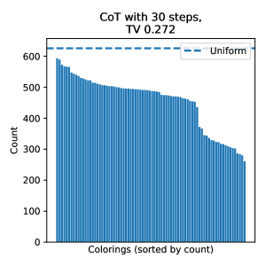
### Visual Description
## Bar Chart: CoT with 30 steps, TV 0.272
### Overview
This is a vertical bar chart displaying the frequency distribution of "Colorings" from an experiment or simulation involving a Chain-of-Thought (CoT) process with 30 steps. The chart compares the observed counts of various colorings against a theoretical uniform distribution baseline. The title includes a metric "TV 0.272," which likely stands for Total Variation distance.
### Components/Axes
* **Title:** "CoT with 30 steps, TV 0.272" (Centered at the top).
* **Y-Axis:**
* **Label:** "Count" (Vertical text on the left side).
* **Scale:** Linear scale from 0 to 600, with major tick marks at 0, 100, 200, 300, 400, 500, and 600.
* **X-Axis:**
* **Label:** "Colorings (sorted by count)" (Centered at the bottom).
* **Scale:** Categorical. Each bar represents a distinct "coloring." The categories are sorted in descending order of their count from left to right.
* **Legend:**
* **Label:** "Uniform"
* **Visual:** A horizontal dashed blue line.
* **Placement:** Top-right corner of the chart area.
* **Data Series:**
* A single series of vertical blue bars representing the "Count" for each "Coloring."
### Detailed Analysis
* **Uniform Baseline:** The dashed "Uniform" line is positioned at a count of approximately **620**. This represents the expected count if all colorings occurred with equal frequency.
* **Data Distribution (Trend Verification):** The bars exhibit a clear, monotonically decreasing trend from left to right.
* The **leftmost bar** (the most frequent coloring) has a height of approximately **600**, just below the uniform line.
* The bars decrease gradually in height across the majority of the chart. By the midpoint, the count is approximately **480**.
* A **notable drop** occurs in the rightmost quarter of the chart. The counts fall more steeply from around **450** to below **300**.
* The **rightmost bar** (the least frequent coloring) has a height of approximately **280**.
* **Spatial Grounding:** The legend is placed in the top-right, overlapping slightly with the upper portion of the bars. The uniform line extends horizontally across the entire width of the plot area at its designated y-value.
### Key Observations
1. **Non-Uniform Distribution:** The observed counts for all colorings are below the uniform baseline (620). No coloring reaches the expected frequency of a perfectly uniform distribution.
2. **Significant Skew:** The distribution is heavily skewed. A small number of colorings on the left have counts near 600, while a larger number of colorings on the right have counts below 350.
3. **Steep Tail:** The sharp decline in the rightmost section indicates a "long tail" of colorings that occur much less frequently than the most common ones.
4. **Total Variation (TV):** The stated TV of 0.272 quantifies the overall difference between this observed distribution and the uniform distribution. A value of 0 would be a perfect match; 0.272 indicates a moderate to substantial deviation.
### Interpretation
This chart visualizes the outcome of a stochastic process (CoT with 30 steps) applied to a combinatorial problem involving "colorings." The key insight is that the process does **not** generate outcomes uniformly. Instead, it exhibits a strong bias:
* **Favored Outcomes:** A subset of colorings (left side) is generated relatively frequently, approaching but not reaching the theoretical uniform rate.
* **Disfavored Outcomes:** A larger subset of colorings (right side) is generated significantly less often, with some being quite rare.
The **Total Variation distance of 0.272** is a critical metric. It suggests the CoT process has a measurable and non-trivial preference structure. This could be due to the inherent logic of the 30-step process, the structure of the problem space, or biases in the step-by-step reasoning. The "sorted by count" presentation makes this inequality immediately visible, highlighting that the process is not exploring the solution space evenly. For a technical audience, this indicates that conclusions drawn from samples generated by this process may be biased towards the more frequent colorings on the left.
</details>
<details>
<summary>x15.png Details</summary>
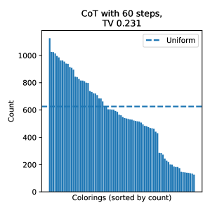
### Visual Description
## Bar Chart with Overlay Line: CoT with 60 steps, TV 0.231
### Overview
The image is a vertical bar chart displaying the frequency distribution of "Colorings," sorted by count. A horizontal dashed line representing a "Uniform" distribution is overlaid for comparison. The chart's title indicates it relates to a "CoT with 60 steps" and a "TV" value of 0.231.
### Components/Axes
* **Title:** "CoT with 60 steps, TV 0.231" (Top center).
* **Y-Axis:**
* **Label:** "Count" (Left side, rotated vertically).
* **Scale:** Linear scale from 0 to 1000, with major tick marks at 0, 200, 400, 600, 800, and 1000.
* **X-Axis:**
* **Label:** "Colorings (sorted by count)" (Bottom center).
* **Scale:** Categorical, representing individual colorings. The bars are sorted in descending order of their count value from left to right.
* **Legend:** Located in the top-right corner of the plot area.
* **Label:** "Uniform"
* **Symbol:** A blue dashed line (`--`).
* **Data Series:**
1. **Bars (Primary Data):** Solid blue vertical bars representing the count for each coloring.
2. **Dashed Line (Reference):** A horizontal blue dashed line representing the "Uniform" distribution value.
### Detailed Analysis
* **Bar Data Series (Counts):**
* **Trend:** The bars show a clear, steeply decreasing trend from left to right. The leftmost bar has the highest count, and the rightmost bar has the lowest.
* **Key Data Points (Approximate):**
* **Maximum (Leftmost bar):** ~1100.
* **Initial Plateau:** The first ~15-20 bars show a gradual decline from ~1100 to ~800.
* **Steep Decline:** A pronounced, steep drop occurs in the middle section of the chart. The count falls from ~800 to ~400 over a relatively short span of colorings.
* **Tail:** The rightmost portion of the chart shows a long tail of colorings with low counts, tapering down to values near or below 100.
* **"Uniform" Line (Reference):**
* **Value:** The horizontal dashed line is positioned at a Y-value of approximately **620**.
* **Position:** It intersects the bar series roughly one-third of the way from the left, indicating that only the most frequent colorings (the leftmost bars) have counts significantly above the uniform expectation.
### Key Observations
1. **Highly Skewed Distribution:** The data is not uniform. A small number of colorings (on the left) occur very frequently, while the vast majority (the long tail to the right) occur rarely.
2. **Sharp Transition:** There is a distinct "cliff" or sharp transition point in the middle of the distribution where the frequency drops dramatically.
3. **Uniform Baseline:** The "Uniform" line at ~620 serves as a benchmark. The fact that most bars are below this line indicates that the distribution of colorings is concentrated in a few high-frequency items, with the rest being sparse.
### Interpretation
This chart visualizes the output distribution of a process (likely a Chain-of-Thought reasoning process with 60 steps) across different "colorings" (which could represent distinct reasoning paths, outputs, or states). The Total Variation (TV) distance of 0.231 quantifies the difference between this observed distribution and a uniform one.
The data suggests the process is **highly deterministic or biased**, favoring a small subset of outcomes. The sharp drop-off implies a potential phase transition or a threshold effect in the generation process—perhaps where certain constraints or rules cause a rapid decrease in the viability of many colorings. The long tail indicates that while most outcomes are rare, a non-zero probability exists for a wide variety of them. This pattern is common in generative processes where a few "attractor" states dominate, but exploration still produces a diverse, low-frequency tail. The uniform line highlights how far the system is from a random, unbiased exploration of the coloring space.
</details>
<details>
<summary>x16.png Details</summary>
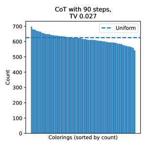
### Visual Description
## Bar Chart with Reference Line: CoT with 90 steps, TV 0.027
### Overview
The image displays a bar chart titled "CoT with 90 steps, TV 0.027". It visualizes the frequency distribution ("Count") of various "Colorings," which are sorted in descending order by their count. A horizontal dashed line labeled "Uniform" serves as a reference, indicating the expected count if all colorings were equally probable. The chart suggests an analysis of the output distribution from a process (likely "Chain-of-Thought" with 90 steps), comparing it to a uniform baseline.
### Components/Axes
* **Chart Title:** "CoT with 90 steps, TV 0.027" (Top center).
* **Y-Axis:**
* **Label:** "Count" (Vertical, left side).
* **Scale:** Linear scale from 0 to 700, with major tick marks at 0, 100, 200, 300, 400, 500, 600, 700.
* **X-Axis:**
* **Label:** "Colorings (sorted by count)" (Horizontal, bottom).
* **Scale:** Categorical. Each bar represents a distinct "coloring." The specific labels for individual colorings are not visible; they are anonymized or aggregated into a sorted sequence.
* **Legend:**
* **Location:** Top-right corner of the plot area.
* **Entry:** A dashed blue line symbol followed by the text "Uniform".
* **Data Series:**
1. **Bars (Primary Data):** A series of vertical blue bars. Their height represents the observed count for each coloring.
2. **Dashed Line (Reference):** A horizontal, dashed blue line extending across the chart's width.
### Detailed Analysis
* **Bar Series Trend:** The bars are sorted from tallest on the left to shortest on the right, creating a clear, monotonically decreasing slope from left to right.
* **Bar Values (Approximate):**
* The tallest bar (far left) has a count of approximately **690-700**.
* The counts decrease gradually. The bar at the approximate midpoint has a count of roughly **625-630**.
* The shortest bar (far right) has a count of approximately **540-550**.
* **Uniform Reference Line:** The dashed "Uniform" line is positioned at a constant y-value of approximately **625**. This represents the expected count per coloring under a uniform distribution.
* **Spatial Relationship:** For the first ~60% of the colorings (from the left), the bar heights are **above** the uniform reference line. For the remaining ~40% (on the right), the bar heights fall **below** the uniform line.
### Key Observations
1. **Non-Uniform Distribution:** The distribution of counts across colorings is not uniform. There is a clear hierarchy, with some colorings being significantly more frequent than others.
2. **Skew:** The distribution is right-skewed (or positively skewed), with a longer tail of less frequent colorings on the right.
3. **Crossover Point:** The observed counts transition from being above the uniform expectation to below it. This crossover occurs slightly to the right of the chart's center.
4. **Magnitude of Deviation:** The most frequent coloring appears about **~12%** more often than the uniform expectation (700 vs. 625), while the least frequent coloring appears about **~14%** less often (540 vs. 625).
### Interpretation
This chart demonstrates that the process generating these "colorings" (CoT with 90 steps) does not produce all possible outcomes with equal probability. The "TV 0.027" in the title likely refers to the **Total Variation distance**, a statistical measure of how different two probability distributions are. A TV of 0.027 quantifies the deviation from uniformity observed visually.
The data suggests an underlying bias or structure in the generation process. Certain colorings are favored, appearing more frequently than a random, uniform process would predict, while others are suppressed. This could be due to constraints in the model's reasoning path (the "90 steps"), biases in the training data, or inherent properties of the coloring problem itself. The sorted presentation effectively highlights the inequality in frequency, making the deviation from the ideal "Uniform" benchmark immediately apparent. The chart is a diagnostic tool, revealing that the system's output distribution is skewed, which may be critical for understanding its behavior, reliability, or fairness.
</details>
Figure 11: Output distributions of CoT compared against the uniform target distribution.