2510.01032

# Meaningless Tokens, Meaningful Gains: How Activation Shifts Enhance LLM Reasoning Abstract Motivated by the puzzling observation that inserting long sequences of meaningless tokens before the query prompt can consistently enhance LLM reasoning performance, this work analyzes the underlying mechanism driving this phenomenon and based on these insights proposes a more principled method that allows for similar performance gains. First, we find that the improvements arise from a redistribution of activations in the LLM’s MLP layers, where near zero activations become less frequent while large magnitude activations increase. This redistribution enhances the model’s representational capacity by suppressing weak signals and promoting stronger, more informative ones. Building on this insight, we propose the Activation Redistribution Module (ARM), a lightweight inference-time technique that modifies activations directly without altering the input sequence. ARM adaptively identifies near-zero activations after the non-linear function and shifts them outward, implicitly reproducing the beneficial effects of meaningless tokens in a controlled manner. Extensive experiments across diverse benchmarks and model architectures clearly show that ARM consistently improves LLM performance on reasoning tasks while requiring only a few lines of simple code to implement. Our findings deliver both a clear mechanistic explanation for the unexpected benefits of meaningless tokens and a simple yet effective technique that harnesses activation redistribution to further improve LLM performance. The code has been released at ARM-Meaningless-tokens. 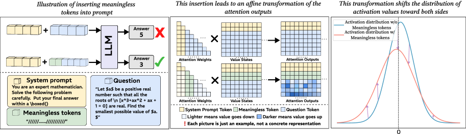1 Introduction Large language models (LLMs) are known to be sensitive to subtle variations in their inputs, which makes it important to understand how tokens influence predictions (Guan et al., 2025; Errica et al., 2024; Zhuo et al., 2024). In this paper, we present a surprisingly counterintuitive finding named meaningless-token effect: inserting long sequences of meaningless tokens, such as repeated punctuation or separators, into prompts can consistently improve the performance of LLMs, particularly on reasoning tasks. Contrary to common intuition that long and irrelevant tokens are like noise and thus useless or even harmful during inference (Jiang et al., 2024; Guan et al., 2025), our experiments reveal the opposite. When long sequences of meaningless tokens are appended before query prompts, models that previously struggled with certain problems can produce correct solutions, as illustrated in the left panel of Figure 1 (see more examples in Appendix J). This effect occurs consistently across tasks and models, suggesting a counterintuitive behavior of LLMs pending deeper investigation. <details> <summary>x1.png Details</summary>  ### Visual Description \n ## Diagram: Insertion of Meaningless Tokens into Prompt & Effect on Attention Outputs ### Overview This diagram illustrates the effect of inserting meaningless tokens into a prompt given to a Large Language Model (LLM). It shows how this insertion leads to an affine transformation of the attention outputs, and consequently shifts the distribution of activation values. The diagram is divided into three main sections: Prompt Insertion, Attention Transformation, and Activation Distribution. ### Components/Axes The diagram contains the following components: * **System Prompt:** A text box containing the prompt: "You are an expert mathematician. Solve the following problem carefully. Put your final answer within a boxed [0]". * **Question:** A text box containing the question: "Let $a$ be a positive real number such that all the roots of $(x^3 + ax^2 + 2x + 1 = 0)$ are real. Find the smallest possible value of $a$." * **Meaningless Tokens:** Represented by a series of dashes ("-----"), these tokens are inserted into the prompt. * **LLM:** A block labeled "LLM" representing the Large Language Model. * **Attention Weights:** A grid of squares representing attention weights, with varying shades of gray. * **Value States:** A grid of squares representing value states, with varying shades of gray. * **Attention Outputs:** A grid of squares representing attention outputs, with varying shades of gray. * **Activation Distribution:** A graph showing the distribution of activation values, with two curves: one representing the distribution without meaningless tokens (blue), and one representing the distribution with meaningless tokens (orange). * **Legend:** A legend explaining the color coding for System Prompt Token, Meaningless Token, and Question Token. * **Scale:** A scale at the bottom of the Activation Distribution graph, labeled "0". * **Annotations:** Text annotations explaining the effects of the insertion and the meaning of the color gradients. ### Detailed Analysis / Content Details **Prompt Insertion (Leftmost Section):** * The top row shows a system prompt and a question being fed into the LLM. The output is "Answer 5" with a red "X" over it. * The bottom row shows the same system prompt and question, but with meaningless tokens inserted before the question. The output is "Answer 3". * The meaningless tokens are visually represented as a series of dashes. **Attention Transformation (Middle Section):** * The top row shows the transformation of Attention Weights, Value States, and Attention Outputs when the prompt *without* meaningless tokens is used. The Attention Weights and Value States are grids of light and dark gray squares. The Attention Outputs are also a grid of squares. * The bottom row shows the same transformation when the prompt *with* meaningless tokens is used. The Attention Weights and Value States are grids of light and dark gray squares. The Attention Outputs are also a grid of squares. * The annotation states: "Lighter means value goes down" and "Darker value goes up". * The annotation states: "Each picture is just an example, not a concrete representation". **Activation Distribution (Rightmost Section):** * The graph shows two curves: * **Blue Curve (Activation distribution w/o Meaningless tokens):** This curve is approximately bell-shaped, peaking around a value of 0.5 on the x-axis. The curve extends from approximately 0 to 1. * **Orange Curve (Activation distribution w/ Meaningless tokens):** This curve is wider and flatter than the blue curve. It has two peaks, one around 0.2 and another around 0.8 on the x-axis. The curve extends from approximately 0 to 1. ### Key Observations * The insertion of meaningless tokens leads to a shift in the distribution of activation values. The blue curve (without tokens) is more concentrated, while the orange curve (with tokens) is more spread out. * The attention outputs appear to be affected by the insertion of meaningless tokens, as indicated by the changes in the grid of squares. * The LLM produces different answers depending on whether meaningless tokens are present in the prompt (5 vs. 3). ### Interpretation The diagram demonstrates that inserting meaningless tokens into a prompt can subtly alter the internal workings of an LLM, specifically affecting the attention mechanism and the distribution of activation values. This alteration can lead to different outputs, even for the same question. The shift in the activation distribution suggests that the meaningless tokens introduce noise or ambiguity into the model's processing, potentially influencing its decision-making process. The diagram highlights the sensitivity of LLMs to even seemingly insignificant changes in input and the importance of carefully crafting prompts to avoid unintended consequences. The annotation "Each picture is just an example, not a concrete representation" suggests that the specific patterns in the attention weights and value states are illustrative rather than definitive. The diagram is a conceptual illustration of a phenomenon rather than a precise empirical measurement. </details> Figure 1: The left panel illustrates how meaningless-token effect can improve model performance. The middle panel shows the changes occurring in the attention module after introducing meaningless tokens. The right panel depicts the redistribution of activations that results from adding these tokens. This unexpected result raises fundamental questions about how LLMs process input and what aspects of their internal computation are being affected. Why should tokens that convey no meaning lead to measurable performance gains? Are they simply acting as noise, or do they restructure representations in a systematic way that supports better reasoning? To answer these questions, we move beyond surface level observations and conduct a detailed investigation of the mechanisms behind this effect. Our analysis shows that the influence of meaningless tokens arises primarily in the first layer, and their effect on meaningful tokens can be approximated as an affine transformation of the attention outputs. As demonstrated in the middle schematic diagram of Figure 1, the resulting transformation shifts the distribution of activations in the MLP: the proportion of near-zero activations decreases, while more activations are pushed outward toward larger positive and negative values. The rightmost plot in Figure 1 gives a visualization of this process. We hypothesize that redistribution fosters richer exploration, enhancing reasoning performance, and clarify the mechanism by decomposing the transformation into coefficient and bias terms. Our theoretical analysis shows how each component shapes activation variance and induces the observed distributional shift. Building on these insights, we propose ARM (an A ctivation R edistribution M odule), a lightweight alternative to explicit meaningless-token insertion. ARM requires only a few lines of code modification and no additional training. It automatically identifies a proportion of near-zero activations after the non-linear function and shifts their values outward, yielding a smoother and less sparse activation distribution. In doing so, ARM reproduces the beneficial effects of meaningless tokens without altering the input sequence and consistently improves LLM performance on reasoning and related tasks. In summary, the key findings and contributions of our work are: - We uncover a meaningless-token effect in LLMs: inserting meaningless tokens, far from being harmful, systematically improves reasoning in LLMs. This runs counter to the common assumption that such tokens only add noise. - Through theoretical and empirical analysis, we show that these tokens induce an activation redistribution effect in the first-layer MLP, reducing near-zero activations and increasing variance. - Building on this understanding, we present ARM, a lightweight inference-time instantiation to demonstrate that the phenomenon can be directly harnessed. 2 Observation: Inserting Meaningless Tokens Induces an Affine Transformation on Meaningful Token Representations We observe that meaningless tokens, such as a sequence of slashes (“/”) with appropriate lengths can enhance the performance of LLMs, particularly on reasoning tasks Varying token length, type, and position affects performance, as shown in Appendix F.. As shown in Table 1, when we insert a fixed-length sequence of meaningless tokens between the system prompt and the question, all evaluated models exhibit performance improvements on Math-500 and AIME2024 to different degrees. This consistent improvement suggests that the inserted meaningless tokens are not simply ignored or detrimental to the models; rather, they exert a positive influence, likely through non-trivial interactions with the models’ internal representations. To investigate this phenomenon, we start our analysis from the attention module. The formula of attention is: Table 1: Performance on mathematical reasoning datasets with and without meaningless tokens across different models. “w/o” denotes the absence of meaningless tokens, while “w/” denotes their presence. We test each model five times to get the average result. | Qwen2.5-Math-1.5B Qwen2.5-Math-7B DS-R1-Qwen-7B | 63.9 72.3 52.7 | 65.9 74.6 53.1 | 14.4 23.1 3.2 | 17.5 23.3 4.4 | | --- | --- | --- | --- | --- | | DS-Math-7B-instruct | 39.5 | 42.1 | 7.8 | 12.3 | | Llama-3.1-8B-Instruct | 41.8 | 42.1 | 7.9 | 9.9 | | Qwen-2.5-32B-Instruct | 81.3 | 81.7 | 17.6 | 22.8 | <details> <summary>x2.png Details</summary>  ### Visual Description \n ## Line Charts: Average Attention Weight vs. Token Position ### Overview The image presents six line charts comparing the average attention weight with and without "meaningless tokens" for three different language models: Owen-2.5-7B-Math, Llama-3-8B-Instruct, and Gemma-3-4b-it. Each model is represented by two charts, one showing attention weights up to token position 60 and the other up to token position 120. The charts aim to visualize the impact of meaningless tokens on attention distribution. ### Components/Axes * **X-axis:** Token Position (ranging from 0 to 60 in the top row and 0 to 120 in the bottom row). * **Y-axis:** Average Attention Weight (ranging from 0 to approximately 0.08 for Owen, 0 to 0.10 for Llama, and 0 to 0.17 for Gemma). * **Lines:** * Blue Line: Represents the average attention weight *without* meaningless tokens ("w/o Meaningless tokens"). * Orange Line: Represents the average attention weight *with* meaningless tokens ("w/ Meaningless tokens"). * **Titles:** Each chart has a title indicating the model name, layer number, and head number. * Owen-2.5-7B-Math Layer 1 Head 22 * Llama-3-8B-Instruct Layer 1 Head 27 * Gemma-3-4b-it Layer 1 Head 3 * **Legend:** Located in the top-left corner of each chart, clearly labeling the blue and orange lines. ### Detailed Analysis or Content Details **Owen-2.5-7B-Math Layer 1 Head 22 (Top Left)** * The blue line (w/o meaningless tokens) exhibits high-frequency oscillations, fluctuating between approximately 0.01 and 0.06. * The orange line (w/ meaningless tokens) also oscillates, but with a generally lower average attention weight, mostly between 0.005 and 0.04. * The trend is generally erratic for both lines, with no clear upward or downward slope. * Approximate data points (blue line): * Token 0: ~0.02 * Token 20: ~0.05 * Token 40: ~0.03 * Token 60: ~0.01 * Approximate data points (orange line): * Token 0: ~0.01 * Token 20: ~0.02 * Token 40: ~0.01 * Token 60: ~0.005 **Llama-3-8B-Instruct Layer 1 Head 27 (Top Middle)** * The blue line (w/o meaningless tokens) shows similar high-frequency oscillations as Owen, ranging from approximately 0.02 to 0.08. * The orange line (w/ meaningless tokens) also oscillates, with a lower average attention weight, mostly between 0.01 and 0.05. * The trend is erratic for both lines. * Approximate data points (blue line): * Token 0: ~0.04 * Token 20: ~0.06 * Token 40: ~0.04 * Token 60: ~0.02 * Approximate data points (orange line): * Token 0: ~0.02 * Token 20: ~0.03 * Token 40: ~0.02 * Token 60: ~0.01 **Gemma-3-4b-it Layer 1 Head 3 (Top Right)** * The blue line (w/o meaningless tokens) oscillates between approximately 0.03 and 0.15. * The orange line (w/ meaningless tokens) oscillates between approximately 0.01 and 0.12. * The trend is erratic for both lines. * Approximate data points (blue line): * Token 0: ~0.06 * Token 20: ~0.12 * Token 40: ~0.08 * Token 60: ~0.05 * Approximate data points (orange line): * Token 0: ~0.02 * Token 20: ~0.06 * Token 40: ~0.04 * Token 60: ~0.03 **Owen-2.5-7B-Math Layer 1 Head 22 (Bottom Left)** * The blue line (w/o meaningless tokens) oscillates between approximately 0.01 and 0.05. * The orange line (w/ meaningless tokens) oscillates between approximately 0.005 and 0.04. * The trend is erratic for both lines. * Approximate data points (blue line): * Token 0: ~0.02 * Token 40: ~0.03 * Token 80: ~0.02 * Token 120: ~0.01 * Approximate data points (orange line): * Token 0: ~0.01 * Token 40: ~0.02 * Token 80: ~0.01 * Token 120: ~0.005 **Llama-3-8B-Instruct Layer 1 Head 27 (Bottom Middle)** * The blue line (w/o meaningless tokens) oscillates between approximately 0.02 and 0.06. * The orange line (w/ meaningless tokens) oscillates between approximately 0.01 and 0.04. * The trend is erratic for both lines. * Approximate data points (blue line): * Token 0: ~0.03 * Token 40: ~0.04 * Token 80: ~0.03 * Token 120: ~0.02 * Approximate data points (orange line): * Token 0: ~0.01 * Token 40: ~0.02 * Token 80: ~0.01 * Token 120: ~0.005 **Gemma-3-4b-it Layer 1 Head 3 (Bottom Right)** * The blue line (w/o meaningless tokens) oscillates between approximately 0.04 and 0.14. * The orange line (w/ meaningless tokens) oscillates between approximately 0.02 and 0.10. * The trend is erratic for both lines. * Approximate data points (blue line): * Token 0: ~0.07 * Token 40: ~0.10 * Token 80: ~0.08 * Token 120: ~0.06 * Approximate data points (orange line): * Token 0: ~0.03 * Token 40: ~0.06 * Token 80: ~0.04 * Token 120: ~0.03 ### Key Observations * In all charts, the attention weights with meaningless tokens are generally lower than those without. * The attention weights exhibit high-frequency oscillations across all models and layers, suggesting a dynamic attention mechanism. * Gemma-3-4b-it consistently shows higher average attention weights compared to Owen-2.5-7B-Math and Llama-3-8B-Instruct. * The extended x-axis (up to 120 tokens) in the bottom row does not reveal any significantly different patterns compared to the top row (up to 60 tokens). ### Interpretation The data suggests that the inclusion of meaningless tokens generally reduces the average attention weight across all three models. This indicates that the models are less focused on these tokens, which is expected. The high-frequency oscillations in attention weights suggest that the models are dynamically adjusting their attention based on the input sequence. The higher attention weights observed in Gemma-3-4b-it might indicate a more sensitive or complex attention mechanism. The lack of significant changes when extending the x-axis suggests that the attention patterns stabilize after a certain number of tokens. These charts provide insights into how different language models distribute their attention and how meaningless tokens affect this distribution. The erratic nature of the attention weights suggests that a more granular analysis, potentially involving averaging over larger datasets or examining specific token types, might be necessary to uncover more nuanced patterns. 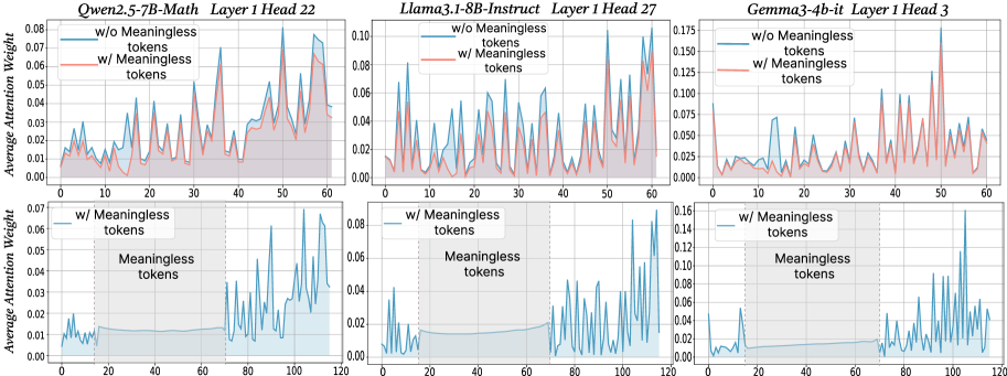</details> Figure 2: The x-axis shows token indices. Subsequent tokens assign lower average attention weights to the original prompt overall, while meaningless tokens receive similarly near-zero weights. We show additional average attention weights in Appendix I and layer-wise analyses in Section F.4. $\text{Attention}(Q,K,V)=\text{softmax}\!\left(\frac{QK^{→p}}{\sqrt{d_{k}}}\right)V$ , where $Q$ , $K$ , $V$ are query vectors, key vectors and value vectors respectively, $d$ is the dimensionality of key/query. From this equation, adding extra tokens introduces additional terms into the softmax normalization, enlarging the softmax normalization denominator. Although the new tokens typically receive small weights, their presence redistributes probability mass and reduces the relative share of attention allocated to the original tokens. To probe the underlying case, we directly compare input’s attention weights with and without meaningless tokens while keeping tokens indices aligned in the first layers. For every token we computed the mean of its column below the diagonal of the attention matrix to measure the extent to which each token receives attention from all downstream tokens (Bogdan et al., 2025). When a string of meaningless tokens are present, the model assigns only small weights to each token, intuitively indicating that the model only pays little attention to them (see Figure 2 bottom row). The top row of Figure 2 presents a direct comparison of the attention to meaningful tokens without (blue) or with meaningless tokens (red; meaningless token indices are removed from visualization to allow for direct comparison). Among meaningful tokens, the average attention is decreased in the meaningless-token condition, especially driven by decreased high-attention spikes. The attention weights of the original prompt after inserting meaningless tokens are: $W^{\prime}=\lambda·\text{softmax}\!\left(\frac{QK^{→p}}{\sqrt{d_{k}}}\right)$ , where $W_{attn}$ are the attention weights after softmax, and $\lambda$ is the drop percentage of attention weights in the original prompt after adding meaningless tokens. Then, the attention output for each token not only obtains the weighted combination of the original tokens, but also includes attention weights and values from the meaningless tokens. Thus, the attention output can be expressed as: $$ \text{Attn\_Output}_{new}=W_{j}^{\prime}V_{j}+W_{i}V_{i}, \tag{1} $$ <details> <summary>x3.png Details</summary>  ### Visual Description ## Scatter Plot: Attention Output Displacement ### Overview This image presents a scatter plot comparing the attention output with and without meaningless tokens. The plot visualizes the displacement between these two outputs, indicated by arrows connecting corresponding points. Two curved lines approximate the general trend of each data set. ### Components/Axes * **X-axis:** The x-axis is not explicitly labeled, but represents a numerical value ranging approximately from 0 to 10. The scale is linear with markers at integer values. * **Y-axis:** The y-axis is also not explicitly labeled, but represents a numerical value ranging approximately from 0 to 6. The scale is linear with markers at integer values. * **Legend:** Located in the top-left corner, the legend defines the following: * Blue 'x' markers: "Attn\_output w/o meaningless tokens" * Red 'x' markers: "Attn\_output w/ meaningless tokens" * Blue dashed arrows: "Displacement from x to x" * Blue dotted line: "Attn\_output set w/o meaningless tokens" * Red solid line: "Attn\_output set w/ meaningless tokens" ### Detailed Analysis The plot contains two sets of scattered data points, one in blue and one in red. Each point represents an attention output value. Arrows connect corresponding points in the two sets, illustrating the displacement caused by the inclusion of meaningless tokens. Two curved lines approximate the trend of each data set. **Blue Data (w/o meaningless tokens):** The blue data points (Attn\_output w/o meaningless tokens) generally follow an upward trend, starting from approximately (0.5, 0.5) and reaching approximately (9.5, 5.5). The blue dotted line (Attn\_output set w/o meaningless tokens) provides a smoothed representation of this trend. * Approximate data points (x, y): (0.5, 0.5), (1.5, 1.0), (2.5, 1.5), (3.5, 2.0), (4.5, 2.5), (5.5, 3.0), (6.5, 3.5), (7.5, 4.0), (8.5, 4.5), (9.5, 5.5). **Red Data (w/ meaningless tokens):** The red data points (Attn\_output w/ meaningless tokens) also exhibit an upward trend, but are generally shifted to the right and slightly above the blue data. The red solid line (Attn\_output set w/ meaningless tokens) represents this trend. * Approximate data points (x, y): (1.0, 1.0), (2.0, 1.5), (3.0, 2.5), (4.0, 3.0), (5.0, 3.5), (6.0, 4.0), (7.0, 4.5), (8.0, 5.0), (9.0, 5.5), (10.0, 6.0). **Displacement Arrows:** The blue dashed arrows indicate the direction and magnitude of the displacement between corresponding blue and red points. The arrows generally point upwards and to the right, indicating that the inclusion of meaningless tokens increases both the x and y values of the attention output. Two large, roughly elliptical shapes are drawn around the data. One encompasses the blue data, and the other the red data. ### Key Observations * The inclusion of meaningless tokens consistently shifts the attention output to higher values. * The displacement is not uniform; the magnitude of the shift varies across the range of x-values. * The trend lines suggest a roughly linear relationship between the attention output and the presence/absence of meaningless tokens. * The elliptical shapes highlight the overall distribution and spread of the data for each condition. ### Interpretation The plot demonstrates the impact of meaningless tokens on attention output. The consistent upward and rightward displacement suggests that these tokens introduce a bias, inflating the attention scores. This could be problematic in applications where accurate attention weights are crucial, as it might lead to the model focusing on irrelevant information. The trend lines provide a visual summary of this effect, while the individual data points and displacement arrows reveal the variability in the impact of meaningless tokens. The elliptical shapes suggest that the data is somewhat clustered, but also exhibits some degree of spread, indicating that the effect of meaningless tokens is not entirely consistent. The visualization strongly suggests that removing meaningless tokens is beneficial for obtaining more accurate and reliable attention outputs. 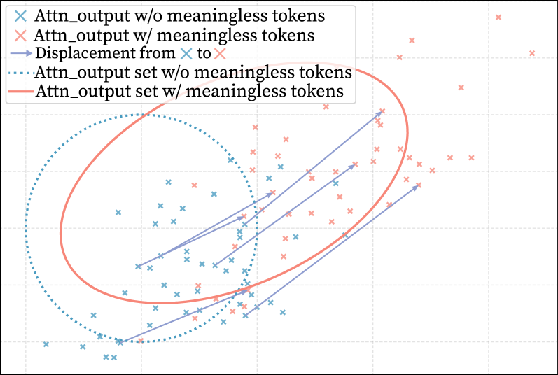</details> Figure 3: After adding meaningless tokens, each token vector is affinely transformed: blue points show the original vectors, and red points show them after the addition. Arrow is change direction. where Attn_Output corresponds to the output of attention mechanism for each token in the original prompt, $W_{j}^{\prime}$ and $V_{j}$ are the attention weight and value vectors of the original prompt, and $W_{i}$ and $V_{i}$ are the attention weight and value vectors of meaningless tokens. As the meaningless tokens are repeated in long sequences and contribute no semantic information, the values of these tokens are identical, and their attention weights are small in a similar magnitude. Therefore, as shown in Equation 1, the term $W_{i}V_{i}$ primarily shifts the final attention output along an approximately unified direction as they accumulate, without introducing diverse semantic components. In this formula, $W_{j}V_{j}$ is the value of original attention output, we see $W_{i}V_{i}$ as $\Sigma_{\sigma}$ . As a result, the attention output of meaningful tokens after adding meaningless tokens can be seen as an affine transformation expressed as: $$ \text{Attn\_Output}_{new}=\lambda\cdot\text{Attn\_Output}+\Sigma_{\sigma}, \tag{2} $$ where Attn_Output is $W_{j}V_{j}$ . Following this equation, the introduction of meaningless tokens transforms the attention output of meaningful tokens into an affine function, consisting of a scaled original term ( $\lambda·\text{Attn\_Output}$ ) and an additional bias ( $\Sigma_{\sigma}$ ). Figure 3 illustrates the process of this transformation. After the attention module the affine transformed output passes through RMSNorm and serves as the input to the MLP. In the next section, we examine in detail how this transformation propagates through the subsequent MLP layers and shapes the model’s overall activation distribution. 3 Analysis: Why Affine Transformation Improve Reasoning Performance Having established in the previous sections that meaningless-token effect induces scaling and bias terms that produce an affine transformation of the attention output, we next examine how this transformation propagates through the subsequent MLP modules and affects reasoning. In Equation 2, we decompose the transformation’s influencing factors into two primary components: the scaling factors $\lambda$ controls the magnitude of activations, and the bias factors $\Sigma_{\sigma}$ , a bounded zero-mean bias term reflecting the variation in attention outputs before and after meaningless-token insertion which introduce structured shifts in the activation distribution. Together, these two factors determine how the transformed attention representations shape the dynamics of the MLP layers. 3.1 Affine Transformation influence the output of gate layer Key Takeaway We demonstrate that applying an affine transformation, through both scaling and bias factors, systematically increases the variance of the gate layer’s output. In this part, we show that these two factors increase the gate projection layer variance in MLP layer. As discussed above, because these tokens have low attention weights and nearly identical values, they shift the RMSNorm input almost entirely along a single direction with small margin; consequently, RMSNorm largely absorbs this change, producing only a minor numerical adjustment without adding semantic information. Specifically, the two factors act through different mechanisms. For the scaling factors, before entering the MLP, the attention output undergoes output projection and residual connection, which can be written as $x(\lambda)=\text{res}+\lambda*\text{U}*\text{A}$ , where A is the attention output and U the projection weights. Treating $\lambda$ as a functional variable, the RMSNorm output becomes $y(\lambda)=\text{RMS}(x(\lambda))$ . For the $j$ -th gate dimension, $z_{j}(\lambda)=w_{j}^{→p}y(\lambda)$ , and a small variation $\Delta\lambda$ leads to the variance change of this dimension. $$ \text{Var}[z_{j}(\lambda+\Delta\lambda)]=\text{Var}[z_{j}(\lambda)]+2\text{Cov}(z_{j}(\lambda),g_{j}(\lambda))\Delta\lambda+\text{Var}[g_{j}(\lambda)]\Delta\lambda^{2}, \tag{3} $$ the third term in Equation 3 remains strictly positive for all admissible parameters. Moreover, as $\Delta\lambda$ increases, this term exhibits monotonic growth and asymptotically dominates the second term, thereby guaranteeing a strictly increasing overall variance. We analyze the range of $\Delta\lambda$ in Appendix E. In the case of bias factors, we model the perturbation as stochastic noise which is bounded, zero-mean and statistically independent from the original attention output across all dimensions, which contributes an additional variance component and interacts non-trivially with the subsequent RMSNorm operation. Formally, after noise injection, the RMSNorm input can be written as $x=x_{0}+W\Sigma_{\sigma}$ , where $W$ is the linear coefficient of matrix $x$ preceding RMSNorm. After normalization, the covariance of the output can be expressed as: $$ \text{Cov}(y)=J_{q}\text{Cov}(x)J_{q}^{{\top}}+o(\|x-x_{0}\|^{2}) \tag{4} $$ where $x_{0}$ is the mean expansion point, $J_{q}$ is the Jacobian matrix of the RMSNorm mapping. Since the variance of the added perturbation is very small, the higher-order terms can be disregarded. In this case, the bias factor will bias the input of RMSNorm and lead to an increase in the covariance $\mathrm{Cov}(y)$ . Subsequently, the input to the activation function can be written as $z=W_{gate}(x+W\Sigma_{\sigma})$ . Based on the properties of the covariance, the variance of the $j$ -th dimension is given by: $$ \text{Var}[z_{j}]\approx e_{j}^{\top}W_{gate}[J_{q}\text{Cov(x)}J_{q}^{{\top}}]W_{gate}^{\top}e_{j}, \tag{5} $$ since the projection of the vector onto the tangent space is almost never zero in LLMs’ high dimensions, the resulting variance must be strictly greater than zero. From this, we can deduce that these two factors increase the variance of the output. In general, the scaling factors increase variance by amplifying inter-sample differences, whereas the bias factors correspondingly increase variance by enlarging the covariance structure across dimensions. 3.2 Variance change leads to activation redistribution Key Takeaway Our analysis shows that an increase in the input variance of activation functions broadens and reshapes the output activation distribution by raising both its mean and its variance. As the variance of gate layer outputs grows under perturbations, the subsequent activation function further reshapes these signals by compressing values near zero. This motivates redistributing near-zero activations. For each sample in the hidden state, the second-order Taylor expansion on $\phi$ , the activation function output is: $$ \phi(\mu+\sigma)=\phi(\mu)+\phi^{{}^{\prime}}(\mu)\sigma+\frac{1}{2}\phi^{{}^{\prime\prime}}(\mu)\sigma^{2}+o(|\sigma|^{3}), \tag{6} $$ where $\sigma$ can represent both $\Delta k$ in scaling factor and $\Sigma_{\sigma}$ in bias factor. We denote the input to the activation function as $z=\mu+\sigma$ . For the $j$ -th dimension of the hidden state, the expectation and variance of the activation output can be expressed as: $$ \mathbb{E}[\phi(z_{j})]=\mathbb{E}[\phi(\mu_{j})]+\mathbb{E}[\phi^{{}^{\prime}}(\mu_{j})\sigma]+\mathbb{E}[\frac{1}{2}\phi^{{}^{\prime\prime}}(\mu_{j})\sigma^{2}]+o(\mathbb{E}|\sigma|^{3}), \tag{7} $$ $$ \text{Var}[\phi(z_{j})]=\phi^{{}^{\prime}}(\mu_{j})^{2}\text{Var}_{j}+o(\text{Var}_{j}^{2}). \tag{8} $$ From above equations, We infer that distributional changes map to variations in expectation and variance. On a single dimension, activations shift in both directions; from Equation 6, higher-order terms are negligible, and the first derivative of GeLU/SiLU near zero is positive. Since perturbations include both signs, extrapolated activations also fluctuate around zero. From Equation 7, $\mathbb{E}[\sigma^{2}]=\text{Var}_{j}$ . For the bias factor, the zero-mean perturbation removes the first-order term. For scaling factors, expanding at the population mean gives $\mathbb{E}[\phi^{{}^{\prime}}(z_{j})g_{j}]=0$ , again canceling the first order. The second derivative near zero is strictly positive. From Equation 8, $\text{Var}_{j}$ increases, and so does the activation histogram variance, as the function is nearly linear near zero. In summary, scaling and bias factors jointly enlarge activation variance, expressed as: $$ \text{Var}_{j}\approx{\color[rgb]{0.28515625,0.609375,0.75390625}\definecolor[named]{pgfstrokecolor}{rgb}{0.28515625,0.609375,0.75390625}\mathbb{E}[\text{Var}_{j}^{(\Sigma_{\sigma})}]}+{\color[rgb]{0.96875,0.53125,0.47265625}\definecolor[named]{pgfstrokecolor}{rgb}{0.96875,0.53125,0.47265625}\text{Var}(g_{j}^{\lambda})}. \tag{9} $$ <details> <summary>x4.png Details</summary>  ### Visual Description \n ## Bar Chart: Sparsity, L1 Norm, L2 Norm, and Gini Comparison with/without Transformation ### Overview This image presents a comparative bar chart showing the values of Sparsity, L1 Norm, L2 Norm, and Gini for three different models: Qwen2.5-7B-Math, Llama3.1-8B-Instruct, and Gemma3-4b-it. Each model is presented in two conditions: with transformation (left) and without transformation (right). The bars are color-coded, with a light blue/red scheme. Each chart also includes a density plot along the x-axis. ### Components/Axes * **X-axis:** Represents the metrics: Sparsity, L1 Norm, L2 Norm, and Gini. * **Y-axis:** Represents the values of the metrics, ranging from 0 to 700,000 (left charts) and 0 to 50,000 (middle chart) and 0 to 400,000 (right chart). * **Legend:** Located at the top-left corner, indicates that light blue bars represent "w/ transformation" and light red bars represent "w/o transformation". * **Model Labels:** Located at the bottom of each chart, identifying the model being analyzed: Qwen2.5-7B-Math, Llama3.1-8B-Instruct, and Gemma3-4b-it. * **Density Plots:** Red shaded areas along the x-axis, likely representing the distribution of values for each metric. ### Detailed Analysis or Content Details **Qwen2.5-7B-Math:** * **Sparsity (w/ transformation):** Approximately 0.185. * **L1 Norm (w/ transformation):** Approximately 0.160. * **L2 Norm (w/ transformation):** Approximately 0.120. * **Gini (w/ transformation):** Approximately 0.045. * **Sparsity (w/o transformation):** Approximately 0.0. * **L1 Norm (w/o transformation):** Approximately 0.0. * **L2 Norm (w/o transformation):** Approximately 0.0. * **Gini (w/o transformation):** Approximately 0.40. **Llama3.1-8B-Instruct:** * **Sparsity (w/ transformation):** Approximately 0.10. * **L1 Norm (w/ transformation):** Approximately 4.50. * **L2 Norm (w/ transformation):** Approximately 7.00. * **Gini (w/ transformation):** Approximately 4.30. * **Sparsity (w/o transformation):** Approximately 0.0. * **L1 Norm (w/o transformation):** Approximately 12.0. * **L2 Norm (w/o transformation):** Approximately 13.0. * **Gini (w/o transformation):** Approximately 5.00. **Gemma3-4b-it:** * **Sparsity (w/ transformation):** Approximately 0.10. * **L1 Norm (w/ transformation):** Approximately 1.4. * **L2 Norm (w/ transformation):** Approximately 0.6. * **Gini (w/ transformation):** Approximately 1.0. * **Sparsity (w/o transformation):** Approximately 0.6. * **L1 Norm (w/o transformation):** Approximately 0.0. * **L2 Norm (w/o transformation):** Approximately 0.0. * **Gini (w/o transformation):** Approximately 0.0. ### Key Observations * The "w/ transformation" condition consistently shows lower L1 and L2 Norm values compared to the "w/o transformation" condition for all three models. * Sparsity is generally low for the "w/o transformation" condition, often close to zero. * Gini values vary significantly between models and conditions. * The density plots show a concentration of values near zero for the "w/o transformation" condition, particularly for L1 and L2 Norms. ### Interpretation The data suggests that applying the transformation significantly impacts the sparsity, L1 norm, L2 norm, and Gini index of the models. The transformation appears to reduce the L1 and L2 norms, indicating a more compressed or regularized representation. The differences in Gini values suggest that the transformation affects the distribution of weights within the models. The near-zero values for L1 and L2 norms in the "w/o transformation" condition, coupled with the density plots, indicate that the models without transformation have a highly concentrated weight distribution, potentially leading to overfitting or reduced generalization ability. The transformation seems to introduce more diversity in the weight distribution, as reflected in the higher Gini values and non-zero L1/L2 norms. The Gemma3-4b-it model exhibits a particularly strong effect from the transformation, with a substantial decrease in L1 and L2 norms. This suggests that the transformation is more effective for this model. 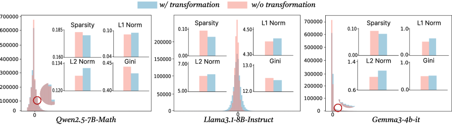</details> Figure 4: The histogram of the frequency of activations after activation functions in MLP, the sub-figure is the comparison of 4 metrics between before and after transformation. The first term represents the expected variance of the $j$ -th hidden states under the influence of the bias factor. Since the bias factor varies across individual cases, taking the expectation is necessary to capture its overall impact. The second term corresponds to the variance induced by scaling factors, which inherently reflects the aggregate change. When combining them, the overall variance of the outputs of nonlinear activation functions increases, the mean shifts upward, and the activation distribution becomes broader, manifested as heavier tails and a thinner center. More details of above analysis and relative proof are in Appendix E. Moreover, we presume the reason that this redistribution has a positive impact on reasoning tasks is that reasoning-critical tokens (digits, operators, conjunctions) have a higher fraction of near-zero activations. Elevating their activation levels strengthens their representations and improves reasoning performance; see Section 6 for details. 3.3 Verification of activation redistribution To verify whether the activation redistribution pattern in Section 3.2 indeed occurs in LLMs, Figure 4 illustrates the activation distribution after the first-layer MLP, explicitly comparing states before and after the transformation defined in Equation 2. We also comprehensively assess the transformation of activation states using several quantitative indicators, including: - Relative Sparsity: Defined as the proportion of activations after the transformation whose values fall below the pre-transformation threshold. - L1 Norm: The sum of the absolute activation values; smaller values indicate higher sparsity. - L2 Norm: A measure of the overall magnitude of activations. - Gini Coefficient: An indicator of the smoothness of the histogram distribution, where smaller absolute values correspond to smoother distributions. From Figure 4, we observe that after transformation, the frequency of near-zero activations decreases, while the frequency of absolute high-magnitude activations increases. Both sparsity and smoothness in the activation distribution are improved. Specifically, the relative sparsity consistently decreases across all three models while the L1 and L2 norms increase, aligning with the previous phenomenon. 4 Method: Activation Redistribution Module <details> <summary>x5.png Details</summary>  ### Visual Description \n ## Diagram: Layer 1 Architecture ### Overview This diagram illustrates the architecture of Layer 1 in a neural network, likely a transformer-based model. It depicts the flow of data through several components, including Attention, RoPE, RMSNorm, MLP (Multi-Layer Perceptron), and activation functions. The diagram also includes visualizations of data distribution before and after a redistribution process. ### Components/Axes The diagram is segmented into three main regions: a left-side processing chain, a central MLP block, and a right-side visualization of data distributions. * **Left Side:** * "Output" * "Attention" * "RoPE" * "Q K V" (Query, Key, Value) * "RMSNorm" * **Central MLP Block:** * "MLP" (title) * "down" * "up" * "ARM" * "SiLU/GeLU" * "gate" * "RMSNorm" * **Right Side:** * "before redistribution" (title of top histogram) * "after redistribution" (title of bottom histogram) * X-axis: Numerical scale, ranging from approximately -4 to +4. * Y-axis: Represents frequency or probability density. ### Detailed Analysis or Content Details The diagram shows a data flow starting from the bottom with "RMSNorm". The output of "RMSNorm" feeds into "Q K V". The output of "Q K V" is then passed to "RoPE", which in turn feeds into "Attention". The output of "Attention" is labeled "Output". The "MLP" block receives input from "RMSNorm" (bottom) and "Attention" (top). Inside the MLP: * The input splits into two paths: "up" and "down". * "down" feeds into "ARM" and then into "SiLU/GeLU". * "up" feeds into "RMSNorm" and then into "gate". * The outputs of "ARM/SiLU/GeLU" and "gate" are combined at a circular node (likely an addition operation). The right side shows two histograms: * **Before Redistribution:** The histogram is multi-modal, with several peaks. The peaks are centered around approximately -2.5, -1, 0, +1, and +2.5. The height of the peaks are roughly equal. Arcs are drawn from the top of each peak to the x-axis, indicating the spread of the distribution. * **After Redistribution:** The histogram is unimodal, centered around approximately 0. The distribution is more concentrated and has a narrower spread than the "before redistribution" histogram. ### Key Observations * The diagram illustrates a typical transformer layer structure with attention and a feedforward network (MLP). * The MLP block includes a complex internal structure with "ARM", "SiLU/GeLU", and "gate" components. * The redistribution process appears to transform a multi-modal distribution into a unimodal distribution, suggesting a regularization or normalization effect. * The circular node within the MLP suggests an additive operation. ### Interpretation The diagram likely represents a component within a larger neural network architecture, possibly a transformer model. The "RoPE" component suggests the use of Rotary Positional Embeddings, a technique for incorporating positional information into the attention mechanism. The MLP block is designed to process the output of the attention mechanism and introduce non-linearity. The redistribution process, as visualized by the histograms, is a key aspect of the architecture. It transforms a potentially complex and dispersed distribution into a more focused and stable distribution. This could be a form of normalization, regularization, or feature selection. The change from a multi-modal to a unimodal distribution suggests that the redistribution process is reducing the variance and concentrating the data around a central value. The diagram provides a high-level overview of the data flow and component interactions within Layer 1. It does not provide specific numerical values or parameters, but it conveys the overall structure and functionality of the layer. </details> ⬇ def forward (x, layer_idx): # in first layer activation = self. act_fn (self. gate_proj (x)) #Our function activation_alter = self. arm (activation. clone ()) down_proj = self. down_proj (activation_alter * self. 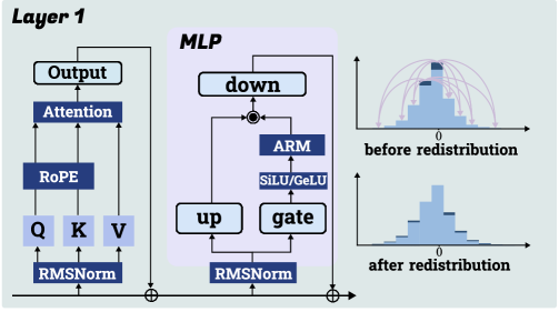up_proj (x)) return down_proj Figure 5: The upper panel illustrates the first-layer LLM architecture with ARM, while the lower panel presents the corresponding ARM code in the MLP module. Inspired by the previous finding that meaningless tokens can shift meaningful activations and boost LLM performance, we propose ARM—a simple method replacing explicit meaningless tokens with an implicit mechanism that adjusts the MLP activation distribution after the activation function. Our approach has two steps: First, adaptively identify a proportion of near-zero activations based on the model and input; Then, extrapolate them outward to redistribute the activation pattern. The top half of Figure 5 shows the first-layer MLP with ARM, where selected activations around zero are shifted outward, reducing their frequency and increasing larger-magnitude activations. The bottom half of Figure 5 presents the ARM-specific code, a lightweight function inserted into the first-layer MLP without affecting inference speed. As shown in Appendix D, ARM’s time complexity is negligible within the MLP context. The significance of the ARM method is twofold. Firstly, it adds further evidence deductively supporting our theoretical analysis in Section 3. By directly replacing explicit meaningless token insertion with implicit activation redistribution, ARM yields a similar improvement in reasoning across models and benchmarks, thus strengthening our theoretical framework. Secondly, we introduce ARM as a lightweight inference time trick for boosting reasoning, which is not only robustly effective on its own (see experiments in Section 5) but also compatible with existing inference time scaling methods (see Appendix G.3). 4.1 Select Appropriate Change proportion Our method first selects a proportion of activations to be modified. However, different models exhibit varying sensitivities to meaningless tokens. To address this, we propose a dynamic strategy that adjusts the fraction of near-zero activations to be altered during inference. To determine this proportion, we measure the dispersion of activations around zero. Specifically, we define a neighborhood $\epsilon$ based on the activation distribution to identify which activations are considered “close to zero”. We adopt the Median Absolute Deviation (MAD) as our dispersion metric, since MAD is robust to outliers and better captures the core distribution. The threshold $\epsilon$ is given by: $\epsilon=\kappa*\text{MAD}*c$ , where $\kappa$ is a consistency constant, $c$ is a hyperparameter controlling the width of the near-zero range. Next, we compute the fraction of activations falling within $[-\epsilon,\epsilon]$ This fraction $p$ represents the proportion of activations that we think to be near zero. As a result, the fraction we want to change is $\text{fraction}=clip(p,(p_{\text{min}},p_{\text{max}}))$ . Here, $p$ denotes the calculated fraction, while $p_{\text{min}}$ and $p_{\text{max}}$ serve as bounds to prevent the scale from becoming either too small or excessively large. In our experiments, we set $p_{\text{min}}=0.02$ and $p_{\text{max}}=0.25$ . 4.2 Redistribution of Activation Values After selecting the elements, we preserve its sign and adjust only its magnitude. Specifically, we add a positive or negative value depending on the element’s sign. To constrain the modified values within a reasonable range, the range is defined as follows: $$ \text{R}=\begin{cases}[0,\text{Q}_{p_{1}}(\text{Activations)}],&\text{sign}=1,\\[6.0pt] [\text{min(Activations)},0],&\text{sign}=-1.\end{cases} \tag{10} $$ Where R is the range of modified values. In this range, we set the lower bound to the minimum activation value when $\text{sign}=-1$ , since activation functions such as SiLU and GeLU typically attain their smallest values on the negative side. For the upper bound when $\text{sign}=1$ , we select the value corresponding to the $p_{1}$ -th percentile of the activation distribution. Here, $p_{1}$ is a hyperparameter that depends on the distribution of activations. $\text{Q}_{p_{1}}(\text{Activations)}$ is the upper bound when we changing the chosen activations. The value of $p_{1}$ depends on the distribution of activations and the value of $c$ . Finally, we generate a random value in R and add it to the activation in order to modify its value. In this way, we adaptively adjust an appropriate proportion of activations, enriching the distribution with more effective values. We shows how to choose hyperparameter in Appendix H. Table 2: After adding ARM to the first-layer MLP, we report reasoning-task performance for six models, using a dash (‘–’) for accuracies below 5% to indicate incapability. | Model | Setting | GPQA Diamond | Math-500 | AIME 2024 | AIME 2025 | LiveCodeBench | Humaneval | | --- | --- | --- | --- | --- | --- | --- | --- | | Pass@1 | Pass@1 | Pass@1 | Pass@1 | Pass@1 | Pass@1 | | | | Qwen2.5 Math-1.5B | Baseline | 27.3 | 63.8 | 14.4 | 6.7 | - | 6.1 | | \cellcolor cyan!15ARM | \cellcolor cyan!1528.8 | \cellcolor cyan!1567.0 | \cellcolor cyan!1518.9 | \cellcolor cyan!1510.0 | \cellcolor cyan!15- | \cellcolor cyan!158.5 | | | \cellcolor gray!15 Improve Rate (%) | \cellcolor gray!15 1.5 $\uparrow$ | \cellcolor gray!15 3.2 $\uparrow$ | \cellcolor gray!15 4.5 $\uparrow$ | \cellcolor gray!15 3.3 $\uparrow$ | \cellcolor gray!15 - | \cellcolor gray!15 2.4 $\uparrow$ | | | Qwen2.5 Math-7B | Baseline | 30.3 | 72.4 | 23.3 | 10.0 | - | 15.2 | | \cellcolor cyan!15ARM | \cellcolor cyan!1534.9 | \cellcolor cyan!1573.4 | \cellcolor cyan!1525.6 | \cellcolor cyan!1513.3 | \cellcolor cyan!15- | \cellcolor cyan!1517.7 | | | \cellcolor gray!15 Improve Rate (%) | \cellcolor gray!15 4.6 $\uparrow$ | \cellcolor gray!15 1.0 $\uparrow$ | \cellcolor gray!15 2.3 $\uparrow$ | \cellcolor gray!15 3.3 $\uparrow$ | \cellcolor gray!15 - | \cellcolor gray!15 2.5 $\uparrow$ | | | Qwen2.5 7B-Instruct | Baseline | 28.3 | 61.4 | 20.0 | 10.0 | 29.7 | 43.9 | | \cellcolor cyan!15ARM | \cellcolor cyan!1529.8 | \cellcolor cyan!1562.4 | \cellcolor cyan!1520.0 | \cellcolor cyan!1523.3 | \cellcolor cyan!1531.9 | \cellcolor cyan!1547.6 | | | \cellcolor gray!15 Improve Rate (%) | \cellcolor gray!15 1.5 $\uparrow$ | \cellcolor gray!15 1.0 $\uparrow$ | \cellcolor gray!150 | \cellcolor gray!15 13.3 $\uparrow$ | \cellcolor gray!15 2.2 $\uparrow$ | \cellcolor gray!15 3.7 $\uparrow$ | | | Qwen2.5 32B-Instruct | Baseline | 35.4 | 82.6 | 16.7 | 20.0 | 49.5 | 50.0 | | \cellcolor cyan!15ARM | \cellcolor cyan!1535.9 | \cellcolor cyan!1582.6 | \cellcolor cyan!1518.8 | \cellcolor cyan!1526.7 | \cellcolor cyan!1549.5 | \cellcolor cyan!1551.2 | | | \cellcolor gray!15 Improve Rate (%) | \cellcolor gray!15 0.5 $\uparrow$ | \cellcolor gray!150 | \cellcolor gray!15 2.1 $\uparrow$ | \cellcolor gray!15 6.7 $\uparrow$ | \cellcolor gray!150 | \cellcolor gray!15 1.2 $\uparrow$ | | | Llama3.1 8B-Instruct | Baseline | 28.3 | 43.0 | 11.1 | - | 11.9 | 45.7 | | \cellcolor cyan!15ARM | \cellcolor cyan!1531.3 | \cellcolor cyan!1545.8 | \cellcolor cyan!1513.3 | \cellcolor cyan!15- | \cellcolor cyan!1517.0 | \cellcolor cyan!1547.6 | | | \cellcolor gray!15 Improve Rate (%) | \cellcolor gray!15 3.0 $\uparrow$ | \cellcolor gray!15 2.8 $\uparrow$ | \cellcolor gray!15 2.2 $\uparrow$ | \cellcolor gray!15- | \cellcolor gray!15 5.1 $\uparrow$ | \cellcolor gray!15 1.9 $\uparrow$ | | | Gemma3 4b-it | Baseline | 34.3 | 72.6 | 13.3 | 20.0 | 20.2 | 17.1 | | \cellcolor cyan!15ARM | \cellcolor cyan!1535.9 | \cellcolor cyan!1574.0 | \cellcolor cyan!1517.8 | \cellcolor cyan!1523.3 | \cellcolor cyan!1520.6 | \cellcolor cyan!1520.7 | | | \cellcolor gray!15 Improve Rate (%) | \cellcolor gray!15 1.5 $\uparrow$ | \cellcolor gray!15 1.4 $\uparrow$ | \cellcolor gray!15 4.5 $\uparrow$ | \cellcolor gray!15 3.3 $\uparrow$ | \cellcolor gray!15 0.4 $\uparrow$ | \cellcolor gray!15 3.6 $\uparrow$ | | | Gemma3 27b-it | Baseline | 33.3 | 85.4 | 25.6 | 26.7 | 31.9 | 9.1 | | \cellcolor cyan!15ARM | \cellcolor cyan!1533.8 | \cellcolor cyan!1586.2 | \cellcolor cyan!1531.1 | \cellcolor cyan!1530.0 | \cellcolor cyan!1534.2 | \cellcolor cyan!1511.6 | | | \cellcolor gray!15 Improve Rate (%) | \cellcolor gray!15 0.5 $\uparrow$ | \cellcolor gray!15 0.8 $\uparrow$ | \cellcolor gray!15 4.4 $\uparrow$ | \cellcolor gray!15 3.3 $\uparrow$ | \cellcolor gray!15 2.3 $\uparrow$ | \cellcolor gray!15 2.5 $\uparrow$ | | 5 Experiments We evaluate our method on reasoning and non-reasoning tasks using seven models: Qwen2.5-Math-1.5B, Qwen2.5-Math-7B, Qwen2.5-Instruct-7B, Qwen2.5-Instruct-32B (qwe, 2025), Llama3.1-8B-Instruct (gra, 2024), Gemma3-4b-it, and Gemma3-27b-it (gem, 2025). All models use default generation parameters. For reasoning tasks, we cover three skill areas: (1) General: GPQA (Rein et al., 2024), a challenging expert-authored multiple-choice dataset; (2) Math & Text Reasoning: MATH-500 (Lightman et al., 2023), AIME’24 (AIME, 2024), and AIME’25 (AIME, 2025); (3) Agent & Coding: LiveCodeBench (Jain et al., 2024) and HumanEval (Chen et al., 2021). For non-reasoning tasks, we use GSM8K (Cobbe et al., 2021), ARC-E (Clark et al., 2018), ARC-C (Clark et al., 2018), MMLU (Hendrycks et al., 2021), BoolQ (Clark et al., 2019), HellaSwag (Zellers et al., 2019), and OpenBookQA (Mihaylov et al., 2018). 5.1 Experiment Results Analysis For reasoning tasks, the results in Table 2 show pass@1 accuracy across multiple benchmarks. Our method consistently improves performance across most models and datasets, with the effect more pronounced in smaller models (e.g., Qwen2.5-Math-7B shows larger gains than Qwen2.5-32B-Instruct). On challenging benchmarks, however, improvements are limited when models lack sufficient capacity or when baseline accuracy is near saturation. For non-reasoning tasks (see 3(b)), applying ARM to the first-layer MLP yields little change. We attribute this to their largely factual nature, where models already have the necessary knowledge and response formats, requiring minimal reasoning. By contrast, for reasoning tasks, altering early activations helps reorganize knowledge, strengthens intermediate representations, and facilitates more effective and consistent reasoning. 5.2 Comparison of Meaningless tokens and ARM In 3(a), we provide a direct comparison between our proposed ARM method and the strategy of inserting a suitable number of meaningless tokens. The results demonstrate that both approaches are capable of improving model performance and neither requires post-training, therefore presenting lightweight interventions that lead to robust performance gains. However, since ARM directly utilizes the fundamental principle driving the meaningless-token effect, it provides more stable results. While the meaningless-token effect is pervasive, our experiments show that the effect itself depends heavily on the specific choice of token length and placement, and thus may be unstable or difficult to generalize across tasks. ARM provides a more principled and model-internal mechanism that directly reshapes the activation distribution within the MLP, yielding more consistent gains without relying on heuristic token engineering. In sum, while the insertion of a meaningless token string on the prompt level might seem like a promising prompt-tuning adjustment on the surface, it comes with an instability of the effect which ARM eliminates. This contrast highlights the trade-off between ease of use and robustness, and further underscores the value of ARM as a systematic method for enhancing the reasoning ability in large language models. <details> <summary>x6.png Details</summary>  ### Visual Description \n ## Bar Charts: Performance Comparison of Baseline and ARM Models ### Overview The image presents three bar charts comparing the performance of "Baseline" and "ARM" models across three different metrics: Pass@3 on Math-500, Pass@3 on AIME2024, and 2-gram diversity score. The x-axis of each chart represents different models: Qwen2.5-Math-1.5B, Gemma3-4b-it, and Qwen2.5-Math-7B. ### Components/Axes * **Chart 1:** * Title: "Pass@3 on Math-500" * X-axis: Model names (Qwen2.5-Math-1.5B, Gemma3-4b-it, Qwen2.5-Math-7B) * Y-axis: Accuracy (ranging from 0.60 to 0.90) * Legend: * Baseline (Light Green) * ARM (Dark Green) * **Chart 2:** * Title: "Pass@3 on AIME2024" * X-axis: Model names (Qwen2.5-Math-1.5B, Gemma3-4b-it, Qwen2.5-Math-7B) * Y-axis: Pass@3 Score (ranging from 0.15 to 0.40) * Legend: * Baseline (Light Red) * ARM (Dark Red) * **Chart 3:** * Title: "2-gram diversity score" * X-axis: Model names (Qwen2.5-Math-1.5B, Gemma3-4b-it, Qwen2.5-Math-7B) * Y-axis: Diversity score (ranging from 0.1 to 0.6) * Legend: * Baseline (Light Blue) * ARM (Dark Blue) ### Detailed Analysis or Content Details **Chart 1: Pass@3 on Math-500** * Qwen2.5-Math-1.5B: Baseline ≈ 0.72, ARM ≈ 0.78 * Gemma3-4b-it: Baseline ≈ 0.82, ARM ≈ 0.85 * Qwen2.5-Math-7B: Baseline ≈ 0.85, ARM ≈ 0.88 * Trend: ARM consistently outperforms Baseline across all models. The performance increases with model size. **Chart 2: Pass@3 on AIME2024** * Qwen2.5-Math-1.5B: Baseline ≈ 0.22, ARM ≈ 0.28 * Gemma3-4b-it: Baseline ≈ 0.32, ARM ≈ 0.30 * Qwen2.5-Math-7B: Baseline ≈ 0.36, ARM ≈ 0.38 * Trend: ARM generally outperforms Baseline, but the difference is smaller than in the Math-500 chart. Gemma3-4b-it shows a slight decrease in ARM performance compared to Baseline. **Chart 3: 2-gram diversity score** * Qwen2.5-Math-1.5B: Baseline ≈ 0.52, ARM ≈ 0.55 * Gemma3-4b-it: Baseline ≈ 0.58, ARM ≈ 0.57 * Qwen2.5-Math-7B: Baseline ≈ 0.60, ARM ≈ 0.60 * Trend: ARM and Baseline perform similarly, with slight variations. The diversity score appears relatively stable across different models. ### Key Observations * ARM consistently improves accuracy on the Math-500 dataset. * The performance gain from ARM is less pronounced on the AIME2024 dataset, and even slightly negative for Gemma3-4b-it. * The 2-gram diversity score is relatively consistent across models and between Baseline and ARM. * Larger models (Qwen2.5-Math-7B) generally achieve higher accuracy on Math-500. ### Interpretation The data suggests that the ARM technique is effective in improving performance on the Math-500 benchmark, indicating its ability to enhance mathematical reasoning capabilities. However, its impact on the AIME2024 benchmark is less significant, and in some cases, slightly detrimental. This could indicate that ARM is more specialized for mathematical problem-solving than general reasoning tasks. The consistent 2-gram diversity scores suggest that ARM does not significantly alter the diversity of generated responses. The positive correlation between model size and accuracy on Math-500 highlights the importance of model capacity for complex mathematical tasks. The slight dip in ARM performance for Gemma3-4b-it on AIME2024 could be due to specific characteristics of that model or dataset interaction. Further investigation is needed to understand the reasons behind this anomaly. 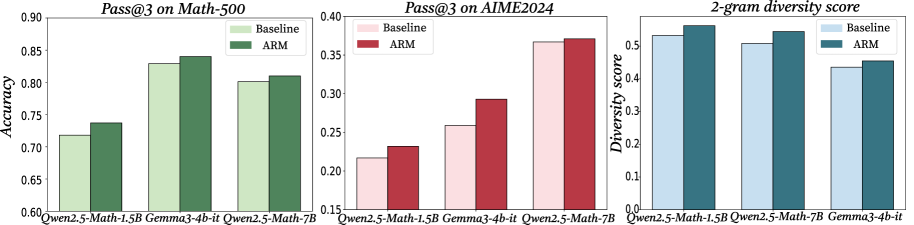</details> Figure 6: The first two figures show pass@3 on Math-500 and AIME2024 for three models with and without ARM, and the last shows their 2-gram diversity under both conditions. Table 3: Table (a) compares the performance of meaningless tokens and ARM, and Table (b) reports ARM’s results on non-reasoning tasks. (a) Pass@1 on Math-500 and AIME2024 with meaningless tokens (Mless) or ARM. | Qwen2.5 Math-7B Mless ARM | Baseline 75.0 73.4 | 72.4 24.4 25.6 | 23.3 | | --- | --- | --- | --- | | Llama3.1 8B-Instruct | Baseline | 43.0 | 11.1 | | Mless | 44.9 | 13.3 | | | ARM | 45.8 | 13.3 | | (b) Performance of models with ARM on non-reasoning tasks. Additional results are in Appendix G. | Model Qwen2.5 Math-1.5B ARM | Setting Baseline 78.6 | GSM8K 78.0 39.3 | ARC-E 39.3 39.5 | HellaSwag 39.1 | | --- | --- | --- | --- | --- | | \cellcolor gray!15 Improve Rate (%) | \cellcolor gray!15 0.6 $\uparrow$ | \cellcolor gray!150 | \cellcolor gray!15 0.4 $\uparrow$ | | | Llama3.1 8B-Instruct | Baseline | 80.0 | 46.6 | 56.8 | | ARM | 82.4 | 47.1 | 57.3 | | | \cellcolor gray!15 Improve Rate (%) | \cellcolor gray!15 2.4 $\uparrow$ | \cellcolor gray!15 0.5 $\uparrow$ | \cellcolor gray!15 0.5 $\uparrow$ | | 5.3 Exploration capabilities after ARM As discussed earlier, we hypothesize that redistributing activations enables the model to explore the reasoning space more effectively. To test this hypothesis, we evaluate the model’s pass@3 performance on the Math-500 and AIME2024 benchmarks as well as its 2-gram diversity. As shown in Figure 6, applying activation redistribution consistently yields higher pass@3 scores compared to the baselines on both tasks. In addition, the 2-gram diversity under ARM is also greater than that without ARM. These findings indicate that activation redistribution not only improves the likelihood of arriving at correct solutions within multiple samples but also promotes more diverse reasoning paths. This dual effect suggests that ARM enhances both the effectiveness and the breadth of the model’s internal reasoning processes, reinforcing our hypothesis that carefully manipulating internal activations can expand a model’s reasoning capacity without additional training or parameter growth. 6 Discussion: Why Activation Redistribution Enhances LLM Reasoning Performance <details> <summary>x7.png Details</summary>  ### Visual Description \n ## Bar Chart: Mean Ratio of Token Types by Model ### Overview This bar chart compares the mean ratio of different token types (digit, operator, conjunction, and other) for two language models: Qwen2.5-7B-Math and Llama3.1-8B-Instruct. The chart uses grouped bars to represent each token type within each model. ### Components/Axes * **X-axis:** Model Name (Qwen2.5-7B-Math, Llama3.1-8B-Instruct) * **Y-axis:** Mean\_ratio (ranging from 0.00 to 0.14) * **Legend:** * digit (light green) * operator (pale green) * conjunction (light blue) * other (pale blue) ### Detailed Analysis The chart consists of two groups of four bars, one for each model. Within each group, each bar represents the mean ratio for a specific token type. **Qwen2.5-7B-Math:** * **digit:** The light green bar for 'digit' is approximately 0.065. * **operator:** The pale green bar for 'operator' is approximately 0.055. * **conjunction:** The light blue bar for 'conjunction' is approximately 0.050. * **other:** The pale blue bar for 'other' is approximately 0.048. **Llama3.1-8B-Instruct:** * **digit:** The light green bar for 'digit' is approximately 0.135. * **operator:** The pale green bar for 'operator' is approximately 0.115. * **conjunction:** The light blue bar for 'conjunction' is approximately 0.105. * **other:** The pale blue bar for 'other' is approximately 0.090. ### Key Observations * Llama3.1-8B-Instruct consistently exhibits higher mean ratios across all token types compared to Qwen2.5-7B-Math. * For both models, the 'digit' token type has the highest mean ratio, followed by 'operator', 'conjunction', and 'other'. * The difference in mean ratios between the two models is most pronounced for the 'digit' token type. ### Interpretation The data suggests that Llama3.1-8B-Instruct is more inclined to generate or process text containing digits, operators, conjunctions, and other token types compared to Qwen2.5-7B-Math. This could indicate that Llama3.1-8B-Instruct is better suited for tasks involving mathematical reasoning or code generation, where these token types are more prevalent. The consistently higher ratios across all categories suggest a fundamental difference in the models' token distribution preferences. The large difference in the 'digit' category is particularly noteworthy, potentially indicating a stronger mathematical capability in Llama3.1-8B-Instruct. The chart provides a quantitative comparison of the token type distributions, offering insights into the models' strengths and weaknesses. 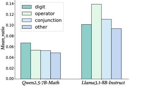</details> Figure 7: Percentage of near-zero activations across the four token types in the Math-500 dataset. We provide one possible explanation for why redistributing the near-zero activations can improve the reasoning performance of LLMs. We categorize all tokens in Math-500 into four classes: digits, conjunctions, operators, and other tokens. For each class, we compute the average proportion of activations falling within near-zero range, which reflects how many dimensions of the hidden representation remain nearly inactive. The results are presented in Figure 7. As shown, normal tokens exhibit the lowest near-zero proportion, while digits, operators, and conjunctions show substantially higher proportions, which means that in the high-frequency near-zero activations after activation function, a larger portion of them are derived from these tokens. This suggests that although these tokens are crucial for reasoning, their information is insufficiently activated by the model. Our observation is consistent with the findings of Huan et al. (2025), which highlight the increasing importance of conjunctions after reinforcement learning, and also aligns with the recognized role of digits and operators in reasoning tasks such as mathematics and coding. Consequently, redistributing activations around zero enhances the representation of under-activated yet semantically important tokens, improving reasoning performance. 7 Related Work Recent studies notice that symbols in an LLM’s input may affect their internal mechanism. Sun et al. (2024) show large activations for separators, periods, or newlines, suggesting that these tokens carry model biases. Razzhigaev et al. (2025) find that commas are essential for contextual memory, while Chauhan et al. (2025) and Min et al. (2024) highlight punctuation as attention sinks, memory aids, and semantic cues. Moreover, Chadimová et al. (2024) show that replacing words with meaningless tokens can reduce cognitive biases, whereas Li et al. (2024) report that such “glitch tokens” may also cause misunderstandings, refusals, or irrelevant outputs. Our work adds explanation to the puzzling downstream benefits that the inclusion of a string of meaningless tokens contributes to reasoning performance and shows how deep investigations of the underlying mechanisms can lead to improved inference solutions. We provide an extended discussion of related works in Appendix B. 8 Conclusion In this paper, we report a meaningless-token effect that inserting long sequences of meaningless tokens improves model performance, particularly on reasoning tasks. Our analysis suggests that it stems from the fact that meaningless tokens induce an affine transformation on meaningful tokens, thereby redistributing their activations and enabling key information to be more effectively utilized. Building on this insight, we introduce ARM, a lightweight and training-free method for activation redistribution, which strengthens our analysis and serves as a practical approach for consistently improving LLM performance on reasoning tasks. Ethics Statement All datasets used in this work are publicly available and contain no sensitive information. Our method enhances LLM reasoning without introducing new data collection or human interaction. While stronger reasoning ability may be misused, we emphasize that this work is intended for beneficial research and responsible applications. Reproducibility Statement We will release our code and data once the paper is published. The appendix includes detailed experimental setups and hyperparameters so that others can reproduce our results. We also encourage the community to follow good research practices when using our code and data, to help maintain the reliability and transparency of future work. References - gra (2024) The llama 3 herd of models, 2024. URL https://arxiv.org/abs/2407.21783. - gem (2025) Gemma 3 technical report, 2025. URL https://arxiv.org/abs/2503.19786. - qwe (2025) Qwen2.5 technical report, 2025. URL https://arxiv.org/abs/2412.15115. - AIME (2024) AIME. Aime problems and solutions, 2024. URL https://aime24.aimedicine.info/. - AIME (2025) AIME. Aime problems and solutions, 2025. URL https://artofproblemsolving.com/wiki/index.php/AIMEProblemsandSolutions. - Bogdan et al. (2025) Paul C Bogdan, Uzay Macar, Neel Nanda, and Arthur Conmy. Thought anchors: Which llm reasoning steps matter? arXiv preprint arXiv:2506.19143, 2025. - Chadimová et al. (2024) Milena Chadimová, Eduard Jurášek, and Tomáš Kliegr. Meaningless is better: hashing bias-inducing words in llm prompts improves performance in logical reasoning and statistical learning. arXiv preprint arXiv:2411.17304, 2024. - Chauhan et al. (2025) Sonakshi Chauhan, Maheep Chaudhary, Koby Choy, Samuel Nellessen, and Nandi Schoots. Punctuation and predicates in language models. arXiv preprint arXiv:2508.14067, 2025. - Chen et al. (2021) Mark Chen, Jerry Tworek, Heewoo Jun, Qiming Yuan, Henrique Ponde de Oliveira Pinto, Jared Kaplan, Harri Edwards, Yuri Burda, Nicholas Joseph, Greg Brockman, Alex Ray, Raul Puri, Gretchen Krueger, Michael Petrov, Heidy Khlaaf, Girish Sastry, Pamela Mishkin, Brooke Chan, Scott Gray, Nick Ryder, Mikhail Pavlov, Alethea Power, Lukasz Kaiser, Mohammad Bavarian, Clemens Winter, Philippe Tillet, Felipe Petroski Such, Dave Cummings, Matthias Plappert, Fotios Chantzis, Elizabeth Barnes, Ariel Herbert-Voss, William Hebgen Guss, Alex Nichol, Alex Paino, Nikolas Tezak, Jie Tang, Igor Babuschkin, Suchir Balaji, Shantanu Jain, William Saunders, Christopher Hesse, Andrew N. Carr, Jan Leike, Josh Achiam, Vedant Misra, Evan Morikawa, Alec Radford, Matthew Knight, Miles Brundage, Mira Murati, Katie Mayer, Peter Welinder, Bob McGrew, Dario Amodei, Sam McCandlish, Ilya Sutskever, and Wojciech Zaremba. Evaluating large language models trained on code. 2021. - Clark et al. (2019) Christopher Clark, Kenton Lee, Ming-Wei Chang, Tom Kwiatkowski, Michael Collins, and Kristina Toutanova. Boolq: Exploring the surprising difficulty of natural yes/no questions. In NAACL, 2019. - Clark et al. (2018) Peter Clark, Isaac Cowhey, Oren Etzioni, Tushar Khot, Ashish Sabharwal, Carissa Schoenick, and Oyvind Tafjord. Think you have solved question answering? try arc, the ai2 reasoning challenge. arXiv:1803.05457v1, 2018. - Cobbe et al. (2021) Karl Cobbe, Vineet Kosaraju, Mohammad Bavarian, Mark Chen, Heewoo Jun, Lukasz Kaiser, Matthias Plappert, Jerry Tworek, Jacob Hilton, Reiichiro Nakano, Christopher Hesse, and John Schulman. Training verifiers to solve math word problems. arXiv preprint arXiv:2110.14168, 2021. - Dhanraj & Eliasmith (2025) Varun Dhanraj and Chris Eliasmith. Improving rule-based reasoning in llms via neurosymbolic representations. arXiv e-prints, pp. arXiv–2502, 2025. - Errica et al. (2024) Federico Errica, Giuseppe Siracusano, Davide Sanvito, and Roberto Bifulco. What did i do wrong? quantifying llms’ sensitivity and consistency to prompt engineering. arXiv preprint arXiv:2406.12334, 2024. - Guan et al. (2025) Bryan Guan, Tanya Roosta, Peyman Passban, and Mehdi Rezagholizadeh. The order effect: Investigating prompt sensitivity to input order in llms. arXiv preprint arXiv:2502.04134, 2025. - Hendrycks et al. (2021) Dan Hendrycks, Collin Burns, Steven Basart, Andrew Critch, Jerry Li, Dawn Song, and Jacob Steinhardt. Aligning ai with shared human values. Proceedings of the International Conference on Learning Representations (ICLR), 2021. - Højer et al. (2025) Bertram Højer, Oliver Jarvis, and Stefan Heinrich. Improving reasoning performance in large language models via representation engineering. arXiv preprint arXiv:2504.19483, 2025. - Huan et al. (2025) Maggie Huan, Yuetai Li, Tuney Zheng, Xiaoyu Xu, Seungone Kim, Minxin Du, Radha Poovendran, Graham Neubig, and Xiang Yue. Does math reasoning improve general llm capabilities? understanding transferability of llm reasoning. arXiv preprint arXiv:2507.00432, 2025. - Jain et al. (2024) Naman Jain, King Han, Alex Gu, Wen-Ding Li, Fanjia Yan, Tianjun Zhang, Sida Wang, Armando Solar-Lezama, Koushik Sen, and Ion Stoica. Livecodebench: Holistic and contamination free evaluation of large language models for code. arXiv preprint arXiv:2403.07974, 2024. - Jiang et al. (2024) Ming Jiang, Tingting Huang, Biao Guo, Yao Lu, and Feng Zhang. Enhancing robustness in large language models: Prompting for mitigating the impact of irrelevant information. In International Conference on Neural Information Processing, pp. 207–222. Springer, 2024. - Kaul et al. (2024) Prannay Kaul, Chengcheng Ma, Ismail Elezi, and Jiankang Deng. From attention to activation: Unravelling the enigmas of large language models. arXiv preprint arXiv:2410.17174, 2024. - Kawasaki et al. (2024) Amelia Kawasaki, Andrew Davis, and Houssam Abbas. Defending large language models against attacks with residual stream activation analysis. arXiv preprint arXiv:2406.03230, 2024. - Li et al. (2024) Yuxi Li, Yi Liu, Gelei Deng, Ying Zhang, Wenjia Song, Ling Shi, Kailong Wang, Yuekang Li, Yang Liu, and Haoyu Wang. Glitch tokens in large language models: Categorization taxonomy and effective detection. Proceedings of the ACM on Software Engineering, 1(FSE):2075–2097, 2024. - Lightman et al. (2023) Hunter Lightman, Vineet Kosaraju, Yuri Burda, Harrison Edwards, Bowen Baker, Teddy Lee, Jan Leike, John Schulman, Ilya Sutskever, and Karl Cobbe. Let’s verify step by step. In The Twelfth International Conference on Learning Representations, 2023. - Liu et al. (2024) Weize Liu, Yinlong Xu, Hongxia Xu, Jintai Chen, Xuming Hu, and Jian Wu. Unraveling babel: Exploring multilingual activation patterns of llms and their applications. arXiv preprint arXiv:2402.16367, 2024. - London & Kanade (2025) Charles London and Varun Kanade. Pause tokens strictly increase the expressivity of constant-depth transformers. arXiv preprint arXiv:2505.21024, 2025. - Luo et al. (2025) Yifan Luo, Zhennan Zhou, and Bin Dong. Inversescope: Scalable activation inversion for interpreting large language models. arXiv preprint arXiv:2506.07406, 2025. - Luo et al. (2024) Yuqi Luo, Chenyang Song, Xu Han, Yingfa Chen, Chaojun Xiao, Xiaojun Meng, Liqun Deng, Jiansheng Wei, Zhiyuan Liu, and Maosong Sun. Sparsing law: Towards large language models with greater activation sparsity. arXiv preprint arXiv:2411.02335, 2024. - Mihaylov et al. (2018) Todor Mihaylov, Peter Clark, Tushar Khot, and Ashish Sabharwal. Can a suit of armor conduct electricity? a new dataset for open book question answering. In EMNLP, 2018. - Min et al. (2024) Junghyun Min, Minho Lee, Woochul Lee, and Yeonsoo Lee. Punctuation restoration improves structure understanding without supervision. arXiv preprint arXiv:2402.08382, 2024. - Owen et al. (2025) Louis Owen, Nilabhra Roy Chowdhury, Abhay Kumar, and Fabian Güra. A refined analysis of massive activations in llms. arXiv preprint arXiv:2503.22329, 2025. - Pfau et al. (2024) Jacob Pfau, William Merrill, and Samuel R Bowman. Let’s think dot by dot: Hidden computation in transformer language models. arXiv preprint arXiv:2404.15758, 2024. - Pham & Nguyen (2024) Van-Cuong Pham and Thien Huu Nguyen. Householder pseudo-rotation: A novel approach to activation editing in llms with direction-magnitude perspective. arXiv preprint arXiv:2409.10053, 2024. - Rai & Yao (2024) Daking Rai and Ziyu Yao. An investigation of neuron activation as a unified lens to explain chain-of-thought eliciting arithmetic reasoning of llms. arXiv preprint arXiv:2406.12288, 2024. - Razzhigaev et al. (2025) Anton Razzhigaev, Matvey Mikhalchuk, Temurbek Rahmatullaev, Elizaveta Goncharova, Polina Druzhinina, Ivan Oseledets, and Andrey Kuznetsov. Llm-microscope: Uncovering the hidden role of punctuation in context memory of transformers. arXiv preprint arXiv:2502.15007, 2025. - Rein et al. (2024) David Rein, Betty Li Hou, Asa Cooper Stickland, Jackson Petty, Richard Yuanzhe Pang, Julien Dirani, Julian Michael, and Samuel R Bowman. Gpqa: A graduate-level google-proof q&a benchmark. In First Conference on Language Modeling, 2024. - Sheng et al. (2025) Yu Sheng, Linjing Li, and Daniel Dajun Zeng. Learning theorem rationale for improving the mathematical reasoning capability of large language models. In Proceedings of the AAAI Conference on Artificial Intelligence, volume 39, pp. 15151–15159, 2025. - Shi et al. (2024) Zeru Shi, Zhenting Wang, Yongye Su, Weidi Luo, Hang Gao, Fan Yang, Ruixiang Tang, and Yongfeng Zhang. Robustness-aware automatic prompt optimization. arXiv preprint arXiv:2412.18196, 2024. - Sun et al. (2024) Mingjie Sun, Xinlei Chen, J Zico Kolter, and Zhuang Liu. Massive activations in large language models. arXiv preprint arXiv:2402.17762, 2024. - Turner et al. (2023) Alexander Matt Turner, Lisa Thiergart, Gavin Leech, David Udell, Juan J Vazquez, Ulisse Mini, and Monte MacDiarmid. Steering language models with activation engineering. arXiv preprint arXiv:2308.10248, 2023. - Voita et al. (2023) Elena Voita, Javier Ferrando, and Christoforos Nalmpantis. Neurons in large language models: Dead, n-gram, positional. arXiv preprint arXiv:2309.04827, 2023. - Wang et al. (2025) Yudong Wang, Damai Dai, Zhe Yang, Jingyuan Ma, and Zhifang Sui. Exploring activation patterns of parameters in language models. In Proceedings of the AAAI Conference on Artificial Intelligence, volume 39, pp. 25416–25424, 2025. - Zellers et al. (2019) Rowan Zellers, Ari Holtzman, Yonatan Bisk, Ali Farhadi, and Yejin Choi. Hellaswag: Can a machine really finish your sentence? In Proceedings of the 57th Annual Meeting of the Association for Computational Linguistics, 2019. - Zhao et al. (2025) Yang Zhao, Li Du, Xiao Ding, Kai Xiong, Ting Liu, and Bing Qin. Analyzing the rapid generalization of sft via the perspective of attention head activation patterns. In Proceedings of the 63rd Annual Meeting of the Association for Computational Linguistics (Volume 1: Long Papers), pp. 16980–16992, 2025. - Zhou et al. (2024) Andy Zhou, Bo Li, and Haohan Wang. Robust prompt optimization for defending language models against jailbreaking attacks. arXiv preprint arXiv:2401.17263, 2024. - Zhuo et al. (2024) Jingming Zhuo, Songyang Zhang, Xinyu Fang, Haodong Duan, Dahua Lin, and Kai Chen. Prosa: Assessing and understanding the prompt sensitivity of llms. arXiv preprint arXiv:2410.12405, 2024. Contents 1. 1 Introduction 1. 2 Observation: Inserting Meaningless Tokens Induces an Affine Transformation on Meaningful Token Representations 1. 3 Analysis: Why Affine Transformation Improve Reasoning Performance 1. 3.1 Affine Transformation influence the output of gate layer 1. 3.2 Variance change leads to activation redistribution 1. 3.3 Verification of activation redistribution 1. 4 Method: Activation Redistribution Module 1. 4.1 Select Appropriate Change proportion 1. 4.2 Redistribution of Activation Values 1. 5 Experiments 1. 5.1 Experiment Results Analysis 1. 5.2 Comparison of Meaningless tokens and ARM 1. 5.3 Exploration capabilities after ARM 1. 6 Discussion: Why Activation Redistribution Enhances LLM Reasoning Performance 1. 7 Related Work 1. 8 Conclusion 1. A Disclosure of LLM Usage 1. B Related Work 1. B.1 Meaningless Tokens in LLMs 1. B.2 Activations Analysis in LLMs 1. C Limitations 1. D Time Complexity 1. E Proof 1. E.1 Scaling factor cause variance rise 1. E.2 bias factor cause variance rise 1. F More Analysis 1. F.1 The impact of inserting length of meaningless tokens 1. F.2 The impact of inserting position of meaningless tokens. 1. F.3 The impact of inserting type of meaningless tokens 1. F.4 Why we only analyze first layer 1. F.5 Repeat Meaningful tokens’ effectiveness 1. F.6 Why random sentence is useless 1. F.7 The optimal hyperparameter range 1. G More Experiments 1. G.1 Results on non-reasoning tasks 1. G.2 Results on Base Model 1. G.3 Inference Time trick comparison 1. H The example of hyper parameters 1. I More Average activation weights 1. J Examples of model’s output change of adding meaningless Appendix A Disclosure of LLM Usage This paper used LLMs to assist with grammar checking. Appendix B Related Work B.1 Meaningless Tokens in LLMs Recent studies have shown that seemingly meaningless tokens, such as punctuation marks, play a non-trivial role in information propagation and reasoning within large language models (LLMs). For example, Sun et al. (2024) report that LLMs exhibit large activations in response to separators, periods, or newline characters, suggesting that these tokens can serve as carriers of model biases. Similarly, Razzhigaev et al. (2025) demonstrate that tokens such as commas act as crucial elements in maintaining contextual memory: removing them significantly degrades performance on context-understanding tasks. Chauhan et al. (2025) further argue that punctuation may function as attention sinks or assist the memory mechanism, while Min et al. (2024) highlight its value in semantic construction, enabling models to better capture contextual structure. In addition, Chadimová et al. (2024) show that substituting certain words with meaningless tokens can mitigate cognitive biases in LLMs. Conversely, Li et al. (2024) illustrate that meaningless “glitch tokens” can induce misunderstandings, refusals, or irrelevant generations. However, these works primarily examine the effects of individual meaningless tokens, without considering the broader impact of longer meaningless token sequences. More recently, several studies have explored the role of long meaningless token sequences and reported their surprising positive influence on LLM performance. For instance, Zhou et al. (2024) find that appending meaningless tokens to the end of prompts can trigger or defend against jailbreak behaviors. Similarly, Shi et al. (2024) show that adding long meaningless sequences after a sentence can improve model performance on certain tasks. Pfau et al. (2024) and London & Kanade (2025) report that substituting meaningful tokens with filler-like tokens (e.g., ‘…’) in the training data preserves the model’s ability to solve questions, suggesting that even without meaningful tokens the model can perform implicit computation. Meanwhile, there are also some methods to improve the reasoning performance of LLMs (Dhanraj & Eliasmith, 2025; Højer et al., 2025; Sheng et al., 2025). Despite these empirical findings and methods, there is still a lack of systematic analysis explaining why meaningless tokens, especially in longer sequences, can play such a counterintuitive yet beneficial role in shaping LLM reasoning behavior. B.2 Activations Analysis in LLMs Activation analysis is a popular method for explaining the mechanics of LLMs (Wang et al., 2025; Kawasaki et al., 2024; Pham & Nguyen, 2024; Rai & Yao, 2024). Owen et al. (2025) supplement Sun et al. (2024) by analyzing the activations after MLP to study how massive values influence bias and large attention. Wang et al. (2025) test hidden states across all layers to examine the importance of parameters in different layers. Zhao et al. (2025) use activations to determine whether an attention head is activated after training. Kaul et al. (2024) analyze attention activations and find that almost all activations focus on the first tokens; they also analyze high activations in the FFN. Luo et al. (2024) systematically study the magnitude law and influencing factors of activation sparsity in decoder Transformer architectures, showing that different activation functions (ReLU vs. SiLU) lead to drastically different sparsity trends during training. In Liu et al. (2024), activation refers to the output behavior of the expert selector: instead of a single neuron activating, the analysis investigates which expert module each token is routed to. Turner et al. (2023) propose steering middle-layer activations to improve model outputs. Voita et al. (2023) uses OPT model to do analysis for FFM neurons. Luo et al. (2025), using activations to understand the semantic information in LLMs. However, most papers analyze activations using activation scores, hidden states, or broader definitions of activation. Few works directly examine the activations right after the non-linear activation functions in the MLP. Appendix C Limitations Different meaningless tokens lead to varying performance outcomes. We only know that this difference arises from their differing degrees of transformation, but the underlying reason why different tokens cause such phenomena remains unclear. Meanwhile, we assume that meaningless tokens can be identified by LLMs in the first layer. Therefore, in our analysis, we focus only on their impact on meaningful tokens and how this interaction influences model performance. As such, we ignore the meaningless tokens themselves. Future work can further investigate the results when explicitly considering meaningless tokens. We restrict our analysis to the first layer, as it is the only layer where the attention scores exhibit a clear phenomenon (see Figure 2). Future work may extend this investigation to examine whether similar effects arise in deeper layers. Appendix D Time Complexity In this section, we will analyze the time complexity of our method in the MLP. In the first layer’s MLP, we have batch size $B$ , sequence length $S$ , feed forward dimensions $D_{f}$ , model dimension $D_{model}$ . For MLP, the module of time complexity contains gate project, up project and down project. The time complexity of each module is $O(2BSD_{f}D_{model})$ , thus the total of MLP is: $$ \text{T}_{mlp}=O(BSD_{f}D_{model}), \tag{11} $$ For ARM module, the operation contains: calculating MAD, comparing threshold, calculating proportion $p$ , selecting elements that need to be changed. The time complexity of all above operations is $O(BSD_{f})$ . So the time complexity of ARM is: $$ \text{T}_{ARM}=O(BSD_{f}), \tag{12} $$ The comparison between the time complexity of ARM and MLP is $\frac{1}{D_{model}}$ . When $D_{model}$ equals to 4096. This proportion value is approximately $\frac{1}{2*4096}≈ 1.2× 10^{-4}$ at the level of one ten-thousandth. Therefore, we believe that the time complexity of ARM can be disregarded in MLP layer. Appendix E Proof E.1 Scaling factor cause variance rise **Lemma E.1** *In LLMs, RMSNorm uses $\varepsilon>0$ ; hence $J_{q}(x_{0})$ is bounded and $\|x_{0}\|≥\varepsilon$* For every $\lambda$ , we have: $$ x(\lambda)=r+\lambda UA,y(\lambda)=\text{RMS}(x(\lambda)),z_{j}(\lambda)=w_{j}^{\top}y(\lambda), \tag{13} $$ For every $\Delta\lambda$ , we have: $$ z_{j}(\lambda+\Delta\lambda)\approx z_{j}(\lambda)+g_{j}(\lambda)\Delta\lambda,g_{j}(\lambda)=w_{j}^{\top}J_{q}(x(\lambda))UA, \tag{14} $$ For $\text{Var}_{j}$ we have following proof: | | $\displaystyle\Delta\mathrm{Var}_{j}$ | $\displaystyle\triangleq\mathrm{Var}\!\big[z_{j}(\lambda+\Delta\lambda)\big]-\mathrm{Var}\!\big[z_{j}(\lambda)\big]$ | | | --- | --- | --- | --- | $$ \Delta\mathrm{Var}_{j}\;\geq\;-2\bigl|\mathrm{Cov}(z_{j},g_{j})\bigr|\,|\Delta\lambda|+\mathrm{Var}(g_{j})\,(\Delta\lambda)^{2}. $$ $$ |\Delta\lambda|\;>\;\frac{2\bigl|\mathrm{Cov}(z_{j},g_{j})\bigr|}{\mathrm{Var}(g_{j})} $$ Meanwhile, we also need to have: $$ \Delta\mathrm{Var}_{j}\;\geq\;-2\bigl|\mathrm{Cov}(z_{j},g_{j})\bigr|\,\bigl|\Delta\lambda\bigr|+A\,(\Delta\lambda)^{2}-\frac{K}{6}\,\bigl|\Delta\lambda\bigr|^{3}. \tag{15} $$ K is upper bound of $\text{Var}[z_{j}(\lambda)]$ , thus we have a range: $$ \frac{2\bigl|\mathrm{Cov}(z_{j},g_{j})\bigr|}{\mathrm{Var}(g_{j})}\leq\Delta\lambda\leq\frac{3\mathrm{Var}(g_{j})}{\text{K}}. \tag{16} $$ For every $|\Delta\lambda|$ , if it is in this range, we will have $\Delta\text{Var}_{j}>0$ . Specially, when $|\Delta\lambda|$ becomes larger, the quadratic term dominates, and A increases monotonically and eventually becomes positive. E.2 bias factor cause variance rise **Lemma E.2** *The bias we add is a uniform distribution sampled independently each time and does not depend on the specific value of attention output.* **Lemma E.3** *In LLM’s high dimensions, bias has a nonzero tangential component and $w_{j}^{→p}J_{q}(x_{0})W≠ 0$ .* According to above lemmas we have: $$ \mathrm{Var}[z_{j}]\approx e_{j}^{\top}W_{gate}J_{q}(x_{0})W\Sigma_{\sigma}W^{\top}J_{q}(x_{0})^{\top}W_{gate}^{\top}e_{j} \tag{17} $$ Thus, we have $\Delta V_{j}>0$ . Appendix F More Analysis F.1 The impact of inserting length of meaningless tokens In this section, we analyze the relationship between the length of inserted tokens and the performance of LLMs. We evaluate five models on MATH-500 while varying the number of inserted tokens from 0 to 70. The results are shown in Figure 8. We observe that when the inserted sequence is relatively short, the models outperform the baseline, although their accuracy fluctuates. However, when too many tokens are inserted, performance drops sharply. This occurs because, as the length of the inserted tokens increases, their influence on the attention output values accumulates (as shown in Equation 1). Once this accumulation reaches a critical level, it no longer produces a small, benign effect; instead, it alters the model’s internal semantic structure and degrades its performance. 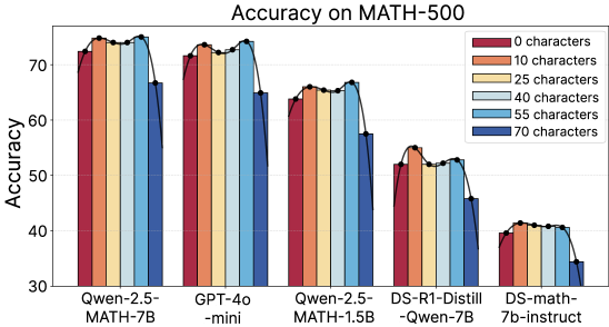<details> <summary>x8.png Details</summary>  ### Visual Description \n ## Bar Chart: Accuracy on MATH-500 ### Overview This bar chart displays the accuracy of several language models on the MATH-500 dataset, broken down by the number of characters in the input. The x-axis represents the different models, and the y-axis represents the accuracy percentage. Each model has a set of bars, one for each character length. ### Components/Axes * **Title:** Accuracy on MATH-500 (positioned at the top-center) * **X-axis Label:** Model Name (bottom-center) * Models: Qwen-2.5-MATH-7B, GPT-4o-mini, Qwen-2.5-MATH-1.5B, DS-R1-Distill-Qwen-7B, DS-math-7b-instruct * **Y-axis Label:** Accuracy (left-center) * Scale: 30 to 75, with increments of 10. * **Legend:** (top-right) * 0 characters (Red) * 10 characters (Brown) * 25 characters (Yellow) * 40 characters (Light Blue) * 55 characters (Blue) * 70 characters (Dark Blue) ### Detailed Analysis The chart consists of five groups of bars, one for each model. Within each group, there are six bars representing the accuracy for different character lengths. **Qwen-2.5-MATH-7B:** * 0 characters: Approximately 73% accuracy. * 10 characters: Approximately 74% accuracy. * 25 characters: Approximately 74.5% accuracy. * 40 characters: Approximately 74% accuracy. * 55 characters: Approximately 73% accuracy. * 70 characters: Approximately 72% accuracy. *Trend: Relatively stable accuracy across character lengths, with a slight peak at 25 characters.* **GPT-4o-mini:** * 0 characters: Approximately 72% accuracy. * 10 characters: Approximately 73% accuracy. * 25 characters: Approximately 73.5% accuracy. * 40 characters: Approximately 73% accuracy. * 55 characters: Approximately 71% accuracy. * 70 characters: Approximately 68% accuracy. *Trend: Accuracy generally decreases with increasing character length.* **Qwen-2.5-MATH-1.5B:** * 0 characters: Approximately 65% accuracy. * 10 characters: Approximately 66% accuracy. * 25 characters: Approximately 67% accuracy. * 40 characters: Approximately 67% accuracy. * 55 characters: Approximately 65% accuracy. * 70 characters: Approximately 64% accuracy. *Trend: Relatively stable accuracy across character lengths.* **DS-R1-Distill-Qwen-7B:** * 0 characters: Approximately 55% accuracy. * 10 characters: Approximately 56% accuracy. * 25 characters: Approximately 56% accuracy. * 40 characters: Approximately 55% accuracy. * 55 characters: Approximately 53% accuracy. * 70 characters: Approximately 52% accuracy. *Trend: Accuracy decreases with increasing character length.* **DS-math-7b-instruct:** * 0 characters: Approximately 40% accuracy. * 10 characters: Approximately 40% accuracy. * 25 characters: Approximately 41% accuracy. * 40 characters: Approximately 41% accuracy. * 55 characters: Approximately 40% accuracy. * 70 characters: Approximately 40% accuracy. *Trend: Relatively stable accuracy across character lengths.* ### Key Observations * Qwen-2.5-MATH-7B and GPT-4o-mini consistently achieve the highest accuracy scores across most character lengths. * The accuracy of GPT-4o-mini decreases noticeably as the character length increases. * DS-math-7b-instruct consistently has the lowest accuracy scores. * The impact of character length on accuracy varies between models. Some models are relatively unaffected, while others show a clear decline in performance with longer inputs. ### Interpretation The chart demonstrates the performance of different language models on a mathematical reasoning task (MATH-500) as a function of input length. The varying performance suggests that the models have different capacities for handling longer and more complex inputs. The decrease in accuracy for GPT-4o-mini with increasing character length could indicate a limitation in its context window or its ability to process longer sequences effectively. The consistently lower performance of DS-math-7b-instruct suggests that it may be less capable in mathematical reasoning compared to the other models tested. The relatively stable performance of Qwen-2.5-MATH-7B across different character lengths suggests a robust ability to handle varying input complexities. This data is valuable for understanding the strengths and weaknesses of each model and for selecting the most appropriate model for a given task based on the expected input length and complexity. </details> Figure 8: The relationship between the length of inserting tokens and the performance of models. F.2 The impact of inserting position of meaningless tokens. In the previous section, we demonstrated that inserting meaningless tokens between the system prompt and the question leads to improved model performance. In this section, we further investigate the effect of inserting meaningless tokens at different positions. Specifically, we consider four settings: ❶ the beginning of the system prompt, ❷ between the system prompt and the question, ❸ the end of the input, and ❹ a random position within the input. The results are reported in Table 4. We observe that only inserting tokens between the system prompt and the question yields performance gains. In contrast, appending tokens to the end of the input causes the model to simply repeat them, leading to zero accuracy. Inserting tokens at random positions disrupts the original semantic structure of the sentence, while inserting them at the beginning alters the values of the system prompt itself, introducing extra terms as shown in Equation 1. We hypothesize that this disrupts the intended initialization and interferes with the task the model is expected to process. Therefore, the most effective position for inserting meaningless tokens is between the system prompt and the question. | w/o meaningless tokens position ❶ position ❷ | 72.4 69.6 75.0 | 23.1 21.1 23.3 | | --- | --- | --- | | position ❸ | 0.0 | 0.0 | | position ❹ | 51.2 | 21.1 | Table 4: Performance on Math-500 and AIME 2024 after inserting meaningless tokens in different positions. F.3 The impact of inserting type of meaningless tokens In this section, we examine the influence of inserting different types of meaningless tokens on reasoning tasks. In our experiments, we insert varying lengths of slashes (“/”) and question marks (“?”) into the inputs and select the best-performing configuration from each set. As shown in Table 5, different types of meaningless tokens produce varying impacts on LLM performance, and no single unified pattern emerges. We attribute this to the fact that different token types carry distinct representational values, leading to different effects of attention during the transformation. Moreover, the sensitivity of individual questions to such transformations also varies. Consequently, the impact of meaningless tokens differs across tasks and models. Table 5: Accuracy of LLM on two mathematical reasoning datasets with inserting different kinds of meaningless tokens. | Qwen2.5-Math-1.5b Qwen2.5-Math-7b DeepSeek-R1-Distill-Qwen-7B | 63.6 72.4 52.0 | 66.8 75.0 55.0 | 58.2 69.6 53.6 | 14.4 23.3 3.3 | 18.8 24.4 3.3 | 16.1 22.2 4.4 | | --- | --- | --- | --- | --- | --- | --- | | DeepSeek-Math-7b-instruct | 39.6 | 41.4 | 43.4 | 7.8 | 12.2 | 12.5 | | Llama-3.1-8B-Instruct | 35.4 | 36.6 | 34.2 | 11.1 | 7.8 | 13.3 | | Qwen-2.5-32B-Instruct | 80.8 | 81.0 | 81.6 | 18.9 | 20.0 | 21.1 | F.4 Why we only analyze first layer <details> <summary>x9.png Details</summary>  ### 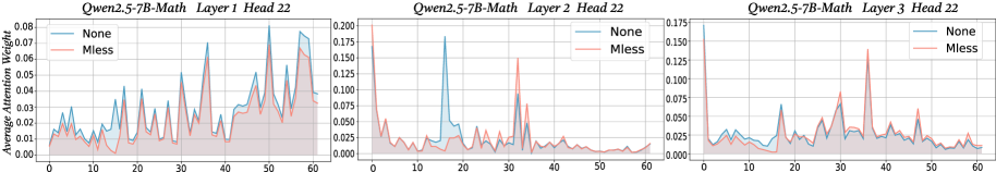Visual Description ## Line Chart: Attention Weight Comparison ### Overview The image presents three line charts, each comparing the "Average Attention Weight" of two conditions ("None" and "Miess") across 60 steps. Each chart corresponds to a different layer of a model named "Qwen2.5-7B-Math", specifically Layer 1 Head 22, Layer 2 Head 22, and Layer 3 Head 22. The charts visually represent how attention weight changes over these steps for both conditions. ### Components/Axes * **X-axis:** Represents the step number, ranging from 0 to 60. * **Y-axis:** Represents the "Average Attention Weight", with scales varying for each chart: * Chart 1 (Layer 1): 0 to 0.08 * Chart 2 (Layer 2): 0 to 0.20 * Chart 3 (Layer 3): 0 to 0.135 * **Legend:** Located in the top-right corner of each chart, distinguishing between two lines: * "None" (Blue line) * "Miess" (Red line) * **Title:** Each chart is titled with the model name and layer information: "Qwen2.5-7B-Math Layer [Number] Head 22". ### Detailed Analysis or Content Details **Chart 1: Qwen2.5-7B-Math Layer 1 Head 22** * **"None" (Blue Line):** The line fluctuates significantly between approximately 0.01 and 0.07. It starts around 0.02 at step 0, rises to a peak of approximately 0.07 around step 10, then dips to around 0.01 at step 20, and continues fluctuating. * **"Miess" (Red Line):** This line also fluctuates, generally staying between 0.01 and 0.06. It begins around 0.03 at step 0, rises to a peak of approximately 0.06 around step 10, then dips to around 0.01 at step 20, and continues fluctuating. * The lines are generally close in value, with "Miess" often slightly higher than "None" in the first half of the chart. **Chart 2: Qwen2.5-7B-Math Layer 2 Head 22** * **"None" (Blue Line):** This line exhibits a more pronounced peak around step 20, reaching approximately 0.15. It generally stays between 0.01 and 0.15, with a relatively stable baseline around 0.02-0.03. * **"Miess" (Red Line):** This line shows a very sharp peak around step 20, reaching approximately 0.18. It fluctuates between 0.00 and 0.18, with a baseline around 0.02. * The "Miess" line is significantly higher than the "None" line around step 20. **Chart 3: Qwen2.5-7B-Math Layer 3 Head 22** * **"None" (Blue Line):** This line fluctuates between approximately 0.01 and 0.09. It starts around 0.03 at step 0, rises to a peak of approximately 0.09 around step 10, then dips to around 0.02 at step 20, and continues fluctuating. * **"Miess" (Red Line):** This line fluctuates between approximately 0.01 and 0.07. It starts around 0.02 at step 0, rises to a peak of approximately 0.07 around step 10, then dips to around 0.02 at step 20, and continues fluctuating. * The lines are generally close in value, with "None" often slightly higher than "Miess". ### Key Observations * All three charts show fluctuating attention weights for both conditions. * Layer 2 exhibits the most significant difference between the "None" and "Miess" conditions, with "Miess" showing a much higher attention weight around step 20. * Layer 1 and Layer 3 show more similar behavior between the two conditions. * The scales of the Y-axis vary between the charts, indicating different magnitudes of attention weight in each layer. ### Interpretation The charts likely represent the impact of the "Miess" condition on the attention mechanism within the Qwen2.5-7B-Math model. The significant peak in attention weight for "Miess" in Layer 2 suggests that this layer is particularly sensitive to the "Miess" condition. This could indicate that the "Miess" condition triggers a specific pattern of attention that is more pronounced in Layer 2. The fluctuations in attention weight across all layers and conditions suggest a dynamic and complex attention process. The varying scales of the Y-axis imply that different layers contribute differently to the overall attention mechanism. The data suggests that the "Miess" condition alters the attention weights, particularly in Layer 2, potentially influencing the model's processing of information. Further investigation would be needed to understand the specific meaning of the "Miess" condition and its impact on the model's performance. </details> Figure 9: Average attention weights for later tokens in Layers 1 to 3 of Qwen2.5-7B-Math. In this section, we explain why our analysis and redistribution of activations focus exclusively on the first layer. As shown in Figure 9, we present the average attention weights of later tokens in Layers 1, 2, and 3 of Qwen2.5-7B-Math. We observe that only the first layer exhibits a clear and consistent phenomenon: after inserting meaningless tokens, the average attention weights decrease to a noticeable extent, suggesting that meaningless tokens directly alter the initial allocation of attention. In contrast, Layers 2 and 3 do not display such regularity—the average attention weights with and without meaningless tokens show no systematic relationship. Consequently, later layers do not undergo an affine transformation of this type. We hypothesize that this disappearance of the phenomenon arises because, beyond the first layer, the model has already integrated and mixed substantial semantic information through residual connections. From the second layer onward, the model begins to reconstruct and redistribute information, thereby diminishing the direct effect of meaningless tokens on average attention weights. In other words, the role of meaningless tokens becomes less distinguishable once meaningful contextual representations dominate, which explains why the first layer is the most critical point for observing and leveraging this effect. F.5 Repeat Meaningful tokens’ effectiveness In this section, we investigate whether adding meaningful tokens can play a role similar to meaningless tokens. Specifically, we insert a long sequence of repeated tokens that are semantically irrelevant to the question. For example, we add 55 repetitions of “he” between the system prompt and the question. The results, shown on the left of Figure 10, indicate that even such repeated but irrelevant meaningful tokens lead to an improvement in model performance. To better understand this effect, we further visualize the average attention weights after inserting these tokens, as presented on the right of Figure 10. The results reveal that the activation changes induced by repeated meaningful tokens closely resemble those caused by meaningless tokens, and the inserted tokens receive similar attention patterns which means the weight value of inserted part’s are similar. Taken together, these findings suggest that when repeated tokens are inserted at appropriate positions without introducing additional semantic content, LLMs are able to recognize them as irrelevant. Consequently, they trigger a redistribution of activations in the MLP, ultimately improving model performance. 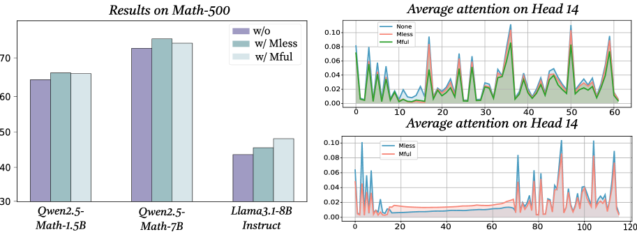<details> <summary>x10.png Details</summary>  ### Visual Description ## Bar Chart & Line Graphs: Results on Math-500 & Average Attention on Head 14 ### Overview The image presents a combination of a bar chart comparing performance on a Math-500 dataset across different models and configurations, alongside two line graphs illustrating average attention on Head 14 for those same configurations. The bar chart shows accuracy scores, while the line graphs depict attention weights over a sequence length. ### Components/Axes **Bar Chart:** * **Title:** "Results on Math-500" * **X-axis:** Model/Configuration: "Qwen2.5-Math-1.5B", "Qwen2.5-Math-7B", "Llama3-1-8B Instruct" * **Y-axis:** Accuracy (approximately 30 to 75) * **Legend:** * "w/o" (Light Blue) - Represents a configuration without a specific method. * "w/ Mless" (Medium Blue) - Represents a configuration with "Mless". * "w/ Mful" (Dark Blue) - Represents a configuration with "Mful". **Line Graphs:** * **Title:** "Average attention on Head 14" (appears twice) * **X-axis:** Sequence Length (0 to 60 in the first graph, 0 to 120 in the second) * **Y-axis:** Average Attention (approximately 0 to 0.10) * **Legend (First Graph):** * "None" (Black) * "Mless" (Green) * "Mful" (Teal) * **Legend (Second Graph):** * "Mless" (Pink) * "Mful" (Red) ### Detailed Analysis or Content Details **Bar Chart:** * **Qwen2.5-Math-1.5B:** * w/o: Approximately 65 * w/ Mless: Approximately 68 * w/ Mful: Approximately 72 * **Qwen2.5-Math-7B:** * w/o: Approximately 70 * w/ Mless: Approximately 73 * w/ Mful: Approximately 75 * **Llama3-1-8B Instruct:** * w/o: Approximately 42 * w/ Mless: Approximately 44 * w/ Mful: Approximately 46 **Line Graph 1 (Sequence Length 0-60):** * **None (Black):** The line fluctuates significantly between approximately 0.02 and 0.08, with several peaks and valleys. * **Mless (Green):** The line generally stays lower than "None", fluctuating between approximately 0.01 and 0.05. * **Mful (Teal):** The line fluctuates between approximately 0.02 and 0.07, showing a similar pattern to "None" but with slightly lower overall values. **Line Graph 2 (Sequence Length 0-120):** * **Mless (Pink):** The line fluctuates between approximately 0.01 and 0.06, with a generally increasing trend towards the end of the sequence. * **Mful (Red):** The line fluctuates between approximately 0.01 and 0.08, showing more pronounced peaks and valleys than "Mless". ### Key Observations * In the bar chart, adding "Mless" and "Mful" consistently improves accuracy across all models. "Mful" generally yields the highest accuracy. * The line graphs show that attention weights vary considerably across sequence length. * The "None" line in the first graph has a higher average attention than both "Mless" and "Mful". * The second line graph shows that "Mful" has higher attention weights than "Mless" for most of the sequence length. ### Interpretation The data suggests that the "Mless" and "Mful" methods are effective in improving the accuracy of the models on the Math-500 dataset. The bar chart clearly demonstrates this improvement, with "Mful" consistently outperforming the other configurations. The line graphs provide insights into how attention is distributed across the sequence length. The fluctuations in attention weights indicate that the model is focusing on different parts of the input sequence at different times. The differences between the "None", "Mless", and "Mful" lines suggest that these methods influence the attention mechanism, potentially by focusing attention on more relevant parts of the sequence. The fact that "None" has higher attention in the first graph could indicate that the "Mless" and "Mful" methods are suppressing attention in certain areas, potentially reducing noise or irrelevant information. The increasing trend of "Mless" and "Mful" in the second graph suggests that these methods may become more effective at longer sequence lengths. The two line graphs focus on different sequence lengths, and different configurations. This suggests a deeper investigation into the interplay between sequence length, attention mechanisms, and model performance is warranted. </details> Figure 10: The left panel illustrates a comparison between adding repeated meaningful tokens and meaningless tokens, while the right panel presents the average attention weights resulting from the addition of meaningful and meaningless tokens. 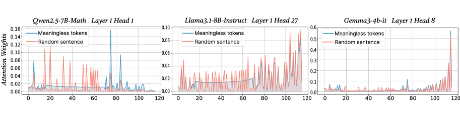F.6 Why random sentence is useless <details> <summary>x11.png Details</summary>  ### Visual Description \n ## Line Chart: Attention Weights for Different Models ### Overview The image presents three line charts, each displaying attention weights over a sequence length of 120. Each chart represents a different language model: Owen2.5-7B-Math, Llama3.1-8B-Instruct, and Gemma3-4b-it. Each chart compares the attention weights assigned to "Meaningless tokens" and a "Random sentence". The y-axis represents "Attention Weights", and the x-axis represents the sequence position from 0 to 120. ### Components/Axes * **X-axis:** Sequence Position (0 to 120) - common to all three charts. * **Y-axis:** Attention Weights (varying scales for each chart). * Owen2.5-7B-Math: 0 to 0.14 * Llama3.1-8B-Instruct: 0 to 0.10 * Gemma3-4b-it: 0 to 0.6 * **Legends:** * "Meaningless tokens" (represented by a blue line) * "Random sentence" (represented by an orange line) * **Titles:** * Owen2.5-7B-Math Layer 1 Head 1 * Llama3.1-8B-Instruct Layer 1 Head 27 * Gemma3-4b-it Layer 1 Head 8 ### Detailed Analysis or Content Details **Owen2.5-7B-Math (Layer 1 Head 1):** The blue line ("Meaningless tokens") exhibits a series of sharp peaks and valleys, fluctuating between approximately 0.00 and 0.12. The orange line ("Random sentence") shows a similar pattern, but with generally lower attention weights, fluctuating between approximately 0.00 and 0.08. There are roughly 8-10 peaks in each line across the sequence length. **Llama3.1-8B-Instruct (Layer 1 Head 27):** The blue line ("Meaningless tokens") shows a more subdued pattern of fluctuations, generally staying between 0.00 and 0.08. The orange line ("Random sentence") is even flatter, mostly remaining below 0.04, with occasional spikes up to approximately 0.06. The fluctuations are less frequent and less pronounced than in the Owen2.5-7B-Math chart. **Gemma3-4b-it (Layer 1 Head 8):** The blue line ("Meaningless tokens") displays significant fluctuations, ranging from approximately 0.00 to 0.55. The orange line ("Random sentence") also shows substantial variation, ranging from approximately 0.00 to 0.35. This chart exhibits the most dramatic attention weight variations of the three. There are several large spikes in both lines, particularly around sequence positions 20, 40, 60, 80, and 100. ### Key Observations * Gemma3-4b-it exhibits significantly higher attention weights overall compared to the other two models. * Owen2.5-7B-Math shows the most frequent and pronounced fluctuations in attention weights. * Llama3.1-8B-Instruct demonstrates the most stable and lowest attention weights. * All three models show a pattern of fluctuating attention weights, suggesting that attention is dynamically shifting across the sequence. ### Interpretation The charts illustrate how different language models allocate attention to "Meaningless tokens" and a "Random sentence" during processing. The varying scales of the y-axis suggest that the models have different sensitivities or internal representations of attention. The higher attention weights in Gemma3-4b-it might indicate a greater focus on specific tokens or a more complex attention mechanism. The fluctuations in all charts suggest that the models are not simply attending to the entire sequence equally but are dynamically focusing on different parts. The differences in fluctuation patterns could reflect variations in model architecture, training data, or the specific task they are designed for. The fact that attention is allocated to "Meaningless tokens" suggests that even seemingly irrelevant parts of the input sequence can influence the model's processing. The comparison between "Meaningless tokens" and a "Random sentence" could be used to understand how the models handle noise or irrelevant information. </details> Figure 11: The average attention weights of adding meaningless tokens and random sentence. When additional tokens are inserted into a sentence, both the attention weights and the resulting attention outputs exhibit consistent patterns: the weights assigned to the original tokens decrease, while the attention outputs gain additional values from the inserted tokens. In this section, we analyze why adding repeated tokens can enhance the performance of LLMs, whereas inserting random or unrelated sentences can have a detrimental effect. The results are shown in Figure 11. We observe that the attention weights associated with the random sentence are highly diverse, and their corresponding value vectors also differ substantially. In contrast, the repeated meaningless tokens exhibit more uniform attention weights and nearly identical value vectors. Consequently, compared with repeated meaningless tokens, a random sentence introduces not only numerical fluctuations but also a pronounced directional shift in the attention outputs—one that carries additional semantic information. The formula of RMSNorm is: $$ \operatorname{RMSNorm}(x)=\gamma\odot\frac{x}{\sqrt{\frac{1}{d}\sum_{i=1}^{d}x_{i}^{2}+\epsilon}}, \tag{18} $$ where $\gamma$ is a learnable rescaling vector and $\epsilon$ ensures numerical stability. For repeated meaningless tokens, the effect manifests as a small and uniform directional bias on the input to RMSNorm, producing only a minor numerical perturbation in its output. In contrast, inserting a random sentence introduces high-rank and structured semantic signals that RMSNorm cannot simply absorb. This leads to systematic shifts in the output direction and subspace, thereby altering the model’s internal semantic representations. 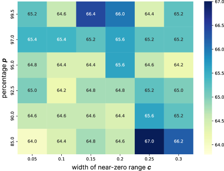F.7 The optimal hyperparameter range <details> <summary>x12.png Details</summary>  ### Visual Description ## Heatmap: Percentage p vs. Width of Near-Zero Range c ### Overview This image presents a heatmap visualizing the relationship between two variables: "percentage p" and "width of near-zero range c". The heatmap uses a color gradient to represent the values associated with each combination of these variables. The color scale ranges from approximately 64.0 to 67.0. ### Components/Axes * **X-axis:** "width of near-zero range c" with values: 0.05, 0.1, 0.15, 0.2, 0.25, 0.3. * **Y-axis:** "percentage p" with values: 85, 90, 92.5, 95, 97, 99.5. * **Color Scale:** Ranges from approximately 64.0 (dark blue) to 67.0 (light yellow). The scale is positioned on the right side of the heatmap. * **Data Points:** Each cell in the heatmap represents a specific combination of "percentage p" and "width of near-zero range c", with the cell's color indicating the corresponding value. ### Detailed Analysis The heatmap contains 36 data points, arranged in a 6x6 grid. Here's a breakdown of the values, row by row: * **p = 85:** * c = 0.05: 64.0 * c = 0.1: 64.4 * c = 0.15: 64.8 * c = 0.2: 64.6 * c = 0.25: 67.0 * c = 0.3: 66.2 * **p = 90:** * c = 0.05: 64.6 * c = 0.1: 64.6 * c = 0.15: 64.6 * c = 0.2: 64.4 * c = 0.25: 65.6 * c = 0.3: 65.2 * **p = 92.5:** * c = 0.05: 65.0 * c = 0.1: 64.2 * c = 0.15: 64.8 * c = 0.2: 64.8 * c = 0.25: 65.2 * c = 0.3: 65.0 * **p = 95:** * c = 0.05: 64.8 * c = 0.1: 64.4 * c = 0.15: 64.4 * c = 0.2: 65.6 * c = 0.25: 64.6 * c = 0.3: 64.2 * **p = 97:** * c = 0.05: 65.4 * c = 0.1: 65.4 * c = 0.15: 65.2 * c = 0.2: 65.6 * c = 0.25: 65.2 * c = 0.3: 65.2 * **p = 99.5:** * c = 0.05: 65.2 * c = 0.1: 64.6 * c = 0.15: 66.4 * c = 0.2: 66.0 * c = 0.25: 64.4 * c = 0.3: 65.2 ### Key Observations * The values generally fall between 64.0 and 67.0. * The highest value (67.0) occurs at p = 85 and c = 0.25. * The lowest value (64.0) occurs at p = 85 and c = 0.05. * There isn't a strong, clear trend across the heatmap. Values appear relatively consistent, with some localized variations. * For p = 90, the values are very similar across all values of c. ### Interpretation The heatmap suggests a complex relationship between "percentage p" and "width of near-zero range c". The relatively small range of values (64.0-67.0) indicates that the variable being measured is not highly sensitive to changes in either "percentage p" or "width of near-zero range c" within the tested ranges. The peak at p=85 and c=0.25 might indicate an optimal condition for whatever process these variables represent, but further investigation would be needed to confirm this. The consistency of values for p=90 suggests that the measured variable is largely independent of the "width of near-zero range c" at that percentage level. Without knowing the context of these variables, it's difficult to draw more specific conclusions. The data could represent the efficiency of an algorithm, the accuracy of a measurement, or any other quantifiable process. </details> Figure 12: This figure illustrates how accuracy varies with changes in the parameters p and c. In this section, we investigate how the hyper-parameters—the percentage p and the width of the near-zero range c —influence model performance on Math-500 when using Qwen2.5-1.5B-Math. The results are summarized in Figure 12. As the figure illustrates, the accuracy does not change monotonically with either p or c; instead, the best-performing settings emerge only within specific regions of the parameter space. This indicates that the choice of hyper-parameters is not trivial and cannot be reduced to cherry-picking. More concretely, we find that balanced combinations of p and c lead to more stable improvements. High accuracy is typically concentrated in two regions: when p is large and c is small, or conversely, when c is large and p is small. In these cases, the redistribution mechanism introduced by ARM effectively amplifies informative activations while suppressing uninformative near-zero activations. Outside of these regions, however, the performance of the model degrades, suggesting that poorly chosen hyper-parameters may distort the activation distribution rather than enhance it. These observations highlight the importance of aligning hyper-parameter choices with the intrinsic properties of activation distributions. To maximize the benefits of ARM, one must take into account both the proportion of near-zero activations and the magnitude of the maximum activation values, thereby ensuring that p and c are set within an appropriate interval. By doing so, ARM can operate in its most effective regime, consistently improving model reasoning performance rather than introducing instability. From each row and column, we can see that the performance of LLMs after ARM depends on both $p$ and $c$ . Since they are equally important, the optimal performance is determined by the range of these two parameters. Appendix G More Experiments G.1 Results on non-reasoning tasks In this section, we present supplementary results on non-reasoning benchmarks, including ARC-C, MMLU, BoolQ, and OpenBookQA, as shown in Table 6. Across all evaluated models, the application of our method yields only marginal variations in performance. For most models and tasks, it either produces slight improvements or maintains parity with the baseline (i.e., vanilla model performance without any inference-time trick), suggesting that the redistribution of activations has little impact when the task primarily requires factual recall or pattern recognition rather than multi-step reasoning. A minor performance drop is observed only on a small subset of tasks with Llama-3.1-8B-Instruct, which we attribute to model-specific characteristics or sensitivity to activation perturbations.These findings indicate that our approach exerts negligible influence on non-reasoning tasks and, in most cases, does not introduce adverse effects on task accuracy. This observation further supports our central claim: the benefits of activation redistribution are most pronounced in reasoning-oriented scenarios, while in non-reasoning settings the method remains stable and does not compromise the model’s inherent ability to answer factual or knowledge-intensive questions. Table 6: Complete results of several models on non-reasoning tasks. | Model Qwen2.5 Math-1.5B ARM | Setting Baseline 78.6 | GSM8K 78.0 39.3 | ARC-E 39.3 35.4 | ARC-C 35.0 32.1 | MMLU 32.1 33.4 | BoolQ 32.6 39.5 | HellaSwag 39.1 42.4 | OpenBookQA 42.0 | | --- | --- | --- | --- | --- | --- | --- | --- | --- | | \cellcolor gray!15 Improve Rate (%) | \cellcolor gray!15 0.6 $\uparrow$ | \cellcolor gray!15 0 | \cellcolor gray!15 0.4 $\uparrow$ | \cellcolor gray!15 0 | \cellcolor gray!15 0.8 $\uparrow$ | \cellcolor gray!15 0.4 $\uparrow$ | \cellcolor gray!15 0.4 $\uparrow$ | | | Qwen2.5 Math-7B | Baseline | 83.8 | 49.7 | 47.9 | 36.9 | 38.6 | 46.9 | 47.6 | | ARM | 83.8 | 49.7 | 47.0 | 37.5 | 38.7 | 47.1 | 47.9 | | | \cellcolor gray!15 Improve Rate (%) | \cellcolor gray!15 0 | \cellcolor gray!15 0 | \cellcolor gray!15 0 | \cellcolor gray!15 0.6 $\uparrow$ | \cellcolor gray!15 0.1 $\uparrow$ | \cellcolor gray!15 0.2 $\uparrow$ | \cellcolor gray!15 0.3 $\uparrow$ | | | Llama3.1 8B-Instruct | Baseline | 80.0 | 46.6 | 49.0 | 38.6 | 43.3 | 56.8 | 52.8 | | ARM | 82.4 | 47.1 | 48.7 | 38.2 | 43.2 | 57.3 | 50.8 | | | \cellcolor gray!15 Improve Rate (%) | \cellcolor gray!15 2.4 $\uparrow$ | \cellcolor gray!15 0.5 $\uparrow$ | \cellcolor gray!15 -0.3 $\downarrow$ | \cellcolor gray!15 -0.4 $\downarrow$ | \cellcolor gray!15 -0.1 $\downarrow$ | \cellcolor gray!15 0.5 $\uparrow$ | \cellcolor gray!15 -2.0 $\downarrow$ | | | Gemma3 4b-it | Baseline | 86.8 | 47.1 | 44.5 | 33.9 | 45.0 | 42.0 | 41.0 | | ARM | 86.8 | 47.1 | 45.0 | 34.1 | 45.2 | 42.0 | 42.0 | | | \cellcolor gray!15 Improve Rate (%) | \cellcolor gray!15 0 | \cellcolor gray!15 0 | \cellcolor gray!15 0.5 $\uparrow$ | \cellcolor gray!15 0.2 $\uparrow$ | \cellcolor gray!15 0.2 $\uparrow$ | \cellcolor gray!15 0 | \cellcolor gray!15 1.0 $\uparrow$ | | G.2 Results on Base Model Table 7: Performance on Math-500 and AIME 2024 after incorporating ARM into the MLP in non-reasoning model. | Model Qwen2.5-1.5B ARM | Setting Baseline 68.2 | Math-500 (Pass@1) 67.8 14.4 | AIME 2024 (Pass@1) 14.4 | | --- | --- | --- | --- | | Improve Rate (%) | 0.4 $\uparrow$ | 0 | | | Qwen2.5-7B | Baseline | 50.4 | 15.6 | | ARM | 50.6 | 16.7 | | | Improve Rate (%) | 0.2 $\uparrow$ | 1.1 $\uparrow$ | | | Qwen2.5-32B | Baseline | 77.2 | 27.8 | | ARM | 77.4 | 28.9 | | | Improve Rate (%) | 0.2 $\uparrow$ | 1.1 $\uparrow$ | | In this section, we evaluate the effect of applying ARM to base models and report their performance on Math-500 and AIME2024 using Qwen2.5-1.5B, Qwen2.5-7B, and Qwen2.5-32B. Since these models achieve accuracy above 5%, we consider them capable of tackling these tasks. In contrast, models such as Llama3.1-8B and Gemma3-4B-PT exhibit poor performance and are therefore excluded from the evaluation. The results in Table 7 show that incorporating ARM into the MLP layers of base models yields measurable performance gains on reasoning tasks, although the improvements are generally smaller than those observed for reasoning, oriented models. We attribute this gap to the weaker inherent reasoning abilities of base models. While activation redistribution can still enhance their internal representations, it may not strongly affect how they process key numerical or symbolic elements, such as digits and operators, compared with models trained specifically for reasoning. Table 8: Performance on Math-500 and AIME 2024 after incorporating ARM into the MLP. | Qwen2.5 Math-1.5B ARM Best-of-N(N=5) | Baseline 67.8 69.4 | 63.8 18.9 14.4 | 14.4 | | --- | --- | --- | --- | | Best-of-N + ARM | 71.2 | 18.9 | | | Qwen2.5 Math-7B | Baseline | 72.4 | 23.3 | | ARM | 73.4 | 25.6 | | | Best-of-N(N=5) | 72.8 | 23.3 | | | Best-of-N + ARM | 73.4 | 25.6 | | G.3 Inference Time trick comparison To more comprehensively evaluate the robustness, effectiveness, and compatibility of ARM with established inference-time scaling techniques, we further compare its performance against the widely used Best-of-N sampling approach during inference. Specifically, Table 8 summarizes the results obtained by applying ARM alone, Best-of-N sampling alone, and their combined usage on two representative reasoning benchmarks. For all settings, we fix the generation hyperparameters to a temperature of 0.5 and a top_p of 0.95 to ensure a consistent sampling regime. As demonstrated in the table, both ARM and Best-of-N independently yield improvements over the baseline, and their combination produces an even larger performance gain, suggesting that ARM complements rather than competes with existing inference-time strategies. These findings collectively underscore the practical value and scalability of ARM as a lightweight inference-time method for enhancing reasoning capabilities across diverse tasks. Table 9: The hyper parameters in 7 models on three benchmarks. For Qwen and Llama, we using near-zero range $c$ to choose proportion, so $p$ is dash(“-”). But for Gemma, due to the activation distribution, we directly decide to skip setting $c$ and choose $p$ . So here, $c$ is dash(“-”). If the task performance doesn’t improve, we replace hyper-parameters with dash(“-”). | Qwen2.5-Math-1.5B Qwen2.5-Math-7B Qwen2.5-7B-Instruct | 0.15/- 0.2/- 0.15/- | 99.5 99.5 99.5 | 0.13/- 0.1/- 0.1/- | 99.5 95.0 99.5 | 0.13/- 0.05/- - | 99.5 90.0 - | 0.13/- 0.13/- 0.13/- | 99.5 99.5 95.0 | 0.13/- 0.13/- 0.05/- | 99.5 95.0 90 | - - 0.3/- | - - 99.5 | | --- | --- | --- | --- | --- | --- | --- | --- | --- | --- | --- | --- | --- | | Qwen2.5-32B-Instruct | 0.05/- | 90.5 | - | - | 0.13/- | 99.5 | 0.05/- | 99.0 | 0.13/- | 99.5 | 0.3/- | 99.5 | | Llama3.1-8B-Instruct | 0.45/- | 80.0 | 0.32/- | 90.0 | 0.32/- | 90.0 | - | - | 0.3/- | 90.0 | 0.3/- | 90.0 | | Gemma3-4B-it | -/0.5 | 96.5 | -/0.25 | 85.0 | -/0.25 | 96.5 | -/0.25 | 85.0 | -/0.25 | 96.5 | -/0.25 | 75.0 | | Gemma3-27B-it | -/0.5 | 96.5 | -/0.25 | 85.0 | -/0.25 | 85.0 | -/0.25 | 70.0 | -/0.25 | 85.0 | -/0.25 | 85.0 | Appendix H The example of hyper parameters The selection of $p_{1}$ and $c$ depends on the distribution of model activations after the activation function. In most cases, when the frequency of near-zero activations greatly exceeds that of other values (as in Qwen), the value of $c$ should be chosen smaller. In contrast, for models like LLaMA, $c$ should be chosen larger. When the proportion of near-zero activations is extremely high (as in Gemma), we recommend directly setting the modification proportion to a value larger than $p_{\text{max}}$ . For the choice of $p_{1}$ , we generally advise selecting more than $80\%$ , which covers regions with higher activation frequencies and thus exerts a stronger influence on near-zero values. Because the proportion of extremely high-frequency activations is small, this choice will not cause large deviations in the near-zero values. Overall, although models from the same family may behave differently across tasks and parameter scales, the selection ranges of $p_{1}$ and $c$ remain relatively consistent within each family. Some examples are in Table 9. Appendix I More Average activation weights In this section, we present additional figures of average attention weights to further validate the previously observed phenomenon. When computing the average attention weights for Llama3.1 and Gemma3, we exclude the first token to make the effect clearer, as position tokens tend to absorb most of the attention. The results are in Figure 13, Figure 14, Figure 15, Figure 16, Figure 17, Figure 18, Figure 19, Figure 20. From results, we can see that in the most layers, models will have same phenomenon like we mentioned before. Appendix J Examples of model’s output change of adding meaningless In this section, we show some examples where, after adding meaningless tokens, the model can turn wrong answers into correct ones. The specific examples are provided in Appendix J. 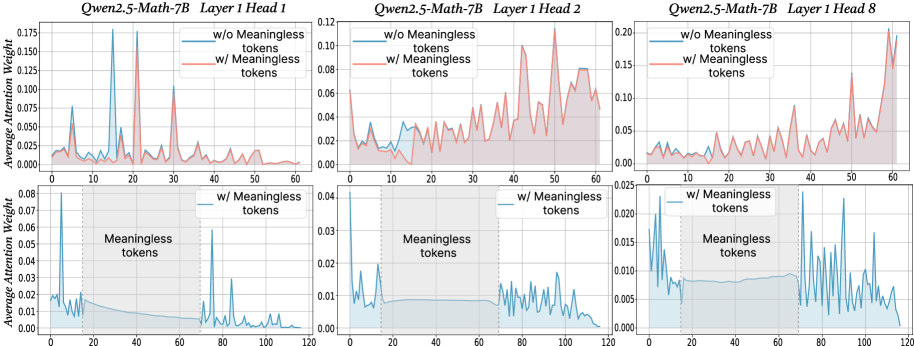<details> <summary>x13.png Details</summary>  ### Visual Description \n ## Line Chart: Attention Weights with and without Meaningless Tokens ### Overview The image presents three sets of line charts, each comparing the average attention weight with and without "meaningless tokens" for different layers and heads of the Qwen2.5-Math-7B model. Each set contains two charts: one showing attention weights for the entire sequence and another focusing on the region where meaningless tokens are present. ### Components/Axes Each chart shares the following components: * **X-axis:** "Tokens" - ranging from 0 to approximately 60-120, depending on the chart. * **Y-axis:** "Average Attention Weight" - ranging from 0 to approximately 0.20. * **Legend:** * "w/o Meaningless tokens" - represented by a reddish-orange line. * "w/ Meaningless tokens" - represented by a teal line. * **Titles:** Each chart is titled with "Qwen2.5-Math-7B", "Layer [number]", and "Head [number]". * **Shaded Region:** A light green shaded region indicates the presence of "Meaningless tokens" in the lower charts. The three sets of charts correspond to: 1. Layer 1, Head 1 2. Layer 1, Head 2 3. Layer 1, Head 8 ### Detailed Analysis or Content Details **Chart 1: Layer 1, Head 1** * **Top Chart:** The reddish-orange line ("w/o Meaningless tokens") exhibits several peaks and valleys, fluctuating between approximately 0.01 and 0.15. The teal line ("w/ Meaningless tokens") shows a generally lower attention weight, mostly below 0.05, with some peaks around 0.08. * **Bottom Chart:** The teal line ("w/ Meaningless tokens") shows a slight increase in attention weight within the shaded region (tokens 20-60), peaking around 0.06, then decreasing again. **Chart 2: Layer 1, Head 2** * **Top Chart:** The reddish-orange line ("w/o Meaningless tokens") fluctuates between approximately 0.01 and 0.12. The teal line ("w/ Meaningless tokens") is generally lower, mostly below 0.04, with some peaks around 0.08. * **Bottom Chart:** The teal line ("w/ Meaningless tokens") shows a slight increase in attention weight within the shaded region (tokens 40-120), peaking around 0.03. **Chart 3: Layer 1, Head 8** * **Top Chart:** The reddish-orange line ("w/o Meaningless tokens") fluctuates between approximately 0.01 and 0.20. The teal line ("w/ Meaningless tokens") is generally lower, mostly below 0.025, with some peaks around 0.05. * **Bottom Chart:** The teal line ("w/ Meaningless tokens") shows a slight increase in attention weight within the shaded region (tokens 40-120), peaking around 0.02. ### Key Observations * In all charts, the attention weights are generally higher when meaningless tokens are *not* present ("w/o Meaningless tokens"). * The presence of meaningless tokens ("w/ Meaningless tokens") appears to slightly increase attention weight in the region where they are located, but the overall attention weight remains lower compared to the case without meaningless tokens. * The magnitude of attention weights varies significantly between different heads (Head 1, Head 2, Head 8). Head 8 shows the highest overall attention weights. * The fluctuations in attention weights suggest that the model attends to different parts of the input sequence at different times. ### Interpretation The data suggests that the Qwen2.5-Math-7B model assigns lower attention weights to meaningless tokens compared to meaningful tokens. This is expected, as the model is likely designed to focus on relevant information. The slight increase in attention weight within the region of meaningless tokens could be due to the model attempting to process or filter out these tokens. The differences in attention weight magnitudes between different heads indicate that different heads may be responsible for attending to different aspects of the input sequence. Head 8, with its higher attention weights, may be more sensitive to the overall input or may be responsible for capturing more important features. The fluctuations in attention weights highlight the dynamic nature of the attention mechanism, which allows the model to adapt its focus based on the input sequence. The charts provide insights into how the model processes information and how it handles meaningless tokens. The consistent pattern across all three heads suggests a robust behavior of the model. </details> Figure 13: The average attention weights of Qwen2.5-Math-7B in Head 1, 2, 8. 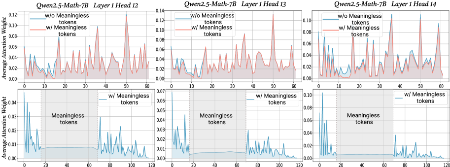<details> <summary>x14.png Details</summary>  ### Visual Description \n ## Line Chart: Average Attention Weight vs. Token Position for Different Model Layers ### Overview This image presents six line charts comparing the average attention weight for two conditions – with and without meaningless tokens – across different layers (12, 13, and 14) of the Qwen2.5-Math-7B model. Each chart displays the average attention weight on the y-axis against the token position on the x-axis. The top row shows charts with x-axis ranging from 0 to 60, while the bottom row shows charts with x-axis ranging from 0 to 120. ### Components/Axes * **X-axis:** Token Position (ranging from 0 to 60 in the top row and 0 to 120 in the bottom row). * **Y-axis:** Average Attention Weight (ranging from 0 to 0.12). * **Legend:** * "w/o Meaningless tokens" (represented by a red line) * "w/ Meaningless tokens" (represented by a teal line) * **Titles:** Each chart is titled "Qwen2.5-Math-7B Layer [Layer Number] Head [Head Number]". * **Gridlines:** Vertical gridlines are present in each chart to aid in reading values. ### Detailed Analysis or Content Details **Chart 1: Qwen2.5-Math-7B Layer 1 Head 12** * The red line ("w/o Meaningless tokens") starts at approximately 0.02, fluctuates between 0.01 and 0.04, and ends around 0.03. It exhibits a generally flat trend with some oscillations. * The teal line ("w/ Meaningless tokens") starts at approximately 0.005, rises to a peak of around 0.06 at token position 20, then declines and oscillates between 0.01 and 0.04, ending around 0.02. This line shows a more pronounced initial increase and subsequent fluctuation. **Chart 2: Qwen2.5-Math-7B Layer 1 Head 13** * The red line ("w/o Meaningless tokens") starts at approximately 0.01, fluctuates between 0.005 and 0.03, and ends around 0.02. Similar to Chart 1, it shows a relatively flat trend with oscillations. * The teal line ("w/ Meaningless tokens") starts at approximately 0.005, rises to a peak of around 0.05 at token position 15, then declines and oscillates between 0.01 and 0.03, ending around 0.01. **Chart 3: Qwen2.5-Math-7B Layer 1 Head 14** * The red line ("w/o Meaningless tokens") starts at approximately 0.02, fluctuates between 0.01 and 0.04, and ends around 0.03. Again, a relatively flat trend with oscillations. * The teal line ("w/ Meaningless tokens") starts at approximately 0.005, rises to a peak of around 0.06 at token position 20, then declines and oscillates between 0.01 and 0.04, ending around 0.02. **Chart 4: Qwen2.5-Math-7B Layer 1 Head 12 (Extended X-axis)** * The teal line ("w/ Meaningless tokens") starts at approximately 0.005, rises to a peak of around 0.04 at token position 20, then declines and oscillates between 0.01 and 0.03, ending around 0.01. **Chart 5: Qwen2.5-Math-7B Layer 1 Head 13 (Extended X-axis)** * The teal line ("w/ Meaningless tokens") starts at approximately 0.005, rises to a peak of around 0.05 at token position 20, then declines and oscillates between 0.01 and 0.03, ending around 0.01. **Chart 6: Qwen2.5-Math-7B Layer 1 Head 14 (Extended X-axis)** * The teal line ("w/ Meaningless tokens") starts at approximately 0.005, rises to a peak of around 0.06 at token position 20, then declines and oscillates between 0.01 and 0.04, ending around 0.02. ### Key Observations * The inclusion of meaningless tokens consistently leads to a higher initial attention weight compared to the condition without meaningless tokens, particularly in the first 20-30 tokens. * The attention weight generally decreases after the initial peak when meaningless tokens are present. * The "w/o Meaningless tokens" lines remain relatively stable throughout the token positions, with minimal fluctuations. * The extended x-axis charts (bottom row) show that the teal lines continue to oscillate at lower average attention weights. ### Interpretation The data suggests that the presence of meaningless tokens initially draws attention from the model, as evidenced by the higher attention weights in the early token positions. However, this attention seems to diminish as the model processes more tokens. The relatively stable attention weights for the "w/o Meaningless tokens" condition indicate that the model focuses more consistently on relevant tokens when meaningless tokens are absent. The differences in attention weight patterns between the two conditions highlight the model's sensitivity to irrelevant information. The initial spike in attention followed by a decline suggests that the model may initially attempt to process the meaningless tokens before recognizing their lack of significance. The extended x-axis charts demonstrate that the effect of meaningless tokens diminishes over time, but still results in a different attention pattern compared to the condition without them. This could have implications for the model's efficiency and performance on tasks requiring focused attention on relevant information. </details> Figure 14: The average attention weights of Qwen2.5-Math-7B in Head 12, 13, 14. 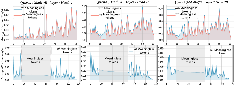<details> <summary>x15.png Details</summary>  ### Visual Description \n ## Line Charts: Attention Weight Analysis with and without Meaningless Tokens ### Overview The image presents six line charts, arranged in two rows and three columns. Each chart compares the attention weight distribution with and without "meaningless tokens" for different layers of the Qwen2.5-Math-7B model. The top row displays attention weight, while the bottom row displays average attention weight. Each chart is labeled with the model name, layer number, and head number. ### Components/Axes Each chart shares the following components: * **X-axis:** Token position, ranging from 0 to approximately 60-120 (depending on the chart). * **Y-axis (Top Row):** Attention Weight, ranging from 0 to approximately 0.15. * **Y-axis (Bottom Row):** Average Attention Weight, ranging from 0 to approximately 0.04. * **Lines:** Two lines are present in each top-row chart: * Red line: "w/o Meaningless tokens" * Blue line: "w/ Meaningless tokens" * **Lines (Bottom Row):** One line is present in each bottom-row chart: * Teal line: "Meaningless tokens" * **Titles:** Each chart has a title indicating the model, layer, and head. For example, "Qwen2.5-Math-7B Layer 1 Head 17". ### Detailed Analysis or Content Details **Chart 1: Qwen2.5-Math-7B Layer 1 Head 17** * **Top Row:** The red line (w/o Meaningless tokens) fluctuates between approximately 0.01 and 0.13, with several peaks. The blue line (w/ Meaningless tokens) fluctuates between approximately 0.005 and 0.08, with generally lower peaks. * **Bottom Row:** The teal line (Meaningless tokens) starts at approximately 0.015 and rises to a peak of around 0.035 at token position 20, then declines to approximately 0.01 by token position 120. **Chart 2: Qwen2.5-Math-7B Layer 1 Head 26** * **Top Row:** The red line (w/o Meaningless tokens) fluctuates between approximately 0.01 and 0.07. The blue line (w/ Meaningless tokens) fluctuates between approximately 0.005 and 0.05, with generally lower peaks. * **Bottom Row:** The teal line (Meaningless tokens) starts at approximately 0.01 and rises to a peak of around 0.025 at token position 20, then declines to approximately 0.01 by token position 120. **Chart 3: Qwen2.5-Math-7B Layer 1 Head 28** * **Top Row:** The red line (w/o Meaningless tokens) fluctuates between approximately 0.01 and 0.06. The blue line (w/ Meaningless tokens) fluctuates between approximately 0.005 and 0.04, with generally lower peaks. * **Bottom Row:** The teal line (Meaningless tokens) starts at approximately 0.01 and rises to a peak of around 0.03 at token position 20, then declines to approximately 0.015 by token position 120. **Trends:** * In all charts, the red line (w/o Meaningless tokens) generally exhibits higher attention weights than the blue line (w/ Meaningless tokens). * The teal lines (Meaningless tokens) in the bottom row all show a similar pattern: an initial rise followed by a decline. ### Key Observations * The inclusion of meaningless tokens consistently reduces the overall attention weight, as evidenced by the lower values of the blue lines compared to the red lines in the top-row charts. * The meaningless tokens themselves receive some attention, as shown by the teal lines in the bottom-row charts, but this attention diminishes over the sequence of tokens. * The attention weight distributions appear to be somewhat noisy, with frequent fluctuations. ### Interpretation The data suggests that the Qwen2.5-Math-7B model allocates less attention to relevant tokens when meaningless tokens are present. This is expected, as the model's attention mechanism is likely distributed across all tokens in the input sequence. The decreasing attention to meaningless tokens over the sequence could indicate that the model learns to ignore them as it processes the input. The differences in attention weight distributions between the layers and heads suggest that different parts of the model may be affected differently by the presence of meaningless tokens. The noisy attention weight distributions could be due to the inherent stochasticity of the attention mechanism or the complexity of the input data. The charts provide insights into how the model handles irrelevant information and how this affects its attention allocation. This information could be useful for improving the model's robustness and efficiency. The consistent pattern across the three charts suggests a generalizable effect of meaningless tokens on attention weights within this model architecture. </details> Figure 15: The average attention weights of Qwen2.5-Math-7B in Head 17, 26, 28. 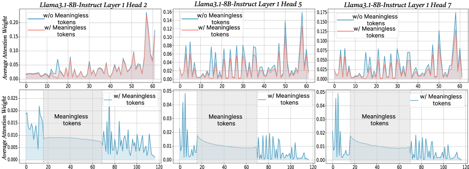<details> <summary>x16.png Details</summary>  ### Visual Description ## Line Chart: Attention Weight Analysis with and without Meaningless Tokens ### Overview This image presents a series of six line charts comparing the average attention weight for two conditions: with and without "meaningless tokens." The charts are arranged in a 2x3 grid, each representing a different layer and head of the Llama3.1-8B-Instruct model (Layer 1 Head 2, Layer 1 Head 5, Layer 1 Head 7, Layer 2 Head 2, Layer 2 Head 5, Layer 2 Head 7). Each chart displays the average attention weight on the y-axis against the token position on the x-axis. A shaded region indicates the presence of "meaningless tokens." ### Components/Axes * **X-axis:** Token Position (ranging from approximately 0 to 120) * **Y-axis:** Average Attention Weight (ranging from 0 to approximately 0.25, depending on the chart) * **Lines:** * "w/o Meaningless tokens" (Blue) * "w/ Meaningless tokens" (Red/Green) * **Shaded Region:** Indicates the range of "Meaningless tokens" * **Titles:** Each chart is titled with "Llama3.1-8B-Instruct Layer [Number] Head [Number]" * **Legend:** Located in the top-left corner of each chart, identifying the lines. ### Detailed Analysis or Content Details **Chart 1: Llama3.1-8B-Instruct Layer 1 Head 2** * The blue line ("w/o Meaningless tokens") fluctuates around an average of 0.02, with peaks around 10, 20, 30, and 40. * The red line ("w/ Meaningless tokens") fluctuates around an average of 0.12, with peaks around 10, 20, 30, and 40. * No shaded region is visible. **Chart 2: Llama3.1-8B-Instruct Layer 1 Head 5** * The blue line ("w/o Meaningless tokens") fluctuates around an average of 0.03, with peaks around 10, 20, 30, and 40. * The red line ("w/ Meaningless tokens") fluctuates around an average of 0.08, with peaks around 10, 20, 30, and 40. * No shaded region is visible. **Chart 3: Llama3.1-8B-Instruct Layer 1 Head 7** * The blue line ("w/o Meaningless tokens") fluctuates around an average of 0.025, with peaks around 10, 20, 30, and 40. * The red line ("w/ Meaningless tokens") fluctuates around an average of 0.06, with peaks around 10, 20, 30, and 40. * No shaded region is visible. **Chart 4: Llama3.1-8B-Instruct Layer 2 Head 2** * The green line ("w/ Meaningless tokens") fluctuates around an average of 0.01, with peaks around 60-80. * A shaded region is visible from approximately token position 40 to 120. * The line shows a significant increase in attention weight within the shaded region. **Chart 5: Llama3.1-8B-Instruct Layer 2 Head 5** * The green line ("w/ Meaningless tokens") fluctuates around an average of 0.02, with peaks around 60-80. * A shaded region is visible from approximately token position 40 to 120. * The line shows a significant increase in attention weight within the shaded region. **Chart 6: Llama3.1-8B-Instruct Layer 2 Head 7** * The green line ("w/ Meaningless tokens") fluctuates around an average of 0.015, with peaks around 60-80. * A shaded region is visible from approximately token position 40 to 120. * The line shows a significant increase in attention weight within the shaded region. ### Key Observations * In Layer 1 charts, the "w/ Meaningless tokens" line consistently exhibits higher average attention weights than the "w/o Meaningless tokens" line. * In Layer 2 charts, the attention weight for "w/ Meaningless tokens" increases significantly when the meaningless tokens are present (within the shaded region). * The attention weights generally fluctuate, suggesting dynamic attention allocation across tokens. * The peaks in attention weight tend to occur at similar token positions across different heads and layers. ### Interpretation The data suggests that the inclusion of "meaningless tokens" impacts the attention mechanism within the Llama3.1-8B-Instruct model. In the first layer, the presence of these tokens consistently increases the overall attention weight. In the second layer, the effect is more pronounced, with a clear increase in attention weight specifically when the meaningless tokens are present. This could indicate that the model is attempting to process or account for these tokens, even if they lack semantic meaning. The consistent peaks in attention weight across different heads and layers suggest that certain token positions are inherently more salient to the model, regardless of the presence of meaningless tokens. The shaded regions help to visually confirm the correlation between the presence of meaningless tokens and increased attention weight. This analysis could be valuable for understanding the model's robustness to noisy or irrelevant input and for optimizing its attention mechanism. </details> Figure 16: The average attention weights of Llama3.1-8B-Instruct in Head 2, 5, 7. 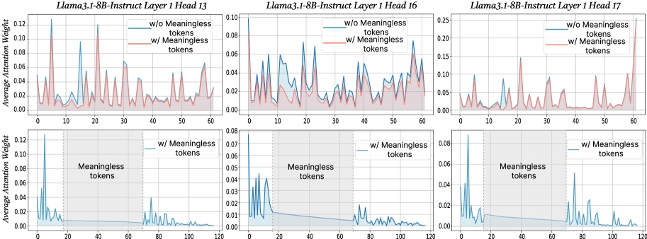<details> <summary>x17.png Details</summary>  ### Visual Description \n ## Chart: Attention Weight Comparison with and without Meaningless Tokens ### Overview This image presents six line charts comparing the average attention weight for two conditions: with and without "meaningless tokens". The charts are arranged in a 2x3 grid, each representing a different layer and head of the Llama3.1-8B-Instruct model (Layer 13, 16, and 17, each with two sub-charts). The x-axis represents token position, and the y-axis represents the average attention weight. ### Components/Axes * **Title:** Each chart is titled "Llama3.1-8B-Instruct Layer [Number] Head [Number]". * **X-axis Label:** "Token Position" (ranging from 0 to approximately 120, depending on the chart). * **Y-axis Label:** "Average Attention Weight" (ranging from 0 to approximately 0.25, depending on the chart). * **Legend:** Each chart has a legend with two entries: * "w/o Meaningless tokens" (represented by a blue line) * "w/ Meaningless tokens" (represented by a red line) * **Sub-chart Labels:** The bottom row of charts are labeled "Meaningless tokens". ### Detailed Analysis **Chart 1: Llama3.1-8B-Instruct Layer 13 Head 13** * **w/o Meaningless tokens (Blue Line):** The line fluctuates significantly between approximately 0.00 and 0.12. There are numerous peaks and valleys. * **w/ Meaningless tokens (Red Line):** The line also fluctuates, but generally remains lower than the blue line, ranging from approximately 0.00 to 0.08. * **Trend:** Both lines exhibit high variability. **Chart 2: Llama3.1-8B-Instruct Layer 16 Head 16** * **w/o Meaningless tokens (Blue Line):** The line shows a decreasing trend from approximately 0.08 to approximately 0.02, with some fluctuations. * **w/ Meaningless tokens (Red Line):** The line is relatively flat, hovering around 0.04. * **Trend:** The blue line demonstrates a clear downward trend, while the red line is stable. **Chart 3: Llama3.1-8B-Instruct Layer 17 Head 17** * **w/o Meaningless tokens (Blue Line):** The line fluctuates significantly, ranging from approximately 0.00 to 0.25. * **w/ Meaningless tokens (Red Line):** The line fluctuates, but generally remains lower than the blue line, ranging from approximately 0.00 to 0.10. * **Trend:** Both lines exhibit high variability. **Chart 4: w/ Meaningless tokens (Layer 13 Head 13)** * **w/ Meaningless tokens (Blue Line):** The line shows a decreasing trend from approximately 0.12 to approximately 0.02, with some fluctuations. * **Trend:** The blue line demonstrates a clear downward trend. **Chart 5: w/ Meaningless tokens (Layer 16 Head 16)** * **w/ Meaningless tokens (Blue Line):** The line shows a decreasing trend from approximately 0.07 to approximately 0.03, with some fluctuations. * **Trend:** The blue line demonstrates a clear downward trend. **Chart 6: w/ Meaningless tokens (Layer 17 Head 17)** * **w/ Meaningless tokens (Blue Line):** The line fluctuates significantly, ranging from approximately 0.00 to 0.08. * **Trend:** The blue line exhibits high variability. ### Key Observations * The attention weights generally decrease as the token position increases, particularly in the charts focusing on "w/ Meaningless tokens". * The inclusion of meaningless tokens appears to reduce the overall attention weight in some layers (e.g., Layer 16). * Layer 17 exhibits the highest variability in attention weights, regardless of the presence of meaningless tokens. * The top row of charts (w/o Meaningless tokens) shows more pronounced fluctuations in attention weights compared to the bottom row (w/ Meaningless tokens). ### Interpretation The data suggests that the introduction of meaningless tokens impacts the attention mechanism within the Llama3.1-8B-Instruct model. The decreasing trend in attention weights with the inclusion of meaningless tokens (particularly in Layer 16) could indicate that the model is less focused on relevant information when presented with these tokens. The high variability in Layer 17 might suggest that this layer is more sensitive to input variations or has a more complex attention pattern. The comparison between the top and bottom rows highlights how the presence of meaningless tokens can dampen the attention fluctuations, potentially leading to a more stable but less nuanced attention distribution. This could have implications for the model's ability to process and understand complex sequences. The charts provide insights into how the model allocates attention resources and how these resources are affected by the quality of the input data. </details> Figure 17: The average attention weights of Llama3.1-8B-Instruct in Head 13, 16, 17. 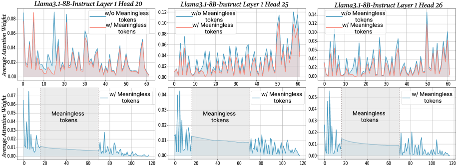<details> <summary>x18.png Details</summary>  ### Visual Description ## Line Chart: Attention Weights for Llama3 Models ### Overview The image presents six line charts comparing the average attention weight for the Llama3 1-8B-Instruct model across different layers (20, 25, and 26) and conditions: with and without "meaningless tokens". Each chart displays attention weight as a function of token position. The top row shows attention weights without meaningless tokens, and the bottom row shows attention weights with meaningless tokens. ### Components/Axes * **X-axis:** Token Position. Scales vary per chart, ranging from 0-60 and 0-120. * **Y-axis:** Average Attention Weight. Scales vary per chart, ranging from 0-0.12. * **Title:** Each chart is titled with "Llama3.1-8B-Instruct Layer [Layer Number] Head [Head Number]". * **Legend:** Each chart has a legend indicating two lines: "w/o Meaningless tokens" (red) and "w/ Meaningless tokens" (blue). * **Shaded Area:** A shaded area under each line represents a smoothed trend. ### Detailed Analysis **Chart 1: Llama3.1-8B-Instruct Layer 1 Head 20** (Top-Left) * **w/o Meaningless tokens (Red):** The line fluctuates significantly between approximately 0.00 and 0.11. It generally slopes downward from position 0 to 50, then remains relatively stable. Approximate data points: (0, 0.08), (20, 0.06), (40, 0.03), (50, 0.02). * **w/ Meaningless tokens (Blue):** The line fluctuates between approximately 0.00 and 0.04. It shows a more erratic pattern with frequent peaks and valleys. Approximate data points: (0, 0.02), (20, 0.03), (40, 0.01), (50, 0.005). **Chart 2: Llama3.1-8B-Instruct Layer 1 Head 25** (Top-Center) * **w/o Meaningless tokens (Red):** The line fluctuates between approximately 0.00 and 0.12. It shows a general upward trend from position 0 to 30, then declines. Approximate data points: (0, 0.02), (20, 0.08), (40, 0.05), (60, 0.03). * **w/ Meaningless tokens (Blue):** The line fluctuates between approximately 0.00 and 0.08. It shows a more stable pattern with less pronounced peaks and valleys. Approximate data points: (0, 0.01), (20, 0.04), (40, 0.03), (60, 0.02). **Chart 3: Llama3.1-8B-Instruct Layer 1 Head 26** (Top-Right) * **w/o Meaningless tokens (Red):** The line fluctuates between approximately 0.00 and 0.14. It shows a general upward trend from position 0 to 30, then declines. Approximate data points: (0, 0.02), (20, 0.10), (40, 0.06), (60, 0.04). * **w/ Meaningless tokens (Blue):** The line fluctuates between approximately 0.00 and 0.08. It shows a more stable pattern with less pronounced peaks and valleys. Approximate data points: (0, 0.01), (20, 0.05), (40, 0.04), (60, 0.03). **Chart 4: Llama3.1-8B-Instruct Layer 1 Head 20** (Bottom-Left) * **w/ Meaningless tokens (Blue):** The line fluctuates between approximately 0.00 and 0.04. It shows a more erratic pattern with frequent peaks and valleys. The x-axis ranges from 0 to 120. Approximate data points: (20, 0.02), (60, 0.01), (100, 0.005). **Chart 5: Llama3.1-8B-Instruct Layer 1 Head 25** (Bottom-Center) * **w/ Meaningless tokens (Blue):** The line fluctuates between approximately 0.00 and 0.03. It shows a more erratic pattern with frequent peaks and valleys. The x-axis ranges from 0 to 120. Approximate data points: (20, 0.015), (60, 0.01), (100, 0.008). **Chart 6: Llama3.1-8B-Instruct Layer 1 Head 26** (Bottom-Right) * **w/ Meaningless tokens (Blue):** The line fluctuates between approximately 0.00 and 0.05. It shows a more erratic pattern with frequent peaks and valleys. The x-axis ranges from 0 to 120. Approximate data points: (20, 0.025), (60, 0.015), (100, 0.01). ### Key Observations * The attention weights are generally higher when meaningless tokens are *not* present (red lines) in the first three charts. * The bottom row charts (with meaningless tokens) show significantly lower attention weights overall. * The attention weights tend to decrease as the token position increases, particularly in the top row charts. * The lines representing "w/o Meaningless tokens" exhibit more pronounced fluctuations than those representing "w/ Meaningless tokens". ### Interpretation The data suggests that the presence of "meaningless tokens" significantly reduces the average attention weight assigned to each token by the Llama3 model. This indicates that the model focuses less on these tokens, potentially treating them as noise. The varying attention weights across different layers (20, 25, and 26) suggest that the model's attention mechanism evolves as information propagates through the network. The downward trend in attention weights with increasing token position could indicate that the model prioritizes earlier tokens in the sequence. The smoothed areas under the lines suggest a general trend, while the fluctuations represent the model's dynamic attention allocation. The difference in scale between the top and bottom rows highlights the substantial impact of meaningless tokens on attention distribution. The charts provide insights into how the model processes information and the role of meaningful vs. meaningless tokens in its attention mechanism. </details> Figure 18: The average attention weights of Llama3.1-8B-Instruct in Head 20, 25, 26. 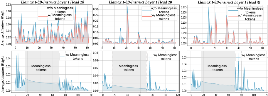<details> <summary>x19.png Details</summary>  ### Visual Description ## Line Chart: Attention Weight Comparison with and without Meaningless Tokens ### Overview The image presents three line charts, arranged horizontally. Each chart compares the average attention weight for two conditions: "w/o Meaningless tokens" (without meaningless tokens) and "w/ Meaningless tokens" (with meaningless tokens). The charts correspond to different layers and heads of the Llama3.1-8B-Instruct model: Head 28, Head 29, and Head 31. Each chart has two subplots, one showing the attention weights up to x=60 and the other showing the attention weights up to x=120. ### Components/Axes * **X-axis:** Represents the token position, ranging from 0 to 60 in the top subplots and 0 to 120 in the bottom subplots. * **Y-axis:** Represents the Average Attention Weight, ranging from 0 to 0.12 in the first chart, 0 to 0.3 in the second chart, and 0 to 0.175 in the third chart. * **Lines:** Two lines are plotted in each chart: * Red line: "w/o Meaningless tokens" * Cyan line: "w/ Meaningless tokens" * **Title:** Each chart is titled with "Llama3.1-8B-Instruct Layer 1 Head [Number]". * **Legend:** Located in the top-right corner of each chart, indicating the color correspondence for each condition. ### Detailed Analysis or Content Details **Chart 1: Llama3.1-8B-Instruct Layer 1 Head 28** * **Top Subplot (0-60):** * The red line ("w/o Meaningless tokens") shows several sharp peaks, with maximum values around 0.10 at approximately x=20, x=40, and x=50. The line generally fluctuates between 0 and 0.10. * The cyan line ("w/ Meaningless tokens") is relatively flat, hovering around 0.02-0.04 for most of the range, with a slight increase towards the end, reaching approximately 0.06 at x=60. * **Bottom Subplot (0-120):** * The cyan line ("w/ Meaningless tokens") remains relatively flat, fluctuating between 0.01 and 0.04. **Chart 2: Llama3.1-8B-Instruct Layer 1 Head 29** * **Top Subplot (0-60):** * The red line ("w/o Meaningless tokens") exhibits several peaks, with maximum values around 0.25 at approximately x=10, x=30, and x=50. The line fluctuates significantly. * The cyan line ("w/ Meaningless tokens") is generally lower, fluctuating between 0.02 and 0.10, with a peak around 0.10 at x=30. * **Bottom Subplot (0-120):** * The cyan line ("w/ Meaningless tokens") remains relatively flat, fluctuating between 0.01 and 0.07. **Chart 3: Llama3.1-8B-Instruct Layer 1 Head 31** * **Top Subplot (0-60):** * The red line ("w/o Meaningless tokens") shows several peaks, with maximum values around 0.13 at approximately x=10, x=30, and x=50. The line fluctuates significantly. * The cyan line ("w/ Meaningless tokens") is generally lower, fluctuating between 0.01 and 0.08, with a peak around 0.08 at x=30. * **Bottom Subplot (0-120):** * The cyan line ("w/ Meaningless tokens") remains relatively flat, fluctuating between 0.01 and 0.05. ### Key Observations * In all three charts, the "w/o Meaningless tokens" (red line) consistently exhibits higher and more pronounced peaks in the top subplots compared to the "w/ Meaningless tokens" (cyan line). * The "w/ Meaningless tokens" lines are generally much flatter, especially in the bottom subplots, indicating a more uniform distribution of attention weights. * The magnitude of the attention weights varies across the different heads (28, 29, 31). Head 29 shows the highest overall attention weights. * The bottom subplots show that the cyan lines remain relatively stable, suggesting that the addition of meaningless tokens doesn't significantly alter the attention distribution beyond the initial 60 tokens. ### Interpretation The data suggests that the inclusion of "meaningless tokens" significantly alters the attention patterns within the Llama3.1-8B-Instruct model. Without meaningless tokens, the model focuses attention on specific tokens (as evidenced by the sharp peaks in the red lines), likely those most relevant to the task. The addition of meaningless tokens appears to diffuse the attention, resulting in a more uniform distribution (flatter cyan lines). The higher attention weights observed in Head 29 might indicate that this head is particularly sensitive to the presence of meaningful information or is more prone to being influenced by the addition of meaningless tokens. The difference between the top and bottom subplots suggests that the initial tokens (0-60) are more affected by the presence of meaningless tokens than the later tokens (60-120). This could be due to the model attempting to integrate the meaningless tokens into the context during the initial stages of processing. The overall trend indicates that meaningless tokens reduce the model's ability to focus on the most important parts of the input sequence, potentially impacting its performance on downstream tasks. This is a critical observation for understanding the impact of data quality and preprocessing on the behavior of large language models. </details> Figure 19: The average attention weights of Llama3.1-8B-Instruct in Head 28, 29, 31. 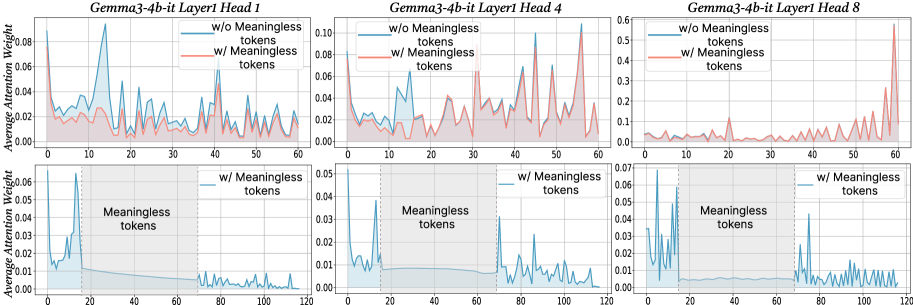<details> <summary>x20.png Details</summary>  ### Visual Description ## Line Chart: Gemma3-4b-it Attention Weight Analysis ### Overview This image presents a series of six line charts comparing the average attention weight for the Gemma3-4b-it model with and without "meaningless tokens" across different layers (Head 1, Head 4, and Head 8). Each chart displays the average attention weight on the y-axis against a token position on the x-axis. The charts are arranged in a 2x3 grid. ### Components/Axes * **X-axis:** Token Position (ranging from 0 to approximately 120, depending on the chart). * **Y-axis:** Average Attention Weight (ranging from 0 to approximately 0.5, depending on the chart). * **Legend:** * Red Line: "w/o Meaningless tokens" (without meaningless tokens) * Blue Line: "w/ Meaningless tokens" (with meaningless tokens) * **Titles:** Each chart is titled with "Gemma3-4b-it Layer [Head Number]" * **Subtitles:** Each chart has a subtitle indicating the token type being displayed ("w/o Meaningless tokens" or "w/ Meaningless tokens"). ### Detailed Analysis **Chart 1: Gemma3-4b-it Layer 1 Head 1** * The red line (w/o Meaningless tokens) shows a fluctuating pattern, generally staying below 0.04, with several peaks and valleys. * The blue line (w/ Meaningless tokens) is relatively flat, hovering around 0.01-0.02. * X-axis ranges from 0 to 60. * Approximate data points (red line): (10, 0.03), (20, 0.01), (30, 0.035), (40, 0.025), (50, 0.03), (60, 0.015). * Approximate data points (blue line): (10, 0.012), (20, 0.015), (30, 0.018), (40, 0.013), (50, 0.016), (60, 0.011). **Chart 2: Gemma3-4b-it Layer 1 Head 4** * The red line (w/o Meaningless tokens) exhibits a more pronounced fluctuating pattern, reaching peaks around 0.08. * The blue line (w/ Meaningless tokens) remains relatively flat, around 0.01-0.02. * X-axis ranges from 0 to 60. * Approximate data points (red line): (10, 0.02), (20, 0.05), (30, 0.07), (40, 0.04), (50, 0.06), (60, 0.03). * Approximate data points (blue line): (10, 0.011), (20, 0.014), (30, 0.017), (40, 0.012), (50, 0.015), (60, 0.010). **Chart 3: Gemma3-4b-it Layer 1 Head 8** * The red line (w/o Meaningless tokens) shows significant fluctuations, with peaks reaching approximately 0.45. * The blue line (w/ Meaningless tokens) remains relatively flat, around 0.01-0.02. * X-axis ranges from 0 to 60. * Approximate data points (red line): (10, 0.1), (20, 0.3), (30, 0.4), (40, 0.25), (50, 0.35), (60, 0.15). * Approximate data points (blue line): (10, 0.012), (20, 0.015), (30, 0.018), (40, 0.013), (50, 0.016), (60, 0.011). **Chart 4: Gemma3-4b-it Layer 1 Head 1 (w/ Meaningless tokens)** * The blue line (w/ Meaningless tokens) shows a fluctuating pattern, generally staying below 0.02. * X-axis ranges from 0 to 120. * Approximate data points (blue line): (20, 0.01), (40, 0.015), (60, 0.012), (80, 0.008), (100, 0.011), (120, 0.009). **Chart 5: Gemma3-4b-it Layer 1 Head 4 (w/ Meaningless tokens)** * The blue line (w/ Meaningless tokens) shows a fluctuating pattern, generally staying below 0.05. * X-axis ranges from 0 to 120. * Approximate data points (blue line): (20, 0.02), (40, 0.03), (60, 0.025), (80, 0.018), (100, 0.022), (120, 0.019). **Chart 6: Gemma3-4b-it Layer 1 Head 8 (w/ Meaningless tokens)** * The blue line (w/ Meaningless tokens) shows a fluctuating pattern, generally staying below 0.07. * X-axis ranges from 0 to 120. * Approximate data points (blue line): (20, 0.03), (40, 0.04), (60, 0.035), (80, 0.028), (100, 0.032), (120, 0.03). ### Key Observations * The "w/o Meaningless tokens" (red line) consistently exhibits higher average attention weights than the "w/ Meaningless tokens" (blue line) in the first three charts (Head 1, Head 4, and Head 8). * The attention weights for the "w/o Meaningless tokens" line fluctuate more significantly than those for the "w/ Meaningless tokens" line, especially in Head 4 and Head 8. * The attention weights for the "w/ Meaningless tokens" line remain relatively stable across all layers and token positions. * The last three charts (w/ Meaningless tokens) show a similar pattern of low and relatively stable attention weights. ### Interpretation The data suggests that the presence of "meaningless tokens" significantly reduces the average attention weight in the Gemma3-4b-it model. The model appears to allocate less attention to these tokens, resulting in lower attention weights. The higher fluctuations in attention weights when "meaningless tokens" are absent indicate that the model is more actively processing and differentiating between relevant tokens. The consistent low attention weights for "meaningless tokens" across all layers suggest that this effect is consistent throughout the model's architecture. This could indicate that the model is effectively filtering out irrelevant information when it is present in the input sequence. The difference in attention weight magnitude between the two conditions is most pronounced in Head 8, suggesting that this layer is particularly sensitive to the presence or absence of meaningful tokens. </details> Figure 20: The average attention weights of Gemma3-4b-it in Head 1, 4, 8. See pages 1-last of case_study.pdf