# Generative World Modelling for Humanoids 1X World Model Challenge Technical Report - Team Revontuli
> equal contribution.
Abstract
World models are a powerful paradigm in AI and robotics, enabling agents to reason about the future by predicting visual observations or compact latent states. The 1X World Model Challenge introduces an open-source benchmark of real-world humanoid interaction, with two complementary tracks: sampling, focused on forecasting future image frames, and compression, focused on predicting future discrete latent codes. For the sampling track, we adapt the video generation foundation model Wan-2.2 TI2V-5B to video-state-conditioned future frame prediction. We condition the video generation on robot states using AdaLN-Zero, and further post-train the model using LoRA. For the compression track, we train a Spatio-Temporal Transformer model from scratch. Our models achieve 23.0 dB PSNR in the sampling task and a Top-500 CE of 6.6386 in the compression task, securing 1st place in both challenges.
1 Introduction
World models [11] equip agents (e.g. humanoid robots) with internal simulators of their environments. By “imagining” the consequences of their actions, agents can plan, anticipate outcomes, and improve decision-making without direct real-world interaction.
A central challenge in world modelling is the design of architectures that are both sufficiently expressive and computationally tractable. Early approaches have largely relied on recurrent networks [13, 14, 15] or multilayer perceptrons [16, 17, 34, 7]. More recently, advances in generative modelling have driven a new wave of architectural choices. A prominent line of work leverages autoregressive transformers over discrete latent spaces [6, 33, 41, 26, 3, 10], while others explore diffusion- and flow-based approaches [1, 8]. At scale, these methods underpin powerful foundation models [21, 39, 36, 28, 12, 23] capable of producing realistic and accurate video predictions.
<details>
<summary>figs/image_1.png Details</summary>
### Visual Description
## Diagram: Tokenizer and Evaluation Process
### Overview
The image illustrates a process involving a tokenizer, generation, and evaluation, likely within a machine learning or robotics context. It shows a sequence of actions involving a robotic arm interacting with objects, followed by data processing steps.
### Components/Axes
* **Top Row:** Sequence of images showing a robotic arm interacting with objects on a table. The images are framed with different colored borders (teal, light green, light green, dark gray). Arrows indicate the flow of the process.
* **Tokenizer:** Text label positioned below the first image sequence. A downward-pointing teal arrow connects the image sequence to a 3D cube representation.
* **Context + States:** Text label in red and teal, positioned below the 3D cube representation associated with the tokenizer.
* **Generation:** Text label in green, positioned below the second 3D cube representation.
* **Evaluation:** Text label in black, positioned below the third 3D cube representation.
* **3D Cube Representations:** Three sets of cubes, each associated with a different stage (Tokenizer, Generation, Evaluation). The first set is teal, the second is light green, and the third is gray.
* **Arrows:** Arrows indicate the flow of data/process between the stages. A teal arrow points from the first image sequence to the first cube representation. A light green arrow points from the first cube representation to the second. A light green double-headed arrow connects the second and third cube representations.
### Detailed Analysis
* **Image Sequence 1 (Top-Left):** Shows a robotic arm reaching into a container with various objects. The image is framed in teal. Multiple ghosted images are overlaid, showing the arm's movement.
* **Image Sequence 2 (Top-Middle-Left):** Shows a robotic arm holding an object from the container. The image is framed in light green. Multiple ghosted images are overlaid, showing the arm's movement.
* **Image Sequence 3 (Top-Middle-Right):** Shows a robotic arm holding an object from the container. The image is framed in light green.
* **Image Sequence 4 (Top-Right):** Shows a robotic arm holding an object from the container. The image is framed in dark gray.
* **Tokenizer Stage:** The "Tokenizer" stage takes the image sequence as input and converts it into a 3D cube representation labeled "Context + States".
* **Generation Stage:** The "Generation" stage takes the output from the "Tokenizer" stage and generates a new 3D cube representation.
* **Evaluation Stage:** The "Evaluation" stage compares the "Generation" output with a final 3D cube representation.
### Key Observations
* The diagram illustrates a sequential process.
* The color of the frames and 3D cube representations changes as the process progresses (teal -> light green -> dark gray).
* The robotic arm interaction with objects is the initial input to the process.
* The 3D cube representations likely symbolize data or states at different stages.
### Interpretation
The diagram likely represents a machine learning or robotics pipeline where a robotic arm's actions are captured as images, tokenized into a state representation, used for generation, and then evaluated. The "Tokenizer" stage likely converts the visual input into a numerical or symbolic representation that can be processed by subsequent stages. The "Generation" stage might involve predicting the next action or state based on the context. The "Evaluation" stage assesses the quality or accuracy of the generated output. The color changes could represent different levels of processing or confidence in the data.
</details>
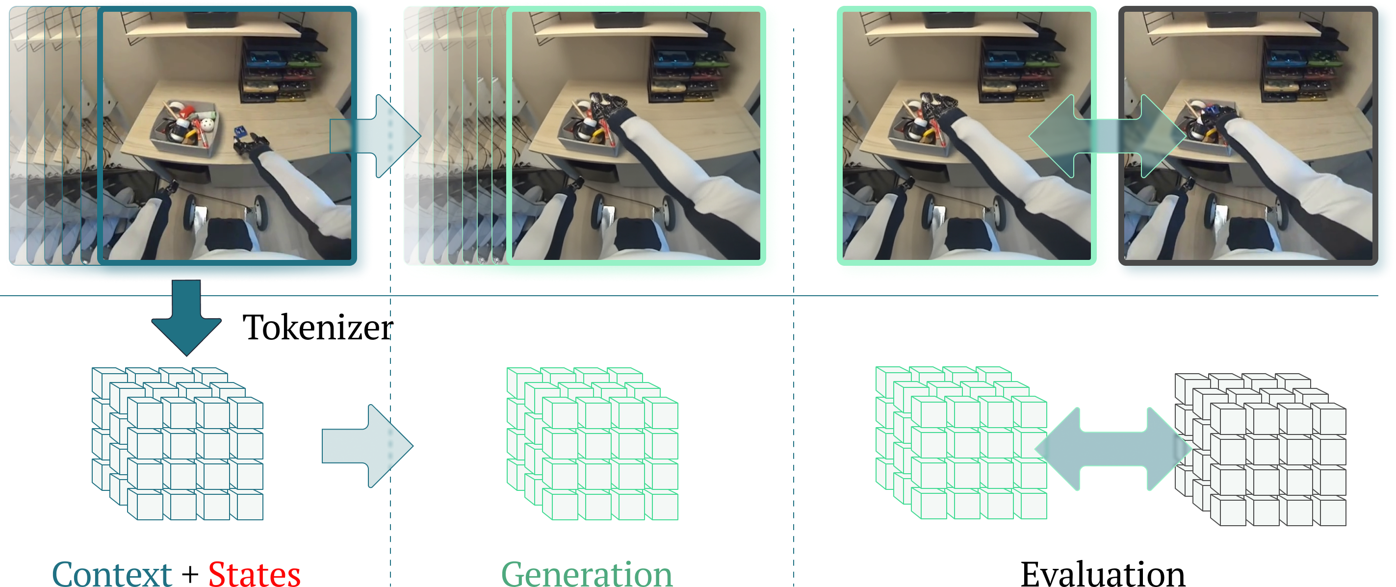
Figure 1: Overview of the 1X World Model Challenges Left depicts the context (inputs), middle the model generations, and right the evaluations. Sampling challenge (top): The model observes 17 past frames along with past and future robot states, then generates future frames in pixel space. Performance is measured by PSNR between the predicted and ground-truth 77th frame. Compression challenge (bottom): The Cosmos $8× 8× 8$ tokeniser encodes the history of 17 RGB frames into three latent token grids of shape $3× 32× 32$ . Models must predict the next three latent token grids corresponding to the next 17 frames. Evaluation is based on Top-500 cross-entropy between predicted and ground-truth tokens.
Table 1: Performance on Public 1X World Model Leaderboard
| Sampling | Revontuli Duke | Test 23.00 21.56 | Val 25.53 25.30 | Test (Top-500) – – | Val – – | 1st 2nd |
| --- | --- | --- | --- | --- | --- | --- |
| Michael | 18.51 | – | – | – | 3rd | |
| Revontuli | – | – | 6.64 | 4.92 | 1st | |
| Compression | Duke | – | – | 7.50 | 5.60 | 2nd |
| a27sridh | – | – | 7.99 | – | 3rd | |
The 1X World Model Challenge evaluates predictive performance on two tracks: Sampling and Compression. Fig. 1 outlines the tasks, and Tab. 1 reports our results. These challenges capture core problems when using world models in robotics. Our methods show strong performance that we hope will shape future efforts.
2 Sampling Challenge
Problem Statement
In the sampling task, the model must predict the $512× 512$ frame observed by the robot $2$ s into the future. Conditioning is provided by the first 17 frames $\mathbf{x}_{0:16}$ and the complete sequence of robot states $\mathbf{s}_{0:76}∈\mathbb{R}^{77× 25}$ . Performance is evaluated using PSNR between the predicted and ground-truth last frames.
Data Pre-processing
We downsample the original 77 frames clips by a factor of four, yielding shorter 21 sample clips. As a result, this gives us five conditioning frames, ( $\mathbf{x}_{0},\mathbf{x}_{4},...,\mathbf{x}_{16}$ ), and the remaining 16 serve as prediction targets. Wan2.2-VAE applies spatial compression to the first frame and temporal compression of 4 to the remaining frames, producing a latent sequence of length $(1+(L-1)/4)$ for a clip of length $L=21$ .
2.1 Model
Base Model
For our solution, we adapt Wan 2.2 TI2V-5B [36], a flow-matching generative video model with a 30-layer DiT backbone [30]. The base model is designed as a text-image-to-video (TI2V), but we modified the architecture to condition the predictions on videos and robot states. The model operates on latent video representations from Wan2.2-VAE, which compresses clips to a size $(1+(L-1)/4)× 16× 16$ .
Video-State Conditioning
To incorporate video conditioning, we modified the masking of the input latents. In a standard image-to-video model, the first latent in the time dimension is masked, treating the input image as fixed during generation, thereby establishing a conditional mapping. We extend this idea by fixing multiple frames during generation, effectively transforming the model from image-to-video to video-to-video. The original Wan 2.2 also conditions textual prompts to generate videos. Since our dataset does not include textual descriptions, we use empty strings as text prompts while retaining the original cross-attention layer, enabling future work to leverage text conditioning.
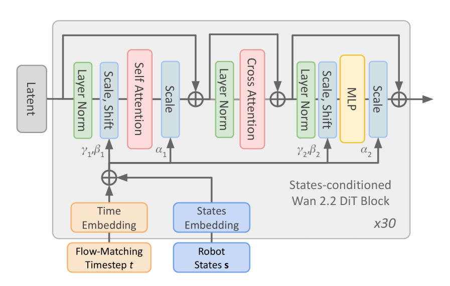
As shown in Fig. 2, we incorporate state conditioning into the model’s predictions using adaLN-Zero [30] within Wan’s DiT blocks. We first downsample the states to match those of the downsampled video. The continuous angle and velocity states are augmented with sinusoidal features, and all states are projected through an MLP to a hidden dimension of $r_{\text{dim}}=256$ .
Then, we compress the projected features along the temporal dimension with a 2-layer 1d convolutional network to match the compression of Wan-VAE for the video frames, mapping the state features to shape $((1+L//4),r_{\text{dim}})$ . Finally, we fed the compressed feature into an MLP layer to get the modulation used by adaLN-Zero layers. The obtained robot modulation is added to the modulation of the flow matching timestep. The robot modulation acts differently on latent since the timestep embedding is the same for the whole latent, while for the states, they will modulate the latent slice associated with the corresponding frames.
<details>
<summary>x1.png Details</summary>
### Visual Description
## Diagram: States-conditioned Wan 2.2 DiT Block
### Overview
The image is a diagram illustrating the architecture of a States-conditioned Wan 2.2 Diffusion Transformer (DiT) Block. It shows the flow of data through various layers and operations, including Layer Normalization, Scale/Shift, Self Attention, Cross Attention, and MLP (Multi-Layer Perceptron). The diagram highlights the conditioning of the block on both time and robot states. The block is repeated 30 times.
### Components/Axes
* **Input:** Latent
* **Processing Blocks (repeated three times):**
* Layer Norm (Green)
* Scale, Shift (Blue)
* Self Attention (Red) or Cross Attention (Red) or MLP (Yellow)
* Scale (Blue)
* **Conditioning Inputs:**
* Time Embedding (Orange) - Flow-Matching Timestep t
* States Embedding (Blue) - Robot States s
* **Parameters:**
* γ1, β1 (associated with the first Layer Norm and Scale/Shift)
* α1 (associated with the first Scale)
* γ2, β2 (associated with the second Layer Norm and Scale/Shift)
* α2 (associated with the second Scale)
* **Output:** Output of the final Scale block.
* **Repetition:** x30 (Indicates the entire block is repeated 30 times)
### Detailed Analysis
The diagram illustrates a repeating block structure. The "Latent" input flows through a series of operations. Each block consists of a "Layer Norm" (green), followed by "Scale, Shift" (blue), then either "Self Attention" (red), "Cross Attention" (red), or "MLP" (yellow), and finally "Scale" (blue). The first block contains "Self Attention", the second contains "Cross Attention", and the third contains "MLP". The output of each block is fed back into the "Time Embedding" and "States Embedding" via an addition operation (⊕). The entire block is repeated 30 times, as indicated by "x30" at the bottom-right.
* **Latent Input:** The process begins with a "Latent" input, represented by a gray box on the top-left.
* **First Block:**
* The latent input flows into a "Layer Norm" block (green).
* The output of "Layer Norm" goes into a "Scale, Shift" block (blue).
* The output of "Scale, Shift" goes into a "Self Attention" block (red).
* The output of "Self Attention" goes into a "Scale" block (blue).
* **Second Block:**
* The output of the first "Scale" block flows into a "Layer Norm" block (green).
* The output of "Layer Norm" goes into a "Cross Attention" block (red).
* The output of "Cross Attention" goes into a "Scale" block (blue).
* **Third Block:**
* The output of the second "Scale" block flows into a "Layer Norm" block (green).
* The output of "Layer Norm" goes into a "Scale, Shift" block (blue).
* The output of "Scale, Shift" goes into an "MLP" block (yellow).
* The output of "MLP" goes into a "Scale" block (blue).
* **Conditioning:**
* "Time Embedding" (orange) and "States Embedding" (blue) provide conditioning signals.
* "Time Embedding" is associated with "Flow-Matching Timestep t".
* "States Embedding" is associated with "Robot States s".
* These embeddings are added (⊕) to the signal after the "Latent" input.
* **Parameters:**
* γ1, β1 are associated with the first "Layer Norm" and "Scale, Shift" blocks.
* α1 is associated with the first "Scale" block.
* γ2, β2 are associated with the third "Layer Norm" and "Scale, Shift" blocks.
* α2 is associated with the third "Scale" block.
### Key Observations
* The diagram illustrates a repeating block structure with variations in the attention mechanism (Self Attention, Cross Attention, and MLP).
* The conditioning inputs (Time Embedding and States Embedding) are crucial for the DiT block's functionality.
* The repetition factor (x30) indicates a deep architecture.
### Interpretation
The diagram represents a key component of a diffusion transformer model, specifically designed for tasks involving robot states and time-dependent data. The repeating block structure allows the model to learn complex relationships between the latent input, time, and robot states. The use of Self Attention, Cross Attention, and MLP within the blocks enables the model to capture different types of dependencies in the data. The conditioning on both time and robot states suggests that the model is designed to generate or process data that is dependent on both the current time step and the robot's state. The repetition of the block 30 times indicates a deep neural network, capable of learning intricate patterns.
</details>
Figure 2: State conditioning of DiT-Block. Wan2.2 TI2V-5B DiT architecture was updated to enable state conditioning using adaLN-Zero [30] and combining it with the timestep of the Flow Matching scheduler [36].
2.2 Training
Models were trained for 23k steps with AdamW [25] with a constant learning rate of $4· 10^{-4}$ . We applied LoRA [22] fine-tuning with rank 32 on the Wan 2.2 DiT backbone. We experimented with and without classifier-free guidance (CFG) [20] during training but observed little improvement in PSNR performance (see Sec. 2.4). Training was conducted on a DataCrunch instant cluster equipped with 4 nodes, each with $8×$ NVIDIA B200 GPUs. We used a total effective batch size of 1024. The B200 VRAM capacity of 184GB allows for more efficient training of memory-hungry video generation models.
2.3 Inference
Since the challenge does not restrict inference compute time, we experimented with different approaches for our submissions. In our initial attempts, we followed [24] post-processing pipeline, applying Gaussian blur and performing histogram matching on the predicted frames. This post-processing improved the PSNR score by $1.2$ dB, as reported in [24]. Because PSNR heavily penalizes outlier deviations from the target image, sharper images with slight errors are typically scored worse than blurrier images with comparable errors.
We found that exploiting predictive uncertainty with an ensemble of predictions outperformed Gaussian blurring. This produces blurring mainly in regions of high motion, such as the humanoid’s arms (see Tab. 2). Increasing the number of ensemble samples improved PSNR on both the validation set and the public leaderboard, with different performance found from tuning the number of inference steps and the classifier-free guidance weight, as shown in Tab. 2.
Table 2: Sampling results on validation and test sets. † The results on test set were obtained after the deadline. ∗ This model has been trained on the whole train + validation raw dataset.
| Num. Inf. Samples 20 | Num. Samples 1 | CFG Scale – | Val. PSNR $[\uparrow]$ 22.63 | Test PSNR $[\uparrow]$ 21.05 | Val. SSIM $[\uparrow]$ 0.707 | Val. LPIPS $[\downarrow]$ 0.137 | Val. FID $[\downarrow]$ 40.23 |
| --- | --- | --- | --- | --- | --- | --- | --- |
| 5 | – | 24.52 | 22.11 | 0.750 | 0.165 | 71.46 | |
| 20 | – | 24.88 | 22.42 | 0.762 | 0.201 | 90.71 | |
| 1st sub. ∗ | 20 | – | 26.62 | 23.00 | 0.836 | 0.082 | 31.70 |
| 20 | 20 | 2.0 | 24.20 | 22.26 | 0.734 | 0.164 | 71.83 |
| 2nd sub. | 20 | 1.5 | 24.59 | 22.53 | 0.746 | 0.169 | 74.10 |
| 100 | 20 | 1.5 | 25.07 | 22.55 † | 0.762 | 0.148 | 65.76 |
| 20 | 1.0 | 25.53 | 23.04 † | 0.773 | 0.158 | 69.25 | |
2.4 Results
Tab. 2 reports the quantitative results of our model on the validation set using the PSNR metric. We further extend the evaluation by reporting Structural Similarity Index Measure (SSIM) [37], Learned Perceptual Image Patch Similarity (LPIPS) [40], and Fréchet Inception Distance (FID) [19], all computed on our model’s predictions over the validation set.
The table is divided into three blocks. The first block contains models trained without classifier-free guidance (CFG) [20]. We ablate over the number of averaged samples used for final predictions, ranging from 1 to 20. Increasing the number of samples has a smoothing effect that improves Val. PSNR scores but degrades visual quality, as reflected in the other metrics. The bottom row of this block contains a model that is additionally trained on the validation dataset. This makes the values reported on the validation dataset not comparable with the rest of the entries in the table. However, the result on the public leaderboard showed a $+0.58$ dB increase on PSNR.
The second and third blocks present models trained with CFG applied during training. Earlier experiments on the validation data showed that raising the cfg_scale beyond a certain point did not improve PSNR scores. Nevertheless, we retained the run with cfg_scale as our second-best competition submission. For completeness, we also report results obtained by increasing the number of sampling steps using the same checkpoint. These results show consistent improvements over the previous CFG-based predictions.
3 Compression Challenge
<details>
<summary>x2.png Details</summary>
### Visual Description
## Diagram: Spatio-Temporal Attention Block
### Overview
The image is a diagram illustrating the architecture of a Spatio-Temporal (ST) attention block within a larger neural network. The diagram shows the flow of data from input tokens, through embedding, spatial and temporal attention mechanisms, and finally to output tokens. The diagram includes components such as Layer Normalization, Multi-Layer Perceptrons (MLPs), and linear transformations.
### Components/Axes
* **Input Tokens:** Represented as a stack of three grids, labeled with dimensions T, H, and W.
* **Embed:** A block that embeds the input tokens.
* **Robot State:** A block containing an image of a robot, followed by MLP and Conv layers.
* **Spatial Attention:** A block that performs spatial attention, including Layer Norm.
* **Temporal Attention:** A block that performs temporal attention, including Layer Norm.
* **ST Block:** A block containing both Spatial and Temporal Attention, and an MLP.
* **L Layers:** Indicates that the ST Block is repeated L times.
* **Layer Norm:** A normalization layer.
* **MLP:** Multi-Layer Perceptron.
* **Linear:** A linear transformation layer.
* **Output Tokens:** Represented as a stack of three grids, similar to the input tokens.
### Detailed Analysis
1. **Input Tokens:** The input consists of a stack of three grids, labeled with T, H, and W, representing the temporal, height, and width dimensions, respectively.
2. **Embedding:** The input tokens are passed through an "Embed" block, which transforms them into a suitable representation for further processing.
3. **Robot State:** The robot state is processed through MLP and Conv layers. The output of the embedding and the robot state are added together.
4. **Spatial Attention:** The embedded tokens are then fed into a Spatial Attention block. This block includes a Layer Norm, followed by an attention mechanism represented by a grid, and another Layer Norm.
5. **Temporal Attention:** The output of the Spatial Attention block is fed into a Temporal Attention block. This block includes a Layer Norm, followed by an attention mechanism represented by a grid with colored squares, and another Layer Norm.
6. **ST Block:** The Spatial and Temporal Attention blocks are combined into an ST Block, which also includes an MLP.
7. **L Layers:** The ST Block is repeated L times, indicating that the network consists of multiple layers of these blocks.
8. **Output Tokens:** Finally, the output of the L layers is passed through a Layer Norm and a Linear transformation layer to produce the output tokens.
### Key Observations
* The diagram highlights the flow of data through the Spatio-Temporal attention mechanism.
* The use of Layer Norm is consistent throughout the architecture.
* The ST Block is the core component of the network, repeated L times.
### Interpretation
The diagram illustrates a neural network architecture designed to process spatio-temporal data, likely for tasks involving robot perception or action. The network uses attention mechanisms to focus on relevant spatial and temporal features in the input. The repetition of the ST Block allows the network to learn hierarchical representations of the data. The inclusion of a "Robot State" input suggests that the network is designed to incorporate information about the robot's current state into its processing. The diagram provides a high-level overview of the network architecture and its key components.
</details>
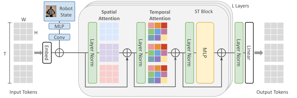
(a) Illustration of our ST-Transformer architecture for the compression challenge Given three grids of past video tokens of shape $3× 32× 32$ , as well as the robot state of shape $64× 25$ as context, the transformer predicts the future three grids of shape $3× 32× 32$ . The ST-Transformer consists of $L$ layers of spatio-temporal blocks, each containing per time step spatial attention over the $H× W$ tokens at time step $t$ , followed by causal temporal attention of the same spatial coordinate across time, and then a feed-forward network. Each colour in the spatial and temporal attention represents a single self-attention map.
<details>
<summary>x3.png Details</summary>
### Visual Description
## Chart: Cross Entropy Loss vs. Step
### Overview
The image is a line chart displaying the cross-entropy loss over training steps for three different configurations: Train (Teacher Forced), Val (Teacher Forced), and Val (Autoregressive). The x-axis represents the training step, and the y-axis represents the cross-entropy loss.
### Components/Axes
* **X-axis:** "Step" with markers at 0k, 20k, 40k, 60k, and 80k.
* **Y-axis:** "Cross Entropy Loss" with markers at 4, 5, 6, 7, and 8.
* **Legend:** Located at the top-right of the chart.
* Blue line: "Train (Teacher Forced)"
* Orange line: "Val (Teacher Forced)"
* Green line: "Val (Autoregressive)"
### Detailed Analysis
* **Train (Teacher Forced) - Blue Line:**
* Trend: The line slopes downward, indicating a decrease in cross-entropy loss as the training step increases.
* Starting point: Approximately 7.2 at step 0k.
* Ending point: Approximately 4.9 at step 80k.
* The line fluctuates more than the other two.
* **Val (Teacher Forced) - Orange Line:**
* Trend: The line slopes downward, indicating a decrease in cross-entropy loss as the training step increases.
* Starting point: Approximately 6.8 at step 0k.
* Ending point: Approximately 4.4 at step 80k.
* The line is smoother than the other two.
* **Val (Autoregressive) - Green Line:**
* Trend: The line slopes downward, indicating a decrease in cross-entropy loss as the training step increases.
* Starting point: Approximately 7.9 at step 0k.
* Ending point: Approximately 4.9 at step 80k.
* The line fluctuates more than the orange line, but less than the blue line.
### Key Observations
* All three lines show a decreasing trend in cross-entropy loss as the training step increases.
* The "Val (Teacher Forced)" line (orange) consistently has the lowest cross-entropy loss after the initial steps.
* The "Train (Teacher Forced)" line (blue) and "Val (Autoregressive)" line (green) converge to approximately the same cross-entropy loss at the end of the training steps.
### Interpretation
The chart illustrates the learning process of a model under different training and validation configurations. The decreasing cross-entropy loss indicates that the model is learning and improving its performance over time. The "Val (Teacher Forced)" configuration appears to be the most effective, as it achieves the lowest validation loss. The convergence of the "Train (Teacher Forced)" and "Val (Autoregressive)" lines suggests that the model's performance is similar under these two configurations at the end of the training process. The fluctuations in the "Train (Teacher Forced)" and "Val (Autoregressive)" lines may indicate some instability or sensitivity to the training data.
</details>
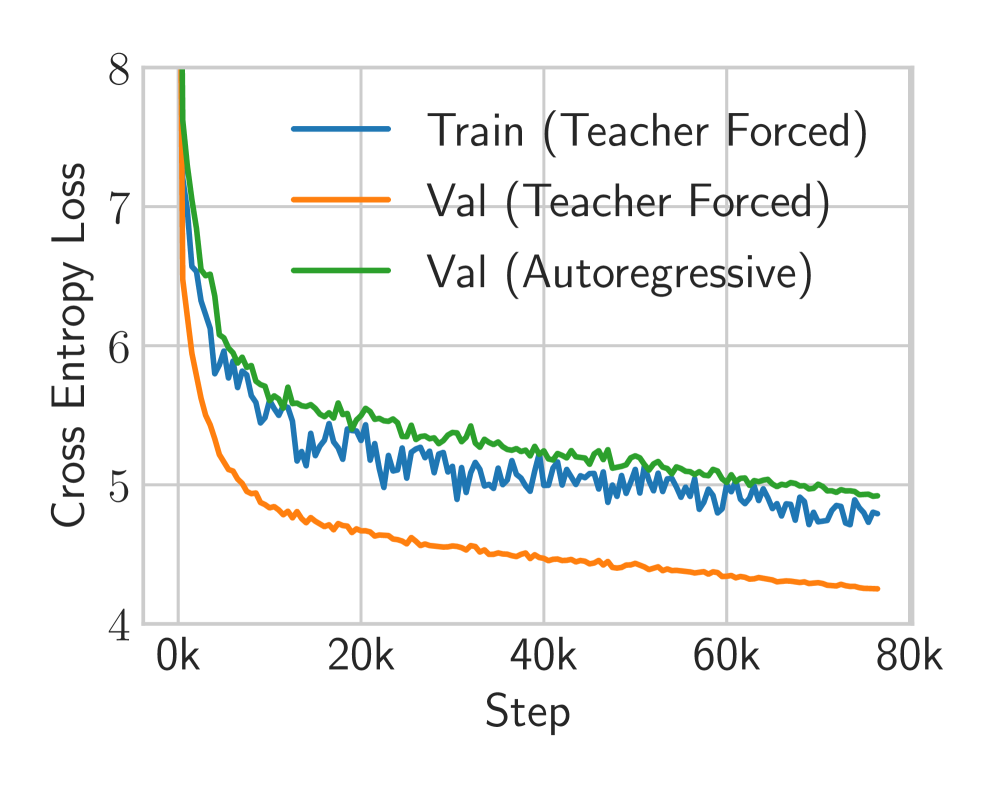
(b) Training curves for compression challenge At train time, we use teacher forcing (blue). We then evaluate on the validation set using unrealistic teacher forcing (orange), as well as with the greedy autoregressive generation that will be used at inference time (green).
Figure 3: Overall figure showing (a) the ST-Transformer world model architecture and (b) its training curves in the compression challenge.
Unlike the Sampling Challenge, which measures prediction directly in pixel space, the Compression Challenge evaluates models in a discrete latent space. Each video sequence is first compressed into a grid of discrete tokens using the Cosmos $8× 8× 8$ tokeniser [28], producing a compact sequence that can be modelled with sequence architectures.
Problem Statement
Given a context of $H=3$ grids of $32× 32$ tokens and robot states for both past and future timesteps, the task is to predict the next $M=3$ grids of $32× 32$ tokens:
$$
\displaystyle\hat{\mathbf{z}}_{H:H+M-1} \displaystyle\sim f_{\theta}({\bm{z}}_{0:H-1},{\bm{s}}_{0:63}) \tag{1}
$$
where $\hat{{\bm{z}}}_{H:H+M-1}$ are the predicted token grids for the future frames. The tokenized training dataset $\mathcal{D}$ contains approximately $306{,}000$ samples. Each sample consists of:
- Tokenised video: $6$ consecutive token grids (3 past, 3 future), each of size $32× 32$ , giving $6144$ tokens per sample and $\sim 1.88$ B tokens overall.
- Robot state: a sequence ${\bm{s}}∈\mathbb{R}^{64× 25}$ aligned with the corresponding raw video frames.
A block of three $32× 32$ token grids corresponds to 17 RGB frames at $256× 256$ resolution, so predictions in token space remain aligned with the original video. Performance is evaluated using top-500 cross-entropy, which considers only the top-500 logits per token.
3.1 Model
Spatio-temporal Transformer
Following Genie [6], our world model builds on the Vision Transformer (ViT) [9, 35]. An overview is shown in Fig. 3. To reduce the quadratic memory cost of standard Transformers, we use a spatio-temporal (ST) Transformer [38], which alternates spatial and temporal attention blocks followed by feed-forward layers. Spatial attention attends over $1× 32× 32$ tokens per frame, while temporal attention (with a causal mask) attends across $T× 1× 1$ tokens over time. This design makes spatial attention, the main bottleneck, scale linearly with the number of frames, improving efficiency for video generation. We apply pre-LayerNorm [2] and QKNorm [18] for stability. Positional information is added via learnable absolute embeddings for both spatial and temporal tokens. Our transformer used 24 layers, 8 heads, an embedding dimension of $512$ , a sequence length of $T=5$ , and dropout of $0.1$ on all attention, MLPs, and residual connections.
State Conditioning
Robot states are encoded as additive embeddings following Bruce et al. [6]. The state vector is projected with an MLP, processed by a 1D convolution (kernel size 3, padding 1), and enriched with absolute position embeddings before being combined with video tokens.
3.2 Training
We implemented our model in PyTorch [29] and trained it using the fused AdamW optimiser [25] with $\beta_{1}=0.9$ and $\beta_{2}=0.95$ for $80$ epochs. Weight decay of $0.05$ was applied only to parameter matrices, while biases, normalisation parameters, gains, and positional embeddings were excluded. Following GPT-2 [32] and Press and Wolf [31], Bertolotti and Cazzola [5], we tied the input and output embeddings. This reduces the memory footprint by removing one of the two largest weight matrices and typically improves both training speed and final performance.
Training Objective
The model was trained to minimise the cross-entropy loss between predicted and ground-truth tokens at future time steps:
| | $\displaystyle\min_{\theta}\,\mathbb{E}_{({\bm{z}}_{t},{\bm{s}}_{t})_{t=0:K+M-1}\sim\mathcal{D},\hat{{\bm{z}}}_{t}\sim f_{\theta}(·)}\left[\sum_{t=K}^{K+M-1}\text{CE}\left(\hat{{\bm{z}}}_{t},{\bm{z}}_{t}\right)\right],$ | |
| --- | --- | --- |
where $\hat{{\bm{z}}}_{t}$ is the model output at time $t$ , CE denotes the cross-entropy loss over all tokens in the grid, and $\mathcal{D}$ is the dataset of tokenised video and state sequences. Training used teacher forcing to allow parallel computation across timesteps, with a linear learning rate schedule from peak $8× 10^{-4}$ to $0$ after a warmup of $2000$ steps.
Implementation
Training used automatic mixed precision (AMP) with bfloat16, but inference used float32 due to degraded performance in bfloat16. Linear layer biases were zero-initialised, and weights (including embeddings) were drawn from $\mathcal{N}(0,0.02)$ . We trained with an effective batch size of 160 on the same B200 DataCrunch instant cluster as in the sampling challenge.
3.3 Inference
Our autoregressive model generates sequences via
| | $\displaystyle p({\bm{z}}_{H:H+M-1}\mid{\bm{z}}_{0:H-1},{\bm{s}}_{0:63})=\prod_{t=H}^{H+M-1}f_{\theta}({\bm{z}}_{t}\mid{\bm{z}}_{<t},{\bm{s}}_{0:63}),$ | |
| --- | --- | --- |
where each step outputs a categorical distribution over each spatial token. Sampling draws ${\bm{z}}_{t}\sim f_{\theta}(·)$ , introducing diversity but typically yields lower-probability trajectories and higher loss. Greedy decoding instead selects
$$
{\bm{z}}_{t}=\arg\max_{{\bm{z}}}f_{\theta}({\bm{z}}\mid{\bm{z}}_{<t},{\bm{s}}_{0:63}),
$$
producing deterministic, high-probability sequences that we found both effective and efficient.
3.4 Results
Fig. 3(b) shows the training curves for our ST-Transformer. The blue curve corresponds to the training loss under teacher-forced training. While the teacher-forced validation loss is optimistic – since it conditions on ground-truth inputs – it can be interpreted as a lower bound on the achievable loss, representing the performance of an idealised autoregressive model with perfect inference. To reduce the gap between teacher-forced and autoregressive performance, we experimented with scheduled sampling [4, 27]. However, this did not lead to meaningful improvements.
4 Conclusion
In this report, we presented two complementary approaches that achieved strong performance across both 1X World Model Challenges. First, we showed how internet-scale data can be leveraged by fine-tuning a pre-trained image–text-to-video foundation model. Using multi-node training on the DataCrunch instant cluster, we reached first place on the leaderboard in only 36 hours—an order of magnitude faster than the runner-up, who required about a month. To further improve inference, we averaged over samples to selectively blur regions of high predictive uncertainty. While this proved effective for optimising PSNR, the most suitable inference strategy for downstream decision-making remains an open question. Second, we demonstrated how a spatio-temporal transformer world model can be trained on the tokenised dataset in under 17 hours. We found that greedy autoregressive inference offered a practical balance of speed and accuracy. Despite its simplicity, the model achieved substantially lower loss values than other leaderboard entries.
References
- Alonso et al. [2024] Eloi Alonso, Adam Jelley, Vincent Micheli, Anssi Kanervisto, Amos Storkey, Tim Pearce, and François Fleuret. Diffusion for World Modeling: Visual Details Matter in Atari. In The Thirty-eighth Annual Conference on Neural Information Processing Systems. Curran Associates, Inc., 2024.
- Ba et al. [2016] Jimmy Lei Ba, Jamie Ryan Kiros, and Geoffrey E. Hinton. Layer Normalization. arXiv preprint arXiv:1607.06450, 2016.
- Bar et al. [2024] Amir Bar, Gaoyue Zhou, Danny Tran, Trevor Darrell, and Yann LeCun. Navigation World Models. arXiv preprint arXiv:2412.03572, 2024.
- Bengio et al. [2015] Samy Bengio, Oriol Vinyals, Navdeep Jaitly, and Noam Shazeer. Scheduled Sampling for Sequence Prediction with Recurrent Neural Networks. In Advances in Neural Information Processing Systems. Curran Associates, Inc., 2015.
- Bertolotti and Cazzola [2024] Francesco Bertolotti and Walter Cazzola. By Tying Embeddings You Are Assuming the Distributional Hypothesis. In Proceedings of the 41st International Conference on Machine Learning, pages 3584–3610, 2024.
- Bruce et al. [2024] Jake Bruce, Michael Dennis, Ashley Edwards, Jack Parker-Holder, Yuge Shi, Edward Hughes, Matthew Lai, Aditi Mavalankar, Richie Steigerwald, Chris Apps, Yusuf Aytar, Sarah Bechtle, Feryal Behbahani, Stephanie Chan, Nicolas Heess, Lucy Gonzalez, Simon Osindero, Sherjil Ozair, Scott Reed, Jingwei Zhang, Konrad Zolna, Jeff Clune, de Nando Freitas, Satinder Singh, and Tim Rocktäschel. Genie: Generative Interactive Environments. arXiv preprint arXiv:2402.15391, 2024.
- Chua et al. [2018] Kurtland Chua, Roberto Calandra, Rowan McAllister, and Sergey Levine. Deep Reinforcement Learning in a Handful of Trials using Probabilistic Dynamics Models. In Advances in Neural Information Processing Systems, 2018.
- Decart et al. [2024] Etched Decart, Quinn McIntyre, Spruce Campbell, Xinlei Chen, and Robert Wachen. Oasis: A Universe in a Transformer. 2024.
- Dosovitskiy et al. [2020] Alexey Dosovitskiy, Lucas Beyer, Alexander Kolesnikov, Dirk Weissenborn, Xiaohua Zhai, Thomas Unterthiner, Mostafa Dehghani, Matthias Minderer, Georg Heigold, Sylvain Gelly, Jakob Uszkoreit, and Neil Houlsby. An Image is Worth 16x16 Words: Transformers for Image Recognition at Scale. In International Conference on Learning Representations, 2020.
- Guo et al. [2025] Junliang Guo, Yang Ye, Tianyu He, Haoyu Wu, Yushu Jiang, Tim Pearce, and Jiang Bian. MineWorld: A Real-Time and Open-Source Interactive World Model on Minecraft. arXiv preprint arXiv:2504.08388, 2025.
- Ha and Schmidhuber [2018] David Ha and Jürgen Schmidhuber. Recurrent World Models Facilitate Policy Evolution. In Advances in Neural Information Processing Systems. Curran Associates, Inc., 2018.
- HaCohen et al. [2024] Yoav HaCohen, Nisan Chiprut, Benny Brazowski, Daniel Shalem, Dudu Moshe, Eitan Richardson, Eran Levin, Guy Shiran, Nir Zabari, Ori Gordon, Poriya Panet, Sapir Weissbuch, Victor Kulikov, Yaki Bitterman, Zeev Melumian, and Ofir Bibi. LTX-Video: Realtime Video Latent Diffusion. arXiv preprint arXiv:2501.00103, 2024.
- Hafner et al. [2019] Danijar Hafner, Timothy Lillicrap, Ian Fischer, Ruben Villegas, David Ha, Honglak Lee, and James Davidson. Learning Latent Dynamics for Planning from Pixels. In International Conference on Machine Learning, 2019.
- Hafner et al. [2022] Danijar Hafner, Timothy P. Lillicrap, Mohammad Norouzi, and Jimmy Ba. Mastering Atari with Discrete World Models. In International Conference on Learning Representations, 2022.
- Hafner et al. [2025] Danijar Hafner, Jurgis Pasukonis, Jimmy Ba, and Timothy Lillicrap. Mastering Diverse Control Tasks through World Models. Nature, 640(8059):647–653, 2025.
- Hansen et al. [2023] Nicklas Hansen, Hao Su, and Xiaolong Wang. TD-MPC2: Scalable, Robust World Models for Continuous Control. In The Twelfth International Conference on Learning Representations, 2023.
- Hansen et al. [2022] Nicklas A. Hansen, Hao Su, and Xiaolong Wang. Temporal Difference Learning for Model Predictive Control. In Proceedings of the 39th International Conference on Machine Learning, 2022.
- [18] Alex Henry, Prudhvi Raj Dachapally, Shubham Shantaram Pawar, and Yuxuan Chen. Query-Key Normalization for Transformers. In Findings of the Association for Computational Linguistics: EMNLP 2020, pages 4246–4253. Association for Computational Linguistics.
- Heusel et al. [2017] Martin Heusel, Hubert Ramsauer, Thomas Unterthiner, Bernhard Nessler, and Sepp Hochreiter. GANs Trained by a Two Time-Scale Update Rule Converge to a Local Nash Equilibrium. In Advances in Neural Information Processing Systems. Curran Associates, Inc., 2017.
- Ho and Salimans [2021] Jonathan Ho and Tim Salimans. Classifier-Free Diffusion Guidance. In NeurIPS 2021 Workshop on Deep Generative Models and Downstream Applications, 2021.
- Hong et al. [2022] Wenyi Hong, Ming Ding, Wendi Zheng, Xinghan Liu, and Jie Tang. CogVideo: Large-scale Pretraining for Text-to-Video Generation via Transformers. arXiv preprint arXiv:2205.15868, 2022.
- Hu et al. [2022] Edward J Hu, yelong shen, Phillip Wallis, Zeyuan Allen-Zhu, Yuanzhi Li, Shean Wang, Lu Wang, and Weizhu Chen. LoRA: Low-Rank Adaptation of Large Language Models. In International Conference on Learning Representations, 2022.
- Kong et al. [2024] Weijie Kong, Qi Tian, Zijian Zhang, Rox Min, Zuozhuo Dai, Jin Zhou, Jiangfeng Xiong, Xin Li, Bo Wu, Jianwei Zhang, et al. HunyuanVideo: A Systematic Framework For Large Video Generative Models. arXiv preprint arXiv:2412.03603, 2024.
- Liu et al. [2025] Peter Liu, Annabelle Chu, and Yiran Chen. Effective World Modeling for Humanoid Robots: Long-Horizon Prediction and Efficient State Compression. Technical Report Team Duke, Duke University, 2025. 1X World Model Challenge, CVPR 2025.
- Loshchilov and Hutter [2019] Ilya Loshchilov and Frank Hutter. Decoupled Weight Decay Regularization. In International Conference on Learning Representations, 2019.
- Micheli et al. [2022] Vincent Micheli, Eloi Alonso, and François Fleuret. Transformers are Sample-Efficient World Models. In The Eleventh International Conference on Learning Representations, 2022.
- Mihaylova and Martins [2019] Tsvetomila Mihaylova and André F. T. Martins. Scheduled Sampling for Transformers. In Proceedings of the 57th Annual Meeting of the Association for Computational Linguistics: Student Research Workshop, pages 351–356. Association for Computational Linguistics, 2019.
- NVIDIA et al. [2025] NVIDIA, Niket Agarwal, Arslan Ali, Maciej Bala, Yogesh Balaji, Erik Barker, Tiffany Cai, Prithvijit Chattopadhyay, Yongxin Chen, Yin Cui, Yifan Ding, Daniel Dworakowski, Jiaojiao Fan, Michele Fenzi, Francesco Ferroni, Sanja Fidler, Dieter Fox, Songwei Ge, Yunhao Ge, Jinwei Gu, Siddharth Gururani, Ethan He, Jiahui Huang, Jacob Huffman, Pooya Jannaty, Jingyi Jin, Seung Wook Kim, Gergely Klár, Grace Lam, Shiyi Lan, Laura Leal-Taixe, Anqi Li, Zhaoshuo Li, Chen-Hsuan Lin, Tsung-Yi Lin, Huan Ling, Ming-Yu Liu, Xian Liu, Alice Luo, Qianli Ma, Hanzi Mao, Kaichun Mo, Arsalan Mousavian, Seungjun Nah, Sriharsha Niverty, David Page, Despoina Paschalidou, Zeeshan Patel, Lindsey Pavao, Morteza Ramezanali, Fitsum Reda, Xiaowei Ren, Vasanth Rao Naik Sabavat, Ed Schmerling, Stella Shi, Bartosz Stefaniak, Shitao Tang, Lyne Tchapmi, Przemek Tredak, Wei-Cheng Tseng, Jibin Varghese, Hao Wang, Haoxiang Wang, Heng Wang, Ting-Chun Wang, Fangyin Wei, Xinyue Wei, Jay Zhangjie Wu, Jiashu Xu, Wei Yang, Lin Yen-Chen, Xiaohui Zeng, Yu Zeng, Jing Zhang, Qinsheng Zhang, Yuxuan Zhang, Qingqing Zhao, and Artur Zolkowski. Cosmos World Foundation Model Platform for Physical AI. arxiv preprint arXiv:2501.03575, 2025.
- [29] Adam Paszke, Sam Gross, Francisco Massa, Adam Lerer, James Bradbury, Gregory Chanan, Trevor Killeen, Zeming Lin, Natalia Gimelshein, Luca Antiga, Alban Desmaison, Andreas Kopf, Edward Yang, Zachary DeVito, Martin Raison, Alykhan Tejani, Sasank Chilamkurthy, Benoit Steiner, Lu Fang, Junjie Bai, and Soumith Chintala. PyTorch: An Imperative Style, High-Performance Deep Learning Library. In Advances in Neural Information Processing Systems. Curran Associates, Inc.
- Peebles and Xie [2023] William Peebles and Saining Xie. Scalable Diffusion Models with Transformers. In Proceedings of the IEEE/CVF international conference on computer vision, pages 4195–4205, 2023.
- [31] Ofir Press and Lior Wolf. Using the Output Embedding to Improve Language Models. In Proceedings of the 15th Conference of the European Chapter of the Association for Computational Linguistics: Volume 2, Short Papers, pages 157–163. Association for Computational Linguistics.
- Radford et al. [2019] Alec Radford, Jeff Wu, Rewon Child, David Luan, Dario Amodei, and Ilya Sutskever. Language Models are Unsupervised Multitask Learners. 2019.
- Robine et al. [2022] Jan Robine, Marc Höftmann, Tobias Uelwer, and Stefan Harmeling. Transformer-based World Models Are Happy With 100k Interactions. In The Eleventh International Conference on Learning Representations, 2022.
- Scannell et al. [2025] Aidan Scannell, Mohammadreza Nakhaei, Kalle Kujanpää, Yi Zhao, Kevin Luck, Arno Solin, and Joni Pajarinen. Discrete Codebook World Models for Continuous Control. In The Thirteenth International Conference on Learning Representations, 2025.
- Vaswani et al. [2017] Ashish Vaswani, Noam Shazeer, Niki Parmar, Jakob Uszkoreit, Llion Jones, Aidan N Gomez, Ł ukasz Kaiser, and Illia Polosukhin. Attention is All you Need. In Advances in Neural Information Processing Systems. Curran Associates, Inc., 2017.
- Wang et al. [2025] Ang Wang, Baole Ai, Bin Wen, Chaojie Mao, Chen-Wei Xie, Di Chen, Feiwu Yu, Haiming Zhao, Jianxiao Yang, Jianyuan Zeng, Jiayu Wang, Jingfeng Zhang, Jingren Zhou, Jinkai Wang, Jixuan Chen, Kai Zhu, Kang Zhao, Keyu Yan, Lianghua Huang, Xiaofeng Meng, Ningyi Zhang, Pandeng Li, Pingyu Wu, Ruihang Chu, Ruili Feng, Shiwei Zhang, Siyang Sun, Tao Fang, Tianxing Wang, Tianyi Gui, Tingyu Weng, Tong Shen, Wei Lin, Wei Wang, Wei Wang, Wenmeng Zhou, Wente Wang, Wenting Shen, Wenyuan Yu, Xianzhong Shi, Xiaoming Huang, Xin Xu, Yan Kou, Yangyu Lv, Yifei Li, Yijing Liu, Yiming Wang, Yingya Zhang, Yitong Huang, Yong Li, You Wu, Yu Liu, Yulin Pan, Yun Zheng, Yuntao Hong, Yupeng Shi, Yutong Feng, Zeyinzi Jiang, Zhen Han, Zhi-Fan Wu, and Ziyu Liu. Wan: Open and Advanced Large-Scale Video Generative Models. CoRR, abs/2503.20314, 2025.
- Wang et al. [2003] Z Wang, EP Simoncelli, and AC Bovik. Multiscale structural similarity for image quality assessment. In The Thrity-Seventh Asilomar Conference on Signals, Systems & Computers, 2003, pages 1398–1402. IEEE, 2003.
- Xu et al. [2021] Mingxing Xu, Wenrui Dai, Chunmiao Liu, Xing Gao, Weiyao Lin, Guo-Jun Qi, and Hongkai Xiong. Spatial-Temporal Transformer Networks for Traffic Flow Forecasting. arXiv preprint arXiv:2001.02908, 2021.
- Yang et al. [2024] Zhuoyi Yang, Jiayan Teng, Wendi Zheng, Ming Ding, Shiyu Huang, Jiazheng Xu, Yuanming Yang, Wenyi Hong, Xiaohan Zhang, Guanyu Feng, et al. CogVideoX: Text-to-Video Diffusion Models with An Expert Transformer. arXiv preprint arXiv:2408.06072, 2024.
- Zhang et al. [2018] Richard Zhang, Phillip Isola, Alexei A Efros, Eli Shechtman, and Oliver Wang. The Unreasonable Effectiveness of Deep Features as a Perceptual Metric. In 2018 IEEE/CVF Conference on Computer Vision and Pattern Recognition (CVPR), pages 586–595. IEEE Computer Society, 2018.
- Zhang et al. [2023] Weipu Zhang, Gang Wang, Jian Sun, Yetian Yuan, and Gao Huang. STORM: Efficient Stochastic Transformer based World Models for Reinforcement Learning. In Advances in Neural Information Processing Systems, pages 27147–27166. Curran Associates, Inc., 2023.