2510.09033v1

# Large Language Models Do NOT Really Know What They Don’t Know Abstract Recent work suggests that large language models (LLMs) encode factuality signals in their internal representations, such as hidden states, attention weights, or token probabilities, implying that LLMs may “ know what they don’t know ”. However, LLMs can also produce factual errors by relying on shortcuts or spurious associations. These error are driven by the same training objective that encourage correct predictions, raising the question of whether internal computations can reliably distinguish between factual and hallucinated outputs. In this work, we conduct a mechanistic analysis of how LLMs internally process factual queries by comparing two types of hallucinations based on their reliance on subject information. We find that when hallucinations are associated with subject knowledge, LLMs employ the same internal recall process as for correct responses, leading to overlapping and indistinguishable hidden-state geometries. In contrast, hallucinations detached from subject knowledge produce distinct, clustered representations that make them detectable. These findings reveal a fundamental limitation: LLMs do not encode truthfulness in their internal states but only patterns of knowledge recall, demonstrating that LLMs don’t really know what they don’t know. 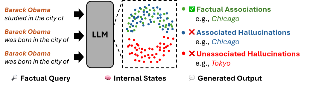Large Language Models Do NOT Really Know What They Don’t Know Chi Seng Cheang 1 Hou Pong Chan 2 Wenxuan Zhang 3 Yang Deng 1 1 Singapore Management University 2 DAMO Academy, Alibaba Group 3 Singapore University of Technology and Design cs.cheang.2025@phdcs.smu.edu.sg, houpong.chan@alibaba-inc.com wxzhang@sutd.edu.sg, ydeng@smu.edu.sg 1 Introduction Large language models (LLMs) demonstrate remarkable proficiency in generating coherent and contextually relevant text, yet they remain plagued by hallucination Zhang et al. (2023b); Huang et al. (2025), a phenomenon where outputs appear plausible but are factually inaccurate or entirely fabricated, raising concerns about their reliability and trustworthiness. To this end, researchers suggest that the internal states of LLMs (e.g., hidden representations Azaria and Mitchell (2023); Gottesman and Geva (2024), attention weights Yüksekgönül et al. (2024), output token logits Orgad et al. (2025); Varshney et al. (2023), etc.) can be used to detect hallucinations, indicating that LLMs themselves may actually know what they don’t know. These methods typically assume that when a model produces hallucinated outputs (e.g., “ Barack Obama was born in the city of Tokyo ” in Figure 1), its internal computations for the outputs (“ Tokyo ”) are detached from the input information (“ Barack Obama ”), thereby differing from those used to generate factually correct outputs. Thus, the hidden states are expected to capture this difference and serve as indicators of hallucinations. <details> <summary>x1.png Details</summary>  ### Visual Description ## Diagram: LLM Factual Associations and Hallucinations ### Overview The image is a diagram illustrating how a Large Language Model (LLM) processes factual queries and generates outputs, highlighting the concepts of factual associations, associated hallucinations, and unassociated hallucinations. It shows the flow of information from factual queries to the LLM, the internal states within the LLM, and the generated outputs, categorized by their accuracy. ### Components/Axes * **Input (Left Side):** * Three example factual queries about Barack Obama: * "Barack Obama studied in the city of" * "Barack Obama was born in the city of" (appears twice) * A magnifying glass icon labeled "Factual Query" * **Processing (Center):** * A gray rounded rectangle labeled "LLM" with three black arrows pointing from the factual queries to the LLM. * **Internal States (Center-Right):** * A dashed rectangle representing "Internal States" containing scattered colored dots: * Green dots: Representing factual associations. * Blue dots: Representing associated hallucinations. * Red dots: Representing unassociated hallucinations. * A brain icon labeled "Internal States" * **Output (Right Side):** * Legend explaining the colored dots: * Green dot with a checkmark: "Factual Associations" (e.g., Chicago) * Blue dot with an X mark: "Associated Hallucinations" (e.g., Chicago) * Red dot with an X mark: "Unassociated Hallucinations" (e.g., Tokyo) * A speech bubble icon labeled "Generated Output" ### Detailed Analysis or ### Content Details * **Factual Queries:** The queries are simple statements about Barack Obama, designed to elicit responses from the LLM. * **LLM Processing:** The LLM block represents the internal processing of the queries. * **Internal States:** The colored dots within the dashed rectangle visually represent the LLM's internal associations and potential errors. The green dots are clustered in the top portion, while the red dots are clustered in the bottom portion, with some blue dots mixed in the top portion. * **Generated Output:** The legend explains the meaning of each color: * Green dots represent correct factual associations. * Blue dots represent hallucinations that are associated with the query context (e.g., a wrong city, but still a city). * Red dots represent hallucinations that are not associated with the query context (e.g., a completely unrelated city). ### Key Observations * The diagram visually separates correct factual associations from different types of hallucinations. * The "Internal States" representation shows a clustering of factual associations (green) and unassociated hallucinations (red), suggesting a degree of separation in the LLM's internal representation. * The examples provided in the legend clarify the distinction between associated and unassociated hallucinations. ### Interpretation The diagram illustrates the challenges of ensuring factual accuracy in LLMs. It highlights that LLMs can generate not only correct information but also different types of incorrect information (hallucinations). The distinction between associated and unassociated hallucinations is important because it suggests different mechanisms for error generation. Associated hallucinations might arise from incorrect associations within the LLM's knowledge base, while unassociated hallucinations might stem from more random or unrelated sources. The diagram suggests that understanding and mitigating these different types of hallucinations is crucial for improving the reliability of LLMs. </details> Figure 1: Illustration of three categories of knowledge. Associated hallucinations follow similar internal knowledge recall processes with factual associations, while unassociated hallucinations arise when the model’s output is detached from the input. However, other research (Lin et al., 2022b; Kang and Choi, 2023; Cheang et al., 2023) shows that models can also generate false information that is closely associated with the input information. In particular, models may adopt knowledge shortcuts, favoring tokens that frequently co-occur in the training corpus over factually correct answers Kang and Choi (2023). As shown in Figure 1, given the prompt: “Barack Obama was born in the city of”, an LLM may rely on the subject tokens’ representations (i.e., “Barack Obama”) to predict a hallucinated output (e.g., “Chicago”), which is statistically associated with the subject entity but under other contexts (e.g., “ Barack Obama studied in the city of Chicago ”). Therefore, we suspect that the internal computations may not exhibit distinguishable patterns between correct predictions and input-associated hallucinations, as LLMs rely on the input information to produce both of them. Only when the model produces hallucinations unassociated with the input do the hidden states exhibit distinct patterns that can be reliably identified. To this end, we conduct a mechanistic analysis of how LLMs internally process factual queries. We first perform causal analysis to identify hidden states crucial for generating Factual Associations (FAs) — factually correct outputs grounded in subject knowledge. We then examine how these hidden states behave when the model produces two types of factual errors: Associated Hallucinations (AHs), which remain grounded in subject knowledge, and Unassociated Hallucinations (UHs), which are detached from it. Our analysis shows that when generating both FAs and AHs, LLMs propagate information encoded in subject representations to the final token during output generation, resulting in overlapping hidden-state geometries that cannot reliably distinguish AHs from FAs. In contrast, UHs exhibit distinct internal computational patterns, producing clearly separable hidden-state geometries from FAs. Building on the analysis, we revisit several widely-used hallucination detection approaches Gottesman and Geva (2024); Yüksekgönül et al. (2024); Orgad et al. (2025) that adopt internal state probing. The results show that these representations cannot reliably distinguish AHs from FAs due to their overlapping hidden-state geometries, though they can effectively separate UHs from FAs. Moreover, this geometry also shapes the limits the effectiveness of Refusal Tuning Zhang et al. (2024), which trains LLMs to refuse uncertain queries using refusal-aware dataset. Because UH samples exhibit consistent and distinctive patterns, refusal tuning generalizes well to unseen UHs but fails to generalize to unseen AHs. We also find that AH hidden states are more diverse, and thus refusal tuning with AH samples prevents generalization across both AH and UH samples. Together, these findings highlight a central limitation: LLMs do not encode truthfulness in their hidden states but only patterns of knowledge recall and utilization, showing that LLMs don’t really know what they don’t know. 2 Related Work Existing hallucination detection methods can be broadly categorized into two types: representation-based and confidence-based. Representation-based methods assume that an LLM’s internal hidden states can reflect the correctness of its generated responses. These approaches train a classifier (often a linear probe) using the hidden states from a set of labeled correct/incorrect responses to predict whether a new response is hallucinatory Li et al. (2023); Azaria and Mitchell (2023); Su et al. (2024); Ji et al. (2024); Chen et al. (2024); Ni et al. (2025); Xiao et al. (2025). Confidence-based methods, in contrast, assume that a lower confidence during the generation led to a higher probability of hallucination. These methods quantify uncertainty through various signals, including: (i) token-level output probabilities (Guerreiro et al., 2023; Varshney et al., 2023; Orgad et al., 2025); (ii) directly querying the LLM to verbalize its own confidence (Lin et al., 2022a; Tian et al., 2023; Xiong et al., 2024; Yang et al., 2024b; Ni et al., 2024; Zhao et al., 2024); or (iii) measuring the semantic consistency across multiple outputs sampled from the same prompt (Manakul et al., 2023; Kuhn et al., 2023; Zhang et al., 2023a; Ding et al., 2024). A response is typically flagged as a hallucination if its associated confidence metric falls below a predetermined threshold. However, a growing body of work reveals a critical limitation: even state-of-the-art LLMs are poorly calibrated, meaning their expressed confidence often fails to align with the factual accuracy of their generations (Kapoor et al., 2024; Xiong et al., 2024; Tian et al., 2023). This miscalibration limits the effectiveness of confidence-based detectors and raises a fundamental question about the extent of LLMs’ self-awareness of their knowledge boundary, i.e., whether they can “ know what they don’t know ” Yin et al. (2023); Li et al. (2025). Despite recognizing this problem, prior work does not provide a mechanistic explanation for its occurrence. To this end, our work addresses this explanatory gap by employing mechanistic interpretability techniques to trace the internal computations underlying knowledge recall within LLMs. 3 Preliminary Transformer Architecture Given an input sequence of $T$ tokens $t_{1},...,t_{T}$ , an LLM is trained to model the conditional probability distribution of the next token $p(t_{T+1}|t_{1},...,t_{T})$ conditioned on the preceding $T$ tokens. Each token is first mapped to a continuous vector by an embedding layer. The resulting sequence of hidden states is then processed by a stack of $L$ Transformer layers. At layer $\ell∈{1,...,L}$ , each token representation is updated by a Multi-Head Self-Attention (MHSA) and a Feed-Forward Network (MLP) module: $$ \mathbf{h}^{\ell}=\mathbf{h}^{\ell-1}+\mathbf{a}^{\ell}+\mathbf{m}^{\ell}, \tag{1} $$ where $\mathbf{a}^{\ell}$ and $\mathbf{m}^{\ell}$ correspond to the MHSA and MLP outputs, respectively, at the $\ell$ -layer. Internal Process of Knowledge Recall Prior work investigates the internal activations of LLMs to study the mechanics of knowledge recall. For example, an LLM may encode many attributes that are associated with a subject (e.g., Barack Obama) (Geva et al., 2023). Given a prompt like “ Barack Obama was born in the city of ”, if the model has correctly encoded the fact, the attribute “ Honolulu ” propagates through self-attention to the last token, yielding the correct answer. We hypothesize that non-factual predictions follow the same mechanism: spurious attributes such as “ Chicago ” are also encoded and propagated, leading the model to generate false outputs. Categorization of Knowledge To investigate how LLMs internally process factual queries, we define three categories of knowledge, according to two criteria: 1) factual correctness, and 2) subject representation reliance. - Factual Associations (FA) refer to factual knowledge that is reliably stored in the parameters or internal states of an LLM and can be recalled to produce correct, verifiable outputs. - Associated Hallucinations (AH) refer to non-factual content produced when an LLM relies on input-triggered parametric associations. - Unassociated Hallucinations (UH) refer to non-factual content produced without reliance on parametric associations to the input. <details> <summary>x2.png Details</summary>  ### Visual Description ## Heatmap: Avg JS Divergence vs. Layer ### Overview The image is a heatmap visualizing the average Jensen-Shannon (JS) divergence across different layers (0-30) for three categories: "Subj.", "Attn.", and "Last.". The color intensity represents the magnitude of the JS divergence, with darker blue indicating higher divergence and lighter blue indicating lower divergence. ### Components/Axes * **Y-axis:** Categorical labels: "Subj.", "Attn.", "Last." * **X-axis:** Layer number, ranging from 0 to 30 in increments of 2. * **Colorbar (Right):** "Avg JS Divergence" ranging from 0.2 to 0.6. Dark blue corresponds to 0.6, and light blue corresponds to 0.2. ### Detailed Analysis * **Subj.:** The "Subj." category exhibits high JS divergence (dark blue) from layer 0 to approximately layer 16. After layer 16, the divergence decreases slightly (lighter blue). The JS divergence for layers 0-16 is approximately 0.55-0.6, while for layers 18-30, it is approximately 0.45-0.5. * **Attn.:** The "Attn." category shows low JS divergence (light blue) from layer 0 to approximately layer 10. From layer 12 to layer 18, the divergence increases (darker blue), reaching a peak around layer 14-16, with a JS divergence of approximately 0.35-0.4. After layer 18, the divergence decreases again to approximately 0.2. * **Last.:** The "Last." category has low JS divergence (light blue) from layer 0 to layer 18, with a JS divergence of approximately 0.2. From layer 20 to layer 30, the divergence increases (darker blue), reaching a JS divergence of approximately 0.3-0.35. ### Key Observations * "Subj." has consistently high JS divergence in the initial layers. * "Attn." shows a peak in JS divergence around layers 14-16. * "Last." shows an increase in JS divergence in the later layers (20-30). ### Interpretation The heatmap suggests that the "Subj." category has the most significant divergence in the initial layers of the model, indicating that these layers are crucial for processing subject-related information. The "Attn." category shows a peak in divergence in the middle layers, suggesting that these layers are important for attention mechanisms. The "Last." category shows an increase in divergence in the later layers, indicating that these layers are important for final processing or output generation. The differences in JS divergence across layers and categories highlight the varying roles of different layers in the model for processing different types of information. </details> (a) Factual Associations <details> <summary>x3.png Details</summary>  ### Visual Description ## Heatmap: Avg JS Divergence by Layer ### Overview The image is a heatmap visualizing the average Jensen-Shannon (JS) divergence across different layers (0-30) for three categories: "Subj.", "Attn.", and "Last.". The heatmap uses a color gradient from light blue to dark blue, representing lower to higher JS divergence values, respectively. ### Components/Axes * **Y-axis:** Categorical labels: "Subj.", "Attn.", "Last." (from top to bottom). * **X-axis:** Numerical labels representing layers, ranging from 0 to 30 in increments of 2. * **Color Scale (Legend):** Located on the right side of the heatmap. * Dark Blue: Represents a high Avg JS Divergence of approximately 0.6. * Light Blue: Represents a low Avg JS Divergence of approximately 0.2. * **Axis Title:** "Avg JS Divergence" on the right side, and "Layer" on the bottom. ### Detailed Analysis * **Subj.:** The "Subj." category shows a consistently high Avg JS Divergence across all layers (0-30). The color is dark blue, indicating values close to 0.6. There is a slight decrease in JS divergence around layers 18-20, where the color becomes slightly lighter blue. * **Attn.:** The "Attn." category shows a low Avg JS Divergence (light blue, approximately 0.2) from layers 0 to approximately 8-10. The JS divergence then increases to a medium value (medium blue, approximately 0.3-0.4) from layers 10 to 20, and then returns to a low value (light blue, approximately 0.2) from layers 20 to 30. * **Last.:** The "Last." category shows a low Avg JS Divergence (light blue, approximately 0.2) from layers 0 to approximately 18-20. The JS divergence then increases to a medium value (medium blue, approximately 0.3-0.4) from layers 20 to 30. ### Key Observations * The "Subj." category consistently exhibits the highest Avg JS Divergence across all layers. * The "Attn." and "Last." categories show a similar pattern: low JS divergence in the initial layers, an increase in the middle layers, and then a return to low values in the later layers. * The transition points for "Attn." and "Last." are slightly different, with "Attn." increasing earlier than "Last.". ### Interpretation The heatmap suggests that the "Subj." category has a significantly different distribution compared to "Attn." and "Last." across all layers. The "Attn." and "Last." categories show a change in distribution in the middle layers, possibly indicating a shift in the information being processed by those layers. The JS divergence measures the similarity between probability distributions; therefore, higher divergence indicates less similarity. The data suggests that the "Subj." category's distribution is consistently different from the other two, while "Attn." and "Last." have distributions that change depending on the layer. </details> (b) Associated Hallucinations <details> <summary>x4.png Details</summary>  ### Visual Description ## Heatmap: Avg JS Divergence by Layer and Category ### Overview The image is a heatmap visualizing the average Jensen-Shannon (JS) divergence across different layers (0-30) for three categories: Subj. (Subject), Attn. (Attention), and Last. The color intensity represents the magnitude of the JS divergence, ranging from light blue (low divergence) to dark blue (high divergence). ### Components/Axes * **X-axis:** Layer, with values ranging from 0 to 30 in increments of 2. * **Y-axis:** Categories: Subj., Attn., Last. * **Color Scale (Legend):** Avg JS Divergence, ranging from 0.2 (light blue) to 0.6 (dark blue). The scale has markers at 0.2, 0.3, 0.4, 0.5, and 0.6. ### Detailed Analysis * **Subj. (Subject):** The JS divergence for the "Subj." category is relatively high (blue color) for layers 0 to approximately 16. The color intensity gradually decreases from layer 0 to 16, indicating a decreasing JS divergence. After layer 16, the JS divergence drops significantly and remains low (light blue). * Layer 0: Approximately 0.55 JS Divergence * Layer 8: Approximately 0.45 JS Divergence * Layer 16: Approximately 0.35 JS Divergence * **Attn. (Attention):** The JS divergence for the "Attn." category is consistently low (light blue) across all layers (0-30). The values appear to be close to 0.2. * **Last.:** The JS divergence for the "Last." category is consistently low (light blue) across all layers (0-30). The values appear to be close to 0.2. ### Key Observations * The "Subj." category exhibits a significantly higher JS divergence in the initial layers (0-16) compared to the "Attn." and "Last." categories. * The JS divergence for the "Attn." and "Last." categories remains consistently low across all layers. * There is a clear transition in the "Subj." category around layer 16, where the JS divergence drops sharply. ### Interpretation The heatmap suggests that the "Subject" category has a higher degree of divergence in the earlier layers of the model, indicating that the representations or information related to the subject are more variable or less stable in these initial layers. The "Attention" and "Last" categories, on the other hand, show consistently low divergence across all layers, suggesting more stable representations. The sharp drop in JS divergence for the "Subject" category after layer 16 could indicate a point where the model has effectively learned or stabilized the subject-related information. This could be due to the model learning to extract relevant features or representations related to the subject in the earlier layers, and then refining or stabilizing these representations in the later layers. 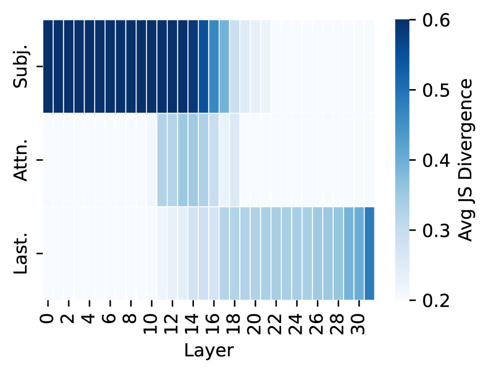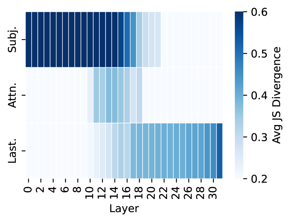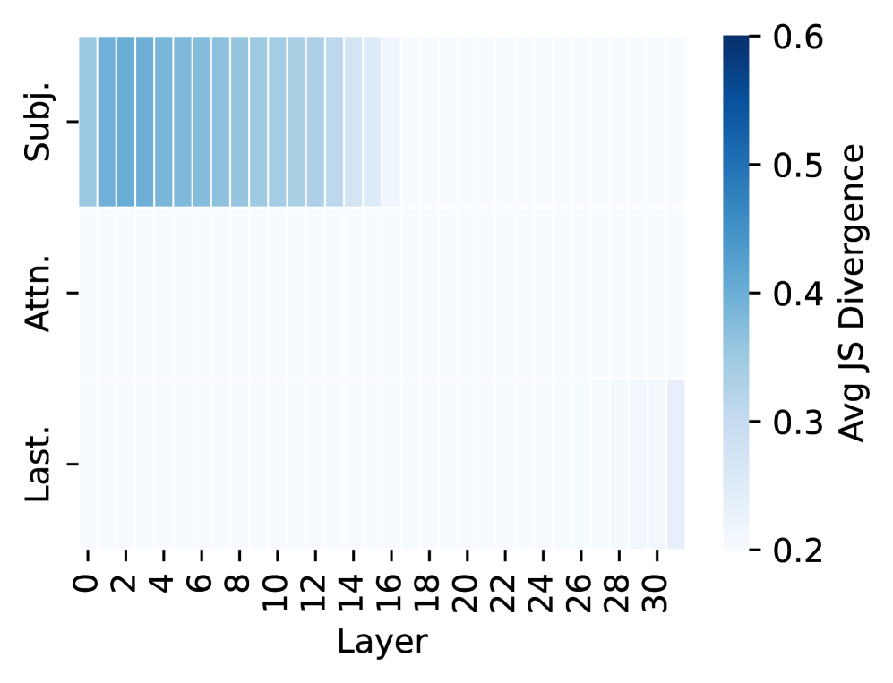</details> (c) Unassociated Hallucinations Figure 2: Effect of interventions across layers of LLaMA-3-8B. The heatmap shows JS divergence between the output distribution before and after intervention. Darker color indicates that the intervened hidden states are more causally influential on the model’s predictions. Top row: patching representations of subject tokens. Middle row: blocking attention flow from subject to the last token. Bottom row: patching representations of the last token. Dataset Construction | Factual Association Associated Hallucination Unassociated Hallucination | 3,506 1,406 7,381 | 3,354 1,284 7,655 | | --- | --- | --- | | Total | 12,293 | 12,293 | Table 1: Dataset statistics across categories. Our study is conducted under a basic knowledge-based question answering setting. The model is given a prompt containing a subject and relation (e.g., “ Barack Obama was born in the city of ”) and is expected to predict the corresponding object (e.g., “ Honolulu ”). To build the dataset, we collect knowledge triples $(\text{subject},\text{relation},\text{object})$ form Wikidata. Each relation was paired with a handcrafted prompt template to convert triples into natural language queries. The details of relation selection and prompt templates are provided in Appendix A.1. We then apply the label scheme presented in Appendix A.2: correct predictions are labeled as FAs, while incorrect ones are classified as AHs or UHs depending on their subject representation reliance. Table 1 summarizes the final data statistics. Models We conduct the experiments on two widely-adopted open-source LLMs, LLaMA-3 Dubey et al. (2024) and Mistral-v0.3 Jiang et al. (2023). Due to the space limit, details are presented in Appendix A.3, and parallel experimental results on Mistral are summarized in Appendix B. 4 Analysis of Internal States in LLMs To focus our analysis, we first conduct causal interventions to identify hidden states that are crucial for eliciting factual associations (FAs). We then compare their behavior across associated hallucinations (AHs) and unassociated hallucinations (UHs). Prior studies Azaria and Mitchell (2023); Gottesman and Geva (2024); Yüksekgönül et al. (2024); Orgad et al. (2025) suggest that hidden states can reveal when a model hallucinates. This assumes that the model’s internal computations differ when producing correct versus incorrect outputs, causing their hidden states to occupy distinct subspaces. We revisit this claim by examining how hidden states update when recalling three categories of knowledge (i.e., FAs, AHs, and UHs). If hidden states primarily signal hallucination, AHs and UHs should behave similarly and diverge from FAs. Conversely, if hidden states reflect reliance on encoded knowledge, FAs and AHs should appear similar, and both should differ from UHs. 4.1 Causal Analysis of Information Flow We identify hidden states that are crucial for factual prediction. For each knowledge tuple (subject, relation, object), the model is prompted with a factual query (e.g., “ The name of the father of Joe Biden is ”). Correct predictions indicate that the model successfully elicits parametric knowledge. Using causal mediation analysis Vig et al. (2020); Finlayson et al. (2021); Meng et al. (2022); Geva et al. (2023), we intervene on intermediate computations and measure the change in output distribution via JS divergence. A large divergence indicates that the intervened computation is critical for producing the fact. Specifically, to test whether token $i$ ’s hidden states in the MLP at layer $\ell$ are crucial for eliciting knowledge, we replace the computation with a corrupted version and observe how the output distribution changes. Similarly, following Geva et al. (2023), we mask the attention flow between tokens at layer $\ell$ using a window size of 5 layers. To streamline implementation, interventions target only subject tokens, attention flow, and the last token. Notable observations are as follows: Obs1: Hidden states crucial for eliciting factual associations. The results in Figure 2(a) show that three components dominate factual predictions: (1) subject representations in early-layer MLPs, (2) mid-layer attention between subject tokens and the final token, and (3) the final token representations in later layers. These results trace a clear information flow: subject representation, attention flow from the subject to the last token, and last-token representation, consistent with Geva et al. (2023). These three types of internal states are discussed in detail respectively (§ 4.2 - 4.4). Obs2: Associated hallucinations follow the same information flow as factual associations. When generating AHs, interventions on these same components also produce large distribution shifts (Figure 2(b)). This indicates that, although outputs are factually wrong, the model still relies on encoded subject information. Obs3: Unassociated hallucinations present a different information flow. In contrast, interventions during UH generation cause smaller distribution shifts (Figure 2(c)), showing weaker reliance on the subject. This suggests that UHs emerge from computations not anchored in the subject representation, different from both FAs and AHs. 4.2 Analysis of Subject Representations The analysis in § 4.1 reveals that unassociated hallucinations (UHs) are processed differently from factual associations (FAs) and associated hallucinations (AHs) in the early layers of LLMs, which share a similar pattern. We examine how these differences emerge in the subject representations and why early-layer modules behave this way. 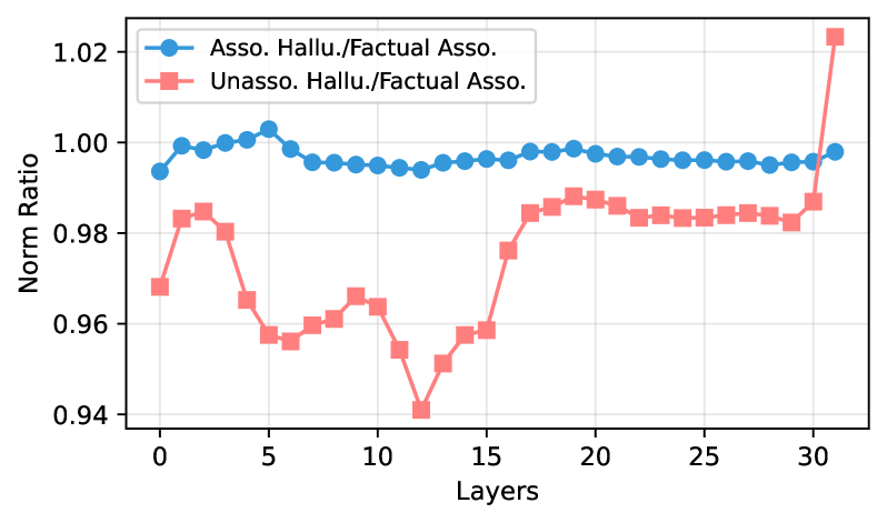4.2.1 Norm of Subject Representations <details> <summary>x5.png Details</summary>  ### Visual Description ## Line Chart: Norm Ratio vs. Layers ### Overview The image is a line chart comparing the "Norm Ratio" across different "Layers" for two categories: "Asso. Hallu./Factual Asso." and "Unasso. Hallu./Factual Asso.". The x-axis represents the layers, ranging from 0 to 30. The y-axis represents the Norm Ratio, ranging from 0.94 to 1.02. ### Components/Axes * **Title:** None explicitly present in the image. * **X-axis:** * Label: "Layers" * Scale: 0 to 30, with tick marks at intervals of 5 (0, 5, 10, 15, 20, 25, 30). * **Y-axis:** * Label: "Norm Ratio" * Scale: 0.94 to 1.02, with tick marks at intervals of 0.02 (0.94, 0.96, 0.98, 1.00, 1.02). * **Legend:** Located in the top-left corner. * Blue line with circle markers: "Asso. Hallu./Factual Asso." * Red line with square markers: "Unasso. Hallu./Factual Asso." ### Detailed Analysis * **Asso. Hallu./Factual Asso. (Blue Line):** * Trend: Relatively stable with minor fluctuations. * Data Points: * Layer 0: Approximately 0.993 * Layer 5: Approximately 1.002 * Layer 10: Approximately 0.993 * Layer 15: Approximately 0.993 * Layer 20: Approximately 0.997 * Layer 25: Approximately 0.995 * Layer 30: Approximately 0.998 * **Unasso. Hallu./Factual Asso. (Red Line):** * Trend: More volatile, with a significant dip around layer 13 and a sharp increase at the end. * Data Points: * Layer 0: Approximately 0.968 * Layer 5: Approximately 0.958 * Layer 10: Approximately 0.964 * Layer 13: Approximately 0.940 * Layer 15: Approximately 0.959 * Layer 20: Approximately 0.987 * Layer 25: Approximately 0.984 * Layer 30: Approximately 0.987 * Layer 31: Approximately 1.025 ### Key Observations * The "Asso. Hallu./Factual Asso." line remains relatively constant across all layers, hovering around a Norm Ratio of 1.00. * The "Unasso. Hallu./Factual Asso." line shows more variation, with a notable dip around layer 13 and a sharp spike at layer 31. * The "Unasso. Hallu./Factual Asso." line is generally below the "Asso. Hallu./Factual Asso." line, except for the final point at layer 31. ### Interpretation The chart compares the norm ratios of two different associations ("Asso. Hallu./Factual Asso." and "Unasso. Hallu./Factual Asso.") across different layers. The relatively stable norm ratio for "Asso. Hallu./Factual Asso." suggests a consistent behavior across layers. In contrast, the "Unasso. Hallu./Factual Asso." exhibits more dynamic behavior, indicating that its norm ratio is more sensitive to the specific layer. The significant dip around layer 13 and the sharp increase at the end suggest that certain layers have a more pronounced effect on the "Unasso. Hallu./Factual Asso." compared to the "Asso. Hallu./Factual Asso.". This could indicate that the "Unasso. Hallu./Factual Asso." is more susceptible to changes or anomalies within specific layers of the model. </details> Figure 3: Norm ratio curves of subject representations in LLaMA-3-8B, comparing AHs and UHs against FAs as the baseline. To test whether subject representations differ across categories, we measure the average $L_{2}$ norm of subject-token hidden activations across layers. For subject tokens $t_{s_{1}},..,t_{s_{n}}$ at layer $\ell$ , the average norm is $||\mathbf{h}_{s}^{\ell}\|=\tfrac{1}{n}\sum_{i=1}^{n}\|\mathbf{h}_{s_{i}}^{\ell}\|_{2}$ , computed by Equation (1). We compare the norm ratio between hallucination samples (AHs or UHs) and correct predictions (FAs), where a ratio near 1 indicates similar norms. Figure 3 shows that in LLaMA-3-8B, AH norms closely match those of correct samples (ratio $≈$ 0.99), while UH norms are consistently smaller, starting at the first layer (ratio $≈$ 0.96) and diverging further through mid-layers. Findings: At early layers, UH subject representations exhibit weaker activations than FAs, whereas AHs exhibit norms similar to FAs. 4.2.2 Relation to Parametric Knowledge <details> <summary>x6.png Details</summary>  ### Visual Description ## Bar Chart: Ratio of Hallucinations and Factual Associations for LLaMA-3-8B and Mistral-7B-v0.3 ### Overview The image is a bar chart comparing the ratio of "Unasso. Hallu./Factual Asso." (Unassociated Hallucinations/Factual Associations) and "Asso. Hallu./Factual Asso." (Associated Hallucinations/Factual Associations) for two language models: LLaMA-3-8B and Mistral-7B-v0.3. The chart uses two different colored bars (red and blue) to represent the two categories for each language model. ### Components/Axes * **X-axis:** Categorical axis representing the language models: "LLaMA-3-8B" and "Mistral-7B-v0.3". * **Y-axis:** Numerical axis labeled "Ratio", ranging from 0.0 to 1.0 with increments of 0.2. * **Legend:** Located at the bottom of the chart. * Red bar: "Unasso. Hallu./Factual Asso." * Blue bar: "Asso. Hallu./Factual Asso." ### Detailed Analysis * **LLaMA-3-8B:** * "Unasso. Hallu./Factual Asso." (Red bar): Approximately 0.68. * "Asso. Hallu./Factual Asso." (Blue bar): Approximately 1.06. * **Mistral-7B-v0.3:** * "Unasso. Hallu./Factual Asso." (Red bar): Approximately 0.37. * "Asso. Hallu./Factual Asso." (Blue bar): Approximately 0.80. ### Key Observations * For both language models, the "Asso. Hallu./Factual Asso." ratio is higher than the "Unasso. Hallu./Factual Asso." ratio. * Mistral-7B-v0.3 has a lower "Unasso. Hallu./Factual Asso." ratio compared to LLaMA-3-8B. * The "Asso. Hallu./Factual Asso." ratio is significantly higher for LLaMA-3-8B compared to Mistral-7B-v0.3. ### Interpretation The chart suggests that both language models exhibit more associated hallucinations/factual associations than unassociated ones. This could indicate that the models are more likely to generate hallucinations that are related to the input context or factual information they have been trained on. Mistral-7B-v0.3 appears to have a lower tendency to generate unassociated hallucinations compared to LLaMA-3-8B. The higher "Asso. Hallu./Factual Asso." ratio for LLaMA-3-8B might imply that it is more prone to generating hallucinations that are somehow linked to factual information, even if incorrect. 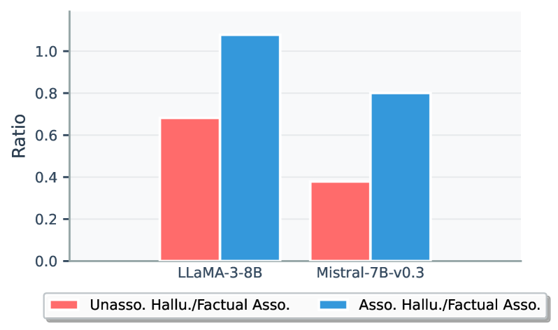</details> Figure 4: Comparison of subspace overlap ratios. We next investigate why early layers encode subject representations differently across knowledge types by examining how inputs interact with the parametric knowledge stored in MLP modules. Inspired by Kang et al. (2024), the output norm of an MLP layer depends on how well its input aligns with the subspace spanned by the weight matrix: poorly aligned inputs yield smaller output norms. For each MLP layer $\ell$ , we analyze the down-projection weight matrix $W_{\text{down}}^{\ell}$ and its input $x^{\ell}$ . Given the input $x_{s}^{\ell}$ corresponding to the subject tokens, we compute its overlap ratio with the top singular subspace $V_{\text{top}}$ of $W_{\text{down}}^{\ell}$ : $$ r(x_{s}^{\ell})=\frac{\left\lVert{x_{s}^{\ell}}^{\top}V_{\text{top}}V_{\text{top}}^{\top}\right\rVert^{2}}{\left\lVert x_{s}^{\ell}\right\rVert^{2}}. \tag{2} $$ A higher overlap ratio $r(x_{s}^{\ell})$ indicates stronger alignment to the subspace spanned by $W_{\text{down}}^{\ell}$ , leading to larger output norms. To highlight relative deviations from the factual baseline (FA), we report the relative ratios between AH/FA and UH/FA. Focusing on the layer with the largest UH norm shift, Figure 4 shows that UHs have significantly lower $r(x_{s}^{\ell})$ than AHs in both LLaMA and Mistral. This reveals that early-layer parametric weights are more aligned with FA and AH subject representations than with UH subjects, producing higher norms for the former ones. These results also suggest that the model has sufficiently learned representations for FA and AH subjects during pretraining but not for UH subjects. Findings: Similar to FAs, AH hidden activations align closely with the weight subspace, while UHs do not. This indicates that the model has sufficiently encoded subject representations into parametric knowledge for FAs and AHs but not for UHs. 4.2.3 Correlation with Subject Popularity <details> <summary>x7.png Details</summary>  ### Visual Description ## Bar Chart: Factual Associations, Associated Hallucinations, and Unassociated Hallucinations ### Overview The image is a bar chart comparing the percentages of "Factual Associations", "Associated Hallucinations", and "Unassociated Hallucinations" across three categories: "Low", "Mid", and "High". The y-axis represents the percentage, ranging from 0% to 100%. The x-axis represents the three categories. ### Components/Axes * **Y-axis:** "Percentage (%)", ranging from 0 to 100. Gridlines are present at intervals of 20. * **X-axis:** Categorical axis with three categories: "Low", "Mid", and "High". * **Legend:** Located at the bottom of the chart. * Green: "Factual Associations" * Blue: "Associated Hallucinations" * Red: "Unassociated Hallucinations" ### Detailed Analysis Here's a breakdown of the data for each category: * **Low:** * Factual Associations (Green): 5% * Associated Hallucinations (Blue): 1% * Unassociated Hallucinations (Red): 94% * **Mid:** * Factual Associations (Green): 27% * Associated Hallucinations (Blue): 7% * Unassociated Hallucinations (Red): 66% * **High:** * Factual Associations (Green): 52% * Associated Hallucinations (Blue): 14% * Unassociated Hallucinations (Red): 34% **Trend Verification:** * **Factual Associations (Green):** The percentage increases from "Low" to "High" (5% -> 27% -> 52%). * **Associated Hallucinations (Blue):** The percentage increases from "Low" to "High" (1% -> 7% -> 14%). * **Unassociated Hallucinations (Red):** The percentage decreases from "Low" to "High" (94% -> 66% -> 34%). ### Key Observations * In the "Low" category, "Unassociated Hallucinations" dominate with 94%. * "Factual Associations" show a significant increase from "Low" to "High", starting at 5% and reaching 52%. * "Associated Hallucinations" are consistently the lowest percentage across all categories. ### Interpretation The data suggests an inverse relationship between "Factual Associations" and "Unassociated Hallucinations" as the category moves from "Low" to "High". As the level increases, the percentage of "Factual Associations" increases, while the percentage of "Unassociated Hallucinations" decreases. "Associated Hallucinations" remain relatively low across all categories, suggesting they are not as prevalent as the other two types. The "Low" category is heavily dominated by "Unassociated Hallucinations", indicating a potential area of concern or focus for improvement. 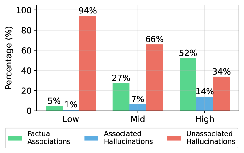</details> Figure 5: Sample distribution across different subject popularity (low, mid, high) in LLaMA-3-8B, measured by monthly Wikipedia page views. We further investigate why AH representations align with weight subspaces as strongly as FAs, while UHs do not. A natural hypothesis is that this difference arises from subject popularity in the training data. We use average monthly Wikipedia page views as a proxy for subject popularity during pre-training and bin subjects by popularity, then measure the distribution of UHs, AHs, and FAs. Figure 5 shows a clear trend: UHs dominate among the least popular subjects (94% for LLaMA), while AHs are rare (1%). As subject popularity rises, UH frequency falls and both FAs and AHs become more common, with AHs rising to 14% in the high-popularity subjects. This indicates that subject representation norms reflect training frequency, not factual correctness. Findings: Popular subjects yield stronger early-layer activations. AHs arise mainly on popular subjects and are therefore indistinguishable from FAs by popularity-based heuristics, contradicting prior work Mallen et al. (2023a) that links popularity to hallucinations. 4.3 Analysis of Attention Flow Having examined how the model forms subject representations, we next study how this information is propagated to the last token of the input where the model generates the object of a knowledge tuple. In order to produce factually correct outputs at the last token, the model must process subject representation and propagate it via attention layers, so that it can be read from the last position to produce the outputs Geva et al. (2023). To quantify the specific contribution from subject tokens $(s_{1},...,s_{n})$ to the last token, we compute the attention contribution from subject tokens to the last position: $$ \mathbf{a}^{\ell}_{\text{last}}=\sum\nolimits_{k}\sum\nolimits_{h}A^{\ell,h}_{\text{last},s_{k}}(\mathbf{h}^{\ell-1}_{s_{k}}W^{\ell,h}_{V})W^{\ell,h}_{O}. \tag{3} $$ where $A^{\ell,h}_{i,j}$ denotes the attention weight assigned by the $h$ -th head in the layer $\ell$ from the last position $i$ to subjec token $j$ . Here, $\mathbf{a}^{\ell}_{\text{last}}$ represents the subject-to-last attention contribution at layer $\ell$ . Intuitively, if subject information is critical for prediction, this contribution should have a large norm; otherwise, the norm should be small. 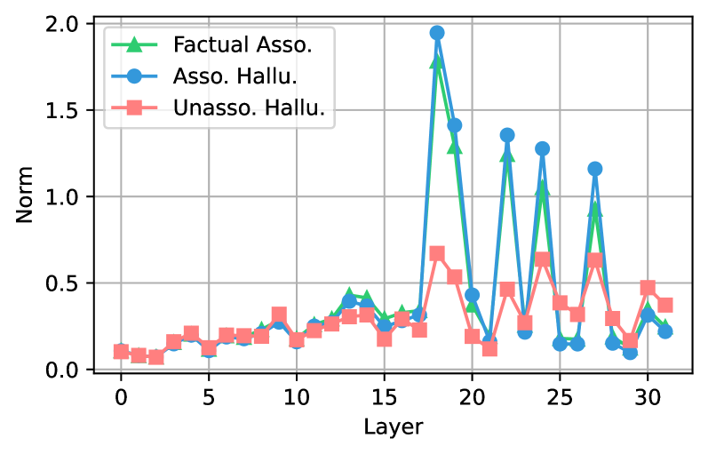Figure 6 shows that in LLaMA-3-8B, both AHs and FAs exhibit large attention-contribution norms in mid-layers, indicating a strong information flow from subject tokens to the target token. In contrast, UHs show consistently lower norms, implying that their predictions rely far less on subject information. Yüksekgönül et al. (2024) previously argued that high attention flow from subject tokens signals factuality and proposed using attention-based hidden states to detect hallucinations. Our results challenge this view: the model propagates subject information just as strongly when generating AHs as when producing correct facts. Findings: Mid-layer attention flow from subject to last token is equally strong for AHs and FAs but weak for UHs. Attention-based heuristics can therefore separate UHs from FAs but cannot distinguish AHs from factual outputs, limiting their reliability for hallucination detection. <details> <summary>x8.png Details</summary>  ### Visual Description ## Line Chart: Norm vs Layer for Different Association Types ### Overview The image is a line chart comparing the "Norm" values across different "Layers" for three categories: "Factual Asso.", "Asso. Hallu.", and "Unasso. Hallu.". The x-axis represents the layer number, ranging from 0 to 30. The y-axis represents the Norm value, ranging from 0.0 to 2.0. The chart displays how the norm changes across layers for each of the three association types. ### Components/Axes * **X-axis:** "Layer", with ticks at 0, 5, 10, 15, 20, 25, and 30. * **Y-axis:** "Norm", with ticks at 0.0, 0.5, 1.0, 1.5, and 2.0. * **Legend (Top-Left):** * Green Triangle: "Factual Asso." * Blue Circle: "Asso. Hallu." * Red Square: "Unasso. Hallu." ### Detailed Analysis * **Factual Asso. (Green Triangle):** * Trend: Relatively low and stable until layer 15, then increases to a peak around layer 19, then decreases and oscillates. * Approximate Values: * Layer 0-15: ~0.1 to 0.4 * Layer 19: ~1.8 * Layer 22: ~0.4 * Layer 27: ~1.0 * Layer 30: ~0.2 * **Asso. Hallu. (Blue Circle):** * Trend: Similar to "Factual Asso.", but with more pronounced peaks and valleys. * Approximate Values: * Layer 0-15: ~0.1 to 0.4 * Layer 19: ~1.95 * Layer 22: ~0.1 * Layer 25: ~1.3 * Layer 27: ~0.15 * Layer 30: ~0.1 * **Unasso. Hallu. (Red Square):** * Trend: Generally lower than the other two lines, with less pronounced peaks. * Approximate Values: * Layer 0-15: ~0.1 to 0.4 * Layer 19: ~0.7 * Layer 22: ~0.1 * Layer 25: ~0.5 * Layer 27: ~0.3 * Layer 30: ~0.4 ### Key Observations * The "Factual Asso." and "Asso. Hallu." lines show similar patterns, with peaks around the same layer numbers. * The "Unasso. Hallu." line generally has lower norm values compared to the other two. * All three lines converge to similar values in the initial layers (0-15). * The greatest divergence between the lines occurs between layers 18 and 28. ### Interpretation The chart suggests that "Factual Asso." and "Asso. Hallu." have similar norm characteristics across the layers, indicating a potential relationship or shared behavior. "Unasso. Hallu." exhibits a different pattern, with lower norm values, suggesting it might be distinct from the other two categories. The peaks in "Factual Asso." and "Asso. Hallu." could indicate specific layers where these associations are more prominent or have a greater impact on the overall norm. The convergence of all three lines in the initial layers might indicate a common baseline or initial state before the associations diverge. </details> Figure 6: Subject-to-last attention contribution norms across layers in LLaMA-3-8B. Values show the norm of the attention contribution from subject tokens to the last token at each layer. 4.4 Analysis of Last Token Representations Our earlier analysis showed strong subject-to-last token information transfer for both FAs and AHs, but minimal transfer for UHs. We now examine how this difference shapes the distribution of last-token representations. When subject information is weakly propagated (UHs), last-token states receive little subject-specific update. For UH samples sharing the same prompt template, these states should therefore cluster in the representation space. In contrast, strong subject-driven propagation in FAs and AHs produces diverse last-token states that disperse into distinct subspaces. To test this, we compute cosine similarity among last-token representations $\mathbf{h}_{T}^{\ell}$ . As shown in Figure 7, similarity is high ( $≈$ 0.9) for all categories in early layers, when little subject information is transferred. From mid-layers onward, FAs and AHs diverge sharply, dropping to $≈$ 0.2 by layer 25. UHs remain moderately clustered, with similarity only declining to $≈$ 0.5. Figure 8 shows the t-SNE visualization of the last token’s representations at layer 25 of LLaMA-3-8B. The hidden representations of UH are clearly separated from FA, whereas AH substantially overlap with FA. These results indicate that the model processes UH differently from FA, while processing AH in a manner similar to FA. More visualization can be found in Appendix C. 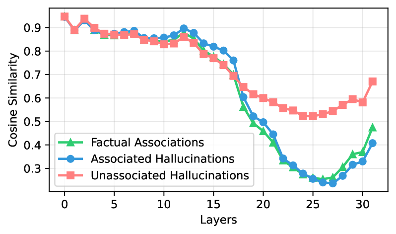<details> <summary>x9.png Details</summary>  ### Visual Description ## Line Chart: Cosine Similarity vs. Layers ### Overview The image is a line chart comparing the cosine similarity across different layers for three categories: Factual Associations, Associated Hallucinations, and Unassociated Hallucinations. The x-axis represents the layers, and the y-axis represents the cosine similarity. ### Components/Axes * **X-axis:** Layers, with markers at 0, 5, 10, 15, 20, 25, and 30. * **Y-axis:** Cosine Similarity, with markers at 0.3, 0.4, 0.5, 0.6, 0.7, 0.8, and 0.9. * **Legend:** Located in the bottom-left corner. * Green line with triangle markers: Factual Associations * Blue line with circle markers: Associated Hallucinations * Red line with square markers: Unassociated Hallucinations ### Detailed Analysis * **Factual Associations (Green):** * Trend: Initially stable, then decreases sharply, reaches a minimum, and then increases. * Values: Starts around 0.9, remains relatively constant until layer 12 (approx. 0.85), then decreases to approximately 0.27 at layer 27, and increases to approximately 0.47 at layer 31. * **Associated Hallucinations (Blue):** * Trend: Similar to Factual Associations, but the decrease is less sharp, and the recovery is also less pronounced. * Values: Starts around 0.93, remains relatively constant until layer 12 (approx. 0.88), then decreases to approximately 0.24 at layer 27, and increases to approximately 0.41 at layer 31. * **Unassociated Hallucinations (Red):** * Trend: Initially stable, then decreases, plateaus, and finally increases slightly. * Values: Starts around 0.94, remains relatively constant until layer 12 (approx. 0.84), then decreases to approximately 0.53 at layer 27, and increases to approximately 0.68 at layer 31. ### Key Observations * All three categories show a decrease in cosine similarity between layers 12 and 27. * Factual Associations and Associated Hallucinations have very similar trends and values. * Unassociated Hallucinations maintain a higher cosine similarity compared to the other two categories after layer 18. * The cosine similarity for Factual Associations and Associated Hallucinations recovers slightly after layer 27, while Unassociated Hallucinations show a plateau. ### Interpretation The chart suggests that as the layers increase, the cosine similarity between the representations of factual associations, associated hallucinations, and unassociated hallucinations initially remains stable, then decreases significantly. This decrease indicates that the representations become less similar as the layers progress. The recovery in cosine similarity for Factual Associations and Associated Hallucinations after layer 27 might indicate a convergence or re-alignment of representations in the later layers. The higher cosine similarity for Unassociated Hallucinations after layer 18 suggests that these representations remain more consistent or stable compared to the other two categories. The data could indicate how different types of information are processed and transformed within the layers of a neural network. </details> Figure 7: Cosine similarity of target-token hidden states across layers in LLaMA-3-8B. 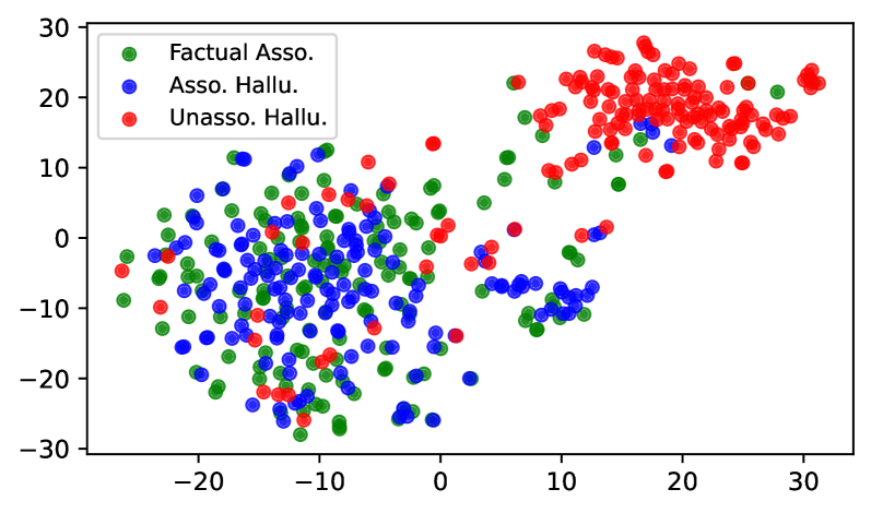<details> <summary>x10.png Details</summary>  ### Visual Description ## Scatter Plot: Factual vs. Associative Hallucinations ### Overview The image is a scatter plot visualizing the distribution of three categories: "Factual Asso.", "Asso. Hallu.", and "Unasso. Hallu." The plot displays data points in a two-dimensional space, with no explicit x and y axis labels. The data points are color-coded: green for "Factual Asso.", blue for "Asso. Hallu.", and red for "Unasso. Hallu.". The plot shows some clustering of the data points, suggesting potential relationships between the categories. ### Components/Axes * **X-axis:** No explicit label, but ranges from approximately -25 to 30. * **Y-axis:** No explicit label, but ranges from approximately -30 to 30. * **Legend (Top-Left):** * Green: "Factual Asso." * Blue: "Asso. Hallu." * Red: "Unasso. Hallu." ### Detailed Analysis * **Factual Asso. (Green):** * Data points are scattered across the plot. * Concentrations appear in the bottom-left quadrant (x: -25 to -5, y: -30 to -10) and the top-right quadrant (x: 10 to 30, y: 10 to 30). * **Asso. Hallu. (Blue):** * Data points are primarily concentrated in the bottom-left quadrant (x: -25 to 0, y: -30 to 10). * Some overlap with "Factual Asso." in this region. * **Unasso. Hallu. (Red):** * Data points are mainly clustered in the top-right quadrant (x: 5 to 30, y: 10 to 30). * Some overlap with "Factual Asso." in this region. * A few points are scattered in the bottom-left quadrant. ### Key Observations * The "Asso. Hallu." category appears to be distinct from the "Unasso. Hallu." category, with minimal overlap. * The "Factual Asso." category is more dispersed and overlaps with both "Asso. Hallu." and "Unasso. Hallu." * There are two distinct clusters, one in the bottom-left and one in the top-right. ### Interpretation The scatter plot suggests that "Associative Hallucinations" and "Unassociated Hallucinations" may represent distinct phenomena, as indicated by their separate clustering. "Factual Associations" seem to be more broadly distributed, potentially indicating that they can occur in conjunction with both types of hallucinations or independently. The lack of axis labels makes it difficult to interpret the specific dimensions along which these categories are being differentiated. Further information about the features represented by the x and y axes would be needed to draw more specific conclusions. </details> Figure 8: t-SNE visualization of last token’s representations at layer 25 of LLaMA-3-8B. 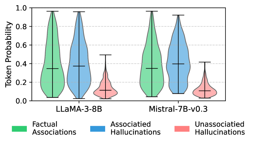<details> <summary>x11.png Details</summary>  ### Visual Description ## Violin Plot: Token Probability Distribution for Language Models ### Overview The image presents a violin plot comparing the token probability distributions of two language models, LLaMA-3-8B and Mistral-7B-v0.3, across three categories: Factual Associations, Associated Hallucinations, and Unassociated Hallucinations. The plot visualizes the spread and central tendency of token probabilities for each model and category. ### Components/Axes * **Y-axis:** "Token Probability" ranging from 0.0 to 1.0, with gridlines at intervals of 0.2. * **X-axis:** Categorical axis representing the two language models: "LLaMA-3-8B" and "Mistral-7B-v0.3". * **Violin Plots:** Each violin plot represents the distribution of token probabilities for a specific model and category. The width of the violin indicates the density of data points at that probability level. * **Legend:** Located at the bottom of the chart. * Green: "Factual Associations" * Blue: "Associated Hallucinations" * Red: "Unassociated Hallucinations" ### Detailed Analysis The plot is structured with two main groups, one for each language model (LLaMA-3-8B and Mistral-7B-v0.3). Within each group, there are three violin plots representing the three categories: Factual Associations (green), Associated Hallucinations (blue), and Unassociated Hallucinations (red). **LLaMA-3-8B:** * **Factual Associations (Green):** The distribution is centered around 0.35, with a wide spread indicating variability in token probabilities. The distribution extends from approximately 0.05 to 0.95. * **Associated Hallucinations (Blue):** Similar to Factual Associations, the distribution is centered around 0.38, with a wide spread. The distribution extends from approximately 0.08 to 0.95. * **Unassociated Hallucinations (Red):** The distribution is centered around 0.12, with a narrower spread compared to the other two categories. The distribution extends from approximately 0.02 to 0.45. **Mistral-7B-v0.3:** * **Factual Associations (Green):** The distribution is centered around 0.35, with a wide spread, similar to LLaMA-3-8B. The distribution extends from approximately 0.05 to 0.95. * **Associated Hallucinations (Blue):** Similar to Factual Associations, the distribution is centered around 0.40, with a wide spread. The distribution extends from approximately 0.08 to 0.92. * **Unassociated Hallucinations (Red):** The distribution is centered around 0.11, with a narrower spread compared to the other two categories, similar to LLaMA-3-8B. The distribution extends from approximately 0.02 to 0.42. ### Key Observations * For both models, the distributions of "Factual Associations" and "Associated Hallucinations" are similar in shape and spread, with medians around 0.35-0.40. * "Unassociated Hallucinations" have a much lower median token probability (around 0.11-0.12) and a narrower distribution compared to the other two categories for both models. * The distributions for each category are very similar between the two models. ### Interpretation The violin plot suggests that both language models exhibit similar patterns in token probability distributions across the three categories. The higher token probabilities for "Factual Associations" and "Associated Hallucinations" compared to "Unassociated Hallucinations" may indicate that the models are more confident in generating tokens related to factual information or associated concepts, even when those associations lead to hallucinations. The lower token probabilities for "Unassociated Hallucinations" might reflect the model's lower confidence in generating tokens that are completely unrelated to the input context. The similarity between the two models suggests that they may share similar biases or patterns in their token generation processes. </details> Figure 9: Distribution of last token probabilities. This separation also appears in the entropy of the output distribution (Figure 9). Strong subject-to-last propagation in FAs and AHs yields low-entropy predictions concentrated on the correct or associated entity. In contrast, weak propagation in UHs produces broad, high-entropy distributions, spreading probability mass across many plausible candidates (e.g., multiple possible names for “ The name of the father of <subject> is ”). Finding: From mid-layers onward, UHs retain clustered last-token representations and high-entropy outputs, while FAs and AHs diverge into subject-specific subspaces with low-entropy outputs. This provides a clear signal to separate UHs from FAs and AHs, but not for FAs and AHs. 5 Revisiting Hallucination Detection The mechanistic analysis in § 4 reveals that Internal states of LLMs primarily capture how the model recalls and utilizes its parametric knowledge, not whether the output is truthful. As both factual associations (FAs) and associated hallucinations (AHs) rely on the same subject-driven knowledge recall, their internal states show no clear separation. We therefore hypothesize that internal or black-box signals cannot effectively distinguish AHs from FAs, even though they could be effective in distinguishing unassociated hallucinations (UHs), which do not rely on parametric knowledge, from FAs. Experimental Setups To verify this, we revisit the effectiveness of widely-adopted white-box hallucination detection approaches that use internal state probing as well as black-box approaches that rely on scalar features. We evaluate on three settings: 1) AH Only (1,000 FAs and 1,000 AHs for training; 200 of each for testing), 2) UH Only (1,000 FAs and 1,000 UHs for training; 200 of each for testing), and 3) Full (1,000 FAs and 1,000 hallucination samples mixed of AHs and UHs for training; 200 of each for testing). For each setting, we use five random seeds to construct the training and testing datasets. We report the mean AUROC along with its standard deviation across seeds. White-box methods: We extract and normalize internal features and then train a probe. - Subject representations: last subject token hidden state from three consecutive layers Gottesman and Geva (2024). - Attention flow: attention weights from the last token to subject tokens across all layers Yüksekgönül et al. (2024). - Last-token representations: final token hidden state from the last layer Orgad et al. (2025). Black-box methods: We test two commonly used scalar features, including answer token probability (Orgad et al., 2025) and subject popularity (average monthly Wikipedia page views) (Mallen et al., 2023a). As discussed in § 4.2.3 and § 4.4, these features are also related to whether the model relies on encoded knowledge to produce outputs rather than with truthfulness itself. Experimental Results | Subject Attention Last Token | $0.65± 0.02$ $0.58± 0.04$ $\mathbf{0.69± 0.03}$ | $0.91± 0.01$ $0.92± 0.02$ $\mathbf{0.93± 0.01}$ | $0.57± 0.02$ $0.58± 0.07$ $\mathbf{0.63± 0.02}$ | $0.81± 0.02$ $0.87± 0.01$ $\mathbf{0.92± 0.01}$ | | --- | --- | --- | --- | --- | | Probability | $0.49± 0.01$ | $0.86± 0.01$ | $0.46± 0.00$ | $0.89± 0.00$ | | Subject Pop. | $0.48± 0.01$ | $0.87± 0.01$ | $0.52± 0.01$ | $0.84± 0.01$ | Table 2: Hallucination detection performance on AH Only and UH Only settings. 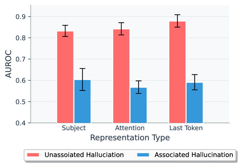<details> <summary>x12.png Details</summary>  ### Visual Description ## Bar Chart: AUROC by Representation Type and Hallucination Association ### Overview The image is a bar chart comparing the Area Under the Receiver Operating Characteristic curve (AUROC) for different representation types (Subject, Attention, Last Token) and their association with hallucinations (Unassociated, Associated). The chart displays the AUROC values on the y-axis, ranging from 0.4 to 0.9. The x-axis represents the representation type. Error bars are included on each bar, indicating the variability or uncertainty in the AUROC values. ### Components/Axes * **Y-axis:** AUROC, ranging from 0.4 to 0.9 in increments of 0.1. * **X-axis:** Representation Type, with three categories: Subject, Attention, and Last Token. * **Legend:** Located at the bottom of the chart. * Red: Unassociated Hallucination * Blue: Associated Hallucination ### Detailed Analysis The chart presents AUROC values for two categories of hallucinations (Unassociated and Associated) across three representation types. * **Subject:** * Unassociated Hallucination (Red): AUROC is approximately 0.83, with an error bar extending from approximately 0.80 to 0.86. * Associated Hallucination (Blue): AUROC is approximately 0.60, with an error bar extending from approximately 0.55 to 0.65. * **Attention:** * Unassociated Hallucination (Red): AUROC is approximately 0.84, with an error bar extending from approximately 0.81 to 0.87. * Associated Hallucination (Blue): AUROC is approximately 0.56, with an error bar extending from approximately 0.53 to 0.59. * **Last Token:** * Unassociated Hallucination (Red): AUROC is approximately 0.88, with an error bar extending from approximately 0.85 to 0.91. * Associated Hallucination (Blue): AUROC is approximately 0.59, with an error bar extending from approximately 0.56 to 0.62. ### Key Observations * For all representation types, the AUROC is higher for Unassociated Hallucinations (red bars) compared to Associated Hallucinations (blue bars). * The "Last Token" representation type shows the highest AUROC for Unassociated Hallucinations, reaching approximately 0.88. * The "Attention" representation type shows the lowest AUROC for Associated Hallucinations, at approximately 0.56. * The error bars indicate some variability in the AUROC values, but the differences between Unassociated and Associated Hallucinations appear consistent across all representation types. ### Interpretation The data suggests that the model is better at distinguishing Unassociated Hallucinations from non-hallucinations compared to distinguishing Associated Hallucinations from non-hallucinations, across all representation types tested. The "Last Token" representation appears to be the most effective for identifying Unassociated Hallucinations. The consistent difference in AUROC values between Unassociated and Associated Hallucinations across all representation types indicates a robust trend. The error bars provide a measure of the uncertainty in these estimates, but the overall pattern remains clear. </details> Figure 10: Hallucination detection performance on the Full setting (LLaMA-3-8B). Table 2 shows that hallucination detection methods behave very differently in the AH Only and UH Only settings. For white-box probes, all approaches effectively distinguish UHs from FAs, with last-token hidden states reaching AUROC scores of about 0.93 for LLaMA and 0.92 for Mistral. In contrast, performance drops sharply on the AH Only setting, where the last-token probe falls to 0.69 for LLaMA and 0.63 for Mistral. Black-box methods follow the same pattern. Figure 10 further highlights this disparity under the Full setting: detection is consistently stronger on UH samples than on AH samples, and adding AHs to the training set significantly dilutes performance on UHs (AUROC $≈$ 0.9 on UH Only vs. $≈$ 0.8 on Full). These results confirm that both internal probes and black-box methods capture whether a model draws on parametric knowledge, not whether its outputs are factually correct. Unassociated hallucinations are easier to detect because they bypass this knowledge, while associated hallucinations are produced through the same recall process as factual answers, leaving no internal cues to distinguish them. As a result, LLMs lack intrinsic awareness of their own truthfulness, and detection methods relying on these signals risk misclassifying associated hallucinations as correct, fostering harmful overconfidence in model outputs. 6 Challenges of Refusal Tuning A common strategy to mitigate potential hallucination in the model’s responses is to fine-tune LLMs to refuse answering when they cannot provide a factual response, e.g., Refusal Tuning Zhang et al. (2024). For such refusal capability to generalize, the training data must contain a shared feature pattern across hallucinated outputs, allowing the model to learn and apply it to unseen cases. Our analysis in the previous sections shows that this prerequisite is not met. The structural mismatch between UHs and AHs suggests that refusal tuning on UHs may generalize to other UHs, because their hidden states occupy a common activation subspace, but will not transfer to AHs. Refusal tuning on AHs is even less effective, as their diverse representations prevent generalization to either unseen AHs or UHs. 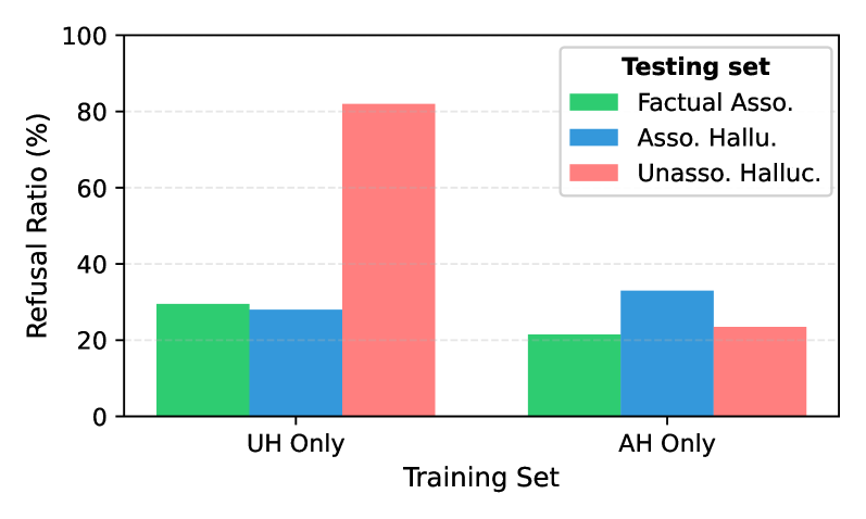Experimental Setups To verify the hypothesis, we conduct refusal tuning on LLMs under two settings: 1) UH Only, where 1,000 UH samples are paired with 10 refusal templates, and 1,000 FA samples are preserved with their original answers. 2) AH Only, where 1,000 AH samples are paired with refusal templates, with 1,000 FA samples again leave unchanged. We then evaluate both models on 200 samples each of FAs, UHs, and AHs. A response matching any refusal template is counted as a refusal, and we report the Refusal Ratio as the proportion of samples eliciting refusals. This measures not only whether the model refuses appropriately on UHs and AHs, but also whether it “over-refuses” on FA samples. Experimental Results <details> <summary>x13.png Details</summary>  ### Visual Description ## Bar Chart: Refusal Ratio by Training Set and Hallucination Type ### Overview The image is a bar chart comparing the refusal ratio (%) for different types of hallucinations (Factual Asso., Asso. Hallu., Unasso. Halluc.) across two training sets (UH Only, AH Only). The chart uses color-coded bars to represent each hallucination type, with the y-axis representing the refusal ratio and the x-axis representing the training set. ### Components/Axes * **Title:** There is no explicit title on the chart. * **X-axis:** * Label: "Training Set" * Categories: "UH Only", "AH Only" * **Y-axis:** * Label: "Refusal Ratio (%)" * Scale: 0 to 100, with gridlines at intervals of 20. * **Legend:** Located in the top-right corner, titled "Testing set". * Factual Asso. (Green) * Asso. Hallu. (Blue) * Unasso. Halluc. (Red) ### Detailed Analysis Here's a breakdown of the refusal ratios for each category: * **UH Only Training Set:** * Factual Asso. (Green): Approximately 30% * Asso. Hallu. (Blue): Approximately 28% * Unasso. Halluc. (Red): Approximately 82% * **AH Only Training Set:** * Factual Asso. (Green): Approximately 22% * Asso. Hallu. (Blue): Approximately 33% * Unasso. Halluc. (Red): Approximately 24% ### Key Observations * For the "UH Only" training set, the "Unasso. Halluc." category has a significantly higher refusal ratio compared to "Factual Asso." and "Asso. Hallu.". * For the "AH Only" training set, the refusal ratios for all three categories are much closer together, with "Asso. Hallu." having a slightly higher ratio. * The "Factual Asso." category has a lower refusal ratio in the "AH Only" training set compared to the "UH Only" training set. * The "Asso. Hallu." category has a higher refusal ratio in the "AH Only" training set compared to the "UH Only" training set. * The "Unasso. Halluc." category has a significantly lower refusal ratio in the "AH Only" training set compared to the "UH Only" training set. ### Interpretation The data suggests that the type of training set significantly impacts the refusal ratio for different types of hallucinations. Specifically, training with "UH Only" leads to a much higher refusal ratio for "Unasso. Halluc." compared to training with "AH Only". This could indicate that the model trained with "UH Only" is better at identifying and refusing to generate unassociated hallucinations. The "AH Only" training set seems to result in a more balanced refusal ratio across all hallucination types. The differences in refusal ratios between the training sets could be due to the specific characteristics and biases present in each training dataset. Further investigation would be needed to understand the underlying reasons for these differences. </details> Figure 11: Refusal tuning performance across three types of samples (LLaMA-3-8B). Figure 11 shows that training with UHs leads to strong generalization across UHs, with refusal ratios of 82% for LLaMA. However, this effect does not transfer to AHs, where refusal ratios fall to 28%, respectively. Moreover, some FA cases are mistakenly refused (29.5%). These results confirm that UHs share a common activation subspace, supporting generalization within the category, while AHs and FAs lie outside this space. By contrast, training with AHs produces poor generalization. On AH test samples, refusal ratio is only 33%, validating that their subject-specific hidden states prevent consistent refusal learning. Generalization to UHs is also weak (23.5%), again reflecting the divergence between AH and UH activation spaces. Overall, these findings show that the generalizability of refusal tuning is fundamentally limited by the heterogeneous nature of hallucinations. UH representations are internally consistent enough to support refusal generalization, but AH representations are too diverse for either UH-based or AH-based training to yield a broadly applicable and reliable refusal capability. 7 Conclusions and Future Work In this work, we revisit the widely accepted claim that hallucinations can be detected from a model’s internal states. Our mechanistic analysis reveals that hidden states encode whether models are reliance on their parametric knowledge rather than truthfulness. As a result, detection methods succeed only when outputs are detached from the input but fail when hallucinations arise from the same knowledge-recall process as correct answers. These findings lead to three key implications. First, future evaluations should report detection performance separately for Associated Hallucinations (AHs) and Unassociated Hallucinations (UHs), as they stem from fundamentally different internal processes and require distinct detection strategies. Second, relying solely on hidden states is insufficient for reliable hallucination detection. Future research should integrate LLMs with external feedback mechanisms, such as fact-checking modules or retrieval-based verifiers, to assess factuality more robustly. Third, future studies should prioritize improving AH detection. Because AHs occur more frequently in widely known or highly popular topics (§ 4.2.3), their undetected errors pose greater risks to user trust and the practical reliability of LLMs. Limitations We identify several limitations of our work. Focus on Factual Knowledge While our analysis identifies failure cases of hallucination detection methods, our study is primarily limited to factual completion prompts. It does not extend to long-form or open-ended text generation tasks Wei et al. (2024); Min et al. (2023); Huang and Chen (2024). Future work should broaden this investigation to these tasks in order to draw more comprehensive conclusions. Lack of Analysis on Prompt-based Hallucination Detection Approaches Our analysis focuses on white-box hallucination detection methods based on internal states and two black-box approaches based on external features. We do not include verbalization-based strategies Lin et al. (2022a); Tian et al. (2023); Xiong et al. (2024); Yang et al. (2024b); Ni et al. (2024); Zhao et al. (2024), such as prompting the model to report or justify its confidence explicitly, which constitute a different line of approach. Exploring such approaches may offer complementary insights into how models internally represent and express uncertainty. Applicability to Black-box LLMs or Large Reasoning Models Our study is limited to open-source LLMs. Conducting mechanistic analyses on commercial black-box LLMs is not permitted due to access restrictions. Future work could explore alternative evaluation protocols or collaboration frameworks that enable partial interpretability analyses on such systems. In addition, recent studies Mei et al. (2025); Zhang et al. (2025) have begun examining the internal states of large reasoning models for hallucination detection, suggesting a promising direction for extending our methodology to models with multi-step reasoning capabilities. Ethical Considerations This work analyzes the internal mechanisms of large language models using data constructed from Wikidata Vrandecic and Krötzsch (2014), which is released under the Creative Commons CC0 1.0 Universal license, allowing unrestricted use and redistribution of its data. All data are derived from publicly available resources, and no private or sensitive information about individuals is included. We employ the LLM tools for polishing. References - Azaria and Mitchell (2023) Amos Azaria and Tom M. Mitchell. 2023. The internal state of an LLM knows when it’s lying. In Findings of the Association for Computational Linguistics: EMNLP 2023, pages 967–976. - Cheang et al. (2023) Chi Seng Cheang, Hou Pong Chan, Derek F. Wong, Xuebo Liu, Zhaocong Li, Yanming Sun, Shudong Liu, and Lidia S. Chao. 2023. Can lms generalize to future data? an empirical analysis on text summarization. In Proceedings of the 2023 Conference on Empirical Methods in Natural Language Processing, EMNLP 2023, Singapore, December 6-10, 2023, pages 16205–16217. Association for Computational Linguistics. - Chen et al. (2024) Chao Chen, Kai Liu, Ze Chen, Yi Gu, Yue Wu, Mingyuan Tao, Zhihang Fu, and Jieping Ye. 2024. INSIDE: llms’ internal states retain the power of hallucination detection. In The Twelfth International Conference on Learning Representations, ICLR 2024, Vienna, Austria, May 7-11, 2024. OpenReview.net. - Daniel Han and team (2023) Michael Han Daniel Han and Unsloth team. 2023. Unsloth. - Dettmers et al. (2023) Tim Dettmers, Artidoro Pagnoni, Ari Holtzman, and Luke Zettlemoyer. 2023. Qlora: Efficient finetuning of quantized llms. In Advances in Neural Information Processing Systems 36: Annual Conference on Neural Information Processing Systems 2023, NeurIPS 2023, New Orleans, LA, USA, December 10 - 16, 2023. - Ding et al. (2024) Hanxing Ding, Liang Pang, Zihao Wei, Huawei Shen, and Xueqi Cheng. 2024. Retrieve only when it needs: Adaptive retrieval augmentation for hallucination mitigation in large language models. CoRR, abs/2402.10612. - Dubey et al. (2024) Abhimanyu Dubey, Abhinav Jauhri, Abhinav Pandey, Abhishek Kadian, Ahmad Al-Dahle, Aiesha Letman, Akhil Mathur, Alan Schelten, Amy Yang, Angela Fan, Anirudh Goyal, Anthony Hartshorn, Aobo Yang, Archi Mitra, Archie Sravankumar, Artem Korenev, Arthur Hinsvark, Arun Rao, Aston Zhang, and 82 others. 2024. The llama 3 herd of models. CoRR, abs/2407.21783. - Finlayson et al. (2021) Matthew Finlayson, Aaron Mueller, Sebastian Gehrmann, Stuart M. Shieber, Tal Linzen, and Yonatan Belinkov. 2021. Causal analysis of syntactic agreement mechanisms in neural language models. In Proceedings of the 59th Annual Meeting of the Association for Computational Linguistics and the 11th International Joint Conference on Natural Language Processing, ACL/IJCNLP 2021, (Volume 1: Long Papers), Virtual Event, August 1-6, 2021, pages 1828–1843. Association for Computational Linguistics. - Gekhman et al. (2025) Zorik Gekhman, Eyal Ben-David, Hadas Orgad, Eran Ofek, Yonatan Belinkov, Idan Szpektor, Jonathan Herzig, and Roi Reichart. 2025. Inside-out: Hidden factual knowledge in llms. CoRR, abs/2503.15299. - Geva et al. (2023) Mor Geva, Jasmijn Bastings, Katja Filippova, and Amir Globerson. 2023. Dissecting recall of factual associations in auto-regressive language models. In Proceedings of the 2023 Conference on Empirical Methods in Natural Language Processing, EMNLP 2023, Singapore, December 6-10, 2023, pages 12216–12235. Association for Computational Linguistics. - Gottesman and Geva (2024) Daniela Gottesman and Mor Geva. 2024. Estimating knowledge in large language models without generating a single token. In Proceedings of the 2024 Conference on Empirical Methods in Natural Language Processing, EMNLP 2024, pages 3994–4019. - Guerreiro et al. (2023) Nuno Miguel Guerreiro, Elena Voita, and André F. T. Martins. 2023. Looking for a needle in a haystack: A comprehensive study of hallucinations in neural machine translation. In Proceedings of the 17th Conference of the European Chapter of the Association for Computational Linguistics, EACL 2023, Dubrovnik, Croatia, May 2-6, 2023, pages 1059–1075. Association for Computational Linguistics. - Huang and Chen (2024) Chao-Wei Huang and Yun-Nung Chen. 2024. Factalign: Long-form factuality alignment of large language models. In Findings of the Association for Computational Linguistics: EMNLP 2024, pages 16363–16375. - Huang et al. (2025) Lei Huang, Weijiang Yu, Weitao Ma, Weihong Zhong, Zhangyin Feng, Haotian Wang, Qianglong Chen, Weihua Peng, Xiaocheng Feng, Bing Qin, and Ting Liu. 2025. A survey on hallucination in large language models: Principles, taxonomy, challenges, and open questions. ACM Trans. Inf. Syst., 43(2):42:1–42:55. - Ji et al. (2024) Ziwei Ji, Delong Chen, Etsuko Ishii, Samuel Cahyawijaya, Yejin Bang, Bryan Wilie, and Pascale Fung. 2024. LLM internal states reveal hallucination risk faced with a query. In Proceedings of the 7th BlackboxNLP Workshop: Analyzing and Interpreting Neural Networks for NLP, pages 88–104, Miami, Florida, US. Association for Computational Linguistics. - Jiang et al. (2023) Albert Q. Jiang, Alexandre Sablayrolles, Arthur Mensch, Chris Bamford, Devendra Singh Chaplot, Diego de las Casas, Florian Bressand, Gianna Lengyel, Guillaume Lample, Lucile Saulnier, Lélio Renard Lavaud, Marie-Anne Lachaux, Pierre Stock, Teven Le Scao, Thibaut Lavril, Thomas Wang, Timothée Lacroix, and William El Sayed. 2023. Mistral 7b. Preprint, arXiv:2310.06825. - Kang and Choi (2023) Cheongwoong Kang and Jaesik Choi. 2023. Impact of co-occurrence on factual knowledge of large language models. In Findings of the Association for Computational Linguistics: EMNLP 2023, pages 7721–7735. - Kang et al. (2024) Katie Kang, Amrith Setlur, Claire J. Tomlin, and Sergey Levine. 2024. Deep neural networks tend to extrapolate predictably. In The Twelfth International Conference on Learning Representations, ICLR 2024. - Kapoor et al. (2024) Sanyam Kapoor, Nate Gruver, Manley Roberts, Katie Collins, Arka Pal, Umang Bhatt, Adrian Weller, Samuel Dooley, Micah Goldblum, and Andrew Gordon Wilson. 2024. Large language models must be taught to know what they don’t know. In Advances in Neural Information Processing Systems 38: Annual Conference on Neural Information Processing Systems 2024, NeurIPS 2024, Vancouver, BC, Canada, December 10 - 15, 2024. - Kuhn et al. (2023) Lorenz Kuhn, Yarin Gal, and Sebastian Farquhar. 2023. Semantic uncertainty: Linguistic invariances for uncertainty estimation in natural language generation. In The Eleventh International Conference on Learning Representations, ICLR 2023, Kigali, Rwanda, May 1-5, 2023. OpenReview.net. - Li et al. (2023) Kenneth Li, Oam Patel, Fernanda Viégas, Hanspeter Pfister, and Martin Wattenberg. 2023. Inference-time intervention: Eliciting truthful answers from a language model. Advances in Neural Information Processing Systems, 36:41451–41530. - Li et al. (2025) Moxin Li, Yong Zhao, Wenxuan Zhang, Shuaiyi Li, Wenya Xie, See-Kiong Ng, Tat-Seng Chua, and Yang Deng. 2025. Knowledge boundary of large language models: A survey. In Proceedings of the 63rd Annual Meeting of the Association for Computational Linguistics (Volume 1: Long Papers), ACL 2025, pages 5131–5157. - Lin et al. (2022a) Stephanie Lin, Jacob Hilton, and Owain Evans. 2022a. Teaching models to express their uncertainty in words. Trans. Mach. Learn. Res., 2022. - Lin et al. (2022b) Stephanie Lin, Jacob Hilton, and Owain Evans. 2022b. Truthfulqa: Measuring how models mimic human falsehoods. In Proceedings of the 60th Annual Meeting of the Association for Computational Linguistics (Volume 1: Long Papers), ACL 2022, pages 3214–3252. - Mallen et al. (2023a) Alex Mallen, Akari Asai, Victor Zhong, Rajarshi Das, Daniel Khashabi, and Hannaneh Hajishirzi. 2023a. When not to trust language models: Investigating effectiveness of parametric and non-parametric memories. In Proceedings of the 61st Annual Meeting of the Association for Computational Linguistics (Volume 1: Long Papers), ACL 2023, pages 9802–9822. - Mallen et al. (2023b) Alex Mallen, Akari Asai, Victor Zhong, Rajarshi Das, Daniel Khashabi, and Hannaneh Hajishirzi. 2023b. When not to trust language models: Investigating effectiveness of parametric and non-parametric memories. In Proceedings of the 61st Annual Meeting of the Association for Computational Linguistics (Volume 1: Long Papers), ACL 2023, Toronto, Canada, July 9-14, 2023, pages 9802–9822. Association for Computational Linguistics. - Manakul et al. (2023) Potsawee Manakul, Adian Liusie, and Mark J. F. Gales. 2023. Selfcheckgpt: Zero-resource black-box hallucination detection for generative large language models. In Proceedings of the 2023 Conference on Empirical Methods in Natural Language Processing, EMNLP 2023, Singapore, December 6-10, 2023, pages 9004–9017. Association for Computational Linguistics. - Mei et al. (2025) Zhiting Mei, Christina Zhang, Tenny Yin, Justin Lidard, Ola Shorinwa, and Anirudha Majumdar. 2025. Reasoning about uncertainty: Do reasoning models know when they don’t know? CoRR, abs/2506.18183. - Meng et al. (2022) Kevin Meng, David Bau, Alex Andonian, and Yonatan Belinkov. 2022. Locating and editing factual associations in gpt. Advances in neural information processing systems, 35:17359–17372. - Min et al. (2023) Sewon Min, Kalpesh Krishna, Xinxi Lyu, Mike Lewis, Wen-tau Yih, Pang Wei Koh, Mohit Iyyer, Luke Zettlemoyer, and Hannaneh Hajishirzi. 2023. Factscore: Fine-grained atomic evaluation of factual precision in long form text generation. In Proceedings of the 2023 Conference on Empirical Methods in Natural Language Processing, EMNLP 2023, pages 12076–12100. - Ni et al. (2024) Shiyu Ni, Keping Bi, Jiafeng Guo, and Xueqi Cheng. 2024. When do llms need retrieval augmentation? mitigating llms’ overconfidence helps retrieval augmentation. In Findings of the Association for Computational Linguistics, ACL 2024, Bangkok, Thailand and virtual meeting, August 11-16, 2024, pages 11375–11388. Association for Computational Linguistics. - Ni et al. (2025) Shiyu Ni, Keping Bi, Jiafeng Guo, Lulu Yu, Baolong Bi, and Xueqi Cheng. 2025. Towards fully exploiting LLM internal states to enhance knowledge boundary perception. In Proceedings of the 63rd Annual Meeting of the Association for Computational Linguistics (Volume 1: Long Papers), ACL 2025, Vienna, Austria, July 27 - August 1, 2025, pages 24315–24329. Association for Computational Linguistics. - Orgad et al. (2025) Hadas Orgad, Michael Toker, Zorik Gekhman, Roi Reichart, Idan Szpektor, Hadas Kotek, and Yonatan Belinkov. 2025. Llms know more than they show: On the intrinsic representation of LLM hallucinations. In The Thirteenth International Conference on Learning Representations, ICLR 2025. - Sciavolino et al. (2021) Christopher Sciavolino, Zexuan Zhong, Jinhyuk Lee, and Danqi Chen. 2021. Simple entity-centric questions challenge dense retrievers. In Proceedings of the 2021 Conference on Empirical Methods in Natural Language Processing, EMNLP 2021, Virtual Event / Punta Cana, Dominican Republic, 7-11 November, 2021, pages 6138–6148. Association for Computational Linguistics. - Su et al. (2024) Weihang Su, Changyue Wang, Qingyao Ai, Yiran Hu, Zhijing Wu, Yujia Zhou, and Yiqun Liu. 2024. Unsupervised real-time hallucination detection based on the internal states of large language models. In Findings of the Association for Computational Linguistics, ACL 2024, Bangkok, Thailand and virtual meeting, August 11-16, 2024, pages 14379–14391. Association for Computational Linguistics. - Tian et al. (2023) Katherine Tian, Eric Mitchell, Allan Zhou, Archit Sharma, Rafael Rafailov, Huaxiu Yao, Chelsea Finn, and Christopher D. Manning. 2023. Just ask for calibration: Strategies for eliciting calibrated confidence scores from language models fine-tuned with human feedback. In Proceedings of the 2023 Conference on Empirical Methods in Natural Language Processing, EMNLP 2023, Singapore, December 6-10, 2023, pages 5433–5442. Association for Computational Linguistics. - Varshney et al. (2023) Neeraj Varshney, Wenlin Yao, Hongming Zhang, Jianshu Chen, and Dong Yu. 2023. A stitch in time saves nine: Detecting and mitigating hallucinations of llms by validating low-confidence generation. CoRR, abs/2307.03987. - Vig et al. (2020) Jesse Vig, Sebastian Gehrmann, Yonatan Belinkov, Sharon Qian, Daniel Nevo, Yaron Singer, and Stuart Shieber. 2020. Investigating gender bias in language models using causal mediation analysis. Advances in neural information processing systems, 33:12388–12401. - Vrandecic and Krötzsch (2014) Denny Vrandecic and Markus Krötzsch. 2014. Wikidata: a free collaborative knowledgebase. Commun. ACM, 57(10):78–85. - Wei et al. (2024) Jerry Wei, Chengrun Yang, Xinying Song, Yifeng Lu, Nathan Hu, Jie Huang, Dustin Tran, Daiyi Peng, Ruibo Liu, Da Huang, Cosmo Du, and Quoc V. Le. 2024. Long-form factuality in large language models. In Advances in Neural Information Processing Systems 38: Annual Conference on Neural Information Processing Systems 2024, NeurIPS 2024. - Wolf et al. (2019) Thomas Wolf, Lysandre Debut, Victor Sanh, Julien Chaumond, Clement Delangue, Anthony Moi, Pierric Cistac, Tim Rault, Rémi Louf, Morgan Funtowicz, and Jamie Brew. 2019. Huggingface’s transformers: State-of-the-art natural language processing. CoRR, abs/1910.03771. - Xiao et al. (2025) Chenghao Xiao, Hou Pong Chan, Hao Zhang, Mahani Aljunied, Lidong Bing, Noura Al Moubayed, and Yu Rong. 2025. Analyzing llms’ knowledge boundary cognition across languages through the lens of internal representations. In Proceedings of the 63rd Annual Meeting of the Association for Computational Linguistics (Volume 1: Long Papers), ACL 2025, Vienna, Austria, July 27 - August 1, 2025, pages 24099–24115. Association for Computational Linguistics. - Xiong et al. (2024) Miao Xiong, Zhiyuan Hu, Xinyang Lu, Yifei Li, Jie Fu, Junxian He, and Bryan Hooi. 2024. Can llms express their uncertainty? an empirical evaluation of confidence elicitation in llms. In The Twelfth International Conference on Learning Representations, ICLR 2024, Vienna, Austria, May 7-11, 2024. OpenReview.net. - Yang et al. (2024a) An Yang, Baosong Yang, Beichen Zhang, Binyuan Hui, Bo Zheng, Bowen Yu, Chengyuan Li, Dayiheng Liu, Fei Huang, Haoran Wei, Huan Lin, Jian Yang, Jianhong Tu, Jianwei Zhang, Jianxin Yang, Jiaxi Yang, Jingren Zhou, Junyang Lin, Kai Dang, and 22 others. 2024a. Qwen2.5 technical report. CoRR, abs/2412.15115. - Yang et al. (2024b) Yuqing Yang, Ethan Chern, Xipeng Qiu, Graham Neubig, and Pengfei Liu. 2024b. Alignment for honesty. In Advances in Neural Information Processing Systems 38: Annual Conference on Neural Information Processing Systems 2024, NeurIPS 2024, Vancouver, BC, Canada, December 10 - 15, 2024. - Yin et al. (2023) Zhangyue Yin, Qiushi Sun, Qipeng Guo, Jiawen Wu, Xipeng Qiu, and Xuanjing Huang. 2023. Do large language models know what they don’t know? In Findings of the Association for Computational Linguistics: ACL 2023, Toronto, Canada, July 9-14, 2023, pages 8653–8665. Association for Computational Linguistics. - Yona et al. (2024) Gal Yona, Roee Aharoni, and Mor Geva. 2024. Narrowing the knowledge evaluation gap: Open-domain question answering with multi-granularity answers. In Proceedings of the 62nd Annual Meeting of the Association for Computational Linguistics (Volume 1: Long Papers), ACL 2024, Bangkok, Thailand, August 11-16, 2024, pages 6737–6751. Association for Computational Linguistics. - Yüksekgönül et al. (2024) Mert Yüksekgönül, Varun Chandrasekaran, Erik Jones, Suriya Gunasekar, Ranjita Naik, Hamid Palangi, Ece Kamar, and Besmira Nushi. 2024. Attention satisfies: A constraint-satisfaction lens on factual errors of language models. In The Twelfth International Conference on Learning Representations, ICLR 2024. - Zhang et al. (2024) Hanning Zhang, Shizhe Diao, Yong Lin, Yi R. Fung, Qing Lian, Xingyao Wang, Yangyi Chen, Heng Ji, and Tong Zhang. 2024. R-tuning: Instructing large language models to say ’i don’t know’. In Proceedings of the 2024 Conference of the North American Chapter of the Association for Computational Linguistics: Human Language Technologies (Volume 1: Long Papers), NAACL 2024, pages 7113–7139. - Zhang et al. (2023a) Jiaxin Zhang, Zhuohang Li, Kamalika Das, Bradley A. Malin, and Kumar Sricharan. 2023a. Sac ${}^{\mbox{3}}$ : Reliable hallucination detection in black-box language models via semantic-aware cross-check consistency. CoRR, abs/2311.01740. - Zhang et al. (2025) Qingjie Zhang, Yujia Fu, Yang Wang, Liu Yan, Tao Wei, Ke Xu, Minlie Huang, and Han Qiu. 2025. On the self-awareness of large reasoning models’ capability boundaries. Preprint, arXiv:2509.24711. - Zhang et al. (2023b) Yue Zhang, Yafu Li, Leyang Cui, Deng Cai, Lemao Liu, Tingchen Fu, Xinting Huang, Enbo Zhao, Yu Zhang, Yulong Chen, Longyue Wang, Anh Tuan Luu, Wei Bi, Freda Shi, and Shuming Shi. 2023b. Siren’s song in the AI ocean: A survey on hallucination in large language models. CoRR, abs/2309.01219. - Zhao et al. (2024) Yukun Zhao, Lingyong Yan, Weiwei Sun, Guoliang Xing, Chong Meng, Shuaiqiang Wang, Zhicong Cheng, Zhaochun Ren, and Dawei Yin. 2024. Knowing what llms DO NOT know: A simple yet effective self-detection method. In Proceedings of the 2024 Conference of the North American Chapter of the Association for Computational Linguistics: Human Language Technologies (Volume 1: Long Papers), NAACL 2024, pages 7051–7063. Appendix Appendix A Datasets and Implementations A.1 Selected Relations and Prompt Templates We employed a set of criteria to select relations from Wikidata in order to construct our dataset. Our criteria largely follow the framework proposed by Gekhman et al. (2025). Specifically, we require that each factual query in the dataset be unambiguous: given a subject–relation pair, the object should be unique and easy verifiable. The criteria are as follows: - Avoid granularity ambiguity. We exclude relations whose answers can vary in their level of detail. For example, in location queries, the response could be expressed as a city, state, or country, making it ill-defined Yona et al. (2024). - Avoid surface-level guessing. We exclude relations whose correct answers can often be inferred from shallow patterns. For instance, country of citizenship can frequently be guessed from shallow lexical patterns, rather then reflecting actual memorization Mallen et al. (2023b). Following these criteria, Gekhman et al. (2025) narrowed the 24 relations introduced by Sciavolino et al. (2021) down to four. However, we observe that their filtering primarily addresses ambiguity at the relation and object levels, but does not consider ambiguity at the subject level. In practice, some relations involve subjects that are inherently ambiguous. For example, the relation record label can be problematic because many songs share identical names, leading to unclear subject–object mappings. To mitigate such cases, we apply an additional subject-level filtering step and restrict our dataset to relations where the subject is a person, thereby reducing ambiguity. In addition, we manually include certain relations to strengthen the dataset. Concretely, we use the following four relations: P22 (father), P25 (mother), P26 (spouse), and P569 (date of birth). We show the list of the templates used to create our dataset in Table 3. | father mother spouse | The name of the father of [subject] is The name of the mother of [subject] is The name of the spouse of [subject] is | | --- | --- | | date of birth | The birth date of [subject] is | Table 3: Relations and prompt templates for querying factual knowledge of models. [subject] is a placeholder replaced with subject entities. | I will give you a factual query (e.g., “The name of the father of <subj>”), a gold answer to the factual query, and a proposed answer generated by an LLM. You need to compare the proposed answer to the gold answer and assign it one of the possible grades using the steps below. | | --- | | Possible grades are: | | A: CORRECT | | B: INCORRECT | | C: WRONG GOLD | | D: ERROR | | Spelling errors, synonyms, abbreviations, or hedging expressions (e.g., “it is possible that”) should not alter the grade if the person referred to in the proposed answer matches the gold answer. | | Steps: | | Step 1: If the gold answer does not correspond to an answer for the question, output “C” and finish. Otherwise, proceed to Step 2. | | Step 2: Extract all predicted entities from the proposed answer. Proceed to Step 3. | | Step 3: If each predicted entity refers to the answer mentioned in the gold answer, output “A” and finish. Otherwise, proceed to Step 4. | | Step 4: If the predicted entity does not refer to the gold answer, output “B” and finish. Otherwise, proceed to Step 5. | | Step 5: Double-check whether the proposed answer refers to a different answer from the gold answer. If it does, output “B.” Otherwise, output “D” and finish. | | Input format: | | Question: {question} | | Gold answer: {gold_answer} | | Proposed answer: {proposed_answer} | | Instruction: Output your reasoning steps. After that, conclude your response with “Output:” followed by the letter (A, B, C, or D). Do not provide any further explanation. | Figure 12: LLM Judge prompt used for evaluation. A.2 Labeling Scheme We follow the criteria in § 3 to label the data samples into different categories: - Factual Correctness: We construct correctness labels through a two-stage process. First, we use spaCy https://spacy.io/ Named Entity Recognizer to extract the target entity from the model’s output. If it matches the ground truth, the answer is marked correct. Otherwise, or if extraction fails, we rely on Qwen2.5-14B-Instruct Yang et al. (2024a) as an automatic judge to compare the predicted answer with the ground truth. Following Gekhman et al. (2025), we design the evaluation prompt, which is shown in Figure 12. - Subject Representation Reliance: We assess whether a prediction relies on the subject’s representation by blocking attention from subject tokens and measuring the resulting distribution shift. If the subject is crucial, masking disrupts information flow and yields a large shift; if not, the effect is minimal. Concretely, we compare the output distributions of the original prompt and the masked prompt (e.g., with “ Barack Obama ” masked), using Jensen–Shannon (JS) divergence to quantify the difference. A high JS divergence indicates strong reliance on the subject, while a low value suggests limited contribution. We then set a threshold based on the average JS divergence across all correct answers, assuming these inherently depend on subject representations. 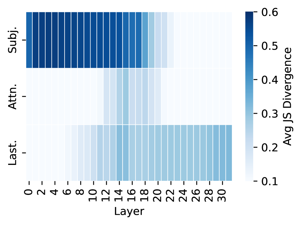<details> <summary>x14.png Details</summary>  ### Visual Description ## Heatmap: Avg JS Divergence Across Layers ### Overview The image is a heatmap visualizing the average Jensen-Shannon (JS) divergence across different layers for three categories: Subj. (Subject), Attn. (Attention), and Last. The x-axis represents the layer number, ranging from 0 to 30. The y-axis represents the three categories. The color intensity represents the magnitude of the average JS divergence, with darker blue indicating higher divergence and lighter blue indicating lower divergence. ### Components/Axes * **X-axis:** Layer (numerical, ranges from 0 to 30 in increments of 2) * **Y-axis:** Categories (Subj., Attn., Last.) * **Color Scale (Legend):** Avg JS Divergence (ranges from 0.1 to 0.6, with darker blue representing higher values and lighter blue representing lower values). The scale has tick marks at 0.1, 0.2, 0.3, 0.4, 0.5, and 0.6. ### Detailed Analysis * **Subj. (Subject):** The JS divergence is high (dark blue) for layers 0 to approximately 18. From layer 20 onwards, the JS divergence decreases (lighter blue). The approximate value for layers 0-18 is around 0.5-0.6. The approximate value for layers 20-30 is around 0.4-0.5. * **Attn. (Attention):** The JS divergence starts low (light blue) and gradually increases (darker blue) as the layer number increases. The approximate value for layers 0-10 is around 0.1-0.2. The approximate value for layers 20-30 is around 0.3-0.4. * **Last.:** The JS divergence is relatively low (light blue) across all layers. The approximate value is around 0.2-0.3. ### Key Observations * The "Subj." category has the highest JS divergence in the initial layers, which decreases as the layer number increases. * The "Attn." category has the lowest JS divergence in the initial layers, which increases as the layer number increases. * The "Last." category has a consistently low JS divergence across all layers. ### Interpretation The heatmap suggests that the "Subject" information is most divergent in the earlier layers of the model, while "Attention" becomes more divergent in the later layers. The "Last" category shows consistently low divergence across all layers, which might indicate that it represents a more stable or less variable aspect of the data. The JS divergence can be interpreted as a measure of how different the probability distributions are between different layers for each category. Higher divergence suggests greater differences in the information being processed at those layers. 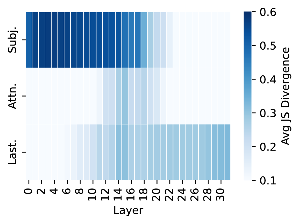</details> (a) Factual Associations <details> <summary>x15.png Details</summary>  ### Visual Description ## Heatmap: Avg JS Divergence by Layer and Category ### Overview The image is a heatmap visualizing the average Jensen-Shannon (JS) divergence across different layers (0-30) for three categories: "Subj.", "Attn.", and "Last.". The color intensity represents the magnitude of the JS divergence, ranging from approximately 0.1 (lightest blue) to 0.6 (darkest blue). ### Components/Axes * **Y-axis:** Categories: "Subj.", "Attn.", "Last." * **X-axis:** Layer number, ranging from 0 to 30 in increments of 2. * **Colorbar (Right):** Represents the "Avg JS Divergence", ranging from 0.1 to 0.6. The color gradient goes from light blue (0.1) to dark blue (0.6). ### Detailed Analysis * **Subj. (Subject):** * From layer 0 to approximately layer 18, the JS divergence is high, indicated by the dark blue color, close to 0.6. * From layer 20 to 30, the JS divergence decreases significantly, indicated by the lighter blue color, around 0.3. * **Attn. (Attention):** * The JS divergence is generally lower than "Subj." across all layers. * From layer 0 to approximately layer 14, the JS divergence is low, around 0.2. * From layer 16 to 30, the JS divergence increases slightly, reaching approximately 0.3. * **Last.:** * The JS divergence is relatively consistent across all layers, with values ranging from approximately 0.2 to 0.3. ### Key Observations * "Subj." has the highest JS divergence in the initial layers (0-18), indicating a greater difference in distributions compared to "Attn." and "Last.". * The JS divergence for "Subj." decreases significantly after layer 18. * "Attn." has the lowest JS divergence in the initial layers. * "Last." exhibits a relatively stable JS divergence across all layers. ### Interpretation The heatmap illustrates how the Jensen-Shannon divergence varies across different layers of a model for three categories: "Subj.", "Attn.", and "Last.". The high JS divergence for "Subj." in the initial layers suggests that the distributions being compared are more dissimilar in these layers compared to the later layers. The lower and more consistent JS divergence for "Attn." and "Last." indicates a more stable and similar distribution across all layers. The data suggests that the "Subj." category undergoes a significant change in its distribution around layer 18, while "Attn." and "Last." remain relatively stable. This could indicate that the model processes or transforms the "Subj." information differently in the later layers. 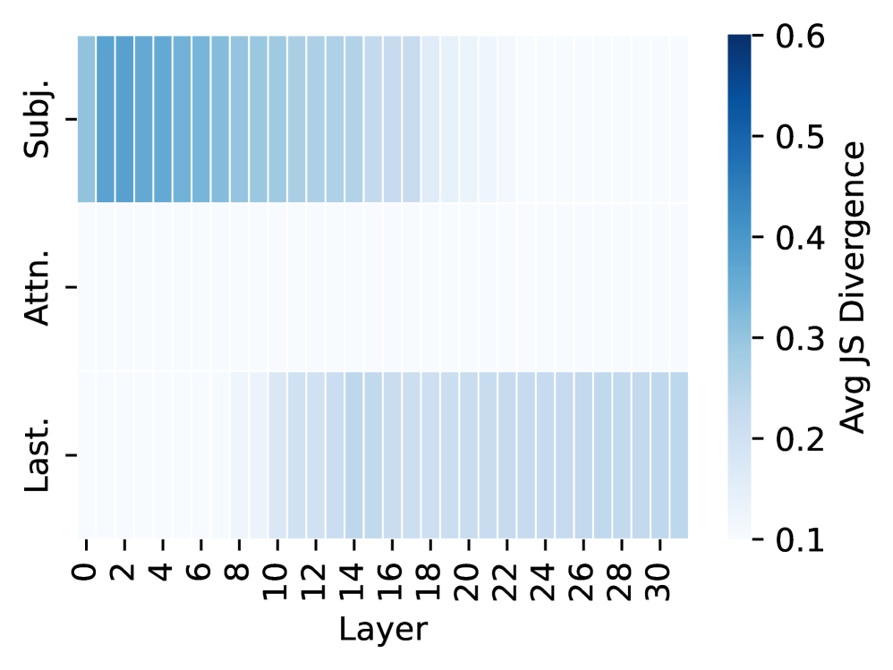</details> (b) Associated Hallucinations <details> <summary>x16.png Details</summary>  ### Visual Description ## Heatmap: Avg JS Divergence vs. Layer for Different Model Components ### Overview The image is a heatmap visualizing the average Jensen-Shannon (JS) divergence across different layers of a model for three components: Subject (Subj.), Attention (Attn.), and Last. The x-axis represents the layer number, ranging from 0 to 30. The y-axis represents the model component. The color intensity indicates the magnitude of the average JS divergence, with darker blue representing higher divergence and lighter blue representing lower divergence. ### Components/Axes * **X-axis:** Layer, ranging from 0 to 30 in increments of 2. * **Y-axis:** Model Component (Subj., Attn., Last.) * **Color Scale (Legend):** Avg JS Divergence, ranging from 0.1 to 0.6. * 0.1: Lightest blue * 0.6: Darkest blue ### Detailed Analysis * **Subject (Subj.):** The JS divergence is high (dark blue) for layers 0 to approximately 8. From layer 10 onwards, the JS divergence decreases significantly (lighter blue). * Layers 0-8: Avg JS Divergence ~0.5-0.6 * Layers 10-30: Avg JS Divergence ~0.2 * **Attention (Attn.):** The JS divergence is consistently low (light blue) across all layers (0 to 30). * Layers 0-30: Avg JS Divergence ~0.1-0.2 * **Last:** The JS divergence is low (light blue) across all layers (0 to 30), with a slight increase compared to the Attention component. * Layers 0-30: Avg JS Divergence ~0.2 ### Key Observations * The Subject component exhibits a high JS divergence in the initial layers, which then decreases. * The Attention component consistently shows low JS divergence across all layers. * The Last component also shows low JS divergence, slightly higher than the Attention component. ### Interpretation The heatmap suggests that the "Subject" component of the model undergoes significant changes in the initial layers (0-8), as indicated by the high JS divergence. This could imply that the model is actively learning or adapting the representation of the subject in these early layers. The "Attention" component, on the other hand, maintains a relatively stable and low JS divergence across all layers, suggesting that its representation remains consistent throughout the model's processing. The "Last" component's behavior is similar to the "Attention" component, indicating a stable representation. The differences in JS divergence between the components may reflect their roles and the types of information they process within the model. The high initial divergence in the "Subject" component could be due to the model initially struggling to represent the subject effectively, and then converging to a more stable representation as the layers progress. </details> (c) Unassociated Hallucinations Figure 13: Effect of interventions across layers of Mistral-7B-v0.3. The heatmap shows JS divergence between the output distribution before and after intervention. Darker color indicates that the intervened hidden states are more causally influential on the model’s predictions. Top row: patching representations of subject tokens. Middle row: blocking attention flow from subject to the last token. Bottom row: patching representations of the last token. A.3 Implementation Details Checkpoints and GPU resources. All the checkpoints used in our experiments are provided by the Hugging Face Transformers library Wolf et al. (2019). Specifically, we use the checkpoint “meta-llama/Meta-Llama-3-8B” https://huggingface.co/meta-llama/Meta-Llama-3-8B and “mistralai/Mistral-7B-v0.3” https://huggingface.co/mistralai/Mistral-7B-v0.3 for the experiments of response generation (§ 3), hidden-state analysis (§ 4) and accessing the performance of hallucination detection methods (§ 5). For refusal tuning (§ 6), we use checkpoints provided by the Unsloth framework Daniel Han and team (2023), namely “unsloth/llama-3-8b” https://huggingface.co/unsloth/llama-3-8b and “unsloth/mistral-7b-v0.3” https://huggingface.co/unsloth/mistral-7b-v0.3, which enable more efficient fine-tuning. All experiments are conducted on 4 NVIDIA L40S GPUs. 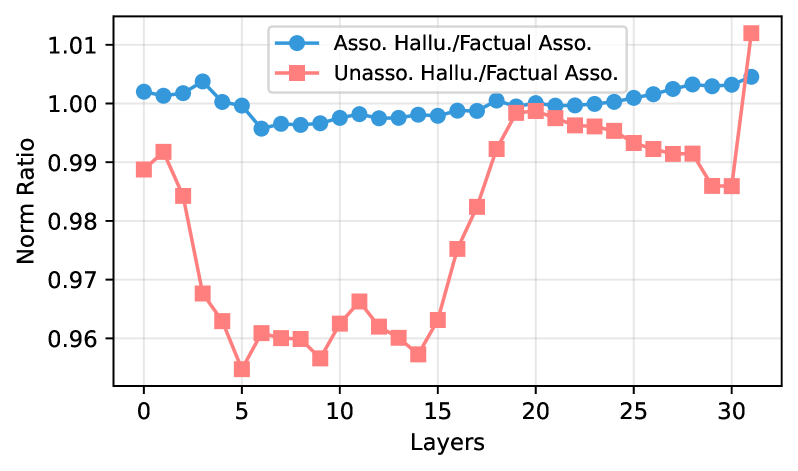<details> <summary>x17.png Details</summary>  ### Visual Description ## Line Chart: Norm Ratio vs. Layers ### Overview The image is a line chart comparing the "Norm Ratio" across different "Layers" for two categories: "Asso. Hallu./Factual Asso." and "Unasso. Hallu./Factual Asso.". The x-axis represents the layers, ranging from 0 to 30. The y-axis represents the Norm Ratio, ranging from 0.96 to 1.01. ### Components/Axes * **X-axis:** Layers, with tick marks at 0, 5, 10, 15, 20, 25, and 30. * **Y-axis:** Norm Ratio, with tick marks at 0.96, 0.97, 0.98, 0.99, 1.00, and 1.01. * **Legend (top-right):** * Blue line with circles: "Asso. Hallu./Factual Asso." * Red line with squares: "Unasso. Hallu./Factual Asso." ### Detailed Analysis * **Asso. Hallu./Factual Asso. (Blue Line):** * Trend: Relatively stable with minor fluctuations. Starts around 1.002, slightly increases to 1.004 at layer 2, then decreases to 0.996 at layer 5, remains stable around 0.998 until layer 30, then increases to 1.005. * Data Points: * Layer 0: ~1.002 * Layer 2: ~1.004 * Layer 5: ~0.996 * Layer 15: ~0.998 * Layer 30: ~1.003 * Layer 31: ~1.005 * **Unasso. Hallu./Factual Asso. (Red Line):** * Trend: More volatile than the blue line. Starts around 0.99, decreases sharply to 0.955 at layer 5, then gradually increases to 0.998 at layer 20, then decreases to 0.886 at layer 30, then increases to 1.005 at layer 31. * Data Points: * Layer 0: ~0.99 * Layer 5: ~0.955 * Layer 10: ~0.96 * Layer 15: ~0.96 * Layer 20: ~0.998 * Layer 30: ~0.986 * Layer 31: ~1.005 ### Key Observations * The "Asso. Hallu./Factual Asso." line is consistently higher than the "Unasso. Hallu./Factual Asso." line until layer 31. * The "Unasso. Hallu./Factual Asso." line experiences a significant drop between layers 0 and 5, and then a gradual recovery. * Both lines converge at layer 31. ### Interpretation The chart compares the normalized ratio between associated and unassociated hallucinations with factual associations across different layers. The "Asso. Hallu./Factual Asso." remains relatively stable, suggesting a consistent level of association. The "Unasso. Hallu./Factual Asso." experiences a significant dip, indicating a period where unassociated hallucinations are less factually grounded. The convergence at layer 31 suggests that, at this layer, the distinction between associated and unassociated hallucinations becomes less pronounced in terms of factual association. The initial dip in the "Unasso. Hallu./Factual Asso." line could indicate a phase where the model is still learning to ground unassociated hallucinations in factual information. </details> Figure 14: Norm ratio curves of subject representations in Mistral-7B-v0.3, comparing AHs and UHs against FAs as the baseline. At earlier layers, the norm of UH samples is significantly lower than that of AH samples. 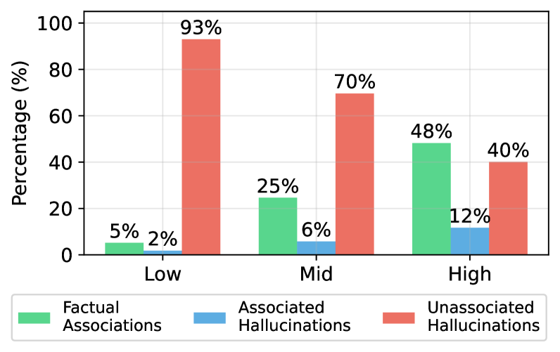<details> <summary>x18.png Details</summary>  ### Visual Description ## Bar Chart: Hallucination Types vs. Association Levels ### Overview The image is a bar chart comparing the percentages of three types of associations (Factual Associations, Associated Hallucinations, and Unassociated Hallucinations) across three levels: Low, Mid, and High. The chart uses different colored bars to represent each association type. ### Components/Axes * **Y-axis:** Percentage (%), with a scale from 0 to 100. * **X-axis:** Categorical axis with three levels: Low, Mid, and High. * **Legend:** Located at the bottom of the chart. * Green: Factual Associations * Blue: Associated Hallucinations * Red: Unassociated Hallucinations ### Detailed Analysis Here's a breakdown of the percentage values for each association type at each level: * **Low:** * Factual Associations (Green): 5% * Associated Hallucinations (Blue): 2% * Unassociated Hallucinations (Red): 93% * **Mid:** * Factual Associations (Green): 25% * Associated Hallucinations (Blue): 6% * Unassociated Hallucinations (Red): 70% * **High:** * Factual Associations (Green): 48% * Associated Hallucinations (Blue): 12% * Unassociated Hallucinations (Red): 40% ### Key Observations * **Unassociated Hallucinations (Red):** The percentage of unassociated hallucinations decreases as the level increases (93% at Low, 70% at Mid, 40% at High). * **Factual Associations (Green):** The percentage of factual associations increases as the level increases (5% at Low, 25% at Mid, 48% at High). * **Associated Hallucinations (Blue):** The percentage of associated hallucinations remains relatively low across all levels (2% at Low, 6% at Mid, 12% at High). ### Interpretation The data suggests an inverse relationship between the level and the occurrence of unassociated hallucinations. As the level increases, the percentage of unassociated hallucinations decreases, while the percentage of factual associations increases. This could indicate that higher levels are associated with more factual and less random or unassociated content. The relatively low percentage of associated hallucinations across all levels suggests that this type of hallucination is less prevalent compared to the other two categories. </details> Figure 15: Sample distribution across different subject popularity (low, mid, high) in Mistral-7B-v0.3, measured by monthly Wikipedia page views. Decoding algorithm. We employ greedy decoding ( $\text{temperature}=0$ ) for response generation, with models run in BF16 precision. PEFT settings for refusal tuning. For refusal tuning, we fine-tune with both models using QLoRA Dettmers et al. (2023), implemented with the Unsloth framework Daniel Han and team (2023), with rank $r=8$ , and $\alpha=8$ . QLoRA adapters are applied to all attention and MLP modules, and each model is fine-tuned for one epoch. 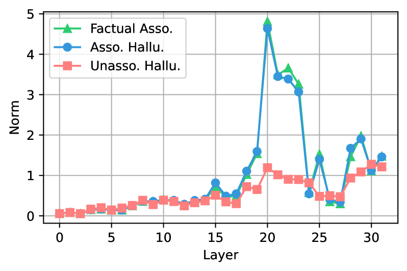<details> <summary>x19.png Details</summary>  ### Visual Description ## Line Chart: Norm vs Layer for Different Association Types ### Overview The image is a line chart comparing the "Norm" values across different "Layers" (0 to 32) for three types of associations: "Factual Asso.", "Asso. Hallu.", and "Unasso. Hallu.". The chart displays how the norm changes across layers for each association type, highlighting differences and trends. ### Components/Axes * **X-axis:** "Layer" - Ranges from 0 to 32 in increments of 5. * **Y-axis:** "Norm" - Ranges from 0 to 5 in increments of 1. * **Legend (Top-Left):** * Green Triangle: "Factual Asso." * Blue Circle: "Asso. Hallu." * Red Square: "Unasso. Hallu." ### Detailed Analysis * **Factual Asso. (Green Triangle):** * Trend: Relatively low values until layer 19, then a sharp increase to a peak at layer 20, followed by a decrease, and then another increase around layer 29. * Approximate Values: * Layer 0-15: ~0.1 to 0.7 * Layer 20: ~4.8 * Layer 25: ~0.3 * Layer 29: ~1.5 * Layer 32: ~1.4 * **Asso. Hallu. (Blue Circle):** * Trend: Similar to "Factual Asso.", with a peak at layer 20, but generally higher values before and after the peak. * Approximate Values: * Layer 0-15: ~0.1 to 0.8 * Layer 20: ~3.5 * Layer 25: ~0.5 * Layer 29: ~1.7 * Layer 32: ~1.5 * **Unasso. Hallu. (Red Square):** * Trend: Relatively stable and low values across all layers, with a slight increase around layer 20. * Approximate Values: * Layer 0-15: ~0.1 to 0.4 * Layer 20: ~1.2 * Layer 25: ~0.5 * Layer 29: ~1.1 * Layer 32: ~1.2 ### Key Observations * Both "Factual Asso." and "Asso. Hallu." exhibit a significant spike in "Norm" at layer 20. * "Unasso. Hallu." remains relatively stable across all layers. * The "Asso. Hallu." line is consistently above the "Factual Asso." line, except at layer 20 where the "Factual Asso." line is slightly higher. ### Interpretation The chart suggests that layer 20 is a critical point where both "Factual Asso." and "Asso. Hallu." experience a significant change in their "Norm" values. The stability of "Unasso. Hallu." across all layers indicates a different behavior or characteristic compared to the other two association types. The data implies that the model's processing at layer 20 might be particularly relevant for factual and associative aspects, while unassociated aspects remain less affected. The difference between "Asso. Hallu." and "Factual Asso." might indicate a distinction in how the model handles these two types of associations, especially considering the peak at layer 20. </details> Figure 16: Subject-to-last attention contribution norms across layers in Mistral-7B-v0.3. Values show the norm of the attention contribution from subject tokens to the last token at each layer. 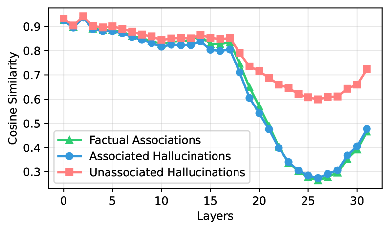<details> <summary>x20.png Details</summary>  ### Visual Description ## Line Chart: Cosine Similarity vs. Layers ### Overview The image is a line chart comparing the cosine similarity across different layers for three categories: Factual Associations, Associated Hallucinations, and Unassociated Hallucinations. The x-axis represents the layers, ranging from 0 to 30. The y-axis represents the cosine similarity, ranging from 0.3 to 0.9. ### Components/Axes * **X-axis:** Layers, ranging from 0 to 30 in increments of 5. * **Y-axis:** Cosine Similarity, ranging from 0.3 to 0.9 in increments of 0.1. * **Legend (bottom-left):** * Green line with triangle markers: Factual Associations * Blue line with circle markers: Associated Hallucinations * Red line with square markers: Unassociated Hallucinations ### Detailed Analysis * **Factual Associations (Green):** * Trend: Initially high, slightly decreasing, then a sharp decline, followed by an increase. * Values: Starts at approximately 0.92 at layer 0, decreases slightly to around 0.88 at layer 5, then drops sharply from approximately 0.82 at layer 15 to around 0.28 at layer 26, then increases to approximately 0.4 at layer 30. * **Associated Hallucinations (Blue):** * Trend: Similar to Factual Associations, with an initial high value, slight decrease, sharp decline, and then an increase. * Values: Starts at approximately 0.92 at layer 0, decreases slightly to around 0.87 at layer 5, then drops sharply from approximately 0.82 at layer 15 to around 0.32 at layer 26, then increases to approximately 0.48 at layer 30. * **Unassociated Hallucinations (Red):** * Trend: Starts high, decreases gradually, then declines more slowly than the other two, and finally increases slightly. * Values: Starts at approximately 0.93 at layer 0, decreases gradually to around 0.86 at layer 15, then drops to approximately 0.6 at layer 26, then increases to approximately 0.72 at layer 31. ### Key Observations * All three categories start with high cosine similarity values at the initial layers. * Factual Associations and Associated Hallucinations show a similar trend, with a sharp decline in cosine similarity around layer 15-20. * Unassociated Hallucinations maintain a higher cosine similarity compared to the other two categories after layer 20. * The cosine similarity for Factual Associations and Associated Hallucinations reaches a minimum around layer 26 before increasing again. ### Interpretation The chart suggests that as the layers increase, the cosine similarity for factual associations and associated hallucinations decreases significantly, indicating a potential divergence or weakening of the relationship. Unassociated hallucinations, however, maintain a relatively higher similarity, suggesting a different behavior or characteristic. The sharp decline around layers 15-20 could indicate a critical point where the representations or associations change significantly. The subsequent increase in similarity for Factual Associations and Associated Hallucinations after layer 26 might indicate a recovery or re-establishment of some form of association. </details> Figure 17: Cosine similarity of target-token hidden states across layers in Mistral-7B-v0.3. From mid-layers onward, FAs and AHs diverge sharply as subject information propagates, while UHs remain more clustered, confirming weaker subject-dependent updates. 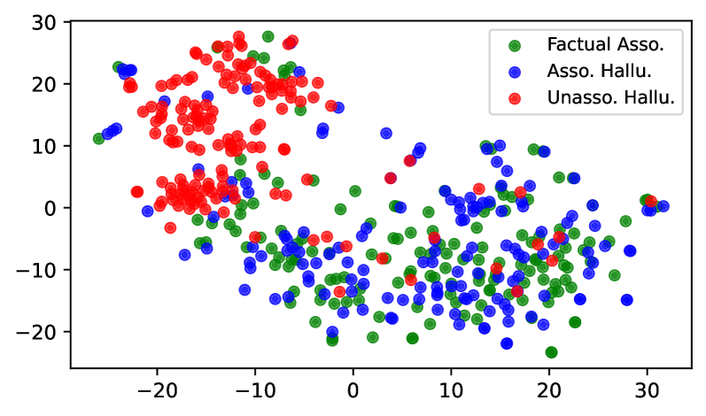<details> <summary>x21.png Details</summary>  ### Visual Description ## Scatter Plot: Factual vs. Hallucinated Associations ### Overview The image is a scatter plot visualizing the distribution of three categories: "Factual Asso.", "Asso. Hallu.", and "Unasso. Hallu." The plot displays data points in a two-dimensional space, with the x and y axes ranging from approximately -25 to 30. The data points are color-coded: green for "Factual Asso.", blue for "Asso. Hallu.", and red for "Unasso. Hallu.". The plot shows the relative positioning and clustering of these three categories. ### Components/Axes * **X-axis:** Ranges from approximately -25 to 30, with no explicit label. * **Y-axis:** Ranges from -20 to 30, with no explicit label. * **Legend (Top-Right):** * Green: "Factual Asso." * Blue: "Asso. Hallu." * Red: "Unasso. Hallu." ### Detailed Analysis * **Factual Asso. (Green):** * Data points are scattered across the plot, with a higher concentration in the top-left quadrant (x: -25 to 0, y: 0 to 30) and the bottom-right quadrant (x: 0 to 30, y: -20 to 0). * Specific data points: (-15, 28), (25, -15), (-5, -15) * **Asso. Hallu. (Blue):** * Data points are primarily clustered in the bottom-right quadrant (x: 0 to 30, y: -20 to 10). * Specific data points: (10, -10), (20, 0), (5, -20) * **Unasso. Hallu. (Red):** * Data points are concentrated in the top-left quadrant (x: -25 to 0, y: 0 to 30). * Specific data points: (-15, 15), (-5, 20), (-20, 5) ### Key Observations * "Unasso. Hallu." (red) is primarily located in the top-left. * "Asso. Hallu." (blue) is primarily located in the bottom-right. * "Factual Asso." (green) is more dispersed, appearing in both the top-left and bottom-right. * There is some overlap between all three categories, indicating that the separation is not absolute. ### Interpretation The scatter plot visualizes the relationships between factual associations and two types of hallucinations ("Asso. Hallu." and "Unasso. Hallu."). The clustering suggests that "Unasso. Hallu." and "Asso. Hallu." tend to occupy different regions in the feature space represented by the x and y axes. "Factual Asso." appears to be more broadly distributed, potentially indicating that it shares characteristics with both types of hallucinations or that it represents a more diverse set of associations. The overlap between the categories suggests that the distinction between factual associations and hallucinations is not always clear-cut, and there may be cases where they are difficult to differentiate based on the features used to generate this plot. The axes are not labeled, so the specific features being visualized are unknown. </details> Figure 18: t-SNE visualization of last token’s representations at layer 25 of Mistral-7B-v0.3. 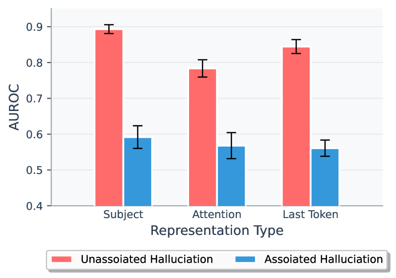<details> <summary>x22.png Details</summary>  ### Visual Description ## Bar Chart: AUROC by Representation Type and Hallucination Association ### Overview The image is a bar chart comparing the Area Under the Receiver Operating Characteristic curve (AUROC) for different representation types (Subject, Attention, Last Token) in the context of hallucination association (Unassociated vs. Associated). The chart displays the AUROC values for each representation type, separated by whether the hallucination is unassociated (red bars) or associated (blue bars). Error bars are included on each bar, indicating the uncertainty in the AUROC measurement. ### Components/Axes * **Y-axis:** AUROC, ranging from 0.4 to 0.9. * **X-axis:** Representation Type, with categories: Subject, Attention, Last Token. * **Legend:** Located at the bottom of the chart. * Red: Unassoiated Halluciation * Blue: Assoiated Halluciation ### Detailed Analysis The chart presents AUROC values for two types of hallucinations (Unassociated and Associated) across three representation types (Subject, Attention, and Last Token). **Unassociated Hallucination (Red Bars):** * **Subject:** AUROC is approximately 0.89, with an error range of +/- 0.01. * **Attention:** AUROC is approximately 0.78, with an error range of +/- 0.03. * **Last Token:** AUROC is approximately 0.84, with an error range of +/- 0.02. **Associated Hallucination (Blue Bars):** * **Subject:** AUROC is approximately 0.59, with an error range of +/- 0.03. * **Attention:** AUROC is approximately 0.56, with an error range of +/- 0.04. * **Last Token:** AUROC is approximately 0.56, with an error range of +/- 0.03. ### Key Observations * For all representation types, the AUROC is significantly higher for unassociated hallucinations compared to associated hallucinations. * The "Subject" representation type shows the highest AUROC for unassociated hallucinations (approximately 0.89). * The AUROC values for associated hallucinations are relatively consistent across all three representation types, hovering around 0.56-0.59. ### Interpretation The data suggests that the model is better at distinguishing unassociated hallucinations from non-hallucinations compared to associated hallucinations. The "Subject" representation type appears to be the most informative for detecting unassociated hallucinations, as indicated by its higher AUROC value. The lower AUROC values for associated hallucinations suggest that these types of hallucinations are more difficult to detect using the given representation types. The consistent performance across representation types for associated hallucinations might indicate that the model struggles to differentiate them regardless of the input feature. </details> Figure 19: Hallucination detection performance on the Full setting (Mistral-v0.3-7B). 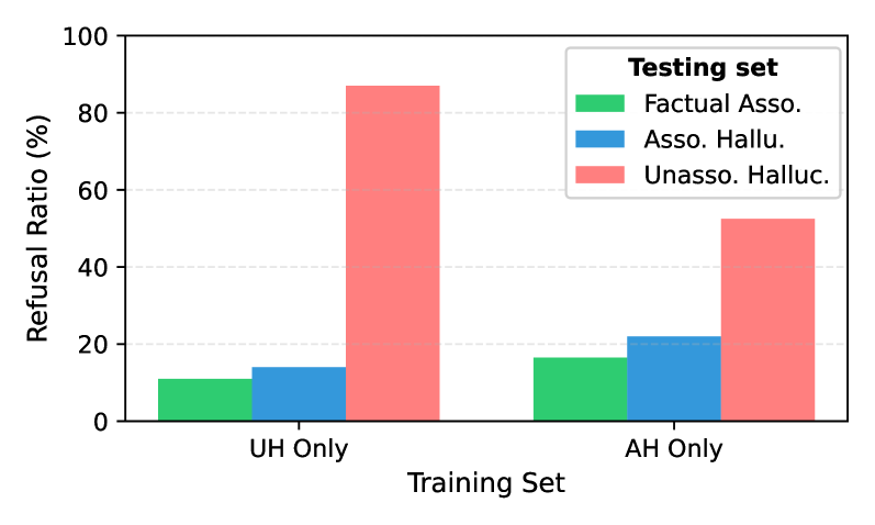<details> <summary>x23.png Details</summary>  ### Visual Description ## Bar Chart: Refusal Ratio by Training Set and Testing Set ### Overview The image is a bar chart comparing the refusal ratio (%) across different training sets (UH Only, AH Only) and testing sets (Factual Asso., Asso. Hallu., Unasso. Halluc.). The chart visualizes how the training data influences the model's refusal to answer based on the type of hallucination present in the testing data. ### Components/Axes * **X-axis:** Training Set (UH Only, AH Only) * **Y-axis:** Refusal Ratio (%) with a scale from 0 to 100, incrementing by 20. * **Legend (Top-Right):** Testing set * Factual Asso. (Green) * Asso. Hallu. (Blue) * Unasso. Halluc. (Red) ### Detailed Analysis **Training Set: UH Only** * **Factual Asso. (Green):** Refusal Ratio is approximately 11%. * **Asso. Hallu. (Blue):** Refusal Ratio is approximately 14%. * **Unasso. Halluc. (Red):** Refusal Ratio is approximately 87%. **Training Set: AH Only** * **Factual Asso. (Green):** Refusal Ratio is approximately 17%. * **Asso. Hallu. (Blue):** Refusal Ratio is approximately 22%. * **Unasso. Halluc. (Red):** Refusal Ratio is approximately 53%. ### Key Observations * For both training sets, the "Unasso. Halluc." testing set has the highest refusal ratio. * The "AH Only" training set generally results in higher refusal ratios across all testing sets compared to the "UH Only" training set. * The difference in refusal ratio between "Unasso. Halluc." and the other two testing sets is much more pronounced for the "UH Only" training set. ### Interpretation The data suggests that the type of training data significantly impacts the model's refusal behavior when faced with different types of hallucinations in the testing data. Specifically, models trained on "UH Only" data are much more likely to refuse to answer when presented with "Unasso. Halluc." compared to "Factual Asso." or "Asso. Hallu.". Training on "AH Only" data seems to mitigate this effect to some extent, leading to a more balanced refusal ratio across different hallucination types. The high refusal rate for "Unasso. Halluc." could indicate that the model struggles to handle or identify this type of hallucination, leading it to refuse to answer more frequently. </details> Figure 20: Refusal tuning performance across three types of samples (Mistral-v0.3-7B). Appendix B Parallel Experiments on Mistral This section is for documenting parallel experiments conducted on the Mistral-7B-v0.3 model under the same settings as described in the main text (Figures 13 – 20). The results from Mistral exhibit similar patterns to those observed in LLaMA, as described before. Specifically, we find consistent patterns in the model’s internal computations, hidden-state behaviors, and the performance of hallucination detection and refusal tuning experiments. 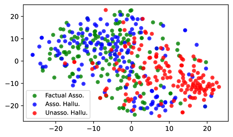<details> <summary>x24.png Details</summary>  ### Visual Description ## Scatter Plot: Semantic Space of Hallucinations ### Overview The image is a scatter plot visualizing the semantic space of different types of hallucinations. The plot displays three categories of data points: "Factual Asso." (green), "Asso. Hallu." (blue), and "Unasso. Hallu." (red). The x and y axes are unlabeled, but the data points are distributed across a range from approximately -25 to 25 on both axes. ### Components/Axes * **X-axis:** Ranges from approximately -25 to 25, with tick marks at -20, -10, 0, 10, and 20. * **Y-axis:** Ranges from approximately -25 to 25, with tick marks at -20, -10, 0, 10, and 20. * **Legend (bottom-left):** * Green: "Factual Asso." * Blue: "Asso. Hallu." * Red: "Unasso. Hallu." ### Detailed Analysis * **Factual Asso. (Green):** The green data points are primarily concentrated in the upper-left quadrant of the plot, with a scattering of points throughout the rest of the space. The green points are mostly between x values of -25 to 5 and y values of -5 to 20. * **Asso. Hallu. (Blue):** The blue data points are more evenly distributed across the plot, with a slight concentration in the upper-center region. The blue points are mostly between x values of -20 to 10 and y values of -10 to 20. * **Unasso. Hallu. (Red):** The red data points are primarily concentrated in the bottom-right quadrant of the plot. The red points are mostly between x values of 0 to 20 and y values of -20 to 10. ### Key Observations * The three categories of data points exhibit some degree of clustering, suggesting that they occupy distinct regions of the semantic space. * The "Unasso. Hallu." category appears to be the most distinct, with a clear concentration in the bottom-right quadrant. * The "Factual Asso." and "Asso. Hallu." categories have more overlap, particularly in the upper-left quadrant. ### Interpretation The scatter plot suggests that different types of hallucinations can be distinguished based on their semantic properties. The clustering of data points indicates that "Factual Asso.", "Asso. Hallu.", and "Unasso. Hallu." occupy different regions of the semantic space. The "Unasso. Hallu." category, which is concentrated in the bottom-right quadrant, may represent hallucinations that are semantically distinct from the other two categories. The overlap between "Factual Asso." and "Asso. Hallu." suggests that these two categories may share some semantic similarities. The plot provides a visual representation of the semantic relationships between different types of hallucinations, which could be useful for understanding the underlying cognitive processes involved in their generation. The lack of axis labels limits the interpretation, but the relative positioning of the clusters is informative. </details> Figure 21: t-SNE visualization of subject tokens’ representations at layer 11 of LLaMA-3-8B. 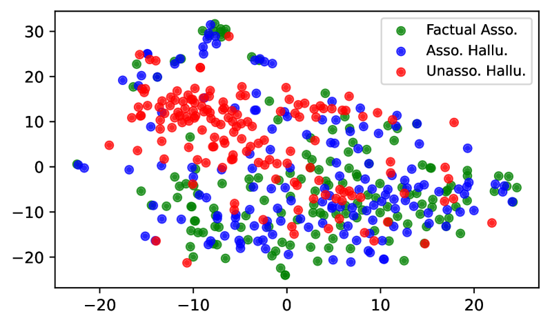<details> <summary>x25.png Details</summary>  ### Visual Description ## Scatter Plot: Association and Hallucination Types ### Overview The image is a scatter plot visualizing the distribution of three categories: "Factual Asso.", "Asso. Hallu.", and "Unasso. Hallu." The plot displays data points in a two-dimensional space, with the x and y axes ranging from approximately -25 to 30. Each category is represented by a different color: green for "Factual Asso.", blue for "Asso. Hallu.", and red for "Unasso. Hallu.". The data points appear to cluster in certain regions, suggesting potential relationships or distinctions between the categories. ### Components/Axes * **X-axis:** Ranges from approximately -25 to 25, with tick marks at -20, -10, 0, 10, and 20. The x-axis label is not explicitly provided in the image. * **Y-axis:** Ranges from approximately -20 to 30, with tick marks at -20, -10, 0, 10, 20, and 30. The y-axis label is not explicitly provided in the image. * **Legend:** Located in the top-right corner of the plot. * Green: "Factual Asso." * Blue: "Asso. Hallu." * Red: "Unasso. Hallu." ### Detailed Analysis * **Factual Asso. (Green):** The green data points are distributed across the plot, with a higher concentration in the bottom-right quadrant and a cluster in the top-left quadrant. * **Asso. Hallu. (Blue):** The blue data points are also distributed across the plot, with a higher concentration in the central region. * **Unasso. Hallu. (Red):** The red data points are primarily concentrated in the top-center region of the plot. **Specific Data Point Analysis (Approximate):** * **Factual Asso. (Green):** * Cluster in top-left: X values range from -15 to -5, Y values range from 20 to 30. * Bottom-right quadrant: X values range from 5 to 25, Y values range from -20 to 0. * **Asso. Hallu. (Blue):** * Central region: X values range from -10 to 10, Y values range from -10 to 10. * Top-left: X values range from -20 to -10, Y values range from 0 to 10. * **Unasso. Hallu. (Red):** * Top-center: X values range from -15 to 0, Y values range from 10 to 25. ### Key Observations * The "Unasso. Hallu." category (red) appears to be more clustered than the other two categories. * The "Factual Asso." category (green) has a wider distribution, with concentrations in the bottom-right and top-left quadrants. * The "Asso. Hallu." category (blue) is more centrally located, with some overlap with the other two categories. ### Interpretation The scatter plot suggests that there are distinct patterns in how "Factual Asso.", "Asso. Hallu.", and "Unasso. Hallu." are distributed in the two-dimensional space. The clustering of "Unasso. Hallu." in the top-center region may indicate that this category has unique characteristics compared to the other two. The wider distribution of "Factual Asso." suggests that it may be more diverse or influenced by different factors. The central location of "Asso. Hallu." may indicate that it shares characteristics with both "Factual Asso." and "Unasso. Hallu.". The plot could represent a dimensionality reduction technique (e.g., t-SNE or PCA) applied to a dataset, where each point represents a data sample, and the colors indicate the category it belongs to. The proximity of points suggests similarity in the original high-dimensional space. Further analysis would be needed to understand the specific features that contribute to these patterns. </details> Figure 22: t-SNE visualization of subject tokens’ representations at layer 11 of Mistral-7B-v0.3. Appendix C More Visualization on Hidden States In this section, we provide t-SNE visualization of subject tokens’ hidden states in Figure 21 and Figure 22. Compared to the last-token representations, the t-SNE visualization of subject-token hidden states shows that unassociated hallucinations (UHs) are moderately separated from factual and associated samples, but the separation is less distinct than in the last-token representations. This observation aligns with the results in § 5, where the hallucination detection performance using last-token hidden states outperforms that based on subject-token representations.