2510.09782

## The Geometry of Reasoning: Flowing Logics in Representation Space Yufa Zhou * , Yixiao Wang * , Xunjian Yin * , Shuyan Zhou, Anru R. Zhang Duke University {yufa.zhou,yixiao.wang,xunjian.yin,shuyan.zhou,anru.zhang}@duke.edu * Equal contribution. We study how large language models (LLMs) 'think' through their representation space. We propose a novel geometric framework that models an LLM's reasoning as flows-embedding trajectories evolving where logic goes. We disentangle logical structure from semantics by employing the same natural deduction propositions with varied semantic carriers, allowing us to test whether LLMs internalize logic beyond surface form. This perspective connects reasoning with geometric quantities such as position, velocity, and curvature, enabling formal analysis in representation and concept spaces. Our theory establishes: (1) LLM reasoning corresponds to smooth flows in representation space, and (2) logical statements act as local controllers of these flows' velocities. Using learned representation proxies, we design controlled experiments to visualize and quantify reasoning flows, providing empirical validation of our theoretical framework. Our work serves as both a conceptual foundation and practical tools for studying reasoning phenomenon, offering a new lens for interpretability and formal analysis of LLMs' behavior. /github Code: https://github.com/MasterZhou1/Reasoning-Flow Dataset: https://huggingface.co/datasets/MasterZhou/Reasoning-Flow 'Reasoning is nothing but reckoning.' -Thomas Hobbes ## 1. Introduction The geometry of concept space, i.e., the idea that meaning can be represented as positions in a structured geometric space, has long served as a unifying perspective across AI, cognitive science, and linguistic philosophy [15, 59, 16]. Early work in this tradition was limited by the absence of precise and scalable semantic representations. With the rise of large language models (LLMs) [28, 52, 19, 21, 75], we revisit this geometric lens: pretrained embeddings now offer high-dimensional vector representations of words, sentences, and concepts [44, 49, 79, 35, 34], enabling geometric analysis of semantic and cognitive phenomena at scale. A seminal recent work [46] formalizes the notion that learned representations in LLMs lie on low-dimensional concept manifolds. Building on this view, we hypothesize that reasoning unfolds as a trajectory, potentially a flow, along such manifolds. To explore this idea, we draw on classical tools from differential geometry [42, 25, 20, 9] and propose a novel geometric framework for analyzing reasoning dynamics in language models. Concretely, we view reasoning as a context-cumulative trajectory in embedding space: at each step, the reasoning prefix is extended, and the model's representation is recorded to trace the evolving flow (Figures 1a and 1b). Our results suggest that LLM reasoning is not merely a random walk on graphs [67, 45]. At the isolated embedding level, trajectories exhibit stochasticity reminiscent of graph-based views; however, when viewed cumulatively, a structured flow emerges on a low-dimensional concept manifold, where local velocities are governed by logical operations. To the best of our knowledge, this is the first work to formalize and empirically validate such a dynamical perspective, offering quantitative evidence together with broad insights and implications. We further rigorously define and formalize Reasoning flows (PCA 3D) Flow answer\_1 answer\_2 answer\_3 answer\_4 answer\_5 answer\_6 - (a) Reasoning flows visualized using PCA in 3 dimensions. -0.4 -0.3 -0.2 -0.1 0.1 answer\_1 answer\_2 answer\_3 answer\_4 answer\_5 answer\_6 0.2 PC 1 - (b) Reasoning flows visualized using PCA in 2 dimensions. 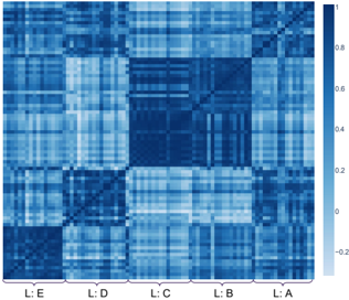- (c) Schematic illustration of mappings between spaces. <details> <summary>Image 1 Details</summary>  ### Visual Description ## Diagram: Transformation and Relationship Between Curve Sets and Representations ### Overview The diagram illustrates a conceptual framework involving transformations between curve sets (Curves(C) and Curves(R)) and their associated representations (L_form and L_rep). It includes mappings, function compositions, and an unresolved relationship denoted by a question mark. ### Components/Axes - **Top Layer**: - **X**: A central node splitting into two paths. - **Γ (Gamma)**: Arrow from X to Curves(C), labeled as a function mapping. - **Ψ (Psi)**: Arrow from X to Curves(R), labeled as a function mapping. - **Middle Layer**: - **A = Ψ ∘ Γ⁻¹**: Transformation between Curves(C) and Curves(R), indicating a composition of Ψ and the inverse of Γ. - **Bottom Layer**: - **FC**: Arrow from Curves(C) to L_form (form representation). - **DR**: Arrow from Curves(R) to L_rep (representation). - **Question Mark (?)**: Dashed bidirectional arrow between L_form and L_rep, indicating an unresolved or unknown relationship. ### Detailed Analysis 1. **Top Layer**: - **X** acts as a source node, branching into two distinct mappings: - **Γ**: Maps X to Curves(C), suggesting a transformation or encoding process for curve set C. - **Ψ**: Maps X to Curves(R), indicating a separate transformation for curve set R. - **Curves(C)** and **Curves(R)** are intermediate sets derived from X via Γ and Ψ, respectively. 2. **Middle Layer**: - **A = Ψ ∘ Γ⁻¹** defines a bidirectional or composite transformation between Curves(C) and Curves(R). This implies that Curves(R) can be derived from Curves(C) via the inverse of Γ followed by Ψ, or vice versa. 3. **Bottom Layer**: - **FC** and **DR** represent mappings from curve sets to their respective representations: - **FC**: Maps Curves(C) to L_form (form representation). - **DR**: Maps Curves(R) to L_rep (representation). - The **question mark (?)**, placed between L_form and L_rep, highlights an unresolved relationship or dependency between these two representations. This could imply uncertainty about how form and representation layers interact or whether they are equivalent, complementary, or independent. ### Key Observations - The diagram emphasizes **transformations** (Γ, Ψ, A) as core mechanisms linking abstract sets (X, Curves(C), Curves(R)) to concrete representations (L_form, L_rep). - The **question mark** is the only ambiguous element, suggesting a gap in understanding or a research question about the relationship between L_form and L_rep. - No numerical data or trends are present; the focus is on structural relationships and mappings. ### Interpretation This diagram likely represents a theoretical framework in a domain such as computational geometry, machine learning (e.g., curve representation learning), or mathematical modeling. Key insights include: 1. **Transformation Hierarchy**: X is the foundational entity, with Γ and Ψ acting as specialized transformations for curve sets C and R. 2. **Compositional Relationship**: The transformation A bridges C and R, implying interoperability or equivalence under specific conditions. 3. **Representation Ambiguity**: The unresolved link between L_form and L_rep raises questions about how form and representation are related. For example: - Are they dual perspectives of the same underlying structure? - Is there a missing function or constraint connecting them? - Do they operate in separate domains (e.g., geometric vs. algebraic representations)? The diagram underscores the importance of clarifying the relationship between form and representation in the context of curve transformations. The question mark serves as a focal point for further investigation, potentially guiding future work to resolve this ambiguity. 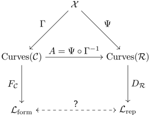</details> Figure 1: Reasoning Flow. (a-b) Visualizations on a selected problem from MATH500 with six distinct answers. (c) Our geometric framework of mapping relationships among input space 𝒳 , concept space 𝒞 , logic space ℒ , and representation space ℛ . See Section 4 for more details. concept, logic, and representation spaces (Figure 1c), and relate them through carefully designed experiments. From Aristotle's syllogistics to Frege's predicate calculus and modern math foundations [4, 8, 11], formal logic isolates validity as form independent of content. Wittgenstein's Tractatus sharpened this view-'the world is the totality of facts, not of things' [72]-underscoring logical form as the substrate of language and reality. In this spirit, we treat logic as a carrier-invariant skeleton of reasoning and test whether LLMs, trained on massive corpora, have internalized such structural invariants on the embedding manifold, effectively rediscovering in data the universal logic that took humans two millennia to formalize. We deliberately construct a dataset that isolates formal logic from its semantic carriers (e.g., topics and languages) to validate our geometric perspective. Our experiments, conducted with Qwen3 [75] hidden states on our newly constructed dataset, reveal that LLMs exhibit structured logical behavior. In the original (0-order) representation space, semantic properties dominate, with sentences on the same topic clustering together. However, when we analyze differences (1- and 2-order representations), logical structure emerges as the dominant factor. Specifically, we find that velocity similarity and Menger curvature similarity remain highly consistent between flows sharing the same logical skeleton, even across unrelated topics and languages. In contrast, flows with different logical structures exhibit lower similarity, even when they share the same semantic carrier. These findings provide quantifiable evidence for our hypothesis that logic governs the velocity of reasoning flows. While interpretability research on LLMs has made substantial empirical progress [1, 58, 48, 61, 40, 13], rigorous theoretical understanding remains comparatively limited, with only a few recent efforts in this direction [31, 54, 46, 55]. Our work contributes to this emerging line by introducing a mathematically grounded framework with formal definitions and analytic tools for quantifying and analyzing how LLMs behave and reason. We hope our theory and empirical evidence open a new perspective for interpretability community and spark practical applications. Our contributions are: - We introduce a geometric perspective that models LLM reasoning as flows, providing formal definitions and analytic tools to study reasoning dynamics. - We empirically validate our framework through experiments and analysis, demonstrating its utility and offering practical insights. - We design a formal logic dataset that disentangles logical structure from semantic surface, enabling direct tests of whether LLMs internalize logic beyond semantics. PC 2 Top-down view (PC1 vs PC2) 0.2 0.15 0.1 0.05 -0.05 -0.1 -0.15 Flow ## 2. Related Work Concept Space Geometry. The Linear Representation Hypothesis (LRH) proposes that concepts align with linear directions in embedding space, a view supported by theoretical analyses and empirically validated in categorical, hierarchical, and truth-false settings [54, 32, 55, 31, 41]. However, strict linearity is limited: features may be multi-dimensional or manifold-like, as seen in concepts like colors, years, dates, and antonym pairs. [12, 46, 34]. Other works emphasize compositionality, showing that concepts require explicit constraints or algebraic subspace operations to compose meaningfully [63, 70]. At a broader scale, hidden-state geometry follows expansion-contraction patterns across layers and exhibits training trajectories whose sharp shifts coincide with emergent capabilities and grokking [65, 53, 39]. Sparse autoencoders further reveal multi-scale structure, from analogy-like 'crystals' to anisotropic spectra [36]. Collectively, these results suggest that concept spaces are locally linear yet globally curved, compositional, and dynamic, motivating our perspective of reasoning as flows on such manifolds. Mechanistic Interpretability. LLMs have exhibited unprecedented intelligence ever since their debut [51]. Yet the underlying mechanisms remain opaque, as transformers are neural networks not readily interpretable by humans-motivating efforts to uncover why such capabilities emerge [61, 40]. Mechanistic Interpretability (MI) pursues this goal by reverse-engineering transformer internals into circuits, features, and algorithms [58, 13, 3]. The Transformer Circuits program at Anthropic exemplifies this agenda, systematically cataloging reusable computational subroutines [1]. Empirical studies reveal concrete algorithmic mechanisms: grokking progresses along Fourier-like structures [48], training can yield divergent solutions for the same task (Clock vs. Pizza) [81], arithmetic emerges via trigonometric embeddings on helical manifolds [33], and spatiotemporal structure is encoded through identifiable neurons [22]. Beyond circuits, in-context learning and fine-tuning yield distinct representational geometries despite comparable performance [10], while safety studies reveal polysemantic vulnerabilities where small-model interventions transfer to larger LLMs [18]. Understanding Reasoning Phenomenon. LLMs benefit from test-time scaling , where allocating more inference compute boosts accuracy on hard tasks [62]. Explanations span expressivity-CoT enabling serial computation [37], reasoning as superposed trajectories [82], and hidden planning in scratch-trained math models [78]-to inductive biases, where small initialization favors deeper chains [77]. Structural analyses view reasoning as path aggregation or graph dynamics with small-world properties [67, 45], while attribution highlights key 'thought anchors' [5]. Empirical work shows inverted-U performance with CoT length and quantifiable reasoning boundaries [73, 6], and embedding-trajectory geometry supports OOD detection [68]. Moving beyond text, latent-reasoning methods scale compute through recurrent depth, continuous 'soft thinking,' and latent CoT for branch exploration and self-evaluation [80, 17, 23, 69]. Applications exploit these insights for steering and efficiency: steering vectors and calibration shape thought processes [66, 7], manifold steering mitigates overthinking [27], and adaptive indices enable early exit [14]. Formal Logic with LLMs. Recent work links transformer computation directly to logic. Log-precision transformers are expressible in first-order logic with majority quantifiers, providing an upper bound on expressivity [43], while temporal counting logic compiles into softmax-attention architectures, giving a constructive lower bound [76]. Beyond these characterizations, pre-pretraining on formal languages with hierarchical structure (e.g., Dyck) imparts syntactic inductive biases and improves efficiency [26]. Synthetic logic corpora and proof-generation frameworks further strengthen reasoning, though benefits diminish as proofs lengthen [47, 74]. Systematic evaluations, including LogicBench and surveys, highlight persistent failures on negation and inductive reasoning, despite partial gains from 'thinking' models and rejection finetuning [56, 30, 38]. In contrast, our work employs formal logic not as an end task, but as a tool to validate our geometric framework in LLMs' representation space, distinguishing our contribution from prior lines of work. ## 3. Preliminaries ## 3.1. Large Language Models Let 𝒱 denote a finite vocabulary of tokens, and let 𝜃 denote the parameters of a large language model (LLM). An LLM defines a conditional probability distribution 𝑝 𝜃 ( 𝑢 𝑡 | 𝑢 <𝑡 , 𝑃 ) , 𝑢 𝑡 ∈ 𝒱 , where 𝑢 <𝑡 := ( 𝑢 1 , . . . , 𝑢 𝑡 -1 ) is the prefix of previously generated tokens and 𝑃 ∈ 𝒱 𝑛 is the tokenized problem prompt. At each step 𝑡 , inference proceeds by sampling 𝑢 𝑡 ∼ 𝑝 𝜃 ( · | 𝑢 <𝑡 , 𝑃 ) . Definition 3.1 (Chain-of-Thought Reasoning) . Given a prompt 𝑃 ∈ 𝒱 𝑛 , Chain-of-Thought ( CoT) reasoning is an iterative stochastic process that generates a sequence 𝒰 = ( 𝑢 1 , 𝑢 2 , . . . , 𝑢 𝑇 ) , 𝑢 𝑡 ∈ 𝒱 , via recursive sampling 𝑢 𝑡 ∼ 𝑝 𝜃 ( · | 𝑃, 𝑢 <𝑡 ) , 𝑡 = 1 , . . . , 𝑇. To enable geometric analysis of reasoning, we need a mapping from discrete token sequences into continuous vectors, a transformation that modern LLMs naturally provide. Definition 3.2 (Representation Operator) . A Representation Operator is a mapping ℰ : 𝒱 * × ℐ → R 𝑑 , where 𝑥 = ( 𝑥 1 , . . . , 𝑥 𝑛 ) ∈ 𝒱 * is a token sequence and 𝜄 ∈ ℐ is an index specifying the representation type (e.g., a token position, a prefix, a pooling rule, or an internal layer state). The output ℰ ( 𝑥, 𝜄 ) ∈ R 𝑑 is the embedding/representaion of 𝑠 under the selection rule 𝜄 . For notational simplicity, we omit the index 𝜄 unless explicitly required. The range of this operator defines the ambient space of reasoning: Definition 3.3 (Representation Space) . Given an representation operator ℰ , the representation space is ℛ := {ℰ ( 𝑥 ) : 𝑥 ∈ 𝒱 * } ⊆ R 𝑑 . Elements of ℛ are continuous embeddings of discrete language inputs, serving as the foundation and empirical proxy for our geometric analysis of reasoning. In practice, ℰ may be instantiated by a pretrained encoder such as Qwen3 Embedding [79] or OpenAI's text-embedding-3-large [49], or by extracting hidden states directly from an LLM. Typical choices of 𝜄 include mean pooling, the hidden state of the final token, or a specific layer-position pair within the model [79, 35, 24, 50]. We interpret ℰ as projecting discrete language sequences into a continuous semantic space, potentially lying on a low-dimensional manifold embedded in R 𝑑 [46, 12, 34]. ## 3.2. Menger Curvature We adopt Menger curvature [42] to quantitatively capture the geometric structure of reasoning flows. As a metricbased notion of curvature, Menger curvature simultaneously reflects both angular deviation and distance variation, making it particularly suitable for reasoning trajectories represented as discrete embeddings. We leave more details to Appendix C.2. Definition 3.4 (Menger Curvature) . Let 𝑥 1 , 𝑥 2 , 𝑥 3 ∈ R 𝑛 be three distinct points. The Menger curvature of the triple ( 𝑥 1 , 𝑥 2 , 𝑥 3 ) is defined as the reciprocal of the radius 𝑅 ( 𝑥 1 , 𝑥 2 , 𝑥 3 ) of the unique circle passing through the three points: 𝑐 ( 𝑥 1 , 𝑥 2 , 𝑥 3 ) = 1 𝑅 ( 𝑥 1 ,𝑥 2 ,𝑥 3 ) . ## 4. Reasoning as Geometric Flows in Representation Space We formalize the view that LLMs reason by tracing trajectories in their representation space. A central question is whether LLMs exhibit intrinsic control over these flows, mirroring the human perspective. We hypothesize semantic content as a curve on a concept manifold, and logical structure acts as a local controller of the trajectory. In this section, we introduce the spaces, maps, and geometric quantities that underpin the paper. We then rigorously formalize this construction and establish the correspondence between the LLM's representation space and the human concept space. ## 4.1. Concept Space and Semantic Trajectories Definition 4.1 (Concept Space) . The concept space 𝒞 is an abstract semantic space that models human-level cognitive structures such as ideas, reasoning states, and problem-solving subtasks. We assume 𝒞 is endowed with a smooth geometric structure, allowing continuous trajectories to represent the evolution of conceptual content. This assumption can be traced back to the classical insight of William James [29], who famously argued that consciousness does not appear to itself 'chopped up in bits.' Chains or trains of thought are, in his words, inadequate metaphors; instead, 'it is nothing jointed; it flows. A river or a stream are the metaphors by which it is most naturally described.' Definition 4.2 (Semantic Subspace as Cognitive Trajectories) . Let ℳ⊆𝒞 denote a semantic subspace corresponding to a coherent domain of meaning (e.g., temporal concepts, colors, or causal relations). Let 𝒳 * denote the set of all finite input sequences over 𝒳 . We introduce a trajectory map <!-- formula-not-decoded --> that assigns each sentence 𝑋 𝑇 = ( 𝑥 1 , . . . , 𝑥 𝑇 ) to a continuous curve 𝛾 𝑋 within ℳ . Formally, <!-- formula-not-decoded --> where 𝑠 ∈ [0 , 1] is a continuous progress parameter along the reasoning flow. For each discrete prefix ( 𝑥 1 , . . . , 𝑥 𝑡 ) , we align it with the point 𝛾 𝑋 (︀ 𝑡 𝑇 )︀ on the curve. The curve 𝛾 𝑋 thus traces the gradual unfolding of semantic content, formalizing the view that human cognition operates as a continuous flow of concepts rather than as a sequence of isolated symbols. We then define the logic space that mirrors the human view of logic. Definition 4.3 (Formal Logical Space) . The formal logical space ℒ is an abstract domain that captures structural dynamics of reasoning (natural deduction [64, 57]; see Definition 5.1). Define the flow operator <!-- formula-not-decoded --> which maps a semantic trajectory to its formal counterpart. Semantically different expressions that correspond to the same natural-deduction proposition map to the same element in ℒ form . ## 4.2. Representation Space We use LLM representations/embeddings as proxies to study human cognition and to investigate why LLMs exhibit reasoning phenomenon. We build on the multidimensional linear representation hypothesis [46], which posits that representations decompose linearly into a superposition of features. Each feature corresponds to a basis direction within a feature-specific subspace of the embedding space, weighted by a non-negative activation coefficient encoding its salience. Hypothesis 4.4 (Multidimensional Linear Representation Hypothesis [46]) . Let 𝒳 denote the input space (e.g., natural language sentences). Let ℱ be a set of semantic features. For each feature 𝑓 ∈ ℱ , let 𝒲 𝑓 ⊆ R 𝑑 denote a feature-specific subspace of the embedding space. Then the representation map Ψ : 𝒳 → R 𝑑 of an input 𝑥 ∈ 𝒳 is assumed to take the form <!-- formula-not-decoded --> where 𝐹 ( 𝑥 ) = { 𝑓 ∈ ℱ : 𝜌 𝑓 ( 𝑥 ) > 0 } is the set of active features in 𝑥 , 𝜌 𝑓 ( 𝑥 ) ∈ R ≥ 0 is a non-negative scaling coefficient encoding the intensity or salience of feature 𝑓 in 𝑥 , 𝑤 𝑓 ( 𝑥 ) ∈ 𝒲 𝑓 is a unit vector ( ‖ 𝑤 𝑓 ( 𝑥 ) ‖ 2 = 1 ) specifying the direction of feature 𝑓 within its subspace 𝒲 𝑓 . ``` ``` Algorithm 1: Get Context Cumulative Reasoning Trajectory 𝒱 : vocabulary space; 𝑃 ∈ 𝒱 𝑛 : tokenized problem prompt; 𝑇 : number of reasoning steps; 𝑥 𝑡 ∈ 𝒱 * : tokens for step 𝑡 ; ℰ : 𝒱 * → R 𝑑 : representation operator; 𝑦 𝑡 ∈ R 𝑑 : embedding at step 𝑡 . Building on this compositional picture, we now move from single inputs to growing contexts . As a model reasons, its internal representation evolves. The next definition formalizes this evolution as a cumulative flow in embedding space. Definition 4.5 (Reasoning Trajectory / Context Cumulative Flow) . Let 𝒳 be the input space, and Ψ : 𝒳 → R 𝑑 the representation map from finite input sequences to the embedding space defined in Hypothesis 4.4. Given a prompt 𝑃 ∈ 𝒳 and a Chain-of-Thought sequence 𝑋 𝑇 = ( 𝑥 1 , . . . , 𝑥 𝑇 ) with 𝑥 𝑡 ∈ 𝒳 , define $$S _ { t } \colon = ( P , x _ { 1 } , \dots , x _ { t } ) , \quad \widetilde { y } _ { t } \colon = \Psi ( S _ { t } ) \in \mathbb { R } ^ { d } , \quad t = 1 , \dots , T .$$ When focusing solely on the reasoning process (ignoring the prompt), we set <!-- formula-not-decoded --> The sequence 𝑌 = [ 𝑦 1 , . . . , 𝑦 𝑇 ] ∈ R 𝑑 × 𝑇 is called the context cumulative flow . The construction of 𝑌 follows Algorithm 1. The embeddings we observe along a sentence are discrete, while reasoning itself is naturally understood to unfold as a continuous process. It is therefore natural to posit an underlying smooth curve from which these discrete points arise as samples, thereby enabling the use of geometric tools such as velocity and curvature. Hypothesis 4.6 (Smooth Representation Trajectory) . The discrete representations { 𝑦 𝑡 } 𝑇 𝑡 =1 produced by context accumulation intrinsically lie on a 𝐶 1 curve ̃︀ Ψ : [0 , 1] → R 𝑑 satisfying $$\widetilde { \Psi } ( s _ { t } ) = y _ { t } \quad f o r a n i n c r e a \sin g s c h e d u l e s _ { 1 } < \dots < s _ { T } .$$ In other words, the sequence is not merely fitted by a smooth curve, but should be regarded as samples from an underlying smooth trajectory. This assumption is reasonable: in Appendix C.1 we show an explicit construction of such a 𝐶 1 trajectory via a relaxed prefix-mask mechanism. Once a smooth trajectory exists, we can canonically align symbolic progress (e.g., 'how far along the derivation we are') with geometric progress in representation space. The following corollary formalizes this alignment on domains where the symbolic schedule is well-behaved. Corollary 4.7 (Canonical Alignment) . On a domain where Γ is injective and ̃︀ Ψ is defined, there exists a canonical alignment $$A \colon \, C u r v e s ( \mathcal { C } ) \to C u r v e s ( \mathcal { R } ) , \quad A \colon = \widetilde { \Psi } \circ \Gamma ^ { - 1 } .$$ ## 4.3. Logic as Differential Constraints on Flow We now turn from the structural hypotheses of representation trajectories to their dynamical regulation . In particular, we view logic not as an external add-on, but as a set of differential constraints shaping how embeddings evolve step by step. This perspective enables us to couple discrete reasoning structure with continuous semantic motion. Definition 4.8 (Representation-Logic Space) . Given a representation trajectory 𝑌 = ( 𝑦 1 , . . . , 𝑦 𝑇 ) defined in Definition 4.5, define local increments ∆ 𝑦 𝑡 := 𝑦 𝑡 -𝑦 𝑡 -1 for 𝑡 ≥ 2 . The representation-logic space is $$\mathcal { L } _ { r e p } \colon = \{ ( \Delta y _ { 2 } , \dots , \Delta y _ { T } ) \ | \ Y \ a c o n t e x t { - c u m u l a t i v e } \ t r a j e c t o r y \ \} .$$ The above constructs a discrete object: a sequence of increments capturing how representations change from one reasoning step to the next. To connect this discrete view with a continuous account of semantic evolution, we next introduce the notion of velocity along embedding trajectories. Definition 4.9 (Flow Velocity) . Let ̃︀ Ψ : [0 , 1] → R 𝑑 be the continuous embedding trajectory associated with a sentence. The flow velocity at progress 𝑠 is defined as 𝑣 ( 𝑠 ) = d d 𝑠 ̃︀ Ψ( 𝑠 ) , which captures the instantaneous rate of change of the embedding w.r.t. the unfolding of the sentence. By relating local increments in representation space (Definition 3.3) to the derivative of a continuous trajectory, we can interpret each discrete reasoning step as an integrated outcome of infinitesimal semantic motion. Proposition 4.10 (Logic as Integrated Thought) . By the fundamental theorem of calculus, the cumulative semantic shift between two successive reasoning steps 𝑠 𝑡 and 𝑠 𝑡 +1 is $$\int _ { s _ { t } } ^ { s _ { t + 1 } } v ( s ) \, d s \ = \ \widetilde { \Psi } ( s _ { t + 1 } ) - \widetilde { \Psi } ( s _ { t } ) \ = \ y _ { t + 1 } - y _ { t } \ = \ \Delta y _ { t + 1 } .$$ Thus, we could view each representation-logic step as the integration of local semantic velocity , which aggregates infinitesimal variations of meaning into a discrete reasoning transition. Definition 4.9 captures the central principle that semantic representations evolve continuously, whereas logical steps are inherently discrete: logic acts as the controller of semantic velocity, governing both its magnitude and its direction. Having established this continuous-discrete correspondence, we can now ask: what properties of reasoning flows should persist across changes in surface semantics? We posit that reasoning instances sharing the same natural-deduction skeleton but differing in semantic carriers (e.g., topics or languages) should yield reasoning flows whose trajectories exhibit highly correlated curvature (Definition 3.4). If logic governs flow velocity (magnitude and direction) then flows instantiated with different carriers may undergo translations or rotations, reflecting dominant semantic components of the original space. Nevertheless, their overall curvature should remain invariant. A more detailed discussion of curvature is provided in Appendix C.2. Such correlation would indicate that the accumulation of semantic variation produces turning points aligned with both LLM reasoning and human logical thought. This directly corresponds to the central research objective of this paper, namely clarifying the relationship between the two logical spaces ℒ form and ℒ rep as illustrated in Figure 1c. Empirical evidence for this claim will be provided later, where we demonstrate cross-carrier similarity in both first-order differences and curvature. In summary, logic functions as the differential regulator of semantic flow, discretizing continuous variations into meaningful steps. For clarity and reference, all mappings and derivational relationships introduced in this subsection are systematically summarized in Appendix B. ## 5. Formal Logic with Semantic Carriers ## 5.1. Logic and Natural Deduction System We construct a dataset of reasoning tasks that instantiate the fundamental logical patterns formalized in Definition 5.1. Each task is presented step by step in both formal symbolic notation and natural language. To test Table 1: Comparison of reasoning-flow similarities across 4 models. We report mean cosine similarity (position, velocity) and Pearson correlation (curvature) under 3 grouping criteria: logic, topic, and language. Results show that position similarity is dominated by surface carriers, while velocity and curvature highlight logical structure as the primary invariant. See Section 6 for more. | Model | Position Similarity | Position Similarity | Position Similarity | Velocity Similarity | Velocity Similarity | Velocity Similarity | Curvature Similarity | Curvature Similarity | Curvature Similarity | |------------|-----------------------|-----------------------|-----------------------|-----------------------|-----------------------|-----------------------|------------------------|------------------------|------------------------| | | Logic | Topic | Lang. | Logic | Topic | Lang. | Logic | Topic | Lang. | | Qwen3 0.6B | 0.26 | 0.30 | 0.85 | 0.17 | 0.07 | 0.08 | 0.53 | 0.11 | 0.13 | | Qwen3 1.7B | 0.44 | 0.46 | 0.89 | 0.19 | 0.08 | 0.09 | 0.46 | 0.13 | 0.15 | | Qwen3 4B | 0.33 | 0.35 | 0.86 | 0.16 | 0.07 | 0.08 | 0.53 | 0.11 | 0.13 | | LLaMA3 8B | 0.31 | 0.34 | 0.74 | 0.15 | 0.06 | 0.07 | 0.58 | 0.13 | 0.17 | whether reasoning relies on surface content or underlying structure, we express the same logical skeletons across diverse carriers , e.g., topics such as weather, education, and sports, as well as multiple languages (en, zh, de). This design disentangles logics from linguistic surface and provides a controlled setting for analyzing how reasoning flows behave under varying contexts. Definition 5.1 (Natural Deduction System [64, 57]) . A natural deduction system is a pair ND = ( 𝐹, 𝑅 ) where: - 𝐹 : a formal language of formulas (e.g., propositional or first-order logic), - 𝑅 : a finite set of inference rules with introduction and elimination rules for each logical constant. A derivation ( or proof) in ND is a tree whose nodes are judgements of the form 'a formula is derivable' and whose edges follow inference rules from 𝑅 . Temporary assumptions may be introduced in sub-derivations and are discharged by certain rules (e.g., → 𝐼 , ¬ 𝐼 ). Each connective is governed by paired introduction and elimination rules, which together determine its proof-theoretic meaning. ## 5.2. Data Design To test whether LLM reasoning trajectories are governed by logical structure rather than semantic content, we generates parallel reasoning tasks that maintain identical logical scaffolding while systematically varying superficial characteristics, specifically topical domain and linguistic realization. Our dataset construction employs a principled two-stage generation pipeline using GPT-5 [52]. It proceeds as follows: (i) abstract logical templates are first constructed, followed by (ii) domain-specific and language-specific rewriting. Our final dataset comprises 30 distinct logical structures, each containing between 8 and 16 reasoning steps. Each logical structure is instantiated across 20 topical domains and realized in four languages (English, Chinese, German, and Japanese), yielding a total corpus of 2,430 reasoning sequences. This controlled design enables direct comparison of trajectories across logical forms and surface carriers, isolating the role of logical structure in embedding dynamics. Full generation prompts and sampled data cases are provided in Appendix D. ## 6. Play with LLMs ## 6.1. Experimental Setup We employ the Qwen3 [75] family models and LLaMA3 [19]. From the final transformer layer (before the LM head), we extract context-dependent hidden states { ℎ ( 𝐿 ) 𝑖 } , where ℎ ( 𝐿 ) 𝑖 ∈ R 𝑑 denotes the representation at layer 𝐿 and position 𝑖 . Each reasoning step 𝑥 𝑡 is a set of tokens indexed by 𝒮 𝑡 , and its step-level embedding is defined by mean pooling: 𝑦 𝑡 = 1 |𝒮 𝑡 | ∑︀ 𝑖 ∈𝒮 𝑡 ℎ ( 𝐿 ) 𝑖 , 𝑦 𝑡 ∈ R 𝑑 . The resulting sequence 𝑌 = ( 𝑦 1 , . . . , 𝑦 𝑇 ) forms the reasoning trajectory in representation space. 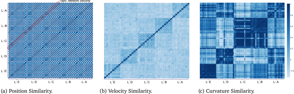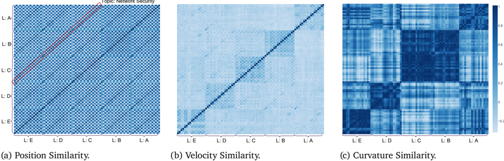Topic: Network Security Figure 2: Similarity of reasoning flows on Qwen3 0.6B. Blocks correspond to logic templates (L:A-E) instantiated with different topics and languages. (a) Position similarity (mean cosine): diagonals correspond to topics (e.g., Network Security), showing that positions are dominated by surface semantics. (b) Velocity similarity (mean cosine): semantic effects diminish, and flows with the same logical skeleton align while differing logics diverge. (c) Curvature similarity (Pearson): separation is further amplified, with logic emerging as the principal invariant and revealing close similarity between logics B and C. See Section 6 for more details. <details> <summary>Image 2 Details</summary>  ### Visual Description ## Heatmaps: Position, Velocity, and Curvature Similarity ### Overview Three heatmaps visualize similarity metrics across five labeled entities (L:A to L:E). Each heatmap uses a blue gradient (0–1) to represent similarity strength, with darker blue indicating higher similarity. The diagonal dominance in all plots suggests self-similarity, while off-diagonal patterns reveal cross-entity relationships. ### Components/Axes - **Axes**: - Vertical and horizontal axes labeled **L:A, L:B, L:C, L:D, L:E** (left to right and top to bottom). - Titles: - (a) **Position Similarity** - (b) **Velocity Similarity** - (c) **Curvature Similarity** - **Legend**: - Right-aligned colorbar with gradient from light blue (0) to dark blue (1). - No explicit legend for the red line in (a). ### Detailed Analysis #### (a) Position Similarity - **Main Diagonal**: Dark blue (near 1.0) across all entities, indicating perfect self-similarity. - **Red Line**: A diagonal band from **L:C** (top-left) to **L:A** (bottom-right), suggesting a threshold or reference path. This line intersects darker blue regions, implying moderate similarity along this trajectory. - **Off-Diagonal**: Gradual darkening from top-left to bottom-right, with **L:C** and **L:A** showing the strongest cross-similarity. #### (b) Velocity Similarity - **Main Diagonal**: Uniform dark blue (1.0), consistent with self-similarity. - **Off-Diagonal**: Lighter blue gradient, with **L:E** and **L:D** showing slightly higher similarity (≈0.6–0.8) compared to other pairs. No distinct patterns beyond diagonal dominance. #### (c) Curvature Similarity - **Main Diagonal**: Dark blue (1.0), as expected. - **Off-Diagonal**: - **L:E** and **L:A** exhibit the lowest similarity (≈0.2–0.4) in the bottom-left and top-right corners. - **L:C** and **L:B** show moderate similarity (≈0.6–0.8) in the central region. - Block-like patterns suggest categorical groupings (e.g., L:C/L:B vs. L:E/L:A). ### Key Observations 1. **Diagonal Dominance**: All heatmaps confirm self-similarity (1.0) along the main diagonal. 2. **Position Similarity (a)**: The red line highlights a specific trajectory with moderate similarity, potentially indicating a predefined path or anomaly. 3. **Curvature Variability (c)**: Greater off-diagonal variation suggests curvature is a more discriminative metric than position or velocity. 4. **Velocity Consistency (b)**: Uniform off-diagonal patterns imply velocity similarity is less variable across entities. ### Interpretation - **Network Security Context**: The labels (L:A–L:E) likely represent network nodes, devices, or traffic patterns. High self-similarity in position/velocity may indicate stable entities, while curvature differences could reflect anomalous behavior (e.g., irregular movement patterns). - **Red Line in (a)**: The highlighted path might represent a critical route or threshold for security monitoring, warranting further investigation. - **Curvature as a Discriminator**: The pronounced variability in curvature similarity suggests it could be a key feature for distinguishing entities in network security applications. ### Spatial Grounding - **Legend**: Right-aligned, adjacent to all heatmaps. - **Red Line (a)**: Starts at **L:C** (top-left) and ends at **L:A** (bottom-right), crossing the central region. - **Color Consistency**: Dark blue consistently represents high similarity (1.0) across all plots. ### Data Extraction - **Position Similarity (a)**: - L:C ↔ L:A: ≈0.7 (dark blue along red line). - L:C ↔ L:E: ≈0.5 (lighter blue). - **Velocity Similarity (b)**: - L:E ↔ L:D: ≈0.7 (moderate similarity). - **Curvature Similarity (c)**: - L:E ↔ L:A: ≈0.3 (low similarity). - L:C ↔ L:B: ≈0.7 (moderate similarity). ### Conclusion The heatmaps reveal that position and velocity similarities are highly consistent across entities, while curvature introduces greater variability. The red line in (a) may indicate a critical path for security analysis, and curvature differences could highlight anomalies in network behavior. </details> ## 6.2. Results Analysis We evaluate four models (Qwen3 0.6B, 1.7B, 4B, and LLaMA3 8B) by extracting hidden states across our dataset (Section 5) and computing similarities under three criteria: (i) Logic , grouping by deduction skeleton and averaging across topics and languages; (ii) Topic ; and (iii) Language , both capturing surface carriers. This yields position, velocity, and curvature similarities (Table 1). Results show that logical similarity is low at zeroth order (position) but becomes dominant at first and second order (velocity and curvature), validating our hypothesis. Topic and language exhibit low velocity similarity, suggesting they might occupy orthogonal subspaces; by contrast, the high logical similarity at first and second order breaks this orthogonality, indicating that logical structure transcends surface carriers. For visualization, we also analyze Qwen3 0.6B on a subset of our dataset (Figure 2). At the position level, embeddings cluster by topic and language. First-order differences reveal logical control: flows sharing the same skeleton align, while differing logics diverge even with identical carriers. Second-order curvature further amplifies this separation, and its strong cross-carrier consistency directly supports Proposition 4.10, confirming that logic governs reasoning velocity. Additional experiments across broader model families are presented in Appendix A. Together, these results show that LLMs internalize latent logical structure beyond surface form. They are not mere stochastic parrots [2]: whereas humans formalized logic only in the 20th century [4], LLMs acquire it emergently from large-scale data-a hallmark of genuine intelligence. ## 7. Discussion Contrast with Graph Perspective. Prior works have modeled chain-of-thought reasoning as a graph structure [45, 67]. While this provides a useful perspective, its predictive power is limited: graphs naturally suggest random walks between discrete nodes, which fits the noisy behavior of isolated embeddings but fails to capture the smooth, directed dynamics we observe under cumulative context. Our results in Section 6 show that well-trained LLMs learn flows governed by logical structure, transcending the surface semantics of language. Such continuity and logic-driven trajectories cannot be explained within a purely graph-based framework, but arise naturally in our differential-geometric view. Other Components in Learned Representation. Beyond logical structure, learned representations also encode a wide spectrum of factors such as semantic objects, discourse tone, natural language identity, and even signals of higher-level cognitive behavior. Extending our framework to systematically isolate these components and characterize their interactions presents a major challenge for future work. A promising direction is to develop methods that disentangle additional attributes, enabling finer-grained insights into how language components co-evolve in representation space. Practical Implications. Our results suggest that reasoning in LLMs unfolds as continuous flows, opening multiple directions. First, trajectory-level control offers principled tools for steering, alignment, and safety , extending vectorbased interventions to flow dynamics [66, 7, 18, 27, 3]. Second, our geometric view provides a formal framework to study abstract language concepts, enabling first-principle analyses of reasoning efficiency, stability, and failure modes. Third, it motivates new approaches to retrieval and representation , where embeddings respect reasoning flows rather than mere similarity, potentially improving RAG, reranking, and search [71]. Finally, it hints at architectural advances , as models parameterizing latent flows may enable more efficient reasoning [23, 17, 80, 60]. ## 8. Conclusion We introduced a novel geometric framework that models LLM reasoning as smooth flows in representation space, with logic acting as a controller of local velocities. By disentangling logical structure from semantic carriers through a controlled dataset, we showed that velocity and curvature invariants reveal logic as the principal organizing factor of reasoning trajectories, beyond surface form. Our theory and experiments provide both a conceptual foundation and practical tools for analyzing reasoning, opening new avenues for interpretability. ## Acknowledgment ARZ was partially supported by NSF Grant CAREER-2203741. ## References - [1] Anthropic. Transformer circuits. https://transformer-circuits.pub/ , 2021. - [2] Emily M Bender, Timnit Gebru, Angelina McMillan-Major, and Shmargaret Shmitchell. On the dangers of stochastic parrots: Can language models be too big? In Proceedings of the 2021 ACM conference on fairness, accountability, and transparency , pages 610-623, 2021. - [3] Leonard F. Bereska and Efstratios Gavves. Mechanistic interpretability for ai safety - a review. TMLR , April 2024. - [4] Joseph M Bochenski and Ivo Thomas. A history of formal logic. 1961. - [5] Paul C Bogdan, Uzay Macar, Neel Nanda, and Arthur Conmy. Thought anchors: Which llm reasoning steps matter? arXiv preprint arXiv:2506.19143 , 2025. - [6] Qiguang Chen, Libo Qin, Jiaqi Wang, Jingxuan Zhou, and Wanxiang Che. Unlocking the capabilities of thought: A reasoning boundary framework to quantify and optimize chain-of-thought. Advances in Neural Information Processing Systems , 37:54872-54904, 2024. - [7] Runjin Chen, Zhenyu Zhang, Junyuan Hong, Souvik Kundu, and Zhangyang Wang. Seal: Steerable reasoning calibration of large language models for free. arXiv preprint arXiv:2504.07986 , 2025. - [8] Irving M Copi, Carl Cohen, and Kenneth McMahon. Introduction to logic . Routledge, 2016. - [9] Manfredo P Do Carmo. Differential geometry of curves and surfaces: revised and updated second edition . Courier Dover Publications, 2016. - [10] Diego Doimo, Alessandro Serra, Alessio Ansuini, and Alberto Cazzaniga. The representation landscape of few-shot learning and fine-tuning in large language models. Advances in Neural Information Processing Systems , 37:18122-18165, 2024. - [11] Herbert B Enderton. A mathematical introduction to logic . Elsevier, 2001. - [12] Joshua Engels, Eric J Michaud, Isaac Liao, Wes Gurnee, and Max Tegmark. Not all language model features are one-dimensionally linear. In The Thirteenth International Conference on Learning Representations , 2025. URL https://openreview.net/forum?id=d63a4AM4hb . - [13] Javier Ferrando, Gabriele Sarti, Arianna Bisazza, and Marta R Costa-Jussà. A primer on the inner workings of transformer-based language models. arXiv preprint arXiv:2405.00208 , 2024. - [14] Yichao Fu, Junda Chen, Siqi Zhu, Zheyu Fu, Zhongdongming Dai, Yonghao Zhuang, Yian Ma, Aurick Qiao, Tajana Rosing, Ion Stoica, et al. Efficiently scaling llm reasoning with certaindex. arXiv preprint arXiv:2412.20993 , 2024. - [15] Peter Gardenfors. Conceptual spaces: The geometry of thought . MIT press, 2004. - [16] Peter Gardenfors. The geometry of meaning: Semantics based on conceptual spaces . MIT press, 2014. - [17] Jonas Geiping, Sean McLeish, Neel Jain, John Kirchenbauer, Siddharth Singh, Brian R Bartoldson, Bhavya Kailkhura, Abhinav Bhatele, and Tom Goldstein. Scaling up test-time compute with latent reasoning: A recurrent depth approach. arXiv preprint arXiv:2502.05171 , 2025. - [18] Bofan Gong, Shiyang Lai, and Dawn Song. Probing the vulnerability of large language models to polysemantic interventions. arXiv preprint arXiv:2505.11611 , 2025. - [19] Aaron Grattafiori, Abhimanyu Dubey, Abhinav Jauhri, Abhinav Pandey, Abhishek Kadian, Ahmad Al-Dahle, Aiesha Letman, Akhil Mathur, Alan Schelten, Alex Vaughan, et al. The llama 3 herd of models. arXiv e-prints , pages arXiv-2407, 2024. - [20] Heinrich W Guggenheimer. Differential geometry . Courier Corporation, 2012. - [21] Daya Guo, Dejian Yang, Haowei Zhang, Junxiao Song, Ruoyu Zhang, Runxin Xu, Qihao Zhu, Shirong Ma, Peiyi Wang, Xiao Bi, et al. Deepseek-r1: Incentivizing reasoning capability in llms via reinforcement learning. arXiv preprint arXiv:2501.12948 , 2025. - [22] Wes Gurnee and Max Tegmark. Language models represent space and time. In The Twelfth International Conference on Learning Representations , 2024. URL https://openreview.net/forum?id=jE8xbmvFin . - [23] Shibo Hao, Sainbayar Sukhbaatar, DiJia Su, Xian Li, Zhiting Hu, Jason Weston, and Yuandong Tian. Training large language models to reason in a continuous latent space. arXiv preprint arXiv:2412.06769 , 2024. - [24] Hesam Sheikh Hessani. Llm embeddings explained: A visual and intuitive guide, 2025. - [25] Noel J Hicks. Notes on differential geometry , volume 1. van Nostrand Princeton, 1965. - [26] Michael Y Hu, Jackson Petty, Chuan Shi, William Merrill, and Tal Linzen. Between circuits and chomsky: Pre-pretraining on formal languages imparts linguistic biases. arXiv preprint arXiv:2502.19249 , 2025. - [27] Yao Huang, Huanran Chen, Shouwei Ruan, Yichi Zhang, Xingxing Wei, and Yinpeng Dong. Mitigating overthinking in large reasoning models via manifold steering. arXiv preprint arXiv:2505.22411 , 2025. - [28] Aaron Hurst, Adam Lerer, Adam P Goucher, Adam Perelman, Aditya Ramesh, Aidan Clark, AJ Ostrow, Akila Welihinda, Alan Hayes, Alec Radford, et al. Gpt-4o system card. arXiv preprint arXiv:2410.21276 , 2024. - [29] William James, Frederick Burkhardt, Fredson Bowers, and Kestutis Skrupskelis. The principles of psychology , volume 1. Macmillan London, 1890. - [30] Jin Jiang, Jianing Wang, Yuchen Yan, Yang Liu, Jianhua Zhu, Mengdi Zhang, Xunliang Cai, and Liangcai Gao. Do large language models excel in complex logical reasoning with formal language? arXiv preprint arXiv:2505.16998 , 2025. - [31] Yibo Jiang, Bryon Aragam, and Victor Veitch. Uncovering meanings of embeddings via partial orthogonality. Advances in Neural Information Processing Systems , 36:31988-32005, 2023. - [32] Yibo Jiang, Goutham Rajendran, Pradeep Kumar Ravikumar, Bryon Aragam, and Victor Veitch. On the origins of linear representations in large language models. In Forty-first International Conference on Machine Learning , 2024. URL https://openreview.net/forum?id=otuTw4Mghk . - [33] Subhash Kantamneni and Max Tegmark. Language models use trigonometry to do addition. arXiv preprint arXiv:2502.00873 , 2025. - [34] Austin C Kozlowski, Callin Dai, and Andrei Boutyline. Semantic structure in large language model embeddings. arXiv preprint arXiv:2508.10003 , 2025. - [35] Jinhyuk Lee, Feiyang Chen, Sahil Dua, Daniel Cer, Madhuri Shanbhogue, Iftekhar Naim, Gustavo Hernández Ábrego, Zhe Li, Kaifeng Chen, Henrique Schechter Vera, et al. Gemini embedding: Generalizable embeddings from gemini. arXiv preprint arXiv:2503.07891 , 2025. - [36] Yuxiao Li, Eric J Michaud, David D Baek, Joshua Engels, Xiaoqing Sun, and Max Tegmark. The geometry of concepts: Sparse autoencoder feature structure. Entropy , 27(4):344, 2025. - [37] Zhiyuan Li, Hong Liu, Denny Zhou, and Tengyu Ma. Chain of thought empowers transformers to solve inherently serial problems. In The Twelfth International Conference on Learning Representations , 2024. URL https://openreview.net/forum?id=3EWTEy9MTM . - [38] Hanmeng Liu, Zhizhang Fu, Mengru Ding, Ruoxi Ning, Chaoli Zhang, Xiaozhang Liu, and Yue Zhang. Logical reasoning in large language models: A survey. arXiv preprint arXiv:2502.09100 , 2025. - [39] Ziming Liu, Ouail Kitouni, Niklas S Nolte, Eric Michaud, Max Tegmark, and Mike Williams. Towards understanding grokking: An effective theory of representation learning. Advances in Neural Information Processing Systems , 35:34651-34663, 2022. - [40] Andreas Madsen, Himabindu Lakkaraju, Siva Reddy, and Sarath Chandar. Interpretability needs a new paradigm. arXiv preprint arXiv:2405.05386 , 2024. - [41] Samuel Marks and Max Tegmark. The geometry of truth: Emergent linear structure in large language model representations of true/false datasets. In First Conference on Language Modeling , 2024. URL https: //openreview.net/forum?id=aajyHYjjsk . - [42] Karl Menger. Untersuchungen über allgemeine metrik. Mathematische Annalen , 100(1):75-163, 1928. - [43] William Merrill and Ashish Sabharwal. A logic for expressing log-precision transformers. Advances in neural information processing systems , 36:52453-52463, 2023. - [44] Tomas Mikolov, Kai Chen, Greg Corrado, and Jeffrey Dean. Efficient estimation of word representations in vector space. In ICLR , 2013. - [45] Gouki Minegishi, Hiroki Furuta, Takeshi Kojima, Yusuke Iwasawa, and Yutaka Matsuo. Topology of reasoning: Understanding large reasoning models through reasoning graph properties. arXiv preprint arXiv:2506.05744 , 2025. - [46] Alexander Modell, Patrick Rubin-Delanchy, and Nick Whiteley. The origins of representation manifolds in large language models. arXiv preprint arXiv:2505.18235 , 2025. - [47] Terufumi Morishita, Gaku Morio, Atsuki Yamaguchi, and Yasuhiro Sogawa. Enhancing reasoning capabilities of llms via principled synthetic logic corpus. Advances in Neural Information Processing Systems , 37:73572-73604, 2024. - [48] Neel Nanda, Lawrence Chan, Tom Lieberum, Jess Smith, and Jacob Steinhardt. Progress measures for grokking via mechanistic interpretability. In The Eleventh International Conference on Learning Representations , 2023. URL https://openreview.net/forum?id=9XFSbDPmdW . - [49] Arvind Neelakantan, Tao Xu, Raul Puri, Alec Radford, Jesse Michael Han, Jerry Tworek, Qiming Yuan, Nikolas Tezak, Jong Wook Kim, Chris Hallacy, et al. Text and code embeddings by contrastive pre-training. arXiv preprint arXiv:2201.10005 , 2022. - [50] Zhijie Nie, Zhangchi Feng, Mingxin Li, Cunwang Zhang, Yanzhao Zhang, Dingkun Long, and Richong Zhang. When text embedding meets large language model: a comprehensive survey. arXiv preprint arXiv:2412.09165 , 2024. - [51] OpenAI. Introducing chatgpt. https://openai.com/index/chatgpt/ , 2022. - [52] OpenAI. Gpt-5 system card. Technical report, OpenAI, August 2025. - [53] Core Francisco Park, Maya Okawa, Andrew Lee, Ekdeep S Lubana, and Hidenori Tanaka. Emergence of hidden capabilities: Exploring learning dynamics in concept space. Advances in Neural Information Processing Systems , 37:84698-84729, 2024. - [54] Kiho Park, Yo Joong Choe, and Victor Veitch. The linear representation hypothesis and the geometry of large language models. In Forty-first International Conference on Machine Learning , 2024. URL https: //openreview.net/forum?id=UGpGkLzwpP . - [55] Kiho Park, Yo Joong Choe, Yibo Jiang, and Victor Veitch. The geometry of categorical and hierarchical concepts in large language models. In The Thirteenth International Conference on Learning Representations , 2025. URL https://openreview.net/forum?id=bVTM2QKYuA . - [56] Mihir Parmar, Nisarg Patel, Neeraj Varshney, Mutsumi Nakamura, Man Luo, Santosh Mashetty, Arindam Mitra, and Chitta Baral. Logicbench: Towards systematic evaluation of logical reasoning ability of large language models. In 62nd Annual Meeting of the Association for Computational Linguistics, ACL 2024 , pages 13679-13707. Association for Computational Linguistics (ACL), 2024. - [57] Francis Jeffry Pelletier and Allen Hazen. Natural Deduction Systems in Logic. In Edward N. Zalta and Uri Nodelman, editors, The Stanford Encyclopedia of Philosophy . Metaphysics Research Lab, Stanford University, Spring 2024 edition, 2024. - [58] Daking Rai, Yilun Zhou, Shi Feng, Abulhair Saparov, and Ziyu Yao. A practical review of mechanistic interpretability for transformer-based language models. arXiv preprint arXiv:2407.02646 , 2024. - [59] John T Rickard. A concept geometry for conceptual spaces. Fuzzy optimization and decision making , 5: 311-329, 2006. - [60] Xuan Shen, Yizhou Wang, Xiangxi Shi, Yanzhi Wang, Pu Zhao, and Jiuxiang Gu. Efficient reasoning with hidden thinking. arXiv preprint arXiv:2501.19201 , 2025. - [61] Chandan Singh, Jeevana Priya Inala, Michel Galley, Rich Caruana, and Jianfeng Gao. Rethinking interpretability in the era of large language models. arXiv preprint arXiv:2402.01761 , 2024. - [62] Charlie Victor Snell, Jaehoon Lee, Kelvin Xu, and Aviral Kumar. Scaling LLM test-time compute optimally can be more effective than scaling parameters for reasoning. In The Thirteenth International Conference on Learning Representations , 2025. URL https://openreview.net/forum?id=4FWAwZtd2n . - [63] Adam Stein, Aaditya Naik, Yinjun Wu, Mayur Naik, and Eric Wong. Towards compositionality in concept learning. In Forty-first International Conference on Machine Learning , 2024. URL https://openreview. net/forum?id=upO8FUwf92 . - [64] A. S. Troelstra and Helmut Schwichtenberg. Basic Proof Theory . Cambridge University Press, 2nd edition, 2000. - [65] Lucrezia Valeriani, Diego Doimo, Francesca Cuturello, Alessandro Laio, Alessio Ansuini, and Alberto Cazzaniga. The geometry of hidden representations of large transformer models. Advances in Neural Information Processing Systems , 36:51234-51252, 2023. - [66] Constantin Venhoff, Iván Arcuschin, Philip Torr, Arthur Conmy, and Neel Nanda. Understanding reasoning in thinking language models via steering vectors. In Workshop on Reasoning and Planning for Large Language Models , 2025. URL https://openreview.net/forum?id=OwhVWNOBcz . - [67] Xinyi Wang, Alfonso Amayuelas, Kexun Zhang, Liangming Pan, Wenhu Chen, and William Yang Wang. Understanding reasoning ability of language models from the perspective of reasoning paths aggregation. In International Conference on Machine Learning , pages 50026-50042. PMLR, 2024. - [68] Yiming Wang, Pei Zhang, Baosong Yang, Derek Wong, Zhuosheng Zhang, and Rui Wang. Embedding trajectory for out-of-distribution detection in mathematical reasoning. Advances in Neural Information Processing Systems , 37:42965-42999, 2024. - [69] Yiming Wang, Pei Zhang, Baosong Yang, Derek F. Wong, and Rui Wang. Latent space chain-of-embedding enables output-free LLM self-evaluation. In The Thirteenth International Conference on Learning Representations , 2025. URL https://openreview.net/forum?id=jxo70B9fQo . - [70] Zihao Wang, Lin Gui, Jeffrey Negrea, and Victor Veitch. Concept algebra for (score-based) text-controlled generative models. Advances in Neural Information Processing Systems , 36:35331-35349, 2023. - [71] Orion Weller, Michael Boratko, Iftekhar Naim, and Jinhyuk Lee. On the theoretical limitations of embeddingbased retrieval. arXiv preprint arXiv:2508.21038 , 2025. - [72] Ludwig Wittgenstein. Tractatus Logico-Philosophicus . Kegan Paul, Trench, Trubner & Co., Ltd., London, 1922. - [73] Yuyang Wu, Yifei Wang, Ziyu Ye, Tianqi Du, Stefanie Jegelka, and Yisen Wang. When more is less: Understanding chain-of-thought length in llms. arXiv preprint arXiv:2502.07266 , 2025. - [74] Yuan Xia, Akanksha Atrey, Fadoua Khmaissia, and Kedar S Namjoshi. Can large language models learn formal logic? a data-driven training and evaluation framework. arXiv preprint arXiv:2504.20213 , 2025. - [75] An Yang, Anfeng Li, Baosong Yang, Beichen Zhang, Binyuan Hui, Bo Zheng, Bowen Yu, Chang Gao, Chengen Huang, Chenxu Lv, et al. Qwen3 technical report. arXiv preprint arXiv:2505.09388 , 2025. - [76] Andy Yang and David Chiang. Counting like transformers: Compiling temporal counting logic into softmax transformers. In First Conference on Language Modeling , 2024. URL https://openreview.net/forum? id=FmhPg4UJ9K . - [77] Junjie Yao, Zhongwang Zhang, and Zhi-Qin John Xu. An analysis for reasoning bias of language models with small initialization. In Forty-second International Conference on Machine Learning , 2025. URL https: //openreview.net/forum?id=4HQaMUYWAT . - [78] Tian Ye, Zicheng Xu, Yuanzhi Li, and Zeyuan Allen-Zhu. Physics of language models: Part 2.1, grade-school math and the hidden reasoning process. In The Thirteenth International Conference on Learning Representations , 2025. - [79] Yanzhao Zhang, Mingxin Li, Dingkun Long, Xin Zhang, Huan Lin, Baosong Yang, Pengjun Xie, An Yang, Dayiheng Liu, Junyang Lin, et al. Qwen3 embedding: Advancing text embedding and reranking through foundation models. arXiv preprint arXiv:2506.05176 , 2025. - [80] Zhen Zhang, Xuehai He, Weixiang Yan, Ao Shen, Chenyang Zhao, Shuohang Wang, Yelong Shen, and Xin Eric Wang. Soft thinking: Unlocking the reasoning potential of llms in continuous concept space. arXiv preprint arXiv:2505.15778 , 2025. - [81] Ziqian Zhong, Ziming Liu, Max Tegmark, and Jacob Andreas. The clock and the pizza: Two stories in mechanistic explanation of neural networks. Advances in neural information processing systems , 36:2722327250, 2023. - [82] Hanlin Zhu, Shibo Hao, Zhiting Hu, Jiantao Jiao, Stuart Russell, and Yuandong Tian. Reasoning by superposition: A theoretical perspective on chain of continuous thought. arXiv preprint arXiv:2505.12514 , 2025. ## Contents | 1 Introduction | 1 Introduction | 1 Introduction | 1 | |-------------------|------------------------------------------------------|------------------------------------------------------|-----| | 2 | Related Work | Related Work | 3 | | 3 | Preliminaries | Preliminaries | 4 | | | 3.1 | Large Language Models . . . . . . . . . | 4 | | | 3.2 | Menger Curvature . . . . . . . . . . . . | 4 | | 4 | Reasoning as Geometric Flows in Representation Space | Reasoning as Geometric Flows in Representation Space | 4 | | | 4.1 | Concept Space and Semantic Trajectories | 5 | | | 4.2 | Representation Space . . . . . . . . . . . | 5 | | | 4.3 | Logic as Differential Constraints on Flow | 7 | | 5 | Formal Logic with Semantic Carriers | Formal Logic with Semantic Carriers | 7 | | | 5.1 | Logic and Natural Deduction System . . | 7 | | | 5.2 | Data Design . . . . . . . . . . . . . . . . | 8 | | 6 | Play with LLMs | Play with LLMs | 8 | | | 6.1 | Experimental Setup . . . . . . . . . . . . | 8 | | | 6.2 | Results Analysis . . . . . . . . . . . . . . | 9 | | 7 | Discussion | Discussion | 9 | | 8 | Conclusion | Conclusion | 10 | | A | Additional Experiments | Additional Experiments | 18 | | B | Symbolic Glossary and Mapping Relations | Symbolic Glossary and Mapping Relations | 18 | | | B.1 | Spaces . . . . . . . . . . . . . . . . . . . | 18 | | | B.2 | Primary maps . . . . . . . . . . . . . . . | 19 | | | B.3 | Reasoning increments and curvature . . | 20 | | | B.4 | Roadmap diagram . . . . . . . . . . . . | 20 | | C | Geometric Foundations of Reasoning Trajectories | Geometric Foundations of Reasoning Trajectories | 20 | | | C.1 | Continuity of Representation Trajectories | 21 | | | C.2 | Menger Curvature . . . . . . . . . . . . | 23 | | D Data Generation | D Data Generation | D Data Generation | 26 | D.1 Prompts for Data Generation . . . . . . . . . . . . . . . . . . . . . . . . . . . . . . . . . . . . . . . | D.2 Data Examples . . . . . . . . . . . . . . . . . . . . . . . . . . . . . . . . . | 27 | |---------------------------------------------------------------------------------------|------| ## A. 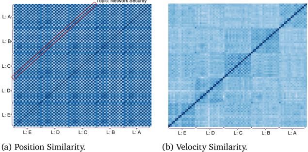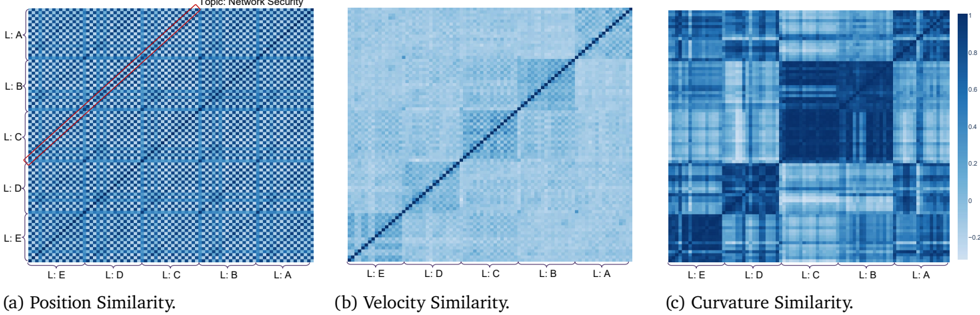Additional Experiments We additionally evaluate LLaMA3 [19] and more Qwen3 [75] models (1.7B, 4B) to test robustness under the same experimental settings as in Section 6. The results (Figures 3, 4 and 5) confirm that our findings generalize across model sizes and families. Topic: Network Security Figure 3: Similarity of reasoning flows on Qwen3 1.7B. <details> <summary>Image 3 Details</summary>  ### Visual Description ## Heatmap: Position and Velocity Similarity Analysis ### Overview The image contains two side-by-side heatmaps labeled **(a) Position Similarity** and **(b) Velocity Similarity**. Both heatmaps use a grid of labels (L:A to L:E) on both axes, with varying shades of blue to represent similarity scores. A diagonal line is overlaid on each heatmap, and a legend in (a) specifies the topic as "Network Security." --- ### Components/Axes - **Vertical Axis (Y-axis)**: Labeled from **L:A** (top) to **L:E** (bottom). - **Horizontal Axis (X-axis)**: Labeled from **L:E** (left) to **L:A** (right). - **Legend**: Located in the **top-right corner** of heatmap (a), with text: - **"Topic: Network Security"** (in English). - **Diagonal Lines**: - **(a)**: A **red dashed line** spans from **L:D (bottom-left)** to **L:B (top-right)**. - **(b)**: A **black solid line** spans the full diagonal from **L:E (bottom-left)** to **L:A (top-right)**. --- ### Detailed Analysis #### (a) Position Similarity - **Heatmap Pattern**: - Darker blue squares cluster along the **red dashed line**, indicating higher similarity between labels along this path. - Lighter blue squares dominate outside this line, suggesting lower similarity. - **Key Data Points**: - **L:D ↔ L:B**: Strongest similarity (darkest blue). - **L:C ↔ L:C**: Perfect self-similarity (darkest blue on the diagonal). - **L:A ↔ L:A**: Perfect self-similarity (darkest blue on the diagonal). - **Trend**: The red line highlights a **cluster of high similarity** between L:D, L:C, and L:B, with diminishing similarity as distance from the line increases. #### (b) Velocity Similarity - **Heatmap Pattern**: - Uniformly lighter blue compared to (a), with no distinct clustering. - The **black diagonal line** suggests a baseline of self-similarity (e.g., L:A ↔ L:A, L:B ↔ L:B). - **Key Data Points**: - **L:A ↔ L:A**: Perfect self-similarity (darkest blue on the diagonal). - **L:E ↔ L:E**: Perfect self-similarity (darkest blue on the diagonal). - Off-diagonal values are uniformly lighter, indicating low cross-label similarity. - **Trend**: No significant clusters; similarity decreases monotonically with distance from the diagonal. --- ### Key Observations 1. **Self-Similarity Dominance**: Both heatmaps show perfect similarity along the diagonal (e.g., L:A ↔ L:A), as expected. 2. **Position Similarity Cluster**: The red line in (a) identifies a **group of labels (L:D, L:C, L:B)** with unusually high mutual similarity, suggesting a shared positional characteristic. 3. **Velocity Similarity Uniformity**: The lack of clustering in (b) implies velocity is less correlated between labels compared to position. 4. **Legend Context**: The "Network Security" topic in (a) may indicate that the red line corresponds to a security-related positional pattern. --- ### Interpretation - **Position Similarity (a)**: The red line likely represents a **critical pathway** in network security, where labels L:D, L:C, and L:B share positional traits (e.g., proximity in a network topology). This could imply these labels are part of a security-critical subsystem. - **Velocity Similarity (b)**: The uniform similarity suggests velocity is an **independent variable** across labels, with no strong interdependencies. - **Anomaly**: The red line in (a) deviates from the main diagonal, indicating a **non-trivial relationship** between L:D, L:C, and L:B that warrants further investigation in the context of network security. --- ### Spatial Grounding & Validation - **Legend Placement**: Top-right corner of (a), ensuring clarity without obscuring data. - **Color Consistency**: - Red line in (a) matches the "Network Security" legend. - Black line in (b) has no legend entry, implying it represents a baseline or default value. - **Axis Labels**: L:A to L:E are consistently ordered, with no ambiguity in spatial mapping. --- ### Conclusion The heatmaps reveal that **position similarity** drives clustering in network security contexts, while **velocity similarity** remains uncorrelated. The red line in (a) highlights a critical positional relationship, suggesting L:D, L:C, and L:B are interconnected in security-critical operations. Further analysis of these labels could uncover vulnerabilities or optimization opportunities. </details> Topic: Network Security Figure 4: Similarity of reasoning flows on Qwen3 4B. <details> <summary>Image 4 Details</summary>  ### Visual Description ## Heatmap Visualization: Network Security Similarity Analysis ### Overview The image presents three comparative heatmaps analyzing similarity metrics across labeled entities (L:A to L:E). Each heatmap uses a blue gradient scale (0-1) to represent similarity strength, with darker blue indicating higher similarity. The visualizations focus on positional, velocity, and curvature similarity patterns within a network security context. ### Components/Axes - **X/Y Axes**: Labeled L:A (top-left) to L:E (bottom-right) on both axes - **Color Scale**: - Blue gradient from light (0) to dark (1) - Dark blue = 1.0 (maximum similarity) - Light blue = 0.0 (no similarity) - **Key Elements**: - Red diagonal line in Position Similarity heatmap - Black diagonal line in Velocity Similarity heatmap - Curvature Similarity heatmap shows block patterns ### Detailed Analysis #### Position Similarity (a) - **Pattern**: Red diagonal line from L:E (bottom-left) to L:A (top-right) - **Key Values**: - L:A-L:A: 1.0 (darkest blue) - L:E-L:E: 1.0 - L:A-L:E: 0.3 (light blue) - L:E-L:A: 0.3 - **Notable**: Symmetric pattern with strongest similarity along diagonal #### Velocity Similarity (b) - **Pattern**: Black diagonal line from L:E to L:A - **Key Values**: - L:A-L:A: 1.0 - L:E-L:E: 1.0 - L:A-L:E: 0.4 - L:E-L:A: 0.4 - **Notable**: Perfect diagonal alignment suggests direct correlation #### Curvature Similarity (c) - **Pattern**: Block-like structure with varying intensity - **Key Values**: - L:C-L:C: 0.9 (darkest block) - L:B-L:B: 0.8 - L:A-L:A: 0.7 - L:E-L:E: 0.6 - **Notable**: Clustered similarity in middle labels (L:C, L:B) ### Key Observations 1. **Diagonal Dominance**: Position and velocity similarity show strong diagonal patterns (L:A-L:A to L:E-L:E) 2. **Curvature Clusters**: Middle labels (L:C, L:B) show higher curvature similarity 3. **Asymmetry**: Position similarity shows slight asymmetry between L:A-L:E and L:E-L:A 4. **Color Consistency**: All heatmaps use identical blue gradient scale (0-1) ### Interpretation The visualizations suggest: - **Positional Relationships**: Entities L:A and L:E maintain consistent similarity across metrics - **Velocity Correlation**: Perfect diagonal in velocity heatmap indicates direct proportional relationships - **Curvature Patterns**: Middle labels (L:C, L:B) form a similarity cluster, suggesting shared characteristics - **Network Security Implications**: The red line in position similarity might represent a critical path or priority connection in network topology The data demonstrates that while positional and velocity similarities follow predictable patterns, curvature similarity reveals more complex relationships between network entities. The consistent diagonal patterns across metrics suggest fundamental structural similarities in the network security framework being analyzed. </details> ## B. Symbolic Glossary and Mapping Relations This section is a standalone roadmap that summarizes the spaces, maps, and commutative structure underlying our geometric view of reasoning. ## B.1. Spaces - Input space 𝒳 (often specialized to a vocabulary 𝒱 ): discrete tokens/sentences. ## Appendix 0.8 0.6 0.4 0.2 (c) Curvature Similarity. <details> <summary>Image 5 Details</summary>  ### Visual Description ## Heatmap: Correlation Matrix of Variables L:A to L:E ### Overview The image is a square heatmap visualizing relationships between five variables labeled L:A, L:B, L:C, L:D, and L:E. The matrix is symmetric, with darker blue shades indicating stronger relationships (higher values) and lighter blue shades indicating weaker relationships (lower values). A color bar on the right quantifies the scale from -0.2 (lightest blue) to 1.0 (darkest blue). ### Components/Axes - **X-axis**: Categories labeled L:A (rightmost) to L:E (leftmost), increasing from right to left. - **Y-axis**: Same categories as X-axis, labeled from top (L:E) to bottom (L:A). - **Color Bar**: Vertical gradient from light blue (-0.2) to dark blue (1.0), positioned to the right of the heatmap. - **Legend**: Matches the color bar, with no additional labels beyond the scale. ### Detailed Analysis - **Diagonal Elements**: - All diagonal cells (e.g., L:E-L:E, L:D-L:D) are dark blue, indicating values close to 1.0. This suggests perfect self-correlation for each variable. - **Off-Diagonal Elements**: - **L:E-L:D**: Medium-dark blue (~0.7). - **L:E-L:C**: Light blue (~0.3). - **L:E-L:B**: Medium blue (~0.5). - **L:E-L:A**: Light blue (~0.2). - **L:D-L:C**: Medium blue (~0.6). - **L:D-L:B**: Light blue (~0.4). - **L:D-L:A**: Medium-dark blue (~0.7). - **L:C-L:B**: Light blue (~0.3). - **L:C-L:A**: Medium blue (~0.5). - **L:B-L:A**: Medium-dark blue (~0.7). - **Symmetry**: The matrix is symmetric (e.g., L:E-L:D ≈ L:D-L:E), confirming bidirectional relationships. ### Key Observations 1. **Strongest Relationships**: - L:D-L:A (~0.7) and L:B-L:A (~0.7) show the strongest off-diagonal correlations. 2. **Weakest Relationships**: - L:E-L:A (~0.2) and L:E-L:C (~0.3) are the weakest. 3. **Pattern**: Relationships generally weaken as the distance between categories increases (e.g., L:E-L:A is weaker than L:E-L:B). ### Interpretation This heatmap likely represents a **correlation matrix** where: - Each variable is perfectly correlated with itself (diagonal = 1.0). - Variables L:A and L:D/B share the strongest relationships (~0.7), suggesting they may be closely related or influenced by common factors. - Variables L:E and L:A/C exhibit the weakest relationships, indicating minimal direct association. - The symmetry confirms that correlations are bidirectional (e.g., L:A’s relationship with L:B is identical to L:B’s relationship with L:A). The data implies a hierarchical or clustered structure among the variables, with L:A acting as a central node in the network of relationships. This could reflect dependencies in a system (e.g., economic indicators, biological traits) where certain variables are more interconnected than others. </details> <!-- formula-not-decoded --> <!-- formula-not-decoded --> realized by token embeddings ℰ and a contextual encoder Φ , producing the continuous trajectory ̃︀ Ψ and sampled states 𝑌 = ( 𝑦 1 , . . . , 𝑦 𝑇 ) . Figure 5: Similarity of reasoning flows on Llama3 8B. <details> <summary>Image 6 Details</summary>  ### Visual Description ## Heatmap Visualization: Position, Velocity, and Curvature Similarity Analysis ### Overview The image presents three heatmaps comparing similarity metrics across five labeled locations (L:A to L:E). Each heatmap uses a blue gradient scale (0 to 1) to represent similarity strength, with darker blue indicating higher similarity. The heatmaps are titled "Position Similarity," "Velocity Similarity," and "Curvature Similarity," with distinct visual patterns in each. --- ### Components/Axes - **X/Y Axes**: Labeled L:A (top-left) to L:E (bottom-right) for all heatmaps. - **Color Scale**: Right-aligned legend with values from 0 (light blue) to 1 (dark blue). - **Annotations**: - **Position Similarity (a)**: Red line connecting L:C → L:B → L:A. - **Velocity Similarity (b)**: Diagonal line from L:E → L:A. - **Curvature Similarity (c)**: Checkerboard pattern with alternating dark/light blue blocks. --- ### Detailed Analysis #### (a) Position Similarity - **Pattern**: Red line diagonally spans from L:C (bottom-left) to L:A (top-right), suggesting a dominant similarity trend along this path. - **Values**: - L:C ↔ L:A: ~0.9 (dark blue) - L:B ↔ L:A: ~0.8 (medium blue) - Other off-diagonal values: ~0.3–0.6 (lighter blue). #### (b) Velocity Similarity - **Pattern**: Diagonal line from L:E (bottom-left) to L:A (top-right), indicating self-similarity (e.g., L:A ↔ L:A = 1.0). - **Values**: - Diagonal: All ~1.0 (dark blue). - Off-diagonal: Gradual decrease from ~0.7 (L:E ↔ L:D) to ~0.2 (L:A ↔ L:E). #### (c) Curvature Similarity - **Pattern**: Checkerboard alternates between dark blue (high similarity) and light blue (low similarity). - **Values**: - High similarity clusters: L:C ↔ L:B (~0.8), L:D ↔ L:C (~0.7). - Low similarity: L:A ↔ L:E (~0.1), L:B ↔ L:E (~0.2). --- ### Key Observations 1. **Position Similarity** emphasizes a strong connection between L:C, L:B, and L:A, with diminishing similarity toward L:D and L:E. 2. **Velocity Similarity** shows perfect self-similarity (diagonal) and weaker pairwise similarities, suggesting location-specific velocity profiles. 3. **Curvature Similarity** reveals alternating high/low similarity between adjacent locations, possibly indicating periodic or opposing curvature patterns. --- ### Interpretation - **Position Similarity** (a) likely highlights a critical pathway or alignment between L:C, L:B, and L:A, possibly related to network topology or spatial constraints. - **Velocity Similarity** (b) suggests that velocity metrics are location-dependent, with minimal cross-location correlation. - **Curvature Similarity** (c) implies alternating curvature characteristics between locations, which could reflect structural or dynamic differences in the network. The heatmaps collectively indicate that positional alignment drives similarity in position metrics, while velocity and curvature exhibit distinct, location-specific patterns. The red line in (a) may represent a prioritized route or boundary in network security analysis. </details> - Concept space 𝒞 : abstract semantic space. A sentence 𝑋 is represented by a smooth semantic trajectory <!-- formula-not-decoded --> where ℳ is a semantic submanifold for a coherent domain of meaning. - Representation space ℛ⊂ R 𝑑 : the model's embedding space. Each prefix 𝑋 𝑡 yields <!-- formula-not-decoded --> sampling a continuous representation trajectory ̃︀ Ψ : [0 , 1] → R 𝑑 . - Representation-based logical space ℒ rep : the space of reasoning increments in the embedding space , defined by local variations of the trajectory , ∆ 𝑦 𝑡 := 𝑦 𝑡 +1 -𝑦 𝑡 . Geometric descriptors such as the Menger curvature 𝜅 𝑡 are evaluated here. This space is non-symbolic, and serves as the model's internal analogue of logic. - Formal logical space ℒ form : symbolic/human logic governed by a natural deduction system ND = ( ℱ , ℛ ) , with formulas ℱ and rules ℛ . Judgements Γ ⊢ 𝜙 and rule-based derivations live here. ## B.2. Primary maps - Semantic interpretation : - Neural representation : - Canonical Alignment. Definition B.1 (Canonical alignment map) . Assume 𝑆 and Ψ are injective on the domain of interest. Define <!-- formula-not-decoded --> Then 𝐴 is a bijection between semantic curves and representation trajectories, and the top-level diagram commutes exactly : <!-- formula-not-decoded --> - Flow vs. differential to logic. We distinguish a human flow operator on concepts from a differential operator on representations: <!-- formula-not-decoded --> The left operator 𝐹 𝒞 is not a discrete difference; it encodes how a semantic trajectory induces formal reasoning steps under ND . The right operator 𝐷 ℛ extracts local increments from the representation trajectory. ## B.3. Reasoning increments and curvature - Formal side (concepts). Human reasoning flow is captured at the semantic level by 𝐹 𝒞 , which maps a semantic curve 𝛾 into a sequence of formally valid steps in ℒ form per the rules ND . - Curvature as geometric intensity. For three consecutive states ( 𝑦 𝑡 -1 , 𝑦 𝑡 , 𝑦 𝑡 +1 ) , the Menger curvature - Representation side (vectors). The local increment ∆ 𝑦 𝑡 = 𝑦 𝑡 +1 -𝑦 𝑡 encodes a step of representation flow in ℒ rep . <!-- formula-not-decoded --> couples angular change with scale, providing a geometry-aware proxy for the 'strength' of a reasoning step in the representation. ## B.4. Roadmap diagram The overall structure can be read from the commutative roadmap below. Here 𝒳 sits at the center; semantic and representation curves live to the left and right; formal and representation-based logics sit below. The top arrow is strict by definition of 𝐴 ; the vertical arrows express how each curve induces its respective notion of reasoning. 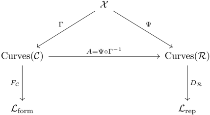<details> <summary>Image 7 Details</summary>  ### Visual Description ## Diagram: Mathematical Relationship Between Curves and Transformations ### Overview The diagram illustrates a bidirectional relationship between two curve sets, **Curves(C)** and **Curves(R)**, mediated by transformations **Γ** and **Ψ**. It also shows mappings to loss functions **L_form** and **L_rep**, suggesting a framework for comparing or transforming curves through mathematical operations. --- ### Components/Axes 1. **Nodes**: - **Curves(C)**: Left curve set. - **Curves(R)**: Right curve set. - **X**: Central node connecting to both curve sets. - **L_form**: Loss function derived from **Curves(C)**. - **L_rep**: Loss function derived from **Curves(R)**. 2. **Arrows/Relationships**: - **Γ**: Transformation from **X** to **Curves(C)**. - **Ψ**: Transformation from **X** to **Curves(R)**. - **A=Ψ∘Γ⁻¹**: Bidirectional relationship between **Curves(C)** and **Curves(R)**, defined as the composition of **Ψ** and the inverse of **Γ**. - **F_C**: Mapping from **Curves(C)** to **L_form**. - **D_R**: Mapping from **Curves(R)** to **L_rep**. --- ### Detailed Analysis - **Transformations**: - **Γ** and **Ψ** are functions that map the central node **X** to distinct curve sets, implying **X** acts as a shared input or latent space. - The bidirectional arrow **A=Ψ∘Γ⁻¹** indicates that **Curves(R)** can be derived from **Curves(C)** via the inverse of **Γ** followed by **Ψ**, and vice versa. This suggests a reversible or invertible relationship between the two curve sets. - **Loss Functions**: - **L_form** and **L_rep** are terminal nodes, likely representing objectives for optimization (e.g., minimizing reconstruction error or divergence between curves). --- ### Key Observations 1. **Bidirectional Symmetry**: The relationship **A=Ψ∘Γ⁻¹** implies that transformations between **Curves(C)** and **Curves(R)** are invertible, assuming **Γ** and **Ψ** are bijective. 2. **Loss Function Dependencies**: Both loss functions depend on their respective curve sets, suggesting separate optimization paths or dual objectives. 3. **Central Node Role**: **X** serves as a unifying source for both curve sets, potentially representing a shared parameter space or input distribution. --- ### Interpretation This diagram likely represents a mathematical or computational framework for: - **Curve Transformation**: Using **Γ** and **Ψ** to map between curve sets, with **A** enabling reversible operations. - **Loss Optimization**: **L_form** and **L_rep** could correspond to tasks like curve reconstruction, alignment, or divergence minimization. - **Shared Input Space**: **X** might represent a latent variable or input distribution that generates both curve sets, enabling comparative analysis. The absence of numerical values or empirical data suggests this is a theoretical or architectural diagram, possibly from a paper on curve analysis, generative models, or optimization frameworks. The bidirectional relationship **A** highlights the importance of invertibility in the transformations, which could be critical for tasks requiring consistency or reversibility (e.g., data augmentation, error correction). </details> Reading guide. (1) Input sequences branch into a semantic curve (left) and a representation curve (right). (2) The canonical alignment 𝐴 = Ψ ∘ 𝑆 -1 identifies the two curves one-to-one. (3) The semantic curve induces human, rule-constrained steps in ℒ form via 𝐹 𝒞 , while the representation curve induces vector increments in ℒ rep via 𝐷 ℛ . (4) Curvature in ℒ rep quantifies the geometric intensity of reasoning transitions and can be related back to formal steps under appropriate correspondences established elsewhere in the paper. ## C. Geometric Foundations of Reasoning Trajectories In this section, we establish the geometric foundations for analyzing reasoning as smooth flows in representation space. We first construct representation trajectories as 𝐶 1 curves via a relaxed prefix-mask mechanism, thereby justifying smoothness as a working principle. Then, we introduce Menger curvature as a computable descriptor that couples angular deviation with distance variation, providing a principled measure of the intensity of reasoning turns. ## C.1. Continuity of Representation Trajectories In this section, we provide a rigorous and explicit construction of a 𝐶 1 trajectory using a relaxed prefix-mask mechanism. This construction justifies our working assumption that representation trajectories are 𝐶 1 . Note that the symbol ℐ (Definition 3.2) is defined with a slight variation compared to main paper: here it is specialized to encode positional information, while the remaining complexities of the model architecture are subsumed into a single mapping Φ . Definition C.1 (Neural Encoding View of Sentence Representation) . Let 𝑥 = ( 𝑢 1 , . . . , 𝑢 𝑛 ) be a sentence with tokens 𝑢 𝑖 drawn from a vocabulary space 𝒱 . Define an embedding map <!-- formula-not-decoded --> which assigns each token a 𝑑 -dimensional vector. Augmenting ℰ ( 𝑢 𝑖 ) with positional information yields the input sequence <!-- formula-not-decoded --> Let Φ : ( R 𝑑 ) 𝑛 ×ℐ → R 𝑑 denote a contextual encoder that maps a sequence of token embeddings together with positional information to a global sentence-level representation, where ℐ is the positional encoding space and ℐ 𝑛 ⊂ ℐ denotes the set of encodings for the first 𝑛 positions. For a fixed 𝜄 = ( 𝜄 1 , . . . , 𝜄 𝑛 ) ∈ ℐ 𝑛 , we define $$\Psi ( x ) \, \colon = \, \Phi \left ( z _ { 0 } , \iota _ { n } \right ) \, = \, \Phi \left ( \mathcal { E } ( u _ { 1 } ) , \dots , \mathcal { E } ( u _ { n } ) , \iota \right ) \in \mathbb { R } ^ { d } .$$ In this view, Ψ subsumes both the static token embeddings and the contextual transformations carried out by the neural network. Hence the hidden state 𝑦 𝑡 = Ψ( 𝑆 𝑡 ) in Definition 4.5 should be interpreted not merely as a sum of embeddings, but as the outcome of the full encoding process applied to the prefix 𝑆 𝑡 . Mask-aware realization (for later use). Fix a maximum length 𝑁 ≥ 𝑛 and consider the mask-aware realization of the same encoder, such that for any length 𝑛 ≤ 𝑁 , $$\begin{array} { r } { \Phi _ { m } \left ( \left ( \mathcal { E } ( u _ { 1 } ) , \dots , \mathcal { E } ( u _ { n } ) , 0 , \dots , 0 , \iota \right ) , \mathbb { 1 } _ { \{ i \leq n \} } \right ) \colon = \Phi \left ( \mathcal { E } ( u _ { 1 } ) , \dots , \mathcal { E } ( u _ { n } ) , ( 1 _ { \{ i \leq n \} } t _ { i } ) _ { i = 1 } ^ { N } \right ) . } \end{array}$$ When the mask is all ones on { 1 , . . . , 𝑛 } , this coincides with the above definition; when we pass a mask explicitly we will write Φ( · , 𝑀 ) . Hypothesis C.2 (Smooth Trajectory Hypothesis) . The sequence of representations 𝑦 𝑡 = Ψ( 𝑋 𝑡 ) generated during a reasoning process lies on a smooth, differentiable trajectory in the embedding space. Definition C.3 (Relaxed-Mask Sentence Representation) . Let each sentence in Hypothesis 4.4 be 𝑥 𝑡 = ( 𝑢 𝑡, 1 , . . . , 𝑢 𝑡,𝑛 𝑡 ) for 𝑡 = 1 , . . . , 𝑇 , and let the full token stream be $$U _ { 1 \colon N } = ( u _ { 1 , 1 } , \dots , u _ { 1 , n _ { 1 } } , u _ { 2 , 1 } , \dots , u _ { 2 , n _ { 2 } } , \dots , u _ { T , 1 } , \dots , u _ { T , n _ { T } } ) ,$$ with total length 𝑁 = ∑︀ 𝑇 𝑡 =1 𝑛 𝑡 and cumulative lengths 𝑁 𝑡 = ∑︀ 𝑡 𝑗 =1 𝑛 𝑗 . Introduce a continuous progress parameter 𝑠 ∈ [0 , 1] and a relaxed prefix mask $$m _ { s } \colon \{ 1 , \dots , N \} \to [ 0 , 1 ] ,$$ which specifies the fractional inclusion of each token at progress 𝑠 . Using the embedding map ℰ and positional information ℐ 𝑁 from Definition C.1, define the masked input sequence at progress 𝑠 by $$z _ { s } = \left ( m _ { s } ( i ) \, \mathcal { E } ( u _ { i } ) \right ) _ { i = 1 } ^ { N } , \quad \iota ^ { s } = \left ( m _ { s } ( i ) \, \iota _ { i } \right ) _ { i = 1 } ^ { N } .$$ $$\Phi _ { m } \colon ( \mathbb { R } ^ { d } ) ^ { N } \times \mathcal { I } _ { N } \times \{ 0 , 1 \} ^ { N } \to \mathbb { R } ^ { d } ,$$ and the associated hard mask is 𝐶 1 by the chain rule. At sentence boundaries 𝑠 𝑡 = 𝑁 𝑡 /𝑁 , choose 𝛿 < 1 2 so that 𝑔 ( 𝑁 𝑡 -𝑖 ) = 1 for 𝑖 ≤ 𝑁 𝑡 and 𝑔 ( 𝑁 𝑡 -𝑖 ) = 0 for 𝑖 ≥ 𝑁 𝑡 +1 . Hence 𝑚 𝑠 𝑡 ( 𝑖 ) ∈ { 0 , 1 } exactly and 𝑀 𝑠 𝑡 ( 𝑖 ) = 1 { 𝑖 ≤ 𝑁 𝑡 } . Substituting into the definition, $$\widetilde { \Psi } ( s _ { t } ) = \Phi \left ( ( \mathcal { E } ( U _ { 1 } ) , \dots , \mathcal { E } ( U _ { N _ { t } } ) , 0 , \dots , 0 , \iota ) , \mathbb { 1 } _ { \{ i \leq N _ { t } \} } \right ) = \Psi ( S _ { t } ) = y _ { t } ,$$ which shows that the discrete embeddings ( 𝑦 𝑡 ) 𝑇 𝑡 =1 are precisely samples of the continuous trajectory ̃︀ Ψ( 𝑠 ) . $$M _ { s } ( i ) \colon = 1 _ { \{ m _ { s } ( i ) = 1 \} } , \quad i = 1 , \dots , N .$$ Let 𝑘 ( 𝑠 ) := ⌈ 𝑠𝑁 ⌉ , denote the number of tokens included at progress 𝑠 . The truncated masked sequences are then defined as $$z _ { s } ^ { ( \leq k ) } \colon = \left ( z _ { s } ( 1 ) , \dots , z _ { s } ( k ( s ) ) \right ) \in ( \mathbb { R } ^ { d } ) ^ { k ( s ) } , \quad \iota ^ { s , ( \leq k ) } \colon = \left ( \iota ^ { s } ( 1 ) , \dots , \iota ^ { s } ( k ( s ) ) \right ) \in \mathcal { I } ^ { k ( s ) } .$$ With the mask-aware encoder Φ 𝑚 : ( R 𝑑 ) 𝑁 ×ℐ 𝑁 ×{ 0 , 1 } 𝑁 → R 𝑑 introduced above, the continuous representation trajectory is defined by $$\widetilde { \Psi } ( s ) \colon = \Phi _ { m } ( z _ { s } , \iota ^ { s } , M _ { s } ) \in \mathbb { R } ^ { d } , \quad w h e r e \, \Phi _ { m } ( z _ { s } , \iota ^ { s } , M _ { s } ) \colon = \Phi \left ( z _ { s } ^ { ( \leq k ) } , \iota ^ { s , ( \leq k ) } \right ) .$$ At sentence boundaries 𝑠 𝑡 := 𝑁 𝑡 /𝑁 , the hard prefix mask is recovered exactly by choosing a smooth function with flat tails (see Proposition C.4); consequently, $$y _ { t } = \Psi ( S _ { t } ) = \Phi \left ( z _ { s _ { t } } , \iota ^ { s _ { t } } , M _ { s _ { t } } \right ) = \widetilde { \Psi } ( s _ { t } ) , \quad t = 1 , \dots , T .$$ Proposition C.4 (Continuity of the Relaxed-Mask Trajectory) . Suppose the relaxed mask takes the form $$m _ { s } ( i ) = g ( s N - i ) ,$$ where 𝑔 ∈ 𝐶 ∞ ( R ) satisfies 𝑔 ( 𝑥 ) = 0 for 𝑥 ≤ -𝛿 , 𝑔 ( 𝑥 ) = 1 for 𝑥 ≥ 𝛿 , with some 0 < 𝛿 < 1 2 (i.e., a smoothstep/bump with flat tails). Assume the encoder Φ is 𝐶 1 . Then the mapping ̃︀ Ψ : [0 , 1] → R 𝑑 defines a 𝐶 1 trajectory in embedding space. Moreover, the discrete sentence embeddings ( 𝑦 𝑡 ) 𝑇 𝑡 =1 are exactly samples of this trajectory at 𝑠 𝑡 = 𝑁 𝑡 /𝑁 : $$y _ { t } = \Psi ( s _ { t } ) , \quad t = 1 , \dots , T .$$ Proof. For each token 𝑈 𝑖 , we define the masked embedding and positional encoding as $$\left ( z _ { s } ( i ) , \iota ^ { s } ( i ) \right ) \, = \, m _ { s } ( i ) \left ( \mathcal { E } ( U _ { i } ) , \iota _ { i } \right ) = g ( s N - i ) \left ( \mathcal { E } ( U _ { i } ) , \iota _ { i } \right ) .$$ Since 𝑔 is 𝐶 ∞ and both ℰ ( 𝑈 𝑖 ) and 𝜄 𝑖 are constant in 𝑠 , each coordinate pair ( 𝑧 𝑠 ( 𝑖 ) , 𝜄 𝑠 ( 𝑖 )) varies smoothly with 𝑠 . Hence the entire masked sequence $$( z _ { s } , \iota ^ { s } ) \, = \, \left ( z _ { s } ( 1 ) , \dots , z _ { s } ( N ) ; \, \iota ^ { s } ( 1 ) , \dots , \iota ^ { s } ( N ) \right )$$ is a smooth trajectory with respect to 𝑠 . The mask 𝑀 𝑠 ( 𝑖 ) = 1 { 𝑚 𝑠 ( 𝑖 )=1 } is piecewise constant in 𝑠 and equals the all-ones indicator on indices where 𝑠𝑁 -𝑖 ≥ 𝛿 , and zeros where 𝑠𝑁 -𝑖 ≤ -𝛿 ; in particular, it is locally constant on neighborhoods that avoid the transition band | 𝑠𝑁 -𝑖 | < 𝛿 . By assumption, Φ is a composition of affine maps, matrix multiplications, LayerNorm, residual connections, softmax attention, and smooth pointwise nonlinearities. As a function of its inputs, such a network is smooth; thus, on any interval where 𝑀 𝑠 is fixed, the composite map $$\widetilde { \Psi } ( s ) = \Phi \left ( z _ { s } , \iota ^ { s } , M _ { s } \right )$$ Remark C.5. Since Φ( · ) implemented with affine maps, matrix multiplications, LayerNorm, residual connections, softmax attention, and smooth pointwise nonlinearities (e.g., GELU/SiLU/Swish), it's reasonable to assume that is 𝐶 1 . If ReLU activations ( or other piecewise smooth nonlinearities) are used instead of smooth ones, the mapping ̃︀ Ψ remains continuous and is differentiable almost everywhere. Since this does not affect the manifold-level geometric reasoning, we idealize Φ as smooth throughout our discussion. The construction above is merely one possible realization of a continuous and 𝐶 1 trajectory ̃︀ Ψ( 𝑠 ) . In fact, many alternative constructions are possible. This abundance of realizations justifies our assumption that the sentence Ψ( 𝑋 𝑇 ) , through its step-by-step variations, can be viewed as 𝑇 points lying on a smooth, differentiable curve. On this basis, we can consistently define the notion of flow velocity in Definition 4.9. ## C.2. Menger Curvature Definition C.6 (Menger Curvature) . Let 𝑥 1 , 𝑥 2 , 𝑥 3 ∈ R 𝑛 be three distinct points. The Menger curvature of the triple ( 𝑥 1 , 𝑥 2 , 𝑥 3 ) is defined as the reciprocal of the radius 𝑅 ( 𝑥 1 , 𝑥 2 , 𝑥 3 ) of the unique circle passing through the three points: $$c ( x _ { 1 } , x _ { 2 } , x _ { 3 } ) \, = \, \frac { 1 } { R ( x _ { 1 } , x _ { 2 } , x _ { 3 } ) } .$$ Proposition C.7 (Computation Formula) . Let 𝑎 = ‖ 𝑥 2 -𝑥 3 ‖ , 𝑏 = ‖ 𝑥 1 -𝑥 3 ‖ , and 𝑐 = ‖ 𝑥 1 -𝑥 2 ‖ . Denote by ∆( 𝑥 1 , 𝑥 2 , 𝑥 3 ) the area of the triangle spanned by the three points. Then the circumradius 𝑅 and the Menger curvature 𝑐 ( 𝑥 1 , 𝑥 2 , 𝑥 3 ) are given by $$R ( x _ { 1 } , x _ { 2 } , x _ { 3 } ) \, = \, \frac { a b c } { 4 \Delta ( x _ { 1 } , x _ { 2 } , x _ { 3 } ) } , \quad c ( x _ { 1 } , x _ { 2 } , x _ { 3 } ) \, = \, \frac { 4 \Delta ( x _ { 1 } , x _ { 2 } , x _ { 3 } ) } { a b c } .$$ Proof. The formula follows from classical Euclidean geometry: for a triangle with side lengths 𝑎, 𝑏, 𝑐 and area ∆ , the circumradius satisfies 𝑅 = 𝑎𝑏𝑐 4Δ . Taking the reciprocal yields the Menger curvature. Figure 6: Circumcircle through three points 𝑥 1 , 𝑥 2 , 𝑥 3 , with radius 𝑅 and Menger curvature 1 /𝑅 . 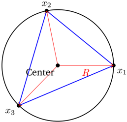<details> <summary>Image 8 Details</summary>  ### Visual Description ## Diagram: Geometric Circle with Inscribed Points ### Overview The image depicts a circle with three labeled points (`x1`, `x2`, `x3`) on its circumference, connected to a central point labeled "Center." A radius labeled `R` extends from the center to `x1`. The diagram emphasizes geometric relationships between the center, radius, and peripheral points. ### Components/Axes - **Circle**: Unlabeled boundary enclosing the diagram. - **Center**: Central point labeled "Center," serving as the origin for all radii. - **Points on Circumference**: - `x1`: Labeled point on the circle, connected to the center via radius `R`. - `x2`: Labeled point on the circle, connected to the center (line unlabeled). - `x3`: Labeled point on the circle, connected to the center (line unlabeled). - **Radius**: Segment from "Center" to `x1`, explicitly labeled `R`. ### Detailed Analysis - **Geometric Structure**: - The circle’s radius `R` is defined by the distance from "Center" to `x1`. - Lines from "Center" to `x2` and `x3` are implied radii but not labeled. - The three points (`x1`, `x2`, `x3`) form a triangle inscribed within the circle. - **Spatial Relationships**: - All points (`x1`, `x2`, `x3`) are equidistant from the center (assuming standard circle properties). - The radius `R` is the only explicitly quantified measurement. ### Key Observations - The diagram lacks numerical values for angles or arc lengths, focusing instead on positional labels. - The unlabeled lines to `x2` and `x3` suggest symmetry or equal importance to `x1` in the context of the diagram. - The absence of a legend or scale implies the diagram is schematic rather than data-driven. ### Interpretation This diagram likely illustrates foundational concepts in geometry, such as: 1. **Radius Definition**: The radius `R` establishes the circle’s scale. 2. **Inscribed Triangle**: The points `x1`, `x2`, `x3` may represent vertices of a triangle, potentially equilateral if equally spaced (though spacing is not confirmed). 3. **Central Angles**: Lines from the center to the points could subtend central angles, relevant to calculations of arc lengths or sector areas. The diagram serves as a visual aid for problems involving circular motion, trigonometry, or coordinate geometry, where the center and radius are critical references. The lack of numerical data suggests it is a conceptual tool rather than a quantitative representation. </details> Proposition C.8 (Menger curvature from three consecutive states) . Let 𝑦 𝑡 -1 , 𝑦 𝑡 , 𝑦 𝑡 +1 ∈ R 𝑑 be three distinct points and set $$u \colon = y _ { t } - y _ { t - 1 } , \quad v \colon = y _ { t + 1 } - y _ { t } .$$ $$a = \| u \| , \quad b = \| v \| , \quad c = \| v - u \| = \| y _ { t + 1 } - y _ { t - 1 } \| .$$ Write the side lengths Figure 7: Two circumcircles through { 𝑦 𝑡 -1 , 𝑦 𝑡 , 𝑦 (1) 𝑡 +1 } and { 𝑦 𝑡 -1 , 𝑦 𝑡 , 𝑦 (2) 𝑡 +1 } , with radii 𝑅 and 𝑅 ′ . Here 𝑦 (1) 𝑡 +1 and 𝑦 (2) 𝑡 +1 lie on the same ray from 𝑦 𝑡 . 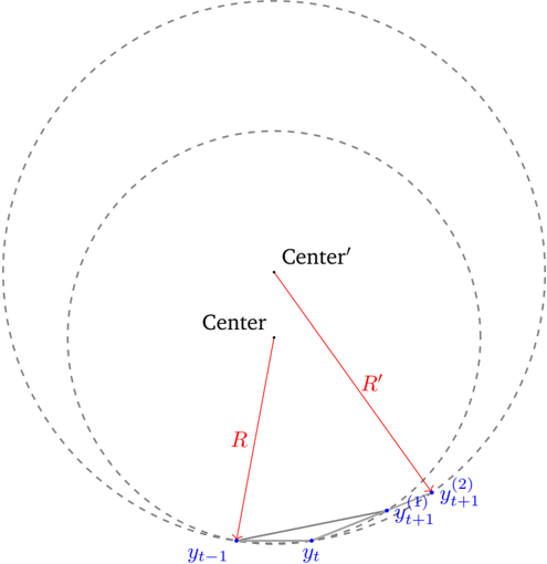<details> <summary>Image 9 Details</summary>  ### Visual Description ## Diagram: Geometric Relationship Between Two Concentric Circles ### Overview The diagram illustrates two concentric circles with labeled centers ("Center" and "Center'") and radii (R and R'). Points on the circumference of the inner and outer circles are marked with indices (yt-1, yt, yt+1, yt+1'). Lines connect the centers to specific points, suggesting geometric relationships or transformations. ### Components/Axes - **Circles**: - Inner circle (dashed line) labeled "Center" with radius **R**. - Outer circle (dashed line) labeled "Center'" with radius **R'**. - **Points**: - **yt-1**, **yt**, **yt+1**: Located on the inner circle's circumference. - **yt+1'**: Located on the outer circle's circumference. - **Lines**: - Red line from "Center" to **yt+1'** (radius **R'**). - Red line from "Center" to **yt-1** (radius **R**). - Gray lines connecting **yt-1** to **yt**, **yt** to **yt+1**, and **yt+1** to **yt+1'**. ### Detailed Analysis - **Radii**: - Inner radius **R** (exact value unspecified). - Outer radius **R'** (exact value unspecified, but visually larger than R). - **Point Indices**: - **yt-1**, **yt**, **yt+1** suggest sequential data points (e.g., time steps). - **yt+1'** implies a transformed or projected version of **yt+1** onto the outer circle. - **Spatial Relationships**: - **yt+1'** lies on the outer circle, directly aligned with the line from "Center'" to the inner circle's **yt+1**. - Gray lines form a polygonal chain connecting sequential points across both circles. ### Key Observations 1. The outer radius **R'** is larger than the inner radius **R** (visual estimation). 2. The point **yt+1'** is positioned such that the line from "Center'" to it passes through **yt+1** on the inner circle, implying a radial projection. 3. The gray lines suggest a stepwise progression or interpolation between points. ### Interpretation This diagram likely represents a geometric transformation or mapping between two concentric circles. The sequential indices (yt-1, yt, yt+1) may denote time-dependent data points, while **yt+1'** could represent a scaled or transformed version of these points onto the outer circle. The relationship between R and R' might indicate a scaling factor or growth rate. The absence of numerical values limits quantitative analysis, but the structure suggests applications in fields like signal processing, geometry, or dynamic systems modeling. **Note**: No numerical data or explicit units are provided in the image. All interpretations are based on spatial and label relationships. </details> The Menger curvature of the triple ( 𝑦 𝑡 -1 , 𝑦 𝑡 , 𝑦 𝑡 +1 ) equals $$c _ { M } ( y _ { t - 1 } , y _ { t } , y _ { t + 1 } ) = \frac { 4 \, \Delta ( y _ { t - 1 } , y _ { t } , y _ { t + 1 } ) } { a b c } = \frac { 2 \sqrt { 1 - C o s S i m ( u , v ) ^ { 2 } } } { \| y _ { t + 1 } - y _ { t - 1 } \| } ,$$ where CosSim( 𝑢, 𝑣 ) := ⟨ 𝑢, 𝑣 ⟩ ‖ 𝑢 ‖ ‖ 𝑣 ‖ . (If the three points are collinear, 𝑐 𝑀 := 0 .) Proof. By classical Euclidean geometry, for a triangle with side lengths 𝑎, 𝑏, 𝑐 and area ∆ , the circumradius satisfies 𝑅 = 𝑎𝑏𝑐 4∆ . The Menger curvature is the reciprocal 𝑐 𝑀 = 1 /𝑅 = 4∆ 𝑎𝑏𝑐 . It remains to express ∆ in terms of 𝑢 and 𝑣 . The (unsigned) area of the triangle spanned by 𝑢 and 𝑣 can be written in a dimension-independent way via the Gram determinant: $$\Delta = \frac { 1 } { 2 } \| u \wedge v \| = \frac { 1 } { 2 } \sqrt { \det \binom { \langle u , u \rangle \quad \langle u , v \rangle } { \langle v , u \rangle \quad \langle v , v \rangle } } = \frac { 1 } { 2 } \sqrt { \| u \| ^ { 2 } \| v \| ^ { 2 } - \langle u , v \rangle ^ { 2 } } .$$ Substituting 𝑎 = ‖ 𝑢 ‖ , 𝑏 = ‖ 𝑣 ‖ , 𝑐 = ‖ 𝑣 -𝑢 ‖ into 𝑐 𝑀 = 4∆ 𝑎𝑏𝑐 gives $$c _ { M } = \frac { 2 \sqrt { \| u \| ^ { 2 } \| v \| ^ { 2 } - \langle u , v \rangle ^ { 2 } } } { \| u \| \, \| v \| \, \| v - u \| } .$$ Divide the numerator and denominator by ‖ 𝑢 ‖ ‖ 𝑣 ‖ and denote 𝑠 := CosSim( 𝑢, 𝑣 ) = ⟨ 𝑢, 𝑣 ⟩ ‖ 𝑢 ‖ ‖ 𝑣 ‖ . Then $$c _ { M } = \frac { 2 \sqrt { 1 - s ^ { 2 } } } { \| v - u \| } = \frac { 2 \sin \theta } { c } ,$$ where 𝜃 is the angle between 𝑢 and 𝑣 (so sin 𝜃 = √ 1 -𝑠 2 ). If the three points are collinear, ∆ = 0 and hence 𝑐 𝑀 = 0 , consistent with the convention. This proves the claim. Remark C.9. As illustrated in Figure 7, using the Menger curvature instead of cosine similarity is significant. Cosine similarity only depends on the angle at 𝑦 𝑡 , so the two triples { 𝑦 𝑡 -1 , 𝑦 𝑡 , 𝑦 (1) 𝑡 +1 } and { 𝑦 𝑡 -1 , 𝑦 𝑡 , 𝑦 (2) 𝑡 +1 } would look identical. In contrast, their circumradii 𝑅 and 𝑅 ′ are different, hence the Menger curvatures distinguish two different curvature regimes. This demonstrates how Menger curvature captures both angle and length information, enabling discrimination that cosine similarity alone cannot provide. ## D. Data Generation We provide the exact prompt templates and the representative sampled data instances used in our data generation process. The two-stage pipeline is run with GPT-5. ## D.1. Prompts for Data Generation The following prompts are used for abstract logical templates construction and domain-specific and language-specific rewriting. ## Prompt for Logic Pattern Generation You are a formal logic pattern generator. Goal: Create an abstract, domain-agnostic reasoning sequence of exactly N steps, written in symbolic form, using standard propositional/first-order logic notation. ## Strict output format: - Exactly N lines, each line starts with a bracketed index and a single formula or conclusion, e.g.: - Use only symbols from: ¬ , ∧ , ∨ , → , ↔ , ∀ , ∃ , parentheses, predicate letters with uppercase (A,B,C,...) and predicate symbols like H(x), J(x). - The sequence must be internally coherent (later steps can be derived from earlier ones), but no proof of a fixed target is required. - You may include brief justifications at the end of lines in parentheses referencing earlier step indices (e.g., (from [2] and [5])). - No extra commentary before or after the lines. No natural-language sentences. ``` * Exactly N lines, each line starts with a bracketed index and a single form [1] A -> B [2] B -> C [3] C -> D [4] (D & E) -> F [5] forall x(H(x) -> J(x)) [6] A [7] E [8] H(a) [9] D (from [1-3] and [6]) [10] F & J(a) (from [4],[7],[5],[8],[9]) ``` ## Parameters (provided by caller): - N: number of steps to output. - logic: a label for this abstract logic (optional). ``` N = {N} logic = {logic} Now produce exactly N lines. ``` ## Prompt for Reasoning Rewriter You are a reasoning rewriter. Task: Given an abstract N-step reasoning scaffold (formal symbolic lines) and a target topic, rewrite the scaffold into a topic-specific natural-language reasoning sequence with exactly the same number of steps and the same dependency structure. ## Inputs (provided by caller): - Topic : the target domain (e.g., weather, software). - N : the total number of steps. - Abstract Steps (1..N) : the neutral scaffold, numbered 1..N. ## Output requirements: - Produce exactly N steps, each line begins with the same bracketed index as the abstract: [1] ... to [N] ... . - Preserve the logical dependencies: if abstract step k enables k+1, your rewrite must preserve that relationship in the topic. - Keep step count and ordering identical to the abstract. Do not merge, split, add, or remove steps. - Use concrete domain terms appropriate to the topic, but keep sentences concise and precise. - No extra commentary before or after the steps. ## Multilingual mode (when Languages: are specified by the caller): - Create a separate section for each requested language code. - Under each header, write the N steps with bracketed indices [1] .. [N] in that language. - Each section starts with a header line === <code> === (e.g., === en === ). - Keep the content aligned across languages (same meaning per step index). ## Inputs you will receive: Topic: {topic} Abstract Steps (1..N): {ABSTRACT\_STEPS} N = {N} Now perform the rewrite. ## D.2. Data Examples Table 2 presents a 9-step logical scaffold from our dataset. We illustrate its instantiation in two distinct domains, weather and finance, providing the corresponding statements in both English (EN) and German (DE). Table 2: Logic Example (9-Step) with Weather and Finance Topics in English and German | Abstract Logic | Topic: Weather | Topic: Finance | |---------------------------------|----------------------------------------------------------------------------------------------------------------------------------------------------------------------------|-------------------------------------------------------------------------------------------------------------------------------------------------------------------------------------------------------------------------------------------------------| | [1] 𝐴 → 𝐵 | EN: If moisture converges over the city , then thunderclouds develop. DE: Wenn über der Stadt Feuchte konvergiert, dann bilden sich Gewitterwolken. | EN: If the firm's interest coverage ratio exceeds 3.0x, then the firm is deemed able to meet interest obligations. DE: Wenn die Zinsdeckungskennzahl des Unternehmens über 3,0x liegt, dann gilt das Unternehmen als fähig, Zinszahlungen zu leisten. | | [2] 𝐵 → 𝐶 | EN: If thunderclouds develop, then heavy rain occurs. DE: Wenn sich Gewitterwolken bilden, dann tritt starker Regen auf. | EN: If the firm is deemed able to meet interest obligations, then the bank will approve a new term loan. DE: Wenn das Unternehmen als fähig gilt, Zinszahlungen zu leisten, dann wird die Bank ein neues Laufzeitdarlehen genehmigen. | | [3] ∀ 𝑥 ( 𝐻 ( 𝑥 ) → 𝐽 ( 𝑥 )) | EN: For any location x, if a cold front passes x, then temperatures drop at x. DE: Für jeden Ort x gilt: Wenn eine Kaltfront x überquert, dann sinkt dort die Temperatur. | EN: For any security x, if x is a U.S. Treasury, then x is acceptable as repo collateral. DE: Für jedes Wertpapier x gilt: Wenn x eine US-Staatsanleihe ist, dann ist x als Repo-Sicherheit zulässig. | | [4] 𝐻 ( 𝑎 ) | EN: A cold front is passing the airport. DE: Eine Kaltfront überquert den Flughafen. | EN: Bond A is a U.S. Treasury. DE: Anleihe A ist eine US-Staatsanleihe. | | [5] 𝐴 | EN: Moisture is converging over the city . DE: Über der Stadt herrscht Feuchtekonvergenz. | EN: The firm's interest coverage ratio exceeds 3.0x. DE: Die Zinsdeckungskennzahl des Unternehmens liegt über 3,0x. | | [6] 𝐵 (from [1], [5]) | EN: From [1] and [5], thunderclouds develop. DE: Aus [1] und [5] folgt, dass sich Gewitterwolken bilden. | EN: The firm is deemed able to meet interest obligations (from [1] and [5]). DE: Daher gilt das Unternehmen als fähig, Zinszahlungen zu leisten (aus [1] und [5]). | | [7] 𝐶 (from [2], [6]) | EN: From [2] and [6], heavy rain occurs. DE: Aus [2] und [6] folgt, dass starker Regen auftritt. | EN: The bank will approve a new term loan (from [2] and [6]). DE: Daher wird die Bank ein neues Laufzeitdarlehen genehmigen (aus [2] und [6]). | | [8] 𝐽 ( 𝑎 ) (from [3], [4]) | EN: From [3] and [4], temperatures drop at the airport. DE: Aus [3] und [4] folgt, dass am Flughafen die Temperatur sinkt. | EN: Bond A is acceptable as repo collateral (from [3] and [4]). DE: Daher ist Anleihe A als Repo-Sicherheit zulässig (aus [3] und [4]). | | [9] 𝐶 ∧ 𝐽 ( 𝑎 ) (from [7], [8]) | EN: From [7] and [8], heavy rain occurs and temperatures drop at the airport. DE: Aus [7] und [8] folgt: Es tritt starker Regen auf und am Flughafen sinkt die Temperatur. | EN: The bank will approve a new term loan and Bond A is acceptable as repo collateral (from [7] and [8]). DE: Somit wird die Bank ein neues Laufzeitdarlehen genehmigen und Anleihe A ist als Repo-Sicherheit zulässig (aus [7] und [8]). |