# ADEPT: Continual Pretraining via Adaptive Expansion and Dynamic Decoupled Tuning
> These authors contributed equally.Corresponding author.
## Abstract
Conventional continual pretraining (CPT) for large language model (LLM) domain adaptation often suffers from catastrophic forgetting and limited domain capacity. Existing strategies adopt layer expansion, introducing additional trainable parameters to accommodate new knowledge. However, the uniform expansion and updates still entangle general and domain learning, undermining its effectiveness. Our pilot studies reveal that LLMs exhibit functional specialization, where layers and units differentially encode general-critical capabilities, suggesting that parameter expansion and optimization should be function-aware. We then propose ADEPT, A daptive Expansion and D ynamic D e coupled Tuning for continual p re t raining, a two-stage framework for domain-adaptive CPT. ADEPT first performs General-Competence Guided Selective Layer Expansion, duplicating layers least critical for the general domain to increase representational capacity while minimizing interference with general knowledge. It then applies Adaptive Unit-Wise Decoupled Tuning, disentangling parameter units within expanded layers according to their general-domain importance and assigning asymmetric learning rates to balance knowledge injection and retention. Experiments on mathematical and medical benchmarks show that ADEPT outperforms full-parameter CPT by up to 5.76% on the general domain and 5.58% on the target domain with only 15% of parameters tuned and less than 50% training time. Ablation studies, theoretical analysis, and extended investigations further demonstrate the necessity of targeted expansion and decoupled optimization, providing new principles for efficient and robust domain-adaptive CPT. Our code is open-sourced at https://github.com/PuppyKnightUniversity/ADEPT.
## 1 Introduction
Large language models (LLMs) have demonstrated remarkable performance across a wide range of general-domain tasks (OpenAI, 2023; Dubey et al., 2024c). However, their deployment in specialized domains, such as mathematics or healthcare, requires targeted adaptation (Ding et al., 2024; Chen et al., 2024; Ahn et al., 2024). Continual pretraining (CPT), which conducts post-pretraining on domain-specific corpora, has emerged as a crucial paradigm for injecting domain knowledge and capabilities into pretrained LLMs (Wu et al., 2024a; Ibrahim et al., 2024; Yıldız et al., 2024).
Despite its promise, CPT faces a persistent challenge: catastrophic forgetting. After pretraining, LLMs already encode substantial general knowledge, leaving limited parameter capacity for integrating new domain-specific information. While domain signals can be forcefully fitted through gradient-based optimization, the aggressive updates on the existing parameters come at the cost of overfitting to the target corpora, which in turn disrupts general abilities and triggers catastrophic forgetting (Liu et al., 2024a; Luo et al., 2025). This tension between new knowledge injection and previous knowledge retention poses a central obstacle to reliable and stable domain adaptation.
To address catastrophic forgetting, some approaches attempt through data-centric strategies, such as data replay or rehearsal (Huang et al., 2024; Zhang et al., 2025). While replay partially preserves prior knowledge, it fails to expand model capacity, leaving the conflict between knowledge injection and retention unresolved. Others focus on increasing capacity via transformer-layer extension (Wu et al., 2024b), yet typically insert new layers uniformly and update all parameters indiscriminately. This expansion strategy neglects the functional specialization within LLMs, where different layers and neurons serve distinct functional roles. Our pilot studies reveal that general-critical layers in LLMs are mainly located in early depths, and functional units within layers contribute unequally to general-domain performance, highlighting functional specialization similar to that found in the human brain (Xu et al., 2025; Zheng et al., 2024; Dai et al., 2022). Consequently, indiscriminate expansion and optimization may overwrite general-critical regions with new knowledge, compromising general competency preservation and leaving forgetting unresolved.
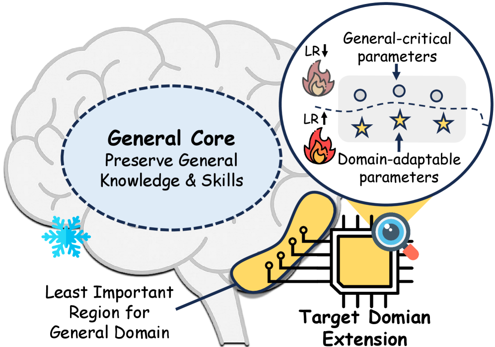
Inspired by the functional specialization perspective, we propose our core insight: effective CPT should expand and update the model adaptively, preserving the regions responsible for the general domain and targeting more adaptable parameters. Specifically, we argue that capacity allocation must be importance-guided, and optimization must be function-decoupled to minimize interference with general competencies. As illustrated in Figure 1, domain-specific extension should be allocated to the regions less constrained by general-domain knowledge and skills, and parameters within these regions should be decoupled and tuned accordingly, preserving general-critical parameters and allowing the rest to be more adaptable to absorb new domain-specific information.
<details>
<summary>x1.png Details</summary>
### Visual Description
## Diagram: Neural Network Adaptation Strategy
### Overview
The image is a conceptual diagram illustrating a method for adapting a pre-trained artificial neural network (represented as a brain) to a new target domain while preserving its general knowledge and skills. It uses visual metaphors to explain a selective parameter tuning strategy.
### Components & Labels
The diagram consists of several interconnected visual elements with the following text labels:
1. **Central Brain Illustration:**
* A large, stylized brain outline forms the background.
* **Dashed Oval Region (Center-Left):** Labeled "**General Core**" with the sub-text "**Preserve General Knowledge & Skills**". This region is enclosed by a dashed blue oval.
* **Snowflake Icon (Bottom-Left of Core):** A blue snowflake is placed adjacent to the "General Core," symbolizing that this region is "frozen" or kept static during adaptation.
2. **Magnified Parameter View (Top-Right Circle):**
* A circular callout, connected by a dashed line to the "General Core," shows a detailed view of model parameters.
* **Top Row:** Three circles labeled "**General-critical parameters**". An arrow points down to them from the label.
* **Bottom Row:** Three star icons labeled "**Domain-adaptable parameters**". An arrow points up to them from the label.
* **Learning Rate (LR) Indicators:**
* Next to the top row: "**LR↓**" with a small, smoldering fire icon, indicating a *decreased* learning rate for general-critical parameters.
* Next to the bottom row: "**LR↑**" with a larger, active fire icon, indicating an *increased* learning rate for domain-adaptable parameters.
3. **Adaptation Pathway (Bottom):**
* **Yellow Brain Region (Bottom-Left):** A specific, highlighted region of the brain is labeled "**Least Important Region for General Domain**". A line connects this label to the region.
* **Connection to Chip:** This yellow region is directly connected via lines to a microchip icon.
* **Microchip Icon (Bottom-Right):** A yellow square chip with circuit lines is labeled "**Target Domain Extension**". (Note: "Domian" is a visible typo for "Domain").
* **Eye Icon:** A stylized eye with a magnifying glass is positioned over the chip, suggesting focused analysis or targeting.
### Detailed Analysis
The diagram proposes a two-pronged strategy for model adaptation:
1. **Preservation of General Knowledge:** The "General Core" of the model, containing "General-critical parameters," is protected. This is visually represented by the snowflake (freezing) and the instruction to use a decreased learning rate (`LR↓`) during any fine-tuning, minimizing changes to these foundational parameters.
2. **Targeted Domain Adaptation:** Adaptation is focused on a specific, identified "Least Important Region for General Domain." This region contains "Domain-adaptable parameters," which are modified using an increased learning rate (`LR↑`) to efficiently absorb knowledge from the "Target Domain Extension." The eye icon over the chip emphasizes the targeted, precise nature of this adaptation.
The flow suggests a process: identify the least important region for general tasks, then aggressively tune its adaptable parameters for the new domain while carefully constraining updates to the critical general parameters elsewhere.
### Key Observations
* **Visual Metaphors:** The diagram effectively uses common metaphors: a snowflake for freezing, fire for learning rate intensity (more fire = higher rate), stars for adaptable/special parameters, and a chip for the new domain/task.
* **Spatial Grounding:** The magnified parameter view is explicitly linked to the "General Core," not the "Least Important Region." This clarifies that the core contains both critical and adaptable parameters, but the adaptation strategy applies different learning rates to each type within that core.
* **Typo:** The label for the chip contains a spelling error: "Target **Domian** Extension" should be "Target **Domain** Extension."
* **Color Coding:** Yellow is used consistently to highlight the components involved in active adaptation (the "least important" brain region and the target domain chip).
### Interpretation
This diagram illustrates a sophisticated approach to **continual learning** or **transfer learning** in neural networks. The core problem it addresses is "catastrophic forgetting," where a model loses its general capabilities when fine-tuned on a new, specific task.
The proposed solution is **selective, asymmetric fine-tuning**. Instead of updating all model parameters equally, it:
1. **Identifies and protects** the parameters most crucial for general intelligence (the "General Core").
2. **Identifies and aggressively updates** parameters in brain regions deemed less critical for general function, repurposing them for the new domain.
This strategy aims to achieve a balance: efficiently acquiring new domain-specific skills ("Target Domain Extension") while maintaining robust general knowledge and capabilities ("Preserve General Knowledge & Skills"). The use of different learning rates (`LR↑` vs. `LR↓`) is a practical implementation detail for achieving this balance during the training process. The diagram suggests that not all parts of a trained model are equally valuable for all tasks, and intelligent adaptation requires diagnosing and acting on this functional hierarchy.
</details>
Figure 1: Illustration of the core idea of ADEPT. Target domain extension are applied on the least important region for general domain, minimizing catastrophic forgetting. Asymmetric learning rates are applied to parameter subsets for targeted knowledge injection.
Building on this insight, we propose A daptive Expansion and D ynamic D e coupled Tuning for continual p re- t raining (ADEPT), a framework for domain-adaptive continual pretraining. ADEPT comprises two stages: General-Competence Guided Selective Layer Expansion, which identifies and duplicates layers least critical for the general domain, allocating additional capacity precisely where interference with general capabilities is minimized, thereby preventing catastrophic forgetting. Adaptive Unit-Wise Decoupled Tuning, which disentangles the parameters within the expanded layers based on their importance to the general domain. Asymmetric learning rates are then applied on their subsets, ensuring that general-critical parameters are preserved while more adaptable parameters can fully absorb domain-specific knowledge. Extensive experiments on mathematical and medicine domains demonstrate that ADEPT enables efficient and robust domain knowledge injection, while substantially alleviating catastrophic forgetting. Specifically, compared to full-parameter CPT, ADEPT achieves up to 5.58% accuracy gain on target-domain benchmarks, and up to 5.76% gain on the general domain, confirming both effective knowledge acquisition and strong retention of general competencies. Furthermore, ADEPT attains these improvements with only 15% of parameters tuned, and reduces training time relative to other baselines greatly, highlighting its efficiency. Ablation studies and theoretical analysis further validate the designs of ADEPT.
To summarize, our contributions are threefold:
1. Insightfully, we highlight the importance of considering functional specialization in LLMs for continual pretraining through empirical experiments and theoretical analysis, advocating for targeted layer expansion and decoupled training as a principled solution to domain adaptation.
1. Technically, we propose ADEPT, a framework that consists of General-Competence Guided Selective Layer Expansion and Adaptive Unit-Wise Decoupled Tuning, enabling adaptive and effective domain knowledge integration while minimizing catastrophic forgetting.
1. Empirically, we conduct extensive experiments on both mathematical and medical domains, demonstrating that ADEPT consistently outperforms baselines in domain performance while preserving general competencies.
<details>
<summary>x2.png Details</summary>
### Visual Description
## Heatmap Series: Qwen3 Model Layer Activation Patterns
### Overview
The image displays three horizontally arranged heatmaps, each visualizing activation patterns across layers and components for different sizes of the Qwen3 language model base variants. The heatmaps use a color gradient to represent numerical values, likely indicating activation intensity, importance, or some normalized metric.
### Components/Axes
**Titles (Top of each heatmap):**
1. Left: `Qwen3-1.7B-Base`
2. Center: `Qwen3-4B-Base`
3. Right: `Qwen3-8B-Base`
**Y-Axis (Vertical, Left side of each heatmap):**
* **Label:** `Layer`
* **Scale:** Represents the model's layer index, starting from 0 at the bottom.
* Qwen3-1.7B-Base: Layers 0 to 27.
* Qwen3-4B-Base: Layers 0 to 34.
* Qwen3-8B-Base: Layers 0 to 34.
**X-Axis (Horizontal, Bottom of each heatmap):**
* **Labels (Identical for all three heatmaps, from left to right):**
1. `mlp.down_proj`
2. `mlp.gate_proj`
3. `mlp.up_proj`
4. `self_attn.k_proj`
5. `self_attn.q_proj`
6. `self_attn.v_proj`
7. `self_attn.o_proj`
8. `post_attention_layernorm`
9. `input_layernorm`
10. `lm_head`
**Color Legend (Far right of the image):**
* A vertical color bar.
* **Scale:** Ranges from `0` (bottom, light green) to `1` (top, dark blue).
* **Interpretation:** The color of each cell in the heatmaps corresponds to a value on this scale. Darker blue indicates a value closer to 1, while lighter green indicates a value closer to 0.
### Detailed Analysis
**General Pattern Across All Models:**
* **Trend Verification:** For all three models, the leftmost columns (corresponding to MLP projection layers: `mlp.down_proj`, `mlp.gate_proj`, `mlp.up_proj`) show a strong vertical gradient. They are darkest blue (high value) in the lowest layers and gradually become lighter (lower value) in the highest layers.
* The middle columns (self-attention projections: `self_attn.k_proj`, `self_attn.q_proj`, `self_attn.v_proj`, `self_attn.o_proj`) show a more complex, patchy pattern with moderate values concentrated in the lower-to-middle layers.
* The rightmost columns (`post_attention_layernorm`, `input_layernorm`, `lm_head`) are uniformly very light green (values near 0) across all layers in all models.
**Model-Specific Details:**
1. **Qwen3-1.7B-Base (28 layers):**
* The highest values (darkest blue) are concentrated in the `mlp.down_proj` and `mlp.gate_proj` columns within layers 0-10.
* The `self_attn.q_proj` column shows a notable cluster of moderate-to-high values in layers 0-15.
* Activation values diminish significantly above layer 20 for most components.
2. **Qwen3-4B-Base (35 layers):**
* The pattern is similar to the 1.7B model but extended over more layers.
* The high-value region for MLP projections (`mlp.down_proj`, `mlp.gate_proj`) extends slightly higher, up to around layer 15.
* The self-attention components show a more dispersed pattern of moderate values in the lower half of the network.
3. **Qwen3-8B-Base (35 layers):**
* The high-value region for MLP projections is the most extensive, with dark blue cells persisting up to layer 20 in the `mlp.down_proj` column.
* The self-attention components, particularly `self_attn.q_proj`, show a broader distribution of moderate values across the lower 25 layers compared to the smaller models.
* The overall contrast between high-value (blue) and low-value (green) regions appears slightly more pronounced.
### Key Observations
1. **Component Hierarchy:** MLP projection layers (`down_proj`, `gate_proj`, `up_proj`) consistently exhibit the highest values, especially in the lower network layers, across all model sizes.
2. **Layer Progression:** There is a clear top-down gradient where activation/importance is highest in the initial processing layers and decreases toward the final layers.
3. **Normalization Invariance:** The layernorm components (`post_attention_layernorm`, `input_layernorm`) and the language modeling head (`lm_head`) show negligible values (near 0) throughout, suggesting they are not the focus of this particular metric.
4. **Scaling Effect:** As model size increases (1.7B -> 4B -> 8B), the region of high activation in the MLP layers extends to a higher layer index, indicating that larger models may distribute these computations deeper into the network.
### Interpretation
This visualization likely represents the **relative importance or activation magnitude** of different weight matrices within the Qwen3 transformer architecture. The data suggests a fundamental architectural insight:
* **Core Computational Load:** The dense MLP layers (`down_proj`, `gate_proj`, `up_proj`) are the primary sites of high-magnitude processing, particularly in the early stages of the network where raw input is being transformed into a more useful representation.
* **Attention's Role:** Self-attention mechanisms show significant but more distributed activity, indicating their role in integrating information across the sequence, which may be less concentrated in specific layers compared to the MLP transformations.
* **Scaling Law Manifestation:** The extension of high MLP activation into deeper layers in larger models could be a visual correlate of scaling laws, where increased model capacity allows for more sustained, complex processing throughout the network depth.
* **Architectural Constants:** The near-zero values for normalization layers and the LM head are expected, as these components typically perform scaling and final projection rather than being sites of high-magnitude feature transformation.
**In essence, the heatmaps provide a "fingerprint" of computational focus, showing that the Qwen3 models, regardless of size, rely heavily on early-layer MLP processing, with the spatial extent of this focus growing with model scale.**
</details>
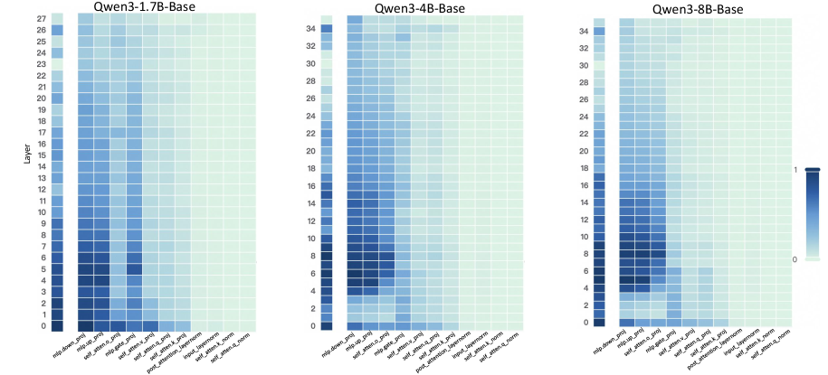
Figure 2: Layer- and unit-level importance distribution of the Qwen3 family. The vertical axis corresponds to different layers, while the horizontal axis denotes parameter units within each layer. Deeper blue indicates higher importance for preserving general-domain competencies.
## 2 Pilot Study: Probing Parameter Importance
### 2.1 Experimental Setup for Importance Probing
To investigate the functional specialization of LLMs and understand how different parameters contribute to preserving general-domain knowledge during CPT, we conduct importance probing on multiple backbone models, including Qwen3-Base (1.7B, 4B, 8B) (Yang et al., 2025a) and LLaMA3-8B (Dubey et al., 2024b). Our analyses focus on probing general-knowledge-critical parameters rather than domain-specific ones. The rationale is that successful CPT must inject new, domain-specific knowledge without inducing catastrophic forgetting. This necessitates identifying and preserving the model’s core parameters that are crucial for its general-domain competencies. By contrast, domain knowledge can then be effectively allocated to less critical parameters, without risking the erosion of pre-existing knowledge and skills. To support this analysis, we construct a General Competence Detection Corpus containing broad world knowledge and instruction-following tasks in both English and Chinese, which servers as the probing ground to reflect a model’s general competencies. Details of its construction are provided in Appendix B.3.
### 2.2 Layer-Level Importance Probing
Our first research question is: How do different layers contribute to preserving general knowledge? To answer this, we measure the importance of each transformer layer by the model’s degradation in general-domain performance when that layer is ablated. Formally, given the General Competence Detection Corpus $D_probe$ , we first compute the baseline next-token prediction loss of the pretrained LLM $M_0$ :
$$
L_base=\frac{1}{|D_probe|}∑_x∈D_probe\ell\big(M_0(x),x\big), \tag{1}
$$
where $\ell(·)$ denotes the standard next-token prediction loss in CPT. For each transformer layer $l∈\{1,…,L\}$ , we mask its output via a residual bypass and recompute the loss:
$$
\hat{L}^(l)=\frac{1}{|D_probe|}∑_x∈D_probe\ell\big(M_0^(-l)(x),x\big), \tag{2}
$$
where $M_0^(-l)$ denotes the model with the $l$ -th layer masked. The importance of layer $l$ is defined as the loss increase relative to the baseline:
$$
I_layer^(l)=\hat{L}^(l)-L_base. \tag{3}
$$
A larger $I_layer^(l)$ indicates that layer $l$ plays a more critical role in preserving general knowledge. Figure 2 (left-hand bars) reports the layer-level importance distributions of the Qwen3 family (results for LLaMA3-8B provided in Appendix D). We find that general-knowledge-critical layers are concentrated in the early layers, with importance gradually decreasing toward later layers. This uneven distribution suggests that uniformly expanding layers across the entire depth would be suboptimal. Since some layers are tightly coupled with general knowledge while others are more flexible, uniform expansion not only risks representational interference in critical layers but also allocates parametric budget where it is too constrained to be leveraged for domain learning. In contrast, identifying more adaptable layers with minimal impact on general knowledge and allocating expansion there for knowledge injection is a superior strategy. This leads to our first key observation:
Observation I: Layers exhibit heterogeneous importance for preserving general competencies, which motivates a selective expansion strategy that targets layers less constrained by general abilities yet more adaptable for domain adaptation.
### 2.3 Unit-Level Importance Probing
Building on the layer-level exploration, our next research question is: How do parameter units within each layer contribute to preserving general knowledge? To answer this, we partition each transformer layer into functional units (e.g., attention projections, MLP components, and normalization) and assess their relative contributions to preserving general competencies. The detailed partitioning scheme is provided in Appendix C. This granularity provides a more fine-grained perspective than layer-level probing, while avoiding the prohibitive cost of neuron-level analysis. Formally, for each parameter $θ_j$ in a unit $U$ , we estimate its importance using a first-order Taylor approximation:
$$
I_j=θ_j·∇_θ_{j}L, \tag{4}
$$
where $L$ is the autoregressive training loss. The importance of unit $U$ is then defined as the average importance of its parameters:
$$
I_unit=\frac{1}{|U|}∑_j∈ UI_j. \tag{5}
$$
A higher $I_unit$ indicates that the unit plays a more critical role in preserving general competencies. Figure 2 (right-hand heatmaps) illustrates the unit-level importance distributions of the Qwen3 family (results for LLaMA3-8B provided in Appendix D). We observe that importance is unevenly distributed across modules within a layer, with some units contributing more to general competencies and others more flexible. This finding suggests that treating all parameter units equally would be suboptimal, as a single update rule cannot simultaneously protect critical units and fully train adaptable ones, risking either damaging previous knowledge or failing to sufficiently learn new knowledge. This motivates us to pursue unit-level decoupling, where training can selectively protect critical units while enabling less general-relevant units to absorb new knowledge without constraint. This leads to our second key observation:
Observation II: Parameter units within each layer exhibit heterogeneous importance, which motivates unit-level decoupling that selectively protects critical units while enabling more adaptable ones to sufficiently absorb domain knowledge.
Summary. Building on the above observations, we propose ADEPT, a continual pretraining framework designed to enable effective domain knowledge injection while preserving general competencies. Inspired by the uneven importance distribution of layers (Observation I), ADEPT selectively expands layers less constrained by general abilities but more receptive to domain adaptation, thereby introducing fresh parameter capacity rather than uniformly expanding layers as in LLaMA-Pro (Wu et al., 2024b). Guided by the heterogeneous importance of parameter units within layers (Observation II), ADEPT further performs unit-level decoupling on the expanded layers, protecting critical units while enabling adaptable ones to specialize in domain knowledge.
<details>
<summary>x3.png Details</summary>
### Visual Description
\n
## Diagram: Two-Stage Framework for Efficient LLM Tuning
### Overview
The image is a technical diagram illustrating a two-stage framework for efficiently tuning Large Language Models (LLMs). The process aims to improve model performance on specific domains while preserving general capabilities. The diagram is divided into two main stages, each containing two steps, with a detailed legend on the right side.
### Components/Axes
The diagram is structured into four main quadrants, representing the sequential steps of the process.
**Legend (Right Side):**
* **Trainable:** Represented by a flame icon.
* **Frozen:** Represented by a snowflake icon.
* **Identity Copy:** Represented by a dashed arrow.
* **Update Flow:** Represented by an orange dotted arrow.
* **Forward Flow:** Represented by a solid black arrow.
* **Probing:** Represented by a magnifying glass icon.
* **Domain Units:** Represented by a yellow star.
* **General Units:** Represented by a white circle.
* **Original Layer:** A beige rectangle.
* **Masked Layer:** A grey rectangle.
* **Expanded Layer:** A pinkish-red rectangle.
* **Next Token Prediction Loss (ℒ):** The loss function symbol.
**Stage 1: General-Competence Guided Selective Layer Expansion**
* **Step 1: General-Competence Aware Layer Importance Probing**
* **Components:** An LLM icon, a "General-Competence Detection Corpus" document icon, and a series of model layers labeled L₁, L₂, ..., Lᵢ, ..., Lₘ.
* **Process:** The corpus is fed into the LLM. A "Probing Iteration" process evaluates each layer. Layer Lᵢ is shown as "Deactivated" (grey), while others are "Activated" (beige). The output is a change in loss (Δℒᵢ) for each layer.
* **Step 2: Selective Expansion via Identity Copy**
* **Components:** A bar chart titled "General-Competence Importance Δℒᵢ" with "Layer Index" on the x-axis. Below it, a series of layers undergoing "Selective Expansion."
* **Process:** The bar chart identifies the "Select Lowest-K Layers" (highlighted with a green oval). These selected layers are then duplicated ("Copy") to create new "Expanded Layers" (pinkish-red), resulting in a model with layers L₁, L₂, ..., Lₘ, Lₘ₊₁, ..., Lₘ₊ₖ.
**Stage 2: Adaptive Unit-Wise Decoupled Tuning**
* **Step 1: Unit-wise Neuron Decoupling**
* **Components:** A "General-Competence Detection Corpus," a neural network visualization, and two 3D surface plots.
* **Process:** The corpus is used to "Calculate Unit-wise Importance" using the formula I(wᵢⱼ) = |wᵢⱼ ∇wᵢⱼ ℒ|. This process decouples neurons into "Domain-adaptive Units" (associated with a red/orange surface plot) and "General-critical Units" (associated with a purple/blue surface plot).
* **Step 2: Dynamic Learning Rate Adaptation**
* **Components:** A "Pretrain Dataset," a neural network with mixed frozen (snowflake) and trainable (flame) units, and the two surface plots from the previous step.
* **Process:** During "Decoupled Tuning," different learning rates are applied. "Domain-adaptive Units" (red/orange plot) receive a "Higher Learning Rate ↑," while "General-critical Units" (purple/blue plot) receive a "Lower Learning Rate ↓." The process is guided by the Next Token Prediction Loss (ℒ).
### Detailed Analysis
The diagram meticulously details a pipeline for parameter-efficient fine-tuning.
**Stage 1 Analysis:**
1. **Probing:** The system first identifies which layers in the pre-trained LLM are least important for maintaining general competence (low Δℒᵢ). This is a diagnostic step.
2. **Expansion:** It then selectively adds capacity (new layers) only after these identified low-importance layers. The "Identity Copy" suggests the new layers are initialized as copies of existing ones, providing a scaffold for specialization.
**Stage 2 Analysis:**
1. **Decoupling:** Within each layer, individual neurons (units) are classified based on their importance for the general task. This creates a fine-grained, unit-level mask.
2. **Adaptive Tuning:** The core innovation is applying different optimization dynamics. Neurons deemed critical for general knowledge are updated slowly (low learning rate) to prevent catastrophic forgetting. Neurons identified as adaptable to the new domain are updated aggressively (high learning rate) to quickly acquire new skills.
### Key Observations
* **Spatial Grounding:** The legend is positioned on the far right, vertically aligned with the main diagram. The two stages are clearly separated by a vertical dashed line. Within each stage, the two steps are arranged top-to-bottom.
* **Visual Metaphors:** The use of fire (trainable) and ice (frozen) is a clear visual metaphor. The 3D surface plots effectively visualize the concept of different "optimization landscapes" for domain-adaptive vs. general-critical units.
* **Flow Clarity:** The diagram uses a combination of solid, dashed, and dotted arrows to distinguish between forward pass, copying operations, and update flows, making the process logic easy to follow.
* **Color Consistency:** Colors are used consistently: beige for original/frozen components, grey for masked/deactivated, pinkish-red for expanded/trainable, and the red/orange vs. purple/blue dichotomy for domain vs. general units.
### Interpretation
This diagram presents a sophisticated, multi-faceted approach to solving a core challenge in LLM adaptation: **balancing specialization with generalization.**
The framework's logic is Peircean in its investigative approach:
1. **Abduction (Inference to the Best Explanation):** It hypothesizes that not all model components are equally valuable for general knowledge. By probing with a general-competence corpus, it abduces which layers are "weakest" in this regard and thus best candidates for expansion and specialization.
2. **Induction (Pattern Recognition):** It induces, at a finer granularity, that within any layer, some neurons are more critical for general tasks than others. This pattern is used to create the unit-wise decoupling.
3. **Deduction (Applying the Rule):** The deduced rule is: "If a unit is general-critical, update it slowly; if it is domain-adaptive, update it quickly." This rule is then applied during the tuning stage.
The **notable innovation** is the move from layer-level to neuron-level (unit-wise) control. This allows for a much more surgical and efficient tuning process than methods that freeze or adapt entire layers uniformly. The "Selective Expansion" in Stage 1 is also notable—it doesn't just tune existing parameters but intelligently adds new capacity where it's most likely to be beneficial, guided by the initial probing.
In essence, the diagram illustrates a method to make LLM tuning both **more effective** (by aggressively learning new domain patterns) and **more efficient** (by only modifying the most relevant parameters and adding capacity judiciously), while actively protecting the model's foundational general abilities.
</details>
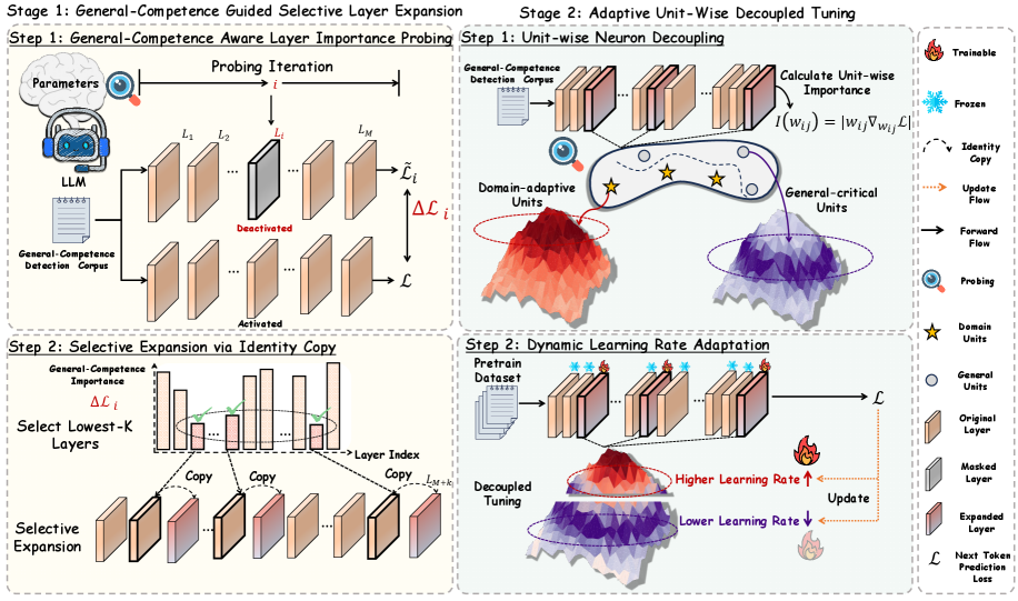
Figure 3: Illustration of ADEPT.
## 3 Methodology
As illustrated in Figure 3, ADEPT includes two stages:
- # Stage 1: General-Competence Guided Selective Layer Expansion. adaptively selects and duplicates layers that minimally affect general competencies while being more adaptable to domain-specific knowledge, thereby introducing fresh representational capacity for domain adaptation.
- # Stage 2: Adaptive Unit-Wise Decoupled Tuning. further decouples units within the expanded layers and apply learning-rate–driven adaptive tuning according to their importance to the general domain, ensuring knowledge injection while preserving general competencies.
### 3.1 General-Competence Guided Selective Layer Expansion
This stage aims to selectively expand model parameters in a way that introduces fresh representational capacity for domain adaptation while preserving general-domain competencies. To this end, we first estimate the contribution of each transformer layer to preserving general knowledge through General-Competence Aware Layer Importance Probing, and then perform Selective Parameter Expansion via Identity Copy to duplicate layers that are least critical for general abilities yet more adaptable to domain-specific knowledge.
General-Competence Aware Layer Importance Probing. To guide selective expansion, we leverage the layer importance scores $I_layer^(l)$ defined as Eq. 3. Intuitively, $I_layer^(l)$ quantifies how much the $l$ -th layer contributes to preserving general-domain knowledge. Layers with lower scores are deemed less critical for general competencies and are thus selected for expansion, as they can accommodate domain-specific adaptation with minimal risk of catastrophic forgetting.
Selective Parameter Expansion via Identity Copy. Based on the importance scores $I_layer^(l)$ , we sort layers by ascending importance and select the $k$ least-important ones for general competence:
$$
S_k=\operatorname*{arg min}_\begin{subarray{c}S⊆\{1,…,L\}\\
|S|=k\end{subarray}}∑_l∈SI_layer^(l). \tag{6}
$$
We denote the selected set $S_k$ as the Domain-Adaptable Layers. For each selected layer $l∈S_k$ , we create a parallel copy by directly duplicating its parameters without re-initialization ( $\tilde{Θ}^(l)=Θ^(l)$ ). To preserve stability, we follow the Function Preserving Initialization (FPI) principle (Chen et al., 2015), ensuring that the expanded model $M_1$ produces identical outputs as the original model $M_0$ at initialization. Concretely, in the duplicated branch, we set the output projections of both attention and feed-forward sublayers to zero ( $W_MHSA^out=0, W_FFN^out=0$ ), so the forward computation remains unchanged ( $M_1(x)=M_0(x), ∀ x$ ). The duplicated layers thus provide fresh representational capacity that can specialize for domain signals with minimal risk of eroding general-knowledge-critical parameters in the original pathway. As formally established in Appendix F.1, expanding the layers with the lowest general-competence importance provably minimizes the risk of forgetting. Intuitively, this strategy ensures that new capacity is added where interference with general abilities is weakest, yielding the most favorable trade-off between domain adaptation and knowledge retention.
### 3.2 Adaptive Unit-Wise Decoupled Tuning
This stage aims to further reduce catastrophic forgetting and enable fine-grained control over parameters within the expanded layers. To achieve this, we first decouple each expanded layer into semantic units and evaluate their importance using gradient-based estimation (Unit-wise Neuron Decoupling), and then dynamically adjust learning rates for different units according to their importance scores during training (Dynamic Learning Rate Adaptation).
Unit-wise Neuron Decoupling. Guided by the heterogeneous importance of parameter units within layers, we performs unit-level decoupling on the expanded layers. Following the probing analysis in Section 2.3, we quantify unit importance $I_unit$ using gradient sensitivity signals (cf. Eq. 5), which aggregate the first-order contributions of parameters $θ_j$ to the training loss $L$ via $∇_θ_{j}L$ . A higher $I_unit$ indicates greater contribution to general competencies and thus warrants more conservative updates, whereas less important units are encouraged to adapt more aggressively to domain-specific signals.
Dynamic Learning Rate Adaptation. Based on the unit importance $I_unit$ in Eq. 5, we assign adaptive learning rates to different units within the expanded layers:
$$
lr_U=2·(1-I_unit)·lr_base, \tag{7}
$$
where $lr_base$ is the base learning rate, and the coefficient $2$ normalizes the global scale to keep the effective average approximately unchanged. Units more important for general knowledge (higher $I_unit$ ) receive smaller learning rates to reduce overwriting, while less important units are encouraged to adapt more aggressively to domain-specific data. Training proceeds with the standard autoregressive objective: $L=-∑_t=1^T\log P(x_t\mid x_<t;Θ)$ . Since the importance of units may change as training progresses, we periodically recompute $I_unit$ and update learning rates accordingly, ensuring dynamic adaptation throughout learning. The full training procedure is provided in Appendix L. Appendix F.2 further shows that allocating learning rates inversely to unit importance minimizes an upper bound on general-domain forgetting. In essence, this design formalizes the intuition that highly general-critical units should be preserved via conservative updates, while less critical yet more adaptable ones can update more aggressively to absorb domain-specific information.
Table 1: Performance comparison across Mathematical and Medical domains. Bold numbers indicate the best performance, and underlined numbers denote the second best.
| Method | Mathematics | Medical | | | | | | | | |
| --- | --- | --- | --- | --- | --- | --- | --- | --- | --- | --- |
| General | Domain | General | Domain | | | | | | | |
| MMLU | CMMLU | GSM8K | ARC-Easy | ARC-Challenge | MMLU | CMMLU | MedQA | MMCU-Medical | CMB | |
| Qwen3-1.7B-Base | | | | | | | | | | |
| Vanilla | 62.57 | 66.86 | 57.62 | 81.44 | 51.19 | 62.57 | 66.86 | 48.39 | 69.17 | 63.67 |
| PT-Full | 60.07 | 62.84 | 51.86 | 81.24 | 49.65 | 59.44 | 62.84 | 48.45 | 67.45 | 62.77 |
| Replay | 60.69 | 63.52 | 54.74 | 81.01 | 49.73 | 60.52 | 63.85 | 49.00 | 67.32 | 62.20 |
| Llama-Pro | 61.54 | 63.40 | 60.03 | 81.08 | 49.80 | 59.80 | 65.51 | 50.43 | 66.51 | 63.54 |
| PT-LoRA | 60.07 | 62.69 | 59.50 | 80.22 | 49.34 | 57.31 | 59.68 | 47.29 | 61.55 | 57.60 |
| TaSL | 60.34 | 62.95 | 59.07 | 79.76 | 48.89 | 62.48 | 66.14 | 47.06 | 67.62 | 61.15 |
| ADEPT | 62.62 | 67.06 | 70.51 | 82.48 | 52.62 | 62.80 | 66.89 | 50.75 | 71.98 | 65.43 |
| Qwen3-4B-Base | | | | | | | | | | |
| Vanilla | 73.19 | 77.92 | 69.07 | 85.52 | 59.13 | 73.19 | 77.92 | 62.77 | 82.44 | 78.92 |
| PT-Full | 70.33 | 73.07 | 60.96 | 85.31 | 57.59 | 69.48 | 72.77 | 62.84 | 81.34 | 76.88 |
| Replay | 70.46 | 73.72 | 63.91 | 85.06 | 57.68 | 70.74 | 73.81 | 63.55 | 80.60 | 76.74 |
| Llama-Pro | 72.42 | 77.39 | 73.16 | 85.14 | 57.76 | 72.28 | 77.28 | 62.53 | 81.20 | 78.12 |
| PT-LoRA | 70.20 | 72.90 | 71.34 | 84.18 | 57.25 | 72.73 | 76.78 | 61.59 | 80.49 | 76.92 |
| TaSL | 70.50 | 73.20 | 70.84 | 83.68 | 56.75 | 73.03 | 77.08 | 60.99 | 79.20 | 77.08 |
| ADEPT | 73.21 | 78.30 | 76.19 | 88.44 | 60.98 | 72.95 | 78.77 | 64.49 | 84.58 | 79.87 |
| Qwen3-8B-Base | | | | | | | | | | |
| Vanilla | 76.94 | 82.09 | 69.98 | 87.12 | 64.25 | 76.94 | 82.09 | 66.30 | 86.45 | 81.67 |
| PT-Full | 74.90 | 78.49 | 80.21 | 85.90 | 61.77 | 74.06 | 78.82 | 67.24 | 87.69 | 85.27 |
| Replay | 75.19 | 78.92 | 81.12 | 85.98 | 62.37 | 74.51 | 78.86 | 68.89 | 86.66 | 84.73 |
| Llama-Pro | 76.16 | 81.42 | 80.97 | 86.62 | 63.91 | 76.58 | 81.69 | 66.77 | 87.19 | 83.76 |
| PT-LoRA | 75.66 | 80.81 | 82.87 | 86.36 | 62.46 | 76.60 | 81.57 | 67.01 | 86.70 | 83.04 |
| TaSL | 76.63 | 80.37 | 80.54 | 84.81 | 59.09 | 76.42 | 81.86 | 66.51 | 86.20 | 82.54 |
| ADEPT | 76.80 | 82.11 | 83.87 | 89.29 | 64.51 | 76.77 | 82.11 | 69.24 | 89.84 | 85.80 |
| Llama3-8B-Base | | | | | | | | | | |
| Vanilla | 65.33 | 50.83 | 36.84 | 84.18 | 54.01 | 65.33 | 50.83 | 58.91 | 46.29 | 35.61 |
| PT-Full | 61.62 | 46.21 | 49.73 | 84.01 | 53.52 | 59.15 | 51.39 | 59.23 | 66.58 | 61.65 |
| Replay | 62.00 | 53.31 | 49.51 | 82.49 | 54.18 | 59.98 | 54.52 | 59.07 | 65.84 | 61.71 |
| Llama-Pro | 64.53 | 50.26 | 48.29 | 83.29 | 53.07 | 64.19 | 50.59 | 59.94 | 53.96 | 47.05 |
| PT-LoRA | 64.86 | 49.82 | 48.82 | 83.80 | 54.01 | 64.34 | 50.13 | 58.84 | 56.05 | 48.22 |
| TaSL | 65.16 | 50.11 | 35.43 | 83.29 | 53.51 | 64.64 | 50.43 | 55.55 | 58.34 | 47.69 |
| ADEPT | 65.35 | 51.90 | 50.57 | 84.96 | 55.52 | 65.17 | 51.92 | 61.17 | 67.03 | 61.78 |
## 4 Experiment
### 4.1 Experimental Setup
Datasets. We evaluate ADEPT across two domains, Mathematics and Medicine. For the mathematical domain, we use OpenWebMath (Paster et al., 2023), together with AceReason-Math (Chen et al., 2025), concatenated into the continual pretraining corpora. For the medical domain, we adopt the multilingual MMedC corpus (Qiu et al., 2024), together with IndustryIns and MMedBench, forming the medical pretraining corpora. Dataset statistics are provided in Appendix B.1 and Appendix B.2. In addition, for detecting general-knowledge-critical regions, we construct a General Competence Detection Corpus, following the same setting as in Section 2 and described in Appendix B.3.
Baselines. We compare ADEPT with a broad range of baselines from four perspectives:
- Full-parameter tuning. PT-Full directly updates all model parameters on the target corpora.
- Replay-based tuning. Replay mitigates catastrophic forgetting by mixing general-domain data into the training process (Que et al., 2024).
- Architecture expansion. LLaMA-Pro (Wu et al., 2024b) expands the model by uniformly inserting new layers into each transformer block while freezing the original weights. Only the newly introduced parameters are trained, enabling structural growth while preserving prior knowledge.
- Parameter-efficient tuning. PT-LoRA performs CPT using Low-Rank Adaptation (Hu et al., 2022), updating only a small set of task-adaptive parameters. TaSL (Feng et al., 2024a) extends PT-LoRA to a multi-task regime by decoupling LoRA matrices across transformer layers, allowing different subsets of parameters to specialize for different tasks.
See Appendix B.6 for implementation details of all baselines.
Backbone Models. To assess the generality of our method, we instantiate ADEPT on multiple backbone models, including Qwen3-Base (1.7B, 4B, 8B) (Yang et al., 2025a) and LLaMA3.1-8B-Base (Dubey et al., 2024b), covering a wide range of parameter scales and architectural variants.
Evaluation Metrics and Strategy. We adopt multiple-choice question answering accuracy as the primary evaluation metric across all tasks (see Appendix B.9 for further details). For the Mathematics domain, we evaluate on GSM8K (Cobbe et al., 2021), ARC-Easy (Clark et al., 2018), and ARC-Challenge (Clark et al., 2018), which collectively span a wide range of reasoning difficulties. For the Medical domain, we use MedQA (Jin et al., 2021), MMCU-Medical (Zeng, 2023), and CMB (Wang et al., 2023b), covering diverse medical subjects and varying levels of complexity. Among them, MedQA is an English benchmark, while MMCU-Medical and CMB are in Chinese. To assess the model’s ability to retain general-domain knowledge during continual pretraining, we additionally evaluate on MMLU (Hendrycks et al., 2020) and CMMLU (Li et al., 2023), two broad-coverage benchmarks for general knowledge and reasoning in English and Chinese, respectively.
### 4.2 Experimental Results
Performance Comparison. As shown in Table 1, ADEPT consistently outperforms all CPT baselines across both mathematical and medical domains, confirming its effectiveness in domain-specific knowledge acquisition while substantially alleviating catastrophic forgetting. Concretely, ADEPT achieves substantial domain-specific improvements. Across all backbones and domain benchmarks, ADEPT consistently surpasses baselines, achieving the strongest performance. For instance, on Qwen3-1.7B-Base, ADEPT boosts GSM8K accuracy from 57.62% to 70.51% $↑$ , bringing a large gain that highlights its advantage on enhancing LLMs’ complex reasoning. Similarly, on LLaMA3-8B-Base, it drastically improves CMB accuracy improves from 35.61% to 61.78% $↑$ , underscoring the strong enhancement of medical-domain capabilities. On average, ADEPT achieves up to 5.58% gains over full-parameter CPT on target-domain benchmarks, confirming its advantage in domain knowledge acquisition. Furthermore, ADEPT demonstrates clear advantages in mitigating catastrophic forgetting. Whereas most baselines suffer noticeable degradation on general benchmarks such as MMLU and CMMLU, ADEPT preserves the pretrained LLMs’ general-domain competencies, and in some cases even surpasses the vanilla backbone. Notably, with Qwen3-4B under medical CPT, ADEPT improves CMMLU accuracy from 77.92% to 78.77% $↑$ . It also results in an average performance increase of 5.76% on general benchmarks over full-parameter CPT. We attribute this to the disentanglement of domain-specific and general parameters, which prevents harmful representational interference during adaptation, ensuring that learning specialized knowledge does not corrupt the model’s foundational abilities. Instead, this focused learning process appears to refine the model’s overall competencies, leading to synergistic improvements on general-domain tasks. In summary, ADEPT offers a robust solution for CPT achieving superior domain adaptation while effectively preserving general knowledge.
Table 2: Ablation study on ADEPT in Medical domain. Bold numbers indicate the best performance, and underlined numbers denote the second best.
| Method | Qwen3-1.7B-Base | Llama3-8B-Base | | | | | | | | |
| --- | --- | --- | --- | --- | --- | --- | --- | --- | --- | --- |
| MMLU | CMMLU | MedQA | MMCU-Medical | CMB | MMLU | CMMLU | MedQA | MMCU-Medical | CMB | |
| ADEPT | 62.80 | 66.89 | 50.75 | 70.98 | 65.43 | 65.17 | 51.92 | 61.17 | 61.78 | 67.03 |
| w/o Stage-1 | 57.31 | 59.68 | 47.29 | 61.55 | 57.60 | 57.88 | 50.76 | 58.32 | 53.32 | 60.32 |
| w/o Stage-2 | 61.56 | 64.33 | 49.23 | 66.19 | 64.36 | 64.34 | 50.74 | 59.60 | 50.68 | 57.36 |
| Uniform Expansion | 59.80 | 65.51 | 50.43 | 66.51 | 63.54 | 64.19 | 50.59 | 59.94 | 47.05 | 53.96 |
Ablation Study. To investigate the effectiveness of each component in ADEPT, we conduct ablation experiments in the medical domain using two representative backbones, Qwen3-1.7B and Llama3-8B. In w/o Stage-1, we remove the General-Competence Guided Selective Layer Expansion and directly apply Adaptive Unit-Wise Decoupled Tuning on the $k$ Domain-Adaptable Layers without introducing any new parameters. In w/o Stage-2, we discard the dynamic decoupled tuning stage and instead directly fine-tune the expanded layers from Stage-1. In Uniform Expansion, we replace importance-guided expansion with uniformly inserted layers followed by fine-tuning, which is equivalent to the strategy adopted in LLaMA-Pro. As shown in Table 2, removing either Stage-1 or Stage-2 leads to clear degradation in both general and domain-specific performance, confirming that both adaptive expansion and decoupled tuning are indispensable. In particular, eliminating Stage-1 results in the largest performance drop, suggesting that adaptive capacity allocation is crucial for enabling effective domain adaptation without sacrificing general-domain competencies. Meanwhile, replacing importance-guided expansion with uniform expansion yields inferior results, underscoring the advantage of expanding only the most domain-adaptable layers.
<details>
<summary>x4.png Details</summary>
### Visual Description
\n
## Comparative Contour Plot with Marginal Distributions: Vanilla, W/o stage1, ADEPT
### Overview
The image displays three side-by-side plots comparing the 2D embedding distributions of "General Text" and "Medical Text" as produced by three different models or model variants: "Vanilla", "W/o stage1" (Without stage 1), and "ADEPT". Each plot is a contour plot with marginal density distributions shown on the top and right axes.
### Components/Axes
* **Plot Titles (Top Center):** "Vanilla", "W/o stage1", "ADEPT".
* **Axes Labels:**
* X-axis (Bottom): "dim 1" for all three plots.
* Y-axis (Left): "dim 2" for all three plots.
* **Axis Scales:**
* **Vanilla:** dim 1 ranges approximately from -75 to 75. dim 2 ranges approximately from -75 to 100.
* **W/o stage1:** dim 1 ranges approximately from -100 to 100. dim 2 ranges approximately from -60 to 60.
* **ADEPT:** dim 1 ranges approximately from -100 to 100. dim 2 ranges approximately from -60 to 60.
* **Legend (Top-right corner of each main plot area):**
* A blue line labeled "General Text".
* A red line labeled "Medical Text".
* **Plot Elements:**
* **Main Area:** 2D contour plots showing the density of data points for each text type. Blue contours represent "General Text", red contours represent "Medical Text".
* **Marginal Plots:** Density curves (histograms/KDEs) along the top (for dim 1 distribution) and right side (for dim 2 distribution) of each main plot, colored blue and red to match their respective text type.
### Detailed Analysis
**1. Vanilla Plot (Left):**
* **Contour Analysis:** The blue ("General Text") and red ("Medical Text") contour clouds show significant overlap, particularly in the central region around dim1=0, dim2=0. The "General Text" distribution appears more spread out, especially along the positive dim2 axis. The "Medical Text" distribution is more concentrated but still overlaps substantially with the blue contours.
* **Marginal Distributions (Top - dim1):** Both the blue and red density curves are broad and overlapping, with multiple peaks. The red curve ("Medical Text") has a slightly more pronounced peak near dim1=0.
* **Marginal Distributions (Right - dim2):** The blue curve is very broad, spanning from approximately -75 to 100. The red curve is narrower, centered around dim2=0, but still overlaps with the lower portion of the blue curve.
**2. W/o stage1 Plot (Center):**
* **Contour Analysis:** The separation between the two distributions is more pronounced than in the "Vanilla" plot. The blue ("General Text") contours form a cluster primarily in the lower-left quadrant (negative dim1, negative dim2). The red ("Medical Text") contours form a cluster primarily in the upper-right quadrant (positive dim1, positive dim2). There is a region of overlap in the center.
* **Marginal Distributions (Top - dim1):** The blue and red curves are now clearly bimodal and separated. The blue curve peaks in the negative dim1 region, while the red curve peaks in the positive dim1 region.
* **Marginal Distributions (Right - dim2):** Similar separation is visible. The blue curve peaks in the negative dim2 region, and the red curve peaks in the positive dim2 region.
**3. ADEPT Plot (Right):**
* **Contour Analysis:** This plot shows the clearest separation between the two text types. The blue ("General Text") contours are densely clustered in a distinct region, primarily in the lower-left to central area. The red ("Medical Text") contours form a separate, dense cluster in the upper-right area. The overlap between the two is minimal compared to the other plots.
* **Marginal Distributions (Top - dim1):** The separation is very clear. The blue curve has a sharp peak in the negative dim1 region (around -50). The red curve has a sharp peak in the positive dim1 region (around +25).
* **Marginal Distributions (Right - dim2):** The separation is also very clear here. The blue curve peaks in the negative dim2 region (around -20). The red curve peaks in the positive dim2 region (around +20).
### Key Observations
1. **Progressive Separation:** There is a clear visual progression from high overlap ("Vanilla") to moderate separation ("W/o stage1") to strong separation ("ADEPT") between the embedding distributions of General Text and Medical Text.
2. **Cluster Tightening:** As the models progress from Vanilla to ADEPT, the contour clusters for each text type become tighter and more defined, indicating less variance within each category in the learned embedding space.
3. **Marginal Distribution Clarity:** The marginal density plots provide a clear, 1D confirmation of the separation observed in the 2D contours. The peaks for General and Medical text become sharper and move further apart along both dimensions in the ADEPT model.
4. **Spatial Grounding:** In all plots, the legend is consistently placed in the top-right corner of the main plot area. The color coding (blue=General, red=Medical) is consistent across all elements (contours, marginal lines, legend).
### Interpretation
This visualization demonstrates the effectiveness of the "ADEPT" model (and to a lesser extent, the "W/o stage1" variant) in learning a disentangled representation space for text from different domains. The "Vanilla" model fails to distinguish between general and medical text, mapping them to largely overlapping regions. This could hinder performance on domain-specific tasks.
The progression suggests that the architectural or training modifications in "W/o stage1" and especially "ADEPT" successfully encourage the model to encode domain-specific semantic features into distinct dimensions of the embedding space. The clear separation in the ADEPT plot implies that a classifier or downstream task could more easily distinguish between or specialize for these text types using its embeddings. This is a desirable property for building specialized NLP models for fields like medicine, where domain-specific language understanding is critical. The tight clustering also suggests more consistent and confident representations within each domain.
</details>
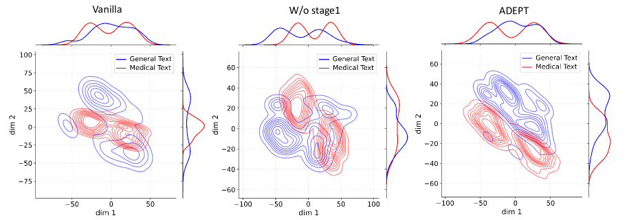
Figure 4: Activation distribution analysis of Qwen3-8B.
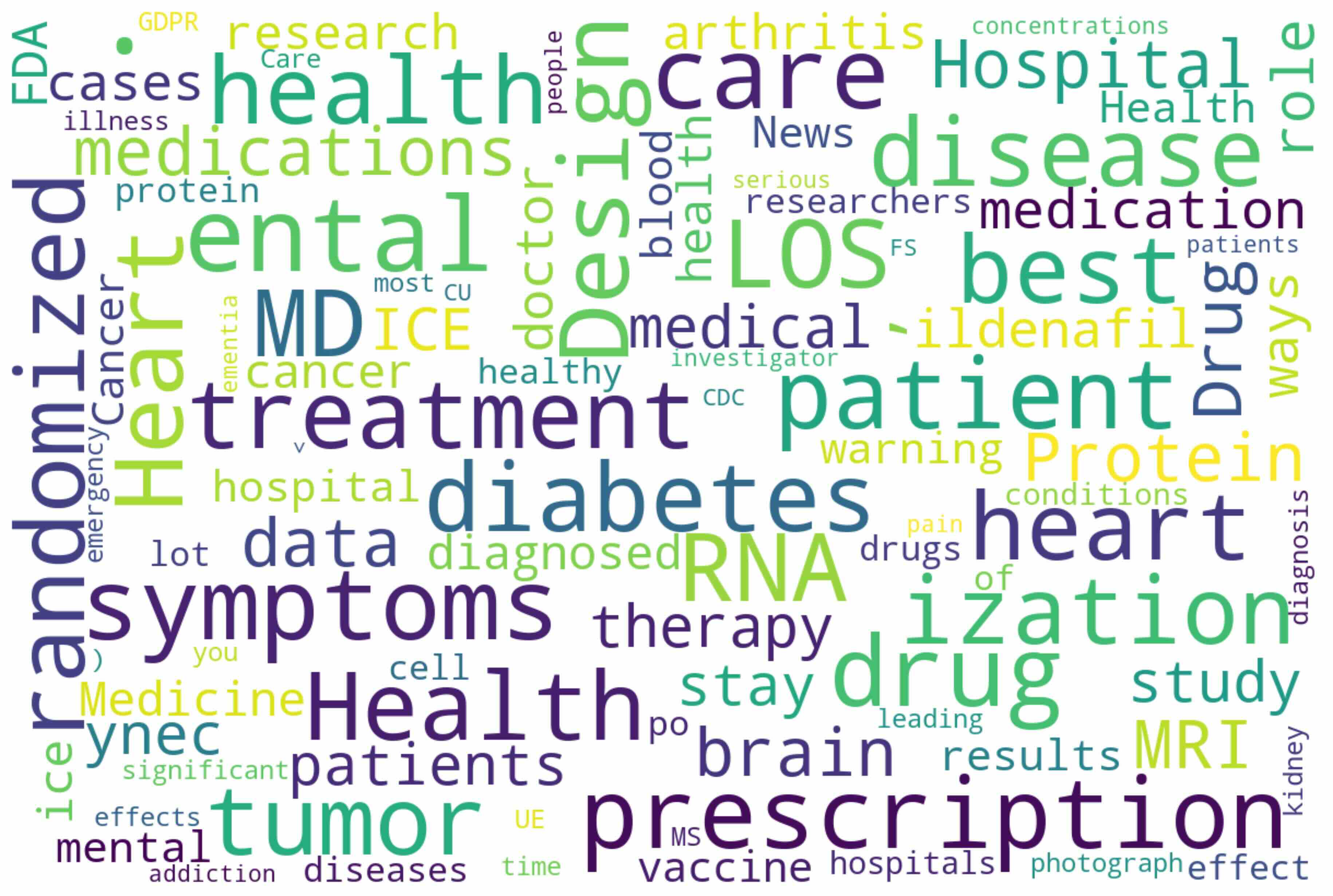
Decoupling Effectiveness on Expanded Parameters. We visualize cross-domain activations using Kernel Density Estimation (KDE) (Silverman, 2018), sampling 500 instances from both Medical and General corpora. For the original Qwen3-8B-Base (left in Figure 4), the most domain-adaptable layer (lowest $I_layer$ ) still shows heavy overlap between general and medical activations, evidencing strong parameter coupling. Direct decoupling without expansion (w/o Stage-1, middle) on the same layer fails to reduce this entanglement, confirming that pretrained parameters are inherently difficult to separate. In contrast, after expansion (right), the duplicated layers serve as a “blank slate,” yielding clearly separated activations across domains. Additional analyses on more backbones are provided in Appendix C.1, where we observe that this trend consistently holds across nearly all evaluated LLMs, further validating the generality of our approach.
<details>
<summary>figures/wordcloud_med.jpg Details</summary>
### Visual Description
## Word Cloud: Healthcare and Medical Research Terminology
### Overview
The image is a word cloud visualization. In a word cloud, the size of each word typically represents its frequency or importance within a source text or dataset. The words are presented in various colors (primarily shades of green, blue, purple, and yellow) and orientations (horizontal and vertical) against a white background. The overall theme is heavily focused on healthcare, medicine, clinical research, and patient care.
### Components/Axes
As a word cloud, there are no formal axes, legends, or data points. The primary components are the words themselves. Their relative size is the key visual variable conveying information.
### Detailed Analysis
The words can be categorized by their apparent visual prominence (size). Below is a comprehensive list, grouped by approximate size tier for clarity.
**Tier 1 - Largest/Prominent Words:**
* treatment
* patient
* diabetes
* symptoms
* Health
* prescription
* randomized
* disease
* care
* drug
* hospital
* data
* heart
* tumor
* RNA
* mental
* best
* medical
* ization (likely a suffix, e.g., from "hospitalization" or "randomization")
* Design
**Tier 2 - Medium-Sized Words:**
* health
* medications
* cancer
* protein
* therapy
* brain
* study
* patients
* doctor
* blood
* research
* cases
* medicine
* results
* MRI
* vaccine
* diseases
* effect
* role
* pain
* conditions
* warning
* diagnosis
* cell
* significant
* effects
* time
* hospitals
* photograph
* leading
* ways
* stay
* lot
* diagnosed
* healthy
* investigator
* serious
* researchers
* News
* concentrations
* arthritis
* people
* illness
* emergency
* dementia
* CU (likely an abbreviation)
* most
* v (likely an abbreviation)
* CDC
* FS (likely an abbreviation)
* MS (likely an abbreviation)
* UE (likely an abbreviation)
* po (medical abbreviation for "by mouth")
* y nec (likely a fragment, e.g., from "gynecology")
* ice (likely a fragment, e.g., from "device" or "practice")
* drugs
* of
* you
* ild enafil (likely a fragment of "sildenafil")
**Tier 3 - Smaller Words:**
* FDA
* GDPR
* Care
* Cancer
* kidney
### Key Observations
1. **Dominant Themes:** The largest words form the core themes: `treatment`, `patient`, `diabetes`, `symptoms`, `Health`, `prescription`, `randomized`, `disease`, `care`, `drug`, `hospital`, `data`, `heart`, `tumor`, `RNA`, `mental`. This strongly suggests the source data is related to clinical studies, patient outcomes, and therapeutic interventions.
2. **Research Context:** The prominence of `randomized`, `data`, `study`, `research`, `results`, and `investigator` indicates a focus on clinical trial methodology and evidence-based medicine.
3. **Specific Conditions:** Key medical conditions highlighted include `diabetes`, `heart` (disease), `cancer`, `tumor`, `arthritis`, `mental` (health), and `dementia`.
4. **Medical Interventions:** Terms like `treatment`, `drug`, `prescription`, `medications`, `therapy`, `vaccine`, and `MRI` point to diagnostic and therapeutic procedures.
5. **Institutional & Regulatory:** Words such as `hospital`, `FDA`, `GDPR`, `CDC`, and `doctor` reference the healthcare system and its regulatory environment.
6. **Visual Design:** The color palette (greens, blues, purples) is common in medical and scientific visualizations. The mix of horizontal and vertical text increases density but can reduce readability for some words.
### Interpretation
This word cloud visually synthesizes a large body of text, likely from medical literature, clinical trial reports, or healthcare news. The data suggests a primary focus on **managing chronic and serious diseases** (diabetes, heart disease, cancer) through **evidence-based treatments** (`randomized` trials, `drug` therapies, `prescription` management) within the **hospital and clinical care** system.
The equal prominence of `patient`, `symptoms`, and `data` underscores a modern healthcare paradigm that balances patient-centered care with quantitative analysis. The presence of `RNA` and `protein` alongside `tumor` and `cancer` hints at discussions around targeted therapies or biomarkers. The inclusion of `mental` health and `dementia` reflects an expanding scope of medical research beyond purely physical ailments.
**Notable Anomaly/Observation:** The word `ization` appears very large but is a suffix. This is a common artifact in automated word cloud generation from raw text, where word stemming or splitting is imperfect. Its size suggests that words ending in "-ization" (e.g., hospitalization, randomization, immunization) are extremely frequent in the source material, reinforcing the themes of clinical processes and procedures.
In essence, the cloud depicts the interconnected lexicon of modern clinical research and practice, where patient care, specific diseases, therapeutic drugs, and rigorous data collection are the central, interlocking components.
</details>
(a) Token distributions shift in Medical
<details>
<summary>figures/wordcloud_math.jpg Details</summary>
### Visual Description
## Word Cloud: Academic/Technical Terminology
### Overview
The image is a word cloud visualization. It displays a collection of words and short phrases, primarily in English, with varying font sizes, colors, and orientations. The size of each word typically represents its frequency or importance within an underlying source text, which appears to be from academic, scientific, or technical literature. There is no quantitative data, axis, or legend; the information is purely textual and relational based on visual prominence.
### Components/Axes
* **Type:** Word Cloud.
* **Primary Language:** English.
* **Visual Variables:**
* **Font Size:** Indicates relative frequency/importance. Larger words are more prominent.
* **Color:** Words are rendered in a palette of dark purple, teal/green, and yellow/lime green. Color may be used for aesthetic grouping or to denote different categories from the source, but no legend is provided to define this.
* **Orientation:** Most words are horizontal. A few are rotated vertically (e.g., "algorithm", "students", "paper", "user", "example", "Tony's", "ric", "the", "value", "chmer", "features", "case", "qu", "de", "s").
* **Layout:** Words are densely packed and overlapping in a seemingly random arrangement to fill the rectangular space.
### Detailed Analysis
**Extracted Text (Grouped by approximate visual prominence/color):**
* **Large, Prominent Terms (Likely High Frequency):**
* `effects` (dark purple, top-left)
* `space` (teal, top-center)
* `mathematic` (yellow, upper-center)
* `question` (dark purple, upper-right)
* `the` (dark purple, vertical, center-right)
* `following` (dark purple, center)
* `problem` (teal, lower-left)
* `bit` (teal, center-bottom)
* `Oct` (dark purple, bottom-left)
* `previous` (teal, bottom-center)
* `quantum` (yellow, bottom-right)
* `answer` (teal, bottom)
* `isation` (teal, bottom-right corner)
* **Medium-Sized Terms:**
* `paper` (yellow, vertical, left)
* `et` (dark purple, left)
* `scripts` (yellow, left-center)
* `talk` (dark purple, left-center)
* `sense` (dark purple, left-center)
* `editor` (dark purple, center)
* `esium` (teal, center-right)
* `results` (teal, bottom-right)
* `model` (teal, bottom-center)
* `PhD` (yellow, upper-right)
* `groups` (dark purple, upper-right)
* `physics` (yellow, center)
* `CM` (teal, center)
* `scatter` (dark purple, upper-left)
* `reaction` (teal, center)
* `identity` (teal, center-right)
* `parameters` (dark purple, bottom)
* `theorem` (dark purple, bottom)
* **Smaller Terms and Fragments:**
* `ob`, `ariance`, `Sch`, `phenotype`, `$x`, `ex`, `quant`, `new`, `)`, `{`, `b1`, `code`, `FT`, `ATE`, `he`, `error`, `profit`, `open`, `al`, `value`, `Rig`, `2`, `ule`, `ormal`, `to`, `A`, `chmer`, `features`, `ja`, `Sized`, `ric`, `Tony's`, `F..`, `?`, `example`, `students`, `user`, `algorithm`, `de`, `udos`, `s`, `connected`, `qu`, `ag`, `sh`, `case`, `I`, `{`, `$$`, `pton`, `papers`.
* **Symbols and Punctuation:**
* `$x`, `$$`, `?`, `..`, `'`, `(`, `)`, `{`, `}`, `.`, `,`
### Key Observations
1. **Dominant Themes:** The largest words point to core themes: **problem-solving** (`problem`, `answer`, `question`, `sense`), **academic/research context** (`paper`, `PhD`, `results`, `model`, `theorem`, `parameters`, `editor`), **technical/scientific domains** (`quantum`, `physics`, `mathematic`, `algorithm`, `space`, `effects`), and **process/structure** (`following`, `previous`, `Oct`, `bit`, `isation`).
2. **Color Distribution:** The three-color scheme (dark purple, teal, yellow) is distributed throughout the cloud without an immediately obvious categorical pattern based on word meaning. It may be purely aesthetic or derived from an unstated grouping in the source data.
3. **Textual Nature:** The cloud contains many academic shorthand terms (`et`, `al`, `ob`, `ric`, `qu`), mathematical symbols (`$x`, `$$`), and potential name fragments (`Tony's`, `Sch`, `CM`, `AG`).
4. **No Quantitative Data:** As a word cloud, it conveys relative importance through size but provides no exact counts, frequencies, or statistical measures.
### Interpretation
This word cloud visually summarizes a body of text likely drawn from academic or technical writing, possibly in fields like computational science, physics, or quantitative research. The prominence of "problem," "answer," "question," and "following" suggests a focus on methodology, inquiry, and logical progression. Terms like "quantum," "physics," "mathematic," and "algorithm" indicate a strong scientific and computational foundation. The presence of "PhD," "paper," "editor," and "results" firmly places the context within research and publication.
The cloud effectively highlights the lexicon's core components but abstracts away the specific relationships and narrative. It serves as a thematic fingerprint, showing that the source material is concerned with defining and solving problems using mathematical and computational models within a formal academic framework. The inclusion of fragments and symbols (`$x`, `et`, `al`) reinforces the technical and citation-heavy nature of the original text.
</details>
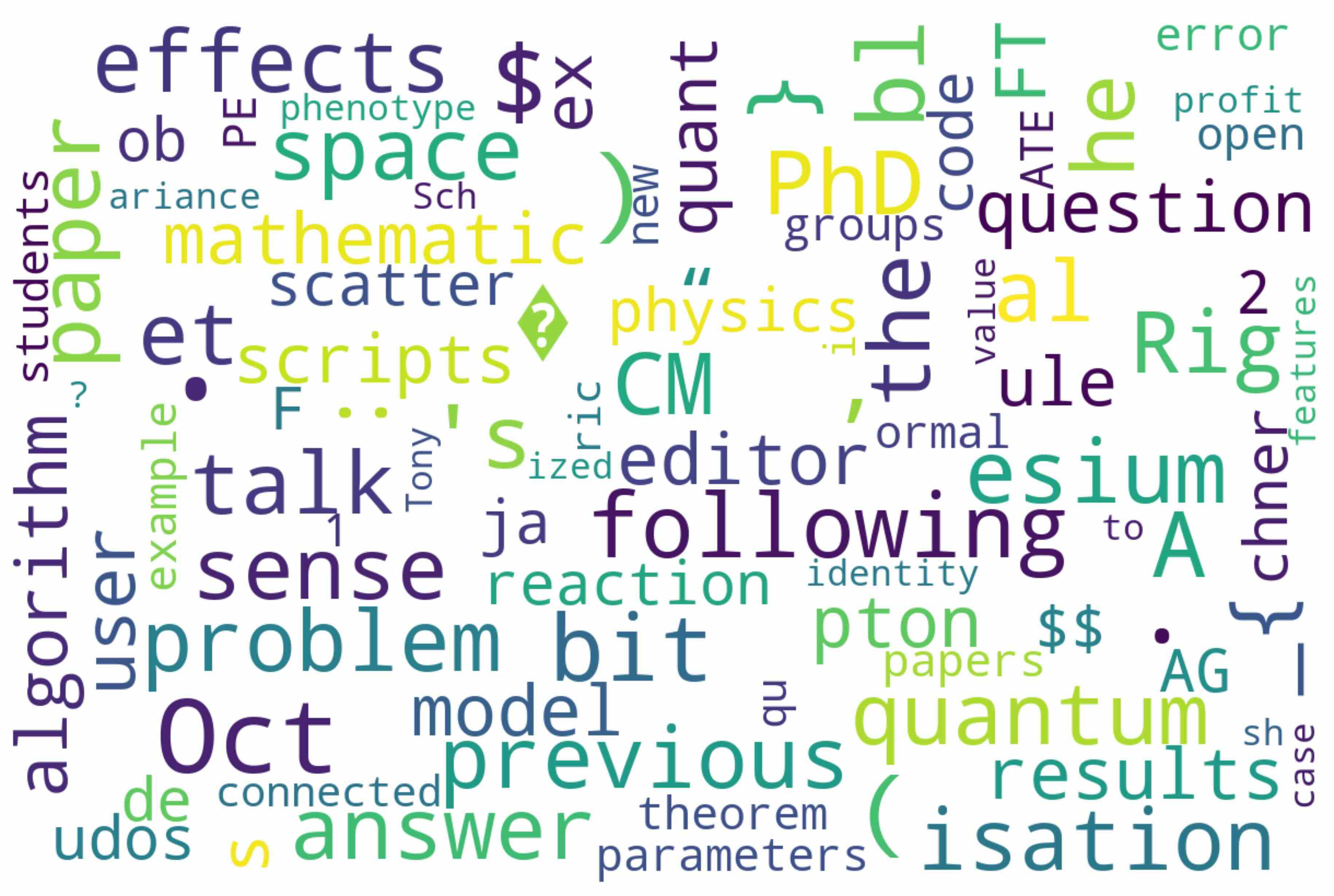
(b) Token distributions shift in Mathematical
Figure 5: Token distribution shifts across domains. Word cloud visualizations of shifted tokens reveal that ADEPT achieves highly focused alignment, with most changes concentrated on domain-specific terminology.
Token Distribution Shift Analysis. To assess how ADEPT injects domain knowledge while preserving general competencies, we analyze token-level shifts between the base and continually pretrained models. Following Lin et al. (2024), tokens are categorized as unshifted, marginal, or shifted. Only a small proportion of tokens shift, while most remain unchanged, indicating stable adaptation. In the medical domain, merely 2.18% shift (vs. 5.61% under full pretraining), largely medical terms such as “prescription,” “diagnosis,” and “therapy” (Figure 5(a)). In the mathematical domain, only 1.24% shift, mainly scientific terms such as “theorem” and “equation” (Figure 5(b)). Further details and analyses are provided in Appendix I. These results demonstrate that ADEPT achieves precise and economical domain knowledge injection while minimizing perturbation to general competence.
Extended Investigations and Key Insights. We further investigate several design choices of ADEPT in appendix: In Appendix E, we investigate alternative strategies for probing layer importance and observe the consistency of different measurement methods, offering insight into how importance estimation affects adaptation outcomes. Appendix G explores the effect of expanding different numbers of layers and reveals how the number of expansion layers should be selected under different circumstances and the potential reasons behind this. Appendix H shows that even with relatively low-quality importance detection corpus from pretrain data, our approach maintains strong generalization across domains, suggesting the robustness of ADEPT. Appendix J demonstrates our insights into the potential for merging expanded layers that are independently trained on different domains, offering an intriguing direction for achieving multi-domain adaptation with minimal catastrophic forgetting. In addition, Appendix B.8 analyzes the training efficiency of ADEPT, showing that our selective updating design substantially accelerates convergence compared to baselines.
## 5 Conclusions and Future Works
We present ADEPT, a framework for LLM continual pretraining for domain adaptation that effectively tackles catastrophic forgetting, leveraging functional specialization in LLMs. By selectively expanding layers less critical to the general domain and adaptively updating decoupled parameter units, ADEPT minimizes catastrophic forgetting while efficiently incorporating domain-specific expertise. Our experiments show significant improvements in both domain performance and general knowledge retention compared to baselines. Future work could focus on refining the decoupled tuning mechanism, designing more sophisticated learning rate strategies beyond linear mapping to allow for more precise adjustments. Another direction is to explore better dynamic and real-time methods for measuring parameter importance during training.
## 6 Ethics Statement
All datasets used for training and evaluation in this study are publicly available versions obtained from the Hugging Face platform. The datasets have been curated, cleaned, and de-identified by their respective data providers prior to release. No patient personal information or identifiable medical data is present. Consequently, the research does not involve human subjects, and there are no related concerns regarding privacy, confidentiality, or legal liability. And for full transparency, we report all aspects of large language model (LLM) involvement in the Appendix K.
We strictly adhered to the usage and redistribution licenses provided by the original dataset authors and hosting platforms. Our research poses no risk of harm to individuals or groups and does not contain any potentially harmful insights, models, or applications. Additionally, there are no conflicts of interest or sponsorship concerns associated with this work. We are committed to research integrity and ethical standards consistent with the ICLR Code of Ethics.
## 7 Reproducibility Statement
We actively support the spirit of openness and reproducibility advocated by ICLR. To ensure the reproducibility of our research, we have taken the following measures:
1. Disclosure of Base Models: All base models used in our experiments are explicitly identified and described in the main text. This allows readers to directly reference and obtain these models.
1. Datasets and Experimental Details: All experiments are conducted on publicly available datasets from the Hugging Face platform. In Appendix B, we provide a comprehensive description of our experimental implementation, including dataset sources, browser links, and detailed data processing procedures. We also detail the experimental setup, such as training duration, hardware environment (e.g., GPU type), and configuration of hyperparameters, including LoRA_rank, number of extended layers, batch_size, and max_length. These details facilitate transparent verification and replication of our results.
1. Open-Source Code Release: To further support reproducibility, we release all training and evaluation code in an anonymous repository (https://anonymous.4open.science/status/ADEPT-F2E3). The repository contains clear instructions on installation, data downloading, preprocessing, and experimentation, allowing interested researchers to replicate our results with minimal effort.
## References
- Aghajanyan et al. (2021) Armen Aghajanyan, Sonal Gupta, and Luke Zettlemoyer. Intrinsic dimensionality explains the effectiveness of language model fine-tuning. In Chengqing Zong, Fei Xia, Wenjie Li, and Roberto Navigli (eds.), Proceedings of the 59th Annual Meeting of the Association for Computational Linguistics and the 11th International Joint Conference on Natural Language Processing, ACL/IJCNLP 2021, (Volume 1: Long Papers), Virtual Event, August 1-6, 2021, pp. 7319–7328. Association for Computational Linguistics, 2021. doi: 10.18653/V1/2021.ACL-LONG.568. URL https://doi.org/10.18653/v1/2021.acl-long.568.
- Ahn et al. (2024) Janice Ahn, Rishu Verma, Renze Lou, Di Liu, Rui Zhang, and Wenpeng Yin. Large language models for mathematical reasoning: Progresses and challenges. In Proceedings of the 18th Conference of the European Chapter of the Association for Computational Linguistics: Student Research Workshop, pp. 225–237, 2024.
- Arbel et al. (2024) Iftach Arbel, Yehonathan Refael, and Ofir Lindenbaum. Transformllm: Adapting large language models via llm-transformed reading comprehension text. arXiv preprint arXiv:2410.21479, 2024.
- Chen et al. (2024) Junying Chen, Zhenyang Cai, Ke Ji, Xidong Wang, Wanlong Liu, Rongsheng Wang, Jianye Hou, and Benyou Wang. Huatuogpt-o1, towards medical complex reasoning with llms. arXiv preprint arXiv:2412.18925, 2024.
- Chen et al. (2015) Tianqi Chen, Ian Goodfellow, and Jonathon Shlens. Net2net: Accelerating learning via knowledge transfer. arXiv preprint arXiv:1511.05641, 2015.
- Chen et al. (2025) Yang Chen, Zhuolin Yang, Zihan Liu, Chankyu Lee, Peng Xu, Mohammad Shoeybi, Bryan Catanzaro, and Wei Ping. Acereason-nemotron: Advancing math and code reasoning through reinforcement learning. arXiv preprint arXiv:2505.16400, 2025.
- Cheng et al. (2023) Daixuan Cheng, Shaohan Huang, and Furu Wei. Adapting large language models via reading comprehension. In The Twelfth International Conference on Learning Representations, 2023.
- Clark et al. (2019) Kevin Clark, Urvashi Khandelwal, Omer Levy, and Christopher D. Manning. What does BERT look at? an analysis of bert’s attention. In Tal Linzen, Grzegorz Chrupala, Yonatan Belinkov, and Dieuwke Hupkes (eds.), Proceedings of the 2019 ACL Workshop BlackboxNLP: Analyzing and Interpreting Neural Networks for NLP, BlackboxNLP@ACL 2019, Florence, Italy, August 1, 2019, pp. 276–286. Association for Computational Linguistics, 2019. doi: 10.18653/V1/W19-4828. URL https://doi.org/10.18653/v1/W19-4828.
- Clark et al. (2018) Peter Clark, Isaac Cowhey, Oren Etzioni, Tushar Khot, Ashish Sabharwal, Carissa Schoenick, and Oyvind Tafjord. Think you have solved question answering? try arc, the ai2 reasoning challenge. arXiv preprint arXiv:1803.05457, 2018.
- Cobbe et al. (2021) Karl Cobbe, Vineet Kosaraju, Mohammad Bavarian, Mark Chen, Heewoo Jun, Lukasz Kaiser, Matthias Plappert, Jerry Tworek, Jacob Hilton, Reiichiro Nakano, et al. Training verifiers to solve math word problems. arXiv preprint arXiv:2110.14168, 2021.
- Dai et al. (2022) Damai Dai, Li Dong, Yaru Hao, Zhifang Sui, Baobao Chang, and Furu Wei. Knowledge neurons in pretrained transformers. In Proceedings of the 60th Annual Meeting of the Association for Computational Linguistics (Volume 1: Long Papers), pp. 8493–8502, 2022.
- Ding et al. (2024) Hongxin Ding, Yue Fang, Runchuan Zhu, Xinke Jiang, Jinyang Zhang, Yongxin Xu, Xu Chu, Junfeng Zhao, and Yasha Wang. 3ds: Decomposed difficulty data selection’s case study on llm medical domain adaptation. arXiv preprint arXiv:2410.10901, 2024.
- Ding et al. (2025) Hongxin Ding, Baixiang Huang, Yue Fang, Weibin Liao, Xinke Jiang, Zheng Li, Junfeng Zhao, and Yasha Wang. Promed: Shapley information gain guided reinforcement learning for proactive medical llms. arXiv preprint arXiv:2508.13514, 2025.
- Dubey et al. (2024a) Abhimanyu Dubey, Abhinav Jauhri, Abhinav Pandey, Abhishek Kadian, Ahmad Al-Dahle, Aiesha Letman, Akhil Mathur, Alan Schelten, Amy Yang, Angela Fan, Anirudh Goyal, Anthony Hartshorn, Aobo Yang, Archi Mitra, Archie Sravankumar, Artem Korenev, Arthur Hinsvark, Arun Rao, Aston Zhang, Aurélien Rodriguez, Austen Gregerson, Ava Spataru, Baptiste Rozière, Bethany Biron, Binh Tang, Bobbie Chern, Charlotte Caucheteux, Chaya Nayak, Chloe Bi, Chris Marra, Chris McConnell, Christian Keller, Christophe Touret, Chunyang Wu, Corinne Wong, Cristian Canton Ferrer, Cyrus Nikolaidis, Damien Allonsius, Daniel Song, Danielle Pintz, Danny Livshits, David Esiobu, Dhruv Choudhary, Dhruv Mahajan, Diego Garcia-Olano, Diego Perino, Dieuwke Hupkes, Egor Lakomkin, Ehab AlBadawy, Elina Lobanova, Emily Dinan, Eric Michael Smith, Filip Radenovic, Frank Zhang, Gabriel Synnaeve, Gabrielle Lee, Georgia Lewis Anderson, Graeme Nail, Grégoire Mialon, Guan Pang, Guillem Cucurell, Hailey Nguyen, Hannah Korevaar, Hu Xu, Hugo Touvron, Iliyan Zarov, Imanol Arrieta Ibarra, Isabel M. Kloumann, Ishan Misra, Ivan Evtimov, Jade Copet, Jaewon Lee, Jan Geffert, Jana Vranes, Jason Park, Jay Mahadeokar, Jeet Shah, Jelmer van der Linde, Jennifer Billock, Jenny Hong, Jenya Lee, Jeremy Fu, Jianfeng Chi, Jianyu Huang, Jiawen Liu, Jie Wang, Jiecao Yu, Joanna Bitton, Joe Spisak, Jongsoo Park, Joseph Rocca, Joshua Johnstun, Joshua Saxe, Junteng Jia, Kalyan Vasuden Alwala, Kartikeya Upasani, Kate Plawiak, Ke Li, Kenneth Heafield, Kevin Stone, and et al. The llama 3 herd of models. CoRR, abs/2407.21783, 2024a. doi: 10.48550/ARXIV.2407.21783. URL https://doi.org/10.48550/arXiv.2407.21783.
- Dubey et al. (2024b) Abhimanyu Dubey, Abhinav Jauhri, Abhinav Pandey, Abhishek Kadian, Ahmad Al-Dahle, Aiesha Letman, Akhil Mathur, Alan Schelten, Amy Yang, Angela Fan, et al. The llama 3 herd of models. arXiv e-prints, pp. arXiv–2407, 2024b.
- Dubey et al. (2024c) Abhimanyu Dubey, Abhinav Jauhri, Abhinav Pandey, Abhishek Kadian, Ahmad Al-Dahle, Aiesha Letman, Akhil Mathur, Alan Schelten, Amy Yang, Angela Fan, et al. The llama 3 herd of models. arXiv e-prints, pp. arXiv–2407, 2024c.
- Fang et al. (2025) Yue Fang, Yuxin Guo, Jiaran Gao, Hongxin Ding, Xinke Jiang, Weibin Liao, Yongxin Xu, Yinghao Zhu, Zhibang Yang, Liantao Ma, et al. Toward better ehr reasoning in llms: Reinforcement learning with expert attention guidance. arXiv preprint arXiv:2508.13579, 2025.
- Feng et al. (2024a) Yujie Feng, Xu Chu, Yongxin Xu, Guangyuan Shi, Bo Liu, and Xiao-Ming Wu. Tasl: Continual dialog state tracking via task skill localization and consolidation. arXiv preprint arXiv:2408.09857, 2024a.
- Feng et al. (2024b) Yujie Feng, Xu Chu, Yongxin Xu, Guangyuan Shi, Bo Liu, and Xiao-Ming Wu. Tasl: Continual dialog state tracking via task skill localization and consolidation. In Lun-Wei Ku, Andre Martins, and Vivek Srikumar (eds.), Proceedings of the 62nd Annual Meeting of the Association for Computational Linguistics (Volume 1: Long Papers), ACL 2024, Bangkok, Thailand, August 11-16, 2024, pp. 1266–1279. Association for Computational Linguistics, 2024b. doi: 10.18653/V1/2024.ACL-LONG.69. URL https://doi.org/10.18653/v1/2024.acl-long.69.
- Hendrycks et al. (2020) Dan Hendrycks, Collin Burns, Steven Basart, Andy Zou, Mantas Mazeika, Dawn Song, and Jacob Steinhardt. Measuring massive multitask language understanding. arXiv preprint arXiv:2009.03300, 2020.
- Hewitt & Manning (2019) John Hewitt and Christopher D. Manning. A structural probe for finding syntax in word representations. In Jill Burstein, Christy Doran, and Thamar Solorio (eds.), Proceedings of the 2019 Conference of the North American Chapter of the Association for Computational Linguistics: Human Language Technologies, NAACL-HLT 2019, Minneapolis, MN, USA, June 2-7, 2019, Volume 1 (Long and Short Papers), pp. 4129–4138. Association for Computational Linguistics, 2019. doi: 10.18653/V1/N19-1419. URL https://doi.org/10.18653/v1/n19-1419.
- Hu et al. (2022) Edward J Hu, Yelong Shen, Phillip Wallis, Zeyuan Allen-Zhu, Yuanzhi Li, Shean Wang, Lu Wang, Weizhu Chen, et al. Lora: Low-rank adaptation of large language models. ICLR, 1(2):3, 2022.
- Huang et al. (2024) Jianheng Huang, Leyang Cui, Ante Wang, Chengyi Yang, Xinting Liao, Linfeng Song, Junfeng Yao, and Jinsong Su. Mitigating catastrophic forgetting in large language models with self-synthesized rehearsal. In Proceedings of the 62nd Annual Meeting of the Association for Computational Linguistics (Volume 1: Long Papers), pp. 1416–1428, 2024.
- Ibrahim et al. (2024) Adam Ibrahim, Benjamin Thérien, Kshitij Gupta, Mats L Richter, Quentin Anthony, Timothée Lesort, Eugene Belilovsky, and Irina Rish. Simple and scalable strategies to continually pre-train large language models. arXiv preprint arXiv:2403.08763, 2024.
- Jacot et al. (2018) Arthur Jacot, Clément Hongler, and Franck Gabriel. Neural tangent kernel: Convergence and generalization in neural networks. In Samy Bengio, Hanna M. Wallach, Hugo Larochelle, Kristen Grauman, Nicolò Cesa-Bianchi, and Roman Garnett (eds.), Advances in Neural Information Processing Systems 31: Annual Conference on Neural Information Processing Systems 2018, NeurIPS 2018, December 3-8, 2018, Montréal, Canada, pp. 8580–8589, 2018. URL https://proceedings.neurips.cc/paper/2018/hash/5a4be1fa34e62bb8a6ec6b91d2462f5a-Abstract.html.
- Jiang et al. (2024) Xinke Jiang, Yue Fang, Rihong Qiu, Haoyu Zhang, Yongxin Xu, Hao Chen, Wentao Zhang, Ruizhe Zhang, Yuchen Fang, Xu Chu, et al. Tc-rag: turing-complete rag’s case study on medical llm systems. arXiv preprint arXiv:2408.09199, 2024.
- Jiang et al. (2025) Xinke Jiang, Ruizhe Zhang, Yongxin Xu, Rihong Qiu, Yue Fang, Zhiyuan Wang, Jinyi Tang, Hongxin Ding, Xu Chu, Junfeng Zhao, et al. Hykge: A hypothesis knowledge graph enhanced rag framework for accurate and reliable medical llms responses. In Proceedings of the 63rd Annual Meeting of the Association for Computational Linguistics (Volume 1: Long Papers), pp. 11836–11856, 2025.
- Jin et al. (2021) Di Jin, Eileen Pan, Nassim Oufattole, Wei-Hung Weng, Hanyi Fang, and Peter Szolovits. What disease does this patient have? a large-scale open domain question answering dataset from medical exams. Applied Sciences, 11(14):6421, 2021.
- Ke et al. (2023) Zixuan Ke, Yijia Shao, Haowei Lin, Tatsuya Konishi, Gyuhak Kim, and Bing Liu. Continual pre-training of language models. In The Eleventh International Conference on Learning Representations, ICLR 2023, Kigali, Rwanda, May 1-5, 2023. OpenReview.net, 2023. URL https://openreview.net/forum?id=m_GDIItaI3o.
- Kirkpatrick et al. (2017) James Kirkpatrick, Razvan Pascanu, Neil Rabinowitz, Joel Veness, Guillaume Desjardins, Andrei A Rusu, Kieran Milan, John Quan, Tiago Ramalho, Agnieszka Grabska-Barwinska, et al. Overcoming catastrophic forgetting in neural networks. Proceedings of the national academy of sciences, 114(13):3521–3526, 2017.
- Li et al. (2023) Haonan Li, Yixuan Zhang, Fajri Koto, Yifei Yang, Hai Zhao, Yeyun Gong, Nan Duan, and Timothy Baldwin. Cmmlu: Measuring massive multitask language understanding in chinese. arXiv preprint arXiv:2306.09212, 2023.
- Lin et al. (2024) Bill Yuchen Lin, Abhilasha Ravichander, Ximing Lu, Nouha Dziri, Melanie Sclar, Khyathi Raghavi Chandu, Chandra Bhagavatula, and Yejin Choi. The unlocking spell on base llms: Rethinking alignment via in-context learning. In The Twelfth International Conference on Learning Representations, ICLR 2024, Vienna, Austria, May 7-11, 2024. OpenReview.net, 2024. URL https://openreview.net/forum?id=wxJ0eXwwda.
- Liu et al. (2024a) Chengyuan Liu, Yangyang Kang, Shihang Wang, Lizhi Qing, Fubang Zhao, Chao Wu, Changlong Sun, Kun Kuang, and Fei Wu. More than catastrophic forgetting: Integrating general capabilities for domain-specific LLMs. In Yaser Al-Onaizan, Mohit Bansal, and Yun-Nung Chen (eds.), Proceedings of the 2024 Conference on Empirical Methods in Natural Language Processing, pp. 7531–7548, Miami, Florida, USA, November 2024a. Association for Computational Linguistics. doi: 10.18653/v1/2024.emnlp-main.429. URL https://aclanthology.org/2024.emnlp-main.429/.
- Liu et al. (2024b) Shih-Yang Liu, Chien-Yi Wang, Hongxu Yin, Pavlo Molchanov, Yu-Chiang Frank Wang, Kwang-Ting Cheng, and Min-Hung Chen. Dora: Weight-decomposed low-rank adaptation. In International Conference on Machine Learning, pp. 32100–32121. PMLR, 2024b.
- Luo et al. (2025) Yun Luo, Zhen Yang, Fandong Meng, Yafu Li, Jie Zhou, and Yue Zhang. An empirical study of catastrophic forgetting in large language models during continual fine-tuning. IEEE Transactions on Audio, Speech and Language Processing, 2025.
- OpenAI (2023) OpenAI. Gpt-4 technical report. ArXiv, abs/2303.08774, 2023.
- Paster et al. (2023) Keiran Paster, Marco Dos Santos, Zhangir Azerbayev, and Jimmy Ba. Openwebmath: An open dataset of high-quality mathematical web text. arXiv preprint arXiv:2310.06786, 2023.
- Peng et al. (2025) Ru Peng, Kexin Yang, Yawen Zeng, Junyang Lin, Dayiheng Liu, and Junbo Zhao. Dataman: Data manager for pre-training large language models. In The Thirteenth International Conference on Learning Representations, ICLR 2025, Singapore, April 24-28, 2025. OpenReview.net, 2025. URL https://openreview.net/forum?id=eNbA8Fqir4.
- Qiu et al. (2024) Pengcheng Qiu, Chaoyi Wu, Xiaoman Zhang, Weixiong Lin, Haicheng Wang, Ya Zhang, Yanfeng Wang, and Weidi Xie. Towards building multilingual language model for medicine. Nature Communications, 15(1):8384, 2024.
- Que et al. (2024) Haoran Que, Jiaheng Liu, Ge Zhang, Chenchen Zhang, Xingwei Qu, Yinghao Ma, Feiyu Duan, Zhiqi Bai, Jiakai Wang, Yuanxing Zhang, et al. D-cpt law: Domain-specific continual pre-training scaling law for large language models. Advances in Neural Information Processing Systems, 37:90318–90354, 2024.
- Silverman (2018) Bernard W Silverman. Density estimation for statistics and data analysis. Routledge, 2018.
- Song et al. (2023) Yifan Song, Peiyi Wang, Weimin Xiong, Dawei Zhu, Tianyu Liu, Zhifang Sui, and Sujian Li. Infocl: Alleviating catastrophic forgetting in continual text classification from an information theoretic perspective. In Findings of the Association for Computational Linguistics: EMNLP 2023, pp. 14557–14570, 2023.
- Wang et al. (2023a) Xiao Wang, Tianze Chen, Qiming Ge, Han Xia, Rong Bao, Rui Zheng, Qi Zhang, Tao Gui, and Xuan-Jing Huang. Orthogonal subspace learning for language model continual learning. In Findings of the Association for Computational Linguistics: EMNLP 2023, pp. 10658–10671, 2023a.
- Wang et al. (2023b) Xidong Wang, Guiming Hardy Chen, Dingjie Song, Zhiyi Zhang, Zhihong Chen, Qingying Xiao, Feng Jiang, Jianquan Li, Xiang Wan, Benyou Wang, et al. Cmb: A comprehensive medical benchmark in chinese. arXiv preprint arXiv:2308.08833, 2023b.
- Wu et al. (2024a) C Wu, W Lin, X Zhang, Y Zhang, W Xie, and Y Wang. Pmc-llama: toward building open-source language models for medicine. Journal of the American Medical Informatics Association: JAMIA, pp. ocae045–ocae045, 2024a.
- Wu et al. (2024b) Chengyue Wu, Yukang Gan, Yixiao Ge, Zeyu Lu, Jiahao Wang, Ye Feng, Ying Shan, and Ping Luo. Llama pro: Progressive llama with block expansion. arXiv preprint arXiv:2401.02415, 2024b.
- Xiong et al. (2023) Weimin Xiong, Yifan Song, Peiyi Wang, and Sujian Li. Rationale-enhanced language models are better continual relation learners. In Proceedings of the 2023 Conference on Empirical Methods in Natural Language Processing, pp. 15489–15497, 2023.
- Xu et al. (2025) Yongxin Xu, Ruizhe Zhang, Xinke Jiang, Yujie Feng, Yuzhen Xiao, Xinyu Ma, Runchuan Zhu, Xu Chu, Junfeng Zhao, and Yasha Wang. Parenting: Optimizing knowledge selection of retrieval-augmented language models with parameter decoupling and tailored tuning. In Wanxiang Che, Joyce Nabende, Ekaterina Shutova, and Mohammad Taher Pilehvar (eds.), Proceedings of the 63rd Annual Meeting of the Association for Computational Linguistics (Volume 1: Long Papers), pp. 11643–11662, Vienna, Austria, July 2025. Association for Computational Linguistics. ISBN 979-8-89176-251-0. doi: 10.18653/v1/2025.acl-long.571. URL https://aclanthology.org/2025.acl-long.571/.
- Yang et al. (2025a) An Yang, Anfeng Li, Baosong Yang, Beichen Zhang, Binyuan Hui, Bo Zheng, Bowen Yu, Chang Gao, Chengen Huang, Chenxu Lv, et al. Qwen3 technical report. arXiv preprint arXiv:2505.09388, 2025a.
- Yang et al. (2025b) Zhibang Yang, Xinke Jiang, Rihong Qiu, Ruiqing Li, Yihang Zhang, Yue Fang, Yongxin Xu, Hongxin Ding, Xu Chu, Junfeng Zhao, et al. Dfams: Dynamic-flow guided federated alignment based multi-prototype search. arXiv preprint arXiv:2508.20353, 2025b.
- Yang et al. (2024) Zitong Yang, Neil Band, Shuangping Li, Emmanuel Candes, and Tatsunori Hashimoto. Synthetic continued pretraining. arXiv preprint arXiv:2409.07431, 2024.
- Yıldız et al. (2024) Çağatay Yıldız, Nishaanth Kanna Ravichandran, Nitin Sharma, Matthias Bethge, and Beyza Ermis. Investigating continual pretraining in large language models: Insights and implications. arXiv preprint arXiv:2402.17400, 2024.
- Zeng (2023) Hui Zeng. Measuring massive multitask chinese understanding. arXiv preprint arXiv:2304.12986, 2023.
- Zhang et al. (2023) Hongbo Zhang, Junying Chen, Feng Jiang, Fei Yu, Zhihong Chen, Jianquan Li, Guiming Chen, Xiangbo Wu, Zhiyi Zhang, Qingying Xiao, et al. Huatuogpt, towards taming language model to be a doctor. arXiv preprint arXiv:2305.15075, 2023.
- Zhang et al. (2025) Yunan Zhang, Shuoran Jiang, Mengchen Zhao, Yuefeng Li, Yang Fan, Xiangping Wu, and Qingcai Chen. Gere: Towards efficient anti-forgetting in continual learning of llm via general samples replay. arXiv preprint arXiv:2508.04676, 2025.
- Zheng et al. (2024) Zifan Zheng, Yezhaohui Wang, Yuxin Huang, Shichao Song, Mingchuan Yang, Bo Tang, Feiyu Xiong, and Zhiyu Li. Attention heads of large language models: A survey. arXiv preprint arXiv:2409.03752, 2024.
## Appendix A Related Work
### A.1 Continual Pretraining for LLMs
Continual pretraining updates pretrained LLMs with new corpora to equip them with new knowledge and capabilities. Data-centric approaches adopt data replay to mitigate catastrophic forgetting (Huang et al., 2024; Zhang et al., 2025; Xiong et al., 2023; Song et al., 2023), or utilize data construction strategies to synthesize training corpora (Yang et al., 2024; Arbel et al., 2024). However, these methods make no changes to the model or training procedure, failing to effective inject new knowledge due to capacity saturation and only partially alleviating forgetting. Another line of works focus on adjusting model architecture and training strategy. LoRA (Hu et al., 2022) improve efficiency for fine-tuning by adapting low-rank updates on top of frozen backbones, but their limited adjustments to LLMs can not effectively address continual pretraining for deep domain adaptation. LLaMA-Pro (Wu et al., 2024b) expands model blocks and tunes the added parameters on new corpora, improving knowledge injection and mitigating forgetting compared to vanilla CPT. Yet existing expansion policies insert layers uniformly across depths and treat all expanded parameters indiscriminately during optimization, leaving open how to place capacity where domain signals concentrate and update it without disturbing general knowledge. Classical continual-learning regularizers (Kirkpatrick et al., 2017) constrain updates on weights deemed important to previous tasks, but they do not guide where capacity allocation nor how to target LLM domain adaptation learning.
### A.2 Functional Specialization in LLMs
Growing evidence indicates that, akin to human brains, LLMs exhibit functional specialization, where different regions such as layers, attention heads and neurons play distinct roles. A series of causal and studies show that factual knowledge are predominantly stored in FFN layers (Dai et al., 2022), and attention heads usually play specialized roles for certain functions (Zheng et al., 2024), suggesting that knowledge and skills are unevenly distributed in LLMs. Inspired by this specialization, several methods have tried to decouple functional modules during training. For instance, Parenting (Xu et al., 2025) separates the subspaces responsible for evidence-following and noise-robustness in retrieval-augmented generation, and optimizes them with tailored objectives to improve performance under noisy retrieval. Similarly, TaSL (Feng et al., 2024a) addresses multi-task adaptation by disentangling LoRA parameters from different tasks and merging them in a weighted manner, which helps reduce interference. Other works on orthogonal (Wang et al., 2023a) or decomposed LoRA (Liu et al., 2024b) further reflects the idea that training different parameter subspaces separately improves robustness and transfer. Despite these advances, prior work does not address CPT, where the tension between knowledge injection and retention needs to be tackled. To our knowledge, our work is the first to explicitly leverage functional specialization during CPT to simultaneously improve domain performance and alleviate catastrophic forgetting.
### A.3 Domain Adaptation via Other Paradigms.
Beyond continual pretraining, prior studies have explored other paradigms for adapting large language models to specific domains. Retrieval-augmented generation approaches, such as HyKGE (Jiang et al., 2025), TC-RAG (Jiang et al., 2024), and DFAMS (Yang et al., 2025b), enhance domain adaptation through external retrieval and knowledge grounding. Supervised fine-tuning methods, including 3DS (Ding et al., 2024) and HuatuoGPT (Zhang et al., 2023), align general models to domain distributions via instruction tuning on curated data. Reinforcement learning approaches, such as ProMed (Ding et al., 2025) and EAG-RL (Fang et al., 2025), further refine reasoning and decision-making through reward optimization. While these directions provide complementary insights into domain adaptation, they are beyond the scope of this work, which focuses on continual pretraining as a self-contained and scalable solution.
## Appendix B Data Recipe and Experiment Settings
To demonstrate the applicability and generalizability of our approach, we conducted domain-adaptive continual pretraining experiments on two distinct and highly significant domains: Mathematics and Medicine, both of which play crucial roles in the advancement of artificial intelligence and the applications of LLM. The mathematical domain often poses challenges that emphasize a model’s reasoning and computational abilities, while the medical domain predominantly requires a deep understanding and memorization of medical concepts. From a cognitive perspective, we believe that the capabilities that need to be infused into the model differ significantly between these two domains, which further demonstrates the generalisability of our approach.
The continual pretraining process leverages both pretraining datasets for foundational knowledge and supervised fine-tuning (SFT) datasets for task-specific optimization (Cheng et al., 2023). Below, we detail the data composition and processing details. All data used will be processed into the format of pre-training data.
### B.1 Medical Pretrain Data Source
Our medicine datasets are divided into pre-training data, designed to provide extensive general knowledge, and supervised fine-tuning (SFT) data, which refine the model’s understanding for specific instructions in the medicine domain (will be converted to pretrain data format when training).
- Pre-training data: we utilize English and Chinese portions of MMedC dataset, a multilingual medical dataset, furnishing a total of 14.3 billion tokens.
- Instrution tuning data: we incorporate two supervised datasets:
1. IndustryIns, contributing 1.6 billion tokens from instruction-based examples
2. MMedBench, with 18 million tokens focused on medical reasoning tasks.
Table 3: Overview of medicine Datasets. This table summarizes medicine-specific pre-training and SFT datasets, including their language coverage, dataset links, and used token counts. For MMedC, we only use the English and Chinese parts and we only use the Health-Medicine subset.
| Dataset Name | Dataset Type | Language | Dataset Link | #Token Used |
| --- | --- | --- | --- | --- |
| MMedC | Pre-training | Multilingual | Henrychur/MMedC | 14.3B |
| IndustryIns | SFT | Chinese and English | BAAI/IndustryInstruction | 1.6B |
| MMedBench | SFT | Chinese and English | Henrychur/MMedBench | 18M |
### B.2 Mathematics Pretrain Data Source
Mathematics pretrain datasets include both pre-training and fine-tuning data (will be converted to pretrain data format when training), structured similarly to the medicine datasets.
- Pre-training data: we use the Open-Web-Math (Paster et al., 2023) dataset, containing a diverse set of general mathematics knowledge amounting to 14.7 billion tokens.
- For Instruction-tuning data: we use the AceReason-Math (Chen et al., 2025), contributing 102 million tokens, with a strong emphasis on chain-of-thought reasoning and problem-solving.
Table 4: Overview of Mathematics Datasets. This table includes the pre-training and SFT datasets for mathematical reasoning, highlighting their contents, links, and used token counts.
| Dataset Name | Dataset Type | Language | Dataset Link | #Used Token |
| --- | --- | --- | --- | --- |
| Open-Web-Math | Pre-training | English | open-web-math/open-web-math | 14.7B |
| AceReason-Math | SFT | English | nvidia/AceReason-Math | 102M |
### B.3 General Competence Detection Corpus
To accurately probe which parameters are critical for preserving general knowledge during continual pretraining, we construct a General Importance Detection Corpus. This corpus is designed to capture both broad world knowledge and instruction-following capability in English and Chinese. Specifically, we include the development splits of two widely recognized multi-task benchmarks, MMLU_dev and CMMLU_dev to capture general knowledge without data leakage.
MMLU and CMMLU are formatted as multiple-choice question answering tasks with explicit prompts and ground-truth answers. For these, we compute gradient-based importance only on the target answer tokens to avoid biases from prompt formatting, thereby capturing each parameter group’s contribution to accuracy.
To clarify how gradient signals are obtained, we illustrate two examples. In SFT-style corpora (e.g., MMLU, CMMLU), only the ground-truth answer token contributes to gradient computation, ensuring clean signals for decision-making importance. In PT-style corpora (e.g., FineWeb_Edu), all tokens contribute under the causal LM objective, providing dense gradients that reflect general modeling capacity. Examples are shown in Example 1 and Example 2.
Table 5: General Competence Detection Corpus. #Examples means the number of examples we used.
| Dataset | Language | #Examples | Hugging Face Link |
| --- | --- | --- | --- |
| MMLU_dev | English | 285 | cais/mmlu |
| CMMLU_dev | Chinese | 295 | haonan-li/cmmlu |
The statistics of the selected datasets are summarized in Table 5.
Example 1
Gradient Flow in SFT Data for Importance Estimation Input Prompt: Question: Find all $c∈ℤ_3$ such that $ℤ_3[x]/(x^2+c)$ is a field. A. 0 B. 1 C. 2 D. 3 Answer: B Explanation: In this SFT setup, only the target answer token (e.g., B) is used to compute gradients for parameter importance. The input question and options are excluded from gradient computation to avoid encoding biases from instruction formatting. By focusing gradient signals solely on the correct answer token, we measure how each parameter contributes to decision-making accuracy under structured knowledge tasks, while preventing overfitting to input patterns and ensuring clean separation between training and probing data.
Example 2
Gradient Flow in PT Data for Importance Estimation Context (Compute Gradient): The heart is a muscular organ responsible for pumping blood throughout the body. It consists of four chambers: the left and right atria, and the left and right ventricles. Oxygen-poor blood enters the right atrium, then flows to the right ventricle, which pumps it to the lungs. After oxygenation, blood returns to the left atrium, moves to the left ventricle, and is finally pumped into the aorta for systemic circulation. This process is regulated by electrical signals originating in the sinoatrial node. These signals ensure synchronized contraction and efficient blood flow. Explanation: In PT-style training, parameter importance is computed using causal language modeling loss across the entire sequence. Every token — both context and continuation — contributes to the gradient signal. This captures how parameters support general language modeling over natural text distributions. Unlike SFT, there is no explicit input/output separation; instead, each token is predicted from its prefix, making the gradient flow dense and continuous. This allows us to assess parameter sensitivity in open-ended, domain-relevant pre-training scenarios such as those provided by FineWeb_Edu.
### B.4 Data Processing
To generate training corpus in pretrain format, SFT data is structured by concatenating questions, chain-of-thought (CoT) reasoning, and final answers for each instance. This ensures that the model is optimized for multi-step reasoning tasks common in medicine applications. We take Example 3 as an example.
Example 3
Problem: On Liar Island, half the people lie only on Wednesday, Friday, and Saturday, while the other half lie only on Tuesday, Thursday, and Sunday. One day, everyone on the island says: “I will tell the truth tomorrow.” What day is it? (2021 Xin Xiwang Bei Competition, Grade 2, Preliminary Math Exam) Analysis: We examine the truth-telling patterns over the week: •
First group (lies on Wed, Fri, Sat): Truth pattern across 7 days: True, True, False, True, False, False, True. •
Second group (lies on Tue, Thu, Sun): Truth pattern: True, False, True, False, True, True, False. Now evaluate each option: Option A (Tuesday): If today is Tuesday, the first group tells the truth today, so their statement “I will tell the truth tomorrow” implies they should tell the truth on Wednesday. But they lie on Wednesday — contradiction. The second group lies today, so their statement is false, meaning they will not tell the truth tomorrow (i.e., lie on Wednesday). But they actually tell the truth on Wednesday — also a contradiction. So A is invalid. Option B (Wednesday): First group lies today; their statement is false → they will not tell the truth tomorrow (i.e., lie on Thursday). But they tell the truth on Thursday — contradiction. Second group tells the truth today → they should tell the truth on Thursday. But they lie on Thursday — contradiction. So B is invalid. Option C (Friday): First group lies today → statement is false → they will not tell the truth tomorrow (i.e., lie on Saturday). They do lie on Saturday — consistent. Second group tells the truth today → they will tell the truth on Saturday. They do tell the truth on Saturday — consistent. So C is correct. Option D (Saturday): First group lies today → should lie on Sunday. But they tell the truth on Sunday — contradiction. Second group tells the truth today → should tell the truth on Sunday. But they lie on Sunday — contradiction. So D is invalid. Option E (Sunday): First group tells the truth today → should tell the truth on Monday. They do — consistent. Second group lies today → their statement is false → they will not tell the truth on Monday (i.e., lie). But they tell the truth on Monday — contradiction. So E is invalid. Therefore, the correct answer is C (Friday).
[This example demonstrates how structured SFT data — consisting of a standalone problem (in blue), detailed step-by-step analysis (in green) and a short answer (in red) — is concatenated into a single coherent narrative. In PT-style training, such concatenation enables models to learn implicit reasoning patterns from natural language flow, bridging supervised fine-tuning signals with pre-training objectives.]
To handle input sequences that exceed the maximum context length of 4096 tokens imposed by transformer-based models, we apply a sliding window segmentation strategy with overlap, following the approach used in DataMan (Peng et al., 2025). For any sequence longer than 4096 tokens, we split it into multiple segments, each of length at most 4096, using a sliding window with a stride of 3072 tokens and an overlap of 1024 tokens (i.e., 1/4 of the window size). This ensures that consecutive segments share contextual information when training in the same or adjacent batches, preserving semantic continuity and high data utilization rate across boundaries.
Formally, given a token sequence $D=[t_1,t_2,\dots,t_L]$ of length $L>4096$ , we generate $K=≤ft\lceil\frac{L-1024}{3072}\right\rceil$ segments. The $k$ -th segment is defined as $S_k=D[\ell_k:r_k]$ , where $\ell_k=(k-1)· 3072+1$ and $r_k=\min(\ell_k+4097,L)$ . The overlapping region between $S_k$ and $S_k+1$ consists of the last 1024 tokens of $S_k$ , which are identical to the first 1024 tokens of $S_k+1$ .
This method prevents information loss due to truncation and allows the model to learn from continuous context during training. The 1024-token overlap helps maintain coherence at segment boundaries, which is crucial for tasks requiring long-range understanding, while keeping computational overhead manageable.
### B.5 Final Data Organization Scheme
Our final training data is organized as follows:
1. English pre-training corpus
1. Chinese pre-training corpus (if have)
1. English supervised fine-tuning (SFT) corpus
1. Chinese SFT corpus (if have)
This organization is motivated by several key points in Qwen3 Technical Report (Yang et al., 2025a) and Llama3 Technical Report (Dubey et al., 2024a). First, we follow the principle that high-quality data (SFT data in our work) should be used after extensive pre-training on large-scale general corpora, allowing the model to first acquire broad knowledge and language structure, and then specialize on more curated tasks and instructions.
What’s more, according to the technical reports, it is further beneficial to place the same language’s data together during training—this maximizes the coherence within each mini-batch and reduces unintended cross-lingual transfer until later stages. Most LLMs are dominated by English corpora in their pre-training phase, supporting the choice of placing English data first. Finally, during later training stages, continued training and decay are performed on SFT examples, which aligns with established recipes for improving supervised task performance.
### B.6 Compared Methods.
- Full-parameter tuning. PT-Full directly updates all model parameters on the target corpus, serving as the most straightforward yet commonly used baseline for continual pretraining.
- Replay-based tuning. Replay mitigates catastrophic forgetting by mixing general-domain data into the continual pretraining process (Que et al., 2024), thereby preserving part of the original knowledge distribution while adapting to the new domain. Following (Zhang et al., 2025), based on the data from Data Recipe, we randomly sampled totally 1.91B data from FinewebEdu and FinewebEdu-Chinese at a ratio of 7:3, and randomly shuffled them into the domain-specific data, helping the model better recall general domain knowledge.
- Architecture expansion. LLaMA-Pro (Wu et al., 2024b) expands the model by uniformly inserting new layers into each transformer block while freezing the original weights. Only the newly introduced parameters are trained, enabling structural growth while preserving prior knowledge.
- Parameter-efficient tuning. PT-LoRA performs continual pretraining using Low-Rank Adaptation (Hu et al., 2022), updating only a small set of task-adaptive parameters. TaSL (Feng et al., 2024a) extends PT-LoRA to a multi-task regime by decoupling LoRA matrices across transformer layers, allowing different subsets of parameters to specialize for different tasks. This enables more fine-grained adaptation to domain-specific signals. We used the DEV sets of MMLU and CMMLU to assess general capabilities, and their mathematics and medical subsets to specifically evaluate mathematical and medical competencies, respectively. Taking the medical domain as an example, we treat the original model as one equipped with a LoRA module initialized to all zeros. The final LoRA module is then obtained by merging the domain-specific LoRA with the original (empty) LoRA using TaSL.
### B.7 Experimental Implementation.
We conduct our all pre-training experiments on the Qwen3-1.7B-Base/Qwen3-4B-Base/Qwen3-8B-Base/Llama3-8B model with the following hyperparameter configuration. Training is performed for 3 epochs using a batch size of 512 (8 NVIDIA H800 GPUs) and a maximum sequence length of 4096 tokens. We utilize a cosine learning rate scheduler with an initial learning rate of 3.0e-5 and a warmup ratio of 0.03. Optimization is performed in bf16 precision.
For methods requiring block expansion, we expand 4 layers; for methods based on LoRA, we set the LoRA rank to 256 to ensure the number of trainable parameters is roughly comparable between the two approaches. For the medicine injection into Llama models, which have poor Chinese support, we expand 8 layers for block expansion methods and set the LoRA rank to 512 for LoRA-based methods.
For our ADEPT, we calculate the importance score and update learning rate per 500 iterations. (It does not affect the impact of warmup, decay scheduler on the learning rate, but only performs a reallocation.)
### B.8 Efficiency Analysis of ADEPT for Medical Applications
Table 6: Training Time Comparison in the Medical Domain. We select representative baselines including full-parameter (PT-Full) training, PT-Lora, and Llama Pro to validate the effectiveness of our method. The bold entries denote the optimal results.
| | Qwen3-1.7B | Qwen3-4B | Qwen3-8B | Llama3-8B |
| --- | --- | --- | --- | --- |
| PT-Full | 2 days, 17h | 5 days, 14h | 8 days, 9h | 7 days, 22h |
| ADEPT | 1 day, 9h | 2 days, 11h | 3 days, 15h | 3 days, 19h |
| PT-Lora | 3 days, 0h | 6 days, 4h | 8 days, 23h | 8 days, 2h |
| Llama Pro | 2 days, 1h | 3 days, 14h | 5 days, 8h | 4 days, 21h |
As shown in the Table 6, our ADEPT approach achieves the fastest training time across all tested model sizes, with Llama Pro being the next most efficient competitor. The substantial efficiency gain of our method is mainly attributed to its design: ADEPT only updates a small subset of parameters, primarily located in the deeper layers of the network. This structure allows the backward computation graph to terminate earlier, significantly reducing the overall training time.
### B.9 Evaluation Setting
We evaluate the performance of large language models on multiple-choice question answering tasks using accuracy as the primary metric. For a given question with $N$ candidate options (typically $N=4$ , labeled A, B, C, D), the model’s prediction is determined by computing the sequence-level likelihood of each option when appended to the question stem.
Specifically, let $Q$ denote the input question and $O_i$ represent the $i$ -th answer option (e.g., A. True, B. False). The model computes the conditional probability of the full sequence $Q\parallel O_i$ (i.e., the concatenation of the question and the $i$ -th option) under the causal language modeling objective. We calculate the average negative log-likelihood (or perplexity, PPL) of the tokens in $O_i$ given $Q$ :
$$
PPL(O_i\mid Q)=\exp≤ft(-\frac{1}{|O_i|}∑_t=1^|O_i|\log P(o_t\mid Q,o_1,\dots,o_t-1)\right) \tag{8}
$$
The model selects the option with the lowest perplexity as its predicted answer:
$$
\hat{y}=\arg\min_O_{i∈\{A,B,C,D\}}PPL(O_i\mid Q) \tag{9}
$$
This method, often referred to as perplexity-based decoding, does not require fine-tuning or additional parameters and is widely used for evaluation of base models. It leverages the pre-training objective directly by predicting the next token, making it particularly suitable for evaluating general knowledge in base LLMs.
Finally, accuracy is defined as the percentage of questions for which the model’s predicted answer matches the ground-truth label:
$$
Accuracy=\frac{1}{M}∑_j=1^MI(\hat{y}_j=y_j) \tag{10}
$$
where $M$ is the total number of test questions, $\hat{y}_j$ is the model’s prediction on the $j$ -th question, $y_j$ is the true label, and $I(·)$ is the indicator function.
For our experiments, we evaluate all model checkpoints using the lm_harness https://github.com/EleutherAI/lm-evaluation-harness framework. For the Mathematics domain, we adopt the default configurations of GSM8K_cot, ARC-Easy, and ARC-Challenge. For the Medical domain, we design custom configuration files for MedQA, MMCU-Medical, and CMB, following the official evaluation protocols of MMLU and CMMLU. For the General domain, we directly evaluate on MMLU and CMMLU. In all cases, we use 5-shot prompts and greedy decoding (temperature = 0) for inference. This standardized evaluation protocol ensures fair comparison across models and tasks.
## Appendix C Model Parameter Group
To enable efficient and semantically meaningful parameter decoupling during fine-tuning, we partition the model parameters into modular units based on their functional roles within the transformer architecture. Given the substantial number of model parameters, extremely fine-grained control at the neuron level—as used in methods like DAS (Ke et al., 2023) —is computationally prohibitive and contradicts the goal of parameter-efficient adaptation. Moreover, such fine granularity often leads to training instability due to noisy importance estimation.
On the other hand, treating an entire layer as a single unit (e.g., standard LoRA) is too coarse and lacks semantic discrimination. While TaSL (Feng et al., 2024b) proposes decomposing LoRA into LoRA_A and LoRA_B, this approach is specific to low-rank adapters and does not generalize well to full-layer decomposition.
To strike a balance between granularity and efficiency, we introduce a semantic-aware module partitioning strategy, which divides each transformer layer into multiple functional units according to their architectural semantics. This design allows us to manipulate parameters at a meaningful intermediate level—finer than whole layers, but coarser than individual neurons—achieving a practical trade-off between controllability and computational feasibility.
Table 7 presents the detailed parameter grouping scheme used in this work, exemplified on the LLaMA architecture.
Table 7: Model Parameter Grouping Scheme
| Parameter Type | Parameter Name | Description |
| --- | --- | --- |
| Attention | self_attn.q_proj.weight | Query projection weight; maps input to query space |
| self_attn.k_proj.weight | Key projection weight; maps input to key space | |
| self_attn.v_proj.weight | Value projection weight; maps input to value space | |
| self_attn.o_proj.weight | Output projection weight; projects attention output back to target dimension | |
| MLP | mlp.gate_proj.weight | Gating projection weight; controls information flow in SwiGLU activation |
| mlp.up_proj.weight | Up-projection weight; maps features to higher-dimensional intermediate space | |
| mlp.down_proj.weight | Down-projection weight; projects features back to original dimension | |
| LayerNorm | input_layernorm.weight | Input layer normalization weight; normalizes input before attention |
| post_attention_layernorm.weight | Normalization weight after attention; stabilizes post-attention outputs | |
As shown in Table 7, each transformer layer is decomposed into three primary functional modules: Attention, MLP, and LayerNorm. Within each module, parameters are grouped by their semantic role:
- The Attention module includes all four linear projections ( $Q$ , $K$ , $V$ , $O$ ), which collectively handle context modeling through self-attention.
- The MLP module contains the up, gate, and down projection layers, responsible for non-linear feature transformation.
- The LayerNorm components are kept separate due to their distinct role in stabilizing activations and gradient flow.
This grouping enables targeted manipulation of specific sub-functions (e.g., disabling attention outputs or freezing normalization statistics) while maintaining training stability and interpretability.
### C.1 Compatibility between Layer Expansion and Decoupling
First, we would like to share our understanding of the Compatibility between Layer Expansion and Decoupling:
1. Although layer expansion can minimize changes to the original parameter space, this alone makes it difficult to fully prevent model drift during long-term pre-training. Parameter decoupling offers a more fine-grained means of controlling this phenomenon.
2. Since our models are pre-trained on a large corpus, their parameter space is inherently uncontrollable, making thorough decoupling of the original model parameters challenging. In contrast, the newly expanded parameters initially contribute nothing to the model’s output. As we continue domain-specific training in the medical field, gradually decoupling these new parameters is more conducive to achieving complete decoupling.
<details>
<summary>figures/1.7B_Base_27_layers.jpg Details</summary>
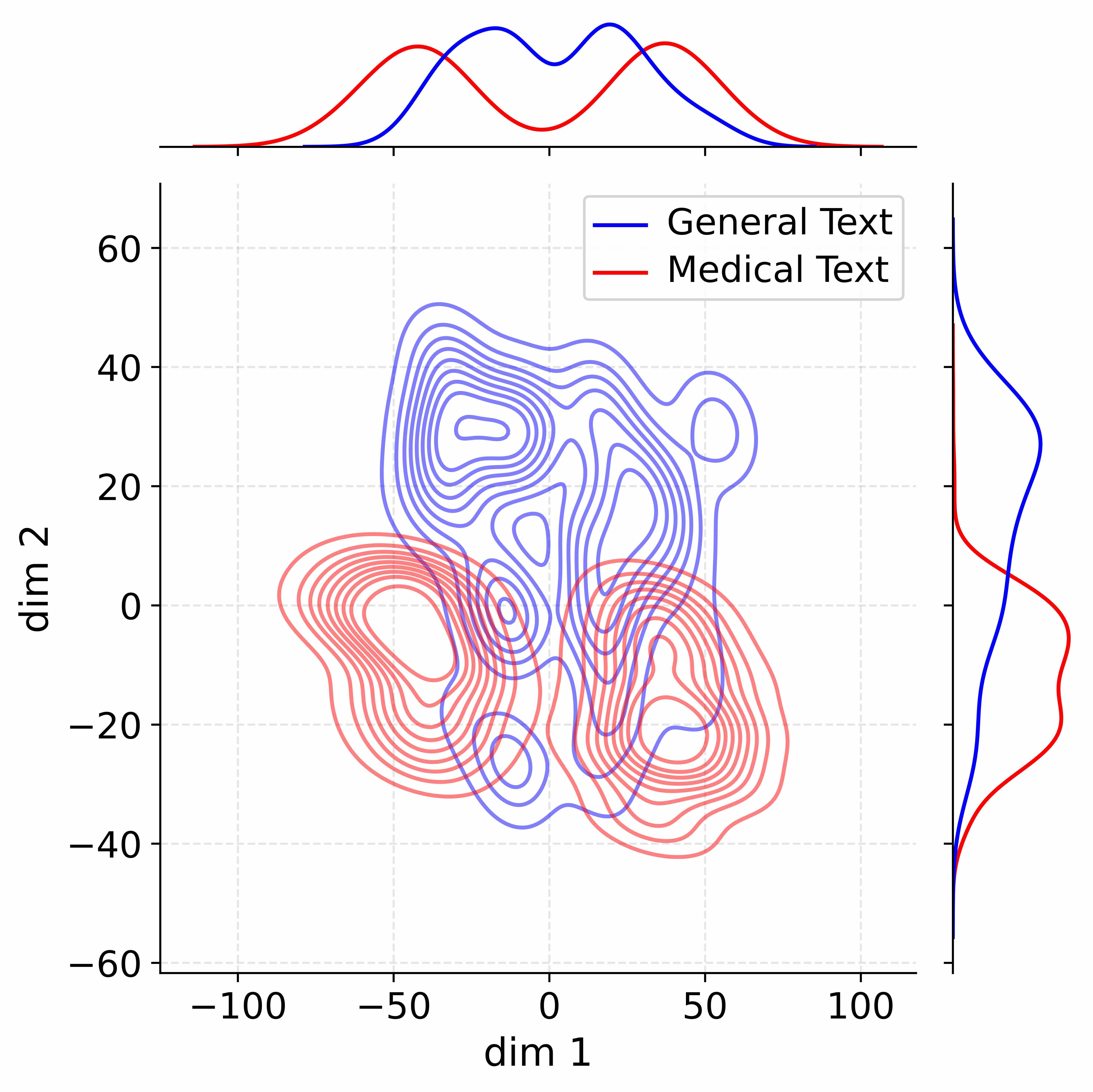
### Visual Description
## 2D Contour Plot with Marginal Distributions: General Text vs. Medical Text
### Overview
The image is a technical visualization comparing the distribution of two text corpora—"General Text" and "Medical Text"—in a two-dimensional space. It consists of a central 2D contour plot showing the joint density of the data points, accompanied by marginal density plots (1D distributions) along the top (for the x-axis) and right (for the y-axis). The plot uses color coding to distinguish between the two text categories.
### Components/Axes
* **Main Plot (Center):**
* **X-axis Label:** `dim 1`
* **X-axis Scale:** Linear scale ranging from approximately -120 to +120. Major tick marks are at -100, -50, 0, 50, 100.
* **Y-axis Label:** `dim 2`
* **Y-axis Scale:** Linear scale ranging from approximately -70 to +70. Major tick marks are at -60, -40, -20, 0, 20, 40, 60.
* **Grid:** A light gray dashed grid is present.
* **Legend:** Located in the top-right quadrant of the main plot area.
* **Blue Line:** Labeled `General Text`
* **Red Line:** Labeled `Medical Text`
* **Marginal Plots:**
* **Top Marginal Plot:** Shows the 1D density distribution along the `dim 1` axis. It contains two curves: a blue curve for General Text and a red curve for Medical Text.
* **Right Marginal Plot:** Shows the 1D density distribution along the `dim 2` axis. It also contains a blue curve (General Text) and a red curve (Medical Text).
### Detailed Analysis
**1. Main 2D Contour Plot:**
* **General Text (Blue Contours):** The density is concentrated in the upper half of the plot. The primary cluster is centered approximately at (`dim 1` ≈ -20, `dim 2` ≈ +30). The contours show a complex, multi-modal shape with several local density peaks. The distribution extends broadly across `dim 1` from about -70 to +70 and is most dense between `dim 2` values of +10 to +50.
* **Medical Text (Red Contours):** The density is concentrated in the lower half of the plot. The primary cluster is centered approximately at (`dim 1` ≈ 0, `dim 2` ≈ -15). This distribution also appears multi-modal but is more compact vertically compared to the blue contours. It spans a similar range on `dim 1` but is most dense between `dim 2` values of -40 to +10.
* **Overlap:** There is a region of overlap between the two distributions in the central area of the plot, roughly between `dim 1` -20 to +20 and `dim 2` -10 to +10, where the contour lines intermingle.
**2. Marginal Density Plots:**
* **Top Marginal (dim 1 Distribution):**
* **General Text (Blue):** Shows a broad, bimodal distribution. One peak is near `dim 1` = -20, and a second, slightly higher peak is near `dim 1` = +20. The distribution tails off towards -100 and +100.
* **Medical Text (Red):** Shows a distribution that is also bimodal but with peaks shifted slightly inward compared to the blue curve. Peaks are near `dim 1` = -10 and `dim 1` = +10. The overall spread is slightly narrower than the General Text distribution.
* **Right Marginal (dim 2 Distribution):**
* **General Text (Blue):** Shows a broad, unimodal distribution with a clear peak at approximately `dim 2` = +25. The density is highest in the positive `dim 2` range.
* **Medical Text (Red):** Shows a broad, unimodal distribution with a peak at approximately `dim 2` = -10. The density is highest in the negative `dim 2` range. The two marginal curves intersect near `dim 2` = +5.
### Key Observations
1. **Clear Separation along dim 2:** The most striking feature is the distinct separation of the two text categories along the `dim 2` axis. General Text is predominantly associated with positive `dim 2` values, while Medical Text is associated with negative `dim 2` values.
2. **Similar Spread on dim 1:** Both categories show a wide and somewhat similar spread along the `dim 1` axis, with overlapping bimodal marginal distributions. This suggests `dim 1` captures variation common to both text types.
3. **Multi-modal Structure:** The contour lines for both categories are complex and non-elliptical, indicating that the underlying data distributions are not simple single clusters but have multiple sub-groups or modes.
4. **Density Gradient:** The contour lines are tightly packed in the core regions of each distribution (e.g., blue around (-20, 30), red around (0, -15)), indicating high data density, and become more spaced out towards the periphery.
### Interpretation
This visualization likely results from applying a dimensionality reduction technique (like PCA, t-SNE, or UMAP) to text data (e.g., document embeddings) and then plotting the density of points for two different domains.
* **What the data suggests:** The plot demonstrates that "General Text" and "Medical Text" occupy distinct, though partially overlapping, regions in this derived feature space. The strong separation along `dim 2` implies this dimension captures a fundamental axis of variation that distinguishes general language from specialized medical language. This could relate to vocabulary specificity, syntactic complexity, or topic focus.
* **Relationship between elements:** The marginal plots directly summarize the 1D projections of the 2D contours. The bimodal `dim 1` marginals for both categories suggest there might be two major sub-themes or styles within each corpus that are captured by this dimension. The overlap region indicates documents or passages that share characteristics of both general and medical text.
* **Notable patterns/anomalies:** The complexity of the contours (multiple "islands" and irregular shapes) is notable. It suggests the text data is not homogeneous within each category. For example, the blue contours show a secondary, smaller cluster to the right (around `dim 1`=50, `dim 2`=30), which could represent a specific sub-genre of general text. The clear separation is the primary pattern, while the internal multi-modality is a secondary, important detail about the data's structure.
</details>
(a) Vanilla
<details>
<summary>figures/1.7B_only_grad_27_layers.jpg Details</summary>
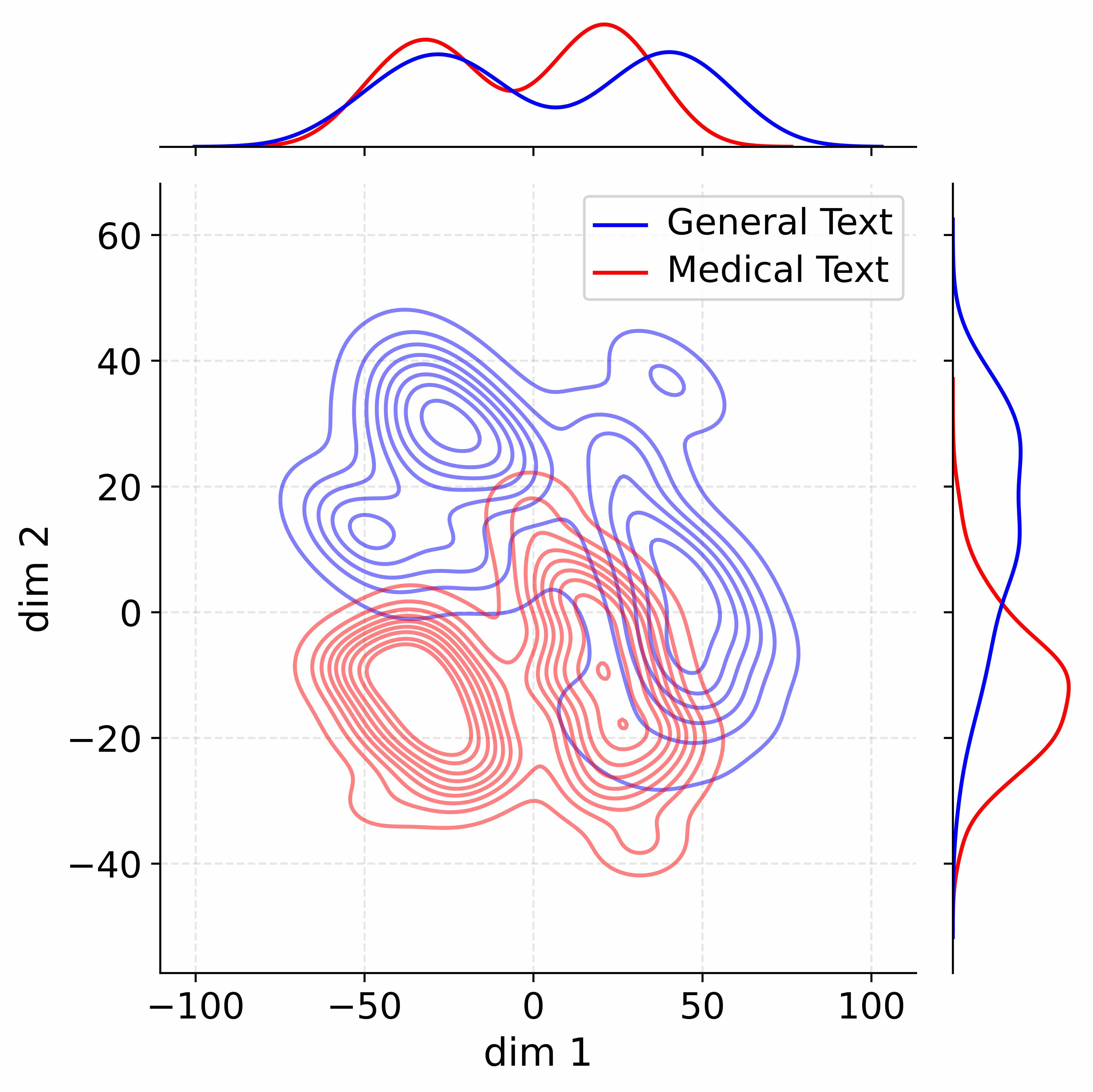
### Visual Description
## 2D Kernel Density Estimate Plot with Marginal Distributions: General Text vs. Medical Text
### Overview
The image displays a 2D kernel density estimate (KDE) plot comparing the distribution of two datasets in a two-dimensional space. The central plot shows contour lines representing data density, with marginal density plots on the top and right axes showing the 1D distributions for each dimension separately. The data appears to be the result of a dimensionality reduction technique (e.g., PCA, t-SNE) applied to text data, projecting high-dimensional text embeddings into two dimensions (`dim 1` and `dim 2`).
### Components/Axes
* **Main Plot (Center):**
* **X-axis:** Labeled `dim 1`. Scale ranges from approximately -100 to 100, with major tick marks at -100, -50, 0, 50, and 100.
* **Y-axis:** Labeled `dim 2`. Scale ranges from approximately -40 to 60, with major tick marks at -40, -20, 0, 20, 40, and 60.
* **Data Series (Contour Lines):**
* **Blue Contours:** Represent the density of the "General Text" dataset.
* **Red Contours:** Represent the density of the "Medical Text" dataset.
* **Legend:** Located in the top-right quadrant of the main plot area. It contains two entries:
* A blue line labeled `General Text`.
* A red line labeled `Medical Text`.
* **Marginal Plot (Top):**
* Shows the 1D density distribution along the `dim 1` axis.
* Contains a blue line (General Text) and a red line (Medical Text).
* **Marginal Plot (Right):**
* Shows the 1D density distribution along the `dim 2` axis.
* Contains a blue line (General Text) and a red line (Medical Text).
### Detailed Analysis
**1. Main Contour Plot (dim 1 vs. dim 2):**
* **General Text (Blue):** Exhibits a **bimodal distribution** in the 2D space.
* **Cluster 1 (Upper-Left):** Centered approximately at `dim 1` = -30, `dim 2` = 30. This is a dense, tightly packed cluster.
* **Cluster 2 (Lower-Right):** Centered approximately at `dim 1` = 40, `dim 2` = -10. This cluster is more spread out and elongated vertically.
* The two clusters are connected by a region of lower density.
* **Medical Text (Red):** Exhibits a **unimodal, more concentrated distribution**.
* **Primary Cluster:** Centered approximately at `dim 1` = -10, `dim 2` = -15. The highest density core is very tight.
* The distribution has a tail extending towards positive `dim 1` values, overlapping with the lower-right cluster of the General Text.
* It shows very little presence in the upper-left region (`dim 2` > 20) where the first General Text cluster is located.
**2. Marginal Density Plots:**
* **Top Marginal (dim 1 Distribution):**
* **General Text (Blue):** Clearly **bimodal**. Peaks are at approximately `dim 1` = -30 and `dim 1` = 40. The valley between them is near `dim 1` = 5.
* **Medical Text (Red):** Appears **unimodal** with a single peak near `dim 1` = -10. The distribution is skewed to the right (positive direction).
* **Right Marginal (dim 2 Distribution):**
* **General Text (Blue):** Appears **bimodal**. Peaks are at approximately `dim 2` = 30 and `dim 2` = -10, corresponding to its two main clusters.
* **Medical Text (Red):** Appears **unimodal** with a single, sharp peak near `dim 2` = -15.
### Key Observations
1. **Clear Separation in `dim 2`:** The most significant separation between the two text types occurs along the `dim 2` axis. General Text has substantial density in the positive `dim 2` region (20 to 50), which is almost entirely absent in Medical Text.
2. **Overlap in Lower-Right Quadrant:** There is considerable spatial overlap between the lower-right cluster of General Text and the primary cluster of Medical Text, particularly in the region where `dim 1` is between 0 and 50 and `dim 2` is between -30 and 10.
3. **Distribution Shape:** General Text is characterized by two distinct modes/clusters, suggesting potential sub-categories or diverse topics within the general corpus. Medical Text is more homogeneous, clustering tightly around a central semantic region.
4. **Marginal Confirmation:** The 1D marginal plots perfectly corroborate the 2D contour observations, confirming the bimodal vs. unimodal nature of the distributions for each dimension.
### Interpretation
This visualization strongly suggests that **"General Text" and "Medical Text" occupy distinct, though partially overlapping, regions in the semantic embedding space**. The separation, especially along `dim 2`, indicates that the underlying language model or feature extraction method has captured fundamental differences in vocabulary, syntax, or context between general-domain and medical-domain text.
* **The bimodal nature of General Text** could reflect two broad sub-domains within the general corpus (e.g., narrative vs. informational text, or different topic clusters).
* **The tight, unimodal cluster of Medical Text** implies a more specialized and consistent lexicon and structure, centered around a core set of medical concepts.
* **The area of overlap** is particularly interesting. It likely represents text that uses common language or discusses topics where general and medical contexts intersect (e.g., public health announcements, patient-facing educational material, or news articles about medical research). This overlap region is a potential source of ambiguity for text classification systems.
From a practical standpoint, this analysis demonstrates that a classifier trained on these two dimensions could achieve high accuracy in distinguishing medical from general text, but would likely make errors primarily on documents falling within the overlapping region. The plot provides a visual justification for using such dimensionality-reduced features for domain-specific text classification tasks.
</details>
(b) W/o stage1
<details>
<summary>figures/1.7B_final_Layer31_true.jpg Details</summary>
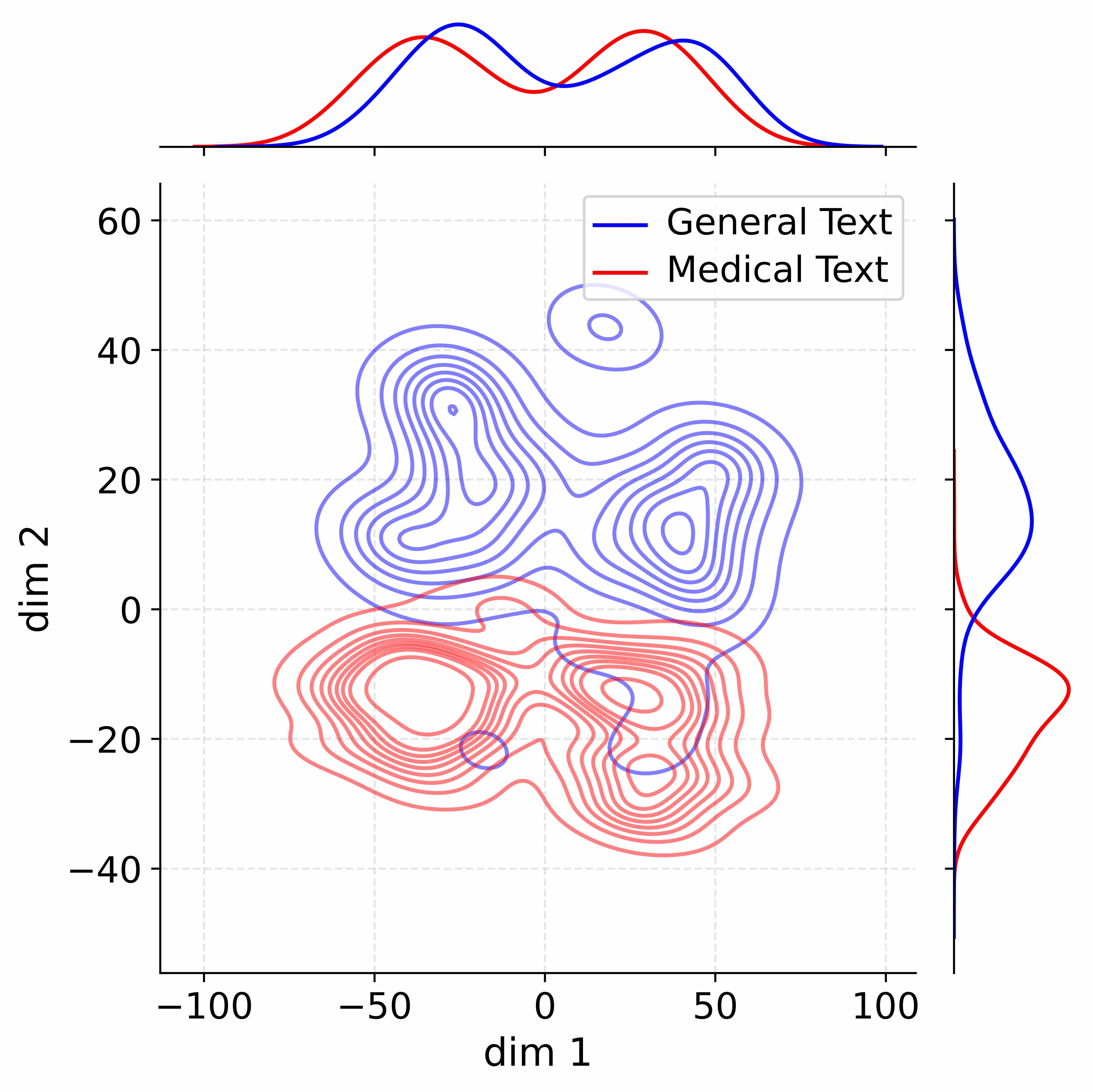
### Visual Description
## 2D Contour Plot with Marginal Distributions: Text Type Clustering
### Overview
The image is a statistical visualization comparing the distribution of two text corpora ("General Text" and "Medical Text") in a two-dimensional latent space. It consists of a central 2D contour plot showing the joint density of the data points, accompanied by marginal distribution plots (1D density curves) along the top (for dim 1) and right side (for dim 2). The plot suggests the data has been projected or embedded into two dimensions, likely via a technique like PCA, t-SNE, or UMAP.
### Components/Axes
* **Main Plot (Center):**
* **X-axis:** Labeled "dim 1". Scale ranges from -100 to 100, with major tick marks at -100, -50, 0, 50, 100.
* **Y-axis:** Labeled "dim 2". Scale ranges from -40 to 60, with major tick marks at -40, -20, 0, 20, 40, 60.
* **Content:** Overlaid contour plots for two categories.
* **Legend:** Positioned in the top-right quadrant of the main plot area.
* A blue line corresponds to the label "General Text".
* A red line corresponds to the label "Medical Text".
* **Marginal Distribution Plots:**
* **Top Plot:** Shows the 1D density distribution along "dim 1". The x-axis aligns with the main plot's x-axis (-100 to 100). The y-axis represents probability density (unlabeled).
* **Right Plot:** Shows the 1D density distribution along "dim 2". The y-axis aligns with the main plot's y-axis (-40 to 60). The x-axis represents probability density (unlabeled).
### Detailed Analysis
**1. Main Contour Plot (Joint Distribution):**
* **General Text (Blue Contours):**
* **Spatial Grounding:** Primarily occupies the upper half of the plot (positive "dim 2" values).
* **Trend/Shape:** Forms a complex, multi-modal distribution. The highest density region (innermost contours) is centered approximately at (dim1 ≈ -25, dim2 ≈ 30). A secondary, smaller high-density cluster is visible around (dim1 ≈ 25, dim2 ≈ 15). A distinct, isolated small cluster appears at approximately (dim1 ≈ 15, dim2 ≈ 45). The overall spread spans dim1 from roughly -75 to 75 and dim2 from 0 to 50.
* **Medical Text (Red Contours):**
* **Spatial Grounding:** Primarily occupies the lower half of the plot (negative "dim 2" values).
* **Trend/Shape:** Also forms a multi-modal distribution. The highest density region is centered around (dim1 ≈ -25, dim2 ≈ -15). Another significant high-density cluster is located at approximately (dim1 ≈ 25, dim2 ≈ -25). The overall spread spans dim1 from roughly -75 to 75 and dim2 from -40 to 0.
* **Overlap:** There is a region of moderate overlap between the two distributions along the "dim 1" axis, particularly between dim1 values of -25 and 25, and around dim2 = 0. However, their primary densities are clearly separated along the "dim 2" axis.
**2. Marginal Distribution Plots:**
* **Top Marginal (dim 1):**
* **General Text (Blue):** Shows a bimodal distribution. Peaks are located at approximately dim1 = -30 and dim1 = 30. The valley between peaks is near dim1 = 0.
* **Medical Text (Red):** Also shows a bimodal distribution. Peaks are located at approximately dim1 = -35 and dim1 = 25. The valley is near dim1 = -5.
* **Comparison:** The distributions along dim 1 are similar in shape and range for both text types, with significant overlap. The Medical Text peaks appear slightly shifted left compared to the General Text peaks.
* **Right Marginal (dim 2):**
* **General Text (Blue):** Shows a unimodal distribution with a peak at approximately dim2 = 25. The distribution is skewed, with a longer tail extending towards lower dim2 values.
* **Medical Text (Red):** Shows a unimodal distribution with a peak at approximately dim2 = -20. The distribution is also skewed, with a longer tail extending towards higher dim2 values.
* **Comparison:** This plot reveals the most significant separation. The two distributions have distinct peaks on opposite sides of dim2 = 0, with minimal overlap. This confirms that "dim 2" is the primary axis differentiating the two text types.
### Key Observations
1. **Clear Separation on dim 2:** The most prominent feature is the distinct separation of the two text corpora along the "dim 2" axis. General Text clusters in the positive region, Medical Text in the negative region.
2. **Similarity on dim 1:** Both text types exhibit similar, bimodal distributions along "dim 1", suggesting this dimension captures a common structural variation present in both general and medical language.
3. **Multi-modal Structure:** Both distributions in the 2D space are multi-modal, indicating that each text type likely contains several distinct sub-categories or topics within the analyzed corpus.
4. **Isolated Cluster:** The small, isolated blue cluster at (15, 45) represents a subset of General Text that is distinct from the main body of general text in this latent space.
### Interpretation
This visualization demonstrates that when text data (likely from embeddings or feature vectors) is reduced to two dimensions, **"General Text" and "Medical Text" form largely separable clusters.** The axis labeled "dim 2" appears to capture a semantic or stylistic feature that strongly differentiates medical discourse from general language. This could relate to vocabulary specificity, syntactic complexity, or topic focus inherent to medical literature.
The overlap along "dim 1" suggests that both text types share some underlying common structure or variability. The multi-modal nature of each cluster implies that neither "General Text" nor "Medical Text" is monolithic; each contains internal groupings, which could correspond to different genres (e.g., news vs. fiction for general; clinical reports vs. research articles for medical).
The plot provides strong visual evidence that a model or analysis using these two dimensions could effectively distinguish between general and medical text, with "dim 2" being the most discriminative feature. The isolated blue cluster is an outlier warranting further investigation to understand what specific subset of general text it represents.
</details>
(c) ADEPT
Figure 6: Kernel Density Estimation of activations for Qwen3-1.7B-Base under different configurations. Our layer extension strategy enables effective parameter decoupling. Expanded layers: 22, 23, 25, and 27.
To examine the effectiveness of our layer extension strategy, we conduct activation distribution analysis across multiple backbones. For each model, we first identify the most domain-adaptable layer (i.e., the layer with the lowest $I_layer$ ). We then randomly sample 500 instances from both the Medical and General corpora, compute activations at the selected layer, and visualize their distributions using Kernel Density Estimation (KDE). The following three configurations are compared: (1) the original base model, where we visualize the most domain-adaptable layer; (2) direct decoupling without expansion (w/o Stage-1), where we visualize the same most domain-adaptable layer; (3) our method with expanded layers, where we visualize the newly created expanded layer (copied from the most domain-adaptable layer).
Figure 6 presents the results from three different model configurations, providing compelling evidence for the advantages of our proposed approach.
Figure 6 a) shows the activation distribution in layer 27 of the original Qwen3-1.7B-Base model. The substantial overlap between general and medical text distributions indicates strong parameter coupling, which is an expected consequence of mixed-domain pretraining. This coupling makes it challenging to achieve clean separation of domain-specific functionalities through conventional fine-tuning approaches. However, the divergence between the peak values in the general domain and the medical domain also indicates the potential for decoupling.
This coupling phenomenon persisted in our ablation studies with only the decoupling method in Figure 6 b). Despite our attempts to decouple the medical and general modules when training, the model’s activation distributions remained largely entangled (the graph still shows substantial overlap), failing to achieve distinct separation between domains. This observation further supports our argument that pre-existing parameter coupling from mixed-domain pretraining creates inherent challenges for direct decoupling approaches.
In contrast, Figure 6 c) demonstrates the activation distribution in layer 31 of our extended model, where we first expanded the model by copying parameters from layer 27 and then applied decoupling training. The clear separation between general and medical text distributions suggests successful parameter decoupling. This superior decoupling effect can be attributed to our “blank slate” approach: the extended layers, while initialized with copied parameters, provide a fresh parameter space that hasn’t been constrained by mixed-domain pretraining. During decoupling training, these extended layers can adapt more freely to domain-specific patterns through gradient descent and importance-based learning rate adjustments.
To validate our hypothesis, we also examine the effect of applying in Qwen3-4B-Base (Figure 7), Qwen3-8B-Base (Figure 8), Llama3-8B (Figure 9). The results indicate limited separation between domains, which supports our argument that the entangled parameters from mixed-domain pretraining are challenging to decouple through training alone.
These findings demonstrate that our layer extension strategy provides a more effective pathway for parameter decoupling compared to direct decoupling training. By creating a new parameter space through layer extension, we avoid the constraints of pre-existing parameter coupling, allowing for cleaner separation of domain-specific functionalities during subsequent training. This approach offers a promising direction for developing more modular and domain-adaptable language models.
<details>
<summary>figures/4B_Base_Layer35.jpg Details</summary>
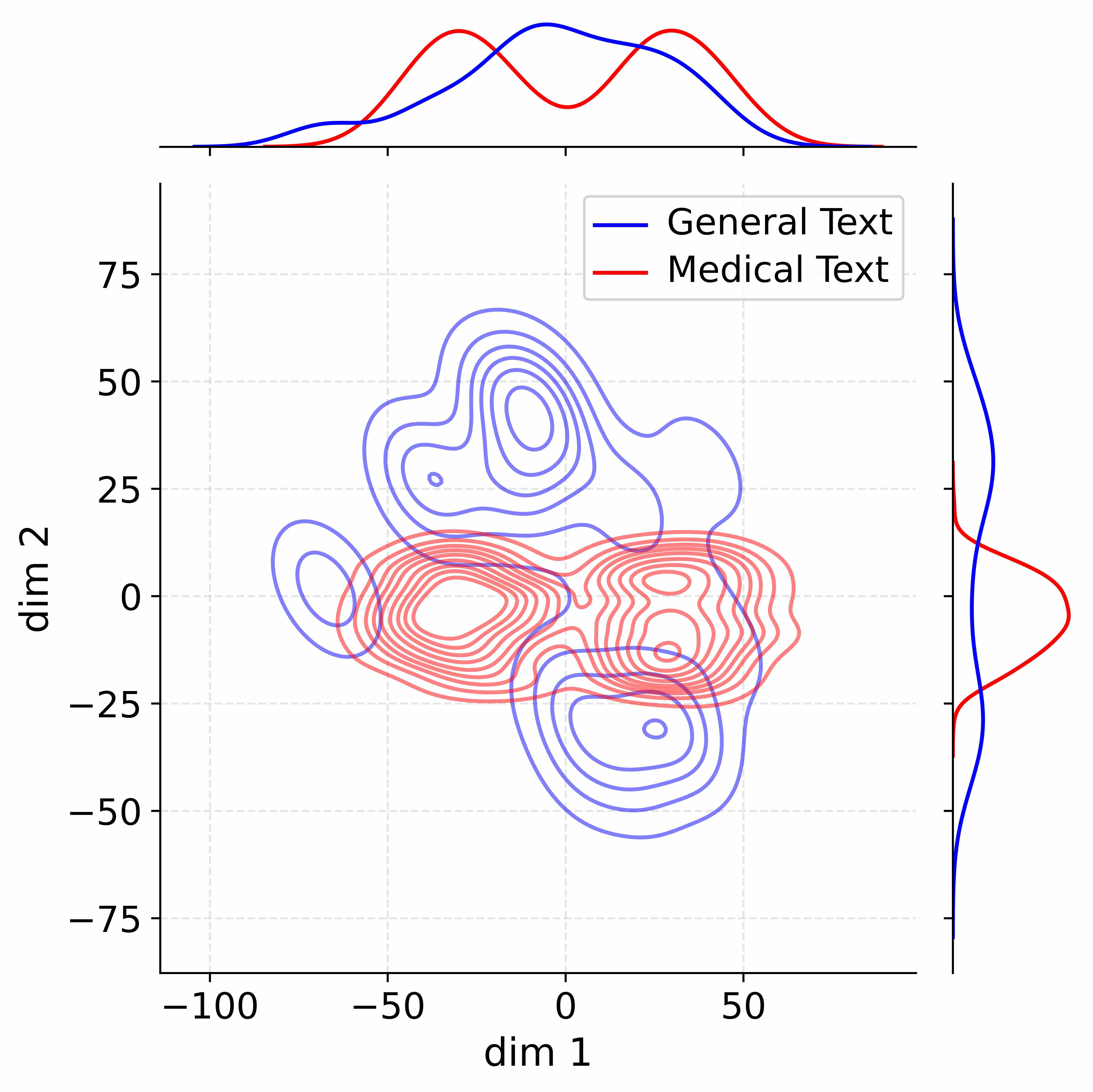
### Visual Description
## 2D Contour Plot with Marginal Distributions: Text Domain Embedding Analysis
### Overview
The image displays a 2D contour plot visualizing the distribution of two categories of text data in a two-dimensional embedding space. The plot includes marginal density distributions along the top (for the horizontal axis) and right side (for the vertical axis). The data is separated into "General Text" (blue) and "Medical Text" (red).
### Components/Axes
* **Main Plot (Center):**
* **X-axis (dim 1):** Labeled "dim 1". Ticks are at -100, -50, 0, and 50.
* **Y-axis (dim 2):** Labeled "dim 2". Ticks are at -75, -50, -25, 0, 25, 50, and 75.
* **Legend:** Located in the top-right quadrant of the main plot area. It contains:
* A blue line labeled "General Text".
* A red line labeled "Medical Text".
* **Grid:** A light gray dashed grid is present.
* **Marginal Plot (Top):** Shows the density distribution along "dim 1". The x-axis aligns with the main plot's x-axis. It contains two curves: a blue curve for "General Text" and a red curve for "Medical Text".
* **Marginal Plot (Right):** Shows the density distribution along "dim 2". The y-axis aligns with the main plot's y-axis. It contains two curves: a blue curve for "General Text" and a red curve for "Medical Text".
### Detailed Analysis
**1. Main Contour Plot:**
* **General Text (Blue Contours):**
* **Trend/Shape:** The distribution is bimodal in the vertical dimension (dim 2). It forms two distinct, separate clusters.
* **Cluster 1 (Upper):** Centered approximately at (dim1 ≈ 0, dim2 ≈ 50). This cluster is dense, with many concentric contour lines indicating a high probability density peak.
* **Cluster 2 (Lower):** Centered approximately at (dim1 ≈ 0, dim2 ≈ -30). This cluster is also dense and well-defined.
* **Spatial Relationship:** The two clusters are vertically separated with minimal overlap. They are horizontally centered around dim1=0.
* **Medical Text (Red Contours):**
* **Trend/Shape:** The distribution is more horizontally spread and appears unimodal or possibly bimodal in the horizontal dimension (dim 1), but centered around dim2=0.
* **Primary Mass:** The main body of the distribution is centered around dim2 ≈ 0, spanning from approximately dim1 = -75 to dim1 = 75.
* **Peaks:** There appear to be two density peaks within this mass: one near (dim1 ≈ -25, dim2 ≈ 0) and another near (dim1 ≈ 25, dim2 ≈ 0).
* **Spatial Relationship:** This distribution is largely contained within the vertical band of dim2 between -25 and 25, overlapping the space between the two blue clusters.
**2. Marginal Distributions:**
* **Top Marginal (dim 1):**
* **General Text (Blue):** Shows a single, broad peak centered near dim1 = 0.
* **Medical Text (Red):** Shows a clear bimodal distribution with two distinct peaks. One peak is near dim1 = -25, and the other is near dim1 = 25. The valley between them is near dim1 = 0.
* **Right Marginal (dim 2):**
* **General Text (Blue):** Shows a clear bimodal distribution with two distinct peaks. One peak is near dim2 = 50, and the other is near dim2 = -30. The valley between them is near dim2 = 10.
* **Medical Text (Red):** Shows a single, broad peak centered near dim2 = 0.
### Key Observations
1. **Orthogonal Separation:** The two text domains are separated primarily along the "dim 2" axis. "General Text" occupies extreme positive and negative values of dim2, while "Medical Text" is concentrated around the center (dim2=0).
2. **Complementary Bimodality:** The bimodality is orthogonal between categories. "Medical Text" is bimodal along "dim 1" (horizontal), while "General Text" is bimodal along "dim 2" (vertical).
3. **Overlap Region:** There is a region of overlap in the center of the plot (around dim1=0, dim2=0), where the lower tail of the upper blue cluster, the upper tail of the lower blue cluster, and the main mass of the red distribution intersect.
4. **Density:** The contour lines for both categories are densely packed at their respective peaks, indicating high concentration of data points in those regions of the embedding space.
### Interpretation
This plot likely visualizes the output of a dimensionality reduction technique (like t-SNE or UMAP) applied to text embeddings. The clear separation suggests that the underlying model or feature space effectively distinguishes between general-domain text and domain-specific medical text.
* **What the data suggests:** The distinct, non-overlapping clusters imply that "General Text" and "Medical Text" have fundamentally different statistical properties in this embedding space. The bimodal nature of each could indicate the presence of two major subtypes or topics within each broad category (e.g., general text might split into formal/informal, medical text into clinical/research).
* **How elements relate:** The marginal distributions perfectly corroborate the 2D contours. The top marginal explains the horizontal spread of the red contours and the central concentration of the blue contours. The right marginal explains the vertical separation of the blue clusters and the central concentration of the red cluster.
* **Notable patterns/anomalies:** The most striking pattern is the orthogonal bimodality. It suggests that the primary axis of variation for medical text (dim1) is different from the primary axis of variation for general text (dim2). This could be an artifact of the embedding method or a genuine reflection of the data structure. The central overlap region is also significant, as it may represent text that is ambiguous or hybrid in nature, sharing characteristics of both domains.
</details>
(a) Vanilla
<details>
<summary>figures/4B_only_grad_Layer35.jpg Details</summary>
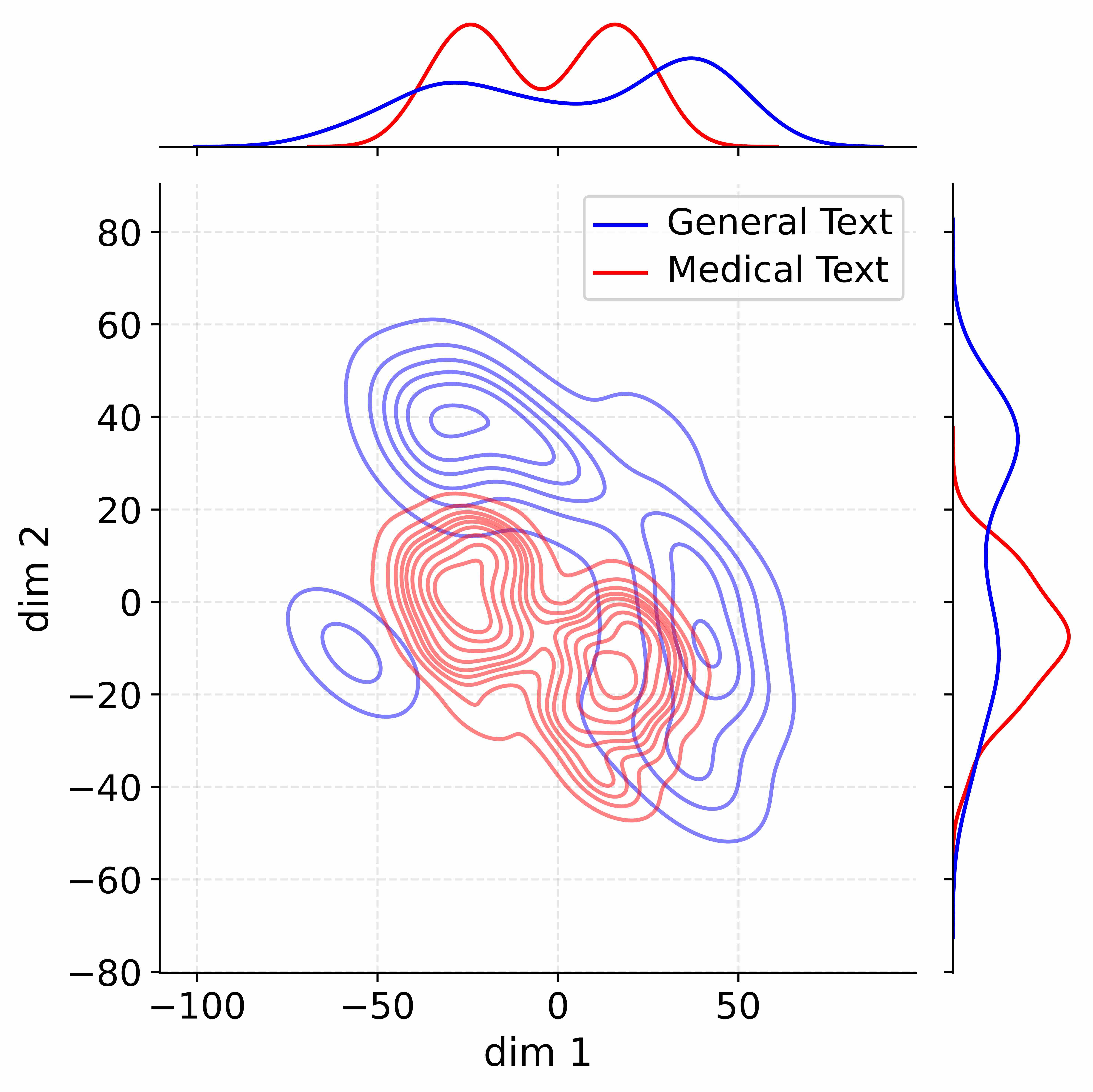
### Visual Description
## Joint Contour Plot with Marginal Distributions: General Text vs. Medical Text
### Overview
The image is a joint plot visualizing the two-dimensional distribution of two datasets, labeled "General Text" and "Medical Text." It consists of a central contour plot showing the density of data points across two dimensions (`dim 1` and `dim 2`), accompanied by marginal distribution plots (density curves) on the top and right edges. The plot compares the spatial distribution and density of these two text categories in a reduced-dimensional space.
### Components/Axes
* **Main Plot (Center):**
* **X-axis:** Labeled `dim 1`. Ticks are at -100, -50, 0, 50.
* **Y-axis:** Labeled `dim 2`. Ticks are at -80, -60, -40, -20, 0, 20, 40, 60, 80.
* **Data Series:** Represented by contour lines.
* **Blue Contours:** Correspond to "General Text" (confirmed by legend).
* **Red Contours:** Correspond to "Medical Text" (confirmed by legend).
* **Legend:** Located in the top-right quadrant of the main plot area. It contains:
* A blue line segment followed by the text "General Text".
* A red line segment followed by the text "Medical Text".
* **Top Marginal Plot:**
* Displays the kernel density estimate (KDE) for `dim 1`.
* Contains a blue curve (General Text) and a red curve (Medical Text).
* **Right Marginal Plot:**
* Displays the kernel density estimate (KDE) for `dim 2`.
* Contains a blue curve (General Text) and a red curve (Medical Text).
### Detailed Analysis
**1. Main Contour Plot (dim 1 vs. dim 2):**
* **General Text (Blue):** The distribution is broad and multi-modal. The primary density cluster is centered approximately at (`dim 1` ≈ -25, `dim 2` ≈ 40). A secondary, less dense cluster appears around (`dim 1` ≈ 40, `dim 2` ≈ -10). The contours span a wide range: `dim 1` from roughly -80 to +60, and `dim 2` from roughly -50 to +60.
* **Medical Text (Red):** The distribution is more concentrated and appears bimodal. One dense cluster is centered near (`dim 1` ≈ -20, `dim 2` ≈ 0). A second, slightly less dense cluster is near (`dim 1` ≈ 20, `dim 2` ≈ -20). The overall spread is narrower than the General Text: `dim 1` ranges from about -50 to +40, and `dim 2` from about -40 to +20.
* **Overlap:** There is significant overlap between the two distributions in the central region of the plot, roughly between `dim 1` -40 to +30 and `dim 2` -30 to +20.
**2. Marginal Distribution for `dim 1` (Top Plot):**
* **General Text (Blue):** Shows a broad, slightly bimodal distribution. Peaks are approximately at `dim 1` ≈ -30 and `dim 1` ≈ +30. The distribution has a wide base, extending from below -80 to above +60.
* **Medical Text (Red):** Shows a sharper, clearly bimodal distribution. The two peaks are more pronounced and closer together, located approximately at `dim 1` ≈ -20 and `dim 1` ≈ +10. The distribution is narrower, confined mostly between -50 and +40.
**3. Marginal Distribution for `dim 2` (Right Plot):**
* **General Text (Blue):** Exhibits a broad, unimodal (or very subtly bimodal) distribution. The single major peak is centered around `dim 2` ≈ +30. The distribution spans from approximately -60 to +80.
* **Medical Text (Red):** Shows a distinct bimodal distribution. The two peaks are located at approximately `dim 2` ≈ 0 and `dim 2` ≈ -20. The distribution is more compact, ranging from about -50 to +20.
### Key Observations
1. **Dispersion:** The "General Text" dataset is significantly more dispersed in both dimensions compared to the "Medical Text" dataset.
2. **Modality:** The "Medical Text" distribution is clearly bimodal in both the `dim 1` and `dim 2` marginals, suggesting two distinct sub-groups or clusters within this category. The "General Text" is more broadly distributed, with weaker evidence for multiple modes.
3. **Central Tendency:** The center of mass for "Medical Text" is shifted towards lower values on both `dim 1` and `dim 2` compared to the primary cluster of "General Text."
4. **Separation:** While there is overlap, the highest density regions (innermost contours) of the two datasets are distinct. The core of "General Text" is in the upper-left quadrant (negative `dim 1`, positive `dim 2`), while the cores of "Medical Text" are in the lower-central region (near-zero `dim 1`, negative `dim 2`).
### Interpretation
This plot likely visualizes the output of a dimensionality reduction technique (like PCA, t-SNE, or UMAP) applied to text data, where `dim 1` and `dim 2` represent the two most significant derived features.
The data suggests that **"Medical Text" occupies a more specialized and constrained region of this feature space** compared to "General Text." This could reflect the use of a more standardized, technical vocabulary and formulaic structures in medical writing, leading to less variation. The bimodality might indicate two common types of medical documents (e.g., clinical notes vs. research abstracts) or two distinct sub-domains within the medical corpus.
Conversely, **"General Text" is more heterogeneous**, covering a wider range of topics, styles, and vocabularies, which manifests as a broader, more diffuse distribution. The overlap region represents text that shares characteristics with both categories, potentially indicating general health articles or patient-facing materials written in plain language.
The clear separation of the dense cores implies that, based on these two dimensions, it is possible to distinguish between typical medical text and general text with reasonable accuracy. The marginal distributions reinforce this, showing that the statistical properties of the individual dimensions also differ markedly between the two categories.
</details>
(b) W/o stage1
<details>
<summary>figures/4B_Layer39.jpg Details</summary>
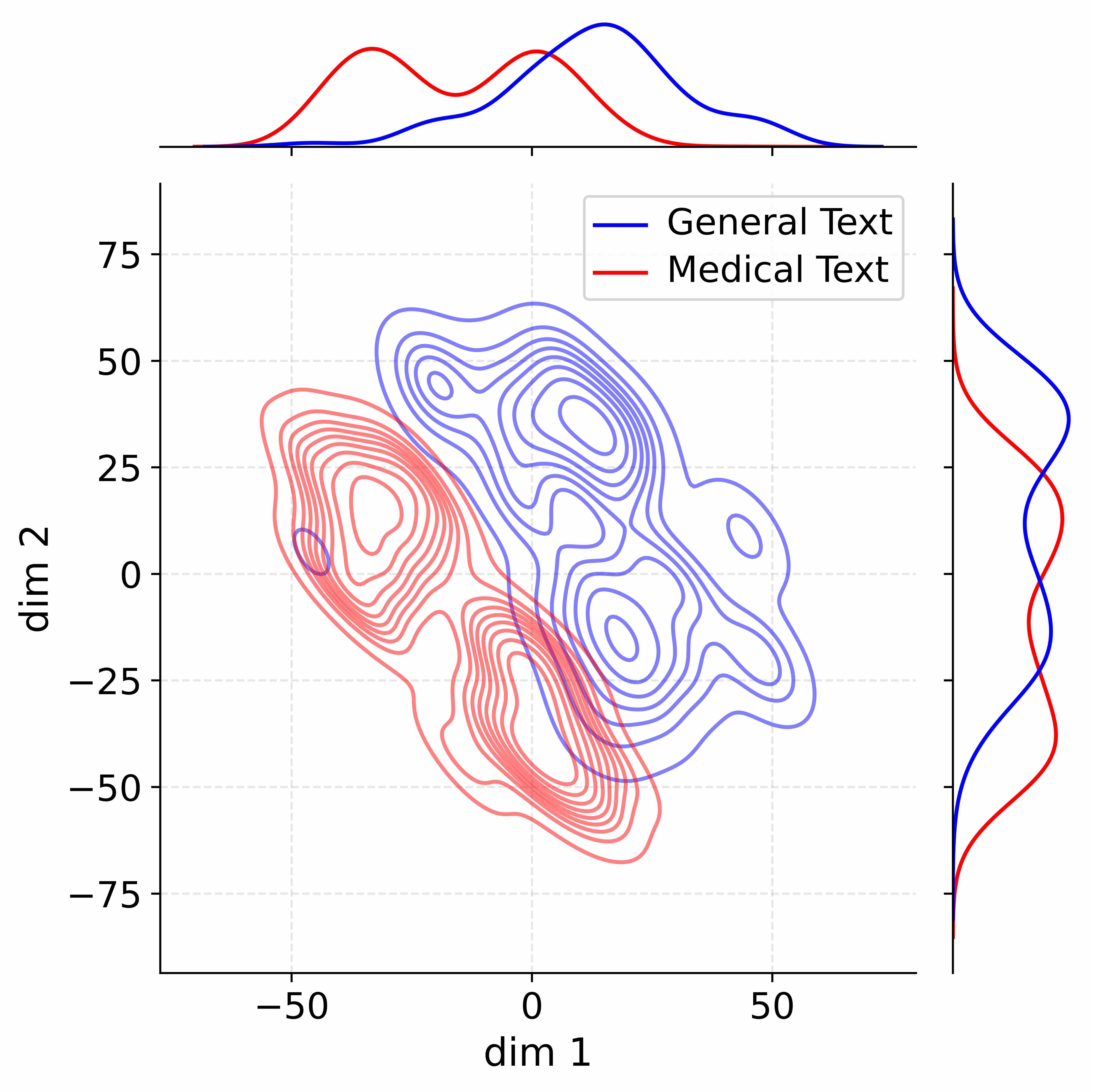
### Visual Description
## 2D Contour Plot with Marginal Distributions: General Text vs. Medical Text
### Overview
This image is a 2D contour plot comparing the distribution of two datasets, labeled "General Text" and "Medical Text," across two dimensions (`dim 1` and `dim 2`). The plot includes marginal density plots (univariate distributions) along the top (for `dim 1`) and right side (for `dim 2`). The visualization aims to show how the two text types cluster differently in this two-dimensional feature space.
### Components/Axes
* **Main Plot (Center):**
* **X-axis:** Labeled `dim 1`. Major tick marks are at -50, 0, and 50. The axis spans approximately from -75 to +75.
* **Y-axis:** Labeled `dim 2`. Major tick marks are at -75, -50, -25, 0, 25, 50, and 75. The axis spans approximately from -80 to +80.
* **Data Series (Contour Lines):**
* **Blue Contours:** Represent the density of "General Text" data points.
* **Red Contours:** Represent the density of "Medical Text" data points.
* **Legend:** Located in the top-right quadrant of the main plot area. It contains:
* A blue line segment followed by the text "General Text".
* A red line segment followed by the text "Medical Text".
* **Top Marginal Plot:**
* Shows the 1D density distribution along the `dim 1` axis.
* Contains a blue curve (General Text) and a red curve (Medical Text).
* The x-axis aligns with the main plot's `dim 1` axis.
* **Right Marginal Plot:**
* Shows the 1D density distribution along the `dim 2` axis.
* Contains a blue curve (General Text) and a red curve (Medical Text).
* The y-axis aligns with the main plot's `dim 2` axis.
### Detailed Analysis
**1. Main Contour Plot:**
* **General Text (Blue):** The contours form a large, complex cluster primarily located in the quadrant where `dim 1` is positive and `dim 2` is positive. The highest density peaks (innermost contours) are centered approximately at (`dim 1` ≈ 10 to 30, `dim 2` ≈ 20 to 40). The distribution is broad, extending from `dim 1` ≈ -20 to +60 and `dim 2` ≈ -40 to +60. There is a secondary, smaller density peak near (`dim 1` ≈ 40, `dim 2` ≈ 10).
* **Medical Text (Red):** The contours form a distinct cluster primarily located where `dim 1` is negative and `dim 2` is negative. The highest density peak is centered approximately at (`dim 1` ≈ -30, `dim 2` ≈ -10). The distribution is more compact than the General Text cluster, extending roughly from `dim 1` ≈ -50 to +10 and `dim 2` ≈ -60 to +30. There is a noticeable secondary lobe extending towards (`dim 1` ≈ -10, `dim 2` ≈ -40).
* **Overlap:** There is a region of overlap between the two distributions, primarily in the area around (`dim 1` ≈ -10 to 0, `dim 2` ≈ -20 to 0).
**2. Top Marginal Plot (dim 1 Distribution):**
* **General Text (Blue):** The distribution is broad and appears bimodal. The primary, higher peak is centered at approximately `dim 1` = +20. A secondary, lower peak or shoulder is visible around `dim 1` = -10.
* **Medical Text (Red):** The distribution is also broad and appears bimodal. The primary peak is centered at approximately `dim 1` = -30. A secondary peak is centered near `dim 1` = 0.
* **Comparison:** The Medical Text distribution is shifted significantly to the left (more negative values) compared to the General Text distribution on the `dim 1` axis.
**3. Right Marginal Plot (dim 2 Distribution):**
* **General Text (Blue):** The distribution is broad with a primary peak at approximately `dim 2` = +30 and a secondary peak or shoulder near `dim 2` = -10.
* **Medical Text (Red):** The distribution is also broad with a primary peak at approximately `dim 2` = -10 and a secondary peak near `dim 2` = +20.
* **Comparison:** The Medical Text distribution is shifted downward (more negative values) compared to the General Text distribution on the `dim 2` axis, though the overlap is greater here than on `dim 1`.
### Key Observations
1. **Clear Separation:** The two text types form distinct clusters in the 2D space, with General Text favoring positive values on both dimensions and Medical Text favoring negative values.
2. **Multimodality:** Both marginal distributions for each text type appear to have more than one peak, suggesting potential sub-categories or modes within each text domain.
3. **Different Spread:** The General Text cluster (blue) appears more diffuse and covers a larger area of the plot than the more concentrated Medical Text cluster (red).
4. **Axis-Specific Shifts:** The separation between the groups is more pronounced along the `dim 1` axis than the `dim 2` axis.
### Interpretation
This plot likely visualizes the output of a dimensionality reduction technique (like PCA, t-SNE, or UMAP) applied to textual data. The two dimensions (`dim 1`, `dim 2`) represent abstract features derived from the text.
The data suggests that **"Medical Text" and "General Text" have fundamentally different statistical profiles** in this feature space. Medical text is characterized by more negative values on both derived dimensions, forming a tighter, more specific cluster. This could reflect the use of specialized, consistent vocabulary and structure in medical documents. In contrast, General Text is more varied (broader spread) and occupies a different region of the feature space, likely reflecting a wider range of topics, styles, and vocabularies.
The multimodal nature of the distributions hints at **internal structure within each category**. For example, the two peaks in the Medical Text `dim 1` distribution could correspond to different sub-fields (e.g., clinical notes vs. research papers) or document types. The overlap region indicates that some medical texts may share characteristics with general texts, and vice-versa, but the core distributions are distinct. This visualization provides strong evidence that a model or analysis can successfully differentiate between these two text domains based on their underlying features.
</details>
(c) ADEPT
Figure 7: Visualization of activation distributions for Qwen3-4B-Base model configurations showing the effectiveness of our layer extension strategy for parameter decoupling. We expand the layer 28, 30, 31, 35 of Qwen3-4B-Base.
<details>
<summary>figures/8B_Base_Layer30.jpg Details</summary>
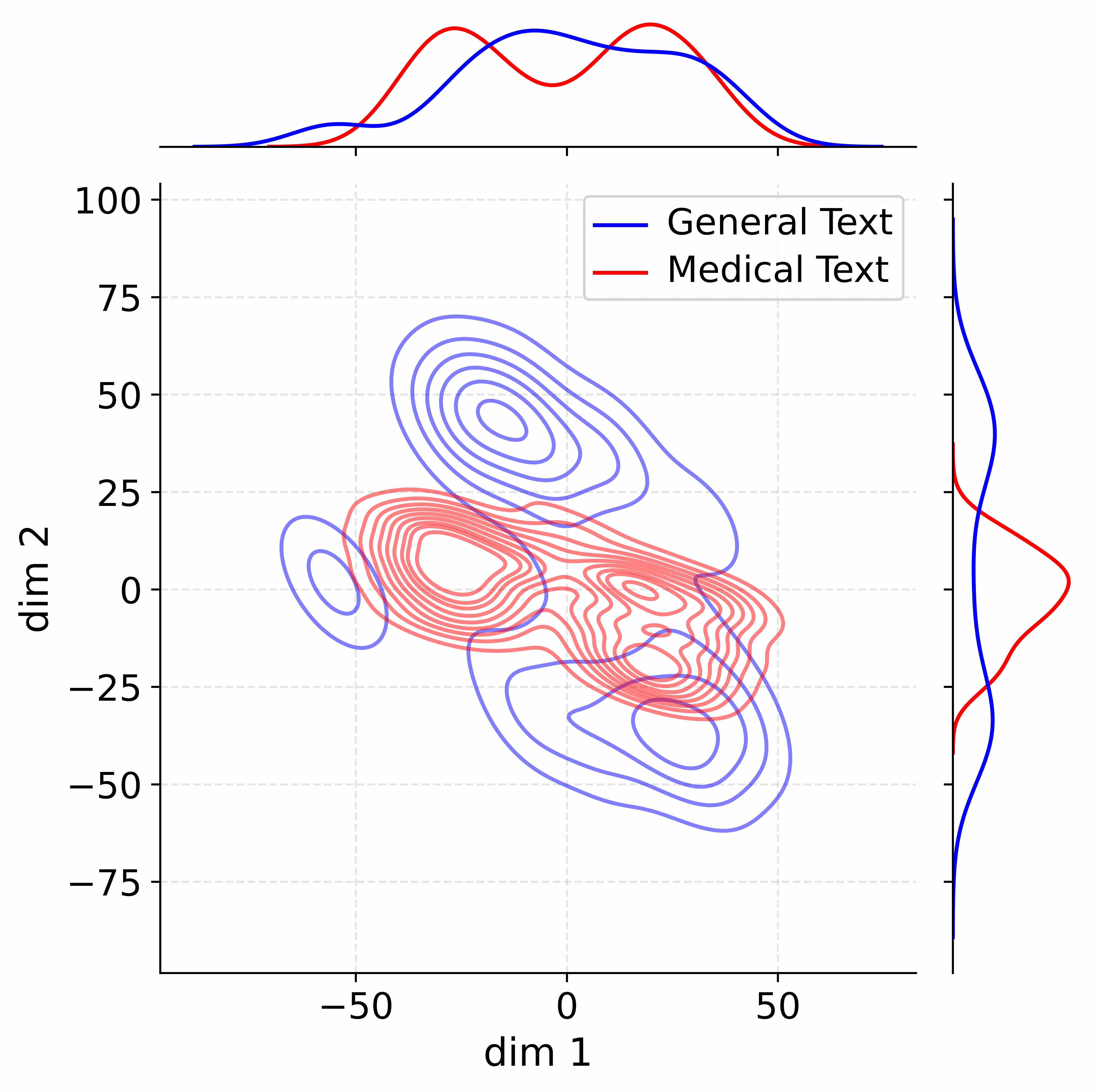
### Visual Description
## Joint Contour Plot with Marginal Distributions: General Text vs. Medical Text
### Overview
The image is a joint plot displaying the two-dimensional distribution of two datasets, labeled "General Text" and "Medical Text," across two dimensions ("dim 1" and "dim 2"). The plot consists of a central contour plot showing the density of data points for each category, accompanied by marginal distribution plots (density curves) on the top and right sides. The visualization compares the spread, clustering, and overlap of the two text categories in this reduced-dimensional space.
### Components/Axes
* **Main Plot (Center):**
* **X-axis:** Labeled "dim 1". Ticks are visible at approximately -50, 0, and 50. The axis spans roughly from -75 to 75.
* **Y-axis:** Labeled "dim 2". Ticks are visible at -75, -50, -25, 0, 25, 50, 75, and 100. The axis spans roughly from -80 to 100.
* **Data Series:**
* **General Text:** Represented by blue contour lines.
* **Medical Text:** Represented by red contour lines.
* **Legend:** Located in the top-right quadrant of the main plot area. It contains two entries: a blue line labeled "General Text" and a red line labeled "Medical Text".
* **Marginal Plots:**
* **Top Marginal (above main plot):** Shows the density distribution along "dim 1". Contains a blue curve (General Text) and a red curve (Medical Text).
* **Right Marginal (to the right of main plot):** Shows the density distribution along "dim 2". Contains a blue curve (General Text) and a red curve (Medical Text).
### Detailed Analysis
**1. Main Contour Plot (dim 1 vs. dim 2):**
* **General Text (Blue):** Exhibits a multi-modal distribution with at least three distinct clusters.
* A primary, dense cluster is centered approximately at (dim1 ≈ -10, dim2 ≈ 50). This cluster has tightly packed concentric contours, indicating high density.
* A secondary cluster is located around (dim1 ≈ 25, dim2 ≈ -30).
* A smaller, less dense cluster appears near (dim1 ≈ -60, dim2 ≈ 0).
* The overall spread is wide, covering a large area from dim1 ≈ -70 to 50 and dim2 ≈ -60 to 70.
* **Medical Text (Red):** Shows a more concentrated, bi-modal distribution.
* The largest and densest cluster is centered near (dim1 ≈ -20, dim2 ≈ 0). The contours are very tightly packed, suggesting extremely high data density in this core region.
* A second, smaller cluster is visible around (dim1 ≈ 20, dim2 ≈ -10).
* The distribution is more compact than the General Text, primarily confined to dim1 between -40 and 40, and dim2 between -25 and 25.
* **Overlap:** There is significant spatial overlap between the two distributions, particularly in the region around dim1 ≈ 0, dim2 ≈ 0. The red (Medical) contours are largely contained within the broader spatial extent of the blue (General) contours.
**2. Top Marginal Distribution (dim 1):**
* **General Text (Blue):** The distribution is broad and relatively flat-topped, spanning from approximately -70 to 60 on dim1. It appears to have multiple subtle peaks.
* **Medical Text (Red):** The distribution is narrower and more peaked. It shows a clear bimodal shape with peaks near dim1 ≈ -20 and dim1 ≈ 20, and a dip near dim1 ≈ 0. Its range is roughly -40 to 40.
**3. Right Marginal Distribution (dim 2):**
* **General Text (Blue):** The distribution is very broad, spanning from approximately -75 to 90 on dim2. It has a complex shape with a major peak around dim2 ≈ 50 and a secondary shoulder or peak near dim2 ≈ -30.
* **Medical Text (Red):** The distribution is much narrower and sharply peaked around dim2 ≈ 0. Its range is approximately -25 to 25.
### Key Observations
1. **Dispersion vs. Concentration:** General Text data is significantly more dispersed across both dimensions compared to Medical Text, which is highly concentrated in a specific region of the space.
2. **Cluster Structure:** General Text forms multiple, separated clusters, suggesting heterogeneity within the dataset. Medical Text forms fewer, tighter clusters, indicating greater homogeneity or specialization.
3. **Central Overlap:** Despite their differences, both distributions share a common region of high density near the origin (0,0), implying some underlying similarity or shared features between a subset of general and medical texts.
4. **Dimensional Range:** The range of values for General Text on dim2 (up to ~90) is notably larger than for Medical Text (up to ~25).
### Interpretation
This plot likely visualizes the embedding or feature representations of text documents from two domains after dimensionality reduction (e.g., via PCA, t-SNE, or UMAP). The "dim 1" and "dim 2" axes represent the two most significant latent features capturing the variance in the data.
* **What the data suggests:** The visualization demonstrates that "Medical Text" occupies a more specialized, constrained region within the broader semantic or feature space defined by "General Text." The multi-modal nature of the General Text distribution reflects the diversity of topics, styles, and contexts inherent in general language. In contrast, the tighter clustering of Medical Text suggests it uses a more consistent, domain-specific vocabulary and structure, leading to more similar representations.
* **Relationship between elements:** The marginal distributions confirm the patterns seen in the joint plot. The broad, multi-peaked marginals for General Text correspond to its dispersed, multi-cluster 2D shape. The narrow, peaked marginals for Medical Text correspond to its concentrated 2D clusters. The overlap region indicates that not all medical text is distinct; some documents may use more general language or cover topics that bridge the two domains.
* **Notable implications:** This pattern is typical when comparing domain-specific corpora to general corpora. The analysis could be used to validate that a text classification model is learning domain-discriminative features, or to identify outlier documents (e.g., a medical text that falls far outside the red cluster might be misclassified or contain unusual language). The distinct clusters within each category (especially General Text) might warrant further investigation to see if they correspond to specific sub-topics or genres.
</details>
(a) Vanilla
<details>
<summary>figures/8B_only_grad_Layer30.jpg Details</summary>
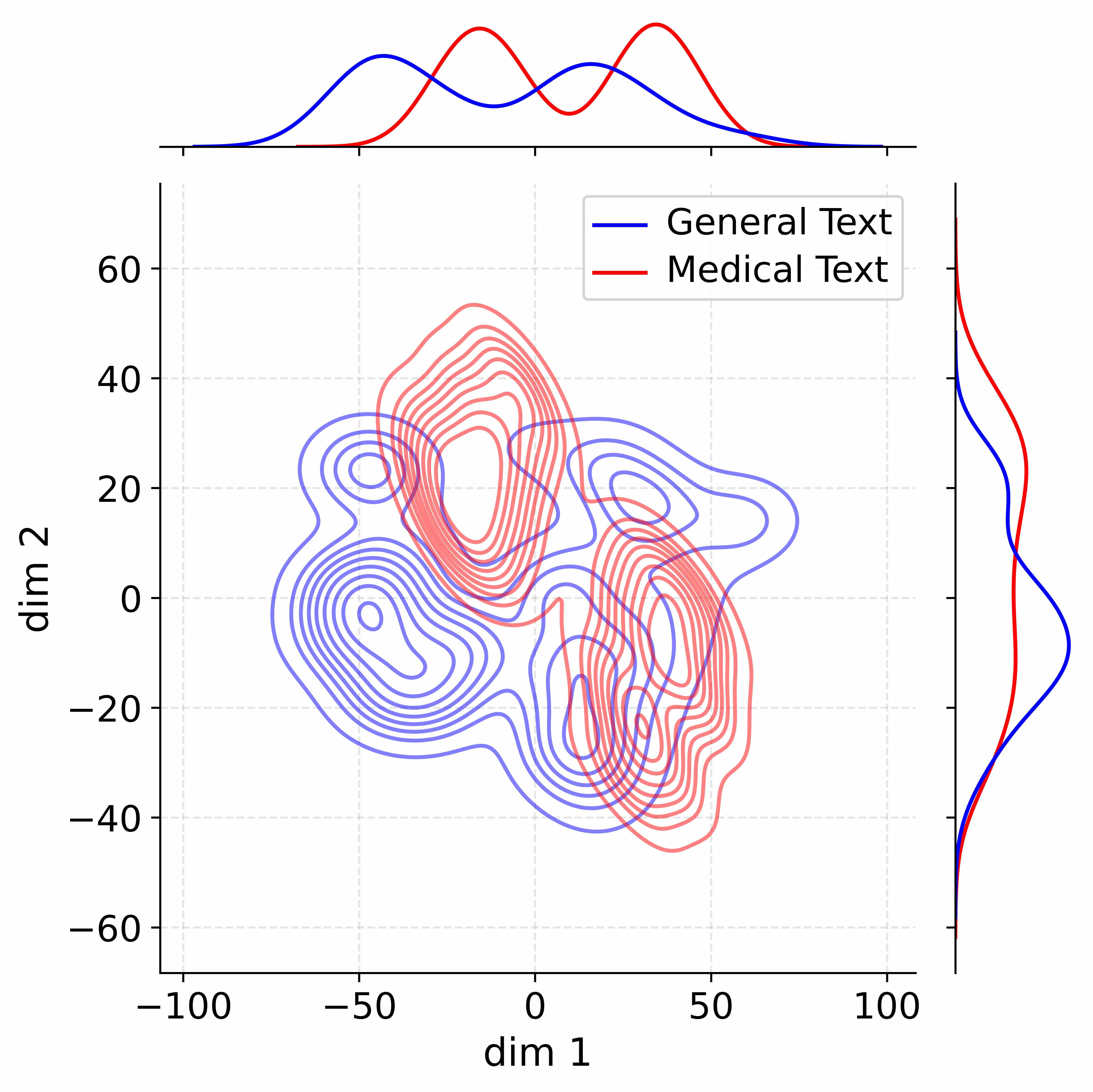
### Visual Description
## 2D Kernel Density Estimate Plot with Marginal Distributions: General vs. Medical Text
### Overview
The image is a statistical visualization comparing the distribution of two datasets in a two-dimensional space. It consists of a central contour plot (a 2D kernel density estimate) and two marginal distribution plots (1D kernel density estimates) on the top and right edges. The plot compares "General Text" (blue) and "Medical Text" (red).
### Components/Axes
* **Main Plot (Center):**
* **X-axis:** Labeled "dim 1". Scale ranges from -100 to 100, with major tick marks at -100, -50, 0, 50, and 100.
* **Y-axis:** Labeled "dim 2". Scale ranges from -60 to 60, with major tick marks at -60, -40, -20, 0, 20, 40, and 60.
* **Legend:** Located in the top-right quadrant of the main plot area. It contains two entries:
* A blue line labeled "General Text".
* A red line labeled "Medical Text".
* **Grid:** A light gray dashed grid is present in the background.
* **Marginal Plot (Top):**
* Aligned with the x-axis ("dim 1") of the main plot. It shows the 1D density distribution for each dataset along this dimension.
* **Marginal Plot (Right):**
* Aligned with the y-axis ("dim 2") of the main plot. It shows the 1D density distribution for each dataset along this dimension.
### Detailed Analysis
**1. Main Contour Plot (2D Density):**
* **General Text (Blue Contours):**
* **Trend/Shape:** The distribution is multimodal, showing several distinct clusters or modes.
* **Key Density Peaks (Approximate Centers):**
* A major, dense cluster centered near `dim1 ≈ -50, dim2 ≈ 0`.
* Another significant cluster centered near `dim1 ≈ 50, dim2 ≈ 20`.
* A smaller, less dense cluster near `dim1 ≈ -25, dim2 ≈ 25`.
* **Spatial Spread:** The distribution spans a wide range, roughly from `dim1 = -80 to 80` and `dim2 = -40 to 40`.
* **Medical Text (Red Contours):**
* **Trend/Shape:** The distribution is also multimodal but appears more concentrated in specific regions compared to the blue contours.
* **Key Density Peaks (Approximate Centers):**
* A very prominent, dense cluster centered near `dim1 ≈ 0, dim2 ≈ 40`.
* Another dense cluster centered near `dim1 ≈ 30, dim2 ≈ -20`.
* **Spatial Spread:** The distribution is more vertically oriented, spanning roughly `dim1 = -40 to 60` and `dim2 = -50 to 55`.
* **Overlap:** There is significant overlap between the two distributions, particularly in the central region around `dim1 = 0 to 30` and `dim2 = -20 to 20`.
**2. Marginal Distribution Plots:**
* **Top Marginal (dim 1):**
* **General Text (Blue):** Shows a bimodal distribution with peaks at approximately `dim1 = -50` and `dim1 = 50`. The valley between them is near `dim1 = 0`.
* **Medical Text (Red):** Shows a bimodal distribution with peaks at approximately `dim1 = -10` and `dim1 = 30`. The valley is near `dim1 = 10`.
* **Right Marginal (dim 2):**
* **General Text (Blue):** Shows a broad, roughly unimodal distribution centered near `dim2 = 0`, with a slight shoulder or secondary peak near `dim2 = 20`.
* **Medical Text (Red):** Shows a bimodal distribution with peaks at approximately `dim2 = 40` and `dim2 = -20`.
### Key Observations
1. **Multimodality:** Both datasets exhibit multimodal distributions in 2D space, suggesting the presence of distinct subgroups or categories within each text type.
2. **Cluster Separation:** The primary clusters for "General Text" (blue) are separated along the `dim 1` axis (left vs. right). The primary clusters for "Medical Text" (red) are separated along both axes, creating a diagonal separation (top-center vs. bottom-right).
3. **Density Concentration:** The "Medical Text" clusters appear to have higher peak densities (more tightly packed contour lines) than the "General Text" clusters, particularly the cluster at `(0, 40)`.
4. **Marginal Confirmation:** The 1D marginal plots clearly reflect the cluster separations seen in the 2D plot. The blue line's two peaks on the top marginal correspond to its left and right clusters. The red line's two peaks on the right marginal correspond to its top and bottom clusters.
### Interpretation
This visualization likely represents the output of a dimensionality reduction technique (like t-SNE or UMAP) applied to text data, where "dim 1" and "dim 2" are the two retained dimensions. The plot demonstrates that:
* **General Text** and **Medical Text** occupy partially overlapping but distinct regions in this learned feature space. This suggests that while there is commonality, the underlying semantic or stylistic features of medical text are distinguishable from general text.
* The **multimodal nature** of each distribution implies that neither "General Text" nor "Medical Text" is a monolithic category. Each likely contains several sub-types or topics. For example, the two blue clusters might represent different genres of general text (e.g., news vs. fiction), while the two red clusters might represent different medical domains (e.g., clinical reports vs. research articles).
* The **tight clustering** of Medical Text, especially the prominent mode at `(0, 40)`, indicates a highly consistent and specific set of features defining a major subset of medical documents. The separation between its clusters suggests these subtypes are quite distinct from each other.
* The **overlap region** contains text samples that share features common to both general and medical domains, potentially representing medical texts written for a lay audience or general texts discussing health topics.
In essence, the chart provides a visual fingerprint of how two broad text categories differ and are internally structured within a common analytical space.
</details>
(b) W/o stage1
<details>
<summary>figures/8B_final_grad_Layer30.jpg Details</summary>
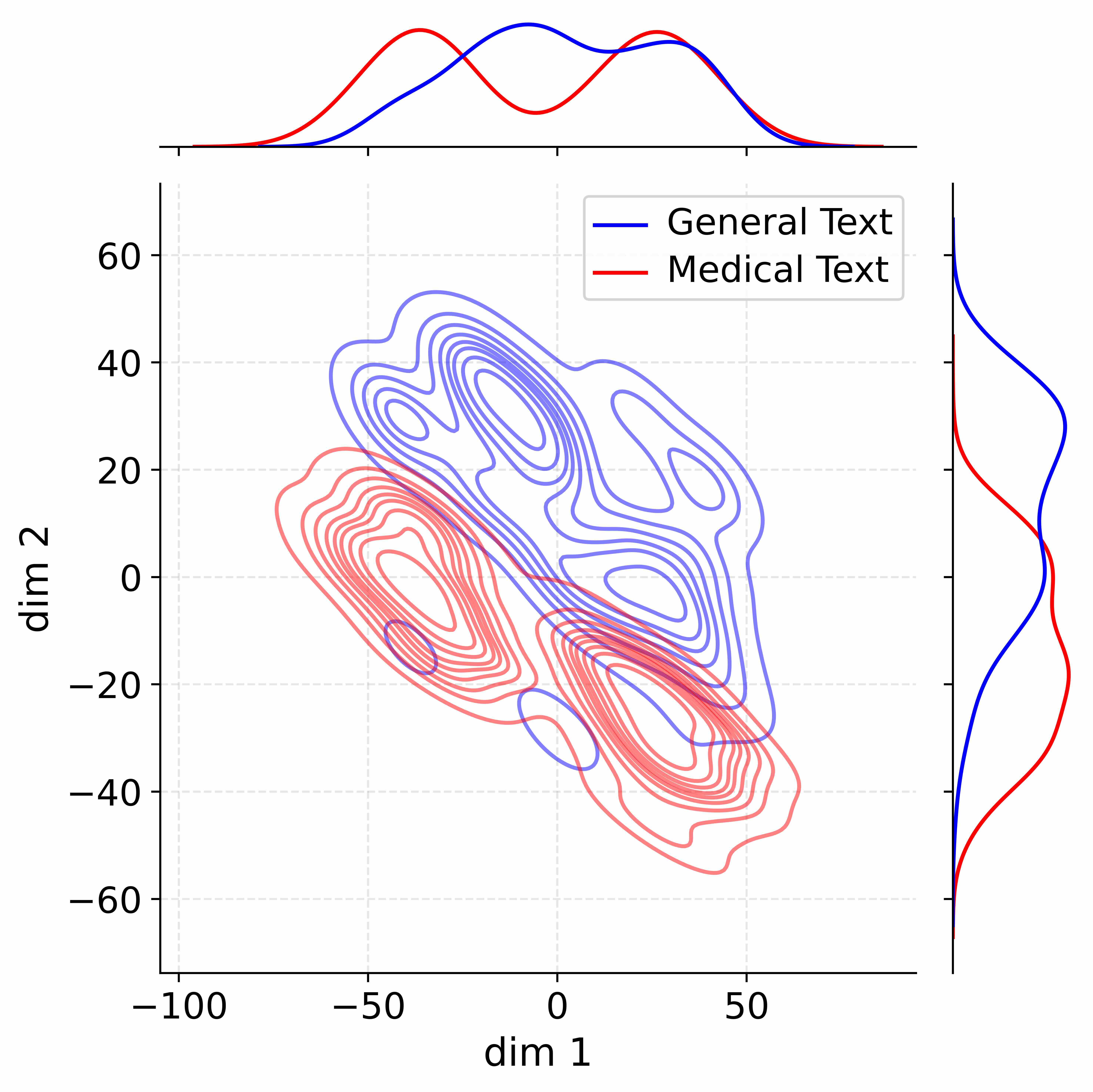
### Visual Description
## 2D Contour Plot with Marginal Distributions: General vs. Medical Text Embedding Distributions
### Overview
The image is a technical visualization comparing the distribution of two text corpora—"General Text" and "Medical Text"—in a two-dimensional latent space. It consists of a central 2D contour plot showing the joint density of the data points, accompanied by marginal density plots (1D distributions) along the top (for the x-axis) and right side (for the y-axis). The plot uses color coding to distinguish between the two text types.
### Components/Axes
* **Main Plot (Center):**
* **X-axis:** Labeled "dim 1". Ticks are at -100, -50, 0, and 50. The axis spans approximately from -100 to +75.
* **Y-axis:** Labeled "dim 2". Ticks are at -60, -40, -20, 0, 20, 40, and 60. The axis spans approximately from -70 to +70.
* **Data Series (Contour Lines):**
* **Blue Lines:** Represent "General Text" (as per legend). These contours are more spread out, covering a broad region from the lower-left to the upper-right of the plot.
* **Red Lines:** Represent "Medical Text" (as per legend). These contours are more concentrated, primarily in the lower-left quadrant, with a secondary cluster extending towards the lower-right.
* **Legend:** Located in the top-right corner of the main plot area. It contains:
* A blue line segment followed by the text "General Text".
* A red line segment followed by the text "Medical Text".
* **Marginal Distribution Plots:**
* **Top Marginal (for dim 1):** Positioned above the main plot, sharing the same x-axis scale. It shows two 1D density curves:
* A **blue curve** (General Text) with two distinct peaks: a smaller one near dim 1 ≈ -40 and a larger, broader peak centered near dim 1 ≈ +10.
* A **red curve** (Medical Text) with a single, prominent peak near dim 1 ≈ -30 and a smaller shoulder/peak near dim 1 ≈ +20.
* **Right Marginal (for dim 2):** Positioned to the right of the main plot, sharing the same y-axis scale. It shows two 1D density curves:
* A **blue curve** (General Text) with a broad, dominant peak centered near dim 2 ≈ +30 and a smaller peak near dim 2 ≈ -10.
* A **red curve** (Medical Text) with a sharp, dominant peak near dim 2 ≈ -30 and a smaller peak near dim 2 ≈ +10.
### Detailed Analysis
* **Spatial Distribution (Main Contour Plot):**
* **General Text (Blue):** The density is highest (innermost contours) in two main regions: one centered approximately at (dim 1: -20, dim 2: +30) and another near (dim 1: +20, dim 2: 0). The overall distribution forms a diagonal band from the lower-left to the upper-right, indicating a positive correlation between dim 1 and dim 2 for this corpus.
* **Medical Text (Red):** The highest density is concentrated in a tight cluster centered approximately at (dim 1: -40, dim 2: -20). A secondary, less dense cluster extends towards (dim 1: +20, dim 2: -40). The distribution is more compact and located primarily in the region where both dim 1 and dim 2 are negative.
* **Marginal Trends:**
* **dim 1 (Top Plot):** The General Text (blue) distribution is bimodal, suggesting two subpopulations or modes within the general text data along this dimension. The Medical Text (red) distribution is unimodal with a slight right skew, centered firmly in the negative range.
* **dim 2 (Right Plot):** The General Text (blue) distribution is again broad and centered in the positive range. The Medical Text (red) distribution is sharply peaked in the negative range, confirming its concentration in the lower part of the main plot.
### Key Observations
1. **Clear Separation:** The two text types occupy largely distinct regions of the 2D space. Medical Text is tightly clustered in the lower-left (negative dim 1, negative dim 2), while General Text is more diffuse and centered in the upper-right (positive dim 1, positive dim 2).
2. **Overlap Zone:** There is a region of moderate overlap between the contours of both distributions, roughly between dim 1: -10 to +30 and dim 2: -20 to +10. This suggests some texts from both corpora share similar characteristics in this latent space.
3. **Density Contrast:** The Medical Text contours are more tightly packed, indicating lower variance or higher consistency within that corpus along these dimensions. The General Text contours are more spread out, indicating greater diversity.
4. **Marginal Confirmation:** The marginal plots perfectly corroborate the spatial separation seen in the main plot. The peaks of the red and blue curves in both marginal plots are offset from each other.
### Interpretation
This visualization likely represents the output of a dimensionality reduction technique (like PCA, t-SNE, or UMAP) applied to text embeddings. The "dim 1" and "dim 2" are abstract axes capturing the most significant variance in the high-dimensional embedding space.
The data strongly suggests that **general-purpose text and specialized medical text have fundamentally different semantic or structural properties** that are captured by this embedding model. The tight clustering of medical text implies it uses a more specialized, consistent, and constrained vocabulary and syntax. In contrast, general text is more varied, leading to a broader distribution.
The positive correlation (diagonal trend) for General Text might reflect a common axis of variation in everyday language (e.g., from concrete to abstract topics). The Medical Text's concentration in the negative-negative quadrant could indicate it scores low on whatever abstract or general-language features define the positive ends of these dimensions.
The overlap region is particularly interesting from a Peircean investigative perspective—it represents the "ground" where medical and general discourse intersect. This could be text from patient education materials, health news articles, or medical narratives intended for a lay audience. The plot provides a quantitative map of linguistic domain separation, useful for tasks like domain adaptation in NLP, text classification, or analyzing the specificity of technical language.
</details>
(c) ADEPT
Figure 8: Kernel Density Estimation of activations for Qwen3-8B-Base, showing that our layer extension strategy enables clear parameter decoupling. We expand layers 26, 28, 29, and 30.
<details>
<summary>figures/Llama_8B_Layer30.jpg Details</summary>
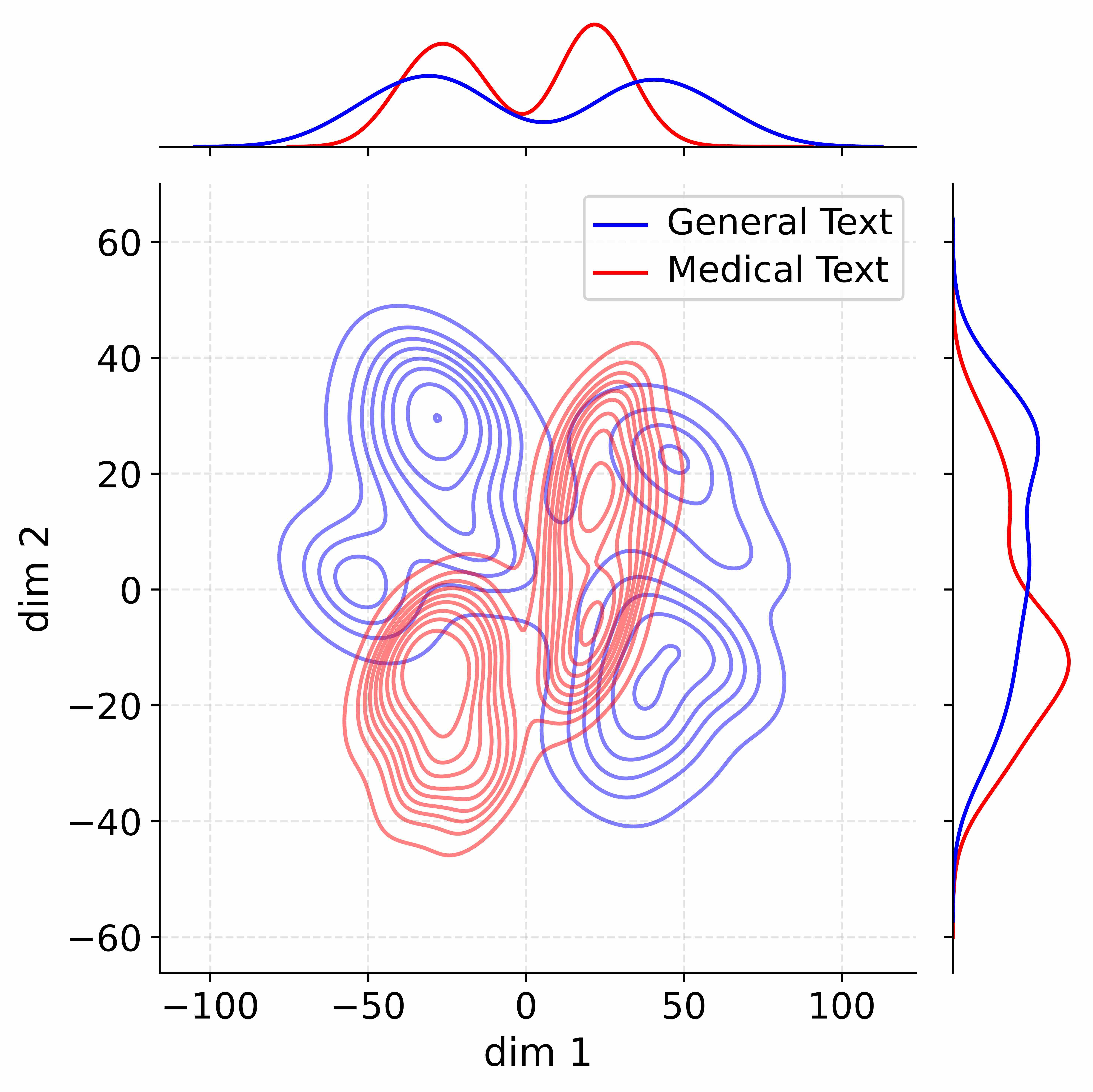
### Visual Description
## 2D Contour Plot with Marginal Distributions: General Text vs. Medical Text
### Overview
The image is a 2D kernel density estimate (KDE) contour plot comparing the distribution of two datasets, labeled "General Text" and "Medical Text," across two dimensions (`dim 1` and `dim 2`). The plot includes marginal distribution curves along the top (for `dim 1`) and right side (for `dim 2`). The visualization aims to show how the two text types cluster differently in this 2D feature space.
### Components/Axes
* **Main Plot (Center):**
* **X-axis:** Labeled `dim 1`. Scale ranges from approximately -120 to +120, with major tick marks at -100, -50, 0, 50, and 100.
* **Y-axis:** Labeled `dim 2`. Scale ranges from approximately -70 to +70, with major tick marks at -60, -40, -20, 0, 20, 40, and 60.
* **Data Series:** Represented by contour lines.
* **Blue Contours:** Correspond to "General Text" (as per legend).
* **Red Contours:** Correspond to "Medical Text" (as per legend).
* **Legend:** Located in the top-right quadrant of the main plot area. It contains two entries: a blue line labeled "General Text" and a red line labeled "Medical Text".
* **Top Marginal Plot:**
* Shows the 1D density distribution for `dim 1`.
* Contains a blue curve (General Text) and a red curve (Medical Text).
* **Right Marginal Plot:**
* Shows the 1D density distribution for `dim 2`.
* Contains a blue curve (General Text) and a red curve (Medical Text).
### Detailed Analysis
**1. Main Contour Plot (2D Distribution):**
* **General Text (Blue):** Exhibits a **multimodal distribution** with at least three distinct, separated clusters.
* **Cluster 1 (Top-Left):** Centered approximately at (`dim 1` ≈ -30, `dim 2` ≈ 30). This is a dense, roughly circular cluster.
* **Cluster 2 (Bottom-Right):** Centered approximately at (`dim 1` ≈ 30, `dim 2` ≈ -20). This cluster is elongated diagonally.
* **Cluster 3 (Top-Right):** Centered approximately at (`dim 1` ≈ 40, `dim 2` ≈ 20). This cluster is less dense and more diffuse than the others.
* The contours are widely spread, indicating a high variance across both dimensions.
* **Medical Text (Red):** Exhibits a **bimodal distribution** with two primary, connected clusters.
* **Cluster A (Bottom-Left):** Centered approximately at (`dim 1` ≈ -20, `dim 2` ≈ -25). This is a very dense, vertically oriented cluster.
* **Cluster B (Center-Right):** Centered approximately at (`dim 1` ≈ 15, `dim 2` ≈ 10). This cluster is also dense and appears to connect to Cluster A via a narrower band of density.
* The overall spread of the red contours is more compact than the blue, especially along `dim 1`.
**2. Top Marginal Distribution (`dim 1`):**
* **General Text (Blue):** The distribution is broad and appears **trimodal**, with peaks roughly at `dim 1` values of -30, 10, and 50. The peak at -30 is the highest.
* **Medical Text (Red):** The distribution is narrower and **bimodal**, with two sharp peaks at approximately `dim 1` = -20 and `dim 1` = 20. The peak at 20 is the highest.
**3. Right Marginal Distribution (`dim 2`):**
* **General Text (Blue):** The distribution is broad and appears **bimodal**, with peaks at approximately `dim 2` = 30 and `dim 2` = -10.
* **Medical Text (Red):** The distribution is also broad and **bimodal**, with peaks at approximately `dim 2` = 10 and `dim 2` = -30. The peak at -30 is the highest.
### Key Observations
1. **Distinct Clustering:** The two text types form largely separate clusters in the 2D space. The "General Text" clusters are positioned more towards the top-left and right, while the "Medical Text" clusters are positioned more towards the bottom-left and center.
2. **Overlap Region:** There is a region of moderate overlap between the distributions, primarily between the "General Text" cluster at (`dim 1`≈40, `dim 2`≈20) and the "Medical Text" cluster at (`dim 1`≈15, `dim 2`≈10).
3. **Variance Difference:** "General Text" shows greater dispersion (wider spread) across both dimensions compared to the more concentrated "Medical Text."
4. **Marginal Agreement:** The peaks and spreads observed in the 2D contour plot are consistent with the peaks shown in the 1D marginal distributions.
### Interpretation
This plot likely visualizes the output of a dimensionality reduction technique (like PCA or t-SNE) applied to text data, where `dim 1` and `dim 2` represent the two most significant derived features.
* **What the data suggests:** The clear separation indicates that "General Text" and "Medical Text" have fundamentally different statistical properties in this feature space. Medical text appears to be more specialized and consistent (tighter clusters), while general text is more diverse and variable (wider, multiple clusters).
* **Relationship between elements:** The marginal plots confirm the 1D projections of the 2D patterns. The top marginal shows that the most significant difference between the text types occurs along `dim 1`, where medical text has two sharp, distinct modes, while general text is more spread out.
* **Notable patterns/anomalies:** The most striking pattern is the **bimodal vs. multimodal** nature. The two sharp peaks for medical text along `dim 1` could correspond to two distinct sub-domains or styles within medical writing (e.g., clinical reports vs. research articles). The three clusters for general text might represent broad categories like news, fiction, and web content. The region of overlap suggests there may be some texts that share characteristics of both categories.
</details>
(a) Vanilla
<details>
<summary>figures/Llama_8B_only_grad_Layer30.jpg Details</summary>
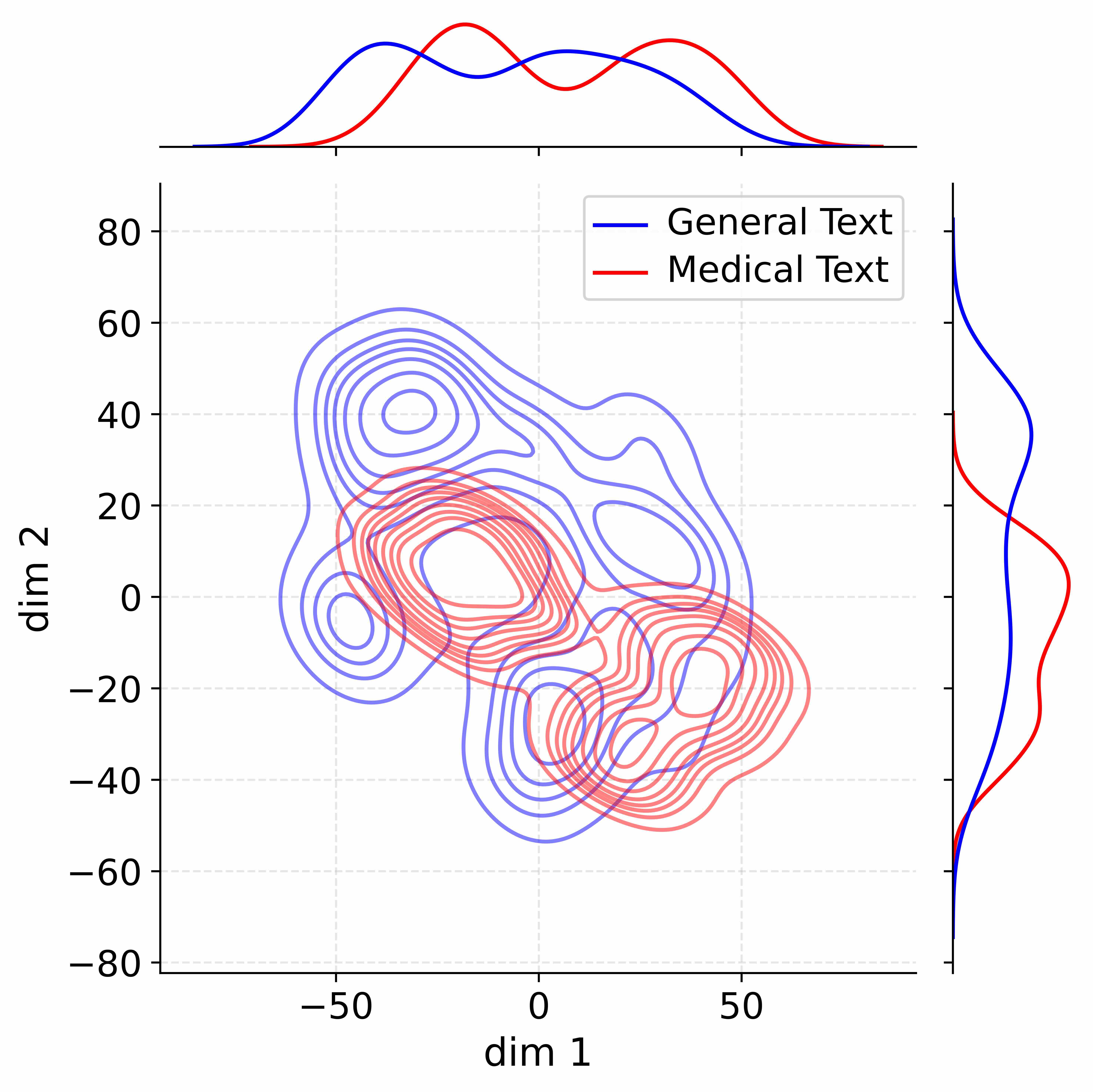
### Visual Description
## 2D Kernel Density Estimate Plot with Marginal Distributions: General Text vs. Medical Text
### Overview
The image displays a 2D kernel density estimate (KDE) plot comparing the distribution of two datasets in a two-dimensional space. The central plot shows contour lines representing data density, accompanied by marginal density plots on the top and right edges. The data appears to be the result of a dimensionality reduction technique (e.g., PCA, t-SNE) applied to text corpora, projecting high-dimensional text embeddings into two dimensions labeled "dim 1" and "dim 2".
### Components/Axes
* **Main Plot (Center):**
* **X-axis:** Labeled "dim 1". Ticks are marked at -50, 0, and 50. The axis spans approximately from -75 to +75.
* **Y-axis:** Labeled "dim 2". Ticks are marked at intervals of 20, from -80 to 80.
* **Grid:** A light gray dashed grid is present.
* **Data Series (Contour Lines):**
* **Blue Contours:** Represent "General Text". Lines are solid blue.
* **Red Contours:** Represent "Medical Text". Lines are solid red.
* **Legend:** Located in the top-right quadrant of the main plot area. It contains:
* A blue line segment followed by the text "General Text".
* A red line segment followed by the text "Medical Text".
* **Marginal Plot (Top):**
* Shows the 1D density distribution for "dim 1".
* Contains a blue curve (General Text) and a red curve (Medical Text).
* Shares the x-axis scale with the main plot.
* **Marginal Plot (Right):**
* Shows the 1D density distribution for "dim 2".
* Contains a blue curve (General Text) and a red curve (Medical Text).
* Shares the y-axis scale with the main plot.
### Detailed Analysis
**1. Main Contour Plot Analysis:**
* **General Text (Blue):** The distribution is broad and multi-modal. The highest density regions (innermost contours) are located in two primary clusters:
* A large cluster in the upper-left quadrant, centered approximately at (dim1 ≈ -30, dim2 ≈ 40).
* A smaller, distinct cluster in the lower-left quadrant, centered approximately at (dim1 ≈ -40, dim2 ≈ -10).
* The contours extend widely, covering a range from approximately dim1: -60 to +50 and dim2: -60 to +70.
* **Medical Text (Red):** The distribution is more concentrated and unimodal. The highest density region is a single, tight cluster centered near the origin, approximately at (dim1 ≈ 0, dim2 ≈ 0). The contours are densely packed, indicating a steep density gradient. The overall spread is smaller than the General Text, ranging approximately from dim1: -40 to +60 and dim2: -50 to +30.
* **Overlap:** There is significant spatial overlap between the two distributions, particularly in the central region around (0,0). However, the General Text distribution has substantial density in areas (especially upper-left) where the Medical Text density is very low.
**2. Marginal Distribution Analysis:**
* **Top Marginal (dim 1):**
* **General Text (Blue):** Shows a bimodal distribution. One peak is centered around dim1 ≈ -30, and a second, slightly lower peak is around dim1 ≈ +10.
* **Medical Text (Red):** Shows a unimodal distribution with a single peak centered near dim1 ≈ 0. The distribution is narrower than the blue curve.
* **Right Marginal (dim 2):**
* **General Text (Blue):** Shows a broad, somewhat bimodal distribution. The primary peak is around dim2 ≈ 40, with a secondary shoulder or peak around dim2 ≈ -10.
* **Medical Text (Red):** Shows a sharp, unimodal distribution with a single peak centered near dim2 ≈ 0. It is significantly narrower than the blue curve.
### Key Observations
1. **Cluster Separation:** The two text types form distinct clusters in the 2D space. "Medical Text" forms a single, tight cluster near the origin, while "General Text" forms a more dispersed, multi-cluster structure primarily in the left half of the plot.
2. **Variance Difference:** The "General Text" dataset exhibits much higher variance in both dimensions compared to the "Medical Text" dataset, as evidenced by the wider spread of its contours and broader marginal distributions.
3. **Multimodality:** The "General Text" distribution is clearly multimodal in both dimensions (bimodal in dim1, bimodal in dim2), suggesting the presence of distinct subgroups within the general text corpus. The "Medical Text" distribution is consistently unimodal.
4. **Central Overlap:** Despite their differences, the core of the Medical Text distribution overlaps with a region of moderate density in the General Text distribution, indicating some shared characteristics in the embedded space.
### Interpretation
This visualization suggests fundamental differences in the structure of general-purpose text versus domain-specific medical text when projected into a lower-dimensional embedding space.
* **Homogeneity vs. Heterogeneity:** The tight, unimodal cluster for Medical Text indicates that medical documents are relatively homogeneous in their semantic or stylistic content as captured by the embedding model. They occupy a specific, well-defined region of the semantic space.
* **Diversity of General Text:** The broad, multi-modal distribution of General Text reflects the inherent diversity of topics, styles, and contexts found in non-specialized text. The multiple clusters likely correspond to different genres or subject areas (e.g., news, fiction, technical writing, conversational text).
* **Domain Specificity:** The separation of the main Medical Text cluster from the densest parts of the General Text cluster (particularly the upper-left mode) implies that medical text possesses distinctive features that set it apart from typical general language. The overlap near the origin, however, suggests that medical text still shares a common linguistic foundation with general text.
* **Implication for Models:** This disparity has implications for training language models. A model trained primarily on general text may not adequately capture the concentrated, specific patterns of medical text, potentially leading to poorer performance on medical NLP tasks. Conversely, the distinct cluster for medical text justifies the use of domain-specific pre-training or fine-tuning.
</details>
(b) W/o stage1
<details>
<summary>figures/Llama_8B_final_grad_Layer30.jpg Details</summary>
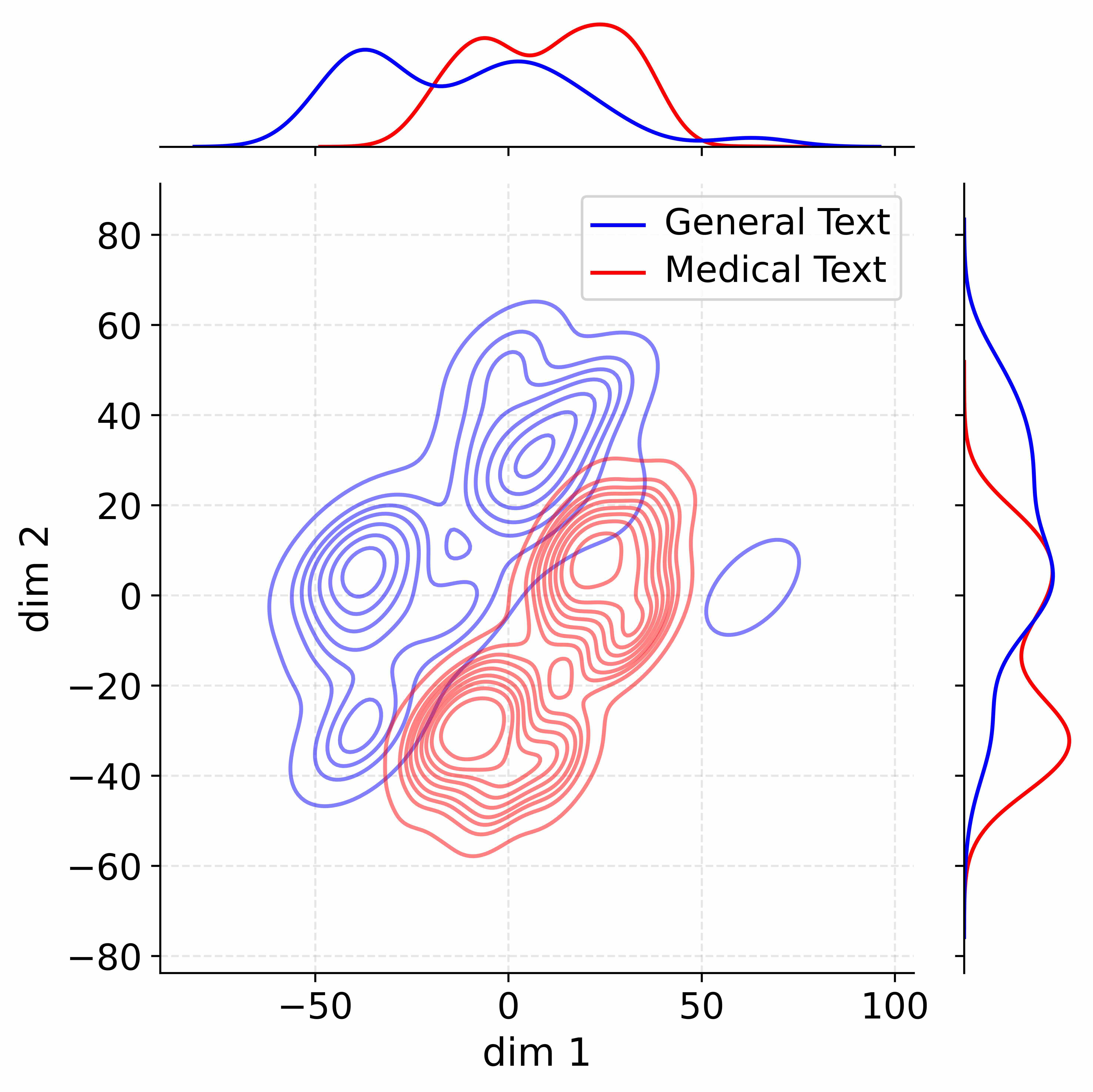
### Visual Description
\n
## 2D Contour Plot with Marginal Distributions: Comparison of General Text vs. Medical Text
### Overview
The image is a statistical visualization comparing the distribution of two text corpora ("General Text" and "Medical Text") across a two-dimensional latent space. It consists of a central 2D contour plot showing the joint density of the data points, accompanied by marginal density plots (histograms/KDEs) on the top and right sides, which show the distribution along each individual dimension. The plot uses color to distinguish between the two text categories.
### Components/Axes
* **Main Plot (Center):**
* **X-axis:** Labeled "dim 1". Scale ranges from approximately -70 to 110. Major tick marks are at -50, 0, 50, 100.
* **Y-axis:** Labeled "dim 2". Scale ranges from approximately -85 to 85. Major tick marks are at -80, -60, -40, -20, 0, 20, 40, 60, 80.
* **Data Representation:** Filled contour plots (Kernel Density Estimation - KDE). Blue contours represent "General Text". Red contours represent "Medical Text". The density of contour lines indicates the concentration of data points.
* **Marginal Plot (Top):**
* **X-axis:** Aligned with the main plot's "dim 1" axis.
* **Y-axis:** Represents probability density (unlabeled). Shows the 1D distribution of data along "dim 1".
* **Data Lines:** A blue line for "General Text" and a red line for "Medical Text".
* **Marginal Plot (Right):**
* **X-axis:** Represents probability density (unlabeled).
* **Y-axis:** Aligned with the main plot's "dim 2" axis.
* **Data Lines:** A blue line for "General Text" and a red line for "Medical Text".
* **Legend:** Located in the top-right quadrant of the main plot area.
* A blue line segment followed by the text "General Text".
* A red line segment followed by the text "Medical Text".
### Detailed Analysis
**1. Joint Distribution (Main Contour Plot):**
* **General Text (Blue):** Exhibits a multi-modal distribution with at least three distinct high-density clusters.
* **Cluster 1 (Primary):** Centered approximately at (dim1 ≈ 0, dim2 ≈ 40). This is the densest region, indicated by the tightest concentric contours.
* **Cluster 2:** Centered approximately at (dim1 ≈ -30, dim2 ≈ 0).
* **Cluster 3:** Centered approximately at (dim1 ≈ -20, dim2 ≈ -30).
* There is also a small, isolated, low-density region (a single contour loop) around (dim1 ≈ 60, dim2 ≈ 0).
* **Medical Text (Red):** Exhibits a more concentrated, bi-modal distribution.
* **Primary Cluster:** Centered approximately at (dim1 ≈ 20, dim2 ≈ -20). This is the densest region for the medical text.
* **Secondary Cluster:** Centered approximately at (dim1 ≈ 30, dim2 ≈ 10). This cluster partially overlaps with the primary cluster of the General Text.
* The overall spread of the red contours is smaller than the blue, indicating less variance in the medical text's representation in this 2D space.
**2. Marginal Distribution along "dim 1" (Top Plot):**
* **General Text (Blue):** Shows a broad, multi-modal distribution. Peaks are visible around dim1 ≈ -20 and dim1 ≈ 20, with a significant dip between them. The distribution has a long tail extending towards positive values.
* **Medical Text (Red):** Shows a sharper, more peaked distribution. The primary peak is around dim1 ≈ 20, aligning with its main cluster in the 2D plot. A smaller shoulder or secondary peak is visible around dim1 ≈ 0.
**3. Marginal Distribution along "dim 2" (Right Plot):**
* **General Text (Blue):** Shows a broad distribution with a major peak around dim2 ≈ 40 (corresponding to its primary cluster) and a secondary, lower peak around dim2 ≈ 0.
* **Medical Text (Red):** Shows a distribution with a major peak around dim2 ≈ -20 (corresponding to its primary cluster) and a secondary peak around dim2 ≈ 10.
### Key Observations
1. **Distinct Distributions:** The two text types occupy largely different regions of the 2D space. "General Text" is more dispersed and multi-modal, while "Medical Text" is more concentrated.
2. **Partial Overlap:** There is a region of overlap between the distributions, primarily where the secondary cluster of "Medical Text" (around dim1≈30, dim2≈10) intersects with the primary cluster of "General Text" (around dim1≈0, dim2≈40).
3. **Dimensional Separation:** The separation is most pronounced along "dim 2". The core of "General Text" is in the positive dim2 region, while the core of "Medical Text" is in the negative dim2 region.
4. **Outlier Region:** The small, isolated blue contour at (dim1≈60, dim2≈0) suggests a small subset of "General Text" data points that are distinct from the main clusters.
### Interpretation
This visualization likely represents the output of a dimensionality reduction technique (like t-SNE, UMAP, or PCA) applied to text embeddings. The "dim 1" and "dim 2" are abstract axes capturing the most significant variance in the high-dimensional text data.
The data suggests that **"Medical Text" forms a more coherent and specialized semantic cluster** compared to "General Text". Its tighter, bi-modal distribution implies that medical documents share a more consistent set of features or vocabulary that distinguish them from general language. The two modes within the medical text could represent sub-domains (e.g., clinical notes vs. research articles).
Conversely, **"General Text" is inherently more diverse**, as reflected in its multi-modal and widespread distribution. It encompasses a broader range of topics, styles, and contexts, leading to several distinct sub-clusters in the embedding space.
The partial overlap indicates that some medical texts share characteristics with general language, perhaps in introductory sections, patient-facing summaries, or topics at the intersection of medicine and general life. The separation along "dim 2" is particularly strong, suggesting this dimension captures a key feature that differentiates medical from non-medical discourse (e.g., technical jargon, formality, or subject specificity).
From a Peircean perspective, the contour lines are **icons** representing the density of data points. The spatial separation between the blue and red masses is an **index** of an underlying difference in the nature of the two text corpora. The legend provides the **symbolic** key to interpret this indexical relationship. The plot as a whole is a sign that the semantic "space" of medical language is a distinct, more focused subset within the broader universe of general language.
</details>
(c) ADEPT
Figure 9: Kernel Density Estimation of activations for Llama3-8B, showing that our layer extension strategy enables clear parameter decoupling. We expand layers 22, 23, 24, and 28.
## Appendix D Detailed Importance Distribution
<details>
<summary>figures/importance_1.7B_new.jpg Details</summary>
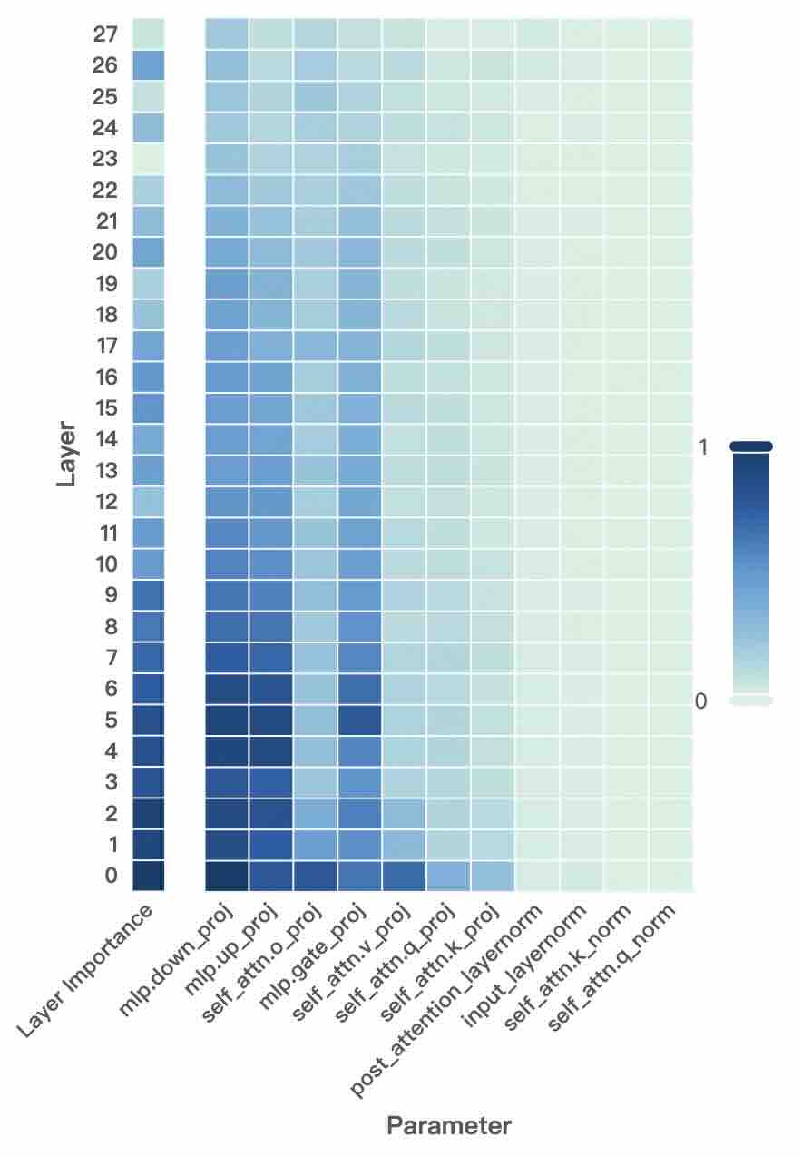
### Visual Description
## Heatmap: Layer-wise Parameter Importance in a Neural Network
### Overview
The image is a heatmap visualizing the importance of different parameters across 28 layers (0 to 27) of a neural network, likely a transformer-based model. The importance is represented by a color gradient, with darker blue indicating higher importance (closer to 1) and lighter blue/green indicating lower importance (closer to 0). The heatmap reveals a clear pattern where importance is concentrated in the lower layers and specific parameter types.
### Components/Axes
* **Y-axis (Vertical):** Labeled "Layer". It lists discrete layer numbers from 0 at the bottom to 27 at the top.
* **X-axis (Horizontal):** Labeled "Parameter". It lists 11 distinct parameter types, which are components of a transformer block. From left to right:
1. `Layer Importance` (An aggregate column)
2. `mlp.down_proj`
3. `mlp.up_proj`
4. `self_attn.o_proj`
5. `mlp.gate_proj`
6. `self_attn.v_proj`
7. `self_attn.q_proj`
8. `self_attn.k_proj`
9. `post_attention_layernorm`
10. `input_layernorm`
11. `self_attn.k_norm`
12. `self_attn.q_norm`
* **Color Bar/Legend:** Positioned on the right side of the chart. It is a vertical gradient bar labeled from `0` (bottom, light greenish-blue) to `1` (top, dark blue). This defines the scale for interpreting the color of each cell in the heatmap.
### Detailed Analysis
The heatmap is a grid where each cell's color corresponds to the importance value of a specific parameter at a specific layer.
**Spatial Grounding & Trend Verification:**
* **Aggregate Trend (Leftmost Column - `Layer Importance`):** This column shows a strong vertical gradient. Importance is highest (darkest blue) in the lowest layers (0-6), gradually becomes medium blue in the middle layers (7-19), and is lowest (lightest blue) in the highest layers (20-27). This indicates a general trend where lower layers are more critical to the model's function.
* **Parameter-Specific Trends:**
* **High Importance Cluster (Left-Center):** The columns for `mlp.down_proj`, `mlp.up_proj`, `self_attn.o_proj`, and `mlp.gate_proj` show the darkest blue cells, particularly in layers 0 through approximately 12. The darkest cells appear in layers 0-6 for `mlp.down_proj` and `mlp.up_proj`.
* **Moderate Importance Cluster (Center):** The columns for `self_attn.v_proj`, `self_attn.q_proj`, and `self_attn.k_proj` show medium blue shades, primarily in the lower to middle layers (0-15), fading to light blue in higher layers.
* **Low Importance Cluster (Right):** The four normalization parameter columns (`post_attention_layernorm`, `input_layernorm`, `self_attn.k_norm`, `self_attn.q_norm`) are consistently very light greenish-blue (near 0) across all 28 layers. This indicates these parameters have uniformly low measured importance.
**Key Data Points (Approximate):**
* **Highest Importance:** Cells in the `mlp.down_proj` and `mlp.up_proj` columns for layers 0-5 are the darkest, suggesting importance values likely in the range of 0.8 to 1.0.
* **Layer 0 Anomaly:** Layer 0 shows high importance across almost all parameter types except the normalization layers, making it the most "important" layer overall.
* **Transition Zone:** Around layers 12-15, there is a visible transition where the blue in the MLP and attention projection columns becomes noticeably lighter.
* **Uniformly Low:** All cells in the four rightmost normalization columns appear to have values < 0.1 across all layers.
### Key Observations
1. **Layer Hierarchy:** There is a clear importance hierarchy by layer depth: Lower Layers > Middle Layers > Higher Layers.
2. **Parameter Type Hierarchy:** MLP projection parameters (`down_proj`, `up_proj`, `gate_proj`) and the attention output projection (`o_proj`) are deemed more important than the attention query/key/value projections (`q_proj`, `k_proj`, `v_proj`), which are in turn more important than all normalization parameters.
3. **Normalization Insignificance:** Layer normalization parameters (`layernorm`, `k_norm`, `q_norm`) show negligible importance across the entire network depth according to this metric.
4. **Concentrated Criticality:** The most critical parameters for the model's operation appear to be concentrated in the first quarter of the network (layers 0-6), specifically within the MLP blocks.
### Interpretation
This heatmap likely visualizes the results of a parameter pruning sensitivity analysis or an attribution method (like integrated gradients) applied to a transformer model. The data suggests:
* **Functional Load Distribution:** The model's core computational "work" or feature transformation is heavily front-loaded. The lower layers are performing the most critical transformations on the input data, with the MLP layers (which typically handle non-linear feature processing) being paramount.
* **Redundancy in Depth:** The higher layers (20+) contribute less to the final output, as measured by this importance metric. This could indicate redundancy, suggesting the model might be pruned or compressed by removing or simplifying these higher layers with minimal performance impact.
* **Normalization as a Stable Framework:** The consistently low importance of normalization parameters aligns with their role as stabilizing, scaling components rather than primary feature extractors. They are necessary for training dynamics but may not be individually critical for the final inference output.
* **Architectural Insight:** The high importance of `mlp.down_proj` and `mlp.up_proj` highlights the significance of the expansion and contraction of dimensionality within the MLP blocks for model performance. The `self_attn.o_proj` (output projection of attention) being more important than `q_proj`, `k_proj`, `v_proj` suggests that the final combination of attention heads is a more critical operation than the initial projection into query, key, and value spaces.
**In summary, this heatmap provides a diagnostic map of the model's "brain," showing that its foundational processing in early-layer MLPs is most vital, while later layers and normalization functions play a less critical, possibly supportive or redundant, role.**
</details>
Figure 10: Layer-wise and parameter-wise importance distribution of Qwen3-1.7B-Base model
<details>
<summary>figures/importance_4B_new.jpg Details</summary>
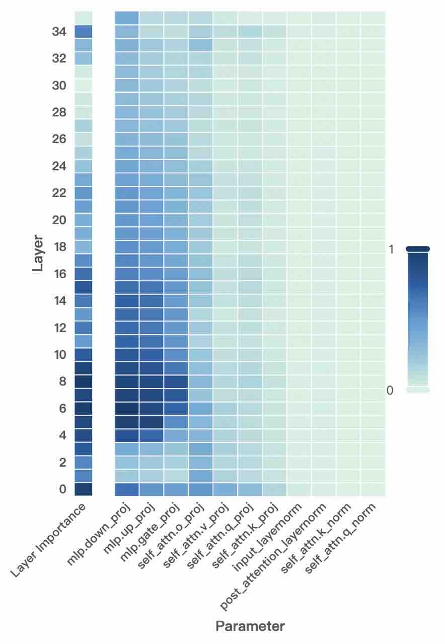
### Visual Description
## Heatmap: Layer-wise Parameter Importance in a Neural Network
### Overview
The image is a heatmap visualizing the relative importance of different parameters across the layers of a neural network model. The heatmap uses a color gradient to represent importance values, with darker blue indicating higher importance (closer to 1) and lighter green/white indicating lower importance (closer to 0). The data suggests an analysis of which components within a model's architecture are most significant at different depths.
### Components/Axes
* **Vertical Axis (Y-axis):** Labeled **"Layer"**. It lists numerical layer indices from **0** at the bottom to **34** at the top, incrementing by 2 (0, 2, 4, ..., 34). This represents the depth of the neural network.
* **Horizontal Axis (X-axis):** Labeled **"Parameter"**. It lists 12 specific parameter types, which are components of a transformer-based model architecture. From left to right:
1. `Layer Importance`
2. `mlp.down_proj`
3. `mlp.up_proj`
4. `mlp.gate_proj`
5. `self_attn.o_proj`
6. `self_attn.v_proj`
7. `self_attn.q_proj`
8. `self_attn.k_proj`
9. `input_layernorm`
10. `post_attention_layernorm`
11. `self_attn.k_norm`
12. `self_attn.q_norm`
* **Color Scale/Legend:** Positioned on the **right side** of the chart. It is a vertical bar showing a gradient from a very light green/white at the bottom (labeled **"0"**) to a dark blue at the top (labeled **"1"**). This defines the mapping of color to importance value.
### Detailed Analysis
The heatmap is a grid where each cell's color corresponds to the importance of a specific parameter at a specific layer.
**Trend Verification & Data Point Extraction:**
* **`Layer Importance` (First Column):** This column is consistently the darkest blue across **all layers (0-34)**, indicating a very high importance value (≈1.0) throughout the network. This likely represents an aggregate or baseline metric.
* **MLP Projection Layers (`mlp.down_proj`, `mlp.up_proj`, `mlp.gate_proj`):** These three columns show a distinct pattern. They are **darkest blue (high importance, ≈0.8-1.0) in the lower-to-mid layers (approximately layers 4-16)**. The importance gradually fades to a medium blue (≈0.4-0.6) in the higher layers (18-34). `mlp.down_proj` and `mlp.up_proj` appear slightly more important than `mlp.gate_proj` in the mid-layers.
* **Self-Attention Output & Value Projections (`self_attn.o_proj`, `self_attn.v_proj`):** These columns are a **medium blue (≈0.3-0.5)** in the lower layers (0-10), becoming lighter (≈0.1-0.3) in the mid and upper layers.
* **Self-Attention Query & Key Projections (`self_attn.q_proj`, `self_attn.k_proj`):** These are **light blue to very light green (≈0.1-0.3)** across most layers, with slightly higher values in the very early layers (0-6).
* **Layer Normalization Terms (`input_layernorm`, `post_attention_layernorm`, `self_attn.k_norm`, `self_attn.q_norm`):** These four rightmost columns are the **lightest in color (very light green/white, ≈0.0-0.15)** across the entire layer range, indicating consistently low measured importance in this analysis.
### Key Observations
1. **Dominance of MLP Layers:** The Multi-Layer Perceptron (MLP) projection layers (`down_proj`, `up_proj`, `gate_proj`) are the most important parameters after the aggregate `Layer Importance`, especially in the first half of the network.
2. **Layer-Dependent Importance:** Importance is not uniform. MLP parameters are critical in early/mid layers, while attention projections (`o_proj`, `v_proj`) have moderate importance early on that diminishes. Query/Key projections and normalization layers have low importance throughout.
3. **Clear Gradient:** There is a smooth visual gradient from left to right (high to low importance) and a vertical gradient within the MLP columns (high in early layers, decreasing later).
4. **Anomaly/Notable Point:** The `Layer Importance` column is uniformly maximal. This suggests it may be a different type of metric (e.g., a normalized sum or a separate importance score for the layer as a whole) rather than a parameter weight importance like the others.
### Interpretation
This heatmap provides a diagnostic view of a trained neural network's internal mechanics, likely from an interpretability or pruning study.
* **What the data suggests:** The analysis indicates that the **MLP blocks, particularly their down-projection and up-projection matrices, are the primary carriers of important information or computation in the earlier to middle stages of this model**. This aligns with some research suggesting MLP layers act as key "knowledge storage" components.
* **Relationship between elements:** The flow of importance seems to move from the MLP layers in the early network towards the attention output projections (`o_proj`), with the raw query/key projections and normalization layers being less critical for the specific importance metric used here. The uniform high value of `Layer Importance` implies that while individual parameter importance varies, the layers themselves are all considered significant contributors.
* **Potential implications:** If the goal were model compression or pruning, this chart suggests that the MLP projection layers in the first half of the network are the most sensitive to modification. Conversely, the normalization layers and query/key projections might be more candidates for aggressive pruning with less impact on performance. The diminishing importance of MLPs in later layers might indicate a shift in the type of processing performed deeper in the network.
</details>
Figure 11: Layer-wise and parameter-wise importance distribution of the Qwen3-4B-Base model
<details>
<summary>figures/importance_8B_new.jpg Details</summary>
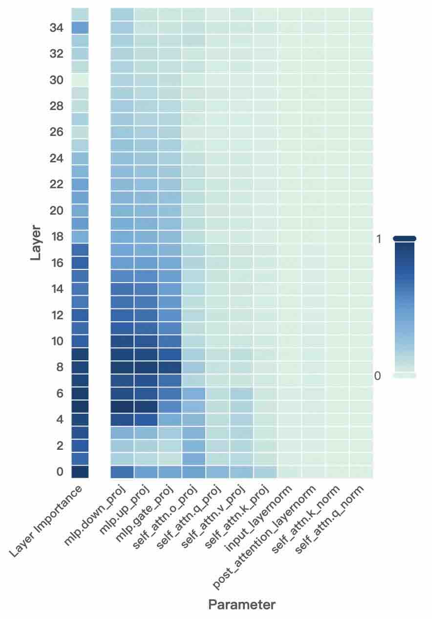
### Visual Description
## Heatmap: Neural Network Parameter Importance Across Layers
### Overview
The image is a heatmap visualizing the relative importance of different parameters across the layers of a neural network, likely a transformer-based model. The chart uses a color gradient to represent importance values, with darker blue indicating higher importance (closer to 1) and lighter blue/green indicating lower importance (closer to 0).
### Components/Axes
* **Y-Axis (Vertical):** Labeled **"Layer"**. It represents the depth of the network, with layer numbers increasing from bottom to top. The axis is marked with even numbers: 0, 2, 4, 6, 8, 10, 12, 14, 16, 18, 20, 22, 24, 26, 28, 30, 32, 34.
* **X-Axis (Horizontal):** Labeled **"Parameter"**. It lists specific components or weight matrices within each layer. The labels are rotated approximately 45 degrees for readability. From left to right, the parameters are:
1. `Layer Importance` (This appears to be a summary column for the entire layer).
2. `mlp.down_proj`
3. `mlp.up_proj`
4. `mlp.gate_proj`
5. `self_attn.o_proj`
6. `self_attn.q_proj`
7. `self_attn.v_proj`
8. `self_attn.k_proj`
9. `input_layernorm`
10. `post_attention_layernorm`
11. `self_attn.k_norm`
12. `self_attn.q_norm`
* **Color Scale/Legend:** Positioned on the right side of the chart. It is a vertical bar showing a gradient from a very light greenish-blue at the bottom (labeled **0**) to a dark blue at the top (labeled **1**). This scale maps color intensity to an importance value between 0 and 1.
### Detailed Analysis
The heatmap is a grid where each cell's color corresponds to the importance of a specific parameter at a specific layer.
* **`Layer Importance` Column (Far Left):** This column shows a strong vertical trend. Importance is highest (darkest blue) in the lowest layers (0-8), remains moderately high through the middle layers (10-20), and then gradually decreases (becomes lighter) in the highest layers (22-34). Layer 0 is the darkest cell in this column.
* **MLP Parameters (`mlp.down_proj`, `mlp.up_proj`, `mlp.gate_proj`):** These three columns show a very similar pattern. They exhibit high importance (dark blue) in the lower to middle layers, roughly from layer 4 to layer 18. The intensity peaks around layers 8-14. Importance drops off significantly in the higher layers (above 20), becoming very light.
* **Self-Attention Output & Query Projections (`self_attn.o_proj`, `self_attn.q_proj`):** These columns show moderate importance concentrated in the lower-middle layers. The darkest cells appear between layers 4 and 12, with `self_attn.q_proj` showing slightly higher intensity than `self_attn.o_proj` in that range. They fade to low importance in higher layers.
* **Self-Attention Value & Key Projections (`self_attn.v_proj`, `self_attn.k_proj`):** These parameters show lower overall importance compared to the previous groups. There is a faint band of slightly higher importance (light blue) in the lower layers (approximately 0-10), but it is much less pronounced. They are very light (near 0) for most layers.
* **Normalization Layers (`input_layernorm`, `post_attention_layernorm`, `self_attn.k_norm`, `self_attn.q_norm`):** These four rightmost columns are uniformly very light greenish-blue across all layers, indicating consistently low importance values (near 0) throughout the network. There is no significant variation by layer.
### Key Observations
1. **Layer-Depth Gradient:** There is a clear overall trend where parameters in the lower and middle layers of the network are deemed more important than those in the highest layers.
2. **Parameter-Type Hierarchy:** A distinct hierarchy of importance exists among parameter types:
* **High Importance:** MLP projection layers (`down_proj`, `up_proj`, `gate_proj`).
* **Moderate Importance:** Self-attention output and query projections (`o_proj`, `q_proj`).
* **Low Importance:** Self-attention value and key projections (`v_proj`, `k_proj`).
* **Very Low Importance:** All normalization layers.
3. **Concentration of Importance:** The most critical parameters (darkest blues) are not evenly distributed but are concentrated in a "band" spanning the lower-middle layers (approximately layers 4 through 18).
4. **Uniformity of Norm Layers:** The normalization parameters show almost no variation in importance across the entire depth of the network, suggesting they play a consistently minor role according to this metric.
### Interpretation
This heatmap likely visualizes the results of a parameter pruning or importance scoring analysis (e.g., using methods like movement pruning, Taylor expansion, or gradient-based saliency) on a trained transformer model. The data suggests several key insights about the model's functional anatomy:
* **Core Computational Pathways:** The high importance of MLP projections, especially in mid-layers, indicates these components are crucial for the model's core feature transformation and processing capabilities. The network relies heavily on these non-linear transformations.
* **Selective Attention Mechanism:** Within the attention mechanism, the query (`q_proj`) and output (`o_proj`) projections are more vital than the key (`k_proj`) and value (`v_proj`) projections. This could imply that the model's ability to *form* queries and *integrate* attention results is more critical than the precise representation of keys and values for this particular task or metric.
* **Depth-Dependent Processing:** The concentration of importance in lower-middle layers aligns with theories that early-to-mid layers in deep networks are responsible for building rich, abstract representations, while the very highest layers may perform more task-specific, fine-grained adjustments that are less sensitive to individual parameter perturbation.
* **Normalization as a Stable Foundation:** The uniformly low importance of normalization layers does not mean they are unimportant for model function or training stability. Instead, it suggests that their specific parameter values are highly robust or redundant; small changes to them have minimal impact on the model's output according to this importance measure. They provide a stable, but not highly tunable, foundation.
**Notable Anomaly:** The `Layer Importance` summary column shows a slightly different trend than the individual MLP parameters. Its importance decays more smoothly and remains somewhat higher in the top layers compared to the sharp drop-off of `mlp.*` parameters. This could indicate that while specific MLP weights become less critical, the layer as a whole retains some functional significance, possibly due to residual connections or other components not broken out in this chart.
</details>
Figure 12: Layer-wise and parameter-wise importance distribution of the Qwen3-8B-Base model
<details>
<summary>figures/importance_Llama_new.jpg Details</summary>
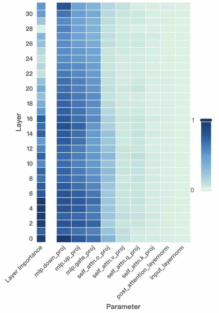
### Visual Description
## Heatmap: Layer-wise Parameter Importance in a Neural Network
### Overview
The image is a heatmap visualizing the relative importance of different parameters across the layers of a neural network model. The heatmap uses a color gradient from light (value 0) to dark blue (value 1) to represent importance scores. The data suggests an analysis of which components within the model's architecture are most significant for its function, likely derived from an interpretability technique like gradient-based attribution or parameter pruning sensitivity.
### Components/Axes
* **Y-Axis (Vertical):** Labeled **"Layer"**. It represents the depth of the network, with layers numbered from **0** (bottom) to **30** (top). The axis has tick marks at every even number (0, 2, 4, ..., 30).
* **X-Axis (Horizontal):** Labeled **"Parameter"**. It lists specific components or weight matrices within each layer. The categories, from left to right, are:
1. `Layer Importance` (This appears to be an aggregate or summary column for the entire layer).
2. `mlp.down_proj`
3. `mlp.up_proj`
4. `mlp.gate_proj`
5. `self_attn.o_proj`
6. `self_attn.v_proj`
7. `self_attn.q_proj`
8. `self_attn.k_proj`
9. `post_attention_layernorm`
10. `input_layernorm`
* **Legend/Color Scale:** Located on the right side of the chart. It is a vertical bar showing a gradient from **light greenish-white (labeled "0")** at the bottom to **dark blue (labeled "1")** at the top. This scale maps color intensity to an importance value between 0 and 1.
### Detailed Analysis
The heatmap displays a grid where each cell's color corresponds to the importance value of a specific parameter at a specific layer.
**Trend Verification & Data Point Extraction:**
* **`Layer Importance` Column:** This column shows a clear gradient. Importance is highest (darkest blue, ~0.9-1.0) in the lowest layers (0-6). It gradually becomes lighter (decreasing to ~0.5-0.7) in the middle layers (8-20), and is lightest (lowest importance, ~0.2-0.4) in the highest layers (22-30).
* **MLP Parameters (`mlp.down_proj`, `mlp.up_proj`, `mlp.gate_proj`):** These three columns exhibit a very similar and strong pattern. They are consistently the **darkest blue (highest importance, ~0.8-1.0)** across almost all layers, from 0 to 30. There is a very slight lightening in the topmost layers (28-30), but they remain significantly darker than most other parameters.
* **Self-Attention Output & Value Projections (`self_attn.o_proj`, `self_attn.v_proj`):** These columns show moderate importance. They are a medium blue (~0.5-0.7) in the lower to middle layers (0-18) and become progressively lighter (~0.2-0.4) in the higher layers (20-30).
* **Self-Attention Query & Key Projections (`self_attn.q_proj`, `self_attn.k_proj`):** These are lighter than the `o_proj` and `v_proj`. They start as a light-medium blue (~0.4-0.6) in lower layers and fade to very light (~0.1-0.3) in higher layers.
* **Layer Normalization Parameters (`post_attention_layernorm`, `input_layernorm`):** These two rightmost columns are the **lightest overall (lowest importance, ~0.0-0.2)**. They show a very faint greenish-white color across all layers, with `input_layernorm` being marginally lighter than `post_attention_layernorm`.
### Key Observations
1. **Dominance of MLP Layers:** The Multi-Layer Perceptron (MLP) projection layers (`down_proj`, `up_proj`, `gate_proj`) are unequivocally the most important parameters throughout the entire network depth.
2. **Layer Depth vs. Importance:** There is a general trend where parameter importance decreases as the layer number increases (i.e., deeper into the network). This is most pronounced in the `Layer Importance` summary and the attention projection parameters.
3. **Attention Component Hierarchy:** Within the self-attention mechanism, a clear hierarchy exists: `o_proj` and `v_proj` are more important than `q_proj` and `k_proj`.
4. **Minimal Role of LayerNorm:** The layer normalization parameters (`input_layernorm` and `post_attention_layernorm`) have consistently negligible importance scores according to this metric.
### Interpretation
This heatmap provides a Peircean investigative window into the functional architecture of the analyzed model (likely a Transformer-based LLM). The data suggests:
* **Core Computational Engine:** The MLP blocks are the primary drivers of the model's representational power or task-specific processing, as their parameters are deemed highly important across all layers. This aligns with theories that MLPs store factual knowledge and perform complex transformations.
* **Feature Processing in Early Layers:** The higher importance in lower layers indicates that the initial processing of input features is critical. The model's foundational understanding is built here.
* **Attention's Role:** The attention mechanism, while important, shows a differentiated role. The output (`o_proj`) and value (`v_proj`) projections, which combine information from different tokens, are more crucial than the query (`q_proj`) and key (`k_proj`) projections, which determine attention patterns. This could imply that *how* information is aggregated is more vital than the precise matching of queries and keys for this specific importance metric.
* **Normalization as a Utility:** The very low importance of LayerNorm parameters suggests they act as stable, routine utility functions—essential for training stability but not carrying significant "information" or "importance" in terms of the model's final output decision, as measured by this analysis.
**Anomaly/Notable Point:** The `Layer Importance` column is an aggregate. Its gradient from dark to light confirms the overall trend that lower layers are more "important" than higher layers by this metric, which is a key insight for model compression or pruning strategies—pruning higher layers may be less damaging.
</details>
Figure 13: Layer-wise and parameter-wise importance distribution of the Llama3-8B model
To investigate which layers should be expanded, we conduct a comprehensive importance analysis at both the layer and parameter levels. Specifically, we compute the importance scores for each layer and parameter across multiple models, and visualize their detailed distributions (see Figure 10, Figure 11, Figure 12, and Figure 13). Our analysis yields the following key observations:
1. Layer and parameter importance alignment. Overall, the distributions of layer-wise importance and parameter-wise importance are highly aligned across all four models. This alignment is expected, as both metrics are fundamentally computed under the same principle—estimating the impact of masking out (setting to zero) a given layer or parameter on model performance. Since parameter importance essentially decomposes the contribution at the layer level, this consistency reflects the intrinsic, nested relationship between the two. It also indicates that layer-level and parameter-level interventions affect the model’s predictive capability in a coherent manner.
2. High importance in lower layers and the penultimate layer exception. A notable pattern across all models is that the most important layers tend to be concentrated in the lower (early to middle) layers of the network, with importance values generally decreasing towards higher layers. This pattern suggests that the early layers play a critical role in the overall function of the model.
One plausible explanation, is that lower layers are responsible for capturing general syntactic properties and foundational compositionality (Clark et al., 2019; Hewitt & Manning, 2019), such as basic grammar and phrase structure. In contrast, deeper layers are typically responsible for integrating more task- or context-specific semantic information. This division of labor (earlier layers for generic linguistic structure, deeper layers for task semantics) naturally results in higher sensitivity to interventions at the bottom layers. This also provides a theoretical basis for layer expansion in deep layers.
An interesting exception observed in all models is that the penultimate layer does not follow this general trend: its importance appears elevated relative to immediately adjacent layers. This may stem from the model’s need to consolidate high-level semantic features just before producing the output prediction. The penultimate layer may act as a “bottleneck” for aggregating information necessary for the final decision or token generation—potentially as a final representation refinement step. Similar phenomena have been observed in works such as Intrinsic Dimensionality Explains the Effectiveness of Language Model Pruning (Aghajanyan et al., 2021), which highlight the special role of upper- and penultimate layers in output formation.
3. Intra- and inter-family patterns: Qwen vs. Llama models.
Qwen family: Across the Qwen models (Qwen3-1.7B, 4B, 8B), the overall trends are similar:
- Importance is strongly concentrated in the lower and middle layers, particularly within the first 10 layers, regardless of total model depth.
- Among parameters, mlp.down_proj and mlp.up_proj typically dominate in the most important layers, suggesting that feed-forward (MLP) components contribute substantially to the information processing in the Qwen series.
- With increasing model size (from 1.7B to 8B), the importance distribution appears to spread out slightly, showing less sharpness at the very bottom—possibly reflecting increased capacity and redundancy in larger networks.
Cross-family: Comparing Qwen models to Llama3-8B, we observe both notable similarities and differences:
- Both model families consistently exhibit high importance in MLP-related parameters (mlp.down_proj, mlp.up_proj, and mlp.gate_proj), especially in the most important layers. This underscores the universal role of the feed-forward network in transforming and integrating information beyond the capabilities of self-attention alone.
- Llama3-8B shows a broader distribution of importance across layers, with non-negligible values extending further into the middle and upper layers, suggesting a more distributed processing pipeline. In contrast, Qwen models tend to concentrate importance more in the lower layers.
- The dominance of MLP components in Llama3-8B is somewhat less pronounced than in Qwen, with parameter importance appearing more diffuse overall. These inter-family differences may be attributable to variations in architecture (such as normalization, attention mechanisms, or feed-forward design), pre-training data, or other modeling choices, leading to distinct strategies of information flow and representation across the network depth.
## Appendix E Layer-wise Importance Estimation Methods Comparison
To investigate which layers contribute most to model performance, we employed four different strategies to compute layer-wise importance:
1. Cumulate importance of parameters: For each parameter $p$ in a layer, we compute the product $p\frac{∂L}{∂ p}$ , and sum across all parameters in the layer:
$$
I_layer=∑_p∈layerp\frac{∂L}{∂ p} \tag{11}
$$
1. Module-wise rank aggregation: For each module (e.g., attention, MLP, normalization), we calculate the importance score, rank layers by their score within each module, and aggregate rankings to obtain a total rank for each layer.
1. Masking out: For each layer, we mask out its parameters (i.e., set to zero) and evaluate the change in loss:
$$
I_layer=L(model with layer $l$ masked)-L(original model) \tag{12}
$$
1. Fisher information: For each parameter $p$ in a layer, using the Fisher information approximation
$$
F(p)=E≤ft[≤ft(\frac{∂\log p(y|x)}{∂ p}\right)^2\right] \tag{13}
$$
Layer-level Fisher importance is obtained by summing over all parameters in the layer.
To further understand the significance and robustness of these metrics, we conducted a preliminary experiment on the Qwen3-1.7B-Base in the medical domain with dev subset of MMLU, CMMLU to detect the importance of layers, focusing on how different gradient computation strategies affect downstream performance.
Table 8: Performance of different expansion methods on medical-domain tasks (best result in each column is bolded). The numbers in parentheses after each method in the table indicate which layers were expanded. The Qwen3-1.7B-Base model has a total of 28 layers, indexed from 0 to 27.
| Methods Name | mmlu | cmmlu | medqa | cmb | mmcu |
| --- | --- | --- | --- | --- | --- |
| Qwen3-1.7B-Base | 62.57 | 66.86 | 48.39 | 63.67 | 69.17 |
| Uniformly Expansion (6,13,20,27) | 59.06 | 64.98 | 48.78 | 64.25 | 70.10 |
| Uniformly Expansion for first 16 layers (3,7,11,15) | 59.60 | 64.91 | 48.78 | 64.07 | 69.80 |
| Uniformly Expansion for last 16 layers (15,19,23,27) | 61.60 | 66.15 | 49.32 | 65.55 | 71.09 |
| Importance Cumulatation (23,24,25,27) | 62.63 | 66.81 | 50.19 | 63.85 | 69.48 |
| Rank Aggregation (22,24,25,27) | 62.72 | 66.86 | 50.57 | 63.97 | 69.78 |
| Masking Out (22,23,25,27) | 62.80 | 66.89 | 50.75 | 65.43 | 71.98 |
| Fisher (23,24,25,26) | 61.84 | 66.43 | 49.15 | 64.13 | 68.82 |
Table 8 compares the effect of different layer selection methods for expansion on a variety of medical-domain tasks using Qwen3-1.7B-Base. Several key observations can be made:
1. Similarity of selected layers across methods. All importance calculation methods lead to the selection of similar layers for expansion. For instance, the layers chosen by methods such as Importance Cumulatation (23,24,25,27), Rank Aggregation (22,24,25,27), Masking Out (22,23,25,27), and Fisher (23,24,25,26) significantly overlap, especially in the last 6 layers of the model (layers 22 and above). This convergence strongly validates our previous observations that general capability-critical layers tend to be concentrated in the latter half of the model in Appendix D.
In addition, the results show that uniform expansion into the last 16 layers (Uniformly Expansion for last 16 layers (15,19,23,27)) consistently outperforms expansion into the first 16 layers (Uniformly Expansion for first 16 layers (3,7,11,15)) or uniformly across all layers, further supporting the result in Appendix D.
2. Robustness of expansion results across methods. Despite minor variability in the specific layers chosen by each method, the final performance of all importance-based expansion approaches is consistently better than both the vanilla baseline and uniform expansion. For example, on the MedQA dataset, all methods using calculated importance exceed the baseline score (e.g., Masking Out achieves 50.75 vs. baseline 48.39), and on MMLU-med, Rank Aggregation achieves 67.95 versus the baseline 66.49. Crucially, the differences in scores among Masking Out, Rank Aggregation, Importance Cumulatation, and Fisher are relatively small for most tasks (typically less than 2 points), indicating that the overall framework is robust to the choice of importance calculation technique. Since our principal contribution is the training paradigm rather than the specific importance metric, for subsequent experiments, we employ the masking out approach, which demonstrated the strongest effect in preliminary experiment.
## Appendix F Theoretical Analysis
Our theoretical analysis relies on several simplifying assumptions as outlined below. We discuss the rationality and limitations of each assumption:
1. Linearized Model Structure: We model the transformer as a stack of $L$ independent residual blocks, effectively ignoring cross-layer coupling effects such as those arising from pre-norm and residual connections.
Justification: In our layer expansion scheme, the newly added layers are always separated by at least one original frozen layer and never arranged in a cascading manner. This design substantially weakens direct coupling between newly expanded layers, which, in turn, reduces the degree of inter-layer interaction and nonlinearity affecting our analysis. And this abstraction is commonly used in theoretical studies (e.g., NTK analysis or pruning literature) to make layerwise analysis tractable.
1. Loss Function Smoothness: We assume the loss function $\ell(·,·)$ is $β$ -smooth and $L_∞$ -Lipschitz with respect to predictions.
Justification: Standard loss functions such as cross-entropy (with stability improvement) and mean squared error are widely established to satisfy these properties. These conditions allow us to relate small output perturbations to controlled changes in loss, facilitating theoretical bounds.
1. Training Dynamics: Our analysis assumes training is performed with a first-order SGD-like optimizer, disregarding effects from Adam or other adaptive methods.
Justification: First-order SGD provides well-understood theoretical properties and is commonly used in theoretical deep learning research. While Adam introduces adaptive scaling that can affect convergence, many results (e.g., generalization gap bounds) transfer qualitatively between SGD and Adam in practice.
1. NTK Regime and Sensitivity: Our analysis of layer sensitivity relies on the NTK (Neural Tangent Kernel) approximation (Jacot et al., 2018), which essentially assumes the model behaves locally linearly around its current parameters. Moreover, we should consider the model training process to be relatively stable, with no anomalous occurrences such as gradient explosion.
Justification: This assumption is particularly well-motivated in our setting for two reasons. First, our adaptation protocol only updates a small number of newly introduced parameters while keeping the vast majority of the pre-trained weights frozen and decouples parameters to maximize the retention of general capabilities. This ensures that the parameter changes remain minimal, keeping the network within the local linear (NTK) regime throughout adaptation. Second, unlike random initialization, our starting point is a well-trained model on a large general-domain corpus, which already provides robust and meaningful representations. Perturbations induced by finetuning are thus intrinsically local in the function space and less likely to induce sudden or nonlinear model behavior, further enhancing the validity of the NTK approximation.
Overall, these assumptions enable us to derive interpretable upper bounds and provide actionable layer selection criteria, but should be considered as idealizations. The correspondence between these theoretical insights and practical behavior is also validated in our empirical experiments.
### F.1 Optimality of Least-Important Block Expansion for Preserving General Capabilities
Notation: Let $M_0$ denote the original base model, and $M_S^(T)$ denote the model after $T$ steps of adaptation, wherein only the set $S$ of $k$ layers are unfrozen and updated, and $\ell(·,y)$ is the loss function (e.g., cross-entropy) which is $L$ -Lipschitz and $β$ -smooth in its first argument. $Δ^(l)$ represents the importance score of layer $l$ as defined below.
Layer Importance Score:
$$
Δ^(l):=E_x∼ D_{gen}\big[\ell(M_0^(-l)(x),y(x))-\ell(M_0(x),y(x))\big]
$$
where $M_0^(-l)$ is $M_0$ with the $l$ -th layer masked out.
**Theorem F.1 (Upper Bound on Generalization Gap by Layer Importance)**
*Let $S⊆[L]$ be the set of layers selected for expansion/adaptation, and $G(S)$ denote the source-domain generalization gap after adaptation, i.e.,
$$
G(S):=E_x∼ D_{gen}≤ft[\ell(M_S^(T)(x),y(x))-\ell(M_0(x),y(x))\right].
$$
Under function-preserving initialization, limited adaptation steps, and $L$ -Lipschitz and $β$ -smooth loss, the following upper bound holds:
$$
G(S)≤ C∑_l∈ SΔ^(l)+O≤ft(k(\overline{Δ W})^2\right)
$$
where $C$ is a constant depending on the learning rate, steps, loss smoothness, and initialization, and $\overline{Δ W}$ is the maximal per-layer parameter change over adaptation.*
* Proof*
Step 1: Output Deviation Linearization. By function-preserving initialization, $M_S^(0)(x)=M_0(x)$ . After adaptation, since only layers in $S$ are modified and changes are small (Assumption A4), the output difference admits a first-order Taylor expansion:
$$
M_S^(T)(x)-M_0(x)≈∑_l∈ SJ_l(x) Δ W_l
$$
where $J_l(x)=≤ft.\frac{∂ M}{∂ W_l}\right|_W=W_0$ and $Δ W_l=W_l^(T)-W_l^(0)$ . Step 2: Lipschitz Property Application. By $L$ -Lipschitzness of $\ell(·,y)$ in its first argument,
$$
|\ell(M_S^(T)(x),y)-\ell(M_0(x),y)|≤ L≤ft\|M_S^(T)(x)-M_0(x)\right\|_2.
$$
Taking the expectation over $x∼ D_gen$ ,
$$
G(S)≤ L E_x≤ft[\|M_S^(T)(x)-M_0(x)\|_2\right].
$$ Step 3: Breaking by Layer via Triangle Inequality. According to Assumption A1 and using the triangle inequality,
$$
\|M_S^(T)(x)-M_0(x)\|_2≤∑_l∈ S\|J_l(x) Δ W_l\|_2,
$$
thus,
$$
G(S)≤ L∑_l∈ SE_x\big[\|J_l(x) Δ W_l\|_2\big].
$$ Step 4: Relating to Layer Importance Score. Recall the definition:
$$
Δ^(l)=E_x≤ft[\ell(M_0^(-l)(x),y)-\ell(M_0(x),y)\right].
$$
By Taylor expansion and Lipschitz continuity,
$$
|\ell(M_0^(-l)(x),y)-\ell(M_0(x),y)|≈ L\|J_l(x)W_l^(0)\|_2, \tag{0}
$$
so for small modifications,
$$
E_x[\|J_l(x) Δ W_l\|_2]≤\frac{\|Δ W_l\|_2}{\|W_l^(0)\|_2}Δ^(l)+O(\|Δ W_l\|_2^2). \tag{0}
$$
Assume $\|Δ W_l\|_2≤\overline{Δ W}$ for all $l∈ S$ and $\|W_l^(0)\|_2$ are similar or lower-bounded by $w_0>0$ , so
$$
G(S)≤ L\frac{\overline{Δ W}}{w_0}∑_l∈ SΔ^(l)+O\big(k(\overline{Δ W})^2\big).
$$ Step 5: Optimization Control. In standard SGD (Assumption A3), $\overline{Δ W}$ is controlled by learning rate $η$ , steps $T$ , batch size $N$ , and bounded gradients:
$$
\overline{Δ W}≤sssim\frac{η T}{N} \max_t,i\|∇_W_{l}\ell(M_0(x_i),y_i)\|_2.
$$
Thus, all learning and initialization constants can be absorbed into a scalar constant $C$ (Assumption A3 and A4). Step 6: Conclusion. Thus,
$$
G(S)≤ C∑_l∈ SΔ^(l)+O≤ft(k(\overline{Δ W})^2\right).
$$
which completes the proof. ∎
Due to the use of residual connections, the original block and the expanded block can be viewed as a single aggregated unit. Importantly, before training, the addition of the new block does not alter the model’s output, and thus the overall importance of the aggregated block remains exactly the same as that of the original block (i.e., $Δ^(l)$ ). As a result, when we train the parameters of the new block, it is effectively equivalent to adapting the aggregated block as a whole, whose importance is still characterized by the original importance score $Δ^(l)$ . This justifies why the potential impact of training the expanded layer is governed by the original layer’s importance.
The tightness of the derived upper bound hinges on both the local linearity of the expansion regime and the control over parameter updates during adaptation. In cases where the expansion layers are initialized to be function-preserving and the adaptation is performed with sufficiently small learning rates and moderate step sizes, the Taylor and Lipschitz approximations used in the proof become increasingly sharp. Thus, the upper bound is not only theoretically attainable, but also approaches the realistic generalization gap observed in practice under these conditions. This means that minimizing the sum $∑_l∈ SΔ^(l)$ when selecting layers for expansion is not merely a mathematical convenience—it is a principled, actionable strategy for controlling catastrophic forgetting and generalization degradation. As a consequence, our criterion provides practical guidance: by limiting updates to those layers with the lowest importance scores, practitioners can reliably minimize negative transfer from domain adaptation, especially when adapting large pre-trained models with limited new capacity.
### F.2 Optimality of Importance-Based Learning Rate Adjustment for Modules
We provide a rigorous analysis of learning rate reallocation in Stage 2. Specifically, let the importance of each parameter $θ_j$ in the general domain be defined as
$$
I_θ_{j}=≤ft|\frac{∂ L_gen}{∂θ_j}\right|
$$
where $L_gen$ denotes the general-domain loss and $I_θ_{j}$ quantifies the sensitivity of the overall performance with respect to $θ_j$ . Under the constraint of a fixed average learning rate, our strategy assigns lower learning rates to parameters with high general-domain importance, and higher learning rates to those deemed less important. This importance-weighted reallocation is provably optimal for minimizing the upper bound of catastrophic forgetting in the general domain, subject to the constant average learning rate constraint. Furthermore, we formulate and analytically solve the underlying constrained optimization problem to ensure that our reallocation approach achieves relative optimality in practice.
Setup and Notation
Let $D_gen$ be the general domain distribution with loss $L_gen(θ)$ . With $θ^*$ as the original pre-trained parameters, we define parameter importance $I_j\triangleqθ_j\frac{∂ L_gen}{∂θ_j}|_θ^*$ and unit importance:
$$
I_U_{i}\triangleq\frac{1}{|U_i|}∑_j∈ U_{i}I_j∈[0,1] \tag{14}
$$
under learning rate budget constraint:
$$
∑_i\frac{|U_i|}{|Θ_∼|}lr_U_{i}=lr_base \tag{15}
$$
#### F.2.1 Upper Bound on Forgetting
Define forgetting as:
$$
F\triangleq L_gen(θ(T))-L_gen(θ^*) \tag{16}
$$
Assuming $L_gen$ is $β$ -smooth, the first-order Taylor expansion provides:
$$
F≤∇_θL_gen(θ^*)^⊤Δ(T)+\frac{β}{2}\|Δ(T)\|^2 \tag{17}
$$
Due to parameter freezing, the gradient $∇_θL_gen(θ^*)$ is only non-zero for expanded parameters:
$$
∇_θL_gen(θ^*)=∑_i∑_j∈ U_{i}I_je_j \tag{18}
$$
where $I_j=\frac{∂ L_gen}{∂θ_j}$ , $e_j$ are basis vectors.
Assuming gradient descent with per-group step size $η_U_{i}$ and $T$ steps, for each parameter $j∈ U_i$ (Assumption A4):
$$
Δ_j(T)≈-Tη_U_{i}\frac{∂ L_med}{∂θ_j} \tag{19}
$$
Substitute into the smoothness bound:
$$
\displaystyle F \displaystyle≤∑_i∑_j∈ U_{i}I_jΔ_j(T)+\frac{β}{2}∑_i∑_j∈ U_{i}(Δ_j(T))^2 \displaystyle≤∑_i|U_i|·|I_U_{i}|·(Tη_U_{i}G)+\frac{β}{2}T^2∑_i|U_i|η_U_{i}^2G^2 \tag{20}
$$
where $G:=\max_j|\frac{∂ L_med}{∂θ_j}|$ upper-bounds the adaptation gradients.
The derived upper bound encompasses all possible learning rate allocations and ensures conservative control over catastrophic forgetting. Note that if group gradients $G$ or importance scores $I_U_{i}$ are heterogeneous, a more refined bound can be obtained by analyzing variance rather than worst-case values.
### F.3 Optimal Importance-Driven Learning Rate Reallocation
Problem Statement: We aim to allocate learning rates $η_U_{i}$ for each parameter group $U_i$ so as to minimize the upper bound on forgetting:
$$
F≤ a∑_iw_iI_iη_U_{i}+b∑_iw_iη_U_{i}^2
$$
where $w_i=|U_i|$ is the number of parameters in group $U_i$ , $I_i=|I_U_{i}|$ indicates the average importance of parameters in $U_i$ , $a,b>0$ are constants determined by training steps, gradient norms, and the smoothness constant ( $β$ (Assumption A2)). The constraint is that the average learning rate remains fixed:
$$
∑_iw_iη_U_{i}=Wη_avg
$$
where $W=∑_iw_i$ is the total number of trainable parameters.
Lagrangian Formulation: Introduce a Lagrange multiplier $λ$ and write the Lagrangian:
$$
L(\{η_U_{i}\},λ)=a∑_iw_iI_iη_U_{i}+b∑_iw_iη_U_{i}^2+λ≤ft(∑_iw_iη_U_{i}-Wη_avg\right)
$$
Optimality Condition: Taking derivatives and setting to zero, we obtain for each $j$ :
$$
\frac{∂L}{∂η_U_{j}}=aw_jI_j+2bw_jη_U_{j}+λ w_j=0
$$
$$
\Longrightarrowη_U_{j}^*=-\frac{a}{2b}I_j-\frac{λ}{2b}
$$
Including the constraint:
$$
∑_jw_jη_U_{j}^*=Wη_avg
$$
Plugging in the expression for $η_U_{j}^*$ gives:
$$
-\frac{a}{2b}∑_jw_jI_j-\frac{λ}{2b}W=Wη_avg
$$
Solving for $λ$ :
$$
λ=-2bη_avg-\frac{a}{W}∑_jw_jI_j
$$
So the optimal learning rate for group $U_j$ is:
$$
η_U_{j}^*=η_avg-\frac{a}{2b}≤ft(I_j-\frac{1}{W}∑_j^\primew_j^\primeI_j^\prime\right) \tag{22}
$$
Interpretation and Guidance: When the theoretical upper bound is tight—which is often the case in well-controlled, locally linear training regimes—this result has direct practical utility. Notably, the optimal learning rate allocation $η_U_{j}^*$ is an affine (linear) function of the group importance $I_j$ . Our method, which assigns $lr_U=2·(1-I_unit)·lr_base$ , can be viewed as a simplified implementation of the derived optimal form. By decreasing the learning rate for groups with high general-domain importance and increasing it for those with low importance, this strategy effectively minimizes the risk of catastrophic forgetting while respecting the global learning rate constraint. Thus, our approach provides actionable guidance for tailoring learning rates based on parameter importance in continual learning and domain adaptation.
## Appendix G Experiment about the number of expanded layers
In Stage 1, determining the optimal number of expanded layers emerges as a crucial hyperparameter. To investigate this, we conducted systematic experiments across various model scales in the medical domain by expanding different numbers of layers. These comprehensive experiments aim to provide empirical insights into selecting the most effective layer expansion strategy, offering valuable guidance for future research in this direction.
Table 9: Comparative Performance of Different Layer Expansion Strategies across Model Scales and Medical Tasks. Bold indicates the best-performing setup for each task; underline shows the second-best. This highlights optimal and near-optimal choices for each scenario.
| Model | MMLU | CMMLU | MedQA | MMCU-Medical | CMB |
| --- | --- | --- | --- | --- | --- |
| Qwen3-1.7B | | | | | |
| Vanilla | 62.57 | 66.86 | 48.39 | 69.17 | 63.67 |
| 1-layer | 62.31 | 66.23 | 48.08 | 69.95 | 61.40 |
| 2-layer | 62.48 | 66.91 | 48.63 | 70.78 | 62.89 |
| 4-layer | 62.80 | 66.89 | 50.75 | 71.98 | 65.43 |
| 8-layer | 61.84 | 66.02 | 49.57 | 72.41 | 65.00 |
| 16-layer | 60.96 | 64.65 | 48.86 | 70.13 | 64.88 |
| Qwen3-4B | | | | | |
| Vanilla | 73.19 | 77.92 | 62.77 | 82.44 | 78.92 |
| 1-layer | 72.98 | 77.69 | 63.39 | 82.83 | 78.21 |
| 2-layer | 73.10 | 77.84 | 63.08 | 82.80 | 78.48 |
| 4-layer | 72.95 | 78.77 | 64.49 | 84.58 | 79.87 |
| 8-layer | 73.06 | 77.65 | 65.02 | 84.22 | 78.81 |
| 16-layer | 72.06 | 77.11 | 62.61 | 82.09 | 78.61 |
| Qwen3-8B | | | | | |
| Vanilla | 76.94 | 82.09 | 66.30 | 86.45 | 81.67 |
| 1-layer | 76.84 | 82.06 | 67.87 | 86.95 | 81.50 |
| 2-layer | 76.70 | 82.10 | 67.93 | 87.99 | 82.90 |
| 4-layer | 76.77 | 82.11 | 69.24 | 89.84 | 85.80 |
| 8-layer | 76.77 | 82.15 | 68.34 | 88.02 | 84.85 |
| 16-layer | 77.12 | 82.28 | 68.56 | 87.76 | 84.32 |
| LLaMA3-8B | | | | | |
| Vanilla | 65.33 | 50.83 | 58.91 | 46.29 | 35.61 |
| 1-layer | 65.29 | 51.12 | 58.97 | 50.83 | 40.45 |
| 2-layer | 65.61 | 50.98 | 59.56 | 55.92 | 47.83 |
| 4-layer | 65.25 | 51.73 | 60.82 | 63.17 | 54.65 |
| 8-layer | 65.17 | 51.92 | 61.17 | 67.03 | 61.78 |
| 16-layer | 65.12 | 52.45 | 61.92 | 70.86 | 65.31 |
For general language tasks such as MMLU and CMMLU, all models largely preserve their baseline performance regardless of the number of expanded layers. This indicates that layer expansion does not compromise the models’ general language capabilities and robustness.
However, for domain-specific medical tasks (MedQA, MMCU-Medical, and CMB), the impact of layer expansion is more pronounced. Across all Qwen model variants (1.7B, 4B, and 8B), expanding 4 layers consistently yields optimal performance, as shown by the bolded results in Table 9. Specifically, the Qwen3-1.7B, 4B, and 8B models improve on MMCU-Medical by up to 2.8%, 2.1%, and 3.4%, respectively, when increasing from baseline to 4-layer expansion. Notably, expanding beyond 4 layers (e.g., to 8 or 16 layers) does not systematically improve performance—and in several cases, results in diminishing or even degraded accuracy. This suggests that moderate layer expansion (4 layers) achieves a balance between performance gain and model stability, while excessive expansion may introduce optimization difficulties, overfitting, or disrupt the pre-trained knowledge representations, leading to suboptimal outcomes.
In contrast, the LLaMA3-8B model displays a unique trend: performance improvements are continuous as more layers are expanded, with the best results observed at expanding 16 layers. The gains are considerable for tasks like MMCU-Medical and CMB, where scores rise dramatically from 46.29% and 35.61% in the vanilla model to 70.86% and 65.31% with 16 expanded layers. This behavior contrasts with the Qwen models and is likely due to LLaMA’s more limited Chinese capability in its original configuration. The need for extensive architectural expansion reflects the necessity to build new, specialized representations to compensate for baseline deficiencies when addressing Chinese-centric tasks. Therefore, while moderate layer expansion is optimal for models pre-trained on Chinese data (Qwen), more substantial expansion may be required for models less adapted to the target language or domain (LLaMA).
Overall, these results indicate that expanding more layers does not guarantee better performance. For well-aligned models, excessive expansion may lead to interference with the original knowledge or cause optimization instability. In contrast, for models lacking target domain competence, increased expansion helps establish the missing representations, albeit at the cost of greater computational complexity.
## Appendix H Take Pretrain data as Importance Source
Our previous experiments employed the dev sets of MMLU and CMMLU as benchmark datasets for gradient-based importance estimation. However, such high-quality and carefully curated benchmarks are often scarce, especially in practical industrial scenarios. To investigate the robustness of our ADEPT method under more realistic conditions where benchmark data may not be available, we explore the use of noisier pretraining data for importance estimation.
Table 10: General Competence Detection Pretrain Corpus. #Examples means the number of examples we used.
| Dataset | #Examples | Hugging Face Link |
| --- | --- | --- |
| FineWeb_Edu | 500 | HuggingFaceFW/fineweb-edu |
| FineWeb_Edu_Chinese V2.1 | 500 | HuggingFaceFW/fineweb-edu |
Specifically, we utilize the FineWebEdu and FineWebEdu-Chinese datasets (Data overview and links in Table 10), extracting the top 500 samples with the highest educational scores from the first 10,000 entries in each corpus to serve as our importance estimation set. Compared to curated benchmarks, these datasets are much more accessible in real-world applications. Furthermore, the computational cost for filtering out such high-quality samples is negligible relative to the overall cost of large-scale pretraining.
This experimental setting allows us to rigorously evaluate the robustness of ADEPT when real-world, easily accessible pretraining data replaces ideal benchmark datasets for importance-based layer expansion decisions.
Table 11: Performance comparison of ADEPT with benchmark-based and pretraining-data-based importance estimation across model scales. Bold indicates the best performance per column; underline marks the second-best.
| Model | MMLU | CMMLU | MedQA | MMCU-Medical | CMB |
| --- | --- | --- | --- | --- | --- |
| Qwen3-1.7B | | | | | |
| Vanilla | 62.57 | 66.86 | 48.39 | 69.17 | 63.67 |
| ADEPT (Benchmark) | 62.80 | 66.89 | 50.75 | 71.98 | 65.43 |
| ADEPT (PT Data) | 62.85 | 66.87 | 49.39 | 70.84 | 63.07 |
| Qwen3-4B | | | | | |
| Vanilla | 73.19 | 77.92 | 62.77 | 82.44 | 78.92 |
| ADEPT (Benchmark) | 72.95 | 78.77 | 64.49 | 84.58 | 79.87 |
| ADEPT (PT Data) | 73.14 | 77.96 | 63.94 | 83.34 | 79.62 |
| Qwen3-8B | | | | | |
| Vanilla | 76.94 | 82.09 | 66.30 | 86.45 | 81.67 |
| ADEPT (Benchmark) | 76.77 | 82.11 | 69.24 | 89.84 | 85.80 |
| ADEPT (PT Data) | 76.83 | 82.20 | 67.56 | 87.20 | 83.92 |
| LLaMA3-8B | | | | | |
| Vanilla | 65.33 | 50.83 | 58.91 | 46.29 | 35.61 |
| ADEPT (Benchmark) | 65.25 | 51.73 | 60.82 | 63.17 | 54.65 |
| ADEPT (PT Data) | 65.21 | 50.27 | 59.13 | 60.29 | 51.32 |
Table 11 summarizes the performance of our ADEPT method when the importance estimation is conducted with either high-quality benchmark data or more easily accessible pretraining data across different model scales. Overall, the results demonstrate that ADEPT not only consistently outperforms the vanilla baseline but also shows remarkable robustness across most scenarios when using pretraining data for importance calculation. In Qwen3 series models, the difference between benchmark-based and pretraining-data-based importance estimation is minimal. In several cases, the latter even slightly surpasses the benchmark version (e.g., Qwen3-1.7B on MMLU and Qwen3-8B on MMLU and CMMLU), validating the practical applicability and flexibility of our approach.
For LLaMA3-8B, ADEPT with pretraining data still yields clear improvements over the vanilla baseline on all tasks, particularly in domain-specific metrics such as MedQA and MMCU-Medical. However, compared to the benchmark-based ADEPT, the pretraining-data variant shows slightly lower performance, with a gap of approximately 1–5% across tasks. This modest drop can be attributed to two main factors: first, the inherent discrepancy between noisier pretraining data and expertly curated benchmarks introduces less precise gradient signals for importance estimation. Second, LLaMA3-8B’s weaker baseline in Chinese tasks means its optimization is more sensitive to the quality of importance source, and benefits more from highly targeted benchmark data. Nonetheless, even with this gap, the pretraining-data approach remains highly valid, especially in practical scenarios where access to dedicated benchmarks is limited.
In summary, ADEPT demonstrates strong effectiveness and robustness when layer expansion is guided by pretraining data, making it highly suitable for real-world deployment. The slight performance drop observed in LLaMA3-8B highlights the additional value of benchmark data for models or tasks with substantial baseline limitations, but does not diminish the overall utility of our method in resource-constrained settings.
## Appendix I Token Distribution Shift
Following the methodology proposed by Lin et al. (2024), we conducted a comprehensive analysis of token distribution shifts between the base and aligned models using the MMLU (Massive Multitask Language Understanding) dataset. The analysis focuses on identifying and quantifying the changes in token prediction patterns that occur during the alignment process.
Our analysis procedure consists of the following steps:
1) For each position in the input text, we use the aligned model with greedy decoding to generate the output token $o_t$ .
2) We then examine how this token is ranked in the base model’s probability distribution $P_base$ . This ranking, denoted as $η$ , serves as our primary metric for categorizing token shifts.
3) Based on the base ranking $η$ , we classify each token position into three categories:
- Unshifted positions ( $η=1$ ): The token is top-ranked in both base and aligned models
- Marginal positions ( $1<η≤ 3$ ): The token has a relatively high probability in the base model
- Shifted positions ( $η>3$ ): The token is unlikely to be sampled by the base model
4) For shifted tokens, we calculate Rank Improvement Ratio: $\frac{base\_rank}{aligned\_rank}$
Our analysis of the MMLU dataset revealed significant distribution shifts between the base and continual pretrained models by ADEPT. Figure 14 visualizes the most significantly shifted tokens, where the size of each token is proportional to its rank improvement ratio.
<details>
<summary>figures/wordcloud_med.jpg Details</summary>

### Visual Description
## Word Cloud: Healthcare and Medical Research Terminology
### Overview
The image is a word cloud visualization. In a word cloud, the size of each word typically represents its frequency or importance within a source text or dataset. The words are presented in various colors (primarily shades of green, blue, purple, and yellow) and orientations (horizontal and vertical) against a white background. The overall theme is heavily focused on healthcare, medicine, clinical research, and patient care.
### Components/Axes
As a word cloud, there are no formal axes, legends, or data points. The primary components are the words themselves. Their relative size is the key visual variable conveying information.
### Detailed Analysis
The words can be categorized by their apparent visual prominence (size). Below is a comprehensive list, grouped by approximate size tier for clarity.
**Tier 1 - Largest/Prominent Words:**
* treatment
* patient
* diabetes
* symptoms
* Health
* prescription
* randomized
* disease
* care
* drug
* hospital
* data
* heart
* tumor
* RNA
* mental
* best
* medical
* ization (likely a suffix, e.g., from "hospitalization" or "randomization")
* Design
**Tier 2 - Medium-Sized Words:**
* health
* medications
* cancer
* protein
* therapy
* brain
* study
* patients
* doctor
* blood
* research
* cases
* medicine
* results
* MRI
* vaccine
* diseases
* effect
* role
* pain
* conditions
* warning
* diagnosis
* cell
* significant
* effects
* time
* hospitals
* photograph
* leading
* ways
* stay
* lot
* diagnosed
* healthy
* investigator
* serious
* researchers
* News
* concentrations
* arthritis
* people
* illness
* emergency
* dementia
* CU (likely an abbreviation)
* most
* v (likely an abbreviation)
* CDC
* FS (likely an abbreviation)
* MS (likely an abbreviation)
* UE (likely an abbreviation)
* po (medical abbreviation for "by mouth")
* y nec (likely a fragment, e.g., from "gynecology")
* ice (likely a fragment, e.g., from "device" or "practice")
* drugs
* of
* you
* ild enafil (likely a fragment of "sildenafil")
**Tier 3 - Smaller Words:**
* FDA
* GDPR
* Care
* Cancer
* kidney
### Key Observations
1. **Dominant Themes:** The largest words form the core themes: `treatment`, `patient`, `diabetes`, `symptoms`, `Health`, `prescription`, `randomized`, `disease`, `care`, `drug`, `hospital`, `data`, `heart`, `tumor`, `RNA`, `mental`. This strongly suggests the source data is related to clinical studies, patient outcomes, and therapeutic interventions.
2. **Research Context:** The prominence of `randomized`, `data`, `study`, `research`, `results`, and `investigator` indicates a focus on clinical trial methodology and evidence-based medicine.
3. **Specific Conditions:** Key medical conditions highlighted include `diabetes`, `heart` (disease), `cancer`, `tumor`, `arthritis`, `mental` (health), and `dementia`.
4. **Medical Interventions:** Terms like `treatment`, `drug`, `prescription`, `medications`, `therapy`, `vaccine`, and `MRI` point to diagnostic and therapeutic procedures.
5. **Institutional & Regulatory:** Words such as `hospital`, `FDA`, `GDPR`, `CDC`, and `doctor` reference the healthcare system and its regulatory environment.
6. **Visual Design:** The color palette (greens, blues, purples) is common in medical and scientific visualizations. The mix of horizontal and vertical text increases density but can reduce readability for some words.
### Interpretation
This word cloud visually synthesizes a large body of text, likely from medical literature, clinical trial reports, or healthcare news. The data suggests a primary focus on **managing chronic and serious diseases** (diabetes, heart disease, cancer) through **evidence-based treatments** (`randomized` trials, `drug` therapies, `prescription` management) within the **hospital and clinical care** system.
The equal prominence of `patient`, `symptoms`, and `data` underscores a modern healthcare paradigm that balances patient-centered care with quantitative analysis. The presence of `RNA` and `protein` alongside `tumor` and `cancer` hints at discussions around targeted therapies or biomarkers. The inclusion of `mental` health and `dementia` reflects an expanding scope of medical research beyond purely physical ailments.
**Notable Anomaly/Observation:** The word `ization` appears very large but is a suffix. This is a common artifact in automated word cloud generation from raw text, where word stemming or splitting is imperfect. Its size suggests that words ending in "-ization" (e.g., hospitalization, randomization, immunization) are extremely frequent in the source material, reinforcing the themes of clinical processes and procedures.
In essence, the cloud depicts the interconnected lexicon of modern clinical research and practice, where patient care, specific diseases, therapeutic drugs, and rigorous data collection are the central, interlocking components.
</details>
Figure 14: Word cloud visualization of shifted tokens. The size of each token represents its rank improvement ratio ( $\frac{base\_rank}{aligned\_rank}$ ), indicating the magnitude of distributional shift during alignment. Larger tokens indicate more significant shifts in the model’s prediction patterns.
Our analysis of the MMLU dataset revealed significant and efficient distribution shifts between the base and aligned models. Figure 14 visualizes the most significantly shifted tokens, where the size of each token is proportional to its rank improvement ratio.
The analysis revealed a notably efficient token distribution shift pattern. Specifically, only 2.18% of tokens underwent significant shifts (compared to 5.61% in full pretraining), with 88.78% remaining unshifted and 9.04% showing marginal changes (Totally 645496 tokens analyzed). This represents a more focused and efficient alignment compared to full pretraining scenarios, which typically show higher shift percentages (unshifted: 75.59%, marginal: 18.80%, shifted: 5.61%).
Most remarkably, the shifted tokens demonstrate a clear concentration in medical terminology and medicine-related concepts. Key examples include: ”prescription”, ”diagnosis”, ”symptoms”, ”diabetes”, ”arthritis”, ”tumor”, ”MRI”, ”therapy”, ”treatment”, ”hospital”, ”care”, ”patients”.
This specialized distribution stands in stark contrast to the more general token shifts observed in full pretraining, where top shifted tokens (such as <|im_end|>, ”CIF”, ”Registered”, ”progression”, ”median”) show no particular domain focus and more noise. This comparison suggests that ADEPT achieved a more targeted and efficient knowledge injection, specifically enhancing the model’s medical domain expertise while maintaining stability in other areas. The lower percentage of shifted tokens (2.18% vs 5.61%) combined with their high domain relevance indicates a more precise and economical alignment process that effectively injects medical knowledge without unnecessary perturbation of the model’s general language capabilities.
These findings suggest that domain-specific alignment can be achieved with minimal token distribution disruption while maintaining high effectiveness in knowledge injection. This efficiency in token shifting demonstrates the potential for targeted domain adaptation without the broader distributional changes typically seen in full pretraining scenarios.
Similarly, in mathematical domain alignment (Figure 15), we observed an even more efficient token distribution shift. The analysis shows only 1.24% of tokens underwent significant shifts, with 91.51% remaining unshifted and 7.25% showing marginal changes. This represents an even more concentrated alignment compared to full pretraining (unshifted: 85.45%, marginal: 10.18%, shifted: 4.37%).
The shifted tokens clearly reflect mathematical and scientific terminology, as evidenced by terms such as ”theorem”, ”quantum”, ”parameters”, ”physics”, and ”equation”. This highly focused shift pattern, utilizing merely one-third of the token shifts compared to full pretraining (1.24% vs 4.37%), demonstrates the effectiveness of our approach in precisely targeting mathematical knowledge injection while maintaining model stability in other domains.
<details>
<summary>figures/wordcloud_math.jpg Details</summary>

### Visual Description
## Word Cloud: Academic/Technical Terminology
### Overview
The image is a word cloud visualization. It displays a collection of words and short phrases, primarily in English, with varying font sizes, colors, and orientations. The size of each word typically represents its frequency or importance within an underlying source text, which appears to be from academic, scientific, or technical literature. There is no quantitative data, axis, or legend; the information is purely textual and relational based on visual prominence.
### Components/Axes
* **Type:** Word Cloud.
* **Primary Language:** English.
* **Visual Variables:**
* **Font Size:** Indicates relative frequency/importance. Larger words are more prominent.
* **Color:** Words are rendered in a palette of dark purple, teal/green, and yellow/lime green. Color may be used for aesthetic grouping or to denote different categories from the source, but no legend is provided to define this.
* **Orientation:** Most words are horizontal. A few are rotated vertically (e.g., "algorithm", "students", "paper", "user", "example", "Tony's", "ric", "the", "value", "chmer", "features", "case", "qu", "de", "s").
* **Layout:** Words are densely packed and overlapping in a seemingly random arrangement to fill the rectangular space.
### Detailed Analysis
**Extracted Text (Grouped by approximate visual prominence/color):**
* **Large, Prominent Terms (Likely High Frequency):**
* `effects` (dark purple, top-left)
* `space` (teal, top-center)
* `mathematic` (yellow, upper-center)
* `question` (dark purple, upper-right)
* `the` (dark purple, vertical, center-right)
* `following` (dark purple, center)
* `problem` (teal, lower-left)
* `bit` (teal, center-bottom)
* `Oct` (dark purple, bottom-left)
* `previous` (teal, bottom-center)
* `quantum` (yellow, bottom-right)
* `answer` (teal, bottom)
* `isation` (teal, bottom-right corner)
* **Medium-Sized Terms:**
* `paper` (yellow, vertical, left)
* `et` (dark purple, left)
* `scripts` (yellow, left-center)
* `talk` (dark purple, left-center)
* `sense` (dark purple, left-center)
* `editor` (dark purple, center)
* `esium` (teal, center-right)
* `results` (teal, bottom-right)
* `model` (teal, bottom-center)
* `PhD` (yellow, upper-right)
* `groups` (dark purple, upper-right)
* `physics` (yellow, center)
* `CM` (teal, center)
* `scatter` (dark purple, upper-left)
* `reaction` (teal, center)
* `identity` (teal, center-right)
* `parameters` (dark purple, bottom)
* `theorem` (dark purple, bottom)
* **Smaller Terms and Fragments:**
* `ob`, `ariance`, `Sch`, `phenotype`, `$x`, `ex`, `quant`, `new`, `)`, `{`, `b1`, `code`, `FT`, `ATE`, `he`, `error`, `profit`, `open`, `al`, `value`, `Rig`, `2`, `ule`, `ormal`, `to`, `A`, `chmer`, `features`, `ja`, `Sized`, `ric`, `Tony's`, `F..`, `?`, `example`, `students`, `user`, `algorithm`, `de`, `udos`, `s`, `connected`, `qu`, `ag`, `sh`, `case`, `I`, `{`, `$$`, `pton`, `papers`.
* **Symbols and Punctuation:**
* `$x`, `$$`, `?`, `..`, `'`, `(`, `)`, `{`, `}`, `.`, `,`
### Key Observations
1. **Dominant Themes:** The largest words point to core themes: **problem-solving** (`problem`, `answer`, `question`, `sense`), **academic/research context** (`paper`, `PhD`, `results`, `model`, `theorem`, `parameters`, `editor`), **technical/scientific domains** (`quantum`, `physics`, `mathematic`, `algorithm`, `space`, `effects`), and **process/structure** (`following`, `previous`, `Oct`, `bit`, `isation`).
2. **Color Distribution:** The three-color scheme (dark purple, teal, yellow) is distributed throughout the cloud without an immediately obvious categorical pattern based on word meaning. It may be purely aesthetic or derived from an unstated grouping in the source data.
3. **Textual Nature:** The cloud contains many academic shorthand terms (`et`, `al`, `ob`, `ric`, `qu`), mathematical symbols (`$x`, `$$`), and potential name fragments (`Tony's`, `Sch`, `CM`, `AG`).
4. **No Quantitative Data:** As a word cloud, it conveys relative importance through size but provides no exact counts, frequencies, or statistical measures.
### Interpretation
This word cloud visually summarizes a body of text likely drawn from academic or technical writing, possibly in fields like computational science, physics, or quantitative research. The prominence of "problem," "answer," "question," and "following" suggests a focus on methodology, inquiry, and logical progression. Terms like "quantum," "physics," "mathematic," and "algorithm" indicate a strong scientific and computational foundation. The presence of "PhD," "paper," "editor," and "results" firmly places the context within research and publication.
The cloud effectively highlights the lexicon's core components but abstracts away the specific relationships and narrative. It serves as a thematic fingerprint, showing that the source material is concerned with defining and solving problems using mathematical and computational models within a formal academic framework. The inclusion of fragments and symbols (`$x`, `et`, `al`) reinforces the technical and citation-heavy nature of the original text.
</details>
Figure 15: Word cloud visualization of shifted tokens in mathematical domain alignment. The predominance of mathematical and scientific terminology demonstrates the precise targeting of domain-specific knowledge.
## Appendix J Linear Merge of Domain-Specific Extensions: Results and Insights
Table 12: Performance comparison of Vanilla and Merged Models on multiple benchmarks (Qwen3-1.7B and Qwen3-4B).
| | MMLU | CMMLU | GSM8K | ARC-E | ARC-C | MedQA | MMCU | CMB |
| --- | --- | --- | --- | --- | --- | --- | --- | --- |
| Qwen3-1.7B | | | | | | | | |
| Vanilla | 62.57 | 66.86 | 57.62 | 81.44 | 51.19 | 48.39 | 69.17 | 63.67 |
| Merged Model | 62.70 | 65.83 | 60.80 | 81.06 | 51.94 | 48.39 | 68.61 | 64.83 |
| Qwen3-4B | | | | | | | | |
| Vanilla | 73.19 | 77.92 | 69.07 | 85.52 | 59.13 | 62.77 | 82.44 | 78.92 |
| Merged Model | 72.96 | 77.99 | 73.16 | 85.27 | 58.96 | 62.83 | 82.83 | 78.42 |
In Table 12, we compare the performance of the Vanilla model and the Merged Model, which was constructed by linearly merging the domain-specific extension layers (with equal weights of 0.5 for medical and mathematical domains) after independent training. Our results show that the merged model does not exhibit any significant collapse, and in some indicators even surpasses the original base model. For example, on the GSM8K benchmark for Qwen3-1.7B, the merged model achieves 60.80%, compared to 57.62% for the vanilla model. This demonstrates the generalization and extensibility of our method, enabling fusion across multiple vertical domains.
Our extension approach ensures that each newly added layer is separated by at least one original frozen layer, rather than being directly adjacent. This design leads to greater stability during model merging. On one hand, if the merged models were purely cascaded, the non-linear transformations introduced could lead to more unpredictable interactions between layers. On the other hand, because each layer operates within a consistent contextual environment provided by surrounding frozen layers during continual pre-training, we believe that this fixed hierarchical structure imposes constraints that make the semantic representations learned by the new layers more aligned in certain dimensions. As a result, the merging process becomes more reliable and beneficial to overall model performance.
It is worth noting that our merging strategy adopts the simplest possible weighted average. The specific merging algorithm is not the focus of this work; we believe that with more scientific weighting schemes, even better results can be obtained. Here, we hope to stimulate further research and provide preliminary insights based on our observations.
## Appendix K Use of LLM
In the preparation of this article, we utilized large language models (LLM) solely for writing assistance purposes. Specifically, we employed the GPT-4.1-0414 model to polish language expressions, condense sentences, and improve the overall clarity and readability of the text. The model was used exclusively for editing and refining manuscript language and did not participate in any conceptual or technical aspects of this work.
All research ideas, theoretical proof methods, experimental designs, and visualizations were conceived, executed, and finalized by the authors without the involvement of any LLM tools. The development of new concepts, formulation and validation of proofs, experimental setups, analysis of results, and the creation of figures were performed independently by the research team. At no point was the LLM model used to generate, modify, or validate the scientific content, methodology, or results presented in this article.
We emphasize that the role of GPT-4.1-0414 in this research was strictly limited to linguistic enhancement at the writing stage, and that all substantive intellectual and scientific contributions originate solely from the authors.
## Appendix L Algorithm
Algorithm 1 ADEPT
1: Pretrained LLM $M_0$ with layers $\{Θ^(1),\dots,Θ^(L)\}$ , domain probing corpus $D_probe$ , continual pretraining corpus $D_train$ , number of layers to expand $k$ , base learning rate $lr_base$ , update interval $T_update$
2: # Stage 1: General-Competence Guided Selective Layer Expansion
3: Compute base loss $L_base←\frac{1}{|D_probe|}∑_x\ell(M_0(x),x)$
4: for $l← 1$ to $L$ do
5: Temporarily mask layer $l$ to get $M_0^(-l)$
6: Compute masked loss $\hat{L}^(l)←\frac{1}{|D_probe|}∑_x\ell(M_0^(-l)(x),x)$
7: Compute importance score $Δ^(l)←\hat{L}^(l)-L_base$
8: end for
9: Select $k$ least-important layers $S_k←LowestK(\{Δ^(l)\})$
10: for each $l∈S_k$ do
11: Duplicate parameters $\tilde{Θ}^(l)←Θ^(l)$ $\triangleright$ Identity copy
12: Initialize $W_MHSA^out=0$ , $W_FFN^out=0$ $\triangleright$ Function Preserving Init
13: Freeze original $Θ^(l)$ , mark $\tilde{Θ}^(l)$ as trainable
14: end for
15: # Stage 2: Adaptive Unit-Wise Decoupled Tuning
16: for each training step $t$ do
17: if $t\mod T_update==0$ then
18: for each expanded layer $\tilde{Θ}^(l)$ do
19: Partition into semantic units $\{U_1,\dots,U_n\}$
20: for each unit $U_i$ do
21: Compute gradient-based importance $I_U_{i}←\frac{1}{|U_i|}∑_j∈ U_{i}θ_j·∇_θ_{j}L$
22: Assign adaptive learning rate $lr_U_{i}← 2·(1-I_U_{i})·lr_base$
23: end for
24: end for
25: end if
26: Sample training sequence $x=(x_1,x_2,\dots,x_T)∼D_train$
27: Compute autoregressive loss:
28: $L=-∑_t=1^T\log P(x_t\mid x_<t;Θ)$
29: Update parameters $\{\tilde{Θ}^(l)\}$ using adaptive learning rates $\{lr_U_{i}\}$
30: end for