# XQuant: Achieving Ultra-Low Bit KV Cache Quantization with Cross-Layer Compression
## Abstract
Large Language Models (LLMs) have demonstrated remarkable capabilities across diverse natural language processing tasks. However, their extensive memory requirements, particularly due to KV cache growth during long-text understanding and generation, present significant challenges for deployment in resource-constrained environments. Quantization has emerged as a promising solution to reduce memory consumption while preserving historical information. We propose XQuant, a training-free and plug-and-play framework that achieves ultra-low equivalent bit-width KV cache quantization. XQuant introduces two key innovations: a computationally negligible data-free calibration method and cross-layer KV cache compression, enabling quantization to sub-1.4 bits. Extensive experiments on TruthfulQA and LongBench demonstrate that XQuant outperforms state-of-the-art methods (e.g., KIVI-2bit and AsymKV-1.5bit) by achieving lower bit-width while maintaining superior performance, establishing a better trade-off between memory efficiency and model accuracy. The source code is available at https://github.com/brinenick511/XQuant.
XQuant: Achieving Ultra-Low Bit KV Cache Quantization with Cross-Layer Compression
Haoqi Yang 2, Yao Yao 3, Zuchao Li 1 Corresponding author., Baoyuan Qi 4, Guoming Liu 4, Hai Zhao 3 1 School of Artificial Intelligence, Wuhan University, Wuhan, China, 2 School of Computer Science, Wuhan University, Wuhan, China, 3 School of Computer Science, Shanghai Jiao Tong University, Shanghai, China, 4 Xiaomi Inc., Beijing, China {yanghq, zcli-charlie}@whu.edu.cn, yaoyao27@sjtu.edu.cn, {qibaoyuan, liuguoming}@xiaomi.com, zhaohai@cs.sjtu.edu.cn
## 1 Introduction
The rapid advancement of Large Language Models (LLMs) has propelled significant progress in a wide array of natural language processing (NLP) applications, including code generation, search systems, and many others Ouyang et al. (2023); Sharma et al. (2024); Ma et al. (2024). The exceptional performance of LLMs is primarily driven by their immense parameter scales, which enable them to excel across diverse tasks. However, this remarkable success comes with substantial costs: the computational and memory demands associated with deploying LLMs have increased exponentially due to increasing models parameters and growing input and output, posing a formidable bottleneck for practical deployment. In particular, GPU memory consumption has surged to levels that frequently surpass the capacities of current hardware infrastructures, making large-scale deployment increasingly challenging Shi et al. (2024).
To mitigate this challenge, the Key-Value (KV) cache mechanism has been widely adopted Yao et al. (2024); Yang et al. (2024d); Ainslie et al. (2023); Kwon et al. (2023). The KV cache optimizes memory efficiency by storing and reusing previously computed keys and values in the attention mechanism, thereby reducing redundant computations and GPU memory usage. Despite its advantages, as model sizes and the input/output sequence lengths continue to grow, the storage overhead of the KV cache itself becomes increasingly significant Shi et al. (2024). For instance, a 30-billion-parameter language model with a batch size of 128 and a sequence length of 1024 may require up to 180 GB of memory solely for storing the KV cache Zhang et al. (2023). Although the computational and memory requirements are reduced compared to not using it, such escalating demands still pose substantial challenges for deploying LLMs with constrained hardware resources.
To address this problem, prior works have explored various strategies from different perspectives. Some studies Sheng et al. (2023); Hooper et al. (2024); Liu et al. (2024b); Tao et al. (2024) focus on quantizing the floating-point KV cache (and, in some cases, model weights) to lower precision. However, these approaches often experience performance degradation under extreme compression ratios, particularly around 2-bit precision. Alternatively, other methods Xiao et al. (2023); Zhang et al. (2023); Li et al. (2024); Cai et al. (2024) aim to alleviate the storage burden by evicting unimportant tokens. These methods dynamically or statically identify and discard less critical tokens to reduce memory usage. Nevertheless, these methods inherently introduce information loss, resulting in reduced memory retention and severe forgetting issues, which can undermine the model’s ability to maintain consistent performance on longer sequences. Existing KV cache quantization methods, due to inherent architectural constraints, fail to mitigate the severe performance degradation when operating under ultra-low-bit settings.
To address these limitations, this paper focuses on training-free KV cache quantization scenarios under extreme compression ratios and introduces XQuant, a plug-and-play framework for ultra-low-bit KV cache quantization. XQuant delivers two key improvements over existing quantization methods: (1) Data-Free Calibration: Traditional quantization methods often face significant limitations when mapping values to low-bit precision. Specifically, they tend to use the two endpoint values (e.g., 0 and 1 in 1-bit quantization) as representative values, which can result in substantial quantization errors, particularly under low bit-width settings. To address this issue, XQuant introduces a parameterized calibration scheme that allows for more fine-grained mapping of values. By adjusting the representative values to better reflect the actual data distribution, this method significantly reduces quantization errors and minimizes performance loss without the need for additional data. (2) Cross-Layer KV Cache Compression: We observe enhanced KV cache similarity between adjacent layers after quantization - a previously overlooked phenomenon. This enables effective cross-layer compression, where the quantized KV cache of one layer is shared across subsequent layers, significantly reducing computational and memory costs. Meanwhile, a subset of layer-specific parameters is preserved to retain the unique characteristics of each layer, ensuring minimal loss of model performance.
To evaluate the effectiveness of XQuant, we conduct extensive experiments on a consumer-grade NVIDIA GeForce RTX 3090 GPU (24GB) across diverse datasets, including TruthfulQA Lin et al. (2022) and subsets of LongBench Bai et al. (2024). Experimental results demonstrate that XQuant achieves an equivalent bit-width of less than 1.4-bit across various LLMs, outperforming existing methods such as KIVI-2bit Liu et al. (2024b) and AsymKV-1.5bit Tao et al. (2024). Notably, XQuant achieves comparable performance to full-precision baselines while offering a significantly improved trade-off between model performance and compression ratio.
## 2 Related Work
Two mainstream approaches for addressing KV cache challenges are Quantization and Eviction methods Shi et al. (2024).
Quantization has emerged as a prominent technique for compressing large-scale models by mapping high-precision data to lower-precision formats (e.g., 16-bit, 8-bit, or even 4-bit integers). This significantly reduces memory footprints while maintaining acceptable levels of model performance. A substantial body of work focuses on quantizing model weights. AWQ Lin et al. (2024) optimizes neural network weight quantization by dynamically adapting the bit-width based on the weights’ significance. By retaining higher precision for more impactful weights and reducing precision for less critical ones, AWQ minimizes performance loss while achieving compression. However, aggressive compression is constrained by "model hemorrhage" Ma et al. (2025), a phenomenon identifying that models possess inherent robustness thresholds beyond which performance degrades sharply. This makes maintaining stability in the ultra-low-bit regime a critical challenge.
Another line of research concentrates on the quantization of the KV cache. KVQuant, introduced by Hooper et al. (2024), employs distinct quantization strategies for keys and values. It applies per-channel quantization to the keys—particularly before Rotary Positional Embeddings (RoPE)—and per-token quantization to the values, effectively managing outliers and minimizing RoPE-induced distortions. Similarly, MiKV Yang et al. (2024c) introduces a mixed-precision KV-cache strategy that retains important KV pairs in high precision. Concurrently, KIVI Liu et al. (2024b) develops a tuning-free 2-bit KV cache quantization scheme, where the key cache is quantized per-channel, and the value cache is quantized per-token. Building on this, AsymKV Tao et al. (2024) further combines 1-bit and 2-bit representations through an asymmetric and layer-wise quantization configuration, achieving a better trade-off between precision and compression ratio.
In contrast, some works simultaneously quantize both the model weights and the attention cache. For example, FlexGen Sheng et al. (2023) introduces a high-throughput inference framework that applies group-wise 4-bit quantization to compress both the model weights and KV cache. FlexGen divides tensors into small groups, computes the minimum and maximum values within each group, and performs asymmetric quantization. The resulting tensors are stored in 4-bit format and later dequantized to FP16 during computation, achieving a reduction in memory usage and I/O costs with minimal accuracy degradation. Despite the advancements of these methods, significant performance degradation remains a challenge when quantizing KV cache activations to extremely low-precision levels, particularly below 2-bit.
Eviction methods aim to discard unnecessary tokens during inference to reduce memory usage. StreamingLLM Xiao et al. (2023) identifies the phenomenon of attention sinks, where initial tokens are retained to stabilize attention computations. StreamingLLM combines these attention sinks with a sliding window of recent tokens to introduce a rolling KV cache, effectively balancing memory efficiency and model performance. Building on this, SirLLM Yao et al. (2024) uses token entropy to preserve critical tokens’ KV cache and incorporates a memory decay mechanism to enhance LLMs’ long-term memory while maintaining short-term reasoning abilities.
Other methods, such as H2O Zhang et al. (2023) and SnapKV Li et al. (2024), dynamically identify and evict non-important tokens based on attention scores. PyramidKV Cai et al. (2024); Yang et al. (2024a) observes that attention scores are more sparse in higher layers and accordingly allocates different memory budgets across layers. SpindleKV Tang et al. (2025) further develops a hybrid approach to balance reduction across layers, combining attention-based eviction in deep layers with a codebook-based replacement strategy for shallow layers. However, most existing KV eviction methods depend on attention scores to identify non-important tokens, which limits their compatibility with common optimizations like FlashAttention Dao (2023), reducing their practical usability.
Structural Approaches modify the model’s architecture, in contrast to post-hoc data compression. For instance, some methods cache only partial layers of the KV cache Wu and Tu (2024); Sun et al. (2024); Brandon et al. (2024), while KV-Latent Luohe et al. (2025) reduces the dimensionality of K and V vectors. A key characteristic of these approaches is that they all require additional training, which contrasts with our plug-and-play framework. We further clarify the key differences and highlight our contributions in Appendix G.
Compared to existing methods, we introduce XQuant with two key innovations: (1) A novel, simple yet effective data-free calibration method that achieves superior compression performance even under ultra-low-bit settings, eliminating the need for additional calibration data. (2) cross-layer KV cache compression that leverages previously overlooked quantization-enhanced layer similarities to achieve significant memory and computational savings. While prior work has studied layer representation similarities, our approach uniquely exploits the quantization-enhanced similarities to enable effective ultra-low-bit compression.
## 3 XQuant
<details>
<summary>x1.png Details</summary>
### Visual Description
## Diagram: KV Cache Quantization and Compression Workflow
### Overview
This diagram illustrates a technical workflow for optimizing Key-Value (KV) cache in a neural network, specifically targeting the attention mechanism across adjacent layers ($L$ and $L+1$). The process involves quantization, calibration, and a compression mechanism designed to share cache data between layers, with the explicit goal of achieving a "Speedup."
### Components/Axes
The diagram is organized as a flow chart reading from left to right, with a legend on the right side.
**Legend (Right side, enclosed in a dashed box):**
* **Dark Blue (Two squares):** "Original scaling factor and zero point"
* **Light Blue (Two squares):** "Calibrated scaling factor and zero point"
* **Green (One rectangle):** "Quantized cache shared between layers"
**Main Flow Components:**
* **Inputs (Far Left):** "Original KV L" and "Original KV L+1".
* **Processing Steps:** "Quantization" (arrows), "Calibration" (arrows), and "Compression" (central block).
* **Outputs (Far Right):** "Attention L" and "Attention L+1".
* **Speedup Zone (Bottom-Center):** A dashed box labeled "Speedup" highlighting the input processing of Layer $L+1$ and the compression mechanism.
### Detailed Analysis
**1. Layer L Path (Top):**
* **Input:** Starts at "Original KV L".
* **Transformation:** Passes through "Quantization" (resulting in Dark Blue blocks) and "Calibration" (resulting in Light Blue blocks).
* **Output:** The calibrated data feeds into "Attention L".
* **Compression Link:** A solid black line connects the Light Blue block (Calibrated) of Layer $L$ to the central "Compression" block (Green).
**2. Layer L+1 Path (Bottom):**
* **Input:** Starts at "Original KV L+1".
* **Transformation:** Passes through "Quantization" (resulting in Dark Blue blocks) and "Calibration" (resulting in Light Blue blocks).
* **Output:** The calibrated data feeds into "Attention L+1".
* **Compression Link:** A dashed line connects the Green block (Quantized cache shared) of Layer $L+1$ to the central "Compression" block (Green).
**3. Central Compression Hub:**
* The "Compression" block (Green) acts as a central node.
* It receives input from the Layer $L$ path (solid line) and the Layer $L+1$ path (dashed line).
* The output of this "Compression" block connects to a vertical line that bridges "Attention L" and "Attention L+1".
### Key Observations
* **Asymmetric Connections:** The connection from Layer $L$ to the Compression block is solid, while the connection from Layer $L+1$ to the Compression block is dashed. This suggests a difference in how the cache is derived or prioritized between the two layers.
* **Shared Resource:** The Green block ("Quantized cache shared between layers") is the only component that is shared/compressed, acting as a bridge between the two attention layers.
* **Speedup Context:** The "Speedup" label is spatially positioned over the Layer $L+1$ input and the compression mechanism, implying that the optimization is specifically targeting the processing of subsequent layers in the stack.
### Interpretation
This diagram depicts a memory-optimization strategy for Large Language Models (LLMs), likely related to **KV Cache Quantization**.
* **The Problem:** Storing KV caches for every layer in a transformer model consumes significant VRAM and memory bandwidth, which is a primary bottleneck during inference.
* **The Solution:** The diagram demonstrates a method to reduce this footprint by:
1. **Quantizing and Calibrating:** Converting high-precision "Original" KV data into lower-precision "Calibrated" formats (likely INT8 or INT4).
2. **Sharing/Compression:** Instead of keeping unique caches for every layer, the model compresses and shares the cache between adjacent layers ($L$ and $L+1$).
* **Why it matters:** By sharing the "Quantized cache" (the Green block) between layers, the system reduces the total memory footprint. The "Speedup" label indicates that this reduction in memory usage likely leads to faster inference times, as the system spends less time moving data between memory and the compute units (Attention mechanisms). The vertical line connecting the attention layers suggests that the compressed cache is utilized by both layers simultaneously or sequentially, effectively reusing the computed values.
</details>
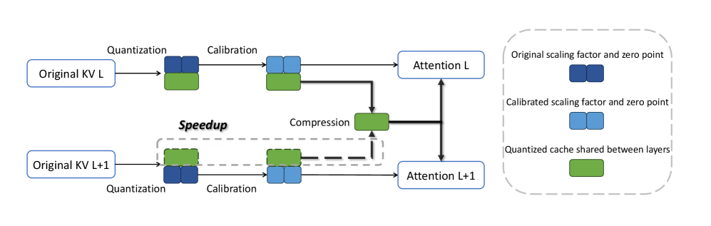
Figure 1: The illustration of XQuant workflow. XQuant partitions the KV cache into layer-wise pairs. For every higher layer in a pair, XQuant only computes and stores the scaling factors and zero-points during quantization phase, and then fetches the quantized cache from the lower layer during dequantization phase.
In this section, we present XQuant, a novel quantization framework for efficient KV cache compression. As illustrated in Figure 1, our framework introduces two key innovations: a data-free calibration technique that asymmetrically adjusts quantization parameters without additional calibration data, and a cross-layer KV cache compression mechanism that leverages the similarity of quantized caches between adjacent layers to effectively reduce both computational and memory overhead.
### 3.1 Background
To formalize KV cache quantization, we consider a group of floating-point keys or values $X$ . The quantization process transforms $X$ into three components: a B-bit quantized cache $X_Q$ , a zero-point $z$ , and a scaling factor $s$ Liu et al. (2024b):
Quantization Phase:
$$
z=min(X),s=\frac{max(X)-min(X)}{(2^B-1)} \tag{1}
$$
$$
X_T=(X-z)/s,X_Q=\lceilX_T\rfloor \tag{2}
$$
Dequantization Phase:
$$
\hat{X}=X_Q*s+z \tag{3}
$$
where $X^*$ is the dequantized counterpart and $\lceil·\rfloor$ is the rounding function. $X_T$ , the transformed matrix, is not explicitly cached but is introduced as an intermediate variable to facilitate subsequent mathematical derivations.
Building upon this framework, prior works introduce various configurations to enhance performance. For example, Liu et al. (2024b) focuses on the element-wise distribution within the KV cache, adopting per-channel quantization for the key cache and per-token quantization for the value cache. Similarly, Tao et al. (2024) introduces layer-wise quantization configurations, employing asymmetric bit-widths for the key and value caches across different layers. While effective, these approaches often suffer from significant performance degradation under low-bit quantization settings, particularly around 2-bit precision. This limitation motivates the need for further advancements in KV cache compression techniques.
### 3.2 Data-Free Calibration
Since existing quantization methods often experience significant performance degradation at 2-bit precision, achieving ultra-low-bit compression first requires bridging this performance gap. In this section, we propose a data-free calibration method that effectively preserves model performance, enabling more aggressive compression ratios.
To analyze extreme quantization scenarios, we start with 1-bit quantization where each parameter is constrained to a binary state. Formally, the round-to-nearest operation $\lceil·\rfloor$ is defined as:
$$
\lceil e\rfloor=\begin{cases}0&if e∈[0,0.5],\\
1&if e∈(0.5,1].\end{cases} \tag{4}
$$
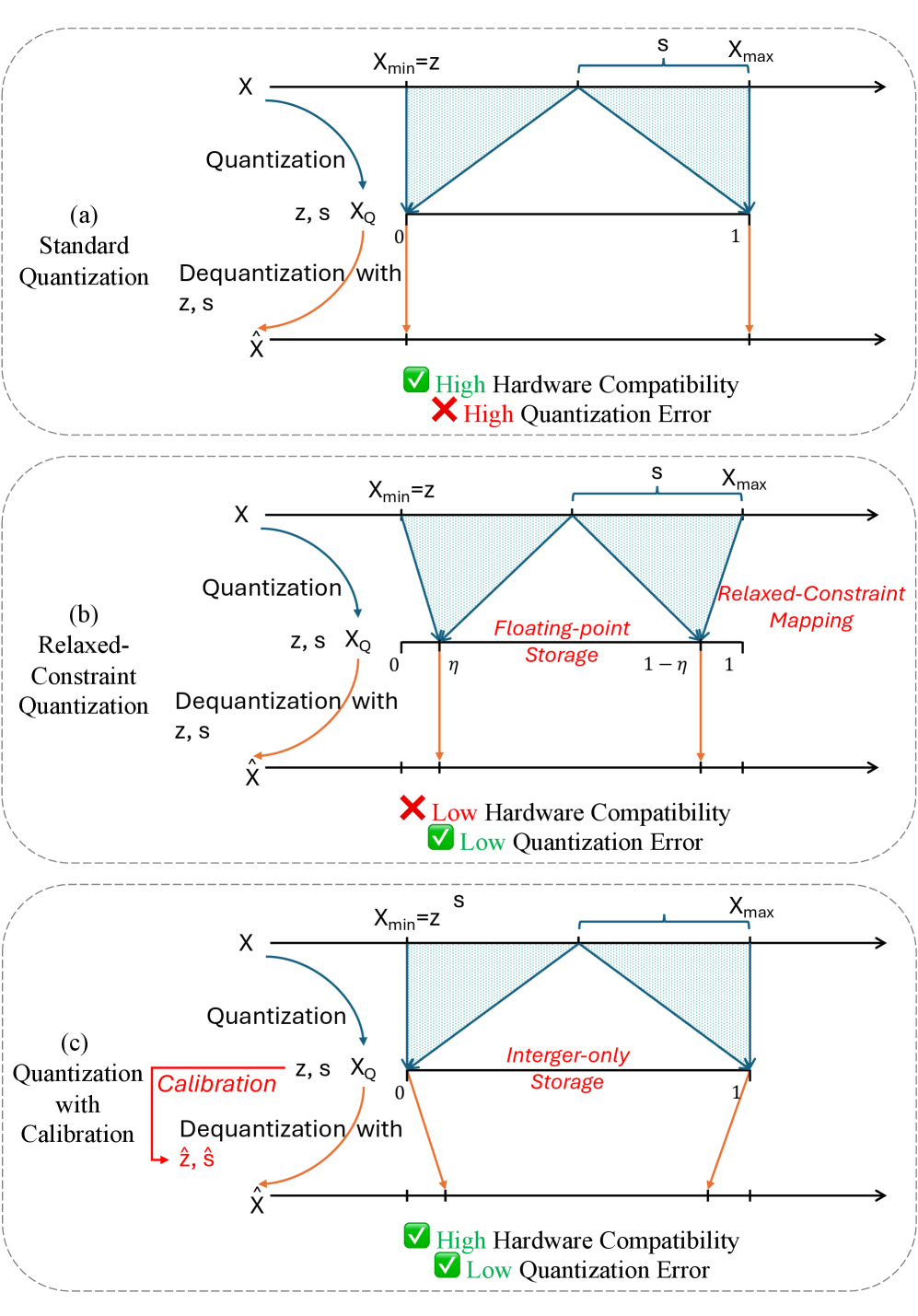
where $e$ denotes an element of the transformed matrix. For any bit-width $B$ , this rounding operation maps values to a discrete set within $[0,2^B-1]$ , where each original value is assigned to its nearest representative in the quantized space. As shown in Figure 2 (a), fixed representative values at endpoints (0 and 1) yield substantial quantization error for 1-bit quantization. We therefore introduce a relaxed-constraint mapping function that adaptively determines the quantization levels, formulated as:
$$
f(e,η)=\begin{cases}η&if e∈[0,0.5],\\
1-η&if e∈(0.5,1].\end{cases} \tag{5}
$$
where $η∈[0,0.5]$ serves as a calibration parameter for determining quantization tendencies. Clearly, $f(e,0)$ is equivalent to the round-to-nearest function $\lceil e\rfloor$ . We extend this formulation to the general case of $B$ -bit quantization and denote the corresponding parameter as $η_B$ .
We relax the constraint that quantized values must be integers and apply fake quantization as a preliminary experiment. Table 7 shows that using this constraint-relaxed mapping function improves model performance, validating our proposed insight.
However, storing floating-point numbers as so-called quantized caches is impractical, as shown in Figure 2 (b). To address the aforementioned problem, we establish an equivalent implementation, with the mathematical proof provided below. We formalize the final data-free calibration approach as:
Consider a group of floating-point keys or values $X∈R^g$ , where $g$ stands for the group size. Note that $X∈[min(X),max(X)]^g=[z,s*(2^B-1)+z]^g$ , we can deduce:
$$
X_Q∈[0,2^B-1]^g \tag{6}
$$
from Equation 1 and Equation 2. If we choose $η*(2^B-1)$ and $(1-η)*(2^B-1)$ generalized from Equation 5 as two endpoints, it is equivalent to calibrate the zero-point and scaling factor to $\hat{z}$ and $\hat{s}$ , and then dequantize with them. Note that the dequantized matrix
$$
\hat{X}=X_Q*\hat{s}+\hat{z}∈[\hat{s}*0+\hat{z},\hat{s}*(2^B-1)+\hat{z}]^g \tag{7}
$$
and the corresponding interval given by two endpoints:
$$
[z+η s(2^B-1),z+s(2^B-1)(1-η)] \tag{8}
$$
By calculation we get the final operations for calibration:
$$
\hat{z}=z+η s(2^B-1),\hat{s}=(1-2η)s \tag{9}
$$
<details>
<summary>x2.png Details</summary>
### Visual Description
## Diagram: Comparison of Quantization Techniques
### Overview
This image presents a conceptual comparison of three distinct quantization methodologies used in data processing (likely for neural network model compression). The diagram illustrates how continuous data ($X$) is mapped to a quantized space ($X_Q$) and subsequently dequantized back to an approximation ($\hat{X}$). The three methods are: (a) Standard Quantization, (b) Relaxed-Constraint Quantization, and (c) Quantization with Calibration. The diagram evaluates each method based on "Hardware Compatibility" and "Quantization Error."
### Components/Axes
Each of the three panels shares a consistent structural layout:
* **Top Axis ($X$):** Represents the continuous input domain. It is bounded by $X_{min}$ (labeled as $z$) and $X_{max}$. The distance between these points is labeled $s$.
* **Middle Axis ($X_Q$):** Represents the quantized domain. It is bounded by $0$ and $1$.
* **Bottom Axis ($\hat{X}$):** Represents the dequantized/reconstructed domain.
* **Flow Arrows:**
* **Blue curved arrows:** Represent the "Quantization" process.
* **Orange curved arrows:** Represent the "Dequantization with $z, s$" process.
* **Shaded Regions:** Triangular shaded areas between the $X$ and $X_Q$ axes represent the mapping transformation.
---
### Detailed Analysis
#### (a) Standard Quantization
* **Position:** Top panel.
* **Mapping:** A direct, linear mapping from the full range $[X_{min}, X_{max}]$ to the quantized range $[0, 1]$.
* **Evaluation:**
* ✅ **High Hardware Compatibility**
* ❌ **High Quantization Error**
* **Logic:** This is the baseline approach. It is simple and compatible with standard hardware but suffers from high error because the mapping is rigid and does not adapt to the data distribution.
#### (b) Relaxed-Constraint Quantization
* **Position:** Middle panel.
* **Mapping:** The mapping is adjusted using a parameter $\eta$. The quantized range is restricted to $[\eta, 1-\eta]$, labeled as "Floating-point Storage." The mapping is explicitly labeled "Relaxed-Constraint Mapping."
* **Evaluation:**
* ❌ **Low Hardware Compatibility**
* ✅ **Low Quantization Error**
* **Logic:** By relaxing the constraints (allowing floating-point storage), the system can reduce quantization error. However, this creates a dependency on floating-point operations, which reduces compatibility with standard integer-only hardware.
#### (c) Quantization with Calibration
* **Position:** Bottom panel.
* **Mapping:** Similar to Standard Quantization, but introduces a "Calibration" step. This step modifies the parameters from $(z, s)$ to $(\hat{z}, \hat{s})$ before dequantization. The quantized range is labeled "Integer-only Storage."
* **Evaluation:**
* ✅ **High Hardware Compatibility**
* ✅ **Low Quantization Error**
* **Logic:** This method uses calibration to adjust the quantization parameters. This allows the system to maintain the efficiency of integer-only storage (high hardware compatibility) while simultaneously minimizing the quantization error (low error).
---
### Key Observations
* **Evolution of Strategy:** The diagram demonstrates a progression from a rigid, high-error method (a) to a flexible, low-error method (b) that sacrifices hardware compatibility, and finally to an optimized method (c) that achieves both goals via calibration.
* **Visual Consistency:** The shaded triangular regions in (a) and (c) are identical, suggesting that the structural mapping is similar, but the *parameters* ($z, s$ vs $\hat{z}, \hat{s}$) are what change in (c) due to calibration.
### Interpretation
This diagram serves as a high-level architectural justification for using **Calibration** in quantization pipelines.
1. **The Problem:** Standard quantization is hardware-friendly but inaccurate. Relaxing constraints improves accuracy but breaks hardware compatibility (e.g., it might require floating-point units that aren't available on low-power edge devices).
2. **The Solution:** Calibration acts as a bridge. By mathematically adjusting the quantization parameters ($z, s$) to $(\hat{z}, \hat{s})$ based on the specific data distribution, the system can "fit" the data better into the integer-only range without needing to change the underlying hardware storage format.
3. **Conclusion:** The diagram demonstrates that calibration is the optimal strategy for deploying neural networks on hardware, as it provides the best trade-off between performance (low error) and efficiency (high hardware compatibility).
</details>
Figure 2: The illustration of the proposed data-free calibration method.
Since $X_T=(X-z)/s$ , the reconstruction loss $MSE(X,\hat{X})=s^2· MSE(X_T,f(X_T,η))$ . For analytical tractability, particularly for 1-bit quantization within small group sizes, we can assume that $X_T∼ U(0,1)$ . Thus the expected MSE in the transformed space can be formulated as:
| | $\displaystyle MSE(X_T,f(X_T,η))$ | |
| --- | --- | --- |
Since the standard quantization scheme is equivalent to setting $η=0$ , this result confirms that any value of $η∈(0,1/2)$ will strictly reduce the theoretical reconstruction error.
As shown in Figure 2 (c), we propose the improved quantization scheme with this data-free calibration as follows:
Quantization Phase with Calibration:
$$
z=min(X),s=\frac{max(X)-min(X)}{(2^B-1)} \tag{10}
$$
$$
X_T=(X-z)/s,X_Q=\lceilX_T\rfloor \tag{11}
$$
$$
\hat{z}=z+η s(2^B-1),\hat{s}=(1-2η)s \tag{12}
$$
Dequantization Phase with Calibration:
$$
\hat{X}=X_Q*\hat{s}+\hat{z} \tag{13}
$$
<details>
<summary>src/delta.png Details</summary>
### Visual Description
## Stacked Area Chart: Distribution of Delta Values by Layer
### Overview
The image is a stacked area chart displaying the percentage distribution of four distinct categories (labeled "Delta=0" through "Delta=3") across 30 layers. The chart illustrates that the distribution of these categories remains remarkably consistent and stable across the entire range of layers (0 to 30).
### Components/Axes
* **X-Axis:** Labeled "Layer". The scale ranges from 0 to 30, with major grid lines marked at intervals of 5.
* **Y-Axis:** Labeled "Percentage (%)". The scale ranges from 0 to 100, with major grid lines marked at intervals of 20.
* **Legend:** Positioned in the bottom-center of the chart area.
* **Dark Blue:** Delta=3
* **Medium Blue:** Delta=2
* **Light Blue:** Delta=1
* **Pale Yellow:** Delta=0
### Detailed Analysis
The chart is a stacked area plot, meaning the total height of all combined areas equals 100% at every point along the X-axis.
* **Trend Verification:**
* **Delta=0 (Pale Yellow):** This category occupies the base of the chart. It maintains a consistent height of approximately 34% across all layers. There is a very slight, negligible upward shift around Layer 12.
* **Delta=1 (Light Blue):** This is the dominant category. It sits on top of the Pale Yellow area, starting at ~34% and extending to ~82%. This represents roughly 48% of the total distribution. The boundary line is nearly horizontal.
* **Delta=2 (Medium Blue):** This category sits above the Light Blue area, starting at ~82% and extending to ~98%. This represents roughly 16% of the total distribution.
* **Delta=3 (Dark Blue):** This is the top-most, thinnest category. It occupies the space from ~98% to 100%, representing a very small minority (approximately 2% of the total).
* **Spatial Grounding:**
* The boundaries between the color bands are almost perfectly parallel to the X-axis, indicating minimal variance in the data distribution as the "Layer" index increases.
### Key Observations
* **High Stability:** The most striking feature of this chart is the lack of significant change across the layers. The distribution of "Delta" values is essentially static from Layer 0 to Layer 30.
* **Dominant Category:** "Delta=1" is the most prevalent category, consistently accounting for nearly half of the total percentage.
* **Minority Category:** "Delta=3" is consistently the least frequent category, maintaining a thin, stable sliver at the top of the chart.
### Interpretation
* **Data Meaning:** This chart likely represents a metric (Delta) tracked across the depth of a computational model, such as a deep neural network (e.g., Transformer layers).
* **Invariance:** The fact that the distribution is flat suggests that the phenomenon being measured is invariant to the depth of the model. Whatever "Delta" represents, it is established early in the process and does not evolve or shift significantly as data passes through subsequent layers.
* **Investigative Insight:** If this were a model analysis, one might conclude that the "Delta" values are intrinsic properties of the input data or the initial embedding, rather than features learned or transformed by the deeper layers. The lack of dynamic change suggests the model's internal state regarding this specific metric is "locked in" from the start.
</details>
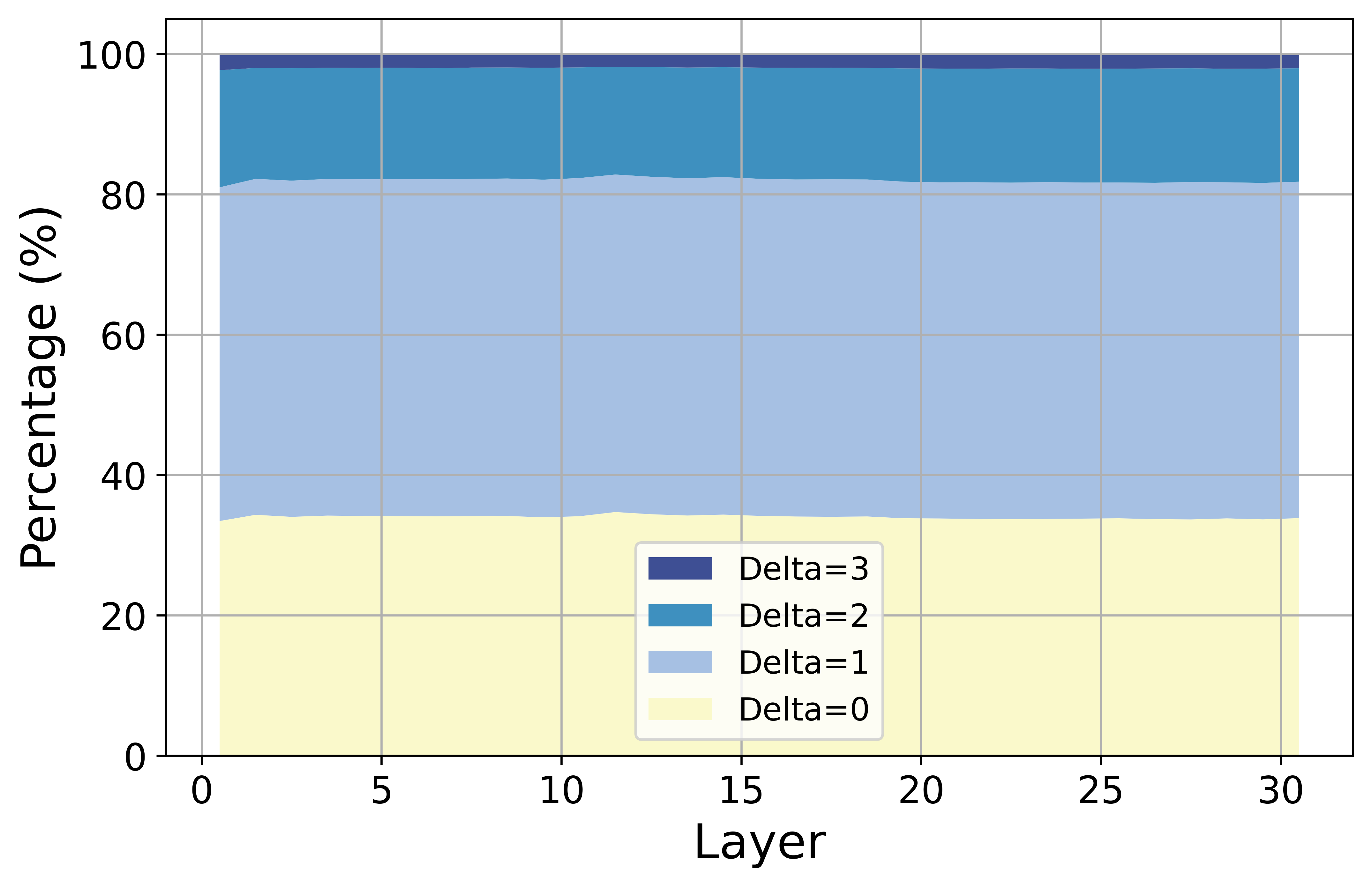
Figure 3: Layer-wise analysis of absolute differences between adjacent layers in quantized KV Cache matrices. Here, delta represents the absolute difference of quantized values between consecutive layers.
### 3.3 Cross-Layer Compression
#### 3.3.1 Motivation
Building upon Tao et al. (2024) ’s investigation of ultra-low-bit KV cache asymmetric quantization, our reproduction experiments on LongBench Bai et al. (2023) with Mistral Jiang et al. (2023) demonstrate severe limitations of existing approaches, as shown in Table 8.
We found that 1-bit asymmetric quantization of the key cache is practically infeasible. Even when restricting 1-bit quantization to the top 8 layers (AsymKV-24/32), significant performance degradation occurs. Given the limitations of further key cache quantization, we turn to cross-layer compression techniques as a viable alternative to achieve comparable ultra-low-bit quantization without compromising performance.
#### 3.3.2 Analysis on Quantized KV Cache
To enable cross-layer compression, we first analyze the characteristics of quantized KV caches by examining inter-layer similarities. We hypothesize that significant redundancy between adjacent layers could create opportunities for more aggressive compression. Using the KIVI-2 framework Liu et al. (2024b), we conduct preliminary experiments on the Mistral-7B-Instruct-v0.2 model Jiang et al. (2023) with random samples from LongBench Bai et al. (2023).
Under the 2-bit quantization scheme in KIVI-2, quantized cache values are restricted to {0, 1, 2, 3}, naturally constraining element-wise absolute differences to the same range. Our analysis, illustrated in Figure 3, reveals a striking pattern: over 80% of positions between adjacent layers exhibit minimal differences (0 or 1), while extreme differences (3) occur in less than 5% of positions. This pattern becomes even more pronounced in the 1-bit scenario, where mapping {0,1} to 0 and {2,3} to 1 maintains identical values in over 80% of positions between adjacent layers. These empirical findings demonstrate substantial redundancy in quantized KV caches between adjacent layers, suggesting significant potential for further compression.
#### 3.3.3 Compression Algorithm
Leveraging these insights into inter-layer similarities, we propose a novel cross-layer compression method that decomposes KV caches into two components: shared quantized caches and layer-specific parameters. Specifically, adjacent layers share a common set of quantized value caches ( $X_Q$ ), while maintaining their individual scaling factors and zero-points for dequantization. This decomposition enables efficient compression by allowing each layer to reuse the merged cache from its group, while preserving the layer-specific characteristic through its unique quantization parameters, namely zero-points and scaling factors.
In the implementation, for a model with $L$ layers, we organize the layers into groups of size $G$ . Within each group, KV caches are compressed using weighted averaging, where each layer $l$ ( $0≤ l≤ L$ ) is assigned a weight $γ_l$ , subject to the constraint $∑γ_l=1$ .
Formally, for every layer $l$ in a group $G$ , the quantization workflow with cross-layer compression and calibration is utilized as follows:
Quantization Phase with Cross-Layer Compression and Calibration:
$$
∀ l∈G,
$$
$$
z_l=min(X_l), s_l=\frac{max(X_l)-min(X_l)}{(2^B-1)}
$$
$$
\hat{z}_l=z_l+η s_l(2^B-1), \hat{s}_l=(1-2η)s_l
$$
$$
X_Q=∑_l∈Gγ_l\bigg\lceil\frac{X_l-z_l}{s_l}\bigg\rfloor
$$
Dequantization Phase with Cross-Layer Compression and Calibration:
$$
\hat{X}_l=X_Q*\hat{s}_l+\hat{z}_l
$$
We present the pseudo code for the whole workflow as shown in Appendix J.
| Model Mistral-7b | Method Full Cache | Bit-width 16 | TruthfulQA 32.09 |
| --- | --- | --- | --- |
| KIVI | 2 | 32.17 | |
| AsymKV | 1.5 | 32.80 | |
| XQuant | 1.38 | 34.93 | |
| Llama2-7b | Full Cache | 16 | 30.77 |
| KIVI | 2 | 33.92 | |
| AsymKV | 1.5 | 33.84 | |
| XQuant | 1.4 | 34.22 | |
Table 1: Evaluation on TruthfulQA task with normal context length.
| Model | Method | Bit-width | HQA | 2Wiki | MSQ | TREC | TQA | SAMS | PC | Avg |
| --- | --- | --- | --- | --- | --- | --- | --- | --- | --- | --- |
| Mistral-7b-ins | Full Cache | 16 | 43.02 | 27.10 | 18.78 | 71.00 | 86.23 | 42.75 | 2.75 | 41.66 |
| PyramidInfer | / | 35.08 | 23.92 | 16.90 | 62.00 | 85.06 | 41.45 | 1.04 | 32.55 | |
| KIVI | 2 | 41.96 | 26.08 | 18.13 | 71.00 | 86.00 | 43.70 | 2.78 | 41.38 | |
| AsymKV | 1.5 | 37.17 | 22.77 | 15.76 | 70.50 | 86.25 | 43.44 | 3.16 | 39.86 | |
| XQuant | 1.38 | 42.90 | 26.65 | 17.44 | 71.50 | 84.50 | 45.18 | 5.71 | 41.98 | |
| Llama2-7b-chat | Full Cache | 16 | 30.09 | 26.48 | 9.98 | 63.00 | 84.19 | 41.22 | 4.50 | 37.07 |
| PyramidInfer | / | 29.14 | 24.53 | 7.49 | 54.00 | 81.79 | 40.71 | 4.00 | 34.52 | |
| KIVI | 2 | 29.10 | 25.12 | 9.86 | 63.00 | 84.98 | 40.18 | 4.00 | 36.61 | |
| AsymKV | 1.5 | 27.75 | 24.82 | 8.45 | 62.00 | 84.21 | 41.22 | 2.75 | 35.89 | |
| XQuant | 1.4 | 29.21 | 25.56 | 9.69 | 62.50 | 84.57 | 40.01 | 4.00 | 36.51 | |
Table 2: Evaluation of different KV cache compression methods on LongBench tasks.
#### 3.3.4 Speedup through Cross-layer Compression
While our previous discussion introduced weighted averaging with the weight $γ$ for compressing $X_Q$ within a group, we can further optimize the computation by setting $γ_k=1$ for a chosen dominant layer $k$ , which consequently forces all other $γ$ values within the group to zero. In this accelerated configuration, each subordinate layer only needs to compute and store its own scaling factors and zero-points, significantly reducing computational overhead. Specifically,
$$
X_Q=\bigg\lceil\frac{X_k-z_k}{s_k}\bigg\rfloor\\
$$
As illustrated in Figure 1, this optimization eliminates the computations shown in the dashed line, effectively streamlining the process. Experimental results show that selecting the first layer within the group as the dominant layer yields optimal performance, as demonstrated in Table 4 and Table 5.
## 4 Evaluation
### 4.1 Experimental Setup
Models.
We evaluate our XQuant on Llama-2-7b / Llama-2-7b-chat Touvron et al. (2023) and Mistral-7B-v0.3 / Mistral-7B-instruct-v0.2 Jiang et al. (2023).
Tasks.
For the normal context length task, we choose TruthfulQA (BLEU score) from LM-Eval Gao et al. (2021). We also select several subsets from LongBench Bai et al. (2023) for the long context length tasks, including HotpotQA (F1 score), 2WikiMultihopQA (F1 score), MuSiQue (F1 score), TREC (classification accuracy), TriviaQA (F1 score), SAMSum (Rouge-L) and PassageCount (Exact match accuracy). MultiFieldQA-Zh (F1 score) is selected for some ablation studies as well.
Baselines and Implementations.
We compare our framework with previous works, including original 16-bit floating implementation, KIVI-2 Liu et al. (2024b) and AsymKV Tao et al. (2024). All relevant configurations adhere as in KIVI, i.e., quantizing key cache per-channel and value cache per-token, and with a group size of 32 and a residual length of 128. We reproduce AsymKV based on the official implementation of KIVI, with a typical configuration (AsymKV-32/0) selected from the original paper, i.d., quantizing all the key cache into 2-bit and value cache into 1-bit, which corresponds to an equivalent bit-width of 1.5.
A token eviction method Yang et al. (2024b), configured with a 40% KV cache budget, is also included as a baseline for the LongBench tasks.
We set the maximum sequence length to 30000 for the Mistral model to conduct our experiments with a single NVIDIA GeForce RTX 3090 GPU (24GB), and 8192 for the Llama model as default. We do not consider SLERP Shoemake (1985); Liu et al. (2024a) because of the incompatibility between rescale-recover operations and quantized cache.
### 4.2 Performance Comparison
LM-Eval Results.
Table 1 presents the evaluation of different quantization methods on the TruthfulQA task with a standard context length. XQuant not only achieves competitive performance but surpasses the full cache baseline, with a TruthfulQA score of 34.93 on Mistral-7b and 34.22 on Llama2-7b, outperforming all other methods at significantly lower bit-widths. These results highlight that XQuant provides superior performance in conventional context length settings.
LongBench Results.
We evaluate XQuant on the LongBench benchmark using two widely adopted models: Mistral-7b-Instruct-v0.2 and Llama-2-7b-chat. As shown in Table 2, XQuant achieves significant improvements over other KV cache compression methods, particularly under ultra-low-bit settings.
In all datasets of LongBench, XQuant achieves performance comparable to the full cache baseline while reducing bit-width by 31% compared to KIVI-2bit. Notably, XQuant achieves an average score of 41.98 for Mistral, surpassing KIVI-2bit while maintaining a significantly lower bit-width of 1.38. Moreover, XQuant outperforms AsymKV on nearly all datasets while simultaneously reducing bit-width by 8% relative to AsymKV. Additionally, compared to PyramidInfer, which sacrifices precision to reduce storage overhead, XQuant demonstrates clear advantages in maintaining high accuracy across tasks while achieving lower bit-width.
### 4.3 Ablation and Analysis
In this section, we conduct ablation studies in some randomly selected lightweight LongBench subsets.
| Method Full Cache KIVI | Bit-width 16 2 | $η_1$ / / | $η_2$ / 0 | MFQA-Zh 48.26 42.27 |
| --- | --- | --- | --- | --- |
| AsymKV | 1.5 | 0 | 0 | 36.30 |
| XQuant | 1.375 | 0 | 0 | 37.20 |
| 0 | 0.05 | 40.32 | | |
| 0.2 | 0 | 41.98 | | |
| 0.2 | 0.05 | 44.20 | | |
Table 3: Ablation study on the effect of data-free calibration in XQuant on the MultiFieldQA-Zh benchmark from LongBench.
Calibration Parameter.
Table 3 presents an ablation study on the impact of data-free calibration in XQuant on the MultiFieldQA-Zh benchmark. The results indicate that applying calibration ( $η_1≠ 0$ or $η_2≠ 0$ ) significantly improves XQuant’s performance, reducing the performance gap with the full cache baseline.
| Method Full Cache KIVI | Bit-width 16 2 | $γ_0$ / / | MuSiQue 18.78 18.13 |
| --- | --- | --- | --- |
| Flooring | 1.63 | / | 16.79 |
| Ceiling | 1.63 | / | 16.36 |
| Weighted Average | 1.63 | [0,1/6) | 12.20 |
| 1.63 | (1/6,1/4) | 14.05 | |
| 1.63 | (1/4,1/2) | 16.84 | |
| 1.63 | (1/2,3/4) | 17.32 | |
| 1.63 | (3/4,5/6) | 17.60 | |
| 1.63 | (5/6,1] | 17.32 | |
Table 4: The comparison between different cross-layer compression method with group size $G=2$ , where $γ_0,γ_1$ stands for the coefficient in the weighted average $(γ_1+γ_0=1)$ .
Cross-Layer Compression Method.
We further explore the weighted average with a group size $G=2$ and coefficients $γ_0,γ_1=1-γ_0$ , where $γ_0$ falls into six intervals derived in Appendix F. Notably, when $γ_0∈[0,1/6)$ or $γ_0∈(5/6,1]$ , the operation is optimized to directly sharing the quantized cache. We evaluate KIVI-2 on Mistral-7B-Instruct-v0.2 without our proposed calibration methods starting from the 8-th layer. As summarized in Table 4, the accelerated compression methods ( $γ_0∈[0,1/6)∪(5/6,1]$ ) avoid redundant operations seen in the workflow of Liu et al., 2024b, which rounds quantized integers into floating-point numbers. As shown in Table 4, the accelerated compression operation demonstrates its effectiveness in maintaining sufficient information for model performance, particularly when $γ_0∈(5/6,1]$ . This configuration effectively allows odd-numbered layers to reuse the quantized cache from the preceding even-numbered layers without requiring additional quantization or storage overhead for odd-numbered layers.
We adopt this accelerated compression strategy across all experiments due to its favorable balance between computational efficiency and information preservation.
| Method | Bit-width | $G$ | $k$ | MSQ | MFQA-Zh |
| --- | --- | --- | --- | --- | --- |
| Full Cache | 16 | / | / | 18.78 | 48.26 |
| KIVI | 2 | / | / | 18.13 | 42.27 |
| 0 | 17.32 | 37.44 | | | |
| 2 | 1 | 12.20 | 20.48 | | |
| 0 | 14.92 | 17.53 | | | |
| 1 | 16.97 | 37.37 | | | |
| 3 | 2 | 13.21 | 20.80 | | |
| 0 | 14.82 | 23.53 | | | |
| 1 | 12.44 | 18.68 | | | |
| 2 | 16.12 | 35.48 | | | |
| XQuant | 1.63 | 4 | 3 | 15.39 | 20.32 |
Table 5: The comparison of different group sizes $G$ and selection indices $k$ within each group, where XQuant is employed without the calibration step for a clearer analysis.
Group Size.
After optimizing the cross-layer compression method, another factor is the group size. To investigate the effects of layer grouping, we partition the total $L$ layers of a model (where $L=32$ for Mistral-7B and Llama 2-7B) into $L/G$ contiguous groups of size $G$ . The parameter $k$ indicates that we store and share the quantized cache only in the $k$ -th layer of each group. We evaluate group sizes $G∈\{2,3,4\}$ . This range is motivated by the empirical observation that while adjacent layers exhibit high similarity in their quantized representations (i.e., $G=2$ , as shown in Figure 3), this similarity diminishes gradually for layer distances greater than three. For models with $L=32$ layers, $G=4$ thus serves as a sufficient upper bound for investigation due to this diminishing similarity. We set all configurations under the same compression ratio, namely keep all layers in key cache and 20 layers in value cache based on KIVI-2bit framework, using Mistral-7b-instruct-v0.2. As shown in Table 5, the model achieves the best performance with the configuration of $G=2$ and $k=0$ .
| Method | Bit-width | TREC | SAMS |
| --- | --- | --- | --- |
| Full Cache | 16 | 71 | 42.75 |
| KIVI | 2 | 71 | 43.7 |
| AsymKV | 1.5 | 70.5 | 43.44 |
| AsymKV | 1.375 | 69.5 | 42.76 |
| XQuant | 1.375 | 71.5 | 45.18 |
| AsymKV | 1.28 | 58.5 | 37.41 |
| XQuant | 1.28 | 68.5 | 39.84 |
| AsymKV | 1.15625 | 41 | 23.47 |
| XQuant | 1.15625 | 68.5 | 39.47 |
Table 6: The comparison of different configurations under extremely-low compression ratio.
Performance-Compression Trade-offs.
Table 6 evaluates the trade-offs between bit-width reduction and performance degradation across different quantization methods. As shown in Table 6, XQuant consistently outperforms other methods at the same bit-width, achieving higher scores on both TREC and SAMS benchmarks. Notably, even at an extremely low bit-width of 1.15625, XQuant preserves a significant portion of the model’s performance, maintaining a TREC score of 68.5 compared to the full-cache baseline of 71. These results demonstrate that XQuant effectively balances performance retention and compression, achieving state-of-the-art trade-offs in ultra-low-bit KV cache quantization.
## 5 Conclusion
To alleviate the growing memory overhead in LLM inference, we propose XQuant, a plug-and-play framework that quantizes KV cache at an extreme compression ratio. Based on our observations on classical training-free quantization and the distributions of quantized integers, we propose a data-free calibration method and a compute-efficient cross-layer compression method. Extensive experiments show that XQuant achieves state-of-the-art trade-offs between performance degradation and compression ratio, without sacrificing computational efficiency. Integrating these two novel methods, our XQuant achieves comparable performance with full-precision baseline under 1.4-bit quantization, and still maintains competitive performance for some tasks around an extremely 1.16-bit quantization.
## Limitations and Future Work
Our work presents several avenues for future exploration. First, while XQuant demonstrates promising results on representative models and benchmarks, its robustness and generalizability could be further validated by extending evaluations to a wider range of newer-generation or larger-scale models and more diverse downstream scenarios. Second, our current work relies on task-specific configurations. Although a unified setting proves robust (as shown in Appendix E), the development of an automated method to search for optimal configurations presents a valuable direction for future research. Finally, the key innovations of XQuant — Data-Free Calibration and Cross-layer Compression — are in principle orthogonal to other KV cache compression paradigms. A fruitful area for future work would be to investigate their compatibility and potential synergies with these existing methods, potentially yielding even greater efficiency gains.
## Acknowledgements
This work was supported by the National Natural Science Foundation of China (Grant No. 62306216) and the Natural Science Foundation of Hubei Province of China (Grant No. 2023AFB816).
Hai Zhao’s contribution was funded by the Major Program of the Chinese National Foundation of Social Sciences under Grant "The Challenge and Governance of Smart Media on News Authenticity" [No. 23&ZD213].
The authors also gratefully acknowledge support from the Xiaomi Open-Competition Research Program.
## References
- Ainslie et al. (2023) Joshua Ainslie, James Lee-Thorp, Michiel de Jong, Yury Zemlyanskiy, Federico Lebron, and Sumit Sanghai. 2023. GQA: Training generalized multi-query transformer models from multi-head checkpoints. In Proceedings of the 2023 Conference on Empirical Methods in Natural Language Processing, pages 4895–4901, Singapore. Association for Computational Linguistics.
- Bai et al. (2024) Yushi Bai, Xin Lv, Jiajie Zhang, Hongchang Lyu, Jiankai Tang, Zhidian Huang, Zhengxiao Du, Xiao Liu, Aohan Zeng, Lei Hou, Yuxiao Dong, Jie Tang, and Juanzi Li. 2024. Longbench: A bilingual, multitask benchmark for long context understanding. In Proceedings of the 62nd Annual Meeting of the Association for Computational Linguistics (Volume 1: Long Papers), ACL 2024, Bangkok, Thailand, August 11-16, 2024, pages 3119–3137. Association for Computational Linguistics.
- Bai et al. (2023) Yushi Bai, Xin Lv, Jiajie Zhang, Hongchang Lyu, Jiankai Tang, Zhidian Huang, Zhengxiao Du, Xiao Liu, Aohan Zeng, Lei Hou, et al. 2023. Longbench: A bilingual, multitask benchmark for long context understanding. arXiv preprint arXiv:2308.14508.
- Brandon et al. (2024) William Brandon, Mayank Mishra, Aniruddha Nrusimha, Rameswar Panda, and Jonathan Ragan Kelly. 2024. Reducing transformer key-value cache size with cross-layer attention. arXiv preprint arXiv:2405.12981.
- Cai et al. (2024) Zefan Cai, Yichi Zhang, Bofei Gao, Yuliang Liu, Tianyu Liu, Keming Lu, Wayne Xiong, Yue Dong, Baobao Chang, Junjie Hu, et al. 2024. Pyramidkv: Dynamic kv cache compression based on pyramidal information funneling. arXiv preprint arXiv:2406.02069.
- Dao (2023) Tri Dao. 2023. Flashattention-2: Faster attention with better parallelism and work partitioning. arXiv preprint arXiv:2307.08691.
- Frantar et al. (2022) Elias Frantar, Saleh Ashkboos, Torsten Hoefler, and Dan Alistarh. 2022. GPTQ: Accurate post-training compression for generative pretrained transformers. arXiv preprint arXiv:2210.17323.
- Gao et al. (2021) Leo Gao, Jonathan Tow, Stella Biderman, Sid Black, Anthony DiPofi, Charles Foster, Laurence Golding, Jeffrey Hsu, Kyle McDonell, Niklas Muennighoff, et al. 2021. A framework for few-shot language model evaluation. Version v0. 0.1. Sept, 10:8–9.
- Hooper et al. (2024) Coleman Hooper, Sehoon Kim, Hiva Mohammadzadeh, Michael W Mahoney, Yakun Sophia Shao, Kurt Keutzer, and Amir Gholami. 2024. Kvquant: Towards 10 million context length llm inference with kv cache quantization. arXiv preprint arXiv:2401.18079.
- Jiang et al. (2023) Albert Q Jiang, Alexandre Sablayrolles, Arthur Mensch, Chris Bamford, Devendra Singh Chaplot, Diego de las Casas, Florian Bressand, Gianna Lengyel, Guillaume Lample, Lucile Saulnier, et al. 2023. Mistral 7b. arXiv preprint arXiv:2310.06825.
- Kwon et al. (2023) Woosuk Kwon, Zhuohan Li, Siyuan Zhuang, Ying Sheng, Lianmin Zheng, Cody Hao Yu, Joseph Gonzalez, Hao Zhang, and Ion Stoica. 2023. Efficient memory management for large language model serving with pagedattention. In Proceedings of the 29th Symposium on Operating Systems Principles, pages 611–626.
- Li et al. (2024) Yuhong Li, Yingbing Huang, Bowen Yang, Bharat Venkitesh, Acyr Locatelli, Hanchen Ye, Tianle Cai, Patrick Lewis, and Deming Chen. 2024. Snapkv: Llm knows what you are looking for before generation. arXiv preprint arXiv:2404.14469.
- Lin et al. (2024) Ji Lin, Jiaming Tang, Haotian Tang, Shang Yang, Wei-Ming Chen, Wei-Chen Wang, Guangxuan Xiao, Xingyu Dang, Chuang Gan, and Song Han. 2024. Awq: Activation-aware weight quantization for on-device llm compression and acceleration. Proceedings of Machine Learning and Systems, 6:87–100.
- Lin et al. (2022) Stephanie Lin, Jacob Hilton, and Owain Evans. 2022. Truthfulqa: Measuring how models mimic human falsehoods. In Proceedings of the 60th Annual Meeting of the Association for Computational Linguistics (Volume 1: Long Papers), ACL 2022, Dublin, Ireland, May 22-27, 2022, pages 3214–3252. Association for Computational Linguistics.
- Liu et al. (2024a) Akide Liu, Jing Liu, Zizheng Pan, Yefei He, Gholamreza Haffari, and Bohan Zhuang. 2024a. Minicache: Kv cache compression in depth dimension for large language models. arXiv preprint arXiv:2405.14366.
- Liu et al. (2024b) Zirui Liu, Jiayi Yuan, Hongye Jin, Shaochen Zhong, Zhaozhuo Xu, Vladimir Braverman, Beidi Chen, and Xia Hu. 2024b. Kivi: A tuning-free asymmetric 2bit quantization for kv cache. ArXiv, abs/2402.02750.
- Luohe et al. (2025) Shi Luohe, Zuchao Li, Lefei Zhang, Baoyuan Qi, Liu Guoming, and Hai Zhao. 2025. KV-latent: Dimensional-level KV cache reduction with frequency-aware rotary positional embedding. In Proceedings of the 63rd Annual Meeting of the Association for Computational Linguistics (Volume 1: Long Papers), pages 1535–1550, Vienna, Austria. Association for Computational Linguistics.
- Ma et al. (2024) Xinbei Ma, Zhuosheng Zhang, and Hai Zhao. 2024. Comprehensive cognitive llm agent for smartphone gui automation. arXiv preprint arXiv:2402.11941.
- Ma et al. (2025) Ziyang Ma, Zuchao Li, Lefei Zhang, Gui-Song Xia, Bo Du, Liangpei Zhang, and Dacheng Tao. 2025. Model hemorrhage and the robustness limits of large language models. arXiv preprint arXiv:2503.23924.
- Ouyang et al. (2023) Shuyin Ouyang, Jie M Zhang, Mark Harman, and Meng Wang. 2023. Llm is like a box of chocolates: the non-determinism of chatgpt in code generation. arXiv preprint arXiv:2308.02828.
- Qwen et al. (2025) Qwen, :, An Yang, Baosong Yang, Beichen Zhang, Binyuan Hui, Bo Zheng, Bowen Yu, Chengyuan Li, Dayiheng Liu, Fei Huang, Haoran Wei, Huan Lin, Jian Yang, Jianhong Tu, Jianwei Zhang, Jianxin Yang, Jiaxi Yang, Jingren Zhou, Junyang Lin, Kai Dang, Keming Lu, Keqin Bao, Kexin Yang, Le Yu, Mei Li, Mingfeng Xue, Pei Zhang, Qin Zhu, Rui Men, Runji Lin, Tianhao Li, Tianyi Tang, Tingyu Xia, Xingzhang Ren, Xuancheng Ren, Yang Fan, Yang Su, Yichang Zhang, Yu Wan, Yuqiong Liu, Zeyu Cui, Zhenru Zhang, and Zihan Qiu. 2025. Qwen2.5 technical report. Preprint, arXiv:2412.15115.
- Sharma et al. (2024) Nikhil Sharma, Q Vera Liao, and Ziang Xiao. 2024. Generative echo chamber? effect of llm-powered search systems on diverse information seeking. In Proceedings of the CHI Conference on Human Factors in Computing Systems, pages 1–17.
- Sheng et al. (2023) Ying Sheng, Lianmin Zheng, Binhang Yuan, Zhuohan Li, Max Ryabinin, Beidi Chen, Percy Liang, Christopher Ré, Ion Stoica, and Ce Zhang. 2023. Flexgen: High-throughput generative inference of large language models with a single gpu. In International Conference on Machine Learning, pages 31094–31116. PMLR.
- Shi et al. (2024) Luohe Shi, Hongyi Zhang, Yao Yao, Zuchao Li, and Hai Zhao. 2024. Keep the cost down: A review on methods to optimize llm’s kv-cache consumption. arXiv preprint arXiv:2407.18003.
- Shoemake (1985) Ken Shoemake. 1985. Animating rotation with quaternion curves. In Proceedings of the 12th annual conference on Computer graphics and interactive techniques, pages 245–254.
- Sun et al. (2024) Yutao Sun, Li Dong, Yi Zhu, Shaohan Huang, Wenhui Wang, Shuming Ma, Quanlu Zhang, Jianyong Wang, and Furu Wei. 2024. You only cache once: Decoder-decoder architectures for language models. arXiv preprint arXiv:2405.05254.
- Tang et al. (2025) Zicong Tang, Shi Luohe, Zuchao Li, Baoyuan Qi, Liu Guoming, Lefei Zhang, and Ping Wang. 2025. SpindleKV: A novel KV cache reduction method balancing both shallow and deep layers. In Proceedings of the 63rd Annual Meeting of the Association for Computational Linguistics (Volume 1: Long Papers), pages 28428–28442, Vienna, Austria. Association for Computational Linguistics.
- Tao et al. (2024) Qian Tao, Wenyuan Yu, and Jingren Zhou. 2024. Asymkv: Enabling 1-bit quantization of kv cache with layer-wise asymmetric quantization configurations. arXiv preprint arXiv:2410.13212.
- Touvron et al. (2023) Hugo Touvron, Thibaut Lavril, Gautier Izacard, Xavier Martinet, Marie-Anne Lachaux, Timothée Lacroix, Baptiste Rozière, Naman Goyal, Eric Hambro, Faisal Azhar, et al. 2023. Llama: Open and efficient foundation language models. arXiv preprint arXiv:2302.13971.
- Wu and Tu (2024) Haoyi Wu and Kewei Tu. 2024. Layer-condensed kv cache for efficient inference of large language models. arXiv preprint arXiv:2405.10637.
- Xiao et al. (2023) Guangxuan Xiao, Yuandong Tian, Beidi Chen, Song Han, and Mike Lewis. 2023. Efficient streaming language models with attention sinks. arXiv.
- Yang et al. (2024a) Dongjie Yang, Xiaodong Han, Yan Gao, Yao Hu, Shilin Zhang, and Hai Zhao. 2024a. Pyramidinfer: Pyramid KV cache compression for high-throughput LLM inference. In Findings of the Association for Computational Linguistics, ACL 2024, Bangkok, Thailand and virtual meeting, August 11-16, 2024, pages 3258–3270. Association for Computational Linguistics.
- Yang et al. (2024b) Dongjie Yang, XiaoDong Han, Yan Gao, Yao Hu, Shilin Zhang, and Hai Zhao. 2024b. Pyramidinfer: Pyramid kv cache compression for high-throughput llm inference. arXiv preprint arXiv:2405.12532.
- Yang et al. (2024c) June Yong Yang, Byeongwook Kim, Jeongin Bae, Beomseok Kwon, Gunho Park, Eunho Yang, Se Jung Kwon, and Dongsoo Lee. 2024c. No token left behind: Reliable KV cache compression via importance-aware mixed precision quantization. CoRR, abs/2402.18096.
- Yang et al. (2024d) Yifei Yang, Zouying Cao, Qiguang Chen, Libo Qin, Dongjie Yang, Hai Zhao, and Zhi Chen. 2024d. Kvsharer: Efficient inference via layer-wise dissimilar kv cache sharing. arXiv preprint arXiv:2410.18517.
- Yao et al. (2024) Yao Yao, Zuchao Li, and Hai Zhao. 2024. Sirllm: Streaming infinite retentive llm. arXiv preprint arXiv:2405.12528.
- Zhang et al. (2023) Zhenyu Zhang, Ying Sheng, Tianyi Zhou, Tianlong Chen, Lianmin Zheng, Ruisi Cai, Zhao Song, Yuandong Tian, Christopher Ré, Clark Barrett, et al. 2023. H2o: Heavy-hitter oracle for efficient generative inference of large language models. Advances in Neural Information Processing Systems, 36:34661–34710.
## Appendix A Preliminary Study on Relaxed-Contraint Mapping
| Method Full Cache KIVI | Bit-width 16 2 | $η_1$ / / | $η_2$ / 0 | MFQA-Zh 48.26 42.27 |
| --- | --- | --- | --- | --- |
| KIVI | 2 | / | 0.05 | 44.34 |
| AsymKV | 1.5 | 0 | 0 | 36.30 |
| AsymKV | 1.5 | 0 | 0.05 | 41.28 |
| AsymKV | 1.5 | 0.2 | 0 | 42.78 |
| AsymKV | 1.5 | 0.2 | 0.05 | 43.81 |
Table 7: The comparison using different quantization methods with and without our calibration method in MultiFieldQA-Zh tasks from LongBench.
As demonstrated in Figure 2, the traditional quantization workflow faces higher quantization error in low-bit scenarios. In Section 3.2, we propose a flexible mapping to mitigate the quantization error in this aspect. Moreover, to provide empirical evidence supporting the effectiveness of the flexible mapping in the proposed calibration method, we employ its generalized form and conduct a preliminary study on the default KIVI-2bit and AsymKV-32/0 configurations. We extend this approach to a generalized B-bit quantization mechanism, where $η_B$ serves as the corresponding parameter. Notably, when $η_B=0$ , the B-bit quantization operates without the flexible mapping.
The results in Table 7 demonstrate that incorporating the flexible mapping function enhances model performance across different quantization settings.
## Appendix B Preliminary Experiment on Layer-Wise Asymmetric Quantization
In the existing method Tao et al. (2024), the KV cache for each layer is quantized using either 1-bit or 2-bit precision. A straightforward strategy to maximize the compression ratio is to apply 1-bit quantization to a greater number of layers.
However, a significant bottleneck arises, as it is nearly impossible to quantize the key cache at 1-bit precision without compromising performance. As shown in Table 8, further compression by increasing the number of 1-bit quantized key cache layers is not feasible, as it leads to substantial performance degradation. This observation motivates us to explore alternative compression methodologies.
| Method | Bit-width | # Key Layers in 1-bit | MFQA-Zh |
| --- | --- | --- | --- |
| Full Cache | 16 | / | 48.26 |
| KIVI (32/32) | 2 | 0 | 42.27 |
| AsymKV-24/32 | 1.875 | 8 | 37.10 |
| AsymKV-16/32 | 1.75 | 16 | 21.36 |
| AsymKV-8/32 | 1.625 | 24 | 13.16 |
| AsymKV-0/32 | 1.5 | 32 | 7.66 |
Table 8: Evaluation on LongBench based on AsymKV shows that the key cache is nearly impossible to quantized under 1-bit.
## Appendix C Equivalent Bit-width Analysis
Formally, let $b,h,s,d$ be the batch size, the number of heads in GQA Ainslie et al. (2023), the sequence length and the dimension per head. The original $L$ layers of KV cache occupies $2L*bhsd*16 bit$ , which equals to $2L*n*16 bit$ if we set $n=bhsd$ for convenience.
Consider a typical KV cache quantization scheme Liu et al. (2024b). If we quantize all $L$ layers of key cache and value cache into $b$ -bit, the quantized KV cache memory usage is $2L*n*b bit$ . Tao et al., 2024 uses a asymmetrical configurations for key and value caches across different layers. In their paper, Asym- $l_k$ / $l_v$ means quantizing the initial $l_k$ layers of key cache and $l_v$ of value cache into 2-bit, and quantizating 1-bit for others. So the quantized KV cache memory usage is $(2*l_k+(32-l_k)+2*l_v+(32-l_v))*n bit$ . For example, Asym-1.5bit stands for Asym-32/0 in our paper, which can be calculated to $3L*n bit$ and can be equivalently considered as a 1.5-bit symmetrical quantization for better understanding of the compression ratio.
The related parameters in XQuant are $kq$ , $vq$ , $km$ , and $vm$ . The equivalent bit-width $B$ can be expressed as follows: $B=((32-max(kq,km))/2+(max(kq,km)-min(kq,km))+(max(kq,km)+min(kq,km))*2+(32-max(vq,vm))/2+(max(vq,vm)+min(vq,vm))+(max(vq,vm)+min(vq,vm))*2)/64$ .
In the classical configuration in our paper, $kq=30$ , $vq=2$ , $km=32$ , and $vm=16$ , in key cache we apply 2-bit quantization to the layers $[0,kq)$ and 1-bit quantization to the layers $[kq,32)$ , and cross-layer compression to the layers $[km,32)$ . The value cache is processed in the same manner. Therefore, the equivalent bit-widths of the key and value caches are computed as follows:
$$
B_k=\frac{(32-30)+30*2}{32}=1.9375
$$
$$
B_v=\frac{(32-16)/2+(16-2)+2*2}{32}=0.8125
$$
The average bit-width is therefore 1.375, which appears as 1.38 in most parts of this paper. More parameter sets used in our experiments are listed in Appendix I.
To maintain consistency with seminal works (e.g., KIVI Liu et al. (2024b) and GPTQ Frantar et al. (2022)), our reported "equivalent bit-width" for asymmetrical quantization methods considers only the quantized integer tensors, excluding metadata overhead like scaling factors and zero-points. The comparisons remain rigorous, as all evaluated quantization methods were implemented with identical group sizes and residual lengths. This ensures the unaccounted overhead is uniform across all methods and does not affect their relative performance rankings.
<details>
<summary>x3.png Details</summary>
### Visual Description
## Bar Chart: Performance Comparison (Latency in ms)
### Overview
The image is a vertical bar chart comparing the latency (measured in milliseconds) of two distinct quantization methods: "KIVI" and "Xquant". The chart demonstrates that the "Xquant" method, labeled as "Ours," achieves a lower latency compared to the "KIVI" method.
### Components/Axes
* **Y-Axis (Vertical):** Represents time in milliseconds (ms). The scale ranges from 18000ms at the bottom to 22000ms at the top, with grid lines marked at 500ms intervals (18000, 18500, 19000, 19500, 20000, 20500, 21000, 21500, 22000).
* **X-Axis (Horizontal):** Categorical labels for the two methods being compared.
* **Left Category:** "KIVI (2-bit)"
* **Right Category:** "Xquant (1.38-bit, Ours)"
* **Data Series:**
* **KIVI (2-bit):** Represented by a dark green bar.
* **Xquant (1.38-bit, Ours):** Represented by a light green bar.
### Detailed Analysis
* **KIVI (2-bit):**
* **Position:** Left side of the chart.
* **Visual Trend:** The bar is the tallest in the chart, extending nearly to the 22000ms mark.
* **Value:** 21842ms.
* **Xquant (1.38-bit, Ours):**
* **Position:** Right side of the chart.
* **Visual Trend:** The bar is significantly shorter than the KIVI bar, extending just above the 18500ms mark.
* **Value:** 18807ms.
### Key Observations
* **Performance Delta:** The "Xquant" method is faster than the "KIVI" method. The difference in latency is approximately 3035ms (21842ms - 18807ms).
* **Efficiency:** The "Xquant" method achieves this lower latency while utilizing a lower bit-width (1.38-bit) compared to the KIVI method (2-bit).
* **Visual Hierarchy:** The chart uses color to distinguish the methods, with the "Ours" method (Xquant) using a lighter shade of green, perhaps to denote a newer or different approach.
### Interpretation
This chart is a performance benchmark likely derived from a research paper regarding Large Language Model (LLM) inference acceleration or quantization techniques.
The data suggests a "Pareto improvement" for the "Xquant" method: it is both more compressed (1.38-bit vs 2-bit) and faster (lower latency) than the KIVI baseline. In the context of technical research, this is a strong result, as it demonstrates that the authors' method ("Ours") provides both better memory efficiency (via lower bit-width) and better computational speed (via lower latency) compared to the existing KIVI standard. The chart is designed to visually validate the superiority of the Xquant approach.
</details>
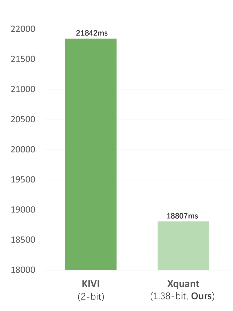
Figure 4: Comparison of Execution Time.
## Appendix D Efficiency analysis
Using Mistral-7B as an example, we theoretically analyze the computational cost of our two key improvements. During the calibration step, generating each token incurs only 64 additional floating-point multiplications and 32 additions (Equation 12), which are negligible in practice. Moreover, as described in Section 3.3.4, the cross-layer compression step optimizes efficiency by skipping certain parts of the quantization process (Equation 2).
To evaluate inference efficiency, we adopt the same experimental setup as implemented in KIVI’s repository, using a batch size of 16, a prompt length of 1024, and an output length of 128. As shown in Figure 4, XQuant, by leveraging its unique speedup mechanism, demonstrates competitive inference efficiency.
## Appendix E Hyperparameter
The related parameters in XQuant are $kq$ , $vq$ , $km$ , and $vm$ . In XQuant, we quantize the lower $kq$ , $vq$ layers of key and value cache into 2-bit, while quantizing others into 1-bit. We apply cross-layer compression from the $km$ th, $vm$ th layer of key and value cache. All the configurations are summarized in Table 11.
As demonstrated in Table 9, additional experiments on the Mistral-7B-Instruct model using the LongBench benchmark show that XQuant, with a fixed $η_1=1/6$ and $η_2=0.045$ , consistently delivers strong performance as well. These results suggest that this fixed set of hyperparameters are robust and can generalize effectively across different datasets. Therefore, task-specific hyperparameter tuning is superior but not necessary, and the method can achieve reliable performance with a fixed, pre-selected set of hyperparameters.
| Full Cache AsymKV XQuant | 16 1.5 1.38 | / / Task-specific | 43.02 37.17 42.90 | 27.10 22.77 26.65 | 18.78 15.76 17.44 | 71.00 70.50 71.50 | 86.23 86.25 84.50 | 42.75 43.44 45.18 | 2.75 3.16 5.71 | 41.66 39.86 41.98 |
| --- | --- | --- | --- | --- | --- | --- | --- | --- | --- | --- |
| XQuant | 1.38 | Static | 42.64 | 25.16 | 16.91 | 70.50 | 84.50 | 42.64 | 4.57 | 40.99 |
Table 9: Evaluation of different KV cache compression methods using static hyperparameters setting.
## Appendix F Cross-Layer Compression Strategy
Under 2-bit quantization, the values in the KV cache are restricted to the discrete integer set $\{i∈Z\mid 0≤ i≤ 3\}$ . Therefore, a rounding operation is required after weighted averaging. If standard rounding-to-nearest is applied, the range of $γ_0$ can be divided into six disjoint intervals, as summarized in Table 4. The derivation is as follows:
Let $e_0$ and $e_1$ denote the $B$ -bit quantized values at the same position in adjacent layers of $X_Q$ . Then the merged value $e_m$ after cross-layer compression is computed as:
| | $\displaystyle e_m$ | $\displaystyle=≤ft\lfloor\frac{γ_0e_0+γ_1e_1}{γ_0+γ_1}\right\rceil$ | |
| --- | --- | --- | --- |
Without loss of generality, assume $e_0≥ e_1$ and define $δ=e_0-e_1≥ 0$ . Then we have:
$$
e_m=e_1+≤ft\lfloorγ_0δ\right\rceil, \tag{14}
$$
where $γ_0∈[0,1]$ and $δ∈Z∩[0,3]$ . Since $γ_0δ∈[0,δ]$ , the rounding term $≤ft\lfloorγ_0δ\right\rceil$ in Eq. 14 can only take $δ+1$ discrete values. Let $≤ft\lfloorγ_0δ\right\rceil=c$ , where $c∈Z∩[0,δ]$ . Then:
$$
γ_0δ∈≤ft(c-\frac{1}{2},c+\frac{1}{2}\right)∩[0,δ], \tag{15}
$$
which yields the following constraint for $γ_0$ , when $δ>0$ :
$$
γ_0∈≤ft(\frac{c-1/2}{δ},\frac{c+1/2}{δ}\right)∩[0,1]. \tag{16}
$$
We now enumerate all valid combinations of $δ$ and $c$ from Equation 16:
- $δ=0$ : Only one possible value exists; trivial case omitted.
- $δ=1$ :
- $c=0$ : $γ_0∈[0,1/2)$
- $c=1$ : $γ_0∈(1/2,1]$
- $δ=2$ :
- $c=0$ : $γ_0∈[0,1/4)$
- $c=1$ : $γ_0∈(1/4,3/4)$
- $c=2$ : $γ_0∈(3/4,1]$
- $δ=3$ :
- $c=0$ : $γ_0∈[0,1/6)$
- $c=1$ : $γ_0∈(1/6,1/2)$
- $c=2$ : $γ_0∈(1/2,5/6)$
- $c=3$ : $γ_0∈(5/6,1]$
Collectively, this yields six effective intervals of $γ_0$ , as summarized in Table 4.
## Appendix G Comparison with Other Cross-Layer Compression Methods
Several prior works have explored inter-layer redundancy from different perspectives. To eliminate potential confusion, we clarify several key distinctions and highlight innovations as follows: (a) Most existing methods compute KV caches at a subset of layers. However, these approaches require additional training steps and, in some cases, even full retraining, significantly limiting scalability. In contrast, XQuant is designed as a plug-and-play solution that leverages deeper insights to enable effective redundancy reduction without any additional training. (b) XQuant is the only method that explicitly considers inter-layer redundancy through the lens of quantization. After quantization, the KV cache is decomposed into three components: the quantized cache, zero-points, and scaling factors. We demonstrate that the quantized cache, consisting solely of integers, exhibits substantial inter-layer similarity. Meanwhile, the zero-points and scaling factors, which require minimal storage, are retained individually to preserve per-layer characteristics without being compressed. (c) MiniCache Liu et al. (2024a) is another training-free method that primarily introduces a retention-recovery mechanism for cache magnitudes and unmergable tokens. However, such operations are not directly compatible in mainstream open-source KV quantization frameworks. Furthermore, its use of the SLERP function imposes several constraints, making it inapplicable to quantized caches, which fundamentally differs from XQuant.
| Full Cache AsymKV XQuant | 16 1.4 1.4 | 58.20 38.55 54.16 | 61.88 44.69 57.44 |
| --- | --- | --- | --- |
Table 10: Comparison of XQuant with Full Cache and AsymKV on the Qwen2.5-14B model using the LongBench benchmark.
## Appendix H Evaluation on Qwen2.5-14B
As shown in Table 10, we evaluated XQuant on a larger-scale and newer-generation model, Qwen2.5-14B Qwen et al. (2025), using the LongBench benchmark. The results demonstrate that XQuant generalizes well to different models, maintaining a superior trade-off between model performance and compression ratio.
| Mistral-7b-instruct-v0.2 | HQA | 30 | 2 | 32 | 16 | 1/6 | 0.045 |
| --- | --- | --- | --- | --- | --- | --- | --- |
| 2Wiki | 32 | 0 | 32 | 16 | 0 | 0.09 | |
| MSQ | 32 | 0 | 32 | 16 | 1/6 | 0 | |
| TREC | 30 | 2 | 32 | 16 | 1/6 | 0 | |
| TQA | 30 | 2 | 32 | 16 | 1/6 | 0.09 | |
| SAMS | 30 | 2 | 32 | 16 | 0 | 0 | |
| PC | 32 | 0 | 32 | 16 | 0 | 0.045 | |
| Llama2-7b | TruthfulQA | 28 | 0 | 32 | 28 | 1/3 | 0 |
| Llama2-7b-chat | HQA | 28 | 0 | 32 | 28 | 1/6 | 0.045 |
| 2Wiki | 28 | 0 | 32 | 28 | 1/3 | 0.045 | |
| MSQ | 28 | 0 | 32 | 28 | 1/3 | 0 | |
| TREC | 32 | 0 | 32 | 20 | 1/6 | 0 | |
| TQA | 32 | 0 | 32 | 20 | 1/6 | 0 | |
| SAMS | 32 | 0 | 32 | 20 | 0 | 0 | |
| PC | 32 | 0 | 32 | 20 | 1/3 | 0.045 | |
Table 11: The configurations of our main experiments.
## Appendix I Configurations
The Configurations of XQuant in our main experiments are summarized in Table 11
## Appendix J XQuant Pseudo Code
The pseudo code for the whole workflow is provided in Algorithm 1 and 2.
1
2
Input : $kq$ , $vq$ , $km$ , $vm$ , $η[2]$
Output : Optimized Quantized Cache
3
4 for $l← 0$ to $31$ do
5 if $l<vm$ or $l\bmod 2==0$ then
6 $KeyCache[l]←\textbf{Quantize}\big(X^l_k, 2 \textbf{if }l<kq \textbf{else }1\big)$
7
8 else
9 $KeyCache[l]←\textbf{PseudoQuantize}\big(X^l_k, 2 \textbf{if }l<kq \textbf{else }1\big)$
10
11 if $l<vq$ or $l\bmod 2==0$ then
12 $ValueCache[l]←\textbf{Quantize}\big(X^l_v, 2 \textbf{if }l<vq \textbf{else }1\big)$
13
14 else
15 $ValueCache[l]←\textbf{PseudoQuantize}\big(X^l_v, 2 \textbf{if }l<vq \textbf{else }1\big)$
16
17 for $l← 0$ to $31$ do
18 if $l<km$ or $l\bmod 2==0$ then
19 $DequantizedKey←\textbf{Dequantize}\big($
20 $KeyCache[l][0],$
21 $KeyCache[l][1],$
22 $KeyCache[l][2]\big)$
23
24 else
25 $DequantizedKey←\textbf{Dequantize}\big($
26 $KeyCache[l-1][0],$
27 $KeyCache[l-1][1],$
28 $KeyCache[l][2]\big)$
29
30 if $l<vm$ or $l\bmod 2==0$ then
31 $DequantizedValue←\textbf{Dequantize}\big($
32 $ValueCache[l][0],$
33 $ValueCache[l][1],$
34 $ValueCache[l][2]\big)$
35
36 else
37 $DequantizedValue←\textbf{Dequantize}\big($
38 $ValueCache[l-1][0],$
39 $ValueCache[l-1][1],$
40 $ValueCache[l][2]\big)$
41
Algorithm 1 XQuant Procedure
1
2
3 Function PseudoQuantize( $X$ , $n\_bits$ ):
4 $zero\_point←\min(X)$ // Find the minimum value of $X$
5 $scaling\_factor←\frac{\max(X)-\min(X)}{2^n\_bits-1}$ // Calculate scaling factor
6 return
7 $\textbf{Calibrate}(zero\_point,$ $scaling\_factor, n\_bits)$ ,
8 None
9
10
11 Function Quantize( $X$ , $n\_bits$ ):
12 $zero\_point←\min(X)$
13 $scaling\_factor←\frac{\max(X)-\min(X)}{2^n\_bits-1}$
14 $quantized\_cache←\textbf{round}≤ft(\frac{X-zero\_point}{scaling\_factor}\right)$ // Round to nearest quantized value
15 return
16 $\textbf{Calibrate}(zero\_point,$ $scaling\_factor, n\_bits)$ ,
17 $quantized\_cache$
18
19
20 Function Dequantize( $zero\_point$ , $scaling\_factor$ , $quantized\_cache$ ):
21 return $quantized\_cache· scaling\_factor+zero\_point$ // Reconstruct original value
22
23
24 Function Calibrate( $zero\_point$ , $scaling\_factor$ , $n\_bits$ ):
25 $zero\_point\_cali← zero\_point+scaling\_factor·η[n\_bits]$ // Adjust zero point based on $η$
26
27 $scaling\_factor\_cali← scaling\_factor·\big(1-2·η[n\_bits]\big)$ // Adjust scaling factor based on $η$
28
29 return
30 $zero\_point\_cali, scaling\_factor\_cali$ // Return calibrated values
31
32
Algorithm 2 Supporting Functions