2510.12157v1

# Self-Verifying Reflection Helps Transformers with CoT Reasoning Abstract Advanced large language models (LLMs) frequently reflect in reasoning chain-of-thoughts (CoTs), where they self-verify the correctness of current solutions and explore alternatives. However, given recent findings that LLMs detect limited errors in CoTs, how reflection contributes to empirical improvements remains unclear. To analyze this issue, in this paper, we present a minimalistic reasoning framework to support basic self-verifying reflection for small transformers without natural language, which ensures analytic clarity and reduces the cost of comprehensive experiments. Theoretically, we prove that self-verifying reflection guarantees improvements if verification errors are properly bounded. Experimentally, we show that tiny transformers, with only a few million parameters, benefit from self-verification in both training and reflective execution, reaching remarkable LLM-level performance in integer multiplication and Sudoku. Similar to LLM results, we find that reinforcement learning (RL) improves in-distribution performance and incentivizes frequent reflection for tiny transformers, yet RL mainly optimizes shallow statistical patterns without faithfully reducing verification errors. In conclusion, integrating generative transformers with discriminative verification inherently facilitates CoT reasoning, regardless of scaling and natural language. 1 Introduction Numerous studies have explored the ability of large language models (LLMs) to reason through a chain of thought (CoT), an intermediate sequence leading to the final answer. While simple prompts can elicit CoT reasoning [13], subsequent works have further enhanced CoT quality through reflective thinking [10] and the use of verifiers [4]. Recently, reinforcement learning (RL) [33] has achieved notable success in advanced reasoning models, such as OpenAI-o1 [20] and Deepseek-R1 [5], which show frequent reflective behaviors that self-verify the correctness of current solutions and explore alternatives, integrating generative processes with discriminative inference. However, researchers also report that the ability of these LLMs to detect errors is rather limited, and a large portion of reflection fails to bring correct solutions [11]. Given the weak verification ability, the experimental benefits of reflection and the emergence of high reflection frequency in RL require further explanation. To address this challenge, we seek to analyze two main questions in this paper: 1) what role self-verifying reflection plays in training and execution of reasoning models, and 2) how reflective reasoning evolves in RL with verifiable outcome rewards [15]. However, the complexity of natural language and the prohibitive training cost of LLMs make it difficult to draw clear conclusions from theoretical abstraction and comprehensive experiments across settings. Inspired by Zeyuan et al. [2], we observe that task-specific reasoning and self-verifying reflection do not necessitate complex language. This allows us to investigate reflective reasoning through tiny transformer models [36], which provide efficient tools to understand self-verifying reflection through massive experiments. To enable tiny transformers to produce long reflective CoTs and ensure analytic simplicity, we introduce a minimalistic reasoning framework, which supports essential reasoning behaviors that are operable without natural language. In our study, the model self-verifies the correctness of each thought step; then, it may resample incorrect steps or trace back to previous steps. Based on this framework, we theoretically prove that self-verifying reflection improves reasoning accuracy if verification errors are properly bounded, which does not necessitate a strong verifier. Additionally, a trace-back mechanism that allows revisiting previous solutions conditionally improves performance if the problem requires a sufficiently large number of steps. Our experiments evaluate 1M, 4M, and 16M transformers in solving integer multiplication [7] and Sudoku puzzles [3], which have simple definitions (thus, operable by transformers without language) yet still challenging for even LLM solvers. To maintain relevance to broader LLM research, the tiny transformers are trained from scratch through a pipeline similar to that of training LLM reasoners. Our main findings are listed as follows: 1) Learning to self-verify greatly facilitates the learning of forward reasoning. 2) Reflection improves reasoning accuracy if true correct steps are not excessively verified as incorrect. 3) Resembling the results of DeepSeek-R1 [5], RL can incentivize reflection if the reasoner can effectively explore potential solutions. 4) However, RL fine-tuning increases performance mainly statistically, with limited improvements in generalizable problem-solving skills. Overall, this paper contributes to the fundamental understanding of reflection in reasoning models by clarifying its effectiveness and synergy with RL. Our findings based on minimal reasoners imply a general benefit of reflection for more advanced models, which operate on a super-set of our simplified reasoning behaviors. In addition, our implementation also provides insights into the development of computationally efficient reasoning models. 2 Related works CoT reasoning Pretrained LLMs emerge the ability to produce CoTs from simple prompts [13, 38], which can be explained via the local dependencies [25] and probabilistic distribution [35] of natural-language reasoning. Many recent studies develop models targeted at reasoning, e.g., scaling test-time inference with external verifiers [4, 17, 18, 32] and distilling large general models to smaller specialized models [34, 9]. In this paper, we train tiny transformers from scratch to not only generate CoTs but also self-verify, i.e., detect errors in their own thoughts without external models. RL fine-tuning for CoT reasoning RL [33] recently emerges as a key method for CoT reasoning [31, 40]. It optimizes the transformer model by favoring CoTs that yield high cumulated rewards, where PPO [29] and its variant GRPO [31] are two representative approaches. Central to RL fine-tuning are reward models that guide policy optimization: the 1) outcome reward models (ORM) assessing final answers, and the 2) process reward models (PRM) [17] evaluating intermediate reasoning steps. Recent advances in RL with verifiable rewards (RLVR) [5, 41] demonstrate that simple ORM based solely on answer correctness can induce sophisticated reasoning behaviors. Reflection in LLM reasoning LLM reflection provides feedback to the generated solutions [19] and may accordingly refine the solutions [10]. Research shows that supervised learning from verbal reflection improves performance, even though the reflective feedback is omitted during execution [42]. Compared to the generative verbal reflection, self-verification uses discriminative labels to indicate the correctness of reasoning steps, which supports reflective execution and is operable without linguistic knowledge. Recently, RL is widely used to develop strong reflective abilities [14, 27, 20]. In particular, DeepSeek-R1 [5] shows that RLVR elicits frequent reflection, and such a result is reproduced in smaller LLMs [24]. In this paper, we further investigate how reflection evolves during RLVR by examining the change of verification errors. Understanding LLMs through small transformers Small transformers are helpful tools to understand LLMs, for their architectural consistency with LLMs and low development cost to support massive experiments. For example, transformers smaller than 1B provide insights into how data mixture and data diversity influence LLM training [39, 2]. They also contribute to foundational understanding of CoT reasoning, such as length generalization [12], internalization of thoughts [6], and how CoTs inherently extend the problem-solving ability [8, 16]. In this paper, we further use tiny transformers to better understand reflection in CoT reasoning. 3 Reflective reasoning for transformers In this section, we develop transformers to perform simple reflective reasoning in long CoTs. Focusing on analytic clarity and broader implications, the design of our framework follows the minimalistic principle, providing only essential reasoning behavior operable without linguistic knowledge. More advanced reasoning frameworks optimized for small-scale models are certainly our next move in future work. In the following, we first introduce the basic formulation of CoT reasoning; then, based on this formulation, we introduce our simple reasoning framework for self-verifying reflection; afterwards, we describe how transformers are trained to reason through this framework. 3.1 Reasoning formulation <details> <summary>x1.png Details</summary>  ### Visual Description \n ## Diagram: Reasoning Steps Model ### Overview The image depicts a diagram illustrating a model of reasoning steps, showing a sequence of reasoning stages from an initial question (Q) to an answer (A). The diagram uses boxes to represent reasoning steps (R1 to RT-1) and arrows to indicate the flow of reasoning. Below the diagram, a corresponding state transition sequence is provided. ### Components/Axes The diagram consists of the following components: * **Q:** Initial Question (Dark Gray Rectangle, positioned at the far left) * **R1 to RT-1:** Reasoning Steps (Rectangular Boxes, arranged horizontally in a sequence) * **A:** Answer (Dark Gray Rectangle, positioned at the far right) * **Arrows:** Indicate the flow of reasoning from Q to R1, then from R1 to R2, and so on, until reaching A. * **State Transition:** A sequence of equations describing the state changes at each step. ### Detailed Analysis or Content Details The diagram shows a sequential process. The state transition equations below the diagram detail the process: * **S0 = Q:** The initial state is the question Q. * **S1 = T(S0, R1):** The first state transition occurs from the initial question S0 to S1, influenced by the first reasoning step R1, using a function T. * **S2 = T(S1, R2):** The second state transition occurs from S1 to S2, influenced by the second reasoning step R2, using the same function T. * **...** This pattern continues for intermediate reasoning steps. * **ST-1 = T(ST-2, RT-1):** The (T-1)th state transition occurs from ST-2 to ST-1, influenced by the (T-1)th reasoning step RT-1, using the function T. * **ST = T(ST-1, A):** The final state transition occurs from ST-1 to ST, influenced by the answer A, using the function T. Above the boxes, the following equations are present: * **R1 ~ π(S0):** R1 is sampled from a distribution π conditioned on S0. * **R2 ~ π(S1):** R2 is sampled from a distribution π conditioned on S1. * **...** This pattern continues for intermediate reasoning steps. * **AT ~ π(ST-1):** A is sampled from a distribution π conditioned on ST-1. ### Key Observations The diagram illustrates a Markovian process where each reasoning step depends only on the previous state. The use of the symbol "~" indicates a probabilistic sampling process. The function "T" represents a state transition function, which is not further defined in the diagram. The diagram emphasizes the sequential nature of reasoning, where each step builds upon the previous one. ### Interpretation This diagram represents a model of reasoning as a series of state transitions. The initial question (Q) is the starting point, and each reasoning step (R1, R2, ..., RT-1) modifies the current state based on a probabilistic distribution (π). The final state (A) represents the answer. The function T encapsulates the process of updating the state based on the reasoning step. This model suggests that reasoning can be formalized as a sequence of probabilistic state transitions, where each step refines the understanding of the problem until an answer is reached. The diagram is abstract and doesn't specify the nature of the reasoning steps or the state representation, but it provides a general framework for modeling reasoning processes. The use of probabilistic sampling suggests that reasoning is not deterministic and involves uncertainty. 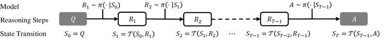</details> Figure 1: The illustration of MTP, where the transformer model $\pi$ reasons the answer $A$ of a query $Q$ through $T-1$ intermediate steps. <details> <summary>x2.png Details</summary>  ### Visual Description \n ## Diagram: State Transition with Calculation Steps ### Overview The image depicts a diagram illustrating a state transition process, likely within a computational or mathematical model. It shows a transformation from state *S_t* to state *S_t+1* via an intermediate state *R_t+1*. The diagram includes specific calculations performed during the transition. ### Components/Axes The diagram consists of three rectangular boxes labeled *S_t*, *R_t+1*, and *S_t+1*, connected by arrows representing transformations. The arrows are labeled *π* and *T*. Within each box, numerical calculations are shown. ### Detailed Analysis or Content Details **S_t (Left Box):** * Label: *S_t* * Calculations: * 145 * × 340 * + 290 **R_t+1 (Center Box):** * Label: *R_t+1* * Calculations: * 340 → 300 (Green text) * 145 × 4 = 580 (Green text) * 290 + 580 = 6090 (Red text) **S_t+1 (Right Box):** * Label: *S_t+1* * Calculations: * 145 * × 300 * + 6090 **Arrows:** * Arrow 1: From *S_t* to *R_t+1*, labeled *π* * Arrow 2: From *R_t+1* to *S_t+1*, labeled *T* ### Key Observations The diagram shows a process where the initial state *S_t* undergoes a transformation *π* to reach *R_t+1*. The value 340 is modified to 300 within *R_t+1*. The calculations within *R_t+1* involve multiplication and addition, resulting in the value 6090. This value is then used in the calculation for *S_t+1*. The color coding of the calculations within *R_t+1* (green for intermediate steps, red for the final result) highlights the flow of computation. ### Interpretation This diagram likely represents a step in an iterative process or a state update rule within a larger system. The transformations *π* and *T* could represent functions or operators that modify the state. The calculations suggest a weighted sum or a linear transformation. The change from 340 to 300 within *R_t+1* could represent a scaling or normalization step. The overall process appears to be updating a state *S* based on a previous state and some intermediate calculations. The diagram is a visual representation of a mathematical or computational procedure, potentially related to a dynamic system or an algorithm. The use of subscripts (t and t+1) indicates a time-series or sequential nature of the state transitions. </details> (a) Multiplication <details> <summary>x3.png Details</summary>  ### Visual Description \n ## Diagram: State Transition with Permutation ### Overview The image depicts a diagram illustrating a state transition process. It shows a grid-based state *S_t* at time *t*, a permutation operation *π*, a transformation *T*, and the resulting state *S_t+1* at time *t+1*. The diagram highlights specific cell updates within the grid. ### Components/Axes The diagram consists of three main grid structures labeled *S_t*, *R_t+1*, and *S_t+1*, connected by arrows representing operations. The grid is 8x8. There is a box labeled *R_t+1* between *S_t* and *S_t+1* with text inside. An arrow labeled *π* connects *S_t* to *R_t+1*. An arrow labeled *T* connects *R_t+1* to *S_t+1*. ### Content Details * **S_t (Initial State):** An 8x8 grid filled with numerical values ranging from 1 to 9. The values are distributed seemingly randomly across the grid. * Row 1: 1, 7, _, _, _, _, 8, _ * Row 2: _, 2, 3, _, 5, _, _, _ * Row 3: _, _, 9, _, _, _, 4, 7 * Row 4: 5, 2, 8, 6, _, 9, _, _ * Row 5: _, _, 3, 9, 4, 1, _, 6 * Row 6: _, _, _, _, _, _, _, 4 * Row 7: 7, _, _, 8, _, _, _, _ * **R_t+1 (Permutation):** A rectangular box containing the following text: * "Cell_6,2 ← 7" * "Cell_7,8 ← 2" * **S_t+1 (Next State):** An 8x8 grid, largely identical to *S_t*, but with two specific cells updated. * Row 1: 1, 7, _, _, _, _, 8, _ * Row 2: _, 2, 3, _, 5, _, _, _ * Row 3: _, _, 9, _, _, _, 4, 7 * Row 4: 5, 2, 8, 6, _, 9, _, _ * Row 5: _, _, 3, 9, 4, 1, _, 6 * Row 6: _, 7, _, _, _, _, _, 4 * Row 7: 7, _, _, 8, _, _, 2, _ ### Key Observations The diagram illustrates a state update where specific cells in the initial state *S_t* are modified to produce the next state *S_t+1*. The permutation *π* appears to select cells from *S_t* and assign their values to specific cells in *R_t+1*. The transformation *T* then applies these changes from *R_t+1* to *S_t+1*. Specifically, the value in cell (6,2) of *S_t+1* is changed from its original value in *S_t* to 7, and the value in cell (7,8) of *S_t+1* is changed from its original value in *S_t* to 2. ### Interpretation This diagram likely represents a step in a larger process, such as a cellular automaton or a reinforcement learning environment. The state *S_t* represents the environment's configuration at a given time step. The permutation *π* and transformation *T* define the rules governing how the environment evolves. The diagram highlights that only a small number of cells are updated in each time step, suggesting a sparse update rule. The notation "Cell_6,2 ← 7" indicates that the value of cell (6,2) is *assigned* the value 7, not incremented or modified in a more complex way. This suggests a discrete state space. The diagram is a simplified representation of a dynamic system, focusing on the key elements of state, transition, and update. The use of subscripts (t and t+1) indicates a time-series or sequential nature to the process. 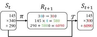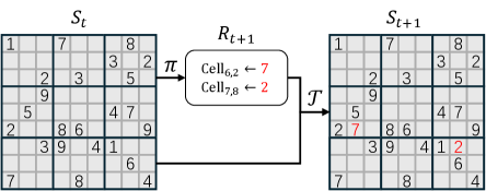</details> (b) Sudoku Figure 2: Example reasoning steps for multiplication and Sudoku, where the core planning is presented in the reasoning step ${R}_{t+1}$ . CoT Reasoning as a Markov decision process A general form of CoT reasoning is given as a tuple $({Q},\{{R}\},{A})$ , where ${Q}$ is the input query, $\{{R}\}=({R}_{1},...,{R}_{T-1})$ is the sequence of $T-1$ intermediate steps, and ${A}$ is the final answer. Following Wang [37], we formulate the CoT reasoning as a Markov thought process (MTP). As shown in Figure 1, an MTP follows that [37]: $$ \displaystyle{R}_{t+1}\sim\pi(\cdot\mid{S}_{t}),\ {S}_{t+1}=\mathcal{T}({S}_{t},{R}_{t+1}), \tag{1} $$ where ${S}_{t}$ is the $t$ -th reasoning state, $\pi$ is the planning policy (the transformer model), and $\mathcal{T}$ is the (usually deterministic) transition function. The initial state ${S}_{0}:=Q$ is given by the input query. In each reasoning step ${R}_{t+1}$ , the policy $\pi$ plans the next reasoning action that determines the state transition, which is then executed by $\mathcal{T}$ to obtain the next state. The process terminates when the step presents the answer, i.e., $A={R}_{T}$ . For clarity, a table of notations is presented in Appendix A. An MTP is implemented by specifying the state representations and transition function $\mathcal{T}$ . Since we use tiny transformers that are weak in inferring long contexts, we suggest reducing the length of state representations, so that each state ${S}_{t}$ carries only necessary information for subsequent reasoning. Here, we present two examples to better illustrate how MTPs are designed for tiny transformers. **Example 1 (An MTP for integer multiplication)** *As shown in Figure 2(a), to reason the product of two integers $x,y≥ 0$ , each state is an expression ${S}_{t}:=[x_{t}× y_{t}+z_{t}]$ mathematically equal to $x× y$ , initialized as ${S}_{0}=[x× y+0]$ . On each step, $\pi$ plans $y_{t+1}$ by eliminate a non-zero digit in $y_{t}$ to $0$ , and it then computes $z_{t+1}=z_{t}+x_{t}(y_{t}-y_{t+1})$ . Consequently, $\mathcal{T}$ updates ${S}_{t+1}$ as $[x_{t+1}× y_{t+1}+z_{t+1}]$ with $x_{t+1}=x_{t}$ . Similarly, $\pi$ may also eliminate non-zero digits in $x_{t}$ in a symmetric manner. Finally, $\pi$ yields $A=z_{t}$ as the answer if either $x_{t}$ or $y_{t}$ becomes $0$ .* **Example 2 (An MTP for Sudoku[3])** *As shown in Figure 2(b), each Sudoku state is a $9× 9$ game board. On each step, the model $\pi$ fills some blank cells to produce a new board, which is exactly the next state. The answer $A$ is a board with no blank cells.* 3.2 The framework of self-verifying reflection <details> <summary>x4.png Details</summary>  ### Visual Description \n ## Diagram: State Transition/Flow Diagram ### Overview The image depicts a state transition or flow diagram, likely representing a process or algorithm. It starts with an initial state 'Q' and progresses through a series of states (R1 to R6) and a final state 'A'. Each transition is associated with a transformation 'T' and a state update (S). Some transitions are marked with a red 'X' indicating failure, while others are marked with a green checkmark indicating success. ### Components/Axes The diagram consists of: * **States:** Represented by labeled rectangles (Q, R1, R2, R3, R4, R5, R6, A). * **Transitions:** Represented by arrows connecting the states. * **Labels:** Text associated with each state and transition, including state updates (S1 to S7) and transformation function (T). * **Indicators:** Red 'X' and green checkmarks indicating success or failure of a transition. * **Initial State:** 'Q' is a gray rectangle, indicating the starting point. ### Detailed Analysis or Content Details The diagram can be broken down as follows: 1. **Initial State:** Q, with S0 = Q. 2. **Transition 1:** From Q to R1. This transition is marked with a red 'X', indicating failure. S1 = S0. 3. **Transition 2:** From Q to R2. This transition is marked with a green checkmark, indicating success. S2 = T(S1, R2). 4. **Transition 3:** From R2 to R3. This transition is marked with a green checkmark, indicating success. S3 = T(S2, R3). 5. **Transition 4:** From R3 to R6. This transition is marked with a green checkmark, indicating success. S6 = T(S5, R6). 6. **Transition 5:** From R6 to A. This transition is marked with a green checkmark, indicating success. S7 = T(S6, A). 7. **Branching from R3:** There are two branches originating from R3. * **Branch 1:** From R3 to R4. This transition is marked with a red 'X', indicating failure. S4 = S3. * **Branch 2:** From R3 to R5. This transition is marked with a red 'X', indicating failure. S5 = S4. ### Key Observations * The diagram shows a branching process with potential failure points. * The success path leads from Q -> R2 -> R3 -> R6 -> A. * The failure paths lead to states R1, R4, and R5, which do not contribute to reaching the final state A. * The state updates (S) are dependent on the previous state and the target state, using the transformation function T. * The diagram suggests a process where multiple attempts or paths are possible, but only one leads to the desired outcome. ### Interpretation This diagram likely represents a search or optimization algorithm, or a decision-making process with multiple possible outcomes. The 'T' function could represent a test or evaluation, and the checkmarks/Xs indicate whether the test passed or failed. The states R1, R4, and R5 represent dead ends or unsuccessful attempts, while the path through R2, R3, R6 leads to the successful outcome A. The state updates (S) suggest that the algorithm maintains and modifies a state variable as it progresses through the process. The diagram illustrates a scenario where the algorithm may need to explore multiple paths before finding the correct one. The repeated use of the transformation function 'T' suggests an iterative process. The diagram does not provide specific details about the nature of the transformation 'T' or the meaning of the states, but it provides a clear visual representation of the process flow and potential outcomes. </details> (a) Reflective MTP <details> <summary>x5.png Details</summary>  ### Visual Description \n ## Diagram: State Transition Diagram ### Overview The image depicts a state transition diagram, illustrating a sequence of states and transitions between them. The diagram uses labeled nodes representing states and directed arrows representing transitions. Each transition is associated with a transformation function and a checkmark or cross indicating success or failure. ### Components/Axes The diagram consists of the following components: * **States:** Represented by rectangular nodes labeled Q, R1, R2, R3, R4, R5, R6, R7, R8, R9, A. * **Transitions:** Represented by directed arrows connecting states. * **Labels:** Each transition arrow is labeled with a transformation function (T) and a state variable (S). * **Success/Failure Indicators:** Each state node has a checkmark (✓) or cross (✗) indicating the outcome of the transition leading to that state. * **Initial State:** The state Q is represented by a gray hexagon. ### Detailed Analysis or Content Details The diagram shows the following state transitions: 1. **Q → R1:** Arrow color: Green. Label: `S₁ = T(S₀, R₁)` . R1 has a checkmark (✓). 2. **R1 → R2:** Arrow color: Orange. Label: `S₂ = S₁`. R2 has a cross (✗). 3. **R1 → R3:** Arrow color: Orange. Label: `S₃ = T(S₂, R₃)`. R3 has a checkmark (✓). 4. **R2 → R4:** Arrow color: Red. Label: `S₄ = T(S₃, R₄)`. R4 has a checkmark (✓). 5. **R3 → R7:** Arrow color: Orange. Label: `S₇ = S₀`. R7 has a cross (✗). 6. **R4 → R5:** Arrow color: Red. Label: `S₅ = S₄`. R5 has a cross (✗). 7. **R4 → R6:** Arrow color: Red. Label: `S₆ = S₃`. R6 has a cross (✗). 8. **R3 → R8:** Arrow color: Green. Label: `S₈ = T(S₇, R₈)`. R8 has a checkmark (✓). 9. **R8 → R9:** Arrow color: Green. Label: `S₉ = T(S₈, R₉)`. R9 has a checkmark (✓). 10. **R9 → A:** Arrow color: Green. Label: `S₁₀ = T(S₉, A)`. A has a checkmark (✓). The initial state is Q, labeled as `S₀ = Q`. ### Key Observations * The diagram shows multiple paths from the initial state Q. * Some paths lead to successful states (checkmark), while others lead to failed states (cross). * The transformation function `T` is used in multiple transitions, suggesting a consistent operation applied to different state variables. * The state variables `S₀` through `S₁₀` are used to track the system's state throughout the transitions. * The diagram appears to model a process with potential failure points (R2, R5, R6, R7). ### Interpretation This diagram likely represents a process or algorithm with multiple possible outcomes. The states represent different stages of the process, and the transitions represent the steps taken to move between those stages. The transformation function `T` could represent an operation performed on the state variable, and the checkmarks and crosses indicate whether the operation was successful. The presence of both successful and failed states suggests that the process is not deterministic and that the outcome depends on the specific conditions encountered during the transitions. The diagram could be used to analyze the process, identify potential bottlenecks, and improve its reliability. The initial state Q represents the starting point, and the final state A represents a successful completion of the process. The diagram provides a visual representation of the possible paths and outcomes, allowing for a clear understanding of the process flow. The use of state variables (S₀ to S₁₀) suggests a system where the current state is explicitly tracked and used in subsequent transitions. 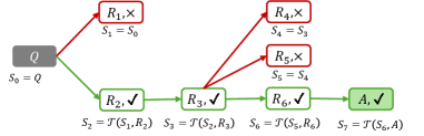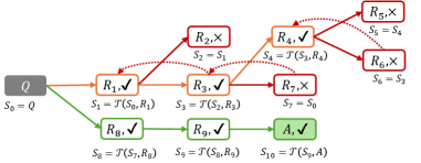</details> (b) Reflective trace-back search (width $m=2$ ) Figure 3: Reflective reasoning based on MTP. “ $\checkmark$ ” and “ $×$ ” are self-verification labels for positive and negative steps, respectively. The steps that are instantly verified as negative are highlighted in red. In RTBS, the dashed-line arrows back-propagate the negative labels, causing parental steps to be recursively rejected (orange). The green shows the steps that successfully lead to the answer. Conceptually, reflection provides feedback for the proposed steps and may alter the subsequent reasoning accordingly. Reflection takes flexible forms in natural language (e.g., justifications and comprehensive evaluations), making it extremely costly to analyze. In this work, we propose to equip transformers with the simplest discriminative form of reflection, where the model self-verifies the correctness of each step and is allowed to retry those incorrect attempts. We currently do not consider the high-level revisory behavior that maps incorrect steps to correct ones, as we find learning such a mapping is challenging for tiny models and leads to no significant gain in practice. Specifically, we analyze two basic variants of reflective reasoning in this paper: the reflective MTP and the reflective trace-back search, as described below (see pseudo-code in Appendix D.1). Reflective MTP (RMTP) Given any MTP with a policy $\pi$ and transition $\mathcal{T}$ , we use a verifier $\mathcal{V}$ to produce a verification sequence after each reasoning step, denoted as ${V}_{t}\sim\mathcal{V}(·|{R}_{t})$ . Such ${V}_{t}$ includes verification label(s): The positive “ $\checkmark$ ” and negative “ $×$ " signifying correct and incorrect reasoning of ${R}_{t}$ , respectively. Given the verified step ${\tilde{R}}_{t+1}:=({R}_{t+1},{V}_{t+1})$ that contains verification, we define $\tilde{\mathcal{T}}$ as the reflective transition function that rejects incorrect steps: $$ {S}_{t+1}=\tilde{\mathcal{T}}({S}_{t},{\tilde{R}}_{t+1})=\tilde{\mathcal{T}}({S}_{t},({R}_{t+1},{V}_{t+1})):=\begin{cases}{S}_{t},&\text{``$\times$''}\in{V}_{t+1};\\ \mathcal{T}({S}_{t},{R}_{t+1}),&\text{otherwise.}\end{cases} \tag{2} $$ In other words, if $\mathcal{V}$ detects any error (i.e. “ $×$ ") in ${R}_{t+1}$ , the state remains unchanged so that $\pi$ may re-sample another attempt. Focusing on self-verification, we use a single model called the self-verifying policy $\tilde{\pi}:=\{\pi,\mathcal{V}\}$ to serve simultaneously as the planning policy $\pi$ and the verifier $\mathcal{V}$ . By operating tokens, $\tilde{\pi}$ outputs the verified step ${\tilde{R}}_{t}$ for each input state ${S}_{t}$ . In this way, $\tilde{\mathcal{T}}$ and $\tilde{\pi}$ constitute a new MTP called the RMTP, with illustration in Figure 3(a). Reflective trace-back search (RTBS) Though RMTP allows instant rejections of incorrect steps, sometimes the quality of a step can be better determined by actually trying it. For example, a Sudoku solver occasionally makes tentative guesses and traces back if the subsequent reasoning fails. Inspired by o1-journey [26], a trace-back search allowing the reasoner to revisit previous states may be applied to explore solution paths in an MTP. We implement simple RTBS by simulating the depth-first search in the trajectory space. Let $m$ denote the RTBS width, i.e., the maximal number of attempts on each step. As illustrated in Figure 3(b), if $m$ proposed steps are rejected on a state ${S}_{t}$ , the negative label “ $×$ ” will be propagated back to recursively reject the previous step ${R}_{t}$ . As a result, the state traces back to the closest ancestral state that has remaining attempt opportunities. 3.3 Training <details> <summary>x6.png Details</summary>  ### Visual Description ## Diagram: Training Pipeline for Conversational Agents ### Overview The image depicts a four-stage training pipeline for conversational agents, starting with pretraining on a mixture of CoT (Chain-of-Thought) examples and culminating in Reinforcement Learning fine-tuning (RL fine-tuning). The pipeline leverages techniques like MTP (Model-based Trajectory Planning), RMTMP (Reward-Model-based Trajectory Planning), and an Expert Verifier. The diagram illustrates the flow of data and the transformations applied at each stage. ### Components/Axes The diagram is divided into four main sections, labeled (I) through (IV), representing the stages of the training process. Each section contains boxes and arrows illustrating data flow and processing. Key elements include: * **CoT examples (data mixture):** The initial training data, consisting of question-reasoning-answer sequences. * **Q:** Represents a question. * **R1, R2, R3...:** Represents reasoning steps. * **A:** Represents the answer. * **S1, S2, S3...:** Represents states. * **π:** Represents a policy. * **ν:** Represents ground-truth verification. * **V1, V2, V3...:** Represents verification scores. * **MTP:** Model-based Trajectory Planning. * **RMTMP:** Reward-Model-based Trajectory Planning. * **Reward Model:** A component used in RL fine-tuning. * **Policy Optimization:** A component used in RL fine-tuning. ### Detailed Analysis or Content Details **(I) Pretraining:** * The process begins with a "Training Data" block containing CoT examples. These examples are represented as sequences of Q, R1, R2, A, etc. * "Context windows (randomly drawn)" are extracted from the CoT examples. These windows are fed into the next stage. **(II) Non-reflective SFT:** * The output of the Pretraining stage is fed into the "Non-reflective SFT" (Supervised Fine-Tuning) stage. * The input is a sequence of states and steps/answers. * The policy π is used to generate an action A based on the current state S. * The state transitions to S<sub>t</sub> = τ(S<sub>t-1</sub>, R<sub>t</sub>). **(III) Reflective SFT:** * This stage introduces an "Expert Verifier" that evaluates the generated reasoning steps. * The Expert Verifier provides verification scores (V1, V2, V3...) for the ground-truth verification. * The policy π is used to generate an action A based on the current state S. * The state transitions to S<sub>t</sub> = τ(S<sub>t-1</sub>, R<sub>t</sub>). * Sampling CoTs is done through MTP. **(IV) RL fine-tuning:** * This stage utilizes both MTP and RMTMP. * MTP takes the policy π and generates actions A based on states Q and reasoning steps R1, R2. * RMTMP incorporates a "Reward Model" to evaluate the generated responses. * The state transitions to S<sub>t</sub> = τ(S<sub>t-1</sub>, R<sub>t</sub>, V<sub>t</sub>). * "Policy Optimization" is performed based on the rewards received from the Reward Model. * An arrow indicates feedback from the RL fine-tuning stage back to the Non-reflective SFT stage. ### Key Observations * The pipeline progressively refines the conversational agent's capabilities. * The introduction of the Expert Verifier in stage (III) adds a layer of quality control. * The use of MTP and RMTMP in stage (IV) enables reinforcement learning based on both model-based and reward-based feedback. * The feedback loop from RL fine-tuning to Non-reflective SFT suggests iterative refinement of the model. ### Interpretation The diagram illustrates a sophisticated training pipeline for building high-quality conversational agents. The pipeline moves from initial pretraining on a large dataset of CoT examples to supervised fine-tuning, then to a reflective SFT stage that incorporates expert verification, and finally to reinforcement learning fine-tuning. The use of MTP and RMTMP suggests a focus on planning and reward maximization. The feedback loop indicates a commitment to continuous improvement. The diagram highlights the importance of both supervised learning and reinforcement learning in achieving optimal performance. The inclusion of an Expert Verifier suggests a desire to ensure the generated reasoning steps are accurate and reliable. The overall architecture is designed to create a conversational agent that can not only generate coherent responses but also provide accurate and well-reasoned answers. The diagram suggests a focus on building agents that can "think" through problems and explain their reasoning, rather than simply providing answers. 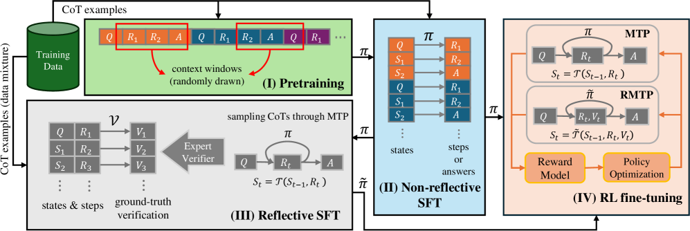</details> Figure 4: The training workflow for transformers to perform CoT reasoning. As shown in Figure 4, we train the tiny transformers from scratch through consistent techniques of LLM counterparts, such as pretraining, supervised fine-tuning (SFT), and RL fine-tuning. First, we use conventional pipelines to train a baseline model $\pi$ with only the planning ability in MTPs. During (I) pretraining, these CoT examples are treated as a textual corpus, where sequences are randomly drawn to minimize cross-entropy loss of next-token prediction. Then, in (II) non-reflective SFT, the model learns to map each state ${S}_{t}$ to the corresponding step ${R}_{t+1}$ by imitating examples. Next, we employ (III) reflective SFT to integrate the planning policy $\pi$ with the knowledge of self-verification. To produce ground-truth verification labels, we use $\pi$ to sample non-reflective CoTs, in which the sampled steps are then labeled by an expert verifier (e.g., a rule-based process reward model). Reflective SFT learns to predict these labels from the states and the proposed steps, i.e., $({S}_{t},{R}_{t+1})→{V}_{t+1}$ . To prevent disastrous forgetting, we also mix the same CoT examples as in non-reflective SFT. This converts $\pi$ to a self-verifying policy $\tilde{\pi}$ that can self-verify reasoning steps. Thus far, we have obtained the planning policy $\pi$ and the self-verifying policy $\tilde{\pi}$ , which can be further strengthened through (IV) RL fine-tuning. As illustrated in Figure 4, RL fine-tuning involves iteratively executing $\pi$ ( $\tilde{\pi}$ ) to collect experience CoTs through an MTP (RMTP), evaluating these CoTs with a reward model, and updating the policy to favor higher-reward solutions. Following the RLVR paradigm [15], we use binary outcome rewards (i.e., $1$ for correct answers and $0$ otherwise) computed by a rule-based answer checker $\operatorname{ORM}(Q,A)$ . When training the self-verifying policy $\tilde{\pi}$ , the RMTP treats verification ${V}_{t}$ as a part of the augmented step ${\tilde{R}}_{t}$ , simulating R1-like training [5] where reflection and solution planning are jointly optimized. We mainly use GRPO [31] as the algorithms to optimize policies. Details of RL fine-tuning are elaborated in Appendix B. 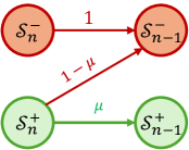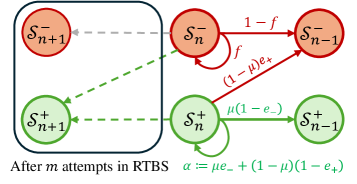4 Theoretical results This section establishes theoretical conditions under which self-verifying reflection (RMTP or RTBS in Section 3.2) enhances reasoning accuracy (the probability of deriving correct answers). The general relationship between the verification ability and reasoning accuracy (discussed in Appendix C.1) for any MTP is intractable as the states and transitions can be arbitrarily specified. Therefore, to derive interpretable insights, we discuss a simplified prototype of reasoning that epitomizes the representative principle of CoTs — to incrementally express complex relations by chaining the local relation in each step [25]. Specifically, Given query $Q$ as the initial state, we view a CoT as the step-by-step process that reduces the complexity within states: - We define $\mathcal{S}_{n}$ as the set of states with a complexity scale of $n$ . For simplicity, we assume that each step, if not rejected by reflection, reduces the complexity scale by $1$ . Therefore, the scale $n$ is the number of effective steps required to derive an answer. - An answer $A$ is a state with a scale of $0$ , i.e. $A∈\mathcal{S}_{0}$ . Given an input query $Q$ , the answers $\mathcal{S}_{0}$ are divided into positive (correct) answers $\mathcal{S}_{0}^{+}$ and negative (wrong) answers $\mathcal{S}_{0}^{-}$ . - States $\mathcal{S}_{n}$ ( $n$ > 0) are divided into 1) positive states $\mathcal{S}_{n}^{+}$ that potentially lead to correct answers and 2) negative states $\mathcal{S}_{n}^{-}$ leading to only incorrect answers through forward transitions. Consider a self-verifying policy $\tilde{\pi}=\{\pi,\mathcal{V}\}$ to solve this simplified task. We describe its fundamental abilities using the following probabilities (whose meanings will be explained afterwards): $$ \displaystyle\mu:=p_{{R}\sim\pi}(\mathcal{T}({S},{R})\in\mathcal{S}^{+}_{n-1}\mid{S}\in\mathcal{S}_{n}^{+}) \displaystyle e_{+}:=p_{{R},{V}\sim\tilde{\pi}}(\mathcal{T}({S},{R})\in\mathcal{S}^{-}_{n-1},\text{``$\times$''}\notin{V}\mid{S}\in\mathcal{S}_{n}^{+}), \displaystyle e_{-}:=p_{{R},{V}\sim\tilde{\pi}}(\mathcal{T}({S},{R})\in\mathcal{S}^{+}_{n-1},\text{``$\times$''}\in{V}\mid{S}\in\mathcal{S}_{n}^{+}), \displaystyle f:=p_{{R},{V}\sim\tilde{\pi}}(\text{``$\times$''}\in{V}\mid{S}\in\mathcal{S}_{n}^{-}). \tag{3} $$ To elaborate, $\mu$ measures the planning ability, defined as the probability that $\pi$ plans a step that leads to a positive next state, given that the current state is positive. For verification abilities, we measure the rates of two types of errors: $e_{+}$ (false positive rate) is the probability of accepting a step that leads to a negative state, and $e_{-}$ (false negative rate) is the probability of rejecting a step that leads to a positive state. Additionally, $f$ is the probability of rejecting any step on negative states, providing the chance of tracing back to previous states. Given these factors, Figure 5 illustrates the state transitions in non-reflective (vanilla MTP) and reflective (RMTB and RTBS) reasoning. <details> <summary>x7.png Details</summary>  ### Visual Description \n ## Diagram: State Transition Diagram ### Overview The image depicts a state transition diagram with four states represented by colored circles and transitions between them indicated by arrows labeled with probabilities. The diagram appears to model a stochastic process with two possible states, positive (+) and negative (-), at different time steps 'n' and 'n-1'. ### Components/Axes The diagram consists of the following components: * **States:** * S_n^- (Top-left, Red circle) * S_n-1^- (Top-right, Red circle) * S_n⁺ (Bottom-left, Green circle) * S_n-1⁺ (Bottom-right, Green circle) * **Transitions:** * From S_n^- to S_n-1^-: Labeled "1", Red arrow. * From S_n^- to S_n-1⁺: Labeled "1 - μ", Red arrow. * From S_n⁺ to S_n-1⁺: Labeled "μ", Green arrow. ### Detailed Analysis or Content Details The diagram shows transitions between states at time 'n' and 'n-1'. The probabilities associated with these transitions are: * **S_n^- to S_n-1^-:** Probability = 1. This indicates a certain transition. * **S_n^- to S_n-1⁺:** Probability = 1 - μ. This represents the probability of transitioning from the negative state at time 'n' to the positive state at time 'n-1'. * **S_n⁺ to S_n-1⁺:** Probability = μ. This represents the probability of remaining in the positive state from time 'n' to 'n-1'. There is no explicit indication of a transition from S_n⁺ to S_n-1^-. ### Key Observations The diagram suggests a Markov process where the future state depends only on the current state. The parameter μ likely represents the probability of staying in the positive state. The transitions are directed, indicating a temporal aspect to the process. The probabilities associated with the transitions sum to 1 for each state, ensuring that the system remains within the defined states. ### Interpretation This diagram likely represents a simplified model of a system that can exist in two states (positive and negative) and transitions between them with certain probabilities. The parameter μ controls the tendency of the system to remain in the positive state. This type of diagram is commonly used in fields like stochastic modeling, queuing theory, or hidden Markov models. The absence of a transition from S_n⁺ to S_n-1^- could indicate a constraint or assumption within the model. The diagram could be used to analyze the long-term behavior of the system, such as the probability of being in a particular state after a certain number of time steps. The use of red and green colors may be intended to visually represent negative and positive states, respectively. The diagram is a visual representation of a probabilistic process, and the values of μ would determine the specific behavior of the system. </details> (a) Non-reflective reasoning <details> <summary>x8.png Details</summary>  ### Visual Description \n ## Diagram: State Transition Diagram for RTBS ### Overview The image depicts a state transition diagram, likely representing a model within a Reinforcement Learning framework, specifically related to a process called RTBS (Reinforcement Training by Simulated annealing). The diagram illustrates transitions between four states: S_n+1^-, S_n^-, S_n-1^-, S_n+1⁺, S_n⁺, and S_n-1⁺. The states are represented as colored circles, and the transitions between them are indicated by arrows labeled with probabilities or transition rates. A rectangular box encompasses the states S_n+1^- and S_n+1⁺. ### Components/Axes The diagram consists of the following components: * **States:** S_n+1^- (top-left, red), S_n^- (top-center, red), S_n-1^- (top-right, red), S_n+1⁺ (bottom-left, green), S_n⁺ (bottom-center, green), S_n-1⁺ (bottom-right, green). * **Transitions:** Arrows connecting the states, labeled with probabilities or rates. * **Enclosing Box:** A gray dashed rectangle encompassing S_n+1^- and S_n+1⁺. * **Text Labels:** "After *m* attempts in RTBS" (bottom-left) and "α := μe_- + (1 - μ)(1 - e₊)" (bottom-right). ### Detailed Analysis or Content Details The diagram shows the following transitions and their associated labels: 1. **S_n^- to S_n-1^-:** Labeled "1 - *f*". 2. **S_n^- to S_n+1^-:** Labeled "*f*". 3. **S_n^- to S_n+1⁺:** Labeled "(1 - μ)e₊". 4. **S_n⁺ to S_n-1⁺:** Labeled "μ(1 - e_-)". 5. **S_n⁺ to S_n+1⁺:** A dashed gray arrow, no label. 6. **S_n+1^- to S_n^-:** A dashed gray arrow, no label. 7. **S_n+1⁺ to S_n⁺:** A dashed gray arrow, no label. The text label "After *m* attempts in RTBS" suggests that this diagram represents the state of the system after a certain number of iterations within the RTBS algorithm. The equation "α := μe_- + (1 - μ)(1 - e₊)" defines a variable α in terms of μ, e_-, and e₊. The ":=" symbol indicates assignment. ### Key Observations * The states are grouped into two sets: those with a negative superscript (-) and those with a positive superscript (+). * The transitions between states are probabilistic, indicated by the labels on the arrows. * The enclosing box around S_n+1^- and S_n+1⁺ might indicate a specific stage or condition within the RTBS process. * The dashed arrows suggest a different type of transition or a less direct relationship between the states. ### Interpretation This diagram likely represents a Markov chain or a similar stochastic process used to model the behavior of an agent learning through reinforcement learning with simulated annealing (RTBS). The states S_n⁺ and S_n^- could represent different "modes" or "phases" of the agent's behavior, with the superscript indicating a characteristic (e.g., positive or negative reward expectation). The parameters *f*, μ, e₊, and e_- likely represent probabilities or rates governing the transitions between these states. *f* could represent the probability of staying in the negative state, while μ might represent the probability of transitioning to the positive state. e₊ and e_- could be error terms or exploration rates. The equation for α suggests that it is a weighted average of two terms, one related to the negative state (μe_-) and the other to the positive state ((1 - μ)(1 - e₊)). This could represent a measure of the agent's overall performance or a parameter controlling its learning rate. The diagram suggests a cyclical process where the agent transitions between positive and negative states, with the probabilities of these transitions influenced by the parameters *f*, μ, e₊, and e_-. The RTBS algorithm likely adjusts these parameters over time to optimize the agent's behavior. The dashed lines indicate a possible feedback loop or a less direct influence between states. The box around the n+1 states could indicate a step in the algorithm. </details> (b) Reflective reasoning through an RMTP or RTBS Figure 5: The diagram of state transitions starting from scale $n$ in the simplified reasoning, where probabilities are attached to solid lines. In (b) reflective reasoning, the dashed-line arrow presents the trace-back move after $m$ attempts in RTBS. For input problems with scale $n$ , we use $\rho(n)$ , $\tilde{\rho}(n)$ , and $\tilde{\rho}_{m}(n)$ to respectively denote the reasoning accuracy using no reflection, RMTP, and RTBS (with width $m$ ). Obviously, we have $\rho(n)=\mu^{n}$ . In contrast, the mathematical forms of $\tilde{\rho}(n)$ and $\tilde{\rho}_{m}(n)$ are more complicated and therefore left to Appendix C.2. Our main result provides simple conditions for the above factors $(\mu,e_{-},e_{+},f)$ to ensure an improved accuracy when reasoning through an RMTP or RTBS. **Theorem 1** *In the above simplified problem, consider a self-verifying policy $\tilde{\pi}$ where $\mu$ , $e_{-}$ , and $e_{+}$ are non-trivial (i.e. neither $0$ nor $1$ ). Let $\alpha:=\mu e_{-}+(1-\mu)(1-e_{+})$ denote the rejection probability on positive states. Given an infinite computation budget, for $n>0$ we have: - $\tilde{\rho}(n)≥\rho(n)$ if and only if $e_{-}+e_{+}≤ 1$ , where equalities hold simultaneously; furthermore, reducing either $e_{-}$ or $e_{+}$ strictly increases $\tilde{\rho}(n)$ . - $\tilde{\rho}_{m}(n)>\tilde{\rho}(n)$ for a sufficiently large $n$ if and only if $f>\alpha$ and $m>\frac{1}{1-\alpha}$ ; furthermore, such a gap of $\tilde{\rho}_{m}(n)$ over $\tilde{\rho}(n)$ increases strictly with $f$ .* Does reflection require a strong verifier? Theorem 1 shows that RMTP improves performance over vanilla MTP if the verification errors $e_{+}$ and $e_{-}$ are properly bounded, which does not necessitate a strong verifier. In our simplified setting, this only requires the verifier $\mathcal{V}$ to be better than random guessing (which ensures $e_{-}+e_{+}=1$ ). This also indicates a trivial guarantee of RTBS, as an infinitely large width ( $m→+∞$ ) substantially converts RTBS to RMTB. When does trace-back search facilitate reflection? Theorem 1 provides the conditions for RTBS to outperform RMTP for a sufficiently large $n$ : 1) The width $m$ is large enough to ensure effective exploration. 2) $f>\alpha$ indicates that negative states are inherently discriminated from positive ones, leading to a higher rejection probability on negative states than on positive states (see Figure 5(b)). In other words, provided $f>\alpha$ , RTBS is ensured to be more effective on complicated queries using a finite $m$ . However, this also implies a risk of over-thought on simple queries that have a small $n$ . The derivation and additional details of Theorem 1 are provided in Appendix C.3. In addition, we also derive how many steps it costs to find a correct solution in RMTP. The following Proposition 1 (see proof in Appendix C.4) shows that a higher $e_{-}$ causes more steps to be necessarily rejected and increases the solution cost. In contrast, although a higher $e_{+}$ reduces accuracy, it forces successful solutions to rely less on reflection, leading to fewer expected steps. Therefore, a high false negative rate $e_{-}$ is worse than a high $e_{+}$ given the limited computational budget in practice. **Proposition 1 (RMTP Reasoning Length)** *For a simplified reasoning problem with scale $n$ , the expected number of steps $\bar{T}$ for $\tilde{\pi}$ to find a correct answer is $\bar{T}=\frac{n}{(1-\mu)e_{+}+\mu(1-e_{-})}$ . Especially, a correct answer will never be found if the denominator is $0$ .* Appendix C.5 further extends our analysis to more realistic reasoning, where rejected attempts lead to a posterior drop of $\mu$ (or rise of $e_{-}$ ), indicating that the model may not well generalize the current state. In this case, the bound of $e_{-}$ to ensure improvements becomes stricter than that in Theorem 1. 5 Experiments We conduct comprehensive experiments to examine the reasoning performance of tiny transformers under various settings. We trained simple causal-attention transformers [36] (implemented by LitGPT [1]) with 1M, 4M, and 16M parameters, through the pipelines described in Section 3.3. Details of training data, model architectures, tokenization, and hyperparameters are included in Appendix D. The source code is available at https://github.com/zwyu-ai/self-verifying-reflection-reasoning. We test tiny transformers in two reasoning tasks: The integer multiplication task (Mult for short) computes the product of two integers $x$ and $y$ ; the Sudoku task fills numbers into blank positions of a $9× 9$ matrix, such that each row, column, or $3× 3$ block is a permutation of $\{1,...,9\}$ . For both tasks, we divide queries into 3 levels of difficulties: The in-distribution (ID) Easy, ID Hard, and out-of-distribution (OOD) Hard. The models are trained on ID-Easy and ID-Hard problems, while tested additionally on OOD-Hard cases. We define the difficulty of a Mult query by the number $d$ of digits of the greater multiplicand, and that of a Sudoku puzzle is determined by the number $b$ of blanks to be filled. Specifically, we have $1≤ d≤ 5$ or $9≤ b<36$ for ID Easy, $6≤ d≤ 8$ or $36≤ b<54$ for ID Hard, and $9≤ d≤ 10$ or $54≤ b<63$ for OOD Hard. Our full results are presented in Appendix E. Shown in Appendix E.1, these seemingly simple tasks pose challenges even for some well-known LLMs. Remarkably, through simple self-verifying reflection, our best 4M Sudoku model is as good as OpenAI o3-mini [21], and our best 16M Mult model outperforms DeepSeek-R1 [5] in ID difficulties. 5.1 Results of supervised fine-tuning First, we conduct (I) pretraining, (II) non-reflective SFT, and (III) reflective SFT as described in Section 3.3. In reflective SFT, we consider learning two types of self-verification: 1) The binary verification includes a single binary label indicating the overall correctness of a planned step; 2) the detailed verification includes a series of binary labels checking the correctness of each meaningful element in the step. The implementation of verification labels is elaborated in Appendix D.2.3. We present our full SFT results in Appendix E.2, which includes training 30 models and executing 54 tests. In the following, we discuss our main findings through visualizing representative results. <details> <summary>x9.png Details</summary>  ### Visual Description ## Bar Charts: Verification Accuracy vs. Model Size ### Overview This image presents three bar charts comparing the accuracy of a verification process under different conditions: "ID Easy", "ID Hard", and "OOD Hard". The charts compare the performance of three model sizes: "1M", "4M", and "16M", across three verification types: "None", "Binary", and "Detailed". The y-axis represents accuracy in percentage (%), and the x-axis represents model size. ### Components/Axes * **X-axis:** Model Size (1M, 4M, 16M) * **Y-axis:** Accuracy (%) - Scale ranges from 0 to 100 for "ID Easy" and "ID Hard", and from 0 to 10 for "OOD Hard". * **Charts:** Three separate bar charts, each representing a different condition: * "ID Easy" (top-left) * "ID Hard" (top-center) * "OOD Hard" (top-right) * **Legend:** Located in the top-right corner, defining the colors for each Verification Type: * Blue: None * Orange: Binary * Green: Detailed ### Detailed Analysis or Content Details **ID Easy Chart:** * **None (Blue):** The accuracy increases with model size. Approximately 23% at 1M, 87% at 4M, and 98% at 16M. * **Binary (Orange):** The accuracy increases with model size. Approximately 25% at 1M, 90% at 4M, and 99% at 16M. * **Detailed (Green):** The accuracy increases with model size. Approximately 23% at 1M, 89% at 4M, and 99% at 16M. **ID Hard Chart:** * **None (Blue):** The accuracy increases with model size. Approximately 0% at 1M, 55% at 4M, and 70% at 16M. * **Binary (Orange):** The accuracy increases with model size. Approximately 53% at 1M, 78% at 4M, and 88% at 16M. * **Detailed (Green):** The accuracy increases with model size. Approximately 50% at 1M, 75% at 4M, and 86% at 16M. **OOD Hard Chart:** * **None (Blue):** The accuracy increases with model size. Approximately 1% at 1M, 2% at 4M, and 3% at 16M. * **Binary (Orange):** The accuracy increases with model size. Approximately 1% at 1M, 3% at 4M, and 6% at 16M. * **Detailed (Green):** The accuracy increases with model size. Approximately 1% at 1M, 4% at 4M, and 9% at 16M. ### Key Observations * Accuracy consistently increases with model size across all conditions and verification types. * The "ID Easy" condition shows the highest overall accuracy, with all verification types achieving near-perfect accuracy at 16M model size. * The "OOD Hard" condition exhibits the lowest accuracy, even with the largest model size. * The "Detailed" verification type generally performs better than "Binary" and "None", especially in the "OOD Hard" scenario. * The difference in accuracy between verification types is most pronounced in the "OOD Hard" condition. ### Interpretation The data suggests that increasing model size improves verification accuracy across all tested conditions. However, the difficulty of the verification task ("ID Easy", "ID Hard", "OOD Hard") significantly impacts the achievable accuracy. The "OOD Hard" condition, representing out-of-distribution data, presents the greatest challenge, indicating that the model struggles to generalize to unseen data. The "Detailed" verification type consistently outperforms the others, suggesting that providing more information during verification leads to more accurate results, particularly when dealing with challenging data. The consistent upward trend for each verification type across model sizes indicates a clear benefit to increasing model capacity. The relatively low accuracy for "None" verification suggests that some form of verification is crucial for reliable performance. The large gap between "ID Easy" and "OOD Hard" highlights the importance of robust models that can handle diverse and potentially unseen data. 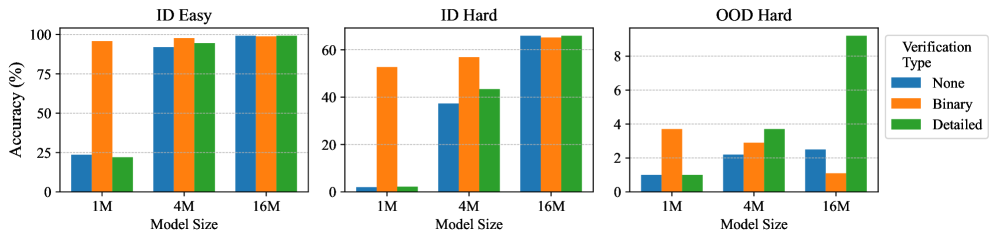</details> Figure 6: The accuracy of non-reflective execution of models in Mult. In each group, we compare training with various types of verification (“None” for no reflective SFT). Does learning self-verification facilitate learning the planning policy? We compare our models under the non-reflective execution, where self-verification is not actively used in test time. As shown in Figure 6, reflective SFT with binary verification brings remarkable improvements for 1M and 4M in ID-Easy and ID-Hard Mult problems, greatly reducing the gap among model sizes. Although detailed verification does not benefit as much as binary verification in ID problems, it significantly benefits the 16M model in solving OOD-Hard problems. Therefore, learning to self-verify benefits the learning of forward planning, increasing performance even if test-time reflection is not enabled. Since reflective SFT mixes the same CoT examples as used in non-reflective SFT, an explanation for this phenomenon is that learning to self-verify serves as a regularizer to the planning policy. This substantially improves the quality of hidden embeddings in transformers, which facilitates the learning of CoT examples. Binary verification is inherently a harder target to learn, which produces stronger regularizing effects than detailed verification. However, the complexity (length) of the verification should match the capacity of the model; otherwise, it could severely compromise the benefits of learning self-verification. For instance, learning binary verification and detailed verification fails to improve the 16M model and the 1M model, respectively. <details> <summary>x10.png Details</summary>  ### Visual Description \n ## Bar Charts: Verification Accuracy and Error Metrics for Different Model Sizes and Techniques ### Overview The image presents four pairs of bar charts. Each pair compares "Binary Verification" and "Detailed Verification" for two different problem types: "Mult ID-Hard" and "Sudoku ID-Hard". The top row displays accuracy (in percentage) while the bottom row displays error metrics (also in percentage). The charts compare the performance of three techniques: "None", "RMTP", and "RTBS" across different model sizes: "1M", "4M", and "16M". ### Components/Axes * **X-axis:** Model Size (1M, 4M, 16M) * **Y-axis (Top Charts):** Accuracy (%) - Scale ranges from 0 to 80. * **Y-axis (Bottom Charts):** Error (%) - Scale ranges from 0 to 75. * **Legend (Top-Right, applies to all top charts):** * "None" (Grey) * "RMTP" (Dark Green) * "RTBS" (Red) * **Legend (Bottom-Right, applies to all bottom charts):** * "RMTP e -" (Green with 'x' marker) * "RMTP e +" (Light Green with '+' marker) * "RTBS e -" (Red with 'x' marker) * "RTBS e +" (Light Red with '+' marker) * **Titles (Top Row):** * "Mult ID-Hard Binary Verification" * "Mult ID-Hard Detailed Verification" * "Sudoku ID-Hard Binary Verification" * "Sudoku ID-Hard Detailed Verification" ### Detailed Analysis or Content Details **Mult ID-Hard Binary Verification:** * 1M Model Size: "None" ~52%, "RMTP" ~58%, "RTBS" ~60% * 4M Model Size: "None" ~54%, "RMTP" ~64%, "RTBS" ~66% * 16M Model Size: "None" ~56%, "RMTP" ~74%, "RTBS" ~78% **Mult ID-Hard Detailed Verification:** * 1M Model Size: "None" ~46%, "RMTP" ~54%, "RTBS" ~56% * 4M Model Size: "None" ~48%, "RMTP" ~60%, "RTBS" ~62% * 16M Model Size: "None" ~50%, "RMTP" ~70%, "RTBS" ~74% **Sudoku ID-Hard Binary Verification:** * 1M Model Size: "None" ~50%, "RMTP" ~54%, "RTBS" ~56% * 4M Model Size: "None" ~52%, "RMTP" ~58%, "RTBS" ~60% * 16M Model Size: "None" ~54%, "RMTP" ~66%, "RTBS" ~68% **Sudoku ID-Hard Detailed Verification:** * 1M Model Size: "None" ~46%, "RMTP" ~50%, "RTBS" ~52% * 4M Model Size: "None" ~48%, "RMTP" ~54%, "RTBS" ~56% * 16M Model Size: "None" ~50%, "RMTP" ~64%, "RTBS" ~66% **Error Metrics - Mult ID-Hard Binary Verification:** * 1M Model Size: "RMTP e -" ~30%, "RMTP e +" ~5%, "RTBS e -" ~20%, "RTBS e +" ~10% * 4M Model Size: "RMTP e -" ~20%, "RMTP e +" ~5%, "RTBS e -" ~15%, "RTBS e +" ~5% * 16M Model Size: "RMTP e -" ~10%, "RMTP e +" ~5%, "RTBS e -" ~10%, "RTBS e +" ~5% **Error Metrics - Mult ID-Hard Detailed Verification:** * 1M Model Size: "RMTP e -" ~30%, "RMTP e +" ~5%, "RTBS e -" ~20%, "RTBS e +" ~10% * 4M Model Size: "RMTP e -" ~20%, "RMTP e +" ~5%, "RTBS e -" ~15%, "RTBS e +" ~5% * 16M Model Size: "RMTP e -" ~10%, "RMTP e +" ~5%, "RTBS e -" ~10%, "RTBS e +" ~5% **Error Metrics - Sudoku ID-Hard Binary Verification:** * 1M Model Size: "RMTP e -" ~25%, "RMTP e +" ~5%, "RTBS e -" ~20%, "RTBS e +" ~5% * 4M Model Size: "RMTP e -" ~20%, "RMTP e +" ~5%, "RTBS e -" ~15%, "RTBS e +" ~5% * 16M Model Size: "RMTP e -" ~10%, "RMTP e +" ~5%, "RTBS e -" ~10%, "RTBS e +" ~5% **Error Metrics - Sudoku ID-Hard Detailed Verification:** * 1M Model Size: "RMTP e -" ~25%, "RMTP e +" ~5%, "RTBS e -" ~20%, "RTBS e +" ~5% * 4M Model Size: "RMTP e -" ~20%, "RMTP e +" ~5%, "RTBS e -" ~15%, "RTBS e +" ~5% * 16M Model Size: "RMTP e -" ~10%, "RMTP e +" ~5%, "RTBS e -" ~10%, "RTBS e +" ~5% ### Key Observations * Accuracy generally increases with model size (1M to 16M) for all techniques and problem types. * "RTBS" consistently outperforms "RMTP" in terms of accuracy, and both significantly outperform "None". * The error metrics show that "RMTP e -" is the dominant source of error, while "RMTP e +" and "RTBS e +" contribute relatively little. * The error metrics decrease with increasing model size. * The difference in accuracy between "Binary Verification" and "Detailed Verification" is relatively small for both problem types. ### Interpretation The data suggests that both "RMTP" and "RTBS" are effective techniques for improving verification accuracy, and that increasing model size leads to further improvements. "RTBS" appears to be the superior technique overall. The error metrics indicate that the primary source of error is related to the "RMTP e -" component, suggesting a potential area for optimization. The relatively small difference between "Binary Verification" and "Detailed Verification" suggests that the added complexity of "Detailed Verification" may not be justified in these cases, although further investigation might be warranted. The consistent trends across both problem types (Mult ID-Hard and Sudoku ID-Hard) suggest that these findings are generalizable. The consistent low error values for "RMTP e +" and "RTBS e +" suggest these components are well-behaved and contribute positively to the overall verification process. 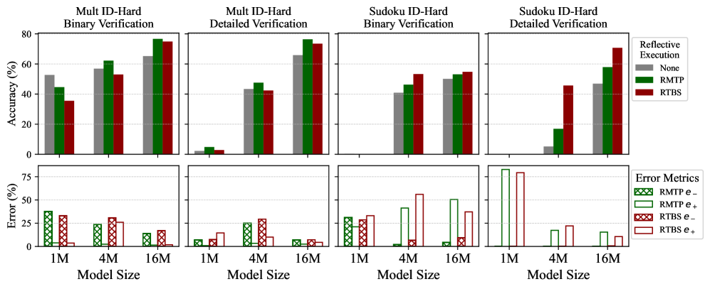</details> Figure 7: Performance of reflective execution methods across different model sizes, including the accuracy (top) and the self-verification errors (bottom). When do reflective executions improve reasoning accuracy? Figure 7 evaluates the non-reflective, RMTP, and RTBS executions for models in solving ID-Hard problems. Apart from the accuracy, the rates of verification error (i.e., the false positive rate $e_{+}$ and false negative rate $e_{-}$ defined in Section 4) are measured using an oracle verifier. In these results, RMTP reasoning raises the performance over non-reflective reasoning except for the 1M models (which fail in ID-hard Sudoku). Smaller error rates (especially $e_{-}$ ) generally lead to higher improvements, whereas a high $e_{-}$ in binary verification severely compromises the performance of the 1M Mult Model. Overall, reflection improves reasoning if the chance of rejecting correct steps ( $e_{-}$ ) is sufficiently small. In what task is the trace-back search helpful? As seen in Figure 7, though RTBS shows no advantage against RMTP in Mult, it outperforms RMTP in Sudoku, especially the 4M model with detailed verification. This aligns with Theory 1 — The state of Sudoku (the $9× 9$ matrix) is required to comply with explicit verifiable rules, making incorrect states easily discriminated from correct states. However, errors in Mult states can only be checked by recalculating all historical steps. Therefore, we are more likely to have $f>\alpha$ in Sudoku, which grants a higher chance of solving harder problems. This suggests that RTBS can be more helpful than RMTP if incorrect states in the task carry verifiable errors, which validates our theoretical results. 5.2 Results of reinforcement learning <details> <summary>x11.png Details</summary>  ### Visual Description \n ## Bar Charts: Accuracy and Error Metrics for Reflective Execution ### Overview The image presents a set of four bar charts arranged horizontally, each representing a different experimental condition. The top row displays accuracy metrics, while the bottom row displays error metrics. The charts compare the performance of different verification types (None, Binary, Detailed) under various reflective execution scenarios (None, RMTP, RTBS). The conditions are "Mult ID-Hard (4M)", "Mult OOD-Hard (4M)", "Mult ID-Hard (16M)", and "Mult OOD-Hard (16M)". ### Components/Axes * **X-axis (all charts):** Verification Type - with categories: None, Binary, Detailed. * **Y-axis (top row):** Accuracy (%) - Scale ranges from 0 to 80. * **Y-axis (bottom row):** Error (%) - Scale ranges from 0 to 75. * **Legend (top row):** Reflective Execution - with categories: None (light green), RMTP (dark green), RTBS (red). * **Legend (bottom row):** Error Metrics - with categories: RMTP e- (green diagonal stripes), RMTP e+ (green crosses), RTBS e- (red diagonal stripes), RTBS e+ (red crosses). * **Chart Titles:** "Mult ID-Hard (4M)", "Mult OOD-Hard (4M)", "Mult ID-Hard (16M)", "Mult OOD-Hard (16M)". * **Arrows:** Upward arrows indicate statistically significant increases in accuracy. Downward arrows indicate statistically significant decreases in accuracy. ### Detailed Analysis or Content Details **Chart 1: Mult ID-Hard (4M)** * **Accuracy:** * None: Approximately 62% for all reflective execution types. * Binary: Approximately 65% for None, 68% for RMTP, and 63% for RTBS. An upward arrow is present between None and RMTP. * Detailed: Approximately 65% for None, 68% for RMTP, and 63% for RTBS. An upward arrow is present between None and RMTP. * **Error:** * None: Low error (around 5-10%) for all error metrics. * Binary: RMTP e- is around 20%, RMTP e+ is around 10%, RTBS e- is around 25%, RTBS e+ is around 15%. * Detailed: RMTP e- is around 30%, RMTP e+ is around 10%, RTBS e- is around 35%, RTBS e+ is around 15%. **Chart 2: Mult OOD-Hard (4M)** * **Accuracy:** * None: Approximately 60% for all reflective execution types. * Binary: Approximately 65% for None, 68% for RMTP, and 63% for RTBS. An upward arrow is present between None and RMTP. * Detailed: Approximately 65% for None, 68% for RMTP, and 63% for RTBS. An upward arrow is present between None and RMTP. * **Error:** * None: Low error (around 5-10%) for all error metrics. * Binary: RMTP e- is around 20%, RMTP e+ is around 10%, RTBS e- is around 25%, RTBS e+ is around 15%. * Detailed: RMTP e- is around 30%, RMTP e+ is around 10%, RTBS e- is around 35%, RTBS e+ is around 15%. **Chart 3: Mult ID-Hard (16M)** * **Accuracy:** * None: Approximately 75% for all reflective execution types. * Binary: Approximately 78% for None, 80% for RMTP, and 76% for RTBS. An upward arrow is present between None and RMTP. * Detailed: Approximately 78% for None, 80% for RMTP, and 76% for RTBS. An upward arrow is present between None and RMTP. * **Error:** * None: Low error (around 5-10%) for all error metrics. * Binary: RMTP e- is around 15%, RMTP e+ is around 5%, RTBS e- is around 20%, RTBS e+ is around 10%. * Detailed: RMTP e- is around 25%, RMTP e+ is around 5%, RTBS e- is around 30%, RTBS e+ is around 10%. **Chart 4: Mult OOD-Hard (16M)** * **Accuracy:** * None: Approximately 75% for all reflective execution types. * Binary: Approximately 78% for None, 80% for RMTP, and 76% for RTBS. An upward arrow is present between None and RMTP. * Detailed: Approximately 78% for None, 80% for RMTP, and 76% for RTBS. An upward arrow is present between None and RMTP. * **Error:** * None: Low error (around 5-10%) for all error metrics. * Binary: RMTP e- is around 15%, RMTP e+ is around 5%, RTBS e- is around 20%, RTBS e+ is around 10%. * Detailed: RMTP e- is around 25%, RMTP e+ is around 5%, RTBS e- is around 30%, RTBS e+ is around 10%. ### Key Observations * RMTP consistently improves accuracy compared to None across all conditions. * RTBS generally performs similarly to None in terms of accuracy. * Error metrics show that RMTP e- and RTBS e- are the highest contributors to error, especially with Detailed verification. * Increasing the model size from 4M to 16M generally improves accuracy. * The effect of RMTP is more pronounced with larger model sizes (16M). ### Interpretation The data suggests that reflective execution with RMTP significantly improves accuracy, particularly for larger models and more challenging conditions (OOD-Hard). The increased accuracy comes at the cost of higher error rates for RMTP e- and RTBS e-, indicating that these error types are more frequent when using reflective execution. The consistent performance of RTBS suggests it doesn't offer a substantial benefit over no reflective execution. The upward arrows consistently pointing from "None" to "RMTP" across all charts strongly indicate a statistically significant positive impact of RMTP on accuracy. The error metrics provide a more nuanced understanding of the trade-offs involved in using reflective execution, highlighting the need to address the specific error types that are exacerbated by these techniques. The fact that the benefits of RMTP are more pronounced with larger models suggests that reflective execution may be particularly valuable for scaling up model size. 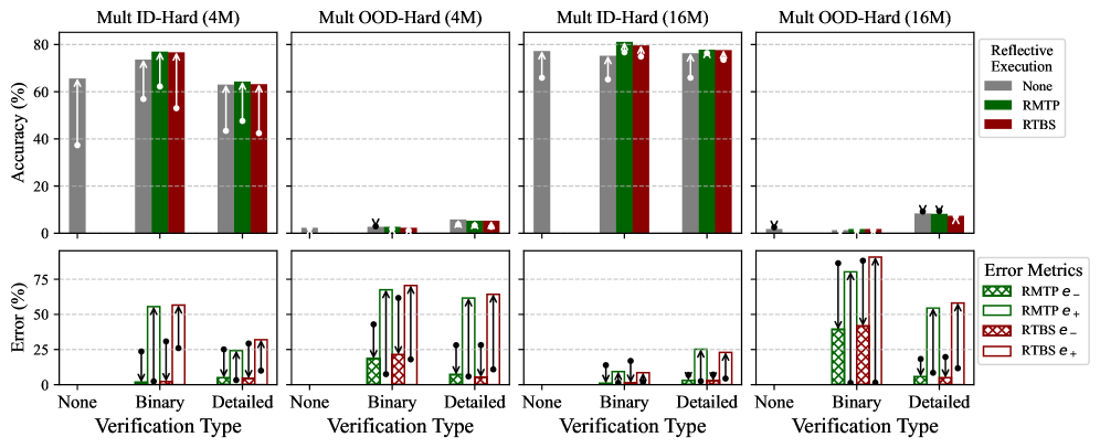</details> Figure 8: Performance of the 4M and 16M models in Mult after GRPO, including accuracy and the verification error rates. As an ablation, we also include non-reflective models. The vertical arrows start from the baseline accuracy after SFT, presenting the relative change caused by GRPO. As introduced in Section 3.3, we further apply GRPO to fine-tune the models after SFT. Especially, GRPO based on RMTP allows solution planning and verification to be jointly optimized for self-verifying policies. The full GRPO results are presented in Appendix E.3, and the main findings are presented below. Overall, RL does enable most models to better solve ID problems, yet such improvements arise from a superficial shift in the distribution of known reasoning skills. How does RL improve reasoning accuracy? Figure 8 presents the performance of 4M and 16M models in Mult after GRPO, where the differences from SFT results are visualized. GRPO effectively enhances accuracy in solving ID-Hard problems, yet the change in OOD performance is marginal. Therefore, RL can optimize ID performance, while failing to generalize to OOD cases. Does RL truly enhance verification? From the change of verification errors in Figure 8, we find that the false negative rate $e_{-}$ decreases along with an increase in the false positive rate $e_{+}$ . This suggests that models learn an optimistic bias, which avoids rejecting correct steps through a high false positive rate that bypasses verification. In other words, instead of truly improving the verifier (where $e_{-}$ and $e_{+}$ both decrease), RL mainly induces an error-type trade-off, shifting from false negatives ( $e_{+}$ ) to false positives ( $e_{-}$ ). To explain this, we note that a high $e_{-}$ raises the computational cost (Proposition 1) and thus causes a significant performance loss under the limited budget of RL sampling, making reducing $e_{-}$ more rewarding than maintaining a low $e_{+}$ . Meanwhile, shifting the error type is easy to learn, achievable by adjusting only a few parameters in the output layer of the transformer. Inspired by DeepSeek-R1 [5], we additionally examine how RL influences the frequency of reflective behavior. To simulate the natural distribution of human reasoning, we train models to perform optional detailed verification by adding examples of empty verification (in the same amount as the full verification) into reflective SFT. This allows the policy to optionally omit self-verification, usually with a higher probability than producing full verification, since empty verification is easier to learn. Consequently, we can measure the reflection frequency by counting the proportion of steps that include non-empty verification. Since models can implicitly omit binary verification by producing false positive labels, we do not explicitly examine the optional binary verification. When does RL incentivize frequent reflection? Figure 9 shows reflection frequency in Mult before and after GRPO, comparing exploratory ( $1.25$ ) and exploitative ( $1$ ) temperatures when sampling experience CoTs. With a temperature $1.25$ , GRPO elicits frequent reflection, especially on hard queries. However, reflection frequency remains low if using temperature $1$ . Additional results for other model sizes and Sudoku appear in Appendix E.3.3. In conclusion, RL can adapt reflection frequency to align with the exploratory ability of the planning policy $\pi$ , encouraging more reflection if the policy can potentially explore rewards. This helps explain why RL promotes frequent reflection in LLMs [5], as the flexibility of language naturally fosters exploratory reasoning. 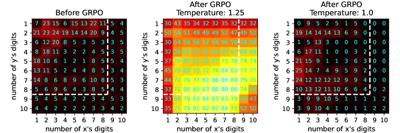<details> <summary>x12.png Details</summary>  ### Visual Description ## Heatmaps: Digit Distribution Before and After GRPO ### Overview This image presents three heatmaps illustrating the distribution of digits in 'x' and 'y' before and after applying a process called "GRPO" with varying temperature parameters. The heatmaps display the frequency of digit pairs, where the x-axis represents the number of digits in 'x', and the y-axis represents the number of digits in 'y'. The color intensity indicates the frequency of occurrence, with warmer colors (red, orange, yellow) representing higher frequencies and cooler colors (green, blue) representing lower frequencies. ### Components/Axes Each heatmap shares the following components: * **X-axis:** "number of x's digits", ranging from 1 to 10. * **Y-axis:** "number of y's digits", ranging from 1 to 10. * **Color Scale/Legend:** Located on the right side of each heatmap. The scale ranges from blue (low frequency, approximately 0) to yellow/red (high frequency, approximately 88). * **Titles:** * "Before GRPO" (left heatmap) * "After GRPO Temperature: 1.25" (center heatmap) * "After GRPO Temperature: 1.0" (right heatmap) ### Detailed Analysis or Content Details **1. Before GRPO:** * The heatmap shows a relatively even distribution of digit pairs, with a slight concentration in the lower-left corner (small digit counts for both x and y). * The highest values (dark red) are around (2,2) with a value of approximately 24, (3,2) with a value of approximately 20, and (2,3) with a value of approximately 20. * The lowest values (dark blue) are concentrated in the upper-right corner, with values around 1-4. **2. After GRPO - Temperature: 1.25:** * The distribution is significantly different from the "Before GRPO" heatmap. There's a strong concentration of higher frequencies in the central region of the heatmap (digits 5-9 for both x and y). * The highest value (bright red) is at (8,8) with a value of approximately 89. * The lowest values (dark blue) are in the lower-left corner, with values around 30-35. * A clear diagonal trend is visible, indicating a higher frequency of digit pairs where the number of digits in 'x' and 'y' are similar. **3. After GRPO - Temperature: 1.0:** * This heatmap shows a distribution that is more concentrated than the "Before GRPO" heatmap, but less concentrated than the "Temperature: 1.25" heatmap. * The highest value (bright red) is at (7,7) with a value of approximately 74. * The lowest values (dark blue) are in the upper-left corner, with values around 0-1. * A diagonal trend is also visible, but less pronounced than in the "Temperature: 1.25" heatmap. ### Key Observations * The GRPO process, regardless of temperature, shifts the distribution of digit pairs towards higher digit counts. * Increasing the GRPO temperature (from 1.0 to 1.25) leads to a more concentrated distribution, with a stronger diagonal trend. * The "Before GRPO" heatmap shows a more uniform distribution, suggesting that the GRPO process introduces a bias towards specific digit pair frequencies. * The values in the "After GRPO" heatmaps are significantly higher than those in the "Before GRPO" heatmap, indicating that the GRPO process increases the frequency of certain digit pairs. ### Interpretation The data suggests that the GRPO process alters the distribution of digit pairs in 'x' and 'y'. The temperature parameter controls the degree of this alteration. A higher temperature leads to a more pronounced shift towards higher digit counts and a stronger correlation between the number of digits in 'x' and 'y'. This could indicate that GRPO is a process that favors the combination of larger digit numbers. The diagonal trend suggests that the process is more likely to generate digit pairs where 'x' and 'y' have similar digit counts. The significant difference between the "Before GRPO" and "After GRPO" heatmaps suggests that GRPO is not merely a random process, but rather a transformation that introduces a specific pattern into the digit distribution. The temperature parameter likely controls the intensity of this pattern. Further investigation would be needed to understand the underlying mechanism of the GRPO process and the reasons for the observed temperature-dependent behavior. The data could be used to optimize the GRPO process for specific applications or to identify potential biases in the generated digit pairs. </details> Figure 9: The hot-maps of reflection frequencies of the 4M transformer in multiplication before and after GRPO using temperatures $1$ and $1.25$ , tested with RMTP execution. The $i$ -th row and $j$ -th column shows the frequency (%) for problems $x× y$ where $x$ has $j$ digits and $y$ has $i$ digits. 6 Conclusion and Discussion In this paper, we provide a foundational analysis of self-verifying reflection in multi-step CoTs using small transformers. Through minimalistic prototypes of reflective reasoning (the RMTP and RTBS), we demonstrate that self-verification benefits both training and execution. Compared to natural-language reasoning based on LLMs, the proposed minimalistic framework performs effective reasoning and reflection using limited computational resources. We also show that RL fine-tuning can enhance the performance in solving in-distribution problems and incentivize reflective thinking for exploratory reasoners. However, the improvements from RL rely on shallow patterns and lack generalizable new skills. Overall, we suggest that self-verifying reflection is inherently beneficial for CoT reasoning, yet its synergy with RL fine-tuning is limited in superficial statistics. Limitations and future work Although the current training pipeline enables tiny transformers to reason properly through reflective CoTs, the generalization ability is still low and not improved in RL. Therefore, future work will extend reflection frameworks and explore novel training approaches. Observing the positive effect of learning self-verification, a closer connection between generative and discriminative reasoning may be the key to addressing this challenge. Additionally, how our findings transfer from small transformers to natural-language LLMs needs to be further examined. However, the diversity of natural language and high computational cost pose significant challenges to comprehensive evaluation, and our proposed framework does not sufficiently exploit the emergent linguistic ability of LLMs. To this end, we expect to investigate a more flexible self-verification framework with an efficient evaluator of natural-language reflection in future work. Acknowledgments and Disclosure of Funding We gratefully acknowledge Dr. Linyi Yang for providing partial computational resources. References - [1] Lightning AI “LitGPT”, https://github.com/Lightning-AI/litgpt, 2023 - [2] Zeyuan Allen-Zhu and Yuanzhi Li “Physics of Language Models: Part 3.1, Knowledge Storage and Extraction” arXiv, 2024 DOI: 10.48550/arXiv.2309.14316 - [3] Eric C. Chi and Kenneth Lange “Techniques for Solving Sudoku Puzzles” arXiv, 2013 DOI: 10.48550/arXiv.1203.2295 - [4] Karl Cobbe et al. “Training Verifiers to Solve Math Word Problems” arXiv, 2021 arXiv: 2110.14168 [cs] - [5] DeepSeek-AI et al. “DeepSeek-R1: Incentivizing Reasoning Capability in LLMs via Reinforcement Learning” arXiv, 2025 DOI: 10.48550/arXiv.2501.12948 - [6] Yuntian Deng, Yejin Choi and Stuart Shieber “From Explicit CoT to Implicit CoT: Learning to Internalize CoT Step by Step” arXiv, 2024 DOI: 10.48550/arXiv.2405.14838 - [7] Nouha Dziri et al. “Faith and Fate: Limits of Transformers on Compositionality” arXiv, 2023 DOI: 10.48550/arXiv.2305.18654 - [8] Guhao Feng et al. “Towards Revealing the Mystery behind Chain of Thought: A Theoretical Perspective” arXiv, 2023 DOI: 10.48550/arXiv.2305.15408 - [9] Yao Fu et al. “Specializing Smaller Language Models towards Multi-Step Reasoning” In Proceedings of the 40th International Conference on Machine Learning PMLR, 2023, pp. 10421–10430 - [10] Alex Havrilla et al. “GLoRe: When, Where, and How to Improve LLM Reasoning via Global and Local Refinements” arXiv, 2024 DOI: 10.48550/arXiv.2402.10963 - [11] Yancheng He et al. “Can Large Language Models Detect Errors in Long Chain-of-Thought Reasoning?” arXiv, 2025 DOI: 10.48550/arXiv.2502.19361 - [12] Kaiying Hou et al. “Universal Length Generalization with Turing Programs” arXiv, 2024 DOI: 10.48550/arXiv.2407.03310 - [13] Takeshi Kojima et al. “Large Language Models Are Zero-Shot Reasoners” arXiv, 2023 DOI: 10.48550/arXiv.2205.11916 - [14] Aviral Kumar et al. “Training Language Models to Self-Correct via Reinforcement Learning” arXiv, 2024 arXiv: 2409.12917 [cs] - [15] Nathan Lambert et al. “Tulu 3: Pushing Frontiers in Open Language Model Post-Training” arXiv, 2025 DOI: 10.48550/arXiv.2411.15124 - [16] Zhiyuan Li, Hong Liu, Denny Zhou and Tengyu Ma “Chain of Thought Empowers Transformers to Solve Inherently Serial Problems” arXiv, 2024 DOI: 10.48550/arXiv.2402.12875 - [17] Hunter Lightman et al. “Let’s Verify Step by Step” arXiv, 2023 arXiv: 2305.20050 [cs] - [18] Liangchen Luo et al. “Improve Mathematical Reasoning in Language Models by Automated Process Supervision” arXiv, 2024 arXiv: 2406.06592 [cs] - [19] Aman Madaan et al. “Self-Refine: Iterative Refinement with Self-Feedback” arXiv, 2023 DOI: 10.48550/arXiv.2303.17651 - [20] OpenAI “Learning to Reason with LLMs”, https://openai.com/index/learning-to-reason-with-llms/ - [21] OpenAI “OpenAI O3-Mini System Card” In OpenAI o3-mini System Card, https://openai.com/index/o3-mini-system-card - [22] OpenAI et al. “GPT-4o System Card” arXiv, 2024 DOI: 10.48550/arXiv.2410.21276 - [23] Long Ouyang et al. “Training Language Models to Follow Instructions with Human Feedback” In Advances in Neural Information Processing Systems 35 (NeurIPS 2022), 2022 arXiv: 2203.02155 [cs] - [24] Jiayi Pan et al. “TinyZero” Accessed: 2025-01-24, https://github.com/Jiayi-Pan/TinyZero, 2025 - [25] Ben Prystawski, Michael Y. Li and Noah D. Goodman “Why Think Step by Step? Reasoning Emerges from the Locality of Experience” arXiv, 2023 arXiv: 2304.03843 [cs] - [26] Yiwei Qin et al. “O1 Replication Journey: A Strategic Progress Report – Part 1” arXiv, 2024 DOI: 10.48550/arXiv.2410.18982 - [27] Yuxiao Qu, Tianjun Zhang, Naman Garg and Aviral Kumar “Recursive Introspection: Teaching Language Model Agents How to Self-Improve” arXiv, 2024 DOI: 10.48550/arXiv.2407.18219 - [28] John Schulman et al. “High-Dimensional Continuous Control Using Generalized Advantage Estimation” arXiv, 2018 arXiv: 1506.02438 [cs] - [29] John Schulman et al. “Proximal Policy Optimization Algorithms” arXiv, 2017 arXiv: 1707.06347 [cs] - [30] Rico Sennrich, Barry Haddow and Alexandra Birch “Neural Machine Translation of Rare Words with Subword Units” arXiv, 2016 DOI: 10.48550/arXiv.1508.07909 - [31] Zhihong Shao et al. “DeepSeekMath: Pushing the Limits of Mathematical Reasoning in Open Language Models” arXiv, 2024 arXiv: 2402.03300 [cs] - [32] Charlie Snell, Jaehoon Lee, Kelvin Xu and Aviral Kumar “Scaling LLM Test-Time Compute Optimally Can Be More Effective than Scaling Model Parameters” arXiv, 2024 arXiv: 2408.03314 [cs] - [33] Richard S. Sutton and Andrew G. Barto “Reinforcement Learning: An Introduction” Cambridge, Massachusetts: The MIT Press, 2018 - [34] Yijun Tian et al. “TinyLLM: Learning a Small Student from Multiple Large Language Models” arXiv, 2024 DOI: 10.48550/arXiv.2402.04616 - [35] Rasul Tutunov et al. “Why Can Large Language Models Generate Correct Chain-of-Thoughts?” arXiv, 2024 DOI: 10.48550/arXiv.2310.13571 - [36] Ashish Vaswani et al. “Attention Is All You Need” In Proceedings of the 31st International Conference on Neural Information Processing Systems, 2017 - [37] Jun Wang “A Tutorial on LLM Reasoning: Relevant Methods behind ChatGPT O1” arXiv, 2025 DOI: 10.48550/arXiv.2502.10867 - [38] Jason Wei et al. “Chain-of-Thought Prompting Elicits Reasoning in Large Language Models” arXiv, 2023 DOI: 10.48550/arXiv.2201.11903 - [39] Sang Michael Xie et al. “DoReMi: Optimizing Data Mixtures Speeds Up Language Model Pretraining” arXiv, 2023 DOI: 10.48550/arXiv.2305.10429 - [40] An Yang et al. “Qwen2.5-Math Technical Report: Toward Mathematical Expert Model via Self-Improvement” arXiv, 2024 arXiv: 2409.12122 [cs] - [41] Yang Yue et al. “Does Reinforcement Learning Really Incentivize Reasoning Capacity in LLMs Beyond the Base Model?” arXiv, 2025 DOI: 10.48550/arXiv.2504.13837 - [42] Zhihan Zhang et al. “Learn Beyond The Answer: Training Language Models with Reflection for Mathematical Reasoning” arXiv, 2024 DOI: 10.48550/arXiv.2406.12050 Contents 1. 1 Introduction 1. 2 Related works 1. 3 Reflective reasoning for transformers 1. 3.1 Reasoning formulation 1. 3.2 The framework of self-verifying reflection 1. 3.3 Training 1. 4 Theoretical results 1. 5 Experiments 1. 5.1 Results of supervised fine-tuning 1. 5.2 Results of reinforcement learning 1. 6 Conclusion and Discussion 1. A Notations 1. B Details of reinforcement learning 1. B.1 Proximal policy optimization 1. B.2 Group-reward policy optimization 1. B.3 Technical Implementation 1. C Theory 1. C.1 A general formulation of reasoning performance 1. C.1.1 Bellman equations in RMTP 1. C.1.2 Bellman equations in RTBS 1. C.2 Accuracy derivation in the simplified reasoning task 1. C.3 Derivation of Theorem 1 1. C.3.1 Proof of Proposition 3 1. C.3.2 Proof of Proposition 4 1. C.4 Derivation of RMTP reasoning cost 1. C.5 Considering posterior risks of rejected attempts 1. D Implementation details 1. D.1 Algorithmic descriptions of reflective reasoning 1. D.2 Example CoT data 1. D.2.1 Multiplication CoT 1. D.2.2 Sudoku CoT 1. D.2.3 Verification of reasoning steps 1. D.3 Model architectures and tokenization 1. D.4 Hyperparameters 1. D.5 Computational resources 1. E Supplementary results of experiments 1. E.1 Evaluation of LLMs 1. E.2 Results of supervised fine tuning 1. E.3 Results of GRPO 1. E.3.1 The verification errors after GRPO 1. E.3.2 The planning correctness rate after GRPO 1. E.3.3 Reflection frequency of optional detailed verification 1. E.4 Reflection frequency under controlled verification error rates 1. E.5 Results of PPO Appendix A Notations The notations used in the main paper are summarized in Table 1. Notations only appear in the appendix are not included. Table 1: Notations in the main paper. | ${Q}$ $\{{R}\}$ ${R}_{t}$ | The query of CoT reasoning The sequence of intermediate reasoning steps The $t$ -th intermediate step in CoT reasoning | | --- | --- | | ${A}$ | The answer of CoT reasoning. | | $T$ | The number of steps (including the final answer) in an CoT | | $\pi$ | The planning policy in MTP reasoning | | ${s}_{t}$ | The $t$ -th state in CoT reasoning | | $\mathcal{T}$ | The transition function in an MTP | | “ $\checkmark$ ” | The special token as the positive label of verification. | | “ $×$ ” | The special token as the negative label of verification | | ${V}_{t}$ | The verification sequence for the proposed step ${R}_{t}$ . | | $\mathcal{V}$ | The verifier such that ${V}_{t+1}\sim\mathcal{V}(·|{S}_{t},{R}_{t+1})$ | | $\tilde{{R}_{t}}$ | The verified reasoning step, i.e. $({R}_{t},{V}_{t})$ | | $\tilde{\mathcal{T}}$ | The reflective transition function in an RMTP | | $\tilde{\mathcal{\pi}}$ | The self-verifying policy, i.e. $\{\pi,\mathcal{V}\}$ | | $m$ | The RTBS width, i.e. maximal number of attempts on each state | | $\mu$ | The probability of proposing a correct step on positive states | | $e_{-}$ | The probability of instantly rejecting a correct step on positive states | | $e_{+}$ | The probability of accepting an incorrect step on positive states | | $f$ | The probability of instantly rejecting any step on negative states | | $\alpha$ | The shorthand of $\mu e_{-}+(1-\mu)(1-e_{+})$ | | $\rho(n)$ | The accuracy of non-reflective MTP reasoning | | $\tilde{\rho}(n)$ | The accuracy of RMTP reasoning for queries with scale $n$ | | $\tilde{\rho}_{m}(n)$ | The accuracy of RTBS reasoning with width $m$ for queries with scale $n$ | Appendix B Details of reinforcement learning This section introduces PPO and GRPO algorithms used in RL fine-tuning. We introduce PPO and GRPO under the context of MTP, which is described in Section 3.1. This also applies to RMTP reasoning in Section 3.2, as RMTP is a special MTP given the self-verifying policy $\tilde{\pi}$ and the reflective transition function $\tilde{\mathcal{T}}$ . For any sequence ${X}$ of tokens, we additionally define the following notations: ${{X}^{[i]}}$ denotes the $i$ -th token, ${{X}^{[<i]}}$ ( ${{X}^{[≤ i]}}$ ) denotes the former $i-1$ ( $i$ ) tokens, and $|{X}|$ denotes the length (i.e., the number of tokens). Both PPO and GRPO iteratively update the reasoning policy through online experience. Let $\pi_{\theta}$ to denote a reasoning policy parameterized by $\theta$ . On each iteration, PPO and GRPO use a similar process to update $\theta$ : 1. Randomly draw queries from the task or taring set, and apply the old policy $\pi_{\theta_{old}}$ to sample experience CoTs. 1. Use reward models to assign rewards to the experience CoTs. Let $\operatorname{ORM}$ and $\operatorname{PRM}$ be the outcome reward model and process reward model, respectively. For each CoT $({Q},{R}_{1},...,{R}_{T-1},A)$ , we obtain outcome rewards $r_{o}=\operatorname{ORM}(Q,A)$ and the process rewards $r_{t}=\operatorname{PRM}({S}_{t},{R}_{t+1})$ for $t=0,1,...,T-1$ (where ${R}_{T}=A$ ). In our case, we only use the outcome reward model and thus all process rewards are $0$ . 1. Then, $\theta$ is updated by maximizing an objective function based on the experience CoTs with above rewards. Especially, PPO additionally needs to update an value approximator. B.1 Proximal policy optimization PPO [29] is a classic RL algorithm widely used in various applications. It includes a value model $v$ to approximate the value function, namely the expected cumulated rewards: $$ v({S}_{t},{{R}_{t}^{[<i]}})=\mathbb{E}_{\pi}\left(r_{o}+\sum_{k=t}^{T}r_{k}\right) \tag{7} $$ Let $q_{t,i}(\theta)=\frac{\pi_{\theta}\left({{R}_{t}^{[i]}}\middle|{S}_{t},{{R}_{t}^{[<i]}}\right)}{\pi_{\theta_{old}}\left({{R}_{t}^{[i]}}\middle|{S}_{t},{{R}_{t}^{[<i]}}\right)}$ be the relative likelihood of the $i$ -th token in the $t$ -th step, and $\pi_{ref}$ be the reference model (e.g., the policy before RL-tuning). Then, the PPO algorithm maximizes $$ \displaystyle J_{PPO}(\theta)= \displaystyle\mathbb{E}_{{Q}\sim P({Q}),\{{R}\}\sim\pi_{\theta_{old}}}\frac{1}{\sum_{t=1}^{T}|{R}_{t}|}\sum_{t=1}^{T}\sum_{i=1}^{|{R}_{t}|} \displaystyle\left\{\min\left[q_{t,i}(\theta)\hat{A}_{t,i},\operatorname{clip}\left(q_{t,i}(\theta),1-\varepsilon,1+\varepsilon\right)\hat{A}_{t,i}\right]-\beta\mathbb{D}_{KL}\left[\pi_{\theta}\|\pi_{ref}\right]\right\}. \tag{8} $$ Here, $\hat{A}_{t,i}$ is the advantage of the $i$ -th token in step $t$ , computed using the value model $v$ . For example, $\hat{A}_{t,i}=v({S}_{t},{{R}_{t}^{[<i]}},{{R}_{t}^{[i]}})-v({S}_{t},{{R}_{t}^{[<i]}})$ is a simple way to estimate advantage. In practice, advantages can be estimated using the general advantage estimation (GAE) [28]. The value model $v$ is implemented using the same architecture as the reasoner except for the output layer, which is replaced by a linear function that outputs a scalar value. The value model is initialized using the same parameters as the reasoner, apart from the output layer. Assuming that $v$ is parameterized by $\omega$ , we learn $v$ by minimizing the temporal-difference error: $$ J_{v}(\omega)=\mathbb{E}_{{Q}\sim P({Q}),{R}\sim\pi_{\theta_{old}}}\sum_{t=1}^{T}\sum_{i=1}^{|{R}_{t}|}\left(v_{\omega}({S}_{t},{{R}_{t}^{[<i]}})-v_{\omega_{old}}({S}_{t+1})\right)^{2}. \tag{9} $$ Although PPO proves effective in training LLMs [23], we deprecate using it in training tiny transformers due to the difficulty of learning the value function. Since the value model $v$ is also a tiny transformer, its weakness in model capacity severely compromise the precision of value approximation, leading to unreliable advantage estimation. B.2 Group-reward policy optimization PPO requires learning an additional value model, which can be expensive and unstable. Alternatively, GRPO [31] directly computes the advantages using the relative rewards from a group of $G$ solutions. For each query ${Q}$ , it samples a group of $G$ solutions: $$ \{{R}_{g}\}=({R}_{g,1},\ldots,{R}_{g,T_{g}-1},A_{g})\sim\pi_{\theta_{old}},\qquad\text{for}\ g=1,\ldots,G. \tag{10} $$ In this group, each solution $\{{R}_{g}\}$ contains $T_{g}$ steps, where the answer $A_{g}$ is considered as the final step ${R}_{g,T_{g}}$ . Using the reward models, we obtain process rewards $\boldsymbol{r}_{p}:=\{(r_{g,1},...,r_{g,T_{g}})\}_{g=1}^{G}$ and outcome rewards $\boldsymbol{r}_{o}:=\{r_{g,o}\}_{g=1}^{G}$ . Then, GPRO computes the normalized rewards, given by: $$ \tilde{r}_{g,t}=\frac{r_{g,t}-\operatorname{mean}\boldsymbol{r}_{p}}{\operatorname{std}\boldsymbol{r}_{p}},\ \tilde{r}_{g,o}=\frac{r_{g,o}-\operatorname{mean}\boldsymbol{r}_{o}}{\operatorname{std}\boldsymbol{r}_{o}} \tag{11} $$ Afterwards, the advantage of step $t$ in the $g$ -th solution of the group is $\hat{A}_{g,t}=\tilde{r}_{g,o}+\sum_{k=t}^{T_{g}}\tilde{r}_{g,t^{\prime}}$ . Let $q_{g,t,i}(\theta)=\frac{\pi_{\theta}\left({{R}_{g,t}^{[i]}}\middle|{S}_{g,t},{{R}_{g,t}^{[<i]}}\right)}{\pi_{\theta_{old}}\left({{R}_{g,t}^{[i]}}\middle|{S}_{g,t},{{R}_{g,t}^{[<i]}}\right)}$ be the relative likelihood of the $i$ -th token in the $t$ -th step from the $g$ -th solution. Then, the GRPO objective is to maximize the following: $$ \displaystyle J_{GRPO}(\theta)= \displaystyle\mathbb{E}_{{Q}\sim P({Q}),\{{R}_{g}\}\sim\pi_{old}}\frac{1}{G}\sum_{g=1}^{G}\frac{1}{\sum_{t=1}^{T_{g}}|\tau^{(t)}|}\sum_{t=1}^{T_{g}}\sum_{i=1}^{|{R}_{g,t}|} \displaystyle\left\{\min\left[q_{g,t,i}(\theta)\hat{A}_{g,t},\operatorname{clip}\left(q_{g,t,i}(\theta),1-\varepsilon,1+\varepsilon\right)\hat{A}_{g,t}\right]-\beta\mathbb{D}_{KL}\left[\pi_{\theta}\|\pi_{ref}\right]\right\} \tag{12} $$ B.3 Technical Implementation We made two technical modifications that make RL more suitable in our case, described in the following. First, in RMTP, we mask off the advantage of rejected steps, while the advantage of self-verification labels is reserved. This prevents the algorithm from increasing the likelihood of rejected steps, allowing the planning policy $\pi$ to be properly optimized. In practice, we find this modification facilitates the training of models that perform mandatory detailed verification. Otherwise, RL could make the reasoner excessively rely on reflection, leading to CoTs that are unnecessarily long. Second, we employ an early-truncating strategy when sampling trajectories in training. If the model has already made a clear error at some step (detected using an oracle process reward model), we truncate the trajectory as it is impossible to find a correct answer. This avoids unnecessarily punishing later steps due to previous deviations, as some later steps may be locally correct in their own context. Empirically, we find this modification reduces the training time required to reach the same performance, while the difference in final performance is marginal. Appendix C Theory C.1 A general formulation of reasoning performance Let $\mathcal{S}$ denote the state space and $\mathcal{A}$ denote the answer space. We use $\mathcal{A}_{{Q}}⊂eq\mathcal{A}$ to denote the set of correct answers for some input query ${Q}$ . Given any thought state ${S}$ , the accuracy, namely the probability of finding a correct answer, is denoted as $$ \rho_{{Q}}({S})=p_{({R}_{t+1},{R}_{t+2},\ldots,{A})\sim\pi}({A}\in\mathcal{A}_{{Q}}\mid{S}_{t}={S}) \tag{13} $$ C.1.1 Bellman equations in RMTP By considering the reasoning correctness as the binary outcome reward, we may use Bellman equations [33] to provide a general formulation of the reasoning performance for arbitrary MTPs (RMTP). For simplicity, we use ${S}$ , ${R}$ , and ${S}^{\prime}$ to respectively denote the state, step, and next state in a transition. Initially, in the absence of a trace-back mechanism, the accuracy $\rho_{{Q}}(s)$ can be interpreted as the value function when considering the MTP as a goal-directed decision process. For simplicity, we denote the transition probability drawn from the reasoning dynamics $\mathcal{T}$ as $p({S^{\prime}}\mid{S},{R})$ . In non-reflective reasoning, the state transition probability $p({S^{\prime}}\mid{S})$ can be expressed as: $$ p({S^{\prime}}|{S})=\sum_{{R}}p({S^{\prime}}|{S},{R})\pi({R}|{S}) \tag{14} $$ When using RMTP execution, assuming that $\xi({S},{R}):=p_{{V}\sim\mathcal{V}}(\text{``$×$''}∈{V}\mid{S},{R})$ represents the probability of rejecting the step ${R}$ , we have: $$ p({S^{\prime}}|{S})=\begin{cases}\sum_{R}\pi({R}|{S})(1-\xi({S},{R}))p({S^{\prime}}|{S},{R}),&\text{if }{S^{\prime}}\neq{S}\\ \sum_{R}\pi({R}|{S})\left((1-\xi({S},{R}))p({S^{\prime}}|{S},{R})+\xi({S},{R})\right),&\text{if }{S^{\prime}}={S}\end{cases} \tag{15} $$ Consequently, the Bellman equation follows: $$ \rho_{{Q}}({S})=\begin{cases}1,&\text{if }{S}\in\mathcal{A}_{{Q}}\\ 0,&\text{if }{S}\in\mathcal{A}\setminus\mathcal{A}_{{Q}}\\ \sum_{{S^{\prime}}}\rho_{{Q}}({S^{\prime}})p({S^{\prime}}\mid{S}),&\text{if }s\in\mathcal{S}\setminus\mathcal{A}\end{cases} \tag{16} $$ C.1.2 Bellman equations in RTBS Let $m$ denote the number of attempts at each state, and let $\phi({S})$ represent the failure probability (i.e., the probability of tracing back after $m$ rejected steps) at state ${S}$ . The probability of needing to retry a proposed step due to instant rejection or recursive rejection is given by: $$ \epsilon({S})=\sum_{{R}}\pi({R}|{S})\left(\xi({S},{R})+\sum_{{S^{\prime}}}(1-\xi({S},{R}))p({S^{\prime}}|{S},{R})\phi({S^{\prime}})\right) \tag{17} $$ The failure probability is then given by $\phi({S})=\epsilon^{m}({S})$ . When there are $k$ attempts remaining at the current state ${S}$ , we denote the accuracy as $\rho_{x}({S},k)$ , given by: $$ \rho_{Q}({S},k)=\begin{cases}\epsilon({S})\rho_{x}({S},k-1)+\sum_{{R}}\pi({R}|{S})(1-\xi({S},{R}))\sum_{{S^{\prime}}}p({S^{\prime}}|{S},{R})\rho_{Q}({S^{\prime}}),&k>0\\ 0,&k=0\end{cases} \tag{18} $$ It follows that $\rho_{x}({S})=\rho_{x}({S},m)$ . This leads to a recursive formulation that ultimately results in the following equations for each $s∈\mathcal{S}$ : $$ \displaystyle\epsilon({S})=\sum_{{R}}\pi({R}|{S})\left(\xi({S},{R})+\sum_{{S^{\prime}}}(1-\xi({S},{R}))p({S^{\prime}}|{S},{R})\epsilon^{m}({S^{\prime}})\right), \displaystyle\rho_{x}({S})=\frac{1-\epsilon^{m}({S})}{1-\epsilon({S})}\sum_{{S^{\prime}}}\rho_{Q}({S^{\prime}})\pi({R}|{S})(1-\xi({S},{R}))p({S^{\prime}}|{S},{R}). \tag{19} $$ C.2 Accuracy derivation in the simplified reasoning task In the following, we derive the accuracy of reflective reasoning with and without the trace-back search, given the simplified reasoning task in Section 4. For each proposed step on a correct state, we define several probabilities to simplify notations: $\alpha:=\mu e_{-}+(1-\mu)(1-e_{+})$ is the probability of being instantly rejected; $\beta=\mu(1-e_{-})$ is the probability of being correct and accepted; $\gamma=(1-\mu)e_{+}$ is the probability of being incorrect but accepted. Note that $\beta$ here no longer refers to the KL-divergence factor in Appendix B. **Proposition 2** *The RTMP accuracy $\tilde{\rho}(n)$ for problems with a scale of $n$ is $$ \tilde{\rho}(n)=\left(\frac{\beta}{1-\alpha}\right)^{n} \tag{21} $$ Let $m$ be the width of RTBS. Let $\delta_{m}(n)$ and $\epsilon_{m}(n)$ be the probability of a proposed step being rejected (either instantly or recursively) on a correct state and incorrect state of scale $n$ , respectively. We have $\sigma_{m}(0)=\epsilon_{m}(0)=0$ and the following recursive equations for $n>0$ : $$ \displaystyle\delta_{m}(n)=\alpha+\beta(\delta_{m}(n-1))^{m}+\gamma(\epsilon_{m}(n-1))^{m} \displaystyle\epsilon_{m}(n)=f+(1-f)\left(\epsilon_{m}(n-1)\right)^{m} \tag{22} $$ Then, the RTBS accuracy $\tilde{\rho}_{m}(n)$ for problems with a scale of $n$ is given by $$ \tilde{\rho}_{m}(n)=\prod_{t=1}^{n}\sigma_{m}(t),\qquad\text{where }\sigma_{m}(t)=\beta\sum_{i=0}^{m-1}(\delta_{m}(t))^{i}=\frac{1-(\delta_{m}(t))^{m}}{1-\delta_{m}(t)}\beta. \tag{24} $$ In addition, $\delta_{m}(n)$ , $\epsilon_{m}(n)$ and $\sigma_{m}(n)$ all motonously increase and converge in relation to $n$ .* * Proof* We first consider reasoning through RTBS. Let $\phi_{m}(n)$ and $\psi_{m}(n)$ denote the probabilities of failure (reaching the maximum number of attempts) in correct and incorrect states, respectively. Let $\tilde{\rho}_{i|m}(n)$ indicate the accuracy after the $i$ attempts at the current sub-problem of scale $n$ . Therefore, we have $\tilde{\rho}_{m}(n)=\tilde{\rho}_{0|m}(n)$ and $\tilde{\rho}_{m|m}(n)=0$ . At a correct state, we have the following possible cases: - A correct step is proposed and instantly accepted with probability $\beta=\mu(1-e_{-})$ . In this case, the next state has a scale of $n-1$ , which is correctly solved with probability $\rho_{0|m}(n-1)$ and fails (i.e., is recursively rejected) with probability $\phi_{m}(n-1)$ . - A correct step is proposed and instantly rejected with probability $\mu e_{-}$ . - An incorrect step is proposed and instantly accepted with probability $\gamma=(1-\mu)e_{+}$ . In this scenario, the next state has a scale of $n-1$ , which fails with probability $\psi_{m}(n-1)$ . - An incorrect step is proposed and instantly rejected with probability $\beta=(1-\mu)(1-e_{+})$ . Thus, we have a probability of $\alpha=\mu e_{-}+(1-\mu)(1-e_{+})$ to instantly reject the step, and a probability of $\beta\phi_{m}(n-1)+\gamma\psi_{m}(n-1)$ to recursively reject the step. Therefore, the overall probability of rejecting an attempt on correct states is: $$ \delta_{m}(n)=\alpha+\beta\phi_{m}(n-1)+\gamma\psi_{m}(n-1). \tag{25} $$ Since failure occurs after $m$ rejections, we have: $$ \phi_{m}(n)=\left(\delta_{m}(n)\right)^{m} \tag{26} $$ At an incorrect state, we have a probability $f$ to instantly reject a step. Otherwise, we accept the step, and the next state fails with probability $\psi_{m}(n-1)$ . Therefore, the overall probability of rejecting an attempt for incorrect states is: $$ \epsilon_{m}(n)=f+(1-f)\psi_{m}(n-1). \tag{27} $$ Similarly, we obtain: $$ \psi_{m}(n)=\left(\epsilon_{m}(n)\right)^{m} \tag{28} $$ By substituting Equations (26) and (28) into Equations (25) and (27), we obtain Equations (22) and (23). If an attempt is rejected (either instantly or recursively), we initiate another attempt which solves the problem with a probability of $\rho_{i+1|m}(n)$ . Therefore, we have the recursive form of the accuracy, given by: $$ \tilde{\rho}_{i|m}(n)=\beta\tilde{\rho}_{0|m}(n-1)+\delta(n,m)\tilde{\rho}_{i+1|m}(n) \tag{29} $$ Thus, we can expand $\tilde{\rho}_{m}(n)$ as: $$ \displaystyle\tilde{\rho}_{m}(n) \displaystyle=\tilde{\rho}_{0|m}(n) \displaystyle=\beta\tilde{\rho}_{m}(n-1)+\delta_{m}(n)\tilde{\rho}_{1|m}(n) \displaystyle\cdots \displaystyle=(\beta+\delta_{m}(n)\beta+\delta_{m}^{2}(n)\beta+\cdots+\delta_{m}^{m}(n)\beta)\tilde{\rho}_{m}(n-1) \displaystyle=\sigma_{m}(n)\tilde{\rho}_{m}(n-1) \tag{30} $$ Note that $n=0$ indicates that the state is exactly the outcome, which means $\tilde{\rho}_{m}(0)=1$ . Then, Equation (24) is evident given the recursive form in Equation (31). For reflective reasoning without trace-back, we can simply replace $\delta_{m}(n)$ with $\alpha$ in $\sigma_{m}(n)$ , as only instant rejections are allowed. We then set $m→∞$ , leading to Equation (21). Monotonicity We first prove the monotonic increase of $\epsilon_{m}(n)$ . Equation (23) gives $\epsilon_{m}(n)=f+(\epsilon_{m}(n-1))^{m}$ and $\epsilon_{m}(n+1)=f+(\epsilon_{m}(n))^{m}$ for each $n>1$ . Therefore, if $\epsilon_{m}(n)≥\epsilon_{m}(n-1)$ , we have: $$ \epsilon_{m}(n+1)=f+(\epsilon_{m}(n))^{m}\geq f+(\epsilon_{m}(n-1))^{m}=\epsilon_{m}(n). \tag{32} $$ Additionally, it is clear that $\epsilon_{m}(1)=f≥ 0=\epsilon_{m}(0)$ . Using mathematical induction, we conclude that $\epsilon_{m}(n+1)>\epsilon_{m}(n)$ for all $n≥ 0$ . The monotonicity of $\delta_{m}(n)$ can be proven similarly, and the monotonicity of $\sigma_{m}(n)$ is evident from that of $\delta_{m}(n)$ . Since $\delta_{m}(n)$ and $\epsilon_{m}(n)$ are probabilities, they are bounded in $[0,1]$ and thus converge monotonically. ∎ Illustration of accuracy curves Using the recursive formulae in Proposition 2, we are able to implement a program to compute the reasoning accuracy in the simplified reasoning problem in Section 4 and thereby visualize the accuracy curves of various reasoning algorithms. For example, Figure 10 presents the reasoning curves given $\mu=0.8$ , $e_{-}=0.3$ , $e_{+}=0.2$ , and $f=0.8$ , which lead to $\alpha=0.4<f$ . For this example, we may observe the following patterns: 1) An overly small width $m$ in RTBS leads to poor performance; and 2) by choosing $m$ properly, $\tilde{\rho}_{m}(n)$ remains stable when $n→∞$ . These observations are formally described and proved in Appendix C.3. 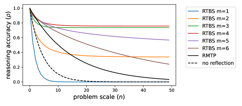<details> <summary>x13.png Details</summary>  ### Visual Description ## Line Chart: Reasoning Accuracy vs. Problem Scale ### Overview This image presents a line chart illustrating the relationship between reasoning accuracy (ρ) and problem scale (n) for different methods. The chart compares the performance of several "RTBS" methods (with varying 'm' values) against "RMTP" and a "no reflection" baseline. ### Components/Axes * **X-axis:** "problem scale (n)", ranging from approximately 0 to 50. * **Y-axis:** "reasoning accuracy (ρ)", ranging from 0 to 1.0. * **Legend:** Located in the top-right corner, listing the following data series: * RTBS m=1 (Blue) * RTBS m=2 (Orange) * RTBS m=3 (Green) * RTBS m=4 (Red) * RTBS m=5 (Purple) * RTBS m=6 (Gray) * RMTP (Black) * no reflection (Black dashed) ### Detailed Analysis The chart displays several downward-sloping curves, representing the decrease in reasoning accuracy as the problem scale increases. * **RTBS m=1 (Blue):** This line starts at approximately 0.95 at n=0 and rapidly declines, reaching near 0 at n=10. It remains close to 0 for the rest of the scale. * **RTBS m=2 (Orange):** Starts at approximately 0.95 at n=0, declines more gradually than m=1, reaching approximately 0.3 at n=20, and continues to decrease, reaching approximately 0.1 at n=50. * **RTBS m=3 (Green):** Starts at approximately 0.95 at n=0, declines at a slower rate than m=2, reaching approximately 0.5 at n=20, and approximately 0.2 at n=50. * **RTBS m=4 (Red):** Starts at approximately 0.95 at n=0, declines slowly, remaining above 0.6 until n=30, and reaching approximately 0.3 at n=50. * **RTBS m=5 (Purple):** Starts at approximately 0.95 at n=0, declines very slowly, remaining above 0.7 until n=40, and reaching approximately 0.4 at n=50. * **RTBS m=6 (Gray):** Starts at approximately 0.95 at n=0, declines the slowest of all RTBS methods, remaining above 0.8 until n=40, and reaching approximately 0.5 at n=50. * **RMTP (Black):** Starts at approximately 0.95 at n=0, declines moderately, reaching approximately 0.4 at n=20, and approximately 0.2 at n=50. * **no reflection (Black dashed):** Starts at approximately 0.95 at n=0, declines rapidly, reaching approximately 0.1 at n=10, and remaining close to 0 for the rest of the scale. All lines begin at approximately 1.0 on the y-axis when n=0. ### Key Observations * The "RTBS" methods with higher 'm' values (5 and 6) maintain higher reasoning accuracy for larger problem scales compared to those with lower 'm' values. * The "no reflection" method exhibits the most rapid decline in reasoning accuracy as the problem scale increases. * The "RMTP" method performs better than "no reflection" but worse than most of the "RTBS" methods, especially at larger problem scales. * All methods show a decrease in reasoning accuracy as the problem scale increases. ### Interpretation The chart demonstrates the impact of different methods on maintaining reasoning accuracy as the complexity of the problem (problem scale) increases. The "RTBS" methods, particularly those with higher 'm' values, appear to be more robust to increasing problem scale, suggesting they are better equipped to handle more complex reasoning tasks. The "no reflection" method's rapid decline indicates that reflection is crucial for maintaining accuracy in these types of problems. The "RMTP" method offers some improvement over not reflecting, but is not as effective as the RTBS methods. The 'm' parameter in the RTBS methods likely controls some aspect of the reflection process, with higher values leading to better performance at larger scales. This suggests a trade-off between the complexity of the method and its ability to scale to larger problems. The initial high accuracy across all methods suggests that all are effective for very simple problems. </details> Figure 10: The accuracy curves of non-reflective MTP $\rho(n)$ , RMTP $\tilde{\rho}(n)$ , and RTBS $\tilde{\rho}_{m}(n)$ , using $\mu=0.8$ , $e_{-}=0.3$ , $e_{+}=0.2$ , and $f=0.8$ . Furthermore, in Figure 10 we see that a small $m$ stabilizes the drop of $\tilde{\rho}_{m}(n)$ when $n$ is large, yet it also makes $\tilde{\rho}_{m}(n)$ drop sharply in the area where $n$ is small. This indicates the potential of using an adaptive width in RTBS, where $m$ is set small when the current subproblem (state) requires a large number $n$ of steps to solve, and $m$ increases when $n$ is reduced by previous reasoning steps. Since this paper currently focuses on the minimalistic reflection framework, we expect to explore such an extension in future work. C.3 Derivation of Theorem 1 Theorem 1 is obtained by merging the following Proposition 3 and Proposition 4, which also provide supplementary details on the non-trivial assumptions of factors $\mu$ , $e_{-}$ , and $e_{+}$ . Additionally, Proposition 4 also shows that there exists an ideal range of RTBS width $m$ such that stabilizes the drop of $\tilde{\rho}_{m}(n)$ when $n→∞$ . **Proposition 3 (RMTP Validity conditions)** *For all $n≥ 0$ , we have $\tilde{\rho}(n)≥\rho(n)\iff e_{-}+e_{+}≤ 1$ . Additionally, if $\mu>0$ and $e_{-}<1$ , then for all $n≥ 1$ we have that $\tilde{\rho}(n)=\rho(n)\iff e_{-}+e_{+}=1$ and $\tilde{\rho}(n)$ decreases strictly with either $e_{-}$ or $e_{+}$ .* **Proposition 4 (RTBS Validity Condition)** *Assuming $0<\mu<1$ , $e_{-}<1$ , and $e_{+}>0$ , then $$ \lim_{n\to\infty}\frac{\tilde{\rho}_{m}(n)}{\tilde{\rho}(n)}>1\iff\left(m>\frac{1}{1-\alpha}\ \text{and}\ f>\alpha\right). \tag{33} $$ Furthermore, we have - $\lim_{n→∞}\frac{\tilde{\rho}_{m}(n)}{\tilde{\rho}_{m}(n-1)}=1$ if $m∈[\frac{1}{\mu(1-e_{-})},\frac{1}{1-f}]$ . - $\tilde{\rho}_{m}(n)$ increases strictly with $f$ for all $n≥ 2$ .* The proof of propositions 3 and 4 is given in Appendix C.3.1 and Appendix C.3.2, which are based on the previous derivation in Appendix C.2. C.3.1 Proof of Proposition 3 In any case, we have $\tilde{\rho}(0)=\rho(0)=1$ . If $\mu=0$ or $e_{-}=1$ , we clearly have $\tilde{\rho}(n)=\rho(n)=0$ for $n≥ 1$ . If $0>\mu$ and $e_{-}<1$ , we can transform $\tilde{\rho}(n)$ (given in Proposition 2) as: $$ \tilde{\rho}(n)=\left(\frac{1}{1+\frac{e_{+}}{1-e_{-}}(\mu^{-1}-1)}\right)^{n}=\left(\frac{\mu(1-e_{-})}{\mu(1-e_{+}-e_{-})+e_{+}}\right)^{n}. \tag{34} $$ This shows that $\rho(n)$ strictly decreases with both $e_{+}$ and $e_{-}$ , and $\tilde{\rho}(n)=\mu^{n}\iff e_{+}+e_{-}=1$ . Therefore, we also have $\tilde{\rho}(n)>\mu^{n}\iff e_{+}+e_{-}<1$ . The Proposition is proved by combining all the above cases. C.3.2 Proof of Proposition 4 The assumptions $0<\mu<1$ , $e_{-}<1$ , and $e_{+}>0$ ensure that $\beta>0$ and $\gamma>0$ . Proposition 2 suggests the monotonous convergence of $\delta_{m}(n)$ , $\epsilon_{m}(n)$ , and $\sigma_{m}(n)$ . For simplicity, we denote $\delta:=\lim_{n→∞}\delta_{m}(n)$ , $\epsilon:=\lim_{n→∞}\epsilon_{m}(n)$ , and $\sigma:=\lim_{n→∞}\sigma_{m}(n)$ . From Equations (22) and (23), we have: $$ \displaystyle\delta \displaystyle=\alpha+\beta\delta^{m}+\gamma\epsilon^{m} \displaystyle\epsilon \displaystyle=f+(1-f)\epsilon^{m} \tag{35} $$ Note that $\epsilon=\delta=1$ gives the trivial solution of the above equations. However, there may exist another solution (if any) such that $\delta<1$ or $\epsilon<1$ under certain circumstances. Since $\epsilon_{m}(0)=0$ and $\delta_{m}(0)=0$ , the limits $\epsilon$ and $\delta$ take the smaller solution within $[0,1]$ . In the following, we first discuss when another non-trivial solution exists. **Lemma 1** *For any $m≥ 1$ , if $0≤ p<\frac{m-1}{m}$ , then $x=p+(1-p)x^{m}$ has a unique solution $x_{*}∈[p,1)$ , which strictly increases with $p$ . Otherwise, if $\frac{m-1}{m}≤ p≤ 1$ , the only solution in $[0,1]$ is $x_{*}=1$ .* * Proof* Define $F(x):=p+(1-p)x^{m}-x$ . We find: $$ F^{\prime}(x)=m(1-p)x^{m-1}-1. $$ It is observed that $F^{\prime}(x)$ increases monotonically with $x$ . Additionally, we have $F^{\prime}(0)=-1<0$ , $F^{\prime}(1)=m(1-p)-1$ , and $F(1)=0$ . We only consider the scenario where $p>0$ , since $x=0∈[0,1)$ is obviously the unique solution. If $0≤ p<\frac{m-1}{m}$ , we have $1-p>\frac{1}{m}$ . This implies $F^{\prime}(1)>0$ . Combining $F^{\prime}(0)<0$ , there exists $\xi∈(0,1)$ such that $F^{\prime}(\xi)=0$ . As a result, $F(x)$ strictly decreases in $[0,\xi]$ and increases in $[\xi,1)$ . Therefore, we have $F(\xi)<F(1)=0$ . Since $F(p)=(1-p)p^{m}>0$ , we know that there exists a unique $x_{*}∈[p,\xi)$ such that $F(x_{*})=0$ . If $\frac{m-1}{m}≤ p≤ 1$ , we have $1-p≤\frac{1}{m}$ and $F^{\prime}(1)≤ 0$ . In this case, $F^{\prime}(x)<0$ in $[0,1)$ due to the monotonicity of $F^{\prime}(x)$ . Thus, $F(x)>F(1)=0$ for all $x∈[0,1)$ . Therefore, $x_{*}=1$ is the only solution within $[0,1]$ . Now, we prove the monotonic increase of $x_{*}$ when $0≤ p<\frac{m-1}{m}$ . We have: $$ \displaystyle\frac{\mathrm{d}x_{*}}{\mathrm{d}p}=1+m(1-p)x_{*}^{m-1}\frac{\mathrm{d}x_{*}}{\mathrm{d}p}-x_{*}^{m} \displaystyle\frac{\mathrm{d}x_{*}}{\mathrm{d}p}=\frac{1-x_{*}^{m}}{1-m(1-p)x_{*}^{m-1}}=\frac{1-x_{*}^{m}}{-F^{\prime}(x_{*})} \tag{37} $$ The previous discussion shows that with $x_{*}<[p,\xi)$ for some $\xi$ such that $F^{\prime}(\xi)=0$ . Given that $F^{\prime}(x)$ increases monotonically, we have $F^{\prime}(x_{*})<0$ and thus $\frac{\mathrm{d}x_{*}}{\mathrm{d}p}>0$ . ∎ **Lemma 2** *Assume $p≥ 0$ , $q>0$ , and $p+q≤ 1$ . Then, the equation $x=p+qx^{m}$ has a unique solution $x_{*}∈[0,1)$ , which increases monotonically with $p∈[0,1-q]$ .* * Proof* Define $F(x):=p+qx^{m}-x$ . Since $F(0)≥ 0$ and $F(1)<0$ , there exists a solution $x_{*}∈[0,1)$ . Since $F$ is convex, we know there is at most one other solution. Clearly, the other solution appears in $(1,+∞)$ , since $F(+∞)>0$ . Therefore, $F(x)=0$ must have a unique solution $x_{*}$ in $[0,1)$ . Additionally, $x_{*}$ must appear to the left of the minimum of $F$ , which yields $F^{\prime}(x_{*})<0$ . Using the Implicit Function Theorem, we write: $$ \frac{\mathrm{d}x_{*}}{\mathrm{d}{p}}=\frac{1}{1-mqx_{*}^{m-1}}=-\frac{1}{F^{\prime}(x_{*})}>0 \tag{39} $$ Thus, we conclude that $x_{*}$ increases monotonically with $p$ . ∎ Applying Lemmas 1 and 2 to Equation (36), we find that $\epsilon=1$ if and only if $f≥\frac{m-1}{m}$ ; otherwise, $\epsilon$ strictly increases with $p$ . Therefore, $f<\frac{m-1}{m}$ indicates that $\epsilon<1$ , leading to $(\alpha+\gamma\epsilon)+\gamma<1$ . Using Lemma 2 again in Equation (35), we have $f<\frac{m-1}{m}\implies\delta<1$ . Conversely, $f≥\frac{m-1}{m}$ yields $\epsilon=1$ . and thus $f,\alpha+\gamma≥\frac{m-1}{m}\implies\delta=1$ . First, we consider the special case where $\delta=1$ , which occurs if both $f,\alpha+\gamma≥\frac{m-1}{m}$ , namely $m≤\min\{\frac{1}{1-f},\frac{1}{\beta}\}$ . In this case, we write $\sigma=(1+\delta+·s+\delta^{m-1})\beta=m\beta$ . Therefore, we have: | | $\displaystyle\lim_{n→∞}\frac{{\tilde{\rho}(n)}}{\rho(n)}>1$ | $\displaystyle\iff\sigma>\frac{\beta}{1-\alpha}$ | | | --- | --- | --- | --- | This leads to the validity condition that $\frac{1}{1-\alpha}<m≤\min\{\frac{1}{1-f},\frac{1}{\beta}\}$ . Next, we consider the case where $\delta<1$ , which occurs when $f<\frac{m-1}{m}$ or $\alpha+\gamma<\frac{m-1}{m}$ . This leads to $\beta≥\frac{1}{m}>0$ , and we can write: $$ \displaystyle\delta^{m}=\frac{1}{\beta}\left(\delta-\alpha-\gamma\epsilon^{m}\right), \displaystyle\sigma=\frac{1-\delta^{m}}{1-\delta}=\frac{(1-\delta^{m})\beta}{(1-\alpha)-(\beta\delta^{m}+\gamma\epsilon^{m})}. \tag{40} $$ Then, we can derive: | | $\displaystyle\lim_{n→∞}\frac{{\tilde{\rho}(n)}}{\rho(n)}<1$ | $\displaystyle\iff\sigma>\frac{\beta}{1-\alpha}$ | | | --- | --- | --- | --- | Since we have assumed $\delta<1$ , we have $\epsilon=1>\delta$ if $f≥\frac{m-1}{m}$ ; otherwise if $f=\alpha<\frac{m-1}{m}$ , then $\epsilon=\delta$ leads to $\delta=\epsilon$ being a solution of Equation (35). Additionally, from Lemmas 1 and 2, we know that a higher $\alpha$ would increase $(\alpha+\gamma\epsilon)$ , which eventually raises $\delta$ above $\epsilon$ ; conversely, a lower $\alpha$ causes $\delta$ to drop below $\epsilon$ . To summarize, we have the following conditions when $\delta<1$ : $$ \displaystyle 1\geq\epsilon>\delta \displaystyle\iff\left(\alpha+\gamma<\frac{m-1}{m}\leq f\right)\text{ or }\left(\alpha<f<\frac{m-1}{m}\right) \displaystyle\iff\left(\frac{1}{\beta}<m\leq\frac{1}{1-f}\right)\text{ or }\left(\alpha<f\text{ and }m>\frac{1}{1-f}\right) \tag{42} $$ Combining the conditions when $\delta=1$ , we have: $$ \displaystyle\lim_{n\to\infty}\frac{{\tilde{\rho}(n)}}{\rho(n)}>1 \displaystyle\iff \displaystyle\left(\frac{1}{1-\alpha}<m\leq\min\left\{\frac{1}{1-f},\frac{1}{\beta}\right\}\right)\text{ or }\left(\frac{1}{\beta}<m\leq\frac{1}{1-f}\right)\text{ or }\left(\alpha<f\text{ and }m>\frac{1}{1-f}\right) \displaystyle\iff \displaystyle m>\frac{1}{1-\alpha}\text{ and }f>\alpha \tag{44} $$ Thus far, we have obtained Equation (33). Now, we start proving the two additional statements in Proposition 4. First, we prove that $\frac{1}{\beta}≤ m≤\frac{1}{1-f}$ ensures that $\sigma=1$ . First, if $\delta=1$ , we have $m≤\frac{1}{\beta}≤\frac{1}{1-f}$ . In this case, $\sigma=m\beta$ , and thus $\sigma=1$ when $m=\frac{1}{\beta}$ . Alternatively, if $\delta<1$ , we have $m>\min\{\frac{1}{\beta},\frac{1}{1-f}\}$ . We can express that: $$ \sigma=\frac{1-\delta^{m}}{1-\delta}\beta=\frac{\beta-(\delta-\alpha-\gamma\epsilon^{m})}{1-\delta}=1-\gamma\frac{1-\epsilon}{(1-\delta)(1-f)} \tag{46} $$ Using Lemma 2, we know that $\delta$ increases with $\alpha+\gamma\epsilon$ , which increases with $\epsilon$ . Therefore, we have $\frac{\mathrm{d}\delta}{\mathrm{d}\epsilon}>0$ . Then, we obtain $$ \mathrm{d}\sigma/\mathrm{d}\epsilon=\sum_{i=1}^{m}i\delta^{m-1}\beta\frac{\mathrm{d}\delta}{\mathrm{d}\epsilon}>0, \tag{47} $$ $$ \displaystyle\sigma \displaystyle=\frac{1-\delta^{m}}{1-\delta}\beta=\frac{\beta-(\delta-\alpha-\gamma\epsilon^{m})}{1-\delta}=\frac{\alpha+\beta+\gamma-(1-\epsilon^{m})\gamma-\delta}{1-\delta} \displaystyle=\frac{1-\delta-\gamma(1-\frac{\epsilon-f}{1-f})}{1-\delta} \tag{48} $$ Therefore, $\sigma$ increases with $\epsilon$ and reaches its maximum value of $1$ when $\epsilon=1$ . As a result, we conclude that $\frac{1}{\beta}≤ m≤\frac{1}{1-f}$ ensures that $\sigma=1$ . Combining $\beta=\mu(1-e_{-})$ and $\sigma=\lim_{n→∞}\sigma_{m}(n)=\lim_{n→∞}\frac{\tilde{\rho}_{m}(n)}{\tilde{\rho}_{m}(n-1)}$ , we have proved that $\lim_{n→∞}\frac{\tilde{\rho}_{m}(n)}{\tilde{\rho}_{m}(n-1)}=1$ if $m∈[\frac{1}{\mu(1-e_{-})},\frac{1}{1-f}]$ . Next, we prove the monotonicity of $\tilde{\rho}_{m}(n)$ with respect to $f$ . To prove this, we first prove the monotonicity of $\epsilon_{m}(t)$ for all $t$ with respect to $f$ . **Lemma 3** *For $n>0$ , $\epsilon_{m}(t)$ as defined in Equation 23 increases strictly with $f$ .* * Proof* We regard $$ \epsilon_{m}(0;f)\equiv 0,\qquad\epsilon_{m}(t;f)=f+(1-f)\bigl[\epsilon_{m}(t-1;f)\bigr]^{m} \tag{49} $$ as a function of $f$ on $[0,1]$ . When $t=1$ we have $$ \epsilon_{m}(1;f)=f+(1-f)\bigl[\epsilon_{m}(0;f)\bigr]^{m}=f, \tag{50} $$ so $\frac{∂\epsilon_{m}(1;f)}{∂ f}=1>0$ . Thus $\epsilon_{m}(1;f)$ is strictly increasing with $f$ . Further, assume for some $k≥ 1$ that $$ 0\leq\epsilon_{m}(k;f)<1\quad\text{and}\quad\frac{\partial\epsilon_{m}(k;f)}{\partial f}>0\quad\forall f\in[0,1]. \tag{51} $$ Differentiate the recursion for $t=k+1$ : $$ \epsilon_{m}(k+1;f)=f+(1-f)\bigl[\epsilon_{m}(k;f)\bigr]^{m}, \tag{52} $$ $$ \frac{\partial\epsilon_{m}(k+1;f)}{\partial f}=1-\bigl[\epsilon_{m}(k;f)\bigr]^{m}+(1-f)\,m\bigl[\epsilon_{m}(k;f)\bigr]^{m-1}\,\frac{\partial\epsilon_{m}(k;f)}{\partial f}. \tag{53} $$ By the inductive hypothesis, $\epsilon_{m}(k;f)<1$ implies $\bigl[\epsilon_{m}(k;f)\bigr]^{m}<1$ . Therefore, we have $$ 1-\bigl[\epsilon_{m}(k;f)\bigr]^{m}>0. \tag{54} $$ Since $1-f≥ 0$ , $m≥ 1$ , $\bigl[\epsilon_{m}(k;f)\bigr]^{m-1}≥ 0$ , and $\frac{∂\epsilon_{m}(k;f)}{∂ f}>0$ , the second term is also positive. Hence $$ \frac{\partial\epsilon_{m}(k+1;f)}{\partial f}>0, \tag{55} $$ showing that $\epsilon_{m}(k+1;f)$ is strictly increasing. This completes the induction. ∎ Given Lemma 3, we can also prove the monotonicity of $\delta_{m}(t)$ using mathematical induction: It is easy to write that $\delta_{m}(2)=\alpha+\beta\alpha^{m}+\gamma f^{m}$ , showing that $\delta_{m}(2)$ increases strictly with $f$ . Then, for $t>2$ , assuming that $\delta_{m}(t-1)$ increases strictly with $f$ and using Given Lemma 3, we know that $\delta_{m}(t)$ increases strictly with $f$ from Equation (22). Therefore, we have $\delta_{m}(1)=\alpha$ and that $\delta_{m}(t)$ strictly increases with $f$ for $n≥ 2$ . According to Equation (24), from the above monotonicity of $\delta_{m}(t)$ , it is obvious that $\sigma_{m}(t)$ increases with respect to $f$ for all $t$ . This gives the corollary that $\tilde{\rho}_{m}(n)$ increases with $f$ for all $n$ . C.4 Derivation of RMTP reasoning cost In this section, we derive how many steps it costs to find a correct solution in RMTP and thereby prove Proposition 1. * Proposition1* The probability of accepting the correct step after the $i$ -th attempt is given by $\alpha^{i-1}\beta$ . Assuming a maximum number of attempts $m$ , the number of attempts consumed at each step satisfies: $$ \Pr(i\ \text{attempts}\mid\text{correct})=\frac{\alpha^{i-1}\beta}{\beta+\alpha\beta+\cdots+\alpha^{m-1}\beta}=\frac{(1-\alpha)\alpha^{i-1}}{1-\alpha^{m}} \tag{56} $$ Therefore, the average number of attempts required for a correct reasoning step is given by $$ A_{m}=\sum_{i=1}^{m}i\cdot\frac{(1-\alpha)\alpha^{i}}{1-\alpha^{m}}=\frac{1-\alpha}{1-\alpha^{m}}\sum_{i=1}^{m}i\alpha^{i-1} \tag{57} $$ To simplify the summation expression $\sum_{i=1}^{m}i\alpha^{i-1}$ (where $0<\alpha<1$ ), we can use the method of telescoping series. Let $S=\sum_{i=1}^{m}i\alpha^{i-1}$ . We calculate $\alpha S$ : $$ \alpha S=\sum_{i=1}^{m}i\alpha^{i} \tag{58} $$ Thus, $$ S-\alpha S=\sum_{i=1}^{m}i\alpha^{i-1}-\sum_{i=1}^{m}i\alpha^{i} \tag{59} $$ This gives us $$ (1-\alpha)S=1+\alpha+\alpha^{2}+\cdots+\alpha^{m-1}-m\alpha^{m}=\frac{1-\alpha^{m}}{1-\alpha}-m\alpha^{m} \tag{60} $$ Rearranging, we have $$ \sum_{i=1}^{m}i\alpha^{i-1}=\frac{1-\alpha^{m}-(1-\alpha)m\alpha^{m}}{(1-\alpha)^{2}} \tag{61} $$ Thus, the average number of attempts can be further expressed as: $$ \displaystyle A_{m} \displaystyle=\frac{1-\alpha}{1-\alpha^{m}}\cdot\frac{1-\alpha^{m}-(1-\alpha)m\alpha^{m}}{(1-\alpha)^{2}} \displaystyle=\frac{1-\alpha^{m}-(1-\alpha)m\alpha^{m}}{(1-\alpha)(1-\alpha^{m})} \displaystyle=\frac{1}{1-\alpha}-m\frac{\alpha^{m}}{1-\alpha^{m}} \tag{62} $$ Considering the limit as $m→∞$ , it can be shown using limit properties that $\lim_{m→∞}m\frac{\alpha^{m}}{1-\alpha^{m}}=0$ . If the correct solution is obtained (i.e., correct steps are accepted at each step), the average number of steps taken is given by $$ \bar{T}=nA_{\infty}=\frac{n}{1-\alpha}=\frac{n}{1-\mu e_{-}-(1-\mu)(1-e_{+})}=\frac{n}{(1-\mu)e_{+}+\mu(1-e_{-})} \tag{66} $$ ∎ C.5 Considering posterior risks of rejected attempts Our previous analysis is based on a coarse binary partition of states (correct and incorrect) for each scale, which enhances clarity yet does not apply to real-world complexity. Therefore, we can introduce stronger constraints by taking into account the posterior distribution of states in $\mathcal{S}_{n}^{+}$ after multiple attempts. For example, if the state has produced several incorrect attempts on state ${S}$ (or rejected several correct attempts), it is more likely that the current state has not been well generalized by the model. Consequently, the chances of making subsequent errors increase. In this case, $\mu$ is likely to decrease with the number of attempts, while $e_{-}$ increases with the number of attempts. Thus, the probability of accepting the correct action will decrease as the number of attempts increases. Therefore, we consider the scenario where the probabilities of error increase while the correctness rate $\mu$ drops after each attempt. We define $e_{i+},e_{i-},\mu_{i}$ , etc., to represent the probabilities related to the $i$ -th attempt, corresponding to the calculations of $\alpha_{i},\beta_{i},\gamma_{i}$ , etc. We have that $\beta_{i}=\mu_{i}(1-e_{i-})$ is monotonically decreasing, and $\gamma_{i}=(1-\mu_{i})e_{i+}$ is monotonically increasing with the index $i$ of the attempt. In this case, the derivation is similar to that of Proposition 2. Therefore, we skip all unnecessary details and present the results directly. **Proposition 5** *Given the above posterior risks, the RTMP accuracy $\tilde{\rho}(n)$ for problems with a scale of $n$ is $$ \tilde{\rho}(n)=\left(\beta_{1}+\sum_{i=2}^{\infty}\beta_{i}\prod_{j=1}^{i-1}\alpha_{i}\right)^{n} \tag{67} $$ Let $m$ be the width of RTBS. Let $\delta_{i|m}(n)$ denote the probability of a proposed step being rejected (either instantly or recursively) at the $i$ -th attempt on a correct state, and $\epsilon_{m}(n)$ follows the same definition as in Proposition 2. We have $\delta_{i|m}(0)=\epsilon_{m}(0)=0$ and the following recursive equations for $n>0$ : $$ \displaystyle\delta_{i|m}(n)=\alpha_{i}+\beta_{i}\prod_{j=1}^{m}\delta_{j|m}(n-1)+\gamma_{i}(\epsilon_{m}(n-1))^{m},\qquad i=1,\cdots,m \displaystyle\epsilon_{m}(n)=f+(1-f)\left(\epsilon_{m}(n-1)\right)^{m} \tag{68} $$ Then, the RTBS accuracy $\tilde{\rho}_{m}(n)$ for problems of scale $n$ is given by: $$ \tilde{\rho}_{m}(n)=\prod_{t=1}^{n}\sigma_{m}(t),\qquad\text{where }\sigma_{m}(t)=\beta_{1}+\sum_{j=2}^{m}\beta_{j}\prod_{i=1}^{j-1}\delta_{i|m}(t,m)\beta. \tag{70} $$ In addition, $\delta_{i|m}(n)$ , $\epsilon_{m}(n)$ , and $\sigma_{m}(n)$ all monotonically increase and converge with respect to $n$ .* The theoretical result in this new setting becomes much more challenging to derive an exact validity condition that remains clear and understandable. However, it is still useful to derive a bound that sufficiently guarantees the effectiveness of reflection. In the following, we show that a sufficient condition becomes much stricter than that in Proposition 3. **Proposition 6** *Assume $\mu_{1}<1$ and $k=∈f_{i}\frac{\beta_{i+1}}{\beta_{i}}$ is the lower bound of the decay rate of the probability of accepting the correct step in multiple attempts. Then, a sufficient condition for $\tilde{\rho}(n)>\rho(n)$ is: $$ \frac{e_{1-}}{k(1-\mu_{1})}+\sup_{i}e_{i+}<1 \tag{71} $$* * Proof* Considering $\alpha_{i}=\mu_{i}e_{i-}+(1-\mu_{i})(1-\max_{i}e_{i+})$ , let $\underline{\alpha}=(1-\mu_{1})(1-\sup_{i}e_{i+})$ be its lower bound. It can be seen that $$ \displaystyle\beta_{1}+\alpha_{1}\beta_{2}+\alpha_{1}\alpha_{2}\beta_{3}+\cdots+\beta_{m}\prod_{i=1}^{m-1}\alpha_{i}\geq\sum_{j=1}^{m}(\underline{\alpha}k)^{m-1}\beta_{1}=\beta_{1}\frac{1-(\underline{\alpha}k)^{m}}{1-\underline{\alpha}k} \tag{72} $$ As $m→∞$ , the sufficient condition for reflection validity is: $$ \displaystyle\frac{\beta_{1}}{1-\underline{\alpha}k}>\mu_{1} \displaystyle\iff \displaystyle\frac{1-e_{1-}}{1-k(1-\mu_{1})(1-\sup_{i}e_{i+})}>1 \displaystyle\iff \displaystyle(1-\mu_{1})(1-\sup_{i}e_{i+})>\frac{e_{-}}{k} \displaystyle\iff \displaystyle\frac{e_{1-}}{k}-\sup_{i}e_{i+}(1-\mu_{1})<1 \displaystyle\iff \displaystyle\frac{e_{1-}}{k(1-\mu_{1})}+\sup_{i}e_{i+}<1 \tag{73} $$ ∎ Appendix D Implementation details This section describes the details of the training datasets, model architectures, and hyper-parameters used in experiments. Our implementation derives the models architectures, pretraining, and SFT from LitGPT [1] (version 0.4.12) under Apache License 2.0. D.1 Algorithmic descriptions of reflective reasoning Algorithms 1 and 2 presents the pseudo-code of reasoning execution through RMTP and RTBS, respectively. In practice, we introduce a reflection budget $M$ to avoid infinite iteration. If reflective reasoning fails to find a solution within $M$ steps, the algorithm retrogrades to non-reflective reasoning. To implement RTBS, we maintain a stack to store the reversed list of parental states, allowing them to be restored if needed. Different from our theoretical analysis, our practical implementation does not limit the number of attempts on the input query $Q$ (as long as the total budget $M$ is not used up) as $Q$ has no parent (i.e. the stack is empty). Algorithm 1 Reflective reasoning through RMTP 0: the query ${Q}$ , the augmented policy $\tilde{\pi}=\{\pi,\mathcal{V}\}$ , transition function $\mathcal{T}$ , and reflective reasoning budget $M$ 1: $t← 0,{S}_{t}← Q$ 2: repeat 3: Infer $R_{t+1}\sim\pi(·\mid{S}_{t})$ 4: $Reject←\text{False}$ 5: if $t≤ M$ then 6: Infer ${V}_{t+1}\sim\mathcal{V}(·\mid{S}_{t},{R}_{t+1})$ 7: $Reject←\text{True}$ if “ $×$ ” $∈{V}_{t+1}$ 8: if $Reject=\text{True}$ then 9: ${S}_{t+1}←{S}_{t}$ 10: else 11: ${S}_{t+1}←\mathcal{T}({S}_{t},{R}_{t+1})$ 12: if ${R}_{t+1}$ is the answer then 13: $T← t+1,{A}←{R}_{t+1}$ 14: else 15: $t← t+1$ 16: until The answer $A$ is produced 17: return $A$ Algorithm 2 Reflective trace-back search 0: the query ${Q}$ , the augmented policy $\tilde{\pi}=\{\pi,\mathcal{V}\}$ , transition function $\mathcal{T}$ , search width $m$ , and reflective reasoning budget $M$ 1: $t← 0,{S}_{t}← Q$ 2: $i← 0$ {The index of attempts} 3: Initialize an empty stack $L$ 4: repeat 5: Infer $R_{t+1}\sim\pi(·\mid{S}_{t})$ 6: $i← i+1$ 7: $Reject←\text{False}$ 8: if $t≤ M$ then 9: Infer ${V}_{t+1}\sim\mathcal{V}(·\mid{S}_{t},{R}_{t+1})$ 10: $Reject←\text{True}$ if “ $×$ ” $∈{V}_{t+1}$ 11: if $Reject=\text{True}$ then 12: if $i<m$ then 13: ${S}_{t+1}←{S}_{t}$ 14: else 15: {Find a parent state that has remaining number of attempts.} 16: repeat 17: Pop $(s_{k},j)$ from $L$ 18: ${S}_{t+1}← s_{k},i← j$ 19: until $i<m$ or $L$ is empty 20: else 21: Push $({S}_{t+1},i)$ into $L$ 22: ${S}_{t+1}←\mathcal{T}({S}_{t},{R}_{t+1}),i← 0$ 23: if ${R}_{t+1}$ is the answer then 24: $T← t+1,{A}←{R}_{t+1}$ 25: else 26: $t← t+1$ 27: until the answer $A$ is produced 28: return $A$ D.2 Example CoT data We implement predefined programs to generate examples of CoTs and self-verification. Figure 11 presents the example reasoning steps (correct) for non-reflective training and the example detailed verification for reflective training. In our practical implementations, the reasoning steps include additional tokens, such as preprocessing and formatting, to assist planning and transition. To simplify transition function $\mathcal{T}$ , the example steps also include exactly how the states are supposed to be updated, which removes the task-specific prior in $\mathcal{T}$ . 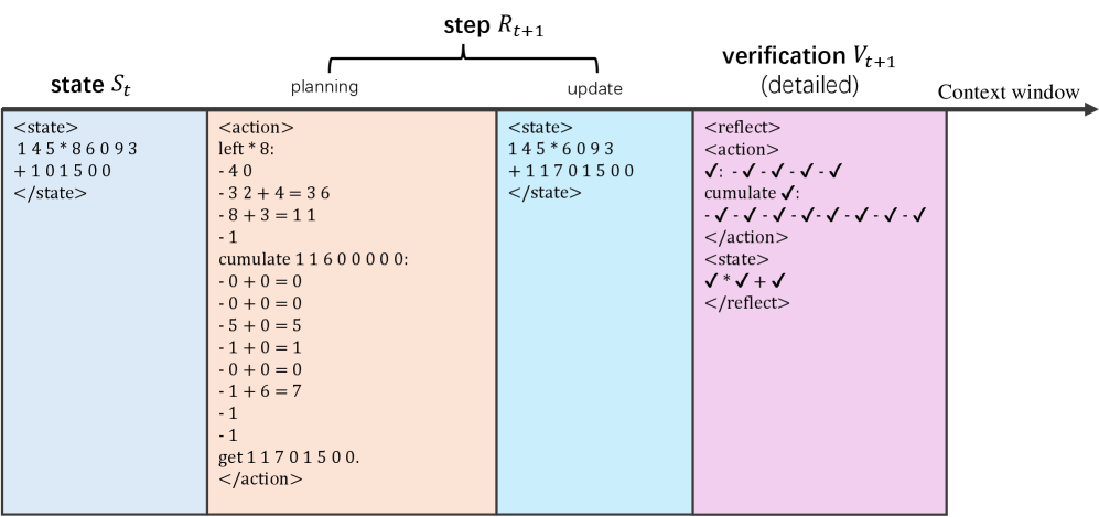<details> <summary>x14.png Details</summary>  ### Visual Description \n ## Diagram: State Transition with Planning, Update, and Verification ### Overview The image depicts a diagram illustrating a state transition process, broken down into four columns: `state St`, `planning`, `update`, and `verification Vt+1`, with a final column labeled `Context window`. Each column represents a stage in a sequential process, likely within a reinforcement learning or similar iterative system. The diagram uses XML-like tags to denote state and action elements. ### Components/Axes The diagram is structured into four main columns, visually separated by colored backgrounds: * **State St (Blue):** Represents the current state of the system. * **Planning (Peach):** Shows the actions planned to transition to the next state. * **Update (Light Blue):** Displays the updated state after applying the planned actions. * **Verification Vt+1 (Pink):** Indicates the verification of the updated state. * **Context Window (Grey):** A final column indicating the context window. The top of the diagram has a label: `step Rt+1`. ### Detailed Analysis or Content Details **1. State St (Blue Column)** * `<state>` tag: * `145 * 86093` * `+101500` * `</state>` **2. Planning (Peach Column)** * `<action>` tag: * `left * 8:` * `-40` * `-32 + 4 = 36` * `-8 + 3 = 11` * `-1` * `cumulate 11600000:` * `-0 + 0 = 0` * `-0 + 0 = 0` * `-5 + 0 = 5` * `-1 + 0 = 1` * `-0 + 0 = 0` * `-1 + 6 = 7` * `-1` * `-1` * `get 11701500.` * `</action>` **3. Update (Light Blue Column)** * `<state>` tag: * `145 * 6093` * `+11701500` * `</state>` **4. Verification Vt+1 (Pink Column)** * `<reflect>` tag: * `√ · √ · √ · √` * `cumulate √:` * `· √ · √ · √ · √ · √` * `</action>` * `<state>` tag: * `√ √ √ √` * `</reflect>` **5. Context Window (Grey Column)** * This column is empty. ### Key Observations * The `planning` column contains a series of arithmetic operations and a cumulative calculation. * The `update` column shows a modified state based on the planning stage. * The `verification` column uses checkmarks (√) and dots (·) to indicate verification status, potentially representing successful or failed checks. * The `cumulate` operation appears in both the `planning` and `verification` stages. * The values within the `<state>` tags change between the initial state and the updated state. ### Interpretation This diagram likely represents a step in a reinforcement learning or control system. The `state` represents the system's current condition. The `planning` stage calculates actions to take based on the current state. The `update` stage applies these actions, resulting in a new state. Finally, the `verification` stage checks the validity or correctness of the updated state. The use of checkmarks and dots suggests a binary verification process. The `Context window` may represent the information available to the system during this step. The arithmetic operations in the `planning` stage suggest a calculation of rewards or penalties associated with different actions. The `cumulate` operation likely accumulates these rewards or penalties over time. The change in the state values between the `state` and `update` columns indicates that the actions taken in the `planning` stage have modified the system's state. The diagram provides a high-level overview of a state transition process, focusing on the planning, update, and verification stages. 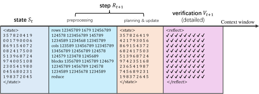</details> (a) Mult <details> <summary>x15.png Details</summary>  ### Visual Description \n ## Diagram: Data Processing Pipeline ### Overview The image depicts a data processing pipeline with four stages: State (S_t), Preprocessing, Planning & Update, and Verification (V_t+1). An arrow labeled "step R_t+1" connects the stages, indicating the flow of data. Each stage displays a block of numerical data enclosed within `<state>` or `<reflect>` tags. A "Context window" is shown on the far right. ### Components/Axes The diagram consists of four rectangular blocks representing the processing stages, arranged horizontally. Each block contains a matrix of numbers. The blocks are labeled as follows: * **State S_t**: The initial state of the data. * **Preprocessing**: The stage where initial data manipulation occurs. * **Planning & Update**: The stage where the data is planned and updated. * **Verification V_t+1**: The final stage where the data is verified. * **Context window**: A region to the right of the verification stage. ### Detailed Analysis or Content Details **1. State S_t:** The data within the `<state>` tag is a 5x5 matrix of numbers: ``` 3 5 7 8 2 0 0 1 7 9 8 6 9 1 5 0 8 2 4 1 5 1 3 9 6 ``` **2. Preprocessing:** The data within this block is organized into rows, columns, and blocks. * **rows**: 12345789 1679 12456789 * **cols**: 123589 13456789 12345789 * **blocks**: 1356789 1245789 124679 * **reduce**: 12345789 1456789 124578 * The numerical data is a 5x5 matrix: ``` 1 2 3 4 5 1 2 3 4 5 1 2 3 4 5 1 2 3 4 5 1 2 3 4 5 ``` **3. Planning & Update:** The data within the `<state>` tag is a 5x5 matrix of numbers: ``` 3 5 7 8 2 4 2 1 7 9 8 6 9 1 5 6 8 2 4 1 5 1 3 9 6 ``` **4. Verification V_t+1:** The data within the `<reflect>` tag consists of a series of checkmark symbols (√) arranged in a 5x9 grid. ``` √ √ √ √ √ √ √ √ √ √ √ √ √ √ √ √ √ √ √ √ √ √ √ √ √ √ √ √ √ √ √ √ √ √ √ √ √ √ √ √ √ √ √ √ √ ``` ### Key Observations * Each stage transforms the data in a different way. * The "Preprocessing" stage explicitly mentions operations on "rows", "cols", and "blocks", suggesting a data restructuring process. * The "Verification" stage uses checkmarks, indicating a confirmation or validation process. * The data within the "State" and "Planning & Update" stages are numerical matrices, while the "Preprocessing" stage includes both numerical matrices and textual descriptions of data organization. ### Interpretation This diagram illustrates a simplified data processing pipeline. The initial "State" represents the raw data. "Preprocessing" involves restructuring and potentially reducing the data. "Planning & Update" likely applies some algorithm or model to the preprocessed data, resulting in an updated state. Finally, "Verification" confirms the validity or correctness of the updated data. The "Context window" suggests that the pipeline operates within a defined scope or boundary. The use of tags `<state>` and `<reflect>` implies a programmatic or computational context. The diagram is a high-level representation and doesn't specify the exact algorithms or transformations used in each stage. The consistent matrix size (5x5) across the "State" and "Planning & Update" stages suggests a structured data format. The checkmarks in the "Verification" stage indicate a successful validation process, but the diagram doesn't provide information about the criteria for validation. </details> (b) Sudoku Figure 11: Example reasoning steps with detailed verfication for integer multiplication and Sudoku. D.2.1 Multiplication CoT Each state is an expression $x_{t}× y_{t}+r_{t}$ , where $x_{t}$ and $y_{t}$ are the remaining values of two multiplicands, and $r_{t}$ is the cumulative result. For an input query $x× y$ , the expert reasoner assigns $x_{1}=x$ , $y_{1}=y$ , and $r_{1}=0$ . For each step, the reasoner plans a number $u∈\{1,...,9\}$ to eliminate in $x_{t}$ (or $y_{t}$ ). Specifically, it computes $\delta=u× y_{t}$ or ( $\delta=u× x_{t}$ ). Next, it finds the digits in $x_{t}$ (or $y_{t}$ ) that are equal to $u$ and set them to $0$ in $x_{t+1}$ (or $y_{t+1}$ ). For each digit set to $0$ , the reasoner cumulates $\delta× 10^{i}$ to $r_{t}$ , where $i$ is the position of the digit (starting from $0$ for the unit digit). An example of a reasoning step is shown in Figure 11(a). Such steps are repeated until either $x_{T}$ or $y_{T}$ becomes $0$ , then the answer is $r_{T}$ . D.2.2 Sudoku CoT Each state is a $9× 9$ matrix representing the partial solution, where blank numbers are represented by $0$ . On each step, the reasoner preprocesses the state by listing the determined numbers of each row, columns, and blocks. Given these information, the model reduces the blank positions that has only one valid candidate. If no blank can be reduced, the model randomly guess a blank position that has the fewest candidates. Such process continues until there exist no blanks (i.e., zeros) in the matrix. An example of a reasoning step is shown in the right of Figure 11(b). The planned updates (i.e., which positions are filled with which numbers) is intrinsically included in a new puzzle, which is directly taken as the next state by the transition function $\mathcal{T}$ . D.2.3 Verification of reasoning steps Binary Verification The Binary verification labels are generated using a rule-based checker of each reasoning step. In Multiplication, it simply checks whether the next state $x_{t+1}× y_{t+1}+r_{t+1}$ is equal to the current state $x_{t}× y_{t}+r_{t}$ . In Sudoku, it checks whether existing numbers in the old matrix are modified and whether the new matrix has duplicated numbers in any row, column, and block. Detailed Verification In Multiplication, we output a label for each elemental computation — addition or unit-pair product — is computed correctly. In Sudoku, we output a label for each position in the new matrix, signifying whether the number violates the rule of Sudoku (i.e. conflicts with other numbers in the same row, column, or block) or is inconsistent with the previous matrix. These labels are organized using a consistent format as the CoT data. Examples of detailed reflection for correct steps is in Figure 11(b). If the step contains errors, we replace the corresponding “ $\checkmark$ ” with “ $×$ ”. D.3 Model architectures and tokenization Table 2: The model architectures of models for the transitional implementation. | Vocabulary size | 128 | | | | | | | --- | --- | --- | --- | --- | --- | --- | | Embedding size | 128 | 256 | 512 | 128 | 256 | 512 | | Number of layers | 5 | | | | | | | Number of attention Heads | 4 | 8 | 8 | 4 | 8 | 8 | Our models architectures uses multi-head causal attention with LayerNorm [36] with implementation provided by LitGPT [1]. Table 2 specifies the architecture settings of transformer models with 1M, 4M, 16M parameters. Tokenizers We employ the byte-pair encoding algorithm [30] to train tokenizers on reasoning CoT examples for tiny transformers. Special tokens for reflection and reasoning structure (e.g., identifiers for the beginning and ending positions of states and reasoning steps) are manually added to the vocabulary. Since the vocabulary size is small (128 in our experiments), the learned vocabulary is limited to elemental characters and the high-frequency words for formatting. D.4 Hyperparameters Table 3 presents the hyper-parameters used in training and testing the tiny-transformer models. In the following sections, we describe how these parameters are involved in our implementation. Table 3: The main hyper-parameters used in this work. | Task | Mult | Sudoku | | | | | | --- | --- | --- | --- | --- | --- | --- | | Model size | 1M | 4M | 16M | 1M | 4M | 16M | | Training CoT examples: $N_{CoT}$ | 32K | 36K | | | | | | Total pretraining tokens: $N_{pre\_tok}$ | 1B | | | | | | | Pretraining batch size: $B_{pre}$ | 128 | | | | | | | Pretraining learning rate: $\eta_{pre}$ | 0.001 $→$ 0.00006 | | | | | | | SFT batch size: $B_{SFT}$ | 128 | | | | | | | SFT learning rate: $\eta_{SFT}$ | 0.001 $→$ 0.00006 | | | | | | | Non-reflective SFT epochs: $E_{SFT}$ | 5 | | | | | | | Reflective sampling temperature: Solving $\tau_{refl:s}$ | 0.75 | | | | | | | Reflective sampling temperature: Proposing $\tau_{refl:p}$ | 1 | 1.25 | 1.5 | 1 | 1.25 | 1.5 | | Reflective SFT epochs: $E_{RSFT}$ | 3 | | | | | | | PPO replay buffer size: $N_{PPO:buf}$ | 512 | | | | | | | GRPO replay buffer size: $N_{GRPO:buf}$ | 1024 | | | | | | | RL sampling interval: $E_{RL:int}$ | 4 | | | | | | | RL sampling temperature: Planning $\tau_{RL:\pi}$ | 1.25 | 1 | 1.25 | 1.25 | | | | RL sampling temperature: Feedback $\tau_{RL:\pi_{f}}$ | 1 | | | | | | | RL clipping factor: $\varepsilon$ | 0.1 | | | | | | | RL KL-divergence factor: $\beta$ | 0.1 | | | | | | | GRPO group size: $G$ | 8 | | | | | | | RL total epochs: $E_{RL}$ | 512 | | | | | | | RL learning rate: $\eta_{RL}$ | 0.00005 $→$ 0.00001 | | | | | | | PPO warm-up epochs: $E_{PPO:warmup}$ | 64 | | | | | | | Testing first-attempt temperature: $\tau_{\pi:first}$ | 0 | 1 | | | | | | Testing revision temperature: $\tau_{\pi:rev}$ | 1 | | | | | | | Testing verification temperature: $\tau_{\pi_{f}}$ | 0 | | | | | | | Testing non-reflective steps $T$ : | 32 | | | | | | | Testing reflective steps $\tilde{T}$ : | 64 | | | | | | | RTBS width: $m$ | 4 | | | | | | Non-reflective training The pretraining and SFT utilize a dataset $N_{CoT}$ of CoT examples generated by an expert reasoning program. Pretraining treats these CoT examples as plain text and minimizes the cross-entropy loss for next-token prediction, using the batch size $B_{pre}$ and the learning rate $\eta_{pre}$ . The pretraining process terminates after predicting a total of $N_{pre\_tok}$ tokens. The non-reflective SFT uses the same dataset as that used in pretraining. It maximizes the likelihood of predicting example outputs (reasoning steps) from prompts (reasoning states), using the batch size $B_{SFT}$ and the learning rate $\eta_{SFT}$ . The total number of non-reflective SFT epochs is $E_{SFT}$ . Reflective SFT To perform non-reflective SFT, we use the model after non-reflective training to sample trajectories for each input query in the training set. The reflective sampling involves two decoding temperatures: the lower solving temperature $\tau_{refl:s}$ is used to walk through the solution path, while a higher proposing temperature $\tau_{refl:p}$ is used to generate diverse steps, which are fed into the reflective dataset. Then, the verification examples, which include binary or detailed labels, are generated by an expert verifier program. The reflective SFT includes $E_{RSFT}$ epochs, using the same batch size and learning rate as the non-reflective SFT. Reinforcement learning We use online RL algorithms as described in Appendix B, including PPO and GRPO. These algorithms include an experience replay buffer to store $N_{PPO:buf}$ and $N_{GRPO:buf}$ example trajectories, respectively. After every $E_{RL:int}$ epochs trained on the buffer, the buffer is updated by sampling new trajectories, using the temperature $\tau_{RL:\pi}$ for planning steps and the temperature $\tau_{RL:\tilde{\pi}}$ for reflective feedback. According to Equations 8 and 12, the hyper-parameters in both the PPO and GRPO objectives include the clipping factor $\varepsilon$ and the KL-Divergence factor $\beta$ . Additionally, GRPO defines $G$ as the number of trajectories in a group. We run RL algorithms for $E_{RL}$ epochs, using the learning rate $\eta_{RL}$ . PPO involves $E_{PPO:warmup}$ warm-up epochs at the beginning of training, during which only the value model is optimized. Testing During testing, we execute the reasoner using three decoding temperatures: $\tau_{\pi:first}$ for the first planning attempt, $\tau_{\pi:rev}$ for the revised planning attempt after being rejected, and $\tau_{\pi_{f}}$ for self-verification. We use low temperatures to improve accuracy for more deterministic decisions, such as self-verifying feedback and the first attempt in Mult. We use higher temperatures for exploratory decisions, such as planning in Sudoku and revised attempts in Mult. We set the non-reflective reasoning budget to $T$ steps and the reflective reasoning budget to $\tilde{T}$ steps. If the reflective budget is exhausted, the reasoner reverts to non-reflective reasoning. We set the search width of RTBS to $m$ . D.5 Computational resources Since our models are very small, it is entirely feasible to reproduce all our results on any PC (even laptops) that has a standard NVIDIA GPU. Using our hyper-parameters, the maximum GPU memory used for training the 1M, 4M, and 16M models is approximately 4GB, 12GB, and 16GB, respectively, which can be easily reduced by using smaller batch sizes. To run multiple experiments simultaneously, we utilize cloud servers with a total of 5 GPUs (one NVIDIA RTX-3090 GPU and four NVIDIA A10 GPUs). For each model size and task, a complete pipeline (non-reflective training, reflective training, and RL) takes about two days on a single GPU. This includes 1-2 hours for non-reflective training, 8-12 hours for data collection for reflective training, 1-2 hours for reflective SFT, 6-12 hours for RL, and 6-12 hours for testing. Appendix E Supplementary results of experiments In this section, we present supplementary results from our experiments: 1) we assess the reasoning accuracy of various large language models on integer multiplication and Sudoku tasks; 2) we report the accuracy outcomes of models after implementing different supervised fine-tuning strategies; 3) we provide full results of reasoning accuracy after GRPO; 4) we additionally provide the results of PPO, which is weaker than GRPO in reflective reasoning. E.1 Evaluation of LLMs In this section, we provide the reasoning accuracy of LLMs on Mult and Sudoku, including GPT-4o [22], OpenAI o3-mini [21], and DeepSeek-R1 [5]. Since GPT-4o is not a CoT-specialized model, we use the magic prompt “let’s think step-by-step” [13] to elicit CoT reasoning. For o3-mini and DeepSeek-R1, we only prompt with the natural description of the queries. As shown in Table 4, among these LLMs, OpenAI o3-mini produces the highest accuracy in both tasks. To illustrate how well tiny transformers can do in these tasks, we also present the best performance (results selected from Tables 5 and 7) of our 1M, 4M, and 16M models for each difficulty level, respectively, showing a performance close to or even better than some of the LLM reasoners. For example, according to our GRPO results (see Table 7), our best 4M Sudoku reasoner performs (RTBS through optional detailed verification) equally well to OpenAI o3-mini, and our best 16M Mult reasoner (through binary verification) outperforms DeepSeek-R1 in ID difficulties. Note that this paper mainly focuses on fundamental analysis and does not intend to compete with the general-purpose LLM reasoners, which can certainly gain better accuracy if specially trained on our tasks. Such a comparison is inherently unfair due to the massive gap in resource costs and data scale. The purpose of these results is to show how challenging these tasks can be, providing a conceptual notion of how well a tiny model can perform. Table 4: The accuracy (%) of GRT-4o, DeepSeek-R1, and OpenAI o3-mini in integer multiplication and Sudoku, compared with the best performance of our 1M (1M*), 4M (4M*), and 16M (16M*) transformers. The “OOD-Hard” for LLMs only refers to the same difficulty as used in testing our tiny transformers, as OOD-Hard questions may have been seen in the training of LLMs. | Mult ID-Hard OOD-Hard | ID-Easy 32.6 18.6 | 73.2 97.2 96.4 | 100 77.0 61.4 | 96.8 52.7 3.7 | 96.2 77.0 5.8 | 98.7 81.1 9.4 | 99.7 | | --- | --- | --- | --- | --- | --- | --- | --- | | Sudoku | ID-Easy | 40.7 | 99.6 | 90.4 | 33.9 | 97.2 | 99.8 | | ID-Hard | 2.8 | 52.8 | 4.4 | 0.4 | 58.1 | 72.2 | | | OOD-Hard | 0.0 | 0.0 | 0.0 | 0.0 | 6.9 | 14.4 | | E.2 Results of supervised fine tuning Table 5 includes our complete results of reasoning accuracy after non-reflective and reflective SFT. As discussed in Section 3.1, our implementation uses Reduced states that maintain only useful information for tiny transformers. To justify this, we also test the vanilla Complete implementation, where each state ${S}_{t}=({Q}_{t},{R}_{1}...,{R}_{t-1})$ includes the full history of past reasoning steps. As a baseline, the Direct thought without intermediate steps is also presented. Table 5: The reasoning accuracy (%) for 1M, 4M, and 16M transformers after SFT. | 1M | Mult | ID Easy | 21.8 | 10.6 | 23.6 | 95.8 | 94.5 | 93.4 | 22.0 | 33.4 | 24.2 | | --- | --- | --- | --- | --- | --- | --- | --- | --- | --- | --- | --- | | ID Hard | 3.0 | 1.4 | 2.0 | 52.7 | 44.6 | 35.5 | 2.2 | 4.8 | 2.8 | | | | OOD Hard | 1.4 | 0.3 | 1.0 | 3.7 | 2.2 | 1.2 | 1.0 | 0.8 | 0.4 | | | | Sudoku | ID Easy | 2.8 | 0 | 1.4 | 33.0 | 32.4 | 2.4 | 17.4 | 18.7 | 19.4 | | | ID Hard | 0 | 0 | 0 | 0.3 | 0.1 | 0 | 0.1 | 0 | 0 | | | | OOD Hard | 0 | 0 | 0 | 0 | 0 | 0 | 0 | 0 | 0 | | | | 4M | Mult | ID Easy | 15.6 | 17.2 | 92.0 | 97.7 | 97.6 | 97.3 | 94.5 | 93.8 | 93.3 | | ID Hard | 1.7 | 1.9 | 37.3 | 56.9 | 62.2 | 53.0 | 43.4 | 47.6 | 42.4 | | | | OOD Hard | 1.2 | 1.0 | 2.2 | 2.9 | 1.8 | 1.1 | 3.7 | 3.3 | 2.7 | | | | Sudoku | ID Easy | 13.0 | 3.9 | 52.2 | 92.1 | 96.8 | 96.0 | 54.4 | 81.9 | 88.5 | | | ID Hard | 0.1 | 0 | 3.3 | 40.9 | 46.3 | 53.3 | 5.2 | 16.9 | 45.7 | | | | OOD Hard | 0 | 0 | 0 | 0.4 | 4.0 | 6.7 | 0.0 | 1.1 | 2.0 | | | | 16M | Mult | ID Easy | 15.1 | 59.2 | 99.2 | 98.8 | 98.9 | 98.8 | 99.2 | 99.5 | 98.5 | | ID Hard | 1.6 | 9.6 | 65.9 | 65.2 | 76.7 | 74.9 | 65.9 | 76.4 | 73.5 | | | | OOD Hard | 1.2 | 1.0 | 2.5 | 1.1 | 1.3 | 1.3 | 9.2 | 9.4 | 7.2 | | | | Sudoku | ID Easy | 35.8 | 15.9 | 95.7 | 97.1 | 97.9 | 92.5 | 93.0 | 99.0 | 99.7 | | | ID Hard | 0.4 | 0 | 48.8 | 50.1 | 53.1 | 54.8 | 46.9 | 57.9 | 70.7 | | | | OOD Hard | 0 | 0 | 0.4 | 0.9 | 4.4 | 6.0 | 0.7 | 8.2 | 14.4 | | | Reducing the redundancy of states in long CoTs benefits tiny transformers. The left three columns in Table 5 compare the above thought implementations for non-reflective models. We see that both direct and complete thoughts fail to provide an acceptable performance even in ID-Easy difficulty. This proves the importance of avoiding long-context inference by reducing redundancy in representing states. Considering the huge performance gap, we exclude the complete and direct implementations from our main discussion. Estimated errors of self-verification For RMTP and RTBS executions, we employ the oracle verifiers to maintain test-time statistics of the average $e_{-}$ and $e_{+}$ (see definition in Section 4) of reasoning states. The results are shown in Table 6, where we also present the difference in how much reflective reasoning raises the performance over non-reflective reasoning. We only count the errors in the first attempts on reasoning states to avoid positive bias, as the reasoner may be trapped in some state and repeat the same error for many steps. Table 6: The percentage (%) of test-time verification errors (i.e., $e_{-}$ and $e_{+}$ ) after reflective SFT. Additionally, we compute $\Delta$ as the difference of how much reflective reasoning raises the performance over non-reflective reasoning, i.e. RMTP (RTBS) accuracy minus non-reflective accuracy. | 1M ID Hard OOD Hard | Mult 3.8 16.4 | ID Easy 37.6 32.9 | 19.3 $-8.1$ $-1.5$ | 4.4 3.6 6.0 | $-1.3$ 33.0 22.5 | 14.9 $-17.2$ $-2.5$ | 4.9 0.9 13.6 | $-2.4$ 6.9 2.2 | 10.2 $+2.6$ $-0.2$ | 18.3 14.5 13.2 | $+11.4$ 7.4 2.4 | 24.4 $+0.6$ $-0.6$ | 19.4 | $+2.2$ | | --- | --- | --- | --- | --- | --- | --- | --- | --- | --- | --- | --- | --- | --- | --- | | Sudoku | ID Easy | 9.9 | 35.2 | $-0.6$ | 31.1 | 43.9 | $-30.6$ | 87.1 | 0.1 | $+1.3$ | 85.1 | 0.1 | $+2$ | | | ID Hard | 21.1 | 31.0 | $-0.2$ | 33.1 | 28.6 | $-0.3$ | 82.8 | 0 | $-0.1$ | 79.4 | 0 | $-0.1$ | | | | OOD Hard | 60.3 | 7.5 | $0$ | 60.2 | 13.4 | $0$ | 87.9 | 0 | $0$ | 84.5 | 0 | $0$ | | | | 4M | Mult | ID Easy | 25.1 | 5.9 | $-0.1$ | 58.1 | 8.9 | $-0.4$ | 30.4 | 3.7 | $-0.7$ | 28.7 | 7.5 | $-1.2$ | | ID Hard | 2.4 | 23.6 | $+5.3$ | 26.0 | 30.8 | $-3.9$ | 3.3 | 25.1 | $+4.2$ | 10.0 | 29.3 | $-1.0$ | | | | OOD Hard | 7.5 | 42.9 | $-1.1$ | 18.0 | 61.7 | $-1.8$ | 5.9 | 28.1 | $-0.4$ | 10.9 | 28.2 | $-1.0$ | | | | Sudoku | ID Easy | 39.5 | 9.5 | $+4.7$ | 40.4 | 11.5 | $+3.9$ | 23.8 | 0.1 | $+27.5$ | 46.7 | 0.3 | $+34.1$ | | | ID Hard | 41.3 | 1.9 | $+5.4$ | 56.0 | 6.7 | $+12.4$ | 17.3 | 0.2 | $+11.7$ | 22.1 | 0.3 | $+40.5$ | | | | OOD Hard | 78.5 | 0.8 | $+3.6$ | 70.6 | 0.6 | $+6.3$ | 31.5 | 0.1 | $+1.1$ | 35.9 | 0.1 | $+2$ | | | | 16M | Mult | ID Easy | 11.3 | 8.6 | $+0.1$ | 6.1 | 9.4 | $+0.0$ | 15.7 | 2.1 | $+0.3$ | 3.8 | 2.9 | $-0.7$ | | ID Hard | 1.4 | 13.9 | $+11.5$ | 1.8 | 16.9 | $+9.7$ | 2.5 | 7.0 | $+10.5$ | 4.4 | 7.2 | $+7.6$ | | | | OOD Hard | 1.3 | 86.4 | $+0.2$ | 1.5 | 88.2 | $+0.2$ | 8.5 | 18.3 | $+0.2$ | 11.7 | 19.7 | $-2$ | | | | Sudoku | ID Easy | 40.1 | 3.3 | $+0.8$ | 10.1 | 4.7 | $-4.6$ | 6.6 | 1.7 | $+6$ | 9.1 | 6.4 | $+6.7$ | | | ID Hard | 50.5 | 4.3 | $+3$ | 37.2 | 9.4 | $+4.7$ | 15.4 | 0.1 | $+11.0$ | 10.6 | 0.6 | $+23.8$ | | | | OOD Hard | 75.2 | 4.2 | $+3.5$ | 65.0 | 3.1 | $+5.1$ | 28.3 | 0.1 | $+7.5$ | 24.8 | 0.0 | $+13.7$ | | | Our full results provide more evidence for the findings discussed in Section 5.1: - Learning to self-verify enhances non-reflective execution for 9 out of 12 models (2 verification types, 3 model sizes, and 2 tasks), such that accuracy does not decrease in any difficulty and increases in at least one difficulty. - RMTP improves performance over non-reflective execution for all 4M and 16M models. However, RMTP based on binary verification fails to benefit the 1M models, which suffer from a high $e_{-}$ . - 4M and 16M Sudoku models greatly benefit from RTBS, especially using detailed verification. E.3 Results of GRPO The complete results of models after GRPO are given in Table 7. To have a convenient comparison, Table 8 presents the difference of accuracy across Table 5 and Table 7, showing that the difference of accuracy is caused by GRPO. Table 7: The accuracy (%) of the 1M, 4M, and 16M transformers after GRPO. | Verification Type | None | Binary | Detailed | Optional Detailed | | | | | | | | | | --- | --- | --- | --- | --- | --- | --- | --- | --- | --- | --- | --- | --- | | Reflective Execution | None | None | RMTP | RTBS | None | RMTP | RTBS | None | RMTP | RTBS | | | | 1M | Mult | ID Easy | 52.6 | 96.2 | 95.9 | 95.7 | 53.0 | 49.5 | 45.1 | 48.6 | 47.7 | 48.8 | | ID Hard | 11.6 | 50.0 | 44.0 | 42.0 | 11.4 | 9.7 | 8.1 | 12.2 | 12.7 | 12.6 | | | | OOD Hard | 1.1 | 2.5 | 1.9 | 1.6 | 1.0 | 0.9 | 0.4 | 1.2 | 1.3 | 1.2 | | | | Sudoku | ID Easy | 1.3 | 33.9 | 29.2 | 4.5 | 17.6 | 20.7 | 18.7 | 23.0 | 23.0 | 22.6 | | | ID Hard | 0 | 0.4 | 0 | 0.2 | 0 | 0.1 | 0 | 0.1 | 0.1 | 0 | | | | OOD Hard | 0 | 0 | 0 | 0 | 0 | 0 | 0 | 0 | 0 | 0 | | | | 4M | Mult | ID Easy | 98.0 | 98.6 | 98.7 | 98.8 | 98.2 | 98.0 | 98.4 | 98.2 | 98.4 | 98.6 | | ID Hard | 65.6 | 73.6 | 77.0 | 76.7 | 63.0 | 64.3 | 63.2 | 63.9 | 66.8 | 66.1 | | | | OOD Hard | 2.3 | 2.7 | 2.7 | 2.3 | 5.8 | 5.3 | 5.3 | 3.3 | 3.2 | 3.3 | | | | Sudoku | ID Easy | 58.7 | 93.8 | 97.2 | 96.7 | 57.8 | 85.3 | 92.2 | 77.0 | 94 | 98.2 | | | ID Hard | 3.2 | 43.9 | 53.8 | 58.1 | 5.6 | 24.7 | 47.7 | 21.4 | 37.7 | 61.3 | | | | OOD Hard | 0 | 0.4 | 4.9 | 6.9 | 0 | 0.4 | 2.0 | 0 | 1.8 | 4.2 | | | | 16M | Mult | ID Easy | 99.8 | 99.2 | 99.2 | 99.1 | 99.7 | 99.6 | 99.4 | 99.2 | 99.4 | 99.3 | | ID Hard | 77.2 | 75.2 | 81.1 | 79.6 | 76.3 | 77.8 | 77.6 | 75.9 | 78.4 | 77.7 | | | | OOD Hard | 1.8 | 1.3 | 1.8 | 1.8 | 8.4 | 8.2 | 7.4 | 6.0 | 5.5 | 5.6 | | | | Sudoku | ID Easy | 96.3 | 97.6 | 98.8 | 94.6 | 93.3 | 98.8 | 99.8 | 88.7 | 97.6 | 99.0 | | | ID Hard | 51.3 | 51.7 | 58.0 | 62.3 | 46.7 | 60.4 | 72.2 | 42.2 | 57.3 | 70.9 | | | | OOD Hard | 0.7 | 0.7 | 6.0 | 7.8 | 0.2 | 6.7 | 12.0 | 0.2 | 6.7 | 11.1 | | | Table 8: The difference of accuracy (%) of the 1M, 4M, and 16M transformers after GRPO. Positive values mean that GRPO raises the accuracy of the models above SFT. | 1M | Mult | ID Easy | $+29.0$ | $+0.4$ | $+1.4$ | $+2.3$ | $+31.0$ | $+16.1$ | $+20.9$ | | --- | --- | --- | --- | --- | --- | --- | --- | --- | --- | | ID Hard | $+9.6$ | $-2.7$ | $-0.6$ | $+6.5$ | $+9.2$ | $+4.9$ | $+5.3$ | | | | OOD Hard | $+0.1$ | $-1.2$ | $-0.3$ | $+0.4$ | $0.0$ | $+0.1$ | $0.0$ | | | | Sudoku | ID Easy | $-0.1$ | $+0.9$ | $-3.2$ | $+2.1$ | $+0.2$ | $+2.0$ | $-0.7$ | | | ID Hard | $0.0$ | $+0.1$ | $-0.1$ | $+0.2$ | $-0.1$ | $+0.1$ | $0.0$ | | | | OOD Hard | $0.0$ | $0.0$ | $0.0$ | $0.0$ | $0.0$ | $0.0$ | $0.0$ | | | | 4M | Mult | ID Easy | $+6.0$ | $+0.9$ | $+1.1$ | $+1.5$ | $+3.7$ | $+4.2$ | $+5.1$ | | ID Hard | $+28.3$ | $+16.7$ | $+14.8$ | $+23.7$ | $+19.6$ | $+16.7$ | $+20.8$ | | | | OOD Hard | $0.1$ | $-0.2$ | $+0.9$ | $+1.2$ | $+2.1$ | $+2.0$ | $+2.6$ | | | | Sudoku | ID Easy | $+6.5$ | $+1.7$ | $+0.4$ | $+0.7$ | $+3.4$ | $+3.4$ | $+3.7$ | | | ID Hard | $-0.1$ | $+3.0$ | $+7.5$ | $+4.8$ | $+0.4$ | $+7.8$ | $+2.0$ | | | | OOD Hard | $0.0$ | $+0.4$ | $+4.9$ | $+6.9$ | $0$ | $-0.7$ | $0$ | | | | 16M | Mult | ID Easy | $+0.6$ | $+0.4$ | $+0.3$ | $+0.3$ | $+0.5$ | $+0.1$ | $+0.9$ | | ID Hard | $+11.3$ | $+10.0$ | $+4.4$ | $+4.7$ | $+10.4$ | $+1.4$ | $+4.1$ | | | | OOD Hard | $-0.7$ | $+0.2$ | $+0.5$ | $+0.5$ | $-0.8$ | $-1.2$ | $+0.2$ | | | | Sudoku | ID Easy | $+0.6$ | $+0.5$ | $+0.9$ | $+2.1$ | $+0.3$ | $-0.2$ | $+0.1$ | | | ID Hard | $+2.5$ | $+1.6$ | $+4.9$ | $+7.5$ | $-0.2$ | $+2.5$ | $+1.5$ | | | | OOD Hard | $+0.3$ | $-0.2$ | $+1.6$ | $+1.8$ | $-0.5$ | $-1.5$ | $-2.4$ | | | Reflection usually extends the limit of RL. For reflective models, GRPO samples experience CoTs through RMTP, where self-verification $\mathcal{V}$ and the forward policy $\pi$ are jointly optimized in the form of a self-verifying policy $\tilde{\pi}$ . By comparing the RMTP results (columns 3, 6, and 9) with the non-reflective model (the first column) in Table 7, we find that GRPO usually converges to higher accuracy solving ID-Hard problems in RMTP. This shows that having reflection in long CoTs extends the limit of RL, compared to only exploiting a planning policy. Interestingly, optional detailed verification generally demonstrates higher performance after GRPO than mandatory verification. A probable explanation is that a mandatory verification may cause the reasoner to overly rely on reflection, which stagnates the learning of the planning policy. Overall, our full results provide more evidence to better support our findings discussed in Section 5.2: - RL enhances 24 out of 42 ID-Hard results in Table 8 by no less than 3% (measured in absolute difference). However, only 8 out of 42 OOD-Hard results are improved by no less than 1%. - In table 9, an increase of $e_{+}$ is observed in 20 out of 25 cases where $e_{-}$ decreases by more than 5% (measured in absolute difference). E.3.1 The verification errors after GRPO Furthermore, we also present the estimated errors of verification after GRPO in Table 9, in order to investigate how self-verification evolves during RL. Our main observation is that if a model has a high $e_{-}$ before GPRO, then GRPO tends to reduce $e_{-}$ and also increases $e_{+}$ . This change in verification errors is a rather superficial (lazy) way to obtain improvements. If the model faithfully improves verification through RL, both types of errors should simultaneously decrease — such a case occurs only in the ID-Easy difficulty or when $e_{-}$ is already low after SFT. This highlights a potential retrograde of self-verification ability after RL. Table 9: The percentage (%) of test-time verification errors (i.e., $e_{-}$ and $e_{+}$ ) after GRPO. The arrows “↑” (increase) and “↓” (decrease) present the change compared to the results in SFT (Table 6). | 1M ID Hard OOD Hard | Mult 16.5↑ 20.3 41.2↑ 57.6 | ID Easy 17.6↓ 20.0 1.6↓ 31.3 | 6.8↓ 12.5 7.0↑ 10.6 40.2↑ 46.2 | 3.3↓ 1.1 13.7↓ 19.3 1.5↑ 24.0 | 5.0↓ 9.9 54.6↑ 55.5 53.9↑ 67.5 | 3.5↓ 1.4 4.6↓ 2.3 16.4↑ 18.6 | 12.4↑ 22.6 42.1↑ 56.6 57.3↑ 70.5 | 17.2↓ 1.1 5.7↓ 1.7 19.1↑ 21.5 | 3.5↑ 27.9 | 17.6↓ 1.8 | | --- | --- | --- | --- | --- | --- | --- | --- | --- | --- | --- | | Sudoku | ID Easy | 1.2↑ 11.1 | 1.7↓ 36.9 | 13.1↓ 18.0 | 4.0↑ 47.9 | 0.1↑ 87.2 | 0.0↓ 0.0 | 0.0↑ 87.1 | 0.4↑ 0.5 | | | ID Hard | 2.9↑ 24.0 | 0.9↓ 30.1 | 5.5↓ 27.6 | 0.4↑ 29.0 | 0.1↓ 83.7 | 0.0↓ 0.0 | 0.1↓ 80.3 | 0.0↓ 0.0 | | | | OOD Hard | 3.1↑ 63.4 | 0.8↑ 8.3 | 4.5↓ 55.7 | 0.9↑ 14.3 | 0.5↑ 88.4 | 0.0↓ 0.0 | 0.6↑ 85.1 | 0.0↓ 0.0 | | | | 4M | Mult | ID Easy | 2.5↓ 22.6 | 4.8↓ 1.1 | 30.2↓ 27.9 | 7.1↓ 1.8 | 21.1↓ 9.3 | 3.0↓ 0.7 | 5.0↓ 23.7 | 6.8↓ 0.7 | | ID Hard | 53.1↑ 55.5 | 21.8↓ 1.8 | 30.6↑ 56.6 | 28.5↓ 2.3 | 20.9↑ 24.2 | 20.1↓ 5.0 | 22.0↑ 32.0 | 24.8↓ 4.5 | | | | OOD Hard | 60.0↑ 67.5 | 24.3↓ 18.6 | 52.5↑ 70.5 | 40.2↓ 21.5 | 55.7↑ 61.6 | 20.9↓ 7.2 | 53.4↑ 64.3 | 22.9↓ 5.3 | | | | Sudoku | ID Easy | 7.9↓ 31.6 | 3.2↓ 6.3 | 2.8↑ 43.2 | 7.7↓ 3.8 | 11.5↓ 12.3 | 1.3↑ 1.4 | 27.1↓ 19.6 | 1.9↑ 2.2 | | | ID Hard | 28.7↑ 70.0 | 0.5↓ 1.4 | 2.2↑ 58.2 | 4.7↓ 2.0 | 4.5↓ 12.8 | 1.6↑ 1.8 | 9.2↓ 12.9 | 0.1↓ 0.2 | | | | OOD Hard | 6.9↑ 85.4 | 0.7↓ 0.1 | 11.0↑ 81.6 | 0.2↓ 0.4 | 2.1↓ 29.4 | 0↓ 0.1 | 5.9↓ 30.0 | 0.1↑ 0.2 | | | | 16M | Mult | ID Easy | 4.2↓ 7.1 | 7.2↓ 1.4 | 0.4↓ 5.7 | 7.8↓ 1.6 | 8.1↓ 7.6 | 1.9↓ 0.2 | 7.8↑ 11.6 | 2.7↓ 0.2 | | ID Hard | 7.9↑ 9.3 | 12.8↓ 1.1 | 6.7↑ 8.5 | 15.6↓ 1.3 | 22.7↑ 25.2 | 3.9↓ 3.1 | 18.6↑ 23.0 | 4.3↓ 2.9 | | | | OOD Hard | 79.0↑ 80.3 | 47.1↓ 39.3 | 89.2↑ 90.7 | 46.4↓ 41.8 | 46.0↑ 54.5 | 12.5↓ 5.8 | 46.4↑ 58.1 | 14.7↓ 5.0 | | | | Sudoku | ID Easy | 24.5↑ 64.6 | 6.2↑ 9.5 | 25.6↑ 35.7 | 8.5↑ 13.2 | 2.1↑ 8.7 | 0.6↓ 1.1 | 3.3↓ 5.8 | 5.4↓ 1.0 | | | ID Hard | 25.3↑ 75.8 | 0.0↓ 4.3 | 16.4↑ 53.6 | 2.0↓ 7.4 | 0.5↑ 15.9 | 0.0↓ 0.1 | 2.4↑ 13.0 | 0.4↑ 1.0 | | | | OOD Hard | 7.9↑ 83.1 | 3.5↓ 0.7 | 12.7↑ 77.7 | 2.1↓ 1.0 | 7.8↑ 36.1 | 0.0↓ 0.1 | 6.8↑ 31.6 | 0.1↑ 0.1 | | | E.3.2 The planning correctness rate after GRPO Table 10: The planning correctness rate ( $\mu$ ) before and after GRPO. Each result is reported by $\mu_{\text{SFT}}→\mu_{\text{GRPO}}$ . | Mult 4M 16M | Detailed $98.3→ 99.5$ $99.7→ 99.9$ | 1M $68.4→ 79.1$ $80.0→ 85.9$ | $70.2→ 81.7$ $35.0→ 38.0$ $47.9→ 43.4$ | $54.4→ 59.5$ | $42.9→ 41.9$ | | --- | --- | --- | --- | --- | --- | | Binary | 1M | $98.8→ 99.1$ | $81.2→ 80.3$ | $42.7→ 38.6$ | | | 4M | $99.3→ 99.7$ | $77.6→ 89.9$ | $57.1→ 48.1$ | | | | 16M | $99.4→ 99.8$ | $79.6→ 85.1$ | $75.2→ 44.8$ | | | | Sudoku | Detailed | 1M | $34.1→ 33.0$ | $13.2→ 12.4$ | $9.0→ 8.6$ | | 4M | $85.0→ 86.8$ | $65.2→ 72.0$ | $70.1→ 70.3$ | | | | 16M | $98.6→ 98.1$ | $92.5→ 94.0$ | $84.9→ 83.9$ | | | | Binary | 1M | $59.1→ 60.3$ | $36.6→ 36.1$ | $19.5→ 19.9$ | | | 4M | $97.3→ 97.8$ | $80.2→ 81.4$ | $74.5→ 70.9$ | | | | 16M | $99.0→ 99.2$ | $88.5→ 85.1$ | $68.4→ 64.6$ | | | We also report how GRPO influences the step-wise planning ability, measured by $\mu$ (defined in Section 4), across various tasks, verification types, and model sizes. Shown in Table 10, GRPO increases the planning correctness rate $\mu$ in most ID cases, except for the Sudoku models with binary verification. This indicates that the proposed steps are more likely to be correct and further reduces the overall penalties of false positive verification, making an optimistic verification bias (a high $e_{+}$ in exchange for a low $e_{-}$ ) even more rewarding. In particular, the planning ability shows almost no improvement in OOD problems. E.3.3 Reflection frequency of optional detailed verification To show how GRPO adapts the reflection frequency for optional detailed verification, Figure 12 shows the reflection frequency of 1M and 16M transformers before and after GRPO, and the reflection frequency of the 4M model is previously shown in Section 5.2. Similarly, Figure 13 shows the reflection frequency for 1M, 4M, and 16M models in Sudoku. According to results in Table 5, reflective execution does not improve performance for the 1M model, implying its weakness in exploring correct solutions. Therefore, GRPO does not much incentivize reflection for the 1M model. Contrarily, it greatly encourages reflection for 4M and 16M models, for they explore more effectively than the 1M model. These results align with the discussion in Section 5.2 that RL adapts the reflection frequency based on how well the proposing policy can explore higher rewards. 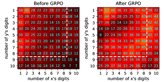<details> <summary>x16.png Details</summary>  ### Visual Description ## Heatmap: Comparison of Digit Distributions Before and After GRPO ### Overview This image presents two heatmaps side-by-side, visually comparing the distribution of digits 'x' and 'y' before and after a process labeled "GRPO". Each heatmap represents a 10x10 grid, where the x-axis represents the number of digits 'x', and the y-axis represents the number of digits 'y'. The color intensity within each cell indicates a numerical value, with warmer colors (reds) representing higher values and cooler colors (blues) representing lower values. ### Components/Axes * **Title (Left):** "Before GRPO" * **Title (Right):** "After GRPO" * **X-axis Label (Both):** "number of x's digits" (ranging from 1 to 10) * **Y-axis Label (Both):** "number of y's digits" (ranging from 1 to 10) * **Color Scale:** A gradient from dark blue (low values) to bright red (high values). The exact scale is not provided, but values are displayed within each cell. * **Grid:** 10 rows and 10 columns in each heatmap. ### Detailed Analysis or Content Details **Left Heatmap (Before GRPO):** The heatmap shows a general trend of decreasing values as both the number of 'x' digits and the number of 'y' digits increase. The highest values are concentrated in the top-left corner. * **Row 1:** Values decrease from 38 (x=1, y=1) to 11 (x=10, y=1). * **Row 2:** Values decrease from 33 (x=1, y=2) to 14 (x=10, y=2). * **Row 3:** Values decrease from 41 (x=1, y=3) to 16 (x=10, y=3). * **Row 4:** Values decrease from 30 (x=1, y=4) to 17 (x=10, y=4). * **Row 5:** Values decrease from 30 (x=1, y=5) to 19 (x=10, y=5). * **Row 6:** Values decrease from 41 (x=1, y=6) to 17 (x=10, y=6). * **Row 7:** Values decrease from 38 (x=1, y=7) to 12 (x=10, y=7). * **Row 8:** Values decrease from 32 (x=1, y=8) to 12 (x=10, y=8). * **Row 9:** Values decrease from 23 (x=1, y=9) to 8 (x=10, y=9). * **Row 10:** Values decrease from 17 (x=1, y=10) to 7 (x=10, y=10). **Right Heatmap (After GRPO):** The heatmap shows a different distribution compared to the "Before GRPO" heatmap. The highest values are more dispersed, and there's a noticeable increase in values along the diagonal and in the upper-right corner. * **Row 1:** Values decrease from 52 (x=1, y=1) to 32 (x=10, y=1). * **Row 2:** Values decrease from 44 (x=1, y=2) to 44 (x=10, y=2). * **Row 3:** Values decrease from 34 (x=1, y=3) to 42 (x=10, y=3). * **Row 4:** Values decrease from 19 (x=1, y=4) to 38 (x=10, y=4). * **Row 5:** Values decrease from 22 (x=1, y=5) to 37 (x=10, y=5). * **Row 6:** Values decrease from 21 (x=1, y=6) to 36 (x=10, y=6). * **Row 7:** Values decrease from 38 (x=1, y=7) to 34 (x=10, y=7). * **Row 8:** Values decrease from 26 (x=1, y=8) to 30 (x=10, y=8). * **Row 9:** Values decrease from 23 (x=1, y=9) to 30 (x=10, y=9). * **Row 10:** Values decrease from 25 (x=1, y=10) to 23 (x=10, y=10). ### Key Observations * The "After GRPO" heatmap generally exhibits higher values than the "Before GRPO" heatmap, suggesting that the GRPO process increases the frequency of certain digit combinations. * The "Before GRPO" heatmap shows a clear negative correlation between the number of 'x' digits and the number of 'y' digits. * The "After GRPO" heatmap shows a more complex pattern, with higher values along the diagonal (equal numbers of 'x' and 'y' digits) and in the upper-right corner (more 'x' digits than 'y' digits). * The maximum value shifts from 48 (Before GRPO) to 52 (After GRPO). * The minimum value remains at 7 in both heatmaps. ### Interpretation The data suggests that the GRPO process alters the distribution of digits 'x' and 'y'. Before GRPO, there's a tendency for lower counts of both digits to occur together. After GRPO, the process seems to increase the frequency of combinations where the number of 'x' digits is equal to or greater than the number of 'y' digits. This could indicate that GRPO is a process that either generates more 'x' digits, reduces 'y' digits, or preferentially combines them in certain ways. The increase in values along the diagonal in the "After GRPO" heatmap suggests that the process might be creating more instances where the number of 'x' digits and 'y' digits are equal. The higher values in the upper-right corner suggest an increase in instances where there are more 'x' digits than 'y' digits. Without knowing what GRPO represents, it's difficult to provide a more specific interpretation. However, the data clearly demonstrates that GRPO has a significant impact on the distribution of these digits. Further investigation into the nature of GRPO is needed to understand the underlying mechanisms driving these changes. 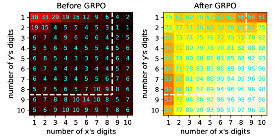</details> (a) 1M <details> <summary>x17.png Details</summary>  ### Visual Description \n ## Heatmap: Performance Comparison Before and After GRPO ### Overview This image presents two heatmaps, visually comparing a performance metric "Before GRPO" and "After GRPO". Both heatmaps represent the relationship between the number of 'x' digits and the number of 'y' digits, with color intensity indicating the corresponding value. The x-axis represents the number of 'x' digits (ranging from 1 to 10), and the y-axis represents the number of 'y' digits (also ranging from 1 to 10). ### Components/Axes * **Title (Left):** "Before GRPO" * **Title (Right):** "After GRPO" * **X-axis Label (Both):** "number of x's digits" * **Y-axis Label (Both):** "number of y's digits" * **X-axis Markers (Both):** 1, 2, 3, 4, 5, 6, 7, 8, 9, 10 * **Y-axis Markers (Both):** 1, 2, 3, 4, 5, 6, 7, 8, 9, 10 * **Color Scale (Left):** Ranges from dark blue (low values) to red (high values). * **Color Scale (Right):** Ranges from dark blue (low values) to yellow (high values). * **Legend (Implicit):** Color intensity represents the value at each (x, y) coordinate. ### Detailed Analysis or Content Details **Before GRPO (Left Heatmap):** The heatmap shows a generally decreasing trend as both the number of 'x' digits and the number of 'y' digits increase. The highest values are concentrated in the top-left corner. * **(1, 1):** 38 * **(1, 2):** 19 * **(1, 3):** 29 * **(1, 4):** 15 * **(1, 5):** 12 * **(1, 6):** 9 * **(1, 7):** 6 * **(1, 8):** 4 * **(1, 9):** 2 * **(1, 10):** 4 * **(2, 1):** 15 * **(2, 2):** 4 * **(2, 3):** 5 * **(2, 4):** 5 * **(2, 5):** 4 * **(2, 6):** 3 * **(2, 7):** 1 * **(2, 8):** 1 * **(2, 9):** 1 * **(2, 10):** 1 * **(3, 1):** 6 * **(3, 2):** 7 * **(3, 3):** 4 * **(3, 4):** 9 * **(3, 5):** 6 * **(3, 6):** 4 * **(3, 7):** 2 * **(3, 8):** 5 * **(3, 9):** 6 * **(3, 10):** 6 * **(4, 1):** 5 * **(4, 2):** 5 * **(4, 3):** 6 * **(4, 4):** 5 * **(4, 5):** 5 * **(4, 6):** 4 * **(4, 7):** 5 * **(4, 8):** 6 * **(4, 9):** 6 * **(4, 10):** 6 * **(5, 1):** 6 * **(5, 2):** 8 * **(5, 3):** 5 * **(5, 4):** 3 * **(5, 5):** 3 * **(5, 6):** 5 * **(5, 7):** 4 * **(5, 8):** 6 * **(5, 9):** 4 * **(5, 10):** 4 * **(6, 1):** 6 * **(6, 2):** 7 * **(6, 3):** 4 * **(6, 4):** 4 * **(6, 5):** 3 * **(6, 6):** 4 * **(6, 7):** 5 * **(6, 8):** 7 * **(6, 9):** 6 * **(6, 10):** 6 * **(7, 1):** 6 * **(7, 2):** 4 * **(7, 3):** 4 * **(7, 4):** 3 * **(7, 5):** 5 * **(7, 6):** 5 * **(7, 7):** 6 * **(7, 8):** 7 * **(7, 9):** 6 * **(7, 10):** 6 * **(8, 1):** 5 * **(8, 2):** 7 * **(8, 3):** 5 * **(8, 4):** 6 * **(8, 5):** 7 * **(8, 6):** 10 * **(8, 7):** 9 * **(8, 8):** 8 * **(8, 9):** 6 * **(8, 10):** 6 * **(9, 1):** 6 * **(9, 2):** 7 * **(9, 3):** 8 * **(9, 4):** 8 * **(9, 5):** 10 * **(9, 6):** 14 * **(9, 7):** 10 * **(9, 8):** 8 * **(9, 9):** 5 * **(9, 10):** 7 * **(10, 1):** 5 * **(10, 2):** 6 * **(10, 3):** 9 * **(10, 4):** 10 * **(10, 5):** 9 * **(10, 6):** 7 * **(10, 7):** 8 * **(10, 8):** 6 * **(10, 9):** 6 * **(10, 10):** 6 **After GRPO (Right Heatmap):** The heatmap shows a generally increased value across the board, with the highest values concentrated in the bottom-right corner. * **(1, 1):** 75 * **(1, 2):** 69 * **(1, 3):** 70 * **(1, 4):** 67 * **(1, 5):** 67 * **(1, 6):** 56 * **(1, 7):** 54 * **(1, 8):** 51 * **(1, 9):** 53 * **(1, 10):** 51 * **(2, 1):** 72 * **(2, 2):** 71 * **(2, 3):** 70 * **(2, 4):** 68 * **(2, 5):** 70 * **(2, 6):** 67 * **(2, 7):** 67 * **(2, 8):** 75 * **(2, 9):** 75 * **(2, 10):** 75 * **(3, 1):** 73 * **(3, 2):** 74 * **(3, 3):** 75 * **(3, 4):** 76 * **(3, 5):** 72 * **(3, 6):** 75 * **(3, 7):** 78 * **(3, 8):** 82 * **(3, 9):** 82 * **(3, 10):** 82 * **(4, 1):** 71 * **(4, 2):** 80 * **(4, 3):** 79 * **(4, 4):** 78 * **(4, 5):** 79 * **(4, 6):** 81 * **(4, 7):** 82 * **(4, 8):** 88 * **(4, 9):** 88 * **(4, 10):** 88 * **(5, 1):** 74 * **(5, 2):** 80 * **(5, 3):** 81 * **(5, 4):** 83 * **(5, 5):** 85 * **(5, 6):** 88 * **(5, 7):** 92 * **(5, 8):** 93 * **(5, 9):** 93 * **(5, 10):** 93 * **(6, 1):** 71 * **(6, 2):** 78 * **(6, 3):** 85 * **(6, 4):** 85 * **(6, 5):** 89 * **(6, 6):** 93 * **(6, 7):** 95 * **(6, 8):** 96 * **(6, 9):** 96 * **(6, 10):** 96 * **(7, 1):** 53 * **(7, 2):** 67 * **(7, 3):** 84 * **(7, 4):** 86 * **(7, 5):** 90 * **(7, 6):** 94 * **(7, 7):** 95 * **(7, 8):** 96 * **(7, 9):** 96 * **(7, 10):** 96 * **(8, 1):** 52 * **(8, 2):** 68 * **(8, 3):** 81 * **(8, 4):** 87 * **(8, 5):** 89 * **(8, 6):** 94 * **(8, 7):** 96 * **(8, 8):** 96 * **(8, 9):** 96 * **(8, 10):** 96 * **(9, 1):** 52 * **(9, 2):** 72 * **(9, 3):** 84 * **(9, 4):** 88 * **(9, 5):** 92 * **(9, 6):** 96 * **(9, 7):** 98 * **(9, 8):** 97 * **(9, 9):** 96 * **(9, 10):** 96 * **(10, 1):** 77 * **(10, 2):** 86 * **(10, 3):** 90 * **(10, 4):** 93 * **(10, 5):** 97 * **(10, 6):** 97 * **(10, 7):** 96 * **(10, 8):** 95 * **(10, 9):** 95 * **(10, 10):** 95 ### Key Observations * The "After GRPO" heatmap consistently shows higher values than the "Before GRPO" heatmap across all combinations of 'x' and 'y' digits. * Before GRPO, the highest values are concentrated in the upper-left corner, while after GRPO, they shift towards the bottom-right corner. * The color scale on the right heatmap is shifted towards yellow, indicating a general increase in values. ### Interpretation The data suggests that GRPO (presumably a process or intervention) has a positive impact on the performance metric being measured. The shift in the highest values from the top-left to the bottom-right corner indicates that the performance improvement is more pronounced when both the number of 'x' digits and the number of 'y' digits are higher. This could imply that GRPO is particularly effective in scenarios involving more complex inputs or larger datasets. The consistent increase in values across the board suggests a broad and systemic improvement due to GRPO. The heatmap provides a clear visual representation of this improvement, making it easy to identify the areas where GRPO has the greatest effect. </details> (b) 16M Figure 12: The hot-maps of reflection frequency (%) of 1M and 16M multiplication models before and after GRPO, which uses a sampling temperature of $1.25$ . All models are tested using RMTP execution. <details> <summary>x18.png Details</summary>  ### Visual Description \n ## Bar Charts: Reflection Frequency vs. Number of Blanks ### Overview The image presents two bar charts, side-by-side, comparing the reflection frequency distribution before and after a process labeled "GRPO". Both charts depict the relationship between the number of blanks and the reflection frequency, expressed as a percentage. A vertical dashed red line is present in both charts, marking a value of approximately 54 on the x-axis. ### Components/Axes * **X-axis:** "number of blanks" ranging from 9 to 54, with tick marks at intervals of 9. * **Y-axis:** "reflection frequency (%)" ranging from 0.0 to 1.0, with tick marks at intervals of 0.2. * **Chart Titles:** * Left Chart: "Before GRPO" * Right Chart: "After GRPO" * **Data Series:** Each chart displays a single data series represented by blue bars. * **Vertical Line:** A dashed red vertical line is present in both charts at approximately x = 54. ### Detailed Analysis or Content Details **Left Chart: Before GRPO** The bar chart shows a relatively low and consistent reflection frequency for most values of "number of blanks" up to approximately 45. The reflection frequency increases noticeably around the value of 45, peaking at approximately 0.23, and then decreases again. The dashed red line at 54 appears to highlight a region of higher reflection frequency. * At x = 9, reflection frequency is approximately 0.02%. * At x = 18, reflection frequency is approximately 0.04%. * At x = 27, reflection frequency is approximately 0.07%. * At x = 36, reflection frequency is approximately 0.12%. * At x = 45, reflection frequency is approximately 0.23%. * At x = 54, reflection frequency is approximately 0.18%. **Right Chart: After GRPO** The bar chart shows a similar pattern to the left chart, but with a generally lower and more uniform distribution of reflection frequency. The increase in reflection frequency around x = 45 is less pronounced than in the "Before GRPO" chart. The dashed red line at 54 again highlights a region, but the difference in reflection frequency before and after this point is less dramatic. * At x = 9, reflection frequency is approximately 0.03%. * At x = 18, reflection frequency is approximately 0.05%. * At x = 27, reflection frequency is approximately 0.08%. * At x = 36, reflection frequency is approximately 0.11%. * At x = 45, reflection frequency is approximately 0.16%. * At x = 54, reflection frequency is approximately 0.14%. ### Key Observations * The "GRPO" process appears to have reduced the reflection frequency, particularly for values of "number of blanks" greater than 45. * The peak in reflection frequency around x = 45 is less prominent after the GRPO process. * The overall distribution of reflection frequency is more uniform after the GRPO process. * The dashed red line at x = 54 seems to be a point of interest, potentially indicating a threshold or boundary. ### Interpretation The data suggests that the GRPO process effectively reduces the reflection frequency, particularly in the range of "number of blanks" above 45. This could indicate that GRPO is a process designed to eliminate or mitigate factors contributing to higher reflection frequencies in this range. The reduction in the peak at x = 45 suggests that GRPO specifically addresses the cause of this increased reflection. The dashed red line at x = 54 might represent a critical value or a point where the effect of GRPO becomes more noticeable. The charts demonstrate a clear shift in the distribution of reflection frequency as a result of the GRPO process, indicating its effectiveness in modifying the underlying phenomenon being measured. The data implies that the GRPO process improves the consistency of reflection frequency across the measured range of "number of blanks". 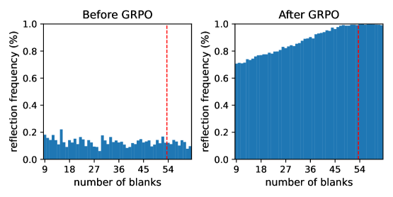</details> (a) 1M <details> <summary>x19.png Details</summary>  ### Visual Description \n ## Histograms: Reflection Frequency vs. Number of Blanks ### Overview The image presents two histograms comparing the distribution of "reflection frequency" against the "number of blanks" before and after a process labeled "GRPO". Both histograms share the same x and y axes scales. A vertical dashed line is present in both histograms, marking a value of approximately 54 on the x-axis. ### Components/Axes * **X-axis Label:** "number of blanks" (ranging from approximately 9 to 54) * **Y-axis Label:** "reflection frequency (%)" (ranging from 0.0 to 1.0) * **Title (Left Histogram):** "Before GRPO" * **Title (Right Histogram):** "After GRPO" * **Vertical Dashed Line:** Present in both histograms, positioned at approximately x = 54. ### Detailed Analysis or Content Details **Left Histogram (Before GRPO):** * The histogram shows a relatively flat distribution with many small peaks. * The reflection frequency is generally low, mostly below 0.2. * There is a slight increase in frequency around the x-axis value of 9, peaking at approximately 0.22. * The frequency remains relatively constant between approximately 18 and 45, hovering around 0.1 to 0.15. * There is a small peak around x=27 at approximately 0.2. * The dashed line at x=54 does not correspond to a significant peak in the distribution. **Right Histogram (After GRPO):** * The histogram shows a monotonically increasing distribution. * The reflection frequency starts near 0 at x=9 and increases steadily to approximately 1.0 at x=54. * The frequency is approximately 0.2 at x=18. * The frequency is approximately 0.4 at x=27. * The frequency is approximately 0.6 at x=36. * The frequency is approximately 0.8 at x=45. * The dashed line at x=54 corresponds to a frequency of approximately 1.0. ### Key Observations * The distribution of reflection frequency changes dramatically after the GRPO process. * Before GRPO, the reflection frequency is low and relatively constant across most of the "number of blanks" range. * After GRPO, the reflection frequency increases consistently with the "number of blanks". * The dashed line at x=54 appears to mark a threshold or significant point in the "number of blanks" for the "After GRPO" distribution. ### Interpretation The data suggests that the GRPO process significantly improves the relationship between the "number of blanks" and the "reflection frequency". Before GRPO, there is little correlation between these two variables. After GRPO, a strong positive correlation emerges: as the "number of blanks" increases, the "reflection frequency" also increases. The dashed line at x=54 might represent a saturation point, where further increases in the "number of blanks" do not lead to significant increases in "reflection frequency". The GRPO process appears to have transformed a random or noisy distribution into a predictable and increasing trend. The nature of "blanks" and "reflection frequency" is not provided, but the data suggests GRPO is a successful intervention. 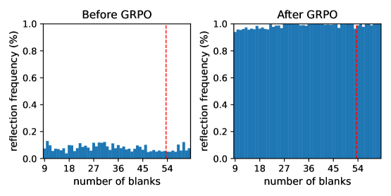</details> (b) 4M <details> <summary>x20.png Details</summary>  ### Visual Description \n ## Histograms: Reflection Frequency vs. Number of Blanks ### Overview The image presents two histograms, side-by-side, comparing the distribution of "reflection frequency" against the "number of blanks" before and after a process labeled "GRPO". Both histograms share the same x and y axes scales. A vertical dashed red line is present in both histograms, marking a value of approximately 54 on the x-axis. ### Components/Axes * **X-axis Label:** "number of blanks" (ranging from approximately 9 to 54) * **Y-axis Label:** "reflection frequency (%)" (ranging from 0.0 to 1.0) * **Title (Left Histogram):** "Before GRPO" * **Title (Right Histogram):** "After GRPO" * **Vertical Dashed Red Line:** Present in both histograms, positioned at approximately x = 54. * **Data Series:** Each histogram represents a single data series, showing the frequency distribution. ### Detailed Analysis or Content Details **Left Histogram (Before GRPO):** * **Trend:** The histogram shows a relatively flat distribution with low reflection frequencies across most of the "number of blanks" range. There is a slight increase in frequency around the 9-18 range, and a small peak around 45. The most significant feature is a sharp increase in reflection frequency at and beyond approximately 54 blanks, indicated by the vertical dashed line. * **Approximate Data Points:** * 9-18 blanks: Reflection frequency ~ 0.05 - 0.1 * 18-27 blanks: Reflection frequency ~ 0.02 - 0.06 * 27-36 blanks: Reflection frequency ~ 0.01 - 0.04 * 36-45 blanks: Reflection frequency ~ 0.01 - 0.03 * 45-54 blanks: Reflection frequency ~ 0.02 - 0.15 * 54+ blanks: Reflection frequency ~ 0.15 - 0.3 (increasing rapidly) **Right Histogram (After GRPO):** * **Trend:** The histogram shows a very different distribution. The reflection frequency is consistently high (close to 1.0) for most values of "number of blanks". There is a slight decrease in frequency around the 54 blanks mark, but it remains significantly higher than in the "Before GRPO" histogram. * **Approximate Data Points:** * 9-18 blanks: Reflection frequency ~ 0.95 - 1.0 * 18-27 blanks: Reflection frequency ~ 0.9 - 1.0 * 27-36 blanks: Reflection frequency ~ 0.85 - 1.0 * 36-45 blanks: Reflection frequency ~ 0.8 - 1.0 * 45-54 blanks: Reflection frequency ~ 0.8 - 0.95 * 54+ blanks: Reflection frequency ~ 0.7 - 0.9 (slight decrease) ### Key Observations * The "GRPO" process appears to have dramatically altered the distribution of reflection frequency. * Before GRPO, high reflection frequencies were only observed for a small subset of samples with a large number of blanks (>= 54). * After GRPO, high reflection frequencies are observed across almost all values of "number of blanks". * The vertical dashed line at 54 appears to be a threshold or cutoff point, with a significant change in behavior around this value. ### Interpretation The data suggests that the "GRPO" process has effectively increased the reflection frequency for samples with a lower "number of blanks". Before GRPO, only samples with a high number of blanks exhibited significant reflection. After GRPO, the reflection is consistent across a wider range of blank counts. This could indicate that GRPO is improving the quality or effectiveness of the reflection process, making it less dependent on the number of blanks. The sharp change at the 54 blank mark before GRPO might represent a critical threshold for the original process, which GRPO has mitigated. The histograms demonstrate a clear shift in the distribution of reflection frequency, indicating a positive impact of the GRPO process. </details> (c) 16M Figure 13: The histograms of reflection frequency of 1M, 4M, and 16M Sudoku models before and after GRPO, which uses a sampling temperature of $1.25$ . All models are tested using RMTP execution. E.4 Reflection frequency under controlled verification error rates To investigate how verification error rates ( $e_{-}$ and $e_{+}$ ) influence the reflection frequency in GRPO, we ran a controlled experiment in which the error rates were fixed by intervening with expert verifications. After each time the transformer generated a non-empty verification, we replaced the verification sequence with the expert verification, where randomized noise is injected to achieve the prescribed false-negative rate $e_{-}$ and false-positive rate $e_{+}$ . We used the 4M Mult model and ran GRPO (sampling temperature = 1.25) for 25 epochs in the in-distribution setting. We measured the fraction of steps at which the model invoked non-empty reflection (“reflection frequency”) after 25 epochs. Especially, we are interested in how reflection frequency changes, given a low $e_{-}=0.1$ or a high $e_{-}=0.4$ . In both cases, we set $e_{+}=0.1$ . The results are as follows: - Using a low $e_{-}=0.1$ , the reflection frequency increases to $59.8\%$ after 25 GRPO epochs. - Using a high $e_{-}=0.4$ , the reflection frequency drops to $0.0\%$ after 25 GRPO epochs. That is, the model learns to completely disuse reflection. Discussion. When the verifier rejects many correct steps (high $e_{-}$ ), the model learns to avoid invoking reflection, driving the observed reflection frequency to nearly $0\%$ . Conversely, when $e_{-}$ is low (with the same $e_{+}$ ), reflection becomes beneficial and the model increases reflection usage (here to $60\%$ ). Intuitively, reducing excessive false negatives shortens CoT lengths and makes reflection more rewarding; when $e_{-}$ is large, the model can trade off reflection for a no-reflection policy (which corresponds to the extreme $e_{-}=0,e_{+}=1$ ), thereby avoiding costly rejections. This experiment demonstrates that the model learns to reduce $e_{-}$ by strategically bypassing verification. E.5 Results of PPO As discussed in Appendix B.1, we prefer GRPO over PPO for tiny transformers, as the value model in PPO increases computational cost and introduces additional approximation bias in computing advantages. Table 11 presents the reasoning accuracy after PPO, and Table 12 gives the difference compared to the SFT results in Table 5. Our results show that PPO is much weaker than GRPO. Although PPO effectively improves the non-reflective models, the performance of reflective reasoning deteriorates after PPO. To explain this, self-verification in reasoning steps causes a higher complexity of the value function, which may obfuscate tiny transformers. Overall, we suggest that GRPO is a more suitable algorithm to optimize reflective reasoning for tiny transformers. Table 11: The accuracy (%) of the 1M, 4M, and 16M transformers after PPO. | Verification Type | None | Binary | Detailed | Optional Detailed | | | | | | | | | | --- | --- | --- | --- | --- | --- | --- | --- | --- | --- | --- | --- | --- | | Reflective Execution | None | None | RMTP | RTBS | None | RMTP | RTBS | None | RMTP | RTBS | | | | 1M | Mult | ID Easy | 39.6 | 96.5 | 94.1 | 90.6 | 28.3 | 30.1 | 27.2 | 37.9 | 49.0 | 44.4 | | ID Hard | 7.8 | 49.6 | 43.7 | 32.2 | 2.4 | 3.1 | 2.4 | 5.9 | 9.6 | 7.3 | | | | OOD Hard | 1.1 | 2.6 | 1.8 | 1.2 | 0.7 | 0.8 | 0.7 | 1.0 | 1.0 | 0.8 | | | | Sudoku | ID Easy | 1.7 | 36.1 | 33.7 | 5.6 | 17.3 | 20.6 | 20.1 | 23.8 | 21.9 | 20.1 | | | ID Hard | 0 | 0.4 | 1.0 | 0 | 0 | 0.1 | 0 | 0 | 0 | 0 | | | | OOD Hard | 0 | 0 | 0 | 0 | 0 | 0 | 0 | 0 | 0 | 0 | | | | 4M | Mult | ID Easy | 97.7 | 95.5 | 98.6 | 93.8 | 96.6 | 95.7 | 94.9 | 97.2 | 96.9 | 94.6 | | ID Hard | 63.0 | 52.8 | 68.6 | 54.7 | 54.0 | 54.6 | 45.5 | 58.7 | 61.7 | 56.8 | | | | OOD Hard | 2.2 | 3.1 | 2.9 | 1.6 | 5.3 | 3.9 | 2.2 | 4.4 | 3.3 | 3.7 | | | | Sudoku | ID Easy | 56.4 | 88.4 | 97.3 | 97.6 | 49.3 | 82.1 | 80.6 | 76.2 | 94.1 | 97.3 | | | ID Hard | 0 | 28.6 | 47.4 | 47.7 | 0 | 15.1 | 35.9 | 15.2 | 35.3 | 55.6 | | | | OOD Hard | 0 | 0.2 | 1.6 | 3.3 | 3.1 | 0.4 | 0.9 | 0 | 1.1 | 2.7 | | | | 16M | Mult | ID Easy | 99.3 | 99.0 | 99.0 | 98.2 | 98.5 | 98.7 | 97.8 | 99.0 | 99.5 | 99.2 | | ID Hard | 64.8 | 62.9 | 75.7 | 71.9 | 63.2 | 68.6 | 65.6 | 65.1 | 77.1 | 74.6 | | | | OOD Hard | 1.9 | 1.0 | 1.2 | 1.1 | 9.1 | 8.1 | 7.5 | 5.4 | 5.6 | 5.4 | | | | Sudoku | ID Easy | 96.5 | 91.8 | 97.3 | 96.7 | 87.6 | 98.1 | 98.9 | 94.5 | 96.7 | 97.1 | | | ID Hard | 49.0 | 41.0 | 51.4 | 52.7 | 34.7 | 55.7 | 66.3 | 47.8 | 53.8 | 53.0 | | | | OOD Hard | 0.6 | 0 | 2.4 | 4.0 | 0 | 1.1 | 2.0 | 0 | 3.8 | 2.9 | | | Table 12: The difference of accuracy (%) of the 1M, 4M, and 16M transformers after PPO. Positive values mean that PPO raises the accuracy of the models above SFT. | 1M | Mult | ID Easy | $+16.0$ | $+0.7$ | $-0.4$ | $-2.8$ | $+6.3$ | $-3.3$ | $+3.0$ | | --- | --- | --- | --- | --- | --- | --- | --- | --- | --- | | ID Hard | $+5.8$ | $-3.1$ | $-0.9$ | $-3.3$ | $+0.2$ | $-1.7$ | $-0.4$ | | | | OOD Hard | $+0.1$ | $-1.1$ | $-0.4$ | $+0.0$ | $-0.3$ | $+0.0$ | $+0.3$ | | | | Sudoku | ID Easy | $+0.3$ | $+3.1$ | $+1.3$ | $+3.2$ | $-0.1$ | $+1.9$ | $+0.7$ | | | ID Hard | $+0.0$ | $+0.1$ | $+0.9$ | $+0.0$ | $-0.1$ | $+0.1$ | $+0.0$ | | | | OOD Hard | $+0.0$ | $+0.0$ | $+0.0$ | $+0.0$ | $+0.0$ | $+0.0$ | $+0.0$ | | | | 4M | Mult | ID Easy | $+5.7$ | $-2.2$ | $+1.0$ | $-3.5$ | $+2.1$ | $+1.9$ | $+1.6$ | | ID Hard | $+25.7$ | $-4.1$ | $+6.4$ | $+1.7$ | $+10.6$ | $+7.0$ | $+3.1$ | | | | OOD Hard | $+0.0$ | $+0.2$ | $+1.1$ | $+0.5$ | $+1.6$ | $+0.6$ | $-0.5$ | | | | Sudoku | ID Easy | $+4.2$ | $-3.7$ | $+0.5$ | $+1.6$ | $-5.1$ | $+0.2$ | $-7.9$ | | | ID Hard | $-3.3$ | $-12.3$ | $+1.1$ | $-5.6$ | $-5.2$ | $-1.8$ | $-9.8$ | | | | OOD Hard | $+0.0$ | $+0.2$ | $+1.6$ | $+3.3$ | $+2.7$ | $-3.6$ | $-5.8$ | | | | 16M | Mult | ID Easy | $+0.1$ | $+0.2$ | $+0.1$ | $-0.6$ | $-0.7$ | $-0.8$ | $-0.7$ | | ID Hard | $-1.1$ | $-2.3$ | $-1.0$ | $-3.0$ | $-2.7$ | $-7.8$ | $-7.9$ | | | | OOD Hard | $-0.6$ | $-0.1$ | $-0.1$ | $-0.2$ | $-0.1$ | $-1.3$ | $+0.3$ | | | | Sudoku | ID Easy | $+0.8$ | $-5.3$ | $-0.6$ | $+4.2$ | $-5.4$ | $-0.9$ | $-0.8$ | | | ID Hard | $+0.2$ | $-9.1$ | $-1.7$ | $-2.1$ | $-12.2$ | $-2.2$ | $-4.4$ | | | | OOD Hard | $+0.2$ | $-0.9$ | $-2.0$ | $-2.0$ | $-0.7$ | $-7.1$ | $-12.4$ | | | NeurIPS Paper Checklist 1. Claims 1. Question: Do the main claims made in the abstract and introduction accurately reflect the paper’s contributions and scope? 1. Answer: [Yes] 1. Justification: Our title, abstract, and introduction clearly state our main claim that transformers can benefit from self-verifying reflection. Our theoretical and experimental results support this claim. 1. Guidelines: - The answer NA means that the abstract and introduction do not include the claims made in the paper. - The abstract and/or introduction should clearly state the claims made, including the contributions made in the paper and important assumptions and limitations. A No or NA answer to this question will not be perceived well by the reviewers. - The claims made should match theoretical and experimental results, and reflect how much the results can be expected to generalize to other settings. - It is fine to include aspirational goals as motivation as long as it is clear that these goals are not attained by the paper. 1. Limitations 1. Question: Does the paper discuss the limitations of the work performed by the authors? 1. Answer: [Yes] 1. Justification: We mention limitations in the conclusion. 1. Guidelines: - The answer NA means that the paper has no limitation while the answer No means that the paper has limitations, but those are not discussed in the paper. - The authors are encouraged to create a separate "Limitations" section in their paper. - The paper should point out any strong assumptions and how robust the results are to violations of these assumptions (e.g., independence assumptions, noiseless settings, model well-specification, asymptotic approximations only holding locally). The authors should reflect on how these assumptions might be violated in practice and what the implications would be. - The authors should reflect on the scope of the claims made, e.g., if the approach was only tested on a few datasets or with a few runs. In general, empirical results often depend on implicit assumptions, which should be articulated. - The authors should reflect on the factors that influence the performance of the approach. For example, a facial recognition algorithm may perform poorly when image resolution is low or images are taken in low lighting. Or a speech-to-text system might not be used reliably to provide closed captions for online lectures because it fails to handle technical jargon. - The authors should discuss the computational efficiency of the proposed algorithms and how they scale with dataset size. - If applicable, the authors should discuss possible limitations of their approach to address problems of privacy and fairness. - While the authors might fear that complete honesty about limitations might be used by reviewers as grounds for rejection, a worse outcome might be that reviewers discover limitations that aren’t acknowledged in the paper. The authors should use their best judgment and recognize that individual actions in favor of transparency play an important role in developing norms that preserve the integrity of the community. Reviewers will be specifically instructed to not penalize honesty concerning limitations. 1. Theory assumptions and proofs 1. Question: For each theoretical result, does the paper provide the full set of assumptions and a complete (and correct) proof? 1. Answer: [Yes] 1. Justification: The main paper describes the assumptions of our theoretical results. The proof is provided in the appendix. 1. Guidelines: - The answer NA means that the paper does not include theoretical results. - All the theorems, formulas, and proofs in the paper should be numbered and cross-referenced. - All assumptions should be clearly stated or referenced in the statement of any theorems. - The proofs can either appear in the main paper or the supplemental material, but if they appear in the supplemental material, the authors are encouraged to provide a short proof sketch to provide intuition. - Inversely, any informal proof provided in the core of the paper should be complemented by formal proofs provided in the appendix or supplemental material. - Theorems and Lemmas that the proof relies upon should be properly referenced. 1. Experimental result reproducibility 1. Question: Does the paper fully disclose all the information needed to reproduce the main experimental results of the paper to the extent that it affects the main claims and/or conclusions of the paper (regardless of whether the code and data are provided or not)? 1. Answer: [Yes] 1. Justification: We include necessary information to reproduce our results in the appendix, such as hyper-parameters, model architecture, data examples, and detailed implementation. 1. Guidelines: - The answer NA means that the paper does not include experiments. - If the paper includes experiments, a No answer to this question will not be perceived well by the reviewers: Making the paper reproducible is important, regardless of whether the code and data are provided or not. - If the contribution is a dataset and/or model, the authors should describe the steps taken to make their results reproducible or verifiable. - Depending on the contribution, reproducibility can be accomplished in various ways. For example, if the contribution is a novel architecture, describing the architecture fully might suffice, or if the contribution is a specific model and empirical evaluation, it may be necessary to either make it possible for others to replicate the model with the same dataset, or provide access to the model. In general. releasing code and data is often one good way to accomplish this, but reproducibility can also be provided via detailed instructions for how to replicate the results, access to a hosted model (e.g., in the case of a large language model), releasing of a model checkpoint, or other means that are appropriate to the research performed. - While NeurIPS does not require releasing code, the conference does require all submissions to provide some reasonable avenue for reproducibility, which may depend on the nature of the contribution. For example 1. If the contribution is primarily a new algorithm, the paper should make it clear how to reproduce that algorithm. 1. If the contribution is primarily a new model architecture, the paper should describe the architecture clearly and fully. 1. If the contribution is a new model (e.g., a large language model), then there should either be a way to access this model for reproducing the results or a way to reproduce the model (e.g., with an open-source dataset or instructions for how to construct the dataset). 1. We recognize that reproducibility may be tricky in some cases, in which case authors are welcome to describe the particular way they provide for reproducibility. In the case of closed-source models, it may be that access to the model is limited in some way (e.g., to registered users), but it should be possible for other researchers to have some path to reproducing or verifying the results. 1. Open access to data and code 1. Question: Does the paper provide open access to the data and code, with sufficient instructions to faithfully reproduce the main experimental results, as described in supplemental material? 1. Answer: [Yes] 1. Justification: Full code is in the supplementary materials. No data is provided as it is generated by the code. “README.md” introduces the commands to perform the complete pipeline and reproduce our results. We will open-source our code once it is formally accepted. 1. Guidelines: - The answer NA means that paper does not include experiments requiring code. - Please see the NeurIPS code and data submission guidelines (https://nips.cc/public/guides/CodeSubmissionPolicy) for more details. - While we encourage the release of code and data, we understand that this might not be possible, so “No” is an acceptable answer. Papers cannot be rejected simply for not including code, unless this is central to the contribution (e.g., for a new open-source benchmark). - The instructions should contain the exact command and environment needed to run to reproduce the results. See the NeurIPS code and data submission guidelines (https://nips.cc/public/guides/CodeSubmissionPolicy) for more details. - The authors should provide instructions on data access and preparation, including how to access the raw data, preprocessed data, intermediate data, and generated data, etc. - The authors should provide scripts to reproduce all experimental results for the new proposed method and baselines. If only a subset of experiments are reproducible, they should state which ones are omitted from the script and why. - At submission time, to preserve anonymity, the authors should release anonymized versions (if applicable). - Providing as much information as possible in supplemental material (appended to the paper) is recommended, but including URLs to data and code is permitted. 1. Experimental setting/details 1. Question: Does the paper specify all the training and test details (e.g., data splits, hyperparameters, how they were chosen, type of optimizer, etc.) necessary to understand the results? 1. Answer: [Yes] 1. Justification: Most relevant hyper-parameters and experiment details are in the appendix. Full settings are clearly defined in our code. 1. Guidelines: - The answer NA means that the paper does not include experiments. - The experimental setting should be presented in the core of the paper to a level of detail that is necessary to appreciate the results and make sense of them. - The full details can be provided either with the code, in appendix, or as supplemental material. 1. Experiment statistical significance 1. Question: Does the paper report error bars suitably and correctly defined or other appropriate information about the statistical significance of the experiments? 1. Answer: [No] 1. Justification: It is too expensive to run multiple instances of our experiments, which include training 78 models under various settings (sizes, tasks, verification types, etc). Each model is tested using at most 3 different executions. Given our limited resources, it would take several months to compute error bars. Since our paper focuses on analysis instead of best performance or accurate evaluation, it is acceptable not to include error bars. 1. Guidelines: - The answer NA means that the paper does not include experiments. - The authors should answer "Yes" if the results are accompanied by error bars, confidence intervals, or statistical significance tests, at least for the experiments that support the main claims of the paper. - The factors of variability that the error bars are capturing should be clearly stated (for example, train/test split, initialization, random drawing of some parameter, or overall run with given experimental conditions). - The method for calculating the error bars should be explained (closed form formula, call to a library function, bootstrap, etc.) - The assumptions made should be given (e.g., Normally distributed errors). - It should be clear whether the error bar is the standard deviation or the standard error of the mean. - It is OK to report 1-sigma error bars, but one should state it. The authors should preferably report a 2-sigma error bar than state that they have a 96% CI, if the hypothesis of Normality of errors is not verified. - For asymmetric distributions, the authors should be careful not to show in tables or figures symmetric error bars that would yield results that are out of range (e.g. negative error rates). - If error bars are reported in tables or plots, The authors should explain in the text how they were calculated and reference the corresponding figures or tables in the text. 1. Experiments compute resources 1. Question: For each experiment, does the paper provide sufficient information on the computer resources (type of compute workers, memory, time of execution) needed to reproduce the experiments? 1. Answer: [Yes] 1. Justification: We roughly describe the computational resource used in the appendix. Since our models are very small, this paper can be easily reproduced by a single NVIDIA GPU. 1. Guidelines: - The answer NA means that the paper does not include experiments. - The paper should indicate the type of compute workers CPU or GPU, internal cluster, or cloud provider, including relevant memory and storage. - The paper should provide the amount of compute required for each of the individual experimental runs as well as estimate the total compute. - The paper should disclose whether the full research project required more compute than the experiments reported in the paper (e.g., preliminary or failed experiments that didn’t make it into the paper). 1. Code of ethics 1. Question: Does the research conducted in the paper conform, in every respect, with the NeurIPS Code of Ethics https://neurips.cc/public/EthicsGuidelines? 1. Answer: [Yes] 1. Justification: As far as we may perceive, this research does not involve human subjects or negative societal impacts. 1. Guidelines: - The answer NA means that the authors have not reviewed the NeurIPS Code of Ethics. - If the authors answer No, they should explain the special circumstances that require a deviation from the Code of Ethics. - The authors should make sure to preserve anonymity (e.g., if there is a special consideration due to laws or regulations in their jurisdiction). 1. Broader impacts 1. Question: Does the paper discuss both potential positive societal impacts and negative societal impacts of the work performed? 1. Answer: [N/A] 1. Justification: This paper focuses on the fundamental analysis of reasoning instead and is tied to no practical applications. 1. Guidelines: - The answer NA means that there is no societal impact of the work performed. - If the authors answer NA or No, they should explain why their work has no societal impact or why the paper does not address societal impact. - Examples of negative societal impacts include potential malicious or unintended uses (e.g., disinformation, generating fake profiles, surveillance), fairness considerations (e.g., deployment of technologies that could make decisions that unfairly impact specific groups), privacy considerations, and security considerations. - The conference expects that many papers will be foundational research and not tied to particular applications, let alone deployments. However, if there is a direct path to any negative applications, the authors should point it out. For example, it is legitimate to point out that an improvement in the quality of generative models could be used to generate deepfakes for disinformation. On the other hand, it is not needed to point out that a generic algorithm for optimizing neural networks could enable people to train models that generate Deepfakes faster. - The authors should consider possible harms that could arise when the technology is being used as intended and functioning correctly, harms that could arise when the technology is being used as intended but gives incorrect results, and harms following from (intentional or unintentional) misuse of the technology. - If there are negative societal impacts, the authors could also discuss possible mitigation strategies (e.g., gated release of models, providing defenses in addition to attacks, mechanisms for monitoring misuse, mechanisms to monitor how a system learns from feedback over time, improving the efficiency and accessibility of ML). 1. Safeguards 1. Question: Does the paper describe safeguards that have been put in place for responsible release of data or models that have a high risk for misuse (e.g., pretrained language models, image generators, or scraped datasets)? 1. Answer: [N/A] 1. Justification: This paper poses no such risks. 1. Guidelines: - The answer NA means that the paper poses no such risks. - Released models that have a high risk for misuse or dual-use should be released with necessary safeguards to allow for controlled use of the model, for example by requiring that users adhere to usage guidelines or restrictions to access the model or implementing safety filters. - Datasets that have been scraped from the Internet could pose safety risks. The authors should describe how they avoided releasing unsafe images. - We recognize that providing effective safeguards is challenging, and many papers do not require this, but we encourage authors to take this into account and make a best faith effort. 1. Licenses for existing assets 1. Question: Are the creators or original owners of assets (e.g., code, data, models), used in the paper, properly credited and are the license and terms of use explicitly mentioned and properly respected? 1. Answer: [Yes] 1. Justification: Assets used in this paper are cited in the paper. The appendix mentions the version of the asset and the license. 1. Guidelines: - The answer NA means that the paper does not use existing assets. - The authors should cite the original paper that produced the code package or dataset. - The authors should state which version of the asset is used and, if possible, include a URL. - The name of the license (e.g., CC-BY 4.0) should be included for each asset. - For scraped data from a particular source (e.g., website), the copyright and terms of service of that source should be provided. - If assets are released, the license, copyright information, and terms of use in the package should be provided. For popular datasets, paperswithcode.com/datasets has curated licenses for some datasets. Their licensing guide can help determine the license of a dataset. - For existing datasets that are re-packaged, both the original license and the license of the derived asset (if it has changed) should be provided. - If this information is not available online, the authors are encouraged to reach out to the asset’s creators. 1. New assets 1. Question: Are new assets introduced in the paper well documented and is the documentation provided alongside the assets? 1. Answer: [N/A] 1. Justification: This paper does not release assets besides our code. 1. Guidelines: - The answer NA means that the paper does not release new assets. - Researchers should communicate the details of the dataset/code/model as part of their submissions via structured templates. This includes details about training, license, limitations, etc. - The paper should discuss whether and how consent was obtained from people whose asset is used. - At submission time, remember to anonymize your assets (if applicable). You can either create an anonymized URL or include an anonymized zip file. 1. Crowdsourcing and research with human subjects 1. Question: For crowdsourcing experiments and research with human subjects, does the paper include the full text of instructions given to participants and screenshots, if applicable, as well as details about compensation (if any)? 1. Answer: [N/A] 1. Justification: This paper does not involve crowdsourcing nor research with human subjects. 1. Guidelines: - The answer NA means that the paper does not involve crowdsourcing nor research with human subjects. - Including this information in the supplemental material is fine, but if the main contribution of the paper involves human subjects, then as much detail as possible should be included in the main paper. - According to the NeurIPS Code of Ethics, workers involved in data collection, curation, or other labor should be paid at least the minimum wage in the country of the data collector. 1. Institutional review board (IRB) approvals or equivalent for research with human subjects 1. Question: Does the paper describe potential risks incurred by study participants, whether such risks were disclosed to the subjects, and whether Institutional Review Board (IRB) approvals (or an equivalent approval/review based on the requirements of your country or institution) were obtained? 1. Answer: [N/A] 1. Justification: the paper does not involve crowdsourcing nor research with human subjects. 1. Guidelines: - The answer NA means that the paper does not involve crowdsourcing nor research with human subjects. - Depending on the country in which research is conducted, IRB approval (or equivalent) may be required for any human subjects research. If you obtained IRB approval, you should clearly state this in the paper. - We recognize that the procedures for this may vary significantly between institutions and locations, and we expect authors to adhere to the NeurIPS Code of Ethics and the guidelines for their institution. - For initial submissions, do not include any information that would break anonymity (if applicable), such as the institution conducting the review. 1. Declaration of LLM usage 1. Question: Does the paper describe the usage of LLMs if it is an important, original, or non-standard component of the core methods in this research? Note that if the LLM is used only for writing, editing, or formatting purposes and does not impact the core methodology, scientific rigorousness, or originality of the research, declaration is not required. 1. Answer: [N/A] 1. Justification: Although this research is related to LLM reasoning, we focus on tiny transformers. The appendix includes the evaluation of LLMs, yet these results do not impact our core methodology and originality. 1. Guidelines: - The answer NA means that the core method development in this research does not involve LLMs as any important, original, or non-standard components. - Please refer to our LLM policy (https://neurips.cc/Conferences/2025/LLM) for what should or should not be described.