# SMEC:Rethinking Matryoshka Representation Learning for Retrieval Embedding Compression
**Authors**: Hangzhou, China, &Bo Zheng, Beijing, China
## Abstract
Large language models (LLMs) generate high-dimensional embeddings that capture rich semantic and syntactic information. However, high-dimensional embeddings exacerbate computational complexity and storage requirements, thereby hindering practical deployment. To address these challenges, we propose a novel training framework named Sequential Matryoshka Embedding Compression (SMEC). This framework introduces the Sequential Matryoshka Representation Learning(SMRL) method to mitigate gradient variance during training, the Adaptive Dimension Selection (ADS) module to reduce information degradation during dimension pruning, and the Selectable Cross-batch Memory (S-XBM) module to enhance unsupervised learning between high- and low-dimensional embeddings. Experiments on image, text, and multimodal datasets demonstrate that SMEC achieves significant dimensionality reduction while maintaining performance. For instance, on the BEIR dataset, our approach improves the performance of compressed LLM2Vec embeddings (256 dimensions) by 1.1 points and 2.7 points compared to the Matryoshka-Adaptor and Search-Adaptor models, respectively.
SMEC:Rethinking Matryoshka Representation Learning for Retrieval Embedding Compression
Biao Zhang, Lixin Chen, Tong Liu Taobao & Tmall Group of Alibaba Hangzhou, China {zb372670,tianyou.clx,yingmu}@taobao.com Bo Zheng Taobao & Tmall Group of Alibaba Beijing, China bozheng@alibaba-inc.com
## 1 Introduction
<details>
<summary>figures/fig_intr.png Details</summary>
### Visual Description
## Line Chart: Performance of LLM2Vec Models with and without SMEC Across Embedding Dimensions
### Overview
This image is a line chart comparing the performance (measured by NDCG@10) of four different model configurations as the embedding dimension increases. The chart demonstrates the impact of a technique called "SMEC" on two base models (LLM2Vec-7B and LLM2Vec-1B) and highlights significant "lossless dimension compression" capabilities.
### Components/Axes
* **X-Axis (Horizontal):** Labeled "Embedding dimensions". It has discrete, non-linearly spaced tick marks at the values: 128, 256, 512, 1024, 1536, and 3584.
* **Y-Axis (Vertical):** Labeled "NDCG@10". It is a linear scale ranging from 0.4 to 0.9, with major tick marks at 0.1 intervals (0.4, 0.5, 0.6, 0.7, 0.8, 0.9).
* **Legend:** Located in the bottom-right corner. It defines four data series:
1. `LLM2Vec-7B`: Represented by a solid light blue line with upward-pointing triangle markers.
2. `LLM2Vec-7B(w/ SMEC)`: Represented by a solid dark red/brown line with upward-pointing triangle markers.
3. `LLM2Vec-1B`: Represented by a dotted light blue line with circle markers.
4. `LLM2Vec-1B(w/ SMEC)`: Represented by a dotted dark blue line with circle markers.
* **Annotations:**
* Top-left area: Text "~ 14× lossless dimension compression" in dark red/brown, with a dashed green arrow pointing from the `LLM2Vec-7B(w/ SMEC)` line at dimension 128 to the `LLM2Vec-7B` line at dimension 1536.
* Center-right area: Text "~ 12 × lossless dimension compression" in dark red/brown, with a dashed green arrow pointing from the `LLM2Vec-1B(w/ SMEC)` line at dimension 128 to the `LLM2Vec-1B` line at dimension 1536.
### Detailed Analysis
**Data Series and Trends:**
1. **LLM2Vec-7B (Light Blue, Solid Line, Triangles):**
* **Trend:** Slopes steeply upward, showing significant performance gains as dimensions increase, with the rate of improvement slowing at higher dimensions.
* **Data Points:**
* Dimension 128: NDCG@10 ≈ 0.568
* Dimension 256: NDCG@10 ≈ 0.648
* Dimension 512: NDCG@10 ≈ 0.707
* Dimension 1024: NDCG@10 ≈ 0.757
* Dimension 1536: NDCG@10 ≈ 0.79
* Dimension 3584: NDCG@10 ≈ 0.802
2. **LLM2Vec-7B(w/ SMEC) (Dark Red/Brown, Solid Line, Triangles):**
* **Trend:** Slopes gently upward. It starts at a much higher performance level than the base model and maintains a consistent lead across all dimensions.
* **Data Points:**
* Dimension 128: NDCG@10 ≈ 0.772
* Dimension 256: NDCG@10 ≈ 0.803
* Dimension 512: NDCG@10 ≈ 0.832
* Dimension 1024: NDCG@10 ≈ 0.844
* Dimension 1536: NDCG@10 ≈ 0.852
* Dimension 3584: NDCG@10 ≈ 0.862
3. **LLM2Vec-1B (Light Blue, Dotted Line, Circles):**
* **Trend:** Slopes upward, but its performance is consistently lower than the 7B models. The curve is less steep than the base 7B model.
* **Data Points:**
* Dimension 128: NDCG@10 ≈ 0.492
* Dimension 256: NDCG@10 ≈ 0.576
* Dimension 512: NDCG@10 ≈ 0.635
* Dimension 1024: NDCG@10 ≈ 0.684
* Dimension 1536: NDCG@10 ≈ 0.715
4. **LLM2Vec-1B(w/ SMEC) (Dark Blue, Dotted Line, Circles):**
* **Trend:** Slopes gently upward. Similar to the 7B SMEC variant, it starts at a much higher performance than its base model and maintains a lead.
* **Data Points:**
* Dimension 128: NDCG@10 ≈ 0.718
* Dimension 256: NDCG@10 ≈ 0.743
* Dimension 512: NDCG@10 ≈ 0.77
* Dimension 1024: NDCG@10 ≈ 0.784
* Dimension 1536: NDCG@10 ≈ 0.793
### Key Observations
1. **SMEC Provides a Major Boost:** For both the 1B and 7B models, applying SMEC results in a substantial performance increase at every embedding dimension. The SMEC variants (dark lines) are always above their corresponding base models (light lines).
2. **Performance at Low Dimensions:** The most dramatic relative improvement is at the lowest dimension (128). For example, LLM2Vec-7B(w/ SMEC) at 128 dimensions (0.772) outperforms the base LLM2Vec-7B at 1536 dimensions (0.79) by a small margin, achieving comparable performance with ~12x fewer dimensions.
3. **Diminishing Returns:** All curves show diminishing returns; the performance gain from doubling the dimension decreases as the dimension grows larger.
4. **Model Size Comparison:** The 7B models consistently outperform their 1B counterparts, both with and without SMEC, indicating that larger base model capacity leads to better retrieval performance.
5. **Compression Claims:** The annotations explicitly state that SMEC enables "~14×" and "~12×" lossless dimension compression for the 7B and 1B models, respectively. This is visually supported by the dashed green arrows connecting a high-performing low-dimension SMEC point to a similarly performing high-dimension base model point.
### Interpretation
This chart presents a compelling case for the effectiveness of the SMEC technique in the context of dense retrieval models (LLM2Vec). The core message is one of **efficiency without sacrifice**.
* **What the data suggests:** SMEC allows models to achieve high retrieval performance (high NDCG@10) using drastically fewer embedding dimensions. This is "lossless" in the sense that a compressed model (e.g., 7B with SMEC at 128 dims) can match or exceed the performance of a much larger uncompressed model (e.g., 7B without SMEC at 1536 dims).
* **How elements relate:** The x-axis (dimensions) is a proxy for memory and computational cost. The y-axis (NDCG@10) is a proxy for quality. The SMEC lines demonstrate a superior Pareto frontier—better quality at every cost point. The gap between the SMEC and non-SMEC lines for a given model size quantifies the "free" performance gain from the technique.
* **Notable Implications:** The practical implication is significant. Deploying a retrieval system with SMEC could reduce storage requirements for vector databases by an order of magnitude (12-14x) and lower the computational cost of similarity search, all while maintaining or improving result quality. This makes high-performance retrieval more feasible for resource-constrained environments. The consistent results across two different model scales (1B and 7B) suggest the technique is robust.
</details>
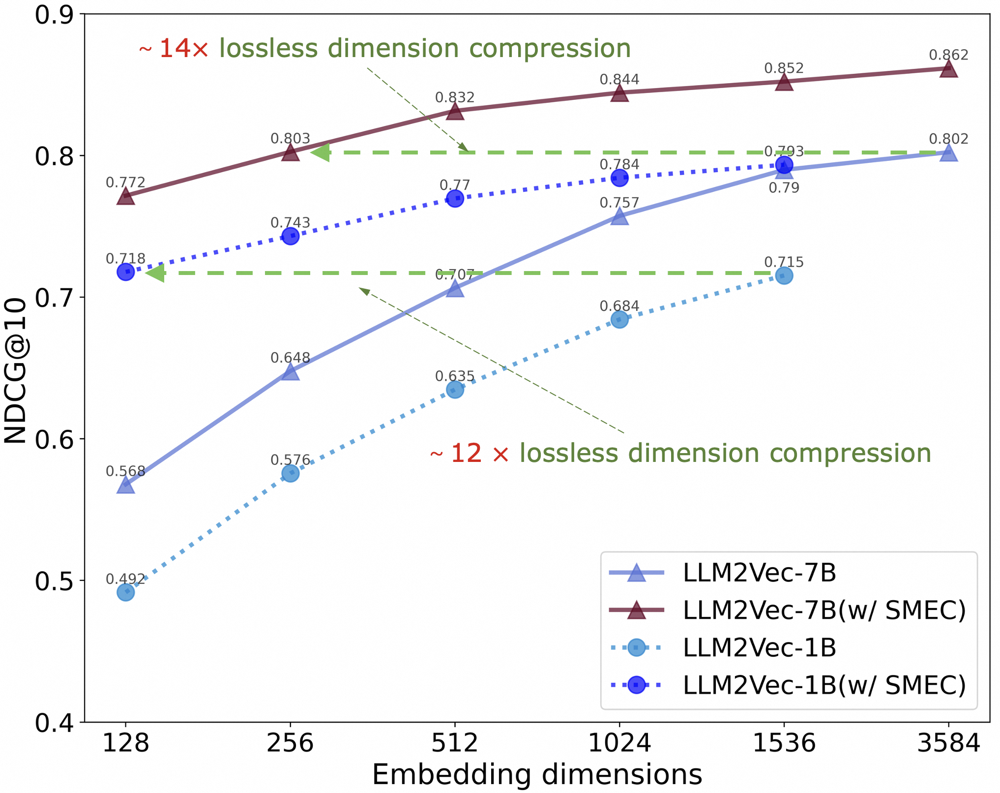
Figure 1: The effectiveness of the SMEC in dimensionality reduction. After customized training with the SMEC method on BEIR Quora dataset, the embeddings of LLM2Vec-7B (3584 dimensions) and LLM2Vec-1B (1536 dimensions) can achieve 14 $\times$ and 12 $\times$ lossless compression, respectively.
<details>
<summary>figures/overview.png Details</summary>
### Visual Description
\n
## Technical Diagram: Comparison of Three Adaptor Architectures
### Overview
The image presents a side-by-side comparison of three neural network adaptor architectures, labeled (a) Search-Adaptor, (b) Matryoshka-Adaptor, and (c) SMEC(ours). Each diagram illustrates the flow of data from an input through an encoder and subsequent fully connected layers, culminating in various loss function calculations. The diagrams use a consistent visual language: yellow boxes for input, blue trapezoids for encoders, orange bars for feature vectors, green boxes for fully connected layers, and colored blocks (red, grey, blue, orange) to represent different dimensional outputs. The rightmost diagram (c) includes an inset analogy using Matryoshka dolls to conceptualize the method.
### Components/Axes
**Common Components Across All Diagrams:**
* **Input:** A yellow rectangular box at the top.
* **Encoder:** A blue trapezoidal block below the input.
* **N:** A label indicating the dimension of the feature vector output by the encoder.
* **Feature Vector:** An orange horizontal bar representing the encoded output of dimension N.
* **Loss Functions:** Denoted by the script L, e.g., `L(x_{1:N})`. These are the final outputs of each branch.
**Diagram-Specific Components:**
**(a) Search-Adaptor:**
* **Layer Label:** "Fully Connected Layer × 4" inside a green box.
* **Sub-layer Dimensions:** Four smaller green boxes below, labeled: `M×N`, `M×N/2`, `M×N/4`, `M×N/8`.
* **Output Blocks:** Four vertical colored blocks (red, grey, blue, orange) of decreasing height, each feeding into a separate loss function.
* **Loss Functions:** Four distinct losses: `L(x_{1:N/8})`, `L(x_{1:N/4})`, `L(x_{1:N/2})`, `L(x_{1:N})`.
**(b) Matryoshka-Adaptor:**
* **Layer Label:** "Fully Connected Layer × 1" inside a green box, with `M×N` noted to its right.
* **Output Structure:** A single, segmented horizontal bar composed of four contiguous colored blocks (red, grey, blue, orange).
* **Loss Functions:** Four losses are calculated from prefixes of the segmented bar: `L(x_{1:N/8})`, `L(x_{1:N/4})`, `L(x_{1:N/2})`, `L(x_{1:N})`. These are collectively bracketed as `L(x)`.
**(c) SMEC(ours):**
* **Inset Analogy (Top-Right):** A beige box containing two rows.
* **Row 1:** Labeled "Matryoshka-Adaptor". Shows a large Matryoshka doll pointing to three smaller, nested dolls.
* **Row 2:** Labeled "SMEC(ours)". Shows a large Matryoshka doll pointing to three separate, non-nested dolls of different sizes.
* **Main Architecture:** A three-step process enclosed in a dashed box.
* **Step 1 (step1):** A green box "Fully Connected Layer × 1" (`M×N`). Outputs a segmented bar (blue, orange) leading to losses `L(x_{1:N/2})` and `L(x_{1:N})`, bracketed as `L₁(x)`.
* **Step 2 (step2):** A yellow box "Sub Fully Connected Layer" (`M×N/2`). Takes input from the blue segment of Step 1. Outputs a segmented bar (grey, blue) leading to losses `L(x_{1:N/4})` and `L(x_{1:N/2})`, bracketed as `L₂(x)`.
* **Step 3 (step3):** A blue box "Sub-sub Fully Connected Layer" (`M×N/4`). Takes input from the grey segment of Step 2. Outputs a segmented bar (red, grey) leading to losses `L(x_{1:N/8})` and `L(x_{1:N/4})`, bracketed as `L₃(x)`.
### Detailed Analysis
**Data Flow and Dimensionality:**
1. **Search-Adaptor (a):** The encoder output (dim N) is fed into four *parallel* fully connected layers of decreasing width (`M×N` to `M×N/8`). Each produces an independent output vector, and a separate loss is computed for each. This suggests a search over multiple representation granularities simultaneously.
2. **Matryoshka-Adaptor (b):** The encoder output (dim N) is processed by a *single* fully connected layer (`M×N`). The resulting vector is conceptually segmented. Losses are computed on progressively longer prefixes of this single vector (from the first `N/8` dimensions to all `N` dimensions). This creates nested, multi-scale representations within one vector.
3. **SMEC(ours) (c):** This is a *sequential, hierarchical* process.
* **Step 1:** Processes the full N-dimensional input to produce a coarse, two-segment representation.
* **Step 2:** Refines one segment (the blue one, representing the first `N/2` dimensions) using a sub-layer, creating a finer two-segment representation.
* **Step 3:** Further refines a sub-segment (the grey one from Step 2, representing the first `N/4` dimensions) using a sub-sub-layer.
* Losses are computed at each step on the available segments. The Matryoshka doll analogy highlights that SMEC creates separate, non-nested representations at each scale, unlike the nested dolls of the Matryoshka-Adaptor.
### Key Observations
* **Structural Paradigm Shift:** The diagrams show a clear evolution from parallel multi-branch (a), to single-branch nested (b), to hierarchical sequential refinement (c).
* **Loss Function Consistency:** All three methods ultimately compute losses for the same four dimensional granularities: `N/8`, `N/4`, `N/2`, and `N`. The difference lies in *how* the representations for these granularities are generated.
* **Visual Metaphor:** The Matryoshka doll inset in (c) is a critical explanatory element. It visually argues that the proposed SMEC method avoids the "nesting" constraint of the Matryoshka-Adaptor, potentially allowing for more independent and flexible feature learning at each scale.
* **Spatial Grounding:** In diagram (c), the "Sub Fully Connected Layer" (step2) is positioned to the right of and below the main step1 block, with a dashed arrow indicating it processes a segment from step1. Similarly, the "Sub-sub Fully Connected Layer" (step3) is further right and below step2, processing a segment from step2. This spatial arrangement reinforces the sequential, hierarchical nature of the process.
### Interpretation
This technical diagram serves as a conceptual blueprint for different methods of creating multi-scale or multi-granularity representations in neural networks, likely for tasks like retrieval or metric learning where representation size impacts efficiency and performance.
* **What the data suggests:** The progression from (a) to (c) suggests a research trajectory aimed at improving the efficiency and independence of multi-scale feature learning. Search-Adaptor (a) is computationally expensive (4 parallel layers). Matryoshka-Adaptor (b) is efficient (1 layer) but couples all scales via nesting. SMEC (c) proposes a middle ground: a structured, sequential process that maintains some independence between scales (as per the doll analogy) while potentially being more parameter-efficient than the parallel approach.
* **How elements relate:** The core relationship is between the dimensionality of the feature vector (`N`, `N/2`, etc.) and the architectural path taken to produce a useful representation at that scale. The loss functions `L(x_{1:N/k})` are the common objective, but the means of generating `x_{1:N/k}` differ fundamentally.
* **Notable anomalies/outliers:** The most significant "outlier" is the SMEC architecture itself. Its three-step, dashed-box structure breaks the visual pattern of the first two diagrams, emphasizing its novel, proposed nature. The explicit use of a cultural metaphor (Matryoshka dolls) to explain a technical concept is also a distinctive communicative choice.
* **Underlying purpose:** The diagram is designed to persuade. It visually argues that the authors' method (SMEC) combines the benefits of the prior approaches—multi-scale learning—while introducing a new hierarchical decomposition that may offer advantages in representation independence or training dynamics. The careful labeling of all dimensions (`M×N`, `M×N/2`, etc.) provides the necessary technical rigor to support this conceptual argument.
</details>
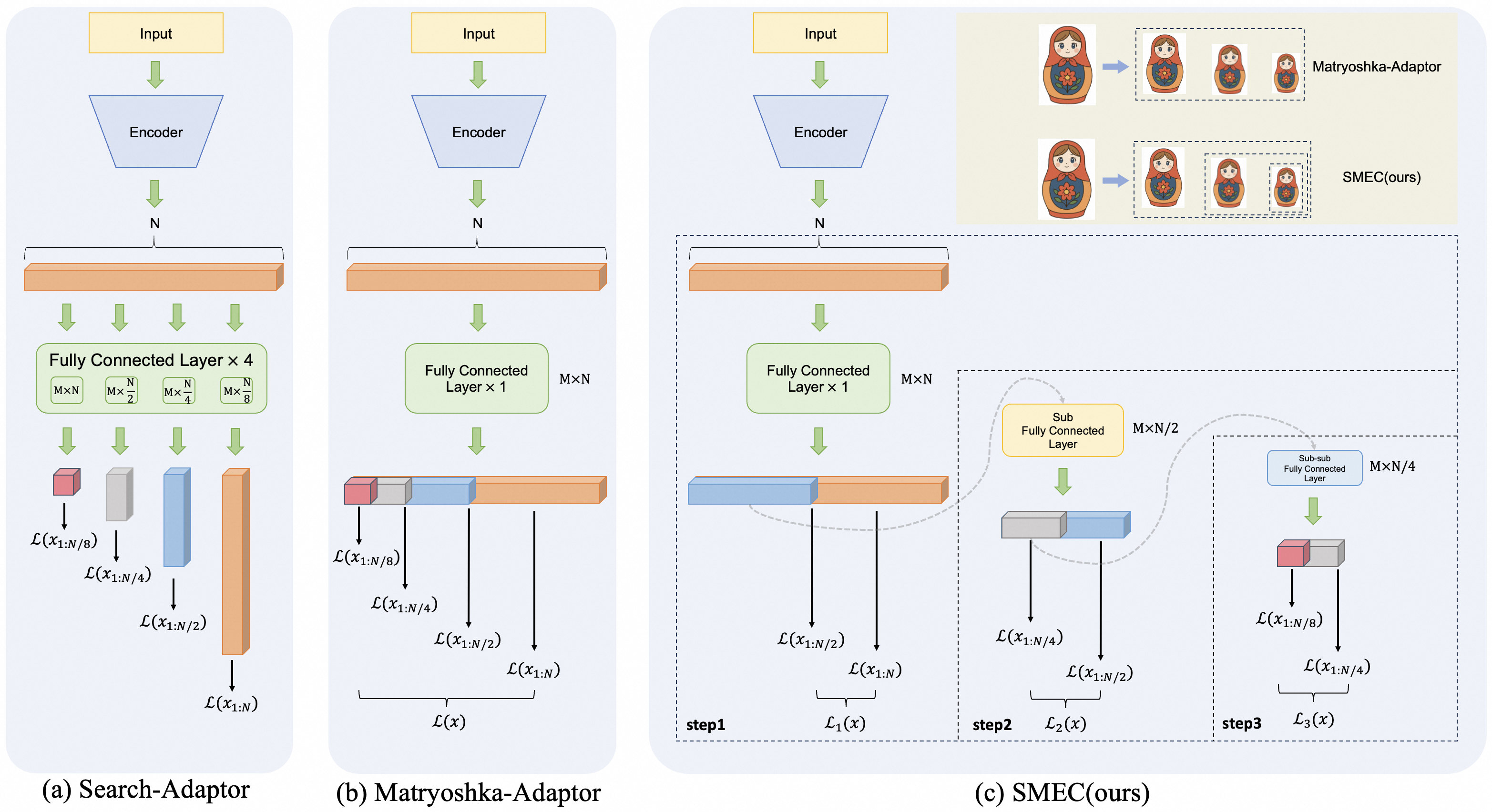
Figure 2: Illustration of embedding compression architectures and our proposed approach. (a) presents the direct feature dimensionality reduction performed by the Search-Adaptor using FC layers. (b) illustrates the Matryoshka-Adaptor, which employs a shared set of FC layers to generate low-dimensional embeddings with multiple output dimensions. A Matryoshka-like hierarchical inclusion relationship exists between the high- and low-dimensional embeddings. (c) presents our proposed Sequential Matryoshka Embedding Compression (SMEC) framework, which adopts a sequential approach to progressively reduce high-dimensional embeddings to the target dimension. The animated diagram in the upper-right corner vividly highlights the distinction between Matryoshka-Adaptor and SMEC.
Large language models excel in diverse text tasks due to their ability to capture nuanced linguistic structures and contextual dependencies. For instance, GPT-4 achieves state-of-the-art performance on benchmarks like GLUE Wang et al. (2018) and SuperGLUE Wang et al. (2019), demonstrating its proficiency in tasks such as natural language inference (NLI), question answering (QA), and text classification. This success is attributed to their transformer-based architectures Vaswani et al. (2017), which enable parallel processing of sequential data and capture long-range dependencies through self-attention mechanisms. Similarly, Llama-3 Grattafiori et al. (2024) and ChatGPT Brown et al. (2020) leverage similar principles to achieve comparable or superior performance in domain-specific and multi-lingual tasks.
LLMs are increasingly integrated into commercial information retrieval (IR) systems, such as search engines (e.g., Google’s MUM) and recommendation platforms (e.g., Netflix’s content retrieval). Their ability to generate embeddings for long documents (e.g., books, research papers) and dynamic queries (e.g., conversational search) makes them indispensable for modern applications. For example, the BEIR benchmark Thakur et al. (2021) evaluates cross-domain retrieval performance, where LLMs outperform traditional BM25 Robertson and Walker (1994) and BERT-based models Devlin et al. (2019) by leveraging contextual embeddings.
While LLMs’ high-dimensional embeddings enable sophisticated semantic modeling, their storage and computational costs hinder scalability. Embedding dimensions of LLMs typically range from 1,024 (e.g., GPT-3) to 4,096 (e.g., Llama-3), exacerbating storage overhead and computational inefficiency—especially in real-time systems requiring dynamic updates. Moreover, high-dimensional vectors degrade the performance of retrieval algorithms due to the curse of dimensionality Beyer et al. (1999). For example: exact nearest-neighbor search in high-dimensional spaces becomes computationally infeasible, necessitating approximate methods like FAISS Johnson et al. (2017) or HNSW Yury et al. (2018). Even with optimizations, query latency increases exponentially with dimensionality, limiting responsiveness in real-world applications.
To address these challenges, Matryoshka Representation Learning (MRL) Kusupati et al. (2022) encodes multi-scale information into a single embedding, balancing task complexity and efficiency. It achieves strong results in large-scale classification and retrieval tasks and has inspired variants like Matryoshka-Adaptor Yoon et al. (2024), which offers a scalable framework for transforming embeddings into structured representations with Matryoshka properties under both supervised and unsupervised settings. However, MRL’s multi-scale parallel training strategy simultaneously limits its practical application in industry. When the retrieval system requires a new low-dimensional embedding, retraining from scratch is necessary to achieve effective dimensionality reduction.
In this paper, we systematically analyze the limitations of MRL and its variants in embedding compression and propose three key enhancements: (1) a continued-training-friendly training framework named Sequential Matryoshka Representation Learning (SMRL); (2) an adaptive dimension selection (ADS) mechanism to minimize information degradation during dimension pruning; and (3) a Selectable Cross-batch Memory (S-XBM) strategy to enhance unsupervised learning between high- and low-dimensional embeddings.
## 2 Related Work
### 2.1 Matryoshka representation learning
Matryoshka representation learning introduces a novel paradigm where embeddings are pretrained to inherently support progressive dimension truncation. This enables fine-grained control over the trade-off between computational latency (via reduced dimensionality) and accuracy (via retained semantic structure). Key innovations include the design of Matryoshka properties, such as hierarchical information encoding and intra-cluster compactness, which ensure that even truncated embeddings retain utility for downstream tasks.
In addition to representation learning, the concept of MRL have been applied to image generation, such as Matryoshka Diffusion Models (MDM) Gu et al. (2023); multimodal content understanding, such as $M^{3}$ Cai et al. (2024); and Multimodal Large Language Model (MLLM), such as Matryoshka Query Transformer (MQT) Hu et al. (2024).
### 2.2 Embedding Compression
Embedding compression aims to reduce the computational and memory footprint of neural network models or embeddings while preserving their utility for downstream tasks. This objective has driven research across multiple paradigms, each addressing different trade-offs between compression efficiency, performance retention, and adaptability. Early approaches primarily focused on unsupervised techniques based on linear algebra, such as Principal Component Analysis (PCA) Jolliffe and Cadima (2016), Linear Discriminant Analysis (LDA) Mclachlan , and Non-negative Matrix Factorization (NMF) Lee and Seung (2000). Building upon these, autoencoders and their variants, such as Variational Autoencoders (VAEs) Kingma et al. (2013), have gradually emerged as powerful tools for nonlinear dimensionality reduction, capable of capturing complex data distributions. With the development of deep learning, methods such as Contrastive Predictive Coding (CPC) Oord et al. (2018) and Momentum Contrast (MoCo) He et al. (2020) are capable of learning robust and compact representations from unlabeled data.
Recently, customized methods such as Search-Adaptor Yoon et al. (2023) and Matryoshka-Adaptor Yoon et al. (2024) have emerged as a new trend in embedding compression. They achieve significant dimensionality reduction by adding only a small number of parameters to the original representation model and retraining it on specific data.
## 3 Method
### 3.1 Rethinking MRL for embedding compression
MRL employs a nested-dimensional architecture to train models that learn hierarchical feature representations across multiple granularities. This allows adaptive deployment of models based on computational constraints. Specifically, MRL defines a series of models $f_{1},f_{2},\ldots,f_{M}$ that share identical input and output spaces but progressively expand their hidden dimensions.
The term Matryoshka derives from the hierarchical parameter structure where the parameters of model $f_{m}$ are nested within those of its successor $f_{m+1}$ . To illustrate, consider a FC layer within the largest model $f_{M}$ , which contains $d_{M}$ neurons in its hidden layer. Correspondingly, the FC layer of $f_{m}$ retains the first $d_{m}$ neurons of this structure, with dimensions satisfying $d_{1}\leq d_{2}\leq\dots\leq d_{M}$ . MRL jointly trains these models using the following objective:
$$
\sum_{m=1}^{M}c_{m}\cdot\mathcal{L}(f_{m}(\mathbf{x});y), \tag{1}
$$
where $\mathcal{L}$ denotes the loss function, $y$ represents the ground-truth label, and $c_{m}$ are task-specific weighting coefficients. Notably, each training iteration requires forward and backward propagation for all $M$ models, resulting in substantial computational overhead compared to training a single standalone model. Upon convergence, MRL enables flexible inference by selecting any intermediate dimension $d_{i}\leq d_{M}$ , thereby accommodating diverse computational constraints.
Although the MRL method has partially mitigated the performance degradation of representations during dimensionality reduction, we contend that it still faces the following three unresolved issues:
Gradient Fluctuation. In large-scale vector retrieval systems, sample similarity is measured by the distance between their representation vectors. Consequently, the optimization of embedding models typically employs loss functions based on embedding similarity. In this condition, according to the derivation in Appendix A, the loss function $\mathcal{L}^{d}$ of MRL under dimension $d$ satisfies the following relationship with respect to the parameter $\mathbf{w}_{i}$ in the $i$ -th dimension of the FC layer:
$$
\frac{\partial\mathcal{L}^{d}}{\partial\mathbf{w}_{i}}\propto\frac{1}{\delta(d)^{2}}. \tag{2}
$$
Here, $\delta(d)$ is a complex function that is positively correlated with the dimension $d$ . This equation provides a mathematical foundation for analyzing gradient fluctuations in multi-dimensional joint optimization architecture. It indicates that during the MRL training process, loss functions from various dimensions result in gradients of varying magnitudes on the same model parameter, thereby increasing gradient variance. In Section 5.2, we empirically demonstrated that the conclusion above is applicable to different loss functions. We propose a solution to resolve the aforementioned problem in Section 3.2.
Information Degradation. Neural network parameters exhibit heterogeneous contributions to model performance, as demonstrated by the non-uniform distribution of their gradients and feature importance metrics Frankle and Carbin (2018). The MRL method employs a dimension truncation strategy (e.g., $D\rightarrow D/2\rightarrow D/4\ldots$ ) to prune parameters and reduce feature dimensions by retaining partial parameters. However, this approach fails to adequately preserve critical parameters because it relies on a rigid, static truncation rule. Although MRL employs joint training of high- and low-dimensional vectors to redistribute information between truncated and retained parameters, this process is unavoidably accompanied by information degradation. Specifically, discarded parameters may contain essential information, such as unique feature mappings or high-order dependencies, that cannot be effectively recovered by the remaining ones. Empirical evidence, such as accuracy degradation and increased generalization gaps, demonstrates that such loss leads to suboptimal model performance and slower convergence Li et al. (2023). In summary, while MRL enables hierarchical dimensionality reduction, its inability to selectively retain critical parameters and the inherent information degradation during post-truncation training ultimately undermine its effectiveness in maintaining model performance. In Section 3.3, we propose a more effective dimension pruning method.
<details>
<summary>figures/fig_ads.png Details</summary>
### Visual Description
## Diagram: Learnable Dimension Pruning with Rank Loss
### Overview
The image is a technical flowchart illustrating a machine learning process for dimensionality reduction or feature selection. It depicts a two-pathway system where a learnable parameter guides the selection of specific dimensions (features) from an input data stack, followed by a pruning step that reduces the dimensionality. The process is evaluated using a "Rank Loss" function at two different stages.
### Components/Axes
The diagram is organized into two main horizontal pathways (top and bottom) within a dashed-line border. All text is in English.
**Key Components & Labels:**
1. **Learnable Parameter:** A block of four light-green squares in the top-left.
2. **Selection Mechanism:** An arrow labeled `gumbel_softmax + topk select` points from the "Learnable Parameter" to a list.
3. **Selected Indices:** The list is denoted as `[1,3,..., X_{i-2}, X_{i-1}]`. Small colored squares (light green, medium green, dark green) are shown above this list.
4. **Input Data Stacks:** Two identical vertical stacks of colored rectangles, representing data dimensions or features. They are labeled from top to bottom:
* `X_1` (lightest green)
* `X_2`
* `X_3`
* `...` (ellipsis)
* `X_{i-2}`
* `X_{i-1}`
* `X_i` (darkest green)
* One stack is in the top-center, the other in the bottom-left.
5. **Dimension Pruning:** A blue arrow labeled `Dimension Pruning` points from the selected indices list to the bottom data stack.
6. **Output Dimension Blocks:** Two orange vertical blocks.
* Top pathway: Labeled `D dim`.
* Bottom pathway: Labeled `D/2 dim`.
7. **Loss Function:** The text `Rank Loss` appears twice, at the end of both the top and bottom pathways.
8. **Flow Arrows:** Blue arrows indicate the direction of data/process flow throughout the diagram.
### Detailed Analysis
**Spatial Layout and Flow:**
* **Top Pathway (Full Dimension):** Starts with the "Learnable Parameter" (top-left). The selection mechanism (`gumbel_softmax + topk select`) produces a list of selected indices. This list points to the top "Input Data Stack" (top-center), implying these indices select specific rows (`X` features) from the stack. The selected data flows (blue arrow) into the `D dim` block (top-right), which then flows to the `Rank Loss` calculation.
* **Bottom Pathway (Pruned Dimension):** Starts with the second "Input Data Stack" (bottom-left). The same list of selected indices from the top pathway points down to this stack via the `Dimension Pruning` arrow. This results in a reduced stack (bottom-center) containing only the selected rows (e.g., `X_1`, `X_2`, `...`, `X_{i-2}`, `X_{i-1}`). This pruned data flows into the `D/2 dim` block (bottom-right), which then flows to a second `Rank Loss` calculation.
**Component Relationships:**
* The "Learnable Parameter" and `gumbel_softmax + topk select` mechanism are the control unit, determining which dimensions (`X` features) are important.
* The two "Input Data Stacks" represent the same original high-dimensional data.
* "Dimension Pruning" is the action that physically removes the unselected dimensions, creating a smaller dataset.
* The `D dim` and `D/2 dim` blocks represent the data after selection (full set of selected dimensions) and after pruning (a reduced set, hypothetically half the original dimension `D`), respectively.
* `Rank Loss` is the objective function applied to both the selected full-dimension representation and the pruned representation, likely to ensure the pruning preserves the relative ranking or structural information of the data.
### Key Observations
1. **Color Coding:** A consistent green gradient is used for data dimensions (`X_1` light to `X_i` dark). The selection list uses matching colored squares. Orange is used for dimensionality blocks (`D dim`, `D/2 dim`). Blue is used for process arrows.
2. **Dimension Reduction:** The bottom pathway explicitly reduces the data from a stack of `i` dimensions to a smaller stack. The label `D/2 dim` suggests the output dimension is half of some original dimension `D`.
3. **Differentiable Selection:** The use of `gumbel_softmax` indicates this is a method for making discrete selection (top-k) differentiable, allowing the "Learnable Parameter" to be trained via backpropagation.
4. **Dual Evaluation:** The process is evaluated with `Rank Loss` at two points: on the data after selection but before pruning (top), and on the data after pruning (bottom). This suggests the loss is used to train the learnable parameters to select dimensions that are important for maintaining the data's rank structure.
### Interpretation
This diagram illustrates a **learnable feature selection or dimension pruning technique** for machine learning models. The core idea is to use a small set of learnable parameters, optimized via a Gumbel-Softmax trick, to automatically identify and select the most important input dimensions (`X` features). The selected dimensions are then used to create a pruned, lower-dimensional representation of the data (`D/2 dim`).
The use of **Rank Loss** is critical. It implies the goal is not merely to reconstruct the input data, but to preserve the *relative ordering* or *similarity structure* within the data after dimensionality reduction. This is common in tasks like retrieval, ranking, or metric learning. By applying the loss to both the selected and pruned representations, the model likely ensures that the selection process itself is optimal for the final, compressed output.
The process flow suggests an end-to-end trainable system where the selection mechanism and the downstream task (modeled by the Rank Loss) are optimized jointly. The "Dimension Pruning" step is the practical application, resulting in a more efficient model with fewer input features (`D/2` instead of `D`), while the dual loss calculation ensures fidelity to the original data's structure.
</details>
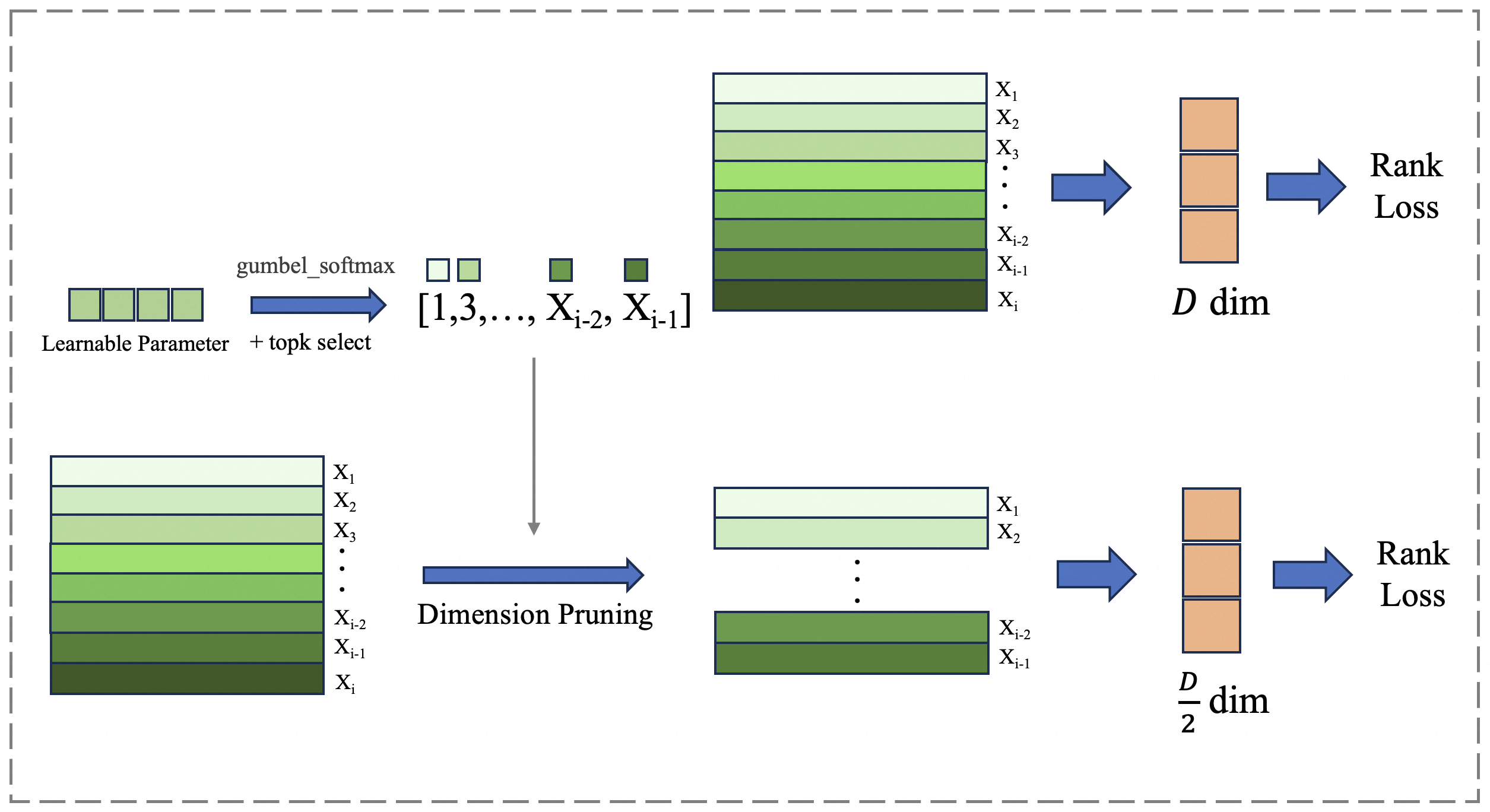
Figure 3: The ADS module introduces a set of learnable parameters to dynamically select dimensions based on their importance during the dimensionality reduction process.
Sample Selection. The MRL framework employs supervised learning to jointly train high-dimensional ( $D$ ) and low-dimensional ( $D^{\prime}$ ) features. However, the number of available samples is limited by manual annotation. Matryoshka-Adaptor introduces in-batch sample mining strategies to expand the training sample scale, thereby addressing the inherent limitation. Specifically, it generates cross-sample pairs via the cartesian product of batch samples:
$$
\mathcal{P}=\{(x_{i},x_{j})\mid x_{i},x_{j}\in\text{Batch},\ i\neq j\}. \tag{3}
$$
This approach creates $B(B-1)$ pairs per batch (where $B$ denotes the batch size), enabling cross-sample comparisons within large batches. However, this indiscriminate pairing introduces noise from non-representative or irrelevant sample pairs.
In light of this limitation, the method employs Top- $k$ similarity-based selection:
$$
\begin{split}\mathcal{P}_{\text{top-}k}&=\text{Top}_{k}\left(\text{similarity}(x_{i},x_{j})\right),\\
&\quad\forall\ (x_{i},x_{j})\in\mathcal{P}.\end{split} \tag{4}
$$
Here, only the top- $k$ most similar pairs are retained for training, reducing computational overhead while focusing on informative interactions. Despite this improvement, the diversity of effective samples remains fundamentally constrained by the original batch size $B$ . In Section 3.4, we develop a strategy that empowers the model to mine global sample beyond the current batch.
### 3.2 Sequential Matryoshka Representation Learning
Applying the conclusions from Section 3.1 to the MRL training process, and take the parallel dimensionality reduction process $[D,D/2,D/4]$ as an example. The ratio of the average gradients for parameters $\mathbf{w}_{i}(i\in[0,D/4])$ and $\mathbf{w}_{j}(j\in[D/4,D/2])$ is as follows:
$$
\displaystyle\overline{\text{grad}_{i}} \displaystyle:\overline{\text{grad}_{j}}=\left(\frac{\partial\mathcal{L}^{D}}{\partial\mathbf{w}_{i}}+\frac{\partial\mathcal{L}^{D/2}}{\partial\mathbf{w}_{i}}+\frac{\partial\mathcal{L}^{D/4}}{\partial\mathbf{w}_{i}}\right) \displaystyle:\left(\frac{\partial\mathcal{L}^{D}}{\partial\mathbf{w}_{i}}+\frac{\partial\mathcal{L}^{D/2}}{\partial\mathbf{w}_{i}}\right)\approx 1+\frac{\delta(D/2)^{2}}{\delta(D/4)^{2}}. \tag{5}
$$
As shown in Equation 3.2, the average gradient magnitude of parameter $\mathbf{w}_{i}$ can be approximated as $1+\frac{\delta(D/2)^{2}}{\delta(D/4)^{2}}$ times that of parameter $\mathbf{w}_{j}$ , primarily due to the influence of the lower-dimensional loss function $\mathcal{L}^{D/4}$ . To resolve this issue, we propose Sequential Matryoshka Representation Learning (SMRL), which substitutes the original parallel compression of embeddings with a sequential approach, as illustrated in the Figure 2. Assuming a dimensionality reduction trajectory of $[D,D/2,D/4,\dots,D/2^{n}]$ . In each iteration, only the immediate transition (e.g., $D/2^{n-1}\rightarrow D/2^{n}$ ) is trained, avoiding the inclusion of lower-dimensional losses that amplify gradients for low-dimensional parameters. By eliminating the above factor, the gradients of $\mathbf{w}_{i}(i\in[0,D/2^{n}])$ follow a consistent distribution with reduced variance, improving convergence speed and performance. Once the loss converges in the current iteration, the dimensionality reduction $D/2^{n-1}\rightarrow D/2^{n}$ is complete, and the process proceeds to the next stage $D/2^{n}\rightarrow D/2^{n+1}$ , repeating the procedure until the target dimension is reached. Additionally, after convergence in one iteration, the optimal parameters for the current dimension are fixed to prevent subsequent reductions from degrading their performance. Notably, compared to MRL, the SMRL framework is more amenable to continued training. In scenarios where low-dimensional retrieval embeddings (e.g., D/8) or intermediate embeddings (e.g., D/3) are required, these can be obtained through further dimensionality reduction training based on the already preserved D/4 or D/2 parameters, eliminating the need for retraining from scratch as is typically required in MRL.
### 3.3 Adaptive Dimension Selection Module
Since directly truncating dimensions to obtain low-dimensional representations in MRL inevitably leads to information degradation, we propose the Adaptive Dimension Selection (ADS) module to dynamically identify important dimensions during training. As illustrated in Figure 3, we introduce a set of learnable parameters that represent the importance of different dimensions in the original representation $\mathbf{Z}(\text{dim}=D)$ , and use these parameters to perform dimensional sampling, obtaining a reduced-dimension representation $\mathbf{Z}^{\prime}(\text{dim}=D/2)$ . Since the sampling operation is non-differentiable, during the training phase, we utilize the Gumbel-Softmax Jang et al. (2016) to approximate the importance of different dimensions. This is achieved by adding Gumbel-distributed noise $G\sim\text{Gumbel}(0,1)$ to the logits parameters $\hat{\mathbf{z}}$ for each dimension, followed by applying the softmax function to the perturbed logits to approximate the one-hot vector representing dimension selection. Mathematically, this can be expressed as:
$$
\mathbf{z}=\text{softmax}_{\tau}(\hat{\mathbf{z}}+G). \tag{6}
$$
Importantly, the Gumbel approximation allows the softmax scores of dimension importance to be interpreted as the probability of selecting each dimension, rather than enforcing a deterministic selection of the top- $k$ dimensions. This achieves a fully differentiable reparameterization, transforming the selection of embedding dimensions into an optimizable process.
<details>
<summary>figures/fig3.png Details</summary>
### Visual Description
## Diagram: Machine Learning Pipeline with Cross-Batch Memory (XBM)
### Overview
This image is a technical diagram illustrating a machine learning training pipeline. The system processes data through a frozen model, utilizes a memory bank (XBM) to store and retrieve feature representations, computes similarity scores, performs top-k sampling, and finally calculates a pair-based loss. The flow is primarily left-to-right with a vertical memory interaction.
### Components/Axes
The diagram consists of several distinct components connected by arrows indicating data flow. There are no traditional chart axes. The key labeled components are:
1. **Frozen model**: A gray box on the far left, representing a pre-trained model whose parameters are not updated during this training phase.
2. **XBM (Cross-Batch Memory)**: A vertically oriented, dashed-line box containing a stack of colored rectangles. It has two labeled operations:
* `enqueue`: An arrow pointing into the bottom of the XBM.
* `dequeue`: An arrow pointing out of the top of the XBM.
3. **Score matrix**: A 4x4 grid of empty squares, representing a matrix of similarity scores.
4. **Top-k sample**: A label next to a large blue arrow pointing downward.
5. **FC Layer**: A vertical rectangle labeled "FC Layer" (Fully Connected Layer).
6. **Pair-based loss**: A green, rounded rectangle on the far right, representing the final loss function.
### Detailed Analysis
**Data Flow and Component Relationships:**
1. **Input to Frozen Model**: The process begins with data (not shown) entering the "Frozen model" (leftmost gray box).
2. **Feature Extraction & Memory Enqueue**: The frozen model outputs a batch of feature vectors, represented by three light green vertical bars inside a dashed box. A blue arrow points from this output to the right. A branch from this path, indicated by a gray line and an upward blue arrow labeled `enqueue`, sends these new features into the bottom of the **XBM** memory bank.
3. **XBM Memory Bank**: The XBM is depicted as a stack of horizontal bars in three colors:
* Top three bars: Yellow
* Middle three bars: Light blue
* Bottom three bars: Light green
This color-coding likely represents different batches or types of stored features. The `dequeue` arrow at the top indicates older features are removed from the memory.
4. **Score Matrix Computation**: The current batch's features (the three light green bars) and the features retrieved from the XBM (implied by the gray line connecting the XBM to the multiplication symbol) are combined. A green circle with a white "X" (multiplication operator) symbolizes a dot product or similarity computation. The result is the **Score matrix**, a 4x4 grid. This suggests the current batch is compared against a set of features from memory, producing a matrix of pairwise similarity scores.
5. **Top-k Sampling**: A large blue arrow labeled `Top-k sample` points downward from the Score matrix to a new set of feature bars. This operation selects the top-k most similar (or dissimilar, depending on the loss) pairs from the score matrix. The resulting set, shown in a dashed box, contains a mix of light green and light blue bars, indicating it's a sampled subset combining current and memory features.
6. **Loss Calculation**: The sampled features are passed through an **FC Layer** (a transformation). The output then flows to the final component, the **Pair-based loss** function (green rounded rectangle), which computes the training objective (e.g., contrastive loss, triplet loss) based on the selected pairs.
### Key Observations
* **Color Consistency**: The light green color is used consistently for the output of the frozen model and the corresponding bars in the XBM and the top-k sampled set, indicating these are the "current" or "anchor" features. Light blue appears in the XBM and the sampled set, representing "memory" or "positive/negative" features. Yellow bars are only in the XBM and are not selected in the top-k sample shown.
* **Spatial Layout**: The XBM is positioned above the main data flow, emphasizing its role as an external memory bank that interacts with the primary pipeline. The flow is linear until the score computation, which involves a vertical interaction with memory.
* **Data Transformation**: The diagram clearly shows a transformation from raw features (green bars) to a similarity space (score matrix), then to a selected subset (sampled bars), and finally to a loss value.
### Interpretation
This diagram depicts a sophisticated training strategy, likely for **metric learning** or **self-supervised learning** (e.g., MoCo, BYOL variants). The core innovation is the **Cross-Batch Memory (XBM)**.
* **Purpose**: The pipeline addresses the limitation of small batch sizes in contrastive learning. By maintaining a memory bank (XBM) of feature representations from previous batches, the model can compare the current batch against a much larger and more diverse set of examples, improving training stability and performance.
* **Mechanism**: The frozen model ensures stable feature extraction. The `enqueue`/`dequeue` mechanism implements a FIFO queue, keeping the memory bank updated with recent features. The **Score matrix** computes similarities between the current batch and the memory bank. **Top-k sampling** is a critical step that selects the most informative pairs (e.g., hardest positives or negatives) for loss computation, making the training more efficient and effective.
* **Flow Logic**: The system creates a dynamic, expanding set of comparisons for each training step. The pair-based loss then updates the trainable part of the network (not shown, but implied to be connected to the frozen model or a separate projector) to improve the feature space, pulling positive pairs closer and pushing negative pairs apart.
* **Notable Design**: The separation of the "Frozen model" suggests this could be part of a larger architecture where only a projection head or a specific module is being trained, while the backbone remains fixed to preserve learned representations. The use of a memory bank is a key technique for scaling contrastive learning beyond the GPU batch size.
</details>
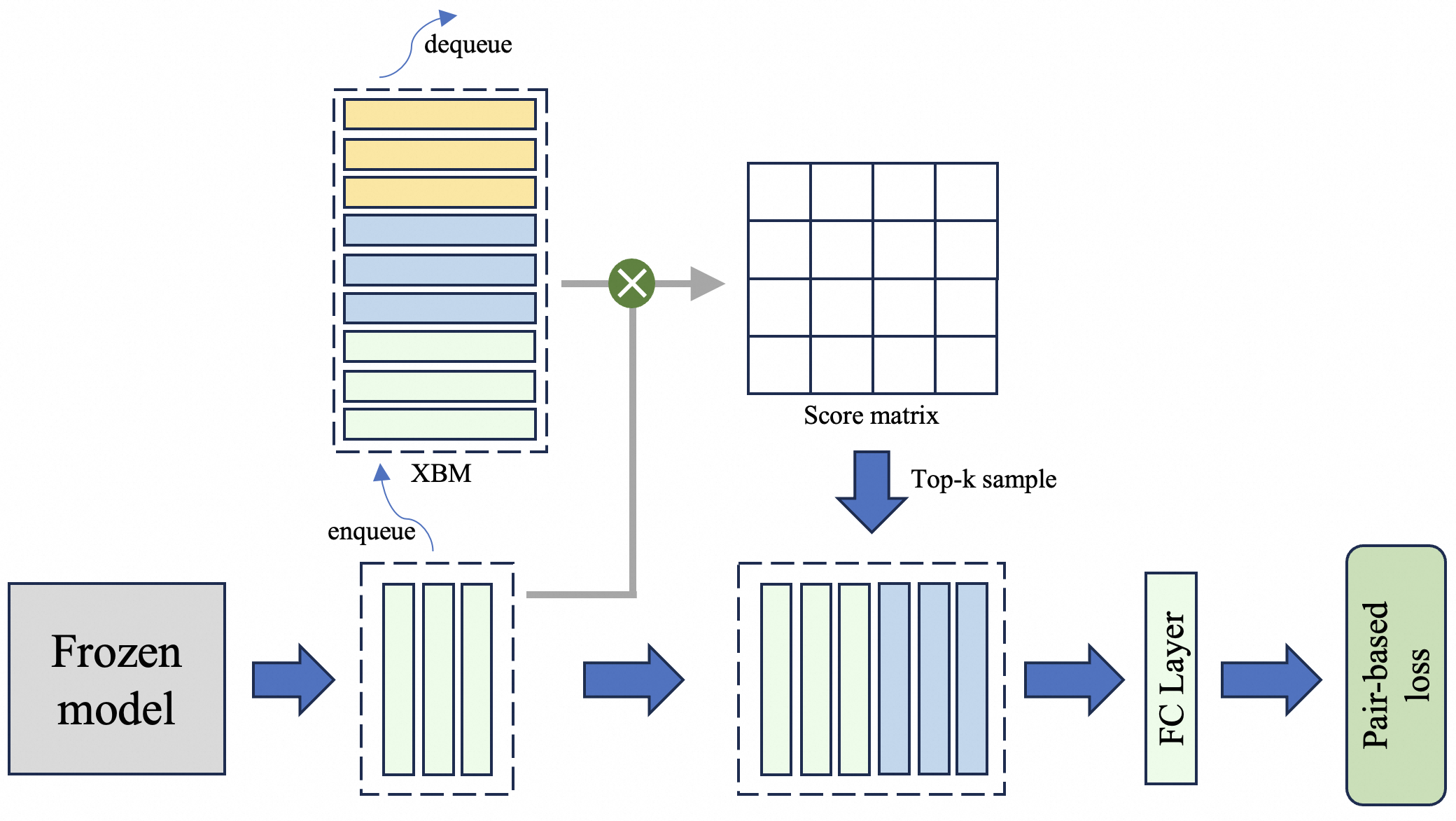
Figure 4: S-XBM maintains a queue during training to store historical features across batches. Rather than incorporating all stored features into the current batch, it selectively leverages hard samples that exhibit high similarity to the current batch samples.
### 3.4 Selectable Cross-Batch Memory
A natural teacher-student relationship inherently exists between the original embedding and its reduced-dimensional counterpart, making it feasible to improve the compressed embedding through unsupervised learning Yoon et al. (2024). However, as discussed in Section 3.1, performing this process within a single batch suffers from sample noise and insufficient diversity. As illustrated in Figure 4, we propose the Selectable Cross-Batch Memory (S-XBM) module, which constructs a first-in-first-out (FIFO) queue during training to store original embeddings across batches, with the aim of addressing this limitation. Unlike the original XBM Wang et al. (2020), we introduce two task-specific improvements: (1) retrieving only the top‑ $k$ most similar samples from the memory bank to construct new batches, and (2) deferring the trainable FC layer and only storing features generated by the frozen backbone, thereby avoiding feature drift. The unsupervised loss between original embedding $emb$ and low-dimensional embedding $emb[:d]$ is as follows:
$$
\displaystyle{\mathcal{L}_{un-sup}} \displaystyle=\sum_{i}\sum_{j\in\mathcal{N}_{K}(i)}\left|\text{Sim}(emb_{i},emb_{j})\right. \displaystyle\quad\left.-\text{Sim}(emb_{i}[:d],emb_{j}[:d])\right| \tag{7}
$$
where $\mathcal{N}_{K}(i)$ denotes the set of the top $k$ most similar embeddings to $emb_{i}$ within the S-XBM module.
<details>
<summary>figures/fig_openai.png Details</summary>
### Visual Description
## Line Chart: Performance (NDCG@10) vs. Embedding Dimensions
### Overview
The image is a line chart comparing the performance of four different methods or models as a function of embedding dimension size. The performance metric is NDCG@10 (Normalized Discounted Cumulative Gain at rank 10), expressed as a percentage. The chart demonstrates how each method's effectiveness scales with increased dimensionality.
### Components/Axes
* **Chart Type:** Multi-series line chart with markers.
* **Y-Axis:**
* **Label:** `NDCG@10/%`
* **Scale:** Linear, ranging from 50 to 62.
* **Major Ticks:** 50, 52, 54, 56, 58, 60, 62.
* **X-Axis:**
* **Label:** `Dimensions`
* **Scale:** Appears to be logarithmic (base 2), with discrete points.
* **Tick Labels (Categories):** 128, 256, 512, 768, 1536, 3072.
* **Legend:** Located in the bottom-right quadrant of the chart area.
* **Position:** Bottom-right, inside the plot area.
* **Series (in order of appearance in legend):**
1. `Original(MRL)` - Blue line with circle markers.
2. `search-adaptor` - Orange line with 'x' (cross) markers.
3. `MRL-Adaptor` - Green line with triangle markers.
4. `SMEC` - Yellow/Gold line with square markers.
### Detailed Analysis
**Data Series and Approximate Values:**
Values are estimated based on the grid lines. The trend for all series is upward (positive slope) as dimensions increase.
1. **Original(MRL) [Blue, Circle]:**
* **Trend:** Steady, moderate upward slope. Consistently the lowest-performing series.
* **Data Points (Approx.):**
* 128: ~49.2%
* 256: ~53.9%
* 512: ~55.5%
* 768: ~56.1%
* 1536: ~56.6%
* 3072: ~57.0%
2. **search-adaptor [Orange, 'x']:**
* **Trend:** Steep initial increase from 128 to 512 dimensions, then a more gradual rise. Performs better than Original(MRL) but worse than MRL-Adaptor and SMEC.
* **Data Points (Approx.):**
* 128: ~51.6%
* 256: ~57.1%
* 512: ~59.3%
* 768: ~60.1%
* 1536: ~61.0%
* 3072: ~61.3%
3. **MRL-Adaptor [Green, Triangle]:**
* **Trend:** Strong upward slope, closely following but slightly below the SMEC line. Second-best performer.
* **Data Points (Approx.):**
* 128: ~54.6%
* 256: ~58.4%
* 512: ~59.8%
* 768: ~60.5%
* 1536: ~61.3%
* 3072: ~61.8%
4. **SMEC [Yellow/Gold, Square]:**
* **Trend:** Consistently the highest-performing series across all dimensions. Shows a strong, steady increase.
* **Data Points (Approx.):**
* 128: ~56.7%
* 256: ~59.4%
* 512: ~60.4%
* 768: ~61.0%
* 1536: ~61.6%
* 3072: ~61.9%
### Key Observations
1. **Performance Hierarchy:** A clear and consistent performance hierarchy is maintained across all tested dimensions: **SMEC > MRL-Adaptor > search-adaptor > Original(MRL)**.
2. **Diminishing Returns:** All curves show signs of diminishing returns. The performance gain from doubling dimensions is much larger at the lower end (e.g., 128 to 256) than at the higher end (e.g., 1536 to 3072).
3. **Convergence at High Dimensions:** The performance gaps between the top three methods (SMEC, MRL-Adaptor, search-adaptor) narrow significantly as dimensions increase towards 3072, suggesting they may be approaching a performance ceiling for this task.
4. **Baseline Performance:** The `Original(MRL)` method serves as a baseline, and all three "adaptor" or enhanced methods (`search-adaptor`, `MRL-Adaptor`, `SMEC`) provide substantial improvements over it, especially at lower dimensions.
### Interpretation
This chart likely comes from a research paper or technical report in the field of information retrieval, machine learning, or natural language processing, where embedding dimensionality is a key hyperparameter.
* **What the data suggests:** The data demonstrates that the proposed methods (`search-adaptor`, `MRL-Adaptor`, and particularly `SMEC`) are effective at improving ranking performance (NDCG@10) over a baseline (`Original(MRL)`). The `SMEC` method appears to be the most efficient, achieving higher performance at every dimension size.
* **How elements relate:** The x-axis (Dimensions) represents a resource cost (model size, computational complexity). The y-axis (NDCG@10) represents the quality of the output. The chart visualizes the trade-off between cost and quality for each method. The steeper slopes of the adaptor methods at lower dimensions indicate they are more "data- or parameter-efficient" – they achieve a greater performance boost per added dimension compared to the baseline.
* **Notable trends/anomalies:** The most notable trend is the consistent superiority of SMEC. There are no anomalous data points; all series follow smooth, logical trajectories. The convergence at the high end is a common phenomenon in scaling experiments, indicating that simply increasing model size yields progressively smaller benefits, and architectural innovations (like those in SMEC) become more critical for pushing performance boundaries. The chart argues that using an advanced method like SMEC allows one to achieve the same performance as a simpler method but with a much smaller (and thus cheaper) model dimension. For example, SMEC at 256 dimensions (~59.4%) outperforms Original(MRL) at 3072 dimensions (~57.0%).
</details>
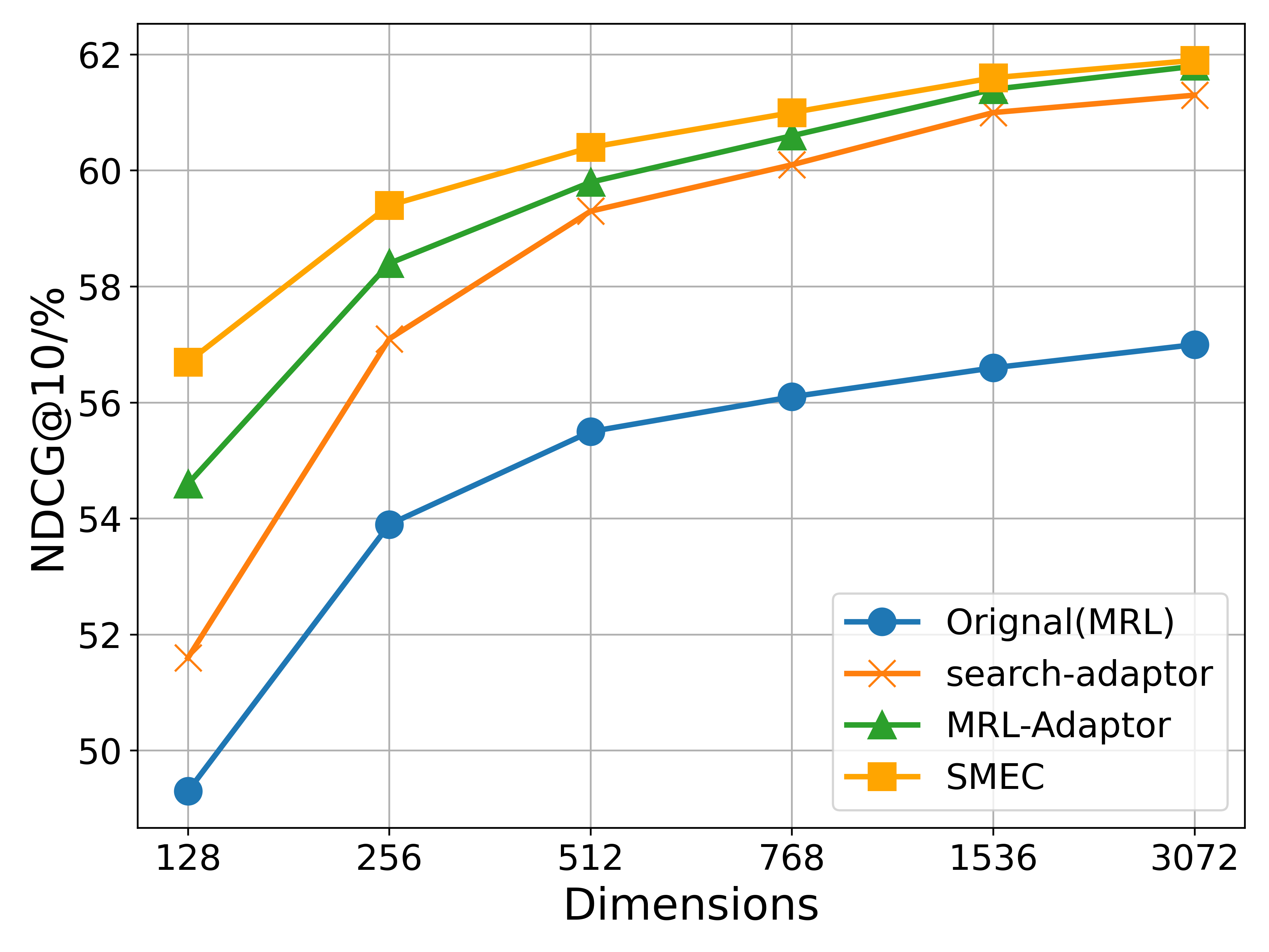
(a) OpenAI text embeddings
<details>
<summary>figures/fig_llm2vec.png Details</summary>
### Visual Description
## Line Chart: Performance of Dimensionality Reduction Methods on NDCG@10
### Overview
This is a line chart comparing the performance of four different dimensionality reduction or adaptation methods across varying embedding dimensions. The performance metric is NDCG@10 (Normalized Discounted Cumulative Gain at rank 10), expressed as a percentage. The chart demonstrates how each method's effectiveness scales with increased dimensionality.
### Components/Axes
* **X-Axis (Horizontal):** Labeled "Dimensions". It represents the dimensionality of the embedding space. The axis markers are at specific, non-linear intervals: 128, 256, 512, 768, 1536, and 3584.
* **Y-Axis (Vertical):** Labeled "NDCG@10/%". It represents the ranking performance score as a percentage. The scale ranges from 30 to approximately 62, with major gridlines at intervals of 5 (30, 35, 40, 45, 50, 55, 60).
* **Legend:** Located in the bottom-right quadrant of the chart area. It contains four entries, each associating a line color and marker style with a method name:
1. **Blue line with circle markers:** "Orignal(PCA)" [sic - likely a typo for "Original"].
2. **Orange line with 'x' markers:** "Search-Adaptor".
3. **Green line with triangle markers:** "MRL-Adaptor".
4. **Yellow/Orange line with square markers:** "SMEC".
### Detailed Analysis
**Trend Verification & Data Point Extraction:**
All four data series show a positive trend: NDCG@10 increases as the number of dimensions increases. The rate of improvement generally slows down (diminishing returns) at higher dimensions.
1. **Orignal(PCA) [Blue, Circle]:**
* **Trend:** Steep, consistent upward slope across the entire range. It shows the most dramatic relative improvement.
* **Approximate Data Points:**
* 128 Dimensions: ~31%
* 256 Dimensions: ~40.5%
* 512 Dimensions: ~46.5%
* 768 Dimensions: ~50.5%
* 1536 Dimensions: ~53.5%
* 3584 Dimensions: ~55.5%
2. **Search-Adaptor [Orange, 'x']:**
* **Trend:** Starts lower than MRL-Adaptor and SMEC, rises sharply until 512 dimensions, then continues to rise more gradually. It remains the lowest-performing of the three adaptor methods throughout.
* **Approximate Data Points:**
* 128 Dimensions: ~51%
* 256 Dimensions: ~56.5%
* 512 Dimensions: ~58.5%
* 768 Dimensions: ~59.5%
* 1536 Dimensions: ~60.2%
* 3584 Dimensions: ~60.8%
3. **MRL-Adaptor [Green, Triangle]:**
* **Trend:** Starts above Search-Adaptor but below SMEC. Follows a similar growth curve, rising quickly initially and then plateauing. It consistently performs between Search-Adaptor and SMEC.
* **Approximate Data Points:**
* 128 Dimensions: ~54%
* 256 Dimensions: ~58%
* 512 Dimensions: ~59.5%
* 768 Dimensions: ~60%
* 1536 Dimensions: ~61%
* 3584 Dimensions: ~61.5%
4. **SMEC [Yellow/Orange, Square]:**
* **Trend:** The top-performing method at all dimension levels. It shows a strong initial increase and maintains a slight but consistent lead over MRL-Adaptor.
* **Approximate Data Points:**
* 128 Dimensions: ~56%
* 256 Dimensions: ~59%
* 512 Dimensions: ~60.2%
* 768 Dimensions: ~60.8%
* 1536 Dimensions: ~61.5%
* 3584 Dimensions: ~61.8%
### Key Observations
1. **Performance Hierarchy:** A clear and consistent performance hierarchy is maintained across all dimensions: SMEC > MRL-Adaptor > Search-Adaptor > Orignal(PCA).
2. **Diminishing Returns:** All methods exhibit diminishing returns. The most significant performance gains occur when increasing dimensions from 128 to 512. Beyond 768 dimensions, the curves flatten considerably.
3. **Gap Narrowing:** The performance gap between the three adaptor methods (SMEC, MRL, Search) and the baseline PCA method narrows as dimensions increase. At 128 dimensions, the gap is ~25 percentage points; at 3584 dimensions, it narrows to ~6 percentage points.
4. **Typo in Legend:** The legend contains a likely typo: "Orignal(PCA)" should probably read "Original(PCA)".
### Interpretation
This chart evaluates the efficacy of different techniques for optimizing dense vector representations for retrieval tasks (as measured by NDCG@10). The data suggests several key insights:
* **Superiority of Adaptor Methods:** The three specialized adaptor methods (SMEC, MRL-Adaptor, Search-Adaptor) significantly outperform the standard PCA baseline, especially at lower dimensions. This indicates that task-specific adaptation is far more effective than generic dimensionality reduction for preserving ranking quality.
* **SMEC as the State-of-the-Art:** SMEC demonstrates the highest effectiveness, suggesting its underlying methodology (likely a more sophisticated compression or adaptation technique) is the most successful at maintaining retrieval performance while reducing dimensionality.
* **Scalability vs. Efficiency Trade-off:** While all methods improve with more dimensions, the flattening curves after 512-768 dimensions imply a practical efficiency frontier. For resource-constrained applications, using 512 or 768 dimensions with an adaptor like SMEC may offer the best balance between performance and computational cost, as further increases yield minimal gains.
* **Baseline Limitation:** The steep slope of the PCA line shows it is highly sensitive to dimensionality, performing poorly in very low-dimensional spaces. The adaptors are much more robust, maintaining high performance even at 128 dimensions, which is crucial for applications requiring extreme compression.
In summary, the chart provides strong evidence that for retrieval-oriented tasks, employing specialized adaptation techniques like SMEC is crucial for achieving high performance with compact vector representations, and that there is a clear point of diminishing returns in scaling up dimensionality.
</details>
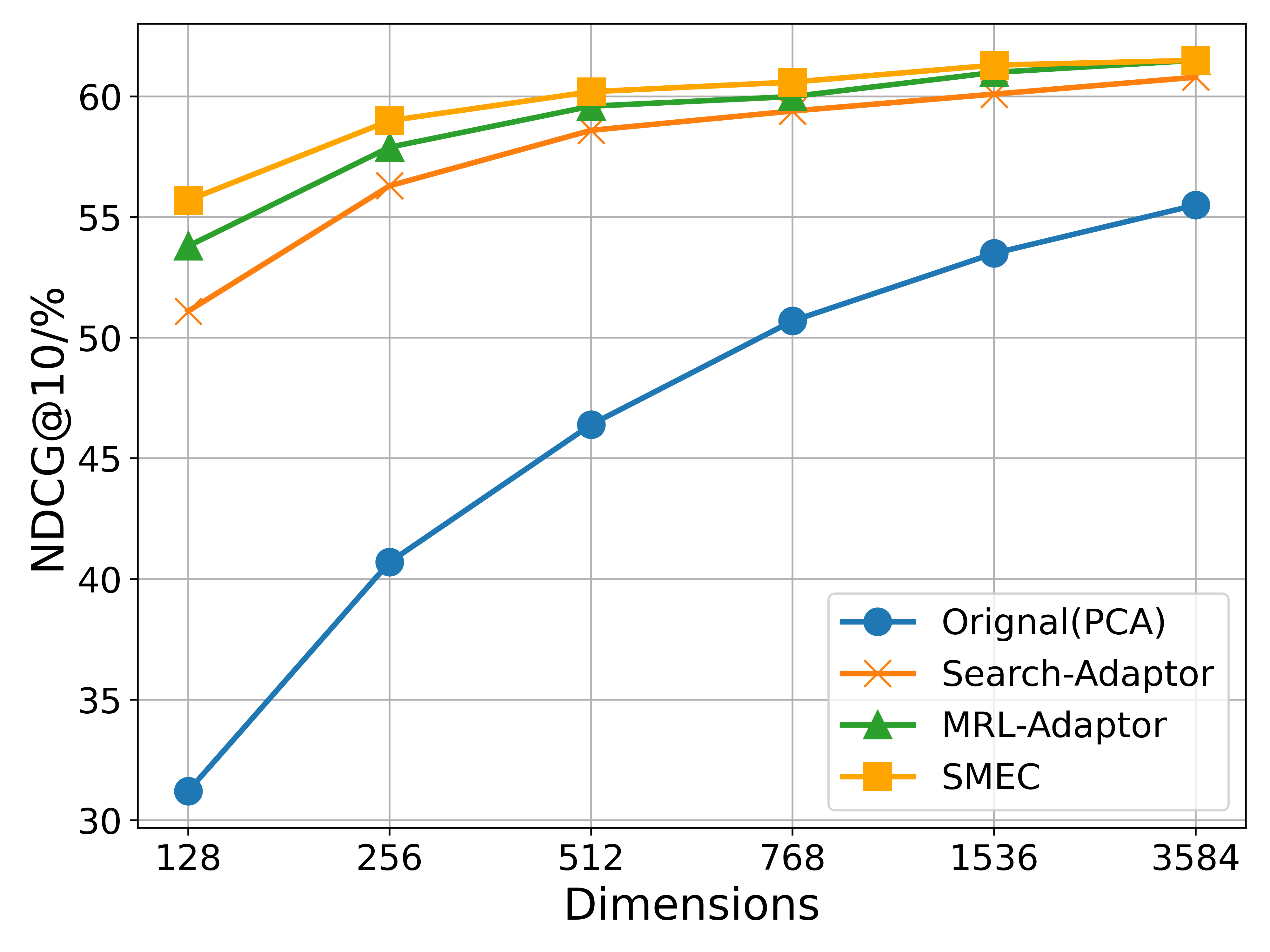
(b) LLM2Vec
Figure 5: Experimental results on the BEIR dataset comparing two models: OpenAI’s text-embedding-3-large (with 3072 dimensions) and LLM2Vec (with 3548 dimensions), the latter built upon the Qwen2-7B model. OpenAI text embeddings inherently contain multi-scale representations (enabled by MRL during pretraining), while LLM2Vec obtains its orignal low-dimensional representations via PCA.
## 4 Experiments
In this section, we compare our approach with state-of-the-art methods in the field of embedding dimensionality reduction.
### 4.1 Dataset Description
We evaluate the model’s retrieval performance across diverse datasets: BEIR Thakur et al. (2021) (text retrieval), Products-10K Bai et al. (2020) (image retrieval), and Fashion-200K Han et al. (2017) (cross-modal retrieval). BEIR is a comprehensive text retrieval benchmark consisting of 13 selected datasets from diverse domains. Products-10K contains approximately 10,000 products with over 150,000 images for large-scale product image retrieval. Fashion-200K includes over 200,000 fashion items with paired image-text data for cross-modal tasks.
### 4.2 Implementation Details
We use state-of-the-art models to extract the original embeddings for different datasets. Specifically, the BEIR dataset employs OpenAI text embeddings ope and LLM2Vec BehnamGhader et al. (2024) for text representation; the Products-10K dataset utilizes LLM2CLIP Huang et al. (2024) to obtain cross-modal embeddings; and the Fashion-200K dataset extracts image embeddings using the ViT-H Dosovitskiy et al. (2020) model. All dimensionality reduction methods are performed based on these original representations. To align with other methods, SMEC also adopts rank loss Yoon et al. (2023) as the supervised loss function, which is defined as follows:
$$
\displaystyle\mathcal{L}_{rank} \displaystyle=\sum_{i}\sum_{j}\sum_{k}\sum_{m}I(y_{ij}>y_{ik})(y_{ij}-y_{ik}) \displaystyle\log(1+\exp(s_{ik}[:m]-s_{ij}[:m])), \tag{8}
$$
where $I(y_{ij}>y_{ik})$ is an indicator function that is equal to 1 if $y_{ij}$ > $y_{ik}$ and 0 otherwise. $s_{ij}[:m]$ represents the cosine similarity between the query embedding $emb_{i}[:m]$ and the corpus embedding $emb_{j}[:m]$ . The total loss function is:
$$
\displaystyle\mathcal{L}_{total}=\mathcal{L}_{rank}+\alpha\mathcal{L}_{un-sup}, \tag{9}
$$
with $\alpha$ being hyper-parameters with fixed values as $\alpha=1.0$ . As SMEC involves multi-stage training, the training epochs of other methods are aligned with the total number of epochs costed by SMEC, and their best performance is reported.
### 4.3 Results
In this subsection, the results on the BEIR, Fashion-200K, and Products-10K datasets are given. Retrieval performance is evaluated using the normalized discounted cumulative gain at rank 10 (nDCG@10) Kalervo et al. (2002) metric.
BEIR. As shown in Figure 5, we compare the performance of SMEC and other state-of-the-art methods on two types of models: the API-based OpenAI text embedding and the open-source LLM2vec, across various compressed dimensions. Significantly, SMEC exhibits the strongest performance retention, particularly at lower compression ratios. For example, when compressed to 128 dimensions, SMEC improves the performance of the OpenAI and LLM2vec models by 1.9 and 1.1 points respectively, compared to the best-performing Matryoshka-Adaptor.
Products-10K. Images naturally contain denser features than text O Pinheiro et al. (2020). As shown in Figure 8(a) of Appendix C, SMEC surpasses other dimensionality reduction methods in image retrieval tasks, highlighting the effectiveness of the ADS module in mitigating information degradation during dimension pruning.
Fashion-200K. Unlike unimodal datasets, Fashion-200K involves cross-modal queries and documents, such as image-to-text and text-to-image retrieval. As illustrated in the Figure 8(b) and 8(c) of Appendix C, SMEC achieves superior performance in both directions, demonstrating strong robustness in multimodal scenarios.
<details>
<summary>figures/fig_var.png Details</summary>
### Visual Description
## Line Chart: Gradient Variance vs. Training Epochs
### Overview
This image is a line chart comparing the "Gradient Variance" of two methods, labeled **MRL** and **SMRL**, over the course of 40 training epochs. The chart uses a logarithmic scale for the y-axis to visualize data spanning multiple orders of magnitude.
### Components/Axes
* **Chart Type:** Line chart with a logarithmic y-axis.
* **X-Axis:**
* **Label:** "Epochs"
* **Scale:** Linear, from 0 to 40.
* **Major Ticks:** 0, 5, 10, 15, 20, 25, 30, 35, 40.
* **Y-Axis:**
* **Label:** "Gradient Variance"
* **Scale:** Logarithmic (base 10).
* **Major Ticks (Labels):** 10⁻⁹, 10⁻⁸, 10⁻⁷.
* **Minor Ticks:** Visible between major ticks, indicating intermediate values (e.g., 2x10⁻⁹, 5x10⁻⁹).
* **Legend:**
* **Position:** Top-right corner of the plot area.
* **Items:**
1. **MRL:** Represented by a dark gray/black solid line.
2. **SMRL:** Represented by a cyan/light blue solid line.
* **Grid:** A light gray grid is present, aligned with the major ticks on both axes.
### Detailed Analysis
**Trend Verification & Data Points:**
Both data series exhibit a clear downward trend, indicating that gradient variance decreases as training progresses (epochs increase). The y-axis is logarithmic, so a straight line would indicate exponential decay.
1. **MRL (Dark Gray Line):**
* **Trend:** Starts at the highest point on the chart and follows a generally decreasing, slightly jagged path. The rate of decrease is steepest in the first ~15 epochs and becomes more gradual thereafter.
* **Approximate Key Points:**
* Epoch 0: ~4 x 10⁻⁷ (Highest point)
* Epoch 5: ~1 x 10⁻⁷
* Epoch 10: ~3 x 10⁻⁸
* Epoch 15: ~6 x 10⁻⁹
* Epoch 20: ~5 x 10⁻⁹
* Epoch 30: ~2 x 10⁻⁹ (with a small local peak)
* Epoch 40: ~1 x 10⁻⁹
2. **SMRL (Cyan Line):**
* **Trend:** Also starts high but consistently remains below the MRL line. It shows a steeper initial decline than MRL and maintains a lower variance throughout. The line has more visible small fluctuations (e.g., around epochs 3, 10, 32).
* **Approximate Key Points:**
* Epoch 0: ~9 x 10⁻⁸
* Epoch 5: ~4 x 10⁻⁸
* Epoch 10: ~9 x 10⁻⁹
* Epoch 15: ~3 x 10⁻⁹
* Epoch 20: ~1.5 x 10⁻⁹
* Epoch 30: ~6 x 10⁻¹⁰
* Epoch 40: ~3 x 10⁻¹⁰ (Lowest point on the chart)
**Spatial Grounding:** The legend is positioned in the top-right, clearly associating the dark gray line with "MRL" and the cyan line with "SMRL." The SMRL line is visually below the MRL line for the entire duration shown.
### Key Observations
1. **Consistent Performance Gap:** The SMRL method demonstrates consistently lower gradient variance than the MRL method at every epoch from 0 to 40.
2. **Convergence Behavior:** Both methods show a reduction in gradient variance over time, which is typical of a converging training process. The variance for both appears to plateau or decrease very slowly after approximately epoch 25.
3. **Relative Magnitude:** By epoch 40, the gradient variance for SMRL (~3x10⁻¹⁰) is approximately one-third to one-fourth that of MRL (~1x10⁻⁹).
4. **Volatility:** The SMRL line exhibits slightly more short-term volatility (small peaks and valleys) compared to the somewhat smoother descent of the MRL line, particularly in the later epochs.
### Interpretation
This chart provides a technical comparison of training stability between two methods, likely in the context of machine learning or optimization. Gradient variance is a metric often associated with the noise in gradient estimates during stochastic optimization; lower variance generally implies more stable and reliable updates.
* **What the data suggests:** The SMRL method appears to achieve significantly more stable training dynamics (lower gradient noise) than the MRL method. The faster initial drop in variance for SMRL might indicate quicker adaptation or more effective variance reduction in the early training phase.
* **How elements relate:** The x-axis (Epochs) represents training time/progress, while the y-axis (Gradient Variance) is a measure of optimization stability. The inverse relationship shown (variance decreases as epochs increases) is the expected behavior for a well-behaved training process. The separation between the two lines quantifies the performance difference between the MRL and SMRL algorithms.
* **Notable implications:** If gradient variance is a critical metric for the application (e.g., in reinforcement learning or fine-tuning large models), SMRL demonstrates a clear advantage. The persistent gap suggests the improvement is not transient but sustained throughout training. The chart does not show the final model performance (e.g., accuracy, reward), so while SMRL has more stable gradients, one cannot conclude from this chart alone that it results in a better final model—only that its optimization process is less noisy.
</details>
(a) Gradient Variance
<details>
<summary>figures/fig_loss.png Details</summary>
### Visual Description
## Line Chart: Loss vs. Epochs for MRL and SMRL Methods
### Overview
The image is a line chart comparing the training loss over 40 epochs for two different methods or models, labeled "MRL" and "SMRL". The chart demonstrates the learning curves, showing how the loss metric decreases as training progresses for both approaches.
### Components/Axes
* **Chart Type:** Line chart with two data series.
* **X-Axis:**
* **Label:** "Epochs"
* **Scale:** Linear, from 0 to 40.
* **Major Tick Marks:** 0, 5, 10, 15, 20, 25, 30, 35, 40.
* **Y-Axis:**
* **Label:** "Loss"
* **Scale:** Linear, from approximately 0.045 to 0.105.
* **Major Tick Marks:** 0.05, 0.06, 0.07, 0.08, 0.09, 0.10.
* **Legend:**
* **Position:** Top-right corner of the chart area.
* **Entries:**
1. **MRL:** Represented by a dark gray (almost black) solid line.
2. **SMRL:** Represented by a cyan (light blue) solid line.
* **Grid:** A light gray grid is present, aligned with the major tick marks on both axes.
### Detailed Analysis
**Data Series 1: MRL (Dark Gray Line)**
* **Trend:** The line shows a steep, rapid decrease in loss initially, followed by a gradual, steady decline that begins to plateau after approximately epoch 20.
* **Approximate Data Points:**
* Epoch 0: Loss ≈ 0.101
* Epoch 5: Loss ≈ 0.073
* Epoch 10: Loss ≈ 0.063
* Epoch 20: Loss ≈ 0.059
* Epoch 30: Loss ≈ 0.056
* Epoch 40: Loss ≈ 0.056 (final value)
**Data Series 2: SMRL (Cyan Line)**
* **Trend:** Similar to MRL, this line exhibits a very sharp initial drop in loss, followed by a slower rate of decrease. It consistently maintains a lower loss value than the MRL line throughout the entire training period shown.
* **Approximate Data Points:**
* Epoch 0: Loss ≈ 0.090
* Epoch 5: Loss ≈ 0.059
* Epoch 10: Loss ≈ 0.052
* Epoch 20: Loss ≈ 0.049
* Epoch 30: Loss ≈ 0.048
* Epoch 40: Loss ≈ 0.047 (final value)
### Key Observations
1. **Performance Gap:** The SMRL method achieves a lower loss value at every epoch compared to the MRL method. The gap between the two lines is established early (by epoch 5) and remains relatively consistent.
2. **Convergence Behavior:** Both curves show classic convergence patterns: a phase of rapid improvement (steep descent) in the first ~5-10 epochs, followed by a phase of fine-tuning and diminishing returns (gradual descent/plateau).
3. **Final Values:** By epoch 40, the loss for SMRL (~0.047) is approximately 16% lower than the loss for MRL (~0.056).
4. **Stability:** Both lines exhibit minor fluctuations or "noise" in the later epochs (post epoch 20), but the overall downward trend is clear and stable.
### Interpretation
This chart provides a direct performance comparison between two training methodologies, MRL and SMRL. The data strongly suggests that the **SMRL method is more effective** for the given task, as evidenced by its consistently lower loss values throughout the training process.
The relationship between the elements is clear: the x-axis (Epochs) represents training time or iterations, and the y-axis (Loss) represents the error or cost function being minimized. The downward slope of both lines confirms that both models are learning. The key differentiator is the **efficiency and final performance** of SMRL.
The notable anomaly is not a single outlier point but the **persistent performance gap**. This indicates a fundamental difference in how the two methods optimize or represent the problem, leading SMRL to find a better solution (lower loss) faster and maintain that advantage. The plateauing of both curves suggests that further significant gains beyond epoch 40 would require changes to the training regimen (e.g., learning rate adjustment) or model architecture, as the current optimization process is nearing its limit for both methods.
</details>
(b) Validation loss
<details>
<summary>figures/fig_ndcg.png Details</summary>
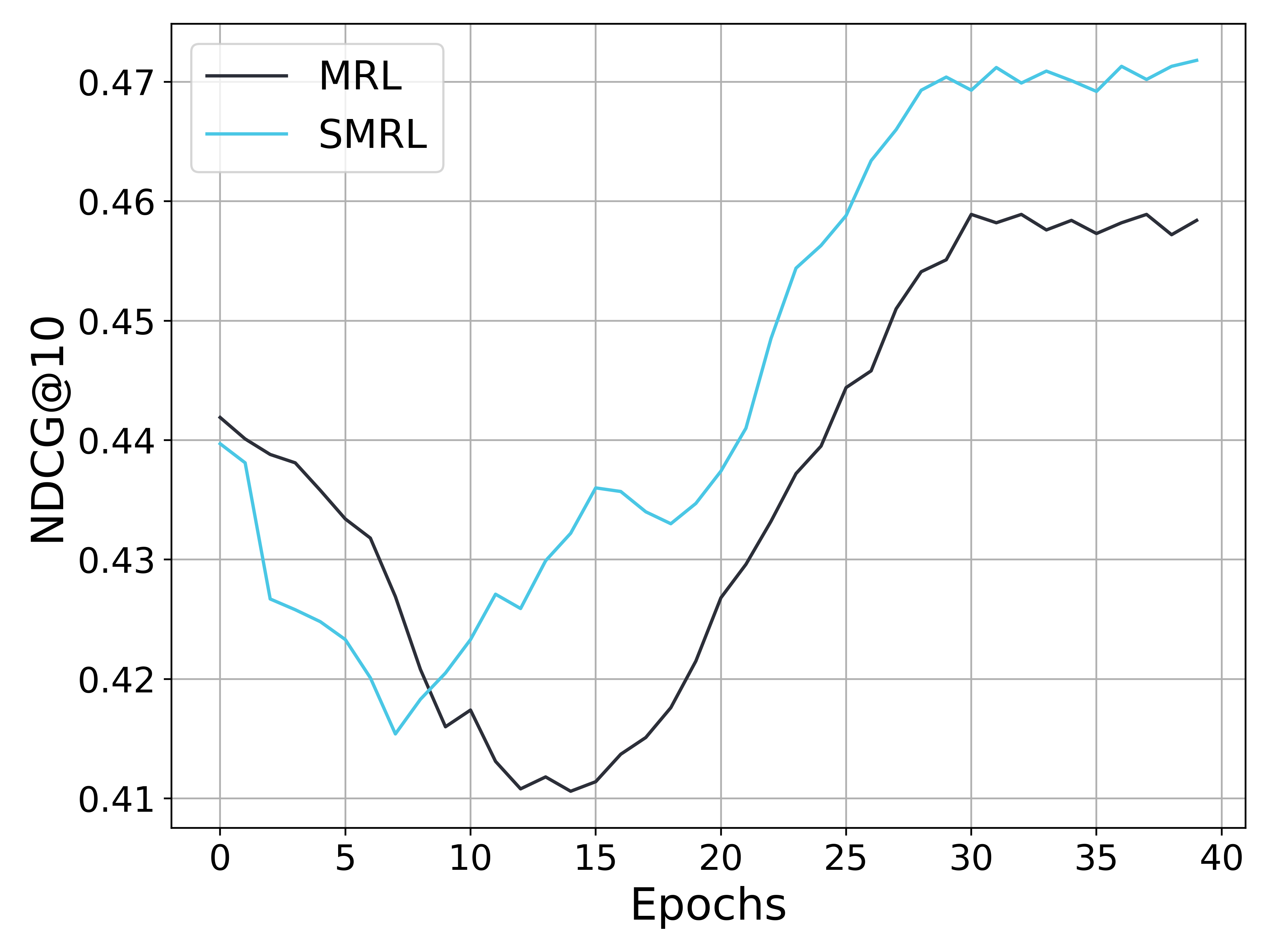
### Visual Description
## Line Chart: NDCG@10 Performance Over Training Epochs
### Overview
The image displays a line chart comparing the performance of two models, labeled MRL and SMRL, over the course of 40 training epochs. The performance metric is NDCG@10 (Normalized Discounted Cumulative Gain at rank 10), a common measure for ranking quality in information retrieval and recommendation systems. The chart shows that both models experience an initial performance decline followed by a recovery and improvement, with SMRL ultimately achieving a higher final score.
### Components/Axes
* **Chart Type:** Line chart with two data series.
* **X-Axis:**
* **Label:** "Epochs"
* **Scale:** Linear, from 0 to 40.
* **Major Tick Marks:** 0, 5, 10, 15, 20, 25, 30, 35, 40.
* **Y-Axis:**
* **Label:** "NDCG@10"
* **Scale:** Linear, from approximately 0.41 to 0.47.
* **Major Tick Marks:** 0.41, 0.42, 0.43, 0.44, 0.45, 0.46, 0.47.
* **Legend:**
* **Position:** Top-left corner of the plot area.
* **Items:**
1. **MRL:** Represented by a solid black line.
2. **SMRL:** Represented by a solid cyan (light blue) line.
* **Grid:** A light gray grid is present, aligning with the major tick marks on both axes.
### Detailed Analysis
**Trend Verification & Data Point Extraction (Approximate Values):**
* **MRL (Black Line):**
* **Trend:** Starts high, declines to a minimum around epoch 12-15, then recovers with a strong upward trend, plateauing after epoch 30.
* **Key Points:**
* Epoch 0: ~0.442
* Epoch 5: ~0.433
* Epoch 10: ~0.417 (Local low)
* Epoch 15: ~0.411 (Approximate global minimum)
* Epoch 20: ~0.427
* Epoch 25: ~0.445
* Epoch 30: ~0.459
* Epoch 35: ~0.458
* Epoch 40: ~0.459
* **SMRL (Cyan Line):**
* **Trend:** Starts slightly lower than MRL, declines to a minimum around epoch 7, then begins a recovery earlier and more steeply than MRL. It surpasses MRL around epoch 15 and maintains a lead, ending at the highest value on the chart.
* **Key Points:**
* Epoch 0: ~0.440
* Epoch 5: ~0.423
* Epoch 7: ~0.415 (Approximate global minimum)
* Epoch 10: ~0.423
* Epoch 15: ~0.436
* Epoch 20: ~0.438
* Epoch 25: ~0.459
* Epoch 30: ~0.470
* Epoch 35: ~0.470
* Epoch 40: ~0.472
### Key Observations
1. **Initial Performance Drop:** Both models show a significant decrease in NDCG@10 during the first ~10-15 epochs, suggesting a period of adjustment or instability early in training.
2. **Divergent Recovery:** The SMRL model begins its recovery sooner (around epoch 7) and at a faster rate than MRL (which bottoms around epoch 15).
3. **Crossover Point:** The performance lines intersect between epoch 10 and 15. After this point, SMRL consistently outperforms MRL.
4. **Final Performance Gap:** By epoch 40, SMRL achieves an NDCG@10 of ~0.472, while MRL reaches ~0.459, indicating a clear performance advantage for SMRL in the later stages of training.
5. **Volatility:** Both lines exhibit minor fluctuations, particularly during the recovery phase, but the overall trends are distinct and clear.
### Interpretation
This chart likely presents results from an experiment comparing two machine learning models (MRL and SMRL) on a ranking task. The NDCG@10 metric evaluates how well the models order relevant items at the top of a list.
The data suggests that the **SMRL model is more effective and robust in the long run**. While both models suffer from an initial "learning dip," SMRL demonstrates a superior ability to recover and improve. Its steeper learning curve after epoch 7 and higher final plateau indicate it may have a better optimization strategy, architecture, or regularization technique that prevents it from getting stuck in the poor local minimum that affects MRL until later in training.
The initial decline could be due to factors like aggressive learning rates, the model moving away from a pre-trained state, or the inherent difficulty of the task before the model finds a good gradient direction. The fact that SMRL overcomes this faster is a key finding. For a practitioner, this chart would argue for the adoption of the SMRL method over MRL for this specific task, as it yields a ~1.3 percentage point higher NDCG@10 score after 40 epochs, which can be a significant margin in ranking applications.
</details>
(c) Retrieval performance
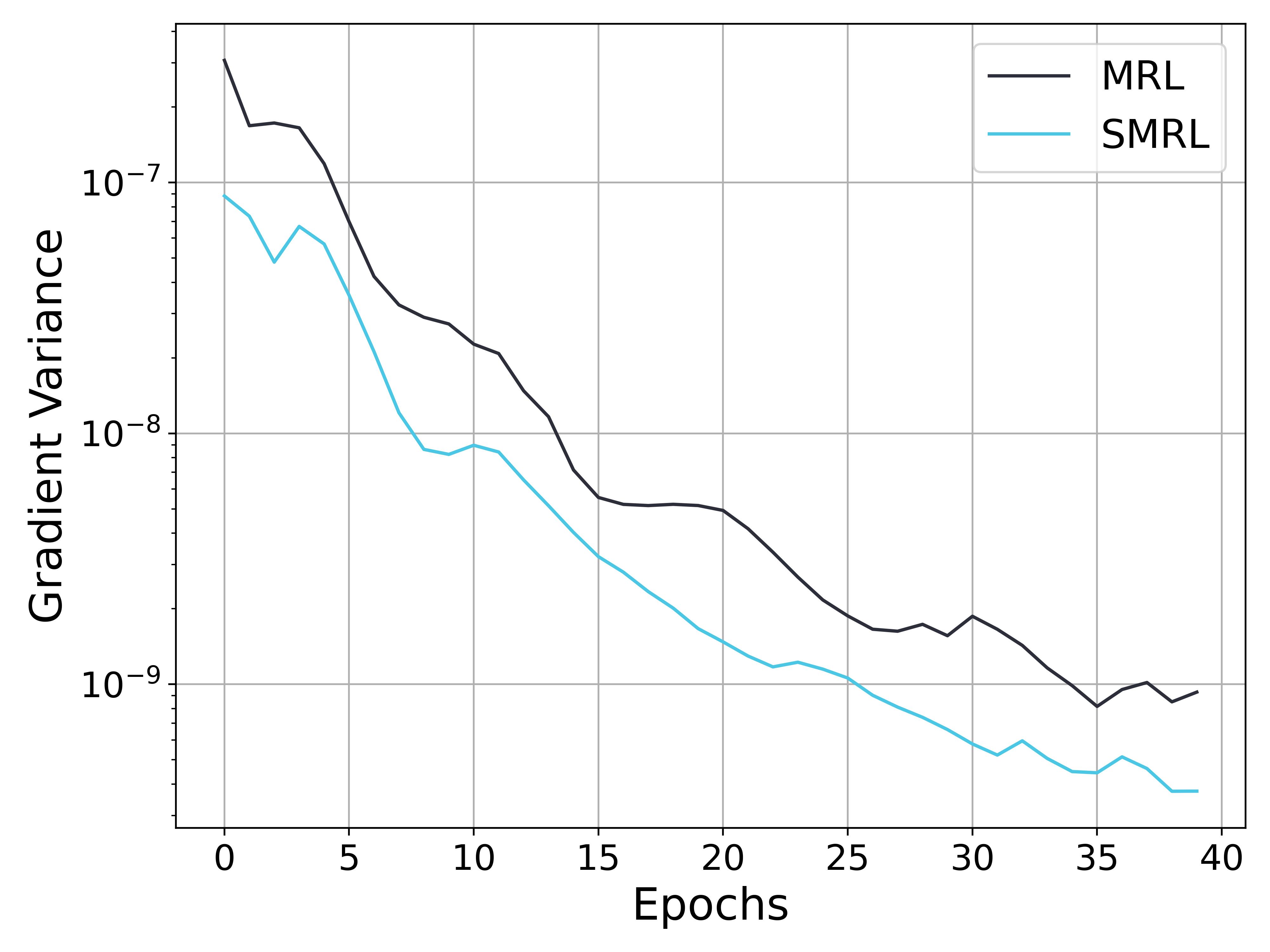
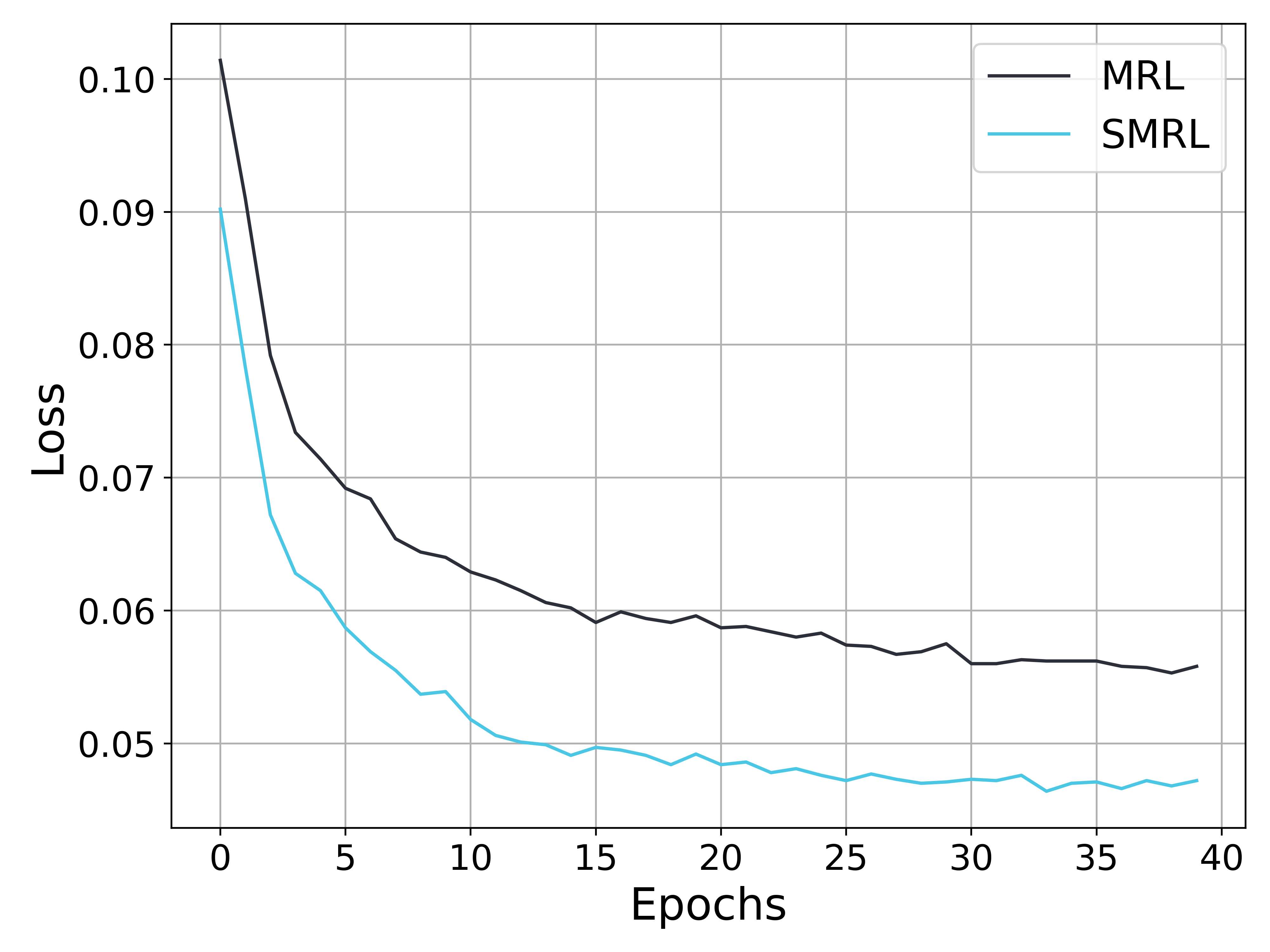
Figure 6: Analysis of metrics during the training process. (a) shows the gradient variance curve (with the vertical axis in a logarithmic scale), (b) presents the loss curve on the validation set, and (c) illustrates the performance variations on the test set. As training progresses, the gradient variances of both MRL and SMRL decrease; however, the gradient variance of MRL remains several times higher than that of SMRL. Consequently, the loss curve of SMRL converges more quickly to a lower value, and the compressed embedding demonstrates better retrieval performance.
## 5 Discussions
### 5.1 The influence of gradient variance
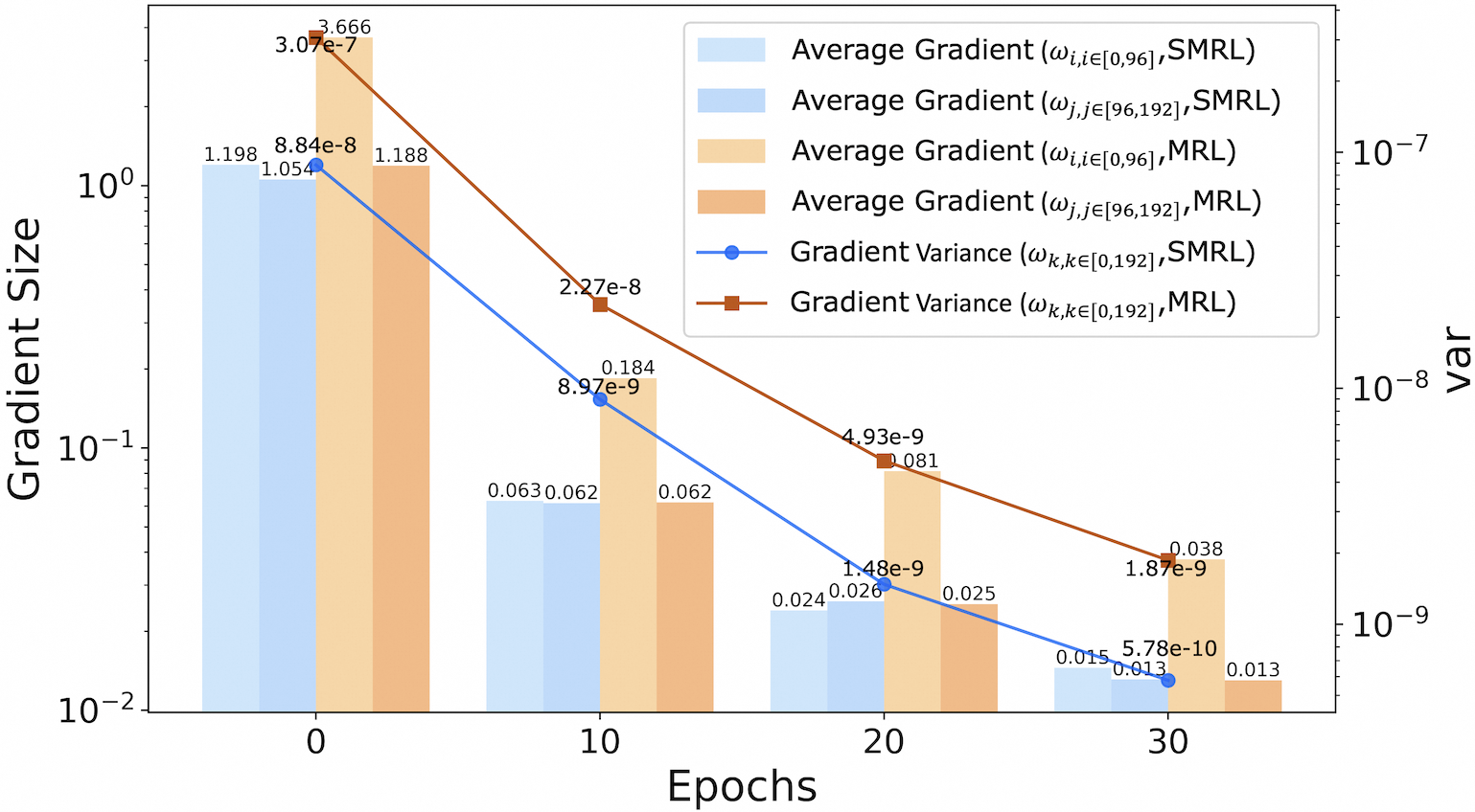
To validate the impact of gradient variance on convergence speed and model performance (as discussed in Section 3.2), we conducted comparative experiments between SMRL and MRL using the MiniLM model on the BEIR dataset. As shown in Figure 6(a), MRL consistently exhibits significantly higher gradient variance than SMRL throughout training. Consequently, the training loss of MRL continues to decline beyond the 20th epoch, whereas SMRL’s loss starts to converge at the 15th epoch. A similar trend is observed in subfigure 6(c), where SMRL enters the improvement phase earlier and converges to superior performance.
<details>
<summary>figures/fig_discuss2_rank.png Details</summary>
### Visual Description
## Dual-Axis Combination Chart: Gradient Size and Variance over Epochs
### Overview
This image is a technical chart combining bar and line plots on a dual y-axis. It visualizes the evolution of gradient statistics (average size and variance) for two different methods, labeled "SMRL" and "MRL," across training epochs. The chart uses a logarithmic scale for both y-axes.
### Components/Axes
* **Chart Type:** Combination bar and line chart with dual y-axes.
* **X-Axis:**
* **Label:** "Epochs"
* **Markers/Ticks:** 0, 10, 20, 30.
* **Primary Y-Axis (Left):**
* **Label:** "Gradient Size"
* **Scale:** Logarithmic (base 10), ranging from 10⁻² to 10⁰.
* **Secondary Y-Axis (Right):**
* **Label:** "var" (presumably variance)
* **Scale:** Logarithmic (base 10), ranging from 10⁻⁹ to 10⁻⁷.
* **Legend (Top-Right Corner):** Contains six entries, differentiating data series by color and marker type.
1. **Light Blue Bar:** `Average Gradient (ω_i,i∈[0,96], SMRL)`
2. **Medium Blue Bar:** `Average Gradient (ω_j,j∈[96,192], SMRL)`
3. **Light Orange Bar:** `Average Gradient (ω_i,i∈[0,96], MRL)`
4. **Dark Orange Bar:** `Average Gradient (ω_j,j∈[96,192], MRL)`
5. **Blue Line with Circle Marker:** `Gradient Variance (ω_k,k∈[0,192], SMRL)`
6. **Brown Line with Square Marker:** `Gradient Variance (ω_k,k∈[0,192], MRL)`
### Detailed Analysis
The chart presents data at four discrete epochs (0, 10, 20, 30). At each epoch, four bars are clustered, and two line data points are plotted.
**Data Series & Trends:**
* **Trend Verification:** All four bar series (average gradients) show a clear, steep downward trend from epoch 0 to 30. Both line series (variances) also show a consistent downward trend.
* **Component Isolation - Epoch 0:**
* **Bars (Gradient Size):**
* SMRL (ω_i,i∈[0,96]): ~1.198
* SMRL (ω_j,j∈[96,192]): ~1.054
* MRL (ω_i,i∈[0,96]): ~3.666 **(Highest initial value)**
* MRL (ω_j,j∈[96,192]): ~1.188
* **Lines (Variance):**
* SMRL Variance: ~8.84e-8
* MRL Variance: ~3.07e-7 **(Highest initial variance)**
* **Component Isolation - Epoch 10:**
* **Bars (Gradient Size):**
* SMRL (ω_i,i∈[0,96]): ~0.063
* SMRL (ω_j,j∈[96,192]): ~0.062
* MRL (ω_i,i∈[0,96]): ~0.184
* MRL (ω_j,j∈[96,192]): ~0.062
* **Lines (Variance):**
* SMRL Variance: ~8.97e-9
* MRL Variance: ~2.27e-8
* **Component Isolation - Epoch 20:**
* **Bars (Gradient Size):**
* SMRL (ω_i,i∈[0,96]): ~0.024
* SMRL (ω_j,j∈[96,192]): ~0.026
* MRL (ω_i,i∈[0,96]): ~0.081
* MRL (ω_j,j∈[96,192]): ~0.025
* **Lines (Variance):**
* SMRL Variance: ~1.48e-9
* MRL Variance: ~4.93e-9
* **Component Isolation - Epoch 30:**
* **Bars (Gradient Size):**
* SMRL (ω_i,i∈[0,96]): ~0.015
* SMRL (ω_j,j∈[96,192]): ~0.013
* MRL (ω_i,i∈[0,96]): ~0.038
* MRL (ω_j,j∈[96,192]): ~0.013
* **Lines (Variance):**
* SMRL Variance: ~5.78e-10
* MRL Variance: ~1.87e-9
### Key Observations
1. **Consistent Decline:** All measured quantities (average gradient sizes for both weight subsets and both methods, as well as overall gradient variance) decrease by approximately two orders of magnitude over 30 epochs.
2. **Method Comparison (MRL vs. SMRL):**
* **Gradient Size:** The MRL method's average gradient for the first weight subset (`ω_i,i∈[0,96]`) starts significantly higher (3.666 vs. 1.198) and remains higher than its SMRL counterpart at every epoch, though the gap narrows.
* **Variance:** The MRL method consistently exhibits higher gradient variance than SMRL at every measured epoch. The initial variance for MRL is about 3.5 times that of SMRL.
3. **Within-Method Comparison:** For both methods, the average gradient sizes for the two different weight subsets (`ω_i` and `ω_j`) become very similar after the initial epoch, suggesting convergence in gradient magnitude across different parts of the model.
4. **Outlier:** The initial average gradient for MRL on `ω_i,i∈[0,96]` (3.666) is a clear outlier, being the largest value on the chart by a significant margin.
### Interpretation
This chart likely analyzes the training dynamics of two machine learning optimization or regularization methods, SMRL and MRL. The data demonstrates that both methods successfully drive down gradient magnitudes and variances over time, which is a typical sign of training convergence and stabilization.
The key investigative insight is the **performance gap between MRL and SMRL**. The consistently higher gradient variance for MRL suggests its optimization landscape may be noisier or less stable than SMRL's. The notably larger initial gradients for MRL could indicate a different parameter initialization scheme, a more aggressive early learning rate, or a fundamental difference in how the method scales gradients. The fact that MRL's gradients start larger but still converge to small values implies the method is effective, but potentially through a different, higher-variance trajectory compared to SMRL. The convergence of gradient sizes between different weight subsets (`ω_i` and `ω_j`) within each method suggests that, over time, the optimization pressure becomes evenly distributed across the model's parameters for both techniques.
</details>
(a) Rank Loss
<details>
<summary>figures/fig_discuss2_mse.png Details</summary>
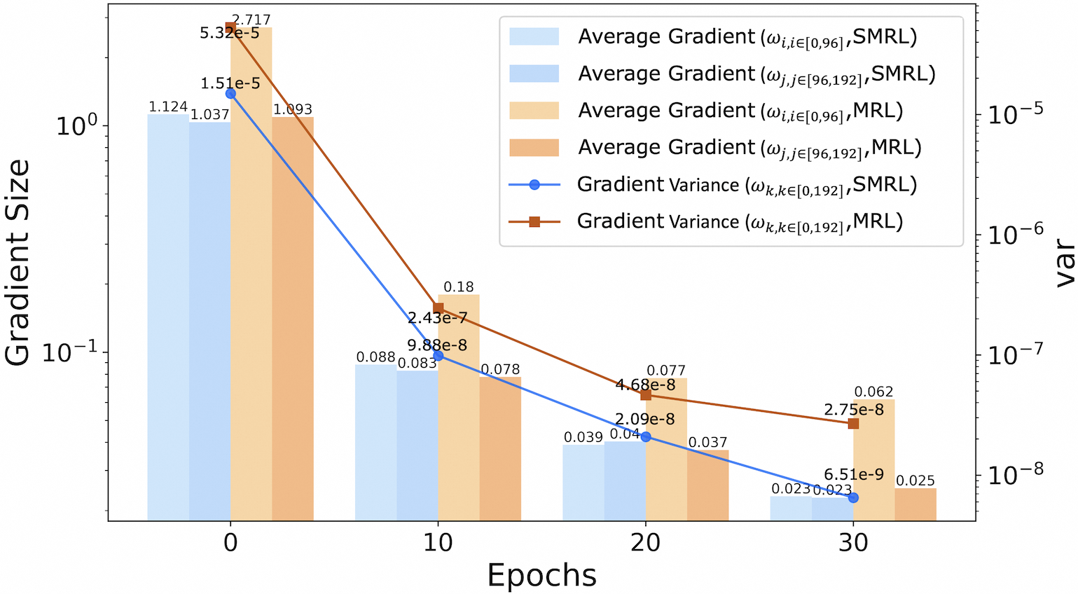
### Visual Description
## Chart: Gradient Size and Variance Across Epochs for SMRL and MRL Methods
### Overview
This is a dual-axis chart combining a grouped bar chart and two line plots. It visualizes the evolution of gradient statistics (average size and variance) over training epochs for two different methods: SMRL and MRL. The chart uses a logarithmic scale for both y-axes to accommodate the wide range of values.
### Components/Axes
* **X-Axis (Bottom):** Labeled "Epochs". Major tick marks and labels are at 0, 10, 20, and 30.
* **Primary Y-Axis (Left):** Labeled "Gradient Size". It is a logarithmic scale ranging from below 10⁻¹ to above 10⁰.
* **Secondary Y-Axis (Right):** Labeled "var" (presumably variance). It is a logarithmic scale ranging from 10⁻⁸ to 10⁻⁵.
* **Legend (Top-Right Corner):** Contains six entries, differentiating data series by color and marker:
1. Light Blue Bar: `Average Gradient (ω_i, i∈[0,96], SMRL)`
2. Medium Blue Bar: `Average Gradient (ω_j, j∈[96,192], SMRL)`
3. Light Orange Bar: `Average Gradient (ω_i, i∈[0,96], MRL)`
4. Dark Orange Bar: `Average Gradient (ω_j, j∈[96,192], MRL)`
5. Blue Line with Circle Markers: `Gradient Variance (ω_k, k∈[0,192], SMRL)`
6. Brown Line with Square Markers: `Gradient Variance (ω_k, k∈[0,192], MRL)`
### Detailed Analysis
**Data Series and Values (by Epoch):**
* **Epoch 0:**
* **Bars (Gradient Size):**
* SMRL (ω_i, [0,96]): ~1.124
* SMRL (ω_j, [96,192]): ~1.037
* MRL (ω_i, [0,96]): ~2.717 (annotated)
* MRL (ω_j, [96,192]): ~1.093
* **Lines (Gradient Variance):**
* SMRL (Blue Circle): ~1.51e-5 (annotated)
* MRL (Brown Square): ~5.32e-5 (annotated)
* **Epoch 10:**
* **Bars (Gradient Size):**
* SMRL (ω_i, [0,96]): ~0.088
* SMRL (ω_j, [96,192]): ~0.083
* MRL (ω_i, [0,96]): ~0.18 (annotated)
* MRL (ω_j, [96,192]): ~0.078
* **Lines (Gradient Variance):**
* SMRL (Blue Circle): ~9.88e-8 (annotated)
* MRL (Brown Square): ~2.43e-7 (annotated)
* **Epoch 20:**
* **Bars (Gradient Size):**
* SMRL (ω_i, [0,96]): ~0.039
* SMRL (ω_j, [96,192]): ~0.04
* MRL (ω_i, [0,96]): ~0.077 (annotated)
* MRL (ω_j, [96,192]): ~0.037
* **Lines (Gradient Variance):**
* SMRL (Blue Circle): ~2.09e-8 (annotated)
* MRL (Brown Square): ~4.68e-8 (annotated)
* **Epoch 30:**
* **Bars (Gradient Size):**
* SMRL (ω_i, [0,96]): ~0.023
* SMRL (ω_j, [96,192]): ~0.023
* MRL (ω_i, [0,96]): ~0.062 (annotated)
* MRL (ω_j, [96,192]): ~0.025
* **Lines (Gradient Variance):**
* SMRL (Blue Circle): ~6.51e-9 (annotated)
* MRL (Brown Square): ~2.75e-8 (annotated)
### Key Observations
1. **Consistent Downward Trend:** All six data series (four bar categories and two line plots) show a clear, monotonic decrease from Epoch 0 to Epoch 30. This indicates that both the magnitude of the gradients and their variance diminish as training progresses.
2. **Method Comparison (MRL vs. SMRL):**
* **Gradient Size:** At every epoch, the average gradient for the `ω_i` parameter subset (first 96 parameters) is significantly larger for MRL than for SMRL. The difference is most pronounced at Epoch 0 (2.717 vs. 1.124) and narrows but persists through Epoch 30 (0.062 vs. 0.023). For the `ω_j` subset (parameters 96-192), the sizes are much closer between methods.
* **Gradient Variance:** The variance for MRL (brown line) is consistently higher than for SMRL (blue line) at all measured epochs. The gap is largest at Epoch 0 and decreases over time.
3. **Parameter Subset Differences:** Within each method, the gradient size for the `ω_i` subset is generally larger than for the `ω_j` subset, especially for MRL in early epochs.
### Interpretation
This chart provides a technical comparison of optimization dynamics between two methods, likely in a machine learning context. The data suggests:
* **Training Progress:** The universal decrease in gradient size and variance is a classic sign of model convergence. As the model parameters approach an optimal point, the updates (gradients) become smaller and more consistent.
* **Method Behavior:** The MRL method exhibits larger gradients and higher gradient variance, particularly in the early stages of training (Epoch 0). This could imply that MRL takes more aggressive or exploratory steps initially. The SMRL method shows more conservative, lower-variance updates from the start.
* **Parameter Sensitivity:** The difference in gradient sizes between the `ω_i` and `ω_j` subsets indicates that the model's parameters are not updated uniformly. The first 96 parameters (`ω_i`) appear to be more active or sensitive, especially under the MRL method. This could reflect the model's architecture or the nature of the learning task.
* **Convergence Pattern:** While both methods show convergence, SMRL converges to a state with lower gradient variance. Whether this leads to a better or worse final model performance cannot be determined from this chart alone; it would require corresponding loss or accuracy metrics. The chart effectively visualizes the *process* of optimization for each method.
</details>
(b) MSE Loss
<details>
<summary>figures/fig_discuss2_ce.png Details</summary>
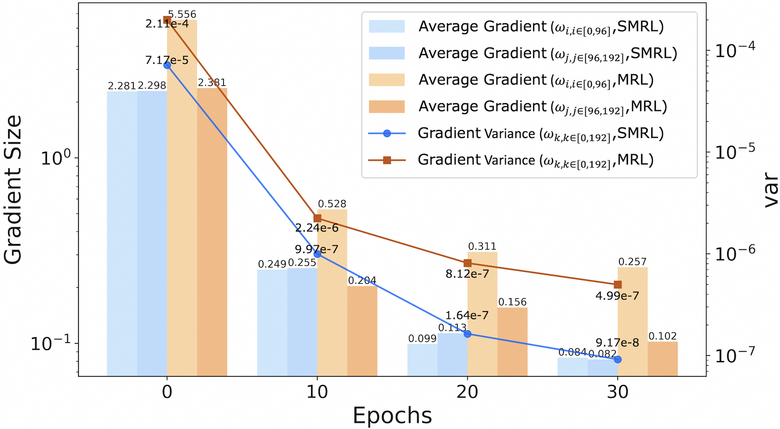
### Visual Description
\n
## Combination Bar and Line Chart: Gradient Size and Variance Across Epochs for SMRL and MRL
### Overview
This image is a technical chart comparing gradient statistics between two methods, SMRL and MRL, over the course of training epochs. It uses a dual-axis format: the primary (left) y-axis shows "Gradient Size" on a logarithmic scale, and the secondary (right) y-axis shows "var" (variance), also on a logarithmic scale. The x-axis represents training "Epochs". The chart combines grouped bar plots for average gradient magnitudes and line plots for gradient variance.
### Components/Axes
* **X-Axis:** Labeled "Epochs". Major tick marks and labels are at values 0, 10, 20, and 30.
* **Primary Y-Axis (Left):** Labeled "Gradient Size". It is a logarithmic scale with major ticks at 10⁻¹ (0.1) and 10⁰ (1).
* **Secondary Y-Axis (Right):** Labeled "var". It is a logarithmic scale with major ticks at 10⁻⁷, 10⁻⁶, 10⁻⁵, and 10⁻⁴.
* **Legend:** Located in the top-right quadrant of the chart. It defines six data series:
1. **Light Blue Bar:** `Average Gradient (ω_i, i∈[0,96], SMRL)`
2. **Medium Blue Bar:** `Average Gradient (ω_j, j∈[96,192], SMRL)`
3. **Light Orange Bar:** `Average Gradient (ω_i, i∈[0,96], MRL)`
4. **Medium Orange Bar:** `Average Gradient (ω_j, j∈[96,192], MRL)`
5. **Blue Line with Circle Markers:** `Gradient Variance (ω_k, k∈[0,192], SMRL)`
6. **Brown Line with Square Markers:** `Gradient Variance (ω_k, k∈[0,192], MRL)`
### Detailed Analysis
Data is presented at four discrete epochs: 0, 10, 20, and 30. Values are approximate, read from the chart annotations.
**Epoch 0:**
* **Bars (Gradient Size):**
* SMRL (ω_i, [0,96]): ~2.281
* SMRL (ω_j, [96,192]): ~2.298
* MRL (ω_i, [0,96]): ~5.556
* MRL (ω_j, [96,192]): ~2.381
* **Lines (Variance):**
* SMRL Variance: ~7.17e-5 (Blue circle)
* MRL Variance: ~2.11e-4 (Brown square)
**Epoch 10:**
* **Bars (Gradient Size):**
* SMRL (ω_i, [0,96]): ~0.249
* SMRL (ω_j, [96,192]): ~0.255
* MRL (ω_i, [0,96]): ~0.528
* MRL (ω_j, [96,192]): ~0.204
* **Lines (Variance):**
* SMRL Variance: ~9.97e-7 (Blue circle)
* MRL Variance: ~2.24e-6 (Brown square)
**Epoch 20:**
* **Bars (Gradient Size):**
* SMRL (ω_i, [0,96]): ~0.099
* SMRL (ω_j, [96,192]): ~0.113
* MRL (ω_i, [0,96]): ~0.311
* MRL (ω_j, [96,192]): ~0.156
* **Lines (Variance):**
* SMRL Variance: ~1.64e-7 (Blue circle)
* MRL Variance: ~8.12e-7 (Brown square)
**Epoch 30:**
* **Bars (Gradient Size):**
* SMRL (ω_i, [0,96]): ~0.084
* SMRL (ω_j, [96,192]): ~0.082
* MRL (ω_i, [0,96]): ~0.257
* MRL (ω_j, [96,192]): ~0.102
* **Lines (Variance):**
* SMRL Variance: ~9.17e-8 (Blue circle)
* MRL Variance: ~4.99e-7 (Brown square)
### Key Observations
1. **Overall Trend:** All metrics (average gradient size for both weight groups and both methods, and gradient variance for both methods) show a clear, consistent downward trend from Epoch 0 to Epoch 30.
2. **Method Comparison (Gradient Size):** At every epoch, the average gradient sizes for MRL (orange bars) are larger than their SMRL (blue bar) counterparts for the same weight group (i∈[0,96] or j∈[96,192]). The difference is most pronounced at Epoch 0.
3. **Method Comparison (Variance):** The gradient variance for MRL (brown line) is consistently higher than for SMRL (blue line) at all measured epochs. The gap between them narrows slightly in absolute terms on the log scale but remains significant.
4. **Weight Group Comparison:** For both methods, the average gradient size for the first weight group (ω_i, i∈[0,96]) is generally larger than for the second group (ω_j, j∈[96,192]), especially for MRL at Epoch 0.
5. **Rate of Decay:** The steepest decline for all metrics occurs between Epoch 0 and Epoch 10. The rate of decrease slows between Epochs 10, 20, and 30.
### Interpretation
This chart provides a comparative analysis of gradient dynamics during the training of two machine learning models or methods, SMRL and MRL. The data suggests several key insights:
* **Training Progression:** The universal decrease in gradient size and variance is a classic signature of model convergence. As training progresses, the model's parameters make smaller and more consistent adjustments.
* **Method Behavior:** MRL exhibits larger gradient magnitudes and higher variance throughout the observed training period. This could indicate that MRL's optimization landscape is more volatile or that it takes larger, more variable steps during learning compared to SMRL. The higher initial variance for MRL (2.11e-4 vs. 7.17e-5) is particularly notable.
* **Layer/Parameter Sensitivity:** The difference in average gradient size between the two weight groups (ω_i and ω_j) suggests that different parts of the model (perhaps different layers or parameter types) experience different learning signals. The first group (i∈[0,96]) consistently receives stronger gradients, implying it may be more actively updated or more sensitive to the loss function.
* **Convergence Characteristics:** While both methods show convergence, SMRL appears to stabilize with smaller and less variable gradients. Whether this leads to better final model performance or simply faster convergence to a (potentially different) local minimum cannot be determined from this chart alone. The chart effectively visualizes the "how" of the training dynamics, not the "how well" of the final outcome.
</details>
(c) CE Loss
Figure 7: Gradient statistics with Rank, MSE and CE loss (with the vertical axis in a logarithmic scale): average gradient magnitudes of parameters in the ranges $[0,96]$ and $[96,192]$ , as well as the gradient variance over all parameters in the range $[0,192]$ , during training.
### 5.2 Gradient variance of different loss functions
Section 5.1 demonstrates that MRL exhibits higher gradient variance compared to SMRL when rank loss is employed as the loss function, thereby corroborating the findings presented in Section 3.2. To enhance the validation, we conducted additional experiments on the BEIR dataset using rank loss, MSE loss and cross-entropy (CE) loss under identical settings. The results depicted in Figure 7 reveal a consistent pattern across both loss functions, validating the robustness of our conclusions.
### 5.3 Ablation studies
To evaluate the contribution of each component in SMEC to the overall performance, we conduct ablation studies using MRL as the baseline. Different modules are incrementally added on top of MRL, as detailed in table 1. When examined individually, the SMRL strategy achieves the most significant performance gain, suggesting that its reduced gradient variance contributes positively to model performance. In addition, both the ADS module and the S-XBM module also provide notable improvements. The combination of all three components improves the performance of the 128-dimensional embedding by 3.1 points.
| w/ SMRL w/ ADS w/ S-XBM | 0.3808 0.3765 0.3778 | 0.4621 0.4583 0.4583 | 0.4895 0.4863 0.4853 | 0.5283 0.5254 0.5256 |
| --- | --- | --- | --- | --- |
| SMEC (Ours) | 0.4053 | 0.4848 | 0.5002 | 0.5459 |
Table 1: Ablation studies of SMEC on 8 BEIR datasets with MRL as the baseline.
### 5.4 The contribution of ADS in preserving key information
The selection of important parameters in neural networks is a well-established research area, with numerous studies demonstrating that network parameters are often redundant. As a result, Parameter Pruning have been widely adopted for model compression. We consider ADS (or more generally, the MEC family of methods), although it focuses on dimension selection within embeddings, to be fundamentally implemented through network parameter selection. Therefore, ADS can be regarded as a form of pruning method with theoretical feasibility.
To fully demonstrate the effectiveness of ADS, we evaluate both the dimension selection strategies of ADS and MRL using WARE Yu et al. (2018) (Weighted Average Reconstruction Error), a commonly used metric in the pruning area for assessing parameter importance. The WARE is defined as follows:
$$
\text{WARE}=\frac{1}{M}\sum_{m=1}^{M}\frac{|\hat{y}_{m}-y_{m}|}{|y_{m}|} \tag{10}
$$
,where $M$ denotes the number of samples; $\hat{y}_{m}$ and $y_{m}$ represent the model’s score (which can be interpreted as the similarity between embedding pairs) for the $m$ -th sample before and after dimension pruning, respectively. The core idea of WARE is to quantify the change in the model’s output induced by removing a specific dimension; a larger change indicates higher importance of that dimension.
We randomly sampled 10,000 instances from multiple sub-datasets of BEIR. For the LLM2VEC embeddings (3072dim), we computed the WARE for each dimension. Then, we used both ADS and MRL to generate low-dimensional embeddings of 1536, 768, and 256 dimensions, respectively. For each method and compression level, we calculated the achievement rate, which is defined as the proportion of selected dimensions that appear in the top-N most important dimensions according to the WARE-based ranking.
| Dimension 1536 768 | ADS (Dimension Selection) 94.3% 90.1% | MRL (Dimension Truncation) 50.3% 32.8% |
| --- | --- | --- |
| 256 | 83.6% | 17.4% |
Table 2: Achievement Rate of Important Dimension Selection at Different Dimension Levels.
The results in table 2 show that the achievement rate of MRL is roughly linear with the compression ratio, indicating that the importance of dimensions has no strong correlation with their positions. The achievement rate of ADS also decreases as the number of retained dimensions reduces, which is due to the increased difficulty of selecting the top-N most important dimensions under higher compression ratios. However, even when compressed by a factor of 6, ADS still selects over 80 of the most important dimensions. This explains why, as seen in Figure 5, SMEC demonstrates stronger performance at lower dimensions.
### 5.5 Memory size of S-XBM
In this subsection, we explore how the memory size of S-XBM module affects training speed and model performance. Theoretically, as the memory size increases, it is easier for the S-XBM module to mine more hard samples, thereby improving model performance. However, an excessively large memory size may increase the retrieval time for top-k samples, which could negatively affect training efficiency. To prove this observation experimentally, we train the SMEC framework with varying memory sizes (e.g., 1000, 2000, 5000, 10000, and 15000), as illustrated in the table 3. The results demonstrate a clear trade-off between training speed and model performance. We select a memory size of 5000 as our final choice to strike a balance between them.
| Forward Time/s $\downarrow$ NDCG@10 $\uparrow$ | 0.06 0.4631 | 0.08 0.4652 | 0.11 0.4675 | 0.15 0.4682 | 0.21 0.4689 |
| --- | --- | --- | --- | --- | --- |
Table 3: Trade-off analysis of training speed and model performance under different memory size of S-XBM.
## 6 Conclusions
Although high-dimensional embeddings from large language models (LLMs) capture rich semantic features, their practical use is often limited by computational efficiency and storage constraints. To mitigate these limitations, Sequential Matryoshka Embedding Compression (SMEC) framework is proposed in this paper to achieve efficient embedding compression. Our proposed SMEC framework contains Sequential Matryoshka Representation Learning(SMRL) module, adaptive dimension selection (ADS) module and Selectable Cross-batch Memory (S-XBM) module. The SMRL module is designed to mitigate gradient variance during training. The ADS module is utilized to minimize information degradation during feature compression. And the S-XBM is utilized to enhance unsupervised learning between high- and low-dimensional embeddings. Compared to existing approaches, our approaches preserve higher performance at the same compression rate.
## Limitations
The SMEC framework introduces only a small number of additional parameters on top of a pre-trained model and is trained using labeled data from a specific domain, along with mined hard samples, with the aim of reducing the dimensionality of the original embeddings. However, this design and objective limit its generalizability and applicability to broader scenarios. Future work could explore extending the SMEC approach to full-parameter training of representation models, enabling them to directly generate embeddings of multiple dimensions. Additionally, the feasibility of training the model on diverse datasets is also worth investigating.
## References
- (1) Openai text embedding. https://platform.openai.com/docs/guides/embeddings/embeddings.
- Bai et al. (2020) Yalong Bai, Yuxiang Chen, Wei Yu, Linfang Wang, and Wei Zhang. 2020. Products-10k: A large-scale product recognition dataset.
- BehnamGhader et al. (2024) Parishad BehnamGhader, Vaibhav Adlakha, Marius Mosbach, Dzmitry Bahdanau, Nicolas Chapados, and Siva Reddy. 2024. Llm2vec: Large language models are secretly powerful text encoders. arXiv preprint arXiv:2404.05961.
- Beyer et al. (1999) K. Beyer, J. Goldstein, R. Ramakrishnan, and U. Shaft. 1999. When is nearest neighbor meaningful. Springer.
- Brown et al. (2020) Tom Brown, Benjamin Mann, Nick Ryder, Melanie Subbiah, Jared D Kaplan, Prafulla Dhariwal, Arvind Neelakantan, Pranav Shyam, Girish Sastry, Amanda Askell, and 1 others. 2020. Language models are few-shot learners. Advances in neural information processing systems, 33:1877–1901.
- Cai et al. (2024) Mu Cai, Jianwei Yang, Jianfeng Gao, and Yong Jae Lee. 2024. Matryoshka multimodal models. In Workshop on Video-Language Models@ NeurIPS 2024.
- Devlin et al. (2019) Jacob Devlin, Ming Wei Chang, Kenton Lee, and Kristina Toutanova. 2019. Bert: Pre-training of deep bidirectional transformers for language understanding. ArXiv, abs/1810.04805.
- Dosovitskiy et al. (2020) Alexey Dosovitskiy, Lucas Beyer, Alexander Kolesnikov, Dirk Weissenborn, Xiaohua Zhai, Thomas Unterthiner, Mostafa Dehghani, Matthias Minderer, Georg Heigold, Sylvain Gelly, and 1 others. 2020. An image is worth 16x16 words: Transformers for image recognition at scale. arXiv preprint arXiv:2010.11929.
- Frankle and Carbin (2018) Jonathan Frankle and Michael Carbin. 2018. The lottery ticket hypothesis: Finding sparse, trainable neural networks. arXiv preprint arXiv:1803.03635.
- Grattafiori et al. (2024) Aaron Grattafiori, Abhimanyu Dubey, Abhinav Jauhri, Abhinav Pandey, Abhishek Kadian, Ahmad Al-Dahle, Aiesha Letman, Akhil Mathur, Alan Schelten, Alex Vaughan, and 1 others. 2024. The llama 3 herd of models. arXiv preprint arXiv:2407.21783.
- Gu et al. (2023) Jiatao Gu, Shuangfei Zhai, Yizhe Zhang, Joshua M Susskind, and Navdeep Jaitly. 2023. Matryoshka diffusion models. In The Twelfth International Conference on Learning Representations.
- Han et al. (2017) Xintong Han, Zuxuan Wu, Phoenix X. Huang, Xiao Zhang, and Larry S. Davis. 2017. Automatic spatially-aware fashion concept discovery. IEEE.
- He et al. (2020) Kaiming He, Haoqi Fan, Yuxin Wu, Saining Xie, and Ross Girshick. 2020. Momentum contrast for unsupervised visual representation learning. In Proceedings of the IEEE/CVF conference on computer vision and pattern recognition, pages 9729–9738.
- Hu et al. (2024) Wenbo Hu, Zi-Yi Dou, Liunian Li, Amita Kamath, Nanyun Peng, and Kai-Wei Chang. 2024. Matryoshka query transformer for large vision-language models. Advances in Neural Information Processing Systems, 37:50168–50188.
- Huang et al. (2024) Weiquan Huang, Aoqi Wu, Yifan Yang, Xufang Luo, Yuqing Yang, Liang Hu, Qi Dai, Xiyang Dai, Dongdong Chen, Chong Luo, and Lili Qiu. 2024. Llm2clip: Powerful language model unlock richer visual representation. Preprint, arXiv:2411.04997.
- Jang et al. (2016) Eric Jang, Shixiang Gu, and Ben Poole. 2016. Categorical reparameterization with gumbel-softmax. arXiv preprint arXiv:1611.01144.
- Johnson et al. (2017) Jeff Johnson, Matthijs Douze, and Hervé Jégou. 2017. Billion-scale similarity search with gpus.
- Jolliffe and Cadima (2016) Ian T. Jolliffe and Jorge Cadima. 2016. Principal component analysis: a review and recent developments. Philos Trans A Math Phys Eng, 374(2065):20150202.
- Kalervo et al. (2002) Järvelin Kalervo, Jaana Kekäläinen, and Almahairi. 2002. Cumulated gain-based evaluation of ir techniques. ACM Transactions on Information Systems (TOIS), 20(4):422–446.
- Kingma et al. (2013) Diederik P Kingma, Max Welling, and 1 others. 2013. Auto-encoding variational bayes.
- Kusupati et al. (2022) Aditya Kusupati, Gantavya Bhatt, Aniket Rege, Matthew Wallingford, Aditya Sinha, Vivek Ramanujan, William Howard-Snyder, Kaifeng Chen, Sham Kakade, Prateek Jain, and 1 others. 2022. Matryoshka representation learning. Advances in Neural Information Processing Systems, 35:30233–30249.
- Lee and Seung (2000) Daniel Lee and H Sebastian Seung. 2000. Algorithms for non-negative matrix factorization. Advances in neural information processing systems, 13.
- Li et al. (2023) Yixiao Li, Yifan Yu, Qingru Zhang, Chen Liang, Pengcheng He, Weizhu Chen, and Tuo Zhao. 2023. Losparse: Structured compression of large language models based on low-rank and sparse approximation. In International Conference on Machine Learning, pages 20336–20350. PMLR.
- (24) Geoffrey J Mclachlan. Discriminant analysis and statistical pattern recognition. Wiley-Interscience,.
- O Pinheiro et al. (2020) Pedro O O Pinheiro, Amjad Almahairi, Ryan Benmalek, Florian Golemo, and Aaron C Courville. 2020. Unsupervised learning of dense visual representations. Advances in neural information processing systems, 33:4489–4500.
- Oord et al. (2018) Aaron van den Oord, Yazhe Li, and Oriol Vinyals. 2018. Representation learning with contrastive predictive coding. arXiv preprint arXiv:1807.03748.
- Robertson and Walker (1994) Stephen E. Robertson and Steve Walker. 1994. Some simple effective approximations to the 2-poisson model for probabilistic weighted retrieval. ACM.
- Thakur et al. (2021) Nandan Thakur, Nils Reimers, Andreas Rücklé, Abhishek Srivastava, and Iryna Gurevych. 2021. Beir: A heterogenous benchmark for zero-shot evaluation of information retrieval models.
- Vaswani et al. (2017) Ashish Vaswani, Noam Shazeer, Niki Parmar, Jakob Uszkoreit, Llion Jones, Aidan N Gomez, Łukasz Kaiser, and Illia Polosukhin. 2017. Attention is all you need. Advances in neural information processing systems, 30.
- Wang et al. (2019) Alex Wang, Yada Pruksachatkun, Nikita Nangia, Amanpreet Singh, Julian Michael, Felix Hill, Omer Levy, and Samuel Bowman. 2019. Superglue: A stickier benchmark for general-purpose language understanding systems. Advances in neural information processing systems, 32.
- Wang et al. (2018) Alex Wang, Amanpreet Singh, Julian Michael, Felix Hill, Omer Levy, and Samuel R Bowman. 2018. Glue: A multi-task benchmark and analysis platform for natural language understanding.
- Wang et al. (2020) Xun Wang, Haozhi Zhang, Weilin Huang, and Matthew R Scott. 2020. Cross-batch memory for embedding learning. In Proceedings of the IEEE/CVF conference on computer vision and pattern recognition, pages 6388–6397.
- Yoon et al. (2023) Jinsung Yoon, Sercan O Arik, Yanfei Chen, and Tomas Pfister. 2023. Search-adaptor: Embedding customization for information retrieval. arXiv preprint arXiv:2310.08750.
- Yoon et al. (2024) Jinsung Yoon, Rajarishi Sinha, Sercan O Arik, and Tomas Pfister. 2024. Matryoshka-adaptor: Unsupervised and supervised tuning for smaller embedding dimensions. In Proceedings of the 2024 Conference on Empirical Methods in Natural Language Processing, pages 10318–10336, Miami, Florida, USA. Association for Computational Linguistics.
- Yu et al. (2018) Ruichi Yu, Ang Li, Chun-Fu Chen, Jui-Hsin Lai, Vlad I Morariu, Xintong Han, Mingfei Gao, Ching-Yung Lin, and Larry S Davis. 2018. Nisp: Pruning networks using neuron importance score propagation. In Proceedings of the IEEE conference on computer vision and pattern recognition, pages 9194–9203.
- Yury et al. (2018) Yury, A, Malkov, Dmitry, A, and Yashunin. 2018. Efficient and robust approximate nearest neighbor search using hierarchical navigable small world graphs. IEEE Transactions on Pattern Analysis and Machine Intelligence.
## Appendix A Derivation of the Gradient Fluctuation
To formalize this issue, we analyze the Mean Squared Error (MSE) loss as a representative case. Let $\mathbf{x}_{1}=[x_{1},x_{2},\ldots,x_{n}]^{\top}\in\mathbb{R}^{n}$ and $\mathbf{x}_{2}=[y_{1},y_{2},\ldots,y_{n}]^{\top}\in\mathbb{R}^{n}$ denote two input feature vectors. The final FC layer employs a matrix $\mathbf{W}=[\mathbf{w}_{1},\mathbf{w}_{2},\ldots,\mathbf{w}_{n}]^{\top}\in\mathbb{R}^{m\times n}$ to generate scalar outputs $\mathbf{y}_{1}=\mathbf{W}\mathbf{x}_{1}\in\mathbb{R}^{m}$ and $\mathbf{y}_{2}=\mathbf{W}\mathbf{x}_{2}\in\mathbb{R}^{m}$ . The MSE loss at dimension $d$ is defined as:
$$
\mathcal{L}^{d}=\left[\mathcal{Y}_{label}-sim(\mathbf{y}^{d}_{1},\mathbf{y}^{d}_{2})\right]^{2}, \tag{11}
$$
where $\mathcal{Y}_{label}$ denotes the binary classification label for pairs (0 or 1), and $sim(\cdot)$ represents the normalized similarity of the learned representations.
According to the chain rule, the partial derivative of $\mathcal{L}^{d}$ with respect to the $i$ -th dimension parameter of the FC layer is derived as:
$$
\frac{\partial\mathcal{L}^{d}}{\partial\mathbf{w}_{i}}=\frac{\partial\mathcal{L}^{d}}{\partial\left[\mathbf{y}^{d}_{1}\right]_{i}}\cdot\frac{\partial\left[\mathbf{y}^{d}_{1}\right]_{i}}{\partial\mathbf{w}_{i}}+\frac{\partial\mathcal{L}^{d}}{\partial\left[\mathbf{y}^{d}_{2}\right]_{i}}\cdot\frac{\partial\left[\mathbf{y}^{d}_{2}\right]_{i}}{\partial\mathbf{w}_{i}}. \tag{12}
$$
Utilizing cosine similarity (clamp to $[0,1]$ ) as the similarity function $sim(\cdot)$ , the equation 11 can be rewritten as:
$$
\mathcal{L}^{d}=\left[\mathcal{Y}_{label}-\frac{{\mathbf{y}^{d}_{1}}^{\top}{\mathbf{y}^{d}_{2}}}{\|\mathbf{y}^{d}_{1}\|\|\mathbf{y}^{d}_{2}\|}\right]^{2}. \tag{13}
$$
Let $\|\mathbf{y}^{d}_{1}\|=A$ , $\|\mathbf{y}^{d}_{2}\|=B$ , ${\mathbf{y}^{d}_{1}}^{\top}{\mathbf{y}^{d}_{2}}=C$ and $s=\frac{C}{AB}$ . The partial derivatives of the $\mathcal{L}^{d}$ with respect to $\left[\mathbf{y}^{d}_{1}\right]_{i}$ and $\left[\mathbf{y}^{d}_{2}\right]_{i}$ are given as follows:
$$
\frac{\partial\mathcal{L}^{d}}{\partial\left[\mathbf{y}^{d}_{1}\right]_{i}}=2\left(s-\mathcal{Y}_{label}\right)\left(\frac{\left[\mathbf{y}^{d}_{2}\right]_{i}}{AB}-\frac{s}{A^{2}}\left[\mathbf{y}^{d}_{1}\right]_{i}\right), \tag{14}
$$
$$
\frac{\partial\mathcal{L}^{d}}{\partial\left[\mathbf{y}^{d}_{2}\right]_{i}}=2\left(s-\mathcal{Y}_{label}\right)\left(\frac{\left[\mathbf{y}^{d}_{1}\right]_{i}}{AB}-\frac{s}{B^{2}}\left[\mathbf{y}^{d}_{2}\right]_{i}\right). \tag{15}
$$
Substituting $\left[\mathbf{y}^{d}_{1}\right]_{i}=\mathbf{w}_{i}\mathbf{x}_{1}$ and $\left[\mathbf{y}^{d}_{2}\right]_{i}=\mathbf{w}_{i}\mathbf{x}_{2}$ , the partial derivatives of the $\left[\mathbf{y}^{d}_{1}\right]_{i}$ and $\left[\mathbf{y}^{d}_{2}\right]_{i}$ with respect to $\mathbf{w}_{i}$ are given as follows:
$$
\frac{\partial\left[\mathbf{y}^{d}_{1}\right]_{i}}{\partial\mathbf{w}_{i}}=\mathbf{x}_{1},\frac{\partial\left[\mathbf{y}^{d}_{2}\right]_{i}}{\partial\mathbf{w}_{i}}=\mathbf{x}_{2}. \tag{16}
$$
Based on the above equations, the partial derivative of $\mathcal{L}^{d}$ with respect to $\mathbf{w}_{i}$ is derived as:
$$
\displaystyle\frac{\partial\mathcal{L}^{d}}{\partial\mathbf{w}_{i}}= \displaystyle\ 2\left(s-\mathcal{Y}_{label}\right)\left[\left(\frac{\left[\mathbf{y}^{d}_{2}\right]_{i}}{AB}-\frac{s}{A^{2}}\left[\mathbf{y}^{d}_{1}\right]_{i}\right)\mathbf{x}_{1}+\left(\frac{\left[\mathbf{y}^{d}_{1}\right]_{i}}{AB}-\frac{s}{B^{2}}\left[\mathbf{y}^{d}_{2}\right]_{i}\right)\mathbf{x}_{2}.\right] \tag{17}
$$
Assume that $A$ and $B$ can be approximated by $\delta(d)\cdot a$ and $\delta(d)\cdot b$ , respectively. Under this approximation, $\delta(d)$ can be used to fit the relationship between the magnitude of vector $\mathbf{x}$ or $\mathbf{y}$ and the variation of $d$ (It is evident that this is a positive correlation). Therefore, Equation 17 can be approximated by the following expression:
$$
\frac{\partial\mathcal{L}^{d}}{\partial\mathbf{w}_{i}}=2\left(s-\mathcal{Y}_{label}\right)\frac{1}{\delta(d)^{2}}\Bigg[\left(\frac{\left[\mathbf{y}^{d}_{2}\right]_{i}}{ab}-\frac{s}{a^{2}}\left[\mathbf{y}^{d}_{1}\right]_{i}\right)\mathbf{x}_{1}+\left(\frac{\left[\mathbf{y}^{d}_{1}\right]_{i}}{ab}-\frac{s}{b^{2}}\left[\mathbf{y}^{d}_{2}\right]_{i}\right)\mathbf{x}_{2}\Bigg]. \tag{18}
$$
In equation 18, $a$ , $b$ , $\left[\mathbf{y}^{d}_{1}\right]_{i}$ , $\left[\mathbf{y}^{d}_{2}\right]_{i}$ are constants, $\mathbf{x}_{1}$ and $\mathbf{x}_{2}$ are constant vectors, while $s$ and $\mathcal{Y}_{label}$ are invariant with respect to the index $d$ . Therefore, we can conclude the following:
$$
\frac{\partial\mathcal{L}^{d}}{\partial\mathbf{w}_{i}}\propto\frac{1}{\delta(d)^{2}}. \tag{19}
$$
In theory, this rule can also be extended to other pair-wise similarity-based functions, such as rank loss, which is experimentally verified in Section 5.2.
## Appendix B Results on BEIR Sub-datasets.
We compare the performance of different compression methods on several representative sub-datasets of BEIR, and the results are shown in Table 4.
| Model Sub-dataset–Scifact | NDCG@10 128 | 256 | 512 | 768 | 1536 | 3072 |
| --- | --- | --- | --- | --- | --- | --- |
| LLM2Vec | - | - | - | - | - | 0.787 |
| w/ Search-Adaptor | 0.806 | 0.845 | 0.864 | 0.879 | 0.886 | 0.884 |
| w/ MRL-Adaptor | 0.826 | 0.861 | 0.876 | 0.880 | 0.886 | 0.887 |
| w/ SMEC (ours) | 0.841 | 0.874 | 0.879 | 0.882 | 0.885 | 0.886 |
| Sub-dataset–FiQA | | | | | | |
| LLM2Vec | - | - | - | - | - | 0.498 |
| w/ Search-Adaptor | 0.475 | 0.505 | 0.529 | 0.540 | 0.545 | 0.550 |
| w/ MRL-Adaptor | 0.496 | 0.523 | 0.534 | 0.543 | 0.547 | 0.550 |
| w/ SMEC (ours) | 0.521 | 0.533 | 0.540 | 0.546 | 0.549 | 0.551 |
| Sub-dataset–Quora | | | | | | |
| LLM2Vec | - | - | - | - | - | 0.775 |
| w/ Search-Adaptor | 0.771 | 0.805 | 0.830 | 0.845 | 0.861 | 0.864 |
| w/ MRL-Adaptor | 0.784 | 0.812 | 0.834 | 0.847 | 0.862 | 0.863 |
| w/ SMEC (ours) | 0.794 | 0.818 | 0.839 | 0.850 | 0.862 | 0.865 |
| Sub-dataset–NFCorpus | | | | | | |
| LLM2Vec | - | - | - | - | - | 0.389 |
| w/ Search-Adaptor | 0.345 | 0.375 | 0.396 | 0.412 | 0.425 | 0.426 |
| w/ MRL-Adaptor | 0.364 | 0.384 | 0.403 | 0.419 | 0.426 | 0.427 |
| w/ SMEC (ours) | 0.389 | 0.402 | 0.418 | 0.426 | 0.430 | 0.431 |
| Sub-dataset–SciDocs | | | | | | |
| LLM2Vec | - | - | - | - | - | 0.232 |
| w/ Search-Adaptor | 0.204 | 0.225 | 0.245 | 0.250 | 0.258 | 0.263 |
| w/ MRL-Adaptor | 0.220 | 0.240 | 0.250 | 0.255 | 0.262 | 0.265 |
| w/ SMEC (ours) | 0.239 | 0.246 | 0.251 | 0.255 | 0.261 | 0.264 |
Table 4: Comparison of retrieval performance on 5 BEIR sub-datasets.
## Appendix C Experimental results on Products-10K and Fashion-200k.
<details>
<summary>figures/fig_img.png Details</summary>
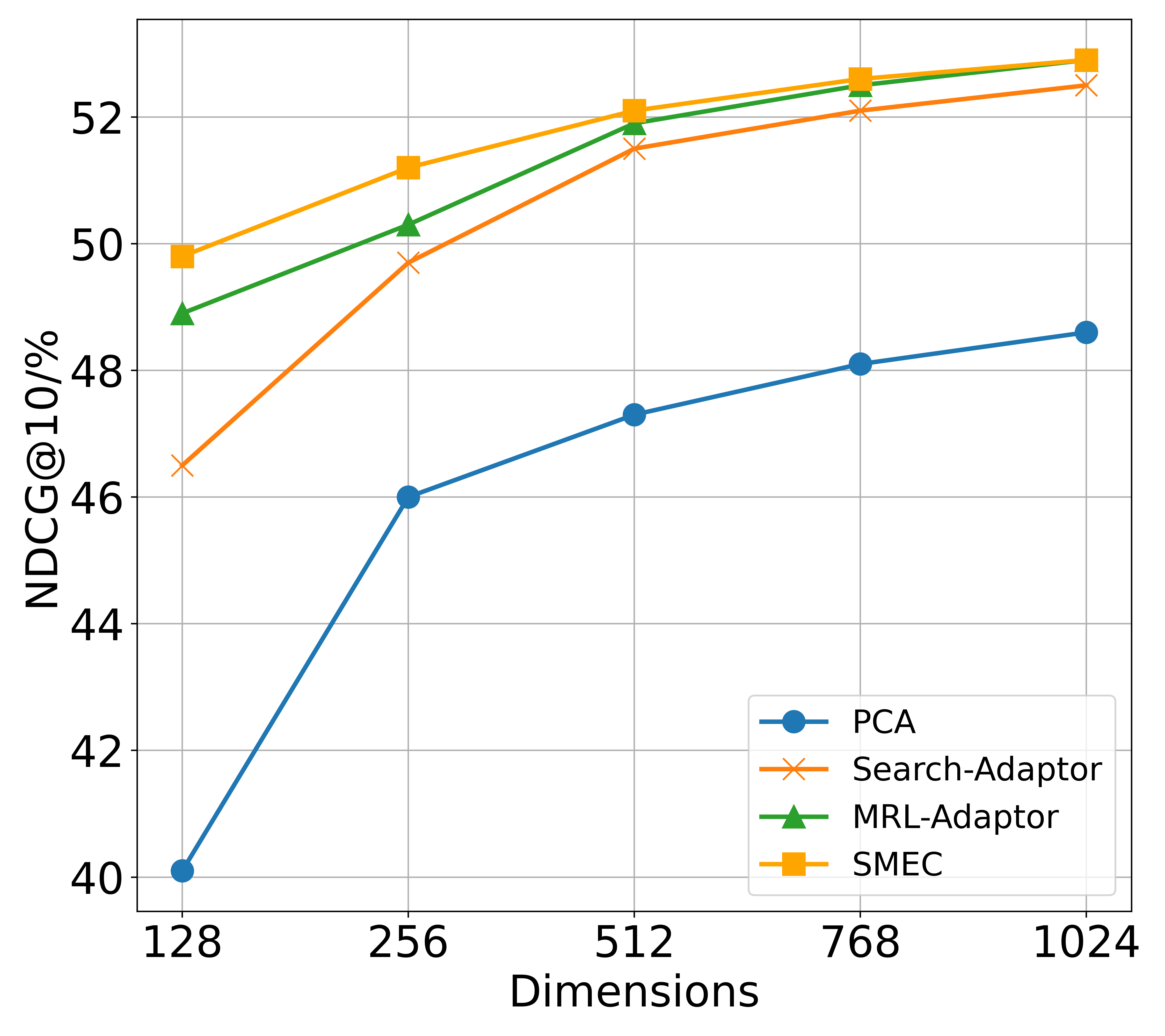
### Visual Description
\n
## Line Chart: Performance Comparison of Dimensionality Reduction Methods
### Overview
The image is a line chart comparing the performance of four different dimensionality reduction or adaptation methods across varying embedding dimensions. The performance metric is NDCG@10 (Normalized Discounted Cumulative Gain at rank 10), expressed as a percentage. The chart demonstrates how each method's effectiveness changes as the dimensionality of the representation increases.
### Components/Axes
* **X-Axis (Horizontal):** Labeled "Dimensions". It represents the dimensionality of the embedding space. The axis has five discrete, evenly spaced tick marks at values: **128, 256, 512, 768, 1024**.
* **Y-Axis (Vertical):** Labeled "NDCG@10/%". It represents the retrieval performance metric. The axis ranges from **40 to 52**, with major grid lines at intervals of 2 (40, 42, 44, 46, 48, 50, 52).
* **Legend:** Located in the **bottom-right corner** of the chart area. It contains four entries, each associating a line color and marker style with a method name:
* **Blue line with circle markers (●):** PCA
* **Orange line with 'x' markers (×):** Search-Adaptor
* **Green line with triangle markers (▲):** MRL-Adaptor
* **Yellow line with square markers (■):** SMEC
### Detailed Analysis
All four data series show a positive, monotonic trend: performance (NDCG@10) increases as the number of dimensions increases. The rate of improvement generally slows down at higher dimensions, suggesting diminishing returns.
**Data Series and Approximate Values:**
1. **PCA (Blue, ●):**
* **Trend:** Starts as the lowest-performing method and shows the most dramatic relative improvement, especially between 128 and 256 dimensions. The slope is steep initially and then becomes more gradual.
* **Data Points (Approximate):**
* 128 Dimensions: ~40.1%
* 256 Dimensions: ~46.0%
* 512 Dimensions: ~47.3%
* 768 Dimensions: ~48.1%
* 1024 Dimensions: ~48.6%
2. **Search-Adaptor (Orange, ×):**
* **Trend:** Starts significantly above PCA. Shows steady improvement, with a consistent upward slope that is less steep than PCA's initial jump.
* **Data Points (Approximate):**
* 128 Dimensions: ~46.5%
* 256 Dimensions: ~49.7%
* 512 Dimensions: ~51.5%
* 768 Dimensions: ~52.1%
* 1024 Dimensions: ~52.5%
3. **MRL-Adaptor (Green, ▲):**
* **Trend:** Starts as the second-highest method. Its performance line runs very close to, but consistently slightly below, the SMEC line. The gap between them narrows at higher dimensions.
* **Data Points (Approximate):**
* 128 Dimensions: ~48.9%
* 256 Dimensions: ~50.3%
* 512 Dimensions: ~51.9%
* 768 Dimensions: ~52.5%
* 1024 Dimensions: ~52.9%
4. **SMEC (Yellow, ■):**
* **Trend:** The top-performing method across all measured dimensions. It maintains a small but consistent lead over MRL-Adaptor.
* **Data Points (Approximate):**
* 128 Dimensions: ~49.8%
* 256 Dimensions: ~51.2%
* 512 Dimensions: ~52.1%
* 768 Dimensions: ~52.7%
* 1024 Dimensions: ~53.0%
### Key Observations
* **Performance Hierarchy:** A clear and consistent hierarchy is maintained across all dimensions: **SMEC > MRL-Adaptor > Search-Adaptor > PCA**.
* **Convergence at High Dimensions:** The performance gap between the top two methods (SMEC and MRL-Adaptor) and between the middle two (Search-Adaptor and MRL-Adaptor) becomes very small at 768 and 1024 dimensions. The lines for SMEC and MRL-Adaptor nearly converge at 1024 dimensions.
* **PCA's Lag:** PCA consistently underperforms the other three specialized adaptation methods by a significant margin (approximately 3-9 percentage points), though it does benefit from increased dimensionality.
* **Diminishing Returns:** All curves show a concave shape, indicating that the gain in NDCG@10 from doubling the dimensions decreases as the dimensions get larger. The most significant gains for all methods occur between 128 and 512 dimensions.
### Interpretation
This chart provides strong evidence for two key conclusions in the context of representation learning for retrieval tasks:
1. **Specialized Adaptation Outperforms Generic Reduction:** Methods designed specifically for the search/retrieval task (Search-Adaptor, MRL-Adaptor, SMEC) dramatically outperform a generic dimensionality reduction technique (PCA). This suggests that simply compressing vectors is insufficient; the adaptation must be tailored to preserve or enhance the properties needed for effective ranking.
2. **Higher Dimensionality is Beneficial, but with Limits:** Increasing the dimensionality of the embedding space consistently improves retrieval performance for all methods. However, the flattening curves suggest a practical ceiling. The cost (computational, storage) of moving from 512 to 1024 dimensions yields a smaller performance benefit than moving from 128 to 256. The optimal dimensionality likely involves a trade-off between performance and efficiency, with 512 or 768 appearing as potential sweet spots where performance is high and the rate of improvement begins to plateau.
3. **SMEC and MRL-Adaptor are State-of-the-Art:** The near-identical performance of SMEC and MRL-Adaptor at high dimensions indicates they are both highly effective approaches. The choice between them might depend on other factors not shown here, such as training stability, inference speed, or performance on other metrics. SMEC's slight edge at lower dimensions (128, 256) could be meaningful in resource-constrained scenarios.
</details>
(a) Image retrieval
<details>
<summary>figures/fig_t2i.png Details</summary>
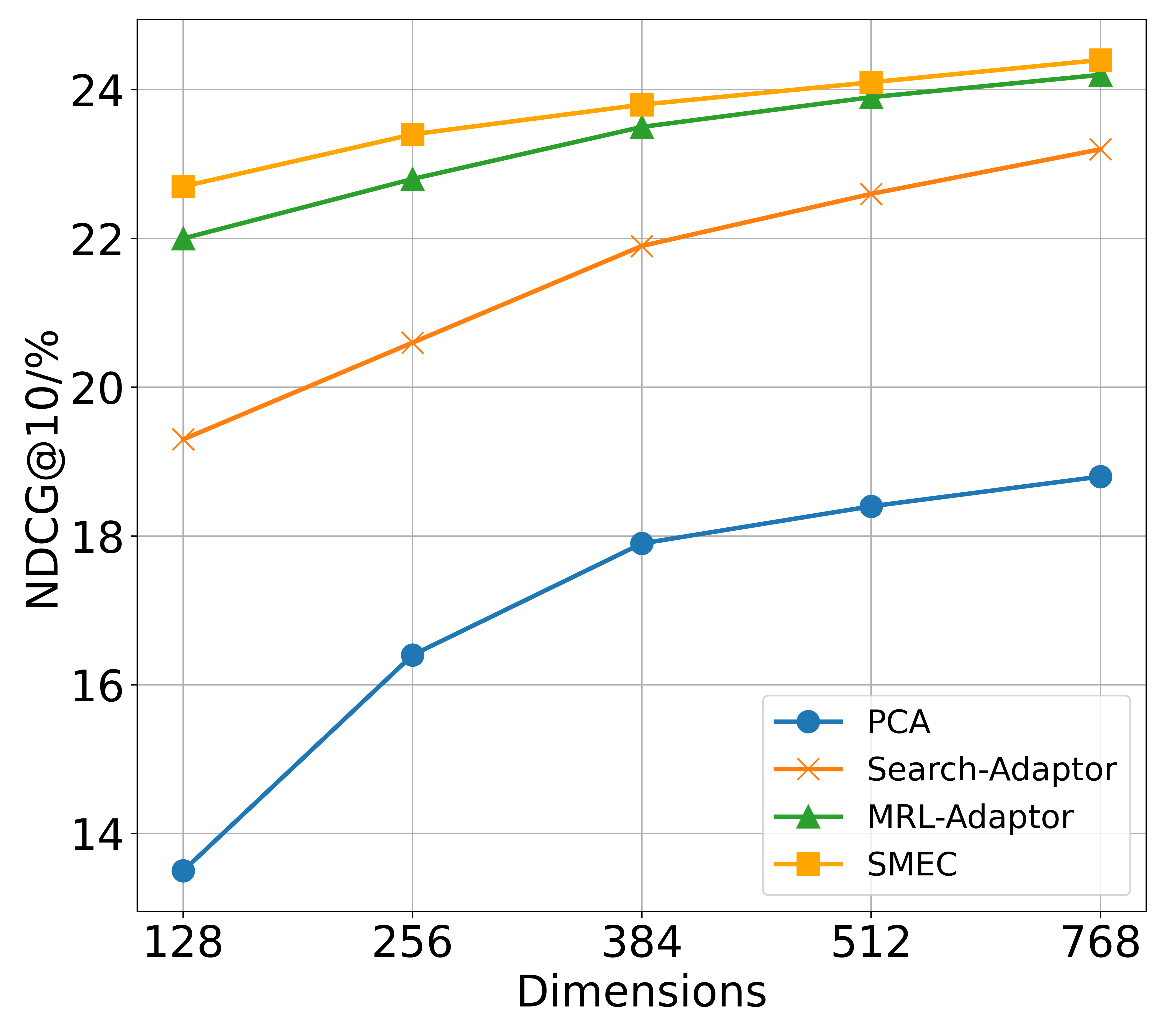
### Visual Description
## Line Chart: Performance Comparison of Dimensionality Reduction Methods
### Overview
The image is a line chart comparing the performance of four different dimensionality reduction or adaptation methods across varying numbers of dimensions. The performance metric is NDCG@10 (Normalized Discounted Cumulative Gain at rank 10), expressed as a percentage. The chart demonstrates how each method's effectiveness changes as the dimensionality of the representation increases.
### Components/Axes
* **Chart Type:** Multi-series line chart with markers.
* **X-Axis:**
* **Label:** "Dimensions"
* **Scale:** Categorical/ordinal with discrete values: 128, 256, 384, 512, 768.
* **Y-Axis:**
* **Label:** "NDCG@10/%"
* **Scale:** Linear, ranging from approximately 13 to 25. Major gridlines are at intervals of 2 (14, 16, 18, 20, 22, 24).
* **Legend:**
* **Position:** Bottom-right corner of the chart area.
* **Entries (from top to bottom as listed):**
1. **PCA:** Blue line with circle markers.
2. **Search-Adaptor:** Orange line with 'x' (cross) markers.
3. **MRL-Adaptor:** Green line with triangle markers.
4. **SMEC:** Yellow/gold line with square markers.
### Detailed Analysis
**Trend Verification:** All four data series show a clear upward trend, indicating that NDCG@10 performance improves as the number of dimensions increases from 128 to 768.
**Data Series & Approximate Values:**
1. **PCA (Blue line, circle markers):**
* **Trend:** Steepest initial increase, then continues to rise steadily. It is the lowest-performing method at all dimension points.
* **Approximate Values:**
* 128 Dimensions: ~13.5%
* 256 Dimensions: ~16.4%
* 384 Dimensions: ~17.9%
* 512 Dimensions: ~18.4%
* 768 Dimensions: ~18.8%
2. **Search-Adaptor (Orange line, 'x' markers):**
* **Trend:** Consistent, nearly linear upward slope. It is the third-best performing method.
* **Approximate Values:**
* 128 Dimensions: ~19.3%
* 256 Dimensions: ~20.6%
* 384 Dimensions: ~21.9%
* 512 Dimensions: ~22.6%
* 768 Dimensions: ~23.2%
3. **MRL-Adaptor (Green line, triangle markers):**
* **Trend:** Steady upward slope, slightly less steep than Search-Adaptor. It is the second-best performing method.
* **Approximate Values:**
* 128 Dimensions: ~22.0%
* 256 Dimensions: ~22.8%
* 384 Dimensions: ~23.5%
* 512 Dimensions: ~23.9%
* 768 Dimensions: ~24.2%
4. **SMEC (Yellow/gold line, square markers):**
* **Trend:** Gradual upward slope, consistently the highest-performing method. The performance gap between SMEC and MRL-Adaptor narrows slightly as dimensions increase.
* **Approximate Values:**
* 128 Dimensions: ~22.7%
* 256 Dimensions: ~23.4%
* 384 Dimensions: ~23.8%
* 512 Dimensions: ~24.1%
* 768 Dimensions: ~24.4%
### Key Observations
1. **Performance Hierarchy:** A clear and consistent performance hierarchy is maintained across all tested dimensions: **SMEC > MRL-Adaptor > Search-Adaptor > PCA**.
2. **Diminishing Returns:** All methods show signs of diminishing returns; the performance gain from increasing dimensions is larger at the lower end (e.g., 128 to 256) than at the higher end (e.g., 512 to 768).
3. **Significant Gap:** There is a substantial performance gap (approximately 5-6 percentage points) between the traditional PCA method and the three adaptor-based methods (Search-Adaptor, MRL-Adaptor, SMEC) at every dimension level.
4. **Convergence at Top:** The top two methods, SMEC and MRL-Adaptor, have very similar performance, with their lines nearly converging at 768 dimensions (a difference of only ~0.2%).
### Interpretation
This chart likely comes from a research paper in information retrieval or machine learning, evaluating methods for creating efficient vector representations for search or recommendation tasks. NDCG@10 is a standard metric for ranking quality.
The data suggests that:
* **Adaptor-based methods are superior:** The three methods labeled as "Adaptor" or a related technique (SMEC) significantly outperform the classical PCA baseline. This indicates that task-specific adaptation or learning of the dimensionality reduction projection is more effective than a generic, unsupervised method like PCA for this ranking task.
* **SMEC is the most effective:** Among the compared techniques, SMEC achieves the highest ranking quality across all tested dimensionalities, making it the most effective method in this evaluation.
* **More dimensions help, but cost more:** Increasing the dimensionality of the vector representation improves retrieval quality for all methods, but the benefit per added dimension decreases. This presents a trade-off between performance and computational/storage cost. The chart helps identify a potential "sweet spot" (e.g., 384 or 512 dimensions) where most of the performance gain has been realized.
* **Robustness of advanced methods:** The relatively flat slopes of MRL-Adaptor and SMEC compared to PCA and Search-Adaptor suggest their performance is more robust and less sensitive to reductions in dimensionality, which is a desirable property for efficient systems.
</details>
(b) Text-to-Image retrieval
<details>
<summary>figures/fig_i2t.png Details</summary>
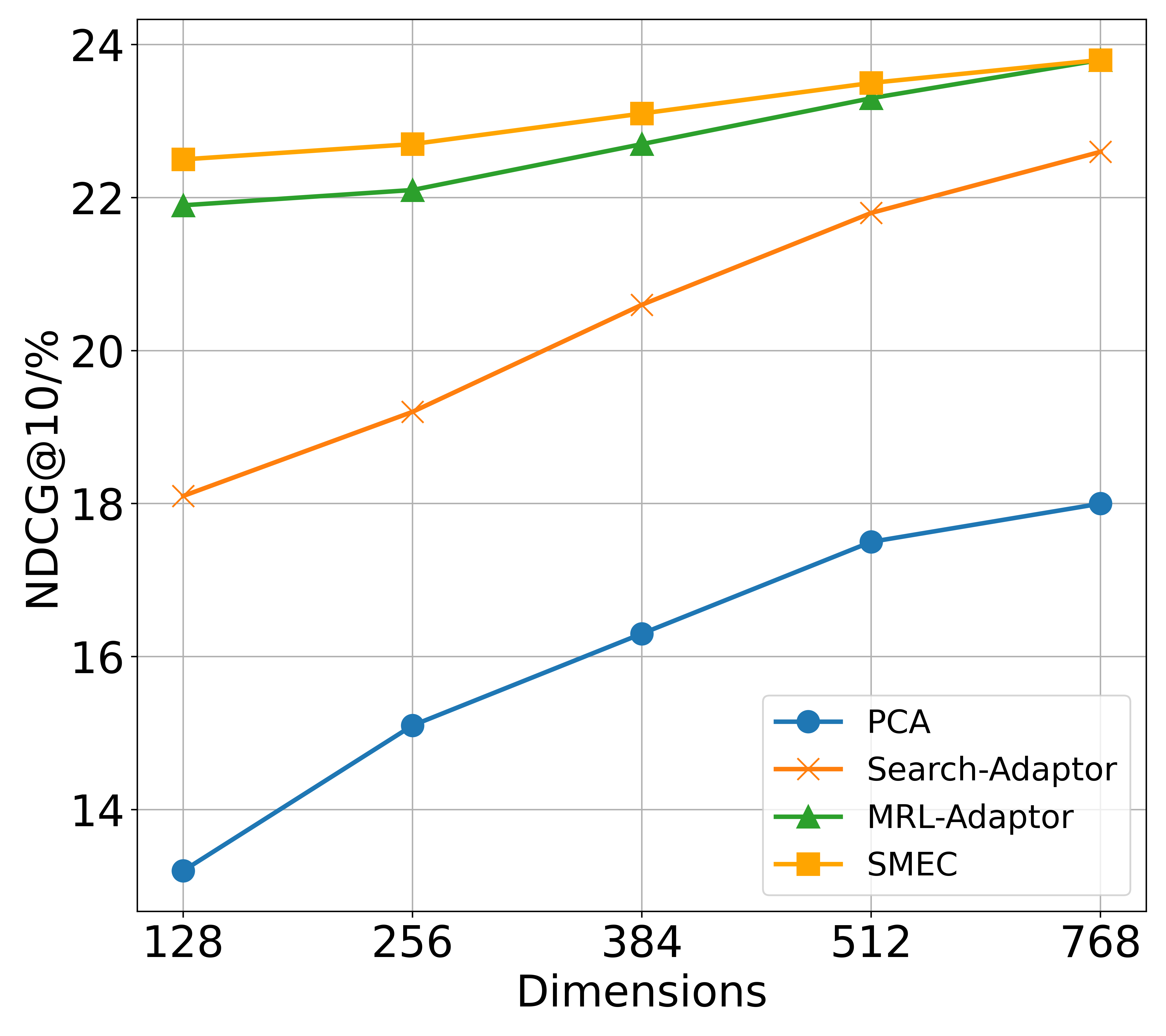
### Visual Description
\n
## Line Chart: Performance Comparison of Dimensionality Reduction Methods
### Overview
This is a line chart comparing the performance of four different dimensionality reduction or adaptation methods (PCA, Search-Adaptor, MRL-Adaptor, SMEC) across five different dimensionality settings. The performance metric is NDCG@10 (Normalized Discounted Cumulative Gain at rank 10), expressed as a percentage. The chart demonstrates how each method's effectiveness changes as the number of dimensions increases.
### Components/Axes
* **X-Axis (Horizontal):** Labeled "Dimensions". It represents the dimensionality of the data or model embedding space. The axis has five discrete, evenly spaced tick marks at values: 128, 256, 384, 512, and 768.
* **Y-Axis (Vertical):** Labeled "NDCG@10/%". It represents the performance score, with a scale ranging from approximately 13% to 24%. Major gridlines are present at intervals of 2% (14, 16, 18, 20, 22, 24).
* **Legend:** Located in the bottom-right quadrant of the chart area. It contains four entries, each associating a line color and marker style with a method name:
* **PCA:** Blue line with solid circle markers (●).
* **Search-Adaptor:** Orange line with cross markers (×).
* **MRL-Adaptor:** Green line with solid triangle markers (▲).
* **SMEC:** Yellow-orange line with solid square markers (■).
### Detailed Analysis
The chart plots four data series, each showing a positive correlation between dimensionality and NDCG@10 score.
1. **PCA (Blue line, circle markers):**
* **Trend:** Shows a steady, nearly linear upward slope. It is the lowest-performing method at all dimension points.
* **Data Points (Approximate):**
* 128 Dimensions: ~13.1%
* 256 Dimensions: ~15.1%
* 384 Dimensions: ~16.3%
* 512 Dimensions: ~17.5%
* 768 Dimensions: ~18.0%
2. **Search-Adaptor (Orange line, cross markers):**
* **Trend:** Exhibits a strong, consistent upward slope, steeper than PCA. It starts as the third-best method but closes the gap with the top performers at higher dimensions.
* **Data Points (Approximate):**
* 128 Dimensions: ~18.1%
* 256 Dimensions: ~19.2%
* 384 Dimensions: ~20.6%
* 512 Dimensions: ~21.8%
* 768 Dimensions: ~22.6%
3. **MRL-Adaptor (Green line, triangle markers):**
* **Trend:** Shows a moderate upward slope. It is the second-best performer at lower dimensions and converges with the top performer (SMEC) at the highest dimension.
* **Data Points (Approximate):**
* 128 Dimensions: ~21.9%
* 256 Dimensions: ~22.1%
* 384 Dimensions: ~22.7%
* 512 Dimensions: ~23.3%
* 768 Dimensions: ~23.8%
4. **SMEC (Yellow-orange line, square markers):**
* **Trend:** Shows a gentle upward slope. It is the top-performing method at all dimensions, though its advantage over MRL-Adaptor diminishes as dimensions increase.
* **Data Points (Approximate):**
* 128 Dimensions: ~22.5%
* 256 Dimensions: ~22.7%
* 384 Dimensions: ~23.1%
* 512 Dimensions: ~23.5%
* 768 Dimensions: ~23.8%
### Key Observations
* **Universal Improvement:** All four methods show improved NDCG@10 scores as the number of dimensions increases from 128 to 768.
* **Performance Hierarchy:** A clear and consistent performance hierarchy is maintained across most dimensions: SMEC > MRL-Adaptor > Search-Adaptor > PCA.
* **Convergence at the Top:** The performance gap between the top two methods, SMEC and MRL-Adaptor, narrows significantly. At 768 dimensions, their scores are nearly identical (~23.8%).
* **Greatest Gains:** Search-Adaptor shows the largest relative improvement, increasing its score by approximately 4.5 percentage points (from ~18.1% to ~22.6%). PCA shows the second-largest gain of about 4.9 points, but from a much lower baseline.
* **Diminishing Returns:** The rate of improvement for the top-performing methods (SMEC, MRL-Adaptor) appears to slow slightly at higher dimensions (512 to 768), suggesting potential performance saturation.
### Interpretation
This chart likely comes from a study on information retrieval, recommendation systems, or embedding compression, where NDCG is a standard metric for ranking quality. The data suggests that:
1. **Increased Dimensionality is Beneficial:** For all tested methods, allocating more dimensions (i.e., using a larger embedding or representation space) leads to better ranking performance. This is an expected trade-off between model/representation size and effectiveness.
2. **Specialized Adaptors Outperform General PCA:** The two "Adaptor" methods and SMEC significantly outperform standard PCA at all dimension levels. This indicates that task-specific or learned adaptation techniques are far more effective at preserving or enhancing retrieval-relevant information than a general-purpose linear projection like PCA.
3. **SMEC and MRL-Adaptor are State-of-the-Art:** These two methods are the top performers. SMEC holds a slight but consistent edge, except at the highest dimension where they tie. The choice between them at 768 dimensions might depend on other factors like computational cost or training stability.
4. **Search-Adaptor is a Strong Contender:** While starting lower, its steep improvement curve suggests it scales very well with dimensionality and could become competitive with the top methods at even higher dimensions not shown on the chart.
5. **Practical Implication:** For a system designer, this chart provides a clear cost-benefit analysis. If computational resources are severely constrained (low dimensions), SMEC or MRL-Adaptor are the only viable high-performance choices. If resources allow for 768 dimensions, the performance difference between the top methods becomes negligible, potentially allowing selection based on other engineering constraints.
</details>
(c) Image-to-Text retrieval
Figure 8: Experimental results on image and multimodal datasets. (a) presents the results on the Products-10K dataset using an image representation model based on ViT-H (with 1024 dimensions). (b) and (c) show the results on the Fashion-200K dataset for text-to-image and image-to-text retrieval tasks, respectively, using the LLM2CLIP model (with 768 dimensions, base on ViT-L/14 and Llama-3.2-1B).