2510.13999v1

# REAP the Experts: Why Pruning Prevails for One-Shot MoE compression **Authors**: - Yani Ioannou, Vithursan Thangarasa (Cerebras Systems Inc., Schulich School of Engineering, University of Calgary) Abstract Sparsely-activated Mixture-of-Experts (SMoE) models offer efficient pre-training and low latency but their large parameter counts create significant memory overhead, motivating research into expert compression. Contrary to recent findings favouring expert merging on discriminative benchmarks, we demonstrate that expert pruning is a superior strategy for generative tasks. We prove that merging introduces an irreducible error by causing a “functional subspace collapse”, due to the loss of the router’s independent, input-dependent control over experts. Leveraging this insight, we propose Router-weighted Expert Activation Pruning (REAP), a novel pruning criterion that considers both router gate-values and expert activation norms. Across a diverse set of SMoE models ranging from 20B to 1T parameters, REAP consistently outperforms merging and other pruning methods on generative benchmarks, especially at 50% compression. Notably, our method achieves near-lossless compression on code generation and tool-calling tasks with Qwen3-Coder-480B and Kimi-K2, even after pruning 50% of experts. Correspondence to mklasby@ucalgary.ca & vithu@cerebras.net $\dagger$ Work completed while on internship at Cerebras | <details> <summary>x1.png Details</summary>  ### Visual Description Icon/Small Image (25x24) </details> | https://github.com/CerebrasResearch/reap | | --- | --- | | <details> <summary>x2.png Details</summary>  ### Visual Description Icon/Small Image (26x24) </details> | https://hf.co/cerebras/Qwen3-Coder-REAP-363B-A35B-FP8 | | <details> <summary>x3.png Details</summary>  ### Visual Description Icon/Small Image (26x24) </details> | https://hf.co/cerebras/Qwen3-Coder-REAP-246B-A35B-FP8 | 1 Introduction Interest in the Sparsely-activated Mixture-of-Experts (SMoE) architecture for Large Language Models (LLMs) surged following the release of DeepSeek-V3 (DeepSeek-AI et al., 2024) and other high-quality open-weight SMoE LLMs (Jiang et al., 2024; Meta AI Team, 2025; Yang et al., 2025a; Zeng et al., 2025; Baidu, 2025; Kimi Team et al., 2025). Compared to dense models, the SMoEs offer lower latency and more efficient pre-training (Fedus et al., 2022). However, SMoEs require more parameters than dense models to achieve similar accuracy, resulting in significant memory overhead. Further, expert usage imbalance during inference causes poor accelerator utilization, leading to increased latency or compromises such as dropped tokens (Balmau et al., 2025). Expert usage imbalance also represents an opportunity, motivating prior work which investigates whether experts can be compressed without negatively impairing accuracy (Li et al., 2023; Lu et al., 2024). By eliminating or compressing redundant experts, memory overhead is reduced. A more uniform distribution of expert usage would also improve hardware utilization. Expert compression is particularly valuable for use cases which feature small batch sizes such as local deployments and academic research. Initial expert compression efforts focused on expert pruning, the removal of experts in their entirety. However, expert pruning is a strong intervention on the model’s weights. Techniques such as quantization, low-rank compression, and expert merging also offer memory savings but maintain a lossy representation of the less important experts. Crucially, expert merging has recently been demonstrated to outperform expert pruning when evaluated with perplexity and on Multiple Choice (MC) question answering benchmarks (Li et al., 2023; Liu et al., 2024b). However, an evaluation comparing these methods on generative benchmarks has yet to be conducted. In this work, we demonstrate that — when paired with a suitable saliency criterion — expert pruning outperforms expert merging, particularly on generative benchmark tasks such as code generation, creative writing, and mathematical reasoning. Specifically, our main contributions are as follows: - We prove that expert merging introduces irreducible error due to the loss of the router’s independent, input-dependant modulation of the expert outputs resulting in functional subspace collapse, substantially reducing the functional output space of the compressed SMoE layer. In contrast, in expert pruned SMoEs the router maintains independent control over the remaining experts; - We introduce Router-weighted Expert Activation Pruning (REAP), a novel expert pruning saliency criterion, which selects experts to prune which contribute minimally to the layer output by considering both the router gate-values and average activation norm of the experts; - Across diverse SMoE architectures ranging from 20B to 1T parameters and a suite of generative evaluations, we demonstrate the significant and consistent advantage of REAP over existing expert pruning and merging approaches, particularly at 50% compression. Notably, our method achieves near-lossless compression on code generation tasks after pruning 50% of experts from Qwen3-Coder-480B and Kimi-K2; - We open-source our code and select compressed model checkpoints to facilitate further research on compressed SMoEs and their applications. 2 Related Work Sparsely activated SMoE architecture. A Mixture-of-Experts (MoE) layer is comprised of multiple, specialized feed-forward subnetworks known as experts and a router which produces gate-values (i.e., gates) to dynamically modulate the output of the experts based on the input. The architecture was revived in the deep learning era by the introduction of the SMoE by Shazeer et al. (2017). SMoEs layers only select a subset of experts to use for each input, enabling massive scaling of model parameters without a commensurate increase in computational cost (Lepikhin et al., 2021; Fedus et al., 2022). In transformer-based LLMs, SMoE layers are integrated by replacing the traditional feed-forward layers. Further innovations such as auxiliary-loss-free load balancing (DeepSeek-AI et al., 2024), shared experts, and fined-grained experts (Dai et al., 2024) have propelled SMoE architectures to become the de facto standard for LLMs in recent months. Expert pruning. Although SMoE layers effectively decouple total model parameters from inference costs, the memory overhead of storing large SMoEs restricts their deployment in resourced-constrained environments, motivating research in expert pruning to reduce total number of parameters. Early efforts demonstrated that progressively pruning experts based on router weights during fine-tuning until a single expert remained could preserve model quality in task-specific settings (Chen et al., 2022). Koishekenov et al. (2023) found expert pruning to be effective without further fine-tuning despite aggressively pruning up to 80% of experts. Muzio et al. (2024) found that global pruning using gate-values as a saliency criterion was more effective than uniform, layer-wise frequency-based pruning. Other sophisticated pruning criteria have been proposed: Lu et al. (2024) introduced an exhaustive search strategy which prunes experts that minimize the reconstruction loss between the original and pruned layer outputs; Liu et al. (2024a) used a gradient-free evolutionary algorithm to prune experts. Both of these works demonstrated significant improvements over naive frequency-based pruning. A comprehensive evaluation of 16 diverse pruning criteria was conducted by Jaiswal et al. (2025). Expert Activation Norm (EAN) was empirically found to be the highest performing criterion and the benefits of iterative pruning were presented. Expert merging. While the above-noted works prove that expert compression is feasible via pruning, an alternative compression technique is to merge experts. Generally, merging requires both a clustering algorithm and a merging technique. Li et al. (2023) introduced Merge Sparse Mixture of Experts (M-SMoE) which first initializes expert cluster centres by identifying the dominant experts with the highest usage frequency globally across all layers. The remaining non-dominant experts are clustered based on the cosine similarity of router logits. Finally, experts weights are aligned via permutation with the weight matching algorithm (Ainsworth et al., 2023) and merged using frequency-weighted parameter averaging. Li et al. (2023) found that their technique outperformed Chen et al. ’s (2022) pruning method on MC benchmarks. Chen et al. (2025) proposed Hierarchical Clustering for Sparsely activated Mixture of Experts (HC-SMoE). HC-SMoE clusters experts based on the euclidean similarity of their representative vectors — the average activation of each expert measured on every token in a calibration dataset — using hierarchical agglomerative clustering. Similar to M-SMoE, HC-SMoE uses frequency-weighted parameter averaging to merge clusters into a single merged expert. Without any fine-tuning, Chen et al. (2025) found that their technique outperformed expert pruning based on router logits (He et al., 2025a), frequency, and Lu et al. ’s (2024) method when benchmarked on a suite of MC question answering tasks. Other compression techniques. In addition to pruning and merging, experts may be compressed through quantization (Huang et al., 2025), low-rank decomposition (Yang et al., 2024a; Gu et al., 2025; He et al., 2025b), weight sparsity (He et al., 2025a), or a combination of any of the above techniques (Liu et al., 2025). These other approaches are orthogonal to expert pruning and merging; however, note that expert merging necessitates re-quantization for block quantization formats that share common scaling coefficients across a group of weights. Model merging. Model merging aims to combine parameters from multiple trained neural networks and has been rapidly adopted as a cost-effective way to improve model quality across diverse domains. The initial motivation for merging was based on the finding that mode connectivity exists between the loss landscapes of two or more trained neural networks, enabling interpolation of their parameters without incurring an increase in loss (Garipov et al., 2018; Ainsworth et al., 2023; Ito et al., 2024). Simple parameter averaging remains an effective technique; however, more sophisticated strategies based on task vectors have also been proposed to minimize interference in the merged model parameters (Ilharco et al., 2023; Yadav et al., 2023; Yu et al., 2024). Much of the existing literature focuses on the setting in which multiple fine-tunes of a single checkpoint are merged. Non-local merging in which the models do not share a common checkpoint is more closely related to expert merging. Sharma et al. (2024) found that re-scaling of model activations was necessary to achieve high-quality non-local merging. LLM evaluation. Evaluating LLMs is challenging; prior work demonstrated that simple metrics such as perplexity can be misleading when used to evaluate compressed LLMs (Jaiswal et al., 2024). MC benchmarks typically measure the log-likelihood of answer tokens to determine a model’s response to a question (Gao et al., 2023; Chandak et al., 2025). As such, each response choice is evaluated in a single forward pass, without any tokens being generated by the model. Perplexity and MC accuracy can therefore be viewed as discriminative metrics. In contrast, generative benchmarks require the model to output a response, more closely corresponding with real-world use-cases of LLMs. Tasks such as code generation, mathematical reasoning with structured outputs, and creative writing are examples of generative benchmarks. 3 Merging Experts Causes Functional Subspace Collapse Setup. To motivate our proposed expert pruning method, we first formally develop the expected errors of both expert merging and pruning. Consider a SMoE layer with $K$ experts $f_{1},...,f_{K}$ , each a function $f_{k}:\mathbb{R}^{d}→\mathbb{R}^{d}$ , and a router producing non-negative gates $\mathbf{g(x)}=(g_{1}(x),...,g_{K}(x))∈\Delta^{K-1}$ . Top- $k$ routing is achieved by zeroing all but the largest $k$ gates. The output of the original layer is $$ h(x):=\sum_{k=1}^{K}g_{k}(x)\,f_{k}(x). \tag{1} $$ Two operations at fixed compression. To analyse the fundamental difference between compression operations, we focus on the elementary case of reducing two experts, $(f_{i},f_{j})$ , to one. This pairwise analysis is the building block for any larger merge within a cluster. Pruning removes expert $j$ and re-normalizes the router outputs over the remaining $K-1$ experts, producing a new set of gates $\bar{g}(x)$ . Merging replaces $(f_{i},f_{j})$ with a new expert $\tilde{f}$ . Existing one-shot expert merging methods such as HC-SMoE and M-SMoE sum the gates for the original experts $g_{i}(x)+g_{j}(x)$ . The pruned, $\bar{h}(x)$ , and merged, $\tilde{h}(x)$ , layer outputs are $$ \bar{h}(x):=\sum_{k\neq j}\bar{g}_{k}(x)\,f_{k}(x), \tag{2} $$ $$ \tilde{h}(x):=\sum_{k\neq i,j}g_{k}(x)f_{k}(x)+\big(g_{i}(x)+g_{j}(x)\big)\tilde{f}(x). \tag{3} $$ 3.1 Merging induces an input-dependent target a single expert cannot realize Define the router’s input-dependent mixing ratio $r(x):=\frac{g_{i}(x)}{g_{i}(x)+g_{j}(x)}∈[0,1]$ on the set where $g_{i}+g_{j}>0$ . Substituting $g_{i}(x)$ and $g_{j}(x)$ in terms of $r(x)$ , the original contribution of the pair $(i,j)$ can be written as $$ \displaystyle g_{i}(x)f_{i}(x)+g_{j}(x)f_{j}(x) \displaystyle=\big[r(x)(g_{i}(x)+g_{j}(x))\big]f_{i}(x)+\big[(1-r(x))(g_{i}(x)+g_{j}(x))\big]f_{j}(x) \displaystyle=\big(g_{i}(x)+g_{j}(x)\big)\underbrace{\Big(r(x)f_{i}(x)+\big(1-r(x)\big)f_{j}(x)\Big)}_{\text{The ideal, input-dependent target expert}}. \tag{4} $$ After merging, the router must apply the summed gate, $g_{i}(x)+g_{j}(x)$ , to a constant convex combination of the constituent experts which is independent of $x$ . The core issue is that the merged model is forced to approximate the dynamic, input-dependent target expert with a static one. The following theorem quantifies this unavoidable approximation error. **Theorem 1 (Irreducible error of merging)** *Let $\tilde{f}_{\alpha}(x)=\alpha f_{i}(x)+(1-\alpha)f_{j}(x)$ with a constant $\alpha∈[0,1]$ and define $\Delta_{ij}:=f_{i}(x)-f_{j}(x)$ . The $L^{2}$ error of the merged pair is minimized when $\alpha$ is chosen to be the expected mixing ratio, $\alpha^{\star}:=\mathbb{E}[r(x)]$ . Omitting the argument $(x)$ for brevity, this minimal error is $$ \displaystyle\big\|\,\big(g_{i}{+}g_{j}\big)\!\big(rf_{i}{+}(1{-}r)f_{j}\big)\;-\;\big(g_{i}{+}g_{j}\big)\!\big(\alpha f_{i}{+}(1{-}\alpha)f_{j}\big)\big\|^{2} \displaystyle=\underbrace{\mathbb{E}\!\left[(g_{i}{+}g_{j})^{2}\right]}_{\text{router scale}}\cdot\underbrace{\mathrm{Var}[r(x)]}_{\text{policy variability}}\cdot\underbrace{\|\Delta_{ij}\|^{2}}_{\text{expert gap}}. \tag{5} $$ In particular, if the router’s policy is not constant ( $\mathrm{Var}[r(x)]>0$ ) and the experts are not functionally identical ( $\|\Delta_{ij}\|>0$ ), then every constant- $\alpha$ merge incurs strictly positive excess risk.* * Proof* The error term simplifies to $\big\|\big(g_{i}{+}g_{j}\big)\big(r-\alpha\big)\Delta_{ij}\big\|^{2}$ . Assuming independence between the router policy and expert functions, this is proportional to $\mathbb{E}[(r-\alpha)^{2}]$ . This is a standard least-squares problem minimized when $\alpha=\mathbb{E}[r]$ , and the minimal value is $\mathrm{Var}[r]$ . ∎ Consequences. Theorem 1 illustrates that merging with summed gates is fundamentally flawed whenever (i) the router has learned an input-dependent policy for mixing two experts ( $\mathrm{Var}[r]>0$ ), and (ii) the experts are themselves distinct ( $\|\Delta_{ij}\|>0$ ). Any fixed $\alpha$ cannot overcome the irreducible error bound established in equation 5. 3.2 Pruning preserves independent control Pruning removes one function but importantly does not tie the remaining gates. The router still modulates each surviving expert independently. In contrast, merging removes a degree of freedom in the policy by replacing individual experts with their mergers. For a direct comparison under no fine-tuning, pruning expert $j$ and reallocating its gate-value to expert $i$ produces the error $$ \big\|(g_{i}(x)f_{i}(x)+g_{j}(x)f_{j}(x))-(g_{i}(x){+}g_{j}(x))f_{i}(x)\big\|^{2}\;=\;\mathbb{E}\!\left[g_{j}(x)^{2}\,\|\Delta_{ij}(x)\|_{2}^{2}\right]. \tag{6} $$ Unlike equation 5, equation 6 does not penalize policy variability, the router still controls surviving experts independently. Whenever the router substantially mixes $i$ and $j$ (large $\mathrm{Var}[r]$ ) while the pruned expert $j$ has a small average gate-value ( $\mathbb{E}[g_{j}^{2}]$ ), pruning admits a strictly smaller error than merging. Synthesis. Theorem 1 establishes that summed gate merging incurs an irreducible error directly proportional to the router’s policy variability ( $\mathrm{Var}[r(x)]$ ). In contrast, the error from pruning a low-usage expert (Eq. 6) is proportional to its gate-value ( $\mathbb{E}[g_{j}^{2}]$ ) and is insensitive to policy variability. Therefore, when the router actively mixes between two distinct experts, merging is fundamentally disadvantaged. Remarks. (i) The constant-mixture model $\tilde{f}_{\alpha}$ is mathematically related to the frequency weighted parameter averaging merge used in practice. (ii) Even if $\tilde{f}$ was dependent on $x$ , the router after merging cannot independently modulate the two latent functions, so the original policy is invalidated. (iii) With top-k routers, the specific irreducible error from policy variability ( $\mathrm{Var}[r(x)]$ ) is generated exclusively on the support where both experts are selected. Outside that support, this component vanishes, leaving only a static error term that depends on the functional expert gap. (iv) See Appendix ˜ A for an extension of the above analysis to hierarchical clustering. 3.3 Empirical evidence for loss of independent control Setup. 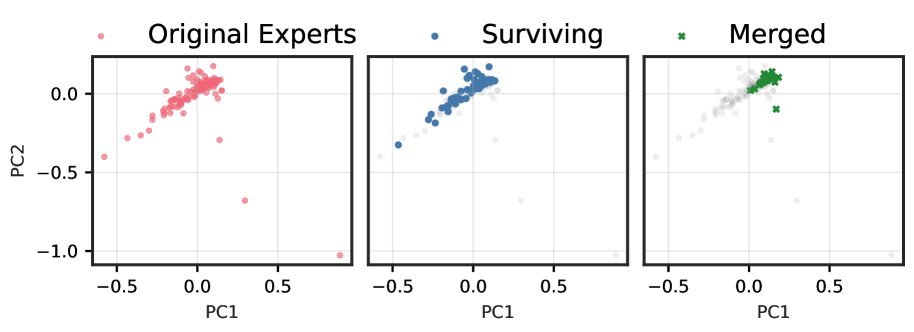We analyse the functional subspaces of expert outputs across four diverse state-of-the-art SMoE architectures by recording mean expert activations from 32 samples of 2048 tokens from the c4 dataset (Raffel et al., 2020). By projecting expert activations onto their first two principal components, we visualize how pruning and merging affect the learned representations. See Appendix ˜ B for additional discussion. Early vs. late behaviour. 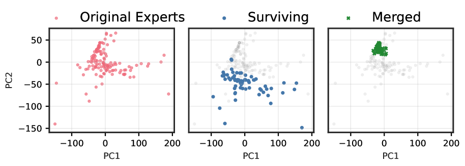Figures ˜ 1 and A4 demonstrate a striking progression of functional collapse from early to late layers across all architectures. In early layers, the original experts form relatively compact manifolds with moderate spread. After pruning, the surviving experts maintain their positions on the original manifold, preserving its geometric structure with reduced density. In contrast, merging produces a visible contraction toward the manifold’s centre. The contrast becomes dramatic in late layers, where experts are more specialized, and in high granularity architectures with many experts per layer. The progression from early to late layers validates our theoretical prediction that the irreducible error is proportional to $\mathrm{Var}[r(x)]$ . Early layers, which typically learn more generic features, exhibit lower policy variability and thus less dramatic collapse. Late layers, where experts have specialized for distinct computational roles, demonstrate high policy variability, resulting in the severe functional collapse observed when these specialized experts are merged into static averages. Synthesis across architectures. The consistency of these patterns across architectures with vastly different expert counts (8 to 128), sparsity levels (6.25% to 25% active), and parameter scales (21.9B to 109B) demonstrates that functional collapse under merging is a fundamental property of the operation rather than an artifact of specific implementations. These visualizations reveal that the core issue is not the reduction in the number of experts per se, but rather the qualitative change in the router’s control structure. <details> <summary>x4.png Details</summary>  ### Visual Description ## Principal Component Analysis (PCA) of Expert Data ### Overview The image displays a Principal Component Analysis (PCA) plot, which is a dimensionality reduction technique used to visualize high-dimensional data in a lower-dimensional space. The plot is divided into three sections, each representing a different group of experts: Original Experts, Surviving Experts, and Merged Experts. The x-axis represents the first principal component (PC1), and the y-axis represents the second principal component (PC2). Each data point is color-coded to indicate the group it belongs to. ### Components/Axes - **X-Axis (PC1)**: Represents the first principal component, which captures the most variance in the data. - **Y-Axis (PC2)**: Represents the second principal component, which captures the second most variance in the data. - **Legend**: Color-coded to indicate the group of experts (Original Experts, Surviving Experts, Merged Experts). - **Data Points**: Each point represents an expert, and its position on the plot indicates its principal component scores. ### Detailed Analysis or ### Content Details - **Original Experts**: The data points for Original Experts are scattered across the plot, with a mix of positive and negative values for both PC1 and PC2. The majority of these points are in the upper left quadrant, suggesting that Original Experts tend to have higher values for both principal components. - **Surviving Experts**: The data points for Surviving Experts are more clustered towards the upper right quadrant, indicating that they tend to have higher values for PC1 and PC2 compared to Original Experts. - **Merged Experts**: The data points for Merged Experts are spread out across the plot, with a mix of positive and negative values for both principal components. The majority of these points are in the lower right quadrant, suggesting that Merged Experts tend to have lower values for both principal components compared to Original Experts. ### Key Observations - **Clusters**: There are distinct clusters of data points for each group, indicating that the experts can be grouped based on their principal component scores. - **Outliers**: There are no significant outliers in the plot, suggesting that the data points are relatively close to the mean. - **Trends**: The plot shows that the Merged Experts tend to have lower values for both principal components compared to Original Experts, while the Surviving Experts tend to have higher values for both principal components. ### Interpretation The PCA plot suggests that the experts can be grouped based on their principal component scores. The Original Experts tend to have higher values for both principal components, indicating that they may have more diverse or complex data. The Surviving Experts tend to have higher values for PC1 and PC2, suggesting that they may have more consistent or predictable data. The Merged Experts tend to have lower values for both principal components, indicating that they may have less diverse or complex data. The plot also suggests that the experts can be grouped based on their principal component scores, which can be useful for further analysis and interpretation of the data. </details> (a) Qwen3-30B Layer 0 <details> <summary>x5.png Details</summary>  ### Visual Description ## Principal Component Analysis (PCA) of Expert Data ### Overview The image displays three scatter plots representing the principal component analysis (PCA) of expert data. Each plot is labeled with a different category: "Original Experts," "Surviving," and "Merged." The plots are visualized in a two-dimensional space with PC1 on the x-axis and PC2 on the y-axis. ### Components/Axes - **X-axis (PC1)**: Represents the first principal component, which captures the most variance in the data. - **Y-axis (PC2)**: Represents the second principal component, which captures the second most variance in the data. - **Legend**: The legend indicates the color coding for each category: red for "Original Experts," blue for "Surviving," and green for "Merged." - **Data Points**: Each data point represents an individual expert's data, with its position determined by its values on PC1 and PC2. ### Detailed Analysis or ### Content Details - **Original Experts**: The red data points are scattered across the entire two-dimensional space, indicating a wide range of values on both PC1 and PC2. - **Surviving**: The blue data points are more clustered towards the center of the plot, suggesting that these experts have more similar values on both principal components. - **Merged**: The green data points are concentrated in a specific region of the plot, indicating a more defined and distinct cluster of experts. ### Key Observations - **Notable Patterns**: The "Surviving" category shows a more compact distribution of data points, while the "Merged" category has a more defined and isolated cluster. - **Outliers**: There are no significant outliers visible in any of the categories. ### Interpretation The PCA analysis suggests that the "Original Experts" have a broader range of values on both principal components, indicating more variability in their data. The "Surviving" category shows a more centralized distribution, suggesting that these experts have more similar values and possibly more consistent data. The "Merged" category has a more defined and isolated cluster, indicating a more distinct group of experts with similar characteristics. This analysis could be used to identify patterns, outliers, and clusters within the expert data, which could be valuable for further analysis or decision-making. </details> (b) Qwen3-30B Layer 47 Figure 1: (1(a)) Functional subspace (PCA) for early SMoE layers in Qwen3-30B. Pruning (blue) preserves the manifold geometry; merging (green) collapses it toward the centre. (1(b)) Functional subspace (PCA) for late MoE layers. The contraction under merging is dramatically more pronounced, with up to 100 $×$ reduction in spread for models with many experts. See Figure ˜ A4 for results from other models. 4 Router-weighted Expert Activation Pruning (REAP) The above analysis demonstrates that the functional output space of a SMoE layer is defined by the coordinated behaviour of the router and experts. An expert’s total contribution to its layer’s output is determined by both its gate-value, $g_{k}(x)$ , and the magnitude of its output vector, $\big\|f_{k}(x)\big\|_{2}$ . However, naive frequency-based pruning fails to consider these properties. Intuitively, pruning experts which contribute minimally to the layer output minimizes the difference between the original and pruned layer outputs. Let $h(x)$ be the original output and $\bar{h}_{\setminus j}(x)$ be the output after pruning expert $j$ and re-normalizing the remaining router weights. The error induced by pruning expert $j$ is $$ \Delta\bar{h}_{\setminus j}(x):=h(x)-\bar{h}_{\setminus j}(x)=\sum_{k}g_{k}(x)f_{k}(x)-\sum_{k\neq j}\frac{g_{k}(x)}{1-g_{j}(x)}f_{k}(x). \tag{7} $$ Re-normalization of the router weights after pruning expert $j$ modulates all other remaining expert outputs, making direct minimization of $\Delta h_{j}$ complex. However, since our goal is to prune unimportant experts, we can reasonably assume their gate-values are small when active $\mathbb{E}_{x\sim\mathcal{X}}[g_{j}(x)]\ll 1$ . Under this assumption, the weight re-normalization factor is negligible, i.e., $1-g_{j}(x)≈ 1$ , and the error induced by pruning expert $j$ is approximately equal to the expert’s direct contribution to the layer output $$ \Delta\bar{h}_{\setminus j}(x)\approx\sum_{k}g_{k}(x)f_{k}(x)-\sum_{k\neq j}g_{k}(x)f_{k}(x))=g_{j}(x)f_{j}(x). \tag{8} $$ To select which experts to prune, we propose a novel saliency criterion, REAP, which approximates an expert’s importance by measuring its direct contribution to the layer’s output magnitude. Specifically, the saliency score, $S_{j}$ , is defined as the average of this contribution over tokens for which the expert is active where $S_{j}$ is the saliency of expert $f_{j}$ and $\mathcal{X}_{j}$ is the set of inputs where $g_{j}(x)∈ TopK(\mathbf{g(x))}$ . $$ S_{j}=\frac{1}{|\mathcal{X}_{j}|}\sum_{x\in\mathcal{X}_{j}}g_{j}(x)\cdot\big\|f_{j}(x)\big\|_{2}, \tag{9} $$ where $\mathcal{X}_{j}$ is the set of tokens where expert $j$ is active (i.e., $\mathcal{X}_{j}=\{x\mid j∈\text{TopK}(\mathbf{g}(x))\}$ ). The experts with the minimum saliency score are selected for pruning. REAP is robust to outlier activations and has a direct, intuitive interpretation by quantifying the average magnitude an expert adds to the output vector when it is selected by the router. Pruning experts with the lowest $S_{j}$ removes those with the least impactful contribution. 5 Experiments Setup. We implement REAP and other expert compression baselines in PyTorch (Ansel et al., 2024). We collect router logits and expert activation data to calibrate the compression algorithms using a variety of general pre-training and domain-specific Supervised Fine-Tuning (SFT) datasets. For calibration, 1,024 samples are randomly selected and packed to 2,048 sequence length for models with $≤$ 110B parameters. For models with $≥$ 110B parameters, we select 12,228 samples with a maximum sequence length of 16,384 tokens without truncation or packing. We compress models by pruning or merging 25% or 50% of experts in each layer, except for M-SMoE which determines the number of clusters per layer based on global expert usage frequency. When evaluating models with $≤$ 50B parameters on coding and MC, we calibrate and compress the models using three different seeds and report the mean. Larger models, creative writing, and mathematical reasoning evaluations are reported using a single seed, except where explicitly noted otherwise. All models are evaluated in the one-shot setting, with no additional fine-tuning after compression. Models and data. We evaluate the expert compression algorithms on a diverse set of six SMoE architectures covering model sizes from 21B to 1T with varying degrees of sparsity and expert granularity, see Table ˜ 1 for details. For MC question answering and code generation benchmarks, we use c4 (Raffel et al., 2020; Allen Institute for AI, 2024) and evol-codealpaca (Chaudhary, 2023; Luo et al., 2024; Tam, 2023) datasets to assess both general and domain-specific calibration. Models with $≥$ 110B parameters are additionally calibrated with data from xlam-function-calling (Liu et al., 2024c; Salesforce, 2025) and SWE-smith-trajectories (Yang et al., 2025c; b) datasets. For creative writing and math benchmarks we employ WritingPrompts curated (Pritsker, 2024) and tulu-3-sft-personas-math (Lambert et al., 2025; Allen Institute for AI, 2025), respectively. The default chat template is applied to all SFT datasets and </think> tags are explicitly closed to disable reasoning in hybrid reasoning models. Table 1: Comparison of SMoE models included in our study. | Model | Routed Experts | Shared Experts | Top-K | Sparsity | Parameters (1e9) | Active Params. (1e9) | First layer dense | | --- | --- | --- | --- | --- | --- | --- | --- | | ERNIE-4.5-21B-A3B-PT | 64 | 2 | 6 | 87.88% | 21.9 | 3 | Yes | | Qwen3-30B-A3B | 128 | 0 | 8 | 93.75% | 30.5 | 3 | No | | Mixtral-8x7B-Instruct-v0.1 | 8 | 0 | 2 | 75.00% | 46.7 | 13 | No | | GLM-4.5-Air | 128 | 1 | 8 | 93.02% | 106.9 | 12 | Yes | | Llama-4-Scout-17B-16E-Instruct | 16 | 1 | 1 | 88.24% | 107.8 | 17 | No | | Qwen3-Coder-480B-A35B-Instruct-FP8 | 160 | 0 | 8 | 95.00% | 480.2 | 35 | No | | Kimi-K2-Instruct-W4A16 (RedHatAI, 2025) | 384 | 1 | 8 | 97.66% | 1026.4 | 32 | Yes | Evaluation. Compressed SMoE models are evaluated on a suite of benchmarks including MC question answering, code generation, mathematical reasoning, creative writing, and tool calling. See Appendix ˜ C for details. We implement HC-SMoE and M-SMoE as expert merging baselines. Average linkage criterion is used for HC-SMoE. M-SMoE does not include low-rank compression from the complete MC-SMoE method. Pruning baselines consist of frequency-based pruning and EAN. See Appendix ˜ D for formal definitions. 5.1 Results In Tables ˜ 2 and 2 code generation, creative writing, math reasoning, and MC results are presented for Qwen3-30B and GLM-4.5-Air after calibration with the evol-codealpaca dataset. Table ˜ 3 contains results for large-scale SMoE pruned models on code generation, tool calling, and MC benchmarks. See Table ˜ A4 and Table ˜ A5 for detailed MC and code generation results, respectively. Figure ˜ A5 depicts coding generation and MC accuracy verses model parameters. See Appendix ˜ E for additional results. Zero-shot MC question answering. Both merging and pruning are capable of producing accurate compressed SMoE models for MC question answering. HC-SMoE and REAP have a mean decrease in accuracy of approximately 4% and 13% for compression ratios of 25% and 50%, respectively, excluding large-scale SMoEs. REAP achieves first or second rank among all methods, models and compression ratios, suggesting strong consistency regardless of specific model architecture. When calibrated on c4, we find slightly improved accuracies for all compression methods with similar rankings as noted above, see Table ˜ A6. Generative benchmarks. 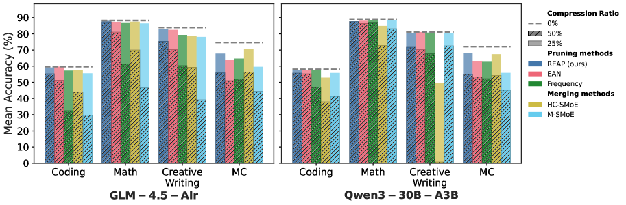Compared to MC, generative benchmarks are more representative of real-world use cases of LLMs. In this setting, pruning emerges as the clearly superior compression method on the generative task benchmarks. Excluding large-scale SMoEs, REAP achieves a mean decrease in accuracy of 2.8% and 8.0% at 25% and 50% compression ratios, respectively, on coding. In comparison, both HC-SMoE and M-SMoE produce mean decreases in accuracy >5% at 25% compression and >20% at 50% compression. Notably, REAP maintains significantly higher accuracy at 50% compression than other pruning methods. On creative writing, REAP and EAN are near-lossless at 25% compression with REAP offering improved quality at 50% compression. Merging methods are less consistent across various model architectures and compression ratios. For example, M-SMoE is the best method for Qwen3-30B at 50% compression, but the worst on GLM-4.5-Air. REAP attains the best mathematical reasoning results with a remarkable mean decrease in accuracy of just 1.1% at 50% compression. HC-SMoE and M-SMoE offer high accuracy at 25% compression but are significantly less accurate than pruning at 50% compression. Table 2: MC and generative benchmark results for Qwen3-30B and GLM-4.5-Air. | | Coding | Creative Writing | Math | MC | | | | | | | | | --- | --- | --- | --- | --- | --- | --- | --- | --- | --- | --- | --- | | Model | Compression | Technique | Method | Eval+ | LiveCode | Code Avg | WildBench | GSM8K | MATH-500 | Math Avg | MC Avg | | Qwen3-30B-A3B | Baseline | 0.859 | 0.302 | 0.581 | 0.811 | 0.903 | 0.872 | 0.887 | 0.721 | | | | 25% | Merging | M-SMoE | 0.822 | 0.293 | 0.558 | 0.805 | 0.901 | 0.872 | 0.886 | 0.558 | | | HC-SMoE | 0.800 | 0.258 | 0.529 | 0.497 | 0.864 | 0.834 | 0.849 | 0.674 | | | | | Pruning | Frequency | 0.849 | 0.302 | 0.576 | 0.807 | 0.905 | 0.864 | 0.885 | 0.600 | | | | EAN | 0.840 | 0.311 | 0.576 | 0.811 | 0.895 | 0.866 | 0.881 | 0.603 | | | | | REAP | 0.843 | 0.308 | 0.575 | 0.804 | 0.892 | 0.864 | 0.878 | 0.669 | | | | | 50% | Merging | M-SMoE | 0.621 | 0.205 | 0.413 | 0.725 | 0.824 | 0.838 | 0.831 | 0.451 | | | HC-SMoE | 0.574 | 0.185 | 0.379 | 0.008 | 0.760 | 0.696 | 0.728 | 0.542 | | | | | Pruning | Frequency | 0.704 | 0.236 | 0.470 | 0.677 | 0.882 | 0.860 | 0.871 | 0.483 | | | | EAN | 0.798 | 0.306 | 0.552 | 0.702 | 0.886 | 0.842 | 0.864 | 0.493 | | | | | REAP | 0.821 | 0.293 | 0.557 | 0.718 | 0.878 | 0.872 | 0.875 | 0.518 | | | | | GLM-4.5-Air | Baseline | 0.820 | 0.374 | 0.597 | 0.839 | 0.846 | 0.918 | 0.882 | 0.747 | | | | 25% | Merging | M-SMoE | 0.781 | 0.330 | 0.555 | 0.781 | 0.848 | 0.880 | 0.864 | 0.596 | | | HC-SMoE | 0.793 | 0.363 | 0.578 | 0.788 | 0.842 | 0.908 | 0.875 | 0.704 | | | | | Pruning | Frequency | 0.805 | 0.341 | 0.573 | 0.793 | 0.832 | 0.908 | 0.870 | 0.648 | | | | EAN | 0.821 | 0.374 | 0.597 | 0.824 | 0.839 | 0.908 | 0.874 | 0.637 | | | | | REAP | 0.794 | 0.390 | 0.592 | 0.831 | 0.835 | 0.926 | 0.880 | 0.678 | | | | | 50% | Merging | M-SMoE | 0.493 | 0.099 | 0.296 | 0.391 | 0.465 | 0.466 | 0.465 | 0.444 | | | HC-SMoE | 0.662 | 0.220 | 0.441 | 0.593 | 0.667 | 0.732 | 0.700 | 0.564 | | | | | Pruning | Frequency | 0.546 | 0.104 | 0.325 | 0.604 | 0.615 | 0.612 | 0.613 | 0.521 | | | | EAN | 0.773 | 0.253 | 0.513 | 0.702 | 0.781 | 0.838 | 0.809 | 0.511 | | | | | REAP | 0.755 | 0.352 | 0.553 | 0.754 | 0.820 | 0.926 | 0.873 | 0.559 | | | | Table 3: Large-scale pruned SMoEs on agentic, non-agentic coding, tool-use tasks, and MC benchmarks. | | Non-Agentic Coding | Agentic Coding | Tool-Use (BFCLv3) | MC | | | | | | | | | --- | --- | --- | --- | --- | --- | --- | --- | --- | --- | --- | --- | | Model | Compression | Method | Eval+ | LiveCode | Code Avg | SWE-Bench-Verified | Non-Live | Live | Multi-Turn | Overall | MC Avg | | Qwen3-Coder- 480B-A35B- Instruct-FP8 | Baseline | 0.889 | 0.431 | 0.660 | 0.540 | 0.866 | 0.825 | 0.380 | 0.690 | 0.750 | | | 25% | Frequency | 0.792 | 0.296 | 0.544 | 0.378 | 0.844 | 0.763 | 0.355 | 0.654 | 0.606 | | | EAN | 0.876 | 0.419 | 0.647 | 0.534 | 0.831 | 0.813 | 0.384 | 0.676 | 0.702 | | | | REAP | 0.884 | 0.416 | 0.650 | 0.540 | 0.878 | 0.823 | 0.392 | 0.698 | 0.748 | | | | 50% | Frequency | 0.011 | 0.012 | 0.011 | 0.000 | 0.200 | 0.392 | 0.000 | 0.197 | 0.506 | | | EAN | 0.831 | 0.382 | 0.607 | 0.536 | 0.822 | 0.774 | 0.383 | 0.659 | 0.591 | | | | REAP | 0.873 | 0.415 | 0.644 | 0.522 | 0.849 | 0.801 | 0.371 | 0.674 | 0.692 | | | | Kimi-K2- Instruct- W4A16 | Baseline | 0.883 | 0.434 | 0.659 | 0.554 | 0.840 | 0.802 | 0.355 | 0.666 | 0.780 | | | 25% | Frequency | 0.524 | 0.082 | 0.303 | 0.000 | 0.644 | 0.603 | 0.045 | 0.431 | 0.604 | | | EAN | 0.831 | 0.379 | 0.605 | 0.562 | 0.819 | 0.802 | 0.335 | 0.652 | 0.703 | | | | REAP | 0.889 | 0.440 | 0.664 | 0.580 | 0.842 | 0.801 | 0.263 | 0.635 | 0.773 | | | | 50% | Frequency | 0.124 | 0.000 | 0.062 | 0.000 | 0.255 | 0.397 | 0.003 | 0.218 | 0.439 | | | EAN | 0.772 | 0.253 | 0.513 | 0.576 | 0.778 | 0.767 | 0.173 | 0.573 | 0.587 | | | | REAP | 0.863 | 0.429 | 0.646 | 0.576 | 0.785 | 0.743 | 0.164 | 0.564 | 0.643 | | | <details> <summary>x6.png Details</summary>  ### Visual Description ## Bar Chart: Mean Accuracy (%) for Different Writing Tasks ### Overview The bar chart compares the mean accuracy percentages for different writing tasks across two models: GLM-4.5-Air and Qwen3-30B-A3B. The tasks include Coding, Math, Creative, and MC (Multiple Choice). ### Components/Axes - **X-axis**: Different writing tasks (Coding, Math, Creative, MC) - **Y-axis**: Mean Accuracy (%) ranging from 0 to 90 - **Legend**: - Compression Ratio (0%, 25%) - Pruning methods (REAP, Frequency, Merging methods, EAN, M-SMOE) - Line colors represent different pruning methods ### Detailed Analysis or ### Content Details - **GLM-4.5-Air**: - Coding: Mean Accuracy ≈ 50% - Math: Mean Accuracy ≈ 75% - Creative: Mean Accuracy ≈ 65% - MC: Mean Accuracy ≈ 60% - **Qwen3-30B-A3B**: - Coding: Mean Accuracy ≈ 55% - Math: Mean Accuracy ≈ 80% - Creative: Mean Accuracy ≈ 70% - MC: Mean Accuracy ≈ 65% ### Key Observations - **Math Task**: Qwen3-30B-A3B consistently outperforms GLM-4.5-Air in the Math task. - **Creative Task**: GLM-4.5-Air shows slightly higher accuracy in the Creative task compared to Qwen3-30B-A3B. - **MC Task**: Both models perform similarly in the MC task. ### Interpretation The data suggests that Qwen3-30B-A3B is more accurate in generating text for the Math task compared to GLM-4.5-Air. For the Creative task, GLM-4.5-Air performs slightly better. In the MC task, both models have similar performance. The compression ratio and pruning methods do not significantly impact the accuracy in this comparison. The visual trend shows that as the compression ratio increases, the accuracy generally decreases for both models. </details> Figure 2: GLM-4.5-Air and Qwen3-30B accuracy vs. task type. REAP offers significant improvements compared to other methods at 50% compression. Note the significant performance drop for merging methods on generative tasks (Coding, Math, Creative Writing) compared to their relative strength on MC. Expert pruning at scale. To asses whether pruning remains viable at scale, we prune Qwen3-Coder-480B and Kimi-K2-Instruct. On MC questions, REAP outperforms other pruning methods. On non-agentic coding tasks, REAP achieves near-lossless accuracy with a 0.20% and 1.4% mean decrease in accuracy compared to baseline at 25% and 50%, respectively, outperforming EAN and frequency-based pruning, particularly at 50% compression. On the challenging SWE-Bench task, both REAP and EAN maintain high accuracy at 25% and 50% compression, with some scores slightly exceeding the baseline. On tool use, EAN and REAP are comparable, with REAP slightly outperforming at 50% compression with a mean decrease in accuracy of 5.9% versus 6.2% for EAN. Frequency-based pruning suffers from a sharp degradation in quality at 50% compression, highlighting the importance of pruning saliency criteria which consider expert activations. Scaling the pruning methods is relatively trivial. Unlike HC-SMoE, calibration for pruning does not require recording activations from every expert for every token, facilitating efficient calibration. Further, pruning can be easily applied to quantized models without any additional steps required to reconcile block scales or re-quantize following compression. <details> <summary>x7.png Details</summary>  ### Visual Description ## Box Plot Comparison: N-gram Diversity ### Overview The image displays a box plot comparison of N-gram diversity across different N-gram sizes (2, 3, and 4). The plot is divided into three groups, each representing a different method of calculating N-gram diversity: Baseline, REAP, M-SMoE, and HC-SMoE. ### Components/Axes - **X-axis (Horizontal)**: Represents the N-gram size, with values ranging from 2 to 4. - **Y-axis (Vertical)**: Represents the N-gram diversity, with values ranging from 0.2 to 1.0. - **Legend**: Located at the bottom right, it provides color coding for each method. - **Gray**: Baseline - **Blue**: REAP - **Light Blue**: M-SMoE - **Yellow**: HC-SMoE ### Detailed Analysis or ### Content Details - **Baseline**: The box plot for the Baseline method shows a relatively stable N-gram diversity across all N-gram sizes, with a median value slightly above 0.5. - **REAP**: The REAP method exhibits a higher median N-gram diversity compared to the Baseline, with values consistently above 0.5. - **M-SMoE**: The M-SMoE method shows a moderate N-gram diversity, with values slightly above 0.5. - **HC-SMoE**: The HC-SMoE method has the highest N-gram diversity, with values consistently above 0.5. ### Key Observations - **Trend**: All methods show an increase in N-gram diversity as the N-gram size increases. - **Outliers**: There are no significant outliers in any of the methods. - **Variability**: The variability in N-gram diversity is highest for the HC-SMoE method, indicating more fluctuation in diversity across different N-gram sizes. ### Interpretation The data suggests that the HC-SMoE method consistently results in the highest N-gram diversity across all N-gram sizes, indicating a more diverse set of N-grams. The REAP method also shows a high level of diversity, but slightly lower than HC-SMoE. The Baseline and M-SMoE methods have similar levels of diversity, with the Baseline being slightly lower. The trend of increasing diversity with N-gram size is consistent across all methods. The high variability in the HC-SMoE method may indicate that it is more sensitive to changes in the data, leading to more diverse N-grams. </details> (a) N-Gram diversity <details> <summary>x8.png Details</summary>  ### Visual Description ## Box Plot: Cross-Perplexity ### Overview The image displays a box plot comparing the cross-perplexity of three different generator models: REAP, M-SMoE, and HC-SMoE. The plot is designed to show the distribution of cross-perplexity values for each model, with the median, quartiles, and potential outliers represented. ### Components/Axes - **Y-axis**: Cross-perplexity, measured on a logarithmic scale from 10^0 to 10^1. - **X-axis**: Generator model, labeled as REAP, M-SMoE, and HC-SMoE. - **Legend**: The legend is located at the bottom of the plot, indicating the color coding for each model. - **Box Plot**: Each box plot represents the distribution of cross-perplexity values for a specific model. The boxes show the interquartile range (IQR), the median (line inside the box), and the whiskers extend to the minimum and maximum values within 1.5 times the IQR. ### Detailed Analysis or ### Content Details - **REAP Model**: The box plot for REAP shows a relatively narrow distribution with a median around 10^0.5. The IQR is smaller, and the whiskers are shorter, indicating less variability and a more consistent performance. - **M-SMoE Model**: The box plot for M-SMoE has a slightly wider distribution compared to REAP, with a median around 10^0.7. The IQR is larger, and the whiskers are longer, suggesting more variability and potentially better performance. - **HC-SMoE Model**: The box plot for HC-SMoE is the widest, with a median around 10^0.9. The IQR is the largest, and the whiskers are the longest, indicating the highest variability and potentially the best performance among the three models. ### Key Observations - **REAP Model**: Shows the least variability and the most consistent performance. - **M-SMoE Model**: Shows moderate variability and potentially better performance than REAP. - **HC-SMoE Model**: Shows the highest variability and potentially the best performance. ### Interpretation The data suggests that the HC-SMoE model has the highest cross-perplexity, indicating it may be less efficient or less effective in generating data compared to REAP and M-SMoE. The REAP model has the lowest cross-perplexity, suggesting it is the most efficient. The M-SMoE model falls in between, showing a balance between efficiency and variability. The wide distribution of the HC-SMoE model indicates that it may be more prone to generating data with a wide range of complexity, which could be a trade-off for its performance. </details> (b) Cross perplexity <details> <summary>x9.png Details</summary>  ### Visual Description ## Line Chart: JSD vs Token Position ### Overview The line chart displays the JSD (Joint Similarity Distribution) values across different token positions. The chart shows three different methods: REAP, M-SMoE, and HC-SMoE, each represented by a distinct line color. ### Components/Axes - **X-axis (Token Position)**: The horizontal axis represents the token positions, ranging from 0 to 20. - **Y-axis (JSD)**: The vertical axis represents the JSD values, ranging from 0.0 to 0.7. - **Legend**: The legend on the right side of the chart identifies the three methods used to calculate the JSD. ### Detailed Analysis or ### Content Details - **REAP**: The blue line shows the highest JSD values, indicating the most similarity between tokens at different positions. - **M-SMoE**: The light blue line has moderate JSD values, suggesting a balance between similarity and dissimilarity. - **HC-SMoE**: The yellow line has the lowest JSD values, indicating the least similarity between tokens at different positions. ### Key Observations - All three methods show an increasing trend in JSD values as the token position increases. - The REAP method consistently has the highest JSD values, while the HC-SMoE method has the lowest. - The M-SMoE method shows a more gradual increase in JSD values compared to the other two methods. ### Interpretation The data suggests that the REAP method captures more similarity between tokens across different positions compared to the M-SMoE and HC-SMoE methods. This could indicate that the REAP method is more effective at identifying and preserving the relationships between tokens in the dataset. The M-SMoE method, while still capturing similarity, does so at a more moderate rate, and the HC-SMoE method, which has the lowest JSD values, may be less effective at preserving the relationships between tokens. </details> (c) Completion logit JSD <details> <summary>x10.png Details</summary>  ### Visual Description ## Heatmap: Distance Analysis ### Overview The heatmap illustrates the singular vector alignment (SVA) and L2 distance between different layers of a model, categorized by the type of distance used. The layers are labeled from 0 to 40, and the distance types are singular vector alignment and L2 distance. ### Components/Axes - **X-Axis (Layer)**: Represents the layers of the model, ranging from 0 to 40. - **Y-Axis (SV Align. / L2 Distance)**: Shows the singular vector alignment and L2 distance values, ranging from 0.0 to 1.4. - **Legend**: Contains two categories: "Dist. Type" and "Expert clusters." - **Dist. Type**: Singular-vector alignment and L2 distance. - **Expert clusters**: Base to IFT, HC-SMoE, M-SMoE, M-SMoE - permuted. ### Detailed Analysis or ### Content Details - **Singular-vector alignment (SVA)**: The lines representing SVA are consistently above the L2 distance lines, indicating that SVA values are generally higher than L2 distance values across all layers. - **L2 distance**: The L2 distance lines are relatively flat, suggesting that the L2 distance values are relatively stable across the layers. - **Expert clusters**: The lines for HC-SMoE and M-SMoE are consistently above the base to IFT line, indicating that these clusters have higher singular vector alignment and L2 distance values compared to the base to IFT cluster. ### Key Observations - **Singular-vector alignment**: The SVA values are consistently higher than the L2 distance values across all layers. - **Expert clusters**: HC-SMoE and M-SMoE clusters have higher singular vector alignment and L2 distance values compared to the base to IFT cluster. - **Stability**: The L2 distance values are relatively stable across the layers. ### Interpretation The heatmap suggests that the singular vector alignment is a more robust measure of distance between layers compared to the L2 distance. The expert clusters, particularly HC-SMoE and M-SMoE, show higher singular vector alignment and L2 distance values, indicating that these clusters may be more effective or accurate in their analysis. The stability of the L2 distance values across the layers suggests that the L2 distance may not be as sensitive to changes in the model's layers. 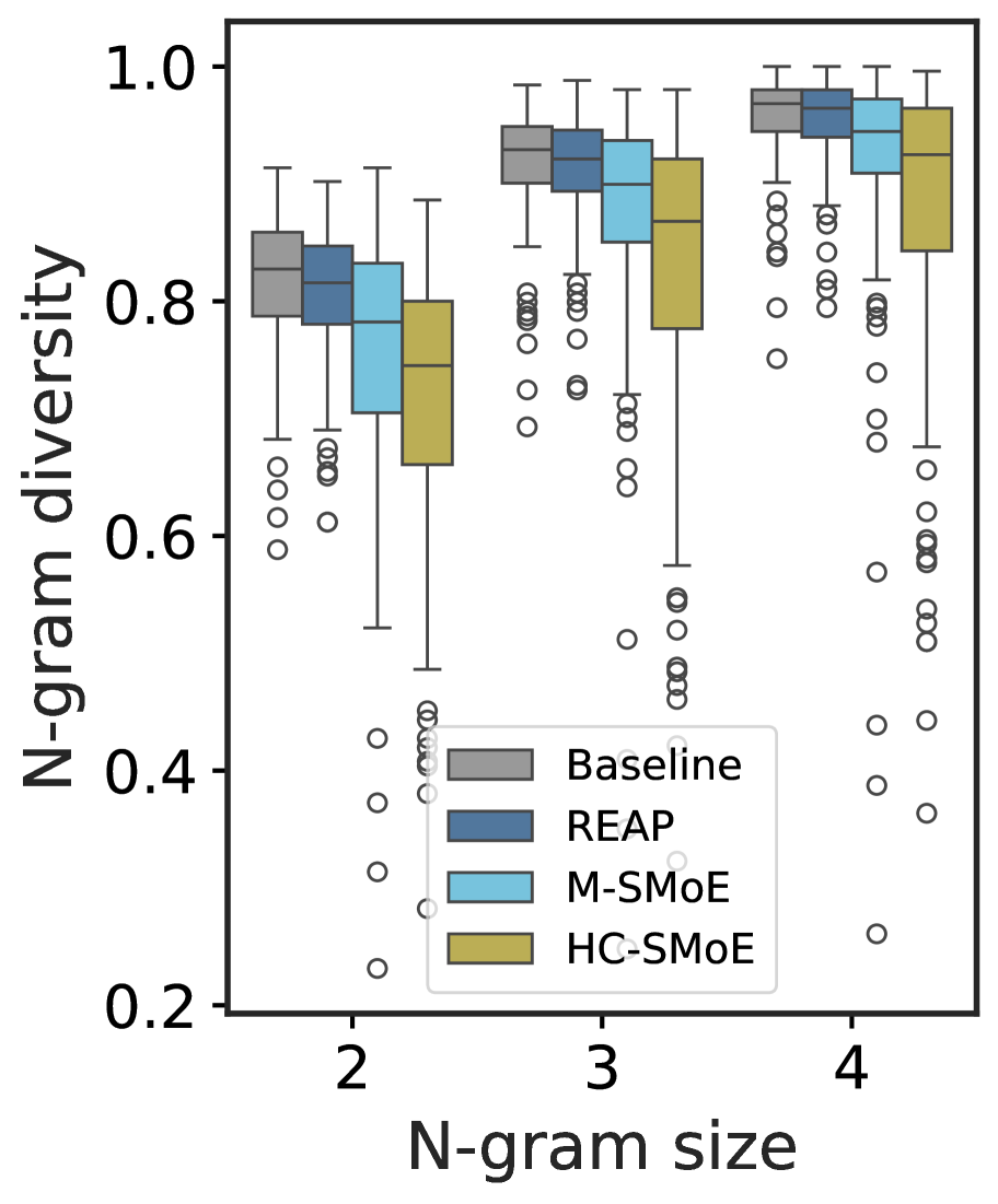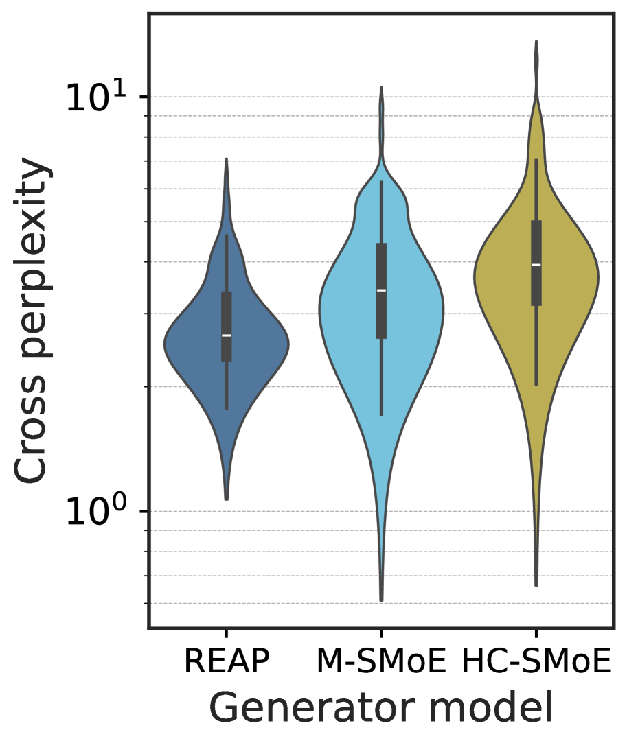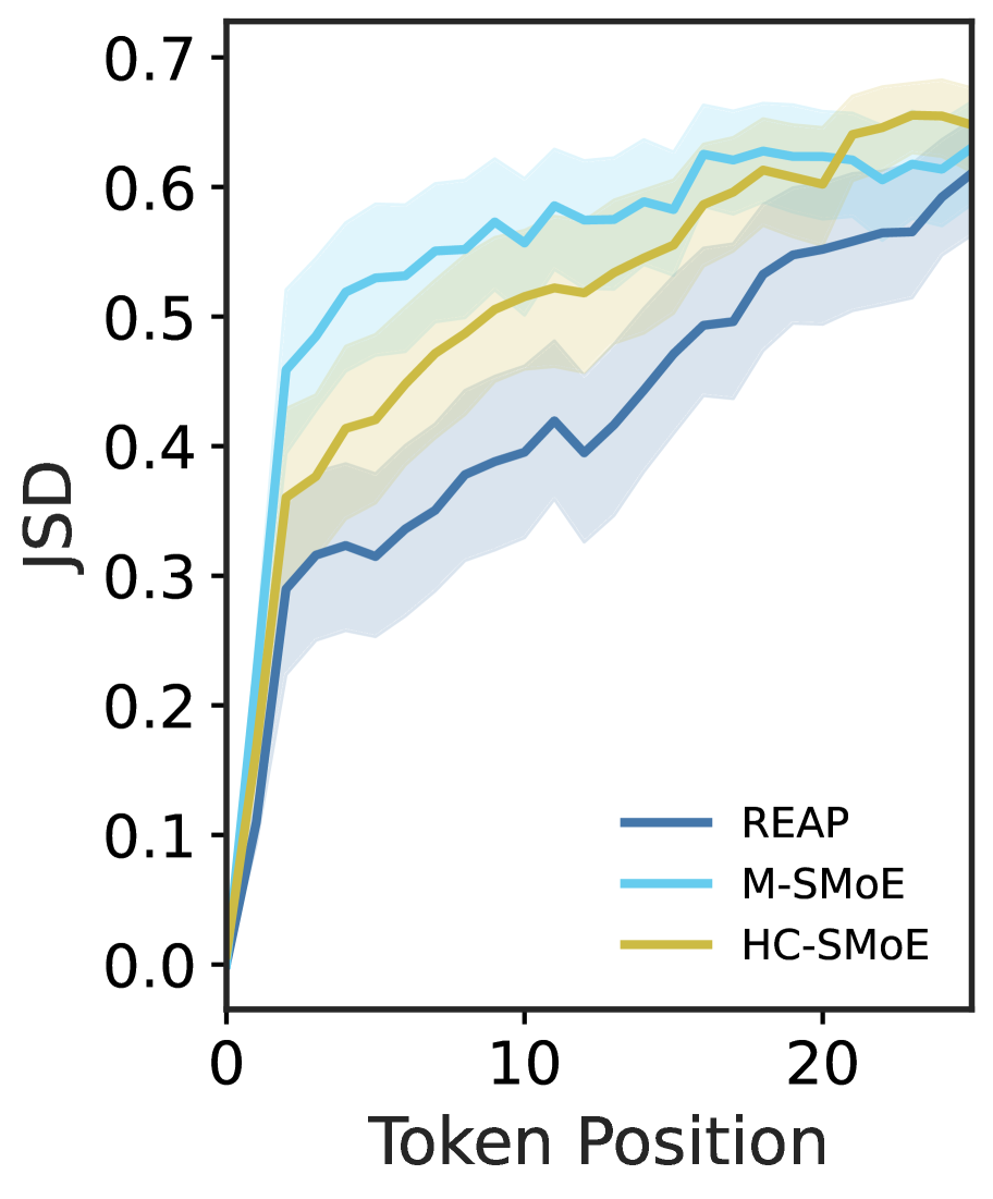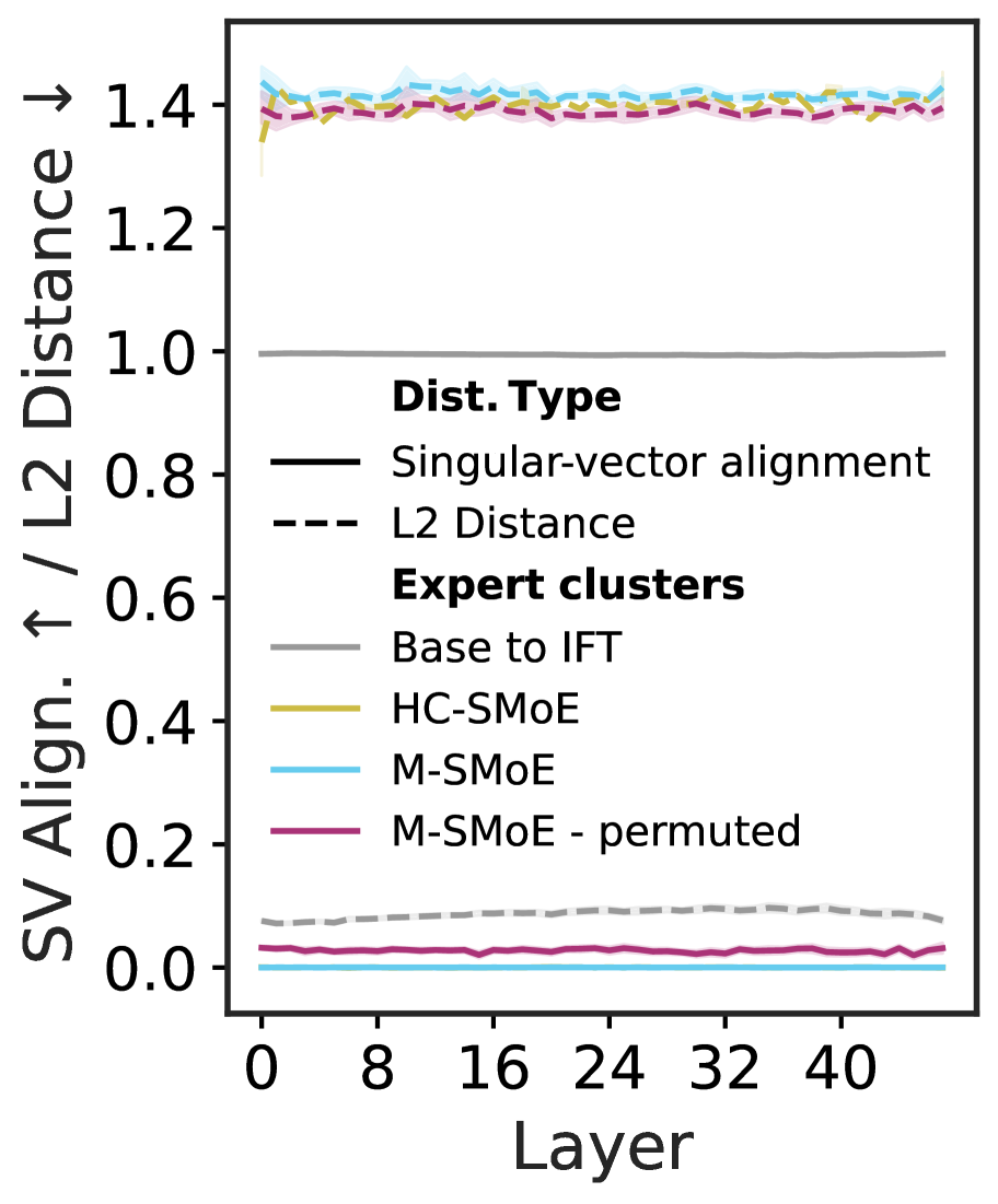</details> (d) Expert distance Figure 3: (3(a)) & (3(b)) N-Gram diversity and cross-perplexity of compressed Qwen3-30B-A3B models at 50% compression, respectively. (3(c)) JSD of compressed and baseline model logits vs. completion token position for Qwen3-30B-A3B at 50% compression. Initially, all compressed models share close alignment with the baseline model. However, as the completion token position increases the merged models diverge from the baseline more rapidly than the REAP pruned model. (3(d)) The mean relative L2-distance and singular-vector alignment between Qwen3-30B expert weights at 50% compression. Expert merging is more challenging than model merging due to large distances between experts in weight space and low singular-vector alignment. Quantifying merged MoE generation quality. While merged expert SMoEs offer reasonable quality for discriminative tasks such as MC question and answering, they fail to remain competitive on generative tasks. To help explain the performance gap of merged models between discriminative and generative tasks, we perform an analysis of the compressed model outputs and compare with REAP pruned models. We prompt 50% compressed Qwen3-30B models with 100 questions randomly sampled from the evol-codealpaca dataset and record their outputs. In Figure ˜ 3(a), we measure the N-gram diversity and find that the merged models have significantly lower diversity across all N-gram sizes measured. In contrast, the REAP pruned model remains similar to the base model, albeit slightly less diverse. In Figure ˜ 3(b), we measure the perplexity of the text generated by the compressed models with the original baseline model. The text generated by the merged models has both a higher mean and higher variance than the pruned model generations, suggesting that the REAP pruned model outputs are more closely aligned to the original model. The alignment between the baseline and REAP pruned SMoEs is further supported by Figure ˜ 3(c), which plots the JSD of the compressed and baseline logits vs. output token position. The merged model logits diverge from the baseline more rapidly than the pruned model. The challenges of expert merging. Model merging has been widely adopted to facilitate LLM fine-tuning. Why does expert merging miss the mark? In addition to the loss of the router’s input-dependent modulation of experts explored in Section ˜ 3, we argue that the non-local nature of expert merging and high cardinality of expert clusters pose significant unresolved challenges. In Figure ˜ 3(d), we plot the mean relative L2-distance between experts clustered by HC-SMoE or M-SMoE and compare with the distance between expert weights from the pretrained to Instruct Fine-Tuned (IFT) checkpoints. We find that the distance between clustered experts within the same layer greatly exceeds that of experts in the IFT checkpoint after fine-tuning. Ito et al. (2024) found that weight matching permutations improved alignment of parameters’ singular vectors. Following their approach, we decompose expert weights with Singular Value Decomposition (SVD) and plot the singular-vector alignment in Figure ˜ 3(d). Even after applying weight matching permutations, the M-SMoE expert clusters remain far apart both in weight space and singular-vector alignment. The relatively poorly aligned experts highlight the considerable challenge of coherently merging their parameters. When merging works well, it’s more closely related to pruning than one might expect. In Figure ˜ 6(a), we depict the frequency of singleton clusters — clusters containing a single expert — for both HC-SMoE and M-SMoE. A singleton cluster is directly analogous to an expert that remains after pruning. We find that HC-SMoE in particular has a high prevalence of singleton clusters, leaving important experts unadulterated and compressing the rest into a few mega -clusters containing tens of experts. This is particularly true of the high granularity models which contain more experts per layer. We hypothesize that the cardinality of these mega-clusters poses a challenge for existing merging algorithms and test this intuition in Figure ˜ 6(b). Unfortunately, even modest restrictions of the maximum cluster size to 32 — half the number of experts to compress — results in large decreases in model quality on coding tasks. The importance of domain-specific calibration. In Figure ˜ A7, we plot the code generation accuracy of the various compression methods and models when calibrated on either c4 or evol-codealpaca. The difference is stark, c4 calibration results in a collapse in accuracy, with several compressed model instances failing to produce coherent outputs, resulting in 0% accuracy. In Figure ˜ A8, we compare the accuracy of compressed Qwen3-30B models calibrated with either domain-specific data or the combined calibration data across all generative tasks. The domain-specific calibrated models achieve significantly higher accuracy, especially at 50% compression. 6 Discussion Similar to prior work, we find that expert merging performs reasonably well on MC benchmarks. This may be because MC tasks only require a discriminative function that can be approximated by an average expert. In contrast, merging fails to maintain model quality on generative tasks, particularly at 50% compression. Generative tasks require auto-regressive generation, a capability that is lost when the router’s fine-grained control is removed. Compared to expert pruning, merging is less consistent, exhibiting higher variance across models and compression ratios. The outputs of expert merged models are more repetitive and less closely aligned with the base model compared with pruned models. Taken together, these observations are direct evidence of alterations to the functional manifold of the SMoE layers discussed in Section ˜ 3.3 stemming from the loss of the router’s input-dependent control over the experts and subsequent introduction of novel functions due to tying of the merged expert gates. Overall, expert pruned models offer consistently higher accuracy than merged models on generative tasks. REAP is a robust pruning criterion that generalizes across a wide array of SMoE architectures, compression ratios, and generative tasks. By taking into consideration both the router gate-values and expert activation norms, REAP prunes the experts which contribute the least to each layers output on a per-token average, regardless of usage frequency. REAP is scalable, achieving near-lossless compression on coding tasks with Qwen3-Coder-480B and Kimi-K2. The successes of REAP highlights the crucial importance of preserving coordination between the router and experts. Compression methods which impair the router’s ability to independently modulate expert outputs or tie gate-values are less likely to succeed. Finally, this work highlights the importance of comprehensive downstream evaluations and the significant challenges involved with evaluating LLMs. Discriminative metrics such as perplexity and log-likelihood based MC benchmarks are not necessarily good proxies for generative model quality. 7 Conclusion Our analysis of current SMoE expert merging techniques finds that the router’s loss of independent control over experts results in functional subspace collapse. In contrast, expert pruning produces a coordinate subspace of the original layer which maintains the topology of the functional manifold. Based on our findings that the coordination between the router and experts is fundamental, we introduce REAP, a novel expert pruning method which prunes experts that contribute the least to the layer’s output. Empirically, we demonstrate that REAP retains remarkably high accuracy on an wide array of generative tasks across a diverse set of model architectures. We hope that this work inspires further compression techniques for SMoEs and facilitates the deployment of accurate, domain-specific models in resource constrained settings. Acknowledgments We would like to acknowledge the helpful feedback of Mohammed Adnan and Rohan Jain. ML and YI gratefully acknowledge the support of Alberta Innovates (ALLRP-577350-22, ALLRP-222301502), the Natural Sciences and Engineering Research Council of Canada (NSERC) (RGPIN-2022-03120, DGECR-2022-00358), and Defence Research and Development Canada (DGDND-2022-03120). ML and YI are grateful for computational resources made available to us by the Digital Research Alliance of Canada. YI is supported by a Schulich Research Chair. Ethics Statement This work research focused on the algorithmic compression of SMoE models and does not involve the use of human subjects, personally identifiable information, or sensitive data. The datasets used for calibration and evaluation (e.g., c4, evol-codealpaca) are publicly available. Our aim is enable the use of large-scale SMoE models in resource constrained settings. However, we acknowledge that compression techniques such as REAP could potentially facilitate deployment of models for malicious purposes. Further, our compression methods are applied to pre-trained models and any biases related to fairness, discrimination, or representation inherent in the original models may be present in their compressed versions. We make no attempt in this work to mitigate these potential biases. The primary contribution of this paper is technical, and we do not foresee any new, direct ethical concerns arising from our proposed methodology beyond those already associated with the deployment of large language models. Reproducibility Statement We are committed to ensuring the reproducibility of our research. We have open-sourced our code and released select compressed model checkpoints to facilitate further research on compressed SMoEs. REAP is formally described in Section 4. The baseline methods we compare against, including frequency-based pruning, EAN, M-SMoE, and HC-SMoE, are formally defined in Appendix D. Section 5 provides a detailed description of our experimental setup, including the specific models used, the calibration and evaluation datasets, and the implementation details for all compression experiments. Further evaluation details are provided in Appendix C. References - Ainsworth et al. (2023) Samuel Ainsworth, Jonathan Hayase, and Siddhartha Srinivasa. Git re-basin: Merging models modulo permutation symmetries. In Proceedings of the Eleventh International Conference on Learning Representations, 2023. URL https://openreview.net/forum?id=CQsmMYmlP5T. - Allen Institute for AI (2024) Allen Institute for AI. allenai/c4 · Datasets at Hugging Face, August 2024. URL https://huggingface.co/datasets/allenai/c4. - Allen Institute for AI (2025) Allen Institute for AI. allenai/tulu-3-sft-personas-math · Datasets at Hugging Face, 2025. URL https://huggingface.co/datasets/allenai/tulu-3-sft-personas-math. - Ansel et al. (2024) Jason Ansel, Edward Yang, Horace He, Natalia Gimelshein, Animesh Jain, Michael Voznesensky, Bin Bao, Peter Bell, David Berard, Evgeni Burovski, Geeta Chauhan, Anjali Chourdia, Will Constable, Alban Desmaison, Zachary DeVito, Elias Ellison, Will Feng, Jiong Gong, Michael Gschwind, Brian Hirsh, Sherlock Huang, Kshiteej Kalambarkar, Laurent Kirsch, Michael Lazos, Mario Lezcano, Yanbo Liang, Jason Liang, Yinghai Lu, CK Luk, Bert Maher, Yunjie Pan, Christian Puhrsch, Matthias Reso, Mark Saroufim, Marcos Yukio Siraichi, Helen Suk, Michael Suo, Phil Tillet, Eikan Wang, Xiaodong Wang, William Wen, Shunting Zhang, Xu Zhao, Keren Zhou, Richard Zou, Ajit Mathews, Gregory Chanan, Peng Wu, and Soumith Chintala. PyTorch 2: Faster Machine Learning Through Dynamic Python Bytecode Transformation and Graph Compilation. In 29th ACM International Conference on Architectural Support for Programming Languages and Operating Systems, Volume 2 (ASPLOS ’24). ACM, April 2024. doi: 10.1145/3620665.3640366. URL https://docs.pytorch.org/assets/pytorch2-2.pdf. - Artificial Analysis (2025) Artificial Analysis. Artificial analysis intelligence benchmarking methodology. https://artificialanalysis.ai/methodology/intelligence-benchmarking, September 2025. Version 3.0. - Baidu (2025) Baidu. Ernie 4.5 technical report, 2025. URL https://yiyan.baidu.com/blog/publication/ERNIE_Technical_Report.pdf. - Balmau et al. (2025) Oana Balmau, Anne-Marie Kermarrec, Rafael Pires, André Loureiro Espírito Santo, Martijn de Vos, and Milos Vujasinovic. Accelerating moe model inference with expert sharding. In Proceedings of the 5th Workshop on Machine Learning and Systems, pp. 192–199, 2025. - Barres et al. (2025) Victor Barres, Honghua Dong, Soham Ray, Xujie Si, and Karthik Narasimhan. $\tau^{2}$ -bench: Evaluating conversational agents in a dual-control environment. arXiv preprint arXiv:2506.07982, 2025. - Bentivogli et al. (2009) Luisa Bentivogli, Peter Clark, Ido Dagan, and Danilo Giampiccolo. The fifth pascal recognizing textual entailment challenge. TAC, 7(8):1, 2009. - Chandak et al. (2025) Nikhil Chandak, Shashwat Goel, Ameya Prabhu, Moritz Hardt, and Jonas Geiping. Answer Matching Outperforms Multiple Choice for Language Model Evaluation, July 2025. URL http://arxiv.org/abs/2507.02856. arXiv:2507.02856 [cs]. - Chaudhary (2023) Sahil Chaudhary. Code alpaca: An instruction-following llama model for code generation. https://github.com/sahil280114/codealpaca, 2023. - Chen et al. (2025) I-Chun Chen, Hsu-Shen Liu, Wei-Fang Sun, Chen-Hao Chao, Yen-Chang Hsu, and Chun-Yi Lee. Retraining-free merging of sparse moe via hierarchical clustering. In Proceedings of the Forty-second International Conference on Machine Learning, 2025. URL https://openreview.net/forum?id=hslOzRxzXL. - Chen et al. (2022) Tianyu Chen, Shaohan Huang, Yuan Xie, Binxing Jiao, Daxin Jiang, Haoyi Zhou, Jianxin Li, and Furu Wei. Task-Specific Expert Pruning for Sparse Mixture-of-Experts, June 2022. URL http://arxiv.org/abs/2206.00277. arXiv:2206.00277 [cs]. - Clark et al. (2019) Christopher Clark, Kenton Lee, Ming-Wei Chang, Tom Kwiatkowski, Michael Collins, and Kristina Toutanova. BoolQ: Exploring the surprising difficulty of natural yes/no questions. In Jill Burstein, Christy Doran, and Thamar Solorio (eds.), Proceedings of the 2019 Conference of the North American Chapter of the Association for Computational Linguistics: Human Language Technologies, Volume 1 (Long and Short Papers), pp. 2924–2936, Minneapolis, Minnesota, June 2019. Association for Computational Linguistics. doi: 10.18653/v1/N19-1300. URL https://aclanthology.org/N19-1300/. - Clark et al. (2018) Peter Clark, Isaac Cowhey, Oren Etzioni, Tushar Khot, Ashish Sabharwal, Carissa Schoenick, and Oyvind Tafjord. Think you have solved question answering? try arc, the ai2 reasoning challenge, 2018. URL https://arxiv.org/abs/1803.05457. arXiv:1803.05457 [cs]. - Cobbe et al. (2021) Karl Cobbe, Vineet Kosaraju, Mohammad Bavarian, Mark Chen, Heewoo Jun, Lukasz Kaiser, Matthias Plappert, Jerry Tworek, Jacob Hilton, Reiichiro Nakano, Christopher Hesse, and John Schulman. Training verifiers to solve math word problems, 2021. URL https://arxiv.org/abs/2110.14168. arXiv:2110.14168 [cs]. - Dai et al. (2024) Damai Dai, Chengqi Deng, Chenggang Zhao, R. X. Xu, Huazuo Gao, Deli Chen, Jiashi Li, Wangding Zeng, Xingkai Yu, Y. Wu, Zhenda Xie, Y. K. Li, Panpan Huang, Fuli Luo, Chong Ruan, Zhifang Sui, and Wenfeng Liang. DeepSeekMoE: Towards Ultimate Expert Specialization in Mixture-of-Experts Language Models, January 2024. URL http://arxiv.org/abs/2401.06066. arXiv:2401.06066 [cs] version: 1. - DeepSeek-AI et al. (2024) DeepSeek-AI, Aixin Liu, Bei Feng, Bing Xue, Bingxuan Wang, Bochao Wu, Chengda Lu, Chenggang Zhao, Chengqi Deng, Chenyu Zhang, Chong Ruan, Damai Dai, Daya Guo, Dejian Yang, Deli Chen, Dongjie Ji, Erhang Li, Fangyun Lin, Fucong Dai, Fuli Luo, Guangbo Hao, Guanting Chen, Guowei Li, H. Zhang, Han Bao, Hanwei Xu, Haocheng Wang, Haowei Zhang, Honghui Ding, Huajian Xin, Huazuo Gao, Hui Li, Hui Qu, J. L. Cai, Jian Liang, Jianzhong Guo, Jiaqi Ni, Jiashi Li, Jiawei Wang, Jin Chen, Jingchang Chen, Jingyang Yuan, Junjie Qiu, Junlong Li, Junxiao Song, Kai Dong, Kai Hu, Kaige Gao, Kang Guan, Kexin Huang, Kuai Yu, Lean Wang, Lecong Zhang, Lei Xu, Leyi Xia, Liang Zhao, Litong Wang, Liyue Zhang, Meng Li, Miaojun Wang, Mingchuan Zhang, Minghua Zhang, Minghui Tang, Mingming Li, Ning Tian, Panpan Huang, Peiyi Wang, Peng Zhang, Qiancheng Wang, Qihao Zhu, Qinyu Chen, Qiushi Du, R. J. Chen, R. L. Jin, Ruiqi Ge, Ruisong Zhang, Ruizhe Pan, Runji Wang, Runxin Xu, Ruoyu Zhang, Ruyi Chen, S. S. Li, Shanghao Lu, Shangyan Zhou, Shanhuang Chen, Shaoqing Wu, Shengfeng Ye, Shengfeng Ye, Shirong Ma, Shiyu Wang, Shuang Zhou, Shuiping Yu, Shunfeng Zhou, Shuting Pan, T. Wang, Tao Yun, Tian Pei, Tianyu Sun, W. L. Xiao, Wangding Zeng, Wanjia Zhao, Wei An, Wen Liu, Wenfeng Liang, Wenjun Gao, Wenqin Yu, Wentao Zhang, X. Q. Li, Xiangyue Jin, Xianzu Wang, Xiao Bi, Xiaodong Liu, Xiaohan Wang, Xiaojin Shen, Xiaokang Chen, Xiaokang Zhang, Xiaosha Chen, Xiaotao Nie, Xiaowen Sun, Xiaoxiang Wang, Xin Cheng, Xin Liu, Xin Xie, Xingchao Liu, Xingkai Yu, Xinnan Song, Xinxia Shan, Xinyi Zhou, Xinyu Yang, Xinyuan Li, Xuecheng Su, Xuheng Lin, Y. K. Li, Y. Q. Wang, Y. X. Wei, Y. X. Zhu, Yang Zhang, Yanhong Xu, Yanhong Xu, Yanping Huang, Yao Li, Yao Zhao, Yaofeng Sun, Yaohui Li, Yaohui Wang, Yi Yu, Yi Zheng, Yichao Zhang, Yifan Shi, Yiliang Xiong, Ying He, Ying Tang, Yishi Piao, Yisong Wang, Yixuan Tan, Yiyang Ma, Yiyuan Liu, Yongqiang Guo, Yu Wu, Yuan Ou, Yuchen Zhu, Yuduan Wang, Yue Gong, Yuheng Zou, Yujia He, Yukun Zha, Yunfan Xiong, Yunxian Ma, Yuting Yan, Yuxiang Luo, Yuxiang You, Yuxuan Liu, Yuyang Zhou, Z. F. Wu, Z. Z. Ren, Zehui Ren, Zhangli Sha, Zhe Fu, Zhean Xu, Zhen Huang, Zhen Zhang, Zhenda Xie, Zhengyan Zhang, Zhewen Hao, Zhibin Gou, Zhicheng Ma, Zhigang Yan, Zhihong Shao, Zhipeng Xu, Zhiyu Wu, Zhongyu Zhang, Zhuoshu Li, Zihui Gu, Zijia Zhu, Zijun Liu, Zilin Li, Ziwei Xie, Ziyang Song, Ziyi Gao, and Zizheng Pan. DeepSeek-V3 Technical Report, December 2024. URL http://arxiv.org/abs/2412.19437. arXiv:2412.19437 [cs] version: 1. - Fedus et al. (2022) William Fedus, Barret Zoph, and Noam Shazeer. Switch Transformers: Scaling to Trillion Parameter Models with Simple and Efficient Sparsity, June 2022. URL http://arxiv.org/abs/2101.03961. arXiv:2101.03961 [cs]. - Gao (2021) Leo Gao. Multiple Choice Normalization in LM Evaluation, October 2021. URL https://blog.eleuther.ai/multiple-choice-normalization/. - Gao et al. (2023) Leo Gao, Jonathan Tow, Baber Abbasi, Stella Biderman, Sid Black, Anthony DiPofi, Charles Foster, Laurence Golding, Jeffrey Hsu, Alain Le Noac’h, Haonan Li, Kyle McDonell, Niklas Muennighoff, Chris Ociepa, Jason Phang, Laria Reynolds, Hailey Schoelkopf, Aviya Skowron, Lintang Sutawika, Eric Tang, Anish Thite, Ben Wang, Kevin Wang, and Andy Zou. A framework for few-shot language model evaluation, 12 2023. URL https://github.com/EleutherAI/lm-evaluation-harness. - Garipov et al. (2018) Timur Garipov, Pavel Izmailov, Dmitrii Podoprikhin, Dmitry P Vetrov, and Andrew G Wilson. Loss surfaces, mode connectivity, and fast ensembling of dnns. Advances in neural information processing systems, 31, 2018. - Gu et al. (2025) Hao Gu, Wei Li, Lujun Li, Zhu Qiyuan, Mark G. Lee, Shengjie Sun, Wei Xue, and Yike Guo. Delta decompression for moe-based LLMs compression. In Proceedings of the Forty-second International Conference on Machine Learning, 2025. URL https://openreview.net/forum?id=ziezViPoN1. - He et al. (2025a) Shwai He, Daize Dong, Liang Ding, and Ang Li. Towards Efficient Mixture of Experts: A Holistic Study of Compression Techniques, March 2025a. URL http://arxiv.org/abs/2406.02500. arXiv:2406.02500 [cs] version: 3. - He et al. (2025b) Yifei He, Yang Liu, Chen Liang, and Hany Hassan Awadalla. Efficiently Editing Mixture-of-Experts Models with Compressed Experts, March 2025b. URL http://arxiv.org/abs/2503.00634. arXiv:2503.00634 [cs]. - Hendrycks et al. (2021a) Dan Hendrycks, Collin Burns, Steven Basart, Andy Zou, Mantas Mazeika, Dawn Song, and Jacob Steinhardt. Measuring massive multitask language understanding. In Proceedings of the Ninth International Conference on Learning Representations, 2021a. URL https://openreview.net/forum?id=d7KBjmI3GmQ. - Hendrycks et al. (2021b) Dan Hendrycks, Collin Burns, Saurav Kadavath, Akul Arora, Steven Basart, Eric Tang, Dawn Song, and Jacob Steinhardt. Measuring mathematical problem solving with the MATH dataset. In Proceedings of the Thirty-fifth Conference on Neural Information Processing Systems Datasets and Benchmarks Track (Round 2), 2021b. URL https://openreview.net/forum?id=7Bywt2mQsCe. - Huang et al. (2025) Wei Huang, Yue Liao, Jianhui Liu, Ruifei He, Haoru Tan, Shiming Zhang, Hongsheng Li, Si Liu, and XIAOJUAN QI. Mixture compressor for mixture-of-experts LLMs gains more. In The Thirteenth International Conference on Learning Representations, 2025. URL https://openreview.net/forum?id=hheFYjOsWO. - Ilharco et al. (2023) Gabriel Ilharco, Marco Tulio Ribeiro, Mitchell Wortsman, Ludwig Schmidt, Hannaneh Hajishirzi, and Ali Farhadi. Editing models with task arithmetic. In The Eleventh International Conference on Learning Representations, 2023. URL https://openreview.net/forum?id=6t0Kwf8-jrj. - Ito et al. (2024) Akira Ito, Masanori Yamada, and Atsutoshi Kumagai. Analysis of Linear Mode Connectivity via Permutation-Based Weight Matching: With Insights into Other Permutation Search Methods. In Proceedings of the Forty-Second International Conference on Machine Learning, October 2024. URL https://openreview.net/forum?id=lYRkGZZi9D. - Jain et al. (2025) Naman Jain, King Han, Alex Gu, Wen-Ding Li, Fanjia Yan, Tianjun Zhang, Sida Wang, Armando Solar-Lezama, Koushik Sen, and Ion Stoica. Livecodebench: Holistic and contamination free evaluation of large language models for code. In Proceedings of the Thirteenth International Conference on Learning Representations, 2025. URL https://openreview.net/forum?id=chfJJYC3iL. - Jaiswal et al. (2025) Ajay Jaiswal, Jianyu Wang, Yixiao Li, Pingzhi Li, Tianlong Chen, Zhangyang Wang, Chong Wang, Ruoming Pang, and Xianzhi Du. Finding Fantastic Experts in MoEs: A Unified Study for Expert Dropping Strategies and Observations, April 2025. URL http://arxiv.org/abs/2504.05586. arXiv:2504.05586 [cs]. - Jaiswal et al. (2024) Ajay Kumar Jaiswal, Zhe Gan, Xianzhi Du, Bowen Zhang, Zhangyang Wang, and Yinfei Yang. Compressing llms: The truth is rarely pure and never simple. In Proceedings of the Twelfth International Conference on Learning Representations, 2024. URL https://openreview.net/forum?id=B9klVS7Ddk. - Jiang et al. (2024) Albert Q. Jiang, Alexandre Sablayrolles, Antoine Roux, Arthur Mensch, Blanche Savary, Chris Bamford, Devendra Singh Chaplot, Diego de las Casas, Emma Bou Hanna, Florian Bressand, Gianna Lengyel, Guillaume Bour, Guillaume Lample, Lélio Renard Lavaud, Lucile Saulnier, Marie-Anne Lachaux, Pierre Stock, Sandeep Subramanian, Sophia Yang, Szymon Antoniak, Teven Le Scao, Théophile Gervet, Thibaut Lavril, Thomas Wang, Timothée Lacroix, and William El Sayed. Mixtral of Experts, January 2024. URL http://arxiv.org/abs/2401.04088. arXiv:2401.04088 [cs]. - Jimenez et al. (2024) Carlos E Jimenez, John Yang, Alexander Wettig, Shunyu Yao, Kexin Pei, Ofir Press, and Karthik R Narasimhan. Swe-bench: Can language models resolve real-world github issues? In The Twelfth International Conference on Learning Representations, 2024. URL https://openreview.net/forum?id=VTF8yNQM66. - Kimi Team et al. (2025) Kimi Team, Yifan Bai, Yiping Bao, Guanduo Chen, Jiahao Chen, Ningxin Chen, Ruijue Chen, Yanru Chen, Yuankun Chen, Yutian Chen, Zhuofu Chen, Jialei Cui, Hao Ding, Mengnan Dong, Angang Du, Chenzhuang Du, Dikang Du, Yulun Du, Yu Fan, Yichen Feng, Kelin Fu, Bofei Gao, Hongcheng Gao, Peizhong Gao, Tong Gao, Xinran Gu, Longyu Guan, Haiqing Guo, Jianhang Guo, Hao Hu, Xiaoru Hao, Tianhong He, Weiran He, Wenyang He, Chao Hong, Yangyang Hu, Zhenxing Hu, Weixiao Huang, Zhiqi Huang, Zihao Huang, Tao Jiang, Zhejun Jiang, Xinyi Jin, Yongsheng Kang, Guokun Lai, Cheng Li, Fang Li, Haoyang Li, Ming Li, Wentao Li, Yanhao Li, Yiwei Li, Zhaowei Li, Zheming Li, Hongzhan Lin, Xiaohan Lin, Zongyu Lin, Chengyin Liu, Chenyu Liu, Hongzhang Liu, Jingyuan Liu, Junqi Liu, Liang Liu, Shaowei Liu, T. Y. Liu, Tianwei Liu, Weizhou Liu, Yangyang Liu, Yibo Liu, Yiping Liu, Yue Liu, Zhengying Liu, Enzhe Lu, Lijun Lu, Shengling Ma, Xinyu Ma, Yingwei Ma, Shaoguang Mao, Jie Mei, Xin Men, Yibo Miao, Siyuan Pan, Yebo Peng, Ruoyu Qin, Bowen Qu, Zeyu Shang, Lidong Shi, Shengyuan Shi, Feifan Song, Jianlin Su, Zhengyuan Su, Xinjie Sun, Flood Sung, Heyi Tang, Jiawen Tao, Qifeng Teng, Chensi Wang, Dinglu Wang, Feng Wang, Haiming Wang, Jianzhou Wang, Jiaxing Wang, Jinhong Wang, Shengjie Wang, Shuyi Wang, Yao Wang, Yejie Wang, Yiqin Wang, Yuxin Wang, Yuzhi Wang, Zhaoji Wang, Zhengtao Wang, Zhexu Wang, Chu Wei, Qianqian Wei, Wenhao Wu, Xingzhe Wu, Yuxin Wu, Chenjun Xiao, Xiaotong Xie, Weimin Xiong, Boyu Xu, Jing Xu, Jinjing Xu, L. H. Xu, Lin Xu, Suting Xu, Weixin Xu, Xinran Xu, Yangchuan Xu, Ziyao Xu, Junjie Yan, Yuzi Yan, Xiaofei Yang, Ying Yang, Zhen Yang, Zhilin Yang, Zonghan Yang, Haotian Yao, Xingcheng Yao, Wenjie Ye, Zhuorui Ye, Bohong Yin, Longhui Yu, Enming Yuan, Hongbang Yuan, Mengjie Yuan, Haobing Zhan, Dehao Zhang, Hao Zhang, Wanlu Zhang, Xiaobin Zhang, Yangkun Zhang, Yizhi Zhang, Yongting Zhang, Yu Zhang, Yutao Zhang, Yutong Zhang, Zheng Zhang, Haotian Zhao, Yikai Zhao, Huabin Zheng, Shaojie Zheng, Jianren Zhou, Xinyu Zhou, Zaida Zhou, Zhen Zhu, Weiyu Zhuang, and Xinxing Zu. Kimi K2: Open Agentic Intelligence, July 2025. URL http://arxiv.org/abs/2507.20534. arXiv:2507.20534 [cs]. - Koishekenov et al. (2023) Yeskendir Koishekenov, Alexandre Berard, and Vassilina Nikoulina. Memory-efficient NLLB-200: Language-specific Expert Pruning of a Massively Multilingual Machine Translation Model. In Anna Rogers, Jordan Boyd-Graber, and Naoaki Okazaki (eds.), Proceedings of the 61st Annual Meeting of the Association for Computational Linguistics (Volume 1: Long Papers), pp. 3567–3585, Toronto, Canada, July 2023. Association for Computational Linguistics. doi: 10.18653/v1/2023.acl-long.198. URL https://aclanthology.org/2023.acl-long.198/. - Lambert et al. (2025) Nathan Lambert, Jacob Morrison, Valentina Pyatkin, Shengyi Huang, Hamish Ivison, Faeze Brahman, Lester James Validad Miranda, Alisa Liu, Nouha Dziri, Xinxi Lyu, Yuling Gu, Saumya Malik, Victoria Graf, Jena D. Hwang, Jiangjiang Yang, Ronan Le Bras, Oyvind Tafjord, Christopher Wilhelm, Luca Soldaini, Noah A. Smith, Yizhong Wang, Pradeep Dasigi, and Hannaneh Hajishirzi. Tulu 3: Pushing frontiers in open language model post-training. In Second Conference on Language Modeling, 2025. URL https://openreview.net/forum?id=i1uGbfHHpH. - Lepikhin et al. (2021) Dmitry Lepikhin, HyoukJoong Lee, Yuanzhong Xu, Dehao Chen, Orhan Firat, Yanping Huang, Maxim Krikun, Noam Shazeer, and Zhifeng Chen. Gshard: Scaling giant models with conditional computation and automatic sharding. In Proceedings of the Ninth International Conference on Learning Representations, 2021. URL https://openreview.net/forum?id=qrwe7XHTmYb. - Li et al. (2023) Pingzhi Li, Zhenyu Zhang, Prateek Yadav, Yi-Lin Sung, Yu Cheng, Mohit Bansal, and Tianlong Chen. Merge, Then Compress: Demystify Efficient SMoE with Hints from Its Routing Policy. In Proceedings of the Twelfth International Conference on Learning Representations, October 2023. URL https://openreview.net/forum?id=eFWG9Cy3WK. - Lightman et al. (2023) Hunter Lightman, Vineet Kosaraju, Yuri Burda, Harrison Edwards, Bowen Baker, Teddy Lee, Jan Leike, John Schulman, Ilya Sutskever, and Karl Cobbe. Let’s verify step by step. In The Twelfth International Conference on Learning Representations, 2023. - Lin et al. (2024) Bill Yuchen Lin, Yuntian Deng, Khyathi Chandu, Abhilasha Ravichander, Valentina Pyatkin, Nouha Dziri, Ronan Le Bras, and Yejin Choi. WildBench: Benchmarking LLMs with Challenging Tasks from Real Users in the Wild. In Proceedings of the Thirteenth International Conference on Learning Representations, October 2024. URL https://openreview.net/forum?id=MKEHCx25xp. - Liu et al. (2024a) Enshu Liu, Junyi Zhu, Zinan Lin, Xuefei Ning, Matthew B. Blaschko, Shengen Yan, Guohao Dai, Huazhong Yang, and Yu Wang. Efficient Expert Pruning for Sparse Mixture-of-Experts Language Models: Enhancing Performance and Reducing Inference Costs, July 2024a. URL http://arxiv.org/abs/2407.00945. arXiv:2407.00945 [cs]. - Liu et al. (2024b) James Liu, Pragaash Ponnusamy, Tianle Cai, Han Guo, Yoon Kim, and Ben Athiwaratkun. Training-Free Activation Sparsity in Large Language Models, October 2024b. URL http://arxiv.org/abs/2408.14690. arXiv:2408.14690 [cs]. - Liu et al. (2025) Jiacheng Liu, Peng Tang, Wenfeng Wang, Yuhang Ren, Xiaofeng Hou, Pheng-Ann Heng, Minyi Guo, and Chao Li. A Survey on Inference Optimization Techniques for Mixture of Experts Models, January 2025. URL http://arxiv.org/abs/2412.14219. arXiv:2412.14219 [cs] version: 2. - Liu et al. (2023) Jiawei Liu, Chunqiu Steven Xia, Yuyao Wang, and Lingming Zhang. Is your code generated by chatgpt really correct? rigorous evaluation of large language models for code generation. Advances in Neural Information Processing Systems, 36:21558–21572, 2023. - Liu et al. (2024c) Zuxin Liu, Thai Quoc Hoang, Jianguo Zhang, Ming Zhu, Tian Lan, Shirley Kokane, Juntao Tan, Weiran Yao, Zhiwei Liu, Yihao Feng, Rithesh R N, Liangwei Yang, Silvio Savarese, Juan Carlos Niebles, Huan Wang, Shelby Heinecke, and Caiming Xiong. APIGen: Automated PIpeline for generating verifiable and diverse function-calling datasets. In The Thirty-eight Conference on Neural Information Processing Systems Datasets and Benchmarks Track, 2024c. URL https://openreview.net/forum?id=Jfg3vw2bjx. - Lu et al. (2024) Xudong Lu, Qi Liu, Yuhui Xu, Aojun Zhou, Siyuan Huang, Bo Zhang, Junchi Yan, and Hongsheng Li. Not All Experts are Equal: Efficient Expert Pruning and Skipping for Mixture-of-Experts Large Language Models. In Lun-Wei Ku, Andre Martins, and Vivek Srikumar (eds.), Proceedings of the 62nd Annual Meeting of the Association for Computational Linguistics (Volume 1: Long Papers), pp. 6159–6172, Bangkok, Thailand, August 2024. Association for Computational Linguistics. doi: 10.18653/v1/2024.acl-long.334. URL https://aclanthology.org/2024.acl-long.334/. - Luo et al. (2024) Ziyang Luo, Can Xu, Pu Zhao, Qingfeng Sun, Xiubo Geng, Wenxiang Hu, Chongyang Tao, Jing Ma, Qingwei Lin, and Daxin Jiang. Wizardcoder: Empowering code large language models with evol-instruct. In Proceedings of the Twelfth International Conference on Learning Representations, 2024. URL https://openreview.net/forum?id=UnUwSIgK5W. - Meta AI Team (2025) Meta AI Team. The Llama 4 herd: The beginning of a new era of natively multimodal AI innovation, 2025. URL https://ai.meta.com/blog/llama-4-multimodal-intelligence/. - Mihaylov et al. (2018) Todor Mihaylov, Peter Clark, Tushar Khot, and Ashish Sabharwal. Can a suit of armor conduct electricity? a new dataset for open book question answering. In EMNLP, 2018. - ModelScope Team (2024) ModelScope Team. EvalScope: Evaluation framework for large models, 2024. URL https://github.com/modelscope/evalscope. - Muzio et al. (2024) Alexandre Muzio, Alex Sun, and Churan He. SEER-MoE: Sparse Expert Efficiency through Regularization for Mixture-of-Experts, April 2024. URL http://arxiv.org/abs/2404.05089. arXiv:2404.05089 [cs]. - Neil Chowdhury et al. (2024) Neil Chowdhury, James Aung, Chan Jun Shern, Oliver Jaffe, Dane Sherburn, Giulio Starace, Evan Mays, Rachel Dias, Marwan Aljubeh, Mia Glaese, Carlos E. Jimenez, John Yang, Leyton Ho, Tejal Patwardhan, Kevin Liu, and Aleksander Madry. Introducing SWE-bench Verified, August 2024. URL https://openai.com/index/introducing-swe-bench-verified/. - Patil et al. (2024) Shishir G Patil, Tianjun Zhang, Xin Wang, and Joseph E. Gonzalez. Gorilla: Large language model connected with massive APIs. In Proceedings of the Thirty-eighth Annual Conference on Neural Information Processing Systems, 2024. URL https://openreview.net/forum?id=tBRNC6YemY. - Patil et al. (2025) Shishir G Patil, Huanzhi Mao, Fanjia Yan, Charlie Cheng-Jie Ji, Vishnu Suresh, Ion Stoica, and Joseph E. Gonzalez. The berkeley function calling leaderboard (BFCL): From tool use to agentic evaluation of large language models. In Forty-second International Conference on Machine Learning, 2025. URL https://openreview.net/forum?id=2GmDdhBdDk. - Pritsker (2024) Jade Pritsker. euclaise/WritingPrompts_curated · Datasets at Hugging Face, December 2024. URL https://huggingface.co/datasets/euclaise/WritingPrompts_curated. - Raffel et al. (2020) Colin Raffel, Noam Shazeer, Adam Roberts, Katherine Lee, Sharan Narang, Michael Matena, Yanqi Zhou, Wei Li, and Peter J Liu. Exploring the limits of transfer learning with a unified text-to-text transformer. Journal of Machine Learning Research, 21(140):1–67, 2020. - RedHatAI (2025) RedHatAI. RedHatAI/Kimi-K2-Instruct-quantized.w4a16 · Hugging Face, September 2025. URL https://huggingface.co/RedHatAI/Kimi-K2-Instruct-quantized.w4a16. - Sakaguchi et al. (2021) Keisuke Sakaguchi, Ronan Le Bras, Chandra Bhagavatula, and Yejin Choi. Winogrande: An adversarial winograd schema challenge at scale. Communications of the ACM, 64(9):99–106, 2021. URL https://dl.acm.org/doi/abs/10.1145/3474381. - Salesforce (2025) Salesforce. Salesforce/xlam-function-calling-60k · Datasets at Hugging Face, May 2025. URL https://huggingface.co/datasets/Salesforce/xlam-function-calling-60k. - Sharma et al. (2024) Ekansh Sharma, Daniel M. Roy, and Gintare Karolina Dziugaite. The Non-Local Model Merging Problem: Permutation Symmetries and Variance Collapse, October 2024. URL http://arxiv.org/abs/2410.12766. arXiv:2410.12766 [cs]. - Shazeer (2020) Noam Shazeer. GLU Variants Improve Transformer, February 2020. URL http://arxiv.org/abs/2002.05202. arXiv:2002.05202 [cs]. - Shazeer et al. (2017) Noam Shazeer, Azalia Mirhoseini, Krzysztof Maziarz, Andy Davis, Quoc Le, Geoffrey Hinton, and Jeff Dean. Outrageously Large Neural Networks: The Sparsely-Gated Mixture-of-Experts Layer, January 2017. URL http://arxiv.org/abs/1701.06538. arXiv:1701.06538 [cs, stat]. - Tam (2023) Zhi Rui Tam. theblackcat102/evol-codealpaca-v1 · Datasets at Hugging Face, July 2023. URL https://huggingface.co/datasets/theblackcat102/evol-codealpaca-v1. - Yadav et al. (2023) Prateek Yadav, Derek Tam, Leshem Choshen, Colin Raffel, and Mohit Bansal. TIES-merging: Resolving interference when merging models. In Thirty-seventh Conference on Neural Information Processing Systems, 2023. URL https://openreview.net/forum?id=xtaX3WyCj1. - Yang et al. (2025a) An Yang, Anfeng Li, Baosong Yang, Beichen Zhang, Binyuan Hui, Bo Zheng, Bowen Yu, Chang Gao, Chengen Huang, Chenxu Lv, Chujie Zheng, Dayiheng Liu, Fan Zhou, Fei Huang, Feng Hu, Hao Ge, Haoran Wei, Huan Lin, Jialong Tang, Jian Yang, Jianhong Tu, Jianwei Zhang, Jianxin Yang, Jiaxi Yang, Jing Zhou, Jingren Zhou, Junyang Lin, Kai Dang, Keqin Bao, Kexin Yang, Le Yu, Lianghao Deng, Mei Li, Mingfeng Xue, Mingze Li, Pei Zhang, Peng Wang, Qin Zhu, Rui Men, Ruize Gao, Shixuan Liu, Shuang Luo, Tianhao Li, Tianyi Tang, Wenbiao Yin, Xingzhang Ren, Xinyu Wang, Xinyu Zhang, Xuancheng Ren, Yang Fan, Yang Su, Yichang Zhang, Yinger Zhang, Yu Wan, Yuqiong Liu, Zekun Wang, Zeyu Cui, Zhenru Zhang, Zhipeng Zhou, and Zihan Qiu. Qwen3 Technical Report, May 2025a. URL http://arxiv.org/abs/2505.09388. arXiv:2505.09388 [cs]. - Yang et al. (2024a) Cheng Yang, Yang Sui, Jinqi Xiao, Lingyi Huang, Yu Gong, Yuanlin Duan, Wenqi Jia, Miao Yin, Yu Cheng, and Bo Yuan. MoE-i 2: Compressing mixture of experts models through inter-expert pruning and intra-expert low-rank decomposition. In Yaser Al-Onaizan, Mohit Bansal, and Yun-Nung Chen (eds.), Findings of the Association for Computational Linguistics: EMNLP 2024, pp. 10456–10466, Miami, Florida, USA, November 2024a. Association for Computational Linguistics. doi: 10.18653/v1/2024.findings-emnlp.612. URL https://aclanthology.org/2024.findings-emnlp.612/. - Yang et al. (2024b) John Yang, Carlos E Jimenez, Alexander Wettig, Kilian Lieret, Shunyu Yao, Karthik R Narasimhan, and Ofir Press. SWE-agent: Agent-computer interfaces enable automated software engineering. In Proceedings of the Thirty-eighth Annual Conference on Neural Information Processing Systems, 2024b. URL https://openreview.net/forum?id=mXpq6ut8J3. - Yang et al. (2025b) John Yang, Carlos E Jimenez, Alexander Wettig, Kilian Lieret, Shunyu Yao, Karthik R Narasimhan, and Ofir Press. SWE-bench/SWE-smith-trajectories · Datasets at Hugging Face, May 2025b. URL https://huggingface.co/datasets/SWE-bench/SWE-smith-trajectories. - Yang et al. (2025c) John Yang, Kilian Lieret, Carlos E. Jimenez, Alexander Wettig, Kabir Khandpur, Yanzhe Zhang, Binyuan Hui, Ofir Press, Ludwig Schmidt, and Diyi Yang. SWE-smith: Scaling Data for Software Engineering Agents, May 2025c. URL http://arxiv.org/abs/2504.21798. arXiv:2504.21798 [cs]. - Yu et al. (2024) Le Yu, Bowen Yu, Haiyang Yu, Fei Huang, and Yongbin Li. Language models are super mario: Absorbing abilities from homologous models as a free lunch. In Forty-first International Conference on Machine Learning, 2024. - Zellers et al. (2019) Rowan Zellers, Ari Holtzman, Yonatan Bisk, Ali Farhadi, and Yejin Choi. HellaSwag: Can a machine really finish your sentence? In Anna Korhonen, David Traum, and Lluís Màrquez (eds.), Proceedings of the 57th Annual Meeting of the Association for Computational Linguistics, pp. 4791–4800, Florence, Italy, July 2019. Association for Computational Linguistics. doi: 10.18653/v1/P19-1472. URL https://aclanthology.org/P19-1472/. - Zeng et al. (2025) Aohan Zeng, Xin Lv, Qinkai Zheng, Zhenyu Hou, Bin Chen, Chengxing Xie, Cunxiang Wang, Da Yin, Hao Zeng, Jiajie Zhang, Kedong Wang, Lucen Zhong, Mingdao Liu, Rui Lu, Shulin Cao, Xiaohan Zhang, Xuancheng Huang, Yao Wei, Yean Cheng, Yifan An, Yilin Niu, Yuanhao Wen, Yushi Bai, Zhengxiao Du, Zihan Wang, Zilin Zhu, Bohan Zhang, Bosi Wen, Bowen Wu, Bowen Xu, Can Huang, Casey Zhao, Changpeng Cai, Chao Yu, Chen Li, Chendi Ge, Chenghua Huang, Chenhui Zhang, Chenxi Xu, Chenzheng Zhu, Chuang Li, Congfeng Yin, Daoyan Lin, Dayong Yang, Dazhi Jiang, Ding Ai, Erle Zhu, Fei Wang, Gengzheng Pan, Guo Wang, Hailong Sun, Haitao Li, Haiyang Li, Haiyi Hu, Hanyu Zhang, Hao Peng, Hao Tai, Haoke Zhang, Haoran Wang, Haoyu Yang, He Liu, He Zhao, Hongwei Liu, Hongxi Yan, Huan Liu, Huilong Chen, Ji Li, Jiajing Zhao, Jiamin Ren, Jian Jiao, Jiani Zhao, Jianyang Yan, Jiaqi Wang, Jiayi Gui, Jiayue Zhao, Jie Liu, Jijie Li, Jing Li, Jing Lu, Jingsen Wang, Jingwei Yuan, Jingxuan Li, Jingzhao Du, Jinhua Du, Jinxin Liu, Junkai Zhi, Junli Gao, Ke Wang, Lekang Yang, Liang Xu, Lin Fan, Lindong Wu, Lintao Ding, Lu Wang, Man Zhang, Minghao Li, Minghuan Xu, Mingming Zhao, Mingshu Zhai, Pengfan Du, Qian Dong, Shangde Lei, Shangqing Tu, Shangtong Yang, Shaoyou Lu, Shijie Li, Shuang Li, Shuang-Li, Shuxun Yang, Sibo Yi, Tianshu Yu, Wei Tian, Weihan Wang, Wenbo Yu, Weng Lam Tam, Wenjie Liang, Wentao Liu, Xiao Wang, Xiaohan Jia, Xiaotao Gu, Xiaoying Ling, Xin Wang, Xing Fan, Xingru Pan, Xinyuan Zhang, Xinze Zhang, Xiuqing Fu, Xunkai Zhang, Yabo Xu, Yandong Wu, Yida Lu, Yidong Wang, Yilin Zhou, Yiming Pan, Ying Zhang, Yingli Wang, Yingru Li, Yinpei Su, Yipeng Geng, Yitong Zhu, Yongkun Yang, Yuhang Li, Yuhao Wu, Yujiang Li, Yunan Liu, Yunqing Wang, Yuntao Li, Yuxuan Zhang, Zezhen Liu, Zhen Yang, Zhengda Zhou, Zhongpei Qiao, Zhuoer Feng, Zhuorui Liu, Zichen Zhang, Zihan Wang, Zijun Yao, Zikang Wang, Ziqiang Liu, Ziwei Chai, Zixuan Li, Zuodong Zhao, Wenguang Chen, Jidong Zhai, Bin Xu, Minlie Huang, Hongning Wang, Juanzi Li, Yuxiao Dong, and Jie Tang. GLM-4.5: Agentic, Reasoning, and Coding (ARC) Foundation Models, August 2025. URL http://arxiv.org/abs/2508.06471. arXiv:2508.06471 [cs]. Appendix A Extension to Hierarchical Clustering While Theorem 1 analyses pairwise merging, practical implementations often employ hierarchical clustering to form groups of experts. Consider a cluster $C=\{f_{i_{1}},...,f_{i_{k}}\}$ of $k$ experts merged into a single representative $\tilde{f}_{C}$ . The original contribution of this cluster can be decomposed as: $$ \sum_{j\in C}g_{i_{j}}(x)f_{i_{j}}(x)=\left(\sum_{j\in C}g_{i_{j}}(x)\right)\cdot\underbrace{\sum_{j\in C}w_{j}(x)f_{i_{j}}(x)}_{\text{Dynamic, input-dependent mixture}} \tag{10} $$ where $w_{j}(x)=\frac{g_{i_{j}}(x)}{\sum_{l∈ C}g_{i_{l}}(x)}$ are the within-cluster mixing ratios that sum to 1. After hierarchical merging, the router must apply the summed gate $\sum_{j∈ C}g_{i_{j}}$ to a single, static cluster representative $\tilde{f}_{C}$ , typically computed as a weighted average of the cluster members based on calibration data. This induces an irreducible error: **Theorem 2 (Hierarchical clustering error)** *For a cluster $C$ merged into $\tilde{f}_{C}=\sum_{j∈ C}\alpha_{j}f_{i_{j}}$ with fixed weights $\alpha_{j}≥ 0$ , $\sum_{j}\alpha_{j}=1$ , the minimal $L^{2}$ error is: $$ \min_{\{\alpha_{j}\}}\left\|\sum_{j\in C}g_{i_{j}}f_{i_{j}}-\left(\sum_{j\in C}g_{i_{j}}\right)\tilde{f}_{C}\right\|^{2}=\mathbb{E}\left[\left(\sum_{j\in C}g_{i_{j}}\right)^{2}\right]\cdot\mathrm{Var}_{x}\left[\sum_{j\in C}w_{j}(x)f_{i_{j}}(x)\right] \tag{11} $$ The error grows with both the cluster’s total gate-value and the variance of the dynamic mixture that the cluster must approximate with a static representative.* Implications for cluster formation. The hierarchical error bound reveals a fundamental tension: - Large clusters ( $|C|$ large) aggregate more gate-value $\sum_{j∈ C}g_{i_{j}}$ , amplifying any approximation error - Diverse clusters (high $\|\Delta_{ij}\|$ for $i,j∈ C$ ) increase the variance term, as the static representative must approximate a wider range of functions - Imbalanced clustering (many singletons, few mega-clusters) combines the worst aspects: mega-clusters suffer severe collapse while singletons provide minimal compression Distance metrics like Euclidean distance that consider magnitude can exacerbate these issues by creating clusters based on norm similarity rather than functional role, potentially grouping experts with different specializations but similar scales. The resulting mega-clusters force the router to apply a single control signal to what were previously dozens of independently modulated experts, explaining the catastrophic functional collapse observed empirically in late layers where $\mathrm{Var}[w_{j}(x)]$ is highest. Appendix B Additional empirical evidence for loss of independent control In Figure ˜ 1(a), Qwen3’s layer 0 exemplifies the contraction of the functional output space by merging in early layers. The original 128 experts span from $-0.4$ to $1.0$ along PC1, pruning maintains this full range with 64 experts, while merging contracts the distribution to approximately $[-0.2,0.3]$ , a 5-fold reduction. This contraction is dramatic in late layers, where experts are more specialized. As depicted in Figure ˜ 4(f), the original 15 experts of Llama-4’s layer 47 occupy a vast, multi-modal space spanning PC1 coordinates from $-800$ to $600$ . Pruning preserves this remarkable diversity, with the 8 surviving experts distributed across the same multi-modal regions. However, merging induces a catastrophic collapse to a tiny cluster around coordinates $(200,0)$ , representing nearly two orders of magnitude reduction in functional diversity. This pattern intensifies with the number of experts: Qwen3’s layer 47 (Figure ˜ 1(b)) shows the most severe collapse, with 128 original experts spanning PC1 from $-200$ to $300$ reduced to a minute region after merging, while its 64 pruned experts maintain the original distribution’s full breadth. Manifold geometry preservation Across all models and layers, we observe a fundamental geometric principle: pruning preserves the topology of the functional manifold while merging fundamentally alters it. This distinction is most clearly visible in ERNIE’s representations (Figures 4(a) and 4(b)). In layer 1, the original 64 routed experts plus 2 shared experts form a characteristic curved structure with several outliers representing specialized experts. After pruning, the red points precisely overlay the gray ghost of the original distribution, including the outlier positions, demonstrating that each surviving expert maintains its exact functional role. The merged configuration, however, shows all experts collapsed into a tight cluster at the distribution’s centre, eliminating both the outliers and the manifold’s curvature. The preservation of manifold geometry under pruning reflects the mathematical structure of the operation: the pruned hypothesis class is a coordinate subspace of the original, with the router maintaining independent control over each surviving expert. The geometric collapse under merging visualizes the loss of independent control when gates $g_{i}$ and $g_{j}$ are tied into their sum $(g_{i}+g_{j})$ , the router can no longer independently modulate the two underlying functions, forcing the model to approximate the dynamic mixture $r(x)f_{i}(x)+(1-r(x))f_{j}(x)$ with a static expert $\tilde{f}_{\alpha}$ . Mixtral, with only 8 experts, provides an interesting edge case (Figures 4(c) and 4(d)). Even with fewer experts, the same geometric principles apply. Pruning maintains the convex hull of the original distribution while merging contracts it. The less dramatic collapse compared to models with more experts suggests that with fewer experts, each must remain more general, leading to lower $\|\Delta_{ij}\|^{2}$ (expert gap) and lower $\mathrm{Var}[r(x)]$ (policy variability), both factors in our irreducible error bound. 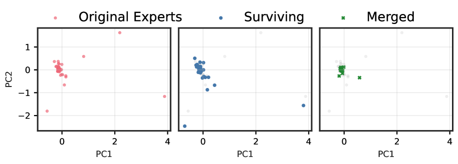<details> <summary>x11.png Details</summary>  ### Visual Description ## Heatmap: Expert Performance Analysis ### Overview The heatmap displays the performance of original experts, surviving experts, and merged experts across two principal components (PC1 and PC2). Each color represents a different category, and the intensity of the color indicates the magnitude of performance. ### Components/Axes - **X-axis (PC1)**: Represents the first principal component, which likely captures the most significant variance in the data. - **Y-axis (PC2)**: Represents the second principal component, which captures the variance that is not explained by PC1. - **Legend**: Shows the categories of experts (Original Experts, Surviving Experts, Merged Experts) and their corresponding colors. - **Data Points**: Each point represents an expert's performance on the two principal components. ### Detailed Analysis or ### Content Details - **Original Experts**: These experts are represented by red dots. Their performance varies across PC1 and PC2, with some points clustering towards the top-left quadrant and others towards the bottom-right quadrant. - **Surviving Experts**: These experts are represented by blue dots. Their performance is more concentrated in the middle of the heatmap, with some points clustering towards the top-left quadrant and others towards the bottom-right quadrant. - **Merged Experts**: These experts are represented by green dots. Their performance is more spread out across the heatmap, with some points clustering towards the top-left quadrant and others towards the bottom-right quadrant. ### Key Observations - **Original Experts**: Show a wide range of performance across both principal components, with some experts performing well on PC1 and others on PC2. - **Surviving Experts**: Have a more consistent performance across both principal components, with a concentration of points in the middle of the heatmap. - **Merged Experts**: Have a more varied performance, with some points performing well on PC1 and others on PC2, and a spread out distribution across the heatmap. ### Interpretation The heatmap suggests that the performance of experts varies significantly across different categories and principal components. The original experts show a wide range of performance, indicating that some experts may have specialized skills in one area while others have specialized skills in another. The surviving experts have a more consistent performance, suggesting that they have maintained their skills over time. The merged experts have a more varied performance, indicating that the merging process may have led to a mix of skills and expertise. Overall, the heatmap provides insights into the performance of experts across different categories and principal components, which can be used to identify areas for improvement and to develop strategies for enhancing expert performance. 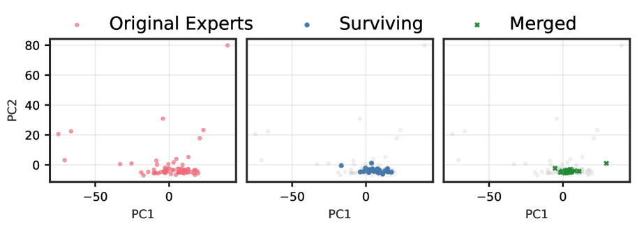</details> (a) ERNIE-4.5-21B Layer 1 <details> <summary>x12.png Details</summary>  ### Visual Description ## Principal Component Analysis (PCA) of Expert Data ### Overview The image displays a Principal Component Analysis (PCA) plot that visualizes the distribution of data points in two principal components (PC1 and PC2). The plot is divided into three sections, each representing a different group of data: Original Experts, Surviving, and Merged. The data points are color-coded to distinguish between these groups. ### Components/Axes - **X-axis (PC1)**: Represents the first principal component, which captures the most variance in the data. - **Y-axis (PC2)**: Represents the second principal component, which captures the second most variance in the data. - **Legend**: The legend on the right side of the plot indicates the color-coding for each group: Original Experts (red), Surviving (blue), and Merged (green). - **Data Points**: Each data point represents an individual expert, with its position on the plot determined by its values on PC1 and PC2. ### Detailed Analysis or ### Content Details - **Original Experts**: The data points for Original Experts are scattered across the plot, with no clear clustering. This suggests that the original experts have a wide range of values on both PC1 and PC2. - **Surviving**: The data points for Surviving experts are more concentrated towards the center of the plot, indicating that these experts have similar values on both PC1 and PC2. - **Merged**: The data points for Merged experts are also concentrated towards the center, but they are slightly more spread out compared to the Surviving group. This suggests that the merged experts have a similar distribution of values on both PC1 and PC2, but with a slight variation. ### Key Observations - **No Clear Clustering**: There is no clear clustering of data points within any of the groups, suggesting that the data does not have a strong underlying structure. - **Similar Distribution**: The Merged and Surviving groups have a similar distribution of data points, indicating that the merging process did not significantly alter the distribution of the data. - **No Outliers**: There are no data points that stand out significantly from the rest, suggesting that the data is relatively homogeneous. ### Interpretation The PCA plot suggests that the data does not have a strong underlying structure, as there is no clear clustering of data points within any of the groups. The merging process did not significantly alter the distribution of the data, as indicated by the similar distribution of data points in the Merged and Surviving groups. The lack of outliers suggests that the data is relatively homogeneous. 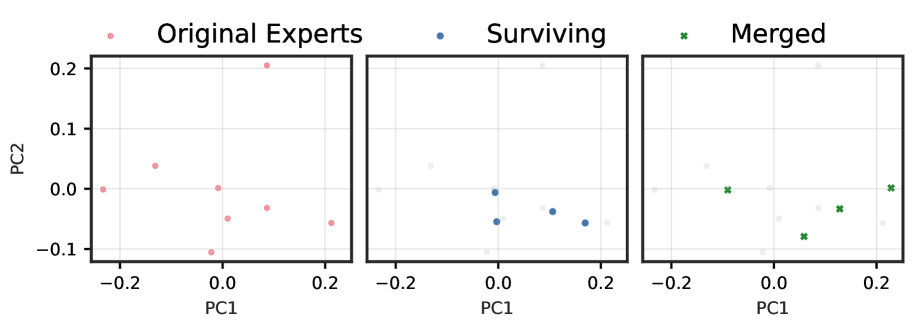</details> (b) ERNIE-4.5-21B Layer 27 <details> <summary>x13.png Details</summary>  ### Visual Description ## Principal Component Analysis (PCA) of Expert Data ### Overview The image displays three separate PCA plots, each representing a different group of experts: Original Experts, Surviving Experts, and Merged Experts. The plots are used to visualize the principal components (PC1 and PC2) of the data, which are likely derived from a dataset related to expert opinions or performance metrics. ### Components/Axes - **X-axis (PC1)**: Represents the first principal component, which captures the amount of variance in the data along the horizontal axis. - **Y-axis (PC2)**: Represents the second principal component, which captures the amount of variance in the data along the vertical axis. - **Legend**: The legend on the right side of each plot indicates the color coding for each group of experts. - **Data Points**: Each data point is represented by a colored dot, corresponding to the group it belongs to. ### Detailed Analysis or ### Content Details - **Original Experts**: The data points for Original Experts are colored in pink. They are spread across the entire range of PC1 and PC2, indicating a diverse set of opinions or performance metrics. - **Surviving Experts**: The data points for Surviving Experts are colored in blue. They are more clustered towards the lower end of PC1 and PC2, suggesting a more homogeneous group with similar opinions or performance metrics. - **Merged Experts**: The data points for Merged Experts are colored in green. They are also spread across the entire range of PC1 and PC2, similar to Original Experts, indicating a diverse set of opinions or performance metrics. ### Key Observations - **Original Experts**: The spread of data points suggests a wide range of opinions or performance metrics among Original Experts. - **Surviving Experts**: The clustering of data points towards the lower end of PC1 and PC2 indicates a more homogeneous group with similar opinions or performance metrics. - **Merged Experts**: The spread of data points is similar to Original Experts, suggesting a diverse set of opinions or performance metrics among Merged Experts. ### Interpretation The PCA plots provide insights into the distribution and clustering of expert opinions or performance metrics. The Original Experts have a wide range of opinions, while the Surviving Experts and Merged Experts have more homogeneous opinions. This could indicate that the Merged Experts have a more diverse set of opinions or performance metrics, which might be a result of the merging process. The plots also suggest that the first principal component (PC1) is the most significant in explaining the variance in the data, while the second principal component (PC2) captures a smaller portion of the variance. 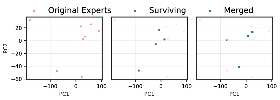</details> (c) Mixtral-8x7B Layer 0 <details> <summary>x14.png Details</summary>  ### Visual Description ## Principal Component Analysis (PCA) of Expert Data ### Overview The image displays a Principal Component Analysis (PCA) plot, which is a dimensionality reduction technique used to visualize high-dimensional data in a lower-dimensional space. The plot is divided into three sections, each representing a different group of experts: Original Experts, Surviving, and Merged. ### Components/Axes - **X-axis (PC1)**: Represents the first principal component, which captures the most variance in the data. - **Y-axis (PC2)**: Represents the second principal component, which captures the second most variance in the data. - **Legend**: The legend indicates the color coding for each group of experts. - **Original Experts**: Red dots - **Surviving**: Blue dots - **Merged**: Green crosses ### Detailed Analysis or ### Content Details - **Original Experts**: The red dots are scattered across the plot, indicating a wide range of values for PC1 and PC2. There is no clear clustering or pattern. - **Surviving**: The blue dots are more concentrated towards the upper right quadrant of the plot, suggesting that these experts have higher values for both PC1 and PC2. - **Merged**: The green crosses are also scattered, but they are more towards the lower left quadrant, indicating lower values for both PC1 and PC2. ### Key Observations - **Original Experts**: No clear trend or pattern, suggesting that the original experts have diverse characteristics. - **Surviving**: The concentration of blue dots in the upper right quadrant suggests that these experts have similar characteristics, possibly indicating a commonality or a group. - **Merged**: The green crosses in the lower left quadrant suggest that the merged group has different characteristics compared to the original and surviving groups. ### Interpretation The PCA plot suggests that the original experts have a wide range of characteristics, while the surviving and merged groups have more similar characteristics. The surviving group is more concentrated, indicating a commonality or a group, while the merged group has different characteristics. This could imply that the merging process has resulted in a group with distinct characteristics, possibly due to the merging of different expert groups with varying characteristics. 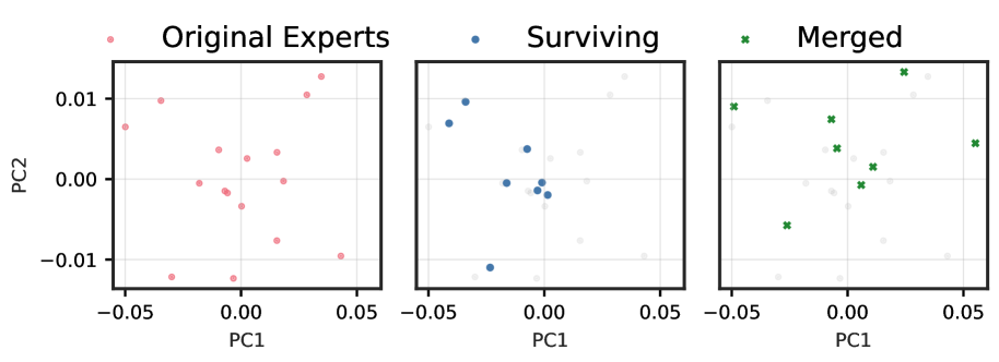</details> (d) Mixtral-8x7B Layer 31 <details> <summary>x15.png Details</summary>  ### Visual Description ## Heatmap: Data Distribution and Clustering ### Overview The heatmap displays the distribution of data points across two principal components (PC1 and PC2). The data is clustered into three groups: Original Experts, Surviving, and Merged. Each group is represented by a different color, and the data points are plotted to show their positions relative to each other. ### Components/Axes - **X-axis (PC1)**: Represents the first principal component, ranging from -0.05 to 0.05. - **Y-axis (PC2)**: Represents the second principal component, ranging from -0.01 to 0.01. - **Legend**: Shows the color coding for each group: Original Experts (red), Surviving (blue), and Merged (green). - **Data Points**: Each point represents an individual data point, with its position determined by its values on PC1 and PC2. ### Detailed Analysis or ### Content Details - **Original Experts**: The data points for Original Experts are scattered across the entire range of PC1 and PC2, indicating a diverse distribution. - **Surviving**: The data points for Surviving are more concentrated towards the center of the heatmap, suggesting a more clustered distribution. - **Merged**: The data points for Merged are also clustered but are more spread out compared to the Surviving group, indicating a mix of Original Experts and Surviving data points. ### Key Observations - **Clusters**: There are distinct clusters of data points for each group, with Original Experts showing the most spread out distribution. - **Outliers**: No single data point stands out as an outlier in any group. - **Trends**: The data points for Merged show a trend of being more spread out compared to the other two groups. ### Interpretation The heatmap suggests that the data is clustered into three distinct groups, with Original Experts showing the most spread out distribution. The Surviving group is more concentrated, and the Merged group is a mix of both Original Experts and Surviving data points. This clustering could indicate different characteristics or behaviors within each group. The trend of the Merged group being more spread out suggests a mix of characteristics from both Original Experts and Surviving groups. 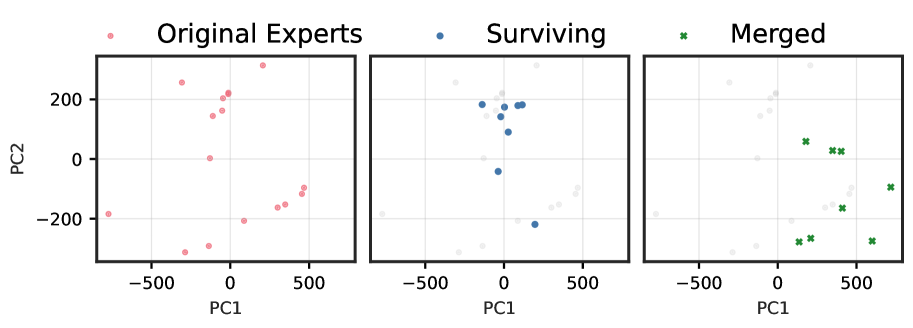</details> (e) Llama-4 Layer 0 <details> <summary>x16.png Details</summary>  ### Visual Description ## Principal Component Analysis (PCA) of Expert Data ### Overview The image displays three separate PCA plots, each representing a different group of experts: Original Experts, Surviving Experts, and Merged Experts. The plots are visualizations of the principal components (PC1 and PC2) of the data, which are likely derived from a dataset of expert opinions or performance metrics. ### Components/Axes - **X-axis (PC1)**: Represents the first principal component, which captures the most variance in the data. - **Y-axis (PC2)**: Represents the second principal component, which captures the second most variance in the data. - **Legend**: The legend on the right side of each plot indicates the color coding for the three groups of experts. - **Data Points**: Each point on the plot corresponds to an individual expert, with its position determined by its values on PC1 and PC2. ### Detailed Analysis or ### Content Details - **Original Experts**: The data points for Original Experts are scattered across the entire range of PC1 and PC2, indicating a wide variety of opinions or performance metrics. - **Surviving Experts**: The data points for Surviving Experts are more clustered towards the center of the plot, suggesting a more cohesive group with similar opinions or performance metrics. - **Merged Experts**: The data points for Merged Experts are also clustered but are more spread out compared to the Surviving Experts, indicating a mix of opinions or performance metrics. ### Key Observations - **Original Experts**: The wide spread of data points suggests a diverse group with varying opinions or performance metrics. - **Surviving Experts**: The clustering of data points towards the center suggests a more cohesive group with similar opinions or performance metrics. - **Merged Experts**: The spread out data points suggest a mix of opinions or performance metrics, indicating a combination of different expertise or perspectives. ### Interpretation The PCA plots provide insights into the distribution and clustering of expert opinions or performance metrics. The Original Experts show a wide variety of opinions, while the Surviving Experts and Merged Experts show more cohesion. This could indicate that the Merged Experts have a mix of different expertise or perspectives, which may be beneficial for a more comprehensive analysis. The Surviving Experts, on the other hand, may have a more unified approach or set of criteria for evaluation. The plots suggest that the data is well-structured and that the principal components are effective in capturing the underlying patterns in the data. </details> (f) Llama-4 Layer 47 Figure A4: (4(a), 4(c), 4(e)) Functional subspace (PCA) for early SMoE layers. Pruning (blue) preserves the manifold geometry; merging (green) collapses it toward the centre. (4(b), 4(d), 4(f)) Functional subspace (PCA) for late MoE layers. Appendix C Evaluation details Multiple choice (MC) evaluation. Following Chen et al. (2025), our MC benchmarks include: AI2 Reasoning Challenge (ARC-c & ARC-e) (Clark et al., 2018), BoolQ (Clark et al., 2019), HellaSwag (Zellers et al., 2019), MMLU (Hendrycks et al., 2021a), OpenBookQA (OBQA) (Mihaylov et al., 2018), Recognizing Textual Entailment Challenge (RTE) (Bentivogli et al., 2009), and WinoGrande (WinoG.) (Sakaguchi et al., 2021). We evaluate the models in the zero-shot setting using the standard log-likelihood approach with lm-eval-harness (Gao et al., 2023). We report byte-length normalized accuracies for ARC-c, ARC-e, HellaSwag, and OBQA Reported as the acc_norm field in the EleutherAI evaluation harness outputs. See Gao (2021) for details. . Coding evaluation. For code generation, all models are evaluated on EvalPlus (Liu et al., 2023) and 182 LiveCodeBench (Jain et al., 2025) questions collected between January and April 2025. We extend the original source code for these benchmarks to evaluate our models. We additionally evaluate Kimi-K2-Instruct-W4A16 and Qwen3-Coder-480B on the agentic coding benchmark SWE-Bench (Jimenez et al., 2024) and tool-calling benchmark BFCLv3 (Patil et al., 2025). For BFCLv3, we use the original Gorilla framework for evaluating our models (Patil et al., 2024). For SWE-Bench evaluation, we run our compressed models with the mini-SWE-agent scaffolding (Yang et al., 2024b) and report the score on the SWE-Bench Verified test set (Neil Chowdhury et al., 2024). We use 4,096 and 16,384 as the maximum number of output tokens for evaluating Qwen3-Coder-480B and Kimi-K2-Instruct-W4A16 on SWE-Bench, respectively. The input context length for both models is limited to 65,536. We do not limit the number of turns in mini-SWE-agent flow, but restart the rollout in cases where the model could not generate a valid patch (that is, in the case when the output of the final turn does not contain a diff --git substring). We set the maximum number of restarts to 20, which we found to be sufficient to generate patches for all samples with pruned models, unless the model produces degenerate responses like repeating strings. We use the cloud-based evaluation provided with the sb-cli tool to get the final scores for all evaluated models. For $\tau^{2}$ -bench Barres et al. (2025), we use greedy decoding and 4,096 as the maximum number of output tokens for each LLM call. For user simulation, we use the gpt-4.1-2025-04-14 model; maximum number of steps is 100 and number of trials is set to three for each domain. Following Artificial Analysis (2025), we additionally implement an LLM-based repetition checking step. Every 30 steps of the simulation, a model (in our case, gpt-4.1-mini-2025-04-14) is given the past 30 episodes of the conversation trajectory with a repetition checking prompt to determine whether the agent is stuck in the loop or making meaningful progress. This allows early task termination if the agent is stuck. We use the same decoding parameters for the repetition model as for the user and assistant models. Math and creative writing evaluation. Mathematical reasoning is assessed on GSM8K (Cobbe et al., 2021) and MATH-500 (Hendrycks et al., 2021b; Lightman et al., 2023) benchmarks using the evalscope (ModelScope Team, 2024) framework. To assess creative writing, we use 146 creative writing prompts sampled from WildBench (Lin et al., 2024) with GPT-4o used as the judge to evaluate the model responses. We report normalized scores using the WildBench rubric. Generation configuration. For models with $≤$ 110B parameters, we use greedy sampling (i.e, temperature = 0.0) to evaluate code generation and math reasoning. For creative writing we use the default temperature, top-P, and top-K settings for each respective model. The maximum number of output tokens is extended to 16,384 for all generative tasks to account for the verbosity of some models. For hybrid reasoning models such as Qwen3-30B-A3B, we disable reasoning on all tasks by setting enable $\_$ thinking=False in the chat template. For larger models with $≥$ 110B parameters, we use greedy sampling for EvalPlus, SWE-Bench, and BFCLv3. On LiveCodeBench, Qwen3-Coder-480B and Kimi-K2 are evaluated with default sampling parameters and greedy sampling, respectively. We report the mean and standard deviation for Qwen3-Coder-480B on LiveCodeBench over five random seeds. We use a repetition penalty of 1.05 for all large model evaluations. For EvalPlus we use 768 as the maximum number of output tokens and 16,384 for LiveCodeBench. For BFCLv3 we set the maximum number of output tokens to 4,096. Model details. The Kimi-K2-Instruct-W4A16 model used throughout this study is an INT4 weight-quantized version of Kimi-K2-Instruct released by RedHatAI (2025). Appendix D Baseline methods The following formally describes the baselines compression methods we consider. Notation. Let $\mathcal{X}_{cal}$ be a calibration dataset. Consider a SMoE model with $n$ layers, $L_{n}$ , $K$ experts per layer $f_{1},...,f_{K}$ , each a function $f_{k}:\mathbb{R}^{d}→\mathbb{R}^{d}$ , and a router producing non-negative gates $\mathbf{g}(x)=(g_{1}(x),...,g_{K}(x))∈\Delta^{K-1}$ . The output of layer $L_{n}$ is $$ h_{n}=\sum_{i}^{K}g_{i}(x)f_{i}(x). $$ The expert usage frequency, $\nu_{i}$ , for expert $f_{i}$ is the number of tokens in $\mathcal{X}_{cal}$ for which $f_{i}$ is activated $$ \nu_{i}=|\mathcal{X}_{i}|, $$ where $\mathcal{X}_{i}=\{x∈\mathcal{X}_{cal}\mid i∈\text{TopK}(\mathbf{g}(x))\}$ . Given saliency scores, $\mathbf{S}∈\mathbb{R}^{K}$ , pruning removes experts with the minimum saliency score. For merging, we first cluster experts based on their pairwise distances, $\mathbf{D}∈\mathbb{R}^{K× K}$ , and then merge the parameters of experts contained within each cluster. Frequency-based pruning. The frequency-based pruning saliency criterion prunes experts with the lowest usage frequency across the calibration dataset. The saliency of $f_{i}$ is simply $S_{i}=\nu_{i}$ . EAN pruning. EAN pruning introduced by Jaiswal et al. (2025) accumulates the activation norm of each expert across tokens for which the expert is activated. The saliency of $f_{i}$ is $$ S_{i}=\sum_{x\in\mathcal{X}_{i}}\|f_{i}(x)\|_{2}. \tag{12} $$ M-SMoE merging. Proposed by Li et al. (2023), M-SMoE first uses weight-matching (Ainsworth et al., 2023) to find a permutation matrix $\mathbf{P_{j}}$ which aligns expert $f_{j}$ to expert $f_{i}$ . In the models we study, each expert is a two-layer feed-forward SwiGLU block (Shazeer, 2020) with up, gate, and down projections: $f_{j}=\{W_{up}^{(j)},W_{gate}^{(j)},W_{down}^{(j)}\}$ . The permutation matrix is applied to the intermediate dimension of the experts such that the expert outputs are invariant to the transformation | | $\displaystyle W^{\prime(j)}_{up}=W^{(j)}_{up}\mathbf{P}_{j},$ | $\displaystyle W^{\prime(j)}_{gate}=W^{(j)}_{gate}\mathbf{P}_{j},$ | $\displaystyle W^{\prime(j)}_{down}=\mathbf{P}_{j}^{T}W^{(j)}_{down}.$ | | | --- | --- | --- | --- | --- | The permuted expert is defined as $\tilde{f}_{j}=\{W^{\prime(j)}_{up},W^{\prime(j)}_{gate},W^{\prime(j)}_{down}\}$ . To initialize the expert clusters, M-SMoE identifies the set of $m$ dominant experts $\mathbb{F}_{dom}$ , as the experts across all layers with the highest usage frequency $\nu$ . The pairwise expert distance is based on the cosine distance of the router gate-values measured on the calibration dataset $$ D_{i,j}=\frac{1}{|\mathcal{X}_{cal}|}\sum_{x\in\mathcal{X}_{cal}}1-\frac{g_{i}(x)\cdot g_{j}(x)}{\|g_{i}(x)\|\|g_{j}(x)\|}. \tag{13} $$ Non-dominant expert $j$ is clustered by selecting the dominant expert with the smallest pairwise distance $$ i^{*}=\operatorname*{arg\,min}_{i\in\mathbb{F}_{dom}}D_{i,j}. $$ The merged expert $f_{\alpha}$ is created by calculating the frequency-weighted average of the permuted parameters, $W^{\prime}$ , of all experts in the cluster $\mathbb{C}_{\alpha}$ $$ \tilde{W}_{a}=\frac{\sum_{i\in\mathbb{C}_{\alpha}}\nu_{i}W^{\prime}_{i}}{\sum_{i\in\mathbb{C}_{\alpha}\nu_{i}}}. \tag{14} $$ HC-SMoE merging. Chen et al. (2025) clusters experts based on their representative vectors, $A_{i}$ , defined as the average activation across every token in the calibration dataset $$ A_{i}:=\mathbb{E}_{x\sim\mathcal{X}_{cal}}[f_{i}(x)]=\frac{1}{|\mathcal{X}_{cal}|}\sum_{x\in\mathcal{X}_{cal}}f_{i}(x). $$ The expert pairwise distance is defined as the cosine distance between representative vectors $$ D_{i,j}=1-\frac{A_{i}\cdot A_{j}}{\|A_{i}\|\|A_{j}\|}. \tag{15} $$ Clusters are formed using hierarchical agglomerative clustering with average linkage criterion. We start by initializing each expert as a singleton cluster. At every iteration, the closest pair of clusters, $\mathbb{C}_{i}^{*},\mathbb{C}_{j}^{*}$ are joined and the pairwise distances updated as the average of the constituents | | $\displaystyle i^{*},j^{*}=\operatorname*{arg\,min}_{i,j}D_{i,j},$ | $\displaystyle\mathbb{C}_{\alpha}=\mathbb{C}_{i^{*}}\cup\mathbb{C}_{j^{*}},$ | $\displaystyle D_{a,k}=\frac{\sum_{i∈\mathbb{C}_{\alpha}}D_{i,k}}{|\mathbb{C}_{\alpha}|}.$ | | | --- | --- | --- | --- | --- | The clusters are merged with equation 14. Appendix E Additional results Table ˜ A4 shows the full suite of MC question answering benchmarks and the average result across all models and methods. Table ˜ A5 tabulates code generation accuracy of compressed SMoE models calibrated on evol-codealpaca. Eval+ is the average of MBPP, MBPP+, HumanEval (HE), HE+. The Code Avg column is the average of Eval+ and LiveCodeBench (LiveCode). Table ˜ A6 summarizes the accuracy of the various compression methods studied when calibrated with the c4 dataset on coding and MC benchmarks. Notably, while the MC performance is generally slightly higher than models calibrated on evol-codealpaca, the resulting code generation quality is abysmal, with most models failing to generate coherent output. Table A4: Detailed benchmark results for multiple-choice QA tasks. | Model | Compression | Technique | Method | ARC-c | ARC-e | BoolQ | Hellaswag | MMLU | OBQA | RTE | WinoG. | MC Avg | | --- | --- | --- | --- | --- | --- | --- | --- | --- | --- | --- | --- | --- | | ERNIE-4.5-21B- A3B-PT | Baseline | 0.564 | 0.782 | 0.873 | 0.813 | 0.737 | 0.462 | 0.812 | 0.724 | 0.721 | | | | 25% | Merging | M-SMoE | 0.434 $±$ 0.006 | 0.652 $±$ 0.008 | 0.846 $±$ 0.001 | 0.597 $±$ 0.002 | 0.591 $±$ 0.001 | 0.350 $±$ 0.006 | 0.819 $±$ 0.010 | 0.655 $±$ 0.003 | 0.618 $±$ 0.002 | | | HC-SMoE | 0.506 $±$ 0.000 | 0.717 $±$ 0.001 | 0.849 $±$ 0.001 | 0.714 $±$ 0.001 | 0.652 $±$ 0.002 | 0.371 $±$ 0.002 | 0.799 $±$ 0.002 | 0.674 $±$ 0.004 | 0.660 $±$ 0.001 | | | | | Pruning | Frequency | 0.486 $±$ 0.004 | 0.711 $±$ 0.000 | 0.852 $±$ 0.004 | 0.675 $±$ 0.003 | 0.628 $±$ 0.003 | 0.373 $±$ 0.003 | 0.780 $±$ 0.006 | 0.676 $±$ 0.005 | 0.648 $±$ 0.001 | | | | EAN | 0.498 $±$ 0.005 | 0.713 $±$ 0.002 | 0.863 $±$ 0.002 | 0.717 $±$ 0.004 | 0.625 $±$ 0.001 | 0.405 $±$ 0.011 | 0.811 $±$ 0.009 | 0.702 $±$ 0.005 | 0.667 $±$ 0.000 | | | | | REAP | 0.527 $±$ 0.004 | 0.759 $±$ 0.002 | 0.857 $±$ 0.003 | 0.717 $±$ 0.003 | 0.644 $±$ 0.001 | 0.409 $±$ 0.009 | 0.756 $±$ 0.008 | 0.690 $±$ 0.001 | 0.670 $±$ 0.002 | | | | | 50% | Merging | M-SMoE | 0.294 $±$ 0.033 | 0.452 $±$ 0.040 | 0.764 $±$ 0.010 | 0.341 $±$ 0.011 | 0.385 $±$ 0.001 | 0.270 $±$ 0.004 | 0.687 $±$ 0.017 | 0.529 $±$ 0.010 | 0.465 $±$ 0.012 | | | HC-SMoE | 0.411 $±$ 0.003 | 0.641 $±$ 0.002 | 0.822 $±$ 0.001 | 0.523 $±$ 0.001 | 0.495 $±$ 0.002 | 0.330 $±$ 0.005 | 0.742 $±$ 0.011 | 0.587 $±$ 0.009 | 0.569 $±$ 0.001 | | | | | Pruning | Frequency | 0.400 $±$ 0.002 | 0.584 $±$ 0.006 | 0.830 $±$ 0.001 | 0.522 $±$ 0.003 | 0.506 $±$ 0.006 | 0.303 $±$ 0.004 | 0.758 $±$ 0.004 | 0.625 $±$ 0.004 | 0.566 $±$ 0.002 | | | | EAN | 0.417 $±$ 0.005 | 0.633 $±$ 0.005 | 0.830 $±$ 0.003 | 0.572 $±$ 0.001 | 0.509 $±$ 0.002 | 0.336 $±$ 0.003 | 0.785 $±$ 0.014 | 0.626 $±$ 0.003 | 0.589 $±$ 0.003 | | | | | REAP | 0.417 $±$ 0.009 | 0.626 $±$ 0.007 | 0.803 $±$ 0.006 | 0.556 $±$ 0.003 | 0.505 $±$ 0.003 | 0.325 $±$ 0.006 | 0.775 $±$ 0.014 | 0.623 $±$ 0.008 | 0.579 $±$ 0.002 | | | | | Qwen3-30B-A3B | Baseline | 0.563 | 0.790 | 0.887 | 0.778 | 0.779 | 0.454 | 0.816 | 0.702 | 0.721 | | | | 25% | Merging | M-SMoE | 0.357 $±$ 0.006 | 0.519 $±$ 0.003 | 0.843 $±$ 0.006 | 0.529 $±$ 0.002 | 0.536 $±$ 0.004 | 0.310 $±$ 0.005 | 0.735 $±$ 0.027 | 0.635 $±$ 0.005 | 0.558 $±$ 0.003 | | | HC-SMoE | 0.478 $±$ 0.006 | 0.722 $±$ 0.006 | 0.863 $±$ 0.003 | 0.714 $±$ 0.000 | 0.684 $±$ 0.002 | 0.417 $±$ 0.001 | 0.805 $±$ 0.004 | 0.710 $±$ 0.004 | 0.674 $±$ 0.001 | | | | | Pruning | Frequency | 0.401 $±$ 0.011 | 0.600 $±$ 0.016 | 0.847 $±$ 0.003 | 0.593 $±$ 0.005 | 0.600 $±$ 0.004 | 0.342 $±$ 0.012 | 0.781 $±$ 0.002 | 0.637 $±$ 0.005 | 0.600 $±$ 0.005 | | | | EAN | 0.406 $±$ 0.007 | 0.603 $±$ 0.014 | 0.847 $±$ 0.005 | 0.607 $±$ 0.006 | 0.600 $±$ 0.002 | 0.337 $±$ 0.003 | 0.764 $±$ 0.002 | 0.660 $±$ 0.009 | 0.603 $±$ 0.004 | | | | | REAP | 0.481 $±$ 0.005 | 0.720 $±$ 0.005 | 0.852 $±$ 0.003 | 0.706 $±$ 0.006 | 0.674 $±$ 0.002 | 0.405 $±$ 0.005 | 0.813 $±$ 0.006 | 0.701 $±$ 0.008 | 0.669 $±$ 0.003 | | | | | 50% | Merging | M-SMoE | 0.278 $±$ 0.003 | 0.402 $±$ 0.003 | 0.753 $±$ 0.004 | 0.399 $±$ 0.002 | 0.366 $±$ 0.004 | 0.278 $±$ 0.002 | 0.586 $±$ 0.014 | 0.546 $±$ 0.004 | 0.451 $±$ 0.002 | | | HC-SMoE | 0.368 $±$ 0.002 | 0.593 $±$ 0.003 | 0.740 $±$ 0.003 | 0.473 $±$ 0.002 | 0.516 $±$ 0.003 | 0.301 $±$ 0.007 | 0.724 $±$ 0.004 | 0.620 $±$ 0.005 | 0.542 $±$ 0.001 | | | | | Pruning | Frequency | 0.285 $±$ 0.001 | 0.424 $±$ 0.002 | 0.779 $±$ 0.003 | 0.458 $±$ 0.003 | 0.397 $±$ 0.002 | 0.286 $±$ 0.004 | 0.659 $±$ 0.012 | 0.570 $±$ 0.009 | 0.483 $±$ 0.001 | | | | EAN | 0.296 $±$ 0.006 | 0.426 $±$ 0.009 | 0.759 $±$ 0.007 | 0.471 $±$ 0.002 | 0.443 $±$ 0.001 | 0.291 $±$ 0.009 | 0.668 $±$ 0.020 | 0.589 $±$ 0.009 | 0.493 $±$ 0.003 | | | | | REAP | 0.344 $±$ 0.004 | 0.504 $±$ 0.008 | 0.745 $±$ 0.005 | 0.489 $±$ 0.013 | 0.507 $±$ 0.005 | 0.311 $±$ 0.003 | 0.625 $±$ 0.031 | 0.623 $±$ 0.007 | 0.518 $±$ 0.004 | | | | | Mixtral-8x7B- Instruct-v0.1 | Baseline | 0.650 | 0.842 | 0.887 | 0.861 | 0.691 | 0.496 | 0.722 | 0.740 | 0.736 | | | | 25% | Merging | M-SMoE | 0.532 $±$ 0.004 | 0.769 $±$ 0.007 | 0.847 $±$ 0.001 | 0.747 $±$ 0.002 | 0.553 $±$ 0.001 | 0.429 $±$ 0.008 | 0.632 $±$ 0.010 | 0.656 $±$ 0.004 | 0.646 $±$ 0.001 | | | HC-SMoE | 0.590 $±$ 0.004 | 0.797 $±$ 0.004 | 0.869 $±$ 0.003 | 0.835 $±$ 0.002 | 0.626 $±$ 0.000 | 0.482 $±$ 0.004 | 0.703 $±$ 0.012 | 0.731 $±$ 0.007 | 0.704 $±$ 0.001 | | | | | Pruning | Frequency | 0.616 $±$ 0.014 | 0.826 $±$ 0.007 | 0.875 $±$ 0.001 | 0.825 $±$ 0.002 | 0.637 $±$ 0.003 | 0.451 $±$ 0.003 | 0.706 $±$ 0.017 | 0.692 $±$ 0.005 | 0.704 $±$ 0.002 | | | | EAN | 0.607 $±$ 0.004 | 0.831 $±$ 0.001 | 0.884 $±$ 0.001 | 0.836 $±$ 0.001 | 0.646 $±$ 0.002 | 0.484 $±$ 0.005 | 0.700 $±$ 0.004 | 0.732 $±$ 0.004 | 0.715 $±$ 0.000 | | | | | REAP | 0.611 $±$ 0.003 | 0.825 $±$ 0.001 | 0.874 $±$ 0.002 | 0.830 $±$ 0.002 | 0.643 $±$ 0.001 | 0.475 $±$ 0.006 | 0.761 $±$ 0.002 | 0.718 $±$ 0.001 | 0.717 $±$ 0.001 | | | | | 50% | Merging | M-SMoE | 0.446 $±$ 0.005 | 0.700 $±$ 0.001 | 0.788 $±$ 0.003 | 0.630 $±$ 0.002 | 0.430 $±$ 0.001 | 0.386 $±$ 0.003 | 0.570 $±$ 0.000 | 0.596 $±$ 0.005 | 0.568 $±$ 0.001 | | | HC-SMoE | 0.539 $±$ 0.003 | 0.759 $±$ 0.000 | 0.851 $±$ 0.001 | 0.791 $±$ 0.001 | 0.543 $±$ 0.000 | 0.442 $±$ 0.000 | 0.700 $±$ 0.004 | 0.712 $±$ 0.002 | 0.667 $±$ 0.001 | | | | | Pruning | Frequency | 0.541 $±$ 0.004 | 0.781 $±$ 0.003 | 0.824 $±$ 0.013 | 0.759 $±$ 0.002 | 0.516 $±$ 0.002 | 0.411 $±$ 0.006 | 0.708 $±$ 0.023 | 0.650 $±$ 0.005 | 0.649 $±$ 0.004 | | | | EAN | 0.551 $±$ 0.014 | 0.774 $±$ 0.008 | 0.859 $±$ 0.004 | 0.794 $±$ 0.002 | 0.550 $±$ 0.006 | 0.452 $±$ 0.014 | 0.717 $±$ 0.023 | 0.693 $±$ 0.008 | 0.674 $±$ 0.005 | | | | | REAP | 0.544 $±$ 0.005 | 0.785 $±$ 0.005 | 0.837 $±$ 0.003 | 0.778 $±$ 0.002 | 0.554 $±$ 0.001 | 0.462 $±$ 0.005 | 0.715 $±$ 0.013 | 0.679 $±$ 0.005 | 0.669 $±$ 0.001 | | | | | Llama-4-Scout- 17B-16E- Instruct | Baseline | 0.627 | 0.848 | 0.879 | 0.823 | 0.803 | 0.462 | 0.765 | 0.692 | 0.738 | | | | 25% | Merging | M-SMoE | 0.573 | 0.802 | 0.872 | 0.752 | 0.719 | 0.434 | 0.769 | 0.671 | 0.699 | | | HC-SMoE | 0.588 | 0.814 | 0.876 | 0.779 | 0.720 | 0.424 | 0.729 | 0.695 | 0.703 | | | | | Pruning | Frequency | 0.584 | 0.817 | 0.876 | 0.779 | 0.733 | 0.438 | 0.773 | 0.691 | 0.711 | | | | EAN | 0.582 | 0.816 | 0.872 | 0.777 | 0.735 | 0.446 | 0.791 | 0.679 | 0.712 | | | | | REAP | 0.594 | 0.830 | 0.872 | 0.788 | 0.756 | 0.452 | 0.769 | 0.683 | 0.718 | | | | | 50% | Merging | M-SMoE | 0.498 | 0.717 | 0.856 | 0.676 | 0.609 | 0.388 | 0.787 | 0.665 | 0.649 | | | HC-SMoE | 0.526 | 0.781 | 0.862 | 0.718 | 0.628 | 0.386 | 0.726 | 0.660 | 0.661 | | | | | Pruning | Frequency | 0.518 | 0.734 | 0.860 | 0.704 | 0.652 | 0.398 | 0.765 | 0.657 | 0.661 | | | | EAN | 0.510 | 0.750 | 0.857 | 0.712 | 0.650 | 0.398 | 0.762 | 0.662 | 0.663 | | | | | REAP | 0.561 | 0.802 | 0.869 | 0.745 | 0.682 | 0.432 | 0.762 | 0.664 | 0.689 | | | | | GLM-4.5-Air | Baseline | 0.619 | 0.825 | 0.882 | 0.858 | 0.789 | 0.478 | 0.747 | 0.776 | 0.747 | | | | 25% | Merging | M-SMoE | 0.429 | 0.651 | 0.808 | 0.671 | 0.578 | 0.362 | 0.578 | 0.695 | 0.596 | | | HC-SMoE | 0.577 | 0.782 | 0.860 | 0.815 | 0.722 | 0.458 | 0.668 | 0.755 | 0.704 | | | | | Pruning | Frequency | 0.493 | 0.715 | 0.827 | 0.732 | 0.653 | 0.422 | 0.614 | 0.725 | 0.648 | | | | EAN | 0.492 | 0.705 | 0.805 | 0.736 | 0.656 | 0.368 | 0.603 | 0.730 | 0.637 | | | | | REAP | 0.555 | 0.756 | 0.813 | 0.796 | 0.701 | 0.434 | 0.643 | 0.724 | 0.678 | | | | | 50% | Merging | M-SMoE | 0.291 | 0.452 | 0.693 | 0.433 | 0.382 | 0.266 | 0.484 | 0.551 | 0.444 | | | HC-SMoE | 0.428 | 0.671 | 0.761 | 0.590 | 0.524 | 0.318 | 0.603 | 0.613 | 0.564 | | | | | Pruning | Frequency | 0.334 | 0.535 | 0.767 | 0.566 | 0.478 | 0.288 | 0.567 | 0.635 | 0.521 | | | | EAN | 0.358 | 0.530 | 0.682 | 0.573 | 0.489 | 0.300 | 0.516 | 0.635 | 0.511 | | | | | REAP | 0.427 | 0.604 | 0.662 | 0.642 | 0.569 | 0.318 | 0.606 | 0.640 | 0.559 | | | | | Qwen3-Coder- 480B-A35B- Instruct-FP8 | Baseline | 0.644 | 0.822 | 0.906 | 0.841 | 0.850 | 0.468 | 0.751 | 0.717 | 0.750 | | | | 25% | Pruning | Frequency | 0.443 | 0.673 | 0.845 | 0.651 | 0.621 | 0.280 | 0.704 | 0.632 | 0.606 | | | EAN | 0.555 | 0.766 | 0.891 | 0.769 | 0.795 | 0.404 | 0.747 | 0.691 | 0.702 | | | | | REAP | 0.635 | 0.824 | 0.900 | 0.841 | 0.836 | 0.466 | 0.754 | 0.725 | 0.748 | | | | | 50% | Pruning | Frequency | 0.314 | 0.470 | 0.791 | 0.502 | 0.451 | 0.262 | 0.679 | 0.580 | 0.506 | | | EAN | 0.402 | 0.596 | 0.858 | 0.629 | 0.615 | 0.216 | 0.744 | 0.666 | 0.591 | | | | | REAP | 0.546 | 0.772 | 0.872 | 0.756 | 0.696 | 0.430 | 0.762 | 0.701 | 0.692 | | | | | Kimi-K2- Instruct- W4A16 | Baseline | 0.712 | 0.879 | 0.913 | 0.765 | 0.872 | 0.504 | 0.783 | 0.811 | 0.780 | | | | 25% | Pruning | Frequency | 0.518 | 0.771 | 0.825 | 0.787 | 0.242 | 0.420 | 0.653 | 0.613 | 0.604 | | | EAN | 0.615 | 0.819 | 0.893 | 0.843 | 0.500 | 0.446 | 0.762 | 0.743 | 0.703 | | | | | REAP | 0.671 | 0.854 | 0.907 | 0.860 | 0.809 | 0.470 | 0.805 | 0.809 | 0.773 | | | | | 50% | Pruning | Frequency | 0.285 | 0.498 | 0.620 | 0.436 | 0.241 | 0.314 | 0.617 | 0.500 | 0.439 | | | EAN | 0.426 | 0.682 | 0.863 | 0.663 | 0.324 | 0.356 | 0.726 | 0.659 | 0.587 | | | | | REAP | 0.476 | 0.661 | 0.883 | 0.643 | 0.636 | 0.350 | 0.816 | 0.681 | 0.643 | | | | Table A5: Detailed benchmark results for non-agentic code generation tasks. Eval+ is the average of MBPP, MBPP+, HE, HE+. The Code Avg column is the average of Eval+ and LiveCodeBench (LiveCode). | Model | Compression | Technique | Method | HE | HE+ | MBPP | MBPP+ | Eval+ | LiveCode | Code Avg | | --- | --- | --- | --- | --- | --- | --- | --- | --- | --- | --- | | ERNIE-4.5-21B- A3B-PT | Baseline | 0.902 | 0.866 | 0.910 | 0.765 | 0.861 | 0.231 | 0.546 | | | | 25% | Merging | M-SMoE | 0.774 $±$ 0.011 | 0.730 $±$ 0.009 | 0.768 $±$ 0.015 | 0.647 $±$ 0.017 | 0.730 $±$ 0.005 | 0.194 $±$ 0.022 | 0.462 $±$ 0.011 | | | HC-SMoE | 0.837 $±$ 0.007 | 0.805 $±$ 0.000 | 0.827 $±$ 0.003 | 0.696 $±$ 0.008 | 0.791 $±$ 0.004 | 0.207 $±$ 0.008 | 0.499 $±$ 0.003 | | | | | Pruning | Frequency | 0.890 $±$ 0.006 | 0.846 $±$ 0.009 | 0.837 $±$ 0.010 | 0.709 $±$ 0.010 | 0.820 $±$ 0.006 | 0.151 $±$ 0.096 | 0.486 $±$ 0.045 | | | | EAN | 0.890 $±$ 0.006 | 0.848 $±$ 0.011 | 0.840 $±$ 0.006 | 0.727 $±$ 0.004 | 0.826 $±$ 0.004 | 0.161 $±$ 0.111 | 0.494 $±$ 0.054 | | | | | REAP | 0.892 $±$ 0.009 | 0.854 $±$ 0.012 | 0.876 $±$ 0.000 | 0.738 $±$ 0.003 | 0.840 $±$ 0.005 | 0.167 $±$ 0.124 | 0.504 $±$ 0.060 | | | | | 50% | Merging | M-SMoE | 0.104 $±$ 0.022 | 0.100 $±$ 0.029 | 0.239 $±$ 0.036 | 0.207 $±$ 0.040 | 0.162 $±$ 0.012 | 0.024 $±$ 0.008 | 0.093 $±$ 0.008 | | | HC-SMoE | 0.425 $±$ 0.004 | 0.404 $±$ 0.007 | 0.608 $±$ 0.018 | 0.511 $±$ 0.011 | 0.487 $±$ 0.008 | 0.082 $±$ 0.015 | 0.285 $±$ 0.009 | | | | | Pruning | Frequency | 0.699 $±$ 0.031 | 0.640 $±$ 0.022 | 0.696 $±$ 0.014 | 0.584 $±$ 0.006 | 0.655 $±$ 0.015 | 0.083 $±$ 0.066 | 0.369 $±$ 0.025 | | | | EAN | 0.675 $±$ 0.019 | 0.642 $±$ 0.009 | 0.713 $±$ 0.015 | 0.591 $±$ 0.016 | 0.655 $±$ 0.014 | 0.112 $±$ 0.064 | 0.384 $±$ 0.035 | | | | | REAP | 0.797 $±$ 0.009 | 0.764 $±$ 0.007 | 0.767 $±$ 0.017 | 0.644 $±$ 0.013 | 0.743 $±$ 0.008 | 0.137 $±$ 0.119 | 0.440 $±$ 0.064 | | | | | Qwen3-30B-A3B | Baseline | 0.927 | 0.884 | 0.881 | 0.743 | 0.859 | 0.302 | 0.581 | | | | 25% | Merging | M-SMoE | 0.878 $±$ 0.012 | 0.833 $±$ 0.007 | 0.849 $±$ 0.007 | 0.728 $±$ 0.007 | 0.822 $±$ 0.004 | 0.293 $±$ 0.017 | 0.558 $±$ 0.006 | | | HC-SMoE | 0.866 $±$ 0.011 | 0.805 $±$ 0.016 | 0.832 $±$ 0.006 | 0.698 $±$ 0.005 | 0.800 $±$ 0.004 | 0.258 $±$ 0.000 | 0.529 $±$ 0.002 | | | | | Pruning | Frequency | 0.921 $±$ 0.006 | 0.874 $±$ 0.007 | 0.868 $±$ 0.000 | 0.735 $±$ 0.003 | 0.849 $±$ 0.004 | 0.302 $±$ 0.011 | 0.576 $±$ 0.004 | | | | EAN | 0.909 $±$ 0.006 | 0.864 $±$ 0.004 | 0.859 $±$ 0.009 | 0.729 $±$ 0.008 | 0.840 $±$ 0.004 | 0.311 $±$ 0.018 | 0.576 $±$ 0.010 | | | | | REAP | 0.917 $±$ 0.007 | 0.876 $±$ 0.004 | 0.853 $±$ 0.002 | 0.727 $±$ 0.006 | 0.843 $±$ 0.002 | 0.308 $±$ 0.015 | 0.575 $±$ 0.008 | | | | | 50% | Merging | M-SMoE | 0.687 $±$ 0.013 | 0.638 $±$ 0.004 | 0.618 $±$ 0.004 | 0.541 $±$ 0.007 | 0.621 $±$ 0.006 | 0.205 $±$ 0.019 | 0.413 $±$ 0.007 | | | HC-SMoE | 0.577 $±$ 0.023 | 0.541 $±$ 0.013 | 0.631 $±$ 0.010 | 0.546 $±$ 0.004 | 0.574 $±$ 0.010 | 0.185 $±$ 0.018 | 0.379 $±$ 0.005 | | | | | Pruning | Frequency | 0.787 $±$ 0.016 | 0.756 $±$ 0.022 | 0.692 $±$ 0.016 | 0.579 $±$ 0.016 | 0.704 $±$ 0.017 | 0.236 $±$ 0.025 | 0.470 $±$ 0.021 | | | | EAN | 0.886 $±$ 0.025 | 0.837 $±$ 0.020 | 0.798 $±$ 0.006 | 0.669 $±$ 0.008 | 0.798 $±$ 0.013 | 0.306 $±$ 0.003 | 0.552 $±$ 0.005 | | | | | REAP | 0.919 $±$ 0.007 | 0.870 $±$ 0.004 | 0.805 $±$ 0.009 | 0.692 $±$ 0.008 | 0.821 $±$ 0.003 | 0.293 $±$ 0.003 | 0.557 $±$ 0.001 | | | | | Mixtral-8x7B- Instruct-v0.1 | Baseline | 0.524 | 0.476 | 0.556 | 0.463 | 0.505 | 0.123 | 0.314 | | | | 25% | Merging | M-SMoE | 0.315 $±$ 0.007 | 0.270 $±$ 0.015 | 0.446 $±$ 0.007 | 0.380 $±$ 0.015 | 0.353 $±$ 0.008 | 0.033 $±$ 0.010 | 0.193 $±$ 0.008 | | | HC-SMoE | 0.439 $±$ 0.028 | 0.386 $±$ 0.020 | 0.530 $±$ 0.022 | 0.441 $±$ 0.007 | 0.449 $±$ 0.005 | 0.110 $±$ 0.010 | 0.279 $±$ 0.002 | | | | | Pruning | Frequency | 0.400 $±$ 0.034 | 0.358 $±$ 0.035 | 0.541 $±$ 0.006 | 0.453 $±$ 0.012 | 0.438 $±$ 0.018 | 0.099 $±$ 0.014 | 0.269 $±$ 0.004 | | | | EAN | 0.413 $±$ 0.027 | 0.366 $±$ 0.024 | 0.477 $±$ 0.009 | 0.409 $±$ 0.013 | 0.416 $±$ 0.015 | 0.111 $±$ 0.006 | 0.264 $±$ 0.006 | | | | | REAP | 0.439 $±$ 0.018 | 0.370 $±$ 0.007 | 0.535 $±$ 0.011 | 0.452 $±$ 0.011 | 0.449 $±$ 0.002 | 0.102 $±$ 0.010 | 0.275 $±$ 0.005 | | | | | 50% | Merging | M-SMoE | 0.085 $±$ 0.026 | 0.076 $±$ 0.022 | 0.139 $±$ 0.121 | 0.118 $±$ 0.102 | 0.091 $±$ 0.079 | 0.004 $±$ 0.006 | 0.047 $±$ 0.037 | | | HC-SMoE | 0.175 $±$ 0.015 | 0.146 $±$ 0.000 | 0.335 $±$ 0.026 | 0.282 $±$ 0.031 | 0.235 $±$ 0.018 | 0.013 $±$ 0.008 | 0.124 $±$ 0.008 | | | | | Pruning | Frequency | 0.187 $±$ 0.015 | 0.148 $±$ 0.007 | 0.342 $±$ 0.016 | 0.287 $±$ 0.012 | 0.241 $±$ 0.007 | 0.023 $±$ 0.004 | 0.132 $±$ 0.003 | | | | EAN | 0.220 $±$ 0.006 | 0.189 $±$ 0.006 | 0.375 $±$ 0.020 | 0.325 $±$ 0.015 | 0.277 $±$ 0.005 | 0.031 $±$ 0.011 | 0.154 $±$ 0.007 | | | | | REAP | 0.232 $±$ 0.018 | 0.193 $±$ 0.013 | 0.274 $±$ 0.106 | 0.241 $±$ 0.087 | 0.235 $±$ 0.056 | 0.035 $±$ 0.003 | 0.135 $±$ 0.027 | | | | | Llama-4-Scout- 17B-16E- Instruct | Baseline | 0.829 | 0.768 | 0.788 | 0.640 | 0.757 | 0.341 | 0.549 | | | | 25% | Merging | M-SMoE | 0.823 | 0.762 | 0.786 | 0.635 | 0.752 | 0.324 | 0.538 | | | HC-SMoE | 0.787 | 0.738 | 0.735 | 0.587 | 0.712 | 0.148 | 0.430 | | | | | Pruning | Frequency | 0.835 | 0.768 | 0.788 | 0.630 | 0.755 | 0.317 | 0.536 | | | | EAN | 0.823 | 0.762 | 0.804 | 0.648 | 0.759 | 0.328 | 0.544 | | | | | REAP | 0.829 | 0.787 | 0.788 | 0.622 | 0.756 | 0.242 | 0.499 | | | | | 50% | Merging | M-SMoE | 0.787 | 0.732 | 0.762 | 0.614 | 0.723 | 0.187 | 0.455 | | | HC-SMoE | 0.604 | 0.530 | 0.500 | 0.399 | 0.508 | 0.077 | 0.293 | | | | | Pruning | Frequency | 0.823 | 0.756 | 0.751 | 0.595 | 0.731 | 0.223 | 0.477 | | | | EAN | 0.805 | 0.744 | 0.754 | 0.601 | 0.726 | 0.209 | 0.468 | | | | | REAP | 0.841 | 0.768 | 0.762 | 0.624 | 0.749 | 0.248 | 0.499 | | | | | GLM-4.5-Air | Baseline | 0.848 | 0.829 | 0.860 | 0.743 | 0.820 | 0.374 | 0.597 | | | | 25% | Merging | M-SMoE | 0.866 | 0.793 | 0.807 | 0.659 | 0.781 | 0.330 | 0.555 | | | HC-SMoE | 0.872 | 0.805 | 0.825 | 0.669 | 0.793 | 0.363 | 0.578 | | | | | Pruning | Frequency | 0.848 | 0.811 | 0.854 | 0.706 | 0.805 | 0.341 | 0.573 | | | | EAN | 0.872 | 0.817 | 0.876 | 0.720 | 0.821 | 0.374 | 0.597 | | | | | REAP | 0.866 | 0.805 | 0.828 | 0.677 | 0.794 | 0.390 | 0.592 | | | | | 50% | Merging | M-SMoE | 0.518 | 0.500 | 0.519 | 0.437 | 0.493 | 0.099 | 0.296 | | | HC-SMoE | 0.707 | 0.659 | 0.706 | 0.577 | 0.662 | 0.220 | 0.441 | | | | | Pruning | Frequency | 0.628 | 0.573 | 0.534 | 0.450 | 0.546 | 0.104 | 0.325 | | | | EAN | 0.841 | 0.780 | 0.807 | 0.661 | 0.773 | 0.253 | 0.513 | | | | | REAP | 0.878 | 0.841 | 0.712 | 0.587 | 0.755 | 0.352 | 0.553 | | | | | Qwen3-Coder- 480B-A35B- Instruct-FP8 | Baseline | 0.951 | 0.890 | 0.923 | 0.791 | 0.889 | 0.431 $±$ 0.011 | 0.660 | | | | 25% | Pruning | Frequency | 0.884 | 0.805 | 0.810 | 0.669 | 0.792 | 0.296 $±$ 0.017 | 0.544 | | | EAN | 0.939 | 0.878 | 0.911 | 0.775 | 0.876 | 0.419 $±$ 0.015 | 0.647 | | | | | REAP | 0.957 | 0.890 | 0.917 | 0.772 | 0.884 | 0.416 $±$ 0.013 | 0.650 | | | | | 50% | Pruning | Frequency | 0.020 | 0.012 | 0.007 | 0.003 | 0.011 | 0.012 $±$ 0.001 | 0.011 | | | EAN | 0.915 | 0.841 | 0.854 | 0.714 | 0.831 | 0.382 $±$ 0.012 | 0.607 | | | | | REAP | 0.939 | 0.872 | 0.910 | 0.772 | 0.873 | 0.415 $±$ 0.015 | 0.644 | | | | | Kimi-K2- Instruct- W4A16 | Baseline | 0.963 | 0.921 | 0.913 | 0.735 | 0.883 | 0.434 | 0.659 | | | | 25% | Pruning | Frequency | 0.530 | 0.463 | 0.595 | 0.508 | 0.524 | 0.082 | 0.303 | | | EAN | 0.909 | 0.860 | 0.857 | 0.698 | 0.831 | 0.379 | 0.605 | | | | | REAP | 0.957 | 0.921 | 0.918 | 0.759 | 0.889 | 0.440 | 0.664 | | | | | 50% | Pruning | Frequency | 0.098 | 0.079 | 0.175 | 0.146 | 0.124 | 0.000 | 0.062 | | | EAN | 0.866 | 0.811 | 0.780 | 0.632 | 0.772 | 0.253 | 0.513 | | | | | REAP | 0.915 | 0.884 | 0.899 | 0.754 | 0.863 | 0.429 | 0.646 | | | | Table A6: C4 calibrated results for coding and MC tasks. | | Coding | MC | | | | | | | | | | | | | | | --- | --- | --- | --- | --- | --- | --- | --- | --- | --- | --- | --- | --- | --- | --- | --- | | Model | Compression | Technique | Method | Eval+ | LiveCode | Code Avg | ARC-c | ARC-e | BoolQ | Hellaswag | MMLU | OBQA | RTE | WinoG. | MC Avg | | ERNIE-4.5-21B- A3B-PT | Baseline | 0.861 | 0.231 | 0.546 | 0.564 | 0.782 | 0.873 | 0.813 | 0.737 | 0.462 | 0.812 | 0.724 | 0.721 | | | | 25% | Merging | M-SMoE | 0.065 | 0.016 | 0.041 | 0.497 | 0.729 | 0.860 | 0.723 | 0.602 | 0.424 | 0.801 | 0.699 | 0.667 | | | HC-SMoE | 0.403 | 0.099 | 0.251 | 0.515 | 0.728 | 0.860 | 0.745 | 0.649 | 0.428 | 0.794 | 0.694 | 0.677 | | | | | Pruning | Frequency | 0.274 | 0.000 | 0.137 | 0.515 | 0.735 | 0.841 | 0.719 | 0.588 | 0.382 | 0.791 | 0.683 | 0.657 | | | | EAN | 0.282 | 0.000 | 0.141 | 0.528 | 0.750 | 0.853 | 0.790 | 0.558 | 0.442 | 0.783 | 0.706 | 0.676 | | | | | REAP | 0.242 | 0.023 | 0.133 | 0.490 | 0.716 | 0.855 | 0.783 | 0.656 | 0.452 | 0.809 | 0.723 | 0.685 | | | | | 50% | Merging | M-SMoE | 0.000 | 0.000 | 0.000 | 0.297 | 0.460 | 0.674 | 0.449 | 0.312 | 0.280 | 0.671 | 0.575 | 0.465 | | | HC-SMoE | 0.000 | 0.000 | 0.000 | 0.409 | 0.615 | 0.666 | 0.515 | 0.489 | 0.290 | 0.632 | 0.580 | 0.524 | | | | | Pruning | Frequency | 0.000 | 0.000 | 0.000 | 0.393 | 0.625 | 0.717 | 0.569 | 0.496 | 0.324 | 0.758 | 0.619 | 0.563 | | | | EAN | 0.007 | 0.003 | 0.005 | 0.451 | 0.676 | 0.742 | 0.687 | 0.474 | 0.398 | 0.736 | 0.691 | 0.607 | | | | | REAP | 0.033 | 0.000 | 0.016 | 0.406 | 0.612 | 0.754 | 0.654 | 0.468 | 0.396 | 0.718 | 0.656 | 0.583 | | | | | Qwen3-30B-A3B | Baseline | 0.859 | 0.302 | 0.581 | 0.563 | 0.790 | 0.887 | 0.778 | 0.779 | 0.454 | 0.816 | 0.702 | 0.721 | | | | 25% | Merging | M-SMoE | 0.000 | 0.000 | 0.000 | 0.551 | 0.768 | 0.883 | 0.761 | 0.733 | 0.418 | 0.848 | 0.701 | 0.708 | | | HC-SMoE | 0.831 | 0.269 | 0.550 | 0.470 | 0.713 | 0.833 | 0.622 | 0.646 | 0.376 | 0.805 | 0.665 | 0.641 | | | | | Pruning | Frequency | 0.000 | 0.000 | 0.000 | 0.548 | 0.789 | 0.889 | 0.775 | 0.735 | 0.438 | 0.801 | 0.694 | 0.709 | | | | EAN | 0.000 | 0.000 | 0.000 | 0.569 | 0.802 | 0.889 | 0.774 | 0.735 | 0.438 | 0.801 | 0.697 | 0.713 | | | | | REAP | 0.735 | 0.227 | 0.481 | 0.557 | 0.781 | 0.872 | 0.746 | 0.718 | 0.436 | 0.794 | 0.704 | 0.701 | | | | | 50% | Merging | M-SMoE | 0.000 | 0.000 | 0.000 | 0.262 | 0.348 | 0.693 | 0.479 | 0.237 | 0.290 | 0.523 | 0.542 | 0.422 | | | HC-SMoE | 0.728 | 0.209 | 0.468 | 0.316 | 0.495 | 0.715 | 0.354 | 0.422 | 0.282 | 0.603 | 0.536 | 0.465 | | | | | Pruning | Frequency | 0.000 | 0.000 | 0.000 | 0.349 | 0.488 | 0.782 | 0.672 | 0.503 | 0.364 | 0.588 | 0.619 | 0.545 | | | | EAN | 0.000 | 0.000 | 0.000 | 0.480 | 0.736 | 0.876 | 0.760 | 0.607 | 0.424 | 0.762 | 0.694 | 0.667 | | | | | REAP | 0.006 | 0.000 | 0.003 | 0.421 | 0.640 | 0.837 | 0.653 | 0.495 | 0.388 | 0.704 | 0.635 | 0.596 | | | | | Mixtral-8x7B- Instruct-v0.1 | Baseline | 0.505 | 0.123 | 0.314 | 0.650 | 0.842 | 0.887 | 0.861 | 0.691 | 0.496 | 0.722 | 0.740 | 0.736 | | | | 25% | Merging | M-SMoE | 0.320 | 0.044 | 0.182 | 0.532 | 0.775 | 0.828 | 0.746 | 0.529 | 0.424 | 0.603 | 0.632 | 0.634 | | | HC-SMoE | 0.420 | 0.121 | 0.271 | 0.608 | 0.811 | 0.876 | 0.838 | 0.631 | 0.484 | 0.736 | 0.726 | 0.714 | | | | | Pruning | Frequency | 0.396 | 0.070 | 0.233 | 0.612 | 0.816 | 0.868 | 0.836 | 0.593 | 0.482 | 0.675 | 0.739 | 0.703 | | | | EAN | 0.399 | 0.092 | 0.246 | 0.613 | 0.814 | 0.875 | 0.842 | 0.613 | 0.498 | 0.690 | 0.733 | 0.710 | | | | | REAP | 0.415 | 0.077 | 0.246 | 0.606 | 0.807 | 0.875 | 0.835 | 0.633 | 0.486 | 0.791 | 0.709 | 0.718 | | | | | 50% | Merging | M-SMoE | 0.000 | 0.000 | 0.000 | 0.260 | 0.460 | 0.614 | 0.395 | 0.240 | 0.302 | 0.527 | 0.526 | 0.416 | | | HC-SMoE | 0.174 | 0.033 | 0.103 | 0.540 | 0.764 | 0.862 | 0.795 | 0.544 | 0.448 | 0.675 | 0.709 | 0.667 | | | | | Pruning | Frequency | 0.173 | 0.008 | 0.090 | 0.504 | 0.739 | 0.793 | 0.771 | 0.463 | 0.426 | 0.675 | 0.646 | 0.627 | | | | EAN | 0.139 | 0.008 | 0.074 | 0.550 | 0.756 | 0.842 | 0.804 | 0.529 | 0.460 | 0.726 | 0.716 | 0.673 | | | | | REAP | 0.167 | 0.012 | 0.089 | 0.525 | 0.774 | 0.856 | 0.794 | 0.533 | 0.454 | 0.751 | 0.688 | 0.672 | | | | Table A7: $\tau^{2}$ -bench results with REAP compression across different benchmark domains on Qwen3-480B-A35B-Coder-FP8. | Dataset | Compression | Method | passˆ1 | passˆ2 | passˆ3 | | --- | --- | --- | --- | --- | --- | | Retail | Baseline | 0.643 | 0.544 | 0.500 | | | 25% | REAP | 0.661 | 0.535 | 0.465 | | | 50% | REAP | 0.632 | 0.515 | 0.456 | | | Airline | Baseline | 0.460 | 0.340 | 0.280 | | | 25% | REAP | 0.487 | 0.367 | 0.320 | | | 50% | REAP | 0.447 | 0.333 | 0.280 | | | Telecom | Baseline | 0.500 | 0.398 | 0.325 | | | 25% | REAP | 0.529 | 0.456 | 0.421 | | | 50% | REAP | 0.471 | 0.339 | 0.263 | | Figure ˜ A5 plots non-agentic coding and MC accuracy versus compressed model size. Figure ˜ 6(a) depict the proportion of singleton clusters for HC-SMoE and M-SMoE. Figure ˜ 6(b) plots accuracy vs. maximum cluster sizes when the maximum cardinality of clusters is restricted. Figures ˜ A7 and A8 show the importance of using domain-specific calibration data, particularly at high compression ratios. Table ˜ A7 presents the complete $\tau^{2}$ -bench results across three domains (Retail, Airline, and Telecom) for the baseline model and REAP compression at 25% and 50% levels. The results show passˆk metrics for k=1, 2, and 3, demonstrating the impact of pruning on evaluating conversational agents, specifically designed to test their ability to collaborate with a user in real-world scenarios. 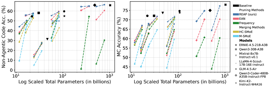<details> <summary>x17.png Details</summary>  ### Visual Description ## Heatmap: Model Performance on Non-Agentic Code ### Overview The heatmap illustrates the performance of various models on a non-agentic code dataset, measured by MC Accuracy. The x-axis represents the log-scaled total parameters in billions, while the y-axis shows the MC Accuracy percentage. ### Components/Axes - **X-Axis**: Log-scaled total parameters in billions (ranging from 10^1 to 10^3). - **Y-Axis**: MC Accuracy percentage (ranging from 0% to 75%). - **Legend**: Contains the names of different models and their corresponding colors. - **Data Points**: Represent the performance of each model at different parameter scales. ### Detailed Analysis or ### Content Details - **Baseline Model**: The solid black line represents the baseline model, which consistently performs well across different parameter scales. - **Pruning Methods**: The dashed blue line indicates the performance of models using pruning methods, which show a slight improvement in accuracy compared to the baseline. - **EAN**: The dotted green line represents the EAN model, which performs well at lower parameter scales but shows a decline in accuracy as the number of parameters increases. - **Frequency**: The dashed red line indicates the frequency-based model, which performs well at lower parameter scales but shows a significant decline in accuracy as the number of parameters increases. - **M-SMOE**: The solid yellow line represents the M-SMOE model, which shows a consistent improvement in accuracy across different parameter scales. - **Models**: The legend includes the names of different models, such as Baseline, Pruning Methods, EAN, Frequency, M-SMOE, and others. - **Data Points**: The data points are scattered across the heatmap, with some models performing better at lower parameter scales and others at higher scales. ### Key Observations - The baseline model consistently performs the best across different parameter scales. - Models using pruning methods show a slight improvement in accuracy compared to the baseline. - The EAN model performs well at lower parameter scales but shows a significant decline in accuracy as the number of parameters increases. - The frequency-based model performs well at lower parameter scales but shows a significant decline in accuracy as the number of parameters increases. - The M-SMOE model shows a consistent improvement in accuracy across different parameter scales. ### Interpretation The heatmap suggests that the baseline model is the most effective for non-agentic code, as it consistently performs the best across different parameter scales. Models using pruning methods show a slight improvement in accuracy compared to the baseline. The EAN and frequency-based models perform well at lower parameter scales but show a significant decline in accuracy as the number of parameters increases. The M-SMOE model shows a consistent improvement in accuracy across different parameter scales. Overall, the heatmap demonstrates that the baseline model is the most effective for non-agentic code, while the other models show varying degrees of performance. </details> Figure A5: Coding and MC accuracy across all models vs. parameters. The benefits of REAP over other compression methods are evident at 50% compression. For large-scale SMoEs, REAP is near-lossless whereas the shortcomings of frequency-based pruning become apparent. 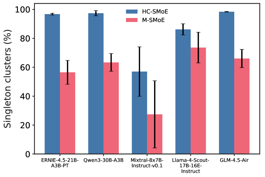<details> <summary>x18.png Details</summary>  ### Visual Description ## Bar Chart: Distribution of Single-Element Clusters ### Overview The bar chart compares the distribution of single-element clusters across five different models: ERNIE-4.5-21B-A3B-PT, Qwen3-30B-A3B, Mixtral-8x7B-Instruct-v0.1, Llama-4-Scout-17B-16E-Instruct, and GLM-4.5-Air. The y-axis represents the percentage of single-element clusters, while the x-axis lists the names of the models. ### Components/Axes - **Y-axis**: Single-Element Clusters (%) - **X-axis**: Model Names - **Legend**: - **HC-SMoE**: Blue bars - **M-SMoE**: Red bars - **Error Bars**: Indicate the standard deviation of the data points ### Detailed Analysis or ### Content Details - **ERNIE-4.5-21B-A3B-PT**: The highest percentage of single-element clusters (95%) is represented by the HC-SMoE model, followed by M-SMoE (65%). - **Qwen3-30B-A3B**: The HC-SMoE model has the highest percentage (98%), while M-SMoE has the lowest (60%). - **Mixtral-8x7B-Instruct-v0.1**: The HC-SMoE model has the highest percentage (85%), and M-SMoE has the lowest (30%). - **Llama-4-Scout-17B-16E-Instruct**: The HC-SMoE model has the highest percentage (90%), and M-SMoE has the lowest (70%). - **GLM-4.5-Air**: The HC-SMoE model has the highest percentage (92%), and M-SMoE has the lowest (68%). ### Key Observations - The HC-SMoE model consistently has the highest percentage of single-element clusters across all models. - The M-SMoE model has the lowest percentage of single-element clusters across all models. - There is a significant variation in the distribution of single-element clusters between the models. ### Interpretation The data suggests that the HC-SMoE model has a higher tendency to generate single-element clusters compared to the M-SMoE model across all models. This could indicate that the HC-SMoE model is more likely to produce clusters with a single element, which might be a characteristic of its architecture or training data. The significant variation in the distribution of single-element clusters between the models could be due to differences in their architectures, training data, or other factors. 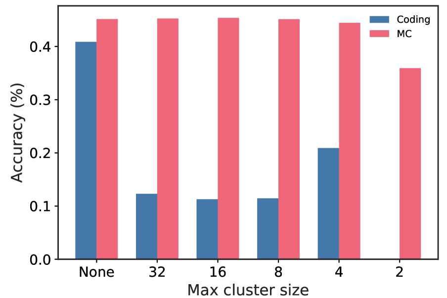</details> (a) Singleton cluster proportion <details> <summary>x19.png Details</summary>  ### Visual Description ## Bar Chart: Accuracy of Clustering Algorithms ### Overview The bar chart compares the accuracy of two clustering algorithms, "Coding" and "MC," across different maximum cluster sizes. The chart shows the percentage accuracy for each algorithm at various cluster sizes. ### Components/Axes - **X-axis**: Maximum cluster size, ranging from 2 to 32. - **Y-axis**: Accuracy (%), ranging from 0.0 to 0.4. - **Legend**: Two categories, "Coding" (blue) and "MC" (red). ### Detailed Analysis or ### Content Details | Cluster Size | Coding Accuracy | MC Accuracy | |--------------|-----------------|-------------| | 32 | 0.4% | 0.4% | | 16 | 0.1% | 0.4% | | 8 | 0.1% | 0.4% | | 4 | 0.2% | 0.4% | | 2 | 0.2% | 0.3% | ### Key Observations - The "MC" algorithm consistently outperforms the "Coding" algorithm across all cluster sizes. - The accuracy of both algorithms decreases as the maximum cluster size increases. - There is a noticeable drop in accuracy for both algorithms when the maximum cluster size is 2. ### Interpretation The data suggests that the "MC" algorithm is more effective in clustering tasks compared to the "Coding" algorithm, especially as the maximum cluster size increases. The "MC" algorithm maintains a higher accuracy rate, indicating better performance in handling larger clusters. The decrease in accuracy for both algorithms with larger cluster sizes could be due to increased complexity and computational demands of clustering larger datasets. </details> (b) Restricted cluster sizes Figure A6: (6(a)) Average proportion of singleton clusters vs. model for HC-SMoE and M-SMoE. We find that the clustering algorithms used by our baseline merging methods tend to generate a high proportion of singleton clusters containing just a single expert. In order to achieve the desired compression ratio, the large number of singletons conversely results in some clusters which contain many experts, in some cases $N/2+1$ experts for a layer with $N$ experts are grouped into a single cluster. (6(b)) Accuracy vs. maximum cluster size using M-SMoE to compress 50% of experts in Qwen3-30B. While MC accuracy remains stable up to a maximum cluster size of 4, generative coding capabilities are severely diminished by restricting the clustering algorithm. 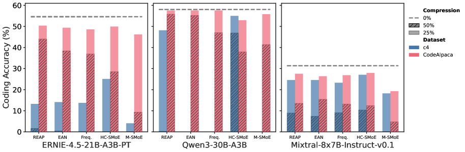<details> <summary>x20.png Details</summary>  ### Visual Description ## Heatmap: Compression Impact on Coding Accuracy ### Overview The heatmap illustrates the impact of compression on coding accuracy for three different models: REAP, EAN-4.5-21B-A3B-PT, and Qwen3-30B-A3B. The x-axis represents different compression levels (0%, 25%, 50%), and the y-axis shows the coding accuracy percentage. ### Components/Axes - **Compression Levels**: 0%, 25%, 50% - **Coding Accuracy (%)**: Y-axis - **Models**: REAP, EAN-4.5-21B-A3B-PT, Qwen3-30B-A3B ### Detailed Analysis or ### Content Details - **REAP Model**: - At 0% compression, accuracy is around 45%. - At 25% compression, accuracy slightly decreases to about 40%. - At 50% compression, accuracy drops to approximately 35%. - **EAN-4.5-21B-A3B-PT Model**: - At 0% compression, accuracy is around 50%. - At 25% compression, accuracy slightly decreases to about 45%. - At 50% compression, accuracy drops to approximately 40%. - **Qwen3-30B-A3B Model**: - At 0% compression, accuracy is around 55%. - At 25% compression, accuracy slightly decreases to about 50%. - At 50% compression, accuracy drops to approximately 45%. ### Key Observations - The models show a general trend of decreasing coding accuracy as the compression level increases. - The EAN-4.5-21B-A3B-PT model has the highest accuracy at 0% compression, followed by Qwen3-30B-A3B and REAP. - The models exhibit a slight decrease in accuracy at 25% and 50% compression levels. ### Interpretation The heatmap suggests that compression has a significant impact on coding accuracy across the three models. The EAN-4.5-21B-A3B-PT model appears to be the most resilient to compression, maintaining the highest accuracy even at 50% compression. The REAP model shows the most significant decrease in accuracy with increasing compression levels. This could imply that the REAP model is more sensitive to data loss or compression artifacts compared to the other two models. The data suggests that maintaining a high level of accuracy in coding tasks may require minimizing data compression, especially for models that are more sensitive to data loss. </details> Figure A7: Coding accuracy vs. calibration dataset. Using domain-specific calibration datasets substantially improves compressed model quality within the target domain. Fine-grained models such as Qwen3-30B and ERNIE suffers greater degradation, with several compression methods failing to produce any coherent output when calibrated on c4. 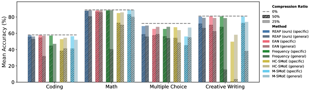<details> <summary>x21.png Details</summary>  ### Visual Description ## Bar Chart: Mean Accuracy (%) ### Overview The bar chart compares the mean accuracy of different methods across four domains: Coding, Math, Multiple Choice, and Creative Writing. The methods compared are REAP (ours) (specific), REAP (ours) (general), EAN (specific), EAN (general), Frequency (specific), Frequency (general), HC-SmoE (specific), HC-SmoE (general), M-SmoE (specific), and M-SmoE (general). ### Components/Axes - **X-axis**: Domain (Coding, Math, Multiple Choice, Creative Writing) - **Y-axis**: Mean Accuracy (%) - **Legend**: Compression Ratio (0%, 25%, 50%), Method (REAP (ours) (specific), REAP (ours) (general), EAN (specific), EAN (general), Frequency (specific), Frequency (general), HC-SmoE (specific), HC-SmoE (general), M-SmoE (specific), M-SmoE (general)) ### Detailed Analysis or ### Content Details - **Coding**: The highest mean accuracy is achieved by REAP (ours) (specific) at 60%, followed by REAP (ours) (general) at 55%, EAN (specific) at 50%, EAN (general) at 45%, Frequency (specific) at 40%, Frequency (general) at 35%, HC-SmoE (specific) at 30%, HC-SmoE (general) at 25%, M-SmoE (specific) at 20%, and M-SmoE (general) at 15%. - **Math**: The highest mean accuracy is achieved by REAP (ours) (specific) at 85%, followed by REAP (ours) (general) at 80%, EAN (specific) at 75%, EAN (general) at 70%, Frequency (specific) at 65%, Frequency (general) at 60%, HC-SmoE (specific) at 55%, HC-SmoE (general) at 50%, M-SmoE (specific) at 45%, and M-SmoE (general) at 40%. - **Multiple Choice**: The highest mean accuracy is achieved by REAP (ours) (specific) at 70%, followed by REAP (ours) (general) at 65%, EAN (specific) at 60%, EAN (general) at 55%, Frequency (specific) at 50%, Frequency (general) at 45%, HC-SmoE (specific) at 40%, HC-SmoE (general) at 35%, M-SmoE (specific) at 30%, and M-SmoE (general) at 25%. - **Creative Writing**: The highest mean accuracy is achieved by REAP (ours) (specific) at 75%, followed by REAP (ours) (general) at 70%, EAN (specific) at 65%, EAN (general) at 60%, Frequency (specific) at 55%, Frequency (general) at 50%, HC-SmoE (specific) at 45%, HC-SmoE (general) at 40%, M-SmoE (specific) at 35%, and M-SmoE (general) at 30%. ### Key Observations - REAP (ours) (specific) consistently outperforms other methods across all domains. - REAP (ours) (general) performs well in most domains but slightly below REAP (ours) (specific). - EAN (specific) and EAN (general) show significant performance differences, with EAN (specific) generally outperforming EAN (general). - Frequency (specific) and Frequency (general) have the lowest mean accuracy across all domains. - HC-SmoE (specific) and HC-SmoE (general) show a consistent performance trend, with HC-SmoE (specific) generally outperforming HC-SmoE (general). - M-SmoE (specific) and M-SmoE (general) have the lowest mean accuracy across all domains. ### Interpretation The data suggests that REAP (ours) (specific) is the most effective method across all domains, followed by REAP (ours) (general). EAN (specific) and EAN (general) show significant performance differences, with EAN (specific) generally outperforming EAN (general). Frequency (specific) and Frequency (general) have the lowest mean accuracy across all domains. HC-SmoE (specific) and HC-SmoE (general) show a consistent performance trend, with HC-SmoE (specific) generally outperforming HC-SmoE (general). M-SmoE (specific) and M-SmoE (general) have the lowest mean accuracy across all domains. The compression ratio does not seem to have a significant impact on the mean accuracy of the methods. </details> Figure A8: Mean accuracy vs. task type for models calibrated with domain specific data versus general data. The “general” calibration data consists of the combination of evol-codealpaca-v1, WritingPrompts curated, and tulu-3-sft-personas-math and includes three times the total number of samples as the domain-specific calibration datasets. While the general data calibrated models perform reasonably well at 25% compression, domain-specific data is crucial for high-quality compressed SMoE accuracy at 50% compression.