2510.14538

# Symbol Grounding in Neuro-Symbolic AI: A Gentle Introduction to Reasoning Shortcuts **Authors**: - Emanuele Marconato (University of Trento) - &Samuele Bortolotti (University of Trento) - &Emile van Krieken - Vrije Universiteit Amsterdam - The Netherlands - Paolo Morettin (University of Trento) - &Elena Umili (Sapienza University of Rome) - &Antonio Vergari (University of Edinburgh) - United Kingdom - Efthymia Tsamoura (Huawei Labs) - Cambridge United Kingdom - &Andrea Passerini (University of Trento) - &Stefano Teso (University of Trento) > ∗Corresponding author.†\daggerEqual contribution.‡\ddaggerWork started before Efthymia Tsamoura joined Huawei Labs. Abstract Neuro-symbolic (NeSy) AI aims to develop deep neural networks whose predictions comply with prior knowledge encoding, e.g., safety or structural constraints. As such, it represents one of the most promising avenues for reliable and trustworthy AI. The core idea behind NeSy AI is to combine neural and symbolic steps: neural networks are typically responsible for mapping low-level inputs into high-level symbolic concepts, while symbolic reasoning infers predictions compatible with the extracted concepts and the prior knowledge. Despite their promise, it was recently shown that – whenever the concepts are not supervised directly – NeSy models can be affected by Reasoning Shortcuts (RSs). That is, they can achieve high label accuracy by grounding the concepts incorrectly. RSs can compromise the interpretability of the model’s explanations, performance in out-of-distribution scenarios, and therefore reliability. At the same time, RSs are difficult to detect and prevent unless concept supervision is available, which is typically not the case. However, the literature on RSs is scattered, making it difficult for researchers and practitioners to understand and tackle this challenging problem. This overview addresses this issue by providing a gentle introduction to RSs, discussing their causes and consequences in intuitive terms. It also reviews and elucidates existing theoretical characterizations of this phenomenon. Finally, it details methods for dealing with RSs, including mitigation and awareness strategies, and maps their benefits and limitations. By reformulating advanced material in a digestible form, this overview aims to provide a unifying perspective on RSs to lower the bar to entry for tackling them. Ultimately, we hope this overview contributes to the development of reliable NeSy and trustworthy AI models. Contents 1. 1 Introduction 1. 2 Preliminaries 1. 2.1 From Neuro-Symbolic AI to Neuro-Symbolic Predictors 1. 2.2 The Variety of NeSy Predictor Architectures 1. 2.3 NeSy Predictor Architectures: Differences and Similarities 1. 2.4 NeSy Predictors: Benefits 1. 3 A Gentle Introduction to Reasoning Shortcuts 1. 3.1 Causes, Frequency and Impact 1. 4 Theory of Reasoning Shortcuts 1. 4.1 Setting and Assumptions 1. 4.2 Perspective: Identification 1. 4.2.1 Model class of NeSy predictors 1. 4.2.2 Non-identifiability of the concept extractor 1. 4.2.3 Concept remapping distributions. 1. 4.2.4 Reasoning shortcuts as unintended, optimal concept remapping distributions 1. 4.2.5 Characterization of deterministic reasoning shortcuts. 1. 4.3 Perspective: Statistical Learning 1. 4.3.1 Knowledge complexity 1. 4.3.2 Impossibility result in bounding the reasoning shortcut risk 1. 4.3.3 Setting 1. 4.3.4 PAC learnability with $k$ -unambiguous inference layers 1. 4.4 Relationship between Theories 1. 5 Handling Reasoning Shortcuts 1. 5.1 Root Causes 1. 5.1.1 The knowledge 1. 5.1.2 The training distribution 1. 5.1.3 The optimality condition 1. 5.1.4 The family of learnable maps 1. 5.2 How to Diagnose Reasoning Shortcuts 1. 5.2.1 Task-level diagnosis 1. 5.2.2 Model metrics 1. 5.3 A Tour of Mitigation Strategies 1. 5.3.1 Concept supervision 1. 5.3.2 Multi-task learning 1. 5.3.3 Abductive weak supervision 1. 5.3.4 Entropy maximization 1. 5.3.5 Smoothing 1. 5.3.6 Reconstruction 1. 5.3.7 Contrastive learning 1. 5.3.8 Architectural disentanglement 1. 5.3.9 Which mitigation strategy is best? 1. 5.3.10 Can one simply recover learned concepts? 1. 5.4 Awareness Strategies 1. 5.4.1 RS-awareness as mixtures of deterministic RSs 1. 5.4.2 Building RS-aware NeSy predictors 1. 5.4.3 RS-Awareness via Ensembles 1. 5.4.4 RS-Awareness via Diffusion 1. 5.5 Awareness Helps Mitigation 1. 6 Extensions and Open Problems 1. 6.1 Reasoning Shortcuts in NeSy AI Beyond Predictors 1. 6.2 Reasoning Shortcuts in Concept-based Models 1. 6.3 Foundation and Large Language Models 1. 6.4 Reasoning Shortcuts in Reinforcement Learning 1. 6.5 Imbalanced Learning 1. 6.6 Additional open problems 1. 7 Related Work 1. 8 Conclusion 1 Introduction In cognitive science and psychology, symbols —or more generally, concepts —are the compositional building blocks of human thought (Mandler, 2004; Spelke and Kinzler, 2007). They enable the abstraction and structuring of perception, supporting high-level cognitive functions (Whitehead, 1927; Johnson-Laird, 1994) such as language, reasoning, and planning. In recent years, there has been growing interest in using concepts in neural networks (Smolensky, 1987; Sun, 1992; Greff et al., 2020), which bring not only improved generalization but also greater interpretability to their decision-making processes. While the emergence of abstract concepts in the human brain is well-documented (Mandler, 2004), how—and even whether—such entities arise in neural networks remains fundamentally unclear (Jo and Bengio, 2017; Lake and Baroni, 2018; Park et al., 2024). Neuro-symbolic (NeSy) models aim to bridge this gap by integrating neural learning with symbolic reasoning (Harnad, 1990; McMillan et al., 1991; Sun, 1992), thereby enabling explicit manipulation of concepts within the inference process. Some approaches embed prior symbolic structure—such as logical rules (De Raedt et al., 2021) —while others attempt to learn such structure through specialized, trainable components (Lake and Baroni, 2018; Ellis et al., 2021). A key promise of this integration is reliability and trustworthiness: by making all decisions traceable to interpretable, well-defined concepts, decisions become more transparent (Kambhampati et al., 2022). Moreover, thanks to the modularity of symbolic components, learned concepts can be reused in novel scenarios without significant performance degradation. Yet, the effectiveness of this integration hinges on solving a core challenge in NeSy AI: the problem of symbol grounding (Harnad, 1990) —that is, how to connect low-level perceptual data with high-level, abstract concepts. 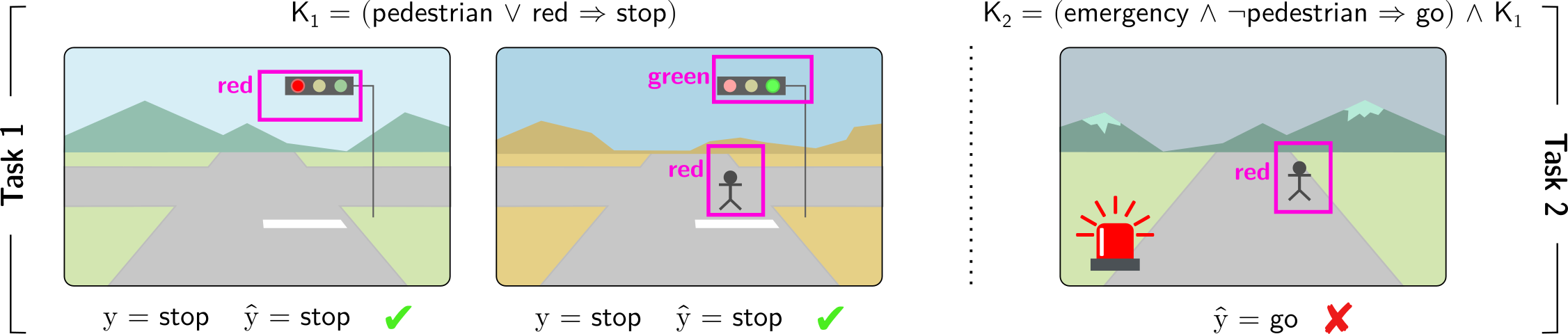**Example 1.1** *Consider a model trained on autonomous driving scenarios, where the car must decide whether to stop or go based on the visual input, as per Fig. 1. The model leverages prior knowledge $\mathsf{K}_{1}$ which imposes that whenever pedestrian or red_light are detected, the car must stop. Attaining accurate action predictions requires assigning valid binary values to the concepts pedestrian and red_light (among others) from the visual input. Therefore, concepts are grounded by the model through learning to give correct driving predictions. Because pedestrian and red_light are treated symmetrically by the knowledge (due to the disjunction) We will precisely define the symmetries of the knowledge in later sections. the self-driving car may confuse the two while still achieving correct predictions (e.g., in Fig. 1 (Left), red_light fires when either “pedestrians” or “red lights” are detected). This example shows that model concepts can be grounded differently from their intended meaning: training the autonomous car to give correct predictions does not guarantee that concepts activate when they should; e.g., the autonomous car’s red_light may not solely contain information about the presence of “red lights” in the raw sensory data.* Footnote 1 illustrates the central challenge of symbol grounding in Neuro-Symbolic AI: ensuring that abstract predicted concepts inside the model maintain a consistent and semantically correct link to the real-world entities they are meant to represent. Unfortunately, in many learning contexts NeSy models— even when they perform nearly optimally on a task—may fail to assign the right meaning to learned concepts, leading to concepts with unintended semantics (Marconato et al., 2023a, b). This issue originates from reasoning shortcuts (RSs): unwanted concept assignments that allow models to reach correct label predictions. These have been shown to affect many NeSy models (Marconato et al., 2023b; Yang et al., 2024). While the decision-making appears correct on the surface, the underlying concepts are flawed, undermining the reliability and trustworthiness of the NeSy model. This directly impacts the model’s interpretability, as well as generalization when concepts are reused in out-of-distribution scenarios and continual learning. For example, in the context of autonomous driving of Footnote 1 and of Fig. 1, the correct “ stop ” prediction can be achieved by mistaking “ pedestrians ” with “ red lights ”, as both concepts induce the same decision. While this misalignment does not induce a drop in prediction on data in-distribution, it becomes critical in situations where such distinctions matter. In fact, poorly grounded concepts do not transfer to out-of-distribution scenarios, as displayed in Fig. 1 (Right), where the wrong activation of model concepts leads to a faulty prediction. RSs were observed in early NeSy work (Manhaeve et al., 2018; Chang et al., 2020; Topan et al., 2021), but only recently received a formal treatment, revealing that RSs are hard to tackle (Marconato et al., 2023b; Umili et al., 2024a; Yang et al., 2024; DeLong et al., 2024), despite arising naturally from certain symmetries in the symbolic component of NeSy systems. In turn, theoretical studies (Marconato et al., 2023b; Wang et al., 2023; Yang et al., 2024; Bortolotti et al., 2025) have begun to identify under which conditions RSs can be provably avoided. This often requires pairing standard NeSy training methods with mitigation strategies that encourage better concept grounding. However, designing effective mitigation strategies that do not require a significant annotation cost remains an open problem. In this paper, we aim to consolidate the scattered literature on RSs in NeSy AI and offer a comprehensive overview of different approaches to mitigating them. Contributions This article provides a gentle introduction to reasoning shortcuts, unifies the existing literature on the topic, and connects it to the well-known symbol grounding problem. We provide a general perspective on RSs, highlighting that they cannot be avoided simply by designing different neuro-symbolic architectures. To this end, we compile all relevant theory on RSs through the perspectives of identifiability and statistical learning. We then present known mitigation strategies to prevent RSs using a taxonomy, and explain which strategies can effectively reduce the likelihood of RSs. Finally, we identify open problems and future directions, showing that RSs — and thus correct symbol grounding — extend beyond the NeSy models studied so far. <details> <summary>figures/nesy-road-kill.png Details</summary>  ### Visual Description ## Logical Reasoning with Visual Scenes ### Overview The image presents a series of visual scenes depicting traffic scenarios, each associated with a logical rule and a predicted outcome. The scenes are divided into two tasks, each involving a different set of conditions and rules. The image evaluates the correctness of the predicted outcomes based on the given rules and visual inputs. ### Components/Axes * **Task 1**: Labeled vertically on the left side of the first two images. * **Task 2**: Labeled vertically on the right side of the third image. * **Visual Scenes**: Three distinct scenes depicting roads, traffic lights, pedestrians, and emergency vehicles. * **Logical Rules**: * K1 = (pedestrian ∨ red → stop) * K2 = (emergency ∧ ¬pedestrian → go) ∧ K1 * **Object Detection**: Magenta bounding boxes around traffic lights and pedestrians, with labels indicating the color of the traffic light (red or green) or the presence of a pedestrian (red). * **Predicted Outcomes**: "y = stop", "ŷ = stop", "ŷ = go" * **Correctness Indicators**: Green checkmark for correct predictions, red "X" for incorrect predictions. ### Detailed Analysis **Scene 1 (Task 1)** * **Visual Elements**: A road scene with a traffic light showing red. The background includes mountains and a sky. * **Object Detection**: A magenta box surrounds the traffic light, labeled "red". * **Logical Rule**: K1 = (pedestrian ∨ red → stop) * **Predicted Outcome**: y = stop, ŷ = stop * **Correctness**: Green checkmark, indicating the prediction is correct. **Scene 2 (Task 1)** * **Visual Elements**: A road scene with a traffic light showing green and a pedestrian crossing. The background includes mountains and a sky. * **Object Detection**: A magenta box surrounds the traffic light, labeled "green". Another magenta box surrounds the pedestrian, labeled "red". * **Logical Rule**: K1 = (pedestrian ∨ red → stop) * **Predicted Outcome**: y = stop, ŷ = stop * **Correctness**: Green checkmark, indicating the prediction is correct. **Scene 3 (Task 2)** * **Visual Elements**: A road scene with a pedestrian crossing and an emergency vehicle with flashing red lights. The background includes mountains and a sky. * **Object Detection**: A magenta box surrounds the pedestrian, labeled "red". The emergency vehicle is also visible. * **Logical Rule**: K2 = (emergency ∧ ¬pedestrian → go) ∧ K1 * **Predicted Outcome**: ŷ = go * **Correctness**: Red "X", indicating the prediction is incorrect. ### Key Observations * Task 1 focuses on the basic rule of stopping at a red light or when a pedestrian is present. * Task 2 introduces an additional rule involving emergency vehicles and the absence of pedestrians. * The third scene highlights a potential conflict between the two rules, where the presence of an emergency vehicle might suggest "go," but the presence of a pedestrian should override this and require a "stop." ### Interpretation The image demonstrates a system for evaluating logical reasoning in visual scenes. The system uses object detection to identify relevant elements (traffic lights, pedestrians, emergency vehicles), applies logical rules to these elements, and predicts an outcome (stop or go). The correctness of the prediction is then assessed. The incorrect prediction in the third scene suggests a limitation in the system's ability to resolve conflicts between different rules or to prioritize rules based on context. Specifically, the system incorrectly predicts "go" when an emergency vehicle is present, even though a pedestrian is also present, which should trigger the "stop" rule. This highlights the need for more sophisticated reasoning mechanisms that can handle complex scenarios and prioritize rules appropriately. </details> Figure 1: Reasoning shortcuts are failures of correct symbol grounding. Consider an autonomous driving car that must drive in compliance with traffic rules. (Left) The car learns to make correct predictions by leveraging background knowledge $\mathsf{K}_{1}$ in Task $1$ , i.e., “if there is a pedestrian or a red light the car has to stop”. However, in the process, it may incorrectly associate the concept of red_light with the presence of either pedestrians or red lights in the dashcam, resulting in what is known as a reasoning shortcut. (Right) Consequently, the learned concepts can lead to incorrect (and potentially catastrophic) predictions when the background knowledge changes. For example, $\mathsf{K}_{2}$ in Task $2$ introduces an exception in the presence of an emergency situation, i.e., “if there is an emergency and no pedestrians are on the street, the car may proceed”. Outline The remainder of the article is organized as follows. Section 2 introduces the preliminaries necessary for understanding the theoretical material. Section 3 presents the problem of reasoning shortcuts at a high level, providing examples and discussing their causes and impacts. Section 4 delves into the details by introducing the mathematical tools required to analyze reasoning shortcuts, exploring the issue from two perspectives: identification and statistical learning. Section 5 adopts a more applied perspective by examining the root causes of RSs, together with practical strategies for diagnosing their presence and for mitigating or addressing their effects, and discusses the benefits of each strategy. Section 6 explores various extensions of the reasoning shortcut problem across different domains and discusses open problems and future directions. Finally, Section 7 reviews relevant related research, and Section 8 provides concluding remarks. 2 Preliminaries Table 1: Glossary of used symbols. | $x$ , $y$ , $z$ , $X$ , $Y$ , $Z$ ${\bm{\mathrm{x}}}$ , ${\bm{\mathrm{X}}}$ | Scalar constants Scalar variables Vectors | | --- | --- | | $\mathcal{X},\mathcal{Y},\mathcal{C}$ | Sets | | $f({\bm{\mathrm{x}}})$ , $p({\bm{\mathrm{c}}}\mid{\bm{\mathrm{x}}})$ | Concept extractor | | $\beta({\bm{\mathrm{c}}})$ , $p({\bm{\mathrm{y}}}\mid{\bm{\mathrm{c}}};\mathsf{K})$ | Inference layer | | $\models$ | Logical entailment | | $\mathsf{K}$ | Prior knowledge | | $\theta$ | Network parameters | | $\mathcal{D}$ | Dataset | Notation. Throughout, we denote scalar constants by lowercase letters $x$ , scalar (random) variables by uppercase letters $X$ , vectors of constants ${\bm{\mathrm{x}}}$ and (random) variables ${\bm{\mathrm{X}}}$ in bold typeface, and sets (e.g., $\mathcal{X}$ ) by calligraphic letters. If $\varphi$ is a logical formula over variables ${\bm{\mathrm{X}}}$ , we say that the constants ${\bm{\mathrm{x}}}$ entail the formula $\varphi$ ( ${\bm{\mathrm{x}}}\models\varphi$ ) if and only if replacing the variables ${\bm{\mathrm{X}}}$ in the formula $\varphi$ with ${\bm{\mathrm{x}}}$ makes the formula true. In this case, we say that ${\bm{\mathrm{x}}}$ satisfies or is consistent with the formula; otherwise, it violates or is inconsistent with the formula. See Table 1 for a glossary. 2.1 From Neuro-Symbolic AI to Neuro-Symbolic Predictors Neuro-symbolic models aim to solve the long-standing problem of integrating learning and reasoning. Over time, many radically different NeSy architectures have emerged (Garcez et al., 2022; De Raedt et al., 2021; Feldstein et al., 2024) that differ not only in what kind of logic they implement reasoning with (e.g., propositional (Hoernle et al., 2022; Ahmed et al., 2022; Buffelli and Tsamoura, 2023) vs. first-order (Lippi and Frasconi, 2009; Diligenti et al., 2012; Manhaeve et al., 2018) and classical (Zhou, 2019) vs. fuzzy (Donadello et al., 2017; van Krieken et al., 2020) vs. probabilistic (Manhaeve et al., 2018; Ahmed et al., 2022; Feldstein et al., 2023)), but also in how they interpret logic reasoning itself (e.g., model vs. proof-based inference (De Raedt et al., 2021)) and in how they implement the computations (e.g., fully neural (Rocktäschel and Riedel, 2016) vs. hybrid neural-symbolic (Manhaeve et al., 2018)). This variety is reflected by the diversity of tasks that NeSy architectures can tackle, which range from hierarchical classification (Giunchiglia and Lukasiewicz, 2020; Hoernle et al., 2022; Ahmed et al., 2022) and knowledge base completion (Rocktäschel and Riedel, 2016), to open-ended reasoning (Manhaeve et al., 2018; Badreddine et al., 2022) and learning knowledge graph embeddings (Maene and Tsamoura, 2025). Reasoning shortcuts have been studied mainly in the context of NeSy predictors, a class of NeSy architectures specialized for constrained prediction tasks (Giunchiglia et al., 2022; Dash et al., 2022; Marconato et al., 2023a), denoted here as NeSy tasks; a discussion of RS in other NeSy architectures is left to Section 6.1. A NeSy task requires predicting labels that are consistent with known constraints. Each such task is defined by four elements: a description of the input ${\bm{\mathrm{X}}}$ with domain $\mathcal{X}$ , a description of the $k$ concepts ${\bm{\mathrm{C}}}=(C_{1},...,C_{k})$ with domain $\mathcal{C}=\mathcal{C}_{1}×...×\mathcal{C}_{k}$ , a description of $m$ discrete labels ${\bm{\mathrm{Y}}}=(Y_{1},...,Y_{m})$ with domain $\mathcal{Y}=\mathcal{Y}_{1}×...×\mathcal{Y}_{m}$ , and prior knowledge $\mathsf{K}$ . Here, $\mathcal{X}$ is the input domain (e.g., a vector space), $\mathcal{C}$ is a finite set of concept vectors ${\bm{\mathrm{c}}}$ , and so are the label sets $\mathcal{Y}_{i}$ . The input ${\bm{\mathrm{X}}}$ is usually high-dimensional and sub-symbolic (e.g., an image), while the concepts ${\bm{\mathrm{C}}}$ are high-level and possibly human readable properties of the input (e.g., the objects appearing in the image). The prior knowledge $\mathsf{K}$ encodes the constraints that we wish the model to satisfy— e.g., safety constraints or relevant regulations—as a single propositional logical formula. Although some NeSy predictor architectures support first-order logical formulas, we restrict our description to propositional formulas, for ease of exposition. We postpone a discussion of how RSs transfer to the first-order case to Section 6.1. Both the concepts ${\bm{\mathrm{C}}}$ and the labels ${\bm{\mathrm{Y}}}$ appear as logic variables in $\mathsf{K}$ . We ground these notions using a running example: **Example 2.1** *Consider the simplified BDD-OIA autonomous driving task (Xu et al., 2020). Here, the inputs ${\bm{\mathrm{x}}}$ are dashcam images and the (binary) label $y$ indicates whether the vehicle is allowed to proceed. The task involves three binary concepts $C_{\texttt{grn}}$ , $C_{\texttt{red}}$ , $C_{\texttt{ped}}$ encoding the presence of green lights, red lights, and pedestrians in the input image, respectively, and the prior knowledge $\mathsf{K}$ encodes the constraint that if either a pedestrian or a red light is visible in the image, the vehicle must stop: $\mathsf{K}=(C_{\texttt{ped}}\lor C_{\texttt{red}}\Leftrightarrow\lnot Y)$ . In this scenario, a NeSy predictor has to predict vehicle actions that are both accurate and comply with traffic regulations.* Given a (noiseless) training set $\mathcal{D}=\{({\bm{\mathrm{x}}},{\bm{\mathrm{y}}})\}$ , a NeSy predictor is tasked with learning a mapping from inputs ${\bm{\mathrm{x}}}$ to labels ${\bm{\mathrm{y}}}$ that comply with the knowledge, that is, $({\bm{\mathrm{c}}},{\bm{\mathrm{y}}})\models\mathsf{K}$ . Here, $({\bm{\mathrm{c}}},{\bm{\mathrm{y}}})$ is to be read as the concatenation of ${\bm{\mathrm{c}}}$ and ${\bm{\mathrm{y}}}$ . The key challenge is that, just like in Example 2.1, the prior knowledge $\mathsf{K}$ is not specified at the input level, but rather over the concepts. These, in turn, are complex functions of the input that, in practice, cannot be manually specified. For this reason, NeSy predictors adopt modular architectures that comprise a learnable concept extractor responsible for predicting the concepts ${\bm{\mathrm{C}}}$ from the inputs ${\bm{\mathrm{X}}}$ , and an inference layer responsible for inferring the labels ${\bm{\mathrm{Y}}}$ from ${\bm{\mathrm{C}}}$ compatibly with the prior knowledge $\mathsf{K}$ . The former is typically implemented as a feed-forward neural network, Although other architectures can be used (Diligenti et al., 2012). and the latter using some form of (differentiable) symbolic reasoning. Given an input ${\bm{\mathrm{x}}}$ , a NeSy predictor first applies the concept extractor to obtain a distribution $p({\bm{\mathrm{C}}}\mid{\bm{\mathrm{x}}})$ over concepts, and then applies the inference layer to obtain a distribution $p({\bm{\mathrm{Y}}}\mid{\bm{\mathrm{C}}};\mathsf{K})$ over outputs ${\bm{\mathrm{y}}}$ , given the concepts. Overall, the predictor defines a predictive distribution $p({\bm{\mathrm{Y}}}\mid{\bm{\mathrm{X}}};\mathsf{K})$ (see Section 2.2 for details). **Example 2.2** *Consider the BDD-OIA (Xu et al., 2020) dataset illustrated in Example 2.1. Here, the input ${\bm{\mathrm{x}}}∈\mathcal{X}$ is a dashcam image. The concept extractor is a neural network that takes ${\bm{\mathrm{x}}}$ and predicts the probabilities of three binary concepts $(C_{\texttt{grn}},C_{\texttt{red}},C_{\texttt{ped}})$ . For example, given an image ${\bm{\mathrm{x}}}$ , the extractor may output $p(C_{\texttt{red}}=1\mid{\bm{\mathrm{x}}})=0.9,\quad p(C_{\texttt{ped}}=1\mid{\bm{\mathrm{x}}})=0.2,\quad p(C_{\texttt{grn}}=1\mid{\bm{\mathrm{x}}})=0.1$ . These concept predictions are then passed to an inference layer, which combines them with prior knowledge $\mathsf{K}=(C_{\texttt{ped}}\lor C_{\texttt{red}})\Leftrightarrow\texttt{stop}$ to obtain the final decision $y$ . Depending on the chosen implementation, this reasoning step may enforce the rule strictly, approximate it through fuzzy logic, or learn it implicitly during training. In this example, since the concept extractor assigns high probability to $C_{\texttt{red}}=1$ , the system will likely infer $Y=\texttt{stop}$ , indicating that the vehicle should stop.* In most cases, NeSy predictors can be, and in fact are, trained using label supervision only. This is not surprising if we consider that per-concept annotations can be expensive to collect in practice. However – and this is critical for our discussion of RSs – this also means that the concepts themselves are often not supervised, and that therefore they act as latent variables. 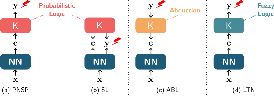2.2 The Variety of NeSy Predictor Architectures Different NeSy predictor architectures differ in how they implement and use the concept extractor and the reasoning layer. Next, we introduce the four architectures that have been most extensively studied in the RS literature, namely probabilistic NeSy predictors, the Semantic Loss, Logic Tensor Networks, and Abductive Learning. These are illustrated in Fig. 2. <details> <summary>x1.png Details</summary>  ### Visual Description ## Diagram: Neural-Symbolic Architectures ### Overview The image presents a comparative diagram illustrating four different neural-symbolic architectures: PNSP, SL, ABL, and LTN. Each architecture combines a neural network (NN) with a symbolic component (K) and depicts the flow of information between them. The diagrams highlight the type of logic associated with each architecture, such as Probabilistic Logic, Abduction, and Fuzzy Logic. ### Components/Axes * **NN:** Represents the Neural Network component, depicted as a rounded rectangle. Input is 'x', output is 'c'. * **K:** Represents the symbolic knowledge component, depicted as a rounded rectangle. * **x:** Input to the Neural Network. * **c:** Output from the Neural Network, input to the symbolic component K. * **y:** Output from the symbolic component K. * **Arrows:** Indicate the direction of information flow. * **Dotted Lines:** Connect the symbolic component K to the type of logic it represents. * **Lightning Bolt:** Indicates a point of potential error or uncertainty. * **(a) PNSP:** Probabilistic Neural-Symbolic Program. * **(b) SL:** Semantic Loss. * **(c) ABL:** Abductive Learning. * **(d) LTN:** Logic Tensor Networks. ### Detailed Analysis **Diagram (a) PNSP:** * **NN:** Located at the bottom, receives input 'x' and outputs 'c'. * **K:** Located above the NN, receives input 'c' and outputs 'y'. K is colored red. * **Logic:** "Probabilistic Logic" is associated with K via a dotted line. The text "Probabilistic Logic" is colored red. * **Flow:** Information flows from NN to K. * **Error:** A red lightning bolt is present near the output 'y' of K, indicating a potential error. **Diagram (b) SL:** * **NN:** Located at the bottom, receives input 'x' and outputs 'c' and 'y'. * **K:** Located above the NN, receives input 'c' and 'y'. K is colored red. * **Flow:** Information flows from NN to K. * **Error:** A red lightning bolt is present near the output 'y' of the NN, indicating a potential error. **Diagram (c) ABL:** * **NN:** Located at the bottom, receives input 'x' and outputs 'c'. * **K:** Located above the NN, receives input 'c' and outputs 'y'. K is colored orange. * **Logic:** "Abduction" is associated with K via a dotted line. The text "Abduction" is colored orange. * **Flow:** Information flows from NN to K. **Diagram (d) LTN:** * **NN:** Located at the bottom, receives input 'x' and outputs 'c'. * **K:** Located above the NN, receives input 'c' and outputs 'y'. K is colored teal. * **Logic:** "Fuzzy Logic" is associated with K via a dotted line. The text "Fuzzy Logic" is colored teal. * **Flow:** Information flows from NN to K. ### Key Observations * All four architectures share a common structure: an NN feeding into a symbolic component K. * The architectures differ in the type of logic associated with K and the flow of information between NN and K. * PNSP and SL diagrams include a lightning bolt symbol, suggesting potential errors or uncertainties in these architectures. * The color of the K component and the associated logic text are consistent within each diagram. ### Interpretation The diagram illustrates different approaches to integrating neural networks with symbolic reasoning. Each architecture leverages a specific type of logic (Probabilistic, Abductive, Fuzzy) to enhance the capabilities of the neural network. The presence of error indicators in PNSP and SL suggests potential challenges or limitations in these specific approaches. The diagram provides a high-level overview of the design and information flow in these neural-symbolic systems, highlighting the diversity of approaches in this field. </details> Figure 2: Schematic illustration of NeSy predictors. All of them employ a neural network for extracting concepts and prior knowledge $\mathsf{K}$ . PNSPs (a) map inputs ${\bm{\mathrm{x}}}$ to (a distribution over) concepts ${\bm{\mathrm{c}}}$ and then uses probabilistic logic to infer labels ${\bm{\mathrm{y}}}$ consistent with $\mathsf{K}$ . The SL (b) maps inputs to both concepts ${\bm{\mathrm{c}}}$ and labels ${\bm{\mathrm{y}}}$ and uses $\mathsf{K}$ to define a loss term penalizing inconsistent predictions. During training, ABL (c) abduces concepts from the ground-truth label ${\bm{\mathrm{y}}}$ using $\mathsf{K}$ and uses them as pseudo-labels to train the concept extractor. LTN (d) works similarly to PNSPs but uses fuzzy logic to make $\mathsf{K}$ differentiable. Lightning strikes indicate supervision. Probabilistic NeSy Predictors A common method for designing NeSy architectures is the family of Probabilistic NeSy Predictors (PNSPs) (Manhaeve et al., 2018, 2021a; Yang et al., 2020; Huang et al., 2021a). PNSPs can be viewed as combining a neural concept extractor with a probabilistic-logic reasoning layer (De Raedt and Kimmig, 2015), as shown in Fig. 2 (a). Perhaps the best-known member of this family is DeepProbLog (DPL) (Manhaeve et al., 2018, 2021a), a fully-fledged neuro-symbolic programming language based on Prolog and its probabilistic extension, ProbLog (De Raedt et al., 2007; Kimmig et al., 2011). From a simplified point of view, PNSPs define the following predictive distribution for any ${\bm{\mathrm{x}}}$ and ${\bm{\mathrm{y}}}$ : $$ p({\bm{\mathrm{y}}}\mid{\bm{\mathrm{x}}};\mathsf{K})=\sum_{{\bm{\mathrm{c}}}}p({\bm{\mathrm{y}}},{\bm{\mathrm{c}}}\mid{\bm{\mathrm{x}}};\mathsf{K})=\sum_{{\bm{\mathrm{c}}}}p({\bm{\mathrm{y}}}\mid{\bm{\mathrm{c}}};\mathsf{K})\,p({\bm{\mathrm{c}}}\mid{\bm{\mathrm{x}}})=\frac{1}{Z_{{\bm{\mathrm{x}}}}}\sum_{{\bm{\mathrm{c}}}}\text{1}\!\left\{({\bm{\mathrm{c}}},{\bm{\mathrm{y}}})\models\mathsf{K}\right\}\,p({\bm{\mathrm{c}}}\mid{\bm{\mathrm{x}}}) \tag{1} $$ Here, $p({\bm{\mathrm{C}}}\mid{\bm{\mathrm{x}}})$ is the predictive distribution over concepts computed by the concept extractor, $\text{1}\!\left\{·\right\}$ is the indicator function, and $Z_{{\bm{\mathrm{x}}}}$ is a normalization constant ensuring that the result is indeed a conditional distribution. In words, the probability of a label ${\bm{\mathrm{y}}}$ is the sum of the probabilities of all concept vectors ${\bm{\mathrm{c}}}$ that are consistent with that label ${\bm{\mathrm{y}}}$ according to the knowledge $\mathsf{K}$ . Inference in PNSPs amounts to computing a most likely label, which usually requires solving the MAP problem $\operatorname*{argmax}_{{\bm{\mathrm{y}}}}\ p({\bm{\mathrm{y}}}\mid{\bm{\mathrm{x}}};\mathsf{K})$ (Koller and Friedman, 2009). Importantly, if a label ${\bm{\mathrm{y}}}$ , together with the predicted concepts, would violate the knowledge $\mathsf{K}$ , then its probability is exactly zero and it will not be predicted. Learning in PNSPs is implemented via maximum likelihood estimation. That is, given a training set $\mathcal{D}=\{({\bm{\mathrm{x}}},{\bm{\mathrm{y}}})\}$ , learning amounts to maximizing the log-likelihood of the data, namely $$ \mathcal{L}(p,\mathcal{D},\mathsf{K})=\frac{1}{|\mathcal{D}|}\sum_{({\bm{\mathrm{x}}},{\bm{\mathrm{y}}})\in\mathcal{D}}\ \log{p({\bm{\mathrm{y}}}\mid{\bm{\mathrm{x}}};\mathsf{K})}. \tag{2} $$ by tuning the parameters of the concept extractor. In practice, this is done via gradient descent, as the predictive distribution $p({\bm{\mathrm{y}}}\mid{\bm{\mathrm{x}}};\mathsf{K})$ is differentiable (Manhaeve et al., 2018). PNSPs require evaluating the predictive probability $p({\bm{\mathrm{y}}}\mid{\bm{\mathrm{x}}};\mathsf{K})$ , which involves summing over a potentially exponential number (in the cardinality of the concept vector $k$ ) of vectors ${\bm{\mathrm{c}}}$ , as per Eq. 1. Hence, both inference and learning are worst-case intractable. DPL works around this issue by exploiting knowledge compilation techniques (Darwiche and Marquis, 2002) that leverage symmetries in the summation to rewrite it into a data structure – a probabilistic circuit (Choi et al., 2020; Vergari et al., 2021; Maene et al., 2025; Derkinderen et al., 2025a) – that is potentially much more compact and supports efficient evaluation. This allows DPL to scale to practical NeSy tasks. Other PNSPs refine and approximate these ideas (specifically, Eq. 1) to further improve scalability (Manhaeve et al., 2021b; Huang et al., 2021a; Winters et al., 2022; De Smet et al., 2023a; van Krieken et al., 2023; Choi et al., 2025; Chen et al., 2025). Semantic Loss The Semantic Loss (SL) (Xu et al., 2018) also relies on probabilistic logic and knowledge compilation, but rather than defining an inference layer proper, it uses them to convert the prior knowledge $\mathsf{K}$ into a differentiable penalty term. This can be used to steer any neural network classifier toward allocating low or even zero probability to inconsistent outputs. While the SL is a general purpose strategy, here we discuss how it can be exploited for defining a NeSy predictor (Marconato et al., 2023a). The idea is to apply the SL to a neural network that acts both as concept extractor and as classifier, i.e., that outputs both $p({\bm{\mathrm{C}}}\mid{\bm{\mathrm{X}}})$ and $p({\bm{\mathrm{Y}}}\mid{\bm{\mathrm{X}}})$ . This encourages the concepts and labels predicted by the network to be logically consistent with each other according to $\mathsf{K}$ . Whether this is a single neural network or two specialized networks makes no difference from a modeling perspective. The SL grows proportionally to how much probability mass the concept extractor associates to invalid configurations, or more precisely: $$ \texttt{SL}(p_{\theta},({\bm{\mathrm{x}}},{\bm{\mathrm{y}}}),\mathsf{K})=-\log\sum_{\bm{\mathrm{c}}}\text{1}\!\left\{({\bm{\mathrm{c}}},{\bm{\mathrm{y}}})\models\mathsf{K}\right\}p_{\theta}({\bm{\mathrm{c}}}\mid{\bm{\mathrm{x}}}) \tag{3} $$ As in DPL, efficient computation of this sum relies on knowledge compilation. During training, the SL is paired with a standard supervised loss $\ell$ (e.g., the cross-entropy loss), resulting in a joint objective of the form: $$ \mathcal{L}(p_{\theta},\mathcal{D},\mathsf{K})=\frac{1}{|\mathcal{D}|}\sum_{({\bm{\mathrm{x}}},{\bm{\mathrm{y}}})\in\mathcal{D}}\ell(p_{\theta},({\bm{\mathrm{x}}},{\bm{\mathrm{y}}}))+\mu\,\texttt{SL}(p_{\theta},({\bm{\mathrm{x}}},{\bm{\mathrm{y}}}),\mathsf{K}) \tag{4} $$ with $\mu>0$ a hyperparameter. Learning amounts to minimizing this joint objective on training data. At test time, predictions are computed directly by the neural network classifier $p_{\theta}({\bm{\mathrm{y}}}\mid{\bm{\mathrm{x}}})$ rather than by a symbolic layer as in PNSPs. Logic Tensor Networks Another well-known approach is Logic Tensor Networks (LTN s) (Donadello et al., 2017; Badreddine et al., 2022), which share elements with both PNSPs and SL. As with the SL, they transform the symbolic knowledge $\mathsf{K}$ into a differentiable real-valued function $\mathcal{T}_{\mathsf{K}}$ that evaluates how well predictions conform to the logical constraints using fuzzy logic (van Krieken et al., 2020). This transformation is a proper relaxation. Specifically, it converts all the original Boolean variables in $\mathsf{K}$ (namely, the concepts and the labels) into real-valued variables in the range $[0,1]$ encoding degrees of truth. At the same time, it converts all logic connectives (conjunctions, disjunctions, and negations) into real-valued operators capable of handling soft degrees of truth. The translation yields a function $\mathcal{T}_{\mathsf{K}}$ that takes as input a distribution over the concepts ${\bm{\mathrm{C}}}$ and a distribution over the labels ${\bm{\mathrm{Y}}}$ , and outputs the degree (in $[0,1]$ ) to which these satisfy the knowledge $\mathsf{K}$ , the higher the better. By default, LTN s employ a transformation based on the product real logic (Donadello et al., 2017) T-norm to ensure that $\mathcal{T}_{\mathsf{K}}$ is fully differentiable, although other options are available (van Krieken et al., 2020). During training, LTN s penalize the concept extractor $p({\bm{\mathrm{C}}}\mid{\bm{\mathrm{X}}})$ for violating the prior knowledge by minimizing the following: $$ \mathcal{L}(p,\mathcal{D},\mathsf{K})=1-\frac{1}{|\mathcal{D}|}\sum_{({\bm{\mathrm{x}}},{\bm{\mathrm{y}}})\in\mathcal{D}}\mathcal{T}_{\mathsf{K}}(p({\bm{\mathrm{C}}}\mid{\bm{\mathrm{x}}}),\text{1}\!\left\{{\bm{\mathrm{Y}}}={\bm{\mathrm{y}}}\right\}) \tag{5} $$ Here, $\text{1}\!\left\{{\bm{\mathrm{Y}}}={\bm{\mathrm{y}}}\right\}$ is a (deterministic) distribution that assigns all probability mass to the ground-truth label ${\bm{\mathrm{y}}}$ . The purpose of this objective is to encourage $p({\bm{\mathrm{C}}}\mid{\bm{\mathrm{X}}})$ to concentrate its mass on concepts that satisfy $\mathsf{K}$ . Similarly to PNSPs, LTN s employ the prior knowledge at inference time. They proceed in two steps: they first compute the most probable concept vector $\hat{\bm{\mathrm{c}}}=\operatorname*{argmax}_{{\bm{\mathrm{c}}}}p_{\theta}({\bm{\mathrm{c}}}\mid{\bm{\mathrm{x}}})$ in a forward pass, then select the label $\hat{\bm{\mathrm{y}}}$ that maximizes the satisfaction of the knowledge $\mathcal{T}_{\mathsf{K}}(\hat{\bm{\mathrm{c}}},\text{1}\!\left\{{\bm{\mathrm{Y}}}=\hat{\bm{\mathrm{y}}}\right\})$ . Abductive Learning Another well-studied approach is Abductive Learning (ABL) (Zhou, 2019). Compared to the above NeSy predictors, it works backwards: rather than inferring a prediction from the concepts, it constrains the predicted concepts using the ground-truth label. To this end, during training, ABL finds the concepts vectors $\hat{\bm{\mathrm{c}}}$ that are both close to those predicted by the concept extractor (according to some pre-defined distance metric) and that according to $\mathsf{K}$ entail the ground-truth label ${\bm{\mathrm{y}}}$ . It then uses them as pseudo-labels to supervise the concept extractor. The pseudo-labels are obtained by solving the following optimization problem: $$ \hat{\bm{\mathrm{c}}}=\operatorname*{argmin}_{{\bm{\mathrm{c}}}^{\prime}\in\mathcal{C}}d(\bar{\bm{\mathrm{c}}},{\bm{\mathrm{c}}}^{\prime})\qquad\mathrm{s.t.}\qquad({\bm{\mathrm{c}}}^{\prime},{\bm{\mathrm{y}}})\models\mathsf{K} \tag{6} $$ where $\bar{\bm{\mathrm{c}}}=\operatorname*{argmax}_{{\bm{\mathrm{c}}}∈\mathcal{C}}p({\bm{\mathrm{c}}}\mid{\bm{\mathrm{x}}})$ , and $d$ is a suitable distance metric. The constraint ensures that $\hat{\bm{\mathrm{c}}}$ entail the ground-truth label ${\bm{\mathrm{y}}}$ . The choice of distance metric influences the type of weak supervision obtained, thereby intuitively biasing learning toward certain solutions. The training objective of the concept extractor is to maximize the (log)-likelihood of the pseudo-labels using $\hat{\bm{\mathrm{c}}}$ from Eq. 6: $$ \mathcal{L}(p,\mathcal{D},\mathsf{K})=\cfrac{1}{|\mathcal{D}|}\sum_{({\bm{\mathrm{x}}},\hat{\bm{\mathrm{c}}})}\log p(\hat{\bm{\mathrm{c}}}\mid{\bm{\mathrm{x}}}) \tag{7} $$ At inference time, ABL first predicts the concepts and then uses the symbolic knowledge to obtain the final prediction. 2.3 NeSy Predictor Architectures: Differences and Similarities These different NeSy predictor architectures all share a key property: if the concept extractor allocates all probability mass to a single concept vector, then all architectures will output a label compatible with the rules of propositional logic. Consider MNIST-Add: if the concepts $C_{1}=2$ and $C_{2}=3$ are predicted with certainty, then all architectures will predict the label $Y=5$ with certainty—thus matching what any any logical encoding of the arithmetic sum would do. However, for concept predictions that are not certain, different architectures can output different label distributions. This fact will become relevant in Section 4. At the same time, these four NeSy predictor architectures differ in several subtle but significant ways. The first one concerns efficiency. LTN and ABL can have an advantage over probabilistic logic approaches (like PNSPs and the SL) in that inference—and therefore training–does not require to sum over all possible concept configurations, making it potentially more efficient, although knowledge compilation and approximation strategies help bridge the gap (Huang et al., 2021a). This, however, often comes at a cost, in that LTN and ABL tend to be more susceptible to local minima (Badreddine et al., 2022). On the other hand, fuzzy relaxations (as used by LTN) may not be entirely accurate to the original prior knowledge, in the sense that, for certain problems, the optima of the satisfaction function $\mathcal{T}_{\mathsf{K}}$ may not correspond to models (that is, $0$ – $1$ solutions) of $\mathsf{K}$ (Giannini et al., 2018; van Krieken et al., 2022). Moreover, the fuzzy transformation may lead to mathematically different relaxations for logically equivalent constraints (Di Liello et al., 2020; van Krieken et al., 2022). Probabilistic logic is not affected by these issues (Xu et al., 2018). ABL is special in that it does not require the reasoning step to be differentiable, and as such it does not need to relax or extend the semantics of the prior knowledge at all. A second difference concerns validity guarantees, which set apart layer-based approaches from penalty-based ones. The SL “bakes” the prior knowledge directly into the neural network, meaning that finding a high-quality output amounts to a simple forward pass over the network: $\mathsf{K}$ plays no role during inference. This also results in a lower memory footprint compared to PNSPs, as the probabilistic circuit can be dropped after training (Di Liello et al., 2020). The downside is that, while PNSPs and ABL ensure invalid outputs will not be predicted, this is not the case for the SL, unless the neural network attains exactly zero Semantic Loss during training, and even so this property might not carry over to test and out-of-distribution samples. Regardless, it has been shown that PNSPs and the SL have the same effect on the underlying neural network, that is, when learned to optimality both models yield concept extractors that comply with the prior knowledge $\mathsf{K}$ (Marconato et al., 2023a). LTN sits in-between these alternatives, as it uses the prior knowledge at inference time, but may output inconsistent predictions if the most likely inputs violate the knowledge. To resolve this issue, fuzzy logic layers such as CCN+ (Giunchiglia et al., 2024) ensure all outputs comply with the knowledge. 2.4 NeSy Predictors: Benefits Despite these differences, all NeSy predictors offer a number of key benefits: - Performance: Just like regular neural networks, they are fully-fledged deep learning architectures that can handle complex low-level inputs via end-to-end training and latent representations. - Validity: Unlike regular neural networks, their predictions comply with the prior knowledge $\mathsf{K}$ , possibly also with guarantees and out-of-distribution, cf. Section 2.3. This is essential in high-stakes applications where predictions have to comply with safety or structural constraints. - Reusability: It is straightforward to reuse the learned concept extractors in downstream tasks, e.g., out-of-distribution tasks (Marconato et al., 2023b), continual learning scenarios (Marconato et al., 2023a), model verification (Xie et al., 2022; Zaid et al., 2023; Morettin et al., 2024), and shielding (Yang et al., 2023a). - Interpretability: Users can not only inspect the concept-level predictions and the symbolic inference steps to make sense of the model’s predictions, they can also trace back the model’s prediction to the underlying concepts using gradient-based (Sundararajan et al., 2017) or formal (Huang et al., 2021b) explainability techniques. This supports stakeholders in assessing the reliability of the predictor and potentially enables them to supply corrective feedback (Teso et al., 2023). Compared to regular neural networks, which primarily target B1, benefits B2 – B4 make NeSy predictors an ideal choice for high-stakes applications (Di Liello et al., 2020; Hoernle et al., 2022; Marconato et al., 2023b; Yang et al., 2023a). However, reusability (B3) and interpretability (B4) hinge on the concepts being grounded appropriately. In fact, unless the learned concepts possess reasonable semantics, their meaning might be opaque to stakeholders, making it difficult to properly explain the model’s predictions with them. Furthermore, as exemplified by Fig. 1, reusing poorly grounded concepts in downstream applications may lead to unintended consequences. This is precisely where reasoning shortcuts enter the picture, as discussed next. 3 A Gentle Introduction to Reasoning Shortcuts When does a NeSy predictor ground the concepts incorrectly? It may be tempting to assume that – as long as the training data $\mathcal{D}=\{({\bm{\mathrm{x}}},{\bm{\mathrm{y}}})\}$ is abundant and noiseless, and the prior knowledge is complete and correct – NeSy predictors that minimize the training loss will predict the concepts correctly, just like in standard supervised learning. However, this is not the case. This is because of reasoning shortcuts (RSs), which we informally define as follows: Definition 3.1 (Reasoning Shortcut, Informal). A reasoning shortcut is a situation in which a NeSy predictor attains accurate label predictions that comply with the prior knowledge by grounding concepts incorrectly. We illustrate two prototypical RSs in the following examples. **Example 3.2 (RSs inMNIST-Add(Manhaeve et al.,2018))** *In MNIST-Add, the task is to predict the sum (e.g., $y=9$ ) of the digits appearing in two MNIST (LeCun, 1998) images (e.g., ${\bm{\mathrm{x}}}=\raisebox{-1.0pt}{∈cludegraphics[width=7.96527pt]{figures/mnist-4.png}}\raisebox{-1.0pt}{∈cludegraphics[width=7.96527pt]{figures/mnist-5.png}}$ ). The concepts ${\bm{\mathrm{C}}}=(C_{1},C_{2})$ encode the individual digits (e.g., ${\bm{\mathrm{c}}}=(4,5)$ ). Here and elsewhere, we simplify the presentation by using numerical variables. It is always possible to encode these and the corresponding constraints into propositional logic. The prior knowledge enforces the prediction to be their arithmetic sum: $$ \mathsf{K}=(Y=C_{1}+C_{2}), \tag{8} $$ Consider a toy scenario where the training set consists of just two examples: $$ (\raisebox{-1.0pt}{\includegraphics[width=7.96527pt]{figures/mnist-4.png}}\raisebox{-1.0pt}{\includegraphics[width=7.96527pt]{figures/mnist-5.png}})\mapsto 9\quad\text{and}\quad(\raisebox{-1.0pt}{\includegraphics[width=7.96527pt]{figures/mnist-3.png}}\raisebox{-1.0pt}{\includegraphics[width=7.96527pt]{figures/mnist-2.png}})\mapsto 5. \tag{9} $$ Assume that the concept extractor processes the MNIST images separately. In this case, it may learn the intended image-concept mapping – that is, $\{\raisebox{-1.0pt}{∈cludegraphics[width=7.96527pt]{figures/mnist-2.png}}\mapsto 2,\raisebox{-1.0pt}{∈cludegraphics[width=7.96527pt]{figures/mnist-3.png}}\mapsto 3,\raisebox{-1.0pt}{∈cludegraphics[width=7.96527pt]{figures/mnist-4.png}}\mapsto 4,\raisebox{-1.0pt}{∈cludegraphics[width=7.96527pt]{figures/mnist-5.png}}\mapsto 5\}$ – as it adheres to the constraints and attains high label accuracy. But it can alternatively learn a different input-concept mapping $\{\raisebox{-1.0pt}{∈cludegraphics[width=7.96527pt]{figures/mnist-2.png}}\mapsto 4,\raisebox{-1.0pt}{∈cludegraphics[width=7.96527pt]{figures/mnist-3.png}}\mapsto 1,\raisebox{-1.0pt}{∈cludegraphics[width=7.96527pt]{figures/mnist-4.png}}\mapsto 3,\raisebox{-1.0pt}{∈cludegraphics[width=7.96527pt]{figures/mnist-5.png}}\mapsto 6\}$ , which also complies with the constraints and achieves high label accuracy, but it does so by grounding the concepts incorrectly.* While this is not a realistic application, the same issue affects also high-stakes tasks: **Example 3.3 (RSs inBDD-OIA)** *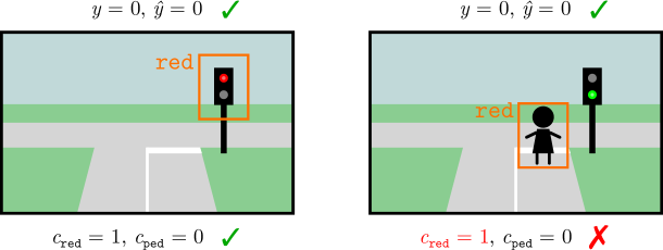Consider Example 2.1. A NeSy predictor that grounds the concepts of green light, red light, and pedestrian correctly achieves high accuracy, as it will also correctly infer that it has to stop whenever a pedestrian or a red light appear in the input image. However, a different NeSy predictor that systematically confuses pedestrians with red lights achieves the same accuracy, since, according to $\mathsf{K}$ , both lead to the correct ${\tt stop}$ action (Marconato et al., 2023b), as shown in Fig. 3.* | 0 | 0 | 1 (go) | | --- | --- | --- | | 0 | 1 | 0 (stop) | | 1 | 0 | 0 (stop) | | 1 | 1 | 0 (stop) | <details> <summary>x2.png Details</summary>  ### Visual Description ## Image Analysis: Object Detection Scenarios ### Overview The image presents two scenarios related to object detection in a street scene. Each scenario depicts a simplified street intersection with a traffic light. The scenarios are used to illustrate the success or failure of an object detection model in identifying specific objects (traffic light color and pedestrians) and their corresponding labels. ### Components/Axes Each scenario includes the following elements: * **Street Scene:** A simplified representation of a street intersection with roads, sidewalks, and grass. * **Traffic Light:** A traffic light with three lights (red, yellow, green). * **Bounding Box:** An orange rectangle indicating the detected object. * **Object Label:** Text indicating the type of object detected (e.g., "red"). * **Ground Truth Labels:** Variables representing the actual state of the scene (y), the predicted state (ŷ), the presence of a red light (c_red), and the presence of a pedestrian (c_ped). * **Correctness Indicator:** A green checkmark or a red "X" indicating whether the prediction is correct or incorrect. ### Detailed Analysis or ### Content Details **Scenario 1 (Left):** * **Scene:** A street intersection with a traffic light showing a red light. * **Bounding Box:** An orange bounding box surrounds the red light. * **Object Label:** The text "red" is displayed above the bounding box. * **Ground Truth Labels:** * `y = 0, ŷ = 0`: Indicates that the model correctly predicted the absence of a pedestrian. * `c_red = 1, c_ped = 0`: Indicates that a red light is present and no pedestrian is present. * **Correctness Indicator:** A green checkmark indicates that the prediction is correct. **Scenario 2 (Right):** * **Scene:** A street intersection with a traffic light showing a green light. A stick figure representing a pedestrian is present. * **Bounding Box:** An orange bounding box surrounds the pedestrian. * **Object Label:** The text "red" is displayed above the bounding box. * **Ground Truth Labels:** * `y = 0, ŷ = 0`: Indicates that the model correctly predicted the absence of a pedestrian. * `c_red = 1, c_ped = 0`: Indicates that a red light is present and no pedestrian is present. * **Correctness Indicator:** A red "X" indicates that the prediction is incorrect. ### Key Observations * In the first scenario, the model correctly identifies the red light and its absence of a pedestrian. * In the second scenario, the model incorrectly identifies the pedestrian as "red" and incorrectly identifies the traffic light as red. ### Interpretation The image demonstrates a scenario where an object detection model performs well in one case (correctly identifying a red light) but fails in another (misidentifying a pedestrian as "red"). This highlights the challenges of object detection, particularly in scenarios with varying object appearances and potential for misclassification. The model seems to be confusing the pedestrian with the "red" class, possibly due to visual similarities or biases in the training data. The incorrect prediction in the second scenario indicates a need for improvement in the model's ability to distinguish between different object classes and to generalize to new scenarios. </details> Figure 3: Left: truth table of the simplified prior knowledge $\mathsf{K}$ used in Example 2.1: the two concepts are interchangeable, in that as soon as one of them fires, the predictor infers the same (correct) action. Right: illustration of this RS: the model can confuse pedestrians and red lights with no drop in training loss. These examples show that correct and faulty NeSy predictors cannot be distinguished by label accuracy alone, and therefore there is no reason why, during training, NeSy methods should favor one concept mapping over the other. They also indicate that RSs can occur even when the prior knowledge is accurate and complete, and the training data is noiseless. Moreover, RSs can persist even if the training data is exhaustive (e.g., if the BDD-OIA training set encompasses examples containing all possible combinations of green lights, red lights and pedestrians), as the correct and faulty models yield the same predictions on all examples. 3.1 Causes, Frequency and Impact Why do RSs arise? Roughly speaking, RSs stem from two related issues: on the one hand, the prior knowledge $\mathsf{K}$ may allow inferring the correct labels ${\bm{\mathrm{y}}}$ from improperly grounded concept vectors ${\bm{\mathrm{c}}}$ ; on the other, the concept extractor is expressive enough to learn the improperly grounded concepts. Our two examples satisfy both conditions. Their combination introduces ambiguity in the learning problem, meaning that NeSy predictors are free to learn incorrect concept mappings and still achieve high accuracy. Properly understanding the root causes of RSs, however, requires more technical background, which we provide in Section 4, hence we postpone a more comprehensive discussion to Section 5.1. Importantly, clarifying the causes of RSs allows us to discriminate between risky and safe NeSy tasks, and to design RS mitigation strategies. We explore these topics in Section 5. Do RSs occur in practice? The above discussion entails that RSs can occur whenever the prior knowledge is not “strict” enough, but it does not prove that they must occur. Arguably, NeSy predictors can learn the intended concepts even in this case. The question is then whether RSs occur in practice. While it is difficult to gauge their frequency in real-world applications, the literature abounds with situations in which NeSy predictors, trained in standard conditions, fall prey to RSs (Manhaeve et al., 2018; Wang et al., 2019; Chang et al., 2020; Manhaeve et al., 2021a; Marconato et al., 2023b, 2024; Bortolotti et al., 2024; Yang et al., 2024; DeLong et al., 2024), suggesting that RSs occur naturally in NeSy benchmarks. Do RSs make NeSy predictors unusable? The short answer is no. More precisely, in applications where the only goal is to obtain accurate (B1) and valid (B2) predictions, RSs are not an issue. In fact, Definition 3.1 makes it clear that RSs are a symbol grounding issue that leaves label accuracy unchanged. Hence, the label predictions of affected and unaffected NeSy can be just as accurate. We also remark that RSs have no impact on validity (B2). As mentioned in Section 2.3, predictors like PNSPs, ABL, and LTN ensure their output is always consistent with the prior knowledge by explicitly searching for a label ${\bm{\mathrm{y}}}$ that, paired with the predicted concepts vectors $\hat{\bm{\mathrm{c}}}$ (or their predictive distribution $p({\bm{\mathrm{C}}}\mid{\bm{\mathrm{x}}})$ ), satisfies the knowledge $\mathsf{K}$ . Validity is built-in, i.e., it does not depend on the concepts predicted by the model. A tricky aspect of RSs is that we cannot detect them by monitoring label predictions alone. We will discuss more reliable diagnostic techniques in Section 5.2 and strategies for rendering predictors aware of their own RSs in Section 5.4. Furthermore, RS mitigation strategies can greatly reduce the presence of RSs or even entirely remove them to ensure NeSy predictors are also reusable (B3) and interpretable (B4). We overview these strategies in Section 5.3. What consequences do RSs have? RSs can seriously compromise reusability (B3) and interpretability (B4). Let us begin from reusability. RSs may exploit concept groundings that do not work in other application settings, meaning that affected concepts suffer from poor generalization beyond the specific data and prior knowledge used during training (Marconato et al., 2023b; Li et al., 2023; Bortolotti et al., 2024). To see this, consider the following example, taken from (Marconato et al., 2023b): **Example 3.4** *Consider the NeSy predictor confusing pedestrians with red lights in Example 3.3. Imagine pairing it with prior knowledge intended for an autonomous ambulance use-case, encoding that, in case of an emergency, it is allowed to cross red lights. When emergencies arise, the resulting NeSy predictor would decide to $y={\tt go}$ when there are pedestrians on the road.* RSs also affect concept reuse in downstream applications where the semantics of the concepts matters. For instance, in continual learning one is concerned with learning models that generalize across a sequence of learning tasks. NeSy predictors were shown to struggle with this precisely because of RSs (Marconato et al., 2023a): **Example 3.5** *Consider the shortcut predictor from Example 3.3. Imagine fine-tuning it on a new NeSy task that also includes the concept of “stop sign” and a new rule based on it, and specifically that whenever a stop sign is detected, the vehicle must stop. When fine-tuned on this new task, the concept extractor may mistakenly learn to equate stop signs and red lights, whose semantics is corrupted.* Another affected application is neuro-symbolic verification (Xie et al., 2022; Zaid et al., 2023; Morettin et al., 2024; Manginas et al., 2025). In model verification, the goal is to formally verify whether a neural network satisfies some property of interest, such as robustness to adversarial attacks or fairness. This involves writing a formal specification of the property, translating the model into a logical formula (or a similar representation), and then using tools from automated reasoning to check whether the model’s formula is compatible with the specification. NeSy verification is similar, except that the property of interest is specified in terms of high-level concepts. Following the neuro-symbolic setup, their definitions are provided by a trained concept extractor – provided by a third party – that also gets translated into a logical formula for the purpose of verification. Clearly, if the concepts are incorrect, this will affect the meaning of the property to be verified. Finally, interpretability (B4) also relies on the concepts being grounded appropriately (Marconato et al., 2023b; Koh et al., 2020; Poeta et al., 2023). Unless these possess human-aligned semantics, their meaning might be opaque to stakeholders, impairing understanding: **Example 3.6** *In Example 3.3, imagine the input scene portrays a pedestrian. An affected NeSy predictor would (correctly) predict stop, but its explanation would indicate that the decision depends on the presence of a red light. This explanation is misleading, and in fact it does not reflect the input at all.* 4 Theory of Reasoning Shortcuts In this section, we outline the two mainstream formalizations of RSs. Section 4.2 discusses RSs from an identifiability perspective, investigating under what conditions models achieving high likelihood can in fact learn correct concepts in the infinite sample case. Section 4.3 instead is concerned with guarantees – in terms of empirical risk minimization – for learning correct concepts from finite data. The so-far vague notion of “correct” concept will be clarified in the following sections. Additional notation Going forward, we will often treat distributions over a finite set of values as vectors in a simplex. This simplex has one dimension for each value in the set. We will write $\Delta_{\mathcal{C}}$ to indicate the simplex defined by the values contained in $\mathcal{C}$ : $$ \textstyle\Delta_{\mathcal{C}}=\{{\bm{\mathrm{p}}}\in[0,1]^{|\mathcal{C}|}\mid\sum_{i=1}^{|\mathcal{C}|}p_{i}=1\} $$ Furthermore, we will write $\mathrm{Vert}(\Delta_{\mathcal{C}})=\{{\bm{\mathrm{p}}}∈\{0,1\}^{|\mathcal{C}|}\mid\sum_{i=1}^{|\mathcal{C}|}p_{i}=1\}$ to indicate the vertices of the simplex $\Delta_{\mathcal{C}}$ . This is simply a collection of one-hot vectors, one for each value in $\mathcal{C}$ . 4.1 Setting and Assumptions In order to formally describe RSs, we have to clarify the link between the observed data, the concepts it implicitly encodes, and the concepts learned by the predictor. This link is provided by the data generating process, described next, which forms a solid basis for both theoretical approaches. $C_{1}$ $·s$ $C_{k}$ ${\bm{\mathrm{X}}}$ $G_{k}$ $·s$ $G_{1}$ ${\bm{\mathrm{X}}}$ ${\bm{\mathrm{Y}}}$ ${\bm{\mathrm{Y}}}$ $\alpha_{f}$ $f$ $f^{*}$ $\beta$ $\beta^{*}$ Figure 4: Left. The data generation process: $f^{*}$ maps inputs ${\bm{\mathrm{X}}}$ onto (distributions over) ground-truth concepts ${\bm{\mathrm{G}}}$ , and $\beta^{*}$ maps these to (distributions over) labels ${\bm{\mathrm{Y}}}$ . In a standard learning setting, only ${\bm{\mathrm{X}}}$ and ${\bm{\mathrm{Y}}}$ are observed (in light gray), whereas ${\bm{\mathrm{G}}}$ are latent. Right. A NeSy predictor maps inputs ${\bm{\mathrm{X}}}$ to concepts ${\bm{\mathrm{C}}}$ via a learned $f$ and infers labels ${\bm{\mathrm{Y}}}$ via an inference layer $\beta$ . By Eq. 20, doing so entails a map $\alpha_{f}$ (in orange) from ground-truth concepts ${\bm{\mathrm{G}}}$ to learned concepts ${\bm{\mathrm{C}}}$ . The data generating process First we distinguish between ground-truth concepts ${\bm{\mathrm{g}}}=(g_{1},...,g_{k})∈\mathcal{C}$ underlying the data and learned concepts ${\bm{\mathrm{c}}}=(c_{1},...,c_{k})∈\mathcal{C}$ . For instance, in Example 3.3 there are two binary concepts encoding the presence of pedestrians and red traffic lights: $g_{\tt ped}$ and $g_{\tt red}$ are the true values, while $c_{\tt ped}$ and $c_{\tt red}$ are the predicted values. The training examples $({\bm{\mathrm{x}}},{\bm{\mathrm{y}}})$ are sampled from a ground-truth joint distribution $p^{*}({\bm{\mathrm{X}}},{\bm{\mathrm{Y}}})=p^{*}({\bm{\mathrm{Y}}}\mid{\bm{\mathrm{X}}})p^{*}({\bm{\mathrm{X}}})$ , which is determined by the ground-truth concepts ${\bm{\mathrm{g}}}∈\mathcal{C}$ associated with the input ${\bm{\mathrm{x}}}$ . Specifically, the values of the ground-truth concepts are sampled from a ground-truth conditional distribution $p^{*}({\bm{\mathrm{G}}}\mid{\bm{\mathrm{X}}})$ , while the ground-truth labels ${\bm{\mathrm{y}}}$ are sampled from $p^{*}({\bm{\mathrm{Y}}}\mid{\bm{\mathrm{G}}};\mathsf{K})$ . It is assumed that this distribution implements the background knowledge $\mathsf{K}$ , that is, it assigns zero or low probability to labels incompatible with the constraints. For technical reasons, it is assumed it implements the same reasoning process as the target NeSy predictor. It is useful to think of these two distributions as functions: the former as a function $f^{*}:\mathcal{X}→\Delta_{\mathcal{C}}$ mapping each input to a distribution over ground-truth concepts, and the latter as a function $\beta^{*}:\Delta_{\mathcal{C}}→\Delta_{\mathcal{Y}}$ mapping each distribution over concepts to a distribution over labels. Elements $f({\bm{\mathrm{x}}})∈\Delta_{\mathcal{C}}$ are probability distributions $p({\bm{\mathrm{C}}}\mid{\bm{\mathrm{x}}})$ over the possible concept vectors ${\bm{\mathrm{c}}}∈\mathcal{C}$ . Whenever $f({\bm{\mathrm{x}}})$ allocates all probability mass to one specific ${\bm{\mathrm{c}}}∈\mathcal{C}$ , i.e., it is one-hot, it is a vertex of the simplex and as such it belongs to $\mathrm{Vert}(\Delta_{\mathcal{C}})⊂\Delta_{\mathcal{C}}$ . Overall, $p^{*}({\bm{\mathrm{Y}}}\mid{\bm{\mathrm{X}}},{\color[rgb]{1,0,0}\definecolor[named]{pgfstrokecolor}{rgb}{1,0,0}\mathsf{K}})$ results from composing $f^{*}$ and $\beta^{*}$ . A visualization of the data generation process is reported in Fig. 4 (Left). With this in mind, we present the first assumption capturing how data are generated, which will be used throughout the theoretical material. Assumption 4.1 (Completeness). Let $f^{*}:\mathcal{X}→\Delta_{\mathcal{C}}$ be the ground-truth concept extractor, and $\beta^{*}:\Delta_{\mathcal{C}}→\Delta_{\mathcal{Y}}$ the inference function induced by the prior knowledge $\mathsf{K}$ . Let $p^{*}({\bm{\mathrm{X}}})$ be the marginal distribution over input variables. Then, we have: $p^{*}({\bm{\mathrm{X}}},{\bm{\mathrm{G}}},{\bm{\mathrm{Y}}})=p^{*}({\bm{\mathrm{Y}}}\mid{\bm{\mathrm{X}}};\mathsf{K})p^{*}({\bm{\mathrm{G}}}\mid{\bm{\mathrm{X}}})p^{*}({\bm{\mathrm{X}}})$ (10) where $p^{*}({\bm{\mathrm{G}}}\mid{\bm{\mathrm{X}}}):=f^{*}({\bm{\mathrm{X}}})$ and $p^{*}({\bm{\mathrm{Y}}}\mid{\bm{\mathrm{X}}};\mathsf{K}):=(\beta^{*}\circ f^{*})({\bm{\mathrm{X}}})$ . Under Assumption 4.1, the ground-truth concept extractor $f^{*}$ becomes a sufficient statistic of the input ${\bm{\mathrm{X}}}$ for inferring the labels ${\bm{\mathrm{Y}}}$ through its composition with $\beta^{*}$ . In other words, mapping inputs to the concept distribution with $f^{*}$ retains all information necessary to infer the labels. For concreteness, this assumption fails when the concept space is “too restrictive”. For example, in MNIST-Add with two digits, sums above $18$ cannot be generated. The above assumption excludes such cases from the training data. Simplifying assumptions on the data generation process While Assumption 4.1 underlies all theoretical works on RSs (Yang et al., 2024; Marconato et al., 2023b), we introduce two additional assumptions that make the theoretical analysis more manageable. The first assumption restricts the ground-truth concept extractor $f^{*}$ : It should assign all probability mass to a single vector of concepts ${\bm{\mathrm{g}}}$ for each input ${\bm{\mathrm{x}}}$ . Assumption 4.2 (Extrapolability). The ground-truth concept extractor is a function $f^{*}:\mathcal{X}→\mathrm{Vert}(\Delta_{\mathcal{C}})$ , i.e., for all inputs ${\bm{\mathrm{x}}}∈\mathcal{X}$ , the ground-truth concept distribution $f^{*}({\bm{\mathrm{x}}})$ is a one-hot (deterministic) distribution. Assumption 4.2 allows us to retrieve ground-truth concepts ${\bm{\mathrm{G}}}$ from inputs ${\bm{\mathrm{X}}}$ via $f^{*}$ . The second assumption ensures that, with the prior knowledge $\mathsf{K}$ , each vector of concepts ${\bm{\mathrm{g}}}$ is associated with a single label ${\bm{\mathrm{y}}}$ . To formally introduce this assumption, we define, overloading notation, $$ \beta^{*}({\bm{\mathrm{c}}}):=\beta^{*}(\text{1}\!\left\{{\bm{\mathrm{C}}}={\bm{\mathrm{c}}}\right\}),\;\forall{\bm{\mathrm{c}}}\in\mathcal{C}. \tag{11} $$ $\beta^{*}:\mathcal{C}→\Delta_{\mathcal{Y}}$ is a map from the set of concepts to distribution over labels. It describes how deterministic distributions are mapped to distributions over labels by the knowledge $\mathsf{K}$ . Assumption 4.3 (Determinism). The ground-truth inference layer defines a function $\beta^{*}:\mathcal{C}→\mathrm{Vert}(\Delta_{\mathcal{Y}})$ that maps each concept vector ${\bm{\mathrm{c}}}∈\mathcal{C}$ to a one-hot (deterministic) distribution over labels $\beta^{*}({\bm{\mathrm{c}}})$ . In words, Assumption 4.3 ensures that $\beta^{*}$ assigns a single label ${\bm{\mathrm{y}}}$ to each concept vector ${\bm{\mathrm{c}}}$ . Assumptions 4.2 and 4.3 often apply in experimental regimes. For MNIST-Add and BDD-OIA, the concepts in the input image can be unambiguously determined (Assumption 4.2 is satisfied), and all concept vectors ${\bm{\mathrm{c}}}$ determine a single output label (Assumption 4.3 is satisfied), e.g., in MNIST-Add we use $Y=C_{1}+C_{2}$ . Together, Assumptions 4.2 and 4.3 ensure that each input ${\bm{\mathrm{x}}}∈\mathcal{X}$ is mapped to a single label ${\bm{\mathrm{y}}}∈\mathcal{Y}$ . The same holds for many common NeSy datasets (Bortolotti et al., 2024). Before proceeding, we have to define the support of the input and ground-truth concept distributions. We consider the marginal distributions $p^{*}({\bm{\mathrm{X}}})$ and $p^{*}({\bm{\mathrm{G}}}):=\mathbb{E}_{{\bm{\mathrm{x}}}\sim p^{*}({\bm{\mathrm{X}}})}[f^{*}({\bm{\mathrm{x}}})]$ . We indicate the support of input data with $\mathrm{supp}({\bm{\mathrm{X}}})⊂eq\mathcal{X}$ , which contains the inputs with non-zero probability according to $p^{*}({\bm{\mathrm{X}}})$ . Similarly, we denote the support of ground-truth concepts by $\mathrm{supp}({\bm{\mathrm{G}}})⊂eq\mathcal{C}$ . 4.2 Perspective: Identification In this section, we ask whether a NeSy predictor trained in a standard supervised fashion is guaranteed to learn the ground-truth concept extractor. Specifically, we want to determine whether—depending on the choice of knowledge, training data, and architectural bias—the ground-truth concept extractor is the unique maximum of the likelihood of the training data. If so, then any NeSy predictor that attains maximum likelihood will necessarily learn the ground-truth concept extractor, and thus ground all concepts correctly. This question puts us firmly in the context of identifiability theory; for an expanded presentation, please see Section 7. Below we provide a revised perspective on the identifiability of RSs (Marconato et al., 2023a, b; Bortolotti et al., 2025) by clarifying the setting, presenting a first non-identifiability result from (Marconato et al., 2023a) in Theorem 4.4, and reviewing the characterization of RSs from (Marconato et al., 2023b; Bortolotti et al., 2025) in Theorems 4.10 and 4.12. All results assume the data follows the generating process described in Fig. 4 and that we have access to possibly infinite amounts of data. 4.2.1 Model class of NeSy predictors Like in the data generation process, NeSy predictors can be understood as a pair of functions: a concept extractor $f:\mathcal{X}→\Delta_{\mathcal{C}}$ and an inference layer $\beta:\Delta_{\mathcal{C}}→\Delta_{\mathcal{Y}}$ . We indicate with $\mathcal{F}$ the space of learnable concept extractors $f$ . Most theoretical accounts on RSs work in a non-parametric setting, whereby $\mathcal{F}$ contains all possible functions from $\mathcal{X}$ to $\Delta_{\mathcal{C}}$ . In words, they assume the neural network implementing the concept extractor can express any function $f:\mathcal{X}→\Delta_{\mathcal{C}}$ (Marconato et al., 2023b; Yang et al., 2024; Bortolotti et al., 2025). We do the same, but we will relax this assumption when discussing mitigation and awareness strategies in Section 5.3 and Section 5.4. Furthermore, we also assume that, when provided with the prior knowledge $\mathsf{K}$ , the inference layer $\beta$ of a NeSy predictor architecture behaves exactly like the ground-truth inference layer $\beta^{*}$ , i.e., $$ \beta({\bm{\mathrm{c}}})=\beta^{*}({\bm{\mathrm{c}}}),\;\forall{\bm{\mathrm{c}}}\in\mathcal{C}. \tag{12} $$ We denote with $\mathcal{B}$ the space of inference layers that satisfy Eq. 12. The choice of the NeSy predictor architecture (e.g., PNSPs or LTN) determines how the inference layer $\beta$ behaves, as discussed in Section 2.2. A specific NeSy predictor thus amounts to a pair $(f,\beta)∈\mathcal{F}×\mathcal{B}$ , Unless mentioned otherwise, we present the results in the non-parametric setting where $\mathcal{F}$ contains all possible concept extractors that map inputs to concept conditional probabilities (Bortolotti et al., 2025). ; its label distribution is given by: $$ p_{f}({\bm{\mathrm{Y}}}\mid{\bm{\mathrm{X}}};\mathsf{K}):=(\beta\circ f)({\bm{\mathrm{X}}})\,, \tag{13} $$ For this class of models, we consider the maximum log-likelihood objective over infinite data: $$ {\arg\max}_{f\in\mathcal{F}}\ \mathbb{E}_{({\bm{\mathrm{x}}},{\bm{\mathrm{y}}})\sim p^{*}({\bm{\mathrm{X}}},{\bm{\mathrm{Y}}})}[\log p_{f}({\bm{\mathrm{y}}}\mid{\bm{\mathrm{x}}};\mathsf{K})]\,. \tag{14} $$ It turns out that this problem may not admit a unique solution, as explained next. 4.2.2 Non-identifiability of the concept extractor We start by presenting the necessary and sufficient conditions for a NeSy predictor to achieve maximum likelihood on data and then show that this can lead to non-identifiability. Before proceeding, for a probability measure $p^{*}({\bm{\mathrm{X}}})$ and any two measurable functions $r({\bm{\mathrm{x}}})$ and $s({\bm{\mathrm{x}}})$ with respect to $p^{*}$ , we will use the shorthand $$ r({\bm{\mathrm{X}}})=s({\bm{\mathrm{X}}}) \tag{15} $$ to mean that $r$ takes values equal to $s$ for $p^{*}$ -almost every ${\bm{\mathrm{x}}}∈\mathrm{supp}({\bm{\mathrm{X}}})$ . Theorem 4.4 (Revisited from (Marconato et al., 2023a)). Under Assumption 4.1, a NeSy predictor $(f,\beta)∈\mathcal{F}×\mathcal{B}$ attains maximum likelihood with respect to the distribution $p^{*}({\bm{\mathrm{X}}},{\bm{\mathrm{Y}}})$ if and only if $(\beta\circ f)({\bm{\mathrm{X}}})=(\beta^{*}\circ f^{*})({\bm{\mathrm{X}}})\,.$ (16) This immediately yields the following important corollary: when the same label can be predicted using different concept vectors, we cannot identify the concept extractor, i.e., $f^{*}∈\mathcal{F}$ is not the only choice that leads to obtaining maximum likelihood for the ground-truth inference layer $\beta^{*}$ , but there are alternatives $f≠ f^{*}$ . Corollary 4.5 (Non-identifiability). Let $\Delta_{\mathcal{Y}}^{*}⊂eq\Delta_{\mathcal{Y}}$ be the subspace obtained from mapping inputs to labels, which is given by $\Delta^{*}_{\mathcal{Y}}:=(\beta^{*}\circ f^{*})(\mathrm{supp}({\bm{\mathrm{X}}}))$ , and let $\Delta^{*}_{\mathcal{C}}⊂eq\Delta_{\mathcal{C}}$ be the preimage of $\Delta^{*}_{\mathcal{Y}}$ over the ground-truth inference layer $\beta^{*}$ , defined as $\Delta^{*}_{\mathcal{C}}:=\{{\bm{\mathrm{p}}}∈\Delta_{\mathcal{C}}\mid\,\beta^{*}({\bm{\mathrm{p}}})∈\Delta_{\mathcal{Y}}^{*}\}$ . Under Assumption 4.1, if $\beta^{*}$ is not injective from $\Delta_{\mathcal{C}}^{*}$ to $\Delta_{\mathcal{Y}}^{*}$ , then $(\beta^{*}\circ f)({\bm{\mathrm{X}}})=(\beta^{*}\circ f^{*})({\bm{\mathrm{X}}})\mathchoice{\mathrel{\hbox to0.0pt{\kern 3.75pt\kern-5.30861pt$\displaystyle\not$\hss}{\implies}}}{\mathrel{\hbox to0.0pt{\kern 3.75pt\kern-5.30861pt$\textstyle\not$\hss}{\implies}}}{\mathrel{\hbox to0.0pt{\kern 2.625pt\kern-4.48917pt$\scriptstyle\not$\hss}{\implies}}}{\mathrel{\hbox to0.0pt{\kern 1.875pt\kern-3.9892pt$\scriptscriptstyle\not$\hss}{\implies}}}f({\bm{\mathrm{X}}})=f^{*}({\bm{\mathrm{X}}})\,.$ (17) * Proof* By construction. If $\beta^{*}:\Delta^{*}_{\mathcal{C}}→\Delta^{*}_{\mathcal{Y}}$ is not injective, we can find ${\bm{\mathrm{p}}},{\bm{\mathrm{p}}}^{\prime}∈\Delta_{\mathcal{C}}^{*}$ such that ${\bm{\mathrm{p}}}≠{\bm{\mathrm{p}}}^{\prime}$ and $$ \beta^{*}({\bm{\mathrm{p}}})=\beta^{*}({\bm{\mathrm{p}}}^{\prime})\,. \tag{18} $$ Hence, for all ${\bm{\mathrm{x}}}∈\mathrm{supp}({\bm{\mathrm{X}}})$ such that $f^{*}({\bm{\mathrm{x}}})={\bm{\mathrm{p}}}$ we can construct another function $f∈\mathcal{F}$ such that $f({\bm{\mathrm{x}}})={\bm{\mathrm{p}}}^{\prime}$ . By Eq. 18, the NeSy predictor $(f,\beta^{*})$ will obtain maximum likelihood (Theorem 4.4), but $f({\bm{\mathrm{X}}})≠ f^{*}({\bm{\mathrm{X}}})$ . ∎ Corollary 4.5 formalizes the intuition in (Marconato et al., 2023a) that, when ground-truth inference layer $\beta^{*}$ maps multiple concept vectors to the same label, an optimal NeSy predictor can learn an RS. The important consequence is that the concept extractor $f$ attaining maximum likelihood is not unique, even when using the ground-truth inference layer $\beta^{*}$ and an infinite amount of data. In other words, we do not always correctly ground concepts. Motivated by these failures modes, we provide a formal definition of faulty NeSy predictors: This was the original definition of RSs in (Marconato et al., 2023b). Here, we change the original name to specialize it to NeSy predictors and distinguish it from the abstract notion of RSs, as explained in Definition 4.7. Definition 4.6 (Faulty NeSy predictor (Marconato et al., 2023b)). Consider a data generation process that satisfies Assumption 4.1 and let $(f^{*},\beta^{*})∈\mathcal{F}×\mathcal{B}$ be the ground-truth concept extractor and inference layer. We say that $(f,\beta)∈\mathcal{F}×\mathcal{B}$ is a faulty NeSy predictor if $(f,\beta)$ attains maximum likelihood on data (Theorem 4.4) and the disagreement set $D(f,f^{*}):=\{{\bm{\mathrm{x}}}∈\mathrm{supp}({\bm{\mathrm{X}}}):f({\bm{\mathrm{x}}})≠ f^{*}({\bm{\mathrm{x}}})\}$ (19) has strictly positive $p^{*}$ -measure, i.e., $p^{*}(D(f,f^{*}))>0$ . From the definition, the set of faulty NeSy predictors both depends on the choice of admitted concept extractors $\mathcal{F}$ and the possible inference layers $\mathcal{B}$ . We will show in Section 5.3 how, by constraining the space $\mathcal{F}$ through mitigation strategies, certain faulty NeSy predictors can vanish. From Section 2.2, each NeSy architecture specifies a particular $\beta∈\mathcal{B}$ , which limits faulty NeSy predictors to concept extractors $f∈\mathcal{F}$ for which $(f,\beta)$ is faulty. This also implies that some concept extractors $f≠ f^{*}$ may constitute a faulty NeSy predictor when paired with the inference layer of one model class, e.g., PNSPs, but not of another, e.g., LTN. While Corollary 4.5 establishes non-identifiability in general, it does not provide insight on what characterizes faulty NeSy predictors. Without this characterization, it is unclear when the ground-truth concept extractor can be identified and RSs consistently avoided. We next describe results that characterize such concept extractors $f∈\mathcal{F}$ . 4.2.3 Concept remapping distributions. Following (Marconato et al., 2023b; Bortolotti et al., 2025), we shift the perspective from describing which concept extractors $f∈\mathcal{F}$ are valid optima of the likelihood, to studying how ground-truth concept vectors can be remapped by NeSy models while retaining optimal likelihood. Formally, under Assumption 4.1, we let $p^{*}({\bm{\mathrm{X}}}\mid{\bm{\mathrm{G}}})$ be the posterior distribution induced by the ground-truth concept extractor $f^{*}$ . Then, to describe how concepts learned by a NeSy predictor $(f,\beta)∈\mathcal{F}×\mathcal{B}$ relate to ground-truth concepts, we define $$ \textstyle\alpha_{f}({\bm{\mathrm{g}}}):=\mathbb{E}_{{\bm{\mathrm{x}}}\sim p^{*}({\bm{\mathrm{X}}}\mid{\bm{\mathrm{g}}})}\left[f({\bm{\mathrm{x}}})\right]\,, \tag{20} $$ the concept remapping distribution $\alpha_{f}:\mathcal{C}→\Delta_{\mathcal{C}}$ induced by $f$ (van Krieken et al., 2025a) . These distributions $\alpha_{f}$ ’s describe how ground-truth concept vectors are mapped to learned concept vectors by $f$ . Hereafter, we use $\mathcal{A}$ to denote the space of these $\alpha_{f}$ ’s, which is a simplex (Bortolotti et al., 2025). Furthermore, we call $\mathrm{Vert}(\mathcal{A})$ the set of (deterministic) concept remappings: for each ground-truth vector ${\bm{\mathrm{g}}}∈\mathcal{C}$ , the output of a concept remapping $\alpha_{f}({\bm{\mathrm{g}}})$ is one-hot. That is, for such (deterministic) concept remappings $\alpha_{f}$ , there is a single concept vector ${\bm{\mathrm{c}}}∈\mathcal{C}$ with probability one: $$ \max_{{\bm{\mathrm{c}}}\in\mathcal{C}}\alpha_{f}({\bm{\mathrm{g}}})_{\bm{\mathrm{c}}}=1\,. \tag{21} $$ Any element $\alpha_{f}∈\mathcal{A}$ can be expressed using convex combinations of concept remappings, ${\bm{\mathrm{a}}}∈\mathrm{Vert}(\mathcal{A})$ , that is: $$ \textstyle\alpha_{f}({\bm{\mathrm{g}}})=\sum_{{\bm{\mathrm{a}}}\in\mathrm{Vert}(\mathcal{A})}\lambda^{f}_{\bm{\mathrm{a}}}\,{\bm{\mathrm{a}}}({\bm{\mathrm{g}}}), \tag{22} $$ where we have $\lambda^{f}_{\bm{\mathrm{a}}}≥ 0$ for all ${\bm{\mathrm{a}}}∈\mathrm{Vert}(\mathcal{A})$ and $\sum_{{\bm{\mathrm{a}}}∈\mathrm{Vert}(\mathcal{A})}\lambda^{f}_{\bm{\mathrm{a}}}=1$ . Hence, a NeSy predictor can be seen both as a pair $(f,\beta)∈\mathcal{F}×\mathcal{B}$ and as a pair $(\alpha_{f},\beta)∈\mathcal{A}×\mathcal{B}$ . Notice that, because the learnable $\alpha$ ’s depend on the space of learnable concept extractors $\mathcal{F}$ , constraining $\mathcal{F}$ also reduces the size of $\mathcal{A}$ . This fact is also explicit in some mitigation strategies (see Section 5.3.8). Therefore, the intended $\alpha_{f^{*}}$ implies that the learned concepts match the ground-truth concepts. 4.2.4 Reasoning shortcuts as unintended, optimal concept remapping distributions Based on this construction, we can give a formal definition of what a reasoning shortcut is and illustrate it with an example: Definition 4.7 (Reasoning Shortcut for $\beta$ (Formal)). Let $\beta∈\mathcal{B}$ be the inference layer of a NeSy predictor (e.g., PNSPs or LTN) and $\mathcal{F}$ the space of learnable concept extractors. We say that a concept remapping distribution $\alpha∈\mathcal{A}$ is a reasoning shortcut for the inference layer $\beta$ if there exists a concept extractor $f∈\mathcal{F}$ , such that $(f,\beta)$ is a faulty NeSy predictor (Definition 4.6) and $\mathbb{E}_{{\bm{\mathrm{x}}}\sim p^{*}({\bm{\mathrm{X}}}\mid{\bm{\mathrm{G}}})}[f({\bm{\mathrm{x}}})]=\alpha({\bm{\mathrm{G}}}).$ (23) <details> <summary>x3.png Details</summary>  ### 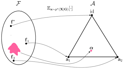Visual Description ## Diagram: Mapping between Sets F and A ### Overview The image is a diagram illustrating a mapping between two sets, labeled F and A. Set F is represented by an oval containing elements f*, f1, and f2, along with an irregular pink shape. Set A is represented by a triangle with vertices labeled id, a1, and a2, and a point labeled α inside the triangle. Dashed arrows indicate mappings from elements in F to elements in A. The expression "E_x~p*(X|G)[·]" is positioned above the diagram, indicating a mapping process. ### Components/Axes * **Set F:** Represented by an oval shape on the left. Contains elements f*, f1, f2, and a pink irregular shape. * **Set A:** Represented by a triangle shape on the right. Contains vertices labeled id, a1, and a2, and a point labeled α inside the triangle. * **Mapping:** Dashed arrows indicate the mapping from elements in set F to elements in set A. * **Expression:** "E_x~p*(X|G)[·]" is positioned above the diagram, indicating a mapping process. ### Detailed Analysis * **Set F:** * f* is mapped to id. * f1 is mapped to a1. * f2 is mapped to a2. * The pink irregular shape has no explicit mapping shown. * **Set A:** * The triangle vertices are labeled id, a1, and a2. * The point α is located inside the triangle. * **Mappings:** * A dashed arrow connects f* to id. * A dashed arrow connects f1 to a1. * A dashed arrow connects f2 to a2. ### Key Observations * The diagram illustrates a mapping between elements of two sets, F and A. * The mapping is represented by dashed arrows. * The expression "E_x~p*(X|G)[·]" suggests a probabilistic mapping process. * The pink irregular shape in set F has no explicit mapping shown. ### Interpretation The diagram represents a mapping process between two sets, F and A. The expression "E_x~p*(X|G)[·]" likely represents an expected value calculation with respect to a probability distribution p*(X|G). The mapping shows how elements from set F are transformed or associated with elements in set A. The presence of the pink irregular shape in set F without a direct mapping could indicate an element or subset that is not explicitly mapped or has a different mapping rule. The point α inside the triangle in set A might represent a specific state or value within the space defined by the triangle's vertices. The diagram could be used to illustrate a concept in machine learning, statistics, or optimization, where mappings between different spaces or sets are common. </details> Figure 5: We connect concept extractors $f∈\mathcal{F}$ and maps $\alpha∈\mathcal{A}$ through Eq. 20. Here, we represent the space of learnable concept extractors $\mathcal{F}$ and the space $\mathcal{A}$ as a two-dimensional simplex. The three vertices correspond to the concept remappings $\mathrm{id},{\bm{\mathrm{a}}}_{1},{\bm{\mathrm{a}}}_{2}∈\mathrm{Vert}(\mathcal{A})$ . $\mathrm{id}$ is the intended solution, and the remaining mappings are deterministic RSs. From (Marconato et al., 2023b, Lemma 1), any concept remapping ${\bm{\mathrm{a}}}∈\mathrm{Vert}(\mathcal{A})$ is in one-to-one correspondence with a concept extractor $f∈\mathcal{F}$ with domain restricted to $\mathrm{supp}({\bm{\mathrm{X}}})$ and, under Assumption 4.2, $f^{*}$ is in one-to-one correspondence with the identity function. However, non-deterministic concept remapping distributions $\alpha∈\mathcal{A}\setminus\mathrm{Vert}(\mathcal{A})$ can arise from several concept extractors in $\mathcal{F}$ , here represented by the magenta colored subset mapping to one point in the simplex $\mathcal{A}$ . With this definition, we formalize reasoning shortcuts as concept remapping distributions that originate from faulty NeSy predictors. In contrast to (Marconato et al., 2023b, Definition 1), we refer to RSs as the maps $\alpha∈\mathcal{A}$ for a given $\beta∈\mathcal{B}$ , not as the concept extractors $f∈\mathcal{F}$ that induce faulty NeSy predictors. That is, a NeSy predictor $(f,\beta)∈\mathcal{F}×\mathcal{B}$ subsumes an RS $\alpha_{f}$ when its concept extractor $f$ is optimal but does not match the ground-truth one, $f^{*}$ . The definition of RSs allows us to focus on concept remapping distributions $\alpha∈\mathcal{A}$ instead of concept extractors, that is, on the symbolic level rather than the sub-symbolic level. We depict the precise relation between the learnable concept extractors $\mathcal{F}$ and concept remapping distributions $\mathcal{A}$ in Fig. 5, where a one-to-one correspondence exists only between concept remappings $\alpha∈\mathrm{Vert}(\mathcal{A})$ and functions $f∈\mathcal{F}$ restricted to the support of ${\bm{\mathrm{X}}}$ . For the precise relation, refer to (Marconato et al., 2023b, Lemma 1). Studying concept remapping distributions is especially helpful under Assumption 4.2. Then, the concept remapping for the ground-truth concept extractor $f^{*}$ is the identity function $\mathrm{id}(·)$ (Bortolotti et al., 2024), i.e., $$ \alpha_{f^{*}}({\bm{\mathrm{G}}})=\mathrm{id}({\bm{\mathrm{G}}}). \tag{24} $$ Notice that Definition 4.7 specializes RSs to the specific inference layer $\beta$ at hand. This, in turn, implies that some concept remapping distributions $\alpha$ ’s can be an RS for one NeSy model class, say PNSPs, but not for another, say LTN. This may happen when two inference layers $\beta,\beta^{\prime}∈\mathcal{B}$ differ in behavior when mapping non-deterministic distributions $p({\bm{\mathrm{C}}}\mid{\bm{\mathrm{x}}})∈\Delta_{\mathcal{C}}\setminus\mathrm{Vert}(\Delta_{\mathcal{C}})$ . This distinction is particularly evident between probabilistic logic approaches (which essentially implement integration through marginalization, like PNSPs and SL) and fuzzy logic methods (where the inference layer depends on the fuzzy logic chosen). However, all deterministic concept remappings $\alpha∈\mathrm{Vert}(\mathcal{A})$ that are RSs, are RSs for all inference layers. This is because, by Eq. 12, they output the same values on one-hot concept distributions $\mathrm{Vert}(\Delta_{\mathcal{C}})$ (see also (Marconato et al., 2023b, Appendix A)). We will refer to these RSs as deterministic RSs. Definition 4.8 (Deterministic Reasoning Shortcut). We say that $\alpha∈\mathrm{Vert}(\mathcal{A})$ is a deterministic reasoning shortcut if $\alpha$ is a reasoning shortcut for $\beta^{*}∈\mathcal{B}$ (Definition 4.7). **Example 4.9** *Consider a simplified version of BDD-OIA (Xu et al., 2020) with label $y∈\{\tt go,stop\}=\mathcal{Y}$ , three binary concepts $(C_{\tt green},C_{\tt red},C_{\tt ped})$ with domain $\mathcal{C}$ , and prior knowledge $\mathsf{K}=(C_{\tt ped}\lor C_{\tt red}\Leftrightarrow(Y=\tt stop))\land(C_{\tt green}\land\lnot(Y={\tt stop})\Leftrightarrow(Y=\tt go))$ . In Fig. 6, we visualize the four concept remapping distributions appearing in Fig. 5. The concept remapping distributions $\alpha∈\mathcal{A}$ determine how ground-truth concepts are mapped to conditional probability distributions on model concepts. First, we can find an RS ( ${\bm{\mathrm{a}}}_{1}$ in Fig. 6 left-center) that predicts $C_{\tt ped}=1$ with probability one whenever $G_{\tt red}=1$ or $G_{\tt ped}=1$ . Similarly, we have an RS ( ${\bm{\mathrm{a}}}_{2}$ in Fig. 6 right-center) that predicts $C_{\tt red}=1$ with probability one whenever $G_{\tt red}=1$ or $G_{\tt ped}=1$ . A nondeterministic RS ( $\alpha$ in the rightmost part of Fig. 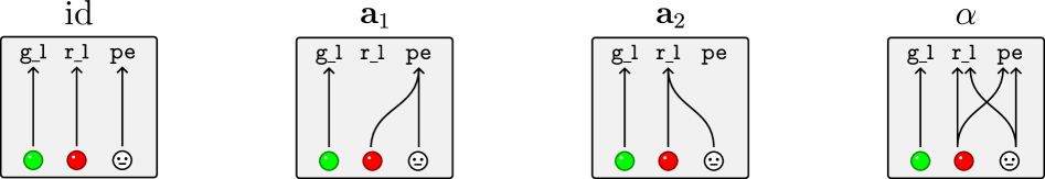6) assigns non-zero probability to both $C_{\tt red}=1$ and $C_{\tt ped}=1$ .* <details> <summary>x4.png Details</summary>  ### Visual Description ## Diagram: Category Theory Morphisms ### Overview The image presents four diagrams illustrating different morphisms in a category theory context. Each diagram is contained within a rounded rectangle and depicts the transformation of three inputs (represented by colored circles at the bottom) to three outputs (labeled at the top). The diagrams are labeled "id", "a₁", "a₂", and "α". ### Components/Axes Each diagram has the following components: * **Title:** Located above the rounded rectangle, identifying the morphism (id, a₁, a₂, α). * **Inputs:** Three circles at the bottom of the rectangle, representing the inputs. The circles are colored green, red, and white (with a smiley face inside). * **Outputs:** Three labels at the top of the rectangle, representing the outputs: "g\_l", "r\_l", and "pe". * **Arrows/Lines:** Lines connecting the inputs to the outputs, indicating the transformation or mapping. These lines can be straight or curved. ### Detailed Analysis **1. Diagram "id" (Identity Morphism):** * **Title:** id * **Inputs:** Green circle, Red circle, White circle (smiley face) * **Outputs:** g\_l, r\_l, pe * **Mapping:** * Green circle connects to g\_l with a straight arrow. * Red circle connects to r\_l with a straight arrow. * White circle connects to pe with a straight arrow. * **Trend:** Each input maps directly to its corresponding output. **2. Diagram "a₁":** * **Title:** a₁ * **Inputs:** Green circle, Red circle, White circle (smiley face) * **Outputs:** g\_l, r\_l, pe * **Mapping:** * Green circle connects to g\_l with a straight arrow. * Red circle connects to pe with a curved arrow. * White circle connects to r\_l with a curved arrow. * **Trend:** The red and white inputs are swapped in their mapping to the r\_l and pe outputs. **3. Diagram "a₂":** * **Title:** a₂ * **Inputs:** Green circle, Red circle, White circle (smiley face) * **Outputs:** g\_l, r\_l, pe * **Mapping:** * Green circle connects to r\_l with a curved arrow. * Red circle connects to g\_l with a curved arrow. * White circle connects to pe with a straight arrow. * **Trend:** The green and red inputs are swapped in their mapping to the g\_l and r\_l outputs. **4. Diagram "α":** * **Title:** α * **Inputs:** Green circle, Red circle, White circle (smiley face) * **Outputs:** g\_l, r\_l, pe * **Mapping:** * Green circle connects to g\_l with a straight arrow. * Red circle connects to pe with a curved arrow. * White circle connects to r\_l with a curved arrow. * **Trend:** The red and white inputs are swapped in their mapping to the r\_l and pe outputs. ### Key Observations * The "id" diagram represents the identity morphism, where each input is directly mapped to its corresponding output. * The "a₁", "a₂", and "α" diagrams represent different non-identity morphisms, where the inputs are rearranged or transformed in their mapping to the outputs. * The inputs are consistently represented by the same colors (green, red, white) across all diagrams. * The outputs are consistently labeled as "g\_l", "r\_l", and "pe" across all diagrams. ### Interpretation The diagrams illustrate different types of morphisms in a category theory context. The "id" morphism represents the simplest case, where the inputs are unchanged. The "a₁", "a₂", and "α" morphisms represent more complex transformations, where the inputs are rearranged or combined in some way. These diagrams are likely used to visually represent the relationships between objects and morphisms in a specific category. The specific meaning of "g\_l", "r\_l", and "pe" would depend on the context of the category being represented. The diagrams likely represent some kind of algebraic structure or computation. </details> Figure 6: The four concept remapping distributions appearing in Fig. 5 according to Example 4.9. To simplify visualization, we display the concept remapping distributions $\alpha$ as directed graphs where arrows denote how ground-truth concepts are mapped to the predicted concepts. On the left, $\mathrm{id}$ corresponds to the ground-truth map $\alpha_{f^{*}}$ from the data generation process. At the center, ${\bm{\mathrm{a}}}_{1},{\bm{\mathrm{a}}}_{2}∈\mathrm{Vert}(\mathcal{A})$ represent two deterministic RSs. On the right, $\alpha∈\mathcal{A}\setminus\mathrm{Vert}(\mathcal{A})$ is a non-deterministic RS. Among these RSs, $C_{\tt green}$ is always predicted correctly, whereas $C_{\tt red}$ and $C_{\tt ped}$ are incorrectly predicted. 4.2.5 Characterization of deterministic reasoning shortcuts. The description using maps $\alpha∈\mathcal{A}$ is useful because we can count the number of deterministic RSs explicitly. As noted above, under Assumption 4.2, the ground-truth concept remapping $\alpha_{f^{*}}$ is the identity $\mathrm{id}(·)$ . Therefore, any $\alpha∈\mathrm{Vert}(\mathcal{A})$ that differs from the identity function is a deterministic RS. The following result makes the number of deterministic RSs explicit: Theorem 4.10 (Number of deterministic reasoning shortcuts (Marconato et al., 2023b)). Let $\mathcal{F}$ be a space of concept extractors. Under Assumptions 4.1, 4.2 and 4.3, the number of deterministic RSs (Definition 4.7) is $\textstyle\sum_{\alpha∈\mathrm{Vert}(\mathcal{A}_{\mathcal{F}})}\text{1}\!\left\{\bigwedge_{{\bm{\mathrm{g}}}∈\mathrm{supp}({\bm{\mathrm{G}}})}(\beta^{*}\circ\alpha)({\bm{\mathrm{g}}})=\beta^{*}({\bm{\mathrm{g}}})\right\}-1\,,$ (25) where $\mathcal{A}_{\mathcal{F}}:=\{\alpha∈\mathcal{A}:∃\ f∈\mathcal{F}\text{ s.t. }\alpha=\alpha_{f}\}$ . When this count is greater than $1$ , the NeSy task admits (deterministic) RSs. A NeSy predictor can attain high label accuracy by learning any one of them or any (non-deterministic) mixture thereof. Because the count does not depend on the particular choice of $\beta∈\mathcal{B}$ , all NeSy architectures have the same deterministic reasoning shortcuts (Marconato et al., 2023b). This happens because all NeSy inference layers $\beta∈\mathcal{B}$ integrating the prior knowledge $\mathsf{K}$ satisfy Eq. 12. When $\mathrm{Vert}(\mathcal{A}_{\mathcal{F}})$ contains all maps, i.e., $\mathrm{Vert}(\mathcal{A}_{\mathcal{F}})=\mathrm{Vert}(\mathcal{A})$ , and $\mathrm{supp}({\bm{\mathrm{G}}})$ is complete, i.e., $\mathrm{supp}({\bm{\mathrm{G}}})=\mathcal{C}$ , it is possible to explicitly count the number of deterministic reasoning shortcuts in the task (Marconato et al., 2023b). Refer to (Marconato et al., 2023b, Appendix C) for the analytical expression of the count. The number of deterministic RSs rapidly explodes based on how many concept vectors correspond to a single label through $\beta$ . For example, if we can predict a label ${\bm{\mathrm{y}}}_{0}$ from $M$ different concept vectors, the number multiplies by a factor of $M^{M}$ . Accounting for practical restrictions in the set $\mathrm{Vert}(\mathcal{A}_{\mathcal{F}})⊂eq\mathrm{Vert}(\mathcal{A})$ due to, e.g., the choice of specific neural backbones, complicates the explicit counting of RSs, but this can be done using model counting, see Section 5.2.1. Theorem 4.10 only counts deterministic RSs. If the count is reduced to zero, then NeSy predictors may still suffer from non-deterministic RSs (those $\alpha$ ’s in $\mathcal{A}\setminus\mathrm{Vert}(\mathcal{A}_{\mathcal{F}})$ ). To ensure that we can deal with all RSs by avoiding deterministic RSs, we need to introduce an additional assumption on the inference layer $\beta$ : Assumption 4.11 (Extremality (Bortolotti et al., 2025)). The inference layer $\beta∈\mathcal{B}$ satisfies extremality if, for all $\lambda∈(0,1)$ and for all ${\bm{\mathrm{c}}}≠{\bm{\mathrm{c}}}^{\prime}∈\mathcal{C}$ such that $\operatorname*{argmax}_{{\bm{\mathrm{y}}}∈\mathcal{Y}}\beta({\bm{\mathrm{c}}})_{\bm{\mathrm{y}}}≠\operatorname*{argmax}_{{\bm{\mathrm{y}}}∈\mathcal{Y}}\beta({\bm{\mathrm{c}}}^{\prime})_{\bm{\mathrm{y}}}$ , where $\beta(·)_{\bm{\mathrm{y}}}$ is the ${\bm{\mathrm{y}}}$ -th component of $\beta$ , we have $\max_{{\bm{\mathrm{y}}}∈\mathcal{Y}}\beta(\lambda\text{1}\!\left\{{\bm{\mathrm{C}}}={\bm{\mathrm{c}}}\right\}+(1-\lambda)\text{1}\!\left\{{\bm{\mathrm{C}}}={\bm{\mathrm{c}}}^{\prime}\right\})_{\bm{\mathrm{y}}}<\max\left(\max_{{\bm{\mathrm{y}}}∈\mathcal{Y}}\beta({\bm{\mathrm{c}}})_{\bm{\mathrm{y}}},\max_{{\bm{\mathrm{y}}}∈\mathcal{Y}}\beta({\bm{\mathrm{c}}}^{\prime})_{\bm{\mathrm{y}}}\right)\,.$ <details> <summary>x5.png Details</summary>  ### 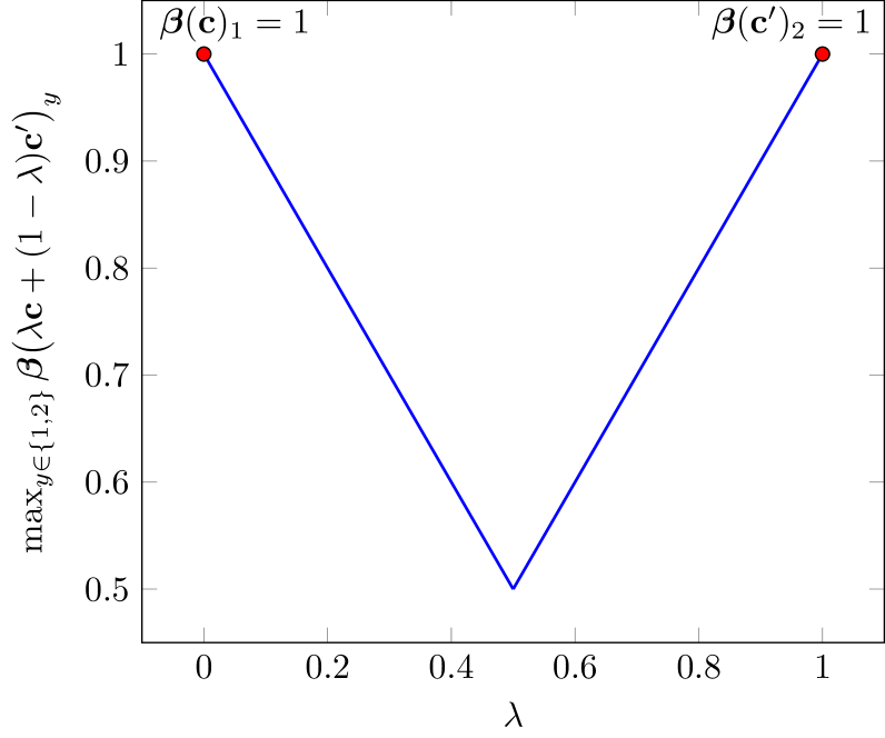Visual Description ## Line Chart: Beta Function Plot ### Overview The image is a line chart plotting the maximum value of a beta function, max_{y ∈ {1,2}} β(λc + (1 - λ)c')_y, against the variable λ. The chart shows a V-shaped curve, with the minimum value occurring around λ = 0.5. The two endpoints, at λ = 0 and λ = 1, have a beta function value of 1. ### Components/Axes * **X-axis (Horizontal):** λ (lambda), ranging from 0 to 1 in increments of 0.2. * **Y-axis (Vertical):** max_{y ∈ {1,2}} β(λc + (1 - λ)c')_y, ranging from 0.5 to 1 in increments of 0.1. * **Data Series:** A single blue line representing the beta function's maximum value. * **Labels:** * β(c)_1 = 1 at the top-left corner, corresponding to the red dot at (0, 1). * β(c')_2 = 1 at the top-right corner, corresponding to the red dot at (1, 1). ### Detailed Analysis * **Data Series Trend:** The blue line starts at (0, 1), decreases linearly to a minimum value at approximately (0.5, 0.5), and then increases linearly to (1, 1). * **Data Points:** * At λ = 0, max_{y ∈ {1,2}} β(λc + (1 - λ)c')_y = 1 (indicated by a red dot). * At λ = 0.5, max_{y ∈ {1,2}} β(λc + (1 - λ)c')_y ≈ 0.5 (the minimum point of the V-shape). * At λ = 1, max_{y ∈ {1,2}} β(λc + (1 - λ)c')_y = 1 (indicated by a red dot). ### Key Observations * The chart shows a symmetrical V-shape, with the minimum value of the beta function occurring at λ = 0.5. * The beta function reaches its maximum value of 1 at both λ = 0 and λ = 1. ### Interpretation The chart illustrates how the maximum value of a beta function changes as λ varies between 0 and 1. The function represents a weighted average of two components, 'c' and 'c'', with λ determining the weight. The V-shape suggests that the maximum value is minimized when the two components are equally weighted (λ = 0.5). The fact that the function reaches a maximum of 1 at the extremes (λ = 0 and λ = 1) indicates that the individual components 'c' and 'c'' each contribute a maximum value of 1 to the overall function. The symmetry of the graph implies that the roles of 'c' and 'c'' are interchangeable in this context. </details> Figure 7: The extremality condition holds for PNSPs and SL. A NeSy predictor satisfies Assumption 4.11 if its inference layer $\beta$ is “peaked”: for any two concept vectors ${\bm{\mathrm{c}}}$ and ${\bm{\mathrm{c}}}^{\prime}$ with different predictions, the label probability given by $\beta$ for a mixture of these predictions is no larger than the label probability it associates to ${\bm{\mathrm{c}}}$ and ${\bm{\mathrm{c}}}^{\prime}$ . This happens in PNSPs on MNIST-Add, where the knowledge specifies that $\beta:({\bm{\mathrm{C}}}=(0,1)^{→p})\mapsto(Y=1)$ and $\beta:({\bm{\mathrm{C}}}=(0,2)^{→p})\mapsto(Y=2)$ , both with probability one. Any convex combination crossing ${\bm{\mathrm{c}}}=(0,1)^{→p}$ to ${\bm{\mathrm{c}}}^{\prime}=(0,2)^{→p}$ would not result in any label with probability one, see Fig. 7. E.g., PNSPs will assign a higher probability to the sum $Y=1$ when $\lambda<0.5$ . In essence, distributing probability mass across different sets of concepts does not increase label likelihood. Extremality holds for PNSPs and SL, but for LTN it depends on the fuzzy logic chosen (van Krieken et al., 2022). Under Assumption 4.11, the next result holds: Theorem 4.12 (Identifiability (Bortolotti et al., 2025)). Under Assumptions 4.1, 4.2 and 4.3 and for all $\beta∈\mathcal{B}$ satisfying Assumption 4.11, any NeSy predictor $(f,\beta)∈\mathcal{F}×\mathcal{B}$ attaining maximum likelihood (Theorem 4.4) finds the ground-truth concept extractor, i.e., $f({\bm{\mathrm{X}}})=f^{*}({\bm{\mathrm{X}}})$ , if and only if the count of deterministic RSs is zero (Eq. 25). This theorem indicates a viable way to mitigate RSs for all NeSy predictors that obey Assumption 4.11. In fact, zeroing the count on deterministic RSs (Theorem 4.10) implies avoiding all RSs in the learning task. For NeSy predictors model classes obeying Assumption 4.11, the identifiability result gives that, in the absence of deterministic RSs, maximizing the likelihood on labels permits the correct grounding of the concepts. This, in turn, presupposes finding additional mitigations that, paired with maximum-likelihood Eq. 2, guarantee the updated count of deterministic reasoning shortcuts equals zero. We will discuss next (Section 5.3) how different mitigations act on the count reduction. **Remark 4.13** *As a corollary of Theorem 4.12, for probabilistic logic methods (including PNSPs like DPL (Manhaeve et al., 2018), SL (Xu et al., 2018), and SPL (Ahmed et al., 2022)), all non-deterministic RSs can be constructed from convex combinations of deterministic RSs (Marconato et al., 2023b, Proposition 3). This guarantees that if there are no deterministic RSs, then there are also no other RSs. Moreover, as will be discussed in Section 5.4, it is possible to leverage this geometrical aspect to construct non-deterministic RSs from convex combinations of deterministic ones, whose uncertainty on (some of) the learned concepts reveals which of them are affected by RSs.* 4.3 Perspective: Statistical Learning Learning a NeSy model amounts to learning (the parameters of) a concept extractor that—once combined with the inference layer—attains high label likelihood. From a statistical learning perspective, this is equivalent to finding a model with minimal empirical label risk. Statistical learning theory allows one to bound the true risk of a model—that is, to assess how well it generalizes—based on its observed empirical risk and other factors, such as training set size and model complexity (Vapnik, 2013; Shalev-Shwartz and Ben-David, 2014). Since the inference layer of a NeSy model is fixed and supplied upfront via the background knowledge $\mathsf{K}$ it is natural to ask when and how minimizing the label risk causes a reduction of the concept risk. Or similarly, when does low risk on label predictions bound the mismatch between the predicted and the ground-truth concepts? We expect that if RSs are present, such a bound could be vacuous for some concepts. In fact, from the results in the previous section, we know that the concepts predicted by a faulty NeSy predictor can drastically differ from ground-truth ones, even when the model is trained with an infinite amount of data.To make this explicit, we follow the analysis of (Yang et al., 2024), which indicates from a statistical learning perspective the relation between label and concept risks. 4.3.1 Knowledge complexity The statistical learning perspective on RSs follows steps similar to identifiability analysis (Section 4.2). First, data are assumed to be generated as per Assumption 4.1, whereby the ground-truth concepts and labels are sampled from the ground-truth concept extractor $f^{*}:\mathcal{X}→\Delta_{\mathcal{C}}$ and inference function $\beta^{*}:\Delta_{\mathcal{C}}→\Delta_{\mathcal{Y}}$ . From the joint distribution $p^{*}({\bm{\mathrm{X}}},{\bm{\mathrm{G}}},{\bm{\mathrm{Y}}})$ of Eq. 10, it is possible to determine the marginal distribution over labels $p^{*}({\bm{\mathrm{Y}}})$ . This marginal distribution is used together with the knowledge $\mathsf{K}$ to determine the complexity of the knowledge: Definition 4.14 (Knowledge complexity (Yang et al., 2024)). The knowledge complexity of $\mathsf{K}$ for labels distributed according to the label distribution $p^{*}({\bm{\mathrm{Y}}})$ (Assumption 4.1) is defined as $\mathrm{KC}(\mathsf{K};p^{*}):=\mathbb{E}_{{\bm{\mathrm{y}}}\sim p^{*}({\bm{\mathrm{Y}}})}[\sum_{{\bm{\mathrm{c}}}∈\mathcal{C}}\text{1}\!\left\{({\bm{\mathrm{c}}},{\bm{\mathrm{y}}})\not\models\mathsf{K}\right\}]\,.$ (26) This quantity gives a global description of how many concepts are not compatible with the knowledge, based on the labels ${\bm{\mathrm{y}}}∈\mathrm{supp}({\bm{\mathrm{Y}}})$ observed during training. Intuitively, when a few concepts are associated with a single label vector, the knowledge complexity increases, indicating that the knowledge is more explicit about what concept vectors lead to that label vector. On the other hand, a low knowledge complexity indicates that many concept vectors are mapped to same label vector. For example, in the go/stop example of BDD-OIA (Example 2.1) with three binary concepts ( $|\mathcal{C}|=8$ ), the go label is predicted only when $C_{green}=1$ , $C_{ped}=0$ , and $C_{red}=0$ , giving $7$ out of $8$ concept vectors ${\bm{\mathrm{c}}}$ such that $({\bm{\mathrm{c}}},\texttt{go})\not\models\mathsf{K}$ . The label stop, on the contrary, gives only $1$ out of $8$ concept vectors ${\bm{\mathrm{c}}}$ such that $({\bm{\mathrm{c}}},\texttt{stop})\not\models\mathsf{K}$ . Hence, whenever both go and stop instances are observed, we get $\mathrm{KC}(\mathsf{K};p^{*})<|\mathcal{C}|-1=7$ . Notice that, by construction, the complexity of any knowledge $\mathsf{K}$ on any distribution $p^{*}({\bm{\mathrm{Y}}})$ over labels is upper-bounded: $$ \mathrm{KC}(\mathsf{K};p^{*})\leq|\mathcal{C}|-1\,. \tag{27} $$ Next, we show how the complexity of the knowledge is intimately connected to the emergence of RSs. 4.3.2 Impossibility result in bounding the reasoning shortcut risk We start by recalling the relevant notation introduced in Section 4.2. For a NeSy predictor $(f,\beta)∈\mathcal{F}×\mathcal{B}$ , the corresponding concept and label distributions are given by $$ p_{f}({\bm{\mathrm{C}}}\mid{\bm{\mathrm{X}}}):=f({\bm{\mathrm{X}}}),\quad p_{f}({\bm{\mathrm{Y}}}\mid{\bm{\mathrm{X}}};\mathsf{K}):=(\beta\circ f)({\bm{\mathrm{X}}})\,. \tag{28} $$ We assume, as before, that the space of learnable concept extractors $\mathcal{F}$ is unrestricted and that the inference layer $\beta$ matches the ground-truth inference layer at the vertices (Eq. 12). The expected label risk and expected concept risk are given by $$ \mathcal{R}_{\bm{\mathrm{Y}}}(f):=-\mathbb{E}_{({\bm{\mathrm{x}}},{\bm{\mathrm{y}}})\sim p^{*}({\bm{\mathrm{X}}},{\bm{\mathrm{Y}}})}[\log p_{f}({\bm{\mathrm{y}}}\mid{\bm{\mathrm{x}}};\mathsf{K})],\quad\mathcal{R}_{\bm{\mathrm{C}}}(f):=-\mathbb{E}_{({\bm{\mathrm{x}}},{\bm{\mathrm{g}}})\sim p^{*}({\bm{\mathrm{X}}},{\bm{\mathrm{G}}})}[\log p_{f}({\bm{\mathrm{C}}}={\bm{\mathrm{g}}}\mid{\bm{\mathrm{x}}})]\,, \tag{29} $$ respectively. Their difference gives the expected reasoning shortcut risk (Yang et al., 2024): $$ \mathcal{R}_{RS}(f):=\mathcal{R}_{\bm{\mathrm{C}}}(f)-\mathcal{R}_{\bm{\mathrm{Y}}}(f)\,. \tag{30} $$ Notice that the RS risk, when it is positive, indicates that concept risk exceeds label risk; hence, despite having more accurate label predictions, concepts are less accurately predicted. Vice versa, a concept risk less than or equal to zero indicates that concept predictions are at least as accurate as label predictions. The next result connects RSs to the knowledge complexity showing that, when it is not high enough, an analogous result to Corollary 4.5 holds: Theorem 4.15 (Unbounded RSs risk (Yang et al., 2024)). Under Assumption 4.1, if the knowledge complexity is bounded by the size of the concept space as $\mathrm{KC}(\mathsf{K};p^{*})<|\mathcal{C}|-1$ , then there is a concept extractor $f$ such that $\mathcal{R}_{\bm{\mathrm{Y}}}=0$ and $\mathcal{R}_{\bm{\mathrm{C}}}→∞$ , so that the RS risk approaches infinity, i.e., $\mathcal{R}_{RS}→∞\,.$ (31) Notice that the main causes for RSs are that: (1) the knowledge complexity does not reach the maximum, and therefore each label ${\bm{\mathrm{y}}}∈\mathrm{supp}({\bm{\mathrm{Y}}})$ is associated to multiple concept vectors ${\bm{\mathrm{c}}}∈\mathcal{C}$ , (2) the fact that the space of learnable concept extractors is unrestricted and can express all possible conditional concept distributions. Both causes are targets to design mitigation strategies: (1) making knowledge more explicit by increasing the knowledge of the model, and (2) reducing the space of learnable concept extractors $\mathcal{F}$ by constraining the family of concept extractor, either through architectural biases, or through concept supervision. This perspective on RSs can naturally be used to estimate bounds on the reasoning shortcut risk, which was done for the case of concept smoothing and pretraining of the concept extractor. We refer the reader to (Yang et al., 2024) for more details on these bounds. At the same time, we will provide in Section 5.3 the main intuitions behind how mitigation strategies that can reduce the RS risk. PAC learnability with factorized concept extractors Theorem 4.15 shows that for an unconstrained space $\mathcal{F}$ of concept extractors and a not-enough-complex knowledge $\mathsf{K}$ , the NeSy task is subject to RSs. As mentioned above, restricting the space of learnable concept extractors is one primary route to investigate whether RSs can be mitigated. The work by Wang et al. (2023) investigate one special case which is often available in NeSy tasks: when the input can be naturally decomposed in a tuple of independent units, e.g., the digits in MNIST-Add, and the same concept extractor can be employed to predict the concepts of each input instance, e.g., the value of each digit is obtained by mapping the input alone, what conditions are required to avoid RSs and guarantee correct learning of the concept extractor? This setting, which builds on factorized concept extractors of the form $f=\bar{f}_{1}×·s×\bar{f}_{k}$ , has been studied via the probably approximate correct (PAC) framework (Shalev-Shwartz and Ben-David, 2014), and connects the learnability of NeSy predictors to that of weakly-supervised models (Steinhardt and Liang, 2015; Raghunathan et al., 2016). 4.3.3 Setting Following (Wang et al., 2023), we consider training samples described as pairs $({\bm{\mathrm{x}}},y)∈\mathcal{X}×\mathcal{Y}$ , Following (Wang et al., 2023), we consider one categorical label associated to each input $\bar{\bm{\mathrm{x}}}_{i}$ and we explicitly use a scalar label $y$ instead of the vector-valued ${\bm{\mathrm{y}}}$ , as in previous sections. where inputs ${\bm{\mathrm{x}}}$ represent a sequence of high-dimensional vectors ${{\bm{\mathrm{x}}}=(\bar{\bm{\mathrm{x}}}_{1},...,\bar{\bm{\mathrm{x}}}_{k})}∈\mathcal{X}=\bar{}\mathcal{X}^{k}$ and $\bar{}\mathcal{X}⊂eq\mathbb{R}^{n}$ . For example, this is the case when sequence elements $\bar{\bm{\mathrm{x}}}_{i}$ are MNIST digits and the final label corresponds to their sum (Example 3.2). In this setting, we can write the overall concept vector ${\bm{\mathrm{c}}}=(c_{1},...,c_{k})∈\mathcal{C}$ , where the concept space repeats a fixed set of symbols $\bar{}\mathcal{C}$ $k$ times, i.e., $\mathcal{C}=\bar{}\mathcal{C}^{k}$ . We also consider a restricted space of learnable concept extractors $f∈\mathcal{F}$ constructed as $$ f({\bm{\mathrm{x}}})=(\bar{f}(\bar{\bm{\mathrm{x}}}_{1}),\ldots,\bar{f}(\bar{\bm{\mathrm{x}}}_{k})), \tag{32} $$ where a shared classifier $\bar{f}:\bar{}\mathcal{X}→\Delta_{\bar{}\mathcal{C}}$ maps sequence elements $\bar{\bm{\mathrm{x}}}_{i}$ to a probability distribution over the possible values of the concept. Hence, each MNIST digit is processed independently from the others and mapped by the same classifier $\bar{f}∈\bar{}\mathcal{F}$ , where $\bar{}\mathcal{F}$ is a hypothesis class of classifiers. This construction restricts the space of learnable concept extractors $\mathcal{F}$ to be factorized as $\mathcal{F}=\bar{}\mathcal{F}^{k}$ . This is equivalent to imposing that the concept extractor is architecturally disentangled, as we will discuss in Section 5.3.8. In contrast, both the results of Corollaries 4.5 and 4.15 assume a non-factorized concept extractor space and violate this construction. In this section, we also use $[\bar{f}](\bar{\bm{\mathrm{x}}}):=\operatorname*{argmax}\bar{f}(\bar{\bm{\mathrm{x}}})$ to denote the concept-wise prediction of $\bar{f}$ . By construction, we have that $[\bar{f}]:\bar{}\mathcal{X}→\bar{}\mathcal{C}$ , and we denote with $[\bar{}\mathcal{F}]$ the space of these functions. Training data $({\bm{\mathrm{x}}},y)∈\mathcal{X}×\mathcal{Y}$ are distributed according to a joint $p^{*}({\bm{\mathrm{X}}},Y)$ and we refer to $p^{*}({\bm{\mathrm{X}}},{\bm{\mathrm{G}}})$ for the joint distribution of inputs and ground-truth concept vectors. Similarly to Section 4.3, we consider the concept risk associated to the concept extractor, but for the zero-one loss, defined as $\ell^{01}_{\bm{\mathrm{C}}}(c,c^{\prime}):=\text{1}\!\left\{c≠ c^{\prime}\right\}$ for two values $c,c^{\prime}∈\bar{}\mathcal{C}$ . In this case, we have the expected concept risk $$ \textstyle\mathcal{R}^{01}_{\bm{\mathrm{C}}}(f):=\mathbb{E}_{({\bm{\mathrm{x}}},{\bm{\mathrm{g}}})\sim p^{*}({\bm{\mathrm{X}}},{\bm{\mathrm{G}}})}\left[\frac{1}{k}\sum_{j=1}^{k}\ell^{01}_{\bm{\mathrm{C}}}([\bar{f}](\bar{\bm{\mathrm{x}}}_{j}),g_{j})\right]. \tag{33} $$ Also, we consider the zero-one loss of the label for a given $\beta^{*}∈\mathcal{B}$ , also referred to as the zero-one partial loss in (Wang et al., 2023), given by $\ell^{01}_{\beta^{*}}({\bm{\mathrm{c}}},y):=\text{1}\!\left\{\beta^{*}({\bm{\mathrm{c}}})≠ y\right\}$ . The expected label risk is given by $$ \mathcal{R}^{01}_{\bm{\mathrm{Y}}}(f,\beta^{*}):=\mathbb{E}_{({\bm{\mathrm{x}}},y)\sim p^{*}({\bm{\mathrm{X}}},Y)}\left[\ell_{\beta^{*}}^{01}\big(([\bar{f}](\bar{\bm{\mathrm{x}}}_{1}),\ldots,[\bar{f}](\bar{\bm{\mathrm{x}}}_{k})),y\big)\right]. \tag{34} $$ When there is a concept extractor ${f^{*}∈\mathcal{F}}$ such that ${\mathcal{R}}^{01}_{\bm{\mathrm{Y}}}(f^{*};\beta^{*})=0$ , we say that the space $\mathcal{F}$ is realizable under $\ell^{01}_{\beta^{*}}$ . As customary in empirical risk minimization, we consider learning the concept extractor through a finite number of samples $({\bm{\mathrm{x}}},y)$ , which we denote by $m_{p^{*}}$ . The corresponding dataset of these pairs is denoted as $\mathcal{D}_{p^{*}}$ . Here, the empirical risk associated to the dataset is defined as $$ \hat{\mathcal{R}}^{01}_{\bm{\mathrm{Y}}}(f,\beta^{*},\mathcal{D}_{p^{*}}):=\frac{1}{m_{p^{*}}}\sum_{({\bm{\mathrm{x}}},y)\in\mathcal{D}_{p^{*}}}\ell_{\beta^{*}}^{01}(([\bar{f}](\bar{x}_{1}),\dots,[\bar{f}](\bar{x}_{k})),y). \tag{35} $$ For PAC learnability of this NeSy task (Shalev-Shwartz and Ben-David, 2014; Wang et al., 2023), we ask if for any given distribution $p^{*}({\bm{\mathrm{X}}},Y)$ of input-label pairs and any $\epsilon,\delta∈(0,1)$ , the zero-one concept risk of $f$ is less or equal to $\epsilon$ , i.e., $\mathcal{R}_{\bm{\mathrm{C}}}^{01}(f)≤\epsilon$ , with probability at least $1-\delta$ when the number of training samples $m_{p^{*}}$ is greater or equal than an integer $m_{\epsilon,\delta}$ . Next, we present how Wang et al. (2023) derive such a $m_{p^{*}}$ for this learning setting. 4.3.4 PAC learnability with $k$ -unambiguous inference layers To prove the PAC learnability of the NeSy task, we have to find the conditions that $\beta^{*}$ should satisfy so that the concept risk ${\mathcal{R}_{\bm{\mathrm{C}}}^{01}(f)}$ is bounded by the label risk ${\mathcal{R}^{01}_{\bm{\mathrm{Y}}}(f;\beta^{*})}$ for any distribution of the training data. The next condition is central to find such a guarantee: Definition 4.16 ( $k$ -unambiguity (Wang et al., 2023)). An inference layer $\beta^{*}$ is $k$ -unambiguous if for any two concept vectors ${\bm{\mathrm{c}}}=(c,...,c)$ and ${\bm{\mathrm{c}}}^{\prime}=(c^{\prime},...,c^{\prime})$ $∈\mathcal{C}$ , such that $c≠ c^{\prime}$ , we have that ${\beta^{*}({\bm{\mathrm{c}}}^{\prime})≠\beta^{*}({\bm{\mathrm{c}}})}$ . Otherwise, the inference layer $\beta^{*}$ is $k$ -ambiguous. This definition essentially guarantees that passing concept vectors of the form ${\bm{\mathrm{c}}}=c(1,...,1)^{→p}$ and ${\bm{\mathrm{c}}}^{\prime}=c^{\prime}(1,...,1)^{→p}$ to $\beta^{*}$ never returns the same label predictions for $c≠ c^{\prime}$ , guaranteeing the injectivity of $\beta^{*}$ for these pairs. Although Definition 4.16 might seem strict, NeSy tasks like MNIST-Add satisfy this condition, see Example 3.2. Moreover, it is possible to extend $k$ -unambiguity to the case where $\beta^{*}$ is non-deterministic and to establish the relationship with small ambiguity degree from partial label learning (Liu and Dietterich, 2014). With this condition, the following result holds: Lemma 4.17 (Risk bounds under $k$ -unambiguity (Wang et al., 2023)). If the space of learnable concept extractors $\mathcal{F}$ is constructed like in Eq. 33 and $\beta^{*}$ is $k$ -unambigous, then we have: $\mathcal{R}^{01}_{\bm{\mathrm{C}}}(f)≤\mathcal{O}(\mathcal{R}^{01}_{\bm{\mathrm{Y}}}(f;\beta^{*})^{1/k})\quad\text{as}\;\;\;\mathcal{R}^{01}_{\bm{\mathrm{Y}}}(f;\beta^{*})→ 0$ (36) Moreover, if $\beta^{*}$ is $k$ -ambiguous, then a concept extractor $f$ attaining label risk ${\mathcal{R}^{01}_{\bm{\mathrm{Y}}}(f;\beta^{*})=0}$ can have a concept risk of ${\mathcal{R}^{01}_{\bm{\mathrm{C}}}(f)=1}$ . This result highlights that $k$ -unambiguity is central to avoiding RSs for the specific concept extractors modeled in $\mathcal{F}$ . In fact, whenever $\beta^{*}$ is $k$ -ambiguous, concept risk can be non-zero, resulting in RSs. This happens naturally for the XOR of two bits, but not for the sum of the two, as detailed next. **Example 4.18** *Consider a setting where the input ${\bm{\mathrm{x}}}=(\bar{\bm{\mathrm{x}}}_{1},\bar{\bm{\mathrm{x}}}_{2})$ comprises two bits, e.g., ${\bm{\mathrm{x}}}=(\raisebox{-1.0pt}{∈cludegraphics[width=7.96527pt]{figures/mnist-0.png}},\raisebox{-1.0pt}{∈cludegraphics[width=7.96527pt]{figures/mnist-1.png}})$ . Consider the knowledge for the XOR between the two, i.e., $\mathsf{K}=(C_{1}\oplus C_{2}\Leftrightarrow Y)$ . The function $\beta^{*}$ constructed from $\mathsf{K}$ is $k$ -ambiguous ( $k=2$ ), as there are two vectors with only the same concept value that return the label. That is, $\beta^{*}((0,0)^{→p})=\beta^{*}((1,1)^{→p})$ , since $0\oplus 0=1\oplus 1=0$ . We can see that, in this setting, there is a deterministic RS that confuses the zero for one and vice versa, that is, $\raisebox{-1.0pt}{∈cludegraphics[width=7.96527pt]{figures/mnist-0.png}}\mapsto 1$ and $\raisebox{-1.0pt}{∈cludegraphics[width=7.96527pt]{figures/mnist-1.png}}\mapsto 0$ . Consider now, instead, the sum of the two digits, with the knowledge given by $\mathsf{K}=(Y=C_{1}+C_{2})$ . Here, the inference layer $\beta^{*}$ is $k$ -unambiguous ( $k=2$ ), and there are no concept remapping distributions other than the identity that give the correct label prediction. $k$ -unambiguity is also satisfied for the complete MNIST-Add, which is a NeSy task that does not have any RS for the disentangled concept extractors in $\mathcal{F}$ .* Based on this result, Wang et al. (2023) show that it is possible to guarantee PAC learnability of the NeSy task. The result incorporates the Natarajan dimension of the space of classifiers $[\bar{f}]$ , denoted as $d_{[\bar{}\mathcal{F}]}$ . We refer readers to (Shalev-Shwartz and Ben-David, 2014) for the explicit definition of the Natarajan dimension. Theorem 4.19 (ERM learnability under $k$ -unambiguity (Wang et al., 2023)). Let $\mathcal{F}$ be the space of learnable concept extractors $\mathcal{F}$ constructed like in Eq. 33. Suppose that $\mathcal{F}$ is realizable under $\ell^{01}_{\bm{\mathrm{Y}}}$ and $[\bar{}\mathcal{F}]$ has a finite Natarajan dimension $d_{[\bar{}\mathcal{F}]}$ . Then, for any $\epsilon,\delta∈(0,1)$ , there exists a universal constant $C_{0}>0$ , such that with probability at least $1-\delta$ , the empirical label risk minimizer $f$ on the dataset $\mathcal{T}_{p^{*}}$ , such that $\hat{\mathcal{R}}^{01}_{\bm{\mathrm{Y}}}(f;\beta^{*};\mathcal{T}_{p^{*}})=0$ , has a concept risk $\mathcal{R}^{01}_{\bm{\mathrm{C}}}(f)<\epsilon$ , if $\displaystyle m_{p^{*}}≥ C_{0}\frac{\eta_{1}}{\epsilon^{k}}\left(\eta_{2}\log\frac{1}{\epsilon^{k}}+\log\frac{1}{\delta}+\eta_{3}\right),$ (37) where $\eta_{1},\eta_{2},\eta_{3}∈\mathbb{R}^{+}$ are constants that depend on $k$ , the $d_{[\bar{}\mathcal{F}]}$ , and the number of labels $|\mathcal{Y}|$ . We refer the reader to (Wang et al., 2023) for the explicit values of the constants. Furthermore, the work presents other results regarding the PAC learnability of the NeSy task under unknown $\beta^{*}$ ’s and error bounds when considering the semantic loss (Xu et al., 2018). 4.4 Relationship between Theories A common trait between the two perspectives can be found in Corollary 4.5 and Theorem 4.15: both results indicate that, even in the limit of infinite data, when conditions on the knowledge are not met (either because of non-injectivity or low knowledge complexity), RSs can be found during training. Both results highlight a general problem in NeSy predictors: when we have a large hypothesis space of learnable concept extractors $\mathcal{F}$ and if the knowledge admits multiple solutions for label predictions, there is no unique and correct grounding of the concepts. Vice versa, if a one-to-one mapping between concept and labels is implemented by the knowledge (both because the ground-truth inference layer $\beta^{*}$ is injective in Corollary 4.5 and $\mathrm{KC}(\mathsf{K},p^{*})=|\mathcal{C}|-1$ in Theorem 4.15), achieving optimal likelihood on data implies learning well-grounded concepts. Achieving this condition, however, may be difficult in practice whenever the number of possible concept vectors exceeds that of labels, see e.g. BDD-OIA in Example 4.9. Constrained hypothesis spaces for the concept extractor can likelier meet the conditions for avoiding RSs with a less restricted $\mathsf{K}$ , as shown in Lemma 4.17, and lead to statistical learning bounds for recovering ground-truth concepts with finite-sized estimates (Theorem 4.19). The two perspectives differ in how they specialize in treating mitigations. The identifiability perspective (Marconato et al., 2023b, 2024) has investigated so far the impact of strategies on count reduction for deterministic $\alpha$ ’s, studying how different mitigations change the quantities in the count (Eq. 25). This also includes evaluating how the count reduces when different strategies are used together, but it is limited to study optima of the learning problem. The statistical learning perspective (Wang et al., 2023; Yang et al., 2024) has mainly explored how different mitigations that constrain the space of learnable concept extractors $\mathcal{F}$ can be used to bound the empirical RSs risk. These results do not explicitly require studying the optima of the learning problem, in the sense that, constraints on $\mathcal{F}$ can be directly translated to bounds on the RS risk (Eq. 30). In fact, strategies like concept smoothing change the optima of the learning problem, and may not allow reaching maximum likelihood. Despite the different treatments, we advance that the effect of some mitigation strategies can be described from both perspectives: a mitigation strategy can both reduce the count in Eq. 25 and reduce the risk Eq. 30. In this sense, we view both perspectives as complementary: through identifiability theory, one can analyze how mitigations act to reduce deterministic RSs at optimal likelihood, whereas through statistical learning theory, bounds on the empirical concept risk can be found even when likelihood is not optimal. Formulating a theory that takes both perspectives into account remains open. 5 Handling Reasoning Shortcuts We proceed by detailing the root causes of RSs (in Section 5.1), and outlining existing diagnostic tools (Section 5.2), mitigation strategies (Section 5.3), and awareness strategies (Section 5.4). 5.1 Root Causes As anticipated in Section 3.1, RSs arise whenever the NeSy learning process does not penalize models that learn incorrect concepts, i.e., concepts that do not match the ground-truth ones. Moreover, the theory in Section 4 provides additional details. Specifically, Theorem 4.15 suggests that RSs can occur when the knowledge complexity $\mathrm{KC}$ (Definition 4.14) is less than $|\mathcal{C}|-1$ and the space of learnable concept extractors $\mathcal{F}$ is broad enough. Corollary 4.5 supports the same conclusion. Following (Marconato et al., 2023b), additional insights can be gleaned by studying the structure of Eq. 25, reported below for reference, which counts the number of deterministic RSs (Definition 4.8) affecting a NeSy task. Since this is useful for understanding the mitigation strategies in Section 5.3, we analyze it here: learnable maps $\alpha$ support prior knowledge $\mathsf{K}$ optimality condition $\mathcal{L}$ The count is controlled by the four colored elements, which we discuss below. 5.1.1 The knowledge The prior knowledge $\mathsf{K}$ determines the inference layer $\beta^{*}$ . To understand its role, | 0 | 0 | 0 | 0 | | --- | --- | --- | --- | | 0 | 1 | 1 | 1 | | 1 | 0 | 2 | 1 | | 1 | 1 | 3 | 1 | Figure 8: $\mathsf{K}_{1}$ is immune to RSs, $\mathsf{K}_{2}$ is not. imagine two NeSy tasks with two binary concepts that are identical except for the prior knowledge $\mathsf{K}$ : one uses $\mathsf{K}_{1}=(Y_{1}=2C_{1}+C_{2})$ and the other $\mathsf{K}_{2}=(Y_{2}=C_{1}\lor C_{2})$ , see Fig. 8. Assuming the training set covers all classes (see Section 5.1.2), the task using $\mathsf{K}_{1}$ does not admit any RSs: each label $y$ can only be inferred by a unique choice of ${\bm{\mathrm{c}}}$ , so high label accuracy entails high concept accuracy. The task using $\mathsf{K}_{2}$ , however, is affected by RSs: the positive label can be inferred from ${\bm{\mathrm{c}}}=(0,1)$ , ${\bm{\mathrm{c}}}=(1,0)$ and ${\bm{\mathrm{c}}}=(1,1)$ , hence NeSy predictors can confuse them with no impact on accuracy. From the perspective of Eq. 38, this happens because, all else being equal, swapping $\mathsf{K}_{1}$ with $\mathsf{K}_{2}$ softens the equality condition, increasing the count. 5.1.2 The training distribution Another important factor is the set of configurations of ground-truth concepts ${\bm{\mathrm{g}}}$ that underly the training data, that is, the support $\mathrm{supp}({\bm{\mathrm{G}}})$ of the training distribution. To see this, consider the MNIST-Add example in Example 3.2. Suppose we add two new examples, $(\raisebox{-1.0pt}{∈cludegraphics[width=7.96527pt]{figures/mnist-5.png}}\raisebox{-1.0pt}{∈cludegraphics[width=7.96527pt]{figures/mnist-5.png}},10)$ and $(\raisebox{-1.0pt}{∈cludegraphics[width=7.96527pt]{figures/mnist-5.png}}\raisebox{-1.0pt}{∈cludegraphics[width=7.96527pt]{figures/mnist-3.png}},8)$ , to the training set. Intuitively, the concept extractor has to map <details> <summary>figures/mnist-5.png Details</summary>  ### Visual Description Icon/Small Image (48x48) </details> to the digit $5$ , otherwise it would mispredict the $(\raisebox{-1.0pt}{∈cludegraphics[width=7.96527pt]{figures/mnist-5.png}}\raisebox{-1.0pt}{∈cludegraphics[width=7.96527pt]{figures/mnist-5.png}},10)$ example; likewise, now that <details> <summary>figures/mnist-5.png Details</summary>  ### Visual Description Icon/Small Image (48x48) </details> has only one correct grounding, it has to map <details> <summary>figures/mnist-4.png Details</summary>  ### Visual Description Icon/Small Image (48x48) </details> to $4$ otherwise it would mispredict the $(\raisebox{-1.0pt}{∈cludegraphics[width=7.96527pt]{figures/mnist-5.png}}\raisebox{-1.0pt}{∈cludegraphics[width=7.96527pt]{figures/mnist-4.png}},9)$ example. The same reasoning applies for the remaining examples, namely ( <details> <summary>figures/mnist-5.png Details</summary>  ### Visual Description Icon/Small Image (48x48) </details> <details> <summary>figures/mnist-3.png Details</summary>  ### Visual Description Icon/Small Image (48x48) </details> , 8) and ( <details> <summary>figures/mnist-3.png Details</summary>  ### Visual Description Icon/Small Image (48x48) </details> <details> <summary>figures/mnist-2.png Details</summary>  ### Visual Description Icon/Small Image (48x48) </details> , 5). In summary, this small change completely removes all RSs, as the only way to match all training examples is to assign each MNIST digit to its correct numeric value. Intuitively, the larger the support – i.e., the more combinations of ground-truth concepts ${\bm{\mathrm{g}}}$ the training set represents – the more restrictive the conjunction in Eq. 38, lowering the count. 5.1.3 The optimality condition The optimality condition $\mathcal{L}$ is responsible for filtering out those maps $\alpha$ that do not fit the ground-truth labels. Consider Example 3.2 again. One possible RS is $\{\raisebox{-1.0pt}{∈cludegraphics[width=7.96527pt]{figures/mnist-2.png}}\mapsto 4,\raisebox{-1.0pt}{∈cludegraphics[width=7.96527pt]{figures/mnist-3.png}}\mapsto 1,\raisebox{-1.0pt}{∈cludegraphics[width=7.96527pt]{figures/mnist-4.png}}\mapsto 5,\raisebox{-1.0pt}{∈cludegraphics[width=7.96527pt]{figures/mnist-5.png}}\mapsto 4\}$ , which collapses <details> <summary>figures/mnist-5.png Details</summary>  ### Visual Description Icon/Small Image (48x48) </details> and <details> <summary>figures/mnist-2.png Details</summary>  ### Visual Description Icon/Small Image (48x48) </details> into the same concept value, $4$ . Now, imagine augmenting the training objective, by default the cross-entropy, with a reconstruction loss. This mapping no longer achieves low loss, since the value $4$ decodes to both <details> <summary>figures/mnist-2.png Details</summary>  ### Visual Description Icon/Small Image (48x48) </details> and <details> <summary>figures/mnist-5.png Details</summary>  ### Visual Description Icon/Small Image (48x48) </details> , which clearly hinders reconstruction. In terms of Eq. 38, modifying the training objective changes the optimality condition, potentially decreasing the number of RSs. 5.1.4 The family of learnable maps Finally, the sum in Eq. 25 runs over (the vertices of) the space of learnable concept remappings $\alpha$ , denoted by $\mathrm{Vert}(\mathcal{A}_{\mathcal{F}})$ . This, in turn, depends on the space of learnable concept extractors $\mathcal{F}$ (Theorem 4.10). By introducing architectural bias in the architecture of the concept extractor (e.g., smoothing concept extractors by tuning a temperature parameter), we can constrain the space of learnable concept remappings $\alpha$ ’s and therefore decrease the number of learnable RSs $\mathrm{Vert}(\mathcal{A}_{\mathcal{F}})$ . We will see in Section 5.3 how to effectively control this aspect of the learning problem. 5.2 How to Diagnose Reasoning Shortcuts As mentioned in Section 3, in-distribution label accuracy is not affected by RSs and therefore insufficient for diagnosing them. In this section, we briefly outline more effective diagnostic techniques. 5.2.1 Task-level diagnosis Even before we commit to an architecture and train the model, we can quantify how many deterministic RSs can affect a given NeSy task. We accomplish this by evaluating Eq. 25, which is defined on known properties, such as the number of concepts, their cardinality and the given annotations. However, the count is very hard to compute manually, even for relatively small problems, as the number of maps $\alpha$ increases doubly exponentially with the number of concepts $k$ . The countrss tool (Bortolotti et al., 2024) works around this by building on the following observation: all deterministic maps $\alpha$ in $\mathrm{Vert}(\mathcal{A})$ can be viewed as binary matrices that indicate which predicted concepts $C_{j}$ correspond to which ground-truth concepts $G_{i}$ . The assumptions that constrain the number of mappings can be encoded into a propositional logical formula, whose solutions (that is, admissible binary matrices) are in one-to-one correspondence to the deterministic RSs $\alpha$ . Then, the count in Eq. 25 can be reduced to model counting (#SAT) (Gomes et al., 2021), i.e., the task of counting the solutions of a logical formula. | $G_{\tt red}$ $\neg G_{\tt red}$ $G_{\tt ped}$ | 0 0 1 | 0 0 0 | 1 0 0 | 0 1 0 | | --- | --- | --- | --- | --- | | $\neg G_{\tt ped}$ | 0 | 1 | 0 | 0 | (a) | $G_{\tt red}$ $\neg G_{\tt red}$ $G_{\tt ped}$ | 1 0 0 | 0 1 0 | 0 0 0 | 0 0 1 | | --- | --- | --- | --- | --- | | $\neg G_{\tt ped}$ | 0 | 0 | 0 | 1 | (b) Figure 9: Binary matrices encoding two possible mappings $\alpha$ from Example 2.1. (a) is a solution, resulting in a mapping that mistakes red lights with pedestrians and vice versa but is otherwise consistent with $\mathsf{K}$ for any combination of ground truth concepts. (b) is not a solution, since the resulting mapping makes the predictor unable to detect pedestrians and give correct predictions on some, but not all, combinations of ground truth concepts. Although one could use any #SAT procedure, the complexity of the encoding for any task of practical interest warrants the use of approximate #SAT solvers (Chakraborty et al., 2021). Under the hood, countrss employs the state-of-the-art hashing-based counter ApproxMC https://github.com/meelgroup/approxmc, which outputs an $\epsilon$ approximation of the exact count with probability $\delta$ . countrss inherits these statistical (PAC-style) guarantees, providing close approximations to Eq. 25 with high probability Regardless of the solver used, the reduction assumes disentanglement. Otherwise, the resulting number of logical variables in the encoding would be orders of magnitude above the capabilities of current solvers.. The estimates returned by countrss can provide an initial indication of the hardness of the learning problem and help making informed architectural choices according to the task at hand. countrss is included in the rsbench library (Bortolotti et al., 2024). 5.2.2 Model metrics Whenever concept annotations are available, the most effective way to evaluate the quality of the learned concepts is to use standard metrics such as accuracy, $F_{1}$ score, and concept-level confusion matrices. Another useful metric is concept collapse (Bortolotti et al., 2024). Roughly speaking, it quantifies to what extent the learned concept extractor compresses distinct ground-truth concepts into the same learned concept. More formally, let $C∈[0,1]^{m× m}$ be a concept confusion matrix, where $m$ denotes its size (e.g.,, $m=2^{k}$ when all ground-truth concepts are observed). We define $\mathrm{Cls}=1-\tfrac{p}{m}$ , where $p=\sum_{j=1}^{m}\text{1}\!\left\{∃ i\,:\,C_{ij}>0\right\}$ . We remark that, however, collapse cannot detect all RSs. For instance, imagine a NeSy predictor trained on some variant of MNIST-Add affected by an RS mapping <details> <summary>figures/mnist-0.png Details</summary>  ### Visual Description Icon/Small Image (48x48) </details> to $1$ and <details> <summary>figures/mnist-1.png Details</summary>  ### Visual Description Icon/Small Image (48x48) </details> to $0$ . This RS is completely invisible to the collapse metric, as the model does not collapse ground-truth concepts together, cf. Section 5.3.6. Still, it can be useful to gauge the presence of RSs that do. Finally, a major downside of these metrics is that they all require concept-level annotations, which are not always available. With insufficient or missing concept annotations, another approach is to train multiple NeSy predictors to high label accuracy, and check their concept extractors align on concept predictions. When (deterministic) RSs are many in a NeSy task, it is likely that each predictor finds a different RS. Furthermore, if there are no RSs, concept extractors giving optimal likelihood must predict the same concepts, although the reverse is not necessarily true. The alignment between different concept extractors of the ensemble can be indirectly measured via the overall conditional entropy of the averaged concept predictions of the ensemble. Precisely, for $r∈\mathbb{N}$ members of the ensemble, we can account the mean conditional Shannon entropy $\mathsf{H}(\frac{1}{r}\sum_{j}p_{j}({\bm{\mathrm{C}}}\mid{\bm{\mathrm{x}}}))$ . This quantity is central for unsupervised RS-aware methods such as bears (Marconato et al., 2024) and NeSyDM (van Krieken et al., 2025b), see Section 5.4. 5.3 A Tour of Mitigation Strategies A wealth of strategies for mitigating RSs have been proposed. We list them in Table 2 and discuss them next. 5.3.1 Concept supervision The most direct approach for encouraging correct grounding is to exploit concept annotations during training, thus altering the optimality condition. This requires introducing an additional loss term penalizing mispredicted concepts. Doing so effectively constraints the concept extractor $f$ to recover the annotations, dramatically reducing the number of learnable RSs, and potentially avoiding them altogether. This solution is however neither cheap nor perfect. It can be costly because concept-level annotations are frequently unavailable in the wild, and collecting them involves running potentially expensive annotation campaigns. Following recent trends (Oikarinen et al., 2022; Yang et al., 2023b; Rao et al., 2024; Srivastava et al., 2024; Yuksekgonul et al., 2023), one could obtain these with foundation models. This solution, however, risks injecting substantial amounts of noise into the learning loop (Debole et al., 2025): despite being trained on vast amounts of data, foundation models can mispredict even basic concepts (Wüst et al., 2025). It is also imperfect because, in the worst case, ruling out all RSs requires exhaustively annotating all possible combinations of concepts. Unless this is the case, a sufficiently expressive concept extractor might fit all annotations on the supervised combinations and fluke the remaining ones. Naturally, annotating an exponential (in the number of concepts) number of combinations can be infeasible. A possible work-around is to restrict the expressivity of the concept extractor – e.g., by processing inputs separately, as typically done in MNIST-Add – so as to effectively transfer concept annotations across concept combinations. Another option is to smartly select instances or concepts to be annotated, see Section 5.5. Table 2: Overview of mitigation strategies. The columns indicate, for each strategy, what component(s) of Eq. 38 it targets (Target), whether it requires extra annotations (Annot) and guarantees reducing the count in Eq. 25 (Count), and how well it worked on different NeSy Tasks. Specifically, “ ✓ ” means that it prevents all RSs, “ ✗ ” that it fails to do so, and “? ” that it has not been evaluated. Note: With MNIST-Add ∗ we refer to the family of datasets based on the MNIST-Add benchmark (Manhaeve et al., 2018). Strategy Properties Arithmetic Logic High-Stakes Target Annot Count MNIST-Add ∗ Kandinsky Clevr BDD-OIA Concept Supervision (Koh et al., 2020) ${\color[rgb]{1,.5,0}\definecolor[named]{pgfstrokecolor}{rgb}{1,.5,0}\mathcal{L}}$ ✓ ✓ ✓ ✓ ✓ ✗ Multi-task Learning (Caruana, 1997) ${\color[rgb]{0,.5,.5}\definecolor[named]{pgfstrokecolor}{rgb}{0,.5,.5}\mathsf{K}}$ ✓ ✓ ✓ ? ? ? Weak Supervision (Yang et al., 2024) ${\color[rgb]{1,.5,0}\definecolor[named]{pgfstrokecolor}{rgb}{1,.5,0}\mathcal{L}}$ ✗ ✗ ✓ ? ? ✗ Entropy Maximization (Manhaeve et al., 2021a) ${\color[rgb]{1,.5,0}\definecolor[named]{pgfstrokecolor}{rgb}{1,.5,0}\mathcal{L}}$ ✗ ✗ ? ? ? ✗ Smoothing (Szegedy et al., 2016) ${\color[rgb]{1,.5,0}\definecolor[named]{pgfstrokecolor}{rgb}{1,.5,0}\mathcal{L}}$ ✗ ✗ ? ? ? ? Reconstruction (Kingma, 2013) ${\color[rgb]{1,.5,0}\definecolor[named]{pgfstrokecolor}{rgb}{1,.5,0}\mathcal{L}}$ ✗ ✓ ✓ ? ? ? Contrastive Learning (Chen et al., 2020) ${\color[rgb]{1,.5,0}\definecolor[named]{pgfstrokecolor}{rgb}{1,.5,0}\mathcal{L}}$ ✗ ✗ ? ? ? ? Disentanglement (Suter et al., 2019) $$ ✗ ✓ ? ✗ ? ? 5.3.2 Multi-task learning Another way to improve the prior knowledge $\mathsf{K}$ is to train a NeSy predictor to solve multiple NeSy tasks (sharing some of the same concepts) jointly (Caruana, 1997). Doing so equates to training on a single NeSy task whose prior knowledge is the conjunction of the prior knowledge of the different tasks (Marconato et al., 2023b). As per Eq. 38, doing so reduces the number of potential RSs. However, not all combinations of NeSy tasks are equally effective. To see this, imagine training a NeSy predictor to output both the sum of two MNIST digits and whether the first one is greater than the second one. Observations take the form $((\raisebox{-1.0pt}{∈cludegraphics[width=7.96527pt]{figures/mnist-4.png}}\raisebox{-1.0pt}{∈cludegraphics[width=7.96527pt]{figures/mnist-5.png}}),(9,0))$ and $((\raisebox{-1.0pt}{∈cludegraphics[width=7.96527pt]{figures/mnist-3.png}}\raisebox{-1.0pt}{∈cludegraphics[width=7.96527pt]{figures/mnist-2.png}}),(5,1))$ , where the second label indicates whether the inequality holds. The RS in Example 3.2, i.e., $\{\raisebox{-1.0pt}{∈cludegraphics[width=7.96527pt]{figures/mnist-2.png}}\mapsto 4,\ \raisebox{-1.0pt}{∈cludegraphics[width=7.96527pt]{figures/mnist-3.png}}\mapsto 1,\ \raisebox{-1.0pt}{∈cludegraphics[width=7.96527pt]{figures/mnist-4.png}}\mapsto 3,\ \raisebox{-1.0pt}{∈cludegraphics[width=7.96527pt]{figures/mnist-5.png}}\mapsto 6\}$ , is no longer valid, as it incorrectly predicts $(5,0)$ for the second example. However, an alternative shortcut exists, namely $\{\raisebox{-1.0pt}{∈cludegraphics[width=7.96527pt]{figures/mnist-2.png}}\mapsto 1,\ \raisebox{-1.0pt}{∈cludegraphics[width=7.96527pt]{figures/mnist-3.png}}\mapsto 4,\ \raisebox{-1.0pt}{∈cludegraphics[width=7.96527pt]{figures/mnist-4.png}}\mapsto 3,\ \raisebox{-1.0pt}{∈cludegraphics[width=7.96527pt]{figures/mnist-5.png}}\mapsto 6\}$ . A better alternative is to pair MNIST addition and multiplication. This is identical to Example 3.2, except now there are two labels, e.g., $((\raisebox{-1.0pt}{∈cludegraphics[width=7.96527pt]{figures/mnist-4.png}}\raisebox{-1.0pt}{∈cludegraphics[width=7.96527pt]{figures/mnist-5.png}}),(9,20))$ and $((\raisebox{-1.0pt}{∈cludegraphics[width=7.96527pt]{figures/mnist-3.png}}\raisebox{-1.0pt}{∈cludegraphics[width=7.96527pt]{figures/mnist-2.png}}),(5,6))$ . It can be verified that the only concept mapping that correctly predicts both the sum and the product is the intended one, i.e., the identity, ruling out all RSs. Naturally, multi-task learning requires gathering label annotations for all involved tasks, which can be non-trivial. Another downside is that it may not be obvious how to construct a “natural” NeSy task that guarantees the removal of all RSs. We will discuss possible solutions in Section 6.6. 5.3.3 Abductive weak supervision This strategy requires training the concept extractor using procedurally generated pseudo-labels obtained with logical abduction (Yang et al., 2024). ABL embodies this approach: in ABL, the model uses logical abduction to infer the most plausible concept vector ${\bm{\mathrm{c}}}$ that logically explains the ground-truth label ${\bm{\mathrm{y}}}$ according to the prior knowledge. In practice, ABL uses a pre-defined distance function $d({\bm{\mathrm{c}}},{\bm{\mathrm{c}}}^{\prime})$ to select this concept vector from alternatives. Then, ABL uses this new concept vector as the learning target for the loss function. Choosing an appropriate distance function can provide ABL with concept risk reduction; specifically, when the distance metric is always zero, Yang et al. (2024) showed that the risk of learning a shortcut solution reduces compared to other approaches. The downside is that there is no guarantee that the abduction process will recover the ground-truth concepts. 5.3.4 Entropy maximization Perhaps the simplest unsupervised mitigation strategy is entropy maximization (Manhaeve et al., 2021a). A simple idea here is to introduce an entropy-based loss term encouraging the model to evenly distribute probability mass across all concept combinations. This can be made practical by averaging over all predictions in a batch, and maximizing the Shannon entropy $\mathsf{H}(p({\bm{\mathrm{C}}}))$ (Manhaeve et al., 2021a). Entropy maximization is easy to implement and computationally lightweight. However, it only encourages the predictor to spread concept predictions, but does not guarantee that the learned concepts will match the ground-truth ones. Furthermore, there are no formal results that show this method reduces the number of RSs. 5.3.5 Smoothing The idea behind concept smoothing is to encourage the probabilities of the most and least probable concept vectors ${\bm{\mathrm{c}}}$ to be “close”. The main idea is to never allow NeSy predictors to learn ”peaked” concept distributions, i.e., $p({\bm{\mathrm{C}}}\mid{\bm{\mathrm{X}}})$ of the model is never one-hot. Smoothing can be enforced either architecturally, e.g., by introducing a temperature parameter that reduces the magnitude of the concept activations, or during training, by penalizing high activations on input samples. This strategy permits reducing the RSs risk (Eq. 30), the full derivation can be found in (Yang et al., 2024). This strategy, however, only circumvents some RSs: while smoothing prevents deterministic RSs, it does not affect non-deterministic ones. E.g., imagine that $\mathsf{K}$ allows inferring the same label vector ${\bm{\mathrm{y}}}$ from both ${\bm{\mathrm{c}}}^{\prime}$ and ${\bm{\mathrm{c}}}^{\prime\prime}$ (that is, $\beta^{*}({\bm{\mathrm{c}}}^{\prime})=\beta^{*}({\bm{\mathrm{c}}}^{\prime\prime})={\bm{\mathrm{y}}}$ , and that a NeSy predictor predicts a mixture of the two, e.g., because it has learned the map $\alpha({\bm{\mathrm{g}}})=0.5\text{1}\!\left\{{\bm{\mathrm{C}}}={\bm{\mathrm{c}}}^{\prime}\right\}+0.5\text{1}\!\left\{{\bm{\mathrm{C}}}={\bm{\mathrm{c}}}^{\prime\prime}\right\}$ , where ${\bm{\mathrm{g}}}∈\{{\bm{\mathrm{c}}}^{\prime},{\bm{\mathrm{c}}}^{\prime\prime}\}$ . The mapping $\alpha$ is smooth – the highest probability it can output is $0.5$ – but it is also a (non-deterministic) reasoning shortcut for PNSPs and SL, as it produces a correct prediction: $0.5\beta^{*}({\bm{\mathrm{c}}}^{\prime})+0.5\beta^{*}({\bm{\mathrm{c}}}^{\prime\prime})=\text{1}\!\left\{{\bm{\mathrm{Y}}}={\bm{\mathrm{y}}}\right\}$ . 5.3.6 Reconstruction Another option is to introduce a reconstruction penalty into the learning process (Cottrell et al., 1987). Doing so encourages learning concepts that allow reconstructing the input ${\bm{\mathrm{x}}}$ , or part of it. This rules out RSs that conflate unrelated concepts together and thus prevent reconstruction. To see how it works, consider MNIST-Add (Example 3.2) again: NeSy predictors achieving low reconstruction loss cannot map different MNIST digits to the same concept, as doing so prevents them from faithfully reconstructing the original inputs (see Section 5.1.3). For instance, the mapping ${\raisebox{-1.0pt}{∈cludegraphics[width=7.96527pt]{figures/mnist-2.png}}\mapsto 4,\raisebox{-1.0pt}{∈cludegraphics[width=7.96527pt]{figures/mnist-3.png}}\mapsto 1,\raisebox{-1.0pt}{∈cludegraphics[width=7.96527pt]{figures/mnist-4.png}}\mapsto 5,\raisebox{-1.0pt}{∈cludegraphics[width=7.96527pt]{figures/mnist-5.png}}\mapsto 4}$ implies that a single concept, $2$ , has to decode into two different digits, <details> <summary>figures/mnist-2.png Details</summary>  ### Visual Description Icon/Small Image (48x48) </details> and <details> <summary>figures/mnist-5.png Details</summary>  ### Visual Description Icon/Small Image (48x48) </details> , leading to subpar reconstruction loss. While reconstruction can effectively rule out such RSs, it cannot prevent all of them. In fact, a mapping like ${\raisebox{-1.0pt}{∈cludegraphics[width=7.96527pt]{figures/mnist-2.png}}\mapsto 4,\raisebox{-1.0pt}{∈cludegraphics[width=7.96527pt]{figures/mnist-3.png}}\mapsto 1,\raisebox{-1.0pt}{∈cludegraphics[width=7.96527pt]{figures/mnist-4.png}}\mapsto 3,\raisebox{-1.0pt}{∈cludegraphics[width=7.96527pt]{figures/mnist-5.png}}\mapsto 6}$ satisfies the knowledge and does not hinder reconstruction. It is easy to see that this mitigation targets the optimality condition in Eq. 38, and that as such it can decrease the number of RSs. Moreover, it comes at a cost: reconstruction requires adding a decoder module, increasing model size, computational overhead, and training complexity in practice. Crucially, for reconstruction to be effective, the learned concepts must correspond to distinct and separable visual features, as in MNIST-Add. This is not always the case. In real-world settings, e.g., BDD-OIA (Xu et al., 2020), reconstructing the input image can be very difficult, requiring additional information such as object bounding boxes and segmentation masks. E.g., reconstructing a pedestrian requires isolating it from the background, which is not possible from raw pixel input alone. This makes reconstruction impractical in NeSy tasks involving complex, real-world inputs. 5.3.7 Contrastive learning Another effective unsupervised strategy targeting the optimality condition is contrastive learning (Chen et al., 2020). The core idea is to encourage similar inputs to produce the same concepts. This is typically achieved by forcing augmented views of the same input (positive pairs) to predict the same concepts, while ensuring that different inputs (negative pairs) yield distinct ones. For instance, given a MNIST digit, slight rotations or shifts can be applied to create positive pairs, while the remaining images in the batch serve as negatives. This encourages the model to map together different visual appearances of the same concept (e.g., <details> <summary>figures/mnist-3.png Details</summary>  ### Visual Description Icon/Small Image (48x48) </details> ) while keeping the others separate (e.g., <details> <summary>figures/mnist-5.png Details</summary>  ### Visual Description Icon/Small Image (48x48) </details> ). Although contrastive learning provides no formal guarantees for reducing RSs, in practice contrastive learning has a similar effect to reconstruction, in that it addresses those RSs that collapse semantically distinct inputs into the same concept. For instance, in Example 3.2 both strategies can prevent the model from mapping visually distinct digits such as <details> <summary>figures/mnist-3.png Details</summary>  ### Visual Description Icon/Small Image (48x48) </details> and <details> <summary>figures/mnist-5.png Details</summary>  ### Visual Description Icon/Small Image (48x48) </details> to the same concept, e.g., $4$ . Contrastive learning is, however, easier to implement (e.g., using stock implementations of the infoNCE loss (Oord et al., 2018)) and significantly easier to optimize than reconstruction-based approaches. Nevertheless, we must take care when designing augmentations to ensure they preserve the semantic meaning of the underlying concepts. For example, rotating a digit such as <details> <summary>figures/mnist-6.png Details</summary>  ### Visual Description Icon/Small Image (48x48) </details> in MNIST can transform it into a <details> <summary>figures/mnist-9.png Details</summary>  ### Visual Description Icon/Small Image (48x48) </details> , which completely changes the semantics of the image, introducing noise (Chang et al., 2020). 5.3.8 Architectural disentanglement The last unsupervised strategy we consider is architectural disentanglement. While the notion of disentanglement has different meanings in the literature (Higgins et al., 2018; Suter et al., 2019), here it simply means that the concept extractor processes independent objects in the input separately. For instance, in visual recognition tasks in which multiple objects appear in the scene and each object has is associated with a separate set of concepts (e.g., shape, size and color), architectural disentanglement amounts to processing each object separately. To see why this makes sense, consider MNIST-Add again. Here, the input comprises two digits. When using a single concept extractor that processes both digits at once, there is a chance that it will swap the order of the two digits, as doing so leaves their sum unchanged. Separate processing resolves this ambiguity. More generally, this strategy prevents the model from confusing the concepts of one object with those of a different object, thus reducing the number of RSs. A nice benefit of this architectural bias is that it dramatically reduces the space of learnable concept extractors $\mathcal{F}$ , which shrinks the space of learnable models (aka $\mathrm{Vert}(\mathcal{A}_{\mathcal{F}})$ in Eq. 38) and therefore the number of learnable RSs. Moreover, it enables parameter sharing across objects, reducing sample complexity. It is however not always applicable or easy to implement. On the one hand, it only makes sense for NeSy tasks in which the inputs contain multiple independent objects, such as MNIST-Add. On the other hand, it requires being able to isolate what part of the input encodes what object, which can be non-trivial depending on the complexity of the input. For instance, applying disentanglement to tasks like BDD-OIA requires using either ground-truth bounding boxes, which are seldom available, or predicted segmentations from tools such as Yolo (Redmon et al., 2016; Shindo et al., 2023) and FastRCNN (Girshick, 2015; Marconato et al., 2023b). These, however, can introduce noise in the learning process. 5.3.9 Which mitigation strategy is best? As shown in Table 2, different strategies offer different efficacy-cost trade-offs. The main take-away is twofold: on the one hand, supervised strategies like concept supervision Section 5.3.1 and multi-task learning Section 5.3.2 can be very effective but also expensive; on the other, unsupervised strategies are cheaper to implement but also less reliable. Specifically, while some of them (like reconstruction Section 5.3.6, abduction-based weak supervision Section 5.3.3 and smoothing Section 5.3.5) provably avoid certain kinds of RSs, they are ineffective for others. There is no one-size-fits-all strategy and the best option is application specific, in that it depends on factors like the cost of obtaining annotations and on the kind of RSs that one wishes to get rid of. One option is to mix multiple strategies, yet not all combinations are useful. For instance, high smoothness is at odds with both concept supervision and reconstruction: the former aims to spread probability mass across concepts, increasing their uncertainty and un-informativeness, the latter attempt to fit the annotations with high certainty and to inject as much information as possible into the concepts, respectively. No model can fully satisfy both objectives. Finally, combining multiple strategies can yield overly complex loss functions that are challenging to optimize in practice, e.g., requiring careful hyperparameter tuning. 5.3.10 Can one simply recover learned concepts? Concepts learned without supervision risk encoding incorrect, misaligned semantics. A natural workaround, that has been sometimes used in the literature (Daniele et al., 2023; Tang and Ellis, 2023), is to figure out what concepts the model has learned in a post-hoc fashion, by matching concept predictions with ground-truth concept annotations. However, this strategy may not work: it only works insofar as the concept extractor identifies (in a technical sense, see (Bortolotti et al., 2025)) the ground-truth concepts modulo a permutation of their indices and element-wise invertible transformations (Bortolotti et al., 2025). Given how difficult it is to ensure latent variables can be identified (Hyvärinen et al., 2024), this is unlikely to happen by chance. For instance, in MNIST-Add, this strategy only works if the concept extractory has learned to predict the ground-truth digits, excepts shuffled – e.g., it predicts $4$ with $8$ , but predicts them perfectly when reordered. On the flip side, this strategy cannot work whenever the concept extractor collapses together multiple ground-truth concepts, e.g., it predicts $6$ whenever it sees a <details> <summary>figures/mnist-5.png Details</summary>  ### Visual Description Icon/Small Image (48x48) </details> and an <details> <summary>figures/mnist-6.png Details</summary>  ### Visual Description Icon/Small Image (48x48) </details> . 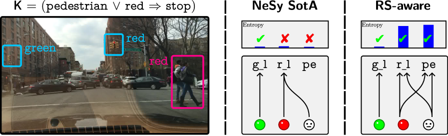5.4 Awareness Strategies <details> <summary>x6.png Details</summary>  ### Visual Description ## Image Analysis: Scene Understanding and Reasoning ### Overview The image presents a scene understanding and reasoning comparison between two approaches: "NeSy SotA" and "RS-aware". The image is divided into three sections. The left section shows a street scene with bounding boxes around objects, and an associated logical rule. The middle and right sections are diagrams representing the reasoning process of the two approaches, including entropy visualizations and connections between ground-level perceptions and higher-level concepts. ### Components/Axes **Left Section (Street Scene):** * **Image:** A photograph of a street scene with cars, buildings, traffic lights, and pedestrians. * **Bounding Boxes:** * A cyan box around a green traffic light, labeled "green". * A cyan box around a red traffic light, labeled "red". * A magenta box around two pedestrians, labeled "red". * **Logical Rule:** "K = (pedestrian ∨ red ⇒ stop)" **Middle Section (NeSy SotA):** * **Title:** "NeSy SotA" * **Entropy Visualization:** A horizontal bar with three segments. * First segment: A green checkmark. * Second segment: A red "X". * Third segment: A red "X". * Label: "Entropy" above the bar. * **Diagram:** * Labels: "g_l", "r_l", "pe" (likely representing green light, red light, and pedestrian, respectively) * Nodes: Green circle, red circle, and a smiley face icon. * Arrows: An arrow from the green circle to "g_l", an arrow from the red circle to "r_l", and a curved arrow from the smiley face to "r_l". **Right Section (RS-aware):** * **Title:** "RS-aware" * **Entropy Visualization:** A horizontal bar with three segments. * First segment: A green checkmark. * Second segment: A blue bar. * Third segment: A blue bar. * Label: "Entropy" above the bar. * **Diagram:** * Labels: "g_l", "r_l", "pe" * Nodes: Green circle, red circle, and a smiley face icon. * Arrows: An arrow from the green circle to "g_l", an arrow from the red circle to "r_l", and two crossing arrows, one from the smiley face to "r_l" and one from the red circle to "pe". ### Detailed Analysis or Content Details **Left Section (Street Scene):** * The street scene depicts a typical urban environment with traffic and pedestrians. * The bounding boxes highlight the objects of interest for the reasoning task: traffic lights and pedestrians. * The logical rule "K = (pedestrian ∨ red ⇒ stop)" states that the system should stop if there are pedestrians or the traffic light is red. **Middle Section (NeSy SotA):** * The entropy visualization shows a green checkmark for the first segment and red "X"s for the second and third segments. This suggests that the system correctly identifies the green light but fails to correctly identify the red light and pedestrian. * The diagram shows that the green light is correctly associated with "g_l", the red light is correctly associated with "r_l", but the pedestrian is incorrectly associated with "r_l" instead of "pe". **Right Section (RS-aware):** * The entropy visualization shows a green checkmark for the first segment and blue bars for the second and third segments. This suggests that the system correctly identifies the green light and also identifies the red light and pedestrian. * The diagram shows that the green light is correctly associated with "g_l", the red light is correctly associated with "r_l", and the pedestrian is correctly associated with "pe". ### Key Observations * The image compares the performance of two scene understanding and reasoning approaches. * "NeSy SotA" struggles to correctly identify the red light and pedestrian, while "RS-aware" performs better. * The entropy visualizations provide a measure of uncertainty for each approach. * The diagrams illustrate the connections between ground-level perceptions and higher-level concepts. ### Interpretation The image demonstrates the importance of robust scene understanding and reasoning for autonomous systems. The "NeSy SotA" approach, while being state-of-the-art, fails to correctly identify the red light and pedestrian, which could lead to dangerous situations. The "RS-aware" approach, on the other hand, performs better by correctly identifying the objects of interest and associating them with the appropriate concepts. This suggests that "RS-aware" is a more reliable approach for scene understanding and reasoning in this scenario. The logical rule "K = (pedestrian ∨ red ⇒ stop)" highlights the importance of safety in autonomous systems, as the system should stop if there are pedestrians or the traffic light is red. </details> Figure 10: NeSy predictors are not RS-aware (Marconato et al., 2024). Left: in the BDD-OIA autonomous driving task (Xu et al., 2020), NeSy predictors can achieve high accuracy and satisfy the prior knowledge even when they confuse pedestrians (ped) and red lights (red) (Marconato et al., 2023b). Right: An RS-aware predictor assigns high confidence to shortcut concepts, while giving low confidence to concepts not affected by RS. Another strategy for dealing with RSs is to make NeSy predictors aware of the RSs they are affected by. We say that a NeSy predictor is RS-aware if it picks a non-deterministic RS that exhibits high confidence for those predicted concepts that are not affected by RSs and low confidence for the others (Marconato et al., 2024). As customary, confidence can be assessed using the entropy of the predictive concept distribution $p({\bm{\mathrm{C}}}\mid{\bm{\mathrm{x}}})$ . While awareness does not reduce RSs, RS-aware models supply stakeholders with valuable insights into the quality of the learned concepts, helping them to identify and distrust predictions obtained with poorly ground concepts. To see this, consider the following example adapted from (Marconato et al., 2024): **Example 5.1** *The left NeSy predictor in Fig. 10 is not RS-aware: despite confusing pedestrians with red lights, it is highly certain about the concepts it predicts. The one on the right is equally confused, but it is also RS-aware, in that it is more uncertain about low-quality concepts (pedestrian and red lights) than about high-quality ones (green lights). This enables users to distinguish between these cases.* Moreover, meaningful uncertainty estimates are also a powerful tool for steering interactive acquisition of annotations (Section 5.5), which can substantially reduce the cost of supervised mitigation (see Section 5.3.1). RS-awareness is complementary to mitigation strategies: when all realistic mitigation strategies are exhausted, some RSs may still be present. Then RS-aware models will improve uncertainty quantification. Unfortunately, in practice, NeSy predictors are not RS-aware: they tend to be very confident even about poorly ground concepts (Marconato et al., 2024; van Krieken et al., 2025b). What sets awareness apart from sheer mitigation is that it is possible to make NeSy predictors RS-aware in a principled manner, but without concept supervision, as we will see. As mentioned in Section 5.3.4, a simple heuristic is to maximize the entropy of the predictive concept distribution. Is this always the best we can do? To answer this question, we will need to define RS-awareness. 5.4.1 RS-awareness as mixtures of deterministic RSs RS awareness can be understood as mixing over the set of deterministic RSs that the NeSy predictor is affected by (van Krieken et al., 2025a). We denote this set as $\mathrm{Vert}(\mathcal{A})_{\text{RS}}⊂eq\mathrm{Vert}(\mathcal{A})$ , and it can be seen as the set of “irreducible” deterministic RSs that are still present after exhausting the feasible mitigation strategies. Formally, we consider RS-aware NeSy predictors as distributions that “mix” over the concept remapping distributions (Eq. 20) induced by each irreducible deterministic RS ${\bm{\mathrm{a}}}∈\mathrm{Vert}(\mathcal{A})_{\text{RS}}$ . We achieve this using the convex combination of deterministic RSs from Eq. 22, where each weight $\lambda_{{\bm{\mathrm{a}}}}>0$ . The convex combination ensures each RS contributes to the final concept remapping distribution. The resulting distribution is itself a (nondeterministic) RS (Marconato et al., 2024, Lemma 1), and hence has perfect label accuracy. 5.4.2 Building RS-aware NeSy predictors How do we achieve such nondeterministic RSs in NeSy predictors? This usually requires that the space of learnable concept extractors $\mathcal{F}$ (Section 4.2.1) is powerful enough to model dependencies between different concepts (van Krieken et al., 2025a). However, many implementations of NeSy predictors use concept extractors that assume (when conditioned on the input ${\bm{\mathrm{x}}}$ ) the different concepts $C_{1},...,C_{k}$ are independent, i.e., $p(C_{1},...,C_{k}\mid{\bm{\mathrm{x}}})=\prod_{i=1}^{k}p(C_{i}\mid{\bm{\mathrm{x}}})$ (van Krieken et al., 2024a). NeSy predictors exploit the independence assumption for efficient inference (Darwiche and Marquis, 2002; van Krieken et al., 2023; Choi et al., 2025; De Smet et al., 2023a). However, it also greatly restricts the space of learnable concept extractors $\mathcal{F}$ . **Example 5.2 (Example in(van Krieken et al.,2025a))** *We consider the MNIST-XOR task where the NeSy predictor should predict the output of the XOR function applied to two MNIST digit. The XOR function returns 1 if the two input digits are different, and 0 otherwise. E.g., ${\bm{\mathrm{x}}}=\raisebox{-1.0pt}{∈cludegraphics[width=7.96527pt]{figures/mnist-1.png}}\raisebox{-1.0pt}{∈cludegraphics[width=7.96527pt]{figures/mnist-0.png}}$ gives $y=1$ , while ${\bm{\mathrm{x}}}=\raisebox{-1.0pt}{∈cludegraphics[width=7.96527pt]{figures/mnist-1.png}}\raisebox{-1.0pt}{∈cludegraphics[width=7.96527pt]{figures/mnist-1.png}}$ gives $y=0$ . This problem contains the shortcut $\raisebox{-1.0pt}{∈cludegraphics[width=7.96527pt]{figures/mnist-1.png}}\mapsto 0,\raisebox{-1.0pt}{∈cludegraphics[width=7.96527pt]{figures/mnist-0.png}}\mapsto 1$ (under disentanglement, Section 5.3.8). Given input ${\bm{\mathrm{x}}}=\raisebox{-1.0pt}{∈cludegraphics[width=7.96527pt]{figures/mnist-1.png}}\raisebox{-1.0pt}{∈cludegraphics[width=7.96527pt]{figures/mnist-0.png}}$ , an RS-aware NeSy predictor should assign 0.5 probability to both the ground-truth concept vector $(1,0)$ and the RS concept vector $(0,1)$ . If we would try to model this distribution with the independence assumption, we find that $p(C_{1}=1\mid{\bm{\mathrm{x}}})=p(C_{2}=1\mid{\bm{\mathrm{x}}})=0.5$ . But then $p(C_{1}=1,C_{2}=1\mid{\bm{\mathrm{x}}})=p(C_{1}=1\mid{\bm{\mathrm{x}}})· p(C_{2}=1\mid{\bm{\mathrm{x}}})=0.25$ , i.e., it assigns probability to a concept vector that does not give the correct output label. Hence, the resulting distribution is not an RS, and might make incorrect label predictions.* In general, van Krieken et al. (2025a) proves that the independence assumption prevents models from being aware of RSs for most inference layers. Motivated by these results, we discuss two recent methods that go beyond the independence assumption to build RS-aware NeSy predictors. 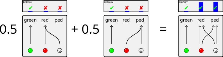<details> <summary>x7.png Details</summary>  ### Visual Description ## Diagram: Weighted Sum of State Transitions ### Overview The image depicts a diagram illustrating a weighted sum of state transitions, likely in the context of a Markov process or similar probabilistic model. It shows two separate transition diagrams, each weighted by 0.5, which are then combined to produce a final transition diagram. Each individual diagram represents transitions between three states: "green," "red," and "ped" (pedestrian). The "Entropy" above each diagram indicates the uncertainty associated with each state distribution. ### Components/Axes * **Diagram Structure:** The image is divided into three main sections, representing the two initial diagrams and their combined result. Each diagram is enclosed in a gray box. * **States:** Each diagram represents three states: "green," "red," and "ped" (pedestrian). These states are labeled at the top of each box. * **State Indicators:** Below each state label, there is a visual representation of the state: a green circle for "green," a red circle for "red," and a smiley face for "ped." * **Transitions:** Transitions between states are represented by arrows. The shape and direction of the arrows indicate the probability and direction of the transition. * **Weights:** The diagrams are weighted by "0.5" and "+ 0.5," indicating that each contributes equally to the final result. * **Entropy Indicators:** Above each diagram, there is a small chart labeled "Entropy." This chart shows the entropy associated with each state. The entropy is represented by a blue bar, and a green checkmark or red "X" indicates whether the entropy is low or high, respectively. ### Detailed Analysis **Left Diagram (Weighted by 0.5):** * **Entropy:** Low entropy for "green" (checkmark), high entropy for "red" and "ped" (X marks). * **Transitions:** * "green" transitions directly to "green" (straight upward arrow). * "red" transitions to "ped" (curved arrow from "red" to "ped"). **Middle Diagram (Weighted by + 0.5):** * **Entropy:** Low entropy for "green" (checkmark), high entropy for "red" and "ped" (X marks). * **Transitions:** * "green" transitions directly to "green" (straight upward arrow). * "red" transitions to "ped" (curved arrow from "red" to "ped"). **Right Diagram (Result):** * **Entropy:** Low entropy for all three states: "green," "red," and "ped" (checkmark for each). The entropy is represented by blue bars. * **Transitions:** * "green" transitions directly to "green" (straight upward arrow). * "red" transitions directly to "red" (straight upward arrow). * "ped" transitions directly to "ped" (straight upward arrow). * "red" transitions to "ped" (curved arrow from "red" to "ped"). * "ped" transitions to "red" (curved arrow from "ped" to "red"). ### Key Observations * The initial diagrams have high entropy for "red" and "ped," indicating uncertainty in those states. * The final diagram has low entropy for all states, suggesting that the combination of the initial diagrams has reduced the overall uncertainty. * The transitions in the final diagram represent a combination of the transitions in the initial diagrams. ### Interpretation The diagram illustrates how combining multiple probabilistic models (represented by the initial diagrams) can lead to a more deterministic model (represented by the final diagram). The weighting of 0.5 for each initial diagram suggests that they are equally important in determining the final state transitions. The reduction in entropy from the initial diagrams to the final diagram indicates that the combined model is more predictable and less uncertain. The transitions in the final diagram show a complex interplay between the "red" and "ped" states, with transitions occurring in both directions. This could represent a situation where the "red" state influences the "ped" state, and vice versa. </details> Figure 11: Intuition behind bears. bears (Marconato et al., 2024) constructs ensembles of concept predictors that employ different sets of concepts to solve the task. Concepts that need to be learned correctly have to match across models, while those that cannot will have different groundings. As a result, averaging their predictions increases uncertainty only where disagreement exists. 5.4.3 RS-Awareness via Ensembles bears (Marconato et al., 2024) is a model-agnostic technique for making NeSy predictors RS-aware. bears replaces the concept extractor with an ensemble of concept extractors, each using the independence assumption. bears constructs this ensemble specifically such that each member captures a different deterministic RS in $\mathrm{Vert}(\mathcal{A})_{\text{RS}}$ . This construction has ties with Bayesian deep learning techniques (Wang and Yeung, 2020; Daxberger et al., 2021; Osawa et al., 2019; Lakshminarayanan et al., 2017; Gal and Ghahramani, 2016) but it is also backed by a separate theoretical setup (Marconato et al., 2024). For instance, in BDD-OIA (Example 3.3) one extractor might conflate pedestrians with red lights, while another might do the opposite, as in Fig. 11 (left). bears computes the predictive concept distribution by averaging over all extractors in the ensemble. Intuitively, this works for two reasons. First, if all extractors have high label accuracy, their average will as well (Eq. 22). Second, the concept entropy of the ensemble hinges on the semantics associated by the different extractors to the concepts themselves. Then, the ensemble has high entropy for concepts are affected by RSs – like pedestrian and red light – as different extractors each learn different semantics. For unaffected concepts – like green light – the extractors agree on their semantics and the ensemble has low entropy. This intuition is illustrated in Fig. 11 (right). In practice, bears extends deep ensembles (Lakshminarayanan et al., 2017) with a loss term that encourages ensemble members to model different RSs, and an entropy term (reminiscent of Section 5.3.4) that spreads concept predictions. Compared to other Bayesian deep learning methods, such as MC dropout (Gal and Ghahramani, 2016) and the Laplace approximation (Daxberger et al., 2021), deep ensembles allow learning highly multi-modal distributions, making them an excellent choice for learning multiple, diverse RSs. This is supported by experiments, which show that bears significantly improves RS-awareness of NeSy architectures on different tasks and that it does so better than other Bayesian alternatives (Marconato et al., 2024). One downside of bears is that it requires learning an ensemble of concept extractors. Fortunately, small ensembles of $5$ to $10$ members were shown to be sufficient in practice. 5.4.4 RS-Awareness via Diffusion Motivated by going beyond the independence assumption, NeSyDM (van Krieken et al., 2025b) uses expressive discrete diffusion models as concept extractors. Unlike bears, it trains a single concept extractor $p({\bm{\mathrm{C}}}\mid{\bm{\mathrm{x}}})$ via masked diffusion models (MDMs) (Austin et al., 2021; Sahoo et al., 2024). MDMs start with a concept vector that consists entirely of masks. Masks essentially indicate we do not yet know what the value of the concept should be. Then, MDMs are tasked with iteratively unmasking the various concepts. The main motivation for using MDMs to go beyond independence is scalability: each unmasking step can be seen as a concept extractor with the independence assumption. Hence, NeSyDM can directly reuse existing inference methods that exploit the independence assumption. NeSyDM consists of three loss components. The first loss aims to unmask partially masked concept, the second unmasks partially masked labels, and the final loss encourages high entropy among the concepts. One benefit compared to bears is that NeSyDM ’s only train a single model, preventing the need to choose the ensemble size. Experimentally, NeSyDM also matches or improves on calibration and out-of-distribution concept accuracy compared to bears. 5.5 Awareness Helps Mitigation To support mitigation strategies, specifically concept supervision (discussed in Section 5.3.1), one can leverage human input to request targeted annotations. This idea is well established in the field of Interactive Machine Learning (Ware et al., 2001; Fails and Olsen, 2003; Amershi et al., 2014; Teso and Kersting, 2019). In the context of RSs, the most relevant method explored so far is Active Learning (Settles, 2012), which we briefly describe below. Active Learning Rather than relying on costly full supervision, Active Learning (Settles, 2012) allows a model to interactively query a human (or oracle) for labels on the most informative or uncertain examples. The core idea is to focus annotation efforts where they are most impactful, thereby improving model performance while minimizing human effort. As demonstrated in (Marconato et al., 2024), uncertainty estimates over concepts – provided by bears (see Section 5.4) or NeSyDM (van Krieken et al., 2025b) (see Section 5.4.4) – can be used to identify and query the most uncertain concepts, effectively addressing RSs with fewer annotations on concepts. This targeted strategy outperforms traditional active learning methods, such as querying concept uncertainty in PNSPs, where the uncertainty signal is often uninformative (Marconato et al., 2024). 6 Extensions and Open Problems In this section, we discuss RSs in contexts beyond those studied in this paper, and outline potential extensions and open research problems. 6.1 Reasoning Shortcuts in NeSy AI Beyond Predictors RSs stem from the intrinsic ambiguity of logic inference when the prior knowledge $\mathsf{K}$ admits inferring the ground-truth label from unintended concepts. This suggests that RSs arise regardless of how the reasoning step is implemented, that is, also for NeSy architectures beyond the four predictors we considered here. Models like DPL and LTN are full-fledged first-order programming languages, i.e., they can handle first-order logic specifications and work with a variable number of logic entities and concepts. Given that RSs affect them in the propositional case and that FOL is a strict generalization of propositional logic, we can safely assume that RSs exist also in the FOL case. E.g., RSs plausibly affect extensions of these models, such as (Huang et al., 2021a; Winters et al., 2022; De Smet et al., 2023b; Badreddine et al., 2023), as well as predictors that combine probabilistic and fuzzy semantics, like NeuPSL (Pryor et al., 2022), models that embed symbols into continuous vector spaces, such as neural theorem provers with fuzzy semantics (Rocktäschel and Riedel, 2016) and probabilistic semantics (Maene and Raedt, 2023), models that implement hard constraints with fuzzy logic, such as (Giunchiglia and Lukasiewicz, 2020; Giunchiglia et al., 2024), and diffusion-based models (van Krieken et al., 2025b). Moreover, RSs have also been identified in SatNet (Wang et al., 2019; Simard et al., 1991), an architecture that performs perception and reasoning entirely in embedding space. This leads us to postulate that—barring implicit mitigation due to the use of reconstruction penalties, see Section 5.3.6 —RSs might also affect generative NeSy models, such as (Misino et al., 2022; Ferber et al., 2024). While it is likely that RSs affect a broad class of NeSy architectures, more work is needed to extend the existing theoretical frameworks and mitigation strategies to these models. 6.2 Reasoning Shortcuts in Concept-based Models So far, we only considered NeSy predictors where the prior knowledge $\mathsf{K}$ , and therefore the inference layer, is supplied externally and fixed. Recently, RSs have also been studied in two related families of models whose inference layer is learned (Bortolotti et al., 2025): i) NeSy modular predictors that acquire the knowledge from data, and ii) Concept-based Models (CBMs), which pair a concept extractor with an interpretable (typically linear) inference layer (Koh et al., 2020; Espinosa Zarlenga et al., 2022; Marconato et al., 2022; Schwalbe, 2022; Poeta et al., 2023). It was shown that, without the aid of concept supervision, these models suffer from joint reasoning shortcuts (JRSs): failure modes involving extracting wrong concepts and/or wrong logical assignments that lead to correct label predictions (see Example 6.1 for an example). **Example 6.1 (MNIST-SumParity)** *To provide an example, imagine a variant of MNIST-Add where the goal is to predict whether the sum of two digits is odd or even, that is, $Y=(C_{1}+C_{2})\!\mod 2$ . Suppose that the training set includes only examples for which $C_{2}$ is odd. A possible JRS amounts to mapping all even digits to $0$ , i.e., $\{\raisebox{-1.0pt}{∈cludegraphics[width=7.96527pt]{figures/mnist-0.png}},\raisebox{-1.0pt}{∈cludegraphics[width=7.96527pt]{figures/mnist-2.png}},\raisebox{-1.0pt}{∈cludegraphics[width=7.96527pt]{figures/mnist-4.png}},\raisebox{-1.0pt}{∈cludegraphics[width=7.96527pt]{figures/mnist-6.png}},\raisebox{-1.0pt}{∈cludegraphics[width=7.96527pt]{figures/mnist-8.png}}\}\mapsto 0$ , and all odd digits to $1$ , i.e., $\{\raisebox{-1.0pt}{∈cludegraphics[width=7.96527pt]{figures/mnist-1.png}},\raisebox{-1.0pt}{∈cludegraphics[width=7.96527pt]{figures/mnist-3.png}},\raisebox{-1.0pt}{∈cludegraphics[width=7.96527pt]{figures/mnist-5.png}},\raisebox{-1.0pt}{∈cludegraphics[width=7.96527pt]{figures/mnist-7.png}},\raisebox{-1.0pt}{∈cludegraphics[width=7.96527pt]{figures/mnist-9.png}}\}\mapsto 1$ . Consistently, the learned knowledge is the difference among the predicted digits $\hat{Y}=\hat{C}_{1}-\hat{C}_{2}$ , as it would return the very same labels as using $Y=(C_{1}+C_{2})\!\mod 2$ . In contrast to regular RSs, here both the concepts and the learned knowledge are “wrong”, with the result that in the OOD setting where $C_{2}$ includes even digits, the learned model can predict $\hat{Y}=-1$ (see Fig. 12 for a visual representation).* All RSs can also be viewed as JRSs, but the opposite is not true: the set of learnable JRSs can vastly outnumber that of regular RSs (Bortolotti et al., 2025). For example, permuting concept values does not alter the concept semantics and the learned rules, leading to equivalent solutions upon renaming the extracted concepts. Specifically, since concepts are anonymous during training, they can be easily aligned to ground-truth concepts at test time by leveraging annotations. This, however, is not possible if a joint-RS is learned by the model (Bortolotti et al., 2025). Counting RSs can be adapted to joint-RSs, and an equivalent result to Theorem 4.12 also holds when $\mathsf{K}$ is learned, showing that dealing with deterministic joint-RSs is, in many cases, sufficient to rule out all joint-RSs. However, the benefits of many mitigation strategies for RSs discussed in Section 5.3 do not transfer to joint-RSs. Supervised strategies, like concept supervision and multi-tasking learning, offer some improvement but are insufficient to address all joint-RSs. In particular, concept supervision can lead to high concept accuracy, yet it does not necessarily return the correct knowledge. It is unknown whether more powerful strategies for combating JRSs exist, and a theoretical characterization of JRSs from a statistical learning perspective is currently missing. In the context of RSs, investigating the scenario where learned concept vectors ( ${\bm{\mathrm{c}}}∈\mathcal{C}$ ) and ground-truth concept vectors ( ${\bm{\mathrm{g}}}∈\mathcal{G}$ ) belong to different spaces, i.e., $\mathcal{C}≠\mathcal{G}$ , is open and so far not explored. Considering two different spaces $\mathcal{C}$ and $\mathcal{G}$ results in having the NeSy predictor inference layer $\beta$ structurally different from $\beta^{*}$ , because of the different mapping domain. This setting naturally draws a connection between RSs and JRSs, where in the latter a concept-based model may learn to use fewer concepts in the bottleneck and fine-tune a $\beta≠\beta^{*}$ that still matches label predictions. In this sense, because NeSy predictors $(f,\beta)$ have $\beta≠\beta^{*}$ , one has to check if learned concepts and the inference layer possess (a variation of) the intended semantics (Bortolotti et al., 2025, Definition 3.3) We expect that, in this scenario, RSs can likely increase due to mismatch between the NeSy predictor’s and the ground-truth knowledge. <details> <summary>x8.png Details</summary>  ### Visual Description ## Diagram: Neural Network Architectures for Odd Number Detection ### Overview The image presents three distinct neural network architectures designed to determine if the ratio of two numbers (7 and 2) is odd. Each architecture consists of an input (the fraction 7/2), a neural network (NN) component, and an output component (β). The architectures differ in the internal processing within the NN and the final operation performed to determine the "odd" status. ### Components/Axes * **Input:** The fraction 7/2, represented visually as the numbers stacked on top of each other. * **Neural Network (NN) Component:** A blue trapezoidal shape labeled "NN" (with a "*" superscript in the first architecture). This represents the neural network processing the input. * **Output Component (β):** A trapezoidal shape labeled "β" (with a "*" superscript in the first two architectures), representing the final output stage. The color of this component varies: red in the first two architectures and purple in the third. * **Output Vector:** A vector of two numbers, either [7, 2] or [1, 0], representing the internal state after the NN component. * **Odd Label:** The word "odd" indicates the final classification result. * **Mathematical Formula:** Each architecture is accompanied by a formula: * Architecture 1 & 2: y = (c₁ + c₂) mod 2 * Architecture 3: y = (c₁ - c₂) ### Detailed Analysis **Architecture 1 (Left)** * **Input:** 7/2 * **NN Component:** Labeled "NN*" (blue). * **Output Vector:** [7, 2] * **Output Component:** Labeled "β*" (red). * **Output:** "odd" * **Formula:** y = (c₁ + c₂) mod 2 **Architecture 2 (Middle)** * **Input:** 7/2 * **NN Component:** Labeled "NN" (blue). * **Output Vector:** [1, 0] * **Output Component:** Labeled "β*" (red). * **Output:** "odd" * **Formula:** y = (c₁ + c₂) mod 2 **Architecture 3 (Right)** * **Input:** 7/2 * **NN Component:** Labeled "NN" (blue). * **Output Vector:** [1, 0] * **Output Component:** Labeled "β" (purple). * **Output:** "odd" * **Formula:** y = (c₁ - c₂) ### Key Observations * All three architectures correctly classify 7/2 as "odd". * The first architecture uses a different internal representation ([7, 2]) compared to the other two ([1, 0]). * The first two architectures use the same formula (y = (c₁ + c₂) mod 2), while the third uses a different formula (y = (c₁ - c₂)). * The color of the output component (β) changes between the architectures, potentially indicating a different type of processing or output representation. ### Interpretation The diagram illustrates different ways a neural network can be structured to solve the same classification problem (determining if a number is odd). The variations in the internal representation (output vector) and the final calculation (formula) highlight the flexibility of neural networks. The change in color of the output component (β) might signify different activation functions or output encoding schemes used in each architecture. The fact that all architectures arrive at the same correct classification ("odd") demonstrates that multiple valid solutions can exist for a given problem within the neural network paradigm. The "*" superscript on NN and Beta in the first two architectures may indicate a specific configuration or training method applied to those components. </details> Figure 12: Example of Joint Reasoning Shortcuts. The task is to predict whether the sum of two MNIST digits is odd, using training data that cover all (even, even), (odd, odd), and (odd, even) pairs. Red denotes fixed knowledge, purple denotes learned knowledge. In all the presented cases, the models achieve optimal performance. Left: ground-truth concepts with the correct inference layer. Middle: NeSy model with prior knowledge may still learn shortcuts by assigning unintended semantics to concepts. Right: CBMs, both concepts and the inference layer are misaligned, resulting in joint reasoning shortcuts. Note: In both of the previous cases, the OOD setting (even, odd) produces a consistent prediction, whereas the joint reasoning shortcut yields $-1$ as the predicted value. 6.3 Foundation and Large Language Models An interesting direction for future research is to investigate the connection between RSs and foundation models (Bommasani et al., 2021; Radford et al., 2021). Several recent approaches already leverage information elicited from foundation models to prime NeSy (Stammer et al., 2024) and concept-based architectures (Oikarinen et al., 2022; Yang et al., 2023b; Rao et al., 2024; Srivastava et al., 2024; Yuksekgonul et al., 2023), e.g., using pre-trained representations or weak concept annotations obtained by prompting visual-language models. Clearly, the benefit is that foundation models are trained on vast amounts of data, which allow covering a large support of (potentially new) inputs, and are multimodal — allowing to use concept textual description to estimate the concepts in the data. Moreover, we expect that pre-training implicitly implements some of the RS mitigation strategies we outlined: concept supervision (Section 5.3.1) and multi-task learning (Section 5.3.2). In fact, it is quite likely that some elementary concepts, like the color or shape of objects, need to be separated in model representations to allow them to match a huge amount of image-caption pairs (e.g., from the Web Image Text dataset (Srinivasan et al., 2021)). For these reasons, it is plausible that, depending on the domain, foundation models may produce useful, high-quality concepts. Empirical evidence, however, calls for caution. Recent findings (Debole et al., 2025; Wüst et al., 2025) in the context of VLM-augmented CBMs indicate that foundation models can fail to identify some basic visual concepts. In addition, they may fall short due to issues such as hallucinations (Huang et al., 2024), shortcuts (Yuan et al., 2024), and limited logical (Calanzone et al., 2025) and conceptual consistency (Sahu et al., 2022). In a direction closely related to RSs, Stein et al. (2025) have shown that foundation models are affected by symbol hallucinations, a phenomenon where models prompted to generate concepts and executable programs to solve a task end up hallucinating poorly ground symbols that still manage to achieve high accuracy. Intuitively, symbol hallucinations can be thought as the analog of RSs for prompting (although, they have not been characterized so far). An important direction is to prove whether foundation models themselves are affected by (joint) RSs proper, but we expect that the current theory need to be extended to also treat models that cannot be described as NeSy predictors. Attempts to provide identifiability guarantees for concept learning in model representations (among which those of foundation models) have recently surfaced (Zheng et al., 2025; Liu et al., 2025; Rajendran et al., 2024), but it remains to be understood how this relates to shortcuts when these guarantees are not given. Reasoning shortcuts have also been studied in language modelling, though with a different extent from the one of this paper. In question answering, multi-hop reasoning is the model’s ability to answer a question by combining information from multiple pieces of evidence rather than relying on a single fact (Yang et al., 2018). As an example of two-hop reasoning, we would expect that to answer the question “In which city of the Orange Free State was the author of The Lord of the Rings born?”, the model first has to identify J. R. R. Tolkien as the author of The Lord of the Rings, and second has to determine that Tolkien was born in Bloemfontein, which is in the Orange Free State. Jiang and Bansal (2019) found that when models are trained on certain multi-hop QA datasets, such as HotpotQA (Yang et al., 2018), they often exploit shortcuts that allow them to return correct answers by matching keywords or surface patterns in the question and context, without performing the intended multi-hop reasoning steps. In this context, the authors refer to it as a reasoning shortcut for the model. For instance, in the example above, an incorrect reasoning step consists of predicting Bloemfontein just because of the presence of ”the Orange Free State”. Although these unintended solutions differ from the reasoning shortcuts discussed in our manuscript, they can be related to joint reasoning shortcuts, whereby correct concept assignments are given but the learned knowledge fails to capture the ground-truth. Making this link concrete is open and is an important research direction. 6.4 Reasoning Shortcuts in Reinforcement Learning NeSy reinforcement learning (RL) (Acharya et al., 2024) is a new field in which logical knowledge is integrated into the interactive reinforcement learning workflow for various purposes, including guiding exploration (Anderson et al., 2020), ensuring safe trajectories (Yang et al., 2023c), improving explainability (Baugh et al., 2025; Deane and Ray, 2025), performance (Umili et al., 2024b; Mitchener et al., 2022), or generalization to new environments (Garnelo et al., 2016; Badreddine and Spranger, 2019). Most of the works consider environments with symbolic observations, where grounding symbols or concepts is not required. A smaller set, instead, tackles more realistic environments by discretizing or clustering the neural features extracted from high-dimensional inputs (Umili et al., 2021; Garnelo et al., 2016; Hafner et al., 2021). In such cases, the extracted concepts lack a predefined meaning, potentially limiting the human interpretability of the agent’s behavior. Only a few works have investigated embedding prior symbolic knowledge into RL policy learning (Badreddine and Spranger, 2019; Umili et al., 2024b; Amador and Gierasimczuk, 2025). While reasoning shortcuts are still relatively underexplored in NeSy RL, first studies in this direction have already proven valuable for: (i) certifying the quality of learned concepts and its reusability in single-task vs. multitask settings (Umili et al., 2024b), and (ii) improving the explainability of NeSy-RL agents when knowledge is learned rather than injected (Umili and Capobianco, 2025). Badreddine and Spranger (2019) and Amador and Gierasimczuk (2025) focus on solving the RL environment introduced in (Garnelo et al., 2016) and shown in Fig. 13 (Left). They both employ a NeSy shape recognizer exploiting knowledge encoded in LTN. In these works, RSs do not appear because they rely on mitigation strategies specifically tailored to that particular environment, such as the use of pretrained shape detectors in (Badreddine and Spranger, 2019), the additional knowledge of the environment model in (Amador and Gierasimczuk, 2025), and patch discretization in both works. 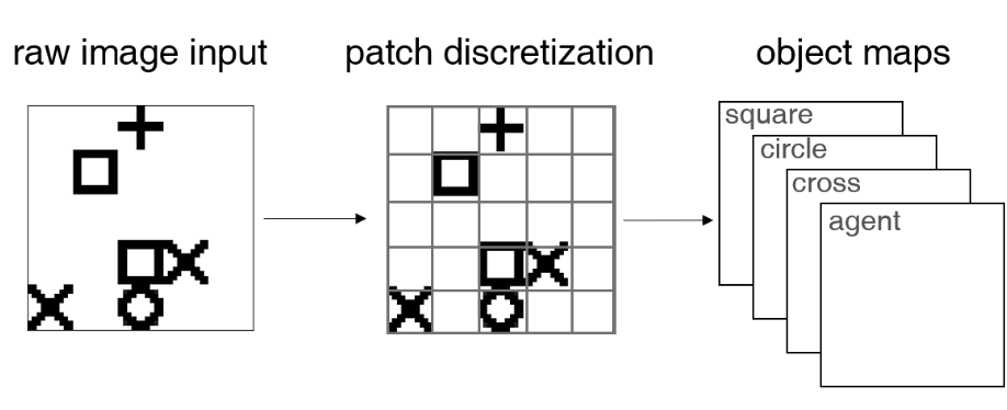| <details> <summary>figures/plus_env_2.png Details</summary>  ### Visual Description ## Diagram: Image Processing Pipeline ### Overview The image illustrates a simplified image processing pipeline. It shows the transformation of a raw image input through patch discretization into object maps. The pipeline consists of three stages: raw image input, patch discretization, and object maps. ### Components/Axes * **Titles:** * raw image input * patch discretization * object maps * **Objects in raw image input:** * cross * square * circle * x * **Objects in patch discretization:** * cross * square * circle * x * **Object maps:** * square * circle * cross * agent * **Arrows:** Two arrows indicate the flow of information from left to right. ### Detailed Analysis The diagram shows the transformation of a raw image into object maps. 1. **Raw Image Input:** The raw image contains a collection of simple shapes: a cross, a square, a circle, and an "x". These shapes are arranged in a seemingly random configuration. 2. **Patch Discretization:** The raw image is then discretized into a grid of patches. The shapes from the raw image are now represented within this grid. The grid appears to be 6x6. 3. **Object Maps:** Finally, the discretized image is transformed into a series of object maps. Each object map corresponds to a specific object type (square, circle, cross, agent). These maps likely represent the probability or confidence of each patch containing the corresponding object. ### Key Observations * The diagram simplifies the process of object recognition by breaking it down into distinct stages. * The patch discretization stage is crucial for converting the continuous raw image into a discrete representation suitable for further processing. * The object maps represent the final output of the pipeline, providing information about the location and type of objects present in the image. ### Interpretation The diagram illustrates a basic image processing pipeline for object recognition. The raw image is first discretized into patches, and then object maps are generated for each object type. This pipeline demonstrates a common approach to object recognition, where the image is first preprocessed to extract relevant features, and then these features are used to identify objects. The "agent" object map suggests the system might be designed to identify agents or actors within the scene, implying a potential application in robotics or autonomous systems. The transformation from raw pixels to discrete patches and then to object-specific maps highlights a hierarchical approach to image understanding. 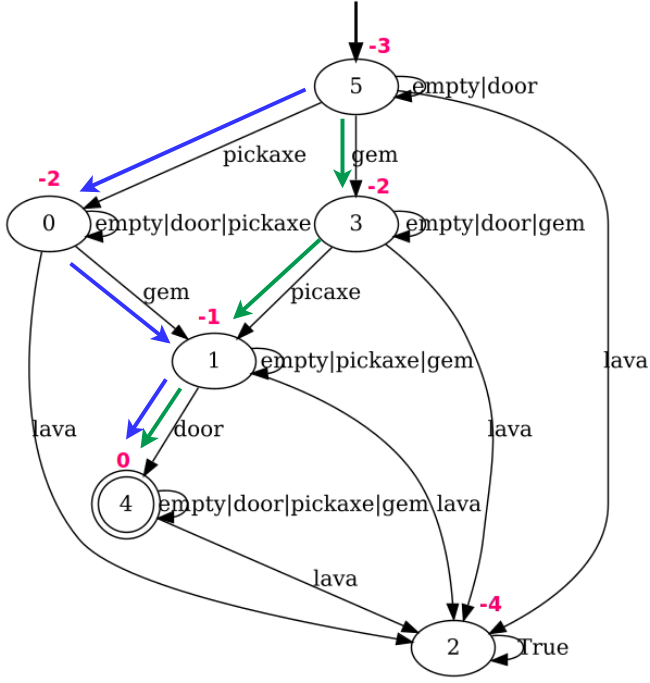</details> | | | <details> <summary>figures/reward_machine_trajectories_2.png Details</summary>  ### Visual Description ## State Transition Diagram: Resource Acquisition ### Overview The image is a state transition diagram representing a system that transitions between states based on resource acquisition and environmental factors. The diagram consists of nodes representing states, and directed edges representing transitions between states, labeled with the conditions that trigger the transition and associated costs. ### Components/Axes * **Nodes:** Represented by circles, each labeled with a number (0, 1, 2, 3, 4, 5) indicating the state. State 4 is a double circle, indicating it is an accepting state. * **Edges:** Directed arrows connecting the nodes, indicating possible transitions between states. Each edge is labeled with a condition (resource or event) and a cost (shown in magenta). * **Conditions:** Text labels on the edges, indicating the resources or events that trigger the transition (e.g., "empty|door|pickaxe", "gem", "lava"). * **Costs:** Numerical values in magenta near the edges, representing the cost associated with the transition (e.g., -1, -2, -3, -4, 0). * **Colors:** Edges are colored either blue or green. ### Detailed Analysis * **State 5:** * Initial state, indicated by an incoming arrow from the top. * Transition to State 3 (green arrow) with condition "gem" and cost -2. * Transition to State 0 (blue arrow) with condition "pickaxe" and cost -2. * Self-loop with condition "empty|door" and no cost indicated. * **State 3:** * Transition to State 1 (green arrow) with condition "picaxe" and cost -1. * Transition to State 2 (black arrow) with condition "lava" and no cost indicated. * Self-loop with condition "empty|door|gem" and no cost indicated. * **State 0:** * Transition to State 1 (blue arrow) with condition "gem" and cost -1. * Transition to State 4 (blue arrow) with condition "door" and cost 0. * Self-loop with condition "empty|door|pickaxe" and no cost indicated. * **State 1:** * Transition to State 2 (black arrow) with condition "lava" and no cost indicated. * Self-loop with condition "empty|pickaxe|gem" and no cost indicated. * **State 4:** * Accepting state (double circle). * Transition to State 2 (black arrow) with condition "lava" and no cost indicated. * Self-loop with condition "empty|door|pickaxe|gem|lava" and no cost indicated. * **State 2:** * Transition to itself (self-loop) with condition "True" and cost -4. ### Key Observations * The diagram represents a system where the state changes based on acquiring resources ("gem", "pickaxe", "door") or encountering environmental factors ("lava"). * Transitions have associated costs, indicated by the magenta numbers. * State 4 is the accepting state, suggesting a successful outcome. * The "empty" condition appears in conjunction with other resources, possibly indicating the absence of those resources. * The "True" condition on the self-loop of State 2 suggests a stable state that is maintained indefinitely with a cost. ### Interpretation The state transition diagram models a resource acquisition process. The system starts in State 5 and transitions between states based on the availability of resources like "gem", "pickaxe", and "door", and the presence of "lava". The magenta numbers represent the cost associated with each transition, which could be interpreted as energy expenditure, risk, or other negative consequences. The goal of the system appears to be reaching State 4, the accepting state, which likely represents a successful completion of the resource acquisition task. The self-loop in State 2 with the "True" condition and a cost of -4 suggests a state where the system is stuck in a loop, continuously incurring a cost without progressing towards the goal. The blue and green arrows may represent different types of actions or strategies for acquiring resources. The diagram provides a visual representation of the possible states, transitions, and costs involved in the resource acquisition process, allowing for analysis and optimization of the system's behavior. 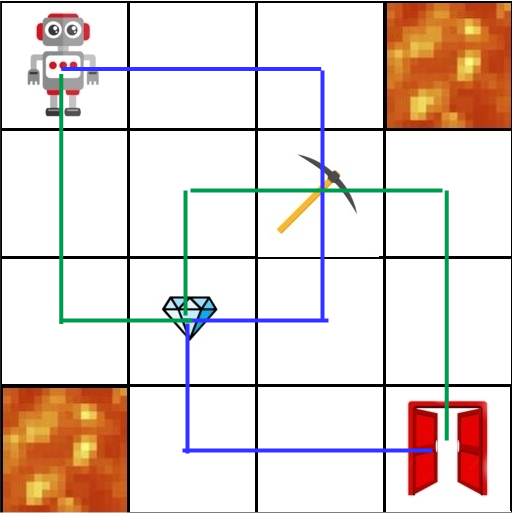</details> | <details> <summary>figures/nesy_env_ltl.png Details</summary>  ### Visual Description ## Diagram: Robot Path Planning ### Overview The image depicts a 6x6 grid representing a path-planning scenario for a robot. The robot starts at the top-left corner and needs to navigate to a door located at the bottom-right corner. The grid also contains obstacles (lava), a diamond, and a pickaxe. Two distinct paths are shown: a blue path and a green path. ### Components/Axes * **Grid:** A 6x6 grid structure forming the base of the diagram. * **Robot:** Located in the top-left cell. * **Door:** Located in the bottom-right cell. * **Lava:** Located in the top-right and bottom-left cells. * **Diamond:** Located in the center-left area. * **Pickaxe:** Located in the center-right area. * **Blue Path:** A path marked in blue, starting from the robot, passing by the diamond, and ending at the door. * **Green Path:** A path marked in green, starting from the robot, passing by the pickaxe, and ending at the door. ### Detailed Analysis * **Robot's Starting Position:** Top-left cell (row 1, column 1). * **Door's Final Position:** Bottom-right cell (row 6, column 6). * **Lava Locations:** Top-right cell (row 1, column 6) and bottom-left cell (row 6, column 1). * **Diamond Location:** Row 4, column 2. * **Pickaxe Location:** Row 2, column 4. * **Blue Path:** * Starts at the robot (1,1). * Moves down to (2,1). * Moves right to (2,2). * Moves down to (4,2) where the diamond is located. * Moves right to (4,6). * Moves down to (6,6) where the door is located. * **Green Path:** * Starts at the robot (1,1). * Moves right to (1,4). * Moves down to (2,4) where the pickaxe is located. * Moves left to (2,1). * Moves down to (6,1). * Moves right to (6,6) where the door is located. ### Key Observations * The robot has two possible paths to reach the door. * The blue path involves collecting the diamond. * The green path involves collecting the pickaxe. * Both paths avoid the lava cells. * The paths intersect at the starting and ending points. ### Interpretation The diagram illustrates a simple path-planning problem where a robot needs to navigate a grid to reach a destination while potentially collecting items along the way. The two paths represent different strategies: one prioritizing the diamond and the other prioritizing the pickaxe. The presence of lava cells introduces constraints that the robot must avoid. The diagram could be used to demonstrate basic concepts in robotics, pathfinding algorithms, and decision-making under constraints. </details> | | --- | --- | --- | --- | --- | Figure 13: (Left) Environment introduced in (Garnelo et al., 2016) and mainly used in (Badreddine and Spranger, 2019; Amador and Gierasimczuk, 2025). The agent (+ sign) has to maximize the sum of rewards by collecting shapes, each shape gives a different immediate reward. In both works, they use a sort of soft knowledge injection that is biased for this specific environment: they divide the input image into 25 patches (one per grid cell), and the shape recognizer classifies each patch singularly. (Right) Environment introduced in (Umili et al., 2024b) for temporally extended visual tasks. The agent has to maximize the reward on the automaton. It changes automaton state by reaching specific items in the environment. On the left side, the automaton for the task ”reach the pickaxe and the gem before the door, while always avoiding the ” lava ”, is displayed.On the rightmost side, a visualization of the environment is portrayed. In green and blue two optimal trajectories causing the indistinguishability of symbols ” pickaxe ” and ” gem ” due to the structure of the task. A more recent work in NeSy-RL (Umili et al., 2024b) explicitly investigates reasoning shortcuts through neural reward machines (NRMs). There, the RL agent learns to solve temporally extended tasks expressed in linear temporal logic over finite traces (LTLf) (Giacomo and Vardi, 2013) formulas. Fig. 13 (Right) illustrates an example of such a task. NRMs encode temporal knowledge through a probabilistic relaxation of the deterministic finite automaton (DFA) equivalent to LTLf task. Here, the only bias is that rewards are shaped accordingly to the automaton: reward is maximum at the automaton’s accepting states (reachable only by satisfying trajectories) and reduced elsewhere. This is a minimal bias that allows applying the framework to diverse environments and tasks without any change in the framework. In the context of the example of Fig. 13, green and blue trajectories correspond to equivalent solutions for the agent, which may induce the agent to swap the concepts ‘‘gem’’ and ‘‘pickaxe’’, resulting in an RS. Moreover, in (Umili et al., 2024b) an efficient algorithm to identify all reasoning shortcuts that depend on the temporal logical specification is introduced, allowing to count RSs over three order of magnitude faster than a brute-force baseline. While the brute-force baseline constructs all possible $\alpha$ ’s in $\mathrm{Vert}(\mathcal{A})$ , the algorithm introduced in (Umili et al., 2024b) exploits common properties of RL tasks, such as terminal states and self-loop transitions in automata, to reduce the space of the search. Applying this algorithm to the LTLf formulas commonly used in non-Markovian RL showed an extremely high number of RSs. Interestingly, in single-task RL, these RSs do not harm learning performance, since they involve only concept renamings and do not induce any concept collapse. Thus, all task-relevant concepts remain distinguished, but they may be swapped. However, this swap can harm transferring the learned concepts to new multitask settings (Kuo et al., 2021). A follow-up work (Dewidar and Umili, 2025) extends NRMs to the cases where the task logical knowledge is not provided a priori: both the knowledge and the concepts are learned directly from exploration data (Umili and Capobianco, 2025). It investigates an algorithm to jointly minimize the automaton states and concepts learned via RSs detection, yielding a knowledge that is significantly more compact and explainable. Future research can likely explore RSs in multitask generalization. In this context, prior knowledge is increasingly used to automatically generate new environments and tasks (Team et al., 2021; Bauer et al., 2023), making it timely to exploit (parts of) this knowledge during training to boost the RL agent’s performance. Another important open question concerns the role of temporal dependencies in NeSy RL. Unlike static tasks (e.g., classification or regression), RL data consists of exploration traces, where each observation depends on the previous ones, raising the challenge of how best to exploit this interdependence for better RS detection (van Krieken et al., 2025a). 6.5 Imbalanced Learning Tsamoura et al. (2025) identified another phenomenon that is inherent to NeSy, that of learning imbalances, which are major differences in errors that occur when classifying instances of different classes (aka class-specific risks) and can lead to poor learning of concept extractor. Existing research on machine learning (Menon et al., 2021; Cao et al., 2019; Wang et al., 2022) has studied imbalances, but this was only under the prism of long-tailed (aka imbalanced) data: data in which instances of different classes occur with very different frequencies, (He and Garcia, 2009; Horn and Perona, 2017). However, these results cannot fully characterize learning imbalances in all NeSy tasks. This is due to the fact that the background knowledge may cause learning imbalances even when the data is uniformly distributed. We illustrate the above phenomenon by the following example: **Example 6.2 (Learning Imbalances inMNIST-Max(Tsamoura et al.,2025))** *Let us consider a variant of the classical MNIST-Add scenario, referred to as MNIST-Max, in which instead of predicting the sum, we predict the maximum of two MNIST digits. We will adopt the notation in Wang et al. (2023) and denote each training sample by $(x_{1},x_{2},y)$ , where $y$ corresponds to the target maximum. We distinguish the following two cases: 1. The marginal of $Y$ is uniform. To put it differently, the number of training samples where $y=0$ is equal to the number of training samples where $y$ is any of the remaining nine digits. In this case, we expect that learning the digit zero will be easier than learning the digit nine, i.e., the classifier will incur fewer errors in recognizing the zero digit than in any other digit. This is because training samples of the form $(x_{1},x_{2},0)$ reduce our NeSy task to learning under known concepts. 1. The marginal of the hidden concept $C$ , i.e., the hidden gold concept of each MNIST digit, is uniform. When creating $(x_{1},x_{2},y)$ training samples by sampling from the MNIST distribution in an i.i.d. way, then the number of training samples where $y=9$ is much larger than the number of training samples where $y=0$ . As a consequence, learning the digit nine will be easier than learning the digit zero, despite the fact that learning using samples of the form $(x_{1},x_{2},0)$ reduces our NeSy task to learning under known concepts.* Tsamoura et al. (2025) theoretically characterized this phenomenon in NeSy, extending previous results (Cour et al., 2011). The characterization involved solving a non-linear program whose solutions are upper bounds to class-specific risks. In addition, the authors proposed algorithms to mitigate imbalances during training and testing time. The former algorithm assigns pseudolabels to training data based on a novel formulation of NeSy as an integer linear program (Srikumar and Roth, 2023). The latter algorithm constrains the model’s predictions on test data using robust semi-constrained optimal transport (Le et al., 2021). Both mitigation algorithms rely on a common idea in long-tailed learning: enforcing the class priors to the predictions of a concept extractor. The intuition is that the concept extractor will tend to predict the labels that appear more often in the training data. Hence, enforcing the priors gives more importance to the minority concepts at training time and encourages the model to predict minority concepts at testing time. 6.6 Additional open problems Here, we list few more directions which were not treated in previous subsections: 1. Although several mitigation strategies have been proposed (some of them quite powerful, such as relying on concept supervision (Koh et al., 2020)), the most effective ones are costly in terms of human annotations. Related to this, multitask learning ( Section 5.3.2) can be employed to obtain such annotations by designing combinations of NeSy tasks that promote the removal of reasoning shortcuts. However, it remains unclear how to construct such tasks effectively. A naive approach might involve combining learned programs (Muggleton and De Raedt, 1994; De Raedt and Kersting, 2008; Wüst et al., 2024) with rs-count (Bortolotti et al., 2024) to evaluate how the newly generated programs affect the number of reasoning shortcuts. This, however, requires access to ground-truth concepts, which is typically infeasible in real-world applications, and can also be highly inefficient in terms of computational cost. Developing efficient methods for artificially constructing such NeSy tasks therefore remains an open research problem. On the other hand, inexpensive methods such as entropy regularization (Manhaeve et al., 2021a) do not offer guarantees regarding their effectiveness in reducing the reasoning shortcuts count. There is thus a need for mitigation strategies that are both theoretically grounded and cost-efficient, requiring minimal human annotation effort while still providing provable guarantees of effectiveness. 1. Another open direction concerns the development of stronger concept detection pipelines, which could improve the overall identification process (Locatello et al., 2020a). For example, in computer vision, RSs are closely related to visual grounding (Xiao et al., 2024), where much work has focused, for instance, on object detection; however, a concrete link between object detection and RSs has yet to be established. Moreover, incorporating temporal dependencies (e.g., in reinforcement learning or in textual data) may further improve early detection and mitigation of RSs (Lippe et al., 2022, 2023). 1. To better advance the study of RSs, it is also extremely useful to extend the available experimental resources. While rsbench (Bortolotti et al., 2024) represents the first benchmark suite for a standardized evaluation of the impact of RSs in NeSy predictors and the efficacy of mitigation strategies, the field lacks benchmarks to examine how RSs affect model performance in highly challenging settings. An unexplored direction is to evaluate RSs on large, real-world NeSy datasets such as ROAD-R (Giunchiglia et al., 2023). Furthermore, to facilitate deploying NeSy predictors, it is beneficial to develop modular implementations of NeSy models that are both easy to use and freely available. Recent initiatives, like ULLER (van Krieken et al., 2024b) and DeepLog (Derkinderen et al., 2025b), are promising steps towards these implementations. 7 Related Work Symbol Grounding. The symbol grounding problem concerns how symbols acquire meaning independently of human interpretation (Harnad, 1990). Reasoning shortcuts correspond to a faulty attribution of meaning to symbols (w.r.t. to their human-interpretable semantics), which can hinder interpretability and out-of-distribution generalization. Harnad (1990) pioneered that symbol grounding should chiefly depend on the identification of the symbols. He argues that discrimination is the ability of systems to assign inputs representing different concepts with different symbols (e.g., images of horses and cats are associated to different symbols), but that this is not sufficient: identification further requires that these symbols are exactly the concepts we have in mind for them (e.g., for an image of a horse, the symbol must be exactly the concept of horse). Identification is precisely what underlies the grounding of the symbols. Similarly, an RS (Section 4) is when we discriminate for the purposes of the task, but fail to completely identify concepts. The symbol grounding problem has inspired challenging datasets for visual reasoning like CLEVR (Johnson et al., 2017) and the visual abstractions benchmark (Hsu et al., 2025). The former requires scene understanding based on multiple 3D objects annotated with textual description, whereas the latter focuses on grounding highly varied instantiations of the same concept (e.g., mazes). They argue that schemas, a collection of connected lower-level concepts, together form the basis for grounding higher-level abstract concepts like a maze. Symbol grounding is also closely related to binding (Greff et al., 2020) in neural networks, that is how models derive a compositional understanding of the world in terms of symbolic entities, like objects or concepts. Recently, researchers asked to what degree foundation models require — or even have already achieved — symbol grounding (Hsu et al., 2023; Jiang et al., 2024). Some authors argue that the problem remains for models that are trained purely on language (Pavlick, 2023; Levine, 2025), which are symbolic in nature. Others argue that forming meaningful concepts requires embodied experiences (Barsalou, 2020, 1999), which current models fundamentally lack (Dove, 2024; Levine, 2025). Steels et al. (2008) argues the focus should be on AI systems that autonomously create and maintain the grounding of concepts, and that supervised machine learning is insufficient as the semantics still comes from humans. Part of the focus has shifted to what forms of grounding —if linguistic, multimodal, or embodied— are necessary for genuine conceptual understanding (Barsalou, 2020; Gubelmann, 2024) and to whether this should be more framed specifically for distributed representations (Mollo and Millière, 2023). While NeSy predictors go beyond supervised machine learning and reduce reliance on direct concept supervision, they still require human-provided knowledge to be effective and currently do not support autonomous concept acquisition. Inductive Logic Programming Inductive logic programming (ILP) (De Raedt and Kersting, 2008; Muggleton and De Raedt, 1994) is a branch of machine learning that induces logic programs from examples and background knowledge. Hypotheses are typically represented as sets of first-order Horn clauses, and the goal is to find a symbolic program that entails all positive examples while excluding negative ones. One important technique in ILP is predicate invention, where the system autonomously generates new predicates to capture latent relationships in the data (Stahl, 1993). By creating intermediate concepts, predicate invention allows ILP models to abstract complex relational patterns, simplify rule sets, and improve generalization. For example, in an animal classification task, an ILP system might invent a mammalian(X) predicate to encode the mammal concept. However, the grounding of invented predicates can misalign with the one intended by the human, which makes predicate invention an interesting research direction to study connections with reasoning shortcuts and human interpretability. A recurring challenge in ILP, both with and without predicate invention, is the presence of symmetries in the hypothesis space, which often leads to redundant search (Tarzariol et al., 2022). For instance, two clauses such as parent(X,Y) :- mother(X,Y). and parent(A,B) :- mother(A,B). are equivalent as they differ only in variable naming. Similarly, two clauses that differ only in the order of their literals are identical: for example, sibling(X,Y) :- parent(Z,X), parent(Z,Y). is equivalent to sibling(X,Y) :- parent(Z,Y), parent(Z,X). Exploring the hypothesis space in ILP without addressing symmetries can lead to the generation of many redundant, equivalent clauses. To mitigate this issue, various ILP systems employ symmetry-breaking techniques that constrain the search space and avoid unnecessary symmetries. For example, FOIL (Quinlan, 1990) addressed this by enforcing a consistent left-to-right ordering of literals, while Progol (Muggleton, 1995) and Aleph (Srinivasan, 2001) used mode declarations, which restrict the possible forms that clauses can take, and Metagol (Cropper and Muggleton, 2016), instead, provided metarules, which define general clause schemata that implicitly prevent the generation of equivalent variants. In ILP, symmetries arise from structural redundancies in the hypothesis space, such as clauses that are equivalent up to variable renaming, literal order, or clause permutation. These symmetries may not permit identification: there can be multiple programs that fit the data equally well, yet differ in how they capture the intended abstraction. In particular, recurring relational patterns in the optimal hypothesis space can create multiple equivalent representations, each providing the same explanatory power. An analogous problem also occurs in satisfiability (SAT), where variables or clauses that play equivalent roles introduce redundancy in the search space (Sakallah, 2021). Just as in ILP, SAT solvers employ symmetry-breaking techniques to eliminate redundant solutions (Anders et al., 2024; Ulyantsev et al., 2016; Bogaerts et al., 2022). Studying the connection between symmetries in the search space and reasoning shortcuts can be of interest, as it may offer insights into both improving learning efficiency and understanding how learned hypotheses relate to intended abstractions. Shortcuts in Machine Learning. Machine learning models often rely on shortcuts, spurious correlations between input features and target labels that are not causally related, leading to poor performance, particularly in OOD settings (Geirhos et al., 2020; Teso et al., 2023; Ye et al., 2024; Steinmann et al., 2024). Prior work related to concepts has examined how spurious correlations affect both CBMs and NeSy models (Margeloiu et al., 2021; Mahinpei et al., 2021; Havasi et al., 2022; Raman et al., 2023; Stammer et al., 2021). These studies primarily focus on understanding and correcting concept quality in the presence of spurious confounders in the data. To address this problem, strategies such as Explanatory Interactive Learning (Teso and Kersting, 2019; Teso et al., 2023; Bontempelli et al., 2021; Teso et al., 2021; Bontempelli et al., 2023) have been developed, aiming to identify such spurious correlation and allow humans to correct them during the model debugging process. However, this line of work does not consider the high-level abstraction required to connect symbols to input features, a challenge central to the symbol grounding problem. In contrast, this paper focuses on reasoning shortcuts (Li et al., 2023; Marconato et al., 2023b; Wang et al., 2023; Umili et al., 2024a; Marconato et al., 2024; Bortolotti et al., 2024; DeLong et al., 2024; Bortolotti et al., 2025), which arise not from low-level feature correlations but from the misuse of concepts during decision making, as their semantics differ from the intended ones. Identifiability Identifiability has been largely studied in representation learning, especially within independent component analysis (ICA) (Hyvärinen et al., 2009, 2024) and causal representation learning (CRL) (Schölkopf et al., 2021). In ICA, the goal is to determine the independent underlying components from observed data. There, the central question of identifiability is: under what conditions can the same independent components (up to tolerable ambiguities) be consistently recovered (Buchholz et al., 2022; Gresele, 2023)? If components are not identifiable, re-estimating them at different times may yield conflicting results, meaning there is no unique way to determine the same independent factors. The same lack of uniqueness also appears in reasoning shortcuts. Seminal works have explored conditions under which non-linear independent components can be uniquely recovered, including using auxiliary variables (Hyvarinen et al., 2019; Khemakhem et al., 2020), sparsity (Lachapelle et al., 2022), anchor points (Moran et al., 2021), weak supervision (Locatello et al., 2020b), multiple views (Gresele et al., 2020), and constraints to the model family (Gresele et al., 2021). These ideas have also been extended to CRL, where identifiability is necessary not only to discover the underlying components but also to reconstruct the causal relationships between them (Von Kügelgen et al., 2021; Lippe et al., 2022; Buchholz et al., 2023; Ahuja et al., 2023; Lippe et al., 2023; von Kügelgen et al., 2024; Fokkema et al., 2025). We foresee that many techniques and learning setups which give guarantees for identification can be of help also to mitigating RSs, but so far the connection to ICA and CRL has not been investigated. Identifiability is also studied in supervised classification (Reizinger et al., 2024), multi-task learning (Lachapelle et al., 2023; Fumero et al., 2023), contrastive learning (Von Kügelgen et al., 2021; Zimmermann et al., 2021), and language models (Roeder et al., 2021; Marconato et al., 2025). In these settings, models may achieve close predictive performance while learning dissimilar internal representations (Nielsen et al., 2024, 2025). This situation is analogous to reasoning shortcuts, where correct outputs are obtained through misaligned or unintended representations. Revealing the precise connection between these models and RSs may help us extend beyond the current paradigm of NeSy predictors. 8 Conclusion Symbol grounding aims to link humans’ and machines’ high-level abstractions of the world. Well-grounded symbols, or concepts, contribute to generalization and interpretability. NeSy AI holds the great promise of facilitating this alignment in hybrid systems that are human interpretable and understandable. Our work characterizes the past, present and future challenges of symbol grounding in NeSy AI systems through the lens of RSs. The presence of RSs prevents identification of the correct concepts, and thus possibly compromises the benefits of NeSy AI. Our theoretical analysis in Section 4 indicates that, in general, all NeSy predictors we consider – and likely most others – are naturally susceptible to RSs. That is, concepts are non-identifiable in general. However, the theory also characterizes the mechanisms behind the occurrence of RSs, and therefore paves the way for designing a new generation of NeSy AI systems that are more reliable and easier to align to humans’ expectations effective mitigation strategies. More work is however needed to articulate what conditions guarantee provable retrieval of the ground-truth concepts without requiring dense concept annotations. We expect that this can done in a similar spirit and with similar strategies as those use for guaranteeing of representations in independent component analysis and causal representation learning (see Section 7). Acknowledgements Funded by the European Union. The views and opinions expressed are however those of the author(s) only and do not necessarily reflect those of the European Union, the European Health and Digital Executive Agency (HaDEA) or the European Research Executive Agency. Neither the European Union nor the granting authority can be held responsible for them. Grant Agreement no. 101120763 - TANGO. Emile van Krieken is funded by the NWO AiNed project “Human-Centric AI Agents with Common Sense” under contract number NGF.1607.22.044. Paolo Morettin is supported by the MSCA project “Probabilistic Formal Verification for Provably Trustworthy AI - PFV-4-PTAI” under GA no. 101110960. AV is supported by the “UNREAL: Unified Reasoning Layer for Trustworthy ML” project (EP/Y023838/1) selected by the ERC and funded by UKRI EPSRC. We thank Samy Badreddine for useful input while writing this paper. References - Mandler [2004] Jean Matter Mandler. The foundations of mind: Origins of conceptual thought. Oxford University Press, 2004. - Spelke and Kinzler [2007] Elizabeth S Spelke and Katherine D Kinzler. Core knowledge. Developmental science, 10(1):89–96, 2007. - Whitehead [1927] Alfred North Whitehead. Symbolism, its meaning and effect. Macmillan, 1927. - Johnson-Laird [1994] Philip N Johnson-Laird. Mental models and probabilistic thinking. Cognition, 50(1-3):189–209, 1994. - Smolensky [1987] Paul Smolensky. Analysis of distributed representation of constituent structure in connectionist systems. In Neural Information Processing Systems, 1987. - Sun [1992] Ron Sun. On variable binding in connectionist networks. Connection Science, 4(2):93–124, 1992. - Greff et al. [2020] Klaus Greff, Sjoerd Van Steenkiste, and Jürgen Schmidhuber. On the binding problem in artificial neural networks. arXiv preprint arXiv:2012.05208, 2020. - Jo and Bengio [2017] Jason Jo and Yoshua Bengio. Measuring the tendency of cnns to learn surface statistical regularities. arXiv preprint arXiv:1711.11561, 2017. - Lake and Baroni [2018] Brenden Lake and Marco Baroni. Generalization without systematicity: On the compositional skills of sequence-to-sequence recurrent networks. In International conference on machine learning, pages 2873–2882. PMLR, 2018. - Park et al. [2024] Kiho Park, Yo Joong Choe, and Victor Veitch. The linear representation hypothesis and the geometry of large language models. In International Conference on Machine Learning, pages 39643–39666. PMLR, 2024. - Harnad [1990] Stevan Harnad. The symbol grounding problem. Physica D: Nonlinear Phenomena, 42(1–3):335–346, June 1990. ISSN 0167-2789. doi: 10.1016/0167-2789(90)90087-6. - McMillan et al. [1991] Clayton McMillan, Michael C Mozer, and Paul Smolensky. Rule induction through integrated symbolic and subsymbolic processing. Advances in neural information processing systems, 4, 1991. - De Raedt et al. [2021] Luc De Raedt, Sebastijan Dumančić, Robin Manhaeve, and Giuseppe Marra. From statistical relational to neural-symbolic artificial intelligence. In IJCAI, 2021. - Ellis et al. [2021] Kevin Ellis, Catherine Wong, Maxwell Nye, Mathias Sablé-Meyer, Lucas Morales, Luke Hewitt, Luc Cary, Armando Solar-Lezama, and Joshua B Tenenbaum. Dreamcoder: Bootstrapping inductive program synthesis with wake-sleep library learning. In Proceedings of the 42nd acm sigplan international conference on programming language design and implementation, pages 835–850, 2021. - Kambhampati et al. [2022] Subbarao Kambhampati, Sarath Sreedharan, Mudit Verma, Yantian Zha, and Lin Guan. Symbols as a lingua franca for bridging human-ai chasm for explainable and advisable ai systems. In Proceedings of the AAAI Conference on Artificial Intelligence, volume 36, pages 12262–12267, 2022. - Marconato et al. [2023a] Emanuele Marconato, Gianpaolo Bontempo, Elisa Ficarra, Simone Calderara, Andrea Passerini, and Stefano Teso. Neuro symbolic continual learning: Knowledge, reasoning shortcuts and concept rehearsal. In ICML, 2023a. - Marconato et al. [2023b] Emanuele Marconato, Stefano Teso, Antonio Vergari, and Andrea Passerini. Not all neuro-symbolic concepts are created equal: Analysis and mitigation of reasoning shortcuts. In NeurIPS, 2023b. - Yang et al. [2024] Xiao-Wen Yang, Wen-Da Wei, Jie-Jing Shao, Yu-Feng Li, and Zhi-Hua Zhou. Analysis for abductive learning and neural-symbolic reasoning shortcuts. In ICML, 2024. - Manhaeve et al. [2018] Robin Manhaeve, Sebastijan Dumancic, Angelika Kimmig, Thomas Demeester, and Luc De Raedt. DeepProbLog: Neural Probabilistic Logic Programming. NeurIPS, 2018. - Chang et al. [2020] Oscar Chang, Lampros Flokas, Hod Lipson, and Michael Spranger. Assessing satnet’s ability to solve the symbol grounding problem. Advances in Neural Information Processing Systems, 33:1428–1439, 2020. - Topan et al. [2021] Sever Topan, David Rolnick, and Xujie Si. Techniques for symbol grounding with satnet. Advances in Neural Information Processing Systems, 34:20733–20744, 2021. - Umili et al. [2024a] Elena Umili, Francesco Argenziano, and Roberto Capobianco. Neural reward machines. In ECAI 2024, pages 3055–3062. Ios Press, 2024a. - DeLong et al. [2024] Lauren Nicole DeLong, Yojana Gadiya, Paola Galdi, Jacques D Fleuriot, and Daniel Domingo-Fernández. Mars: A neurosymbolic approach for interpretable drug discovery. arXiv preprint arXiv:2410.05289, 2024. - Wang et al. [2023] Kaifu Wang, Efthymia Tsamoura, and Dan Roth. On learning latent models with multi-instance weak supervision. In NeurIPS, 2023. - Bortolotti et al. [2025] Samuele Bortolotti, Emanuele Marconato, Paolo Morettin, Andrea Passerini, and Stefano Teso. Shortcuts and identifiability in concept-based models from a neuro-symbolic lens, 2025. URL https://arxiv.org/abs/2502.11245. - Garcez et al. [2022] Artur d’Avila Garcez, Sebastian Bader, Howard Bowman, Luis C Lamb, Leo de Penning, BV Illuminoo, Hoifung Poon, and COPPE Gerson Zaverucha. Neural-symbolic learning and reasoning: A survey and interpretation. Neuro-Symbolic Artificial Intelligence: The State of the Art, 342:1, 2022. - Feldstein et al. [2024] Jonathan Feldstein, Paulius Dilkas, Vaishak Belle, and Efthymia Tsamoura. Mapping the neuro-symbolic ai landscape by architectures: A handbook on augmenting deep learning through symbolic reasoning, 2024. URL https://arxiv.org/abs/2410.22077. - Hoernle et al. [2022] Nick Hoernle, Rafael Michael Karampatsis, Vaishak Belle, and Kobi Gal. Multiplexnet: Towards fully satisfied logical constraints in neural networks. In AAAI, 2022. - Ahmed et al. [2022] Kareem Ahmed, Stefano Teso, Kai-Wei Chang, Guy Van den Broeck, and Antonio Vergari. Semantic probabilistic layers for neuro-symbolic learning. In S. Koyejo, S. Mohamed, A. Agarwal, D. Belgrave, K. Cho, and A. Oh, editors, Advances in Neural Information Processing Systems, volume 35, pages 29944–29959. Curran Associates, Inc., 2022. URL https://proceedings.neurips.cc/paper_files/paper/2022/file/c182ec594f38926b7fcb827635b9a8f4-Paper-Conference.pdf. - Buffelli and Tsamoura [2023] Davide Buffelli and Efthymia Tsamoura. Scalable theory-driven regularization of scene graph generation models. In Thirty-Seventh AAAI Conference on Artificial Intelligence, Washington, DC, USA, February 7-14, 2023, pages 6850–6859, 2023. doi: 10.1609/AAAI.V37I6.25839. URL https://doi.org/10.1609/aaai.v37i6.25839. - Lippi and Frasconi [2009] Marco Lippi and Paolo Frasconi. Prediction of protein $\beta$ -residue contacts by markov logic networks with grounding-specific weights. Bioinformatics, 2009. - Diligenti et al. [2012] Michelangelo Diligenti, Marco Gori, Marco Maggini, and Leonardo Rigutini. Bridging logic and kernel machines. Machine learning, 86(1):57–88, 2012. - Zhou [2019] Zhi-Hua Zhou. Abductive learning: towards bridging machine learning and logical reasoning. Science China. Information Sciences, 62(7):76101, 2019. - Donadello et al. [2017] Ivan Donadello, Luciano Serafini, and Artur D’Avila Garcez. Logic tensor networks for semantic image interpretation. In IJCAI, 2017. - van Krieken et al. [2020] Emile van Krieken, Erman Acar, and Frank van Harmelen. Analyzing differentiable fuzzy implications. In Proceedings of the International Conference on Principles of Knowledge Representation and Reasoning, volume 17, pages 893–903, 2020. - Feldstein et al. [2023] Jonathan Feldstein, Modestas Jurcius, and Efthymia Tsamoura. Parallel neurosymbolic integration with concordia. In International Conference on Machine Learning (ICML), 23-29 July 2023, Honolulu, Hawaii, USA, volume 202 of Proceedings of Machine Learning Research, pages 9870–9885, 2023. - Rocktäschel and Riedel [2016] Tim Rocktäschel and Sebastian Riedel. Learning knowledge base inference with neural theorem provers. In Proceedings of the 5th workshop on automated knowledge base construction, pages 45–50, 2016. - Giunchiglia and Lukasiewicz [2020] Eleonora Giunchiglia and Thomas Lukasiewicz. Coherent hierarchical multi-label classification networks. NeurIPS, 2020. - Badreddine et al. [2022] Samy Badreddine, Artur d’Avila Garcez, Luciano Serafini, and Michael Spranger. Logic tensor networks. Artificial Intelligence, 303:103649, 2022. - Maene and Tsamoura [2025] Jaron Maene and Efthymia Tsamoura. Embeddings as probabilistic equivalence in logic programs. In Proceedings of the Thirty-Ninth Conference on Neural Information Processing Systems (NeurIPS), 2025. - Giunchiglia et al. [2022] Eleonora Giunchiglia, Mihaela Catalina Stoian, and Thomas Lukasiewicz. Deep learning with logical constraints. arXiv preprint arXiv:2205.00523, 2022. - Dash et al. [2022] Tirtharaj Dash, Sharad Chitlangia, Aditya Ahuja, and Ashwin Srinivasan. A review of some techniques for inclusion of domain-knowledge into deep neural networks. Scientific Reports, 2022. - Xu et al. [2020] Yiran Xu, Xiaoyin Yang, Lihang Gong, Hsuan-Chu Lin, Tz-Ying Wu, Yunsheng Li, and Nuno Vasconcelos. Explainable object-induced action decision for autonomous vehicles. In IEEE/CVF Conference on Computer Vision and Pattern Recognition (CVPR), June 2020. - Manhaeve et al. [2021a] Robin Manhaeve, Sebastijan Dumančić, Angelika Kimmig, Thomas Demeester, and Luc De Raedt. Neural probabilistic logic programming in deepproblog. Artificial Intelligence, 298:103504, 2021a. - Yang et al. [2020] Zhun Yang, Adam Ishay, and Joohyung Lee. Neurasp: Embracing neural networks into answer set programming. In IJCAI 2020, 2020. - Huang et al. [2021a] Jiani Huang, Ziyang Li, Binghong Chen, Karan Samel, Mayur Naik, Le Song, and Xujie Si. Scallop: From probabilistic deductive databases to scalable differentiable reasoning. NeurIPS, 2021a. - De Raedt and Kimmig [2015] Luc De Raedt and Angelika Kimmig. Probabilistic (logic) programming concepts. Machine Learning, 100:5–47, 2015. - De Raedt et al. [2007] Luc De Raedt, Angelika Kimmig, and Hannu Toivonen. Problog: A probabilistic prolog and its application in link discovery. In IJCAI, 2007. - Kimmig et al. [2011] Angelika Kimmig, Bart Demoen, Luc De Raedt, Vitor Santos Costa, and Ricardo Rocha. On the implementation of the probabilistic logic programming language problog. Theory and Practice of Logic Programming, 2011. - Koller and Friedman [2009] Daphne Koller and Nir Friedman. Probabilistic graphical models: principles and techniques. MIT press, 2009. - Darwiche and Marquis [2002] Adnan Darwiche and Pierre Marquis. A knowledge compilation map. Journal of Artificial Intelligence Research, 17:229–264, 2002. - Choi et al. [2020] Y Choi, Antonio Vergari, and Guy Van den Broeck. Probabilistic circuits: A unifying framework for tractable probabilistic models. UCLA. URL: http://starai. cs. ucla. edu/papers/ProbCirc20. pdf, page 6, 2020. - Vergari et al. [2021] Antonio Vergari, YooJung Choi, Anji Liu, Stefano Teso, and Guy Van den Broeck. A compositional atlas of tractable circuit operations for probabilistic inference. Advances in Neural Information Processing Systems, 34:13189–13201, 2021. - Maene et al. [2025] Jaron Maene, Vincent Derkinderen, and Pedro Zuidberg Dos Martires. Klay: Accelerating arithmetic circuits for neurosymbolic ai. In ICLR, 2025. - Derkinderen et al. [2025a] Vincent Derkinderen, Robin Manhaeve, Rik Adriaensen, Lucas Van Praet, Lennert De Smet, Giuseppe Marra, and Luc De Raedt. The deeplog neurosymbolic machine, 2025a. URL https://arxiv.org/abs/2508.13697. - Manhaeve et al. [2021b] Robin Manhaeve, Giuseppe Marra, and Luc De Raedt. Approximate inference for neural probabilistic logic programming. In KR, 2021b. - Winters et al. [2022] Thomas Winters, Giuseppe Marra, Robin Manhaeve, and Luc De Raedt. DeepStochLog: Neural Stochastic Logic Programming. In AAAI, 2022. - De Smet et al. [2023a] Lennert De Smet, Emanuele Sansone, and Pedro Zuidberg Dos Martires. Differentiable sampling of categorical distributions using the catlog-derivative trick. Advances in Neural Information Processing Systems, 36:30416–30428, 2023a. - van Krieken et al. [2023] Emile van Krieken, Thiviyan Thanapalasingam, Jakub M Tomczak, Frank van Harmelen, and Annette ten Teije. A-nesi: A scalable approximate method for probabilistic neurosymbolic inference. In Thirty-seventh Conference on Neural Information Processing Systems, 2023. - Choi et al. [2025] Seewon Choi, Alaia Solko-Breslin, Rajeev Alur, and Eric Wong. Ctsketch: Compositional tensor sketching for scalable neurosymbolic learning. arXiv preprint arXiv:2503.24123, 2025. - Chen et al. [2025] Weixin Chen, Simon Yu, Huajie Shao, Lui Sha, and Han Zhao. Neural probabilistic circuits: Enabling compositional and interpretable predictions through logical reasoning. arXiv preprint arXiv:2501.07021, 2025. - Xu et al. [2018] Jingyi Xu, Zilu Zhang, Tal Friedman, Yitao Liang, and Guy Broeck. A semantic loss function for deep learning with symbolic knowledge. In ICML, 2018. - Giannini et al. [2018] Francesco Giannini, Michelangelo Diligenti, Marco Gori, and Marco Maggini. On a convex logic fragment for learning and reasoning. IEEE Transactions on Fuzzy Systems, 27(7):1407–1416, 2018. - van Krieken et al. [2022] Emile van Krieken, Erman Acar, and Frank Van Harmelen. Analyzing differentiable fuzzy logic operators. Artificial Intelligence, 302:103602, 2022. - Di Liello et al. [2020] Luca Di Liello, Pierfrancesco Ardino, Jacopo Gobbi, Paolo Morettin, Stefano Teso, and Andrea Passerini. Efficient generation of structured objects with constrained adversarial networks. Advances in neural information processing systems, 33:14663–14674, 2020. - Giunchiglia et al. [2024] Eleonora Giunchiglia, Alex Tatomir, Mihaela Cătălina Stoian, and Thomas Lukasiewicz. Ccn+: A neuro-symbolic framework for deep learning with requirements. International Journal of Approximate Reasoning, page 109124, 2024. - Xie et al. [2022] Xuan Xie, Kristian Kersting, and Daniel Neider. Neuro-symbolic verification of deep neural networks. In IJCAI, 2022. - Zaid et al. [2023] Faried Abu Zaid, Dennis Diekmann, and Daniel Neider. Distribution-aware neuro-symbolic verification. AISoLA, pages 445–447, 2023. - Morettin et al. [2024] Paolo Morettin, Andrea Passerini, and Roberto Sebastiani. A unified framework for probabilistic verification of ai systems via weighted model integration. arXiv preprint arXiv:2402.04892, 2024. - Yang et al. [2023a] Wen-Chi Yang, Giuseppe Marra, Gavin Rens, and Luc De Raedt. Safe reinforcement learning via probabilistic logic shields. In Proceedings of the Thirty-Second International Joint Conference on Artificial Intelligence, pages 5739–5749, 2023a. - Sundararajan et al. [2017] Mukund Sundararajan, Ankur Taly, and Qiqi Yan. Axiomatic attribution for deep networks. In International conference on machine learning, pages 3319–3328. PMLR, 2017. - Huang et al. [2021b] Xuanxiang Huang, Yacine Izza, Alexey Ignatiev, Martin C Cooper, Nicholas Asher, and Joao Marques-Silva. Efficient explanations for knowledge compilation languages. arXiv preprint arXiv:2107.01654, 2021b. - Teso et al. [2023] Stefano Teso, Öznur Alkan, Wolfang Stammer, and Elizabeth Daly. Leveraging explanations in interactive machine learning: An overview. Frontiers in Artificial Intelligence, 2023. - LeCun [1998] Yann LeCun. The mnist database of handwritten digits. http://yann. lecun. com/exdb/mnist/, 1998. - Wang et al. [2019] Po-Wei Wang, Priya Donti, Bryan Wilder, and Zico Kolter. Satnet: Bridging deep learning and logical reasoning using a differentiable satisfiability solver. In International Conference on Machine Learning, pages 6545–6554. PMLR, 2019. - Marconato et al. [2024] Emanuele Marconato, Samuele Bortolotti, Emile van Krieken, Antonio Vergari, Andrea Passerini, and Stefano Teso. BEARS Make Neuro-Symbolic Models Aware of their Reasoning Shortcuts. Uncertainty in AI, 2024. - Bortolotti et al. [2024] Samuele Bortolotti, Emanuele Marconato, Tommaso Carraro, Paolo Morettin, Emile van Krieken, Antonio Vergari, Stefano Teso, and Andrea Passerini. A neuro-symbolic benchmark suite for concept quality and reasoning shortcuts. In A. Globerson, L. Mackey, D. Belgrave, A. Fan, U. Paquet, J. Tomczak, and C. Zhang, editors, Advances in Neural Information Processing Systems, volume 37, pages 115861–115905. Curran Associates, Inc., 2024. URL https://proceedings.neurips.cc/paper_files/paper/2024/file/d1d11bf8299334d354949ba8738e8301-Paper-Datasets_and_Benchmarks_Track.pdf. - Li et al. [2023] Zenan Li, Zehua Liu, Yuan Yao, Jingwei Xu, Taolue Chen, Xiaoxing Ma, L Jian, et al. Learning with logical constraints but without shortcut satisfaction. In ICLR, 2023. - Manginas et al. [2025] Vasileios Manginas, Nikolaos Manginas, Edward Stevinson, Sherwin Varghese, Nikos Katzouris, Georgios Paliouras, and Alessio Lomuscio. A scalable approach to probabilistic neuro-symbolic robustness verification. In 19th International Conference on Neurosymbolic Learning and Reasoning, 2025. URL https://openreview.net/forum?id=DAp8WCTGVj. - Koh et al. [2020] Pang Wei Koh, Thao Nguyen, Yew Siang Tang, Stephen Mussmann, Emma Pierson, Been Kim, and Percy Liang. Concept bottleneck models. In International Conference on Machine Learning, pages 5338–5348. PMLR, 2020. - Poeta et al. [2023] Eleonora Poeta, Gabriele Ciravegna, Eliana Pastor, Tania Cerquitelli, and Elena Baralis. Concept-based explainable artificial intelligence: A survey. arXiv preprint arXiv:2312.12936, 2023. - van Krieken et al. [2025a] Emile van Krieken, Pasquale Minervini, Edoardo Ponti, and Antonio Vergari. Neurosymbolic reasoning shortcuts under the independence assumption. In Proceedings of the 19th International Conference on Neurosymbolic Learning and Reasoning, volume 284 of Proceedings of Machine Learning Research. PMLR, 2025a. - Vapnik [2013] Vladimir Vapnik. The nature of statistical learning theory. Springer science & business media, 2013. - Shalev-Shwartz and Ben-David [2014] Shai Shalev-Shwartz and Shai Ben-David. Understanding Machine Learning: From Theory to Algorithms. Cambridge University Press, USA, 2014. ISBN 1107057132. - Steinhardt and Liang [2015] Jacob Steinhardt and Percy S Liang. Learning with relaxed supervision. In NeurIPS, volume 28, 2015. - Raghunathan et al. [2016] Aditi Raghunathan, Roy Frostig, John Duchi, and Percy Liang. Estimation from indirect supervision with linear moments. In ICML, volume 48, pages 2568–2577, 2016. - Liu and Dietterich [2014] Li-Ping Liu and Thomas G. Dietterich. Learnability of the superset label learning problem. In ICML, pages 1629––1637, 2014. - Gomes et al. [2021] Carla P. Gomes, Ashish Sabharwal, and Bart Selman. Model counting. In Armin Biere, Marijn Heule, Hans van Maaren, and Toby Walsh, editors, Handbook of Satisfiability - Second Edition, volume 336 of Frontiers in Artificial Intelligence and Applications, pages 993–1014. IOS Press, 2021. doi: 10.3233/FAIA201009. URL https://doi.org/10.3233/FAIA201009. - Chakraborty et al. [2021] Supratik Chakraborty, Kuldeep S. Meel, and Moshe Y. Vardi. Approximate model counting. In Armin Biere, Marijn Heule, Hans van Maaren, and Toby Walsh, editors, Handbook of Satisfiability - Second Edition, volume 336 of Frontiers in Artificial Intelligence and Applications, pages 1015–1045. IOS Press, 2021. doi: 10.3233/FAIA201010. URL https://doi.org/10.3233/FAIA201010. - van Krieken et al. [2025b] Emile van Krieken, Pasquale Minervini, Edoardo Ponti, and Antonio Vergari. Neurosymbolic diffusion models. arXiv preprint arXiv:2505.13138, 2025b. - Oikarinen et al. [2022] Tuomas Oikarinen, Subhro Das, Lam M Nguyen, and Tsui-Wei Weng. Label-free concept bottleneck models. In ICLR, 2022. - Yang et al. [2023b] Yue Yang, Artemis Panagopoulou, Shenghao Zhou, Daniel Jin, Chris Callison-Burch, and Mark Yatskar. Language in a bottle: Language model guided concept bottlenecks for interpretable image classification. In CVPR, 2023b. - Rao et al. [2024] Sukrut Rao, Sweta Mahajan, Moritz Böhle, and Bernt Schiele. Discover-then-name: Task-agnostic concept bottlenecks via automated concept discovery. In European Conference on Computer Vision, 2024. - Srivastava et al. [2024] Divyansh Srivastava, Ge Yan, and Tsui-Wei Weng. Vlg-cbm: Training concept bottleneck models with vision-language guidance. In A. Globerson, L. Mackey, D. Belgrave, A. Fan, U. Paquet, J. Tomczak, and C. Zhang, editors, Advances in Neural Information Processing Systems, volume 37, pages 79057–79094. Curran Associates, Inc., 2024. URL https://proceedings.neurips.cc/paper_files/paper/2024/file/90043ebd68500f9efe84fedf860a64f3-Paper-Conference.pdf. - Yuksekgonul et al. [2023] Mert Yuksekgonul, Maggie Wang, and James Zou. Post-hoc concept bottleneck models. In The Eleventh International Conference on Learning Representations, 2023. URL https://openreview.net/forum?id=nA5AZ8CEyow. - Debole et al. [2025] Nicola Debole, Pietro Barbiero, Francesco Giannini, Andrea Passerini, Stefano Teso, and Emanuele Marconato. If concept bottlenecks are the question, are foundation models the answer?, 2025. URL https://arxiv.org/abs/2504.19774. - Wüst et al. [2025] Antonia Wüst, Tim Tobiasch, Lukas Helff, Inga Ibs, Wolfgang Stammer, Devendra S. Dhami, Constantin A. Rothkopf, and Kristian Kersting. Bongard in wonderland: Visual puzzles that still make ai go mad?, 2025. - Caruana [1997] Rich Caruana. Multitask learning. Machine learning, 1997. - Szegedy et al. [2016] Christian Szegedy, Vincent Vanhoucke, Sergey Ioffe, Jon Shlens, and Zbigniew Wojna. Rethinking the inception architecture for computer vision. In Proceedings of the IEEE conference on computer vision and pattern recognition, pages 2818–2826, 2016. - Kingma [2013] Diederik P Kingma. Auto-encoding variational bayes. arXiv preprint arXiv:1312.6114, 2013. - Chen et al. [2020] Ting Chen, Simon Kornblith, Mohammad Norouzi, and Geoffrey Everest Hinton. A simple framework for contrastive learning of visual representations. 2020. - Suter et al. [2019] Raphael Suter, Djordje Miladinovic, Bernhard Schölkopf, and Stefan Bauer. Robustly disentangled causal mechanisms: Validating deep representations for interventional robustness. In ICML, 2019. - Cottrell et al. [1987] Garrison W Cottrell, Paul Munro, and David Zipser. Learning internal representation from gray-scale images: An example of extensional programming. In Proceedings of the Annual Meeting of the Cognitive Science Society, volume 9, 1987. - Oord et al. [2018] Aaron van den Oord, Yazhe Li, and Oriol Vinyals. Representation learning with contrastive predictive coding. arXiv preprint arXiv:1807.03748, 2018. - Higgins et al. [2018] Irina Higgins, David Amos, David Pfau, Sebastien Racaniere, Loic Matthey, Danilo Rezende, and Alexander Lerchner. Towards a definition of disentangled representations. arXiv preprint arXiv:1812.02230, 2018. - Redmon et al. [2016] Joseph Redmon, Santosh Divvala, Ross Girshick, and Ali Farhadi. You only look once: Unified, real-time object detection. In Proceedings of the IEEE conference on computer vision and pattern recognition, pages 779–788, 2016. - Shindo et al. [2023] Hikaru Shindo, Viktor Pfanschilling, Devendra Singh Dhami, and Kristian Kersting. (alpha)ilp: thinking visual scenes as differentiable logic programs. Machine Learning, 112(5):1465–1497, 2023. - Girshick [2015] Ross Girshick. Fast r-cnn. In Proceedings of the IEEE international conference on computer vision, pages 1440–1448, 2015. - Daniele et al. [2023] Alessandro Daniele, Tommaso Campari, Sagar Malhotra, and Luciano Serafini. Deep symbolic learning: discovering symbols and rules from perceptions. In IJCAI, 2023. - Tang and Ellis [2023] Hao Tang and Kevin Ellis. From perception to programs: regularize, overparameterize, and amortize. In ICML, 2023. - Hyvärinen et al. [2024] Aapo Hyvärinen, Ilyes Khemakhem, and Ricardo Monti. Identifiability of latent-variable and structural-equation models: from linear to nonlinear. Annals of the Institute of Statistical Mathematics, 76(1):1–33, 2024. - van Krieken et al. [2024a] Emile van Krieken, Pasquale Minervini, Edoardo Ponti, and Antonio Vergari. On the independence assumption in neurosymbolic learning. In Proceedings of the 41st International Conference on Machine Learning, volume 235 of Proceedings of Machine Learning Research, pages 49078–49097. PMLR, 21–27 Jul 2024a. - Wang and Yeung [2020] Hao Wang and Dit-Yan Yeung. A survey on bayesian deep learning. ACM computing surveys (csur), 53(5):1–37, 2020. - Daxberger et al. [2021] Erik Daxberger, Agustinus Kristiadi, Alexander Immer, Runa Eschenhagen, Matthias Bauer, and Philipp Hennig. Laplace redux-effortless bayesian deep learning. Advances in neural information processing systems, 34:20089–20103, 2021. - Osawa et al. [2019] Kazuki Osawa, Siddharth Swaroop, Mohammad Emtiyaz E Khan, Anirudh Jain, Runa Eschenhagen, Richard E Turner, and Rio Yokota. Practical deep learning with bayesian principles. Advances in neural information processing systems, 32, 2019. - Lakshminarayanan et al. [2017] Balaji Lakshminarayanan, Alexander Pritzel, and Charles Blundell. Simple and scalable predictive uncertainty estimation using deep ensembles. Advances in neural information processing systems, 30, 2017. - Gal and Ghahramani [2016] Yarin Gal and Zoubin Ghahramani. Dropout as a bayesian approximation: Representing model uncertainty in deep learning. In international conference on machine learning, pages 1050–1059. PMLR, 2016. - Austin et al. [2021] Jacob Austin, Daniel D Johnson, Jonathan Ho, Daniel Tarlow, and Rianne Van Den Berg. Structured denoising diffusion models in discrete state-spaces. Advances in neural information processing systems, 34:17981–17993, 2021. - Sahoo et al. [2024] Subham Sahoo, Marianne Arriola, Yair Schiff, Aaron Gokaslan, Edgar Marroquin, Justin Chiu, Alexander Rush, and Volodymyr Kuleshov. Simple and effective masked diffusion language models. Advances in Neural Information Processing Systems, 37:130136–130184, 2024. - Ware et al. [2001] Malcom Ware, Eibe Frank, Geoffrey Holmes, Mark Hall, and Ian Witten. Interactive machine learning: Letting users build classifiers. International Journal of Human-Computer Studies, 55:281–292, 09 2001. doi: 10.1006/ijhc.2001.0499. - Fails and Olsen [2003] Jerry Alan Fails and Dan R. Olsen. Interactive machine learning. In Proceedings of the 8th International Conference on Intelligent User Interfaces, IUI ’03, page 39–45, New York, NY, USA, 2003. Association for Computing Machinery. ISBN 1581135866. doi: 10.1145/604045.604056. URL https://doi.org/10.1145/604045.604056. - Amershi et al. [2014] Saleema Amershi, Maya Cakmak, William Bradley Knox, and Todd Kulesza. Power to the people: The role of humans in interactive machine learning. AI Magazine, 35(4):105–120, Dec. 2014. doi: 10.1609/aimag.v35i4.2513. URL https://ojs.aaai.org/aimagazine/index.php/aimagazine/article/view/2513. - Teso and Kersting [2019] Stefano Teso and Kristian Kersting. Explanatory interactive machine learning. In Proceedings of the 2019 AAAI/ACM Conference on AI, Ethics, and Society, pages 239–245, 2019. - Settles [2012] Burr Settles. Active Learning, volume 6. 06 2012. doi: 10.2200/S00429ED1V01Y201207AIM018. - De Smet et al. [2023b] Lennert De Smet, Pedro Zuidberg Dos Martires, Robin Manhaeve, Giuseppe Marra, Angelika Kimmig, and Luc De Raedt. Neural probabilistic logic programming in discrete-continuous domains. In Robin J. Evans and Ilya Shpitser, editors, Proceedings of the Thirty-Ninth Conference on Uncertainty in Artificial Intelligence, volume 216 of Proceedings of Machine Learning Research, pages 529–538. PMLR, 31 Jul–04 Aug 2023b. URL https://proceedings.mlr.press/v216/de-smet23a.html. - Badreddine et al. [2023] Samy Badreddine, Luciano Serafini, and Michael Spranger. logltn: Differentiable fuzzy logic in the logarithm space, 2023. URL https://arxiv.org/abs/2306.14546. - Pryor et al. [2022] Connor Pryor, Charles Dickens, Eriq Augustine, Alon Albalak, William Wang, and Lise Getoor. Neupsl: Neural probabilistic soft logic. arXiv preprint arXiv:2205.14268, 2022. - Maene and Raedt [2023] Jaron Maene and Luc De Raedt. Soft-unification in deep probabilistic logic. In Thirty-seventh Conference on Neural Information Processing Systems, 2023. - Simard et al. [1991] Patrice Simard, Bernard Victorri, Yann LeCun, and John S Denker. Tangent prop-a formalism for specifying selected invariances in an adaptive network. In NIPS, volume 91, pages 895–903, 1991. - Misino et al. [2022] Eleonora Misino, Giuseppe Marra, and Emanuele Sansone. VAEL: Bridging Variational Autoencoders and Probabilistic Logic Programming. NeurIPS, 2022. - Ferber et al. [2024] Aaron M Ferber, Arman Zharmagambetov, Taoan Huang, Bistra Dilkina, and Yuandong Tian. GenCO: Generating diverse designs with combinatorial constraints. In Ruslan Salakhutdinov, Zico Kolter, Katherine Heller, Adrian Weller, Nuria Oliver, Jonathan Scarlett, and Felix Berkenkamp, editors, Proceedings of the 41st International Conference on Machine Learning, volume 235 of Proceedings of Machine Learning Research, pages 13445–13459. PMLR, 21–27 Jul 2024. URL https://proceedings.mlr.press/v235/ferber24a.html. - Espinosa Zarlenga et al. [2022] Mateo Espinosa Zarlenga, Pietro Barbiero, Gabriele Ciravegna, Giuseppe Marra, Francesco Giannini, Michelangelo Diligenti, Frederic Precioso, Stefano Melacci, Adrian Weller, Pietro Lio, et al. Concept embedding models. In NeurIPS 2022-36th Conference on Neural Information Processing Systems, 2022. - Marconato et al. [2022] Emanuele Marconato, Andrea Passerini, and Stefano Teso. Glancenets: Interpretable, leak-proof concept-based models. Advances in Neural Information Processing Systems, 35:21212–21227, 2022. - Schwalbe [2022] Gesina Schwalbe. Concept embedding analysis: A review. arXiv preprint arXiv:2203.13909, 2022. - Bommasani et al. [2021] Rishi Bommasani, Drew A. Hudson, Ehsan Adeli, Russ Altman, Simran Arora, Sydney von Arx, Michael S. Bernstein, Jeannette Bohg, Antoine Bosselut, Emma Brunskill, Erik Brynjolfsson, Shyamal Buch, Dallas Card, Rodrigo Castellon, Niladri Chatterji, Annie Chen, Kathleen Creel, Jared Quincy Davis, Dora Demszky, Chris Donahue, Moussa Doumbouya, Esin Durmus, Stefano Ermon, John Etchemendy, Kawin Ethayarajh, Li Fei-Fei, Chelsea Finn, Trevor Gale, Lauren Gillespie, Karan Goel, Noah Goodman, Shelby Grossman, Neel Guha, Tatsunori Hashimoto, Peter Henderson, John Hewitt, Daniel E. Ho, Jenny Hong, Kyle Hsu, Jing Huang, Thomas Icard, Saahil Jain, Dan Jurafsky, Pratyusha Kalluri, Siddharth Karamcheti, Geoff Keeling, Fereshte Khani, Omar Khattab, Pang Wei Koh, Mark Krass, Ranjay Krishna, Rohith Kuditipudi, Ananya Kumar, Faisal Ladhak, Mina Lee, Tony Lee, Jure Leskovec, Isabelle Levent, Xiang Lisa Li, Xuechen Li, Tengyu Ma, Ali Malik, Christopher D. Manning, Suvir Mirchandani, Eric Mitchell, Zanele Munyikwa, Suraj Nair, Avanika Narayan, Deepak Narayanan, Ben Newman, Allen Nie, Juan Carlos Niebles, Hamed Nilforoshan, Julian Nyarko, Giray Ogut, Laurel Orr, Isabel Papadimitriou, Joon Sung Park, Chris Piech, Eva Portelance, Christopher Potts, Aditi Raghunathan, Rob Reich, Hongyu Ren, Frieda Rong, Yusuf Roohani, Camilo Ruiz, Jack Ryan, Christopher Ré, Dorsa Sadigh, Shiori Sagawa, Keshav Santhanam, Andy Shih, Krishnan Srinivasan, Alex Tamkin, Rohan Taori, Armin W. Thomas, Florian Tramèr, Rose E. Wang, William Wang, Bohan Wu, Jiajun Wu, Yuhuai Wu, Sang Michael Xie, Michihiro Yasunaga, Jiaxuan You, Matei Zaharia, Michael Zhang, Tianyi Zhang, Xikun Zhang, Yuhui Zhang, Lucia Zheng, Kaitlyn Zhou, and Percy Liang. On the opportunities and risks of foundation models. arXiv preprint arXiv:2108.07258, July 2021. - Radford et al. [2021] Alec Radford, Jong Wook Kim, Chris Hallacy, Aditya Ramesh, Gabriel Goh, Sandhini Agarwal, Girish Sastry, Amanda Askell, Pamela Mishkin, Jack Clark, et al. Learning transferable visual models from natural language supervision. In International conference on machine learning, pages 8748–8763. PmLR, 2021. - Stammer et al. [2024] Wolfgang Stammer, Antonia Wüst, David Steinmann, and Kristian Kersting. Neural concept binder. In The Thirty-eighth Annual Conference on Neural Information Processing Systems, 2024. - Srinivasan et al. [2021] Krishna Srinivasan, Karthik Raman, Jiecao Chen, Michael Bendersky, and Marc Najork. Wit: Wikipedia-based image text dataset for multimodal multilingual machine learning. In Proceedings of the 44th International ACM SIGIR Conference on Research and Development in Information Retrieval, SIGIR ’21, page 2443–2449, New York, NY, USA, 2021. Association for Computing Machinery. ISBN 9781450380379. doi: 10.1145/3404835.3463257. URL https://doi.org/10.1145/3404835.3463257. - Huang et al. [2024] Lei Huang, Weijiang Yu, Weitao Ma, Weihong Zhong, Zhangyin Feng, Haotian Wang, Qianglong Chen, Weihua Peng, Xiaocheng Feng, Bing Qin, et al. A survey on hallucination in large language models: Principles, taxonomy, challenges, and open questions. ACM Transactions on Information Systems, 2024. - Yuan et al. [2024] Yu Yuan, Lili Zhao, Kai Zhang, Guangting Zheng, and Qi Liu. Do llms overcome shortcut learning? an evaluation of shortcut challenges in large language models. In Proceedings of the 2024 Conference on Empirical Methods in Natural Language Processing, pages 12188–12200, 2024. - Calanzone et al. [2025] Diego Calanzone, Stefano Teso, and Antonio Vergari. Logically consistent language models via neuro-symbolic integration. In The Thirteenth International Conference on Learning Representations, 2025. - Sahu et al. [2022] Pritish Sahu, Michael Cogswell, Yunye Gong, and Ajay Divakaran. Unpacking large language models with conceptual consistency. arXiv preprint arXiv:2209.15093, 2022. - Stein et al. [2025] Adam Stein, Aaditya Naik, Neelay Velingker, Mayur Naik, and Eric Wong. Neuro-symbolic programming in the age of foundation models: Pitfalls and opportunities. Proceedings of Machine Learning Research vol vvv, 1:18, 2025. - Zheng et al. [2025] Yujia Zheng, Shaoan Xie, and Kun Zhang. Nonparametric identification of latent concepts. In Forty-second International Conference on Machine Learning, 2025. - Liu et al. [2025] Yuhang Liu, Dong Gong, Yichao Cai, Erdun Gao, Zhen Zhang, Biwei Huang, Mingming Gong, Anton van den Hengel, and Javen Qinfeng Shi. I predict therefore i am: Is next token prediction enough to learn human-interpretable concepts from data? arXiv preprint arXiv:2503.08980, 2025. - Rajendran et al. [2024] Goutham Rajendran, Simon Buchholz, Bryon Aragam, Bernhard Schölkopf, and Pradeep Kumar Ravikumar. From causal to concept-based representation learning. In The Thirty-eighth Annual Conference on Neural Information Processing Systems, 2024. - Yang et al. [2018] Zhilin Yang, Peng Qi, Saizheng Zhang, Yoshua Bengio, William Cohen, Ruslan Salakhutdinov, and Christopher D Manning. Hotpotqa: A dataset for diverse, explainable multi-hop question answering. In Proceedings of the 2018 Conference on Empirical Methods in Natural Language Processing, pages 2369–2380, 2018. - Jiang and Bansal [2019] Yichen Jiang and Mohit Bansal. Avoiding reasoning shortcuts: Adversarial evaluation, training, and model development for multi-hop QA. In Anna Korhonen, David Traum, and Lluís Màrquez, editors, Proceedings of the 57th Annual Meeting of the Association for Computational Linguistics, pages 2726–2736, Florence, Italy, July 2019. Association for Computational Linguistics. doi: 10.18653/v1/P19-1262. URL https://aclanthology.org/P19-1262/. - Acharya et al. [2024] Kamal Acharya, Waleed Raza, Carlos M. J. M. Dourado Júnior, Alvaro Velasquez, and Houbing Herbert Song. Neurosymbolic reinforcement learning and planning: A survey. IEEE Trans. Artif. Intell., 5(5):1939–1953, 2024. doi: 10.1109/TAI.2023.3311428. URL https://doi.org/10.1109/TAI.2023.3311428. - Anderson et al. [2020] Greg Anderson, Abhinav Verma, Isil Dillig, and Swarat Chaudhuri. Neurosymbolic reinforcement learning with formally verified exploration. In Advances in Neural Information Processing Systems 33: Annual Conference on Neural Information Processing Systems 2020, NeurIPS 2020, December 6-12, 2020, virtual, 2020. URL https://proceedings.neurips.cc/paper/2020/hash/448d5eda79895153938a8431919f4c9f-Abstract.html. - Yang et al. [2023c] Wen-Chi Yang, Giuseppe Marra, Gavin Rens, and Luc De Raedt. Safe reinforcement learning via probabilistic logic shields. In Proceedings of the Thirty-Second International Joint Conference on Artificial Intelligence, IJCAI 2023, 19th-25th August 2023, Macao, SAR, China, pages 5739–5749, 2023c. doi: 10.24963/IJCAI.2023/637. URL https://doi.org/10.24963/ijcai.2023/637. - Baugh et al. [2025] Kexin Gu Baugh, Luke Dickens, and Alessandra Russo. Neural DNF-MT: A neuro-symbolic approach for learning interpretable and editable policies. In Proceedings of the 24th International Conference on Autonomous Agents and Multiagent Systems, AAMAS 2025, Detroit, MI, USA, May 19-23, 2025, pages 252–260, 2025. doi: 10.5555/3709347.3743538. URL https://dl.acm.org/doi/10.5555/3709347.3743538. - Deane and Ray [2025] Oliver Deane and Oliver Ray. Neuro-symbolic inverse constrained reinforcement learning. In 19th International Conference on Neurosymbolic Learning and Reasoning, 2025. URL https://openreview.net/forum?id=oVb3sJAnfx. - Umili et al. [2024b] Elena Umili, Francesco Argenziano, and Roberto Capobianco. Neural reward machines. In ECAI 2024 - 27th European Conference on Artificial Intelligence, 19-24 October 2024, Santiago de Compostela, Spain - Including 13th Conference on Prestigious Applications of Intelligent Systems (PAIS 2024), pages 3055–3062, 2024b. doi: 10.3233/FAIA240847. URL https://doi.org/10.3233/FAIA240847. - Mitchener et al. [2022] Ludovico Mitchener, David Tuckey, Matthew Crosby, and Alessandra Russo. Detect, understand, act: A neuro-symbolic hierarchical reinforcement learning framework. Mach. Learn., 111(4):1523–1549, 2022. doi: 10.1007/S10994-022-06142-7. URL https://doi.org/10.1007/s10994-022-06142-7. - Garnelo et al. [2016] Marta Garnelo, Kai Arulkumaran, and Murray Shanahan. Towards deep symbolic reinforcement learning. CoRR, abs/1609.05518, 2016. URL http://arxiv.org/abs/1609.05518. - Badreddine and Spranger [2019] Samy Badreddine and Michael Spranger. Injecting prior knowledge for transfer learning into reinforcement learning algorithms using logic tensor networks. In Proceedings of the 2019 International Workshop on Neural-Symbolic Learning and Reasoning (NeSy 2019), Annual workshop of the Neural-Symbolic Learning and Reasoning Association, Macao, China, August 12, 2019, 2019. - Umili et al. [2021] Elena Umili, Emanuele Antonioni, Francesco Riccio, Roberto Capobianco, Daniele Nardi, and Giuseppe De Giacomo. Learning a symbolic planning domain through the interaction with continuous environments. In Workshop on Bridging the Gap Between AI Planning and Reinforcement Learning (PRL), 2021. - Hafner et al. [2021] Danijar Hafner, Timothy P Lillicrap, Mohammad Norouzi, and Jimmy Ba. Mastering atari with discrete world models. In International Conference on Learning Representations, 2021. URL https://openreview.net/forum?id=0oabwyZbOu. - Amador and Gierasimczuk [2025] Ivo Amador and Nina Gierasimczuk. SymDQN: Symbolic knowledge and reasoning in neural network-based reinforcement learning. In 19th International Conference on Neurosymbolic Learning and Reasoning, 2025. URL https://openreview.net/forum?id=ncEGGRYska. - Umili and Capobianco [2025] Elena Umili and Roberto Capobianco. Learning minimal symbolic representations and temporal rules from visual sequences. 04 2025. doi: 10.13140/RG.2.2.27713.26729. URL http://dx.doi.org/10.13140/RG.2.2.27713.26729. - Giacomo and Vardi [2013] Giuseppe De Giacomo and Moshe Y. Vardi. Linear temporal logic and linear dynamic logic on finite traces. In IJCAI 2013, Proceedings of the 23rd International Joint Conference on Artificial Intelligence, Beijing, China, August 3-9, 2013, pages 854–860, 2013. URL http://www.aaai.org/ocs/index.php/IJCAI/IJCAI13/paper/view/6997. - Kuo et al. [2021] Yen-Ling Kuo, Boris Katz, and Andrei Barbu. Compositional RL agents that follow language commands in temporal logic. Frontiers Robotics AI, 8:689550, 2021. doi: 10.3389/FROBT.2021.689550. URL https://doi.org/10.3389/frobt.2021.689550. - Dewidar and Umili [2025] Hazem Dewidar and Elena Umili. Fully learnable reward machines. In 7th International Workshop on Artificial Intelligence and fOrmal VERification, Logic, Automata, and sYnthesis (OVERLAY 2025), 2025. URL https://arxiv.org/pdf/2509.19017. - Team et al. [2021] Open Ended Learning Team, Adam Stooke, Anuj Mahajan, Catarina Barros, Charlie Deck, Jakob Bauer, Jakub Sygnowski, Maja Trebacz, Max Jaderberg, Michaël Mathieu, Nat McAleese, Nathalie Bradley-Schmieg, Nathaniel Wong, Nicolas Porcel, Roberta Raileanu, Steph Hughes-Fitt, Valentin Dalibard, and Wojciech Marian Czarnecki. Open-ended learning leads to generally capable agents. CoRR, abs/2107.12808, 2021. URL https://arxiv.org/abs/2107.12808. - Bauer et al. [2023] Jakob Bauer, Kate Baumli, Feryal Behbahani, Avishkar Bhoopchand, Nathalie Bradley-Schmieg, Michael Chang, Natalie Clay, Adrian Collister, Vibhavari Dasagi, Lucy Gonzalez, Karol Gregor, Edward Hughes, Sheleem Kashem, Maria Loks-Thompson, Hannah Openshaw, Jack Parker-Holder, Shreya Pathak, Nicolas Perez-Nieves, Nemanja Rakicevic, Tim Rocktäschel, Yannick Schroecker, Satinder Singh, Jakub Sygnowski, Karl Tuyls, Sarah York, Alexander Zacherl, and Lei M Zhang. Human-timescale adaptation in an open-ended task space. In Andreas Krause, Emma Brunskill, Kyunghyun Cho, Barbara Engelhardt, Sivan Sabato, and Jonathan Scarlett, editors, Proceedings of the 40th International Conference on Machine Learning, volume 202 of Proceedings of Machine Learning Research, pages 1887–1935. PMLR, 23–29 Jul 2023. URL https://proceedings.mlr.press/v202/bauer23a.html. - Tsamoura et al. [2025] Efthymia Tsamoura, Kaifu Wang, and Dan Roth. Imbalances in neurosymbolic learning: Characterization and mitigating strategies. In Proceedings of the Thirty-Ninth Conference on Neural Information Processing Systems (NeurIPS), 2025. - Menon et al. [2021] Aditya Krishna Menon, Sadeep Jayasumana, Ankit Singh Rawat, Himanshu Jain, Andreas Veit, and Sanjiv Kumar. Long-tail learning via logit adjustment. In ICLR, 2021. - Cao et al. [2019] Kaidi Cao, Colin Wei, Adrien Gaidon, Nikos Arechiga, and Tengyu Ma. Learning imbalanced datasets with label-distribution-aware margin loss. In NeurIPS, pages 1567–1578, 2019. - Wang et al. [2022] Haobo Wang, Mingxuan Xia, Yixuan Li, Yuren Mao, Lei Feng, Gang Chen, and Junbo Zhao. Solar: Sinkhorn label refinery for imbalanced partial-label learning. In NeurIPS, 2022. - He and Garcia [2009] Haibo He and Edwardo A. Garcia. Learning from imbalanced data. IEEE Transactions on Knowledge and Data Engineering, 21(9):1263–1284, 2009. - Horn and Perona [2017] Grant Van Horn and Pietro Perona. The devil is in the tails: Fine-grained classification in the wild. CoRR, abs/1709.01450, 2017. - Cour et al. [2011] Timothee Cour, Ben Sapp, and Ben Taskar. Learning from partial labels. Journal of Machine Learning Research, 12:1501–1536, 2011. ISSN 1532-4435. - Srikumar and Roth [2023] Vivek Srikumar and Dan Roth. The integer linear programming inference cookbook. ArXiv, abs/2307.00171, 2023. URL https://api.semanticscholar.org/CorpusID:259316294. - Le et al. [2021] Khang Le, Huy Nguyen, Quang M Nguyen, Tung Pham, Hung Bui, and Nhat Ho. On robust optimal transport: Computational complexity and barycenter computation. In Advances in Neural Information Processing Systems, pages 21947–21959, 2021. - Muggleton and De Raedt [1994] Stephen Muggleton and Luc De Raedt. Inductive logic programming: Theory and methods. The Journal of Logic Programming, 19:629–679, 1994. - De Raedt and Kersting [2008] Luc De Raedt and Kristian Kersting. Probabilistic inductive logic programming. In Probabilistic inductive logic programming: theory and applications, pages 1–27. Springer, 2008. - Wüst et al. [2024] Antonia Wüst, Wolfgang Stammer, Quentin Delfosse, Devendra Singh Dhami, and Kristian Kersting. Pix2code: Learning to compose neural visual concepts as programs. arXiv preprint arXiv:2402.08280, 2024. - Locatello et al. [2020a] Francesco Locatello, Dirk Weissenborn, Thomas Unterthiner, Aravindh Mahendran, Georg Heigold, Jakob Uszkoreit, Alexey Dosovitskiy, and Thomas Kipf. Object-centric learning with slot attention. Advances in neural information processing systems, 33:11525–11538, 2020a. - Xiao et al. [2024] Linhui Xiao, Xiaoshan Yang, Xiangyuan Lan, Yaowei Wang, and Changsheng Xu. Towards visual grounding: A survey. arXiv preprint arXiv:2412.20206, 2024. - Lippe et al. [2022] Phillip Lippe, Sara Magliacane, Sindy Löwe, Yuki M Asano, Taco Cohen, and Stratis Gavves. Citris: Causal identifiability from temporal intervened sequences. In International Conference on Machine Learning, pages 13557–13603. PMLR, 2022. - Lippe et al. [2023] Phillip Lippe, Sara Magliacane, Sindy Löwe, Yuki M Asano, Taco Cohen, and Efstratios Gavves. Biscuit: Causal representation learning from binary interactions. In Uncertainty in Artificial Intelligence, pages 1263–1273. PMLR, 2023. - Giunchiglia et al. [2023] Eleonora Giunchiglia, Mihaela Cătălina Stoian, Salman Khan, Fabio Cuzzolin, and Thomas Lukasiewicz. Road-r: the autonomous driving dataset with logical requirements. Machine Learning, 112(9):3261–3291, 2023. - van Krieken et al. [2024b] Emile van Krieken, Samy Badreddine, Robin Manhaeve, and Eleonora Giunchiglia. Uller: A unified language for learning and reasoning, 2024b. URL https://arxiv.org/abs/2405.00532. - Derkinderen et al. [2025b] Vincent Derkinderen, Robin Manhaeve, Rik Adriaensen, Lucas Van Praet, Lennert De Smet, Giuseppe Marra, and Luc De Raedt. The deeplog neurosymbolic machine, 2025b. URL https://arxiv.org/abs/2508.13697. - Johnson et al. [2017] Justin Johnson, Bharath Hariharan, Laurens Van Der Maaten, Li Fei-Fei, C Lawrence Zitnick, and Ross Girshick. Clevr: A diagnostic dataset for compositional language and elementary visual reasoning. In CVPR, 2017. - Hsu et al. [2025] Joy Hsu, Jiayuan Mao, Joshua B Tenenbaum, Noah D Goodman, and Jiajun Wu. What makes a maze look like a maze? International Conference on Learning Representations (ICLR), 2025. - Hsu et al. [2023] Joy Hsu, Jiayuan Mao, Josh Tenenbaum, and Jiajun Wu. What’s left? concept grounding with logic-enhanced foundation models. Advances in Neural Information Processing Systems, 36:38798–38814, 2023. - Jiang et al. [2024] Bowen Jiang, Yangxinyu Xie, Xiaomeng Wang, Weijie J Su, Camillo Jose Taylor, and Tanwi Mallick. Multi-modal and multi-agent systems meet rationality: A survey. In ICML 2024 Workshop on LLMs and Cognition, 2024. URL https://openreview.net/forum?id=9Rtm2gAVjo. - Pavlick [2023] Ellie Pavlick. Symbols and grounding in large language models. Philosophical Transactions of the Royal Society A, 381(2251):20220041, 2023. - Levine [2025] Sergey Levine. Language models in plato’s cave, 2025. URL https://sergeylevine.substack.com/p/language-models-in-platos-cave. Accessed: 2025-10-02. - Barsalou [2020] Lawrence W Barsalou. Challenges and opportunities for grounding cognition. Journal of Cognition, 3(1):31, 2020. - Barsalou [1999] Lawrence W. Barsalou. Perceptual symbol systems. Behavioral and Brain Sciences, 22(4):577–660, 1999. doi: 10.1017/S0140525X99002149. - Dove [2024] Guy Dove. Symbol ungrounding: what the successes (and failures) of large language models reveal about human cognition. Philosophical Transactions B, 379(1911):20230149, 2024. - Steels et al. [2008] Luc Steels et al. The symbol grounding problem has been solved. so what’s next. Symbols and embodiment: Debates on meaning and cognition, pages 223–244, 2008. - Gubelmann [2024] Reto Gubelmann. Pragmatic norms are all you need – why the symbol grounding problem does not apply to LLMs. In Yaser Al-Onaizan, Mohit Bansal, and Yun-Nung Chen, editors, Proceedings of the 2024 Conference on Empirical Methods in Natural Language Processing, pages 11663–11678, Miami, Florida, USA, November 2024. Association for Computational Linguistics. doi: 10.18653/v1/2024.emnlp-main.651. URL https://aclanthology.org/2024.emnlp-main.651/. - Mollo and Millière [2023] Dimitri Coelho Mollo and Raphaël Millière. The vector grounding problem. arXiv preprint arXiv:2304.01481, 2023. - Stahl [1993] Irene Stahl. Predicate invention in ilp—an overview. In European conference on machine learning, pages 311–322. Springer, 1993. - Tarzariol et al. [2022] Alice Tarzariol, Martin Gebser, and Konstantin Schekotihin. Lifting symmetry breaking constraints with inductive logic programming. Machine Learning, 111(4):1303–1326, 2022. - Quinlan [1990] J. Ross Quinlan. Learning logical definitions from relations. Machine learning, 5(3):239–266, 1990. - Muggleton [1995] Stephen Muggleton. Inverse entailment and progol. New generation computing, 13(3):245–286, 1995. - Srinivasan [2001] Ashwin Srinivasan. The aleph manual. 2001. - Cropper and Muggleton [2016] Andrew Cropper and Stephen H Muggleton. Metagol system, 2016. - Sakallah [2021] Karem A Sakallah. Symmetry and satisfiability. In Handbook of Satisfiability, pages 509–570. IOS press, 2021. - Anders et al. [2024] Markus Anders, Sofia Brenner, and Gaurav Rattan. Satsuma: Structure-based symmetry breaking in sat. arXiv preprint arXiv:2406.13557, 2024. - Ulyantsev et al. [2016] Vladimir Ulyantsev, Ilya Zakirzyanov, and Anatoly Shalyto. Symmetry breaking predicates for sat-based dfa identification. arXiv preprint arXiv:1602.05028, 2016. - Bogaerts et al. [2022] Bart Bogaerts, Stephan Gocht, Ciaran McCreesh, and Jakob Nordström. Certified symmetry and dominance breaking for combinatorial optimisation. In Proceedings of the AAAI Conference on Artificial Intelligence, volume 36, pages 3698–3707, 2022. - Geirhos et al. [2020] Robert Geirhos, Jörn-Henrik Jacobsen, Claudio Michaelis, Richard Zemel, Wieland Brendel, Matthias Bethge, and Felix A Wichmann. Shortcut learning in deep neural networks. Nature Machine Intelligence, 2(11):665–673, 2020. - Ye et al. [2024] Wenqian Ye, Guangtao Zheng, Xu Cao, Yunsheng Ma, and Aidong Zhang. Spurious correlations in machine learning: A survey. arXiv preprint arXiv:2402.12715, 2024. - Steinmann et al. [2024] David Steinmann, Felix Divo, Maurice Kraus, Antonia Wüst, Lukas Struppek, Felix Friedrich, and Kristian Kersting. Navigating shortcuts, spurious correlations, and confounders: From origins via detection to mitigation. arXiv preprint arXiv:2412.05152, 2024. - Margeloiu et al. [2021] Andrei Margeloiu, Matthew Ashman, Umang Bhatt, Yanzhi Chen, Mateja Jamnik, and Adrian Weller. Do concept bottleneck models learn as intended? arXiv preprint arXiv:2105.04289, 2021. - Mahinpei et al. [2021] Anita Mahinpei, Justin Clark, Isaac Lage, Finale Doshi-Velez, and Weiwei Pan. Promises and pitfalls of black-box concept learning models. In International Conference on Machine Learning: Workshop on Theoretic Foundation, Criticism, and Application Trend of Explainable AI, volume 1, pages 1–13, 2021. - Havasi et al. [2022] Marton Havasi, Sonali Parbhoo, and Finale Doshi-Velez. Addressing leakage in concept bottleneck models. 2022. - Raman et al. [2023] Naveen Raman, Mateo Espinosa Zarlenga, Juyeon Heo, and Mateja Jamnik. Do concept bottleneck models obey locality? In XAI in Action: Past, Present, and Future Applications, 2023. - Stammer et al. [2021] Wolfgang Stammer, Patrick Schramowski, and Kristian Kersting. Right for the right concept: Revising neuro-symbolic concepts by interacting with their explanations. In Proceedings of the IEEE/CVF Conference on Computer Vision and Pattern Recognition (CVPR), pages 3619–3629, June 2021. - Bontempelli et al. [2021] Andrea Bontempelli, Fausto Giunchiglia, Andrea Passerini, and Stefano Teso. Toward a Unified Framework for Debugging Gray-box Models. In The AAAI-22 Workshop on Interactive Machine Learning, 2021. - Teso et al. [2021] Stefano Teso, Andrea Bontempelli, Fausto Giunchiglia, and Andrea Passerini. Interactive Label Cleaning with Example-based Explanations. In Proceedings of the 35th International Conference on Neural Information Processing Systems, 2021. - Bontempelli et al. [2023] Andrea Bontempelli, Stefano Teso, Fausto Giunchiglia, and Andrea Passerini. Concept-level debugging of part-prototype networks. In International Conference on Learning Representations, 2023. - Hyvärinen et al. [2009] Aapo Hyvärinen, Jarmo Hurri, and Patrik O. Hoyer. Independent Component Analysis, pages 151–175. Springer London, London, 2009. ISBN 978-1-84882-491-1. doi: 10.1007/978-1-84882-491-1˙7. URL https://doi.org/10.1007/978-1-84882-491-1_7. - Schölkopf et al. [2021] Bernhard Schölkopf, Francesco Locatello, Stefan Bauer, Nan Rosemary Ke, Nal Kalchbrenner, Anirudh Goyal, and Yoshua Bengio. Toward causal representation learning. Proceedings of the IEEE, 109(5):612–634, 2021. - Buchholz et al. [2022] Simon Buchholz, Michel Besserve, and Bernhard Schölkopf. Function classes for identifiable nonlinear independent component analysis. Advances in Neural Information Processing Systems, 35:16946–16961, 2022. - Gresele [2023] Luigi Gresele. Learning Identifiable Representations: Independent Influences and Multiple Views. PhD thesis, Eberhard Karls Universität Tübingen Tübingen, 2023. - Hyvarinen et al. [2019] Aapo Hyvarinen, Hiroaki Sasaki, and Richard Turner. Nonlinear ica using auxiliary variables and generalized contrastive learning. In The 22nd international conference on artificial intelligence and statistics, pages 859–868. PMLR, 2019. - Khemakhem et al. [2020] Ilyes Khemakhem, Diederik Kingma, Ricardo Monti, and Aapo Hyvarinen. Variational autoencoders and nonlinear ica: A unifying framework. In AISTATS, 2020. - Lachapelle et al. [2022] Sébastien Lachapelle, Pau Rodriguez, Yash Sharma, Katie E Everett, Rémi Le Priol, Alexandre Lacoste, and Simon Lacoste-Julien. Disentanglement via mechanism sparsity regularization: A new principle for nonlinear ica. In Conference on Causal Learning and Reasoning, pages 428–484. PMLR, 2022. - Moran et al. [2021] Gemma E Moran, Dhanya Sridhar, Yixin Wang, and David M Blei. Identifiable deep generative models via sparse decoding. arXiv preprint arXiv:2110.10804, 2021. - Locatello et al. [2020b] Francesco Locatello, Ben Poole, Gunnar Rätsch, Bernhard Schölkopf, Olivier Bachem, and Michael Tschannen. Weakly-supervised disentanglement without compromises. In International conference on machine learning, pages 6348–6359. PMLR, 2020b. - Gresele et al. [2020] Luigi Gresele, Paul K Rubenstein, Arash Mehrjou, Francesco Locatello, and Bernhard Schölkopf. The incomplete rosetta stone problem: Identifiability results for multi-view nonlinear ica. In Uncertainty in Artificial Intelligence, pages 217–227. PMLR, 2020. - Gresele et al. [2021] Luigi Gresele, Julius Von Kügelgen, Vincent Stimper, Bernhard Schölkopf, and Michel Besserve. Independent mechanism analysis, a new concept? Advances in neural information processing systems, 34:28233–28248, 2021. - Von Kügelgen et al. [2021] Julius Von Kügelgen, Yash Sharma, Luigi Gresele, Wieland Brendel, Bernhard Schölkopf, Michel Besserve, and Francesco Locatello. Self-supervised learning with data augmentations provably isolates content from style. Advances in neural information processing systems, 34:16451–16467, 2021. - Buchholz et al. [2023] Simon Buchholz, Goutham Rajendran, Elan Rosenfeld, Bryon Aragam, Bernhard Schölkopf, and Pradeep Ravikumar. Learning linear causal representations from interventions under general nonlinear mixing. Advances in Neural Information Processing Systems, 36:45419–45462, 2023. - Ahuja et al. [2023] Kartik Ahuja, Divyat Mahajan, Yixin Wang, and Yoshua Bengio. Interventional causal representation learning. In International conference on machine learning, pages 372–407. PMLR, 2023. - von Kügelgen et al. [2024] Julius von Kügelgen, Michel Besserve, Liang Wendong, Luigi Gresele, Armin Kekić, Elias Bareinboim, David Blei, and Bernhard Schölkopf. Nonparametric identifiability of causal representations from unknown interventions. Advances in Neural Information Processing Systems, 36, 2024. - Fokkema et al. [2025] Hidde Fokkema, Tim van Erven, and Sara Magliacane. Sample-efficient learning of concepts with theoretical guarantees: from data to concepts without interventions. arXiv preprint arXiv:2502.06536, 2025. - Reizinger et al. [2024] Patrik Reizinger, Alice Bizeul, Attila Juhos, Julia E Vogt, Randall Balestriero, Wieland Brendel, and David Klindt. Cross-entropy is all you need to invert the data generating process. arXiv preprint arXiv:2410.21869, 2024. - Lachapelle et al. [2023] Sébastien Lachapelle, Tristan Deleu, Divyat Mahajan, Ioannis Mitliagkas, Yoshua Bengio, Simon Lacoste-Julien, and Quentin Bertrand. Synergies between disentanglement and sparsity: Generalization and identifiability in multi-task learning. In International Conference on Machine Learning, pages 18171–18206. PMLR, 2023. - Fumero et al. [2023] Marco Fumero, Florian Wenzel, Luca Zancato, Alessandro Achille, Emanuele Rodolà, Stefano Soatto, Bernhard Schölkopf, and Francesco Locatello. Leveraging sparse and shared feature activations for disentangled representation learning. Advances in Neural Information Processing Systems, 36:27682–27698, 2023. - Zimmermann et al. [2021] Roland S Zimmermann, Yash Sharma, Steffen Schneider, Matthias Bethge, and Wieland Brendel. Contrastive learning inverts the data generating process. In International conference on machine learning, pages 12979–12990. PMLR, 2021. - Roeder et al. [2021] Geoffrey Roeder, Luke Metz, and Durk Kingma. On linear identifiability of learned representations. In International Conference on Machine Learning, pages 9030–9039. PMLR, 2021. - Marconato et al. [2025] Emanuele Marconato, Sebastien Lachapelle, Sebastian Weichwald, and Luigi Gresele. All or none: Identifiable linear properties of next-token predictors in language modeling. In The 28th International Conference on Artificial Intelligence and Statistics, 2025. URL https://openreview.net/forum?id=XCmIlemQP5. - Nielsen et al. [2024] Beatrix Miranda Ginn Nielsen, Luigi Gresele, and Andrea Dittadi. Challenges in explaining representational similarity through identifiability. In UniReps: 2nd Edition of the Workshop on Unifying Representations in Neural Models, 2024. - Nielsen et al. [2025] Beatrix M. G. Nielsen, Emanuele Marconato, Andrea Dittadi, and Luigi Gresele. When does closeness in distribution imply representational similarity? an identifiability perspective, 2025. URL https://arxiv.org/abs/2506.03784.