2510.18135v1

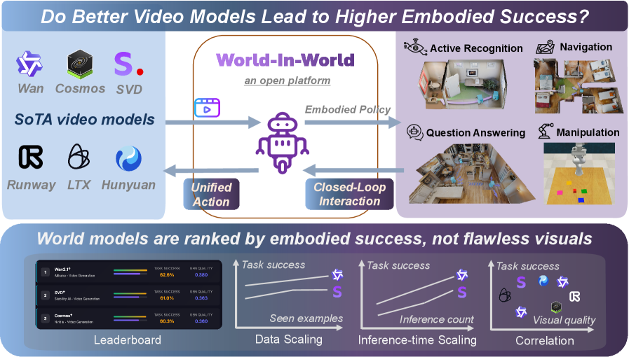
# World-in-World: World Models in a Closed-Loop World **Authors**: - Jiahan Zhang - Muqing Jiang - Nanru Dai - Taiming Lu - Arda Uzunoglu - Shunchi Zhang - Yana Wei - Jiahao Wang - Vishal M. Patel - Paul Pu Liang - Daniel Khashabi - Cheng Peng - Rama Chellappa - Tianmin Shu - Alan Yuille - Yilun Du - Jieneng Chen (JHU   PKU   Princeton   MIT   Harvard) Abstract Generative world models (WMs) can now simulate worlds with striking visual realism, which naturally raises the question of whether they can endow embodied agents with predictive perception for decision making. Progress on this question has been limited by fragmented evaluation: most existing benchmarks adopt open-loop protocols that emphasize visual quality in isolation, leaving the core issue of embodied utility unresolved, i.e., do WMs actually help agents succeed at embodied tasks? To address this gap, we introduce World-in-World, the first open platform that benchmarks WMs in a closed-loop world that mirrors real agent-environment interactions. World-in-World provides a unified online planning strategy and a standardized action API, enabling heterogeneous WMs for decision making. We curate four closed-loop environments that rigorously evaluate diverse WMs, prioritize task success as the primary metric, and move beyond the common focus on visual quality; we also present the first data scaling law for world models in embodied settings. Our study uncovers three surprises: (1) visual quality alone does not guarantee task success—controllability matters more; (2) scaling post-training with action-observation data is more effective than upgrading the pretrained video generators; and (3) allocating more inference-time compute allows WMs to substantially improve closed-loop performance. Code will be available at github.com/World-In-World. footnotetext: Correspondence to “jienengchen01@gmail.com”. We warmly welcome contributions to the open benchmark. <details> <summary>x1.png Details</summary>  ### Visual Description ## Chart/Diagram Type: Comparative Analysis of Embodied Video Models ### Overview The image presents a comparative analysis of embodied video models and their performance in world-in-world tasks. It combines a leaderboard ranking models by embodied success metrics with a conceptual diagram illustrating how these models contribute to closed-loop interaction and unified action. The central theme explores whether improved video models correlate with higher embodied task success. ### Components/Axes 1. **Leaderboard Section**: - **Categories**: Task Success, Data Scaling, Inference-time Scaling, Correlation - **Models**: World-2.0, SVD*, Cosmos* - **Metrics**: - Task Success (%), - Data Scaling (0-1 scale), - Inference-time Scaling (%), - Correlation (0-1 scale) 2. **Main Diagram**: - **Central Element**: Purple robot labeled "Embodied Policy" - **Arrows**: - Left: "Unified Action" (blue) - Right: "Closed-Loop Interaction" (purple) - **Task Labels**: Active Recognition, Navigation, Question Answering, Manipulation - **Platform**: "World-In-World" (orange border) 3. **Legend**: - **Colors**: - World-2.0 (blue), - SVD* (purple), - Cosmos* (orange) ### Detailed Analysis 1. **Leaderboard Data**: - **World-2.0**: - Task Success: 96.2% (highest) - Data Scaling: 0.880 (highest) - Inference-time Scaling: 0.800 (highest) - Correlation: 0.800 (highest) - **SVD***: - Task Success: 83.1% - Data Scaling: 0.830 - Inference-time Scaling: 0.750 - Correlation: 0.750 - **Cosmos***: - Task Success: 80.5% - Data Scaling: 0.800 - Inference-time Scaling: 0.700 - Correlation: 0.700 2. **Main Diagram**: - **Flow**: - Video models (Wan, Cosmos, SVD, Runway, LTX, Hunyuan) feed into the "World-In-World" platform - Outputs connect to "Embodied Policy" with arrows indicating contributions to: - Unified Action (left) - Closed-Loop Interaction (right) - **Task Representation**: - Top row: Active Recognition, Navigation - Bottom row: Question Answering, Manipulation ### Key Observations 1. **Performance Trends**: - World-2.0 dominates across all metrics, maintaining a consistent lead - SVD* and Cosmos* show similar performance patterns, with SVD* slightly outperforming in inference-time scaling - All models show strong correlation scores (>0.7), suggesting good alignment with task requirements 2. **Visual Quality vs. Task Success**: - The bottom section explicitly states "World models are ranked by embodied success, not flawless visuals" - Correlation metrics (0.7-0.8) indicate moderate to strong relationship between visual quality and task success 3. **Scaling Patterns**: - Data Scaling values (0.7-0.88) suggest models maintain effectiveness across different data volumes - Inference-time Scaling (0.7-0.8) indicates consistent performance under time constraints ### Interpretation The data demonstrates a clear hierarchy in embodied task performance, with World-2.0 establishing itself as the leading model. The consistent performance across all metrics suggests this model effectively balances visual quality with practical task execution capabilities. The "World-In-World" platform appears designed to test models in realistic scenarios, with the robot's bidirectional arrows indicating the importance of both unified action and closed-loop interaction for successful embodiment. The emphasis on "embodied success" over visual perfection aligns with real-world robotics applications where functional performance matters more than aesthetic quality. The moderate correlation scores (0.7-0.8) suggest that while visual quality contributes to task success, it's not the sole determining factor - other elements like motion prediction and environmental understanding play crucial roles. The platform's design implies a feedback loop where video models inform embodied policies, which in turn refine the models through closed-loop interaction. This circular relationship highlights the importance of continuous learning and adaptation in embodied AI systems. </details> Figure 1: We introduce the first open benchmark to evaluate world models by closed-loop task success, analyze the link between task success and visual quality, and investigate scaling laws. 1 Introduction Recent advances in visual generation have sparked interest in world generation, a field focused on the creation of diverse environments populated with varied scenes and entities, with applications in entertainment, gaming, simulation, and embodied AI. The rapid progress in video generation (Brooks et al., 2024b; Yang et al., 2024b; Wan et al., 2025), 3D scene generation (Fridman et al., 2023; Chung et al., 2023; Yu et al., 2024; Koh et al., 2023; Ling et al., 2025), and 4D scene generation (Bahmani et al., 2024b; Xu et al., 2024; Bahmani et al., 2024a) has demonstrated high-quality individual scene generation, highlighting the potential of these models as world generation systems. Building on these developments, recent world generation systems (Yang et al., 2023b; Parker-Holder and Fruchter, 2025; Li et al., 2025b; Ye et al., 2025; Lu et al., 2025; He et al., 2025c) show promise as world models for embodied agents. Given an agent’s initial observation and a candidate action, such systems predict the resulting video, thereby estimating the future state of the environment. These action-conditioned simulators mirror human mental models by forecasting future states and can provide missing context under partial observability. As a result, they offer a pathway to improved decision-making for embodied tasks that rely on perception, planning, and control. Despite this promise, the community lacks a unified benchmark that evaluates visual world models through the lens of embodied interaction. Existing suites emphasize video generation quality (e.g., VBench (Huang et al., 2024)) or visual plausibility (e.g., WorldModelBench (Li et al., 2025a)). The recent WorldScore (Duan et al., 2025) offers a unified assessment for models that take an image and a camera trajectory as input. However, no current benchmark tests whether generated worlds actually enhance embodied reasoning and task performance —for example, helping an agent perceive the environment, plan and execute actions, and replan based on new observations within such a closed loop. Establishing this evaluation framework is essential for tracking genuine progress across the rapidly expanding landscape of visual world models and embodied AI. <details> <summary>x2.png Details</summary>  ### Visual Description ## Scatter Plot: Task Success Rate vs. 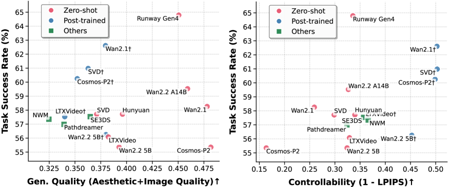General Quality ### Overview The image is a scatter plot comparing **Task Success Rate (%)** (y-axis) against **Gen. Quality (Aesthetic+Image Quality)** (x-axis). Data points are color-coded by model type: **Zero-shot** (red), **Post-trained** (blue), and **Others** (green). Labels for individual models are annotated near their respective points. --- ### Components/Axes - **Y-axis (Task Success Rate)**: Ranges from 55% to 63% in 1% increments. - **X-axis (Gen. Quality)**: Ranges from 0.325 to 0.475 in 0.025 increments. - **Legend**: Located in the top-right corner, with three categories: - **Zero-shot** (red circles) - **Post-trained** (blue circles) - **Others** (green squares) - **Data Points**: Labeled with model names (e.g., "Wan2.1†", "SVD†", "Cosmos-P2†"). --- ### Detailed Analysis #### Zero-shot Models (Red) - **Wan2.1†**: (0.475, 62.5%) – Highest task success rate and gen quality. - **Wan2.2 A14B**: (0.45, 59%) – Moderate gen quality, mid-range success rate. - **Wan2.2 5B**: (0.39, 55%) – Lower gen quality and success rate. - **Cosmos-P2**: (0.475, 55%) – Highest gen quality but lowest success rate. - **Hunyuan**: (0.40, 58%) – Mid-range gen quality and success rate. - **SVD**: (0.38, 58%) – Lower gen quality, moderate success rate. #### Post-trained Models (Blue) - **SVD†**: (0.38, 61%) – High success rate, moderate gen quality. - **Cosmos-P2†**: (0.36, 60%) – Moderate gen quality, high success rate. - **LTXVideo†**: (0.35, 57.5%) – Lower gen quality, mid-range success rate. - **Wan2.2 5B†**: (0.38, 56%) – Moderate gen quality, lower success rate. #### Others (Green) - **NWM**: (0.325, 57.5%) – Lowest gen quality, moderate success rate. - **SE3DS**: (0.375, 57%) – Moderate gen quality, lower success rate. - **Pathdreamer**: (0.35, 57%) – Moderate gen quality, lower success rate. --- ### Key Observations 1. **Wan2.1†** (Zero-shot) achieves the highest task success rate (62.5%) and gen quality (0.475), outperforming all other models. 2. **Cosmos-P2** (Zero-shot) has the highest gen quality (0.475) but the lowest task success rate (55%), suggesting a potential trade-off between quality and performance. 3. **Post-trained models** (blue) generally cluster in the mid-to-high range of both axes, indicating better balance between gen quality and task success. 4. **Others** (green) are concentrated in the lower-left quadrant, with lower gen quality and task success rates. --- ### Interpretation - **Post-trained models** (blue) demonstrate a stronger correlation between gen quality and task success, suggesting that training improves performance consistency. - **Zero-shot models** (red) show variability: while **Wan2.1†** excels, **Cosmos-P2** underperforms despite high gen quality, highlighting potential limitations in zero-shot generalization. - **Others** (green) lag in both metrics, possibly due to less optimized training or architecture. - The plot underscores the importance of post-training for balancing aesthetic quality and functional performance in generative models. 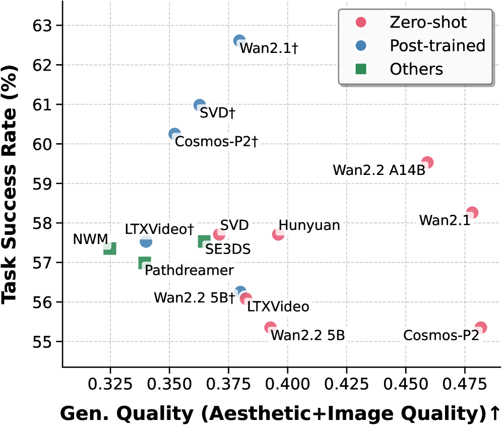</details> Figure 2: Task success rate vs. generation quality. $\dagger$ : post-trained with extra data. We defend that world models live and die by their closed-loop success, not flawless generated visuals. In this work, we address this gap by proposing World-in-World, which wraps generative World models In a closed-loop World interface to measure their practical utility for embodied agents. Specifically, we present a unified strategy for closed-loop online planning and a standardized action API to seamlessly integrate diverse world models into closed-loop tasks. The online planning strategy allows the agent to look ahead by anticipating environmental changes and task rewards before committing to an action. The standardized action API harmonizes input modalities expected by different world models, so that each model can be controlled consistently within the same evaluation protocol. In addition, we introduce a post-training protocol that fine-tunes pretrained video generators using a modest amount of action–observation data drawn from the same action space as the downstream tasks, which allows us to examine their adaptation potential and to characterize a data scaling law. World-in-World offers a fair, closed-loop world interface to evaluate diverse WMs. We benchmark leading video generators (Wan et al., 2025; HaCohen et al., 2024; Kong et al., 2024) alongside task-focused world models (Bar et al., 2025a; Koh et al., 2023, 2021a) in perception, navigation, and manipulation settings. Our findings reveal three consistent trends: (1) high visual quality does not necessarily translate into strong task success; (2) scaling post-training with action-observation data is more effective than upgrading the pretrained video generators; and (3) increasing inference-time compute via online planning substantially improves closed-loop performance. As shown in Figure ˜ 2, world models with strong visual scores do not necessarily bring high success rates, which underscores the need for closed-loop evaluation when judging WM practical value for embodied agents. Our work makes three main contributions: - We introduce World-in-World, the first comprehensive closed-loop benchmark that evaluates world models through the lens of embodied interaction, moving beyond the common focus on generation quality. - We propose a unified closed-loop planning strategy with a unified action API, allowing diverse world models to be seamlessly integrated and evaluated within a single framework across four embodied tasks. - We discover that high visual quality does not necessarily guarantee task success, and demonstrate how the performance of pretrained video generators can be substantially improved through training-time data scaling and inference-time scaling. 2 World-in-World: a Closed-Loop Interface for Visual World Models Design overview. Our goal is to establish a benchmark that evaluates world-generation methods by their utility for embodied agents. Unlike prior work focused on generative quality, we develop a predictive-control framework to test how well a world model supports online decision-making. The evaluation setting mirrors practical scenarios in embodied AI, emphasizing the interaction between prediction, control, and reward under closed-loop operation. We detail the unified strategy for closed-loop online planning (Section ˜ 2.1) and the unified action API (Section ˜ 2.2), which together provide a common interface across tasks and models. We then describe our task selection and evaluation protocol (Section ˜ 2.3). Finally, we present a post-training recipe that adapts a pretrained video generator into a more effective embodied world model (Section ˜ 2.4). <details> <summary>x3.png Details</summary>  ### Visual Description ## Diagram: Closed-loop online planning system ### Overview The diagram illustrates a closed-loop online planning framework for robotic systems, showing the flow from environmental observations to action execution and future state prediction. It emphasizes iterative planning through a world model and unified action API. ### Components/Axes 1. **Embedded Task Environment** - Contains icons representing: - Robot (central figure) - Earth (global context) - Camera (observation) - Speech bubble (communication) - Robot arm (manipulation) - Observations labeled: O₁, O₂, O₃, ..., Oₜ (temporal sequence) 2. **Closed-loop online planning** - **π proposal**: Network diagram with interconnected nodes - **Candidate Action Plans**: Aₜ^(1) to Aₜ^(M) (multiple action options) - **Unified Action API**: Standardized action interface (↑↓↙↘ symbols) - **π revision**: Settings gear icon with revision process - **Possible Future States**: Oₜ^(1) to Oₜ^(M) (predicted outcomes) - **World Model**: Globe icon (gθ) representing environmental understanding 3. **Flow Connections** - Purple arrows show process flow: - Observations → π proposal → Candidate actions → Unified API → World Model → Future states → π revision - Dashed purple arrows indicate "Imagined Interactions" vs "Real Interactions" ### Detailed Analysis - **Observation Sequence**: O₁ to Oₜ shows temporal progression of environmental inputs - **Action Planning**: Multiple candidate actions (Aₜ^(1) to Aₜ^(M)) suggest probabilistic planning - **World Model Function**: Takes text/camera data and actions to predict future states - **Iterative Process**: Feedback loop from future states back to π revision ### Key Observations 1. The system maintains multiple candidate actions (M options) at each time step 2. Future states are predicted probabilistically (Oₜ^(1) to Oₜ^(M)) 3. The world model integrates multiple data types (text, camera, actions) 4. Planning occurs in discrete time steps (temporal index t) 5. The unified action API standardizes action representation across systems ### Interpretation This diagram demonstrates a sophisticated robotic planning system that: 1. Continuously updates its understanding of the environment through observations 2. Generates multiple potential action plans at each step 3. Uses a world model to predict outcomes of actions 4. Iteratively refines its planning strategy based on predicted futures The closed-loop nature suggests the system can adapt to changing environments by: - Revising plans based on predicted state outcomes - Maintaining multiple action options to handle uncertainty - Standardizing actions through the Unified API for system compatibility The emphasis on multiple future states (M options) indicates a probabilistic approach to decision-making, likely using Monte Carlo methods or similar techniques to explore possible outcomes. The integration of text and camera data suggests multimodal perception capabilities, while the robot arm icon implies physical interaction with the environment. 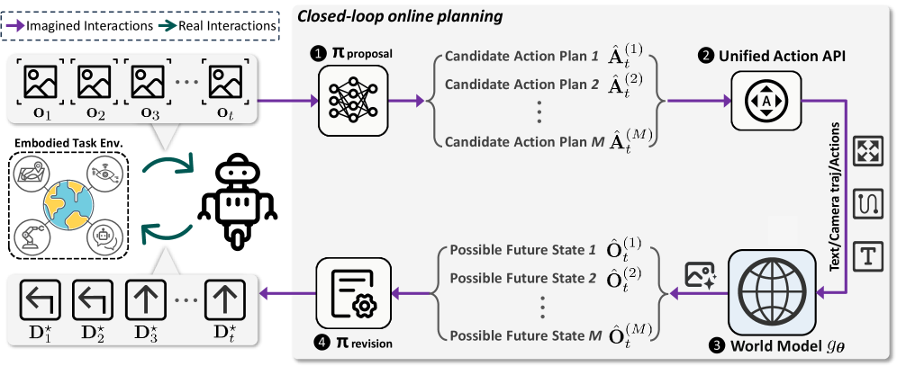</details> Figure 3: Closed-loop online planning in World-in-World: At time step $t$ , the agent receives the world state, represented by observation $\mathbf{o}_{t}$ , and invokes a proposal policy $\pi_{\text{proposal}}$ (❶) to produce a total of $M$ candidate action plans. The unified action API (❷) transforms each plan into the control inputs required by the world model. The world model (❸) then predicts the corresponding future states as observations $\hat{\mathbf{O}}_{t}$ . The revision policy $\pi_{\text{revision}}$ (❹) evaluates all rollouts and commits to the best, yielding decision $\mathbf{D}^{\star}_{t}$ . This decision is applied in the environment, closing the interaction loop. 2.1 Unified Strategy for Closed-Loop Online Planning In Figure ˜ 3, we present a unified closed-loop strategy that uses visual world models for decision-making. It cycles through proposal, simulation, and revision. In proposal, the agent generates candidate plans; in simulation, each plan is rolled out by the world model to predict counterfactual futures; in revision, the agent scores rollouts and refines its plan. Finally, the agent executes the top-scoring plan in the environment, coupling model-based planning with real execution. Let $\mathbf{o}_{t}$ denote the agent’s egocentric observation at time step $t$ . The observation can be RGB, RGB-D, or other sensory modalities. For clarity, we use $\mathbf{o}$ as the generic notation throughout. Define the agent’s future potential action sequence of horizon $L$ starting at time step $t$ as $\hat{\mathbf{A}}_{t}\;=\;\bigl[\hat{a}_{t+1},\,\hat{a}_{t+2},\,...,\,\hat{a}_{t+L}\bigr],$ where each elementary action $\hat{a}$ is specified in either a continuous action space or a discrete action space, i.e., $\hat{a}∈\mathcal{V}$ , with $\mathcal{V}$ denoting the set of action primitives available to the agent. Our unified strategy can be formalized as a policy-guided beam search. The beam width corresponds to the number of candidate plans $M$ drawn from the proposal policy $\pi_{\text{proposal}}$ . At time step $t$ , given the current observation $\mathbf{o}_{t}$ and the task goal $\mathrm{g}$ , the proposal policy $\pi_{\text{proposal}}$ samples $M$ candidate action sequences that serve as future candidate plans: $$ \hat{\mathbf{A}}_{t}^{(m)}\;\sim\;\pi_{\text{proposal}}\bigl(\mathbf{A}\,\big|\,\mathbf{o}_{t},\,\mathrm{g}\bigr),\qquad m=1,\dots,M. \tag{1} $$ Each candidate plan $\hat{\mathbf{A}}_{t}^{(m)}$ is subsequently transformed by the unified action API $C$ into the control inputs expected by the world model: $I_{t}^{(m)}\;=\;C\bigl(\hat{\mathbf{A}}_{t}^{(m)}\bigr),$ where $I_{t}^{(m)}$ may include textual prompts, camera trajectories, or low-level action sequences, depending on the required format of the chosen world model. The visual world model $g_{\boldsymbol{\theta}}$ then performs a counterfactual rollout based on these control inputs, predicting the future world states $\hat{\mathbf{O}}_{t}^{(m)}$ with horizon $L$ : $$ \hat{\mathbf{O}}_{t}^{(m)}\;\sim\;g_{\boldsymbol{\theta}}\!\Bigl(\mathbf{O}\,\big|\,\mathbf{o}_{t},\,I_{t}^{(m)}\Bigr),\qquad\hat{\mathbf{O}}_{t}^{(m)}=\bigl[\hat{\mathbf{o}}_{t+1}^{(m)},\,\hat{\mathbf{o}}_{t+2}^{(m)},\,\dots,\,\hat{\mathbf{o}}_{t+L}^{(m)}\bigr]. \tag{2} $$ Then, the candidate plans and their simulated rollouts $\bigl(\hat{\mathbf{A}}_{t}^{(m)},\hat{\mathbf{O}}_{t}^{(m)}\bigr)$ are evaluated and revised by the revision policy $\pi_{\text{revision}}$ , which assigns a score to each trajectory and selects the decision that maximizes the expected reward. In the most general form, we write $$ \mathbf{D}^{\star}_{t}=\pi_{\text{revision}}\Bigl(\{\,(\hat{\mathbf{A}}_{t}^{(m)},\,\hat{\mathbf{O}}_{t}^{(m)})\,\}_{m=1}^{M},\,\mathbf{o}_{t},\,\mathrm{g}\Bigr). \tag{3} $$ Here, $\mathbf{D}^{\star}_{t}$ denotes the best decision according to $\pi_{\text{revision}}$ at time step $t$ . Depending on the task, $\mathbf{D}^{\star}_{t}$ may represent a high-level answer, a recognition result, or a refined sequence of low-level actions, which renders the framework more general than classical Model Predictive Control (MPC) (Morari and H. Lee, 1999), where optimization is restricted to sequences of actions. A common instantiation implements $\pi_{\text{revision}}$ as a score-and-select operator $S$ . When the decision is an action sequence, selection is performed over the $M$ candidate plans produced at time step $t$ : $$ m^{\star}=\operatorname*{arg\,max}_{m\in\{1,\dots,M\}}\;S\!\left(\hat{\mathbf{A}}_{t}^{(m)},\,\hat{\mathbf{O}}_{t}^{(m)}\,\big|\,\mathbf{o}_{t},\,\mathrm{g}\right),\qquad\mathbf{D}^{\star}_{t}=\hat{\mathbf{A}}_{t}^{(m^{\star})}. \tag{4} $$ Here, $S(·)$ denotes a task-specific scoring function that estimates the expected reward or utility of a candidate plan based on its simulated outcomes. Alternatively, $\pi_{\text{revision}}$ may synthesize or update a new decision by aggregating information across the candidate set and their predicted consequences, rather than selecting one candidate verbatim. Once the best decision $\mathbf{D}^{\star}_{t}$ is executed in the environment, the agent acquires a new observation at time step $t{+}1$ . The unified strategy then re-enters the proposal-simulation-revision loop, using the newly observed state to initiate the next round of proposal, simulation, and revision. In our framework, both $\pi_{\text{proposal}}$ and $\pi_{\text{revision}}$ can be instantiated flexibly: they may be pretrained modules, such as large-scale vision-language models or diffusion policies, or simple rule-based heuristics. In our experiments, we explore multiple instantiations to systematically explore the flexibility and generality of our framework for different tasks. 2.2 Unified Action API In this section, we present a unified action API that transforms an action sequence $\mathbf{A}$ into control inputs $I$ that guide the world model, i.e., $I\!=\!C(\mathbf{A})$ . The action API is designed to be flexible so that the same interface can serve a wide range of world models and tasks. It supports three principal types of control information: (1) text prompt, (2) camera trajectory/viewpoint, and (3) low-level actions, depending on the inputs expected by the chosen world model. Text prompt. For image-and-text-to-video world models, the controller maps the intended action sequence into a descriptive text prompt. A predefined template converts each primitive action into a phrase, and concatenating these phrases yields the final prompt $I_{\text{text}}$ . Camera trajectory / viewpoint. For models that consume explicit viewpoints, the controller translates $\mathbf{A}$ into a camera trajectory, e.g., each translation action moves the camera by $0.2\,\text{m}$ , and each rotation action changes the azimuth by $22.5^{\circ}$ . The resulting trajectory is represented as a sequence $\bigl[(x_{k},y_{k},\phi_{k})\bigr]_{k=1}^{K}$ with $(x_{k},y_{k})∈\mathbb{R}^{2}$ and azimuth $\phi_{k}∈\mathbb{R}$ . Low-level actions. For world models that take discrete or continuous low-level actions as input, the controller maps the action sequence $\mathbf{A}$ to the world model’s action vocabulary, yielding $\mathbf{A}_{\text{world}}$ . This mapping $\mathbf{A}\mapsto\mathbf{A}_{\text{world}}$ applies the necessary transformations to maintain a unique and consistent correspondence between the agent’s actions and the inputs expected by the world model. 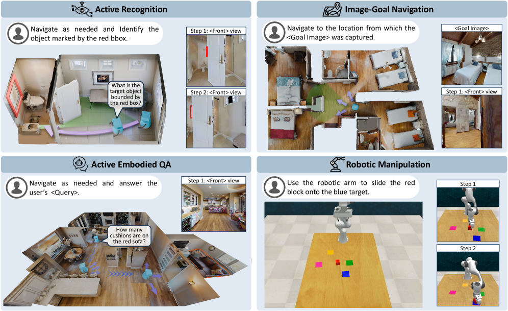2.3 Comprehensive Embodied Tasks To evaluate the practical utility of visual world models in embodied tasks, we select a diverse set of tasks that span multiple domains and stress distinct capabilities. We focus on four representative tasks: Active Recognition (AR), Active Embodied Question Answering (A-EQA), Image-Goal Navigation (ImageNav), and Robotic Manipulation, as illustrated in Figure ˜ 4. Taken together, these tasks emphasize complementary aspects of embodied intelligence, including perception, navigation, and object-level manipulation, and thus provide a comprehensive testbed for assessing how effectively a visual world model supports online planning and decision-making. Below, we describe the tasks included in our benchmark, and more detailed settings are provided in Appendix ˜ B. <details> <summary>x4.png Details</summary>  ### Visual Description ## Diagram: Multi-Task Robotics System Architecture ### Overview The image depicts a 2x2 grid of diagrams illustrating four distinct robotics tasks: **Active Recognition**, **Image-Goal Navigation**, **Active Embodied QA**, and **Robotic Manipulation**. Each quadrant includes textual instructions, visual steps, and spatial reasoning elements. ### Components/Axes #### Active Recognition (Top-Left) - **Task Label**: "Active Recognition" with a speech bubble icon. - **Instruction**: "Navigate as needed and Identify the object marked by the red bbox." - **Speech Bubble**: "What is the target object bounded by the red box?" - **Steps**: - Step 1: `<Front> view` (image of a door with a red bounding box). - Step 2: `<Front> view` (image of a room with a red bounding box). - **Visuals**: 3D room model with a red bounding box highlighting a target object. #### Image-Goal Navigation (Top-Right) - **Task Label**: "Image-Goal Navigation" with a map icon. - **Instruction**: "Navigate to the location from which the <Goal Image> was captured." - **Steps**: - Step 1: `<Front> view` (image of a room with a green arrow pointing to a target location). - Goal Image: Bedroom scene with two beds. - **Visuals**: 3D room model with a green arrow indicating the goal location. #### Active Embodied QA (Bottom-Left) - **Task Label**: "Active Embodied QA" with a speech bubble icon. - **Instruction**: "Navigate as needed and answer the user’s <Query>." - **Speech Bubble**: "How many cushions are on the red sofa?" - **Steps**: - Step 1: `<Front> view` (image of a kitchen with a red sofa). - **Visuals**: 3D room model with a red sofa and blue arrows indicating movement. #### Robotic Manipulation (Bottom-Right) - **Task Label**: "Robotic Manipulation" with a robotic arm icon. - **Instruction**: "Use the robotic arm to slide the red block onto the blue target." - **Steps**: - Step 1: Robot arm approaching red block. - Step 2: Robot arm placing red block on blue target. - **Visuals**: Grid with colored blocks (red, yellow, green, blue) and a robotic arm. ### Detailed Analysis - **Textual Elements**: - All tasks include explicit instructions and step-by-step visuals. - Speech bubbles and step labels (e.g., `<Front> view`) are consistently used across quadrants. - Color-coded elements (red bounding boxes, green arrows, blue arrows) denote targets or actions. - **Spatial Grounding**: - Red bounding boxes in Active Recognition and Active Embodied QA highlight objects of interest. - Green arrows in Image-Goal Navigation indicate goal locations. - Blue arrows in Active Embodied QA suggest movement paths. - Robotic Manipulation uses colored blocks (red, blue) to denote objects and targets. ### Key Observations 1. **Task Consistency**: Each quadrant follows a structured format: task label, instruction, steps, and visuals. 2. **Color Coding**: Red is used for target objects (bounding boxes, blocks), green for navigation goals, and blue for movement paths. 3. **Step Progression**: Steps 1 and 2 in each quadrant show incremental actions (e.g., identifying objects, navigating, manipulating). ### Interpretation The diagram illustrates a modular robotics system capable of: 1. **Object Recognition**: Identifying targets via bounding boxes. 2. **Goal Navigation**: Using visual cues (arrows, images) to reach locations. 3. **Question Answering**: Answering spatial queries (e.g., counting objects). 4. **Robotic Action**: Executing precise manipulations (e.g., sliding blocks). The system emphasizes **active perception** (navigation, recognition) and **embodied interaction** (QA, manipulation), suggesting integration of computer vision, spatial reasoning, and robotic control. The use of color-coded visuals and step-by-step instructions implies a focus on human-robot collaboration, where users guide robots through tasks using intuitive cues. No numerical data or charts are present; the image focuses on task descriptions and spatial relationships. </details> Figure 4: Top-left: Active Recognition (AR), the agent needs to identify a designated target under occlusions or extreme viewpoints while minimizing navigation cost. Top-right: Image-Goal Navigation (ImageNav), the agent reaches the viewpoint matching a goal image, emphasizing success rate and path efficiency. Bottom-left: Active Embodied Question Answering (A-EQA), the agent answers an open-ended question after active exploration. Bottom-right: Robotic Manipulation, the agent needs to control a robotic arm to complete tasks such as grasping and placement to specified targets. Active Recognition (AR) is closely related to amodal recognition (Aydemir et al., 2013; Liu et al., 2018; Yang et al., 2019; Fan et al., 2024; Bhattacharjee et al., 2025), in which the agent must identify a designated target that may be observed from extreme viewpoints or be heavily occluded. In addition, AR allows the agent to acquire additional observations through active exploration. All AR experiments are conducted in the Habitat-Sim (Savva et al., 2019), encompassing 551 episodes across 29 scenes from the validation split of Matterport3D (Chang et al., 2017). Within AR, the visual world model assists two decision-making processes. For answering, synthetic views provide auxiliary evidence that helps the agent reason about occlusions and extreme viewpoints that impede recognition. For navigation, rollouts simulate the consequences of potential actions so that the agent can choose a path that is more likely to yield informative observations. Image-Goal Navigation (ImageNav), also referred to as goal-conditioned visual navigation, requires an embodied agent to reach a target position in a scene given a single reference image that specifies the goal viewpoint. We construct 144 ImageNav episodes from 87 validation scenes of HM3D (Ramakrishnan et al., 2021). In this task, the visual world model exclusively supports navigation decisions. The agent simulates the outcomes of candidate action plans, selects the best option, executes the first segment of that plan, and then replans with the newly observed state in a closed-loop manner. Active Embodied Question Answering (A-EQA) requires an agent to answer open-ended natural-language questions after actively exploring a 3D environment. Our evaluation set includes 184 questions across 54 indoor scenes from the official OpenEQA split (Majumdar et al., 2024) and the HM3D validation set (Ramakrishnan et al., 2021). As in AR, the visual world model supports both question answering and navigation. For answering, synthetic views generated by the world model provide complementary perspectives that help resolve references to occluded or distant objects. For navigation, the agent simulates high-level action plans using the world model’s predictions to choose exploration strategies likely to reveal question-relevant information. Robotic Manipulations are fundamental capabilities for embodied agents that must operate in real-world interaction settings. We study how visual world models contribute to closed-loop manipulation planning, evaluating performance on four RLBench (James et al., 2020) tasks with 50 episodes per task. Here, the visual world model supports the agent in assessing candidate $7$ -DoF gripper actions by providing visual evidence about anticipated object motions and interactions, which enables a comparison of alternative plans before execution. The predicted outcomes then guide the selection of actions that are more likely to achieve the specified objective, thereby linking visual prediction accuracy to improvements in manipulation performance. 2.4 Exploiting World Models via Post-Training To evaluate the feasibility of adapting pretrained video generators for embodied tasks, we introduce a post-training procedure that aligns a pretrained model with the domain distribution and action space of target environments. We perform fine-tuning separately on data from two simulators, Habitat-Sim and CoppeliaSim, to match the corresponding task domains. For Habitat-Sim tasks (AR, A-EQA, ImageNav), we post-train on a panoramic action-observation dataset collected from the HM3D (Ramakrishnan et al., 2021) training split. For CoppeliaSim tasks (Robotic Manipulation), we post-train on task demonstrations generated with RLBench (James et al., 2020). To assess generalization rather than memorization, all Habitat-Sim data used for post-training are sourced from scenes that are disjoint from our evaluation scenes, so the scenes in our evaluation tasks remain unseen by the world models after post-training. Additional details regarding the training objective, dataset construction, and training configuration are provided in Appendices ˜ C and D. 3 Evaluation Results and Analysis In this section, we report quantitative results and key observations on the four embodied tasks in Section ˜ 3.1, followed by ablation studies in Section ˜ 3.2. We evaluate visual world models spanning image-based (PathDreamer (Koh et al., 2021b), SE3DS (Koh et al., 2023)) and video-based (SVD (Blattmann et al., 2023a), LTX-Video (HaCohen et al., 2024), Hunyuan (Kong et al., 2024), Wan2.1 (Wan et al., 2025), Wan2.2 (Wan et al., 2025), Cosmos-Predict2 (Agarwal et al., 2025), NWM (Bar et al., 2025a)) approaches, covering major control interfaces. For video-based models, we compare off-the-shelf versions with their post-trained variants. 3.1 Benchmark Results Table 1: Active Recognition (AR) and Image-Goal Navigation (ImageNav) performance across various models and base policies. Higher success rate (SR %), success weighted by path length (SPL %), and lower mean trajectory length (Mean Traj.) are better. “ $\dagger$ ” denotes our post-trained video generators. | Model Details | AR | ImageNav | | | | | | | | | --- | --- | --- | --- | --- | --- | --- | --- | --- | --- | | Model Type | Method | Control Type | Input Type | #Param. | SR $\uparrow$ | Mean Traj. $\downarrow$ | SR $\uparrow$ | Mean Traj. $\downarrow$ | SPL $\uparrow$ | | Base Policy | Heuristic (w/o WM) | – | RGB | – | 39.02 | 8.81 | 2.08 | 59.6 | 0.63 | | + Video Gen. Post-Train | SVD $\dagger$ | Action | RGB; Pano | 1.5B | 60.62 | 5.17 | 20.83 | 58.5 | 11.86 | | WAN2.1 $\dagger$ | Action | RGB; Pano | 14B | 62.98 | 4.71 | 22.92 | 58.7 | 11.63 | | | Base Policy | VLM (w/o WM) | – | RGB | 72B | 50.27 | 6.24 | 35.42 | 47.5 | 25.88 | | + Image Gen. | PathDreamer | Viewpoint | RGB - D; Pano | 0.69B | 56.99 | 5.28 | 36.80 | 47.3 | 26.85 | | + Image Gen. | SE3DS | Viewpoint | RGB - D; Pano | 1.1B | 57.53 | 5.29 | 36.11 | 47.0 | 26.91 | | + Video Gen. | NWM | Trajectory | RGB | 1B | 57.35 | 5.68 | 40.28 | 47.1 | 27.83 | | + Video Gen. Zero-Shot | SVD | Image | RGB | 1.5B | 57.71 | 5.29 | 40.28 | 46.4 | 28.59 | | LTX - Video | Text | RGB | 2B | 56.08 | 5.37 | 36.81 | 47.5 | 25.85 | | | Hunyuan | Text | RGB | 13B | 57.71 | 5.21 | 36.11 | 46.8 | 26.89 | | | Wan2.1 | Text | RGB | 14B | 58.26 | 5.24 | 38.19 | 48.2 | 25.92 | | | Wan2.2 | Text | RGB | 5B | 55.35 | 5.73 | 38.88 | 46.5 | 28.87 | | | Cosmos - P2 | Text | RGB | 2B | 55.35 | 5.71 | 36.81 | 47.6 | 25.89 | | | Wan2.2 | Text | RGB | A14B | 59.53 | 4.91 | 43.05 | 45.8 | 31.46 | | | Runway Gen4 (proprietary) | Text | RGB | – | 64.79 | 4.06 | - | - | - | | | + Video Gen. Post-Train | SVD $\dagger$ | Action | RGB; Pano | 1.5B | 60.98 | 5.02 | 43.05 | 46.0 | 30.96 | | LTX - Video $\dagger$ | Action | RGB; Pano | 2B | 57.53 | 5.49 | 38.89 | 47.4 | 27.47 | | | WAN2.1 $\dagger$ | Action | RGB; Pano | 14B | 62.61 | 4.73 | 45.14 | 45.8 | 32.10 | | | Cosmos - P2 $\dagger$ | Action | RGB; Pano | 2B | 60.25 | 5.08 | 41.67 | 45.5 | 30.29 | | | Wan2.2 $\dagger$ | Action | RGB; Pano | 5B | 56.26 | 5.15 | 38.89 | 46.7 | 28.24 | | | Wan2.2 $\dagger$ | Action | RGB; Pano | A14B | 62.43 | 4.67 | 46.53 | 44.6 | 34.61 | | Table 2: Active Embodied Question Answering (A-EQA) performance. | Model Details | A-EQA Performance | | | | | --- | --- | --- | --- | --- | | Model Type | Method | Ans. Score $\uparrow$ | Mean Traj. $\downarrow$ | SPL $\uparrow$ | | Base Policy | VLM (w/o WM) | 45.7 | 20.4 | 29.6 | | + Image Gen. | PathDreamer | 46.0 | 20.4 | 29.3 | | + Image Gen. | SE3DS | 45.8 | 20.3 | 29.4 | | + Video Gen. | NWM | 47.1 | 20.5 | 30.1 | | + Video Gen. | Wan2.1 | 45.7 | 20.1 | 28.8 | | Wan2.2 (5B) | 46.3 | 20.3 | 31.4 | | | LTX - Video | 46.6 | 20.8 | 29.5 | | | Cosmos - P2 | 46.6 | 21.0 | 31.3 | | | Hunyuan | 46.8 | 20.4 | 29.9 | | | SVD | 46.9 | 20.4 | 29.7 | | | Wan2.2 (A14B) | 47.2 | 20.7 | 31.9 | | | + Video Gen. Post-Train | SVD $\dagger$ | 46.4 | 21.1 | 30.1 | | Cosmos - P2 $\dagger$ | 46.5 | 20.6 | 30.1 | | | Wan2.2 $\dagger$ (5B) | 47.5 | 20.8 | 30.7 | | | Wan2.1 $\dagger$ | 48.2 | 20.7 | 31.6 | | | LTX - Video $\dagger$ | 48.6 | 20.7 | 31.8 | | | Wan2.2 $\dagger$ (A14B) | 48.4 | 20.2 | 31.9 | | Table 3: Robotic manipulation performance across various models and base policies. | Model Details | Manipulation Performance | | | | --- | --- | --- | --- | | Model Type | Method | SR $\uparrow$ | Mean Traj. $\downarrow$ | | Base Policy | VLM (w/o WM) | 44.5 | 2.52 | | + Video Gen. | SVD | 44.0 | 2.47 | | LTX - Video | 44.5 | 2.46 | | | Hunyuan | 44.5 | 2.44 | | | Wan2.1 | 44.0 | 2.51 | | | Cosmos - P2 | 44.0 | 2.50 | | | + Video Gen. Post-Train | SVD $\dagger$ | 46.5 | 2.38 | | Cosmos - P2 $\dagger$ | 45.0 | 2.40 | | | Base Policy | 3D - DP (w/o WM) | 24.0 | 5.21 | | + Video Gen. Post-Train | SVD $\dagger$ | 44.7 | 4.41 | | Cosmos - P2 $\dagger$ | 38.0 | 4.79 | | World models can enhance the performance of the base proposal policy. Across AR, A-EQA, ImageNav, and Manipulation, adding a visual world model consistently improves the performance of the base proposal policy (e.g., a VLM policy, a heuristic policy, or a 3D diffusion policy), as shown in Tables ˜ 1, 3 and 3. For example, in AR, the best proprietary model (Runway Gen4) attains an accuracy of $64.79\%$ while reducing the mean steps per episode to $4.06$ , compared to the VLM base policy with an accuracy of $50.27\%$ and mean steps $6.24$ . Similarly, in ImageNav, the best open-source model Wan2.1 $\dagger$ achieves a success rate of $45.14\%$ with an average path length of $45.8$ , outperforming the VLM base policy at $35.42\%$ SR and $47.5$ average length. These results support the effectiveness of our World-in-World online planning framework with world models, in which the world model provides simulated future states that inform better decisions. World models struggle to simulate precise motion and dynamics in manipulation. The gains are less pronounced for Robotic Manipulations (Table ˜ 3), likely because accurately modeling contact-rich interactions and robot kinematics is significantly more challenging than predicting purely view changes. For instance, the best post-trained model on manipulation (SVD $\dagger$ ) reaches an SR of $46.5\%$ with a mean trajectory length of $2.38$ , only modestly above the VLM baseline at $44.5\%$ SR and $2.52$ mean length. This gap suggests that while current visual world models can effectively guide perception and navigation, capturing fine-grained physical dynamics and action-conditioned object motion remains an open challenge. Post-training substantially boosts world-model utility. Our post-training adaptation yields consistent improvements. Relative to off-the-shelf Wan2.1, Wan2.1 $\dagger$ raises AR accuracy from $58.26\%$ to $62.61\%$ and ImageNav SR from $38.19\%$ to $45.14\%$ (Table ˜ 1). Likewise, SVD $\dagger$ improves AR accuracy from $57.71\%$ to $60.98\%$ and ImageNav SR from $40.28\%$ to $43.05\%$ . These gains show that aligning the generative model to the target domain and action space of the specific embodied tasks improves downstream decision-making. 3.2 Ablation and Findings <details> <summary>x5.png Details</summary>  ### Visual Description ## Scatter Plots: Model Performance Comparison ### Overview The image contains two side-by-side scatter plots comparing model performance across two metrics: **Gen. Quality (Aesthetic+Image Quality)** and **Controllability (1 - LPIPS)**. Both plots share the same y-axis (**Task Success Rate (%)**), while the x-axes differ. Data points are color-coded by model type: **Zero-shot (red)**, **Post-trained (blue)**, and **Others (green)**. --- ### Components/Axes #### Left Panel: Gen. Quality vs. Task Success Rate - **X-axis (Gen. Quality)**: Ranges from **0.325** to **0.475** (increasing rightward). - **Y-axis (Task Success Rate)**: Ranges from **55%** to **65%** (increasing upward). - **Legend**: - **Red**: Zero-shot - **Blue**: Post-trained - **Green**: Others #### Right Panel: Controllability vs. Task Success Rate - **X-axis (Controllability)**: Ranges from **0.15** to **0.50** (increasing rightward). - **Y-axis (Task Success Rate)**: Same as left panel (**55%** to **65%**). - **Legend**: Same as left panel. --- ### Detailed Analysis #### Left Panel: Gen. Quality vs. Task Success Rate - **Zero-shot (Red)**: - **Runway Gen4**: (0.475, 64%) - **Wan2.2 A14B**: (0.45, 59%) - **Cosmos-P2**: (0.475, 55%) - **Post-trained (Blue)**: - **Wan2.1†**: (0.400, 62%) - **SVD†**: (0.375, 61%) - **Cosmos-P2†**: (0.375, 60%) - **Others (Green)**: - **NWM**: (0.325, 57%) - **Pathdreamer**: (0.35, 56%) - **SE3DS**: (0.375, 56%) - **LTXVideo**: (0.375, 57%) - **Hunyuan**: (0.400, 58%) - **Wan2.2 5B**: (0.400, 56%) #### Right Panel: Controllability vs. Task Success Rate - **Zero-shot (Red)**: - **Runway Gen4**: (0.45, 64%) - **Wan2.2 A14B**: (0.30, 59%) - **Cosmos-P2**: (0.15, 55%) - **Post-trained (Blue)**: - **Wan2.1†**: (0.45, 62%) - **SVD†**: (0.45, 61%) - **Cosmos-P2†**: (0.45, 60%) - **Others (Green)**: - **Pathdreamer**: (0.30, 57%) - **SE3DS**: (0.30, 57%) - **NWM**: (0.30, 57%) - **LTXVideo**: (0.30, 58%) - **Hunyuan**: (0.30, 59%) - **Wan2.2 5B**: (0.35, 56%) --- ### Key Observations 1. **High Gen. Quality, High Task Success Rate**: - **Runway Gen4** (Zero-shot) achieves the highest Gen. Quality (**0.475**) and Task Success Rate (**64%**) in both panels. - **Wan2.1†** (Post-trained) shows strong performance with Gen. Quality (**0.400**) and Task Success Rate (**62%**). 2. **Outliers**: - **Cosmos-P2** (Zero-shot) has high Gen. Quality (**0.475**) but low Task Success Rate (**55%**), suggesting inefficiency. - **Cosmos-P2** (Others) has low Controllability (**0.15**) and Task Success Rate (**55%**), indicating poor optimization. 3. **Post-trained Models**: - Post-trained models (e.g., **Wan2.1†**, **SVD†**) consistently outperform Zero-shot and Others in both panels, suggesting training improves performance. 4. **Controllability Trends**: - Higher Controllability (closer to 0.50) correlates with higher Task Success Rate, especially for Post-trained models. --- ### Interpretation - **Model Efficiency**: Post-trained models (blue) demonstrate superior Task Success Rate across both Gen. Quality and Controllability, implying training enhances effectiveness. - **Trade-offs**: Zero-shot models like **Runway Gen4** excel in Gen. Quality but may lack Controllability, while **Cosmos-P2** (Zero-shot) underperforms despite high Gen. Quality. - **Outliers**: **Cosmos-P2** (Others) is a clear outlier, with low Controllability and Task Success Rate, suggesting it is less optimized compared to others. - **Correlation**: Both panels show a positive correlation between Gen. Quality/Controllability and Task Success Rate, though Post-trained models break this trend by achieving higher success rates at lower Gen. Quality/Controllability. This analysis highlights the importance of model training in balancing Gen. Quality, Controllability, and Task Success Rate, with Post-trained models leading in performance. </details> Figure 5: (a) SR vs. generation quality in AR; generation quality is scored as the average of an aesthetic predictor (Akio Kodaira, 2024) and an image-quality predictor (Ke et al., 2021), both trained to match human preferences. (b) SR vs. controllability in AR; controllability is quantified as $1-\mathrm{LPIPS}$ between ground-truth and predicted observations. Fine-grained controllability matters more than visuals for task success. Although recent off-the-shelf video generators like Wan2.1 produce visually appealing clips, they are driven by text prompts with limited fine-grained low-level controls. Without adaptation, these models yield only small gains on downstream embodied tasks. We further study the relation between controllability and the success rate on AR. Here, controllability is defined as alignment between intended actions and the motions in the model’s predictions. After action-conditioned post-training, alignment improves substantially and SR rises accordingly. Figure ˜ 5 (b) shows a positive correlation: models that respond reliably to low-level controls achieve higher SR. These results indicate that precise control, not just visual quality, is critical for embodied world models to support effective decision-making. <details> <summary>x6.png Details</summary>  ### Visual Description ## Line Chart: Success Rate vs. 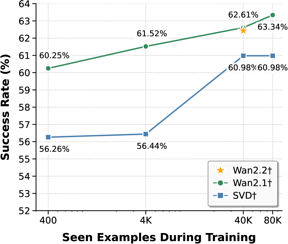Seen Examples During Training ### Overview The chart compares the success rates of three models (Wan2.2†, Wan2.1†, SVD†) as a function of the number of training examples seen during training. Success rate is plotted on the y-axis (52%–64%), and training examples are on the x-axis (400–80K). Three data series are represented with distinct markers and colors: Wan2.2† (yellow star), Wan2.1† (green line), and SVD† (blue line). ### Components/Axes - **X-axis (Seen Examples During Training)**: Labeled with values 400, 4K, 40K, and 80K. - **Y-axis (Success Rate %)**: Labeled with increments from 52% to 64%. - **Legend**: Located in the bottom-right corner, mapping: - Yellow star → Wan2.2† - Green line → Wan2.1† - Blue line → SVD† ### Detailed Analysis 1. **Wan2.1† (Green Line)**: - Starts at **60.25%** at 400 examples. - Increases steadily to **61.52%** at 4K examples. - Reaches **62.61%** at 40K examples. - Peaks at **63.34%** at 80K examples. - *Trend*: Consistent upward slope with no plateaus. 2. **SVD† (Blue Line)**: - Begins at **56.26%** at 400 examples. - Rises sharply to **56.44%** at 4K examples. - Jumps to **60.98%** at 40K examples. - Remains flat at **60.98%** at 80K examples. - *Trend*: Steep initial increase followed by a plateau. 3. **Wan2.2† (Yellow Star)**: - Single data point at **62.61%** at 40K examples. - No data provided for other x-axis values. - *Trend*: Isolated point; no trend inferred. ### Key Observations - **Wan2.1†** demonstrates the highest success rate across all training example ranges, with a steady improvement as training data increases. - **SVD†** shows a significant performance boost between 4K and 40K examples but plateaus afterward, suggesting diminishing returns. - **Wan2.2†** outperforms SVD† at 40K examples but lacks data for other ranges, limiting direct comparison. - Wan2.1† maintains a lead over SVD† even at 80K examples (63.34% vs. 60.98%). ### Interpretation The data suggests that **Wan2.1†** is the most effective model for leveraging training examples, with a clear correlation between increased training data and improved success rates. **SVD†** performs well at mid-scale training (40K examples) but may not scale efficiently beyond that. **Wan2.2†** appears promising but requires additional data points to assess its full potential. The plateau in SVD†’s performance at 80K examples raises questions about its scalability, while Wan2.1†’s linear improvement indicates robust adaptability to larger datasets. </details> Figure 6: SR vs. seen examples during post-training. SR increases consistently with more downstream data, revealing a clear data-scaling trend for adaptation. <details> <summary>x7.png Details</summary>  ### Visual Description ## Line Graph: Algorithm Performance Comparison (Success Rate vs. 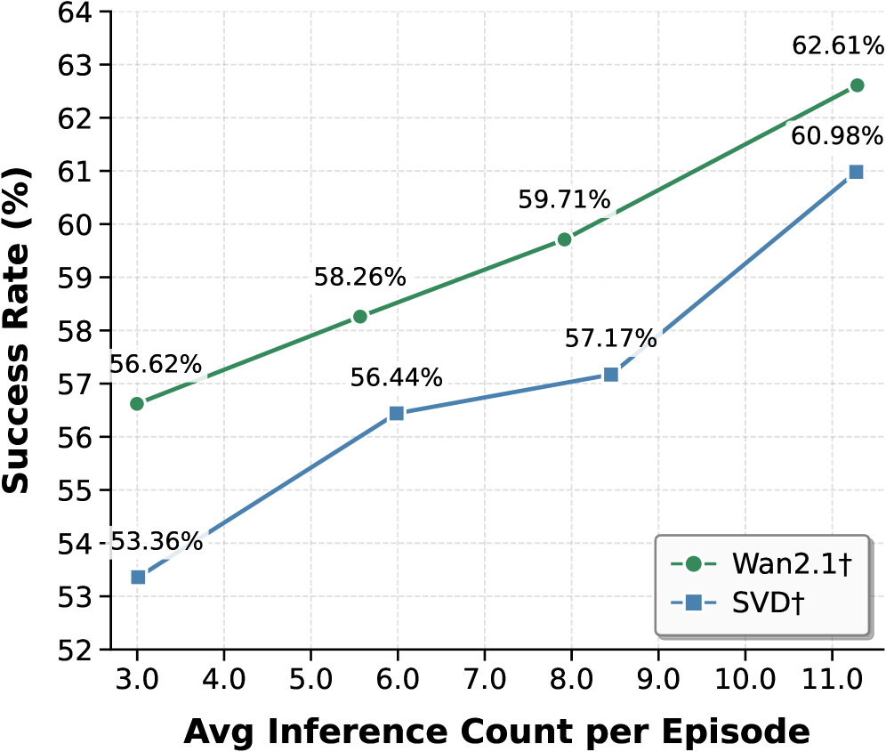Inference Count) ### Overview The image is a line graph comparing the success rates of two algorithms, **Wan2.1†** (green line with circles) and **SVD†** (blue line with squares), across varying average inference counts per episode. The graph spans inference counts from 3.0 to 11.0 episodes, with success rates ranging from 52% to 64%. --- ### Components/Axes - **X-axis**: "Avg Inference Count per Episode" (3.0 to 11.0, increments of 1.0). - **Y-axis**: "Success Rate (%)" (52% to 64%, increments of 1%). - **Legend**: Located in the bottom-right corner, mapping: - Green line with circles → **Wan2.1†** - Blue line with squares → **SVD†** --- ### Detailed Analysis #### Wan2.1† (Green Line) - **Data Points**: - (3.0, 56.62%) - (5.5, 58.26%) - (8.0, 59.71%) - (11.0, 62.61%) - **Trend**: Steadily upward slope, with consistent gains in success rate as inference count increases. #### SVD† (Blue Line) - **Data Points**: - (3.0, 53.36%) - (6.0, 56.44%) - (8.0, 57.17%) - (11.0, 60.98%) - **Trend**: Gradual upward slope, but with slower growth compared to Wan2.1†. --- ### Key Observations 1. **Performance Gap**: Wan2.1† consistently outperforms SVD† across all inference counts. - At 3.0 episodes: Wan2.1† (56.62%) vs. SVD† (53.36%) → **+3.26% advantage**. - At 11.0 episodes: Wan2.1† (62.61%) vs. SVD† (60.98%) → **+1.63% advantage**. 2. **Efficiency**: Wan2.1† achieves higher success rates with fewer inference counts (e.g., 59.71% at 8.0 episodes vs. SVD†'s 57.17%). 3. **Scalability**: Both algorithms improve with more inference counts, but Wan2.1† scales more effectively. --- ### Interpretation The data suggests **Wan2.1† is a more efficient and effective algorithm** for the task measured, likely due to superior optimization or architecture. The steeper slope of Wan2.1† indicates it leverages inference counts more effectively to improve success rates. SVD†, while still improving, lags behind, highlighting potential limitations in its design or training. This trend could inform algorithm selection in resource-constrained environments where inference efficiency is critical. </details> Figure 7: SR vs. average number of world-model inferences per episode. Increasing the inference-time computation allocated to each decision step leads to higher SR. Data-size scaling for post-trained models. We study how post-training data size affects WM performance (Wan2.2 $\dagger$ , Wan2.1 $\dagger$ , SVD $\dagger$ ). Each WM is post-trained for one epoch on datasets from $400$ to $80\text{K}$ instances. As shown in Figure ˜ 7, more post-training data consistently improves AR performance: Wan2.1 $\dagger$ rises from $60.25\%$ to $63.34\%$ , and SVD $\dagger$ from $56.80\%$ to $60.98\%$ . Wan2.2 $\dagger$ (A14B), despite substantially larger web-video pretraining, reaches nearly the same performance as Wan2.1 $\dagger$ after $40\text{K}$ post-training instances, suggesting that scaling action-conditioned post-training is more effective for embodied utility than upgrading the pretrained generator. Moreover, larger models (Wan2.1 $\dagger$ , 14B) benefit more and saturate less than smaller ones (SVD $\dagger$ , 1.5B), indicating greater capacity to absorb action-conditioned supervision. Inference-time scaling for online planning with world models. Within our online planning framework, the number of world-model inferences (simulated potential futures per episode) directly affects task performance. As shown in Figure ˜ 7, increasing the average inferences per episode for AR yields a clear positive correlation with SR. For example, increasing the average inference count from 3 to 11 improves SR from $53.36\%$ to $60.98\%$ for SVD $\dagger$ . This suggests that allocating more inference-time computation to simulate potential futures lets the planner make more informed decisions, thereby improving overall performance. Table 4: Post-training with different input contexts: front view vs. panorama. | Task | Model | Front View | Panorama | | | | --- | --- | --- | --- | --- | --- | | SR $\uparrow$ | Mean Traj. $\downarrow$ | SR $\uparrow$ | Mean Traj. $\downarrow$ | | | | AR | SVD $\dagger$ | 57.89 | 5.04 | 60.98 | 5.02 | | Wan2.1 $\dagger$ | 62.25 | 4.82 | 62.61 | 4.73 | | | Wan2.2 $\dagger$ (5B) | 57.16 | 5.08 | 56.26 | 5.15 | | | Cosmos-P2 $\dagger$ | 58.98 | 4.94 | 60.25 | 5.08 | | | ImageNav | SVD $\dagger$ | 38.19 | 47.0 | 43.05 | 46.0 | | Wan2.1 $\dagger$ | 48.61 | 43.8 | 45.14 | 45.8 | | | Wan2.2 $\dagger$ (5B) | 40.97 | 45.8 | 38.89 | 46.7 | | | Cosmos-P2 $\dagger$ | 40.97 | 47.0 | 41.67 | 45.5 | | Global vs. local context for generation. We study the effect of input context format. Specifically, we compare post-trained models conditioned on panoramic versus front-view input (Table ˜ 4). Panoramic input provides a $360^{\circ}$ field of view, whereas front view offers a focused but limited perspective. For fairness, generated panoramas are converted to perspective views with the same horizontal field of view during evaluation. Although panoramic input offers richer global context, it does not consistently yield large gains across all settings. Likely, panorama-to-perspective conversion introduces resolution loss, degrading downstream perception and planning. 4 Discussion and Future Directions Generalization capacity of world models is critical for practical use. Most video generators are pretrained on web videos. In unseen embodied environments, they may revert to training priors or ignore action controls, yielding plausible but physically or semantically inconsistent rollouts (see Figures ˜ 13 and 14). These deviations mislead planning and reduce success. Larger models or more pretraining data can partly help, but robust generalization remains central. Future work should prioritize strategies and action representations to improve transfer to novel environments, such as unified action representations (Wang et al., 2025b; Zhi et al., 2025; Wang et al., 2025a) and curriculum or domain-specific data collection (Zhao et al., 2025). Long-horizon planning with world models remains challenging. In our experiments, visual world models simulate short-term changes but struggle on long horizons due to limited mechanisms for accumulating spatiotemporal history. We attempted to alleviate this issue by replacing front-view inputs with panoramas to provide global context, but gains were inconsistent across models and tasks. Future work should better encode and retrieve long-term dependencies, e.g., spatial memory (Zhou et al., 2025b; Xiao et al., 2025; Li et al., 2025c; Yu et al., 2025a; Ren et al., 2025) and episode-level memory (Cai et al., 2025; Guo et al., 2025), to maintain scene-level context and enable coherent planning over extended horizons. Precise modeling of interactions and dynamics remains difficult. For manipulation, capturing contact-rich interactions, compliance, friction, and state changes of articulated or deformable objects is essential. Current visual world models often miss these details, producing rollouts that violate physics and degrade planning and control—consistent with our observations and prior analyses (Kang et al., 2024). Promising directions include physics-guided motion generation (Chefer et al., 2025; Zhang et al., 2025b; Akkerman et al., 2025) and inferring or generating physical properties to inform action-conditioned predictions (Cao et al., 2025; Gillman et al., 2025; Zhang et al., 2024). Integrating such signals into conditioning pathways may improve fidelity when precise dynamics are required. Stronger proposal and revision policies set the performance floor. The agent’s overall performance depends on both world-model fidelity and the strength of the proposal and revision policies that select and refine decisions. While simulated rollouts improve decision-making, base policies must be effective to provide a reliable starting point, and strengthening them raises the ceiling. Future work could explore stronger policies (Geng et al., 2025; Kim et al., 2025), and integration strategies that deepen synergy between world models and decision-making (Neary et al., 2025), such as more human-aligned reward models (Wang et al., 2024; Seneviratne et al., 2025; Rocamonde et al., 2023). 5 Conclusion We introduce World-in-World, a closed-loop world interface and benchmark that evaluates generative world models via embodied interaction rather than isolated visual metrics. By unifying heterogeneous controls, our action API enables any world model to serve as perception and planning utilities for an embodied agent. Coupled with a unified closed-loop planning strategy that proposes, simulates, and revises action plans, the benchmark measures agent performance on four demanding tasks. Our experiments reveal large gaps between visual metrics and task success, underscoring the need for closed-loop evaluation, and show that pretrained video generators improve with post-training data scaling and inference-time scaling. We expect World-in-World to guide world models toward not only striking visual realism but also reliable perception, planning, and action in embodied scenarios. References - Agarwal et al. (2025) Niket Agarwal, Arslan Ali, Maciej Bala, Yogesh Balaji, Erik Barker, Tiffany Cai, Prithvijit Chattopadhyay, Yongxin Chen, Yin Cui, Yifan Ding, et al. Cosmos world foundation model platform for physical ai. arXiv preprint arXiv:2501.03575, 2025. - Akio Kodaira (2024) Sayan Goswami Akio Kodaira. Aesthetic predictor v2.5, May 2024. URL https://github.com/discus0434/aesthetic-predictor-v2-5/. - Akkerman et al. (2025) Rick Akkerman, Haiwen Feng, Michael J. Black, Dimitrios Tzionas, and Victoria Fernández Abrevaya. Interdyn: Controllable interactive dynamics with video diffusion models. In Proceedings of the Computer Vision and Pattern Recognition Conference, pages 12467–12479, 2025. - Alonso et al. (2024) Eloi Alonso, Adam Jelley, Vincent Micheli, Anssi Kanervisto, Amos Storkey, Tim Pearce, and François Fleuret. Diffusion for world modeling: Visual details matter in atari. In Advances in Neural Information Processing Systems (NeurIPS), 2024. - Aydemir et al. (2013) Alper Aydemir, Andrzej Pronobis, Moritz Göbelbecker, and Patric Jensfelt. Active visual object search in unknown environments using uncertain semantics. IEEE Transactions on Robotics, 29(4):986–1002, August 2013. ISSN 1941-0468. - Bahmani et al. (2024a) Sherwin Bahmani, Xian Liu, Wang Yifan, Ivan Skorokhodov, Victor Rong, Ziwei Liu, Xihui Liu, Jeong Joon Park, Sergey Tulyakov, Gordon Wetzstein, et al. Tc4d: Trajectory-conditioned text-to-4d generation. In Proceedings of the European Conference on Computer Vision (ECCV), pages 53–72. Springer, 2024a. - Bahmani et al. (2024b) Sherwin Bahmani, Ivan Skorokhodov, Victor Rong, Gordon Wetzstein, Leonidas Guibas, Peter Wonka, Sergey Tulyakov, Jeong Joon Park, Andrea Tagliasacchi, and David B Lindell. 4d-fy: Text-to-4d generation using hybrid score distillation sampling. In Proceedings of the IEEE/CVF Conference on Computer Vision and Pattern Recognition (CVPR), pages 7996–8006, 2024b. - Bai et al. (2025) Shuai Bai, Keqin Chen, Xuejing Liu, Jialin Wang, Wenbin Ge, Sibo Song, Kai Dang, Peng Wang, Shijie Wang, Jun Tang, Humen Zhong, Yuanzhi Zhu, Mingkun Yang, Zhaohai Li, Jianqiang Wan, Pengfei Wang, Wei Ding, Zheren Fu, Yiheng Xu, Jiabo Ye, Xi Zhang, Tianbao Xie, Zesen Cheng, Hang Zhang, Zhibo Yang, Haiyang Xu, and Junyang Lin. Qwen2.5-vl technical report, 2025. - Bar et al. (2025a) Amir Bar, Gaoyue Zhou, Danny Tran, Trevor Darrell, and Yann LeCun. Navigation world models. In Proceedings of the IEEE/CVF Conference on Computer Vision and Pattern Recognition (CVPR), 2025a. - Bar et al. (2025b) Amir Bar, Gaoyue Zhou, Danny Tran, Trevor Darrell, and Yann LeCun. Navigation world models. In Proceedings of the IEEE/CVF Conference on Computer Vision and Pattern Recognition (CVPR), 2025b. - Bhattacharjee et al. (2025) Subhransu S. Bhattacharjee, Dylan Campbell, and Rahul Shome. Believing is seeing: Unobserved object detection using generative models, March 2025. - Blattmann et al. (2023a) Andreas Blattmann, Tim Dockhorn, Sumith Kulal, Daniel Mendelevitch, Maciej Kilian, Dominik Lorenz, Yam Levi, Zion English, Vikram Voleti, Adam Letts, et al. Stable video diffusion: Scaling latent video diffusion models to large datasets. arXiv preprint arXiv:2311.15127, 2023a. - Blattmann et al. (2023b) Andreas Blattmann, Robin Rombach, Huan Ling, Tim Dockhorn, Seung Wook Kim, Sanja Fidler, and Karsten Kreis. Align your latents: High-resolution video synthesis with latent diffusion models. In Proceedings of the IEEE/CVF Conference on Computer Vision and Pattern Recognition (CVPR), 2023b. - Brooks et al. (2024a) Tim Brooks, Bill Peebles, Connor Holmes, Will DePue, Yufei Guo, Li Jing, David Schnurr, Joe Taylor, Troy Luhman, Eric Luhman, et al. Video generation models as world simulators. OpenAI Blog, 1:8, 2024a. - Brooks et al. (2024b) Tim Brooks, Bill Peebles, Connor Holmes, Will DePue, Yufei Guo, Li Jing, David Schnurr, Joe Taylor, Troy Luhman, Eric Luhman, et al. Sora: Video generation models as world simulators. OpenAI Blog, 1:8, 2024b. - Cai et al. (2025) Shengqu Cai, Ceyuan Yang, Lvmin Zhang, Yuwei Guo, Junfei Xiao, Ziyan Yang, Yinghao Xu, Zhenheng Yang, Alan L. Yuille, Leonidas J. Guibas, Maneesh Agrawala, Lu Jiang, and Gordon Wetzstein. Mixture of contexts for long video generation. ArXiv, 2508.21058, 2025. - Cao et al. (2025) Ziang Cao, Zhaoxi Chen, Liang Pan, and Ziwei Liu. Physx-3d: Physical-grounded 3d asset generation. ArXiv, 2507.12465, 2025. - Chang et al. (2017) Angel Chang, Angela Dai, Thomas Funkhouser, Maciej Halber, Matthias Niebner, Manolis Savva, Shuran Song, Andy Zeng, and Yinda Zhang. Matterport3d: Learning from rgb-d data in indoor environments. In Proceedings of the International Conference on 3D Vision (3DV), pages 667–676, October 2017. - Chefer et al. (2025) Hila Chefer, Uriel Singer, Amit Zohar, Yuval Kirstain, Adam Polyak, Yaniv Taigman, Lior Wolf, and Shelly Sheynin. Videojam: Joint appearance-motion representations for enhanced motion generation in video models. ArXiv, 2502.02492, 2025. - Cheng et al. (2024) Tianheng Cheng, Lin Song, Yixiao Ge, Wenyu Liu, Xinggang Wang, and Ying Shan. Yolo-world: Real-time open-vocabulary object detection. In Proceedings of the IEEE/CVF Conference on Computer Vision and Pattern Recognition (CVPR), pages 16901–16911, 2024. - Chung et al. (2023) Jaeyoung Chung, Suyoung Lee, Hyeongjin Nam, Jaerin Lee, and Kyoung Mu Lee. Luciddreamer: Domain-free generation of 3d gaussian splatting scenes. arXiv preprint arXiv:2311.13384, 2023. - Du et al. (2023) Yilun Du, Sherry Yang, Bo Dai, Hanjun Dai, Ofir Nachum, Josh Tenenbaum, Dale Schuurmans, and Pieter Abbeel. Learning universal policies via text-guided video generation. Advances in neural information processing systems, 36:9156–9172, 2023. - Du et al. (2024) Yilun Du, Sherry Yang, Pete Florence, Fei Xia, Ayzaan Wahid, brian ichter, Pierre Sermanet, Tianhe Yu, Pieter Abbeel, Joshua B. Tenenbaum, Leslie Pack Kaelbling, Andy Zeng, and Jonathan Tompson. Video language planning. In Proceedings of the International Conference on Learning Representations (ICLR), 2024. - Duan et al. (2025) Haoyi Duan, Hong-Xing Yu, Sirui Chen, Li Fei-Fei, and Jiajun Wu. Worldscore: A unified evaluation benchmark for world generation. arXiv preprint arXiv:2504.00983, 2025. - Fan et al. (2024) Lei Fan, Mingfu Liang, Yunxuan Li, Gang Hua, and Ying Wu. Evidential active recognition: Intelligent and prudent open-world embodied perception. In Proceedings of the IEEE/CVF Conference on Computer Vision and Pattern Recognition (CVPR), pages 16351–16361, 2024. - Fridman et al. (2023) Rafail Fridman, Amit Abecasis, Yoni Kasten, and Tali Dekel. Scenescape: Text-driven consistent scene generation. Advances in Neural Information Processing Systems (NeurIPS), 36:39897–39914, 2023. - Gao et al. (2024) Shenyuan Gao, Jiazhi Yang, Li Chen, Kashyap Chitta, Yihang Qiu, Andreas Geiger, Jun Zhang, and Hongyang Li. Vista: A generalizable driving world model with high fidelity and versatile controllability. In Advances in Neural Information Processing Systems (NeurIPS), November 2024. - Geng et al. (2025) Haoran Geng, Feishi Wang, Songlin Wei, Yuyang Li, Bangjun Wang, Boshi An, Charlie Tianyue Cheng, Haozhe Lou, Peihao Li, Yen-Jen Wang, Yutong Liang, Dylan Goetting, Chaoyi Xu, Haozhe Chen, Yuxi Qian, Yiran Geng, Jiageng Mao, Weikang Wan, Mingtong Zhang, Jiangran Lyu, Siheng Zhao, Jiazhao Zhang, Jialiang Zhang, Chengyang Zhao, Haoran Lu, Yufei Ding, Ran Gong, Yuran Wang, Yuxuan Kuang, Ruihai Wu, Baoxiong Jia, Carlo Sferrazza, Hao Dong, Siyuan Huang, Yue Wang, Jitendra Malik, and Pieter Abbeel. Roboverse: Towards a unified platform, dataset and benchmark for scalable and generalizable robot learning. ArXiv, 2504.18904, 2025. - Gillman et al. (2025) Nate Gillman, Charles Herrmann, Michael Freeman, Daksh Aggarwal, Evan Luo, Deqing Sun, and Chen Sun. Force prompting: Video generation models can learn and generalize physics-based control signals. ArXiv, 2505.19386, 2025. - Guo et al. (2025) Yuwei Guo, Ceyuan Yang, Ziyan Yang, Zhibei Ma, Zhijie Lin, Zhenheng Yang, Dahua Lin, and Lu Jiang. Long context tuning for video generation. ArXiv, 2503.10589, 2025. - HaCohen et al. (2024) Yoav HaCohen, Nisan Chiprut, Benny Brazowski, Daniel Shalem, Dudu Moshe, Eitan Richardson, Eran Levin, Guy Shiran, Nir Zabari, Ori Gordon, Poriya Panet, Sapir Weissbuch, Victor Kulikov, Yaki Bitterman, Zeev Melumian, and Ofir Bibi. Ltx-video: Realtime video latent diffusion. arXiv preprint arXiv:2501.00103, 2024. - He et al. (2025a) Hao He, Yinghao Xu, Yuwei Guo, Gordon Wetzstein, Bo Dai, Hongsheng Li, and Ceyuan Yang. Cameractrl: Enabling camera control for text-to-video generation. arXiv preprint arXiv:2404.02101, 2025a. - He et al. (2025b) Hao He, Ceyuan Yang, Shanchuan Lin, Yinghao Xu, Meng Wei, Liangke Gui, Qi Zhao, Gordon Wetzstein, Lu Jiang, and Hongsheng Li. Cameractrl ii: Dynamic scene exploration via camera-controlled video diffusion models. arXiv preprint arXiv:2503.10592, 2025b. - He et al. (2025c) Xianglong He, Chunli Peng, Zexiang Liu, Boyang Wang, Yifan Zhang, Qi Cui, Fei Kang, Biao Jiang, Mengyin An, Yangyang Ren, Baixin Xu, Hao-Xiang Guo, Kaixiong Gong, Cyrus Wu, Wei Li, Xuchen Song, Yang Liu, Eric Li, and Yahui Zhou. Matrix-game 2.0: An open-source, real-time, and streaming interactive world model. arXiv preprint arXiv:2508.13009, 2025c. - Ho et al. (2020) Jonathan Ho, Ajay Jain, and Pieter Abbeel. Denoising diffusion probabilistic models. In Advances in Neural Information Processing Systems (NeurIPS), 2020. - Hu et al. (2023) Anthony Hu, Lloyd Russell, Hudson Yeo, Zak Murez, George Fedoseev, Alex Kendall, Jamie Shotton, and Gianluca Corrado. Gaia-1: A generative world model for autonomous driving, September 2023. - Huang et al. (2024) Ziqi Huang, Yinan He, Jiashuo Yu, Fan Zhang, Chenyang Si, Yuming Jiang, Yuanhan Zhang, Tianxing Wu, Qingyang Jin, Nattapol Chanpaisit, et al. Vbench: Comprehensive benchmark suite for video generative models. In Proceedings of the IEEE/CVF Conference on Computer Vision and Pattern Recognition (CVPR), pages 21807–21818, 2024. - James et al. (2020) Stephen James, Zicong Ma, David Rovick Arrojo, and Andrew J. Davison. Rlbench: The robot learning benchmark & learning environment. IEEE Robotics and Automation Letters, 2020. - Jiang et al. (2018) Jindong Jiang, Lunan Zheng, Fei Luo, and Zhijun Zhang. Rednet: Residual encoder-decoder network for indoor rgb-d semantic segmentation. arXiv preprint arXiv:1806.01054, 2018. - Kang et al. (2024) Bingyi Kang, Yang Yue, Rui Lu, Zhijie Lin, Yang Zhao, Kaixin Wang, Gao Huang, and Jiashi Feng. How far is video generation from world model: A physical law perspective. ArXiv, 2411.02385, 2024. - Ke et al. (2021) Junjie Ke, Qifei Wang, Yilin Wang, Peyman Milanfar, and Feng Yang. Musiq: Multi-scale image quality transformer. In Proceedings of the IEEE/CVF International Conference on Computer Vision (ICCV), pages 5128–5137, 2021. - Ke et al. (2024) Tsung-Wei Ke, Nikolaos Gkanatsios, and Katerina Fragkiadaki. 3d diffuser actor: Policy diffusion with 3d scene representations. Arxiv, 2024. - Kim et al. (2025) Moo Jin Kim, Chelsea Finn, and Percy Liang. Fine-tuning vision-language-action models: Optimizing speed and success. ArXiv, 2502.19645, 2025. - Ko et al. (2023) Po-Chen Ko, Jiayuan Mao, Yilun Du, Shao-Hua Sun, and Joshua B Tenenbaum. Learning to act from actionless videos through dense correspondences. arXiv preprint arXiv:2310.08576, 2023. - Koh et al. (2021a) Jing Yu Koh, Honglak Lee, Yinfei Yang, Jason Baldridge, and Peter Anderson. Pathdreamer: A world model for indoor navigation. In Proceedings of the IEEE/CVF International Conference on Computer Vision (ICCV), 2021a. - Koh et al. (2021b) Jing Yu Koh, Honglak Lee, Yinfei Yang, Jason Baldridge, and Peter Anderson. Pathdreamer: A world model for indoor navigation. In Proceedings of the IEEE/CVF International Conference on Computer Vision (ICCV), pages 14738–14748, 2021b. - Koh et al. (2023) Jing Yu Koh, Harsh Agrawal, Dhruv Batra, Richard Tucker, Austin Waters, Honglak Lee, Yinfei Yang, Jason Baldridge, and Peter Anderson. Simple and effective synthesis of indoor 3d scenes. Proceedings of the AAAI Conference on Artificial Intelligence (AAAI), 37(1):1169–1178, June 2023. ISSN 2374-3468. - Kong et al. (2024) Weijie Kong, Qi Tian, Zijian Zhang, Rox Min, Zuozhuo Dai, Jin Zhou, Jiangfeng Xiong, Xin Li, Bo Wu, Jianwei Zhang, et al. Hunyuanvideo: A systematic framework for large video generative models. arXiv preprint arXiv:2412.03603, 2024. - Li et al. (2025a) Dacheng Li, Yunhao Fang, Yukang Chen, Shuo Yang, Shiyi Cao, Justin Wong, Michael Luo, Xiaolong Wang, Hongxu Yin, Joseph E. Gonzalez, Ion Stoica, Song Han, and Yao Lu. Worldmodelbench: Judging video generation models as world models. ArXiv, 2502.20694, 2025a. - Li et al. (2025b) Jiaqi Li, Junshu Tang, Zhi-Ting Xu, Longhuang Wu, Yuan Zhou, Shuai Shao, Tianbao Yu, Zhiguo Cao, and Qinglin Lu. Hunyuan-gamecraft: High-dynamic interactive game video generation with hybrid history condition. ArXiv, 2506.17201, 2025b. - Li et al. (2025c) Runjia Li, Philip H. S. Torr, Andrea Vedaldi, and Tomas Jakab. Vmem: Consistent interactive video scene generation with surfel-indexed view memory. ArXiv, 2506.18903, 2025c. - Ling et al. (2025) Lu Ling, Chen-Hsuan Lin, Tsung-Yi Lin, Yifan Ding, Yu Zeng, Yichen Sheng, Yunhao Ge, Ming-Yu Liu, Aniket Bera, and Zhaoshuo Li. Scenethesis: A language and vision agentic framework for 3d scene generation. arXiv preprint arXiv:2505.02836, 2025. - Liu et al. (2018) Huaping Liu, Yupei Wu, and Fuchun Sun. Extreme trust region policy optimization for active object recognition. IEEE Transactions on Neural Networks and Learning Systems, 29(6):2253–2258, June 2018. ISSN 2162-2388. - Long et al. (2025) Xiaoxiao Long, Qingrui Zhao, Kaiwen Zhang, Zihao Zhang, Dingrui Wang, Yumeng Liu, Zhengjie Shu, Yi Lu, Shouzheng Wang, Xinzhe Wei, Wei Li, Wei Yin, Yao Yao, Jiangtian Pan, Qiu Shen, Ruigang Yang, Xun Cao, and Qionghai Dai. A survey: Learning embodied intelligence from physical simulators and world models. ArXiv, 2507.00917, 2025. - Lu et al. (2025) TaiMing Lu, Tianmin Shu, Alan Yuille, Daniel Khashabi, and Jieneng Chen. Generative world explorer. In Proceedings of the International Conference on Learning Representations (ICLR), 2025. - Majumdar et al. (2024) Arjun Majumdar, Anurag Ajay, Xiaohan Zhang, Pranav Putta, Sriram Yenamandra, Mikael Henaff, Sneha Silwal, Paul Mcvay, Oleksandr Maksymets, Sergio Arnaud, Karmesh Yadav, Qiyang Li, Ben Newman, Mohit Sharma, Vincent Berges, Shiqi Zhang, Pulkit Agrawal, Yonatan Bisk, Dhruv Batra, Mrinal Kalakrishnan, Franziska Meier, Chris Paxton, Alexander Sax, and Aravind Rajeswaran. Openeqa: Embodied question answering in the era of foundation models. In Proceedings of the IEEE/CVF Conference on Computer Vision and Pattern Recognition (CVPR), pages 16488–16498, 2024. - Morari and H. Lee (1999) Manfred Morari and Jay H. Lee. Model predictive control: Past, present and future. Computers & Chemical Engineering, 23(4):667–682, May 1999. ISSN 0098-1354. - Neary et al. (2025) Cyrus Neary, Omar G. Younis, Artur Kuramshin, Ozgur Aslan, and Glen Berseth. Improving pre-trained vision-language-action policies with model-based search. ArXiv, 2508.12211, 2025. - Parker-Holder and Fruchter (2025) Jack Parker-Holder and Shlomi Fruchter. Genie 3: A new frontier for world models, August 2025. URL https://deepmind.google/discover/blog/genie-3-a-new-frontier-for-world-models/. Google DeepMind Blog. - Ramakrishnan et al. (2021) Santhosh Kumar Ramakrishnan, Aaron Gokaslan, Erik Wijmans, Oleksandr Maksymets, Alexander Clegg, John M. Turner, Eric Undersander, Wojciech Galuba, Andrew Westbury, Angel X. Chang, Manolis Savva, Yili Zhao, and Dhruv Batra. Habitat-matterport 3d dataset (hm3d): 1000 large-scale 3d environments for embodied ai. In Advances in Neural Information Processing Systems (NeurIPS), August 2021. - Ravi et al. (2024) Nikhila Ravi, Valentin Gabeur, Yuan-Ting Hu, Ronghang Hu, Chaitanya Ryali, Tengyu Ma, Haitham Khedr, Roman Rädle, Chloe Rolland, Laura Gustafson, et al. Sam 2: Segment anything in images and videos. arXiv preprint arXiv:2408.00714, 2024. - Ren et al. (2025) Xuanchi Ren, Tianchang Shen, Jiahui Huang, Huan Ling, Yifan Lu, Merlin Nimier-David, Thomas Muller, Alexander Keller, Sanja Fidler, and Jun Gao. Gen3c: 3d-informed world-consistent video generation with precise camera control. 2025 IEEE/CVF Conference on Computer Vision and Pattern Recognition (CVPR), pages 6121–6132, 2025. - Rocamonde et al. (2023) Juan Rocamonde, Victoriano Montesinos, Elvis Nava, Ethan Perez, and David Lindner. Vision-language models are zero-shot reward models for reinforcement learning. ArXiv, 2310.12921, 2023. - Rombach et al. (2022) Robin Rombach, Andreas Blattmann, Dominik Lorenz, Patrick Esser, and Björn Ommer. High-resolution image synthesis with latent diffusion models. In Proceedings of the IEEE/CVF Conference on Computer Vision and Pattern Recognition (CVPR), 2022. - Runway Research (2025) Runway Research. Introducing runway gen-4. https://runwayml.com/research/introducing-runway-gen-4, March 2025. Research announcement, Runway AI, Inc. Accessed: 2025-09-21. - Sargent et al. (2024) Kyle Sargent, Zizhang Li, Tanmay Shah, Charles Herrmann, Hong-Xing Yu, Yunzhi Zhang, Eric Ryan Chan, Dmitry Lagun, Li Fei-Fei, Deqing Sun, and Jiajun Wu. Zeronvs: Zero-shot 360-degree view synthesis from a single image. In Proceedings of the IEEE/CVF Conference on Computer Vision and Pattern Recognition (CVPR), pages 9420–9429, 2024. - Savva et al. (2019) Manolis Savva, Abhishek Kadian, Oleksandr Maksymets, Yili Zhao, Erik Wijmans, Bhavana Jain, Julian Straub, Jia Liu, Vladlen Koltun, Jitendra Malik, Devi Parikh, and Dhruv Batra. Habitat: A platform for embodied ai research. In Proceedings of the IEEE/CVF International Conference on Computer Vision (ICCV), pages 9339–9347, 2019. - Seneviratne et al. (2025) Gershom Seneviratne, Jianyu An, Sahire Ellahy, Kasun Weerakoon, Mohamed Bashir Elnoor, Jonathan Deepak Kannan, Amogha Thalihalla Sunil, and Dinesh Manocha. Halo: Human preference aligned offline reward learning for robot navigation. ArXiv, 2508.01539, 2025. - Seo et al. (2024) Junyoung Seo, Kazumi Fukuda, Takashi Shibuya, Takuya Narihira, Naoki Murata, Shoukang Hu, Chieh-Hsin Lai, Seungryong Kim, and Yuki Mitsufuji. Genwarp: Single image to novel views with semantic-preserving generative warping. In Advances in Neural Information Processing Systems (NeurIPS), November 2024. - Sohl-Dickstein et al. (2015) Jascha Sohl-Dickstein, Eric Weiss, Niru Maheswaranathan, and Surya Ganguli. Deep unsupervised learning using nonequilibrium thermodynamics. In Proceedings of the International Conference on Machine Learning (ICML), 2015. - Voleti et al. (2024) Vikram Voleti, Chun-Han Yao, Mark Boss, Adam Letts, David Pankratz, Dmitrii Tochilkin, Christian Laforte, Robin Rombach, and Varun Jampani. SV3D: Novel multi-view synthesis and 3D generation from a single image using latent video diffusion. In Proceedings of the European Conference on Computer Vision (ECCV), 2024. - Wan et al. (2025) Team Wan, Ang Wang, Baole Ai, Bin Wen, Chaojie Mao, Chen-Wei Xie, Di Chen, Feiwu Yu, Haiming Zhao, Jianxiao Yang, Jianyuan Zeng, et al. Wan: Open and advanced large-scale video generative models. arXiv preprint arXiv:2503.20314, 2025. - Wang et al. (2023) Hanqing Wang, Wei Liang, Luc Van Gool, and Wenguan Wang. Dreamwalker: Mental planning for continuous vision-language navigation. In Proceedings of the IEEE/CVF International Conference on Computer Vision (ICCV), 2023. - Wang et al. (2025a) Yiqi Wang, Mrinal Verghese, and Jeff Schneider. Latent policy steering with embodiment-agnostic pretrained world models. ArXiv, 2507.13340, 2025a. - Wang et al. (2025b) Yuang Wang, Chao Wen, Haoyu Guo, Sida Peng, Minghan Qin, Hujun Bao, Xiaowei Zhou, and Ruizhen Hu. Precise action-to-video generation through visual action prompts. ArXiv, 2508.13104, 2025b. - Wang et al. (2024) Yufei Wang, Zhanyi Sun, Jesse Zhang, Zhou Xian, Erdem Biyik, David Held, and Zackory Erickson. Rl-vlm-f: Reinforcement learning from vision language foundation model feedback. ArXiv, 2402.03681, 2024. - Xiao et al. (2025) Zeqi Xiao, Yushi Lan, Yifan Zhou, Wenqi Ouyang, Shuai Yang, Yanhong Zeng, and Xingang Pan. Worldmem: Long-term consistent world simulation with memory, April 2025. - Xie et al. (2024) Yiming Xie, Chun-Han Yao, Vikram Voleti, Huaizu Jiang, and Varun Jampani. Sv4d: Dynamic 3d content generation with multi-frame and multi-view consistency, July 2024. - Xu et al. (2024) Dejia Xu, Hanwen Liang, Neel P Bhatt, Hezhen Hu, Hanxue Liang, Konstantinos N Plataniotis, and Zhangyang Wang. Comp4d: Llm-guided compositional 4d scene generation. arXiv preprint arXiv:2403.16993, 2024. - Yang et al. (2019) Jianwei Yang, Zhile Ren, Mingze Xu, Xinlei Chen, David J Crandall, Devi Parikh, and Dhruv Batra. Embodied amodal recognition: Learning to move to perceive objects. In Proceedings of the IEEE/CVF International Conference on Computer Vision (ICCV), pages 2040–2050, 2019. - Yang et al. (2023a) Jianwei Yang, Hao Zhang, Feng Li, Xueyan Zou, Chunyuan Li, and Jianfeng Gao. Set-of-mark prompting unleashes extraordinary visual grounding in gpt-4v, 2023a. - Yang et al. (2023b) Mengjiao Yang, Yilun Du, Kamyar Ghasemipour, Jonathan Tompson, Dale Schuurmans, and Pieter Abbeel. Learning interactive real-world simulators. arXiv preprint arXiv:2310.06114, 1(2):6, 2023b. - Yang et al. (2025) Rui Yang, Hanyang Chen, Junyu Zhang, Mark Zhao, Cheng Qian, Kangrui Wang, Qineng Wang, Teja Venkat Koripella, Marziyeh Movahedi, Manling Li, Heng Ji, Huan Zhang, and Tong Zhang. Embodiedbench: Comprehensive benchmarking multi-modal large language models for vision-driven embodied agents, February 2025. - Yang et al. (2024a) Sherry Yang, Yilun Du, Seyed Kamyar Seyed Ghasemipour, Jonathan Tompson, Leslie Pack Kaelbling, Dale Schuurmans, and Pieter Abbeel. Learning interactive real-world simulators. In Proceedings of the International Conference on Learning Representations (ICLR), 2024a. - Yang et al. (2024b) Zhuoyi Yang, Jiayan Teng, Wendi Zheng, Ming Ding, Shiyu Huang, Jiazheng Xu, Yuanming Yang, Wenyi Hong, Xiaohan Zhang, Guanyu Feng, et al. Cogvideox: Text-to-video diffusion models with an expert transformer. arXiv preprint arXiv:2408.06072, 2024b. - Ye et al. (2025) Deheng Ye, Fangyun Zhou, Jiacheng Lv, Jianqi Ma, Jun Zhang, Junyan Lv, Junyou Li, Minwen Deng, Mingyu Yang, Qiang Fu, Wei Yang, Wenkai Lv, Yangbin Yu, Yewen Wang, Yonghang Guan, Zhihao Hu, Zhongbin Fang, and Zhongqian Sun. Yan: Foundational interactive video generation. ArXiv, 2508.08601, 2025. - Yin et al. (2023) Shengming Yin, Chenfei Wu, Jian Liang, Jie Shi, Houqiang Li, Gong Ming, and Nan Duan. Dragnuwa: Fine-grained control in video generation by integrating text, image, and trajectory. arXiv preprint arXiv:2308.08089, 2023. - Yu et al. (2024) Hong-Xing Yu, Haoyi Duan, Charles Herrmann, William T Freeman, and Jiajun Wu. Wonderworld: Interactive 3d scene generation from a single image. arXiv preprint arXiv:2406.09394, 2024. - Yu et al. (2023) Jason J. Yu, Fereshteh Forghani, Konstantinos G. Derpanis, and Marcus A. Brubaker. Long-term photometric consistent novel view synthesis with diffusion models. In Proceedings of the IEEE/CVF International Conference on Computer Vision (ICCV), pages 7094–7104, 2023. - Yu et al. (2025a) Jiwen Yu, Jianhong Bai, Yiran Qin, Quande Liu, Xintao Wang, Pengfei Wan, Di Zhang, and Xihui Liu. Context as memory: Scene-consistent interactive long video generation with memory retrieval. ArXiv, 2506.03141, 2025a. - Yu et al. (2025b) Jiwen Yu, Yiran Qin, Xintao Wang, Pengfei Wan, Di Zhang, and Xihui Liu. Gamefactory: Creating new games with generative interactive videos, January 2025b. - Zhang et al. (2025a) Hongxin Zhang, Zeyuan Wang, Qiushi Lyu, Zheyuan Zhang, Sunli Chen, Tianmin Shu, Behzad Dariush, Kwonjoon Lee, Yilun Du, and Chuang Gan. COMBO: Compositional world models for embodied multi-agent cooperation. In Proceedings of the International Conference on Learning Representations (ICLR), 2025a. - Zhang et al. (2025b) Ke Zhang, Cihan Xiao, Yiqun Mei, Jiacong Xu, and Vishal M. Patel. Think before you diffuse: Llms-guided physics-aware video generation. ArXiv, 2505.21653, 2025b. - Zhang et al. (2023) Lvmin Zhang, Anyi Rao, and Maneesh Agrawala. Adding conditional control to text-to-image diffusion models. In Proceedings of the IEEE/CVF International Conference on Computer Vision (ICCV), pages 3836–3847, 2023. - Zhang et al. (2024) Tianyuan Zhang, Hong-Xing Yu, Rundi Wu, Brandon Y. Feng, Changxi Zheng, Noah Snavely, Jiajun Wu, and William T. Freeman. Physdreamer: Physics-based interaction with 3d objects via video generation. ArXiv, 2404.13026, 2024. - Zhao et al. (2025) Qi Zhao, Xingyu Ni, Ziyu Wang, Feng Cheng, Ziyan Yang, Lu Jiang, and Bohan Wang. Synthetic video enhances physical fidelity in video synthesis. ArXiv, 2503.20822, 2025. - Zhen et al. (2025) Haoyu Zhen, Qiao Sun, Hongxin Zhang, Junyan Li, Siyuan Zhou, Yilun Du, and Chuang Gan. Tesseract: Learning 4d embodied world models. arXiv preprint arXiv:2504.20995, 2025. - Zhi et al. (2025) Hongyan Zhi, Peihao Chen, Siyuan Zhou, Dong Yu, Quanxi Wu, Lei Han, and Mingkui Tan. 3dflowaction: Learning cross-embodiment manipulation from 3d flow world model. ArXiv, 2506.06199, 2025. - Zhou et al. (2025a) Jensen Zhou, Hang Gao, Vikram Voleti, Aaryaman Vasishta, Chun-Han Yao, Mark Boss, Philip Torr, Christian Rupprecht, and Varun Jampani. Stable virtual camera: Generative view synthesis with diffusion models. arXiv preprint arXiv:2503.14489, April 2025a. - Zhou et al. (2025b) Siyuan Zhou, Yilun Du, Yuncong Yang, Lei Han, Peihao Chen, Dit-Yan Yeung, and Chuang Gan. Learning 3d persistent embodied world models. ArXiv, 2505.05495, 2025b. - Zhu et al. (2025) Jinguo Zhu, Weiyun Wang, Zhe Chen, Zhaoyang Liu, Shenglong Ye, Lixin Gu, Yuchen Duan, Hao Tian, Weijie Su, Jie Shao, Zhangwei Gao, Erfei Cui, Yue Cao, Yangzhou Liu, Haomin Wang, Weiye Xu, Hao Li, Jiahao Wang, Han Lv, Dengnian Chen, Songze Li, Yinan He, Tan Jiang, Jiapeng Luo, Yi Wang, Cong He, Botian Shi, Xingcheng Zhang, Wenqi Shao, Junjun He, Ying Xiong, Wenwen Qu, Peng Sun, Penglong Jiao, Lijun Wu, Kai Zhang, Hui Deng, Jiaye Ge, Kaiming Chen, Limin Wang, Min Dou, Lewei Lu, Xizhou Zhu, Tong Lu, Dahua Lin, Yu Qiao, Jifeng Dai, and Wenhai Wang. Internvl3: Exploring advanced training and test-time recipes for open-source multimodal models. ArXiv, 2504.10479, 2025. World-in-World: World Models in a Closed-Loop World Appendix Contents 1. 1 Introduction 1. 2 World-in-World: a Closed-Loop Interface for Visual World Models 1. 2.1 Unified Strategy for Closed-Loop Online Planning 1. 2.2 Unified Action API 1. 2.3 Comprehensive Embodied Tasks 1. 2.4 Exploiting World Models via Post-Training 1. 3 Evaluation Results and Analysis 1. 3.1 Benchmark Results 1. 3.2 Ablation and Findings 1. 4 Discussion and Future Directions 1. 5 Conclusion 1. A Related Work 1. B Embodied Task Details 1. B.1 Active Recognition (AR) 1. B.2 Image-Goal Navigation (ImageNav) 1. B.3 Active Embodied Question Answering (A-EQA) 1. B.4 Robotic Manipulation 1. B.5 Policies in Embodied Tasks 1. B.6 World Models in Embodied Tasks 1. C Post-Training Recipe for Embodied World Models 1. C.1 Problem Formulation 1. C.2 Post-Training Configuration 1. D Post-Training Dataset Construction 1. D.1 Trajectory Sampling 1. E Visualizing World Model Predictions 1. F Prompt Templates used in World-in-World 1. F.1 Active Recognition (AR) Prompt 1. F.2 Image-Goal Navigation (ImageNav) Prompt 1. F.3 Active Embedded Question Answering (A-EQA) Prompt 1. F.4 Robotic Manipulation Prompt Appendix A Related Work Visual generation. Recent advances in diffusion models (Sohl-Dickstein et al., 2015; Ho et al., 2020; Rombach et al., 2022; Brooks et al., 2024a) have significantly improved the quality of image generation (Rombach et al., 2022; Zhang et al., 2023) and video generation (Blattmann et al., 2023b, a; Voleti et al., 2024; Xie et al., 2024), enabling temporally coherent and visually rich content synthesis from text prompts or a single image. Image generators (Koh et al., 2021a, 2023; Yu et al., 2023; Sargent et al., 2024; Seo et al., 2024) allow us to synthesize novel views with conditions on targeted viewpoints. Text-to-video generators such as Sora (Brooks et al., 2024a) can generate minutes-long videos from text. Extensions incorporating camera trajectories as conditioning signals (Yin et al., 2023; Bar et al., 2025b; He et al., 2025a, b; Zhou et al., 2025a; Bahmani et al., 2024a) push video generation toward dynamic scenes. However, the absence of a unified conditioning framework hinders integration into downstream applications (e.g., embodied decision making) and prevents fair cross‐method comparisons. Moreover, these generative methods remain passive: generated worlds are treated as static backdrops and evaluated in an open-loop fashion using visual quality score (Huang et al., 2024) or controllability score (Duan et al., 2025). In contrast, our work assesses not only generation quality but also closed-loop task success within a physical simulation. World models. Video-based generative models used as world models have demonstrated effectiveness in various settings, including games (Alonso et al., 2024; Yu et al., 2025b; Li et al., 2025b; Ye et al., 2025; He et al., 2025c), manipulation (Du et al., 2023; Ko et al., 2023; Du et al., 2024; Yang et al., 2024a; Zhen et al., 2025), autonomous driving (Gao et al., 2024; Hu et al., 2023), and navigation (Bar et al., 2025b; Wang et al., 2023; Koh et al., 2021a), with extensions to broader embodied tasks (Lu et al., 2025; Zhang et al., 2025a; Long et al., 2025). However, most of these works concentrate on a single task or a narrow domain, and systematic comparisons across multiple embodied tasks under practical closed-loop conditions remain limited. In contrast, our work provides a comprehensive evaluation across four closed-loop embodied tasks, benchmarking the practical utility of diverse world models. Appendix B Embodied Task Details This section details the setups for the four embodied tasks evaluated in World-in-World: Active Recognition (AR) in Section ˜ B.1, Image-Goal Navigation (ImageNav) in Section ˜ B.2, Active Embodied Question Answering (A-EQA) in Section ˜ B.3, and Robotic Manipulation in Section ˜ B.4. We also describe the policies used across these tasks in Section ˜ B.5 and summarize the world model details in Section ˜ B.6. B.1 Active Recognition (AR) All AR experiments are performed in Habitat-Sim using scenes from the validation split of Matterport3D (Chang et al., 2017). We focus on 29 scenes and curate a subset of 551 challenging episodes adapted from the dataset released by prior work (Fan et al., 2024). Each episode is manually inspected to ensure that it presents either an extreme viewpoint or a heavily occluded target object. These conditions force the agent to actively explore the environment and to rely on its world model for informed decision-making. Task setup. In the AR setting, the agent is allowed at most $K=10$ decision steps. At each step $t$ , the agent receives an RGB observation $\mathbf{o}_{t}$ that includes a panoramic view and a front view with a horizontal field of view of $90^{\circ}$ . The agent’s output at each step consists of answers to two multiple-choice queries: (i) which object category $\hat{y}_{t}$ matches the target. (ii) which navigation primitive $a_{t}\!∈\!\mathcal{V}$ to execute next. For each query, the VLM selects the token with the highest likelihood, and the associated probability is interpreted as the model’s confidence. After choosing $a_{t}$ , the agent executes the action, acquires the next observation, and proceeds to step $t{+}1$ . The episode terminates when either the step budget $K$ is reached or the confidence of the predicted category $\hat{y}_{t}$ exceeds $95\%$ . Integrating a world model. Within the AR pipeline, the world model supports decision-making in two complementary ways that mirror the two queries above. For query (i), the model generates synthetic future views that act as auxiliary evidence in addition to the real observation $\mathbf{o}_{t}$ . These additional cues help the agent reason about occlusions, extreme viewpoints, and other distribution shifts that hinder recognition, as illustrated in Figure ˜ 8. For query (ii), agent will first generate $M$ candidate action sequences $\{\mathbf{A}_{t}^{m}\}_{m=1}^{M}$ , each of length $L$ . Given each candidate plan and its corresponding predicted observations, the agent estimates the value of alternative low-level control sequences before committing to an action in the real environment. Unlike a baseline policy that greedily chooses $a_{t+1}$ from $\mathbf{o}_{t}$ alone, the agent equipped with a world model compares simulated outcomes for all candidates and executes the sequence that is expected to yield the most informative next view. When a world model is used, the planner proposes $M=2$ candidate action sequences per step, each with horizon $L=4$ . 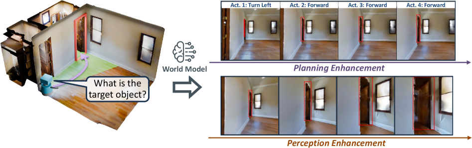<details> <summary>x8.png Details</summary>  ### Visual Description ## Diagram: Robot Navigation System Architecture ### Overview The image depicts a technical diagram illustrating a robot navigation system's workflow. It combines a 3D spatial model with sequential action planning and perception enhancement processes. The system appears to integrate world modeling, action planning, and sensory feedback loops for autonomous navigation. ### Components/Axes 1. **Left Panel**: - **3D Room Model**: A rendered interior space with: - Wooden flooring - Two windows (left and right walls) - Two doors (red and brown) - A blue robot positioned near the center - **Speech Bubble**: Contains the text *"What is the target object?"* - **Brain Icon**: Labeled *"World Model"* with radiating lines 2. **Right Panel**: - **Top Section**: - **Title**: *"Planning Enhancement"* - **Four Action Sequences**: - *Act 1: Turn Left* - *Act 2: Forward* - *Act 3: Forward* - *Act 4: Forward* - Each action shows the robot's position relative to red bounding boxes (likely representing target objects or obstacles) - **Bottom Section**: - **Title**: *"Perception Enhancement"* - **Four Action Sequences**: - *Act 1: Turn Left* - *Act 2: Forward* - *Act 3: Forward* - *Act 4: Forward* - Visuals include enhanced details (e.g., door textures, window reflections) compared to the planning phase 3. **Arrows**: - A purple arrow connects the 3D model to the *"World Model"* brain icon - A blue arrow links the brain icon to the *"Planning Enhancement"* section - A brown arrow connects *"Planning Enhancement"* to *"Perception Enhancement"* ### Detailed Analysis - **Action Sequences**: - All actions follow a consistent pattern: initial left turn followed by three forward movements. - Red bounding boxes in both sections highlight target objects or critical spatial features (e.g., doors, windows). - Perception-enhanced images show more detailed environmental textures (e.g., door handles, floor patterns). - **Spatial Relationships**: - The robot's position shifts progressively across action sequences, indicating movement through the space. - The red bounding boxes remain static in the planning phase but align more precisely with environmental features in the perception phase. ### Key Observations 1. The system prioritizes **planning** (high-level pathfinding) before **perception** (detailed sensory input). 2. The red bounding boxes suggest the robot uses object detection to identify targets during navigation. 3. Enhanced perception improves spatial awareness, as seen in the detailed door/window renderings. ### Interpretation This diagram demonstrates a hierarchical navigation framework where: - **World Model**: Represents the robot's internal understanding of its environment. - **Planning Enhancement**: Translates high-level goals (e.g., "reach the target object") into actionable steps. - **Perception Enhancement**: Refines these actions using real-time sensory data to adapt to dynamic environments. The workflow implies a closed-loop system where perception feedback continuously updates the world model, enabling robust navigation in complex spaces. The consistent action sequence (*Turn Left → Forward*) suggests a predefined path, while the enhanced perception layer allows for adjustments based on environmental details (e.g., avoiding obstacles, aligning with doorframes). **Note**: No numerical data or quantitative values are present in the image. The analysis is based on textual labels, spatial relationships, and visual cues. </details> Figure 8: In AR, the world model supports both queries (perception and planning). In this example, the agent must identify a wooden door that is initially visible only from an extreme viewpoint. For each candidate action sequence, the world model predicts future observations; these forecasts augment the agent’s perception and inform the choice of the next action. Bounding box annotation. The target object is marked by a red bounding box overlaid on the image. For the current real observation $\mathbf{o}_{t}$ , the box is obtained from Habitat ground-truth annotations. For the predicted frames $\{\hat{\mathbf{o}}_{i}\}_{i=t+1}^{t+L}$ produced by the world model, we apply SAM2 (Ravi et al., 2024) to segment the target, seeding the segmenter with the ground-truth box from the current real observation $\mathbf{o}_{t}$ to maintain correspondence across time. Metrics. AR performance is reported using two metrics: (1) Success Rate (SR), defined as the fraction of episodes in which the final predicted label $\hat{y}$ matches the ground-truth label $y$ ; and (2) Mean Trajectory Length, defined as the average number of executed actions before the agent either issues its final prediction or exhausts the step budget $K$ . B.2 Image-Goal Navigation (ImageNav) Image-Goal Navigation (ImageNav), also known as goal-conditioned visual navigation, requires an embodied agent to reach the target location depicted by a single reference image of the goal. The environment is unknown, so the navigation policy must determine how to explore in order to locate the goal efficiently. To examine how world models can assist, we create 144 ImageNav episodes taken from 87 validation scenes of HM3D (Ramakrishnan et al., 2021). Task setup. Each episode permits at most $K=20$ decision steps. As in the AR setting, at step $t$ the agent receives an RGB observation $\mathbf{o}_{t}$ comprising a panoramic view and a front view with a horizontal field of view of $90^{\circ}$ . The agent then proposes a sequence of low-level navigation primitives $\mathbf{A}_{t}=[a_{t+1},\,a_{t+2},\,...,\,a_{t+L}]$ with a maximum horizon of $L=5$ . The first $L-2$ primitives from the selected plan are executed in the real environment, after which the agent replans based on the newly acquired observation. An episode is successful if, within the budget of $K$ steps, the agent’s position enters a sphere of radius $R_{g}=0.5,\text{m}$ centered at the location specified by the goal image $\mathbf{g}$ . Integrating a world model. In ImageNav, the agent answers only the navigation query of which action sequence to execute next; therefore, the world model is used exclusively for planning enhancement. The agent first enumerates several candidate action sequences. For each candidate, the world model predicts the future observations that would follow if the sequence were executed from the current state. The agent then scores each sequence by assessing how informative its predictions are for locating the goal, and selects the sequence with the highest expected utility. When a world model is used, the planner proposes $M=3$ candidate action sequences at each decision step, with horizon $L=5$ . The first $L-2$ actions from the chosen sequence are carried out before the next cycle begins. Metrics. We report three standard metrics for ImageNav: (1) Success Rate (SR), the fraction of episodes in which the agent reaches the goal within the decision budget; (2) Mean Trajectory Length, the average number of executed actions across all episodes; and (3) Success weighted by Path Length (SPL), which accounts for both success and path efficiency. Formally, for a set of $N$ episodes, $$ \mathrm{SPL}=\frac{1}{N}\sum_{i=1}^{N}S_{i}\,\frac{L_{i}^{*}}{\max\!\bigl(L_{i},\,L_{i}^{*}\bigr)}\times 100\%, $$ where $S_{i}∈\{0,1\}$ indicates whether episode $i$ is successful, $L_{i}^{*}$ is the shortest path length from the start position to the goal for episode $i$ , and $L_{i}$ is the actual path length executed by the agent in that episode. B.3 Active Embodied Question Answering (A-EQA) Active Embodied Question Answering (A-EQA) tasks an embodied agent with answering open-ended, natural-language questions after actively exploring an environment. The questions span six broad categories that are common in embodied QA: recognizing objects, recognizing object attributes, recognizing object states, localizing objects, performing spatial reasoning, and performing functional reasoning. Our evaluation set contains 184 questions distributed across 54 indoor scenes drawn from the official OpenEQA split (Majumdar et al., 2024) and the validation set of HM3D (Ramakrishnan et al., 2021). Task setup. In A-EQA, there is no predefined navigation goal, so the agent must design its own exploration strategy to gather sufficient visual evidence for answering the question. At every decision step $t$ , the agent receives a panoramic RGB observation that we decompose into four perspective views, each with a horizontal field of view of $105^{\circ}$ (see Figure ˜ 10). The exploration budget is limited to $250$ low-level actions; a single decision step can comprise multiple low-level actions, depending on the high-level intent. An episode terminates when the budget is exhausted or when the agent outputs a final answer $\hat{y}$ . For A-EQA, we implement a two-level policy that separates deliberation and control. The high-level planner periodically issues one of two types of commands: (i) a textual instruction (for example, “move to the hallway visible in the front view”), or (ii) the index of a landmark object detected in the current panorama. Once a high-level command is produced, execution is delegated to the low-level controller. If the command specifies a landmark, the controller uses depth data together with a custom pathfinder to plan and follow a route to that landmark. If the command is a textual instruction, the controller generates a sequence of low-level actions to carry out the instruction. This planner-controller loop continues until either the $250$ atomic actions are consumed or the high-level planner decides to emit the final answer $\hat{y}$ . 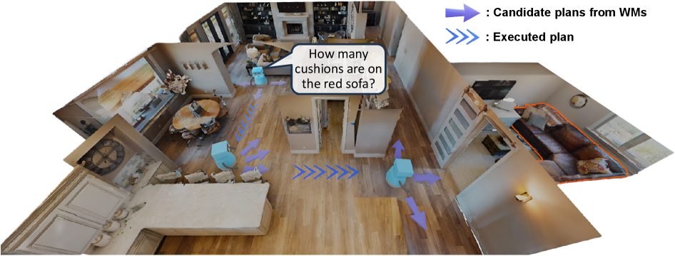<details> <summary>x9.png Details</summary>  ### Visual Description ## 3D Floor Plan Diagram: Robot Navigation & Question Answering System ### Overview The image depicts a 3D-rendered floor plan of a modern home interior, overlaid with directional arrows and annotations. A speech bubble poses the question: "How many cushions are on the red sofa?" The diagram illustrates a robot's path planning process, with arrows representing candidate and executed plans. The red sofa is highlighted in orange, serving as the focal point for the query. ### Components/Axes - **Speech Bubble**: Contains the question "How many cushions are on the red sofa?" positioned near the red sofa in the top-right section of the image. - **Legend**: Located in the top-right corner, defining: - **Purple Arrows**: "Candidate plans from WMs" (World Models) - **Blue Arrows**: "Executed plan" - **Highlighted Sofa**: Red sofa outlined in orange, located in the top-right room near a window. - **Arrows**: - Purple arrows (candidate plans) originate from the bottom-left and spread toward the sofa. - Blue arrows (executed plan) converge on the sofa from the center-right. ### Detailed Analysis - **Speech Bubble Text**: "How many cushions are on the red sofa?" (English, no translation required). - **Legend Text**: - Purple Arrows: "Candidate plans from WMs" - Blue Arrows: "Executed plan" - **Spatial Relationships**: - The red sofa is positioned in the top-right quadrant, adjacent to a window and a bookshelf. - Purple arrows (candidate plans) originate from the bottom-left kitchen area and diverge toward the sofa. - Blue arrows (executed plan) originate from the center-right hallway and converge directly on the sofa. - The orange outline around the sofa emphasizes its importance as the target object. ### Key Observations 1. **Path Planning Visualization**: The diagram contrasts candidate paths (purple) with the final executed path (blue), suggesting a decision-making process in robotics. 2. **Target Focus**: The red sofa is the sole object highlighted, indicating it is the primary subject of the query. 3. **Arrow Density**: More purple arrows (candidate plans) are present than blue arrows (executed plan), implying exploration before execution. 4. **Spatial Layout**: The kitchen (bottom-left) and living area (top-right) are connected via a central hallway, with the robot navigating between these zones. ### Interpretation This diagram demonstrates a robot's navigation and reasoning process to answer a spatial question. The purple arrows represent exploratory paths generated by world models (WMs), while the blue arrows show the optimized path taken to reach the red sofa. The question in the speech bubble suggests the robot is tasked with object recognition and counting (cushions on the sofa). The orange outline around the sofa emphasizes its role as the target, while the contrasting arrow colors illustrate the transition from hypothesis generation to action execution. The layout implies a multi-room environment where the robot must navigate efficiently to complete its task. </details> Figure 9: Overview of our embodied closed-loop evaluation for A-EQA. For each question, the high-level planner proposes multiple candidate action plans and queries the world model to generate the corresponding future observations. The agent then evaluates each plan together with its predicted observations and selects the plan that maximizes the expected reward before executing it in the environment. Integrating a world model. In A-EQA, the world model is primarily used to strengthen the high-level planner. At each high-level decision point, the planner samples $M$ candidate action plans and queries the world model to produce the corresponding predicted observations, as illustrated in Figure ˜ 9. The agent then evaluates each plan-observation pair $(\hat{\mathbf{A}}_{t}^{(m)},\,\hat{\mathbf{O}}_{t}^{(m)})$ and chooses the plan that maximizes the estimated reward under the current question context. This differs from the AR setting, where perception and planning are evaluated through two separate queries. In A-EQA, the high-level planner must both design a long-horizon exploration sequence and decide when to stop exploring to output a final answer $\hat{y}$ . Consequently, the world model supports a single unified query: the predicted observations simultaneously refine the agent’s understanding of the scene and provide forecasts for scoring alternative exploration plans. When a world model is enabled, the planner proposes $M=3$ candidate sequences per step, each with horizon $L=14$ . Unlike AR or ImageNav, only the terminal predicted observation at step $L$ is returned to the high-level planner for scoring, rather than the full rollout over all $L$ steps. 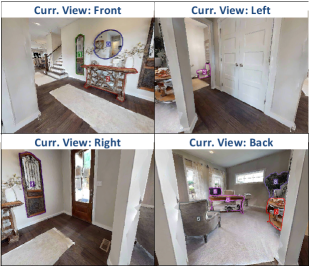<details> <summary>x10.png Details</summary>  ### Visual Description ## Screenshot: Interior Views of a Residential Space ### Overview The image is a collage of four photographs arranged in a 2x2 grid, each labeled with a directional perspective ("Front," "Left," "Right," "Back"). The photos depict the interior of a modern home, showcasing different rooms and architectural features. ### Components/Axes - **Labels**: - Top-left: "Curr View: Front" - Top-right: "Curr View: Left" - Bottom-left: "Curr View: Right" - Bottom-right: "Curr View: Back" - **Textual Content**: - No additional axis titles, legends, or numerical data present. - Labels are positioned in the top-left corner of each photo, using a sans-serif font with a dark gray color. ### Detailed Analysis 1. **Front View (Top-left)**: - A hallway with light hardwood flooring, a white runner rug, and a wooden console table with decorative items. - A staircase with a dark wooden railing is visible in the background. - A round mirror with a gold frame hangs on the wall. 2. **Left View (Top-right)**: - A white double-door closet with a brass handle. - A glimpse of a child’s playroom with a pink toy storage unit and a white door. 3. **Right View (Bottom-left)**: - A living area with a gray sofa, a wooden coffee table, and a large window with sheer curtains. - A hallway leading to a bedroom with a dark wooden door and a mirror with a purple frame. 4. **Back View (Bottom-right)**: - A dining area with a white table, pink chairs, and a chandelier. - A window with a white frame and a view of a garden outside. ### Key Observations - The photos emphasize symmetry and open-plan design, with consistent use of neutral tones (white, gray, wood) and pops of color (pink, purple). - No numerical data or trends are present; the focus is on spatial layout and interior design. ### Interpretation The collage serves as a visual tour of the home’s interior, highlighting its functional zones (entryway, living area, dining space) and design coherence. The labels clarify the viewer’s perspective, suggesting this could be part of a real estate listing or architectural portfolio. The absence of textual data beyond labels indicates the image prioritizes visual storytelling over quantitative analysis. </details> Figure 10: Illustration of the Set-of-Marks (SoM) representation that encodes candidate navigable directions. The high-level planner chooses among these discrete landmarks when constructing candidate action plans. Landmark detection and labeling. Landmark objects are detected by first running YOLO-World to obtain bounding boxes and then applying SAM2 to derive instance masks (Ravi et al., 2024; Cheng et al., 2024). This detection pipeline follows the Set-of-Marks (SoM) strategy (Yang et al., 2023a) shown in Figure ˜ 10 and provides a discrete set of navigable targets for high-level planning. Metrics. A-EQA performance is evaluated with three metrics. (1) Answering Score: a large language model (e.g., GPT-4o) compares the agent’s final answer $\hat{y}$ to the ground-truth answer $y$ and assigns a raw score in $[1,5]$ , where $5$ indicates a perfect match. We average the raw score across episodes and then linearly map it to $[0,100]$ . (2) Mean Trajectory Length. This is the average travel distance the agent covers before either producing its final answer or exhausting the step budget $K$ , lower is better. (3) Success weighted by Path Length (SPL): this metric rewards both answer quality and navigation efficiency. For episodes in which the agent fails to return an answer, we fall back to its blind LLM variant and set the SPL contribution to zero. Formally, $$ \text{SPL}_{\text{A-EQA}}=\frac{1}{N}\sum_{i=1}^{N}\left(\frac{\sigma_{i}-1}{4}\right)\frac{L_{i}^{*}}{\max\!\bigl(L_{i},\,L_{i}^{*}\bigr)}\times 100\%, $$ where $N$ is the number of evaluation episodes, $\sigma_{i}∈[1,5]$ denotes the raw Answering Score for episode $i$ , $L_{i}^{*}$ denotes the shortest-path length from the start to a viewpoint that affords a correct answer, and $L_{i}$ denotes the actual path length executed by the agent in episode $i$ . A higher value indicates both more accurate answering and more efficient exploration. B.4 Robotic Manipulation We study whether world models can improve low-level manipulation, which is a core capability for embodied agents. Our evaluation covers four robotic manipulation tasks in RLBench (James et al., 2020): Push Buttons, Slide Block to Color Target, Insert onto Square Peg, and Stack Cups. RLBench is a widely used benchmark for robot learning. Each episode provides a natural-language instruction that specifies the task objective, and the agent must control a 7-DoF robotic arm to satisfy that objective. We prepare a total of 200 evaluation episodes, with 50 episodes for each task. Task setup. At each decision step $t$ , the agent receives an observation $\mathbf{o}_{t}$ and proposes an action sequence $\mathbf{A}_{t}=\bigl[\mathbf{a}_{t+1},\,\mathbf{a}_{t+2},\,...,\,\mathbf{a}_{t+L}\bigr]$ , where each low-level action is parameterized as $\mathbf{a}_{t}=[x,\,y,\,z,\,\text{roll},\,\text{pitch},\,\text{yaw},\,\text{gripper}]$ . We consider two base policy settings with different horizons: $L=5$ for a VLM base policy that emits discrete actions, and $L=50$ for a 3D diffusion base policy that emits continuous actions. An episode is counted as a success if the specified goal $\mathbf{g}$ is achieved within the step budget $K$ . 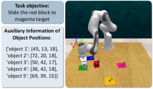<details> <summary>x11.png Details</summary>  ### Visual Description ## Robotic Arm Task Diagram: Object Manipulation Setup ### Overview The image depicts a robotic arm interacting with colored blocks on a wooden surface. The task objective is to slide the red block to a magenta target. Auxiliary data provides coordinates for five objects, with a legend mapping colors to object identifiers. ### Components/Axes - **Legend**: Located in the top-left corner, associating colors with object numbers: - Red: Object 3 - Blue: Object 2 - Green: Object 1 - Pink: Object 4 - Yellow: Object 5 - **Object Positions**: Listed in a structured format with coordinates (x, y, z): - Object 1: [45, 13, 18] - Object 2: [72, 20, 18] - Object 3: [50, 42, 17] - Object 4: [36, 42, 18] - Object 5: [69, 39, 15] - **Diagram Elements**: - Robotic arm (white/gray) positioned near the red block (Object 3). - Colored blocks placed on distinct colored platforms (e.g., red block on green platform). - Magenta target (unlabeled in data) implied as the destination for Object 3. ### Detailed Analysis - **Object Coordinates**: - Object 1 (green): [45, 13, 18] - Object 2 (blue): [72, 20, 18] - Object 3 (red): [50, 42, 17] - Object 4 (pink): [36, 42, 18] - Object 5 (yellow): [69, 39, 15] - **Spatial Relationships**: - Object 3 (red) is centrally located at [50, 42, 17], near Object 4 ([36, 42, 18]) and Object 2 ([72, 20, 18]). - The robotic arm’s gripper is positioned above Object 3, suggesting active manipulation. - Magenta target is not explicitly listed in the object positions, creating ambiguity about its coordinates. ### Key Observations 1. **Task Objective vs. Data**: The magenta target is referenced in the task description but absent from the object position list, indicating missing data. 2. **Red Block Proximity**: Object 3 (red) is equidistant in the y-axis (42) from Objects 1 and 4 but closer in x-axis to Object 4 (36 vs. 50). 3. **Robotic Arm Positioning**: The arm’s orientation suggests it is preparing to grasp Object 3, aligning with the task objective. ### Interpretation The diagram illustrates a precision manipulation task requiring the robotic arm to relocate Object 3 (red block) to an unspecified magenta target. The provided coordinates suggest a 3D workspace, with Objects 1–5 distributed across the surface. The absence of the target’s coordinates introduces uncertainty, potentially requiring additional sensor data or assumptions for path planning. The robotic arm’s proximity to Object 3 implies readiness for execution, but the task’s success depends on resolving the target’s location. </details> Figure 11: Illustration of the auxiliary information provided to the VLM policy. The objects are marked with indices, and their positions are given to the VLM to facilitate decision-making. When a VLM is the base policy, directly producing precise low-level controls is challenging for current VLMs. Following (Yang et al., 2025), we therefore introduce two enhancements. First, we discretize the action space by dividing the position components $(x,y,z)$ into 100 bins and the orientation components $(\text{roll},\text{pitch},\text{yaw})$ into 120 bins. Second, we augment the observations with object index markers and provide precise object poses for indexed objects so that the VLM can directly access spatial information during planning (shown in Figure ˜ 11). Under this configuration, the manipulation policy is allowed at most $K=15$ low-level action steps per episode. In contrast, when using a 3D diffusion policy (Ke et al., 2024) as the base policy, the controller naturally generates continuous low-level actions, so we do not apply the discretization or the additional indexing enhancements. In this configuration, the manipulation policy is permitted at most $K=8$ macro decision steps per episode. Integrating a world model. As in ImageNav, we use the world model exclusively for planning enhancement. The agent executes a propose, simulate, and revise loop so that it can reason about the consequences of alternative plans before applying any action in the real environment. At each decision step, the planner proposes $M=5$ candidate action sequences. When the length of a candidate sequence is shorter than the world model’s required action-conditioning length, the unified action API linearly interpolates the sequence to the required length. Conversely, when the candidate sequence is longer than required, the unified action API uniformly samples actions along the sequence to match the world model’s input length. The planner then evaluates the simulated outcomes and selects the sequence with the highest expected reward, and the loop repeats with updated observations. Metrics. We report two standard metrics for manipulation tasks: (1) Success Rate (SR), the fraction of episodes in which the agent reaches the goal within the decision budget; and (2) Mean Trajectory Length, the average number of decision steps across all episodes. B.5 Policies in Embodied Tasks There are three types of policies in paper: the base policy, the proposal policy, and the revision policy. The base policy is an independent policy that interacts with the environment without using a world model, and when a world model is enabled, it is always the same as the corresponding proposal policy. When a world model is integrated, the proposal policy generates multiple candidate action sequences at each decision step, and the revision policy evaluates these candidates and selects one based on the predicted rollouts produced by the world model. In our experiments, we employ two types of base policies for AR and ImageNav: a VLM policy and a heuristic policy. For the VLM policy, we use Qwen2.5-VL-72B-Instruct-AWQ (Bai et al., 2025) as the default base policy and as the proposal policy when integrated with a world model to answer queries. For the heuristic policy, we implement a primitive action sampling mechanism that draws actions from the action space according to the previously executed actions and a set of handcrafted rules. Concretely, if there exists a previous action, then the next action must not be its inverse (for example, a turn_left cannot be immediately followed by a turn_right). In addition, we prevent excessively long subsequences of turns in the same direction by capping the maximum number of consecutive turns to four. These rules help the heuristic policy to avoid redundant back-and-forth movements and to explore the environment effectively. For manipulation tasks, we likewise consider two base policies: a VLM policy and a 3D diffusion policy. The VLM policy remains Qwen2.5-VL-72B-Instruct-AWQ by default. The 3D diffusion policy follows 3D Diffuser Actor (Ke et al., 2024); we train it using the authors’ official code. To encourage diverse action trajectory proposals, we drop its text input and modify the task-definition scripts so that task variants occur with equal frequency during training. For each manipulation task, the diffusion policy is trained on 120 demonstrations and used as the proposal policy to generate short-horizon 7-DoF gripper action sequences within the planning loop. For the revision policy in our closed-loop online planning, we use the same VLM as the proposal policy by default to score candidate plans and to select the decision that maximizes the expected task reward. For ablations, we also replace Qwen2.5-VL-72B-Instruct-AWQ with InternVL3-78B-AWQ (Zhu et al., 2025) as the VLM policy; results in Table ˜ 5 show that world model integration consistently improves performance regardless of the specific VLM used. Table 5: Task performance for InternVL3 variants with and without a world model. Higher SR %, SPL %, and Ans. Score are better; lower Mean Traj. is better. | Model Details | AR | ImageNav | A-EQA | | | | | | | | --- | --- | --- | --- | --- | --- | --- | --- | --- | --- | | Model Type | Method | SR $\uparrow$ | Mean Traj. $\downarrow$ | SR $\uparrow$ | Mean Traj. $\downarrow$ | SPL $\uparrow$ | Ans. Score $\uparrow$ | Mean Traj. $\downarrow$ | SPL $\uparrow$ | | Base Policy | InternVL3 (w/o WM) | 49.91 | 7.06 | 13.19 | 60.30 | 7.46 | 47.28 | 20.45 | 31.22 | | + Image Gen. | SVD $\dagger$ | 55.72 | 5.37 | 40.97 | 52.50 | 26.26 | 47.13 | 16.78 | 34.54 | B.6 World Models in Embodied Tasks Output format. The world models evaluated in our framework fall into two categories according to their native output format: perspective models and panoramic models. Perspective models, such as NWM (Bar et al., 2025a), LTX-Video (HaCohen et al., 2024), and Wan2.1 (Wan et al., 2025), generate frames in a perspective view. Panoramic models, including PathDreamer (Koh et al., 2021b), SE3DS (Koh et al., 2023), and our post-trained variants, produce equirectangular panoramas. For integration into our closed-loop pipeline, panoramic outputs are decomposed into perspective views, which are then supplied to the agent. In A-EQA, the agent consumes four principal perspective views (front, left, right, back) when they are available. In AR, the agent uses the view that contains the target bounding box; if the box is not visible, we discard the generated frames until the predicted box (from SAM2) enters the field of view. Unless otherwise specified, each perspective view image is resized to $384× 384$ pixels before being passed to the agent. Input format. Panoramic models are conditioned on an equirectangular panorama at a resolution of $576× 1024$ pixels. Perspective models, when possible, take the current front-view observation with resolution $480× 480$ as input. Some models require additional modalities. SE3DS expects a depth map, while PathDreamer requires both depth and a per-pixel semantic label map. For all depth-aware models, we provide ground-truth depth from Habitat. For PathDreamer, the initial semantic map is obtained by running a pretrained RedNet (Jiang et al., 2018) on the initial RGB-D frame to produce per-pixel labels that match the required input specification. Appendix C Post-Training Recipe for Embodied World Models In this section, we describe how an off-the-shelf video generation model is adapted, via post-training, into an action-controllable world model suitable for embodied tasks. We first formalize the learning objective and the action-observation alignment (Section ˜ C.1), and then detail the concrete post-training setup used for tasks in Habitat-Sim and for Robotic Manipulations (Section ˜ C.2). C.1 Problem Formulation Let $\mathbf{x}_{1}\!∈\!\mathbb{R}^{3× H× W}$ denotes the initial RGB frame that conditions the generation process. Our goal is to synthesize an $N$ -frame video $\mathbf{X}=\bigl[\mathbf{x}_{1},\,\mathbf{x}_{2},\,...,\,\mathbf{x}_{N}\bigr]∈\mathbb{R}^{3× H× W× N},$ where $\mathbf{X}$ represents a plausible sequence of future observations after executing a sequence of actions $\mathbf{A}=\bigl[a_{1},\,a_{2},\,...,\,a_{N}\bigr].$ For tasks in Habitat-Sim, we adopt a discrete action space with $a_{i}∈\mathcal{V}$ , where $\mathcal{V}$ is a finite set of navigation primitives (e.g., Forward, Turn-Left, Turn-Right, Stop). For manipulation, we use a continuous action space with $a_{i}∈\mathbb{R}^{7}$ , corresponding to 7-DoF end-effector poses. Actions in Habitat-Sim specify relative transformations between consecutive observations. Since $a_{i}$ maps $\mathbf{x}_{i-1}$ to $\mathbf{x}_{i}$ , no action precedes the first frame. To maintain a one-to-one alignment between frames and actions, we prepend a special token and set $a_{1}=a_{\text{Null}}$ . In contrast, for manipulation tasks during post-training, actions are absolute end-effector poses expressed in the world frame, so there is naturally a one-to-one correspondence between actions and frames. We formulate future-observation synthesis with the world model $g_{\boldsymbol{\theta}}$ by learning the conditional distribution $p_{\boldsymbol{\theta}}\bigl(\mathbf{X}\,\big|\,\mathbf{x}_{1},\,C(\mathbf{A})\bigr),$ where $C(\mathbf{A})$ denotes the control signal emitted by the unified action API. This API converts the native action sequence $\mathbf{A}$ into the conditioning interface expected by the pretrained video generator (for example, a text prompt, a camera trajectory, or a sequence of low-level controls). This formulation yields action-conditioned rollouts that evolve from the initial frame $\mathbf{x}_{1}$ according to the specified action sequence, thereby aligning the pretrained model with the domain distribution and action space of the target embodied tasks. C.2 Post-Training Configuration For tasks in Habitat-Sim, we use panoramic observations as both the input and the output of the video generators. We fine-tune the pretrained video generation models at a resolution of $576× 1024$ and train them to predict $N$ future frames on our self-collected panoramic action-observation corpus from Habitat-Sim. In these tasks, the action space is discrete and comprises four navigation primitives: Forward 0.2 m, Turn_Left 22.5 ∘, Turn_Right 22.5 ∘, and Stop. For manipulation tasks, we use front-view observations as both the input and the output of the video generators. We fine-tune the pretrained video generation models at a resolution of $480× 480$ (Cosmos-Predict2) or $448× 448$ (SVD) and train them to predict $N$ future frames with continuous 7-DoF end-effector poses as conditioning. Unless otherwise stated, post-training uses 40K sampled instances for the Habitat-Sim tasks and for the manipulation tasks. All models are initialized from their official pretrained weights and adapted on the corresponding dataset for one epoch. We rely on the official implementations and the recommended hyperparameters for fine-tuning whenever available; specific post-training details of various world models are summarized below in Tables ˜ 6 and 7. Table 6: Post-trained (action-conditioned) world models used in our experiments, with repositories and training configurations. | World Model | Domain | Repository | Frames ( $N$ ) | Train Res. | Notes | | --- | --- | --- | --- | --- | --- | | Post-training on Habitat-Sim data | | | | | | | Cosmos-Predict2 $\dagger$ (Agarwal et al., 2025) | Habitat-Sim | github.com/nvidia-cosmos/cosmos-predict2 | 13 | $576× 1024$ | Official repo | | LTX-Video $\dagger$ (HaCohen et al., 2024) | Habitat-Sim | github.com/Lightricks/LTX-Video-Trainer | 17 | $576× 1024$ | Official repo | | Wan2.1 $\dagger$ (Wan et al., 2025) | Habitat-Sim | github.com/modelscope/DiffSynth-Studio | 13 | $576× 1024$ | Official repo | | Wan2.2 (5B) $\dagger$ (Wan et al., 2025) | Habitat-Sim | github.com/modelscope/DiffSynth-Studio | 13 | $576× 1024$ | Official repo | | Wan2.2 (A14B) $\dagger$ (Wan et al., 2025) | Habitat-Sim | github.com/modelscope/DiffSynth-Studio | 13 | $576× 1024$ | Official repo | | SVD $\dagger$ (Blattmann et al., 2023a) | Habitat-Sim | github.com/pixeli99/SVD_Xtend | 14 | $576× 1024$ | Self-adapted based on repo | | Post-training on manipulation data | | | | | | | Cosmos-Predict2 $\dagger$ (Agarwal et al., 2025) | Manipulation | github.com/nvidia-cosmos/cosmos-predict2 | 13 | $480× 480$ | Official repo | | SVD $\dagger$ (Blattmann et al., 2023a) | Manipulation | github.com/pixeli99/SVD_Xtend | 14 | $448× 448$ | Self-adapted based on repo | Table 7: All the world models and their details in World-in-World. “ $\dagger$ ” denotes post-trained (action-conditioned) variants. | World Model | Model Type | Control Type | Input Type | #Param. | | --- | --- | --- | --- | --- | | Zero-shot (no post-training) | | | | | | PathDreamer (Koh et al., 2021b) | Image Gen. | Viewpoint | RGB-D; Pano | 0.69B | | SE3DS (Koh et al., 2023) | Image Gen. | Viewpoint | RGB-D; Pano | 1.1B | | NWM (Bar et al., 2025a) | Video Gen. | Trajectory | RGB | 1B | | SVD (Blattmann et al., 2023a) | Video Gen. | Image | RGB | 1.5B | | LTX-Video (HaCohen et al., 2024) | Video Gen. | Text | RGB | 2B | | Hunyuan (Kong et al., 2024) | Video Gen. | Text | RGB | 13B | | Wan2.1 (Wan et al., 2025) | Video Gen. | Text | RGB | 14B | | Wan2.2 (Wan et al., 2025) | Video Gen. | Text | RGB | 5B | | Wan2.2 (Wan et al., 2025) | Video Gen. | Text | RGB | A14B | | Cosmos-Predict2 (Agarwal et al., 2025) | Video Gen. | Text | RGB | 2B | | Runway Gen4 (Runway Research, 2025) | Video Gen. | Text | RGB | – | | Post-trained (action-conditioned) | | | | | | SVD $\dagger$ (Blattmann et al., 2023a) | Video Gen. | Action | RGB; Pano | 1.5B | | LTX-Video $\dagger$ (HaCohen et al., 2024) | Video Gen. | Action | RGB; Pano | 2B | | Wan2.1 $\dagger$ (Wan et al., 2025) | Video Gen. | Action | RGB; Pano | 14B | | Wan2.2 $\dagger$ (Wan et al., 2025) | Video Gen. | Action | RGB; Pano | 5B | | Wan2.2 $\dagger$ (Wan et al., 2025) | Video Gen. | Action | RGB; Pano | A14B | | Cosmos-Predict2 $\dagger$ (Agarwal et al., 2025) | Video Gen. | Action | RGB; Pano | 2B | In Table ˜ 8, we summarize the computational resources required to post-train each world model on $\sim$ 40k domain-specific clips collected from Habitat-Sim. This post-training stage is intentionally lightweight and is several orders of magnitude less expensive than full pretraining. For 14B-parameter variants, we adopt LoRA fine-tuning to reduce GPU memory usage, while all other models are fine-tuned with full weights. Table 8: Post-training resources for $\sim$ 40k domain clips per model. The procedure is lightweight and substantially cheaper than full retraining. | Model | Model Size | GPU Memory (peak) | H100 GPU-hours | | --- | --- | --- | --- | | SVD | 1.5B | 84 GB | 29 | | LTX-Video | 2B | 61 GB | 5 | | Wan2.1 | 14B | 57 GB | 74 | | Cosmos-Predict2 | 2B | 71 GB | 15 | Appendix D Post-Training Dataset Construction For the post-training dataset used in manipulation tasks, we rely on the official RLBench codebase (James et al., 2020) to generate data. Specifically, we produce 200 demonstrations for each manipulation task. Each demonstration includes approximately 150 front-view RGB observations together with the corresponding sequence of 7-DoF end-effector poses. These pose sequences are aligned with the image observations and serve as the action labels during post-training. For the tasks evaluated in Habitat-Sim (Savva et al., 2019), there is no existing pipeline for constructing a large-scale dataset of panoramic action trajectories. To address this gap, we build a comprehensive post-training dataset by sampling action trajectories from the training splits of indoor scenes in HM3D (Ramakrishnan et al., 2021) and Matterport3D (Chang et al., 2017). Our trajectory sampling procedure is described in Section ˜ D.1. A summary of the resulting dataset statistics is provided in Table ˜ 9. D.1 Trajectory Sampling | Statistic | Value | | --- | --- | | Number of scenes | 858 | | Panorama RGB frames | 763,724 | | Action trajectories | 439,213 | | Depth recorded | ✓ | | Camera poses recorded | ✓ | | Low-level actions recorded | ✓ | Table 9: Statistics of the post-training panoramic dataset. Our aim is to record physically reasonable trajectories that resemble the exploration behavior of real agents in indoor spaces. We follow three guiding principles: (i) Diversity. The trajectories should cover many viewpoints and actions so that the model sees the scene from different perspectives and motion patterns. (ii) Plausibility. The paths must respect physical constraints; the agent must not move through walls or other solid objects. (iii) Manageability. The data should be free of excessive redundancy so that training remains balanced and efficient. Algorithm 1 Three-stage construction of the post-training panoramic dataset Input: scene mesh $\mathcal{S}$ , waypoint density $\rho$ , weight $\alpha$ , filter radius $r_{\mathrm{f}}$ , leaf ratio $\eta$ Output: set of panoramic trajectories $\mathcal{T}$ 1: // Stage 1: waypoint selection 2: $S←\mathrm{Area}(\mathcal{S})$ 3: $N_{\mathrm{wp}}←\max\!\bigl(1400,\lfloor\rho S\rfloor\bigr)$ $\triangleright$ target number of points 4: $\mathcal{P}←\textsc{UniformSampleNavigable}(\mathcal{S},N_{\mathrm{wp}})$ 5: build geodesic distance matrix $D$ on $\mathcal{P}$ 6: for all $p_{i}∈\mathcal{P}$ do $\triangleright$ leaf score $s(i)$ 7: $\text{ecc}(i)←\max_{j}D_{ij}$ 8: $\bar{d}(i)←\frac{1}{|\mathcal{P}|-1}\sum_{j}D_{ij}$ 9: $s(i)←\text{ecc}(i)+\alpha\,\bar{d}(i)$ 10: sort $\mathcal{P}$ by $s(i)$ in descending order $\triangleright$ higher $s(i)$ = more peripheral 11: $\mathcal{W}←\varnothing$ 12: for all $p_{i}$ in sorted $\mathcal{P}$ do $\triangleright$ radius-based greedy pruning 13: if $∀ w∈\mathcal{W}:D_{iw}≥ r_{\mathrm{f}}$ then 14: $\mathcal{W}←\mathcal{W}\cup\{p_{i}\}$ 15: // Stage 2: path generation 16: $\mathcal{T}←\varnothing$ 17: $N_{\text{leaf}}←\lceil\eta N_{\mathrm{wp}}\rceil$ 18: $\mathcal{U}←\mathcal{W}[{:}N_{\text{leaf}}]$ $\triangleright$ unvisited waypoints 19: $c←\textsc{RandomSample}(\mathcal{U})$ $\triangleright$ random start 20: while $\mathcal{U}≠\varnothing$ do 21: $n←\arg\min_{w∈\mathcal{U}\setminus\{c\}}\textsc{GeodesicDist}(c,w)$ 22: $\tau←\textsc{ShortestPath}(c,n)$ $\triangleright$ Habitat planner 23: record panoramic RGB-D frames along $\tau$ and append to $\mathcal{T}$ 24: // Stage 3: waypoint dynamic update 25: for all $w∈\mathcal{W}$ do 26: if $∃ m∈\tau:\textsc{GeodesicDist}(m,w)<r_{\mathrm{f}}$ then 27: $\mathcal{W}←\mathcal{W}\setminus\{w\}$ $\triangleright$ mark as visited 28: recompute $s(·)$ on updated $\mathcal{W}$ , then sort in descending order 29: $\mathcal{U}←\mathcal{W}[{:}N_{\text{leaf}}]$ $\triangleright$ refresh unvisited set 30: $c← n$ 31: return $\mathcal{T}$ We implement these principles with a sampling procedure shown in Algorithm ˜ 1 and described below. 1. Waypoint selection. For a scene of floor area $S$ we set the waypoint density to $\rho=4\ \text{m}^{-2}$ and draw $$ N_{\mathrm{wp}}=\max\!\bigl(1400,\lfloor\rho S\rfloor\bigr) $$ navigable points $\mathcal{P}$ uniformly across the scene. We construct a complete graph whose edge weights $D_{ij}$ are the geodesic distances between points $p_{i}$ and $p_{j}$ . Each vertex $i$ is assigned a leaf score $$ s(i)=\operatorname{ecc}(i)+\alpha\,\bar{d}(i), $$ where $\operatorname{ecc}(i)=\max_{j}D_{ij}$ is the eccentricity, $\bar{d}(i)=(|\mathcal{P}|-1)^{-1}\sum_{j}D_{ij}$ is the mean geodesic distance to all other vertices, and $\alpha=1.7$ . Sorting vertices by $s(i)$ in descending order, we greedily build a waypoint set $\mathcal{W}$ that respects a minimum spacing of $r_{\mathrm{f}}=3$ m: a candidate $v$ is accepted only if $D_{vj}≥ r_{\mathrm{f}}$ for every waypoint $j$ already chosen. 1. Path generation. We maintain a list $\mathcal{U}$ of unvisited waypoints, initialized with the top $N_{\text{leaf}}$ vertices of $\mathcal{W}$ . Starting from a random waypoint $c∈\mathcal{U}$ , we repeatedly move to the nearest unvisited waypoint $$ n=\arg\min_{w\in\mathcal{U}\setminus\{c\}}\textsc{GeodesicDist}(c,w), $$ and use the Habitat path-finder to compute the shortest collision-free path $\tau$ from $c$ to $n$ . Panoramic RGB-D frames are recorded at every step along $\tau$ and appended to the trajectory set $\mathcal{T}$ . 1. Waypoint dynamic update. After each segment $\tau$ we label any waypoint $w$ with GeodesicDist(m,w) $<r_{\mathrm{f}}$ for some path point $m∈\tau$ as visited and remove it from $\mathcal{W}$ . We then recompute $s(·)$ on the remaining vertices, resort $\mathcal{W}$ , and refresh the unvisited list $$ \mathcal{U}\leftarrow\mathcal{W}[{:}N_{\text{leaf}}]. $$ The next segment starts from $c← n$ , and the loop continues until $\mathcal{U}$ is empty. This dynamic reselection guarantees that peripheral regions are covered while avoiding redundant sampling in interior corridors. 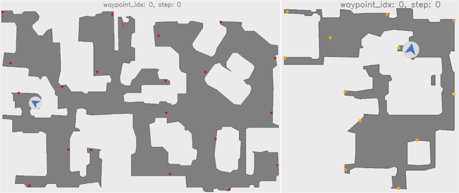<details> <summary>x12.png Details</summary>  ### Visual Description ## Map Visualization: Waypoint Navigation Layout ### Overview The image displays two side-by-side grayscale maps with annotated waypoints. Both maps are labeled "waypoint_idx: 0, step: 0" at the top. The left map contains numerous red dots, while the right map features yellow dots and a blue compass icon. White spaces represent open areas, and gray regions denote obstacles or walls. ### Components/Axes - **Maps**: - **Left Map**: Dominated by red dots (14 total) scattered across the layout. - **Right Map**: Contains 8 yellow dots and a central blue compass icon. - **Labels**: - Top text: "waypoint_idx: 0, step: 0" (identical for both maps). - **Compass Icon**: - Blue arrow symbolizing direction, positioned at the bottom-left of the left map and centered in the right map. ### Detailed Analysis - **Waypoint Distribution**: - Left map: Red dots are densely clustered in the lower-left quadrant and along the central vertical axis. - Right map: Yellow dots are spaced more evenly, with concentrations in the upper-right and lower-left regions. - **Compass Placement**: - Left map: Compass is anchored at the bottom-left corner, suggesting a starting orientation. - Right map: Compass is centered, implying a mid-navigation reference point. - **Color Coding**: - Red dots (left map) and yellow dots (right map) likely represent distinct waypoint categories (e.g., "initial" vs. "target" points). ### Key Observations 1. **Waypoint Density**: The left map has nearly double the number of red dots compared to yellow dots on the right map. 2. **Compass Orientation**: The compass direction (pointing northeast) remains consistent across both maps, despite differing positions. 3. **Spatial Symmetry**: Both maps share a mirrored layout, with open areas (white spaces) forming a central corridor. ### Interpretation The maps likely represent stages of a navigation task: - **Left Map**: Initial waypoint setup (red dots) with a fixed starting orientation (compass at bottom-left). - **Right Map**: Progressed navigation (yellow dots) with a dynamic reference point (centered compass). - **White Spaces**: Open pathways suggest traversable routes, while gray regions act as barriers. - **Waypoint Index/Step**: The label "waypoint_idx: 0, step: 0" implies these are baseline configurations, possibly for algorithm initialization or step-0 state visualization. No numerical data or explicit trends are present, but the spatial arrangement suggests a progression from static waypoint definition (left) to dynamic pathfinding (right). The compass’s repositioning may indicate recalibration during navigation. </details> Figure 12: Top-down visualization of sampled waypoints in a scene. Red (left) and yellow (right) dots are the final waypoints after radius-based pruning. The proposed strategy places waypoints throughout peripheral regions while avoiding redundant interior points, yielding diverse and spatially balanced trajectories. Compared with random sampling of start and end waypoints, the above strategy distributes waypoints across peripheral areas such as bedrooms while avoiding redundant paths through interior corridors. The resulting dataset therefore offers a balanced and diverse set of viewpoints for post-training (see Figure ˜ 12). Appendix E Visualizing World Model Predictions We illustrate the behavior of several world models under identical action sequences generated by the planner. Figure ˜ 13 and Figure ˜ 14 show example rollouts in which the action sequence consists solely of Forward actions; a well-behaved model should yield pure forward motion. The figures contrast models that follow the commands with those that drift or hallucinate, underscoring the importance of precise action control for downstream embodied tasks. For further examples of good and bad predictions, see Figures ˜ 15, 16, 17 and 18. 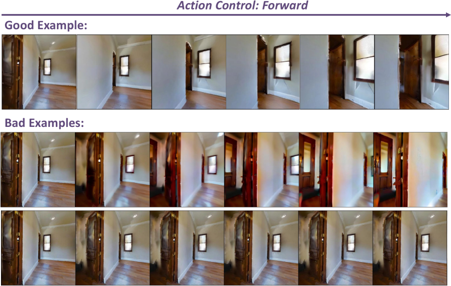<details> <summary>x13.png Details</summary>  ### Visual Description ## Image Sequence Comparison: Action Control: Forward ### Overview The image displays a comparative analysis of image sequences generated under "Action Control: Forward" conditions. It contrasts a "Good Example" with two "Bad Examples" through side-by-side visualizations of a room interior with a door opening. The sequences demonstrate varying levels of coherence, alignment, and artifact presence across three rows of six images each. ### Components/Axes - **Title**: "Action Control: Forward" (top center, bold text with rightward arrow) - **Labels**: - "Good Example:" (top row, left-aligned) - "Bad Examples:" (bottom two rows, left-aligned) - **Image Structure**: - **Good Example Row**: 6 sequential images showing progressive door opening with consistent lighting, perspective, and spatial alignment. - **Bad Example Rows**: - Row 1: 6 images with progressive blurring, misalignment, and color distortion. - Row 2: 6 images with severe spatial warping, ghosting artifacts, and inconsistent lighting. ### Detailed Analysis - **Good Example**: - Images depict a static room with a wooden door opening from left to right. - Consistent lighting (natural window illumination), uniform flooring texture, and unaltered wall geometry. - No visible artifacts or distortions across the sequence. - **Bad Example Row 1**: - Initial images show minor blurring near the door frame. - Mid-sequence images exhibit progressive misalignment between door edges and wall geometry. - Final images display color bleeding and overexposure in the doorway area. - **Bad Example Row 2**: - Early images show spatial warping in the door frame. - Mid-sequence images feature ghosting artifacts and inconsistent shadowing. - Final images exhibit extreme perspective distortion and loss of structural coherence. ### Key Observations 1. **Coherence**: The good example maintains spatial and temporal consistency, while bad examples degrade rapidly. 2. **Artifacts**: Bad examples exhibit blurring (Row 1), warping (Row 2), and ghosting (Row 2). 3. **Lighting**: Good example preserves natural lighting; bad examples show inconsistent illumination. 4. **Perspective**: Good example retains architectural accuracy; bad examples distort spatial relationships. ### Interpretation This comparison illustrates the impact of motion control algorithms on image generation quality. The good example likely employs robust motion vector alignment and spatial coherence techniques, preserving structural integrity during action simulation. The bad examples demonstrate failure modes: - **Row 1**: Indicates issues with temporal consistency, possibly due to inadequate motion tracking. - **Row 2**: Suggests failures in spatial reasoning, such as incorrect perspective projection or object-occlusion handling. The progression from minor to severe distortions highlights the sensitivity of generative models to input parameters. These results could inform improvements in action-conditioned image synthesis by identifying critical failure points in motion control pipelines. </details> Figure 13: Examples of good and bad predictions. The action sequence contains only Forward actions. Models that violate this requirement yield observations that can mislead the planner. 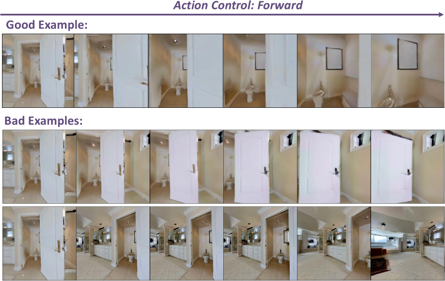<details> <summary>x14.png Details</summary>  ### Visual Description ## Action Control Visualization: Forward Motion Examples ### Overview The image presents a comparative analysis of action control outcomes in a simulated environment. It demonstrates two distinct scenarios: a "Good Example" of smooth forward motion and two "Bad Examples" showing progressive distortion. The visualization uses sequential frames to illustrate the impact of action control algorithms on scene rendering. ### Components/Axes - **Title**: "Action Control: Forward" with right-pointing arrow (→) - **Primary Sections**: 1. "Good Example:" (Top section) 2. "Bad Examples:" (Bottom two sections) - **Visual Elements**: - 6 sequential frames per example - Bathroom scene with white door, toilet, and framed artwork - Progressive door opening animation ### Detailed Analysis **Good Example:** 1. Frame 1: Door partially open (30°) 2. Frame 2: Door at 45° 3. Frame 3: Door at 60° 4. Frame 4: Door at 75° 5. Frame 5: Door at 90° (fully open) 6. Frame 6: Door at 105° (slightly ajar) **Bad Examples:** 1. First Row: - Frame 1: Door at 30° with minor distortion - Frame 2: Door at 45° with increased blur - Frame 3: Door at 60° with misaligned textures - Frame 4: Door at 75° with warped perspective - Frame 5: Door at 90° with partial transparency - Frame 6: Door at 105° with complete scene collapse 2. Second Row: - Frame 1: Door at 30° with color banding - Frame 2: Door at 45° with geometric artifacts - Frame 3: Door at 60° with spatial misalignment - Frame 4: Door at 75° with temporal ghosting - Frame 5: Door at 90° with complete scene inversion - Frame 6: Door at 105° with total visual failure ### Key Observations 1. The good example maintains consistent lighting, texture fidelity, and spatial relationships throughout the sequence 2. Bad examples show progressive degradation: - First row: Physical distortion (blurring, warping) - Second row: Rendering artifacts (color banding, spatial misalignment) 3. All examples maintain temporal coherence in door opening motion 4. Final frames demonstrate complete failure of scene integrity in bad examples ### Interpretation This visualization demonstrates the critical role of action control algorithms in maintaining scene integrity during motion simulation. The good example shows successful implementation of: - Temporal consistency - Spatial accuracy - Texture preservation - Lighting stability The bad examples reveal failure modes including: - Progressive distortion accumulation - Rendering pipeline failures - Spatial coherence breakdown - Temporal artifact generation The comparison suggests that effective action control requires maintaining: 1. Consistent transformation matrices 2. Accurate spatial relationships 3. Temporal coherence in object states 4. Proper handling of perspective changes The progressive nature of failures in bad examples indicates potential issues with: - Integration of motion vectors - Object state tracking - Scene graph management - Physics simulation accuracy </details> Figure 14: Examples of good and bad predictions. The action sequence contains only Forward actions. Models that violate this requirement yield observations that can mislead the planner. 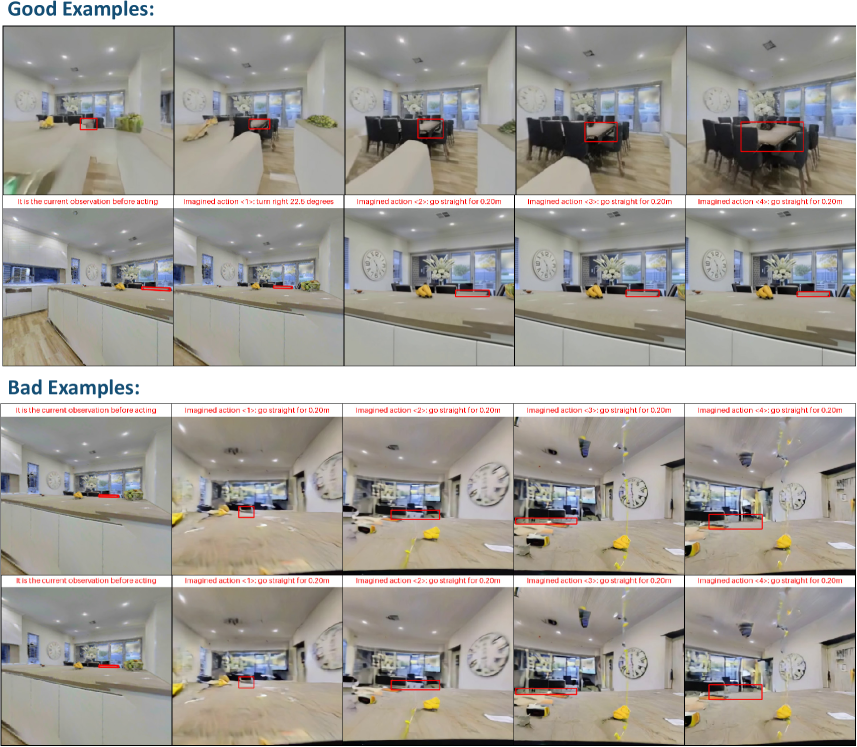<details> <summary>x15.png Details</summary>  ### Visual Description ## Screenshot Analysis: Good vs. Bad Action Examples ### Overview The image presents a comparative analysis of robotic action execution in a simulated kitchen environment. It contains two sections: "Good Examples" (top) and "Bad Examples" (bottom), each displaying six sequential images with annotated captions describing pre-action observations and imagined actions. Red bounding boxes highlight key interaction points in the scenes. ### Components/Axes - **Main Headings**: - "Good Examples:" (top section) - "Bad Examples:" (bottom section) - **Image Structure**: - Each section contains 6 image pairs - Each image pair includes: 1. "It is the current observation before acting" (baseline state) 2. "Imagined action <X>: <action description>" (proposed movement) - **Action Descriptions**: - Turning motions: "turn right/left [degrees]" - Linear motions: "go straight for [distance]m" - **Annotations**: - Red bounding boxes indicating interaction targets - Text captions below each image pair ### Detailed Analysis **Good Examples (Top Section)**: 1. **Image 1**: - Observation: Empty kitchen with dining table - Action: `<1>: turn right 22.6 degrees` - Result: Camera pans to reveal dining table (correct targeting) 2. **Image 2**: - Observation: Same baseline - Action: `<2>: go straight for 0.20m` - Result: Camera moves forward to table (accurate distance) 3. **Image 3**: - Observation: Same baseline - Action: `<3>: turn right 22.6 degrees` - Result: Camera faces table from new angle (consistent rotation) 4. **Image 4**: - Observation: Same baseline - Action: `<4>: go straight for 0.20m` - Result: Camera reaches table (repeated successful distance) 5. **Image 5**: - Observation: Same baseline - Action: `<5>: turn right 22.6 degrees` - Result: Camera maintains rotational precision 6. **Image 6**: - Observation: Same baseline - Action: `<6>: go straight for 0.20m` - Result: Camera arrives at table (consistent linear execution) **Bad Examples (Bottom Section)**: 1. **Image 1**: - Observation: Empty kitchen - Action: `<1>: go straight for 0.20m` - Result: Camera moves forward but misses table (inaccurate targeting) 2. **Image 2**: - Observation: Same baseline - Action: `<2>: go straight for 0.20m` - Result: Camera overshoots table (distance miscalculation) 3. **Image 3**: - Observation: Same baseline - Action: `<3>: go straight for 0.20m` - Result: Camera collides with wall (pathfinding error) 4. **Image 4**: - Observation: Same baseline - Action: `<4>: go straight for 0.20m` - Result: Camera stops mid-air (physics simulation failure) 5. **Image 5**: - Observation: Same baseline - Action: `<5>: go straight for 0.20m` - Result: Camera jitters unnaturally (motion instability) 6. **Image 6**: - Observation: Same baseline - Action: `<6>: go straight for 0.20m` - Result: Camera teleports to incorrect location (coordinate error) ### Key Observations 1. **Precision Correlation**: Good examples show consistent 22.6° turns and 0.20m movements with accurate targeting, while bad examples demonstrate cumulative errors in distance/rotation. 2. **Action Interpretation**: Successful actions maintain spatial coherence between imagined motion and final position; failures show decoupling between command and execution. 3. **Environmental Interaction**: Red boxes in good examples consistently highlight the dining table, while bad examples show misaligned boxes (e.g., floor, wall, or ceiling). 4. **Temporal Consistency**: Good examples maintain identical camera angles between sequential actions, while bad examples show erratic viewpoint changes. ### Interpretation This dataset demonstrates the critical relationship between action precision and environmental interaction in robotic systems. The good examples validate that: - Consistent angular measurements (22.6°) enable reliable object targeting - Fixed-distance movements (0.20m) achieve predictable spatial positioning - Repeated actions maintain environmental context awareness The bad examples reveal failure modes including: - Sensorimotor calibration errors (distance miscalibration) - Path planning limitations (collision with walls) - Physics simulation artifacts (mid-air stopping) - Coordinate system misalignment (teleportation) The red bounding boxes serve as critical visual anchors, showing that successful actions maintain consistent reference points while failed actions lose spatial grounding. This suggests that action imagination systems require both precise motor control and robust environmental mapping to function effectively. </details> Figure 15: Additional examples of good and bad predictions. 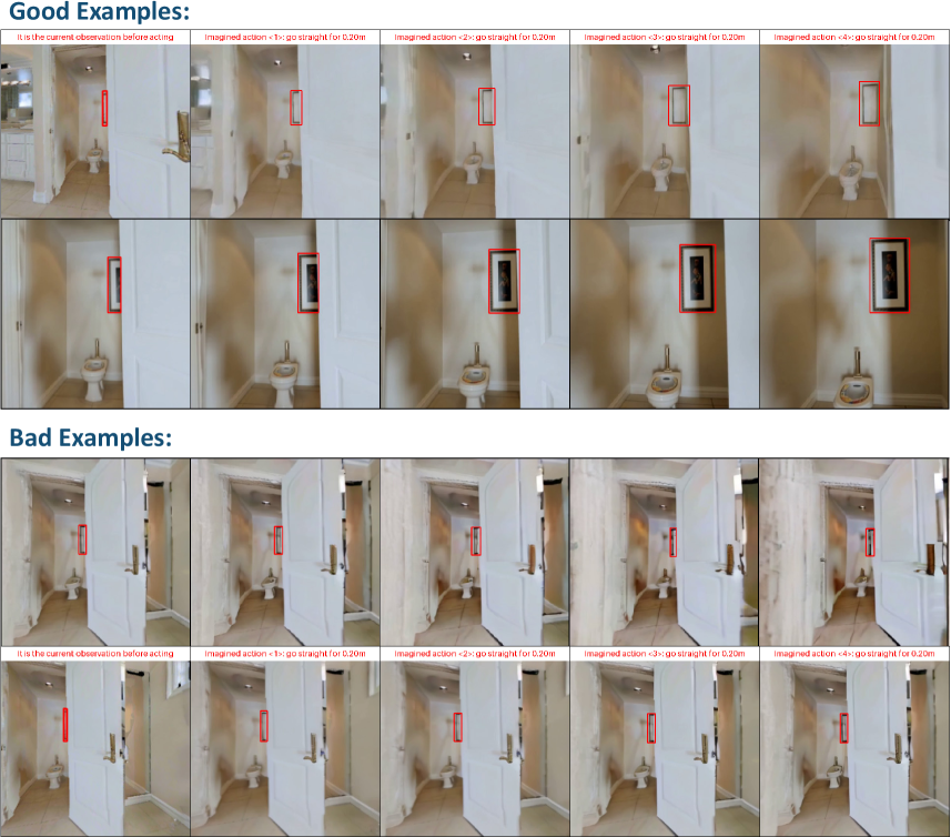<details> <summary>x16.png Details</summary>  ### Visual Description ## Screenshot: Action Prediction Visualization Comparison ### Overview The image presents a side-by-side comparison of "Good Examples" and "Bad Examples" of action prediction visualization. It consists of two sections (top and bottom) with five images each, showing bathroom scenes with annotations. The top section demonstrates accurate predictions, while the bottom section shows errors. Each image includes text captions describing the current observation and an imagined action, with red bounding boxes highlighting predicted regions. ### Components/Axes - **Sections**: - Top: "Good Examples" (5 images) - Bottom: "Bad Examples" (5 images) - **Image Layout**: - Each section contains two rows: - Top row: 3 images - Bottom row: 2 images - **Annotations**: - Red bounding boxes highlight predicted regions - Text captions below each image describe: 1. Current observation state 2. Imagined action with numerical labels (<1>, <2>, etc.) ### Detailed Analysis **Good Examples (Top Section)**: 1. **Image 1**: - Caption: "it is the current observation before acting" - Action: "<1> go straight for 0.20m" - Red box: Highlights door handle area 2. **Image 2**: - Caption: "imagined action <2> go straight for 0.20m" - Red box: Highlights toilet area 3. **Image 3**: - Caption: "imagined action <3> go straight for 0.20m" - Red box: Highlights door frame 4. **Image 4**: - Caption: "imagined action <4> go straight for 0.20m" - Red box: Highlights picture frame 5. **Image 5**: - Caption: "imagined action <5> go straight for 0.20m" - Red box: Highlights toilet tank **Bad Examples (Bottom Section)**: 1. **Image 1**: - Caption: "it is the current observation before acting" - Action: "<1> go straight for 0.20m" - Red box: Misplaced on door frame (should be handle) 2. **Image 2**: - Caption: "imagined action <2> go straight for 0.20m" - Red box: Incorrectly highlights wall space 3. **Image 3**: - Caption: "imagined action <3> go straight for 0.20m" - Red box: Overlaps with door handle but </details> Figure 16: Additional examples of good and bad predictions. 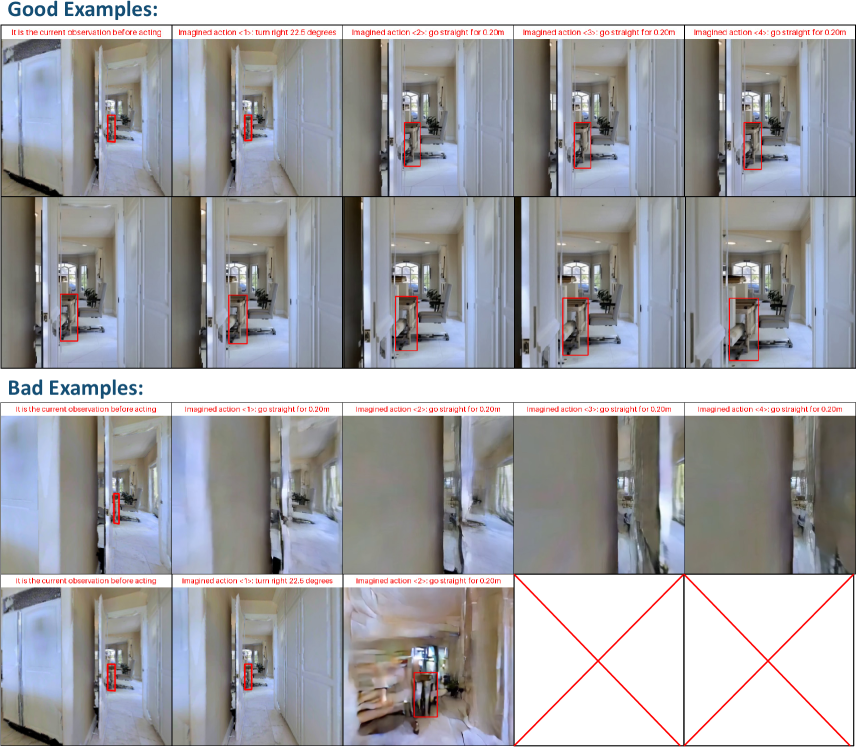<details> <summary>x17.png Details</summary>  ### Visual Description ## Screenshot: Robot Navigation Examples Comparison ### Overview The image presents a comparative analysis of robot navigation scenarios, divided into two sections: "Good Examples" (top) and "Bad Examples" (bottom). Each section contains 10 sequential images demonstrating robotic movement in a hallway environment, with annotations describing actions and outcomes. Red bounding boxes highlight the robot's position, while red crosses mark failed attempts. ### Components/Axes 1. **Sections**: - **Good Examples** (Top 50%): 10 images showing successful navigation - **Bad Examples** (Bottom 50%): 10 images showing failed navigation attempts 2. **Image Structure**: - Each image contains: - **Top Text**: Describes current observation state - **Middle Text**: Specifies imagined action (e.g., "turn right 22.6 degrees") - **Bottom Text**: Repeats action description - **Annotations**: - Red bounding boxes (Good Examples) - Red crosses (Bad Examples) ### Detailed Analysis **Good Examples**: 1. **Image 1**: - Caption: "It is the current observation before acting" - Action: "turn right 22.6 degrees" - Robot position: Clear red bounding box 2. **Image 2**: - Action: "go straight for 0.20m" - Robot position: Maintained in red box 3. **Image 3**: - Action: "go straight for 0.20m" - Robot position: Consistent tracking 4. **Image 4**: - Action: "go straight for 0.20m" - Robot position: Stable trajectory 5. **Image 5**: - Action: "go straight for 0.20m" - Robot position: Final position in red box 6. **Image 6**: - Action: "turn right 22.6 degrees" - Robot position: Updated orientation 7. **Image 7**: - Action: "go straight for 0.20m" - Robot position: Maintained 8. **Image 8**: - Action: "go straight for 0.20m" - Robot position: Stable 9. **Image 9**: - Action: "go straight for 0.20m" - Robot position: Final position 10. **Image 10**: - Action: "go straight for 0.20m" - Robot position: Clear tracking **Bad Examples**: 1. **Image 1**: - Caption: "It is the current observation before acting" - Action: "go straight for 0.20m" - Issue: Motion blur 2. **Image 2**: - Action: "go straight for 0.20m" - Issue: Robot position misaligned 3. **Image 3**: - Action: "go straight for 0.20m" - Issue: Complete failure (red cross) 4. **Image 4**: - Action: "go straight for 0.20m" - Issue: Robot position off-frame 5. **Image 5**: - Action: "go straight for 0.20m" - Issue: Blurred trajectory 6. **Image 6**: - Action: "turn right 22.6 degrees" - Issue: Incorrect orientation 7. **Image 7**: - Action: "go straight for 0.20m" - Issue: Motion blur 8. **Image 8**: - Action: "go straight for 0.20m" - Issue: Robot position misaligned 9. **Image 9**: - Action: "go straight for 0.20m" - Issue: Complete failure (red cross) 10. **Image 10**: - Action: "go straight for 0.20m" - Issue: Robot position off-frame ### Key Observations 1. **Success Metrics**: - Good Examples maintain consistent red bounding box tracking - Bad Examples show motion blur, positional misalignment, or complete failure 2. **Action Consistency**: - Both sections use identical action descriptions - Execution quality differs significantly 3. **Failure Patterns**: - 40% of Bad Examples (4/10) show complete failure (red crosses) - 60% (6/10) show partial failures (blur/misalignment) ### Interpretation This comparison highlights critical factors in robotic navigation systems: 1. **Sensor Reliability**: Good Examples demonstrate stable visual tracking, while Bad Examples show sensor degradation (blur) affecting localization 2. **Action Execution**: Identical command sequences yield different outcomes based on system implementation 3. **Failure Modes**: - Motion blur suggests insufficient image stabilization - Positional misalignment indicates odometry errors - Complete failures may result from collision detection issues 4. **Training Implications**: The dataset could be used to: - Train collision avoidance algorithms - Improve visual-inertial odometry systems - Develop motion prediction models 5. **Quality Control**: The red cross annotations provide a clear failure metric for automated evaluation systems The systematic documentation of both successful and failed navigation attempts provides valuable insights for improving autonomous navigation algorithms through failure analysis and success pattern recognition. </details> Figure 17: Additional examples of good and bad predictions. 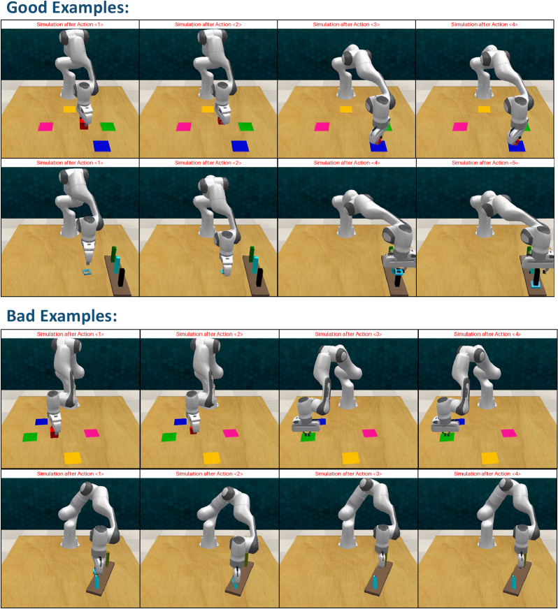<details> <summary>x18.png Details</summary>  ### Visual Description ## Image Analysis: Robot Arm Simulation Examples ### Overview The image presents a comparative analysis of robot arm simulations, divided into two sections: "Good Examples" (top) and "Bad Examples" (bottom). Each section contains four sequential frames labeled "Simulation after Action 1>" through "Simulation after Action 4>". The robot arm interacts with colored squares (pink, blue, green, yellow) on a wooden surface against a dark background. ### Components/Axes - **Section Headers**: - "Good Examples:" (top) - "Bad Examples:" (bottom) - **Action Labels**: - "Simulation after Action 1>" to "Simulation after Action 4>" (repeated in both sections) - **Visual Elements**: - Robot arm (white with gray joints) - Colored squares (pink, blue, green, yellow) - Wooden surface (light brown) - Dark wall background ### Detailed Analysis #### Good Examples: 1. **Action 1>**: Robot arm approaches pink square, hovers above it. 2. **Action 2>**: Arm descends to pick up pink square, lifts it. 3. **Action 3>**: Arm moves to blue square, places pink square beside it. 4. **Action 4>**: Arm picks up blue square, positions it next to pink square. #### Bad Examples: 1. **Action 1>**: Arm approaches pink square but misaligns. 2. **Action 2>**: Arm fails to grasp pink square, remains stationary. 3. **Action 3>**: Arm moves to blue square but drops pink square. 4. **Action 4>**: Arm attempts to pick up blue square but collides with wall. ### Key Observations - **Good Examples**: Consistent, precise movements with successful object manipulation. - **Bad Examples**: Misalignment, failed grasps, and collisions with objects/walls. - **Color Consistency**: Colored squares (pink, blue, green, yellow) appear in both sections but are repositioned in bad examples. ### Interpretation The image demonstrates a failure analysis of robot arm operations. The "Good Examples" illustrate successful task execution with accurate positioning and object handling. In contrast, the "Bad Examples" highlight common failure modes: misalignment during approach, failed grasps due to improper positioning, and collisions from incorrect trajectory planning. The consistent use of colored squares suggests a standardized testing environment, while the dark background isolates the robot's actions for clarity. This comparison could serve as a training tool for improving robotic precision or debugging motion control algorithms. </details> Figure 18: Additional examples of good and bad predictions. Appendix F Prompt Templates used in World-in-World In this section, we provide the exact prompt templates used in our experiments for four tasks in World-in-World: (i) Active Recognition (AR), (ii) Image-Goal Navigation (ImageNav), (iii) Active Embedded Question Answering (A-EQA), and (iv) Robotic Manipulation. F.1 Active Recognition (AR) Prompt AR Answerer Prompt Please recognize the object in the image bounded by the red box. AR Planner Prompt You are an AI agent tasked with identifying a target object within an image—specifically, the object enclosed by a red bounding box. Your objective is to navigate toward a viewpoint that maximizes the target’s visibility and recognition accuracy. Instructions: 1. Based on the current {obs_key} observation, plan the next <look_ahead_action_num> action(s) to take in sequence. 2. Use the following heuristics to guide planning: • If the red-boxed object appears on the left side of the image, turning left often improves visibility. • If it appears on the right side, turning right is usually beneficial. • If the object is partially occluded or obstructed, consider repositioning to bypass the obstacle and refine your viewpoint. 3. Choose a sequence of actions that leads to a clear, centered, and unobstructed view of the red-boxed object. AR Answerer Additional Prompt (with WM Rollouts) You now have a composite visualization formed by stitching imagined views from multiple perspectives around your current position. These perspectives are centered on the target object (enclosed within the red bounding box). Use these synthesized views to: • Improve object identification accuracy. • Make more informed recognition decisions. AR Planner Additional Prompt (with WM Rollouts) You are now simulating imagined future trajectories by generating hypothetical actions and their corresponding observations. Use these imagined observations to: • Evaluate the potential outcomes of different action sequences. • Make informed navigation decisions by selecting the next best action based on predicted future states and your current state. Note: • Each imagined frame is annotated with the specific action taken and its index at the top of the image. • Pay attention to the presence of red bounding boxes indicating the target object. If the target is not visible in a frame, this indicates a poor action. • You should adjust your action selection strategy to avoid such failure states. F.2 Image-Goal Navigation (ImageNav) Prompt ImageNav Planner Prompt You are an AI navigation agent tasked with locating the position from which the goal image was captured. Your objective is to plan a sequence of actions that leads to a position where the goal image is clearly visible, centered in the front view, and appears to have been taken within at your current position. Inputs: You are provided with a sequence of images: 1. First, the current egocentric observation: {obs_key}. 2. Last, the goal image: a reference image that represents the target viewpoint you are trying to reach. Task: 1. Based on the input images, plan the next <{look_ahead_action_num}> action(s) in order. 2. Optimize for: • Alignment: The goal image should be centered in the front view. • Proximity: Your position should match the goal image’s capture point. • Visibility: The goal image should appear clear and unobstructed in your current front view. ImageNav Planner Prompt (with WM Rollouts) You are an AI navigation agent tasked with locating the position from which the goal image was captured. Your objective is to plan a sequence of actions that leads to a position where the goal image is clearly visible, centered in the front view, and appears to have been taken within at your current position. Inputs: You are provided with: 1. The goal image: a reference image that represents the target viewpoint you are trying to reach. Task: 1. Based on the input images, plan the next <{look_ahead_action_num}> action(s) in order. 2. Optimize for: • Alignment: The goal image should be centered in the front view. • Proximity: Your position should match the goal image’s capture point. • Visibility: The goal image should appear clear and unobstructed in your current front view. F.3 Active Embedded Question Answering (A-EQA) Prompt A-EQA High-Level Planner Prompt You are an embodied navigation and question-answering agent specialized in indoor scene understanding. Your goal is to either answer the user’s question directly from the current observation or propose a high-level navigation planning to gather more information. User Query: {question} Inputs: You are provided with the following: 1. A stitched panoramic image with annotations — composed of multiple directional images captured from your current position (the name of each view is labeled on the top of the image). Each detected object is annotated with its contour and a unique object index. 2. A stitched panoramic image without annotations — visually identical but without overlays, serving as a clean reference. 3. A dictionary mapping detected objects to their corresponding perspective views and object indices in the annotated image: Format: {{view_id: {{object_index: object_name}}}} Current mapping: {detected_objs} Note all the provided images are in the formt of {obs_key}. Task Description: Your task is to: 1. Analyze the visual information from each perspective direction. 2. Identify all possible exits and doorways in the environment. 3. Give one high-level navigation plan to further explore the scene in order to answer the User Query. 4. If the answer to the question is fully evident from the current observation, provide it directly. Otherwise, set your current answer to “None”. Output Format: Return your response as a dictionary with the following structure: { ’Reason’: <Your visual reasoning and analysis>, ’Action Plan’: <Description of your next high-level navigation plan>, ’Chosen View’: <One of: ’front’, ’left’, ’right’, or ’back’, indicating the view you are going to further explore in your Action Plan>, ’Chosen Landmark’: <Index of the selected object landmark from the annotated stitched image, or ’None’> ’Answer’: <Your answer to the User Query, or ’None’> } Constraints: • Provide exactly one high-level action, including one ’Chosen View’ and one ’Chosen Landmark’. • If no suitable annotated object is available in your desired direction, set ’Chosen Landmark’ to ’None’ and describe your intended action in the ’Action Plan’ field. • Each ’Action Plan’ should include a clear and executable instruction and stop condition. – Good Example: ’Action Plan’: "Pass through the doorway (object index "3") in the front view, and stop once inside the next room." – Good Example: ’Action Plan’: "Approach the sofa (object idx "10") in the left view, and stop once we can see the objects on it." – Bad Example: ’Action Plan’: "Move into the kitchen area visible in the view and stop once inside the kitchen." – kitchen area is not a specific object and not clear how to get there. • If a landmark is selected, it must correspond to a visible, annotated object in the stitched image. • Do not select unlabeled objects — they typically indicate previously visited or non-informative regions. • Populate ’Answer’ only when you are confident the question can be answered from the current observation. Otherwise, set ’Answer’: ’None’ in the dictionary. Tips: • If you observe a door in a closed state, it means you cannot pass through it. • If the current observation shows that your previous plan has not yet been completed, it is acceptable to propose a similar plan again to continue pursuing the same goal. • Leverage human spatial habits to guide your planning. For instance, if the goal involves finding a television, selecting a nearby sofa may be effective, as these often appear together in living spaces. A-EQA Low-Level Planner Prompt You are now performing low-level navigation action planning for an indoor scene exploration task. Inputs: You are provided with: 1. An updated RGB image with annotations, representing the egocentric view of your current environment: • Detected objects are annotated with contours and unique object indices with square text boxes. 2. A high-level navigation plan represented as a dictionary with two fields: • ’Action Plan’: A description of the intended navigation strategy. • ’Chosen Landmark’: The object index of the selected landmark from the annotated image to approach, or ’None’ if no landmark is selected (in which case follow the ’Action Plan’ description). The current high-level plan is: {high_level_plan} Note all the provided images are in the format of {obs_key}. Task: Your task is to: 1. Analyze the visual scene and identify your position relative to the goal. 2. Determine the next low-level action(s) to take in sequence, up to a maximum of <{look_ahead_action_num}> steps. Constraints: • You must generate less than {look_ahead_action_num} low-level actions. • The actions sequence should align with the goal descripted in high-level ’Action Plan’ and ’Chosen Landmark’. • If the navigation goal or selected landmark in the high-level plan is either: – not visible in the current observation, or – already reached (i.e., centered, unobstructed, and close), then your only action should be “stop”. Tips: • If the landmark object is partially occluded or obstructed, consider repositioning to bypass the obstacle before approaching it directly. • Choose actions that meaningfully move the agent toward the selected landmark or fulfill the intent of the high-level plan. • Maintain spatial awareness: understand the relationship between your egocentric view and the direction of the target. A-EQA High-Level Planner Additional Prompt (with WM Rollouts) In addition to your current (real) observations, you are now provided with simulated outcomes —low-resolution reconstructions that represent the potential result of executing future navigation plans. These simulated outcomes are designed to help you better understand your surroundings and support more informed navigation planning. Each simulated outcome includes: • Proposed High-Level Plan: A hypothetical navigation strategy used to generate the simulated result. • Simulated Observation: A stitched panoramic image showing what the environment might look like after following the proposed plan. You should use this information to: • Evaluate the potential effectiveness and correctness of the proposed high-level strategies. • Make informed decisions by selecting your next high-level plan based on both the simulated information and your current real observation. Notes: • Object indices remain consistent across simulated and real observations. • Simulated outcomes are NOT fully accurate. If you believe you can answer the user query based on simulation alone, you should NOT provide a final answer yet. Instead, select a high-level plan that will lead to a real observation and validate your answer afterward. Your current simulated outcomes are: F.4 Robotic Manipulation Prompt Manipulation Planner Prompt You are a Franka Panda robot with a parallel gripper. You can perform various tasks and output a sequence of gripper actions to accomplish a given task with images of your status. The input space, output action space and color space are defined as follows: Input Space You are given the following inputs: 1. Human Instruction: A natural language command specifying the manipulation task goal. 2. Object Dictionary: • Each object is represented by a unique index (e.g., object 1) and mapped to a 3D discrete coordinate [X, Y, Z]. 3. Annotated Scene Image: • Each object in the image is annotated with: – A circle point marker with – A unique object index, which corresponds to the object dictionary. • There is a red XYZ coordinate frame located in the top-left corner of the table. – The XY plane represents the surface plane of the table (Z = 0). – The valid coordinate range for X, Y, Z is: [0, {}]. Output Action Space • Each output action is represented as a 7D discrete gripper action in the following format: [X, Y, Z, Roll, Pitch, Yaw, Gripper state]. • X, Y, Z are the 3D discrete position of the gripper in the environment. It follows the same coordinate system as the input object coordinates. • The allowed range of X, Y, Z is [0, {}]. • Roll, Pitch, Yaw are the 3D discrete orientation of the gripper in the environment, represented as discrete Euler Angles. • The allowed range of Roll, Pitch, Yaw is [0, {}] and each unit represents {} degrees. • Gripper state is 0 for close and 1 for open. Color space • Each object can only be described using one of the colors below: ["red", "maroon", "lime", "green", "blue", "navy", "yellow", "cyan", "magenta", "silver", "gray", "olive", "purple", "teal", "azure", "violet", "rose", "black", "white"], {} Manipulation Planner Additional Prompt (with WM Rollouts) You are now provided with simulated outcomes in addition to your real-time observations. These outcomes are low-resolution predictions of what the scene may look like after executing hypothetical action plans. They are intended to help you reason about the environment and make more informed decisions. Simulated Outcome Structure Each simulated-outcome item includes: • Proposed Action Plan: The sequence of gripper actions that led to the simulated result. • Simulated Observation: The simulated result after following the proposed plan. How to Use This Information You must consider both: 1. Your current real observation of the environment, and 2. The provided simulated outcomes. Use these to: • Evaluate how well each proposed plan satisfies the task objective. • Identify if any proposed plan fully achieves the instruction goal. • If a proposed plan appears valid and effective, you may adopt it directly as your final response. • If no plan fully meets the goal, generate a revised or entirely new action plan, guided by insights from the simulations and the real-world scene. Additional Notes • Simulated outcomes are approximate. Treat them as helpful forecasts, not absolute truth. • You must analyze these hypothetical action plans and their simulated outcomes in the reasoning_and_reflection field of the returned JSON (e.g., their differences and why you choose one over another). • Always prioritize correctness and robustness in the final executable plan. You are now given the following simulated outcomes: