# Learning Interpretable Features in Audio Latent Spaces via Sparse Autoencoders
**Authors**: Nathan Paek, Yongyi Zang, Qihui Yang, Randal Leistikow
1]Smule Labs 2]University of California, San Diego 3]Stanford University [†]Work done during internship at Smule [‡]These authors contributed equally.
## Abstract
While sparse autoencoders (SAEs) successfully extract interpretable features from language models, applying them to audio generation faces unique challenges: audio’s dense nature requires compression that obscures semantic meaning, and automatic feature characterization remains limited. We propose a framework for interpreting audio generative models by mapping their latent representations to human-interpretable acoustic concepts. We train SAEs on audio autoencoder latents, then learn linear mappings from SAE features to discretized acoustic properties (pitch, amplitude, and timbre). This enables both controllable manipulation and analysis of the AI music generation process, revealing how acoustic properties emerge during synthesis. We validate our approach on continuous (DiffRhythm-VAE) and discrete (EnCodec, WavTokenizer) audio latent spaces, and analyze DiffRhythm, a state-of-the-art text-to-music model, to demonstrate how pitch, timbre, and loudness evolve throughout generation. While our work is only done on audio modality, our framework can be extended to interpretable analysis of visual latent space generation models.
## 1 Introduction
As powerful neural networks become more integrated into society, their lack of interpretability raises a significant concern (Hendrycks et al., 2023). To address this challenge, sparse autoencoders (SAEs) have emerged as a key tool in mechanistic interpretability research (Olah et al., 2020; Cammarata et al., 2021; Nelson et al., 2021). They are motivated by the polysemantic hypothesis (Olah et al., 2020; Elhage et al., 2022; Marshall and Kirchner, 2024): that neurons encode more features than dimensions by superposing multiple concepts. SAEs work by finding sparse directions in activation space to isolate these underlying, disentangled features. This approach has proven effective in large language models (LLMs), where SAEs can extract highly monosemantic features that are automatically characterized by using the model itself to summarize the results of token-level perturbations (Cunningham et al., 2023).
However, extending this approach to audio generative networks presents fundamental challenges. Unlike text, audio is inherently dense (Wu et al., 2024), and thus typically requires learned compression through autoencoders before tokenization (Liu et al., 2023). This compression step, whether producing continuous or discrete latent codes, obscures the semantic meaning of individual “tokens,” making perturbation-based analysis less interpretable (Wu et al., 2024; Ye et al., 2025). Moreover, while language models excel at summarizing textual patterns, current audio understanding models are not yet capable of providing an equally robust automatic characterization of SAE feature behaviors (Su et al., 2025; Yang et al., 2025). These limitations necessitate new approaches for interpretable feature discovery in audio generative systems.
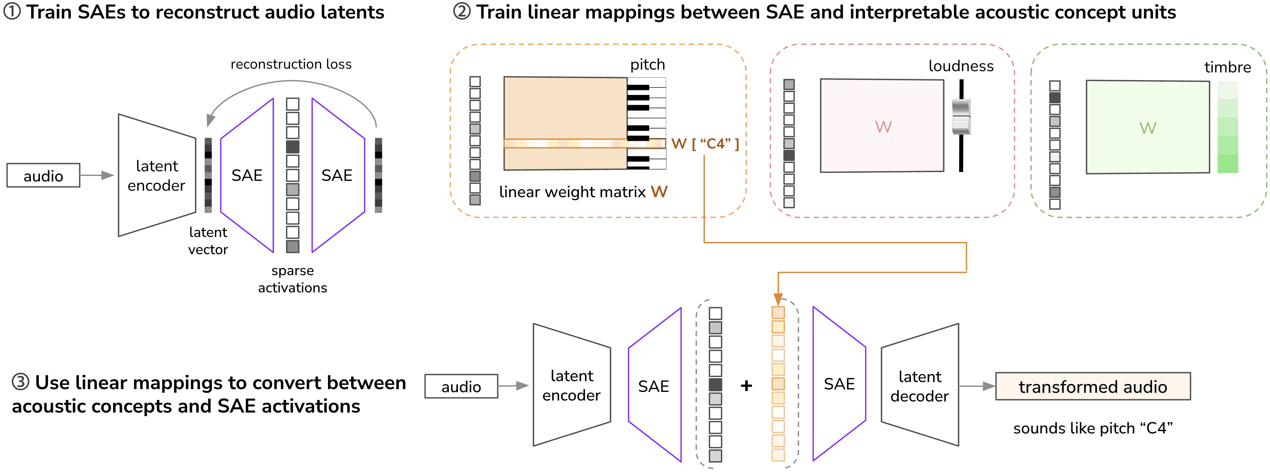
In this work, we propose a novel framework for understanding audio generative models by analyzing their latent space representations through human-interpretable acoustic concepts. Our approach proceeds in three stages. First, we train SAEs on the latent representations of audio autoencoders to extract sparse features. Second, we learn linear mappings from these SAE features to human-interpretable acoustic concepts: pitch, amplitude, and timbre (represented here by spectral centroid as a simplified proxy (Schubert et al., 2004; Schubert and Wolfe, 2006)). To enable discrete analysis, we quantize each acoustic property into interpretable “units”: pitch is discretized according to the Western tonal system (e.g., C4, C#4), while amplitude and spectral centroid are binned with equal spacing within their physical ranges. The effectiveness of linear mappings suggests that SAE features already encode acoustic properties in a near-linear fashion, validating the hypothesis that these learned representations align with human-interpretable concepts. Finally, by decomposing the audio synthesis process into an interpretable feature hierarchy, our framework traces how specific acoustic properties emerge. We empirically validate this approach on DiffRhythm, a state-of-the-art text-to-music model. Although our experiments focus on audio, we believe this framework is generalizable to other generative models that operate within learned latent spaces, including those for image and video.
<details>
<summary>figur1.png Details</summary>
### Visual Description
## Flowchart: Audio Latent Reconstruction and Acoustic Concept Mapping
### Overview
The diagram illustrates a three-stage process for training Sparse Autoencoders (SAEs) to reconstruct audio latents and map them to interpretable acoustic concepts. It combines neural network architectures with linear algebraic transformations to bridge latent representations and human-understandable sound properties.
### Components/Axes
1. **Stage 1: Latent Reconstruction**
- **Inputs**: Audio signal
- **Components**:
- Latent Encoder (black box)
- Latent Vector (gray vertical bars)
- Two SAEs (purple boxes with "SAE" labels)
- Reconstruction Loss (gray arrow forming a loop)
- Sparse Activations (vertical gray bars between SAEs)
2. **Stage 2: Acoustic Concept Mapping**
- **Concept Units**:
- Pitch (piano keyboard with "W [“C4”]" label)
- Loudness (speaker icon)
- Timbre (color gradient from white to green)
- **Mathematical Elements**:
- Linear Weight Matrix W (orange boxes connecting SAE to concepts)
3. **Stage 3: Audio Transformation**
- **Components**:
- Latent Encoder (repeated from Stage 1)
- SAE (repeated from Stage 1)
- Latent Decoder (black box)
- Transformed Audio Output (beige box labeled "sounds like pitch 'C4'")
### Detailed Analysis
1. **Latent Reconstruction Flow**:
- Audio → Latent Encoder → Latent Vector
- Latent Vector → SAE₁ → Sparse Activations → SAE₂ → Reconstruction Loss loop
2. **Acoustic Concept Mapping**:
- SAE outputs connect to three linear weight matrices (W)
- Each W matrix maps to a specific acoustic concept:
- Pitch: Mapped to C4 note (middle C on piano)
- Loudness: Represented by speaker icon
- Timbre: Color-coded gradient (white→green)
3. **Audio Transformation**:
- SAE activations combined with W matrices
- Final output: Audio transformed to sound like specific pitch (C4)
### Key Observations
1. **Sparse Activation Pattern**:
- Vertical gray bars show non-uniform activation distribution
- Indicates SAE's ability to capture essential features while maintaining sparsity
2. **Concept-Specific Mappings**:
- Pitch mapping includes explicit note designation ("C4")
- Timbre uses color gradients rather than discrete categories
- Loudness represented by physical iconography
3. **Bidirectional Flow**:
- Training loop (Stage 1) enables reconstruction
- Linear mappings (Stage 2) allow concept interpretation
- Combined system (Stage 3) enables audio transformation
### Interpretation
This architecture demonstrates a neuro-symbolic approach to audio processing:
1. **SAE Training**: First establishes efficient latent representations through reconstruction loss minimization
2. **Concept Bridging**: Linear mappings translate abstract latents into interpretable dimensions (pitch/loudness/timbre)
3. **Practical Application**: Enables targeted audio manipulation by modifying specific acoustic properties
The use of sparse activations suggests the system identifies critical features for reconstruction, while the linear mappings provide a transparent bridge between neural representations and human-understandable sound properties. The explicit note designation ("C4") indicates the system can target specific musical intervals, suggesting potential applications in music generation and audio editing.
</details>
Figure 1: Framework for interpreting and controlling audio generative models through sparse features learned on their generation space. Sparse autoencoders extract interpretable features from audio latents, which are then linearly mapped to acoustic concepts. Control vectors extracted from these linear mappings can then be used to transform audio.
## 2 Methodology
### 2.1 Sparse Autoencoder Training
We train SAEs on latent representations from three pretrained audio encoders: the continuous VAE space of Stable Audio Open and DiffRhythm (Evans et al., 2025; Ning et al., 2025), and the discrete latent spaces of EnCodec (Défossez et al., 2022) and WavTokenizer (Ji et al., 2025). To address the unique requirements of audio latents, we modify the standard SAE architecture by adding an RMS normalization layer after the ReLU activation. This modification maintains consistent activation magnitudes and, as we empirically found, prevents out-of-distribution artifacts during feature manipulation. Following standard practice (Cunningham et al., 2023), we optimize the SAEs using a composite loss function:
$$
L=\|x-\hat{x}\|_2^2+λ\|h\|_1 \tag{1}
$$
where the first term ensures reconstruction fidelity and the $L_1$ penalty promotes sparsity in the hidden activations $h$ . We conduct systematic grid searches over hidden dimensionalities (ranging from $4×$ to $256×$ the input dimension) and sparsity coefficients $λ$ (ranging from 0.005 to 0.15) to identify optimal configurations for each latent space.
### 2.2 Linear Mapping to Acoustic Concepts
To connect SAE features to interpretable acoustic properties, we train linear probes that predict discretized audio attributes from sparse activations. Given a latent vector $x∈ℝ^d$ , our SAE produces sparse features:
$$
h=ReLU(W_encx+b_enc), f=RMSNorm(h) \tag{2}
$$
where $f∈ℝ^m$ are the normalized features used for both reconstruction and interpretation.
For each acoustic attribute $a∈\{pitch,amplitude,timbre\}$ , we first extract continuous measurements from the audio: pitch via CREPE (Kim et al., 2018), amplitude via windowed RMS energy using librosa (McFee, 2025), and timbre via windowed spectral centroid using librosa. We then discretize these continuous curves into $K_a$ classes (pitch using logarithmic bins aligned with MIDI note numbers, and amplitude/timbre using linear bins) and train a linear classifier:
$$
p^(a)=softmax(W^(a)f+b^(a)) \tag{3}
$$
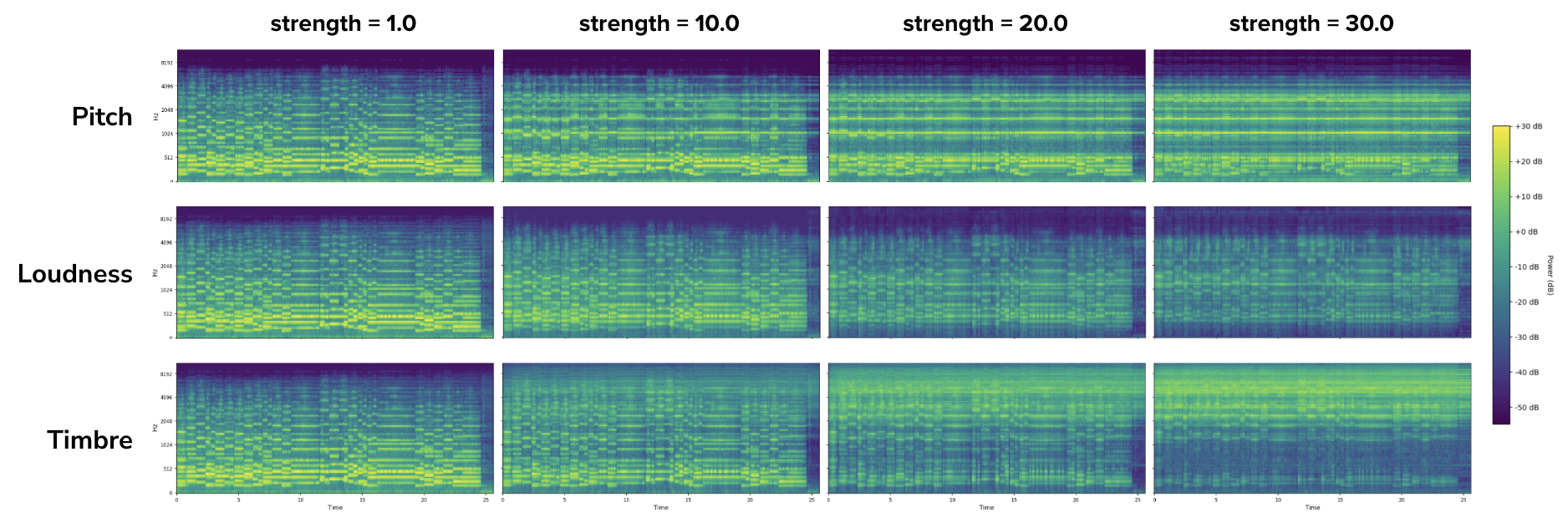
where $W^(a)∈ℝ^K_a× m$ maps SAE features to class logits. The linearity provides bidirectional interpretability, as the contribution of SAE feature $j$ to acoustic class $k$ is simply $c_j→ k^(a)=W^(a)_kj· f_j$ , where the weights $W^(a)_kj$ reveal both which features encode specific acoustic properties and how acoustic concepts decompose into SAE features. For targeted intervention, we leverage this linearity directly by adding the scaled probe weight vector $α·wk^(a)$ (”control vectors”) to the SAE features to shift the audio toward acoustic class $k$ . After re-normalizing to maintain valid activation magnitudes, we decode through both SAE and audio decoders to generate the modified audio (shown in Figure 2).
## 3 Experiments
<details>
<summary>edit_str_fig.png Details</summary>
### Visual Description
## Heatmap: Audio Feature Analysis Across Strength Levels
### Overview
The image displays a comparative heatmap analysis of three audio features (Pitch, Loudness, Timbre) across four strength levels (1.0, 10.0, 20.0, 30.0). Each panel visualizes power distribution (in dB) across time (0-25s) and frequency (122-9132 Hz). Color intensity corresponds to power levels, with darker blues indicating lower values and brighter yellows representing higher values.
### Components/Axes
- **X-axis (Time):** 0-25 seconds, labeled "Time" in all panels.
- **Y-axis (Frequency):** 122-9132 Hz, labeled "Frequency" in all panels.
- **Legend:** Vertical colorbar on the right, ranging from -50 dB (dark blue) to +30 dB (bright yellow).
- **Panels:** Four columns labeled "strength = 1.0", "strength = 10.0", "strength = 20.0", and "strength = 30.0".
- **Rows:** Three rows labeled "Pitch", "Loudness", and "Timbre".
### Detailed Analysis
#### Pitch Row
- **Strength = 1.0:** Horizontal bands of alternating yellow/green (10-20 dB) dominate, with occasional blue streaks (-10 dB). Frequency range shows consistent activity.
- **Strength = 10.0:** Bands become denser, with yellow regions extending to ~+20 dB. Blue streaks reduce in frequency.
- **Strength = 20.0:** Yellow bands occupy ~70% of the panel, reaching +25 dB. Blue regions nearly disappear.
- **Strength = 30.0:** Uniform yellow across most frequencies, peaking at +30 dB. Only minor blue patches remain at the top.
#### Loudness Row
- **Strength = 1.0:** Vertical streaks of yellow/green (10-20 dB) appear sporadically. Most of the panel is dark blue (-30 dB).
- **Strength = 10.0:** Streaks increase in density, with yellow regions reaching ~+15 dB. Dark blue areas reduce to ~40%.
- **Strength = 20.0:** Vertical yellow streaks dominate (~80% coverage), peaking at +20 dB. Blue regions concentrate at the bottom.
- **Strength = 30.0:** Nearly uniform yellow across all frequencies, with +30 dB peaks. Blue regions are confined to the top 10% of the frequency range.
#### Timbre Row
- **Strength = 1.0:** Scattered yellow/green dots (10-20 dB) on a dark blue background. No clear pattern.
- **Strength = 10.0:** Dots cluster into horizontal bands, with yellow regions reaching ~+15 dB. Dark blue areas reduce to ~60%.
- **Strength = 20.0:** Bands merge into larger blocks, with yellow regions covering ~50% of the panel. Peaks at +25 dB.
- **Strength = 30.0:** Large contiguous yellow blocks dominate (~75% coverage), with +30 dB peaks. Blue regions are minimal.
### Key Observations
1. **Strength Correlation:** Higher strength levels consistently increase power (dB) across all features.
2. **Feature Patterns:**
- **Pitch:** Horizontal bands suggest sustained frequency components.
- **Loudness:** Vertical streaks indicate transient events or rhythmic patterns.
- **Timbre:** Scattered dots evolve into blocky structures, implying harmonic complexity.
3. **Color Consistency:** Yellow regions (high dB) align with the legend’s +30 dB threshold in all panels.
4. **Temporal Progression:** Patterns become more pronounced and dense as strength increases.
### Interpretation
The data demonstrates that increasing strength amplifies specific audio characteristics:
- **Pitch** exhibits harmonic resonance, with higher strengths producing sustained tonal bands.
- **Loudness** shows rhythmic or percussive elements, with vertical streaks becoming continuous at maximum strength.
- **Timbre** transitions from random noise to structured harmonic content, suggesting increased complexity.
Notably, the dB scale reveals that higher strengths concentrate power in specific frequency ranges, particularly for Pitch and Loudness. The Timbre feature’s evolution from scattered dots to blocks implies a shift from dissonance to harmonic coherence. These patterns could reflect how audio processing algorithms prioritize features at different amplification levels.
</details>
Figure 2: Controlled audio manipulation via control vectors. When $α$ increases, isolated changes in pitch (imminent C5), amplitude (decreasing loudness), and timbre (brightening via high-frequency emphasis) can be observed. Corresponding audio samples can be found here: https://anonymous.4open.science/r/audio_samples-A301/
### 3.1 Acoustic Concept Mapping Discovery
Dataset. We use a composite dataset of $∼$ 31 hours of audio sampled from several sources: CocoChorales (Wu et al., 2022) —11.2 hours of four-part Bach chorales, DAMP-VSEP (Smule, 2019) —11.7 hours of pop/rock singing, the Extended Groove MIDI Dataset (Callender et al., 2020) —7.8 hours of drums, GuitarSet (Xi et al., 2018) —24 minutes of solo guitar, and MAESTRO (Hawthorne et al., 2019) —33 minutes containing classical piano.
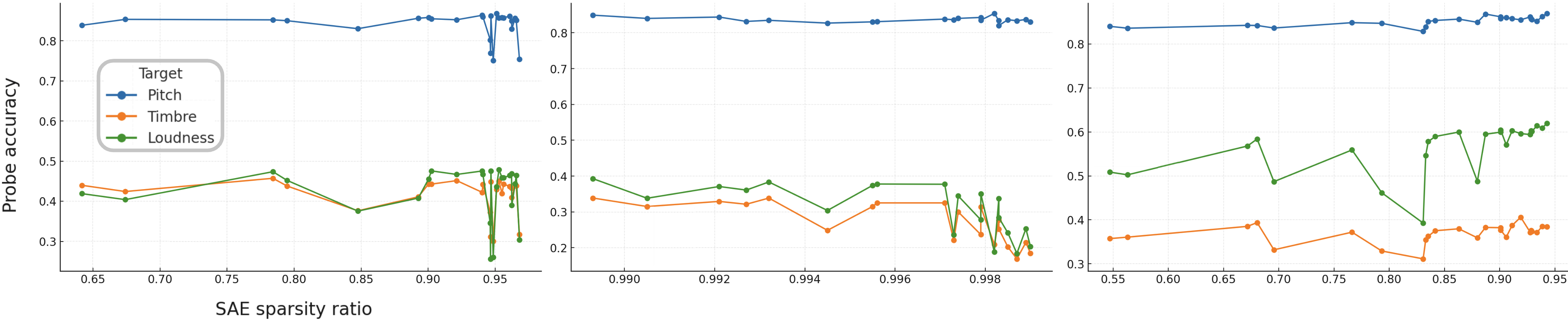
Training SAEs on audio latent spaces. We conduct grid searches over SAE hidden dimensions $\{2048,4096,8192,12288,16384\}$ and sparsity coefficients $λ∈\{0.005,0.01,0.05,0.1,0.15\}$ for each audio encoder. The resulting SAEs exhibit distinct characteristics across latent spaces. DiffRhythm achieves sparsity ratios ranging from 0.65 to 0.98. WavTokenizer produces the sparsest representations (0.993–0.999), suggesting its discrete tokens already encode highly disentangled features. EnCodec demonstrates the widest sparsity range (0.55–0.95). Across all models, larger hidden dimensions consistently improve reconstruction quality.
Training linear probes from SAE features to acoustic concepts. We train linear probes to predict pitch (with 66 bins spanning the pitch range present in our dataset), loudness (20 bins), and timbre (20 bins) from SAE features. Plotting the probe classification accuracy on a test set vs. the sparsity of its SAE in Figure 3 shows a hierarchy of linear decodability across acoustic properties. Pitch proves most linearly separable (0.75–0.87 accuracy) and remains stable across all sparsity levels, suggesting fundamental frequency encoding. EnCodec excels at loudness (0.56–0.63) compared to DiffRhythm and WavTokenizer (0.17–0.49). Timbre remains challenging across all models (0.17–0.46).
Applying targeted interventions to audio samples. We test controllability on diverse audio sources (singing voice, drums, four-part harmony). Figure 2 shows a chordal audio sample from the CocoChorales dataset encoded with EnCodec and our highest-sparsity SAE (hidden_dim=16384, $λ=0.1$ ). We apply control vectors targeting pitch (MIDI C5), timbre (spectral centroid class 17), and loudness (class 2) with strengths $α∈\{1,10,20,30\}$ . As $α$ increases, edits are isolated in the targeted attribute, while non-targeted properties remain largely preserved.
<details>
<summary>acc_v_sparse.png Details</summary>
### Visual Description
## Line Graph: Probe Accuracy vs. SAE Sparsity Ratio
### Overview
The image displays three line graphs comparing probe accuracy across different SAE sparsity ratios (0.65–0.95). Three data series are represented: **Target** (blue), **Pitch** (orange), and **Timbre** (green). The graphs are divided into three panels, each showing similar trends but with slight variations in data point distributions.
---
### Components/Axes
- **X-axis**: SAE sparsity ratio (0.65–0.95, incrementing by 0.05).
- **Y-axis**: Probe accuracy (0.2–0.8, incrementing by 0.1).
- **Legend**:
- **Target** (blue line)
- **Pitch** (orange line)
- **Timbre** (green line)
- **Loudness** (blue line, but no corresponding line in the graph; likely a legend error).
---
### Detailed Analysis
#### Panel 1 (Left)
- **Target (blue)**: Stable at ~0.85 across all sparsity ratios.
- **Pitch (orange)**: Fluctuates between ~0.3 and ~0.4, peaking near 0.75 sparsity.
- **Timbre (green)**: Peaks at ~0.45 near 0.75 sparsity, then declines.
#### Panel 2 (Middle)
- **Target (blue)**: Consistent at ~0.85.
- **Pitch (orange)**: Drops to ~0.3 at 0.95 sparsity, with minor fluctuations.
- **Timbre (green)**: Peaks at ~0.4 near 0.90 sparsity, then declines sharply.
#### Panel 3 (Right)
- **Target (blue)**: Stable at ~0.85.
- **Pitch (orange)**: Peaks at ~0.35 near 0.90 sparsity, with erratic drops.
- **Timbre (green)**: Peaks at ~0.55 near 0.90 sparsity, with significant volatility.
---
### Key Observations
1. **Target Stability**: The blue line (Target) remains consistently high (~0.85) across all panels, suggesting robustness to sparsity changes.
2. **Pitch Variability**: The orange line (Pitch) shows the most pronounced fluctuations, particularly in Panels 2 and 3, where accuracy drops sharply at higher sparsity ratios.
3. **Timbre Trends**: The green line (Timbre) exhibits moderate stability in Panel 1 but becomes increasingly volatile in Panels 2 and 3, with notable dips at 0.95 sparsity.
4. **Legend Discrepancy**: The legend includes "Loudness" (blue) but no corresponding line in the graph, indicating a potential error in labeling.
---
### Interpretation
- **Target Consistency**: The Target’s stable accuracy implies it is less sensitive to SAE sparsity changes, possibly due to optimized feature extraction or redundancy.
- **Pitch and Timbre Sensitivity**: The orange and green lines suggest that Pitch and Timbre accuracy degrade as sparsity increases, with Timbre showing greater instability in later panels. This could indicate that these features rely more heavily on dense data representations.
- **Anomalies**: The sharp drops in Pitch and Timbre at 0.95 sparsity (Panels 2 and 3) may reflect data sparsity thresholds where critical information is lost, leading to accuracy declines.
- **Legend Error**: The inclusion of "Loudness" in the legend without a corresponding line suggests a mislabeling or missing data series, which could mislead interpretation.
---
### Conclusion
The data highlights a trade-off between SAE sparsity and probe accuracy, with Target maintaining high performance while Pitch and Timbre degrade under higher sparsity. The legend inconsistency underscores the need for careful validation of data series labels. These trends may inform strategies for balancing model efficiency (via sparsity) and accuracy in applications like audio or speech processing.
</details>
Figure 3: Linear probe accuracy for acoustic property classification across different sparsity levels. Left: Stable Audio Open/DiffRhythm VAE, Middle: WavTokenizer, Right: EnCodec.
### 3.2 Generation Process Visualization
<details>
<summary>generation_progress.png Details</summary>
### Visual Description
## Line Chart: Generation Progress (Mean/Std across prompts)
### Overview
The chart visualizes the convergence of three audio generation metrics (Pitch, Loudness, Timbre) across sampling steps. All three metrics start at 0 and asymptotically approach 1.0, with shaded regions representing standard deviation variability. The blue line (Pitch) shows the highest progress and widest variability, while the green line (Loudness) demonstrates the slowest convergence.
### Components/Axes
- **X-axis**: Sampling Step (0–30, linear scale)
- **Y-axis**: Progress s_t (0–1.0, linear scale)
- **Legend**:
- Blue: Pitch Mean
- Green: Loudness Mean
- Red: Timbre Mean
- **Shaded Regions**: Standard deviation bounds (mean ± 1σ)
### Detailed Analysis
1. **Pitch Mean (Blue)**:
- Steepest initial ascent (0.2→0.8 between steps 5–15)
- Reaches 0.95 by step 20, 1.0 by step 30
- Widest shaded region (std ~0.05–0.10 across steps)
- Notable: Overshoots Timbre Mean at step 10 (0.65 vs 0.55)
2. **Loudness Mean (Green)**:
- Slowest progression (0.2→0.7 between steps 5–20)
- Reaches 0.9 by step 25, 1.0 by step 30
- Narrowest shaded region (std ~0.03–0.07)
- Crosses Timbre Mean at step 22 (0.82 vs 0.80)
3. **Timbre Mean (Red)**:
- Intermediate trajectory (0.2→0.85 between steps 5–25)
- Reaches 0.98 by step 28, 1.0 by step 30
- Moderate variability (std ~0.04–0.09)
### Key Observations
- All metrics converge to 1.0 by step 30, but with different rates
- Pitch shows highest variability (std 1.5× greater than Loudness at step 15)
- Loudness demonstrates most consistent progress (lowest std deviation)
- Timbre Mean crosses Loudness Mean at step 22, then diverges upward
### Interpretation
The data suggests:
1. **Sampling Efficiency**: Pitch converges fastest but with greatest instability, while Loudness requires more steps for reliable generation
2. **Metric Interdependence**: Timbre's intermediate progress implies it may be influenced by both pitch and loudness parameters
3. **Variability Tradeoff**: Higher progress rates (Pitch) correlate with increased standard deviation, suggesting tradeoffs between speed and reliability
4. **Convergence Pattern**: All metrics exhibit asymptotic behavior, indicating diminishing returns after ~25 sampling steps
The chart demonstrates that while all three audio features eventually reach full generation quality, the efficiency and reliability vary significantly between metrics. This has implications for optimizing sampling strategies in audio generation pipelines.
</details>
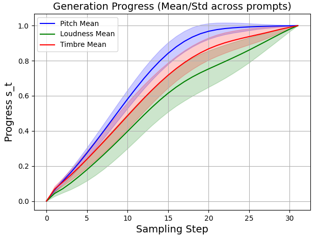
Figure 4: Probes Variation in Generation Progress
We demonstrate how our learned mappings can help us understand the audio generation process by analyzing DiffRhythm (Ning et al., 2025), a rectified flow model designed for full-length song synthesis. In this analysis, the model was configured to generate a 95-second audio segment, encompassing a verse and a chorus, over 32 inference steps. At each generation step $t∈\{0,...,31\}$ , we extract the latent $X_t∈ℝ^C× F$ , and decompose it through our SAE and linear probes to obtain acoustic concept activations $P^(a)_t∈ℝ^F× K_a$ . After applying a mean pooling over frames ( $F$ ), we obtain distributions $p^(a)_t$ for each attribute $a$ . To quantify the evolution of acoustic properties, we track how these distributions interpolate from noise to the final audio. Specifically, for each attribute $a$ and step $t$ , we compute the per-class normalized $L^1$ distance:
$$
s^(a)_t=\frac{1}{K_a}∑_k=1^K_a\frac{|p^(a)_t,k-p^(a)_0,k|}{|p^(a)_T,k-p^(a)_0,k|} \tag{4}
$$
where $s^(a)_t∈[0,1]$ measures the progression from initial noise ( $t=0$ ) toward the final acoustic structure ( $t=T=31$ ). This reveals when different acoustic properties emerge during generation. We sample 500 prompts from MusicCaps (Agostinelli et al., 2023), then plot the mean and standard deviation of the generation progress in Figure 4, which indicates a clear hierarchy. Pitch converges first (around step 21), followed by timbre, while loudness converges last and remains unresolved by the final step. This coarse-to-fine progression suggests the model establishes fundamental frequency before refining textural and dynamic details.
## 4 Conclusion
We present a framework for interpreting audio generative models by mapping their latent representations to human-interpretable acoustic properties through sparse autoencoders and linear probes. Our experiments demonstrate that SAE features naturally align with acoustic properties, enabling both controllable manipulation and better understanding of music generative models.
In future work, we plan to apply our method to other generative architectures, such as RAVE (Caillon and Esling, 2021), ACE-Step (Gong et al., 2025), and AudioLDM (Liu et al., 2023). Beyond the three acoustic properties explored here, we will train probes for richer audio features such as rhythm, harmony, and instrument identity. Finally, we aim to use these interpretable features to directly guide generation behavior during inference, potentially enabling fine-grained control over specific attributes while maintaining generation quality.
## References
- Agostinelli et al. (2023) Andrea Agostinelli, Timo I Denk, Zalán Borsos, Jesse Engel, Mauro Verzetti, Antoine Caillon, Qingqing Huang, Aren Jansen, Adam Roberts, Marco Tagliasacchi, et al. Musiclm: Generating music from text. arXiv preprint arXiv:2301.11325, 2023.
- Caillon and Esling (2021) Antoine Caillon and Philippe Esling. Rave: A variational autoencoder for fast and high-quality neural audio synthesis, 2021. URL https://arxiv.org/abs/2111.05011.
- Callender et al. (2020) Lee Callender, Curtis Hawthorne, and Jesse Engel. Improving perceptual quality of drum transcription with the expanded groove midi dataset, 2020.
- Cammarata et al. (2021) Nick Cammarata, Gabriel Goh, Shan Carter, Chelsea Voss, Ludwig Schubert, and Chris Olah. Curve circuits. Distill, 6(1):e00024–006, 2021.
- Cunningham et al. (2023) Hoagy Cunningham, Aidan Ewart, Logan Riggs, Robert Huben, and Lee Sharkey. Sparse autoencoders find highly interpretable features in language models, 2023. URL https://arxiv.org/abs/2309.08600.
- Défossez et al. (2022) Alexandre Défossez, Jade Copet, Gabriel Synnaeve, and Yossi Adi. High fidelity neural audio compression, 2022. URL https://arxiv.org/abs/2210.13438.
- Elhage et al. (2022) Nelson Elhage, Tristan Hume, Catherine Olsson, Nicholas Schiefer, Tom Henighan, Shauna Kravec, Zac Hatfield-Dodds, Robert Lasenby, Dawn Drain, Carol Chen, et al. Toy models of superposition. arXiv preprint arXiv:2209.10652, 2022.
- Evans et al. (2025) Zach Evans, Julian D. Parker, CJ Carr, Zack Zukowski, Josiah Taylor, and Jordi Pons. Stable audio open. In ICASSP 2025 - 2025 IEEE International Conference on Acoustics, Speech and Signal Processing (ICASSP), pages 1–5, 2025. 10.1109/ICASSP49660.2025.10888461.
- Gong et al. (2025) Junmin Gong, Sean Zhao, Sen Wang, Shengyuan Xu, and Joe Guo. Ace-step: A step towards music generation foundation model, 2025. URL https://arxiv.org/abs/2506.00045.
- Hawthorne et al. (2019) Curtis Hawthorne, Andriy Stasyuk, Adam Roberts, Ian Simon, Cheng-Zhi Anna Huang, Sander Dieleman, Erich Elsen, Jesse Engel, and Douglas Eck. Enabling factorized piano music modeling and generation with the MAESTRO dataset. In International Conference on Learning Representations, 2019. URL https://openreview.net/forum?id=r1lYRjC9F7.
- Hendrycks et al. (2023) Dan Hendrycks, Mantas Mazeika, and Thomas Woodside. An overview of catastrophic ai risks. arXiv preprint arXiv:2306.12001, 2023.
- Ji et al. (2025) Shengpeng Ji, Ziyue Jiang, Wen Wang, Yifu Chen, Minghui Fang, Jialong Zuo, Qian Yang, Xize Cheng, Zehan Wang, Ruiqi Li, Ziang Zhang, Xiaoda Yang, Rongjie Huang, Yidi Jiang, Qian Chen, Siqi Zheng, and Zhou Zhao. Wavtokenizer: an efficient acoustic discrete codec tokenizer for audio language modeling, 2025. URL https://arxiv.org/abs/2408.16532.
- Kim et al. (2018) Jong Wook Kim, Justin Salamon, Peter Li, and Juan Pablo Bello. Crepe: A convolutional representation for pitch estimation. In 2018 IEEE international conference on acoustics, speech and signal processing (ICASSP), pages 161–165. IEEE, 2018.
- Liu et al. (2023) Haohe Liu, Zehua Chen, Yi Yuan, Xinhao Mei, Xubo Liu, Danilo Mandic, Wenwu Wang, and Mark D Plumbley. Audioldm: Text-to-audio generation with latent diffusion models. arXiv preprint arXiv:2301.12503, 2023.
- Marshall and Kirchner (2024) Simon C Marshall and Jan H Kirchner. Understanding polysemanticity in neural networks through coding theory. arXiv preprint arXiv:2401.17975, 2024.
- McFee (2025) B. McFee. librosa/librosa: 0.11.0, March 2025. URL https://doi.org/10.5281/zenodo.15006942.
- Nelson et al. (2021) Elhage Nelson, Nanda Neel, Olsson Catherine, Henighan Tom, Joseph Nicholas, Mann Ben, Askell Amanda, Bai Yuntao, Chen Anna, Conerly Tom, et al. A mathematical framework for transformer circuits. Transformer Circuits Thread, 2021.
- Ning et al. (2025) Ziqian Ning, Huakang Chen, Yuepeng Jiang, Chunbo Hao, Guobin Ma, Shuai Wang, Jixun Yao, and Lei Xie. Diffrhythm: Blazingly fast and embarrassingly simple end-to-end full-length song generation with latent diffusion, 2025. URL https://arxiv.org/abs/2503.01183.
- Olah et al. (2020) Chris Olah, Nick Cammarata, Ludwig Schubert, Gabriel Goh, Michael Petrov, and Shan Carter. Zoom in: An introduction to circuits. Distill, 5(3):e00024–001, 2020.
- Schubert and Wolfe (2006) Emery Schubert and Joe Wolfe. Does timbral brightness scale with frequency and spectral centroid? Acta acustica united with acustica, 92(5):820–825, 2006.
- Schubert et al. (2004) Emery Schubert, Joe Wolfe, Alex Tarnopolsky, et al. Spectral centroid and timbre in complex, multiple instrumental textures. In Proceedings of the international conference on music perception and cognition, North Western University, Illinois, pages 112–116. sn, 2004.
- Smule (2019) I. Smule. DAMP-VSEP: Smule Digital Archive of Mobile Performances - Vocal Separation. Zenodo, oct 2019. URL https://doi.org/10.5281/zenodo.3553059.
- Su et al. (2025) Yi Su, Jisheng Bai, Qisheng Xu, Kele Xu, and Yong Dou. Audio-language models for audio-centric tasks: A survey. arXiv preprint arXiv:2501.15177, 2025.
- Wu et al. (2024) Haibin Wu, Xuanjun Chen, Yi-Cheng Lin, Kai-wei Chang, Ho-Lam Chung, Alexander H Liu, and Hung-yi Lee. Towards audio language modeling–an overview. arXiv preprint arXiv:2402.13236, 2024.
- Wu et al. (2022) Yusong Wu, Josh Gardner, Ethan Manilow, Ian Simon, Curtis Hawthorne, and Jesse Engel. The chamber ensemble generator: Limitless high-quality mir data via generative modeling. arXiv preprint arXiv:2209.14458, 2022.
- Xi et al. (2018) Q. Xi, R. Bittner, J. Pauwels, X. Ye, and J. P. Bello. GuitarSet: A Dataset for Guitar Transcription. In Proceedings of the 19th International Society for Music Information Retrieval Conference (ISMIR), Paris, France, sep 2018.
- Yang et al. (2025) Chih-Kai Yang, Neo S Ho, and Hung-yi Lee. Towards holistic evaluation of large audio-language models: A comprehensive survey. arXiv preprint arXiv:2505.15957, 2025.
- Ye et al. (2025) Zhen Ye, Peiwen Sun, Jiahe Lei, Hongzhan Lin, Xu Tan, Zheqi Dai, Qiuqiang Kong, Jianyi Chen, Jiahao Pan, Qifeng Liu, et al. Codec does matter: Exploring the semantic shortcoming of codec for audio language model. In Proceedings of the AAAI Conference on Artificial Intelligence, volume 39, pages 25697–25705, 2025.