2510.23937v1

# Optimized Loudspeaker Panning for Adaptive Sound-Field Correction and Non-stationary Listening Areas **Authors**: Yuancheng Luo \expresspapernumber 65 \correspondence Yuancheng Luoluoyuancheng@gmail.com \lastnames Luo {onecolabstract} Surround sound systems commonly distribute loudspeakers along standardized layouts for multichannel audio reproduction. However in less controlled environments, practical layouts vary in loudspeaker quantity, placement, and listening locations / areas. Deviations from standard layouts introduce sound-field errors that degrade acoustic timbre, imaging, and clarity of audio content reproduction. This work introduces both Bayesian loudspeaker normalization and content panning optimization methods for sound-field correction. Conjugate prior distributions over loudspeaker-listener directions update estimated layouts for non-stationary listening locations; digital filters adapt loudspeaker acoustic responses to a common reference target at the estimated listening area without acoustic measurements. Frequency-domain panning coefficients are then optimized via sensitivity / efficiency objectives subject to spatial, electrical, and acoustic domain constraints; normalized and panned loudspeakers form virtual loudspeakers in standardized layouts for accurate multichannel reproduction. Experiments investigate robustness of Bayesian adaptation, and panning optimizations in practical applications. 1 Introduction Surround sound systems for multichannel audio reproduction have risen in popularity in home theater setups that accommodate proper loudspeaker selection, layout, acoustic room treatment, and calibration established by the international telecommunication union (ITU) standards [1]. Conversely, the same accommodations present a barrier to entry for extemporary arrangements where loudspeakers differ in quality and placement, and operate in changeable listening locations / areas, and reverberant environments. Deviating from the standards degrade accurate reproduction of multichannel audio content as intended by the content authors. Therefore, methods from sound-field control and reconstruction correct for the effects of irregular loudspeaker placements and room reverberation in the listening area via acoustic measurement system inversion [2, 3, 4], and modal / planewave decomposition [5, 6, 7]; such methods however are inapplicable when acoustic measurements remain unavailable. In the absence of acoustic measurements, other sensing modalities can infer the loudspeaker layout and listening area location. Inertial measurement unit [8, 9] and bluetooth low energy [10, 11] indoor tracking can estimate changes in loudspeaker position and orientation. Ultrasound [12], camera, and video can track in-room listener and loudspeaker positions within fields-of-view. Such meta-data yields a 2D layout of the estimated loudspeaker placements, listening location, and a front direction. We therefore reproduce multichannel content at the listener’s area by incorporating Bayesian uncertainty of the estimated layout inputs with loudspeaker distance and orientation normalization [13, 14] to the listener, and then reformulate conventional amplitude panning methods [15, 16, 17] in terms of constrained optimization along joint spatial [18, 19], electrical [20], and acoustical [21] domains. The paper is organized as follows: Section 2 introduces our normalization method for aligning loudspeaker acoustic transfer functions in an arbitrary layout to a common axial-reference target at the listener location; acoustic delay and attenuation compensate for varying loudspeaker-listener distances whereas minimum-phase and all-pass factorizations [22] normalize for loudspeaker orientations relative to listener locations. We integrate estimates of the loudspeaker-listener normalization directions via Bayesian posterior updates of a novel circular distribution conjugate prior, and provide a sample calibration for a sequence of normalization angles. Section 3 presents our novel normalized loudspeaker panning optimization, which solves for frequency-dependent magnitude-gains that satisfy spatial vector-bases, electrical headroom, and acoustic power constraints; we augment the former vector-base amplitude panning with slack (VBAPS) to accommodate constraints in electric and acoustic domains. Next, we derive a panning sensitivity / efficiency objective from the augmented form that measures panned-source discreteness, and give equivalent primary and null-space formulations in fewer variables. Planewave acoustic covariances model anechoic to diffuse-field assumptions for variable sized listening areas. Optimal solutions are found via second-order cone program [23]. Section 4 applies our model to several practical applications of loudspeaker correction under varying constraints. For high loudness targets, we find optimal gains across loudspeakers for overdriven content that maximize source discreteness. For anechoic to diffuse-field environments, we show that our panning optimization solutions converge from discrete panning to Rayleigh quotient maximizers [24]. For circular-panning over varying loudspeaker layouts, we evaluate panning sensitivity across azimuth steering-angles and recommend preferred layouts for different number of loudspeakers. Section 5 discusses results and future work. 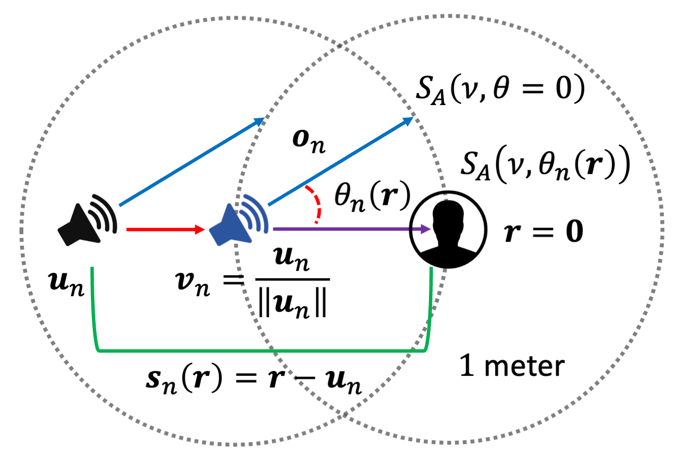2 Loudspeaker Normalization Let $S(\nu,\theta)$ be the loudspeaker’s electrical-acoustical transfer function at frequency $\nu$ measured at $1$ meter distance along azimuth $\theta$ (radians) in the horizontal plane, with the acoustic path-delay removed. Under far-field assumptions, the loudspeaker frequency response attenuates by the inverse-distance and undergoes pure-delay. It is useful to express the far-field transfer function along a listener-centric coordinate frame, which centers the origin at the listener’s location and aligns the $+x$ axis with the listener’s facing direction. The acoustic transfer function $H_{n}(\kappa,\bm{r})$ at coordinate $\bm{r}∈\mathbb{R}^{2× 1}$ for the $n^{th}$ loudspeaker located at coordinate $\bm{u}_{n}∈\mathbb{R}^{2× 1}$ with the orientation unit-vector $\bm{o}_{n}∈\mathbb{R}^{2× 1}$ follows $$ \begin{split}H_{n}(\nu,\bm{r})&=S\left({\nu,\theta_{n}(\bm{r})}\right)\frac{e^{\minus j\kappa\left\lVert\bm{s}_{n}(\bm{r})\right\rVert}}{\left\lVert\bm{s}_{n}(\bm{r})\right\rVert},\quad\kappa=\frac{2\pi\nu}{c},\\ \theta_{n}(\bm{r})&=\cos^{-1}\left({\frac{\bm{o}_{n}^{T}\bm{s}_{n}(\bm{r})}{\left\lVert\bm{s}_{n}(\bm{r})\right\rVert}}\right),\quad\bm{s}_{n}(\bm{r})=\bm{r}-\bm{u}_{n},\end{split} \tag{1} $$ where $\kappa$ is the angular wavenumber, $c$ is the speed of sound in meters/second, $\bm{s}_{n}(\bm{r})$ is the evaluation direction relative to the loudspeaker’s location, and $\theta_{n}(\bm{r})$ is the evaluation angle relative to the loudspeaker’s orientation. We can normalize the loudspeaker’s transfer function to approximate the original loudspeaker’s response $S(\nu,\theta)$ within a listening window at the listener’s location $\bm{r}=\bm{0}$ . Consider the following decomposition of the loudspeaker transfer function $S(\nu,\theta)=S_{E}(\nu)S_{A}(\nu,\theta)$ into acoustical and electrical domain transfer functions $S_{A}(\nu,\theta)$ and $S_{E}(\nu)$ respectively. A filter with frequency response $G_{n}(\nu)$ that normalizes (1) to the loudspeaker’s on-axis response $H_{n}(\nu,\bm{0})G_{n}(\nu)=S(\nu,0)$ is given by $$ \begin{split}G_{n}(\nu)=Q_{n}(\nu)\left\lVert\bm{u}_{n}\right\rVert e^{j\kappa\left\lVert\bm{u}_{n}\right\rVert},\quad Q_{n}(\nu)=\frac{S_{A}(\nu,0)}{S_{A}\left({\nu,\bm{\bar{\theta}}_{n}}\right)},\end{split} \tag{2} $$ where $\bm{\bar{\theta}}_{n}=\theta_{n}(\bm{0})$ is the normalization angle between the loudspeaker’s orientation and the listener. The electrical domain term $S_{E}(\nu)$ cancels within the quotient $Q_{n}(\nu)$ in (2), thereby negating prior signal processing in loudspeaker playback. $Q_{n}(\nu)$ is therefore the acoustic relative-transfer-function between loudspeaker’s axial and listener-direction acoustic responses. Moreover, if $S_{A}(\nu,\theta)$ share a common acoustic delay and the remainder is minimum-phase for bounded $\theta$ that define a listening window, then $Q_{n}(\nu)$ must also be minimum-phase. Thus, the normalized transfer function $G_{n}(\nu)$ compensates for both loudspeakers’ orientation and distance relative to the listener as shown in Fig. 1. <details> <summary>figs/pretransform.png Details</summary>  ### Visual Description ## Diagram: Sound Field Propagation Model ### Overview The diagram illustrates a sound propagation model involving two overlapping circular regions representing sound fields. A speaker emits sound waves, which interact with a human figure positioned at the origin (r = 0). Key elements include directional vectors, normalization operations, and spatial transformations. ### Components/Axes 1. **Circular Regions**: - Left circle: Labeled $ S_A(v, \theta = 0) $, representing a baseline sound field. - Right circle: Labeled $ S_A(v, \theta_n(r)) $, indicating a transformed sound field dependent on position $ r $ and angle $ \theta_n(r) $. 2. **Speaker**: Emits sound waves (blue arrow) with a red arrow indicating direction. 3. **Human Figure**: Positioned at $ r = 0 $, with a purple arrow pointing toward it. 4. **Vectors**: - $ \mathbf{u}_n $: Green vector originating from the speaker, labeled with magnitude $ \|\mathbf{u}_n\| $. - $ \mathbf{v}_n $: Blue vector derived from $ \mathbf{u}_n $, calculated as $ \mathbf{v}_n = \frac{\mathbf{u}_n}{\|\mathbf{u}_n\|} $. - $ \mathbf{o}_n $: Blue arrow pointing from the speaker to the human figure. 5. **Equations**: - $ s_n(r) = r - \mathbf{u}_n $: Spatial transformation equation. - $ \theta_n(r) $: Angle parameter dependent on position $ r $. 6. **Distance Marker**: Explicitly labeled "1 meter" between the speaker and human figure. ### Detailed Analysis - **Vector Relationships**: - $ \mathbf{v}_n $ is a unit vector derived from $ \mathbf{u}_n $, normalized by its magnitude. - $ \mathbf{o}_n $ directly connects the speaker to the human figure, suggesting a reference path for sound propagation. - **Spatial Transformations**: - $ s_n(r) = r - \mathbf{u}_n $ implies a positional adjustment relative to the speaker's emission point. - $ \theta_n(r) $ modulates the sound field based on the human's position, altering the baseline $ S_A(v, \theta = 0) $. - **Overlapping Regions**: The intersection of the two circles may represent overlapping sound fields or interference effects. ### Key Observations 1. The human figure is anchored at the origin ($ r = 0 $), serving as a reference point for spatial calculations. 2. The normalization of $ \mathbf{u}_n $ to $ \mathbf{v}_n $ ensures directional consistency in sound propagation. 3. The 1-meter distance provides a fixed scale for spatial relationships. 4. The angle $ \theta_n(r) $ introduces a dynamic parameter that varies with position, affecting the sound field $ S_A $. ### Interpretation This diagram models how sound fields interact with a human listener in a controlled environment. The speaker's emission ($ \mathbf{u}_n $) is normalized to $ \mathbf{v}_n $, ensuring directional accuracy. The transformed sound field $ S_A(v, \theta_n(r)) $ accounts for the listener's position ($ r $) and angular adjustments ($ \theta_n(r) $), suggesting applications in acoustic engineering or spatial audio systems. The 1-meter scale anchors the model in a real-world context, while the overlapping circles may represent constructive/destructive interference or multi-path propagation effects. The equations emphasize the importance of vector normalization and positional dependency in sound field analysis. </details> Figure 1: Acoustic transfer function $G_{n}(\nu)$ in (2) normalizes the direct acoustic path between the listener and loudspeaker at $\bm{u}_{n}$ to be its on-axis response $S_{A}(\nu,0)$ at the normalized coordinate $\bm{v}_{n}$ . In practice, we can find the rational function approximation [25, 26] to $Q_{n}(\nu)$ , expressed in terms of minimum-phase $\mathbb{M}_{n}(\nu)$ and all-pass $\mathbb{A}_{n}(\nu)$ transfer functions given by $$ \begin{split}Q_{n}(\nu)\approx\mathbb{M}_{n}(\nu)\mathbb{A}_{n}(\nu),\quad\mathbb{A}_{n}(\nu)=\bar{\mathbb{A}}_{n}(\nu)\ddot{\mathbb{A}}_{n}(\nu),\end{split} \tag{3} $$ where $\bar{\mathbb{A}}_{n}(\nu)$ and $\ddot{\mathbb{A}}_{n}(\nu)$ are all-pass transfer functions belonging to stable and unstable components respectively. The unstable all-pass $\ddot{\mathbb{A}}_{n}(\nu)$ contains the reciprocal poles and zeros of the Padé approximant outside the complex unit-circle, and is ideally empty or low-order for $\theta$ in the listening window. We can realize a causal-stable filter-response $G_{n}(\nu)$ for an all-passed loudspeaker transfer function in (2) as follows: $$ \begin{split}H_{n}(\nu,\bm{0})G_{n}(\nu)=S(\nu,0)\frac{e^{\minus j\kappa d}}{\ddot{\mathbb{A}}_{lcm}(\nu)}\quad\Rightarrow\quad\\ G_{n}(\nu)=\mathbb{M}_{n}(\nu)\bar{\mathbb{A}}_{n}(\nu)\frac{\ddot{\mathbb{A}}_{n}(\nu)}{\ddot{\mathbb{A}}_{lcm}(\nu)}\left\lVert\bm{u}_{n}\right\rVert e^{j\kappa\left\lVert\bm{u}_{n}\minus d\right\rVert},\\ \end{split} \tag{4} $$ where $d=\max_{1≤ n≤ N}\left\lVert\bm{u}_{n}\right\rVert$ is the furthest loudspeaker distance, and $\ddot{\mathbb{A}}_{lcm}(\nu)$ is the transfer function of the set of least common multiple (LCM) reciprocal poles and zeros across the unstable all-passes $\left\{{\ddot{\mathbb{A}}_{1}(\nu),...,\ddot{\mathbb{A}}_{N}(\nu)}\right\}$ . In the $z$ -domain, we can therefore express the all-pass and LCM transfer functions as follows: $$ \begin{split}\ddot{\mathbb{A}}_{n}(z)&=\prod_{p\in P_{n}}\left({\frac{1-p^{*}z}{1-pz^{\minus 1}}}\right)^{k_{pn}},\quad P_{n}=\left\{{p_{1n},\ldots,p_{M_{n}n}}\right\},\\ \ddot{\mathbb{A}}_{lcm}(z)&=\prod_{p\in P}\left({\frac{1-p^{*}z}{1-pz^{\minus 1}}}\right)^{\max\limits_{1\leq n\leq N}k_{pn}},\quad P=\cup_{n=1}^{N}P_{n},\end{split} \tag{5} $$ where $p^{*}$ is the conjugate transpose, and $P_{n}$ is the set of unique poles and $k_{pn}$ is the multiplicity of pole $p$ for the $n^{th}$ loudspeaker. By taking the maximum multiplicity for each unique and unstable pole across all $\ddot{\mathbb{A}}_{n}(z)$ , and dividing by the subsequent LCM $\ddot{\mathbb{A}}_{lcm}(z)$ , the unstable poles in $\ddot{\mathbb{A}}_{n}(z)$ cancel and the remaining all-pass adds minimal additional group-delay in $G_{n}(\nu)$ . The filtered loudspeakers’ direct paths are thus matched with a common all-passed on-axis response. Lastly, we gain the loudspeaker filter $G_{n}(\nu)$ to match the expected acoustic power at a common distance $D$ , such as the median of all loudspeakers-to-listener distances, via the following room acoustic attenuation model: Let us consider the inverse-distance law $\rho_{DP}(r)=\bar{\rho}r^{\minus 2}$ for the attenuation of the direct acoustic path response’s nominal power $\bar{\rho}$ at distance $r$ from a loudspeaker. In a room environment, let $\rho_{IP}(r)$ be the total power of indirect acoustic paths at distance $r$ . We can model the ratio of the direct-to-indirect acoustic path’s power at $r$ and total power as follows: $$ \begin{split}\frac{\rho_{DP}(r)}{\rho_{IP}(r)}&=\left({\frac{d_{c}}{r}}\right)^{2\beta},\quad\beta=10^{\frac{\gamma\textrm{ dB/dd}}{10}},\quad\textrm{Attenuation rate}\\ \rho(r)&=\rho_{DP}(r)+\rho_{IP}(r)=\bar{\rho}r^{\minus 2}\left({1+\left({\frac{d_{c}}{r}}\right)^{2\beta}}\right),\end{split} \tag{6} $$ where $d_{c}$ is the so-called critical distance (meters) where the direct and indirect acoustic powers are equivalent, and $\beta$ a decay-rate parameterized by $\gamma$ decibels (dB) per double-distance (dd); typical $\gamma∈\left\{{0,-3}\right\}$ and $0.5≤ d_{c}≤ 1.5$ span idealized concert-hall to small-room spaces [27]. Normalizing the power at distance $r$ to $D$ therefore follows $$ \begin{split}F(r,\,D,\,d_{c})=\sqrt{\frac{\rho(D)}{\rho(r)}}=\frac{r}{D}\sqrt{\frac{d_{c}^{2\beta}+D^{2\beta}}{d_{c}^{2\beta}+r^{2\beta}}},\end{split} \tag{7} $$ whereby substituting $\left\lVert\bm{u}_{n}\right\rVert$ with $F(\left\lVert\bm{u}_{n}\right\rVert,\,D,\,d_{c})$ in (4) compensates for loudspeaker distances to the listener in a room. Model Uncertainty for Non-stationary Targets: In instances where the listener’s location changes over time or require online estimation, we normalize the loudspeaker via the mean listener distance $\frac{1}{T}∈t_{0}^{T}\left\lVert\bm{u}_{n}(t)\right\rVert dt$ , and treat the normalization angle $\bm{\bar{\theta}}_{n}$ relative to the loudspeaker orientation $\bm{o}_{n}$ in (2) as a random variable. The target transfer function $G_{n}(\nu)$ and quotient term $Q_{n}(\nu)$ are re-defined to minimize the expected squared-differences between the anechoic responses $S_{A}(\nu,\theta)$ sampled over axial-centered and loudspeaker-listener centered circular probability distribution functions (PDFs) $f_{0}(\theta)$ and $f_{n}(\theta)$ , $∀ 1≤ n≤ N$ respectively; circular PDFs satisfy $f(\theta)=f(\theta+2\pi k)$ , $∀ k∈\mathbb{Z}$ . We present two acoustic averages: $$ \begin{split}\bar{S}_{A}(\nu,f(\theta))&=\mathbb{E}\left[{S_{A}(\nu,\theta)}\right]=\int S_{A}(\nu,\theta)f(\theta)d\theta,\\ \hat{S}_{A}(\nu,f(\theta))&=\mathbb{E}\left[{\left|{S_{A}(\nu,\theta)}\right|^{2}}\right]=\int\left|{S_{A}(\nu,\theta)}\right|^{2}f(\theta)d\theta,\end{split} \tag{8} $$ where $\bar{S}_{A}(\nu,f(\theta))$ and $\hat{S}_{A}(\nu,f(\theta))$ are spatial windowed averages of the acoustic response and power respectively; axial window response average $\bar{S}_{A}(\nu,f_{0}(\theta))$ and power average $\hat{S}_{A}(\nu,f_{0}(\theta))$ sample from the $f_{0}(\theta)$ distribution. The modified quotient term $Q_{n}(\nu)$ in (2) is replaced with the weighted least-squares minimizer of $\operatorname*{arg\,min}_{X}∈t\left|{S_{A}(\nu,\theta)X-\bar{S}_{A}(\nu,f_{0}(\theta))}\right|^{2}f_{n}(\theta)d\theta$ given by $$ \begin{split}\bar{Q}_{n}(\nu)=\bar{S}_{A}(\nu,f_{0}(\theta))\frac{\bar{S}_{A}^{*}(\nu,f_{n}(\theta))}{\hat{S}_{A}(\nu,f_{n}(\theta))},\end{split} \tag{9} $$ where $\bar{S}_{A}^{*}(\nu,f_{n}(\theta))$ is the conjugate transpose, and $\bar{Q}_{n}(\nu)$ accounts for both amplitude and phase differences in the averaged responses. The analogous quotient for the spatial windowed acoustic power average follows $$ \begin{split}\hat{Q}_{n}(\nu)&=\sqrt{\frac{\hat{S}_{A}(\nu,f_{0}(\theta))}{\hat{S}_{A}(\nu,f_{n}(\theta))}},\end{split} \tag{10} $$ where $\hat{Q}_{n}(\nu)$ has zero-phase and therefore compensates for only the amplitude. Both quotients can be efficiently evaluated if $f_{0}(\theta)$ , $f_{n}(\theta)$ are both uni-modal and smooth over azimuth, have expansions along a common orthogonal basis with $S_{A}(\nu,\theta)$ , and follow the contours of a listening window. 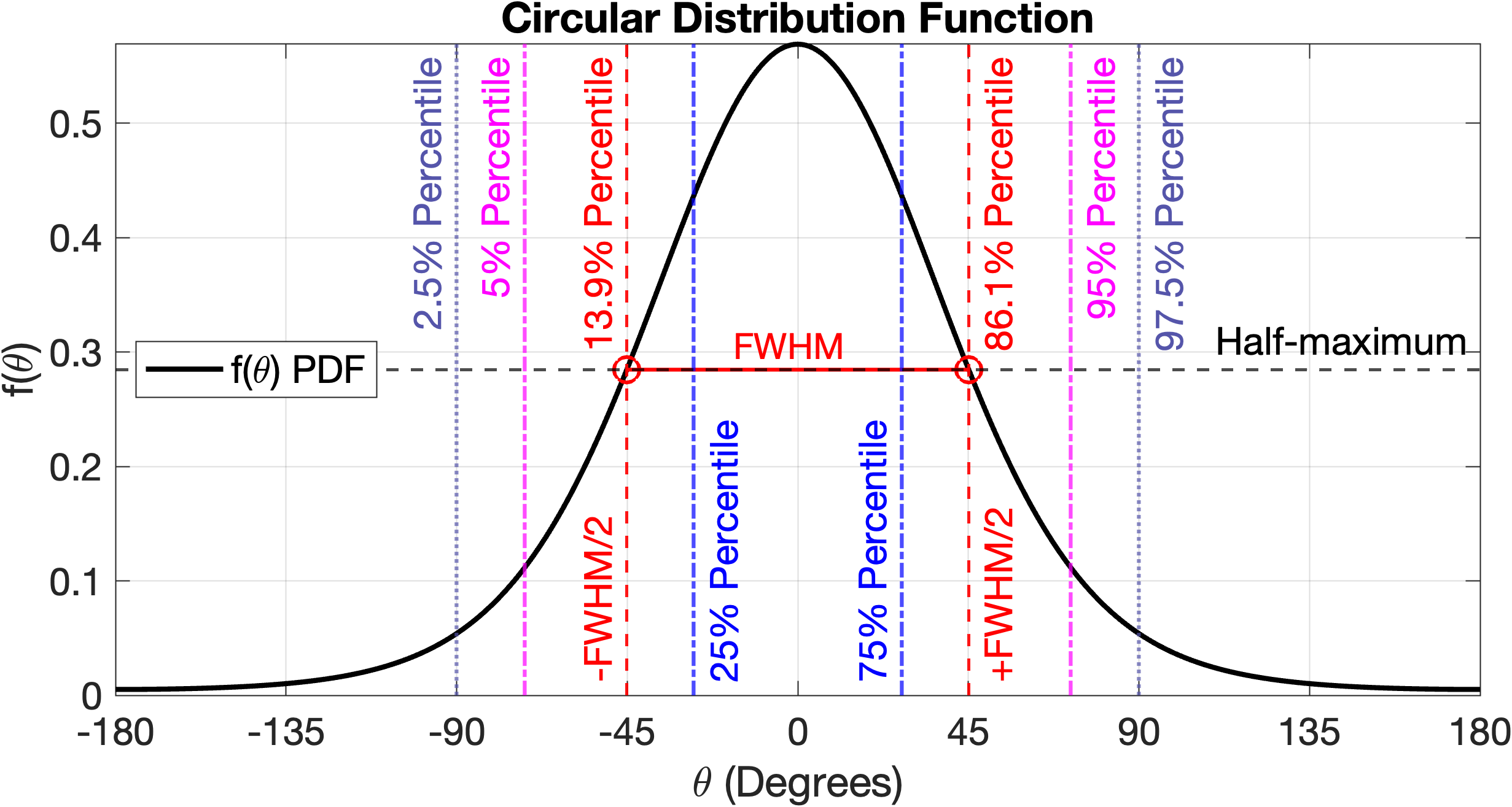Let us consider the circular distribution $f(\theta)$ defined by the squared-exponential of the chordal distance $d(\theta)$ on a unit-disk, which along with $S_{A}(\nu)$ has a series-expansion over the Legendre polynomials [28], and normalized over the domain of all azimuth angles $-\pi≤\theta≤\pi$ : $$ \begin{split}f(\theta)&=\frac{e^{\frac{\minus d^{2}(\theta\minus\mu)}{2\ell^{2}}}}{2\pi e^{\minus\ell^{\minus 2}}J_{0}(j\ell^{\minus 2})},\quad d(\theta)=2\sin\left({\frac{{\theta}\textrm{ mod }{2\pi}}{2}}\right),\end{split} \tag{11} $$ where $J_{0}$ is the Bessel function of the first kind, $\mu$ is the mean azimuth, and $\ell$ is the dispersion. The function is symmetric w.r.t. its maximum $f(\mu)$ and minimum $f(\mu±\pi)$ , infinitely differentiable in all azimuths, and its percentiles computable via series expansion in appendix (26). Large dispersion $\ell$ gives a uniform distribution as $\lim_{\ell→∞}f(\theta)=(2\pi)^{\minus 1}$ ; small dispersion gives the dirac distribution as $\lim_{\ell→ 0}f(\theta-\mu)=\delta$ . We can bound the dispersion via design parameters characterizing a listening window’s peak such as the full-width at half-maximum (FWHM) measure: $$ \begin{split}\frac{f(\mu)}{2}&=f\left({\mu\pm\frac{\textrm{FWHM}}{2}}\right),\quad 0\leq\textrm{FWMH}\leq 2\pi,\\ \ell&=\frac{2\sin\left({\frac{\textrm{FWMH}}{4}}\right)}{\sqrt{2\ln(2)}}\,\,\,\Rightarrow\,\,\,0\leq\ell\leq\sqrt{2/\ln(2)},\end{split} \tag{2} $$ which defines the angular width where $f(\theta)$ spans half its maximum amplitude as shown in Fig. 2. At the upper-limit FWHM $360^{\circ}$ , $f(\theta)$ contains $\left\{{60.9,\,33.2,\,22.5}\right\}\%$ of its mass within the frontal intervals $\left|{\theta-\mu}\right|≤\left\{{90,\,45,\,30}\right\}^{\circ}$ respectively. For tighter FWHM $≤ 90.22^{\circ}$ bounds, $f(\theta)$ contains the $95\%$ confidence interval in the half-space $\left|{\theta-\mu}\right|≤ 90^{\circ}$ of its mean azimuth $\mu$ . For the axial-centered PDF in (8), we set the window’s FWHM to $60^{\circ}$ where $f_{0}(\theta)=f(\theta\,|\,\mu=0,\ell=0.4396)$ . We now proceed with online adaptation of the normalization angles $\bm{\bar{\theta}}_{n}$ over time. <details> <summary>figs/circular_distribution.png Details</summary>  ### Visual Description ## Chart: Circular Distribution Function ### Overview The chart depicts a symmetric bell-shaped probability density function (PDF) centered at 0 degrees, representing a circular distribution. Key features include percentile markers, full width at half maximum (FWHM), and half-maximum thresholds. ### Components/Axes - **X-axis**: θ (Degrees), ranging from -180° to 180° in 45° increments. - **Y-axis**: f(θ) PDF, scaled from 0 to 0.5. - **Legend**: - Black line: "f(θ) PDF" (probability density function). - **Vertical Lines**: - Dashed blue lines at -90°, -45°, 0°, 45°, 90°, and 135°. - Red dashed lines at -45° and 45° labeled "-FWHM/2" and "+FWHM/2". - Dotted purple lines at -90° and 90° labeled "2.5% Percentile" and "97.5% Percentile". - Dotted pink lines at -45° and 45° labeled "5% Percentile" and "95% Percentile". - **Annotations**: - "FWHM" at the peak (0°). - "Half-maximum" at y = 0.3 (dashed horizontal line). ### Detailed Analysis - **Percentile Markers**: - 2.5%: -90° (left tail). - 5%: -45° (left tail). - 25%: 0° (center). - 75%: 45° (right tail). - 95%: 45° (right tail). - 97.5%: 90° (right tail). - **FWHM**: - Full width at half maximum spans from -45° to +45° (red dashed lines). - Half-maximum threshold at y = 0.3 (dashed line). - **Symmetry**: The curve is symmetric about θ = 0°, with identical slopes on both sides. ### Key Observations 1. The distribution peaks sharply at 0°, with f(θ) ≈ 0.5. 2. 99.7% of the distribution lies within ±90° (2.5% and 97.5% percentiles). 3. The FWHM (90° total width) captures 50% of the distribution (area under the curve between -45° and +45°). 4. The half-maximum line (y = 0.3) intersects the curve at approximately ±67.5° (interpolated from the bell shape). ### Interpretation This chart models a circular distribution with a unimodal, symmetric PDF. The FWHM (90°) quantifies the spread of the central 50% of data, while percentiles demarcate cumulative probabilities. The half-maximum threshold (y = 0.3) provides a secondary measure of spread, indicating where the density drops to half its peak value. The symmetry suggests no directional bias in the data, and the sharp peak at 0° implies a strong central tendency. The use of percentile markers aligns with standard statistical practice for characterizing distributions. </details> Figure 2: Circular distribution prior (FWHM $90.2^{\circ}$ ) contains $\left\{{50,90,95}\right\}\%$ of normalization angles within $\left|{\theta}\right|≤\left\{{27.4,\,72,\,90}\right\}^{\circ}$ of the mean angle. 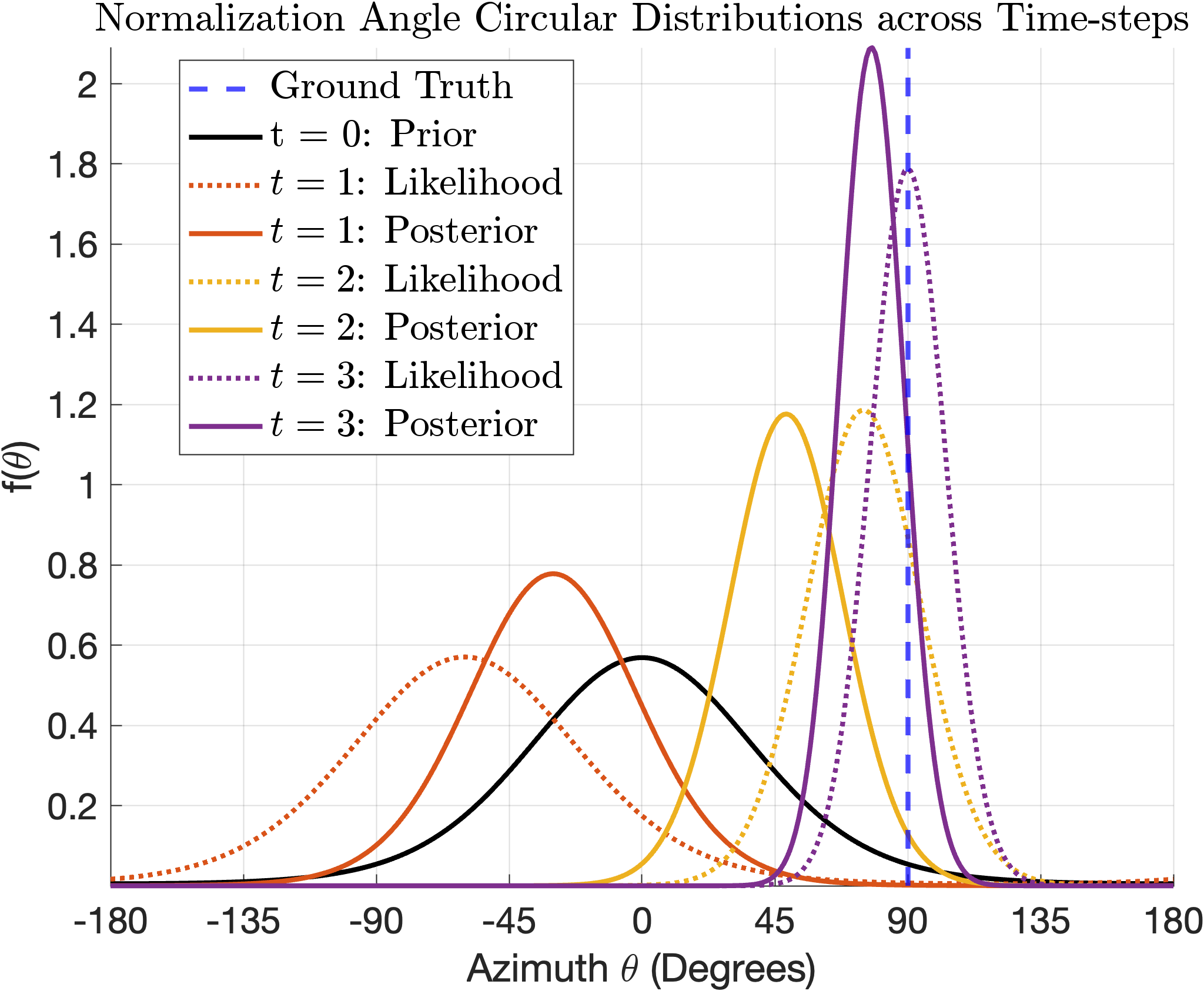Suppose we have measured a normalization angle $\bar{\theta}$ belonging to the $n^{th}$ loudspeaker with known measurement dispersion $\bar{\ell}$ such that the likelihood function $f(\bar{\theta}\,|\,\mu=\bm{\bar{\theta}}_{n},\ell=\bar{\ell})$ follows the squared-exponential chordal function in (11). Let the unknown normalization angle $\bm{\bar{\theta}}_{n}$ of the $n^{th}$ loudspeaker have a squared-exponential chordal prior-distribution $f(\bm{\bar{\theta}}_{n}|\,\mu=\mu_{n},\ell=\ell_{n})$ with initial hyperparameters $\mu_{n}=0$ mean azimuth and $\ell=\sqrt{2/\ln(2)}$ maximum dispersion. The posterior normalization angle therefore has a conjugate distribution with hyperparameters following appendix (27). Over multiple time-steps $t$ , the likelihood, prior, and posterior functions across measured angles $\bm{\bar{\theta}}^{\left\{{t}\right\}}_{n}$ with dispersion $\bar{\ell}_{n}^{\left\{{t}\right\}}$ are given by $$ \begin{split}L\left({\bm{\bar{\theta}}_{n}\,|\,\bm{\bar{\theta}}^{\left\{{t}\right\}}_{n}}\right)&=f\left({\bm{\bar{\theta}}^{\left\{{t}\right\}}_{n}\,|\,\mu=\bm{\bar{\theta}}_{n},\ell=\bar{\ell}_{n}^{\left\{{t}\right\}}}\right),\quad\textrm{Likelihood}\\ P(\bm{\bar{\theta}}_{n})&=f\left({\bm{\bar{\theta}}_{n}\,|\,\mu=\mu_{n}^{\left\{{t\minus 1}\right\}},\,\ell=\ell_{n}^{\left\{{t\minus 1}\right\}}}\right),\quad\textrm{Prior}\\ P\left({\bm{\bar{\theta}}_{n}\,|\,\bm{\bar{\theta}}^{\left\{{t}\right\}}_{n}}\right)&\propto L\left({\bm{\bar{\theta}}_{n}\,|\,\bm{\bar{\theta}}^{\left\{{t}\right\}}_{n}}\right)P(\bm{\bar{\theta}}_{n}),\qquad\textrm{Posterior}\end{split} \tag{13} $$ 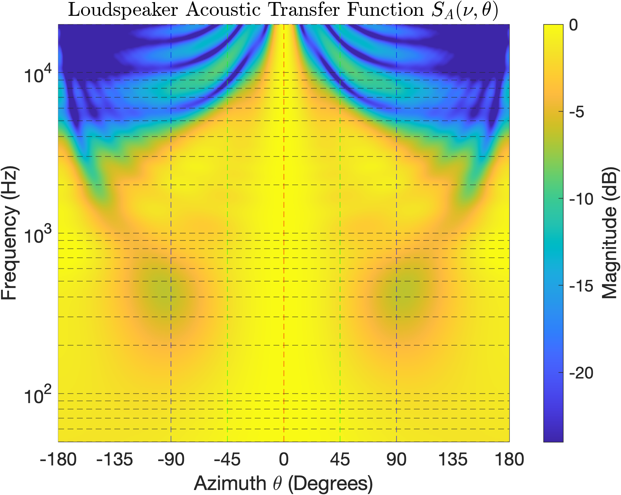where the reported normalization angle $\bm{\bar{\theta}}^{\left\{{t}\right\}}_{n}$ is a point-estimate taken within a measurement session, and the dispersion $\bar{\ell}_{n}^{\left\{{t}\right\}}$ is proportional to the point-estimate’s confidence interval. Both quantities can vary over time as the listener’s location may change between sessions (e.g. different seating), and measured under different noise conditions. The initial hyperparameters for mean $\mu_{n}^{\left\{{0}\right\}}=0$ and dispersion $\ell_{n}^{\left\{{0}\right\}}=0.6515$ (FWHM $90.22^{\circ}$ ) are informative as loudspeakers generally orient towards the intended listening area. The posterior estimate of $\bm{\bar{\theta}}_{n}$ follows Bayes’ theorem, where the current mean $\mu_{n}^{\left\{{t}\right\}}$ and dispersion $\ell_{n}^{\left\{{t}\right\}}$ hyperparameters are updated from the measurement terms $\bm{\bar{\theta}}^{\left\{{t}\right\}}_{n},\bar{\ell}_{n}^{\left\{{t}\right\}}$ in the likelihood function and the previous hyperparameters $\mu_{n}^{\left\{{t-1}\right\}},\ell_{n}^{\left\{{t-1}\right\}}$ via appendix (28). Lastly, the normalization filter’s quotient terms (9), (10) are updated for PDF $f_{n}(\theta)=f(\theta\,|\,\mu=\mu_{n}^{\left\{{t}\right\}},\ell=\ell_{n}^{\left\{{t}\right\}})$ , and the filters $G_{n}(\nu)$ are re-computed. Let us step-through the following example: <details> <summary>figs/fst_window_kernel_sample_transfer_functions.png Details</summary>  ### Visual Description ## Heatmap: Loudspeaker Acoustic Transfer Function \( S_A(\nu, \theta) \) ### Overview The image is a heatmap visualizing the magnitude of a loudspeaker's acoustic transfer function across frequency (Hz) and azimuth angle (degrees). The color gradient represents sound pressure level (dB), with blue indicating lower magnitudes and yellow higher magnitudes. The plot uses a logarithmic frequency scale and spans a full 360° azimuth range. --- ### Components/Axes 1. **X-Axis (Azimuth θ)**: - Label: "Azimuth θ (Degrees)" - Range: -180° to 180° (full circle) - Key markers: Solid vertical lines at -180°, -90°, 0°, 90°, 180°; dashed lines at intermediate intervals. 2. **Y-Axis (Frequency)**: - Label: "Frequency (Hz)" - Scale: Logarithmic (10² to 10⁴ Hz) - Key markers: Horizontal dashed lines at 100 Hz, 1 kHz, 10 kHz. 3. **Color Bar (Magnitude)**: - Label: "Magnitude (dB)" - Range: -20 dB (blue) to 0 dB (yellow) - Position: Right of the plot. 4. **Grid**: - Dashed black lines for frequency and azimuth subdivisions. - Solid lines at critical points (e.g., 0°, ±90°, ±180°). --- ### Detailed Analysis - **Color Gradient**: - Blue (-20 dB) to yellow (0 dB) indicates decreasing sound magnitude. - Central region (0° azimuth) is predominantly yellow, suggesting maximum transfer. - Blue lobes appear near ±90° azimuth at higher frequencies (1 kHz–10 kHz). - **Frequency Trends**: - **Low frequencies (100–1 kHz)**: Uniform yellow across most azimuths, except near ±90° where faint blue regions emerge. - **Mid frequencies (1–10 kHz)**: Strong blue lobes at ±90°, indicating directional attenuation. - **High frequencies (10 kHz–100 kHz)**: Blue lobes dominate, with minimal yellow regions. - **Azimuth Trends**: - **0° azimuth**: Consistently yellow (highest magnitude) across all frequencies. - **±90° azimuth**: Blue regions (lowest magnitude) become more pronounced at higher frequencies. --- ### Key Observations 1. **Directional Sensitivity**: - The loudspeaker exhibits strong directional behavior at higher frequencies, with significant attenuation at ±90° azimuth. - At lower frequencies, the response is more omnidirectional. 2. **Resonance Peaks**: - Yellow regions near 0° azimuth suggest resonant frequencies where sound is amplified. 3. **Logarithmic Scale Impact**: - The logarithmic frequency axis emphasizes relative changes in magnitude, highlighting directional effects at higher frequencies. --- ### Interpretation The heatmap demonstrates that the loudspeaker’s acoustic performance is highly directional at higher frequencies, with a pronounced "null" (attenuation) at ±90° azimuth. This suggests the speaker is optimized for frontal sound projection, with reduced performance at side angles. The logarithmic frequency scale reveals that directional effects become more critical as frequency increases, which is critical for applications like concert hall acoustics or directional audio systems. The central axis (0°) consistently shows maximum transfer, indicating the speaker’s primary design focus on frontal sound delivery. </details> <details> <summary>figs/fst_window_kernel_bayes_circular_dist.png Details</summary>  ### Visual Description ## Line Graph: Normalization Angle Circular Distributions across Time-steps ### Overview The graph depicts the evolution of normalized angle distributions (f(θ)) across four time-steps (t=0 to t=3), comparing prior, likelihood, and posterior estimates against a ground truth. Distributions are plotted against azimuth angles (θ) in degrees, with distinct line styles and colors for each data series. ### Components/Axes - **X-axis**: Azimuth θ (Degrees), ranging from -180° to 180° in 45° increments. - **Y-axis**: Normalized frequency f(θ), scaled from 0 to 2. - **Legend**: Located in the top-right corner, mapping colors and line styles to time-steps and distribution types: - **Blue dashed**: Ground Truth - **Black solid**: t=0: Prior - **Red dotted**: t=1: Likelihood - **Red solid**: t=1: Posterior - **Orange dotted**: t=2: Likelihood - **Orange solid**: t=2: Posterior - **Purple dotted**: t=3: Likelihood - **Purple solid**: t=3: Posterior ### Detailed Analysis 1. **Ground Truth (Blue Dashed Line)**: - Peaks sharply at θ ≈ 90° with f(θ) ≈ 2.0. - Symmetric decline to near-zero values at θ = ±180°. 2. **t=0: Prior (Black Solid Line)**: - Broad, low-peak distribution centered at θ ≈ 0°. - f(θ) ≈ 0.6 at peak, tapering symmetrically to ±180°. 3. **t=1: Likelihood (Red Dotted Line)**: - Narrower than prior, centered at θ ≈ 0°. - f(θ) ≈ 0.8 at peak, with sharper decline. 4. **t=1: Posterior (Red Solid Line)**: - Shifted toward θ ≈ 45°, f(θ) ≈ 1.0. - Asymmetric shape with a secondary peak near θ ≈ 90°. 5. **t=2: Likelihood (Orange Dotted Line)**: - Further narrowed, centered at θ ≈ 45°. - f(θ) ≈ 1.2 at peak, with reduced spread. 6. **t=2: Posterior (Orange Solid Line)**: - Dominant peak at θ ≈ 90°, f(θ) ≈ 1.8. - Minimal presence at θ < 45°. 7. **t=3: Likelihood (Purple Dotted Line)**: - Very narrow, centered at θ ≈ 90°. - f(θ) ≈ 2.0 at peak, nearly matching ground truth. 8. **t=3: Posterior (Purple Solid Line)**: - Sharpest distribution, f(θ) ≈ 2.0 at θ ≈ 90°. - Overlaps almost entirely with ground truth. ### Key Observations - **Convergence**: Posterior distributions (solid lines) progressively align with the ground truth as t increases. - **Likelihood vs. Posterior**: Likelihoods (dotted lines) are broader and less peaked than posteriors, reflecting uncertainty before Bayesian updating. - **Peak Shift**: The posterior peak shifts from θ ≈ 0° (t=0) to θ ≈ 90° (t=3), mirroring the ground truth. - **Symmetry**: Early time-steps (t=0, t=1) show symmetric distributions, while later steps (t=2, t=3) exhibit asymmetry favoring θ ≈ 90°. ### Interpretation The graph demonstrates iterative Bayesian updating, where prior assumptions (t=0) are refined through likelihood calculations and posterior updates. By t=3, the model’s posterior distribution closely matches the ground truth, indicating high confidence in the angle estimate. The likelihood distributions represent intermediate uncertainty, while posteriors incorporate prior knowledge to sharpen estimates. The sharp peak at θ ≈ 90° suggests a strong signal or constraint in the data favoring this angle. The asymmetry in later posteriors implies potential biases or directional dependencies in the data. 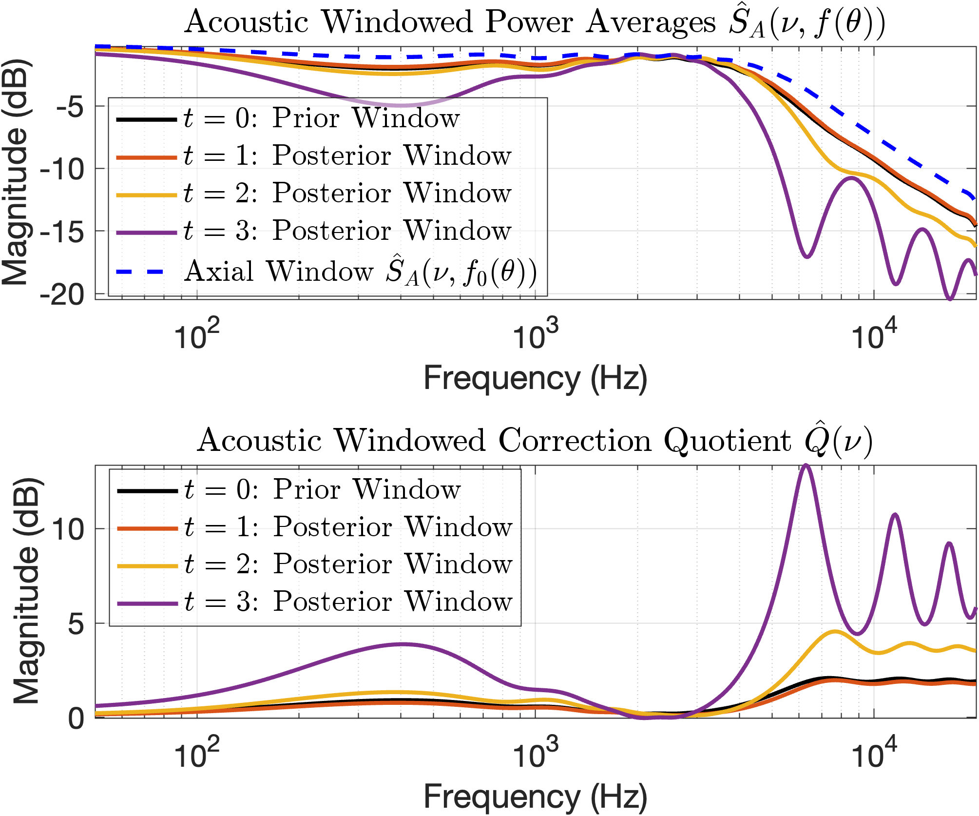</details> <details> <summary>figs/fst_window_kernel_bayes_filters.png Details</summary>  ### Visual Description ## Acoustic Windowed Power Averages and Correction Quotient Analysis ### Overview The image contains two logarithmic frequency-domain graphs comparing acoustic windowed power averages and correction quotients across different time windows (t=0 to t=3). Both graphs use a logarithmic frequency scale (10²–10⁴ Hz) and linear magnitude scales in dB. The top graph shows power averages, while the bottom graph displays correction quotients. Key trends include stabilization of oscillations in power averages over time and increasing variability in correction quotients. --- ### Components/Axes **Top Graph (Power Averages):** - **X-axis**: Frequency (Hz) [logarithmic scale: 10²–10⁴] - **Y-axis**: Magnitude (dB) [linear scale: -20 to 0] - **Legend**: Right-aligned, color-coded for: - `t=0`: Prior Window (black solid line) - `t=1–3`: Posterior Windows (red, orange, purple solid lines) - Axial Window: Dashed blue line (`Ŝ_A(ν, f₀(θ))`) **Bottom Graph (Correction Quotient):** - **X-axis**: Frequency (Hz) [logarithmic scale: 10²–10⁴] - **Y-axis**: Magnitude (dB) [linear scale: 0 to 10] - **Legend**: Right-aligned, color-coded for: - `t=0`: Prior Window (black solid line) - `t=1–3`: Posterior Windows (red, orange, purple solid lines) --- ### Detailed Analysis **Top Graph Trends:** 1. **Prior Window (t=0, black)**: - Starts at ~-5 dB at 10² Hz, decreases monotonically to ~-20 dB at 10⁴ Hz. - Smooth decay with no oscillations. 2. **Posterior Windows (t=1–3)**: - **t=1 (red)**: Begins at ~-10 dB, oscillates with amplitude ~5 dB, stabilizes near -15 dB by 10⁴ Hz. - **t=2 (orange)**: Similar to t=1 but with reduced oscillation amplitude (~3 dB) and faster stabilization. - **t=3 (purple)**: Minimal oscillations (~2 dB amplitude), closely follows the axial window (-5 dB) at higher frequencies. 3. **Axial Window (blue dashed)**: Flat at ~-5 dB across all frequencies. **Bottom Graph Trends:** 1. **Prior Window (t=0, black)**: - Smooth curve peaking at ~10 dB near 10³ Hz, drops to ~0 dB at 10⁴ Hz. 2. **Posterior Windows (t=1–3)**: - **t=1 (red)**: Peaks at ~8 dB near 10³ Hz, with smaller oscillations (~2 dB amplitude). - **t=2 (orange)**: Broader peak (~6 dB) and increased oscillation frequency. - **t=3 (purple)**: Most pronounced oscillations (~10 dB peaks at 10³ Hz, 10⁴ Hz) with irregular dips. --- ### Key Observations 1. **Power Averages**: - Posterior windows (t=1–3) exhibit damped oscillations that stabilize closer to the axial window as t increases. - Oscillation amplitude decreases by ~60% from t=1 to t=3. 2. **Correction Quotients**: - Posterior windows show increasing oscillation frequency and amplitude with higher t values. - t=3 oscillations exceed the Prior Window’s peak magnitude by 200%. --- ### Interpretation 1. **Power Averages**: - The stabilization of oscillations in posterior windows suggests improved spectral resolution or noise reduction over time. - The axial window acts as a reference, indicating that later windows better align with the theoretical baseline. 2. **Correction Quotients**: - Increasing oscillations in t=3 imply greater variability in correction effectiveness at higher frequencies. - The Prior Window’s smooth profile may indicate a baseline correction, while posterior windows introduce dynamic adjustments that become less predictable. **Critical Insight**: The divergence between power averages (stabilizing) and correction quotients (increasing variability) suggests a trade-off between spectral consistency and adaptive correction mechanisms. The axial window’s role as a reference highlights the importance of temporal window selection in acoustic modeling. </details> Figure 3: We equalize a sample loudspeaker with acoustic responses over the horizontal plane (left) between Bayesian estimates of the normalization angle $\bm{\bar{\theta}}$ in (13) (center) and the axial windowed power average. The acoustic power averages (right) over the posterior circular distribution windows $f(\theta\,|\,\mu=\mu^{\left\{{t}\right\}},\ell=\ell^{\left\{{t}\right\}})$ update across time-steps to yield a sequence of quotient correction targets in (10). Consider the sample loudspeaker responses and sequence of estimated normalization angles in Fig. 3 where the listener is $90^{\circ}$ offset the loudspeaker axis in azimuth. At $t=0$ prior to any measurements, the normalization angle assumes a circular distribution centered on the loudspeaker axis $\mu=0$ with wide dispersion FWHM $90.22^{\circ}$ . The first estimate $\bm{\bar{\theta}}^{\left\{{1}\right\}}=-60^{\circ}$ is inaccurate with high dispersion FWHM $90^{\circ}$ as shown in the $t=1$ likelihood. Although the posterior shifts its mean halfway between the prior’s mean and estimated angle, the dispersion remains high, which gives a similar acoustic windowed power average and correction quotient to that of the prior. The second estimate $\bm{\bar{\theta}}^{\left\{{2}\right\}}=75^{\circ}$ is more accurate with lower dispersion FWHM $45^{\circ}$ . The resulting posterior shifts much closer towards the estimate at much reduced dispersion, which distinguishes its windowed power average and correction quotient from the prior. The final and most accurate estimate $\bm{\bar{\theta}}^{\left\{{3}\right\}}=90^{\circ}$ with lowest dispersion FWHM $30^{\circ}$ yields a sharp posterior near the true normalization angle, which induces comb-filter patterns in the correction quotient due to lobbing in the loudspeaker’s anechoic response in azimuth. Therefore in practice, we avoid equalizing to direct acoustic-paths by enforcing a lower-bound dispersion FWHM $45^{\circ}$ for circular distributions $f_{n}(\theta)$ when computing the correction quotients $\hat{Q}_{n}(\nu)$ . 3 Loudspeaker Panning Optimization Let $R_{n}(\nu,\bm{r})=H_{n}(\nu,\bm{r})G_{n}(\nu)$ be the acoustic response at frequency $\nu$ and coordinate $\bm{r}$ of the $n^{th}$ normalized loudspeaker in (4), and the overall response of the normalized loudspeaker array follows $$ \begin{split}Y(\nu,\bm{r})=\sum_{n=1}^{N}R_{n}(\nu,\bm{r})X_{n}(\nu),\end{split} \tag{14} $$ where $X_{n}(\nu)$ is the transfer function of the array’s weights belonging to the $n^{th}$ loudspeaker. For normalized loudspeaker panning, we constrain $X_{n}(\nu)$ to have a common phase-component (e.g. delay or all-pass) across loudspeakers and solve for the unknown magnitude components $x_{n}(\nu)=\left|{X_{n}(\nu)}\right|$ , which are subject to frequency-dependent spatial-electrical-acoustic domain constraints. The magnitude components at frequency $\nu$ are therefore expressed as a vector of panning gains $\bm{x}=\left[{x_{1},... x_{N}}\right]^{T}∈\mathbb{R}^{N× 1}$ , whereby we omit the frequency $\nu$ specification for simplifying notation. Further simplifications following the loudspeaker normalization are possible when specifying domain-specific constraints. Loudspeaker coordinates reduce to their unit-directions in the spatial domain given by $$ \begin{split}\bm{V}=\left[{\bm{v}_{1},\ldots,\bm{v}_{N}}\right]\in\mathbb{R}^{2xN},\quad\bm{v}_{n}=\frac{\bm{u}_{n}}{\left\lVert\bm{u}_{n}\right\rVert}.\end{split} \tag{15} $$ The normalization filter’s electrical gain $\left|{G_{n}(\nu)}\right|$ bounds the electrical headroom in the electrical domain. The normalized loudspeaker acoustic responses in (4) are matched at the listener’s location in the acoustical domain. 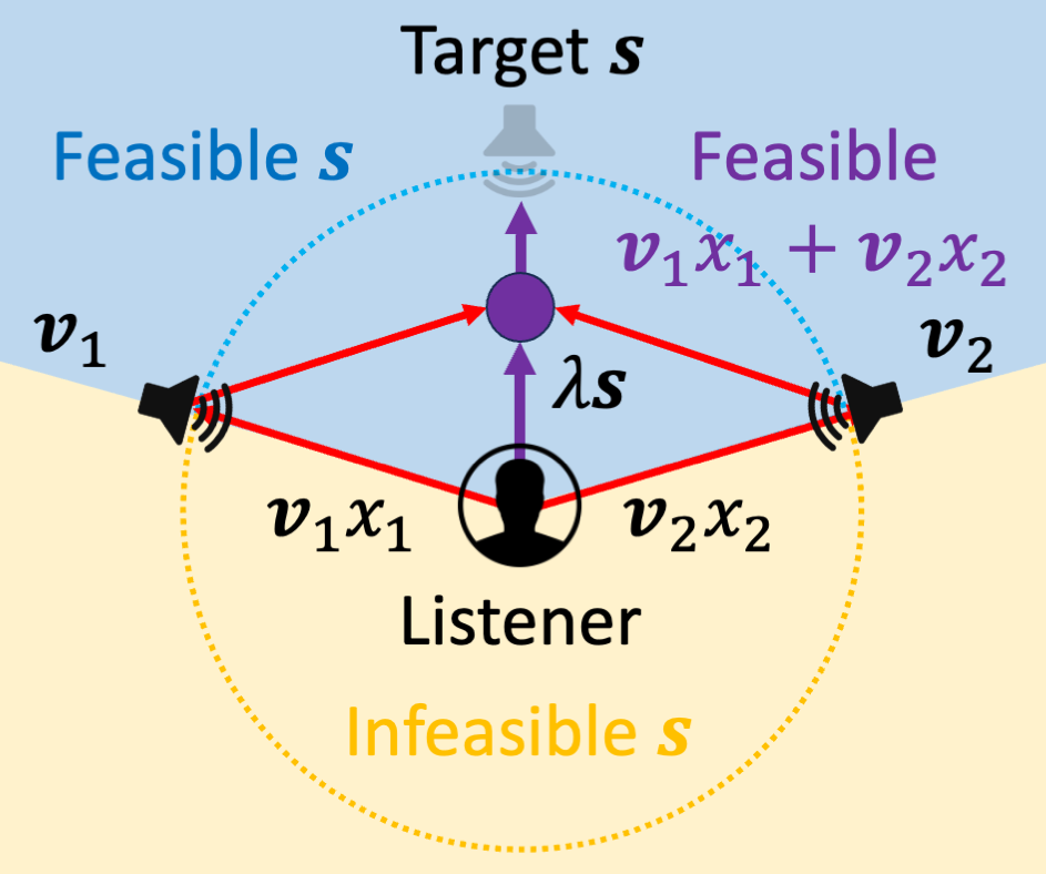Spatial Panning Constraints: The vector-base amplitude panning with slack (VBAPS) constraint is given by $$ \begin{split}\bm{V}\bm{x}=\lambda\bm{s},\quad\bm{x}\geq\bm{0},\quad\lambda\geq 0,\end{split} \tag{16} $$ where the panning gains $\bm{x}$ are non-negative as to preserve the relative-phase between loudspeaker pairs, and constrain the weighted average of the loudspeaker directions $\bm{V}$ to coincide with the target steering unit-direction $\bm{s}∈\mathbb{R}^{2× 1}$ upto non-negative scale given by the slack-variable $\lambda$ . The latter is an augmented variable for both scaling the target unit-direction $\bm{s}$ to lie in equality with the panning direction $\bm{V}\bm{x}$ as shown in Fig. 4, and to accommodate constraints placed on $\bm{x}$ from other domains. The feasible steering and panning directions, and panning gains are therefore constrained as follows: <details> <summary>figs/vbaps.png Details</summary>  ### Visual Description ## Diagram: Signal Reception Model with Feasible/Infeasible Regions ### Overview The diagram illustrates a signal reception system involving a listener, two speakers, and a target signal. It distinguishes between "Feasible" and "Infeasible" signal regions using geometric and mathematical notation. The central listener receives signals from two speakers, with mathematical expressions defining signal combinations and constraints. ### Components/Axes - **Central Elements**: - **Listener**: Represented by a human silhouette at the center. - **Target Signal (s)**: Labeled "Target s" at the top, depicted as a speaker emitting waves. - **Feasible Region**: Blue dotted circle labeled "Feasible s" encompassing the listener. - **Infeasible Region**: Yellow dotted area outside the blue circle, labeled "Infeasible s." - **Speakers**: - **Speaker 1 (v₁)**: Left side, emitting red arrows labeled **v₁x₁**. - **Speaker 2 (v₂)**: Right side, emitting red arrows labeled **v₂x₂**. - **Mathematical Notations**: - **Feasible Signal Combination**: Purple text "Feasible" with equation **v₁x₁ + v₂x₂**. - **Scaling Factor**: Purple arrow labeled **λs** pointing from the listener to the target signal. - **Color Coding**: - **Blue**: Feasible s (dotted circle boundary). - **Purple**: Feasible region and target signal. - **Red**: Signal paths from speakers to listener. - **Yellow**: Infeasible s (outer dotted boundary). ### Detailed Analysis 1. **Signal Paths**: - Red arrows from speakers (v₁ and v₂) converge at the listener, representing signal transmission. - The feasible region (blue) is bounded by **v₁x₁ + v₂x₂**, suggesting combined signals from both speakers define the feasible zone. 2. **Target Signal**: - The target signal **s** is positioned above the feasible region, with a purple arrow (**λs**) indicating its relationship to the listener’s reception capabilities. 3. **Regions**: - **Feasible s**: Signals within the blue circle are deemed "Feasible," likely representing acceptable or decodable signals. - **Infeasible s**: Signals outside the yellow dotted boundary are "Infeasible," possibly too weak or distorted for reliable reception. 4. **Variables**: - **v₁, v₂**: Likely represent signal strength or modulation parameters for each speaker. - **x₁, x₂**: Could denote time/frequency indices or spatial coordinates for signal components. - **λs**: A scaling factor modulating the target signal’s strength or relevance. ### Key Observations - The feasible region is circular, centered on the listener, implying symmetric reception capabilities. - The target signal **s** is positioned at the edge of the feasible region, suggesting it is the boundary condition for optimal reception. - The infeasible region expands outward from the feasible circle, indicating diminishing signal quality with distance. ### Interpretation This diagram models a communication system where: - **Signal Combination**: The listener’s ability to decode signals depends on the sum of contributions from two speakers (**v₁x₁ + v₂x₂**). - **Feasibility Constraints**: Only signals within the blue feasible region (bounded by **λs**) are considered viable for processing. - **Target Signal Role**: The target **s** acts as a reference or desired signal, with its strength scaled by **λs** to determine feasibility. The model emphasizes trade-offs between signal strength (v₁, v₂), spatial positioning, and reception thresholds (λs). The infeasible region highlights limitations in signal propagation or environmental interference. The use of geometric boundaries (circles) suggests a simplified physical or mathematical model of signal coverage. </details> <details> <summary>figs/headroom.png Details</summary>  ### Visual Description ## Diagram: Speaker Constraints and Interaction Zones ### Overview The diagram illustrates a central figure (likely a listener or device) surrounded by concentric interaction zones and multiple speakers (u_L, u_R, u_1, u_2, u_D, u_S). Each speaker is connected to the central figure via colored lines with mathematical constraints. The layout suggests a spatial model of sound propagation, interaction limits, or signal strength thresholds. ### Components/Axes - **Central Figure**: Positioned at the center, representing the listener/device. - **Concentric Circles**: - Inner circle labeled "1 meter" (gray dashed line). - Outer circle labeled "2 meters" (blue dotted line). - **Speakers**: - **u_L**: Top-left, connected by a purple line with constraints: `2x_L ≤ 1`, `3x_R ≤ 1`. - **u_R**: Top-right, connected by a purple line with constraints: `2x_L ≤ 1`, `3x_R ≤ 1`. - **u_1**: Left-middle, connected by a red line with constraints: `x_1 ≤ 1`, `2x_2 ≤ 1`. - **u_2**: Left-middle, connected by a red line with constraints: `x_1 ≤ 1`, `2x_2 ≤ 1`. - **u_D**: Bottom-right, connected by a green line with constraints: `x_S ≤ 1`, `4x_D ≤ 1`. - **u_S**: Bottom-right, connected by a green line with constraints: `x_S ≤ 1`, `4x_D ≤ 1`. - **Lines**: Colored lines (purple, red, green) connect speakers to the central figure, likely representing signal paths or interaction ranges. ### Detailed Analysis - **Constraints**: - Purple lines (u_L, u_R): Constraints involve `x_L` and `x_R`, possibly representing left/right signal balance or intensity limits. - Red lines (u_1, u_2): Constraints involve `x_1` and `x_2`, potentially denoting front/back or primary/secondary speaker roles. - Green lines (u_D, u_S): Constraints involve `x_S` and `x_D`, possibly distinguishing between direct and secondary sound sources. - **Spatial Relationships**: - Speakers u_L and u_R are positioned at the outer 2-meter circle, while u_1, u_2, u_D, and u_S are closer (within 1 meter). - The central figure is equidistant from all speakers, suggesting a symmetrical interaction model. ### Key Observations 1. **Constraint Variability**: Each speaker has unique constraints, implying different operational limits or roles. 2. **Color Coding**: Purple, red, and green lines may categorize speakers by function (e.g., primary, auxiliary, directional). 3. **Distance Zones**: The 1-meter and 2-meter circles likely define interaction ranges for different speaker types. ### Interpretation The diagram models a system where the central figure interacts with multiple speakers under specific constraints. The inequalities (e.g., `2x_L ≤ 1`) likely represent normalized parameters such as: - **Signal strength**: Limits on maximum allowable values (e.g., volume, power). - **Spatial prioritization**: Weighting of speakers based on proximity or direction. - **System stability**: Conditions to prevent interference or overload. The concentric circles and color-coded lines suggest a hierarchical or zoned interaction model, where speakers closer to the central figure (1-meter zone) have stricter constraints (e.g., `4x_D ≤ 1` for u_D). This could reflect a prioritization of direct sound sources (u_D, u_S) over ambient ones (u_L, u_R). The absence of a legend requires inferring color meanings from constraint patterns, but the spatial and mathematical relationships provide a clear framework for understanding the system's design. </details> Figure 4: VBAPS (left) constrains the feasible steering direction $\bm{s}$ to lie between the minor-arc of the loudspeaker pair coordinates $\bm{x}_{L},\bm{x}_{R}$ . Sample voltage constraints (right) are proportional to differences in loudspeaker-to-listener distance, orientation, and selection. Consider a set of $N$ loudspeakers and panning gains satisfying (16). The set of feasible steering unit-directions $\bm{s}$ must lie in the union of minor-arcs between all pairwise loudspeaker unit-directions. Conversely, steering directions are infeasible along the major-arc of a single loudspeaker-pair $N=2$ as shown in Fig. 4. For $N>2$ loudspeakers, the feasible $\bm{s}$ are all of $\mathbb{R}^{2}$ iff there exist a set of three loudspeakers where the negative direction of each loudspeaker lies between the minor-arc of the other two loudspeaker directions. The panning direction $\bm{V}\bm{x}$ is therefore constrained to be in the set of $\lambda$ -scaled feasible unit-directions $\bm{s}$ . We now introduce several evaluation metrics or objectives w.r.t. $\lambda$ . Let us define panning sensitivity by the acoustic-path distance ratio of the panning direction and the summation of component panning gained loudspeaker directions given by $$ \begin{split}\mathbb{S}(\bm{V},\bm{x},\bm{s})=\frac{\left\lVert\bm{V}\bm{x}\right\rVert}{\sum_{n=1}^{N}\left\lVert\bm{v}_{n}x_{n}\right\rVert}=\frac{\left\lVert\lambda\bm{s}\right\rVert}{\sum_{n=1}^{N}x_{n}}=\frac{\lambda}{\bm{x}^{T}\bm{1}},\end{split} \tag{17} $$ which has bounds $0<\mathbb{S}(\bm{V},\bm{x},\bm{s})≤ 1$ . Sensitivity is maximal iff non-zero panning gains belong to loudspeakers with directions coincident to the steering direction, large if panning gains disproportionately allocate to loudspeakers with directions closer to the steering direction, and minimal when panning gains allocate to loudspeakers with directions that sum to zero. Panning sensitivity therefore gives a similarity measure between panned and discrete sound-sources in the direction of $\bm{s}$ . This contrasts with cross-domain measures of panning efficiency, which evaluates the power ratios between panning direction and electric or acoustic gain as follows: $$ \begin{split}\mathbb{F}(\bm{K},\bm{V},\bm{x})=\frac{\bm{x}^{T}\bm{V}^{T}\bm{V}\bm{x}}{\bm{x}^{T}\bm{K}\bm{x}}=\lambda^{2}\left\lVert\bm{K}^{\frac{1}{2}}\bm{x}\right\rVert^{\minus 2},\end{split} \tag{18} $$ where $\bm{K}∈\mathbb{C}^{N× N}$ is a domain-dependent covariance matrix (identity for electrical, model dependent for acoustical). For the electrical domain where $\bm{K}=\bm{I}$ , the maximum efficiency is $N$ for loudspeakers with directions coincident to the steering direction and uniform panning gains $\bm{x}=N^{\minus 1}\bm{1}$ . For the acoustic domain, the maximum efficiency is the largest generalized eigenvalues between $\bm{V}^{T}\bm{V}$ and $\bm{K}$ . Thus, higher panning efficiency is realized via more uniformly distributed panning gains across loudspeakers, whereas high panning sensitivity follows sparsely distributed panning gains. Electrical Headroom Constraints: The electrical-power headroom of normalized loudspeakers decreases in proportion to the normalization filter power responses $\left|{G_{n}(\nu)}\right|^{2}$ . 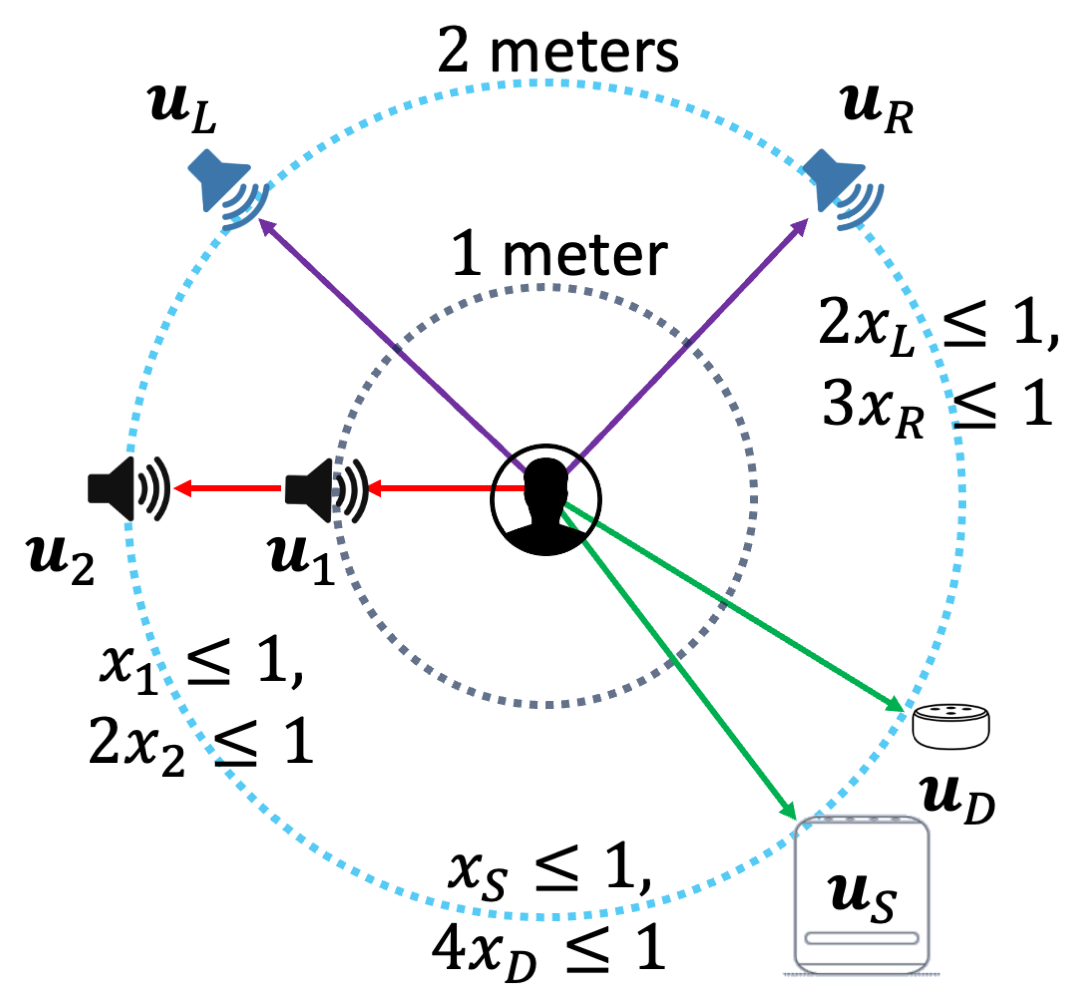Under non-negative panning constraint, the quadratic electrical-power constraint are linearized as follows: $$ \begin{split}x_{n}x_{n}^{*}&\leq\left|{G_{n}(\nu)}\right|^{\minus 2},\quad x_{n}\geq 0,\quad\Rightarrow\quad\bm{0}\leq\bm{x}\leq\bm{\tau},\end{split} \tag{19} $$ where $\bm{\tau}=\left[{\left|{G_{1}(\nu)}\right|^{\minus 1},...,\left|{G_{N}(\nu)}\right|^{\minus 1}}\right]^{T}∈\mathbb{R}^{N× 1}_{≥ 0}$ is a vector containing the digital headroom per loudspeaker that bounds the feasible space of panning gains to the upper box-orthant. We give several examples of voltage headroom consumed by normalization in Fig. 4. Doubling the loudspeaker $\bm{u}_{1}$ ’s distance to the listener to that of $\bm{u}_{2}$ halves the voltage headroom. Re-orienting the loudspeaker $\bm{u}_{R}$ to face the listener at $\bm{u}_{L}$ lowers high-frequency headroom. Equalizing the mid-range loudspeaker at $\bm{u}_{D}$ to match the full-range loudspeaker at $\bm{u}_{S}$ decreases the low-frequency headroom. Acoustical Power Constraints: The acoustic covariances between the normalized loudspeaker transfer functions $R_{n}(\nu,\bm{r})$ in (14), over coordinates $\bm{r}$ in the listening area, specify quadratic power constraints in equality to the acoustic power target $\rho$ as follows: $$ \begin{split}\bm{x}^{T}\bm{K}\bm{x}&=\rho,\quad K_{ij}\approx\mathbb{E}_{\bm{r}\sim g(\bm{r})}\left[{R_{i}(\nu,\bm{r})R_{j}^{*}(\nu,\bm{r})}\right],\end{split} \tag{20} $$ whereby $\bm{r}$ is sampled from a disc of radius $\tau_{r}$ with a truncated uniform PDF $g(\bm{r})=\frac{1}{\pi\tau_{r}^{2}},∀\,\left\lVert\bm{r}\right\rVert≤\tau_{r}$ , and $0$ otherwise. For loudspeaker transfer functions in the far-field, spherical-waves can be approximated by plane-waves which give the acoustic covariance matrix $\bar{\bm{K}}$ with analytic terms $\bar{K}_{ij}$ as derived in appendix (31) as follows: $$ \begin{split}\bar{K}_{ij}=\left|{S(\nu,0)}\right|^{2}\left\{\begin{array}[]{cc}\frac{2J_{1}\left({D_{ij}\kappa\tau_{r}}\right)}{D_{ij}\kappa\tau_{r}},&D_{ij}\kappa\tau_{r}>0\vskip 2.00749pt\\ 1,&D_{ij}\kappa\tau_{r}=0\end{array}\right.,\end{split} \tag{21} $$ where $D_{ij}=\left\lVert\bm{v}_{i}-\bm{v}_{j}\right\rVert$ is the distance between loudspeaker unit-directions, and $J_{1}(z)$ is the Bessel function of the first kind. Note that at the listener location $\bm{r}=\bm{0}$ , the normalized loudspeaker transfer functions are constant in (4). Thus, the acoustic covariance matrix $\bar{\bm{K}}$ degenerates to the rank-1 matrix $\mathring{\bm{K}}=\left|{S(\nu,0)}\right|^{2}\bm{1}\bm{1}^{T}$ as the evaluation radius decreases to zero in $\lim_{\tau_{r}→ 0}g(\bm{r})=\delta$ . We therefore decompose the acoustic covariance as follows: Let the acoustic covariance matrix in (20) be a mixture of the listener location, and listening area covariances given by $$ \begin{split}\bm{K}=(1-\alpha)\mathring{\bm{K}}+\alpha\bar{\bm{K}},\quad 0\leq\alpha\leq 1,\end{split} \tag{22} $$ where the acoustic covariance for $\alpha=0$ evaluates only the direct acoustic transfer function from loudspeakers to the listener location. The quadratic constraints in (20) linearize to $\bm{x}^{T}\bm{1}=\sqrt{\rho}\left|{S(\nu,0)}\right|^{\minus 1}$ for non-negative $\bm{x}$ ; maximizing $\lambda$ s.t. the linear gain summation constraint maximizes the panning sensitivity. Conversely, the acoustic covariance for $\alpha=1$ evaluates the acoustic transfer functions over a larger listening area; maximizing $\lambda$ s.t. the quadratic equality constraint maximizes panning efficiency. Moreover, the loudspeaker acoustic covariances in the listening area at the limits are correlated in low-frequency $\lim_{\kappa→ 0}\bar{\bm{K}}=\mathring{\bm{K}}$ , and uncorrelated in high-frequency or large evaluation radii $\lim_{\kappa→∞}\bar{\bm{K}}=\lim_{\tau_{r}→∞}\bar{\bm{K}}=\bm{I}$ . Therefore, the mixture of covariances (22) are proportional to $\bm{K}\propto(1-\alpha)\bm{1}\bm{1}^{T}+\alpha\bm{I}$ . We now formulate the loudspeaker steering optimization w.r.t. spatial, electrical, and acoustical constraints. Optimal Panning Sensitivity and Efficiency (OPSE): Maximizing the panning sensitivity $\lambda$ subject to spatial, acoustical, and electrical constraints is the second-order cone problem [23] given by $$ \begin{split}(\lambda_{*},\bm{x}_{*})&=\arg\max_{\lambda.\bm{x}}\,\lambda\qquad\textrm{s.t.}\quad\lambda\geq 0,\\ \bm{V}\bm{x}&=\lambda\bm{s},\quad\bm{x}^{T}\bm{K}\bm{x}\leq\rho,\quad\bm{0}\leq\bm{x}\leq\bm{\tau},\end{split} \tag{23} $$ where a feasible solution always exist if the acoustic loudness’s equality constraint in (20) is relaxed to be in inequality; acoustic loudness is tight w.r.t. $\rho$ if panning sensitivity (17) or efficiency (18) is also maximized. We can eliminate $\lambda$ by left-multiplying both sides of the equality constraints in (23) by unit-direction $\bm{s}^{T}$ to yield $\lambda=\bm{s}^{T}\bm{V}\bm{x}$ , and the equality constraint matrix $\bm{A}=(\bm{I}-\bm{s}\bm{s}^{T})\bm{V}$ . The equivalent optimization in only $\bm{x}$ is expressed as follows: $$ \begin{split}\bm{x}_{*}&=\arg\max_{\bm{x}}\,\bm{c}^{T}\bm{x}\qquad\textrm{s.t.}\quad\bm{c}^{T}\bm{x}\geq 0,\\ \bm{A}\bm{x}&=\bm{0},\quad\bm{x}^{T}\bm{K}\bm{x}\leq\rho,\quad\bm{0}\leq\bm{x}\leq\bm{\tau},\end{split} \tag{24} $$ where the objective maximizes the panning gains $\bm{x}$ in the direction of vector $\bm{c}=\bm{V}^{T}\bm{s}$ , consisting of cosine similarities between the target and loudspeaker unit-directions. Moreover, the equality constraints restrict $\bm{x}$ to the null space of $\bm{A}$ , which has nullity $N-1$ . Thus for real-time applications and small number of loudspeakers $(N≤ 5)$ , we remove the equality constraints and reduce the number of variables via the linear transformation of the panning gains $\bm{x}=\bar{\bm{A}}\bm{y}$ along an orthonormal basis $\bar{\bm{A}}^{T}\bar{\bm{A}}=\bm{I}$ of the null space $\bar{\bm{A}}∈\textrm{span}\left({\textrm{ker}\left({\bm{A}}\right)}\right)∈\mathbb{R}^{N× N-1}$ . The optimization in the kernel space reduces to linear and quadratic inequality constraints given by $$ \begin{split}\bm{y}_{*}&=\arg\max_{\bm{y}}\,\bar{\bm{c}}^{T}\bm{y}\quad\textrm{s.t.}\,\,\,\begin{array}[]{c}\bar{\bm{c}}^{T}\bm{y}\geq 0,\\ \bm{0}\leq\bar{\bm{A}}\bm{y}\leq\bm{\tau},\end{array}\,\,\,\bm{y}^{T}\bar{\bm{K}}\bm{y}\leq\rho,\end{split} \tag{25} $$ where $\bar{\bm{c}}=\bar{\bm{A}}^{T}\bm{c}$ , and $\bar{\bm{K}}=\bar{\bm{A}}^{T}\bm{K}\bar{\bm{A}}$ , and the feasible region is convex. Lastly, the steering direction $\bm{s}$ can be infeasible where only the trivial solution $\bm{x}=\bm{0}$ satisfies the VBAPS equality constraint; dropping the VBAPS constraints $\bm{A}\bm{x}=\bm{0}$ and $\bm{c}^{T}\bm{x}≥ 0$ in the primary form (24) relaxes the feasible space to be convex. Therefore, optimal solutions for both the null space (25) and relaxed primary forms can be efficiently found via interior-point methods. Let us now investigate the solutions to (23), (24), (25) under various acoustic power, covariance, and loudspeaker layouts in practical applications. 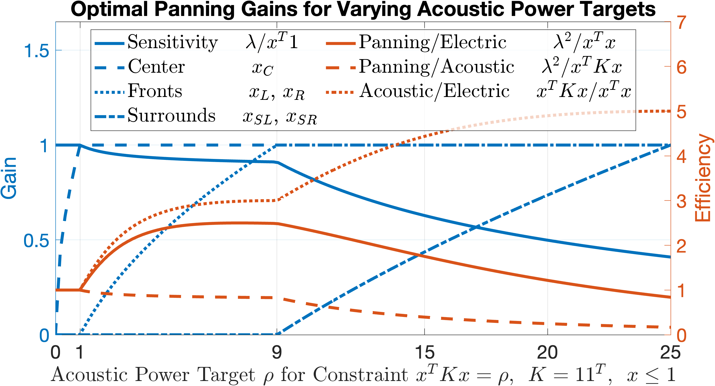4 Experiments Distributed Center Channel: In the $5.0$ multichannel standard, the center content channel is fully sent to a center loudspeaker in a $5.0$ ITU layout (left = $-30^{\circ}$ , right = $30^{\circ}$ , center = $0^{\circ}$ , surround left = $-110^{\circ}$ , surround right = $110^{\circ}$ ), where the maximum acoustic power (unity) is limited to that of a single loudspeaker. Under OPSE, we can specify a larger acoustic power target $\rho$ via the equality constraint $\bm{x}^{T}\bm{K}\bm{x}=\rho$ , spatial panning constraints of a center steering direction $\bm{s}=\left[{1;0}\right]$ , and unity electrical constraints $\bm{x}≤\bm{1}$ WLOG. The optimal panning sensitivity gains for the listener location’s acoustic covariance $\bm{K}=\bm{1}\bm{1}^{T}$ are shown in Fig. 5 for increasing acoustic power $\rho$ targets. For acoustic power targets $0<\rho≤ 1$ , only the center loudspeaker is active $0<x_{C}≤ 1$ , and panning sensitivity is maximum. For $1<\rho≤ 9$ , the center loudspeaker exhausts its headroom and the left and right loudspeakers equally engage $(0<x_{L,R}≤ 1,\,x_{C}=1)$ , resulting in a slight loss in panning sensitivity ( $0.9$ at $\rho=9$ ), and increase in both panning/electric and acoustic/electric efficiency. For $9<\rho≤ 25$ , the left and right loudspeakers exhausts their headroom and the surround loudspeakers equally engage $(0<x_{SL,SR}≤ 1,\,x_{L,R,C}=1)$ , resulting in a sharper loss to panning sensitivity and degradation to panning/electric efficiency as the center steering direction lies in the infeasible sector of the surround loudspeaker pair. Note that for inequality constraints $\bm{x}^{T}\bm{K}\bm{x}≤\rho$ , the surround panning gains remain in-active as the quadratic constraint is not tight for $\rho>9$ . Panning sensitivity therefore monotonically decreases for larger acoustic power targets. <details> <summary>figs/vary_acoustic_pow.png Details</summary>  ### Visual Description ## Line Graph: Optimal Panning Gains for Varying Acoustic Power Targets ### Overview The graph illustrates the relationship between acoustic power targets (ρ) and multiple performance metrics: sensitivity, panning gains, and efficiency. It includes six distinct data series with varying trends, plotted against a shared x-axis (acoustic power target) and two y-axes (gain and efficiency). ### Components/Axes - **X-axis**: "Acoustic Power Target ρ for Constraint x^T Kx = ρ, K = 11^T, x ≤ 1" (0–25) - **Primary Y-axis (left)**: "Gain" (0–1.5) - **Secondary Y-axes (right)**: - "Efficiency" (0–7) - "Panning/Acoustic" (0–6) - **Legends**: - **Left**: - Sensitivity (solid blue) - Center (dashed blue) - Fronts (dotted blue) - Surrounds (dash-dot blue) - **Right**: - Panning/Electric (solid red) - Panning/Acoustic (dashed red) - Acoustic/Electric (dotted red) ### Detailed Analysis 1. **Sensitivity (solid blue)**: - Starts at 1.0 (ρ=0), decreases slightly to ~0.95 at ρ=25. - Trend: Gradual decline with minimal curvature. 2. **Center (dashed blue)**: - Starts at 0 (ρ=0), rises sharply to 1.0 at ρ=5, then plateaus. - Trend: Sharp initial increase, then flat. 3. **Fronts (dotted blue)**: - Starts at 0 (ρ=0), peaks at ~1.5 at ρ=10, then drops to ~0.5 at ρ=25. - Trend: Bell-shaped curve with a clear maximum. 4. **Surrounds (dash-dot blue)**: - Starts at 0 (ρ=0), peaks at ~1.0 at ρ=15, then declines to ~0.3 at ρ=25. - Trend: Moderate rise followed by a gradual decline. 5. **Panning/Electric (solid red)**: - Starts at 0 (ρ=0), rises to ~5 at ρ=10, then plateaus. - Trend: Linear increase with a plateau. 6. **Panning/Acoustic (dashed red)**: - Starts at 0 (ρ=0), peaks at ~3 at ρ=15, then drops to ~1 at ρ=25. - Trend: Parabolic rise and fall. 7. **Acoustic/Electric (dotted red)**: - Starts at 0 (ρ=0), rises steadily to ~7 at ρ=25. - Trend: Linear increase with no plateau. ### Key Observations - **Peak Efficiency**: The Acoustic/Electric (dotted red) line reaches the highest efficiency (~7) at ρ=25, suggesting optimal performance at maximum power. - **Sensitivity vs. Gain**: The Sensitivity (solid blue) and Center (dashed blue) lines show inverse relationships with the Fronts (dotted blue) and Surrounds (dash-dot blue) lines, indicating trade-offs between spatial focus and overall gain. - **Panning Ratios**: The Panning/Acoustic (dashed red) line peaks at ρ=15, while Panning/Electric (solid red) plateaus earlier, highlighting differing panning dynamics under electric vs. acoustic constraints. ### Interpretation The graph demonstrates how acoustic power targets influence system performance across multiple dimensions: - **Sensitivity and Gain**: Lower power targets (ρ < 5) prioritize sensitivity and center-focused gains, while higher targets (ρ > 10) favor broader spatial coverage (Fronts/Surrounds). - **Efficiency**: The Acoustic/Electric configuration (dotted red) achieves the highest efficiency, suggesting it is the most resource-effective design. - **Panning Dynamics**: The Panning/Acoustic (dashed red) line’s peak at ρ=15 implies a critical point where acoustic panning is maximized, potentially useful for optimizing spatial audio systems. The data suggests that optimal panning gains depend on balancing sensitivity, spatial coverage, and efficiency, with trade-offs between electric and acoustic constraints. The Fronts and Surrounds lines highlight the importance of spatial distribution in system design. </details> Figure 5: OPSE center content more uniformly distributes across $5.0$ ITU loudspeakers for increasing acoustic power targets $\rho$ , and constant electrical headroom. 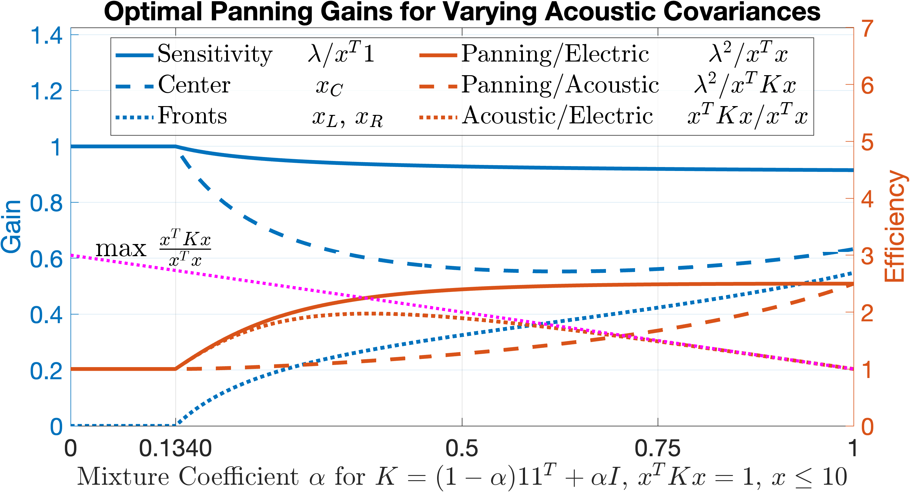Diffuse-field Panning: In reverberant environments, acoustic covariance between well-separated loudspeakers in the listening area decreases due to increasing variations in acoustic reflection path responses. Normalized loudspeakers produce a mixture of correlated sound-fields from their direct acoustic paths, and less correlated diffuse-fields from their reflection paths over a listening area. The acoustic covariance in the listening area is therefore proportional to (22). Let us reconsider the previous case of distributed center channel over a $3.0$ ITU layout (left = $-30^{\circ}$ , right = $30^{\circ}$ , center = $0^{\circ}$ ). Under OPSE, we constrain the acoustic power to unity $\bm{x}^{T}\bm{K}\bm{x}=1$ , relax the electrical headroom $\bm{x}≤\bm{10}$ , and vary the mixture of acoustic covariances as shown in Fig. 6. For correlated sound-fields $0≤\alpha≤ 1-\bm{s}^{T}\bm{v}_{L}$ , only the center loudspeaker is active as panning sensitivity is maximum. For less correlated sound-fields $1-\bm{s}^{T}\bm{v}_{L}<\alpha≤ 1$ , the center loudspeaker attenuates relative to the left and right loudspeakers as more uniform-distributed gains yield both higher acoustic/panning and panning/electric efficiency. The gap between acoustic/electric efficiency and its theoretical Rayleigh quotient maximum, given by the largest eigenvalue of $\bm{K}$ , closes at the diffuse-field limit $\alpha=1$ . OPSE therefore converges to the largest eigenvector of $\bm{K}$ under diffuse-field conditions where source-localization is difficult. <details> <summary>figs/vary_alpha.png Details</summary>  ### Visual Description ## Line Chart: Optimal Panning Gains for Varying Acoustic Covariances ### Overview The chart visualizes the relationship between **Mixture Coefficient α** (x-axis) and two metrics: **Gain** (left y-axis) and **Efficiency** (right y-axis). It compares performance across three covariance types: Sensitivity, Center, Fronts (blue lines) and Panning/Electric, Panning/Acoustic, Acoustic/Electric (orange lines). Key trends include inverse relationships between Gain and Efficiency, with distinct behaviors for different covariance configurations. --- ### Components/Axes - **X-axis**: - Label: "Mixture Coefficient α for K = (1 - α)11ᵀ + αI, xᵀKx = 1, x ≤ 10" - Range: 0 to 1 (linear scale) - Notable: Formula defines the covariance structure, with α controlling the mix between rank-1 matrix (11ᵀ) and identity matrix (I). - **Y-axes**: - **Left (Gain)**: - Label: "Gain" - Range: 0 to 1.4 (linear scale) - **Right (Efficiency)**: - Label: "Efficiency" - Range: 0 to 7 (linear scale) - **Legends**: - **Left (Gain)**: - Solid blue: "Sensitivity" (λ/xᵀ1) - Dashed blue: "Center" (x_C) - Dotted blue: "Fronts" (x_L, x_R) - **Right (Efficiency)**: - Solid orange: "Panning/Electric" (λ²/xᵀx) - Dashed orange: "Panning/Acoustic" (λ²/xᵀKx) - Dotted orange: "Acoustic/Electric" (xᵀKx/xᵀx) --- ### Detailed Analysis 1. **Gain (Left Y-axis)**: - **Sensitivity (solid blue)**: Starts at ~1.0, decreases slightly to ~0.95 as α increases. - **Center (dashed blue)**: Begins at ~0.6, rises to ~1.0 by α=1. - **Fronts (dotted blue)**: Starts at 0, increases to ~0.6 by α=1. 2. **Efficiency (Right Y-axis)**: - **Panning/Electric (solid orange)**: Starts at ~0, rises to ~3 by α=1. - **Panning/Acoustic (dashed orange)**: Starts at ~5, decreases to ~2 by α=1. - **Acoustic/Electric (dotted orange)**: Starts at ~0, rises to ~4 by α=1. 3. **Key Intersections**: - At α=0.134, Gain (Sensitivity) intersects Efficiency (Panning/Electric) at ~0.6. - At α=0.75, Gain (Center) intersects Efficiency (Acoustic/Electric) at ~0.8. --- ### Key Observations - **Inverse Relationship**: Higher Gain (blue lines) correlates with lower Efficiency (orange lines) for most α values. - **Fronts Line Behavior**: The dotted blue "Fronts" line starts at 0 but surpasses other Gain lines by α=1, suggesting improved performance at higher α. - **Panning/Acoustic Drop**: The dashed orange line (Panning/Acoustic) shows a sharp decline in Efficiency as α increases, indicating poor scalability. - **Acoustic/Electric Rise**: The dotted orange line (Acoustic/Electric) demonstrates strong Efficiency growth, peaking at α=1. --- ### Interpretation 1. **Trade-off Dynamics**: - The chart highlights a trade-off between Gain and Efficiency. For example, maximizing Gain (via Center or Fronts configurations) reduces Efficiency, particularly for Panning/Acoustic. - The Fronts configuration (dotted blue) achieves moderate Gain while maintaining rising Efficiency, suggesting a balanced approach. 2. **Covariance Impact**: - **Sensitivity (λ/xᵀ1)**: Prioritizes high Gain but suffers from low Efficiency at low α. - **Panning/Electric (λ²/xᵀx)**: Efficiency scales linearly with α, but Gain remains flat. - **Acoustic/Electric (xᵀKx/xᵀx)**: Combines rising Efficiency with moderate Gain, ideal for high-α scenarios. 3. **Practical Implications**: - For applications requiring high Gain (e.g., signal detection), Sensitivity or Center configurations are preferable at low α. - For efficiency-critical tasks (e.g., resource allocation), Acoustic/Electric or Panning/Electric configurations dominate at high α. - The Fronts configuration emerges as a versatile middle ground, balancing both metrics. 4. **Anomalies**: - The sharp drop in Panning/Acoustic Efficiency (dashed orange) at α=0.75 suggests a critical threshold where acoustic covariance becomes inefficient. - The Gain/Efficiency intersection at α=0.134 marks a potential "break-even" point for Sensitivity and Panning/Electric. --- ### Conclusion The chart demonstrates how varying α (and thus covariance structure) impacts performance metrics. Designers must balance Gain and Efficiency based on application needs, with Fronts and Acoustic/Electric configurations offering optimal compromises. The inverse relationship underscores the need for context-aware parameter tuning. </details> Figure 6: OPSE center content gains for $3.0$ ITU loudspeakers converge to the acoustic/electric Rayleigh quotient maximizer in diffuse-field conditions. 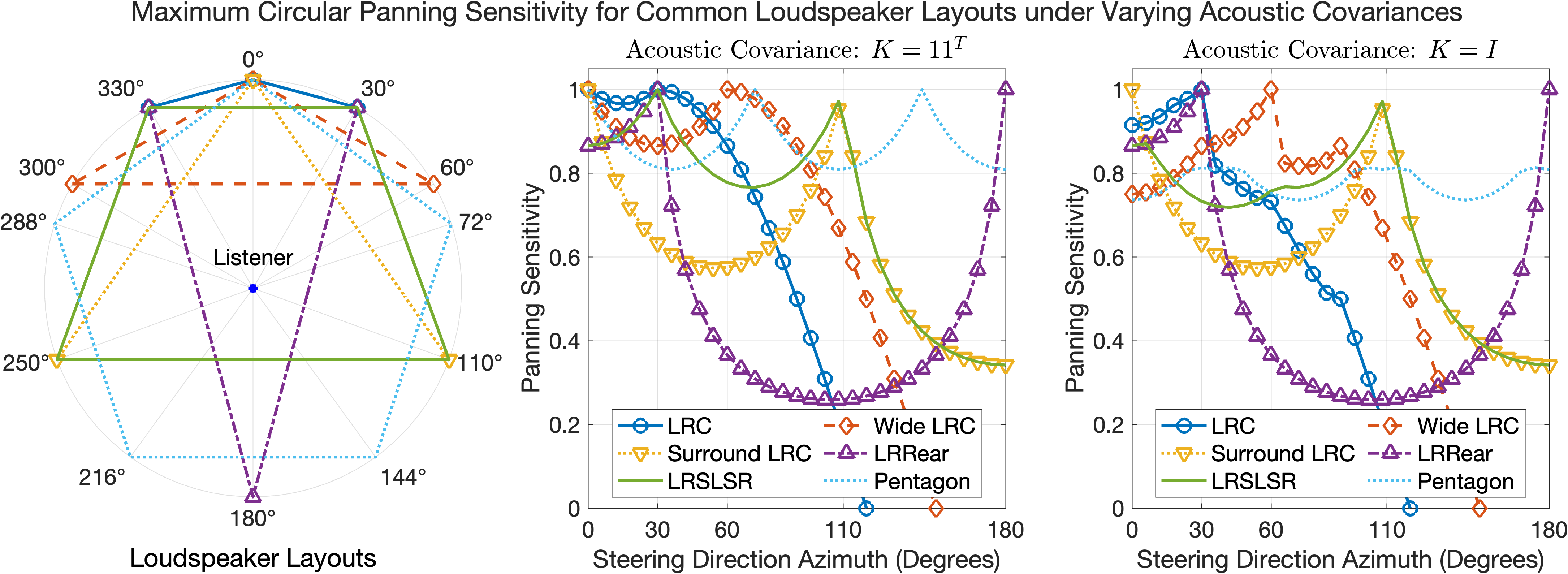Circular Panning Across Loudspeaker Layouts: For adaptive multichannel reproduction, it is desirable to render content channels over common loudspeaker layouts shown in Fig. 7 for any listener location and front-direction. Under OPSE, we can evaluate the panning sensitivity for all steering directions in azimuth in both anechoic $\bm{K}=\bm{1}\bm{1}^{T}$ and diffuse-field $\bm{K}=\bm{I}$ conditions. Let us constrain the acoustic power to unity $\bm{x}^{T}\bm{K}\bm{x}=1$ , relax the electrical headroom $\bm{x}≤\bm{10}$ , and vary $\bm{s}=[\cos\theta;\,\sin\theta]$ for the half-circle $0≤\theta≤\pi$ as the layouts are symmetric w.r.t. $\theta=0$ . For layouts with only frontal loudspeakers such as LRC, and wide LRC, the panning sensitivity remains high $>0.85$ for feasible steering directions. For infeasible steering directions, the VBAPS constraints are dropped in (24), and the panning sensitivity, taken to be $\bm{c}^{T}\bm{x}/\bm{x}^{T}\bm{1}$ , decrease for larger $\theta$ . The solutions are continuous w.r.t. $\theta$ for the anechoic covariance but discontinuous for the diffuse-field covariance at the feasibility boundary of $\theta$ . For triangular loudspeaker layouts (surround LRC, LRRear) containing the listener, only $2/3$ loudspeakers are active for any given $\theta$ . The solutions therefore uniquely satisfy the VBAPS constraints and are equivalent in both anechoic and diffuse-field conditions. LRRear has acceptable panning sensitivity between $\left|{\theta}\right|≤ 30^{\circ}$ , but minimal panning sensitivity near surround steering angles $100≤\theta≤ 110$ . Surround LRC has low panning sensitivity for the left and right steering angles $\theta=± 30^{\circ}$ . For the LRSLSR layout, the panning sensitivity degrades in diffuse-field conditions for frontal angles $\left|{\theta}\right|≤ 60^{\circ}$ , and is minimal in the surround loudspeaker pair’s gap $110^{\circ}≤\theta≤ 250^{\circ}$ . For the pentagon layout of uniformly spaced loudspeakers, anechoic and diffuse-field conditions have acceptable $>0.8$ and borderline $>0.7$ panning sensitivity respectively, with the latter also having lower variance. Under OPSE, the pentagon layout is therefore suited for uniform directional circular panning, LRSLSR for non-rear directional panning, and wide LRC for frontal to semi-surround directional panning for content reproduction. <details> <summary>figs/vary_layouts_mixed.png Details</summary>  ### Visual Description ## Radar Chart: Maximum Circular Panning Sensitivity for Common Loudspeaker Layouts under Varying Acoustic Covariances ### Overview The radar chart visualizes the maximum circular panning sensitivity of five loudspeaker layouts (LRC, Wide LRC, LRRear, LRSLSR, Pentagon) across 360° of steering direction azimuth. The "Listener" is centered, and sensitivity is represented by the distance from the center. ### Components/Axes - **Axes**: 360° labeled in 30° increments (0° to 360°). - **Lines**: - Blue (LRC) - Orange (Wide LRC) - Purple (LRRear) - Green (LRSLSR) - Cyan (Pentagon) - **Legend**: Located at the bottom-right of the radar chart. ### Detailed Analysis - **LRC (Blue)**: Peaks at 0°, 30°, 180°, and 210°. Sensitivity drops sharply at 90° and 270°. - **Wide LRC (Orange)**: Peaks at 0°, 30°, 150°, and 180°. Sensitivity is lower at 90° and 270°. - **LRRear (Purple)**: Peaks at 0°, 30°, 180°, and 210°. Similar to LRC but with slightly lower sensitivity at 210°. - **LRSLSR (Green)**: Peaks at 0°, 30°, 150°, and 180°. Sensitivity is lower at 90° and 270°. - **Pentagon (Cyan)**: Peaks at 0°, 30°, 150°, and 210°. Sensitivity is lower at 90° and 270°. ### Key Observations - LRC and LRRear show the highest sensitivity at 0°, 30°, 180°, and 210°, suggesting robustness in these directions. - Wide LRC and LRSLSR have peaks at 0°, 30°, 150°, and 180°, indicating directional optimization. - Pentagon’s sensitivity peaks at 0°, 30°, 150°, and 210°, with a unique pattern compared to others. ### Interpretation The radar chart highlights that LRC and LRRear layouts maintain higher sensitivity across multiple angles, likely due to their symmetrical design. Wide LRC and LRSLSR are optimized for specific directions (e.g., 150°), while Pentagon balances sensitivity across 0°, 30°, 150°, and 210°. The "Listener" position at the center implies the data is normalized for a central reference point. --- ## Line Graph: Acoustic Covariance: K = 11^T ### Overview This line graph compares panning sensitivity (y-axis: 0–1) across steering direction azimuth (x-axis: 0°–180°) for five loudspeaker layouts under K = 11^T covariance. ### Components/Axes - **X-axis**: Steering Direction Azimuth (Degrees) from 0° to 180°. - **Y-axis**: Panning Sensitivity (0–1). - **Lines**: - Blue (LRC) - Orange (Wide LRC) - Purple (LRRear) - Green (LRSLSR) - Cyan (Pentagon) - **Legend**: Located at the bottom-left of the graph. ### Detailed Analysis - **LRC (Blue)**: Peaks at 30°, 90°, 150°, and 180°. Sensitivity drops sharply at 0° and 60°. - **Wide LRC (Orange)**: Peaks at 0°, 60°, 120°, and 180°. Sensitivity is lower at 30° and 90°. - **LRRear (Purple)**: Peaks at 0°, 30°, 90°, 150°, and 180°. Maintains high sensitivity across most angles. - **LRSLSR (Green)**: Peaks at 0°, 60°, 120°, and 180°. Sensitivity drops at 30° and 90°. - **Pentagon (Cyan)**: Peaks at 0°, 30°, 90°, 150°, and 180°. Similar to LRRear but with slightly lower sensitivity at 90°. ### Key Observations - LRRear and Pentagon show the most consistent sensitivity across all angles. - LRC and LRSLSR have sharper peaks, indicating directional optimization. - Wide LRC’s peaks at 0°, 60°, 120°, and 180° suggest it is tailored for specific azimuths. ### Interpretation Under K = 11^T covariance, LRRear and Pentagon layouts demonstrate the highest and most uniform sensitivity, making them suitable for dynamic environments. LRC and LRSLSR excel in specific directions, while Wide LRC is optimized for 0°, 60°, 120°, and 180°. --- ## Line Graph: Acoustic Covariance: K = I ### Overview This line graph compares panning sensitivity (y-axis: 0–1) across steering direction azimuth (x-axis: 0°–180°) for five loudspeaker layouts under K = I covariance. ### Components/Axes - **X-axis**: Steering Direction Azimuth (Degrees) from 0° to 180°. - **Y-axis**: Panning Sensitivity (0–1). - **Lines**: - Blue (LRC) - Orange (Wide LRC) - Purple (LRRear) - Green (LRSLSR) - Cyan (Pentagon) - **Legend**: Located at the bottom-left of the graph. ### Detailed Analysis - **LRC (Blue)**: Peaks at 0°, 30°, 90°, 150°, and 180°. Sensitivity is lower at 60° and 120°. - **Wide LRC (Orange)**: Peaks at 0°, 60°, 120°, and 180°. Sensitivity drops at 30° and 90°. - **LRRear (Purple)**: Peaks at 0°, 30°, 90°, 150°, and 180°. Maintains high sensitivity across all angles. - **LRSLSR (Green)**: Peaks at 0°, 60°, 120°, and 180°. Sensitivity is lower at 30° and 90°. - **Pentagon (Cyan)**: Peaks at 0°, 30°, 90°, 150°, and 180°. Similar to LRRear but with slightly lower sensitivity at 90°. ### Key Observations - LRRear and Pentagon again show the most consistent sensitivity. - LRC and LRSLSR have sharper peaks, similar to the K = 11^T case. - Wide LRC’s peaks at 0°, 60°, 120°, and 180° remain consistent with the previous graph. ### Interpretation Under K = I covariance, the trends align closely with K = 11^T, but the sensitivity values are slightly more uniform. LRRear and Pentagon remain the most robust, while LRC and LRSLSR maintain directional optimization. This suggests that covariance structure (K = 11^T vs. K = I) has minimal impact on the relative performance of these layouts. --- ## Interpretation The data demonstrates that loudspeaker layouts like LRC and LRRear are highly sensitive to steering direction azimuth, particularly at 0°, 30°, 90°, 150°, and 180°, making them ideal for applications requiring broad coverage. Wide LRC and LRSLSR are optimized for specific angles (e.g., 0°, 60°, 120°, 180°), while Pentagon balances sensitivity across multiple directions. The acoustic covariance conditions (K = 11^T and K = I) show similar trends, indicating that the covariance structure has limited influence on the relative performance of these layouts. This analysis is critical for designing loudspeaker systems that prioritize either broad coverage or directional precision. </details> Figure 7: Maximum panning sensitivity in (24) varies across azimuth steering directions for different loudspeaker layouts, and in anechoic and diffuse-field conditions. All triangle arrangements have low-sensitivity gaps. A minimum of five uniform-spaced loudspeakers (Pentagon) achieves moderate sensitivity in diffuse-field conditions across all of azimuth. 5 Discussion While Bayesian loudspeaker normalization and OPSE formulations are acoustic measurement-free sound-field correction methods, their accuracy may be improved with indirect acoustic measurements. Loudspeaker acoustic covariances at the listening area, critical distances, and distance attenuation rates may be estimated from simplified room acoustic models such as image-sources [29] if the room dimensions are known, and from loudspeaker-to-microphone acoustic transfer functions co-located on supporting smart-loudspeaker devices. In such instances, we may couple loudspeaker normalization with OPSE by substituting the in-situ loudspeaker acoustic covariance estimates in-place of anechoic and planewave mixture. Extension to 3D layouts can be considered for some loudspeaker arrangements, but may be impractical for satisfying VBAPS constraints and ensuring feasible coverage over spherical coordinates. 6 Conclusion We presented a loudspeaker filtering method that normalizes multiple loudspeakers to a common acoustic target for a non-stationary listening location or area. Loudspeaker normalization angles w.r.t. the listener location were adapted via Bayesian posteriors over circular distribution probability density functions. We then formulated panning gain optimization problems by relaxing VBAP constraints to give a novel panning sensitivity / efficiency objective, and specified electrical, acoustical domain constraints. Augmented, primary, null-space, and relaxed forms of the OPSE problem were derived. Lastly, practical experiments quantified the OPSE solutions in applications for distributing excess content channels, evaluating efficiency in anechoic to diffuse-field conditions, and recommending loudspeaker layouts for circular panning and multichannel content reproduction. 7 Appendix Circular Distribution: We can evaluate $P(-a≤\theta≤ a)$ for $f(\theta)$ in (11) via the power-series approximation and cosine-integral [30] given by $$ \begin{split}\int_{\minus a}^{a}e^{\frac{\minus d^{2}(\theta)}{2\ell^{2}}}d\theta&=\int_{\minus a}^{a}e^{\frac{\cos(\theta)\minus 1}{\ell^{2}}}d\theta=\sum_{n=0}^{\infty}\frac{\int_{\minus a}^{a}\cos^{n}(\theta)d\theta\minus 1}{\ell^{2n}n!}.\end{split} \tag{26} $$ The product of circular distributions is a circular distribution as the sum of weighted and phase-shifted cosines in the exponents’ terms is a cosine given by $$ \begin{split}f_{i}(\theta)&\propto e^{\frac{\minus d^{2}(\theta-\mu_{i})}{2\ell_{i}^{2}}}\propto e^{\frac{\cos(\theta-\mu_{i})}{\ell_{i}^{2}}}\quad\Rightarrow\\ f_{i}(\theta)f_{j}(\theta)&\propto e^{\frac{\ell_{j}^{2}\cos(\theta-\mu_{i})+\ell_{i}^{2}\cos(\theta-\mu_{j})}{\ell_{i}^{2}\ell_{j}^{2}}}=e^{\frac{\cos(\theta-\mu)}{\ell^{2}}},\end{split} \tag{27} $$ where the mean and dispersion of the product are given by $$ \begin{split}\mu_{ij}&=\operatorname{atan2}\left({\frac{\sin(\mu_{i})}{\ell_{i}^{2}}+\frac{\sin(\mu_{j})}{\ell_{j}^{2}},\,\frac{\cos(\mu_{i})}{\ell_{i}^{2}}+\frac{\cos(\mu_{j})}{\ell_{j}^{2}}}\right),\\ \ell_{ij}^{2}&=\ell_{i}^{2}\ell_{j}^{2}\left({\ell_{i}^{4}+2\cos(\mu_{i}-\mu_{j})\ell_{i}^{2}\ell_{j}^{2}+\ell_{j}^{4}}\right)^{\minus\frac{1}{2}}.\end{split} \tag{28} $$ The posterior dispersion depends on both prior mean and dispersion unlike that of a normal distribution. Substituting the empirical mean $\mu_{i}=\bm{\bar{\theta}}^{\left\{{t}\right\}}_{n}$ , dispersion $\ell_{i}=\bar{\ell}_{n}^{\left\{{t}\right\}}$ , and the prior’s mean $\mu_{j}=\mu_{n}^{\left\{{t-1}\right\}}$ , dispersion $\ell_{j}=\ell_{n}^{\left\{{t-1}\right\}}$ in (13) gives the posterior mean $\mu_{ij}=\mu_{n}^{\left\{{t}\right\}}$ , dispersion $\ell_{ij}=\ell_{n}^{\left\{{t}\right\}}$ . Plane-wave Covariance: Let $p(\bm{r})=e^{\minus j\kappa\bm{v}^{T}\bm{r}}$ be the $2$ D plane-wave equation with incident direction $\bm{v}$ , and the region of integration be the $2$ D disc of radius $R$ where $\bm{r}=\left[{x,y}\right]^{T}$ , $-R≤ x≤ R$ , $y=\sqrt{R^{2}-x^{2}}$ . We may express the incident angle and evaluation point in polar coordinates as follows: $$ \begin{split}\bm{v}&=\left\lVert\bm{v}\right\rVert\left[{\cos\theta_{v},\,\sin\theta_{v}}\right]^{T},\quad\bm{r}=r\left[{\cos\theta,\,\sin\theta}\right]^{T},\\ \bm{v}^{T}\bm{r}&=\left\lVert\bm{v}\right\rVert r\left({\cos\theta_{v}\cos\theta+\sin\theta_{v}\sin\theta}\right)\\ &=\left\lVert\bm{v}\right\rVert r\cos\left({\theta-\theta_{v}}\right),\\ -\bm{v}^{T}\bm{r}&=\left\lVert\bm{v}\right\rVert r\cos\left({\pi-\theta+\theta_{v}}\right),\quad\textrm{ Cosine reflection}\end{split} \tag{29} $$ where $0≤ r≤ R$ and $0≤\theta≤ 2\pi$ , which removes the dependence on the plane-wave incident angle in subsequent integrals. The first moment is analytic w.r.t. the Bessel function of the first kind $J_{n}(x)$ and given by $$ \begin{split}\mathbb{E}\left[{p(\bm{r})}\right]&=\frac{1}{\pi R^{2}}\int_{0}^{2\pi}\int_{0}^{R}re^{-jk\bm{v}^{T}\bm{r}}\,dr\,d\theta\\ &=\frac{1}{\pi R^{2}}\int_{0}^{R}r\int_{0}^{2\pi}e^{jk\left\lVert\bm{v}\right\rVert r\cos\left({\pi-\theta+\theta_{v}}\right)}\,d\theta\,dr\\ &=\frac{2}{R^{2}}\int_{0}^{R}rJ_{0}(k\left\lVert\bm{v}\right\rVert r)\,dr\quad\textrm{Hansen-Bessel \cite[citep]{[\@@bibref{Number}{TEMME_1996}{}{}]}}\\ &=\frac{2J_{1}(k\left\lVert\bm{v}\right\rVert R)}{k\left\lVert\bm{v}\right\rVert R}.\quad\textrm{Bessel integral identity \cite[citep]{[\@@bibref{Number}{WEISSTEIN_BESSEL_FIRST_KIND}{}{}]}}\\ \end{split} \tag{30} $$ Let $p_{n}(\bm{r})=e^{\minus j\kappa\bm{v}_{n}^{T}\bm{r}}$ be the plane-wave equation of the $n^{th}$ loudspeaker. The second moment can be expressed as $\bm{v}=\bm{v}_{m}-\bm{v}_{n}$ , which after substitution in (30) follows $$ \begin{split}\mathbb{E}\left[{p_{m}(\bm{r})p_{n}^{*}(\bm{r})}\right]=\frac{1}{\pi R^{2}}\int_{0}^{2\pi}\int_{0}^{R}re^{\minus jk\left({\bm{v}_{m}\minus\bm{v}_{n}}\right)^{T}\bm{r}}\,dr\,d\theta\\ =\left\{\begin{array}[]{cc}\frac{2J_{1}\left({k\left\lVert\bm{v}_{m}-\bm{v}_{n}\right\rVert R}\right)}{k\left\lVert\bm{v}_{m}-\bm{v}_{n}\right\rVert R},&\left\lVert\bm{v}_{m}-\bm{v}_{n}\right\rVert>0\vskip 2.00749pt\\ 1,&\left\lVert\bm{v}_{m}-\bm{v}_{n}\right\rVert=0\end{array}\right..\end{split} \tag{31} $$ References - Recommendation [2022] Recommendation, I., “ITU-R Recommendation BS. 775-4,” Multi-channel stereophonic sound system with or without accompanying picture, 2022. - De Sena et al. [2013] De Sena, E., Hacıhabiboğlu, H., and Cvetković, Z., “Analysis and design of multichannel systems for perceptual sound field reconstruction,” IEEE Trans. Audio Speech Lang. Process., 21(8), pp. 1653–1665, 2013. - López et al. [2005] López, J. J., González, A., and Fuster, L., “Room compensation in wave field synthesis by means of multichannel inversion,” in IEEE Workshop on Applications of Signal Processing to Audio and Acoustics, 2005., pp. 146–149, IEEE, 2005. - Brännmark et al. [2013] Brännmark, L.-J., Bahne, A., and Ahlén, A., “Compensation of loudspeaker–room responses in a robust MIMO control framework,” IEEE Trans. Audio Speech Lang. Process., 21(6), pp. 1201–1216, 2013. - Jin and Kleijn [2015] Jin, W. and Kleijn, W. B., “Theory and design of multizone soundfield reproduction using sparse methods,” IEEE/ACM Trans. Audio Speech Lang. Process., 23(12), pp. 2343–2355, 2015. - Talagala et al. [2014] Talagala, D. S., Zhang, W., and Abhayapala, T. D., “Efficient multi-channel adaptive room compensation for spatial soundfield reproduction using a modal decomposition,” IEEE/ACM Trans. Audio Speech Lang. Process., 22(10), pp. 1522–1532, 2014. - Kolundzija et al. [2011] Kolundzija, M., Faller, C., and Vetterli, M., “Reproducing sound fields using MIMO acoustic channel inversion,” Journal of the Audio Engineering Society, 59(10), pp. 721–734, 2011. - Poulose et al. [2019] Poulose, A., Eyobu, O. S., and Han, D. S., “An indoor position-estimation algorithm using smartphone IMU sensor data,” Ieee Access, 7, pp. 11165–11177, 2019. - Won et al. [2009] Won, S.-h. P., Melek, W. W., and Golnaraghi, F., “A Kalman/particle filter-based position and orientation estimation method using a position sensor/inertial measurement unit hybrid system,” IEEE Transactions on Industrial Electronics, 57(5), pp. 1787–1798, 2009. - Daniş and Cemgil [2017] Daniş, F. S. and Cemgil, A. T., “Model-based localization and tracking using bluetooth low-energy beacons,” Sensors, 17(11), p. 2484, 2017. - Wang et al. [2013] Wang, Y., Yang, X., Zhao, Y., Liu, Y., and Cuthbert, L., “Bluetooth positioning using RSSI and triangulation methods,” in 2013 IEEE 10th Consumer Communications and Networking Conference (CCNC), pp. 837–842, IEEE, 2013. - Kim et al. [2016] Kim, K.-W., Kwon, J., Lee, C.-G., and Han, J., “Accurate indoor location tracking exploiting ultrasonic reflections,” IEEE Sensors Journal, 16(24), pp. 9075–9088, 2016. - Greenfield and Hawksford [1991] Greenfield, R. and Hawksford, M. J., “Efficient filter design for loudspeaker equalization,” Journal of the Audio Engineering Society, 39(10), pp. 739–751, 1991. - Mäkivirta et al. [2018] Mäkivirta, A., Liski, J., and Välimäki, V., “Modeling and delay-equalizing loudspeaker responses,” AES: Journal of the Audio Engineering Society, 66(11), pp. 922–934, 2018. - Pulkki [1997] Pulkki, V., “Virtual sound source positioning using vector base amplitude panning,” Journal of the audio engineering society, 45(6), pp. 456–466, 1997. - Pulkki et al. [2001] Pulkki, V. et al., Spatial sound generation and perception by amplitude panning techniques, Helsinki University of Technology Ph. D. dissertation, 2001. - Pulkki [1999] Pulkki, V., “Uniform spreading of amplitude panned virtual sources,” in Proceedings of the 1999 IEEE Workshop on Applications of Signal Processing to Audio and Acoustics, pp. 187–190, IEEE, 1999. - Franck et al. [2017] Franck, A., Fazi, F. M., and Hamdan, E., “An optimization approach to control sound source spread with multichannel amplitude panning,” in 24th International Congress on Sound and Vibration, 2017. - Luo [2023] Luo, Y., “Active Barycentric Beamformed Stereo Upmixing,” in 2023 31st European Signal Processing Conference (EUSIPCO), pp. 316–320, 2023. - Sadek and Kyriakakis [2004] Sadek, R. and Kyriakakis, C., “A novel multichannel panning method for standard and arbitrary loudspeaker configurations,” 2004. - Batke and Keiler [2010] Batke, J.-M. and Keiler, F., “Investigation of Robust Panning Functions for 3-D Loudspeaker Setups,” in Audio Engineering Society Convention 128, Audio Engineering Society, 2010. - Oppenheim [1999] Oppenheim, A. V., Discrete-time signal processing, Pearson Education India, 1999. - Alizadeh and Goldfarb [2003] Alizadeh, F. and Goldfarb, D., “Second-order cone programming,” Mathematical programming, 95(1), pp. 3–51, 2003. - Horn and Johnson [1990] Horn, R. and Johnson, C., Matrix Analysis, Cambridge University Press, 1990, ISBN 9780521386326. - Sanathanan and Koerner [2003] Sanathanan, C. and Koerner, J., “Transfer function synthesis as a ratio of two complex polynomials,” IEEE Trans. Autom. Control, 8(1), pp. 56–58, 2003. - Lai and Lin [2010] Lai, X. and Lin, Z., “Minimax design of IIR digital filters using a sequential constrained least-squares method,” IEEE Trans. Signal Process, 58(7), pp. 3901–3906, 2010. - Toole [2006] Toole, F. E., “Loudspeakers and rooms for sound reproduction—A scientific review,” Journal of the Audio Engineering Society, 54(6), pp. 451–476, 2006. - Luo [2021] Luo, Y., “Spherical harmonic covariance and magnitude function encodings for beamformer design,” EURASIP Journal on Audio, Speech, and Music Processing, 2021, pp. 1–17, 2021. - Lehmann and Johansson [2008] Lehmann, E. A. and Johansson, A. M., “Prediction of energy decay in room impulse responses simulated with an image-source model,” The Journal of the Acoustical Society of America, 124(1), pp. 269–277, 2008. - Weisstein [2025] Weisstein, E. W., “Cosine Integral,” https://mathworld.wolfram.com/CosineIntegral.html, 2025, From MathWorld–A Wolfram Web Resource. - Temme [1996] Temme, N. M., Special Functions: An Introduction to the Classical Functions of Mathematical Physics, pp. 228–231, Wiley-Interscience, 1996. - Weisstein [2023] Weisstein, E. W., “Bessel Function of the First Kind,” https://mathworld.wolfram.com/BesselFunctionoftheFirstKind.html, 2023, From MathWorld–A Wolfram Web Resource.