2510.24616v3

## Statistical physics of deep learning: Optimal learning of a multi-layer perceptron near interpolation Jean Barbier, 1 Francesco Camilli, 2 Minh-Toan Nguyen, 1 Mauro Pastore, 1 and Rudy Skerk 3, ∗ 1 The Abdus Salam International Centre for Theoretical Physics Strada Costiera 11, 34151 Trieste, Italy 2 Alma Mater Studiorum - Universit` a di Bologna, Dipartimento di Matematica Piazza di Porta S. Donato 5, 40126 Bologna, Italy 3 International School for Advanced Studies Via Bonomea 265, 34136 Trieste, Italy For four decades statistical physics has been providing a framework to analyse neural networks. A long-standing question remained on its capacity to tackle deep learning models capturing rich feature learning effects, thus going beyond the narrow networks or kernel methods analysed until now. We positively answer through the study of the supervised learning of a multi-layer perceptron. Importantly, ( i ) its width scales as the input dimension, making it more prone to feature learning than ultra wide networks, and more expressive than narrow ones or ones with fixed embedding layers; and ( ii ) we focus on the challenging interpolation regime where the number of trainable parameters and data are comparable, which forces the model to adapt to the task. We consider the matched teacher-student setting. Therefore, we provide the fundamental limits of learning random deep neural network targets and identify the sufficient statistics describing what is learnt by an optimally trained network as the data budget increases. A rich phenomenology emerges with various learning transitions. With enough data, optimal performance is attained through the model's 'specialisation' towards the target, but it can be hard to reach for training algorithms which get attracted by sub-optimal solutions predicted by the theory. Specialisation occurs inhomogeneously across layers, propagating from shallow towards deep ones, but also across neurons in each layer. Furthermore, deeper targets are harder to learn. Despite its simplicity, the Bayes-optimal setting provides insights on how the depth, non-linearity and finite (proportional) width influence neural networks in the feature learning regime that are potentially relevant in much more general settings. ## I. INTRODUCTION Neural networks (NNs) are the powerhouse of modern machine learning, with applications in all fields of science and technology. Their use is now widespread in society much beyond the scientific realm. Understanding their expressive power and generalisation capabilities is therefore not only a stimulating intellectual activity, producing surprising results that seem to defy established common sense in statistics and optimisation [1], but is also of major practical and economic importance. One issue is that even the models dating back to the inception of deep learning [2] are not theoretically well understood when operating in the 'feature learning regime' (a task-dependent term that will be clear later). The simplest deep learning model is the multilayer fully connected feed-forward neural network, also called multi-layer perceptron (MLP). It corresponds to a function F θ ( x ) = v ⊺ σ ( W ( L ) σ ( W ( L -1) · · · σ ( W (1) x ) · · · ) going from R d to R , parametrised by L + 1 matrices θ = ( v ∈ R k L × 1 , ( W ( l ) ∈ R k l × k l -1 ) l ≤ L ), with k l denoting the width of the l -th hidden layer (with k 0 = d ), and an activation function σ ( · ) applied entrywise to vectors. ∗ All authors contributed equally and names are ordered alphabetically. R. Skerk is the student author and has carried the numerical experiments with M.-T. Nguyen in addition to theoretical work. Corresponding author: rskerk@sissa.it Until now, the quantitative theories for such NNs predicting which relevant features they can extract, how much data n they need to do so and how well they generalise beyond their training data, relied on over-simplified architectural and/or data-abundance assumptions. This prevented to precisely capture the combined role of the depth and non-linearity of NNs when they are trained from sufficiently many data for them to fully express their representation power. This paper offers answers to these questions in a richer scenario than what current statistical approaches could tackle. ## A. A pit in the neural networks landscape Given the difficulty of the theoretical analysis of NNs, a zoology of tractable simplifications reported here have emerged, each coming with pros and cons. 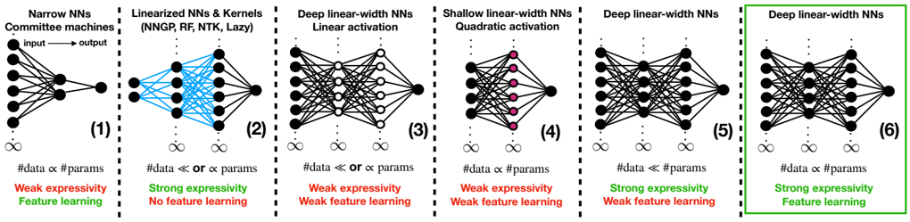(1) Narrow networks. Triggered by pioneering works employing spin glass techniques to study NNs [3-5], the interest of the statistical physics community for the equilibrium properties of the narrow commitee machines ( L = 1 with k 1 = Θ(1) while n = Θ( d ) → ∞ , (1) in FIG. 1) rose quickly in the nineties [6-20]. This line of classical works is at the inception of the discovery of learning phase transitions (found concurrently also in single-layer architectures with constrained weights or peculiar activations [21-26]). The main issue with narrow NNs is their restricted expressivity. Nevertheless, <latexi sh 1\_b 64="3m7ZLQ z0djGS XTU/yc wf >A C2H VFN E + R B P K9g Ik r u J q O M n v p Y W o D p <latexi sh 1\_b 64="oBZS7 VY JFA0NQ/ ny g k > C cj zGr q Iv H WM PT E m f wR+ K U X O L d pD u <latexi sh 1\_b 64="oBZS7 VY JFA0NQ/ ny g k > C cj zGr q Iv H WM PT E m f wR+ K U X O L d pD u →∞ FIG. 1. Classification of models of fully connected feed-forward neural networks analysed in the theoretical literature (see the main text for references). Class ( 1 ) models are very narrow, i.e., with a width independent of the large input dimension d . This includes the perceptron and committee machines studied in the statistical mechanics literature (the latter are linked to the so-called multi-index models). They are analysed near-interpolation, where the number of data and model's parameters are proportional. In this regime, feature learning emerges through phase transitions but these models suffer from their limited expressivity. ( 2 ) encompasses all 'kernel-like models' whose inner weights are frozen to random values (which is represented by the blue colour) either by construction as in the random feature model, or as a consequence of their overwhelming width/overparametrisation (as in neural networks Gaussian processes, or in gradient-based dynamics in the lazy regime, where the weights effectively remain at initialisation and the networks behave as neural tangent kernels). These models are expressive but do not learn task-relevant features due to their effectively frozen embedding layers. However, with readout weights (black last layer) to be O (1 /d ) rather than the standard scaling O (1 / √ d ), feature learning emerges despite the width being infinite. Another tractable simplification are ( 3 ) deep linear networks, where the weights are learnable but activation functions linear (white circled nodes), thus reducing expressivity to that of a linear model, which allows for limited feature learning. A recent simplification is the linear-width shallow network with quadratic activation (pink nodes), ( 4 ). Even if trained near interpolation, it can only learn a quadratic approximation of the target, which limits its expressivity. Moreover, we will see that in the teacher-student setting we consider, it cannot recover the target weights, thus preventing strong feature-learning in this sense. Models ( 5 ) are the same as studied here, but set in the strongly overparametrised 'proportional regime': with a sample size only scaling as the width. Yet, weak forms of feature learning can emerge. The present paper considers fully trainable proportional-width non-linear NNs trained near interpolation , ( 6 ). This is the most challenging regime, where the model expressivity can fully manifest via strong task-adaptation (i.e., recovery of the target). <details> <summary>Image 1 Details</summary>  ### Visual Description ## Neural Network Architectures: A Comparative Diagram ### Overview The image presents a comparative diagram of six different neural network architectures, highlighting their structural differences, data-parameter relationships, expressivity, and feature learning capabilities. Each architecture is visually represented with nodes and connections, accompanied by textual descriptions. ### Components/Axes The diagram is divided into six distinct sections, each representing a different neural network architecture. The sections are numbered (1) through (6). * **Titles:** Each section has a title describing the network architecture: * (1) Narrow NNs Committee machines * (2) Linearized NNs & Kernels (NNGP, RF, NTK, Lazy) * (3) Deep linear-width NNs Linear activation * (4) Shallow linear-width NNs Quadratic activation * (5) Deep linear-width NNs * (6) Deep linear-width NNs * **Network Diagrams:** Each section contains a schematic diagram of the neural network, showing nodes (neurons) and connections (synapses). * **Data-Parameter Relationship:** Each section includes a statement about the relationship between the amount of data and the number of parameters. * **Expressivity:** Each section indicates whether the network has "Weak expressivity" or "Strong expressivity." * **Feature Learning:** Each section indicates whether the network exhibits "Feature learning" or "No feature learning" or "Weak feature learning." * **Infinity Symbol:** An infinity symbol is present below each network diagram. ### Detailed Analysis **Section 1: Narrow NNs Committee machines** * **Diagram:** A narrow network with an input layer of approximately 5 nodes, a hidden layer of approximately 5 nodes, and a single output node. Connections are dense between layers. An arrow indicates the flow from "input" to "output". * **Data-Parameter Relationship:** "#data α #params" (Data is proportional to parameters) * **Expressivity:** Weak expressivity * **Feature Learning:** Feature learning **Section 2: Linearized NNs & Kernels (NNGP, RF, NTK, Lazy)** * **Diagram:** A network with an input layer of approximately 5 nodes, a hidden layer of approximately 5 nodes, and a single output node. The connections between the input and hidden layers are colored in blue. * **Data-Parameter Relationship:** "#data << or α params" (Data is much less than or proportional to parameters) * **Expressivity:** Strong expressivity * **Feature Learning:** No feature learning **Section 3: Deep linear-width NNs Linear activation** * **Diagram:** A deep network with an input layer of approximately 5 nodes, multiple hidden layers (approximately 3), and a single output node. The hidden layers have approximately 5 nodes each. Connections are dense between layers. The nodes in the hidden layers are white. * **Data-Parameter Relationship:** "#data << or α params" (Data is much less than or proportional to parameters) * **Expressivity:** Weak expressivity * **Feature Learning:** Weak feature learning **Section 4: Shallow linear-width NNs Quadratic activation** * **Diagram:** A shallow network with an input layer of approximately 5 nodes, a hidden layer of approximately 5 nodes, and a single output node. The nodes in the hidden layer are colored in pink. Connections are dense between layers. * **Data-Parameter Relationship:** "#data α #params" (Data is proportional to parameters) * **Expressivity:** Weak expressivity * **Feature Learning:** Weak feature learning **Section 5: Deep linear-width NNs** * **Diagram:** A deep network with an input layer of approximately 5 nodes, multiple hidden layers (approximately 3), and a single output node. The hidden layers have approximately 5 nodes each. Connections are dense between layers. * **Data-Parameter Relationship:** "#data << #params" (Data is much less than parameters) * **Expressivity:** Strong expressivity * **Feature Learning:** Weak feature learning **Section 6: Deep linear-width NNs** * **Diagram:** A deep network with an input layer of approximately 5 nodes, multiple hidden layers (approximately 3), and a single output node. The hidden layers have approximately 5 nodes each. Connections are dense between layers. This section is enclosed in a green box. * **Data-Parameter Relationship:** "#data α #params" (Data is proportional to parameters) * **Expressivity:** Strong expressivity * **Feature Learning:** Feature learning ### Key Observations * The diagram contrasts different neural network architectures based on depth, width, activation functions, and data-parameter relationships. * Expressivity and feature learning capabilities vary across the architectures. * The relationship between data and parameters seems to influence expressivity and feature learning. ### Interpretation The diagram illustrates the trade-offs between different neural network architectures. Narrow networks and deep linear-width networks (Section 6) with a proportional data-parameter relationship exhibit feature learning, while linearized networks prioritize strong expressivity but sacrifice feature learning. The choice of architecture depends on the specific task and the available data. The diagram suggests that the relationship between data size and the number of parameters, along with the network's depth and activation functions, plays a crucial role in determining its expressivity and feature learning capabilities. </details> their analysis yielded important insights on NNs learning mechanisms, some of which are also occurring in more expressive models. One of particular importance is the so-called specialisation transition [27, 28], where hidden neurons start learning different features. However, as we will see, in more expressive models a richer phenomenology emerges. This field has since then remained very much alive, with the goal of treating more complex architectures as in the present paper, see [29, 30] for reviews. Narrow NNs are multi-index functions , i.e., functions projecting their argument on a low-dimensional subspace, see [31] for a review. Their study allows to understand which properties of non-linearities makes learning hard for gradient-based or message-passing algorithms [32-36]. (2) Kernel limit: ultra wide and linearised NNs, and the mean-field regime. On the other hand, in the ultra wide limit ( L fixed, k l ≫ n ) fully connected Bayesian NNs behave as kernel machines (the so-called neural network Gaussian processes, NNGPs) [37-41], and hence suffer from these models' limitations. Indeed, kernel machines infer the decision rule by first embedding the data in a fixed a priori feature space, the renowned kernel trick , then operating linear regression/classification over the features. In this respect, they do not learn taskrelevant features and therefore need larger and larger feature spaces and training sets to fit their higher order statistics [42-47]. 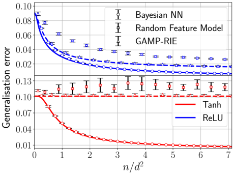The same conclusions hold for NNs trained with gradient-based methods but linearised around initialisation [48], i.e., with frozen weights represented in blue in FIG. 1. These include the random feature model (RF) with fixed random inner layer [49] (which is a finite size approximation of kernel machines), or the closely related neural tangent kernel (NTK) [50] and lazy regimes [51], see models (2) in FIG. 1. Such models are thus 'effectively linearised' because only the readouts are learnt. FIG. 2 illustrates the importance of feature learning: despite having a larger number of parameters, the best RF model or kernel are outperformed by an optimally trained NN, see also [52, 53]. One way to probe minimal feature learning effects is through perturbative expansions around the ultra wide limit, where k ≫ n but O (1 /k ) corrections are kept [5460]. This connects to expansions around free fields in quantum field theory, where diagrammatic rules are used to manage complex combinatorial sums, see [61, 62] for introductions. Another way to force feature-learning in infinitely wide models is the mean-field scaling obtained by taking the readout weights v vanishingly small ( O (1 /k ) rather than the standard O (1 / √ k ) scaling we consider). Originally proposed as a mean to escape the lazy regime of gradient-based dynamics [51] via a specific weights initialisation [63-69], it was later extended to the Bayesian framework [70-73]. NNs in this scaling converge to kernel machines with data-dependent kernels (rather than fixed a priori, as in the lazy regime). We also <latexi sh 1\_b 64="3m7ZLQ z0djGS XTU/yc wf >A C2H VFN E + R B P K9g Ik r u J q O M n v p Y W o D <latexi sh 1\_b 64="3m7ZLQ z0djGS XTU/yc wf >A C2H VFN E + R B P K9g Ik r u J q O M n v p Y W o D <latexi sh 1\_b 64="oBZS7 VY JFA0NQ/ ny g k > C cj zGr q Iv H WM PT E m f wR+ K U X O L d pD u <latexi sh 1\_b 64="oBZS7 VY JFA0NQ/ ny g k > C cj zGr q Iv H WM PT E m f wR+ K U X O L d pD u <latexi sh 1\_b 64="oBZS7 VY JFA0NQ/ ny g k > C cj zGr q Iv H WM PT E m f wR+ K U X O L d pD u <latexi sh 1\_b 64="oBZS7 VY JFA0NQ/ ny g k > C cj zGr q Iv H WM PT E m f wR+ K U X O L d pD u <latexi sh 1\_b 64="3m7ZLQ z0djGS XTU/yc wf >A C2H VFN E + R B P K9g Ik r u J q O M n v p Y W o D <latexi sh 1\_b 64="3m7ZLQ z0djGS XTU/yc wf >A C2H VFN E + R B P K9g Ik r u J q O M n v p Y W o D <latexi sh 1\_b 64="oBZS7 VY JFA0NQ/ ny g k > C cj zGr q Iv H WM PT E m f wR+ K U X O L d pD u <latexi sh 1\_b 64="oBZS7 VY JFA0NQ/ ny g k > C cj zGr q Iv H WM PT E m f wR+ K U X O L d pD u <latexi sh 1\_b 64="3m7ZLQ z0djGS XTU/yc wf >A C2H VFN E + R B P K9g Ik r u J q O M n v p Y W o D <latexi sh 1\_b 64="oBZS7 VY JFA0NQ/ ny g k > C cj zGr q Iv H WM PT E m f wR+ K U X O L d pD u <latexi sh 1\_b 64="oBZS7 VY JFA0NQ/ ny g k > C cj zGr q Iv H WM PT E m f wR+ K U X O L d pD u <latexi sh 1\_b 64="oBZS7 VY JFA0NQ/ ny g k > C cj zGr q Iv H WM PT E m f wR+ K U X O L d pD u <latexi sh 1\_b 64="oBZS7 VY JFA0NQ/ ny g k > C cj zGr q Iv H WM PT E m f wR+ K U X O L d pD u <latexi sh 1\_b 64="3m7ZLQ z0djGS XTU/yc wf >A C2H VFN E + R B P K9g Ik r u J q O M n v p Y W o D <latexi sh 1\_b 64="3m7ZLQ z0djGS XTU/yc wf >A C2H VFN E + R B P K9g Ik r u J q O M n v p Y W o D <latexi sh 1\_b 64="oBZS7 VY JFA0NQ/ ny g k > C cj zGr q Iv H WM PT E m f wR+ K U X O L d pD u <latexi sh 1\_b 64="oBZS7 VY JFA0NQ/ ny g k > C cj zGr q Iv H WM PT E m f wR+ K U X O L d pD u <latexi sh 1\_b 64="oBZS7 VY JFA0NQ/ ny g k > C cj zGr q Iv H WM PT E m f wR+ K U X O L d pD u <latexi sh 1\_b 64="oBZS7 VY JFA0NQ/ ny g k > C cj zGr q Iv H WM PT E m f wR+ K U X O L d pD u <latexi sh 1\_b 64="3m7ZLQ z0djGS XTU/yc wf >A C2H VFN E + R B P K9g Ik r u J q O M n v p Y W o D <latexi sh 1\_b 64="3m7ZLQ z0djGS XTU/yc wf >A C2H VFN E + R B P K9g Ik r u J q O M n v p Y W o D <latexi sh 1\_b 64="oBZS7 VY JFA0NQ/ ny g k > C cj zGr q Iv H WM PT E m f wR+ K U X O L d pD u <latexi sh 1\_b 64="oBZS7 VY JFA0NQ/ ny g k > C cj zGr q Iv H WM PT E m f wR+ K U X O L d pD u <latexi sh 1\_b 64="3m7ZLQ z0djGS XTU/yc wf >A C2H VFN E + R B P K9g Ik r u J q O M n v p Y W o D <latexi sh 1\_b 64="oBZS7 VY JFA0NQ/ ny g k > C cj zGr q Iv H WM PT E m f wR+ K U X O L d pD u <latexi sh 1\_b 64="oBZS7 VY JFA0NQ/ ny g k > C cj zGr q Iv H WM PT E m f wR+ K U X O L d pD u <latexi sh 1\_b 64="oBZS7 VY JFA0NQ/ ny g k > C cj zGr q Iv H WM PT E m f wR+ K U X O L d pD u <latexi sh 1\_b 64="oBZS7 VY JFA0NQ/ ny g k > C cj zGr q Iv H WM PT E m f wR+ K U X O L d pD u <latexi sh 1\_b 64="3m7ZLQ z0djGS XTU/yc wf >A C2H VFN E + R B P K9g Ik r u J q O M n v p Y W o D <latexi sh 1\_b 64="3m7ZLQ z0djGS XTU/yc wf >A C2H VFN E + R B P K9g Ik r u J q O M n v p Y W o D <latexi sh 1\_b 64="oBZS7 VY JFA0NQ/ ny g k > C cj zGr q Iv H WM PT E m f wR+ K U X O L d pD u <latexi sh 1\_b 64="oBZS7 VY JFA0NQ/ ny g k > C cj zGr q Iv H WM PT E m f wR+ K U X O L d pD u <latexi sh 1\_b 64="3m7ZLQ z0djGS XTU/yc wf >A C2H VFN E + R B P K9g Ik r u J q O M n v p Y W o D <latexi sh 1\_b 64="oBZS7 VY JFA0NQ/ ny g k > C cj zGr q Iv H WM PT E m f wR+ K U X O L d pD u <latexi sh 1\_b 64="oBZS7 VY JFA0NQ/ ny g k > C cj zGr q Iv H WM PT E m f wR+ K U X O L d pD u <latexi sh 1\_b 64="oBZS7 VY JFA0NQ/ ny g k > C cj zGr q Iv H WM PT E m f wR+ K U X O L d pD u <latexi sh 1\_b 64="oBZS7 VY JFA0NQ/ ny g k > C cj zGr q Iv H WM PT E m f wR+ K U X O L d pD u mention [74, 75] which alternatively rescale the Bayesian likelihood to induce feature learning at infinite width. (3) Deep linear networks. Another way to linearise networks, thus making them tractable, is by allowing fully trainable weights while placing linear activations in the inner layers. Linear networks are a major theoretical playground from the dynamical perspective [76] but also at the equilibrium (Bayesian) level [70, 77-80]. In the same vein, theoreticians considered linear diagonal networks of the form F diag w , v ( x ) = v ⊺ diag( w ) x [81, 82], which exhibit an implicit bias in gradient descent learning [8386]. A main issue with linear networks, however, is their intrinsically small expressivity, so only weak notions of feature learning can manifest. (4) Shallow quadratic networks. Various works have recently exploited the fact that a shallow NN with quadratic activation σ ( x ) = x 2 simplifies drastically [8797]. However, we will see that this prevents strong feature learning to emerge. The closest settings to ours are [9496]. There, the analysis based on results for the GLM [98] and matrix denoising [99-102] follows thanks to a specific mapping to a linear matrix sensing problem , where the goal is to infer a Wishart-like matrix given its projection along random rank-one matrices. (5) Proportional data regime. This overparametrised regime considers a sample size much smaller than the number of model parameters ( L fixed, d large, k l , n = Θ( d )). Recent works show how a limited amount of feature learning makes the network equivalent to optimally regularised kernels [71, 77, 103-105]. MLPs thus reduce to linear networks (GLMs) in the sense conjectured in [106] and proven in [107, 108] and thus suffer from their limitations. This could be a consequence of the fully connected architecture, as, e.g., convolutional networks can learn more informative features in this regime [70, 109111]. In a similar data regime, Yoshino and co-authors have developed a replica theory for overparametrised deep NNs with a non-standard architecture [112-114]. (6) A timely challenge: Deep non-linear networks of linear width trained near interpolation. Despite the wealth of methods developed to study the aforementioned models, none is able to tackle NNs enjoying all the following realistic properties: - ( P 1 ) a width proportional to the input dimension; - ( P 2 ) with broad classes of non-linear activations; - ( P 3 ) with possibly multiple hidden layers; ( P 4 ) learning in the interpolation regime . The property ( P 1 ) combined with ( P 2 ) , ( P 3 ) allows to capture finite-width effects in NNs that are highly expressive, while still allowing to take the large system limit needed to obtain sharp theoretical predictions. Even if it is not entirely clear whether a finite width improves the performance of Bayesian MLPs compared to their kernel limit [115, 116], it is certainly one of the most natural ways to allow for the emergence of representation learning, which really is the crux of deep learning [2]. FIG. 2. Bayes-optimal mean-square generalisation error achievable by a two-layer NN F θ ( x ) = v ⊺ σ ( Wx ) as a function of the amount of training data n over the squared input dimension d 2 when d, n and the NN width k all diverge with n/d 2 and k/d → 0 . 5 fixed (solid curves), with activation σ ( x ) = ReLU( x ) and tanh(2 x ) (same setting as right panel of FIG. 5). These theoretical curves follow from the results in Sec. II. The task is regression with standard Gaussian inputs ( x µ ) µ ≤ n and noisy responses ( y µ ) µ ≤ n generated by a target two-layer NN F θ 0 ( x ) with Gaussian random weights and same activation. In the experiments, d = 150 and k = 75. Empty circles are obtained by training the Bayesian NN using Hamiltonian Monte Carlo initialised close to the target (yielding the best achievable error), and then computing its generalisation error on 10 5 test data (error bars are the standard deviation over 10 instances of the training set and target). Crosses show the generalisation error empirically achievable by the random feature model F RF a ∗ ( x ) = a ∗ ⊺ σ ( W RF x ) trained by exact empirical risk minimisation a ∗ = argmin( ∑ µ ≤ n ( y µ -F RF a ( x µ )) 2 + t ∥ a ∥ 2 ) with optimised a ∈ R r and L 2 -regularisation strength t picked by crossvalidation. The fixed Gaussian features matrix W RF ∈ R r × d has width r = 3 kd roughly three times larger than the total number k ( d +1) of parameters of the NN. Triangles are the error of GAMP-RIE [94] extended to generic activations (see App. B4), which reaches the performance of an optimally regularised kernel. <details> <summary>Image 2 Details</summary>  ### Visual Description ## Chart: Generalization Error vs. n/d^2 ### Overview The image is a line chart comparing the generalization error of different models as a function of the ratio n/d^2. The chart displays two distinct sets of models: Bayesian NN, Random Feature Model, and GAMP-RIE in the upper portion, and Tanh and ReLU in the lower portion. The x-axis represents n/d^2, and the y-axis represents the generalization error. Error bars are included for some data series. ### Components/Axes * **X-axis:** n/d^2, ranging from 0 to 7. Axis markers are present at integer values. * **Y-axis:** Generalisation error, ranging from 0.01 to 0.10 in the lower portion and from 0.02 to 0.10 in the upper portion, with an additional marker at 0.13. * **Legend (Top-Right):** * Bayesian NN (Black, circles): Data points are marked with circles. * Random Feature Model (Black, crosses): Data points are marked with crosses. * GAMP-RIE (Black, triangles): Data points are marked with triangles. * **Legend (Bottom-Right):** * Tanh (Red, circles): Data points are marked with circles. * ReLU (Blue, solid line): No data points are explicitly marked on the line. ### Detailed Analysis **Upper Portion:** * **Bayesian NN (Blue, circles):** The blue line with circle markers starts at approximately 0.085 at n/d^2 = 0 and decreases to approximately 0.015 at n/d^2 = 7. The trend is downward, indicating decreasing generalization error with increasing n/d^2. * n/d^2 = 0: ~0.085 * n/d^2 = 1: ~0.045 * n/d^2 = 2: ~0.03 * n/d^2 = 3: ~0.02 * n/d^2 = 7: ~0.015 * **Random Feature Model (Blue, crosses):** The blue dashed line with cross markers starts at approximately 0.09 at n/d^2 = 0 and decreases to approximately 0.03 at n/d^2 = 7. The trend is downward, indicating decreasing generalization error with increasing n/d^2. * n/d^2 = 0: ~0.09 * n/d^2 = 1: ~0.06 * n/d^2 = 2: ~0.045 * n/d^2 = 3: ~0.035 * n/d^2 = 7: ~0.03 * **GAMP-RIE (Blue, triangles):** The blue dashed line with triangle markers starts at approximately 0.09 at n/d^2 = 0 and decreases to approximately 0.03 at n/d^2 = 7. The trend is downward, indicating decreasing generalization error with increasing n/d^2. * n/d^2 = 0: ~0.09 * n/d^2 = 1: ~0.05 * n/d^2 = 2: ~0.035 * n/d^2 = 3: ~0.03 * n/d^2 = 7: ~0.025 **Lower Portion:** * **Tanh (Red, circles):** The red line with circle markers starts at approximately 0.10 at n/d^2 = 0 and decreases to approximately 0.01 at n/d^2 = 7. The trend is downward, indicating decreasing generalization error with increasing n/d^2. * n/d^2 = 0: ~0.10 * n/d^2 = 1: ~0.04 * n/d^2 = 2: ~0.025 * n/d^2 = 3: ~0.015 * n/d^2 = 7: ~0.01 * **ReLU (Red, triangles):** The red dashed line with triangle markers remains relatively constant at approximately 0.11 across all values of n/d^2. The trend is flat, indicating no significant change in generalization error with increasing n/d^2. Error bars are present. * n/d^2 = 0: ~0.11 * n/d^2 = 1: ~0.11 * n/d^2 = 2: ~0.115 * n/d^2 = 3: ~0.11 * n/d^2 = 7: ~0.11 ### Key Observations * The generalization error for Bayesian NN, Random Feature Model, GAMP-RIE, and Tanh decreases as n/d^2 increases. * The generalization error for ReLU remains relatively constant as n/d^2 increases. * The Tanh model exhibits the lowest generalization error at higher values of n/d^2. * The ReLU model exhibits a higher, relatively constant generalization error. ### Interpretation The chart suggests that, for the given models, increasing the ratio of 'n' to 'd^2' generally leads to a reduction in generalization error, implying better model performance with more data relative to the model's complexity. However, this trend is not universal, as demonstrated by the ReLU model, which shows no significant improvement with increasing n/d^2. The Tanh model appears to be the most effective in reducing generalization error as n/d^2 increases, outperforming the other models at higher values of n/d^2. The error bars on the ReLU model indicate some variability in its performance, but the overall trend remains consistent. The Bayesian NN, Random Feature Model, and GAMP-RIE models exhibit similar trends, with decreasing generalization error as n/d^2 increases, but their performance is generally worse than Tanh at higher values of n/d^2. </details> The interpolation regime ( P 4 ) means L fixed, d large with k l = Θ( d ) (from ( P 1 )) and n = Θ( d 2 ), i.e., a sample size comparable to the number of trainable parameters. This regime is difficult to analyse for expressive models but also very interesting, because it forces them to adapt to the data in order to perform well. Hence, taskdependent feature learning emerges, thus escaping the reduction to linear models discussed above. Analysing MLPs in the interpolation regime has been an open problem for decades, and is widely recognised as one of the major theoretical challenges in the physics of learning [94, 106]. That statistical mechanics is up to the task is an encouraging signal for physicists working on deep learning [117, 118]. This setting is relevant and timely also from a practical perspective. Indeed, the latest NN architectures such as generative diffusion and large language models (LLMs) do operate near interpolation: the computeoptimal training scales parameters and tokens in equal proportion [119, 120], with typical sizes ranging in 10 10 -10 12 . These models of utmost interest are highly expressive and also exhibit signs of feature learning [121, 122]. From that perspective, it places them in a similar regime as considered in the present paper. LLMs are far more intricate than MLPs. Yet, they have things in common: in addition to the fact that one of the basic building block of LLMs is actually the MLP (together with the attention head), both correspond to deep non-linear architectures. We thus consider essential to tackle the interpolation regime of MLPs, with the hope that some insights brought forward by our theoretically tractable idealised setting remain qualitatively relevant for the NN architectures deployed in applications. ## B. Main contributions and setting We address questions pertaining to the foundations of learning theory for NN models possessing all four properties ( P 1 )-( P 4 ). The first one is information-theoretic : Q1 : Assuming the training data is generated by a target MLP, how much is needed to achieve a certain generalisation performance using an MLP with same architecture and Bayes-optimally trained in a supervised manner? The answer, provided analytically by Result 2 in Sec. II, yields the Bayes-optimal limits of learning an MLP target function, thus bounding the performance of any model trained on the same data. The setting where the datagenerating process is itself an MLP may look artificial at first, but given the high expressivity and universal approximation property of neural networks, studying their learning provides insights applicable to very general classes of functions. For this reason, and the analytical tractability of the teacher-student scenario explained below, this question has always been a starting point in the statistical physics literature on NNs [5]. Secondly, using statistical physics we will answer another important question concerning interpretability : Q2 : Given a certain data budget, which target features can the MLP learn? This is key in order to understand the evolution of the best learning strategy for an MLP as a function of the amount of available data. Consequently, we will precisely explain what a perfectly trained MLP does to beat the random feature model or an optimally regularised kernel (see FIG. 2). In few words, the reason is that given enough data, strong feature learning emerges within the NN, in the sense of recovery of the target weights. This happens through a specialisation phase transition ; in the deep case there will be one transition per layer. This mechanism is not possible with the random feature model, which explains the gap in performance. These insights will follow from the detailed analysis of the suf- ficient statistics (i.e., the order parameters, OPs) of the model as the data increases, obtained from the large deviation perspective provided in Results 1, 3 and 4. The OPs carry more information than merely computing the achievable generalisation performance (see Q1 ). Finally, based on experiments, we provide in Sec. III algorithmic insights for MLPs with L ≤ 2 layers: Q3 : Given a reasonable compute and data budget, can practical training algorithms reach optimal performance or are they blocked by statistical-computational gaps? The short answer is that it depends on the target, in particular on whether its readout weights are discrete. Answering these questions will provide a phase diagram depicting the optimal performance, the features that are learnt to attain it, and the limitations faced by algorithms, as a function of the data budget, see Sec. III. Before presenting the setting needed to do so, let us emphasise once more that the theoretical component of this paper will be only concerned with static aspects, i.e., generalisation capabilities of trained networks (after a manageable or unconstrained compute time). We do not provide any theoretical claims on how learning occurs during training. Teacher-student set-up. We consider the supervised learning of an MLP with L hidden layers when the datagenerating model, i.e., the target function (or 'teacher'), is also an MLP of the same form with unknown weights. These are the readouts v 0 ∈ R k and inner weights W ( l )0 ∈ R k l × k l -1 for ℓ ≤ L (with k 0 = d ), drawn entrywise i.i.d. from P 0 v and P 0 W , respectively (the latter being the same law for all ℓ ≤ L ). We assume P 0 W to be centred while P 0 v has mean ¯ v , and both priors have unit second moment. We denote the set of unknown parameters of the target as θ 0 = ( v 0 , ( W ( l )0 ) l ≤ L ). For a given input vector x µ ∈ R d , for µ ≤ n , the response/label y µ is drawn from a kernel P 0 out : $$\begin{array} { r l } { y _ { \mu } \sim P _ { o u t } ^ { 0 } ( \, \cdot \, | \, \lambda _ { \mu } ^ { 0 } ) \quad w i t h \quad \lambda _ { \mu } ^ { 0 } \colon = \mathcal { F } _ { \theta ^ { 0 } } ^ { ( L ) } ( x _ { \mu } ) , \quad ( 1 ) } \end{array}$$ where the MLP target function is defined as $$\begin{array} { r l } & { f a n \, - } \\ & { J \colon \quad \mathcal { F } _ { \theta ^ { 0 } } ^ { ( L ) } ( x ) \colon = \frac { v ^ { 0 \tau } } { \sqrt { k ^ { L } } } \sigma \left ( \frac { W ^ { ( L ) 0 } } { \sqrt { k _ { L - 1 } } } \sigma \left ( \frac { W ^ { ( L - 1 ) 0 } } { \sqrt { k _ { L - 2 } } } \cdots \sigma \left ( \frac { W ^ { ( 1 ) 0 } } { \sqrt { k _ { 0 } } } x \right ) \cdots \right ) . } \end{array}$$ We will analyse the case of an arbitrary number a layers L (that remains d -independent). However, we will give a special attention to the shallow, one hidden layer MLP (we drop layer indices in this case) $$\begin{array} { r l r } { \mathcal { F } _ { \boldsymbol \theta ^ { 0 } } ^ { ( 1 ) } ( x ) = \frac { 1 } { \sqrt { k } } v ^ { 0 T } \sigma \left ( \frac { 1 } { \sqrt { d } } W ^ { 0 } x \right ) } & { ( 2 ) } \end{array}$$ as well as the MLP with two hidden layers: $$\begin{array} { r l } { i s } & \mathcal { F } _ { \theta ^ { 0 } } ^ { ( 2 ) } ( x ) = \frac { 1 } { \sqrt { k _ { 2 } } } v ^ { 0 } \tau \sigma \left ( \frac { 1 } { \sqrt { k _ { 1 } } } W ^ { ( 2 ) 0 } \sigma ( \frac { 1 } { \sqrt { d } } W ^ { ( 1 ) 0 } x \right ) . \quad ( 3 ) } \end{array}$$ The kernel can be stochastic or model a deterministic rule if P 0 out ( y | λ ) = δ ( y -f 0 ( λ )) for some function f 0 . Our main example P 0 out ( y | λ ) = exp( -1 2∆ ( y -λ ) 2 ) / √ 2 π ∆ is the linear readout with Gaussian label noise. <latexi sh 1\_b 64="wg3 pMYuBTvd Nnf / SD5WV >A C X cj HL F G oJ k q U E + rZ K P Q O m y I z R <latexi sh 1\_b 64="cy OPY3/ H7 JoN+Xmfk 9IGwM >A B V S8 E W K j0 r F v p Td D Q g z u n L R q Z C U <latexi sh 1\_b 64="X + 8m9TBqInOL K H cG Ng >A VD S F W r w U E u P 0M kz f o v d y Z p C J Y R Q j / <latexi sh 1\_b 64=" 3IrG XWN2jP/ A VMcdf k Lw > B n S8 EJ U q F 7Q o y pZ C z Y u +O g H D T R v m K <latexi sh 1\_b 64="jUVzSgk Po p 7CXJ I >A B+n c DL N F r fq d u ZwT W y R m Q3 G MK v E H O Y / <latexi sh 1\_b 64=" GXyOmjzY q k u MR0Fp BU >A n c V NS8 EJ3 W K rHo +w v Td Cf I D PQ g / Z L <latexi sh 1\_b 64="H cN+AI f ZYo5kR M jr Q > Cz3 V LT J FD U d m E S g G O P BW/8 X p2 y9 q w u v n K <latexi sh 1\_b 64="3UN2jorn T Y vC m B05IA > H c VDLSgM F X7W+q d y J k KE /Q R Z zu G O P w f p <latexi sh 1\_b 64=" UCN d E ncjypX + 2k >A Q3 VDL F W Zu R mB T f PO w S I J o q 0G Hv / z r M Y K g <latexi sh 1\_b 64="OuD 0k3wJ g 8S nU 2Rr9I >A CH c V N M G zW/ q FL K Z p X E T + Q v f o m y B d Y j P <latexi sh 1\_b 64="m K grGu/7JMXTYjC RI+Z0 >A c VHLS QwFD W vUp qo B O k f y 5N n z d P E <latexi sh 1\_b 64="cy OPY3/ H7 JoN+Xmfk 9IGwM >A B V S8 E W K j0 r F v p Td D Q g z u n L R q Z C U <latexi sh 1\_b 64="zqym+d L Y rJ QT8 I >A B X c VD S N F W H p Rj K9g P Z GE/ k U O2 7u v f C n o M w <latexi sh 1\_b 64=" 3IrG XWN2jP/ A VMcdf k Lw > B n S8 EJ U q F 7Q o y pZ C z Y u +O g H D T R v m K <latexi sh 1\_b 64="kKB vo G Rf TjmQJNECy U >A +X c VDLS F 2pr Zdu 0W3 Y / q I n M w8 H O z P7 g <latexi sh 1\_b 64=" GXyOmjzY q k u MR0Fp BU >A n c V NS8 EJ3 W K rHo +w v Td Cf I D PQ g / Z L <latexi sh 1\_b 64="5XrM F2Y z+kD O /vCR KNB g >A cjVHLT J 3U I d m Z E G f Sq o Pn p W y w u Q <latexi sh 1\_b 64="gR 8+G B qQv SH3IYc 9y2JE >A n VDL N F U k w K o d Cf m O z X M P Z j p / r u W T 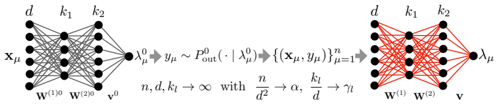FIG. 3. The teacher-student scenario for the case of two hidden layers. The teacher NN is used to produce the responses given the inputs. A student NN with matched architecture (but who is not aware of the parameters of the teacher) is then trained in a Bayesian manner given the training data. We also display the scaling limit considered given by (4). <details> <summary>Image 3 Details</summary>  ### Visual Description ## Neural Network Diagram: Forward and Backward Propagation ### Overview The image depicts a neural network diagram illustrating forward and backward propagation. The diagram is split into two sections, showing the network's state before and after training. The left side represents the initial state with gray connections, while the right side represents the trained state with red connections. ### Components/Axes * **Nodes:** The diagram features nodes arranged in layers. The number of nodes in each layer varies. * **Connections:** Lines connecting the nodes represent the weights between neurons. The color of the lines changes from gray (initial state) to red (trained state). * **Labels:** * Input Layer: x<sub>μ</sub> * Hidden Layers: d, k<sub>1</sub>, k<sub>2</sub> * Output Layer: λ<sub>μ</sub><sup>0</sup> (left), λ<sub>μ</sub> (right) * Weights: w<sup>(1)0</sup>, w<sup>(2)0</sup> (left), w<sup>(1)</sup>, w<sup>(2)</sup> (right), v<sup>0</sup> (left), v (right) * **Equations:** * Left side: λ<sub>μ</sub><sup>0</sup> → y<sub>μ</sub> ~ P<sub>out</sub>(· | λ<sub>μ</sub><sup>0</sup>) * Center: {(x<sub>μ</sub>, y<sub>μ</sub>)}<sub>μ=1</sub><sup>n</sup> * Right side: n, d, k<sub>l</sub> → ∞ with n/d<sup>2</sup> → α, k<sub>l</sub>/d → γ<sub>l</sub> ### Detailed Analysis **Left Side (Initial State):** * The input layer is labeled x<sub>μ</sub> and has approximately 5 nodes. * The first hidden layer is labeled 'd' and also has approximately 5 nodes. * The second hidden layer is labeled 'k<sub>1</sub>' and has approximately 4 nodes. * The third hidden layer is labeled 'k<sub>2</sub>' and has approximately 5 nodes. * The output layer is labeled λ<sub>μ</sub><sup>0</sup> and has a single node. * The connections between the layers are gray, indicating the initial, untrained state of the network. * The weights associated with the connections are labeled w<sup>(1)0</sup>, w<sup>(2)0</sup>, and v<sup>0</sup>. **Right Side (Trained State):** * The input layer is labeled 'd' and has approximately 5 nodes. * The first hidden layer is labeled 'k<sub>1</sub>' and has approximately 4 nodes. * The second hidden layer is labeled 'k<sub>2</sub>' and has approximately 5 nodes. * The output layer is labeled λ<sub>μ</sub> and has a single node. * The connections between the layers are red, indicating the trained state of the network. * The weights associated with the connections are labeled w<sup>(1)</sup>, w<sup>(2)</sup>, and v. **Equations and Relationships:** * The equation λ<sub>μ</sub><sup>0</sup> → y<sub>μ</sub> ~ P<sub>out</sub>(· | λ<sub>μ</sub><sup>0</sup>) describes the forward pass, where λ<sub>μ</sub><sup>0</sup> is the initial output, y<sub>μ</sub> is the target output, and P<sub>out</sub> is the output distribution. * The term {(x<sub>μ</sub>, y<sub>μ</sub>)}<sub>μ=1</sub><sup>n</sup> represents the training dataset consisting of input-output pairs. * The equation n, d, k<sub>l</sub> → ∞ with n/d<sup>2</sup> → α, k<sub>l</sub>/d → γ<sub>l</sub> describes the asymptotic behavior of the network as the number of training samples (n), input dimension (d), and hidden layer sizes (k<sub>l</sub>) approach infinity. α and γ<sub>l</sub> are constants. ### Key Observations * The color change from gray to red signifies the transition from an untrained to a trained network. * The diagram illustrates the flow of information from the input layer to the output layer during both forward and backward propagation. * The equations provide a mathematical description of the network's behavior and training process. ### Interpretation The diagram illustrates the fundamental concept of training a neural network. The left side represents the initial, random state of the network, where the connections (weights) are untrained. The right side represents the trained network, where the connections have been adjusted to map the input data to the desired output. The equations describe the mathematical relationships between the input, output, and network parameters. The asymptotic behavior equation suggests that the network's performance improves as the size of the network and the amount of training data increase. The diagram effectively visualizes the transformation of a neural network from a random mapping to a learned mapping through the process of training. </details> We will first consider i.i.d. standard Gaussian vectors as inputs x µ . In that case the whole data structure is dictated by the input-output relation only, allowing us to focus solely on the influence of the target function on the learning. In Sec. III we generalise the results to include structured data: Gaussian with a covariance and real data (MNIST). The input/output pairs D = { ( x µ , y µ ) } µ ≤ n form the training set for a student network with matching architecture. The Bayesian student learns via the posterior distribution of the weights matrices θ = ( v , ( W ( l ) ) l ≤ L ) (of same respective sizes as the teacher's) given the training data: $$d P ( \pm b { \theta } | \, \mathcal { D } ) \colon = \mathcal { Z } ( \mathcal { D } ) ^ { - 1 } d P _ { \theta } ( \pm b { \theta } ) \prod _ { \mu \leq n } P _ { o u t } \left ( y _ { \mu } | \, \lambda _ { \mu } ( \pm b { \theta } ) \right )$$ where dP θ ( θ ) := dP v ( v ) ∏ l ≤ L dP W ( W ( l ) ) (with the notation dP ( M ) := ∏ i,j dP ( M ij )), with post-activations $$\lambda _ { \mu } ( \boldsymbol \theta ) \colon = \mathcal { F } _ { \boldsymbol \theta } ^ { ( L ) } ( x _ { \mu } ) , \quad \mu \leq n .$$ The posterior normalisation Z ( D ) = Z ( L ) ( D ) for the model with L hidden layers is the partition function, and P W , P v are the priors assumed by the student. We focus on the Bayes-optimal setting P W = P 0 W , P v = P 0 v and P out = P 0 out , but the approach can be extended to account for a mismatch. As stated above, we study the linear-width regime with quadratically many samples , which places the model in the interpolation regime, i.e., a large size limit $$\begin{array} { r l } { d , k _ { l } , n \rightarrow + \infty \, w i t h \, \frac { k _ { l } } { d } \rightarrow \gamma _ { l } \, f o r \, l \leq L , \, \frac { n } { d ^ { 2 } } \rightarrow \alpha . ( 4 ) } & { t h e p r i b u m a l y } \end{array}$$ Given the cost of training deep Bayesian MLPs and specific difficulties discussed below associated with an increasing number of layers, we distinguish the cases of one, two and more than two hidden layers for what concerns the hypotheses we impose on the activation σ . ( H 1 ) For shallow NNs with L = 1 hidden layer our results are valid for an arbitrary activation function as long as it admits an expansion in Hermite polynomials with coefficients ( µ ℓ ) ℓ ≥ 0 , see App. A 2: $$\sigma ( x ) = \sum _ { \ell \geq 0 } \frac { \mu _ { \ell } } { \ell ! } \, H e _ { \ell } ( x ) . \quad \quad ( 5 ) \quad t h a n$$ We also assume it has vanishing 0th Hermite coefficient µ 0 = 0, i.e., that it is centred E z ∼N (0 , 1) σ ( z ) = 0; in App. B1g we relax this assumption. We will mainly consider tanh, ReLU and Hermite polynomial activations. Through Hermite expansion, the MLP function can be decomposed as $$\begin{array} { r l } { \mathcal { F } _ { \theta } ^ { ( 1 ) } ( x ) = \frac { \mu _ { 1 } } { \sqrt { d } } \frac { v ^ { \intercal } W } { \sqrt { k } } x + \frac { \mu _ { 2 } } { 2 d } T r ( \frac { W ^ { \intercal } d i a g ( v ) W } { \sqrt { k } } ( x ^ { \otimes 2 } - I _ { d } ) ) + \cdots } \end{array}$$ where · · · contains terms made of tensors of all orders constructed from θ , contracted with input rank-one tensors ( x ⊗ ℓ ) ℓ . In each such term, at least one tensor is of order ℓ ≥ 3. Therefore an equivalent interpretation of the learning problem of an MLP target is that of a 'tensor sensing problem' where the tensors entering the observed responses, v 0 ⊺ W 0 ∈ R d , W 0 ⊺ diag( v 0 ) W 0 ∈ R d × d , . . . are all constructed from the same fundamental parameters θ 0 (see, e.g., [123]). The first term in the above expansion is called the 'linear term/component'. The one of the target is perfectly learnable in the quadratic data regime we consider. The second term is the 'quadratic term/component'. Both will play a special role because, as we will see, the terms · · · effectively behave as (Gaussian) noise when n = Θ( d 2 ), unless θ 0 is partially recovered. Learning through recovery of θ 0 is called specialisation . In contrast, the linear and quadratic terms are learnable without specialisation. This is reassuring given that we will argue that for many targets, it takes a time growing as exp( c d ) for the network to specialise, for some positive σ -dependent constant c < 1. This separation in algorithmic learnability of first and second components versus all the others is at the root of the emergence of different learning strategies employed by the network, and the crux of the generalisation of a learning algorithm in App. B 4 coined GAMP-RIE (generalised approximate message-passing with rotational invariant estimator) [94]. ( H 2 ) For L = 2 we require µ 0 = µ 2 = 0, which is e.g. the case for odd activations. Our main example is tanh. In the tensor inference problem appearing when expanding all activations, µ 2 = 0 means that no quadratic term is present. However, a 'product term' W (2) W (1) appears (in addition to v ⊺ W (2) W (1) ). We will see in Sec. III that skipping the quadratic term implies that learning terms beyond the linear ones will be possible only through specialisation. However, the presence of the product term will have interesting consequences on the learning curves. Importantly, W (2) W (1) is a matrix learnable partly independently of its factors, and consequently requires its own OP in the analysis. ( H 3 ) For L ≥ 3 we require µ 0 = µ 1 = µ 2 = 0. This does not include standard activations and we consider the hyperbolic tangent after setting µ 1 = 0 in its Hermite decomposition. µ 2 = 0 again entails that learning beyond-linear terms requires the network to specialise, and µ 1 = 0 prevents the multiplication of OPs by avoiding the presence of many product terms. Related to this last comment, we wish to emphasise that these hypotheses are not due to restrictions of the techniques we develop. The issue is purely practical: relaxing them while increasing the number of layers yields a combinatorial explosion (in L ) of the number of OPs to track in the theory as well as cumbersome formulas. We have therefore decided to leave for future work the analysis of the most general case, and focus here on these special ones which already yield an extremely rich picture while remaining interpretable. ## C. Replica method and HCIZ combined A key component of our approach is the way we blend tools from spin glasses (the replica method [124]) and matrix models, in particular, the so-called Harish ChandraItzykson-Zuber (HCIZ) 'spherical' integral [125-127]. Here, we review the growing corpus of works utilising it jointly with the replica method. Let us first define this matrix integral: $$\begin{array} { r l } & { \mathcal { Z } _ { H C I Z } ^ { ( \beta ) } ( A , B ) \colon = \int d \mu ^ { ( \beta ) } ( 0 ) \exp \left ( \frac { \beta N } { 2 } T r [ O A O ^ { \dagger } B ] \right ) \quad ( 6 ) } \\ & { t h e n j . } \end{array}$$ where β = 2 if A , B are N × N Hermitian matrices, β = 1 if real symmetric. Respectively the integral is over the unitary U ( N ) or orthogonal group O ( N ), w.r.t. the corresponding uniform Haar measure µ ( β ) . For β = 2 it admits a closed form for any N [125] and a known large N limit for β = 1 , 2 [126-129]. It is crucial to analyse matrix models in physics and random geometry [130-132]. In spite of having an 'explicit' limit, it can be tackled only in few cases [100, 133]. However, if one matrix, say A , has small rank compared to N ≫ 1, the corresponding low-rank spherical integral is simple [134, 135]. Spherical integrals were used in the replica method for spin glasses with correlated disorder in the seminal paper [136]. It triggered a long series of works in spin glasses [137-141], in analysing simple NNs [142, 143] or in inference and message-passing algorithms [144-160]. In these papers the degrees of freedom are few vectors (e.g., the replicas of the system forming a low-rank matrix A ) interacting with a quenched rotationally invariant matrix B of rank Θ( N ). Rotational invariance, a crucial property for employing spherical integrals, means distributional invariance under orthogonal transformations, i.e., P ( B ) = P ( OBO ⊺ ) ∀ O ∈ O ( N ) if B is symmetric. Consequently, only the low-rank spherical integral intervenes when integrating B 's eigenvectors. An active research line tries to include models where the degrees of freedom themselves are linear-rank matrices in addition to the quenched disorder. This presents a whole new challenge. Seminal papers in the context of matrix denoising are [161, 162] which provided a spectral denoising algorithm (on which the GAMP-RIE [94] relies), also analysed in [101, 102]. Extensions to nonsymmetric matrix denoising exist [163, 164]. An early attempt at combining linear-rank spherical integration (where both A , B in (6) have rank Θ( N )) with the replica method is [165], which tried to improve on the replica approach for matrix denoising in [166, 167] that was missing important correlations among variables. It was followed by two concurrent papers yielding intractable [99] or perturbative [100] results for non-Gaussian signals. Remark 1. No method in the aforementioned papers is satisfactory beyond the realm of denoising problems involving strictly rotational invariant signal matrices (Gaussian, Wishart,...). E.g., the HCIZ/replica combination in the latest works [94, 168] requires it, because after using the replica trick to integrate the quenched disorder, the HCIZ is used directly to integrate the annealed matrix degrees of freedom (representing the replicas of the signal matrix), which is possible by rotational invariance. Recently, matrix denoising without rotational invariance was analysed in [169] by assuming that the model behaves as a pure matrix model (due to an 'effective rotational invariance') in a first phase, and then as a 'standard' planted mean-field spin glass in a second. The phases were thus treated separately via different formalisms -HCIZ in one phase, a cavity method under mean-field decoupling assumptions in the other- and then joined using a criterion to locate the transition. This approach yielded a good match with numerics. However, we now understand that this treatment can be improved, because the 'matrix nature' of the model and associated correlations discarded by mean-field methods do play a role also in the second phase. Thus, a major conceptual (and technical) issue remained: whether there exists a theory based on a unified formalism able to describe the whole phase diagram of inference/learning problems involving linear-rank matrices which lack rotational invariance. Ideally, it should be able to handle the correlations induced by the matrix nature of the problem while still capturing the phase transitions and symmetry breaking effects connected to its mean-field component. The present paper provides this theory in the context of NNs, through a replica/HCIZ combination of a different nature than previous works, see Sec. IV. ̸ Related to this last point, we emphasise that previous works on extensive-widths shallow NNs ( k = Θ( d c ) for 0 < c ≤ 1) considered either purely quadratic activation [91, 92, 94-97] or, on the contrary, with µ ≤ 2 = 0 [170]. Both settings enjoy intrinsic simplifications. On one hand, the quadratic NN reduces to a matrix sensing problem [94, 96]. It is therefore a 'pure matrix model' with rotational invariance when considering Gaussian weights: the target (and model) only depends on them via W 0 ⊺ W 0 . Therefore, by rotational invariance (from the left and right) of the Gaussian matrix W 0 , it cannot be recovered, so no specialisation transitions can occur. The advantage is that a large toolbox from random matrix theory is then available: the HCIZ integral to study static aspects [94-96], or Oja's flow and matrix Riccati differential equations for the dynamics [92, 97, 171]. On the other hand, [170] considers µ ℓ = 0 for ℓ ≥ 3 only. In this case, the model is 'purely mean-field': strong decoupling phenomena take place which allow a treatment in term of an effective one-body equivalent system as in mean-field spin systems. In contrast, the techniques we develop in the present paper can deal with truly hybrid models where the two types of characteristics manifest and are taken into ac- ̸ count using a single formalism: the correlations among the entries of the matrix degrees of freedom entering the problem, and specialisation phase transitions induced by mean-field terms. The emerging phase diagram will consequently be extremely rich. In particular, we are able to treat the shallow MLP with generic activation function (Result 1), or the two-layer MLP with µ 1 = 1 (Result II B). The case of L ≥ 3 requires hypothesis ( H 3 ) on σ which, in turn, makes the model 'purely mean-field'. ## D. Organisation of the paper · Section II first discusses the main hypothesis underlying the theory and the meaning of functions entering it. We then present the theoretical results: replica symmetric formulas for the free entropy and OPs for shallow NNs (Result 1), with two hidden layers (Result 3), or arbitrary L ( Result 4). These provide an answer to Q2 . The Bayes generalisation error is deduced automatically from Result 2 in all cases, thus answering Q1 . · Section III is the core experimental part. It validates the theory through the numerical exploration of the rich learning phase diagram. Our main message concerning Q2 is as follows. As α increases two phases appear: ( i ) Universal phase. Before a critical sample rate α sp , the NN makes predictions by exploiting specific nonlinear combinations of the teacher's features without disentangling them; effectively, the student learns the best 'quadratic network approximation' of the target. In this phase, performance is (asymptotically) independent of the detailed law of the target hidden weights (hence the term 'universal'). Yet, the (effectively quadratic) NN outperforms kernel ridge regression (and thus the random feature model too, FIG. 2), see [94, 96]. ( ii ) Specialisation phase. Increasing the data beyond α sp triggers specialisation transitions: individual hidden units start aligning with target units. Which features specialise first is governed by the readout strengths of the target: stronger features (larger readout amplitudes) emerge earlier. For heterogeneous readouts, this yields a sequence of specialisation events; for homogeneous readouts, a collective transition occurs. If L ≥ 2, possible heterogeneity both in the rows and columns of individual weight matrices induces non-trivial specialisation profiles in each layer. In turn, different layers can experience different phases and do not necessarily specialise concurrently. We will also show that learning propagates from inner to outer hidden layers, because deeper layers require more data to be recovered through specialisation. Consequently, deeper target functions appear harder to learn than shallow ones. In summary, despite the model's 'matrix nature' at the source of the universal phase, additional mean-fieldlike terms in the free entropy (in information theory parlance, Gaussian scalar channels) imply the existence of specialisation events. These terms depend explicitly on the weights prior and interact with the matrix degrees of freedom, and ultimately break the numerous effective symmetries holding before the transition. The theoretical phase diagram will be extensively tested against various training algorithms: two Monte Carlo-based Bayesian samplers, a first-order optimisation procedure (ADAM), and a mixed spectral/approximate message-passing algorithm generalising the GAMP-RIE of [94] to accommodate general activation functions σ when L = 1. The performance of these algorithms belonging to different classes, even when sub-optimal, can be exactly (or, for ADAM, at least accurately) predicted by non-equilibrium solutions of the theoretical equations. Focusing on L ≤ 2 for what pertains algorithmic hardness of learning, Q3 , we will show empirically that specialisation is potentially hard to reach for some target functions, in particular when the readouts are discrete. The tested algorithms fail to find it and instead get trapped by sub-optimal non-specialised solutions, probably due to statistical-computational gaps. We will also generalise the theory to structured data, i.e., Gaussian with a covariance. It will capture the model's performance when trained from non-Gaussian inputs too. Tests with real (MNIST images) and synthetic data generated by one layer of a NN will confirm it. · Section IV contains the main steps of our replica theory, with an emphasis on its novel ingredients. Along the derivation, the mixed matrix model/mean-field planted spin glass nature of the problem will become apparent. · Finally, Section V summarises our contributions and discusses the numerous perspectives this work opens. The appendices are found after the references. · Appendix A gathers some important pre-requisites: App. A1 summarises all notations used in the paper (we advise the reader to give it a look before reading the main results); the definition of the Hermite polynomials and Mehler's formula are found in App. A 2; the Nishimori identities in Bayes-optimal inference in App. A 3; the link between free entropy and mutual information in App. A4; and a simplification of the expression for the optimal mean-square generalisation error in App. A 5. · Appendix B groups all sub-appendices related to the shallow MLP: App. B1 details all the steps of the replica calculation; App. B 2 proposes alternative routes to take care of the entropy of the order parameters associated with the matrix degrees of freedom in the model; App. B3 analyses the large sampling rate limit of the theoretical free entropy; App. B 4 provides the generalisation of the GAMP-RIE algorithm needed to deal with general σ ; App. B5 is an empirical analysis of the hardness of learning shallow targets; App. B 6 is a partial proof for a special case of activation function; finally, App. B 7 provides additional experimental validations of the fact that the readout weights of the model being learnable or fixed has no effect on its optimal performance. · Appendix C concerns only the deep MLP: App. C 1 is the replica calculation; App. C 2 shows the consistency of the formulas provided for structured inputs with L = 1 in the main, and the ones for a special case of non-Gaussian data obtainable from the theory for two hidden layers when freezing the first one (which induces a structure for the inputs of the second, learnable layer). · Appendix D provides all information needed to reproduce the simulations with the provided codes [172]. ## II. MAIN RESULTS: THEORY OF THE MLP We aim at evaluating the expected optimal generalisation error in the teacher-student setting of FIG. 3. Let ( x test , y test ∼ P out ( · | λ 0 test )) be a test sample independent of D drawn using the teacher, where λ 0 test is defined as in (1) with x µ replaced by x test (and similarly for λ test ( θ )). Given a prediction function f , the Bayes estimator for the test response is ˆ y f ( x test , D ) := ⟨ f ( λ test ( θ )) ⟩ , where ⟨ · ⟩ := E [ · | D ]. Then, for a performance measure C : R × R ↦→ R ≥ 0 the Bayes generalisation error is $$\begin{array} { r l } & { \varepsilon ^ { \mathcal { C } , f } \colon = \mathbb { E } _ { \theta ^ { 0 } , \mathcal { D } , x _ { t e s t } , y _ { t e s t } } \mathcal { C } \left ( y _ { t e s t } , \left \langle f ( \lambda _ { t e s t } ( \theta ) ) \right \rangle \right ) . \quad ( 7 ) \quad a v e r a l T o p } \end{array}$$ The case of square loss C ( y, ˆ y ) = ( y -ˆ y ) 2 with the choice f ( λ ) = ∫ dy y P out ( y | λ ) =: E [ y | λ ] yields the Bayesoptimal mean-square generalisation error: <!-- formula-not-decoded --> In order to access ε C , f , ε opt and other relevant observables, one can tackle the computation of the average logpartition function, or free entropy in statistical physics: $$\begin{array} { r l } { f _ { n } \colon = \frac { 1 } { n } \mathbb { E } _ { \theta ^ { 0 } , \mathcal { D } } \ln \mathcal { Z } ( \mathcal { D } ) . } & { ( 9 ) \quad ( s e c o r m a l i t y ) } \end{array}$$ The mutual information I ( θ 0 ; D ) between the target and data is related to the free entropy f n , see App. A 4. Before presenting the results we will first detail the main hypothesis for their derivation and explain the physical meaning of the quantities entering them. This will ease their interpretation. We postpone the core of the theoretical derivations to Sec. IV. Main hypothesis. Let s be any positive integer independent of d and define a Gaussian vector ( λ a ) s a =0 := ( λ 0 , λ 1 , · · · , λ s ) ⊺ ∼ N ( 0 , K ∗ ) with covariance (for a, b = 0 , . . . , s ) $$( K ^ { * } ) _ { a b } \colon = \mathbb { E } \lambda ^ { a } \lambda ^ { b } = K ^ { * } + ( K _ { d } - K ^ { * } ) \delta _ { a b } . \quad ( 1 0 ) \quad N o t i o n$$ Let ( θ a ) s a =1 be i.i.d. from the posterior dP ( · | D ) and θ 0 are the random target weights. Our main assumption is that there exists a non-random K ∗ s.t., under the randomness of a common test input x test / ∈ D and ( θ a ) s a =0 , the post-activations ( λ test ( θ a )) s a =0 (called 'replicas'), converge in law towards ( λ a ) s a =0 in the limit (4): $$\begin{array} { r l } { H y p o t h e s i s \colon \exists K ^ { * } | ( \lambda _ { t e s t } ( \theta ^ { a } ) ) _ { a = 0 } ^ { s } \xrightarrow { L a w } ( \lambda ^ { a } ) _ { a = 0 } ^ { s } . 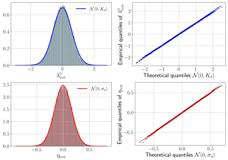( 1 1 ) } & { t e r i o r i n } \\ { p r e d i c u l y } \end{array}$$ The goal of the replica method will be to derive K ∗ in terms of fundamental low-dimensional OPs capturing the FIG. 4. Experimental evidence for the Gaussian hypothesis. In all experiments, d = 300 , γ = 0 . 5 , α = 3 . 0 , ∆ = 0 . 1 , σ ( x ) = ReLU( x ) -1 / √ 2 π , both readout and inner weights have standard Gaussian prior. Empirical evaluations are based on a test set of size 5 × 10 4 . The results have been averaged over 10 instances of the training set and teacher. Top left : Histogram of the teacher post-activations λ 0 test evaluated on x test compared with the theoretically predicted Gaussian density N (0 , K d ) (see (13) for the definition of K d ). Top right : Quantile-quantile plot comparing the theoretical quantiles of N (0 , K d ) with the empirical ones of λ 0 test . Bottom left : Histogram of the student's projection along the orthogonal direction to the teacher: η test = λ test -[ E x test λ 0 test λ test / E x test ( λ 0 test ) 2 ] λ 0 test ≈ λ test -( K ∗ /K d ) λ 0 test , where λ test ( v , W ) is the student post-activation with both v and W sampled from the posterior via Hamiltonian Monte Carlo, evaluated on the same test set, and compared with the theoretical density N (0 , σ η ), where σ η = K d -K ∗ 2 /K d (see (16) for K ∗ ). Bottom right : Quantile-quantile plot comparing the theoretical quantiles of N (0 , σ η ) with the empirical quantiles of η test . <details> <summary>Image 4 Details</summary>  ### Visual Description ## Chart Type: Distribution and Quantile-Quantile (Q-Q) Plots ### Overview The image presents four plots arranged in a 2x2 grid. The top-left and bottom-left plots are histograms overlaid with normal distribution curves. The top-right and bottom-right plots are quantile-quantile (Q-Q) plots, comparing empirical quantiles against theoretical quantiles from normal distributions. ### Components/Axes **Top-Left Plot:** * **Type:** Histogram with overlaid normal distribution curve * **X-axis:** λ⁰test, ranging from approximately -2 to 2. * **Y-axis:** Implicitly represents frequency or density, ranging from 0.0 to 0.6. * **Curve:** Blue curve labeled "N(0, Kd)", representing a normal distribution with mean 0 and standard deviation Kd. * **Bars:** Gray bars representing the histogram of the data. **Top-Right Plot:** * **Type:** Quantile-Quantile (Q-Q) plot * **X-axis:** Theoretical quantiles N(0, Kd), ranging from approximately -2 to 2. * **Y-axis:** Empirical quantiles of λ⁰test, ranging from approximately -2 to 2. * **Data Points:** Blue dots representing the quantiles. **Bottom-Left Plot:** * **Type:** Histogram with overlaid normal distribution curve * **X-axis:** ηtest, ranging from approximately -0.5 to 0.5. * **Y-axis:** Implicitly represents frequency or density, ranging from 0.0 to 2.5. * **Curve:** Red curve labeled "N(0, ση)", representing a normal distribution with mean 0 and standard deviation ση. * **Bars:** Red bars representing the histogram of the data. **Bottom-Right Plot:** * **Type:** Quantile-Quantile (Q-Q) plot * **X-axis:** Theoretical quantiles N(0, ση), ranging from approximately -0.5 to 0.5. * **Y-axis:** Empirical quantiles of ηtest, ranging from approximately -0.5 to 0.5. * **Data Points:** Red dots representing the quantiles. * **Reference Line:** Dashed black line representing y=x. ### Detailed Analysis **Top-Left Plot (λ⁰test Distribution):** * The histogram shows a distribution centered around 0. * The blue curve "N(0, Kd)" closely fits the histogram, suggesting the data is approximately normally distributed with a mean of 0. * The peak of the distribution is around 0.6 on the y-axis. **Top-Right Plot (λ⁰test Q-Q Plot):** * The blue dots closely follow a straight line, indicating that the empirical distribution of λ⁰test is close to a normal distribution. * There is a slight deviation from the line at the extreme tails. **Bottom-Left Plot (ηtest Distribution):** * The histogram shows a distribution centered around 0. * The red curve "N(0, ση)" closely fits the histogram, suggesting the data is approximately normally distributed with a mean of 0. * The peak of the distribution is around 2.5 on the y-axis. **Bottom-Right Plot (ηtest Q-Q Plot):** * The red dots closely follow the dashed black line, indicating that the empirical distribution of ηtest is close to a normal distribution. * There is a slight deviation from the line at the extreme tails. ### Key Observations * Both λ⁰test and ηtest appear to be approximately normally distributed with a mean of 0. * The Q-Q plots confirm the normality, with minor deviations at the tails. * The distribution of ηtest has a higher peak (2.5) than the distribution of λ⁰test (0.6), indicating a smaller standard deviation. ### Interpretation The plots suggest that both λ⁰test and ηtest are well-modeled by normal distributions with a mean of 0. The Q-Q plots provide a visual assessment of how well the empirical distributions match the theoretical normal distributions. The close alignment of the points with the straight line in the Q-Q plots indicates a good fit, with only slight deviations at the extreme quantiles. This suggests that the assumption of normality is reasonable for these datasets. The difference in peak heights between the two distributions indicates that ηtest has a smaller standard deviation than λ⁰test. </details> statistical dependencies among ( θ a ) s a =0 . The above convergence can be equivalently assumed conditionally on ( θ a ) s a =0 , if well sampled, by concentration of the OPs. E ( λ a ) [ · ] must therefore be interpreted as the asymptotic equivalent of the expectation w.r.t. the 'quenched Gibbs measure' (i.e., the whole randomness): given a function f : R s +1 ↦→ R ¯ s of s + 1 replicas of the post-activation (with s, ¯ s independent of d ), $$\mathbb { E } _ { \theta ^ { 0 } , \mathcal { D } , x _ { t e s t } , y _ { t e s t } } \langle f ( ( \lambda _ { t e s t } ( \theta ^ { a } ) ) _ { a } ) \rangle \to \mathbb { E } _ { ( \lambda ^ { a } ) } \, f ( ( \lambda ^ { a } ) _ { a } ) .$$ ̸ Notice that the covariance for a = b does not depend on whether one of the indices is the teacher's index 0. That the teacher is statistically indistinguishable from the other replicas a ≥ 1 is a consequence of the Bayes-optimal setting and the Nishimori identities, see App. A 3. In the non-Bayes-optimal setting, which is treatable with a similar approach, the covariance would be more complicated, with the teacher playing a special role. The Gaussian hypothesis (11) will be justified a posteriori in Sec. III, by the excellent match between our predictions for the learning curves and OPs and the experimental ones. It can also be tested directly: FIG. 4 displays the histogram of the teacher post-activation for multiple test inputs (blue) and of the projection of the student post-activation along the orthogonal direction to the teacher, when trained by Hamiltonian Monte Carlo and evaluated on the same test data (red). Our hypothesis implies that they should both be Gaussian distributed and indeed they are, with laws correctly predicted by the theory (see next two sections). We also compare the empirical moment generating function of ( λ 0 test , λ test ) and its theoretical prediction based on the Gaussian hypothesis, respectively given by M emp ( t 0 , t 1 ) = E x test exp( t 0 λ 0 test + t 1 λ test ), where E x test is an average over a test set of size 10 5 and M th ( t 0 , t 1 ) = exp( K d ( t 2 0 + t 2 1 ) / 2 + K ∗ t 0 t 1 ). Their relative error | 1 -M emp ( t 0 , t 1 ) /M th ( t 0 , t 1 ) | , computed over a 21 × 21 regular grid in [0 , 1] 2 , has mean 0.015 and standard deviation 0.016. This confirms that the theoretical Gaussian laws provide a remarkably accurate fit of the observed ones. Remark 2. Gaussian assumptions on the postactivations are at the core of a fruitful series of works mapping the generalisation capabilities of random feature models [173-178] and overparametrised NNs [106108] to the ones of equivalent Gaussian covariate models. In these settings, formal proofs support the hypothesis, but the covariance of the post-activations matches the one of a statistically equivalent model which is linear in the input data. For this reason, many results in these settings go under the name of 'Gaussian equivalence principle' (GEP) or 'theorem' (GET). The failure of the approaches based on the GEP to capture non-linear effects in learning around interpolation has been attributed to non-Gaussian corrections becoming relevant in this regime [106]. Instead, we show here that the Gaussian hypothesis (11), once non-linear effects are taken into account in the form of K ∗ as in our Results below, works remarkably well to make predictions in the interpolation asymptotics, to the point we conjecture it to be exact in some cases, see Remark 4. A recent rigorous work provides examples where GEPs break down and describes how they can be redeemed [179]. Auxiliary potentials and their interpretation. As usual with the replica formalism used in the context of inference [180, 181], the derived formulas are expressed in terms of auxiliary potential functions that are related to the log-normalisation constants of the posterior distributions of auxiliary inference problems. These potentials shall be denoted by ψ P W , ϕ P out , ι and ˜ ι . We describe their meaning hereby. · Let w 0 , w ∼ P W and ξ ∼ N (0 , 1) all independent. We define the potential $$\psi _ { P _ { W } } ( x ) \colon = \mathbb { E } _ { w ^ { 0 } , \xi } \ln \mathbb { E } _ { w } \exp ( - \frac { 1 } { 2 } x w ^ { 2 } + x w ^ { 0 } w + \sqrt { x } \, \xi w ) . \quad \text {ing $\langle$} [ 182 ]$$ This is the free entropy of a scalar Gaussian observation channel y G = √ xw 0 + ξ with prior P W on the signal w 0 . Parameter x plays the role of signal-to-noise ratio (SNR). · Let ξ, u, u 0 ∼ N (0 , 1) be all independent. Define $$\phi _ { P _ { o u t } } ( x ; r ) \colon = \int d y \, \mathbb { E } _ { \xi , u ^ { 0 } } P _ { o u t } ( y | \sqrt { x } \, \xi + \sqrt { r - x } \, u ^ { 0 } ) \\ \times \ln \mathbb { E } _ { u } P _ { o u t } ( y | \sqrt { x } \, \xi + \sqrt { r - x } \, u ) .$$ This is the free entropy associated with the scalar observation channel y out ∼ P out ( · | √ xξ + √ r -xu 0 ) with Gaussian signal u 0 , given a quenched variable ξ . · In contrast with the two previous free entropies, which are associated with scalar inference problems, ι ( x ) is the mutual information between signal and data of a high-dimensional , yet tractable, problem: matrix denoising. In this inference problem the goal is, given the matrix observation Y ( x ) = √ x ˜ S 0 + Z , to recover a generalised Wishart matrix ˜ S 0 := ˜ W 0 ⊺ diag( v 0 ) ˜ W 0 / √ kd ∈ R d × d . Here, ˜ W 0 ∈ R k × d has i.i.d. standard Gaussian entries, the noise Z is a GOE matrix (symmetric with upper triangular part made of entries i.i.d. from N (0 , (1 + δ ij ) /d )) and x is the SNR. The potential is then defined as ι ( x ) := lim d →∞ 1 d 2 I ( Y ( x ) , ˜ S 0 ). It was conjectured [99, 100] and proven [101] that this mutual information is linked to the HCIZ integral: $$\begin{array} { r l } & { \i m e s i s , \quad } \\ & { \quad \iota ( x ) = \frac { x } { 2 } \int s ^ { 2 } \rho _ { \tilde { S } ^ { 0 } } ( s ) d s - \lim _ { d ^ { 2 } } \frac { 1 } { d ^ { 2 } } \ln \mathcal { Z } _ { H C I Z } ^ { ( 1 ) } ( \sqrt { x } \, \tilde { S } ^ { 0 } , Y ( x ) ) , } \end{array}$$ where ρ ˜ S 0 is the limiting spectral density of ˜ S 0 as d →∞ . The limit of the log-HCIZ integral is generally intractable in practice despite admitting a dimension-independent variational expression [126, 127]. Luckily, the one needed in the present setting is explicit [100, 101]. The most convenient expression for numerical evaluation is based on the I-MMSE relation [101, 182] which requires an expression for the minimum mean-square error (MMSE). Using the results of [101], the limiting MMSE for matrix denoising verifies $$\begin{array} { r l } & { m m s e _ { S } ( x ) \colon = \lim _ { d \to \infty } \frac { 1 } { d } \mathbb { E } \| \tilde { S } ^ { 0 } - \mathbb { E } [ \tilde { S } ^ { 0 } | Y ( x ) ] \| ^ { 2 } } \\ & { = \frac { 1 } { x } \left ( 1 - \frac { 4 \pi ^ { 2 } } { 3 } \int \rho _ { Y ( x ) } ( y ) ^ { 3 } d y \right ) . } \end{array}$$ Using this, ι ( x ) admits a compact expression: $$\begin{array} { r } { \iota ( x ) = \frac { 1 } { 4 } \int _ { 0 } ^ { x } m m s e _ { S } ( t ) d t . } \end{array}$$ · Consider now a rectangular matrix denoising problem with observations ˜ Y ( x ) = √ x/ ( pk ) U 0 V 0 + N / √ p ∈ R p × d , where U 0 ∈ R p × k , V 0 ∈ R k × d and N ∈ R p × d are all made of i.i.d. standard Gaussian entries. ˜ ι ( x ; η, γ ) is then defined as the limit (when d, k, p →∞ ) of the mutual information 1 pd I ( ˜ Y ( x ); U 0 V 0 ) while fixing p/d → η , and k/d → γ . Similarly to its symmetric version, the mutual information is computed by means of a 'rectangular spherical integral' [183], see (C28). The noise being Gaussian, we can again exploit the I-MMSE relation [182]. The MMSE function for this problem [163, 164] is $$\begin{array} { r l } & { v a t i o n \quad m m s e ( x ; \eta , \gamma ) \colon = \lim _ { d } \frac { 1 } { p k d } \mathbb { E } \| U ^ { 0 } V ^ { 0 } - \mathbb { E } [ U ^ { 0 } V ^ { 0 } | \tilde { Y } ( x ) ] \| ^ { 2 } } \\ & { a l w ^ { 0 } . \quad = \frac { 1 } { x } \left [ 1 - \int \left ( \eta ( \frac { 1 } { \eta } - 1 ) ^ { 2 } y ^ { - 2 } \tilde { \rho } _ { \tilde { Y } ( x ) } ( y ) - \frac { \pi ^ { 2 } \eta } { 3 } \tilde { \rho } _ { \tilde { Y } ( x ) } ( y ) ^ { 3 } \right ) d y \right ] . } \end{array}$$ Here ˜ ρ ˜ Y ( x ) is the limiting singular value density of ˜ Y ( x ), which is the so-called rectangular free convolution [163, 183] between the asymptotic singular value density of √ x/ ( pk ) U 0 V 0 and a Marchenko-Pastur distribution of parameter η . The potential ˜ ι ( x ; η, γ ) is then given by $$\begin{array} { r } { \tilde { \iota } ( x ; \eta , \gamma ) = \frac { 1 } { 2 } \int _ { 0 } ^ { x } m m s e ( t ; \eta , \gamma ) d t . } \end{array}$$ ## A. Shallow MLP Starting with L = 1, our first result is a formula for the free entropy based on the Gaussianity assumption (11). The strategy to evaluate it, based on the replica method, relies on identifying the sufficient statistics (order parameters), the free entropy being related to their large deviations rate function. This formula will therefore also give us access to their equilibrium values. We note that before the present work, no existing method could tackle linear-width NNs in the interpolation regime with a generic activation even for this shallow case . Order parameters. In the definitions below, a superscript ∗ emphasises that the student is sampled at equilibrium, θ ∼ dP ( · | D ), and that the thermodynamic limit (4) is taken (even if not explicit). All the OPs involve the target θ 0 and student θ weights. By Bayesoptimality and the Nishimori identities (App. A 3), the target weights can be equivalently replaced by θ ′ ∼ dP ( · | D ) coming from another independent student. · R ∗ 2 ∝ Tr( W 0 ⊺ diag( v 0 ) W 0 W ⊺ diag( v ) W ) measures the alignment between the teacher's and student's quadratic terms, which is non trivial with n = Θ( d 2 ) data even when the student is not able to reconstruct W 0 itself (i.e., to specialise). ̸ · Q ∗ ( v ) ∝ ∑ { i | v 0 i = v } ( W 0 W ⊺ ) ii measures the overlap between the teacher and student's inner weights that are connected to readouts with the same amplitude v : Q ∗ ( v ) = 0 signals that the student learns part of W 0 . Thus, the specialisation transition for the neurons connected to readouts with amplitude v is defined as $$\alpha _ { s p , v } ( \gamma ) \coloneqq \sup \, \{ \alpha | \ Q ^ { * } ( v ) = 0 \} . \quad \ \ ( 1 2 )$$ For non-homogeneous readouts, the specialisation transition is defined as $$\alpha _ { s p } ( \gamma ) \colon = \min _ { v } \alpha _ { s p , v } ( \gamma ) = \min _ { v } \sup \left \{ \alpha | \mathcal { Q } ^ { * } ( v ) = 0 \right \} .$$ Associated with these OPs, the 'hat variables' ˆ R ∗ 2 , ˆ Q ∗ ( v ) in Result 1 are conjugate OPs. Their meaning is that of effective fields (called 'cavity fields' in spin glasses), which self-consistently determine the OPs through the replica symmetric saddle point equations given in the result. To state our first result we need additional definitions. Let Q ( v ) , ˆ Q ( v ) ∈ R for v ∈ Supp( P v ), Q := {Q ( v ) | v ∈ Supp( P v ) } and similarly for ˆ Q . Let also (see (B6) for a more explicit expression of g ) $$\begin{array} { r l } & { g ( x ) \colon = \sum _ { \ell \geq 3 } ^ { \infty } x ^ { \ell } \mu _ { \ell } ^ { 2 } / \ell ! , } \\ & { K ( x , \mathcal { Q } ) \colon = \mu _ { 1 } ^ { 2 } + \mu _ { 2 } ^ { 2 } \, x / 2 + \mathbb { E } _ { v \sim P _ { v } } \, v ^ { 2 } g ( \mathcal { Q } ( v ) ) , \quad ( 1 3 ) } \\ & { K _ { d } \colon = \mu _ { 1 } ^ { 2 } + \mu _ { 2 } ^ { 2 } ( 1 + \gamma \bar { v } ^ { 2 } ) / 2 + g ( 1 ) . } \end{array}$$ The physical meaning of K ( · , · ), when evaluated at the equilibrium R ∗ 2 , Q ∗ , is that of the covariance K ∗ appearing in (10) (i.e., the large d limiting covariance between two post-activations λ test ( θ a ) , λ test ( θ b ) evaluated from the same test input x test but with weights θ a , θ b i.i.d. from the posterior); K d is instead their variance, which matches that of the target by Bayes-optimality. Replica symmetric formulas. We are ready to state the replica symmetric (RS) formula giving access to the equilibrium order parameters. From now on, we denote the joint d, k, n →∞ limit with rates (4) simply by 'lim'. Result 1 (Replica symmetric free entropy for the MLP with L = 1) . Assume that µ 0 = 0 in the Hermite decomposition (5) . Let the functional $$\tau ( \mathcal { Q } ) \colon = m m s e _ { S } ^ { - 1 } ( 1 - \mathbb { E } _ { v \sim P _ { v } } v ^ { 2 } \mathcal { Q } ( v ) ^ { 2 } ) . \quad ( 1 4 )$$ The replica symmetric formula for the limiting free entropy lim f n is f (1) RS ( R ∗ 2 , ˆ R ∗ 2 , Q ∗ , ˆ Q ∗ ) with RS potential f (1) RS = f (1) RS ( R 2 , ˆ R 2 , Q , ˆ Q ) which, given ( α, γ ) , reads $$f _ { R S } ^ { ( 1 ) } \colon = \phi _ { P _ { o u t } } ( K ( R _ { 2 } , \mathcal { Q } ) ; K _ { d } ) + \frac { 1 } { 4 \alpha } ( 1 + \gamma \bar { v } ^ { 2 } - R _ { 2 } ) \hat { R } _ { 2 } \\ + \frac { \gamma } { \alpha } \mathbb { E } _ { v \sim P _ { v } } \left [ \psi _ { P _ { W } } ( \hat { \mathcal { Q } } ( v ) ) - \frac { 1 } { 2 } \mathcal { Q } ( v ) \hat { \mathcal { Q } } ( v ) \right ] \\ + \frac { 1 } { \alpha } \left [ \iota ( \tau ( \mathcal { Q } ) ) - \iota ( \hat { R } _ { 2 } + \tau ( \mathcal { Q } ) ) \right ] . $$ The order parameters equilibrium values ( R ∗ 2 , ˆ R ∗ 2 , Q ∗ , ˆ Q ∗ ) are obtained from the RS saddle point equations (B41) derived from the extremisation condition ∇ f (1) RS = 0 , as a solution (there may be more than one) maximising f (1) RS . Result 1 provides R ∗ 2 , Q ∗ through the solution of a tractable variational problem. Consequently, under our joint-Gaussianity hypothesis (11) on ( λ test ( θ a )) s a =0 with i.i.d. θ a ∼ dP ( · | D ) for a = 1 , . . . , s , we can also access their asymptotic covariance (and thus their law) given by $$\begin{array} { r l } { \tan ^ { * } ( K ^ { * } ) _ { a b } = K ^ { * } + ( K _ { d } - K ^ { * } ) \delta _ { a b } , \, K ^ { * } = K ( R _ { 2 } ^ { * } , Q ^ { * } ) . } & { ( 1 6 ) } \end{array}$$ The Bayes error can then be computed as in App. A 5. Result 2 (Bayes generalisation error) . Let ( λ a ) a ≥ 0 ∼ N ( 0 , K ∗ ) with covariance (16) , y test | λ 0 ∼ P out ( · | λ 0 ) . Assume C has series expansion C ( y, ˆ y ) = ∑ i ≥ 0 c i ( y )ˆ y i . The RS formula for the lim ε C , f of the Bayes error (7) is $$\begin{array} { r } { \mathbb { E } _ { ( \lambda ^ { a } ) } \mathbb { E } _ { y _ { t e s t } | \lambda ^ { 0 } } \sum _ { i \geq 0 } c _ { i } ( y _ { t e s t } ) \prod _ { a = 1 } ^ { i } f ( \lambda ^ { a } ) . \quad ( 1 7 ) } \end{array}$$ Letting E [ · | λ ] = ∫ dy ( · ) P out ( y | λ ) , the RS formula for the lim ε opt of the Bayes-optimal mean-square generalisation error (8) is $$\mathbb { E } _ { ( \lambda ^ { 0 } , \lambda ^ { 1 } ) } \left ( \mathbb { E } [ y ^ { 2 } | \lambda ^ { 0 } ] - \mathbb { E } [ y | \lambda ^ { 0 } ] \mathbb { E } [ y | \lambda ^ { 1 } ] \right ) . \quad ( 1 8 )$$ ̸ The presence of the HCIZ matrix integral in our replica formulas suggests that the usual asymptotic decoupling of the finite marginals of the posterior in terms of products of the single-variable marginals does not occur here, in contrast with standard Bayes-optimal inference problems [184]. In the related context of matrix denoising, this may explain why the approximate message-passing algorithms proposed in [167, 185, 186] are, as stated by the authors, not properly converging nor matching their corresponding theoretical predictions based on the cavity method, as it relies on such decouplings. This result assumed µ 0 = 0; see App. B 1 g if µ 0 = 0. We remind the reader that Sec. III provides a generalisation of the theory able to tackle structured input data (valid also for the deep case L ≥ 2). Remark 3. No OP related to the readout weights appears in our results. The reason is the following. The kd = Θ( d 2 ) inner weights W 0 and n = Θ( d 2 ) data are overwhelmingly many compared to the k unknowns v 0 , which thus contribute trivially to the leading order of the thermodynamic equilibrium quantities we aim for. Let us prove that the mutual information stays the same at leading order if the readouts are fixed to v 0 rather than learnable/unknown. By the chain rule for mutual information I (( W 0 , v 0 ); D ) = I ( W 0 ; D | v 0 ) + I ( v 0 ; D ). Moreover I ( v 0 ; D ) = H ( v 0 ) -H ( v 0 | D ). For a discrete-valued v 0 both these Shannon entropies are non-negative. Additionally H ( v 0 ) = O ( k ). Because H ( v 0 ) ≥ H ( v 0 | D ), then H ( v 0 | D ) = O ( k ) too. Therefore, in the limit (4), $$\begin{array} { r } { \frac { 1 } { n } I ( ( W ^ { 0 } , v ^ { 0 } ) ; \mathcal { D } ) = \frac { 1 } { n } I ( W ^ { 0 } ; \mathcal { D } | v ^ { 0 } ) + O ( 1 / d ) } \end{array}$$ and similarly for the free entropy. The same also holds for the generalisation error given its link with the mutual information, see [98]. The argument can be extended to continuous-valued readouts and L ≥ 2. Another way to understand this is through the symmetry of the NNs under permutation of their k hidden neurons. It implies that only the law of v 0 matters. Consequently, if one draws v ′ from the correct P v and fixes it in the student (thus only learning W ), it will have the same law as v 0 (up to small fluctuations) and is therefore equally good as v 0 when d ≫ 1. This implies that in the Bayes-optimal setting, knowing P v is equivalent to v 0 for large d . For additional illustration, in the paper we test our theory with numerical experiments both with fixed and learnable readouts, as explicit from the caption of each figure. Moreover, FIG. 30 of App. B 5 (obtained with learnable readouts), to be compared directly with FIG. 5 (right) and 7 (bottom), obtained with fixed readouts, is showing that equilibrated Bayesian NNs achieve the same generalisation performance independently of whether the readouts are trainable or fixed to the truth. The same holds for L = 2 (see FIG. 31). FIG. 4 is another confirmation because the theory there, which describes well the empirical distribution of post-activations over test samples, is done fixing directly the readouts, while they are trained in the experiments for this figure. However, the readouts being fixed or learnable does influence the learning dynamics, see e.g. the difference for ADAM in FIG. 9 and 27, but its theoretical analysis is out of the scope of the paper. ## B. Two hidden layers MLP For L = 2 we consider activations without 0th and 2nd Hermite components, see ( H 2 ). The results are obtained by an expansion of the nested activations in the Hermite basis. This produces different terms that can be interpreted as equivalent sub-networks with 'effective' readouts and inner weights built as combinations of the original ones, as detailed in Sec. IV B. When the linear component of the last activation is involved, the readouts v combine with the second layer inner weights and give rise to 'effective readouts' v (2) := W (2) ⊺ v / √ k 2 that act on the non-linear first layer. By binning through finite discretisation the distribution of the components of this vector, we denote the admitted amplitudes as v (2) . Similarly, when the linear component of the first layer is considered, the two sets of inner weights combine in an effective layer with weights W (2:1) := W (2) W (1) / √ k 1 , which can be reconstructed partly independently of its factors W (2) and W (1) , and thus comes with an OP. Order parameters. Already with two hidden layers, the OPs detailed below describe a much richer phase diagram than in the shallow case. Until now it was unclear what OPs should be tracked. · Q ∗ 1 ( v ( 2 ) ) ∝ ∑ { i | v (2)0 i = v ( 2 ) } ( W (1)0 W (1) ⊺ ) ii is the overlap between teacher and student's first layer weights connected to the effective readouts v (2) with amplitude v ( 2 ) . As in Remark 3, the vector v (2) can be treated as quenched on the teacher's. In virtue of this, from its definition, v (2) has Gaussian distributed entries by the central limit theorem. · Q ∗ 2 ( v , v (2) ) ∝ ∑ { i,j | v 0 i = v ,v (2)0 j = v ( 2 ) } W (2)0 ij W (2) ij is the overlap for the second layer. It is labelled by two values. The first, v , as for the shallow case, is the value of a readout. It takes into account the learning inhomogeneity along the output dimension ( i ≤ k 2 ) of the second layer weight matrix induced by the readouts v . v (2) is instead the same variable labelling Q ∗ 1 ( v ( 2 ) ). It captures the inhomogeneity along the input dimension ( j ≤ k 1 ) of the second layer induced by the inhomogeneity of the first layer output, itself induced by (and therefore labelled according to) the effective readouts v (2) . Notice that this implies a non-trivial feedback loop of interactions: inhomogeneities of W (2) influence W (1) via v (2) , and at the same time the inhomogeneities in W (1) 's rows influence the columns of W (2) directly. We wish to emphasise a conceptually important point. Q ∗ 2 ( v , v (2) ) being a matrix may lead to believe that it does not help in reducing the dimensionality of the problem, because the 'microscopic degrees of freedom' are weight matrices , too. However, v and v (2) are indexing intensive, d -independent dimensions. Indeed, the binning of K 12 := { 1 , . . . , k 1 } × { 1 , . . . , k 2 } in terms of the nonoverlapping sets { i, j | v 0 i = v , v (2)0 j = v ( 2 ) } entering Q ∗ 2 's definition (i.e., the mapping from K 12 to { v } × { v (2) } ) is done as follows. Firstly, K 12 is partitioned into finitelymany 'macroscopic' sets; secondly the thermodynamic limit d → + ∞ is taken, see (4); finally, only after this limit is the number of bins allowed to diverge. This implies that each set always includes a number of terms growing to infinity as d 2 times a small constant. Consequently, Q ∗ 2 ( v , v (2) ) (or any OP function with continuous argument) is a proper 'macroscopic (or intensive)' OP summarising the behaviour of a large assembly of degrees of freedom, for each pair of arguments. Dimensionality reduction therefore takes place and justifies the use of saddle point integration w.r.t. to the OPs when evaluating the (replicated) log-partition function in Sec. IV. · Lastly, Q ∗ 2:1 ( v ) ∝ ∑ { i | v 0 i = v } ( W (2:1)0 W (2:1) ⊺ ) ii is the teacher-student overlap for specific rows of W (2:1) . This OP arises from the linear term in the Hermite expansion of the inner activation. It is needed because the product W (2:1) between first and second layer weights can in principle be learned partly independently from W (1) and W (2) . Observe that W (2:1) 'connects' the input directly to the output, which is why it is labelled only by the readout values v . The reader eager to already gain intuition on the behaviour of these functional 'vector' and 'matrix order parameters' can look at FIG. 15 and 16. We remark that extrapolating to the linear-width setting the replica techniques successful for narrow NNs also yields overlap matrix order parameters, but with a prohibitive dimension. However, if in the shallow case one takes k → ∞ after d →∞ , simple parametrisations of the k × k overlaps allow to solve it [28]. This double limit is however not an extensive-width limit and, indeed, the resulting formulas are similar to those for GLMs [187-189]. For L = 2 specialisation transitions can happen layerwise: we defined the specialisation transitions as $$\alpha _ { s p , l } \colon = \sup \left \{ \alpha | \mathcal { Q } _ { l } ^ { * } \equiv 0 \right \} f o r l = 1 , 2$$ where Q ∗ l ≡ 0 means the constant null function. Keep in mind that a non-vanishing overlap Q ∗ 2:1 entails another kind of learning mechanism than specialisation. Our result for the two hidden layers MLP requires the following function: letting v (2) ∼ N (0 , 1) , v ∼ P v , $$& K ^ { ( 2 ) } ( \bar { \mathcal { Q } } ) \colon = \mu _ { 1 } ^ { 4 } + \mu _ { 1 } ^ { 2 } \mathbb { E } _ { v ^ { ( 2 ) } } ( v ^ { ( 2 ) } ) ^ { 2 } g ( \mathcal { Q } _ { 1 } ( v ^ { ( 2 ) } ) ) \\ & + \mathbb { E } _ { v } v ^ { 2 } g \left ( \mu _ { 1 } ^ { 2 } \mathcal { Q } _ { 2 \colon 1 } ( v ) + \mathbb { E } _ { v ^ { ( 2 ) } } \mathcal { Q } _ { 2 } ( v , v ^ { ( 2 ) } ) g \left ( \mathcal { Q } _ { 1 } ( v ^ { ( 2 ) } ) \right ) \right ) , \\ & i .$$ with ¯ Q := {Q 1 , Q 2 , Q 2:1 } , which are functions of v , v (2) . Analogous notations hold for the conjugate OPs ˆ Q 1 , ˆ Q 2 , ˆ Q 2:1 . The meaning of K (2) ( ¯ Q ∗ ) evaluated at equilibrium is, as in the shallow case, that of asymptotic covariance between different replicas of the postactivation with same test input entering (10): $$( K ^ { * } ) _ { a b } = K ^ { * } + ( 1 - K ^ { * } ) \delta _ { a b } , \ K ^ { * } = K ^ { ( 2 ) } ( \bar { Q } ^ { * } ) . \quad ( 1 9 )$$ That the variance is 1 is a consequence of our convention E z ∼N (0 , 1) σ ( z ) 2 = 1 which greatly simplifies notations in the deep case, see App. C 1 for an explanation. Replica symmetric formula. Recall the definitions of mmse( x ; η, γ ) , ˜ ι ( x ; η, γ ) in Sec. II. The equilibrium OPs are determined by the following RS formula: Result 3 (Replica symmetric free entropy for the MLP with L = 2) . Consider an activation with µ 0 = µ 2 = 0 in (5) and E z ∼N (0 , 1) σ ( z ) 2 = 1 . Let v (2) ∼ N (0 , 1) , v ∼ P v . Define mmse v := mmse( · ; γ 2 P v ( v ) , γ 1 ) , ˜ ι v := ˜ ι ( · ; γ 2 P v ( v ) , γ 1 ) and τ v = τ v ( Q 1 , Q 2 ) solves $$\ m m { s e } _ { v } ( \tau _ { v } ) \colon = 1 - \mathbb { E } _ { v ^ { ( 2 ) } } \mathcal { Q } _ { 2 } ( v , v ^ { ( 2 ) } ) \mathcal { Q } _ { 1 } ( v ^ { ( 2 ) } ) .$$ The RS formula for the limiting free entropy lim f n for the MLP with L = 2 hidden layers is given by f (2) RS ( Q ∗ 1 , ˆ Q ∗ 1 , Q ∗ 2 , ˆ Q ∗ 2 , Q ∗ 2:1 , ˆ Q ∗ 2:1 ) with RS potential $$\begin{array} { r l } & { f _ { R S } ^ { ( 2 ) } \colon = \phi _ { P _ { o u t } } ( K ^ { ( 2 ) } ( \bar { Q } ) ; 1 ) } \\ & { + \frac { \gamma _ { 1 } } { \alpha } \mathbb { E } [ \psi _ { P _ { W _ { 1 } } } ( \hat { \mathcal { Q } } _ { 1 } ( v ^ { ( 2 ) } ) ) - \frac { 1 } { 2 } \mathcal { Q } _ { 1 } ( v ^ { ( 2 ) } ) \hat { \mathcal { Q } } _ { 1 } ( v ^ { ( 2 ) } ) ] } \\ & { + \frac { \gamma _ { 1 } \gamma _ { 2 } } { \alpha } \mathbb { E } [ \psi _ { P _ { W _ { 2 } } } ( \hat { \mathcal { Q } } _ { 2 } ( v , v ^ { ( 2 ) } ) ) - \frac { 1 } { 2 } \mathcal { Q } _ { 2 } ( v , v ^ { ( 2 ) } ) \hat { \mathcal { Q } } _ { 2 } ( v , v ^ { ( 2 ) } ) ] } \\ & { + \frac { \gamma _ { 2 } } { \alpha } \mathbb { E } [ \frac { \hat { Q } _ { 2 \colon 1 } ( v ) } { 2 } ( 1 - \mathcal { Q } _ { 2 \colon 1 } ( v ) ) - \tilde { \iota } _ { v } ( \tau _ { v } + \hat { \mathcal { Q } } _ { 2 \colon 1 } ( v ) ) + \tilde { \iota } _ { v } ( \tau _ { v } ) ] . } \end{array}$$ The order parameters equilibrium values ( Q ∗ 1 , ˆ Q ∗ 1 , Q ∗ 2 , . . . ) are obtained from the RS saddle point equations (C31) derived from the extremisation condition ∇ f (2) RS = 0 , as a solution (there may be more than one) maximising f (2) RS . Deducing the Bayes error is done as in the shallow case: from Result 3 we get ¯ Q ∗ and thus the covariance K ∗ given by (19), which simply replaces (16) in Result 2. ## C. Three or more hidden layers MLP Order parameters. For L ≥ 3 we consider activations verifying ( H 3 ). In this setting, our theory predicts specialisation of all layers as only non-trivial learning mechanism. Accordingly, the OPs are: · Q ∗ l ∝ Tr( W ( l )0 W ( l ) ⊺ ) for l ≤ L -1 are the teacherstudent layer-wise overlaps. They are simple scalars rather than functions: indeed, the neurons in all layers but the last enter the theory in a symmetric way, such that we can freely sum over their indices. · Q ∗ L ( v ) ∝ ∑ { i | v 0 i = v } ( W ( L )0 W ( L ) ⊺ ) ii is the overlap between teacher and student's L th layer weights connected to the readouts v 0 with amplitude v . As before, weights connected to larger readouts are learned from less data. For the considered class of activation functions, a single specialisation transition occurs jointly for all layers at $$\begin{array} { r l } { a t } & \alpha _ { s p } \colon = \sup \left \{ \alpha | Q _ { 1 } ^ { * } = \cdots = Q _ { L - 1 } ^ { * } = 0 a n d \mathcal { Q } _ { L } ^ { * } \equiv 0 \right \} . } \\ { p \ast } & \bar { \bar { \alpha } } , } \end{array}$$ Redefining ¯ Q := { ( Q l ) l ≤ L -1 , Q L } , and letting v ∼ P v , we introduce $$( 1 9 ) \quad K ^ { ( L ) } ( \bar { \mathcal { Q } } ) \colon = \mathbb { E } _ { v } v ^ { 2 } g \left ( \mathcal { Q } _ { L } ( v ) g \left ( Q _ { L - 1 } g ( \cdots Q _ { 2 } g ( Q _ { 1 } ) \cdots ) \right ) \right ) .$$ The asymptotic covariance K ∗ between replicas of the post-activation with same test input is of the form (19) with K ∗ = K ( L ) ( ¯ Q ∗ ). Replica symmetric formula. The equilibrium order parameters and Bayes error are derived from the replica symmetric formula below, which applies to MLPs with any number of layers as long as σ verifies ( H 3 ) and has normalised variance. Result 4 (Replica symmetric free entropy for the MLP with arbitrary L ) . Consider an activation σ with µ 0 = µ 1 = µ 2 = 0 in (5) and such that E z ∼N (0 , 1) σ ( z ) 2 = 1 . The replica symmetric formula for the limiting free entropy lim f n for the MLP with L hidden layers is given by f ( L ) RS ( Q ∗ 1 , ˆ Q ∗ 1 , . . . , Q ∗ L -1 , ˆ Q ∗ L -1 , Q ∗ L , ˆ Q ∗ L ) with RS potential $$& f _ { R S } ^ { ( L ) } \colon = \phi _ { P _ { o u t } } ( K ^ { ( L ) } ( \bar { \mathcal { Q } } ) ; 1 ) \\ & + \frac { \gamma _ { L - 1 } \gamma _ { L } } { \alpha } \mathbb { E } _ { v \sim P _ { v } } \left [ \psi _ { P _ { W _ { L } } } ( \hat { Q } _ { L } ( v ) ) - \frac { 1 } { 2 } \mathcal { Q } _ { L } ( v ) \hat { \mathcal { Q } } _ { L } ( v ) \right ] \\ & + \sum _ { l = 1 } ^ { L - 1 } \frac { \gamma _ { l - 1 } \gamma _ { l } } { \alpha } \left [ \psi _ { P _ { W _ { l } } } ( \hat { Q } _ { l } ) - \frac { 1 } { 2 } Q _ { l } \hat { Q } _ { l } \right ] ,$$ where γ 0 := 1 . The order parameters equilibrium values . . . ∗ are obtained from the RS saddle point equations derived from the extremisation condition ∇ f ( L ) RS = 0 , as a solution (there may be more than one) maximising f ( L ) RS . The Bayes error follows by plugging K ∗ in Result 2. Our results provide a precise quantitative theory for the sufficient statistics and generalisation capabilities of shallow and deep Bayesian MLPs with data generated by a random MLP target with matched architecture, for broad classes of activations and weight distributions. ̸ Remark 4. For L = 1 we conjecture that our theory is exact for activations σ with µ 2 = 0. This is strengthened by a partial proof in App. B 6. The case µ 2 = 0 is special as it involves the HCIZ integral with possibly approximative steps, see the discussion in App. B 2 b. When the theory does not rely on matrix integrals, the assumptions we make and which we believe are exact are mostly (and in order) ( i ) the Gaussian hypothesis (11) on pre-activations which can be accurately tested; ( ii ) that entries of Wishart-like overlap matrices can be considered small w.r.t. to their diagonal when taken at a large enough power; ( iii ) the identification and indexing of the OPs as well as their concentration in the thermodynamic limit (4) (i.e., replica symmetry), which is justified in the Bayes-optimal setting we consider [184, 190]. For NNs with arbitrary L we are confident that Result 4 is exact as, again, matrix integrals do not appear. See FIG. 19 that confirms its high accuracy. Another nice property is its simplicity. Even more so if P v = δ 1 when all OPs are scalars. Yet, it takes into account all key aspects of the model: its depth, the linear-width of the layers and the interpolation regime. Consequently, despite not capturing all intricacies emerging when considering a more general σ , it has a high pedagogical value. Beyond these cases, when matrix integrals appear in the formulas, due to the unconventional nature of their derivation we cannot confidently assess nor discard their exactness despite their excellent match with numerics. One reason is that it is numerically difficult to test our theory against the rigorous result [95] for the special case L = 1 , σ ( x ) = x 2 , P W = N (0 , 1) that they cover. When numerically solving the extremisation of (15), the saddle point equations seem to predict a maximiser at Q ( v ) > 0 when γ ≲ 1. The equations of [95] instead match the universal branch of the theory, i.e., Q ( v ) = 0 ∀ v , for any ( α, γ ). Yet, we cannot confidently discard the exactness of the theory because the difference between the correct free entropy and the predicted one never exceeds ≈ 1%: our RS potential is very flat in Q . It could be that the true maximiser is at Q ( v ) = 0 even when γ ≲ 1, and that we observe otherwise due to numerical errors. Indeed, evaluating the spherical integrals ι ( · ) in f (1) RS is challenging, in particular when γ is small. Actually, for γ ≳ 1 we correctly get that Q ( v ) = 0 is the maximiser. ## III. TESTING THE THEORY, AND ALGORITHMIC INSIGHTS Experimental setting. In this section we compare our theory with simulations. For all experiments but the ones in the dedicated paragraph on structured data, we use standard Gaussian input vectors x µ ∼ N ( 0 , I d ). We tested both the case of frozen and learnable readouts. For the equilibrium values obtained through sampling algorithms it makes no difference, as explained in Remark 3 and App. B7, and further tested in FIG. 4 and 30. For the ADAM optimiser we tested, this can change its dynamics but the overall conclusions remain the same. ̸ ̸ ̸ We consider three different priors for the readouts: the standard Gaussian prior P v = N (0 , 1), homogeneous readouts P v = δ 1 , and the 4-point prior P v = 1 4 ( δ -3 / √ 5 + δ -1 / √ 5 + δ 1 / √ 5 + δ 3 / √ 5 ) (which is centred and has unit variance). To reduce finite-size sampling fluctuations we fix the empirical frequencies of the entries in each readout vector, rather than sampling them. For the 4-point prior this means enforcing 1 / 4 frequencies to each symbol. For the Gaussian prior we use an almostdeterministic Gaussian readout: the k entries are set to the population quantiles of a standard normal. The case of random Gaussian readouts is presented in App. B 7. For the activation functions, we remind the reader about the hypotheses ( H 1 ), ( H 2 ), ( H 3 ) depending on the NN depth L . We consider polynomial activations made of sums of Hermite polynomials used in conjunction with Rademacher inner weights P W = 1 2 ( δ -1 + δ 1 ) in FIG. 6. For the other figures on standard Gaussian inner weights for all hidden layers we take σ ( x ) = ReLU( x ) as example of activation with both µ 1 = 0 and µ 2 = 0, and σ ( x ) = tanh(2 x ) with µ 1 = 0 but µ 2 = 0. We also consider its normalised version which is analytically convenient (but not necessary) when there are more than one hidden layer: σ ( x ) = tanh(2 x ) /σ tanh with σ tanh enforcing E z ∼N (0 , 1) σ ( z ) 2 = 1. In all experiments we consider the regression task with linear readout and Gaussian label noise of variance ∆. We thus focus on the mean-square generalisation error. We always remove the irreducible error from it present in definition (18) for the linear readout, ε opt → ε opt -∆, still denoting it ε opt by a slight abuse of notation. Probing the solutions of the RS saddle point equations. The various theoretical errors (with ∆ removed) we will analyse are all obtained from the same formula: $$\varepsilon ^ { \square } = \mathbb { E } _ { ( \lambda ^ { 0 } , \lambda ) } [ ( \lambda ^ { 0 } ) ^ { 2 } - \lambda ^ { 0 } \lambda ] = K _ { d } - K ^ { \square } , \quad ( 2 0 ) \quad \begin{array} { l l } { { t i o n } } \\ { { i n i t i a l } } \end{array}$$ where ( λ 0 , λ ) ∼ N ( 0 , K □ ), with □ ∈ {∗ , uni , sp } and K □ , K d are respectively the covariance off-diagonal and diagonal (the latter being 1 for L ≥ 2). For L = 1, K □ has the form (16), but where the equilibrium solution ∗ of the RS saddle point equations (simply called 'RS equations' from now one) can also be replaced by the universal solution (or branch), yielding ε uni , or by the specialisation solution , yielding ε sp . The latter probes the performance of a Bayesian student initialised in the vicinity of the target rather than completely randomly. The equilibrium solution corresponds to the Bayes-optimal error: ε ∗ = ε opt . In the same way, for L ≥ 2, K □ generalises (19) using K (2) , K ( L ) and we get the errors similarly. We now explain how to concretely find the solutions of the RS equations. For any L the universal solution is obtained using the fully uninformative initialisation, i.e., setting all physical order parameters to 0 in the RS equations and then solving them by fixed point iterations (the conjugate OPs never require an initialisation). In contrast, the specialisation solution is obtained from the fully informative initialisation where all physical OPs start from a strictly positive value (generally close to 1 to speed up convergence). When the universal solution is the equilibrium one (i.e., maximises the RS potential among all fixed points) it defines the universal phase. Similarly, when the specialisation solution is the equilibrium one it defines the specialisation phase. For L = 1, inhomogeneous readouts imply multiple specialisation transitions associated with different solutions of the RS equations, in addition to the one discussed above. Each one is associated to a different 'state' where only some of the (macroscopic) sub-populations of neurons connected to the same readout value have specialised, see (12). These 'partially specialised solutions' are accessed by initialising the RS equations with Q ( v ) = c ( v ≥ ¯ v ) for some ¯ v and constant c close to 1. ✶ For L = 2 each layer can live in a different phase (i.e., specialise at different sampling rates), which are defined similarly as for L = 1 but layer-wise using the layerindexed overlaps. Additionally, in a given layer, partial specialisation as described above is also possible, making the overall picture extremely rich: for deep NNs, specialisation transitions can happen inhomogeneously across layers, but also across neurons in a given layer . The theory predicts these two types of learning inhomogeneities observed in simulations. In order to get the corresponding solutions of the RS equations, we proceed as before by playing with the initialisation of the OPs. We focus on three representative specialisation scenarios across layers, the equilibrium solution always corresponding to one of them: ( i ) Q 2:1 > 0 (i.e., positive for any argument value) and Q 1 , Q 2 ≡ 0, because the product matrix W (2)0 W (1)0 can be learned without specialisation; ( ii ) Q 1 > 0 and Q 2:1 , Q 2 ≡ 0 to probe partial specialisation of the first layer only; and recall ( iii ) the fully informative initialisation Q 1 , Q 2 , Q 2:1 > 0 for complete specialisation. Other initialisations converge either to the universal solution or match the solution reached from ( iii ). Having access to this rich family of solutions, the corresponding errors are again obtained by plugging them in K □ in (20). For L ≥ 3, under the ( H 3 ) hypothesis, specialisation of all layers occurs concurrently so we only consider the universal and specialisation solutions. Notice that (20) relies on the simplification of the optimal mean-square generalisation error in App. A 5, which is a direct consequence of the Nishimori identity at equilibrium (App. A 3). By construction of the theory, any solution of the RS equations verifies the Nishimori identities, which justifies using (20) beyond the equilibrium solution ∗ . This reflects the property that metastable states 'behave as the equilibrium' for what concerns the validity of the Nishimori identities and concentration properties, see Remark 5 for a discussion and FIG. 8, 18 and 21 for numerical confirmations. Tested algorithms. The theory is tested against four algorithms: the first two are based on Monte Carlo, the third is a spectral algorithm combined with approximate message-passing, and the last is a popular first-order optimiser: ADAM. We thus cover different classes of algorithms, and we will see that our theory is linked to all. (Algo 1 ) Hamiltonian Monte Carlo (HMC) initialised uninformatively, i.e., from a random initialisation, will be used to sample the posterior when the inner weights have a Gaussian prior. We will also use HMC to sample it but starting from an informative (i.e., on the teacher) initialisation. These may lead to different results and are used to probe the two solutions of the theory: universal and specialisation. (Algo 2 ) Another algorithm used for sampling the posterior but with binary valued weight matrices is the standard Metropolis-Hastings algorithm. It will also be tested from the two kinds of initialisations. Remark 5. The optimal way to construct a predictor for a test sample using these Monte Carlo sampling algorithms is Bayesian, i.e., through an empirical average of the network output over sampled configurations: ⟨ λ test ( θ ) ⟩ MonteCarlo . This is costly, as we would need to do that for many instances of the problem and hyperparameters. A computationally more efficient alternative, but in general sub-optimal, is a oneshot estimator λ test ( θ ): a student constructed from one sample θ of the parameters. The average mean-square FIG. 5. Theoretical prediction (solid curves) of the Bayes-optimal mean-square generalisation error (with the irreducible error ∆ removed) for L = 1 with Gaussian inner weights, ReLU( x ) (blue curves) and tanh(2 x ) activation (red curves), d = 200 , γ = 0 . 5 , ∆ = 0 . 1 and different P v laws. Dashed and dotted lines denote, respectively, the universal and multiple specialisation branches where they are metastable (i.e., a solution of the RS equations not corresponding to the equilibrium). The readouts are fixed to the teacher's during sampling. Left : Homogeneous readouts. Centre : 4-point readouts. Right : Gaussian readouts. For these two latter cases, the specialisation transitions correspond to partial specialisation (of just some neurons). The numerical points correspond to the half Gibbs error obtained with HMC with informative initialisation on the target. Triangles are the error of GAMP-RIE [94] extended to generic activation, see App. B 4. Each point has been averaged over 12 instances of the training set (including the teacher). Error bars are the standard deviation over instances. The empirical test error is computed empirically from 10 5 i.i.d. test samples. 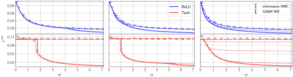<details> <summary>Image 5 Details</summary>  ### Visual Description ## Chart: Comparison of ReLU and Tanh Activation Functions with Different Methods ### Overview The image presents three line charts comparing the performance of ReLU (Rectified Linear Unit) and Tanh (Hyperbolic Tangent) activation functions under different conditions. The charts share the same x-axis, labeled "α", and y-axis, labeled "εopt". Each chart represents a different method (informative HMC and GAMP-RIE). The performance is evaluated based on the error rate, with lower values indicating better performance. ### Components/Axes * **X-axis:** "α" - Ranges from 0 to 7, with tick marks at every integer value. * **Y-axis:** "εopt" - Ranges from 0.02 to 0.08 in the top half of the chart and 0.02 to 0.11 in the bottom half of the chart. * **Legend (Top-Right):** * Blue Line: ReLU * Red Line: Tanh * Informative HMC: Error bars with circles * GAMP-RIE: Error bars with horizontal bars ### Detailed Analysis Each of the three charts displays two sets of curves: one for ReLU (blue) and one for Tanh (red). Each set contains three curves: a solid line, a dashed line, and a dotted line. The solid and dashed lines have error bars. **Chart 1 (Left):** * **ReLU (Blue):** The solid blue line with circular error bars (informative HMC) starts at approximately 0.08 at α=0 and decreases to approximately 0.02 at α=7. The dashed blue line with horizontal error bars (GAMP-RIE) starts at approximately 0.07 at α=0 and decreases to approximately 0.02 at α=7. The dotted blue line starts at approximately 0.06 at α=0 and decreases to approximately 0.02 at α=7. * **Tanh (Red):** The solid red line with circular error bars (informative HMC) starts at approximately 0.11 at α=0, drops sharply to approximately 0.05 at α=1.5, and then decreases to approximately 0.02 at α=7. The dashed red line with horizontal error bars (GAMP-RIE) remains constant at approximately 0.105 from α=0 to α=7. The dotted red line starts at approximately 0.10 at α=0, drops sharply to approximately 0.05 at α=1.5, and then decreases to approximately 0.02 at α=7. **Chart 2 (Middle):** * **ReLU (Blue):** The solid blue line with circular error bars (informative HMC) starts at approximately 0.08 at α=0 and decreases to approximately 0.02 at α=7. The dashed blue line with horizontal error bars (GAMP-RIE) starts at approximately 0.07 at α=0 and decreases to approximately 0.02 at α=7. The dotted blue line starts at approximately 0.06 at α=0 and decreases to approximately 0.02 at α=7. * **Tanh (Red):** The solid red line with circular error bars (informative HMC) starts at approximately 0.11 at α=0, drops sharply to approximately 0.05 at α=1.5, and then decreases to approximately 0.02 at α=7. The dashed red line with horizontal error bars (GAMP-RIE) remains constant at approximately 0.105 from α=0 to α=7. The dotted red line starts at approximately 0.10 at α=0, drops sharply to approximately 0.05 at α=1.5, and then decreases to approximately 0.02 at α=7. **Chart 3 (Right):** * **ReLU (Blue):** The solid blue line with circular error bars (informative HMC) starts at approximately 0.08 at α=0 and decreases to approximately 0.02 at α=7. The dashed blue line with horizontal error bars (GAMP-RIE) starts at approximately 0.07 at α=0 and decreases to approximately 0.02 at α=7. The dotted blue line starts at approximately 0.06 at α=0 and decreases to approximately 0.02 at α=7. * **Tanh (Red):** The solid red line with circular error bars (informative HMC) starts at approximately 0.11 at α=0, drops sharply to approximately 0.05 at α=1.5, and then decreases to approximately 0.02 at α=7. The dashed red line with horizontal error bars (GAMP-RIE) remains constant at approximately 0.105 from α=0 to α=7. The dotted red line starts at approximately 0.10 at α=0, drops sharply to approximately 0.05 at α=1.5, and then decreases to approximately 0.02 at α=7. ### Key Observations * **ReLU Performance:** The ReLU activation function consistently shows a decreasing error rate as α increases across all three charts. * **Tanh Performance:** The Tanh activation function exhibits a sharp drop in error rate around α=1.5 when using the solid line with circular error bars (informative HMC) and the dotted line. The dashed line with horizontal error bars (GAMP-RIE) remains relatively constant. * **Error Bar Placement:** The error bars are placed vertically on the solid and dashed lines. * **Chart Similarity:** The three charts are nearly identical. ### Interpretation The charts suggest that the ReLU activation function generally performs better than the Tanh activation function, especially at lower values of α. The sharp drop in error rate for Tanh around α=1.5 indicates a critical point where the function's behavior changes significantly. The consistent performance of ReLU across different values of α suggests it might be a more stable choice in these scenarios. The dashed line with horizontal error bars (GAMP-RIE) for Tanh shows a constant error rate, indicating that this method might not be as effective for the Tanh activation function. The similarity of the three charts suggests that the underlying conditions being varied between the charts have little impact on the relative performance of ReLU and Tanh. </details> generalisation error of the latter is called Gibbs error : ε Gibbs := E θ 0 , D , x test ⟨ ( λ test ( θ ) -λ 0 test ) 2 ⟩ . At equilibrium, ε Gibbs / 2 = ε opt , see Remark 8 or [98] for a justification based on the Nishimori identities. For the experiments, we use this formula also during sampling. In practice we compute the half Gibbs error as E x test ( λ test ( θ t ) -λ 0 test ) 2 / 2 based on a single sample θ t at time t (per α value and dataset), where E x test is an empirical average over many test inputs (10 4 -10 5 ). When the chains have mixed and the samples are correctly drawn according to the posterior, which is guaranteed for long enough times, this replacement is justified if also assuming the concentration of the square-error w.r.t. θ t onto the Gibbs error, i.e., E x test ( λ test ( θ t ) -λ 0 test ) 2 = E x test ⟨ ( λ test ( θ ) -λ 0 test ) 2 ⟩ + o d (1). This concentration is numerically verified to hold for t sufficiently large. Consequently, our way to evaluate the Bayes error holds at equilibrium for large d . However, out of equilibrium these guarantees are lost. This is a priori an issue given that we will need to evaluate errors in 'metastable states' which are empirically the only reachable ones in polynomial time. Yet, we claim that when probing the error at a metastable state, the relation E θ 0 , D , x test ⟨ ( λ test ( θ ) -λ 0 test ) 2 ⟩ meta / 2 = E θ 0 , D , x test ( ⟨ λ test ( θ ) ⟩ meta -λ 0 test ) 2 , where ⟨ · ⟩ meta means 'sampling at the metastable state', remains valid, but not while dynamically reaching it (where half the error of the one-shot estimator is merely a proxy for the Bayesian one). In other words, a hypothesis we make for the rest of the discussion is that metastable states (if present) 'behave' as the equilibrium for what concerns Nishimori identities and concentration properties, which are the only ones we need to use this relation. This is verified in other Bayes-optimal inference problems [98], and it will be justified a posteriori by the match of the theoretical predictions (which always agree with the Nishi- mori identities) associated with a metastable state and the numerics. One can also build s -shot estimators from HMC samples of (meta)stable states, namely λ test (( θ ( p ) ) p ≤ s ) := 1 s ∑ s p =1 λ test ( θ ( p ) ) where θ ( p ) are HMC samples for long enough times. Assuming, as above, that Nishimori identities hold also at metastable states, and that the generalization error of such an estimator concentrates in ( θ ( p ) ) p ≤ s , i.e. E x test ( λ test (( θ ( p ) ) p ≤ s ) -λ 0 test ) 2 = E θ 0 , D , x test ⟨ ( λ test (( θ ( p ) ) p ≤ s ) -λ 0 test ) 2 ⟩ meta + o d (1), then we can predict the generalization error of an s -shot estimator. It suffices to expand the square in the ⟨ · ⟩ meta in the last expression to find E θ 0 , D , x test ⟨ ( λ test (( θ ( p ) ) p ≤ s ) -λ 0 test ) 2 ⟩ meta = s +1 s E θ 0 , D , x test ( ⟨ λ test ( θ ) ⟩ meta -λ 0 test ) 2 . The latter, for s = 1, indeed yields the correct relation for one-shot estimators. It is also clear that when s becomes larger, and HMC is sampling the equilibrium state, the above is approaching ε opt . As a numerical test of these claims, FIG. 8, 10 and 18 show that the theory (which is 'Nishimori-compliant') captures the HMC error, both for one and s -shot estimators, not only at long times, but also during the earlier plateau it experiences when sampling a metastable state. On top of this evidence, in Appendix A 3 and FIG. 21 we also plot the evolution of a deviation from the Nishimori identities during posterior sampling by HMC. We see that on the states that HMC finds for long enough times, the Nishimori identities are verified, regardless of them being stable, or only metastable. (Algo 3 ) We extended the GAMP-RIE of [94], publicly available at [191], to obtain a polynomial-time predictor for test data in the shallow networks case. Extending this algorithm, initially proposed for quadratic activation, to a generic one is possible thanks to the identification of an effective GLMonto which the learning problem can be mapped, see App. B 4 (the mapping being exact FIG. 6. Theoretical prediction (solid curves) of the Bayesoptimal mean-square generalisation error for L = 1 with binary inner weights and polynomial activations: σ 1 = He 2 / √ 2, σ 2 = He 3 / √ 6, σ 3 = He 2 / √ 2 + He 3 / 6, with γ = 0 . 5 , d = 150 , ∆ = 1 . 25, and quenched homogeneous readouts v = 1 . Dots are the half Gibbs error computed using the MetropolisHastings algorithm initialised informatively. Circles are the error of GAMP-RIE [94] extended to generic activation. Points are averaged over 16 data and teacher instances. Error bars for MCMC are the standard deviation over instances (omitted for GAMP-RIE, but of the same order). Dashed and dotted lines denote, respectively, the universal and specialisation branches where they are metastable. 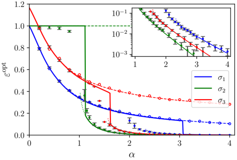<details> <summary>Image 6 Details</summary>  ### Visual Description ## Line Chart: Epsilon Optimal vs. Alpha ### Overview The image contains a line chart showing the relationship between epsilon optimal (εopt) and alpha (α) for three different sigma values (σ1, σ2, σ3). The main chart displays a linear y-axis, while an inset chart in the top-right corner shows the same data with a logarithmic y-axis. The chart includes data points with error bars and fitted curves for each sigma value. ### Components/Axes * **Main Chart:** * **X-axis:** α (alpha), ranging from 0 to 4. * **Y-axis:** εopt (epsilon optimal), ranging from 0.0 to 1.2. * **Legend (bottom-right):** * Blue line: σ1 * Green line: σ2 * Red line: σ3 * **Inset Chart (top-right):** * **X-axis:** α (alpha), ranging from 1 to 4. * **Y-axis:** Logarithmic scale, ranging from 10^-3 to 10^-1. ### Detailed Analysis **Main Chart:** * **σ1 (Blue):** The blue line starts at approximately 1.0 at α = 0 and decreases rapidly until α ≈ 1.0. It then continues to decrease at a slower rate, reaching approximately 0.3 at α = 1.5, and then drops to approximately 0.1 at α = 3.0, remaining relatively constant thereafter. * α = 0: εopt ≈ 1.0 * α = 1.0: εopt ≈ 0.3 * α = 1.5: εopt ≈ 0.2 * α = 3.0: εopt ≈ 0.1 * α = 4.0: εopt ≈ 0.1 * **σ2 (Green):** The green line remains constant at approximately 1.0 from α = 0 to α ≈ 1.0. It then drops sharply to approximately 0.1 at α = 1.2, and continues to decrease to approximately 0.0 at α = 1.5, remaining relatively constant thereafter. * α = 0 to 1.0: εopt ≈ 1.0 * α = 1.2: εopt ≈ 0.1 * α = 1.5: εopt ≈ 0.0 * α = 4.0: εopt ≈ 0.0 * **σ3 (Red):** The red line starts at approximately 1.2 at α = 0 and decreases rapidly until α ≈ 1.5. It then continues to decrease at a slower rate, reaching approximately 0.4 at α = 2.0, and then drops to approximately 0.1 at α = 3.0, remaining relatively constant thereafter. * α = 0: εopt ≈ 1.2 * α = 1.5: εopt ≈ 0.4 * α = 2.0: εopt ≈ 0.3 * α = 3.0: εopt ≈ 0.1 * α = 4.0: εopt ≈ 0.1 **Inset Chart:** * **σ1 (Blue):** The blue line decreases from approximately 0.05 at α = 1.0 to approximately 0.001 at α = 4.0. * **σ2 (Green):** The green line decreases from approximately 0.08 at α = 1.0 to approximately 0.001 at α = 4.0. * **σ3 (Red):** The red line decreases from approximately 0.1 at α = 1.0 to approximately 0.002 at α = 4.0. ### Key Observations * All three sigma values show a decrease in εopt as α increases. * σ2 exhibits a sharp drop in εopt at α ≈ 1.0, while σ1 and σ3 show a more gradual decrease. * The inset chart provides a clearer view of the behavior of εopt at lower values, showing an exponential decay for all three sigma values. * The data points have error bars, indicating the uncertainty in the measurements. ### Interpretation The chart illustrates the relationship between epsilon optimal (εopt) and alpha (α) for different sigma values. The data suggests that as alpha increases, epsilon optimal decreases for all three sigma values. The sharp drop in εopt for σ2 indicates a critical point or threshold behavior, while the more gradual decrease for σ1 and σ3 suggests a more continuous relationship. The inset chart, with its logarithmic y-axis, highlights the exponential decay of εopt as alpha increases, particularly at lower values of εopt. The error bars on the data points indicate the variability or uncertainty in the measurements, which should be considered when interpreting the results. The different sigma values likely represent different experimental conditions or parameters, and the chart allows for a comparison of their effects on the relationship between epsilon optimal and alpha. </details> only when σ ( x ) = x 2 , [94]). The key observation is that our effective GLM representation holds not only from a theoretical perspective when describing the universal phase, but also algorithmically. The GAMP-RIE is P W -independent as it exploits only the asymptotic spectral law of W 0 ⊺ diag( v 0 ) W 0 , which is the same for Gaussian or binary weight matrices by spectral universality [192]. It is therefore in general sub-optimal. In order to evaluate the generalisation error of GAMP-RIE in the experiments, we plug the estimator (B75) in (8). (Algo 4 ) We also test the standard Python implementation of the ADAM optimiser [193] initialised uninformatively for Gaussian teacher weights. The generalisation error for ADAM for a given training set is evaluated as E x test ( λ test ( θ t ) -λ 0 test ) 2 using parameters θ t obtained by training a student network through empirical risk minimisation with non-regularised cost function C ( θ ) = 1 n ∑ µ ≤ n ( λ µ ( θ ) -y µ ) 2 . Adding weight decay does not change the global picture. Notice that in contrast with the Monte Carlo algorithms where the Gibbs error (divided by 2) is a computationally simpler way to access their mean-square generalisation error, the error of ADAM is not divided by two because it provides a oneshot estimator and is used as such for predictions. The codes needed to reproduce our experiments are accessible online [172]. ## A. Shallow MLP Generalisation error and specialisation transition. Starting with the shallow case, in FIG. 5 and 6 we report the theoretical generalisation errors from Result 2 for both the universal and specialisation solutions. FIG. 5 considers networks with Gaussian inner weights sampled with informatively initialised HMC in order to focus on the specialisation solution. Tests with uninformative initialisation are discussed later on. Experiments and theory show that HMC initialised close to the target precisely follows the theoretical specialisation solution ε sp (which is not always the equilibrium). In contrast, GAMP-RIE's generalisation error follows the universal branch of the theory ε uni . It can actually be shown analytically that it is the case when d →∞ . An interesting observation is that non-homogeneous readouts trigger the appearance of the specialisation transition earlier and shrink the region where the equilibrium solution coexist with a metastable one (dotted line). In the case of 4point prior (middle panel), we see two partial specialisation transitions as defined in (12). The first corresponds to the specialisation of the neurons connected to readouts with the largest amplitude only, and thus yields a greater improvement in the error than the second. With continuous readouts (right panel), we notice two differences. First, the equilibrium always corresponds to the solution with smallest error, which suggests a simpler learning problem than with discrete readouts; this theoretical observation is supported by experimental findings in App. B5. Second, the specialisation transitions are now infinitely many and the equilibrium corresponds to the envelope of all the associated solutions. In the figure we show three of them. FIG. 6 concerns networks with Rademacher inner weights. The numerical points are of two kinds: the dots, obtained from Metropolis-Hastings sampling, and the circles for the GAMP-RIE. We report analogous simulations for ReLU and ELU activations in FIG. 24, App. B 4. Notice an important thing here: although our theoretical framework presented in Sec. IV uses the HCIZ integral, which relies on the strict rotational invariance of the matrices involved, it is able to accommodate any prior on the weights. It is thus able to deal with non-rotationally invariant matrices, as in the case of Rademacher weights. In the two considered set-ups (Gaussian P W of FIG. 5 and Rademacher of FIG. 6), when data are scarce, α < α sp , the student cannot break the numerous symmetries of the problem, resulting in an 'effective rotational invariance' at the source of the prior universality of the free entropy and OPs, with posterior samples having a vanishing overlap with W 0 . In this universal phase , feature learning occurs because the student tunes its weights to match a quadratic approximation of the teacher, rather than aligning to those weights themselves. This phase is universal in the law of the i.i.d. teacher inner weights (centred, with unit variance): our numerics obtained both with binary and Gaussian inner weights match well the FIG. 7. Theoretical prediction (solid curves) for the equilibrium overlaps as function of the sampling ratio α for L = 1 with Gaussian inner weights, d = 200 , γ = 0 . 5 , ∆ = 0 . 1. The empirical crossed curves were obtained from informed HMC using a single posterior sample W (per α and data instance), and shaded regions around them correspond to one standard deviation w.r.t. to data instances. Top : σ ( x ) = tanh(2 x ) and 4-point readouts, and average over 12 instances of the data. Bottom : σ ( x ) = ReLU( x ) and Gaussian readouts. Q ( v ) is evaluated numerically by dividing the interval [ -2 , 2] into bins and then computing the value of the overlap associated to the readout value in that bin. We averaged over 100 data instances. Readouts are fixed to v 0 . 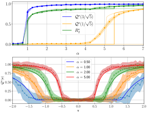<details> <summary>Image 7 Details</summary>  ### Visual Description ## Line Charts: Phase Transition Behavior ### Overview The image contains two line charts that depict phase transition behavior. The top chart shows the relationship between 'α' and three different quantities: Q*(3/√5), Q*(1/√5), and R₂*. The bottom chart shows the relationship between 'v' and Q*(v) for different values of 'α'. Both charts include shaded regions around the lines, representing uncertainty or variance. ### Components/Axes **Top Chart:** * **X-axis:** α (alpha), ranging from 0 to 7. Axis markers are present at every integer value. * **Y-axis:** No label, but the values range from 0 to 1.0. Axis markers are present at 0.0, 0.5, and 1.0. * **Legend (Top-Right):** * Blue: Q*(3/√5) * Orange: Q*(1/√5) * Green: R₂* **Bottom Chart:** * **X-axis:** v (nu), ranging from -2.0 to 2.0. Axis markers are present at every 0.5 interval. * **Y-axis:** Q*(v), ranging from 0.00 to 1.00. Axis markers are present at 0.00, 0.25, 0.50, 0.75, and 1.00. * **Legend (Top-Left):** * Blue: α = 0.50 * Orange: α = 1.00 * Green: α = 2.00 * Red: α = 5.00 ### Detailed Analysis **Top Chart:** * **Blue Line (Q*(3/√5)):** Starts near 0 at α=0, rapidly increases to approximately 0.95 around α=1, and then plateaus around 1.0 for α > 1. The line is marked with square data points. * **Orange Line (Q*(1/√5)):** Stays near 0 until approximately α=5, then rapidly increases to approximately 0.9 around α=6, and then plateaus around 1.0 for α > 6. The line is marked with circle data points. * **Green Line (R₂*):** Starts near 0 at α=0, rapidly increases to approximately 0.7 around α=1, and then gradually increases to approximately 0.9 for α > 1. The line is marked with triangle data points. **Bottom Chart:** * **Blue Line (α = 0.50):** Starts around 0.6 at v=-2.0, decreases to approximately 0 around v=0, and then increases back to approximately 0.6 at v=2.0. The line is marked with 'x' data points. * **Orange Line (α = 1.00):** Starts around 0.9 at v=-2.0, decreases to approximately 0 around v=0, and then increases back to approximately 0.9 at v=2.0. The line is marked with '+' data points. * **Green Line (α = 2.00):** Starts around 0.95 at v=-2.0, decreases to approximately 0 around v=0, and then increases back to approximately 0.95 at v=2.0. The line is marked with '+' data points. * **Red Line (α = 5.00):** Starts around 1.0 at v=-2.0, decreases to approximately 0 around v=0, and then increases back to approximately 1.0 at v=2.0. The line is marked with 'x' data points. ### Key Observations * In the top chart, Q*(3/√5) transitions much earlier (lower α) than Q*(1/√5). * R₂* has a more gradual transition compared to Q*(3/√5). * In the bottom chart, as α increases, the Q*(v) curves become steeper around v=0. * The minimum value of Q*(v) is always near 0, regardless of α. * The shaded regions indicate the variability or uncertainty in the data. ### Interpretation The charts likely represent phase transitions in a physical or computational system. The top chart shows how different order parameters (Q*(3/√5), Q*(1/√5), and R₂*) change as a function of a control parameter α. The bottom chart shows the behavior of Q*(v) as a function of 'v' for different values of α. The data suggests that the system undergoes a phase transition around α=1, where Q*(3/√5) and R₂* become non-zero. Another phase transition occurs around α=5, where Q*(1/√5) becomes non-zero. The bottom chart shows that as α increases, the system becomes more ordered, as indicated by the steeper Q*(v) curves. The fact that Q*(v) always reaches a minimum near 0 suggests that there is always some degree of disorder in the system. The shaded regions around the lines indicate that there is some variability or uncertainty in the data, which could be due to finite-size effects, noise, or other factors. </details> theory. This phase is superseded at α sp by a specialisation phase where the prior P W matters. There, a finite fraction of the student weights aligns with the teacher's, which lowers the generalisation error. The phenomenology depends on the activation function due to the following reason. Recall the interpretation in terms of a tensor inference problem discussed in Sec. I B, in particular that before the specialisation, components in the Hermite expansion of the target beyond the first two play the role of effective noise when learning. Only with α > α sp the student can realise that they are informative and exploit them. Consequently, for odd activation (tanh in FIG. 5, σ 2 in FIG. 6), where µ 2 = 0, we observe that the generalisation error is constant for α < α sp , whereas at the phase transition it suddenly drops. This is because the learning of the second component is skipped entirely, and the only way to perform better is to learn all terms jointly through specialisation. We emphasise that our theory is consistent with [106], which considers the simpler regime of strong overparametrisation n = Θ( d ) rather than the interpolation one n = Θ( d 2 ): our generalisation curves at α → 0 match theirs at α 1 := n/d → + ∞ , which is when the student learns perfectly the linear component v 0 ⊺ W 0 of the target but nothing more. This is also the best a network can do in the quadratic data regime when µ 2 = 0 if it does not specialise. Order parameters and learning mechanisms. FIG. 7 reveals sequences of phase transitions in α . The top panel shows the evolution of the two relevant overlaps Q ∗ ( v ) in the case of readouts with discrete values: as α increases, the student weights start aligning with the target weights with highest readout amplitude, marking the first phase transition. At the same time R ∗ 2 jumps, indicating that learning of the quadratic term of the target occurs concurrently. As these alignments strengthen, the last transition occurs when the weights corresponding to the next largest readout amplitude are learnt. We see the (relatively small) effect of this latter transition also at the level of the generalisation error, see red middle curve in FIG. 5 at α ≈ 5. Through the same mechanism, continuous readouts produce an infinite sequence of learning transitions in the limit (4), as supported by the lower part of FIG. 7 for Gaussian readouts. From these observations, we conclude that the readout amplitudes | v j | , controlling the strength with which the responses ( y µ ) depend on feature (neuron) W 0 j , play the role of an SNR. Algorithmic hardness of specialising, and ADAM as an approximate Bayesian sampler. Even when dominating the posterior measure, the specialisation solution can be algorithmically hard to reach. With discrete readouts, simulations for binary inner weights exhibit specialisation only when sampling with informative initialisation. Moreover, even in cases where algorithms (such as ADAM or HMC for Gaussian inner weights) are able to find the specialisation solution, they manage to do so only after a training time increasing exponentially with d . For the continuous distribution P v = N (0 , 1), our tests are inconclusive on hardness and deserve numerical investigation at a larger scale. We refer to App. B 5 for a detailed discussion and systematic tests. As an illustration of the conclusions reached in this appendix, FIG. 8 and FIG. 9 display the evolution of the generalisation error reached with HMC and ADAM, respectively (recall that for HMC we plot the half Gibbs error proxy). FIG. 8 shows that HMC, for a discrete readout prior, converges fast to the universal solution where it is abruptly stopped (for d large), before very slowly approaching the specialisation solution. The time it takes to escape the plateau scales exponentially with the dimension, meaning that improving upon ε uni is hard given quadratically many data. The behaviour is the same for both ReLU( x ) and tanh(2 x ) activations. We observe the same phenomenology when the teacher's inner weights are drawn from a binary distribution while HMC sampling wrongly assumes a Gaussian prior, indicating prior universality of the metastable state. Concerning ADAM, FIG. 9, the picture remains globally the same: an initial fast convergence followed by a long plateau before a slow descent toward a closeto-specialisation solution (the precise analysis of where ADAM lands in this case and its associated generalisation error is out of the scope of the paper). In the case of σ = ReLU (top panel) and homogeneous readouts the plateau is at 2 ε uni . It takes again exponentially many FIG. 8. Half Gibbs error of HMC from random initialisation as a function of the number of updates for various d with L = 1 and Gaussian inner weights. The errors are averaged over 10 data instances and shaded regions represent one standard deviation. The black dashed line corresponds to the error associated with the universal solution while the red corresponds to the specialised solution. Top: σ ( x ) = ReLU( x ) , α = 3 . 0 , γ = 0 . 5 , ∆ = 0 . 1 and 4-point quenched readouts. Bottom: σ ( x ) = tanh(2 x ) , α = 2 . 5 , γ = 0 . 5 , ∆ = 0 . 1 and homogeneous quenched readouts. For both activations, larger d lead to an important slowing down of the convergence towards the specialised solution happening precisely when crossing the error predicted by the universal solution ε uni of the theory. 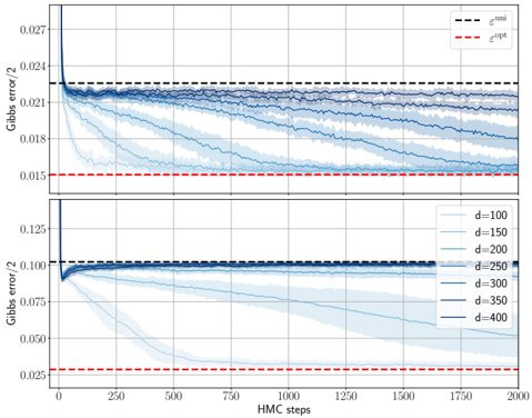<details> <summary>Image 8 Details</summary>  ### Visual Description ## Chart: Gibbs Error vs. HMC Steps for Varying Dimensions ### Overview The image presents two line charts, one above the other, displaying the Gibbs error/2 as a function of HMC (Hamiltonian Monte Carlo) steps. The charts illustrate how the error changes with increasing HMC steps for different dimensions (d). The top chart shows the error for lower dimensions, while the bottom chart shows the error for higher dimensions. Both charts include horizontal dashed lines representing epsilon_bnn and epsilon_opt. ### Components/Axes * **Y-axis (Left):** Gibbs error/2. The top chart ranges from approximately 0.015 to 0.027. The bottom chart ranges from approximately 0.025 to 0.125. * **X-axis (Bottom):** HMC steps, ranging from 0 to 2000. * **Horizontal Dashed Lines:** * Black dashed line: epsilon_bnn (approximately 0.023 in the top chart and 0.10 in the bottom chart). * Red dashed line: epsilon_opt (approximately 0.015 in the top chart and 0.028 in the bottom chart). * **Legend (Right, between the two charts):** * d=100 (lightest blue) * d=150 (lighter blue) * d=200 (mid-light blue) * d=250 (mid-dark blue) * d=300 (dark blue) * d=350 (darker blue) * d=400 (darkest blue) ### Detailed Analysis **Top Chart (Lower Dimensions):** * **d=100 (lightest blue):** Starts at approximately 0.024 and decreases rapidly, then slowly converges towards 0.018. * **d=150 (lighter blue):** Starts at approximately 0.024 and decreases, converging towards 0.020. * **d=200 (mid-light blue):** Starts at approximately 0.024 and decreases slightly, converging towards 0.021. * **d=250 (mid-dark blue):** Starts at approximately 0.024 and remains relatively stable, fluctuating around 0.022. * **d=300 (dark blue):** Starts at approximately 0.024 and remains relatively stable, fluctuating around 0.022. * **d=350 (darker blue):** Starts at approximately 0.024 and remains relatively stable, fluctuating around 0.022. * **d=400 (darkest blue):** Starts at approximately 0.024 and remains relatively stable, fluctuating around 0.022. **Bottom Chart (Higher Dimensions):** * **d=100 (lightest blue):** Starts at approximately 0.125 and decreases rapidly, then slowly converges towards 0.05. * **d=150 (lighter blue):** Starts at approximately 0.125 and decreases rapidly, then slowly converges towards 0.075. * **d=200 (mid-light blue):** Starts at approximately 0.125 and decreases rapidly, then slowly converges towards 0.0875. * **d=250 (mid-dark blue):** Starts at approximately 0.125 and decreases rapidly, then slowly converges towards 0.09375. * **d=300 (dark blue):** Starts at approximately 0.125 and decreases rapidly, then slowly converges towards 0.096875. * **d=350 (darker blue):** Starts at approximately 0.125 and decreases rapidly, then slowly converges towards 0.0984375. * **d=400 (darkest blue):** Starts at approximately 0.125 and decreases rapidly, then slowly converges towards 0.10. ### Key Observations * For lower dimensions (top chart), the Gibbs error/2 converges to lower values compared to higher dimensions (bottom chart). * As the dimension (d) increases, the initial Gibbs error/2 in the bottom chart is higher, and the convergence is slower. * The black dashed line (epsilon_bnn) represents a threshold, and the error for higher dimensions in the bottom chart tends to stay close to or above this threshold. * The red dashed line (epsilon_opt) represents an optimal error level, which the error curves approach but do not consistently reach, especially for higher dimensions. ### Interpretation The charts illustrate the relationship between the Gibbs error, HMC steps, and dimensionality. The data suggests that as the dimensionality increases, the Gibbs error tends to be higher and the convergence to a lower error value requires more HMC steps. The epsilon_bnn and epsilon_opt lines provide benchmarks for evaluating the performance of the HMC algorithm under different dimensionalities. The fact that the error for higher dimensions remains close to or above epsilon_bnn suggests that achieving optimal performance becomes more challenging as the dimensionality increases. The shaded regions around the lines likely represent the variance or uncertainty in the Gibbs error estimates. </details> updates to escape it. ADAM thus reaches precisely the same error as the Gibbs error of HMC, i.e., when also using HMC as a one-shot estimator. This suggests that ADAM is essentially sampling the posterior the best it can given only a polynomial-ind number of updates, and ends up in a similar metastable state as HMC. The same observation was made for pure gradient-descent in the special case of one hidden layer with quadratic activation [94]. Our observations contribute in a quantitatively precise manner, and in a rather general NN model, to the recent line of works on 'stochastic gradient descent behaves as a Bayes sampler' [194-197] but for ADAM. There is however one major difference compared to HMC in the case of σ ( x ) = tanh(2 x ) (bottom panel): ADAM plateaus close to ε uni , not twice this value. By calling θ algorithm a sample from that algorithm, this means that the ADAM one-shot estimator λ test ( θ ADAM ) performs almost as a Bayesian, ensemble-averaged estimator ⟨ λ test ( θ HMC ) ⟩ meta sampling the metastable state. The performance of the latter is what we conjecture to be the best achievable in polynomial time. Notice instead that HMC, when also used as a one-shot estimator, does not perform as well (see again FIG. 8, bottom panel). This is at odds with the ReLU case, where ADAM and one-shot HMC were comparable, and both worse than the Bayesian estimator. We believe that these different behaviours are a con- FIG. 9. Generalisation error of ADAM from random initialisation as a function of the gradient updates for various d with L = 1 and Gaussian inner weights. The initial learning rate is 0 . 01 and batch size ⌊ n/ 4 ⌋ . The error is averaged over 10 data instances and shaded regions represent one standard deviation and computed empirically from 10 4 i.i.d. test samples. In both plots α = 5 . 0 , γ = 0 . 5 , ∆ = 10 -4 , the target readouts are homogeneous while the student has learnable readouts. Top: σ ( x ) = ReLU( x ). The error plateaus at the purple dashed line corresponding to twice the error associated with the universal solution of the theory ε uni . Bottom: σ ( x ) = tanh(2 x ). The error plateaus at the black dashed line corresponding to the universal solution. The number of gradient updates necessary to improve upon the universal solution (or twice its value) grows exponentially with d , see App. B 5. 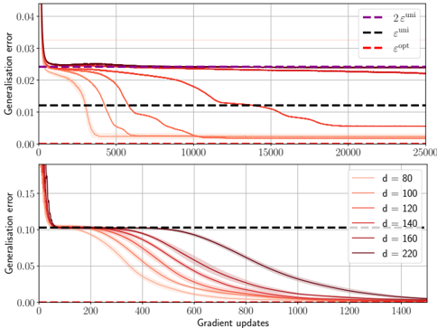<details> <summary>Image 9 Details</summary>  ### Visual Description ## Generalization Error vs. Gradient Updates Chart ### Overview The image contains two line charts displaying the generalization error as a function of gradient updates. The top chart shows the generalization error for different theoretical bounds, while the bottom chart shows the generalization error for different values of 'd' (likely representing model complexity or dimensionality). ### Components/Axes **Top Chart:** * **Y-axis:** Generalisation error, ranging from 0.00 to 0.04. * **X-axis:** Gradient updates, ranging from 0 to 25000. * **Legend (Top-Right):** * Purple dashed line: "2 ε<sup>uni</sup>" * Black dashed line: "ε<sup>uni</sup>" * Red dashed line: "ε<sup>opt</sup>" **Bottom Chart:** * **Y-axis:** Generalisation error, ranging from 0.00 to 0.15. * **X-axis:** Gradient updates, ranging from 0 to 1400. * **Legend (Right):** * Light red line: d = 80 * Red line: d = 100 * Dark red line: d = 120 * Gray dashed line: d = 140 * Light gray line: d = 160 * Dark gray line: d = 220 ### Detailed Analysis **Top Chart:** * **2 ε<sup>uni</sup> (Purple Dashed):** A horizontal line at approximately 0.024, indicating a constant error bound. * **ε<sup>uni</sup> (Black Dashed):** A horizontal line at approximately 0.012, indicating a constant error bound. * **ε<sup>opt</sup> (Red Dashed):** Starts at approximately 0.04, rapidly decreases to approximately 0.024, then gradually decreases to approximately 0.002. **Bottom Chart:** * **d = 80 (Light Red):** Starts at approximately 0.15, decreases to approximately 0.00 after about 600 gradient updates. * **d = 100 (Red):** Starts at approximately 0.15, decreases to approximately 0.00 after about 700 gradient updates. * **d = 120 (Dark Red):** Starts at approximately 0.15, decreases to approximately 0.00 after about 800 gradient updates. * **d = 140 (Gray Dashed):** Starts at approximately 0.15, decreases to approximately 0.00 after about 900 gradient updates. * **d = 160 (Light Gray):** Starts at approximately 0.15, decreases to approximately 0.00 after about 1000 gradient updates. * **d = 220 (Dark Gray):** Starts at approximately 0.15, decreases to approximately 0.00 after about 1200 gradient updates. ### Key Observations * In the top chart, the theoretical error bounds (2 ε<sup>uni</sup> and ε<sup>uni</sup>) remain constant, while the optimized error (ε<sup>opt</sup>) decreases with gradient updates. * In the bottom chart, as the value of 'd' increases, the number of gradient updates required to reach a generalization error of approximately 0.00 also increases. ### Interpretation The top chart illustrates the difference between theoretical error bounds and the actual optimized error during training. The constant theoretical bounds suggest a fixed upper limit on the error, while the decreasing optimized error shows the model's learning progress. The bottom chart demonstrates the impact of model complexity ('d') on the training process. Higher values of 'd' (more complex models) require more gradient updates to achieve a similar level of generalization error. This suggests that more complex models may need more training data or iterations to converge to an optimal solution. The trend indicates a trade-off between model complexity and training efficiency. </details> ̸ sequence of the fact that µ 2 = 0 for ReLU, while it is vanishing for tanh, a crucial element also in our replica analysis of Sec. IV. Indeed, with no 2nd component in the activation the theory predicts the linear term as the only one learnable without specialising. Thus, the nonspecialised NN effectively behaves as a linear model trying to fit a noisy linear target. In this respect, the picture is similar to what happens in the proportional regime n = Θ( d ), where the mapping to a GLM is known to hold in the whole phase diagram [106-108]: in [106], it is shown that optimisers, such as optimally regularised ridge regression, achieve the performance of the Bayes estimator. Here we observe that the picture changes with n = Θ( d 2 ) when also the quadratic term is present, as in the top panel of FIG. 9. A gap between the performance of optimisers and Bayesian estimators has been recently shown in [96] limited to purely quadratic activation, and requires future investigation in our more general setting. In FIG. 10, we show the impact of overparameterisation with respect to the target function in ADAM. This figure refers to a setting where L = 1 and the number of hidden units for the target is fixed to 100. K in the left panel is instead the number of hidden neurons of the (possibly mismatched) student. In the right panel we show the performance that an HMC sampler would attain with s -shot estimator. Both plots display gen- FIG. 10. Generalisation error of different estimators, initialised randomly, as a function of the number of gradient updates or HMC steps. The errors are averaged over 10 data instances and shaded regions represent one standard deviation. The black and purple dashed lines correspond, respectively, to the error associated with the universal solution and twice the universal solution, while the red dashed line corresponds to the specialised solution. The dashed lines between the black and purple lines indicate the universal performance of s -shot estimators, which is simply [( s +1) /s ] ε uni , see Remark 5. In both panels σ ( x ) = ReLU( x ) , α = 4 . 0 , γ = 0 . 5 , ∆ = 0 . 03, d = 200 and readouts are homogeneous. The number of hidden units of the teacher is k = 100. Left : Generalisation error of an overparametrised student trained with ADAM as a function of gradient updates; the readouts are learnable during training. K represents the width of the possibly mismatched student. Right : Generalisation error of an s -shot estimator, obtained averaging the output of s posterior HMC samples, as a function of HMC steps; the readouts are fixed during sampling. 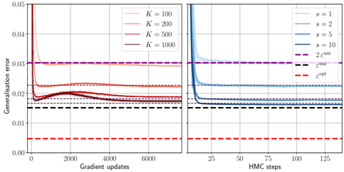<details> <summary>Image 10 Details</summary>  ### Visual Description ## Chart Type: Comparative Line Graphs ### Overview The image presents two line graphs side-by-side, comparing the generalization error of different models. The left graph shows the error as a function of gradient updates, with different lines representing different values of 'K'. The right graph shows the error as a function of HMC steps, with different lines representing different values of 's'. Both graphs also include horizontal dashed lines representing "2 ε<sup>uni</sup>" and "ε<sup>opt</sup>". ### Components/Axes **Left Graph:** * **X-axis:** "Gradient updates", ranging from 0 to 6000. * **Y-axis:** "Generalisation error", ranging from 0.00 to 0.05. * **Legend (top-right):** * K = 100 (light red) * K = 200 (red) * K = 500 (dark red) * K = 1000 (dark brown) **Right Graph:** * **X-axis:** "HMC steps", ranging from 0 to 125. * **Y-axis:** "Generalisation error", ranging from 0.00 to 0.05. * **Legend (top-right):** * s = 1 (light blue) * s = 2 (blue) * s = 5 (dark blue) * s = 10 (dark grey-blue) **Shared Elements:** * **Horizontal Dashed Lines:** * 2 ε<sup>uni</sup> (purple, dashed) - Located at approximately y = 0.03 on both graphs. * ε<sup>opt</sup> (red, dashed) - Located at approximately y = 0.005 on both graphs. * ε<sup>opt</sup> (black, dashed) - Located at approximately y = 0.015 on both graphs. ### Detailed Analysis **Left Graph (Gradient Updates):** * **K = 100 (light red):** Starts at approximately 0.05, rapidly decreases to approximately 0.02, then slightly increases and stabilizes around 0.021 after 2000 gradient updates. * **K = 200 (red):** Starts at approximately 0.05, rapidly decreases to approximately 0.02, then slightly increases and stabilizes around 0.020 after 2000 gradient updates. * **K = 500 (dark red):** Starts at approximately 0.05, rapidly decreases to approximately 0.018, then slightly increases and stabilizes around 0.019 after 2000 gradient updates. * **K = 1000 (dark brown):** Starts at approximately 0.05, rapidly decreases to approximately 0.017, then slightly increases and stabilizes around 0.018 after 2000 gradient updates. **Right Graph (HMC Steps):** * **s = 1 (light blue):** Starts at approximately 0.045, rapidly decreases to approximately 0.018, and stabilizes around 0.018 after 25 HMC steps. * **s = 2 (blue):** Starts at approximately 0.04, rapidly decreases to approximately 0.016, and stabilizes around 0.016 after 25 HMC steps. * **s = 5 (dark blue):** Starts at approximately 0.035, rapidly decreases to approximately 0.015, and stabilizes around 0.015 after 25 HMC steps. * **s = 10 (dark grey-blue):** Starts at approximately 0.03, rapidly decreases to approximately 0.014, and stabilizes around 0.014 after 25 HMC steps. ### Key Observations * In both graphs, the generalization error decreases rapidly in the initial steps (gradient updates or HMC steps) and then stabilizes. * Higher values of 'K' (left graph) generally lead to lower generalization errors. * Higher values of 's' (right graph) generally lead to lower generalization errors. * The "2 ε<sup>uni</sup>" line represents an upper bound for the generalization error in both cases. * The "ε<sup>opt</sup>" line represents a lower bound for the generalization error in both cases. ### Interpretation The graphs illustrate the convergence behavior of different models during training. The left graph suggests that increasing 'K' (likely a parameter related to model complexity or data representation) improves the generalization performance, up to a point. The right graph suggests that increasing 's' (likely a parameter related to the sampling method) also improves generalization performance. The dashed lines provide benchmarks for the error, with "2 ε<sup>uni</sup>" representing a theoretical upper bound and "ε<sup>opt</sup>" representing an optimal error level. The fact that the error curves approach but do not consistently fall below "ε<sup>opt</sup>" suggests that there may be limitations to the models or training procedures used. The rapid initial decrease in error indicates efficient learning in the early stages of training. </details> eralisation errors for the ReLU activation. The dashed lines correspond to the theoretical predictions for s -shot estimators as discussed in Remark 5. As we can see, overparameterised students are able to reach, with ADAM, the same performance predicted with an s -shot estimator produced via HMC. There is an intuitive reason for this: when the student has, say, K = 500 hidden units, which means 5 times more than the target, then ADAM is somehow picking 5 sets of weights which, when combined via the readouts, yield the performance of a 5-shot estimator. This suggests that ADAM is effectively 'sampling' s = 5 i.i.d. configurations from the metastable state; this aligns with the results of [194-197]. This experiment shows that introducing overparameterisation can help to reduce the generalisation error to ε uni in polynomial time with ADAM, even when matched students would get stuck at 2 ε uni . However, the specialisation value remains out of reach in polynomial time according to this picture. In summary, these experiments show a clear timescale separation between the universal solution (or twice the universal solution) reachable in polynomial time and the specialisation solution requiring exponential time (when it corresponds to the equilibrium). The sub-optimal solution is due to the presence of an attractive metastable state experienced by both algorithms. Moreover, ADAM behaves similarly to a Bayesian sampler like HMC. FIG. 11. Theoretical prediction for the Bayes-optimal meansquare generalisation error for L = 1 with fixed Gaussian readouts, Gaussian inner weights, structured inputs drawn from N ( 0 , C ), where C = W 0 W ⊺ 0 /d 0 , where W 0 ∈ R d × d 0 is a Gaussian matrix, tanh(2 x ) activation, d = 150 , γ = 0 . 5 , ∆ = 0 . 1. The dotted line shows the theoretical result for standard Gaussian inputs, with the other settings unchanged. Experimental points are obtained with informative HMC, by averaging over 9 instances of data, with error bars representing the standard deviation. As the ratio d 0 /d grows, the data become less structured and the theoretical curve rapidly approach that of standard Gaussian input. 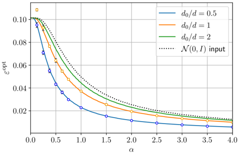<details> <summary>Image 11 Details</summary>  ### Visual Description ## Line Chart: Epsilon Opt vs. Alpha ### Overview The image is a line chart displaying the relationship between epsilon opt (εopt) on the y-axis and alpha (α) on the x-axis for different values of d0/d. There are four data series represented by different colored lines: blue (d0/d = 0.5), orange (d0/d = 1), green (d0/d = 2), and a black dotted line representing N(0, I) input. The chart shows how epsilon opt decreases as alpha increases for each value of d0/d. ### Components/Axes * **X-axis:** α (alpha), ranging from 0.0 to 4.0 in increments of 0.5. * **Y-axis:** εopt (epsilon opt), ranging from 0.00 to 0.10 in increments of 0.02. * **Legend (Top-Right):** * Blue line: d0/d = 0.5 * Orange line: d0/d = 1 * Green line: d0/d = 2 * Black dotted line: N(0, I) input ### Detailed Analysis * **Blue Line (d0/d = 0.5):** This line starts at approximately 0.10 at α = 0.0 and decreases rapidly initially, then plateaus as α increases. Data points are marked with blue circles. * α = 0.0, εopt ≈ 0.10 * α = 0.5, εopt ≈ 0.04 * α = 1.0, εopt ≈ 0.028 * α = 1.5, εopt ≈ 0.02 * α = 2.0, εopt ≈ 0.015 * α = 2.5, εopt ≈ 0.012 * α = 3.0, εopt ≈ 0.01 * α = 3.5, εopt ≈ 0.008 * α = 4.0, εopt ≈ 0.007 * **Orange Line (d0/d = 1):** This line also starts near 0.10 at α = 0.0 and decreases, but at a slower rate than the blue line. Data points are marked with orange squares. * α = 0.0, εopt ≈ 0.10 * α = 0.5, εopt ≈ 0.065 * α = 1.0, εopt ≈ 0.04 * α = 1.5, εopt ≈ 0.03 * α = 2.0, εopt ≈ 0.023 * α = 2.5, εopt ≈ 0.019 * α = 3.0, εopt ≈ 0.016 * α = 3.5, εopt ≈ 0.014 * α = 4.0, εopt ≈ 0.012 * **Green Line (d0/d = 2):** This line starts near 0.10 at α = 0.0 and decreases, but at a slower rate than the orange line. * α = 0.0, εopt ≈ 0.10 * α = 0.5, εopt ≈ 0.08 * α = 1.0, εopt ≈ 0.055 * α = 1.5, εopt ≈ 0.04 * α = 2.0, εopt ≈ 0.03 * α = 2.5, εopt ≈ 0.025 * α = 3.0, εopt ≈ 0.021 * α = 3.5, εopt ≈ 0.018 * α = 4.0, εopt ≈ 0.016 * **Black Dotted Line (N(0, I) input):** This line starts near 0.10 at α = 0.0 and decreases, with a rate between the orange and green lines. * α = 0.0, εopt ≈ 0.10 * α = 0.5, εopt ≈ 0.085 * α = 1.0, εopt ≈ 0.06 * α = 1.5, εopt ≈ 0.045 * α = 2.0, εopt ≈ 0.035 * α = 2.5, εopt ≈ 0.028 * α = 3.0, εopt ≈ 0.023 * α = 3.5, εopt ≈ 0.019 * α = 4.0, εopt ≈ 0.016 ### Key Observations * As alpha (α) increases, epsilon opt (εopt) decreases for all values of d0/d. * The rate of decrease in epsilon opt is highest for the blue line (d0/d = 0.5) and lowest for the green line (d0/d = 2). * The black dotted line (N(0, I) input) falls between the orange (d0/d = 1) and green (d0/d = 2) lines. * All lines converge towards a similar, low value of epsilon opt as alpha increases towards 4.0. ### Interpretation The chart illustrates the relationship between alpha (α) and epsilon opt (εopt) for different ratios of d0/d. The data suggests that a smaller d0/d ratio (e.g., 0.5) results in a faster decrease in epsilon opt as alpha increases, indicating a potentially more efficient or sensitive system in this parameter range. Conversely, a larger d0/d ratio (e.g., 2) leads to a slower decrease in epsilon opt, suggesting a less sensitive system. The N(0, I) input serves as a reference, showing a performance level between d0/d = 1 and d0/d = 2. The convergence of all lines at higher alpha values indicates that the impact of d0/d diminishes as alpha becomes sufficiently large. </details> Structured data. Let us consider structured data where the input distribution is different from the standard Gaussian. The most basic example of this is Gaussian inputs with covariance C . In this case, the model can be transformed into one with standard Gaussian inputs at the cost of losing independence among entries within the same row W . Indeed, by writing x µ = C 1 / 2 ˜ x µ , where ˜ x µ ∼ N ( 0 , I d ), the model can be viewed as having ˜ x µ as input and ˜ W = WC 1 / 2 as first layer weights. The weight matrix ˜ W has independent rows but dependent entries within the same row. With this relaxed condition, where ˜ W 's rows are independent and follow a law P w in R d , for activations that have zero second Hermite coefficient, Result 1 still holds, with the only modification being the replacement of the scalar free entropy function ψ P W by its vector version: $$\begin{array} { r l } { e \cdot } & \lim _ { d \rightarrow \infty } \frac { 1 } { d } \mathbb { E } _ { w ^ { 0 } , \xi } \ln \mathbb { E } _ { w } e ^ { - \frac { 1 } { 2 } x \| w \| ^ { 2 } + x w ^ { T } w ^ { 0 } + \sqrt { x } \, \xi ^ { T } w } \quad ( 2 1 ) } \end{array}$$ where w , w 0 are i.i.d. from P w in R d and ξ ∼ N ( 0 , I d ). This is evident from the replica computation, where the i.i.d. assumption on the weights is required in equation (B23) to factorise the integral over the weights, yielding the log-integral term that later becomes the scalar free entropy. If dependencies within the same row are allowed, the factorisation can only be performed over the rows, yielding the free entropy (21). For activations with a non-zero second Hermite coefficient, analysing the model with structured data is an open problem. Even for N (0 , C ) input, the task requires solving a denoising problem for the matrix C 1 / 2 W ⊺ diag( v ) WC 1 / 2 , which is FIG. 12. Top: Theoretical prediction of the optimal meansquare generalisation error for non-Gaussian data. The inputs are taken from the MNIST image dataset or as the outputs of one layer of another NN fed with standard Gaussian vectors (synthetic data). More precisely, the synthetic data is generated as x µ = σ 0 ( W (0) x (0) µ / √ d 0 ) where W (0) ∈ R d × d 0 is a Gaussian matrix with d 0 /d = 0 . 5 , x (0) µ ∼ N ( 0 , I d 0 ) , σ 0 ( x ) = (ReLU( x ) -µ 0 ) /c 0 where µ 0 is the 0-th Hermite coefficient of ReLU( x ) and c 0 enforces E z ∼N (0 , 1) σ 0 ( z ) 2 = 1. ( x µ ) are then passed through the random MLP target with L = 1 , σ ( x ) = tanh(2 x ) , γ = 0 . 5 and Gaussian weights (inner and readouts) to generate the noisy responses ( y µ ) with ∆ = 0 . 1. The trainable NN has fixed v = v 0 . The MNIST dataset consists of 60000 training samples and 10000 test samples. Each one is a 28 × 28 pixel image representing a digit from 0 to 9. To make the dataset manageable for HMC, each image is downsampled to a 12 × 12 resolution. This is achieved by partitioning each side of the original image into blocks of sizes 4 , 2 , 2 . . . , 2 , 4, resulting in 12 × 12 regions, over which pixel values are averaged. The maximum value for the sampling rate is thus 60000 / 144 2 ≈ 2 . 9. Subsequently, the images are centred and normalised to have zero mean and a covariance matrix C satisfying Tr( C ) = d = 144. Importantly, the responses are still generated by a random target NN with the same architecture as the trained one: the purpose of this experiment is to test input data with realistic correlations. Inset: Histogram of the eigenvalues of covariance matrices computed from the training and test datasets. Both exhibit a few eigenvalues that are significantly larger than the rest which may explain the discrepancy between theoretical and experimental results at low α . Bottom: Examples of MNIST images after being downsampled, centred and normalised, showing that their integrity is preserved after the process. 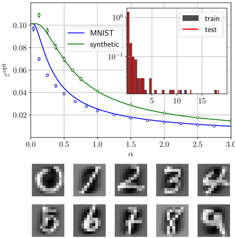<details> <summary>Image 12 Details</summary>  ### Visual Description ## Chart/Diagram Type: Line Graph with Histogram and Image Grid ### Overview The image presents a line graph comparing the performance of MNIST and synthetic datasets, a histogram showing the distribution of training and testing data, and a grid of sample images. The line graph plots epsilon-opt (εopt) against alpha (α), showing a decreasing trend for both datasets. The histogram displays the frequency of data points, and the image grid shows examples of handwritten digits. ### Components/Axes **Main Chart:** * **X-axis:** α (alpha), ranging from 0.0 to 3.0 in increments of 0.5. * **Y-axis:** εopt (epsilon-opt), ranging from 0.00 to 0.10 in increments of 0.02. * **Legend (Top-Left):** * Blue line: MNIST * Green line: synthetic **Histogram (Top-Right Inset):** * **X-axis:** Values ranging from approximately 0 to 18. * **Y-axis:** Frequency, on a logarithmic scale from 10^-1 to 10^0 to 10^1 (100). * **Legend (Top-Right of Inset):** * Dark Gray bars: train * Red bars: test **Image Grid (Bottom):** * A 2x5 grid displaying sample images of handwritten digits (0-9). ### Detailed Analysis **Line Graph:** * **MNIST (Blue):** The blue line represents the MNIST dataset. It starts at approximately εopt = 0.10 at α = 0.0 and decreases to approximately εopt = 0.015 at α = 3.0. The data points are marked with blue circles. * **Synthetic (Green):** The green line represents the synthetic dataset. It starts at approximately εopt = 0.105 at α = 0.0 and decreases to approximately εopt = 0.02 at α = 3.0. The data points are marked with white circles with error bars. **Histogram:** * **Train (Dark Gray):** The training data is represented by dark gray bars. The frequency is low, with most values concentrated between approximately 10 and 18. * **Test (Red):** The testing data is represented by red bars. The frequency is highest between approximately 1 and 5, with a rapid decrease as the value increases. **Image Grid:** * The grid displays ten images of handwritten digits, representing the numbers 0 through 9. ### Key Observations * Both MNIST and synthetic datasets show a decreasing trend in εopt as α increases. * The synthetic dataset generally has a slightly higher εopt value than the MNIST dataset for the same α value. * The histogram shows that the test data is more concentrated at lower values than the training data. ### Interpretation The line graph suggests that as the value of alpha (α) increases, the error (εopt) decreases for both the MNIST and synthetic datasets. This could indicate that a higher alpha value leads to better model performance. The synthetic dataset appears to have a slightly higher error rate compared to the MNIST dataset across the range of alpha values. The histogram indicates a different distribution between the training and testing datasets, which could affect the model's generalization performance. The image grid provides a visual representation of the data being used, which are handwritten digits. </details> not analytically tractable due to the lack of rotational invariance. In general there is no analytical simplification for (21) except when w has i.i.d. entries or when w is a Gaussian vector. In the latter case, suppose P w = N ( 0 , C ), then ψ P w ( x ) = lim d →∞ 1 2 d ( x Tr( C ) -ln det( I d + x C )). If C admits a limiting spectral density ρ C , $$\begin{array} { r } { \psi _ { P w } ( x ) = \frac { 1 } { 2 } \int ( x s - \ln ( 1 + x s ) ) \rho _ { C } ( s ) d s . \quad ( 2 2 ) } \end{array}$$ In App. C2, we show that by quenching the first hidden layer's weights and taking the first activation to be linear, via a procedure similar to that followed to derive Result 3, it is possible to describe such structured data within our replica formalism. FIG. 11 shows that structure in the input helps reduce the optimal generalisation error. Here, the covariance matrices are of the Wishart form W 0 W ⊺ 0 /d 0 , where W 0 ∈ R d × d 0 is a Gaussian matrix, with varying ratios d 0 /d . It is known that as d 0 /d increases, the spectrum of the Wishart matrix approaches that of the identity matrix, meaning the inputs become less structured. The figure demonstrates that as d 0 /d grows, the curves quickly approach that of the standard Gaussian inputs. For a broad class of non-Gaussian inputs, our experiments show that the Bayes-optimal error is unchanged if the inputs entering the random MLP target are replaced by Gaussian vectors with the same covariance. This behaviour, implied in our theory by the Gaussian hypothesis (11), was verified using inputs generated by feeding standard Gaussian vectors into one NN layer with Gaussian weights as well as real data from MNIST, see FIG. 12. The discrepancy between theoretical and experimental results at low α for MNIST data can be attributed to the few large outlier eigenvalues, while our theory is only dependent on the spectral density of the data covariance, which the outliers do not influence. ## B. Two hidden layers MLP In this section we present experiments for L = 2 hidden layers, similar to the ones conducted for the shallow case. Adding one layer already makes the picture richer, in particular in terms of the learning phase transitions taking place and the information flow across layers. Learning propagates from inner towards outer layers. FIG. 13 displays the mean-square generalisation error for a network with hyperbolic tangent activation. The general picture is similar to the shallow case: at small α a single prior-independent solution exists; with more data, the specialisation solution branches out continuously. A clear transition occurs in the specialisation solution. The mechanism behind it is explained by FIG. 14 showing the evolution of the average over neurons of the overlap profile in each layers. We first discuss the case of Gaussian v 0 , bottom of FIG. 14 and right of FIG. 13. The ordering of the specialisations along layers is clear: ( i ) The network starts specialising from the inner layer W (1) . The information then propagates outwards. ( ii ) The deep layer W (2) is then getting learned. This experimentally observed shallowto-deep layers ordering of the learning is encoded in our FIG. 13. Theoretical prediction (green solid curve) of the Bayes-optimal mean-square generalisation error for L = 2 with Gaussian inner weights, σ ( x ) = tanh(2 x ) /σ tanh , d = 200 , γ 1 = γ 2 = 0 . 5 , ∆ = 0 . 2 and different P v laws. The dashed line represents the universal branch. Dotted lines denote metastable specialisation branches of the RS saddle-point equations reached from different initialisations for the overlaps. From the top, the first green dotted line represents the solution reached by initialising Q 2:1 > 0 (i.e., positive for any argument value) and Q 1 , Q 2 ≡ 0 (0 for all arguments), the second to Q 1 , Q 2:1 , Q 2 > 0 (it yields in the left panel the small metastable solution just before the transition around α = 2 . 8; in the right panel, this solution collapses on the equilibrium curve), the third is Q 1 > 0 , Q 2:1 , Q 2 ≡ 0. The magenta dotted curve corresponds to initialisation Q 1 ( v (2) ) > 0 only for sufficiently large v (2) , while Q 2:1 , Q 2 ≡ 0: this solution is an inhomogeneous specialisation across layers (only the first specialises), and across the neurons in that layer (only some neurons specialise). Points are obtained with Hamiltonian Monte Carlo with informative initialisation. Each point has been averaged over 20 instances of the data, with error bars representing one standard deviation. The generalisation error is computed empirically from 10 4 i.i.d. test samples. The readouts are fixed to the teacher's during sampling. Left : Homogeneous readouts. Inset : Optimal generalisation error of a shallow MLP (black line: L = 1) and deep MLP (red line: L = 2). The activation for both curves is σ ( x ) = tanh(2 x ) /σ tanh , γ, γ 1 , γ 2 = 1 and ∆ = 0 . 2, while α is divided by L for comparison. Right : Gaussian readouts. 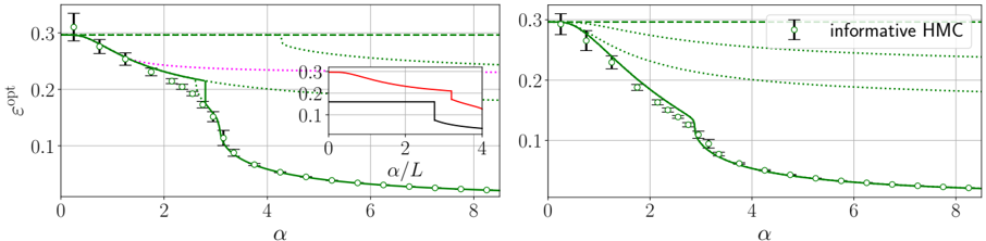<details> <summary>Image 13 Details</summary>  ### Visual Description ## Line Chart: Optimal Epsilon vs. Alpha ### Overview The image contains two line charts comparing optimal epsilon values against alpha. Both charts display similar trends, with a rapid decrease in epsilon as alpha increases, eventually plateauing at a low value. The left chart includes an inset plot and additional horizontal lines, while the right chart features a legend identifying the "informative HMC" data series. ### Components/Axes * **Left Chart:** * Y-axis: ε<sup>opt</sup>, ranging from 0 to 0.3. * X-axis: α, ranging from 0 to 8. * Inset Plot: * Y-axis: Unlabeled, ranging from approximately 0 to 0.3. * X-axis: α/L, ranging from 0 to 4. * Lines: * Solid Green Line: Represents the primary data series. * Dashed Green Line: Horizontal line at approximately ε<sup>opt</sup> = 0.3. * Dotted Green Line: Starts at approximately ε<sup>opt</sup> = 0.3 and decreases to approximately 0.2. * Dotted Magenta Line: Horizontal line at approximately ε<sup>opt</sup> = 0.24. * Inset Red Line: Starts at approximately 0.3 and decreases to approximately 0.2 at α/L = 4. * Inset Black Line: Horizontal line at approximately 0.15 until α/L = 3, then decreases to approximately 0.05 at α/L = 4. * Data Points: Green circles with error bars along the solid green line. * **Right Chart:** * Y-axis: ε<sup>opt</sup>, ranging from 0 to 0.3. * X-axis: α, ranging from 0 to 8. * Lines: * Solid Green Line: Represents the primary data series. * Dashed Green Line: Horizontal line at approximately ε<sup>opt</sup> = 0.3. * Dotted Green Line: Starts at approximately ε<sup>opt</sup> = 0.3 and decreases to approximately 0.2. * Data Points: Green circles with error bars along the solid green line. * Legend (Top-Right): "informative HMC" associated with the green data points. ### Detailed Analysis * **Left Chart:** * Solid Green Line: Starts at approximately (0, 0.3) and rapidly decreases to approximately (4, 0.03), then plateaus. * Dashed Green Line: Constant at approximately ε<sup>opt</sup> = 0.3. * Dotted Green Line: Starts at approximately (0, 0.3) and decreases to approximately (4, 0.2). * Dotted Magenta Line: Constant at approximately ε<sup>opt</sup> = 0.24. * Inset Red Line: Starts at approximately (0, 0.3) and decreases to approximately (4, 0.2). * Inset Black Line: Constant at approximately (0, 0.15) until α/L = 3, then decreases to approximately (4, 0.05). * **Right Chart:** * Solid Green Line: Starts at approximately (0, 0.3) and rapidly decreases to approximately (4, 0.03), then plateaus. * Dashed Green Line: Constant at approximately ε<sup>opt</sup> = 0.3. * Dotted Green Line: Starts at approximately (0, 0.3) and decreases to approximately (4, 0.2). * Data points (informative HMC): The green circles with error bars follow the solid green line. ### Key Observations * Both charts show a similar trend: a rapid decrease in optimal epsilon as alpha increases, followed by a plateau. * The left chart provides additional context with the inset plot and magenta line, potentially showing different models or parameters. * The right chart explicitly labels the data series as "informative HMC." * The error bars on the data points are relatively small, indicating a degree of precision in the measurements. ### Interpretation The charts likely illustrate the relationship between a parameter "alpha" and the optimal value of "epsilon" in a Hamiltonian Monte Carlo (HMC) simulation or related algorithm. The rapid decrease in epsilon<sup>opt</sup> suggests that as alpha increases, the system becomes more stable or efficient, requiring a smaller step size (epsilon) for optimal performance. The plateau indicates a point of diminishing returns, where further increases in alpha do not significantly improve the system's behavior. The inset plot in the left chart may represent a different scaling or a different model altogether, providing a comparative perspective. The magenta line could represent a theoretical limit or a different optimization strategy. The "informative HMC" label on the right chart suggests that this particular configuration or algorithm is being highlighted for its performance. </details> FIG. 14. Solid and dotted curves represent, respectively, the mean of different overlaps at equilibrium and in metastable specialised states, as function of the sampling ratio α for L = 2 with Gaussian inner weights, σ ( x ) = tanh(2 x ) /σ tanh , d = 200 , γ 1 = γ 2 = 0 . 5 , ∆ = 0 . 2. The shaded curves were obtained from informed HMC. Each point has been averaged over 20 instances of the training set, with one standard deviation depicted. The readouts are fixed to the teacher's during sampling. Top : Homogeneous readouts. Bottom : Gaussian readouts. 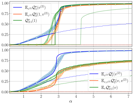<details> <summary>Image 14 Details</summary>  ### Visual Description ## Chart: Two-Panel Plot of Probabilities vs. Alpha ### Overview The image presents two line plots arranged vertically, each displaying the relationship between different probability measures and the variable alpha (α). The plots share the same x-axis (α) but may represent different scenarios or conditions. Each plot contains multiple data series, represented by lines of different colors, some with shaded regions indicating uncertainty. ### Components/Axes * **X-axis (Horizontal):** Labeled "α". The scale ranges from approximately 0 to 7, with tick marks at integer values. * **Y-axis (Vertical):** Ranges from 0.00 to 1.00 in both plots, with tick marks at intervals of 0.25. * **Top Plot Legend (Top-Left):** * Blue Line: E<sub>v(2)</sub>Q<sup>\*</sup><sub>1</sub>(v<sup>(2)</sup>) * Orange Line: E<sub>v(2)</sub>Q<sup>\*</sup><sub>2</sub>(1, v<sup>(2)</sup>) * Green Line: Q<sup>\*</sup><sub>2:1</sub>(1) * **Bottom Plot Legend (Bottom-Right):** * Blue Line: E<sub>v(2)</sub>Q<sup>\*</sup><sub>1</sub>(v<sup>(2)</sup>) * Orange Line: E<sub>v,v(2)</sub>Q<sup>\*</sup><sub>2</sub>(v, v<sup>(2)</sup>) * Green Line: E<sub>v</sub>Q<sup>\*</sup><sub>2:1</sub>(v) ### Detailed Analysis **Top Plot:** * **Blue Line (E<sub>v(2)</sub>Q<sup>\*</sup><sub>1</sub>(v<sup>(2)</sup>)):** This line exhibits a sharp increase around α = 2.5 to 3, reaching a value close to 1.00. Before the increase, the value is near 0. After the increase, the line remains near 1.00. There is a shaded region around the line, indicating a confidence interval. A dotted blue line is also present, starting at approximately (3, 0.25) and increasing linearly to approximately (7, 0.4). * **Orange Line (E<sub>v(2)</sub>Q<sup>\*</sup><sub>2</sub>(1, v<sup>(2)</sup>)):** This line also shows a sharp increase, but slightly delayed compared to the blue line, around α = 2.75 to 3.25, reaching a value close to 1.00. Before the increase, the value is near 0. After the increase, the line remains near 1.00. There is a shaded region around the line, indicating a confidence interval. * **Green Line (Q<sup>\*</sup><sub>2:1</sub>(1)):** This line shows a step function behavior. It remains at 0 until approximately α = 3, then jumps to a value near 0.75, and then slowly increases to 1.00. A dotted green line is also present, starting at approximately (3, 0.25) and increasing linearly to approximately (7, 0.75). **Bottom Plot:** * **Blue Line (E<sub>v(2)</sub>Q<sup>\*</sup><sub>1</sub>(v<sup>(2)</sup>)):** Similar to the top plot, this line exhibits a sharp increase around α = 2.5 to 3, reaching a value close to 1.00. Before the increase, the value is near 0. After the increase, the line remains near 1.00. There is a shaded region around the line, indicating a confidence interval. A dotted blue line is also present, starting at approximately (3, 0.25) and increasing linearly to approximately (7, 0.4). * **Orange Line (E<sub>v,v(2)</sub>Q<sup>\*</sup><sub>2</sub>(v, v<sup>(2)</sup>)):** This line also shows a sharp increase, but slightly delayed compared to the blue line, around α = 2.75 to 3.25, reaching a value close to 1.00. Before the increase, the value is near 0. After the increase, the line remains near 1.00. There is a shaded region around the line, indicating a confidence interval. * **Green Line (E<sub>v</sub>Q<sup>\*</sup><sub>2:1</sub>(v)):** This line remains near 0 for the entire range of α. A dotted green line is also present, starting at approximately (3, 0.0) and remaining at 0. ### Key Observations * The blue and orange lines in both plots exhibit a similar sigmoidal shape, indicating a transition or phase change around α = 3. * The green line behaves differently in the top and bottom plots, suggesting a change in the underlying system or parameters. * The shaded regions around the lines indicate uncertainty in the measurements, which is more pronounced in the transition region. * The dotted lines in the top plot show a linear increase after the transition point, while in the bottom plot, the green dotted line remains at 0. ### Interpretation The plots likely represent the behavior of some system as a function of the parameter α. The sharp increases in the blue and orange lines suggest a critical point or threshold behavior. The different behavior of the green line in the two plots indicates that the quantity it represents is sensitive to some change in the system's conditions between the top and bottom plots. The dotted lines may represent theoretical predictions or asymptotic behavior. The shaded regions indicate the level of confidence in the experimental measurements. The data suggests that the system undergoes a phase transition or a significant change in behavior around α = 3, and the nature of this transition depends on the specific conditions represented by the top and bottom plots. </details> formulas (including for L ≥ 3): the RS equations imply that the overlap for the second layer can become non-zero only if the one for the first layer is itself non-vanishing. Concerning the recovery of W (2) W (1) , it should be understood that products of weight matrices from different layers are learnable partly independently of their factors. This is similar to the shallow case, where the quadratic term W 0 ⊺ diag( v 0 ) W 0 in the target can be partially recovered without learning W 0 , and thus comes with its own OP which can be non-zero even if the one for W 0 vanishes (in the universal phase). The equations consistently encompass this possibility. The learning transitions occur more abruptly with homogeneous readouts, top of FIG. 14 and left of FIG. 13: the learning of the product matrix and the deep one occur jointly and sharply. The homogeneity of the readouts is the source of the discontinuity of the learning transition which makes learning harder. Interestingly, continuous rather than discrete readouts induce smoother transitions. Nevertheless, notice the richer behaviour of the generalisation error and overlaps right after the first transition for homogeneous readouts, and also that in that region of α , the ordering of overlaps values is different between the two readouts distributions. We mention that [112-114] also predicted learning inhomogeneities across layers in a teacher-student setting but in a strongly overparametrised data regime. Inhomogeneous learning profile across neurons and matrix order parameters. When there are two or more hidden layers, non-trivial overlap profiles emerge in each. This effect is a joint consequence of the depth and linear width of the network but also of the complex interactions among the layers (recall the discussion when we introduced Q ∗ 2 ( v , v (2) ) in Sec. II B). For the first hidden layer, top panel of FIG. 15, the overlap inhomogeneity is related to the fluctuations in the effective readouts of the target v (2)0 := W (2)0 ⊺ v 0 / √ k 2 : its components are Gaussian random variables. It implies that neurons are not all 'measured equally well' (in particular through the linear term in the Hermite expansion of σ in the first layer). The profile therefore manifests itself along the output (row) dimension. For the second layer, with homogeneous readouts, the only inhomogeneity is along its input (column) dimension and is induced by the output profile of the first layer weights, second panel. For completeness we checked that, consistently with the theory, the profile of the second layer overlap along its output dimension is indeed constant, third panel. Due to the homogeneity of readouts, a similar constant overlap profile along the output dimension of the product matrix W (2:1) appears (last panel). These experiments probing all possible overlap inhomogeneities in a three layers MLP vindicate our definitions and indexing of OPs in the theory. As an illustration of what is learnt in the deep NN when increasing the data, we plot in FIG. 16 the three functional overlap OPs using heat-maps. Two carry a single argument and the one for the second inner layer possesses two, as it captures at a macroscopic level the learning inhomogeneities along both the rows and columns of W (2) (we restricted the domains of the OPs for visualisation despite the true ones are in principle infinite). As α exceeds the smooth transition happening around α = 2 . 8 in the same setting of bottom panel of FIG. 14, we see that specialisation nucleates in W (2) starting from its neurons (i.e, rows) indexed by the largest readouts amplitudes, | v | , and concurrently from its 'dual neurons' (i.e., its columns) connected to the largest effective readouts amplitudes | v (2) | . Specialisation then propagates towards lower values as α increases. The figures emphasise how the learning of the other matrices (the first layer weights and the product matrix, which both display learning inhomogeneities along one dimension only) interact with the deep one and yield such an intricate behaviour. Finally, in FIG. 17, we display a result of a numerical experiment for Q 2 ( v , v (2) ). This figure was realised by averaging over different instances of a data-student pair, with the overlap values ordered as those of FIG. 16 for each pair, and then by performing a 'local average' of neighbouring indices on the grid ( v , v (2) ) in order to suppress the 'microscopic fluctuations'. The latter should be interpreted in the thermodynamic limit as being over a relatively small patch, which still contains Θ( d 2 ) weights. Remarkably, this figure could have also been generated from a single instance of the student, as the local average alone is sufficient to reproduce the patterns of FIG. 16. Notice that in contrast with the shallow case where Q ( v ) vanishes for v small even at large sampling ratios (see FIG. 7), the top panel of FIG. 15 and FIG. 16, 17 show that, for sufficiently large α , overlaps indexed by v (2) become non-zero for any value of the index. This occurs because the effective readouts enter the covariance K (2) ( ¯ Q ) from Result II B in a different way compared to the actual readouts v . Algorithmic hardness and partial specialisation. We repeated experiments probing the behaviour of HMC and ADAM similar to the shallow case, see FIG. 18. Start- FIG. 15. Theoretical predictions (solid curves) for the overlaps obtained from informative initialisation as functions of v (2)0 or i = 1 , . . . , k 2 for L = 2 with activation tanh(2 x ) /σ tanh , d = 200 , γ 1 = γ 2 = 0 . 5 , ∆ = 0 . 2, Gaussian inner weights, homogeneous quenched readouts and different α values. The shaded curves were obtained from informed HMC. Using singles posterior samples, the overlaps have been evaluated numerically by dividing the interval [ -2 , 2] into bins and by computing their value in each bin. Each point has been averaged over 20 instances of the data, and shaded regions around them correspond to one standard deviation. First (top) : First layer overlap Q ∗ 1 ( v ( 2 ) ) profile ordered according to the amplitude of the effective readouts v (2)0 . Second : The input (or column)-indexed overlap for the second layer Q ∗ 2 (1 , v ( 2 ) ) also ordered according to the effective readouts. Third : The neuron (i.e., output or row)-indexed overlap profile for the second layer. Last : The output-indexed overlap profile for the product matrix W (2:1) . 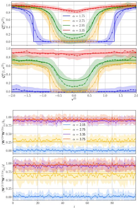<details> <summary>Image 15 Details</summary>  ### Visual Description ## Chart: Spectral Properties vs. Parameter α ### Overview The image presents four line charts arranged in two pairs. The top two charts display the spectral properties Q1 and Q2 as a function of v^(2) for different values of parameter α. The bottom two charts show the normalized quantities (W^(2)0 W^(2)τ)i/k1 and (W^(2:1)0 W^(2:1)τ)i/d as a function of index i, also for different α values. Each line is accompanied by a shaded region indicating uncertainty. ### Components/Axes **Top Two Charts (Q1 and Q2 vs. v^(2))** * **Y-axis (Left):** Q1^(vp)(v^(2)) (Top Chart), Q2^(vp)(1, v^(2)) (Bottom Chart). Scale ranges from 0.0 to 1.0. * **X-axis (Bottom):** v^(2). Scale ranges from -2.0 to 2.0. * **Legend (Top-Right):** * Blue: α = 1.75 * Orange: α = 2.75 * Green: α = 2.95 * Red: α = 3.35 **Bottom Two Charts (Normalized W vs. i)** * **Y-axis (Left):** (W^(2)0 W^(2)τ)i/k1 (Top Chart), (W^(2:1)0 W^(2:1)τ)i/d (Bottom Chart). Scale ranges from 0.00 to 1.00. * **X-axis (Bottom):** i. Scale ranges from 0 to 100. * **Legend (Right):** * Blue: α = 2.15 * Orange: α = 2.75 * Purple: α = 3.35 * Red: α = 3.75 ### Detailed Analysis **Top Chart: Q1^(vp)(v^(2)) vs. v^(2)** * **α = 1.75 (Blue):** The line is approximately 1.0 from v^(2) = -2.0 to approximately -1.0. It then drops sharply to approximately 0.0 between v^(2) = -1.0 and v^(2) = -0.5. It remains at approximately 0.0 until v^(2) = 0.5, then rises sharply back to approximately 1.0 between v^(2) = 0.5 and v^(2) = 1.0, and remains at 1.0 until v^(2) = 2.0. * **α = 2.75 (Orange):** The line starts at approximately 0.9 at v^(2) = -2.0, decreases gradually to approximately 0.2 at v^(2) = -0.5, reaches a minimum of approximately 0.1 at v^(2) = 0.0, and then increases gradually back to approximately 0.9 at v^(2) = 2.0. * **α = 2.95 (Green):** The line starts at approximately 0.9 at v^(2) = -2.0, decreases gradually to approximately 0.4 at v^(2) = -0.5, reaches a minimum of approximately 0.3 at v^(2) = 0.0, and then increases gradually back to approximately 0.9 at v^(2) = 2.0. * **α = 3.35 (Red):** The line remains relatively constant at approximately 0.9 across the entire range of v^(2). **Second Chart: Q2^(vp)(1, v^(2)) vs. v^(2)** * **α = 1.75 (Blue):** The line is approximately 0.0 across the entire range of v^(2). * **α = 2.75 (Orange):** The line starts at approximately 0.1 at v^(2) = -2.0, increases gradually to approximately 0.6 at v^(2) = -0.5, reaches a maximum of approximately 0.7 at v^(2) = 0.0, and then decreases gradually back to approximately 0.1 at v^(2) = 2.0. * **α = 2.95 (Green):** The line starts at approximately 0.6 at v^(2) = -2.0, increases gradually to approximately 0.8 at v^(2) = -0.5, reaches a maximum of approximately 0.85 at v^(2) = 0.0, and then decreases gradually back to approximately 0.6 at v^(2) = 2.0. * **α = 3.35 (Red):** The line remains relatively constant at approximately 0.9 across the entire range of v^(2). **Third Chart: (W^(2)0 W^(2)τ)i/k1 vs. i** * **α = 2.15 (Blue):** The line fluctuates around approximately 0.1 across the entire range of i. * **α = 2.75 (Orange):** The line fluctuates around approximately 0.3 across the entire range of i. * **α = 3.35 (Purple):** The line fluctuates around approximately 0.9 across the entire range of i. * **α = 3.75 (Red):** The line fluctuates around approximately 0.9 across the entire range of i. **Fourth Chart: (W^(2:1)0 W^(2:1)τ)i/d vs. i** * **α = 2.15 (Blue):** The line fluctuates around approximately 0.1 across the entire range of i. * **α = 2.75 (Orange):** The line fluctuates around approximately 0.7 across the entire range of i. * **α = 3.35 (Purple):** The line fluctuates around approximately 0.9 across the entire range of i. * **α = 3.75 (Red):** The line fluctuates around approximately 0.9 across the entire range of i. ### Key Observations * In the top two charts, as α increases, the dip in Q1 and Q2 around v^(2) = 0 becomes less pronounced. * In the bottom two charts, as α increases, the normalized quantities (W^(2)0 W^(2)τ)i/k1 and (W^(2:1)0 W^(2:1)τ)i/d tend to increase. * The shaded regions indicate the uncertainty associated with each line, and the uncertainty appears to be greater in the regions where the lines are changing rapidly. ### Interpretation The charts illustrate the relationship between the parameter α and various spectral properties (Q1, Q2) and normalized quantities (W). The top two charts suggest that higher values of α lead to a more uniform spectral distribution, as the dip around v^(2) = 0 diminishes. The bottom two charts indicate that higher values of α are associated with larger normalized quantities (W), suggesting a stronger correlation or interaction. The uncertainty regions highlight the variability in the data, which is particularly noticeable in regions where the spectral properties are changing rapidly. Overall, the data suggests that α plays a significant role in shaping the spectral characteristics and correlations within the system being studied. </details> ing with HMC, two noticeable differences appear compared to L = 1. Firstly, reaching the specialised equilibrium state from uninformative initialisation seems much harder/costly than in the shallow case; we do observe the descent towards it only for a rather small size ( d = 50). The most striking difference, however, is the nature of the state that HMC experiences. For L = 1, HMC was FIG. 16. Heat-maps of all the theoretical equilibrium overlap as function of the sampling rate α ∈ { 1 . 75 , 2 . 75 , 3 . 75 } (increasing from top to bottom) for L = 2 with Gaussian inner and readout weights, σ ( x ) = tanh(2 x ) /σ tanh , γ 1 = γ 2 = 0 . 5 , ∆ = 0 . 2, which is the same setting as the right panel of FIG. 13 and bottom panel of FIG. 14. Left column: Product matrix overlap Q ∗ 2:1 ( v ). Bottom row: First layer overlap Q ∗ 1 ( v (2) ). Central square: Second layer overlap Q ∗ 2 ( v, v (2) ). The overlaps arguments in the theory are amplitudes v , v (2) > 0. However, we plot them here as a function of the actual signed readouts and effective readouts values v, v (2) for better visualisation of what is going on in the network. These figures fully capture the features learnt along the layers, and across the rows and columns of each layer weight matrix, in a three layers neural network. 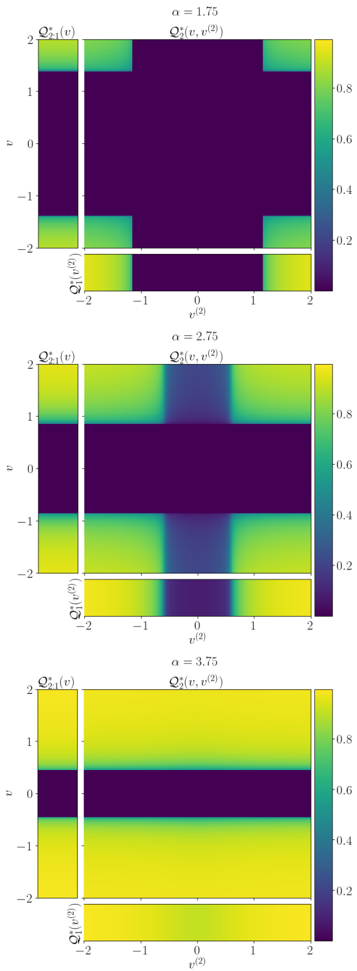<details> <summary>Image 16 Details</summary>  ### Visual Description ## Heatmaps: Q* Functions vs. v and v^(2) ### Overview The image presents three heatmaps, each displaying the function Q*(v, v^(2)) for different values of α (1.75, 2.75, and 3.75). Each heatmap is accompanied by marginal distributions Q*21(v) and Q*1(v^(2)) along the y and x axes, respectively. The color intensity represents the value of the Q* function, ranging from approximately 0.2 (dark purple) to 0.8 (yellow). ### Components/Axes * **Titles:** Each heatmap has a title indicating the value of α: "α = 1.75", "α = 2.75", and "α = 3.75". Each heatmap also has the title "Q*(v, v^(2))". * **Y-Axis (v):** The y-axis represents the variable 'v', ranging from -2 to 2 in increments of 1. The marginal distribution Q*21(v) is plotted along the left side of each heatmap. * **X-Axis (v^(2)):** The x-axis represents the variable 'v^(2)', ranging from -2 to 2 in increments of 1. The marginal distribution Q*1(v^(2)) is plotted along the bottom of each heatmap. * **Colorbar:** A vertical colorbar on the right side of each heatmap indicates the value of the Q* function, ranging from approximately 0.2 (dark purple) to 0.8 (yellow). * **Marginal Distributions:** Each heatmap has a marginal distribution plotted along the y-axis, labeled "Q*21(v)", and along the x-axis, labeled "Q*1(v^(2))". ### Detailed Analysis **Heatmap 1: α = 1.75** * The central region of the heatmap (around v=0, v^(2)=0) has low values (dark purple, ~0.2). * The corners (v=±2, v^(2)=±2) and the edges (v=±2 or v^(2)=±2) have higher values (yellow, ~0.8). * The marginal distributions Q*21(v) and Q*1(v^(2)) show high values at v=±2 and v^(2)=±2, respectively, and low values elsewhere. **Heatmap 2: α = 2.75** * The central horizontal band (around v=0) has low values (dark purple, ~0.2). * The regions above and below the central band have higher values (yellow, ~0.8). * The marginal distribution Q*21(v) shows low values around v=0 and high values at v=±2. The marginal distribution Q*1(v^(2)) is relatively uniform with a slight dip around v^(2)=0. **Heatmap 3: α = 3.75** * The central horizontal band (around v=0) has low values (dark purple, ~0.2). * The regions above and below the central band have higher values (yellow, ~0.8). * The marginal distribution Q*21(v) shows low values around v=0 and high values at v=±2. The marginal distribution Q*1(v^(2)) is relatively uniform. ### Key Observations * As α increases, the central region of low values in the heatmaps becomes more concentrated around v=0. * The marginal distributions Q*21(v) consistently show high values at v=±2 and low values around v=0. * The marginal distributions Q*1(v^(2)) become more uniform as α increases. ### Interpretation The heatmaps illustrate how the function Q*(v, v^(2)) changes with different values of α. The parameter α seems to control the concentration of low values around v=0. The marginal distributions provide additional information about the behavior of Q* with respect to individual variables v and v^(2). The data suggests that as α increases, the function Q* becomes more sensitive to the value of v, with a stronger distinction between values near 0 and values near ±2. The relative uniformity of Q*1(v^(2)) as alpha increases suggests that the function becomes less sensitive to v^(2). </details> v FIG. 17. Heat-map of all the empirical overlaps on grids of (effective) readouts ( v , v (2) ). Besides the local average performed by binning the distribution of the weights according to the grid of readouts, we average over 100 instances of datastudent pairs. Here d = 200, α = 1 . 75 ( top ), α = 2 . 75 ( middle ) and α = 3 . 75 ( bottom ), while the rest is as in FIG. 16. For the second layer overlap, the values are rearranged putting those associated to highest readout values on the corners of the image, as in FIG. 16. Up to finite size fluctuations, the same patterns as the theoretically predicted ones, top and bottom panels of FIG. 16, clearly appear. 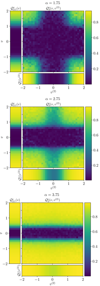<details> <summary>Image 17 Details</summary>  ### Visual Description ## Heatmaps: Q2*(v, v^(2)) vs. v^(2) and Q2:1*(v) vs. v ### Overview The image presents three heatmaps arranged vertically, each displaying the relationship between Q2*(v, v^(2)) and v^(2), along with an adjacent plot of Q2:1*(v) vs. v. Each heatmap corresponds to a different value of α (1.75, 2.75, and 3.75). The heatmaps use a color gradient to represent the magnitude of Q2*(v, v^(2)) and Q2:1*(v), ranging from dark purple (low values) to bright yellow (high values). ### Components/Axes Each heatmap has the following components: * **Title:** Indicates the value of α for that specific heatmap (α = 1.75, α = 2.75, α = 3.75). * **Main Heatmap:** Displays Q2*(v, v^(2)) as a function of v and v^(2). * X-axis: v^(2), ranging from -2 to 2. * Y-axis: v, ranging from -2 to 2. * **Side Plot:** Displays Q2:1*(v) as a function of v. * Y-axis: v, ranging from -2 to 2. * X-axis: Q2:1*(v). * **Bottom Plot:** Displays Q1*(v^(2)) as a function of v^(2). * X-axis: v^(2), ranging from -2 to 2. * Y-axis: Q1*(v^(2)). * **Colorbar:** Located on the right side of each heatmap, indicating the mapping between color and value. The colorbar ranges from approximately 0.2 (dark purple) to 0.8 (bright yellow). ### Detailed Analysis **Heatmap 1: α = 1.75** * **Main Heatmap:** The central region around (0,0) is dark purple, indicating low values of Q2*(v, v^(2)). The corners and the edges tend to be more yellow/green, indicating higher values. * **Side Plot:** Q2:1*(v) shows higher values (yellow/green) at the extremes (v ≈ -2 and v ≈ 2) and lower values (purple) around v = 0. * **Bottom Plot:** Q1*(v^(2)) shows higher values (yellow/green) at the extremes (v^(2) ≈ -2 and v^(2) ≈ 2) and lower values (purple) around v^(2) = 0. **Heatmap 2: α = 2.75** * **Main Heatmap:** A horizontal band around v = 0 is dark purple, indicating low values of Q2*(v, v^(2)). The regions above and below this band are more yellow/green. * **Side Plot:** Q2:1*(v) shows low values (purple) around v = 0 and higher values (yellow/green) at the extremes. * **Bottom Plot:** Q1*(v^(2)) shows higher values (yellow/green) at the extremes (v^(2) ≈ -2 and v^(2) ≈ 2) and lower values (purple) around v^(2) = 0. **Heatmap 3: α = 3.75** * **Main Heatmap:** Similar to α = 2.75, a horizontal band around v = 0 is dark purple, but the band is wider. The regions above and below are yellow/green. * **Side Plot:** Q2:1*(v) shows low values (purple) around v = 0 and higher values (yellow/green) at the extremes. The difference between the high and low values is more pronounced than in the previous heatmaps. * **Bottom Plot:** Q1*(v^(2)) shows higher values (yellow/green) at the extremes (v^(2) ≈ -2 and v^(2) ≈ 2) and lower values (purple) around v^(2) = 0. ### Key Observations * As α increases, the dark purple band in the main heatmap becomes wider, indicating a stronger suppression of Q2*(v, v^(2)) around v = 0. * The side plots consistently show that Q2:1*(v) is suppressed around v = 0 and enhanced at the extremes, regardless of the value of α. * The bottom plots consistently show that Q1*(v^(2)) is suppressed around v^(2) = 0 and enhanced at the extremes, regardless of the value of α. ### Interpretation The heatmaps illustrate how the parameter α influences the distribution of Q2*(v, v^(2)). The increasing suppression of Q2*(v, v^(2)) around v = 0 as α increases suggests that α plays a role in shaping the relationship between v and v^(2). The consistent behavior of Q2:1*(v) and Q1*(v^(2)) across different values of α indicates that these functions may be less sensitive to changes in α, or that their behavior is intrinsically linked to the underlying system being modeled. The data suggests that α is a parameter that controls the correlation or interaction between v and v^(2), with higher values of α leading to a stronger decoupling or suppression of Q2*(v, v^(2)) when v is close to zero. </details> getting attracted by the metastable state associated with the universal solution (top panel of FIG. 8), with the single inner layer not specialising. With one more hidden layer a richer pictures emerges. The top panel of FIG. 18 shows that in polynomial-ind time, before complete specialisation ultimately occurs when the chain equilibrates, HMC is now stuck in a partially specialised metastable state . There, the first layer has specialised (i.e., has been partly recovered) while the second has not. We tracked the experimental overlaps, not depicted here, and they confirm this picture. The theory correctly predicts this state: it is the third green dotted curve from the top in FIG. 13 left panel, which at α = 4 corresponds to the dashed blue curve ε meta = 0 . 2 in FIG. 18 (the two plots are done in the same setting). This is very interesting: somehow, depth helps from that perspective, since this mechanism cannot be observed in the shallow case. The reason is the presence of the effective readouts in the target v (2)0 = W (2)0 ⊺ v 0 / √ k 2 when L = 2, that inhomogeneously 'measure' the inner layer. Apart from this stable metastable state, there are other solutions of the RS equations. The magenta curve in FIG. 13 depicts a case where only the first layer specialises, and only for a subset of its neurons. The same effect is observed in shallow MLPs for their single hidden layer (see FIG. 5, right panel). Although these solutions exist, their stability is not systematically analysed here, as this poses a significant challenge both for the theory and even more so in the numerical experiments due to strong finite-size effects and the difficulty to train large deep Bayesian NNs. We leave an investigation of their stability for future work. When learning with ADAM (bottom panel of FIG. 18), we instead observe a similar scenario as with L = 1 with tanh activation (lower panel of FIG. 9): as d increases ADAM gets stopped by the metastable state associated with the universal solution, and does not reach the better partially specialised one. This suggests that HMC is able to 'see' metastable states that outperform ε uni , while ADAM is not in the tested cases. It would be interesting to understand why. ## C. Three or more hidden layers Deeper is harder. FIG. 19 displays the theoretical and experimental Bayes-error and the theoretical overlaps corresponding to informative initialisation. A number of observations can be made. Let us start with the left panel. Note that the sampling rate α in the abcissa is rescaled by the number of layers to make a fair comparison between targets with different depths. We conclude based on the location of the specialisation transition (common to all layers under ( H 3 )) and the ordering of the generalisation error curves with L that the deeper the target, the more data per layer it requires to be recovered, and the higher is the ε opt at given α/L . This vindicates information-theoretically the intuitive picture that FIG. 18. Generalisation errors, computed empirically from 10 4 i.i.d. test samples, of HMC (ADAM) as function of the number of steps (gradient updates). Errors are averaged over 10 instances; shaded areas indicate one standard deviation. Here L = 2 , σ ( x ) = tanh(2 x ) /σ tanh , γ 1 = γ 2 = 0 . 5 , α = 4 . 0 with Gaussian inner weights and homogeneous target readouts for both plots. Dashed lines represent the theoretical errors associated to equilibrium and metastable solutions. Top : Half Gibbs error of HMC from random initialisation as a function of the number of updates for various d with ∆ = 0 . 2. The readouts are quenched during sampling. Bottom : Generalisation error of ADAM from random initialisation as a function of the gradient updates for various d with ∆ = 10 -4 . The initial learning rate is 0 . 01 and batch size ⌊ n/ 4 ⌋ . The student has learnable readout layer. 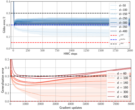<details> <summary>Image 18 Details</summary>  ### Visual Description ## Chart: Gibbs Error and Generalization Error vs. Steps/Updates ### Overview The image presents two line charts comparing Gibbs error and generalization error against the number of HMC steps and gradient updates, respectively. The charts illustrate the performance of different models (parameterized by 'd') during training. The top chart shows Gibbs error/2 versus HMC steps, while the bottom chart shows generalization error versus gradient updates. ### Components/Axes **Top Chart:** * **Title:** Gibbs error/2 * **X-axis:** HMC steps (range: 0 to 2000) * **Y-axis:** Gibbs error/2 (range: 0 to 0.4) * **Data Series (d values):** 50, 100, 150, 250, 300, 350, 400 * **Horizontal Lines:** * Red dashed line: labeled as "e^opt" at approximately 0.05 * Blue dashed line: labeled as "e^meta" at approximately 0.22 * Black dashed line: labeled as "e^uni" at approximately 0.30 **Bottom Chart:** * **Title:** Generalisation error * **X-axis:** Gradient updates (range: 0 to 8000) * **Y-axis:** Generalisation error (range: 0 to 0.5) * **Data Series (d values):** 60, 100, 140, 160, 300, 400 * **Horizontal Lines:** * Black dashed line: labeled as "e^uni" at approximately 0.30 ### Detailed Analysis **Top Chart (Gibbs error/2 vs. HMC steps):** * **d = 50 (lightest blue):** Starts at approximately 0.4, rapidly decreases to approximately 0.2, and then plateaus. * **d = 100 (lighter blue):** Starts at approximately 0.35, decreases to approximately 0.22, and then plateaus. * **d = 150 (mid-light blue):** Starts at approximately 0.3, decreases to approximately 0.23, and then plateaus. * **d = 250 (mid-blue):** Starts at approximately 0.27, decreases to approximately 0.23, and then plateaus. * **d = 300 (darker blue):** Starts at approximately 0.25, decreases to approximately 0.23, and then plateaus. * **d = 350 (dark blue):** Starts at approximately 0.24, decreases to approximately 0.23, and then plateaus. * **d = 400 (darkest blue):** Starts at approximately 0.23, remains relatively constant around 0.23. **Bottom Chart (Generalisation error vs. Gradient updates):** * **d = 60 (lightest red):** Starts at approximately 0.5, decreases to approximately 0.25 around 1000 gradient updates, and then gradually increases to approximately 0.38. * **d = 100 (lighter red):** Starts at approximately 0.45, decreases to approximately 0.25 around 1000 gradient updates, and then gradually increases to approximately 0.35. * **d = 140 (mid-light red):** Starts at approximately 0.4, decreases to approximately 0.25 around 1000 gradient updates, and then gradually increases to approximately 0.33. * **d = 160 (mid-red):** Starts at approximately 0.38, decreases to approximately 0.26 around 1000 gradient updates, and then gradually increases to approximately 0.32. * **d = 300 (darker red):** Starts at approximately 0.35, decreases to approximately 0.27 around 1000 gradient updates, and then gradually increases to approximately 0.31. * **d = 400 (darkest red):** Starts at approximately 0.33, decreases to approximately 0.28 around 1000 gradient updates, and then gradually increases to approximately 0.30. ### Key Observations * In the top chart, all Gibbs error lines converge to a similar value after a certain number of HMC steps. * In the bottom chart, all generalization error lines initially decrease and then increase, suggesting an initial learning phase followed by overfitting. * The "e^opt" line represents the optimal error, "e^meta" represents the meta error, and "e^uni" represents the uniform error. ### Interpretation The charts demonstrate the relationship between model complexity (represented by 'd'), training steps/updates, and error rates. The top chart suggests that Gibbs error converges relatively quickly with HMC steps, regardless of the model complexity. The bottom chart indicates that generalization error initially decreases as the models learn, but then increases as the models start to overfit the training data. The optimal error (e^opt) is significantly lower than the meta error (e^meta) and uniform error (e^uni), suggesting that the models can achieve better performance with proper training and regularization techniques. The uniform error (e^uni) serves as a baseline, and the models generally perform better than this baseline after sufficient training. </details> ̸ the more 'non-linear' is a task/target, in the present case through more layers, the harder it should be to learn it. Another confirmation of this fact is provided by the inset of FIG. 13: also in the case of normalised tanh activation the amount of data per layer remains greater for the deep case, in spite of the fact that µ 1 = 0 implies the presence of effective Gaussian readouts v (2)0 := W (2)0 ⊺ v 0 / √ k 2 'measuring' the inner layer W (1)0 , which allow it to specialise for small sampling rate. Another way to see from the results that depth is linked to hardness is through the right panel depicting the overlaps in each layers: for a given L ≥ 2 and at fixed sampling rate (non rescaled by L this time), overlaps Q ∗ l are monotonically decreasing with the layer index l . In other words, deeper features are harder to learn than the shallow ones, which confirms for generic L the shallowto-deep ordering of the learning observed for L = 2 in the previous section. This is again rather intuitive and matches what is observed when deploying neural networks on real tasks [198]; see also [199] for the role of depth in NNs when learning in a hierarchical task. In addition to the ordering of overlaps across layers within the same NN, another ordering is also evident from FIG. 19. Letting Q ( L ) ∗ l be the l -th layer equilib- FIG. 19. Theoretical predictions for deep NNs with the activation on every layer given by σ ( x ) = (tanh(2 x ) -µ 1 x ) /c , where µ 1 is the first Hermite coefficient of tanh(2 x ) and the constant c is s.t. E z ∼N (0 , 1) σ ( z ) 2 = 1; γ L = · · · = γ 1 = 1, and the number of hidden layers L ∈ { 1 , . . . , 5 } . Left: Bayes-optimal error (solid curves) as function of α/L for L ≤ 3, while dotted lines are metastable solutions of the RS equations. The points and error bars represent the mean and standard deviation of half the Gibbs errors, evaluated on 9 data instances at d = 50 for all points except the second and third points (from left to right) for L = 3, which are computed at d = 30 since HMC remains stuck at initialisation for higher d . Right: Overlap Q ( L ) ∗ l of the l -th layer weights in the L -hidden layers NN for each pair ( l ≤ L, L ). For each L , all phase transitions for different Q ( L ) ∗ l occur concurrently, with the overlaps decreasing with the layer index: Q ( L ) ∗ 1 > · · · > Q ( L ) ∗ L after the transition. 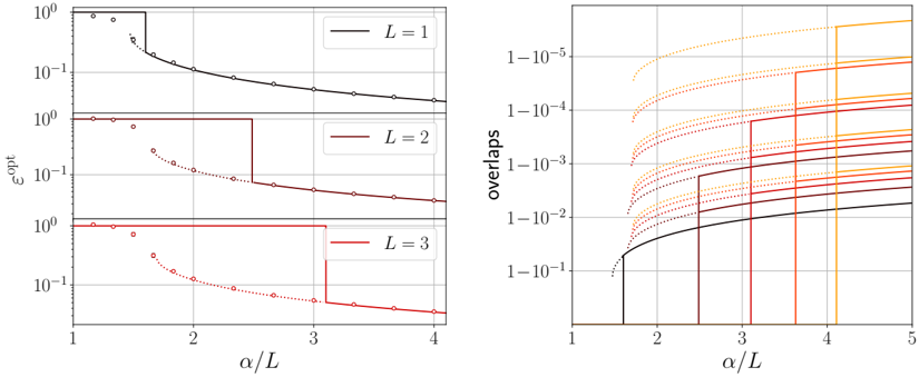<details> <summary>Image 19 Details</summary>  ### Visual Description ## Combined Line Charts: Epsilon Opt vs. Alpha/L and Overlaps vs. Alpha/L ### Overview The image presents two line charts side-by-side. The left chart displays epsilon optimal (εopt) as a function of alpha/L (α/L) for three different values of L (1, 2, and 3). The right chart shows overlaps as a function of alpha/L (α/L). Both charts use a logarithmic scale for the y-axis. ### Components/Axes **Left Chart:** * **Title:** Implicitly, "Epsilon Opt vs. Alpha/L" * **Y-axis:** εopt (epsilon optimal), logarithmic scale. Axis markers at 10^-1 and 10^0. * **X-axis:** α/L (alpha/L), linear scale. Axis markers at 1, 2, 3, and 4. * **Legend:** Located in the top-right corner of the left chart. * L = 1 (Black line) * L = 2 (Brown line) * L = 3 (Red line) **Right Chart:** * **Title:** Implicitly, "Overlaps vs. Alpha/L" * **Y-axis:** overlaps, logarithmic scale. Axis markers at 1e-1, 1e-2, 1e-3, 1e-4, and 1e-5. * **X-axis:** α/L (alpha/L), linear scale. Axis markers at 1, 2, 3, 4, and 5. * **Legend:** Implicit, colors correspond to different parameter values, but no explicit legend is provided. Colors range from black to yellow. ### Detailed Analysis **Left Chart:** * **L = 1 (Black):** The black line starts at approximately 1.0 for α/L = 1. It remains constant until approximately α/L = 1.5, then decreases sharply, following a curve with superimposed circles. * **L = 2 (Brown):** The brown line starts at approximately 1.0 for α/L = 1. It remains constant until approximately α/L = 2.5, then drops to approximately 0.07 and remains constant. A dotted brown line with circles follows a curve that decreases from α/L = 1 to α/L = 4. * **L = 3 (Red):** The red line starts at approximately 1.0 for α/L = 1. It remains constant until approximately α/L = 3, then drops to approximately 0.05 and remains constant. A dotted red line with circles follows a curve that decreases from α/L = 1 to α/L = 4. **Right Chart:** * **Black Line:** The black line starts at approximately 0 for α/L = 1. It remains at 0 until approximately α/L = 1.5, then increases sharply to approximately 0.01 at α/L = 2, and continues to increase gradually. * **Other Lines (Brown to Yellow):** There are multiple lines, some solid and some dotted, ranging in color from brown to yellow. These lines generally increase with α/L. The solid lines exhibit step-like increases, while the dotted lines increase more smoothly. The dotted lines are above the solid lines of similar color. ### Key Observations * In the left chart, as L increases, the point at which εopt drops shifts to the right (higher α/L values). * In the right chart, the overlaps generally increase with α/L. The dotted lines consistently show higher overlap values than the solid lines of similar color. ### Interpretation The left chart likely represents the performance of an optimization algorithm, where εopt represents the error or loss. The parameter L seems to influence the threshold at which the error starts to decrease as α/L increases. The right chart shows how overlaps between different solutions or states change with α/L. The step-like increases in the solid lines might indicate phase transitions or critical points. The dotted lines could represent a different type of overlap or a different regime of the system. The data suggests that increasing α/L generally leads to higher overlaps, and the parameter L in the left chart affects the optimal operating point. </details> rium overlap for a NN with L hidden layers we have $$Q _ { l + 1 } ^ { ( L + 1 ) * } \leq Q _ { l } ^ { ( L ) * } \quad f o r \quad 1 \leq l \leq L .$$ It follows from Q ( L +1) ∗ l +1 ≤ Q ( L +1) ∗ l +1 | W (1) = W (1)0 = Q ( L ) ∗ l , where the equality is a consequence from the fact that, since σ has µ 0 = µ 1 = µ 2 = 0 and E z ∼N (0 , 1) σ ( z ) 2 = 1, the data after the first layer have a covariance indistinguishable from I d from the perspective of the NN. Thus, the ( L + 1)-hidden layer NN with quenched first layer is equivalent to one with L hidden layers and standard Gaussian inputs. ## IV. REPLICAS PLUS HCIZ, REVAMPED ̸ The goal is to compute the asymptotic free entropy by the replica method [124], a powerful approach from spin glass theory also used in machine learning [29], combined with the HCIZ integral. We focus first on the derivation of the results for the shallow case L = 1 which comes with its own set of difficulties due to the presence of µ 2 = 0 in σ . We will later move on to the deep case where, even when considering µ 2 = 0, a different kind of difficulty will appear due to the multi-layer structure. Our derivation is based on three key ingredients. ( i ) The first ingredient is a Gaussian ansatz on the replicated post-activations, which generalises Conjecture 3.1 of [106], now proved in [108], where it is specialised to the case of linearly many data ( n = Θ( d )). To obtain this generalisation, we will write the kernel arising from the covariance of the post-activations as an infinite series of scalar OPs derived from the expansion of the activation function in the Hermite basis, following an approach recently devised in [200] in the context of the random feature model (see also [201] and [48]). ( ii ) The second ingredient, exposed in 'Simplifying the order parameters', amounts to a drastic reduction of the number of OPs entering the covariance of the postactivations through the realisation that infinitely many of them are expressible in terms of a few, more fundamental (functional) OPs. ̸ ( iii ) The last ingredient is a generalisation of an ansatz used in the replica method by [166] for dictionary learning, which will allow us to capture important correlations discarded by these earlier approaches [166, 167]. Our ansatz, explained in subsection 'Tackling the entropy', is the crux for capturing the lack of rotational invariance and matrix nature of the problem when σ possesses µ 2 = 0 when L = 1 or µ 1 = 0 when L = 2. We will see that, surprisingly, the HCIZ integral remains central despite the absence of rotational symmetry. App. B2 provides a comparison with the approach of [166]. ̸ For the sake of presentation, we discuss in the main only the non-standard steps corresponding to these ingredients. The complete derivations are presented in App. B1 for the shallow case and App. C 1 for the deep. Fixing the readouts. We use the fact that, having as goal the computation of the leading order of the free entropy, the readouts v of the learner can be fixed from the beginning to those of the target v 0 . The proof has been given in Remark 3 for the mutual information (and further discussed and tested in App. B 7), and implies directly at the level of free entropy that $$\begin{array} { r } { \frac { 1 } { n } \mathbb { E } \ln \mathcal { Z } _ { v = v ^ { 0 } } = \frac { 1 } { n } \mathbb { E } \ln \mathcal { Z } _ { v l a r m a b l e } + O ( 1 / d ) . } \end{array}$$ Consequently, for the rest of the derivations we set without loss of generality v = v 0 , thus leaving as learnable parameters the (many more) inner weights. If keeping learnable readouts, the (equivalent) replica calculation would be more cumbersome and ultimately yield that the overlap between v and v 0 is irrelevant for what matters all the other OPs in the universal phase; and once the student specialises, the readouts corresponding to specialised neurons are concurrently exactly recovered. ## A. Shallow MLP We start with the shallow case L = 1. Having directly fixed the readouts, the partition function is re-defined as $$\begin{array} { r } { \mathcal { Z } ( \ m a t h s c r { D } ) \colon = \mathcal { Z } _ { v = v ^ { 0 } } = \int d P _ { W } \left ( W \right ) \prod _ { \mu \leq n } P _ { o u t } \left ( y _ { \mu } | \lambda _ { \mu } ( \theta ) \right ) } \end{array}$$ with λ µ ( θ ) := F (1) θ ( x µ ) and θ = ( W , v 0 ). The quenched variables, averaged by the symbol E = E D , are the data D which depend on inputs and teacher. Equivalently, E [ · ] = E ( x µ ) E θ 0 E ( y µ ) | ( x µ ) , θ 0 [ · ]. Replicated system and order parameters. The starting point to tackle the data average is the usual replica trick: $$\lim _ { n } \frac { 1 } { \mathbb { E } } \ln \mathcal { Z } ( \mathcal { D } ) & = \lim \lim _ { s \to 0 ^ { + } } \frac { 1 } { n s } \ln \mathbb { E } \mathcal { Z } ^ { s } \\ & = \lim _ { s \to 0 ^ { + } } \lim _ { n s } \frac { 1 } { \mathbb { N } } \ln \mathbb { E } \mathcal { Z } ^ { s }$$ assuming the limits commute. Consider first s ∈ N + . Let θ a = ( W a , v 0 ), ( x , y ) = ( x 1 , y 1 ) and the 'replicas' of the post-activation, including the teacher's a = 0: $$\left \{ \lambda ^ { a } ( \pm b \theta ^ { a } ) \colon = \frac { 1 } { \sqrt { k } } v ^ { 0 T } \sigma \left ( \frac { 1 } { \sqrt { d } } W ^ { a } x \right ) \right \} _ { a = 0 } ^ { s } .$$ We directly get $$\mathbb { E } \mathcal { Z } ^ { s } & = \mathbb { E } _ { v ^ { 0 } } \int \prod _ { a } ^ { 0 , s } d P _ { W } ( \mathbf W ^ { a } ) \\ & \quad \times \left [ \mathbb { E } _ { x } \int d y \prod _ { a } ^ { 0 , s } P _ { o u t } ( y | \lambda ^ { a } ( \theta ^ { a } ) ) \right ] ^ { n } .$$ The key is to identify the law of the replicas { λ a } s a =0 , which are dependent random variables due to the common random Gaussian input x , conditionally on ( θ a ). As explained and checked numerically in Sec. II, our main hypothesis is that { λ a } are jointly Gaussian for the ( θ a ) that dominate the partition function (i.e., posterior samples), an ansatz we cannot prove but that we validate a posteriori thanks to the excellent match between the theory and the empirical generalisation curves, see (11), Remark 2 and Sec. III. Given two replica indices a, b ∈ { 0 , . . . , s } we define the neuron-neuron overlap matrix $$\begin{array} { r } { \Omega _ { i j } ^ { a b } \colon = \frac { 1 } { d } W _ { i } ^ { a \top } W _ { j } ^ { b } , \quad i , j \in [ k ] . } \end{array}$$ Recalling σ 's Hermite expansion, Mehler's formula (see App. A2) implies that the post-activations covariance is $$\begin{array} { r } { K ^ { a b } \colon = \mathbb { E } [ \lambda ^ { a } \lambda ^ { b } | \theta ^ { a } , \theta ^ { b } ] = \sum _ { \ell \geq 1 } ^ { \infty } \frac { \mu _ { \ell } ^ { 2 } } { \ell ! } R _ { \ell } ^ { a b } , \quad ( 2 4 ) } \end{array}$$ with the infinitely many overlap OPs $$\begin{array} { r } { R _ { \ell } ^ { a b } \colon = \frac { 1 } { k } \sum _ { i , j \leq k } v _ { i } ^ { 0 } v _ { j } ^ { 0 } ( \Omega _ { i j } ^ { a b } ) ^ { \ell } , \quad \ell \geq 1 . \quad ( 2 5 ) } \end{array}$$ This covariance K is complicated but, as we argue hereby, simplifications occur as d → ∞ . In particular, the first two overlaps R ab 1 , R ab 2 are special. We claim that higher order overlaps ( R ab ℓ ) ℓ ≥ 3 can be simplified as functions of simpler OPs. Simplifying the order parameters. In this section we show how to drastically reduce the number of OPs (25) to track. To build some intuition, it is convenient to define the symmetric tensors S a ℓ with $$\begin{array} { r } { S _ { \ell ; \alpha _ { 1 } \dots \alpha _ { \ell } } ^ { a } \colon = \frac { 1 } { \sqrt { k } } \sum _ { i \leq k } v _ { i } ^ { 0 } W _ { i \alpha _ { 1 } } ^ { a } \cdots W _ { i \alpha _ { \ell } } ^ { a } . \quad ( 2 6 ) } \end{array}$$ Indeed, the generic ℓ -th overlap (25) can be written as R ab ℓ = ( S a ℓ · S b ℓ ) /d ℓ (where ' · ' is the inner product among tensors obtained by contracting all the indices), e.g., R ab 2 = Tr S a 2 S b 2 /d 2 . The following assumptions amount in considering how these tensors behave for ℓ = 1 , 2 and ℓ ≥ 3. Let us start from the latter case. First, we assume that for Hadamard powers ℓ ≥ 3, the off-diagonal of the overlap ( Ω ab ) ◦ ℓ , obtained from i.i.d. weight matrices sampled from the posterior, is small enough to be discarded: $$\begin{array} { r l } { ( \Omega _ { i j } ^ { a b } ) ^ { \ell } \approx \delta _ { i j } ( \Omega _ { i i } ^ { a b } ) ^ { \ell } } & { i f \quad \ell \geq 3 . \quad } \\ { ( 2 7 ) } \end{array}$$ Approximate equality is up to a matrix with o d (1) operator norm. In other words, the weights W a i of a student (replica) is assumed to possibly align, for each i , only with a single W b j of the teacher (or, by Bayes-optimality, of another replica) indexed by j = π i , with π a permutation. The model is symmetric under permutations of hidden neurons with same readout value, we thus take π to be the identity without loss of generality. The same 'concentration on the diagonal' happens, e.g., for a standard Wishart matrix, which is the extreme case for Ω ab if W a = W b and P W = N (0 , 1): its eigenvectors and those of its Hadamard square are delocalised, while higher Hadamard powers ℓ ≥ 3 have strongly localised eigenvectors [134] (consequently, R ab 2 will require a separate treatment). Moreover, assume that the readout prior has discrete support Supp( P v ) =: V = { v } ; this can be relaxed by binning to a continuous support, as mentioned in Sec. II. By exchangeability among neurons with the same readout value, we further assume that all diagonal elements { Ω ab ii | i ∈ I v } concentrate onto the constant Q ab ( v ), where I v := { i ≤ k | v 0 i = v } : $$\begin{array} { r } { ( \Omega _ { i j } ^ { a b } ) ^ { \ell } \approx \delta _ { i j } \mathcal { Q } ^ { a b } ( v ) ^ { \ell } \, i f \ell \geq 3 a n d i o r j \in \mathcal { I } _ { v } . \quad ( 2 8 ) } \end{array}$$ FIG. 20. Hamiltonian Monte Carlo dynamics of the overlaps R ℓ = R 01 ℓ between student and teacher weights for ℓ ∈ [5], with activation function for L = 1 with ReLU( x ) activation, d = 200 , γ = 0 . 5, linear readout with ∆ = 0 . 1 and two choices of sample rates and readouts: α = 1 . 0 with P v = δ 1 ( Left ) and α = 3 . 0 with P v = N (0 , 1) ( Right ). The teacher weights W 0 are Gaussian and the readouts are fixed during sampling to the teacher ones. The dynamics is initialised informatively, i.e., on W 0 . The overlap R 1 always fluctuates around 1. Left : The overlaps R ℓ for ℓ ≥ 3 at equilibrium converge to 0, while R 2 is well estimated by the theory (orange dashed line). Right : At higher sample rate α , also the R ℓ for ℓ ≥ 3 are non zero and agree with their theoretical prediction (dashed lines). Insets show the mean-square generalisation error attained by HMC (solid) and the theoretical prediction ε opt (dashed). 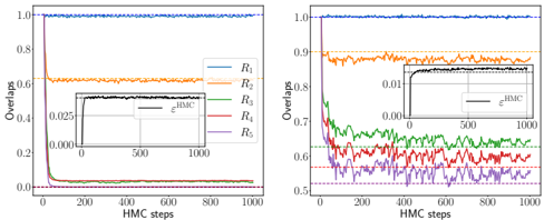<details> <summary>Image 20 Details</summary>  ### Visual Description ## Line Charts: Overlaps vs. HMC Steps (Two Plots) ### Overview The image contains two line charts, each plotting "Overlaps" on the y-axis against "HMC steps" on the x-axis. Both charts display five data series, labeled R1 through R5, and an inset plot showing a series labeled "εHMC". The charts appear to compare the convergence behavior of different methods or parameters related to Hybrid Monte Carlo (HMC). ### Components/Axes **Both Charts Share the Following:** * **X-axis:** "HMC steps", ranging from 0 to 1000. * **Y-axis:** "Overlaps", ranging from 0.0 to 1.0. * **Legend:** Located in the top-right of the left chart, indicating the data series R1 (blue), R2 (orange), R3 (green), R4 (red), and R5 (purple). The legend is implied to be the same for the right chart. * **Inset Plot:** Located in the center of each chart, showing "εHMC" (black) plotted against "HMC steps". **Left Chart:** * **Y-axis Markers:** 0.0, 0.2, 0.4, 0.6, 0.8, 1.0 * **Inset Plot X-axis:** 0 to 1000 HMC steps * **Inset Plot Y-axis:** 0.000, 0.025 * **Horizontal Dashed Lines:** At approximately 0.0, 0.65, and 1.0 **Right Chart:** * **Y-axis Markers:** 0.5, 0.6, 0.7, 0.8, 0.9, 1.0 * **Inset Plot X-axis:** 0 to 1000 HMC steps * **Inset Plot Y-axis:** 0.00, 0.01 * **Horizontal Dashed Lines:** At approximately 0.52, 0.57, 0.63, 0.75, 0.89, and 1.0 ### Detailed Analysis **Left Chart:** * **R1 (blue):** Starts at approximately 1.0 and remains stable around 1.0 throughout the HMC steps. * **R2 (orange):** Starts at approximately 1.0, rapidly decreases to approximately 0.65 within the first 50 HMC steps, and then remains stable around 0.65. * **R3 (green):** Starts at approximately 1.0, rapidly decreases to approximately 0.0 within the first 50 HMC steps, and then remains stable around 0.0. * **R4 (red):** Starts at approximately 1.0, rapidly decreases to approximately 0.0 within the first 50 HMC steps, and then remains stable around 0.0. * **R5 (purple):** Starts at approximately 1.0, rapidly decreases to approximately 0.0 within the first 50 HMC steps, and then remains stable around 0.0. * **εHMC (black, inset):** Starts at approximately 0.0, increases rapidly to approximately 0.025 within the first 200 HMC steps, and then remains stable around 0.025. **Right Chart:** * **R1 (blue):** Starts at approximately 1.0 and remains stable around 1.0 throughout the HMC steps. * **R2 (orange):** Starts at approximately 0.9, fluctuates between 0.85 and 0.9 throughout the HMC steps. * **R3 (green):** Starts at approximately 0.7, decreases to approximately 0.65 within the first 200 HMC steps, and then fluctuates between 0.6 and 0.7 throughout the HMC steps. * **R4 (red):** Starts at approximately 0.8, decreases to approximately 0.6 within the first 200 HMC steps, and then fluctuates between 0.58 and 0.65 throughout the HMC steps. * **R5 (purple):** Starts at approximately 0.7, decreases to approximately 0.55 within the first 200 HMC steps, and then fluctuates between 0.5 and 0.6 throughout the HMC steps. * **εHMC (black, inset):** Starts at approximately 0.0, increases rapidly to approximately 0.012 within the first 200 HMC steps, and then remains stable around 0.012. ### Key Observations * In both charts, R1 (blue) maintains a high overlap value close to 1.0, indicating stable behavior. * In the left chart, R3, R4, and R5 converge rapidly to near-zero overlap, suggesting a loss of correlation or a failure to maintain the desired state. * In the right chart, R2, R3, R4, and R5 exhibit more dynamic behavior, fluctuating around different overlap values. * The inset plots show that εHMC converges to a stable value in both charts, but the stable value is different between the two charts. ### Interpretation The charts likely compare the performance of different HMC configurations or parameters. The "Overlaps" metric probably measures the similarity between the current state of the HMC simulation and some target distribution or reference state. The left chart suggests that the configurations corresponding to R3, R4, and R5 are not effective, as they quickly lose overlap. The right chart shows more nuanced behavior, with R2, R3, R4, and R5 maintaining some level of overlap, albeit with fluctuations. The εHMC metric, shown in the inset plots, might represent an error or convergence measure for the HMC algorithm. The fact that it converges to different values in the two charts suggests that the overall performance of the HMC simulation differs significantly between the two scenarios represented by the charts. The horizontal dashed lines likely represent target values or thresholds for the overlap metric. </details> Equivalently, under the neuron exchangeability assumption, by summing over the indices i ∈ I v and dividing by their number the constant Q ab ( v ) can be written as $$\begin{array} { r } { \mathcal { Q } ^ { a b } ( v ) \colon = \frac { 1 } { | \mathcal { I } _ { v } | d } \sum _ { i \in \mathcal { I } _ { v } } ( W ^ { a } W ^ { b \top } ) _ { i i } . } \end{array}$$ This definition is directly related to the way we measure overlaps in numerical experiments, as empirical averages are less affected by finite size effects than specific choices of i ∈ I v ; thus, we adopt this definition also in our theoretical analysis. The advantage in switching from (27) to (28), i.e. in labelling the neurons with their readout value, is an expression suitable for the asymptotic regime we are considering, where the neurons are infinitely many. Indeed, with these simplifications we can write $$R _ { \ell } ^ { a b } = \mathbb { E } _ { v \sim P _ { v } } v ^ { 2 } \mathcal { Q } ^ { a b } ( v ) ^ { \ell } + o _ { d } ( 1 ) \, f o r \, \ell \geq 3 . \quad ( 2 9 )$$ This assumption has also a natural interpretation in terms of the tensors S a ℓ : in absence of specialisation, Q ab ( v ) = 0 for all v , so R ab ℓ = ( S a ℓ · S b ℓ ) /d ℓ = 0 according to (29). Indeed, a non-specialised model with kd = Θ( d 2 ) parameters and n = Θ( d 2 ) data cannot learn these tensors, as this would require the knowledge of Θ( d ℓ /ℓ !) entries and a comparable amount of tunable parameters; on the contrary, once specialisation occurs the model is able to factorise them using the r.h.s. of (26). ̸ Our assumption is verified numerically a posteriori as follows. Identity (29) is true (without o d (1)) for the predicted theoretical values of the OPs by construction of our theory. FIG. 7 verified the good agreement between theoretical and experimental overlap profiles Q 01 ( v ) for all v ∈ V (which is statistically the same as Q ab ( v ) for any a = b by the so-called Nishimori identity following from Bayes-optimality, see App. A 3), while FIG. 20 checks the agreement at the level of ( R ab ℓ ). Consequently, (29) also holds for the experimental overlaps. Having simplified the ℓ ≥ 3 terms in the series (24), let us pass to the ℓ = 1 case. Given that the number of data n = Θ( d 2 ) and that the corresponding ( S a 1 ) are only d -dimensional, they are reconstructed perfectly (the same argument was used in Remark 3 to argue that the readouts v can be quenched). We thus assume right away that at equilibrium the overlaps R ab 1 = 1 (or saturate to their maximum value; if tracked, the corresponding saddle point equations end up being trivial and do fix this). In other words, in the quadratic data regime, the µ 1 contribution in the Hermite decomposition of σ for the target is perfectly learnable, while higher order ones play a non-trivial role. In contrast, [106] study the regime n = Θ( d ) where µ 1 is the only learnable term. Then, the average replicated partition function reads $$\begin{array} { r } { \mathbb { E Z ^ { s } = \int d R _ { 2 } d Q \exp ( F _ { S } + n F _ { E } ) } \end{array}$$ where F E , F S depend on R 2 = ( R ab 2 ) and Q := {Q ab | a ≤ b } , where Q ab := {Q ab ( v ) | v ∈ V } . The 'energetic potential' is defined as $$\begin{array} { r l } { \text mp-} & e^{nF_{E}} \colon = [ \int d y d \lambda \frac { \exp ( - \frac { 1 } { 2 } \lambda ^ { \intercal } K ^ { - 1 } \lambda ) } { ( ( 2 \pi ) ^ { s + 1 } \det K ) ^ { 1 / 2 } } \prod _ { a } ^ { 0 , s } P _ { o u t } ( y | \lambda ^ { a } ) ] ^ { n } . } \end{array}$$ It takes this form due to our Gaussian assumption on the replicated post-activations and is thus easily computed, see App. B 1 a. The 'entropic potential' F S taking into account the degeneracy of the OPs entering the covariance of the post-activations is obtained by averaging delta functions fixing their definitions w.r.t. the 'microscopic degrees of freedom' ( W a ). It can be written compactly using the following conditional law over the tensors ( S a 2 ): $$\begin{array} { r l } & { P ( ( \mathbf S _ { 2 } ^ { a } ) | \mathbf Q ) \colon = V _ { W } ^ { k d } ( \mathbf Q ) ^ { - 1 } \int \prod _ { a } ^ { 0 , s } d P _ { W } ( \mathbf W ^ { a } ) } \\ & { \quad \times \prod _ { a \leq b } ^ { 0 , s } \prod _ { v \in V } \delta ( | \mathcal { I } _ { v } | d \mathcal { Q } ^ { a b } ( \mathbf v ) - \sum _ { i \in \mathcal { I } _ { v } } W _ { i } ^ { a \top } \mathbf W _ { i } ^ { b } ) } \\ & { \quad \times \prod _ { a } ^ { 0 , s } \delta ( \mathbf S _ { 2 } ^ { a } - \mathbf W ^ { a \top } d i a g ( \mathbf v ^ { 0 } ) \mathbf W ^ { a } / \sqrt { k } ) , \quad ( 3 0 ) } \end{array}$$ with normalisation V kd W = V kd W ( Q ) given by $$\begin{array} { r l } & { d i n g } \\ & { \quad V _ { W } ^ { k d } = \int \prod _ { a } ^ { 0 , s } d P _ { W } ( { W } ^ { a } ) } \\ & { \quad \times \prod _ { a \leq b } ^ { 0 , s } \prod _ { v \in \vee } \delta ( | \mathcal { I } _ { v } | d \, \mathcal { Q } ^ { a b } ( v ) - \sum _ { i \in \mathcal { I } _ { v } } { W } _ { i } ^ { a \top } { W } _ { i } ^ { b } ) . } \end{array}$$ The entropy of ( R 2 , Q ), which is the challenging term to compute, then reads $$\begin{array} { r l } { i a s } & e ^ { F _ { S } } \colon = V _ { W } ^ { k d } \int d P ( ( S _ { 2 } ^ { a } ) | Q | \, \mathcal { Q } ) \prod _ { a \leq b } ^ { 0 , s } \delta ( d ^ { 2 } R _ { 2 } ^ { a b } - T r \, S _ { 2 } ^ { a } S _ { 2 } ^ { b } ) . } \end{array}$$ Tackling the entropy: measure simplification by moment matching. The delta functions above fixing R ab 2 in the entropy of R 2 conditional on Q induce quartic constraints between the degrees of freedom ( W a iα ) instead of quadratic as usual. A direct computation thus seems out of reach. However, we will exploit the fact that the constraints are quadratic in the matrices ( S a 2 ). Consequently, shifting our focus towards ( S a 2 ) as the basic degrees of freedom to integrate rather than ( W a iα ) will allow us to move forward by simplifying their measure (30). Note that while ( W a iα ) i,α are i.i.d. under the prior P W , S a 2 has dependent entries under its corresponding prior. This important fact is taken into account as follows. Define P S as the probability density of a generalised Wishart random matrix ˜ W ⊺ diag( v 0 ) ˜ W / √ k , where ˜ W ∈ R k × d is made of i.i.d. standard Gaussian entries. The simplification we consider consists in replacing (30) by the effective measure $$\begin{array} { r l } & { \tilde { P } ( ( S _ { 2 } ^ { a } ) | \mathcal { Q } ) \colon = } \\ & { \quad \tilde { V } _ { W } ^ { k d } ( \mathcal { Q } ) ^ { - 1 } \prod _ { a } ^ { 0 , s } P _ { S } ( S _ { 2 } ^ { a } ) \prod _ { a < b } ^ { 0 , s } e ^ { \frac { 1 } { 2 } \tau ( \mathcal { Q } ^ { a b } ) T r } S _ { 2 } ^ { a } S _ { 2 } ^ { b } \quad ( 3 1 ) } \end{array}$$ where ˜ V kd W = ˜ V kd W ( Q ) is a normalisation constant, and $$\tau ( \mathcal { Q } ^ { a b } ) \colon = m m s e _ { S } ^ { - 1 } ( 1 - \mathbb { E } _ { v \sim P _ { v } } [ v ^ { 2 } \mathcal { Q } ^ { a b } ( v ) ^ { 2 } ] ) . \quad ( 3 2 ) \quad O P S$$ The rationale behind this choice goes as follows. The matrices ( S a 2 ) are, under the measure (30), ( i ) similar to generalised Wishart matrices, but instead constructed from ( ii ) non-Gaussian factors ( W a ), which ( iii ) are coupled between different replicas, thus inducing a coupling among replicas ( S a ). The proposed simplified measure captures all three aspects while remaining tractable, as we explain now. The first assumption is that in the measure (30) the details of the (centred, unit variance) prior P W enter only through Q at leading order. Due to the conditioning, we can thus relax it to Gaussian (with the same two first moments) by universality, as is often the case in random matrix theory. P W will instead explicitly enter in the entropy of Q related to V kd W . Point ( ii ) is thus taken care by the conditioning. Then, the generalised Wishart prior P S encodes ( i ) and, finally, the exponential tilt in ˜ P induces the replica couplings of point ( iii ). It now remains to capture the correct dependence of measure (30) on Q . This is done by realising that <!-- formula-not-decoded --> This is shown in App. B1c. The Lagrange multiplier τ ( Q ab ) to plug into ˜ P enforcing this moment matching condition between true and simplified measures as s → 0 + is (32), see App. B 1 e. For completeness, we provide in App. B 2 alternatives to the simplification (31), whose analysis are left for future work. Final steps and spherical integration. Combining all our findings, the average replicated partition function is simplified as $$\begin{array} { r l } & { \mathbb { E Z } ^ { s } = \int d { R } _ { 2 } d \pm b { Q } e ^ { n F _ { E } + k d \ln V _ { W } ( \pm b { Q } ) - k d \ln \tilde { V } _ { W } ( \pm b { Q } ) } } \\ & { \times \prod _ { a } ^ { 0 , s } P _ { S } ( S _ { 2 } ^ { a } ) \prod _ { a < b } ^ { 0 , s } e ^ { \frac { 1 } { 2 } \tau ( \pm b { Q } ^ { a b } ) T r \, S _ { 2 } ^ { a } s _ { 2 } ^ { b } } } \\ & { \times \prod _ { a \leq b } ^ { 0 , s } \delta ( d ^ { 2 } R _ { 2 } ^ { a b } - T r \, S _ { 2 } ^ { a } S _ { 2 } ^ { b } ) . } \end{array}$$ The equality should be interpreted as holding at leading exponential order exp(Θ( n )), assuming the validity of our previous measure simplification. All remaining steps but the last are standard: ( i ) Express the delta functions fixing Q , R 2 in exponential form using their Fourier representation; this introduces additional Fourier conjugate OPs ˆ Q , ˆ R 2 of same respective dimensions. ( ii ) Once this is done, the terms coupling different replicas of ( W a ) or of ( S a ) are all quadratic. Using the Hubbard-Stratonovich transformation (i.e., E Z exp( d 2 Tr MZ ) = exp( d 4 Tr M 2 ) for a d × d symmetric matrix M with Z a standard GOE matrix) therefore allows us to linearise all replica-replica coupling terms, at the price of introducing new Gaussian fields interacting with all replicas. ( iii ) After these manipulations, we identify at leading exponential order an effective action S depending on the OPs only, which allows a saddle point integration w.r.t. them as n →∞ : $$\begin{array} { r l } { m i l a r } & \lim \frac { 1 } { n s } \ln \mathbb { E Z ^ { s } = l i m \, \frac { 1 } { n s } \ln \int d R _ { 2 } d \hat { R } _ { 2 } d \mathcal { Q } d \hat { \mathcal { Q } } e ^ { n \mathcal { S } } = \frac { 1 } { s } e x t r \, \mathcal { S } . } \end{array}$$ ( iv ) Next, the replica limit s → 0 + of the previously obtained expression has to be considered. To do so, we make a replica symmetric assumption, i.e., we consider that at the saddle point, all OPs entering the action S , and thus K ab too, take a simple form of the type R ab = R d δ ab + R (1 -δ ab ). Replica symmetry is rigorously known to be correct in Bayes-optimal learning and is thus justified here, see [184, 202]. ( v ) The resulting expression still includes two highdimensional integrals related to the S 2 matrices. They correspond to the free entropies associated with the Bayes-optimal denoising of a generalised Wishart matrix, described above Result 1, for two signal-to-noise ratios. The last step deals with these matrix integrals over rationally invariant matrices using the HCIZ integral, whose form is tractable in this case [100, 101]. These free entropies yield the two last terms ι ( · ) in f (1) RS , (15). The complete derivation in App. B 1 gives Result 1. From the meaning of the OPs, this analysis also yields the post-activations covariance K and thus Result 2. As a final remark, we emphasise again a key difference between our approach and earlier works on extensiverank systems. If, instead of taking the generalised Wishart prior P S as the base measure over the matrices ( S a 2 ) in the simplified ˜ P with moment matching, one takes a factorised Gaussian measure, thus entirely forgetting the dependencies among S a 2 entries, this mimics the Sakata-Kabashima replica method [166]. Our ansatz thus captures important correlations neglected in [166, 167, 169, 186] in the context of linear-rank matrix inference. For completeness, we show in App. B 2 that our ansatz indeed improves the prediction compared to these earlier approaches. ## B. Two hidden layers MLP We now move to the deep MLP, by first considering the L = 2 case. We highlight here only the crucial steps that make the derivation different with respect to the one sketched above, deferring the reader to App. C 1 for more details. We assume this time that µ 2 = 0 (in addition to µ 0 = 0): in this way, our approach simplifies considerably, as the matrix degrees of freedom involved in the 2nd Hermite components of the activation functions do not appear in the theory. We will see however that, due to the deep structure of the network, matrix degrees of freedom coming from combinations of the model's hidden weights are still entering the theory, and will require the use of a rectangular spherical integral (see App. C 1). Popular activation functions (e.g., all the odd ones) comply with the requirement µ 2 = 0. Replicated system, order parameters and their simplification. Replicas of the post-activations can now be written recursively as $$\begin{array} { r l } & { \left \{ \lambda ^ { a } ( \boldsymbol \theta ^ { a } ) \colon = \frac { 1 } { \sqrt { k _ { 2 } } } v ^ { 0 T } \sigma ^ { ( 2 ) } ( h ^ { ( 2 ) a } ) \right \} _ { a = 0 } ^ { s } , } & { l o n s i e d } \\ & { \left \{ h ^ { ( l ) a } \colon = \frac { 1 } { \sqrt { k _ { l - 1 } } } W ^ { ( l ) a } \sigma ^ { ( l - 1 ) } ( h ^ { ( l - 1 ) a } ) \right \} _ { a = 0 , \dots , s ; \, l = 1 , 2 } , } & { ( \Omega ) } \end{array}$$ where we allowed different activations at each layer, we used the notation σ (0) ( x ) := x , k 0 = d and h (0) a = x for all a . For the sake of presentation, we further require the normalisation E z ∼N (0 , 1) σ ( l ) ( z ) 2 = 1 for all l , to avoid tracking this variance in the following (the case of generic variance can be derived from App. A 2). The expectation over the input x at given weights can be done as in (23), by assuming the same joint-Gaussianity of the post-activations ( λ a ) as in the shallow case. Moreover, to use recursively Mehler's formula we also assume that the pair of pre-activations ( h (2) a i , h (2) b j ) is jointly Gaussian for any choice of a, b = 0 , . . . , s and i, j ≤ k 2 . With these assumptions the covariances K ab := E x λ a λ b and Ω ( l ) ab := E x h ( l ) a h ( l ) b ⊺ can be written as $$\begin{array} { r } { \Omega ^ { ( i ) a b } \colon = \mathbb { E } _ { x } \mathbf h ^ { ( i ) a } \mathbf h ^ { ( i ) b } \, c a n \, b e w r t e n t e s } \end{array}$$ where the functions $$\begin{array} { r } { g ^ { ( l ) } ( x ) \colon = \sum _ { \ell = 3 } ^ { \infty } \frac { ( \mu _ { \ell } ^ { ( l ) } ) ^ { 2 } } { \ell ! } \, x ^ { \ell } } \end{array}$$ are applied entry-wise to matrices and µ ( l ) ℓ is the ℓ -th Hermite coefficient of σ ( l ) . Unfolding the above recursion, the covariance K ab can be written in terms of overlaps of 'effective' hidden weights and readout vectors $$\begin{array} { r l } & { W ^ { ( 2 \colon 1 ) a } \colon = \frac { W ^ { ( 2 ) a } W ^ { ( 1 ) a } } { \sqrt { k _ { 1 } } } , } \\ & { v ^ { ( 1 ) a } \colon = \frac { W ^ { ( 1 ) a \top } W ^ { ( 2 ) a \top } v ^ { 0 } } { \sqrt { k _ { 2 } k _ { 1 } } } , \quad v ^ { ( 2 ) a } \colon = \frac { W ^ { ( 2 ) a \top } v ^ { 0 } } { \sqrt { k _ { 2 } } } , } \end{array}$$ each of them arising from combinations of the activation's linear components. We also set v (3) a := v 0 . Moreover, simplifications can be taken along the three following lines: ( i ) v (1) a ⊺ v (1) b /k 0 is an overlap of d -dimensional vectors: as explained above (see the discussion on R ab 1 in the shallow case), it can be directly taken to be 1 in the quadratic data regime. ( ii ) Wherever a function g ( l ) , involving only Hadamard powers greater than 2, is applied to a matrix overlap, we assume the resulting matrix to be diagonal in the limit, g ( l ) ( Ω ( l ) ab ) ij ≈ δ ij g ( l ) ( Ω ( l ) ab ) ii , as we did in (27). ̸ From point ( ii ), and extending the approach we followed for the shallow case, we are naturally led to consider as OPs the diagonal profiles of the overlap matrices, (Ω ( l ) ab ii ) i . Moreover, from point ( iii ) we can label internal neurons (say, the ones in layer l ) with the value of the effective readout to which they are connected ( v ( l +1)0 i ) rather than with their index ( i ≤ k l ). By binning the distribution of the elements of v ( l )0 , we define the sets of indices I v ( l ) := { i ≤ k l -1 | v ( l )0 i = v ( l ) } , while keeping I v (with no layer label) as in (28). As before, in order to define the OPs we further assume exchangeability among neurons with the same effective readout value (e.g., ( W (1) a W (1) b ⊺ ) ii /d =: Q ab 1 ( v ( 2 ) ) for all i ∈ I v (2) ). Equivalently, by summing over these indices and normalising by their number, we obtain: ( iii ) The components v (2) a i , v (2) b i of the effective readouts enter the above expressions only if Ω (1) ab ii = 0, that is if some specialisation has occurred in the previous layer. As these components are Θ( k 1 ) in number, they can be reconstructed exactly with Θ( d 2 ) data. We can thus take these vectors as given, v (2) a ⊺ = v (2)0 ⊺ . From central limit theorem, the components of v (2)0 ⊺ are standard Gaussian variables, v (2)0 i ∼ N (0 , 1). $$\begin{array} { r l } & { i n g b y t h e n u m b e r , w e o b a t . } \\ & { \quad \mathcal { Q } _ { 1 } ^ { a b } ( v ^ { ( 2 ) } ) \colon = \frac { 1 } { | \mathcal { I } _ { v ^ { ( 2 ) } } | d } \sum _ { i \in \mathcal { I } _ { v ^ { ( 2 ) } } } ( W ^ { ( 1 ) a } W ^ { ( 1 ) b \top } ) _ { i i } , } \\ & { \quad \mathcal { Q } _ { 2 } ^ { a b } ( v , v ^ { ( 2 ) } ) \colon = \frac { 1 } { | \mathcal { I } _ { v ^ { ( 2 ) } } | | \mathcal { I } _ { v } | } \sum _ { i \in \mathcal { I } _ { v ^ { ( 2 ) } } , j \in \mathcal { I } _ { v } } W _ { j i } ^ { ( 2 ) a } W _ { j i } ^ { ( 2 ) b } , } \\ & { \quad \mathcal { Q } _ { 2 \colon 1 } ^ { a b } ( v ) \colon = \frac { 1 } { | \mathcal { I } _ { v } | d } \sum _ { i \in \mathcal { I } _ { v } } ( W ^ { ( 2 \colon 1 ) a } W ^ { ( 2 \colon 1 ) b \top } ) _ { i i } . } \end{array}$$ The bold notations Q 1 , Q 2 and Q 2:1 are defined analogously to the shallow case. In terms of these, the covariance of the post-activations reads $$a n c e o f t h e p o s t - a c t i v a t i o n s r e a d s \\ K ^ { a b } & = ( \mu _ { 1 } ^ { ( 2 ) } \mu _ { 1 } ^ { ( 1 ) } ) ^ { 2 } \\ & + ( \mu _ { 1 } ^ { ( 2 ) } ) ^ { 2 } \mathbb { E } _ { v ^ { ( 2 ) } \sim \mathcal { N } ( 0 , 1 ) } ( v ^ { ( 2 ) } ) ^ { 2 } g ^ { ( 1 ) } \left ( \mathcal { Q } _ { 1 } ^ { a b } ( v ^ { ( 2 ) } ) \right ) \\ & + \mathbb { E } _ { v \sim P _ { v } } v ^ { 2 } g ^ { ( 2 ) } \left [ ( \mu _ { 1 } ^ { ( 1 ) } ) ^ { 2 } \mathcal { Q } _ { 2 \colon 1 } ^ { a b } ( v ) \\ \ell - t h & \quad + \mathbb { E } _ { v ^ { ( 2 ) } \sim \mathcal { N } ( 0 , 1 ) } \mathcal { Q } _ { 2 } ^ { a b } ( v , v ^ { ( 2 ) } ) g ^ { ( 1 ) } \left ( \mathcal { Q } _ { 1 } ^ { a b } ( v ^ { ( 2 ) } ) \right ) \right ] . \\ \text {can} & \quad T h e s t r u c t i o n f o r t h i s c o v a r i a n c e i n f o r m s u s o n h o w t h e$$ The structure of this covariance informs us on how the learning can or cannot take place. E.g., if the first layer does not specialise, Q ab 1 ( v (2) ) = 0, then the second layer cannot either because its associated overlap disappears. From this point on, the energetic potential F E follows: it is the very same as for L = 1 but using the above covariance. Tackling the entropy using the rectangular spherical integral. The entropic potential, accounting for the degeneracy of the OPs, requires some care. We first define the conditional law over the matrices ( W (2:1) a ): $$P (( \mathbf W ^ { ( 2 \colon 1 ) a } ) | \mathbf Q _ { 1 } , \mathbf Q _ { 2 } ) \, \infty \int \prod _ { a = 0 } ^ { s } \prod _ { l = 1 } ^ { 2 } d P _ { W i } ( \mathbf W ^ { ( l ) a } ) \\ \times \delta ( \mathbf W ^ { ( 2 \colon 1 ) a } - \mathbf W ^ { ( 2 ) a } \mathbf W ^ { ( 1 ) a } / \sqrt { k _ { 1 } } ) \\ \times \prod _ { a \leq b } ^ { 0 , s } \prod _ { v ^ { ( 2 ) } \in V ^ { ( 2 ) } } \delta ( | \mathbf I _ { v ^ { ( 2 ) } } | \mathbf Q _ { 1 } ^ { a b } ( d P _ { W i } ^ { ( 1 ) a } ) \\ - \sum _ { i \in \mathcal { I } _ { v ^ { ( 2 ) } } } \delta ( | \mathbf I _ { v ^ { ( 2 ) } } | \mathbf Q _ { 2 } ^ { a b } ( v , v ^ { ( 2 ) } ) \\ \begin{array} { r l } & { w h e r e V ^ { ( 2 ) } i s t h e b n i n d u p o r t o f N ( 0 , 1 ) . I n t h i s w a y , } \\ & { \quad v = | \mathbf W _ { j i } ^ { ( 2 ) } | \mathbf Q _ { 1 } ^ { a b } ( d P _ { W i } ^ { ( 1 ) a } ) } \\ & { \quad - \sum _ { i \in \mathcal { I } _ { v ^ { ( 2 ) } } , j \in \mathcal { I } _ { v } } W _ { j i } ^ { ( 2 ) a } W _ { j i } ^ { ( 1 ) b } ) , } \\ & { w h e r e V ^ { ( 2 ) } i s t h e b n i n d u p o r t o f N ( 0 , 1 ) . I n t h i s w a y , } \end{array}$$ where V ( 2 ) is the binned support of N (0 , 1). In this way, we can write the entropic contribution as $$e ^ { F _ { s } } = V _ { 2 \colon 1 } ^ { k _ { 2 } d } \int d P ( ( W ^ { ( 2 \colon 1 ) a } ) \, | \, \mathcal { Q } _ { 1 } , \mathcal { Q } _ { 2 } ) \prod _ { a \leq b } ^ { 0 , s } \prod _ { v \in V } \\ \times \delta ( | \mathcal { I } _ { v } | d \mathcal { Q } _ { 2 \colon 1 } ^ { a b } ( v ) - \sum _ { i \in \mathcal { I } _ { v } } ( W ^ { ( 2 \colon 1 ) a } W ^ { ( 2 \colon 1 ) b } _ { T } ) _ { i i } ) ,$$ where V k 2 d 2:1 , depending implicitly on Q 1 , Q 2 , is the normalisation factor of P (( W (2:1) a ) | Q 1 , Q 2 ). The evaluation of the last integral involves coupled replicas of matrices with correlated entries. We deal with it by relaxing the measure P (( W (2:1) a ) | Q 1 , Q 2 ) to a tractable one, still able to capture the correlations between these degrees of freedom. To this aim, we first observe that, asymptotically, under the true conditional measure $$\begin{array} { r l } & { \frac { 1 } { | \mathcal { I } _ { v } | d } \sum _ { i \in \mathcal { I } _ { v } } \mathbb { E } [ ( W ^ { ( 2 \colon 1 ) a } W ^ { ( 2 \colon 1 ) b } \tau ) _ { i i } | \mathcal { Q } _ { 1 } , \mathcal { Q } _ { 2 } ] } & { c a n \, . } \end{array}$$ In order to match this moment in our relaxation, we take a tractable base measure with exponential tilts for each value v ∈ V : $$d \bar { P } ( ( W ^ { ( 2 \colon 1 ) a } ) | \mathcal { Q } _ { 1 } , \mathcal { Q } _ { 2 } ) = \prod _ { v \in V } V ( \tau _ { v } ) ^ { - 1 } \\ \times \prod _ { a = 0 } ^ { s } d P _ { U V } ( W _ { v } ^ { ( 2 \colon 1 ) a } ) e ^ { \sum _ { a < b , 0 } ^ { s } \tau _ { v } ^ { a b } T r W _ { v } ^ { ( 2 \colon 1 ) a } w _ { v } ^ { ( 2 \colon 1 ) b } }$$ where W (2:1) a v = ( W (2:1) a i ) i ∈I v and dP UV is the law of the product of two matrices with i.i.d. Gaussian entries ( U ∈ R |I v |× k 1 , V ∈ R k 1 × d ), τ v = ( τ ab v ) a,b is a function of Q 1 , Q 2 fixed by the previous moment matching, and V ( τ v ) is a normalisation factor. With this relaxation, the entropic contribution can be evaluated explicitly using the rectangular spherical integral, leading eventually to Result 3 (see App. C 1 for more details). ## C. Three or more hidden layers MLP To tackle the L ≥ 3 case, one could push forward the approach we presented in the previous section. However, even with the simplification of considering only activations with no second Hermite component, the analysis remains very challenging, as the post-activation covariance involves the 'effective weights' $$\begin{array} { r l } & { h e \quad W ^ { ( l ^ { \prime } ; l ) a } \colon = \frac { 1 } { \sqrt { k _ { l ^ { \prime } - 1 } k _ { l ^ { \prime } - 2 } \dots k _ { l } } } W ^ { ( l ^ { \prime } ) a } W ^ { ( l ^ { \prime } - 1 ) a } \dots W ^ { ( l ) a } , } \end{array}$$ as shown in App. C 1. These terms appear through combinations of the linear components of the activation functions σ ( l ′ -1) , . . . , σ ( l ) . To evaluate the entropic contributions of the OPs Q l ′ : l , defined as overlaps between replicas of the above effective weights, one has to consider all the possible learning mechanisms the network could adopt: a totally unspecialised strategy, where no W ( l ′′ ) a entering W ( l ′ : l ) a is learned by itself, but still W ( l ′ : l ) a is learned as a whole; a totally specialised strategy, where the model is able to learn separately all the W ( l ′′ ) a ; mixed strategies where some subsets of layers are specialised while others are not. All these mechanisms give explicit contributions to the correlation between teacher and student, and could correspond to different phases of the system. We leave the study of this rich phase diagram for future works. To simplify the picture, we require activations such that µ ( l ) 0 = µ ( l ) 1 = µ ( l ) 2 = 0 and set E z ∼N (0 , 1) σ ( l ) ( z ) 2 = 1 for all l ≤ L , which this time implies g ( l ) (1) = 1. In this case, the effective weights W ( l ′ : l ) a do not enter the post-activations covariance, simplifying considerably our analysis because the only possible learning strategy is specialisation at all layers. Indeed, $$\begin{array} { r l } { t i o n a l } & \left \{ \lambda ^ { a } ( \boldsymbol \theta ^ { a } ) \colon = \frac { 1 } { \sqrt { k _ { L } } } v ^ { 0 T } \sigma ^ { ( L ) } ( h ^ { ( L ) a } ) \right \} _ { a = 0 } ^ { s } , a n d K ^ { a b } \colon = \mathbb { E } _ { x } \lambda ^ { a } \lambda ^ { b } } \end{array}$$ can now be written recursively as $$\begin{array} { r l } & { K ^ { a b } = \frac { 1 } { k _ { L } } v ^ { 0 \intercal } g ^ { ( L ) } ( \Omega ^ { ( L ) a b } ) v ^ { 0 } \, , } \\ & { \Omega ^ { ( l ) a b } = \frac { 1 } { k _ { l - 1 } } W ^ { ( l ) a } g ^ { ( l - 1 ) } ( \Omega ^ { ( l - 1 ) a b } ) W ^ { ( l ) b \intercal } , \quad ( 3 3 ) } \end{array}$$ with Ω (0) ab = I d for all a, b and g (0) = id (the identity map). We make the same concentration assumption as before, namely g ( l ) ( Ω ( l ) ab ) ij ≈ δ ij g ( l ) ( Ω ( l ) ab ) ii . Moreover, we notice that only the neurons in the L -th layer can contribute with different importances to the output of the network, being connected to the (potentially) non-homogeneous readout vector v 0 ; nothing, in the post-activation covariance, distinguishes neurons in a layer l < L . For this reason, the OPs in this case are $$\begin{array} { r l } & { Q _ { l } ^ { a b } \colon = \frac { 1 } { k _ { l } k _ { l - 1 } } T r W ^ { ( l ) a } W ^ { ( l ) b } \text { for } l = 1 , \dots , L - 1 , } \\ & { \mathcal { Q } _ { L } ^ { a b } ( v ) \colon = \frac { 1 } { | \mathcal { I } _ { v } | k _ { L - 1 } } \sum _ { i \in \mathcal { I } _ { v } } ( W ^ { ( L ) a } W ^ { ( L ) b } \text { } ) _ { i i } . } \\ & { t o \quad } \end{array}$$ In terms of these, the post-activations covariance reads $$\begin{array} { r l } & { K ^ { a b } = \mathbb { E } _ { v \sim P _ { v } } v ^ { 2 } g ^ { ( L ) } \left ( \mathcal { Q } _ { L } ^ { a b } ( v ) g ^ { ( L - 1 ) } \left ( Q _ { L - 1 } ^ { a b } } \\ & { \quad \times g ^ { ( L - 2 ) } ( \cdots Q _ { 2 } ^ { a b } g ^ { ( 1 ) } ( Q _ { 1 } ^ { a b } ) \cdots ) \right ) \right ) . \, ( 3 4 ) } \end{array}$$ The entropic contribution of the OPs is easily computable, as they are all independent of each other. The calculation, reported in App. C 1, ultimately yields the free entropy reported in Result 4. ## V. CONCLUSION AND PERSPECTIVES In this paper we have derived a quantitatively accurate statistical physics description of the optimal generalisation capability of fully-trained linear-width MLPs with an arbitrary number of layers, for broad classes of activation functions, in the challenging scaling regime where the number of parameters is comparable to that of the training data. Even for shallow MLPs, this feature learning regime has resisted for a long time to mean-field approaches used, e.g., in the study of the narrow committee machines [7, 13, 15, 27]. Our theory has been validated through extensive numerical experiments using Monte Carlo samplers, a generalisation we proposed of the GAMP-RIE algorithm, and a popular algorithm used to train NNs, ADAM, showing in all cases a phenomenological picture consistent with our predictions. Phase transitions in supervised learning are known in the statistical physics literature at least since [22], when the analysis was limited to linear models. In this sense, our theory contributes to enrich this landscape, unveiling numerous phase transitions in the learning of different layers' weights for MLPs. Such transitions can occur heterogeneously across layers, and inside each layer. This rich behaviour is captured by functional order parameters with up to two arguments, which nevertheless allow a tractable dimensionality reduction of the problem. Concerning limitations, for L ≥ 2 we made some simplifying assumptions on the activation functions in order to reduce the number of order parameters and possible 'learning strategies' accessible to the trained network. A direction we intend to pursue is to relax them. Specifically, we aim at a theory encompassing a broader class of activation functions for an arbitrary finite number of layers. An additional difficulty is the systematic stability analysis of the potentially many fixed points of the RS equations, each corresponding to a different learning strategy of the network. Our theory opens an avenue for these extensions, as all the order parameters needed are now identifiable, but the analytical treatment and numerical exploration of the problem require further effort. Moreover, as hinted at in App. B 6, for L = 1 and activations without the second Hermite coefficient, we foresee a path for a possible rigorous proof of our results. A key novelty of our approach is the way we blend matrix models and spin glass techniques in a unified formalism, which is able to handle matrix degrees of freedom which are not necessarily rotationally invariant. It applies to NNs, but also to matrix sensing problems. We foresee that it will be useful beyond the realm of inference/learning problems. Another limitation of the approach is linked to the restricted class of solvable matrix models [130, 132]. Indeed, as explained in App. B 2, possible improvements would require additional order parameters. Taking them into account yields matrix models when computing their entropy which, to the best of our knowledge, are not currently solvable. This is an exciting program at the crossroad of matrix models, inference and learning of extensive-rank matrices. Accounting for structured inputs is another challenging perspective. Here we took into consideration a rather simple data model, i.e., Gaussian data with a covariance in the vein of [203, 204]. It would be desirable to study richer data models like mixture models [205, 206], hidden manifolds [174], object manifolds and simplexes [207210], hierarchical data [199, 211]. We have considered the idealised matched teacherstudent setting as a first step, with the goal of tackling the methodological bottlenecks associated with the depth and linear-width of the NN. Even in this simpler Bayesoptimal scenario, which in particular prevents replica symmetry breaking [124], the solution required the development of a non-standard approach. A natural next step is to consider targets belonging to a different function class than the trainable MLP, and focus on training by empirical risk minimisation (zero temperature) rather than Bayesian (finite temperature). We believe this generalisation can be carried out without major modifications of the theory, at least in the case where the target remains an MLP but with a different architecture. A complementary natural continuation is to push our formalism further in order to tackle deep architectures beyond the MLP, such as convolutional networks, restricted Boltzmann machines or transformers. The identification of the relevant order parameters for the characterisation of the equilibrium state carried out in our contribution paves the way for the study of the learning dynamics of first-order methods in similar settings. Indeed, there exist classical methods rooted in physics to study the learning dynamics of NNs [212215]. Recently, [216] exploits these techniques to study the learning dynamics of a large NN trained on a GLM target, observing a separation of timescales between generalisation and over-fitting: it could be interesting to use the insights from our equilibrium analysis to extend their approach to more expressive targets. In the context of the dynamics of learning, it is also relevant to consider power-law distributed readouts in the target, as many groups are currently doing in order to capture neural scaling laws [170, 217-220] in extensive-width shallow NNs. ## ACKNOWLEDGEMENTS F.C. was affiliated with the Abdus Salam International Centre for Theoretical Physics during the conduction of this work. J.B., F.C., M.-T.N. and M.P. were funded by the European Union (ERC, CHORAL, project number 101039794). Views and opinions expressed are however those of the authors only and do not necessarily reflect those of the European Union or the European Research Council. Neither the European Union nor the granting authority can be held responsible for them. M.P. thanks Vittorio Erba and Pietro Rotondo for interesting discussions and suggestions. - [1] P. L. Bartlett, A. Montanari, and A. Rakhlin, Deep learning: a statistical viewpoint, Acta Numerica 30 , 87 (2021). - [2] Y. LeCun, Y. Bengio, and G. Hinton, Deep learning, Nature 521 , 436 (2015). - [3] D. J. Amit, H. Gutfreund, and H. Sompolinsky, Spinglass models of neural networks, Phys. Rev. A 32 , 1007 (1985). - [4] E. Gardner, The space of interactions in neural network models, Journal of Physics A: Mathematical and General 21 , 257 (1988). - [5] E. Gardner and B. Derrida, Three unfinished works on the optimal storage capacity of networks, Journal of Physics A: Mathematical and General 22 , 1983 (1989). - [6] H. S. Seung, M. Opper, and H. Sompolinsky, Query by committee, in Proceedings of the Fifth Annual Workshop on Computational Learning Theory , COLT '92 (Association for Computing Machinery, New York, NY, USA, 1992) pp. 287-294. - [7] A. Engel, H. M. K¨ ohler, F. Tschepke, H. Vollmayr, and A. Zippelius, Storage capacity and learning algorithms for two-layer neural networks, Phys. Rev. A 45 , 7590 (1992). - [8] K. Kang, J.-H. Oh, C. Kwon, and Y. Park, Generalization in a two-layer neural network, Phys. Rev. E 48 , 4805 (1993). - [9] D. O'Kane and O. Winther, Learning to classify in large committee machines, Phys. Rev. E 50 , 3201 (1994). - [10] H. Schwarze and J. Hertz, Generalization in fully connected committee machines, Europhysics Letters 21 , 785 (1993). - [11] R. Urbanczik, Storage capacity of the fully-connected committee machine, Journal of Physics A: Mathematical and General 30 , L387 (1997). - [12] O. Winther, B. Lautrup, and J.-B. Zhang, Optimal learning in multilayer neural networks, Phys. Rev. E 55 , 836 (1997). - [13] H. Schwarze and J. Hertz, Generalization in a large committee machine, Europhysics Letters 20 , 375 (1992). - [14] H. Schwarze, M. Opper, and W. Kinzel, Generalization in a two-layer neural network, Phys. Rev. A 46 , R6185 (1992). - [15] G. Mato and N. Parga, Generalization properties of multilayered neural networks, Journal of Physics A: Mathematical and General 25 , 5047 (1992). - [16] R. Monasson and R. Zecchina, Weight space structure and internal representations: A direct approach to learning and generalization in multilayer neural networks, Phys. Rev. Lett. 75 , 2432 (1995). - [17] B. Schottky, Phase transitions in the generalization behaviour of multilayer neural networks, Journal of Physics A: Mathematical and General 28 , 4515 (1995). - [18] A. Engel, Correlation of internal representations in feedforward neural networks, Journal of Physics A: Mathematical and General 29 , L323 (1996). - [19] D. Malzahn, A. Engel, and I. Kanter, Storage capacity of correlated perceptrons, Phys. Rev. E 55 , 7369 (1997). - [20] D. Malzahn and A. Engel, Correlations between hidden units in multilayer neural networks and replica symmetry breaking, Phys. Rev. E 60 , 2097 (1999). - [21] H. Sompolinsky, N. Tishby, and H. S. Seung, Learning from examples in large neural networks, Phys. Rev. Lett. 65 , 1683 (1990). - [22] G. Gy¨ orgyi, First-order transition to perfect generalization in a neural network with binary synapses, Phys. Rev. A 41 , 7097 (1990). - [23] R. Meir and J. F. Fontanari, Learning from examples in weight-constrained neural networks, Journal of Physics A: Mathematical and General 25 , 1149 (1992). - [24] D. M. L. Barbato and J. F. Fontanari, The effects of lesions on the generalization ability of a perceptron, Journal of Physics A: Mathematical and General 26 , 1847 (1993). - [25] A. Engel and L. Reimers, Reliability of replica symmetry for the generalization problem of a toy multilayer neural network, Europhysics Letters 28 , 531 (1994). - [26] G. J. Bex, R. Serneels, and C. Van den Broeck, Storage capacity and generalization error for the reversed-wedge Ising perceptron, Phys. Rev. E 51 , 6309 (1995). - [27] E. Barkai, D. Hansel, and H. Sompolinsky, Broken symmetries in multilayered perceptrons, Phys. Rev. A 45 , 4146 (1992). - [28] H. Schwarze, Learning a rule in a multilayer neural network, Journal of Physics A: Mathematical and General 26 , 5781 (1993). - [29] A. Engel and C. Van den Broeck, Statistical mechanics of learning (Cambridge University Press, 2001). - [30] H. Cui, High-dimensional learning of narrow neural networks, Journal of Statistical Mechanics: Theory and Experiment 2025 , 023402 (2025). - [31] J. Bruna and D. Hsu, Survey on Algorithms for MultiIndex Models, Statistical Science 40 , 378 (2025). - [32] G. B. Arous, R. Gheissari, and A. Jagannath, Online stochastic gradient descent on non-convex losses from high-dimensional inference, J. Mach. Learn. Res. 22 , 10.5555/3546258.3546364 (2021). - [33] A. Damian, L. Pillaud-Vivien, J. Lee, and J. Bruna, Computational-statistical gaps in Gaussian single-index models (extended abstract), in Proceedings of Thirty Seventh Conference on Learning Theory , Proceedings of Machine Learning Research, Vol. 247, edited by S. Agrawal and A. Roth (PMLR, 2024) pp. 1262-1262. - [34] E. Abbe, E. Boix-Adsera, M. Brennan, G. Bresler, and D. Nagaraj, The staircase property: how hierarchical structure can guide deep learning, in Proceedings of the 35th International Conference on Neural Information Processing Systems , NIPS '21 (Curran Associates Inc., Red Hook, NY, USA, 2021). - [35] E. Abbe, E. B. Adser` a, and T. Misiakiewicz, SGD learning on neural networks: leap complexity and saddle-tosaddle dynamics, in Proceedings of Thirty Sixth Conference on Learning Theory , Proceedings of Machine Learning Research, Vol. 195, edited by G. Neu and L. Rosasco (PMLR, 2023) pp. 2552-2623. - [36] E. Troiani, Y. Dandi, L. Defilippis, L. Zdeborova, B. Loureiro, and F. Krzakala, Fundamental computational limits of weak learnability in high-dimensional multi-index models, in Proceedings of The 28th International Conference on Artificial Intelligence and Statistics , Proceedings of Machine Learning Research, Vol. 258, edited by Y. Li, S. Mandt, S. Agrawal, and E. Khan (PMLR, 2025) pp. 2467-2475. - [37] R. M. Neal, Priors for infinite networks, in Bayesian Learning for Neural Networks (Springer New York, New York, NY, 1996) pp. 29-53. - [38] C. Williams, Computing with infinite networks, in Advances in Neural Information Processing Systems , Vol. 9, edited by M. Mozer, M. Jordan, and T. Petsche (MIT Press, 1996). - [39] J. Lee, J. Sohl-dickstein, J. Pennington, R. Novak, S. Schoenholz, and Y. Bahri, Deep neural networks as Gaussian processes, in International Conference on Learning Representations (2018). - [40] A. G. D. G. Matthews, J. Hron, M. Rowland, R. E. Turner, and Z. Ghahramani, Gaussian process behaviour in wide deep neural networks, in International Conference on Learning Representations (2018). - [41] B. Hanin, Random neural networks in the infinite width limit as Gaussian processes, The Annals of Applied Probability 33 , 4798 (2023). - [42] H. Yoon and J.-H. Oh, Learning of higher-order perceptrons with tunable complexities, Journal of Physics A: Mathematical and General 31 , 7771 (1998). - [43] R. Dietrich, M. Opper, and H. Sompolinsky, Statistical mechanics of support vector networks, Phys. Rev. Lett. 82 , 2975 (1999). - [44] F. Gerace, B. Loureiro, F. Krzakala, M. M´ ezard, and L. Zdeborov´ a, Generalisation error in learning with random features and the hidden manifold model, Journal of Statistical Mechanics: Theory and Experiment 2021 , 124013 (2021). - [45] B. Bordelon, A. Canatar, and C. Pehlevan, Spectrum dependent learning curves in kernel regression and wide neural networks, in Proceedings of the 37th International Conference on Machine Learning , Proceedings of Machine Learning Research, Vol. 119, edited by H. D. III and A. Singh (PMLR, 2020) pp. 1024-1034. - [46] A. Canatar, B. Bordelon, and C. Pehlevan, Spectral bias and task-model alignment explain generalization in kernel regression and infinitely wide neural networks, Nature Communications 12 , 2914 (2021). - [47] L. Xiao, H. Hu, T. Misiakiewicz, Y. M. Lu, and J. Pennington, Precise learning curves and higher-order scaling limits for dot-product kernel regression, Journal of Statistical Mechanics: Theory and Experiment 2023 , 114005 (2023). - [48] B. Ghorbani, S. Mei, T. Misiakiewicz, and A. Montanari, Linearized two-layers neural networks in high dimension, The Annals of Statistics 49 , 1029 (2021). - [49] A. Rahimi and B. Recht, Random features for largescale kernel machines, in Advances in Neural Information Processing Systems , Vol. 20, edited by J. Platt, D. Koller, Y. Singer, and S. Roweis (Curran Associates, Inc., 2007). - [50] A. Jacot, F. Gabriel, and C. Hongler, Neural tangent kernel: Convergence and generalization in neural networks, in Advances in Neural Information Processing Systems , Vol. 31, edited by S. Bengio, H. Wallach, H. Larochelle, K. Grauman, N. Cesa-Bianchi, and R. Garnett (Curran Associates, Inc., 2018). - [51] L. Chizat, E. Oyallon, and F. Bach, On lazy training in differentiable programming, in Advances in Neural Information Processing Systems , Vol. 32, edited by H. Wallach, H. Larochelle, A. Beygelzimer, F. d ' Alch´ eBuc, E. Fox, and R. Garnett (Curran Associates, Inc., 2019). - [52] B. Ghorbani, S. Mei, T. Misiakiewicz, and A. Montanari, When do neural networks outperform kernel methods?, in Advances in Neural Information Processing Systems , Vol. 33, edited by H. Larochelle, M. Ranzato, R. Hadsell, M. Balcan, and H. Lin (Curran Associates, Inc., 2020) pp. 14820-14830. - [53] M. Refinetti, S. Goldt, F. Krzakala, and L. Zdeborova, Classifying high-dimensional Gaussian mixtures: Where kernel methods fail and neural networks succeed, in Proceedings of the 38th International Conference on Machine Learning , Proceedings of Machine Learning Research, Vol. 139, edited by M. Meila and T. Zhang (PMLR, 2021) pp. 8936-8947. - [54] E. Dyer and G. Gur-Ari, Asymptotics of wide networks from Feynman diagrams, in International Conference on Learning Representations (2020). - [55] S. Yaida, Non-Gaussian processes and neural networks at finite widths, in Proceedings of The First Mathematical and Scientific Machine Learning Conference , Proceedings of Machine Learning Research, Vol. 107, edited by J. Lu and R. Ward (PMLR, 2020) pp. 165-192. - [56] J. Zavatone-Veth, A. Canatar, B. Ruben, and C. Pehlevan, Asymptotics of representation learning in finite Bayesian neural networks, in Advances in Neural Information Processing Systems , Vol. 34, edited by M. Ranzato, A. Beygelzimer, Y. Dauphin, P. Liang, and J. W. Vaughan (Curran Associates, Inc., 2021) pp. 2476524777. - [57] K. T. Grosvenor and R. Jefferson, The edge of chaos: quantum field theory and deep neural networks, SciPost Phys. 12 , 081 (2022). - [58] K. Fischer, J. Lindner, D. Dahmen, Z. Ringel, M. Kr¨ amer, and M. Helias, Critical feature learning in deep neural networks, in Proceedings of the 41st International Conference on Machine Learning , Proceedings of Machine Learning Research, Vol. 235, edited by R. Salakhutdinov, Z. Kolter, K. Heller, A. Weller, N. Oliver, J. Scarlett, and F. Berkenkamp (PMLR, 2024) pp. 13660-13690. - [59] I. Banta, T. Cai, N. Craig, and Z. Zhang, Structures of neural network effective theories, Phys. Rev. D 109 , 105007 (2024). - [60] M. Guillen, P. Misof, and J. E. Gerken, Finite-width neural tangent kernels from Feynman diagrams (2025), arXiv:2508.11522 [cs.LG]. - [61] Y. Bahri, B. Hanin, A. Brossollet, V. Erba, C. Keup, R. Pacelli, and J. B. Simon, Les Houches lectures on deep learning at large and infinite width*, Journal of Statistical Mechanics: Theory and Experiment 2024 , 104012 (2024). - [62] Z. Ringel, N. Rubin, E. Mor, M. Helias, and I. Seroussi, Applications of statistical field theory in deep learning (2025), arXiv:2502.18553 [stat.ML]. - [63] S. Mei, A. Montanari, and P.-M. Nguyen, A mean field view of the landscape of two-layer neural networks, Proceedings of the National Academy of Sciences 115 , E7665 (2018). - [64] S. Mei, T. Misiakiewicz, and A. Montanari, Meanfield theory of two-layers neural networks: dimensionfree bounds and kernel limit, in Proceedings of the Thirty-Second Conference on Learning Theory , Proceedings of Machine Learning Research, Vol. 99, edited by A. Beygelzimer and D. Hsu (PMLR, 2019) pp. 2388- 2464. - [65] G. Yang and E. J. Hu, Tensor programs IV: Feature learning in infinite-width neural networks, in Proceedings of the 38th International Conference on Machine Learning , Proceedings of Machine Learning Research, Vol. 139, edited by M. Meila and T. Zhang (PMLR, 2021) pp. 11727-11737. - [66] G. Rotskoff and E. Vanden-Eijnden, Trainability and accuracy of artificial neural networks: An interacting particle system approach, Communications on Pure and Applied Mathematics 75 , 1889 (2022). - [67] J. Sirignano and K. Spiliopoulos, Mean field analysis of neural networks: A central limit theorem, Stochastic Processes and their Applications 130 , 1820 (2020). - [68] B. Bordelon and C. Pehlevan, Self-consistent dynamical field theory of kernel evolution in wide neural networks, in Advances in Neural Information Processing Systems , Vol. 35, edited by S. Koyejo, S. Mohamed, A. Agarwal, D. Belgrave, K. Cho, and A. Oh (Curran Associates, Inc., 2022) pp. 32240-32256. - [69] P.-M. Nguyen and H. T. Pham, A rigorous framework for the mean field limit of multilayer neural networks, Mathematical Statistics and Learning 6 , 201 (2023). - [70] F. Bassetti, M. Gherardi, A. Ingrosso, M. Pastore, and P. Rotondo, Feature learning in finite-width Bayesian deep linear networks with multiple outputs and convolutional layers, Journal of Machine Learning Research 26 , (88):1 (2025). - [71] N. Rubin, Z. Ringel, I. Seroussi, and M. Helias, A unified approach to feature learning in Bayesian neural networks, in High-dimensional Learning Dynamics 2024: The Emergence of Structure and Reasoning (2024). - [72] A. van Meegen and H. Sompolinsky, Coding schemes in neural networks learning classification tasks, Nature Communications 16 , 3354 (2025). - [73] C. Lauditi, B. Bordelon, and C. Pehlevan, Adaptive kernel predictors from feature-learning infinite limits of neural networks (2025), arXiv:2502.07998 [cs.LG]. - [74] A. X. Yang, M. Robeyns, E. Milsom, B. Anson, N. Schoots, and L. Aitchison, A theory of representation learning gives a deep generalisation of kernel methods, in Proceedings of the 40th International Conference on Machine Learning , Proceedings of Machine Learning Research, Vol. 202, edited by A. Krause, E. Brunskill, K. Cho, B. Engelhardt, S. Sabato, and J. Scarlett (PMLR, 2023) pp. 39380-39415. - [75] N. Rubin, I. Seroussi, and Z. Ringel, Grokking as a first order phase transition in two layer networks, in The Twelfth International Conference on Learning Representations (2024). - [76] A. M. Saxe, J. McClelland, and S. Ganguli, Exact solutions to the nonlinear dynamics of learning in deep linear neural networks, in Proceedings of the International Conference on Learning Representations 2014 (2014). - [77] Q. Li and H. Sompolinsky, Statistical mechanics of deep linear neural networks: The backpropagating kernel renormalization, Phys. Rev. X 11 , 031059 (2021). - [78] L. Aitchison, Why bigger is not always better: on finite and infinite neural networks, in International Conference on Machine Learning (PMLR, 2020) pp. 156-164. - [79] B. Hanin and A. Zlokapa, Bayesian interpolation with deep linear networks, Proceedings of the National Academy of Sciences 120 , e2301345120 (2023). - [80] J. A. Zavatone-Veth, W. L. Tong, and C. Pehlevan, Contrasting random and learned features in deep Bayesian linear regression, Phys. Rev. E 105 , 064118 (2022). - [81] B. Neyshabur, R. Tomioka, and N. Srebro, Norm-based capacity control in neural networks, in Proceedings of The 28th Conference on Learning Theory , Proceedings of Machine Learning Research, Vol. 40, edited by P. Gr¨ unwald, E. Hazan, and S. Kale (PMLR, Paris, France, 2015) pp. 1376-1401. - [82] S. Pesme and N. Flammarion, Saddle-to-saddle dynamics in diagonal linear networks, in Advances in Neural Information Processing Systems , Vol. 36, edited by A. Oh, T. Naumann, A. Globerson, K. Saenko, M. Hardt, and S. Levine (Curran Associates, Inc., 2023) pp. 7475-7505. - [83] D. Soudry, E. Hoffer, M. S. Nacson, S. Gunasekar, and N. Srebro, The implicit bias of gradient descent on separable data, Journal of Machine Learning Research 19 , 1 (2018). - [84] S. Pesme, L. Pillaud-Vivien, and N. Flammarion, Implicit bias of SGD for diagonal linear networks: a provable benefit of stochasticity, in Advances in Neural Information Processing Systems , edited by A. Beygelzimer, Y. Dauphin, P. Liang, and J. W. Vaughan (2021). - [85] R. Berthier, Incremental learning in diagonal linear networks, J. Mach. Learn. Res. 24 , 10.5555/3648699.3648870 (2023). - [86] H. Labarri` ere, C. Molinari, L. Rosasco, S. Villa, and C. Vega, Optimization insights into deep diagonal linear networks (2025), arXiv:2412.16765 [cs.LG]. - [87] S. Du and J. Lee, On the power of over-parametrization in neural networks with quadratic activation, in Proceedings of the 35th International Conference on Machine Learning , Proceedings of Machine Learning Research, Vol. 80, edited by J. Dy and A. Krause (PMLR, 2018) pp. 1329-1338. - [88] M. Soltanolkotabi, A. Javanmard, and J. D. Lee, Theoretical insights into the optimization landscape of overparameterized shallow neural networks, IEEE Transactions on Information Theory 65 , 742 (2019). - [89] L. Venturi, A. S. Bandeira, and J. Bruna, Spurious valleys in one-hidden-layer neural network optimization landscapes, Journal of Machine Learning Research 20 , (133):1 (2019). - [90] S. Sarao Mannelli, E. Vanden-Eijnden, and L. Zdeborov´ a, Optimization and generalization of shallow neural networks with quadratic activation functions, in Advances in Neural Information Processing Systems , Vol. 33, edited by H. Larochelle, M. Ranzato, R. Hadsell, M. Balcan, and H. Lin (Curran Associates, Inc., 2020) pp. 13445-13455. - [91] D. Gamarnik, E. C. Kızılda˘ g, and I. Zadik, Stationary points of a shallow neural network with quadratic activations and the global optimality of the gradient descent algorithm, Mathematics of Operations Research 50 , 209 (2024). - [92] S. Martin, F. Bach, and G. Biroli, On the impact of overparameterization on the training of a shallow neural network in high dimensions, in Proceedings of The 27th International Conference on Artificial Intelligence and Statistics , Proceedings of Machine Learning Research, Vol. 238, edited by S. Dasgupta, S. Mandt, and Y. Li (PMLR, 2024) pp. 3655-3663. - [93] Y. Arjevani, J. Bruna, J. Kileel, E. Polak, and M. Trager, Geometry and optimization of shallow polynomial networks (2025), arXiv:2501.06074 [cs.LG]. - [94] A. Maillard, E. Troiani, S. Martin, L. Zdeborov´ a, and F. Krzakala, Bayes-optimal learning of an extensivewidth neural network from quadratically many samples, in Advances in Neural Information Processing Systems , Vol. 37, edited by A. Globerson, L. Mackey, D. Belgrave, A. Fan, U. Paquet, J. Tomczak, and C. Zhang (Curran Associates, Inc., 2024) pp. 82085-82132. - [95] Y. Xu, A. Maillard, L. Zdeborov´ a, and F. Krzakala, Fundamental limits of matrix sensing: Exact asymptotics, universality, and applications (2025). - [96] V. Erba, E. Troiani, L. Zdeborov´ a, and F. Krzakala, The nuclear route: Sharp asymptotics of erm in overparameterized quadratic networks (2025), arXiv:2505.17958 [stat.ML]. - [97] G. Ben Arous, M. A. Erdogdu, N. M. Vural, and D. Wu, Learning quadratic neural networks in high dimensions: SGD dynamics and scaling laws (2025), arXiv:2508.03688 [stat.ML]. - [98] J. Barbier, F. Krzakala, N. Macris, L. Miolane, and L. Zdeborov´ a, Optimal errors and phase transitions in high-dimensional generalized linear models, Proceedings of the National Academy of Sciences 116 , 5451 (2019). - [99] J. Barbier and N. Macris, Statistical limits of dictionary learning: Random matrix theory and the spectral replica method, Phys. Rev. E 106 , 024136 (2022). - [100] A. Maillard, F. Krzakala, M. M´ ezard, and L. Zdeborov´ a, Perturbative construction of mean-field equations in extensive-rank matrix factorization and denoising, Journal of Statistical Mechanics: Theory and Experiment 2022 , 083301 (2022). - [101] F. Pourkamali, J. Barbier, and N. Macris, Matrix inference in growing rank regimes, IEEE Transactions on Information Theory 70 , 8133 (2024). - [102] G. Semerjian, Matrix denoising: Bayes-optimal estimators via low-degree polynomials, Journal of Statistical Physics 191 , 139 (2024). - [103] R. Pacelli, S. Ariosto, M. Pastore, F. Ginelli, M. Gherardi, and P. Rotondo, A statistical mechanics framework for Bayesian deep neural networks beyond the infinitewidth limit, Nature Machine Intelligence 5 , 1497 (2023), arXiv:2209.04882 [cond-mat.dis-nn]. - [104] P. Baglioni, R. Pacelli, R. Aiudi, F. Di Renzo, A. Vezzani, R. Burioni, and P. Rotondo, Predictive power of a Bayesian effective action for fully connected one hidden layer neural networks in the proportional limit, Phys. Rev. Lett. 133 , 027301 (2024). - [105] A. Ingrosso, R. Pacelli, P. Rotondo, and F. Gerace, Statistical mechanics of transfer learning in fully connected networks in the proportional limit, Phys. Rev. Lett. 134 , 177301 (2025). - [106] H. Cui, F. Krzakala, and L. Zdeborova, Bayes-optimal learning of deep random networks of extensive-width, in Proceedings of the 40th International Conference on Machine Learning , Proceedings of Machine Learning Research, Vol. 202, edited by A. Krause, E. Brunskill, K. Cho, B. Engelhardt, S. Sabato, and J. Scarlett (PMLR, 2023) pp. 6468-6521. - [107] F. Camilli, D. Tieplova, and J. Barbier, Fundamental limits of overparametrized shallow neural networks for supervised learning, Bollettino dell'Unione Matematica Italiana 10.1007/s40574-025-00506-2 (2025). - [108] F. Camilli, D. Tieplova, E. Bergamin, and J. Barbier, Information-theoretic reduction of deep neural networks to linear models in the overparametrized proportional regime, in Proceedings of Thirty Eighth Conference on Learning Theory , Proceedings of Machine Learning Research, Vol. 291, edited by N. Haghtalab and A. Moitra (PMLR, 2025) pp. 757-798. - [109] G. Naveh and Z. Ringel, A self consistent theory of Gaussian processes captures feature learning effects in finite CNNs, in Advances in Neural Information Processing Systems , Vol. 34, edited by M. Ranzato, A. Beygelzimer, Y. Dauphin, P. Liang, and J. W. Vaughan (Curran Associates, Inc., 2021) pp. 2135221364. - [110] I. Seroussi, G. Naveh, and Z. Ringel, Separation of scales and a thermodynamic description of feature learning in some CNNs, Nature Communications 14 , 908 (2023), arXiv:2112.15383 [stat.ML]. - [111] R. Aiudi, R. Pacelli, P. Baglioni, A. Vezzani, R. Burioni, and P. Rotondo, Local kernel renormalization as a mechanism for feature learning in overparametrized convolutional neural networks, Nature Communications 16 , 568 (2025), arXiv:2307.11807 [cs.LG]. - [112] H. Yoshino, From complex to simple: hierarchical freeenergy landscape renormalized in deep neural networks, SciPost Phys. Core 2 , 005 (2020). - [113] H. Yoshino, Spatially heterogeneous learning by a deep student machine, Phys. Rev. Res. 5 , 033068 (2023). - [114] G. Huang, L. S. Chan, H. Yoshino, G. Zhang, and Y. Jin, Liquid and solid layers in a thermal deep learning machine (2025), arXiv:2506.06789 [cond-mat.dis-nn]. - [115] J. Yao, Y. Yacoby, B. Coker, W. Pan, and F. DoshiVelez, An empirical analysis of the advantages of finitev.s. infinite-width Bayesian neural networks (2022). - [116] J. Lee, S. S. Schoenholz, J. Pennington, B. Adlam, L. Xiao, R. Novak, and J. Sohl-Dickstein, Finite versus infinite neural networks: an empirical study, in Proceedings of the 34th International Conference on Neural Information Processing Systems , NIPS '20 (Curran Associates Inc., Red Hook, NY, USA, 2020). - [117] L. Zdeborov´ a, Understanding deep learning is also a job for physicists, Nature Physics 16 , 602 (2020). - [118] Y. Bahri, J. Kadmon, J. Pennington, S. S. Schoenholz, J. Sohl-Dickstein, and S. Ganguli, Statistical mechanics of deep learning, Annual review of condensed matter physics 11 , 501 (2020). - [119] J. Hoffmann et al. , Training compute-optimal large language models, in Advances in Neural Information Processing Systems , Vol. 35, edited by S. Koyejo, S. Mohamed, A. Agarwal, D. Belgrave, K. Cho, and A. Oh (Curran Associates, Inc., 2022) pp. 30016-30030. - [120] J. Ni, Q. Liu, C. Du, L. Dou, H. Yan, Z. Wang, T. Pang, and M. Q. Shieh, Training optimal large diffusion language models, arXiv preprint arXiv:2510.03280 (2025). - [121] M. Lan, P. Torr, A. Meek, A. Khakzar, D. Krueger, and F. Barez, Quantifying feature space universality across large language models via sparse autoencoders (2025), arXiv:2410.06981 [cs.LG]. - [122] Z. Li, C. Fan, and T. Zhou, Grokking in LLM pretraining? Monitor memorization-to-generalization without test (2025), arXiv:2506.21551 [cs.LG]. - [123] M. Mondelli and A. Montanari, On the connection between learning two-layer neural networks and tensor decomposition, in Proceedings of the Twenty-Second International Conference on Artificial Intelligence and Statistics , Proceedings of Machine Learning Research, Vol. 89, edited by K. Chaudhuri and M. Sugiyama (PMLR, 2019) pp. 1051-1060. - [124] M. Mezard, G. Parisi, and M. Virasoro, Spin Glass Theory and Beyond (World Scientific, 1986). - [125] C. Itzykson and J. Zuber, The planar approximation. II, Journal of Mathematical Physics 21 , 411 (1980). - [126] A. Matytsin, On the largeN limit of the Itzykson-Zuber integral, Nuclear Physics B 411 , 805 (1994). - [127] A. Guionnet and O. Zeitouni, Large deviations asymptotics for spherical integrals, Journal of Functional Analysis 188 , 461 (2002). - [128] A. Guionnet, First order asymptotics of matrix integrals; a rigorous approach towards the understanding of matrix models, Communications in Mathematical Physics 244 , 527 (2004). - [129] J.-B. Zuber, The largeN limit of matrix integrals over the orthogonal group, Journal of Physics A: Mathematical and Theoretical 41 , 382001 (2008). - [130] V. A. Kazakov, Solvable matrix models (2000), arXiv:hep-th/0003064 [hep-th]. - [131] E. Br´ ezin, S. Hikami, et al. , Random matrix theory with an external source (Springer, 2016). - [132] D. Anninos and B. M¨ uhlmann, Notes on matrix models (matrix musings), Journal of Statistical Mechanics: Theory and Experiment 2020 , 083109 (2020). - [133] J. Bun, J. P. Bouchaud, S. N. Majumdar, and M. Potters, Instanton approach to large N Harish-ChandraItzykson-Zuber integrals, Phys. Rev. Lett. 113 , 070201 (2014). - [134] M. Potters and J.-P. Bouchaud, A first course in random matrix theory: for physicists, engineers and data scientists (Cambridge University Press, 2020). - [135] J. Husson and J. Ko, Spherical integrals of sublinear rank, Probability Theory and Related Fields 193 , 1 (2025). - [136] G. Parisi and M. Potters, Mean-field equations for spin models with orthogonal interaction matrices, Journal of Physics A: Mathematical and General 28 , 5267 (1995). - [137] M. Opper and O. Winther, Adaptive and self-averaging Thouless-Anderson-Palmer mean-field theory for probabilistic modeling, Phys. Rev. E 64 , 056131 (2001). - [138] M. Opper, B. C ¸akmak, and O. Winther, A theory of solving TAP equations for Ising models with general invariant random matrices, Journal of Physics A: Mathematical and Theoretical 49 , 114002 (2016). - [139] Z. Fan, Y. Li, and S. Sen, TAP equations for orthogonally invariant spin glasses at high temperature (2022), arXiv:2202.09325 [math.PR]. - [140] J. Barbier and M. S´ aenz, Marginals of a spherical spin glass model with correlated disorder, Electronic Communications in Probability 27 , 1 (2022). - [141] Z. Fan and Y. Wu, The replica-symmetric free energy for Ising spin glasses with orthogonally invariant couplings, Probability Theory and Related Fields 190 , 1 (2024). - [142] Y. Kabashima, Inference from correlated patterns: a unified theory for perceptron learning and linear vector channels, Journal of Physics: Conference Series 95 , 012001 (2008). - [143] M. Gabri´ e, A. Manoel, C. Luneau, J. Barbier, N. Macris, F. Krzakala, and L. Zdeborov´ a, Entropy and mutual information in models of deep neural networks, in Advances in Neural Information Processing Systems , Vol. 31, edited by S. Bengio, H. Wallach, H. Larochelle, K. Grauman, N. Cesa-Bianchi, and R. Garnett (Curran Associates, Inc., 2018). - [144] K. Takeda, S. Uda, and Y. Kabashima, Analysis of CDMA systems that are characterized by eigenvalue spectrum, Europhysics Letters 76 , 1193 (2006). - [145] A. Tulino, G. Caire, S. Shamai, and S. Verd´ u, Support recovery with sparsely sampled free random matrices, in 2011 IEEE International Symposium on Information Theory Proceedings (2011) pp. 2328-2332. - [146] T. Hou, Y. Liu, T. Fu, and J. Barbier, Sparse superposition codes under VAMP decoding with generic rotational invariant coding matrices, in 2022 IEEE International Symposium on Information Theory (ISIT) (2022) pp. 1372-1377. - [147] J. Barbier, F. Camilli, Y. Xu, and M. Mondelli, Information limits and Thouless-Anderson-Palmer equations for spiked matrix models with structured noise, Phys. Rev. Res. 7 , 013081 (2025). - [148] S. Rangan, P. Schniter, and A. K. Fletcher, Vector approximate message passing, IEEE Transactions on Information Theory 65 , 6664 (2019). - [149] J. Ma and L. Ping, Orthogonal AMP, IEEE Access 5 , 2020 (2017). - [150] A. Maillard, L. Foini, A. L. Castellanos, F. Krzakala, M. M´ ezard, and L. Zdeborov´ a, High-temperature expansions and message passing algorithms, Journal of Statistical Mechanics: Theory and Experiment 2019 , 113301 (2019). - [151] L. Liu, S. Huang, and B. M. Kurkoski, Memory AMP, IEEE Transactions on Information Theory 68 , 8015 (2022). - [152] K. Takeuchi, On the convergence of orthogonal/vector AMP: Long-memory message-passing strategy, in 2022 IEEE International Symposium on Information Theory (ISIT) (2022) pp. 1366-1371. - [153] T. Takahashi and Y. Kabashima, Macroscopic analysis of vector approximate message passing in a modelmismatched setting, IEEE Transactions on Information Theory 68 , 5579 (2022). - [154] Z. Fan, Approximate Message Passing algorithms for rotationally invariant matrices, The Annals of Statistics 50 , 197 (2022). - [155] J. Barbier, N. Macris, A. Maillard, and F. Krzakala, The mutual information in random linear estimation beyond i.i.d. matrices, in 2018 IEEE International Symposium on Information Theory (ISIT) (2018) pp. 1390-1394. - [156] C. Gerbelot, A. Abbara, and F. Krzakala, Asymptotic errors for high-dimensional convex penalized linear regression beyond Gaussian matrices, in Proceedings of Thirty Third Conference on Learning Theory , Proceedings of Machine Learning Research, Vol. 125, edited by J. Abernethy and S. Agarwal (PMLR, 2020) pp. 16821713. - [157] C. Gerbelot, A. Abbara, and F. Krzakala, Asymptotic errors for teacher-student convex generalized linear models (or: How to prove Kabashima's replica formula), IEEE Transactions on Information Theory 69 , 1824 (2023). - [158] R. Dudeja, Y. M. Lu, and S. Sen, Universality of approximate message passing with semirandom matrices, The Annals of Probability 51 , 1616 (2023). - [159] J. Barbier, F. Camilli, M. Mondelli, and M. S´ aenz, Fundamental limits in structured principal component anal- ysis and how to reach them, Proceedings of the National Academy of Sciences 120 , e2302028120 (2023). - [160] R. Dudeja, S. Liu, and J. Ma, Optimality of approximate message passing algorithms for spiked matrix models with rotationally invariant noise (2025), arXiv:2405.18081 [math.ST]. - [161] O. Ledoit and S. P´ ech´ e, Eigenvectors of some large sample covariance matrix ensembles, Probability Theory and Related Fields 151 , 233 (2011). - [162] J. Bun, R. Allez, J.-P. Bouchaud, and M. Potters, Rotational invariant estimator for general noisy matrices, IEEE Transactions on Information Theory 62 , 7475 (2016). - [163] F. Pourkamali and N. Macris, Rectangular rotational invariant estimator for general additive noise matrices, in 2023 IEEE International Symposium on Information Theory (ISIT) (2023) pp. 2081-2086. - [164] E. Troiani, V. Erba, F. Krzakala, A. Maillard, and L. Zdeborova, Optimal denoising of rotationally invariant rectangular matrices, in Proceedings of Mathematical and Scientific Machine Learning , Proceedings of Machine Learning Research, Vol. 190, edited by B. Dong, Q. Li, L. Wang, and Z.-Q. J. Xu (PMLR, 2022) pp. 97-112. - [165] H. C. Schmidt, Statistical physics of sparse and dense models in optimization and inference , Ph.D. thesis, IPHT - Institut de Physique Th´ eorique (2018). - [166] A. Sakata and Y. Kabashima, Statistical mechanics of dictionary learning, Europhysics Letters 103 , 28008 (2013). - [167] Y. Kabashima, F. Krzakala, M. M´ ezard, A. Sakata, and L. Zdeborov´ a, Phase transitions and sample complexity in Bayes-optimal matrix factorization, IEEE Transactions on Information Theory 62 , 4228 (2016). - [168] V. Erba, E. Troiani, L. Biggio, A. Maillard, and L. Zdeborov´ a, Bilinear sequence regression: A model for learning from long sequences of high-dimensional tokens, Phys. Rev. X 15 , 021092 (2025). - [169] J. Barbier, F. Camilli, J. Ko, and K. Okajima, Phase diagram of extensive-rank symmetric matrix denoising beyond rotational invariance, Phys. Rev. X 15 , 021085 (2025). - [170] Y. Ren, E. Nichani, D. Wu, and J. D. Lee, Emergence and scaling laws in SGD learning of shallow neural networks (2025), arXiv:2504.19983 [cs.LG]. - [171] A. Bodin and N. Macris, Gradient flow on extensiverank positive semi-definite matrix denoising, in 2023 IEEE Information Theory Workshop (ITW) (IEEE, 2023) pp. 365-370. - [172] J. Barbier, F. Camilli, M.-T. Nguyen, M. Pastore, and R. Skerk, https://github.com/Minh-Toan/ statphys-deep-NN (2025). - [173] S. Mei and A. Montanari, The generalization error of random features regression: Precise asymptotics and the double descent curve, Communications on Pure and Applied Mathematics 75 , 667 (2022), arXiv:1908.05355 [math.ST]. - [174] S. Goldt, M. M´ ezard, F. Krzakala, and L. Zdeborov´ a, Modeling the influence of data structure on learning in neural networks: The hidden manifold model, Phys. Rev. X 10 , 041044 (2020). - [175] T. Hastie, A. Montanari, S. Rosset, and R. J. Tibshirani, Surprises in high-dimensional ridgeless least squares interpolation, The Annals of Statistics 50 , 949 (2022). - [176] S. Goldt, B. Loureiro, G. Reeves, F. Krzakala, M. Mezard, and L. Zdeborov´ a, The Gaussian equivalence of generative models for learning with shallow neural networks, in Proceedings of the 2nd Mathematical and Scientific Machine Learning Conference , Proceedings of Machine Learning Research, Vol. 145, edited by J. Bruna, J. Hesthaven, and L. Zdeborov´ a (PMLR, 2022) pp. 426-471. - [177] H. Hu and Y. M. Lu, Universality laws for highdimensional learning with random features, IEEE Transactions on Information Theory 69 , 1932 (2023). - [178] A. Montanari and B. N. Saeed, Universality of empirical risk minimization, in Proceedings of Thirty Fifth Conference on Learning Theory , Proceedings of Machine Learning Research, Vol. 178, edited by P.-L. Loh and M. Raginsky (PMLR, 2022) pp. 4310-4312, arXiv:2202.08832 [math.ST]. - [179] G. G. Wen, H. Hu, Y. M. Lu, Z. Fan, and T. Misiakiewicz, When does Gaussian equivalence fail and how to fix it: Non-universal behavior of random features with quadratic scaling (2025), arXiv:2512.03325 [math.ST]. - [180] H. Nishimori, Statistical Physics of Spin Glasses and Information Processing: An Introduction (Oxford University Press, 2001). - [181] L. Zdeborov´ a and F. K. and, Statistical physics of inference: thresholds and algorithms, Advances in Physics 65 , 453 (2016). - [182] D. Guo, S. Shamai, and S. Verd´ u, Mutual information and minimum mean-square error in Gaussian channels, IEEE Transactions on Information Theory 51 , 1261 (2005). - [183] A. Guionnet and J. Huang, Asymptotics of rectangular spherical integrals, Journal of Functional Analysis 285 , 110144 (2023). - [184] J. Barbier and D. Panchenko, Strong replica symmetry in high-dimensional optimal Bayesian inference, Communications in Mathematical Physics 393 , 1199 (2022). - [185] J. T. Parker, P. Schniter, and V. Cevher, Bilinear generalized approximate message passing-Part I: Derivation, IEEE Transactions on Signal Processing 62 , 5839 (2014). - [186] F. Krzakala, M. M´ ezard, and L. Zdeborov´ a, Phase diagram and approximate message passing for blind calibration and dictionary learning, in 2013 IEEE International Symposium on Information Theory (2013) pp. 659-663. - [187] B. Aubin, A. Maillard, J. Barbier, F. Krzakala, N. Macris, and L. Zdeborov´ a, The committee machine: Computational to statistical gaps in learning a two-layers neural network, in Advances in Neural Information Processing Systems , Vol. 31, edited by S. Bengio, H. Wallach, H. Larochelle, K. Grauman, N. Cesa-Bianchi, and R. Garnett (Curran Associates, Inc., 2018). - [188] C. Baldassi, E. M. Malatesta, and R. Zecchina, Properties of the geometry of solutions and capacity of multilayer neural networks with rectified linear unit activations, Phys. Rev. Lett. 123 , 170602 (2019). - [189] J. Barbier, F. Gerace, A. Ingrosso, C. Lauditi, E. M. Malatesta, G. Nwemadji, and R. P. Ortiz, Generalization performance of narrow one-hidden layer networks in the teacher-student setting (2025), arXiv:2507.00629 [cond-mat.dis-nn]. - [190] J. Barbier, Overlap matrix concentration in optimal Bayesian inference, Information and Inference: A Journal of the IMA 10 , 597 (2020). - [191] A. Maillard, E. Troiani, S. Martin, F. Krzakala, and L. Zdeborov´ a, Github repository ExtensiveWidthQuadraticSamples, https://github. com/SPOC-group/ExtensiveWidthQuadraticSamples (2024). - [192] T. Tao and V. Vu, Random matrices: Universality of local eigenvalue statistics up to the edge, Communications in Mathematical Physics 298 , 549 (2010). - [193] D. P. Kingma and J. Ba, Adam: A method for stochastic optimization (2017), arXiv:1412.6980 [cs.LG]. - [194] M. Hennick and S. D. Baerdemacker, Almost Bayesian: The fractal dynamics of stochastic gradient descent (2025), arXiv:2503.22478 [cs.LG]. - [195] C. Mingard, G. Valle-P´ erez, J. Skalse, and A. A. Louis, Is SGD a Bayesian sampler? Well, almost, Journal of Machine Learning Research 22 , 1 (2021). - [196] S. L. Smith, D. Duckworth, S. Rezchikov, Q. V. Le, and J. Sohl-Dickstein, Stochastic natural gradient descent draws posterior samples in function space (2018), arXiv:1806.09597 [cs.LG]. - [197] S. Mandt, M. D. Hoffman, and D. M. Blei, Stochastic gradient descent as approximate Bayesian inference, Journal of Machine Learning Research 18 , 1 (2017). - [198] M. Raghu, J. Gilmer, J. Yosinski, and J. Sohl-Dickstein, SVCCA: Singular vector canonical correlation analysis for deep learning dynamics and interpretability, in Advances in Neural Information Processing Systems , Vol. 30, edited by I. Guyon, U. V. Luxburg, S. Bengio, H. Wallach, R. Fergus, S. Vishwanathan, and R. Garnett (Curran Associates, Inc., 2017). - [199] F. Cagnetta, L. Petrini, U. M. Tomasini, A. Favero, and M. Wyart, How deep neural networks learn compositional data: The random hierarchy model, Phys. Rev. X 14 , 031001 (2024). - [200] F. Aguirre-L´ opez, S. Franz, and M. Pastore, Random features and polynomial rules, SciPost Phys. 18 , 039 (2025). - [201] H. Hu, Y. M. Lu, and T. Misiakiewicz, Asymptotics of random feature regression beyond the linear scaling regime (2024), arXiv:2403.08160 [stat.ML]. - [202] J. Barbier and N. Macris, The adaptive interpolation method: a simple scheme to prove replica formulas in Bayesian inference, Probability Theory and Related Fields 174 , 1133 (2019). - [203] R. Monasson, Properties of neural networks storing spatially correlated patterns, Journal of Physics A: Mathematical and General 25 , 3701 (1992). - [204] B. Loureiro, C. Gerbelot, H. Cui, S. Goldt, F. Krzakala, M. Mezard, and L. Zdeborov´ a, Learning curves of generic features maps for realistic datasets with a teacher-student model, in Advances in Neural Information Processing Systems , Vol. 34, edited by M. Ranzato, A. Beygelzimer, Y. Dauphin, P. Liang, and J. W. Vaughan (Curran Associates, Inc., 2021) pp. 1813718151. - [205] Del Giudice, P., Franz, S., and Virasoro, M. A., Perceptron beyond the limit of capacity, J. Phys. France 50 , 121 (1989). - [206] B. Loureiro, G. Sicuro, C. Gerbelot, A. Pacco, F. Krzakala, and L. Zdeborov´ a, Learning Gaussian mixtures with generalized linear models: Precise asymptotics in high-dimensions, in Advances in Neural Information Processing Systems , Vol. 34, edited by M. Ranzato, A. Beygelzimer, Y. Dauphin, P. Liang, and J. W. Vaughan (Curran Associates, Inc., 2021) pp. 1014410157. - [207] B. Lopez, M. Schroder, and M. Opper, Storage of correlated patterns in a perceptron, Journal of Physics A: Mathematical and General 28 , L447 (1995). - [208] S. Chung, D. D. Lee, and H. Sompolinsky, Classification and geometry of general perceptual manifolds, Phys. Rev. X 8 , 031003 (2018). - [209] P. Rotondo, M. Pastore, and M. Gherardi, Beyond the storage capacity: Data-driven satisfiability transition, Phys. Rev. Lett. 125 , 120601 (2020). - [210] M. Pastore, P. Rotondo, V. Erba, and M. Gherardi, Statistical learning theory of structured data, Phys. Rev. E 102 , 032119 (2020). - [211] A. Sclocchi, A. Favero, and M. Wyart, A phase transition in diffusion models reveals the hierarchical nature of data, Proceedings of the National Academy of Sciences 122 , e2408799121 (2025). - [212] D. Saad and S. A. Solla, On-line learning in soft committee machines, Phys. Rev. E 52 , 4225 (1995). - [213] D. Saad and S. Solla, Dynamics of on-line gradient descent learning for multilayer neural networks, in Advances in Neural Information Processing Systems , Vol. 8, edited by D. Touretzky, M. Mozer, and M. Hasselmo (MIT Press, 1995). - [214] S. Goldt, M. S. Advani, A. M. Saxe, F. Krzakala, and L. Zdeborov´ a, Dynamics of stochastic gradient descent for two-layer neural networks in the teacher-student setup*, Journal of Statistical Mechanics: Theory and Experiment 2020 , 124010 (2020). - [215] L. F. Cugliandolo, Recent applications of dynamical mean-field methods, Annual Review of Condensed Matter Physics 15 , 177 (2024). - [216] A. Montanari and P. Urbani, Dynamical decoupling of generalization and overfitting in large two-layer networks (2025), arXiv:2502.21269 [stat.ML]. - [217] B. Bordelon, A. Atanasov, and C. Pehlevan, A dynamical model of neural scaling laws, in Proceedings of the 41st International Conference on Machine Learning , Proceedings of Machine Learning Research, Vol. 235, edited by R. Salakhutdinov, Z. Kolter, K. Heller, A. Weller, N. Oliver, J. Scarlett, and F. Berkenkamp (PMLR, 2024) pp. 4345-4382. - [218] E. Paquette, C. Paquette, L. Xiao, and J. Pennington, 4+3 phases of compute-optimal neural scaling laws, in Advances in Neural Information Processing Systems , Vol. 37, edited by A. Globerson, L. Mackey, D. Belgrave, A. Fan, U. Paquet, J. Tomczak, and C. Zhang (Curran Associates, Inc., 2024) pp. 16459-16537. - [219] L. Lin, J. Wu, S. M. Kakade, P. L. Bartlett, and J. D. Lee, Scaling laws in linear regression: Compute, parameters, and data, in Advances in Neural Information Processing Systems , Vol. 37, edited by A. Globerson, L. Mackey, D. Belgrave, A. Fan, U. Paquet, J. Tomczak, and C. Zhang (Curran Associates, Inc., 2024) pp. 60556-60606. - [220] K. Oko, Y. Song, T. Suzuki, and D. Wu, Learning sum of diverse features: computational hardness and efficient gradient-based training for ridge combinations, in Proceedings of Thirty Seventh Conference on Learning The- ory , Proceedings of Machine Learning Research, Vol. 247, edited by S. Agrawal and A. Roth (PMLR, 2024) pp. 4009-4081. - [221] T. M. Cover, Elements of information theory (John Wiley & Sons, 1999). - [222] M. Abadi et al. , TensorFlow: Large-scale machine learning on heterogeneous systems (2015), software available from tensorflow.org. - [223] M. D. Hoffman and A. Gelman, The No-U-Turn Sampler: Adaptively setting path lengths in Hamiltonian Monte Carlo, Journal of Machine Learning Research 15 , 1593 (2014). - [224] E. Bingham et al. , Pyro: Deep universal probabilistic programming, J. Mach. Learn. Res. 20 , 28:1 (2019). ## APPENDICES ## CONTENTS | I. Introduction | 1 | |-----------------------------------------------------------------------------------|-----| | A. A pit in the neural networks landscape | 1 | | B. Main contributions and setting | 4 | | C. Replica method and HCIZ combined | 6 | | D. Organisation of the paper | 7 | | II. Main results: theory of the MLP | 8 | | A. Shallow MLP | 10 | | B. Two hidden layers MLP | 11 | | C. Three or more hidden layers MLP | 12 | | III. Testing the theory, and algorithmic insights | 13 | | A. Shallow MLP | 16 | | B. Two hidden layers MLP | 20 | | C. Three or more hidden layers | 24 | | IV. Replicas plus HCIZ, revamped | 25 | | A. Shallow MLP | 26 | | B. Two hidden layers MLP | 29 | | C. Three or more hidden layers MLP | 30 | | V. Conclusion and perspectives | 31 | | Acknowledgements | 31 | | References | 32 | | A. Notations, pre-requisites and auxiliary results | 41 | | 1. Notations | 41 | | 2. Hermite basis and Mehler's formula | 41 | | 3. Nishimori identities | 43 | | 4. Linking free entropy and mutual information | 44 | | 5. Alternative representation for ε opt with L = 1 | 44 | | B. Shallow MLP | 46 | | 1. Details of the replica calculation | 46 | | a. Energetic potential | 47 | | b. Entropic potential | 48 | | c. Exact second moment of P (( S a 2 ) | Q ) | 49 | | d. Relaxation of P (( S a 2 ) | Q ) via maximum entropy with moment matching | 50 | | e. Entropic potential with the relaxed measure | 50 | | f. RS free entropy and saddle point equations | 51 | | g. Non-centred activations | 52 | | 2. Alternative simplifications of P (( S a 2 ) | Q ) through moment matching | 53 | | a. A factorised simplified distribution | 53 | | b. Possible refined analyses with structured S 2 matrices | 55 | | 3. Large sample rate limit of f (1) RS | 57 | | 4. Extension of GAMP-RIE to arbitrary activation for L = 1 | 58 | | 5. Algorithmic complexity of finding the specialisation solution for L = 1 | 60 | | 6. A potential route for a proof for L = 1 | 65 | | 7. Generalisation errors for learnable readouts | 68 | | C. Deep MLP | 69 | | 1. Details of the replica calculation | 69 | |-------------------------------------------------------|------| | a. Two hidden layers L = 2 | 72 | | b. Three or more hidden layers | 74 | | 2. Structured data: quenching the first layer weights | 75 | | Details on the numerical procedures | 75 | | Sampling algorithms | 76 | | ADAM-based optimisation | 77 | | Random feature model trained by ridge regression | 77 | ## Appendix A: Notations, pre-requisites and auxiliary results ## 1. Notations - Fonts: Bold symbols are reserved for vectors and matrices. For the order parameters, a calligraphic symbol such as Q will emphasise that it is a function, while Q is a scalar. - Thermodynamics limit: The limit lim without further specification will always correspond to the joint limit of large input dimension, NN layer widths and number of data all diverging, d, k l , n → + ∞ , with scaling (4); it will be called the thermodynamic limit . - Hermite decomposition of the activation: ( µ ℓ ) are the Hermite coefficients of the activation σ when expressed in the orthogonal basis of Hermite polynomials (He ℓ ( x )), see (5). When different activations at each layer are considered, σ ( l ) denotes the activation at layer l and µ ( l ) ℓ its ℓ -th Hermite coefficient. - Replicas: The superscript 0 will always indicate a quantity associated with the target function, while superscript a, b = 1 , . . . , s will be used for 'replicas' in the replica method, or for i.i.d. samples from the posterior distribution. - Vectors and matrices: A vector x is always considered to be in column form, its transpose x ⊺ is a row and the inner product is thus u ⊺ v = ∑ i u i v i . The norm ∥ A ∥ = ( ∑ ij A 2 ij ) 1 / 2 is the Frobenius norm and the Euclidean norm for a vector. The trace operator for matrices is Tr. The ℓ -th Hadamard (entry-wise) power of a matrix is denoted with a superscript ◦ ℓ . - Probability and expectations: Symbol ∼ expresses that a random variable is drawn from a certain law. P ( · ) is a probability, P ( · ) is a density function w.r.t. Lebesgue measure, dP ( · ) the associated probability, P ( · | Y ) is the conditional density given Y . N ( m, Σ) is the density of a Gaussian with mean m and variance Σ; N ( m , Σ ) is the multivariate version. The expectation operator w.r.t. to a generic random variable X is denoted E X , the conditional expectation of X given Y is E [ · | Y ], and the expectation w.r.t. to all ensuing random variables entering an expression is simply E . The bracket notation is reserved for an expectation w.r.t. an arbitrary (but d -independent) number of samples ( θ a ) a from the posterior given the training data dP ( · | D ) ⊗∞ : ⟨ f (( θ a ) a ) ⟩ := E [ f (( θ a ) a ) | D ]. - Integrals and densities: When unspecified, the integration domain of an integral ∫ f ( X ) dX is R dim( X ) . For a sequence of symmetric real matrices X = X d indexed by the dimension d , the density ρ X ( s ) w.r.t. to Lebesgue measure is the weak limit of the empirical law of its (real) eigenvalues lim d →∞ 1 d ∑ i ≤ d δ ( s -λ i ( X d )), where δ ( · ) is the delta Dirac function; the Kronecker delta is denoted δ ij . - Scalings and proportionalities: Symbol ∝ means equality up to a multiplicative constant (which may be d -dependent). We use the standard BigO and smallO notations O ( · ) , o ( · ). In particular, o d (1) means a sequence vanishing as d → ∞ . The notation f d = Θ( g d ) means that the two sequences verify f d /g d → C for some constant C ∈ (0 , + ∞ ) as d →∞ . ≈ means equality up to a correction o d (1). - Information-theoretic notions: The mutual information between two random variables X,Y with joint law P X,Y and marginals P X , P Y is the Kullback-Leibler divergence I ( X ; Y ) = I ( Y ; X ) := D KL ( P X,Y ∥ P X ⊗ P Y ) = H ( Y ) -H ( Y | X ) = H ( X ) -H ( X | Y ), where H ( X ) is the Shannon entropy if X is discrete, and it is instead the differential entropy if continuous-valued. Similarly, H ( Y | X ) is the conditional Shannon or differential entropy. We refer to [221] if these information-theoretic notions are not familiar. ## 2. Hermite basis and Mehler's formula Recall the Hermite expansion of the activation: $$\sigma ( x ) = \sum _ { \ell = 0 } ^ { \infty } \frac { \mu _ { \ell } } { \ell ! } H e _ { \ell } ( x ) . \tag* { ( A 1 ) }$$ We are expressing it on the basis of the probabilist's Hermite polynomials, generated through $$H e _ { \ell } ( z ) = \frac { d ^ { \ell } } { d t ^ { \ell } } \exp \left ( t z - t ^ { 2 } / 2 \right ) \Big | _ { t = 0 } .$$ The Hermite basis has the property of being orthogonal with respect to the standard Gaussian measure, which is the distribution of the input data. Specifically, if z ∼ N (0 , 1) $$\mathbb { E } \, H e _ { k } ( z ) H e _ { \ell } ( z ) = \ell ! \, \delta _ { k \ell } . & & ( A 3 )$$ By orthogonality, the coefficients of the expansions can be obtained as $$\mu _ { \ell } = \mathbb { E } \, H e _ { \ell } ( z ) \sigma ( z ) . & & ( A 4 ) </doctag>$$ $$\mathbb { E } [ \sigma ( z ) ^ { 2 } ] = \sum _ { \ell = 0 } ^ { \infty } \frac { \mu _ { \ell } ^ { 2 } } { \ell ! } . ( A 5 ) & & ( A 5 ) \\ & & ( A 5 )$$ These coefficients for some popular choices of σ are reported in Table I for reference. The Hermite basis can be generalised to an orthogonal basis with respect to the Gaussian measure with generic variance. Let z ∼ N (0 , r ), then $$H e _ { \ell } ^ { [ r ] } ( z ) = \frac { d ^ { \ell } } { d t ^ { \ell } } \exp \left ( t z - t ^ { 2 } r / 2 \right ) \Big | _ { t = 0 } .$$ $$\mathbb { E } \, H e _ { k } ^ { [ r ] } ( z ) H e _ { \ell } ^ { [ r ] } ( z ) = \ell ! \, r ^ { \ell } \delta _ { k \ell } . & & ( A 7 )$$ Consider now a couple of jointly Gaussian random variables x = ( u, v ) ∼ N (0 , C ) with $$C = \begin{pmatrix} r & q \\ q & r \end{pmatrix} .$$ Moreover, For this basis one has Then, by Mehler's formula $$\frac { 1 } { 2 \pi \sqrt { r ^ { 2 } - q ^ { 2 } } } \exp \left [ - \, \frac { 1 } { 2 } x ^ { \intercal } C ^ { - 1 } x \right ] = \frac { e ^ { - \frac { v ^ { 2 } } { 2 r } } } { \sqrt { 2 \pi r } } \frac { e ^ { - \frac { v ^ { 2 } } { 2 r } } } { \sqrt { 2 \pi r } } \sum _ { \ell = 0 } ^ { + \infty } \frac { q ^ { \ell } } { \ell ! r ^ { 2 \ell } } H e _ { \ell } ^ { [ r ] } ( u ) H e _ { \ell } ^ { [ r ] } ( v ) ,$$ and by orthogonality of the Hermite basis, (24) readily follows by noticing that the variables ( h a i = ( W a x ) i / √ d ) i,a at given ( W a ) are Gaussian with covariances Ω ab ij = W a ⊺ i W b j /d : $$\mathbb { E } \, \sigma ( h _ { i } ^ { a } ) \sigma ( h _ { j } ^ { b } ) = \sum _ { \ell = 0 } ^ { \infty } \frac { ( \mu _ { \ell } ^ { [ r ] } ) ^ { 2 } } { \ell ! r ^ { 2 \ell } } ( \Omega _ { i j } ^ { a b } ) ^ { \ell } , \quad \mu _ { \ell } ^ { [ r ] } = \mathbb { E } _ { z \sim \mathcal { N } ( 0 , r ) } H e _ { \ell } ^ { [ r ] } ( z ) \sigma ( z ) . \quad ( A 1 0 )$$ Moreover, as Ω aa ii , to be identified with r above, converges to the variance of the prior of W 0 for large d by Bayesoptimality, whenever Ω aa ii → 1 we can specialise this formula to the simpler case r = 1 we reported in the main text. TABLE I. First Hermite coefficients of some activation functions reported in the figues. θ is the Heaviside step function. | σ ( z ) | µ 0 | µ 1 | µ 2 | µ 3 | µ 4 | µ 5 | · · · | E z ∼N (0 , 1) [ σ ( z ) 2 ] | |----------------------|-----------|---------|-----------|----------|-------------|--------|---------|--------------------------------| | ReLU( z ) = zθ ( z ) | 1 / √ 2 π | 1 / 2 | 1 / √ 2 π | 0 | - 1 / √ 2 π | 0 | · · · | 1/2 | | tanh(2 z ) | 0 | 0.72948 | 0 | -0.61398 | 0 | 1.5632 | · · · | 0.63526 | | tanh(2 z ) /σ tanh | 0 | 0.91524 | 0 | -0.77033 | 0 | 1.9613 | | 1 | · · · ## 3. Nishimori identities The Nishimori identities are a set of symmetries arising in inference in the Bayes-optimal setting as a consequence of Bayes' rule. To introduce them, consider a test function f of the teacher weights, collectively denoted by θ 0 , of s -1 replicas of the student's weights ( θ a ) 2 ≤ a ≤ s drawn conditionally i.i.d. from the posterior, and possibly also of the training set D : f ( θ 0 , θ 2 , . . . , θ s ; D ). Then <!-- formula-not-decoded --> Then Nishimori identities thus allow us to replace the teacher's weights with another replica from the posterior measure. The proof follows from Bayes' theorem, see e.g. [98]. The Nishimori identities have some consequences also on our replica symmetric ans¨ atze for the free entropy. In particular, they constrain the values of the asymptotic mean of some OPs. For instance, consider the shallow case $$R _ { 2 } ^ { a 0 } = \lim \frac { 1 } { d ^ { 2 } } \mathbb { E } _ { \mathcal { D } , \theta ^ { 0 } } \langle T r [ S _ { 2 } ^ { a } S _ { 2 } ^ { 0 } ] \rangle = \lim \frac { 1 } { d ^ { 2 } } \mathbb { E } _ { \mathcal { D } } \langle T r [ S _ { 2 } ^ { a } S _ { 2 } ^ { b } ] \rangle = R _ { 2 } ^ { a b } , \quad f o r a \neq b . \quad ( A 1 2 )$$ ̸ In addition, within the replica symmetry assumption, all the above overlaps are equal to one another. Combined with the concentration of OPs, which can be proven in great generality in Bayes-optimal inference [184, 190], the Nishimori identities fix the values of some of them. For instance, we have that with high probability $$\frac { 1 } { d ^ { 2 } } \text {Tr} [ ( \mathbf S _ { 2 } ^ { a } ) ^ { 2 } ] \to R _ { d } = \lim \frac { 1 } { d ^ { 2 } } \mathbb { E } _ { \mathcal { D } } \langle \text {Tr} [ ( \mathbf S _ { 2 } ^ { a } ) ^ { 2 } ] \rangle = \lim \frac { 1 } { d ^ { 2 } } \mathbb { E } _ { \boldsymbol \theta } \text {Tr} [ ( \mathbf S _ { 2 } ^ { 0 } ) ^ { 2 } ] = 1 + \gamma \bar { v } ^ { 2 } , \quad ( A 1 3 )$$ with E v = ¯ v . When this happens, as for R d , then the respective Fourier conjugates ˆ R d vanish, since the desired constraints were already asymptotically enforced without the need of additional delta functions. This is because the configurations in which the OPs take those values exponentially (in n ) dominate the posterior measure, so these constraints are automatically imposed by the measure. Another OP for which we have a similar consequence is $$\mathcal { Q } ^ { a a } ( \mathbf v ) = \lim _ { d | \mathcal { I } _ { \nu } | } \frac { 1 } { d | \mathcal { I } _ { \nu } | } \sum _ { i \in \mathcal { I } _ { \nu } } \mathbb { E } _ { \mathcal { D } } \langle W ^ { a } _ { i } \cdot W ^ { a } _ { i } \rangle = \lim _ { d | \mathcal { I } _ { \nu } | } \frac { 1 } { d | \mathcal { I } _ { \nu } | } \sum _ { i \in \mathcal { I } _ { \nu } } \mathbb { E } _ { \theta ^ { 0 } } \| W ^ { 0 } _ { i } \| ^ { 2 } = 1 & & ( A 1 4 ) \\$$ and consequently ˆ Q aa ( v ) = 0. Let us now draw some more generic conclusion we shall need in the following. Given a generic set of OPs labelled by replica indices, say Q = ( Q ab ) a ≤ b =0 ,...,s , a replica symmetric ansatz for it would enforce the following form: $$\begin{array} { r } { Q = \left ( \begin{matrix} \rho & m 1 _ { s } ^ { \intercal } \\ m 1 _ { s } \ ( Q _ { d } - Q ) I _ { s } + Q 1 _ { s } 1 _ { s } ^ { \intercal } \right ) \in \mathbb { R } ^ { s + 1 \times s + 1 } , } \end{matrix} ( A 1 5 ) } \end{array}$$ where 1 s = (1 , 1 , . . . , 1) ∈ R s and I s ∈ R s × s is the identity matrix. Under rather general terms, the Nishimori identities are actually enforcing the following constraints: ρ = Q d , m = Q , yielding $$\mathbf Q = \begin{pmatrix} Q _ { d } & Q 1 ^ { \intercal } _ { s } \\ Q 1 _ { s } & ( Q _ { d } - Q ) I _ { s } + Q 1 _ { s } 1 ^ { \intercal } _ { s } \end{pmatrix} \in \mathbb { R } ^ { s + 1 \times s + 1 } .$$ As we explained in this section, the Nishimori identities are a property of posterior measures sampled at equilibrium in the Bayes optimal setting. In the numerical part of this paper exploiting Monte Carlo sampling, we checked their validity not only at equilibrium, but also whenever the algorithm is stuck in a metastable state captured by sub-optimal branches of our theory (see Remark 5 in the main text). We report an explicit check of this fact in FIG. 21. FIG. 21. Trajectories of E x test ( λ 1 t -λ 2 t ) 2 / E x test ( λ 1 t -λ 0 ) 2 -1, where λ a t := λ test ( θ a t ) and λ 0 := λ test ( θ 0 ). θ 1 t is the HMC sample at step t for the first chain independently initialised from the second; E x test is an average over 5 . 10 4 test samples. Here L = 1 , d = 150 , γ = 0 . 5 , ∆ = 0 . 1 , α = 5 , σ = ReLU , W is Gaussian and v is homogenenous. HMC runs are initialised uninformatively ( left ) and informatively ( right ), in order to probe the metastable and equilibrium states, respectively. This quantity approaches zero for long enough times, indicating the empirical validity of the Nishimori identity E ⟨ λ 1 λ 2 ⟩ = E ⟨ λ 1 ⟩ λ 0 both for the posterior average ⟨ · ⟩ and the average over the metastable state ⟨ · ⟩ meta (see Remark 5 in the main text). 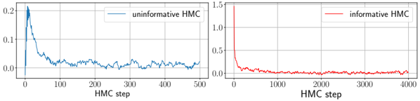<details> <summary>Image 21 Details</summary>  ### Visual Description ## Chart: HMC Performance Comparison ### Overview The image presents two line charts side-by-side, comparing the performance of "uninformative HMC" and "informative HMC" algorithms. The x-axis represents the HMC step, and the y-axis represents an unspecified performance metric. The charts illustrate how the performance metric changes over the course of the HMC steps for each algorithm. ### Components/Axes **Left Chart (Uninformative HMC):** * **X-axis:** "HMC step", ranging from 0 to 500. Axis markers are present at 0, 100, 200, 300, 400, and 500. * **Y-axis:** Scale ranges from 0.0 to 0.2. Axis markers are present at 0.0, 0.1, and 0.2. * **Legend:** Located in the top-right corner, labeled "uninformative HMC" and associated with a blue line. **Right Chart (Informative HMC):** * **X-axis:** "HMC step", ranging from 0 to 4000. Axis markers are present at 0, 1000, 2000, 3000, and 4000. * **Y-axis:** Scale ranges from 0.0 to 1.5. Axis markers are present at 0.0, 0.5, 1.0, and 1.5. * **Legend:** Located in the top-right corner, labeled "informative HMC" and associated with a red line. ### Detailed Analysis **Left Chart (Uninformative HMC):** * **Trend:** The blue line representing "uninformative HMC" starts at approximately 0.0, rapidly increases to a peak around 0.2 at the beginning, then quickly decreases and stabilizes around 0.02 after approximately 100 steps. The line fluctuates slightly around this value for the remainder of the steps. * **Data Points:** * Initial value (step 0): ~0.0 * Peak value (around step 10): ~0.2 * Stabilized value (after step 100): ~0.02 **Right Chart (Informative HMC):** * **Trend:** The red line representing "informative HMC" starts at a high value of approximately 1.5, rapidly decreases to around 0.1 within the first 500 steps, and then gradually stabilizes around 0.02 after approximately 1000 steps. The line fluctuates slightly around this value for the remainder of the steps. * **Data Points:** * Initial value (step 0): ~1.5 * Value at step 500: ~0.1 * Stabilized value (after step 1000): ~0.02 ### Key Observations * Both algorithms show a rapid initial decrease in the performance metric. * The "informative HMC" algorithm starts with a significantly higher value than the "uninformative HMC" algorithm. * Both algorithms stabilize at approximately the same value (~0.02) after a certain number of steps. * The "informative HMC" algorithm requires more steps to stabilize compared to the "uninformative HMC" algorithm. ### Interpretation The charts suggest that while the "informative HMC" algorithm initially performs worse (higher value on the y-axis, which is assumed to be an error or loss metric), it eventually converges to a similar performance level as the "uninformative HMC" algorithm. The "informative HMC" algorithm's initial higher value could be due to a more complex model or a less optimal starting point. The fact that both algorithms converge to a similar value suggests that, given enough steps, the "informative HMC" can achieve comparable performance. The "uninformative HMC" converges faster, possibly because it is a simpler model or starts from a better initial state. The y-axis label is missing, so the exact meaning of the performance metric is unknown, but the trends suggest it is a measure of error or loss that the algorithms are trying to minimize. </details> ## 4. Linking free entropy and mutual information It is possible to relate the mutual information (MI) of the inference problem to the free entropy f n = E ln Z introduced in the main. Indeed, we can write the MI as $$\frac { I ( \boldsymbol \theta ^ { 0 } ; \mathcal { D } ) } { n } = \frac { H ( \mathcal { D } ) } { n } - \frac { H ( \mathcal { D } | \boldsymbol \theta ^ { 0 } ) } { n } ,$$ where H ( Y | X ) is the conditional Shannon entropy of Y given X . Using the chain rule for the entropy, and the definition (9), the free entropy can be recast as $$- f _ { n } = \frac { H ( \{ y _ { \mu } \} _ { \mu \leq n } | \{ x _ { \mu } \} _ { \mu \leq n } ) } { n } = \frac { H ( \mathcal { D } ) } { n } - \frac { H ( \{ x _ { \mu } \} _ { \mu \leq n } ) } { n } .$$ On the other hand H ( D | θ 0 ) = H ( { y µ } | θ 0 , { x µ } ) + H ( { x µ } ), i.e., $$\frac { H ( \mathcal { D } | \boldsymbol \theta ^ { 0 } ) } { n } \approx - \mathbb { E } _ { \lambda } \int d y P _ { o u t } ( y | \lambda ) \ln P _ { o u t } ( y | \lambda ) + \frac { H ( \{ x _ { \mu } \} _ { \mu \leq n } ) } { n } ,$$ where λ ∼ N (0 , K d ), with K d given by (13) for L = 1, while for L = 2 and L = 3, given our normalisation assumptions on the activation functions, K d = 1 (assuming here that µ 0 = 0, see App. B 1 g if the activation σ is non-centred). Equality holds asymptotically in the limit lim. This allows us to express the MI asymptotically as $$\frac { I ( \boldsymbol \theta ^ { 0 } ; \mathcal { D } ) } { n } = - f _ { n } + \mathbb { E } _ { \lambda } \int d y P _ { o u t } ( y | \lambda ) \ln P _ { o u t } ( y | \lambda ) + o _ { n } ( 1 ) .$$ Specialising the equation to the Gaussian channel, one obtains $$\frac { I ( \boldsymbol \theta ^ { 0 } ; \mathcal { D } ) } { n } = - f _ { n } - \frac { 1 } { 2 } \ln ( 2 \pi e \Delta ) . & & ( A 2 1 )$$ We chose to normalise by n because, in our scaling, it is always proportional to the number of total parameters, that is Θ( d 2 ). Hence with this choice one can interpret the parameter α as an effective signal-to-noise ratio. Remark 6. The arguments of [169] to show the existence of an upper bound on the mutual information per variable in the case of discrete variables and the associated inevitable breaking of prior universality beyond a certain threshold in matrix denoising apply to the present model too. It implies, as in the aforementioned paper, that the mutual information per variable cannot go beyond ln 2 for Rademacher inner weights. Our theory is consistent with this fact; this is a direct consequence of the analysis in App. B 3 carried our for the shallow case L = 1 (see in particular (B68)) specialised to binary prior over W . ## 5. Alternative representation for ε opt with L = 1 We recall that θ 0 = ( v 0 , W 0 ) and similarly for θ 1 = θ , θ 2 , . . . which are replicas, i.e., conditionally i.i.d. samples from dP ( W , v | D ) (the reasoning below applies whether v is learnable or quenched, so in general we can consider a joint posterior over both). From its definition (8), the Bayes-optimal generalisation error can be recast as $$\begin{array} { r } { \varepsilon ^ { o p t } = \mathbb { E } _ { \boldsymbol \theta ^ { 0 } , x _ { t e s t } } \mathbb { E } [ y _ { t e s t } ^ { 2 } | \lambda ^ { 0 } ] - 2 \mathbb { E } _ { \boldsymbol \theta ^ { 0 } , \mathcal { D } , x _ { t e s t } } \mathbb { E } [ y _ { t e s t } | \lambda ^ { 0 } ] \langle \mathbb { E } [ y | \lambda ] \rangle + \mathbb { E } _ { \boldsymbol \theta ^ { 0 } , \mathcal { D } , x _ { t e s t } } \langle \mathbb { E } [ y | \lambda ] \rangle ^ { 2 } , \quad ( A 2 2 ) } \end{array}$$ where E [ y | λ ] = ∫ dy y P out ( y | λ ), and ( λ a ) a =0 ,...,s are the random variables (random due to the test input x test , drawn independently of the training data D , and their respective weights θ 0 , θ ) $$\lambda ^ { a } = \lambda _ { t e s t } ( \theta ^ { a } ) = \frac { v ^ { a \top } } { \sqrt { k } } \sigma \left ( \frac { W ^ { a } x _ { t e s t } } { \sqrt { d } } \right ) .$$ Recall that the bracket ⟨ · ⟩ is the average w.r.t. to the posterior and acts on θ 1 = θ , θ 2 , . . . . Notice that the last term on the r.h.s. of (A22) can be rewritten as $$\begin{array} { r } { \mathbb { E } _ { \boldsymbol \theta ^ { 0 } , \mathcal { D } , x _ { t e s t } } \langle \mathbb { E } [ y | \lambda ] \rangle ^ { 2 } = \mathbb { E } _ { \boldsymbol \theta ^ { 0 } , \mathcal { D } , x _ { t e s t } } \langle \mathbb { E } [ y | \lambda ^ { 1 } ] \mathbb { E } [ y | \lambda ^ { 2 } ] \rangle , } \end{array}$$ with superscripts being replica indices. In order to show Result 2 for a generic P out we assume the joint Gaussianity of the variables ( λ 0 , λ 1 , λ 2 , . . . ), with covariance given by K ab with a, b ∈ { 0 , 1 , 2 , . . . } . Indeed, in the limit 'lim', the theory considers ( λ a ) a ≥ 0 as jointly Gaussian under the randomness of a common input, here x test , conditionally on the weights ( θ a ). Their covariance depends on the weights ( θ a ) through various overlap OPs introduced in the main. In the large limit 'lim' these overlaps are assumed to concentrate under the quenched posterior average E θ 0 , D ⟨ · ⟩ towards non-random asymptotic values corresponding to the extremiser globally maximising the RS potential in Result 1, with the overlaps entering K ab through (B10). Using the replica symmetric ansatz (see (B12)), and the Nishimori identities, the covariance evaluated on these overlaps shall be denoted K ∗ as in the main, and its elements are written as K ∗ ab = K ∗ + δ ab ( K d -K ∗ ). This hypothesis is then confirmed by the excellent agreement between our theoretical predictions based on this assumption and the experimental results. This implies directly (17) in Result 2 from definition (7). For the special case of optimal mean-square generalisation error it yields $$\lim \varepsilon ^ { o p t } = \mathbb { E } _ { \lambda ^ { 0 } } \mathbb { E } [ y _ { t e s t } ^ { 2 } | \lambda ^ { 0 } ] - 2 \mathbb { E } _ { \lambda ^ { 0 } , \lambda ^ { 1 } } \mathbb { E } [ y _ { t e s t } | \lambda ^ { 0 } ] \mathbb { E } [ y | \lambda ^ { 1 } ] + \mathbb { E } _ { \lambda ^ { 1 } , \lambda ^ { 2 } } \mathbb { E } [ y | \lambda ^ { 1 } ] \mathbb { E } [ y | \lambda ^ { 2 } ] & & ( A 2 4 ) \\$$ where, in the replica symmetric ansatz, $$\mathbb { E } [ ( \lambda ^ { 0 } ) ^ { 2 } ] = K _ { d } , \quad \mathbb { E } [ \lambda ^ { 0 } \lambda ^ { 1 } ] = \mathbb { E } [ \lambda ^ { 0 } \lambda ^ { 2 } ] = K ^ { * } , \quad \mathbb { E } [ \lambda ^ { 1 } \lambda ^ { 2 } ] = K ^ { * } , \quad \mathbb { E } [ ( \lambda ^ { 1 } ) ^ { 2 } ] = \mathbb { E } [ ( \lambda ^ { 2 } ) ^ { 2 } ] = K _ { d } .$$ We thus have $$\mathbb { E } _ { \lambda ^ { 0 } , \lambda ^ { 1 } } \mathbb { E } [ y _ { t e s t } | \, \lambda ^ { 0 } ] \mathbb { E } [ y | \, \lambda ^ { 1 } ] & = \mathbb { E } _ { \lambda ^ { 1 } , \lambda ^ { 2 } } \mathbb { E } [ y | \, \lambda ^ { 1 } ] \mathbb { E } [ y | \, \lambda ^ { 2 } ] . & ( A 2 6 )$$ Plugging the above in (A24) yields (18). Let us now prove a formula for the optimal mean-square generalisation error written in terms of the overlaps which holds for the special case of linear readout with Gaussian label noise P out ( y | λ ) = exp( -1 2∆ ( y -λ ) 2 ) / √ 2 π ∆. The following derivation is exact and does not require any Gaussianity assumption on the random variables ( λ a ). For the linear Gaussian channel the means verify E [ y | λ ] = λ and E [ y 2 | λ ] = λ 2 +∆. Plugged in (A22) this yields $$\begin{array} { r l } & { \varepsilon ^ { o p t } - \Delta = \mathbb { E } _ { \theta ^ { 0 } , x _ { t e s t } } ( \lambda ^ { 0 } ) ^ { 2 } - 2 \mathbb { E } _ { \theta ^ { 0 } , \mathcal { D } , x _ { t e s t } } \lambda ^ { 0 } \langle \lambda \rangle + \mathbb { E } _ { \theta ^ { 0 } , \mathcal { D } , x _ { t e s t } } \langle \lambda ^ { 1 } \lambda ^ { 2 } \rangle , \quad ( A 2 7 ) } \end{array}$$ whence we clearly see that the generalisation error depends only on the covariance of λ 0 , λ 1 , λ 2 under the randomness of the shared input x test at fixed weights, regardless of the validity of the Gaussian hypothesis on the post-activations (11) we assume in the replica computation. This covariance was already computed in (24); we recall it here for the reader's convenience $$K ( \theta ^ { a } , \theta ^ { b } ) \colon = \mathbb { E } _ { \mathbf x _ { t e s t } } \lambda ^ { a } \lambda ^ { b } = \sum _ { \ell = 1 } ^ { \infty } \frac { \mu _ { \ell } ^ { 2 } } { \ell ! } \frac { 1 } { k } \sum _ { i , j = 1 } ^ { k } v _ { i } ^ { a } ( \Omega _ { i j } ^ { a b } ) ^ { \ell } v _ { j } ^ { b } = \sum _ { \ell = 1 } ^ { \infty } \frac { \mu _ { \ell } ^ { 2 } } { \ell ! } R _ { \ell } ^ { a b } , \quad ( A 2 8 )$$ where Ω ab ij := W a ⊺ i W b j /d , and R ab ℓ as introduced in (24) for a, b = 0 , 1 , 2. We stress that K ( θ a , θ b ) is not the limiting covariance K ab whose elements are in (B12), but rather the finite size one. K ( θ a , θ b ) provides us with an efficient way to compute the generalisation error numerically, used in App. B 4, FIG. 24, that is through the formula $$\varepsilon ^ { o p t } - \Delta = \mathbb { E } _ { \theta ^ { 0 } } K ( \theta ^ { 0 } , \theta ^ { 0 } ) - 2 \mathbb { E } _ { \theta ^ { 0 } , \mathcal { D } } \langle K ( \theta ^ { 0 } , \theta ^ { 1 } ) \rangle + \mathbb { E } _ { \theta ^ { 0 } , \mathcal { D } } \langle K ( \theta ^ { 1 } , \theta ^ { 2 } ) \rangle = \sum _ { \ell = 1 } ^ { \infty } \frac { \mu _ { \ell } ^ { 2 } } { \ell ! } \mathbb { E } _ { \theta ^ { 0 } , \mathcal { D } } \langle R _ { \ell } ^ { 0 0 } - 2 R _ { \ell } ^ { 0 1 } + R _ { \ell } ^ { 1 2 } \rangle .$$ In the above, the posterior measure ⟨ · ⟩ is taken care of by Monte Carlo sampling (when it equilibrates). In addition, as in the main text, we assume that in the large system limit the (numerically confirmed) identity (29) holds. Putting all ingredients together we get $$\varepsilon ^ { o p t } - \Delta & = \mathbb { E } _ { \theta ^ { 0 } , \mathcal { D } } \Big < \mu _ { 1 } ^ { 2 } ( R _ { 1 } ^ { 0 0 } - 2 R _ { 1 } ^ { 0 1 } + R _ { 1 } ^ { 1 2 } ) + \frac { \mu _ { 2 } ^ { 2 } } { 2 } ( R _ { 2 } ^ { 0 0 } - 2 R _ { 2 } ^ { 0 1 } + R _ { 2 } ^ { 1 2 } ) \\ & + \mathbb { E } _ { v \sim P _ { v } } v ^ { 2 } \Big [ g ( \mathcal { Q } ^ { 0 0 } ( v ) ) - 2 g ( \mathcal { Q } ^ { 0 1 } ( v ) ) + g ( \mathcal { Q } ^ { 1 2 } ( v ) ) ] \Big > .$$ In the Bayes-optimal setting one can use again the Nishimori identities that imply E θ 0 , D ⟨ R 12 1 ⟩ = E θ 0 , D ⟨ R 01 1 ⟩ , and analogously E θ 0 , D ⟨ R 12 2 ⟩ = E θ 0 , D ⟨ R 01 2 ⟩ and E θ 0 , D ⟨ g ( Q 12 W ( v )) ⟩ = E θ 0 , D ⟨ g ( Q 01 W ( v )) ⟩ . Inserting these identities in (A30) one gets $$\varepsilon ^ { o p t } - \Delta = \mathbb { E } _ { \theta ^ { 0 } , \mathcal { D } } \left \langle \mu _ { 1 } ^ { 2 } ( R _ { 1 } ^ { 0 0 } - R _ { 1 } ^ { 0 1 } ) + \frac { \mu _ { 2 } ^ { 2 } } { 2 } ( R _ { 2 } ^ { 0 0 } - R _ { 2 } ^ { 0 1 } ) + \mathbb { E } _ { v \sim P _ { v } } v ^ { 2 } \left [ g ( \mathcal { Q } ^ { 0 0 } ( v ) ) - g ( \mathcal { Q } ^ { 0 1 } ( v ) ) \right ] \right \rangle .$$ This formula relies only on the validity of (29), and makes no assumption on the law of the λ 's. That it depends only on their covariance is simply a consequence of the quadratic nature of the mean-square generalisation error. Remark 7. Note that the derivation up to (A29) did not assume Bayes-optimality (while (A31) does). Therefore, one can consider it in cases where the true posterior average ⟨ · ⟩ is replaced by one which does not verify the Nishimori identities. This is the formula we use to compute the generalisation error of Monte Carlo-based estimators in the inset of FIG. 24. There, MCMC cannot equilibrate and experiences a glassy regime. This regime, at variance with the metastable states described in the main text (see Remark 5), does not correspond to any sub-optimal branch of our theory: we verified numerically that indeed the Nishimori identities do not hold there. Remark 8. Using the Nishimory identity of App. A 3 and again that, for the linear readout with Gaussian label noise E [ y | λ ] = λ and E [ y 2 | λ ] = λ 2 +∆, it is easy to check that the so-called Gibbs error $$\varepsilon ^ { \text {Gibbs} } & \colon = \mathbb { E } _ { \theta ^ { 0 } , \mathcal { D } , x _ { t e s t } , y _ { t e s t } } \left < ( y _ { t e s t } - \mathbb { E } [ y | \lambda _ { t e s t } ( \theta ) ] ) ^ { 2 } \right > & & ( A 3 2 )$$ is related for this channel to the Bayes-optimal mean-square generalisation error through the identity $$\varepsilon ^ { G i b b s } - \Delta = 2 ( \varepsilon ^ { o p t } - \Delta ) . & & ( A 3 3 )$$ We exploited this relationship together with the concentration of the Gibbs error w.r.t. the quenched posterior measure E θ 0 , D ⟨ · ⟩ when evaluating the numerical generalisation error of the Monte Carlo algorithms reported in the main text. ## Appendix B: Shallow MLP ## 1. Details of the replica calculation In this section we report all the details needed to derive our results with the replica method when L = 1. The starting point is the assumption of joint Gaussianity of the post-activations $$\left \{ \lambda ^ { a } ( \pm b \theta ^ { a } ) \colon = \frac { 1 } { \sqrt { k } } v ^ { 0 T } \sigma \left ( \frac { 1 } { \sqrt { d } } W ^ { a } x \right ) \right \} _ { a = 0 } ^ { s }$$ under the randomness of x , for typical ( θ a ). The covariance of this Gaussian family is $$K ^ { a b } \colon = \mathbb { E } _ { \mathbf x } \lambda ^ { a } ( \theta ^ { a } ) \lambda ^ { b } ( \theta ^ { b } ) = \frac { 1 } { k } \sum _ { i , j = 1 } ^ { k } v _ { i } ^ { 0 } v _ { j } ^ { 0 } \mathbb { E } _ { \mathbf x } \sigma \left ( \frac { W _ { i } ^ { a } \cdot \mathbf x } { \sqrt { d } } \right ) \sigma \left ( \frac { W _ { j } ^ { b } \cdot \mathbf x } { \sqrt { d } } \right ) .$$ To compute it we use Mehler's formula (A9), plus the assumption that ∥ W a ∥ 2 /d concentrates towards 1, which is verified by Nishimori identities: $$K ^ { a b } = \sum _ { \ell = 1 } ^ { \infty } \, \frac { \mu _ { \ell } ^ { 2 } } { \ell ! } \frac { 1 } { k } \sum _ { i , j = 1 } ^ { k } v _ { i } ^ { 0 } v _ { j } ^ { 0 } \left ( \Omega _ { i j } ^ { a b } \right ) ^ { \ell } , \quad \Omega _ { i j } ^ { a b } \colon = \frac { W _ { i } ^ { a } \cdot W _ { j } ^ { b } } { d } \, .$$ Due to norm concentrations of the W a i 's, one can show that for a fixed i only for a small number of indices j W b j can have an O ( d ) projection onto W a i . As confirmed by our numerics, we assume this projection is large only for one index j , which by permutation invariance, we can assume to be i itself. In other words, we are assuming that ̸ $$\Omega _ { i i } ^ { a b } = O ( 1 ) \, , \quad \Omega _ { i j } ^ { a b } = O \left ( \frac { 1 } { \sqrt { d } } \right ) \text { for $i\neq j$} \, .$$ Note that this is rigorously provable for the diagonal part of the covariance a = b . Then our assumptions imply ̸ $$\frac { 1 } { k } \sum _ { i \neq j } ^ { k } v _ { i } ^ { 0 } v _ { j } ^ { 0 } ( \Omega _ { i j } ^ { a b } ) ^ { \ell } = O ( k / d ^ { \ell / 2 } ) = O ( d ^ { 1 - \ell / 2 } ) ,$$ which vanishes for any ℓ ≥ 3. Hence, the covariance simplifies to $$K ^ { a b } = \mu _ { 1 } ^ { 2 } R _ { 1 } ^ { a b } + \frac { \mu _ { 2 } ^ { 2 } } { 2 } R _ { 2 } ^ { a b } + \frac { 1 } { k } \sum _ { i = 1 } ^ { k } ( v _ { i } ^ { 0 } ) ^ { 2 } g ( \Omega _ { i i } ^ { a b } ) + O ( d ^ { - 1 / 2 } )$$ where $$g ( x ) = \sum _ { \ell = 3 } ^ { \infty } \frac { \mu _ { \ell } ^ { 2 } } { \ell ! } x ^ { \ell } = \mathbb { E } _ { ( y , z ) | x } [ \sigma ( y ) \sigma ( z ) ] - \mu _ { 0 } ^ { 2 } - \mu _ { 1 } ^ { 2 } x - \frac { \mu _ { 2 } ^ { 2 } } { 2 } x ^ { 2 } , \quad ( y , z ) \sim \mathcal { N } \left ( ( 0 , 0 ) , \binom { 1 } { x } \right ) .$$ Here, again by permutation symmetry, we can assume that all overlaps Ω ab ii for i ∈ I v concentrate onto the same value Q ab ( v ) labelled by v , thus leading to $$K ^ { a b } \approx \mu _ { 1 } ^ { 2 } R _ { 1 } ^ { a b } + \frac { \mu _ { 2 } ^ { 2 } } { 2 } R _ { 2 } ^ { a b } + \sum _ { v \in V } \nu ^ { 2 } \frac { | \mathcal { I } _ { v } | } { k } \frac { 1 } { | \mathcal { I } _ { v } | } \sum _ { i \in \mathcal { I } _ { v } } g ( \Omega _ { i i } ^ { a b } ) \approx \mu _ { 1 } ^ { 2 } + \frac { \mu _ { 2 } ^ { 2 } } { 2 } R _ { 2 } ^ { a b } + \sum _ { v \in V } P _ { v } ( \nu ) \nu ^ { 2 } g ( \mathcal { Q } ^ { a b } ( \nu ) ) \, .$$ In the above we have used the aforementioned permutation symmetry and concentration, and the fact that |I v | k → P v ( v ). Furthermore, we assumed that R ab 1 → 1 which is justified by the fact that R ab 1 is a scalar overlap between two vectors S a 1 , S b 1 . In fact, at the present scaling of n, k, d , the vector S 0 1 can be retrieved exactly. K ab is what governs the 'energy' in our model, and the overlaps therein appearing thus play the role of OPs. Recall the form of the replicated partition function: $$\begin{array} { r } { \mathbb { E Z } ^ { s } = \mathbb { E _ { v } } \int \prod _ { a } ^ { 0 , s } d P _ { W } ( W ^ { a } ) \times \left [ \mathbb { E _ { x } } \int d y \prod _ { a } ^ { 0 , s } P _ { o u t } ( y | \lambda ^ { a } ( \pm b \theta ^ { a } ) ) \right ] ^ { n } . } \end{array}$$ which, after the above simplifications, reads $$\mathbb { E } \mathcal { Z } ^ { s } = \int d R _ { 2 } d \mathcal { Q } \exp [ F _ { S } ( R _ { 2 } , \mathcal { Q } ) + n F _ { E } ( R _ { 2 } , \mathcal { Q } ) ]$$ where R 2 = ( R ab 2 ) and Q := {Q ab | a ≤ b } , Q ab := {Q ab ( v ) | v ∈ V } . We split the discussion in the evaluation of the energetic potential F E , the entropic potential F S and finally the derivation of the saddle point equations for the OPs. All the calculation is performed assuming replica symmetry, as explained below. ## a. Energetic potential The replicated energetic term under our Gaussian assumption on the joint law of the post-activations replicas is reported here for the reader's convenience: $$F _ { E } = \ln \int d y \int d \lambda \frac { e ^ { - \frac { 1 } { 2 } \lambda ^ { T } K ^ { - 1 } \lambda } } { \sqrt { ( 2 \pi ) ^ { s + 1 } \det K } } \prod _ { a = 0 } ^ { s } P _ { o u t } ( y | \lambda ^ { a } ) ,$$ <!-- formula-not-decoded --> The energetic term F E is already expressed as a low-dimensional integral, but it simplifies considerably under the replica symmetric (RS) ansatz and after using the Nishimori identities. Let us denote Q ( v ) = ( Q ab ( v )) s a,b =0 , then, using (A15) and (A16) $$\begin{array} { r } { \mathcal { Q } ( v ) = \left ( \begin{matrix} 1 & \mathcal { Q } ( v ) 1 _ { s } ^ { \intercal } \\ \mathcal { Q } ( v ) 1 _ { s } & ( 1 - \mathcal { Q } ( v ) ) I _ { s } + \mathcal { Q } ( v ) 1 _ { s } 1 _ { s } ^ { \intercal } \end{matrix} \right ) \iff \hat { \mathcal { Q } } ( v ) = \left ( \begin{matrix} 0 & - \hat { \mathcal { Q } } ( v ) 1 _ { s } ^ { \intercal } \\ - \hat { \mathcal { Q } } ( v ) 1 _ { s } & \hat { \mathcal { Q } } ( v ) I _ { s } - \hat { \mathcal { Q } } ( v ) 1 _ { s } 1 _ { s } ^ { \intercal } \end{matrix} \right ) , } \end{array}$$ and similarly $$\begin{array} { r } { R _ { 2 } = \binom { R _ { d } } { R _ { 2 } 1 _ { s } } \overset { R _ { 2 } 1 _ { s } ^ { \dagger } } { ( R _ { d } - R _ { 2 } ) I _ { s } + R _ { 2 } 1 _ { s } 1 _ { s } ^ { \dagger } } \right \rangle \iff \hat { R } _ { 2 } = \binom { 0 } { - \hat { R } _ { 2 } 1 _ { s } } \overset { - \hat { R } _ { 2 } 1 _ { s } ^ { \dagger } } { ( - \hat { R } _ { 2 } 1 _ { s } \hat { R } _ { 2 } I _ { s } - \hat { R } _ { 2 } 1 _ { s } 1 _ { s } ^ { \dagger } } \right ) , } \end{array}$$ where we reported the ansatz also for the Fourier conjugates for future convenience, though not needed for the energetic potential. We are going to use repeatedly the Fourier representation of the delta function, namely δ ( x ) = 1 2 π ∫ d ˆ x exp( i ˆ xx ). Because the integrals we will end-up with will always be at some point evaluated by saddle point, implying a deformation of the integration contour in the complex plane, tracking the imaginary unit i in the delta functions will be irrelevant. Similarly, the normalisation 1 / 2 π will always contribute to sub-leading terms in the with integrals at hand. Therefore, we will allow ourselves to formally write δ ( x ) = ∫ d ˆ x exp( r ˆ xx ) for a convenient constant r , keeping in mind these considerations (again, as we evaluate the final integrals by saddle point, the choice of r ends-up being irrelevant). The RS ansatz, which is equivalent to an assumption of concentration of the OPs in the high-dimensional limit, is known to be exact when analysing Bayes-optimal inference and learning, as in the present paper, see [180, 184, 190]. Under the RS ansatz K acquires a similar form: $$K = \begin{pmatrix} K _ { d } & K 1 ^ { \intercal } _ { s } \\ K 1 _ { s } & ( K _ { d } - K ) I _ { s } + K 1 _ { s } 1 ^ { \intercal } _ { s } \end{pmatrix}$$ with $$K \equiv K ( R _ { 2 } , \mathcal { Q } ) = \mu _ { 1 } ^ { 2 } + \frac { \mu _ { 2 } ^ { 2 } } { 2 } R _ { 2 } + \mathbb { E } _ { v \sim P _ { v } } v ^ { 2 } g ( \mathcal { Q } ( v ) ) , & & K _ { d } = \mu _ { 1 } ^ { 2 } + \frac { \mu _ { 2 } ^ { 2 } } { 2 } R _ { d } + g ( 1 ) . & & ( B 1 2 )$$ In the RS ansatz it is thus possible to give a convenient low-dimensional representation of the multivariate Gaussian integral of F E in terms of white Gaussian random variables: $$\lambda ^ { a } = \xi \sqrt { K } + u ^ { a } \sqrt { K _ { d } - K } \quad \text {for $a=0,1,\dots,s$} , \begin{array} { r l } & { ( B 1 3 ) } \\ { \lambda ^ { a } = \xi \sqrt { K } + u ^ { a } \sqrt { K _ { d } - K } } & { f o r $a=0,1,\dots,s$ , } \end{array}$$ where ξ, ( u a ) s a =0 are i.i.d. standard Gaussian variables. Then $$F _ { E } = \ln \int d y \, \mathbb { E } _ { \xi , u ^ { 0 } } P _ { o u t } \left ( y | \xi \sqrt { K } + u ^ { 0 } \sqrt { K _ { d } - K } \right ) \prod _ { a = 1 } ^ { s } \mathbb { E } _ { u ^ { a } } P _ { o u t } ( y | \xi \sqrt { K } + u ^ { a } \sqrt { K _ { d } - K } ) .$$ The last product over the replica index a contains identical factors thanks to the RS ansatz. Therefore, by expanding in s → 0 + we get $$F _ { E } = s \int d y \, \mathbb { E } _ { \xi , u ^ { 0 } } P _ { o u t } ( y | \xi \sqrt { K } + u ^ { 0 } \sqrt { K _ { d } - K } ) \ln \mathbb { E } _ { u } P _ { o u t } ( y | \xi \sqrt { K } + u \sqrt { K _ { d } - K } ) + O ( s ^ { 2 } ) \quad \text {(B15)}$$ $$= \colon s \, \phi _ { P _ { o u t } } ( K ( R _ { 2 } , \mathcal { Q } ) ; K _ { d } ) + O ( s ^ { 2 } ) .$$ Notice that the energetic contribution to the free entropy has the same form as in the generalised linear model [98]. For our running example of linear readout with Gaussian noise the function ϕ P out reduces to $$\phi _ { P _ { o u t } } ( K ( R _ { 2 } , \mathcal { Q } ) ; K _ { d } ) = - \frac { 1 } { 2 } \ln \left [ 2 \pi e ( \Delta + K _ { d } - K ) \right ] .$$ ## b. Entropic potential The entropic potential is obtained by counting the degeneracy of configurations yielding the same values of OPs appearing in K : $$e ^ { F _ { S } } & = \int \prod _ { a = 0 } ^ { s } d S _ { 2 } ^ { a } \int \prod _ { a = 0 } ^ { s } d P _ { W } ( w ^ { a } ) \delta \left ( s _ { 2 } ^ { a } - \frac { w ^ { a } \text {diag} ( v ^ { 0 } ) W ^ { a } } { \sqrt { k } } \right ) \\ & \quad \times \prod _ { a \leq b \in V } \prod _ { v \in V } \delta ( d | \mathcal { I } _ { v } | \, \mathcal { Q } ^ { a b } ( v ) - \sum _ { i \in \mathcal { I } _ { v } } w _ { i } ^ { a \dagger } w _ { i } ^ { b } ) \prod _ { a \leq b } ^ { 0 , s } \delta ( d ^ { 2 } R _ { 2 } ^ { a b } - \text {Tr} \, S _ { 2 } ^ { a } \mathbf s _ { 2 } ^ { b } ) \, ,$$ where we have introduced the integral over the Hermitian matrices d S a 2 = ∏ α 1 ≤ α 2 dS a 2; α 1 α 2 . Defining $$V _ { W } ^ { k d } ( \mathcal { Q } ) \colon = \int \prod _ { a = 0 } ^ { s } d P _ { W } ( W ^ { a } ) \prod _ { a \leq b \lor v \in V } ^ { 0 , s } \prod _ { \delta ( d | \mathcal { I } _ { v } | \, \mathcal { Q } ^ { a b } ( v ) - \sum _ { i \in \mathcal { I } _ { v } } W _ { i } ^ { a \intercal } W _ { i } ^ { b } ) }$$ the entropic potential can be conveniently recast in terms of the following conditional measure $$P ( ( \mathbf S ^ { a } _ { 2 } ) \, | \, \mathbf Q ) = V ^ { k d } _ { W } ( \mathbf Q ) ^ { - 1 } \int \prod _ { a } ^ { 0 , s } d P _ { W } ( \mathbf W ^ { a } ) \delta ( \mathbf S ^ { a } _ { 2 } - \mathbf W ^ { a \Upsilon } d i a g ( \mathbf v ) \mathbf W ^ { a } / \sqrt { k } ) \prod _ { a \leq b } ^ { 0 , s } \prod _ { \mathbf v \in \mathbf V } \delta ( d | \mathcal { I } _ { \mathbf v } | \, \mathcal { Q } ^ { a b } ( \mathbf v ) - \sum _ { i \in \mathcal { I } _ { \mathbf v } } \mathbf W ^ { a \Upsilon } _ { i } \mathbf W ^ { b } _ { i } ) ,$$ as $$e ^ { F _ { S } } \colon = V _ { W } ^ { k d } ( \mathcal { Q } ) \int d P ( ( \mathbf S _ { 2 } ^ { a } ) \, | \, \mathcal { Q } ) \prod _ { a \leq b } ^ { 0 , s } \delta ( d ^ { 2 } R _ { 2 } ^ { a b } - \text {Tr} \, \mathbf S _ { 2 } ^ { a } \mathbf S _ { 2 } ^ { b } ) .$$ Recall V is the support of P v (assumed discrete for the moment). Recall also that we have quenched the readout weights to the ground truth. This is a measure over different replicas of the random matrices S a 2 , defined in terms of the distribution of the matrices W a by the first delta function in (B20), coupled through the term Q ab in the second delta function. This coupling between replicas marks a difference with the computation of [94]: to proceed, we need to relax this measure to something more manageable. We thus first evaluate the exact asymptotic of its trace second moment, to eventually write a relaxation in a moment-matching scheme. ## c. Exact second moment of P (( S a 2 ) | Q ) In this measure, one can compute the asymptotic of its second moment $$\int d P ( ( \mathbf S ^ { a } _ { 2 } ) \, | \, \mathbf Q ) \frac { 1 } { d ^ { 2 } } \text {Tr} \, \mathbf S ^ { a } _ { 2 } \mathbf S ^ { b } _ { 2 } & = V ^ { k d } _ { W } ( \mathbf Q ) ^ { - 1 } \int _ { a } ^ { 0 , s } \prod _ { i } d P _ { W } ( \mathbf W ^ { a } ) \frac { 1 } { k d ^ { 2 } } \text {Tr} [ \mathbf W ^ { a \intercal } \text {diag} ( \mathbf v ) \mathbf W ^ { a } \mathbf W ^ { b \intercal } \text {diag} ( \mathbf v ) \mathbf W ^ { b } ] \\ & \times \prod _ { a \leq b } ^ { 0 , s } \prod _ { i \in \mathcal { I } _ { i } } \delta ( d | \mathcal { I } _ { i } | \, \mathcal { Q } ^ { a b } ( \mathbf v ) - \sum _ { i \in \mathcal { I } _ { i } } \mathbf W ^ { a \intercal } _ { i } \mathbf W ^ { b } _ { i } ) .$$ The measure is coupled only through the last δ 's. We can decouple the measure at the cost of introducing Fourier conjugates whose values will then be fixed by a saddle point computation. The second moment computed will not affect the saddle point, hence it is sufficient to determine the value of the Fourier conjugates through the computation of V kd W ( Q ), which rewrites as $$V _ { W } ^ { k d } ( \mathbf Q ) & = \int \prod _ { a } ^ { 0 , s } d P _ { W } ( \mathbf W ^ { a } ) \prod _ { a \leq b \, \nu \in V } ^ { 0 , s } d \hat { B } ^ { a b } ( \nu ) \exp \left [ - \, \hat { B } ^ { a b } ( \nu ) ( d | \mathcal { I } _ { \nu } | \mathcal { Q } ^ { a b } ( \nu ) - \sum _ { i \in \mathcal { I } _ { \nu } } \mathbf W _ { i } ^ { a \dagger } \mathbf W _ { i } ^ { b } ) \right ] \\ & \approx \prod _ { v \in V } \exp \left ( d | \mathcal { I } _ { \nu } | \text {extr} _ { ( \hat { B } ^ { a b } ( \nu ) ) } \left [ - \sum _ { a \leq b , 0 } ^ { s } \hat { B } ^ { a b } ( \nu ) \mathcal { Q } ^ { a b } ( \nu ) + \ln \int \prod _ { a = 0 } ^ { s } d P _ { W } ( w _ { a } ) e ^ { \sum _ { a \leq b , 0 } ^ { s } \hat { B } ^ { a b } ( \nu ) w _ { a } w _ { b } } \right ] \right ) .$$ In the last line we have used saddle point integration over ˆ B ab ( v ) and the approximate equality is up to a multiplicative exp( o ( n )) constant. From the above, it is clear that the stationary ˆ B ab ( v ) are such that $$\mathcal { Q } ^ { a b } ( \mathbf v ) = \frac { \int \prod _ { r = 0 } ^ { s } d P _ { W } ( w _ { r } ) w _ { a } w _ { b } \prod _ { r \leq t , 0 } ^ { s } e ^ { \hat { B } ^ { r t } ( \mathbf v ) w _ { r } w _ { t } } } { \int \prod _ { r = 0 } ^ { s } d P _ { W } ( w _ { r } ) \prod _ { r \leq t , 0 } ^ { s } e ^ { \hat { B } ^ { r t } ( \mathbf v ) w _ { r } w _ { t } } } = \colon \langle w _ { a } w _ { b } \rangle _ { \hat { B } ( \mathbf v ) } .$$ Using these notations, the asymptotic trace moment of the S 2 's at leading order becomes ̸ $$\int d P ( ( \mathbf S _ { 2 } ^ { a } ) \, | \, \mathbf Q ) & \frac { 1 } { d ^ { 2 } } \text {Tr} \mathbf S _ { 2 } ^ { a } \mathbf S _ { 2 } ^ { b } = \frac { 1 } { k d ^ { 2 } } \sum _ { i , l = 1 } ^ { k } \sum _ { j , p = 1 } ^ { d } \langle W _ { i j } ^ { a } v _ { i } ^ { 0 } W _ { i p } ^ { a } W _ { l j } ^ { b } v _ { l } ^ { 0 } W _ { l p } ^ { b } \rangle _ { \{ \hat { B } ( \nu ) \} _ { \nu \in V } } \\ & = \frac { 1 } { k } \sum _ { \nu \in V } v _ { 2 } ^ { 2 } \sum _ { i \in \mathcal { I } _ { \nu } } \left \langle \left ( \frac { 1 } { d } \sum _ { j = 1 } ^ { d } W _ { i j } ^ { a } W _ { i j } ^ { b } \right ) ^ { 2 } \right \rangle _ { \hat { B } ( \nu ) } + \frac { 1 } { k } \sum _ { j = 1 } ^ { d } \left \langle \sum _ { i = 1 } ^ { k } \frac { v _ { i } ^ { 0 } ( W _ { i j } ^ { a } ) ^ { 2 } } { d } \sum _ { l \neq i , 1 } ^ { k } \frac { v _ { l } ^ { 0 } ( W _ { l j } ^ { b } ) ^ { 2 } } { d } \right \rangle _ { \{ \hat { B } ( \nu ) \} _ { \nu \in V } } .$$ ̸ We have used the fact that ⟨ · ⟩ ˆ B ( v ) is symmetric if the prior P W is, thus forcing us to match j with p if i = l . Considering that by the Nishimori identities Q aa ( v ) = 1, it implies ˆ B aa ( v ) = 0 for any a = 0 , 1 , . . . , s and v ∈ V . Furthermore, the measure ⟨ · ⟩ ˆ B ( v ) is completely factorised over neuron and input indices. Hence every normalised sum can be assumed to concentrate to its expectation by the law of large numbers. Specifically, we can write that with high probability as d, k →∞ , ̸ $$\frac { 1 } { d } \sum _ { i \in \mathcal { I } _ { v } } \sum _ { j = 1 } ^ { d } W _ { i j } ^ { a } W _ { i j } ^ { b } \rightarrow | \mathcal { I } _ { v } | \mathcal { Q } ^ { a b } ( v ) , \quad \frac { 1 } { k } \sum _ { v , v ^ { \prime } \in V } v v ^ { \prime } \sum _ { j = 1 } ^ { d } \sum _ { i \in \mathcal { I } _ { v } } \frac { ( W _ { i j } ^ { a } ) ^ { 2 } } { d } \sum _ { l \in \mathcal { I } _ { v ^ { \prime } } , l \neq i } \frac { ( W _ { l j } ^ { b } ) ^ { 2 } } { d } \approx \gamma \sum _ { v , v ^ { \prime } \in V } \frac { | \mathcal { I } _ { v } | | \mathcal { I } _ { v ^ { \prime } } | } { k ^ { 2 } } v v ^ { \prime } \rightarrow \gamma \bar { v } ^ { 2 } ,$$ where we used |I v | /k → P v ( v ) as k diverges. Consequently, the second moment at leading order appears as claimed: $$\int d P ( ( { \mathbf S } _ { 2 } ^ { a } ) \, | \, { \mathbf Q } ) \frac { 1 } { d ^ { 2 } } T r \, { \mathbf S } _ { 2 } ^ { a } { \mathbf S } _ { 2 } ^ { b } = \sum _ { v \in V } P _ { v } ( v ) v ^ { 2 } { \mathcal { Q } } ^ { a b } ( v ) ^ { 2 } + \gamma \bar { v } ^ { 2 } = { \mathbb { E } } _ { v \sim P _ { v } } v ^ { 2 } { \mathcal { Q } } ^ { a b } ( v ) ^ { 2 } + \gamma \bar { v } ^ { 2 } .$$ d. Relaxation of P (( S a 2 ) | Q ) via maximum entropy with moment matching We now show how to obtain the relaxation ˜ P (( S a 2 ) | Q ) in (31), which we report here for the reader's convenience: $$\tilde { P } ( ( \mathbf S ^ { a } _ { 2 } ) \, | \, \mathcal { Q } ) \colon = \tilde { V } ^ { - k d } _ { W } ( \mathfrak Q ) \prod _ { a } ^ { 0 , s } P _ { S } ( \mathbf S ^ { a } _ { 2 } ) \prod _ { a < b } ^ { 0 , s } e ^ { \frac { 1 } { 2 } \tau ( \mathcal { Q } ^ { a b } ) T r \mathbf S ^ { a } _ { 2 } \mathbf S ^ { b } _ { 2 } }$$ where P S is the probability density of a generalised Wishart random matrix, i.e., of ˜ W ⊺ diag( v ) ˜ W / √ k with ˜ W ∈ R k × d made of i.i.d. standard Gaussian entries, ˜ V kd W ( Q ) is the proper normalisation constant, and τ ( Q ab ) is such that $$\int d \tilde { P } ( ( S _ { 2 } ^ { a } ) \, | \, \mathcal { Q } ) \frac { 1 } { d ^ { 2 } } \text {Tr} \, S _ { 2 } ^ { a } S _ { 2 } ^ { b } = \mathbb { E } _ { v \sim P _ { v } } v ^ { 2 } \mathcal { Q } ^ { a b } ( v ) ^ { 2 } + \gamma \bar { v } ^ { 2 } \, .$$ We shall see that the latter converts into a convenient relation involving the inverse function mmse -1 S when taking the replica symmetric ansatz. The effective law ˜ P (( S a 2 ) | Q ) is the least restrictive choice among the Wishart-type distributions with a trace moment fixed precisely to the one above. In more specific terms, it is the solution of the following maximum entropy problem: $$\inf _ { P , \tau } \left \{ D _ { K L } ( P \, \| \, P _ { S } ^ { \otimes s + 1 } ) + \sum _ { a \leq b , 0 } ^ { s } \tau ^ { a b } \left ( \mathbb { E } _ { P } \frac { 1 } { d ^ { 2 } } T r \, \mathbf S _ { 2 } ^ { a } \mathbf S _ { 2 } ^ { b } - \gamma \bar { v } ^ { 2 } - \mathbb { E } _ { v \sim P _ { v } } v ^ { 2 } \mathcal { Q } ^ { a b } ( v ) ^ { 2 } \right ) \right \} ,$$ where P S is a generalised Wishart distribution (as defined above (31)), and P is in the space of joint probability distributions over s + 1 symmetric matrices of dimension d × d . The rationale behind the choice of P S as a base measure is that, in absence of any other information, a statistician can always use a generalised Wishart measure for the S 2 's if they assume universality in the law of the inner weights. This ansatz would still yield a non-trivial performance, achieved by our adaptation of GAMP-RIE in App. B 4 for generic activations. Note that if a = b then, by the Nishimori identities, the second moment above matches precisely R d = 1 + γ ¯ v 2 . This entails directly τ aa = 0, as the generalised Wishart prior P S already imposes this constraint. ## e. Entropic potential with the relaxed measure We now use the results from the previous paragraphs to compute the entropic contribution F S to the free entropy, (B21). Indeed, let us proceed with the relaxation of the measure P (( S a 2 ) | Q ) by replacing it with ˜ P (( S a 2 ) | Q ) derived above: $$e ^ { F _ { S } } = V _ { W } ^ { k d } ( \boldsymbol Q ) \int d \hat { \mathbf R } _ { 2 } \exp \left ( - \, \frac { d ^ { 2 } } { 2 } \sum _ { a \leq b , 0 } ^ { s } \hat { R } _ { 2 } ^ { a b } R _ { 2 } ^ { a b } \right ) \frac { 1 } { \tilde { V } _ { W } ^ { k d } ( \boldsymbol Q ) } \int \prod _ { a = 0 } ^ { s } d P _ { S } ( \mathbf S _ { 2 } ^ { a } ) \exp \left ( \sum _ { a \leq b , 0 } ^ { s } \frac { \tau _ { a b } + \hat { R } _ { 2 } ^ { a b } } { 2 } T r S _ { 2 } ^ { a } \mathbf S _ { 2 } ^ { b } \right ) \quad ( B 3 1 )$$ where we have introduced another set of Fourier conjugates ˆ R 2 for R 2 . The factor V kd W ( Q ) was already treated in (B23). However, here it will contribute as a tilt of the overall entropic contribution, and the Fourier conjugates ˆ Q ab ( v ) will appear in the final variational principle. As usual, the Nishimori identities impose R aa 2 = R d = 1 + γ ¯ v 2 without the need of any Fourier conjugate. Hence, similarly to τ aa , ˆ R aa 2 = 0 too. Furthermore, in the hypothesis of replica symmetry, we set τ ab = τ and ˆ R ab 2 = ˆ R 2 for all 0 ≤ a < b ≤ s . Then, when the number of replicas s tends to 0 + , we can recognise the free entropy of a matrix denoising problem. More specifically, using the Hubbard-Stratonovich transformation (i.e., E Z exp( d 2 Tr MZ ) = exp( d 4 Tr M 2 ) for a d × d symmetric matrix M with Z a standard GOE matrix) we get $$J _ { n } ( \tau , \hat { R } _ { 2 } ) & \coloneqq \lim _ { s \to 0 ^ { + } } \frac { 1 } { n s } \ln \int _ { a = 0 } ^ { s } d P _ { S } ( \mathbf S _ { 2 } ^ { a } ) \exp \left ( \frac { \tau + \hat { R } _ { 2 } } { 2 } \sum _ { a < b , 0 } ^ { s } \text {Tr} \, \mathbf S _ { 2 } ^ { a } \mathbf S _ { 2 } ^ { b } \right ) \\ & = \frac { 1 } { n } \mathbb { E } \ln \int d P _ { \tilde { S } } ( \tilde { \mathbf S } _ { 2 } ) \exp \frac { d } { 2 } \text {Tr} \left ( \sqrt { \tau + \hat { R } _ { 2 } } \text {Y} \tilde { \mathbf S } _ { 2 } - ( \tau + \hat { R } _ { 2 } ) \frac { \tilde { \mathbf S } _ { 2 } ^ { 2 } } { 2 } \right ) ,$$ where Y = Y ( τ + ˆ R 2 ) = √ τ + ˆ R 2 ˜ S 0 2 + ξ with ξ a standard GOE matrix, ˜ S 2 = S 2 / √ d and analgously for the ground truth matrix, and the outer expectation is w.r.t. Y (or ˜ S 0 , ξ ). Thanks to the fact that the base measure P ˜ S is rotationally invariant, the above can be solved exactly in the limit n →∞ , n/d 2 → α (see e.g. [101]): $$J ( \tau , \hat { R } _ { 2 } ) = \lim J _ { r } ( \tau , \hat { R } _ { 2 } ) = \frac { 1 } { \alpha } \left ( \frac { ( \tau + \hat { R } _ { 2 } ) R _ { d } } { 4 } - \iota ( \tau + \hat { R } _ { 2 } ) \right ) , \quad w i t h \quad \iota ( x ) \colon = \frac { 1 } { 8 } + \frac { 1 } { 2 } \Sigma ( \rho _ { Y ( x ) } ) .$$ Here ι ( x ) = lim I ( Y ( x ); ˜ S 0 2 ) /d 2 is the limiting mutual information between data Y ( x ) and signal ˜ S 0 2 for the channel Y ( x ) = √ x ˜ S 0 2 + ξ , the measure ρ Y ( x ) is the asymptotic spectral law of the observation matrix Y ( x ), and Σ( µ ) := ∫ ln | x -y | dµ ( x ) dµ ( y ). Using free probability, the law ρ Y ( x ) can be obtained as the free convolution of a generalised Marchenko-Pastur distribution (the asymptotic spectral law of ˜ S 0 2 = ˜ W 0 ⊺ diag( v 0 ) ˜ W 0 / √ kd , which is a generalised Wishart random matrix) and the semicircular distribution (the asymptotic spectral law of ξ ), see [134]. We provide the code to obtain this distribution numerically in the attached repository. The function mmse S ( x ) is obtained through a derivative of ι , using the so-called I-MMSE relation [101, 182]: $$4 \frac { d } { d x } \iota ( x ) = m m s e _ { S } ( x ) = \frac { 1 } { x } \left ( 1 - \frac { 4 \pi ^ { 2 } } { 3 } \int \mu _ { \mathbf Y ( x ) } ^ { 3 } ( y ) d y \right ) .$$ The normalisation V ( Q ) in the limit n , s 0 can be simply computed as J ( τ, 0). For the other normalisation, following the same steps as in the previous section, we can simplify V ( Q ) as follows: 1 ns ln ˜ kd W →∞ → + kd W $$\frac { 1 } { n s } \ln V _ { W } ^ { k d } ( \pm b { \ m a t h s c r { Q } } ) \approx \frac { \gamma } { \alpha s } \sum _ { v \in V } \frac { 1 } { k } e x t r | \mathcal { I } _ { v } | \left [ - \sum _ { a \leq b , 0 } ^ { s } \hat { \mathcal { Q } } _ { W } ^ { a b } ( v ) \mathcal { Q } ^ { a b } ( v ) + \ln \int \prod _ { a = 0 } ^ { s } d P _ { W } ( w _ { a } ) e ^ { \sum _ { a \leq b , 0 } ^ { s } \hat { \mathcal { Q } } _ { W } ^ { a b } ( v ) w _ { a } w _ { b } } \right ] ,$$ as n grows, where extremisation is w.r.t. the hatted variables only. Thanks to the Nishimori identities we have that at the saddle point ˆ Q aa ( v ) = 0 and Q aa ( v ) = 1. This, together with standard steps and the RS ansatz, allows to write the d →∞ , s → 0 + limit of the above as $$\lim _ { s \to 0 ^ { + } } \lim _ { n s } \frac { 1 } { n s } \ln V _ { W } ^ { k d } ( \pm b { \mathcal { Q } } ) = \frac { \gamma } { \alpha } \mathbb { E } _ { v \sim P _ { v } } e x t r \left [ - \, \frac { \hat { \mathcal { Q } } ( v ) \mathcal { Q } ( v ) } { 2 } + \psi _ { P _ { W } } ( \hat { \mathcal { Q } } ( v ) ) \right ]$$ with ψ P W ( · ) as in the main. Gathering all these results yields directly $$\lim _ { s \to 0 ^ { + } } \lim \frac { F _ { S } } { n s } = e x t r \left \{ \frac { \hat { R } _ { 2 } ( R _ { d } - R _ { 2 } ) } { 4 \alpha } - \frac { 1 } { \alpha } \left [ \iota ( \tau + \hat { R } _ { 2 } ) - \iota ( \tau ) \right ] + \frac { \gamma } { \alpha } \mathbb { E } _ { v \sim P _ { v } } \left [ \psi _ { P _ { W } } ( \hat { \mathcal { Q } } ( v ) ) - \frac { \hat { \mathcal { Q } } ( v ) \mathcal { Q } ( v ) } { 2 } \right ] \right \} .$$ Extremisation is w.r.t. ˆ R 2 , ˆ Q . τ has to be intended as a function of Q = {Q ( v ) | v ∈ V } through the moment matching condition: $$4 \alpha \, \partial _ { \tau } J ( \tau , 0 ) = R _ { d } - 4 \iota ^ { \prime } ( \tau ) = \mathbb { E } _ { v \sim P _ { v } } v ^ { 2 } \mathcal { Q } ( v ) ^ { 2 } + \gamma \bar { v } ^ { 2 } ,$$ which is the s → 0 + limit of the moment matching condition between P (( S a 2 ) | Q ) and ˜ P (( S a 2 ) | Q ). Simplifying using the value of R d = 1 + γ ¯ v 2 according to the Nishimori identities, and using the I-MMSE relation between ι ( τ ) and mmse S ( τ ), we get $$\ m m { s e } _ { S } ( \tau ) = 1 - \mathbb { E } _ { v \sim P _ { v } } v ^ { 2 } \mathcal { Q } ( v ) ^ { 2 } \quad \Longleftrightarrow \quad \tau = \ m m { s e } _ { S } ^ { - 1 } \left ( 1 - \mathbb { E } _ { v \sim P _ { v } } v ^ { 2 } \mathcal { Q } ( v ) ^ { 2 } \right ) .$$ Since mmse S is a monotonic decreasing function of its argument (and thus invertible), the above always has a solution, and it is unique for a given collection Q . ## f. RS free entropy and saddle point equations Putting the energetic (B16) and entropic (B37) contributions together we obtain the variational replica symmetric free entropy potential: $$f _ { \text {RS} } ^ { ( 1 ) } \colon = & \, \phi _ { P _ { o u t } } ( K ( R _ { 2 } , \mathcal { Q } ) ; K _ { d } ) + \frac { 1 } { 4 \alpha } ( 1 + \gamma \bar { v } ^ { 2 } - R _ { 2 } ) \hat { R } _ { 2 } + \frac { \gamma } { \alpha } \mathbb { E } _ { v \sim P _ { v } } \left [ \psi _ { P _ { W } } ( \hat { \mathcal { Q } } ( v ) ) - \frac { 1 } { 2 } \mathcal { Q } ( v ) \hat { \mathcal { Q } } ( v ) \right ] \\ & + \frac { 1 } { \alpha } \left [ \iota ( \tau ( \mathcal { Q } ) ) - \iota ( \hat { R } _ { 2 } + \tau ( \mathcal { Q } ) ) \right ] ,$$ which is then extremised w.r.t. { ˆ Q ( v ) , Q ( v ) | v ∈ V } , ˆ R 2 , R 2 , while τ is a function of Q through the moment matching condition (B39). The saddle point equations are then $$\left [ \begin{array} { l } \mathcal { Q } ( v ) = \mathbb { E } _ { w ^ { 0 } , \xi } [ w ^ { 0 } \langle w \rangle _ { \hat { Q } ( v ) } ] , \\ P _ { v } ( v ) \hat { \mathcal { Q } } ( v ) = \frac { 1 } { 2 \gamma } ( R _ { 2 } - \gamma \bar { v } ^ { 2 } - \mathbb { E } _ { v \sim P _ { v } } v ^ { 2 } \mathcal { Q } ( v ) ^ { 2 } ) \partial _ { \mathcal { Q } ( v ) } \tau ( \mathcal { Q } ) + 2 \frac { \alpha } { \gamma } \partial _ { \mathcal { Q } ( v ) } \phi _ { P _ { o u t } } ( K ( R _ { 2 } , \mathcal { Q } ) ; K _ { d } ) , \\ R _ { 2 } = R _ { d } - \frac { 1 } { R _ { 2 } + \tau ( \mathcal { Q } ) } ( 1 - \frac { 4 \pi ^ { 2 } } { 3 } \int \mu _ { Y ( \hat { R } _ { 2 } + \tau ( \mathcal { Q } ) ) } ^ { 3 } ( y ) d y ) , \\ \hat { R } _ { 2 } = 4 \alpha \partial _ { R _ { 2 } } \phi _ { P _ { o u t } } ( K ( R _ { 2 } , \mathcal { Q } ) ; K _ { d } ) , \end{array} \right ] ( B 41 ) \\ \text {where } w ^ { 0 } \sim P _ { W } . \xi \sim N ( 0 , 1 ) \text { and we define the measure}$$ where w 0 ∼ P W , ξ ∼ N (0 , 1) and we define the measure $$\langle \cdot \rangle _ { x } = \langle \cdot \rangle _ { x } ( w ^ { 0 } , \xi ) \colon = \frac { \int d P _ { W } ( w ) ( \, \cdot \, ) e ^ { ( \sqrt { x } \xi + x w ^ { 0 } ) w - \frac { 1 } { 2 } x w ^ { 2 } } } { \int d P _ { W } ( w ) e ^ { ( \sqrt { x } \xi + x w ^ { 0 } ) w - \frac { 1 } { 2 } x w ^ { 2 } } } .$$ All the above formulae are easily specialised for the linear readout with Gaussian label noise using (B17). We report here the saddle point equations in this case (recalling that g is defined in (B6)): $$\left [ \begin{array} { l } \mathcal { Q } ( \nu ) = \mathbb { E } _ { w ^ { 0 } , \xi } [ w ^ { 0 } \langle w \rangle _ { \hat { Q } ( v ) } ] , \\ \hat { \mathcal { Q } } ( \nu ) = \frac { 1 } { 2 \gamma P _ { v } ( \nu ) } ( R _ { 2 } - \gamma \bar { v } ^ { 2 } - \mathbb { E } _ { v \sim P _ { v } } v ^ { 2 } \mathcal { Q } ( v ) ^ { 2 } ) \partial _ { Q ( v ) } \tau ( \mathcal { Q } ) + \frac { \alpha } { \gamma } \frac { v ^ { 2 } g ^ { \prime } ( \mathcal { Q } ( \nu ) ) } { \Delta + \frac { 1 } { 2 } \mu _ { 2 } ^ { 2 } ( R _ { d } - R _ { 2 } ) + g ( 1 ) - \mathbb { E } _ { v \sim P _ { v } } v ^ { 2 } g ( \mathcal { Q } ( v ) ) } , \\ R _ { 2 } = R _ { d } - \frac { 1 } { R _ { 2 } + \tau ( \mathcal { Q } ) } ( 1 - \frac { 4 \pi ^ { 2 } } { 3 } \int \mu _ { \mathbf Y } ^ { 3 } ( \hat { R } _ { 2 } + \tau ( \mathcal { Q } ) ) ( y ) d y ) , \\ \hat { R } _ { 2 } = \frac { \alpha \mu _ { 2 } ^ { 2 } } { \Delta + \frac { 1 } { 2 } \mu _ { 2 } ^ { 2 } ( R _ { d } - R _ { 2 } ) + g ( 1 ) - \mathbb { E } _ { v \sim P _ { v } } v ^ { 2 } g ( \mathcal { Q } ( v ) ) } . \end{array} \right ]$$ If one assumes that the overlaps appearing in (A31) are self-averaging around the values that solve the saddle point equations (and maximise the RS potential), that is R 00 1 , R 01 1 → 1 (as assumed in this scaling), R 00 2 → R d , R 01 2 → R ∗ 2 , and Q 00 ( v ) → 1 , Q 01 ( v ) → Q ∗ ( v ), then the limiting Bayes-optimal mean-square generalisation error for the linear readout with Gaussian noise case appears as $$\varepsilon ^ { o p t } - \Delta = K _ { d } - K ^ { * } = \frac { \mu _ { 2 } ^ { 2 } } { 2 } ( R _ { d } - R _ { 2 } ^ { * } ) + g ( 1 ) - \mathbb { E } _ { v \sim P _ { v } } v ^ { 2 } g ( \mathcal { Q } ^ { * } ( v ) ) .$$ ## g. Non-centred activations ̸ Consider a non-centred activation function, i.e., µ 0 = 0 in (A1). This reflects on the law of the post-activations, which will still be Gaussian, centred at $$\mathbb { E } _ { x } \lambda ^ { a } = \frac { \mu _ { 0 } } { \sqrt { k } } \sum _ { i = 1 } ^ { k } v _ { i } = \colon \mu _ { 0 } \Lambda ,$$ and with the covariance given by (24) (we are assuming ∥ W a i ∥ 2 /d → 1). In the above, we have introduced the new mean parameter Λ. Notice that, if the v 's have a ¯ v = O (1) mean, then Λ scales as √ k due to our choice of normalisation. One can carry out the replica computation for a fixed Λ. This new parameter, being quenched, does not affect the entropic term. It will only appear in the energetic term as a shift to the means, yielding $$F _ { E } = F _ { E } ( K , \Lambda ) = \ln \int d y \int d \lambda \frac { e ^ { - \frac { 1 } { 2 } \lambda ^ { \intercal } K ^ { - 1 } \lambda } } { \sqrt { ( 2 \pi ) ^ { s + 1 } \det K } } \prod _ { a = 0 } ^ { s } P _ { o u t } ( y | \lambda ^ { a } + \mu _ { 0 } \Lambda ) .$$ Within the replica symmetric ansatz, the above turns into $$e ^ { F _ { E } } = \int d y \, \mathbb { E } _ { \xi , u ^ { 0 } } P _ { o u t } \left ( y | \mu _ { 0 } \Lambda + \xi \sqrt { \frac { m _ { K } ^ { 2 } } { K } } + u ^ { 0 } \sqrt { \rho _ { K } - \frac { m _ { K } ^ { 2 } } { K } } \right ) \prod _ { a = 1 } ^ { s } \mathbb { E } _ { u ^ { a } } P _ { o u t } ( y | \mu _ { 0 } \Lambda + \xi \sqrt { K } + u ^ { a } \sqrt { K _ { d } - K } ) .$$ Therefore, the simplification of the potential F E proceeds as in the centred activation case, yielding at leading order in the number s of replicas $$\frac { F _ { E } ( K _ { d } , K , \Lambda ) } { s } = \int d y \, \mathbb { E } _ { \xi , u ^ { 0 } } P _ { o u t } \left ( y | \mu _ { 0 } \Lambda + \xi \sqrt { K } + u ^ { 0 } \sqrt { K _ { d } - K } \right ) \ln \mathbb { E } _ { u } P _ { o u t } ( y | \mu _ { 0 } \Lambda + \xi \sqrt { K } + u \sqrt { K _ { d } - K } ) + O ( s )$$ in the Bayes-optimal setting. In the case when P out ( y | λ ) = f ( y -λ ) then one can verify that the contributions due to the means, containing µ 0 , cancel each other. This is verified in our running example where P out is the Gaussian channel: $$\frac { F _ { E } ( K _ { d } , K , \Lambda ) } { s } = - \frac { 1 } { 2 } \ln \left [ 2 \pi ( \Delta + K _ { d } - K ) \right ] - \frac { 1 } { 2 } - \frac { \mu _ { 0 } ^ { 2 } } { 2 } \frac { ( \Lambda - \Lambda ) ^ { 2 } } { \Delta + K _ { d } - K } + O ( s ) = - \frac { 1 } { 2 } \ln \left [ 2 \pi ( \Delta + K _ { d } - K ) \right ] - \frac { 1 } { 2 } + O ( s ) .$$ ## 2. Alternative simplifications of P (( S a 2 ) | Q ) through moment matching A crucial step that allowed us to obtain a closed-form expression for the model's free entropy is the relaxation ˜ P (( S a 2 ) | Q ) (31) of the true measure P (( S a 2 ) | Q ) (30) entering the replicated partition function. The specific form we chose (tilted Wishart distribution with a matching second moment) has the advantage of capturing crucial features of the true measure, such as the fact that the matrices S a 2 are generalised Wishart matrices with coupled replicas, while keeping the problem solvable with techniques derived from random matrix theory of rotationally invariant ensembles. In this appendix, we report some alternative routes one can take to simplify, or potentially improve the theory. ## a. A factorised simplified distribution In the specialisation phase, one can assume that the only crucial feature to keep track in relaxing P (( S a 2 ) | Q ) (30) is the coupling between different replicas, becoming more and more relevant as α increases. In this case, inspired by [166, 167], in order to relax (30) we can propose the Gaussian ansatz $$d \bar { P } ( ( S _ { 2 } ^ { a } ) | \pm b { Q } ) = \prod _ { a = 0 } ^ { s } d S _ { 2 } ^ { a } \prod _ { \alpha = 1 } ^ { d } \delta ( S _ { 2 ; \alpha \alpha } ^ { a } - \sqrt { k } \bar { v } ) \times \prod _ { \alpha _ { 1 } < \alpha _ { 2 } } ^ { d } \frac { e ^ { - \frac { 1 } { 2 } \sum _ { a , b = 0 } ^ { s } S _ { 2 ; \alpha _ { 1 } \alpha _ { 2 } } ^ { a } \bar { \tau } ^ { a b } ( \pm b { Q } ) S _ { 2 ; \alpha _ { 1 } \alpha _ { 2 } } ^ { b } } { \sqrt { ( 2 \pi ) ^ { s + 1 } \det ( \bar { \tau } ( \pm b { Q } ) ^ { - 1 } ) } } ,$$ where ¯ v is the mean of the readout prior P v , and ¯ τ ( Q ) := (¯ τ ab ( Q )) a,b is fixed by $$[ \bar { \tau } ( \mathcal { Q } ) ^ { - 1 } ] _ { a b } = \mathbb { E } _ { v \sim P _ { v } } v ^ { 2 } \mathcal { Q } ^ { a b } ( v ) ^ { 2 } .$$ In words, first, the diagonal elements of S a 2 are d random variables whose O (1) fluctuations cannot affect the free entropy in the asymptotic regime we are considering, being too few compared to n = Θ( d 2 ). Hence, we assume they concentrate to their mean. Concerning the d ( d -1) / 2 off-diagonal elements of the matrices ( S a 2 ) a , they are zero-mean variables whose distribution at given Q is assumed to be factorised over the input indices. The definition of ¯ τ ( Q ) ensures matching with the true second moment (B27). (B48) is considerably simpler than (31): following this ansatz, the entropic contribution to the free entropy gives $$e ^ { \bar { F } _ { S } } \colon = & \int \prod _ { a \leq b , 0 } ^ { s } d \hat { R } _ { 2 } ^ { a b } e ^ { k d \ln V _ { W } ( \mathbf Q ) + \frac { d ^ { 2 } } { 4 } T \hat { R } _ { 2 } ^ { \mathbf I } \mathbf R _ { 2 } } \left [ \int \prod _ { a = 0 } ^ { s } d S _ { 2 } ^ { a } \frac { e ^ { - \frac { 1 } { 2 } \sum _ { a , b = 0 } ^ { s } S _ { 2 } ^ { a } [ \bar { \tau } ^ { a b } ( \mathbf Q ) + \hat { R } _ { 2 } ^ { a b } ] S _ { 2 } ^ { b } } } { \sqrt { ( 2 \pi ) ^ { s + 1 } \det ( \bar { \tau } ( \mathbf Q ) ^ { - 1 } ) } } \right ] ^ { d ( d - 1 ) / 2 } \\ & \times \int \prod _ { a = 0 } ^ { s } \prod _ { \alpha = 1 } ^ { d } d S _ { 2 ; \alpha \alpha } ^ { a } \delta ( S _ { 2 ; \alpha \alpha } ^ { a } - \sqrt { k \bar { v } } ) \, e ^ { - \frac { 1 } { 4 } \sum _ { a , b = 0 } ^ { s } \hat { R } _ { 2 } ^ { a b } \sum _ { \alpha = 1 } ^ { d } S _ { 2 ; \alpha \alpha } ^ { a } S _ { 2 ; \alpha \alpha } ^ { b } } ,$$ instead of (B31). Integration over the diagonal elements ( S a 2; αα ) α can be done straightforwardly, yielding $$e ^ { \bar { F } _ { S } } = \int \prod _ { a \leq b , 0 } ^ { s } d \hat { R } _ { 2 } ^ { a b } \, e ^ { k d \ln V _ { W } ( \boldsymbol Q ) + \frac { d ^ { 2 } } { 4 } T r \hat { R } _ { 2 } ^ { \dagger } ( R _ { 2 } - \gamma 1 1 ^ { \dagger } \bar { v } ^ { 2 } ) } \left [ \int \prod _ { a = 0 } ^ { s } d S _ { 2 } ^ { a } \, \frac { e ^ { - \frac { 1 } { 2 } \sum _ { a , b = 0 } ^ { s } S _ { 2 } ^ { a } [ \bar { \tau } ^ { a b } ( \boldsymbol Q ) + \hat { R } _ { 2 } ^ { a b } ] S _ { 2 } ^ { b } } { \sqrt { ( 2 \pi ) ^ { s + 1 } \det ( \bar { \tau } ( \boldsymbol Q ) ^ { - 1 } ) } } \right ] ^ { d ( d - 1 ) / 2 } .$$ The remaining Gaussian integral over the off-diagonal elements of S 2 can be performed exactly, leading to $$e ^ { \bar { F } _ { S } } = \int \prod _ { a \leq b , 0 } ^ { s } d \hat { R } _ { 2 } ^ { a b } \, e ^ { k d \ln V _ { W } ( \mathbf Q ) + \frac { d ^ { 2 } } { 4 } T r \hat { \mathbf R } _ { 2 } ^ { I } ( \mathbf R _ { 2 } - \gamma 1 1 ^ { \tau } \bar { v } ^ { 2 } ) - \frac { d ( d - 1 ) } { 4 } \ln \det [ I _ { s + 1 } + \hat { \mathbf R } _ { 2 } \bar { \tau } ( \mathbf Q ) ^ { - 1 } ] } .$$ In order to proceed and perform the s → 0 + limit, we use the RS ansatz for the overlap matrices, combined with the Nishimori identities, as explained above. The only difference w.r.t. the approach detailed in App. B 1 is the determinant in the exponent of the integrand of (B51), which reads $$\ln \det [ I _ { s + 1 } + \hat { R } _ { 2 } \bar { \tau } ( \mathcal { Q } ) ^ { - 1 } ] = s \ln [ 1 + \hat { R } _ { 2 } ( 1 - \mathbb { E } _ { v \sim P _ { v } } v ^ { 2 } \mathcal { Q } ( v ) ^ { 2 } ) ] - s \hat { R } _ { 2 } + O ( s ^ { 2 } ) .$$ After taking the replica and high-dimensional limits, the resulting free entropy is $$f _ { \text {sp} } ^ { ( 1 ) } = \phi _ { P _ { \text {out} } } & ( K ( R _ { 2 } , \mathcal { Q } ) ; K _ { d } ) + \frac { ( 1 + \gamma \bar { v } ^ { 2 } - R _ { 2 } ) \hat { R } _ { 2 } } { 4 \alpha } + \frac { \gamma } { \alpha } \mathbb { E } _ { v \sim P _ { v } } \left [ \psi _ { P _ { W } } ( \hat { \mathcal { Q } } ( v ) ) - \frac { 1 } { 2 } \mathcal { Q } ( v ) \hat { \mathcal { Q } } ( v ) \right ] \\ & - \frac { 1 } { 4 \alpha } \ln \left [ 1 + \hat { R } _ { 2 } ( 1 - \mathbb { E } _ { v \sim P _ { v } } v ^ { 2 } \mathcal { Q } ( v ) ^ { 2 } ) \right ] ,$$ to be extremised w.r.t. R 2 , ˆ R 2 , {Q ( v ) , ˆ Q ( v ) } . The main advantage of this expression over (B40) is its simplicity: the moment-matching condition fixing ¯ τ ( Q ) is straightforward (and has been solved explicitly in the final formula) and the result does not depend on the non-trivial (and difficult to numerically evaluate) function ι ( x ), which is the mutual information of the associated matrix denoising problem (which has been effectively replaced by the much simpler denoising problem of independent Gaussian variables under Gaussian noise). Moreover, one can show, in the same fashion as done in App. B 3, that the generalisation error predicted from this expression has the same largeα behaviour than the one obtained from (B40). However, not surprisingly, being derived from an ansatz ignoring the Wishart-like nature of the matrices S a 2 , this expression does not reproduce the expected behaviour of the model in the universal phase, i.e. for α < α sp ( γ ). To fix this issue, one can compare the predictions of the theory derived from this ansatz, with the ones obtained by plugging Q ( v ) = 0 ∀ v (denoted Q ≡ 0) in the theory devised in the main text (15), $$f _ { u n i } ^ { ( 1 ) } \colon = \phi _ { P _ { o u t } } ( K ( R _ { 2 } , \mathcal { Q } \equiv 0 ) ; K _ { d } ) + \frac { 1 } { 4 \alpha } ( 1 + \gamma \bar { v } ^ { 2 } - R _ { 2 } ) \hat { R } _ { 2 } - \frac { 1 } { \alpha } \iota ( \hat { R } _ { 2 } ) ,$$ to be extremised now only w.r.t. the scalar parameters R 2 , ˆ R 2 (one can easily verify that, for Q ≡ 0, τ ( Q ) = 0 and the extremisation w.r.t. ˆ Q in (15) gives ˆ Q ≡ 0). Notice that f (1) uni is not depending on the prior over the inner weights, which is the reason why we are calling it 'universal'. For consistency, the two free entropies f (1) sp , f (1) uni should be compared through a discrete variational principle, that is the free entropy of the model is predicted to be $$\bar { f } _ { \text {RS} } ^ { ( 1 ) } & \colon = \max \{ \text {extr} f _ { \text {uni} } ^ { ( 1 ) } , \text {extr} f _ { \text {sp} } ^ { ( 1 ) } \} , & & ( B 5 5 )$$ instead of the unified variational form (15). Quite generally, extr f (1) uni > extr f (1) sp for low values of α , so that the behaviour of the model in the universal phase is correctly predicted. The curves cross at a critical value $$\bar { \alpha } _ { s p } ( \gamma ) = \sup \{ \alpha \, | \, \text {extr} f ^ { ( 1 ) } _ { \text {uni} } > \text {extr} f ^ { ( 1 ) } _ { s p } \} , & & ( B 5 6 )$$ instead of the value α sp ( γ ) reported in the main. This approach has been profitably adopted in [169] in the context of matrix denoising, a problem sharing some of the challenges presented in this paper. In this respect, it provides a heuristic solution that quantitatively predicts the behaviour of the model in most of its phase diagram. Moreover, for any activation σ with a second Hermite coefficient µ 2 = 0 (e.g., all odd activations) the ansatz (B48) yields the same theory as the one devised in the main text, as in this case K ( R 2 , Q ) entering the energetic part of the free entropy does not depend on R 2 , so that the extremisation selects R 2 = ˆ R 2 = 0 and the remaining parts of (B53) match the ones of (15). Finally, (B48) is consistent with the observation that specialisation never arises in the case of quadratic activation and Gaussian prior over the inner weights: in this case, one can check that the universal branch extr f (1) uni is always higher than extr f (1) sp , and thus never selected by (B55). For a convincing check on the validity of this approach, and a comparison with the theory devised in the main text and numerical results, see FIG. 22, top left panel. However, despite its merits listed above, this Appendix's approach presents some issues, both from the theoretical and practical points of view: - ( i ) the final free entropy of the model is obtained by comparing curves derived from completely different ans¨ atze for the distribution P (( S a 2 ) | Q ) (Gaussian with coupled replicas, leading to f sp , vs. pure generalised Wishart with independent replicas, leading to f uni ), rather than within a unified theory as in the main text; - ( ii ) the predicted critical value ¯ α sp ( γ ) seems to be systematically larger than the one observed in experiments (see FIG. 22, top right panel, and compare the crossing point of the 'sp' and 'uni' free entropies with the actual transition where the numerical points depart from the universal branch in the top left panel); - ( iii ) predictions for the functional overlap Q ∗ from this approach are in much worse agreement with experimental data w.r.t. the ones from the theory presented in the main text (see FIG. 22, bottom panel, and compare with FIG. 7 in the main text); FIG. 22. Different theoretical curves and numerical results for ReLU( x ) activation, P v = 1 4 ( δ -3 / √ 5 + δ -1 / √ 5 + δ 1 / √ 5 + δ 3 / √ 5 ) , d = 200, γ = 0 . 5, with linear readout with Gaussian noise of variance ∆ = 0 . 1 Top left : Optimal mean-square generalisation error predicted by the theory reported in the main text (solid blue) versus the branch obtained from the simplified ansatz (B48) (solid red); the green solid line shows the universal branch corresponding to Q ≡ 0, and empty circles are HMC results with informative initialisation and homogeneous quenched readouts. Top right : Theoretical free entropy curves (colors and linestyles as top left). Bottom : Predictions for the overlaps Q ( v ) and R 2 from the theory devised in the main text ( left ) and in App. B 2 a ( right ). 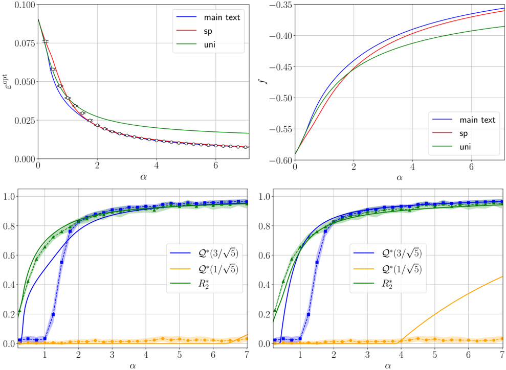<details> <summary>Image 22 Details</summary>  ### Visual Description ## Four Line Charts: Comparative Analysis of Algorithms ### Overview The image presents four line charts arranged in a 2x2 grid, comparing the performance of different algorithms across a range of alpha values. The top-left chart displays epsilon-opt values, the top-right chart displays 'f' values, and the bottom two charts display performance metrics Q*(3/√5), Q*(1/√5), and R*_2. The bottom two charts appear to be variations of the same data, possibly representing different experimental conditions or perspectives. ### Components/Axes **Top-Left Chart:** * **Title:** Implicit, represents epsilon-opt values. * **X-axis:** α (Alpha), ranging from 0 to 7. * **Y-axis:** ε^opt, ranging from 0.000 to 0.100, with increments of 0.025. * **Legend (Top-Right):** * Blue line: "main text" * Red line: "sp" * Green line: "uni" **Top-Right Chart:** * **Title:** Implicit, represents 'f' values. * **X-axis:** α (Alpha), ranging from 0 to 6. * **Y-axis:** f, ranging from -0.60 to -0.35, with increments of 0.05. * **Legend (Bottom-Right):** * Blue line: "main text" * Red line: "sp" * Green line: "uni" **Bottom-Left Chart:** * **Title:** Implicit, represents performance metrics. * **X-axis:** α (Alpha), ranging from 0 to 7. * **Y-axis:** Values ranging from 0.0 to 1.0, with increments of 0.2. * **Legend (Right):** * Blue line: "Q*(3/√5)" * Orange line: "Q*(1/√5)" * Green line: "R*_2" **Bottom-Right Chart:** * **Title:** Implicit, represents performance metrics. * **X-axis:** α (Alpha), ranging from 0 to 7. * **Y-axis:** Values ranging from 0.0 to 1.0, with increments of 0.2. * **Legend (Right):** * Blue line: "Q*(3/√5)" * Orange line: "Q*(1/√5)" * Green line: "R*_2" ### Detailed Analysis **Top-Left Chart (ε^opt vs. α):** * **"main text" (Blue):** Starts at approximately 0.05, decreases rapidly, and plateaus around 0.01 after α = 2. * α = 0: ε^opt ≈ 0.05 * α = 2: ε^opt ≈ 0.015 * α = 6: ε^opt ≈ 0.01 * **"sp" (Red):** Starts at approximately 0.08, decreases rapidly, and plateaus around 0.01 after α = 2. * α = 0: ε^opt ≈ 0.08 * α = 2: ε^opt ≈ 0.015 * α = 6: ε^opt ≈ 0.01 * **"uni" (Green):** Starts at approximately 0.08, decreases gradually, and plateaus around 0.02 after α = 4. * α = 0: ε^opt ≈ 0.08 * α = 2: ε^opt ≈ 0.03 * α = 6: ε^opt ≈ 0.02 **Top-Right Chart (f vs. α):** * **"main text" (Blue):** Starts at approximately -0.60, increases rapidly, and plateaus around -0.38 after α = 4. * α = 0: f ≈ -0.60 * α = 2: f ≈ -0.45 * α = 6: f ≈ -0.38 * **"sp" (Red):** Starts at approximately -0.60, increases rapidly, and plateaus around -0.40 after α = 4. * α = 0: f ≈ -0.60 * α = 2: f ≈ -0.47 * α = 6: f ≈ -0.40 * **"uni" (Green):** Starts at approximately -0.60, increases rapidly, and plateaus around -0.42 after α = 4. * α = 0: f ≈ -0.60 * α = 2: f ≈ -0.49 * α = 6: f ≈ -0.42 **Bottom-Left Chart (Performance Metrics vs. α):** * **"Q*(3/√5)" (Blue):** Starts at approximately 0.0, jumps to approximately 0.8 at α = 1, and plateaus around 0.95 after α = 3. * α = 0: Value ≈ 0.0 * α = 1: Value ≈ 0.8 * α = 3: Value ≈ 0.95 * α = 7: Value ≈ 0.95 * **"Q*(1/√5)" (Orange):** Remains near 0.0 across all alpha values. * α = 0: Value ≈ 0.0 * α = 7: Value ≈ 0.0 * **"R*_2" (Green):** Starts at approximately 0.2, increases rapidly, and plateaus around 0.95 after α = 3. * α = 0: Value ≈ 0.2 * α = 2: Value ≈ 0.8 * α = 3: Value ≈ 0.95 * α = 7: Value ≈ 0.95 **Bottom-Right Chart (Performance Metrics vs. α):** * **"Q*(3/√5)" (Blue):** Starts at approximately 0.0, jumps to approximately 0.8 at α = 1, and plateaus around 0.95 after α = 3. * α = 0: Value ≈ 0.0 * α = 1: Value ≈ 0.8 * α = 3: Value ≈ 0.95 * α = 7: Value ≈ 0.95 * **"Q*(1/√5)" (Orange):** Starts at approximately 0.0, increases gradually, reaching approximately 0.45 at α = 7. * α = 0: Value ≈ 0.0 * α = 7: Value ≈ 0.45 * **"R*_2" (Green):** Starts at approximately 0.2, increases rapidly, and plateaus around 0.95 after α = 3. * α = 0: Value ≈ 0.2 * α = 2: Value ≈ 0.8 * α = 3: Value ≈ 0.95 * α = 7: Value ≈ 0.95 ### Key Observations * In the top-left chart, "main text" and "sp" algorithms have similar performance, achieving lower epsilon-opt values compared to "uni" as alpha increases. * In the top-right chart, all three algorithms ("main text", "sp", and "uni") converge to similar 'f' values as alpha increases. * In the bottom-left chart, "Q*(3/√5)" and "R*_2" metrics show a significant jump in performance around α = 1, while "Q*(1/√5)" remains consistently low. * In the bottom-right chart, "Q*(3/√5)" and "R*_2" metrics show a significant jump in performance around α = 1, while "Q*(1/√5)" increases gradually. * The bottom-left and bottom-right charts differ primarily in the behavior of the "Q*(1/√5)" metric, which remains near zero in the bottom-left chart but increases gradually in the bottom-right chart. ### Interpretation The charts provide a comparative analysis of different algorithms ("main text", "sp", and "uni") and their performance metrics ("Q*(3/√5)", "Q*(1/√5)", and "R*_2") across varying alpha values. The top charts suggest that "main text" and "sp" algorithms are more effective in minimizing epsilon-opt compared to "uni". The bottom charts indicate that "Q*(3/√5)" and "R*_2" metrics exhibit a threshold behavior, with a significant performance jump around α = 1. The difference in "Q*(1/√5)" behavior between the bottom-left and bottom-right charts suggests that this metric is sensitive to specific experimental conditions or parameter settings. The data suggests that the choice of algorithm and alpha value significantly impacts performance, and the optimal configuration depends on the specific metric being optimized. </details> - ( iv ) in the cases we tested, the prediction for the generalisation error from the theory devised in the main text are in much better agreement with numerical simulations than the one from this Appendix (see FIG. 23 for a comparison). Therefore, the more elaborate theory presented in the main is not only more meaningful from the theoretical viewpoint, but also in overall better agreement with simulations. ## b. Possible refined analyses with structured S 2 matrices In the main text, we kept track of the inhomogeneous profile of the readouts induced by the non-trivial distribution P v , which is ultimately responsible for the sequence of specialisation phase transitions occurring at increasing α , thanks to a functional OP Q ( v ) measuring how much the student's hidden weights corresponding to all the readout elements equal to v have aligned with the teacher's. However, when writing ˜ P (( S a 2 ) | Q ) we treated the tensor S a 2 as FIG. 23. Generalisation error for ReLU activation and Rademacher readout prior P v of the theory reported in the main text (solid blue) versus the branch obtained from the simplified ansatz (B48) (solid red); the green solid line shows Q ≡ 0 (universal branch), and empty circles are HMC results with informative initialisation and homogeneous quenched readouts. All hyperparameters are the same as in FIG. 22. 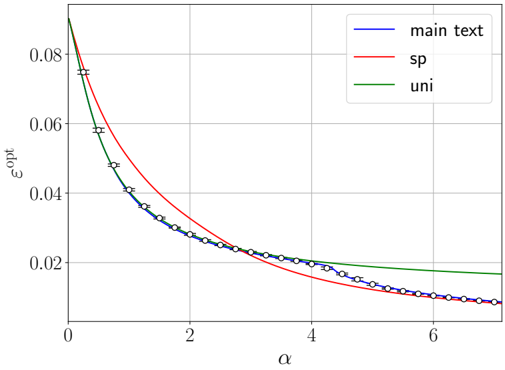<details> <summary>Image 23 Details</summary>  ### Visual Description ## Line Chart: Epsilon Opt vs. Alpha ### Overview The image is a line chart displaying the relationship between "epsilon opt" (εopt) on the y-axis and "alpha" (α) on the x-axis. Three different data series are plotted: "main text", "sp", and "uni". The "main text" series includes error bars. ### Components/Axes * **X-axis:** * Label: α * Scale: 0 to approximately 7, with gridlines at integer values. * **Y-axis:** * Label: εopt * Scale: 0 to approximately 0.09, with gridlines at intervals of 0.02. * **Legend (Top-Right):** * "main text" - Blue line with error bars * "sp" - Red line * "uni" - Green line ### Detailed Analysis * **"main text" (Blue):** * Trend: Decreases rapidly from α = 0 to α = 2, then decreases more gradually. * Data Points (approximate, with error bars): * α = 0: εopt ≈ 0.085 ± 0.003 * α = 1: εopt ≈ 0.048 ± 0.002 * α = 2: εopt ≈ 0.028 ± 0.001 * α = 3: εopt ≈ 0.022 ± 0.001 * α = 4: εopt ≈ 0.019 ± 0.001 * α = 5: εopt ≈ 0.015 ± 0.001 * α = 6: εopt ≈ 0.012 ± 0.001 * α = 7: εopt ≈ 0.009 ± 0.001 * **"sp" (Red):** * Trend: Decreases rapidly from α = 0 to α = 2, then decreases more gradually. * Data Points (approximate): * α = 0: εopt ≈ 0.085 * α = 1: εopt ≈ 0.058 * α = 2: εopt ≈ 0.032 * α = 3: εopt ≈ 0.020 * α = 4: εopt ≈ 0.014 * α = 5: εopt ≈ 0.011 * α = 6: εopt ≈ 0.009 * α = 7: εopt ≈ 0.007 * **"uni" (Green):** * Trend: Decreases from α = 0 to α = 4, then remains relatively constant. * Data Points (approximate): * α = 0: εopt ≈ 0.085 * α = 1: εopt ≈ 0.065 * α = 2: εopt ≈ 0.040 * α = 3: εopt ≈ 0.025 * α = 4: εopt ≈ 0.020 * α = 5: εopt ≈ 0.019 * α = 6: εopt ≈ 0.018 * α = 7: εopt ≈ 0.017 ### Key Observations * The "main text" and "sp" series are very close to each other, especially for α > 2. * The "uni" series has a slower rate of decrease compared to the other two series. * All three series converge to a similar value as α increases. * The error bars for the "main text" series are small, indicating relatively low uncertainty. ### Interpretation The chart illustrates how "epsilon opt" changes with respect to "alpha" for three different scenarios ("main text", "sp", and "uni"). The "main text" and "sp" scenarios exhibit similar behavior, suggesting a close relationship between them. The "uni" scenario shows a different trend, indicating a distinct underlying mechanism. The convergence of all three series at higher values of alpha suggests that the influence of the differentiating factors diminishes as alpha increases. The error bars on the "main text" series provide an indication of the precision of the measurements or calculations for that scenario. </details> a whole, without considering the possibility that its 'components' $$S _ { 2 ; \alpha _ { 1 } \alpha _ { 2 } } ^ { a } ( v ) \colon = \frac { v } { \sqrt { | \mathcal { I } _ { v } | } } \sum _ { i \in \mathcal { I } _ { v } } W _ { i \alpha _ { 1 } } ^ { a } W _ { i \alpha _ { 2 } } ^ { a } P ( V ) = P ( V + V ) - P ( V + V ) + P ( V + V ) + P ( V + V ) + P ( V + V ) + P ( V + V )$$ could follow different laws for different v ∈ V . To do so, let us define $$R _ { 2 } ^ { a b } = \frac { 1 } { k } \sum _ { v , v ^ { \prime } } v ^ { \prime } \sum _ { i \in \mathcal { I } _ { v } , j \in \mathcal { I } _ { v ^ { \prime } } } ( \Omega _ { i j } ^ { a b } ) ^ { 2 } = \sum _ { v , v ^ { \prime } } \frac { \sqrt { | \mathcal { I } _ { v } | | \mathcal { I } _ { v ^ { \prime } } | } } { k } \mathcal { Q } _ { 2 } ^ { a b } ( v , v ^ { \prime } ) , \quad w h e r e \quad \mathcal { Q } _ { 2 } ^ { a b } ( v , v ^ { \prime } ) \colon = \frac { 1 } { d ^ { 2 } } T r S _ { 2 } ^ { a } ( v ) S _ { 2 } ^ { b } ( v ^ { \prime } ) ^ { \intercal } .$$ The generalisation of (B27) then reads $$\int d P ( ( S _ { 2 } ^ { a } ) | \mathcal { Q } ) \frac { 1 } { d ^ { 2 } } T r \, S _ { 2 } ^ { a } ( v ) S _ { 2 } ^ { b } ( v ^ { \prime } ) ^ { \intercal } = \delta _ { v v ^ { \prime } } v ^ { 2 } \mathcal { Q } ^ { a b } ( v ) ^ { 2 } + \gamma \, v v ^ { \prime } \sqrt { P _ { v } ( v ) P _ { v } ( v ^ { \prime } ) }$$ w.r.t. the true distribution P (( S a 2 ) | Q ) reported in (30). Despite the already good match of the theory in the main with the numerics, taking into account this additional level of structure thanks to a refined simplified measure could potentially lead to further improvements. The simplified measure able to enforce this moment-matching while taking into account the Wishart form (B57) of the matrices ( S a 2 ( v )) is $$d \bar { P } ( ( S _ { 2 } ^ { a } ) \, | \, \mathcal { Q } ) \times \prod _ { v \in V } \prod _ { a } d P _ { S } ^ { v } ( S _ { 2 } ^ { a } ( v ) ) \times \prod _ { v \in V } \prod _ { a < b } e ^ { \frac { 1 } { 2 } \bar { \tau } _ { v } ^ { a b } ( Q ) T r S _ { 2 } ^ { a } ( v ) S _ { 2 } ^ { b } ( v ) } , & & ( B 6 0 )$$ where P v S is the law of a random matrix v ¯ W ¯ W ⊺ |I v | -1 / 2 with ¯ W ∈ R d ×|I v | having i.i.d. standard Gaussian entries. For properly chosen (¯ τ ab v ), (B59) is verified for this simplified measure. However, the OPs ( Q ab 2 ( v , v ′ )) are difficult to deal with if keeping a general form, as they not only imply coupled replicas ( S a 2 ( v )) a for a given v (a kind of coupling that is easily linearised with a single Hubbard-Stratonovich transformation, within the replica symmetric treatment justified in Bayes-optimal learning), but also a coupling for different values of the variable v . Linearising it would yield a more complicated matrix model than the integral reported in (B32), because the resulting coupling field would break rotational invariance and therefore the model does not have a form which is known to be solvable, see [130]. A first idea to simplify P (( S a 2 ) | Q ) (30) while taking into account the additional structure induced by (B58), (B59) and keeping the model solvable, is to consider a generalisation of the relaxation (B48). This entails dropping entirely the dependencies among matrix entries, induced by their Wishart-like form (B57), for each S a 2 ( v ). In this case, the moment constraints (B59) can be exactly enforced by choosing the simplified measure $$d \bar { P } ( ( S _ { 2 } ^ { a } ) | \pm b { Q } ) = \prod _ { v \in V } \prod _ { a = 0 } ^ { s } d S _ { 2 } ^ { a } ( v ) \prod _ { \alpha = 1 } ^ { d } \delta ( S _ { 2 ; \alpha \alpha } ^ { a } ( v ) - v \sqrt { | \mathcal { I } _ { v } | } ) \times \prod _ { v \in V } \prod _ { \alpha _ { 1 } < \alpha _ { 2 } } ^ { d } \frac { e ^ { - \frac { 1 } { 2 } \sum _ { a , b = 0 } ^ { s } S _ { 2 ; \alpha _ { 1 } \alpha _ { 2 } } ^ { a } ( v ) \pm b { q } ^ { a b } ( Q ) S _ { 2 ; \alpha _ { 1 } \alpha _ { 2 } } ^ { s } ( v ) } } { \sqrt { ( 2 \pi ) ^ { s + 1 } \det ( \bar { \tau } _ { v } ( Q ) ^ { - 1 } ) } } .$$ The parameters (¯ τ ab v ( Q )) are then properly chosen to enforce (B59) for all 0 ≤ a ≤ b ≤ s and v , v ′ ∈ V . Using this measure, the resulting entropic term, taking into account the degeneracy of the OPs ( Q ab 2 ( v , v ′ )) and ( Q ab ( v )), remains tractable through Gaussian integrals (the energetic term is obviously unchanged once we express ( R ab 2 ) entering it using these new OPs through the identity (B58), and keeping in mind that nothing changes for higher order overlaps compared to the theory in the main). We leave for future work the analysis of this Gaussian relaxation and other possible simplifications of (B60) leading to solvable models. ## 3. Large sample rate limit of f (1) RS In this section we show that when the prior over the weights is discrete the MI can never exceed the entropy of the prior itself. As for the main, we consider the readouts quenched to the ground truth ones, since they cannot affect the MI between weights and data at this scaling. For this appendix we restrict to L = 1, but the argument can be generalised to an arbitrary number of layers. We first need to control the function mmse when its argument is large. By a saddle point argument, one can show that the leading term for mmse S ( τ ) when τ →∞ is of the type C ( γ ) /τ for a proper constant C depending at most on γ . We now notice that the equation for ˆ Q ( v ) in (B41) can be rewritten as $$P _ { v } ( \mathbf v ) \hat { \mathcal { Q } } ( \mathbf v ) = \frac { 1 } { 2 \gamma } [ m m s e _ { S } ( \tau ) - m m s e _ { S } ( \tau + \hat { R } _ { 2 } ) ] \partial _ { \mathcal { Q } ( \nu ) } \tau + 2 \frac { \alpha } { \gamma } \partial _ { \mathcal { Q } ( \nu ) } \phi _ { P _ { o u t } } ( K ( R _ { 2 } , \mathcal { Q } ) ; K _ { d } ) .$$ For α →∞ we make the self-consistent ansatz Q ( v ) = 1 -o α (1). As a consequence, using the aforementioned scaling of the mmse( τ ), 1 /τ has to vanish by the moment matching condition (B39) as o α (1) too. Using the very same equation, we are also able to evaluate ∂ Q ( v ) τ as follows: <!-- formula-not-decoded --> as α →∞ , where we have used mmse S ( τ ) ≈ C ( γ ) /τ to estimate the derivative. We use the same approximation for the two mmse's appearing in the fixed point equation for ˆ Q ( v ): $$\hat { \mathcal { Q } } ( v ) \approx \frac { v ^ { 2 } \mathcal { Q } ( v ) } { \gamma C ( \gamma ) } \frac { \tau ^ { 2 } } { \tau ( \tau + \hat { R } _ { 2 } ) } \hat { R } _ { 2 } + 2 \frac { \alpha } { P _ { v } ( v ) \gamma } \partial _ { \mathcal { Q } ( v ) } \phi _ { P o u t } ( K ( R _ { 2 } , \mathcal { Q } ) ; K _ { d } ) , \quad ( B 6 4 )$$ where we are neglecting multiplicative constants for brevity. From the last equation in (B41) we see that ˆ R 2 cannot diverge more than O ( α ). Thanks to the above approximation and the first equation of (B41) this entails that Q ( v ) is approaching 1 exponentially fast in α (1 -Q ( v ) = O ( e -cα ) for some c > 0) due to the discreteness of its prior, which in turn implies τ is diverging exponentially in α . As a consequence $$\frac { \tau ^ { 2 } } { \tau ( \tau + \hat { R } _ { 2 } ) } \approx 1 . \begin{array} { l } \frac { \tau ^ { 2 } } { \tau ( \tau + \hat { R } _ { 2 } ) } \approx 1 . \end{array}$$ Furthermore, one also has $$\frac { 1 } { \alpha } [ \iota ( \tau ) - \iota ( \tau + \hat { R } _ { 2 } ) ] = - \frac { 1 } { 4 \alpha } \int _ { \tau } ^ { \tau + \hat { R } _ { 2 } } m m s e _ { S } ( t ) \, d t \approx - \frac { C ( \gamma ) } { 4 \alpha } \ln ( 1 + \frac { \hat { R } _ { 2 } } { \tau } ) \xrightarrow [ ] { \alpha \to \infty } 0 ,$$ as ˆ R 2 τ vanishes with exponential speed in α . Concerning the function ψ P W , given that it is related to a Bayes-optimal scalar Gaussian channel, and its SNRs ˆ Q ( v ) are all diverging one can compute the integral by saddle point, which is inevitably attained at the ground truth: $$\psi _ { P _ { W } } ( \hat { \mathcal { Q } } ( v ) ) & - \frac { \hat { \mathcal { Q } } ( v ) \mathcal { Q } ( v ) } { 2 } \approx \mathbb { E } _ { w ^ { 0 } } \ln \int d P _ { W } ( w ) \mathbb { I } ( w = w ^ { 0 } ) \\ & + \mathbb { E } \left [ ( \sqrt { \hat { \mathcal { Q } } ( v ) } \xi + \hat { \mathcal { Q } } ( v ) w ^ { 0 } ) w ^ { 0 } - \frac { \hat { \mathcal { Q } } ( v ) } { 2 } ( w ^ { 0 } ) ^ { 2 } \right ] - \frac { \hat { \mathcal { Q } } ( v ) ( 1 - O ( e ^ { - c \alpha } ) ) } { 2 } = - H ( W ) + o _ { \alpha } ( 1 ) .$$ Considering that ϕ P out ( K ( R 2 , Q ); K d ) α →∞ - - - - → ϕ P out ( K d ; K d ), and using (A20), it is then straightforward to check that our RS version of the MI saturates to the entropy of the prior P W when α →∞ : $$- \frac { \alpha } { \gamma } e x t r \, f _ { R S } ^ { ( 1 ) } + \frac { \alpha } { \gamma } \mathbb { E } _ { \lambda } \int d y P _ { o u t } ( y | \lambda ) \ln P _ { o u t } ( y | \lambda ) \xrightarrow { \alpha \to \infty } H ( W ) ,$$ where the factor α/γ is due to the fact that the components of W are kd , and not n . ## 4. Extension of GAMP-RIE to arbitrary activation for L = 1 For simplicity, let us consider P out ( y | λ ) = exp( -1 2∆ ( y -λ ) 2 ) / √ 2 π ∆, which entails: $$y _ { \mu } \, | \, ( \theta ^ { 0 } , x _ { \mu } ) \stackrel { d } { = } \frac { v ^ { \intercal } } { \sqrt { k } } \sigma \left ( \frac { W ^ { 0 } x _ { \mu } } { \sqrt { d } } \right ) + \sqrt { \Delta } \, z _ { \mu } , \quad \mu = 1 \dots , n ,$$ where z µ are i.i.d. standard Gaussian random variables and d = means equality in law. Expanding σ in the Hermite polynomial basis we have $$y _ { \mu } | ( \theta ^ { 0 } , x _ { \mu } ) \stackrel { d } { = } \mu _ { 0 } \frac { v ^ { \intercal } 1 _ { k } } { \sqrt { k } } + \mu _ { 1 } \frac { v ^ { \intercal } W ^ { 0 } x _ { \mu } } { \sqrt { k d } } + \frac { \mu _ { 2 } } { 2 } \frac { v ^ { \intercal } } { \sqrt { k } } H e _ { 2 } \left ( \frac { W ^ { 0 } x _ { \mu } } { \sqrt { d } } \right ) + \cdots + \sqrt { \Delta } z _ { \mu }$$ where . . . represents the terms beyond second order. Without loss of generality, for this choice of output channel we can set µ 0 = 0 as discussed in App. B 1 g. For low enough α it is reasonable to assume that higher order terms in . . . cannot be learnt given quadratically many samples and, as a result, play the role of effective noise, which we assume independent of the first three terms. We shall see that this reasoning actually applies to the extension of the GAMP-RIE we derive, which plays the role of a 'smart' spectral algorithm, regardless of the value of α . Therefore, these terms accumulate in an asymptotically Gaussian noise thanks to the central limit theorem (it is a projection of a centred function applied entry-wise to a vector with i.i.d. entries), with variance g (1). We thus obtain the effective model $$y _ { \mu } | ( \theta ^ { 0 } , x _ { \mu } ) \overset { d } { = } \mu _ { 1 } \frac { v ^ { \intercal } W ^ { 0 } x _ { \mu } } { \sqrt { k d } } + \frac { \mu _ { 2 } } { 2 } \frac { v ^ { \intercal } } { \sqrt { k } } H e _ { 2 } \left ( \frac { W ^ { 0 } x _ { \mu } } { \sqrt { d } } \right ) + \sqrt { \Delta + g ( 1 ) } \, z _ { \mu } .$$ The first term in this expression can be learnt with vanishing error given quadratically many samples (Remark 9), hence it can be ignored. This further simplifies the model to $$\bar { y } _ { \mu } \colon = y _ { \mu } - \mu _ { 1 } \frac { v ^ { \intercal } W ^ { 0 } x _ { \mu } } { \sqrt { k d } } \stackrel { d } { = } \frac { \mu _ { 2 } } { 2 } \frac { v ^ { \intercal } } { \sqrt { k } } H e _ { 2 } \left ( \frac { W ^ { 0 } x _ { \mu } } { \sqrt { d } } \right ) + \sqrt { \Delta + g ( 1 ) } \, z _ { \mu } ,$$ where ¯ y µ is y µ with the (asymptotically) perfectly learnt linear term removed, and the last equality in distribution is again conditional on ( θ 0 , x µ ). From the formula $$\frac { v ^ { \intercal } } { \sqrt { k } } H e _ { 2 } \left ( \frac { W ^ { 0 } x _ { \mu } } { \sqrt { d } } \right ) = T r \frac { W ^ { 0 \intercal } d i a g ( v ) W ^ { 0 } } { d \sqrt { k } } x _ { \mu } x _ { \mu } ^ { \intercal } - \frac { v ^ { \intercal } 1 _ { k } } { \sqrt { k } } \approx \frac { 1 } { \sqrt { k } d } T r [ ( x _ { \mu } x _ { \mu } ^ { \intercal } - I _ { d } ) W ^ { 0 \intercal } d i a g ( v ) W ^ { 0 } ] ,$$ where ≈ is exploiting the concentration Tr W 0 ⊺ diag( v ) W 0 / ( d √ k ) → v ⊺ 1 k / √ k , and the Gaussian equivalence property that M µ := ( x µ x ⊺ µ -I d ) / √ d behaves like a GOE sensing matrix, i.e., a symmetric matrix whose upper triangular part has i.i.d. entries from N (0 , (1+ δ ij ) /d ) [94], the model can be seen as a GLM with signal ¯ S 0 2 := W 0 ⊺ diag( v ) W 0 / √ kd : $$y _ { \mu } ^ { G L M } = \frac { \mu _ { 2 } } { 2 } T r [ M _ { \mu } \bar { S } _ { 2 } ^ { 0 } ] + \sqrt { \Delta + g ( 1 ) } \, z _ { \mu } . \quad ( B 7 4 )$$ Starting from this equation, the arguments of App. B 1 and [94], based on known results on the GLM [98] and matrix denoising [99-101], allow us to obtain the free entropy of such matrix sensing problem. The result is consistent with the Q ≡ 0 solution of the saddle point equations obtained from the replica method in App. B 1, which, as anticipated, corresponds to the case where the Hermite polynomial combinations of the signal following the second one are not learnt. Note that, as supported by the numerics, the model actually admits specialisation when α is big enough, hence the above equivalence cannot hold on the whole phase diagram at the information theoretic level. In fact, if specialisation Input: Fresh data point x test with unknown associated response y test , dataset D = { ( x µ , y µ ) } µ =1 Output: Estimator ˆ y test of y test . Estimate y (0) := µ 0 v ⊺ 1 / k as n √ Estimate ⟨ W ⊺ v ⟩ / √ k using (B77). Compute $$\hat { y } ^ { ( 0 ) } = \frac { 1 } { n } \sum _ { \mu } y _ { \mu } ;$$ Estimate the µ 1 term in the Hermite expansion (B70) as $$\hat { y } _ { \mu } ^ { ( 1 ) } = \mu _ { 1 } \frac { \langle v ^ { \intercal } W \rangle x _ { \mu } } { \sqrt { k d } } ;$$ $$\tilde { y } _ { \mu } = \frac { y _ { \mu } - \hat { y } _ { \mu } ^ { ( 0 ) } - \hat { y } _ { \mu } ^ { ( 1 ) } } { \mu _ { 2 } / 2 } ; \quad \tilde { \Delta } = \frac { \Delta + g ( 1 ) } { \mu _ { 2 } ^ { 2 } / 4 } ;$$ Input { ( x µ , ˜ y µ ) } n µ =1 and ˜ ∆ into Algorithm 1 in [94] to estimate ⟨ W ⊺ diag( v ) W ⟩ ; Output $$\hat { y } _ { t e s t } = \hat { y } ^ { ( 0 ) } + \mu _ { 1 } \frac { \langle v ^ { \intercal } W \rangle x _ { t e s t } } { \sqrt { k d } } + \frac { \mu _ { 2 } } { 2 } \frac { 1 } { d \sqrt { k } } T r [ ( x _ { t e s t } x _ { t e s t } ^ { \intercal } - \mathbb { I } ) \langle W ^ { \intercal } d i a g ( v ) W \rangle ] .$$ FIG. 24. Theoretical prediction (solid curves) of the Bayes-optimal mean-square generalisation error for binary inner weights and ReLU, eLU activations, with γ = 0 . 5, d = 150, Gaussian label noise with ∆ = 0 . 1, and fixed readouts v = 1 . Dashed lines are obtained from the solution of the fixed point equations (B41) with all Q ( v ) = 0. Circles are the test error of GAMP-RIE [94] extended to generic activation. The MCMC points initialised uninformatively (inset) are obtained using (A29), to account for lack of equilibration due to glassiness, which prevents using (A31) (see Remark 7). Even in the possibly glassy region, the GAMP-RIE attains the universal branch performance. Data for GAMP-RIE and MCMC are averaged over 16 data instances, with error bars representing one standard deviation over instances. GAMP-RIE's performance follows the universal theoretical curve even in the α regime where MCMC sampling experiences a computationally hard phase with worse performance, and in particular after α sp . 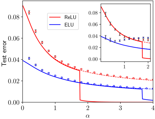<details> <summary>Image 24 Details</summary>  ### Visual Description ## Chart: Test Error vs. Alpha for ReLU and ELU Activation Functions ### Overview The image is a line chart comparing the test error of ReLU and ELU activation functions as a function of a parameter alpha (α). The chart shows two lines, one red (ReLU) and one blue (ELU), representing the test error for each activation function. The x-axis represents the value of alpha, ranging from 0 to 4. The y-axis represents the test error, ranging from 0 to 0.08. An inset plot provides a zoomed-in view of the region where alpha ranges from 0 to 2. Data points are marked on the lines, with error bars visible in the inset. ### Components/Axes * **X-axis:** α (alpha), ranging from 0 to 4. Axis markers are present at 0, 1, 2, 3, and 4. * **Y-axis:** Test error, ranging from 0.00 to 0.08. Axis markers are present at 0.00, 0.02, 0.04, 0.06, and 0.08. * **Legend:** Located in the top-center of the chart. * Red line: ReLU * Blue line: ELU * **Inset Plot:** Located in the top-right corner, showing a zoomed-in view of the data for α ranging from approximately 0 to 2. ### Detailed Analysis * **ReLU (Red Line):** * Trend: The test error decreases rapidly as alpha increases from 0 to approximately 2. At alpha = 2, the test error drops sharply to near zero. The dashed red line represents the data points. * Data Points: * α = 0: Test error ≈ 0.085 * α = 1: Test error ≈ 0.05 * α = 2: Test error ≈ 0.03 * α > 2: Test error ≈ 0.00 * **ELU (Blue Line):** * Trend: The test error decreases as alpha increases from 0 to approximately 4. At alpha = 2, the test error drops sharply, but not to zero. The dashed blue line represents the data points. * Data Points: * α = 0: Test error ≈ 0.04 * α = 1: Test error ≈ 0.03 * α = 2: Test error ≈ 0.02 * α > 2: Test error ≈ 0.01 ### Key Observations * Both ReLU and ELU activation functions exhibit decreasing test error as alpha increases. * ReLU shows a more significant drop in test error at α = 2, reaching near zero. * ELU's test error decreases more gradually and does not reach zero within the plotted range. * The inset plot provides a clearer view of the data points and error bars, especially for smaller values of alpha. ### Interpretation The chart suggests that both ReLU and ELU activation functions benefit from increasing the parameter alpha, as indicated by the decreasing test error. The sharp drop in test error for ReLU at α = 2 indicates a potential threshold or critical value for this parameter. The ELU activation function, while also benefiting from increasing alpha, does not exhibit as dramatic a drop in test error as ReLU. This could indicate that ELU is more stable or less sensitive to the value of alpha within the plotted range. The error bars on the data points in the inset plot provide an indication of the uncertainty in the test error measurements. The dashed lines represent the data points. </details> occurs one cannot consider the . . . terms in (B70) as noise uncorrelated with the first ones, as the model is aligning with the actual teacher's weights, such that it learns all the successive terms at once. We now assume that this mapping holds at the algorithmic level, namely, that we can process the data algorithmically as if they were coming from the identified GLM, and thus try to infer the signal ¯ S 0 2 = W 0 ⊺ diag( v ) W 0 / √ kd and construct a predictor from it. Based on this idea, we propose Algorithm 1 that can indeed reach the performance predicted by the Q ≡ 0 solution of our replica theory. . Remark 9. In the linear data regime, where n/d converges to a fixed constant α 1 , only the first term in (B70) can be learnt while the rest behaves like noise. By the same argument as above, the model is equivalent to $$y _ { \mu } = \mu _ { 1 } \frac { v ^ { \intercal } W ^ { 0 } x _ { \mu } } { \sqrt { k d } } + \sqrt { \Delta + \nu - \mu _ { 0 } ^ { 2 } - \mu _ { 1 } ^ { 2 } } \, z _ { \mu } ,$$ where ν = E z ∼N (0 , 1) σ ( z ) 2 . This is again a GLM with signal S 0 1 = W 0 ⊺ v / √ k and Gaussian sensing vectors x µ . Define q 1 as the limit of S a ⊺ 1 S b 1 /d where S a 1 , S b 1 are drawn independently from the posterior. With k →∞ , the signal converges in law to a standard Gaussian vector. Using known results on GLMs with Gaussian signal [98], we obtain the following equations characterising q 1 : $$q _ { 1 } = \frac { \hat { q } _ { 1 } } { \hat { q } _ { 1 } + 1 } , \quad \hat { q } _ { 1 } = \frac { \alpha _ { 1 } } { 1 + \Delta _ { 1 } - q _ { 1 } } , \quad w h e r e \quad \Delta _ { 1 } = \frac { \Delta + \nu - \mu _ { 0 } ^ { 2 } - \mu _ { 1 } ^ { 2 } } { \mu _ { 1 } ^ { 2 } } .$$ In the quadratic data regime, as α 1 = n/d goes to infinity, the overlap q 1 converges to 1 and the first term in (B70) is learnt with vanishing error. Moreover, since S 0 1 is asymptotically Gaussian, the linear problem (B76) is equivalent to denoising the Gaussian vector ( v ⊺ W 0 x µ / √ kd ) n µ =0 whose covariance is known as a function of X = ( x 1 , . . . , x n ) ∈ R d × n . This leads to the following simple MMSE estimator for S 0 1 : $$\langle { \mathbf S } _ { 1 } ^ { 0 } \rangle = \frac { 1 } { \sqrt { d \Delta _ { 1 } } } \left ( I + \frac { 1 } { d \Delta _ { 1 } } X X ^ { \dagger } \right ) ^ { - 1 } X y$$ where y = ( y 1 , . . . , y n ). Note that the derivation of this estimator does not assume the Gaussianity of x µ . Remark 10. The same argument can be easily generalised for general P out , leading to the following equivalent GLM in the universal Q ∗ ≡ 0 phase of the quadratic data regime: $$y _ { \mu } ^ { G L M } \sim \tilde { P } _ { o u t } ( \, \cdot \, | \, T r [ M _ { \mu } \bar { S } _ { 2 } ^ { 0 } ] ) , \quad w h e r e \quad \tilde { P } _ { o u t } ( y | x ) \colon = \mathbb { E } _ { z \sim \mathcal { N } ( 0 , 1 ) } P _ { o u t } \left ( y | \, \frac { \mu _ { 2 } } { 2 } x + z \sqrt { g ( 1 ) } \right ) ,$$ and M µ are independent GOE sensing matrices. Remark 11. One can show that the system of equations in (B43) with Q ( v ) all set to 0 (and consequently τ = 0) can be mapped onto the fixed point of the state evolution equations (92), (94) of the GAMP-RIE in [94] up to changes of variables. This confirms that when such a system has a unique solution, which is the case in all our tests, the GAMPRIE asymptotically matches our universal solution. Assuming the validity of the aforementioned effective GLM, a potential improvement for discrete weights could come from a generalisation of GAMP which, in the denoising step, would correctly exploit the discrete prior over inner weights rather than using the RIE (which is prior independent). However, the results of [169] suggest that optimally denoising matrices with discrete entries is hard, and the RIE is the best efficient procedure to do so. Consequently, we tend to believe that improving GAMP-RIE in the case of discrete weights is out of reach without strong side information about the teacher, or exploiting non-polynomial-time algorithms (see App. B 5). ## 5. Algorithmic complexity of finding the specialisation solution for L = 1 We now provide empirical evidence concerning the computational complexity to attain specialisation, namely to have one of the Q ( v ) > 0, or equivalently to beat the 'universal' performance ( Q ( v ) = 0 for all v ∈ V ) in terms of generalisation error. We tested two algorithms that can find it in affordable computational time: ADAM with optimised batch size for every dimension tested (the learning rate is automatically tuned), and Hamiltonian Monte Carlo (HMC), both trying to infer a two-layer teacher network with Gaussian inner weights. Both algorithms were tested with readout weights frozen to the teacher ones. We will later on discuss the case of learnable readouts. a. ADAM We focus on ReLU( x ) activation, with γ = 0 . 5, Gaussian output channel with low label noise (∆ = 10 -4 ) and α = 5 . 0 > α sp (= 0 . 22 , 0 . 12 , 0 . 02 for homogeneous, Rademacher and Gaussian readouts respectively, thus we are deep in the specialisation phase in all the cases we report), so that the specialisation solution exhibits a very low generalisation error. We test the learnt model at each gradient update measuring the generalisation error with a moving average of 10 steps to smoothen the curves. Let us define ε uni as the generalisation error associated to the overlap Q ≡ 0, then fixing a threshold ε opt < ¯ ε < ε uni , we define ¯ t ( d ) the time (in gradient updates) needed for the algorithm to cross the threshold for the first time. We optimise over different batch sizes B p as follows: we define FIG. 25. Semilog ( Left ) and log-log ( Right ) plots of the number of gradient updates needed to achieve a test loss below the threshold ¯ ε < ε uni . Student network trained with ADAM with optimised batch size for each point. The dataset was generated from a teacher network with ReLU( x ) activation and parameters ∆ = 10 -4 for the Gaussian noise variance of the linear readout, γ = 0 . 5 and α = 5 . 0 for which ε opt -∆ = 1 . 115 × 10 -5 . Points are obtained averaging over 10 teacher/data instances with error bars representing the standard deviation. Each row corresponds to a different distribution of the readouts, kept fixed during training. Top : homogeneous readouts, for which the error of the universal branch is ε uni -∆ = 1 . 217 × 10 -2 . Centre : Rademacher readouts, for which ε uni -∆ = 1 . 218 × 10 -2 . Bottom : Gaussian readouts, for which ε uni -∆ = 1 . 210 × 10 -2 . The quality of the fits can be read from Table II. 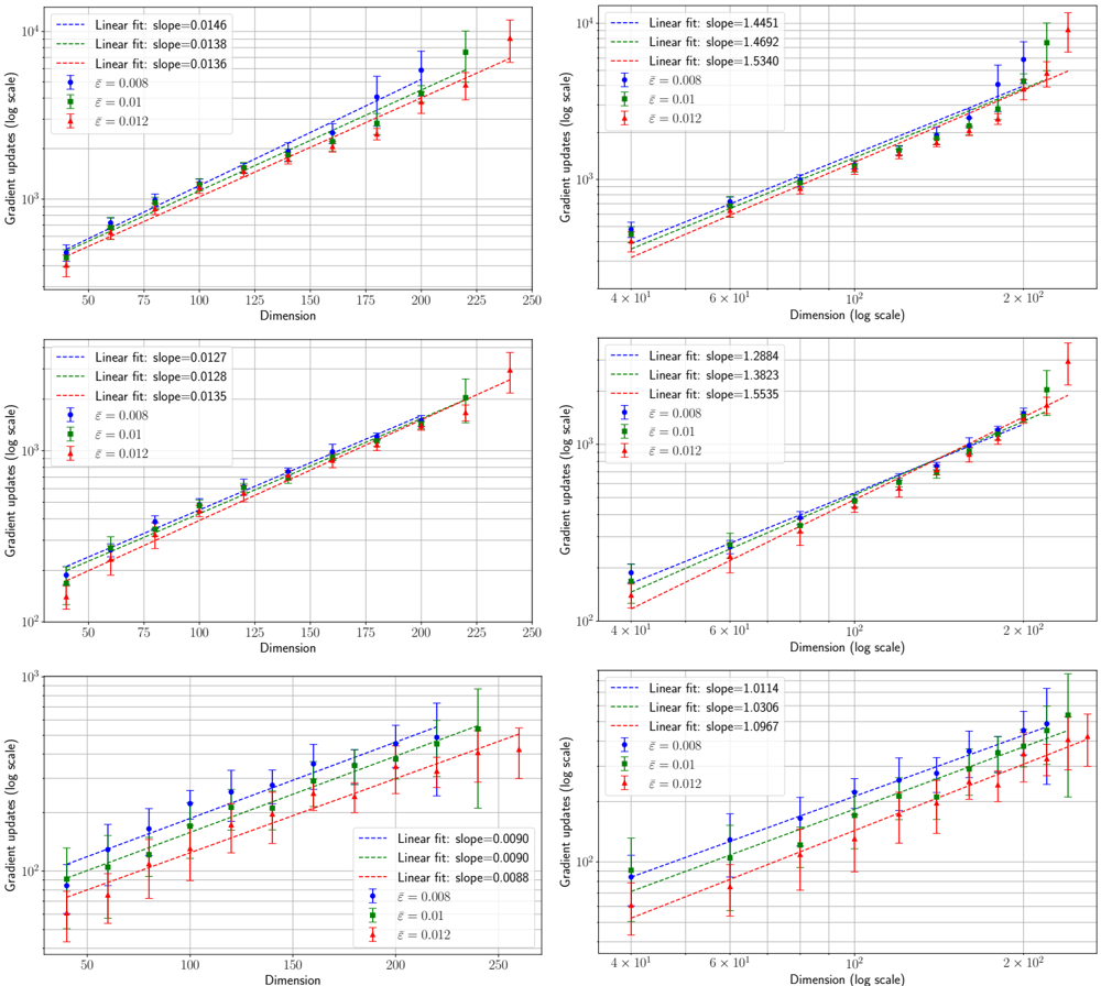<details> <summary>Image 25 Details</summary>  ### Visual Description ## Chart: Gradient Updates vs. Dimension ### Overview The image presents six scatter plots, each displaying the relationship between "Gradient updates (log scale)" and "Dimension". The plots are arranged in a 2x3 grid. Each plot shows data for three different values of epsilon (ε = 0.008, ε = 0.01, and ε = 0.012), along with linear fits for each epsilon value. The x-axis represents "Dimension," and the y-axis represents "Gradient updates (log scale)". The left column uses a linear scale for the x-axis, while the right column uses a logarithmic scale. ### Components/Axes * **Y-axis (all plots):** "Gradient updates (log scale)". The scale ranges from approximately 10^2 to 10^4. * **X-axis (left column):** "Dimension". The scale ranges from 50 to 250 in linear increments. * **X-axis (right column):** "Dimension (log scale)". The scale ranges from approximately 4 x 10^1 to 2 x 10^2 in logarithmic increments. * **Legend (all plots):** Located in the top-left corner of each plot. * Blue: Linear fit for ε = 0.008 * Green: Linear fit for ε = 0.01 * Red: Linear fit for ε = 0.012 * Blue markers: ε = 0.008 * Green markers: ε = 0.01 * Red markers: ε = 0.012 ### Detailed Analysis **Top-Left Plot:** * X-axis: Dimension (linear scale) * Linear fit (blue, ε = 0.008): Slope = 0.0146. The blue data points increase approximately linearly from ~300 at dimension 50 to ~3000 at dimension 250. * Linear fit (green, ε = 0.01): Slope = 0.0138. The green data points increase approximately linearly from ~400 at dimension 50 to ~2500 at dimension 250. * Linear fit (red, ε = 0.012): Slope = 0.0136. The red data points increase approximately linearly from ~500 at dimension 50 to ~2500 at dimension 250. **Top-Right Plot:** * X-axis: Dimension (log scale) * Linear fit (blue, ε = 0.008): Slope = 1.4451. The blue data points increase approximately linearly from ~300 at dimension 40 to ~8000 at dimension 200. * Linear fit (green, ε = 0.01): Slope = 1.4692. The green data points increase approximately linearly from ~400 at dimension 40 to ~9000 at dimension 200. * Linear fit (red, ε = 0.012): Slope = 1.5340. The red data points increase approximately linearly from ~500 at dimension 40 to ~12000 at dimension 200. **Middle-Left Plot:** * X-axis: Dimension (linear scale) * Linear fit (blue, ε = 0.008): Slope = 0.0127. The blue data points increase approximately linearly from ~250 at dimension 50 to ~2000 at dimension 250. * Linear fit (green, ε = 0.01): Slope = 0.0128. The green data points increase approximately linearly from ~300 at dimension 50 to ~2200 at dimension 250. * Linear fit (red, ε = 0.012): Slope = 0.0135. The red data points increase approximately linearly from ~400 at dimension 50 to ~2500 at dimension 250. **Middle-Right Plot:** * X-axis: Dimension (log scale) * Linear fit (blue, ε = 0.008): Slope = 1.2884. The blue data points increase approximately linearly from ~250 at dimension 40 to ~4000 at dimension 200. * Linear fit (green, ε = 0.01): Slope = 1.3823. The green data points increase approximately linearly from ~300 at dimension 40 to ~6000 at dimension 200. * Linear fit (red, ε = 0.012): Slope = 1.5535. The red data points increase approximately linearly from ~400 at dimension 40 to ~10000 at dimension 200. **Bottom-Left Plot:** * X-axis: Dimension (linear scale) * Linear fit (blue, ε = 0.008): Slope = 0.0090. The blue data points increase approximately linearly from ~150 at dimension 50 to ~700 at dimension 250. * Linear fit (green, ε = 0.01): Slope = 0.0090. The green data points increase approximately linearly from ~200 at dimension 50 to ~800 at dimension 250. * Linear fit (red, ε = 0.012): Slope = 0.0088. The red data points increase approximately linearly from ~200 at dimension 50 to ~700 at dimension 250. **Bottom-Right Plot:** * X-axis: Dimension (log scale) * Linear fit (blue, ε = 0.008): Slope = 1.0114. The blue data points increase approximately linearly from ~150 at dimension 40 to ~1500 at dimension 200. * Linear fit (green, ε = 0.01): Slope = 1.0306. The green data points increase approximately linearly from ~200 at dimension 40 to ~2000 at dimension 200. * Linear fit (red, ε = 0.012): Slope = 1.0967. The red data points increase approximately linearly from ~200 at dimension 40 to ~2500 at dimension 200. ### Key Observations * In all plots, the gradient updates generally increase with dimension. * The linear fits suggest a roughly linear relationship between dimension and gradient updates, especially when the x-axis is on a linear scale. * The slopes of the linear fits vary across the different plots, indicating that the rate of increase in gradient updates with dimension depends on the specific scenario represented by each plot. * The plots on the right (log scale for dimension) show a steeper increase in gradient updates compared to the plots on the left (linear scale for dimension), as indicated by the larger slope values. * For a given dimension, a higher epsilon value generally corresponds to a higher gradient update value. ### Interpretation The plots illustrate how gradient updates (on a log scale) change with increasing dimension for different values of epsilon. The use of both linear and logarithmic scales for the dimension axis provides different perspectives on the relationship. The logarithmic scale compresses the higher dimension values, making it easier to visualize the trend over a wider range. The increasing gradient updates with dimension suggest that as the complexity of the model (represented by dimension) increases, the magnitude of the updates required during training also increases. The different slopes indicate that this relationship is not constant and depends on other factors. The effect of epsilon is also notable. A higher epsilon value generally leads to larger gradient updates, which could be related to the learning rate or some other parameter influencing the training process. The error bars on the data points indicate the variability or uncertainty in the gradient updates. The size of these error bars could provide insights into the stability and reliability of the training process. </details> TABLE II. χ 2 test for exponential and power-law fits for the time needed by ADAM to reach the thresholds ¯ ε , for various priors on the readouts. Fits are displayed in FIG. 25. Smaller values of χ 2 (in bold, for given threshold and readouts) indicate a better compatibility with the hypothesis. | | χ 2 exponential fit | χ 2 exponential fit | χ 2 exponential fit | χ 2 exponential fit | χ 2 power law fit | χ 2 power law fit | χ 2 power law fit | |------------------------|-----------------------|-----------------------|-----------------------|-----------------------|---------------------|---------------------|---------------------| | Readouts | ¯ ε = | 0 . 008 | 0 . 010 | 0 . 012 | 0 . 008 | 0 . 010 | 0 . 012 | | Homogeneous | | 5 . 57 | 9 . 00 | 21 . 1 | 32 . 3 | 26 . 5 | 61 . 1 | | Rademacher | | 4 . 51 | 6 . 84 | 12 . 7 | 12 . 0 | 17 . 4 | 16 . 0 | | Uniform [ - √ 3 , √ 3] | | 5 . 08 | 1 . 44 | 4 . 21 | 8 . 26 | 8 . 57 | 3 . 82 | | Gaussian | | 2 . 66 | 0 . 76 | 3 . 02 | 0 . 55 | 2 . 31 | 1 . 36 | them as B p = ⌊ n 2 p ⌋ , p = 2 , 3 , . . . , ⌊ log 2 ( n ) ⌋ -1. Then for each batch size, the student network is trained until the moving average of the test loss drops below ¯ ε and thus outperforms the universal solution; we have checked that in such a scenario, the student ultimately gets close to the performance of the specialisation solution. The batch size that requires the least gradient updates is selected. We used the ADAM routine implemented in PyTorch. We test different distributions for the readout weights (kept fixed to v during training of the inner weights). We report all the values of ¯ t ( d ) in FIG. 25 for various dimensions d at fixed ( α, γ ), providing an exponential fit ¯ t ( d ) = exp( ad + b ) (left panel) and a power-law fit ¯ t ( d ) = ad b (right panel). We report the χ 2 test for the fits in Table II. We observe that for homogeneous and Rademacher readouts, the exponential fit is more compatible with the experiments, while for Gaussian readouts the comparison is inconclusive. In FIG. 27, we report the test loss of ADAM as a function of the gradient updates used for training, for various dimensions and choice of the readout distribution (as before, the readouts are not learnt but fixed to the teacher's). Here, we fix a batch size for simplicity. For both the cases of homogeneous ( v = 1 ) and Rademacher readouts (left and centre panels), the model experiences plateaux in performance increasing with the system size, in accordance with the observation of exponential complexity we reported above. The plateaux happen at values of the test loss comparable with twice the value for the Bayes error predicted by the universal branch of the theory (remember the relationship between Gibbs and Bayes errors reported in App. A 5). The curves are smoother for the case of Gaussian readouts. FIG. 26. Same as in FIG. 25, but in linear scale for better visualisation, for homogeneous readouts ( Left ) and Gaussian readouts ( Right ), with threshold ¯ ε = 0 . 008. 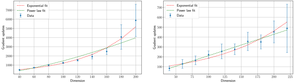<details> <summary>Image 26 Details</summary>  ### Visual Description ## Chart: Gradient Updates vs. Dimension ### Overview The image presents two scatter plots side-by-side, each depicting the relationship between "Gradient updates" and "Dimension." Both plots show data points with error bars, along with exponential and power-law fit curves. The left plot covers a dimension range from approximately 40 to 200, while the right plot covers a dimension range from approximately 50 to 225. ### Components/Axes * **Left Plot:** * X-axis: "Dimension," ranging from 40 to 200 in increments of 20. * Y-axis: "Gradient updates," ranging from 0 to 7000 in increments of 1000. * Legend (top-left): * Red dashed line: "Exponential fit" * Green dashed line: "Power law fit" * Blue data points with error bars: "Data" * **Right Plot:** * X-axis: "Dimension," ranging from 50 to 225 in increments of 25. * Y-axis: "Gradient updates," ranging from 0 to 700 in increments of 100. * Legend (top-left): * Red dashed line: "Exponential fit" * Green dashed line: "Power law fit" * Blue data points with error bars: "Data" ### Detailed Analysis **Left Plot:** * **Data Points (Blue):** The data points generally trend upwards as the dimension increases. * Dimension ~40: Gradient updates ~400 +/- 100 * Dimension ~60: Gradient updates ~700 +/- 100 * Dimension ~80: Gradient updates ~900 +/- 100 * Dimension ~100: Gradient updates ~1200 +/- 100 * Dimension ~120: Gradient updates ~1500 +/- 200 * Dimension ~140: Gradient updates ~1800 +/- 200 * Dimension ~160: Gradient updates ~2000 +/- 200 * Dimension ~180: Gradient updates ~4000 +/- 1000 * Dimension ~200: Gradient updates ~5000 +/- 1000 * **Exponential Fit (Red Dashed):** The exponential fit curve also trends upwards, closely following the initial data points but diverging at higher dimensions. * **Power Law Fit (Green Dashed):** The power law fit curve trends upwards, appearing to provide a better fit to the data at higher dimensions compared to the exponential fit. **Right Plot:** * **Data Points (Blue):** The data points generally trend upwards as the dimension increases. * Dimension ~50: Gradient updates ~80 +/- 20 * Dimension ~75: Gradient updates ~120 +/- 30 * Dimension ~100: Gradient updates ~220 +/- 40 * Dimension ~125: Gradient updates ~160 +/- 50 * Dimension ~150: Gradient updates ~220 +/- 50 * Dimension ~175: Gradient updates ~360 +/- 80 * Dimension ~200: Gradient updates ~380 +/- 100 * Dimension ~225: Gradient updates ~500 +/- 200 * **Exponential Fit (Red Dashed):** The exponential fit curve trends upwards, similar to the left plot. * **Power Law Fit (Green Dashed):** The power law fit curve trends upwards, appearing to provide a better fit to the data at higher dimensions compared to the exponential fit. ### Key Observations * Both plots show an increasing trend in "Gradient updates" as "Dimension" increases. * The error bars on the data points become larger at higher dimensions, indicating greater variability. * The power law fit appears to model the data better than the exponential fit, especially at higher dimensions. * The scale of the Y-axis (Gradient updates) differs significantly between the two plots. ### Interpretation The plots suggest that the number of gradient updates required increases with the dimension of the problem. The increasing error bars at higher dimensions may indicate that the relationship becomes less predictable or more sensitive to other factors as the dimensionality grows. The power law fit's better performance suggests that the relationship between gradient updates and dimension is non-linear and may be characterized by a power function. The difference in scale between the two plots is not explained by the image, but it may be due to different datasets or experimental conditions. </details> FIG. 27. Trajectories of the generalisation error of neural networks trained with ADAM at fixed batch size B = ⌊ n/ 4 ⌋ , learning rate 0.05, for ReLU( x ) activation with parameters ∆ = 10 -4 for the linear readout, γ = 0 . 5 and α = 5 . 0 > α sp (= 0 . 22 , 0 . 12 , 0 . 02 for homogeneous, Rademacher and Gaussian readouts respectively). The error ε uni is the mean-square generalisation error associated to the universal solution with overlap Q ≡ 0. Left : Homogeneous readouts. Centre : Rademacher readouts. Right : Gaussian readouts. Readouts are kept fixed (and equal to the teacher's) in all cases during training. Points on the solid lines are obtained by averaging over 5 teacher/data instances, and shaded regions around them correspond to one standard deviation. 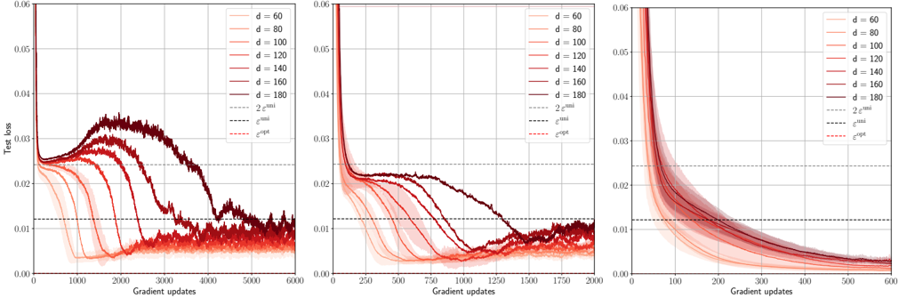<details> <summary>Image 27 Details</summary>  ### Visual Description ## Test Loss vs. Gradient Updates for Varying Dimensions ### Overview The image presents three line charts comparing the test loss against gradient updates for different dimensions (d = 60, 80, 100, 120, 140, 160, 180). Each chart represents a different scaling of the x-axis (Gradient updates), showing the initial behavior in more detail. The charts also include horizontal lines representing `2 * epsilon_uni`, `epsilon_uni`, and `epsilon_opt`. The lines are color-coded according to the legend in the top-right of each chart. ### Components/Axes * **X-axis (Horizontal):** Gradient updates. The scale varies across the three charts. * Left Chart: 0 to 6000 * Middle Chart: 0 to 2000 * Right Chart: 0 to 600 * **Y-axis (Vertical):** Test loss, ranging from 0.00 to 0.06 in all three charts. * **Legend (Top-Right):** * d = 60 (lightest red) * d = 80 (lighter red) * d = 100 (mid-tone red) * d = 120 (slightly darker red) * d = 140 (darker red) * d = 160 (dark red) * d = 180 (darkest red/brown) * 2 * epsilon<sup>uni</sup> (light gray dashed line) * epsilon<sup>uni</sup> (dark gray dashed line) * epsilon<sup>opt</sup> (red dashed line) ### Detailed Analysis **Left Chart (Gradient Updates: 0 to 6000):** * **d = 60 (lightest red):** Starts at approximately 0.022, decreases to approximately 0.005 around 2000 gradient updates, then fluctuates around that value. * **d = 80 (lighter red):** Starts at approximately 0.023, decreases to approximately 0.007 around 2500 gradient updates, then fluctuates. * **d = 100 (mid-tone red):** Starts at approximately 0.024, decreases to approximately 0.008 around 3000 gradient updates, then fluctuates. * **d = 120 (slightly darker red):** Starts at approximately 0.025, decreases to approximately 0.01 around 3500 gradient updates, then fluctuates. * **d = 140 (darker red):** Starts at approximately 0.026, decreases to approximately 0.012 around 4000 gradient updates, then fluctuates. * **d = 160 (dark red):** Starts at approximately 0.027, increases to approximately 0.032 around 2000 gradient updates, then decreases to approximately 0.013 around 4500 gradient updates, then fluctuates. * **d = 180 (darkest red/brown):** Starts at approximately 0.028, increases to approximately 0.035 around 2500 gradient updates, then decreases to approximately 0.014 around 5000 gradient updates, then fluctuates. * **2 * epsilon<sup>uni</sup> (light gray dashed line):** Horizontal line at approximately 0.023. * **epsilon<sup>uni</sup> (dark gray dashed line):** Horizontal line at approximately 0.012. * **epsilon<sup>opt</sup> (red dashed line):** Horizontal line at approximately 0.025. **Middle Chart (Gradient Updates: 0 to 2000):** * **d = 60 (lightest red):** Starts at approximately 0.022, rapidly decreases to approximately 0.005 within the first 500 gradient updates. * **d = 80 (lighter red):** Starts at approximately 0.023, rapidly decreases to approximately 0.007 within the first 750 gradient updates. * **d = 100 (mid-tone red):** Starts at approximately 0.024, rapidly decreases to approximately 0.008 within the first 1000 gradient updates. * **d = 120 (slightly darker red):** Starts at approximately 0.025, decreases to approximately 0.01 around 1250 gradient updates. * **d = 140 (darker red):** Starts at approximately 0.026, decreases to approximately 0.012 around 1500 gradient updates. * **d = 160 (dark red):** Starts at approximately 0.027, increases to approximately 0.022 around 500 gradient updates, then decreases to approximately 0.013 around 1750 gradient updates. * **d = 180 (darkest red/brown):** Starts at approximately 0.028, increases to approximately 0.023 around 750 gradient updates, then decreases to approximately 0.014 around 2000 gradient updates. * **2 * epsilon<sup>uni</sup> (light gray dashed line):** Horizontal line at approximately 0.023. * **epsilon<sup>uni</sup> (dark gray dashed line):** Horizontal line at approximately 0.012. * **epsilon<sup>opt</sup> (red dashed line):** Horizontal line at approximately 0.025. **Right Chart (Gradient Updates: 0 to 600):** * **d = 60 (lightest red):** Starts at approximately 0.06, rapidly decreases to approximately 0.015 within the first 100 gradient updates, then continues to decrease to approximately 0.005 by 600 gradient updates. * **d = 80 (lighter red):** Starts at approximately 0.06, rapidly decreases to approximately 0.017 within the first 100 gradient updates, then continues to decrease to approximately 0.007 by 600 gradient updates. * **d = 100 (mid-tone red):** Starts at approximately 0.06, rapidly decreases to approximately 0.018 within the first 100 gradient updates, then continues to decrease to approximately 0.008 by 600 gradient updates. * **d = 120 (slightly darker red):** Starts at approximately 0.06, rapidly decreases to approximately 0.019 within the first 100 gradient updates, then continues to decrease to approximately 0.01 by 600 gradient updates. * **d = 140 (darker red):** Starts at approximately 0.06, rapidly decreases to approximately 0.02 within the first 100 gradient updates, then continues to decrease to approximately 0.012 by 600 gradient updates. * **d = 160 (dark red):** Starts at approximately 0.06, rapidly decreases to approximately 0.021 within the first 100 gradient updates, then continues to decrease to approximately 0.013 by 600 gradient updates. * **d = 180 (darkest red/brown):** Starts at approximately 0.06, rapidly decreases to approximately 0.022 within the first 100 gradient updates, then continues to decrease to approximately 0.014 by 600 gradient updates. * **2 * epsilon<sup>uni</sup> (light gray dashed line):** Horizontal line at approximately 0.023. * **epsilon<sup>uni</sup> (dark gray dashed line):** Horizontal line at approximately 0.012. * **epsilon<sup>opt</sup> (red dashed line):** Horizontal line at approximately 0.025. ### Key Observations * For smaller dimensions (d = 60, 80, 100), the test loss decreases rapidly and stabilizes at a low value. * For larger dimensions (d = 160, 180), the test loss initially increases before decreasing, and the final loss is higher than for smaller dimensions. * The rate of decrease in test loss is highest in the initial gradient updates (as seen in the right chart). * The horizontal lines representing `2 * epsilon_uni`, `epsilon_uni`, and `epsilon_opt` provide reference points for evaluating the test loss. ### Interpretation The charts suggest that there is an optimal dimension for the model. Smaller dimensions lead to faster convergence and lower final test loss. However, larger dimensions may initially struggle to decrease the loss, and they may also converge to a higher final loss. This could be due to overfitting or other issues related to model complexity. The values of `epsilon_uni` and `epsilon_opt` seem to represent theoretical bounds or target values for the test loss, and the performance of different dimensions can be evaluated relative to these bounds. The initial increase in test loss for larger dimensions suggests that the model may be initially exploring suboptimal regions of the parameter space before finding a better solution. </details> b. Hamiltonian Monte Carlo The experiment is performed for the polynomial activation σ 3 = He 2 / √ 2 + He 3 / 6 with parameters ∆ = 0 . 1 for the Gaussian noise in the linear readout, γ = 0 . 5 and α = 1 . 0 > α sp (= 0 . 26 , 0 . 30 , 0 . 02 for homogeneous, Rademacher and Gaussian readouts respectively). Our HMC consists of 4000 iterations for homogeneous readouts, or 2000 iterations for Rademacher and Gaussian readouts. Each iteration is adaptive (with initial step size of 0 . 01) and uses 10 leapfrog steps. Instead of measuring the Gibbs error, whose relationship with ε opt holds only at equilibrium (see the last remark in App. A 5), we measured the teacher-student R 2 -overlap which is meaningful at any HMC step and is informative about the learning. For a fixed threshold ¯ R 2 and dimension d , we measure ¯ t ( d ) as the number of HMC iterations needed for the R 2 -overlap between the HMC sample (obtained from uninformative initialisation) and the teacher weights W 0 to cross the threshold. This criterion is again enough to assess that the student outperforms the universal solution. As before, we test homogeneous, Rademacher and Gaussian readouts, getting to the same conclusions: while for homogeneous and Rademacher readouts exponential time is more compatible with the observations, the experiments remain inconclusive for Gaussian readouts (see FIG. 29). We report in FIG. 28 the values of the overlap R 2 measured along the HMC runs for different dimensions. Note that, with HMC steps, all R 2 curves saturate to a value that is off by ≈ 1% w.r.t. that predicted by our theory for the selected values of α, γ and ∆. Whether this is a finite size effect, or an effect not taken into account by the current theory is an interesting question requiring further investigation, see App. B2b for possible directions. c. Learnable readouts As discussed in the main text, the static properties of the model remain unchanged whether the readout weights are quenched to the teacher values or learned during training. However, the dynamics can differ when the readouts are learnable. We verified that, for ADAM, the results regarding hardness are qualitatively unchanged when the readouts are learned. Although ADAM can achieve a lower test error in this case, the convergence time required to reach this solution increases substantially. Specifically, when the readouts are fixed, specialisation occurs after approximately 10 4 -10 5 gradient updates for homogeneous priors (see FIG. 27, left). In contrast, as shown in FIG. 8, learning the readouts increases the number of gradient updates required for specialisation by at least an order of magnitude. For HMC, which is constrained to sample according to the prior over both the inner and readout weights, the behaviour is essentially identical whether the readouts are fixed or learnable. The reasoning in Remark 3 therefore applies equally to HMC, as it is a posterior sampler. -overlap q FIG. 28. Trajectories of the overlap R 2 in HMC runs initialised uninformatively for the polynomial activation σ 3 = He 2 / √ 2 + He 3 / 6 with parameters ∆ = 0 . 1 for the linear readout, γ = 0 . 5 and α = 1 . 0. Left : Homogeneous readouts. Centre : Rademacher readouts. Right : Gaussian readouts. Points on the solid lines are obtained by averaging over 10 teacher/data instances, and shaded regions around them correspond to one standard deviation. Notice that the y -axes are limited for better visualisation. For the left and centre plot, any threshold (horizontal line in the plot) between the prediction of the Q ≡ 0 branch of the theory (black dashed line) and its prediction for the R sp 2 (red dashed line, obtained with informative initialisation) crosses the curves in points ¯ t ( d ) more compatible with an exponential fit (see FIG. 29 and Table III, where these fits are reported and χ 2 -tested). For the cases of homogeneous and Rademacher readouts, the value of the overlap at which the dynamics slows down (predicted by the Q ≡ 0 branch) is in quantitative agreement with the theoretical predictions (lower dashed line). The theory is instead off by ≈ 1% for the values R 2 at which the runs ultimately converge. 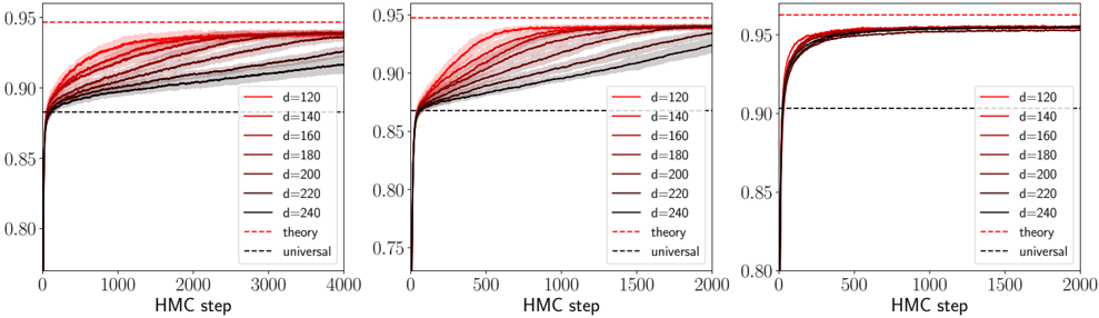<details> <summary>Image 28 Details</summary>  ### Visual Description ## Line Charts: HMC Step vs. Value for Different 'd' Values ### Overview The image presents three line charts arranged horizontally. Each chart plots the relationship between the "HMC step" (x-axis) and a value (y-axis) for different values of 'd' (ranging from 120 to 240). The charts also include lines representing "theory" and "universal" baselines. The x-axis scale varies across the three charts, with the first chart extending to 4000 HMC steps, while the other two extend to 2000 HMC steps. ### Components/Axes * **X-axis (Horizontal):** "HMC step". The first chart ranges from 0 to 4000, while the second and third range from 0 to 2000. * **Y-axis (Vertical):** Value. All three charts share the same y-axis scale, ranging from 0.80 to 0.95. * **Data Series:** * `d=120`: Red line * `d=140`: Dark red line * `d=160`: Brownish-red line * `d=180`: Dark brown line * `d=200`: Dark grey line * `d=220`: Grey line * `d=240`: Black line * `theory`: Dashed red line * `universal`: Dashed black line * **Legend:** Located on the right side of the first and second charts, and in the middle of the third chart. It maps the 'd' values and the "theory" and "universal" baselines to their corresponding line colors and styles. * **Chart Titles:** There are no explicit chart titles. ### Detailed Analysis **Chart 1 (Left):** * **X-axis:** 0 to 4000 HMC steps. * **Y-axis:** 0.80 to 0.95. * **Data Series Trends:** * `d=120` (Red): Starts around 0.88, rises sharply, and plateaus around 0.94 after approximately 2000 steps. * `d=140` (Dark Red): Starts around 0.88, rises sharply, and plateaus around 0.93 after approximately 2000 steps. * `d=160` (Brownish-Red): Starts around 0.88, rises sharply, and plateaus around 0.92 after approximately 2000 steps. * `d=180` (Dark Brown): Starts around 0.88, rises sharply, and plateaus around 0.91 after approximately 2000 steps. * `d=200` (Dark Grey): Starts around 0.88, rises sharply, and plateaus around 0.90 after approximately 2000 steps. * `d=220` (Grey): Starts around 0.88, rises sharply, and plateaus around 0.90 after approximately 2000 steps. * `d=240` (Black): Starts around 0.88, rises sharply, and plateaus around 0.89 after approximately 2000 steps. * `theory` (Dashed Red): Horizontal line at approximately 0.95. * `universal` (Dashed Black): Horizontal line at approximately 0.88. **Chart 2 (Middle):** * **X-axis:** 0 to 2000 HMC steps. * **Y-axis:** 0.75 to 0.95. * **Data Series Trends:** * `d=120` (Red): Starts around 0.88, rises sharply, and plateaus around 0.94 after approximately 500 steps. * `d=140` (Dark Red): Starts around 0.88, rises sharply, and plateaus around 0.93 after approximately 500 steps. * `d=160` (Brownish-Red): Starts around 0.88, rises sharply, and plateaus around 0.92 after approximately 500 steps. * `d=180` (Dark Brown): Starts around 0.88, rises sharply, and plateaus around 0.91 after approximately 500 steps. * `d=200` (Dark Grey): Starts around 0.88, rises sharply, and plateaus around 0.90 after approximately 500 steps. * `d=220` (Grey): Starts around 0.88, rises sharply, and plateaus around 0.90 after approximately 500 steps. * `d=240` (Black): Starts around 0.88, rises sharply, and plateaus around 0.89 after approximately 500 steps. * `theory` (Dashed Red): Horizontal line at approximately 0.95. * `universal` (Dashed Black): Horizontal line at approximately 0.88. **Chart 3 (Right):** * **X-axis:** 0 to 2000 HMC steps. * **Y-axis:** 0.80 to 0.95. * **Data Series Trends:** * `d=120` (Red): Starts around 0.88, rises sharply, and plateaus around 0.94 after approximately 200 steps. * `d=140` (Dark Red): Starts around 0.88, rises sharply, and plateaus around 0.93 after approximately 200 steps. * `d=160` (Brownish-Red): Starts around 0.88, rises sharply, and plateaus around 0.92 after approximately 200 steps. * `d=180` (Dark Brown): Starts around 0.88, rises sharply, and plateaus around 0.91 after approximately 200 steps. * `d=200` (Dark Grey): Starts around 0.88, rises sharply, and plateaus around 0.90 after approximately 200 steps. * `d=220` (Grey): Starts around 0.88, rises sharply, and plateaus around 0.90 after approximately 200 steps. * `d=240` (Black): Starts around 0.88, rises sharply, and plateaus around 0.89 after approximately 200 steps. * `theory` (Dashed Red): Horizontal line at approximately 0.95. * `universal` (Dashed Black): Horizontal line at approximately 0.88. ### Key Observations * All 'd' values start at approximately the same value (around 0.88), which coincides with the "universal" baseline. * As 'd' increases, the plateau value decreases. The red line (`d=120`) plateaus at the highest value, while the black line (`d=240`) plateaus at the lowest value. * The "theory" baseline is consistently higher than all the 'd' values. * The rate at which the lines plateau varies across the three charts. The first chart shows a slower plateauing compared to the second and third charts. ### Interpretation The charts illustrate the convergence behavior of a process (likely an algorithm or simulation) as a function of the number of HMC steps, for different values of a parameter 'd'. The 'd' parameter seems to influence the final value that the process converges to, with smaller 'd' values leading to higher final values. The "universal" baseline represents a lower bound or initial state, while the "theory" baseline represents an upper bound or theoretical limit. The fact that all 'd' values start at the "universal" baseline suggests that this is the initial condition of the process. The difference in plateauing rates across the three charts suggests that the x-axis scaling is different, and the process converges faster in the third chart compared to the first. The data suggests that the process approaches the theoretical limit, but the rate of convergence and the final value depend on the parameter 'd'. 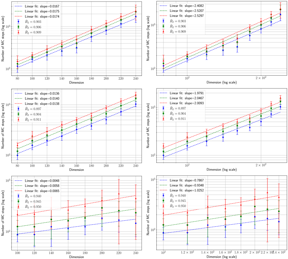</details> <details> <summary>Image 29 Details</summary>  ### Visual Description ## Chart Type: Multiple Scatter Plots with Linear Fits ### Overview The image contains six scatter plots arranged in a 2x3 grid. Each plot shows the relationship between "Dimension" (or "Dimension (log scale)") on the x-axis and "Number of MC steps (log scale)" on the y-axis. Each plot displays three data series, each with a linear fit line. The data series are distinguished by color (blue, green, red) and are associated with different R² values. Error bars are present on each data point. ### Components/Axes * **Title (Y-Axis):** "Number of MC steps (log scale)" - This label is consistent across all six plots. The y-axis is displayed on a log scale. * **Title (X-Axis):** "Dimension" (plots 1, 3, 5) or "Dimension (log scale)" (plots 2, 4, 6). The x-axis is displayed on a linear scale for the left column and a log scale for the right column. * **Y-Axis Scale:** Ranges from approximately 10^2 to 10^3 on all plots. * **X-Axis Scale (Linear):** Ranges from approximately 80 to 240 (plots 1, 3, 5). * **X-Axis Scale (Log):** Ranges from approximately 10^2 to 2.4 x 10^2 (plots 2, 4, 6). * **Legend:** Each plot includes a legend in the top-left corner indicating the color-coded data series and their corresponding R² values, along with the slope of the linear fit. The legend entries are consistently formatted as: * "Linear fit: slope=[value]" * "R² = [value]" * **Data Series:** Each plot contains three data series, represented by blue circles, green squares, and red triangles. Each data point has associated error bars. ### Detailed Analysis **Plot 1 (Top-Left):** * **X-Axis:** Dimension (linear scale) * **Blue Series:** * Linear fit: slope=0.0167 * R² = 0.903 * Trend: Upward sloping * Approximate Data Points: (80, 120), (120, 140), (160, 170), (200, 200), (240, 230) * **Green Series:** * Linear fit: slope=0.0175 * R² = 0.906 * Trend: Upward sloping * Approximate Data Points: (80, 130), (120, 160), (160, 190), (200, 220), (240, 250) * **Red Series:** * Linear fit: slope=0.0174 * R² = 0.909 * Trend: Upward sloping * Approximate Data Points: (80, 140), (120, 170), (160, 200), (200, 230), (240, 260) **Plot 2 (Top-Right):** * **X-Axis:** Dimension (log scale) * **Blue Series:** * Linear fit: slope=2.4082 * R² = 0.903 * Trend: Upward sloping * Approximate Data Points: (100, 120), (130, 250), (160, 400), (200, 700), (240, 1000) * **Green Series:** * Linear fit: slope=2.5207 * R² = 0.906 * Trend: Upward sloping * Approximate Data Points: (100, 140), (130, 300), (160, 500), (200, 800), (240, 1200) * **Red Series:** * Linear fit: slope=2.5297 * R² = 0.909 * Trend: Upward sloping * Approximate Data Points: (100, 150), (130, 350), (160, 550), (200, 900), (240, 1400) **Plot 3 (Middle-Left):** * **X-Axis:** Dimension (linear scale) * **Blue Series:** * Linear fit: slope=0.0136 * R² = 0.897 * Trend: Upward sloping * Approximate Data Points: (80, 110), (120, 130), (160, 150), (200, 170), (240, 190) * **Green Series:** * Linear fit: slope=0.0140 * R² = 0.904 * Trend: Upward sloping * Approximate Data Points: (80, 120), (120, 150), (160, 170), (200, 200), (240, 220) * **Red Series:** * Linear fit: slope=0.0138 * R² = 0.911 * Trend: Upward sloping * Approximate Data Points: (80, 130), (120, 160), (160, 190), (200, 220), (240, 240) **Plot 4 (Middle-Right):** * **X-Axis:** Dimension (log scale) * **Blue Series:** * Linear fit: slope=1.9791 * R² = 0.897 * Trend: Upward sloping * Approximate Data Points: (100, 110), (130, 200), (160, 300), (200, 500), (240, 700) * **Green Series:** * Linear fit: slope=2.0467 * R² = 0.904 * Trend: Upward sloping * Approximate Data Points: (100, 120), (130, 230), (160, 350), (200, 600), (240, 800) * **Red Series:** * Linear fit: slope=2.0093 * R² = 0.911 * Trend: Upward sloping * Approximate Data Points: (100, 130), (130, 250), (160, 400), (200, 650), (240, 900) **Plot 5 (Bottom-Left):** * **X-Axis:** Dimension (linear scale) * **Blue Series:** * Linear fit: slope=0.0048 * R² = 0.940 * Trend: Upward sloping * Approximate Data Points: (100, 85), (140, 90), (180, 95), (220, 100), (240, 105) * **Green Series:** * Linear fit: slope=0.0058 * R² = 0.945 * Trend: Upward sloping * Approximate Data Points: (100, 90), (140, 100), (180, 110), (220, 120), (240, 125) * **Red Series:** * Linear fit: slope=0.0065 * R² = 0.950 * Trend: Upward sloping * Approximate Data Points: (100, 95), (140, 110), (180, 125), (220, 140), (240, 150) **Plot 6 (Bottom-Right):** * **X-Axis:** Dimension (log scale) * **Blue Series:** * Linear fit: slope=0.7867 * R² = 0.940 * Trend: Upward sloping * Approximate Data Points: (100, 85), (140, 100), (180, 120), (220, 140), (240, 150) * **Green Series:** * Linear fit: slope=0.9348 * R² = 0.945 * Trend: Upward sloping * Approximate Data Points: (100, 90), (140, 120), (180, 150), (220, 180), (240, 200) * **Red Series:** * Linear fit: slope=1.0252 * R² = 0.950 * Trend: Upward sloping * Approximate Data Points: (100, 95), (140, 130), (180, 170), (220, 220), (240, 250) ### Key Observations * The "Number of MC steps (log scale)" generally increases with "Dimension" (or "Dimension (log scale)"). * The slopes of the linear fits are significantly higher when the x-axis is on a log scale (right column) compared to a linear scale (left column). * The R² values are generally high (close to 1), indicating a good fit of the linear models to the data. * Within each plot, the red series consistently has the highest "Number of MC steps (log scale)" values, followed by the green series, and then the blue series. * The error bars appear to be relatively consistent across all data points within each plot. * The R² values are slightly different for each series within a plot, suggesting that the linear fit is slightly better for some series than others. ### Interpretation The plots demonstrate the relationship between the dimension of a system and the number of Monte Carlo (MC) steps required for a simulation. The logarithmic scaling of both axes suggests that the number of MC steps increases exponentially with the dimension. The different R² values and slopes for each series likely correspond to different simulation parameters or system configurations. The high R² values indicate that a linear model is appropriate for describing this relationship, especially when both axes are logarithmically scaled. The error bars provide an estimate of the uncertainty in the number of MC steps for each dimension. The plots with the linear x-axis show a more gradual increase in the number of MC steps compared to the plots with the logarithmic x-axis, highlighting the exponential nature of the relationship. The data suggests that as the dimensionality of the system increases, the computational cost (measured by the number of MC steps) grows significantly, particularly when considering the logarithmic scale. The different R² values for each series suggest that the quality of the linear fit varies slightly depending on the specific parameters or configurations represented by each series. </details> FIG. 29. Semilog ( Left ) and log-log ( Right ) plots of the number of Hamiltonian Monte Carlo steps needed to achieve an overlap ¯ R 2 > R uni 2 , that certifies the universal solution is outperformed. The dataset was generated from a teacher with polynomial activation σ 3 = He 2 / √ 2 + He 3 / 6 and parameters ∆ = 0 . 1 for the linear readout, γ = 0 . 5 and α = 1 . 0 > α sp (= 0 . 26 , 0 . 30 , 0 . 02 for homogeneous, Rademacher and Gaussian readouts respectively). Student weights are sampled using HMC (initialised uninformatively) with 4000 iterations for homogeneous readouts ( Top row , for which R uni 2 = 0 . 883), or 2000 iterations for Rademacher ( Centre row , with R uni 2 = 0 . 868) and Gaussian readouts ( Bottom row , for which R uni 2 = 0 . 903). Each iteration is adaptative (with initial step size of 0 . 01) and uses 10 leapfrog steps. R sp 2 = 0 . 941 , 0 . 948 , 0 . 963 in the three cases. The readouts are kept fixed during training. Points are obtained averaging over 10 teacher/data instances with error bars representing the standard deviation. | | | χ 2 exponential fit χ 2 power law fit | χ 2 exponential fit χ 2 power law fit | χ 2 exponential fit χ 2 power law fit | χ 2 exponential fit χ 2 power law fit | χ 2 exponential fit χ 2 power law fit | χ 2 exponential fit χ 2 power law fit | |-------------|---------------------------------------------|-----------------------------------------|-----------------------------------------|-----------------------------------------|-----------------------------------------|-----------------------------------------|-----------------------------------------| | Readouts | | | | | | | | | Homogeneous | ( ¯ R 2 ∈ { 0 . 903 , 0 . 906 , 0 . 909 } ) | 2 . 22 | 1 . 47 | 1 . 14 | 8 . 01 | 7 . 25 | 6 . 35 | | Rademacher | ( ¯ R 2 ∈ { 0 . 897 , 0 . 904 , 0 . 911 } ) | 1 . 88 | 2 . 12 | 1 . 70 | 8 . 10 | 7 . 70 | 8 . 57 | | Gaussian | ( ¯ R 2 0 . 940 , 0 . 945 , 0 . 950 ) | 0 . 66 | 0 . 44 | 0 . 26 | 0 . 62 | 0 . 53 | 0 . 39 | ∈ { } TABLE III. χ 2 test for exponential and power-law fits for the time needed by Hamiltonian Monte Carlo to reach the thresholds ¯ R 2 , for various priors on the readouts. For a given row, we report three values of the χ 2 test per hypothesis, corresponding with the thresholds ¯ R 2 on the left, in the order given. Fits are displayed in FIG. 29. Smaller values of χ 2 (in bold, for given threshold and readouts) indicate a better compatibility with the hypothesis. ## 6. A potential route for a proof for L = 1 Here we provide an argument for a potential proof of our results based the adaptive interpolation technique introduced in [202], used as in [98]. In order to make the model more amenable to rigorous treatment, we select activation functions with µ 0 = µ 1 = µ 2 = 0 and all-ones readouts v = 1 . While assumptions on µ 0 , µ 1 are not that restrictive, µ 2 = 0 is what induces the main simplifications as it erases from the analyses the role of the overlaps R 2 . It is also useful to write the replica potential we are targeting, that in the hypotheses listed above and with a little abuse of notation reads $$f _ { R S } ^ { ( 1 ) } ( \mathcal { Q } , \hat { \mathcal { Q } } ) = \frac { \gamma } { \alpha } \psi _ { P W } ( \hat { \mathcal { Q } } ) + \phi _ { P o u t } \left ( g ( \mathcal { Q } ) , g ( 1 ) \right ) - \frac { \gamma } { 2 \alpha } \mathcal { Q } \hat { \mathcal { Q } } .$$ A part from the presence of g ( Q ) inside ϕ P out the above formula looks like the one of a standard generalised linear model [98], we shall thus use a similar formalism. Let us define an interpolating model: $$S _ { t \mu } \colon = \frac { \sqrt { 1 - t } } { \sqrt { k } } \sum _ { i = 1 } ^ { k } \varphi \left ( \frac { 1 } { \sqrt { d } } W _ { i } ^ { * T } x _ { \mu } \right ) + \sqrt { G ( t ) } \, V _ { \mu } + \sqrt { g ( 1 ) t - G ( t ) } \, U _ { \mu } ^ { * }$$ where t ∈ [0 , 1], G ( t ) is a non-negative interpolating function, and V µ , U ∗ µ iid ∼ N (0 , 1). Note that U ∗ µ is a starred variable, thus we consider it as learnable. The labels for this interpolating model are then given by $$Y _ { t \mu } & \sim P _ { o u t } ( \cdot | S _ { t \mu } ) & & ( B 8 1 )$$ To complete the interpolation, we also need another Gaussian observation channel about W ∗ : $$Y _ { t ; i j } ^ { G } = \sqrt { R ( t ) } W _ { i j } ^ { * } + Z _ { i j } \quad ( B 8 2 )$$ where Z ij iid ∼ N (0 , 1). The interpolating functions G ( t ) , R ( t ) have to be appropriately chosen later, in order to make some remainders vanish. The only requirement for now is that G (0) = R (0) = 0. Define u y ( x ) := ln P out ( y | x ), and denote for brevity Y t = ( Y tµ ) µ ≤ n , Y G t = ( Y G t ; ij ) i ≤ k,j ≤ d , U = ( U µ ) µ ≤ n , V = ( V µ ) µ ≤ n and $$s _ { t \mu } \colon = \frac { \sqrt { 1 - t } } { \sqrt { k } } \sum _ { i = 1 } ^ { k } \varphi \left ( \frac { 1 } { \sqrt { d } } W _ { i } ^ { \intercal } x _ { \mu } \right ) + \sqrt { G ( t ) } \, V _ { \mu } + \sqrt { g ( 1 ) t - G ( t ) } \, U _ { \mu }$$ Then the above interpolating model induces a Hamiltonian that reads $$- \mathcal { H } _ { t } ( X , Y _ { t } , Y ^ { G } _ { t } , V , U , W ) = \sum _ { \mu = 1 } ^ { n } u _ { Y _ { t _ { \mu } } } ( s _ { t _ { \mu } } ) - \frac { 1 } { 2 } \| Y ^ { G } _ { t } - \sqrt { R ( t ) } W \| ^ { 2 } .$$ and the corresponding quenched free entropy is with $$\mathbb { E } _ { ( t ) } [ \cdot ] = \mathbb { E } _ { X , V , U ^ { * } , W ^ { * } } \int d Y _ { t } d Y _ { t } ^ { G } e ^ { - \mathcal { H } _ { t } ( X , Y _ { t } , Y _ { t } ^ { G } , V , U ^ { * } , W ^ { * } ) } [ \cdot ] \, , \quad \mathcal { Z } _ { t } \ = \int d P _ { W } ( W ) D U e ^ { - \mathcal { H } _ { t } ( X , Y _ { t } , Y _ { t } ^ { G } , V , U , W ) } \, .$$ At the extrema of interpolation we have $$f _ { n } ( 0 ) & = f _ { n } - \frac { \gamma } { 2 \alpha } \\ f _ { n } ( 1 ) & = \frac { \gamma } { \alpha } \psi _ { P _ { W } } ( R ( 1 ) ) + \phi _ { P _ { o u t } } ( G ( 1 ) , g ( 1 ) ) - \frac { \gamma } { 2 \alpha } ( 1 + R ( 1 ) ) \, .$$ The role of the interpolation is that of decoupling continuously the quenched disorder in the x µ 's from the weights W ∗ , and simultaneously linearising the non-linearity φ . We shall now convince the reader that there are choices for the functions G,R that produce (B79). To begin with, we need to control the t -derivative of the interpolating free entropy: $$\frac { d } { d t } f _ { n } ( t ) = - \, \frac { 1 } { n } \mathbb { E } _ { ( t ) } \frac { d } { d t } \mathcal { H } _ { t } ( X , Y _ { t } , Y _ { t } ^ { G } , V , U ^ { * } , W ^ { * } ) \ln \mathcal { Z } _ { t } - \frac { 1 } { n } \mathbb { E } _ { ( t ) } \langle \frac { d } { d t } \mathcal { H } _ { t } ( X , Y _ { t } , Y _ { t } ^ { G } , V , U , W ) \rangle _ { t } \quad ( B 8 8 )$$ $$f _ { n } ( t ) = \frac { 1 } { n } \mathbb { E } _ { ( t ) } \ln \mathcal { Z } _ { t } & & ( B 8 5 ) </doctag>$$ where ⟨·⟩ t is the Gibbs measure associated with the Hamiltonian H t . Let us focus first on the second term on the r.h.s. Using the Nishimori identities on it we readily get $$I I = \frac { 1 } { n } \mathbb { E } _ { ( t ) } \frac { d } { d t } \mathcal { H } _ { t } ( X , Y _ { t } , Y _ { t } ^ { G } , V , U ^ { * } , W ^ { * } ) = \frac { 1 } { n } \mathbb { E } _ { ( t ) } \left [ \sum _ { \mu = 1 } ^ { n } u _ { Y _ { t \mu } } ^ { \prime } ( S _ { t \mu } ) \dot { S } _ { t \mu } + \frac { \dot { R } ( t ) } { 2 \sqrt { R ( t ) } } \sum _ { i , j } ^ { k , d } W _ { i j } ^ { * } ( Y _ { t ; i j } ^ { G } - \sqrt { R ( t ) } W _ { i j } ^ { * } ) \right ] .$$ Considering that Y G t ; ij -√ R ( t ) W ∗ ij = Z ij , which is independent on W ∗ ij , and that $$\int d Y _ { t \mu } P _ { o u t } ( Y _ { t \mu } | S _ { t \mu } ) u _ { Y _ { t \mu } } ^ { \prime } ( S _ { t \mu } ) = \partial _ { x } \int d y P _ { o u t } ( y | x ) \right | _ { x = S _ { t \mu } } = 0$$ we have that II= 0 identically. Concerning the first term instead: $$I = \mathbb { E } _ { ( t ) } \ln \mathcal { Z } _ { t } \frac { 1 } { n } \left [ \sum _ { \mu = 1 } ^ { n } u ^ { \prime } _ { Y _ { t \mu } } ( S _ { t \mu } ) \dot { S } _ { t \mu } + \sum _ { i , j } ^ { k , d } ( Y ^ { G } _ { t ; i j } - \sqrt { R ( t ) } W ^ { * } _ { i j } ) \frac { \dot { R } ( t ) } { 2 \sqrt { R ( t ) } } W ^ { * } _ { i j } \right ] .$$ We start by the first term on the r.h.s. which requires the most care. After replacing ˙ S tµ with its expression we have $$\mathbb { E } _ { ( t ) } \ln \mathcal { Z } _ { t } \frac { 1 } { 2 n } \sum _ { \mu = 1 } ^ { n } u ^ { \prime } _ { Y _ { t \mu } } ( S _ { t \mu } ) \left [ - \, \frac { 1 } { \sqrt { ( 1 - t ) } } \lambda _ { \mu } ^ { * } + \frac { \dot { G } ( t ) } { \sqrt { G ( t ) } } V _ { \mu } + \frac { g ( 1 ) - \dot { G } ( t ) } { \sqrt { g ( 1 ) t - G ( t ) } } U ^ { * } _ { \mu } \right ] \quad ( B 9 1 )$$ where λ ∗ µ = 1 √ k ∑ i ≤ k φ ( 1 √ d W ∗ ⊺ i x µ ) . In the GLM one aims at integrating x µ by parts, but here it is not possible due to the presence of the non-linearity. Hence we need to make a Gaussian assumption to treat it. Assumption 1. Defining λ µ = 1 √ k ∑ i ≤ k φ ( 1 √ d W ⊺ i x µ ) and λ ∗ µ as above, the following holds under the randomness of x µ : $$\lambda _ { \mu } , \lambda _ { \mu } ^ { * i i d } \sim \mathcal { N } ( 0 , C ( W , W ^ { * } ) ) \, , \quad C _ { a b } \equiv C _ { a b } ( W , W ^ { * } ) = \sum _ { \ell \geq 3 } \frac { \mu _ { \ell } ^ { 2 } } { \ell ! } \frac { 1 } { k } \sum _ { i , j = 1 } ^ { k } \left ( \frac { W ^ { a } W ^ { b \tau } } { d } \right ) _ { i j } ^ { \circ \ell }$$ where a, b = · , ∗ , and · labels a posterior sample. When integrating by parts, one needs to take into account that the probability weights hidden in E ( t ) also depend on S tµ . Bearing this in mind, integration by parts of λ ∗ µ , U ∗ µ , V µ in (B91) yields $$& - \mathbb { E } _ { ( t ) } \ln \mathcal { Z } _ { t } \frac { 1 } { 2 n } \sum _ { \mu = 1 } ^ { n } \left [ u _ { Y _ { t \mu } } ^ { \prime \prime } ( S _ { t \mu } ) + ( u _ { Y _ { t \mu } } ^ { \prime } ( S _ { t \mu } ) ) ^ { 2 } \right ] C _ { * * } - \frac { 1 } { 2 } \mathbb { E } _ { ( t ) } \langle \frac { 1 } { n } \sum _ { \mu = 1 } ^ { n } u _ { Y _ { t \mu } } ^ { \prime } ( S _ { t \mu } ) u _ { Y _ { t \mu } } ^ { \prime } ( s _ { t \mu } ) C _ { * } \rangle _ { t } \\ & + \mathbb { E } _ { ( t ) } \ln \mathcal { Z } _ { t } \frac { 1 } { 2 n } \sum _ { \mu = 1 } ^ { n } \left [ u _ { Y _ { t \mu } } ^ { \prime \prime } ( S _ { t \mu } ) + ( u _ { Y _ { t \mu } } ^ { \prime } ( S _ { t \mu } ) ) ^ { 2 } \right ] \dot { G } ( t ) + \frac { \dot { G } ( t ) } { 2 } \mathbb { E } _ { ( t ) } \langle \frac { 1 } { n } \sum _ { \mu = 1 } ^ { n } u _ { Y _ { t \mu } } ^ { \prime } ( S _ { t \mu } ) u _ { Y _ { t \mu } } ^ { \prime } ( s _ { t \mu } ) \rangle _ { t } \\ & + \mathbb { E } _ { ( t ) } \ln \mathcal { Z } _ { t } \frac { 1 } { 2 n } \sum _ { \mu = 1 } ^ { n } \left [ u _ { Y _ { t \mu } } ^ { \prime \prime } ( S _ { t \mu } ) + ( u _ { Y _ { t \mu } } ^ { \prime } ( S _ { t \mu } ) ) ^ { 2 } \right ] ( g ( 1 ) - \dot { G } ( t ) ) \, .$$ Considering that u ′′ y ( x ) + ( u ′ y ( x )) 2 = ∂ 2 x P out ( y | x ) /P out ( y | x ), by gathering all the previous terms together (B91) becomes $$\mathbb { E } _ { ( t ) } \ln \mathcal { Z } _ { t } \frac { 1 } { 2 n } \sum _ { \mu = 1 } ^ { n } \frac { \partial _ { x } ^ { 2 } P _ { o u t } ( Y _ { t \mu } | S _ { t \mu } ) } { P _ { o u t } ( Y _ { t \mu } | S _ { t \mu } ) } ( g ( 1 ) - C _ { * * } ) + \frac { 1 } { 2 } \mathbb { E } _ { ( t ) } \langle \frac { 1 } { n } \sum _ { \mu = 1 } ^ { n } u ^ { \prime } _ { Y _ { t \mu } } ( S _ { t \mu } ) u ^ { \prime } _ { Y _ { t \mu } } ( s _ { t \mu } ) ( \dot { G } ( t ) - C _ { * } ) \rangle _ { t }$$ Concerning instead the second term on the r.h.s. of I, it can be simplified via a standard integration by parts of the Gaussian random variable Y G t ; ij -√ R ( t ) W ∗ ij = Z ij . We thus report just the final result for I: $$I & = \mathbb { E } _ { ( t ) } \ln \mathcal { Z } _ { t } \frac { 1 } { 2 n } \sum _ { \mu = 1 } ^ { n } \frac { \partial _ { x } ^ { 2 } P _ { o u t } ( Y _ { t \mu } \, | \, S _ { t \mu } ) } { P _ { o u t } ( Y _ { t \mu } \, | \, S _ { t \mu } ) } ( g ( 1 ) - C _ { * * } ) + \frac { 1 } { 2 } \mathbb { E } _ { ( t ) } \langle \frac { 1 } { n } \sum _ { \mu = 1 } ^ { n } u ^ { \prime } _ { Y _ { t \mu } } ( S _ { t \mu } ) u ^ { \prime } _ { Y _ { t \mu } } ( s _ { t \mu } ) ( \dot { G } ( t ) - C _ { * } ) \rangle _ { t } \\ & - \frac { \gamma } { 2 \alpha } \dot { R } ( t ) ( 1 - \mathcal { Q } ( t ) ) - \frac { \gamma } { 2 \alpha } \dot { R } ( t ) \left [ \mathcal { Q } ( t ) - \frac { 1 } { k d } \mathbb { E } _ { ( t ) } \langle \text {Tr} \mathbf W ^ { * } \mathbf W ^ { \intercal } \rangle _ { t } \right ]$$ where we have added and subtracted the term containing Q ( t ) in the second line. Q ( t ) here is an arbitrary non-negative function for the moment. By a simple application of the fundamental theorem of integral calculus we have thus proved the following sum rule : Proposition 1 (Sum rule) . Assume the GEP in (B92) holds. Then: $$f _ { n } = f _ { n } ( 0 ) + \frac { \gamma } { 2 \alpha } = f _ { n } ( 1 ) + \frac { \gamma } { 2 \alpha } - \int _ { 0 } ^ { 1 } I ( t ) d t = \frac { \gamma } { \alpha } \psi _ { P _ { W } } ( R ( 1 ) ) + \phi _ { P _ { o u t } } ( G ( 1 ) , g ( 1 ) ) - \frac { \gamma } { 2 \alpha } R ( 1 ) - \int _ { 0 } ^ { 1 } I ( t ) d t \quad ( B 9 6 )$$ where we have stressed the t -dependence of I. It is now time to make some choices about our interpolating functions. Firstly, we link Q ( t ) and G ( t ) as follows: G ( t ) = ∫ t 0 g ( Q ( s )) ds . Then, out of convenience we call ˆ Q ( t ) = ˙ R ( t ). Secondly, we need the following ## Assumption 2. The equation has a solution. Furthermore, assume unfiromly in t . Assumption (B97) is not trivial, as G ( t ) and Q ( t ) are now linked and thus Q ( t ) appears on both sides of the above equality (it is contained in the definition of E ( t ) ⟨·⟩ t ). A formal proof of (B98) is at reach with standard concentration of measure tools, whereas (B99) requires much more care. The proofs of (B98) and (B99) are both left for future work. Both of them are enforcing that $$\frac { 1 } { k } \sum _ { i , j = 1 } ^ { k } \left ( \frac { W ^ { a } W ^ { b \intercal } } { d } \right ) _ { i j } ^ { \circ \ell } \approx \frac { 1 } { k } \sum _ { i = 1 } ^ { k } \left ( \frac { W _ { i } ^ { a } \cdot W _ { i } ^ { b } } { d } \right ) ^ { \ell }$$ under the E ( t ) ⟨·⟩ t measure for ℓ ≥ 3. Since there is permutation symmetry over the readout neurons when v = 1 , all the terms in the above equation are basically assumed to concentrate onto (B97). Under Assumption 2 the sum rule reads $$f _ { n } = \frac { \gamma } { \alpha } \psi _ { P _ { W } } ( \int _ { 0 } ^ { 1 } \hat { \mathcal { Q } } ( t ) d t ) + \phi _ { P _ { o u t } } ( \int _ { 0 } ^ { 1 } g ( \mathcal { Q } ( t ) ) d t , g ( 1 ) ) - \frac { \gamma } { 2 \alpha } \int _ { 0 } ^ { 1 } \hat { \mathcal { Q } } ( t ) \mathcal { Q } ( t ) d t + o _ { n } ( 1 ) \, .$$ Observe that ϕ P out , g and ψ P W are all non-decreasing and convex functions of their arguments. Furthermore, the above estimate holds for any function ˆ Q ( t ), whereas Q ( t ) has been fixed as the solution of (B97). We start by choosing ˆ Q ( t ) = ˆ Q =const, and we use Jensen's inequality on g : $$f _ { n } \geq \frac { \gamma } { \alpha } \psi _ { P w } ( \hat { \mathcal { Q } } ) + \phi _ { P o u t } ( g ( Q ) , g ( 1 ) ) - \frac { \gamma } { 2 \alpha } \hat { \mathcal { Q } } Q + o _ { n } ( 1 ) \geq \inf _ { \mathcal { Q } } f _ { R S } ^ { ( 1 ) } ( \mathcal { Q } , \hat { \mathcal { Q } } ) + o _ { n } ( 1 ) \quad ( B 1 0 1 )$$ with Q = ∫ 1 0 Q ( t ) dt . The above is then made tight by take the sup r . The converse bound is instead obtained by using Jensen's inequality to take the ∫ 1 0 dt out of the ψ functions, which yields $$f _ { n } \leq \int _ { 0 } ^ { 1 } f _ { R S } ^ { ( 1 ) } ( \mathcal { Q } ( t ) , \hat { \mathcal { Q } } ( t ) ) d t + o _ { n } ( 1 ) \, . ( B 1 0 2 ) & & ( B 1 0 2 ) \\ f _ { n } \leq \int _ { 0 } ^ { 1 } f _ { R S } ^ { ( 1 ) } ( \mathcal { Q } ( t ) , \hat { \mathcal { Q } } ( t ) ) d t + o _ { n } ( 1 ) \, .$$ In order to make the bound tight, we now choose ˆ Q ( t ) as the solution of the optimisation inf ˆ Q f (1) RS ( Q ( t ) , ˆ Q ), which is unique by convexity. Therefore: $$f _ { n } \leq \int _ { 0 } ^ { 1 } \inf _ { \hat { Q } } f _ { R S } ^ { ( 1 ) } ( \mathcal { Q } ( t ) , \hat { \mathcal { Q } } ) d t + o _ { n } ( 1 ) \leq \sup _ { \mathcal { Q } } \inf _ { \hat { Q } } f _ { R S } ^ { ( 1 ) } ( \mathcal { Q } , \hat { \mathcal { Q } } ) + o _ { n } ( 1 ) \, .$$ $$\mathcal { Q } ( t ) = \frac { 1 } { k d } \mathbb { E } _ { ( t ) } \langle T r [ W ^ { * } W ^ { \intercal } ] \rangle _ { t } & & ( B 9 7 )$$ $$\begin{array} { r l } & { \mathbb { E } _ { ( t ) } ( g ( 1 ) - C _ { * * } ) ^ { 2 } = o _ { n } ( 1 ) } \\ & { \mathbb { F } _ { ( t ) } ( c _ { n } ( q ( t ) ) , C _ { n } ) ^ { 2 } = a _ { n } ( 1 ) } \end{array}$$ $$\mathbb { E } _ { ( t ) } \langle ( g ( \mathcal { Q } ( t ) ) - C _ { , * } ) ^ { 2 } \rangle _ { t } = o _ { n } ( 1 ) & & ( B 9 9 )$$ To summarise $$\sup _ { \mathcal { Q } } \inf _ { \mathcal { A } } f _ { R S } ^ { ( 1 ) } ( \mathcal { Q } , \hat { \mathcal { Q } } ) + o _ { n } ( 1 ) \leq f _ { n } \leq \sup _ { \mathcal { Q } } \inf _ { \mathcal { A } } f _ { R S } ^ { ( 1 ) } ( \mathcal { Q } , \hat { \mathcal { Q } } ) + o _ { n } ( 1 ) \, .$$ Strictly speaking, the two variational principles on the two sides of these bounds are different, but for sure they have the same stationary points. Under suitable conditions, see for instance Corollary 7 in the Supplementary Information of [98], they actually yield the same value, which would close the proof. ## 7. Generalisation errors for learnable readouts In the main we prove that, from an information theoretical point of view, having the readouts learnable or fixed to those of the teacher does not alter the problem. In particular, the generalisation errors predicted by our theory should be the same for both cases. This is indeed numerically verified. In FIG. 30, 31 we show that HMC posterior samples, in the case of learnable readouts, yield the generalisation error predicted by our theory. FIG. 30. Top: Theoretical prediction (solid curves) of the specialisation mean-square generalisation error ε sp for Gaussian inner weights with ReLU( x ) activation (blue curves) and tanh(2 x ) activation (red curves), d = 200, γ = 0 . 5, with linear readout and Gaussian label noise of variance ∆ = 0 . 1. The dashed lines show the theoretical prediction associated with the universal branch of our theory, ε uni . Markers are for Hamiltonian Monte Carlo with informative initialisation on the target (empty circles). Each point is averaged over 12 teacher/training-set instances; error bars denote the sample standard deviation across instances. Generalisation errors are numerically evaluated as half Gibbs errors, assuming the validity of Nishimori identities on metastable states as in the main (see also App. A 5 and (A33)). The empirical average over test inputs is computed from 10 5 i.i.d. test samples. Bottom: Theoretical prediction (solid curves) of the overlap for different sampling ratios α for Gaussian inner weights, σ ( x ) = ReLU( x ) , d = 200 , γ = 0 . 5 , ∆ = 0 . 1 and Gaussian readouts. The shaded curves were obtained from informed HMC. Using a single posterior sample W (per α and data instance), Q ( v ) is evaluated numerically by dividing the interval [ -2 , 2] into bins and then computing the value of the overlap associated to the readout value in that bin. Each point has been averaged over 100 instances of the training set, and shaded regions around them correspond to one standard deviation. Note: in these plots the readouts are learnable and drawn from a Gaussian prior, P v = N (0 , 1). 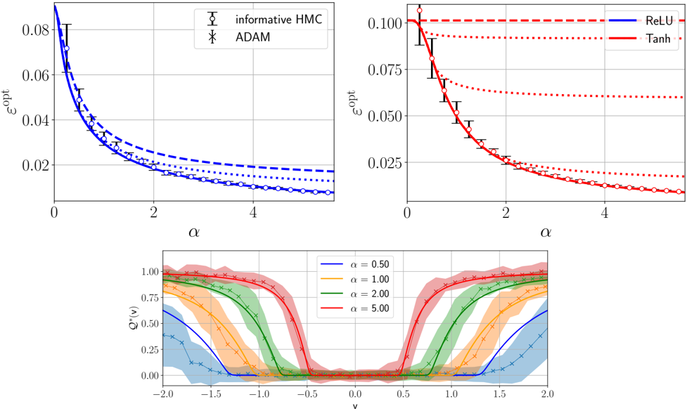<details> <summary>Image 30 Details</summary>  ### Visual Description ## Multiple Line Charts: Optimization Performance ### Overview The image contains three line charts comparing the performance of different optimization algorithms and activation functions. The top-left chart compares "informative HMC" and "ADAM" algorithms. The top-right chart compares "ReLU" and "Tanh" activation functions. The bottom chart shows Q*(v) for different values of alpha. ### Components/Axes **Top-Left Chart:** * **X-axis:** α (Alpha), ranging from 0 to 4. * **Y-axis:** ε^opt (Epsilon-opt), ranging from 0 to 0.08. * **Legend:** Located in the top-right corner. * "informative HMC" (black circles with error bars) * "ADAM" (black x markers) * Three lines are present, all in blue: solid, dashed, and dotted. These lines do not have a direct legend entry in this chart. **Top-Right Chart:** * **X-axis:** α (Alpha), ranging from 0 to 4. * **Y-axis:** ε^opt (Epsilon-opt), ranging from 0 to 0.100. * **Legend:** Located in the top-right corner. * "ReLU" (blue solid line) * "Tanh" (red solid line) * Two additional lines are present: red dotted and red dashed. These lines do not have a direct legend entry in this chart. **Bottom Chart:** * **X-axis:** v, ranging from -2.0 to 2.0. * **Y-axis:** Q*(v), ranging from 0.00 to 1.00. * **Legend:** Located in the top-center. * α = 0.50 (blue line with x markers) * α = 1.00 (yellow/orange line with x markers) * α = 2.00 (green line with x markers) * α = 5.00 (red line with x markers) * Each line has a shaded region around it, indicating uncertainty or variance. ### Detailed Analysis **Top-Left Chart:** * **Informative HMC (black circles):** The epsilon-opt value decreases as alpha increases. * α = 0, ε^opt ≈ 0.08 * α = 1, ε^opt ≈ 0.04 * α = 2, ε^opt ≈ 0.02 * α = 4, ε^opt ≈ 0.01 * **ADAM (black x markers):** The epsilon-opt value decreases as alpha increases. * α = 0, ε^opt ≈ 0.07 * α = 1, ε^opt ≈ 0.03 * α = 2, ε^opt ≈ 0.02 * α = 4, ε^opt ≈ 0.01 * **Blue Solid Line:** Starts at approximately 0.06 and decreases to approximately 0.015. * **Blue Dashed Line:** Starts at approximately 0.05 and decreases to approximately 0.018. * **Blue Dotted Line:** Starts at approximately 0.04 and decreases to approximately 0.01. **Top-Right Chart:** * **ReLU (blue solid line):** The epsilon-opt value decreases as alpha increases. * α = 0, ε^opt ≈ 0.10 * α = 1, ε^opt ≈ 0.07 * α = 2, ε^opt ≈ 0.04 * α = 4, ε^opt ≈ 0.01 * **Tanh (red solid line):** The epsilon-opt value decreases as alpha increases. * α = 0, ε^opt ≈ 0.10 * α = 1, ε^opt ≈ 0.06 * α = 2, ε^opt ≈ 0.03 * α = 4, ε^opt ≈ 0.01 * **Red Dotted Line:** Starts at approximately 0.09 and decreases to approximately 0.02. * **Red Dashed Line:** Remains constant at approximately 0.10. **Bottom Chart:** * **α = 0.50 (blue line):** Starts near 0, rises to approximately 0.5 around v = -1.5, plateaus near 0.5 until v = 1.5, then decreases back to near 0. * **α = 1.00 (yellow/orange line):** Starts near 0, rises to approximately 0.8 around v = -1.2, plateaus near 0.8 until v = 1.2, then decreases back to near 0. * **α = 2.00 (green line):** Starts near 0, rises to approximately 0.9 around v = -1.0, plateaus near 0.9 until v = 1.0, then decreases back to near 0. * **α = 5.00 (red line):** Starts near 0, rises to approximately 1.0 around v = -0.8, plateaus near 1.0 until v = 0.8, then decreases back to near 0. ### Key Observations * In the top-left chart, both "informative HMC" and "ADAM" algorithms show a decrease in epsilon-opt as alpha increases. * In the top-right chart, both "ReLU" and "Tanh" activation functions show a decrease in epsilon-opt as alpha increases. * In the bottom chart, as alpha increases, the Q*(v) function transitions more sharply between 0 and 1. ### Interpretation The charts suggest that increasing the value of alpha generally leads to better optimization performance (lower epsilon-opt) for both the algorithms and activation functions tested. The bottom chart illustrates how the function Q*(v) becomes more step-like as alpha increases, indicating a sharper transition or decision boundary. The shaded regions in the bottom chart represent the variability or uncertainty associated with each alpha value. </details> so that the MLP we will study is $$\mathcal { F } _ { \boldsymbol \theta ^ { 0 } } ^ { ( L ) } ( x ) \colon = \frac { v ^ { 0 \top } } { \sqrt { k ^ { L } } } \sigma ^ { ( L ) } \left ( \frac { W ^ { 0 ( L ) } } { \sqrt { k _ { L - 1 } } } \sigma ^ { ( L - 1 ) } \left ( \frac { W ^ { 0 ( L - 1 ) } } { \sqrt { k _ { L - 2 } } } \cdots \sigma ^ { ( 1 ) } \left ( \frac { W ^ { 0 ( 1 ) } } { \sqrt { k _ { 0 } } } x \right ) \cdots \right ) \right ) ,$$ with θ 0 denoting the whole collection of the teacher's parameters. To make the equations lighter we take centred and normalised activations E z σ ( l ) ( z ) 2 = 1, µ ( l ) 0 = 0, and we allow for different priors over the inner weights W ( l ) ∼ P W l . Importantly, we assume µ ( l ) 2 = 0. Treating terms associated with the second Hermite coefficient would require spherical integration and a measure relaxation analogous to the approach used in the shallow case. We leave this extension for future work. Let us define the pre- and post-activations respectively as $$\left \{ h ^ { ( l ) a } \colon = \frac { 1 } { \sqrt { k _ { l - 1 } } } W ^ { ( l ) a } x ^ { ( l - 1 ) a } \, , \quad x ^ { ( l ) a } \colon = \sigma ^ { ( l ) } ( h ^ { ( l ) a } ) \right \} _ { a = 0 } ^ { s } ,$$ where x a (0) := x , ∀ a = 0 , . . . , s represents the input data and are the replicated read-outs. As for the shallow case, the key assumption is the joint Gaussianity of { λ a ( θ a ) } 0 ≤ a ≤ s under the the common input randomness x . Since they are centred (recall µ ( l ) 0 = 0), in order to characterise their distribution it suffices to evaluate their covariance, which for analogy with the shallow case shall be denoted as $$K ^ { a b } \colon = \mathbb { E } _ { x } \lambda ^ { a } ( \theta ^ { a } ) \lambda ^ { b } ( \theta ^ { b } ) = \frac { 1 } { k _ { L } } \sum _ { i , j = 1 } ^ { k _ { L } } v _ { i } ^ { 0 } v _ { j } ^ { 0 } \, \mathbb { E } _ { x } \sigma ^ { ( L ) } ( h _ { i } ^ { ( L ) a } ) \sigma ^ { ( L ) } ( h _ { j } ^ { ( L ) b } ) \, .$$ FIG. 31. Left : Theoretical prediction (green solid curve) of the Bayes-optimal mean-square generalisation error for L = 2 with Gaussian inner weights, σ ( x ) = tanh(2 x ) /σ tanh , d = 200 , γ 1 = γ 2 = 0 . 5 , ∆ = 0 . 2 and different P v laws. The dashed and dotted lines have the same meaning as in FIG. 13. Points are obtained with Hamiltonian Monte Carlo with informative initialisation. Each point has been averaged over 20 instances of the data, with error bars representing one standard deviation. The generalisation error is computed empirically from 10 4 i.i.d. test samples. Right : Solid and dotted curves represent, respectively, the mean of different overlaps at equilibrium and in metastable specialised states, as function of the sampling ratio α for L = 2 with Gaussian inner weights, σ ( x ) = tanh(2 x ) /σ tanh , d = 200 , γ 1 = γ 2 = 0 . 5 , ∆ = 0 . 2. The shaded curves were obtained from informed HMC. Each point has been averaged over 20 instances of the training set, with one standard deviation depicted. Note: in these plots the readouts are learnable and drawn from a Gaussian prior, P v = N (0 , 1). 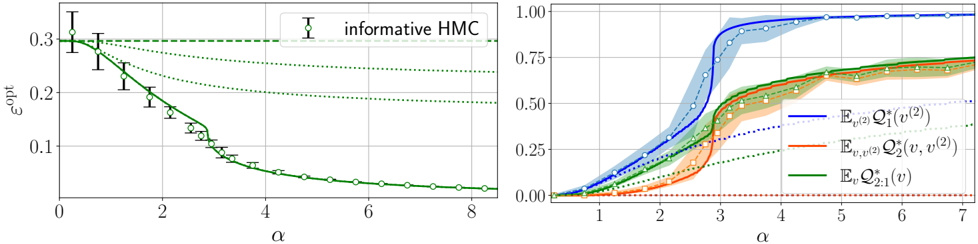<details> <summary>Image 31 Details</summary>  ### Visual Description ## Chart: Two Plots Comparing Performance Metrics vs. Alpha ### Overview The image presents two plots side-by-side, both charting data against the variable alpha (α). The left plot shows epsilon-opt (εopt) versus alpha for "informative HMC". The right plot shows three different metrics, denoted by E[subscript v(2)]Q*[subscript 1](v(2)), E[subscript v,v(2)]Q*[subscript 2](v, v(2)), and E[subscript v]Q*[subscript 2:1](v), versus alpha. ### Components/Axes **Left Plot:** * **X-axis:** α (alpha), ranging from 0 to 8. * **Y-axis:** εopt (epsilon-opt), ranging from 0 to 0.3. * **Legend:** "informative HMC" represented by a green line with circular markers and error bars. There is also a green dashed line and a green dotted line. **Right Plot:** * **X-axis:** α (alpha), ranging from 1 to 7. * **Y-axis:** Values ranging from 0.00 to 1.00. * **Legend (located in the bottom-right):** * E[subscript v(2)]Q*[subscript 1](v(2)) - Blue line with circular markers and shaded region. * E[subscript v,v(2)]Q*[subscript 2](v, v(2)) - Brown/Orange line with square markers and shaded region. * E[subscript v]Q*[subscript 2:1](v) - Green line with triangle markers and shaded region. * There are also dotted lines of the same colors. ### Detailed Analysis **Left Plot:** * **Informative HMC (Green line with circular markers):** The line starts at approximately 0.3 at α=0, decreases sharply until α=4, and then plateaus around 0.05 for α > 4. * At α=0, εopt ≈ 0.3 with error bars extending approximately +/- 0.02. * At α=2, εopt ≈ 0.17. * At α=4, εopt ≈ 0.07. * At α=8, εopt ≈ 0.05. * **Green dashed line:** The line is constant at approximately 0.3. * **Green dotted line:** The line starts at approximately 0.3 at α=0 and decreases to approximately 0.2 at α=8. **Right Plot:** * **E[subscript v(2)]Q*[subscript 1](v(2)) (Blue line with circular markers):** The line starts at approximately 0 at α=1, increases sharply between α=2 and α=3, and then plateaus at approximately 0.95 for α > 3. * At α=1, the value is approximately 0. * At α=2, the value is approximately 0.25. * At α=3, the value is approximately 0.9. * At α=7, the value is approximately 0.95. * **E[subscript v,v(2)]Q*[subscript 2](v, v(2)) (Brown/Orange line with square markers):** The line starts at approximately 0 at α=1, increases gradually between α=1 and α=4, and then plateaus at approximately 0.7 for α > 4. * At α=1, the value is approximately 0. * At α=2, the value is approximately 0.05. * At α=3, the value is approximately 0.4. * At α=7, the value is approximately 0.7. * **E[subscript v]Q*[subscript 2:1](v) (Green line with triangle markers):** The line starts at approximately 0 at α=1, increases gradually between α=1 and α=4, and then plateaus at approximately 0.7 for α > 4. * At α=1, the value is approximately 0. * At α=2, the value is approximately 0.05. * At α=3, the value is approximately 0.5. * At α=7, the value is approximately 0.7. * **Blue dotted line:** The line starts at approximately 0 at α=1, increases sharply between α=2 and α=3, and then plateaus at approximately 1.0 for α > 3. * **Brown/Orange dotted line:** The line is constant at approximately 0.02. * **Green dotted line:** The line starts at approximately 0 at α=1, increases gradually between α=1 and α=4, and then plateaus at approximately 0.15 for α > 4. ### Key Observations * In the left plot, increasing alpha (α) generally decreases epsilon-opt (εopt) for the "informative HMC" method. * In the right plot, all three metrics (E[subscript v(2)]Q*[subscript 1](v(2)), E[subscript v,v(2)]Q*[subscript 2](v, v(2)), and E[subscript v]Q*[subscript 2:1](v)) increase with alpha (α) until they plateau. E[subscript v(2)]Q*[subscript 1](v(2)) reaches a higher plateau than the other two. ### Interpretation The plots suggest that increasing the parameter alpha (α) has a significant impact on both epsilon-opt (εopt) and the three metrics shown in the right plot. The left plot indicates that a higher alpha leads to a lower epsilon-opt for the "informative HMC" method, which could imply better optimization performance. The right plot shows that the metrics E[subscript v(2)]Q*[subscript 1](v(2)), E[subscript v,v(2)]Q*[subscript 2](v, v(2)), and E[subscript v]Q*[subscript 2:1](v) all improve with increasing alpha, eventually reaching a saturation point. The fact that E[subscript v(2)]Q*[subscript 1](v(2)) plateaus at a higher value than the other two suggests it may be a more effective metric under these conditions. The shaded regions around the lines in the right plot likely represent the variance or uncertainty associated with each metric. The dotted lines likely represent a different method or a baseline. </details> $$\left \{ \lambda ^ { a } ( \pm b \theta ^ { a } ) \colon = \frac { 1 } { \sqrt { k _ { L } } } v ^ { 0 T } \sigma ^ { ( L ) } ( h ^ { ( L ) a } ) \right \} _ { a = 0 } ^ { s }$$ ## Appendix C: Deep MLP ## 1. Details of the replica calculation Let us take a multi-layer perceptron with L = O (1) hidden layers. In order to be more general let us take at each layer a different activation function ̸ $$\sigma ^ { ( l ) } \left ( z \right ) = \sum _ { \ell \neq 0 , 2 } \frac { \mu _ { \ell } ^ { ( l ) } } { \ell ! } H e _ { \ell } ( z ) ,$$ To further simplify the above expectation, we need to use recursively Mehler's formula (see App. A 2) from the first pre-activation on, as follows. To begin with, define $$\Omega _ { i _ { 1 } j _ { 1 } } ^ { ( 1 ) a b } \colon = \mathbb { E } _ { x } h _ { i _ { 1 } } ^ { ( 1 ) a } h _ { j _ { 1 } } ^ { ( 1 ) b } = \mathbb { E } _ { x } \left ( \frac { W _ { i _ { 1 } } ^ { ( 1 ) a } \cdot x } { \sqrt { d } } \right ) \left ( \frac { W _ { j _ { 1 } } ^ { ( 1 ) b } \cdot x } { \sqrt { d } } \right ) = \frac { W _ { i _ { 1 } } ^ { a } \cdot w _ { j _ { 1 } } ^ { b } } { d } \, . \quad ( C 2 )$$ This allows us to compute the covariance of the second layer pre-activations under the same randomness: $$\Omega _ { i _ { 2 } j _ { 2 } } ^ { ( 2 ) a b } \colon = \mathbb { E } _ { x } h _ { i _ { 2 } } ^ { ( 2 ) a } h _ { j _ { 2 } } ^ { ( 2 ) b } = \mathbb { E } _ { x } \left ( \frac { W _ { i _ { 2 } } ^ { ( 2 ) a } \cdot x ^ { ( 1 ) a } } { \sqrt { k _ { 1 } } } \right ) \left ( \frac { W _ { j _ { 2 } } ^ { ( 2 ) b } \cdot x ^ { ( 1 ) b } } { \sqrt { k _ { 1 } } } \right ) .$$ The expectation is resolved once one compute the covariance of the first layer post-activations by means of Mehler's formula, yielding $$\Omega _ { i _ { 2 } j _ { 2 } } ^ { ( 2 ) a b } = \frac { 1 } { k _ { 1 } } \mathbf W _ { i _ { 2 } } ^ { ( 2 ) a \intercal } \left ( ( \mu _ { 1 } ^ { ( 1 ) } ) ^ { 2 } \mathbf \Omega ^ { ( 1 ) a b } + g ^ { ( 1 ) } ( \mathbf \Omega ^ { ( 1 ) a b } ) \right ) \mathbf W _ { j _ { 2 } } ^ { ( 2 ) b } & & ( C 4 )$$ where the function g (1) , defined as in (B6), is applied element-wise to the matrix argument. From this moment on we assume that pre-activations are Gaussian at each layer under the common randomness x , as they are always expressed in terms of rescaled sums. Under this assumption we can thus infer a generic recursion for the pre-activation covariances: $$\Omega _ { i _ { l + 1 } j _ { l + 1 } } ^ { ( l + 1 ) a b } \colon = \mathbb { E } _ { x } h _ { i _ { l + 1 } } ^ { ( l + 1 ) a } h _ { j _ { l + 1 } } ^ { ( l + 1 ) b } = \frac { 1 } { k _ { l } } W _ { i _ { l + 1 } } ^ { ( l + 1 ) a \Uparrow } \left ( ( \mu _ { 1 } ^ { ( l ) } ) ^ { 2 } \Omega ^ { ( l ) a b } + g ^ { ( l ) } ( \Omega ^ { ( l ) a b } ) \right ) W _ { j _ { l + 1 } } ^ { ( l + 1 ) b }$$ which naturally leads to the covariance we actually need for K ab , i.e. Ω ( L ) ab ij = E x h ( L ) a i h ( L ) b j : $$K ^ { a b } = \frac { ( \mu _ { 1 } ^ { ( L ) } ) ^ { 2 } } { k _ { L } } v ^ { 0 \top } \left ( \Omega ^ { ( L ) a b } + g ^ { ( L ) } ( \Omega ^ { ( L ) a b } ) \right ) v ^ { 0 } . \tag* { (C6) }$$ Let us define the following set of vectors and matrices for future convenience $$W ^ { ( l ^ { \prime } ; l ) a } & = \frac { 1 } { \sqrt { k _ { l ^ { \prime } - 1 } k _ { l ^ { \prime } - 2 } \dots k _ { l } } } W ^ { ( l ^ { \prime } ) a } W ^ { ( l ^ { \prime } - 1 ) a } \dots W ^ { ( l ) a } , \\ v ^ { ( l ) a } & = \frac { 1 } { \sqrt { k _ { l } k _ { l + 1 } \dots k _ { L } } } W ^ { ( l ) a \top } W ^ { ( l + 1 ) a \top } \dots W ^ { ( L ) a \top } v ^ { 0 } .$$ They will emerge from the computation due to the linear term in the Hermite expansion of the activation functions. These represent effective readout vectors and weight matrices, that the student can learn independently from the actual weights and readouts. With this notation the post-activation covariance reads (recall k 0 = d ) $$K ^ { a b } & = \frac { ( \mu _ { 1 } ^ { ( L ) } \mu _ { 1 } ^ { ( L - 1 ) } \dots \mu _ { 1 } ^ { ( 1 ) } ) ^ { 2 } } { k _ { 0 } } v ^ { a ( 1 ) \intercal } v ^ { b ( 1 ) } + \frac { ( \mu _ { 1 } ^ { ( L - 1 ) } \mu _ { 1 } ^ { ( L - 2 ) } \dots \mu _ { 1 } ^ { ( 1 ) } ) ^ { 2 } } { k _ { 1 } } v ^ { a ( 2 ) \intercal } g ^ { ( 1 ) } ( \Omega ^ { a b ( 1 ) } ) v ^ { b ( 2 ) } \\ & \quad + \dots + \frac { ( \mu _ { 1 } ^ { ( 1 ) } ) ^ { 2 } } { k _ { L - 1 } } v ^ { a ( L ) \intercal } g ^ { ( L - 1 ) } ( \Omega ^ { a b ( L - 1 ) } ) v ^ { b ( L ) } + \frac { 1 } { k _ { L } } v ^ { 0 \intercal } g ^ { ( L ) } ( \Omega ^ { a b ( L ) } ) v ^ { 0 }$$ As in (B3) we will assume that for all l = 1 , . . . , L $$\Omega _ { i _ { l } i _ { l } } ^ { a b ( l ) } = O ( 1 ) \, , \quad \Omega _ { i _ { l } j _ { l } } ^ { a b ( l ) } = O \left ( \frac { 1 } { \sqrt { k _ { l - 1 } } } \right ) \, f o r \, i _ { l } \neq j _ { l } \, .$$ ̸ Therefore, only the diagonal elements of the matrix g ( l ) ( Ω ab ( l ) ) will contribute in the thermodynamic limit. Note that the overlap 1 k 0 v (1) a ⊺ v (1) b is analogous to the OP described by [106] in the deep setting; v (1)0 is the only feature of the target function that is learnable in the n ∝ d regime, which we will consider as known, namely all the overlaps between v (1) a 's are set to 1. Analogously to what happens in the shallow case, the components of the other v ( l ) a 's enter trivially the energetic term. Specifically, only those components of v ( l ) a that are perfectly reconstructible by the student would enter the energy, namely those for which the associated Ω ( l ) ab i l i l = O (1) and not smaller. Hence without loss of generality one can assume that all the v ( l ) a are set to v ( l )0 as in the shallow case. This allows to considerably simplify the equations and leads to $$K ^ { a b } & = ( \mu _ { 1 } ^ { ( L ) } \mu _ { 1 } ^ { ( L - 1 ) } \dots \mu _ { 1 } ^ { ( 1 ) } ) ^ { 2 } + \frac { ( \mu _ { 1 } ^ { ( L - 1 ) } \mu _ { 1 } ^ { ( L - 2 ) } \dots \mu _ { 1 } ^ { ( 1 ) } ) ^ { 2 } } { k _ { 1 } } \sum _ { i _ { 1 } } ^ { k _ { 1 } } ( v _ { i _ { 1 } } ^ { 0 ( 2 ) } ) ^ { 2 } g ^ { ( 1 ) } \left ( \Omega _ { i _ { 1 } i _ { 1 } } ^ { a b ( 1 ) } \right ) \\ & \quad + \dots + \frac { ( \mu _ { 1 } ^ { ( 1 ) } ) ^ { 2 } } { k _ { L - 1 } } \sum _ { i _ { L - 1 } } ^ { k _ { L - 1 } } ( v _ { i _ { L - 1 } } ^ { 0 ( L ) } ) ^ { 2 } g ^ { ( L - 1 ) } \left ( \Omega _ { i _ { L - 1 } i _ { L - 1 } } ^ { a b ( L - 1 ) } \right ) + \frac { 1 } { k _ { L } } \sum _ { i _ { L } } ^ { k _ { L } } ( v _ { i _ { L } } ^ { 0 } ) ^ { 2 } g ^ { ( L ) } \left ( \Omega _ { i _ { L } i _ { L } } ^ { a b ( L ) } \right )$$ with, additionally $$\Omega _ { i _ { l + 1 } i _ { l + 1 } } ^ { a b ( l + 1 ) } \approx \frac { ( \mu _ { 1 } ^ { ( l ) } ) ^ { 2 } } { k _ { l } } W _ { i _ { l + 1 } } ^ { a ( l + 1 ) \tau } \Omega ^ { a b ( l ) } W _ { i _ { l + 1 } } ^ { b ( l + 1 ) } + \frac { 1 } { k _ { l } } \sum _ { i _ { l } } ^ { k _ { l } } W _ { i _ { l + 1 } i _ { l } } ^ { ( l + 1 ) a } W _ { i _ { l + 1 } i _ { l } } ^ { ( l + 1 ) b } g ^ { ( l ) } \left ( \Omega _ { i _ { l } i _ { l } } ^ { ( l ) a b } \right ) .$$ Here is a difference with the shallow case: the way the replicas W ( l +1) a align with one another may depend not only on the 'left' indices, i l +1 in the formula above, but can be affected also by the reconstruction performance from previous layers, encoded in Ω ( l ) ab i l i l . The values of Ω ( l ) ab i l i l are themselves driven by the values of the associated v ( l +1)0 i l that appear coupled to them in the energy through K ab as above. Hence, we can choose to label the values of Ω ( l ) ab i l i l through those of v ( l +1)0 i l . We denote these values as v ( l +1) , collected in the sets V ( l +1) , and I v ( l +1) = { i l | v ( l +1)0 i l = v ( l +1) } . This brings us to defining the following overlaps: $$\mathcal { Q } _ { l } ^ { a b } ( i _ { l } , \mathbf v ^ { ( l ) } ) = \frac { 1 } { | \mathcal { I } _ { \nu ^ { ( l ) } } | } \sum _ { i _ { l - 1 } \in \mathcal { I } _ { \nu ^ { ( l ) } } } W _ { i _ { l } i _ { l - 1 } } ^ { ( l ) a } W _ { i _ { l } i _ { l - 1 } } ^ { ( l ) b } \, ,$$ $$\mathcal { Q } _ { l ^ { \prime } ; l } ^ { a b } ( i _ { l ^ { \prime } } , \mathbf v ^ { ( l ) } ) = \frac { 1 } { | \mathcal { I } _ { \sqrt { ( l ) } } | } \sum _ { i _ { l - 1 } \in \mathcal { I } _ { \vee ( l ) } } W _ { i _ { l ^ { \prime } } i _ { l - 1 } } ^ { ( l ^ { \prime } ; l ) a } W _ { i _ { l ^ { \prime } } i _ { l - 1 } } ^ { ( l ^ { \prime } ; l ) b } .$$ Using (C5), the diagonal elements of each Ω ( l ) ab in terms of those overlaps read $$\Omega ^ { a b ( l + 1 ) } _ { i _ { l + 1 } i _ { l + 1 } } \approx \frac { ( \mu _ { 1 } ^ { ( l ) } ) ^ { 2 } } { k _ { l } } \mathbf w ^ { a ( l + 1 ) \top } _ { i _ { l + 1 } } \Omega ^ { a b ( l ) } \mathbf w ^ { b ( l + 1 ) } _ { i _ { l + 1 } } + \sum _ { v ^ { ( l + 1 ) } \in V ^ { ( l + 1 ) } } \frac { | \mathcal { I } _ { v ^ { ( l + 1 ) } } | } { k _ { l } } \mathcal { Q } ^ { a b } _ { l + 1 } ( i _ { l + 1 } , v ^ { ( l + 1 ) } ) \frac { 1 } { | \mathcal { I } _ { v ^ { ( l + 1 ) } } | } \sum _ { i _ { l } \in \mathcal { I } _ { v ^ { ( l + 1 ) } } } g ^ { ( l ) } \left ( \Omega ^ { a b ( l ) } _ { i _ { l } i _ { l } } \right ) . \text {This is the first step of the recursion} \colon & \text {in order to express everything in terms of the overlaps $\mathcal{Q}$ we need to express} \\ & \text {This is the first step of the recursion} \colon & \text {in order to express everything in terms of the overlaps $\mathcal{Q}$ we need to express}$$ This is the first step of the recursion; in order to express everything in terms of the overlaps Q , we need to express the first term as well in terms of diagonal elements, keeping in mind that Ω (1) ab i 1 i 1 = W (1) a ⊺ i 1 I d W (1) b i 1 /d =: Q ab 1 ( i 1 ). In other words, the firs overlap is not labelled by any other index, as the W (1) 's here do not sandwich any matrix other than the identity. Hence no inhomogeneity can arise. An analogous reasoning holds for Q ab l +1:1 ( i l +1 ). At a generic step of the recursion, we have $$\Omega _ { i l + 1 } ^ { a b ( l + 1 ) } & \approx ( \mu _ { l + 1 } ^ { ( l ) } \dots \mu _ { 1 } ^ { ( 1 ) } ) ^ { 2 } \mathcal { Q } _ { l + 1 \colon 1 } ^ { a b } ( i _ { l + 1 } ) + ( \mu _ { 1 } ^ { ( l ) } \dots \mu _ { 2 } ^ { ( 1 ) } ) ^ { 2 } \sum _ { v ^ { ( 2 ) } \in V ^ { ( 2 ) } } \frac { | \mathcal { I } _ { v ^ { ( 2 ) } } | } { k _ { 1 } } \mathcal { Q } _ { l + 1 \colon 2 } ^ { a b } ( i _ { l + 1 } , v ^ { ( 2 ) } ) \frac { 1 } { | \mathcal { I } _ { v ^ { ( 2 ) } } | } \sum _ { i _ { l } \in \mathcal { I } _ { v ^ { ( 2 ) } } } g ^ { ( 1 ) } \left ( \Omega _ { i _ { 1 } i _ { 1 } } ^ { ( 1 ) a b } \right ) \\ & + \dots + ( \mu _ { l } ^ { ( 1 ) } ) ^ { 2 } \sum _ { v ^ { ( l ) } \in V ^ { ( l ) } } \frac { | \mathcal { I } _ { v ^ { ( l ) } } | } { k _ { l - 1 } } \mathcal { Q } _ { l + 1 \colon l } ^ { a b } ( i _ { l + 1 } , v ^ { ( l ) } ) \frac { 1 } { | \mathcal { I } _ { v ^ { ( l ) } } | } \sum _ { i _ { l - 1 } \in \mathcal { I } _ { v ^ { ( l ) } } } g ^ { ( l - 1 ) } \left ( \Omega _ { i _ { l - 1 } i _ { l - 1 } } ^ { ( l - 1 ) a b } \right ) \\ & + \sum _ { v ^ { ( l + 1 ) } \in V ^ { ( l + 1 ) } } \frac { | \mathcal { I } _ { v ^ { ( l + 1 ) } } | } { k _ { l } } \mathcal { Q } _ { l + 1 } ^ { a b } ( i _ { l + 1 } , v ^ { ( l + 1 ) } ) \frac { 1 } { | \mathcal { I } _ { v ^ { ( l + 1 ) } } | } \sum _ { i _ { l } \in \mathcal { I } _ { v ^ { ( l + 1 ) } } } g ^ { ( l ) } \left ( \Omega _ { i _ { l } i _ { l } } ^ { ( l ) a b } \right ) , <text><loc_41><loc_466><loc_441><loc_500>where Ω ab (1) i$_{1}$i$_{1}$ = Q $_{1}$(i$_{1}$ ). This defines the full recursion, which allows one to compute the covariance K ab only in terms of the abhape m and avarl</text>$$ where Ω ab (1) i 1 i 1 = Q 1 ( i 1 ). This defines the full recursion, which allows one to compute the covariance K ab only in terms of the above mentioned overlaps. As the derivation may become very cumbersome, we specialise to the L = 2 setting in the following section. ## a. Two hidden layers L = 2 In the case of two hidden layers networks the equation for the covariance is $$K ^ { a b } & = ( \mu _ { 1 } ^ { ( 2 ) } \mu _ { 1 } ^ { ( 1 ) } ) ^ { 2 } + \frac { ( \mu _ { 1 } ^ { ( 2 ) } ) ^ { 2 } } { k _ { 1 } } \sum _ { i _ { 1 } } ^ { k _ { 1 } } ( v _ { i _ { 1 } } ^ { 0 ( 2 ) } ) ^ { 2 } g ^ { ( 1 ) } \left ( \mathcal { Q } _ { 1 } ^ { a b } ( i _ { 1 } ) \right ) \\ & + \frac { 1 } { k _ { 2 } } \sum _ { i _ { 2 } } ^ { k _ { 2 } } ( v _ { i _ { 2 } } ^ { 0 } ) ^ { 2 } g ^ { ( 2 ) } \left ( ( \mu _ { 1 } ^ { ( 1 ) } ) ^ { 2 } \mathcal { Q } _ { 2 \colon 1 } ^ { a b } ( i _ { 2 } ) + \sum _ { v ^ { ( 2 ) } \in V ^ { ( 2 ) } } \frac { | \mathcal { I } _ { v ^ { ( 2 ) } } | } { k _ { 1 } } \mathcal { Q } _ { 2 } ^ { a b } ( i _ { 2 } , v ^ { ( 2 ) } ) \frac { 1 } { | \mathcal { I } _ { v ^ { ( 2 ) } } | } \sum _ { i _ { 1 } \in \mathcal { I } _ { v ^ { ( 2 ) } } } g ^ { ( 1 ) } ( \mathcal { Q } _ { 1 } ^ { a b } ( i _ { 1 } ) ) \right ) .$$ Importantly, the index i 1 is linked only to the vector v 0(2) and the overlap Q ab 1 , while the index i 2 to the vector v 0 and the overlaps Q ab 2 and Q ab 2:1 . We can relabel the values of Q 1 with those of v (2) : Q 1 ( v ( 2 ) ) = Q 1 ( i 1 ) for all i 1 ∈ I v (2) . An analogous relabelling can be carried out for Q 2 ( i 2 , v (2) ) in the index i 2 , based on the values of v 0 i 2 . After the relabelling, one could also redefine the overlaps through partial traces, in order to mimic the notation from the main, as follows: $$\mathcal { Q } _ { l } ^ { a b } ( \nu ^ { ( l + 1 ) } , \nu ^ { ( l ) } ) = \frac { 1 } { | \mathcal { I } _ { \nu ^ { ( l + 1 ) } } | | \mathcal { I } _ { \nu ^ { ( l ) } } | } \sum _ { i _ { l } \in \mathcal { I } _ { \nu ^ { ( l + 1 ) } } } \sum _ { i _ { l - 1 } \in \mathcal { I } _ { \nu ^ { ( l ) } } } W _ { i _ { l } i _ { l - 1 } } ^ { ( l ) a } W _ { i _ { l } i _ { l - 1 } } ^ { ( l ) b } \, , & & ( C 1 7 )$$ $$\mathcal { Q } _ { l ^ { \prime } ; l } ^ { a b } ( v ^ { ( l ^ { \prime } + 1 ) } , v ^ { ( l ) } ) = \frac { 1 } { | \mathcal { I } _ { v ^ { ( l ^ { \prime } + 1 ) } } | | \mathcal { I } _ { v ^ { ( l ) } } | } \sum _ { i _ { l ^ { \prime } } \in \mathcal { I } _ { v ^ { ( l ^ { \prime } + 1 ) } } } \sum _ { i _ { l - 1 } \in \mathcal { I } _ { v ^ { ( l ) } } } W _ { i _ { l ^ { \prime } } i _ { l - 1 } } ^ { ( l ^ { \prime } ; l ) a } W _ { i _ { l ^ { \prime } } i _ { l - 1 } } ^ { ( l ^ { \prime } ; l ) b } \, .$$ Consider also that |I v (2) | k 1 → P v (2) ( v (2) ), and |I v | k 2 → P v ( v ). This allows us to recast K ab in the asymptotic limit as $$K ^ { a b } & = ( \mu _ { 1 } ^ { ( 2 ) } \mu _ { 1 } ^ { ( 1 ) } ) ^ { 2 } + ( \mu _ { 1 } ^ { ( 2 ) } ) ^ { 2 } \mathbb { E } _ { v ^ { ( 2 ) } \sim P _ { v ^ { ( 2 ) } } } \left ( v ^ { ( 2 ) } \right ) ^ { 2 } g ^ { ( 1 ) } \left ( \mathcal { Q } _ { 1 } ^ { a b } ( v ^ { ( 2 ) } ) \right ) \\ & \quad + \mathbb { E } _ { v \sim P _ { v } } ( v ) ^ { 2 } g ^ { ( 2 ) } \left ( \left ( \mu _ { 1 } ^ { ( 1 ) } \right ) ^ { 2 } \mathcal { Q } _ { 2 \colon 1 } ^ { a b } ( v ) + \mathbb { E } _ { v ^ { ( 2 ) } \sim P _ { v ^ { ( 2 ) } } } \mathcal { Q } _ { 2 } ^ { a b } ( v , v ^ { ( 2 ) } ) g ^ { ( 1 ) } \left ( \mathcal { Q } _ { 1 } ^ { a b } ( v ^ { ( 2 ) } ) \right ) \right ) .$$ Notice that as soon as the covariance of the post-activation is written in terms of overlaps, this fully determines the energetic part appearing in the free entropy. Indeed, in the RS ansatz, K appears as in (B11), where $$K ^ { ( 2 ) } ( \bar { \mathcal { Q } } ) & = ( \mu _ { 1 } ^ { ( 2 ) } \mu _ { 1 } ^ { ( 1 ) } ) ^ { 2 } + ( \mu _ { 1 } ^ { ( 2 ) } ) ^ { 2 } \mathbb { E } _ { v ^ { ( 2 ) } \sim P _ { v ^ { ( 2 ) } } } ( v ^ { ( 2 ) } ) ^ { 2 } g ^ { ( 1 ) } \left ( \mathcal { Q } _ { 1 } ( v ^ { ( 2 ) } ) \right ) \\ & \quad + \mathbb { E } _ { v \sim P _ { v } } ( v ) ^ { 2 } g ^ { ( 2 ) } \left ( ( \mu _ { 1 } ^ { ( 1 ) } ) ^ { 2 } \mathcal { Q } _ { 2 \colon 1 } ( v ) + \mathbb { E } _ { v ^ { ( 2 ) } \sim P _ { v ^ { ( 2 ) } } } \mathcal { Q } _ { 2 } ( v , v ^ { ( 2 ) } ) g ^ { ( 1 ) } \left ( \mathcal { Q } _ { 1 } ( v ^ { ( 2 ) } ) \right ) \right ) , \\ K _ { d } & = 1 .$$ while ρ K = K d and m K = K using the Nishimori identities. Therefore, the energetic term will be equal to (B15), with K = K (2) ( ¯ Q ) and K d = 1 as defined in the last equations. Let us now discuss the entropic contribution, associated to the OPs defined above. This can be written as $$& \text {us now discuss the entropic contribution, associated to the OPs defined above. This can be written as} \\ & e ^ { F _ { S } } = \int d W ^ { a ( 2 \colon 1 ) } \int \prod _ { a = 0 } ^ { s } \prod _ { l = 1 } ^ { 2 } d P _ { W _ { l } } ( W ^ { a ( l ) } ) \delta \left ( W ^ { a ( 2 \colon 1 ) } - \frac { W ^ { a ( 2 ) } W ^ { a ( 1 ) } } { \sqrt { k _ { 1 } } } \right ) \\ & \quad \times \prod _ { a \leq b \, v \in V ^ { ( 2 ) } } \prod _ { i _ { 2 } \in I _ { v } ( 2 ) } \delta ( | \mathcal { I } _ { v } | | \mathcal { I } _ { v ^ { ( 2 ) } } | \mathcal { Q } _ { 2 } ^ { a b } ( v , v ^ { ( 2 ) } ) - \sum _ { i _ { 2 } \in I _ { v } ( 2 ) } \sum _ { i _ { 1 } \in I _ { v } ( 2 ) } W _ { i _ { 2 } i _ { 1 } } ^ { ( 2 ) a } W _ { i _ { 2 } i _ { 1 } } ^ { ( 2 ) b } ) \\ & \quad \times \prod _ { a \leq b \, v ^ { ( 2 ) } \in V ^ { ( 2 ) } } \prod _ { i _ { 1 } \in I _ { v } ( 2 ) } \delta ( d | \mathcal { I } _ { v ^ { ( 2 ) } } | \, \mathcal { Q } _ { 1 } ^ { a b } ( v ^ { ( 2 ) } ) - \sum _ { i _ { 1 } \in I _ { v } ( 2 ) } W _ { i _ { 1 } } ^ { a ( 1 ) \intercal } W _ { i _ { 1 } } ^ { b ( 1 ) } ) \\ & \quad \times \prod _ { a \leq b \, v \in V } \prod _ { i _ { 2 } \in I _ { v } } \delta ( d | \mathcal { I } _ { v } | \, \mathcal { Q } _ { 2 \colon 1 } ^ { a b } ( v ) - \sum _ { i _ { 2 } \in I _ { v } } W _ { i _ { 2 } } ^ { a ( 2 \colon 1 ) \intercal } W _ { i _ { 2 } } ^ { b ( 2 \colon 1 ) } ) .$$ Besides the labelling of Q 2 in terms of two indices v , v (2) , another important difference with respect to the shallow case is the presence of the overlap Q 2:1 ( v ) between the replicated matrices W (2:1) a = W a (2) W a (1) / √ k 1 . This overlap will depend on the alignment between the first and second layer weights. In order to encode this dependence we use a similar relaxation of the measure as the one described in Section B 1 b. We thus define $$d P ( ( \mathbf W ^ { ( 2 \colon 1 ) a } ) \, | \, \varrho _ { 1 } , \mathbf Q _ { 2 } ) & \, \infty \prod _ { a = 0 } ^ { s } d \mathbf W ^ { ( 2 \colon 1 ) a } \int _ { \real s } \prod _ { a = 0 } ^ { s } \prod _ { l = 1 } ^ { 2 } d P _ { W _ { l } } ( \mathbf W ^ { ( l ) a } ) \delta \left ( \mathbf W ^ { ( 2 \colon 1 ) a } - \frac { \mathbf W ^ { ( 2 ) a } \mathbf W ^ { ( 1 ) a } } { \sqrt { k _ { 1 } } } \right ) \\ & \quad \times \prod _ { a \leq b \, v \in V _ { v } \prod _ { ( 2 ) } \prod _ { v = 0 } ^ { s } } \prod _ { \real s } \delta ( | \mathcal { I } _ { v } | | \mathcal { I } _ { v ^ { ( 2 ) } } | \mathcal { Q } _ { 2 } ^ { a b } ( v , v ^ { ( 2 ) } ) - \sum _ { i _ { 2 } \in \mathcal { I } _ { v } } \sum _ { i _ { 1 } \in \mathcal { I } _ { v ^ { ( 2 ) } } } W _ { i _ { 2 } i _ { 1 } } ^ { ( 2 ) a } W _ { i _ { 2 } i _ { 1 } } ^ { ( 2 ) b } ) \\ & \quad \times \prod _ { a \leq b \, v ^ { ( 2 ) } \in V ^ { ( 2 ) } } \delta ( d | \mathcal { I } _ { v ^ { ( 2 ) } } | \mathcal { Q } _ { 1 } ^ { a b } ( v ^ { ( 2 ) } ) - \sum _ { i _ { 1 } \in \mathcal { I } _ { v ^ { ( 2 ) } } } W _ { i _ { 1 } } ^ { ( a ) \, 1 } \mathbf W _ { i _ { 1 } } ^ { b ( 1 ) } ) \\$$ where the normalisation constant is implicit. The aim is now to relax this measure to the one of a product of two Ginibre matrices with a proper tilt, given by the coupling between replicas. The relaxation we choose is the one with a matched second moment 1 d |I v | ∑ i 2 ∈I v E [ W (2:1) a ⊺ i 2 W (2:1) b i 2 | Q 1 , Q 2 ] where E [ · | Q 1 , Q 2 ] denotes the expectation w.r.t. the conditional measure defined above. As done in App. B 1 c, by rewriting Dirac deltas in Fourier form, the measure decouples and the calculation goes through, yielding asymptotically $$\frac { 1 } { d | \mathcal { I } _ { v } | } \sum _ { i _ { 2 } \in \mathcal { I } _ { v } } \mathbb { E } [ w _ { i _ { 2 } } ^ { ( 2 \colon 1 ) a _ { T } } W _ { i _ { 2 } } ^ { ( 2 \colon 1 ) b } | \mathcal { Q } _ { 1 } , \mathcal { Q } _ { 2 } ] \approx \mathbb { E } _ { v ^ { ( 2 ) } \sim P _ { v ^ { ( 2 ) } } } \mathcal { Q } _ { 2 } ^ { a b } ( v , v ^ { ( 2 ) } ) \mathcal { Q } _ { 1 } ^ { a b } ( v ^ { ( 2 ) } ) \, . \quad ( C 2 3 )$$ In order to fix this moment in our relaxation we thus need a Lagrange multiplier for each value v ∈ V : $$d \bar { P } ( ( W ^ { ( 2 \colon 1 ) a } ) | \mathcal { Q } _ { 1 } , \mathcal { Q } _ { 2 } ) = \prod _ { v \in V } V ( \tau _ { v } ) ^ { - 1 } \prod _ { a = 0 } ^ { s } d \mathcal { N } ( U _ { v } ^ { a } ) d \mathcal { N } ( V ^ { a } ) e ^ { \sum _ { a < b , 0 } ^ { s } \tau _ { v } ^ { a b } T r U _ { v } ^ { a } V ^ { a } ( U _ { v } ^ { b } V ^ { b } ) ^ { T } }$$ where U a v ∈ R |I v |× k 1 , V a ∈ R k 1 × d are matrices with i.i.d. Gaussian elements (their factorised measure being synthetically denoted by N ), W (2:1) a = U a v V a and τ v = ( τ ab v ) a<b =0 ,...,s . With this relaxation we have that $$e ^ { F _ { S } } & = V _ { W _ { 1 } } ^ { k _ { 1 } d } ( \mathbf Q _ { 1 } ) V _ { W _ { 2 } } ^ { k _ { 1 } k _ { 2 } } ( \mathbf Q _ { 2 } ) \int d \hat { \mathbf Q } _ { 2 \colon 1 } \int \prod _ { v \in V } V ( \tau _ { v } ) ^ { - 1 } \prod _ { a = 0 } ^ { s } d \mathcal { N } ( U _ { v } ^ { a } ) d \mathcal { N } ( V ^ { a } ) e ^ { \sum _ { a < b , 0 } ^ { s } ( \tau _ { v } ^ { a b } + \hat { Q } _ { 2 \colon 1 } ^ { a b } ( v ) ) T r U _ { v } ^ { a } V ^ { a } ( U _ { v } ^ { b } V ^ { b } ) ^ { \dagger } } \\ & \times e ^ { - d \sum _ { a < b , 0 } ^ { s } \sum _ { v \in V } | \mathcal { I } _ { v } | \hat { Q } _ { 2 \colon 1 } ^ { a b } ( v ) \mathcal { Q } _ { 2 \colon 1 } ^ { a b } ( v ) } \, .$$ Where not specified, integrals over OPs and their Fourier conjugates run over all replica indices and v values. Standard steps as the ones in App. B 1, after taking the 0 replica limit, yield $$f _ { R S } ^ { ( 2 ) } \colon = & \, \phi _ { P o u t } ( K ^ { ( 2 ) } ( \bar { Q } ) ; 1 ) + \frac { \gamma _ { 1 } } { \alpha } \mathbb { E } _ { v ^ { ( 2 ) } \sim P _ { v ^ { ( 2 ) } } } \left [ \psi _ { P _ { 1 } } ( \hat { Q } _ { 1 } ( v ^ { ( 2 ) } ) ) - \frac { 1 } { 2 } \mathcal { Q } _ { 1 } ( v ^ { ( 2 ) } ) \hat { Q } _ { 1 } ( v ^ { ( 2 ) } ) \right ] \\ & + \frac { \gamma _ { 1 } \gamma _ { 2 } } { \alpha } \mathbb { E } _ { v \sim P _ { v } , v ^ { ( 2 ) } \sim P _ { v ^ { ( 2 ) } } } \left [ \psi _ { P _ { 2 } } ( \hat { Q } _ { 2 } ( v , v ^ { ( 2 ) } ) ) - \frac { 1 } { 2 } \mathcal { Q } _ { 2 } ( v , v ^ { ( 2 ) } ) \hat { Q } _ { 2 } ( v , v ^ { ( 2 ) } ) \right ] \\ & + \frac { \gamma _ { 2 } } { \alpha } \mathbb { E } _ { v \sim P _ { v } } [ \frac { 1 } { 2 } \hat { Q } _ { 2 \colon 1 } ( v ) ( 1 - \mathcal { Q } _ { 2 \colon 1 } ( v ) ) - \iota _ { v } ( \tau _ { v } + \hat { Q } _ { 2 \colon 1 } ( v ) ) + \iota _ { v } ( \tau _ { v } ) ] & & ( C 2 6 )$$ where ι v ( x ) is the MI of the following matrix denoising problem: $$Y _ { \nu } ( x ) = \sqrt { x } \frac { U _ { v } ^ { 0 } V ^ { 0 } } { \sqrt { k _ { 1 } } } + Z _ { v } \in \mathbb { R } ^ { | \mathcal { I } _ { v } | \times d }$$ with U 0 v ∈ R |I v |× k 1 , V 0 ∈ R k 1 × d and Z v ∈ R |I v |× d three Ginibre matrices. Furthermore we assume |I v | /k 2 → P v ( v ), k 2 /d → γ 2 , k 1 /d → γ 1 and n/d 2 → α . Hence |I v | /d → P v ( v ) γ 2 , and $$\iota _ { \nu } ( x ) \colon = \lim _ { d \to \infty } \frac { x \mathbb { E } \| U ^ { 0 } _ { \nu } V ^ { 0 } \| ^ { 2 } } { 2 k _ { 1 } | \mathcal { I } _ { \nu } | d } - \frac { 1 } { | \mathcal { I } _ { \nu } | d } \mathbb { E } \ln \int _ { \mathbb { R } ^ { | \mathcal { I } _ { \nu } | \times k _ { 1 } } } d \mathcal { N } ( U _ { \nu } ) \int _ { \mathbb { R } ^ { k _ { 1 } \times d } } d \mathcal { N } ( V ) \exp \text {Tr} \left ( \sqrt { \frac { x } { k _ { 1 } } } Y _ { \nu } ( x ) ( U V ) ^ { \intercal } - \frac { x } { 2 k _ { 1 } } U V ( U V ) ^ { \intercal } \right ) .$$ The above matrix integral can be solved by means of the rectangular spherical integral, whose asymptotics is studied in [183]. Since we will not be needing explicitly this expression, we report only the one for the associated mmse( x ) function, as derived in [163]: $$\ m m { s e } _ { \nu } ( x ) & \colon = 2 \frac { d } { d x } \iota _ { \nu } ( x ) = \lim _ { d \to \infty } \frac { 1 } { k _ { 1 } | \mathcal { I } _ { \nu } | d } \mathbb { E } \| U ^ { 0 } _ { \nu } V ^ { 0 } - \langle U _ { \nu } V \rangle \| ^ { 2 } \\ & = \frac { 1 } { x } \left [ 1 - P _ { \nu } ( \mathbf v ) \gamma _ { 2 } \left ( \frac { 1 } { P _ { \nu } ( \mathbf v ) \gamma _ { 2 } } - 1 \right ) ^ { 2 } \int \frac { \rho _ { \mathbf Y _ { \nu } ( x ) } ( y ) } { y ^ { 2 } } d y - P _ { \nu } ( \mathbf v ) \gamma _ { 2 } \frac { \pi ^ { 2 } } { 3 } \int \rho _ { \mathbf Y _ { \nu } ( x ) } ^ { 3 } ( y ) d y \right ] .$$ Here ρ Y v ( x ) is the singular value density density of Y v ( x ) √ |I v | obtained from a rectangular free convolution as described in the main. The moment matching condition (C23) in its replica symmetric version thus reads $$\ m m { s e } _ { v } ( \tau _ { v } ) = 1 - \mathbb { E } _ { v ^ { ( 2 ) } \sim P _ { v ^ { ( 2 ) } } } \, \mathcal { Q } _ { 2 } ( \nu , v ^ { ( 2 ) } ) \mathcal { Q } _ { 1 } ( v ^ { ( 2 ) } ) \, .$$ Recalling that τ v = τ v ( Q 2 , Q 1 ), the saddle point equations are obtained by equating the gradient of f (2) RS w.r.t. the order parameters to 0: $$& \left [ \begin{array} { c } \mathcal { Q } _ { 1 } ( v ^ { ( 2 ) } ) = \mathbb { E } _ { w ^ { 0 } _ { 1 } \sim P _ { W _ { 1 } } , \xi \sim N ( 0 , 1 ) } [ w ^ { 0 } _ { 1 } \langle w _ { 1 } \rangle _ { \hat { Q } _ { 1 } ( v ^ { ( 2 ) } ) } ] , \\ P _ { v ^ { ( 2 ) } } ( v ^ { ( 2 ) } ) \hat { \mathcal { Q } } _ { 1 } ( v ^ { ( 2 ) } ) = 2 \alpha _ { \gamma _ { 1 } } \partial _ { \mathbf Q _ { 1 } ( v ^ { ( 2 ) } ) } \phi _ { P o u t } ( K ^ { ( 2 ) } ( \bar { Q } ) ; 1 ) + \frac { \gamma _ { 2 } } { \gamma _ { 1 } } \mathbb { E } _ { v \sim P _ { v } } [ \mathcal { Q } _ { 2 \colon 1 } ( v ) - \mathbb { E } _ { v ^ { ( 2 ) } \sim P _ { v ^ { ( 2 ) } } } \, \mathcal { Q } _ { 2 } ( v , v ^ { ( 2 ) } ) \mathcal { Q } _ { 1 } ( v ^ { ( 2 ) } ) ] \partial _ { \mathbf Q _ { 1 } ( v ^ { ( 2 ) } ) } \tau _ { v } \\ \mathcal { Q } _ { 2 } ( v , v ^ { ( 2 ) } ) = \mathbb { E } _ { w ^ { 0 } _ { 2 } \sim P _ { W _ { 2 } } , \xi \sim N ( 0 , 1 ) } [ w ^ { 0 } _ { 2 } \langle w _ { 2 } \rangle _ { \hat { Q } _ { 2 } ( v , v ^ { ( 2 ) } ) } ] , \\ P _ { v } ( v ) P _ { v ^ { ( 2 ) } } ( v ^ { ( 2 ) } ) \hat { \mathcal { Q } } _ { 2 } ( v , v ^ { ( 2 ) } ) = 2 \alpha _ { \gamma _ { 1 } \gamma _ { 2 } } \partial _ { \mathbf Q _ { 2 } ( v , v ^ { ( 2 ) } ) } \phi _ { P o u t } ( K ^ { ( 2 ) } ( \bar { Q } ) ; 1 ) + \frac { \gamma _ { 2 } } { \gamma _ { 1 } } [ \mathcal { Q } _ { 2 \colon 1 } ( v ) - \mathbb { E } _ { v ^ { ( 2 ) } \sim P _ { v ^ { ( 2 ) } } } \, \mathcal { Q } _ { 2 } ( v , v ^ { ( 2 ) } ) \mathcal { Q } _ { 1 } ( v ^ { ( 2 ) } ) ] \partial _ { \mathbf Q _ { 2 } ( v , v ^ { ( 2 ) } ) } \tau _ { v } \\ \mathcal { Q } _ { 2 \colon 1 } ( v ) = 1 - m m s e _ { v } ( \tau _ { v } + \hat { \mathcal { Q } } _ { 2 \colon 1 } ( v ) ) \\ P _ { v } ( v ) \hat { \mathcal { Q } } _ { 2 \colon 1 } ( v ) = 2 \frac { \alpha _ { \gamma _ { 2 } } } { \gamma _ { 2 } } \partial _ { \mathbf Q _ { 2 \colon 1 } ( v ) } \phi _ { P o u t } ( K ^ { ( 2 ) } ( \bar { Q } ) ; 1 ) . \end{array} \right ] & \quad ( C 3 1 )$$ ## b. Three or more hidden layers To extend the derivations to an arbitrary number of layers, one has to find a way to write the entropic contributions of the overlaps entering the energetic part, see for example (C15). The challenging part is due to the overlaps Q l ′ : l , defined in (C13). Indeed, the analogous of the measure (C22) over the matrices ( W ( l ′ : l ) a ) should be conditioned over all the overlaps defined from subsets of the indices { l ′ , l ′ -1 , · · · , l } , which encode the possibility of all possible partial reconstructions (of ( W ( l ′′ : l ′′′ )0 )). We leave this challenge for future works. Here, we focus on the case of activations with µ ( l ) 1 = 0 (in addition to µ ( l ) 0 = µ ( l ) 2 = 0). In this case, the post-activation covariance (C10) is easy to write: $$K ^ { a b } & = \frac { 1 } { k _ { L } } \sum _ { i _ { L } } ^ { k _ { L } } ( v _ { i _ { L } } ^ { 0 } ) ^ { 2 } g ^ { ( L ) } \left ( \Omega _ { i _ { L } i _ { L } } ^ { a b ( L ) } \right ) \\ & \Omega _ { i _ { l + 1 } i _ { l + 1 } } ^ { a b ( l + 1 ) } \approx \sum _ { v ^ { ( l + 1 ) } \in V ^ { ( l + 1 ) } } \frac { | \mathcal { I } _ { v ^ { ( l + 1 ) } } | } { k _ { l } } \mathcal { Q } _ { l + 1 } ^ { a b } ( i _ { l + 1 } , v ^ { ( l + 1 ) } ) \frac { 1 } { | \mathcal { I } _ { v ^ { ( l + 1 ) } } | } \sum _ { i _ { l } \in \mathcal { I } _ { v ^ { ( l + 1 ) } } } g ^ { ( l ) } \left ( \Omega _ { i _ { l } i _ { l } } ^ { ( l ) a b } \right ) .$$ In this recursion, only single-layer overlaps are entering, which have a simple entropic contribution. Moreover, no effective readout v ( l ) is entering this equation, which means that nothing distinguishes neurons in hidden layers l < L . By our exchangeability hypothesis on neurons connected to readouts with the same amplitude, the order parameters can then be written as $$Q _ { l } ^ { a b } = \frac { 1 } { k _ { l } k _ { l - 1 } } T r W ^ { ( l ) a } W ^ { ( l ) b } \quad f o r l = 1 , \dots , L - 1 ,$$ $$\mathcal { Q } _ { L } ^ { a b } ( \mathbf v ) = \frac { 1 } { | \mathcal { I } _ { \mathbf v } | k _ { L - 1 } } \sum _ { i \in \mathcal { I } _ { \mathbf v } } ( \mathbf W ^ { ( L ) a } \mathbf W ^ { ( L ) b \tau } ) _ { i i } , \mathcal { Q } _ { L } ^ { a b } ( \mathbf v ) = \frac { 1 } { | \mathcal { I } _ { \mathbf v } | k _ { L - 1 } } \sum _ { i \in \mathcal { I } _ { \mathbf v } } ( \mathbf W ^ { ( L ) a } \mathbf W ^ { ( L ) b \tau } ) _ { i i } , & & ( C 3 4 )$$ where we used a non-calligraphic symbol for Q l to emphasise that these are just scalars, not functions of readout values. In terms of the order parameters, the recursion can be solved as $$K ^ { a b } = \mathbb { E } _ { v \sim P _ { v } } v ^ { 2 } g ^ { ( L ) } \left ( \mathcal { Q } _ { L } ^ { a b } ( v ) g ^ { ( L - 1 ) } \left ( Q _ { L - 1 } ^ { a b } g ^ { ( L - 2 ) } ( \cdots Q _ { 2 } ^ { a b } g ^ { ( 1 ) } ( Q _ { 1 } ^ { a b } ) \cdots ) \right ) \right ) .$$ The energetic term follows as before. For the entropic part, we notice that the contributions for each order parameter is factorised, $$e ^ { F _ { S } } = V _ { W _ { L } } ^ { k _ { L } k _ { L - 1 } } ( \mathcal { Q } _ { L } ) \prod _ { l = 1 } ^ { L - 1 } V _ { W _ { l } } ^ { k _ { l } k _ { l - 1 } } ( \boldsymbol Q _ { l } ) ,$$ $$\lim _ { s \to 0 ^ { + } } \lim _ { n s } \frac { 1 } { n s } \ln V _ { W _ { l } } ^ { k _ { l } k _ { l - 1 } } ( Q _ { l } ) = \frac { \gamma _ { l } \gamma _ { l - 1 } } { \alpha } e x t r \left [ - \, \frac { \hat { Q } _ { l } Q _ { l } } { 2 } + \psi _ { P _ { W } } ( \hat { Q } _ { l } ) \right ]$$ $$\lim _ { s \to 0 ^ { + } } \lim _ { n s } \frac { 1 } { n s } \ln V _ { W _ { L } } ^ { k _ { L } k _ { L - 1 } } ( \pm b { Q } _ { L } ) = \frac { \gamma _ { L } \gamma _ { L - 1 } } { \alpha } \mathbb { E } _ { v \sim P _ { v } } e x t r \left [ - \, \frac { \hat { \mathcal { Q } } _ { L } ( v ) \mathcal { Q } _ { L } ( v ) } { 2 } + \psi _ { P _ { W } } ( \hat { \mathcal { Q } } _ { L } ( v ) ) \right ]$$ Denote by K ( L ) ( ¯ Q ) the off-diagonal of the matrix K = K ab ) s a,b =0 in the RS ansatz. The free entropy follows: $$f _ { R S } ^ { ( L ) } = \phi _ { P _ { o u t } } ( K ^ { ( L ) } ( \bar { \mathcal { Q } } ) ; 1 ) + \frac { \gamma _ { L } \gamma _ { L - 1 } } { \alpha } \mathbb { E } _ { v \sim P _ { v } } \left [ \psi _ { P _ { W _ { L } } } ( \hat { \mathcal { Q } } _ { L } ( v ) ) - \frac { 1 } { 2 } \mathcal { Q } _ { L } ( v ) \hat { \mathcal { Q } } _ { L } ( v ) \right ] + \sum _ { l = 1 } ^ { L - 1 } \frac { \gamma _ { l } \gamma _ { l - 1 } } { \alpha } \left [ \psi _ { P _ { W _ { i } } } ( \hat { Q } _ { \iota } ) - \frac { 1 } { 2 } Q _ { l } \hat { Q } _ { l } \right ] .$$ ## 2. Structured data: quenching the first layer weights In this subsection we show consistency between the computations for the L = 2 case and the structured data setting. In fact, the latter is equivalent to taking a 2 hidden layer NN where the first activation is σ (1) = Id and the first set of weights are quenched and given to the student. In the notation of the previous section, this implies directly Q 1 ( v (2) ) = 1 for all v (2) 's. Furthermore, since g (1) = 0 in the definition (C20) of K (2) , Q 2 disappears from the energetic part, letting entropy win. We thus conclude right away that Q 2 ( v, v (2) ) = 0 for all v, v (2) 's. This implies in turn that τ v = 0 for all v 's. The formula for the free entropy thus simplifies to $$f _ { R S } ^ { ( 2 ) } \colon = \phi _ { P _ { o u t } } ( K ^ { ( 2 ) } ( \bar { \mathcal { Q } } ) ; 1 ) + \frac { \gamma _ { 2 } } { \alpha } \mathbb { E } _ { v \sim P _ { v } } [ \frac { 1 } { 2 } \hat { \mathcal { Q } } _ { 2 \colon 1 } ( v ) ( 1 - \mathcal { Q } _ { 2 \colon 1 } ( v ) ) - \iota _ { v } ( \hat { \mathcal { Q } } _ { 2 \colon 1 } ( v ) ) ] & & ( C 4 0 )$$ The correct way to think of ι v is now that of (C28) where the annealed variables V , mimicking the original W (1) , are fixed to the ground truth value V 0 , as they are given to the Statistician. In that case, (C27) reduces to a set of |I v | decoupled random linear estimation problems with a Gaussian prior on U v . This can be integrated via Gaussian integration yielding precisely: $$\iota _ { v } ( x ) = \frac { 1 } { 2 } \int \ln ( 1 + x s ) \rho _ { M P } ( s ; 1 / \gamma _ { 1 } ) d s$$ with ρ MP ( s ; 1 /γ 1 ) the asymptotic spectral density of the Wishart matrix V 0 ⊺ V 0 /k 1 , namely a Marchenko-Pastur of parameter d/k 1 = 1 /γ 1 . Note that ∫ s ρ MP ( s ; 1 /γ 1 ) ds = 1. Hence $$f _ { R S } ^ { ( 2 ) } \colon = \phi _ { P _ { o u t } } ( K ^ { ( 2 ) } ( \bar { \mathcal { Q } } ) ; 1 ) + \frac { \gamma _ { 2 } } { 2 \alpha } \mathbb { E } _ { v \sim P _ { v } } \left [ - \hat { \mathcal { Q } } _ { 2 \colon 1 } ( v ) \mathcal { Q } _ { 2 \colon 1 } ( v ) + \int ( \hat { \mathcal { Q } } _ { 2 \colon 1 } ( v ) s - \ln ( 1 + \hat { \mathcal { Q } } _ { 2 \colon 1 } ( v ) s ) d \mu _ { C } ( s ) \right ] ,$$ the last integral being exactly ψ P w ( ˆ Q 2:1 ( v )) in (22). ## Appendix D: Details on the numerical procedures In this appendix, we detail the implementation of the various numerical experiments involving algorithms such as Hamiltonian Monte Carlo (HMC), Markov Chain Monte Carlo (MCMC) and ADAM. Most of these algorithms were employed through their standard implementations available in numpy , tensorflow and pytorch Python libraries. As already discussed, the GAMP-RIE algorithm introduced in [94] and publicly released in [191] was adapted to accommodate generic activation functions and inhomogeneous readouts. The only algorithm implemented entirely from scratch is the MCMC procedure used to sample from the posterior distribution with a Rademacher prior on the inner weights. where, as before, ## Sampling algorithms Depending on the setting of each experiment, different algorithms and libraries are used to sample from the posterior distribution - Markov Chain Monte-Carlo (MCMC) for Rademacher prior. - Hamiltonian Monte Carlo (HMC) for Gaussian prior. HMC augments the parameter space with auxiliary momenta and simulates Hamiltonian dynamics to propose distant moves with high acceptance probability. HMC is implemented in different Python libraries - -HMC package in tensorflow.probability [222] - -No-U-Turn Sampler (NUTS) [223] implemented in NumPyro [224]. This is an advanced version of HMC that automatically adapts the trajectory length to avoid redundant retracing Let θ a t be the parameter sample obtained by running one of these sampling algorithm in t steps . The experimental Bayes-optimal error evaluated at θ a t is $$\varepsilon _ { t } ^ { e x p } = \frac { 1 } { n _ { t e s t } } \sum _ { \mu = 1 } ^ { n _ { t e s t } } \frac { 1 } { 2 } [ \lambda ( \theta _ { t } ^ { a } , x _ { \mu } ) - \lambda ( \theta ^ { 0 } , x _ { \mu } ) ] ^ { 2 }$$ where x µ are data from a test set of size 10 4 -10 5 . Important experimental parameters include: - Burn-in steps. During the burn-in period, the sampler is run for a sufficiently large number of steps to reach a stationary state, either from informative or uninformative initialisation. Stationarity can be assessed from the plot of ε exp t versus t , where it fluctuates around a constant value. This differs from the case where the sampler gets stuck, in which ε exp t remains constant after a certain number of steps. - Sampling steps. In the sampling period, the sampler continues to run after the burn-in period. The Bayesoptimal error is computed as the average of ε exp t for each value of time step t in this period. This averaging helps reduce the effect of dynamical fluctuations in the trajectory of ε exp t . Without it, the estimated Bayes-optimal errors obtained from half of Gibbs errors exhibit larger standard deviations. The following parameters are library-specific: - Acceptance rate for NUTS NumPyro . This parameter was set between 0.6 and 0.7 in all experiments. - Tree depth for NUTs NumPyro . This parameter specifies the maximum number of binary-doubling expansions of the Hamiltonian trajectory, corresponding to a maximum of 2 depth -1 leapfrog steps per iteration. The depth was chosen between 7 and 8 in all experiments. - Initial step size for HMC tensorflow . This parameter is fixed to 0 . 01 in all experiments. - Number of adaptation steps for HMC tensorflow . This parameter is set to be the total number of steps (burn-in steps plus sampling steps). In other words, every HMC step is adaptive, so the initial step size matters little: it will automatically adjust during the HMC trajectory to optimize sampling efficiency. - Number of leapfrog steps for HMC tensorflow . Leapfrog steps control how long HMC simulates Hamiltonian dynamics before making a proposal. This parameter fixed to 10 in all experiments The following techniques are used are used to reduce finite-dimensional effects - Averaging over sampling steps. This is discussed in the bullet point on sampling steps above. - Reducing readout fluctuations. For experiments with fixed readouts, as k is typically of the order 10 2 , the empirical readout density can considerably differ from the true one. This finite-size effect increases the variance of the Bayes-optimal error estimate. We reduce this variance as follows. For instance, binary readouts are generated with equal numbers of 1 and -1. The same idea applies to other discrete readouts. For readouts with a continuous density such as Gaussian, we generate many (10 2 - 10 4 ) readout samples, sort their entries in increasing order, and average over the sorted vectors. This way of generating readouts yields more accurate estimates for Bayes-optimal error with fewer teacher instances. | Figure | Tool | Burn-in steps | Sampling steps | No. of instances | |----------|----------------|------------------------|---------------------------|--------------------| | 2, 5 | NUTS NumPyro | 5000-8000 | 1 | 12 | | 6 | MCMC | highly varied a | 1/10 no. of burn-in steps | 16 | | 7 | NUTS NumPyro | 1000-8000 | 1-20 | 12-100 | | 11, 12 | HMC tensorflow | 4000 | 500 | 9 | | 13 | NUTS NumPyro | 7000-25000 | 500 | 20 | | 14, 15 | NUTS NumPyro | 7000-25000 | 20 | 20 | | 17 | HMC tensorflow | 50000, 150000, 25000 b | 1 | 100 | | 19 | HMC tensorflow | 2500-8000 | 500 | 9 | | 30 | NUTS NumPyro | 1000-8000 | 1-500 | 12-100 | | 31 | NUTS NumPyro | 7000-25000 | 20-500 | 20 | TABLE IV. Parameters for the experiments. ## ADAM-based optimisation ADAM is a first-order stochastic optimiser that adapts per-parameter learning rates using running estimates of the first and second moments of the gradients. In contrast to HMC, which requires a fully specified probabilistic model and prior, ADAM is a practical optimisation algorithm widely used to train large neural networks. We therefore employ it to estimate the generalisation error achieved by student networks trained with standard optimisation methods on datasets generated by teachers with the same architecture. In our experiments, we examine the generalisation error of student networks trained with ADAM as a function of the number of gradient updates. Networks are initialised randomly from independent standard-normal draws. Typical optimiser settings are no weight decay, learning rates in the range 10 -2 -10 -3 , large mini-batches (typically between ⌊ n/ 4 ⌋ and ⌊ n/ 8 ⌋ ), and up to 3 × 10 5 gradient steps. During optimisation we record the predictive performance (mean squared error) at regular intervals as a function of gradient steps; these test-loss trajectories are averaged across independent teacher runs and reported in FIG. 9, 18 and 27. ## Random feature model trained by ridge regression We also study student networks trained as random feature models (RFMs), where the student does not learn its hidden weights but instead fixes them at random and trains only a linear readout via ridge regression. In this setting, the student network builds its feature matrix Φ RF = σ ( W RF X / √ d ) / √ βkd using randomly drawn standard normal weights W RF ∈ R βkd × d with β = O (1), which are independent of the teacher, and then learns only the readout weights a by solving the ridge-regularised least-squares problem min a ∥ Φ RF a -y ∥ 2 + t ∥ a ∥ 2 . In FIG. 2, we fix β = 3 and sweep over different dataset sizes, drawing independent training and test sets for each realisation. The regularisation strength t is selected through a lightweight validation procedure over a small set of candidate values, while large-scale problems are solved efficiently with standard conjugate gradient procedures.