<details>
<summary>Image 1 Details</summary>

### Visual Description
Icon/Small Image (247x32)
</details>
## AN EXPRESSIVE, EFFICIENT ATTENTION ARCHITECTURE
TECHNICAL REPORT OF KIMI LINEAR
## Kimi Team
/github https://github.com/MoonshotAI/Kimi-Linear
## ABSTRACT
We introduce Kimi Linear, a hybrid linear attention architecture that, for the first time, outperforms full attention under fair comparisons across various scenarios-including short-context, long-context, and reinforcement learning (RL) scaling regimes. At its core lies Kimi Delta Attention (KDA), an expressive linear attention module that extends Gated DeltaNet [111] with a finer-grained gating mechanism, enabling more effective use of limited finite-state RNN memory. Our bespoke chunkwise algorithm achieves high hardware efficiency through a specialized variant of the Diagonal-Plus-LowRank (DPLR) transition matrices, which substantially reduces computation compared to the general DPLR formulation while remaining more consistent with the classical delta rule.
We pretrain a Kimi Linear model with 3B activated parameters and 48B total parameters, based on a layerwise hybrid of KDA and Multi-Head Latent Attention (MLA). Our experiments show that with an identical training recipe, Kimi Linear outperforms full MLA with a sizeable margin across all evaluated tasks, while reducing KV cache usage by up to 75% and achieving up to 6 × decoding throughput for a 1M context. These results demonstrate that Kimi Linear can be a drop-in replacement for full attention architectures with superior performance and efficiency, including tasks with longer input and output lengths.
To support further research, we open-source the KDA kernel and vLLM implementations 1 , and release the pre-trained and instruction-tuned model checkpoints. 2
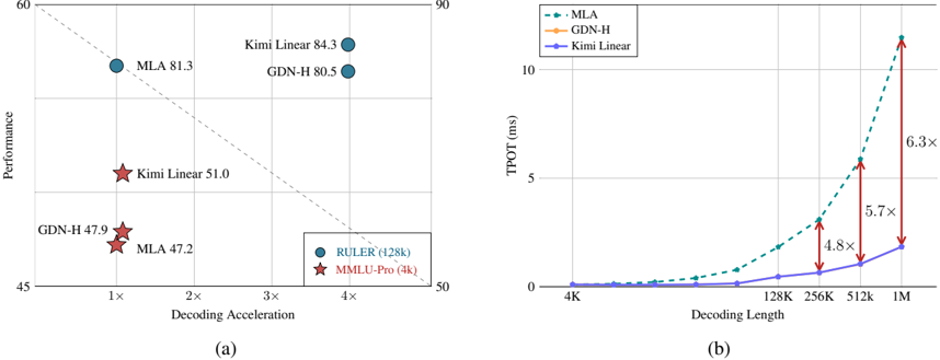
Figure 1: (a) Performance vs. acceleration. With strict fair comparisons with 1.4T training tokens, on MMLU-Pro (4k context length, red stars), Kimi Linear leads performance (51.0) at similar speed. On RULER (128k context length, blue circles), it is Pareto-optimal, achieving top performance (84.3) and 3 . 98 × acceleration. (b) Time per output token (TPOT) vs. decoding length. Kimi Linear (blue line) maintains a low TPOT, matching GDN-H and outperforming MLA at long sequences. This enables larger batches, yielding a 6 . 3 × faster TPOT (1.84ms vs. 11.48ms) than MLA at 1M tokens.
<details>
<summary>Image 2 Details</summary>
### Visual Description
## Chart Type: Scatter Plot and Line Graph
### Overview
The image presents two charts comparing the performance and efficiency of different models (MLA, GDN-H, Kimi Linear) in terms of decoding acceleration, performance, and decoding length. Chart (a) is a scatter plot showing performance vs. decoding acceleration, while chart (b) is a line graph showing TPOT (ms) vs. decoding length.
### Components/Axes
**Chart (a): Scatter Plot**
* **X-axis:** Decoding Acceleration (labeled as "Decoding Acceleration") with markers at 1x, 2x, 3x, and 4x.
* **Y-axis:** Performance (labeled as "Performance") with markers at 45, 50, 60, and 90.
* **Data Points:**
* RULER (128k) - Represented by blue circles.
* MMLU-Pro (4k) - Represented by red stars.
* **Legend:** Located at the bottom-right of the chart.
* **Models:** MLA, GDN-H, Kimi Linear.
**Chart (b): Line Graph**
* **X-axis:** Decoding Length (labeled as "Decoding Length") with markers at 4K, 128K, 256K, 512K, and 1M.
* **Y-axis:** TPOT (ms) (labeled as "TPOT (ms)") with markers at 0, 5, and 10.
* **Data Series:**
* MLA - Represented by a dashed green line with square markers.
* GDN-H - Represented by a solid orange line with circular markers.
* Kimi Linear - Represented by a solid blue line with circular markers.
* **Legend:** Located at the top-left of the chart.
* **Vertical Arrows:** Red arrows indicating the multiplication factor between the Kimi Linear and MLA lines at 256K, 512K, and 1M decoding lengths.
### Detailed Analysis
**Chart (a): Scatter Plot**
* **RULER (128k) - MLA:**
* Decoding Acceleration: Approximately 1x, Performance: Approximately 47.2
* Decoding Acceleration: Approximately 4x, Performance: Approximately 81.3
* **RULER (128k) - GDN-H:**
* Decoding Acceleration: Approximately 4x, Performance: Approximately 80.5
* **RULER (128k) - Kimi Linear:**
* Decoding Acceleration: Approximately 4x, Performance: Approximately 84.3
* **MMLU-Pro (4k) - Kimi Linear:**
* Decoding Acceleration: Approximately 1x, Performance: Approximately 51.0
* **MMLU-Pro (4k) - GDN-H:**
* Decoding Acceleration: Approximately 1x, Performance: Approximately 47.9
**Chart (b): Line Graph**
* **MLA (Dashed Green Line):** The TPOT increases exponentially with decoding length.
* 4K: Approximately 0.1 ms
* 128K: Approximately 0.3 ms
* 256K: Approximately 1.0 ms
* 512K: Approximately 2.5 ms
* 1M: Approximately 8.0 ms
* **GDN-H (Solid Orange Line):** The TPOT increases exponentially with decoding length.
* 4K: Approximately 0.1 ms
* 128K: Approximately 0.3 ms
* 256K: Approximately 0.8 ms
* 512K: Approximately 2.0 ms
* 1M: Approximately 6.0 ms
* **Kimi Linear (Solid Blue Line):** The TPOT increases slowly with decoding length.
* 4K: Approximately 0.1 ms
* 128K: Approximately 0.1 ms
* 256K: Approximately 0.2 ms
* 512K: Approximately 0.4 ms
* 1M: Approximately 1.3 ms
* **Multiplication Factors (Red Arrows):**
* 256K: MLA is approximately 4.8x higher than Kimi Linear.
* 512K: MLA is approximately 5.7x higher than Kimi Linear.
* 1M: MLA is approximately 6.3x higher than Kimi Linear.
### Key Observations
* In Chart (a), Kimi Linear achieves the highest performance at 4x decoding acceleration, while MMLU-Pro (4k) models have lower performance at 1x decoding acceleration.
* In Chart (b), TPOT increases significantly with decoding length for MLA and GDN-H, while Kimi Linear shows a much slower increase.
* The multiplication factors in Chart (b) indicate that the difference in TPOT between MLA and Kimi Linear increases as the decoding length increases.
### Interpretation
The charts compare the performance and efficiency of different models. Chart (a) shows that Kimi Linear achieves the highest performance with RULER (128k), while MMLU-Pro (4k) models have lower performance. Chart (b) demonstrates that MLA and GDN-H have a much higher TPOT (time per output token) as the decoding length increases compared to Kimi Linear. This suggests that Kimi Linear is more efficient in terms of processing time for longer sequences. The increasing multiplication factors highlight that the efficiency gap between MLA and Kimi Linear widens as the decoding length grows. The data suggests a trade-off between performance and efficiency, where Kimi Linear prioritizes efficiency (lower TPOT) while still achieving competitive performance.
</details>
1 /github https://github.com/fla-org/flash-linear-attention/tree/main/fla/ops/kda
2 https://huggingface.co/moonshotai/Kimi-Linear-48B-A3B-Instruct
## 1 Introduction
As large language models (LLMs) evolve into increasingly capable agents [50], the computational demands of inference-particularly in long-horizon and reinforcement learning (RL) settings-are becoming a central bottleneck. This shift toward RL test-time scaling [95, 33, 80, 74, 53], where models must process extended trajectories, tool-use interactions, and complex decision spaces at inference time, exposes fundamental inefficiencies in standard attention mechanisms. In particular, the quadratic time complexity and the linearly growing key-value (KV) cache of softmax attention introduce substantial computational and memory overheads, hindering throughput, context-length scaling, and real-time interactivity.
Linear attention [48] offers a principled approach to reducing computational complexity but has historically underperformed softmax attention in language modeling-even for short sequences-due to limited expressivity. Recent advances have significantly narrowed this gap, primarily through two innovations: gating or decay mechanisms [92, 16, 114] and the delta rule [84, 112, 111, 71]. Together, these developments have pushed linear attention closer to softmaxlevel quality on moderate-length sequences. Nevertheless, purely linear structure remain fundamentally constrained by the finite-state capacity, making long-sequence modeling and in-context retrieval theoretically challenging [104, 4, 45].
Hybrid architectures that combine softmax and linear attention-using a few global-attention layers alongside predominantly faster linear layers-have thus emerged as a practical compromise between quality and efficiency [57, 100, 66, 12, 32, 81]. However, previous hybrid models often operated at limited scale or lacked comprehensive evaluation across diverse benchmarks. The core challenge remains: to develop an attention architecture that matches or surpasses full attention in quality while achieving substantial efficiency gains in both speed and memory-an essential step toward enabling the next generation of agentic, decoding-heavy LLMs.
In this work, we present Kimi Linear , a hybrid linear attention architecture designed to meet the efficiency demands of agentic intelligence and test-time scaling without compromising quality. At its core lies Kimi Delta Attention (KDA) , a hardware-efficient linear attention module that extends Gated DeltaNet [111] with a finer-grained gating mechanism. While GDN, similar to Mamba2 [16], employs a coarse head-wise forget gate, KDA introduces a channel-wise variant in which each feature dimension maintains an independent forgetting rate, akin to Gated Linear Attention (GLA) [114]. This fine-grained design enables more precise regulation of the finite-state RNN memory, unlocking the potential of RNN-style models within hybrid architectures.
Crucially, KDA parameterizes its transition dynamics with a specialized variant of the Diagonal-Plus-Low-Rank (DPLR) matrices [30, 71], enabling a bespoke chunkwise-parallel algorithm that substantially reduces computation relative to general DPLR formulations while remaining consistent with the classical delta rule.
Kimi Linear interleaves KDA with periodic full attention layers in a uniform 3:1 ratio. This hybrid structure reduces memory and KV-cache usage by up to 75% during long-sequence generation while preserving global information flow via the full attention layers. Through matched-scale pretraining and evaluation, we show that Kimi Linear consistently matches or outperforms strong full-attention baselines across short-context, long-context, and RL-style post-training tasks-while achieving up to 6 × higher decoding throughput at 1M context length.
To facilitate further research, we release open-source KDA kernels with vLLM integration, as well as pre-trained and instruction-tuned checkpoints. These components are drop-in compatible with existing full-attention pipelines, requiring no modification to caching or scheduling interfaces, thereby facilitating research on hybrid architectures.
## Contributions
- Kimi Delta Attention (KDA): a linear attention mechanism that refines the gated delta rule with improved recurrent memory management and hardware efficiency.
- The Kimi Linear architecture: a hybrid design adopting a 3:1 KDA-to-global attention ratio, reducing memory footprint while surpassing full-attention quality.
- Fair empirical validation at scale: through 1.4T token training runs, Kimi Linear outperforms full attention and other baselines in short/long context and RL-style evaluations, with full release of kernels, vLLM integration, and checkpoints.
## 2 Preliminary
In this section, we introduce the technical background related to our proposed Kimi Delta Attention.
## 2.1 Notation
In this paper, we define □ t ∈ R d k or R d v , s . t ., □ ∈ { q, k, v, o, u, w } denotes a t -th corresponding column vector, and S t ∈ R d k × d v represents the matrix-form memory state. M and M -denote lower-triangular masks with and without diagonal elements, respectively; for convenience, we also write them as Tril and StrictTril .
Chunk-wise Formulation Suppose the sequence is split into L/C chunks where each chunk is of length C . We define □ [ t ] ∈ R C × d for □ ∈ { Q , K , V , O , U , W } are matrices that stack the vectors within the t -th chunk, and □ r [ t ] = □ tC + r is the r -th element of the chunk. Note that t ∈ [0 , L/C ) , r ∈ [1 , C ] . State matrices are also re-indexed such that S i [ t ] = S tC + i . Additionally, S [ t ] := S 0 [ t ] = S C [ t -1] , i.e., the initial state of a chunk is the last state of the previous chunk.
Decay Formulation We define the cumulative decay γ i → j [ t ] := ∏ j k = i α k [ t ] , and abbreviate γ 1 → r [ t ] as γ r [ t ] . Additionally, A [ t ] := A i/j [ t ] ∈ R C × C is the matrix with elements γ i [ t ] /γ j [ t ] . Diag ( α t ) denotes the fine-grained decay, Diag ( γ i → j [ t ] ) := ∏ j k = i Diag ( α k [ t ] ) , and Γ i → j [ t ] ∈ R C × d k is the matrix stack from γ i [ t ] to γ j [ t ] .
## 2.2 Linear Attention and the Gated Delta Rule
Linear Attention as Online Learning. Linear attention [48] maintains a matrix-valued recurrent state that accumulates key-value associations:
$$S _ { t } = S _ { t - 1 } + k _ { t } v _ { t } ^ { \top } , \quad o _ { t } = S _ { t } ^ { \top } q _ { t } .$$
From the fast-weight perspective [84, 85], S t serves as an associative memory storing transient mappings from keys to values. This update can be viewed as performing gradient descent on the unbounded correlation objective
$$\mathcal { L } _ { t } ( S ) = - \langle S ^ { \top } k _ { t } , v _ { t } \rangle ,$$
which continually reinforces recent key-value pairs without any forgetting. However, such an objective provides no criterion for which memories to erase, and the accumulated state grows unbounded, leading to interference over long contexts.
DeltaNet: Online Gradient Descent on Reconstruction Loss. DeltaNet [84] reinterprets this recurrence as online gradient descent on a reconstruction objective:
$$\begin{array} { r } { \mathcal { L } _ { t } ( S ) = \frac { 1 } { 2 } \| S ^ { \top } k _ { t } - v _ { t } \| ^ { 2 } . } \end{array}$$
Taking a gradient step with learning rate β t gives
$$\begin{array} { r } { S _ { t } = S _ { t - 1 } - \beta _ { t } \nabla _ { s } \mathcal { L } _ { t } ( S _ { t - 1 } ) = ( I - \beta _ { t } k _ { t } k _ { t } ^ { \top } ) S _ { t - 1 } + \beta _ { t } k _ { t } v _ { t } ^ { \top } . } \end{array}$$
This rule-the classical delta rule -treats S as a learnable associative memory that continually corrects itself toward the mapping k t ↦→ v t . The rank-1 update structure, equivalent to a generalized Householder transformation, supports hardware-efficient chunkwise parallelization [11, 112].
Gated DeltaNet as Weight Decay. Although DeltaNet stabilizes learning, it still retains outdated associations indefinitely. Gated DeltaNet (GDN) [111] introduces a scalar forget gate α t ∈ [0 , 1] , yielding
$$S _ { t } = \alpha _ { t } ( I - \beta _ { t } k _ { t } k _ { t } ^ { \top } ) S _ { t - 1 } + \beta _ { t } k _ { t } v _ { t } ^ { \top } .$$
Here, α t acts as a form of weight decay on the fast weights [8], implementing a forgetting mechanism analogous to data-dependent L 2 regularization. This simple yet effective modification provides a principled way to control memory lifespan and mitigate interference, improving both stability and long-context generalization while preserving DeltaNet's parallelizable structure.
From this perspective, we observe that GDN can be interpreted as a form of multiplicative positional encoding where the transition matrix is data-dependent and learnable, relaxing the orthogonality constraint of RoPE [115]. 3
3 When the state transformation matrix preserves its orthogonality, absolute positional encodings can also be applied independently to q and k to be converted into relative positional encodings during the attention computation [87].
## 3 Kimi Delta Attention: Improving Delta Rule with Fine-grained Gating
We propose Kimi Delta Attention (KDA), a new gated linear attention variant that refines GDN's scalar decay by introducing a fine-grained diagonalized gate Diag( α t ) that enables fine-grained control over memory decay and positional awareness (as discussed in §6.1). We begin by introducing the chunkwise parallelization of KDA, showing how a series of rank-1 matrix transformations can be compressed into a dense representation while maintaining stability under diagonal gating. We then highlight the efficiency gains of KDA over the standard DPLR ( Diagonal-Plus-LowRank ) formulation [30, 71].
$$S _ { t } = \left ( I - \beta _ { t } k _ { t } k _ { t } ^ { \top } \right ) D i a g \left ( \alpha _ { t } \right ) S _ { t - 1 } + \beta _ { t } k _ { t } v _ { t } ^ { \top } \in \mathbb { R } ^ { d _ { k } \times d _ { v } } ; \quad o _ { t } = S _ { t } ^ { \top } q _ { t } \in \mathbb { R } ^ { d _ { v } }$$
<details>
<summary>Image 3 Details</summary>

### Visual Description
## Diagram: Matrix Decomposition
### Overview
The image depicts a matrix decomposition equation. A matrix with varying shades of blue is shown to be equal to the result of a series of matrix operations. These operations involve a gray diagonal matrix, orange gradient vectors, and a red diagonal matrix.
### Components/Axes
* **Matrices:** The image contains several matrices represented as grids of colored squares. The colors vary from light to dark shades of blue, gray, orange, and red, indicating different values within the matrices.
* **Operators:** The equation includes the following mathematical operators: "=", "-", "×", and "+".
* **Parentheses:** Parentheses are used to group operations.
### Detailed Analysis
The equation can be broken down as follows:
1. **Left-hand side:** A 4x4 matrix with varying shades of blue. The top-left and bottom-right quadrants have darker shades of blue, while the top-right and bottom-left quadrants have lighter shades.
2. **First term on the right-hand side:** A 4x4 diagonal matrix filled with gray squares. This matrix is subtracted from an orange gradient vector. The orange gradient vector has 4 elements, with the color intensity increasing from top to bottom.
3. **Second term on the right-hand side:** The result of the subtraction is multiplied by a 4x4 diagonal matrix filled with red squares. The red squares have a gradient, with the top-left square being the darkest and the bottom-right square being the lightest.
4. **Third term on the right-hand side:** The result of the previous multiplication is added to an orange gradient vector. The orange gradient vector has 4 elements, with the color intensity increasing from top to bottom.
5. **Right-hand side result:** The final result is a 4x4 matrix with varying shades of blue. The top-left and bottom-right quadrants have darker shades of blue, while the top-right and bottom-left quadrants have lighter shades. This matrix is similar to the matrix on the left-hand side. An orange gradient vector is also present. The orange gradient vector has 4 elements, with the color intensity increasing from top to bottom.
### Key Observations
* The equation demonstrates a matrix decomposition process.
* The color gradients within the matrices and vectors likely represent varying values.
* The diagonal matrices suggest a focus on specific elements or features within the original matrix.
### Interpretation
The image illustrates a matrix decomposition technique, possibly related to dimensionality reduction or feature extraction. The initial blue matrix is decomposed into a series of operations involving diagonal matrices and gradient vectors. The diagonal matrices likely represent specific components or features of the original matrix, while the gradient vectors may represent weights or scaling factors. The equation suggests that the original matrix can be reconstructed from these components. The specific type of decomposition is not explicitly stated, but it could be related to Singular Value Decomposition (SVD) or Principal Component Analysis (PCA).
</details>
## 3.1 Hardware-Efficient Chunkwise Algorithm
By partially expanding the recurrence for Eq. 1 into a chunk-wise formulation, we have:
$$\begin{array} { r l } & { s _ { [ t ] } ^ { r } = \underbrace { \left ( \prod _ { i = 1 } ^ { r } \left ( I - \beta _ { [ t ] } ^ { i } k _ { [ t ] } ^ { i } k _ { [ t ] } ^ { i \top } \right ) D i a g ( \alpha _ { [ t ] } ^ { i } ) \right ) } _ { \colon = P _ { [ t ] } ^ { r } } \cdot s _ { [ t ] } ^ { 0 } + \underbrace { \sum _ { i = 1 } ^ { r } \left ( \prod _ { j = i + 1 } ^ { r } \left ( I - \beta _ { [ t ] } ^ { j } k _ { [ t ] } ^ { j } k _ { [ t ] } ^ { j \top } \right ) D i a g ( \alpha _ { [ t ] } ^ { j } ) \right ) \cdot \beta _ { [ t ] } ^ { i } k _ { [ t ] } ^ { i } v _ { [ t ] } ^ { i \top } } _ { \colon = H _ { [ t ] } ^ { r } } } & { ( 2 ) } \end{array}$$
WYRepresentation shi is typically employed to pack a series rank-1 updates into a single compact representation [11]. We follow the formulation of P in Comba [40] to reduce the need for an additional matrix inversion in subsequent computations.
$$P _ { [ t ] } ^ { r } = D i a g ( \gamma _ { [ t ] } ^ { r } ) - \sum _ { i = 1 } ^ { r } D i a g ( \gamma _ { [ t ] } ^ { i \rightarrow r } ) k _ { [ t ] } ^ { i } w _ { [ t ] } ^ { i \top } & & H _ { [ t ] } ^ { r } = \sum _ { i = 1 } ^ { t } D i a g \left ( \gamma _ { [ t ] } ^ { i \rightarrow r } \right ) k _ { [ t ] } ^ { i } u _ { [ t ] } ^ { i \top } & & ( 3 )$$
where the auxiliary vector w t ∈ R d k and u t ∈ R d v are computed via the following recurrence relation:
$$w _ { [ t ] } ^ { r } = \beta _ { [ t ] } ^ { r } \left ( D i a g ( \gamma _ { [ t ] } ^ { r } ) k _ { [ t ] } ^ { r } - \sum _ { i = 1 } ^ { r - 1 } w _ { [ t ] } ^ { i } \left ( k _ { [ t ] } ^ { i \top } D i a g \left ( \gamma _ { [ t ] } ^ { i \to r } \right ) k _ { [ t ] } ^ { r } \right ) \right )$$
$$\pm b { u } _ { [ t ] } ^ { r } = \beta _ { [ t ] } ^ { r } \left ( v _ { [ t ] } ^ { r } - \sum _ { i = 1 } ^ { r - 1 } u _ { [ t ] } ^ { i } \left ( k _ { [ t ] } ^ { i \top } D i a g \left ( \gamma _ { [ t ] } ^ { i \rightarrow r } \right ) k _ { [ t ] } ^ { r } \right ) \right )$$
UT transform. We apply the UT transform [46] to reduce non-matmul FLOPs, which is crucial to enable better hardware utilization during training.
$$\begin{array} { r } { M _ { [ t ] } = \left ( I + S t r i c t T r i l \left ( D i a g \left ( \beta _ { [ t ] } \right ) \left ( \Gamma _ { [ t ] } ^ { 1 \rightarrow C } \odot K _ { [ t ] } \right ) \left ( \frac { K _ { [ t ] } } { \Gamma _ { [ t ] } ^ { 1 \rightarrow C } } \right ) \right ) \right ) ^ { - 1 } D i a g \left ( \beta _ { [ t ] } \right ) } \end{array} \quad ( 6 )$$
$$\begin{array} { r l } { W _ { [ t ] } = M _ { [ t ] } \left ( \Gamma ^ { 1 \rightarrow C } _ { [ t ] } \odot K _ { [ t ] } \right ) , } & { U _ { [ t ] } = M _ { [ t ] } V _ { [ t ] } } & { ( 7 ) } \end{array}$$
The inverse of a lower triangular matrix can be efficiently computed through an iterative row-wise approach by forward substitution in Gaussian elimination [28].
Equivalently, in matrix form, we can update the state in chunk-wise:
$$\begin{array} { r } { S _ { [ t + 1 ] } = D i a g ( \gamma _ { [ t ] } ^ { C } ) S _ { [ t ] } + \left ( \Gamma _ { [ t ] } ^ { i \rightarrow C } \odot K _ { [ t ] } \right ) ^ { T } \left ( U _ { [ t ] } - W _ { [ t ] } S _ { [ t ] } \right ) \in \mathbb { R } ^ { d _ { k } \times d _ { v } } } \end{array} \quad ( 8 )$$
<details>
<summary>Image 4 Details</summary>
### Visual Description
## Matrix Decomposition Diagram
### Overview
The image depicts a matrix decomposition equation. A 4x4 matrix, represented by blue-toned squares, is decomposed into the sum of a diagonal matrix (represented by red-toned squares) and the element-wise (Hadamard) product of two other 4x4 matrices (represented by red and orange-toned squares).
### Components/Axes
* **Matrices:** The image contains several 4x4 matrices, each represented by a grid of 16 squares.
* **Color Gradient:** The color of each square within a matrix represents a value. Blue represents lower values, red and orange represent higher values.
* **Operators:** The equation includes the following operators:
* "=" (equals sign)
* "+" (addition)
* "⊙" (Hadamard product, element-wise multiplication)
* **Brackets:** Square brackets denote matrices, and parentheses group the Hadamard product.
### Detailed Analysis or ### Content Details
1. **Original Matrix (Leftmost):** A 4x4 matrix with varying shades of blue. The values are not uniform, with some squares being darker blue than others.
* Top-left: Light blue
* Top-right: Light blue
* Bottom-left: Darker blue
* Bottom-right: Light blue
2. **Diagonal Matrix:** A 4x4 diagonal matrix with shades of red. Only the diagonal elements have non-zero values.
* Top-left: Dark red
* Second row, second column: Medium red
* Third row, third column: Light red
* Bottom-right: Very light red
3. **Second Matrix (Addition):** A 4x4 matrix with varying shades of blue, similar to the original matrix.
* Top-left: Dark blue
* Top-right: Light blue
* Bottom-left: Light blue
* Bottom-right: Dark blue
4. **Hadamard Product Matrices:** Two 4x4 matrices enclosed in parentheses, combined using the Hadamard product operator.
* First Matrix: Shades of red, with the top-left being the darkest and the bottom-right being the lightest.
* Second Matrix: Shades of orange, with the top-left being the lightest and the bottom-right being the darkest.
### Key Observations
* The original matrix is decomposed into a diagonal matrix and the Hadamard product of two other matrices.
* The color gradients within each matrix suggest varying values for each element.
* The diagonal matrix only has non-zero values along its diagonal.
* The Hadamard product matrices have opposing color gradients (red increasing downwards, orange increasing rightwards).
### Interpretation
The image illustrates a matrix decomposition technique, likely used in linear algebra or machine learning. The decomposition separates the original matrix into a diagonal component and a component derived from the element-wise product of two other matrices. This type of decomposition can be useful for simplifying matrix operations, reducing dimensionality, or extracting specific features from the original matrix. The Hadamard product suggests an element-wise interaction between the two matrices, potentially capturing relationships or dependencies between different elements. The specific application of this decomposition would depend on the context in which it is used.
</details>
During the output stage, we adopt an inter-block recurrent and intra-block parallel strategy to maximize matrix multiplication throughput, thereby fully utilizing the computational potential of Tensor Cores.
$$O _ { [ t ] } = \underbrace { \left ( \Gamma ^ { 1 \to C } _ { [ t ] } \odot Q _ { [ t ] } \right ) S _ { [ t ] } } _ { i n t e r c h u k } + \underbrace { T r i l \left ( \left ( \Gamma ^ { 1 \to C } _ { [ t ] } \odot Q _ { [ t ] } \right ) \left ( \frac { K _ { [ t ] } } { \Gamma ^ { 1 \to C } _ { [ t ] } } \right ) ^ { \top } \right ) } _ { i n t e r c h u k } \underbrace { \left ( U _ { [ t ] } - W _ { [ t ] } S _ { [ t ] } \right ) \in \mathbb { R } ^ { C \times d _ { v } } } _ { " p s e u n d o r" - value term }$$
## 3.2 Efficiency Analysis
In terms of representational capacity, KDA aligns with the generalized DPLR formulation, i.e., S t = ( D -a t b ⊤ t ) S t -1 + k t v ⊤ t , both exhibiting fine-grained decay behavior. However, such fine-grained decay introduces numerical precision issues during division operations (e.g., the intra-chunk computation in Eq. 9). To address this, prior work such as GLA [114] performs computations in the logarithmic domain and introduces secondary chunking in full precision. This approach, however, prevents full utilization of half-precision matrix multiplications and significantly reduces operator speed. By binding both variables a and b to k , KDA effectively alleviates this bottleneck-reducing the number of second-level chunk matrix computations from four to two, and further eliminating three additional matrix multiplications. As a result, the operator efficiency of KDA improves by roughly 100% compared to the DPLR formulation. A detailed analysis is provided in §6.2.
## 4 The Kimi Linear Model Architecture
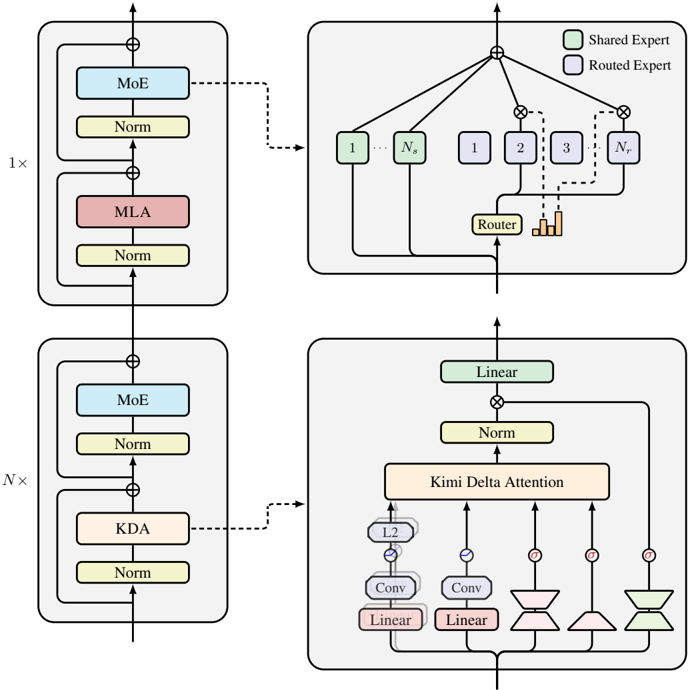
The main backbone of our model architecture follows Moonlight [62]. In addition to fine-grained gating, we also leverage several components to further improve the expressiveness of Kimi Linear. The overall Kimi Linear architecture is shown in Figure 3.
Neural Parameterization Let x t ∈ R d be the t -th token input representation, the input to KDA for each head h is computed as follows
$$q _ { t } ^ { h } , k _ { t } ^ { h } & = L 2 N o r m ( S w i s h ( S h o r t C o n v ( W _ { q / k } ^ { h } x _ { t } ) ) ) \in \mathbb { R } ^ { d _ { k } } \\ v _ { t } ^ { h } & = S w i s h ( S h o r t C o n v ( W _ { v } ^ { h } x _ { t } ) ) \in \mathbb { R } ^ { d _ { v } } \\ \alpha _ { t } ^ { h } & = f ( W _ { \alpha } ^ { \uparrow } W _ { \alpha } ^ { \downarrow } x _ { t } ) \in [ 0 , 1 ] ^ { d _ { k } } \\ \beta _ { t } ^ { h } & = S i g m o i d ( W _ { \beta } ^ { h } x _ { t } ) \in [ 0 , 1 ]$$
where d k , d v represent the key and value head dimensions, which are set to 128 for all experiments. For q , k , v , we apply a ShortConv followed by a Swish activation, following [111]. The q and k representations are further normalized using L2Norm to ensure eigenvalues stability, as suggested by [112]. The per-channel decay α h t is parameterized via a low-rank projection ( W ↓ α and W ↑ α with rank equal to the head dimension) and a decay function f ( · ) similar to those
Figure 2: Execution time of kernels for varying input lengths, with a uniform batch size of 1 and 16 heads.
<details>
<summary>Image 5 Details</summary>
### Visual Description
## Chart: Execution Time vs. Input Length
### Overview
The image is a line chart comparing the execution time (in milliseconds) of two algorithms, DPLR and KDA (ours), as a function of input length. The x-axis represents the input length, ranging from 2K to 64K. The y-axis represents the execution time, ranging from 0 to 64 ms.
### Components/Axes
* **X-axis:** Input length, labeled "Input length". Values: 2K, 4K, 8K, 16K, 32K, 64K.
* **Y-axis:** Execution Time (ms), labeled "Execution Time (ms)". Values: 0, 16, 32, 48, 64.
* **Legend:** Located at the top-left of the chart.
* DPLR: Represented by a dashed green line.
* KDA (ours): Represented by a solid blue line.
### Detailed Analysis
* **DPLR (dashed green line):** The execution time increases rapidly with input length.
* 2K: Approximately 0.8 ms
* 4K: Approximately 1.6 ms
* 8K: Approximately 4 ms
* 16K: Approximately 15 ms
* 32K: Approximately 30 ms
* 64K: Approximately 60 ms
* **KDA (ours) (solid blue line):** The execution time increases with input length, but at a slower rate than DPLR.
* 2K: Approximately 0.8 ms
* 4K: Approximately 0.9 ms
* 8K: Approximately 2 ms
* 16K: Approximately 5 ms
* 32K: Approximately 15 ms
* 64K: Approximately 30 ms
### Key Observations
* Both algorithms show an increase in execution time as the input length increases.
* KDA (ours) consistently outperforms DPLR, exhibiting significantly lower execution times for all input lengths.
* The difference in execution time between the two algorithms becomes more pronounced as the input length increases.
### Interpretation
The chart demonstrates that the KDA (ours) algorithm is more efficient than the DPLR algorithm in terms of execution time, especially for larger input lengths. This suggests that KDA (ours) is a better choice for applications where processing speed is critical, particularly when dealing with large datasets. The trend indicates that the performance gap between the two algorithms would likely widen further with even larger input sizes.
</details>
Outputs
<details>
<summary>Image 6 Details</summary>
### Visual Description
## Neural Network Architecture Diagram
### Overview
The image presents a neural network architecture diagram, illustrating the flow of data through various layers and components. The diagram highlights the use of shared and routed experts, attention mechanisms, and normalization layers. The architecture appears to be a hybrid design, incorporating elements of both feedforward and attention-based models.
### Components/Axes
* **Legend:** Located at the top-right corner.
* Green box: Shared Expert
* Blue box: Routed Expert
* **Blocks:** The diagram is composed of several blocks, each representing a set of operations or layers. These blocks are arranged vertically, indicating the flow of data.
* **Arrows:** Arrows indicate the direction of data flow between blocks and layers. Dashed arrows indicate a different type of connection or routing.
* **Labels:** Labels within the blocks describe the type of operation or layer, such as "MoE," "Norm," "MLA," "KDA," "Linear," "Conv," "Router," and "Kimi Delta Attention."
* **Multiplication Factors:** "1x" and "Nx" indicate the number of times a particular block is repeated.
### Detailed Analysis
The diagram can be broken down into the following sections:
1. **Top Block (1x):**
* A block labeled "1x" is located at the top-left.
* It contains the following layers:
* MoE (Routed Expert - Blue)
* Norm (Normalization - Yellow)
* MLA (Red)
* Norm (Normalization - Yellow)
* The input flows through MoE, Norm, MLA, and Norm sequentially.
* A dashed arrow connects this block to the top-right block.
2. **Top-Right Block (Routing):**
* This block represents a routing mechanism.
* It contains several nodes labeled "1," "2," "3," "Nr," and "Ns." These nodes are connected in a tree-like structure.
* Nodes "1" and "Ns" are blue, indicating "Routed Expert".
* Nodes "1," "2," "3," and "Nr" are blue, indicating "Routed Expert".
* A "Router" (Yellow) is present at the bottom of this block.
* A bar graph is present near the router.
* The output of this block flows upwards.
3. **Bottom Block (Nx):**
* A block labeled "Nx" is located at the bottom-left.
* It contains the following layers:
* MoE (Routed Expert - Blue)
* Norm (Normalization - Yellow)
* KDA (Khaki)
* Norm (Normalization - Yellow)
* The input flows through MoE, Norm, KDA, and Norm sequentially.
* A dashed arrow connects this block to the bottom-right block.
4. **Bottom-Right Block (Attention):**
* This block represents an attention mechanism.
* It contains the following layers:
* Linear (Shared Expert - Green)
* Norm (Normalization - Yellow)
* Kimi Delta Attention (Khaki)
* L2 (Blue)
* Conv (Linear - Red)
* Linear (Red)
* Several hourglass-shaped components are connected to the "Kimi Delta Attention" layer. These components are colored blue, red, and green.
* The input flows through the "Linear" and "Norm" layers. The output of the "Norm" layer is fed into the "Kimi Delta Attention" layer. The "Kimi Delta Attention" layer receives input from the hourglass-shaped components.
### Key Observations
* The architecture utilizes both shared and routed experts.
* Attention mechanisms play a crucial role in the bottom-right block.
* Normalization layers are used extensively throughout the architecture.
* The "Nx" block is repeated multiple times, suggesting a deep network.
### Interpretation
The diagram illustrates a complex neural network architecture that combines different types of layers and mechanisms. The use of shared and routed experts suggests a modular design, where different parts of the network specialize in different tasks. The attention mechanism allows the network to focus on the most relevant parts of the input. The normalization layers help to stabilize training and improve performance. The repetition of the "Nx" block indicates that the network is designed to handle complex data. The architecture appears to be designed for tasks that require both feature extraction and attention-based processing.
</details>
Inputs
Figure 3: Illustration of our Kimi Linear model architecture, which consists of a stack of blocks containing a token mixing layer followed by a MoE channel-mixing layer. Specifically, we interleave N KDA layers with one MLA layer for token mixing, where N is set to 3 in our implementation.
used in GDN and Mamba [111, 16]. Before the output projection through W o ∈ R d × d , we use a head-wise RMSNorm [122] and a data-dependent gating mechanism [79] parameterized as:
$$o _ { t } = W _ { o } \left ( S i g m o i d \left ( W _ { g } ^ { \dagger } W _ { g } ^ { \downarrow } x _ { t } \right ) \odot R M S N o r m \left ( K D A \left ( q _ { t } , k _ { t } , v _ { t } , \alpha _ { t } , \beta _ { t } \right ) \right ) \right )$$
Here, the output gate adopts a low-rank parameterization similar to the forget gate, to ensure a fair parameter comparison, while maintaining performance comparable to full-rank gating and alleviating the Attention Sink [79]. The choice of nonlinear activation function is further discussed in §5.2.
Hybrid model architecture Long-context retrieval remains the primary bottleneck for pure linear attention, we therefore hybridize KDA with a small number of full global-attention (Full MLA) layers [19]. For Kimi Linear, we chose a layerwise approach (alternating entire layers) over a headwise one (mixing heads within layers) for its superior infrastructure simplicity and training stability. Empirically, a uniform 3:1 ratio, i.e., repeating 3 KDA layers to 1 full MLA layer, provided the best quality-throughput trade-off. We discuss other hybridization strategies in § 7.2.
No Position Encoding (NoPE) for MLA Layers. In Kimi Linear, we apply NoPE to all full attention (MLA) layers. This design delegates the entire responsibility for encoding positional information and recency bias (see § 6.1) to the KDA layers. KDA is thus established as the primary position-aware operator, fulfilling a role analogous to, or arguably stronger than, auxiliary components like short convolutions [3] or SWA [76]. Our findings align with prior results [110, 7, 19], who similarly demonstrated that complementing global NoPE attention with a dedicated position-aware mechanism yields competitive long-context performance.
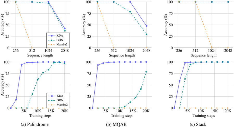
Figure 4: Results on synthetic tasks: palindrome, multi query associative recall, and the state tracking.
<details>
<summary>Image 7 Details</summary>
### Visual Description
## Line Charts: Accuracy vs. Sequence Length and Training Steps for KDA, GDN, and Mamba2
### Overview
The image presents six line charts arranged in a 2x3 grid. Each column represents a different task: Palindrome, MQAR, and Stack. The top row shows accuracy (%) versus sequence length, while the bottom row shows accuracy (%) versus training steps. The charts compare the performance of three models: KDA (solid blue line), GDN (dashed green line with star markers), and Mamba2 (dashed orange line).
### Components/Axes
**General Chart Elements:**
* **Title:** Each column has a title at the bottom: (a) Palindrome, (b) MQAR, (c) Stack.
* **Y-axis:** Labeled "Accuracy (%)" with ticks at 0, 25, 50, 75, and 100.
* **Legend:** Located in the top-left chart of the first column, indicating:
* KDA: Solid blue line
* GDN: Dashed green line with star markers
* Mamba2: Dashed orange line
**Top Row (Accuracy vs. Sequence Length):**
* **X-axis:** Labeled "Sequence length" with ticks at 256, 512, 1024, and 2048.
**Bottom Row (Accuracy vs. Training Steps):**
* **X-axis:** Labeled "Training steps" with ticks at 5K, 10K, 15K, and 20K.
### Detailed Analysis
**1. Palindrome (Column a):**
* **Top Chart (Sequence Length):**
* KDA (blue): Accuracy is 100% at sequence lengths 256, 512, and 1024, then drops to approximately 42% at 2048.
* GDN (green): Accuracy is 100% at sequence lengths 256, 512, and 1024, then drops to approximately 28% at 2048.
* Mamba2 (orange): Accuracy starts at 100% at 256, drops to 0% at 512, and remains at 0% for 1024 and 2048.
* **Bottom Chart (Training Steps):**
* KDA (blue): Accuracy increases sharply from 0% at 0K to approximately 95% at 5K, then reaches 100% and remains constant.
* GDN (green): Accuracy increases from 0% at 0K to approximately 60% at 15K, then reaches approximately 95% at 20K.
* Mamba2 (orange): Accuracy remains at 0% for all training steps.
**2. MQAR (Column b):**
* **Top Chart (Sequence Length):**
* KDA (blue): Accuracy is 100% at sequence lengths 256, 512, and 1024, then drops to approximately 48% at 2048.
* GDN (green): Accuracy is 100% at sequence lengths 256, 512, and 1024, then drops to approximately 25% at 2048.
* Mamba2 (orange): Accuracy starts at 100% at 256, drops to 0% at 512, and remains at 0% for 1024 and 2048.
* **Bottom Chart (Training Steps):**
* KDA (blue): Accuracy increases sharply from 0% at 0K to approximately 95% at 5K, then reaches 100% and remains constant.
* GDN (green): Accuracy increases slowly from 0% at 0K to approximately 75% at 20K.
* Mamba2 (orange): Accuracy remains at 0% for all training steps.
**3. Stack (Column c):**
* **Top Chart (Sequence Length):**
* KDA (blue): Accuracy is 100% for all sequence lengths.
* GDN (green): Accuracy is 100% for all sequence lengths.
* Mamba2 (orange): Accuracy starts at 100% at 256, drops to 0% at 512, and remains at 0% for 1024 and 2048.
* **Bottom Chart (Training Steps):**
* KDA (blue): Accuracy increases sharply from 0% at 0K to 100% at 5K, and remains constant.
* GDN (green): Accuracy increases sharply from 0% at 0K to approximately 98% at 5K, and remains constant.
* Mamba2 (orange): Accuracy remains at 0% for all training steps.
### Key Observations
* KDA and GDN generally perform well with shorter sequence lengths, but their accuracy decreases as the sequence length increases to 2048, except for the Stack task where they maintain 100% accuracy.
* Mamba2 consistently drops to 0% accuracy after a sequence length of 256 for all tasks.
* For all tasks, KDA reaches 100% accuracy with fewer training steps compared to GDN.
* Mamba2 does not improve with increased training steps and remains at 0% accuracy.
### Interpretation
The charts demonstrate the performance of KDA, GDN, and Mamba2 models on different tasks (Palindrome, MQAR, Stack) under varying sequence lengths and training steps. The results suggest that:
* KDA is generally more efficient in terms of training steps to achieve high accuracy.
* GDN requires more training steps to reach comparable accuracy to KDA.
* Mamba2 is not suitable for these tasks, as its accuracy drops to 0% with longer sequence lengths and does not improve with increased training.
* The Stack task is relatively easier for KDA and GDN, as they achieve 100% accuracy even with shorter training steps and maintain it across all sequence lengths.
* The performance of KDA and GDN degrades with longer sequence lengths for Palindrome and MQAR tasks, indicating potential limitations in handling longer sequences for these specific tasks.
</details>
We note that NoPE offers practical advantages, particularly for MLA. First, NoPE enables their conversion to the highly-efficient pure Multi-Query Attention (MQA) during inference. Second, it simplifies long-context training, as it obviates the need for RoPE parameter adjustments, such as frequency base tuning or methods like YaRN [72].
## 5 Experiments
## 5.1 Synthetic tests
We start by evaluating KDA against other competing linear attention methods on three synthetic tasks, serving as benchmark tests for long-context performance. Across all experiments, we adopt a consistent model configuration of 2 layers with 2 attention heads, each having a head dimension of 128. For each task, we train the model for at most 20,000 steps with a grid search over learning rates in { 5 × 10 -5 , 1 × 10 -4 , 5 × 10 -4 , 1 × 10 -3 } . We then present the best-performing training accuracy curves. Specifically, we compare two scenarios: (1) the performance of different tasks as training length increases from 256 to 2,048 tokens, measuring the peak accuracy; and (2) the convergence speed of KDA, GDN, and Mamba2 with a fixed context length of 1,024 tokens.
Palindrome Palindrome requires the model to reproduce a given sequence of random tokens in reverse order. As illustrated in Table 5.1, given an input like 'O G R S U N E', the model must generate its exact reversal. Such copying tasks are known to be difficult for linear attention models [45], as they struggle to precisely retrieve the entire history from a compressed, fixed-size memory state.
<!-- formula-not-decoded -->
Multi Query Associative Recall (MQAR) MQAR assesses the model's ability to retrieve values associated with multiple queries that appear at various positions within the context. For instance, as shown in Table 5.1, the model is asked to recall 0 for the query B and 5 for G. This task is known to be highly correlated with language modeling performance [5].
$$\begin{array} { r c l } \text {Input} & A & 1 & C & 3 & B & 0 & M & 8 & G & 5 & E & 4 & < S P > \\ \text {Output} & \phi & \phi & \phi & \phi & \phi & \phi & \phi & \phi & \phi & \phi & \phi & \phi & \phi & 0 & 5 \end{array}$$
Table 1: Ablation study on the hybrid ratio of KDA to MLA attention and other key components. We list the training and validation perplexities (lower is better) for comparison. The best-performing model, used in our final experiments, is highlighted in gray.
| | Training PPL ( ↓ ) | Validation PPL ( ↓ ) |
|-----------------------|----------------------|------------------------|
| Hybrid ratio | 9.23 | 5.65 |
| 0:1 | 9.45 | 5.77 |
| | 9.29 | 5.66 |
| 7:1 | 9.23 | 5.7 |
| 15:1 | 9.34 | 5.82 |
| w/o output gate 9.25 | w/o output gate 9.25 | 5.67 |
| w/ swish output gate | 9.43 | 5.81 |
| w/o convolution layer | 9.29 | 5.7 |
Stack We assess the state tracking capabilities [27] of each candidate by simulating the standard LIFO (Last In First Out) stack operations. Our setup involves 64 independent stacks, each identified by a unique ID. The model processes a sequence of two operations: 1) PUSH: an action like ' <push> 1 G' adds the element G to stack 1; 2) POP: an action like ' <pop> 0 E' requires the model to predict the element E most recently pushed onto stack 0. The objective is to accurately track the states of all stacks and predict the correct element upon each pop request.
Figure 4 shows the final results. Across all tasks, KDA consistently achieves the highest accuracy as the sequence length increases from 256 to 2,048 tokens. In particular, on the Palindrome and recall-intensive MQAR tasks, KDA converges significantly faster than GDN. This confirms the benefits of our fine-grained decay, which enables the model to selectively forget irrelevant information while preserving crucial memories more precisely. We also observe that Mamba2 [16], a typical linear attention that uses only multiplicative decay and lacks a delta rule, fails on all tasks in our model settings.
## 5.2 Ablation on Key Components of Kimi Linear
We conducted a series of ablation studies by directly comparing different models to the first-scale scaling law model, i.e., 16 heads, 16 layers. All models were trained with the same FLOPs budget and hyperparameters for a fair comparison. We report the training and validation perplexities (PPLs) in Table 1. The validation PPL is calculated on a highquality dataset whose distribution differs significantly from the pre-training corpus, emphasizing generalization under distribution shift, and thus the differences in training and validation perplexities.
Output gate We compare our default Sigmoid output gate against two variants: one with no gating and another with swish gating. The results show that removing the gate degrades performance. Moreover, the swish gate adopted by [111] performs substantially worse than Sigmoid . Our observation is consistent with [79], who also conclude that Sigmoid gating offers superior performance. So we adopt Sigmoid across all of our experiments, including GDN-H.
Convolution Layer Lightweight depthwise convolutions with a small kernel size (e.g., 4) can be effective at capturing local token dependencies [3] and are widely adopted by many recent architectures [16, 5, 112]. We validate its efficacy in Table 1, demonstrating that convolutional layers continue to play a non-negligible role in hybrid models.
Hybrid ratio We performed an ablation study to determine the optimal hybrid ratio of KDA linear attention layers to MLAfull attention layers. Among the configurations tested, the 3:1 ratio (3 KDA layers for every 1 MLA layer) yielded the best results, achieving the lowest training and validation losses. We observed clear trade-offs with other ratios: a higher ratio (e.g., 7:1) produced a comparable training loss but led to significantly worse validation performance, while a lower ratio (e.g., 1:1) maintained a similar validation loss but at the cost of increased inference overhead. Furthermore, the pure full-attention baseline (0:1) performed poorly. Thus, the 3:1 configuration offers the most effective balance between model performance and computational efficiency.
NoPE vs. RoPE As shown in Table 5, the Kimi Linear consistently excels on long-context evaluations, whereas Kimi Linear (RoPE) attains similar scores on short-context tasks. We posit that this divergence arises from how positional bias is distributed across depth. In Kimi Linear (RoPE), the global attention layer carries a strong, explicit relative positional signal, while the linear attention (e.g., GDN) contributes a weaker, implicit positional inductive bias. This mismatch yields an overemphasis on short-range order in the global layer, which benefits short contexts but makes the model less flexible when adapting mid-training to extended contexts. By contrast, Kimi Linear induces a more
Table 2: Model configurations and hyperparameters for scaling law experiments.
| # Act. Params. † | Head | Layer | Hidden | Tokens | lr | batch size ‡ |
|--------------------|--------|---------|----------|----------|------------------|----------------|
| 653M | 16 | 16 | 1216 | 038.8B | 2 . 006 × 10 - 3 | 336 |
| 878M | 18 | 18 | 1376 | 059.8B | 1 . 790 × 10 - 3 | 432 |
| 1.1B | 20 | 20 | 1536 | 085.2B | 1 . 617 × 10 - 3 | 512 |
| 1.4B | 22 | 22 | 1632 | 102.5B | 1 . 486 × 10 - 3 | 576 |
| 1.7B | 24 | 24 | 1776 | 128.0B | 1 . 371 × 10 - 3 | 640 |
Figure 5: The fitted scaling law curves for MLA and Kimi Linear.
<details>
<summary>Image 8 Details</summary>
### Visual Description
## Chart: Loss vs. PFLOP/s-days
### Overview
The image is a chart comparing the loss of two models, MLA and Kimi Linear, as a function of PFLOP/s-days. Both models exhibit a decreasing loss as PFLOP/s-days increases. The chart includes a legend, axis labels, and a visual indicator of the relative difference between the two models at a specific point.
### Components/Axes
* **X-axis:** PFLOP/s-days (logarithmic scale)
* Axis markers: 10^1 (10)
* **Y-axis:** Loss (linear scale)
* Axis markers: 2.0, 2.1, 2.2
* **Legend:** Located at the top of the chart.
* MLA: 2.3092 x C^-0.0536 (represented by a dashed blue line)
* Kimi Linear: 2.2879 x C^-0.0527 (represented by a dashed red line)
* **Data Points:** Represented by star markers.
* MLA: Blue stars
* Kimi Linear: Red stars
* **Annotation:** "1.16x" with an arrow pointing to a specific point on the chart.
### Detailed Analysis
* **MLA Data Series (dashed blue line, blue star markers):** The loss decreases as PFLOP/s-days increases.
* Approximate data points:
* At PFLOP/s-days ~ 2: Loss ~ 2.25
* At PFLOP/s-days ~ 5: Loss ~ 2.10
* At PFLOP/s-days ~ 10: Loss ~ 2.05
* At PFLOP/s-days ~ 20: Loss ~ 2.00
* **Kimi Linear Data Series (dashed red line, red star markers):** The loss decreases as PFLOP/s-days increases.
* Approximate data points:
* At PFLOP/s-days ~ 2: Loss ~ 2.23
* At PFLOP/s-days ~ 5: Loss ~ 2.08
* At PFLOP/s-days ~ 10: Loss ~ 2.03
* At PFLOP/s-days ~ 20: Loss ~ 1.97
* **Annotation:** The "1.16x" annotation with an arrow indicates that at a certain PFLOP/s-days value (approximately 5), the loss of the MLA model is 1.16 times higher than the loss of the Kimi Linear model.
### Key Observations
* Both MLA and Kimi Linear models show a decrease in loss as PFLOP/s-days increases.
* The Kimi Linear model generally has a lower loss than the MLA model across the range of PFLOP/s-days shown.
* The difference between the two models appears to decrease as PFLOP/s-days increases.
### Interpretation
The chart demonstrates the relationship between computational effort (PFLOP/s-days) and model loss for two different models, MLA and Kimi Linear. The decreasing loss with increasing PFLOP/s-days suggests that more computational resources lead to better model performance for both models. The Kimi Linear model consistently outperforms the MLA model, indicating that it is more efficient or better optimized for the given task. The "1.16x" annotation highlights the magnitude of the performance difference between the two models at a specific point. The logarithmic scale on the x-axis suggests that the initial gains in performance are more significant than later gains as PFLOP/s-days increases.
</details>
balanced positional bias across layers, which improves robustness and extrapolation at long ranges, leading to stronger long-context performance. Regarding long context performance, as shown in Table 5, Kimi Linear achieves the best average score across different long context benchmarks, which verifies the benefits we claim in the last section.
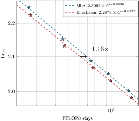
## 5.3 Scaling Law of Kimi Linear
We conducted scaling law experiments on a series of MoE models following the Moonlight [62] architecture. In all experiments, we activated 8 out of 64 experts and utilized the Muon optimizer [62]. Details and hyperparameters are listed in Table 2.
For MLA, following the Chinchilla scaling law methodology [37], we trained five language models of different sizes, carefully tuning their hyperparameters through grid search to ensure optimal performance for each model. For KDA, we maintained the best hybrid ratio of 3:1 as ablated in Table 1. Except for this, we adhered strictly to the MLA training configuration without any modifications. As shown in Figure 5, Kimi Linear achieves ∼ 1 . 16 × computational efficiency compared to the MLA baselines with compute optimal training. We expect that careful hyperparameter tuning will yield superior scaling curves for KDA.
## 5.4 Experimental Setup
Kimi Linear and baselines settings We evaluate our Kimi Linear model against a full-attention MLA baseline and a hybrid Gated DeltaNet (GDN-H) baseline, all of which share the same architecture, parameter count, and training setup for fair comparisons. The model configuration is largely aligned with Moonlight [62], with the key distinction that MoE sparsity is increased to 32. Each model activates 8 out of 256 experts, including one shared expert, resulting in 48 billion total parameters and 3 billion active parameters per forward pass. The first layer is implemented as a dense layer without MoE, ensuring stable training. To evaluate the effectiveness of NoPE in Kimi Linear, we also introduce a hybrid KDA baseline using RoPE with the same model configuration, referred to as Kimi Linear (RoPE).
Evaluation Benchmarks Our evaluation encompasses three primary categories of benchmarks, each designed to assess distinct capabilities of the model:
- Language Understanding and Reasoning : Hellaswag [121], ARC-Challenge [14], Winogrande [83], MMLU [36], TriviaQA [47], MMLU-Redux [26], MMLU-Pro [103], GPQA-Diamond [82], BBH [94], and [105].
- Code Generation : LiveCodeBench v6 4 [44], EvalPlus [60].
- Math & Reasoning : AIME 2025, MATH 500, HMMT 2025, PolyMath-en.
- Long-context : MRCR 5 , RULER [38], Frames [52], HELMET-ICL [118], RepoQA [61], Long Code Arena [13] and LongBench v2 [6].
- Chinese Language Understanding and Reasoning : C-Eval [43], and CMMLU [55].
Evaluation Configurations All models are evaluated using temperature 1.0. For benchmarks with high variance, we report the score of Avg@ k . For base model, We employ perplexity-based evaluation for MMLU, MMLU-Redux, GPQA-Diamond, and C-Eval. Otherwise, generation-based evaluation is adopted. To mitigate the high variance inherent to GPQA-Diamond, we report the mean score across eight independent runs. All evaluations are conducted using our internal framework derived from LM-Harness-Evaluation [10], ensuring consistent settings across all models.
## 5.4.1 Pre-training recipe
Pre-training recipe All models are pretrained using a 4,096-token context window, the MuonClip optimizer, and the WSD learning rate schedule, processing a shared total of 1.4 trillion tokens sampled from the K2 pretraining corpus [50]. The learning rate is set to 1 . 1 × 10 -3 , and the global batch size is fixed at 32 million tokens. They also adopt the same annealing schedule and long-context activation phase established in Kimi K2 [50].
Our final released Kimi Linear checkpoint is pretrained using the same procedure, but with an expanded total of 5.7 trillion tokens to match the pretraining tokens of Moonlight. In addition, the final checkpoint supports a context length of up to 1 million tokens. We compare the performance of Kimi Linear@5.7T and Moonlight in Appendix D
## 5.4.2 Post-training recipe
SFT recipe The SFT dataset extends the Kimi K2 [50] SFT data by incorporating additional reasoning tasks, creating a large-scale instruction-tuning dataset that spans diverse domains with a heavy emphasis on math and coding. We employ a multi-stage SFT approach, initially training the model on a broad range of diverse SFT data for general instruction-following, followed by scheduled targeted training on reasoning-intensive data to enhance the model's reasoning capabilities.
RL recipe For the RL training prompt set, we primarily integrate three data sources: mathematics, code, and STEM. The main purpose of this enhancement is to boost the model's reasoning ability. Before conducting RL, we pre-selected data that matches a moderate difficulty level for the starting checkpoint.
A known risk of RL training is the potential degeneration of general capabilities. To mitigate this, we incorporate the PTX loss [70] during RL, following the practice of K2 [50]. This involves concurrent SFT on a high-quality, distributionally diverse dataset in the RL progress. Our PTX dataset spans both reasoning and general-purpose tasks. All data mentioned above are subsets derived from the training recipe of the K2 model [50].
For the RL algorithm, we use the same algorithm as in K1.5 [95], while introducing several advanced tricks. We noticed that the precision mismatch between training and inference engines may lead to unstable RL learning. Therefore we introduce truncated importance sampling, a method that effectively mitigates the policy mismatch between rollout and training [116]. We also dynamically adjust the KL penalty and the mini batch size ( i.e. , the number of updates per iteration) to make the RL training stable and avoid collapse of entropy [15].
## 5.5 Main results
## 5.5.1 Kimi Linear@1.4T results
Pretrain results We compared our Kimi Linear model against two baselines (MLA and hybrid GDN-H) using a 1.4T pretraining corpus in Table 3. The evaluation focused on three areas: general knowledge, reasoning (math and code), and Chinese tasks. Kimi Linear consistently outperformed both baselines across almost all categories.
4 Questions from 2024.8 to 2025.5
5 https://huggingface.co/datasets/openai/mrcr
- General Knowledge: Kimi Linear scores highest on all of the key benchmarks like BBH, MMLU and HellaSwag.
- Reasoning: It leads in math (GSM8K) and most code tasks (CRUXEval). However, it scores slightly lower on EvalPlus compared to GDN-H.
- Chinese Tasks: Kimi Linear achieves the top scores on CEval and CMMLU.
In summary, Kimi Linear demonstrated the strongest performance, positioning it as a strong alternative to full-attention architectures at short context pretraining.
Table 3: Performance comparison of Kimi Linear with the full-attention MLA baseline and the hybrid GDN baseline, all after the same pretraining recipe. Kimi Linear consistently outperforms both MLA and GDN-H on short-context pretrain evaluations. Best per-column results are bolded .
| | Type Base | MLA | GDN-H | Kimi Linear |
|---------|----------------|-------|---------|---------------|
| | Trained Tokens | 1.4T | 1.4T | 1.4T |
| | HellaSwag | 81.7 | 82.2 | 82.9 |
| | ARC-challenge | 64.6 | 66.5 | 67.3 |
| | Winogrande | 78.1 | 77.9 | 78.6 |
| General | BBH | 71.6 | 70.6 | 72.9 |
| General | MMLU | 71.6 | 72.2 | 73.8 |
| General | MMLU-Pro | 47.2 | 47.9 | 51.0 |
| General | TriviaQA | 68.9 | 70.1 | 71.7 |
| | GSM8K | 83.7 | 81.7 | 83.9 |
| | MATH | 54.7 | 54.1 | 54.7 |
| | EvalPlus | 59.5 | 63.1 | 60.2 |
| | CRUXEval-I-cot | 51.6 | 56.0 | 56.6 |
| | CRUXEval-O-cot | 61.5 | 58.1 | 62.0 |
| Chinese | CEval | 79.3 | 79.1 | 79.5 |
| Chinese | CMMLU | 79.5 | 80.7 | 80.8 |
Table 4: Performance comparison of Kimi Linear with the full-attention MLA baseline and the hybrid GDN baseline, all using the same SFT recipe after pretraining. Kimi Linear consistently outperforms both MLA and GDN-H on short-context instruction-tuned benchmarks. Best per-column results are bolded .
| Type Instruct | MLA | GDN-H | Kimi Linear |
|---------------------------|-------|---------|---------------|
| Trained Tokens | 1.4T | 1.4T | 1.4T |
| BBH | 68.2 | 68.5 | 69.4 |
| MMLU | 75.7 | 75.6 | 77.0 |
| MMLU-Pro | 65.7 | 64.8 | 67.4 |
| MMLU-Redux | 79.2 | 78.7 | 80.3 |
| GPQA-Diamond (Avg@8) | 57.1 | 58.6 | 62.1 |
| LiveBench (Pass@1) | 45.7 | 46.4 | 45.2 |
| AIME 2025 (Avg@64) | 20.6 | 21.1 | 21.3 |
| MATH500 (Acc.) | 80.8 | 83.0 | 81.2 |
| HMMT2025 (Avg@32) | 11.3 | 11.3 | 12.5 |
| PolyMath-en (Avg@4) | 41.3 | 41.5 | 43.6 |
| LiveCodeBench v6 (Pass@1) | 25.1 | 25.4 | 26.0 |
| EvalPlus | 62.6 | 62.5 | 61.0 |
SFT results Kimi Linear demonstrates strong performance across both general and math & code tasks after undergoing the same supervised fine-tuning (SFT) recipe, consistently outperforming MLA and GDN-H. In general tasks, Kimi Linear leads across the board, achieving the top scores on various MMLU benchmarks, BBH, and GPQA-Diamond. In math & code tasks, it surpasses both baselines on difficult benchmarks like AIME 2025, HMMT 2025, PolyMath-en, and LiveCodeBench. Despite some minor exceptions like MATH500 and EvalPlus, Kimi Linear shows robust superiority across the tasks, confirming its clear superiority to the other models tested (GDN-H and MLA).
Table 5: Comparisons of Kimi Linear with MLA, GDN-H, and Kimi Linear (RoPE) across long-context benchmarks. The last column reports the overall average ( ↑ ). All models is trained on 1.4T tokens. Best per-column results are bolded .
| | RULER | MRCR | HELMET-ICL | LongBench V2 | Frames | RepoQA | Long Code Arena | Long Code Arena | Avg. |
|--------------------|---------|--------|--------------|----------------|----------|----------|-------------------|-------------------|--------|
| | | | | | | | Lib | Commit | |
| MLA | 81.3 | 22.6 | 88.0 | 36.1 | 60.5 | 63.0 | 32.8 | 33.2 | 52.2 |
| GDN-H | 80.5 | 23.9 | 85.5 | 32.6 | 58.7 | 63.0 | 34.7 | 30.5 | 51.2 |
| Kimi Linear (RoPE) | 78.8 | 22.0 | 88.0 | 35.4 | 59.9 | 66.5 | 31.3 | 32.5 | 51.8 |
| Kimi Linear | 84.3 | 29.6 | 90.0 | 35.0 | 58.8 | 68.5 | 37.1 | 32.7 | 54.5 |
Figure 6: The training and test accuracy curves for Kimi Linear@1.4T and MLA@1.4T during Math RL training. Kimi Linear consistently outperforms the full attention baseline by a sizable margin during the whole RL process.
<details>
<summary>Image 9 Details</summary>
### Visual Description
## Line Charts: Model Accuracy Comparison
### Overview
The image presents three line charts comparing the accuracy of two models, "MLA@1.4T" and "Kimi Linear@1.4T", across different tasks: "Train", "MATH 500 Test", and "AIME 2025". Each chart plots accuracy against the task or training iterations.
### Components/Axes
**General Chart Elements:**
* **Title:** There is no overall title for the figure.
* **Legend:** Located in the top-left corner of each chart.
* "MLA@1.4T": Represented by a dashed teal line.
* "Kimi Linear@1.4T": Represented by a solid blue-purple line.
**Chart (a): Train**
* **X-axis:** "Train" - Represents the number of training iterations. Scale ranges from approximately 0 to 100, with tick marks at intervals of 20.
* **Y-axis:** "Accuracy" - Represents the accuracy score. Scale ranges from 20 to 65, with tick marks at intervals of 15.
**Chart (b): MATH 500 Test**
* **X-axis:** "MATH 500 Test" - Represents the test iterations. Scale ranges from approximately 0 to 100, with tick marks at intervals of 20.
* **Y-axis:** "Accuracy" - Represents the accuracy score. Scale ranges from 70 to 94, with tick marks at intervals of approximately 8.
**Chart (c): AIME 2025**
* **X-axis:** "AIME 2025" - Represents the test iterations. Scale ranges from approximately 0 to 100, with tick marks at intervals of 20.
* **Y-axis:** "Accuracy" - Represents the accuracy score. Scale ranges from 10 to 25, with tick marks at intervals of 5.
### Detailed Analysis
**Chart (a): Train**
* **MLA@1.4T (dashed teal line):** The accuracy starts at approximately 22 and increases steadily until around 60 training iterations, reaching approximately 48. After 60 iterations, the accuracy plateaus and fluctuates around 50.
* **Kimi Linear@1.4T (solid blue-purple line):** The accuracy starts at approximately 22 and increases steadily throughout the training iterations, reaching approximately 58 at 100 iterations.
**Chart (b): MATH 500 Test**
* **MLA@1.4T (dashed teal line):** The accuracy starts at approximately 77, increases to approximately 85 around 20 iterations, and then fluctuates between 84 and 87 for the remaining iterations.
* **Kimi Linear@1.4T (solid blue-purple line):** The accuracy starts at approximately 72, increases to approximately 86 around 20 iterations, and then fluctuates between 84 and 88 for the remaining iterations.
**Chart (c): AIME 2025**
* **MLA@1.4T (dashed teal line):** The accuracy starts at approximately 11, increases to approximately 20 around 40 iterations, and then fluctuates between 17 and 20 for the remaining iterations.
* **Kimi Linear@1.4T (solid blue-purple line):** The accuracy starts at approximately 11, increases to approximately 22 around 60 iterations, and then fluctuates between 18 and 23 for the remaining iterations.
### Key Observations
* In the "Train" task, "Kimi Linear@1.4T" consistently outperforms "MLA@1.4T" after approximately 40 training iterations.
* In the "MATH 500 Test" task, both models perform similarly, with "Kimi Linear@1.4T" showing slightly higher accuracy overall.
* In the "AIME 2025" task, "Kimi Linear@1.4T" generally outperforms "MLA@1.4T", showing higher peaks and a more volatile accuracy trend.
### Interpretation
The charts suggest that "Kimi Linear@1.4T" generally performs better than "MLA@1.4T" across the three tasks, especially in the "Train" and "AIME 2025" tasks. The "MATH 500 Test" task shows comparable performance between the two models. The increasing accuracy with training iterations in the "Train" task indicates that both models are learning from the data. The fluctuations in accuracy in the "MATH 500 Test" and "AIME 2025" tasks suggest that these tasks are more challenging or that the models are more sensitive to the specific test data.
</details>
Long Context Performance Evaluation We evaluate the long-context performance of Kimi Linear against three baseline models-MLA, GDN-H, and Kimi Linear (RoPE)-across several benchmarks at 128k context length (see Table 5). The results highlight Kimi Linear's clear superiority in these long-context tasks. It consistently outperformed MLA and GDN-H, achieving the highest scores on RULER (84.3) and RepoQA (68.5) by a significant margin. This pattern of outperformance held across most other tasks, except for LongBench V2 and Frames. Overall, Kimi Linear achieved the highest average score (54.5), further reinforcing its effectiveness as a leading attention architecture in long-context scenarios.
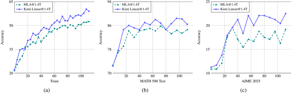
RL results To compare the RL convergence properties of Kimi Linear and MLA, we conduct RLVR using the in-house mathematics training set from [50], and evaluate on mathematics test sets (e.g., AIME 2025, MATH500), while keeping the algorithm and all hyperparameters identical to ensure a fair comparison of performance.
As shown in Figure 6, Kimi Linear demonstrates better efficiency compared to MLA. On the training set, even though both models start at similar points, the growth rate of training accuracy for Kimi Linear is significantly higher than that of MLA, and the gap gradually widens. On the test set, similar phenomena are observed. For example, on MATH500 and AIME2025, Kimi Linear achieves faster and better improvement compared to MLA. Overall, in reasoning-intensive long-form generation under RL, we empirically observe that Kimi Linear performs significantly better than MLA.
Summary of overall findings During the pretraining and SFT stages, a clear performance hierarchy was established: Kimi Linear outperformed GDN-H, which in turn outperformed MLA. However, this hierarchy shifted in long-context evaluations. While Kimi Linear maintained its top position, GDN-H's performance declined, placing it behind MLA. Furthermore, in the RL stage, Kimi Linear also demonstrated superior performance over MLA. Overall, Kimi Linear consistently ranked as the top performer across all stages, establishing itself as a superior alternative to full attention architectures.
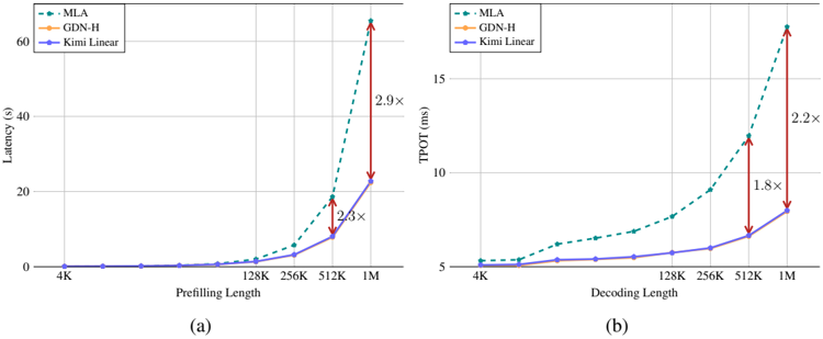
## 5.6 Efficiency Comparison
Prefilling & Decoding speed We compare the training and decoding times for full attention MLA [19], GDN-H, and Kimi Linear in Figure 7a and Figure 7b. Note that all models are based on the Kimi Linear 48B setting, with the same number of layers and attention heads. We observe that: 1) Despite incorporating a more fine-grained decay mechanism, Kimi Linear introduces negligible latency overhead compared to GDN-H during prefilling. As shown in Figure 7a, their
Figure 7: (a) The prefilling time of MLA (full attention), hybrid GDN-H and our Kimi Linear. (b) The time per output token (TPOT) for MLA, GDN-H and Kimi Linear during decoding. (We use batch size = 1 here for tests.)
<details>
<summary>Image 10 Details</summary>
### Visual Description
## Chart Type: Line Graphs Comparing Latency and TPOT
### Overview
The image contains two line graphs comparing the performance of three different models (MLA, GDN-H, and Kimi Linear) in terms of latency and TPOT (likely Throughput Over Time). The left graph (a) shows latency (in seconds) as a function of prefilling length, while the right graph (b) shows TPOT (in milliseconds) as a function of decoding length. Both graphs use a logarithmic scale on the x-axis.
### Components/Axes
**Left Graph (a):**
* **Y-axis:** Latency (s), ranging from 0 to 60 seconds.
* **X-axis:** Prefilling Length, with values 4K, 128K, 256K, 512K, and 1M.
* **Legend (top-left):**
* MLA: Dashed teal line with circular markers.
* GDN-H: Solid orange line with circular markers.
* Kimi Linear: Solid purple line with circular markers.
**Right Graph (b):**
* **Y-axis:** TPOT (ms), ranging from 5 to 15 milliseconds.
* **X-axis:** Decoding Length, with values 4K, 128K, 256K, 512K, and 1M.
* **Legend (top-left):**
* MLA: Dashed teal line with circular markers.
* GDN-H: Solid orange line with circular markers.
* Kimi Linear: Solid purple line with circular markers.
### Detailed Analysis
**Left Graph (a) - Latency vs. Prefilling Length:**
* **MLA (Dashed Teal):** Latency remains near 0 until 128K, then increases sharply.
* 4K: ~0s
* 128K: ~1s
* 256K: ~3s
* 512K: ~10s
* 1M: ~30s
* **GDN-H (Solid Orange):** GDN-H is not visible on the graph, suggesting it has very high latency values.
* **Kimi Linear (Solid Purple):** Latency remains near 0 until 256K, then increases.
* 4K: ~0s
* 128K: ~0s
* 256K: ~0.5s
* 512K: ~4s
* 1M: ~10s
* **Annotations:**
* A red double-arrow indicates the difference between MLA and Kimi Linear at 512K, labeled "2.3x".
* A red double-arrow indicates the difference between MLA and Kimi Linear at 1M, labeled "2.9x".
**Right Graph (b) - TPOT vs. Decoding Length:**
* **MLA (Dashed Teal):** TPOT increases gradually with decoding length.
* 4K: ~5ms
* 128K: ~6ms
* 256K: ~7ms
* 512K: ~9ms
* 1M: ~11ms
* **GDN-H (Solid Orange):** GDN-H is not visible on the graph, suggesting it has very low TPOT values.
* **Kimi Linear (Solid Purple):** TPOT increases gradually with decoding length.
* 4K: ~5ms
* 128K: ~5ms
* 256K: ~5.5ms
* 512K: ~6.5ms
* 1M: ~8ms
* **Annotations:**
* A red double-arrow indicates the difference between MLA and Kimi Linear at 512K, labeled "1.8x".
* A red double-arrow indicates the difference between MLA and Kimi Linear at 1M, labeled "2.2x".
### Key Observations
* In the Latency graph, MLA's latency increases more rapidly than Kimi Linear's as prefilling length increases.
* In the TPOT graph, MLA's TPOT is consistently higher than Kimi Linear's as decoding length increases.
* GDN-H is not visible on either graph, suggesting it has very poor performance in both latency and TPOT.
* The annotations on both graphs highlight the increasing performance gap between MLA and Kimi Linear at higher lengths.
### Interpretation
The data suggests that MLA generally outperforms Kimi Linear in both latency and TPOT, especially at larger prefilling/decoding lengths. The annotations emphasize this performance gap. The absence of GDN-H from the graphs indicates that it is significantly less efficient than both MLA and Kimi Linear, making it an unsuitable choice for these tasks. The logarithmic scale on the x-axis suggests that the performance differences become more pronounced as the input length increases. The "x" values on the red arrows indicate a multiplicative factor, showing how much larger the MLA value is compared to the Kimi Linear value at those specific points.
</details>
performance curves are virtually indistinguishable, confirming that our method maintains high efficiency. The hybrid Kimi Linear model demonstrates a clear efficiency advantage over the MLA baseline as sequence length increases. While its performance is comparable to MLA at shorter lengths (4k-16k), it becomes significantly faster from 128k onwards. This efficiency gap widens dramatically at scale, with Kimi Linear outperforming MLA by a factor of 2 . 3 for 512k sequences and 2 . 9 for 1M sequences. As shown in Figure 1b, Kimi Linear fully demonstrates its advantages during the decoding phase. For decoding at 1M context length, Kimi Linear is 6 × faster than full attention.
## 6 Discussions
## 6.1 Kimi Delta Attention as learnable position embeddings
The standard attention in transformers is by design agnostic to the sequence order of its inputs [99], thus necessitating explicit positional encodings [75, 86]. Among various methods, RoPE [88] has emerged as the de facto standard in modern LLMs due to its effectiveness [98, 1, 19]. The mechanism of multiplicative positional encodings like RoPE can be analyzed through a generalized attention formulation:
$$s _ { t , i } = q _ { t } ^ { \top } \left ( \prod _ { j = i + 1 } ^ { t } R _ { j } \right ) k _ { i } & & ( 1 1 )$$
where the position relationship between the t -th query q t and the i -th key k i is reflected by the cumulative matrix products. RoPE defines the transformation matrix R j as a block diagonal matrix composed of d k / 2 2D rotation matrices R k j = ( cos( jθ k ) -sin( jθ k ) sin( jθ k ) cos( jθ k ) ) with per-2-dimensional angular frequency θ k . Due to the properties of rotation matrices, i.e., R t -i = R ⊤ t R i , absolute positional information R t and R i can be applied separately to q t and k i , which are then transformed into relative positional information t -i encoded as ∏ t j = i +1 R j = ( cos(( t -i ) θ k ) -sin(( t -i ) θ k ) sin(( t -i ) θ k ) cos(( t -i ) θ k ) ) .
Consequently, we show that linear attentions with the gated delta rule can be expressed in a comparable formulation in Eq. 12. Similar forms for other attention variants are summarized in Table 6.
$$o _ { t } = \sum _ { i = 1 } ^ { t } \left ( q _ { t } ^ { \top } \left ( \prod _ { j = i + 1 } ^ { t } A _ { j } \left ( I - \beta _ { j } k _ { j } k _ { j } ^ { \top } \right ) \right ) k _ { j } \right ) v _ { j }$$
From this perspective, GDN can be interpreted as a form of multiplicative positional encoding whose transition matrix is data-dependent, thereby relaxing the orthogonality constraint imposed by RoPE and can be potentially more powerful [115]. 6 This provides a potential solution to the known extrapolation issues of RoPE, whose fixed frequencies can cause overfitting to context lengths seen during training [108, 72]. Some recent works adopt workarounds like partial RoPE
6 When preserving orthogonality, absolute positional encodings can be applied independently to q and k , which are then automatically transformed into relative positional encodings during the attention computation [87].
Table 6: An overview of attention mechanisms in their mathematically equivalent recurrent ( o t ) and parallel ( O ) forms. We omitted the normalization term and β t to achieve a more concise representation. The function ϕ refers to the infinite-dimensional feature space corresponding to the exponential kernel, i.e., ϕ ( q ) ⊤ ϕ ( k ) = exp( q ⊤ k ) .
| | Recurrent form | Parallel form |
|-------------------|-----------------------------------------------------------------------------------------|-----------------------------------------------------------------------------------------|
| SA [99] | t ∑ j =1 exp ( q ⊤ t k j ) v j | ( exp ( QK ⊤ ) ⊙ M ) V |
| SA + RoPE [88] | t ∑ j =1 exp ( q ⊤ t ( t ∏ s = j +1 R s ) k j ) v j | ( exp ( R ( Q ) R ( K ) ⊤ ) ⊙ M ) V |
| LA [101] | t ∑ j =1 ( q ⊤ t k j ) v j | ( QK ⊤ ⊙ M ) V |
| Mamba2 [16] | t ∑ j =1 ( q ⊤ t ( t ∏ s = j +1 α s ) k j ) v j | ( QK ⊤ ⊙A⊙ M ) V |
| GLA [114] | t ∑ j =1 ( q ⊤ t ( t ∏ s = j +1 Diag ( α s ) ) k j ) v j | ( ( Q ⊙ Γ ) ( K Γ ) ⊤ ⊙ M ) V |
| DeltaNet [84] | t ∑ j =1 ( q ⊤ t ( t ∏ s = j +1 ( I - k s k ⊤ s ) ) k j ) v j ( ) | ( QK ⊤ ⊙ M ) ( I + KK ⊤ ⊙ M - ) - 1 V |
| FoX [58] | t ∑ j =1 exp ( q ⊤ t k j ) t ∏ s = j +1 α s v j | ( exp ( QK ⊤ ) ⊙A⊙ M ) V |
| DeltaFormer [125] | t ∑ j =1 ( ϕ ( q t ) ⊤ ( t ∏ s = j +1 ( I - ϕ ( k s ) ϕ ( w s ) ⊤ ) ) ϕ ( k j ) ) v j | ( exp ( QK ⊤ ) ⊙ M ) ( I +exp ( WK ⊤ ) ⊙ M - ) - 1 V |
| PaTH-FoX [115] | t ∑ j =1 exp ( q ⊤ t ( t ∏ s = j +1 ( I - w s w ⊤ s ) ) k j )( t ∏ s = j +1 α s ) v j ) | ( exp ( ( QK ⊤ ⊙ M ) ( I + WW ⊤ ⊙ M - ) - 1 ) ⊙A⊙ M ) V |
| GDN [111] | t ∑ j =1 ( q ⊤ t ( t ∏ s = j +1 α s ( I - k s k ⊤ s ) ) k j v j | ( QK ⊤ ⊙A⊙ M ) ( I + KK ⊤ ⊙A⊙ M - ) - 1 V |
| Comba [40] | t ∑ j =1 ( q ⊤ t ( t ∏ s = j +1 ( α s - k s k ⊤ s ) ) k j ) v j | ( QK ⊤ ⊙A⊙ M ) ( I + KK ⊤ ⊙A i - 1 /j ⊙ M - ) - 1 V |
| RWKV7 [71] | t ∑ j =1 ( q ⊤ t ( t ∏ s = j +1 ( Diag ( α s ) - ( b s ⊙ ˆ k s ) ˆ k ⊤ s ) ) k j ) v j | ( ( Q ⊙ Γ ) ( K Γ ) ⊤ ⊙ M ) ( I + ( ˆ K ⊙ 0 → t - 1 Γ ) ( ˜ K ⊙ B Γ ) ⊤ ⊙ M - 1 ) - 1 V |
| KDA (ours) | t ∑ j =1 ( q ⊤ t ( t ∏ s = j +1 Diag ( α s ) ( I - k s k ⊤ s ) ) k j ) v j | ( ( Q ⊙ Γ ) ( K Γ ) ⊤ ⊙ M )( I +( K ⊙ Γ ) ( K Γ ) ⊤ ⊙ M - 1 ) - 1 V |
[7] or even forgo explicit positional encodings entirely (NoPE) [49, 76, 19]. Given that GDN serves as an analogue role to RoPE, we choose NoPE for global full attention layers (MLA) in our model, allowing positional information to be captured dynamically by our proposed KDA model.
Moreover, a key strength of RoPE is its fine-grained positional encoding, achieved by assigning different rotation frequencies to each pair of dimensions, which functions analogously to a Nonuniform Fourier Transform [7, 41] along the feature dimension. Standard GDN, however, employs a per-head scalar decay and lacks this per-dimensional diversity, which motivates us to propose KDA with a learnable channel-wise gate.
## 6.2 Relation to DPLR
(Gated) DeltaNet can be generalized to a more expressive Diagonal-Plus-Low-Rank (DPLR) structure, defined as D -a t b ⊤ t . This structure was also explored in models such as S4 [30], which employed a static DPLR formulation as the state transition matrix. During computation, this matrix is typically jointly diagonalized into the complex plane, thereby restricting its expressiveness to diagonal transformations [64].
While the DPLR structure introduces richer model interactions and can potentially enhance recall through its key-value update rule, it also suffers from a notable limitation: high computational cost and poor parallelizability. These drawbacks make DPLR inherently slower in large-scale or real-time scenarios, where maintaining parameter efficiency becomes a crucial design challenge.
To address this issue, KDA introduces a constrained variant of DPLR, where Eq. 1 can be rewritten as S t = ( Diag( α t ) -β t k t k ⊤ t Diag( α t ) ) S t -1 + β t k t v ⊤ t with the correspondence between the two given by:
$$S _ { t } = ( D - a _ { t } b _ { t } ^ { \top } ) S _ { t - 1 } + k _ { t } v _ { t } ^ { \top } , s . t . , D = D i a g ( \alpha _ { t } ) , a _ { t } = \beta _ { t } k _ { t } , b _ { t } = k _ { t } \odot \alpha _ { t } .$$
Furthermore, by sharing α t , we can factor it out as in Eq. 1, enabling a fine-grained multiplicative decay over S t in a manner similar to GLA [114], followed by a Householder-style transformation like DeltaNet [84, 112] for efficient
```
""" Kimi Linear: An Expressive, Efficient
```
(a) PyTorch-style pseudo code for chunkwise DPLR.
state updating. We provide a side-by-side comparison of the chunkwise PyTorch-style pseudocode implementations for DPLR and KDA in Listing 8a and Listing 8b.The key improvements are highlighted below:
- Listing 8a Line 13-16 vs., Listing 8b Line 14-15 : the reciprocal of the cumulative decay term 1 / Γ in chunkwise form (Eq. 9) can introduce numerical instability. While we can resolve this issue by secondary chunking [113], it incurs additional computation and I/O overhead. By fixing a = b = k in the DPLR formulation, KDA removes the need for two secondary chunking steps, substantially reducing redundant operations and improving overall efficiency.
- Listing 8a Line 25-27,31-32 vs., Listing 8b Line 26,29 : KDA further eliminates roughly three matrix multiplications during inter-chunk and output computation, leading to significant kernel-level acceleration.
We further benchmark the kernel speed in Fig. 2, showing that KDA achieves nearly 2 × the speed of DPLR for sequence lengths up to 64 k.
## 6.3 Complexity Analysis
Training flops We maintain a similar number of parameters in Kimi Linear as in the full attention MLA. The linear projection calculation remains identical to that of the global attention layer. The key distinction lies in the FLOPs associated with attention computation. For simplicity, we focus on non-variable length scenarios. Based on the implementation of the gated rule kernel, the theoretical FLOPs for a single attention head with headdim d h and a fixed chunk size C = 64 in the gated delta rule [102] (per sequence of length T ) are as follows:
$$\begin{array} { r l } & { F L O P s _ { K D A } ( T ; C , d _ { h } ) = 6 T d _ { h } ^ { 2 } + 3 T C d _ { h } + T C ^ { 2 } . \quad ( 1 3 ) } \end{array}$$
For full (global) attention, the dominant term per head is
$$F L O P s _ { A t t n } ( T ; d _ { h } ) \, = \, 2 T ^ { 2 } d _ { h } . \quad ( 1 4 )$$
Inference strategy and cost The inference strategy in Kimi Linear employs a hybrid approach to optimize both computational and I/O efficiency. During the prefill phase, the model utilizes a FLOP-intensive chunk kernel (see
```
Expressive, Efficient Attention Architecture TECHNICAL REPORT
```
```
mask = torch.triu(torch.ones(BT, BT), diagonal=1)
for i in range(0, NT):
q_i, k_i, u_i, g_i, w_i = (x[:, :, i] for x in (q, k,
-> u, gc, w))
+ o[:,:,i]=(q_i *g_i.exp()) @ S + Aqk @(u_i-w_i @ S)
decay = (g_i[:,:,-1:] - g_i).exp()
S = S * g_i[:, :, -1, :, None].exp()
+ S += (k_i * decay).transpose(-1,-2) @ v_i
return o, S
```
Table 7: An overview of different attention mechanisms through the lens of state updating rules and their learning objective under the TTT framework [90]. We ignore all normalizer terms and activation/kernel functions for brevity.
| | Objective L | Update rule S t = S t - 1 -∇ S t - 1 L |
|---------------|------------------------------------------------------------------------------------------|-----------------------------------------------------------------------|
| LA [48] | - 〈 S ⊤ t - 1 k t , v t 〉 | S t = S t - 1 + k t v ⊤ t |
| RetNet [92] | - β t 〈 S ⊤ t - 1 k t , v t 〉 + 1 2 ∥ ∥ √ 1 - α S t - 1 ∥ ∥ 2 F | S t = α S t - 1 + β t k t v ⊤ t |
| Mamba2 [16] | - β t 〈 S ⊤ t - 1 k t , v t 〉 + 1 2 ∥ ∥ √ 1 - α t S t - 1 ∥ ∥ 2 F | S t = α t S t - 1 + β t k t v ⊤ t |
| GLA [114] | - 〈 S ⊤ t - 1 k t , v t 〉 + 1 2 ∥ ∥ ∥ √ Diag ( 1 - α t ) S t - 1 ∥ ∥ ∥ 2 F | S t = Diag( α t ) S t - 1 + k t v ⊤ t |
| HGRN2 [77] | - 〈 S ⊤ t - 1 ( 1 - α t ) , v t 〉 + 1 2 ∥ ∥ ∥ √ Diag ( 1 - α t ) S t - 1 ∥ ∥ ∥ 2 F | S t = Diag( α t ) S t - 1 +( 1 - α t ) v ⊤ t |
| Longhorn [59] | 1 2 ∥ ∥ S ⊤ t - 1 k t - v t ∥ ∥ 2 Diag( β t ) | S t = ( I - β t 1 + β t k ⊺ t k t k t k ⊺ t ) S t - 1 + β t k t v ⊺ t |
| Comba [40] | β t 2 ∥ ∥ S ⊤ t - 1 k t - v t ∥ ∥ 2 + 1 2 ∥ ∥ √ 1 - α t S t - 1 ∥ ∥ 2 F | S t = ( α t - β t k t ˆ k ⊤ t ) S t - 1 + β t k t v ⊤ t |
| RWKV7 [71] | 1 2 ∥ ∥ ∥ S ⊤ t - 1 ˜ k t - v t ∥ ∥ ∥ 2 + 1 2 ∥ ∥ ∥ √ Diag ( 1 - α t ) S t - 1 ∥ ∥ ∥ 2 F | S t = ( Diag ( α t ) - ( b s ⊙ ˆ k s ) ˆ k ⊤ t ) S t - 1 + k t v ⊤ t |
| GDN [111] | β t 2 ∥ ∥ ∥ ˜ S ⊤ t - 1 k t - v t ∥ ∥ ∥ 2 | S t = ( I - β t k t k ⊤ t ) α t S t - 1 + β t k t v ⊤ t |
| KDA (ours) | β t 2 ∥ ∥ ∥ ˜ S ⊤ t - 1 k t - v t ∥ ∥ ∥ 2 | S t = ( I - β t k t k ⊤ t ) Diag ( α t ) S t - 1 + β t k t v ⊤ t |
For GDN and KDA, the update can be viewed as performing an Stochastic Gradient Descent(SGD) process on the decayed state ˜ S , that is, S t = ˜ S t -1 -∇ ˜ S t -1 L , where ˜ S t -1 is decayed by scalar or fine-grained gate.
§ 3.1), while switching to the more efficient recurrent kernel (Eq. 2) for autoregressive generation. A key advantage of the Linear KDA is its ability to maintain a fixed-sized state ( d k × d v per head, with d k = d v = 128 ) regardless of sequence length. For our hybrid model, as sequence length increases, the I/O-bounded decoding time approaches a maximum hybrid efficiency ratio of 3:1 compared to full attention. This trend is reflected in Fig. 7b, where Kimi Linear achieves a 2 . 3 × speedup at a 1M token context. Additionally, by eliminating the need for a large, linear-scaling KV cache, Kimi Linear is able to reallocate memory resources to support larger batch sizes, enhancing overall throughput. In long-context scenarios (up to 1M tokens), this memory efficiency results in a theoretical decoding speedup of up to 6 . 3 × (see Fig. 1b).
## 7 Related Works
## 7.1 Efficient Subquadratic Attention
The quadratic time complexity of the standard self-attention mechanism [99] remains a fundamental bottleneck for processing long contexts in Transformer-based models. This limitation has become increasingly critical as large language models (LLMs) are now expected to handle million-token sequences for tasks such as agentic tool use and repository-level code analysis [19, 50]. To overcome this challenge, a substantial body of research has explored more efficient attention mechanisms [91, 89], which can broadly be categorized into two main directions: (1) linear attention, and (2) sparse attention.
Linear Attention reformulates the quadratic attention map into kernelized feature interactions, replacing the softmax with a positive feature map so that attention can be computed through two associative matrix products [48]. This eliminates the explicit O ( T 2 ) similarity matrix and enables linear-time computation with respect to sequence length. Subsequent work strengthens the vanilla linear attention significantly through more refined memory control, shifting from data-independent 'decay' [92, 78] to more adaptive, data-dependent mechanisms [29, 93], and refining the decay granularity from coarse headwise [16] to precise, channel-wise decay. GLA generalizes these approaches with diagonal, channel-wise gates that balance expressiveness and efficiency while retaining chunk-wise parallelism [113, 114]. Table 7 summarizes the corresponding update rules. Collectively, these methods cast attention as a compact recurrent memory updated with parallel prefix-scan operators and fused matrix multiplies, aligning well with modern accelerators [42].
A complementary view connects linear attention to fast-weight memory [84]: the state is a low-capacity associative table updated online by Hebbian-like rules [69], while slow weights amortize when to store, update, or forget [68].
In Table 7, we provide a summary of the existing efficient token mixing methods, comparing them from the perspectives of state update mechanisms and optimization objectives.
From this perspective, gating and decay serve as learnable criteria that mitigate interference and stabilize optimization [90]. Despite these advances, linear attention still lags full attention on exact copying and fine-grained selection in extreme long-context retrieval. This motivates hybrid designs (interleaving linear and full attention) and more structured updates. In particular, the gated delta rule used by GDN/KDA introduces rank-1 corrective updates to the fast-weight state, improving targeted retention while remaining parallelizable at the operator level [112].
Linear Attention with Gating Mechanism The vanilla Linear Attention [48] is known to lack the selection mechanism inherent in softmax attention [99], falling short in expressiveness. To address this, Gated Linear Attention models have emerged as memory-efficient and parallelizable alternatives [113, 114, 29]. Instead of storing an everexpanding KV cache, these models employ a fixed-size matrix-valued state and learnable gates to selectively retain and forget information. This design achieves expressive power comparable to softmax attention [65, 125, 64] while maintaining constant time and memory complexity during inference time. The general recurrent formulation of such models for memory update S t ∈ R d k × d v can be expressed as:
$$S _ { t } = A _ { t } S _ { t - 1 } + k _ { t } v _ { t } ^ { \top } , \quad o _ { t } = S _ { t } ^ { \top } q _ { t } .$$
The primary distinction among various gated linear attention mechanisms lies in the parameterization of the forget gate A t , as summarized in Table 7. For instance, RetNet [92] uses a data-independent scalar decay α , and Mamba2 [16] employs a data-dependent scalar α t . Specifically, GLA [114] utilized a diagonalized fine-grained matrix Diag( α t ) ∈ R d k × d k , offering an effective trade-off between efficiency and performance. Other variants are displayed in Table 7.
Sparse Attention A separate body of work reduces the quadratic complexity of standard attention by exploiting its inherent sparsity, approximating the full attention score by performing the computation on a strategically selected subset of tokens. The central challenge lies in identifying this subset effectively without degrading model performance. Early methods often utilized efficient, training-free static patterns, such as sliding and dilated windows [20, 31, 107], or fixed patterns [120, 35], but their rigid structure often compromises model accuracy. More advanced methods determine the important positions based on the context, such as clustering [51, 106] and lightweight routing mechanisms [25, 73, 2, 9], but this dynamic selection process introduces a computational overhead that can prevent them from achieving their full theoretical speedup without dedicated kernel acceleration [21]. Some models further introduce training-free sparsification during the inference stage [107, 109].
Recent approaches to sparse attention have begun to prioritize hardware co-design, as exemplified by NSA [119, 96] and MoBA [63], which both move from token-level to chunk-level selection. In NSA, each query dynamically selects chunks based on scores produced by an MLP. The method's efficiency relies on its use of Grouped-Query Attention (GQA) [98] with a large head count (typically a multiple of 16), a configuration specifically designed to accelerate computation through highly parallelized tensor-matrix multiplications. Similarly, MoBA performs topk chunk selection, but leverages log-sum-exp (LSE) scores computed efficiently via flash-attention kernels [17]. In contrast to NSA and MoBA, the recently proposed DeepSeek-V3.2-Exp Attention (DSA) [18] revives token-level sparsity, maintaining efficiency through a learnable full-attention indexer implemented with low-precision fp8 and a small head dimension for token selection.
Discussion Linear attention and sparse attention represent two distinct pathways toward efficient long-context modeling. Sparse attention tends to retrieve fine-grained historical information more effectively, but this advantage comes at the cost of storing the entire KV cache for token selection, making it less efficient than linear attention models that maintain a constant state. Moreover, sparse attention performs only information selection, and its theoretical expressive upper bound remains that of full attention. In contrast, linear attention, grounded in the principle of 'compression as intelligence', enables generalization with a fixed-size state and, when combined with the Delta learning rule, can achieve theoretically stronger expressive capacity. Although linear attentions have traditionally been criticized for weak retrieval ability, this limitation can be mitigated through state expansion [23, 34, 117, 39] or related techniques. Nevertheless, despite these advantages, linear attention remains limited by current hardware implementations and the absence of optimized inference infrastructure. Our work overcomes these limitations with Kimi Linear, a powerful model integrated with vLLM for efficient inference. Our proposed KDA delivers competitive performance compared to the full-attention baseline (Table 3) and achieves over a 2 × decoding speedup at the one-million-token context (Figure 7b). Despite their distinct approaches to efficient long-context modeling, linear attention and sparse attention are not mutually exclusive. Future work could explore hybrid models that integrate the strengths of both, leveraging the compression and generalization capabilities of linear attention with the fine-grained retrieval advantages of sparse attention to further enhance model performance and efficiency.
## 7.2 Hybrid Model
Despite efficiency, pure Linear Attention still struggle with precise memory retrieval and exact copying [45, 104] This deficiency hinders their adoption in industrial-scale LLMs where robust long-context recall (e.g., beyond 1M tokens) and reliable tool-use over extensive code repositories are critical [50]. Recent work shows that Linear Attention and full attention can effectively complement each other, leading to various hybrid designs.
Intra-layer hybrid One category of hybrid architectures is the intra-layer hybrid, which adaptively fuses the outputs of different mechanisms within each layer. A common implementation fuses outputs from heterogeneous heads within each layer, such as combining standard attention with state space models (SSMs) [22, 56]. In contrast, sequence-level approaches apply distinct mechanisms to different parts of the input. For example, some use linear attention for past context and SWA for recent tokens [123, 54, 67], while NHA [24] compresses the history with GSA [124] and combines it with local sliding window context to emulate a standard attention operation.
Inter-layer Hybrid A key drawback of the intra-layer hybrid is the increased system complexity and inference overhead. The heterogeneous mechanisms require separate computational paths, complicating optimizations like distributed parallelism. To mitigate this challenge, inter-layer hybrids have become a more widely adopted and practical strategy in LLMs [66, 57, 97]. This approach involves stacking distinct layer types, such as full attention and a linear alternative, in a predefined ratio. Building on this paradigm, we implement a simple yet effective strategy: interleaving linear and full attention layers at a fixed 3:1 ratio (see § 5.2 for ablations). This regular, repeating structure simplifies KV cache management and integrates seamlessly with standard optimizations. For the linear component of our hybrid, we deviate from the common practice of using Mamba2 [16]. Instead, we employ KDA, as we found it yields superior overall performance, particularly in retrieval and copying abilities.
Discussion Recent work indicates that hybrid models can be sensitive to adjustments in the RoPE base frequency, a vulnerability that complicates context window extension [126]. This sensitivity can hinder the model's ability to extrapolate to longer sequences. To address this challenge, recent models have trended towards solutions that incorporate No Position Embeddings (NoPE). Falcon-H [126], for example, uses an unconventionally high base frequency (e.g., b ≈ 10 11 ) to push its positional encoding to a near-NoPE state. Architecturally, SwanGPT [76] interleaves RoPE-based layers with NoPE-based full attention layers. Aligning with this direction, we found that hybridizing our KDA layers with NoPE full attention is also a highly effective strategy, facilitating straightforward context window extension.
## Conclusion
We introduce Kimi Linear, a hybrid linear attention architecture designed to meet the efficiency demands of agentic intelligence and test-time scaling without sacrificing quality. Central to Kimi Linear is Kimi Delta Attention (KDA), an advanced linear attention module with a channel-wise gating mechanism that enhances memory control and enables RNN-style models in hybrid architectures. By interleaving KDA with global attention in a 3:1 ratio, Kimi Linear reduces memory usage by up to 75%, while achieving up to 6.3 × higher decoding throughput and outperforming full-attention baselines. Our approach provides a scalable, efficient solution for large language models, with open-source KDA kernels and pre-trained checkpoints facilitating further research.
## References
- [1] Sandhini Agarwal et al. 'gpt-oss-120b & gpt-oss-20b model card'. In: arXiv preprint arXiv:2508.10925 (2025).
- [2] Joshua Ainslie et al. 'Colt5: Faster long-range transformers with conditional computation'. In: arXiv preprint arXiv:2303.09752 (2023).
- [3] Zeyuan Allen-Zhu. 'Physics of Language Models: Part 4.1, Architecture Design and the Magic of Canon Layers'. In: SSRN Electronic Journal (May 2025). Available at SSRN: https://ssrn.com/abstract=5240330 or http://dx.doi.org/10.2139/ssrn.5240330 . DOI: 10.2139/ssrn.5240330 .
- [4] Simran Arora et al. 'Simple linear attention language models balance the recall-throughput tradeoff'. In: Forty-first International Conference on Machine Learning . 2024. URL: https://openreview.net/forum? id=e93ffDcpH3 .
- [5] Simran Arora et al. Zoology: Measuring and Improving Recall in Efficient Language Models . 2023. arXiv: 2312.04927 [cs.CL] .
- [6] Yushi Bai et al. 'Longbench v2: Towards deeper understanding and reasoning on realistic long-context multitasks'. In: arXiv preprint arXiv:2412.15204 (2024).
- [7] Federico Barbero et al. 'Round and Round We Go! What makes Rotary Positional Encodings useful?' In: Proceedings of ICLR . 2025. URL: https://openreview.net/forum?id=GtvuNrk58a .
- [8] Ali Behrouz et al. 'Atlas: Learning to optimally memorize the context at test time'. In: arXiv preprint arXiv:2505.23735 (2025).
- [9] Amanda Bertsch et al. 'Unlimiformer: Long-range transformers with unlimited length input'. In: Advances in NeurIPS 36 (2023), pp. 35522-35543.
- [10] Stella Biderman et al. 'Lessons from the trenches on reproducible evaluation of language models'. In: arXiv preprint arXiv:2405.14782 (2024).
- [11] Christian Bischof and Charles Van Loan. 'The WY Representation for Products of Householder Matrices'. In: SIAM Journal on Scientific and Statistical Computing (1987), s2-s13. URL: https://doi.org/10.1137/ 0908009 .
- [12] Aaron Blakeman et al. 'Nemotron-h: A family of accurate and efficient hybrid mamba-transformer models'. In: arXiv preprint arXiv:2504.03624 (2025).
- [13] Egor Bogomolov et al. 'Long code arena: a set of benchmarks for long-context code models'. In: arXiv preprint arXiv:2406.11612 (2024).
- [14] Peter Clark et al. 'Think you have Solved Question Answering? Try ARC, the AI2 Reasoning Challenge'. In: arXiv:1803.05457v1 (2018).
- [15] Ganqu Cui et al. 'The entropy mechanism of reinforcement learning for reasoning language models'. In: arXiv preprint arXiv:2505.22617 (2025).
- [16] Tri Dao and Albert Gu. 'Transformers are SSMs: Generalized Models and Efficient Algorithms Through Structured State Space Duality'. In: CoRR abs/2405.21060 (2024). DOI: 10.48550/ARXIV.2405.21060 . arXiv: 2405.21060 . URL: https://doi.org/10.48550/arXiv.2405.21060 .
- [17] Tri Dao et al. 'FlashAttention: Fast and Memory-Efficient Exact Attention with IO-Awareness'. In: Advances in NeurIPS . 2022, pp. 16344-16359. URL: https://proceedings.neurips.cc/paper\_files/paper/ 2022/file/67d57c32e20fd0a7a302cb81d36e40d5-Paper-Conference.pdf .
- [18] DeepSeek-AI. DeepSeek-V3.2-Exp: Boosting Long-Context Efficiency with DeepSeek Sparse Attention . 2025.
- [19] DeepSeek-AI et al. DeepSeek-V3 Technical Report . 2025. arXiv: 2412.19437 [cs.CL] . URL: https:// arxiv.org/abs/2412.19437 .
- [20] Jiayu Ding et al. LongNet: Scaling Transformers to 1,000,000,000 Tokens . 2023. arXiv: 2307.02486 [cs.CL] . URL: https://arxiv.org/abs/2307.02486 .
- [21] Juechu Dong et al. Flex Attention: A Programming Model for Generating Optimized Attention Kernels . 2024. arXiv: 2412.05496 [cs.LG] . URL: https://arxiv.org/abs/2412.05496 .
- [22] Xin Dong et al. Hymba: A Hybrid-head Architecture for Small Language Models . 2024. arXiv: 2411.13676 [cs.CL] . URL: https://arxiv.org/abs/2411.13676 .
- [23] Jusen Du et al. 'Mom: Linear sequence modeling with mixture-of-memories'. In: arXiv preprint arXiv:2502.13685 (2025).
- [24] Jusen Du et al. 'Native Hybrid Attention for Efficient Sequence Modeling'. In: arXiv preprint arXiv:2510.07019 (2025).
- [25] Tianyu Fu et al. 'Moa: Mixture of sparse attention for automatic large language model compression'. In: arXiv preprint arXiv:2406.14909 (2024).
- [26] Aryo Pradipta Gema et al. 'Are we done with mmlu?' In: arXiv preprint arXiv:2406.04127 (2024).
- [27] Riccardo Grazzi et al. 'Unlocking State-Tracking in Linear RNNs Through Negative Eigenvalues'. In: Proceedings of ICLR . 2025. URL: https://openreview.net/forum?id=UvTo3tVBk2 .
- [28] Joseph F. Grcar. 'How ordinary elimination became Gaussian elimination'. In: Historia Mathematica 38.2 (May 2011), pp. 163-218. ISSN: 0315-0860. DOI: 10.1016/j.hm.2010.06.003 . URL: http://dx.doi. org/10.1016/j.hm.2010.06.003 .
- [29] Albert Gu and Tri Dao. Mamba: Linear-Time Sequence Modeling with Selective State Spaces . 2023. arXiv: 2312.00752 [cs.LG] .
- [30] Albert Gu, Karan Goel, and Christopher Ré. Efficiently Modeling Long Sequences with Structured State Spaces . 2022. arXiv: 2111.00396 [cs.LG] .
- [31] Xiangming Gu et al. When Attention Sink Emerges in Language Models: An Empirical View . 2025. arXiv: 2410.10781 [cs.CL] . URL: https://arxiv.org/abs/2410.10781 .
- [32] Yuxian Gu et al. Jet-Nemotron: Efficient Language Model with Post Neural Architecture Search . 2025. arXiv: 2508.15884 [cs.CL] . URL: https://arxiv.org/abs/2508.15884 .
- [33] Daya Guo et al. 'DeepSeek-R1 incentivizes reasoning in LLMs through reinforcement learning'. In: Nature 645.8081 (2025), pp. 633-638.
- [34] Han Guo et al. 'Log-linear attention'. In: arXiv preprint arXiv:2506.04761 (2025).
- [35] Qipeng Guo et al. 'Star-transformer'. In: arXiv preprint arXiv:1902.09113 (2019).
- [36] Dan Hendrycks et al. Measuring Massive Multitask Language Understanding . 2021. arXiv: 2009.03300 [cs.CY] . URL: https://arxiv.org/abs/2009.03300 .
- [37] Jordan Hoffmann et al. Training Compute-Optimal Large Language Models . 2022. arXiv: 2203.15556 [cs.CL] . URL: https://arxiv.org/abs/2203.15556 .
- [38] Cheng-Ping Hsieh et al. 'RULER: What's the Real Context Size of Your Long-Context Language Models?' In: arXiv preprint arXiv:2404.06654 (2024).
- [39] Jiaxi Hu et al. 'Attractor memory for long-term time series forecasting: A chaos perspective'. In: Advances in NeurIPS 37 (2024), pp. 20786-20818.
- [40] Jiaxi Hu et al. 'Comba: Improving Nonlinear RNNs with Closed-loop Control'. In: arXiv preprint arXiv:2506.02475 (2025).
- [41] Ermo Hua et al. 'Fourier Position Embedding: Enhancing Attention's Periodic Extension for Length Generalization'. In: arXiv preprint arXiv:2412.17739 (2024).
- [42] Weizhe Hua et al. 'Transformer Quality in Linear Time'. In: Proceedings of ICML . Ed. by Kamalika Chaudhuri et al. PMLR, 2022, pp. 9099-9117. URL: https://proceedings.mlr.press/v162/hua22a.html .
- [43] Yuzhen Huang et al. 'C-eval: A multi-level multi-discipline chinese evaluation suite for foundation models'. In: Advances in NeurIPS 36 (2023), pp. 62991-63010.
- [44] Naman Jain et al. 'Livecodebench: Holistic and contamination free evaluation of large language models for code'. In: arXiv preprint arXiv:2403.07974 (2024).
- [45] Samy Jelassi et al. Repeat After Me: Transformers are Better than State Space Models at Copying . 2024. arXiv: 2402.01032 [cs.LG] .
- [46] Thierry Joffrain et al. 'Accumulating Householder transformations, revisited'. In: (2006), pp. 169-179. URL: https://doi.org/10.1145/1141885.1141886 .
- [47] Mandar Joshi et al. 'Triviaqa: A large scale distantly supervised challenge dataset for reading comprehension'. In: arXiv preprint arXiv:1705.03551 (2017).
- [48] Angelos Katharopoulos et al. 'Transformers are RNNs: Fast Autoregressive Transformers with Linear Attention'. In: Proceedings of ICML . Ed. by Hal Daumé III and Aarti Singh. PMLR, 2020, pp. 5156-5165. URL: https://proceedings.mlr.press/v119/katharopoulos20a.html .
- [49] Amirhossein Kazemnejad et al. 'The impact of positional encoding on length generalization in transformers'. In: Advances in NeurIPS 36 (2023), pp. 24892-24928.
- [50] Team Kimi et al. 'Kimi k2: Open agentic intelligence'. In: arXiv preprint arXiv:2507.20534 (2025).
- [51] Nikita Kitaev, Łukasz Kaiser, and Anselm Levskaya. 'Reformer: The efficient transformer'. In: arXiv preprint arXiv:2001.04451 (2020).
- [52] Satyapriya Krishna et al. 'Fact, fetch, and reason: A unified evaluation of retrieval-augmented generation'. In: arXiv preprint arXiv:2409.12941 (2024).
- [53] Hanyu Lai et al. 'A Survey of Post-Training Scaling in Large Language Models'. In: Proceedings of the 63rd Annual Meeting of the Association for Computational Linguistics (Volume 1: Long Papers) . 2025, pp. 27712791.
- [54] Disen Lan et al. 'Liger: Linearizing Large Language Models to Gated Recurrent Structures'. In: arXiv preprint arXiv:2503.01496 (2025).
- [55] Haonan Li et al. 'CMMLU: Measuring massive multitask language understanding in Chinese'. In: Findings of the Association for Computational Linguistics: ACL 2024 . Ed. by Lun-Wei Ku, Andre Martins, and Vivek Srikumar. Bangkok, Thailand: Association for Computational Linguistics, Aug. 2024, pp. 11260-11285. DOI: 10.18653/v1/2024.findings-acl.671 . URL: https://aclanthology.org/2024.findingsacl.671/ .
- [56] Yixing Li et al. 'Transmamba: Flexibly switching between transformer and mamba'. In: arXiv preprint arXiv:2503.24067 (2025).
- [57] Opher Lieber et al. Jamba: A Hybrid Transformer-Mamba Language Model . 2024. arXiv: 2403.19887 [cs.CL] .
- [58] Zhixuan Lin et al. 'Forgetting transformer: Softmax attention with a forget gate'. In: arXiv preprint arXiv:2503.02130 (2025).
- [59] Bo Liu et al. 'Longhorn: State Space Models are Amortized Online Learners'. In: ArXiv abs/2407.14207 (2024). URL: https://api.semanticscholar.org/CorpusID:271310065 .
- [60] Jiawei Liu et al. 'Is Your Code Generated by ChatGPT Really Correct? Rigorous Evaluation of Large Language Models for Code Generation'. In: Thirty-seventh Conference on NeurIPS . 2023. URL: https://openreview. net/forum?id=1qvx610Cu7 .
- [61] Jiawei Liu et al. 'Repoqa: Evaluating long context code understanding'. In: arXiv preprint arXiv:2406.06025 (2024).
- [62] Jingyuan Liu et al. Muon is Scalable for LLM Training . 2025. arXiv: 2502.16982 [cs.LG] . URL: https: //arxiv.org/abs/2502.16982 .
- [63] Enzhe Lu et al. MoBA: Mixture of Block Attention for Long-Context LLMs . 2025. arXiv: 2502.13189 [cs.LG] . URL: https://arxiv.org/abs/2502.13189 .
- [64] William Merrill, Jackson Petty, and Ashish Sabharwal. 'The illusion of state in state-space models'. In: arXiv preprint arXiv:2404.08819 (2024).
- [65] William Merrill and Ashish Sabharwal. 'The Parallelism Tradeoff: Limitations of Log-Precision Transformers'. In: Transactions of the Association for Computational Linguistics 11 (2023), pp. 531-545. DOI: 10.1162/ tacl\_a\_00562 . URL: https://aclanthology.org/2023.tacl-1.31/ .
- [66] MiniMax et al. MiniMax-01: Scaling Foundation Models with Lightning Attention . 2025. arXiv: 2501.08313 [cs.CL] .
- [67] Tsendsuren Munkhdalai, Manaal Faruqui, and Siddharth Gopal. Leave No Context Behind: Efficient Infinite Context Transformers with Infini-attention . 2024. arXiv: 2404.07143 [cs.CL] .
- [68] Tsendsuren Munkhdalai and Adam Trischler. Metalearning with Hebbian Fast Weights . 2018. arXiv: 1807. 05076 [cs.NE] . URL: https://arxiv.org/abs/1807.05076 .
- [69] Tsendsuren Munkhdalai et al. 'Metalearned Neural Memory'. In: ArXiv abs/1907.09720 (2019). URL: https: //api.semanticscholar.org/CorpusID:198179407 .
- [70] Long Ouyang et al. 'Training language models to follow instructions with human feedback'. In: Advances in NeurIPS 35 (2022), pp. 27730-27744.
- [71] Bo Peng et al. RWKV-7 "Goose" with Expressive Dynamic State Evolution . 2025. arXiv: 2503.14456 [cs.CL] .
- [72] Bowen Peng et al. 'Yarn: Efficient context window extension of large language models'. In: arXiv preprint arXiv:2309.00071 (2023).
- [73] Piotr Pi˛ ekos, Róbert Csordás, and Jürgen Schmidhuber. 'Mixture of Sparse Attention: Content-Based Learnable Sparse Attention via Expert-Choice Routing'. In: arXiv preprint arXiv:2505.00315 (2025).
- [74] Aske Plaat et al. 'Reasoning with large language models, a survey'. In: CoRR (2024).
- [75] Ofir Press, Noah Smith, and Mike Lewis. 'Train Short, Test Long: Attention with Linear Biases Enables Input Length Extrapolation'. In: Proceedings of ICLR . 2022. URL: https://openreview.net/forum?id= R8sQPpGCv0 .
- [76] Krishna C. Puvvada et al. SWAN-GPT: An Efficient and Scalable Approach for Long-Context Language Modeling . 2025. arXiv: 2504.08719 [cs.CL] .
- [77] Zhen Qin et al. HGRN2: Gated Linear RNNs with State Expansion . 2024. arXiv: 2404.07904 [cs.CL] .
- [78] Zhen Qin et al. TransNormerLLM: A Faster and Better Large Language Model with Improved TransNormer . 2024. arXiv: 2307.14995 [cs.CL] .
- [79] Zihan Qiu et al. Gated Attention for Large Language Models: Non-linearity, Sparsity, and Attention-Sink-Free . 2025. arXiv: 2505.06708 [cs.CL] .
- [80] Xiaoye Qu et al. 'A survey of efficient reasoning for large reasoning models: Language, multimodality, and beyond'. In: arXiv preprint arXiv:2503.21614 (2025).
- [81] Qwen Team. Qwen3-Next: Towards Ultimate Training & Inference Efficiency . Accessed: 2025-10-27. Sept. 2025.
- [82] David Rein et al. 'Gpqa: A graduate-level google-proof q&a benchmark'. In: First Conference on Language Modeling . 2024.
- [83] Keisuke Sakaguchi et al. WinoGrande: An Adversarial Winograd Schema Challenge at Scale . 2019. arXiv: 1907.10641 [cs.CL] . URL: https://arxiv.org/abs/1907.10641 .
- [84] Imanol Schlag, Kazuki Irie, and Jürgen Schmidhuber. 'Linear Transformers Are Secretly Fast Weight Programmers'. In: Proceedings of ICML . Ed. by Marina Meila and Tong Zhang. PMLR, 2021, pp. 9355-9366. URL: https://proceedings.mlr.press/v139/schlag21a.html .
- [85] Imanol Schlag, Tsendsuren Munkhdalai, and Jürgen Schmidhuber. Learning Associative Inference Using Fast Weight Memory . 2021. arXiv: 2011.07831 [cs.LG] . URL: https://arxiv.org/abs/2011.07831 .
- [86] Peter Shaw, Jakob Uszkoreit, and Ashish Vaswani. Self-Attention with Relative Position Representations . 2018. arXiv: 1803.02155 [cs.CL] .
- [87] Jianlin Su. Linear Attention: A Brief History of Imitation, Innovation, and Feedback . June 2025. URL: https: //kexue.fm/archives/11033 .
- [88] Jianlin Su et al. 'Roformer: Enhanced transformer with rotary position embedding'. In: Neurocomputing 568 (2024), p. 127063.
- [89] Weigao Sun et al. Speed Always Wins: A Survey on Efficient Architectures for Large Language Models . 2025. arXiv: 2508.09834 [cs.CL] . URL: https://arxiv.org/abs/2508.09834 .
- [90] Yu Sun et al. 'Learning to (Learn at Test Time): RNNs with Expressive Hidden States'. In: ArXiv abs/2407.04620 (2024). URL: https://api.semanticscholar.org/CorpusID:271039606 .
- [91] Yutao Sun et al. 'Efficient attention mechanisms for large language models: A survey'. In: arXiv preprint arXiv:2507.19595 (2025).
- [92] Yutao Sun et al. Retentive Network: A Successor to Transformer for Large Language Models . 2023. arXiv: 2307.08621 [cs.CL] .
- [93] Yutao Sun et al. You Only Cache Once: Decoder-Decoder Architectures for Language Models . 2024. arXiv: 2405.05254 [cs.CL] . URL: https://arxiv.org/abs/2405.05254 .
- [94] Mirac Suzgun et al. 'Challenging big-bench tasks and whether chain-of-thought can solve them'. In: arXiv preprint arXiv:2210.09261 (2022).
- [95] Kimi Team et al. Kimi k1.5: Scaling Reinforcement Learning with LLMs . 2025. arXiv: 2501.12599 [cs.AI] . URL: https://arxiv.org/abs/2501.12599 .
- [96] MiniCPM Team et al. MiniCPM4: Ultra-Efficient LLMs on End Devices . 2025. arXiv: 2506.07900 [cs.CL] . URL: https://arxiv.org/abs/2506.07900 .
- [97] Tencent Hunyuan Team et al. 'Hunyuan-turbos: Advancing large language models through mamba-transformer synergy and adaptive chain-of-thought'. In: arXiv preprint arXiv:2505.15431 (2025).
- [98] Hugo Touvron et al. LLaMA: Open and Efficient Foundation Language Models . 2023. arXiv: 2302.13971 [cs.CL] .
- [99] Ashish Vaswani et al. 'Attention is All you Need'. In: Advances in NeurIPS . Ed. by I. Guyon et al. Curran Associates, Inc., 2017. URL: https://proceedings.neurips.cc/paper\_files/paper/2017/file/ 3f5ee243547dee91fbd053c1c4a845aa-Paper.pdf .
- [100] Roger Waleffe et al. An Empirical Study of Mamba-based Language Models . 2024. arXiv: 2406.07887 [cs.LG] . URL: https://arxiv.org/abs/2406.07887 .
- [101] Sinong Wang et al. Linformer: Self-Attention with Linear Complexity . 2020. arXiv: 2006.04768 [cs.LG] .
- [102] Yaoyu Wang. Understanding DeltaNet from the Perspective of Inference Frameworks . May 2025. URL: https: //yywangcs.notion.site/DeltaNet-1fefc9f5d80580a496f8eb406a496f09 .
- [103] Yubo Wang et al. 'Mmlu-pro: A more robust and challenging multi-task language understanding benchmark'. In: Advances in NeurIPS 37 (2024), pp. 95266-95290.
- [104] Kaiyue Wen, Xingyu Dang, and Kaifeng Lyu. 'Rnns are not transformers (yet): The key bottleneck on in-context retrieval'. In: arXiv preprint arXiv:2402.18510 (2024).
- [105] Colin White et al. 'Livebench: A challenging, contamination-free llm benchmark'. In: arXiv preprint arXiv:2406.19314 4 (2024).
- [106] Yuhuai Wu et al. 'Memorizing transformers'. In: arXiv preprint arXiv:2203.08913 (2022).
- [107] Guangxuan Xiao et al. 'Efficient streaming language models with attention sinks'. In: arXiv preprint arXiv:2309.17453 (2023).
- [108] Wenhan Xiong et al. Effective Long-Context Scaling of Foundation Models . 2023. arXiv: 2309.16039 [cs.CL] . URL: https://arxiv.org/abs/2309.16039 .
- [109] Ruyi Xu et al. 'Xattention: Block sparse attention with antidiagonal scoring'. In: arXiv preprint arXiv:2503.16428 (2025).
- [110] Bowen Yang et al. Rope to Nope and Back Again: A New Hybrid Attention Strategy . 2025. arXiv: 2501.18795 [cs.CL] . URL: https://arxiv.org/abs/2501.18795 .
- [111] Songlin Yang, Jan Kautz, and Ali Hatamizadeh. 'Gated Delta Networks: Improving Mamba2 with Delta Rule'. In: Proceedings of ICLR . 2025. URL: https://openreview.net/forum?id=r8H7xhYPwz .
- [112] Songlin Yang and Bailin Wang. 'Parallelizing Linear Transformers with the Delta Rule over Sequence Length'. In: ArXiv abs/2406.06484 (2024). URL: https://api.semanticscholar.org/CorpusID:270371554 .
- [113] Songlin Yang and Yu Zhang. FLA: A Triton-Based Library for Hardware-Efficient Implementations of Linear Attention Mechanism . 2024. URL: https://github.com/fla-org/flash-linear-attention .
- [114] Songlin Yang et al. 'Gated Linear Attention Transformers with Hardware-Efficient Training'. In: Proceedings of ICML . PMLR, 2024.
- [115] Songlin Yang et al. 'PaTH Attention: Position Encoding via Accumulating Householder Transformations'. In: arXiv preprint arXiv:2505.16381 (2025).
- [116] Feng Yao et al. Your Efficient RL Framework Secretly Brings You Off-Policy RL Training . Aug. 2025. URL: https://fengyao.notion.site/off-policy-rl .
- [117] Morris Yau et al. 'Sequential-Parallel Duality in Prefix Scannable Models'. In: arXiv preprint arXiv:2506.10918 (2025).
- [118] Howard Yen et al. 'HELMET: How to Evaluate Long-Context Language Models Effectively and Thoroughly'. In: International Conference on Learning Representations (ICLR) . 2025.
- [119] Jingyang Yuan et al. Native Sparse Attention: Hardware-Aligned and Natively Trainable Sparse Attention . 2025. arXiv: 2502.11089 [cs.CL] . URL: https://arxiv.org/abs/2502.11089 .
- [120] Manzil Zaheer et al. 'Big bird: Transformers for longer sequences'. In: Advances in NeurIPS 33 (2020), pp. 17283-17297.
- [121] Rowan Zellers et al. 'HellaSwag: Can a Machine Really Finish Your Sentence?' In: Proceedings of the 57th Annual Meeting of the Association for Computational Linguistics . 2019.
- [122] Biao Zhang and Rico Sennrich. 'Root mean square layer normalization'. In: Advances in NeurIPS 32 (2019).
- [123] Michael Zhang et al. 'Lolcats: On low-rank linearizing of large language models'. In: arXiv preprint arXiv:2410.10254 (2024).
- [124] Yu Zhang et al. Gated Slot Attention for Efficient Linear-Time Sequence Modeling . 2024. arXiv: 2409.07146 [cs.CL] .
- [125] Shu Zhong et al. 'Understanding Transformer from the Perspective of Associative Memory'. In: arXiv preprint arXiv:2505.19488 (2025).
- [126] Jingwei Zuo et al. Falcon-H1: A Family of Hybrid-Head Language Models Redefining Efficiency and Performance . 2025. arXiv: 2507.22448 [cs.CL] . URL: https://arxiv.org/abs/2507.22448 .
## A Contributions
The authors are listed in order of the significance of their contributions, with those in project leadership roles appearing last. The project is developed at Moonshot AI, with several external collaborators that are marked with #. Names marked with an asterisk (*) indicate people who are no longer part of our team.
| Yu Zhang 1 | Junjie Yan |
|-----------------|---------------|
| Zongyu Lin ∗ | Zhejun Jiang |
| Xingcheng Yao | Weixiao Huang |
| Jiaxi Hu 2 | Bohong Yin |
| Fanqing Meng | Jiacheng You |
| Chengyin Liu | Chu Wei |
| Xin Men | Zhengtao Wang |
| Songlin Yang #3 | Chao Hong |
| Zhiyuan Li | Yutian Chen |
| Wentao Li | Guanduo Chen |
| Enzhe Lu | Yucheng Wang |
| Weizhou Liu | Huabin Zheng |
| Yanru Chen | Feng Wang |
| Weixin Xu | Yibo Liu |
| Longhui Yu | Mengnan Dong |
| Yejie Wang | Zheng Zhang |
| Yu Fan | Siyuan Pan |
| Longguang Zhong | Wenhao Wu |
| Enming Yuan | Yuhao Wu |
| Dehao Zhang | Longyu Guan |
| Yizhi Zhang | Jiawen Tao |
| T.Y. Liu | Guohong Fu #1 |
| Haiming Wang | Xinran Xu |
| Shengjun Fang | Yuzhi Wang |
| Weiran He | Guokun Lai |
| Shaowei Liu | Yuxin Wu |
| Yiwei Li | Xinyu Zhou |
| Jianlin Su | Zhilin Yang |
| Jiezhong Qiu 4 | Yulun Du |
| Bo Pang | |
<details>
<summary>Image 11 Details</summary>

### Visual Description
Icon/Small Image (21x21)
</details>
## B Derivations for Chunkwise Parallelism of KDA
We first recall the recurrent form of KDA:
$$S _ { [ t ] } ^ { r } & = \underbrace { \left ( \prod _ { i = 1 } ^ { r } \left ( I - \beta _ { [ t ] } ^ { i } k _ { [ t ] } ^ { i } k _ { [ t ] } ^ { i \top } \right ) D i a g ( \alpha _ { [ t ] } ^ { i } ) \right ) } _ { \colon = P _ { [ t ] } ^ { r } } \cdot S _ { [ t ] } ^ { 0 } + \underbrace { \sum _ { i = 1 } ^ { r } \left ( \prod _ { j = i + 1 } ^ { r } \left ( I - \beta _ { [ t ] } ^ { j } k _ { [ t ] } ^ { j } k _ { [ t ] } ^ { j \top } \right ) D i a g ( \alpha _ { [ t ] } ^ { j } ) \right ) \cdot \beta _ { [ t ] } ^ { i } k _ { [ t ] } ^ { i } v _ { [ t ] } ^ { i \top } } _ { \colon = H _ { [ t ] } ^ { r } }$$
Our goal is to transform P r [ t ] and H r [ t ] into matrix forms suitable for parallel computation.
We show that P r [ t ] , which involves the cumulative product of generalized Householder matrices, can be optimized using the classic WY representation.
Proposition 1. The matrix P r [ t ] can be expressed as:
$$P _ { [ t ] } ^ { r } = \text {diag} ( \gamma _ { [ t ] } ^ { r } ) - \sum _ { i = 1 } ^ { r } \text {diag} ( \gamma _ { [ t ] } ^ { i \rightarrow r } ) k _ { [ t ] } ^ { i } w _ { [ t ] } ^ { i \top }$$
where the auxiliary vector w r [ t ] ∈ R d k is computed via the following recurrence relation:
$$w _ { [ t ] } ^ { r } = \beta _ { [ t ] } ^ { r } \left ( D i a g ( \gamma _ { [ t ] } ^ { r } ) k _ { [ t ] } ^ { r } - \sum _ { i = 1 } ^ { r - 1 } w _ { [ t ] } ^ { i } \left ( k _ { [ t ] } ^ { i \top } D i a g \left ( \gamma _ { [ t ] } ^ { i \rightarrow r } \right ) k _ { [ t ] } ^ { r } \right ) \right ) \quad ( 1 7 )$$
Proof. We proceed with a proof by mathematical induction.
Inductive Step: Assume the proposition holds for r -1 , i.e., P r -1 [ t ] = Diag( γ r -1 [ t ] ) -∑ r -1 i =1 Diag( γ i → r -1 [ t ] ) k i [ t ] w i ⊤ [ t ] . We now derive:
<!-- formula-not-decoded -->
The inductive step holds.
Similar to P r [ t ] , H r [ t ] can also be expressed in a parallelizable form.
■
Proposition 2. The matrix H r [ t ] can be expressed as:
$$H _ { [ t ] } ^ { r } = \sum _ { i = 1 } ^ { r } D i a g \left ( \gamma _ { [ t ] } ^ { i \rightarrow r } \right ) k _ { [ t ] } ^ { i } u _ { [ t ] } ^ { i \top }$$
where the auxiliary vector u r [ t ] ∈ R d v is computed via the following recurrence relation:
$$\pm b { u } ^ { r } _ { [ t ] } = \beta ^ { r } _ { [ t ] } \left ( v ^ { r } _ { [ t ] } - \sum _ { i = 1 } ^ { r - 1 } u ^ { i } _ { [ t ] } \left ( k ^ { i \top } _ { [ t ] } \text {diag} \left ( \gamma ^ { i \to r } _ { [ t ] } \right ) k ^ { r } _ { [ t ] } \right ) \right )$$
Proof. We again use mathematical induction.
Inductive Step: Assume the proposition holds for r -1 .
<!-- formula-not-decoded -->
The inductive step holds.
■
## C Pseudo Code for chunkwise KDA
```
```
Listing 1: Pseudo PyTorch-style code snippet for KDA chunked form.
## D Kimi Linear@5.7T results
Following Moonlight, we also trained Kimi Linear with an extended 5.7T token dataset to demonstrate its effectiveness. With 3 × sparsity and a new attention architecture design, Kimi Linear consistently outperforms Moonlight across nearly all benchmarks, underscoring the efficacy of the new architecture. The results are shown in Table 8 for base model and Table 9 for instruction tuned model. Moonlight-Instruct was not evaluated ('-') on tasks exceeding its 8K context limit.
Kimi Linear@5.7T obtains a score of 94.8 on RULER at 1M context length. This long context performance reinforces that Kimi Linear is a promising alternative to full-attention architectures, delivering comparable or superior results while potentially offering more efficient resource utilization.
Table 8: Performance of Kimi-Linear-Base and Moonlight-Base across diverse tasks.
| Benchmark | #Shots | Kimi-Linear-Base | Moonlight-Base |
|----------------------|----------|--------------------|------------------|
| Architecture | - - | MoE | MoE 3B |
| # Activated Params | | 3B | |
| # Total Params | - | 48B | 16B |
| Trained Tokens | - | 5.7T | 5.7T |
| TriviaQA | 5-shots | 75.2 | 66.2 |
| SimpleQA | 5-shots | 10.1 | 05.6 |
| MMLU-Pro | 5-shots | 54.8 | 42.4 |
| MMLU-redux | 5-shots | 79.7 | 73.8 |
| WinoGrande | 5-shots | 81.5 | 74.6 |
| GPQA-Diamond (avg@8) | 5-shots | 40.4 | 35.2 |
| MATH | 4-shots | 58.5 | 45.3 |
| GSM8k | 8-shots | 86.3 | 77.2 |
| GSM8k-platinum | 8-shots | 89.6 | 79.4 |
| CMATH | 6-shots | 85.5 | 79.6 |
| CRUXEval-I-cot | 0-shots | 61.0 | 45.9 |
| CRUXEval-O-cot | 0-shots | 67.0 | 46.6 |
| LiveCodeBench (v6) | 1-shots | 20.0 | 14.3 |
| EvalPlus | - | 64.9 | 50.3 |
| C-Eval | 5-shots | 83.3 | 77.6 |
| CSimpleQA | 5-shots | 53.5 | 34.7 |
Table 9: Performance of Kimi-Linear-Instruct and Moonlight-Instruct across diverse tasks.
| Benchmark | Kimi-Linear-Instruct | Moonlight-Instruct |
|---------------------------|------------------------|----------------------|
| Architecture | MoE | MoE |
| # Activated Params | 3B | 3B |
| # Total Params | 48B | 16B |
| Trained Tokens | 5.7T | 5.7T |
| RULER@128k | 95.4 | - |
| RULER@1M | 94.8 | - |
| GPQA-Diamond (Avg@8) | 71.7 | 24.7 |
| MMLU-Redux (EM) | 86.9 | 66.9 |
| MMLU-Pro (EM) | 72.7 | 43.8 |
| FaithJudge (1-Hallu.) | 64.2 | 56.0 |
| AIME 2025 (Avg@64) | 58.6 | - |
| MATH500 (Acc.) | 94.6 | 58.0 |
| HMMT2025 (Avg@32) | 44.5 | - |
| LiveCodeBench v6 (Pass@1) | 45.7 | 11.9 |
| OJBench (Pass@1) | 14.2 | - |
| Humaneval + | 70.9 | 46.3 |
| MBPP + | 72.4 | 56.3 |