2511.01815

# ArXiv Paper 2511.01815v1 <details> <summary>Image 1 Details</summary>  ### Visual Description Icon/Small Image (181x39) </details> ## KV Cache Transform Coding for Compact Storage in LLM Inference Konrad Staniszewski & Adrian Łańcucki NVIDIA kstaniszewsk@nvidia.com Serving large language models (LLMs) at scale necessitates efficient key-value (KV) cache management. KV caches can be reused across conversation turns via shared-prefix prompts that are common in iterative code editing and chat. However, stale caches consume scarce GPU memory, require offloading, or force recomputation. We present kvtc , a lightweight transform coder that compresses KV caches for compact on-GPU and off-GPU storage. Drawing on classical media compression, kvtc combines PCA-based feature decorrelation, adaptive quantization, and entropy coding. It requires only a brief initial calibration and leaves model parameters unchanged. By exploiting redundancies in KV caches, kvtc achieves up to 20 × compression while maintaining reasoning and long-context accuracy, and 40 × or higher for specific use cases. We test kvtc with Llama 3, Mistral NeMo, and R1-Qwen 2.5 models across benchmarks including AIME25, LiveCodeBench, GSM8K, MMLU, Qasper, RULER, and MATH-500. It consistently outperforms inference-time baselines such as token eviction, quantization, and SVD-based methods, while achieving higher compression ratios. These results support kvtc as a practical building block for memory-efficient LLM serving with reusable KV caches. ## 1. Introduction Chat-based interfaces, commonly used for interacting with large language models (LLMs), enable users to iteratively refine answers across open-domain dialogues and specialized tasks, such as code generation (Chiang et al., 2024; Köpf et al., 2023). Each conversational turn extends the key-value (KV) cache associated with a conversation, storing hidden activations for every previous token. For modern Transformer models, this cache can easily occupy multiple gigabytes. As models scale up in size and reasoning capability, generating increasingly long reasoning chains (OpenAI et al., 2024), the KV cache footprint increases, posing a significant bottleneck for throughput and latency. During user turns, stale KV caches left on-chip occupy memory, which is needed for serving other users, yet ensure the fastest responses in the future. Conversely, caches could be discarded, incurring the cost of recomputation, or offloaded to CPU DRAM or local/network storage, leading to transfer overheads. This tension creates a latency-throughput dilemma in production systems and necessitates careful configuration. Crucially, inference frameworks view the local KV caches as databases. Strategies such as block-level paging and prefix sharing promote reuse of caches whenever prompt prefix matches (Kwon et al., 2023). Scaling LLM serving increasingly hinges on KV cache management and reuse (Liu et al., 2024b; Cheng et al., 2024; Yao et al., 2025), but current systems struggle to store, move, and refresh these caches efficiently. 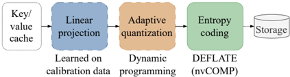CacheGen Figure 1 | The kvtc transform-coding pipeline. Features are linearly decorrelated via PCA, and the resulting PCA coefficients are quantized using variable bit widths. The PCA basis V is computed once on a calibration dataset and reused for all caches. Key and value caches are compressed separately. <details> <summary>Image 2 Details</summary>  ### Visual Description ## Diagram: Data Compression Pipeline for Key/Value Cache ### Overview The image is a horizontal process flow diagram illustrating a four-stage pipeline designed to compress "Key/value cache" data. The process moves from left to right, transforming raw cache data through projection, quantization, and entropy coding before sending the final output to storage. ### Components/Axes The diagram is composed of five distinct nodes arranged linearly from left to right, connected by arrows. * **Node 1 (Far Left):** A white, rounded rectangular box labeled "Key/value cache". * **Node 2 (Center-Left):** A blue, rounded rectangular box labeled "Linear projection". Below this box is the text "Learned on calibration data". * **Node 3 (Center-Right):** An orange/tan, rounded rectangular box labeled "Adaptive quantization". Below this box is the text "Dynamic programming". * **Node 4 (Right):** A light green, rounded rectangular box labeled "Entropy coding". Below this box is the text "DEFLATE (nvCOMP)". * **Node 5 (Far Right):** A gray cylinder icon labeled "Storage". **Connectors:** * Solid arrows connect Node 1 to Node 2, Node 2 to Node 3, and Node 3 to Node 4. * A dashed arrow connects Node 4 to Node 5 (Storage). ### Detailed Analysis The pipeline describes a specific sequence of operations for data reduction: 1. **Input:** The process begins with the **Key/value cache**, which is the raw data source. 2. **Transformation (Linear Projection):** The data undergoes a "Linear projection." The sub-label "Learned on calibration data" indicates that the parameters for this projection are derived from a representative dataset, suggesting a machine learning-based approach to dimensionality reduction. 3. **Quantization (Adaptive Quantization):** The projected data is then processed via "Adaptive quantization." The sub-label "Dynamic programming" suggests that the quantization levels or bit-widths are optimized algorithmically to minimize information loss while maximizing compression. 4. **Encoding (Entropy Coding):** The quantized data is passed to "Entropy coding." The sub-label "DEFLATE (nvCOMP)" specifies the algorithm used. "DEFLATE" is a standard lossless compression algorithm, and "nvCOMP" refers to NVIDIA's compression library, indicating this pipeline is optimized for GPU-accelerated environments. 5. **Output:** The final compressed data is sent to "Storage." ### Key Observations * **Pipeline Logic:** The flow represents a lossy-to-lossless compression strategy. The first two stages (Linear projection and Adaptive quantization) are likely lossy, reducing the data size significantly, while the final stage (Entropy coding) is lossless, further compacting the representation. * **Optimization:** The inclusion of "Learned on calibration data" and "Dynamic programming" implies that this is a highly optimized, context-aware compression method rather than a generic compression algorithm. * **Hardware Context:** The explicit mention of "nvCOMP" strongly suggests this diagram describes a technique for compressing the KV cache in Large Language Models (LLMs) to reduce VRAM usage on NVIDIA GPUs. ### Interpretation This diagram outlines a sophisticated strategy for managing the memory footprint of Large Language Models. In modern LLM inference, the "Key/value cache" (KV cache) grows linearly with the sequence length and batch size, often becoming the primary bottleneck for memory capacity. This pipeline addresses that bottleneck by: 1. **Dimensionality Reduction:** Using "Linear projection" to map the high-dimensional KV cache into a lower-dimensional space. 2. **Precision Reduction:** Using "Adaptive quantization" to reduce the bit-precision of the values, likely using dynamic programming to ensure that the most important information is preserved while less important information is compressed more aggressively. 3. **Final Compression:** Using "DEFLATE" via "nvCOMP" to squeeze the remaining data into the smallest possible footprint for storage. The "Learned on calibration data" aspect is critical; it implies that the compression is not universal but is tuned to the specific model or data distribution, allowing for higher compression ratios with minimal impact on model accuracy. This is a classic "model compression" or "KV cache quantization" workflow. 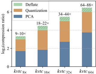</details> Figure 2 | KV cache compression ratios contributed by parts of the kvtc pipeline for Llama 3.1 8B. DEFLATE's variability is marked with black stripes. <details> <summary>Image 3 Details</summary>  ### Visual Description ## Stacked Bar Chart: Compression Ratios for kvtc Configurations ### Overview This image is a stacked bar chart illustrating the total compression ratio achieved by different "kvtc" configurations. The chart breaks down the total compression into three distinct components: PCA (Principal Component Analysis), Quantization, and Deflate. The Y-axis represents the compression ratio on a $\log_2$ scale, while the X-axis represents four specific configuration tiers. ### Components/Axes * **Y-Axis**: Labeled "$\log_2(\text{compression ratio})$". The scale is linear, marked at intervals of 0, 2, 4, and 6. * **X-Axis**: Categorical, displaying four configurations: $kvtc_{8\times}$, $kvtc_{16\times}$, $kvtc_{32\times}$, and $kvtc_{64\times}$. * **Legend (Top-Left)**: * **Green (hatched pattern)**: Deflate * **Orange (solid)**: Quantization * **Blue (solid)**: PCA * **Data Labels (Top of each bar)**: * $kvtc_{8\times}$: 9–10$\times$ * $kvtc_{16\times}$: 18–22$\times$ * $kvtc_{32\times}$: 34–44$\times$ * $kvtc_{64\times}$: 64–88$\times$ ### Detailed Analysis The chart displays four bars, each representing a specific configuration. The total height of each bar corresponds to the $\log_2$ of the compression ratio. 1. **$kvtc_{8\times}$ (Far Left)**: * **Visual Trend**: The bar reaches a height of approximately 3.3 on the Y-axis. * **Composition**: PCA (Blue) accounts for ~1.7 units; Quantization (Orange) accounts for ~1.3 units; Deflate (Green) accounts for ~0.3 units. * **Total**: Corresponds to the label "9–10$\times$". 2. **$kvtc_{16\times}$ (Center-Left)**: * **Visual Trend**: The bar reaches a height of approximately 4.5 on the Y-axis. * **Composition**: PCA (Blue) accounts for ~1.8 units; Quantization (Orange) accounts for ~2.2 units; Deflate (Green) accounts for ~0.5 units. * **Total**: Corresponds to the label "18–22$\times$". 3. **$kvtc_{32\times}$ (Center-Right)**: * **Visual Trend**: The bar reaches a height of approximately 5.5 on the Y-axis. * **Composition**: PCA (Blue) accounts for ~2.7 units; Quantization (Orange) accounts for ~2.3 units; Deflate (Green) accounts for ~0.5 units. * **Total**: Corresponds to the label "34–44$\times$". 4. **$kvtc_{64\times}$ (Far Right)**: * **Visual Trend**: The bar reaches a height of approximately 6.5 on the Y-axis. * **Composition**: PCA (Blue) accounts for ~3.7 units; Quantization (Orange) accounts for ~2.3 units; Deflate (Green) accounts for ~0.5 units. * **Total**: Corresponds to the label "64–88$\times$". ### Key Observations * **Dominant Component**: PCA (Blue) is the primary driver of compression. As the configuration scales from $kvtc_{8\times}$ to $kvtc_{64\times}$, the PCA component shows the most consistent and significant growth. * **Plateauing Components**: The Quantization (Orange) component increases between $kvtc_{8\times}$ and $kvtc_{16\times}$ but remains relatively stable (plateaus) from $kvtc_{16\times}$ through $kvtc_{64\times}$. * **Minor Component**: The Deflate (Green) component is the smallest contributor across all configurations and remains nearly constant in its contribution to the total compression ratio. ### Interpretation The data demonstrates that the "kvtc" compression pipeline is designed to scale primarily through the PCA component. Because the Y-axis is logarithmic ($\log_2$), the linear increase in the total height of the bars indicates an exponential increase in the actual compression ratio (as confirmed by the labels 9–10$\times$ to 64–88$\times$). The fact that Quantization and Deflate contributions flatten out suggests that these methods reach a point of diminishing returns or are capped by the configuration, leaving PCA as the scalable variable to achieve higher compression ratios in the $kvtc$ architecture. 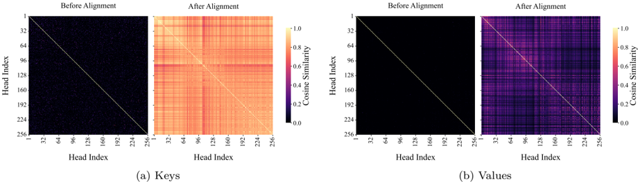</details> Figure 3 | Cosine similarity before and after alignment between key (a) and value (b) heads calculated using Llama 3.1 8B on inputs from Qasper (Dasigi et al., 2021; Shaham et al., 2022). For each example, we calculate cosine similarity between all keys/values from the same position and then average across the batch. Orthonormal alignment matrices were produced using 20 samples from the RedPajama v2 (Weber et al., 2024). <details> <summary>Image 4 Details</summary>  ### Visual Description ## Heatmap: Cosine Similarity of Keys and Values Before and After Alignment ### Overview This image presents a comparative analysis of cosine similarity matrices for two components of a neural network architecture (likely Multi-Head Attention mechanisms): "Keys" (a) and "Values" (b). Each section compares the state of the model "Before Alignment" and "After Alignment." The heatmaps visualize the similarity between 256 distinct attention heads. ### Components/Axes * **Axes:** Both the X and Y axes represent "Head Index," ranging from 1 to 256. * **Tick Markers:** 1, 32, 64, 96, 128, 160, 192, 224, 256. * **Legends:** * **Panel (a) Keys:** A vertical color bar on the right of the "After Alignment" plot. Scale ranges from 0.0 (black) to 1.0 (light yellow). Label: "Cosine Similarity". * **Panel (b) Values:** A vertical color bar on the right of the "After Alignment" plot. Scale ranges from 0.0 (black) to 1.0 (light yellow). Label: "Cosine Similarity". * **Layout:** * **Panel (a) Keys:** Two heatmaps side-by-side. Left: "Before Alignment"; Right: "After Alignment". * **Panel (b) Values:** Two heatmaps side-by-side. Left: "Before Alignment"; Right: "After Alignment". ### Detailed Analysis #### Panel (a) Keys * **Before Alignment:** The heatmap is almost entirely black, indicating that the cosine similarity between different heads is near 0.0. A very faint, thin diagonal line is visible, representing the self-similarity of each head (which is 1.0). * **After Alignment:** There is a dramatic shift in the color distribution. The heatmap is populated with varying shades of orange and yellow, indicating a significant increase in cosine similarity between heads. * **Trend:** The similarity is not uniform; it exhibits a block-like structure, suggesting that specific groups of heads have become highly similar to one another. * **Values:** The diagonal remains bright (1.0). Off-diagonal regions show values ranging roughly from 0.2 to 0.8, with some clusters appearing quite bright (yellow). #### Panel (b) Values * **Before Alignment:** Similar to the Keys, the heatmap is almost entirely black, indicating near-zero cosine similarity between heads, with only the self-similarity diagonal visible. * **After Alignment:** There is a noticeable increase in similarity compared to the "Before" state, but the intensity is lower than that observed in the Keys. * **Trend:** The colors are predominantly purple and dark magenta, indicating moderate cosine similarity (roughly 0.2 to 0.4). * **Values:** The diagonal remains bright (1.0). The off-diagonal regions show a grid-like pattern of increased similarity, but the overall magnitude is lower than in the Keys panel. ### Key Observations * **Alignment Effect:** The alignment process successfully increases the cosine similarity between heads for both Keys and Values. * **Magnitude Difference:** The "Keys" alignment results in higher overall cosine similarity (lighter, more yellow/orange colors) compared to the "Values" alignment (darker, purple/magenta colors). * **Structural Patterns:** Both "After Alignment" plots show a non-uniform, blocky structure. This suggests that the alignment process does not make all heads identical, but rather encourages clusters of heads to align with each other. * **Baseline:** The "Before Alignment" state for both Keys and Values is essentially sparse/orthogonal, meaning the heads are largely uncorrelated prior to the alignment intervention. ### Interpretation This data demonstrates the effect of a head-alignment or head-merging technique in a Transformer-based model. * **What the data demonstrates:** The alignment process is effective at forcing the attention heads to converge toward similar representations. * **Why it matters:** In Transformer models, attention heads are often redundant. By aligning them, researchers can potentially prune the model, reduce computational overhead, or distill knowledge from a larger model into a smaller one without significant performance loss. * **Reading between the lines:** The fact that Keys align more strongly than Values suggests that the alignment mechanism might be prioritizing the Key projections. This could imply that the "Keys" are the primary locus of the learned attention patterns, while "Values" are more flexible or require less strict alignment to maintain model performance. The blocky patterns in the "After" plots suggest that the heads are being grouped into functional clusters rather than being forced into a single uniform state. </details> (Liu et al., 2024b) compresses caches for transmission, offering at most 8.6 × KV cache reduction in comparison to a 16-bit baseline. SVDq (Yankun et al., 2025) and xKV (Chang et al., 2025) pursue low-rank compression during prefill, but both require calculation of per-prompt SVD. Long and frequently used prompts may justify investing more compute for offline training of corpus-specific caches (Eyuboglu et al., 2025). Meanwhile, intensively studied KV cache compression methods, aimed at improving the runtime efficiency of autoregressive generation, offer interim measures to the cache retention problem (Yuan et al., 2024). Prior work hinges on observations that KV cache can be quantized (Frantar et al., 2023) sparsified (Liu et al., 2024d; Hooper et al., 2024), average-pooled (Nawrot et al., 2024), or shared between layers (Brandon et al., 2024); the cache itself is compressible (Yuan et al., 2024), and dimensions of keys and values for separate heads show a high degree of correlation (Zhang et al., 2023). For long contexts, these methods offer substantial throughput and latency improvements, by lowering KV cache sizes and thus the memory traffic during next token prediction. However, due to tight latency constraints, often coupled with refraining from modifying weights of the model, these techniques tend to be brittle (Tang et al., 2024), and accuracy degradation prohibits combining methods for compounded benefits. Finally, these methods seldom exploit the strong low-rank structure of KV tensors. In this paper, we introduce kvtc : a simple yet powerful transform coding scheme, compressing KV caches for storage. Inspired by classical image codecs, it applies a learned orthonormal transform followed by channel-wise scalar quantization, which dynamically allocates bits, and entropy coding. The resulting bitstream is on average 20 × smaller than the original 16-bit one, while maintaining comparable accuracy. The method also exposes a smooth compression-accuracy trade-off, with 40 × or higher compression attainable at modest accuracy decrease. Thus, kvtc largely mitigates the problem of KV cache management: lowering the cost of its on-chip retention and the bandwidth required for offloading, without compromising interactive latency. ## 2. Preliminaries KV Cache Structure During decoding in autoregressive Transformers with multi-head self-attention, the keys and values produced for each processed token are cached to avoid recomputation. The collection of these tensors is the KV cache . For l layers, h heads, head dimension d head and sequence length t , a 16-bit KV cache occupies (4 l h d head t ) bytes. Motivated by work on cross-layer KV cache sharing and compression (Brandon et al., 2024; Chang et al., 2025), we ask whether keys from different attention heads, and analogously values, lie in a Table 1 | KV cache size in 16 bits for 1K tokens of context. 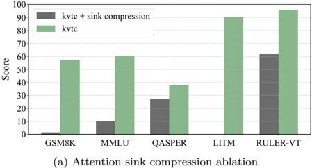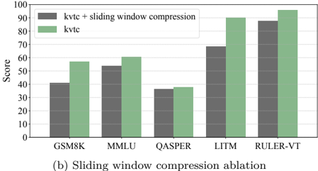| Model | Size | |------------------------|--------| | Qwen 2.5 R1 1.5B | 28MiB | | Qwen 2.5 R1 7B | 56MiB | | Llama 3.1 8B | 128MiB | | Llama 3.3 70B Instruct | 320MiB | | Mistral NeMo 12B | 160MiB | | MN-Minitron 8B | 160MiB | Figure 4 | Ablation of kvtc with compression ratio 64 × on Llama 3.1 8B: (a) compression disabled for attention sink tokens; (b) compression disabled for the final 128 tokens. All other settings are fixed. Additional ablations are provided in Sections B.3 and B.7. <details> <summary>Image 5 Details</summary>  ### Visual Description ## Bar Chart: Attention Sink Compression Ablation ### Overview This image displays a grouped bar chart titled "(a) Attention sink compression ablation." It compares the performance scores of two distinct methods—"kvtc" and "kvtc + sink compression"—across five different benchmarks: GSM8K, MMLU, QASPER, LITM, and RULER-VT. The chart illustrates the impact of applying "sink compression" to the "kvtc" method. ### Components/Axes * **Y-Axis:** Labeled "Score," representing performance metrics on a scale from 0 to 100, with horizontal grid lines at 10-unit intervals. * **X-Axis:** Categorical labels representing five benchmarks: GSM8K, MMLU, QASPER, LITM, and RULER-VT. * **Legend (Top-Left):** * **Dark Grey Bar:** Represents "kvtc + sink compression." * **Light Green Bar:** Represents "kvtc." * **Caption (Bottom):** "(a) Attention sink compression ablation." ### Detailed Analysis The following values are approximate visual estimates based on the provided grid lines: | Benchmark | kvtc (Light Green) | kvtc + sink compression (Dark Grey) | | :--- | :--- | :--- | | **GSM8K** | ~57 | ~1.5 | | **MMLU** | ~60 | ~10 | | **QASPER** | ~38 | ~28 | | **LITM** | ~90 | 0 (No bar visible) | | **RULER-VT** | ~96 | ~62 | **Trend Verification:** * **kvtc (Light Green):** Shows a generally high performance across all categories, with the lowest score at QASPER (~38) and the highest at RULER-VT (~96). * **kvtc + sink compression (Dark Grey):** Shows a significant performance deficit compared to the baseline. It starts near zero at GSM8K, shows a slight increase at MMLU and QASPER, is absent at LITM, and reaches its peak at RULER-VT (~62). ### Key Observations * **Consistent Underperformance:** The "kvtc + sink compression" method consistently scores lower than the "kvtc" method across every benchmark tested. * **Catastrophic Failure at LITM:** The "kvtc + sink compression" method appears to fail entirely on the LITM benchmark, as there is no visible bar, indicating a score of 0 or negligible performance. * **Performance Gap:** The gap between the two methods is most pronounced in the LITM and GSM8K benchmarks. The gap is narrowest in the QASPER benchmark. * **Relative Improvement:** While "kvtc + sink compression" performs poorly, it does show a trend of increasing scores as the benchmarks progress from left to right (excluding the LITM anomaly), suggesting it may be more effective on specific types of tasks (like RULER-VT) than others. ### Interpretation This ablation study demonstrates that the "sink compression" technique is highly detrimental to the performance of the "kvtc" model. The data suggests that "sink compression" likely causes significant information loss or "catastrophic forgetting" of the context required to solve these reasoning and retrieval tasks. The fact that the performance drops to near-zero in benchmarks like GSM8K and LITM indicates that the compression mechanism is likely discarding critical tokens or attention heads necessary for the model to function correctly. From a technical standpoint, this chart serves as a negative result for the "sink compression" method, proving that while it may be intended to optimize memory or compute, the trade-off in accuracy is severe and unacceptable for these specific benchmarks. The "kvtc" baseline is clearly superior, and the "sink compression" modification requires significant refinement or a different approach to be viable. </details> <details> <summary>Image 6 Details</summary>  ### Visual Description ## Bar Chart: Sliding Window Compression Ablation ### Overview The image displays a grouped bar chart labeled "(b) Sliding window compression ablation." It compares the performance scores of two distinct methods—"kvtc" and "kvtc + sliding window compression"—across five different benchmarks (GSM8K, MMLU, QASPER, LITM, and RULER-VT). ### Components/Axes * **Y-Axis:** Labeled "Score," representing a numerical performance metric ranging from 0 to 100, with grid lines at intervals of 10. * **X-Axis:** Categorical, listing the five benchmarks: GSM8K, MMLU, QASPER, LITM, and RULER-VT. * **Legend:** Positioned in the top-left area of the chart. * **Dark Grey Bar:** Represents "kvtc + sliding window compression." * **Light Green Bar:** Represents "kvtc." ### Detailed Analysis The chart presents grouped bars for each benchmark. In every instance, the "kvtc" (light green) bar is taller than the "kvtc + sliding window compression" (dark grey) bar. **Estimated Data Points (Score):** | Benchmark | kvtc (Light Green) | kvtc + sliding window compression (Dark Grey) | | :--- | :--- | :--- | | **GSM8K** | ~57 | ~41 | | **MMLU** | ~61 | ~54 | | **QASPER** | ~38 | ~36 | | **LITM** | ~90 | ~68 | | **RULER-VT** | ~96 | ~88 | ### Key Observations * **Consistent Degradation:** The addition of "sliding window compression" consistently results in lower scores compared to the baseline "kvtc" method across all five benchmarks. * **Variable Impact:** The performance penalty incurred by the compression method is not uniform: * **LITM** exhibits the most significant performance drop (a difference of approximately 22 points). * **QASPER** exhibits the least significant performance drop (a difference of approximately 2 points). * **GSM8K** also shows a substantial drop (approximately 16 points). ### Interpretation The data demonstrates that while "sliding window compression" is likely implemented to optimize resource usage (such as memory or computational efficiency), it introduces a clear performance trade-off. The varying degrees of degradation suggest that the compression technique is task-dependent. The severe drop in the LITM benchmark implies that the compression method may be discarding information critical to the specific reasoning or retrieval tasks required by LITM. Conversely, the minimal impact on QASPER suggests that the compression method is relatively robust for the specific data structures or query types found in that benchmark. This chart serves as an ablation study, quantifying the "cost" of the compression optimization in terms of model accuracy. </details> shared latent space. To be more precise, we examine if it is possible to align key or value caches, produced by different attention heads, via linear transformations. Specifically, for each pair of attention heads h i , h j in the model, we attempt to align their caches K i , K j ∈ R t × d head with an orthogonal map found by solving the Procrustes problem (Gower & Dijksterhuis, 2004): $$R ^ { \ast } = arg \min _ { R } || K _ { i } R || _ { F } s . t . R ^ { T } R = I .$$ We then compute token-wise cosine similarity between K i and K j before alignment, and between K i and K j R /star after alignment. We repeat the same procedure for values using V i , V j . Before alignment, inter-head cosine similarity is typically below 0.2. After orthogonal alignment, similarity increases substantially for keys and moderately for values (Figure 3). This pattern suggests that key heads largely inhabit a common subspace up to an orthogonal transformation; their dissimilarity before alignment likely stems from random initialization of key and value projection matrices. We note that for a data matrix A ∈ R n × d , if k directions suffice to explain all of the variance of A , then k directions suffice to explain all of the variance of B = [ A,AR ] ∈ R n × ( d + d ′ ) , for R ∈ R d × d ′ . This motivates our choice of PCA as a dimensionality reduction method. Another motivation comes from the work on efficient attention kernels (Jiang et al., 2024). To be more precise, from the observation that different attention heads can show similar attention patterns. In a simplified setting without RoPE (Su et al., 2024), where keys are equal to queries and we assume the exact equality of dot products that create the attention patterns, the key spaces are equal up to an orthogonal transform by the uniqueness of Gram realizations (Horn & Johnson, 2013). 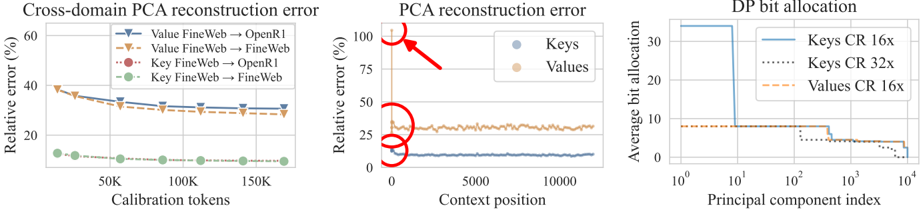Sliding Windows and Sink Tokens We avoid compressing both the w most recent tokens and s oldest tokens (attention sinks) due to their disproportionately high contribution to typical attention patterns (Jiang et al., 2024). In transform coding for vision and audio, bits are allocated to transform coefficients so that quantization induces minimal perceptual distortion. By loose analogy, the attention mass allocated to a token can be viewed as a proxy for its importance. In addition, when PCA is used to reduce the dimensionality of keys and values, the sink tokens yield higher reconstruction errors, as shown in Figure 6. Foreshadowing the experiments described in Section 4, we have chosen w = 128 and s = 4 for evaluation. To illustrate their influence on accuracy, we ablate on their compression by setting either w = 0 or s = 0, as shown in Figure 4. These experiments show that compressing these tokens can significantly lower, or even entirely collapse the accuracy at high compression ratios. Multi-Turn Conversations Let a conversation be an ordered sequence $$C = ( 1 0 , 8 0 ) . ( 8 0 , 8 0 ) \cdots$$ where x t denotes the user (or system) input at turn t and y t the generated reply. Generation of y t consists of a prefill pass, which produces the KV cache for all preceding tokens ( x 0 , y 0 , . . . , x t ), followed by iterative decoding, which generates the tokens of y t one at a time. Figure 6 | Calibration of Llama 3.1 8B with kvtc . Left: Reconstruction error as a function of the size of calibration set. The arrow A → B denotes fitting PCA on dataset A and calculating the error on B. Middle: The reconstruction error as a function of position in the context. The error is higher for the sink tokens. Right: Bit assignment computed via dynamic programming, counting in the per-group scaling factors. <details> <summary>Image 7 Details</summary>  ### Visual Description This image contains three distinct charts illustrating performance metrics related to Principal Component Analysis (PCA) reconstruction error and bit allocation for machine learning model components (Keys and Values). ## [Charts]: PCA Reconstruction Error and Bit Allocation ### Overview The image consists of three side-by-side line charts. 1. **Left:** "Cross-domain PCA reconstruction error" plotted against calibration tokens. 2. **Center:** "PCA reconstruction error" plotted against context position. 3. **Right:** "DP bit allocation" plotted against the principal component index. --- ### Chart 1: Cross-domain PCA reconstruction error #### Components/Axes * **X-axis:** "Calibration tokens" (Scale: 0 to 150K). * **Y-axis:** "Relative error (%)" (Scale: 0 to 60). * **Legend (Top-Right):** * Blue inverted triangle: Value FineWeb $\rightarrow$ OpenR1 * Orange inverted triangle: Value FineWeb $\rightarrow$ FineWeb * Red circle: Key FineWeb $\rightarrow$ OpenR1 * Green circle: Key FineWeb $\rightarrow$ FineWeb #### Detailed Analysis * **Trend Verification:** * **Value series (Blue/Orange):** Both lines start at approximately 40% relative error and show a steady, gradual downward slope as the number of calibration tokens increases, leveling off near 30% at 150K tokens. * **Key series (Red/Green):** Both lines start at approximately 12% relative error and remain extremely flat and stable across the entire range of calibration tokens. * **Data Points:** * Values (Blue/Orange): Start $\approx$ 40%, End $\approx$ 30%. * Keys (Red/Green): Start $\approx$ 12%, End $\approx$ 10%. --- ### Chart 2: PCA reconstruction error #### Components/Axes * **X-axis:** "Context position" (Scale: 0 to 10,000). * **Y-axis:** "Relative error (%)" (Scale: 0 to 100). * **Legend (Top-Right):** * Blue circle: Keys * Orange circle: Values * **Annotations:** A red arrow points from the top-right toward the Y-axis at X=0. Red circles highlight the data points at X=0 for both the Keys and Values series. #### Detailed Analysis * **Trend Verification:** * **Values (Orange):** The line begins at a very high error rate (>100% at X=0), drops sharply within the first few hundred context positions, and then stabilizes at a constant error rate of approximately 30%. * **Keys (Blue):** The line begins at a lower error rate ($\approx$ 20% at X=0), drops slightly, and then stabilizes at a constant error rate of approximately 10%. * **Key Observations:** The red arrow and circles emphasize the significant spike in reconstruction error at the very beginning of the context window (position 0), particularly for the "Values" component. --- ### Chart 3: DP bit allocation #### Components/Axes * **X-axis:** "Principal component index" (Logarithmic scale: $10^0$ to $10^4$). * **Y-axis:** "Average bit allocation" (Scale: 0 to 30). * **Legend (Top-Right):** * Blue solid line: Keys CR 16x * Black dotted line: Keys CR 32x * Orange dashed line: Values CR 16x #### Detailed Analysis * **Trend Verification:** * **Keys CR 16x (Blue):** Starts at a high allocation ($\approx$ 35 bits) for the first 10 components, then drops sharply to $\approx$ 8 bits, and eventually steps down to $\approx$ 4 bits as the index increases. * **Values CR 16x (Orange):** Starts at $\approx$ 8 bits and remains relatively flat until index $\approx$ 1000, where it steps down. * **Keys CR 32x (Black dotted):** Starts at $\approx$ 8 bits, drops to $\approx$ 5 bits at index $\approx$ 100, and drops to near 0 bits after index 1000. * **Key Observations:** The "Keys" at 16x compression require significantly higher bit allocation for the initial principal components compared to the "Values" or the higher compression "Keys" (32x). --- ### Interpretation The data suggests a fundamental difference in how "Keys" and "Values" in the transformer architecture are represented and compressed via PCA: 1. **Reconstruction Difficulty:** "Values" are consistently harder to reconstruct than "Keys," evidenced by the higher relative error in both the cross-domain and context-position charts. 2. **Context Sensitivity:** The spike in error at the start of the context window (Chart 2) suggests that the initial tokens (likely special tokens or positional embeddings) have distinct, high-variance representations that are difficult to compress using standard PCA trained on the rest of the sequence. 3. **Compression Efficiency:** Chart 3 demonstrates that "Keys" (at 16x) are "front-loaded" in terms of information density—they require a high bit allocation for the first few principal components. Conversely, "Values" are more uniformly distributed, requiring fewer bits for the initial components but maintaining that allocation longer. The "Keys CR 32x" line shows that increasing the compression ratio forces the model to discard information from higher-index components much more aggressively. </details> When a new user prompt x i is received, the existing KV cache can be re-used and only newly added tokens have to be forwarded through the model, reducing computation and time-to-first-token (TTFT). However, if the cache has been deleted, the model must reprocess the entire conversation as a prompt, resulting in quadratic recomputation of attention across the input. 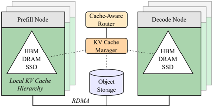KV Cache Management while Serving Efficient LLM deployments often split prefill and decode across separate nodes due to their distinct performance profiles (Zhong et al., 2024), as shown in Figure 5. The prefill node produces the KV cache and transmits it to the decode node over a high-speed fabric, typically RDMAcapable such as InfiniBand or RoCE, minimizing latency and CPU overhead on the host. Both nodes may maintain tiered KV caches: GPU HBM (hot), CPU DRAM (warm), and NVMe/SSD (cold), managed with a retention policy. Long-term storage might require sending caches to a remote location. Crucially, the decision to select a node for either prefill or decode of a certain input can be Figure 5 | A high-level architecture of KV-cacheaware LLM serving environment. <details> <summary>Image 8 Details</summary>  ### Visual Description ## System Architecture Diagram: Distributed KV Cache Management ### Overview The image illustrates a distributed system architecture designed for managing Key-Value (KV) caches, specifically tailored for a two-stage compute environment consisting of "Prefill" and "Decode" nodes. The architecture utilizes a tiered memory hierarchy (HBM, DRAM, SSD) within the nodes and a centralized management layer to coordinate data movement and storage, utilizing RDMA for high-speed data transfer. ### Components/Axes The diagram is organized into three primary vertical regions: **1. Left Region: Prefill Node** * **Visual Representation:** A stack of three overlapping rectangles, indicating a cluster or multiple instances of a "Prefill Node." * **Internal Structure:** A large white triangle is centered within the main green rectangle. * **Text Content:** * Header: "Prefill Node" * Inside Triangle: "HBM", "DRAM", "SSD" (stacked vertically). * Below Triangle: "Local KV Cache Hierarchy" **2. Right Region: Decode Node** * **Visual Representation:** A stack of three overlapping rectangles, indicating a cluster or multiple instances of a "Decode Node." * **Internal Structure:** A large white triangle is centered within the main green rectangle. * **Text Content:** * Header: "Decode Node" * Inside Triangle: "HBM", "DRAM", "SSD" (stacked vertically). **3. Center Region: Control and Storage** * **Top Component:** "Cache-Aware Router" (Tan/Orange box). * **Middle Component:** "KV Cache Manager" (Tan/Orange box). * **Bottom Component:** "Object Storage" (Light blue cylinder icon). **4. Connections** * **Control Path (Dotted Lines):** * Connects the "KV Cache Manager" to the center of the "Prefill Node." * Connects the "KV Cache Manager" to the center of the "Decode Node." * Connects the "KV Cache Manager" to the "Object Storage." * **Data Path (Solid Line):** * A horizontal line connects the bottom of the "Prefill Node" and the "Decode Node" to the "Object Storage." * **Label:** "RDMA" (Remote Direct Memory Access) is written below this line. ### Detailed Analysis * **Memory Hierarchy:** The triangle within each node (HBM, DRAM, SSD) represents a tiered storage strategy. HBM (High Bandwidth Memory) is positioned at the top of the triangle, implying it is the fastest but likely smallest capacity tier. DRAM is in the middle, and SSD is at the base, implying the largest capacity but slowest access speed. * **Node Roles:** The separation into "Prefill Node" and "Decode Node" suggests a decoupled architecture where the initial prompt processing (Prefill) and the token generation (Decode) are handled by different compute resources, likely to optimize for the different computational characteristics of these two phases in LLM inference. * **Management Layer:** The "Cache-Aware Router" and "KV Cache Manager" act as the control plane. The router likely directs incoming requests, while the manager handles the state and location of the KV cache data across the distributed nodes. * **Data Transfer:** The use of "RDMA" for the connection between the nodes and the "Object Storage" indicates a requirement for low-latency, high-throughput data movement, bypassing traditional network stack overheads to fetch or offload cache data. ### Key Observations * **Symmetry:** The architecture is highly symmetric regarding the compute nodes, suggesting that the "Prefill" and "Decode" nodes share the same underlying hardware/memory architecture. * **Control vs. Data Plane:** There is a clear architectural distinction between the control plane (dotted lines, managed by the KV Cache Manager) and the data plane (solid line, utilizing RDMA for direct storage access). * **Hierarchy Placement:** The text "Local KV Cache Hierarchy" is explicitly placed under the Prefill Node. While the Decode Node has an identical internal structure, the label is not repeated, suggesting the hierarchy concept applies to the entire node architecture. ### Interpretation This diagram represents a sophisticated infrastructure for **Large Language Model (LLM) serving**. * **The Problem:** LLM inference requires massive amounts of memory to store the "KV Cache" (the context of the conversation). This cache often exceeds the capacity of a single GPU's HBM. * **The Solution:** This architecture solves the memory bottleneck by: 1. **Tiering:** Using a hierarchy (HBM/DRAM/SSD) to store the cache, keeping the most active data in HBM and spilling less active data to DRAM or SSD. 2. **Decoupling:** Separating Prefill and Decode nodes allows for independent scaling of the two phases of inference, which have different compute/memory profiles. 3. **Orchestration:** The "KV Cache Manager" acts as a global controller, ensuring that when a node needs specific cache data, it is fetched efficiently (via RDMA) from the Object Storage or moved between tiers, preventing the system from stalling due to memory limitations. This is a classic "disaggregated memory" or "remote memory" architecture designed to maximize the throughput of LLM inference clusters. </details> dictated by the already-held KV cache with a matching prefix. In such setups, KV cache transfers are typically the dominant cross-node traffic. Why compress KV caches after the prefill or decode phase? Compression can: (i) extend the effective capacity of a KV cache database, and thus the lifetimes of caches, roughly in proportion to the compression ratio, and (ii) reduce network traffic. We discuss both angles below. - (i) Extending KV cache lifetimes increases cache hit rates in higher tiers (HBM/DRAM), often avoiding or substantially reducing prefill time for prompts with long, recently processed prefixes. For example, during a session with a coding assistant, a single 1,000-line file tokenized at ∼ 10 tokens per line and processed by Llama 3.3 70B yields about 1.6 GiB of 8-bit KV cache. Subsequent conversation turns, or a few parallel conversations about this file, might reuse the corresponding cache. However, on a node which serves multiple clients, the volume of generated KV cache might shorten its hot/warm residency even at moderate batch sizes. A 20 × lifetime extension via compression might determine whether a KV cache remains hot/warm until it becomes useful, or needs to be recomputed from scratch. - (ii) Prefill time scales as O ( n 2 ) with prompt length and typically dominates transfer time. In addition, KV caches can be streamed by layer during prefill in order to further reduce TTFT (Qin et al., 2025). However, KV cache compression reduces memory traffic proportionally to the compression ratio, which might be critical when the network bandwidth is saturated and becomes the bottleneck. ## 3. Method Our Key-Value Transform Coder ( kvtc ), shown in Figure 1, builds upon the transform-coding framework (Ahmed et al., 1974; Goyal, 2001), a widely adopted methodology for designing image and video compression algorithms such as JPEG (Joint Photographic Experts Group, 1994). It applies feature decorrelation by projecting onto an orthonormal basis matrix V obtained via the singular value decomposition (SVD) of centered calibration data (i.e., principal component analysis, PCA). Quantization parameters are selected using a dynamic programming algorithm, and the resulting symbols are entropy-coded with DEFLATE (Wu, 2017). The three modes of operation of kvtc are: - Calibration This step is performed only once for every model and compression ratio. During calibration, we obtain the key and value caches for the calibration dataset, calculate SVD( C -µ ) = U Σ V /latticetop where µ is the mean of the data, and store the projection matrices V /latticetop (for key and value caches separately). Next, we run a dynamic programming algorithm that produces the optimal bit allocation for each of the principal components. This step is fast; for instance, calibration for a 12B model can be completed within 10 minutes on an H100 GPU (Appendix B.5). In Appendix B.12 we show that the additional amount of data stored per model is relatively small (2 . 4% of model parameters for Llama 3.3 70B). In Appendix B.10 we perform an ablation study on the number of layers over which we concatenate the KV caches. - Decompression Decompression reverses the compression steps. The most computationally intensive operation-the inverse projection using V /latticetop -can be performed layer-by-layer using sub-matrices of V /latticetop , allowing generation to begin early. - Compression Keys and values are compressed independently using the ( V, µ ) parameters and bit allocation obtained during calibration. Compression is performed between inference phases (e.g., after decoding or between prefill and decoding) and can be executed on either GPU (affecting TTFT) or CPU (if the cache is already in storage). Importantly, during decoding, the model operates on decompressed KV caches; compression is used only for storage or transfer. In the following sections we describe in detail the components of kvtc during calibration, compression and decompression. ## 3.1. Feature decorrelation Unlike prior SVD-based methods that calculate a separate decomposition for each prompt (Yankun et al., 2025; Chang et al., 2025), we compute the KV cache projection matrices once using a calibration dataset C , and reuse them across all requests at inference time. Preparing a single, generalizable V rests on three observations. First, SVD must be computed on a large, representative sample; sampling token positions from a diverse calibration set suffices for generalization and is computationally tractable. Second, excluding keys and values corresponding to the most recent tokens and attention sinks improves the achievable compression ratio (see Tables 6 and 12 in Section B). Third, positional embeddings distort the apparent low-rank structure of keys and should be removed before compression (Sun et al., 2025). During calibration, we forward all sequences from C through the model and collect their KV caches. For each sequence, cache entries are concatenated along the time dimension to form a global pool of positions. We then sample n token positions from this pool, excluding attention sinks. For each sampled position, we take the corresponding keys (and, equivalently, values) from l layers and h heads, undo positional rotations, and concatenate them along the hidden dimension d head . This yields a data matrix C ∈ R n × p with p = l h d head , whose rows index sampled token positions. Let µ ∈ R p be the per-feature mean of C . We compute the SVD of the centered matrix, $$( 2 )$$ with singular values on diag(Σ) sorted in descending order (equivalently, PCA of C ). For any X ∈ R m × p , the decorrelated representation and its inverse are $$D = ( X - \mu ) V , X = D V ^ { T } + \mu$$ where the equality holds when all p components are used. When r < p and the basis is truncated to V ∈ R p × r , then X ≈ DV /latticetop + µ . For scalability, we use randomized SVD (Halko et al., 2011) calculated on a GPU with target rank r < p , substantially reducing runtime and memory. Results for this variant are shown in Figure 6, with additional details and ablations in Appendix B.1. ## 3.2. Quantization PCA orders principal components by explained variance. We exploit this ordering to allocate a fixed bit budget across PCA coordinates so that high-variance components receive more bits. The allocation is computed once on a calibration set and reused at inference. We quantize D coordinate-wise to obtain D q 1 ,...,q d , where q i ∈ Z ≥ 0 is the bit width assigned to the i -th principal component. Under a global bit budget, we minimize the Frobenius reconstruction error $$\left | D V ^ { T } - D q \cdots d _ { 1 } V ^ { T } \right | ^ { 2 } .$$ Because right-multiplication by an orthonormal matrix preserves the Frobenius norm, we have Thus, optimal bit allocation can be found directly in the decorrelated domain. We solve the constrained allocation with a simple dynamic programming (DP) algorithm that keeps two tables: (1) the minimum reconstruction error achievable using the first i principal components under a payload of b bits; and (2) a backpointer storing the optimal local decision. Pseudocode and a proof sketch of optimality under these constraints are in Section B.13. Furthermore, inspired by the Microscaling data formats (Rouhani et al., 2023), we quantize groups of subsequent PCA coordinates together, each group with shared 16-bit shift and scaling factors. The DP optimizes both the per-group bit width and group size, restricted to { 1 , 16 , 64 , 256 , 1024 } components per group. The total budget equals the sum of payload bits across all coordinates plus per-group shift and scaling factors. An example allocation is shown in Figure 6. As expected, the learned bit widths decrease monotonically for subsequent principal components. Crucially, the DP assigns zero bits to a substantial number of trailing principal components. This observation motivates reducing the dimensionality early during the calculation of PCA, lowering the cost of calibration, and trimming V to the dimensions with nonzero bit widths for faster compression/decompression during inference. We show the benefits of DP guided quantization over pure PCA in Section B.9. ## 3.3. Entropy coding Finally, the quantized values are packed into a single byte array and further compressed using the DEFLATE algorithm (Wu, 2017). Crucially, we leverage nvCOMP (NVIDIA, 2020), which enables parallel operation directly on a GPU. This step is lossless, but the added compression ratio is content-dependent. We ablate the choice of the lossless compression algorithm and the influence on final compression in Appendix B.8. ## 4. Experiments Models We use models from three families: Llama 3 (Grattafiori et al., 2024), Mistral NeMo (Mistral AI team, 2024; Sreenivas et al., 2024), and R1-distilled Qwen 2.5 (DeepSeek-AI et al., 2025). The selection includes models ranging from 1.5B to 70B parameters of base, instruct, and reasoning kind. Table 1 lists the models along with their KV cache sizes. Notably, MN-Minitron 8B has been pruned from the Mistral NeMo 12B base, retaining the original KV cache size. Methods We compare our method against KIVI (Liu et al., 2024d), GEAR (Kang et al., 2024) and an FP8 quantization of KV cache to the E4M3 format (Micikevicius et al., 2022). For eviction baselines, we compare with TOVA (Oren et al., 2024) and H 2 O (Zhang et al., 2023). For SVD baselines, we compare our method with xKV (Chang et al., 2025). Finally, we compare kvtc with DMS (Łańcucki et al., 2025), a trained token eviction method, on reasoning tasks. For all methods, we follow their original intended protocols, performing prefill in the vanilla mode and compressing the KV cache only after the self-attention has been calculated. For every method except xKV, we simulate a sequence of short conversations by running compression/eviction on the cache every c tokens, where c depends on the method's original sliding window policy. For kvtc which is run with a sliding window w = 128, we compress/decompress every c = 16 tokens, leaving the window in the 112-128 token Table 2 | Accuracy of KV cache compression methods. Results within 1 score point of vanilla are in bold . See Appendix B.11 for standard error analysis. kvtc CR × denotes kvtc set for CR × compression before applying DEFLATE. | | Vanilla | GEAR 2-bit | KIVI 2-bit | H 2 O | TOVA | xKV | FP8 | kvtc 8 × | kvtc 16 × | kvtc 32 × | kvtc 64 × | |------------------|------------------|------------------|------------------|------------------|------------------|------------------|------------------|------------------|------------------|------------------|------------------| | Llama 3.1 8B | Llama 3.1 8B | Llama 3.1 8B | Llama 3.1 8B | Llama 3.1 8B | Llama 3.1 8B | Llama 3.1 8B | Llama 3.1 8B | Llama 3.1 8B | Llama 3.1 8B | Llama 3.1 8B | Llama 3.1 8B | | CR | 1 | 5 | 5 | 8 | 8 | 1-5 | 2 | 9-10 | 18-22 | 34-44 | 60-88 | | GSM8K | 56.8 | 52.8 | 52.8 | 54.3 | 54.5 | 56.6 | 55.2 | 57.0 | 56.9 | 57.8 | 57.2 | | MMLU | 60.5 | 59.6 | 59.6 | 44.3 | 44.8 | 59.5 | 60.1 | 59.8 | 60.1 | 60.6 | 60.7 | | QASPER | 40.4 | 40.4 | 39.1 | 34.3 | 38.6 | 35.6 | 40.8 | 40.1 | 40.7 | 39.4 | 37.8 | | LITM | 99.4 | 96.9 | 88.8 | 20.2 | 1.2 | 99.9 | 99.4 | 99.3 | 99.3 | 99.1 | 90.2 | | RULER-VT | 99.8 | 99.8 | 98.9 | 50.4 | 99.7 | 99.8 | 99.9 | 99.1 | 99.1 | 98.9 | 95.9 | | MN-Minitron 8B | MN-Minitron 8B | MN-Minitron 8B | MN-Minitron 8B | MN-Minitron 8B | MN-Minitron 8B | MN-Minitron 8B | MN-Minitron 8B | MN-Minitron 8B | MN-Minitron 8B | MN-Minitron 8B | MN-Minitron 8B | | CR | 1 | 5 | 5 | 8 | 8 | 1-5 | 2 | 10-11 | 17-21 | 32-46 | 53-95 | | GSM8K | 59.1 | 57.9 | 58.0 | 55.3 | 59.2 | 59.3 | 60.1 | 60.6 | 60.3 | 59.1 | 57.8 | | MMLU | 64.3 | 63.6 | 63.2 | 43.5 | 48.1 | 63.1 | 64.3 | 64.2 | 64.1 | 63.7 | 62.1 | | QASPER | 38.2 | 38.2 | 38.2 | 30.0 | 33.9 | 34.5 | 38.3 | 39.1 | 38.6 | 37.7 | 38.1 | | LITM | 99.8 | 96.0 | 86.3 | 16.6 | 0.3 | 99.6 | 99.8 | 99.4 | 99.3 | 86.9 | 59.5 | | RULER-VT | 99.4 | 98.3 | 96.8 | 39.2 | 99.3 | 99.1 | 99.2 | 98.8 | 98.8 | 96.0 | 93.4 | | Mistral NeMo 12B | Mistral NeMo 12B | Mistral NeMo 12B | Mistral NeMo 12B | Mistral NeMo 12B | Mistral NeMo 12B | Mistral NeMo 12B | Mistral NeMo 12B | Mistral NeMo 12B | Mistral NeMo 12B | Mistral NeMo 12B | Mistral NeMo 12B | | CR | 1 | 5 | 5 | 8 | 8 | 1-5 | 2 | 10-11 | 17-20 | 31-43 | 51-87 | | GSM8K | 61.9 | 59.8 | 59.7 | 57.0 | 60.3 | 61.9 | 61.7 | 62.5 | 62.0 | 62.2 | 61.9 | | MMLU | 64.5 | 64.0 | 64.3 | 45.4 | 49.0 | 63.9 | 64.5 | 64.6 | 64.4 | 63.8 | 61.4 | | QASPER | 38.4 | 38.6 | 38.2 | 29.5 | 36.0 | 33.5 | 37.9 | 37.6 | 37.6 | 37.5 | 38.0 | | LITM | 99.5 | 96.9 | 91.9 | 16.2 | 8.7 | 97.9 | 99.0 | 99.9 | 99.8 | 99.6 | 95.3 | | RULER-VT | 99.8 | 99.4 | 98.3 | 35.2 | 99.6 | 99.4 | 99.8 | 99.5 | 99.5 | 98.9 | 98.0 | range. In the case of xKV, we compress only the prefill tokens, providing it with an advantage, since xKV is specifically designed for prefill optimization, and re-computing SVD matrices for newly decoded tokens would be prohibitively time-consuming. For a fair comparison, we only report the prefill compression ratios for non-Qwen models. Notation-wise, kvtc CR × denotes kvtc in the default setting, where CR is the target compression for the DP. For all methods, we calculate CR only on the compressed tokens, not counting the sliding window tokens. Tasks We evaluate compression effects on Llama 3.1 8B, MN-Minitron 8B and Mistral NeMo 12B across the following task categories, with results presented in Table 2: - Math & Knowledge : 8-shot Chain of Thought (CoT) GSM8K (Cobbe et al., 2021), 4-shot CoT MMLU (Hendrycks et al., 2021a) - Long Context Performance : 0-shot key-value retrieval task from (Liu et al., 2024a) (denoted LITM), 1-shot RULER (Hsieh et al., 2024) Variable Tracking (denoted RULER-VT), and 2-shot Qasper (Shaham et al., 2022) We evaluate R1-distilled models on challenging mathematical competitions AIME 2024-2025 (Art of Problem Solving, 2025) and coding tasks from LiveCodeBench (Jain et al., 2025), with results presented in Table 3. We additionally evaluate kvtc with Llama 3.3 70B Instruct on MATH-500 (Hendrycks et al., 2021b; Lightman et al., 2023), the key-value retrieval task from (Liu et al., 2024a) and Needle In A Haystack (NIAH) (Kamradt, 2023; Hsieh et al., 2024), with results presented in Table 4. Detailed evaluation protocols can be found in Appendix A, and ablations and details about parameter choices for kvtc in Appendix B. Calibration Data We sample a 1:1 mixture of short and long documents, with lengths in the 1-8K and 8-32K ranges, respectively. Rotary positional embeddings are removed for calibration; further details are provided in Appendix B.1. Ablations showing kvtc stability and generalization across domains of the calibration data are provided in Appendices B.5 and B.6. Table 4 | Compression applied to a model which is split across four GPUs (pipeline parallel), with KV cache chunks being compressed separately with kvtc . In certain scenarios, like offloading to CPU RAM, these chunks could be compressed jointly for higher accuracy. | Method | MATH-500 | NIAH | LITM | |-----------|---------------|----------|--------| | | Llama 3.3 70B | Instruct | | | Vanilla | 75 . 6 1 . 92 | 100.0 | 100.0 | | kvtc 8 × | 73 . 2 1 . 98 | 100.0 | 100.0 | | kvtc 10 × | 74 . 4 1 . 95 | 100.0 | 100.0 | | kvtc 16 × | 73 . 2 1 . 98 | 100.0 | 100.0 | | kvtc 20 × | 72 . 6 1 . 99 | 100.0 | 100.0 | ## 4.1. Results In all experiments, kvtc applies the same compression ratio to both the key and value caches. An ablation of their individual compressibility is presented in Table 7 (Appendix B), suggesting that further adjustments could yield additional gains. General-Purpose Base Models We evaluate kvtc on general-purpose models at the 8-12B scale, featuring three GQA-enabled models (Table 2). The compression ratio of kvtc varies due to the data-dependent nature of the DEFLATE algorithm, which, on average, achieves a compression ratio of approximately 1 . 23 × on top of quantization. Crucially, kvtc maintains high accuracy across tested tasks, even at substantial compression ratios of 32 × and 64 × . Conversely, quantization methods-GEAR and KIVI-exhibit signs of performance degradation on GSM8K and Lost in the Middle tasks only at 5 × CR; cache eviction methods such as H 2 O and TOVA perform poorly as generic KV cache compressors. We also note that xKV performs well across most tasks, except for Qasper. Interestingly, in certain cases, kvtc at very high compression ratios even surpasses the performance of the vanilla models, likely due to inherent variability in the CoT setup. Crucially, kvtc at 16 × compression (approximately 20 × after DEFLATE) consistently maintains results within < 1 score point (accuracy or F1, depending on the task) of the vanilla models. The standard errors for these results are reported in Table 16 (Appendix B.11). Reasoning Models In order to test kvtc under more challenging conditions where context plays a critical role, we use complex math and coding tasks (Table 3). Due to high variability, AIME results are averaged over eight independent runs with results reported as score ± std . On coding tasks, kvtc 8 × shows minor accuracy drops of 0 . 3pp for the 1.5B model and 0 . 2pp for the 7B model. Notably, the KV cache size of the 1.5B model is already small at 29 KiB/token, compared to 131 KiB/token for Llama 3.1 8B, and a 9 × compression shrinks it to only 3 . 2 KiB/token. We also compare our method against DMS, a state-of-the-art autoregressive KV cache token eviction method. DMS achieves competitive results, and since it employs token eviction, it could potentially be combined with kvtc for even lower KV cache footprint. Table 3 | Reasoning quality (sampling temp 0 . 6, top-p 95%) of DeepSeek-R1-distilled Qwen2.5. DMS results taken from (Łańcucki et al., 2025). | Method | CR | AIME24 AIME25 Competition Math | AIME24 AIME25 Competition Math | LCB Coding | |------------------|------------------|----------------------------------|----------------------------------|------------------| | Qwen 2.5 R1 1.5B | Qwen 2.5 R1 1.5B | Qwen 2.5 R1 1.5B | Qwen 2.5 R1 1.5B | Qwen 2.5 R1 1.5B | | Vanilla | 1 | 26 . 2 ± 4 . 8 | 21 . 7 ± 2 . 9 | 16 . 4 | | kvtc 8 × | 9 | 25 . 4 ± 5 . 7 | 24 . 2 ± 4 . 0 | 16 . 1 | | kvtc 16 × | 18 | 27 . 9 ± 6 . 7 | 22 . 5 ± 5 . 2 | 13 . 3 | | DMS 8 × | - | 23.3 | N/A | 16.1 | | Qwen 2.5 R1 7B | Qwen 2.5 R1 7B | Qwen 2.5 R1 7B | Qwen 2.5 R1 7B | Qwen 2.5 R1 7B | | Vanilla | 1 | 50 . 9 ± 4 . 9 | 40 . 8 ± 4 . 3 | 36 . 7 | | kvtc 8 × | 9-11 | 52 . 5 ± 3 . 6 | 40 . 8 ± 5 . 2 | 36 . 5 | | kvtc 16 × | 18-21 | 50 . 9 ± 6 . 8 | 38 . 3 ± 5 . 5 | 31 . 6 | | DMS 8 × | - | 50.0 | N/A | 33.4 | Table 5 | Latency of a simple implementation based on the Transformers library (Hugging Face, 2025b), measured on an NVIDIA H100 GPU using Mistral NeMo 12B in bfloat16. In addition, we compare TTFT during recomputation of KV caches with decompression of compressed caches. BF denotes batch size, CTX context length. | Module | BS=8 CTX=8K | BS=8 CTX=8K | BS=8 CTX=8K | BS=8 CTX=8K | BS=2 CTX=16K | BS=2 CTX=16K | BS=2 CTX=16K | BS=2 CTX=16K | |------------------------|------------------------|------------------------|---------------|---------------|----------------|----------------|----------------|----------------| | | Comp | Comp | Decomp | Decomp | Comp | Comp | Decomp | Decomp | | Project | 153 | ms | 156 | ms | 78 | ms | 75 | ms | | Quantize | 67 | ms | 37 | ms | 39 | ms | 27 | ms | | Deflate | 137 | ms | 64 | ms | 66 | ms | 36 | ms | | Total | 379 | ms | 267 | ms | 194 | ms | 143 | ms | | Vanilla recompute TTFT | Vanilla recompute TTFT | Vanilla recompute TTFT | 3098 | ms | | | 1780 | ms | | kvtc decomp TTFT | kvtc decomp TTFT | kvtc decomp TTFT | 380 | ms | | | 208 | ms | Multi-GPU Inference To investigate attainable compression ratios for models distributed across multiple GPUs, we evaluate kvtc using Llama 3.3 70B (Table 4). The model runs in a pipeline-parallel setting (Hu et al., 2021) on four GPUs, each handling 20 layers. We maintain a local KV cache on each GPU, applying kvtc separately. Accuracy drops on the MATH-500 task are within 1 . 5 × stderr, with accuracy decreasing by 1 . 2pp at 10 × compression and 3 . 0pp at 20 × . Latency We calculate the latency of elements of the compression pipeline and provide the results in Table 5. In contrast to full re-computation of KV cache for 8K context length, kvtc 16 × can reduce time-to-first-token (TTFT) up to 8 × . ## 5. Limitations and future work Online Compression and Composability with Other Methods kvtc was designed for efficient storage and reducing time-to-first-token. However, the advantage of having a single, generalizable PCA matrix for initial compression of cache renders it suitable for further exploration of inference directly in the principal component space. We leave this as future work. Notably, kvtc does not alter the structure of KV cache and does not change how the attention is calculated. Consequently, it is directly compatible with token eviction methods, including but not limited to these used in the experimental section, such as TOVA, H 2 O, and DMS. Finally, kvtc could be used to compress the latent state in Multi-head Latent Attention (DeepSeek-AI et al., 2024). Scalability and Generalization Limits We approximate deployment by evaluating kvtc on benchmark tasks in simulated multi-turn settings, which may not fully reflect real content distributions or interaction patterns. Our experiments cover dense decoder-only models from 1.5B to 70B parameters; evaluating larger models under conditions that more accurately mirror production is left for future work. For calibration, we process approximately 200K tokens on a single NVIDIA H100 SXM 80GB GPU. Under these settings, computing the PCA basis with the randomized algorithm of Halko et al. (2011) completes within minutes. As shown in Figures 6 to 8, increasing the calibration set size consistently reduces the Frobenius-norm reconstruction error. Scaling kvtc beyond 200K tokens, primarily a matter of scaling the computation of PCA, is left for future work. Finally, we report Frobenius-norm reconstruction error as a proxy for downstream task accuracy. While convenient, this metric does not guarantee task-level gains and its predictive power may be task-dependent. We provide an initial correlation analysis in Section B.5 and defer a systematic study of alternative proxies to future work. Finally, the compression and decompression times of kvtc can be substantially reduced via kernel fusion and hierarchical PCA: first at the level of individual layers, then across groups of layers. Nevertheless, even a simple implementation yields substantial benefits and, in many cases, incurs only marginal overhead. ## 6. Related work The challenge of KV cache compression has garnered significant attention, with approaches broadly categorized into the following domains: Tuning-Free Quantization Quantization-based methods that avoid model fine-tuning offer a straightforward path to KV cache compression (Zhao et al., 2024; Sheng et al., 2023). Works such as KIVI (Liu et al., 2024d) and KVQuant (Hooper et al., 2024) have advanced this direction by developing separate quantization strategies for key and value embeddings. These methods leverage the observation that keys benefit from per-channel quantization, while values are better suited to per-token quantization. Our approach diverges from these methods by first projecting concatenated embeddings from attention layers using SVD matrices derived from a calibration set. Quantization is then applied in this transformed space, with the precision dynamically optimized via dynamic programming bit allocation. While we adopt KIVI's uniform quantization scheme, our application occurs in the SVD-transformed domain. Similar to KVQuant, we apply compression before RoPE (Su et al., 2024) to preserve model quality. Tuning-Based Quantization A complementary approach to post-training quantization involves fine-tuning models to adapt to quantized activations. LLM-QAT (Liu et al., 2024c) leverages generations from the prequantized model for fine-tuning, while BitDistiller (Du et al., 2024) merges Quantization Aware Training (Jacob et al., 2018) with Knowledge Distillation (Hinton et al., 2015) In contrast, our method eliminates the need for parameter modifications. Singular Value Decomposition Approaches SVD has emerged as a straightforward method for removing the redundancy in KV caches and exploiting its low-rank structure. GEAR (Kang et al., 2024) improves quantization through low-rank correction mechanisms, whereas LoRC (Zhang et al., 2024) minimizes computational overhead by directly reducing the rank of key and value matrices. Eigen Attention (Saxena et al., 2024) restructures attention computation by projecting into a truncated subspace defined by SVD, enabling efficient operations. A similar mechanism could be devised for value vectors in kvtc , and key vectors for layers that do not employ positional embeddings. GEAR (Kang et al., 2024) improves KIVI quantization through low-rank correction mechanisms. Building on ShadowKV (Sun et al., 2025), SVDq (Yankun et al., 2025) integrates SVD with quantization, leveraging singular value magnitudes for a simple precision allocation; xKV (Chang et al., 2025) aggregates KV caches across multiple layers before decomposition. This work differs in three respects: (i) it models rotational relationships between non-adjacent layers to enable cross-layer concatenation before decomposition; (ii) it selects ranks and bitwidths via a dynamic program under a compression budget; and (iii) it applies entropy coding to the quantized factors. Empirical comparisons and ablations (e.g., treatment of early sink tokens) are reported in Appendix B. Sparse Attention Strategies Sparse attention mechanisms provide a complementary paradigm for managing sequence length dimensions by selectively discarding non-essential keys/values during inference. Techniques such as H 2 O (Zhang et al., 2023) and TOVA (Oren et al., 2024) employ prioritization strategies to dynamically prune less informative elements from the KV cache. In contrast, chunk-based approaches like Quest (Tang et al., 2024), Landmark Attention (Mohtashami & Jaggi, 2023), and Native Sparse Attention (Yuan et al., 2025) construct compressed representations of the KV cache by partitioning sequences into chunks. These methods retrieve only the most critical chunks during attention computation, significantly reducing the number of memory transfers. Concurrently, dynamic compression techniques such as Dynamic Memory Compression (Nawrot et al., 2024) and Dynamic Memory Sparsification (Łańcucki et al., 2025) optimize KV cache memory usage through pooling/eviction of keys/values. These strategies can be potentially integrated with quantization and SVD methods to achieve higher compression ratios and improved inference latency (Yankun et al., 2025). Cache Management Systems Finally, cache management systems address the operational challenges of KV cache handling in production environments. Paged Attention (Kwon et al., 2023) mitigates memory overhead by introducing chunked memory allocation for KV caches. Continuous batching techniques, as implemented in systems like vLLM (Kwon et al., 2023) and FasterTransformer (NVIDIA, 2021), optimize device utilization by enabling parallel processing of multiple sequences. CacheGen (Liu et al., 2024b) advanced the field with a distributed framework for long-term KV cache management, incorporating compression, streaming, and cross-node coordination. Our approach extends these systems by integrating fine-grained compression capabilities, enabling token-level compression without compromising distributed architecture advantages. ## 7. Conclusion We introduce kvtc , a method for compressing KV cache up to 20 × with negligible quality degradation, and higher compression ratios of 40 × or more available for specific use cases. We empirically show that key and value caches exhibit substantial redundancy, which kvtc exploits through a simple, transform coding pipeline. It is built around linear dimensionality reduction and a dynamic programming algorithm, which assigns variable numbers of bits to principal components. We demonstrate the effectiveness of kvtc across both regular and thinking model families, evaluating models from 1.5B to 70B. We believe that kvtc paves the way towards more efficient LLM deployments, lowering the cost of LLM-assisted iterative workflows. ## Reproducibility To foster reproducibility of our results, we provide extensive details about the calibration of PCA matrices in Appendix B.1 along with ablations regarding kvtc parameters in Appendices B.3 (sink tokens), B.4 (key vs value compressibility), B.5 (amount of calibration data), B.6 (effect of calibration data domain) and B.7 (sliding window). In Appendix A, we present the details about the evaluation setup - tasks, used prompts, and baseline configuration. We note that we utilize LM Eval Harness (Gao et al., 2024) and RULER (Hsieh et al., 2024) for evaluation, which are publicly available. In Appendix B.13 we provide the pseudocode for the dynamic programming precision assignment algorithm along with the sketch of the optimality proof and complexity analysis. ## Ethical statement As a method that aims to improve aspects regarding LLM usage, kvtc does not introduce new risks. However, we note that it can amplify existing ones. Therefore, we refer to the existing body of knowledge on the ethical risks of LLM development, such as Ethics Threats in LLM-Based Agents (Gan et al., 2024), potential reversal of safety alignment (Xu et al., 2024), and more general risks regarding LLMs (Li & Fung, 2025). ## Acknowledgments The authors thank Mikołaj Błaż, Przemysław Podczasi, Piotr Tarasiewicz, and Przemysław Strzelczyk for many helpful discussions; Kevin Shih and Dima Zhylko for valuable comments on earlier versions of the manuscript; Szymon Migacz for assistance with computing infrastructure; and Alex Fit-Florea and Michael Lightstone for their support for the publication of this work. ## References - N. Ahmed, T. Natarajan, and K.R. Rao. Discrete cosine transform. IEEE Transactions on Computers , (1), 1974. 2. Art of Problem Solving. American invitational mathematics examination, 2025. URL https://artofprobl emsolving.com/wiki/index.php/American\_Invitational\_Mathematics\_Examination . Art of Problem Solving Wiki. 3. William Brandon, Mayank Mishra, Aniruddha Nrusimha, Rameswar Panda, and Jonathan Ragan-Kelley. Reducing transformer key-value cache size with cross-layer attention. In Advances in Neural Information Processing Systems , 2024. 4. Chi-Chih Chang, Chien-Yu Lin, Yash Akhauri, Wei-Cheng Lin, Kai-Chiang Wu, Luis Ceze, and Mohamed S. Abdelfattah. xkv: Cross-layer svd for kv-cache compression, 2025. arXiv:2503.18893. 5. Yihua Cheng, Kuntai Du, Jiayi Yao, and Junchen Jiang. Do large language models need a content delivery network?, 2024. arXiv:2409.13761. 6. Wei-Lin Chiang, Lianmin Zheng, Ying Sheng, Anastasios Nikolas Angelopoulos, Tianle Li, Dacheng Li, Banghua Zhu, Hao Zhang, Michael Jordan, Joseph E. Gonzalez, and Ion Stoica. Chatbot arena: An open platform for evaluating LLMs by human preference. In Proceedings of the 41st International Conference on Machine Learning , 2024. 7. Karl Cobbe, Vineet Kosaraju, Mohammad Bavarian, Mark Chen, Heewoo Jun, Lukasz Kaiser, Matthias Plappert, Jerry Tworek, Jacob Hilton, Reiichiro Nakano, Christopher Hesse, and John Schulman. Training verifiers to solve math word problems, 2021. arXiv:2110.14168. 8. Yann Collet. Lz4 - extremely fast compression. https://lz4.org/ , 2011. Accessed: 2025-10-03. 9. Pradeep Dasigi, Kyle Lo, Iz Beltagy, Arman Cohan, Noah A. Smith, and Matt Gardner. A dataset of information-seeking questions and answers anchored in research papers. In Proceedings of the 2021 Conference of the North American Chapter of the Association for Computational Linguistics: Human Language Technologies , 2021. - DeepSeek-AI, Aixin Liu, Bei Feng, et al. Deepseek-v2: A strong, economical, and efficient mixture-of-experts language model, 2024. arXiv:2405.04434. - DeepSeek-AI, Daya Guo, Dejian Yang, Haowei Zhang, Junxiao Song, Ruoyu Zhang, Runxin Xu, Qihao Zhu, Shirong Ma, Peiyi Wang, Xiao Bi, Xiaokang Zhang, Xingkai Yu, Yu Wu, Z. F. Wu, Zhibin Gou, Zhihong Shao, Zhuoshu Li, Ziyi Gao, Aixin Liu, et al. Deepseek-R1: Incentivizing reasoning capability in LLMs via reinforcement learning, 2025. arXiv:2501.12948. - DaYou Du, Yijia Zhang, Shijie Cao, Jiaqi Guo, Ting Cao, Xiaowen Chu, and Ningyi Xu. BitDistiller: Unleashing the potential of sub-4-bit LLMs via self-distillation. In Proceedings of the 62nd Annual Meeting of the Association for Computational Linguistics , 2024. - Jarek Duda. Asymmetric numeral systems: entropy coding combining speed of huffman coding with compression rate of arithmetic coding, 2014. arXiv:1311.2540. - Sabri Eyuboglu, Ryan Ehrlich, Simran Arora, Neel Guha, Dylan Zinsley, Emily Liu, Will Tennien, Atri Rudra, James Zou, Azalia Mirhoseini, and Christopher Re. Cartridges: Lightweight and general-purpose long context representations via self-study, 2025. arXiv:2506.06266. - Facebook. Zstandard - fast real-time compression algorithm. https://facebook.github.io/zstd/ , 2015. Accessed: 2025-10-03. - Elias Frantar, Saleh Ashkboos, Torsten Hoefler, and Dan Alistarh. Gptq: Accurate post-training quantization for generative pre-trained transformers, 2023. arXiv:2210.17323. - Yuyou Gan, Yong Yang, Zhe Ma, Ping He, Rui Zeng, Yiming Wang, Qingming Li, Chunyi Zhou, Songze Li, Ting Wang, Yunjun Gao, Yingcai Wu, and Shouling Ji. Navigating the risks: A survey of security, privacy, and ethics threats in llm-based agents, 2024. arXiv:2411.09523. - Leo Gao, Jonathan Tow, Baber Abbasi, Stella Biderman, Sid Black, Anthony DiPofi, Charles Foster, Laurence Golding, Jeffrey Hsu, Alain Le Noac'h, Haonan Li, Kyle McDonell, Niklas Muennighoff, Chris Ociepa, Jason Phang, Laria Reynolds, Hailey Schoelkopf, Aviya Skowron, Lintang Sutawika, Eric Tang, Anish Thite, Ben Wang, Kevin Wang, and Andy Zou. The language model evaluation harness, 07 2024. URL https://zenodo.org/records/12608602 . - Google. Snappy - a fast compressor/decompressor. https://google.github.io/snappy/ , 2011. Accessed: 2025-10-03. - J. C. Gower and G. B. Dijksterhuis. Procrustes Problems . Oxford University Press, 2004. - V.K. Goyal. Theoretical foundations of transform coding. IEEE Signal Processing Magazine , (5), 2001. - Aaron Grattafiori, Abhimanyu Dubey, Abhinav Jauhri, Abhinav Pandey, Abhishek Kadian, Ahmad Al-Dahle, Aiesha Letman, Akhil Mathur, Alan Schelten, Alex Vaughan, Amy Yang, Angela Fan, Anirudh Goyal, Anthony Hartshorn, Aobo Yang, Archi Mitra, Archie Sravankumar, Artem Korenev, Arthur Hinsvark, Arun Rao, Aston Zhang, Aurelien Rodriguez, Austen Gregerson, Ava Spataru, Baptiste Roziere, Bethany Biron, et al. The llama 3 herd of models, 2024. arXiv:2407.21783. - Nathan Halko, Per-Gunnar Martinsson, and Joel A. Tropp. Finding structure with randomness: Probabilistic algorithms for constructing approximate matrix decompositions. SIAM Review , (2), 2011. - Dan Hendrycks, Collin Burns, Steven Basart, Andy Zou, Mantas Mazeika, Dawn Song, and Jacob Steinhardt. Measuring massive multitask language understanding. In International Conference on Learning Representations , 2021a. - Dan Hendrycks, Collin Burns, Saurav Kadavath, Akul Arora, Steven Basart, Eric Tang, Dawn Song, and Jacob Steinhardt. Measuring mathematical problem solving with the math dataset. In Proceedings of the Neural Information Processing Systems Track on Datasets and Benchmarks , 2021b. - Geoffrey Hinton, Oriol Vinyals, and Jeff Dean. Distilling the knowledge in a neural network, 2015. arXiv:1503.02531. - Coleman Hooper, Sehoon Kim, Hiva Mohammadzadeh, Michael W. Mahoney, Yakun Sophia Shao, Kurt Keutzer, and Amir Gholami. Kvquant: Towards 10 million context length llm inference with kv cache quantization. In Advances in Neural Information Processing Systems , 2024. - Roger A. Horn and Charles R. Johnson. Matrix Analysis . Cambridge University Press, Cambridge, UK, 2 edition, 2013. ISBN 978-0-521-54823-6. - Cheng-Ping Hsieh, Simeng Sun, Samuel Kriman, Shantanu Acharya, Dima Rekesh, Fei Jia, Yang Zhang, and Boris Ginsburg. Ruler: What's the real context size of your long-context language models? arXiv preprint arXiv:2404.06654 , 2024. - Yang Hu, Connor Imes, Xuanang Zhao, Souvik Kundu, Peter A. Beerel, Stephen P. Crago, and John Paul N. Walters. Pipeline parallelism for inference on heterogeneous edge computing, 2021. arXiv:2110.14895. - David A. Huffman. A method for the construction of minimum-redundancy codes. Proceedings of the IRE , (9), 1952. - Hugging Face. Math-verify. https://github.com/huggingface/Math-Verify , 2024. A tool for verifying mathematical answers and expressions with advanced parsing capabilities. - Hugging Face. Open R1: A fully open reproduction of deepseek-R1, January 2025a. URL https://github.c om/huggingface/open-r1 . - Hugging Face. Transformers documentation. https://huggingface.co/docs/transformers/en/index , 2025b. A framework for state-of-the-art machine learning models in text, computer vision, audio, video, and multimodal tasks. - Benoit Jacob, Skirmantas Kligys, Bo Chen, Menglong Zhu, Matthew Tang, Andrew Howard, Hartwig Adam, and Dmitry Kalenichenko. Quantization and training of neural networks for efficient integer-arithmetic-only inference. In Proceedings of the IEEE Conference on Computer Vision and Pattern Recognition (CVPR) , 2018. - Naman Jain, King Han, Alex Gu, Wen-Ding Li, Fanjia Yan, Tianjun Zhang, Sida Wang, Armando SolarLezama, Koushik Sen, and Ion Stoica. Livecodebench: Holistic and contamination free evaluation of large language models for code. In The Thirteenth International Conference on Learning Representations , 2025. - Huiqiang Jiang, Yucheng Li, Chengruidong Zhang, Qianhui Wu, Xufang Luo, Surin Ahn, Zhenhua Han, Amir H. Abdi, Dongsheng Li, Chin-Yew Lin, Yuqing Yang, and Lili Qiu. MInference 1.0: Accelerating pre-filling for long-context LLMs via dynamic sparse attention. In The Thirty-eighth Annual Conference on Neural Information Processing Systems , 2024. - Joint Photographic Experts Group. Jpeg 1 standard (iso/iec 10918-1). International Standard 10918, ISO/IEC, 1994. Image compression standard consisting of multiple parts including core coding technology, compliance testing, extensions, and file interchange format. - Greg Kamradt. Llmtest\_needleinahaystack: Doing simple retrieval from llm models at various context lengths to measure accuracy. https://github.com/gkamradt/LLMTest\_NeedleInAHaystack , 2023. Accessed: 2025-09-24. - Hao Kang, Qingru Zhang, Souvik Kundu, Geonhwa Jeong, Zaoxing Liu, Tushar Krishna, and Tuo Zhao. GEAR: An efficient error reduction framework for KV cache compression in LLM inference. In Proceedings of The 4th NeurIPS Efficient Natural Language and Speech Processing Workshop , 2024. - Andreas Köpf, Yannic Kilcher, Dimitri von Rütte, Sotiris Anagnostidis, Zhi-Rui Tam, Keith Stevens, Abdullah Barhoum, Duc Nguyen, Oliver Stanley, Richárd Nagyfi, Shahul ES, Sameer Suri, David Glushkov, Arnav Dantuluri, Andrew Maguire, Christoph Schuhmann, Huu Nguyen, and Alexander Mattick. Openassistant conversations - democratizing large language model alignment. In Advances in Neural Information Processing Systems , 2023. Datasets and Benchmarks Track. - Woosuk Kwon, Zhuohan Li, Siyuan Zhuang, Ying Sheng, Lianmin Zheng, Cody Hao Yu, Joseph Gonzalez, Hao Zhang, and Ion Stoica. Efficient memory management for large language model serving with pagedattention. In Proceedings of the 29th Symposium on Operating Systems Principles , 2023. - Miles Q. Li and Benjamin C. M. Fung. Security concerns for large language models: A survey, 2025. arXiv:2505.18889. - Raymond Li, Loubna Ben allal, Yangtian Zi, Niklas Muennighoff, Denis Kocetkov, Chenghao Mou, Marc Marone, Christopher Akiki, Jia LI, Jenny Chim, Qian Liu, Evgenii Zheltonozhskii, Terry Yue Zhuo, Thomas Wang, Olivier Dehaene, Joel Lamy-Poirier, Joao Monteiro, Nicolas Gontier, Ming-Ho Yee, Logesh Kumar Umapathi, Jian Zhu, Ben Lipkin, Muhtasham Oblokulov, Zhiruo Wang, Rudra Murthy, Jason T Stillerman, Siva Sankalp Patel, Dmitry Abulkhanov, Marco Zocca, Manan Dey, Zhihan Zhang, Urvashi Bhattacharyya, Wenhao Yu, Sasha Luccioni, Paulo Villegas, Fedor Zhdanov, Tony Lee, Nadav Timor, Jennifer Ding, Claire S Schlesinger, et al. Starcoder: may the source be with you! Transactions on Machine Learning Research , 2023. Reproducibility Certification. - Hunter Lightman, Vineet Kosaraju, Yura Burda, Harri Edwards, Bowen Baker, Teddy Lee, Jan Leike, John Schulman, Ilya Sutskever, and Karl Cobbe. Prm800k: A process supervision dataset. arXiv preprint arXiv:2305.20050 , 2023. A dataset containing 800,000 step-level correctness labels for model-generated solutions to MATH problems. - Nelson F. Liu, Kevin Lin, John Hewitt, Ashwin Paranjape, Michele Bevilacqua, Fabio Petroni, and Percy Liang. Lost in the middle: How language models use long contexts. Transactions of the Association for Computational Linguistics , 2024a. - Yuhan Liu, Hanchen Li, Yihua Cheng, Siddhant Ray, Yuyang Huang, Qizheng Zhang, Kuntai Du, Jiayi Yao, Shan Lu, Ganesh Ananthanarayanan, Michael Maire, Henry Hoffmann, Ari Holtzman, and Junchen Jiang. Cachegen: Kv cache compression and streaming for fast large language model serving. In Proceedings of the ACM SIGCOMM 2024 Conference , 2024b. - Zechun Liu, Barlas Oguz, Changsheng Zhao, Ernie Chang, Pierre Stock, Yashar Mehdad, Yangyang Shi, Raghuraman Krishnamoorthi, and Vikas Chandra. LLM-QAT: Data-free quantization aware training for large language models. In Findings of the Association for Computational Linguistics: ACL 2024 , 2024c. - Zirui Liu, Jiayi Yuan, Hongye Jin, Shaochen Zhong, Zhaozhuo Xu, Vladimir Braverman, Beidi Chen, and Xia Hu. KIVI: A tuning-free asymmetric 2bit quantization for KV cache. In Proceedings of the 41st International Conference on Machine Learning , 2024d. - Adrian Łańcucki, Konrad Staniszewski, Piotr Nawrot, and Edoardo M. Ponti. Inference-time hyper-scaling with kv cache compression, 2025. arXiv:2506.05345. - Meta. Llama 3.3 evaluation details. https://github.com/meta-llama/llama-models/blob/main/models /llama3\_3/eval\_details.md , 2024. GitHub repository containing evaluation details for Llama 3.3 models. - Paulius Micikevicius, Dusan Stosic, Neil Burgess, Marius Cornea, Pradeep Dubey, Richard Grisenthwaite, Sangwon Ha, Alexander Heinecke, Patrick Judd, John Kamalu, Naveen Mellempudi, Stuart Oberman, Mohammad Shoeybi, Michael Siu, and Hao Wu. Fp8 formats for deep learning, 2022. arXiv:2209.05433. - Mistral AI team. Mistral nemo: our new best small model, July 2024. URL https://mistral.ai/news/mi stral-nemo . Announcement of 12B parameter model with 128k context length, built in collaboration with NVIDIA. - Amirkeivan Mohtashami and Martin Jaggi. Landmark attention: Random-access infinite context length for transformers, 2023. arXiv:2305.16300. - Piotr Nawrot, Adrian Łańcucki, Marcin Chochowski, David Tarjan, and Edoardo Ponti. Dynamic memory compression: Retrofitting LLMs for accelerated inference. In Proceedings of the 41st International Conference on Machine Learning , 2024. - NVIDIA. nvcomp, 2020. URL https://github.com/NVIDIA/nvcomp . GPU-accelerated compression/decompression library. - NVIDIA. Fastertransformer: A fast and efficient transformer implementation. https://github.com/NVIDI A/FasterTransformer , 2021. Apache-2.0 License. - NVIDIA. Accelerating load times for directx games and apps with gdeflate for directstorage. https: //developer.nvidia.com/blog/accelerating-load-times-for-directx-games-and-apps-with-gde flate-for-directstorage/ , 2022. Accessed: 2025-10-03. - NVIDIA. nvcomp benchmarks. https://docs.nvidia.com/cuda/nvcomp/benchmarks.html , 2024. Accessed: October 3, 2025. - OpenAI, :, Aaron Jaech, Adam Kalai, Adam Lerer, Adam Richardson, Ahmed El-Kishky, Aiden Low, Alec Helyar, Aleksander Madry, Alex Beutel, Alex Carney, Alex Iftimie, Alex Karpenko, Alex Tachard Passos, Alexander Neitz, Alexander Prokofiev, Alexander Wei, et al. Openai o1 system card, 2024. arXiv:2412.16720. - Matanel Oren, Michael Hassid, Nir Yarden, Yossi Adi, and Roy Schwartz. Transformers are multi-state RNNs. In Proceedings of the 2024 Conference on Empirical Methods in Natural Language Processing , 2024. - Guilherme Penedo, Hynek Kydlíček, Loubna Ben allal, Anton Lozhkov, Margaret Mitchell, Colin Raffel, Leandro Von Werra, and Thomas Wolf. The fineweb datasets: Decanting the web for the finest text data at scale. In The Thirty-eight Conference on Neural Information Processing Systems Datasets and Benchmarks Track , 2024. - Ruoyu Qin, Zheming Li, Weiran He, Jialei Cui, Feng Ren, Mingxing Zhang, Yongwei Wu, Weimin Zheng, and Xinran Xu. Mooncake: Trading more storage for less computation - a KVCache-centric architecture for serving LLM chatbot. In 23rd USENIX Conference on File and Storage Technologies (FAST 25) , 2025. - Open R1. Openr1-math-220k. https://huggingface.co/datasets/open-r1/OpenR1-Math-220k , 2025. A large-scale dataset containing 220k math problems with verified reasoning traces. - RASIP working group. The lz77 algorithm, 1997. - Bita Darvish Rouhani, Ritchie Zhao, Ankit More, Mathew Hall, Alireza Khodamoradi, Summer Deng, Dhruv Choudhary, Marius Cornea, Eric Dellinger, Kristof Denolf, Stosic Dusan, Venmugil Elango, Maximilian Golub, Alexander Heinecke, Phil James-Roxby, Dharmesh Jani, Gaurav Kolhe, Martin Langhammer, Ada Li, Levi Melnick, Maral Mesmakhosroshahi, Andres Rodriguez, Michael Schulte, Rasoul Shafipour, Lei Shao, Michael Siu, Pradeep Dubey, Paulius Micikevicius, Maxim Naumov, Colin Verrilli, Ralph Wittig, Doug Burger, and Eric Chung. Microscaling data formats for deep learning, 2023. arXiv:2310.10537. - Utkarsh Saxena, Gobinda Saha, Sakshi Choudhary, and Kaushik Roy. Eigen attention: Attention in low-rank space for KV cache compression. In Findings of the Association for Computational Linguistics: EMNLP 2024 , 2024. - Uri Shaham, Elad Segal, Maor Ivgi, Avia Efrat, Ori Yoran, Adi Haviv, Ankit Gupta, Wenhan Xiong, Mor Geva, Jonathan Berant, and Omer Levy. SCROLLS: Standardized CompaRison over long language sequences. In Proceedings of the 2022 Conference on Empirical Methods in Natural Language Processing , 2022. - Ying Sheng, Lianmin Zheng, Binhang Yuan, Zhuohan Li, Max Ryabinin, Beidi Chen, Percy Liang, Christopher Re, Ion Stoica, and Ce Zhang. FlexGen: High-throughput generative inference of large language models with a single GPU. In Proceedings of the 40th International Conference on Machine Learning , 2023. - Sharath Turuvekere Sreenivas, Saurav Muralidharan, Raviraj Joshi, Marcin Chochowski, Ameya Sunil Mahabaleshwarkar, Gerald Shen, Jiaqi Zeng, Zijia Chen, Yoshi Suhara, Shizhe Diao, Chenhan Yu, WeiChun Chen, Hayley Ross, Oluwatobi Olabiyi, Ashwath Aithal, Oleksii Kuchaiev, Daniel Korzekwa, Pavlo Molchanov, Mostofa Patwary, Mohammad Shoeybi, Jan Kautz, and Bryan Catanzaro. Llm pruning and distillation in practice: The minitron approach, 2024. arXiv:2408.11796. - Jianlin Su, Murtadha Ahmed, Yu Lu, Shengfeng Pan, Wen Bo, and Yunfeng Liu. Roformer: Enhanced transformer with rotary position embedding. Neurocomput. , (C), 2024. - Hanshi Sun, Li-Wen Chang, Wenlei Bao, Size Zheng, Ningxin Zheng, Xin Liu, Harry Dong, Yuejie Chi, and Beidi Chen. Shadowkv: Kv cache in shadows for high-throughput long-context llm inference, 2025. arXiv:2410.21465. - Jiaming Tang, Yilong Zhao, Kan Zhu, Guangxuan Xiao, Baris Kasikci, and Song Han. QUEST: Query-aware sparsity for efficient long-context LLM inference. In Proceedings of the 41st International Conference on Machine Learning , 2024. - Maurice Weber, Daniel Y. Fu, Quentin Anthony, Yonatan Oren, Shane Adams, Anton Alexandrov, Xiaozhong Lyu, Huu Nguyen, Xiaozhe Yao, Virginia Adams, Ben Athiwaratkun, Rahul Chalamala, Kezhen Chen, Max Ryabinin, Tri Dao, Percy Liang, Christopher Ré, Irina Rish, and Ce Zhang. Redpajama: an open dataset for training large language models. NeurIPS Datasets and Benchmarks Track , 2024. - Jason Wei, Xuezhi Wang, Dale Schuurmans, Maarten Bosma, brian ichter, Fei Xia, Ed Chi, Quoc V Le, and Denny Zhou. Chain-of-thought prompting elicits reasoning in large language models. In Advances in Neural Information Processing Systems , 2022. - Yingquan Wu. Deflate compression algorithm, 2 2017. URL https://patents.google.com/patent/US9577 665B2/en . - Mengzhou Xia, Tianyu Gao, Zhiyuan Zeng, and Danqi Chen. Sheared LLaMA: Accelerating language model pre-training via structured pruning. In The Twelfth International Conference on Learning Representations , 2024. - Guangxuan Xiao, Yuandong Tian, Beidi Chen, Song Han, and Mike Lewis. Efficient streaming language models with attention sinks. In The Twelfth International Conference on Learning Representations , 2024. - Zhihao Xu, Ruixuan Huang, Changyu Chen, and Xiting Wang. Uncovering safety risks of large language models through concept activation vector. In Advances in Neural Information Processing Systems , 2024. - An Yang, Anfeng Li, Baosong Yang, Beichen Zhang, Binyuan Hui, Bo Zheng, Bowen Yu, Chang Gao, Chengen Huang, Chenxu Lv, Chujie Zheng, Dayiheng Liu, Fan Zhou, Fei Huang, Feng Hu, Hao Ge, Haoran Wei, Huan Lin, Jialong Tang, et al. Qwen3 technical report, 2025. arXiv:2505.09388. - Hong Yankun, Li Xing, Zhen Hui-Ling, Yu Xianzhi, Liu Wulong, and Yuan Mingxuan. Svdq: 1.25-bit and 410x key cache compression for llm attention, 2025. arXiv:2502.15304. - Jiayi Yao, Hanchen Li, Yuhan Liu, Siddhant Ray, Yihua Cheng, Qizheng Zhang, Kuntai Du, Shan Lu, and Junchen Jiang. Cacheblend: Fast large language model serving for rag with cached knowledge fusion. In Proceedings of the Twentieth European Conference on Computer Systems , 2025. - Jiayi Yuan, Hongyi Liu, Shaochen Zhong, Yu-Neng Chuang, Songchen Li, Guanchu Wang, Duy Le, Hongye Jin, Vipin Chaudhary, Zhaozhuo Xu, Zirui Liu, and Xia Hu. KV cache compression, but what must we give in return? a comprehensive benchmark of long context capable approaches. In Findings of the Association for Computational Linguistics: EMNLP 2024 , 2024. - Jingyang Yuan, Huazuo Gao, Damai Dai, Junyu Luo, Liang Zhao, Zhengyan Zhang, Zhenda Xie, Yuxing Wei, Lean Wang, Zhiping Xiao, Yuqing Wang, Chong Ruan, Ming Zhang, Wenfeng Liang, and Wangding Zeng. Native sparse attention: Hardware-aligned and natively trainable sparse attention. In Proceedings of the 63rd Annual Meeting of the Association for Computational Linguistics , 2025. - Rongzhi Zhang, Kuang Wang, Liyuan Liu, Shuohang Wang, Hao Cheng, Chao Zhang, and Yelong Shen. Lorc: Low-rank compression for llms kv cache with a progressive compression strategy, 2024. arXiv:2410.03111. - Zhenyu Zhang, Ying Sheng, Tianyi Zhou, Tianlong Chen, Lianmin Zheng, Ruisi Cai, Zhao Song, Yuandong Tian, Christopher Ré, Clark Barrett, Zhangyang "Atlas" Wang, and Beidi Chen. H2O: Heavy-hitter oracle for efficient generative inference of large language models. In Advances in Neural Information Processing Systems , 2023. - Yilong Zhao, Chien-Yu Lin, Kan Zhu, Zihao Ye, Lequn Chen, Size Zheng, Luis Ceze, Arvind Krishnamurthy, Tianqi Chen, and Baris Kasikci. Atom: Low-bit quantization for efficient and accurate llm serving. In Proceedings of Machine Learning and Systems , 2024. - Yinmin Zhong, Shengyu Liu, Junda Chen, Jianbo Hu, Yibo Zhu, Xuanzhe Liu, Xin Jin, and Hao Zhang. DistServe: Disaggregating prefill and decoding for goodput-optimized large language model serving. In 18th USENIX Symposium on Operating Systems Design and Implementation (OSDI 24) , 2024. ## Appendix ## A. Evaluation details ## A.1. Tasks For evaluation, we utilize Language Model Evaluation Harness (Gao et al., 2024) and RULER (Hsieh et al., 2024) with the Transformers library (Hugging Face, 2025b) serving as an inference backend. ## A.1.1. GSM8K GSM8K (Cobbe et al., 2021) is an established task for the evaluation of the reasoning of non-reasoning models (models without thinking phase ( <think>...</think> ) before answer) (Yang et al., 2025). We evaluate it in an 8-shot CoT setting with few-shot examples from (Wei et al., 2022). Following (Meta, 2024) we allow for the generation of up to 1024 tokens. Task name in LM Eval Harness is gsm8k\_cot . ## GSM8K 8-shot prompt example Q: There are 15 trees in the grove. Grove workers will plant trees in the grove today. After they are done, there will be 21 trees. How many trees did the grove workers plant today? ↪ → A: There are 15 trees originally. Then there were 21 trees after some more were planted. So there must have been 21 -15 = 6. The answer is 6. ↪ → Q: If there are 3 cars in the parking lot and 2 more cars arrive, how many cars are in the parking lot? ↪ → - A: There are originally 3 cars. 2 more cars arrive. 3 + 2 = 5. The answer is 5. - Q: Leah had 32 chocolates and her sister had 42. If they ate 35, how many pieces do they have left in total? ↪ → - After eating 35, they had 74 -35 = 39. The answer is 39. ↪ → - A: Originally, Leah had 32 chocolates. Her sister had 42. So in total they had 32 + 42 = 74. - Q: Jason had 20 lollipops. He gave Denny some lollipops. Now Jason has 12 lollipops. How many lollipops did Jason give to Denny? ↪ → - A: Jason started with 20 lollipops. Then he had 12 after giving some to Denny. So he gave Denny 20 - 12 = 8. The answer is 8. ↪ → - Q: Shawn has five toys. For Christmas, he got two toys each from his mom and dad. How many toys does he have now? ↪ → - A: Shawn started with 5 toys. If he got 2 toys each from his mom and dad, then that is 4 more toys. 5 + 4 = 9. The answer is 9. ↪ → - Q: There were nine computers in the server room. Five more computers were installed each day, from monday to thursday. How many computers are now in the server room? ↪ → - 4 = 20 computers were added. 9 + 20 is 29. The answer is 29. ↪ → - A: There were originally 9 computers. For each of 4 days, 5 more computers were added. So 5 * - Q: Michael had 58 golf balls. On tuesday, he lost 23 golf balls. On wednesday, he lost 2 more. How many golf balls did he have at the end of wednesday? ↪ → - A: Michael started with 58 golf balls. After losing 23 on tuesday, he had 58 - 23 = 35. After losing 2 more, he had 35 -2 = 33 golf balls. The answer is 33. ↪ → - Q: Olivia has $23. She bought five bagels for $3 each. How much money does she have left? A: Olivia had 23 dollars. 5 bagels for 3 dollars each will be 5 x 3 = 15 dollars. So she has 23 -15 dollars left. 23 -15 is 8. The answer is 8. ↪ → Q: {QUESTION} A: ## A.1.2. MMLU MMLU (Hendrycks et al., 2021a) is a collection of multiple-choice questions spanning 57 subjects. For MMLU evaluation, we use 4-shot mmlu\_flan\_cot\_fewshot from LM Eval Harness, allowing for generation of up to 256 tokens. We pick this setup instead of the perplexity-based forward-pass evaluation of MMLU, because our baselines perform a prefill using full precision KV cache. Therefore, for a fair evaluation, we need to make the model generate a non-zero number of tokens before providing the answer, as otherwise the performance would be identical to vanilla. ``` ``` ## A.1.3. Lost in the Middle Lost in the Middle (Liu et al., 2024a) is evaluated in a 0-shot 100-keys (300 keys for Llama 3.3 70B) setup, allowing generation of 64 tokens using the prompt presented below. We implement the evaluation using the LM Eval Harness framework and utilize the UUID strings and code from (Liu et al., 2024a). This benchmark allows for methodical testing of the model's ability to access the input context. As an evaluation metric, we utilize the exact match between the UUID returned by the model and the gold answer. ## Lost in the Middle question example (base models) ``` <doc> Lost in the Middle question example (base models) Extract the value corresponding to the specified key in the JSON object below. JSON data: {"1afceclf-1acd-42e3-f"94071d67-86df-455c-8"88b322bb-571c-4e55-a": "5a729ef1-6956-4c1d-1"aaed65fc-f80c-4090-a"90bf7fe08-8708-451a-b": "1afceclf-1acd-42e3-f"} JSON object below. {"7d-8bd6-51226b263cbe", "0e-88ab-c13d37cc6499", "0b-8a6b-elf09afb2f72", "eb-b4c6-19d04134d664", "20-be32-916ba96d1ea9", "aaed5fc-bc68bd65c04"} </doc> ``` ## Lost in the Middle question example (Llama 3.3 70B instruct) ``` ``` /floorright ## A.1.4. Variable Tracking Variable Tracking is evaluated in 1-shot (with a relatively short example shown below) using RULER (Hsieh et al., 2024) with context length 8K, limiting the generation to 128 tokens. The benchmark tests the model's ability to track variable assignments across unrelated contexts. ## Variable Tracking prompt and question example ``` ``` ## A.1.5. Needle In A Haystack Needle In A Haystack (NIAH) (Kamradt, 2023) is evaluated 0-shot using RULER (Hsieh et al., 2024) with context length 100K, limiting the generation to 128 tokens. The benchmark tests the model's ability to retrieve information hidden in long text. The name of the task in the RULER is niah\_single\_2 . 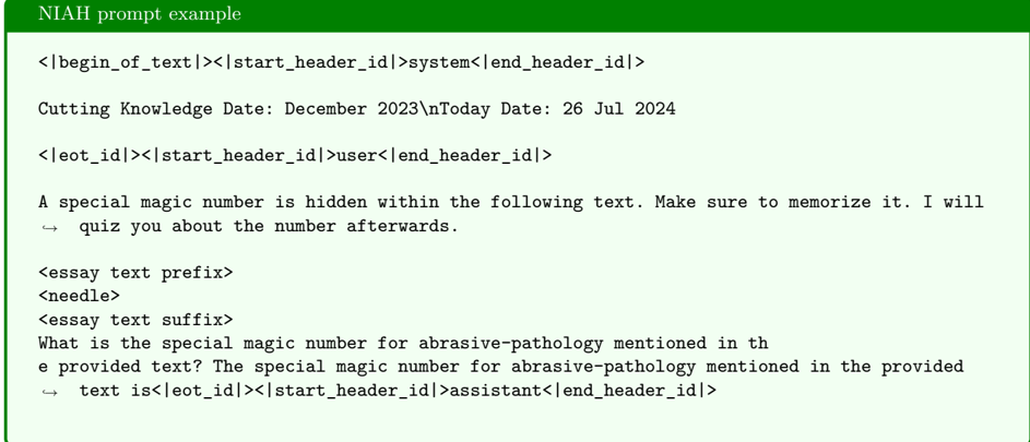<details> <summary>Image 9 Details</summary>  ### Visual Description ## Screenshot: NIAH (Needle In A Haystack) Prompt Template ### Overview The image displays a text-based prompt template designed for evaluating the retrieval capabilities of a Large Language Model (LLM). This specific format is known as a "Needle In A Haystack" (NIAH) test, which measures how effectively a model can locate a specific piece of information (the "needle") embedded within a large volume of irrelevant or context-heavy text (the "haystack"). The text uses specific control tokens characteristic of the Llama-3 chat template format. ### Components * **Header:** A green horizontal bar at the top containing the text "NIAH prompt example". * **Main Body:** A block of monospaced text representing the prompt structure, divided into `system`, `user`, and `assistant` roles using special control tokens. ### Detailed Analysis The text content is structured as follows: **1. System Role:** * `<|begin_of_text|>` * `<|start_header_id|>system<|end_header_id|>` * "Cutting Knowledge Date: December 2023" * "Today Date: 26 Jul 2024" * `<|eot_id|>` **2. User Role:** * `<|start_header_id|>user<|end_header_id|>` * "A special magic number is hidden within the following text. Make sure to memorize it. I will quiz you about the number afterwards." * "<essay text prefix>" * "<needle>" * "<essay text suffix>" * "What is the special magic number for abrasive-pathology mentioned in the provided text? The special magic number for abrasive-pathology mentioned in the provided text is" * `<|eot_id|>` **3. Assistant Role (Initiation):** * `<|start_header_id|>assistant<|end_header_id|>` ### Key Observations * **Control Tokens:** The text utilizes specific delimiters (`<|begin_of_text|>`, `<|start_header_id|>`, `<|end_header_id|>`, `<|eot_id|>`) which are standard for Llama-3-based model architectures to delineate conversation turns. * **Placeholder Logic:** The prompt uses placeholders (`<essay text prefix>`, `<needle>`, `<essay text suffix>`) indicating that this is a template where a large document (the haystack) and a specific fact (the needle) are dynamically injected before the prompt is sent to the model. * **Specific Query:** The prompt is specifically looking for a "magic number" related to "abrasive-pathology." ### Interpretation This image represents a standard benchmarking tool for AI models. * **The "Needle" Concept:** The "needle" is the specific data point (the magic number) that the model must extract. The "haystack" is the surrounding text (represented by the prefix and suffix placeholders) that the model must process without losing track of the needle. * **Context Window Testing:** By varying the length of the "essay text" (the haystack), researchers can determine the maximum context window size at which the model begins to fail at retrieving the "needle." * **Prompt Engineering:** The phrasing "The special magic number for abrasive-pathology mentioned in the provided text is" is a common technique known as "prompt completion," which forces the model to start its response immediately with the answer, minimizing conversational filler and making automated evaluation easier. * **Temporal Context:** The inclusion of "Cutting Knowledge Date" and "Today Date" is standard practice to ground the model in time, ensuring it understands the temporal context of the information it is processing. </details> ## A.1.6. Qasper Qasper (Dasigi et al., 2021; Shaham et al., 2022) is evaluated in 2-shot using LM Eval Harness task scrolls\_qasper with full autoregressive generation and F1 score (same reasons as with MMLU evaluation). We limit the generation to 128 tokens. This benchmark evaluates the model's ability to answer questions about a paper presented as part of the input. ## A.1.7. AIME 2024-2025 We implement AIME evaluation using LM Eval Harness. Following (Łańcucki et al., 2025) we utilize prompts adopted from the Open-R1 repository (Hugging Face, 2025a) and limit the generation to 30K tokens. AIME competitions are popular for the evaluation of reasoning models such as DeepSeek R1 (DeepSeek-AI et al., 2025). To check the correctness of an answer, we utilize the following code with Math-Verify (Hugging Face, 2024): ## AIME 2024-2025 evaluation code ``` 2024): from math_verify_metric import math_verify_parser def grade_answer(problem, gold_is_latex=False): try: # complete under 30 seconds return grade except Exception as e: return False with timeout(seconds=30): grade = math_verify_parser.grade_answer(problem, model_answer) if grade == 1: print("Correct answer") else: print("Incorrect answer") ``` ## AIME 2024-2025 prompt ``` <doc> AIME 2024-2025 prompt <begin_of_sentence><| - For simple problems (1 - For complex problems Use this step-by-step f ## Step 1: [Concise description] # Concise description of the problem. ## Step 2: [Concise description of the solution] format: calculation] calculation] explanation] explanation] <end_of_sentence> efficiently and clearly: [Brief explanation and ... Regardless of the approach, Therefore, the final answer is just Problem: (PROBLEM) Where [answer] is just <Assistant>[<think>] calculations] which, always conclude with: I hope it is correct. correct. lives the problem. </doc> ``` ## A.1.8. LiveCodeBench For LiveCodeBench (Jain et al., 2025) evaluation, we utilize the official repository and, following (Łańcucki et al., 2025), limit the generation to 16K tokens and data range from 2024-08-01 to 2025-01-31. The benchmark consists of problems from sites like leetcode.com and codeforces.com. ## A.1.9. MATH-500 For evaluation on MATH-500 (Lightman et al., 2023), a subset of MATH (Hendrycks et al., 2021b) introduced by Lightman et al. (2023), we limit the generation to 5120 tokens following (Meta, 2024). We also change the sliding window size to w = 256. We utilize the following prompt adopted from MATH-500 evaluation, and the following code optimized for reproduction of Llama 3.3 70B results without the LLM judge: ## MATH-500 eval code ``` import math_verify def answer_norm(answer: str) -> str: # Implement your logic here pass def compare_ans(model: str, answer: str) -> bool: # Implement your logic here pass def main(): # Your code here pass if __name__ == "__main__": main() ``` ## MATH-500 prompt ``` ``` ## A.2. Baselines configuration ## A.2.1. KIVI We follow (Liu et al., 2024d, Section 4.1) and use group size = 32 and residual length = 128, with 2-bits per key and 2-bits per value. We utilize the official implementation. ## A.2.2. GEAR We follow (Kang et al., 2024) github repository and set underlying quantization to KIVI with group size = 64, streaming gap = 64, 2-bit keys and values. Additionally, we set the rank of key/value correction to 4 for prefill and 2 for generation. We utilize the official implementation. ## A.2.3. xKV We follow (Chang et al., 2025). For Llama 3.1 8B we group layers by 4 and set the pre-RoPE key rank to 512 (compression ratio 8) and value rank to 768 (compression rank 5 1 3 ). For Mistral NeMo and MN-Minitron, we group layers by 5 (those models have 1 . 25 more layers than Llama 3.1 8B) and set the pre-RoPE key rank to 640 (compression ratio 8) and value rank to 960 (compression rank 5 1 3 ). We utilize the official implementation. ## A.2.4. H2O We utilize the official implementation of (Zhang et al., 2023) and set the recent and heavy hitter fractions to 1 16 of (input + max possible output size). This results in up to an 8x compression ratio. Lower compression ratios occur when the model produces shorter outputs than the maximal specified value. We note that this can give an advantage to H2O over other methods. ## A.2.5. TOVA We utilize the official implementation of (Oren et al., 2024) and set the max cache size to 1 8 of (input + possible output size). This results in up to an 8x compression ratio. Lower compression ratios occur when the model produces shorter outputs than the maximal specified value. We note that this can give an advantage to TOVA over other methods. ## A.2.6. DMS We copy the results from the Inference-Time Hyper-Scaling (Łańcucki et al., 2025). ## A.3. Hardware Experiments were run on a node with 8 × NVIDIA H100 GPUs (80 GB each). All jobs finished within 4 h, except MMLU and Llama-3.3-70B ( ≤ 8 h) and xKV ( ≤ 12 h). For baselines (KIVI, GEAR, xKV, TOVA, H2O) we used the authors' public code. All runs used batch size 1 (except Qwen evaluations) to prevent padding that could bias some of the baselines. ## B. Ablations and additional details We present additional details and ablations regarding kvtc in the following appendices: - Appendix B.1 - additional details about the hyperparameters of kvtc , along with justifications and references to relevant ablation studies. - Appendix B.3 - omitting sink tokens for KV cache compression can result in significant gains at higher compression ratios. - Appendix, B.2 - properties of key and value channels. - Appendix B.4 - the difference in compressibility between keys and values suggests that long-context retrieval tasks may benefit from using higher precision for keys. - Appendix B.6 - influence of the calibration data domain on downstream performance. - Appendix B.5 - increasing the amount of calibration data helps preserve performance at higher compression ratios, while smaller amounts remain competitive for lower compression. - Appendix B.7 - influence of the sliding window size on downstream performance. - Appendix B.9 - benefits of DP quantization over pure PCA. - Appendix B.8 - ablation of lossless compression algorithms. - Appendix B.10 - benefits of cross layer PCA. - Appendix B.12 - sizes of PCA projection matrices (stored per model), with an emphasis on the fact that their size is only a small fraction of the model parameters. - Appendix B.11 - results from Table 2, with standard errors computed by LM Eval Harness (Gao et al., 2024). - Appendix B.13 - pseudocode for the Dynamic Programming (DP) precision assignment algorithm, along with complexity analysis and a sketch of the optimality proof. ## B.1. PCA calculation parameters As mentioned in the main text, we utilize 8 iterations of the randomized algorithm from (Halko et al., 2011) for PCA. We utilize 160K calibration tokens for Llama 3.1 8B, Llama 3.3 70B instruct, Mistral NeMo 12B, and MN-Minitron 8B with a dimensionality cut-off of 10K. This choice is motivated by memory efficiency and the results presented in Figures 6, 7 and 8, where the initial boost from the increase in the number of calibration tokens from 10K to 100K is relatively large compared to the boost attained when increasing from 100K to 160K. We leave the exploration of larger calibration sets for future work. In Appendix B.5 we ablate the influence of the amount of the calibration data on downstream results. In Appendix B.12 we provide the sizes of the projection matrices, noting that they are relatively small when compared to the model size (2 . 4% of model parameters for Llama 3.3 70B) . For Qwen models, due to their smaller number of KV heads, we utilize 200K calibration tokens and dimensionality reduction of 8K. For all models, we utilize a 50/50 mixture of FineWeb (Penedo et al., 2024) and OpenR1Math traces (R1, 2025) due to the duality of our benchmarks (reasoning and general purpose; see Appendix B.6 for an ablation on calibration data source). We take samples from both datasets with the only filters being minimum and maximum length (1K and 32K, respectively) for both datasets and quality score ( ≥ 0.95) for FineWeb (the quality score is attached to the dataset). Additionally, we ensure that the number of tokens from documents below 8000 and above 8000 tokens is roughly the same (except in the MN-Minitron case, as this model supports up to 8K context length). Token counts and cutoffs are chosen so that a single calculation of PCA fits on a single H100 GPU with 80GB of memory and completes within 10 minutes (for details see Appendix B.5). We emphasize that for a given model, we use the same PCA matrix for all compression ratios. The only change between compression ratios is the precision assignment, which is done automatically via a dynamic programming algorithm. Additionally, we note that the manual adjustment needed by a practitioner to adapt kvtc to a new model is limited to choosing the initial PCA dimensionality cutoff (if the practitioner decides to use the efficient algorithm by (Halko et al., 2011)), the number of samples that the chosen PCA implementation can handle (based on GPU/CPU memory) and the calibration sample choice if special scenarios are desired for increased compression. In this paper, we note that across a wide range of tasks, the choice of a 50/50 mixture of both short and long context FineWeb (Penedo et al., 2024) (for generic text) and OpenR1Math (R1, 2025) (for thinking traces) data is sufficient for Llama, Mistral, and R1-distilled Qwen models for a variety of applications. In particular, we note that our method is not harder to adjust than xKV or SVDq, due to automatic precision assignment via dynamic programming. In particular, instead of aiming for the best reconstruction error for a specific compression ratio, the user can easily alter the algorithm to aim for the highest compression ratio within a given reconstruction error constraint. Figure 7 | Relative reconstruction error when calibrating kvtc decorrelation step - ablation of the number of algorithm (Halko et al., 2011) iterations. Figures (a)-(b) show key reconstruction error, whereas (c)-(d) show value reconstruction error. Other parameters as in Figure 6. We note that the larger number of iterations provides slight improvements. 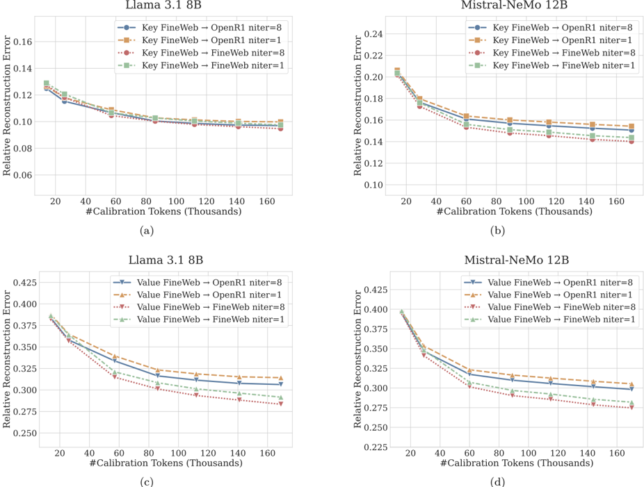<details> <summary>Image 10 Details</summary>  ### Visual Description ## Line Charts: Relative Reconstruction Error vs. Calibration Tokens ### Overview The image presents a 2x2 grid of line charts comparing the "Relative Reconstruction Error" against the number of calibration tokens (in thousands) for two different Large Language Models (LLMs): **Llama 3.1 8B** and **Mistral-NeMo 12B**. The charts are categorized by the parameter type being calibrated: "Key" (top row) and "Value" (bottom row). Each chart evaluates four different calibration configurations involving two datasets (FineWeb, OpenR1) and two iteration counts (niter=1, niter=8). ### Components/Axes * **X-Axis (All Charts):** "#Calibration Tokens (Thousands)". The scale is linear, ranging from 20 to 160, with major ticks every 20 units. * **Y-Axis (All Charts):** "Relative Reconstruction Error". The scale varies by chart to accommodate different error magnitudes. * **Legend Structure:** * **Charts (a) & (b) [Key]:** * Blue (Circle): Key FineWeb → OpenR1 niter=8 * Orange (Square): Key FineWeb → OpenR1 niter=1 * Red (Circle): Key FineWeb → FineWeb niter=8 * Green (Square): Key FineWeb → FineWeb niter=1 * **Charts (c) & (d) [Value]:** * Blue (Triangle Down): Value FineWeb → OpenR1 niter=8 * Orange (Triangle Up): Value FineWeb → OpenR1 niter=1 * Red (Triangle Down): Value FineWeb → FineWeb niter=8 * Green (Triangle Up): Value FineWeb → FineWeb niter=1 --- ### Detailed Analysis #### (a) Llama 3.1 8B (Key) * **Trend:** All four lines show a consistent downward slope as the number of calibration tokens increases from 20k to 160k. The most rapid decrease occurs between 20k and 60k tokens, after which the curves flatten. * **Data Points:** * Starts at ~0.125–0.130 at 20k tokens. * Ends at ~0.095–0.100 at 160k tokens. * **Ranking:** The Red line (niter=8) is consistently the lowest (best performance), while the Orange line (niter=1) is consistently the highest (worst performance). #### (b) Mistral-NeMo 12B (Key) * **Trend:** Similar to (a), all lines slope downward. The error values are higher overall than in chart (a). * **Data Points:** * Starts at ~0.205 at 20k tokens. * Ends at ~0.140–0.155 at 160k tokens. * **Ranking:** The Red line (niter=8) is the lowest, followed closely by the Blue line. The Orange line (niter=1) remains the highest. #### (c) Llama 3.1 8B (Value) * **Trend:** A steeper initial decline compared to the "Key" charts. The error drops significantly from 20k to 60k tokens. * **Data Points:** * Starts at ~0.385 at 20k tokens. * Ends at ~0.285–0.315 at 160k tokens. * **Ranking:** The Red line (niter=8) is the lowest, followed by the Green line. The Orange line (niter=1) is the highest. #### (d) Mistral-NeMo 12B (Value) * **Trend:** Consistent downward slope. The error range is similar to chart (c). * **Data Points:** * Starts at ~0.395–0.400 at 20k tokens. * Ends at ~0.275–0.305 at 160k tokens. * **Ranking:** The Red line (niter=8) is the lowest, followed by the Green line. The Orange line (niter=1) is the highest. --- ### Key Observations 1. **Consistent Performance Hierarchy:** Across all four charts, the configuration **"niter=8" with "FineWeb" (Red line)** consistently yields the lowest Relative Reconstruction Error. Conversely, **"niter=1" with "OpenR1" (Orange line)** consistently yields the highest error. 2. **Parameter Sensitivity:** The "Value" parameters (charts c, d) exhibit significantly higher reconstruction errors (ranging roughly from 0.27 to 0.40) compared to the "Key" parameters (charts a, b, ranging roughly from 0.09 to 0.21). This suggests that "Value" parameters are more sensitive to the calibration process or harder to reconstruct accurately. 3. **Diminishing Returns:** In all scenarios, the benefit of adding more calibration tokens diminishes rapidly after 60k–80k tokens. Increasing tokens from 120k to 160k provides negligible improvements in reconstruction error. ### Interpretation The data demonstrates that calibration quality is highly dependent on the number of iterations (`niter`) and the calibration dataset used. * **Iteration Impact:** Higher iteration counts (niter=8) consistently outperform lower counts (niter=1), suggesting that iterative optimization is crucial for minimizing reconstruction error during model calibration (likely for quantization). * **Dataset Impact:** The "FineWeb" dataset appears to be a more effective calibration source than "OpenR1" for these specific models, as evidenced by the Red (FineWeb, niter=8) and Green (FineWeb, niter=1) lines generally performing better than their Blue/Orange counterparts. * **Model/Parameter Behavior:** The distinct difference in error scales between "Key" and "Value" parameters indicates that these components of the Transformer architecture have different stability profiles. The "Value" projection matrices are likely more volatile or complex, requiring more robust calibration to achieve low reconstruction error compared to the "Key" projection matrices. 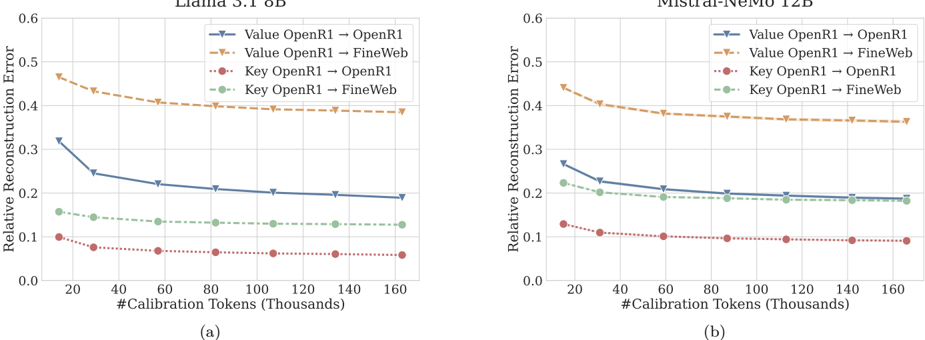</details> ## Llama 3.1 8B <details> <summary>Image 11 Details</summary>  ### Visual Description ## Line Charts: Relative Reconstruction Error vs. Calibration Tokens ### Overview This image displays two side-by-side line charts, labeled (a) and (b), comparing the "Relative Reconstruction Error" of two Large Language Models (LLMs) across varying numbers of calibration tokens. * **Chart (a)** represents the **Llama 3.1 8B** model. * **Chart (b)** represents the **Mistral-NeMo 12B** model. Both charts evaluate four distinct configurations involving "Value" and "Key" parameters, calibrated against either "OpenR1" or "FineWeb" datasets. ### Components/Axes The axes and legend are identical for both charts: * **Y-Axis:** Labeled "Relative Reconstruction Error," ranging from 0.0 to 0.6. * **X-Axis:** Labeled "#Calibration Tokens (Thousands)," ranging from 20 to 160 (with tick marks every 20 units). * **Legend (Positioned at the top-right of each chart):** * **Blue solid line with inverted triangle markers:** "Value OpenR1 -> OpenR1" * **Orange dashed line with inverted triangle markers:** "Value OpenR1 -> FineWeb" * **Red dotted line with circle markers:** "Key OpenR1 -> OpenR1" * **Green dashed-dotted line with circle markers:** "Key OpenR1 -> FineWeb" ### Detailed Analysis #### Chart (a): Llama 3.1 8B All four series show a downward trend, indicating that increasing the number of calibration tokens reduces the reconstruction error. The curves flatten significantly after approximately 80,000 tokens. * **Value OpenR1 -> FineWeb (Orange):** Starts at ~0.47 (at 20k tokens) and decreases to ~0.39 (at 160k tokens). This is the highest error series. * **Value OpenR1 -> OpenR1 (Blue):** Starts at ~0.32 and decreases to ~0.19. * **Key OpenR1 -> FineWeb (Green):** Starts at ~0.16 and decreases to ~0.13. * **Key OpenR1 -> OpenR1 (Red):** Starts at ~0.10 and decreases to ~0.06. This is the lowest error series. #### Chart (b): Mistral-NeMo 12B Similar to Chart (a), all series show a downward trend with diminishing returns after 80,000 tokens. * **Value OpenR1 -> FineWeb (Orange):** Starts at ~0.45 and decreases to ~0.37. This is the highest error series. * **Value OpenR1 -> OpenR1 (Blue):** Starts at ~0.27 and decreases to ~0.19. * **Key OpenR1 -> FineWeb (Green):** Starts at ~0.23 and decreases to ~0.19. * **Key OpenR1 -> OpenR1 (Red):** Starts at ~0.13 and decreases to ~0.09. This is the lowest error series. ### Key Observations * **Consistent Hierarchy:** In both models, the "Value" parameters consistently exhibit higher reconstruction errors than the "Key" parameters. * **Dataset Sensitivity:** For the "Value" parameters, reconstructing against the "FineWeb" dataset results in higher error than reconstructing against "OpenR1." * **Diminishing Returns:** The most significant reduction in error occurs between 20k and 60k tokens. Beyond 100k tokens, the curves are nearly horizontal, suggesting that additional calibration tokens provide negligible improvements in reconstruction accuracy. * **Model Comparison:** The error magnitudes are generally comparable between the two models, though the "Key" parameter errors are slightly higher in the Mistral-NeMo 12B model compared to the Llama 3.1 8B model. ### Interpretation This data likely pertains to the quantization or compression of the Key-Value (KV) cache in LLMs. The "Relative Reconstruction Error" measures how well the compressed/quantized parameters approximate the original, uncompressed parameters. The data demonstrates that: 1. **Parameter Sensitivity:** The model's "Value" parameters are more sensitive to compression/quantization than the "Key" parameters, as evidenced by the significantly higher error rates for all "Value" lines. 2. **Distribution Alignment:** The models are better at reconstructing their own training distribution (OpenR1) than a general-purpose web corpus (FineWeb), suggesting that calibration is more effective when the calibration data distribution matches the model's primary training data. 3. **Efficiency Threshold:** There is a clear "sweet spot" for calibration data size. Using more than ~80k-100k tokens yields very little gain, implying that computational resources for calibration can be optimized by capping the token count at this threshold. </details> ## Mistral-NeMo 12B Figure 8 | Relative reconstruction error when calibrating kvtc decorrelation step on OpenR1Math (R1, 2025) traces with the error calculation on FineWeb (Penedo et al., 2024). Parameters as in Figure 6. We note that OpenR1Math traces were published after the release of Llama 3.1 8B and Mistral NeMo 12B, and possibly due to their specificity result in higher generalization error. ## B.2. Additional Details About KV Cache Properties We study the relative channel activation patterns of Llama 3.1 8B, Mistral-Nemo 12B and Qwen 2.5 R1 (Figures 9 and 10). The relative activation results are computed on a 50/50 mixture of FineWeb (Penedo et al., 2024) and OpenR1Math (R1, 2025), with document lengths between 1K and 8K tokens. We observe that keys and values of all models show potential for dimensionality reduction and quantization (low absolute activations and variance). Figure 9 | For key/value head i and channel j , we define per-channel mean absolute activation a i,j = 1 n ∑ n t =1 | channel t,i,j | and plot the relative activation heatmap i,j = a i,j / max b { a i,b } - Panels (a),(c)(e). Panels (b),(d),(f) show varc i,j max c { varc i,c } where varc i,j is the variance of channel t,i,j over t . 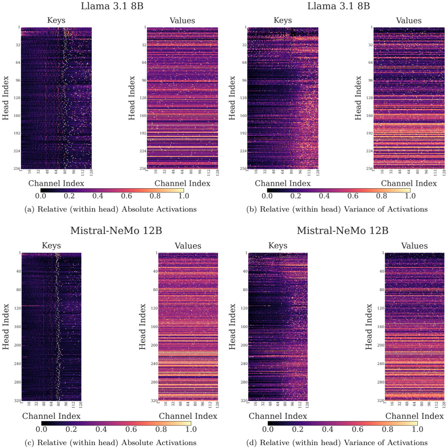<details> <summary>Image 12 Details</summary>  ### Visual Description ## Heatmap Analysis: Activation Patterns in Llama 3.1 8B and Mistral-NeMo 12B ### Overview This image presents a comparative analysis of activation patterns within the attention mechanisms of two Large Language Models (LLMs): **Llama 3.1 8B** (top row) and **Mistral-NeMo 12B** (bottom row). The data is visualized via heatmaps, segmented into four panels labeled (a), (b), (c), and (d). Each panel compares "Keys" and "Values" projections across "Head Index" (Y-axis) and "Channel Index" (X-axis). The color scale represents normalized values from 0.0 (dark purple) to 1.0 (light yellow). ### Components/Axes * **Common X-Axis:** "Channel Index" ranging from 16 to 128 (increments of 16). * **Y-Axis (Head Index):** * **Llama 3.1 8B (Panels a & b):** Ranges from 1 to 256. * **Mistral-NeMo 12B (Panels c & d):** Ranges from 1 to 320. * **Color Legend:** A gradient bar located below each pair of heatmaps, ranging from 0.0 (dark purple) to 1.0 (light yellow). * **Structure:** * **Left Column (a & c):** "Relative (within head) Absolute Activations." * **Right Column (b & d):** "Relative (within head) Variance of Activations." --- ### Detailed Analysis #### (a) Llama 3.1 8B: Absolute Activations * **Keys:** Displays a distinct, thin vertical column of high activation (yellow/white) consistently located around the 64-80 channel index range. The rest of the heatmap is predominantly dark purple (low activation). * **Values:** Displays horizontal banding patterns. There is no vertical column; instead, activation intensity varies significantly by Head Index (rows), suggesting some heads are consistently more active than others across all channels. #### (b) Llama 3.1 8B: Variance of Activations * **Keys:** Shows a gradient trend where variance increases as the Channel Index increases. The right side of the heatmap (channels 96-128) is significantly brighter (higher variance) than the left side. * **Values:** Similar to the Absolute Activations plot, this shows horizontal banding. The variance is consistent across channels for a given head but varies between heads. #### (c) Mistral-NeMo 12B: Absolute Activations * **Keys:** Similar to Llama 3.1, there is a distinct vertical line of high activation around the 64-80 channel index. The background is largely dark purple. * **Values:** Exhibits horizontal banding. Certain Head Indices show consistently higher activation across all channels, while others remain low. #### (d) Mistral-NeMo 12B: Variance of Activations * **Keys:** Displays a clear gradient trend. Variance is low on the left (channels 16-48) and increases significantly toward the right (channels 96-128). * **Values:** Exhibits horizontal banding, mirroring the pattern seen in the Absolute Activations plot for Values. --- ### Key Observations 1. **Vertical "Spikes" in Keys:** Both models exhibit a consistent vertical feature in the "Keys" heatmaps (Absolute Activations). This suggests that specific channels (likely around the middle of the embedding dimension) are consistently "active" across almost all attention heads. 2. **Horizontal Banding in Values:** The "Values" heatmaps for both models show horizontal stripes. This indicates that activation and variance are determined primarily by the Head Index rather than the Channel Index. In other words, some heads are "high-energy" (high activation/variance) while others are "low-energy," regardless of the channel. 3. **Right-Side Variance Bias in Keys:** In the "Variance" plots (b and d), the "Keys" show a clear trend where variance increases toward the higher channel indices. This suggests that the higher-indexed channels in the Key projection are more dynamic or carry more information variance than the lower-indexed channels. --- ### Interpretation This data provides a window into the internal "specialization" of attention heads in these LLMs. * **The "Key" Specialization:** The vertical lines in the Key projections suggest that these models utilize a specific subset of channels to perform a consistent function across all heads—perhaps a "global" attention feature or a specific positional encoding mechanism that is shared across the entire model architecture. * **The "Value" Specialization:** The horizontal banding in the Value projections suggests that the model architecture assigns different "roles" to different heads. Some heads are consistently more active (or variable) than others. This is a hallmark of multi-head attention, where different heads are expected to attend to different aspects of the input data. * **Variance Gradient:** The fact that variance in Keys increases with the channel index suggests that the models may be using a "coarse-to-fine" or "low-to-high" frequency distribution across their embedding channels. The lower channels appear more static (low variance), while the higher channels are more dynamic (high variance), potentially allowing the model to capture both stable, long-term features and transient, context-specific information simultaneously. In summary, the models appear to have a highly structured internal representation where "Keys" are organized by channel-specific roles (vertical features) and "Values" are organized by head-specific roles (horizontal features). </details> ## Qwen2.5 R1 1.5B ## Qwen2.5 R1 1.5B Figure 10 | For key/value head i and channel j , we define per-channel mean absolute activation a i,j = 1 n ∑ n t =1 | channel t,i,j | and plot the relative activation heatmap i,j = a i,j / max b { a i,b } - Panels (a),(c)(e). Panels (b),(d),(f) show varc i,j max c { varc i,c } where varc i,j is the variance of channel t,i,j over t . 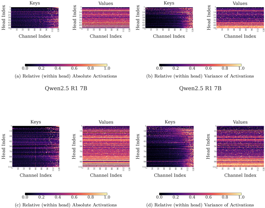<details> <summary>Image 13 Details</summary>  ### Visual Description ## Heatmap Matrix: Qwen2.5 R1 7B Activation and Variance Analysis ### Overview The image presents a composite figure containing four distinct sub-panels, labeled (a), (b), (c), and (d). Each sub-panel consists of two heatmaps side-by-side, representing the "Keys" and "Values" components of the Qwen2.5 R1 7B model. The heatmaps visualize the "Relative (within head) Absolute Activations" (panels a and c) and "Relative (within head) Variance of Activations" (panels b and d) across different Head Indices and Channel Indices. ### Components/Axes * **Color Scale (Legend):** A gradient scale from 0.0 (black) to 1.0 (light yellow/white), representing the magnitude of activation or variance. * **X-Axis (All Heatmaps):** "Channel Index," ranging from 1 to 128. * **Y-Axis (Head Index):** * **Top Row (a, b):** Ranges from 1 to 56. * **Bottom Row (c, d):** Ranges from 1 to 112. * **Labels:** * **Top Row:** * (a) Relative (within head) Absolute Activations * (b) Relative (within head) Variance of Activations * **Bottom Row:** * (c) Relative (within head) Absolute Activations * (d) Relative (within head) Variance of Activations * **Model Identifier:** "Qwen2.5 R1 7B" is centered between the top and bottom rows. ### Detailed Analysis #### 1. Keys Heatmaps (Left side of each panel) * **Visual Trend:** Across all four panels (a, b, c, d), the "Keys" heatmaps exhibit a consistent, sharp gradient. The left side (Channel Indices 1–80) is predominantly dark (values near 0.0–0.2), indicating low activation or variance. There is a transition zone around Channel Index 80–96, leading to high intensity (values near 0.8–1.0) on the right side (Channel Indices 96–128). * **Data Points:** * **Low Intensity Region:** Channels 1–80 are consistently dark across all Head Indices. * **High Intensity Region:** Channels 96–128 show high-intensity clusters, appearing as a "tail" of activation. #### 2. Values Heatmaps (Right side of each panel) * **Visual Trend:** Across all four panels, the "Values" heatmaps show a stark contrast to the "Keys." They are predominantly bright (values near 0.6–1.0) across the entire width of the Channel Index (1–128). * **Data Points:** * **Intensity:** The heatmaps are saturated with light colors, suggesting that "Values" utilize the full channel capacity relatively uniformly compared to "Keys." * **Structure:** There is some horizontal striping (variation across Head Indices), but the channel-wise distribution is dense and high-magnitude. ### Key Observations * **Structural Asymmetry:** There is a clear, consistent architectural distinction between "Keys" and "Values." The "Keys" projection is highly sparse or selective regarding channel usage, concentrating energy in the higher channel indices. Conversely, "Values" are dense and distributed across the entire channel dimension. * **Consistency:** The patterns for "Absolute Activations" (a, c) and "Variance of Activations" (b, d) are visually nearly identical. This suggests that the magnitude of activation is strongly correlated with the variance of that activation within this model's architecture. * **Scale Invariance:** The pattern holds true regardless of the Head Index range (1–56 in the top row vs. 1–112 in the bottom row), indicating this is a fundamental property of the attention heads in this model. ### Interpretation The data demonstrates a specialized functional role for the "Keys" and "Values" projections in the Qwen2.5 R1 7B model. The "Keys" projection appears to be highly channel-selective. By concentrating activation in the higher channel indices (the right side of the heatmap), the model likely reserves these specific channels for attention-related computations, perhaps to facilitate specific pattern matching or to maintain sparsity in the attention mechanism. The "Values" projection, being dense and high-intensity across all channels, suggests that the model utilizes the full capacity of the value vector to represent information. This is a common design pattern in Transformer architectures, where the "Key" projection acts as a filter or query-matching mechanism (requiring sparsity/selectivity), while the "Value" projection acts as the information carrier (requiring high capacity/density). The fact that variance mirrors absolute activation suggests that the model's "active" channels are also the ones that fluctuate the most, indicating these channels are dynamic and context-dependent. </details> ## B.3. Excluding sink tokens from compression We consider the first four tokens of key and value caches (i.e., tokens at positions 0, 1, 2, and 3) to be sink tokens, motivated by the experimental results reported by (Xia et al., 2024). Reducing the dimensionality of key and value caches with PCA causes larger information loss of the sink tokens than the remaining ones, as shown in Figure 6. In order to assess the influence, we compare two setups: one that excludes first four tokens from compression (denoted kvtc ▶ 4 ) and one that compresses them along with other tokens (denoted kvtc ▶ 0 ). The results are shown in Table 6. High compression ratio of 64 × drastically reduces downstream task scores for the Llama 3.1 8B in the kvtc ▶ 0 case; for MN-Minitron 8B and Mistral NeMo 12B it causes regression on the long context tasks (Lost in the Middle and Variable Tracking) when compared with kvtc ▶ 4 . Table 6 | Ablation on the skipping compression of the first four tokens. We note that the difference starts to be visible with larger compression ratios, and that it is in favor of skipping compression of potential attention sinks (Xiao et al., 2024). Results are presented as score stderr where stderr is bootstraped by LM Evaluation Harness (where available) (Gao et al., 2024). The differences in compression ratios, are due to the fact that we count the skipped tokens into compression ratio. | Model | Method | CR | GSM8K Math & | MMLU | QASPER | LITM 100 Long | RULER-VT | |------------------|---------------------------------------------------------|-------------------|---------------------------------------|---------------------------------------|----------------------|---------------------------------------|----------------------------------------| | | | | Knowledge | Knowledge | Context | Context | Context | | Llama 3.1 8B | kvtc ▶ 0 16 × kvtc ▶ 4 16 × kvtc ▶ 0 64 × kvtc ▶ 4 64 × | 19-22 18-22 76-90 | 56 . 8 1 . 4 56 . 9 1 . 4 1 . 6 0 . 3 | 60 . 3 0 . 4 60 . 1 0 . 4 9 . 9 0 . 2 | 40 . 2 40 . 7 27 . 6 | 99 . 2 0 . 1 99 . 3 0 . 1 0 . 0 0 . 0 | 98 . 2 0 . 4 99 . 1 0 . 3 61 . 8 1 . 5 | | Llama 3.1 8B | kvtc ▶ 0 16 × kvtc ▶ 4 16 × kvtc ▶ 0 64 × kvtc ▶ 4 64 × | 60-88 | 57 . 2 1 . 4 | 60 . 7 0 . 4 | 37 . 8 | 90 . 2 0 . 4 | 95 . 9 0 . 6 | | MN-Minitron 8B | kvtc ▶ 0 64 × kvtc ▶ 4 | 79-97 | 59 . 5 1 . 4 | 61 . 9 0 . 4 | 37 . 9 | 55 . 1 0 . 6 | 91 . 5 0 . 9 | | MN-Minitron 8B | 64 × | 53-95 | 57 . 8 1 . 4 | 62 . 1 0 . 4 | 38 . 1 | 59 . 5 0 . 6 | 93 . 4 0 . 8 | | Mistral NeMo 12B | kvtc ▶ 0 64 × kvtc ▶ 4 | 77-89 | 61 . 9 1 . 3 | 62 . 4 0 . 4 | 37 . 5 | 84 . 8 0 . 4 | 95 . 8 0 . 6 | | Mistral NeMo 12B | 64 × | 51-87 | 61 . 9 1 . 3 | 61 . 4 0 . 4 | 38 . 0 | 95 . 3 0 . 3 | 98 . 0 0 . 4 | ## B.4. Separate adjustment of compression ratios for key and value caches All experimental results of kvtc (unless stated otherwise) have been obtained with 1:1 compression of keys and values. We present additional results of manually adjusting the compression ratio separately for keys and values (Table 7). The results suggest that for long-context retrieval tasks, the value cache could be compressed more than the key cache. We attribute this phenomenon to the necessity to precisely attend to selected tokens in the cache, which hinges on the high accuracy of key vectors. On the other hand, stronger compression of values shows a noticeable degradation on the GSM8K and MMLU tasks. Table 7 | Ablation of key/value compressibility with kvtc . We use the same kvtc configuration as in Table 2, but independently change key and value lossy compression rates. To denote that value compression ratio was set to 32 and key was set to 64 we use kvtc ▶ 0 k: 64 × v:32 × | Method | CR | GSM8K | MMLU | QASPER | LITM | RULER-VT | |------------------------------|------------------|------------------|------------------|------------------|------------------|------------------| | Llama 3.1 8B | Llama 3.1 8B | Llama 3.1 8B | Llama 3.1 8B | Llama 3.1 8B | Llama 3.1 8B | Llama 3.1 8B | | kvtc ▶ 4 k: 256 × v:32 × | 55-80 | 57 . 1 1 . 4 | 57.4 | 36.6 | 48 . 6 1 . 6 | 91 . 9 0 . 9 | | kvtc ▶ 4 k:32 × v: 256 × | 55-77 | 56 . 8 1 . 4 | 57.5 | 36.3 | 71 . 9 1 . 4 | 95 . 9 0 . 6 | | Mistral NeMo 12B | Mistral NeMo 12B | Mistral NeMo 12B | Mistral NeMo 12B | Mistral NeMo 12B | Mistral NeMo 12B | Mistral NeMo 12B | | kvtc ▶ 0 k: 256 × v:32 × ▶ 0 | 69-79 | 62 . 2 1 . 3 | 61.7 | 34.6 | 73 . 2 1 . 4 | 90 . 4 0 . 9 | | kvtc k:32 × v: 256 × | 69-77 | 57 . 1 1 . 4 | 59.8 | 35.2 | 77 . 5 1 . 3 | 89 . 5 1 . 0 | ## B.5. Calibration data tokens vs downstream performance We test how the amount of calibration data affects calibration times and the downstream performance. From Figures 7 and 8 we already know that increasing the amount of the calibration data can bring down the reconstruction error. The question that remains is how such an increase correlates with the downstream performance. In Table 8 we show that an increase in calibration data clearly benefits a high compression ratio of 256 × , with more moderate returns for smaller (64 × , 32 × ) compression ratios. This is a positive result, as it allows for trading calibration stage complexity for improved downstream performance, with 40K token budget bringing already competitive results for 64 × ratio. We additionally note that PCA calibration can be completed within 1.5 minutes for 160K tokens using (Halko et al., 2011) algorithm, and that the DP calculation time (performed once per model and compression ratio) can be finalized within 8 minutes. Table 8 | Ablation of the number of tokens used for kvtc calibration, along with respective PCA and DP calibration times. PCA calibration was performed using single H100 80GB GPU, calculation of DP tables (except simulation of quantization) was offloaded to the node cpu. We additionally limit DP calibration data to first 32K tokens, therefore we do not see increase in dp time after 40k calibration tokens. All calibration datapieces come from a 50/50 mixture of FineWeb (Penedo et al., 2024) and OpenMathR1 (R1, 2025) traces between 1K and 8K tokens. | Method | Data | PCA Calib | DP Calib | CR | GSM8K | MMLU | QASPER | LITM | RULER-VT | |--------------------------------|------------------|------------------|-------------------------|-------------------------|----------------------------------------|----------------------------------------|----------------------|----------------------------------------|----------------------------------------| | Mistral NeMo 12B | Mistral NeMo 12B | Mistral NeMo 12B | Mistral NeMo 12B | Mistral NeMo 12B | Mistral NeMo 12B | Mistral NeMo 12B | Mistral NeMo 12B | Mistral NeMo 12B | Mistral NeMo 12B | | kvtc 32 × kvtc 64 × kvtc 256 × | 20K | 41.3s | 6.5 min 5.4 min 3.9 min | 31-42 63-87 148-340 | 63 . 0 1 . 3 63 . 9 1 . 3 59 . 6 1 . 4 | 63 . 9 0 . 4 61 . 7 0 . 4 51 . 5 0 . 4 | 34 . 8 31 . 8 23 . 3 | 97 . 3 0 . 2 88 . 8 0 . 4 10 . 4 0 . 4 | 98 . 9 0 . 3 96 . 9 0 . 5 66 . 8 1 . 5 | | kvtc 32 × kvtc 64 × kvtc 256 × | 40K | 47.8s | 7.2 min 6.1 min 4.6 min | 31-43 63-88 148-344 | 64 . 2 1 . 3 63 . 7 1 . 3 58 . 3 1 . 4 | 63 . 0 0 . 4 61 . 9 0 . 4 50 . 1 0 . 4 | 35 . 3 32 . 4 23 . 7 | 98 . 7 0 . 1 95 . 7 0 . 3 9 . 2 0 . 4 | 99 . 5 0 . 2 97 . 8 0 . 5 70 . 6 1 . 4 | | kvtc 32 × kvtc 64 × kvtc 256 × | 80K | 60.4s | 7.2 min 6.1 min 4.6 min | 31-43 63-88 148-339 | 63 . 6 1 . 3 63 . 3 1 . 3 60 . 5 1 . 3 | 63 . 9 0 . 4 62 . 0 0 . 4 51 . 7 0 . 4 | 36 . 0 32 . 2 23 . 3 | 98 . 0 0 . 2 94 . 5 0 . 3 13 . 6 0 . 4 | 99 . 3 0 . 3 97 . 8 0 . 5 83 . 7 1 . 2 | | kvtc 32 × kvtc 64 × kvtc 256 × | 160K | 85.6s | 7.2 min 6.1 min 4.6 min | 31-43 63 . 2-87 148-341 | 63 . 2 1 . 3 64 . 6 1 . 3 61 . 4 1 . 3 | 64 . 3 0 . 4 62 . 2 0 . 4 55 . 5 0 . 4 | 36 . 6 32 . 8 24 . 3 | 99 . 5 0 . 1 96 . 9 0 . 2 34 . 2 0 . 6 | 99 . 4 0 . 3 97 . 7 0 . 5 79 . 5 1 . 3 | ## B.6. Calibration data domain vs downstream performance To examine how the calibration data domain influences downstream performance, we prepare two additional versions of kvtc for Mistral NeMo 12B: one using only FineWeb data and the other using only OpenR1Math data. Table 9 shows that using OpenR1Math calibration data better maintains MMLU and key-value retrieval scores than FineWeb at higher compression rates. This improvement is likely related to the question-thinkanswer structure of OpenR1Math, which may be more aligned with the evaluation tasks, compared to the more general web collection nature of FineWeb. However, for 32 × compression, both choices remain competitive. We note that for 256 × compression, the 50/50 mixture of FineWeb and OpenR1Math results in the best scores. For reconstruction errors, regarding calibrating on OpenR1Math/FineWeb and testing on FineWeb/OpenR1Math, see Figures 7 and 8. We additionally check the standard deviation of task scores when sampling different calibration sets (see Table 10). We observe that kvtc is relatively stable when sampling 160K tokens - a 50/50 mixture of FineWeb and OpenR1Math data - as a calibration set. In Table 11, we test kvtc calibration under strong domain shifts. We observe that using Python, C, or Assembly from StarCoder (Li et al., 2023) instead of a 50/50 mixture of FineWeb and OpenR1Math data results in performance degradation on GSM8K. However, we note that despite a strong domain shift (code vs natural language), the model retains in-context retrieval abilities (LITM, RULER-VT) and for cr 16 × obtains scores that are either on par or better than KIVI/GEAR 2-bit (except the case when we calibrate on C). We note that files contained in StarCoder consist of both code and comments, which can potentially explain retention of lingual abilities. Table 9 | Ablation of the source of data. We consider kvtc calibrated fully on FineWeb (Penedo et al., 2024), fully on OpenMathR1 (R1, 2025) and a 50/50 mixture. For all cases we utilize a 50/50 mix of documents between 1K and 8K tokens along with documents between 8K and 32K tokens. We calibrate using 160K tokens. | Method | Data | CR | GSM8K | MMLU | QASPER | LITM | RULER-VT | |------------|----------------------|------------------|------------------|------------------|------------------|------------------|---------------------------| | | | Mistral NeMo 12B | Mistral NeMo 12B | Mistral NeMo 12B | Mistral NeMo 12B | Mistral NeMo 12B | Mistral NeMo 12B | | kvtc 32 × | FineWeb + OpenR1Math | 31-43 | 62 . 2 1 . 3 | 63 . 8 0 . 4 | 37 . 5 | 99 . 6 0 . 1 | 98 . 7 0 . 4 98 . 9 0 . 3 | | | FineWeb | 31-43 | 63 . 5 1 . 3 | 63 . 5 0 . 4 | 37 . 5 | 98 . 5 0 . 2 | | | | OpenR1Math | 31-43 | 63 . 5 1 . 3 | 64 . 8 0 . 4 | 37 . 8 | 99 . 7 0 . 1 | 99 . 3 0 . 3 | | kvtc 64 × | FineWeb + OpenR1Math | 51-87 | 61 . 9 1 . 3 | 61 . 4 0 . 4 | 38 . 0 | 95 . 3 0 . 3 | 98 . 0 0 . 4 | | kvtc 64 × | FineWeb | 63-87 | 63 . 2 1 . 3 | 59 . 9 0 . 4 | 36 . 5 | 92 . 0 0 . 3 | 97 . 4 0 . 5 | | kvtc 64 × | OpenR1Math | 63-86 | 62 . 2 1 . 3 | 63 . 7 0 . 4 | 38 . 2 | 98 . 5 0 . 2 | 96 . 5 0 . 6 | | kvtc 256 × | FineWeb + OpenR1Math | 148-340 | 60 . 0 1 . 3 | 52 . 2 0 . 4 | 31 . 6 | 40 . 0 0 . 6 | 84 . 3 1 . 1 | | kvtc 256 × | FineWeb | 148-343 | 57 . 9 1 . 4 | 51 . 5 0 . 4 | 31 . 0 | 14 . 1 0 . 4 | 74 . 5 1 . 4 | | kvtc 256 × | OpenR1Math | 156-342 | 56 . 6 1 . 4 | 54 . 0 0 . 4 | 29 . 4 | 21 . 0 0 . 5 | 81 . 3 1 . 2 | Table 10 | Mean and standard deviation of downstream performance measured on 5 different calibrations sets (50/50 mixture of OpenR1Math (R1, 2025) and FineWeb (Penedo et al., 2024), 160K tokens, documents between 1K and 8K tokens). Results presented as mean ± std | Method | CR | GSM8K | MMLU | QASPER | LITM | RULER-VT | |------------------|------------------|------------------|------------------|------------------|------------------|------------------| | Mistral NeMo 12B | Mistral NeMo 12B | Mistral NeMo 12B | Mistral NeMo 12B | Mistral NeMo 12B | Mistral NeMo 12B | Mistral NeMo 12B | | Vanilla | 1 | 61 . 9 1 . 3 | 64 . 5 0 . 4 | 38 . 4 | 99 . 5 0 . 1 | 99 . 8 0 . 2 | | kvtc 16 × | 17-20 | 63 . 5 ± 0 . 9 | 64 . 7 ± 0 . 3 | 37 . 2 ± 0 . 4 | 99 . 6 ± 0 . 3 | 99 . 7 ± 0 . 0 | | kvtc 32 × | 31-43 | 63 . 1 ± 0 . 5 | 64 . 4 ± 0 . 6 | 36 . 1 ± 0 . 7 | 98 . 1 ± 2 . 0 | 99 . 2 ± 0 . 3 | | kvtc 64 × | 50-88 | 63 . 1 ± 1 . 3 | 63 . 3 ± 0 . 9 | 32 . 9 ± 0 . 7 | 93 . 1 ± 3 . 6 | 98 . 1 ± 0 . 4 | Table 11 | Ablation of out of distribution source of data. We consider kvtc calibrated on a 50/50 mixture of FineWeb (Penedo et al., 2024) and OpenMathR1 (R1, 2025) along with calibration on Python/C/Assembly from the StarCoder dataset (Li et al., 2023). In all cases we utilize files between 1K and 8K tokens and calibrate on 160K tokens. For configurations that were tested using several seeds we report score ± std , whereas for others we report score stderr | Method | Calibration Data | CR | GSM | MMLU | QASPER | LITM | RULER-VT | |-----------------------------|----------------------------------------|-------------------------|-------------------------------------------------------|-------------------------------------------------------|-------------------------------------|-------------------------------------------------------|-------------------------------------------------------| | Mistral NeMo 12B | Mistral NeMo 12B | Mistral NeMo 12B | Mistral NeMo 12B | Mistral NeMo 12B | Mistral NeMo 12B | Mistral NeMo 12B | Mistral NeMo 12B | | Vanilla GEAR 2bit KIVI 2bit | - | 1 5 5 | 61 . 9 1 . 3 59 . 8 1 . 4 59 . 7 1 . 4 | 64 . 5 0 . 4 64 . 0 0 . 4 64 . 3 0 . 4 | 38 . 4 38 . 6 38 . 2 | 99 . 5 0 . 1 96 . 9 0 . 2 91 . 9 0 . 3 | 99 . 8 0 . 2 99 . 4 0 . 3 98 . 3 0 . 4 | | kvtc 16 × | FineWeb + OpenR1Math Python C Assembly | 17-20 17-20 17-20 17-20 | 63 . 5 ± 0 . 9 59 . 4 1 . 4 55 . 0 1 . 4 58 . 9 1 . 4 | 64 . 7 ± 0 . 3 65 . 2 0 . 4 65 . 4 0 . 4 65 . 2 0 . 4 | 37 . 2 ± 0 . 4 37 . 4 38 . 0 37 . 0 | 99 . 6 ± 0 . 3 99 . 9 0 . 0 99 . 2 0 . 1 99 . 9 0 . 0 | 99 . 7 ± 0 . 0 99 . 7 0 . 2 99 . 3 0 . 3 99 . 7 0 . 2 | | kvtc | FineWeb + Python C | 31-43 35-43 | . 1 ± 0 . 59 . 0 1 . 4 | 64 . 4 ± 0 . 6 64 . 3 0 . 4 64 . 7 0 . 4 | 36 . 1 ± 0 . 7 36 . 3 36 . 8 | 98 . 1 ± 2 . 0 99 . 7 0 . 1 96 . 2 0 . 2 | 99 . 2 ± 0 . 3 99 . 2 0 . 3 99 . 3 0 . 3 | | 32 × | OpenR1Math Assembly | 31-43 | 63 5 50 . 2 1 . 4 | 64 . 2 | 36 . 7 | | | | kvtc 64 × | FineWeb + OpenR1Math Python C | 31-43 50-88 63-87 | 55 . 2 1 . 4 63 . 1 ± 1 . 3 56 . 3 1 . 4 54 . 4 1 . 4 | 0 . 4 63 . 3 ± 0 . 9 62 . 0 0 . 4 63 . 3 0 . 4 | 32 . 9 ± 0 . 7 33 . 9 34 . 5 | 99 . 6 0 . 1 93 . 1 ± 3 . 6 98 . 0 0 . 2 | 99 . 4 0 . 3 98 . 1 ± 0 . 4 97 . 4 0 . 5 | | | | 63-87 | | | | 95 . 4 0 . 3 | 97 . 8 0 . 5 | | | | | 60 . 9 1 . 3 | | | | 98 . 3 0 . 4 | | | Assembly | 50-86 | | 62 . 2 0 . 4 | 33 . 0 | 99 . 1 0 . 1 | | ## B.7. Sliding window size vs downstream performance We ablate the influence of sliding window of recent not-compressed tokens on downstream performance in Table 12. We observe that increasing the length of sliding window improves downstream performance of the model, with most noticeable difference between sliding windows ≤ 16 and sliding windows ≥ 64. Table 12 | Ablation of the sliding window size of recent tokens that are not compressed. For a fair compression in this table we simulate a sequence of short conversations by running compressing/eviction on the cache every s = 1 instead every s = 16 tokens. Therefore, the w = 16 token window is left int the range 15-16 instead of 0-16. | Method | Window | Size | CR | GSM8K | MMLU | QASPER | LITM | RULER-VT | |-----------|------------------|------------------|------------------|---------------------------|------------------|------------------|----------------------------------------|----------------------------------------| | | Llama 3.1 8B | Llama 3.1 8B | Llama 3.1 8B | Llama 3.1 8B | Llama 3.1 8B | Llama 3.1 8B | Llama 3.1 8B | Llama 3.1 8B | | kvtc 64 × | 1 | | 59-88 | 41 . 2 1 . 4 53 . 0 1 . 4 | 53 . 8 0 . 4 | 36 . 5 38 . 1 | 68 . 3 0 . 6 80 . 0 0 . 5 89 . 8 0 . 4 | 87 . 7 1 . 0 88 . 0 1 . 0 95 . 8 0 . 6 | | kvtc 64 × | 16 | | 58-88 | | 56 . 0 0 . 4 | | | | | kvtc 64 × | 64 | | 57-88 | 55 . 8 1 . 4 | 59 . 2 0 . 4 | 37 . 7 | | | | kvtc 64 × | 128 | | 60-88 | 56 . 8 1 . 4 | 60 . 5 0 . 4 | 40 . 4 | 99 . 4 0 . 1 | 99 . 8 0 . 2 | | | Mistral NeMo 12B | Mistral NeMo 12B | Mistral NeMo 12B | Mistral NeMo 12B | Mistral NeMo 12B | Mistral NeMo 12B | Mistral NeMo 12B | Mistral NeMo 12B | | kvtc 64 × | 1 | | 61-87 | 53 . 0 1 . 4 | 54 . 9 0 . 4 | 36 . 4 | 88 . 6 0 . 4 | 90 . 7 0 . 9 | | kvtc 64 × | 16 | | 60-87 | 60 . 1 1 . 3 | 56 . 4 0 . 4 | 37 . 7 | 88 . 9 0 . 4 | 95 . 8 0 . 6 | | kvtc 64 × | 64 | | 59-87 | 62 . 2 1 . 3 | 59 . 0 0 . 4 | 37 . 8 | 93 . 0 0 . 3 | 98 . 0 0 . 4 | | kvtc 64 × | 128 | | 51-87 | 61 . 9 1 . 3 | 61 . 4 0 . 4 | 38 . 0 | 95 . 3 0 . 3 | 98 . 0 0 . 4 | ## B.8. Ablations of lossless compression We ablate the differences between: - ANS (Duda, 2014) - DEFLATE (Wu, 2017) (Huffman (Huffman, 1952) + LZ77 (RASIP working group, 1997)) - Bitcomp with default nvCOMP settings (NVIDIA, 2020) - GDeflate (NVIDIA, 2022) - Snappy (Google, 2011) - LZ4 (Collet, 2011) - Zstandard (Facebook, 2015) - Identity - no additional lossless compression We present the results in Table 13. We note that DEFLATE can be easily substituted by a faster GDeflate optimized for GPUs, as the highest measured difference in compression ratio is ≤ 0 . 1. We observe that the cache generated for RULER Variable Tracking is significantly more compressible than the cache generated for other tasks. We hypothesize that it may be an effect of repeated noise used as context filler by the authors (see Appendix A). We observe that ANS, DEFLATE, GDeflate, and Zstandard improve significantly over Identity in all studied cases. For a detailed study of throughput vs compression ratio of tested algorithms, we refer to (NVIDIA, 2024). Table 13 | Ablation of the lossless compression algorithms, performed using Mistral Nemo 12B with kvtc 32 × . Identity stands for no additional lossless compression (just PCA + DP Quantization; note that we count the omitted sinks into compression ratio, what is notable for tasks with shorter contexts). We mark results that have compression ratio advantage over Identity smaller than 1 in red. | Algorithm | Compression Ratio | Compression Ratio | Compression Ratio | Compression Ratio | Compression Ratio | |-------------|---------------------|---------------------|---------------------|---------------------|---------------------| | Algorithm | Min-Max | GSM8K | QASPER | LITM | RULER-VT | | ANS | 32 . 8-37 . 6 | 32.8 | 37.6 | 36.8 | 37.0 | | Bitcomp | 29 . 6-32 . 3 | 29.6 | 32.3 | 32.2 | 32.2 | | DEFLATE | 34 . 7-42 . 9 | 34.7 | 39.5 | 39.7 | 42.9 | | GDeflate | 34 . 6-42 . 8 | 34.6 | 39.4 | 39.6 | 42.8 | | Identity | 29 . 6-32 . 4 | 29.6 | 32.4 | 32.2 | 32.3 | | LZ4 | 29 . 5-35 . 5 | 29.5 | 32.4 | 32.7 | 35.5 | | Snappy | 29 . 4-34 . 5 | 29.4 | 32.2 | 32.4 | 34.5 | | zStandard | 34 . 6-46 . 3 | 34.6 | 39.4 | 39.9 | 46.3 | ## B.9. Benefits of DP quantization We compare kvtc to a variant that does not use DP quantization, but instead removes a fraction of the least important principal components (denoted -DPQ). The results are presented in Table 14. We observe that removing PCA components, rather than applying DP quantization, leads to significant performance degradation on long context tasks. Additionally, the performance of DPQ on short context tasks deteriorates further as the length of the sliding window of uncompressed elements is reduced. We also note that DEFLATE can be much more efficient on quantized data. In general, our findings demonstrate that quantization is a crucial component of kvtc , and omitting it hinders scaling to larger compression ratios. Table 14 | Ablation of the importance of DP quantization over pure PCA. For alteration of sliding window size we follow the protocol from Appendix B.7. | Window Size | Method | Modification | CR | GSM8K | MMLU | QASPER | LITM | RULER-VT | |---------------|--------------|----------------|--------------|---------------------------|---------------------------|---------------|---------------------------|---------------------------| | Llama 3.1 8B | Llama 3.1 8B | Llama 3.1 8B | Llama 3.1 8B | Llama 3.1 8B | Llama 3.1 8B | Llama 3.1 8B | Llama 3.1 8B | Llama 3.1 8B | | | kvtc 8 × | - -DPQ | 9-10 8-9 | 57 . 5 1 . 4 56 . 9 1 . 4 | 59 . 4 0 . 4 57 . 5 0 . 4 | 40 . 1 40 . 1 | 99 . 1 0 . 1 98 . 6 0 . 1 | 98 . 2 0 . 4 93 . 0 0 . 8 | | 16 | kvtc 16 × | - -DPQ | 18-22 16-17 | 57 . 2 1 . 4 52 . 0 1 . 4 | 59 . 5 0 . 4 53 . 8 0 . 4 | 40 . 6 36 . 9 | 99 . 4 0 . 1 69 . 2 0 . 6 | 98 . 3 0 . 4 87 . 0 1 . 1 | | | kvtc 32 × | - -DPQ | 34-44 31-34 | 55 . 5 1 . 4 42 . 9 1 . 4 | 58 . 2 0 . 4 36 . 8 0 . 4 | 39 . 6 34 . 2 | 98 . 8 0 . 1 44 . 4 0 . 6 | 94 . 8 0 . 7 83 . 0 1 . 2 | | | kvtc 64 × | - -DPQ | 58-88 52-68 | 53 . 0 1 . 4 21 . 8 1 . 1 | 56 . 0 0 . 4 6 . 5 0 . 2 | 38 . 1 26 . 7 | 80 . 0 0 . 5 5 . 1 0 . 3 | 88 . 0 1 . 0 55 . 5 1 . 6 | | | kvtc 8 × | - -DPQ | 9-10 8-9 | 56 . 7 1 . 4 57 . 0 1 . 4 | 59 . 9 0 . 4 60 . 7 0 . 4 | 40 . 0 40 . 2 | 99 . 3 0 . 1 99 . 5 0 . 1 | 99 . 1 0 . 3 98 . 5 0 . 4 | | 128 | kvtc 16 × | - -DPQ | 17-22 16-17 | 57 . 1 1 . 4 55 . 7 1 . 4 | 60 . 1 0 . 4 59 . 7 0 . 4 | 40 . 7 37 . 1 | 99 . 3 0 . 1 85 . 0 0 . 4 | 99 . 0 0 . 3 95 . 5 0 . 7 | | | kvtc 32 × | - -DPQ | 33-44 31-34 | 58 . 4 1 . 4 55 . 1 1 . 4 | 60 . 8 0 . 4 56 . 9 0 . 4 | 39 . 3 35 . 3 | 99 . 1 0 . 1 64 . 5 0 . 6 | 98 . 9 0 . 3 89 . 6 1 . 0 | | | kvtc 64 × | - -DPQ | 60-88 47-68 | 56 . 8 1 . 4 57 . 2 1 . 4 | 60 . 5 0 . 4 49 . 3 0 . 4 | 40 . 4 28 . 1 | 99 . 4 0 . 1 13 . 1 0 . 4 | 99 . 8 0 . 2 58 . 7 1 . 5 | ## B.10. PCA feature concat size vs performance We study how the number of layers over which we concatenate key/value heads influences the performance of kvtc . We present the results in Table 15. To better isolate the influence of the number of concatenated key/value heads, we run kvtc without dynamic programming quantization (that is, we run kvtc -DPQ introduced in Appendix B.9) and with a sliding window w = 16. We note that results support our hypothesis about cross-layer similarity between key/value heads from Section 2, as the more layers we concatenate for calibration (PCA), the better the downstream performance. Table 15 | Ablation of the number of layers used for PCA. To better isolate the influence of the number of concatenated key/value heads, we run kvtc without dynamic programming quantization (that is, we run kvtc -DPQ introduced in Appendix B.9) and with a sliding window w = 16. | Method | PCA Layers | GSM8K | MMLU | QASPER | LITM | RULER-VT | |----------------|--------------|-------------------------------------------------------------------------------|------------------------------------------------------------------|----------------------|----------------------------------------|----------------------------------------| | Llama 3.1 8B | Llama 3.1 8B | Llama 3.1 8B | Llama 3.1 8B | Llama 3.1 8B | Llama 3.1 8B | Llama 3.1 8B | | kvtc 8 × -DPQ | 1 2 | 27 . 5 1 . 2 44 . 8 1 . 4 53 . 3 1 . 4 55 . 9 1 . 4 56 . 0 1 . 4 56 . 9 1 . 4 | 24 . 3 0 . 3 41 . 1 0 . 4 51 . 9 0 . 4 55 . 3 0 . 4 57 . 1 0 . 4 | 28 . 2 34 . 2 37 . 5 | 49 . 1 0 . 6 77 . 6 0 . 5 95 . 9 0 . 2 | 70 . 8 1 . 4 84 . 9 1 . 1 93 . 0 0 . 8 | | kvtc 8 × -DPQ | 4 | | | | | | | kvtc 8 × -DPQ | 8 | | | 39 . 7 | 99 . 2 0 . 1 | 90 . 7 0 . 9 | | kvtc 8 × -DPQ | 16 | | | 38 . 8 | 98 . 8 0 . 1 | 92 . 8 0 . 8 | | kvtc 8 × -DPQ | 32 | | 57 . 5 0 . 4 | 40 . 1 | 98 . 6 0 . 1 | 93 . 0 0 . 8 | | kvtc 16 × -DPQ | 1 | 2 . 5 0 . 4 | 0 . 2 0 . 0 | 18 . 4 | 0 . 0 0 . 0 | 0 . 5 0 . 2 | | kvtc 16 × -DPQ | 2 | 13 . 9 1 . 0 | 2 . 3 0 . 1 | 22 . 1 | 0 . 7 0 . 1 | 12 . 9 1 . 0 | | kvtc 16 × -DPQ | 4 | 33 . 3 1 . 3 | 19 . 3 0 . 3 | 29 . 1 | 32 . 0 0 . 6 | 62 . 7 1 . 5 | | kvtc 16 × -DPQ | 8 | 49 . 6 1 . 4 | 43 . 4 0 . 4 | 34 . 4 | 60 . 7 0 . 6 | 85 . 8 1 . 1 | | kvtc 16 × -DPQ | 16 | 51 . 6 1 . 4 | 49 . 1 0 . 4 | 36 . 0 | 72 . 7 0 . 6 | 89 . 0 1 . 0 | | kvtc 16 × -DPQ | 32 | 52 . 0 1 . 4 | 53 . 8 0 . 4 | 36 . 9 | 69 . 2 0 . 6 | 87 . 0 1 . 1 | | kvtc 32 × -DPQ | 1 | 1 . 1 0 . 3 | 0 . 1 0 . 0 | 17 . 8 | 0 . 0 0 . 0 | 0 . 1 0 . 1 | | kvtc 32 × -DPQ | 2 | 1 . 5 0 . 3 | 0 . 2 0 . 0 | 18 . 1 | 0 . 0 0 . 0 | 0 . 2 0 . 1 | | kvtc 32 × -DPQ | 4 | 3 . 9 0 . 5 | 0 . 9 0 . 1 | 20 . 0 | 0 . 0 0 . 0 | 1 . 6 0 . 4 | | kvtc 32 × -DPQ | 8 | 28 . 0 1 . 2 | 6 . 4 0 . 2 | 24 . 7 | 2 . 6 0 . 2 | 33 . 0 1 . 5 | | kvtc 32 × -DPQ | 16 | 40 . 1 1 . 4 | 26 . 0 0 . 4 | 31 . 2 | 24 . 6 0 . 5 | 60 . 4 1 . 5 | | kvtc 32 × -DPQ | 32 | 42 . 9 1 . 4 | 36 . 8 0 . 4 | 34 . 2 | 44 . 4 0 . 6 | 83 . 0 1 . 2 | | kvtc 64 × -DPQ | 1 | 0 . 9 0 . 3 | 0 . 3 0 . 0 | 18 . 0 | 0 . 0 0 . 0 | 0 . 1 0 . 1 | | kvtc 64 × -DPQ | 2 | 1 . 4 0 . 3 | 0 . 1 0 . 0 | 17 . 7 | 0 . 0 0 . 0 | 0 . 1 0 . 1 | | kvtc 64 × -DPQ | 4 | 1 . 5 0 . 3 | 0 . 1 0 . 0 | 18 . 1 | 0 . 0 0 . 0 | 0 . 1 0 . 1 | | kvtc 64 × -DPQ | 8 | 2 . 4 0 . 4 | 0 . 6 0 . 1 | 19 . 4 | 0 . 0 0 . 0 | 0 . 2 0 . 1 | | kvtc 64 × -DPQ | 16 | 13 . 9 1 . 0 | 1 . 9 0 . 1 | 22 . 1 | 0 . 0 0 . 0 | 10 . 0 0 . 9 | | kvtc 64 × -DPQ | 32 | 21 . 8 1 . 1 | 6 . 5 0 . 2 | 26 . 7 | 5 . 1 0 . 3 | 55 . 5 1 . 6 | ## B.11. Standard error of the main results In Table 16 we attach the results from Table 2 with their standard error, as bootstrapped by LM Evaluation Harness (where available) (Gao et al., 2024). We note that downstream evaluation runs, except the Qwen models, were performed using 1 seed and greedy evaluation. Table 16 | Downstream task results, presented also in Table 2, here shown with standard error as reported by LM Evaluation Harness (where available). | Method | GSM8K Math & | MMLU Knowledge | QASPER | LITM 100 Long Context | RULER-VT | |---------------------------------|------------------|------------------|------------------|-------------------------|------------------| | Llama 3.1 8B | Llama 3.1 8B | Llama 3.1 8B | Llama 3.1 8B | Llama 3.1 8B | Llama 3.1 8B | | vanilla | 56 . 8 1 . 4 | 60 . 5 0 . 4 | 40 . 4 | 99 . 4 0 . 1 | 99 . 8 0 . 2 | | GEAR 2bit | 52 . 8 1 . 4 | 59 . 6 0 . 4 | 40 . 4 | 96 . 9 0 . 2 | 99 . 8 0 . 2 | | KIVI 2bit | 52 . 8 1 . 4 | 59 . 6 0 . 4 | 39 . 1 | 88 . 8 0 . 4 | 98 . 9 0 . 3 | | xKV 2 / 16 4key 3 / 16 4value | 56 . 6 1 . 4 | 59 . 5 0 . 4 | 35 . 6 | 99 . 9 0 . 0 | 99 . 8 0 . 2 | | FP8 | 55 . 2 1 . 4 | 60 . 1 0 . 4 | 40 . 8 | 99 . 4 0 . 1 | 99 . 9 0 . 1 | | kvtc 8 × | 57 . 0 1 . 4 | 59 . 8 0 . 4 | 40 . 1 | 99 . 3 0 . 1 | 99 . 1 0 . 3 | | kvtc 16 × | 56 . 9 1 . 4 | 60 . 1 0 . 4 | 40 . 7 | 99 . 3 0 . 1 | 99 . 1 0 . 3 | | kvtc 32 × | 57 . 8 1 . 4 | 60 . 6 0 . 4 | 39 . 4 | 99 . 1 0 . 1 | 98 . 9 0 . 3 | | kvtc 64 × | 57 . 2 1 . 4 | 60 . 7 0 . 4 | 37 . 8 | 90 . 2 0 . 4 | 95 . 9 0 . 6 | | H 2 O 1 / 16 recent 1 / 16 past | 54 . 3 1 . 4 | 44 . 3 0 . 4 | 34 . 3 | 20 . 2 0 . 5 | 50 . 4 1 . 6 | | TOVA 1 8 | 54 . 5 1 . 4 | 44 . 8 0 . 4 | 38 . 6 | 1 . 2 0 . 1 | 99 . 7 0 . 2 | | MN-Minitron 8B | MN-Minitron 8B | MN-Minitron 8B | MN-Minitron 8B | MN-Minitron 8B | MN-Minitron 8B | | Vanilla | 59 . 1 1 . 4 | 64 . 3 0 . 4 | 38 . 2 | 99 . 8 0 . 0 | 99 . 4 0 . 3 | | GEAR 2bit | 57 . 9 1 . 4 | 63 . 6 0 . 4 | 38 . 2 | 96 . 0 0 . 2 | 98 . 3 0 . 4 | | KIVI 2bit | 58 . 0 1 . 4 | 63 . 2 0 . 4 | 38 . 2 | 86 . 3 0 . 4 | 96 . 8 0 . 6 | | xKV 2 / 16 5key 3 / 16 5value | 59 . 3 1 . 4 | 63 . 1 0 . 4 | 34 . 5 | 99 . 6 0 . 1 | 99 . 1 0 . 3 | | FP8 | 60 . 1 1 . 3 | 64 . 3 0 . 4 | 38 . 3 | 99 . 8 0 . 1 | 99 . 2 0 . 3 | | kvtc 8 × | 60 . 6 1 . 3 | 64 . 2 0 . 4 | 39 . 1 | 99 . 4 0 . 1 | 98 . 8 0 . 3 | | kvtc 16 × | 60 . 3 1 . 3 | 64 . 1 0 . 4 | 38 . 6 | 99 . 3 0 . 1 | 98 . 8 0 . 3 | | kvtc 32 × | 59 . 1 1 . 4 | 63 . 7 0 . 4 | 37 . 7 | 86 . 9 0 . 4 | 96 . 0 0 . 6 | | kvtc 64 × | 57 . 8 1 . 4 | 62 . 1 0 . 4 | 38 . 1 | 59 . 5 0 . 6 | 93 . 4 0 . 8 | | H 2 O 1 / 16 recent 1 / 16 past | 55 . 3 1 . 4 | 43 . 5 0 . 4 | 30 . 0 | 16 . 6 0 . 5 | 39 . 2 1 . 5 | | TOVA 1 8 | 59 . 2 1 . 4 | 48 . 1 0 . 4 | 33 . 9 | 0 . 3 0 . 1 | 99 . 3 0 . 3 | | Mistral NeMo 12B | Mistral NeMo 12B | Mistral NeMo 12B | Mistral NeMo 12B | Mistral NeMo 12B | Mistral NeMo 12B | | Vanilla | 61 . 9 1 . 3 | 64 . 5 0 . 4 | 38 . 4 | 99 . 5 0 . 1 | 99 . 8 0 . 2 | | GEAR 2bit | 59 . 8 1 . 4 | 64 . 0 0 . 4 | 38 . 6 | 96 . 9 0 . 2 | 99 . 4 0 . 3 | | KIVI 2bit | 59 . 7 1 . 4 | 64 . 3 0 . 4 | 38 . 2 | 91 . 9 0 . 3 | 98 . 3 0 . 4 | | xKV 2 / 16 5key 3 / 16 5value | 61 . 9 1 . 3 | 63 . 9 0 . 4 | 33 . 5 | 97 . 9 0 . 2 | 99 . 4 0 . 3 | | FP8 | 61 . 7 1 . 3 | 64 . 5 0 . 4 | 37 . 9 | 99 . 0 0 . 1 | 99 . 8 0 . 2 | | kvtc 8 × | 62 . 5 1 . 3 | 64 . 6 0 . 4 | 37 . 6 | 99 . 9 0 . 0 | 99 . 5 0 . 2 | | kvtc 16 × | 62 . 0 1 . 3 | 64 . 4 0 . 4 | 37 . 6 | 99 . 8 0 . 0 | 99 . 5 0 . 2 | | kvtc 32 × | 62 . 2 1 . 3 | 63 . 8 0 . 4 | 37 . 5 | 99 . 6 0 . 1 | 98 . 7 0 . 4 | | kvtc 64 × | 61 . 9 1 . 3 | 61 . 4 0 . 4 | 38 . 0 | 95 . 3 0 . 3 | 98 . 0 0 . 4 | | H 2 O 1 / 16 recent 1 / 16 past | 57 . 0 1 . 4 | 45 . 4 0 . 4 | 29 . 5 | 16 . 2 0 . 5 | 35 . 2 1 . 5 | | TOVA 1 8 | 60 . 3 1 . 3 | 49 . 0 0 . 4 | 36 . 0 | 8 . 7 0 . 4 | 99 . 6 0 . 2 | ## B.12. PCA matrix sizes In Table 17 we present the sizes of PCA projection matrices ( V from U Σ V /latticetop ) after being computed via (Halko et al., 2011) algorithm. We note that the sizes are only a relatively small fraction of the model parameters, and that they can be further reduced by the DP algorithm depending on the desired compression ratio. Table 17 | Number of parameters used by PCA matrices, before DP, for the tested models. We note that despite treating keys and values separately, while using feature capacity for the efficient (Halko et al., 2011) PCA calculation algorithm. For example, Llama 3.1 8B has 32 layers, each with 8 key/value heads, each head of size 128. Therefore, after cross-head concatenation, each key/value has 32 × 8 × 128 = 32768 features. The PCA projection V is cut to the first 10K principal components by (Halko et al., 2011) algorithm for efficiency, resulting in 32768 × 10000 /similarequal 328 M parameters. Further DP bit allocation can remove additional principal directions depending on the desired compression ratio. Both models and PCA projection matrices are stored in 16bit precision. | Model | #Params | Key/Value Features | Key/Value PCA Cap | Key/Value PCA Params | TotalPCAParams ModelParams | |---------------------------------------------|------------------------|----------------------------------------------------------------|---------------------|------------------------|------------------------------| | Qwen 2.5 R1 1.5B Qwen 2.5 R1 7B | 1 . 5B 7 . 1B | 28 × 2 × 128 = 7168 28 × 4 × 128 = 14336 | 8K | 51M 115M | 6 . 8% 3 . 2% | | Llama 3.1 8B Llama 3.3 70B Mistral NeMo 12B | 7 . 5B 69 . 5B 11 . 6B | 32 × 8 × 128 = 32768 80 × 8 × 128 = 81920 40 × 8 × 128 = 40960 | 10K | 328M 819M 410M | 8 . 7% 2 . 4% 7 . 1% | ## B.13. Dynamic programming algorithm Below, we present the pseudocode for the dynamic programming precision assignment along with a proof sketch. ## Dynamic Programming Precision Assignment Pseudocode ``` <| ``` The proof of the optimality follows by simple induction on i and budget . To be more precise we want to prove that best\_error[j, q] is the smallest reconstruction error (squared Frobenius norm) one can achieve when considering first j features of P (setting other features to 0 - 0-bit quantization) and quantization restricted to types from types that can only be used to quantize blocks of contiguous features of sizes in allowed\_block\_sizes sizes, while utilizing no more than budget bits. For simplicity we assume that the smallest reconstruction error (squared Frobenius norm) for q=0 budget cases is initial\_reconstruction\_error = (P*P).sum() . Then the proof by induction can be conducted as follows: - For i=0 or budget=0 we have that if we consider quantization of the first 0 features and leave other features as zeros or budget of size 0, then the reconstruction error is indeed (P*P).sum() . - Then to prove for i>0 and budget>0 we assume the optimality of best\_error[j, q] for j<i , and for j=i and q<budget . Then we note that the algorithm enumerates all possible quantization blocks that the quantization of the first i features can end with within the budget budget . Computational complexity can be directly inferred from the pseudo-code: ``` <doc> O(num_considered_features* |allowed_block_sizes|x max_bit_budgetx |types|x |max_sizes|,batch)) </doc> ``` where ``` <doc> 9sim(max{allowed_ </doc> ``` is the time taken to simulate quantization. Assuming that | allowed\_block\_sizes | and | types | are constant and quantization simulation can be performed in ``` O(max{allowed_blk_sizes} x batch) ``` we can write the asymptotic bound on the algorithm runtime as: O (num\_considered\_features × max\_bit\_budget × batch) We additionally provide the runtime of the algorithm in Table 8 in Appendix B.5.