# IG-Pruning: Input-Guided Block Pruning for Large Language Models
## Abstract
With the growing computational demands of large language models (LLMs), efficient inference has become increasingly critical for practical deployment. Depth pruning has emerged as a promising approach for reducing the computational costs of large language models by removing transformer layers. However, existing methods typically rely on fixed block masks, which can lead to suboptimal performance across different tasks and inputs. In this paper, we propose IG-Pruning, a novel input-aware block-wise pruning method that dynamically selects layer masks at inference time. Our approach consists of two stages: (1) Discovering diverse mask candidates through semantic clustering and $L_{0}$ optimization, and (2) Implementing efficient dynamic pruning without the need for extensive training. Experimental results demonstrate that our method consistently outperforms state-of-the-art static depth pruning methods, making it particularly suitable for resource-constrained deployment scenarios. https://github.com/ictnlp/IG-Pruning
IG-Pruning: Input-Guided Block Pruning for Large Language Models
Kangyu Qiao 1,3, Shaolei Zhang 1,3, Yang Feng 1,2,3 Corresponding author: Yang Feng. 1 Key Laboratory of Intelligent Information Processing, Institute of Computing Technology, Chinese Academy of Sciences (ICT/CAS) 2 Key Laboratory of AI Safety, Chinese Academy of Sciences 3 University of Chinese Academy of Sciences, Beijing, China {qiaokangyu24s, zhangshaolei20z, fengyang}@ict.ac.cn
## 1 Introduction
Large Language Models (LLMs) Brown et al. (2020); AI@Meta (2024); QwenTeam (2025); Zhang et al. (2024b, 2023a) have demonstrated remarkable capabilities across a wide range of natural language processing tasks. However, their immense model size and computational demands present significant deployment challenges Wang et al. (2024); Zhou et al. (2024), particularly in resource-constrained environments and for latency-sensitive real-time inference scenarios. To address this, pruning techniques have become a crucial area of research Ma et al. (2023); Sun et al. (2023); Frantar and Alistarh (2023); Ashkboos et al. (2024); Fang et al. (2024); Ling et al. (2024); Zhang et al. (2023b); Gu et al. (2021), being highly favored due to their potential for reducing parameters for efficient inference.
As large LLMs continue to scale in size, researchers have identified significant redundancy within their layer structures. Studies from Liu et al. (2023); Men et al. (2024); Gromov et al. (2024) reveal that word embeddings in adjacent layers often change slightly due to residual connection, suggesting that selective layer removal may have minimal impact on performance. These findings have motivated increasing research interest in discovering effective depth pruning strategies for LLMs, which aim to reduce the number of transformer layers or blocks in the model architecture while maintaining performance. In recent years, depth pruning methods Song et al. (2024); Sieberling et al. (2024); Kim et al. (2024); Ling et al. (2024) have emerged as a promising approach for reducing LLM computational costs. Compared with fine-grained structured pruning methods (which remove the neurons or channels), depth pruning has demonstrated superior computational efficiency advantages in practical deployments Kim et al. (2024).
<details>
<summary>x1.png Details</summary>
### Visual Description
## Bar Chart: PPL vs. Other Tasks with Masking
### Overview
The image presents a comparison between "PPL" (Perplexity) and "Other Tasks" using bar charts. Below these charts are two mask visualizations, labeled "Mask1" and "Mask2", which appear to correspond to the bars in the charts above. The image aims to visually represent the impact of masking on performance metrics.
### Components/Axes
* **Titles:** "PPL" (left chart), "Other Tasks" (right chart), "Mask1" (bottom-left), "Mask2" (bottom-right).
* **Horizontal Line:** A light blue horizontal line separates the bar charts from the mask visualizations.
* **Y-axis:** The Y-axis is not explicitly labeled, but represents a relative scale of performance or value.
* **X-axis:** The X-axis is not explicitly labeled, but represents different categories or tasks. There are 6 categories.
* **Legend:** The "Other Tasks" chart includes a legend with three icons: a cloud, a plus/minus symbol, and a lightbulb. These icons likely represent different sub-categories within "Other Tasks".
* **Masks:** "Mask1" and "Mask2" are represented as dashed rectangles, with some rectangles filled in, indicating masked or unmasked portions.
### Detailed Analysis or Content Details
**PPL Chart:**
The PPL chart consists of 6 bars.
* Bar 1 (leftmost): Approximately 0.75 (blue).
* Bar 2: Approximately 0.8 (grey).
* Bar 3: Approximately 0.85 (grey).
* Bar 4: Approximately 0.8 (grey).
* Bar 5: Approximately 0.75 (grey).
* Bar 6 (rightmost): Approximately 0.8 (grey).
**Other Tasks Chart:**
The "Other Tasks" chart consists of 6 bars.
* Bar 1 (leftmost): Approximately 0.4 (grey).
* Bar 2: Approximately 0.6 (grey).
* Bar 3: Approximately 0.9 (grey).
* Bar 4: Approximately 0.95 (grey).
* Bar 5: Approximately 0.7 (grey).
* Bar 6 (rightmost): Approximately 0.6 (grey).
**Legend Mapping (Other Tasks):**
* Cloud Icon: Associated with the first bar (approximately 0.4).
* Plus/Minus Icon: Associated with the second and third bars (approximately 0.6 and 0.9).
* Lightbulb Icon: Associated with the fourth, fifth, and sixth bars (approximately 0.95, 0.7, and 0.6).
**Mask Visualizations:**
* **Mask1:** The first, third, fourth, and fifth rectangles are unmasked (white interior with dashed border). The second and sixth rectangles are masked (filled with light orange).
* **Mask2:** The second, third, fourth, and sixth rectangles are unmasked (white interior with dashed border). The first and fifth rectangles are masked (filled with light orange).
### Key Observations
* The PPL values are generally higher than the "Other Tasks" values.
* The "Other Tasks" chart shows significant variation in performance across the different sub-categories (represented by the legend icons).
* The masks appear to selectively mask different portions of the data, potentially representing different masking strategies.
* Mask1 and Mask2 mask different sets of bars, suggesting different masking approaches.
### Interpretation
The image likely illustrates the effect of masking on model performance in natural language processing. "PPL" represents the perplexity of a language model, a measure of how well it predicts a sample of text. "Other Tasks" represent other NLP tasks. The masks indicate which parts of the input data are being masked or hidden from the model.
The higher PPL values suggest that the model performs worse when predicting the full text compared to the "Other Tasks". The masks are used to investigate how masking different parts of the input affects performance on both PPL and the other tasks.
The different masking patterns in Mask1 and Mask2 suggest that different masking strategies are being tested. The goal is likely to identify masking strategies that improve model robustness or generalization ability. The variation in performance across the "Other Tasks" sub-categories suggests that some tasks are more sensitive to masking than others.
The image is a visual aid for understanding the impact of masking on model performance, and it highlights the importance of carefully considering masking strategies in NLP applications.
</details>
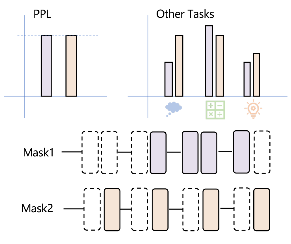
Figure 1: Different Mask structure can lead to similar perplexity scores but exhibit significant performance variations across different downstream tasks.
However, a critical limitation of existing depth pruning methods is their reliance on a fixed layer pruning mask determined offline based on global layer importance metrics at a given sparsity level. This static approach is problematic because different fixed pruning masks, even at the same sparsity level, can exhibit significant performance variations across different downstream tasks. For instance, we observe that perplexity (PPL) is commonly used as a saliency metric for layer pruning Sieberling et al. (2024); Kim et al. (2024), but as illustrated in Figure 1, different mask structures can achieve similar perplexity scores while exhibiting substantially different performance across various downstream tasks. To overcome these limitations and enable adaptive computation pathways, researchers have explored various dynamic routing approaches Elhoushi et al. (2024); Fan et al. (2024); Del Corro et al. ; Schuster et al. (2022); Raposo et al. (2024); Tan et al. (2024); Wu et al. (2024). However, most existing methods perform dynamic routing at the token level, which introduces significant drawbacks: they lack comprehensive understanding of sentence-level semantics, potentially leading to globally inconsistent routing decisions. Furthermore, these approaches typically incur substantial computational overhead from frequent token-level routing calls and require extensive training of additional router networks alongside the original model parameters, making them computationally expensive and time-consuming to implement.
To address the challenges identified in existing works, we propose IG-Pruning, a novel block-wise pruning method that dynamically selects layer masks based on input characteristics at inference time. Our approach consists of two stages: (1) a semantic clustering-based mask discovery stage that identifies diverse, high-quality mask candidates while capturing global information through rapidly converging trainable masks, and (2) a lightweight inference-time routing mechanism that requires no additional training of the base model parameters, enabling efficient dynamic adaptation to varying inputs.
Extensive evaluations demonstrate that our approach consistently outperforms state-of-the-art static pruning methods across different sparsity levels and model architectures on various zero-shot tasks. For Llama-3-8B at 25% sparsity, IG-Pruning preserves 87.18% of dense model performance, surpassing the best baseline by 10.86 percentage points. Similarly, for Qwen-3-8B, IG-Pruning maintains 96.01% of dense model performance at 13.9% sparsity, compared to 90.37% for the best baseline.
Our method trains only mask parameters while keeping model weights frozen, enabling rapid adaptation with minimal computational overhead. During inference stage, it incurs negligible routing overhead by efficiently skipping unimportant layers; and these advancements provides a viable path toward deploying powerful LLMs in environments with limited computational resources.
<details>
<summary>x2.png Details</summary>
### Visual Description
\n
## Diagram: Two-Stage Model Architecture
### Overview
The image depicts a two-stage model architecture, likely for a machine learning or natural language processing task. Stage 1 focuses on initialization and clustering, while Stage 2 appears to be a refinement or processing stage. The diagram illustrates the flow of data and operations between different components.
### Components/Axes
The diagram is divided into two main sections labeled "Stage1" and "Stage2", positioned side-by-side. Key components include: "Calibration Data", "Sentence Encoder", "K-means", "Soft Mask Training", "Router", "Embedding Pool", "Prune", "Select", "Min Distance", "ATTN", and "FFN". There are also four clusters labeled "C1", "C2", "C3", and "C4". Arrows indicate the direction of data flow.
### Detailed Analysis or Content Details
**Stage 1 (Left Side):**
* **Calibration Data:** Input to the "Sentence Encoder".
* **Sentence Encoder:** Processes "Calibration Data" and outputs to "K-means".
* **K-means:** Initializes four clusters labeled "C1", "C2", "C3", and "C4". The output of "K-means" is fed into "Soft Mask Training".
* **Soft Mask Training:** Receives input from "K-means" and outputs to the "Router" in Stage 2.
**Stage 2 (Right Side):**
* **Input:** Input to the "Sentence Encoder".
* **Sentence Encoder:** Processes "Input" and outputs to the "Embedding Pool".
* **Embedding Pool:** Contains a series of circles representing embeddings. This output is fed into the "Router".
* **Router:** Receives input from "Soft Mask Training" (Stage 1) and "Embedding Pool". It performs "Select" and "Prune" operations.
* **Prune:** Filters the output of the "Router".
* **Select:** Selects data from the "Router".
* **Min Distance:** A component within the "Router" that calculates minimum distances.
* **ATTN:** (Attention Mechanism) Appears twice in a stacked configuration.
* **FFN:** (Feed Forward Network) Appears twice in a stacked configuration, interleaved with "ATTN".
* The output of the "Router" (after "Prune") is fed into a series of "ATTN" and "FFN" layers.
**Data Flow:**
* Data flows from "Calibration Data" through "Sentence Encoder" to "K-means", then to "Soft Mask Training".
* Data flows from "Input" through "Sentence Encoder" to "Embedding Pool".
* "Soft Mask Training" and "Embedding Pool" both feed into the "Router".
* The "Router" processes data and sends it through "ATTN" and "FFN" layers.
### Key Observations
The diagram highlights a two-stage process. Stage 1 appears to be a clustering or initialization phase, while Stage 2 is a processing or refinement phase. The "Router" component seems central to integrating information from both stages. The repeated "ATTN" and "FFN" layers suggest a deep learning architecture.
### Interpretation
This diagram likely represents a model that uses a clustering approach (K-means) to initialize a soft mask, which is then used to guide the processing of input data. The "Router" acts as a gatekeeper, selecting and pruning information based on the initialized clusters. The subsequent "ATTN" and "FFN" layers suggest a mechanism for learning complex relationships within the data. The two-stage approach could be designed to improve efficiency or performance by first establishing a coarse-grained representation of the data (Stage 1) and then refining it (Stage 2). The use of "Soft Mask Training" suggests a probabilistic or fuzzy approach to clustering, allowing for overlapping cluster assignments. The diagram does not provide specific numerical data or performance metrics, but it clearly outlines the architectural components and their interconnections.
</details>
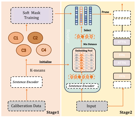
Figure 2: Overview of our method. The approach consists of two stages: (1) Preparing mask candidates through input clustering and soft mask training; (2) Dynamic pruning that selects the appropriate mask for each input at inference time. This enables efficient computation by selectively skipping layers based on input characteristics while maintaining model performance.
## 2 Related Work
Most static depth pruning approaches focus on calculating saliency scores for each transformer block, and removing layers according to these scores. Commonly used saliency metrics include cosine similarity Song et al. (2024); Men et al. (2024), magnitude, second-order derivatives Kim et al. (2024), and perplexity Sieberling et al. (2024). These works calculate layer importance as if they are independent of others, which ignores the coupling connections between layers. As discovered in Fan et al. (2024), contiguous middle layers often exhibit similar saliency scores, which inspired Chen et al. (2024) to use small FFN or transformer blocks to replace contiguous layers. EvoPress Sieberling et al. (2024) found that lower per-layer error does not necessarily lead to better performance, and proposed an evolutionary search algorithm to generate offspring from parent masks, then select better candidates with lower perplexity or KL divergence. Rather than directly removing layers, LaCO Yang et al. (2024) collapses consecutive redundant model layers via layer averaging. MKA Liu et al. (2024a) transforms layer activations into low-dimensional manifolds using diffusion kernel algorithms and evaluates saliency using the NPIB metric.
Beyond one-shot pruning approaches, dynamically skipping unimportant layers during inference has also emerged as a promising research direction. Early approaches include early skipping Del Corro et al. ; Zhu et al. (2024), early exit Elhoushi et al. (2024), and periodic skipping Liu et al. (2024b). However, these methods typically require routers for each layer and demand elaborate training of original weights to recover performance. Dynamic skipping has also been adopted in long-context and multimodal models. Adaskip He et al. (2024) focused on adaptive layer skipping for long-context models, accelerating both prefilling and decoding phases. RoE Wu et al. (2024) employs token-wise routing for multimodal LLMs and trains low-rank adapters to replace the skipped layers.
## 3 Method
As illustrated in Figure 2, our framework consists of two main stages: (1) Mask candidate discovery and (2) Dynamic routing. In the first stage, we cluster the semantic space of inputs and train cluster-specific masks using hard concrete distributions, resulting in diverse yet high-quality mask candidates that each specialize in handling different input patterns. During the second stage, at inference time, we employ a lightweight routing mechanism that maps each input to its most semantically similar cluster and applies the corresponding pre-trained mask, enabling efficient dynamic adaptation without requiring additional training of router networks or base model parameters.
### 3.1 Stage 1: Discovering Mask Candidates
In the first stage, we aim to discover a set of effective mask candidates for dynamic routing. Unlike existing routing methods that typically employ per-layer router networks to make skip decisions, we propose a global routing strategy that dynamically selects routing paths from a carefully curated candidate mask set.
We design our mask candidate discovery process to satisfy two key requirements: Quality: Masks must maintain strong general language generation capabilities. Diversity: The candidate set must provide sufficient variety to handle different input patterns effectively.
To meet these requirements, we leverage hard concrete distribution to model transformer block masks to capture global routing information, and apply $L_{0}$ optimization with cluster-specific calibration data, generating masks that cover diverse computational needs.
Input Clustering.
First, an encoder is used to encode each sentence $x_{i}$ in the calibration dataset into a fixed-dimensional embedding vector $e_{i}$ :
$$
e_{i}=\text{Encoder}(x_{i}) \tag{1}
$$
where $x_{i}$ represents the $i$ -th input, and $e_{i}\in\mathbb{R}^{d}$ , with $d$ being the dimension of the embedding vector. Next, the K-means algorithm is applied to cluster all embedding vectors $e_{1},e_{2},\ldots,e_{M}$ , where $M$ is the size of the calibration set. The K-means algorithm aims to find $N$ clusters $S=\{S_{1},S_{2},\ldots,S_{N}\}$ that minimize the within-cluster sum of squares:
$$
\arg\min_{S}\sum_{k=1}^{N}\sum_{e_{i}\in S_{k}}\|e_{i}-\mu_{k}\|^{2} \tag{2}
$$
where $\mu_{k}$ is the centroid of cluster $S_{k}$ . This results in $N$ cluster centers, each representing a class of semantically similar input sentences.
Mask Training.
Hard concrete distribution Louizos et al. (2018); Xia et al. (2022, 2024) has been widely adopted in structured pruning. Following prior work, we incorporate hard concrete distribution to model transformer block masks, and use $L_{0}$ optimization to generate layer masks, enabling joint learning of all layer masks while incorporating global information.
For each cluster $S_{k}$ , we train a dedicated layer mask $z^{(k)}\in\mathbb{R}^{B}$ using hard concrete distribution and Lagrangian sparsity, where $B$ is the total number of blocks in the model (for block-wise pruning, $B=2L$ where $L$ is the number of transformer layers, representing both attention and FFN blocks separately). Specifically, the masks $z^{(k)}$ are modeled as follows:
First, for each block $i$ in the model, sample $u^{(k)}_{i}$ from a uniform distribution:
$$
u^{(k)}_{i}\sim\text{Uniform}(0,1),\quad i\in\{1,2,\ldots,B\} \tag{3}
$$
Then, compute the soft mask value $s^{(k)}_{i}$ for each block using the sigmoid function:
$$
s^{(k)}_{i}=\sigma\left(\frac{1}{\beta}\log{\frac{u^{(k)}_{i}}{1-u^{(k)}_{i}}}+\log\alpha^{(k)}_{i}\right) \tag{4}
$$
Stretch the soft mask values to a specific interval $[l,r]$ :
$$
\tilde{s}^{(k)}_{i}=s^{(k)}_{i}\times(r-l)+l \tag{5}
$$
Finally, obtain the hardened mask $z^{(k)}_{i}$ for each block by clipping:
$$
z^{(k)}_{i}=\min(1,\max(0,\tilde{s}^{(k)}_{i})) \tag{6}
$$
The complete mask vector for cluster $k$ is then $z^{(k)}=[z^{(k)}_{1},z^{(k)}_{2},\ldots,z^{(k)}_{B}]$ , where each element corresponds to a specific transformer block in the model. During training, these mask values are soft (continuous values between 0 and 1), functioning as scaling parameters. During inference, they are binarized to either 0 (block skipped) or 1 (block executed).
Here, $\sigma$ denotes the sigmoid function. The temperature $\beta$ is fixed hyperparameter, and $l<0,r>0$ are two constants that stretch the sigmoid function output. $\alpha^{(k)}_{i}$ are the main learnable parameters for i-th block mask value in cluster $k$ .
We enforce a target sparsity via a Lagrangian term. Let $s_{\text{target}}$ be the target sparsity and $t^{(k)}$ be the current sparsity of mask $z^{(k)}$ (computed as the proportion of zeroes in the mask), the Lagrangian penalty term $L_{s}^{(k)}$ is:
$$
L_{s}^{(k)}=\lambda_{1}^{(k)}(t^{(k)}-s_{\text{target}})+\lambda_{2}^{(k)}(t^{(k)}-s_{\text{target}})^{2} \tag{7}
$$
For the $k$ -th cluster, the optimization objective for its mask parameters $\log\alpha^{(k)}$ is to minimize:
$$
L_{\text{total}}^{(k)}=\sum_{x_{j}\in S_{k}}L_{\text{LM}}(x_{j};W\odot z^{(k)})+L_{s}^{(k)} \tag{8}
$$
where $L_{\text{LM}}$ is the language modeling loss and $W$ represents the model weights.
Routing Decision.
To implement dynamic routing decisions, we maintain an embedding pool for each semantic cluster to represent the cluster’s features. These embeddings $c_{k}$ are initialized using the cluster centers $\mu_{k}$ . During inference, for each input sequence, we first extract its embedding representation $e_{x}$ through the encoder, then calculate the Euclidean distance between this embedding and each cluster embedding $c_{k}$ . Based on the calculated distances, we select the most similar cluster as the best match for that input:
$$
k^{*}=\arg\min_{k}||e_{x}-c_{k}||_{2}^{2},k\in\{1,2,\ldots,N\} \tag{9}
$$
After determining the best matching cluster, we directly adopt the trained mask corresponding to that cluster as the final execution mask for input $x$ :
$$
M^{x}=z^{(k^{*})} \tag{10}
$$
where $z^{(k^{*})}$ is the binary mask vector associated with cluster $k^{*}$ , containing all block-level mask values.
Dynamic Routing for FFN and Attention Blocks.
Our dynamic routing approach employs different strategies for Feed-Forward layers and Attention layers. During training, the layer mask values are soft, functioning as scaling parameters that directly multiply with the outputs of FFN and Attention components. This enables gradient-based optimization through backpropagation. During inference, we use hard binary masks containing only 0 and 1, where FFN layers are completely skipped when the corresponding mask value is 0. For Attention layers, the approach is more nuanced due to the necessity of maintaining key-value caches for autoregressive generation. When an Attention layer is marked for skipping, we still compute the key and value projections to maintain the KV cache, but we bypass the computationally expensive scaled dot-product operation between queries and keys. Specifically, for a transformer layer $i$ with mask value $M_{i}^{x}=0$ , the FFN computation $\text{FFN}(x_{i})$ is entirely skipped, while for Attention, we compute $K=W_{K}x_{i}$ and $V=W_{V}x_{i}$ for the cache but skip $\text{Attention}(Q,K,V)=\text{softmax}(QK^{T}/\sqrt{d})V$ . This selective computation strategy preserves the model’s autoregressive capabilities while reducing computational overhead.
## 4 Experiment
| Model | Sparsity | Method | OBQA | WG | HS | PIQA | ARC-E | ARC-C | Average | Percentage |
| --- | --- | --- | --- | --- | --- | --- | --- | --- | --- | --- |
| Llama-3-8B | 0% | Dense | 44.6 | 73.24 | 79.16 | 80.79 | 77.82 | 53.24 | 68.14 | 100% |
| 12.5% | SLEB | 38.6 | 69.45 | 70.71 | 77.63 | 70.28 | 43.00 | 61.61 | 90.42% | |
| ShortenedLlama | 39.2 | 61.56 | 66.84 | 76.33 | 67.63 | 38.57 | 58.36 | 85.64% | | |
| EvoPress | 41.2 | 70.17 | 72.03 | 77.75 | 71.00 | 43.69 | 62.64 | 91.93% | | |
| IG-Pruning | 43.6 | 72.93 | 77.26 | 79.38 | 77.06 | 51.62 | 66.98 | 98.29% | | |
| 25% | SLEB | 33.8 | 53.90 | 57.96 | 72.25 | 57.32 | 31.56 | 51.13 | 75.04% | |
| EvoPress | 32.8 | 57.93 | 58.16 | 71.06 | 58.38 | 33.70 | 52.01 | 76.32% | | |
| ShortenedLlama | 33.6 | 53.91 | 57.98 | 72.31 | 57.15 | 31.74 | 51.12 | 75.01% | | |
| IG-Pruning | 40.0 | 68.98 | 67.53 | 76.12 | 63.43 | 40.36 | 59.40 | 87.18% | | |
| 37.5% | SLEB | 28.4 | 52.24 | 46.46 | 65.77 | 46.96 | 28.41 | 44.71 | 65.61% | |
| EvoPress | 28.2 | 51.22 | 45.58 | 65.18 | 48.15 | 28.50 | 44.47 | 65.26% | | |
| ShortenedLlama | 28.6 | 52.41 | 45.90 | 64.69 | 42.68 | 27.47 | 43.63 | 64.02% | | |
| IG-Pruning | 31.8 | 58.01 | 49.63 | 65.94 | 48.44 | 30.38 | 47.37 | 69.51% | | |
| Qwen-3-8B | 0% | Dense | 41.8 | 67.96 | 74.93 | 77.48 | 80.77 | 56.40 | 66.56 | 100% |
| 13.9% | SLEB | 37.4 | 60.85 | 62.45 | 77.52 | 74.45 | 47.09 | 59.96 | 90.09% | |
| ShortenedLlama | 37.0 | 59.27 | 61.82 | 75.14 | 71.00 | 45.14 | 58.23 | 87.49% | | |
| EvoPress | 39.0 | 61.96 | 67.76 | 75.57 | 70.33 | 46.25 | 60.15 | 90.37% | | |
| IG-Pruning | 39.8 | 65.82 | 69.44 | 77.09 | 77.35 | 53.92 | 63.90 | 96.01% | | |
| 25% | SLEB | 36.6 | 56.35 | 53.95 | 72.47 | 65.36 | 37.20 | 53.66 | 80.62% | |
| EvoPress | 37.0 | 58.08 | 57.18 | 71.43 | 62.28 | 38.65 | 54.10 | 81.29% | | |
| ShortenedLlama | 35.6 | 53.99 | 52.20 | 70.84 | 64.69 | 36.43 | 52.29 | 78.56% | | |
| IG-Pruning | 35.6 | 60.46 | 61.65 | 73.39 | 68.94 | 44.80 | 57.47 | 86.35% | | |
| 36.1% | SLEB | 29.6 | 52.40 | 44.02 | 65.77 | 51.68 | 31.39 | 45.81 | 68.82% | |
| EvoPress | 31.6 | 52.17 | 45.29 | 62.95 | 51.09 | 29.18 | 45.38 | 68.18% | | |
| ShortenedLlama | 28.2 | 50.91 | 37.08 | 61.75 | 46.13 | 25.43 | 41.58 | 62.48% | | |
| IG-Pruning | 32.6 | 53.43 | 49.17 | 65.83 | 54.21 | 32.17 | 47.90 | 71.96% | | |
Table 1: Zero-shot evaluation results on Llama-3-8B and Qwen-3-8B across multiple sparsity levels.
### 4.1 Experimental Setup
Datasets and Evaluation Metrics.
Following prior work, we use lm-evaluation-harness Gao et al. (2023) to evaluate our method on six widely-used zero-shot tasks: OpenBookQA Mihaylov et al. (2018), which tests elementary-level science reasoning requiring the combination of facts with commonsense knowledge; Winogrande Sakaguchi et al. (2021), a large-scale adversarial dataset for testing pronoun disambiguation through commonsense reasoning; HellaSwag Zellers et al. (2019), which challenges models to select plausible scenario completions through commonsense inference; PIQA Bisk et al. (2020), focused on physical commonsense knowledge; and the ARC dataset Clark et al. (2018), divided into ARC-Easy and ARC-Challenge subsets for testing scientific reasoning at different difficulty levels. Llama-3-8B AI@Meta (2024) and Qwen-3-8B QwenTeam (2025) are used as our base models, and we use all-MiniLM-L6-v2 from sentence transformer Reimers and Gurevych (2019) as sentence encoder. For calibration data for clustering and layer mask training, we use fineweb-edu Lozhkov et al. (2024), which contains high quality synthetic data used for LLM pretraining.
Baselines and Setups.
To evaluate our dynamic block pruning approach against static methods, we select three representative block pruning techniques for comparison:
- SLEB Song et al. (2024): A method that iteratively eliminates redundant transformer blocks based on cosine similarity between adjacent layers.
- ShortenedLlama Kim et al. (2024): An approach that uses magnitude, second-order derivatives, or perplexity to measure block-level importance. After identifying unimportant blocks, this method removes them in a single pass.
- EvoPress Sieberling et al. (2024): A technique leveraging evolutionary algorithms to search for optimal pruning masks with improved perplexity or KL divergence. Starting with a random initial configuration, in each generation it mutates the compression levels of selected layers and retains the best candidates according to a fitness function. This approach yields better results but incurs higher computational costs.
For all baseline methods, we perform one-shot pruning that identifies and eliminates redundant transformer blocks without retraining, and we use wikitext2 Merity et al. (2016) as calibration set for baselines.
### 4.2 Main Results
IG-Pruning consistently outperforms all baseline methods across all evaluated sparsity configurations for both Llama-3-8B and Qwen-3-8B models. In this paper, the sparsity level is defined as the ratio of the number of skipped blocks to the total number of blocks in the model. For Llama-3-8B at 12.5% sparsity, IG-Pruning maintains 98.29% of the dense model performance, surpassing the best baseline (EvoPress) by 6.36 percentage points. This advantage becomes even more significant at 25% sparsity, where IG-Pruning achieves 87.18% of dense performance compared to the best baseline at 76.32%, representing a 10.86 percentage point improvement. Similarly, for Qwen-3-8B, IG-Pruning preserves 96.01% of dense model performance at 13.9% sparsity, compared to 90.37% for the best baseline. These consistent improvements across different model architectures demonstrate the inherent advantage of our dynamic routing strategy over static pruning methods.
### 4.3 Analysis
Mask Training Efficiency.
In Stage 1 of our approach, model parameters remain frozen while only layer mask parameters undergo optimization. We set a higher learning rate for $L_{0}$ module, enabling rapid mask convergence without extensive training periods. For our experiments, we sample 1,000 examples from each cluster for training, utilizing 4 NVIDIA H800 GPUs. Hyperparameters can be found in Appendix 5. For configurations with sparsity levels below 25% across 16 clusters, all masks can be trained in approximately 15 minutes. Higher sparsity (37%) requires around one hour of training time for mask convergence. Our method requires training, but it only trains the block mask parameters, while the parameters in the original models are frozen. Therefore, it doesn’t require excessive memory, which has been tested successfully on a single RTX 3090 for 8B model.
Block-level vs. Layer-level Pruning.
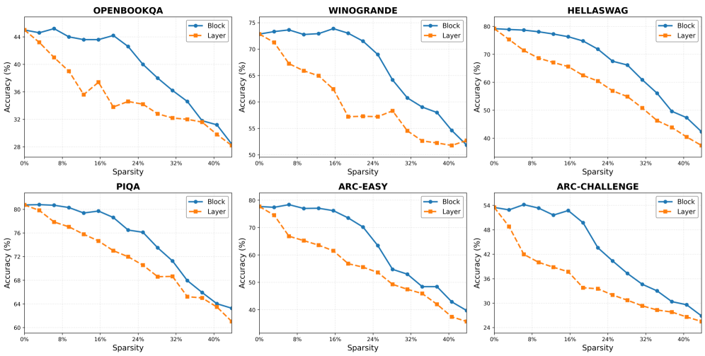
To investigate the impact of pruning granularity on model performance, we conducted comprehensive experiments comparing block-level and layer-level pruning across different sparsity configurations. As shown in Figure 3, block-level pruning consistently outperforms layer-level pruning across all tasks, with performance advantages that vary based on sparsity levels. The gap between these approaches is most significant at sparsity levels around 20%, where block pruning demonstrates substantially better performance. This suggests that independently pruning Attention and FFN components provides the model with greater flexibility to maintain critical capabilities while reducing computational costs.
<details>
<summary>x3.png Details</summary>
### Visual Description
\n
## Charts: Accuracy vs. Sparsity for Different Datasets
### Overview
The image presents six line charts, each depicting the relationship between accuracy (in percentage) and sparsity (in percentage) for different datasets. Each chart compares the accuracy of "Block" and "Layer" methods. The datasets are OPENBOOKQA, WINOGRANDE, HELLASWAG, PIQA, ARC-EASY, and ARC-CHALLENGE.
### Components/Axes
Each chart shares the following components:
* **X-axis:** Sparsity (%), ranging from 0% to 40%, with markers at 0%, 8%, 16%, 24%, 32%, and 40%.
* **Y-axis:** Accuracy (%), ranging from approximately 24% to 80%.
* **Legend:** Located in the top-right corner of each chart, distinguishing between "Block" (represented by a blue line with diamond markers) and "Layer" (represented by an orange line with square markers).
* **Title:** Each chart is labeled with the name of the dataset it represents.
### Detailed Analysis
**1. OPENBOOKQA:**
* **Block:** The blue line starts at approximately 43% accuracy at 0% sparsity, remains relatively stable until around 24% sparsity (approximately 43%), then declines sharply to approximately 28% accuracy at 40% sparsity.
* **Layer:** The orange line starts at approximately 43% accuracy at 0% sparsity, fluctuates slightly until around 24% sparsity (approximately 42%), and then declines steadily to approximately 30% accuracy at 40% sparsity.
**2. WINOGRANDE:**
* **Block:** The blue line starts at approximately 74% accuracy at 0% sparsity, decreases gradually to approximately 65% at 24% sparsity, and then declines sharply to approximately 51% accuracy at 40% sparsity.
* **Layer:** The orange line starts at approximately 72% accuracy at 0% sparsity, decreases steadily to approximately 55% at 24% sparsity, and then declines sharply to approximately 50% accuracy at 40% sparsity.
**3. HELLASWAG:**
* **Block:** The blue line starts at approximately 78% accuracy at 0% sparsity, decreases gradually to approximately 70% at 24% sparsity, and then declines sharply to approximately 44% accuracy at 40% sparsity.
* **Layer:** The orange line starts at approximately 75% accuracy at 0% sparsity, decreases steadily to approximately 60% at 24% sparsity, and then declines sharply to approximately 40% accuracy at 40% sparsity.
**4. PIQA:**
* **Block:** The blue line starts at approximately 81% accuracy at 0% sparsity, decreases gradually to approximately 75% at 24% sparsity, and then declines sharply to approximately 62% accuracy at 40% sparsity.
* **Layer:** The orange line starts at approximately 78% accuracy at 0% sparsity, decreases steadily to approximately 65% at 24% sparsity, and then declines sharply to approximately 60% accuracy at 40% sparsity.
**5. ARC-EASY:**
* **Block:** The blue line starts at approximately 76% accuracy at 0% sparsity, decreases gradually to approximately 65% at 24% sparsity, and then declines sharply to approximately 42% accuracy at 40% sparsity.
* **Layer:** The orange line starts at approximately 70% accuracy at 0% sparsity, decreases steadily to approximately 45% at 24% sparsity, and then declines sharply to approximately 35% accuracy at 40% sparsity.
**6. ARC-CHALLENGE:**
* **Block:** The blue line starts at approximately 54% accuracy at 0% sparsity, decreases gradually to approximately 45% at 24% sparsity, and then declines sharply to approximately 26% accuracy at 40% sparsity.
* **Layer:** The orange line starts at approximately 52% accuracy at 0% sparsity, decreases steadily to approximately 40% at 24% sparsity, and then declines sharply to approximately 24% accuracy at 40% sparsity.
### Key Observations
* In all datasets, both "Block" and "Layer" methods exhibit a general trend of decreasing accuracy as sparsity increases.
* The decline in accuracy is generally gradual up to around 24% sparsity, after which it becomes much steeper.
* The "Block" method consistently outperforms the "Layer" method across all datasets, especially at higher sparsity levels.
* The datasets exhibit varying levels of robustness to sparsity. WINOGRANDE, HELLASWAG, and PIQA show relatively higher initial accuracy and more gradual declines compared to OPENBOOKQA and ARC-CHALLENGE.
### Interpretation
The charts demonstrate the impact of sparsity on the accuracy of two different methods ("Block" and "Layer") across a range of question answering datasets. The consistent outperformance of the "Block" method suggests it is more resilient to the removal of parameters (induced by sparsity) than the "Layer" method. The steep decline in accuracy at higher sparsity levels indicates that beyond a certain point, removing parameters significantly degrades the model's ability to perform well. The varying robustness of different datasets suggests that some tasks are more sensitive to sparsity than others, potentially due to differences in the complexity of the reasoning required or the amount of information encoded in the model's parameters. These results are valuable for understanding the trade-offs between model size (sparsity) and performance, and for guiding the development of more efficient and robust question answering systems. The data suggests that while sparsity can reduce model size, it comes at a cost to accuracy, and the choice of method ("Block" vs. "Layer") can significantly impact the extent of this trade-off.
</details>
Figure 3: Results on average zero-shot task performance of Llama-3-8B, with block and layer pruning.
<details>
<summary>x4.png Details</summary>
### Visual Description
## Heatmaps: MLP and Attention Masks Across Clusters
### Overview
The image presents four heatmaps, arranged in a 2x2 grid. Each heatmap visualizes the distribution of masks (MLP or Attention) across clusters for different layers. The two models being compared are "Llama-3-8B" (bottom-left) and "Qwen-3-8B" (bottom-right). The top row shows "MLP Masks Across Clusters" and the bottom row shows "Attention Masks Across Clusters". The x-axis represents the "Layer" and the y-axis represents the "Cluster". The heatmaps use a two-color scheme: dark blue for low values and light yellow/white for high values.
### Components/Axes
* **Title (Top-Left):** "MLP Masks Across Clusters"
* **Title (Top-Right):** "MLP Masks Across Clusters"
* **Title (Bottom-Left):** "Attention Masks Across Clusters"
* **Title (Bottom-Right):** "Attention Masks Across Clusters"
* **X-axis Label (All):** "Layer" - Scale ranges from 0 to 36.
* **Y-axis Label (All):** "Cluster" - Scale ranges from 0 to 32.
* **Model Labels (Bottom):** "Llama-3-8B" and "Qwen-3-8B"
* **Color Scale:** Dark Blue (low value) to Light Yellow/White (high value).
### Detailed Analysis or Content Details
**1. Llama-3-8B - MLP Masks Across Clusters (Top-Left)**
* The heatmap shows sparse activation of MLP masks.
* There are clusters with high activation around layers 4-7, 12-14, 18-20, and 26-28.
* Specifically, high activation (white/yellow) is observed at:
* Cluster 1, Layers 4-7
* Cluster 6, Layers 12-14
* Cluster 10, Layers 18-20
* Cluster 24, Layers 26-28
* Most other cells are dark blue, indicating low activation.
**2. Qwen-3-8B - MLP Masks Across Clusters (Top-Right)**
* Similar to Llama-3-8B, this heatmap also shows sparse activation.
* High activation is observed in different clusters and layers compared to Llama-3-8B.
* Specifically, high activation (white/yellow) is observed at:
* Cluster 1, Layers 1-3
* Cluster 3, Layers 6-8
* Cluster 7, Layers 12-15
* Cluster 11, Layers 18-21
* Cluster 25, Layers 27-30
* Most other cells are dark blue, indicating low activation.
**3. Llama-3-8B - Attention Masks Across Clusters (Bottom-Left)**
* The heatmap shows a more distributed activation pattern compared to the MLP masks.
* High activation (white/yellow) is observed at:
* Cluster 1, Layers 1-3
* Cluster 6, Layers 6-8
* Cluster 10, Layers 12-14
* Cluster 16, Layers 18-20
* Cluster 24, Layers 26-28
* There are also some scattered activations in other clusters and layers.
**4. Qwen-3-8B - Attention Masks Across Clusters (Bottom-Right)**
* This heatmap shows a very different activation pattern compared to Llama-3-8B.
* High activation (white/yellow) is observed at:
* Cluster 1, Layers 1-3
* Cluster 3, Layers 6-8
* Cluster 7, Layers 12-15
* Cluster 11, Layers 18-21
* Cluster 25, Layers 27-30
* There are also some scattered activations in other clusters and layers.
### Key Observations
* Both models exhibit sparse activation of MLP masks.
* The attention masks show a more distributed activation pattern.
* The activation patterns differ significantly between the two models for both MLP and attention masks.
* Qwen-3-8B appears to have more consistent activation across layers in the attention mask heatmap.
* Llama-3-8B shows more concentrated activation in specific clusters for MLP masks.
### Interpretation
The heatmaps provide insights into how the MLP and attention mechanisms are utilized within each model across different layers and clusters. The differences in activation patterns suggest that the two models may have different internal representations and processing strategies. The sparse activation of MLP masks could indicate that these layers are only selectively engaged during processing. The more distributed activation of attention masks suggests that attention mechanisms are more broadly utilized. The variations between Llama-3-8B and Qwen-3-8B highlight the diversity in model architectures and training procedures. Further analysis would be needed to determine the functional implications of these differences in activation patterns. The data suggests that the models are not identical in their internal workings, even though they are both large language models. The differing patterns could be related to the datasets they were trained on, the specific architectural choices made during development, or the optimization algorithms used during training.
</details>
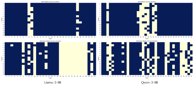
Figure 4: Block mask visualization of Llama-3-8B(left) and Qwen-3-8B(right) with 16 clusters and 25% sparsity. Upper part is FFN Block and the lower part is Attention Block. The color indicates the mask value, with 1 being blue and 0 being yellow.
Interestingly, the performance differential diminishes as sparsity decreases. At sparsity levels higher than 40%, the differences become minimal, and in specific tasks such as Winogrande, layer-level pruning occasionally outperforms block-level pruning. To better understand the results, we analyze the layer masks. Visualization in Figure 4 reveals that Llama attention blocks are more likely to be pruned compared to FFN blocks, especially in middle layers, aligning with previous observations about layer representation similarity in Men et al. (2024). This phenomenon also exists in the Qwen-3 model, but shows a more balanced distribution between attention and FFN blocks. Additionally, attention masks are more separate for Qwen, with no long ranges of consecutive blocks being masked. We analyzed the mask distribution at various sparsity levels and found this phenomenon was commonly observed. This suggests that, in higher sparsity settings, retaining the FFN blocks is more beneficial for model performance, as they are more likely to contain important information. For higher sparsity levels, more FFN blocks are pruned, leading to similar performance between block-level and layer-level pruning.
Computational Efficiency Analysis.
To quantify efficiency improvements, we measured FLOPs (floating point operations) for Llama-3-8B with different sparsity settings, as shown in Table 2. Our analysis reveals that block-wise pruning provides significant computational savings while maintaining model performance. At 25% sparsity, our approach reduces the computational cost to 89.8% of the dense model, representing a reasonable trade-off between efficiency and effectiveness. As sparsity increases to 37.5%, computational requirements drop to 75.8% of the original model.
| 0% 3.12% 6.25% | 32.94T 32.66T 32.39T | 100.0% 99.1% 98.3% | 21.88% 25.00% 28.12% | 31.01T 29.57T 28.71T | 94.1% 89.8% 87.2% |
| --- | --- | --- | --- | --- | --- |
| 9.38% | 32.11T | 97.5% | 31.25% | 27.27T | 82.8% |
| 12.50% | 31.84T | 96.7% | 34.38% | 26.41T | 80.2% |
| 15.62% | 31.56T | 95.8% | 37.50% | 24.97T | 75.8% |
| 18.75% | 31.29T | 95.0% | 40.62% | 24.69T | 74.9% |
Table 2: Computational efficiency at different sparsity for block-wise pruning. The FLOPs values represent the computational cost, while the percentage shows the proportion relative to the dense model.
#### 4.3.1 Analyze clustering effectiveness
Number of Clusters.
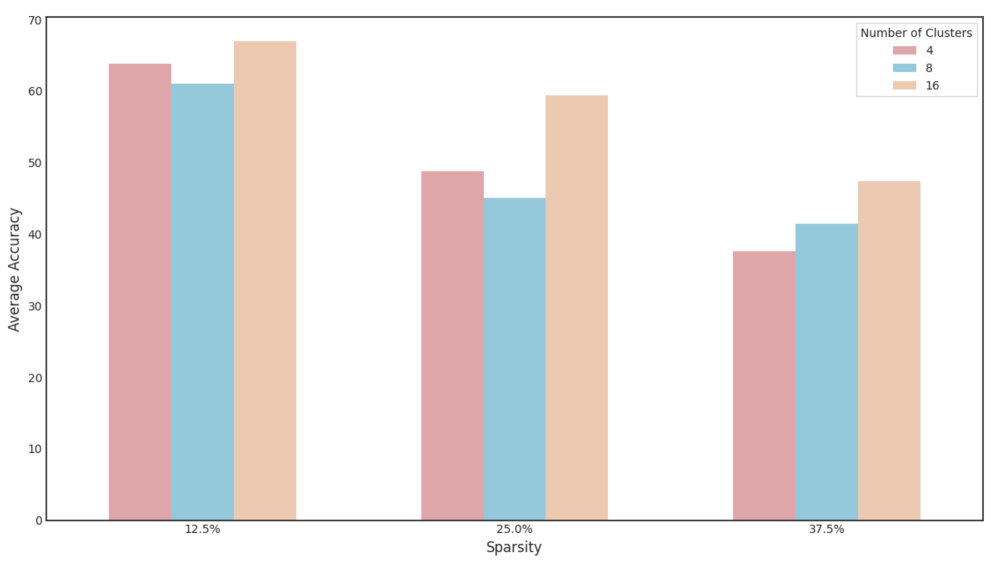
To investigate how the number of clusters affects model performance, we conducted experiments with varying cluster counts (N = 4, 8, 16) at different sparsity levels, as shown in Figure 5. The results demonstrate a clear trend: as the number of clusters increases, overall performance improves consistently across all pruning configurations. At lower sparsity, models with 16 clusters achieve an average performance of 66.98%, compared to 61.05% with 8 clusters and 63.82% with 4 clusters. This advantage becomes even more pronounced at higher sparsity levels. With sparsity of 37.5%, the 16-cluster configuration outperforms the 4-cluster variant by 10.64 percentage points. This pattern confirms that a higher number of clusters enables more specialized mask combinations tailored to different input types. With more clusters, the model can develop a more diverse set of computational paths, each optimized for specific semantic patterns in the input data. The performance improvements with increased cluster count provide strong evidence supporting our hypothesis that dynamic routing significantly benefits model effectiveness by enabling adaptive computation. Rather than forcing all inputs through a single pruned structure, our approach leverages the complementary strengths of mask combinations, explained why our dynamic pruning strategy consistently outperforms static pruning methods.
<details>
<summary>x5.png Details</summary>
### Visual Description
\n
## Bar Chart: Average Accuracy vs. Sparsity for Different Cluster Numbers
### Overview
This bar chart displays the relationship between average accuracy, sparsity, and the number of clusters used in a model. The x-axis represents sparsity levels (12.5%, 25.0%, and 37.5%), and the y-axis represents average accuracy. Three different bar groups are shown for each sparsity level, corresponding to models using 4, 8, and 16 clusters.
### Components/Axes
* **X-axis:** Sparsity (%), with markers at 12.5%, 25.0%, and 37.5%.
* **Y-axis:** Average Accuracy, ranging from 0 to 70.
* **Legend:** Located in the top-right corner, labeling the number of clusters:
* Red: 4
* Orange: 8
* Light Blue: 16
### Detailed Analysis
The chart consists of three groups of bars, one for each sparsity level. Within each group, there are three bars representing the average accuracy for 4, 8, and 16 clusters.
* **12.5% Sparsity:**
* 4 Clusters: Approximately 63.
* 8 Clusters: Approximately 61.
* 16 Clusters: Approximately 65.
* **25.0% Sparsity:**
* 4 Clusters: Approximately 48.
* 8 Clusters: Approximately 56.
* 16 Clusters: Approximately 53.
* **37.5% Sparsity:**
* 4 Clusters: Approximately 39.
* 8 Clusters: Approximately 44.
* 16 Clusters: Approximately 46.
The trend for each sparsity level is as follows:
* **12.5%:** The accuracy increases as the number of clusters increases from 4 to 16.
* **25.0%:** The accuracy increases from 4 to 8 clusters, then decreases slightly from 8 to 16 clusters.
* **37.5%:** The accuracy increases as the number of clusters increases from 4 to 16.
### Key Observations
* At 12.5% sparsity, using 16 clusters yields the highest average accuracy (approximately 65).
* At 25.0% sparsity, using 8 clusters yields the highest average accuracy (approximately 56).
* As sparsity increases, the overall average accuracy tends to decrease.
* The performance difference between 4 and 8 clusters is more pronounced at lower sparsity levels.
### Interpretation
The data suggests that the optimal number of clusters depends on the sparsity level. At lower sparsity levels (12.5%), increasing the number of clusters generally improves accuracy. However, at higher sparsity levels (37.5%), the accuracy improvement from increasing the number of clusters is less significant. The dip in accuracy at 25% sparsity with 16 clusters suggests that there might be an overfitting issue or that the optimal number of clusters is between 8 and 16 for that sparsity level.
The relationship between sparsity and accuracy indicates that as the data becomes more sparse (more missing values or less information), the model's ability to achieve high accuracy decreases. This is likely because sparse data provides less information for the clustering algorithm to work with. The interplay between sparsity and the number of clusters highlights the importance of tuning these parameters to achieve optimal performance for a given dataset.
</details>
Figure 5: Impact of cluster number on performance across evaluation tasks. Results on average zero-shot task performance on Llama-3-8B, with cluster N=4, 8, and 16.
Calibration Data Quality.
The quality of calibration data proves critical for effective mask training, as demonstrated in our ablation studies (Table 3). We found that using high-quality, diverse pretraining data from fineweb-edu Lozhkov et al. (2024) yields the best results, achieving an average score of 59.40. In contrast, using wikitext2, the calibration dataset for baseline models, leads to a significant performance degradation, with the average score dropping to 55.85. Also, instruction dataset in Gou et al. (2023), achieved a competitive score of 58.20 but was still lower than fineweb-edu. Our experiments demonstrate that clustering semantically-rich texts creates more meaningfully differentiated clusters, enabling the discovery of truly specialized computational paths. This finding highlights the importance of data diversity and representational richness in training effective dynamic routing mechanisms.
| Instruction Wikitext2 Fineweb-edu | 36.4 39.0 40.0 | 68.27 63.06 68.98 | 68.14 64.12 67.53 | 73.06 73.07 76.12 | 63.38 60.19 63.43 | 39.93 35.67 40.36 | 58.20 55.85 59.40 |
| --- | --- | --- | --- | --- | --- | --- | --- |
Table 3: Ablation results on Llama-3-8B with 25% sparsity across different datasets. Comparing with fineweb-edu, instruction set show minor difference, while wikitext cause average score degradation.
To verify that the observed performance enhancement is attributable to our proposed method rather than the calibration data, we benchmarked the SLEB baseline on both the wikitext2 and fineweb-edu datasets. As detailed in Table 4, the baseline’s performance did not improve when using fineweb-edu. Crucially, our method continues to outperform the baseline even when using wikitext2. This evidence indicates that the performance gains originate from our method’s dynamic architecture and its ability to leverage high-quality data, rather than from an unfair data advantage.
| SLEB SLEB IG-Pruning | Wikitext2 Fineweb-edu Wikitext2 | 33.8 33.0 39.0 | 53.95 52.56 63.06 | 57.96 57.19 64.12 | 72.25 72.79 73.07 | 57.32 56.60 60.19 | 31.56 32.84 35.67 | 51.13 50.83 55.85 |
| --- | --- | --- | --- | --- | --- | --- | --- | --- |
| IG-Pruning | Fineweb-edu | 40.0 | 68.98 | 67.53 | 76.12 | 63.43 | 40.36 | 59.40 |
Table 4: Comparison with baseline models on different datasets. Our method outperforms the baseline (SLEB) regardless of the dataset used.
## 5 Conclusion
We introduced IG-Pruning, a novel approach for efficient LLM inference through input-adaptive dynamic block pruning. Our method addresses critical limitations of static pruning, and demonstrates that IG-Pruning consistently outperforms state-of-the-art static pruning methods across various configurations and model architectures. Our approach offers four key advantages: (1) improved accuracy through input-adaptive computation that tailors pruning decisions to specific input characteristics, (2) efficient training that keeps model weights frozen while only optimizing lightweight mask parameters, (3) minimal inference overhead via a simple yet effective semantic-based routing mechanism, and (4) flexible block-level pruning granularity that allows independent treatment of attention and FFN components. The success of IG-Pruning highlights the importance of input-adaptive computation in efficient LLM deployment and represents a promising direction for developing high-performing LLMs for resource-constrained environments.
## Limitations
The performance heavily depends on clustering quality, potentially diminishing if semantic clusters aren’t effectively differentiated. Moreover, the result is sensitive to calibration data quality, as instruction datasets led to performance degradation compared to diverse pretraining data. Also, our evaluation focused primarily on specific zero-shot tasks, leaving generalization to other task types or domain-specific applications less thoroughly validated. Additionally, the method introduces sensitivity to multiple hyperparameters, including $L_{0}$ regularization, lagrangian parameters, and cluster numbers. Finally, our work does not investigate the impact of block pruning on model factuality. Removing computational blocks risks eliminating components that are critical for factual recall, which may increase the model’s propensity for hallucination. A promising direction for future work would be to combine our dynamic pruning strategy with hallucination mitigation techniques. For instance, integrating methods like TruthX Zhang et al. (2024a), which enhances truthfulness by editing internal model representations, or Truth-Aware Context Selection Yu et al. (2024), which filters untruthful information from the input context. Such an approach could lead to models that are not only efficient but also more robust and factually reliable.
## Acknowledgements
We thank all the anonymous reviewers for their insightful and valuable comments on this paper. This work was supported by the grant from the National Natural Science Foundation of China (No. 62376260).
## References
- AI@Meta (2024) AI@Meta. 2024. Llama 3 model card.
- Ashkboos et al. (2024) Saleh Ashkboos, Maximilian L Croci, Marcelo Gennari do Nascimento, Torsten Hoefler, and James Hensman. 2024. Slicegpt: Compress large language models by deleting rows and columns. arXiv preprint arXiv:2401.15024.
- Bisk et al. (2020) Yonatan Bisk, Rowan Zellers, Jianfeng Gao, Yejin Choi, and 1 others. 2020. Piqa: Reasoning about physical commonsense in natural language. In Proceedings of the AAAI conference on artificial intelligence, volume 34, pages 7432–7439.
- Brown et al. (2020) Tom Brown, Benjamin Mann, Nick Ryder, Melanie Subbiah, Jared D Kaplan, Prafulla Dhariwal, Arvind Neelakantan, Pranav Shyam, Girish Sastry, Amanda Askell, and 1 others. 2020. Language models are few-shot learners. Advances in neural information processing systems, 33:1877–1901.
- Chen et al. (2024) Xiaodong Chen, Yuxuan Hu, Jing Zhang, Yanling Wang, Cuiping Li, and Hong Chen. 2024. Streamlining redundant layers to compress large language models. arXiv preprint arXiv:2403.19135.
- Clark et al. (2018) Peter Clark, Isaac Cowhey, Oren Etzioni, Tushar Khot, Ashish Sabharwal, Carissa Schoenick, and Oyvind Tafjord. 2018. Think you have solved question answering? try arc, the ai2 reasoning challenge. arXiv preprint arXiv:1803.05457.
- (7) Luciano Del Corro, Allison Del Giorno, Sahaj Agarwal, Bin Yu, Ahmed Hassan Awadallah, and Subhabrata Mukherjee. Skipdecode: Autoregressive skip decoding with batching and caching for efficient llm inference.
- Elhoushi et al. (2024) Mostafa Elhoushi, Akshat Shrivastava, Diana Liskovich, Basil Hosmer, Bram Wasti, Liangzhen Lai, Anas Mahmoud, Bilge Acun, Saurabh Agarwal, Ahmed Roman, and 1 others. 2024. Layerskip: Enabling early exit inference and self-speculative decoding. In Proceedings of the 62nd Annual Meeting of the Association for Computational Linguistics (Volume 1: Long Papers), pages 12622–12642.
- Fan et al. (2024) Siqi Fan, Xin Jiang, Xiang Li, Xuying Meng, Peng Han, Shuo Shang, Aixin Sun, Yequan Wang, and Zhongyuan Wang. 2024. Not all layers of llms are necessary during inference. arXiv preprint arXiv:2403.02181.
- Fang et al. (2024) Gongfan Fang, Hongxu Yin, Saurav Muralidharan, Greg Heinrich, Jeff Pool, Jan Kautz, Pavlo Molchanov, and Xinchao Wang. 2024. Maskllm: Learnable semi-structured sparsity for large language models. In The Thirty-eighth Annual Conference on Neural Information Processing Systems.
- Frantar and Alistarh (2023) Elias Frantar and Dan Alistarh. 2023. Sparsegpt: Massive language models can be accurately pruned in one-shot. In International Conference on Machine Learning, pages 10323–10337. PMLR.
- Gao et al. (2023) Leo Gao, Jonathan Tow, Baber Abbasi, S Biderman, S Black, A DiPofi, C Foster, L Golding, J Hsu, A Le Noac’h, and 1 others. 2023. A framework for few-shot language model evaluation, 12 2023. URL https://zenodo. org/records/10256836, 7.
- Gou et al. (2023) Yunhao Gou, Zhili Liu, Kai Chen, Lanqing Hong, Hang Xu, Aoxue Li, Dit-Yan Yeung, James T Kwok, and Yu Zhang. 2023. Mixture of cluster-conditional lora experts for vision-language instruction tuning. arXiv preprint arXiv:2312.12379.
- Gromov et al. (2024) Andrey Gromov, Kushal Tirumala, Hassan Shapourian, Paolo Glorioso, and Dan Roberts. 2024. The unreasonable ineffectiveness of the deeper layers. In NeurIPS 2024 Workshop on Scientific Methods for Understanding Deep Learning.
- Gu et al. (2021) Shuhao Gu, Yang Feng, and Wanying Xie. 2021. Pruning-then-expanding model for domain adaptation of neural machine translation. arXiv preprint arXiv:2103.13678.
- He et al. (2024) Zhuomin He, Yizhen Yao, Pengfei Zuo, Bin Gao, Qinya Li, Zhenzhe Zheng, and Fan Wu. 2024. AdaSkip: Adaptive sublayer skipping for accelerating long-context LLM inference. 39(22):24050–24058.
- Kim et al. (2024) Bo-Kyeong Kim, Geon-min Kim, Tae-Ho Kim, Thibault Castells, Shinkook Choi, Junho Shin, and Hyoung-Kyu Song. 2024. Shortened llama: A simple depth pruning for large language models. CoRR.
- Ling et al. (2024) Gui Ling, Ziyang Wang, Qingwen Liu, and 1 others. 2024. Slimgpt: Layer-wise structured pruning for large language models. In The Thirty-eighth Annual Conference on Neural Information Processing Systems.
- Liu et al. (2024a) Deyuan Liu, Zhanyue Qin, Hairu Wang, Zhao Yang, Zecheng Wang, Fangying Rong, Qingbin Liu, Yanchao Hao, Bo Li, Xi Chen, and 1 others. 2024a. Pruning via merging: Compressing llms via manifold alignment based layer merging. In Proceedings of the 2024 Conference on Empirical Methods in Natural Language Processing, pages 17817–17829.
- Liu et al. (2024b) Yijin Liu, Fandong Meng, and Jie Zhou. 2024b. Accelerating inference in large language models with a unified layer skipping strategy. arXiv preprint arXiv:2404.06954.
- Liu et al. (2023) Zichang Liu, Jue Wang, Tri Dao, Tianyi Zhou, Binhang Yuan, Zhao Song, Anshumali Shrivastava, Ce Zhang, Yuandong Tian, Christopher Re, and 1 others. 2023. Deja vu: Contextual sparsity for efficient llms at inference time. In International Conference on Machine Learning, pages 22137–22176. PMLR.
- Louizos et al. (2018) Christos Louizos, Max Welling, and Diederik P Kingma. 2018. Learning sparse neural networks through l_0 regularization. In International Conference on Learning Representations.
- Lozhkov et al. (2024) Anton Lozhkov, Loubna Ben Allal, Leandro von Werra, and Thomas Wolf. 2024. Fineweb-edu: the finest collection of educational content.
- Ma et al. (2023) Xinyin Ma, Gongfan Fang, and Xinchao Wang. 2023. Llm-pruner: On the structural pruning of large language models. Advances in neural information processing systems, 36:21702–21720.
- Men et al. (2024) Xin Men, Mingyu Xu, Qingyu Zhang, Bingning Wang, Hongyu Lin, Yaojie Lu, Xianpei Han, and Weipeng Chen. 2024. Shortgpt: Layers in large language models are more redundant than you expect. arXiv preprint arXiv:2403.03853.
- Merity et al. (2016) Stephen Merity, Caiming Xiong, James Bradbury, and Richard Socher. 2016. Pointer sentinel mixture models. Preprint, arXiv:1609.07843.
- Mihaylov et al. (2018) Todor Mihaylov, Peter Clark, Tushar Khot, and Ashish Sabharwal. 2018. Can a suit of armor conduct electricity? a new dataset for open book question answering. In Proceedings of the 2018 Conference on Empirical Methods in Natural Language Processing, pages 2381–2391.
- QwenTeam (2025) QwenTeam. 2025. Qwen3.
- Raposo et al. (2024) David Raposo, Sam Ritter, Blake Richards, Timothy Lillicrap, Peter Conway Humphreys, and Adam Santoro. 2024. Mixture-of-depths: Dynamically allocating compute in transformer-based language models. arXiv preprint arXiv:2404.02258.
- Reimers and Gurevych (2019) Nils Reimers and Iryna Gurevych. 2019. Sentence-bert: Sentence embeddings using siamese bert-networks. In Proceedings of the 2019 Conference on Empirical Methods in Natural Language Processing and the 9th International Joint Conference on Natural Language Processing (EMNLP-IJCNLP), pages 3982–3992.
- Sakaguchi et al. (2021) Keisuke Sakaguchi, Ronan Le Bras, Chandra Bhagavatula, and Yejin Choi. 2021. Winogrande: An adversarial winograd schema challenge at scale. Communications of the ACM, 64(9):99–106.
- Schuster et al. (2022) Tal Schuster, Adam Fisch, Jai Gupta, Mostafa Dehghani, Dara Bahri, Vinh Tran, Yi Tay, and Donald Metzler. 2022. Confident adaptive language modeling. Advances in Neural Information Processing Systems, 35:17456–17472.
- Sieberling et al. (2024) Oliver Sieberling, Denis Kuznedelev, Eldar Kurtic, and Dan Alistarh. 2024. Evopress: Towards optimal dynamic model compression via evolutionary search. arXiv preprint arXiv:2410.14649.
- Song et al. (2024) Jiwon Song, Kyungseok Oh, Taesu Kim, Hyungjun Kim, Yulhwa Kim, and Jae-Joon Kim. 2024. Sleb: Streamlining llms through redundancy verification and elimination of transformer blocks. In International Conference on Machine Learning, pages 46136–46155. PMLR.
- Sun et al. (2023) Mingjie Sun, Zhuang Liu, Anna Bair, and J. Zico Kolter. 2023. A Simple and Effective Pruning Approach for Large Language Models. In ICML.
- Tan et al. (2024) Zhen Tan, Daize Dong, Xinyu Zhao, Jie Peng, Yu Cheng, and Tianlong Chen. 2024. Dlo: Dynamic layer operation for efficient vertical scaling of llms. CoRR.
- Wang et al. (2024) Wenxiao Wang, Wei Chen, Yicong Luo, Yongliu Long, Zhengkai Lin, Liye Zhang, Binbin Lin, Deng Cai, and Xiaofei He. 2024. Model compression and efficient inference for large language models: A survey. arXiv preprint arXiv:2402.09748.
- Wu et al. (2024) Qiong Wu, Zhaoxi Ke, Yiyi Zhou, Xiaoshuai Sun, and Rongrong Ji. 2024. Routing experts: Learning to route dynamic experts in existing multi-modal large language models. In The Thirteenth International Conference on Learning Representations.
- Xia et al. (2024) Mengzhou Xia, Tianyu Gao, Zhiyuan Zeng, and Danqi Chen. 2024. Sheared llama: Accelerating language model pre-training via structured pruning. In 12th International Conference on Learning Representations, ICLR 2024.
- Xia et al. (2022) Mengzhou Xia, Zexuan Zhong, and Danqi Chen. 2022. Structured pruning learns compact and accurate models. In Proceedings of the 60th Annual Meeting of the Association for Computational Linguistics (Volume 1: Long Papers), pages 1513–1528.
- Yang et al. (2024) Yifei Yang, Zouying Cao, and Hai Zhao. 2024. Laco: Large language model pruning via layer collapse. In Findings of the Association for Computational Linguistics: EMNLP 2024, pages 6401–6417.
- Yu et al. (2024) Tian Yu, Shaolei Zhang, and Yang Feng. 2024. Truth-aware context selection: Mitigating hallucinations of large language models being misled by untruthful contexts. In Findings of the Association for Computational Linguistics ACL 2024, pages 10862–10884.
- Zellers et al. (2019) Rowan Zellers, Ari Holtzman, Yonatan Bisk, Ali Farhadi, and Yejin Choi. 2019. Hellaswag: Can a machine really finish your sentence? In Proceedings of the 57th Annual Meeting of the Association for Computational Linguistics, pages 4791–4800.
- Zhang et al. (2023a) Shaolei Zhang, Qingkai Fang, Zhuocheng Zhang, Zhengrui Ma, Yan Zhou, Langlin Huang, Mengyu Bu, Shangtong Gui, Yunji Chen, Xilin Chen, and 1 others. 2023a. Bayling: Bridging cross-lingual alignment and instruction following through interactive translation for large language models. arXiv preprint arXiv:2306.10968.
- Zhang et al. (2024a) Shaolei Zhang, Tian Yu, and Yang Feng. 2024a. Truthx: Alleviating hallucinations by editing large language models in truthful space. In Proceedings of the 62nd Annual Meeting of the Association for Computational Linguistics (Volume 1: Long Papers), pages 8908–8949.
- Zhang et al. (2024b) Shaolei Zhang, Kehao Zhang, Qingkai Fang, Shoutao Guo, Yan Zhou, Xiaodong Liu, and Yang Feng. 2024b. Bayling 2: A multilingual large language model with efficient language alignment. arXiv preprint arXiv:2411.16300.
- Zhang et al. (2023b) Yuxin Zhang, Lirui Zhao, Mingbao Lin, Sun Yunyun, Yiwu Yao, Xingjia Han, Jared Tanner, Shiwei Liu, and Rongrong Ji. 2023b. Dynamic sparse no training: Training-free fine-tuning for sparse llms. In The Twelfth International Conference on Learning Representations.
- Zhou et al. (2024) Zixuan Zhou, Xuefei Ning, Ke Hong, Tianyu Fu, Jiaming Xu, Shiyao Li, Yuming Lou, Luning Wang, Zhihang Yuan, Xiuhong Li, and 1 others. 2024. A survey on efficient inference for large language models. CoRR.
- Zhu et al. (2024) Yunqi Zhu, Xuebing Yang, Yuanyuan Wu, and Wensheng Zhang. 2024. Hierarchical skip decoding for efficient autoregressive text generation. CoRR.
## Appendix A Hyperparameter
The hyperparamters we use in our experiments are listed in Table 5.
| $L_{0}$ Module Learning Rate | 0.1 |
| --- | --- |
| Lagrangian Learning Rate | 0.1 |
| $\epsilon$ | 1e-6 |
| $1/\beta$ | 2/3 |
| $l$ | -0.1 |
| $r$ | 1.1 |
| Number of Clusters | 16, 8, 4 |
| Calibration Data Size for each cluster | 1000 |
| Clustering Stage Sequence Length | 4096 |
| Mask Training Sequence Length | 512 |
Table 5: Hyperparameters used in our experiments.
## Appendix B More results on various models
To further validate the generalizability and robustness of our approach, we conducted additional experiments on a wider range of models, including Llama-3.2-3B (Table 6), Llama-3.2-1B (Table 7), and Qwen-3-4B (Table 8). Across all tested models and architectures, the input-adaptive nature of IG-Pruning allows it to retain significantly more of the original model’s performance compared to baselines, especially at moderate sparsity levels. As sparsity becomes extremely high, the performance of both methods naturally converges. These comprehensive results validate that our dynamic approach is a consistently superior and more robust solution for model pruning.
| Model Llama-3.2-3B 14% (4/28) | Sparsity 0% (0/28) SLEB | Method Dense 35.80 | OpenBookQA 43.20 58.45 | Winogrande 69.38 58.20 | Hellaswag 73.73 73.12 | PIQA 77.27 57.02 | ARC-E 71.84 33.70 | ARC-C 45.99 52.71 | Average 63.55 82.94% | Percentage(%) 100% |
| --- | --- | --- | --- | --- | --- | --- | --- | --- | --- | --- |
| IG-Pruning | 41.40 | 66.45 | 68.20 | 75.95 | 68.13 | 43.34 | 60.58 | 95.32% | | |
| 25% (7/28) | SLEB | 25.00 | 53.82 | 46.67 | 68.28 | 50.96 | 29.01 | 46.79 | 73.63% | |
| IG-Pruning | 36.40 | 57.76 | 60.14 | 71.87 | 54.88 | 33.19 | 52.36 | 82.40% | | |
| 39% (11/28) | SLEB | 26.80 | 51.06 | 37.26 | 61.58 | 40.02 | 24.65 | 40.23 | 63.30% | |
| IG-Pruning | 28.00 | 49.83 | 38.52 | 61.53 | 38.17 | 24.40 | 40.07 | 63.05% | | |
Table 6: Results on Llama-3.2-3B.
| Model Llama-3.2-1B 12.5% (2/16) | Sparsity 0% (0/16) SLEB | Method Dense 30.60 | OpenBookQA 37.40 55.16 | Winogrande 60.36 48.74 | Hellaswag 63.64 68.55 | PIQA 74.43 48.48 | ARC-E 60.27 28.41 | ARC-C 36.26 46.66 | Average 55.38 84.24% | Percentage(%) 100% |
| --- | --- | --- | --- | --- | --- | --- | --- | --- | --- | --- |
| IG-Pruning | 35.00 | 60.45 | 59.65 | 72.79 | 57.32 | 33.87 | 53.18 | 96.02% | | |
| 25% (4/16) | SLEB | 27.80 | 51.63 | 37.50 | 63.11 | 40.19 | 23.72 | 40.65 | 73.40% | |
| IG-Pruning | 27.00 | 54.78 | 40.30 | 62.08 | 40.24 | 27.22 | 41.94 | 75.72% | | |
| 37.5% (6/16) | SLEB | 27.00 | 49.88 | 29.90 | 56.03 | 30.93 | 22.01 | 35.96 | 64.93% | |
| IG-Pruning | 24.40 | 50.98 | 30.90 | 56.31 | 30.72 | 25.08 | 36.40 | 65.72% | | |
Table 7: Results on Llama-3.2-1B.
| Model Qwen-3-4B 14% (5/36) | Sparsity 0% (0/36) SLEB | Method Dense 35.40 | OpenBookQA 40.40 56.19 | Winogrande 65.82 57.36 | Hellaswag 68.42 72.85 | PIQA 75.13 65.78 | ARC-E 53.75 39.84 | ARC-C 53.75 54.57 | Average 59.55 91.64% | Percentage(%) 100% |
| --- | --- | --- | --- | --- | --- | --- | --- | --- | --- | --- |
| IG-Pruning | 37.60 | 62.58 | 59.76 | 73.55 | 68.35 | 44.62 | 57.74 | 96.97% | | |
| 25% (9/36) | SLEB | 32.20 | 53.03 | 46.94 | 67.46 | 58.37 | 31.22 | 48.20 | 80.95% | |
| IG-Pruning | 35.80 | 56.43 | 53.78 | 69.85 | 60.01 | 39.07 | 52.49 | 88.15% | | |
| 36% (13/36) | SLEB | 29.80 | 53.43 | 39.54 | 62.67 | 47.01 | 26.79 | 43.21 | 72.56% | |
| IG-Pruning | 30.60 | 54.69 | 42.74 | 63.65 | 47.26 | 28.66 | 44.60 | 74.90% | | |
Table 8: Results on Qwen-3-4B.