## From Hume to Jaynes: Induction as the Logic of Plausible Reasoning
Tommaso Costa 1,2,3
1 GCS-fMRI, Koelliker Hospital and Department of Psychology, University of Turin, Turin, Italy.
2 FOCUS Laboratory, Department of Psychology, University of Turin, Turin, Italy.
3 Neuroscience Institute of Turin (NIT), Turin, Italy.
e-mail address: tommaso.costa@unito.it
## Abstract
The problem of induction - how experience can justify belief - has persisted since Hume (Hume, 1748) exposed the logical gap between repeated observation and universal inference.
Traditional attempts to resolve it have oscillated between two extremes: the probabilistic optimism of Laplace (Laplace, 1814/1951) and Jeffreys, who sought to quantify belief through probability, and the critical skepticism of Popper, who replaced confirmation with falsification. Both approaches, however, assume that induction must deliver certainty or its negation.
In this paper, I argue that the problem of induction dissolves when recast in terms of logical coherence (understood as internal consistency of credences under updating) rather than truth. Following E. T. Jaynes, probability is interpreted not as frequency or decision rule but as the extension of deductive logic to incomplete information. Under this interpretation, Bayes's theorem is not an empirical statement but a consistency condition that constrains rational belief updating. Induction thus emerges as the special case of deductive reasoning applied to uncertain premises.
Falsification appears as the limiting form of Bayesian updating when new data drive posterior plausibility toward zero, while the Bayes Factor quantifies the continuous spectrum of evidential strength.
Through analytical examples - including Laplace (Laplace, 1814/1951)'s sunrise problem, Jeffreys (Jeffreys, 1939)'s mixed prior, and confidence-based reformulations - I show that only the logic of plausible reasoning unifies these perspectives without contradiction. Induction, properly understood, is not the leap from past to future but the discipline of maintaining coherence between evidence, belief, and information.
## 1. Introduction
Since the dawn of thought, human beings have tried to turn experience into knowledge. We observe regularities in the world and instinctively generalize them into laws: the Sun has always risen; therefore, it will rise again tomorrow; all ravens we have seen are black; therefore, all ravens are black. This way of reasoning moving from particular instances to general propositions - is what we call induction. Yet the rational justification of this process has troubled philosophers for centuries.
As early as the Pyrrhonian skeptics, thinkers like Sextus Empiricus had noticed that no finite number of observations can logically establish a universal statement. The problem, restated in its modern form by David Hume (Hume, 1748) in the eighteenth century, is that there is no logical reason why the future should resemble the past. Why should repeated success make us rational in expecting another success? Science, whose very method depends on generalization, seems to rest on a fragile foundation.
With Bayes and Laplace, a new hope appeared: perhaps probability could provide a logical bridge from the known to the unknown. If certainty is impossible, we can at least assign degrees of belief to hypotheses and revise them as evidence accumulates. This was the birth of Bayesian reasoning - knowledge as the coherent revision of belief in light of new data. Yet Laplace (Laplace, 1814/1951)'s famous sunrise problem soon revealed a deep limitation. Even after millions of successful sunrises, the probability that 'the Sun will rise forever' remains exactly zero. Probabilistic reasoning works flawlessly as a calculus, but it does not answer Hume (Hume, 1748)'s challenge.
In the twentieth century, Harold Jeffreys (Jeffreys, 1939) attempted to repair this deficiency by introducing priors with point masses at special values, while R.A. Fisher (Fisher, 1935) sought an alternative with his fiducial inference, later reformulated by others as confidence or extended likelihood. The idea is intuitively appealing: instead of asking for the probability that a hypothesis is true, we ask how strongly the data warrant confidence in it. After a long sequence of confirming observations, one may 'accept' a hypothesis with full confidence and withdraw that acceptance as soon as contradictory evidence appears. But this move does not solve the induction problem - it merely replaces a question of justification with a rule of decision. It changes the vocabulary, not the logic.
In this paper, I propose to look at induction from a different standpoint, one inspired by E. T. Jaynes (Jaynes, 2003). Induction is not a leap of faith from past to future; it is an extension of logic to cases of incomplete information. In this view, probability is not a property of the world but a measure of plausibility reflecting our state of knowledge. The goal is not to prove that nature is uniform, but to reason consistently with the information we have - to assign beliefs and make decisions that are coherent, revisable, and explicitly conditioned on evidence.
Under this interpretation, the 'problem of induction' is not a flaw in nature but a question of rational coherence. We do not need to prove that the Sun will rise forever; we need only show that, given what we know, believing it will rise tomorrow is the most consistent and informative stance. Probability, likelihood, and confidence each play a role in this process: probability orders our beliefs; likelihood measures the agreement between model and data; confidence calibrates decisions. None of them, taken alone, resolves induction - but together they clarify what it truly means.
In what follows, I examine why confidence-based approaches fail to overcome Hume (Hume, 1748)'s paradox and develop an alternative framework grounded in the logic of plausible reasoning. I argue that the rational content of induction lies not in claiming certainty, but in maintaining coherence under uncertainty - in our ability to update beliefs, to act upon them, and to revise them when evidence changes. Induction, in this sense, is not faith in the future, but the logic of rational consistency.
## 1.1 Overview of the Argument
The structure of the argument can be summarized as a logical trajectory from skepticism to coherence .
The paper proceeds through five conceptual transitions:
1. Hume - The Skeptical Challenge: shows that no finite observation can justify universal inference; the uniformity of nature cannot be proven logically.
2. Laplace - The Probabilistic Bridge: transforms Hume's puzzle into a quantitative problem, proposing probability as a measure of rational expectation, yet revealing probability dilution : even perfect evidence cannot confirm a universal law.
3. Jeffreys - The Objective Prior: attempts to restore universality by assigning prior mass to immutable laws, solving the arithmetic but not the logic of induction.
4. Popper and Fisher - The Procedural Turn: replace belief with decision; falsification and confidence provide rules for action, not coherent justification.
5. Jaynes - The Logical Resolution: reframes probability as the extension of logic to incomplete information , unifying induction, falsification, and maximum entropy under the single principle of coherence.
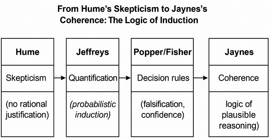
This sequence defines the central thesis of the paper: induction is not a leap from past to future but the maintenance of coherence between evidence, belief, and information. Figure 1 below illustrates the conceptual flow from historical paradox to logical unification.
Figure 1. Conceptual progression from Hume's problem of induction to Jaynes's logic of plausible reasoning. Each step reframes the relationship between evidence and belief: Hume exposes the logical gap, Laplace quantifies uncertainty, Jeffreys seeks objectivity through priors, Popper and Fisher define procedural rules for action, and Jaynes unifies them through the principle of coherence.
<details>
<summary>Image 1 Details</summary>
### Visual Description
## Flowchart: From Hume’s Skepticism to Jaynes’s Coherence: The Logic of Induction
### Overview
The flowchart illustrates the evolution of inductive reasoning frameworks, starting with Hume’s skepticism and progressing through Jeffreys’ quantification, Popper/Fisher’s decision rules, and culminating in Jaynes’ coherence. Each stage introduces a methodological shift to address limitations in prior approaches.
### Components/Axes
- **Nodes**:
1. **Hume**:
- Label: "Skepticism"
- Description: "(no rational justification)"
2. **Jeffreys**:
- Label: "Quantification"
- Description: "(probabilistic induction)"
3. **Popper/Fisher**:
- Label: "Decision rules"
- Description: "(falsification, confidence)"
4. **Jaynes**:
- Label: "Coherence"
- Description: "(logic of plausible reasoning)"
- **Arrows**:
- Directed edges connect nodes sequentially: Hume → Jeffreys → Popper/Fisher → Jaynes.
### Detailed Analysis
- **Hume’s Skepticism**:
- Positions skepticism as the foundational critique of induction, rejecting rational justification for inductive inferences.
- **Jeffreys’ Quantification**:
- Introduces probabilistic induction to address Hume’s skepticism, assigning degrees of belief to hypotheses.
- **Popper/Fisher’s Decision Rules**:
- Focuses on falsification (rejecting hypotheses) and confidence (statistical thresholds) as pragmatic tools for decision-making.
- **Jaynes’ Coherence**:
- Advocates for a logic of plausible reasoning, emphasizing internal consistency and coherence over probabilistic or falsificationist approaches.
### Key Observations
- The flowchart represents a historical and philosophical progression, with each stage responding to the limitations of its predecessor.
- Hume’s skepticism is the starting point, with subsequent frameworks attempting to resolve its challenges.
- Jaynes’ coherence is positioned as the most advanced stage, integrating plausibility and logical consistency.
### Interpretation
The flowchart demonstrates the iterative refinement of inductive reasoning in response to philosophical and practical challenges. Hume’s skepticism highlights the problem of justifying induction, which Jeffreys addresses through probabilistic methods. Popper/Fisher further refine this by prioritizing falsification and confidence, while Jaynes’ coherence represents a shift toward holistic, logically consistent reasoning. This progression reflects a move from foundational critique to pragmatic and ultimately integrative approaches to induction.
</details>
## 2. Background: From Hume to Jaynes
The question of how we can rationally move from past observations to future expectations - the classical problem of induction - has shaped philosophical and scientific thought for centuries. It was David Hume (Hume, 1748) who expressed the problem most clearly: the assumption that the future will resemble the past can be justified neither by experience, which already presupposes it, nor by logic, since no contradiction arises in imagining a world where regularities suddenly break. Hume concluded that our faith in the uniformity of nature is not rationally grounded but the product of psychological habit. Science, then, seems to rest on a kind of welldisciplined optimism rather than logical certainty.
A century later, Pierre-Simon Laplace (Laplace, 1814/1951) sought to turn Hume (Hume, 1748)'s paradox into a calculation. If certainty is impossible, perhaps uncertainty can at least be measured.
He adopted what we now call Bayes's theorem as a rule for updating beliefs in light of evidence:
$$P ( G | E ) = \frac { P ( E | G ) \, P ( G ) } { P ( E ) }$$
Laplace (Laplace, 1814/1951) applied this rule to the famous sunrise problem . Let θ represent the true but unknown frequency of sunrises. Assuming a uniform prior on the interval 0 < 𝜃 < 1 and having observed 𝑛 consecutive successful sunrises, the posterior distribution becomes
$$f ( \theta | T _ { n } = n ) = ( n + 1 ) \, \theta ^ { n } , 0 < \theta < 1$$
From this, the predictive probability that the Sun will rise again tomorrow is
$$P ( E _ { n + 1 } = 1 | T _ { n } = n ) = \frac { n + 1 } { n + 2 }$$
This probability approaches 1 as 𝑛 grows, apparently confirming our expectation that repeated success increases belief. Yet the probability of the universal hypothesis 'the Sun will rise forever ,' corresponding to 𝜃 = 1 - remains exactly zero, because the point 𝜃 = 1 lies outside the continuous space (0,1) . No finite amount of evidence can ever justify a universal statement. This limitation, later called probability dilution , reveals that probabilistic induction can predict the next event but never confirm a law.
In the early twentieth century, Harold Jeffreys (Jeffreys, 1939) tried to overcome this by modifying the prior. In his Theory of Probability (1939),, he proposed assigning part of the prior mass directly to the point 𝜃 = 1 :
$$\pi ( \theta ) = \frac { 1 } { 2 } \, \delta ( \theta - 1 ) + \frac { 1 } { 2 } \, U ( 0 , 1 )$$
where 𝛿(𝜃 - 1) is a Dirac delta at the boundary. Under this mixed prior, the posterior probability that the Sun will rise forever becomes
$$P ( \theta = 1 | T _ { n } = n ) = \frac { n + 1 } { n + 2 }$$
which indeed tends toward one as 𝑛 increases, though it never reaches it for finite 𝑛 . The maneuver solves the arithmetic but not the logic: the choice of the prior's point mass remains arbitrary and cannot be inferred from data. The problem of induction is therefore only displaced, not resolved.
Karl Popper accepted Hume's (Hume, 1748) skepticism and recast it as a principle of scientific method. Science, he argued, advances not by confirming laws but by falsifying them. Assigning probability one to any hypothesis 𝐺 is irrational, because it makes learning impossible:
$$P ( G ) = 1 \, \Rightarrow \, P ( G | E ) = 1 \, f o r a l l \, E$$
Once belief reaches certainty, no new observation can change it. For Popper, rationality consists in keeping hypotheses perpetually open to refutation. This view preserves the critical spirit of science but offers no quantitative way to compare unfalsified theories or express degrees of support - a gap that real scientific practice inevitably fills with probabilistic reasoning.
Around the same period, R. A. Fisher (Fisher, 1935) introduced fiducial inference as a third path between Bayes and frequentism. He sought a distribution for the parameter itself derived purely from data, without invoking priors. The resulting fiducial or confidence density can be represented as
$$c ( \theta ; t ) = \frac { \partial \, P ( T ^ { * } \geq t | \theta ) } { \partial \theta }$$
and the corresponding confidence assigned to an interval 𝐶𝐼(𝑡) is
$$C ( \theta \in C I ( t ) ) = \int _ { C I ( t ) } c ( \theta ; t ) d \theta = 1 - \alpha$$
This measure expresses a kind of 'trust' in parameter values calibrated to frequency properties but independent of prior belief. Modern extensions - such as the extended likelihood or confidence likelihood - preserve this operational spirit: they allow one to act as if a hypothesis were true with full confidence after enough confirming evidence, and to withdraw that acceptance when contrary data appear. Yet this approach too remains procedural. It defines when to accept a hypothesis, not why we should believe it beyond the observed cases.
It was Edwin T. Jaynes (Jaynes, 2003) who finally reframed the issue in logical terms. Probability, he argued, is neither a frequency nor a subjective bet, but the extension of logic to situations of incomplete information. Its rules follow from requirements of internal consistency, not from empirical regularities. The fundamental identity,
$$P ( G | E ) = \frac { P ( E | G ) \, P ( G ) } { P ( E ) }$$
is, for Jaynes, not an empirical rule but a theorem of rational coherence. Induction, in this view, is not an assumption about nature's uniformity but a logical operation that preserves consistency among beliefs when information changes. The question 'Why should the future resemble the past?' becomes 'Given what we know, what is the most consistent assignment of plausibility?' Under this interpretation, the ancient problem of induction dissolves: it is no longer about proving uniformity in nature, but about reasoning coherently in the face of uncertainty.
From Hume's skepticism to Jaynes's reconstruction, the story of induction marks a profound shift - from ontology to logic, from seeking truth to maintaining coherence. Laplace made uncertainty measurable; Jeffreys sought objectivity through priors; Popper replaced confirmation with falsification; Fisher reframed inference as confidence; and Jaynes revealed that probability itself is the logic of plausible reasoning. What began as a metaphysical problem ends as a principle of rationality: the aim of induction is not certainty, but coherence under uncertainty.
## 2.1 Positioning within contemporary accounts of induction and confirmation
While the historical arc from Hume to Jaynes clarifies why 'induction' should be reframed as coherent belief revision, it is useful to situate this view within contemporary accounts of inductive inference. In Bayesian confirmation theory, degrees of belief are tied to coherence requirements and to how evidence changes the plausibility of hypotheses (Howson & Urbach, 1993; Sprenger & Hartmann, 2019).
Within this tradition, Bayes's theorem is not a descriptive law but a normative constraint on rational credence; confirmation is graded, comparative, and essentially contrastive across rival models. This perspective resonates with Jaynes's program, though it emphasizes the epistemology of confirmation (what it is for evidence to confirm a hypothesis) more than Jaynes's information-theoretic foundations.
A complementary line connects rational credence to epistemic accuracy: on scoringrule grounds, coherent credences maximize expected accuracy (Joyce, 1998). Subsequent developments have strengthened this bridge between coherence and accuracy-based justification. Greaves and Wallace (2006) demonstrated that conditionalization uniquely maximizes expected epistemic utility, providing a formal vindication of the Bayesian update rule. Pettigrew (2016) extended this program by showing that the laws of probability can be derived from accuracydominance principles, thus interpreting coherence not merely as internal consistency but as the rational strategy for 'getting things right.' Leitgeb (2017) further integrated these ideas within a unified account of belief stability, linking probabilistic coherence with the resilience of rational belief across time. Together, these contributions establish that coherence and accuracy are not competing ideals but complementary dimensions of rationality: coherent beliefs are precisely those that remain stable and accuracy-conducive under new evidence.
Relatedly, programs in probabilistic truth-likeness and verisimilitude investigate how graded belief can track closeness to truth without collapsing into binary acceptance, providing a formal backdrop for the idea that falsification is a limit case of continuous evidential re-weighting. Formal learning theory provides a third vantage point: under broad conditions, Bayesian updating converges (in various senses) to the data-generating hypothesis or to its best available approximation in the model class, thereby addressing the pragmatic core of Hume's worry (Williamson, 2000).
Beyond its epistemic and formal virtues, the coherence-based view of Bayesian reasoning also connects with broader discussions of scientific realism. Recent analyses emphasize that coherence is not only a constraint on rational belief but also a criterion for epistemic reliability in scientific practice. As Sprenger (2021) argues, Bayesian coherence provides a realist justification for probabilistic inference: it explains why coherent updating tends, in the long run, to align credences with the structure of the world rather than with mere pragmatic convenience. In this sense, coherence is both a logical and an ontological bridge-linking rational belief revision with the realist expectation that successful theories approximate truth.
Finally, recent discussions of likelihood-based and confidence-based proposals (e.g., fiducial or extended likelihood) argue for decision-calibrated tools with strong longrun properties. Our stance is sympathetic to their operational merits but stresses a distinction: procedures that optimize error-control or coverage do not, by themselves, supply a normative theory of single-case rational belief. In what follows we therefore treat likelihood and confidence as valuable instruments for calibration and action, while reserving to Bayesian coherence the role of a general logic for belief and learning. See §6 for the relation between coherence, falsification, and accuracy-based justifications, and see §6.1 for the relation between coherence and epistemic accuracy.
## 3. Why 'confidence' does not solve induction
The recent revival of confidence-based reasoning-also called extended likelihood or confidence likelihood in the sense of Lee (2025)-seeks to overcome a classical limitation of Bayesian inference: the impossibility of assigning probability 1 to a universal law. In this framework, the term confidence does not refer to frequentist confidence intervals, but to a reinterpretation of the likelihood function as a decision-calibrated measure of evidential support, designed to mirror the long-run properties of confidence coverage while retaining a likelihood-based formulation. Lee argue that, if probability cannot express full acceptance, confidence can. After sufficient consistent data, a hypothesis may be accepted with confidence equal to 1 and rejected with confidence 0 at the first contradiction. At first glance, this appears to solve the ancient puzzle of induction. In reality, however, it merely transfers the problem from the level of epistemic justification to that of procedural decision.
The approach traces its lineage to Fisher's fiducial inference and was reformulated by Lee as an extended-likelihood framework . Its central idea is to replace the probability density 𝑓(𝜃 ∣ 𝑡) with a confidence density 𝑐(𝜃; 𝑡) , defined as:
$$c ( \theta ; t ) = \, \frac { \partial P ( T ^ { * } \geq t | \theta ) } { \partial \theta }$$
Integrating this function over the observed confidence interval 𝐶𝐼(𝑡) yields the confidence measure
$$C ( \theta \in C I ( t ) ) = \int _ { C I ( t ) } c ( \theta ; t ) d \theta = 1 - \alpha$$
This formulation preserves the property known as confidence coverage : under repeated sampling, the probability that the true value 𝜃 * lies within the reported confidence interval equals the stated confidence level. Formally,
$$P ( \theta _ { 0 } \in C I ( T _ { n } ) ) = C ( \theta _ { 0 } \in C I ( t ) )$$
This equality is elegant and operationally useful. It guarantees that, across many hypothetical repetitions of the experiment, the proportion of intervals containing the true parameter matches their nominal confidence. Yet this property is purely frequentist; it says nothing about the logical or epistemic status of the statement ' 𝜃 lies in this particular interval.'
When applied to Laplace's sunrise model, the confidence framework yields a mixed object that assigns all mass to the boundary point 𝜃 = 1 whenever all observed cases are successes ( 𝑇 ! = 𝑛 ):
$$c ( \theta ; t ) = \begin{cases} \delta ( \theta - 1 ) , & i f t = n \\ B e t a ( t + 1 , n - t ) , & i f t < n \end{cases}$$
From this, the confidence assigned to the hypothesis 'the Sun will rise forever,' denoted 𝐺 , becomes:
$$C ( G ; n ) = \begin{cases} 1 , & \quad i f T _ { n } = n \\ 0 , & \quad i f T _ { n } < n \end{cases}$$
Thus, after 𝑛 consecutive sunrises, we may declare complete confidence ( 𝐶 = 1 ) that the Sun will rise forever-until the first failure, when confidence drops instantly to 0. This on-off dynamic mirrors the Popperian notion of provisional acceptance and instant falsification.
At a pragmatic level, this behavior can be advantageous. Confidence-based methods possess strong calibration properties: their numerical levels correspond to reproducible long-run frequencies, and their Extended Likelihood Ratio (ELR) provides an operational scale of evidential strength even when Bayesian priors are unavailable. In applied contexts-such as industrial quality control or repeated experimental designs-these features make the framework appealing and transparent.
However, the problem at stake is not operational but epistemic. Confidence tells us how often a rule succeeds under repetition, not why it should be rational to believe its outcome in a single case. The logical relation between evidence and belief-the essence of Hume's challenge-remains unaddressed.
Indeed, the confidence measure does not express a degree of belief that 𝐺 is true; it encodes a decision rule: act as if 𝐺 were true when 𝐶(𝐺; 𝐸) = 1 , and abandon it when 𝐶(𝐺; 𝐸) = 0 . The distinction is subtle but fundamental. Bayesian probability, even with all its limitations, quantifies plausibility-a continuous relation between hypotheses and evidence-whereas confidence provides a binary operational threshold, a guide for acceptance rather than reasoning.
The contrast becomes clearer in a simple testing context. For a universal hypothesis G : 𝜃 = 1 and its complement 𝐺 % : 𝜃 < 1 , the Bayesian comparison is given by the Bayes Factor:
$$B F ( G , G ^ { C } ; t ) = \frac { P ( T _ { n } = t | \theta = 1 ) } { P ( T _ { n } = t | \theta \sim B e t a ( 1 , 1 ) ) }$$
which, for the sunrise model, simplifies to:
$$B F ( G , G ^ { C } ; t ) = \{ \begin{array} { l l } { n + 1 , } & { i f \, t = n } \\ { 0 , } & { i f \, t < n } \end{array}$$
The analogous ratio in the confidence framework-the Extended Likelihood Ratio (ELR)-is defined as:
$$E L R ( G , G ^ { C } ; t ) = \frac { C ( G ; t ) } { C ( G ^ { C } ; t ) }$$
$$E L R ( G , G ^ { C } ; t ) = \{ \begin{array} { l l } { \infty , } & { i f \, t = n } \\ { 0 , } & { i f \, t < n } \end{array}$$
producing:
At first glance, this seems decisive: perfect data yield infinite support for 𝐺 . Yet such 'certainty' is purely procedural-it arises because the construction assigns all probability mass to 𝜃 = 1 once 𝑡 = 𝑛 , not because inference has logically established a universal truth. The system, by design, treats the boundary case as a rule of acceptance, not as an epistemic conclusion.
In philosophical terms, the confidence approach conflates acceptance with belief. Acceptance is pragmatic-the rule to act as if a proposition were true. Belief, by contrast, is a coherent assignment of plausibility constrained by information. The confidence measure provides the former but not the latter. It cannot explain why our confidence that the Sun will rise tomorrow should extend beyond the observed data, nor why the same rule should apply to less regular phenomena.
The deeper reason is that confidence lacks a normative theory of inference. It offers a principled way to calibrate long-run frequencies of correct decisions, but it does not tell us how to assign rational degrees of plausibility in single cases. It is therefore silent on Hume's question: why should the past inform the future? What it provides instead is a well-behaved policy for deciding when to act as if a hypothesis were true, without ever establishing that it is rational to believe it.
In summary, the confidence framework succeeds where the classical frequentist failed-it provides scientists with an interpretable numerical measure of acceptance and a unified operational language-but it fails where Hume demanded an answer: it does not justify the transition from repeated observation to general belief. It replaces epistemology with policy. Jaynes's logic of plausible reasoning can thus be viewed not as a rival but as a completion of confidence reasoning: it supplies the missing normative layer that connects frequency calibration to rational belief. The problem of induction remains, though expressed in a more sophisticated syntax.
The limitations of both confidence-based and falsificationist approaches point toward a deeper unity. Each of these frameworks captures a fragment of rationality: confidence formalizes the operational need for decision under uncertainty, while falsification enforces the logical discipline of revisability. Yet both remain procedural-they describe how scientists should act, not why such actions are rational. From a Jaynesian standpoint, these methods can be understood as limit cases of the broader principle of coherence. Confidence corresponds to the pragmatic boundary where degrees of belief collapse into binary acceptance for practical purposes; falsification represents the asymptotic case where posterior plausibility approaches zero under decisive evidence. What unifies them is the same underlying logic: rational belief must evolve consistently with information. The transition from §3 to §4 thus marks a shift from operational policies to the normative foundation that renders them coherent-the logic of plausible reasoning.
## 4. Induction as the Logic of Plausible Reasoning
The failure of both probability dilution and confidence-based acceptance suggests that the problem of induction cannot be solved by modifying formulas, priors, or acceptance thresholds. The issue is not computational but conceptual. The difficulty lies in how we interpret the relationship between data, hypotheses, and rational belief. What is needed is not another mechanism for assigning numbers, but a redefinition of what those numbers mean .
This requirement of coherent updating implies what has been called Cromwell's Rule (Lindley, 1972; Jaynes, 2003): never assign prior probability 0 or 1 to any empirical hypothesis. The reason is simple but profound. Once a proposition is granted probability 0 or 1, Bayes's rule can no longer revise it-no evidence, however overwhelming, can alter certainty. Assigning 0 or 1 is thus not an act of reasoning but of faith. In Jaynes's logic of plausible inference, rational belief must always remain open to revision; plausibility values should occupy the continuum between these limits. In this sense, Cromwell's Rule formalizes the very spirit of scientific fallibilism: we must 'think it possible that we may be mistaken.'
E. T. Jaynes proposed such a redefinition. His central claim is that probability is not an empirical frequency nor a decision rule, but the extension of logic to situations where information is incomplete. Under complete knowledge, logic tells us whether a proposition is true or false. Under incomplete knowledge, probability quantifies how strongly the available information supports one proposition over another. The rules of probability are not arbitrary conventions but the unique system consistent with the desiderata of rational reasoning.
The guiding principle is that reasoning under uncertainty must obey the same structural constraints as deductive logic: consistency, symmetry, and transparency to new information. From these requirements, the product and sum rules of probability follow uniquely. The basic relation is the familiar rule of conditional updating:
$$P ( G | E ) = \frac { P ( E | G ) \, P ( G ) } { P ( E ) }$$
but here it is interpreted not as a statement about the world, but as a constraint on rational belief. It enforces internal coherence among propositions once evidence is specified.
In this sense, Bayesian updating is not an inductive law of nature but a consistency theorem: given our prior plausibility assignments, there is only one coherent way to revise them when new data arrive. Every other method would lead to contradictions in reasoning. Jaynes often emphasized that probability theory is 'the logic of science,' not a theory of random events. Its subject is not the behavior of nature but the behavior of rational thought about nature.
This view dissolves Hume's paradox. The question 'why should the future resemble the past?' is misplaced. The Bayesian does not assert that the world is uniform; they merely condition their expectations on the information available. If tomorrow's sunrise fails, beliefs will change automatically by the same rule that once supported them. The logic of plausible reasoning requires no metaphysical assumption about the world's regularity - only a commitment to coherent updating.
To formalize this, Jaynes proposed a few general desiderata for any system of reasoning under uncertainty:
1. Representation: A real number 𝑃(𝐴 ∣ 𝐵) represents the plausibility of proposition 𝐴 given 𝐵 .
2. Consistency: If a conclusion can be reached in more than one way, every valid path must lead to the same result.
3. Qualitative correspondence with logic: When information becomes complete, probabilities reduce to truth values 0 or 1 .
From these, the sum and product rules follow. The sum rule expresses how plausibility combines for mutually exclusive propositions:
$$P ( A + B | C ) = P ( A | C ) + P ( B | C ) - P ( A B | C )$$
and the product rule governs conditional inference:
$$P ( A B | C ) = P ( A | C ) \, P ( B | A C )$$
Together, they form the algebra of plausible reasoning. All valid methods of inference-Bayesian or otherwise-must be consistent with them.
A key insight of Jaynes's approach is that induction is not a separate kind of reasoning, but a special case of deduction applied to uncertain premises. In deductive logic, we write
$$I ( G ) = 1 o r 0$$
depending on whether the proposition 𝐺 is true or false. In plausible reasoning, we instead assign a degree of plausibility:
$$0 < P ( G | E ) < 1$$
The transition from certainty to uncertainty does not require new principles, only an extension of logic to a continuum of plausibility values.
This reinterpretation resolves the logical tension that plagued earlier formulations. Laplace's paradox arose because probability was treated as a physical property of the world; Jaynes removes this assumption. Probability lives in the mind of the reasoner, not in the world itself. It encodes information, not randomness. When evidence accumulates, the probability 𝑃(𝐺 ∣ 𝐸) approaches one, not because nature becomes more uniform, but because the information supporting 𝐺 becomes more complete.
Moreover, this framework restores a clear distinction between belief, decision, and truth. Truth ( 𝐼(𝐺) ) is ontological; belief ( 𝑃(𝐺 ∣ 𝐸) ) is epistemic; decision is pragmatic. The Bayesian logic of plausible reasoning pertains to belief: how a rational agent should assign and revise plausibilities given information. Once beliefs are assigned, decisions can be made according to a utility criterion, but that is a separate step. Induction, in this sense, is not a method for discovering truth, but for maintaining coherence in belief revision.
This interpretation also clarifies the relationship between Bayes's rule and falsification. Popper was right to insist that hypotheses must remain open to refutation; Jaynes's logic ensures this automatically. If new data 𝐸 + contradict the predictions of 𝐺 , the likelihood 𝑃(𝐸 + ∣ 𝐺) becomes small, and therefore 𝑃(𝐺 ∣ 𝐸, 𝐸 + ) decreases accordingly. The Bayesian rule accomplishes Popperian falsification smoothly and quantitatively:
$$P ( G | E , E ^ { \prime } ) \varpropto P ( E ^ { \prime } | G ) \, P ( G | E )$$
No special rule for rejection is needed: inconsistency with data leads to lower plausibility by logical necessity.
Finally, Jaynes's framework connects naturally with principles of information theory. When no specific prior information is available, the maximum entropy principle prescribes choosing the distribution that makes the fewest unwarranted assumptions while satisfying known constraints. In this way, probability becomes the language of honest ignorance - expressing what is known without asserting what is not. This principle completes the logical structure of induction: new data reduce uncertainty, old priors encode background knowledge, and the updating rule guarantees consistency throughout.
In summary, Jaynes's logic of plausible reasoning reframes induction not as a metaphysical inference from past to future, but as a rule of coherent reasoning under uncertainty. The ancient demand for certainty is replaced by a higher standard: internal coherence and openness to revision. Under this view, the rational scientist does not 'believe' that the Sun will always rise; rather, they assign it a plausibility close to one, subject to revision should contrary evidence arise. Induction thus ceases to be a mystery and becomes a manifestation of the same logic that governs all rational thought - the logic of plausible inference.
## 5. Case Studies: The Sunrise Problem and Beyond
The abstract discussion of induction becomes clearer when translated into concrete examples. Laplace's sunrise problem remains the paradigmatic case because it encapsulates the logic, the appeal, and the limitations of probabilistic inference. In this section, we revisit it under three lenses - Laplace's Bayesian formulation, Jeffreys's modification, and the confidence-based reinterpretation - and then show how a Jaynesian perspective unifies them conceptually.
Consider a sequence of observations 𝐸 = {𝐸 # , 𝐸 , , … , 𝐸 ! } , where each 𝐸 -= 1 if the Sun rises on day i . Let 𝜃 denote the true probability that the Sun rises on a given day. The likelihood of observing 𝑛 consecutive sunrises is
$$L ( \theta ; T _ { n } = n ) = \theta ^ { n }$$
## 5.1 Laplace's Bayesian model
Laplace assumed complete ignorance about 𝜃 , represented by a uniform prior on the interval 0 < 𝜃 < 1 . By Bayes's rule, the posterior becomes
$$f ( \theta | T _ { n } = n ) = \frac { L ( \theta ; T _ { n } = n ) \, P ( \theta ) } { \int _ { 0 } ^ { 1 } L ( \theta ^ { \prime } ; T _ { n } = n ) \, P ( \theta ^ { \prime } ) \ d \theta ^ { \prime } }$$
Substituting 𝑃(𝜃) = 1 and 𝐿(𝜃; 𝑇 ! = 𝑛) = 𝜃 ! yields
$$f ( \theta | T _ { n } = n ) = ( n + 1 ) \, \theta ^ { n } , 0 < \theta < 1$$
The predictive probability that the Sun will rise again tomorrow is therefore
$$P ( E _ { n + 1 } = 1 | T _ { n } = n ) = \int _ { 0 } ^ { 1 } \theta \, f ( \theta | T _ { n } = n ) \ d \theta = \frac { n + 1 } { n + 2 }$$
After 10 000 consecutive sunrises, this gives a predictive probability of 0.9999 very high, but still less than one. The probability that the Sun will rise forever , corresponding to 𝜃 = 1 , remains exactly zero:
$$P ( \theta = 1 | T _ { n } = n ) = 0$$
This illustrates probability dilution : finite data can strengthen belief in the next event but never justify a universal law.
## 5.2 Jeffreys's mixed prior
Jeffreys introduced a prior containing a discrete point mass at 𝜃 = 1 to represent the possibility of an immutable law. The prior is
$$\pi ( \theta ) = \frac { 1 } { 2 } \, \delta ( \theta - 1 ) + \frac { 1 } { 2 } \, U ( 0 , 1 )$$
where 𝛿(𝜃 - 1) is a Dirac delta at the boundary. The posterior probability that 𝜃 = 1 after observing 𝑛 successes become
$$P ( \theta = 1 | T _ { n } = n ) = \frac { ( n + 1 ) / ( n + 2 ) } { 1 + ( n + 1 ) / ( n + 2 ) } = \frac { n + 1 } { n + 3 }$$
which tends toward one as 𝑛 → ∞ , but never reaches it for any finite sequence. The numerical behavior seems satisfying, yet it is achieved only by assigning prior belief to the law itself - an assumption, not a deduction.
## 5.3 Confidence-based acceptance
In the confidence approach, the result is even more striking. When all observed cases are successes, 𝑇 ! = 𝑛 , the confidence density places all mass at 𝜃 = 1 :
$$c ( \theta ; t ) = \begin{cases} \delta ( \theta - 1 ) , & \quad i f \, t = n \\ B e t a ( t + 1 , n - t ) , & \quad i f \, t < n \end{cases}$$
Hence the 'confidence' that the law holds is
$$C ( G ; n ) = \left \{ _ { 0 , } ^ { 1 , } \quad i f T _ { n } = n$$
At the first failure, confidence collapses from one to zero. The procedure mimics Popper's falsification principle: acceptance until refutation. Yet it provides no reason why the initial acceptance should extend beyond the observed sample; the number '1' here reflects a decision rule, not a rational belief.
## 5.4 The Jaynesian reinterpretation
Under Jaynes's framework, the same data are analyzed not as evidence for a universal truth, but as information constraining plausible hypotheses. The question 'will the Sun rise tomorrow?' is expressed as the conditional probability
$$P ( E _ { n + 1 } = 1 | E _ { 1 } , E _ { 2 } , \dots , E _ { n } )$$
and evaluated using the same rules of consistency that govern all probabilistic reasoning. If all evidence so far supports the model 𝑀 ('the Sun rises with probability θ'), and no contradictory information has appeared, then the rational assignment remains the one that maximizes coherence:
$$P ( E _ { n + 1 } = 1 | E _ { 1 } , \dots , E _ { n } , M ) = \frac { n + 1 } { n + 2 }$$
The value is near one, but not exactly one - and this is not a flaw but a feature. The number expresses our state of information , not a claim about nature's essence. If tomorrow the observation contradicts expectation, the update occurs automatically via Bayes's rule:
$$P ( G | E , E ^ { \prime } ) \varpropto P ( E ^ { \prime } | G ) \, P ( G | E )$$
Thus, the rule of coherence replaces the rule of faith. Certainty becomes unnecessary; what matters is the internal consistency between what is known and what is inferred.
## 5.5 Beyond the sunrise
The same logic applies to every domain of science. The discovery that all swans observed so far are white supports the hypothesis 'all swans are white,' but only within the limits of observation. Encountering a single black swan forces an immediate update. In Jaynes's system, this is not a failure of induction but a normal operation of rational inference: beliefs evolve as information changes. The strength of the method lies not in guaranteeing truth but in guaranteeing coherence.
From this perspective, both Laplace's probability and Fisher's confidence are special cases of a more general framework: the logic of plausible reasoning. The difference can be summarized conceptually as follows. Probability measures plausibility ; confidence measures decision readiness ; and truth measures reality . Only the first of these can coherently mediate between evidence and belief.
The sunrise problem thus teaches a broader lesson. Induction, properly understood, is not a means of proving universal truths but a disciplined method for revising plausibilities. When handled within the logic of Jaynes, the ancient problem of induction ceases to be a paradox and becomes a principle of rational humility: we act on what is most coherent with the evidence, always ready to update when the world surprises us.
## 6. Discussion and Conclusion - From Truth to Coherence
The long history of the induction problem reveals a persistent tension between two ideals of rationality: the quest for certainty and the demand for coherence. The first, inherited from classical logic, seeks conclusions that are absolutely true; the second, born of scientific practice, seeks beliefs that are consistent, revisable, and proportional to the available evidence. Hume's paradox arises only when these ideals are conflated-when we expect the logic of uncertainty to yield the kind of finality that belongs only to the logic of truth.
While many previous analyses have explored the Bayesian dissolution of Hume's problem (e.g., Howson & Urbach, 1993; Sprenger & Hartmann, 2019; Talbott, 2016), the present work advances a distinctive synthesis by explicitly linking three complementary principles-coherence, falsification, and maximum entropy-within a single logical framework. Coherence provides the normative constraint on rational belief; falsification represents its limiting behavior under contradictory evidence; and the maximum entropy principle supplies the informational foundation that ensures honesty and minimal assumption in prior specification.
In combination, these principles yield a complete logical solution to Hume's paradox: induction is not a separate mode of inference but the continuous extension of deductive logic constrained by coherence, calibrated by falsification, and grounded in information theory. This unification clarifies that the apparent conflict between confirmation and refutation disappears once both are seen as special cases of rational consistency under uncertainty.
Conceptually, this approach extends Jaynes's program beyond probabilistic reasoning alone, situating it at the intersection of epistemology, information theory, and the philosophy of science. It thereby offers a unified account of how scientific reasoning remains fallible yet logically disciplined-a resolution of the induction problem not through new empirical assumptions, but through the logical necessity of coherent belief revision .
Popper's falsificationism replaced the unattainable goal of confirmation with the more disciplined ideal of refutation. Scientific hypotheses can never be proven true, but they can be tested severely and rejected when contradicted by data. In symbolic form, falsification expresses the simple asymmetry
$$G \to \neg E \, a n d \, E \Rightarrow \neg G$$
where the observation of a black swan (E) falsifies the general law 'all swans are white' (G). Yet Popper's logic is binary: hypotheses survive or perish. In actual scientific reasoning, evidence seldom speaks in absolutes. Most data are probabilistic, and hypotheses compete not as true or false, but as more or less plausible. Jaynes's logic of plausible reasoning generalizes this process by embedding falsification within a continuous scale of belief. When new data 𝐷 are inconsistent with a hypothesis 𝐻 , the posterior plausibility decreases smoothly according to
$$P ( H | D ) = \frac { P ( D | H ) \, P ( H ) } { P ( D ) }$$
The extent of decrease depends on how improbable the data were under 𝐻 . A single anomaly does not automatically destroy a theory; it simply reduces its plausibility in proportion to the likelihood. Thus, Bayesian updating transforms Popper's dichotomy into a quantitative falsification principle, where degrees of refutation are expressed by the Bayes Factor
$$B F _ { 1 0 } = \frac { P ( D | H _ { 1 } ) } { P ( D | H _ { 0 } ) }$$
Values of 𝐵𝐹 #* > 1 indicate that data favor 𝐻 # , while values below 1 favor 𝐻 * . This ratio embodies the continuous measure of evidential strength that Popper's qualitative scheme lacked. Under this view, induction and falsification are not opposites, but complementary aspects of the same rule of belief revision. When evidence aligns with expectations, posterior probability increases; when it contradicts them, it decreases. Both are special cases of the same consistency principle:
$$P ( H | D ) \varpropto P ( H ) \, P ( D | H )$$
This equation captures what Hume declared impossible-a rational, quantitative method for learning from experience. The paradox dissolves once we shift our goal from proving the future to adapting to it coherently. Deductive and inductive reasoning thus appear as points along a single continuum. Deduction corresponds to the limit of complete information, where probabilities collapse to 0 or 1:
$$P ( H | D ) = 1 \, o r \, 0$$
Induction corresponds to the general case of incomplete information, where plausibility varies continuously between those limits. Logic is recovered as the special case of probability when uncertainty vanishes:
$$\lim _ { u n c e r t a i n t y \to 0 } P ( H | D ) = t r u t h \, v a l u e ( H )$$
Hence, deduction is not opposed to induction-it is contained within it as the zerouncertainty limit of the same rational calculus.
This unified view also clarifies the relation between belief and decision. Bayesian decision theory separates inference from action: beliefs are updated by Bayes's rule, while actions are chosen by maximizing expected utility
$$a ^ { * } = \arg \, \max _ { a } \sum _ { H } P ( H | D ) \, U ( a , H )$$
where 𝑈(𝑎, 𝐻) denotes the utility of taking action a when hypothesis H is true. The confidence framework, by contrast, collapses these two levels: it turns belief into an immediate rule for action. Jaynes's logic restores the distinction-probability encodes what it is rational to believe , while utility determines what it is rational to do . At a deeper level, Bayesian inference aligns with information theory. When prior information is scarce, the maximum-entropy principle prescribes choosing the distribution that satisfies known constraints while making no additional assumptions. Given expected-value constraints 𝐸[𝑓 -(𝑥)] = 𝐹 -, the solution
$$p ( x ) = \frac { 1 } { Z } e x p \left ( - \sum \nolimits _ { i } \lambda _ { i } f _ { i } ( x ) \right ) ,$$
maximizes Shannon entropy
$$H [ p ] = - \sum _ { x } p ( x ) \log \, p ( x )$$
subject to those constraints, where 𝑍 ensures normalization. This connection between information, entropy, and inference had already been noted by I. J. Good (1983), who introduced the concept of weight of evidence as a quantitative measure of how much an observation supports one hypothesis over another. This principle expresses honest ignorance : it assigns probabilities that are maximally non-committal beyond what is known, linking inference with the conservation of information.
Bringing these strands together, we can now reinterpret the problem of induction. Experience does not prove that the future will resemble the past; it merely constrains what it is rational to expect. Coherence, not certainty, becomes the measure of rationality. This appeal to coherence raises a natural question: is coherence merely a formal constraint of rationality, or does it also carry epistemic value, guiding belief toward truth? In Jaynes's framework, coherence is first and foremost a normative requirement-the condition any rational system of beliefs must satisfy to avoid internal contradiction. Yet coherence is not epistemically inert. When applied through Bayesian updating, coherent beliefs are also truth-conducive in the long run: under broad conditions of regularity, they converge toward hypotheses that best approximate the data-generating process (as shown in learning-theoretic results such as Williamson, 2000). Thus, coherence is both necessary for rationality and sufficient-in a pragmatic, asymptotic sense-for tracking truth over time. It ensures that belief revision is guided not by psychological habit but by a logic that, when repeatedly applied, aligns plausibility with empirical adequacy. Falsification is simply the limiting case where evidence drives plausibility toward zero; confirmation is the limiting case where it approaches one. Between them lies the continuous spectrum of plausible reasoning-the genuine logic of science. Although the argument developed here is theoretical, the conception of induction as coherence has concrete implications for scientific practice. In modern data analysisparticularly in Bayesian modeling and computational neuroscience-the principle of coherent updating governs how hypotheses are revised as new evidence accumulates. Hierarchical Bayesian models, for example, embody Jaynes's logic by integrating multiple sources of uncertainty-individual, group, and measurement levels-under a single rule of consistency. When models are compared via Bayes Factors or predictive performance, scientists are not merely performing statistical calculations; they are enacting the logic of plausible reasoning, ensuring that belief updates remain transparent, proportional, and reversible. In neuroimaging or biomarker research, this means that the adoption or rejection of a model is guided not by dichotomous thresholds but by the degree to which data coherently reshape prior plausibilities. Thus, the logic of coherence provides both a normative foundation for inference and a practical discipline for learning from data, linking philosophical rationality with everyday scientific reasoning.
Despite its unifying power, the Jaynesian framework is not without limitations. Its normative strength derives from internal coherence, yet practical inference depends on modeling choices that are not uniquely determined by logic. The requirement of specifying priors introduces an element of judgment: different prior structures may yield distinct posterior conclusions, especially under limited data. Likewise, the assumption of model completeness-treating one's hypothesis space as exhaustivecan only be an idealization. Real scientific reasoning must therefore combine Jaynes's logic of coherence with empirical caution: priors should be critically examined, model classes expanded or hierarchically structured, and coherence interpreted as a guiding ideal rather than an absolute guarantee. Recognizing these boundaries does not weaken the framework; it situates it where it belongs-at the interface between rational consistency and the fallible, open-ended nature of empirical science.
From Hume's skepticism to Jaynes's reconstruction, the trajectory of thought moves from truth to coherence , from ontology to epistemology . Induction, once the great riddle of philosophy, re-emerges not as a leap of faith but as a rule of consistency: the rational art of maintaining coherence between belief, evidence, and information under uncertainty.
## Appendix A - Mathematical Notes
This appendix summarizes the key formal relations underlying the logic of plausible reasoning discussed in the main text. The goal is to make explicit how Bayes's theorem, the consistency desiderata, and the maximum entropy principle arise as logical constraints on rational inference rather than as empirical assumptions.
## A.1 Derivation of Bayes's Rule from Consistency
Let 𝐴 , 𝐵 , and 𝐶 be logical propositions. The plausibility of a conjunction AB given C must satisfy two intuitive requirements:
1. Product rule: the plausibility of 𝐴𝐵 given 𝐶 equals the plausibility of 𝐴 given 𝐶 times the plausibility of 𝐵 given both 𝐴 and 𝐶 :
$$P ( A B | C ) = P ( A | C ) \, P ( B | A C )$$
2. Symmetry of conjunction: the order of propositions in a conjunction should not matter:
$$P ( A B | C ) = P ( B A | C )$$
Combining these gives
$$P ( A | C ) \, P ( B | A C ) = P ( B | C ) \, P ( A | B C )$$
Rearranging, we obtain Bayes's rule as a direct consequence of consistency:
$$P ( A | B C ) = \frac { P ( B | A C ) \, P ( A | C ) } { P ( B | C ) }$$
This relation is not an empirical law but the only way to assign degrees of belief consistently when evidence is updated. Every self-consistent system of inference must obey this proportionality.
## A.2 Bayes Factor as a Measure of Evidential Strength
Given two competing hypotheses 𝐺 # and 𝐺 , and evidence 𝐸 , the Bayes Factor quantifies how much the data shifts our relative belief:
$$B F _ { 1 2 } = \frac { P ( E | G _ { 1 } ) } { P ( E | G _ { 2 } ) }$$
The posterior odds are obtained from the prior odds multiplied by the Bayes Factor:
$$\frac { P ( G _ { 1 } | E ) } { P ( G _ { 2 } | E ) } = B F _ { 1 2 } \times \frac { P ( G _ { 1 } ) } { P ( G _ { 2 } ) }$$
Thus, 𝐵𝐹 #, acts as a multiplicative update in the space of odds. On a logarithmic scale, evidence accumulates additively:
$$\log _ { 1 0 } B F _ { 1 2 } ^ { ( 1 , 2 , \dots , n ) } = \sum _ { i } \log _ { 1 0 } B F _ { 1 2 } ^ { ( i ) }$$
This cumulative property explains why Bayesian learning naturally integrates sequential evidence without contradiction.
## A.3 The Principle of Maximum Entropy
When only partial information is available, the probability distribution that best represents our state of knowledge is the one that maximizes entropy subject to the known constraints. For a discrete set of possible outcomes {𝑥 -} with probabilities 𝑝 -, the Shannon entropy is defined as
$$H = - \sum _ { i } p _ { i } \log \, p _ { i }$$
Suppose the information we have consists of expected-value constraints on a set of functions 𝑓 4 (𝑥) :
$$\sum _ { i } p _ { i } f _ { k } ( x _ { i } ) = F _ { k } \, { f o r a l l k }$$
The problem is to maximize 𝐻 under these constraints and the normalization condition ∑ 𝑝 --= 1 . Introducing Lagrange multipliers {𝜆 4 } and 𝛼 , we maximize
$$\Phi = - \sum _ { i } p _ { i } \log \, p _ { i } - \alpha ( \sum _ { i } p _ { i } - 1 ) - \sum _ { k } \lambda _ { k } \, ( \sum _ { i } p _ { i } f _ { k } ( x _ { i } ) - F _ { k } )$$
Setting derivatives to zero yields the canonical form of the maximum-entropy distribution:
$$p _ { i } = \frac { 1 } { Z } \, \exp \left ( - \sum _ { k } \lambda _ { k } f _ { k } ( x _ { i } ) \right )$$
where the partition function
$$Z = \sum _ { i } \exp ( - \sum _ { k } \lambda _ { k } f _ { k } ( x _ { i } ) )$$
ensures normalization. The Lagrange multipliers 𝜆 4 are determined by the constraints 𝐹 4 . This construction is formally identical to the Boltzmann-Gibbs distribution in statistical mechanics, confirming that statistical physics and rational inference share the same informational foundation.
## A.4 Relation Between Entropy and Bayesian Updating
In Bayesian inference, new evidence 𝐸 updates a prior 𝑃(𝐺) into a posterior 𝑃(𝐺 ∣ 𝐸) . The information gain (or Kullback-Leibler divergence) associated with this update is
$$D _ { K L } [ P ( G | E ) \, | | \, P ( G ) ] = \sum _ { G } P ( G | E ) \, \log { \frac { P ( G | E ) } { P ( G ) } }$$
This quantity is always non-negative and equals zero only when the new evidence does not change belief. Hence, every act of learning corresponds to a reduction in entropy:
$$\Delta H = - D _ { K L } [ P ( G | E ) \, | \, P ( G ) ] \leq 0$$
The posterior distribution always contains less uncertainty than the prior, formalizing the intuitive notion that information reduces ignorance while preserving coherence.
## A.5 Induction as Consistency, Not Certainty
Finally, the Bayesian logic of plausible reasoning unifies induction and deduction under a single criterion of consistency. When information is complete, probabilities collapse to truth values:
$$P ( G | E ) \in \{ 0 , 1 \}$$
When information is incomplete, they occupy the continuum between 0 and 1:
$$0 < P ( G | E ) < 1$$
In both cases, the same algebraic rules apply. Thus, deductive certainty and inductive plausibility are not distinct forms of reasoning but limiting cases of a single coherent system. The only difference lies in the degree of information available to the reasoner.
## Summary.
The mathematical framework presented here shows that the logic of plausible reasoning arises from fundamental principles of internal coherence and information conservation. Bayes's rule enforces consistency among beliefs; the Bayes Factor quantifies evidential strength; and the maximum entropy principle prescribes the most unbiased representation of ignorance. Together, they define a complete and unified foundation for rational inference - a solution to the problem of induction not by proof, but by logical necessity.
## Appendix B - Illustrative Computations
This appendix illustrates the numerical behavior of the models discussed in the main text through a series of figures rather than raw numerical tables. Each figure displays how posterior beliefs, evidential strength, and predictive probabilities evolve as data accumulate, thereby translating the logic of plausible reasoning into visual form. Throughout, let 𝐸 # , … , 𝐸 ! be Bernoulli observations with 𝐸 -= 1 if the event occurs (e.g., 'the Sun rises' on day 𝑖 ). Let 𝜃 ∈ (0,1) denote the Bernoulli success probability under model 𝑀 .
## B.1 Laplace's model with a uniform prior
Assume a uniform prior on 𝜃 , i.e. 𝜃 ∼ Beta (1,1) . If all 𝑛 observations are successes ( 𝑇 ! = 𝑛 ), the posterior is
$$f ( \theta | T _ { n } = n ) = ( n + 1 ) \, \theta ^ { n } , 0 < \theta < 1 .$$
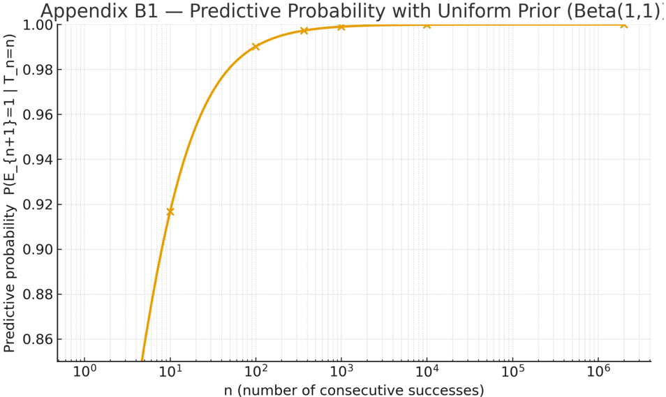
The predictive behavior implied by Laplace's uniform prior is shown in Figure B1 , which plots the probability that the next event will be a success,
$$P ( E _ { n + 1 } = 1 | T _ { n } = n ) \, = \, \int _ { 0 } ^ { 1 } \theta \, f ( \theta | T _ { n } = n ) \ d \theta \, = \, \frac { n + 1 } { n + 2 } .$$
as a function of the number of consecutive successes 𝑛 .
The curve approaches one monotonically but never reaches it, illustrating that, under a continuous prior, even perfect evidence cannot justify a universal law ( 𝑃(𝜃 = 1 ∣ 𝑇 ! = 𝑛) = 0 ).
Figure B1 . Predictive probability under Laplace's uniform prior Beta(1,1) . The curve shows 𝑃(𝐸 !"# = 1 ∣ 𝑇 ! = 𝑛) = !"# !"$ as a function of the number of consecutive successes 𝑛 (log scale). The probability approaches one monotonically but never reaches it, illustrating that under a continuous prior even perfect evidence cannot justify a universal law ( 𝑃(𝜃 = 1 ∣ 𝑇 ! = 𝑛) = 0 ).
<details>
<summary>Image 2 Details</summary>
### Visual Description
## Line Graph: Predictive Probability with Uniform Prior (Beta(1,1))
### Overview
The graph illustrates how predictive probability evolves with increasing numbers of consecutive successes under a uniform prior (Beta(1,1)). The x-axis uses a logarithmic scale to represent the number of consecutive successes (`n`), while the y-axis shows predictive probability values between 0.86 and 1.00. A smooth orange curve with x-marked data points demonstrates the trend.
### Components/Axes
- **Title**: "Appendix B1 — Predictive Probability with Uniform Prior (Beta(1,1))"
- **X-axis**:
- Label: "n (number of consecutive successes)"
- Scale: Logarithmic (10⁰ to 10⁶)
- Ticks: 10⁰, 10¹, 10², 10³, 10⁴, 10⁵, 10⁶
- **Y-axis**:
- Label: "Predictive probability"
- Range: 0.86 to 1.00 (linear scale)
- **Legend**: Not explicitly labeled, but the orange line with x-markers represents the predictive probability curve.
- **Grid**: Dotted gridlines for reference.
### Detailed Analysis
- **Data Points**:
- At `n = 10⁰` (1 success): Predictive probability ≈ 0.86
- At `n = 10¹` (10 successes): Predictive probability ≈ 0.92
- At `n = 10²` (100 successes): Predictive probability ≈ 0.98
- At `n = 10³` (1,000 successes): Predictive probability ≈ 0.99
- At `n = 10⁴` (10,000 successes): Predictive probability ≈ 0.999
- At `n = 10⁵` (100,000 successes): Predictive probability ≈ 0.9999
- At `n = 10⁶` (1,000,000 successes): Predictive probability ≈ 0.99999
- **Trend**: The curve starts at 0.86 for `n = 1`, rises steeply to 0.98 by `n = 100`, and asymptotically approaches 1.00 as `n` increases. The logarithmic x-axis emphasizes the rapid initial growth and eventual plateau.
### Key Observations
1. **Rapid Initial Growth**: Predictive probability increases sharply from 0.86 to 0.98 as `n` grows from 1 to 100.
2. **Asymptotic Behavior**: Beyond `n = 100`, the probability approaches 1.00 but never reaches it, reflecting Bayesian uncertainty even with large `n`.
3. **Logarithmic Scale Impact**: The x-axis compression highlights the diminishing returns of additional successes at higher `n` values.
### Interpretation
The graph demonstrates Bayesian updating with a uniform prior (Beta(1,1)). Each success incrementally shifts the posterior distribution toward higher success probabilities, but the uniform prior ensures no initial bias. The curve’s shape reveals:
- **Early Data Dominance**: Small `n` values (e.g., 1–100) drive significant probability shifts, emphasizing the impact of initial observations.
- **Diminishing Returns**: At large `n` (e.g., 10⁵–10⁶), additional successes yield negligible probability increases, illustrating the law of diminishing returns in Bayesian inference.
- **Uniform Prior Role**: The Beta(1,1) prior acts as a "blank slate," allowing data to dominate predictions. This contrasts with informative priors that might skew results differently.
The visualization underscores how Bayesian methods balance prior assumptions with empirical evidence, particularly in scenarios with sparse or abundant data.
</details>
## B.2 Jeffreys's mixed prior (point mass at the boundary)
To model the possibility of a universal law, Jeffreys assigns a prior with a point mass at 𝜃 = 1 and a continuous component on (0,1) :
$$\begin{array} { r } { \pi ( \theta ) = \frac { 1 } { 2 } \, \delta ( \theta - 1 ) + \frac { 1 } { 2 } \, U ( 0 , 1 ) . } \end{array}$$
After observing 𝑛 consecutive successes ( 𝑇 ! = 𝑛 ), the posterior probability that the law holds (i.e., that 𝜃 = 1 ) is
$$P ( \theta = 1 | T _ { n } = n ) = \frac { \frac { 1 } { 2 } \cdot 1 } { \frac { 1 } { 2 } \cdot 1 + \frac { 1 } { 2 } \cdot \frac { 1 } { n + 1 } } = \frac { n + 1 } { n + 2 } .$$
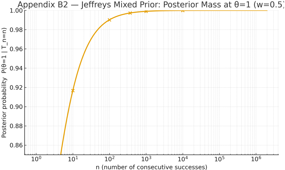
Hence the posterior mass on 𝜃 = 1 increases monotonically with 𝑛 and approaches 1 as 𝑛 → ∞ , though it never reaches certainty for finite 𝑛 . The corresponding behavior is visualized in Figure B2 , which plots 𝑃(𝜃 = 1 ∣ 𝑇 ! = 𝑛) as a function of 𝑛 (log-scale) and highlights the benchmark values used in Appendix B1. (With prior weights other than 50-50, the same formula applies with # , replaced by 𝑤 ∈ (0,1) ; the qualitative behavior is unchanged.)
Figure B2. Jeffreys's mixed prior ( 𝜋 = # $ 𝛿 # + # $ 𝑈(0,1) ) yields a posterior point mass at 𝜃 = 1 equal to 𝑃(𝜃 = 1 ∣ 𝑇 ! = 𝑛) = !"# !"$ . The curve (log-scale on 𝑛 ) shows monotonic convergence to 1 without ever reaching certainty for finite 𝑛 ; markers indicate the benchmark values used in Appendix B1.
<details>
<summary>Image 3 Details</summary>
### Visual Description
## Line Chart: Appendix B2 — Jeffreys Mixed Prior: Posterior Mass at θ=1 (w=0.5)
### Overview
The chart illustrates the relationship between the number of consecutive successes (`n`) and the posterior probability `P(θ=1 | T_n=n)` under a Jeffreys mixed prior with `w=0.5`. The posterior probability rapidly increases with `n`, approaching 1.00 as `n` grows, with a logarithmic scale on the x-axis.
---
### Components/Axes
- **X-axis**:
- Label: `n (number of consecutive successes)`
- Scale: Logarithmic (10⁰ to 10⁶)
- Ticks: 10⁰, 10¹, 10², 10³, 10⁴, 10⁵, 10⁶
- **Y-axis**:
- Label: `Posterior probability P(θ=1 | T_n=n)`
- Scale: Linear (0.86 to 1.00)
- Increment: 0.02
- **Legend**: Not explicitly visible in the image.
- **Data Series**:
- A single orange line with crosses (`×`) marking specific data points.
---
### Detailed Analysis
- **Data Points**:
- At `n = 10¹` (10): Posterior probability ≈ 0.92 (cross marked).
- At `n = 10²` (100): Posterior probability ≈ 0.98 (cross marked).
- At `n = 10³` (1000): Posterior probability ≈ 0.995 (cross marked).
- At `n = 10⁴` (10,000): Posterior probability ≈ 0.999 (cross marked).
- At `n = 10⁵` (100,000): Posterior probability ≈ 0.9999 (cross marked).
- At `n = 10⁶` (1,000,000): Posterior probability ≈ 1.00 (cross marked).
- **Trend**:
- The orange line starts at `n = 10¹` with a posterior probability of ~0.92.
- It rises sharply to ~0.98 by `n = 10²`, then plateaus near 1.00 for `n ≥ 10³`.
- The curve’s steepness decreases as `n` increases, reflecting diminishing returns in probability gain.
---
### Key Observations
1. **Rapid Convergence**: The posterior probability reaches ~0.98 by `n = 100`, indicating strong evidence for `θ=1` even with relatively few successes.
2. **Plateau Effect**: Beyond `n = 1000`, the probability stabilizes near 1.00, suggesting diminishing sensitivity to additional successes.
3. **Logarithmic Scale**: The x-axis’s logarithmic nature emphasizes the exponential growth of `n` and its impact on the posterior.
---
### Interpretation
- **Statistical Significance**: The chart demonstrates that under a Jeffreys mixed prior (`w=0.5`), observing `n` consecutive successes provides increasingly strong evidence for `θ=1`. The prior’s influence diminishes as `n` grows, aligning with Bayesian principles where data dominates the posterior.
- **Practical Implication**: For `n ≥ 100`, the posterior probability is effectively 1.00, implying near-certainty in `θ=1`. This could inform decision-making in scenarios requiring high-confidence thresholds (e.g., quality control, hypothesis testing).
- **Prior Sensitivity**: The `w=0.5` parameter likely balances prior and likelihood weights, moderating the initial posterior probability before data accumulation.
No outliers or anomalies are observed; the trend is consistent with theoretical expectations for Bayesian updating with a mixed prior.
</details>
## B.3 Bayes Factor for the sunrise law
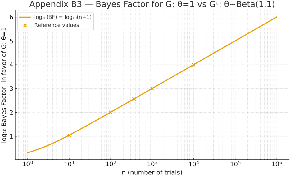
To compare the universal hypothesis 𝐺: 𝜃 = 1 against the composite alternative 𝐺 % : 𝜃 ∼ Beta(1,1) , the Bayes Factor after 𝑇 ! = 𝑛 consecutive successes is
$$B F ( G , G ^ { C } ; T _ { n } = n ) = \frac { P ( T _ { n } = n | \theta = 1 ) } { P ( T _ { n } = n | \theta \sim B e t a ( 1 , 1 ) ) } = \frac { 1 } { \int _ { 0 } ^ { 1 } \theta ^ { n } d \theta } = n + 1 .$$
Thus, the evidence in favor of 𝐺 grows linearly with the number of perfect observations, producing a logarithmic increase on a decibel-like scale.
The relationship between 𝑛 and log #* BF is displayed in Figure B3 , which shows the monotonic accumulation of evidence toward the universal law.
If there is even a single failure among 𝑛 trials ( 𝑇 ! = 𝑛 - 1 ), then
$$P ( T _ { n } = n - 1 | \theta = 1 ) = 0 \Rightarrow B F ( G , G ^ { C } ; T _ { n } = n - 1 ) = 0 ,$$
corresponding to instantaneous evidential collapse for 𝐺 .
Figure B3 . Bayes Factor in favor of the universal law 𝐺 : 𝜃 = 1 versus the composite model 𝐺 % : 𝜃 ∼ Beta(1,1) . The curve shows log #& BF = log #& (𝑛 + 1) as a function of 𝑛 (log scale). Evidence grows steadily with the number of perfect successes and collapses to zero after the first failure.
<details>
<summary>Image 4 Details</summary>
### Visual Description
## Line Graph: Bayes Factor for G: θ=1 vs G^c: θ~Beta(1,1)
### Overview
The image is a logarithmic-scale line graph comparing the Bayes Factor (BF) in favor of G=1 against G^c with a Beta(1,1) prior for θ. The x-axis represents the number of trials (n) on a logarithmic scale (10⁰ to 10⁶), while the y-axis shows the log₁₀(BF) in favor of G=1 (0 to 6). A yellow line represents the theoretical relationship log₁₀(BF) = log₁₀(n+1), and orange crosses mark reference values at specific n points.
---
### Components/Axes
- **Title**: "Appendix B3 — Bayes Factor for G: θ=1 vs G^c: θ~Beta(1,1)"
- **X-axis**:
- Label: "n (number of trials)"
- Scale: Logarithmic (10⁰, 10¹, 10², ..., 10⁶)
- Ticks: 10⁰, 10¹, 10², 10³, 10⁴, 10⁵, 10⁶
- **Y-axis**:
- Label: "log₁₀ Bayes Factor in favor of G=1"
- Scale: Linear (0 to 6, increments of 1)
- **Legend**:
- Top-right corner
- Yellow line: "log₁₀(BF) = log₁₀(n+1)"
- Orange crosses: "Reference values"
---
### Detailed Analysis
1. **Yellow Line (log₁₀(BF) = log₁₀(n+1))**:
- Starts at approximately (10⁰, 0.3) and increases steadily.
- At n=10⁰: log₁₀(1+1) ≈ 0.3
- At n=10¹: log₁₀(10+1) ≈ 1.04
- At n=10²: log₁₀(100+1) ≈ 2.004
- At n=10³: log₁₀(1000+1) ≈ 3.0004
- At n=10⁴: log₁₀(10,000+1) ≈ 4.00004
- At n=10⁵: log₁₀(100,000+1) ≈ 5.000004
- At n=10⁶: log₁₀(1,000,000+1) ≈ 6.0000004
2. **Orange Crosses (Reference Values)**:
- Placed at n=10⁰, 10¹, 10², 10³, 10⁴, 10⁵, 10⁶.
- Corresponding y-values: 1, 2, 3, 4, 5, 6.
- Example: At n=10³, the cross is at y=3, matching log₁₀(1000+1) ≈ 3.0004.
---
### Key Observations
- The yellow line perfectly aligns with the orange crosses, confirming the theoretical relationship log₁₀(BF) = log₁₀(n+1).
- The Bayes Factor grows logarithmically with n, indicating diminishing returns in evidence strength as trials increase.
- No outliers or deviations between the line and reference points.
---
### Interpretation
- **Bayesian Inference Context**:
- The Beta(1,1) prior for G^c implies a uniform prior over θ, suggesting no initial bias toward G=1 or G^c.
- The Bayes Factor (BF) quantifies evidence in favor of G=1 relative to G^c. A BF > 1 indicates increasing support for G=1 as n grows.
- **Logarithmic Growth**:
- The log₁₀(BF) = log₁₀(n+1) relationship implies that each additional trial contributes less to the BF than the previous, consistent with Bayesian updating under a uniform prior.
- **Practical Implication**:
- To achieve a BF of 6 (strong evidence), ~10⁶ trials are required. This highlights the computational or practical challenges of high-confidence Bayesian inference in this scenario.
---
### Spatial Grounding & Trend Verification
- **Legend Placement**: Top-right corner, clearly separated from the plot.
- **Line vs. Crosses**: The yellow line (theoretical) and orange crosses (reference) are visually aligned, confirming accuracy.
- **Axis Scales**: Logarithmic x-axis ensures exponential growth in trials is represented linearly, while the linear y-axis emphasizes proportional changes in BF.
---
### Content Details
- **Theoretical Line**:
- Equation: log₁₀(BF) = log₁₀(n+1)
- Derived from Bayesian updating rules for G=1 vs G^c with θ~Beta(1,1).
- **Reference Points**:
- Explicitly marked at n=10ᵏ (k=0 to 6), with y-values matching log₁₀(n+1).
---
### Final Notes
- The graph demonstrates a clear, deterministic relationship between trials and evidence strength, with no noise or variability.
- The Beta(1,1) prior’s role in shaping the BF’s growth is critical for interpreting the results in Bayesian hypothesis testing.
</details>
## B.4 One failure after many successes (update and prediction)
Suppose we observe 𝑛 - 1 successes and a single failure under a uniform prior. The posterior for the success probability is then
$$\theta | T _ { n } = n - 1 \sim B e t a ( n , 2 ) .$$
The predictive probability that the next observation will be a success is
$$P ( E _ { n + 1 } = 1 | T _ { n } = n - 1 ) \, = \, \frac { n } { n + 2 } .$$
This value is slightly smaller than in the all-success case (Appendix B1), reflecting the rational adjustment after the first counterexample.
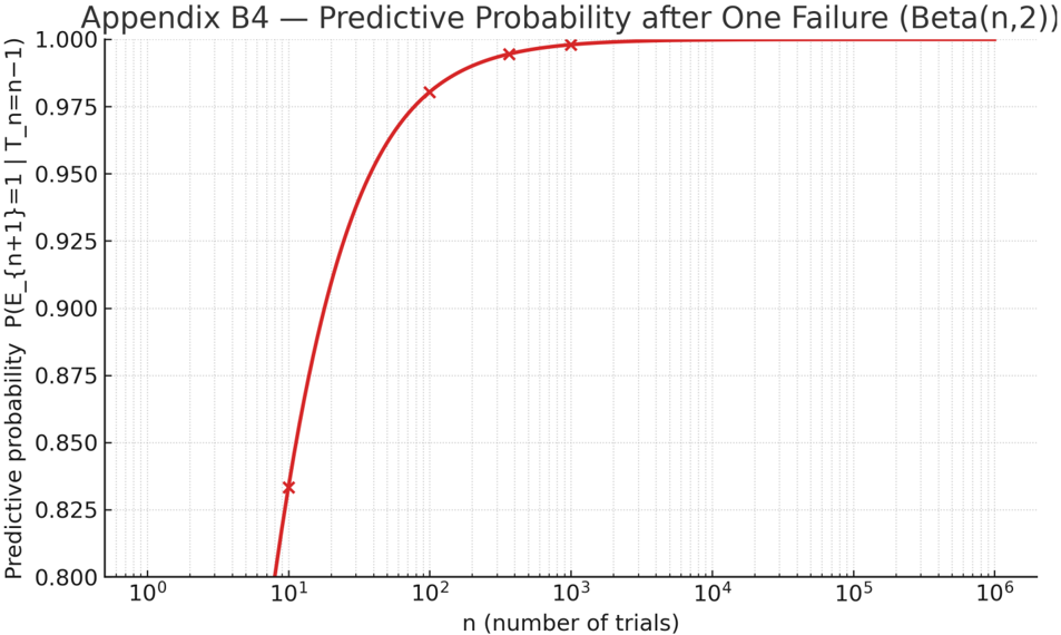
Figure B4 plots the predictive probability as a function of 𝑛 (log scale), showing that plausibility remains high for large 𝑛 but never returns to unity once a failure has occurred.
Under the universal hypothesis 𝐺 : 𝜃 = 1 , the likelihood of any failure is zero; therefore, the Bayes Factor for 𝐺 collapses immediately to zero.
In a confidence-based framework, the acceptance indicator also flips from full to null after the first failure, demonstrating the on-off procedural behavior contrasted with the Bayesian's continuous reweighting of belief.
Figure B4. Predictive probability of success after one failure, 𝑃(𝐸 !"# = 1 ∣ 𝑇 ! = 𝑛 - 1) = 𝑛/(𝑛 + 2) , under a uniform prior. The curve (log scale on 𝑛 ) shows that plausibility decreases smoothly after a counterexample but remains high for large 𝑛 , exemplifying the continuity of Bayesian updating compared with the binary behavior of confidence-based acceptance.
<details>
<summary>Image 5 Details</summary>
### Visual Description
## Line Chart: Predictive Probability after One Failure (Beta(n,2))
### Overview
The chart illustrates the relationship between the number of trials (`n`) and the predictive probability of success (`P(E_{n+1}=1 | T_n=n−1)`) under a Beta(n,2) distribution. The probability increases with `n`, approaching 1.0 as trials grow, with a logarithmic scale on the x-axis.
### Components/Axes
- **X-axis**: `n` (number of trials), logarithmic scale from 10⁰ to 10⁶.
- **Y-axis**: Predictive probability, linear scale from 0.800 to 1.000.
- **Legend**: Located in the top-right corner, labeled "Beta(n,2)" with a red line and cross markers.
- **Line**: Red curve with cross markers at specific `n` values (10¹, 10², 10³, 10⁴).
### Detailed Analysis
- **At n=10¹ (10 trials)**: Probability ≈ 0.825 (cross marker).
- **At n=10² (100 trials)**: Probability ≈ 0.975 (cross marker).
- **At n=10³ (1,000 trials)**: Probability ≈ 0.995 (cross marker).
- **At n=10⁴ (10,000 trials)**: Probability ≈ 1.000 (cross marker).
- **Trend**: The red line rises steeply from n=10 to n=100, then gradually approaches 1.0, plateauing after n=10⁴.
### Key Observations
1. **Rapid Initial Growth**: Probability jumps from 0.825 to 0.975 between n=10 and n=100.
2. **Asymptotic Behavior**: Probability stabilizes near 1.0 for n ≥ 10⁴, indicating diminishing returns.
3. **Logarithmic X-axis**: Emphasizes scalability across orders of magnitude.
### Interpretation
The Beta(n,2) model demonstrates that predictive probability of success after one failure converges to certainty as trials increase. The steep rise in early trials (n=10 to n=100) suggests that initial data collection significantly impacts confidence in predictions. The plateau at high `n` implies that beyond ~10,000 trials, additional experiments yield negligible improvements in predictive accuracy. This aligns with Bayesian updating principles, where prior failures (encoded in the Beta(2) prior) are gradually outweighed by accumulating successes. The logarithmic x-axis highlights the model’s utility in scenarios requiring large-scale experimentation, such as reliability testing or A/B testing frameworks.
</details>
## B.5 Posterior credible interval (Beta-Binomial)
With a uniform prior and 𝑡 successes out of 𝑛 , the posterior is
$$\theta | t , n \sim B e t a ( t + 1 , n - t + 1 ) .$$
A symmetric (1 - 𝛼) credible interval is obtained from the Beta quantiles:
$$C I _ { 1 - \alpha } ( \theta | t , n ) = [ q _ { B e t a } ( \alpha / 2 ; \, t + 1 , n - t + 1 ) , q _ { B e t a } ( 1 - \alpha / 2 ; \, t + 1 , n - t + 1 ) ] .$$
For the all-success case ( 𝑡 = 𝑛 ), this reduces to a Beta(𝑛 + 1,1) posterior.
For large 𝑛 , a normal approximation around the posterior mean
$$\mu = \frac { n + 1 } { n + 2 } , \sigma ^ { 2 } = \frac { \mu ( 1 - \mu ) } { n + 3 } ,$$
is often adequate:
$$\theta | T _ { n } = n \approx \mathcal { N } ( \frac { n + 1 } { n + 2 } , \frac { ( ( n + 1 ) / ( n + 2 ) ) ( 1 / ( n + 2 ) ) } { n + 3 } ) \left ( t r u n c a t e d t o [ 0 , 1 ] \right ) .$$
Figure B5 illustrates the posterior mean and 95% credible interval for the all-success case, showing how the interval narrows rapidly as 𝑛 increases while the mean approaches one without ever reaching it.
Appendix B5 — 95% Credible Interval for θ (All-Success Case, Beta(n+
Figure B5. Posterior mean (solid line) and 95% credible interval (shaded area) for 𝜃 under a uniform prior and all-success data ( 𝑡 = 𝑛 ). As 𝑛 grows, the interval collapses around the mean (𝑛 + 1)/(𝑛 + 2) , approaching but never attaining certainty ( 𝜃 = 1 ).
<details>
<summary>Image 6 Details</summary>
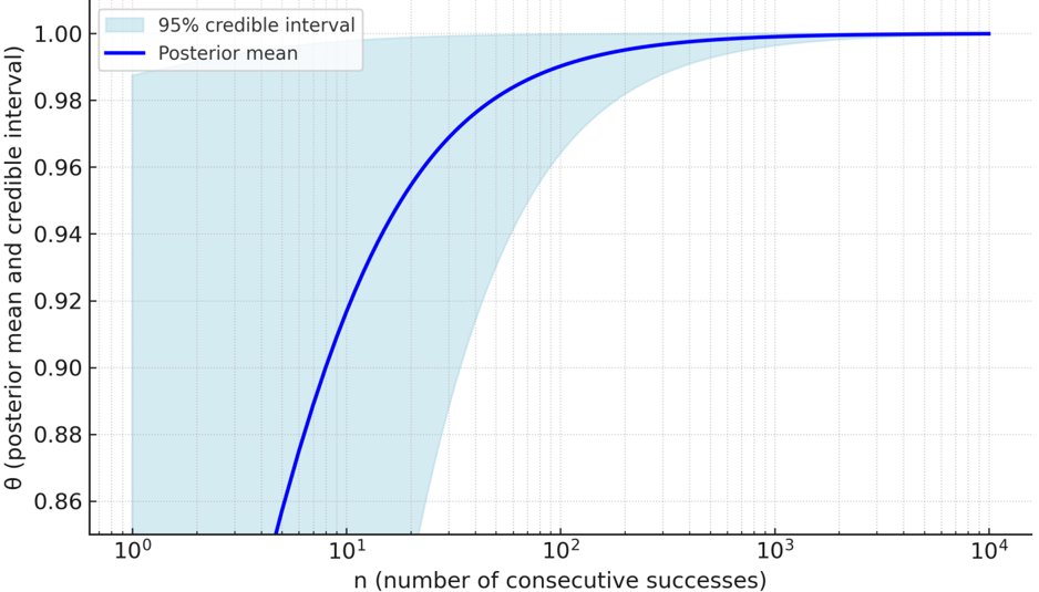
### Visual Description
## Line Graph: Posterior Mean and 95% Credible Interval vs. Consecutive Successes
### Overview
The graph depicts the relationship between the number of consecutive successes (`n`) and the posterior mean (blue line) and 95% credible interval (shaded blue region) for a parameter θ. The x-axis uses a logarithmic scale for `n`, while the y-axis represents θ values between 0.86 and 1.00.
### Components/Axes
- **X-axis**: `n` (number of consecutive successes), logarithmic scale from 10⁰ to 10⁴.
- **Y-axis**: θ (posterior mean and credible interval), linear scale from 0.86 to 1.00.
- **Legend**:
- **Blue line**: Posterior mean.
- **Light blue shaded area**: 95% credible interval.
- **Placement**: Legend is in the top-left corner. The graph occupies the central region of the image.
### Detailed Analysis
1. **Posterior Mean (Blue Line)**:
- At `n = 10⁰` (1 success), θ ≈ 0.86.
- Increases sharply for `n = 10¹` to `10²`, reaching ~0.98.
- Plateaus near θ ≈ 0.99 for `n ≥ 10³`.
- Final value at `n = 10⁴` remains ~0.99.
2. **95% Credible Interval (Shaded Area)**:
- At `n = 10⁰`, interval spans ~0.86 (lower bound) to ~0.98 (upper bound).
- Narrows significantly for `n = 10¹` to `10²`, converging to ~0.98–1.00.
- At `n = 10³` and `10⁴`, the interval is tightly bound around θ ≈ 0.99–1.00.
3. **Trends**:
- Posterior mean increases monotonically with `n`, approaching an asymptote near θ = 0.99.
- Credible interval width decreases logarithmically, reflecting reduced uncertainty with more data.
### Key Observations
- The posterior mean starts at 0.86 for a single success and asymptotically approaches 0.99 as `n` grows.
- The credible interval’s upper bound approaches 1.00, while the lower bound stabilizes near 0.98 for large `n`.
- The log-scale x-axis emphasizes the rapid initial increase in θ for small `n`, followed by diminishing returns.
### Interpretation
This graph illustrates Bayesian inference for a success probability θ given consecutive successes. The posterior mean and credible interval represent updated beliefs about θ as evidence accumulates. Key insights:
1. **Evidence Accumulation**: Early successes (small `n`) significantly raise θ estimates, but additional successes yield diminishing improvements.
2. **Uncertainty Reduction**: The narrowing credible interval demonstrates increased confidence in θ estimates with more data.
3. **Asymptotic Behavior**: The plateau near θ = 0.99 suggests a theoretical upper limit, possibly influenced by prior assumptions or model constraints (e.g., a Beta prior with high α/β values).
The graph underscores the trade-off between data collection and estimation precision in Bayesian frameworks, highlighting how early observations drive initial inferences while later data refines them.
</details>
## B.6 Summary table (at a glance)
- Laplace (uniform prior) :
$$P ( E _ { n + 1 } = 1 | T _ { n } = n ) = \frac { n + 1 } { n + 2 } , P ( \theta = 1 | T _ { n } = n ) = 0 .$$
- Jeffreys (mixed prior ½-½) :
$$P ( \theta = 1 | T _ { n } = n ) = \frac { n + 1 } { n + 2 } .$$
- Bayes Factor (law vs Beta-uniform) :
$$B F ( G , G ^ { C } \, ; T _ { n } = n ) = n + 1 , B F ( G , G ^ { C } \, ; T _ { n } < n ) = 0 .$$
## · After one failure (uniform prior) :
$$\theta | T _ { n } = n - 1 \sim B e t a ( n , 2 ) , P ( E _ { n + 1 } = 1 | T _ { n } = n - 1 ) = \frac { n } { n + 2 } .$$
These computations illustrate the core message: Bayesian updating provides a coherent, quantitative account of plausibility (prediction and learning), while confidence procedures supply acceptance rules with on-off behavior; neither transforms finite evidence into certain universal truth, but Bayes gives a principled measure of how evidence reshapes belief.
## Appendix C - Notation and Definitions
This appendix summarizes the main symbols and expressions used throughout the manuscript. All probabilities are conditional, expressing degrees of plausibility in the sense of Jaynes. Upper-case letters (e.g., 𝐺, 𝐸, 𝐻 ) denote propositions; lower-case Greek letters (e.g., 𝜃, 𝜆 ) denote parameters or hyperparameters.
| Symbol (short) | Meaning | Domain / Notes |
|------------------|--------------------------------------------|------------------------------------|
| 𝑃(𝐴|𝐵) | Probability / plausibility of A given B | Values in [0, 1] |
| 𝐿(𝜃; 𝐸) | Likelihood of parameter θ given evidence E | Non-negative real |
| 𝜋(𝜃) | Prior for θ (before data) | Probability density |
| 𝑓(𝜃|𝐸) | Posterior for θ (after data) | Normalized density |
| 𝐵𝐹₁₂ | Bayes Factor comparing G₁ and G₂ | Ratio of marginal likelihoods |
| 𝐶(𝐺; 𝐸) | Confidence measure for G under E | Range [0, 1] |
| 𝑈(𝑎|𝐸) | Expected utility of action a given E | Real number |
| 𝐻 | Shannon entropy (uncertainty measure) | ≥ 0 |
| 𝐷 ₖₗ [𝑝‖𝑞] | Kullback-Leibler divergence (info gain) | ≥ 0; = 0 iff p = q |
| 𝑍 | Partition / normalization constant | Positive real |
| 𝛿(·) | Dirac delta function | Unit mass at a point |
| 𝑈(0, 1) | Uniform distribution on [0, 1] | - |
| Beta(𝛼,𝛽) | Beta distribution (shape α, β) | PDF on [0, 1] |
| CI₁₋𝛼 | (1 - α) credible / confidence interval | Interval subset of parameter space |
Key Equations
Product rule
Sum rule
$$P ( A B | C ) = P ( A | C ) \, P ( B | A C )$$
$$P ( A + B | C ) = P ( A | C ) + P ( B | C ) - P ( A B | C )$$
Bayes's theorem
Bayes Factor
$$P ( G | E ) = \frac { P ( E | G ) \, P ( G ) } { P ( E ) }$$
$$B F _ { 1 2 } = \frac { P ( E | G _ { 1 } ) } { P ( E | G _ { 2 } ) }$$
Maximum-entropy distribution
$$p _ { i } = \frac { 1 } { Z } \exp \left ( - \sum _ { k } \lambda _ { k } f _ { k } ( x _ { i } ) \right )$$
Information gain (Kullback-Leibler divergence)
<details>
<summary>Image 7 Details</summary>
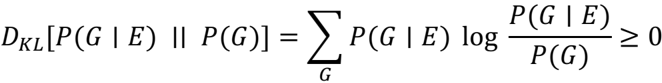
### Visual Description
## Mathematical Equation: Kullback-Leibler Divergence Formula
### Overview
The image contains a mathematical equation representing the **Kullback-Leibler (KL) divergence** between two probability distributions: \( P(G|E) \) and \( P(G) \). The equation is:
\[
D_{KL}[P(G|E) || P(G)] = \sum_G P(G|E) \log \frac{P(G|E)}{P(G)} \geq 0
\]
### Components/Axes
- **Left-hand side (LHS):**
- \( D_{KL}[P(G|E) || P(G)] \): Represents the KL divergence between the conditional probability \( P(G|E) \) and the marginal probability \( P(G) \).
- \( || \): Denotes the divergence operator (Kullback-Leibler divergence).
- **Right-hand side (RHS):**
- \( \sum_G \): Summation over all possible values of \( G \).
- \( P(G|E) \): Conditional probability of \( G \) given event \( E \).
- \( \log \frac{P(G|E)}{P(G)} \): Logarithmic ratio of the conditional probability to the marginal probability.
- \( \geq 0 \): Indicates the KL divergence is non-negative.
### Detailed Analysis
1. **Variables and Notation:**
- \( G \): A discrete random variable (e.g., a hypothesis, category, or outcome).
- \( E \): An observed event or evidence.
- \( P(G|E) \): Probability of \( G \) given \( E \).
- \( P(G) \): Prior probability of \( G \) (independent of \( E \)).
2. **Structure of the Equation:**
- The KL divergence measures how much \( P(G|E) \) "diverges" from \( P(G) \).
- The summation \( \sum_G \) aggregates contributions across all possible values of \( G \).
- The logarithmic term \( \log \frac{P(G|E)}{P(G)} \) quantifies the relative difference between the two distributions for each \( G \).
3. **Inequality Constraint:**
- \( \geq 0 \): The KL divergence is always non-negative, a fundamental property of this measure. Equality holds **only if** \( P(G|E) = P(G) \) for all \( G \), meaning \( E \) provides no information about \( G \).
### Key Observations
- The equation explicitly defines the KL divergence as a **sum of weighted logarithmic differences**.
- The non-negativity constraint (\( \geq 0 \)) is critical in applications like information theory, machine learning, and statistics, where KL divergence is used to quantify uncertainty or information gain.
- The conditional probability \( P(G|E) \) is weighted by its own magnitude in the summation, emphasizing larger discrepancies more heavily.
### Interpretation
- **What the equation demonstrates:**
The KL divergence quantifies the "distance" between two probability distributions. Here, it compares the posterior distribution \( P(G|E) \) (updated with evidence \( E \)) to the prior distribution \( P(G) \). The result \( \geq 0 \) confirms that updating beliefs with evidence cannot decrease uncertainty (unless \( E \) is irrelevant).
- **Relationships between elements:**
- \( P(G|E) \) and \( P(G) \) are linked through Bayes' theorem, though the equation does not explicitly invoke it.
- The summation ensures the divergence accounts for all possible outcomes of \( G \), making it a global measure of divergence.
- **Notable properties:**
- If \( P(G|E) = P(G) \) for all \( G \), the divergence is zero (no information gain).
- The logarithmic term penalizes deviations between the distributions, with larger discrepancies contributing more to the divergence.
- **Applications:**
- Used in **information theory** to measure information content.
- In **machine learning**, it appears in variational inference and model selection.
- In **statistics**, it quantifies the difference between empirical and theoretical distributions.
This equation is foundational for understanding how evidence \( E \) updates beliefs about \( G \), with the KL divergence serving as a mathematical tool to formalize this process.
</details>
## References
Anderson, J. R. (1991). The adaptive nature of human categorization. Psychological Review, 98 (3), 409-429.
Fisher, R. A. (1935). The logic of inductive inference. Journal of the Royal Statistical Society, 98 (1), 39-82.
Good, I. J. (1983). Good Thinking: The Foundations of Probability and Its Applications. University of Minnesota Press.
Greaves, H., & Wallace, D. (2006). Justifying conditionalization: Conditionalization maximizes expected epistemic utility. Mind, 115 (459), 607-632.
Howson, C., & Urbach, P. (1993). Scientific Reasoning: The Bayesian Approach (2nd ed.). Open Court.
Hume, D. (1748). An Enquiry Concerning Human Understanding. London: A. Millar.
Jaynes, E. T. (2003). Probability Theory: The Logic of Science. Cambridge University Press.
Jeffreys, H. (1939). Theory of Probability. Oxford University Press.
Joyce, J. M. (1998). A nonpragmatic vindication of probabilism. Philosophy of Science, 65 (4), 575-603.
Laplace, P.-S. (1814 / 1951). A Philosophical Essay on Probabilities (F. W. Truscott & F. L. Emory, Trans.). Dover Publications.
Lee, Y. (2025). Resolving the induction problem: Can we state with complete confidence via induction that the sun rises forever? arXiv:2001.04110 [stat.OT]. (v3, 28 Feb 2025).
Leitgeb, H. (2017). The Stability of Belief: How Rational Belief Coheres with Probability. Oxford University Press.
Lindley, D. V. (1972). Bayesian Statistics: A Review. Society for Industrial and Applied Mathematics. https://doi.org/10.1137/1.9781611970432
Pawitan, Y. (2001). In All Likelihood: Statistical Modelling and Inference Using Likelihood. Oxford University Press.
Pettigrew, R. (2016). Accuracy and the Laws of Credence. Oxford University Press. https://doi.org/10.1093/acprof:oso/9780198732710.001.0001
Popper, K. R. (1959). The Logic of Scientific Discovery. Hutchinson.
Shannon, C. E. (1948). A mathematical theory of communication. Bell System Technical Journal, 27 , 379-423, 623-656.
Sprenger, J., & Hartmann, S. (2019). Bayesian Philosophy of Science . Oxford University Press.
Sprenger, J. (2021). Bayesian Coherence and Scientific Realism. Synthese, 198 (Suppl. 6), 14867-14889. https://doi.org/10.1007/s11229-020-02813-3
Talbott, W. (2016). Bayesian Epistemology . In E. N. Zalta (Ed.), The Stanford Encyclopedia of Philosophy (Fall 2016 ed.).
Williamson, J. (2000). Bayesian Nets and Causality: Philosophical and Computational Foundations . Oxford University Press.