# Beyond ReAct: A Planner-Centric Framework for Complex Tool-Augmented LLM Reasoning
**Authors**: Xiaolong Wei, Yuehu Dong1, Xingliang Wang, Xingyu Zhang, Zhejun Zhao, Dongdong Shen, Long Xia, Dawei Yin
> Equal contribution.Corresponding author.
Abstract
Existing tool-augmented large language models (LLMs) encounter significant challenges when processing complex queries. Current frameworks such as ReAct are prone to local optimization traps due to their reliance on incremental decision-making processes. To address these limitations, we propose a novel Planner-centric Plan-Execute paradigm that fundamentally resolves local optimization bottlenecks through architectural innovation. Central to our approach is a novel Planner model that performs global Directed Acyclic Graph (DAG) planning for complex queries, enabling optimized execution beyond conventional tool coordination. We also introduce ComplexTool-Plan, a large-scale benchmark dataset featuring complex queries that demand sophisticated multi-tool composition and coordination capabilities. Additionally, we develop a two-stage training methodology that integrates Supervised Fine-Tuning (SFT) with Group Relative Policy Optimization (GRPO), systematically enhancing the Planner’s tool selection accuracy and global planning awareness through structured DAG-based planning. When integrated with a capable executor, our framework achieves state-of-the-art performance on the StableToolBench benchmark for complex user queries, demonstrating superior end-to-end execution capabilities and robust handling of intricate multi-tool workflows. Our code and data are publicly available at https://github.com/weixiaolong94-hub/Beyond-React.
Introduction
Large Language Models (LLMs) have demonstrated remarkable prowess in language processing, yet their inherent knowledge is static and they lack direct interaction with the external world. A transformative solution is tool augmentation, which empowers LLMs to act as autonomous agents by calling external APIs and tools (schick2023toolformer; patil2024gorilla). This paradigm shifts LLMs from being mere text generators to active problem-solvers capable of tackling complex, real-world tasks, a trend exemplified by systems like HuggingGPT (shen2023hugginggpt) and the rise of multi-agent frameworks (hong2023metagpt). The evaluation of these agentic capabilities has itself become a major research thrust, with new benchmarks like AgentBench (liu2023agentbench) setting the stage for more rigorous assessment.
<details>
<summary>example.png Details</summary>
### Visual Description
## Diagram: Task Complexity and Computational Graph Mapping
### Overview
This image presents two distinct scenarios, labeled (a) "Easy task" and (b) "Complex task," each illustrating how a natural language query is transformed into a corresponding computational flow diagram. Both scenarios feature a user query, represented by an icon and text, followed by a directed acyclic graph (DAG) composed of numbered nodes and directional arrows, symbolizing the sequence and dependencies of tasks. The image aims to visually demonstrate how the complexity of a query correlates with the structure and depth of its underlying task graph.
### Components/Axes
The image is divided horizontally into two main sections, each enclosed within a dashed-line rounded rectangle.
**Top Section: (a) Easy task**
* **Header**: Located at the top-left of this section, labeled "(a) Easy task".
* **Query Component**:
* **Icon**: A green circular icon depicting a stylized human bust (brown hair, light blue shirt) is positioned on the left.
* **Label**: Directly below the icon, the text "Query" is displayed.
* **Text Box**: To the right of the icon and label, a light orange rectangular box with rounded corners contains the query text: "For Tesla's Q4, get its total revenue and its stock performance, then combine them into a single summary."
* **Flow Diagram Component**:
* **Initial Arrow**: A light green arrow points horizontally from the right edge of the query text box towards the first node of the diagram.
* **Nodes**: Four yellow circular nodes, each containing a black number, are arranged in a diamond-like structure.
* Node "1" is on the far left.
* Nodes "2" (top-middle) and "3" (bottom-middle) are in the next stage.
* Node "4" is on the far right.
* **Edges (Arrows)**: Black arrows indicate the flow and dependencies between nodes.
* From Node 1 to Node 2.
* From Node 1 to Node 3.
* From Node 2 to Node 4.
* From Node 3 to Node 4.
**Bottom Section: (b) Complex task**
* **Header**: Located at the top-left of this section, labeled "(b) Complex task".
* **Query Component**:
* **Icon**: A green circular icon depicting a stylized human bust (identical to the one in the "Easy task" section) is positioned on the left.
* **Label**: Directly below the icon, the text "Query" is displayed.
* **Text Box**: To the right of the icon and label, a light orange rectangular box with rounded corners contains the query text: "Analyze Tesla's Q4. I need a profit report from its revenue and expenses, and a separate analysis of its stock trend. Then, combine both into a final performance summary."
* **Flow Diagram Component**:
* **Initial Arrow**: A light green arrow points horizontally from the right edge of the query text box towards the first node of the diagram.
* **Nodes**: Seven yellow circular nodes, each containing a black number, are arranged in a multi-stage, branching structure.
* Node "1" is on the far left.
* Nodes "2" (top), "3" (middle), and "4" (bottom) are in the second stage.
* Nodes "5" (top-right) and "6" (bottom-right) are in the third stage.
* Node "7" is on the far right, serving as the final node.
* **Edges (Arrows)**: Black arrows indicate the flow and dependencies between nodes.
* From Node 1 to Node 2.
* From Node 1 to Node 3.
* From Node 1 to Node 4.
* From Node 2 to Node 5.
* From Node 3 to Node 5.
* From Node 3 to Node 6.
* From Node 4 to Node 6.
* From Node 5 to Node 7.
* From Node 6 to Node 7.
### Detailed Analysis
**Scenario (a) Easy task:**
The query asks for two distinct pieces of information ("total revenue" and "stock performance") and then their combination.
The corresponding flow diagram starts with Node 1, which branches into two parallel paths (Node 2 and Node 3). These two paths then converge into a single Node 4. This structure visually represents:
1. An initial processing step (Node 1).
2. Two independent sub-tasks (Node 2 and Node 3) that can potentially be executed in parallel.
3. A final aggregation or combination step (Node 4) that depends on the completion of both Node 2 and Node 3.
The flow is straightforward, with a single entry point and a single exit point, representing a simple fan-out and fan-in pattern.
**Scenario (b) Complex task:**
The query requests a "profit report from its revenue and expenses" AND a "separate analysis of its stock trend," followed by combining "both into a final performance summary." This implies more granular data extraction and intermediate analytical steps.
The corresponding flow diagram is significantly more intricate:
1. An initial processing step (Node 1).
2. Node 1 branches into three parallel paths (Nodes 2, 3, and 4), suggesting more initial data retrieval or decomposition steps.
3. These paths then feed into two intermediate processing nodes (Nodes 5 and 6).
* Node 2 feeds into Node 5.
* Node 3 feeds into both Node 5 and Node 6, indicating it might provide input for multiple subsequent analyses.
* Node 4 feeds into Node 6.
This suggests that Node 5 and Node 6 represent distinct intermediate analyses (e.g., "profit report" and "stock trend analysis" as mentioned in the query).
4. Finally, Nodes 5 and 6 converge into a single Node 7, representing the "final performance summary."
The flow demonstrates multiple levels of branching and merging, reflecting a more complex set of dependencies and intermediate computations required to fulfill the query.
### Key Observations
* **Query-to-Graph Correspondence**: There is a direct visual correlation between the complexity of the natural language query and the complexity of the generated computational graph.
* **Parallelism**: Both diagrams suggest the possibility of parallel execution for independent sub-tasks (e.g., Nodes 2 and 3 in the easy task, or Nodes 2, 3, and 4 in the complex task).
* **Aggregation/Combination**: The convergence of multiple paths into a single node (Node 4 in easy, Node 7 in complex) consistently represents a final aggregation or summary step.
* **Intermediate Steps**: The "Complex task" diagram introduces an additional layer of intermediate processing nodes (5 and 6) before the final aggregation, which aligns with the query's request for "a profit report" and "a separate analysis" before combining "both."
* **Shared Inputs**: In the complex task, Node 3 feeding into both Node 5 and Node 6 indicates that some initial data or processing might be a prerequisite for multiple subsequent analytical branches.
### Interpretation
This diagram illustrates a fundamental concept in automated task execution or query processing systems, particularly those dealing with natural language understanding and computational graph generation. It suggests that such a system can:
1. **Parse Natural Language**: Understand the intent and components of a user's query, even when phrased in natural language.
2. **Decompose Tasks**: Break down a complex query into a series of smaller, manageable sub-tasks.
3. **Identify Dependencies**: Determine the order in which these sub-tasks must be executed and which tasks depend on the output of others.
4. **Construct a Computational Graph**: Represent these decomposed tasks and their dependencies as a directed acyclic graph (DAG), where nodes are tasks and edges are data/control flow.
The "Easy task" demonstrates a simple fan-out/fan-in pattern, suitable for queries requiring parallel data retrieval and a straightforward combination. The "Complex task" showcases a more sophisticated graph, indicating the system's ability to handle multi-stage processing, multiple intermediate analytical steps, and potentially shared data inputs across different analytical branches. The context of "Tesla's Q4" and "revenue," "expenses," "stock performance," and "profit report" strongly implies an application in financial analysis, business intelligence, or data analytics, where natural language queries are translated into data processing pipelines. The visual distinction between "easy" and "complex" tasks highlights the system's adaptability and robustness in handling varying levels of user request intricacy.
</details>
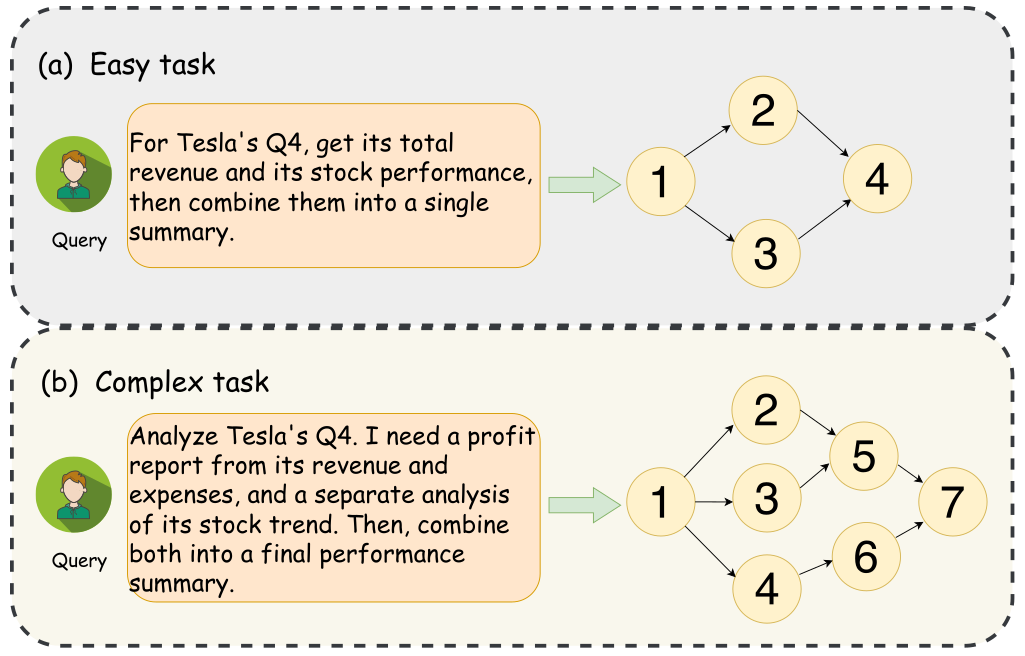
Figure 1: An example of a simple versus a complex task. A simple query results in a basic, parallel DAG, while a complex query involving nested logic is translated into a more elaborate, multi-level DAG.
<details>
<summary>mcp30.png Details</summary>
### Visual Description
## Diagram: AI Agent Training and Execution Process
### Overview
This image is a technical diagram illustrating a two-part process for an AI agent: (a) Training process and (b) Executing process. The diagram uses flowcharts, directed acyclic graphs (DAGs), and various icons to depict the stages of workflow generation, query processing, planning, and execution using a set of tools.
### Components/Axes
The image is divided horizontally into two main sections, each representing a distinct process:
**Section (a): Training process** (Upper half, predominantly light blue and light purple background)
This section is labeled "(a) Training process" at the bottom-center of its boundary. It describes the system's learning phase.
* **Workflow Generation Stage** (Leftmost, light blue background):
* **Multi Tools** box (top-left): A rectangular box containing a list of generic tools.
* Content:
* "Tool_1: Description1"
* "Tool_2: Description1"
* "......" (ellipsis indicating more tools)
* "Tooln_: Description1"
* **Candidate Tools DAG** (center-left): A directed acyclic graph (DAG) representing a potential workflow.
* Label: "Candidate Tools DAG: Task" (at the top)
* Nodes:
* Start Node: "Task" (light blue circle at the top)
* Intermediate Nodes: Numbered circles 1, 2, 3, 4, 5, 6, 7 (light yellow circles)
* End Node: "Finish" (light green circle at the bottom)
* Edges (arrows indicating flow): Task -> 1, Task -> 2; 1 -> 3, 1 -> 4; 2 -> 4, 2 -> 5; 3 -> 6; 4 -> 6, 4 -> 7; 5 -> 7; 6 -> Finish, 7 -> Finish.
* **Query Reverse-Engineering Stage** (Middle, light purple background):
* **Complex Query & Candidate Tools** box (center): A rectangular box containing two sub-labels.
* Content: "Complex Query" (top sub-box), "Candidate Tools" (bottom sub-box)
* **Intent Analysis and Re-planning Stage** (Rightmost, light blue background):
* **New DAG** (center-right): Another directed acyclic graph (DAG), representing a refined workflow.
* Label: "New DAG: Task" (at the top)
* Nodes:
* Start Node: "Task" (light blue circle at the top)
* Intermediate Nodes: Numbered circles 1, 2, 3, 4, 5, 6, 7, 8 (light yellow circles)
* End Node: "Finish" (light green circle at the bottom)
* Edges (arrows indicating flow): Task -> 1, Task -> 2; 1 -> 3, 1 -> 4; 2 -> 5, 2 -> 6; 3 -> 7; 4 -> 7, 4 -> 8; 5 -> 8; 6 -> 8; 7 -> Finish, 8 -> Finish.
* **Training Dataset** box (top-right): A rectangular box.
* Content: "Training Dataset"
* **GRPO Agent Icons** (bottom-right): Two robot icons connected by an arrow.
* Left Robot: Frowning face with red eyes.
* Right Robot: Smiling face with blue eyes.
* Text above arrow: "GRPO"
**Section (b): Executing process** (Lower half, predominantly light yellow background)
This section is labeled "(b) Executing process" at the bottom-center of its boundary. It describes how the trained system performs a task.
* **Query & Candidate Tools Stage** (Leftmost, light yellow background):
* **Query Icon & Text** (top-left): A circular icon of a person (green shirt) with a speech bubble next to it.
* Label: "Query" (below the person icon)
* Speech Bubble Content: "Plan a 5-day hiking retreat. Find a city, get flight and hotel costs, and give me a total budget."
* **Candidate Tools Cloud** (bottom-left): A cloud-shaped area containing various tool icons.
* Label: "Candidate Tools" (below the cloud)
* Icons (from top-left to bottom-right):
* Google Maps pin icon (red, yellow, blue, green)
* Google 'G' logo (red, yellow, blue, green)
* Document icon (blue, white)
* Airplane icon (orange)
* Airplane icon (green)
* Money symbol (Yen/Yuan, blue)
* Hospital/hotel building icon with a red heart (blue, white)
* Envelope icon (blue, white)
* **Planning Stage** (Middle, light yellow background):
* Label: "Planning" (centered at the top of this stage)
* **Planning DAG** (center): A directed acyclic graph (DAG) representing the specific plan for the query.
* Nodes (icons with labels below):
* Top: Google Maps pin icon, labeled "find_city"
* Left: Green airplane icon, labeled "get_flights"
* Right: Yellow hotel/stars icon, labeled "get_hotels"
* Bottom: Blue money symbol, labeled "make_report"
* Edges (arrows indicating flow): find_city -> get_flights; find_city -> get_hotels; get_flights -> make_report; get_hotels -> make_report.
* **Executing Stage** (Rightmost, light yellow background):
* Label: "Executing" (centered at the top of this stage)
* **Execution Steps** (center-right): A rectangular box listing three numbered steps.
* Step 1: "Step 1: Use **find_city** to find a destination for hiking." (Icon: magnifying glass over a map pin)
* Step 2: "Step 2: In parallel, use **get_flights** and **get_hotels** to find costs." (Icon: two magnifying glasses over a map pin)
* Step 3: "Step 3: Use **make_report** to create a final plan and budget." (Icon: document with numbered lines)
* **Final Answer Icon** (bottom-right): An icon depicting a document with a pen.
* Label: "Final answer" (below the icon)
**Connecting Elements and Icons:**
* **Gear/Brain Icon**: Represents a processing or generation step, seen between "Multi Tools" and "Candidate Tools DAG", and between "Complex Query" and "New DAG".
* **Robot Icons**: Represent the AI agent. A frowning robot is fine-tuned into a smiling robot during training. A smiling robot processes the query in the execution phase.
* **Arrows**: Indicate the direction of flow or data transformation between components.
### Detailed Analysis
**Section (a) Training process:**
The training process begins with a collection of "Multi Tools," each having a generic "Description1." These tools are fed into a "Workflow Generation" module (represented by the gear/brain icon) to produce a "Candidate Tools DAG." This DAG outlines a potential sequence of tool usage, starting from a "Task" and ending at "Finish," with intermediate nodes numbered 1 through 7.
Following this, a "Complex Query" and the "Candidate Tools" are processed through "Query Reverse-Engineering" and "Intent Analysis and Re-planning" (another gear/brain icon). This step generates a "New DAG," which is a refined or adapted workflow. This "New DAG" is more complex, featuring 8 intermediate nodes, suggesting a more detailed or optimized plan.
The output of the "New DAG" is used to "Filter Training Dataset" and then for "Fine-tuning" an AI agent. The fine-tuning process, labeled "GRPO," transforms a "frowning" robot (presumably an untrained or poorly performing agent) into a "smiling" robot (a well-trained or high-performing agent). This implies an iterative learning process, possibly using reinforcement learning, where the agent learns to generate and execute effective workflows.
**Section (b) Executing process:**
The execution process starts with a user providing a natural language "Query," such as "Plan a 5-day hiking retreat. Find a city, get flight and hotel costs, and give me a total budget." The system also has access to a pool of "Candidate Tools," represented by various icons like maps, search, documents, flights, hotels, and financial tools.
In the "Planning" stage, the system, likely guided by the trained agent, constructs a specific DAG tailored to the query. This DAG shows a clear dependency structure:
1. `find_city` (using a map tool) is the initial step.
2. Once a city is found, `get_flights` (using a flight tool) and `get_hotels` (using a hotel tool) can proceed in parallel.
3. Finally, `make_report` (using a money/report tool) combines the information from flights and hotels to create a budget.
The "Executing" stage then describes the sequential and parallel steps derived from the "Planning" DAG:
1. "Step 1: Use **find_city** to find a destination for hiking."
2. "Step 2: In parallel, use **get_flights** and **get_hotels** to find costs."
3. "Step 3: Use **make_report** to create a final plan and budget."
This execution leads to a "Final answer," represented by a document and pen icon.
### Key Observations
* **DAG-centric Approach**: Both training and execution heavily rely on Directed Acyclic Graphs (DAGs) to model and manage complex workflows, indicating a structured and dependency-aware approach to task completion.
* **Iterative Refinement in Training**: The transition from "Candidate Tools DAG" to "New DAG" suggests a process of refining or optimizing workflows based on complex queries and intent analysis.
* **Agent Improvement**: The "GRPO" fine-tuning step, transforming a frowning robot to a smiling one, clearly indicates that the training process aims to improve the agent's capability or performance.
* **Tool-Use Specialization**: In the execution phase, generic "Candidate Tools" are mapped to specific, named functions like `find_city`, `get_flights`, `get_hotels`, and `make_report`, demonstrating the system's ability to select and apply relevant tools.
* **Parallelism in Execution**: The "Planning" DAG and "Executing" steps explicitly show that `get_flights` and `get_hotels` can run "in parallel," highlighting the system's ability to optimize task execution time.
### Interpretation
This diagram illustrates a sophisticated AI system designed to understand complex user queries and execute them by orchestrating a series of specialized tools. The core idea is to enable an AI agent to break down a high-level goal into a structured workflow (a DAG) of tool calls.
The **training process** is crucial for teaching the agent how to construct these effective workflows. It starts with a broad set of tools and learns to generate and refine DAGs that represent valid and efficient ways to achieve tasks. The "Query Reverse-Engineering" and "Intent Analysis" steps suggest that the system learns to infer the underlying intent of a complex query and adapt its planning strategy accordingly. The "GRPO" fine-tuning indicates that this learning is likely driven by optimizing some performance metric, possibly through reinforcement learning, where the agent is rewarded for generating successful plans.
The **executing process** demonstrates the practical application of this learned capability. Given a user's query, the agent doesn't just execute a single command but intelligently plans a multi-step, potentially parallel, sequence of tool invocations. For the hiking retreat example, the agent understands that finding a city is a prerequisite for finding flights and hotels, and both are needed before a final budget can be compiled. This shows a hierarchical understanding of tasks and their dependencies.
In essence, the system acts as an intelligent orchestrator, translating human intent into actionable, tool-based workflows. This approach is highly relevant for developing general-purpose AI agents that can interact with a wide array of digital tools and services to solve real-world problems, moving beyond single-task capabilities to complex, multi-faceted problem-solving. The "Description1" for all tools in the training phase might imply that the system learns to generalize from tool descriptions rather than requiring specific examples for each tool, making it adaptable to new tools.
</details>
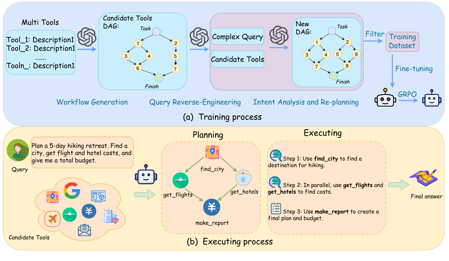
Figure 2: The figure illustrates our proposed framework. (a) The Training Process shows our automated pipeline for creating a training dataset and then training the Planner model via fine-tuning and reinforcement learning (GRPO). (b) The Executing Process demonstrates how the trained Planner takes a user query, generates a parallelizable execution plan as a Directed Acyclic Graph (DAG), and orchestrates the tools to produce the final answer.
The dominant approach for orchestrating tool usage relies on reactive, step-by-step reasoning frameworks like ReAct (yao2023react), often augmented by self-reflection techniques (shinn2023reflexion). However, this paradigm suffers from inherent local optimization traps due to its incremental decision-making process. While potentially effective for simple queries, its reactive nature often falters on complex tasks. As illustrated in Fig. 1, complex tasks involve more intricate dependencies than simple ones. To mitigate this, advanced methods employ tree search (yao2023tree) or explicit planning prompts (wang2023plan) to explore multiple paths. While these methods improve upon purely linear reasoning, they fail to architecturally resolve the fundamental bottleneck of local optimization. Critically, they remain focused on finding an optimal sequential path, overlooking opportunities for parallelism inherent in complex workflows. Moreover, the computational overhead of constructing and traversing search trees, requiring numerous LLM calls, can be prohibitive.
To address this fundamental challenge, we adopt a framework that decouples planning from execution (gao2023pal; chen2022program). Our approach employs a dedicated Planner model, trained to translate complex user queries into an execution plan structured as a DAG. In this DAG, nodes represent selected tools, and directed edges capture dependency relationships between them. By optimizing the Planner to improve the accuracy of both node selection (tool choices) and edge prediction (dependency relationships) in the DAG, we achieve more effective plans for complex queries, improving workflow execution compared to sequential models.
Realizing such a global planner presents two significant hurdles. First, there is a lack of large-scale, structured data required to train a model to generate complex plans, a challenge addressed by recent large-scale tool-use benchmarks like ToolBench (qin2023toolllm) and API-Bank (li2023api). Second, evaluating the quality of a plan is non-trivial. To overcome these, we introduce ComplexTool-Plan, a new, large-scale benchmark with graded difficulty levels. It serves as both the training ground and the evaluation standard for sophisticated planning agents. We then devise a two-stage hybrid training strategy for our Planner, combining Supervised Fine-Tuning (SFT) with subsequent refinement via Reinforcement Learning (RL) (ouyang2022training), a strategy that aligns with recent findings on using self-play and RL to elicit stronger reasoning (chen2024self; wei2025igniting).
Our extensive experiments validate the efficacy of our decoupled approach. On ComplexTool-Plan, our Planner substantially outperforms leading baselines. Crucially, when our Planner is paired with a powerful executor model like GPT-4o, the integrated system establishes a new state-of-the-art (SOTA) on the widely recognized end-to-end benchmark, StableToolBench (guo2024stabletoolbench), underscoring the practical superiority of our framework.
In summary, our key contributions are:
- We enhance task success in tool-augmented LLMs by proposing a planner-centric plan-execute paradigm framework and developing a DAG-optimized Planner, which significantly improves the accuracy of tool selection (nodes) and dependency modeling (edges).
- We construct ComplexTool-Plan, a large-scale, difficulty-graded benchmark designed to foster and evaluate complex agentic planning capabilities.
- Through extensive experiments, we demonstrate that our framework achieves state-of-the-art performance, offering a more scalable, efficient, and robust solution for complex multi-tool orchestration.
Related Works
We survey the rapidly evolving landscape of tool-augmented LLMs (li2025rankexpert; li2025rankelectra) along three primary axes: the evolution of tool-calling paradigms, RL-based policy optimization, and the development of evaluation benchmarks.
Tool Calling Paradigms
The paradigms for integrating LLMs with external tools have evolved from the interleaved ”Reasoning-Acting” steps of ReAct (yao2023react) to more reliable, natively supported structured API calls. A significant branch of research leverages code as a universal tool interface, with works like Program-of-Thought (PoT) (chen2022program) and PAL (gao2023pal) offloading complex computations to code interpreters. This trend has produced highly specialized agents like SWE-agent (yang2024swe), which can autonomously resolve software engineering tasks. For instance, advanced models are increasingly required for challenging real-world applications like multi-modal fake news detection, which involves reasoning over diverse data from various sources and domains (tong2025dapt; lu2025dammfnd).
Recent work is also moving beyond general-purpose models towards those specifically fine-tuned for tool use (zhao2025turatoolaugmentedunifiedretrieval). For instance, Toolformer (schick2023toolformer) demonstrates that a language model can teach itself to use tools by learning to insert beneficial API calls into text, thus significantly improving its ability to handle complex, tool-dependent instructions in a zero-shot manner. Concurrently, the interaction paradigm is expanding to visual environments, with powerful GUI agents like CogAgent (hong2024cogagent) demonstrating the ability to understand and interact with graphical user interfaces. Beyond reactive or single-agent frameworks, Li et al. (li2025towards) introduce an AI Search Paradigm that formalizes reasoning as coordinated planning among multiple LLM-based agents, while Chen et al. (chen2025multi) propose a proactive multi-agent orchestration framework for complex information-seeking tasks. Our work contributes to this evolution by focusing on the upfront, holistic planning of tool interactions, a critical component for efficient orchestration.
RL for Tool Policy Optimization
While Supervised Fine-Tuning (SFT) can teach models to mimic tool-use trajectories, Reinforcement Learning (RL) is superior for strategic decision-making in unseen scenarios. The latest SOTA models, such as Llama 3 (dubey2024llama), heavily rely on advanced RLHF techniques to refine their policy. Building on foundational work demonstrating that RL can enhance reasoning (guo2025deepseek), recent research has shown that RL teaches not just the ”syntax” of tool calling, but the ”strategy” (feng2025retool; jin2025search).
The field is advancing towards more sophisticated, outcome-driven optimization loops. For instance, AlphaCodium (ridnik2024code) employs a test-based, multi-stage iterative process. Similarly, influential frameworks like Tree of Thoughts (ToT) (yao2023tree), which explores multiple reasoning paths, and Reflexion (shinn2023reflexion), which leverages self-reflection, highlight the trend towards more deliberate and verifiable reasoning. Our hierarchical reward function aligns with this trend by providing a structured, outcome-driven signal to teach the model a robust planning strategy.
Benchmarks for Tool Calling
The evaluation of LLM tool-calling capabilities relies on increasingly sophisticated benchmarks, which have evolved from early interactive environments like ALFWorld (shridhar2020alfworld) and WebShop (yao2022webshop). In recent years, benchmarks have grown in scale and realism, with examples like ToolBench (qin2023toolllm) and its more stable successor, StableToolBench (guo2024stabletoolbench). The focus has also expanded towards greater realism, as seen in the web environment of WebArena (zhou2023webarena), and more challenging tasks, as in the GAIA benchmark (mialon2023gaia).
To support this research, new platforms are emerging that focus on specific aspects like evaluating the correctness of API calls in API-Bank (li2023api) and facilitating multi-agent collaboration in open-source frameworks like MetaGPT (hong2023metagpt). Our work contributes a new benchmark, ComplexTool-Plan, which fills a specific gap in this landscape by targeting the evaluation of an agent’s ability to generate complex, non-linear plans.
Methodology
Our method trains a language model to plan complex multi-tool tasks, as shown in Fig. 2. The framework includes: a formal Problem Formulation, our ComplexTool-Plan data generation pipeline, and a Model Training process using both Supervised Fine-Tuning (SFT) and Reinforcement Learning (RL).
Problem Formulation
We formalize multi-tool task planning as a structured prediction task of learning a policy $\pi:Q× T→\mathcal{G}$ . Given a natural language query $Q$ and a toolset $T$ , the policy generates an execution plan as a Directed Acyclic Graph (DAG), $G=(V,E)$ , where vertices $V⊂eq T$ are tools and edges $E$ represent data dependencies. The goal is to train a model $M_{\theta}$ to find the optimal policy $\pi^{*}$ that maximizes the expected plan utility $U(G)$ :
$$
\theta^{*}=\arg\max_{\theta}\mathbb{E}_{(Q,T)\sim p(Q,T)}[U(M_{\theta}(Q,T))] \tag{1}
$$
The utility $U(·)$ is realized through a reward function.
ComplexTool-Plan
To overcome data scarcity, we developed ComplexTool-Plan, a three-stage automated pipeline to generate our training dataset, $D_{train}$ .
- Workflow Generation: We initiate the process by leveraging a powerful LLM-DeepSeek-V3, to author a large set of workflows. For each workflow, the model is provided with a subset of tools from our predefined library $\mathcal{T}$ and prompted to generate a structurally complex and logically consistent execution plan in the form of a DAG, $G_{orig}$ . This LLM-driven approach produces the diverse, high-quality ground-truth solutions for our planning tasks.
- Query Reverse-Engineering: Next, we employ a powerful teacher LLM ( $M_{teacher}$ )-DeepSeek-V3 to reverse-engineer a natural language query $Q$ for each generated workflow $G_{orig}$ . The model’s objective is to capture the user’s intent behind the workflow, effectively transforming the difficult problem of plan generation into a more manageable text-to-text task.
- Intent Analysis and Re-planning: The final stage acts as a crucial quality filter. The reverse-engineered query $Q$ might be ambiguous or fail to fully capture the intent of the original plan $G_{orig}$ . Therefore, we use the same teacher model $M_{teacher}$ , now acting as an expert planner, to re-solve the problem based solely on $Q$ . This ensures that the final DAG plan, $G_{final}$ , is a faithful and optimal solution derivable from the query, thus guaranteeing the high fidelity of our resulting ( $Q$ , $G_{final}$ ) training pairs in $D_{train}$ .
Model Training
Our training process commences with Supervised Fine-Tuning (SFT) on a suite of Qwen3 models—specifically, the 0.6B, 1.7B, 4B, and 8B variants. This initial SFT phase serves to provide an effective initialization (i.e., a cold start), which is subsequently followed by a GRPO training phase for further policy refinement.
Base Models and Supervised Fine-Tuning (SFT)
We first perform Supervised Fine-Tuning (SFT) on our dataset $D_{\text{train}}$ to initialize the model. The objective is to learn to generate the ground-truth plan $G_{gt}$ by minimizing the Negative Log-Likelihood (NLL) loss:
$$
\mathcal{L}_{\text{SFT}}(\theta)=-\mathbb{E}_{(Q,G_{gt})\sim D_{\text{train}}}[\log P(G_{gt}|Q,T;\theta)] \tag{2}
$$
RL Training Set Curation
To ensure a stable and efficient RL phase, we curate the training data to focus on problems at the frontier of the model’s current capabilities (chen2024self). We use the SFT-trained model as a filter: tasks that the model already consistently solves (offering no learning signal) or consistently fails (intractably hard) are excluded from the RL training set. This curation of high-variance instances, where the outcome is uncertain, concentrates the training on the most informative samples, preventing policy degradation and fostering robust optimization.
Reinforcement Learning with Hierarchical Rewards
To move beyond SFT’s limitations, we use Reinforcement Learning (RL). This, however, requires a nuanced reward signal to properly evaluate complex DAGs, distinguishing structural from strategic errors. We address this by introducing a Hierarchical Reward Function $R(y)$ . To optimize this complex, multi-dimensional reward, we utilize the Group Relative Policy Optimization (GRPO) algorithm (shao2024deepseekmath), which is specifically designed for such scenarios and ensures robust policy improvement.
Our reward function, $R(y)$ , where $y$ represents the generated plan, evaluates plan quality through a fail-fast hierarchical process. It prioritizes structural correctness, with critical errors incurring large negative penalties and terminating evaluation.
- Level 1 and 2: Structural and Semantic Penalties. We first apply penalties for critical errors that render a plan invalid. This includes ill-formed syntax (e.g., non-JSON) or the presence of a cycle, both resulting in a large penalty (-10.0). A less severe penalty (-2.0) is given for a lack of connectivity (e.g., isolated nodes), which indicates a semantic flaw.
- Level 3: Planning Fidelity Rewards. If a plan passes all structural checks, it receives a positive reward based on its quality. This reward consists of two parts: (i) an Edge F1 Score Reward ( $R_{F1}$ ), calculated as 5 times the edge-level F1 score against the ground truth to reward partial structural correctness, and (ii) a large Perfect Match Bonus ( $R_{bonus}$ ) of +5.0 if the plan is identical to the ground truth, incentivizing perfect solutions.
The final reward, $R(y)$ , is computed based on these components. If any penalty is applied, the reward is the value of that penalty, checked in a specific order of precedence. Otherwise, it is the sum of the fidelity rewards:
$$
R(y)=\begin{cases}P_{\mathrm{syntax}}(y)&\text{if invalid syntax}\\
P_{\mathrm{cycle}}(y)&\text{else if has cycle}\\
P_{\mathrm{connectivity}}(y)&\text{else if disconnected}\\
R_{F1}(y)+R_{\mathrm{bonus}}(y)&\text{otherwise}\end{cases} \tag{3}
$$
The domain of this reward function, $[-10.0,10.0]$ , provides a rich, multi-faceted learning signal that guides the model not only on whether its plan is correct, but also on the nature and severity of its errors.
<details>
<summary>dataset.png Details</summary>
### Visual Description
## Chart Type: Grouped Bar Chart: Average Metrics by Difficulty Level
### Overview
This image displays a grouped bar chart illustrating the average values of three different metrics—Average Maximum Parallelism, Average tool calls, and Average number of candidate tools—across three distinct difficulty levels: Easy, Medium, and Hard. The chart uses color-coded bars to represent each metric, with numerical values explicitly labeled above each bar.
### Components/Axes
* **Y-axis Label**: "Numbers"
* **Y-axis Scale**: Ranges from 0 to 12, with major tick marks at intervals of 2 (0, 2, 4, 6, 8, 10, 12). Horizontal dashed grid lines are present at each integer value.
* **X-axis Categories**: "Easy", "Medium", "Hard". These categories represent increasing levels of task difficulty.
* **Legend**: Located in the top-left corner of the chart area.
* A yellow bar represents "Average Maximum Parallelism".
* An orange bar represents "Average tool calls".
* A light purple bar represents "Average number of candidate tools".
### Detailed Analysis
The chart presents three groups of bars, one for each difficulty level, with each group containing three bars corresponding to the metrics defined in the legend.
**1. Easy Difficulty Level:**
* **Average Maximum Parallelism** (Yellow bar): 1.55
* **Average tool calls** (Orange bar): 3.25
* **Average number of candidate tools** (Light purple bar): 3.93
**2. Medium Difficulty Level:**
* **Average Maximum Parallelism** (Yellow bar): 1.72
* **Average tool calls** (Orange bar): 3.89
* **Average number of candidate tools** (Light purple bar): 6.84
**3. Hard Difficulty Level:**
* **Average Maximum Parallelism** (Yellow bar): 2.03
* **Average tool calls** (Orange bar): 4.45
* **Average number of candidate tools** (Light purple bar): 9.91
### Key Observations
* **Overall Trend**: All three metrics show an increasing trend as the task difficulty level progresses from Easy to Medium to Hard.
* **Average Maximum Parallelism (Yellow)**: This metric consistently has the lowest values across all difficulty levels (1.55, 1.72, 2.03). It shows a gradual, relatively small increase with difficulty.
* **Average tool calls (Orange)**: This metric is consistently higher than "Average Maximum Parallelism" but lower than "Average number of candidate tools". It also shows a steady increase with difficulty (3.25, 3.89, 4.45).
* **Average number of candidate tools (Light Purple)**: This metric consistently has the highest values across all difficulty levels (3.93, 6.84, 9.91). It exhibits the most significant increase, particularly a substantial jump from Medium to Hard difficulty.
* **Magnitude Differences**: The "Average number of candidate tools" is notably higher than the other two metrics, especially at higher difficulty levels. For "Hard" tasks, it is more than double the "Average tool calls" and nearly five times the "Average Maximum Parallelism".
### Interpretation
The data strongly suggests that increasing task difficulty correlates with an increase in the complexity and resource demands of the underlying system or process.
1. **Increased Resource Utilization**: The upward trend in "Average Maximum Parallelism" indicates that harder tasks require more concurrent operations or a greater degree of parallel processing. This implies a need for more computational resources or a more complex execution strategy.
2. **More Actions/Steps**: The rise in "Average tool calls" suggests that more individual tools, functions, or sub-processes are invoked to complete more difficult tasks. This could mean that harder tasks are broken down into more steps or require a broader range of functionalities.
3. **Expanded Search Space/Decision Complexity**: The most prominent trend is the significant increase in the "Average number of candidate tools." This metric, representing the pool of potential tools considered, grows dramatically with difficulty. This implies that for harder tasks, the system faces a much larger and more complex decision space when selecting appropriate tools. It suggests that the challenge for difficult tasks might not just be in executing more steps or in parallel, but primarily in identifying *which* tools are relevant and necessary from a vast array of possibilities. This could point to increased overhead in tool discovery, filtering, or reasoning for complex problems.
In essence, as tasks become harder, the system not only needs to perform more actions and potentially in parallel, but critically, it must navigate a significantly larger set of potential solutions or tools to find the optimal path. This highlights the growing importance of efficient tool selection and management mechanisms as task complexity increases.
</details>
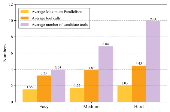
Figure 3: This chart shows our three task difficulties: Easy, Medium, and Hard. Harder tasks have more available tools to choose from (blue) and also require more tools to be used (orange).
Experimental Setup
Dataset
We conduct a comprehensive evaluation of our framework from two primary perspectives: (1) the quality of the generated plans, and (2) the end-to-end task execution success rate. For the former, we use our newly constructed ComplexTool-Plan benchmark. For the latter, we evaluate our system on the established StableToolBench benchmark.
ComplexTool-Plan Benchmark
We evaluate our Planner on ComplexTool-Plan, our benchmark constructed from a comprehensive library of 4,535 tool APIs sourced from ModelScope (li2023modelscope). The benchmark features three difficulty levels (Easy, Medium, and Hard) and provides a curated SFT dataset of 3,000 instances. For RL training, the dataset is filtered to comprise 787 instances, which are subsequently divided into training and test sets using an 8:2 ratio. Further details are available in Fig. 3.
End-to-End Execution Benchmark
To evaluate the practical effectiveness of our framework, we use StableToolBench (guo2024stabletoolbench) for end-to-end evaluation. StableToolBench is an enhanced version of the test set from ToolBench (qin2023toolllm), specifically designed to mitigate execution instability via a caching system and API simulators. It categorizes test cases across two axes: tool generalization and scenario complexity.
- Tool Generalization: Inst. (unseen instructions for seen tools), Tool (unseen tools in seen categories), and Cat. (unseen tool categories).
- Scenario Complexity: I1 (single-tool), I2 (multi-tool in-category), and I3 (multi-tool in-collection).
Task difficulty escalates from I1-Inst. to I3-Cat., providing a comprehensive testbed for agentic capabilities.
In our end-to-end evaluation on StableToolBench, we pair our Planner with GPT-4o as the executor.
Baselines
To ensure a comprehensive evaluation, we benchmark our framework against two categories of state-of-the-art baselines:
- Proprietary Planners: For direct planning evaluation on our ComplexTool-Plan benchmark, we compare against powerful proprietary models prompted to generate DAG plans directly. These include GPT-4o, Claude-3.7, DeepSeek-V3, and Ernie-X1, which serve as a practical upper bound for the task.
- Open-Source Frameworks: For end-to-end evaluation on StableToolBench (guo2024stabletoolbench), we compare against established methods applied to the ToolLLaMA model (qin2023toolllm). This includes the reactive framework ReAct, the planning-based method DFSDT, and a highly relevant concurrent work, LLMCompiler (kim2024llm).
Evaluation Metrics
Planning Quality Metrics
To comprehensively evaluate planning quality, we assess three key aspects: the correctness of tool selection (node-level), the accuracy of inferred dependencies (edge-level), and the holistic accuracy of the entire plan. Our evaluation is conducted on a test set comprising 500 samples from the Easy split and 500 from the Hard split. For each generated Directed Acyclic Graph (DAG), we compute the following metrics against the ground-truth plan, with all final scores macro-averaged.
Let $S_{pred}$ be the set of predicted items (nodes or edges) and $S_{true}$ be the set of ground-truth items.
- Node-level Performance (P/R/F1): Measures the accuracy of tool selection. We compute Precision, Recall, and F1-score between the set of predicted nodes ( $N_{pred}$ ) and ground-truth nodes ( $N_{true}$ ).
- Precision (P): Measures fidelity by calculating the fraction of predicted tools that are correct.
$$
\text{P}=\frac{|N_{pred}\cap N_{true}|}{|N_{pred}|}
$$
- Recall (R): Measures completeness by calculating the fraction of required tools that were identified.
$$
\text{R}=\frac{|N_{pred}\cap N_{true}|}{|N_{true}|}
$$
- F1-Score: The harmonic mean of Precision and Recall.
$$
\text{F1}=2\cdot\frac{\text{P}\cdot\text{R}}{\text{P}+\text{R}}
$$
- Edge-level Performance (P/R/F1): Measures the structural correctness of the plan. We apply the same P/R/F1 metrics to compare the set of predicted edges ( $E_{pred}$ ) against the ground-truth edges ( $E_{true}$ ). This assesses the model’s ability to infer the correct execution flow.
- DAG Exact Match (EM): Our most stringent metric, measuring the holistic correctness of the plan. A plan receives a score of 1 if and only if both its node set and edge set perfectly match the ground truth ( $N_{pred}=N_{true}$ and $E_{pred}=E_{true}$ ), and 0 otherwise.
End-to-End Evaluation Metrics
To evaluate the end-to-end task-solving capabilities of our framework, we adopt the two primary metrics established by the StableToolBench benchmark. The first, Solvable Pass Rate (SoPR), serves as the primary measure of absolute capability and is defined as the percentage of tasks that an agent successfully completes according to the benchmark’s ground-truth criteria. The second, Solvable Win Rate (SoWR), is a comparative metric that evaluates performance relative to a strong baseline. Specifically, it measures the win rate of our agent against the benchmark’s provided GPT-3.5 (ReAct) baseline, offering a clear signal of relative improvement. To ensure statistical robustness and mitigate performance fluctuations, all reported scores are the average of three independent runs for each experimental setting.
| Method | Node-level Performance | Edge-level Performance | DAG Exact Match Acc. | | | | |
| --- | --- | --- | --- | --- | --- | --- | --- |
| Precision | Recall | F1-Score | Precision | Recall | F1-Score | | |
| GPT-4o | 0.916 | 0.943 | 0.929 | 0.765 | 0.793 | 0.779 | 0.635 |
| Deepseek-V3 | 0.777 | 0.763 | 0.770 | 0.641 | 0.645 | 0.643 | 0.511 |
| Claude-3.7 | 0.939 | 0.959 | 0.949 | 0.801 | 0.829 | 0.815 | 0.644 |
| Ernie-X1 | 0.925 | 0.973 | 0.948 | 0.716 | 0.744 | 0.730 | 0.562 |
| Qwen3-0.6B (SFT) | 0.951 | 0.986 | 0.968 | 0.826 | 0.872 | 0.848 | 0.671 |
| Qwen3-1.7B (SFT) | 0.960 | 0.987 | 0.973 | 0.856 | 0.890 | 0.873 | 0.723 |
| Qwen3-1.7B (SFT+RL) | 0.974 | 0.985 | 0.979 | 0.874 | 0.885 | 0.879 | 0.756 |
| Qwen3-4B (SFT) | 0.972 | 0.986 | 0.979 | 0.882 | 0.895 | 0.888 | 0.768 |
| Qwen3-4B (SFT+RL) | 0.978 | 0.988 | 0.983 | 0.887 | 0.898 | 0.892 | 0.778 |
| Qwen3-8B (SFT) | 0.974 | 0.992 | 0.983 | 0.889 | 0.909 | 0.899 | 0.781 |
| Qwen3-8B (SFT+RL) | 0.982 | 0.987 | 0.984 | 0.905 | 0.907 | 0.906 | 0.803 |
Table 1: Results of our Planner models and proprietary baselines on the Easy evaluation set. Metrics include node-level, edge-level, and DAG Exact Match accuracy. Our fine-tuned models show superior performance compared to the baselines, with performance scaling positively with model size and the addition of RL. The Qwen3-0.6B(SFT+RL) variant is excluded due to training instability.
| Method | Node-level Performance | Edge-level Performance | DAG Exact Match Acc. | | | | |
| --- | --- | --- | --- | --- | --- | --- | --- |
| Precision | Recall | F1-Score | Precision | Recall | F1-Score | | |
| GPT-4o | 0.850 | 0.863 | 0.856 | 0.447 | 0.482 | 0.464 | 0.098 |
| Deepseek-V3 | 0.842 | 0.787 | 0.814 | 0.414 | 0.415 | 0.414 | 0.082 |
| Claude-3.7 | 0.884 | 0.910 | 0.897 | 0.476 | 0.508 | 0.491 | 0.106 |
| Ernie-X1 | 0.862 | 0.844 | 0.853 | 0.400 | 0.411 | 0.405 | 0.052 |
| Qwen3-0.6B (SFT) | 0.891 | 0.866 | 0.878 | 0.561 | 0.541 | 0.551 | 0.160 |
| Qwen3-1.7B (SFT) | 0.899 | 0.880 | 0.889 | 0.599 | 0.591 | 0.595 | 0.213 |
| Qwen3-1.7B (SFT+RL) | 0.914 | 0.861 | 0.887 | 0.616 | 0.579 | 0.597 | 0.218 |
| Qwen3-4B (SFT) | 0.918 | 0.894 | 0.906 | 0.632 | 0.623 | 0.627 | 0.241 |
| Qwen3-4B (SFT+RL) | 0.918 | 0.876 | 0.896 | 0.631 | 0.611 | 0.621 | 0.259 |
| Qwen3-8B (SFT) | 0.925 | 0.896 | 0.910 | 0.661 | 0.654 | 0.657 | 0.295 |
| Qwen3-8B (SFT+RL) | 0.937 | 0.873 | 0.904 | 0.678 | 0.641 | 0.659 | 0.319 |
Table 2: Results of our Planner models and proprietary baselines on the Hard evaluation set. Our fine-tuned models show superior performance compared to the baselines, with performance scaling positively with model size and the addition of RL. The Qwen3-0.6B(SFT+RL) variant is excluded due to training instability.
| Method | I1-Inst. | I1-Tool | I1-Cat. | I2-Inst. | I2-Cat. | I3-Inst. | Average | | | | | | | |
| --- | --- | --- | --- | --- | --- | --- | --- | --- | --- | --- | --- | --- | --- | --- |
| SoPR | SoWR | SoPR | SoWR | SoPR | SoWR | SoPR | SoWR | SoPR | SoWR | SoPR | SoWR | SoPR | SoWR | |
| GPT-series | | | | | | | | | | | | | | |
| GPT-3.5 (ReAct) | 53.0 | – | 53.0 | – | 51.2 | – | 37.6 | – | 43.9 | – | 48.6 | – | 47.9 | – |
| GPT-3.5 (DFSDT) | 63.8 | 58.9 | 73.9 | 65.8 | 65.8 | 60.1 | 57.1 | 72.6 | 69.8 | 68.5 | 69.9 | 67.2 | 66.7 | 65.5 |
| GPT-4 (ReAct) | 54.4 | 53.4 | 44.1 | 60.1 | 48.8 | 52.9 | 50.6 | 69.8 | 48.9 | 62.1 | 42.6 | 54.1 | 48.2 | 58.7 |
| GPT-4 (DFSDT) | 69.0 | 57.1 | 69.6 | 66.5 | 68.1 | 61.4 | 70.8 | 73.6 | 68.0 | 62.9 | 76.0 | 63.9 | 70.3 | 64.2 |
| Open-source | | | | | | | | | | | | | | |
| ToolLLaMA (ReAct) | 42.7 | 36.2 | 35.4 | 36.1 | 38.6 | 34.6 | 39.9 | 49.1 | 40.9 | 38.7 | 29.8 | 41.0 | 37.9 | 39.3 |
| ToolLLaMA $\dagger$ (ReAct) | 26.7 | 22.1 | 25.0 | 27.2 | 31.7 | 29.4 | 23.1 | 32.1 | 24.5 | 28.2 | 20.5 | 24.6 | 25.3 | 27.3 |
| ToolLLaMA (DFSDT) | 56.6 | 39.9 | 55.5 | 46.8 | 56.5 | 41.8 | 49.7 | 53.8 | 53.4 | 49.2 | 53.6 | 50.8 | 54.2 | 47.1 |
| ToolLLaMA $\dagger$ (DFSDT) | 41.8 | 35.6 | 39.9 | 37.3 | 44.9 | 39.9 | 36.0 | 47.2 | 39.1 | 39.5 | 33.3 | 26.2 | 39.2 | 37.6 |
| LLMCompiler | 39.2 | 35.6 | 35.1 | 36.0 | 39.8 | 35.3 | 37.5 | 45.6 | 38.4 | 38.1 | 27.0 | 36.5 | 36.2 | 37.9 |
| Qwen3-1.7B (RL) | 61.4 | 52.1 | 51.7 | 42.5 | 58.1 | 49.3 | 48.7 | 45.8 | 46.8 | 48.2 | 44.7 | 40.5 | 51.9 | 46.4 |
| Qwen3-4B (RL) | 62.1 | 54.6 | 55.4 | 47.1 | 61.4 | 53.5 | 59.2 | 55.7 | 48.7 | 51.3 | 50.8 | 48.6 | 56.3 | 51.8 |
| Qwen3-8B (RL) | 67.0 | 57.9 | 56.6 | 49.8 | 59.3 | 51.7 | 60.1 | 58.2 | 54.7 | 56.4 | 61.0 | 55.9 | 59.8 | 55.0 |
Table 3: End-to-end task-solving results on the StableToolBench benchmark. The table compares our Qwen3 models with GPT-series and other open-source methods across various task complexities. Our Qwen3 series, particularly the 8B model, demonstrates the best performance among all open-source baselines in both absolute success (SoPR) and win rate against GPT-3.5(ReAct) (SoWR).
Results and Discussion
RQ1: How does Reinforcement Learning enhance performance over Supervised Fine-Tuning?
Our results demonstrate that the RL stage systematically improves holistic plan accuracy over SFT alone, as measured by our most direct metric: DAG Exact Match Accuracy. As shown in Tab. 2, on the Easy set, our Qwen3-8B model’s accuracy increases from 0.781 (SFT) to 0.803 (SFT+RL). This trend is consistent across all model sizes and becomes even more critical as task complexity increases. Notably, the training instability of our smallest model (Qwen3-0.6B) suggests this trend has a lower bound: sufficient model capacity is crucial to prevent reward hacking, where a model learns a degenerate, low-effort policy simply to avoid penalties rather than solving the task.
On the challenging Hard set (Tab. 2), the impact of RL is more pronounced. The Qwen3-8B model’s DAG Exact Match accuracy jumps from 0.295 (SFT) to 0.319 (SFT+RL), an 8.1% relative improvement. This shows RL is not merely polishing plans but is essential for correcting subtle structural errors that emerge in complex scenarios, a conclusion supported by consistent gains in Edge-level F1-Scores. Essentially, while SFT effectively teaches the model to select the right tools (nodes), RL is crucial for orchestrating them correctly (edges). By optimizing for structural integrity, RL moves the model beyond plausible mimicry to generating functionally correct plans.
RQ2: How does model scaling affect performance robustness as task complexity increases?
Our experiments reveal a clear, positive relationship between model size and planning capability, with larger models demonstrating significantly greater robustness against increasing task complexity.
First, our framework shows strong scalability. This is most evident on the challenging Hard set, where even top-tier models like GPT-4o falter. On this set, the DAG Exact Match Accuracy of our SFT+RL models rises monotonically with scale: from 0.218 (1.7B) to 0.259 (4B) and finally 0.319 (8B). This stark performance gap over general-purpose models validates our specialized training approach.
Second, and more importantly, model scaling directly enhances robustness. While all models degrade on harder tasks, larger models exhibit a more graceful decline. For instance, when moving from the Easy to the Hard set, the accuracy of our Qwen3-1.7B model plummets by 71.2% (from 0.756 to 0.218). In contrast, our largest Qwen3-8B model sees a more contained 60.3% drop (from 0.803 to 0.319). This widening performance gap is crucial, demonstrating that scaling up our specialized Planner not only boosts absolute performance but also enhances its resilience against complex, real-world challenges.
RQ3: What is the end-to-end effectiveness and efficiency of our framework?
Our framework demonstrates highly competitive end-to-end performance. As shown in Tab. 3, our Qwen3-8B (RL) model achieves an average SoPR of 59.8%, substantially outperforming the widely-used reactive approach of GPT-4 (ReAct) at 48.2%. This highlights that a superior planning strategy can be more impactful than raw model capability, unlocking the potential of smaller models.
While iterative paradigms like DTA-Llama (zhu2025divide) report a higher SoPR, their success is largely driven by a multi-turn framework that allows for in-process error correction and adaptation. In contrast, our non-iterative, plan-then-execute paradigm has only one chance to generate a correct global plan upfront. This architectural choice prioritizes predictability and planning quality over the adaptive resilience of iterative feedback loops.
Crucially, this design choice leads to state-of-the-art efficiency. As detailed in Tab. 4, our method requires an average of just 2.29 inference steps to complete a task, significantly fewer than all other methods, including iterative parallel frameworks like DTA-Llama (2.48 steps). This demonstrates that our global planning approach is not only effective but also architecturally more efficient, solving complex tasks with fewer high-level decision rounds.
| Method | I1-I. | I1-T | I1-C. | I2-I. | I2-C. | I3-I. |
| --- | --- | --- | --- | --- | --- | --- |
| GPT-series | | | | | | |
| GPT-3.5 (ReAct) | 4.28 | 4.75 | 4.48 | 5.16 | 5.05 | 5.31 |
| GPT-3.5 (DFSDT) | 11.60 | 13.36 | 11.77 | 16.60 | 14.06 | 12.54 |
| GPT-3.5 (Parallel) | 25.33 | 28.06 | 26.12 | 31.79 | 31.04 | 38.10 |
| GPT-4 (ReAct) | 3.27 | 3.64 | 3.87 | 4.04 | 4.19 | 4.23 |
| GPT-4 (DFSDT) | 5.90 | 8.09 | 6.67 | 9.97 | 18.13 | 14.05 |
| GPT-4 (Parallel) | 4.66 | 9.18 | 12.90 | 3.63 | 5.98 | 10.38 |
| Open-source | | | | | | |
| ToolLLaMA (ReAct) | 3.42 | 3.47 | 3.50 | 3.67 | 3.63 | 3.64 |
| ToolLLaMA (DFSDT) | 8.09 | 8.51 | 8.10 | 10.20 | 9.93 | 9.23 |
| LLMCompiler | 5.48 | 5.56 | 6.07 | 5.36 | 5.68 | 5.62 |
| Qwen2.5 (Parallel) | 9.07 | 9.47 | 12.01 | 14.58 | 14.56 | 12.38 |
| DTA-Llama | 2.41 | 2.41 | 2.51 | 2.32 | 2.34 | 2.48 |
| Qwen3-8B (RL) | 2.26 | 2.33 | 2.29 | 2.16 | 2.29 | 2.41 |
Table 4: Inference steps for different methods.
Conclusion
In this work, we introduced a Planner-centric framework that decouples planning from execution to address the local optimization traps of reactive tool-use agents. Our core contribution is a Planner model trained via a two-stage SFT-GRPO strategy on our new ComplexTool-Plan benchmark. It generates a global, parallelizable DAG plan in a single forward pass.
Our experiments demonstrate that this paradigm is highly effective. The Planner itself produces higher-quality plans than strong proprietary models. When integrated with an executor, our framework achieves state-of-the-art results for open-source models on the challenging StableToolBench benchmark, while requiring the fewest inference steps.
Crucially, our findings show that a sophisticated planning strategy can be more impactful than raw model capability, offering a more scalable and predictable path toward capable autonomous agents.