2511.12793

# Neuro-Logic Lifelong Learning **Authors**: Bowen He, Xiaoan Xu, Alper Kamil Bozkurt, Vahid Tarokh, Juncheng Dong ## Abstract Solving Inductive Logic Programming (ILP) problems with neural networks is a key challenge in Neural-Symbolic Artificial Intelligence (AI). While most research has focused on designing novel network architectures for individual problems, less effort has been devoted to exploring new learning paradigms involving a sequence of problems. In this work, we investigate lifelong learning ILP, which leverages the compositional and transferable nature of logic rules for efficient learning of new problems. We introduce a compositional framework, demonstrating how logic rules acquired from earlier tasks can be efficiently reused in subsequent ones, leading to improved scalability and performance. We formalize our approach and empirically evaluate it on sequences of tasks. Experimental results validate the feasibility and advantages of this paradigm, opening new directions for continual learning in Neural-Symbolic AI. Keywords: Neuro-Symbolic AI, ILP, Lifelong Learning ## 1 Introduction Neuro-Symbolic Artificial Intelligence (Santoro et al. 2017; Manhaeve et al. 2018; Dai et al. 2019; d’Avila Garcez and Lamb 2020; Amizadeh et al. 2020) has emerged as a promising research direction that combines modern neural networks with classic symbolic methods, thereby leveraging the strengths of both. At a high level, neural networks offer the expressivity and end-to-end learning capabilities needed to tackle complex problems where traditional symbolic methods can fall short. Meanwhile, symbolic approaches contribute advantages such as explicit representation of knowledge and reasoning, in which neural networks often underperform (Valmeekam et al. 2023; Li et al. 2024; Sheth, Roy, and Gaur 2023). Although the term Neuro-Symbolic Artificial Intelligence spans a wide range of problems, paradigms, and methodologies, this work focuses specifically on tasks within the field of inductive logic programming (ILP) (Cropper and Dumančić 2022). Unlike standard logic programming, which draws conclusions from a given set of rules, ILP seeks to learn first-order logic rules that best explain observed examples from given relevant background knowledge. To solve ILP problems using neural networks, researchers have introduced a variety of methods and compared them against traditional ILP solvers (Evans and Grefenstette 2018; Glanois et al. 2021; Payani and Fekri 2019; Dong et al. 2019; Badreddine et al. 2022; Sen et al. 2022; Zimmer et al. 2023), demonstrating that neural network-based methods are both robust to noisy data and more efficient for large-scale tasks. However, most existing works primarily focus on designing new model architectures, dedicating relatively little attention to investigate learning paradigms beyond the conventional individual tasks setting. To this end, this work takes the first step to investigate the transferability of knowledge between ILP problems. Our insight is that logic rules, by their nature, are compositional and reusable. Specifically, a logic rule learned from one task can be naturally reused for another task within the same domain. Moreover, cognitive scientists have argued that humans learn, think, and reason in a symbolic manner, i.e., “symbolic models of cognition were the dominant computational approaches of cognition” (Castro et al. 2025; Besold and Kühnberger 2023). Thus, to achieve the remarkable capabilities of lifelong learning and meta-learning observed in human intelligence, we envision that the interplay of neural network and symbolic method presents a promising new direction for lifelong learning. We instantiate the aforementioned insight by introducing a novel lifelong learning problem for ILP. We introduce a compositional structure for neural logic models and evaluate their performance across sequences of tasks. By leveraging rules acquired from previous tasks, the neural logic models achieve significantly improved learning efficiency on new tasks. In comparison to the existing works that primarily focus on the perspective of model parameter optimization—such as regularization-based (Kirkpatrick et al. 2017; Zenke, Poole, and Ganguli 2017), experience replay-based (Rolnick et al. 2019; Buzzega et al. 2020), and architecture-based approaches (Rusu et al. 2016; von Oswald et al. 2020; Li et al. 2019) —lifelong learning for logic rules requires identifying which rules are beneficial for reuse and efficiently constructing new rules based on those already acquired. We take the first step in demonstrating the feasibility of this direction, paving the way for future research. Our empirical results confirm the enhanced learning efficiency achieved through lifelong learning. Furthermore, by simply incorporating experience replay, the model effectively retains its performance across tasks. Additionally, in certain experiments, we observe a backward transfer effect, where training on later tasks further improves performance on earlier tasks. Contribution Statement. We summarize our contributions as follows: - We formally introduce lifelong learning in ILP, framing it as a sequential optimization problem. - We propose a neuro-symbolic approach that leverages the compositionality of logic rules to enable knowledge transfer across tasks. - We validate on challenging logic reasoning tasks how logic rule transfer improves learning efficiency and the acquisition of a common knowledge base during sequential learning. Manuscript Organization. We frist briefly review related works in Section 2. We introduce the definition of lifelong ILP problems in Section 3. We elaborate on our implementation in Section 4. After presenting our experiment results in Section 5, we conclude with a discussion for future directions. ## 2 Related Works We provide review for both inductive logic programming, extending the discussion to more recent neural network based approcach, and lifelong learning that aims to build AI systems that accumulate knowledge in a seuquence of tasks. ### 2.1 Inductive Logic Programming Inductive Logic Programming (ILP) (Cropper and Dumančić 2022) is a longstanding and still unresolved challenge in artificial intelligence, characterized by its aim to solve problems through logical reasoning. Unlike statistical machine learning, where predications are based on statistical inference, ILP relies on logic inference and learns a logic program that could be used further to solve problems. Its integration with reinforcement learning (RL) further leads to the field of relational RL (Džeroski, De Raedt, and Driessens 2001), where the policy comprises logical rules and decisions are made through logical inference. The goal of ILP is to design AI systems that not only solve problems but do so through logical reasoning, which recent literature shows is lacking in purely neural network-based approaches (Valmeekam et al. 2023; Li et al. 2024). This raises a critical question: can we develop neural-symbolic methods that leverage the scalability of neural networks while also solving tasks through sound logical reasoning? (Evans and Grefenstette 2018) made a pioneering step towards this objective by introducing $\partial$ ILP, which integrates neural networks with inductive logic programming (ILP) and addresses 20 ILP tasks sourced from previous literature or designed by the authors themselves. They showed that, compared to traditional ILP methods, $\partial$ ILP is more robust against mislabeled targets that typically impair the performance of conventional approaches, reflecting the generalization capabilities of neural networks. Furthermore, (Jiang and Luo 2019) extends $\partial$ ILP to the reinforcement learning setting by incorporating logic predicates into the state and action spaces. They evaluate its performance on two tasks, Blocksworld and Gridworld, comparing it against MLP neural networks. Their results demonstrate that MLPs are prone to failure on these tasks represented with logic predicates. Neural logic machine (NLM) (Dong et al. 2019) represents another line of research that aims to design better neural network architectures for logic reasoning. They proposed a forward chaining approach to represent logical rules, effectively addressing the memory cost issues associated with handling a large number of objects, a challenge previously encountered by the $\partial$ ILP method. Despite the fact that the logic rules learned by NLMs are not explicitly extractable for human readers, they continue to be the most widely used benchmark in further applications (Wang et al. 2025) and related works. Differentiable Logic Machines (Zimmer et al. 2023) builds upon NLM to replace MLPs used by NLM with soft logic operator, providing more interpretability in the cost more computational requirement. (Campero et al. 2018) proposes to learning vector embeddings for both logic predicates and logic rules. It’s further expended by (Glanois et al. 2021) using the forward-chaining perspective as in NLM. Logic rules, by its nature, provide the property of compositionality, a new logic rule could be always built by composing rules that have been acquired before (Lin et al. 2014). Moreover, logic rules that are learned in a task could be naturally transferred to be used in another task from the same domain. This ability of knowledge transfer and lifelong learing has been considered as essential for human-like AI (Lake et al. 2016). Building on this insight, we investigate the lifelong learning ability of neural logic programming. ### 2.2 Lifelong Learning Lifelong learning or continual learning, has been proposed as a research direction for developing artificial intelligence systems capable of learning a sequence of tasks continuously (Wang et al. 2024). Ideally, a lifelong learning agent should achieve both forward transfer, where knowledge from earlier tasks benefits subsequent ones, and backward transfer, where learning newer tasks enhances performance on previous ones. At the very least, it should mitigate catastrophic forgetting, a phenomenon where learning later tasks causes the model to lose knowledge acquired from earlier tasks. Classic lifelong learning methods typically fall into four categories: (i) Regularization-based approaches, which constrain parameter updates within a certain range to mitigate forgetting (Kirkpatrick et al. 2017; Zenke, Poole, and Ganguli 2017; Li and Hoiem 2017)); (ii) Replay-based approaches, which store or generate data samples from past tasks and replay them during training on newer tasks (Rebuffi et al. 2017; Shin et al. 2017; Lopez-Paz and Ranzato 2017; Chaudhry et al. 2018); (iii) Optimization-based methods, which manipulate gradients to preserve previously acquired knowledge (Zeng et al. 2019; Farajtabar et al. 2020; Saha, Garg, and Roy 2021)); and (iv) Architecture-based methods, which expand or reconfigure model architectures to accommodate new tasks or transfer knowledge (Rusu et al. 2016; Yoon et al. 2017). In all cases, these methods are mainly rooted in neural networks and can be broadly categorized as strategies for optimizing model parameters or architectures. In contrast, approaching lifelong learning from a neuro-symbolic perspective offers additional opportunities by leveraging the properties of symbolic methods. Our work, therefore, falls within this emerging paradigm. One work highly relevant to our study is (Mendez 2022). They propose incorporating compositionality into lifelong training, enabling new tasks to benefit from previously learned neural modules. However, their formulation remains within the domain of pure neural networks and can be categorized as an architecture-based method for lifelong learning. In contrast, we emphasize that logic rules inherently provide compositionality, which can be leveraged for learning. Thus, our work serves as a strong instance of lifelong learning with compositionality, facilitating the systematic reuse and adaptation of learned knowledge across tasks. Another work that explores lifelong learning from a neuro-symbolic perspective is (Marconato et al. 2023). However, their focus is on extracting reusable concepts from sub-symbolic inputs while preventing reasoning shortcuts that could lead to incorrect symbolic knowledge. In contrast, our work centers on the transfer of logic rules, where learning and reusing these rules play a fundamental role. ## 3 Neural Logic Lifelong Learning ### 3.1 Problem Formulation We introduce our problem definition of ILP. We first define objects and their corresponding types within the domain of interest. Next, we define predicates and operations. Finally, we frame ILP as an optimization problem. #### Object Sets. We denote the set of objects in a given domain as $\mathcal{O}$ , while another set $\Lambda=\{\lambda_{1},\lambda_{2},...,\lambda_{n}\}$ defines all possible types that these objects can take, namely, $\forall o\in\mathcal{O},type(o)\in\Lambda$ . A partition of $\mathcal{O}$ is thus induced by grouping objects of the same type into a subset. Formally, we partition the set of objects $\mathcal{O}$ into subsets $\{\mathcal{O}_{\lambda}\}_{\lambda\in\Lambda}$ , where - Each subset is nonempty: $\mathcal{O}_{\lambda}\neq\varnothing$ ; - Subsets are pairwise disjoint: $\mathcal{O}_{\lambda}\cap\mathcal{O}_{\lambda^{\prime}}=\varnothing$ for all $\lambda\neq\lambda^{\prime}$ ; - Their union forms the entire set: $\cup_{\lambda\in\Lambda}\mathcal{O}_{\lambda}=\mathcal{O}$ ; - Objects within a single subset share the same type: $\forall\lambda\in\Lambda,\forall o_{i},o_{j}\in\mathcal{O}_{\lambda},\ type(o_{i})=type(o_{j})$ . #### Predicates. Next we define predicates, which are the cores of ILP programs. Consider $N\in\mathbb{Z}_{\geq 0}$ . A $N$ -ary predicate $\mathcal{P}$ is a binary-valued function $\mathcal{P}:\mathcal{O}(\mathcal{P})\rightarrow\{0,1\}$ where $\mathcal{O}(\mathcal{P})$ is the Cartesian product of $N$ elements, each of which arbitrarily selected from $\{\mathcal{O}_{\lambda_{1}},\mathcal{O}_{\lambda_{2}},\dots,\mathcal{O}_{\lambda_{n}}\}$ , that is, $$ \mathcal{O}(\mathcal{P})=\mathcal{O}_{\lambda_{i_{1}}}\times\mathcal{O}_{\lambda_{i_{2}}}\times\dots\times\mathcal{O}_{\lambda_{i_{N}}}, $$ where $\lambda_{i_{k}}\in\Lambda$ for all $1\leq k\leq N$ . Any set of $N$ -ary predicates $\{\mathcal{P}_{1},\mathcal{P}_{2},\dots,\mathcal{P}_{m}\}$ can be composed to form a new predicate $\widetilde{\mathcal{P}}=F(\mathcal{P}_{1},\mathcal{P}_{2},\dots,\mathcal{P}_{m})$ with a logic rule $F$ . Consider an example with the object set $\mathcal{O}=\{o_{1},o_{2}\}$ where $type(o_{1})=type(o_{2})$ . We define two $1$ -ary predicates $\mathcal{P}_{1}$ and $\mathcal{P}_{2}$ over $\mathcal{O}$ as $\mathcal{P}_{1}(o_{1})=0,\mathcal{P}_{1}(o_{2})=1$ ; $\mathcal{P}_{2}(o_{1})=1,\mathcal{P}_{2}(o_{2})=1.$ With $\mathcal{P}_{1}$ and $\mathcal{P}_{2}$ defined above, we can compose a new predicate $\mathcal{P}_{3}$ defined as $\mathcal{P}_{3}(X)\leftarrow\mathcal{P}_{1}(X)\land\mathcal{P}_{2}(X)$ . Here, the applied logic rule $F(\mathcal{P}_{1},\mathcal{P}_{2})$ is $\mathcal{P}_{1}(X)\land\mathcal{P}_{2}(X)$ , leading to the valuation of $\mathcal{P}_{3}$ as $$ \mathcal{P}_{3}(o_{1})=0,\mathcal{P}_{3}(o_{2})=1. $$ #### ILP Problems. Based on the definitions above, we are now ready to define ILPs. An ILP takes a set of background knowledge $B$ as input. Here, $B$ is a set of $m$ predicates $B=\{\mathcal{P}_{1},\mathcal{P}_{2},...,\mathcal{P}_{m}\}$ . Given a known target predicate $\mathcal{P}^{\star}$ , the goal of an ILP program is to learn a logic rule $F^{\star}$ such that $F^{\star}(B)=\mathcal{P}^{\star}$ . We follow the conventions to assume complete knowledge of $B$ , that is, each $\mathcal{P}_{i}$ from $B$ can be valuated on all possible inputs $o\in\mathcal{O}(\mathcal{P}_{i})$ , where $\mathcal{O}(\mathcal{P}_{i})$ is the input space of $\mathcal{P}_{i}$ . We denote the space of all logic rules in consideration as $\mathcal{F}$ . An instance of the ILP problem is defined by a tuple $(\mathcal{O},\Lambda,B,E)$ , where $(\mathcal{O}$ , $\Lambda$ , $B)$ follow the previous definitions and $E=\{(o,y=\mathcal{P}^{\star}(o))|o\in\mathcal{O}(\mathcal{P}^{\star}),y\in\{0,1\}\}$ describes the knowledge about the target predicate $\mathcal{P}^{\star}$ . The solution to the problem is a logic rule $\widehat{F}$ such that $$ \displaystyle\widehat{F}\in\operatorname*{arg\,max}_{F\in\mathcal{F}}\sum_{o,y\in E}\mathbb{1}(\widehat{\mathcal{P}}(o)=y)\quad\mathrm{s.t.}\quad\widehat{\mathcal{P}}=F(B) \tag{1} $$ ### 3.2 Lifelong Learning ILP Now we define the lifelong learning ILP problem (L2ILP). Consider a sequence of target predicates $\{\mathcal{P}_{1}^{\star},\mathcal{P}^{\star}_{2}\,\dots\}$ sharing the same background knowledge $B$ . Intuitively, this means that we observe a common set of foundational knowledge from which different target conclusions are to be inferred. For example, in a medical diagnosis setting, the background knowledge $B$ could include general medical facts such as symptoms and their possible causes. Each target predicate $\mathcal{P}^{\star}_{i}$ could represent a different diagnostic task, such as fever, infection or other specific disease. We note that a naive approach to the above problem is to independently search for the optimal logic rule $\widehat{F}_{t}$ for each target predicate $\mathcal{P}_{t}^{\star}$ . Yet, this method would largely overlook the potentially shared structure of the predicates among target predicates and result in significant computational inefficiency. To this end, the goal of L2ILP is to efficiently find the logic rule $\widehat{F}_{t}$ for target predicate $\mathcal{P}_{t}^{\star}$ , using knowledge of the previously learned logic rules $\{\widehat{F}_{1},\dots,\widehat{F}_{t-1}\}$ for composing the previous target predicates $\{\mathcal{P}_{1}^{\star},\dots,\mathcal{P}^{\star}_{t-1}\}$ . While there may exist multiple approaches for this purpose, we propose to utilize the compositionality of logic rules and predicates by reusing the intermediate predicates composed during the learning of previous target predicates, thereby efficiently composing new predicates. #### Motivating Example. Consider an example of learning two target predicates on a graph reasoning task. A graph is described by a binary predicate $IsConnected(X,Y)$ , additionally, several unary predicates are used to describe the colors of the nodes, such as $Red(X)$ , $Yellow(X)$ , $Blue(X)$ , etc. A target predicate $AdjacentToRed(X)$ could be defined from a rule $$ AdjacentToRed(X)\leftarrow\exists YIsConnected(X,Y)\land Red(Y) $$ Another target predicate $MultipleRed(X)$ could be similarly defined as $$ \begin{array}[]{rl}\textit{MultiRed}(X)\leftarrow\exists Y\exists Z\hskip-10.00002pt&IsConnected(X,Y)\land Red(Y))\land\\ &IsConnected(X,Z)\land Red(Z))\land\\ &Is\_Not(Y,Z)\end{array} $$ Learning these two predicates separately is computationally wasteful because the two rules share a common structure. Following this observation, we propose to solve the optimization problem through the reuse of logic rules across predicate functions, thus achieving forward transfer of knowledge required by lifelong learning. #### Problem Formulation. Specifically, recall that $\mathcal{F}$ is the set of all possible logic rules in considerable. The goal of L2ILP to find a shared knowledge base $B_{S}\subset H(B)$ where $H(B)=\{F(B)|F\in\mathcal{F}\}$ is the set of all possible predicates that can composed from the background knowledge $B$ . At time step $t$ where the goal is to find a logic rule $\widehat{F}_{t}$ for $\mathcal{P}_{t}^{\star}$ , we can jointly find $B_{S}$ and $\widehat{F}_{t}$ through the following optimization problem, $$ \begin{array}[]{rl}\displaystyle\operatorname*{arg\,max}_{B_{S},\widehat{F}_{t}}&\displaystyle\sum_{t^{\prime}=1}^{t}\sum_{o,y\in E_{i}}\mathbb{1}(\widehat{P}_{t^{\prime}}(o)=y)\\[5.0pt] \text{s.t.}&\widehat{P}_{t^{\prime}}=\widehat{F}_{t^{\prime}}(B_{S}),\quad t^{\prime}\in\{1,\dots,t-1\};\\ &\widehat{P}_{t}=\widehat{F}_{t}(B_{S}),\quad\widehat{F}_{t}\in\widetilde{\mathcal{F}}_{t},\end{array} \tag{2} $$ where $\widehat{F}_{t^{\prime}}$ for $\{1,\dots,t-1\}$ are the learned logic rules for the target predicates previous to $t$ . Problem (2) tries to identify a shared knowledge base $B_{S}$ that can be (i) used by previously learned logical rules $\widehat{F}_{t^{\prime}}$ for previous target predicts and (ii) used to find the logical rule $\widehat{F}_{t}$ for the current target predicate $\mathcal{P}_{t}^{\star}$ . Notably, since L2ILP uses a shared knowledge base $B_{S}$ to employ the compositionality of logic rules for efficient learning, the search space for $\widehat{F}_{t}$ (i.e., $\widetilde{\mathcal{F}}_{t}$ ) can be chosen to be a much smaller space than the space of all possible logic rules in consideration $\mathcal{F}$ , i.e, $|\widetilde{\mathcal{F}}_{t}|\ll|\mathcal{F}|$ . This can significantly increase the efficiency of learning. ## 4 Compositional Neuro-Logic Model #### Knowledge Base. We implement L2ILP using Neural Logic Machine (NLM) (Dong et al. 2019). NLM chains together a sequence of logic layers (i.e., neural network layers with predicates as inputs and outputs), where each layer can be viewed as learning logical rules over the immediate input predicates. In our formulation, each NLM layer can be interpreted as a search space for logical rules, denoted as $\mathcal{F}_{\mathrm{NLM}}$ . Rules in $\mathcal{F}_{\mathrm{NLM}}$ are applied to the input predicates $B$ to construct the output predicate space, i.e., $H_{\mathrm{NLM}}(B)=\{F(B):F\in\mathcal{F}_{\mathrm{NLM}}\}$ . Note that here the search space represented a NLM layer $\mathcal{F}_{\mathrm{NLM}}$ is much smaller than the whole search space $\mathcal{F}$ . While one layer of NLM only generates target predicates with limited variation, chaining multiple layers lead to a complex and expressive target predicate space. Specifically, the target predicate space with $n$ NLM layers can be defined recursively as $$ \begin{array}[]{rl}H_{\mathrm{NLM}}^{n}(B)=\hskip-8.99994pt&\{F(B\cup H_{\mathrm{NLM}}^{n-1}(B))\mid F\in\mathcal{F}\},\\ \text{where}\hskip-8.99994pt\quad&H_{\mathrm{NLM}}^{1}(B)=H_{\mathrm{NLM}}(B)\end{array} $$ to represent the predicate space induced by iteratively applying logic rules from $\mathcal{F}_{\mathrm{NLM}}$ . 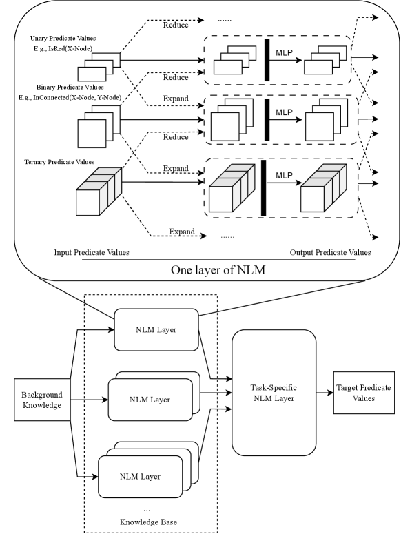We choose to construct the shared knowledge base $B_{S}\subset\bigcup_{i=1}^{n}H_{\mathrm{NLM}}^{i}(B)$ with the union of target predicates of increasing complexity $i\in\{1,\dots,n\}$ where $n$ is a hyperparameter to control the trade-off between the model complexity and target predicate expressiveness. In particular, by constructing the knowledge base with predicates of varying complexity, we achieve fine-grained predicate composition, reminiscent of the success of multi-scale representation-learning methods in the field of computer vision (Fan et al. 2021). Figure 1 illustrates this concept, where the knowledge base $B_{S}$ is constructed by incorporating NLM layers of varying depths. <details> <summary>x1.png Details</summary>  ### Visual Description ## Diagram: Neural Logic Machine (NLM) Architecture ### Overview The image is a technical diagram illustrating the architecture of a Neural Logic Machine (NLM). It is divided into two main sections: a detailed view of a single NLM layer at the top, and a broader system view showing how multiple NLM layers are composed at the bottom. The diagram explains how logical predicates of different arities (unary, binary, ternary) are processed through a neural network structure involving reduction, expansion, and Multi-Layer Perceptron (MLP) operations. ### Components/Axes The diagram is a flowchart with labeled boxes, arrows, and text annotations. There are no traditional chart axes. Key components and labels are: **Top Section: "One layer of NLM"** * **Input Side (Left):** Labeled "Input Predicate Values". Contains three distinct input blocks: 1. **Unary Predicate Values:** Example given: `E.g., IsRed(X-Node)`. Represented by a stack of 2D squares. 2. **Binary Predicate Values:** Example given: `E.g., IsConnected(X-Node, Y-Node)`. Represented by a stack of 3D cubes. 3. **Ternary Predicate Values:** Represented by a stack of larger 3D cubes. * **Processing Operations:** Arrows labeled with operations connect inputs to processing blocks: * `Reduce` (dashed arrows from Unary and Binary inputs). * `Expand` (dashed arrows from Binary and Ternary inputs). * **Processing Blocks:** Three dashed-line boxes, each containing: * Input representation (squares/cubes). * A vertical black bar labeled `MLP` (Multi-Layer Perceptron). * Output representation (squares/cubes). * **Output Side (Right):** Labeled "Output Predicate Values". Arrows point from the processing blocks to this side. **Bottom Section: System Architecture** * **Input (Far Left):** A box labeled `Background Knowledge`. * **Core Processing (Center-Left):** A large dashed box labeled `Knowledge Base`. Inside are multiple stacked boxes labeled `NLM Layer`. Arrows show `Background Knowledge` feeding into each `NLM Layer`. * **Task Processing (Center-Right):** A large rounded rectangle labeled `Task-Specific NLM Layer`. Arrows from all `NLM Layer` boxes in the Knowledge Base feed into this layer. * **Output (Far Right):** A box labeled `Target Predicate Values`. An arrow points from the `Task-Specific NLM Layer` to this box. ### Detailed Analysis The diagram details a hierarchical, modular neural network designed for logical reasoning. **1. Single NLM Layer (Top Section):** * **Data Flow:** The process is parallel for different predicate arities. * **Unary Path:** Unary predicate values (e.g., properties of a single node) undergo a `Reduce` operation, are processed by an MLP, and contribute to the output. * **Binary Path:** Binary predicate values (e.g., relationships between two nodes) can undergo both `Reduce` and `Expand` operations before MLP processing. * **Ternary Path:** Ternary predicate values (e.g., relationships among three nodes) undergo an `Expand` operation before MLP processing. * **Key Insight:** The `Reduce` and `Expand` operations likely transform the dimensionality or scope of the predicate tensors to prepare them for the MLP, which performs the core learned transformation. The output is a new set of "Output Predicate Values." **2. Composed System (Bottom Section):** * **Knowledge Base:** This is a stack of multiple `NLM Layer` modules. The diagram shows three explicitly, with ellipsis (`...`) indicating more. This suggests a deep architecture where logical reasoning is performed in successive stages. * **Information Flow:** `Background Knowledge` (the initial set of facts or predicates) is fed as input to every layer in the Knowledge Base in parallel. The outputs of all these layers are then aggregated. * **Task Specialization:** The aggregated output from the Knowledge Base is fed into a final, dedicated `Task-Specific NLM Layer`. This layer's role is to transform the general knowledge representations into the specific `Target Predicate Values` required for a given task. ### Key Observations * **Arity-Specific Processing:** The architecture explicitly handles logical predicates of different numbers of arguments (unary, binary, ternary) with tailored operations (`Reduce`/`Expand`). * **Modularity and Depth:** The system is built from reusable `NLM Layer` blocks, allowing for scalable depth in the Knowledge Base. * **Two-Stage Reasoning:** The design separates general knowledge processing (the stacked NLM Layers) from task-specific inference (the final Task-Specific NLM Layer). * **Visual Encoding:** The diagram uses dimensionality of shapes (2D squares for unary, 3D cubes for binary/ternary) to visually represent the arity of the predicates. ### Interpretation This diagram illustrates a neuro-symbolic architecture that bridges connectionist neural networks with symbolic logic. The NLM is designed to learn and reason over structured, relational data represented as logical predicates. * **What it demonstrates:** The core innovation is the structured processing within a single layer. Instead of a monolithic neural network, it uses arity-specific pathways with dimensionality manipulation (`Reduce`/`Expand`) followed by an MLP. This likely allows the model to learn rules and inferences that respect the logical structure of the data (e.g., properties of objects vs. relationships between objects). * **Relationship between elements:** The bottom diagram shows how complex reasoning is achieved by composing simple, uniform NLM layers. The Knowledge Base acts as a general-purpose reasoning engine, processing the background knowledge into increasingly abstract or refined representations. The Task-Specific layer then acts as a "conclusion drawer," mapping these rich representations to the desired output for a particular problem (e.g., answering a query, classifying a scene). * **Notable design choice:** The parallel input of `Background Knowledge` to all Knowledge Base layers is significant. It suggests that each layer can access the original facts, potentially allowing for different layers to specialize in different types of inferences or levels of abstraction without losing access to the base data. This is a form of residual or dense connection pattern tailored for logical reasoning tasks. **Language Note:** All text in the diagram is in English. </details> Figure 1: An illustration of Compositional Logic Model. Compositional Logic Model takes object properties and relations as input and outputs relations of the objects. #### Task Specific Module. With the shared knowledge base $B_{S}$ , the task specific module $\widetilde{\mathcal{F}}_{i}$ for $i\in\{1,...,t\}$ is also a NLM layer to take as input all predicates from the knowledge base $B_{S}$ and compose the target predicates for each corresponding task $\mathcal{P}_{i}^{\star}$ . Figure 1 illustrates this concept, showing how a NLM layer utilizes predicates from the knowledge base to compose the target predicates for each task. #### Training Protocol. We facilitate the transfer of the knowledge base across tasks while ensuring that task-specific modules remain distinct and independent from one another. This means that the knowledge base is reused from task to task, while task-specific modules are initialized randomly and trained from scratch. ## 5 Experiments We note that the transfer of logic rules is beneficial to both supervised learning setting (i.e., ILP) and reinforcement learning setting (i.e., Relational RL). To this end, we present experimental results for both settings to comprehensively demonstrate the value of L2ILP. For supervised learning, we build on insights from the experiments conducted by (Dong et al. 2019), (Zimmer et al. 2023), (Glanois et al. 2021), and (Li et al. 2024), proposing task sequences for ILP across three domains: arithmetic, tree, and graph. For reinforcement learning, PDDLGym (Silver and Chitnis 2020) serves as an off-the-shelf tool in which the state and action spaces are represented using logical predicates. We therefore select BlocksWorld from PDDLGym as the testbed, as it is a commonly used benchmark for complex logic reasoning tasks (Džeroski, De Raedt, and Driessens 2001; Glanois et al. 2021; Valmeekam et al. 2023). We provide the code we used for experiments in the supplementary material. ### 5.1 Forward Transfer of Logic Rules #### ILP Experiments. 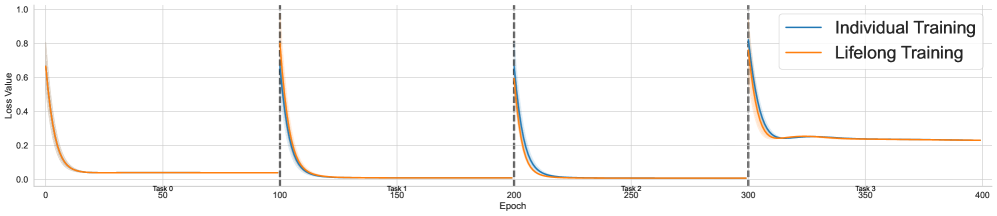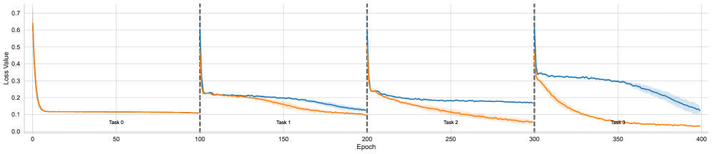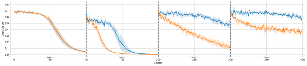The key question regarding the proposed approach is whether the transfer of logical rules is genuinely beneficial. We address this by comparing the learning curves of lifelong learning with those of models trained on tasks individually, while keeping model architectures the same. We provide a detailed description of the sequences of target predicates for each domain in the appendix, and present here the designs for two specific domains: Graph and Tree. In the Graph domain, $IsConnected(X\text{-}Node,Y\text{-}Node)$ and $IsRed(X\text{-}Node)$ , fully describe all possible graphs. The first predicate defines the connectivity between nodes, while the second specifies node properties—in this case, the color of the nodes. The four target predicates are learned sequentially in the following order: - $AdjacentToRed(X\text{-Node})$ , - $ExactConnectivity2(X\text{-Node},Y\text{-Node})$ , - $ExactConnectivity2Red(X\text{-Node})$ , - $ExactConnectivity2MultipleRed(X\text{-Node})$ . The first target predicate determines whether a given node has at least one neighboring node that is red. The second predicate identifies whether the shortest path between two nodes consists of exactly two edges. Building upon this, $ExactConnectivity2Red(X\text{-Node})$ refines the notion of connectivity by verifying whether a node at an exact distance of two from the query node is red. Finally, $ExactConnectivity2MultipleRed(X\text{-Node})$ extends this concept by determining whether there exist multiple such red nodes at the specified distance. We design the tasks in a way that ensures relevance and allows them to share common structures when learning logical rules. In the Tree domain, $IsParent(X\text{-}Node,Y\text{-}Node)$ is sufficient to specify the structure of any tree. We further define four target predicates to be learned sequentially, following the order below: - $IsRoot(X\text{-}Node)$ - $HasOddEdges(X\text{-}Node,Y\text{-}Node)$ - $HasEvenEdges(X\text{-}Node,Y\text{-}Node)$ - $IsAncestor(X\text{-}Node,Y\text{-}Node)$ The first predicate identifies the root node of the tree and serves as the foundational predicate. The second and the third predicates determine whether two nodes in the tree are connected by an odd or even number of edges, respectively. Finally, $IsAncestor(X\text{-}Node,Y\text{-}Node)$ checks whether one node is an ancestor of another, based on their relative depths in the tree. <details> <summary>x2.png Details</summary>  ### Visual Description ## Line Chart: Training Loss Comparison Across Sequential Tasks ### Overview The image displays a line chart comparing the training loss over 400 epochs for two different machine learning training paradigms: "Individual Training" and "Lifelong Training." The chart is segmented into four distinct phases or tasks (Task 0, Task 1, Task 2, Task 3), separated by vertical dashed lines. The primary purpose is to visualize and compare how the loss evolves for each method as the model encounters new tasks sequentially. ### Components/Axes * **Chart Type:** Line chart with two data series. * **X-Axis:** Labeled "Epoch." It runs from 0 to 400 with major tick marks every 50 epochs (0, 50, 100, 150, 200, 250, 300, 350, 400). * **Y-Axis:** Labeled "Loss Value." It runs from 0.0 to 1.0 with major tick marks every 0.2 units (0.0, 0.2, 0.4, 0.6, 0.8, 1.0). * **Legend:** Positioned in the top-right corner of the chart area. * **Blue Line:** "Individual Training" * **Orange Line:** "Lifelong Training" * **Task Segmentation:** Vertical, gray, dashed lines are placed at epochs 100, 200, and 300, dividing the chart into four equal segments. Text labels are placed at the bottom of each segment: * "Task 0" (Epochs 0-100) * "Task 1" (Epochs 100-200) * "Task 2" (Epochs 200-300) * "Task 3" (Epochs 300-400) ### Detailed Analysis The chart shows the loss trajectory for both training methods across four sequential tasks. The general pattern for each task segment is a sharp initial decrease in loss followed by a plateau. **Task 0 (Epochs 0-100):** * **Trend:** Both lines start at a high loss (approximately 0.65-0.70) and decrease rapidly, converging to a very low loss value near 0.0 by epoch 50. They remain nearly identical and flat for the remainder of the task. * **Data Points (Approximate):** * Start (Epoch 0): Loss ~0.68 (Individual), ~0.65 (Lifelong). * End (Epoch 100): Loss ~0.02 for both. **Task 1 (Epochs 100-200):** * **Trend:** At the start of Task 1 (epoch 100), both lines spike upward sharply to a loss of approximately 0.75-0.80. They then decrease rapidly again, converging to a near-zero loss by epoch 150 and remaining flat until epoch 200. The lines are virtually indistinguishable. * **Data Points (Approximate):** * Start (Epoch 100): Loss ~0.78 (Individual), ~0.75 (Lifelong). * End (Epoch 200): Loss ~0.01 for both. **Task 2 (Epochs 200-300):** * **Trend:** A similar pattern occurs. At epoch 200, both lines spike to a loss of approximately 0.70. They decrease rapidly, but a slight separation becomes visible. The "Individual Training" (blue) line appears to descend slightly faster and reaches a marginally lower plateau than the "Lifelong Training" (orange) line. * **Data Points (Approximate):** * Start (Epoch 200): Loss ~0.70 (Individual), ~0.68 (Lifelong). * End (Epoch 300): Loss ~0.01 (Individual), ~0.02 (Lifelong). **Task 3 (Epochs 300-400):** * **Trend:** This task shows the most significant divergence. At epoch 300, both lines spike to their highest point on the chart, approximately 0.85-0.90. They decrease, but the "Lifelong Training" (orange) line plateaus at a notably higher loss value than the "Individual Training" (blue) line. The blue line settles around 0.22, while the orange line settles around 0.25. Both lines show a very slight upward drift or instability in the final 50 epochs. * **Data Points (Approximate):** * Start (Epoch 300): Loss ~0.88 (Individual), ~0.85 (Lifelong). * End (Epoch 400): Loss ~0.22 (Individual), ~0.25 (Lifelong). ### Key Observations 1. **Catastrophic Forgetting/Interference:** The sharp loss spikes at the beginning of each new task (epochs 100, 200, 300) for both methods indicate that the model's performance on the previous task degrades immediately when training on a new task. This is a classic sign of catastrophic forgetting in sequential learning. 2. **Convergence Speed:** In Tasks 0, 1, and 2, both methods converge to a near-zero loss very quickly (within ~50 epochs of starting the task). 3. **Divergence in Later Tasks:** The performance of the two methods is nearly identical for the first three tasks. A clear performance gap emerges only in Task 3, where "Individual Training" achieves a lower final loss than "Lifelong Training." 4. **Final Task Difficulty:** Task 3 appears to be the most challenging, as evidenced by the highest initial loss spike and the highest final plateau loss for both methods. The slight upward drift in loss at the end of Task 3 suggests potential training instability or that the model has reached its capacity for this task. ### Interpretation This chart illustrates a core challenge in continual or lifelong learning: balancing the acquisition of new knowledge with the retention of old knowledge. * **What the data suggests:** The "Individual Training" method, which likely involves training a separate model or resetting the model for each task, consistently achieves the lowest possible loss for each task in isolation. The "Lifelong Training" method, which uses a single model to learn tasks sequentially, performs comparably for the initial tasks but shows a measurable degradation in performance (higher final loss) on the fourth task (Task 3). * **Relationship between elements:** The vertical dashed lines act as critical event markers, triggering the loss spikes that demonstrate the interference between tasks. The legend allows us to attribute the slightly worse final performance in Task 3 specifically to the lifelong learning approach. * **Notable anomaly/trend:** The key anomaly is the **divergence in Task 3**. This suggests that the lifelong model's capacity to mitigate forgetting or integrate new knowledge without interference may be reaching its limit by the fourth task. The accumulated knowledge from Tasks 0-2 might be interfering with the learning of Task 3, or the model's parameters may be becoming "saturated." * **Implication:** The data demonstrates that while lifelong learning can be effective for a small number of sequential tasks, its performance may degrade as the sequence grows longer. This highlights the need for specialized techniques (e.g., replay buffers, parameter isolation, meta-learning) in lifelong learning systems to maintain performance over extended task sequences. The "Individual Training" line serves as an idealized baseline, showing the best possible performance if forgetting were not an issue. </details> (a) Training dynamics for Arithmetic <details> <summary>x3.png Details</summary>  ### Visual Description ## Line Chart: Loss Value vs. Epoch Across Sequential Tasks ### Overview The image displays a line chart tracking the "Loss Value" of two distinct models or training runs (represented by a blue line and an orange line) over 400 training epochs. The training process is segmented into four sequential tasks (Task 0, Task 1, Task 2, Task 3), each spanning 100 epochs. The chart illustrates how the loss for each model evolves as it learns each new task in sequence, a setup typical for evaluating continual or incremental learning systems. ### Components/Axes * **Chart Type:** Multi-series line chart with a shaded confidence interval or variance band. * **X-Axis:** Labeled "Epoch". Linear scale from 0 to 400, with major tick marks every 50 epochs (0, 50, 100, 150, 200, 250, 300, 350, 400). * **Y-Axis:** Labeled "Loss Value". Linear scale from 0.0 to 0.7, with major tick marks every 0.1 units. * **Data Series:** 1. **Blue Line:** Represents one model's loss trajectory. It is accompanied by a light blue shaded area, indicating variance or standard deviation across multiple runs. 2. **Orange Line:** Represents a second model's loss trajectory. No shaded variance area is visible for this series. * **Task Segmentation:** Vertical dashed black lines at Epoch 100, 200, and 300 demarcate the boundaries between tasks. Text labels ("Task 0", "Task 1", "Task 2", "Task 3") are placed centrally within each 100-epoch segment, just above the x-axis. * **Legend:** No explicit legend box is present. The two series are distinguished solely by color (blue and orange). ### Detailed Analysis **Task 0 (Epochs 0-100):** * **Trend:** Both lines show a classic, rapid learning curve. * **Data Points:** Both models start at a high loss of approximately **0.65** at Epoch 0. They experience a steep, near-identical decline, converging to a low, stable loss of approximately **0.1** by Epoch ~20. They remain flat at this level for the remainder of the task. **Task 1 (Epochs 100-200):** * **Trend:** A sharp spike in loss occurs for both models at the task transition (Epoch 100), followed by a new learning phase where the models' performances begin to diverge. * **Data Points:** At Epoch 100, loss spikes to approximately **0.6** for both. Following the spike: * The **blue line** decreases gradually, ending the task at a loss of approximately **0.15**. * The **orange line** decreases more rapidly, ending the task at a lower loss of approximately **0.1**. **Task 2 (Epochs 200-300):** * **Trend:** Another sharp loss spike at the transition, followed by a more pronounced divergence between the models. * **Data Points:** At Epoch 200, loss spikes to approximately **0.55-0.6**. * The **blue line** shows a shallow decline, plateauing around a loss of **0.18-0.2** for most of the task. * The **orange line** continues a steady, strong decline, finishing the task at a loss of approximately **0.05**. **Task 3 (Epochs 300-400):** * **Trend:** A final spike at transition, with the performance gap between the models becoming very large. * **Data Points:** At Epoch 300, loss spikes to approximately **0.6**. * The **blue line** exhibits a very slow, linear decline from ~0.35 to ~0.15 over the 100 epochs. The shaded variance area is most prominent here. * The **orange line** drops precipitously, reaching a near-zero loss (approximately **0.02-0.03**) by Epoch ~350 and remaining there. ### Key Observations 1. **Task Transition Spike:** A consistent, sharp increase in loss occurs at the beginning of each new task (Epochs 100, 200, 300) for both models, indicating the challenge of adapting to new data. 2. **Diverging Performance:** While both models perform identically on the initial task (Task 0), the orange model consistently achieves lower final loss values on all subsequent tasks (1, 2, and 3). 3. **Learning Efficiency:** The orange model demonstrates faster and more effective learning on new tasks, as seen in its steeper post-spike decline. The blue model's learning rate appears to slow significantly in Tasks 2 and 3. 4. **Variance:** The blue model shows increasing variance (wider shaded area) in its loss during Task 3, suggesting less stable training outcomes compared to the orange model. ### Interpretation This chart likely compares a standard neural network (blue line) against a model designed for continual learning (orange line), such as one employing replay buffers, regularization, or modular architectures. * **What the data suggests:** The orange model is successfully mitigating "catastrophic forgetting." It not only learns each new task effectively but also appears to retain knowledge from previous tasks, allowing for better starting points and faster convergence. The blue model, in contrast, struggles more with each successive task, showing signs of interference or capacity saturation. * **How elements relate:** The vertical dashed lines are critical, marking the points where the training data distribution changes. The immediate spike shows the models' initial confusion. The subsequent slope of each line indicates the model's plasticity—its ability to adapt. The orange line's consistently steeper slope post-spike indicates superior plasticity. * **Notable anomalies:** The blue line's plateau during Task 2 is notable; it suggests the model reached a performance limit or a local minimum it could not escape, unlike the orange model. The pronounced variance in the blue line during Task 3 further indicates training instability in later stages of sequential learning. **Conclusion:** The visualization provides strong evidence that the model represented by the orange line is more robust and effective for sequential, multi-task learning scenarios than the model represented by the blue line. </details> (b) Training dynamics for Tree <details> <summary>x4.png Details</summary>  ### Visual Description ## Multi-Task Learning Loss Curve: Sequential Task Performance ### Overview The image is a line chart displaying the training loss (Loss Value) over 400 epochs for two different models or methods (represented by blue and orange lines). The training is divided into four sequential tasks (Task 0 through Task 3), with each task beginning at specific epoch intervals. The chart illustrates how the models learn new tasks and potentially retain knowledge from previous ones. ### Components/Axes * **X-Axis (Horizontal):** Labeled "Epoch". It ranges from 0 to 400, with major tick marks and labels at 0, 50, 100, 150, 200, 250, 300, 350, and 400. * **Y-Axis (Vertical):** Labeled "Loss Value". It ranges from 0.0 to 0.8, with major tick marks and labels at 0.0, 0.1, 0.2, 0.3, 0.4, 0.5, 0.6, 0.7, and 0.8. * **Task Segments:** The chart is divided into four vertical segments by dashed black lines at Epoch 100, 200, and 300. Each segment is labeled at the bottom: * **Task 0:** Epochs 0-100. * **Task 1:** Epochs 100-200. * **Task 2:** Epochs 200-300. * **Task 3:** Epochs 300-400. * **Data Series:** Two primary lines are plotted, each with a shaded region representing variance or confidence interval. * **Blue Line:** Represents one model/method. * **Orange Line:** Represents a second model/method. * **Legend:** No explicit legend is present within the chart area. The color association (Blue vs. Orange) is consistent throughout. ### Detailed Analysis **Task 0 (Epochs 0-100):** * **Trend:** Both lines start at a high loss (~0.7) and follow a nearly identical, steep downward curve, converging to a very low loss (~0.05) by epoch 100. * **Data Points (Approximate):** * Start (Epoch 0): Blue ≈ 0.70, Orange ≈ 0.70. * End (Epoch 100): Blue ≈ 0.05, Orange ≈ 0.05. **Task 1 (Epochs 100-200):** * **Trend:** At the start of Task 1 (Epoch 100), both lines experience a sharp, vertical jump in loss, indicating the introduction of a new task. The orange line then decreases rapidly, reaching near-zero loss by epoch ~175. The blue line decreases more slowly, reaching a similar low loss by epoch ~200. * **Data Points (Approximate):** * Start (Epoch 100): Blue ≈ 0.60, Orange ≈ 0.60. * Mid-point (Epoch 150): Blue ≈ 0.40, Orange ≈ 0.10. * End (Epoch 200): Blue ≈ 0.02, Orange ≈ 0.01. **Task 2 (Epochs 200-300):** * **Trend:** Another sharp loss jump occurs at epoch 200. The orange line shows a steady, consistent decline throughout the task. The blue line declines much more slowly and with more volatility, maintaining a significantly higher loss than the orange line for the entire segment. * **Data Points (Approximate):** * Start (Epoch 200): Blue ≈ 0.70, Orange ≈ 0.65. * Mid-point (Epoch 250): Blue ≈ 0.60, Orange ≈ 0.35. * End (Epoch 300): Blue ≈ 0.50, Orange ≈ 0.15. **Task 3 (Epochs 300-400):** * **Trend:** A final loss jump at epoch 300. The pattern from Task 2 continues and intensifies. The orange line descends steadily. The blue line remains high and relatively flat, showing minimal improvement and high variance. * **Data Points (Approximate):** * Start (Epoch 300): Blue ≈ 0.70, Orange ≈ 0.65. * Mid-point (Epoch 350): Blue ≈ 0.65, Orange ≈ 0.45. * End (Epoch 400): Blue ≈ 0.60, Orange ≈ 0.35. ### Key Observations 1. **Performance Divergence:** While both models perform identically on the first task (Task 0), a significant performance gap emerges from Task 1 onward, with the orange model consistently achieving lower loss values faster. 2. **Catastrophic Forgetting Indicator:** The blue model shows strong signs of catastrophic forgetting. Its loss resets to a high value at the start of each new task (2, 3) and fails to recover to the low loss levels it achieved on previous tasks. Its final loss in Task 3 (~0.60) is much higher than its final loss in Task 0 (~0.05). 3. **Stability:** The orange model demonstrates more stable and efficient learning across sequential tasks. Its loss curves are smoother, and it reaches lower final loss values in each subsequent task compared to the blue model. 4. **Variance:** The shaded confidence intervals are wider for the blue line, especially in Tasks 2 and 3, indicating less consistent training runs or higher sensitivity to initial conditions. ### Interpretation This chart is a classic visualization of **continual** or **sequential learning** in machine learning, where a model is trained on multiple tasks one after another. The data suggests the following: * **The orange method is superior for continual learning.** It effectively learns new tasks (evidenced by decreasing loss within each segment) while mitigating catastrophic forgetting (its performance on the overall sequence remains strong). This could be due to techniques like experience replay, elastic weight consolidation, or a more robust architecture. * **The blue method suffers from severe catastrophic forgetting.** As it learns each new task, it "forgets" the knowledge from previous tasks, causing its performance to degrade on the overall sequence. The high, flat loss in Task 3 suggests it has reached a point of minimal further learning capacity within this sequential framework. * **The initial task (Task 0) is likely the simplest or most foundational,** as both models master it completely. The increasing difficulty or dissimilarity of subsequent tasks exposes the limitations of the blue model's learning approach. * **Practical Implication:** For applications requiring a model to learn from a stream of data over time without retraining from scratch (e.g., robotics, personalized assistants, adaptive systems), the approach represented by the orange line is far more viable. The blue approach would require frequent full retraining on all data to maintain performance, which is often impractical. </details> (c) Training dynamics for Graph Figure 2: Epoch training dynamics for individual learning and lifelong learning <details> <summary>x5.png Details</summary>  ### Visual Description ## Line Chart: Evaluation Steps per Epoch for Individual vs. Lifelong Training ### Overview The image is a line chart comparing the performance of two training methods—"Individual Training" and "Lifelong Training"—across a sequence of five distinct tasks (Task 0 through Task 4). Performance is measured in "Evaluation Steps" over 1000 training epochs. The chart is segmented by vertical dashed lines, indicating the start of each new task. ### Components/Axes * **X-Axis (Horizontal):** Labeled **"Epoch"**. It ranges from 0 to 1000, with major numerical markers at 0, 200, 400, 600, 800, and 1000. * **Y-Axis (Vertical):** Labeled **"Evaluation Steps"**. It ranges from 0 to 350, with major numerical markers at 0, 50, 100, 150, 200, 250, 300, and 350. * **Legend:** Located in the top-right corner of the chart area. * **Blue Line:** "Individual Training" * **Orange Line:** "Lifelong Training" * **Task Segments:** The chart is divided into five sections by vertical dashed gray lines at epochs 200, 400, 600, and 800. Each section is labeled at the bottom: * **Task 0:** Epochs 0-200 * **Task 1:** Epochs 200-400 * **Task 2:** Epochs 400-600 * **Task 3:** Epochs 600-800 * **Task 4:** Epochs 800-1000 * **Data Series:** Each training method is represented by a solid line (blue or orange) surrounded by a semi-transparent shaded area of the same color, indicating variance or confidence intervals around the mean performance. ### Detailed Analysis **Trend Verification & Data Point Extraction (by Task Segment):** * **Task 0 (Epochs 0-200):** * **Trend:** Both lines are flat and near zero. * **Data:** Evaluation Steps for both Individual (blue) and Lifelong (orange) training remain at approximately **0** for the entire duration. * **Task 1 (Epochs 200-400):** * **Trend:** Both lines spike sharply at epoch 200, then decline. The blue line (Individual) drops more rapidly initially but stabilizes. The orange line (Lifelong) declines more gradually. * **Data:** * **Start (Epoch ~200):** Both spike to ~**300** steps. * **Mid-Task (Epoch ~300):** Blue line is at ~**50** steps. Orange line is at ~**100** steps. * **End (Epoch ~400):** Blue line stabilizes around **25-40** steps. Orange line stabilizes around **30-50** steps, slightly above the blue line. * **Task 2 (Epochs 400-600):** * **Trend:** Both spike at epoch 400. The blue line shows a steep, noisy decline. The orange line declines more slowly and smoothly, remaining above the blue line for most of the task. * **Data:** * **Start (Epoch ~400):** Both spike to ~**300** steps. * **Mid-Task (Epoch ~500):** Blue line fluctuates between **75-125** steps. Orange line is around **100-150** steps. * **End (Epoch ~600):** Blue line is around **50-75** steps. Orange line is around **50** steps. * **Task 3 (Epochs 600-800):** * **Trend:** This task shows the most significant divergence. The blue line starts high and fluctuates heavily before a late drop. The orange line starts high but declines steadily and early to a very low baseline. * **Data:** * **Start (Epoch ~600):** Both start around **200** steps. * **Blue Line (Individual):** Fluctuates heavily between **150-200** steps until approximately epoch 750, then drops sharply to ~**50** steps by epoch 800. * **Orange Line (Lifelong):** Begins a steady decline immediately, reaching ~**25** steps by epoch 700 and maintaining that low level (~**10-25** steps) until epoch 800. * **Task 4 (Epochs 800-1000):** * **Trend:** Both spike at epoch 800. The blue line declines gradually with high variance. The orange line declines more steeply. * **Data:** * **Start (Epoch ~800):** Both spike to ~**300** steps. * **Mid-Task (Epoch ~900):** Blue line is around **150-200** steps. Orange line is around **75-100** steps. * **End (Epoch ~1000):** Blue line ends around **100** steps. Orange line ends around **50** steps. ### Key Observations 1. **Task Initiation Spike:** Each new task (at epochs 200, 400, 600, 800) is marked by a sharp increase in evaluation steps for both methods, resetting performance. 2. **Performance Divergence in Task 3:** The most notable pattern occurs in Task 3, where Lifelong Training (orange) achieves and maintains a very low evaluation step count (~10-25) for the second half of the task, while Individual Training (blue) remains highly variable and elevated until the very end. 3. **Variance:** The shaded confidence intervals are generally wider for the Individual Training (blue) series, especially during the middle of tasks (e.g., Task 3), indicating less consistent performance compared to Lifelong Training. 4. **Final Task Performance:** By the end of the final observed task (Task 4), Lifelong Training concludes at a lower evaluation step count (~50) than Individual Training (~100). ### Interpretation The data suggests that the **Lifelong Training** approach is more efficient and stable when learning a sequence of tasks. While both methods experience a "reset" in performance at the start of each new task, the Lifelong model consistently demonstrates a faster or more sustained reduction in the number of evaluation steps required, particularly evident in Task 3. This implies better knowledge retention or more efficient adaptation from previous tasks. The **Individual Training** method shows higher variance and, in later tasks (3 and 4), requires more evaluation steps to reach a comparable performance level, if it reaches it at all. This pattern is consistent with the challenges of catastrophic forgetting in neural networks, where training on a new task degrades performance on previous ones. The Lifelong Training method appears to mitigate this issue, leading to more stable and efficient learning across a task continuum. The chart provides visual evidence for the potential advantage of continual learning algorithms over training models in isolation for each task. 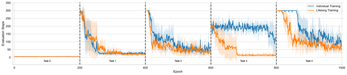</details> Figure 3: Evaluation steps for BlocksWorld tasks Figure 2 illustrates the training dynamics for each task across all domains. For each task, we conducted experiments with four different seeds and plotted the mean, along with the standard deviation for each data point. From top to bottom, the domains are ordered as arithmetic, tree, and graph, while from left to right, the plots are arranged sequentially for tasks 0 to 3. The tasks in the arithmetic domain are relatively simple, allowing both individual and lifelong learning to converge to optimal performance within a short period. However, we observe that the loss curves in lifelong learning decrease more rapidly, as indicated by a small but noticeable gap. In contrast, for the tree and graph domains, the gaps become more pronounced, with no overlap observed between the paired curves. Notably, for the curves corresponding to the first task across all domains, lifelong learning completely overlaps with individual learning. This is expected, as the first task in lifelong learning does not incorporate any previously acquired knowledge, making it equivalent to its individual learning counterpart. This result shows that by leveraging the knowledge base acquired in earlier tasks, we could achieve higher learning efficiency on subsequence tasks, demonstrating the forward transfer effect that is essential in lifelong learning setting. #### Relational RL Experiments. For the BlocksWorld task from PDDLGym, Table 1 summarizes the predicates used to describe the state and action spaces. Since the number of ground predicates depends on the number of objects in a task, the total number of possible actions can be as high as $2x^{2}+2x$ , where $x$ represents the number of blocks. However, not all of these actions are valid in every state. Additionally, the number of possible states grows factorially with the number of blocks in the environment, making the task increasingly complex as more blocks are added. We note that previous works (Jiang and Luo 2019; Zimmer et al. 2023; Valmeekam et al. 2023) typically use 5 blocks, whereas we extend our experiments to 6 blocks. Furthermore, We set the tasks to follow a sparse reward scheme, where a penalty of -0.1 is given for every step taken, while a reward of 100 is granted upon achieving the desired block configuration. To define the sequence of tasks for BlocksWorld, we assign different desired configurations to each task, progressively increasing the difficulty by making the target configurations more challenging to reach. Refer to Appendix for a detailed discussion. | Predicates | Arity | Description | | --- | --- | --- | | $On(X\text{-}Block,Y\text{-}Block)$ | 2 | Block $X$ is on Block $Y$ | | $OnTable(X\text{-}Block)$ | 1 | Block $X$ is on the table | | $Clear(X\text{-}Block)$ | 1 | Block $X$ could be picked up | | $HandEmpty()$ | 0 | Hand is empty | | $HandFull()$ | 0 | Hand is full | | $Holding(X\text{-}Block)$ | 1 | Hand is holding Block $X$ | | Action Space | | | | Predicates | Arity | Description | | $PickUp(X\text{-}Block)$ | 1 | Pick up Block $X$ from the table | | $PutDown(X\text{-}Block)$ | 1 | Put down Block $X$ onto the table | | $Stack(X\text{-}Block,Y\text{-}Block)$ | 2 | Stack Block $X$ onto Block $Y$ | | $Unstack(X\text{-}Block,Y\text{-}Block)$ | 2 | Unstack Block $X$ from Block $Y$ | Table 1: State and action spaces for BlocksWorld from PDDLGym Large state and action spaces pose significant challenges for exploration to RL agents, particularly when rewards are sparse and only provided upon goal completion. As a result, our experiments show that training tasks individually fails to yield sufficient exploration to positive rewards, let alone facilitate the learning of any meaningful policies. To address this issue, we adopt an offline reinforcement learning approach, where a replay buffer is collected in advance to ensure that both lifelong learning and individual training have access to data of the same quality. In BlocksWorld tasks, we use a planner to generate optimal actions at each step while incorporating random exploration to ensure adequate coverage of the state and action spaces. Specifically, we set the exploration rate to 0.8 and collect 50,000 transitions for each task. Figure 3 illustrates the evaluation steps for each task, as the number of steps directly reflects the quality of the learned policy. We ran each experiment using four different seeds and evaluated the policy periodically. For tasks 0–2, lifelong training does not show superior performance compared to individual training, as these tasks are relatively simple. However, for the more challenging tasks 3 and 4, clear gaps emerge: lifelong training converges much faster, while individual training occasionally fails to converge to the optimal policy. This result highlights that forward transfer is not only observed in the relatively straightforward supervised learning setting but also extends to the more complex reinforcement learning paradigm, where effective knowledge transfer accelerates policy learning in later tasks. ### 5.2 Forgetting of Logic Rules #### Forgetting Experiments. 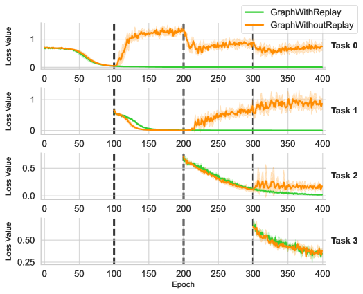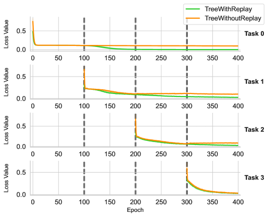Another fundamental challenge in lifelong learning is assessing the extent to which a model forgets previously acquired knowledge (i.e. catastrophic forgetting) and identifying effective strategies to mitigate this issue. In our case, the knowledge base is continuously updated, which may cause task-specific modules for earlier tasks to fail, as they rely on outdated knowledge representations. To investigate this phenomenon, we track the loss values throughout the entire training process and visualize the corresponding curves for each task. Specifically, in the supervised learning setting, we adhere to the training protocol described in the previous section while recording the tested loss values for each task at every epoch whenever feasible. Figure 4 and Figure 5 illustrate the results for the graph and tree domains, respectively, with each plot representing tasks 0 through 3. For results on arithemetic, please refer to appendix for a detailed description. <details> <summary>x6.png Details</summary>  ### Visual Description \n ## Line Chart: Loss Value Comparison Across Tasks ### Overview The image displays a series of four line charts arranged vertically, comparing the training loss of two different methods ("GraphWithReplay" and "GraphWithoutReplay") across four sequential tasks (Task 0, Task 1, Task 2, Task 3). The charts track the "Loss Value" over "Epochs" from 0 to 400. Vertical dashed lines at epochs 100, 200, and 300 likely indicate the boundaries or start points for new tasks. ### Components/Axes * **Chart Type:** Multi-panel line chart with shaded confidence intervals or variance bands. * **Legend:** Located in the top-right corner of the topmost chart (Task 0). * **Green Line:** Labeled "GraphWithReplay". * **Orange Line:** Labeled "GraphWithoutReplay". * **X-Axis (Common to all panels):** Labeled "Epoch". Major tick marks are at 0, 50, 100, 150, 200, 250, 300, 350, 400. * **Y-Axis (Per panel):** Labeled "Loss Value". The scale varies by task: * **Task 0:** 0 to 1 (ticks at 0, 0.5, 1). * **Task 1:** 0 to 1 (ticks at 0, 0.5, 1). * **Task 2:** 0.0 to 0.5 (ticks at 0.0, 0.25, 0.5). * **Task 3:** 0.25 to 0.50 (ticks at 0.25, 0.50). * **Panel Labels:** Each subplot is labeled on the right side: "Task 0", "Task 1", "Task 2", "Task 3". * **Vertical Reference Lines:** Dashed grey lines at Epochs 100, 200, and 300, spanning all four panels. ### Detailed Analysis **Task 0 (Top Panel):** * **GraphWithReplay (Green):** Starts at ~0.7, decreases smoothly to near 0 by epoch 100, and remains flat at ~0 for the remainder. * **GraphWithoutReplay (Orange):** Starts at ~0.7, decreases to near 0 by epoch 100. After epoch 100, it spikes dramatically to a peak of ~1.2 around epoch 150, then gradually decreases but remains noisy and elevated, ending at ~0.7 by epoch 400. * **Trend Verification:** Green shows stable convergence. Orange shows catastrophic forgetting or instability after the first task boundary (epoch 100). **Task 1 (Second Panel):** * **GraphWithReplay (Green):** Data begins at epoch 100. Starts at ~0.7, decreases smoothly to near 0 by epoch 200, and remains flat. * **GraphWithoutReplay (Orange):** Data begins at epoch 100. Starts at ~0.7, decreases to near 0 by epoch 200. After epoch 200, it begins to rise steadily and noisily, reaching ~0.9 by epoch 400. * **Trend Verification:** Green again shows stable convergence on the new task. Orange shows initial learning followed by significant performance degradation after the next task starts (epoch 200). **Task 2 (Third Panel):** * **GraphWithReplay (Green):** Data begins at epoch 200. Starts at ~0.6, decreases steadily to ~0.05 by epoch 400. * **GraphWithoutReplay (Orange):** Data begins at epoch 200. Starts at ~0.6, decreases to ~0.1 by epoch 400, but exhibits much higher variance (wider shaded band) compared to the green line, especially after epoch 300. * **Trend Verification:** Both methods show a decreasing trend on this task. Green is smoother and reaches a lower final loss. Orange is noisier. **Task 3 (Bottom Panel):** * **GraphWithReplay (Green):** Data begins at epoch 300. Starts at ~0.55, decreases to ~0.35 by epoch 400. * **GraphWithoutReplay (Orange):** Data begins at epoch 300. Starts at ~0.55, decreases to ~0.35 by epoch 400, again with noticeably higher variance than the green line. * **Trend Verification:** Both methods show a similar decreasing trend and final value, but the replay method (green) is more stable. ### Key Observations 1. **Catastrophic Forgetting:** The "GraphWithoutReplay" method (orange) shows severe performance degradation on earlier tasks (Task 0, Task 1) after new tasks are introduced (at epochs 100 and 200). Its loss increases significantly. 2. **Stability from Replay:** The "GraphWithReplay" method (green) maintains low, stable loss on previous tasks after new ones are introduced. It successfully mitigates catastrophic forgetting. 3. **Variance:** The orange line consistently shows higher variance (wider shaded area) than the green line, indicating less stable training. 4. **Task Difficulty:** The initial loss values and convergence slopes differ across tasks, suggesting varying difficulty. Task 2 and 3 start at lower loss values than Task 0 and 1. ### Interpretation This visualization demonstrates the effectiveness of a "replay" mechanism in a continual or sequential learning setting. The core problem illustrated is **catastrophic forgetting**, where a neural network ("GraphWithoutReplay") forgets previously learned tasks upon learning new ones. * **What the data suggests:** The "GraphWithReplay" method successfully retains knowledge from Task 0 and Task 1 while learning Tasks 2 and 3, as evidenced by its flat, low loss lines after task boundaries. In contrast, the baseline method's performance on old tasks deteriorates sharply as soon as a new task begins. * **How elements relate:** The vertical dashed lines are critical, acting as event markers. The divergence between the green and orange lines immediately after these markers (especially at epochs 100 and 200) is the primary evidence for the replay method's benefit. The y-axis scale change for Tasks 2 and 3 indicates these tasks may be inherently easier or have a different loss landscape. * **Notable anomalies:** The dramatic spike in Task 0 loss for the orange line after epoch 100 is a stark anomaly, showing not just forgetting but active interference. The increasing noise in the orange line for Task 2 after epoch 300 suggests instability propagates even to the current task. * **Underlying message:** The charts argue that without a mechanism to preserve old knowledge (like replay), sequential learning is unstable and leads to forgetting. The replay method provides stability, lower variance, and prevents performance collapse on prior tasks. </details> Figure 4: Training dynamics of Graph for each task In particular, the orange curves illustrate the loss values as described above. As expected, the loss values for earlier tasks increase as training progresses on later tasks, indicating the occurrence of catastrophic forgetting in the model. #### Replay Experiments. A straightforward approach to addressing catastrophic forgetting is to replay experience from earlier tasks while training on later ones. We adopt this strategy by replaying data from all previously learned tasks when training on a new task. This approach is particularly beneficial in our case, as we aim to build a shared knowledge base that can be effectively leveraged across multiple tasks. To ensure a fair comparison, we align the curves by recording each data point in terms of the training epoch of the current task. This alignment allows us to directly compare the performance of models trained with and without experience replay, providing deeper insights into its effectiveness in mitigating forgetting and preserving previously acquired knowledge. <details> <summary>x7.png Details</summary>  ### Visual Description ## Multi-Panel Line Chart: Loss Value vs. Epoch for Two Methods Across Four Tasks ### Overview The image displays a set of four vertically stacked line charts, each comparing the training loss over time for two different methods: "TreeWithReplay" and "TreeWithoutReplay". The charts track performance across four sequential tasks (Task 0, Task 1, Task 2, Task 3), suggesting a continual or sequential learning scenario. The primary visual pattern is a sharp initial drop in loss, followed by a plateau, with new spikes occurring at specific epoch intervals (100, 200, 300) that correspond to the introduction of new tasks. ### Components/Axes * **Chart Type:** Multi-panel (faceted) line chart. * **Panels:** Four subplots arranged vertically, labeled on the right side as "Task 0", "Task 1", "Task 2", and "Task 3" from top to bottom. * **X-Axis (Common):** Labeled "Epoch" at the bottom of the figure. The scale runs from 0 to 400 with major tick marks at 0, 50, 100, 150, 200, 250, 300, 350, and 400. * **Y-Axis (Per Panel):** Each subplot has its own y-axis labeled "Loss Value". * Task 0: Scale from 0.0 to approximately 0.8 (ticks at 0.0, 0.5). * Task 1: Scale from 0.0 to approximately 0.8 (ticks at 0.0, 0.5). * Task 2: Scale from 0.0 to approximately 0.8 (ticks at 0.0, 0.5). * Task 3: Scale from 0.0 to approximately 0.8 (ticks at 0.0, 0.5). * **Legend:** Positioned in the top-right corner of the entire figure, above the Task 0 plot. * **Green Line:** Labeled "TreeWithReplay". * **Orange Line:** Labeled "TreeWithoutReplay". * **Vertical Reference Lines:** Dashed gray vertical lines are present in all subplots at Epoch = 100, 200, and 300. These likely mark the boundaries where new tasks are introduced. ### Detailed Analysis **Task 0 (Top Panel):** * **Trend:** Both lines start at a high loss value (≈0.7-0.8) at Epoch 0 and drop sharply within the first 10-20 epochs to a low value near 0.1. They then plateau. After the vertical line at Epoch 100, the "TreeWithReplay" (green) line shows a very slight, gradual decrease, while the "TreeWithoutReplay" (orange) line remains flat. * **Key Points (Approximate):** * Epoch 0: Loss ≈ 0.75 (both). * Epoch 20: Loss ≈ 0.1 (both). * Epoch 100: Loss ≈ 0.08 (green), ≈ 0.10 (orange). * Epoch 400: Loss ≈ 0.05 (green), ≈ 0.10 (orange). **Task 1 (Second Panel):** * **Trend:** The plot begins at Epoch 100. Both lines start with a sharp spike to a loss of ≈0.7, then rapidly decrease. The "TreeWithReplay" (green) line consistently maintains a lower loss than the "TreeWithoutReplay" (orange) line after the initial drop. Both lines show a gradual, slight decline from Epoch 150 to 400. * **Key Points (Approximate):** * Epoch 100 (start): Spike to Loss ≈ 0.7 (both). * Epoch 120: Loss ≈ 0.2 (green), ≈ 0.25 (orange). * Epoch 200: Loss ≈ 0.1 (green), ≈ 0.15 (orange). * Epoch 400: Loss ≈ 0.08 (green), ≈ 0.12 (orange). **Task 2 (Third Panel):** * **Trend:** The plot begins at Epoch 200. A sharp spike occurs for both methods, reaching a loss of ≈0.6-0.7. Following the spike, both lines decrease rapidly. The "TreeWithReplay" (green) line again achieves and maintains a lower loss value compared to the "TreeWithoutReplay" (orange) line. * **Key Points (Approximate):** * Epoch 200 (start): Spike to Loss ≈ 0.65 (green), ≈ 0.70 (orange). * Epoch 220: Loss ≈ 0.15 (green), ≈ 0.20 (orange). * Epoch 300: Loss ≈ 0.08 (green), ≈ 0.12 (orange). * Epoch 400: Loss ≈ 0.06 (green), ≈ 0.10 (orange). **Task 3 (Bottom Panel):** * **Trend:** The plot begins at Epoch 300 with a sharp spike for both methods to a loss of ≈0.5-0.6. Both lines then decrease rapidly and converge to a very similar, low loss value by Epoch 400. The performance gap between the two methods is smallest in this final task. * **Key Points (Approximate):** * Epoch 300 (start): Spike to Loss ≈ 0.55 (green), ≈ 0.60 (orange). * Epoch 320: Loss ≈ 0.15 (both). * Epoch 400: Loss ≈ 0.05 (both). ### Key Observations 1. **Task Introduction Spikes:** A clear, sharp increase in loss occurs at the beginning of each new task (Epochs 100, 200, 300), indicating the model's initial poor performance on unfamiliar data. 2. **Consistent Performance Gap:** In Tasks 0, 1, and 2, the "TreeWithReplay" (green) method consistently achieves a lower loss value than the "TreeWithoutReplay" (orange) method after the initial learning phase. This gap is most pronounced in Task 1. 3. **Convergence in Final Task:** In Task 3, the performance of both methods becomes nearly identical by the end of training (Epoch 400). 4. **Learning Dynamics:** All tasks show a pattern of rapid initial learning (steep negative slope) followed by a long tail of gradual refinement (shallow negative slope). ### Interpretation This chart demonstrates the comparative effectiveness of a "replay" mechanism in a continual learning setting. The "TreeWithReplay" method appears to mitigate **catastrophic forgetting** more effectively than the method without replay. * **What the data suggests:** The replay mechanism helps the model retain knowledge from previous tasks when learning new ones. This is evidenced by the green line ("With Replay") maintaining a lower loss on earlier tasks (e.g., Task 0's line continues to improve slightly after Epoch 100) and recovering faster with a lower loss on subsequent tasks (Tasks 1 & 2). * **How elements relate:** The vertical dashed lines are critical anchors, showing that the spikes in loss are not random but systematically tied to the introduction of new tasks. The legend is essential for attributing the performance difference to the specific methodological variable (replay vs. no replay). * **Notable trends/anomalies:** The most significant trend is the consistent advantage of the replay method until the final task. The convergence in Task 3 is an interesting anomaly. It could suggest that by the fourth task, the model's capacity or the task's difficulty leads to similar final performance regardless of replay, or that the benefits of replay are most critical in the intermediate stages of sequential learning. The data strongly implies that the "TreeWithReplay" architecture is more robust for multi-task or continual learning scenarios. </details> Figure 5: Training dynamics of Tree for each task The green curves in Figure 4 and Figure 5 illustrate the loss values when experience replay is applied. As the results indicate, during the training phase for each individual task, replaying experience does not significantly interfere with the learning of the current task. The loss curves for training without replay closely align with those for training with replay, indicating that incorporating past experiences does not disrupt the optimization of the current task. More importantly, experience replay effectively mitigates catastrophic forgetting, as evidenced by the green curves maintaining low loss values throughout the entire training process. This suggests that the model successfully constructs retains previously acquired knowledge, leading to the formation of a robust and reusable knowledge base across all tasks. Surprisingly, we also observe a backward transfer effect in our experiments. The first plot in Figure 5 corresponds to the loss curve for task 0 in the tree domain. Notably, the loss curve plateaus before training on task 1. However, once training on task 1 begins, the loss for task 0 further decreases to zero, indicating that learning task 1 enhances the model’s performance on task 0. This suggests the potential of L2ILP that training on the current task may further improves the performance on previous tasks, as a better knowledge base is acquired during the sequential training. ## 6 Conclusion Neuro-Symbolic Artificial Intelligence introduces a new research paradigm by integrating neural networks with symbolic methods, which were traditionally studied as separate approaches. This integration opens new research opportunities by enabling the formulation of novel problems and providing solutions to challenges that were previously difficult to address using either approach alone. In this work, we take a step toward studying the lifelong learning problem in this domain and demonstrate that by leveraging the compositionality and transferability of logic rules, it becomes straightforward to construct models that achieve higher learning efficiency on later tasks while preserving performance on earlier ones. However, this problem remains far from solved. As discussed, a key challenge is how to efficiently construct logic rules that are meaningful for tasks within a given domain and how to systematically generate new rules from an evolving knowledge base. Our work represents a small step in this direction, demonstrating its feasibility but leaving many open opportunities for future research. We hope this study inspires further research into more effective methods for representing and constructing logic rules—particularly those that support the dynamic addition and removal of rules from a knowledge base—ultimately enabling more efficient and scalable neuro-symbolic lifelong learning systems. ## References - Amizadeh et al. (2020) Amizadeh, S.; Palangi, H.; Polozov, A.; Huang, Y.; and Koishida, K. 2020. Neuro-symbolic visual reasoning: Disentangling. In International Conference on Machine Learning, 279–290. Pmlr. - Badreddine et al. (2022) Badreddine, S.; d’Avila Garcez, A.; Serafini, L.; and Spranger, M. 2022. Logic Tensor Networks. Artificial Intelligence, 303: 103649. - Besold and Kühnberger (2023) Besold, T. R.; and Kühnberger, K.-U. 2023. Symbolic and Hybrid Models of Cognition, 139–172. Cambridge Handbooks in Psychology. Cambridge University Press. - Buzzega et al. (2020) Buzzega, P.; Boschini, M.; Porrello, A.; Abati, D.; and Calderara, S. 2020. Dark experience for general continual learning: a strong, simple baseline. In Advances in Neural Information Processing Systems, volume 33, 15920–15930. - Campero et al. (2018) Campero, A.; Pareja, A.; Klinger, T.; Tenenbaum, J.; and Riedel, S. 2018. Logical rule induction and theory learning using neural theorem proving. arXiv preprint arXiv:1809.02193. - Castro et al. (2025) Castro, P. S.; Tomasev, N.; Anand, A.; Sharma, N.; Mohanta, R.; Dev, A.; Perlin, K.; Jain, S.; Levin, K.; Éltető, N.; Dabney, W.; Novikov, A.; Turner, G. C.; Eckstein, M. K.; Daw, N. D.; Miller, K. J.; and Stachenfeld, K. L. 2025. Discovering Symbolic Cognitive Models from Human and Animal Behavior. bioRxiv. - Chaudhry et al. (2018) Chaudhry, A.; Ranzato, M.; Rohrbach, M.; and Elhoseiny, M. 2018. Efficient lifelong learning with a-gem. arXiv preprint arXiv:1812.00420. - Cropper and Dumančić (2022) Cropper, A.; and Dumančić, S. 2022. Inductive logic programming at 30: a new introduction. arXiv:2008.07912. - Dai et al. (2019) Dai, W.-Z.; Xu, Q.; Yu, Y.; and Zhou, Z.-H. 2019. Bridging machine learning and logical reasoning by abductive learning. Advances in Neural Information Processing Systems, 32. - d’Avila Garcez and Lamb (2020) d’Avila Garcez, A.; and Lamb, L. C. 2020. Neurosymbolic AI: The 3rd Wave. arXiv:2012.05876. - Dong et al. (2019) Dong, H.; Mao, J.; Lin, T.; Wang, C.; Li, L.; and Zhou, D. 2019. Neural Logic Machines. arXiv:1904.11694. - Džeroski, De Raedt, and Driessens (2001) Džeroski, S.; De Raedt, L.; and Driessens, K. 2001. Relational reinforcement learning. Machine learning, 43: 7–52. - Evans and Grefenstette (2018) Evans, R.; and Grefenstette, E. 2018. Learning Explanatory Rules from Noisy Data. arXiv:1711.04574. - Fan et al. (2021) Fan, H.; Xiong, B.; Mangalam, K.; Li, Y.; Yan, Z.; Malik, J.; and Feichtenhofer, C. 2021. Multiscale Vision Transformers. arXiv:2104.11227. - Farajtabar et al. (2020) Farajtabar, M.; Azizan, N.; Mott, A.; and Li, A. 2020. Orthogonal gradient descent for continual learning. In International conference on artificial intelligence and statistics, 3762–3773. PMLR. - Glanois et al. (2021) Glanois, C.; Feng, X.; Jiang, Z.; Weng, P.; Zimmer, M.; Li, D.; and Liu, W. 2021. Neuro-Symbolic Hierarchical Rule Induction. arXiv:2112.13418. - Jiang and Luo (2019) Jiang, Z.; and Luo, S. 2019. Neural Logic Reinforcement Learning. arXiv:1904.10729. - Kirkpatrick et al. (2017) Kirkpatrick, J.; Pascanu, R.; Rabinowitz, N.; Veness, J.; Desjardins, G.; Rusu, A. A.; Milan, K.; Quan, J.; Ramalho, T.; Grabska-Barwinska, A.; et al. 2017. Overcoming catastrophic forgetting in neural networks. Proceedings of the National Academy of Sciences, 114(13): 3521–3526. - Lake et al. (2016) Lake, B. M.; Ullman, T. D.; Tenenbaum, J. B.; and Gershman, S. J. 2016. Building Machines That Learn and Think Like People. arXiv:1604.00289. - Li et al. (2019) Li, X.; Zhou, Y.; Wu, T.; Socher, R.; and Xiong, C. 2019. Learn to grow: A continual structure learning framework for overcoming catastrophic forgetting. In International Conference on Machine Learning, 3925–3934. PMLR. - Li et al. (2024) Li, Z.; Cao, Y.; Xu, X.; Jiang, J.; Liu, X.; Teo, Y. S.; wei Lin, S.; and Liu, Y. 2024. LLMs for Relational Reasoning: How Far are We? arXiv:2401.09042. - Li and Hoiem (2017) Li, Z.; and Hoiem, D. 2017. Learning without forgetting. IEEE transactions on pattern analysis and machine intelligence, 40(12): 2935–2947. - Lin et al. (2014) Lin, D.; Dechter, E.; Ellis, K.; Tenenbaum, J.; and Muggleton, S. 2014. Bias reformulation for one-shot function induction. In ECAI 2014, 525–530. IOS Press. - Lopez-Paz and Ranzato (2017) Lopez-Paz, D.; and Ranzato, M. 2017. Gradient episodic memory for continual learning. Advances in neural information processing systems, 30. - Manhaeve et al. (2018) Manhaeve, R.; Dumančić, S.; Kimmig, A.; Demeester, T.; and Raedt, L. D. 2018. DeepProbLog: Neural Probabilistic Logic Programming. arXiv:1805.10872. - Marconato et al. (2023) Marconato, E.; Bontempo, G.; Ficarra, E.; Calderara, S.; Passerini, A.; and Teso, S. 2023. Neuro-symbolic continual learning: Knowledge, reasoning shortcuts and concept rehearsal. arXiv preprint arXiv:2302.01242. - Mendez (2022) Mendez, J. A. 2022. Lifelong Machine Learning of Functionally Compositional Structures. arXiv:2207.12256. - Payani and Fekri (2019) Payani, A.; and Fekri, F. 2019. Inductive Logic Programming via Differentiable Deep Neural Logic Networks. arXiv:1906.03523. - Rebuffi et al. (2017) Rebuffi, S.-A.; Kolesnikov, A.; Sperl, G.; and Lampert, C. H. 2017. icarl: Incremental classifier and representation learning. In Proceedings of the IEEE conference on Computer Vision and Pattern Recognition, 2001–2010. - Rolnick et al. (2019) Rolnick, D.; Ahuja, A.; Schwarz, J.; Lillicrap, T.; and Wayne, G. 2019. Experience replay for continual learning. In Advances in Neural Information Processing Systems, 350–360. - Rusu et al. (2016) Rusu, A. A.; Rabinowitz, N. C.; Desjardins, G.; Soyer, H.; Kirkpatrick, J.; Kavukcuoglu, K.; Pascanu, R.; and Hadsell, R. 2016. Progressive neural networks. In arXiv preprint arXiv:1606.04671. - Saha, Garg, and Roy (2021) Saha, G.; Garg, I.; and Roy, K. 2021. Gradient projection memory for continual learning. arXiv preprint arXiv:2103.09762. - Santoro et al. (2017) Santoro, A.; Raposo, D.; Barrett, D. G.; Malinowski, M.; Pascanu, R.; Battaglia, P.; and Lillicrap, T. 2017. A simple neural network module for relational reasoning. Advances in neural information processing systems, 30. - Sen et al. (2022) Sen, P.; de Carvalho, B. W.; Riegel, R.; and Gray, A. 2022. Neuro-symbolic inductive logic programming with logical neural networks. In Proceedings of the AAAI conference on artificial intelligence, volume 36, 8212–8219. - Sheth, Roy, and Gaur (2023) Sheth, A.; Roy, K.; and Gaur, M. 2023. Neurosymbolic AI – Why, What, and How. arXiv:2305.00813. - Shin et al. (2017) Shin, H.; Lee, J. K.; Kim, J.; and Kim, J. 2017. Continual learning with deep generative replay. Advances in neural information processing systems, 30. - Silver and Chitnis (2020) Silver, T.; and Chitnis, R. 2020. PDDLGym: Gym Environments from PDDL Problems. arXiv:2002.06432. - Valmeekam et al. (2023) Valmeekam, K.; Marquez, M.; Sreedharan, S.; and Kambhampati, S. 2023. On the Planning Abilities of Large Language Models : A Critical Investigation. arXiv:2305.15771. - von Oswald et al. (2020) von Oswald, J.; Henning, C.; Sacramento, J.; and Grewe, B. F. 2020. Continual learning with hypernetworks. In International Conference on Learning Representations. - Wang et al. (2025) Wang, C.; Ji, K.; Geng, J.; Ren, Z.; Fu, T.; Yang, F.; Guo, Y.; He, H.; Chen, X.; Zhan, Z.; Du, Q.; Su, S.; Li, B.; Qiu, Y.; Du, Y.; Li, Q.; Yang, Y.; Lin, X.; and Zhao, Z. 2025. Imperative Learning: A Self-supervised Neuro-Symbolic Learning Framework for Robot Autonomy. arXiv:2406.16087. - Wang et al. (2024) Wang, L.; Zhang, X.; Su, H.; and Zhu, J. 2024. A comprehensive survey of continual learning: Theory, method and application. IEEE Transactions on Pattern Analysis and Machine Intelligence. - Yoon et al. (2017) Yoon, J.; Yang, E.; Lee, J.; and Hwang, S. J. 2017. Lifelong learning with dynamically expandable networks. arXiv preprint arXiv:1708.01547. - Zeng et al. (2019) Zeng, G.; Chen, Y.; Cui, B.; and Yu, S. 2019. Continual learning of context-dependent processing in neural networks. Nature Machine Intelligence, 1(8): 364–372. - Zenke, Poole, and Ganguli (2017) Zenke, F.; Poole, B.; and Ganguli, S. 2017. Continual learning through synaptic intelligence. In International Conference on Machine Learning, 3987–3995. PMLR. - Zimmer et al. (2023) Zimmer, M.; Feng, X.; Glanois, C.; Jiang, Z.; Zhang, J.; Weng, P.; Li, D.; Hao, J.; and Liu, W. 2023. Differentiable Logic Machines. arXiv:2102.11529. ## Appendix A Design for the Supervised Learning Tasks ### A.1 Arithmetic Input Predicates: | | | $\displaystyle$ | | True if number $X$ is zero | | | --- | --- | --- | --- | --- | --- | Target Predicates: | | | 1. $Plus(X\text{-}Number,Y\text{-}Number,Z\text{-}Number)$ | | True if $X+Y=Z$ | | | --- | --- | --- | --- | --- | --- | ### A.2 Tree Input Predicates: | | | $\displaystyle$ | | True if $X$ is the parent of $Y$ | | | --- | --- | --- | --- | --- | --- | Target Predicates: | | | 1. $IsRoot(X\text{-}Node)$ | | True if $X$ is the root node | | | --- | --- | --- | --- | --- | --- | ### A.3 Graph Input Predicates: | | | $\displaystyle$ | | True if there is an edge between $X$ and $Y$ | | | --- | --- | --- | --- | --- | --- | Target Predicates: | | | 1. $AdjacentToRed(X\text{-}Node)$ | | True if node $X$ is connected to a red node | | | --- | --- | --- | --- | --- | --- | ## Appendix B Design for the reinforcement learning tasks The sequence of tasks in reinforcement learning varies based on their target configurations. For each task, we define specific configurations without considering the order of the blocks and sample a target configuration at the beginning of each episode. For example, if a task’s target configuration requires three blocks to be on the table, two blocks to be stacked on others, and one block to be freely placed anywhere, we first generate possible configurations that meet this requirement and then sample a target configuration accordingly. This task design provides the flexibility to configure the target configuration space, allowing us to adjust the difficulty of the tasks as needed. Thus, we define the five tasks in the following order: - 5 blocks are on table, 1 block is free - 3 blocks on table, 2 blocks are stacked, 1 block is free - 2 blocks on table, 1 block is stacked, 1 block is free - 4 blocks on table, 1 block is stacked, 1 block is free - 1 block is on table, 4 blocks are stacked, 1 block is free The order of the tasks are determined by the performance of the model trained on those tasks individually. 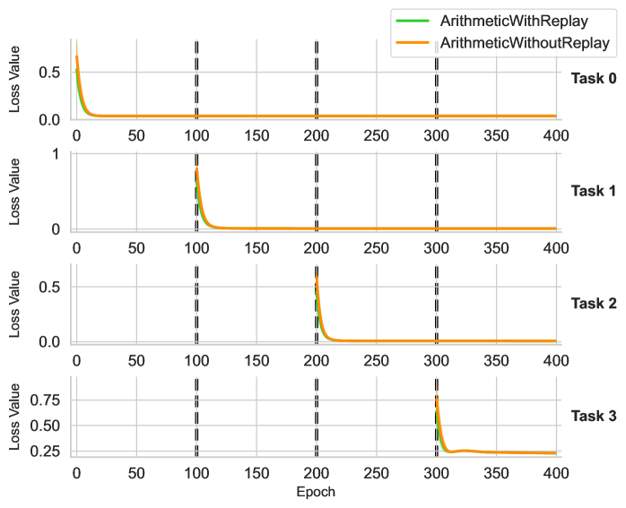## Appendix C curves for forgetting experiments on arithmetic <details> <summary>x8.png Details</summary>  ### Visual Description ## Multi-Panel Line Chart: Sequential Task Learning Loss Curves ### Overview The image displays a vertical arrangement of four line charts, each tracking the "Loss Value" over 400 training "Epochs" for a sequential learning experiment. The charts compare two methods: "ArithmeticWithReplay" (green line) and "ArithmeticWithoutReplay" (orange line). Each subplot corresponds to a distinct task (Task 0 through Task 3) introduced at different points in the training sequence. Vertical dashed lines mark epoch boundaries at 100, 200, and 300. ### Components/Axes * **Legend:** Located at the top-right of the overall figure. It contains two entries: * `ArithmeticWithReplay` - Represented by a solid green line. * `ArithmeticWithoutReplay` - Represented by a solid orange line. * **Subplot Structure:** Four subplots are stacked vertically. * **Y-axis (for all subplots):** Labeled "Loss Value". The scale varies per subplot: * Task 0: 0.0 to ~0.6 * Task 1: 0 to 1 * Task 2: 0.0 to ~0.6 * Task 3: 0.25 to ~0.85 * **X-axis (shared, labeled at the bottom):** Labeled "Epoch". Linear scale from 0 to 400, with major ticks at 0, 50, 100, 150, 200, 250, 300, 350, 400. * **Task Labels:** Positioned to the right of each subplot, aligned with the top of its y-axis. * Top subplot: `Task 0` * Second subplot: `Task 1` * Third subplot: `Task 2` * Bottom subplot: `Task 3` * **Vertical Dashed Lines:** Three black, dashed vertical lines cross all subplots at approximately `Epoch = 100`, `Epoch = 200`, and `Epoch = 300`. ### Detailed Analysis **Task 0 (Top Subplot):** * **Trend:** Both lines start at a high loss (~0.6) at epoch 0 and decay rapidly to near zero by epoch ~25. They remain flat at near-zero loss for the remainder of the 400 epochs. * **Data Points (Approximate):** * Start (Epoch 0): Loss ≈ 0.6 for both lines. * Convergence (Epoch ~25): Loss ≈ 0.0. * End (Epoch 400): Loss ≈ 0.0. **Task 1 (Second Subplot):** * **Trend:** Loss is near zero until epoch 100. At epoch 100, both lines spike sharply (green to ~0.7, orange to ~0.8) and then decay rapidly, converging to near zero by epoch ~125. They remain flat thereafter. * **Data Points (Approximate):** * Pre-spike (Epoch 99): Loss ≈ 0.0. * Spike (Epoch 100): Green ≈ 0.7, Orange ≈ 0.8. * Convergence (Epoch ~125): Loss ≈ 0.0. * End (Epoch 400): Loss ≈ 0.0. **Task 2 (Third Subplot):** * **Trend:** Loss is near zero until epoch 200. At epoch 200, both lines spike sharply (green to ~0.5, orange to ~0.6) and decay rapidly, converging to near zero by epoch ~225. They remain flat thereafter. * **Data Points (Approximate):** * Pre-spike (Epoch 199): Loss ≈ 0.0. * Spike (Epoch 200): Green ≈ 0.5, Orange ≈ 0.6. * Convergence (Epoch ~225): Loss ≈ 0.0. * End (Epoch 400): Loss ≈ 0.0. **Task 3 (Bottom Subplot):** * **Trend:** Loss is near zero until epoch 300. At epoch 300, both lines spike sharply (green to ~0.75, orange to ~0.85). They decay but **do not return to zero**. Instead, they plateau at a significantly higher loss level (~0.25) from approximately epoch 325 onward. * **Data Points (Approximate):** * Pre-spike (Epoch 299): Loss ≈ 0.0. * Spike (Epoch 300): Green ≈ 0.75, Orange ≈ 0.85. * Plateau (Epoch 325-400): Both lines stabilize at Loss ≈ 0.25. ### Key Observations 1. **Task Introduction Points:** The vertical dashed lines at epochs 100, 200, and 300 perfectly coincide with the sudden loss spikes in Tasks 1, 2, and 3, respectively. This strongly indicates these are the points where new tasks are introduced to the model. 2. **Catastrophic Forgetting Pattern:** For Tasks 0, 1, and 2, the loss spikes upon introduction but then decays to zero, indicating successful learning. The flat lines after convergence suggest the model retains performance on earlier tasks (no visible increase in loss for Task 0 after epochs 100, 200, or 300). 3. **Anomaly in Task 3:** Task 3 exhibits a fundamentally different pattern. The loss does not converge to zero but plateaus at a high value (~0.25). This suggests the model fails to fully learn or generalize this final task. 4. **Method Comparison:** The "ArithmeticWithoutReplay" (orange) line consistently shows a slightly higher peak loss at the moment of task introduction compared to "ArithmeticWithReplay" (green). However, their convergence behavior and final plateau values are nearly identical within each task. ### Interpretation This chart visualizes a continual or sequential learning experiment, likely testing a method to mitigate **catastrophic forgetting** (where learning a new task causes forgetting of old ones). The "Replay" in the legend likely refers to a technique where data or representations from previous tasks are interleaved during new task training. * **What the data suggests:** The experiment demonstrates successful sequential learning of three arithmetic tasks (0, 1, 2) with no visible forgetting, as loss on earlier tasks remains low after new tasks are introduced. The "Replay" method results in slightly lower initial loss spikes, suggesting it provides a modest stabilization benefit during the initial phase of learning a new task. * **The Task 3 Anomaly:** The failure to reduce loss on Task 3 is the most critical finding. This could indicate several possibilities: Task 3 is inherently more difficult, the model's capacity is exhausted after learning three tasks, or the replay buffer/method is insufficient for this particular task. The plateau suggests the model has reached a performance limit it cannot improve upon. * **Relationship Between Elements:** The vertical dashed lines are not just markers; they are causal triggers. The system's state changes at these points, forcing adaptation. The near-identical final performance of both methods (except for the initial spike) implies that for this specific set of tasks, the core replay mechanism may not be the differentiating factor for final accuracy, but rather for training stability. * **Peircean Investigation:** The chart is an *index* of a training process. The spikes are *signs* of task boundaries. The plateau in Task 3 is a *symptom* of a learning limitation. A researcher viewing this would hypothesize that the model architecture or learning algorithm has a fixed capacity that was saturated by the fourth task, or that Task 3's data distribution is significantly different from the first three. The next logical experiment would be to analyze Task 3's characteristics or increase model capacity. </details> Figure 6: Loss Curves of Arithmetic for each task ## Appendix D Task Hyper parameter setting The choice of task generation hyper parameters impacts the experimental results. Hyper parameters that make the tasks too easy may lead to trivial performance differences, while excessively difficult tasks can hinder learning altogether. We thus report the choice of task generation hyper parameters we selected in the experiments. ### D.1 Arithmetic - Range of Numbers: 0 to 79 ### D.2 Tree - Number of Nodes: 40 - Maximum Children per Node: 3 - Minimum Children per Node: 2 ### D.3 Graph - Number of Nodes: 30 - Maximum Edge Generation Probability: 0.1 - Minimum Edge Generation Probability: 0.01 ## Appendix E Model Hyper parameters ### E.1 ILP - Knowledge Base Settings: - $[[8,8,8,8]]$ – 8 predicates of arity 0 through 3, 1 layer - $[[8,8,8,8],[8,8,8,8]]$ – 8 predicates of arity 0 through 3, 2 layers - $[[8,8,8,8],[8,8,8,8],[8,8,8,8]]$ – 8 predicates of arity 0 through 3, 3 layers - $[[8,8,8,8],[8,8,8,8],[8,8,8,8],[8,8,8,8]]$ – 8 predicates of arity 0 through 3, 4 layers - Task-Specific Module Setting: - $[[8,8,8,8]]$ – 8 predicates for arity 0 to 3 for composing the target predicate - Learning Rate: 0.001 ### E.2 RL - Knowledge Base Settings: - $[[4,4,4,4]]$ – 4 predicates of arity 0 through 3, 1 layer - $[[4,4,4,4],[4,4,4,4]]$ – 4 predicates of arity 0 through 3, 2 layers - $[[4,4,4,4],[4,4,4,4],[4,4,4,4]]$ – 4 predicates of arity 0 through 3, 3 layers - $[[4,4,4,4],[4,4,4,4],[4,4,4,4],[4,4,4,4]]$ – 4 predicates of arity 0 through 3, 4 layers - Task-Specific Module Setting: - $[[8,8,8,8]]$ – 8 predicates of arity 0 to 3 for composing the action predicates - Actor Learning Rate: 0.003 - Critic Learning Rate: 0.003 - Target Network Copy Rate: 0.05 - Actor Update Delay: 0.05 - Temperature for Generating Action Distribution: 1.5 - Activation for generating Action Logits: tanh - Collected Buffer Size: 50,000 - Random Exploration Rate when Collecting Transitions: 0.8 ## Appendix F Background for Logic Programming and ILP This section includes some background information about logic programming, followed by its learning counterpart, inductive logic programming. Note that the material is primarily adapted from existing sources and can be readily obtained from other resources such as (Cropper and Dumančić 2022). ### F.1 Logic Programming Logic programming is a programming paradigm that execute based on formal logic sentences, rather than commands or functions typical of conventional programming. Knowledge about a domain is typically represented using logic facts and rules in first-order logic, with computation performed by iteratively applying these rules to deduce new facts. Here we include the definitions and concepts that are commonly used in logic programming. Predicate A predicate $p$ characterizes a property of an object or describes a relationship among multiple objects. It functions as a Boolean operator, returning either $True$ or $False$ based on its inputs. Consequently, a predicate can be represented as $p(t)$ in the case of a single-variable predicate or $p(t_{1},t_{2},...)$ for predicates involving multiple variables. Atoms An atom is formed by expressing a predicate along with its terms, which can be either constants or variables. It becomes grounded when all its inputs are replaced by specific constants (objects) within a domain, thereby establishing a definite relationship among these objects, and can be evaluated as $True$ or $False$ . As the fundamental unit in logical expressions, it is aptly termed ”atom”. Literal A literal is an atom or its negation, representing an atomic formula that contains no other logical connectives such as $\land$ , $\lor$ . Clauses A clause is constructed using a finite set of literals and connectives. The most commonly used form of clause is the definite clause, which represents a disjunction of literals with exactly one positive literal included. It is expressed as $$ p_{1}\lor\neg p_{2}\lor\neg p_{3}...\lor\neg p_{n} $$ The truth value of the expression above is equivalent to that of an implication, allowing it to be rewritten in the form of an implication as follows: $$ p_{1}\leftarrow p_{2}\land p_{3}...\land p_{n} $$ The part to the left of the implication arrow is typically referred to as the head of the clause, while the part to the right is known as the body. A clause is read from right to left as the head is entailed by the conjunction of the body. A clause is grounded when all its literals are instantiated with constants from a domain. A ground clause without a body constitutes a fact about the domain, defined by the specific predicate and associated objects. A clause that includes variables is often treated as a rule about a domain. Logic programming involves defining a set of clauses $R$ including both rules and facts. The consequences of the set $R$ is computed by repeatedly applying the rules in $R$ until no more facts could be derived, where a convergence is considered to have been reached. We take the example from (Evans and Grefenstette 2018) to give an illustration on logic programming. Consider the program R as | | $\displaystyle edge(a,b)$ | $\displaystyle\quad edge(b,c)\quad edge(c,a)$ | | | --- | --- | --- | --- | where $\{a,b,c,d\}$ represents the set of objects considered in the domain, while $\{X,Y,Z\}$ are variables in each predicate rule. Thus, $\{edge(a.b),edge(b,c),edge(c,d\}$ are considered ground facts while the other clauses are considered logic rules that could be applied to derived new facts about a domain. The computation of consequences of the program could be summarized as | | $\displaystyle C_{R,1}$ | $\displaystyle=\{edge(a,b),edge(b,c),edge(c,a)\}$ | | | --- | --- | --- | --- | Thus, from the single-direction edge predicate and the rules defining the connection between two nodes, we deduce that all nodes are connected, including self-connections. $C_{R,5}$ constitutes the final conclusions of the program, as no additional facts are added beyond $C_{R,4}$ . ### F.2 Inductive Logic Programming Inductive logic programming(ILP) aims for the opposite goal of logic programming: given a set of facts, it seeks to derive the rules that best explain those facts. We include several more definitions here to better explain the topic. Background and Target Predicates We categorize the predicates involved in a problem into two sets: background predicates, which provide the foundational facts for logical deductions, and target predicates, which represent the conclusions derived from these deductions. Extensional and Intentional Predicates In the context of clauses, extensional predicates never appear in the heads of clauses, whereas intentional predicates can. Background predicates, often the starting points for logical deduction, are typically extensional. In contrast, target predicates, which result from logical deductions, are usually intentional. The concept of intentional predicates is crucial, as ILP often requires inventing intermediary intentional predicates to facilitate program solving. An inductive logic programming problem is defined by a tuple $\{B,E^{+},E^{-}\}$ of ground atoms, where $B$ specifies the background knowledge, which consists of ground atoms formed from the set of background predicates. $E^{+}$ and $E^{-}$ denote the positive and negative targets, respectively, which are ground atoms formed from the set of target predicates. The solution to an ILP involves finding a set of lifted rules $U$ such that, | | $\displaystyle\forall e\in E^{+},B\cup U|\hskip-5.0pt=e$ | | | --- | --- | --- | where $|\hskip-6.99997pt=$ denotes logic entailment. More intuitively, this means that ground atoms from $E^{+}$ are included in the deduction consequences, while ground atoms from $E^{-}$ are excluded. We take an example from (Evans and Grefenstette 2018) to illustrate the idea. Suppose a ILP problem represented as $$ \displaystyle B \displaystyle=\{zero(0),succ(0,1),succ(1,2),.\} \displaystyle E^{+} \displaystyle=\{even(0),even(2),even(4),.\} \displaystyle E^{-} \displaystyle=\{even(1),even(3),even(5),.\} \tag{0} $$ where the predicates $zero()$ and $succ()$ serve as background predicates that facilitate the definition of the knowledge base, while the predicate $even()$ defines the learning target as the target predicate. A possible solution $R$ for the ILP could be | | $\displaystyle even(X)$ | $\displaystyle\leftarrow zero(X)$ | | | --- | --- | --- | --- | An obvious deduction process would be $$ \displaystyle C_{R,1} \displaystyle=B \displaystyle C_{R,2} \displaystyle=C_{R,1}\cup\{even(0),succ2(0,2),succ2(2,4),succ2(4,6),.\} \displaystyle C_{R,3} \displaystyle=C_{R,2}\cup\{even(2),even(4),even(6),.\} \displaystyle C_{R,4} \displaystyle=C_{R,2}=con(R) \tag{0} $$ Clearly, it is satisfied that $\forall e\in E^{+},e\in con(R)$ and $\forall e\in E^{-},e\notin con(R)$ , thus the solution is accepted. The above example is not totally trivial, as it illustrates the concept of predicate invention: $succ2()$ is synthesised to facilitate logic deduction. To connect the example with the concepts defined in the beginning of the section, predicates $zero()$ and $succ()$ are extensional predicates as they never have to be deduced from the rules while $succ2()$ and $even()$ are intentional as they appear in the deduction heads of the rules.