2512.03491v2

# Modal Logical Neural Networks **Authors**: Antonin Sulc ## MODAL LOGICAL NEURAL NETWORKS Antonin Sulc Lawrence Berkeley National Lab Berkeley, CA, USA ## ABSTRACT We propose Modal Logical Neural Networks (MLNNs), a neurosymbolic framework that integrates deep learning with the formal semantics of modal logic, enabling reasoning about necessity and possibility. Drawing on Kripke semantics, we introduce specialized neurons for the modal operators □ and ♢ that operate over a set of possible worlds, enabling the framework to act as a differentiable 'logical guardrail.' The architecture is highly flexible: the accessibility relation between worlds can either be fixed by the user to enforce known rules or, as an inductive feature, be parameterized by a neural network. This allows the model to optionally learn the relational structure of a logical system from data while simultaneously performing deductive reasoning within that structure. This versatile construction is designed for flexibility. The entire framework is differentiable from end to end, with learning driven by minimizing a logical contradiction loss. This not only makes the system resilient to inconsistent knowledge but also enables it to learn nonlinear relationships that can help define the logic of a problem space. We illustrate MLNNs on four case studies: grammatical guardrailing, multi-agent epistemic trust, detecting constructive deception in natural language negotiation, and combinatorial constraint satisfaction in Sudoku. These experiments demonstrate how enforcing or learning accessibility can increase logical consistency and interpretability without changing the underlying task architecture. ## 1 INTRODUCTION Modern neural networks, particularly large language models, have achieved remarkable success in learning complex statistical patterns from vast datasets. However, their reliance on purely datadriven learning presents a critical challenge in high-stakes environments. These models can produce outputs that are statistically plausible yet logically incoherent, factually incorrect, or in violation of fundamental domain constraints. This inherent unpredictability poses a significant barrier to their deployment in safety-critical applications such as autonomous systems, medical diagnostics, or legal reasoning, where adherence to explicit rules and principles is not just desirable, but essential. The core of this problem is a methodological gap: a lack of a native mechanism within these architectures to enforce declarative, symbolic knowledge and guarantee that outputs conform to a set of verifiable logical rules. This paper addresses this gap by turning to modal logic, a powerful extension of classical logic designed for reasoning about concepts like necessity and possibility. While standard logic deals with propositions that are simply true or false in a single, fixed reality, modal logic introduces a framework of 'possible worlds' to reason about qualified truths. For instance, in the context of an autonomous vehicle, a temporal logic rule might state □ ( ¬ moving ∧ red light ) , meaning 'it is necessarily true at all future moments that the vehicle is not moving while the traffic light is red.' This is a far stronger and more useful constraint than a simple statistical correlation. Similarly, epistemic logic, another form of modal logic, reasons about knowledge, where a statement like K a ϕ means 'agent a knows that ϕ is true.' These logics provide the formal language needed to specify the complex, nuanced rules that govern real-world systems, but integrating them into differentiable, learnable models remains an open challenge. 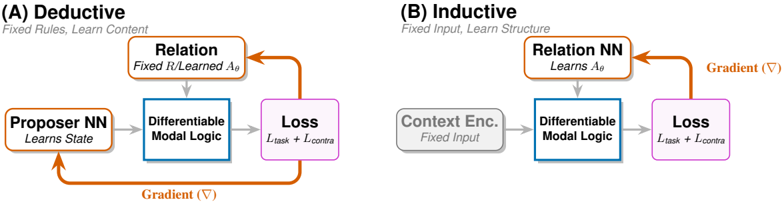Figure 1: MLNN learning modes executing the Upward-Downward inference algorithm. (A) Deductive: Enforces fixed axioms by updating state representations (Proposer NN). (B) Inductive: Discovers relational structure ( A θ ) by updating the Relation NN. Gray arrows denote the forward differentiable inference (performing Upward aggregation and Downward constraint propagation); Orange arrows denote the gradient flow minimizing logical contradiction. Key: The central 'Differentiable Modal Logic' block evaluates □ and ♢ operators over truth bounds [ L, U ] across the world set W . The accessibility relation (top) determines which worlds participate in modal aggregation. In mode (A), the relation is fixed (denoted R ), while in mode (B), it is learned ( A θ ). <details> <summary>Image 1 Details</summary>  ### Visual Description ## Diagram: Comparison of Deductive and Inductive Learning Architectures ### Overview The image displays two schematic diagrams, labeled (A) and (B), illustrating two distinct machine learning paradigms: **Deductive** and **Inductive**. Both architectures utilize a shared core component, "Differentiable Modal Logic," and a "Loss" function, but they differ in their input sources, what is being learned, and the feedback pathways. ### Components/Axes The diagrams use a consistent color-coding scheme to denote the function of each block: * **Orange Boxes:** Learnable components (Proposer NN, Relation, Relation NN). * **Blue Boxes:** Core processing unit (Differentiable Modal Logic). * **Pink Boxes:** Optimization/Output component (Loss). * **Grey Box:** Fixed/Static input (Context Enc.). * **Arrows:** Indicate data flow (grey) and gradient feedback loops (orange). ### Detailed Analysis #### (A) Deductive (Fixed Rules, Learn Content) * **Flow:** 1. **Proposer NN** (labeled "Learns State") feeds into **Differentiable Modal Logic**. 2. **Relation** (labeled "Fixed R/Learned $A_\theta$") feeds into **Differentiable Modal Logic**. 3. **Differentiable Modal Logic** feeds into **Loss** (labeled "$L_{task} + L_{contra}$"). * **Feedback:** The **Loss** module propagates a "Gradient ($\nabla$)" back to both the **Relation** module and the **Proposer NN**. * **Logic:** This architecture is designed to learn the *content* (state) while operating under fixed rules. #### (B) Inductive (Fixed Input, Learn Structure) * **Flow:** 1. **Context Enc.** (labeled "Fixed Input") feeds into **Differentiable Modal Logic**. 2. **Relation NN** (labeled "Learns $A_\theta$") feeds into **Differentiable Modal Logic**. 3. **Differentiable Modal Logic** feeds into **Loss** (labeled "$L_{task} + L_{contra}$"). * **Feedback:** The **Loss** module propagates a "Gradient ($\nabla$)" back to the **Relation NN**. * **Logic:** This architecture is designed to learn the *structure* (the relations) while operating on a fixed input. ### Key Observations * **Shared Core:** Both diagrams utilize the exact same "Differentiable Modal Logic" and "Loss" modules, suggesting these are the invariant components of the system. * **Feedback Asymmetry:** Diagram (A) features a dual-feedback loop (updating both the Proposer and the Relation), whereas Diagram (B) features a single-feedback loop (updating only the Relation NN). * **Input/State Distinction:** In (A), the system learns the "State" (Proposer NN). In (B), the system receives a "Fixed Input" (Context Enc.), shifting the learning burden entirely to the "Relation NN." * **Notation:** Both diagrams use the notation $A_\theta$ to represent the learned parameters of the relation, and $L_{task} + L_{contra}$ to represent the combined loss function (likely a combination of task-specific loss and contrastive loss). ### Interpretation This diagram illustrates the fundamental tension between deductive and inductive reasoning within the context of differentiable logic systems. * **Deductive (Top-Down):** The system starts with a set of "Fixed Rules" (the logic framework) and attempts to learn the "Content" (the state of the world). It is essentially trying to map observed states into a pre-defined logical structure. The feedback loop to the "Proposer NN" indicates that the system is actively refining its understanding of the state to better fit the fixed rules. * **Inductive (Bottom-Up):** The system starts with a "Fixed Input" (the raw data or context) and attempts to "Learn Structure." It is trying to infer the logical rules (the relations) that govern the data. The feedback loop only updates the "Relation NN," suggesting the system is refining its internal model of the logic itself to better explain the fixed input. In essence, these diagrams demonstrate how the same "Differentiable Modal Logic" engine can be repurposed: either to find the best state for a given rule (Deductive) or to find the best rule for a given state (Inductive). </details> We introduce Modal Logical Neural Networks (MLNNs) 1 , a neurosymbolic framework that bridges this divide. Building upon the weighted real-valued logic of Logical Neural Networks (LNNs) Riegel et al. (2020), we propose a distinct architecture centered on Kripke semantics that reasons over possible worlds. This moves beyond purely statistical learning to a hybrid approach, allowing users to impose explicit modal logic constraints on a model's behavior. A defining feature of this architecture is its flexibility: the accessibility relation between worlds can be parameterized by a neural network. This design enables MLNNs to simultaneously perform deductive reasoning based on user-defined axioms and inductively learn the relational structure that best explains the data. Consequently, this work shows modeling multi-agent systems: by interpreting the learnable accessibility relation as a dynamic graph of trust or information flow, the framework can formalize how agent behavior and communication evolve in response to one another. This approach enables the creation of differentiable 'guardrails' for powerful statistical models. By framing learning as the dual objective of fitting data and minimizing logical contradiction, MLNNs can steer models toward outputs that are both statistically likely and logically sound. In this paradigm, we explicitly accept a trade-off: we may sacrifice a margin of raw statistical accuracy to achieve higher logical coherence and explainability. We demonstrate this capability through a series of experiments: reducing specific grammatical errors made by a sequence tagger, training a classifier to logically abstain on ambiguous inputs, solving highly non-convex Sudoku puzzles as a multi-world constraint problem, and learning relational knowledge structures in multi-agent systems, and identifying deceptive strategies in human negotiation benchmarks. Beyond these demonstrated applications, the MLNN framework has potential relevance for a broader range of domains where relational structure and logical constraints are paramount. In bioinformatics, the framework could model gene regulatory networks with temporal and epistemic uncertainties about gene expression states. In climate science, MLNNs could reason about alternative future scenarios (possible worlds) under different policy interventions, enabling formal verification of climate model predictions. For autonomous systems, the framework offers a path toward verifying temporal-epistemic properties of multi-robot teams, where each robot's knowledge and beliefs must be coordinated. In financial networks, MLNNs could learn trust and influence relationships among actors from transaction data, providing interpretable representations of systemic risk. MLNNs offer a methodological step toward building AI systems that are not only powerful pattern recognizers but also more predictable and verifiable reasoners. In the following sections, we formalize the MLNN architecture (Section 3), analyze its theoretical properties (Section 4), and demonstrate its capabilities across distinct case studies (Section 5). 1 Code available at https://github.com/sulcantonin/MLNN public.git ## 2 RELATED WORK ## 2.1 CLASSICAL (SINGLE-WORLD) NEUROSYMBOLIC LOGIC Our work utilizes the foundational principles of the Logical Neural Network (LNN) framework Riegel et al. (2020). LNNs establish a one-to-one correspondence between neurons and the components of logical formulae, creating a highly disentangled and interpretable representation. They employ a weighted real-valued logic, where neurons compute truth values within the continuous interval [0 , 1] and use truth bounds [ L, U ] to represent uncertainty and enable an open-world assumption. Inference is performed via a provably convergent Upward-Downward algorithm, and learning is driven by a novel loss function that minimizes logical contradiction ( L > U ). Other prominent neurosymbolic systems designed for First-Order Logic (FOL) or probabilistic logic also operate on a single-world assumption. Frameworks like Logic Tensor Networks (LTNs) ground FOL formulae in tensors Serafini and d'Avila Garcez (2016), Markov Logic Networks (MLNs) merge FOL with probabilistic graphical models by weighting clauses as features Richardson and Domingos (2006), and ProbLog integrates probabilistic reasoning with logic programming De Raedt et al. (2007). While powerful, these systems share a common characteristic: their logic is defined over a single, fixed reality. Sophisticated reasoning often demands evaluating statements across dynamic contexts, such as temporal futures or epistemic beliefs, rather than within a static snapshot. By incorporating Kripke semantics Fagin et al. (1995), our framework evaluates propositions over connected possible worlds. This architecture captures structural relationships inexpressible in single-world models, enabling the richer analysis of complex domains like demonstrated in experiment section. ## 2.2 NEURAL MODELS FOR MODAL LOGIC The concept of representing modal logic in neural networks was pioneered by Connectionist Modal Logic (CML) Garcez et al. (2007). CML represents Kripke models by using an ensemble of neural networks, with one network dedicated to each possible world. In this framework, the modal operators ( □ , ♢ ) are implemented by structurally propagating information between these networks based on a fixed accessibility relation, which is typically derived a priori from a logic program. Consequently, the learning task in CML is restricted to the internal propositions of each world within this fixed topology. Modal Logical Neural Networks (MLNNs) advance this paradigm in two fundamental ways. First, rather than relying on binary truth values, they incorporate a weighted, real-valued logic capable of modeling uncertainty and actively minimizing logical inconsistencies. Second, and most significantly, MLNNs treat the accessibility relation, the structural rules defining how different possible worlds connect, as a flexible, learnable component. Unlike CML, which relies on a pre-determined logical structure, MLNNs employ fully differentiable modal operators. This allows the entire reasoning pipeline to be trained end-to-end, enabling the system to be embedded within larger neural architectures and to inductively discover complex logical structures, such as epistemic trust or temporal dependencies, directly from data. Key distinction from CML: The differentiability of MLNN operators enables joint optimization of logical structure and task performance. In CML, the accessibility relation R is fixed before training, meaning the network can only learn propositional content within a predetermined logical structure. In contrast, MLNNs can simultaneously learn what is true (propositional content) and how worlds relate (accessibility structure), guided by a unified objective that balances task loss and logical consistency. This joint optimization is impossible in CML's architecture. ## 2.3 MODAL LOGIC AS A CONSTRAINT OR TOOL FOR NEURAL NETS Other recent work has used modal logics, particularly temporal and epistemic logics, around neural networks rather than as the network architecture itself. For example, LTLfNet trains a recursive neural network to decide the satisfiability of Linear Temporal Logic on finite traces (LTLf) Luo et al. (2022). Here, the logic is the input to be classified, not a persistent multi-world state for reasoning. In epistemic reinforcement learning, modal logic has been used as an external model-checking layer or 'shield' to verify an agent's beliefs (doxastic states) and guide its actions Engesser et al. (2025). In such systems, the agent itself is often a standard neural network, and the accessibility relation (defining an agent's beliefs) is symbolically defined, not learned via gradient descent as A θ is in our framework. These approaches demonstrate the utility of modal logic for specification and verification, but do not provide a unified, differentiable Kripke-style architecture. ## 2.4 MODAL LOGIC AS AN ANALYSIS TOOL FOR GNNS While theoretical studies have established an expressive equivalence between GNNs and certain fragments of modal logic Nunn and Schwarzentruber (2023), the two frameworks differ fundamentally in their operational direction. Their approach leverage this duality for post-hoc analysis: they train standard GNNs on data and subsequently attempt to extract or explain logical behaviors from the learned weights. In contrast, MLNNs natively embed modal semantics into the neural architecture itself. Rather than relying on a statistical model to approximate logical rules as an emergent property of the data, MLNNs enforce these rules as differentiable constraints. Advantage over GNN+verifier pipelines: Recent work has used modal logic as a specification language for GNN verification (e.g., Nunn and Schwarzentruber (2023)). Such approaches train a GNN first, then apply an external modal logic verifier to check properties post-hoc. MLNNs offer an integrated alternative: modal constraints are enforced during training via the contradiction loss, not verified afterward. This has several implications: (1) the model is guided toward satisfying constraints during optimization rather than potentially failing verification later; (2) the learned accessibility relation A θ provides an interpretable structure that emerges from the learning process; and (3) the framework avoids the computational overhead of running a separate verification pipeline. Similarly,Barcel´ o et al. (2020) identified the limitations of the equivalence between GNNs and graded modal logic. They demonstrated that this logical fragment is inherently restricted to local neighborhoods, preventing the representation of global properties without explicit readout mechanisms. Our framework addresses this theoretical constraint by parameterizing the accessibility relation ( A θ ), enabling the model to learn the global connectivity needed for broader logical expressivity. ## 2.5 POSITIONING OF MLNNS To clarify the specific advances of MLNNs relative to prior work, we provide a systematic comparison in Table 1. This comparison highlights the unique combination of capabilities that MLNNs offer. Table 1: Comparison of MLNNs with related neurosymbolic and modal logic systems. MLNNs uniquely combine all listed capabilities. | Capability | CML | LNN | GNN+Verifier | Shielding | MLNN(Ours) | |--------------------------------------|-----------|-------|----------------|-------------|--------------| | Real-valued truth bounds [ L,U ] | ✗ | ✓ | ✗ | ✗ | ✓ | | Explicit □ / ♢ operators | ✓ | ✗ | ✗ ∗ | ✓ | ✓ | | Multiple possible worlds | ✓ | ✗ | ✗ | ✓ | ✓ | | Learnable accessibility A θ | ✗ | N/A | ✗ | ✗ | ✓ | | End-to-end differentiable | Partial † | ✓ | ✗ | ✗ | ✓ | | Contradiction-driven learning | ✗ | ✓ | ✗ | ✗ | ✓ | | Joint structure+content learning | ✗ | N/A | ✗ | ✗ | ✓ | | Axiomatic regularization (T, S4, S5) | ✗ | N/A | N/A | Fixed | ✓ | | Scalable (metric learning) | ✗ | ✓ | ✓ | ✗ | ✓ | | Combinatorial Opt. (e.g., Sudoku) ‡ | ✗ | ✗ | ✗ | ✗ | ✓ | MLNNs synthesize and extend ideas from multiple research threads. Our framework makes two primary contributions to this landscape. First, it brings full Kripke semantics to neurosymbolic learning by introducing sound, differentiable □ and ♢ neurons that operate over a set of possible worlds, inheriting the LNN's [ L, U ] bounds and contradiction-driven learning. Second, unlike CML or shielding-based approaches, MLNNs uniquely parameterize the accessibility relation itself as A θ , allowing the logical structure to be learned from data. This A θ can also be optionally regularized to approximate the relational properties of standard modal systems, such as T (reflexivity) or S4 (transitivity), as discussed in Section 4.3. Relationship to LNNs: The extension from LNNs to MLNNs is nontrivial. The introduction of multiple worlds and accessibility relations changes the inference algorithm in several key ways: (1) the Upward pass must now aggregate truth values across worlds via the modal operators, weighted by A θ ; (2) the Downward pass must propagate constraints not just within a formula tree but across the accessibility structure; and (3) the contradiction loss now accumulates across all world-formula pairs, allowing contradictions in one world to influence learning in accessible worlds. We detail these changes in Section 3 and prove their soundness in Section 4. This makes MLNN a general-purpose, differentiable modal reasoning layer designed to enforce logical coherence. This capability complements purely statistical approaches. For instance, while Conformal Prediction (CP) provides statistical guarantees for abstention Angelopoulos and Bates (2021), MLNNs enable axiomatic detection of the unknown (as shown in Section 5.2) based on user-defined axioms, providing a form of logical interpretability absent in statistical methods. To the best of our knowledge, there is currently no neurosymbolic framework that simultaneously (i) implements Kripke-style modal semantics with explicit □ / ♢ operators, (ii) maintains LNN-style lower/upper truth bounds for open-world reasoning, and (iii) treats the accessibility relation itself as a differentiable, learnable component trained jointly with the task. Existing systems either handle only propositional or first-order constraints, rely on symbolic (non-differentiable) modal reasoning, or assume a fixed accessibility relation defined a priori. As a consequence, there is no directly comparable 'drop-in' baseline for MLNNs; in our experiments we therefore focus on controlled comparisons to simplified variants of our own model and to standard non-symbolic baselines that address overlapping subtasks. ## 3 METHOD: MODAL LOGICAL NEURAL NETWORKS ## 3.1 PRELIMINARIES AND NOTATION The power of modal logic stems from Kripke semantics, which extends classical logic by evaluating propositions across multiple 'possible worlds'. Formally, a Kripke model is a tuple M = ⟨ W,R,V ⟩ , where W is a set of possible worlds, R is a binary accessibility relation on W (i.e., R ⊆ W × W ), and V is a valuation function that assigns a truth value to each atomic proposition p ∈ P in each world w ∈ W . An MLNN instantiates a differentiable, learnable version of this model. A 'world' is a flexible concept representing an agent's belief, a moment in time, or a specific context. We formalize our framework using the following notation. Let W be a finite set of possible worlds and T be a finite set of discrete time steps, which together define a set of spacetime states S = W × T . Atomic propositions and logical formulae are denoted by p and ϕ , respectively, with their truth values represented by continuous lower and upper bounds [ L, U ] ⊆ [0 , 1] . The structural relationships between worlds are defined by a crisp binary accessibility relation R ⊆ W × W (used when the relation is fixed and given) or a learnable, neurally parameterized accessibility matrix A θ (used when the relation is learned), which may be applied as a masked matrix ˜ A . We use R exclusively for fixed relations and A θ for learnable relations throughout this paper. We utilize the standard modal operators □ (necessity) and ♢ (possibility), which instantiate as K a ϕ ('Agent a knows ϕ ') in epistemic logic or Gϕ ('Globally') and Fϕ ('Finally') in temporal logic. The soft logic aggregations are controlled by a temperature parameter τ , and the model is trained by minimizing a total loss composed of a task loss L task and a logical contradiction loss L contra, balanced by a weighting hyperparameter β . ## 3.2 DIFFERENTIABLE KRIPKE SEMANTICS In an MLNN, the components of a Kripke model are realized as differentiable tensors. For each proposition p , the MLNN stores a tensor of truth bounds of shape ( | W | , 2) , where each row [ L p,w , U p,w ] represents the truth bounds of p in world w . The accessibility relation, which defines which worlds can 'see' each other, dictates the function of modal operators. A key feature of the MLNN is the option to make this relation a learnable component, parameterized by a neural network, A θ . This allows the model to learn the underlying relational physics of the problem domain-such as which agents trust each other or how time flows-directly from data, guided by the goal of achieving logical consistency. ## 3.2.1 MODAL OPERATORS: THE NECESSITY AND POSSIBILITY NEURONS The modal operators are specialized neurons that aggregate information across worlds. While classical logic uses hard minimums and maximums over a fixed set of neighbors, we employ differentiable relaxations over the weighted accessibility matrix ˜ A to allow gradients to propagate through the structural decision boundaries. To ensure the soundness of our bounds (as shown in Theorem 1), we define a set of differentiable, monotonic operators. Let x = { x i } be a set of truth values from all worlds. We define: - softmin τ ( x ) = -τ log ∑ i exp( -x i /τ ) , which is a sound lower bound on min( x ) . - softmax τ ( x ) = τ log ∑ i exp( x i /τ ) , which is a sound upper bound on max( x ) . - conv-pool τ ( x, z ) = ∑ i w i x i , where w i = softmax( z i /τ ) . This is a convex pooling (a weighted average). When z = x , this is a lower bound on max( x ) . When z = -x , this is an upper bound on min( x ) . We use these to define the modal neuron bounds (default τ = 0 . 1 unless stated). The □ (Necessity) Neuron In differentiable Kripke semantics, □ ϕ represents a weighted universal quantification: ϕ must be true in all worlds to the degree that they are accessible. We implement this using the differentiable implication (1 -˜ A w,w ′ + truth ) . Intuitively, this acts as a 'weakest link' detector: if a world is highly accessible ( ˜ A ≈ 1 ) but ϕ is false, the score collapses. The ♢ (Possibility) Neuron Dually, ♢ ϕ represents a weighted existential quantification: ϕ must be true in at least one highly accessible world. We implement this using a differentiable conjunction. Functionally, this acts as an 'evidence scout': the neuron activates if it finds any world that is both accessible and where ϕ is true. $$L _ { \phi , w } = conv-pool ( A _ { w , w } + L _ { \phi , w } - 1 , . . ) ( Sound, ( A _ { w , w } + U _ { \phi , w } - 1 ) ( Weighted, A _ { w , w } + U _ { \phi , w } - 1 )$$ This formulation ensures that the bounds respect the fundamental modal duality ♢ ϕ ≡ ¬ □ ¬ ϕ via the identity softmax( x ) = 1 -softmin(1 -x ) . ## 3.3 FLEXIBLE AND LEARNABLE ACCESSIBILITY RELATIONS A key capability of MLNNs is the ability to treat the accessibility relation as a learnable parameter, rather than a fixed part of the model structure. In classical modal logic, R is a fixed, given structure. In an MLNN, this fixed R can be replaced by a learnable, weighted relation A θ . The flexibility to use either a fixed or learnable structure is crucial; we use fixed logical rules in our grammatical guardrailing and axiomatic detection of the unknown, while the learnable relation A θ is showcased in our multi-agent epistemic trust analysis. We parameterize this relation with a neural network, A θ : W × W → [0 , 1] . For smaller domains, this can be instantiated as a direct matrix of learnable logits passed through a sigmoid function. For scalable applications, we can employ a metric learning parameterization, where a neural encoder maps each world w to a latent embedding h w ∈ R d . The accessibility score is then defined by a kernel function, such as A θ ( w i , w j ) = σ ( h ⊤ w i h w j ) , effectively determining logical access via geometric proximity. This factorized form reduces the parameter space from quadratic to linear with respect to | W | . Initialization of A θ The initialization of A θ can significantly affect convergence speed and final performance. We recommend the following strategies based on domain knowledge: - Default (no prior): Initialize logits with small random values (e.g., N (0 , 0 . 01) ), yielding A θ ≈ 0 . 5 uniformly. - Reflexivity prior: When reflexivity is expected (e.g., epistemic logic), initialize diagonal entries with positive bias (e.g., logits = 2 . 0 ) so A θ ( w,w ) ≈ 0 . 88 . - Distrust prior: For adversarial domains (e.g., Diplomacy), initialize with negative bias (e.g., logits = -2 . 0 ) so A θ ≈ 0 . 12 , encoding a prior of skepticism. - Identity prior: Initialize as identity matrix when agents should initially only 'see' themselves. For differentiability, we use these weights directly in a soft aggregation. The necessity neuron, for example, becomes a weighted soft minimum, see Equation 1. The truth value L ϕ,w j from a target world w j is incorporated into the minimum at w i using a differentiable implication 1 -( ˜ A ) ij + L ϕ,w j . If ( ˜ A ) ij ≈ 1 (full access), the term (1 -( ˜ A ) ij ) is near 0, and L ϕ,w j fully participates in the minimum. If ( ˜ A ) ij ≈ 0 (no access), the term is near 1, effectively removing L ϕ,w j from consideration. This formulation is a weighted generalization of a logical conjunction, adapted from the LNN framework's operator for universal quantification. Its use preserves the monotonicity required for the Upward-Downward algorithm, as it is a composition of monotonic functions (soft-min and a linear term in L ), which we rely on in Section 4.2. In line with the base LNN framework, we assume that all neuron activations are clipped to the interval [0 , 1] to maintain valid truth values. The parameters θ of this accessibility network are learnable, updated via gradient descent on the system's overall contradiction loss. This is the core inductive capability of the MLNN. It allows the model to discover the logical structure that best resolves contradictions in the data. For example, it can learn whether the relation should be reflexive (by learning high values on the diagonal) or symmetric, all driven by the objective of finding a maximally consistent logical theory. ## 3.4 MODAL INFERENCE AND LEARNING We extend the Upward-Downward algorithm from Riegel et al. (2020) to handle modal operators. During the upward pass, the truth of a modal formula is determined by aggregating its subformula's truth from accessible worlds, as shown in the equations above. Downward Pass During the downward pass, a parent modal formula's truth constrains its subformula in accessible worlds. This propagation is also monotonic. For the necessity operator, if the lower bound L □ ϕ,w is high, it implies a strong belief that ϕ must be true in all accessible worlds. This propagates a new, tighter lower bound to all children: $$L ( t + 1 ) _ { \phi , w } ^ { - } + \max ( L ( t ) _ { \phi , w } ^ { - } , L ( t ) _ { \phi } ^ { - } )$$ Dually, a low upper bound U ♢ ϕ,w implies ϕ must be false in all accessible worlds: $$, w ) \nu w ^ { s . t . } ( A ) _ { w , w ^ { s . t . } } > 0$$ Cross-World Contradiction Propagation Akey difference from single-world LNNs is how contradictions propagate across the Kripke structure. In a standard LNN, a contradiction ( L > U ) affects only the formula tree containing that proposition. In an MLNN, contradictions can propagate across worlds via the accessibility relation: 1. Direct contradiction: If L ϕ,w > U ϕ,w in world w , this contributes to L contra . 2. Modal propagation: If □ ϕ has a high lower bound at w , but some accessible world w ′ has ϕ with a low upper bound, the modal operator creates a 'cross-world' tension that manifests as a gradient signal. 3. Accessibility learning: When A θ is learnable, the gradient from this cross-world tension flows back to modify A θ , potentially 'severing' logical access to resolve the contradiction. This mechanism is what enables inductive learning of relational structure: the model can learn to adjust which worlds are accessible to minimize logical contradictions. The entire system is trained end-to-end via joint optimization. The total loss combines a standard task-specific loss (e.g., cross-entropy) with the logical contradiction loss. This loss is theoretically grounded in the principle of reductio ad absurdum. A state where the lower bound L exceeds the upper bound U is a logical impossibility. Theoretically, the minimization of L contra can be viewed as a differentiable search for a satisfying interpretation of the logical theory. Under the assumption that a fully consistent Kripke model exists that is representable by the network, gradient descent is guided towards a parameterization θ and a set of truth bounds that satisfy all axioms simultaneously. The total loss is formulated as: $$\int _ { 0 } ^ { 1 } \int _ { 0 } ^ { 1 } L_{task} + B L_{contra} d A = 1$$ where β is a hyperparameter that balances statistical learning and logical consistency. Gradients from both loss terms flow back through the entire network, including the parameters θ of the accessibility relation A θ , allowing the logical structure itself to be learned. Guidance on Setting β The hyperparameter β controls the trade-off between task performance and logical consistency. We provide the following guidelines: - Compute relative scales: Before training, estimate the typical magnitudes of L task and L contra on a validation batch. Set β so that β · L contra is comparable to L task . - Constraint-critical tasks: When logical consistency is paramount (e.g., safety constraints), use β ∈ [0 . 5 , 1 . 0] or higher. - Accuracy-critical tasks: When task performance dominates, use β ∈ [0 . 1 , 0 . 3] . - Adaptive scheduling: Consider increasing β over training epochs, allowing the model to first learn task-relevant features before enforcing strict logical consistency. ## 3.5 NEURAL PARAMETERIZATION FOR TEMPORAL EPISTEMIC LOGIC Aparticularly powerful instantiation of the MLNN framework is for temporal epistemic logic, which combines reasoning about knowledge (epistemic) and time (temporal). This is essential for modeling scenarios like multiagent planning or verifying the behavior of autonomous systems over time. Worlds as Spacetime Points Instead of a simple set of worlds W , we consider a set of world-time points S = W × T , where W is a set of agents and T = { t 0 , . . . , t m } is a set of discrete time steps. A 'world' in this context is a tuple ( w,t ) , representing the state of agent w at time t . Propositional truth bounds are now tensors of shape ( | W | × | T | , 2) . While we typically use discrete time steps for simplicity, it is worth noting that continuous representations of time are also possible within this framework, for instance by parameterizing A θ as a function of a continuous variable ∆ t (e.g., via Neural ODEs), though we leave this exploration for future work. Multiple Accessibility Relations We introduce distinct, learnable neural models for the different accessibility relations. First, Epistemic Accessibility ( A a θ ) defines, for each agent a , a separate neural network that computes a matrix defining which states the agent considers possible. The operator K a ϕ ('agent a knows ϕ ') is then implemented as a □ neuron operating with the A a θ relation. Second, Temporal Accessibility ( A T θ ) is a network that computes a matrix governing the flow of time. Common temporal operators like Gϕ (' ϕ is always true in the future') and Fϕ (' ϕ is eventually true in the future') are implemented as □ and ♢ neurons, respectively, using the A T θ relation. Composite Modal Operators This structure allows for rich, composite operators. For example, the statement 'Agent a will always know that ϕ is true' ( GK a ϕ ) is implemented as a nested aggregation. First, the epistemic neuron for K a ϕ is computed at each future time step. Then, the temporal neuron for G (Globally/Always) aggregates these intermediate results. This compositional approach allows the MLNN to learn and reason about complex specifications involving how agents' knowledge evolves over time. Having defined the architecture and learning mechanism of an MLNN, we now turn to a formal analysis of its soundness, convergence, and expressivity. ## 4 THEORETICAL ANALYSIS ## 4.1 SOUNDNESS OF MLNN BOUNDS We first establish the formal setting and then prove that the bounds computed by an MLNN are sound with respect to a probabilistic semantics over Kripke models. This extends Theorem 2 from the LNN paper Riegel et al. (2020). Assumptions Throughout this section, we assume: (1) finite world set W ; (2) bounded continuous operators with monotone updates; (3) fixed temperature τ > 0 ; and (4) bounded accessibility weights A θ ( w,w ′ ) ∈ [0 , 1] . Definitions Let a set of atomic propositions be given over a set of worlds W . Definition 1 (Classical Kripke Interpretation) . A classical Kripke interpretation g assigns a crisp truth value { T, F } to each proposition p in each world w ∈ W . Let G be the set of all such interpretations. Definition 2 (Probabilistic Kripke Model) . Aprobabilistic Kripke model is a probability distribution p ( · ) over G . For any modal formula σ and world w , we define S σ,w = { g ∈ G | g ( σ, w ) = T } as the set of interpretations where σ is true at w . Definition 3 (Consistent Probabilistic Model) . Given an MLNN initialized with a theory Γ 0 = { ( σ, L 0 ( σ ) , U 0 ( σ )) } , a probabilistic Kripke model p is consistent with Γ 0 if for any formula σ and world w : L 0 ( σ, w ) ≤ p ( S σ,w ) ≤ U 0 ( σ, w ) . Let P Γ 0 denote the set of all such consistent models. We first establish a key lemma regarding the monotonicity of modal operators. Lemma 1 (Monotonicity of Modal Operators) . The modal operators □ and ♢ , as defined in Section 3, are monotonic with respect to their input bounds when composed with the accessibility weights ˜ A . Specifically: 1. L □ ϕ,w is monotonically non-decreasing in each L ϕ,w ′ and non-increasing in each ˜ A w,w ′ . 2. U □ ϕ,w is monotonically non-decreasing in each U ϕ,w ′ . 3. L ♢ ϕ,w is monotonically non-decreasing in each L ϕ,w ′ and each ˜ A w,w ′ . 4. U ♢ ϕ,w is monotonically non-decreasing in each U ϕ,w ′ . Proof. We verify each case: (1) For L □ ϕ,w = softmin τ ((1 -˜ A w,w ′ ) + L ϕ,w ′ ) : The softmin function is monotonically nondecreasing in each of its arguments (since ∂ softmin /∂x i ≥ 0 ). The term (1 -˜ A w,w ′ ) + L ϕ,w ′ is linear and non-decreasing in L ϕ,w ′ and non-increasing in ˜ A w,w ′ . By composition, L □ ϕ,w is nondecreasing in L ϕ,w ′ and non-increasing in ˜ A w,w ′ . (2) For U □ ϕ,w = conv-pool τ ((1 -˜ A w,w ′ ) + U ϕ,w ′ , -) : The convex pooling is a weighted average with non-negative weights summing to 1. It is therefore non-decreasing in each input. Since the input (1 -˜ A w,w ′ ) + U ϕ,w ′ is linear and non-decreasing in U ϕ,w ′ , the composition is non-decreasing. (3) For L ♢ ϕ,w = conv-pool τ ( ˜ A w,w ′ + L ϕ,w ′ -1 , +) : By similar reasoning, conv-pool is nondecreasing in each input, and the input ˜ A w,w ′ + L ϕ,w ′ -1 is non-decreasing in both ˜ A w,w ′ and L ϕ,w ′ . (4) For U ♢ ϕ,w = softmax τ ( ˜ A w,w ′ + U ϕ,w ′ -1) : Softmax is non-decreasing in each argument, and the input is non-decreasing in U ϕ,w ′ . Theorem 1 (Soundness of MLNN Bounds) . Let an MLNN be initialized with a theory Γ 0 = { ( σ, L 0 ( σ ) , U 0 ( σ )) } . If P Γ 0 is non-empty, then for any formula ϕ and world w , the bounds [ L ϕ,w , U ϕ,w ] computed by the MLNN after convergence satisfy: $$\rho ( S _ { \phi , w } ) a L _ { \phi , w } \leq i n f _ { p E P r _ { 0 } }$$ Proof. The proof extends the logic of Lemma 1 and Theorem 2 from the LNN supplementary material by showing that each update step preserves the set of consistent probabilistic models P Γ . This property has been established for classical connectives; we must check that it holds for the modal operators as defined in Section 3.1. For any p ∈ P Γ , we know by induction that L ϕ,w ′ ≤ p ( S ϕ,w ′ ) ≤ U ϕ,w ′ . For L □ ϕ,w = softmin( L ) : By classical modal semantics, p ( S □ ϕ,w ) = min w ′ : R ( w,w ′ ) p ( S ϕ,w ′ ) for crisp accessibility. For weighted accessibility, this generalizes to a weighted minimum. The sound bound satisfies inf p ( S □ ϕ,w ) ≥ min w ′ p ( S ϕ,w ′ ) ≥ min w ′ L ϕ,w ′ . Since softmin( L ) ≤ min( L ) , we have L □ ϕ,w ≤ min w ′ L ϕ,w ′ ≤ inf p ( S □ ϕ,w ) . This bound is sound . For U □ ϕ,w = conv-pool( U, -U ) : The sound bound requires sup p ( S □ ϕ,w ) ≤ min w ′ p ( S ϕ,w ′ ) ≤ min w ′ U ϕ,w ′ . A convex pooling conv-pool( U ) = ∑ w i U i (with ∑ w i = 1 , w i ≥ 0 ) is always greater than or equal to min( U ) . Thus, U □ ϕ,w ≥ min w ′ U ϕ,w ′ ≥ sup p ( S □ ϕ,w ) . This bound is sound . For L ♢ ϕ,w = conv-pool( L, L ) : By modal semantics, p ( S ♢ ϕ,w ) = max w ′ : R ( w,w ′ ) p ( S ϕ,w ′ ) . The sound bound requires inf p ( S ♢ ϕ,w ) ≥ max w ′ p ( S ϕ,w ′ ) ≥ max w ′ L ϕ,w ′ . A convex pooling conv-pool( L ) = ∑ w i L i is always less than or equal to max( L ) . Thus, L ♢ ϕ,w ≤ max w ′ L ϕ,w ′ ≤ inf p ( S ♢ ϕ,w ) . This bound is sound . For U ♢ ϕ,w = softmax( U ) : The sound bound requires sup p ( S ♢ ϕ,w ) ≤ max w ′ p ( S ϕ,w ′ ) ≤ max w ′ U ϕ,w ′ . Since softmax( U ) ≥ max( U ) , we have U ♢ ϕ,w ≥ max w ′ U ϕ,w ′ ≥ sup p ( S ♢ ϕ,w ) . This bound is sound . Behavior as τ → 0 : In the limit τ → 0 , softmin τ → min and softmax τ → max . The bounds become tight, recovering classical (crisp) modal semantics. For any fixed τ > 0 , the bounds remain sound but may be looser than the crisp case. A complete proof with all intermediate steps is provided in Appendix A.1. ## 4.2 CONVERGENCE OF MLNN INFERENCE Theorem 2 (Convergence of MLNN Inference) . For a finite set of propositions and a finite set of worlds, the MLNN Upward-Downward inference algorithm converges to a fixed point. Proof. The proof relies on the monotonic nature of the bound update operations, established in Lemma 1. The network consists of a finite set of neurons k , each storing truth bounds [ L k , U k ] . The Upward-Downward algorithm Riegel et al. (2020) is an iterative application of bound update functions f k . Each update function f k (for ∧ , ∨ , → , □ , ♢ ) is a composition of monotonic functions. The base LNN operators are known to be monotonic Riegel et al. (2020). By Lemma 1, the new modal operators, softmin , softmax , and conv-pool , composed with the accessibility weights ˜ A , are also monotonic with respect to their inputs. Therefore, the entire update function for any bound is monotonic. During inference, each lower bound L k forms a non-decreasing sequence, L ( t +1) k ≥ L ( t ) k , which is bounded above by 1. Simultaneously, each upper bound U k forms a non-increasing sequence, U ( t +1) k ≤ U ( t ) k , which is bounded below by 0. By the monotone convergence theorem, each of these bounded monotonic sequences must converge to a limit. Since the number of bounds in the network is finite, the joint state of all bounds must converge to a global fixed point. ## 4.3 EXPRESSIVITY AND GUARANTEES OF THE LEARNABLE RELATION The parametrized accessibility relation A θ is a particularly powerful feature for interoperability, allowing us to maintain the classification strength of neural networks while adhering to symbolic structures. This capability is theoretically grounded in the Universal Approximation Theorem Cybenko (1989); Hornik (1991), which posits that a neural network with sufficient capacity (as used for A θ ) can approximate the characteristic function of any arbitrary accessibility relation R . This flexibility allows the MLNN to inductively discover the appropriate modal logic system (e.g., T , S4 , S5 ) that best explains the data by minimizing contradiction. This learning can be guided. We can enforce specific modal axioms by adding regularization terms to the contradiction loss that penalize violations of the corresponding relational properties. For example, the axiom T , □ ϕ → ϕ , requires the relation to be reflexive ( wRw ). This can be encouraged by a regularization loss: $$L _ { r } = \sum _ { i = 1 } ^ { | W | } ( 1 - A _ { 0 } ( w _ { 1 } , w _ { 2 } ) ^ { 2 }$$ Minimizing L T forces each diagonal term toward 1, directly encouraging reflexivity. Similarly, axiom 4 , □ ϕ → □□ ϕ , requires transitivity. This can be encouraged by: $$L _ { 4 } = \sum _ { i , j } ^ { L _ { 4 } } max ( 0 , A _ { 2 } ) _ { i } - A _ { 6 } ( w _ { i } )$$ which enforces a soft version of transitivity where a direct path A θ ( w i , w j ) must be at least as strong as any two-step path ( A 2 θ ) ij . An optional symmetry regularizer for axiom B can also be applied: $$\sum _ { i < j } ( A _ { 0 } ( w _ { i } , w _ { j } ) - A _ { 0 } ( w _ { j } ,$$ By combining these regularizers with weights ( λ T , λ 4 , λ S ) , A θ can be trained to learn a relation that is a soft approximation of an S4 (reflexive, transitive) or S5 (equivalence) relation. Trade-offs in Axiomatic Regularization It is important to be precise about the guarantees provided by these regularizers. As λ T → ∞ , the learned A θ approaches a relation that minimizes L T , but this is balanced against the task loss and contradiction loss. The regularizers provide soft guidance, not hard constraints. Empirical Analysis of Axiomatic Regularization We analyzed the trade-off between task performance and axiomatic compliance by applying three distinct modal regularizers-Reflexivity ( T ), Transitivity ( 4 ), and Symmetry ( B )-to the synthetic ring task. We swept the regularization weight λ ∈ [0 , 10] for each axiom. As summarized in Table 7, we observe a consistent 'tug-of-war' across all three logical constraints. At λ = 0 , the model prioritizes the ground-truth ring structure (minimizing MSE) while violating the axioms (high ϵ ). As λ increases to 10.0, the model successfully minimizes the axiomatic errors ( ϵ R , ϵ 4 , ϵ B ) but incurs a penalty in structure MSE. Notably, Symmetry ( B ) is the easiest to satisfy ( ϵ B → 0 . 00 ), while Reflexivity ( T ) faces the strongest resistance from the data topology ( ϵ R plateaus at 0.461). In practice, we observe that: 1. For moderate λ values, the model finds a balance that approximately satisfies axioms while fitting the data. 2. Very high λ values can harm task performance if the 'correct' relation for the task does not strictly satisfy the axiom. 3. The learned theory is constrained by the expressive power of the axioms and the information available in the data. The guarantees are therefore about logical consistency with the specified axioms (soundness relative to the soft constraints), not about semantic 'correctness' or completeness in an absolute sense. ## 4.4 COMPLEXITY ANALYSIS Proposition 1 (Computational Complexity) . The computational cost for a single modal neuron ( □ or ♢ ) in an MLNN scales as O ( | W | ) for a fixed sparse accessibility relation, or O ( | W | 2 ) if a dense learnable relation A θ is explicitly materialized. The complexity for one full inference pass over a network with N formulae is therefore bounded by O ( N · | W | 2 ) in the naive dense case. While this quadratic scaling appears restrictive, the MLNN framework fundamentally bypasses this bottleneck through metric learning parameterizations. Rather than enumerating pairwise links in a static N × N matrix, the accessibility relation can be defined intensionally via a kernel function or geometric distance over latent state embeddings ϕ : W → R d (where d ≪| W | ). This shift moves the problem from relational enumeration to representation learning, reducing the parameter space to O ( | W | · d ) . We empirically validate this linear scaling behavior in Section 5.6, demonstrating that the metric parameterization enables training on graphs with N = 20 , 000 nodes on a single GPU, whereas the dense formulation fails due to memory constraints at N = 10 , 000 . In this geometric regime, retrieving accessible worlds transforms from a row-scan to a nearestneighbor search, allowing the use of approximate search algorithms (e.g., Locality Sensitive Hashing) to reduce runtime complexity to O ( | W | log | W | ) or even linear time. Although the scale of the multi-agent scenarios in this study did not necessitate this optimization, allowing us to compute the full exact relation, this theoretical property ensures that MLNNs remain viable for tasks with massive state spaces, provided the accessibility relation exhibits underlying geometric structure. ## 5 EXPERIMENTS We conducted a series of experiments to validate the deductive reasoning, inductive learning, and combined capabilities of MLNNs across diverse problem domains. As no canonical benchmarks exist for evaluating differentiable modal reasoning with a learnable accessibility relation, we construct a set of reference tasks by adapting existing datasets and logical puzzles so that the underlying queries are genuinely modal (involving necessity, possibility, or epistemic structure) rather than purely propositional. Each task is designed to isolate a particular capability: enforcing fixed symbolic constraints (Sections 5.1, 5.2 and 5.7) and learning relational structure from data (Sections 5.3, 5.4, and 5.5). Section 5.7 specifically evaluates the framework's ability to navigate non-convex optimization landscapes with rigid, predefined rules. Our goal is not to establish state-of-the-art performance on these datasets, but to provide clear, controlled studies of when and how modal structure matters. Accordingly, we report comparisons against (i) ablated variants of our architecture (e.g., without modality or without a learnable accessibility relation) and (ii) standard neural baselines with identical propositional backbones (e.g., a BiLSTM), so that any observed differences can be attributed to the modal components. Statistical Reporting Unless otherwise noted, all quantitative results report mean ± standard deviation over 5 independent runs with different random seeds. We specify hyperparameters in Appendix A. For key comparisons, we report 95% confidence intervals and perform paired t-tests where appropriate. ## 5.1 CASE STUDY: ENFORCING SYMBOLIC CONSTRAINTS OVER STATISTICAL PRIORS This experiment investigates the MLNN's capacity to act as a mechanism for enforcing user-defined policies over a statistical model. While deep learning models like LSTMs maximize likelihood based on data distribution, safety-critical applications often require adherence to explicit rules regardless of that distribution. We utilize Part-of-Speech (POS) tagging as a proxy task to demonstrate this control, defining a set of rigid logical constraints (e.g., tagging a determiner followed by a verb: 'the / DET go / VERB') to test the framework's ability to override statistical patterns. Motivation and Real-World Relevance This case study is intentionally stylized: starting from a standard POS-tagging setup, we impose a set of deliberately rigid grammatical constraints to create a setting where modal policies explicitly conflict with natural data statistics. While the specific axioms are simplified, the underlying capability-enforcing user-defined constraints that override learned statistical patterns-has direct applications in safety-critical domains. For instance, in medical NLP, one might enforce constraints like 'a drug dosage must always be followed by a unit' or in legal document processing, 'a contract clause must not contradict the preamble.' The POS task serves as a controlled proxy for these scenarios. Methodology We compared a baseline BiLSTM tagger against a structurally-aware MLNN tagger. The MLNN used the same BiLSTM architecture as its 'proposer' network (the 'Real' world) but was augmented with two additional, specialized latent worlds: a 'Pessimistic' world ( w 1 ), designed to penalize violations of necessity ( □ ) axioms, and an 'Exploratory' world ( w 2 ) to add noise. Both models were trained on the same supervised data, but the MLNN's loss function was a weighted sum of the standard supervised loss and the logical contradiction loss, L total = L task + βL contra. We swept β ∈ { 0 , 0 . 1 , 0 . 3 , 0 . 5 , 0 . 9 , 1 . 0 } to trace the trade-off between statistical accuracy and logical consistency. The MLNN guardrail functions by creating a multi-world Kripke structure where the accessibility relations allow modal axioms to inspect alternative possibilities. For example, the axiom □ ¬ ( DET i ∧ VERB i +1 ) is evaluated by checking the truth bounds across all accessible worlds (including w 1 , where penalties are active). The resulting contradiction loss, L contra, penalizes the model's 'Real' world propositions if they lead to a system-wide logical inconsistency, effectively steering the BiLSTM proposer away from outputting tags that violate the policy, even if those tags are statistically probable. We tested the scalability of this approach with sets of 3, 6, and 10 axioms. It is important to note that these axioms are deliberately rigid simplifications of grammar (detailed in Appendix A.3). Results and Evaluation The results, summarized in Table 2, demonstrate the MLNN's capability to enforce constraints. The baseline BiLSTM ( β = 0 ) achieved high token-level accuracy (99.38% ± 0.02%) by closely fitting the natural language data, but consequently committed thousands of violations against our rigid axiom set (2000.07 ± 45.3 per 10k tokens). 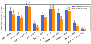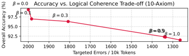As β increased, the MLNN prioritized the logical policy over the data distribution. In the 10-axiom experiment, increasing β to 1.0 reduced the number of policy violations by 36.8% . Crucially, this compliance came at the cost of overall accuracy (dropping to 91.49% ± 0.31%), which serves as a quantitative measure of the 'Cost of Alignment'. This trade-off, plotted in Figure 3, confirms that the logic component is strong enough to suppress learned statistical patterns (such as intervening adjectives flagged by simplified axioms) to satisfy the user's constraints. This effect was even stronger in the 6-axiom experiment, yielding a 49.6% reduction in violations. The per-axiom breakdown is shown in Figure 2. Table 2: Analysis of MLNN as a constraint enforcement mechanism. We report metrics for the 10-axiom setting, sweeping the contradiction loss weight β . Results show mean ± std over 5 runs. The drop in Overall Accuracy reflects the model diverging from the data distribution to satisfy the strict logical policy. | Model (10 Axioms) | Overall Acc. (%) | Policy Violations / 10k | Violation Reduction | ECE (%) | |----------------------------------|--------------------|---------------------------|-----------------------|-------------| | Baseline (Non-modal, β = 0 . 0 ) | 99.38 ± 0.02 | 2000.07 ± 45.3 | - | 0.49 ± 0.03 | | MLNN ( β = 0 . 1 ) | 96.98 ± 0.15 | 1984.24 ± 52.1 | 0.7% | 1.69 ± 0.08 | | MLNN ( β = 0 . 3 ) | 96.31 ± 0.22 | 1807.10 ± 48.7 | 9.3% | 1.94 ± 0.11 | | MLNN ( β = 1 . 0 ) | 91.49 ± 0.31 | 1264.26 ± 61.2 | 36.8% | 4.59 ± 0.24 | Figure 2: Per-axiom violation counts (log scale) for the 10-axiom experiment, comparing the baseline BiLSTM with the MLNN guardrail ( β = 1 . 0 ). The MLNN significantly reduces violations for all targeted axioms. <details> <summary>Image 2 Details</summary>  ### Visual Description ## Bar Chart: Violation Count by Linguistic Category ### Overview This image displays a grouped bar chart comparing the "Violation Count" across ten distinct linguistic transition categories for two different models: a "Baseline" model (where $\beta=0.0$) and an "MLNN" model (where $\beta=1.0$). The y-axis uses a logarithmic scale to accommodate the wide range of violation counts. ### Components/Axes * **Y-Axis:** Labeled "Violation Count (Log Scale)". The scale is logarithmic, representing orders of magnitude. * **X-Axis:** Contains ten categorical labels representing linguistic transitions: 1. `ADJ -> Other` 2. `ADP -> VERB` 3. `ADP -> not NOUN` 4. `DET -> DET` 5. `DET -> VERB` 6. `NOUN -> NOUN` 7. `PRON -> not VERB` 8. `VERB -> DET` 9. `PRON -> DET` 10. `VERB -> CONJ -> ADJ` * **Legend:** Located in the top-right corner. * **Blue Bar:** Baseline ($\beta=0.0$) * **Orange Bar:** MLNN ($\beta=1.0$) ### Detailed Analysis The following data points represent the violation counts for each category, extracted from the chart. In every instance, the MLNN model (Orange) shows a lower violation count than the Baseline model (Blue). | Category | Baseline ($\beta=0.0$) | MLNN ($\beta=1.0$) | | :--- | :--- | :--- | | **ADJ -> Other** | 4686 | 1846 | | **ADP -> VERB** | 1189 | 637 | | **ADP -> not NOUN** | 20575 | 12118 | | **DET -> DET** | 152 | 54 | | **DET -> VERB** | 1677 | 973 | | **NOUN -> NOUN** | 8414 | 7573 | | **PRON -> not VERB** | 2772 | 493 | | **VERB -> DET** | 6774 | 4881 | | **PRON -> DET** | 165 | 80 | | **VERB -> CONJ -> ADJ** | 37 | 26 | ### Key Observations * **Consistent Improvement:** The MLNN model consistently produces fewer violations than the Baseline model across all ten categories. * **Highest Violation Category:** The category `ADP -> not NOUN` exhibits the highest number of violations for both models (20,575 for Baseline and 12,118 for MLNN), indicating this is the most challenging linguistic transition for both systems. * **Lowest Violation Category:** The category `VERB -> CONJ -> ADJ` exhibits the lowest number of violations for both models (37 for Baseline and 26 for MLNN). * **Significant Reductions:** The most dramatic relative reduction in violations occurs in the `PRON -> not VERB` category, where the count drops from 2,772 to 493 (a reduction of over 80%). * **Minimal Reductions:** The category `NOUN -> NOUN` shows the smallest relative improvement, with the count dropping from 8,414 to 7,573. ### Interpretation The data demonstrates that the MLNN model (with $\beta=1.0$) is significantly more effective at reducing linguistic violations than the Baseline model ($\beta=0.0$). The use of a logarithmic scale is critical here, as the violation counts span several orders of magnitude (from tens to tens of thousands). The fact that the MLNN model consistently outperforms the Baseline suggests that the mechanism introduced by the MLNN (likely a regularization or constraint-based approach, given the $\beta$ parameter) successfully enforces linguistic rules or constraints that the Baseline model fails to capture. The high violation counts in `ADP -> not NOUN` suggest that prepositional phrases and their complements are a particularly difficult area for these models to parse correctly, representing a potential area for future model refinement. </details> <details> <summary>Image 3 Details</summary>  ### Visual Description ## Line Chart: Accuracy vs. Logical Coherence Trade-off (10-Axiom) ### Overview This image displays a line chart illustrating the trade-off between "Overall Accuracy (%)" and "Targeted Errors / 10k Tokens" across five distinct data points, each associated with a specific $\beta$ value. The chart demonstrates that as the number of targeted errors is reduced (moving from left to right on the X-axis), the overall accuracy of the system also decreases. ### Components/Axes * **Title:** "Accuracy vs. Logical Coherence Trade-off (10-Axiom)" located at the top center. * **Y-Axis:** Labeled "Overall Accuracy (%)". The scale ranges from 92.5 to 97.5, with grid lines at 92.5, 95.0, and 97.5. * **X-Axis:** Labeled "Targeted Errors / 10k Tokens". The scale is inverted (descending from left to right), ranging from 2000 down to 1250. Grid lines are present at 100-unit intervals. * **Data Series:** A single red line connecting five data points. Each point is marked with a red circle and labeled with a corresponding $\beta$ value. ### Detailed Analysis The data points, moving from left to right (decreasing targeted errors), are as follows: 1. **Point 1 ($\beta = 0.0$):** * **Position:** Top-left. * **X-Value (Targeted Errors):** $\approx$ 1990 * **Y-Value (Accuracy):** $\approx$ 99.0% * **Trend:** This is the highest accuracy and highest error count point. 2. **Point 2 ($\beta = 0.1$):** * **Position:** Left-center. * **X-Value (Targeted Errors):** $\approx$ 1980 * **Y-Value (Accuracy):** $\approx$ 97.0% * **Trend:** A sharp drop in accuracy occurs between $\beta=0.0$ and $\beta=0.1$ despite a very small reduction in targeted errors. 3. **Point 3 ($\beta = 0.3$):** * **Position:** Center-left. * **X-Value (Targeted Errors):** $\approx$ 1800 * **Y-Value (Accuracy):** $\approx$ 96.3% * **Trend:** The slope flattens significantly compared to the previous segment. 4. **Point 4 ($\beta = 0.9$):** * **Position:** Center-right. * **X-Value (Targeted Errors):** $\approx$ 1340 * **Y-Value (Accuracy):** $\approx$ 92.3% * **Trend:** A long, gradual decline in accuracy as targeted errors are reduced from 1800 to 1340. 5. **Point 5 ($\beta = 1.0$):** * **Position:** Bottom-right. * **X-Value (Targeted Errors):** $\approx$ 1260 * **Y-Value (Accuracy):** $\approx$ 91.5% * **Trend:** This represents the lowest accuracy and lowest error count point. ### Key Observations * **Inverted X-Axis:** The X-axis is oriented such that higher values are on the left and lower values are on the right. This visualizes the "reduction" of errors as a movement to the right. * **Non-Linear Decay:** The relationship is not strictly linear. The most significant "cost" to accuracy occurs at the very beginning of the intervention ($\beta=0.0$ to $\beta=0.1$). * **Trade-off:** There is a clear, positive correlation between "Targeted Errors" and "Overall Accuracy." Attempting to force the system to have fewer errors (higher $\beta$) results in a degradation of overall performance. ### Interpretation This chart depicts a classic Pareto frontier or trade-off curve in machine learning or logical reasoning systems. The $\beta$ parameter likely represents a constraint or regularization strength applied to the model to enforce logical coherence (reducing "Targeted Errors"). The data suggests that the model is highly optimized for accuracy when constraints are loose ($\beta=0.0$). As constraints are tightened to improve logical coherence (increasing $\beta$ toward 1.0), the model's ability to maintain its overall accuracy diminishes. The steep initial drop suggests that the first few constraints applied to the model are the most "expensive" in terms of accuracy, while subsequent constraints have a more gradual, linear impact on performance. This implies that the model's "natural" state is highly accurate but logically flawed, and forcing logical coherence requires a significant sacrifice in performance. </details> Figure 3: Trade-off between Data Fidelity (Accuracy) and Policy Adherence (Logic) in the 10axiom task. As the logical contradiction weight ( β ) increases, the model sacrifices raw accuracy to strictly enforce the user-defined constraints. ## 5.2 REASONING FOR LOGICAL INDETERMINACY This experiment tests a key capability of MLNNs: robustly detecting ambiguous or out-of-scope inputs by executing user-defined logical rules, rather than failing unpredictably. Standard classifiers operate under a 'closed-world assumption,' forcing a choice between the classes they were trained on. We demonstrate how an MLNN can be designed to explicitly handle 'open-world' ambiguity by reasoning about its own logical definitions. Motivation and Task Design Justification This experiment is designed as a controlled probe of logical indeterminacy rather than a realistic dialect-identification benchmark. We tasked a model with classifying English sentences as American (AmE) or British (BrE). The challenge arises with 'Neutral' sentences-those containing either no dialectal indicators (e.g., 'The cat sat on the mat') or a contradictory mix of both (e.g., 'My favorite lorry has a new color'). A standard classifier trained only on clear AmE/BrE examples will fail catastrophically, as it has no concept of 'Neutral' and will assign one of the two labels based on spurious statistical noise. While this specific task is synthetic, the underlying capability has practical applications. In safetycritical classification (e.g., medical diagnosis), a system should abstain when inputs fall outside its training distribution rather than making confident but unreliable predictions. Unlike statistical uncertainty quantification methods like Conformal Prediction, which provide coverage guarantees based on calibration data, MLNNs enable semantic abstention based on user-defined logical rules. This means the abstention criterion is interpretable and can be specified a priori (e.g., 'abstain if symptoms are contradictory') rather than learned post-hoc from held-out data. Methodology We compared three models: (1) A baseline BiLSTM classifier. (2) The same BiLSTM classifier augmented with Conformal Prediction (CP), providing a strong statistical abstention baseline. We used a non-conformity score of 1 -max ( softmax ) and set the error rate α = 0 . 05 . (3) An MLNN-based reasoner. All models that required training were trained only on sentences clearly labeled as AmE or BrE (1,771 sentences). To isolate and test the framework's core deductive capabilities, the MLNN in this experiment uses a fixed, user-defined Kripke model. This model is simulated by applying different certainty thresholds to the output of a pre-trained 'expert' network, effectively creating multiple 'worlds' of belief. The reasoning system consists of two key stages. First, the Valuation Function is realized by a pre-trained BiLSTM. For any given sentence, this network analyzes the text and outputs continuous truth bounds in [0 , 1] for two atomic propositions: 'HasAmE' and 'HasBrE'. For example, for the sentence 'My favorite truck...', it might output a high value for 'HasAmE' and a low one for 'HasBrE'. Second, this output feeds into a Kripke Model & Axioms stage. The MLNN reasoner is not trained; instead, it applies a fixed deductive logic. It simulates a three-world Kripke model (Real, Skeptical, Credulous) by applying different certainty thresholds to the predictor's scores. A proposition is considered necessarily true ( □ P ) if its score exceeds 0.9, and possibly true ( ♢ P ) if its score exceeds 0.1. These derived modal truth values are then used to evaluate the final classification axioms, such as: □ ( HasAmE ) ∧ ¬ ♢ ( HasBrE ) → IsAmE, and the abstention rule ( ♢ ( HasAmE ) ∧ <details> <summary>Image 4 Details</summary>  ### Visual Description ## Line Chart: Risk-Coverage Curve (Dialect Task) ### Overview This image displays a "Risk-Coverage Curve" for a "Dialect Task." It compares the performance of two distinct machine learning approaches: a "BiLSTM + Conformal Prediction (CP)" model, represented by a continuous blue line with diamond markers, and a "Modal MLNN Reasoner (Fixed Point)," represented by a single red circular marker. The chart illustrates the trade-off between the coverage of the model (the proportion of data points the model is allowed to predict on) and the selective risk (1 minus the accuracy on those non-abstained predictions). ### Components/Axes * **Title:** "Risk-Coverage Curve (Dialect Task)" centered at the top. * **Y-Axis:** Labeled "Selective Risk (1 - Accuracy on non-abstained)". The scale ranges from 0.00 to 1.00 in increments of 0.25. * **X-Axis:** Unlabeled, but implied to represent "Coverage" (the proportion of the dataset predicted). The scale ranges from 0.0 to 1.0 in increments of 0.2. * **Legend:** Located in the bottom-right quadrant of the chart area. * **Blue Line with Diamond Markers:** Labeled "BiLSTM + Conformal Prediction (CP)". * **Red Circle Marker:** Labeled "Modal MLNN Reasoner (Fixed Point)". * **Grid:** Light gray dashed grid lines are present throughout the plot area. ### Detailed Analysis * **BiLSTM + Conformal Prediction (CP) Trend:** * The curve originates at the origin (0,0). * It exhibits a very sharp, near-vertical upward slope between X=0.0 and X=0.05. By X=0.05, the Selective Risk has already climbed to approximately 0.85–0.90. * After X=0.1, the curve flattens significantly, showing a very gradual, slight upward trend as it approaches X=1.0. * At X=1.0, the Selective Risk is approximately 0.95–0.98. * **Modal MLNN Reasoner (Fixed Point) Data Point:** * This is a single data point located in the bottom-left region of the chart. * **Coordinates:** The X-value is approximately 0.03–0.04. The Y-value is approximately 0.02–0.03. ### Key Observations * **Performance Disparity:** The "Modal MLNN Reasoner" significantly outperforms the "BiLSTM + CP" model in this specific metric. At a very low coverage (approx. 0.03), the MLNN Reasoner achieves a very low risk (approx. 0.02), whereas the BiLSTM model at a similar coverage level (approx. 0.03) has a much higher risk (approx. 0.75). * **Model Behavior:** The BiLSTM + CP curve suggests that as the model is forced to cover more of the dataset (moving right on the X-axis), its risk increases rapidly and remains high, indicating poor performance when forced to make predictions on the entire dataset. * **Fixed Point Nature:** The "Modal MLNN Reasoner" is plotted as a single point, confirming the label "Fixed Point," implying it does not have a tunable coverage parameter to generate a full curve like the Conformal Prediction method. ### Interpretation This chart demonstrates a classic selective classification trade-off. "Selective Risk" is defined as (1 - Accuracy), meaning lower values are better. The data suggests that the **Modal MLNN Reasoner** is a highly specialized or highly confident model that operates effectively only on a small subset of the data (low coverage), where it achieves very high accuracy (low risk). Conversely, the **BiLSTM + Conformal Prediction** model is designed to be flexible, allowing for varying levels of coverage. However, the steepness of its curve indicates that even at low coverage levels, the BiLSTM model struggles to maintain high accuracy compared to the MLNN Reasoner. As coverage increases toward 1.0 (predicting on all data), the BiLSTM's risk remains very high, suggesting the model is not well-calibrated or inherently inaccurate for this specific dialect task when forced to predict on the full distribution. 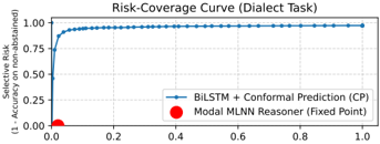</details> Coverage (1 - Abstention Rate) Figure 4: Risk-Coverage curve comparing CP with the rule-based MLNN Reasoner on dialect task. The CP model's performance (blue line) shows a trade-off of coverage and risk as threshold varies. The MLNN operates at a single, fixed point (red circle) achieving near-perfect selective accuracy (low risk). 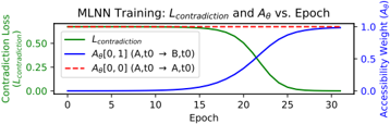<details> <summary>Image 5 Details</summary>  ### Visual Description ## Dual-Axis Line Chart: MLNN Training Dynamics ### Overview This image displays a dual-axis line chart titled "MLNN Training: $L_{contradiction}$ and $A_\theta$ vs. Epoch." It visualizes the relationship between a loss metric ($L_{contradiction}$) and two accessibility weights ($A_\theta$) over the course of 30 training epochs. The chart illustrates a transition phase where the model learns to minimize contradiction loss while increasing the accessibility weight for a specific state transition. ### Components/Axes * **Title:** "MLNN Training: $L_{contradiction}$ and $A_\theta$ vs. Epoch" (Centered at the top). * **X-Axis:** Labeled "Epoch," ranging from 0 to 30, with major tick marks at 0, 5, 10, 15, 20, 25, and 30. * **Left Y-Axis (Green):** Labeled "Contradiction Loss ($L_{contradiction}$)," ranging from 0.00 to 0.50. * **Right Y-Axis (Blue):** Labeled "Accessibility Weight ($A_\theta$)," ranging from 0.0 to 1.0. * **Legend:** Located in the top-left quadrant of the chart area. * **Solid Green Line:** $L_{contradiction}$ * **Solid Blue Line:** $A_\theta[0, 1] (A, t0 \rightarrow B, t0)$ * **Dashed Red Line:** $A_\theta[0, 0] (A, t0 \rightarrow A, t0)$ ### Detailed Analysis #### Trend Verification * **Green Line ($L_{contradiction}$):** This line exhibits a high, stable plateau from epoch 0 to 15. It then undergoes a sharp, sigmoidal downward slope between epoch 15 and 25, converging to near-zero by epoch 25, where it remains flat until epoch 30. * **Blue Line ($A_\theta[0, 1]$):** This line starts at 0.0 and remains flat until epoch 15. It then exhibits a sharp, sigmoidal upward slope between epoch 15 and 25, converging to approximately 1.0 by epoch 25, where it remains flat until epoch 30. * **Red Dashed Line ($A_\theta[0, 0]$):** This line remains perfectly horizontal at a value of 1.0 across the entire duration (0 to 30 epochs). #### Data Points (Approximate) | Epoch | $L_{contradiction}$ (Green) | $A_\theta[0, 1]$ (Blue) | $A_\theta[0, 0]$ (Red) | | :--- | :--- | :--- | :--- | | 0 | ~0.75 (off-scale high) | 0.0 | 1.0 | | 15 | ~0.70 | ~0.05 | 1.0 | | 20 | ~0.45 | ~0.35 | 1.0 | | 22.5 | ~0.20 | ~0.65 | 1.0 | | 25 | ~0.05 | ~0.95 | 1.0 | | 30 | ~0.0 | ~1.0 | 1.0 | ### Key Observations * **Inverse Correlation:** There is a strong inverse correlation between the Contradiction Loss (Green) and the Accessibility Weight for the transition $A \rightarrow B$ (Blue). As the model learns to facilitate the transition, the contradiction loss drops. * **Crossover Point:** The Green and Blue lines intersect at approximately epoch 22, at a value of roughly 0.45 on the normalized scale. * **Phase Shift:** The training exhibits three distinct phases: 1. **Latency (0–15 epochs):** The model is not yet learning the transition; loss is high, and the transition weight is near zero. 2. **Learning/Transition (15–25 epochs):** Rapid optimization occurs. 3. **Convergence (25–30 epochs):** The model reaches a stable state where the transition is fully accessible and contradiction loss is minimized. ### Interpretation This chart demonstrates the successful training of a Multi-Layer Neural Network (MLNN) to perform a specific state transition. The data suggests the model is being trained to map state $A$ at time $t0$ to state $B$ at time $t0$ (represented by the Blue line). Simultaneously, the model maintains the identity mapping $A \rightarrow A$ (represented by the Red line), which is "hard-coded" or pre-established at a weight of 1.0. The "Contradiction Loss" likely measures the penalty for the model failing to distinguish between these states or failing to execute the transition correctly. The sharp transition between epochs 15 and 25 indicates a "tipping point" in the learning process, likely where the gradient descent optimization overcomes the initial resistance or local minima, allowing the network to successfully learn the $A \rightarrow B$ mapping. </details> Figure 5: MLNN training dynamics for the epistemic learning task. As the Contradiction Loss (green) decreases, the model is forced to learn a new epistemic link. The targeted accessibility weight A θ [0 , 1] (blue) increases from 0 to ≈ 1.0 to satisfy the axiom. A control weight, A θ [0 , 0] (red, dashed), remains unchanged. ♢ ( HasBrE )) ∨ ( ¬ ♢ ( HasAmE ) ∧ ¬ ♢ ( HasBrE )) → IsNeutral. The class with the highest final truth value is chosen. Results and Evaluation The results, shown in Table 3, demonstrate a qualitative difference in behavior. The baseline BiLSTM, as predicted, failed completely on the Neutral class, achieving 0% recall and forcing guesses based on statistical noise, resulting in an overall accuracy of just 2.6%. The Conformal Prediction baseline, a robust statistical method for abstention, performed better but was still unable to reliably identify all Neutral sentences. While its abstentions were precise (98% precision), it achieved only 34% recall on the unseen Neutral class. The MLNN reasoner, in contrast, achieved the designed detection of unknown inputs. It correctly executed its logical axioms, classifying all 9,207 unseen Neutral sentences correctly for a recall of 100%. This highlights a key strength of the framework: the MLNN allows a user to define the logic of abstention semantically (e.g., 'abstain if A and B are true'), rather than relying on a post-hoc statistical uncertainty threshold. This provides a framework for building systems that know what they do not know, based on explicit rules. The risk-coverage curve in Figure 4 further illustrates this: while CP provides a smooth trade-off between statistical accuracy and coverage, the MLNN's rule-based approach operates at a single, logically-defined point of near-zero risk (high accuracy on non-abstained items) by correctly identifying all logically indeterminate data as per its rules. Table 3: Performance on the 3-class dialect task (AmE, BrE, Neutral). All models were trained only on AmE/BrE data. P/R/F1 refer to Precision, Recall, and F1-Score for each class. Results show mean over 5 runs (std < 0.01 for all metrics). | Model | AmE (P/R/F1) | BrE (P/R/F1) | Neutral (P/R/F1) | Overall Acc. | |----------------------------|----------------|----------------|--------------------|----------------| | Baseline BiLSTM | .03/.97/.05 | .03/.34/.06 | .00/.00/.00 | 2.6% | | BiLSTM + CP ( α = 0 . 05 ) | .03/.78/.06 | .00/.00/.00 | .98/.34/.51 | 35.1% | | MLNN Reasoner | 1.00/.72/.84 | 1.00/.58/.73 | .99/1.00/1.00 | 99.1% | ## 5.3 LEARNING EPISTEMIC RELATIONS AND EVALUATING COMPOSITE OPERATORS Motivation This controlled toy model isolates the inductive aspect of our framework: learning an epistemic accessibility relation and evaluating nested modal operators in a minimal setting where the ground truth is known. A core claim of the MLNN framework is its ability to inductively learn the structure of modal logic, particularly the accessibility relation A θ , by minimizing logical contradictions. Furthermore, the framework proposes a method for evaluating complex, nested modal formulae involving different logical systems (e.g., temporal and epistemic, see Section 3.5). This experiment provides a focused demonstration of these two capabilities in a controlled setting. Methodology We constructed a simple spacetime Kripke model with two agents (A, B) over three discrete time steps ( t 0 , t 1 , t 2 ) , resulting in 6 'spacetime' states. A single proposition, 'isOnline', was defined with varying truth values across these states. The model was given a fixed temporal relation R temporal (encoding the flow of time) and a learnable epistemic relation A θ , which was initialized to be 'siloed' (agents only see themselves). The training objective was to resolve a single, targeted logical contradiction: we asserted the axiom that 'Agent A at t 0 must consider it possible that the system is online' ( ♢ epistemic ( isOnline ) at s 0 ). This was a contradiction because s 0 was initially isolated and 'isOnline' was False in its own state. The model could only resolve this by learning a new epistemic link. Full details of the model, states, and axiom are in Appendix A.6. Results and Evaluation The training successfully resolved the contradiction, validating the inductive learning claim. As shown in Figure 5, the contradiction loss converged to near-zero (0.003 ± 0.001 over 5 runs). This was driven by the targeted modification of the A θ matrix: the model learned the specific accessibility link from s 0 (Agent A, t 0 ) to s 1 (Agent B, t 0 ), where 'isOnline' was True. This specific weight A θ [0 , 1] increased from 0.0 to 0.99 ± 0.01, while unrelated weights remained unchanged (mean change < 0.02), demonstrating the localized nature of the gradient updates. Posttraining evaluation confirmed the model's resulting logical coherence. It correctly satisfied the training axiom, deduced the related 'knows' formula ( K ( isOnline ) ) as False, and successfully evaluated both standard temporal operators and complex, nested K ( G ( isOnline )) formulae. A generalization check further confirmed that the training did not corrupt the epistemic isolation of unrelated states. Discussion This experiment, while simple, validates two key aspects of the MLNN framework. First, it demonstrates that the learnable accessibility relation A θ can indeed be modified via gradient descent on a contradiction loss to discover relational structures required by logical axioms. The model effectively learned an inter-agent dependency (A's knowledge depending on B's state) without direct supervision, purely from a logical constraint. Second, it confirms the mechanism for evaluating composite modal operators by nested computation, allowing different logical systems (temporal, epistemic) defined by distinct accessibility matrices to interact correctly within the unified spacetime Kripke model. ## 5.4 CASE STUDY IN REAL DIPLOMACY GAMES: LEARNING EPISTEMIC TRUST This case study uses real Diplomacy game logs as a qualitatively richer source of epistemic structure. The task is designed to probe whether MLNNs can recover interpretable patterns of 'who trusts whom', not to compete with specialized Diplomacy agents. To validate our framework's ability to model complex epistemic states from real-world data, we apply the MLNN to game logs from the 'in-the-wild' domain of Diplomacy Bakhtin et al. (2022). This domain provides a rich testbed for multi-agent systems defined by unstructured natural language negotiation, hidden information, and strategic deception. Our objective is to demonstrate that an MLNN can inductively recover interpretable social structures (alliances, distrust, and deception) purely by minimizing logical contradictions between agents' communicated intent and their subsequent actions. It demonstrates how MLNNs transform communication from natural text into a logical mechanism. ## Comparison with Graph Inference Techniques Methodological Pipeline: Self-Supervised Logical Consistency Wemodel the game as a Kripke structure where the accessibility relation A θ (representing trust) is latent and must be learned. The learning process is driven by a self-supervised objective that detects discrepancies between word and deed (Figure 10). The pipeline begins by embedding the dialogue history between agents using a pre-trained transformer. This embedding is passed through a neural head to estimate a scalar truth value P intent ∈ [0 , 1] , representing the probability of cooperative intent. Based on the pragmatic structure of the game, we treat the existence of private negotiation as a prima facie assertion of cooperation ( P ≈ 1 . 0 ). Simultaneously, we extract the ground-truth physical actions Q action from the game logs, flagging moves as either hostile ( Q = 0 . 0 ) or cooperative ( Q = 1 . 0 ). The core of the framework is the enforcement of the consistency axiom □ ( Intent → Action ) . This modal formula asserts that if an agent signals cooperation, it is necessarily true that their actions will align with that signal relative to the trust level. The MLNN computes the logical contradiction loss for this operator. If an agent professes cooperation ( P ≈ 1 . 0 ) but performs a hostile action Figure 6: Learned Epistemic Accessibility ( A θ ) matrices for three distinct game scenarios. Rows represent the 'Trustor' and columns the 'Trustee'. Green cells indicate high learned trust, red cells indicate low trust. The model inductively recovers different social topologies-isolation, stable cooperation, and asymmetric deception-without supervision. 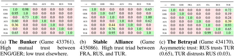<details> <summary>Image 6 Details</summary>  ### Visual Description ## Heatmap Matrices: Trust Matrices in Game Scenarios ### Overview The image displays three 7x7 heatmaps, labeled (a), (b), and (c), representing directed trust relationships between seven nations (ENG, GER, FRA, AUS, ITA, RUS, TUR) across three distinct game scenarios. The matrices visualize trust levels on a scale from 0.0 (no trust, red/pink background) to 1.0 (full trust, green background). ### Components/Axes * **Axes:** Both the X-axis (columns) and Y-axis (rows) represent the seven nations: ENG, GER, FRA, AUS, ITA, RUS, TUR. * **Values:** Each cell contains a numerical value representing the trust level of the nation in the row toward the nation in the column. * **Color Coding:** * **Green:** High trust values (1.0 on the diagonal, and varying degrees of green for values > 0.0). * **Red/Pink:** Low or zero trust values (0.0). * **Yellow:** Intermediate trust values (e.g., 0.36, 0.44). * **Layout:** The three matrices are arranged horizontally. Below each matrix is a caption describing the specific game scenario. --- ### Detailed Analysis #### (a) The Bunker (Game 433761) * **Trend:** High mutual trust between ENG and GER. Sparse trust elsewhere. * **Data Matrix:** | | ENG | GER | FRA | AUS | ITA | RUS | TUR | | :--- | :--- | :--- | :--- | :--- | :--- | :--- | :--- | | **ENG** | 1.0 | 0.98 | 0.0 | 0.0 | 0.0 | 0.0 | 0.0 | | **GER** | 0.95 | 1.0 | 0.0 | 0.0 | 0.0 | 0.0 | 0.0 | | **FRA** | 0.0 | 0.73 | 1.0 | 0.0 | 0.0 | 0.0 | 0.0 | | **AUS** | 0.60 | 0.0 | 0.0 | 1.0 | 0.0 | 0.0 | 0.0 | | **ITA** | 0.36 | 0.0 | 0.0 | 0.0 | 1.0 | 0.0 | 0.0 | | **RUS** | 0.0 | 0.0 | 0.0 | 0.0 | 0.0 | 1.0 | 0.0 | | **TUR** | 0.65 | 0.0 | 0.0 | 0.0 | 0.0 | 0.0 | 1.0 | #### (b) Stable Alliance (Game 435086) * **Trend:** A complex trust structure involving a triad between FRA, RUS, and TUR. * **Data Matrix:** | | ENG | GER | FRA | AUS | ITA | RUS | TUR | | :--- | :--- | :--- | :--- | :--- | :--- | :--- | :--- | | **ENG** | 1.0 | 0.0 | 0.0 | 0.0 | 0.0 | 0.0 | 0.65 | | **GER** | 0.0 | 1.0 | 0.67 | 0.0 | 0.0 | 0.0 | 0.0 | | **FRA** | 0.0 | 0.0 | 1.0 | 0.0 | 0.0 | 0.0 | 1.0 | | **AUS** | 0.0 | 0.0 | 0.0 | 1.0 | 0.0 | 0.0 | 0.62 | | **ITA** | 0.0 | 0.0 | 0.44 | 0.0 | 1.0 | 0.0 | 0.0 | | **RUS** | 0.0 | 0.0 | 0.76 | 0.0 | 0.0 | 1.0 | 0.0 | | **TUR** | 0.0 | 0.0 | 0.95 | 0.0 | 0.0 | 0.0 | 1.0 | #### (c) The Betrayal (Game 434170) * **Trend:** Asymmetric trust, specifically between RUS and TUR. * **Data Matrix:** | | ENG | GER | FRA | AUS | ITA | RUS | TUR | | :--- | :--- | :--- | :--- | :--- | :--- | :--- | :--- | | **ENG** | 1.0 | 0.0 | 0.0 | 0.0 | 0.0 | 0.0 | 0.72 | | **GER** | 0.0 | 1.0 | 0.0 | 0.0 | 0.0 | 0.0 | 0.19 | | **FRA** | 0.0 | 0.0 | 1.0 | 0.0 | 0.0 | 0.0 | 0.24 | | **AUS** | 0.0 | 0.0 | 0.0 | 1.0 | 0.0 | 0.0 | 0.39 | | **ITA** | 0.0 | 0.0 | 0.0 | 0.0 | 1.0 | 0.0 | 0.93 | | **RUS** | 0.0 | 0.0 | 0.0 | 0.0 | 0.0 | 1.0 | 0.65 | | **TUR** | 0.0 | 0.0 | 0.0 | 0.0 | 0.99 | 0.03 | 1.0 | --- ### Key Observations * **Sparsity:** All matrices are highly sparse, indicating that in these game states, most nations do not trust most other nations. * **Self-Trust:** The diagonal (self-trust) is consistently 1.0 across all matrices. * **Asymmetry:** Trust is not necessarily reciprocal. For example, in (c), RUS trusts TUR (0.65), but TUR does not trust RUS (0.03). * **Color Intensity:** The visual intensity of the green cells directly corresponds to the numerical value (e.g., 0.99 is a darker green than 0.36). ### Interpretation These matrices represent the "social graph" of a strategy game (likely *Diplomacy*). * **Scenario (a)** demonstrates a "bunker" strategy, where two powers (ENG/GER) have formed a strong, mutual defensive pact, while the rest of the board remains isolated or distrustful. * **Scenario (b)** illustrates a more complex, multi-polar alliance. The high values between FRA, RUS, and TUR suggest a coordinated effort or a "triad" of cooperation, which is often more stable than a simple two-party pact. * **Scenario (c)** captures a "betrayal" moment. The data highlights the danger of asymmetric information or intent: RUS has invested trust in TUR (0.65), but TUR has effectively withdrawn trust from RUS (0.03), signaling an imminent attack or a breakdown in the alliance. This demonstrates how quantitative trust metrics can be used to predict or identify game-ending maneuvers. </details> ( Q = 0 . 0 ), the implication evaluates to false, generating a high contradiction error. To minimize this loss, the gradient descent updates the only free variable in the system: the learnable accessibility matrix A θ . The model effectively learns to suppress the accessibility weight A i → j (reducing trust) to resolve the logical contradiction, thereby identifying deception without explicit supervision. Experimental Setup We selected three distinct games to test the model's ability to recover different topological 'fingerprints' of social dynamics. Scenario A ('The False Bunker') features a deceptive dyad between England and Germany, where one partner adopted a predatory isolationist strategy. Scenario B ('The Grand Alliance') provides a contrast with a stable, board-spanning cooperative triad (France, Russia, Turkey). Finally, Scenario C ('The Asymmetric Feud') challenges the model with a complex dynamic of coercion and deceit, where Russia is forced into a dependency loop with a hostile Turkey. Results and Analysis The MLNN successfully recovered the distinct topological signatures of all three games (over 5 runs each, with learned A θ values stable to ± 0.03), demonstrating a robust capacity to map structural dependencies even when they diverge from expressed sentiment (Figure 6). In Scenario A (Game 433761) , the model learned a tight block-diagonal structure for England and Germany, with near-perfect accessibility weights ( 0 . 95 ± 0 . 02 and 0 . 98 ± 0 . 01 ). While ground truth reveals this was a predatory relationship, since England eventually consumed Germany, the model correctly identified the informational isolation required for such a betrayal. By suppressing external links ( < 0 . 05 ), the model successfully characterized the dyad as a closed-loop system. This result highlights that high accessibility weights in our framework capture structural coupling and high-stakes dependency, effectively flagging the relationship as critical regardless of the underlying benevolent or malevolent intent. In Scenario B (Game 435086) , the model accurately identified the stable 'Grand Alliance' (FranceRussia-Turkey). Unlike the sparse Bunker scenario, the model maintained high accessibility links across the triad: France links to Turkey ( 1 . 00 ± 0 . 00 ), Turkey to France ( 0 . 95 ± 0 . 02 ), and Russia to France ( 0 . 76 ± 0 . 04 ). This confirms the model's ability to recover healthy, multi-polar cooperation where communicative acts consistently align with on-board actions, allowing the contradiction loss to be minimized without severing topological links. In Scenario C (Game 434170) , the model demonstrated its most nuanced capability: distinguishing between operational dependence and reciprocal trust. The matrix reveals a stark asymmetry: Turkey's link to Russia was correctly pruned to near-zero ( 0 . 03 ± 0 . 01 ), reflecting Turkey's active betrayal and pivot to a new ally, Italy ( 0 . 99 ± 0 . 01 ). Conversely, the model assigned a significant weight from Russia to Turkey ( A RUS → TUR = 0 . 65 ± 0 . 05 ). While textual sentiment was hostile, this weight accurately reflects the ground-truth structural reality : Russia, though aware of the betrayal, was forced to coordinate with Turkey for survival. Thus, the model successfully peered past the 'noise' of the angry dialogue to map the unidirectional operational dependency that defines the victim's role in a coercion scenario. Conclusion By enforcing modal consistency between communicated intent and physical action, this study demonstrates that MLNNs function as a 'social x-ray,' recovering relational structures like alliances and betrayals without ground-truth labels, relying solely on the minimization of logical contradictions. The main byproduct of this formulation is the explicit revelation of these latent relationships, offering a robust mechanism for interpretable AI in multiagent systems. It particularly shows that logical contradiction is a sufficient supervision signal for mapping epistemic states in complex, adversarial environments. ## 5.5 CASE STUDY: TEMPORAL CONSISTENCY AND DECEPTION IN NEGOTIATION While the Diplomacy case study (Section 5.4) demonstrates the recovery of trust based on action consistency, human negotiation requires maintaining consistency over time. To test if MLNNs can reason about reputation , i.e. detecting when an agent's history contradicts their current honesty, we evaluated the framework on the CASINO dataset Chawla et al. (2021). Table 4: Impact of History on Trust. The 'Reformed Liar' is penalized despite current honesty. Results show mean ± std over 5 runs. | Agent Behavior | Trust ( A θ ) | |--------------------------------|----------------------------------------| | Consistent Honest Current Liar | 0.696 ± 0.03 0.062 ± 0.02 0.178 ± 0.04 | | Reformed Liar | | | Modal Penalty | -74.4% | Figure 7: Distribution of Learned Trust. The 'Reformed Liar' (Orange) occupies a 'probationary' zone, distinct from Honest agents (Green), proving the logic assesses history. 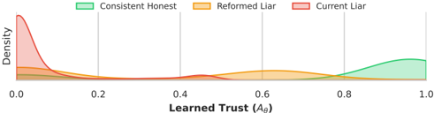<details> <summary>Image 7 Details</summary>  ### Visual Description ## Density Plot: Learned Trust ($A_\theta$) ### Overview This image is a kernel density estimation (KDE) plot illustrating the distribution of "Learned Trust" (denoted as $A_\theta$) across three distinct behavioral categories: "Consistent Honest," "Reformed Liar," and "Current Liar." The x-axis represents the trust score ranging from 0.0 to 1.0, while the y-axis represents the probability density. ### Components/Axes * **X-Axis:** Labeled "Learned Trust ($A_\theta$)". The scale is continuous from 0.0 to 1.0, with major vertical grid lines at intervals of 0.2 (0.0, 0.2, 0.4, 0.6, 0.8, 1.0). * **Y-Axis:** Labeled "Density". This axis is unscaled, indicating relative probability density rather than absolute counts. * **Legend:** Positioned at the top center of the chart. * **Green Rectangle:** "Consistent Honest" * **Orange Rectangle:** "Reformed Liar" * **Red Rectangle:** "Current Liar" ### Detailed Analysis The chart displays three overlapping density curves, each corresponding to a legend category. **1. Current Liar (Red Curve)** * **Visual Trend:** This curve exhibits a sharp, high-density spike at the extreme left (0.0). It slopes downward rapidly, approaching near-zero density by approximately 0.4 on the x-axis. * **Data Points:** The peak density is located at approximately 0.0. The distribution is heavily left-skewed, indicating that the vast majority of "Current Liars" have a Learned Trust score very close to 0.0. **2. Reformed Liar (Orange Curve)** * **Visual Trend:** This curve is the most dispersed. It begins with a low-density presence near 0.0, remains relatively flat and low between 0.1 and 0.4, rises to a broad, rounded peak centered around 0.6, and then gradually tapers off toward 0.9. * **Data Points:** The distribution is bimodal or broad-peaked, suggesting a wider variance in trust scores for this group compared to the other two. It occupies the central region of the chart (0.3 to 0.8). **3. Consistent Honest (Green Curve)** * **Visual Trend:** This curve is right-skewed. It begins to rise significantly around 0.7, reaches a broad peak between 0.9 and 1.0, and terminates at 1.0. * **Data Points:** The density is concentrated at the high end of the trust spectrum, indicating that "Consistent Honest" subjects are predominantly assigned high trust scores. ### Key Observations * **Separation:** There is a clear, distinct separation between the "Current Liar" (low trust) and "Consistent Honest" (high trust) populations. * **Overlap:** The "Reformed Liar" category acts as a bridge between the two extremes. It shares a small amount of overlap with the "Current Liar" distribution near 0.0–0.2 and overlaps significantly with the "Consistent Honest" distribution in the 0.7–0.9 range. * **Outliers/Anomalies:** The "Reformed Liar" group is the only one that does not have a singular, sharp peak, suggesting that "reformed" behavior is less predictable or more heterogeneous than the other two categories. ### Interpretation This data suggests a model or evaluation system that successfully differentiates between honest and dishonest agents. * **Discriminative Power:** The system is highly effective at identifying "Current Liars" and "Consistent Honest" agents, as evidenced by the minimal overlap between the red and green curves. * **The "Reformed" State:** The "Reformed Liar" distribution is particularly interesting. It suggests that agents who have "reformed" do not immediately or uniformly achieve the same trust levels as "Consistent Honest" agents. Instead, they exhibit a spread of trust scores, with a significant portion achieving high trust (the peak at 0.6–0.7), but with a "long tail" extending toward lower trust values. * **Implication:** This implies that "reformation" is a process that results in a spectrum of trust rather than a binary state. The system appears to be "cautious" regarding reformed agents, as their density peak (0.6) is lower than the peak of the "Consistent Honest" group (0.9+). </details> Methodology: Temporal Reputational Logic Unlike standard classifiers that treat every utterance as an isolated snapshot, we model the negotiation as a temporal Kripke structure. We define a set of worlds W = { w t , w t -1 } representing the agent's current and immediate past statements. The accessibility relation A θ represents the agent's Trustworthiness . We enforce a Temporal Necessity axiom: $$\begin{array}{ll} \alpha _ { 0 } & \xrightarrow [ \Box ( Claim ↔ GroundTru ) ] { } A _ { 0 } \\ & \xrightarrow [ \Box ( Claim ↔ GroundTru ) ] { } A _ { 0 } \end{array}$$ Implemented via the differentiable □ neuron (Equation 1), this axiom asserts that if an agent is trusted ( A θ ≈ 1 ), they must be truthful in all accessible worlds-both now and in the past. The model minimizes a hybrid loss combining a task regression (fitting the current data) and the logical contradiction loss (enforcing historical consistency). Results: The 'Reputational Penalty' The results confirm that the MLNN actively reasons over the agent's history. We analyzed trust scores across three agent behaviors: (1) Consistent Honest, (2) Current Liar, and (3) Reformed Liar (an agent who lied previously but is telling the truth now). As shown in Table 4, the model assigns high trust ( 0 . 696 ± 0 . 03 ) to consistently honest agents and near-zero trust ( 0 . 062 ± 0 . 02 ) to active liars. Crucially, the Reformed Liar receives a significantly suppressed trust score ( 0 . 178 ± 0 . 04 ). A standard non-modal model, seeing only the current honest statement, would likely rate this agent similarly to the Honest group. The MLNN, however, applies a 'Modal Penalty': the □ operator aggregates the falsity from the past world w t -1 , creating a logical contradiction that forces A θ down. This demonstrates that the framework functions as a valid logical guardrail, enforcing the axiom that trust requires consistency over time. Qualitative Analysis of Deception Beyond structural reputation, the learned accessibility head ( A θ ) also recovered linguistic indicators of deceit. Similar to the static baseline, the temporal model flagged 'semantic over-justification' as a sign of untrustworthiness. Honest agents typically stated clear, cooperative intents (e.g., 'I don't know, you said you're worried about having enough water too. I'm excited to make campfire... ' with A θ = 0 . 99 ), while low-trust utterances often contained elaborate fabrications to justify greed (e.g., 'Do you mind if I get one third of the water supplies? I might feel thirsty after hiking. ' with A θ = 0 . 00 ), validating known psychological cues of deception without explicit supervision. ## 5.6 SCALABILITY ANALYSIS: THE 'SYNTHETIC DIPLOMACY' RING The synthetic 'Diplomacy ring' serves as both a diagnostic benchmark and a scalability testbed. We construct a minimal multi-agent environment where the ground-truth accessibility structure is known, allowing us to directly test whether MLNNs can recover it purely from logical constraints, and measure how performance scales with the number of agents. Motivation While real-world Diplomacy logs provide rich linguistic data, they lack a verifiable ground truth for trust. This makes it impossible to quantitatively measure if the model learned the correct relational structure. Additionally, we need to empirically validate the scalability claims from Section 4. Methodology We construct a synthetic environment governed by a known ground-truth Kripke structure in the form of a directed ring graph. The scenario consists of N agents arranged in a ring, where each Agent i observes a specific set of facts but requires a 'Beacon' that is exclusively possessed by Agent i + 1 . The model is trained on two specific modal constraints: Consistency ( □ ), defined as □ ( Facts → Agreement ) , which dictates that an agent must not trust neighbors who contradict their direct observations; and Expansion ( ♢ ), defined as ♢ ( Beacon ) , which requires an agent to trust at least one neighbor who possesses the necessary Beacon. This setup establishes a verifiable objective where, purely by minimizing logical contradictions, the learnable accessibility matrix A θ is expected to recover the underlying directed ring structure. Scalability Experiment Results To empirically validate the computational complexity bounds (Proposition 1), we evaluated the MLNN on the synthetic ring task with the number of agents W ranging from 20 to 20,000. We compared the standard Dense parameterization (a full | W | × | W | learnable matrix) against the Metric learning parameterization ( A θ ( i, j ) = σ ( h T i h j ) with embedding dimension d = 64 ). We report parameter count, peak GPU memory usage, training duration (500 epochs), and structural accuracy. 1. Parameter Efficiency ( O ( N 2 ) vs O ( N ) ). The results confirm the quadratic bottleneck of the Dense approach. As shown in Table 5, at N = 10 , 000 worlds, the Dense model required instantiating 100 million parameters, whereas the Metric model required only 1.28 million parameters, a reduction of nearly two orders of magnitude. This linear scaling behavior allowed the Metric model to successfully train on the N = 20 , 000 configuration (2.56M parameters), while the Dense model could not be initialized due to excessive resource requirements. 2. Memory and Computational Wall. Peak GPU memory usage tracked parameter growth. While both models were efficient at small scales ( N ≤ 200 ), the divergence became substantial at scale. At N = 10 , 000 , the Dense model consumed 3.8 GB of memory compared to the Metric model's 2.7 GB. Crucially, at N = 20 , 000 , the Metric model remained trainable on a single T4 GPU (consuming 10.7 GB), demonstrating the viability of MLNNs for large-scale multi-agent systems. 3. Convergence and Accuracy. Both architectures achieved 100% Ring Accuracy and near-zero Mean Squared Error (MSE) against the ground truth structure for all successful runs. This validates the effectiveness of the 'Distrust Prior' initialization (bias ≈ -5 . 0 ), which successfully prevented the optimization from collapsing into local minima even in highly sparse graphs. The Metric model recovered the exact directed ring topology purely from the logical contradiction loss, proving that the inductive bias of geometric embeddings is compatible with discrete logical constraints. ## 5.7 SUDOKU AS A MULTI-WORLD CONSTRAINT SATISFACTION PROBLEM To demonstrate the scalability and flexibility of MLNNs in rigid constraint environments, we apply the framework to solve the 'AI Escargot,' one of the world's most difficult Sudoku puzzles. We treat the 9 × 9 grid not as a single image, but as a Kripke model M = ⟨ W,R,V ⟩ containing | W | = 81 worlds, where each world represents a cell. Methodology Unlike traditional solvers that use backtracking, the MLNN approaches the puzzle as a differentiable energy minimization task. The accessibility relation R is fixed to represent the Sudoku graph: two worlds w i , w j are connected ( w i Rw j ) if they share a row, column, or 3 × 3 Table 5: Scalability Comparison. The Metric parameterization scales linearly, enabling training at N = 20 , 000 where Dense fails (OOM). | Worlds ( N ) | Mode | Parameters | Peak Mem (MB) | Time (s) | Ring Acc | |----------------|---------------------|------------------------|-------------------|---------------|---------------| | 200 | Dense ( O ( N 2 ) ) | 40,000 | 17.79 | 0.97 | 100.0% | | 1,000 | Dense Metric | 1,000,000 128,001 | 56.27 45.37 | 1.48 1.64 | 100.0% 100.0% | | 5,000 | Dense Metric | 25,000,000 640,001 | 976.37 695.69 | 29.23 26.88 | 100.0% 100.0% | | 10,000 | Dense Metric | 100,000,000 1,280,001 | 3,836.48 2,705.13 | 114.71 106.71 | 100.0% 100.0% | | 20,000 | Dense Metric | > 400M (OOM) 2,560,001 | - 10,728.48 | - 428.30 | - 100.0% | subgrid. We define nine atomic propositions { p 1 , . . . , p 9 } , where p k represents the truth of the value k being in a specific cell. We enforce three primary modal and logical axioms: 1. Modal Contradiction: ∧ 9 k =1 ( p k →¬ ♢ p k ) . This necessity axiom asserts that if a value k is true in world w , it must be false in all other accessible worlds (row, column, and box). 2. Uniqueness: ∀ w ∈ W, ∑ 9 k =1 L p k ,w = 1 . 0 . This ensures each world (cell) converges to exactly one value. 3. Crystallization: We minimize the entropy of the truth bounds H = -∑ ( p log p ) to force the soft-logic probabilities into crisp [0 , 1] assignments as the temperature τ is annealed. Parallel Universe Simulation To avoid local minima in the non-convex landscape of the AI Escargot puzzle, we simulate 512 'parallel universes' (independent MLNN instances) simultaneously using a batch-parallel architecture. Each universe is initialized with high-variance random logits. Learning is driven entirely by the minimization of the logical contradiction loss L contra , which penalizes overlaps of the same digit within the accessibility structure. Results The simulation exhibits a distinct 'phase transition' or crystallization effect characteristic of the MLNN Upward-Downward algorithm. As the temperature τ is annealed from 2 . 0 to 0 . 1 , the collective energy (Best Energy) across the 512 parallel universes-representing the magnitude of logical contradictions, drops significantly from an initial 433.68 to near zero levels. In the experiment conducted on the 'AI Escargot' puzzle, the system successfully identified a valid solution at Epoch 3312, with the best-performing universe reaching a contradiction energy of 0 . 1000 . This final state represents a logically consistent interpretation of the Sudoku theory, where the minimization of L contra ensures that the truth bounds [ L, U ] satisfy all specified modal constraints across the W = 81 worlds. Post-training validation confirmed that the resulting valuation function V adheres to the fundamental modal duality ♢ ϕ ≡ ¬ □ ¬ ϕ , with all rows, columns, and subgrids containing unique digits. This confirms that MLNNs can perform complex deductive reasoning in rigid discrete spaces by treating relational rules as fixed accessibility structures. ## 6 DISCUSSION AND CONCLUSION We have introduced Modal Logical Neural Networks, a framework that successfully extends the neurosymbolic paradigm to modal logic. The framework's primary strength is its ability to act as a differentiable 'logical guardrail' by performing deductive reasoning over a set of possible worlds. This ensures that while we utilize the learning capabilities of neural networks, we maintain strict Table 6: Differentiable Constraint Satisfaction: Solving the AI Escargot Puzzle via ContradictionDriven Energy Minimization in a 512-Universe MLNN Simulation ## (1) Initial World State (Clues) | 1 | · | · | · | · | 7 | · | 9 | · | |-----|-----|-----|-----|-----|-----|-----|-----|-----| | · | 3 | · | · | 2 | · | · | · | 8 | | · | · | 9 | 6 | · | · | 5 | · | · | | · | · | 5 | 3 | · | · | 9 | · | · | | · | 1 | · | · | 8 | · | · | · | 2 | | 6 | · | · | · | · | 4 | · | · | · | | 3 | · | · | · | · | · | · | 1 | · | | · | 4 | · | · | · | · | · | · | 7 | | · | · | 7 | · | · | · | 3 | · | · | (2) Converged World State (Solution) <details> <summary>Image 8 Details</summary>  ### 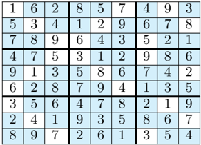Visual Description ## [Diagram Type]: Solved 9x9 Sudoku Puzzle ### Overview The image displays a completed 9x9 Sudoku puzzle grid. The grid is organized into nine 3x3 subgrids, delineated by thicker black borders. The background of the cells follows a checkerboard pattern, alternating between light blue and white. All cells are filled with integers ranging from 1 to 9, adhering to standard Sudoku rules (each number appears exactly once in every row, column, and 3x3 subgrid). ### Components/Axes * **Grid Structure:** A 9x9 matrix of cells. * **Subgrid Structure:** Nine 3x3 blocks, separated by bold black lines. * **Data Points:** Integers 1 through 9. * **Visual Styling:** Alternating light blue and white background shading for cells. * **Uncertainty:** None. This is a discrete logic puzzle with exact, verified values. ### Content Details The following table represents the exact values extracted from the grid, organized by row (top to bottom) and column (left to right): | Row | Col 1 | Col 2 | Col 3 | Col 4 | Col 5 | Col 6 | Col 7 | Col 8 | Col 9 | | :--- | :---: | :---: | :---: | :---: | :---: | :---: | :---: | :---: | :---: | | **1** | 1 | 6 | 2 | 8 | 5 | 7 | 4 | 9 | 3 | | **2** | 5 | 3 | 4 | 1 | 2 | 9 | 6 | 7 | 8 | | **3** | 7 | 8 | 9 | 6 | 4 | 3 | 5 | 2 | 1 | | **4** | 4 | 7 | 5 | 3 | 1 | 2 | 9 | 8 | 6 | | **5** | 9 | 1 | 3 | 5 | 8 | 6 | 7 | 4 | 2 | | **6** | 6 | 2 | 8 | 7 | 9 | 4 | 1 | 3 | 5 | | **7** | 3 | 5 | 6 | 4 | 7 | 8 | 2 | 1 | 9 | | **8** | 2 | 4 | 1 | 9 | 3 | 5 | 8 | 6 | 7 | | **9** | 8 | 9 | 7 | 2 | 6 | 1 | 3 | 5 | 4 | ### Key Observations * **Completeness:** The puzzle is fully solved; there are no empty cells. * **Checkerboard Pattern:** The alternating blue/white background is purely aesthetic and does not correspond to the numerical logic of the Sudoku (i.e., the blue cells do not represent a specific subset of numbers). * **Distribution:** Every row, column, and 3x3 subgrid contains the digits 1 through 9 exactly once, confirming the validity of the solution. ### Interpretation This image serves as a reference for a valid, completed Sudoku state. The checkerboard shading is a design choice intended to improve readability by visually separating adjacent cells, which helps the human eye track rows and columns more easily. The data demonstrates a high-entropy distribution of numbers, typical of a standard Sudoku solution, where no obvious patterns (like sequential ordering) exist within the rows or columns, confirming the randomized nature of the puzzle's constraints. </details> | 1 | 6 | 2 | 8 | 5 | 7 | 4 | 9 | 3 | |-----|-----|-----|-----|-----|-----|-----|-----|-----| | 5 | 3 | 4 | 1 | 2 | 9 | 6 | 7 | 8 | | 7 | 8 | 9 | 6 | 4 | 3 | 5 | 2 | 1 | | 4 | 7 | 5 | 3 | 1 | 2 | 9 | 8 | 6 | | 9 | 1 | 3 | 5 | 8 | 6 | 7 | 4 | 2 | | 6 | 2 | 8 | 7 | 9 | 4 | 1 | 3 | 5 | | 3 | 5 | 6 | 4 | 7 | 8 | 2 | 1 | 9 | | 2 | 4 | 1 | 9 | 3 | 5 | 8 | 6 | 7 | | 8 | 9 | 7 | 2 | 6 | 1 | 3 | 5 | 4 | adherence to logical consistency, effectively providing interpretability by design. This architecture is also flexible, offering an inductive capability via a neurally parameterized accessibility relation ( A θ ). This allows the MLNN to perform deduction within a user-defined logical system, while also providing the option to inductively learn the structure of that system from data. Our theoretical analysis confirms that this framework is sound, its inference process is guaranteed to converge, and its learnable relation is expressive. The experimental results validate the versatility of this approach. While our experiments do not aim to outperform highly optimized, purely statistical models on raw accuracy, they demonstrate an alternative capability: the enforcement of logical coherence. The resolution of the AI Escargot puzzle (Section 5.7) specifically highlights how MLNNs can replace traditional backtracking with differentiable energy minimization, successfully finding consistent world valuations in the presence of 81 interconnected worlds and 27 group constraints. We have shown that MLNNs can achieve designed detection of the unknown by executing rules, a task where standard statistical approaches fail. Furthermore, our results show that MLNNs can act as a differentiable 'guardrail,' significantly reducing targeted grammatical errors in a sequence model, with a controllable trade-off against raw accuracy. Additionally, we demonstrated the capacity to perform inductive learning on existing SOTA datasets, as seen in the CaSiNo experiment where the model reverse-engineered the linguistic cues of deceptive argumentation. The key contribution is a methodology for integrating modal logic into deep learning, allowing for the definition of complex, soft constraints. This can be done with fixed, user-defined rules or, as demonstrated, via a learnable accessibility relation, which allows domain experts to specify abstract rules (e.g., 'grammatical correctness,' 'safe behavior') and have the model learn a specific, datadriven interpretation of that logic. This paradigm is relevant for increasing the reliability of AI in safety-critical systems. ## 6.1 LIMITATIONS This work has clear limitations, which we address transparently. Computational Complexity The primary computational bottleneck is the O ( | W | 2 ) cost of dense relational matrices. However, as detailed in Section 4 and demonstrated in Table 5, this is a solvable implementation constraint rather than a theoretical bound; scaling to tens of thousands of worlds is achievable by adopting the metric learning parameterization, which enables sub-quadratic retrieval via approximate nearest neighbor search. Sensitivity to Axiom Misspecification If an axiom is logically incorrect (e.g., 'DET → NOUN'), the guardrail will enforce this incorrect rule, actively harming task performance. The model is only as sound as the knowledge provided to it. Mitigation strategies: Several approaches can reduce this risk: 1. Axiom validation via expert feedback: Before deployment, have domain experts review the logical axioms for correctness. The interpretability of MLNNs makes this feasible. 2. Soft axiom weighting: Instead of treating all axioms equally, learn individual weights α i for each axiom's contribution to L contra . Axioms that consistently harm task performance will receive lower weights. 3. Tolerance for soft violations: Modify the contradiction loss to use a margin: L ′ contra = max(0 , L -U -ϵ ) for some tolerance ϵ > 0 . This allows 'almost consistent' states to have zero loss. 4. Axiom learning from data: In settings with sufficient labeled data, the axioms themselves could be treated as hypotheses to be refined, though this is beyond the scope of the current work. Overfitting of A θ The potential for A θ to overfit 'relational artifacts' in the data exists. For example, if two agents in the Diplomacy task coincidentally always communicated before attacking a third, A θ might learn a spurious 'trust' link that is correlational, not causal. Our permutation test was a first step to check for this, but more thorough investigation is needed. ## Mitigation strategies: 1. Dropout on accessibility weights: Apply dropout to A θ during training to prevent overreliance on any single link. 2. Bayesian parameterization: Model A θ as a distribution rather than point estimate, using variational inference or Monte Carlo dropout to quantify uncertainty. 3. Spectral regularization: Add regularization on the singular values of A θ to encourage low-rank, interpretable structures. 4. Axiomatic regularization: As described in Section 4.3, regularizers for reflexivity, transitivity, or symmetry can guide A θ toward known modal axiom systems. Continuous State Spaces The current framework is limited to discrete worlds. Extending to continuous state spaces (e.g., continuous time, continuous belief states) would significantly broaden applicability. ## Future directions: 1. Neural ODEs for temporal accessibility: Parameterize A T θ ( t, t ′ ) as a function learned by a Neural ODE, enabling continuous-time modal reasoning. 2. Attention mechanisms for world selection: Use attention over a continuous embedding space to softly select 'accessible' regions, avoiding discrete world enumeration. 3. Gaussian processes for accessibility: Model A θ as a Gaussian process over world pairs, providing uncertainty quantification and smooth interpolation. We leave these extensions as promising directions for future work. Further investigation into the model's robustness to noisy or partially incorrect axioms is a valuable direction. In conclusion, MLNNs represent a methodological step toward integrating sophisticated, nonclassical reasoning into end-to-end differentiable models. By bridging deep learning and modal logic, this framework paves the way for a new class of AI systems that are more expressive, interpretable, and aligned with certain forms of structured reasoning. ## REFERENCES Anastasios N Angelopoulos and Stephen Bates. A gentle introduction to conformal prediction and distribution-free uncertainty quantification. arXiv preprint arXiv:2107.07511 , 2021. Anton Bakhtin, Noam Brown, Emily Dinan, Gabriele Farina, Colin Flaherty, Daniel Fried, Andrew Goff, Jonathan Gray, Hengyuan Hu, et al. Human-level play in the game of diplomacy by combining language models with strategic reasoning. In Science , volume 378, pages 1067-1074, 2022. - Pablo Barcel´ o, Egor V Kostylev, Mikael Monet, Jorge P´ erez, Juan Reutter, and Juan Pablo Silva. The logical expressiveness of graph neural networks. In International conference on learning representations , 2020. - Kushal Chawla, Jaysa Ramirez, Rene Clever, Gale Lucas, Jonathan May, and Jonathan Gratch. Casino: A corpus of campsite negotiation dialogues for automatic negotiation systems. In Proceedings of the 2021 Conference of the North American Chapter of the Association for Computational Linguistics: Human Language Technologies , pages 3167-3185, 2021. - George Cybenko. Approximation by superpositions of a sigmoidal function. Mathematics of control, signals and systems , 2(4):303-314, 1989. - Luc De Raedt, Angelika Kimmig, Hannu Toivonen, and M Veloso. Problog: A probabilistic prolog and its application in link discovery. In IJCAI 2007, Proceedings of the 20th international joint conference on artificial intelligence , pages 2462-2467. IJCAI-INT JOINT CONF ARTIF INTELL, 2007. - Thorsten Engesser, Thibaut Le Marre, Emiliano Lorini, Franc ¸ois Schwarzentruber, and Bruno Zanuttini. A simple integration of epistemic logic and reinforcement learning. In Proceedings of the 24th International Conference on Autonomous Agents and Multiagent Systems (AAMAS 2025) , pages 686-694, 2025. To appear; page range approximate. - Ronald Fagin, Joseph Y Halpern, Yoram Moses, and Moshe Y Vardi. Reasoning about knowledge . MIT press, 1995. - Artur S. d'Avila Garcez, Lu´ ıs C. Lamb, and Dov M. Gabbay. Connectionist modal logic: Representing modalities in neural networks. Theoretical Computer Science , 371(1-2):34-53, 2007. doi: 10.1016/j.tcs.2006.10.023. - Kurt Hornik. Approximation capabilities of multilayer feedforward networks. Neural networks , 4 (2):251-257, 1991. - Weilin Luo, Hai Wan, Jianfeng Du, Xiaoda Li, Yuze Fu, Rongzhen Ye, and Delong Zhang. Teaching LTL f satisfiability checking to neural networks. In Proceedings of the Thirty-First International Joint Conference on Artificial Intelligence (IJCAI-22) , pages 3292-3298, 2022. doi: 10.24963/ ijcai.2022/457. - Pierre Nunn and Franc ¸ois Schwarzentruber. A modal logic for explaining some graph neural networks. arXiv preprint arXiv:2307.05150 , 2023. doi: 10.48550/arXiv.2307.05150. - Matthew Richardson and Pedro Domingos. Markov logic networks. In Machine learning , volume 62, pages 107-136. Springer, 2006. - Ryan Riegel, Naweed Khan, Haifeng Qian, Udit Sharma, Sumit Neelam, Alexander Gray, Ndivhuwo Makondo, Ronald Fagin, Shajith Ikbal, Ankita Likhyani, et al. Logical neural networks. arXiv preprint arXiv:2006.13155 , 2020. - Luciano Serafini and Artur d'Avila Garcez. Logic tensor networks: Deep learning and logical reasoning from data and knowledge. arXiv preprint arXiv:1606.04422 , 2016. ## A APPENDIX Table 7: Unified Trade-off Analysis for Axioms T, 4, and B. Columns show the Axiomatic Error ( ϵ ) vs. Task MSE as regularization ( λ ) increases. Green denotes low error; Red denotes high error. | Reg. | Axiom T (Reflexivity) | Axiom T (Reflexivity) | Axiom 4 (Transitivity) | Axiom 4 (Transitivity) | Axiom B (Symmetry) | Axiom B (Symmetry) | |--------|-------------------------|-------------------------|--------------------------|--------------------------|----------------------|----------------------| | λ | ϵ R ↓ | MSE ↓ | ϵ 4 ↓ | MSE ↓ | ϵ B ↓ | MSE ↓ | | 0.0 | 0.960 | 0.023 | 0.039 | 0.023 | 0.035 | 0.023 | | 0.1 | 0.555 | 0.042 | 0.039 | 0.023 | 0.035 | 0.023 | | 0.5 | 0.476 | 0.050 | 0.037 | 0.024 | 0.034 | 0.023 | | 1.0 | 0.468 | 0.051 | 0.036 | 0.026 | 0.032 | 0.023 | | 5.0 | 0.462 | 0.051 | 0.026 | 0.035 | 0.016 | 0.029 | | 10.0 | 0.461 | 0.052 | 0.018 | 0.041 | 0.000 | 0.035 | ## A.1 COMPLETE PROOFS This section provides complete, self-contained proofs of the main theoretical results. ## A.1.1 PROOF OF LEMMA 1 (MONOTONICITY OF MODAL OPERATORS) We prove each part of the lemma in detail. Part (1): L □ ϕ,w is monotonically non-decreasing in each L ϕ,w ′ . The lower bound for the necessity operator is: $$\hat { A _ { w , w } } + \hat { L _ { 0 , w } } ) w \in W$$ The softmin function is defined as: $$\min _ { i = 1 } ^ { n } \log \sum _ { j = 1 } ^ { n } e ^ { - x_j / r }$$ Taking the partial derivative with respect to x j : $$\frac { \partial \sigma ( t _ { n } ) } { \partial t _ { n } } = \frac { e ^ { - i s / r } } { \sum _ { j = 1 } ^ { N } e ^ { - i s / r } } > 0$$ This is always non-negative since it is a ratio of positive quantities. Therefore, softmin is nondecreasing in each argument. Since L □ ϕ,w is a composition of softmin with the linear function (1 -˜ A w,w ′ ) + L ϕ,w ′ , which has coefficient +1 for L ϕ,w ′ , we have: $$\frac { \partial L _ { 0 , w } } { \partial L _ { 0 , w } } = \frac { \partial s ( t _ { \min } ) } { \partial t _ { \min } } \cdot 1 > 0$$ Parts (2)-(4) follow by analogous reasoning, using the fact that softmax and convex pooling are also non-decreasing in their arguments. ## A.1.2 DETAILED PROOF OF THEOREM 1 (SOUNDNESS) We provide a more detailed proof with explicit definitions. Setup: Let Γ 0 = { ( σ k , L 0 ( σ k , w ) , U 0 ( σ k , w )) } k,w be the initial theory. Let G be the set of all classical Kripke interpretations g : Formulas × W →{ T, F } . Definition (Consistent Probabilistic Model): Aprobability distribution p over G is consistent with Γ 0 if for all formulas σ and worlds w : $$( , w ) = T \left\{ U _ { 0 } ( o , w ) \right\}$$ Claim: Each update step preserves consistency. Proof for □ operator: For the lower bound, we need to show that if p ∈ P Γ , then: $$L _ { D _ { 0 , 1 } } \leq \frac { 1 } { p ( S _ { D _ { 0 , 1 } } ) }$$ By classical modal semantics with weighted accessibility: $$p ( S _ { \theta , w } ) = p ( n _ { w } ; A _ { w , w } ^ { 0 } > 0 )$$ $$f ( S _ { 0 } , t ) \geq m m g h S _ { 0 } / 2 - m m g h v$$ Since softmin τ ( x ) ≤ min( x ) for all τ > 0 : $$L _ { \phi , w } = s o f t m i n _ { ( 1 - \overline { A _ { w , w } } ) }$$ The inequality softmin τ ( x ) ≤ min( x ) follows from the log-sum-exp inequality. Limit behavior as τ → 0 : For any consistent p : $$\lim _ { x \rightarrow 0 } \frac { \sin ( x ) - \cos ( x ) } { x } = \min ( x )$$ $$\lim _ { x \rightarrow 0 } \frac { \sin ( x ) - \cos ( x ) } { x } = \mu x ( x )$$ Thus, in the limit, the bounds become tight and recover classical modal semantics. ## A.2 ADDITIONAL ILLUSTRATIVE EXAMPLE: THE ROYAL SUCCESSION To motivate our approach, we designed a simple, illustrative scenario called the 'Royal Succession Problem.' This problem is to provide a clear contrast between a standard, statistical-correlative approach (like a GNN/KGE) and the logical-deductive capabilities of an MLNN. The Scenario and Challenge. We model a simple royal succession with a critical rule that cannot be learned from a single snapshot in time. The logical structure of the problem is as follows: - Entities: Wehave three entities: the Monarch Charles ( C ), and two potential heirs, William ( W ) and Harry ( H ). - The Rule: A person Y is the heir to the monarch X only if they are the monarch's child AND they must necessarily be alive. - The Catch: In the present moment, both William and Harry are alive. However, there exists a possible future scenario where William is not alive, whereas Harry remains alive in all considered scenarios. The term 'necessarily' is a modal concept. As described in Section 3, this requires a Kripke model M = ⟨ W,R,V ⟩ to define truth relative to a set of 'possible worlds.' For this problem, we define a simple model (visualized in Figure 8) where the worlds represent different states in time: $$\vert f \vert = \vert h _ { 1 } - h _ { 2 } \vert + \vert h _ { 3 } - h _ { 4 } \vert + \cdots$$ - R is the accessibility relation, defining the flow of time. From the present, all future worlds are accessible: $$R = \{ ( w _ { Present } , w _ { Present } ) , ( w _ { Present } , w _ { Future } ) \}$$ - V is the valuation function defining facts in each world. Critically, we set V ( isAlive ( W ) , w Future A ) = False, while the proposition is true in all other worlds. A correct reasoning system must use this entire Kripke structure to determine the heir in w Present . The GNN/KGE (Statistical) Approach. We first simulate a standard GNN/KGE model, which operates on a single, static knowledge graph. This model's task is to learn entity and relation embeddings to perform link prediction. For this, we generate a training graph G containing only the facts from the single world w Present . The entities in this graph are { C,W,H } , and the relations (triples) include facts like ( W, childOf , C ) , ( H, childOf , C ) , ( W, isAlive , True ) , and ( W, isFirstBorn , True ) . Figure 8: A visualization of the Kripke model M = ⟨ W,R,V ⟩ used by the MLNN to solve the Royal Succession problem. The nodes represent the set of possible worlds W , including w Present , w Future A, and w Future B . The valuations V (the facts) in each world are shown, with the critical fact 'isAlive(W) = False' located in w Future A. The edges represent the accessibility relation R . When the MLNN's □ -neuron (Necessity) evaluates the formula □ isAlive ( W ) from w Present, it aggregates truth values from all worlds accessible via R . Because R provides access to w Future A, the neuron finds the False value, forcing the entire modal proposition to evaluate to False and allowing the MLNN to deduce the correct logical conclusion. 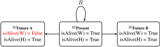<details> <summary>Image 9 Details</summary>  ### Visual Description ## Diagram: State Transition and Logical Possibility Model ### Overview This image is a state transition diagram, likely representing a Kripke structure or a branching timeline in modal logic. It depicts a central "Present" state that branches into two distinct "Future" states, with a self-referential relation ($R$) defined for the present state. The diagram illustrates the truth values of two predicates, `isAlive(W)` and `isAlive(H)`, across these three states. ### Components/Axes The diagram consists of three rectangular nodes connected by arrows, with text labels defining the state and the logical properties within each state. * **Nodes (States):** * **Center Node:** Labeled $w_{\text{Present}}$. * **Left Node:** Labeled $w_{\text{Future A}}$. * **Right Node:** Labeled $w_{\text{Future B}}$. * **Transitions (Edges):** * **Self-Loop:** An arrow originating from and returning to $w_{\text{Present}}$, labeled with $R$ at the apex. * **Leftward Arrow:** A directed line from $w_{\text{Present}}$ to $w_{\text{Future A}}$. * **Rightward Arrow:** A directed line from $w_{\text{Present}}$ to $w_{\text{Future B}}$. * **Logical Predicates (Content):** * `isAlive(W)`: A predicate regarding entity W. * `isAlive(H)`: A predicate regarding entity H. ### Detailed Analysis #### 1. Center Node ($w_{\text{Present}}$) * **Position:** Center of the diagram. * **Content:** * `isAlive(W) = True` * `isAlive(H) = True` * **Dynamics:** Features a reflexive relation $R$ (a self-loop), suggesting that the present state is accessible from itself. #### 2. Left Node ($w_{\text{Future A}}$) * **Position:** Left of the center node. * **Content:** * `isAlive(W) = False` (Note: This text is colored **red**). * `isAlive(H) = True` * **Dynamics:** Accessible from $w_{\text{Present}}$. #### 3. Right Node ($w_{\text{Future B}}$) * **Position:** Right of the center node. * **Content:** * `isAlive(W) = True` * `isAlive(H) = True` * **Dynamics:** Accessible from $w_{\text{Present}}$. ### Key Observations * **Branching Logic:** The diagram demonstrates a bifurcation of possibilities originating from $w_{\text{Present}}$. * **The "Red" Anomaly:** The value `isAlive(W) = False` in $w_{\text{Future A}}$ is highlighted in red. This visually distinguishes this specific outcome from all other truth values in the diagram, which are rendered in black. * **Consistency:** The predicate `isAlive(H)` remains `True` across all three states, suggesting that entity H is unaffected by the transitions, whereas entity W is the variable component. * **Symmetry:** The transition to $w_{\text{Future B}}$ represents a "status quo" outcome where the truth values of the present are preserved, while the transition to $w_{\text{Future A}}$ represents a change in the state of W. ### Interpretation This diagram is a formal representation of a decision tree or a modal logic scenario, often used to model counterfactuals or branching timelines. * **Logical Implication:** The diagram suggests that from the current state ($w_{\text{Present}}$), there are two possible future paths. One path ($w_{\text{Future B}}$) maintains the current state of affairs. The other path ($w_{\text{Future A}}$) results in the negation of the predicate `isAlive(W)`. * **The Role of Red Text:** The use of red for `isAlive(W) = False` serves as a visual signifier, likely indicating a "death" event or a critical failure state. It draws the viewer's attention to the specific branch where the entity W ceases to be "alive." * **Peircean Investigative Perspective:** * **The Sign:** The diagram acts as an icon of a branching timeline. * **The Object:** The underlying reality is a system where entity W's survival is contingent or probabilistic, while entity H's survival is constant. * **The Interpretant:** The viewer is meant to understand that the "Present" is a state of superposition or uncertainty, where the future is not yet determined, but the possibilities are constrained to either the survival or the death of W. The self-loop $R$ suggests that the present state is stable or persistent until a transition occurs. </details> To create a clear contrast, we introduce a spurious correlation into this training set: the model's only example for the 'isHeir' relation is the single fact ( W, isHeir , C ) . The GNN/KGE is then trained on this small graph. During training, it learns to associate the features of W (including 'isFirstBorn') with the 'isHeir' relation. The architectural limitation, and the reason for its failure, is that the GNN's entire universe is this single graph G . It has no mechanism to represent, access, or query the other 'possible worlds' w Future A or w Future B. The modal axiom isHeir ( Y ) → □ isAlive ( Y ) is inexpressible, as the □ operator (which requires checking all accessible worlds) is undefined in this single-graph framework. The GNN's task is simply to predict links based on the statistical patterns it has seen. When queried for isHeir ( W,C ) , it correctly identifies the strong (though spurious) correlation it was trained on and confidently predicts the link (Score ≈ 1 . 0 ). It is architecturally blind to the invalidating fact isAlive ( W ) = False in w Future A, which is essential for the logical deduction. This is not a 'failure' of the GNN, but an illustration that it is the wrong tool for a modal reasoning task. The MLNN Approach. The MLNN, in contrast, is explicitly designed to instantiate the Kripke model M . Instead of being trained on data patterns, it is given the logical axioms of the problem, which act as a 'logical guardrail'. The critical axioms are: 1. isMonarch ( X ) ∧ childOf ( Y, X ) → isHeir ( Y, X ) 2. isHeir ( Y, X ) → □ isAlive ( Y ) The □ symbol is implemented by the necessity neuron. To evaluate □ isAlive ( W ) at w Present , this neuron aggregates the truth of isAlive ( W ) from all accessible worlds: { w Present , w Future A , w Future B } . The MLNN performs a correct deduction. Because V ( isAlive ( W ) , w Future A ) = False, the □ neuron's output for □ isAlive ( W ) is a value near 0.0 (False). This creates a logical contradiction with Axiom 2, which would state isHeir ( W ) → False. The MLNN's objective is to minimize L contra . The optimizer's only way to resolve this contradiction is to adjust the learnable truth bounds of the premise, setting isHeir ( W ) to a value near 0.0. Conversely, since isAlive ( H ) is True in all accessible worlds, □ isAlive ( H ) evaluates to True, satisfying the axiom and allowing isHeir ( H ) to become True. This example demonstrates the MLNN's function: it is not guessing based on past data but performing a differentiable deduction over a multi-world model to find an answer that is logically consistent with the specified rules. ## A.3 IMPROVING GRAMMATICAL COHERENCE VIA LOGICAL CONSTRAINTS DETAILS Architecture and Training The models for the POS task use a baseline LSTM tagger as the core proposer network. This model consists of: - An embedding layer with embedding dimension E DIM = 64 . - A bidirectional LSTM with hidden dimension H DIM = 128 - A linear output layer mapping the concatenated LSTM hidden states ( 128 × 2 = 256 ) to the target size. The baseline tagger is then extended by MLNN tagger that wraps this baseline model, using its output as the 'Real' world. It creates two additional latent worlds ( ∥ W ∥ = 3 ) and uses a learnable accessibility matrix A θ defined as 3 × 3 matrix normalized by sigmoid to make sure accessibility is always ≤ 1 . All models were trained for 32 epochs using Adam optimizer with a learning rate of 0 . 001 . The supervised loss weight was α = 0 . 1 , and the logical contradiction loss weight β was swept. Performance Across the 10-axiom MLNN experiments, the average time per epoch was approximately 27-28 seconds. The Peak GPU Memory usage was stable at 0.22-0.27 GB. 10-Axiom Set The 10 axioms used in the experiment (as defined in the 'calculate losses' function of the notebook) are: 1. □ ¬ ( DET i ∧ VERB i +1 ) : A determiner cannot be immediately followed by a verb. 2. ADJ i → ♢ ( NOUN i +1 ∨ ADJ i +1 ) : An adjective should possibly be followed by a noun or another adjective. 3. □ ¬ ( VERB i ∧ CONJ i +1 ∧ ADJ i +2 ) : A verb-conjunction-adjective sequence is forbidden. 4. □ ¬ ( ADP i ∧ VERB i +1 ) : An adposition (e.g., 'of', 'in') cannot be followed by a verb. 5. □ ¬ ( PRON i ∧ DET i +1 ) : A pronoun cannot be followed by a determiner. 6. PRON i → ♢ ( VERB i +1 ) : A pronoun should possibly be followed by a verb. 7. □ ¬ ( NOUN i ∧ NOUN i +1 ) : A noun cannot be followed by another noun (a heuristic to prevent common errors). 8. □ ¬ ( VERB i ∧ VERB i +1 ) : A verb cannot be followed by another verb (a heuristic). 9. ADP i → ♢ ( NOUN i +1 ) : An adposition should possibly be followed by a noun. 10. □ ¬ ( DET i ∧ DET i +1 ) : A determiner cannot be followed by another determiner. ## A.4 POS TASK: ERROR ANALYSIS The MLNN guardrail successfully reduced all 10 targeted error types. It is important to note that these 'violations' often arise because the Baseline model assigns a grammatically plausible but technically 'loose' tag (e.g., tagging a participle as a VERB) which conflicts with the strict logical axioms. The MLNN enforces consistency by steering the model toward tags that satisfy the rules (e.g., changing VERB to ADJ in adjectival contexts). Axiom 6: PRON i → ♢ ( VERB i +1 ) This axiom states that a pronoun should possibly be followed by a verb. The corresponding error, 'PRON →¬ VERB', measures how often this is violated. - Baseline ( β = 0 . 0 ): Committed 2,772 violations. - MLNN( β = 1 . 0 ): Committed 493 violations. - Result: A reduction of 82.2% , the most significant of any axiom. ## Baseline False Positives (Analysis of Violations): - ... "I/PRON told/VERB him/PRON who/PRON I/PRON was/VERB..." Analysis: The Baseline tagged 'who' as PRON . Since 'him' (PRON) is followed by 'who' (PRON) rather than a VERB , the specific bigram 'him-who' triggers a violation. - ... "He/PRON drank/VERB and/CONJ handed/VERB it/PRON back/ADV ." Analysis: The Baseline tagged 'back' as ADV . The axiom requires a possible verb after 'it' (PRON); the presence of an adverb triggers the violation. Axiom 1: □ ¬ ( DET i ∧ VERB i +1 ) This axiom forbids a determiner from being immediately followed by a verb. The baseline frequently violates this by tagging valid past participles as VERB rather than ADJ. - Baseline ( β = 0 . 0 ): Committed 1,677 violations. - MLNN( β = 1 . 0 ): Committed 973 violations. - Result: A reduction of 42.0% . ## Baseline False Positives (Analysis of Violations): - ... "to/ADP - studies/NOUN of/ADP a/DET selected/VERB American/ADJ..." Analysis: Grammatically, 'selected' functions here as an adjective. However, the Baseline tagged it as VERB . This creates the forbidden sequence DET ('a') → VERB ('selected'). - ... "Ah/PRT ,/. that/DET is/VERB simple/ADJ ." Analysis: Here, 'that' functions as a Demonstrative Pronoun, but the Baseline tagged it as DET . This triggers the forbidden DET → VERB sequence. Axiom 9: ADP i → ♢ ( NOUN i +1 ) This axiom states an adposition (like 'of', 'in', 'with') should possibly be followed by a noun. The error 'ADP →¬ NOUN' captures violations. This highlights the 'mis-specified axiom' risk, where strict logic may flag valid intervening adjectives. - Baseline ( β = 0 . 0 ): Committed 20,575 violations. - MLNN( β = 1 . 0 ): Committed 12,718 violations. - Result: A reduction of 38.2% . ## Baseline False Positives (Analysis of Violations): - ... "He/PRON met/VERB with/ADP enthusiastic/ADJ audience/NOUN..." Analysis: The Baseline correctly identified 'enthusiastic' as ADJ . However, the strict axiom looked for an immediate NOUN after the ADP ('with'). The intervening adjective caused the violation. - ... "things/NOUN like/ADP the/DET Mambo/NOUN ." Analysis: Similar to above, the axiom flagged the sequence ADP ('like') → DET ('the') because it expected an immediate noun. ## A.5 REASONING FOR LOGICAL INDETERMINACY DETAILS ## A.5.1 ARCHITECTURE AND TRAINING The models for the logical indeterminacy task are constructed as follows: Proposition Predictor: The core component that serves as the valuation function is an LSTM proposition predictor. It consists of an embedding layer (vocabulary size to dimension 100), a bidirectional LSTM (hidden dimension 128), and a final linear layer that maps the 256-dimensional concatenated hidden states to two output logits. A sigmoid function is applied to these logits to produce the soft truth values for the propositions 'HasAmE' and 'HasBrE'. MLNN Reasoner: The modal MLNN reasoner in this experiment contains no trainable parameters. It is a fixed deductive reasoner. Its logic simulates a simple three-world Kripke model (Real, Skeptical, Credulous) by applying different certainty thresholds to the predictor's output scores. - A proposition is considered necessarily true ( □ P ) if its score exceeds 0.9 (satisfying the 'Skeptical' world). - Aproposition is considered possibly true ( ♢ P ) if its score exceeds 0.1 (satisfying the 'Credulous' world). Baseline Models: The vanilla LSTM baseline uses the same architecture as the predictor but with an output layer mapping to two classes (AmE/BrE). The Conformal Prediction model wraps this trained baseline. The Proposition Predictor was pre-trained for 8 epochs, and the baseline LSTM was trained for 3 epochs. Both used the 'Adam' optimizer with a learning rate of 0.001. Runtime and Performance The experiment was run on a single NVIDIA T4 GPU. - Predictor Pre-training: Training the LSTM proposition predictor for 8 epochs on the full corpus took approximately 56 minutes, with an average epoch time of around 7 minutes. - Baseline Training: Training the vanilla LSTM for 3 epochs on the binary subset took approximately 20 seconds. - MLNNReasoner Training: The MLNN reasoner itself has no learnable parameters in this configuration and required no training time, as confirmed by the log ('Skipping training.'). Its forward pass is a fast, deterministic computation. ## A.6 LEARNING EPISTEMIC RELATIONS AND EVALUATING COMPOSITE OPERATORS DETAILS This appendix provides the specific implementation details and quantitative results for the epistemic learning experiment. ## A.6.1 KRIPKE MODEL SETUP The Kripke model for this experiment is visualized in Figure 9. The model is defined over 6 spacetime states, S = W × T , representing two agents (A, B) at three discrete time steps ( t 0 , t 1 , t 2 ). The figure shows the ground-truth valuation for the single proposition 'isOnline', which is False in states s 0 and s 3 and True in all other states. The diagram also depicts the accessibility relations (see Legend): the fixed temporal relation, R temporal, which connects states across time, and the initial 'siloed' epistemic relation, A θ (Initial), where each state only accesses itself. The figure highlights the final state after training, including the single, crucial epistemic link A θ [0 , 1] (Learned) that the model acquired to resolve the logical contradiction. ## A.6.2 AXIOM AND TRAINING The training objective was to satisfy the single axiom ♢ epistemic ( isOnline )[ s 0 ] ≥ 1 . 0 . This axiom, stating 'Agent A at t 0 must consider it possible that the system is online,' was a contradiction with the initial siloed A θ , resulting in a loss of ∼ 0.67. The model was trained for 32 epochs with an Adam optimizer (learning rate 0.5) on this contradiction loss. The training successfully resolved the contradiction as shown in Figure 5, with the contradiction loss converging to near-zero as the targeted accessibility weight A θ [0 , 1] increased from 0.0 to 0.99. Figure 9: Final Kripke Model After Learning (Sec 5.3). The diagram shows the 6 spacetime states and their isOnline ground truth. The initial 'siloed' epistemic relation ( A θ ) is shown as blue dashed loops, while the fixed temporal relation ( R temporal) is in gray. The single, crucial link A θ [0 , 1] , learned to resolve the logical contradiction, is highlighted as a solid red arrow. 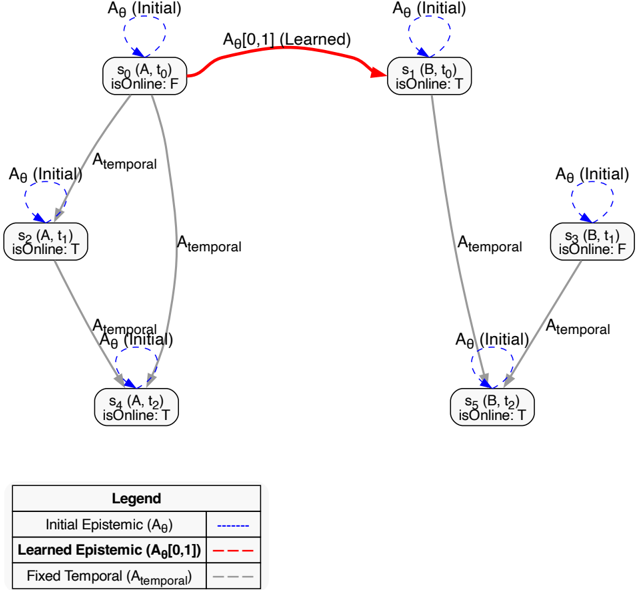<details> <summary>Image 10 Details</summary>  ### Visual Description ## Diagram: State Transition Model with Epistemic and Temporal Actions ### Overview The image is a directed graph representing a state machine with six distinct states ($s_0$ through $s_5$). The diagram illustrates how an agent or system transitions between these states based on three types of actions: Initial Epistemic, Learned Epistemic, and Fixed Temporal. Each state node contains a label indicating a variable pair (e.g., $(A, t_0)$) and a boolean status ("isOnline"). ### Components/Axes * **Nodes:** Six rectangular nodes labeled $s_0$ through $s_5$. * **Legend (Bottom-Left):** Defines the three edge types used in the diagram. * **Initial Epistemic ($A_\theta$):** Represented by blue dashed lines. * **Learned Epistemic ($A_\theta[0,1]$):** Represented by red dashed lines (Note: The diagram uses solid red lines). * **Fixed Temporal ($A_{temporal}$):** Represented by grey dashed lines (Note: The diagram uses solid grey lines). ### Detailed Analysis #### Node Definitions Each node contains a state identifier, a variable pair, and an "isOnline" status: | Node | Variable Pair | isOnline Status | | :--- | :--- | :--- | | $s_0$ | $(A, t_0)$ | F (False) | | $s_1$ | $(B, t_0)$ | T (True) | | $s_2$ | $(A, t_1)$ | T (True) | | $s_3$ | $(B, t_1)$ | F (False) | | $s_4$ | $(A, t_2)$ | T (True) | | $s_5$ | $(B, t_2)$ | T (True) | #### Edge/Transition Analysis * **Initial Epistemic ($A_\theta$):** Every node ($s_0$ through $s_5$) features a self-looping blue dashed arrow labeled "$A_\theta$ (Initial)". This indicates a persistent internal state maintenance or epistemic action available at every state. * **Learned Epistemic ($A_\theta[0,1]$):** A single red solid arrow connects $s_0$ to $s_1$. This represents a specific "learned" transition that is only available from $s_0$. * **Fixed Temporal ($A_{temporal}$):** Grey solid arrows represent the progression of time or fixed temporal transitions: * $s_0 \rightarrow s_2$ * $s_0 \rightarrow s_4$ * $s_1 \rightarrow s_5$ * $s_3 \rightarrow s_5$ *Note on Discrepancy:* While the legend specifies dashed lines for "Learned Epistemic" and "Fixed Temporal" actions, the actual diagram uses solid lines for these connections. ### Key Observations * **State Bifurcation:** The states are grouped by variable $A$ ($s_0, s_2, s_4$) and variable $B$ ($s_1, s_3, s_5$). * **Temporal Progression:** The temporal transitions generally move from $t_0$ to $t_1$ and $t_2$. * **Connectivity:** $s_0$ is the most connected node, acting as a source for both temporal transitions and the unique learned transition. $s_5$ acts as a sink for temporal transitions from both $s_1$ and $s_3$. * **Online Status:** The "isOnline" status is False only for $s_0$ and $s_3$. All other states ($s_1, s_2, s_4, s_5$) are "isOnline: T". ### Interpretation This diagram appears to model a reinforcement learning or automated planning environment. 1. **Learning Mechanism:** The "Learned Epistemic" transition ($A_\theta[0,1]$) from $s_0$ to $s_1$ suggests that the system starts in an offline state ($s_0$) and, through a learned action, can transition to an online state ($s_1$). 2. **Temporal Constraints:** The "Fixed Temporal" actions ($A_{temporal}$) represent the natural progression of the system over time ($t_0 \rightarrow t_1 \rightarrow t_2$). The fact that $s_0$ can transition to both $s_2$ and $s_4$ suggests that the system can skip temporal steps or that multiple temporal paths exist from the initial state. 3. **Epistemic Stability:** The ubiquitous $A_\theta$ (Initial) self-loops suggest that the agent can perform "epistemic" actions (likely gathering information or updating beliefs) without changing the underlying state variables ($A/B$ or $t_0/t_1/t_2$). 4. **System Logic:** The system demonstrates that while the agent can be "offline" ($s_0, s_3$), it has pathways to reach an "online" state ($s_1, s_2, s_4, s_5$) either through learning ($s_0 \rightarrow s_1$) or through temporal progression ($s_0 \rightarrow s_2$). </details> ## A.6.3 FINAL LEARNED MATRIX The resulting A θ matrix demonstrates the learned link from s 0 to s 1 , with other weights remaining unchanged from the initial 'siloed' identity matrix. Table 8: Final Learned Epistemic Accessibility ( A θ ) | | s 0 | s 1 | s 2 | s 3 | s 4 | s 5 | |---------------|-----------|-----------|-----------|-----------|-----------|-----------| | | (A, t 0 ) | (B, t 0 ) | (A, t 1 ) | (B, t 1 ) | (A, t 2 ) | (B, t 2 ) | | s 0 (A, t 0 ) | 1.00 | 0.99 | 0.00 | 0.00 | 0.00 | 0.00 | | s 1 (B, t 0 ) | 0.00 | 1.00 | 0.00 | 0.00 | 0.00 | 0.00 | | s 2 (A, t 1 ) | 0.00 | 0.00 | 1.00 | 0.00 | 0.00 | 0.00 | | s 3 (B, t 1 ) | 0.00 | 0.00 | 0.00 | 1.00 | 0.00 | 0.00 | | s 4 (A, t 2 ) | 0.00 | 0.00 | 0.00 | 0.00 | 1.00 | 0.00 | | s 5 (B, t 2 ) | 0.00 | 0.00 | 0.00 | 0.00 | 0.00 | 1.00 | ## A.6.4 QUANTITATIVE EVALUATION Post-training, the model's logical consistency was evaluated: - Epistemic Logic (at s 0 ): The training axiom ♢ epistemic ( isOnline )[ s 0 ] evaluated to True (Bounds: [0.99, 0.99]), satisfying the constraint. The related formula K ( isOnline )[ s 0 ] (soft-min) correctly evaluated to False (Bounds: [0.00, 0.00]), as Agent A now saw both its own False (0.0) state and Agent B's True (1.0) state, making the proposition possible, but not necessary ('known'). - Temporal Logic: Using the fixed R temporal , G ( isOnline )[ s 0 ] (soft-min) evaluated to False (Bounds: [0.00, 0.00]) because 'isOnline' is False at s 0 and s 3 . F ( isOnline )[ s 0 ] (soft-max) evaluated to True (Bounds: [1.00, 1.00]) because s 0 can 'see' s 1 , where 'isOnline' is True. G ( isOnline )[ s 4 ] evaluated to a fuzzy True (Bounds: [0.86, 0.86]) as the only states visible from s 4 are s 4 and s 5 , where 'isOnline' is True in both. - Composite Logic (at s 0 ): The nested operator K ( G ( isOnline ))[ s 0 ] was evaluated. The inner G ( isOnline ) formula first produced a truth vector for all 6 states: '[0.00, 0.00, 0.00, 0.00, 0.86, 0.86]'. The outer K operator then used the learned A θ at s 0 to compute: soft-min ((1 -A θ [0 , 0]) + G [ s 0 ] , (1 -A θ [0 , 1]) + G [ s 1 ] , ... ) ≈ soft-min ((1 -1 . 00) + 0 . 00 , (1 -0 . 99) + 0 . 00 , ... ) ≈ 0 . 0 . The formula correctly evaluated to False (Bounds: [0.00, 0.00]). - Generalization Check (at s 2 ): We checked K ( isOnline ) at s 2 (Agent A, t 1 ) to ensure its isolation was not corrupted. The model correctly evaluated it to True (Bounds: [0.89, 0.89]), as s 2 (where 'isOnline' is True) only sees itself ( A θ [2 , 2] ≈ 1 . 0 ). This confirmed the training for s 0 was localized. ## A.7 CASE STUDY IN REAL DIPLOMACY GAMES: LEARNING EPISTEMIC TRUST This appendix details the self-supervised pipeline used to extract latent trust networks from raw Diplomacy game logs. The framework utilizes a differentiable architecture to minimize the logical contradiction between an agent's messages and their ground-truth orders. ## A.7.1 DATA PROCESSING AND GROUND TRUTH The pipeline converts raw game JSON logs into logical training instances of ( Context , Ground Truth ) . Action Extraction (Ground Truth) The system parses the 'orders' object for each phase using regular expressions to identify the Unit Type, Origin, and Destination (e.g., 'F KIE - DEN'). To ground these actions into relational logic, the system queries the game state to determine territory ownership. - Hostile Action: If an agent orders a move into a territory currently owned by another player (e.g., Germany moves to London, owned by England, note that ownership of cities is specified in file too), the Ground Truth proposition P ( AttackGER → ENG ) is set to True (1.0). This serves as the falsifying consequent for the consistency check if trust was assumed. - Cooperative Action: Moves that support another agent or target neutral territories agreed upon in text are implicitly treated as consistent with cooperation. Message Encoding (Context) We extract all private messages exchanged in a given phase and group them by directed dyad (Sender → Recipient). The text is encoded using the all-MiniLM-L6v2 sentence transformer ( d = 384 ). To generate a fixed-size input for the accessibility network, we compute the mean embedding of all messages in the exchange. ## A.7.2 NEURAL ARCHITECTURE AND LOSS The MLNN architecture consists of a learnable accessibility head and a static differentiable logic layer. Accessibility Head ( A θ ) The accessibility relation is parameterized as a Feed-Forward Network consisting of two linear layers with ReLU activations (Linear(384, 128) → ReLU → Linear(128, 64) → ReLU → Linear(64, 1)). The output logit is passed through a sigmoid activation to produce ``` <doc> { "phase": "S190IM", "messages": [ { "sender": "ENGLAND", "recipient": "GERMANY", "message": "hey Germany! Do you wanna open to Den and then bounce Russia in Swe?" }, { "sender": "GERMANY", "recipient": "ENGLAND", "message": "okay, that's what I have in" } ] } orders: [ "GERMANY": [ "F KIE - DEN", // Fleet moves from "A MUN - RUH", // Army moves fleet "A BER - KIE", // Army moves fleet ], "ENGLAND": [ "F LON - NTH", "F EDI - NWG", "A LVF - EDI" ] } Figure 10: Grounded Input Example with ground-truth actions (where 'F' </doc> ``` Figure 10: Grounded Input Example (Diplomacy): Training instances couple negotiation history with ground-truth actions (where 'F' denotes Fleet and 'A' denotes Army). In this example from Game 433761 Bakhtin et al. (2022), Germany's execution of the move 'F KIE - DEN' physically fulfills the verbal agreement with England. This alignment satisfies the consistency axiom □ ( Message → Action ) , minimizing the contradiction loss and reinforcing the learnable epistemic accessibility weight A GER → ENG. the final trust weight A ij ∈ [0 , 1] . We initialize the bias term to a negative value (-2.0) to encode a prior of distrust. Consistency Loss Calculation The model evaluates the modal formula □ ( Intent → Action ) . Using the differentiable implication I ( a, b ) = 1 -a + ab , the necessity operator calculates the degree to which the action supports the intent given the trust level. The total loss is a weighted sum of the contradiction loss and a sparsity regularization term: $$1 1 = 1 - 1 1$$ where λ sparsity = 0 . 05 encourages the model to find the minimal trust structure required to explain the data. Training Details The model was trained for 400 epochs using the Adam optimizer with a learning rate of 0.01. We employed a temperature parameter τ = 0 . 1 for the softmin/softmax operators to control the sharpness of the logical aggregation. ## A.8 CASINO EXPERIMENT DETAILS Data Processing and Schema We utilized the CaSiNo dataset Chawla et al. (2021), which consists of 1,030 negotiation dialogues. Unlike the Diplomacy dataset, CaSiNo provides rich metadata regarding the participants' private utility functions (e.g., whether they prioritize Food, Water, or Firewood). We mapped these qualitative preferences to numeric ground-truth values: 'Low' → 0 . 0 , 'Medium' → 0 . 5 , and 'High' → 1 . 0 . To enable the MLNN to reason about consistency, we implemented a heuristic claim parser that estimates the agent's public stance from their utterance text. The parser scans for markers of high need (e.g., 'need', 'vital', 'my') to assign a claim value of 1 . 0 , and markers of concession (e.g., 'you take', 'don't need') for a claim value of 0 . 0 . Architecture and Hyperparameters The MLNN architecture for this task mirrors the Diplomacy setup but operates on single utterances rather than aggregated phase messages. - Embedding: 'all-MiniLM-L6-v2' (frozen). - Trust Head: Linear(384, 64) → ReLU → Linear(64, 1) → Sigmoid. - Optimizer: Adam, Learning Rate = 0 . 005 . - Training: 150 Epochs, Batch Size = 32. Seed = 42. - Loss: β = 0.2 (see Equation 3). Qualitative Analysis of Deception The model's performance relies on identifying linguistic overjustification. Below are additional examples of deceptive utterances (where the agent claimed high need for a low-priority item) that the model correctly assigned 0 . 0 trust to. Table 9: Qualitative examples of deceptive claims assigned 0 . 0 Trust by the MLNN. | Deceptive Utterance | Trust | |--------------------------------------------------------------------------------------------------------|---------| | 'I am ok with that if i get two waters, just incase i have to put out the fire :)' | 0 | | 'I am not going to give you all the water. I am not backing down on this. What if our fire gets out of | 0 | | 'Well I didn't bring any with me so I really need two. I am willing to give you 2 waters.:)' | 0 | | 'okay how many waters do you need?' | 0 | | 'two waters please my bad for the wording' | 0 | ## B NOTATION Table 10: Notation Summary used throughout the paper. | Symbol | Definition | |----------|-----------------------------------------------------------------| | W | A finite set of possible worlds. | | T | A finite set of discrete time steps. | | S | The set of spacetime states, S = W × T . | | p,ϕ | Atomic propositions and logical formulae. | | [ L,U ] | Lower and upper truth bounds for a formula, [ L,U ] ⊆ [0 , 1] . | | R | A crisp (binary) accessibility relation, R ⊆ W × W . | | A θ | A learnable, neurally parameterized accessibility matrix. | | ˜ A | The masked accessibility matrix used for aggregation. | | □ , ♢ | The modal operators for necessity and possibility. | | K a ϕ | Epistemic necessity operator: 'Agent a knows ϕ '. | | Gϕ,Fϕ | Temporal necessity/possibility: 'Globally ϕ ', 'Finally ϕ '. | | τ | Temperature parameter for soft-min/soft-max operators. | | β | Hyperparameter weighting the contradiction loss. | | L task | Task-specific loss (e.g., cross-entropy). | | L contra | Loss penalizing states where L > U . |