# Encoder-Free Knowledge-Graph Reasoning with LLMs via Hyperdimensional Path Retrieval
**Authors**:
- Calvin Yeung Mohsen Imani (University of California, Irvine)
Abstract
Recent progress in large language models (LLMs) has made knowledge-grounded reasoning increasingly practical, yet KG-based QA systems often pay a steep price in efficiency and transparency. In typical pipelines, symbolic paths are scored by neural encoders or repeatedly re-ranked by multiple LLM calls, which inflates latency and GPU cost and makes the decision process hard to audit. We introduce PathHD, an encoder-free framework for knowledge-graph reasoning that couples hyperdimensional computing (HDC) with a single LLM call per query. Given a query, PathHD represents relation paths as block-diagonal GHRR hypervectors, retrieves candidate paths using a calibrated blockwise cosine similarity with Top- $K$ pruning, and then performs a one-shot LLM adjudication that outputs the final answer together with supporting, citeable paths. The design is enabled by three technical components: (i) an order-sensitive, non-commutative binding operator for composing multi-hop paths, (ii) a robust similarity calibration that stabilizes hypervector retrieval, and (iii) an adjudication stage that preserves interpretability while avoiding per-path LLM scoring. Across WebQSP, CWQ, and GrailQA, PathHD matches or improves Hits@1 compared to strong neural baselines while using only one LLM call per query, reduces end-to-end latency by 40-60%, and lowers GPU memory by 3-5 $×$ due to encoder-free retrieval. Overall, the results suggest that carefully engineered HDC path representations can serve as an effective substrate for efficient and faithful KG-LLM reasoning, achieving a strong accuracy-efficiency-interpretability trade-off.
1 Introduction
Large Language Models (LLMs) have rapidly advanced reasoning over both text and structured knowledge. Typical pipelines follow a retrieve–then–reason pattern: they first surface evidence (documents, triples, or relation paths), then synthesize an answer using a generator or a verifier [21, 32, 46, 43, 47]. In knowledge-graph question answering (KGQA), this often becomes path-based reasoning: systems construct candidate relation paths that connect the topic entities to potential answers and pick the most plausible ones for final prediction [38, 17, 15, 16, 25]. While these approaches obtain strong accuracy on WebQSP, CWQ, and GrailQA, they typically depend on heavy neural encoders (e.g., Transformers or GNNs) or repeated LLM calls to rank paths, which makes them slow and expensive at inference time, especially when many candidates must be examined.
<details>
<summary>x1.png Details</summary>
### Visual Description
## Diagram: Two Major Pain Points in KG-LLM Reasoning
### Overview
This diagram illustrates two key challenges in Knowledge Graph (KG) and Large Language Model (LLM) reasoning. The diagram is split into two main sections: a left side demonstrating a reasoning failure with a KG, and a right side illustrating the process of LLM-based path scoring. The diagram uses nodes, edges, and visual cues (checkmarks, crosses) to represent relationships and outcomes.
### Components/Axes
The diagram consists of the following components:
* **Nodes:** Represent entities like "SolarCity", "Tesla", "Elon Musk", "SpaceX", "Renewable Energy", "SolarEdge", "LLM", "Candidate Path Generator", "Best Path".
* **Edges:** Represent relationships between entities, labeled with phrases like "acquired_by", "founded_by", "CEO_of", "operates_in", "related_to".
* **Input Query:** "Which company acquired SolarCity?"
* **Outcome:** "Incorrect reasoning despite access to KG (selected path mismatches the query relation)."
* **Issues (Left Side):**
* "Mismatch between query relation ("acquired_by") and used path (Founder/CEO)."
* "Hallucination due to non-faithful reasoning over KG."
* **LLM-based Path Scoring Methods:** A description stating "A class of prior methods: per-path LLM evaluation".
* **Issue (Right Side):**
* "Repeated LLM calls per candidate path – high latency & cost."
* "Evaluation is sequential / hard to parallelize."
* "Scalability degrades as candidate count increases."
### Detailed Analysis or Content Details
**Left Side: Reasoning Failure**
* **SolarCity** is connected to **Tesla** via an edge labeled "acquired_by" with a checkmark, indicating the correct path.
* **SolarCity** is also connected to **Elon Musk** via "founded_by".
* **Elon Musk** is connected to **SpaceX** via "CEO_of".
* **SolarCity** is connected to **Renewable Energy** via "operates_in".
* **SolarCity** is connected to **SolarEdge** via "related_to" with a cross, indicating an incorrect path.
* The "Outcome" states "Incorrect reasoning despite access to KG (selected path mismatches the query relation)."
* The "Issues" listed are:
* "Mismatch between query relation ("acquired_by") and used path (Founder/CEO)."
* "Hallucination due to non-faithful reasoning over KG."
**Right Side: LLM-based Path Scoring**
* A "Candidate Path Generator" produces multiple paths.
* Each "Path" (Path #1, Path #2, etc.) is fed into an "LLM".
* The LLM assigns a "Score" (s1, s2, etc.) to each path.
* The path with the highest score is selected as the "Best Path".
* The "Issue" listed are:
* "Repeated LLM calls per candidate path – high latency & cost."
* "Evaluation is sequential / hard to parallelize."
* "Scalability degrades as candidate count increases."
### Key Observations
* The diagram highlights a discrepancy between the correct relationship ("acquired_by") and the paths the system explores (Founder/CEO, related_to).
* The LLM-based path scoring method, while attempting to evaluate multiple paths, suffers from scalability and efficiency issues due to repeated LLM calls.
* The use of checkmarks and crosses clearly indicates the correctness or incorrectness of different reasoning paths.
* The diagram visually represents the concept of "hallucination" in LLMs, where the model generates incorrect information despite having access to a knowledge graph.
### Interpretation
The diagram demonstrates the challenges of integrating Knowledge Graphs with Large Language Models for reasoning tasks. While KGs provide structured knowledge, LLMs can struggle to correctly utilize this knowledge, leading to inaccurate conclusions. The diagram suggests that the LLM may be prioritizing paths based on superficial similarities or biases, rather than the specific query relation. The right side of the diagram illustrates a common approach to mitigate this issue – scoring multiple paths – but also reveals its limitations in terms of computational cost and scalability. The diagram implies a need for more robust and efficient methods for aligning LLM reasoning with the underlying knowledge graph structure, and for addressing the issue of "hallucination" in LLM-based systems. The diagram is a visual explanation of a technical problem, not a presentation of data.
</details>
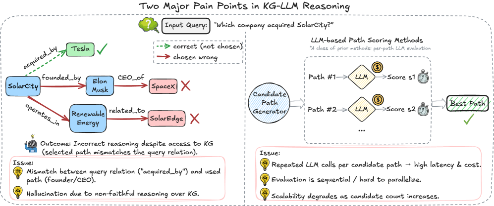
Figure 1: Two major pain points in KG-LLM reasoning. Left: A path-based KGQA system selects a candidate path whose relation sequence does not match the query relation (“acquired_by”), leading to an incorrect answer even though the KG contains the correct evidence. Right: LLM-based scoring evaluates each candidate path in a separate LLM call, which is sequential, hard to parallelize, and incurs high latency and token cost as the candidate set grows.
Figure ˜ 1 highlights two recurring issues in KG–LLM reasoning. ❶ Path–query mismatch: Order-insensitive encodings, weak directionality, and noisy similarity often favor superficially related yet misaligned paths, blurring the question’s intended relation. ❷ Per-candidate LLM scoring: Many systems score candidates sequentially, so latency and token cost grow roughly linearly with set size; batching is limited by context/API, and repeated calls introduce instability, yet models can still over-weight long irrelevant chains, hallucinate edges, or flip relation direction. Most practical pipelines first detect a topic entity, enumerate $10\!\sim\!100$ length- $1$ – $4$ paths, then score each with a neural model or LLM, sending top paths to a final step [38, 25, 16]. This hard-codes two inefficiencies: (i) neural scoring dominates latency (fresh encoding/prompt per candidate), and (ii) loose path semantics (commutative/direction-insensitive encoders conflate founded_by $\!→$ CEO_of with its reverse), which compounds on compositional/long-hop questions.
Hyperdimensional Computing (HDC) offers a different lens: represent symbols as long, nearly-orthogonal hypervectors and manipulate structure with algebraic operations such as binding and bundling [18, 31]. HDC has been used for fast associative memory, robust retrieval, and lightweight reasoning because its core operations are elementwise or blockwise and parallelize extremely well on modern hardware [7]. Encodings tend to be noise-tolerant and compositional; similarity is computed by simple cosine or dot product; and both storage and computation scale linearly with dimensionality. Crucially for KGQA, HDC supports order-sensitive composition when the binding operator is non-commutative, allowing a path like $r_{1}\!→ r_{2}\!→ r_{3}$ to be distinguished from its permutations while remaining a single fixed-length vector. This makes HDC a promising substrate for ranking many candidate paths without invoking a neural model for each one.
Motivated by these advantages, we introduce PathHD (Hyper D imensional Path Retrieval), a lightweight retrieval-and-reason framework for efficient KGQA with LLMs. First, we map every relation to a block-diagonal unitary representation and encode a candidate path by non-commutative Generalized Holographic Reduced Representation (GHRR) binding [48]; this preserves order and direction in a single hypervector. In parallel, we encode the query into the same space to obtain a query hypervector. Second, we score all candidates via cosine similarity to the query hypervector and keep only the top- $K$ paths with a simple, parallel Top- $K$ selection. Finally, instead of per-candidate LLM calls, we make one LLM call that sees the question plus these top- $K$ paths (verbalized), and it outputs the answer along with cited supporting paths. In effect, PathHD addresses both pain points in Figure ˜ 1: order-aware binding reduces path–query mismatch, and vector-space scoring eliminates per-path LLM evaluation, cutting latency and token cost.
Our contributions are as follows:
- A fast, order-aware retriever for KG paths. We present PathHD, which uses GHRR-based, non-commutative binding to encode relation sequences into hypervectors and ranks candidates with plain cosine similarity, without learned neural encoders or per-path prompts. This design keeps a symbolic structure while enabling fully parallel scoring with $\mathcal{O}(Nd)$ complexity.
- An efficient one-shot reasoning stage. PathHD replaces many LLM scoring calls with a single LLM adjudication over the top- $K$ paths. This decouples retrieval from generation, lowers token usage, and improves wall-clock latency while remaining interpretable: the model cites the supporting path(s) it used.
- Extensive validation and operator study. On WebQSP, CWQ, and GrailQA, PathHD achieves competitive Hits@1 and F1 with markedly lower inference cost. An ablation on binding operators shows that our block-diagonal (GHRR) binding outperforms commutative binding and circular convolution, and additional studies analyze the impact of top- $K$ pruning and latency–accuracy trade-offs.
Overall, PathHD shows that carefully designed hyperdimensional representations can act as an encoder-free, training-free path scorer inside KG-based LLM reasoning systems, preserving competitive answer accuracy while substantially improving inference efficiency and providing explicit path-level rationales.
2 Method
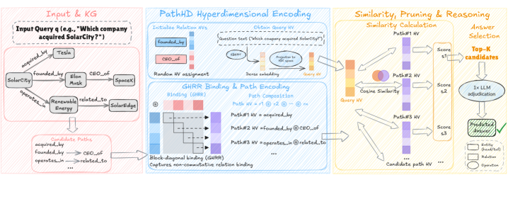
The proposed PathHD follows a Plan $→$ Encode $→$ Retrieve $→$ Reason pipeline (Figure ˜ 2). (i) We first generate or select relation plans that describe how an answer can be reached (schema enumeration optionally refined by a light prompt). (ii) Each plan is mapped to a hypervector via a non-commutative GHRR binding so that order and direction are preserved. (iii) We compute a blockwise cosine similarity in the hypervector space and apply Top- $K$ pruning. (iv) Finally, a single LLM call produces the answer with path-based explanations. This design keeps the heavy lifting in cheap vector operations, delegating semantic adjudication to one-shot LLM reasoning.
2.1 Problem Setup & Notation
Given a question $q$ , a knowledge graph (KG) $\mathcal{G}$ , and a set of relation schemas $\mathcal{Z}$ , the goal is to predict an answer $a$ . Formally, we write $\mathcal{G}=(\mathcal{V},\mathcal{E},\mathcal{R})$ , where $\mathcal{V}$ is the set of entities, $\mathcal{R}$ is the set of relation types, and $\mathcal{E}⊂eq\mathcal{V}×\mathcal{R}×\mathcal{V}$ is the set of directed edges $(e,r,e^{\prime})$ . We denote entities by $e∈\mathcal{V}$ and relations by $r∈\mathcal{R}$ . A relation schema $z∈\mathcal{Z}$ is a sequence of relation types $z=(r_{1},...,r_{\ell})$ . Instantiating a schema $z$ on $\mathcal{G}$ yields concrete KG paths of the form $(e_{0},r_{1},e_{1},...,r_{\ell},e_{\ell})$ such that $(e_{i-1},r_{i},e_{i})∈\mathcal{E}$ for all $i$ . For a given question $q$ , we denote by $\mathcal{P}(q)$ the set of candidate paths instantiated from schemas in $\mathcal{Z}$ and by $N=|\mathcal{P}(q)|$ its size. We write $d$ for the dimensionality of the hypervectors used to represent relations and paths.
A key challenge is to efficiently locate a small set of plausible paths for $q$ from this large candidate pool, and then let an LLM reason over only those paths. A summary of the notation throughout the paper can be found in Appendix ˜ A.
<details>
<summary>x2.png Details</summary>
### Visual Description
\n
## Diagram: Knowledge Graph Reasoning Pipeline
### Overview
This diagram illustrates a pipeline for knowledge graph reasoning, taking a natural language query as input and producing a predicted answer. The pipeline consists of three main stages: Input & Knowledge Graph, PathHD Hyperdimensional Encoding, and Similarity, Pruning & Reasoning. The diagram visually represents the flow of information and the key operations performed at each stage.
### Components/Axes
The diagram is divided into three main sections, visually separated by background colors:
* **Input & KG (Leftmost, Pink Background):** Represents the input query and the knowledge graph.
* **PathHD Hyperdimensional Encoding (Center, Blue Background):** Details the process of encoding paths from the knowledge graph into hyperdimensional vectors.
* **Similarity, Pruning & Reasoning (Rightmost, Yellow Background):** Shows how similarity is calculated between the query vector and path vectors, followed by pruning and answer selection.
Key elements include:
* **Entities:** Represented by rounded rectangles (e.g., "SolarCity", "Tesla", "Elon Musk", "SpaceX", "Renewable Energy", "SolarEdge").
* **Relations:** Represented by arrows connecting entities (e.g., "acquired\_by", "founded\_by", "CEO\_of", "operates\_by", "related\_to").
* **Vectors:** Represented by vertical purple bars labeled "HV" (HyperVector).
* **Operations:** Represented by boxes with text (e.g., "Initialize Relation HVs", "Obtain Query HV", "Dense embedding", "Path Composition", "Cosine Similarity", "1x LLM adjudication").
* **Legend:** Located at the bottom-right, defining the shapes used for entities, relations, and operations.
### Detailed Analysis or Content Details
**1. Input & KG:**
* **Input Query:** "Which company acquired SolarCity?"
* **Knowledge Graph:** Shows relationships between entities:
* SolarCity `acquired_by` Tesla
* Tesla `founded_by` Elon Musk
* Elon Musk `CEO_of` SpaceX
* Renewable Energy `operates_by` SolarEdge
* SolarEdge `related_to` Renewable Energy
* **Candidate Paths:** Lists possible paths: `acquired_by`, `founded_by`, `CEO_of`, `related_to`.
**2. PathHD Hyperdimensional Encoding:**
* **Initialize Relation HVs:** Initializes hypervectors for each relation (e.g., `founded_by`, `CEO_of`).
* **Obtain Query HV:** Converts the input query text ("Which company acquired SolarCity?") into a query hypervector. This involves a "Projection to HV" step.
* **Random HV assignment:** Assigns random hypervectors.
* **GHRR Binding & Path Encoding:**
* **Binding (GHRR):** A visual representation of a matrix with pink and white blocks, labeled "Non-diagonal binding (GHRR) Captures non-commutative relation binding".
* **Path Composition:** Combines relation hypervectors to create path hypervectors. Examples:
* Path #1 HV: `acquired_by`
* Path #2 HV: `founded_by @ CEO_of`
* Path #3 HV: `operates_by @ related_to`
**3. Similarity, Pruning & Reasoning:**
* **Similarity Calculation:** Calculates the cosine similarity between the query hypervector and each path hypervector.
* Path #1 HV: Score s1
* Path #2 HV: Score s2
* Path #3 HV: Score s3
* **Top-K candidates:** Selects the top K candidate paths based on their similarity scores.
* **1x LLM adjudication:** Uses a Large Language Model (LLM) to adjudicate the top candidates and select the final predicted answer.
* **Predicted Answer:** A green checkmark indicates the predicted answer.
**Legend:**
* Rounded Rectangle: Entity (e.g., SolarCity)
* Arrow: Relation (e.g., acquired\_by)
* Rectangle: Operation (e.g., Path Composition)
### Key Observations
* The pipeline leverages hyperdimensional computing to represent entities and relations as vectors.
* The GHRR binding mechanism is highlighted as a key component for capturing non-commutative relation binding.
* An LLM is used as a final step to refine the answer selection process.
* The diagram emphasizes the flow of information from the input query through the knowledge graph encoding and reasoning stages to the final prediction.
### Interpretation
This diagram demonstrates a sophisticated approach to knowledge graph reasoning that combines hyperdimensional computing with LLM adjudication. The use of hypervectors allows for efficient representation and comparison of paths within the knowledge graph. The GHRR binding mechanism suggests an attempt to address the challenges of representing complex relationships where the order of relations matters. The final LLM step likely serves to disambiguate results and provide a more natural language-based answer. The pipeline appears designed to handle complex queries that require reasoning over multiple hops in the knowledge graph. The diagram is a high-level overview and doesn't provide specific details about the implementation of each component (e.g., the dimensionality of the hypervectors, the architecture of the LLM). The diagram is a conceptual illustration of a system, not a presentation of data.
</details>
Figure 2: Overview of PathHD: a Plan $→$ Encode $→$ Retrieve $→$ Reason pipeline. A schema-based planner first generates relation plans over the KG; PathHD encodes these plans and instantiates candidate paths into order-aware GHRR hypervectors, ranks candidates with blockwise cosine similarity and Top- $K$ selection, and then issues a single LLM adjudication call to answer with cited paths, with most computation handled by vector operations and modest LLM use.
2.2 Hypervector Initialization
We work in a Generalized Holographic Reduced Representations (GHRR) space. Each atomic symbol $x$ (relation or, optionally, entity) is assigned a $d$ -dimensional hypervector $\mathbf{v}_{x}\!∈\!\mathbb{C}^{d}$ constructed as a block vector of unitary matrices:
$$
\mathbf{v}_{x}\;=\;[A^{(x)}_{1};\dots;A^{(x)}_{D}],\qquad A^{(x)}_{j}\in\mathrm{U}(m),\;\;d=Dm^{2}. \tag{1}
$$
In practice, we sample each block from a simple unitary family for efficiency, e.g.,
$$
A^{(x)}_{j}=\operatorname{diag}\!\big(e^{i\phi_{j,1}},\ldots,e^{i\phi_{j,m}}\big),\qquad\phi_{j,\ell}\sim\operatorname{Unif}[0,2\pi),
$$
or a random Householder product. Blocks are $\ell_{2}$ -normalized so that all hypervectors have unit norm. This initialization yields near-orthogonality among symbols, which concentrates with dimension (cf. Prop. 1). Hypervectors are sampled once and kept fixed; the retriever itself has no learned parameters.
Query hypervector.
For a question $q$ , we obtain a query hypervector in two ways, depending on the planning route used in Section ˜ 2: (i) plan-based —encode the selected relation plan $z_{q}=(r_{1},...,r_{\ell})$ using the same GHRR binding as paths (see Eq. equation 3); or (ii) text-projection —embed $q$ with a sentence encoder (e.g., SBERT) to $\mathbf{h}_{q}∈\mathbb{R}^{d_{t}}$ and project it to the HDC space using a fixed random linear map $P∈\mathbb{R}^{d× d_{t}}$ , then block-normalize:
$$
\mathbf{v}_{q}\;=\;\mathcal{N}_{\text{block}}\!\big(P\,\mathbf{h}_{q}\big). \tag{2}
$$
Both choices produce a query hypervector compatible with GHRR scoring. Unless otherwise specified, we use the plan-based encoding in all main experiments, and report the text-projection variant only in ablations (Section ˜ J.2).
2.3 GHRR Binding and Path Encoding
A GHRR hypervector is a block vector $\mathbf{H}=[A_{1};...;A_{D}]$ with $A_{j}∈\mathrm{U}(m)$ . Given two hypervectors $\mathbf{X}=[X_{1};...;X_{D}]$ and $\mathbf{Y}=[Y_{1};...;Y_{D}]$ , we define the block-wise binding operator $\mathbin{\raisebox{0.86108pt}{\scalebox{0.9}{$\circledast$}}}$ and the encoding of a length- $\ell$ relation path $z=(r_{1},...,r_{\ell})$ by:
$$
\mathbf{v}_{z}\;=\;\mathbf{v}_{r_{1}}\mathbin{\raisebox{0.86108pt}{\scalebox{0.9}{$\circledast$}}}\mathbf{v}_{r_{2}}\mathbin{\raisebox{0.86108pt}{\scalebox{0.9}{$\circledast$}}}\cdots\mathbin{\raisebox{0.86108pt}{\scalebox{0.9}{$\circledast$}}}\mathbf{v}_{r_{\ell}},\qquad\mathbf{X}\mathbin{\raisebox{0.86108pt}{\scalebox{0.9}{$\circledast$}}}\mathbf{Y}=[X_{1}Y_{1};\dots;X_{D}Y_{D}], \tag{3}
$$
followed by block-wise normalization to unit norm. Binding is applied left-to-right along the path, and because the matrix multiplication is non-commutative ( $X_{j}Y_{j}≠ Y_{j}X_{j}$ ), the encoding preserves the order and directionality of relations, which are critical for multi-hop KG reasoning.
Properties and choice of binding operator.
Although PathHD only uses forward binding for retrieval, GHRR also supports approximate unbinding: for $Z_{j}=X_{j}Y_{j}$ with unitary blocks, we have $X_{j}≈ Z_{j}Y_{j}^{\ast}$ and $Y_{j}≈ X_{j}^{\ast}Z_{j}$ . This property enables inspection of the contribution of individual relations in a composed path and underpins our path-level rationales.
Classical HDC bindings (XOR, element-wise multiplication, circular convolution) are commutative, which collapses $r_{1}{→}r_{2}$ and $r_{2}{→}r_{1}$ to similar codes and hurts directional reasoning. GHRR is non-commutative, invertible at the block level, and offers higher representational capacity via unitary blocks, leading to better discrimination between paths of the same multiset but different order. We empirically validate this choice in the ablation study (Table ˜ 3), where GHRR consistently outperforms commutative bindings. Additional background on binding operations is provided in Appendix ˜ K.
2.4 Query & Candidate Path Construction
We obtain a query plan $z_{q}$ via schema-based enumeration on the relation-schema graph (depth $≤ L_{\max}$ ). In all main experiments reported in Section ˜ 3, this planning stage is purely symbolic: we do not invoke any LLM beyond the single final reasoning call in Section ˜ 2.6. The query hypervector $\mathbf{v}_{q}$ is then constructed from the selected plan $z_{q}$ using the plan-based encoding described above (Eq. equation 3 or, for text projection, Eq. equation 2).
Given a query plan, candidate paths $\mathcal{Z}$ are instantiated from the KG either by matching plan templates to existing edges or by a constrained BFS with beam width $B$ , both of which yield symbolic paths. These paths are then deterministically encoded into hypervectors and scored by our HDC module (Sec. 2.5). An optional lightweight prompt-based refinement of schema plans is described in the appendix as an extension; it is not used in our main experiments and does not change the single-call nature of the system.
2.5 HD Retrieval: Blockwise Similarity and Top- $K$
Let $\langle A,B\rangle_{F}:=\mathrm{tr}(A^{\ast}B)$ be the Frobenius inner product. Given two GHRR hypervectors $\mathbf{X}=[X_{j}]_{j=1}^{D}$ and $\mathbf{Y}=[Y_{j}]_{j=1}^{D}$ , we define the blockwise cosine similarity
$$
\mathrm{sim}(\mathbf{X},\mathbf{Y})=\frac{1}{D}\sum_{j=1}^{D}\,\frac{\Re\,\langle X_{j},\,Y_{j}\rangle_{F}}{\|X_{j}\|_{F}\,\|Y_{j}\|_{F}}. \tag{4}
$$
For each candidate $z∈\mathcal{Z}$ we compute $\mathrm{sim}(\mathbf{v}_{q},\mathbf{v}_{z})$ and (optionally) apply a calibrated score
$$
s(z)\;=\;\mathrm{sim}(\mathbf{v}_{q},\mathbf{v}_{z})\;+\;\alpha\,\mathrm{IDF}(z)\;-\;\beta\,\lambda^{|z|}, \tag{5}
$$
where $\mathrm{IDF}(z)$ is a simple inverse-frequency weight on relation schemas. Let $\text{schema}(z)$ denote the relation schema of path $z$ and $\mathrm{freq}(\text{schema}(z))$ be the number of training questions whose candidate sets contain at least one path with the same schema. With $N_{\text{train}}$ the total number of training questions, we define:
$$
\mathrm{IDF}(z)=\log\!\left(1+\frac{N_{\text{train}}}{1+\mathrm{freq}(\text{schema}(z))}\right). \tag{6}
$$
Thus, frequent schemas (large $\mathrm{freq}(\text{schema}(z))$ ) receive a smaller bonus, while rare schemas receive a larger one. All similarity scores and calibrated scores can be computed fully in parallel over candidates, with overall cost $\mathcal{O}(|\mathcal{Z}|d)$ .
2.6 One-shot Reasoning with Retrieved Paths
Putting the pieces together, PathHD turns a question into (i) a schema-level plan $z_{q}$ , (ii) a set of candidate paths ranked in hypervector space, and (iii) a single LLM call that adjudicates among the top-ranked candidates.
We linearize the Top- $K$ paths into concise natural-language statements and issue a single LLM call with a minimal, citation-style prompt (see Table ˜ 8 from Appendix ˜ C). The prompt lists the question and the numbered paths, and requires the model to return a short answer, the index(es) of supporting path(s), and a 1-2 sentence rationale. This one-shot format constrains reasoning to the provided evidence, resolves near-ties and direction errors, and keeps LLM usage minimal.
2.7 Theoretical & Complexity Analysis
| Method | Candidate Path Gen. | Scoring | Reasoning |
| --- | --- | --- | --- |
| StructGPT [15] | ✓ | ✓ | ✓ |
| FiDeLiS [37] | ✓ | ✗ | ✓ |
| ToG [39] | ✓ | ✓ | ✓ |
| GoG [44] | ✓ | ✓ | ✓ |
| KG-Agent [16] | ✓ | ✓ | ✓ |
| RoG [25] | ✓ | ✗ | ✓ |
| PathHD | ✗ | ✗ | ✓ ( $1$ call) |
Table 1: LLM usage across pipeline stages. A checkmark indicates that the method uses an LLM in that stage. Candidate Path Gen.: using an LLM to propose or expand relation paths; Scoring: using an LLM to score or rank candidates (non-LLM similarity or graph heuristics count as “no”); Reasoning: using an LLM to produce the final answer from the retrieved paths. PathHD uses a single LLM call only in the final reasoning stage.
We briefly characterize the behavior of random GHRR hypervectors and the computational cost of PathHD.
**Proposition 1 (Near-orthogonality and distractor bound)**
*Let $\{\mathbf{v}_{r}\}$ be i.i.d. GHRR hypervectors with zero-mean, unit Frobenius-norm blocks. For a query path $z_{q}$ and any distractor $z≠ z_{q}$ encoded via non-commutative binding, the cosine similarity $X=\mathrm{sim}(\mathbf{v}_{z_{q}},\mathbf{v}_{z})$ (Equation ˜ 4) satisfies, for any $\epsilon>0$ ,
$$
\Pr\!\left(|X|\geq\epsilon\right)\leq 2\exp\!\left(-c\,d\,\epsilon^{2}\right), \tag{7}
$$
for an absolute constant $c>0$ depending only on the sub-Gaussian proxy of entries.*
* Proof sketch*
Each block inner product $\langle X_{j},Y_{j}\rangle_{F}$ is a sum of products of independent sub-Gaussian variables (closed under products for the bounded/phase variables used by GHRR). After normalization, the average in Equation ˜ 4 is a mean-zero sub-Gaussian average over $d$ degrees of freedom, so a standard Bernstein/Hoeffding tail bound applies. Details are deferred to Appendix ˜ E. ∎
**Corollary 1 (Capacity with union bound)**
*Let $\mathcal{M}$ be a collection of $M$ distractor paths scored against a fixed query. With probability at least $1-\delta$ ,
$$
\max_{z\in\mathcal{M}}\mathrm{sim}(\mathbf{v}_{z_{q}},\mathbf{v}_{z})\leq\epsilon\quad\text{whenever}\quad d\;\geq\;\frac{1}{c\,\epsilon^{2}}\,\log\!\frac{2M}{\delta}. \tag{8}
$$*
Thus, the probability of a false match under random hypervectors decays exponentially with the dimension $d$ , and the required dimension scales as $d=\mathcal{O}(\epsilon^{-2}\log M)$ for a target error tolerance $\epsilon$ .
Complexity comparison with neural retrievers.
Let $N$ be the number of candidates, $d$ the embedding dimension, and $L$ the number of encoder layers used by a neural retriever. A typical neural encoder (e.g., Transformer-based path encoder as in RoG) incurs $\mathcal{O}(NLd^{2})$ cost for encoding and scoring. In contrast, PathHD forms each path vector by $|z|\!-\!1$ block multiplications plus one similarity in Equation ˜ 4, i.e., $\mathcal{O}(|z|d)+\mathcal{O}(d)$ per candidate, giving a total of $\mathcal{O}(Nd)$ and an $\mathcal{O}(Ld)$ -fold reduction in leading order.
Beyond the $\mathcal{O}(Nd)$ vs. $\mathcal{O}(NLd^{2})$ compute gap, end-to-end latency is dominated by the number of LLM calls. Table ˜ 1 contrasts pipeline stages across methods: unlike prior agents that query an LLM for candidate path generation and sometimes for scoring, PathHD defers a single LLM call to the final reasoning step. This design reduces both latency and API cost; empirical results in Section ˜ 3.3 confirm the shorter response times.
3 Experiments
We evaluate PathHD against state-of-the-art baselines on reasoning accuracy, measure efficiency with a focus on end-to-end latency, and conduct module-wise ablations followed by illustrative case studies.
3.1 Datasets, Baselines, and Setup
We evaluate on three standard multi-hop KGQA benchmarks: WebQuestionsSP (WebQSP) [49], Complex WebQuestions (CWQ) [40], and GrailQA [9], all grounded in Freebase [2]. These datasets span increasing reasoning complexity (roughly 2-4 hops): WebQSP features simpler single-turn queries, CWQ adds compositional and constraint-based questions, and GrailQA stresses generalization across i.i.d., compositional, and zero-shot splits. Our study is therefore scoped to Freebase-style KGQA, extending PathHD to domain-specific KGs are left for future work.
We compare against four families of methods: embedding-based, retrieval-augmented, pure LLMs (no external KG), and LLM+KG hybrids. All results are reported on dev (IID) splits under a unified Freebase evaluation protocol using the official Hits@1 and F1 scripts, so that numbers are directly comparable across systems. Unless otherwise noted, PathHD uses the schema-based planner from Section ˜ 2.4 (no LLM calls during planning), the plan-based query hypervector in Equation ˜ 3, and a single LLM adjudication call as described in Section ˜ 2.6, with all LLMs and sentence encoders used off the shelf (no fine-tuning). Detailed dataset statistics, baseline lists, model choices, and additional training-free hyperparameters are provided in Appendices ˜ G, H and I.
3.2 Reasoning Performance Comparison
| | | WebQSP | CWQ | GrailQA (F1) | | | |
| --- | --- | --- | --- | --- | --- | --- | --- |
| Type | Methods | Hits@ $1$ | F1 | Hits@ $1$ | F1 | Overall | IID |
| KV-Mem [27] | $46.7$ | $34.5$ | $18.4$ | $15.7$ | $-$ | $-$ | |
| EmbedKGQA [35] | $66.6$ | $-$ | $45.9$ | $-$ | $-$ | $-$ | |
| NSM [10] | $68.7$ | $62.8$ | $47.6$ | $42.4$ | $-$ | $-$ | |
| Embedding | TransferNet [36] | $71.4$ | $-$ | $48.6$ | $-$ | $-$ | $-$ |
| GraftNet [38] | $66.4$ | $60.4$ | $36.8$ | $32.7$ | $-$ | $-$ | |
| SR+NSM [50] | $68.9$ | $64.1$ | $50.2$ | $47.1$ | $-$ | $-$ | |
| SR+NSM+E2E [50] | $69.5$ | $64.1$ | $49.3$ | $46.3$ | $-$ | $-$ | |
| Retrieval | UniKGQA [17] | $77.2$ | $72.2$ | $51.2$ | $49.1$ | $-$ | $-$ |
| ChatGPT [30] | $67.4$ | $59.3$ | $47.5$ | $43.2$ | $25.3$ | $19.6$ | |
| Davinci - 003 [30] | $70.8$ | $63.9$ | $51.4$ | $47.6$ | $30.1$ | $23.5$ | |
| Pure LLMs | GPT - 4 [1] | $73.2$ | $62.3$ | $55.6$ | $49.9$ | $31.7$ | $25.0$ |
| StructGPT [15] | $72.6$ | $63.7$ | $54.3$ | $49.6$ | $54.6$ | $70.4$ | |
| ROG [25] | $\underline{85.7}$ | $70.8$ | $62.6$ | $56.2$ | $-$ | $-$ | |
| Think-on-Graph [39] | $81.8$ | $76.0$ | $68.5$ | $60.2$ | $-$ | $-$ | |
| GoG [44] | $84.4$ | $-$ | $\mathbf{75.2}$ | $-$ | $-$ | $-$ | |
| KG-Agent [16] | $83.3$ | $\mathbf{81.0}$ | $\underline{72.2}$ | $\mathbf{69.8}$ | $\underline{86.1}$ | $\underline{92.0}$ | |
| FiDeLiS [37] | $84.4$ | $78.3$ | $71.5$ | $64.3$ | $-$ | $-$ | |
| LLMs + KG | PathHD | $\mathbf{86.2}$ | $\underline{78.6}$ | $71.5$ | $\underline{65.8}$ | $\mathbf{86.7}$ | $\mathbf{92.4}$ |
Table 2: Comparison on Freebase-based KGQA. Our method PathHD follows exactly the same protocol. “–” indicates that the metric was not reported by the original papers under the Freebase+official-script setting. We bold the best and underline the second-best score for each metric/column.
We evaluate under a unified Freebase protocol with the official Hits@1 / F1 scripts on WebQSP, CWQ, and GrailQA (dev, IID); results are in Table ˜ 2. Baselines cover classic KGQA (embedding/retrieval), recent LLM+KG systems, and pure LLMs (no KG grounding). Our PathHD uses hyperdimensional scoring with GHRR, Top- $K$ pruning, and a single LLM adjudication step.
Key observations are as follows. Obs.❶ SOTA on WebQSP/GrailQA; competitive on CWQ. PathHD attains best WebQSP Hits@1 ( $86.2$ ) and best GrailQA F1 (Overall/IID $86.7/92.4$ ), while staying strong on CWQ (Hits@1 $71.5$ , F1 $65.8$ ), close to the top LLM+KG systems (e.g., GoG $75.2$ Hits@1; KG-Agent $69.8$ F1). Obs.❷ One-shot adjudication rivals multi-step agents. Compared to RoG ( $\sim$ 12 calls) and Think-on-Graph/GoG/KG-Agent ( $3$ – $8$ calls), PathHD matches or exceeds accuracy on WebQSP/GrailQA and remains competitive on CWQ with just one LLM call, which reduces error compounding and focuses the LLM on a high-quality shortlist. Obs.❸ Pure LLMs lag without KG grounding. Zero/few-shot GPT-4 or ChatGPT underperform LLM+KG systems, e.g., on CWQ GPT-4 Hits@1 $55.6$ vs. PathHD $71.5$ . Obs.❹ Classic embedding/retrieval trails modern LLM+KG. KV-Mem, NSM, SR+NSM rank subgraphs well but lack a flexible language component for composing multi-hop constraints, yielding consistently lower scores.
Candidate enumeration strategy. Before turning to efficiency (Section ˜ 3.3), we briefly clarify how candidate paths are enumerated, since this affects both accuracy and cost. In our current implementation, we use a deterministic BFS-style enumeration of relation paths, controlled by the maximum depth $L_{\max}$ and beam width $B$ . This choice is (i) simple and efficient, (ii) guarantees coverage of all type-consistent paths up to length $L_{\max}$ under clear complexity bounds, and (iii) makes it easy to compare against prior KGQA baselines that also rely on BFS-like expansion. In practice, we choose $L_{\max}$ and $B$ to achieve high coverage of gold answer paths while keeping candidate set sizes comparable to RoG and KG-Agent. More sophisticated, adaptive enumeration strategies (e.g., letting the HDC scores or the LLM guide, which relations to expand next) are an interesting extension, but orthogonal to our core contribution.
3.3 Efficiency and Cost Analysis
<details>
<summary>x3.png Details</summary>
### Visual Description
\n
## Scatter Plot: Hits@1 vs. Latency on WebQSP
### Overview
This scatter plot visualizes the relationship between Hits@1 (percentage) on the WebQSP dataset and per-query latency (in seconds, median) for various models. The models are categorized into three families: Embedding, Pure LLM, and LLMs+KG. Each point represents a model, and its position indicates its performance on both metrics.
### Components/Axes
* **X-axis:** Hits@1 on WebQSP (%) - Ranges from approximately 50% to 90%.
* **Y-axis:** Per-query latency 10^x (seconds, median) - Ranges from approximately -0.25 to 1.50. The axis is on a logarithmic scale.
* **Legend (Top-Left):**
* **Embedding (Blue Circles):** Represents models using embedding techniques.
* **Pure LLM (Blue Squares):** Represents models that are purely Large Language Models.
* **LLMs+KG (Black Triangles):** Represents models that combine Large Language Models with Knowledge Graphs.
### Detailed Analysis
The plot contains data points for the following models, categorized by their family:
**Embedding (Blue Circles):**
* **KV-Mem:** Located at approximately (52%, -0.25).
* **NSM:** Located at approximately (71%, -0.25).
**Pure LLM (Blue Squares):**
* **ChatGPT (1 call):** Located at approximately (69%, 0.25).
* **StructGPT:** Located at approximately (74%, 0.50).
* **GPT-4 (1 call):** Located at approximately (76%, 0.50).
* **UniKGQA:** Located at approximately (78%, 0.55).
**LLMs+KG (Black Triangles):**
* **Think-on-Graph:** Located at approximately (78%, 0.80).
* **KG-Agent:** Located at approximately (82%, 0.90).
* **GoG:** Located at approximately (83%, 1.00).
* **DeLIS:** Located at approximately (84%, 1.10).
* **RoG:** Located at approximately (89%, 1.40).
* **PathHD:** Located at approximately (81%, 0.30).
**Trends:**
* **Embedding Models:** Generally exhibit low latency and moderate Hits@1 scores.
* **Pure LLM Models:** Show a moderate increase in both latency and Hits@1 compared to Embedding models.
* **LLMs+KG Models:** Demonstrate the highest latency but also the highest Hits@1 scores. There is a clear upward trend within this category – as Hits@1 increases, so does latency.
### Key Observations
* There's a clear trade-off between latency and accuracy (Hits@1). Models with higher accuracy tend to have higher latency.
* LLMs+KG models consistently outperform the other two families in terms of Hits@1, but at the cost of increased latency.
* KV-Mem and NSM have significantly lower latency than all other models, but also lower Hits@1 scores.
* RoG has the highest latency and Hits@1.
### Interpretation
The data suggests that incorporating Knowledge Graphs (KGs) into LLMs significantly improves performance on the WebQSP dataset, as measured by Hits@1. However, this improvement comes at the expense of increased latency. Embedding models offer the fastest response times but sacrifice accuracy. The choice of model depends on the specific application requirements – whether speed or accuracy is more critical.
The upward trend within the LLMs+KG category indicates that more complex KG integration strategies (or larger KGs) lead to better performance but also higher computational costs. The positioning of models like RoG and DeLIS suggests they represent more sophisticated KG-enhanced LLMs.
The separation of the three families highlights the different approaches to question answering and their respective strengths and weaknesses. This plot provides valuable insights for selecting the appropriate model for a given task, considering the trade-off between accuracy and speed.
</details>
<details>
<summary>x4.png Details</summary>
### Visual Description
\n
## Scatter Plot: Hits@1 vs. Latency on CWQ
### Overview
This scatter plot visualizes the relationship between Hits@1 (percentage) on the CWQ dataset and per-query latency (in seconds, median) for various models. The models are categorized into three families: Embedding, Pure LLM, and LLMs+KG. Each point represents a model, with its position determined by its performance on the two metrics. The shape of the marker indicates the model family.
### Components/Axes
* **X-axis:** Hits@1 on CWQ (%) - Ranges from approximately 20% to 75%.
* **Y-axis:** Per-query latency 10^x (seconds, median) - Ranges from approximately -0.3 to 1.5. The axis is on a logarithmic scale.
* **Legend:** Located in the top-left corner.
* **Embedding (Blue Circles):** Represents models utilizing embedding techniques.
* **Pure LLM (Blue Squares):** Represents models that are purely Large Language Models.
* **LLMs+KG (Red Triangles):** Represents models combining Large Language Models with Knowledge Graphs.
* **Data Points:** Each point represents a specific model. The points are colored according to their family (as defined in the legend).
### Detailed Analysis
Here's a breakdown of the data points, categorized by family and with approximate values:
**Embedding (Blue Circles):**
* **KV-Mem:** Approximately (22%, -0.25).
* **NSM:** Approximately (42%, -0.3).
**Pure LLM (Blue Squares):**
* **ChatGPT (1 call):** Approximately (47%, 0.35).
* **GPT-4 (1 call):** Approximately (50%, 0.5).
* **UniKQA:** Approximately (48%, 0.45).
* **StructGPT:** Approximately (51%, 0.55).
**LLMs+KG (Red Triangles):**
* **RoQ:** Approximately (62%, 1.3).
* **KG-Agent:** Approximately (68%, 0.9).
* **fiDELIS:** Approximately (69%, 0.8).
* **Think-on-Graph:** Approximately (65%, 1.0).
* **PathHD:** Approximately (72%, 0.3).
**Trends:**
* **Embedding Models:** Generally exhibit low latency and moderate Hits@1 scores.
* **Pure LLM Models:** Show a moderate trade-off between latency and Hits@1.
* **LLMs+KG Models:** Tend to have higher latency but also achieve higher Hits@1 scores. There is a positive correlation between latency and Hits@1 within this family.
### Key Observations
* There's a clear separation between the three model families.
* LLMs+KG models consistently outperform the other two families in terms of Hits@1, but at the cost of increased latency.
* KV-Mem and NSM have the lowest latency, but also the lowest Hits@1 scores.
* PathHD is an outlier within the LLMs+KG family, exhibiting relatively low latency compared to its Hits@1 score.
* RoQ has the highest latency.
### Interpretation
The data suggests a trade-off between accuracy (Hits@1) and speed (latency) in question answering systems. Embedding-based models prioritize speed, while LLMs+KG models prioritize accuracy. Pure LLM models offer a balance between the two. The use of Knowledge Graphs appears to significantly improve accuracy, but introduces computational overhead, resulting in higher latency.
The positioning of PathHD suggests it may be a more efficient LLM+KG model, achieving a relatively high Hits@1 score with lower latency than its counterparts. This could be due to optimizations in its architecture or implementation.
The logarithmic scale on the Y-axis emphasizes the impact of latency, particularly for models with higher latency values. The large difference in latency between models like KV-Mem and RoQ is visually amplified by this scaling.
The scatter plot provides valuable insights for selecting the appropriate model for a given application, depending on the relative importance of accuracy and speed.
</details>
<details>
<summary>x5.png Details</summary>
### Visual Description
\n
## Scatter Plot: Hits@1 vs. Latency on GrailQA
### Overview
This scatter plot visualizes the relationship between Hits@1 on GrailQA (percentage) and per-query latency (seconds, median) for several different models. The models are categorized by their "Family" – Embedding, Pure LLM, and LLMs+KG.
### Components/Axes
* **X-axis:** Hits@1 on GrailQA (%). Scale ranges from approximately 20% to 90%.
* **Y-axis:** Per-query latency 10x (seconds, median). Scale ranges from approximately 0.25 seconds to 1.0 seconds.
* **Legend:** Located in the top-left corner, categorizes models by "Family":
* **Embedding (Blue Circles):** Represents models using embedding techniques.
* **Pure LLM (Blue Squares):** Represents models that are purely Large Language Models.
* **LLMs+KG (Orange Triangles):** Represents models combining Large Language Models with Knowledge Graphs.
* **Data Points:** Each point represents a specific model, plotted based on its Hits@1 and latency.
### Detailed Analysis
Here's a breakdown of the data points, referencing the legend colors for verification:
* **KG-Agent (Orange Triangle):** Located at approximately (85%, 1.0 seconds).
* **PathHD (Orange Triangle):** Located at approximately (90%, 0.95 seconds).
* **StructGPT (Blue Square):** Located at approximately (55%, 0.5 seconds).
* **GPT-4 (1 call) (Yellow Square):** Located at approximately (30%, 0.63 seconds).
* **ChatGPT (1 call) (Yellow Square):** Located at approximately (20%, 0.3 seconds).
### Key Observations
* **Trade-off:** There appears to be a general trade-off between Hits@1 and latency. Models with higher Hits@1 tend to have higher latency.
* **KG-based Models:** The LLMs+KG models (KG-Agent and PathHD) achieve the highest Hits@1 scores but also exhibit the highest latency.
* **Pure LLM:** StructGPT has a moderate Hits@1 score and moderate latency.
* **Embedding Models:** No embedding models are present in the plot.
* **GPT-4 and ChatGPT:** These models have the lowest Hits@1 scores but also the lowest latency.
### Interpretation
The data suggests that incorporating Knowledge Graphs (KGs) into LLMs can significantly improve the accuracy (Hits@1) of responses on the GrailQA dataset, but at the cost of increased processing time (latency). The models leveraging KGs (KG-Agent and PathHD) demonstrate this trade-off clearly.
The positioning of GPT-4 and ChatGPT indicates they prioritize speed over accuracy in this context. StructGPT represents a middle ground, offering a balance between the two.
The absence of embedding models from the plot is notable. It could indicate that these models were not tested in this specific evaluation, or that their performance was not competitive with the other approaches.
The "1 call" annotation next to GPT-4 and ChatGPT suggests that the latency measurements are for a single API call, which might not fully represent the end-to-end latency of a more complex application. The use of "median" latency suggests an attempt to mitigate the impact of outliers, but further analysis of the latency distribution would be beneficial.
</details>
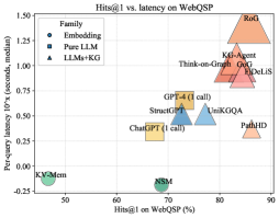
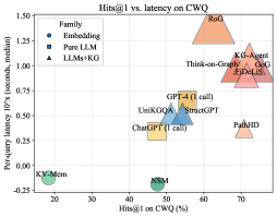
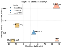
Figure 3: Visualization of performance and latency. The x-axis is Hits@ $1$ (%), the y-axis is per-query latency in seconds (median, log scale). Bubble size indicates the average number of LLM calls; marker shape denotes the method family. PathHD gives strong accuracy with lower latency than multi-call LLMs+KG baselines.
We assess end-to-end cost via a Hits@1–latency bubble plot (Figure ˜ 3) and a lollipop latency chart (Figure ˜ 6). In Figure ˜ 3, $x$ = Hits@1, $y$ = median per-query latency (log-scale); bubble size = average #LLM calls; marker shape = method family. All latencies are measured under a common hardware and LLM-backend setup to enable fair relative comparison. Latencies in Figure ˜ 6 follow a shared protocol: in our implementation, each LLM call takes on the order of a few seconds, whereas non-LLM vector/graph operations are typically within $0.3$ – $0.8$ s. PathHD uses vector-space scoring with Top- $K$ pruning and a single LLM decision; RoG uses beam search ( $B{=}3$ , depth $≤$ dataset hops). A factor breakdown (#calls, depth $d$ , beam $b$ , tools) appears in Table ˜ 10 (Section ˜ I.1).
Key observations are: Obs.❶ Near-Pareto across datasets. With comparable accuracy to multi-call LLM+KG systems (Think-on-Graph/GoG/KG-Agent), PathHD achieves markedly lower latency due to its single-call design and compact post-pruning candidate set. Obs.❷ Latency is dominated by #LLM calls. Methods with 3–8 calls (agent loops) or $≈ d× b$ calls (beam search) sit higher in Figure ˜ 3 and show longer whiskers in Figure ˜ 6; PathHD avoids intermediate planning/scoring overhead. Obs.❸ Moderate pruning improves cost–accuracy. Shrinking the pool before adjudication lowers latency without hurting Hits@1, especially on CWQ, where paths are longer. Obs.❹ Pure LLMs are fast but underpowered. Single-call GPT-4/ChatGPT has similar latency to our final decision yet notably lower accuracy, underscoring the importance of structured retrieval and path scoring.
3.4 Ablation Study
We analyze the contribution of each module/operation in PathHD. Our operation study covers: (1) Path composition operator, (2) Single-LLM adjudicator, and (3) Top- $K$ pruning.
| Operator | WebQSP | CWQ |
| --- | --- | --- |
| XOR / bipolar product | 83.9 | 68.8 |
| Element-wise product (Real-valued) | 84.4 | 69.2 |
| Comm. bind | 84.7 | 69.6 |
| FHRR | 84.9 | 70.0 |
| HRR | 85.1 | 70.2 |
| GHRR | 86.2 | 71.5 |
Table 3: Effect of the path–composition operator. GHRR yields the best performance.
Which path–composition operator works best?
We isolate relation binding by fixing retrieval, scoring, pruning, and the single LLM step, and only swapping the encoder’s path–composition operator. We compare six options (defs. in Appendix ˜ K): (i) XOR/bipolar and (ii) real-valued element-wise products, both fully commutative; (iii) a stronger commutative mix of binary/bipolar; (iv) FHRR (phasors) and (v) HRR (circular convolution), efficient yet effectively commutative; and (vi) our block-diagonal GHRR with unitary blocks, non-commutative and order-preserving. Paths of length $1$ – $4$ use identical dimension/normalization. As in Table ˜ 3, commutative binds lag, HRR/FHRR give modest gains, and GHRR yields the best Hits@1 on WebQSP and CWQ by reliably separating founded_by $→$ CEO_of from its reverse.
| Final step | WebQSP | CWQ |
| --- | --- | --- |
| Vector-only | 85.4 | 70.8 |
| Vector $→$ 1 $×$ LLM | 86.2 | 71.5 |
Table 4: Ablation on the final decision maker. Passing pruned candidates and scores to a single LLM for adjudication yields consistent gains over vector-only selection.
Do we need a final single LLM adjudicator?
We test whether a lightweight LLM judgment helps beyond pure vector scoring. Vector-only selects the top path by cosine similarity; Vector $→$ 1 $×$ LLM instead forwards the pruned top- $K$ paths (with scores and end entities) to a single LLM using a short fixed template (no tools/planning) to choose the answer without long chains of thought. As shown in Table ˜ 4, Vector $→$ 1 $×$ LLM consistently outperforms Vector-only on both datasets, especially when the top two paths are near-tied or a high-scoring path has a subtle type mismatch; a single adjudication pass resolves such cases at negligible extra cost.
| Pruning | Hits@ $1$ (WebQSP) | Lat. | Hits@ $1$ (CWQ) | Lat. |
| --- | --- | --- | --- | --- |
| No-prune | 85.8 | 2.42s | 70.7 | 2.45s |
| $K{=}2$ | 86.0 | 1.98s | 71.2 | 2.00s |
| $K{=}3$ | 86.2 | 1.92s | 71.5 | 1.94s |
| $K{=}5$ | 86.1 | 2.05s | 71.4 | 2.06s |
Table 5: Impact of top- $K$ pruning before the final LLM. Small sets (K=2–3) retain or slightly improve accuracy while reducing latency. We adopt $K{=}3$ by default.
What is the effect of top- $K$ pruning before the final step?
Finally, we study how many candidates should be kept for the last decision. We vary the number of paths passed to the final LLM among $K\!∈\!\{2,3,5\}$ and also include a No-prune variant that sends all retrieved paths. Retrieval and scoring are fixed; latency is the median per query (lower is better). As shown in Table ˜ 5, $K{=}3$ achieves the best Hits@ $1$ on both WebQSP and CWQ with the lowest latency, while $K{=}2$ is a close second and yields the largest latency drop. In contrast, No-prune maintains maximal recall but increases latency and often introduces near-duplicate/noisy paths that can blur the final decision. We therefore adopt $K{=}3$ as the default.
<details>
<summary>x6.png Details</summary>
### Visual Description
## Chart: Hypervector Dimension vs. F1 Score for Different Datasets
### Overview
This image presents three line charts, each displaying the relationship between Hypervector Dimension and F1 Score (%) for three different datasets: WebQSP, CWQ, and GrailQA. Each chart shows how the F1 score changes as the hypervector dimension increases.
### Components/Axes
* **X-axis (all charts):** Hypervector Dimension, with markers at 3/512, 1024, 2048, 3072, 4096, 6144, and 8192.
* **Y-axis (all charts):** F1 Score (%), ranging from approximately 76.5% to 87.0%.
* **Chart 1 (left):** WebQSP dataset.
* **Chart 2 (center):** CWQ dataset.
* **Chart 3 (right):** GrailQA dataset.
* **Line Color (all charts):** Blue.
### Detailed Analysis
**Chart 1: WebQSP**
The line representing WebQSP slopes upward from a value of approximately 76.5% at a hypervector dimension of 3/512 to a peak of approximately 78.8% at 4096. It then declines slightly to approximately 77.8% at 8192.
* 3/512: ~76.5%
* 1024: ~77.8%
* 2048: ~78.4%
* 3072: ~78.7%
* 4096: ~78.8%
* 6144: ~78.2%
* 8192: ~77.8%
**Chart 2: CWQ**
The line representing CWQ starts at approximately 64.2% at a hypervector dimension of 3/512, increases to a peak of approximately 66.3% at 6144, and then decreases to approximately 65.8% at 8192.
* 3/512: ~64.2%
* 1024: ~65.0%
* 2048: ~65.5%
* 3072: ~65.9%
* 4096: ~66.1%
* 6144: ~66.3%
* 8192: ~65.8%
**Chart 3: GrailQA**
The line representing GrailQA begins at approximately 85.8% at a hypervector dimension of 3/512, rises to a peak of approximately 86.7% at 4096, and then declines to approximately 86.3% at 8192.
* 3/512: ~85.8%
* 1024: ~86.1%
* 2048: ~86.3%
* 3072: ~86.5%
* 4096: ~86.7%
* 6144: ~86.5%
* 8192: ~86.3%
### Key Observations
* All three datasets show an initial increase in F1 score as the hypervector dimension increases.
* The F1 scores generally plateau or slightly decrease after reaching a certain hypervector dimension.
* GrailQA consistently exhibits the highest F1 scores across all hypervector dimensions.
* CWQ consistently exhibits the lowest F1 scores across all hypervector dimensions.
* The peak F1 score for each dataset occurs at different hypervector dimensions (WebQSP: 4096, CWQ: 6144, GrailQA: 4096).
### Interpretation
The charts demonstrate the impact of hypervector dimension on the performance (measured by F1 score) of models trained on different datasets. The initial increase in F1 score suggests that increasing the hypervector dimension allows the model to capture more complex relationships within the data. However, the plateau or decline in F1 score at higher dimensions indicates that there is a point of diminishing returns, and potentially overfitting, where adding more dimensions does not further improve performance.
The differences in peak F1 scores and optimal hypervector dimensions across the datasets suggest that the optimal model configuration is dataset-dependent. GrailQA, with its consistently high F1 scores, may be a simpler or more structured dataset compared to WebQSP and CWQ. The fact that the optimal dimension varies suggests that the complexity of the relationships within each dataset differs. The diminishing returns observed in all three charts suggest that there is a trade-off between model complexity (hypervector dimension) and generalization performance.
</details>
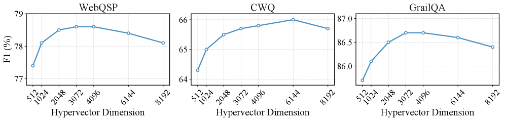
Figure 4: Hypervector dimension study. Each panel reports F1 (%) of PathHD on WebQSP, CWQ, and GrailQA as a function of the hypervector dimension. Overall, performance rises from $512$ to the mid-range and then tapers off: WebQSP and GrailQA peak around 3k–4k, while CWQ prefers a slightly larger size (6k), after which F1 decreases mildly.
3.5 Case Study
To better understand how our model performs step-by-step reasoning, we present two representative cases from the WebQSP dataset in Table ˜ 6. These cases highlight the effects of candidate path pruning and the contribution of LLM-based adjudication in improving answer accuracy. Case 1: Top- $K$ pruning preserves paths aligned with both film.film.music and actor cues; the vector-only scorer already picks the correct path, and a single LLM adjudication confirms Valentine’s Day, illustrating that pruning reduces cost while retaining high-coverage candidates. Case 2: A vector-only top path (film.film.edited_by) misses the actor constraint and yields a false positive, but adjudication over the pruned set, now including performance.actor, corrects to The Perks of Being a Wallflower, showing that LLM adjudication resolves compositional constraints beyond static similarity.
| Case 1: which movies featured Taylor Swift and music by John Debney | |
| --- | --- |
| Top-4 candidates | 1) film.film.music (0.2567) |
| 2) person.nationality $→$ film.film.country (0.2524) | |
| 3) performance.actor $→$ performance.film (0.2479) | |
| 4) people.person.languages $→$ film.film.language (0.2430) | |
| Top- $K$ after pruning (K=3) | film.film.music |
| person.nationality $→$ film.film.country | |
| performance.actor $→$ performance.film | |
| Vector-only (no LLM) | Pick film.film.music ✓ — directly targets the composer-to-film mapping; relevant for filtering by music. |
| 1 $×$ LLM adjudication | Rationale: “To find films with both Taylor Swift and music by John Debney, use actor-to-film and music-to-film relations. The chosen path targets the latter directly.” |
| Final Answer / GT | Valentine’s Day (predict) / Valentine’s Day ✓ |
| Case 2 : in which movies does Logan Lerman act in that was edited by Mary Jo Markey | |
| Top-4 candidates | 1) film.film.edited_by (0.2548) |
| 2) person.nationality $→$ film.film.country (0.2527) | |
| 3) performance.actor $→$ performance.film (0.2505) | |
| 4) award.award_winner.awards_won $→$ | |
| award.award_honor.honored_for (0.2420) | |
| Top- $K$ after pruning (K=3) | film.film.edited_by |
| person.nationality $→$ film.film.country | |
| performance.actor $→$ performance.film | |
| Vector-only (no LLM) | Pick film.film.edited_by ✗ — identifies edited films, but lacks actor constraint; leads to false positives. |
| 1 $×$ LLM adjudication | Rationale: “The question requires jointly filtering for actor and editor. While film.edited_by is relevant, combining it with performance.actor improves precision by ensuring Logan Lerman is in the cast.” |
| Final Answer / GT | Perks of Being a Wallflower (predict) / Perks of Being a Wallflower ✓ |
Table 6: Case studies on multi-hop reasoning over WebQSP. Top- $K$ pruning is applied before invoking LLM, reducing cost while retaining plausible candidates.
Discussion. As PathHD operates in a single-call, fixed-candidate regime, its performance ultimately depends on (i) the Top- $K$ retrieved paths covering at least one valid reasoning chain and (ii) the adjudication LLM correctly ranking these candidates. In practice, we mitigate this by using a relatively generous $K$ (e.g., $K=3$ ) and beam widths that yield high coverage of gold paths (see Section ˜ K.2), but extreme cases can still be challenging. Note that all LLM reasoning systems that first retrieve a Top- $K$ set of candidates will face the same challenge.
4 Related Work
4.1 LLM-based Reasoning
Large language models (LLMs) are now widely adopted across research and industry—powering generation, retrieval, and decision-support systems at scale [5, 28, 22, 23]. LLM-based Reasoning, such as GPT [33, 3], LLaMA [41], and PaLM [6], have demonstrated impressive capabilities in diverse reasoning tasks, ranging from natural language inference to multi-hop question answering [45]. A growing body of work focuses on enhancing the interpretability and reliability of LLM reasoning through symbolic path-based reasoning over structured knowledge sources [38, 4, 11]. For example, Wei et al. [43] proposed chain-of-thought prompting, which improves reasoning accuracy by encouraging explicit intermediate steps. Wang et al. [42] introduced self-consistency decoding, which aggregates multiple reasoning chains to improve robustness.
Knowledge graphs are widely deployed in real-world systems (e.g., web search, recommendation, biomedicine) and constitute an active research area for representation learning and reasoning [14, 52, 24, 51]. In the context of knowledge graphs, recent efforts have explored hybrid neural-symbolic approaches to combine the structural expressiveness of graph reasoning with the generative power of LLMs. Fan et al. [25] proposed Reasoning on Graphs (RoG), which first prompts LLMs to generate plausible symbolic relation paths and then retrieves and verifies these paths over knowledge graphs. Similarly, Khattab et al. [20] leveraged demonstration-based prompting to guide LLM reasoning grounded in external knowledge. Despite their interpretability benefits, these methods rely heavily on neural encoders for path matching, incurring substantial computational and memory overhead, which limits scalability to large KGs or real-time applications.
4.2 Hyperdimensional Computing (HDC)
HDC is an emerging computational paradigm inspired by the properties of high-dimensional representations in cognitive neuroscience [18, 19]. In HDC, information is represented as fixed-length high-dimensional vectors (hypervectors), and symbolic structures are manipulated through simple algebraic operations such as binding, bundling, and permutation [8]. These operations are inherently parallelizable and robust to noise, making HDC appealing for energy-efficient and low-latency computation.
HDC has been successfully applied in domains such as classification [34], biosignal processing [29], natural language understanding [26], and graph analytics [12]. For instance, Imani et al. [12] demonstrated that HDC can encode and process graph-structured data efficiently, enabling scalable similarity search and inference. Recent studies have also explored neuro-symbolic integrations, where HDC complements neural networks to achieve interpretable yet computationally efficient models [13, 34]. However, the potential of HDC in large-scale reasoning over knowledge graphs, particularly when combined with LLMs, remains underexplored. Our work bridges this gap by leveraging HDC as a drop-in replacement for neural path matchers in LLM-based reasoning frameworks, thereby achieving both scalability and interpretability.
Existing KG-LLM reasoning frameworks typically rely on learned neural encoders or multi-call agent pipelines to score candidate paths or subgraphs, often with Transformers, GNNs, or repeated LLM calls. In contrast, our work keeps the retrieval module entirely encoder-free and training-free: PathHD replaces neural path scorers with HDC-based hypervector encodings and similarity, while remaining compatible with standard KG-LLM agents. Our goal is thus not to introduce new VSA theory, but to show that such carefully designed HDC representations can replace learned neural scorers in KG-LLM systems while preserving accuracy and substantially improving latency, memory footprint, and interpretability.
5 Conclusion
In this work, we presented PathHD, an encoder-free and interpretable retrieval mechanism for path-based reasoning over knowledge graphs with LLMs. PathHD replaces neural path scorers with hyperdimensional Computing (HDC): relation paths are encoded into order-aware GHRR hypervectors, ranked via simple vector operations, and passed to a single LLM adjudication step that outputs answers together with cited supporting paths. This Plan $→$ Encode $→$ Retrieve $→$ Reason design removes the need for costly neural encoders in the retrieval module and shifts most computation into cheap, parallel hypervector operations. Experimental results on three standard Freebase-based KGQA benchmarks (WebQSP, CWQ, GrailQA) show that PathHD attains competitive Hits@1 and F1 while substantially reducing end-to-end latency and GPU memory usage, and produces faithful, path-grounded rationales that aid error analysis and controllability. Taken together, these findings indicate that carefully designed HDC representations are a practical substrate for efficient KG-LLM reasoning, offering a favorable accuracy-efficiency-interpretability trade-off. An important direction for future work is to apply CS to domain-specific graphs, such as UMLS and other biomedical or enterprise KGs, as well as to tasks beyond QA (e.g., fact checking or rule induction), and to explore how the HDC representations and retrieval pipeline can be adapted in these settings while retaining the same efficiency benefits.
Acknowledgements
This work was supported in part by the DARPA Young Faculty Award, the National Science Foundation (NSF) under Grants #2127780, #2319198, #2321840, #2312517, and #2235472, #2431561, the Semiconductor Research Corporation (SRC), the Office of Naval Research through the Young Investigator Program Award, and Grants #N00014-21-1-2225 and #N00014-22-1-2067, Army Research Office Grant #W911NF2410360. Additionally, support was provided by the Air Force Office of Scientific Research under Award #FA9550-22-1-0253, along with generous gifts from Xilinx and Cisco.
References
- [1] Josh Achiam, Steven Adler, Sandhini Agarwal, Lama Ahmad, Ilge Akkaya, Florencia Leoni Aleman, Diogo Almeida, Janko Altenschmidt, Sam Altman, Shyamal Anadkat, et al. Gpt-4 technical report. arXiv preprint arXiv:2303.08774, 2023.
- [2] Kurt Bollacker, Colin Evans, Praveen Paritosh, Tim Sturge, and Jamie Taylor. Freebase: a collaboratively created graph database for structuring human knowledge. In Proceedings of the 2008 ACM SIGMOD international conference on Management of data, pages 1247–1250, 2008.
- [3] Tom B Brown, Benjamin Mann, Nick Ryder, Melanie Subbiah, Jared Kaplan, Prafulla Dhariwal, Arvind Neelakantan, Pranav Shyam, Girish Sastry, Amanda Askell, et al. Language models are few-shot learners. In Advances in Neural Information Processing Systems (NeurIPS), volume 33, pages 1877–1901, 2020.
- [4] Shulin Cao, Jiaxin Shi, Liangming Pan, Lunyiu Nie, Yutong Xiang, Lei Hou, Juanzi Li, Bin He, and Hanwang Zhang. Kqa pro: A dataset with explicit compositional programs for complex question answering over knowledge base. In Proceedings of the 60th annual meeting of the Association for Computational Linguistics (volume 1: long papers), pages 6101–6119, 2022.
- [5] Yupeng Chang, Xu Wang, Jindong Wang, Yuan Wu, Linyi Yang, Kaijie Zhu, Hao Chen, Xiaoyuan Yi, Cunxiang Wang, Yidong Wang, et al. A survey on evaluation of large language models. ACM transactions on intelligent systems and technology, 15(3):1–45, 2024.
- [6] Aakanksha Chowdhery, Sharan Narang, Jacob Devlin, Maarten Bosma, Gaurav Mishra, Adam Roberts, Paul Barham, Hyung Won Chung, Charles Sutton, Sebastian Gehrmann, et al. Palm: Scaling language modeling with pathways. Journal of Machine Learning Research, 24(240):1–113, 2023.
- [7] E. Paxon Frady, Denis Kleyko, and Friedrich T. Sommer. Variable binding for sparse distributed representations: Theory and applications. Neural Computation, 33(9):2207–2248, 2021.
- [8] Ross W Gayler. Vector symbolic architectures answer jackendoff’s challenges for cognitive neuroscience. arXiv preprint cs/0412059, 2004.
- [9] Yu Gu, Sue Kase, Michelle Vanni, Brian Sadler, Percy Liang, Xifeng Yan, and Yu Su. Beyond iid: three levels of generalization for question answering on knowledge bases. In Proceedings of the web conference 2021, pages 3477–3488, 2021.
- [10] Gaole He, Yunshi Lan, Jing Jiang, Wayne Xin Zhao, and Ji-Rong Wen. Improving multi-hop knowledge base question answering by learning intermediate supervision signals. In Proceedings of the 14th ACM international conference on web search and data mining, pages 553–561, 2021.
- [11] Haotian Hu, Alex Jie Yang, Sanhong Deng, Dongbo Wang, and Min Song. Cotel-d3x: a chain-of-thought enhanced large language model for drug–drug interaction triplet extraction. Expert Systems with Applications, 273:126953, 2025.
- [12] Mohsen Imani, Yeseong Kim, Sadegh Riazi, John Messerly, Patric Liu, Farinaz Koushanfar, and Tajana Rosing. A framework for collaborative learning in secure high-dimensional space. In 2019 IEEE 12th International Conference on Cloud Computing (CLOUD), pages 435–446. IEEE, 2019.
- [13] Mohsen Imani, Justin Morris, Samuel Bosch, Helen Shu, Giovanni De Micheli, and Tajana Rosing. Adapthd: Adaptive efficient training for brain-inspired hyperdimensional computing. In 2019 IEEE Biomedical Circuits and Systems Conference (BioCAS), pages 1–4. IEEE, 2019.
- [14] Shaoxiong Ji, Shirui Pan, Erik Cambria, Pekka Marttinen, and Philip S Yu. A survey on knowledge graphs: Representation, acquisition, and applications. IEEE transactions on neural networks and learning systems, 33(2):494–514, 2021.
- [15] Jinhao Jiang, Kun Zhou, Zican Dong, Keming Ye, Wayne Xin Zhao, and Ji-Rong Wen. Structgpt: A general framework for large language model to reason over structured data. arXiv preprint arXiv:2305.09645, 2023.
- [16] Jinhao Jiang, Kun Zhou, Wayne Xin Zhao, Yang Song, Chen Zhu, Hengshu Zhu, and Ji-Rong Wen. Kg-agent: An efficient autonomous agent framework for complex reasoning over knowledge graph. arXiv preprint arXiv:2402.11163, 2024.
- [17] Jinhao Jiang, Kun Zhou, Wayne Xin Zhao, and Ji-Rong Wen. Unikgqa: Unified retrieval and reasoning for solving multi-hop question answering over knowledge graph. arXiv preprint arXiv:2212.00959, 2022.
- [18] Pentti Kanerva. Hyperdimensional computing: An introduction to computing in distributed representation with high-dimensional random vectors. Cognitive Computation, 1(2):139–159, 2009.
- [19] Pentti Kanerva et al. Fully distributed representation. PAT, 1(5):10000, 1997.
- [20] Omar Khattab, Keshav Santhanam, Xiang Lisa Li, David Hall, Percy Liang, Christopher Potts, and Matei Zaharia. Demonstrate-search-predict: Composing retrieval and language models for knowledge-intensive nlp. arXiv preprint arXiv:2212.14024, 2022.
- [21] Patrick Lewis, Ethan Perez, Aleksandra Piktus, Fabio Petroni, Vladimir Karpukhin, Naman Goyal, Heinrich Küttler, Mike Lewis, Wen-tau Yih, Tim Rocktäschel, et al. Retrieval-augmented generation for knowledge-intensive nlp. In NeurIPS, 2020.
- [22] Yezi Liu, Hanning Chen, Wenjun Huang, Yang Ni, and Mohsen Imani. Lune: Efficient llm unlearning via lora fine-tuning with negative examples. In Socially Responsible and Trustworthy Foundation Models at NeurIPS 2025.
- [23] Yezi Liu, Hanning Chen, Wenjun Huang, Yang Ni, and Mohsen Imani. Recover-to-forget: Gradient reconstruction from lora for efficient llm unlearning. In Socially Responsible and Trustworthy Foundation Models at NeurIPS 2025.
- [24] Yezi Liu, Qinggang Zhang, Mengnan Du, Xiao Huang, and Xia Hu. Error detection on knowledge graphs with triple embedding. In 2023 31st European Signal Processing Conference (EUSIPCO), pages 1604–1608. IEEE, 2023.
- [25] Linhao Luo, Yuan-Fang Li, Gholamreza Haffari, and Shirui Pan. Reasoning on graphs: Faithful and interpretable large language model reasoning. arXiv preprint arXiv:2310.01061, 2023.
- [26] Raghavender Maddali. Fusion of quantum-inspired ai and hyperdimensional computing for data engineering. Zenodo, doi, 10, 2023.
- [27] Alexander H. Miller, Adam Fisch, Jesse Dodge, Amir-Hossein Karimi, Antoine Bordes, and Jason Weston. Key-value memory networks for directly reading documents. CoRR, abs/1606.03126, 2016.
- [28] Shervin Minaee, Tomas Mikolov, Narjes Nikzad, Meysam Chenaghlu, Richard Socher, Xavier Amatriain, and Jianfeng Gao. Large language models: A survey. arXiv preprint arXiv:2402.06196, 2024.
- [29] Ali Moin, Alex Zhou, Abbas Rahimi, Ankita Menon, Simone Benatti, George Alexandrov, Samuel Tamakloe, Joash Ting, Naoya Yamamoto, Yasser Khan, et al. A wearable biosensing system with in-sensor adaptive machine learning for hand gesture recognition. Nature Electronics, 4(1):54–63, 2021.
- [30] Long Ouyang, Jeffrey Wu, Xu Jiang, Diogo Almeida, Carroll Wainwright, Pamela Mishkin, Chong Zhang, Sandhini Agarwal, Katarina Slama, Alex Ray, et al. Training language models to follow instructions with human feedback. Advances in neural information processing systems, 35:27730–27744, 2022.
- [31] Tony A Plate. Holographic reduced representations. IEEE Transactions on Neural Networks, 6(3):623–641, 1995.
- [32] Ofir Press, Muru Zhang, Sewon Min, Ludwig Schmidt, Noah A. Smith, and Omer Levy. Measuring and narrowing the compositionality gap in language models. arXiv:2210.03350, 2022. Self-Ask.
- [33] Alec Radford, Jeffrey Wu, Rewon Child, David Luan, Dario Amodei, and Ilya Sutskever. Language models are unsupervised multitask learners. OpenAI Blog, 1(8):9, 2019.
- [34] Abbas Rahimi, Pentti Kanerva, José del R Millán, and Jan M Rabaey. Hyperdimensional computing for noninvasive brain–computer interfaces: Blind and one-shot classification of eeg error-related potentials. In 10th EAI International Conference on Bio-Inspired Information and Communications Technologies, page 19. European Alliance for Innovation (EAI), 2017.
- [35] Apoorv Saxena, Aditay Tripathi, and Partha Talukdar. Improving multi-hop question answering over knowledge graphs using knowledge base embeddings. In Proceedings of the 58th annual meeting of the association for computational linguistics, pages 4498–4507, 2020.
- [36] Jiaxin Shi, Shulin Cao, Lei Hou, Juanzi Li, and Hanwang Zhang. Transfernet: An effective and transparent framework for multi-hop question answering over relation graph. arXiv preprint arXiv:2104.07302, 2021.
- [37] Yuan Sui, Yufei He, Nian Liu, Xiaoxin He, Kun Wang, and Bryan Hooi. Fidelis: Faithful reasoning in large language model for knowledge graph question answering. arXiv preprint arXiv:2405.13873, 2024.
- [38] Haitian Sun, Tania Bedrax-Weiss, and William W Cohen. Open domain question answering using early fusion of knowledge bases and text. In Proceedings of the 2018 Conference on Empirical Methods in Natural Language Processing (EMNLP), pages 4231–4242, 2018.
- [39] Jiashuo Sun, Chengjin Xu, Lumingyuan Tang, Saizhuo Wang, Chen Lin, Yeyun Gong, Lionel M Ni, Heung-Yeung Shum, and Jian Guo. Think-on-graph: Deep and responsible reasoning of large language model on knowledge graph. arXiv preprint arXiv:2307.07697, 2023.
- [40] Alon Talmor and Jonathan Berant. The web as a knowledge-base for answering complex questions. arXiv preprint arXiv:1803.06643, 2018.
- [41] Hugo Touvron, Thibaut Lavril, Gautier Izacard, Xavier Martinet, Marie-Anne Lachaux, Timothée Lacroix, Baptiste Rozière, Naman Goyal, Eric Hambro, Faisal Azhar, et al. Llama: Open and efficient foundation language models. arXiv preprint arXiv:2302.13971, 2023.
- [42] Xuezhi Wang, Jason Wei, Dale Schuurmans, Quoc Le, Ed Chi, Sharan Narang, Aakanksha Chowdhery, and Denny Zhou. Self-consistency improves chain of thought reasoning in language models. In Advances in Neural Information Processing Systems (NeurIPS), 2022.
- [43] Jason Wei, Xuezhi Wang, Dale Schuurmans, Maarten Bosma, Brian Ichter, Fei Xia, Ed H Chi, Quoc V Le, and Denny Zhou. Chain-of-thought prompting elicits reasoning in large language models. In Advances in Neural Information Processing Systems (NeurIPS), 2022.
- [44] Yao Xu, Shizhu He, Jiabei Chen, Zihao Wang, Yangqiu Song, Hanghang Tong, Guang Liu, Kang Liu, and Jun Zhao. Generate-on-graph: Treat llm as both agent and kg in incomplete knowledge graph question answering. arXiv preprint arXiv:2404.14741, 2024.
- [45] Zhilin Yang, Peng Qi, Saizheng Zhang, Yoshua Bengio, William W Cohen, Ruslan Salakhutdinov, and Christopher D Manning. Hotpotqa: A dataset for diverse, explainable multi-hop question answering. arXiv preprint arXiv:1809.09600, 2018.
- [46] Shunyu Yao, Dian Yang, Run-Ze Cui, and Karthik Narasimhan. React: Synergizing reasoning and acting in language models. In ICLR, 2023.
- [47] Shunyu Yao, Dian Zhao, Luyu Yu, and Karthik Narasimhan. Tree of thoughts: Deliberate problem solving with large language models. arXiv:2305.10601, 2024.
- [48] Calvin Yeung, Zhuowen Zou, and Mohsen Imani. Generalized holographic reduced representations. arXiv preprint arXiv:2405.09689, 2024.
- [49] Wen-tau Yih, Matthew Richardson, Christopher Meek, Ming-Wei Chang, and Jina Suh. The value of semantic parse labeling for knowledge base question answering. In Proceedings of the 54th Annual Meeting of the Association for Computational Linguistics (Volume 2: Short Papers), pages 201–206, 2016.
- [50] Jing Zhang, Xiaokang Zhang, Jifan Yu, Jian Tang, Jie Tang, Cuiping Li, and Hong Chen. Subgraph retrieval enhanced model for multi-hop knowledge base question answering. arXiv preprint arXiv:2202.13296, 2022.
- [51] Qinggang Zhang, Junnan Dong, Keyu Duan, Xiao Huang, Yezi Liu, and Linchuan Xu. Contrastive knowledge graph error detection. In Proceedings of the 31st ACM International Conference on Information & Knowledge Management, pages 2590–2599, 2022.
- [52] Xiaohan Zou. A survey on application of knowledge graph. In Journal of Physics: Conference Series, volume 1487, page 012016. IOP Publishing, 2020.
Appendix A Notation
| Notation | Definition |
| --- | --- |
| $\mathcal{G}=(\mathcal{V},\mathcal{E})$ | Knowledge graph with entity set $\mathcal{V}$ and edge set $\mathcal{E}$ . |
| $\mathcal{Z}$ | Set of relation schemas/path templates. |
| $q$ , $a$ | Input question and (predicted) answer. |
| $e$ , $r$ | An entity and a relation (schema edge), respectively. |
| $z=(r_{1},...,r_{\ell})$ | A relation path; $|z|=\ell$ denotes path length. |
| $\mathcal{Z}_{\text{cand}}$ | Candidate path set instantiated from $\mathcal{G}$ . |
| $N=|Z_{\text{cand}}|$ | The number of candidate paths instantiated from the KG for a given query. |
| $L_{\max}$ , $B$ , $K$ | Max plan depth, BFS beam width, and number of retrieved paths kept after pruning. |
| $d$ , $D$ , $m$ | Hypervector dimension, # of GHRR blocks, and block size (unitary $m{×}m$ ); flattened $d=Dm^{2}$ . |
| $\mathbf{v}_{x}$ | Hypervector for symbol $x$ (entity/relation/path). |
| $\mathbf{v}_{q}$ , $\mathbf{v}_{z}$ | Query-plan hypervector and a candidate-path hypervector. |
| $\mathbf{H}=[A_{1};...;A_{D}]$ | A GHRR hypervector with unitary blocks $A_{j}∈\mathrm{U}(m)$ . |
| $A^{\ast}$ | Conjugate transpose (unitary inverse) of a block $A$ . |
| $\mathbin{\raisebox{0.77498pt}{\scalebox{0.9}{$\circledast$}}}$ | GHRR blockwise binding operator (matrix product per block). |
| $\langle A,B\rangle_{F}$ | Frobenius inner product $\mathrm{tr}(A^{\ast}B)$ ; $\|A\|_{F}$ is the Frobenius norm. |
| $\mathrm{sim}(·,·)$ | Blockwise cosine similarity used for HD retrieval. |
| $s(z)$ | Calibrated retrieval score; $\alpha,\beta,\lambda$ are calibration hyperparameters; $\mathrm{IDF}(z)$ is an inverse-frequency weight. |
| $\mathcal{M}$ , $M$ | Distractor set and its size $M=\lvert\mathcal{M}\rvert$ (used in capacity bounds). |
| $\epsilon,\delta$ | Tolerance and failure probability in the concentration/union bounds. |
| $c$ | Absolute constant in the sub-Gaussian tail bound. |
Table 7: Notation used throughout the paper.
Appendix B Algorithm
Input: question $q$ ; KG $\mathcal{G}$ ; relation schemas $\mathcal{Z}$ ; max depth $L_{\max}$ ; beam width $B$ ; calibration $(\alpha,\beta,\lambda)$ ; Top- $K$
Output: Top- $K$ reasoning paths $\mathcal{P}_{K}$ and their scores
1
2 Plan (schema-level):
3 Construct a relation-schema graph over $\mathcal{Z}$ and run constrained BFS up to depth $L_{\max}$ with beam width $B$ to obtain a small set of type-consistent relation plans $\mathcal{Z}_{q}⊂eq\mathcal{Z}$ for $q$ .
4
5 Encode Query:
Pick a plan $z_{q}∈\mathcal{Z}_{q}$ and encode it by GHRR binding
$$
\mathbf{v}_{q}\leftarrow\mathrm{BindPath}(z_{q})=\mathop{\mathbin{\raisebox{0.86108pt}{\scalebox{0.9}{$\circledast$}}}}_{r\in z_{q}}\mathbf{v}_{r},
$$
followed by blockwise normalization.
// plan-based query hypervector; no unbinding
6
7 Instantiate Candidates (entity-level):
8 Initialize $\mathcal{P}(q)←\emptyset$ .
9 for $z∈\mathcal{Z}_{q}$ do
10 Instantiate concrete KG paths consistent with schema $z$ by matching its relation pattern to edges in $\mathcal{G}$ or by a constrained BFS on $\mathcal{G}$ (depth $≤ L_{\max}$ , beam width $B$ );
11 Add all instantiated paths to $\mathcal{P}(q)$ .
12 Deduplicate paths in $\mathcal{P}(q)$ and enforce type consistency.
13
14 for $p∈\mathcal{P}(q)$ do
15 Let $z(p)=(r_{1},...,r_{\ell})$ be the relation sequence of path $p$ .
16 [0.2em] Encode Candidate:
$$
\mathbf{v}_{p}\leftarrow\mathrm{BindPath}(z(p))=\mathop{\mathbin{\raisebox{0.86108pt}{\scalebox{0.9}{$\circledast$}}}}_{r\in z(p)}\mathbf{v}_{r}
$$
with blockwise normalization.
17 [0.2em] Score (blockwise cosine):
$$
s_{\mathrm{cos}}(p)\leftarrow\mathrm{sim}(\mathbf{v}_{q},\mathbf{v}_{p})\quad\text{(Eq.~equation~\ref{eq:block-cos})}
$$
Calibrate (optional):
$$
s(p)\leftarrow s_{\mathrm{cos}}(p)+\alpha\,\mathrm{IDF}(\text{schema}(z(p)))-\beta\,\lambda^{|z(p)|}
$$
18 return Top- $K$ paths in $\mathcal{P}(q)$ ranked by $s(p)$ as $\mathcal{P}_{K}$ .
[0.3em] // All steps above are symbolic; no additional LLM calls beyond the final reasoning step.
Algorithm 1 HD-Retrieve: Hyperdimensional Top- $K$ Path Retrieval
Appendix C Prompt Template for One-shot Reasoning
| System | You are a careful reasoner. Only use the provided KG reasoning paths as evidence. Cite the most relevant path(s) and answer concisely. |
| --- | --- |
| User | Question: “$QUESTION” Retrieved paths (Top- $K$ ): 1.
$PATH_1 2.
$PATH_2 3.
… 4.
$PATH_K |
| Assistant (required format) | Answer: $SHORT_ANSWER Supporting path(s): [indexes from the list above] Rationale (1–2 sentences): why those paths imply the answer. |
Table 8: Prompt template for KG path–grounded QA.
Appendix D Additional Theoretical Support
D.1 Near-Orthogonality and Capacity in a Toy Rademacher Model
To build intuition for why high-dimensional hypervectors are effective for retrieval, we first consider a simplified, classical VSA setting: real Rademacher hypervectors with element-wise binding. Our actual method uses complex GHRR hypervectors with blockwise binding (Section 2.2, Proposition 1), but the same sub-Gaussian concentration arguments apply.
We justify the use of high-dimensional hypervectors in PathHD by showing that (i) random hypervectors are nearly orthogonal with high probability, and (ii) this property is preserved under binding, yielding exponential concentration that enables accurate retrieval at scale.
Setup.
Let each entity/relation be encoded as a Rademacher hypervector $\mathbf{x}∈\{-1,+1\}^{d}$ with i.i.d. entries. For two independent hypervectors $\mathbf{x},\mathbf{y}$ , define cosine similarity $\cos(\mathbf{x},\mathbf{y})=\frac{\langle\mathbf{x},\mathbf{y}\rangle}{\|\mathbf{x}\|\,\|\mathbf{y}\|}$ . Since $\|\mathbf{x}\|=\|\mathbf{y}\|=\sqrt{d}$ , we have $\cos(\mathbf{x},\mathbf{y})=\frac{1}{d}\sum_{k=1}^{d}x_{k}y_{k}$ .
**Proposition 2 (Near-orthogonality of random hypervectors)**
*For any $\epsilon∈(0,1)$ ,
$$
\Pr\!\left(\big|\cos(\mathbf{x},\mathbf{y})\big|>\epsilon\right)\;\leq\;2\exp\!\left(-\tfrac{1}{2}\epsilon^{2}d\right).
$$*
* Proof*
Each product $Z_{k}=x_{k}y_{k}$ is i.i.d. Rademacher with $\mathbb{E}[Z_{k}]=0$ and $|Z_{k}|≤ 1$ . By Hoeffding’s inequality, $\Pr\!\left(\left|\sum_{k=1}^{d}Z_{k}\right|>\epsilon d\right)≤ 2\exp(-\epsilon^{2}d/2)$ . Divide both sides by $d$ to obtain the claim. ∎
**Lemma 1 (Closure under binding)**
*Let $\mathbf{r}_{1},...,\mathbf{r}_{n}$ be independent Rademacher hypervectors and define binding (element-wise product) $\mathbf{p}=\mathbf{r}_{1}\odot·s\odot\mathbf{r}_{n}$ . Then $\mathbf{p}$ is also a Rademacher hypervector. Moreover, if $\mathbf{s}$ is independent of at least one $\mathbf{r}_{i}$ used in $\mathbf{p}$ , then $\mathbf{p}$ and $\mathbf{s}$ behave as independent Rademacher hypervectors and $\mathbb{E}[\cos(\mathbf{p},\mathbf{s})]=0$ .*
* Proof*
Each coordinate $p_{k}=\prod_{i=1}^{n}r_{i,k}$ is a product of independent Rademacher variables, hence Rademacher. If $\mathbf{s}$ is independent of some $r_{j}$ , then $p_{k}s_{k}$ has zero mean and remains bounded, so the same Hoeffding-type bound as in Proposition 2 applies. ∎
**Theorem 1 (Separation and error bound for hypervector retrieval)**
*Let the query hypervector be $\mathbf{q}=\mathbf{r}_{1}\odot·s\odot\mathbf{r}_{n}$ and consider a candidate set containing the true path $\mathbf{p}^{\star}=\mathbf{q}$ and $M$ distractors $\{\mathbf{p}_{i}\}_{i=1}^{M}$ , where each distractor differs from $\mathbf{q}$ in at least one relation (thus satisfies Lemma 1). Then for any $\epsilon∈(0,1)$ and $\delta∈(0,1)$ , if
$$
d\;\geq\;\frac{2}{\epsilon^{2}}\,\log\!\Big(\frac{2M}{\delta}\Big),
$$
we have, with probability at least $1-\delta$ ,
$$
\cos(\mathbf{q},\mathbf{p}^{\star})=1\quad\text{and}\quad\max_{1\leq i\leq M}\big|\cos(\mathbf{q},\mathbf{p}_{i})\big|\leq\epsilon.
$$*
* Proof*
By construction, $\mathbf{p}^{\star}=\mathbf{q}$ , hence cosine $=1$ . For each distractor $\mathbf{p}_{i}$ , Lemma 1 implies that $\mathbf{q}$ and $\mathbf{p}_{i}$ behave as independent Rademacher hypervectors; applying Proposition 2, $\Pr(|\cos(\mathbf{q},\mathbf{p}_{i})|>\epsilon)≤ 2e^{-\epsilon^{2}d/2}$ . A union bound over $M$ distractors yields $\Pr(\max_{i}|\cos(\mathbf{q},\mathbf{p}_{i})|>\epsilon)≤ 2Me^{-\epsilon^{2}d/2}≤\delta$ under the stated condition on $d$ . ∎
Appendix E Additional Proofs and Tail Bounds
* Details for Prop.1*
Here, we sketch the argument for the GHRR near-orthogonality bound used in the main text. We view each GHRR block as a unitary matrix with i.i.d. phase (or signed) entries, so blockwise products preserve the unit norm and keep coordinates sub-Gaussian. Let $X=\frac{1}{d}\sum_{j=1}^{d}\xi_{j}$ with $\xi_{j}$ i.i.d., mean zero, and $\psi_{2}$ -norm bounded. Applying Hoeffding/Bernstein, $\Pr(|X|≥\epsilon)≤ 2\exp(-cd\epsilon^{2})$ for some absolute constant $c>0$ , which yields the stated result after $\ell_{2}$ normalization. Unitary blocks ensure no variance blow-up under binding depth; see also [31, 18] for stability of holographic codes. ∎
Appendix F Optional Prompt-Based Schema Refinement
As described in Section ˜ 2.4, all results in Section ˜ 3 use only schema-based enumeration of relation schemas, without any additional LLM calls beyond the final reasoning step. For completeness, we describe here an optional extension that refines schema plans with a lightweight prompt.
Given a small set of candidate relation schemas $\{z^{(1)},...,z^{(M)}\}$ obtained from enumeration, we first verbalize each schema into a short natural-language description (e.g., by mapping each relation type $r$ to a phrase and concatenating them). We then issue a single prompt of the form:
Given the question $q$ and the following candidate relation patterns: (1) [schema 1], (2) [schema 2], …, which $K$ patterns are most relevant for answering $q$ ? Please output only the indices.
The LLM outputs a small subset of indices, which we use to select the top- $K$ schemas $\{z^{(i_{1})},...,z^{(i_{K})}\}$ . These refined schemas are then instantiated into concrete KG paths and encoded into hypervectors exactly as in the main method.
We emphasize that this refinement is not used in any of our reported experiments, and that it can be implemented with at most one additional short LLM call per query. The main system studied in this paper, therefore, remains a single-call KG-LLM pipeline in all empirical results.
Appendix G Dataset Introduction
We provide detailed descriptions of the three benchmark datasets used in our experiments:
WebQuestionsSP (WebQSP). WebQuestionsSP (WebQSP) [49] consists of $4{,}737$ questions, where each question is manually annotated with a topic entity and a SPARQL query over Freebase. The answer entities are within a maximum of $2$ hops from the topic entity. Following prior work [38], we use the standard train/validation/test splits released by GraftNet and the same Freebase subgraph for fair comparison.
Complex WebQuestions–SP (CWQ-SP) [40] is the Freebase/SPARQL–annotated variant of CWQ, aligning each question to a topic entity and an executable SPARQL query over a cleaned Freebase subgraph. Questions are created by compositional expansions of WebQSP (adding constraints, joins, and longer paths), and typically require up to $4$ -hop reasoning. We use the standard train/dev/test split released with CWQ-SP for fair comparison.
GrailQA [9] is a large-scale KGQA benchmark with $64{,}331$ questions. It focuses on evaluating generalization in multi-hop reasoning across three distinct settings: i.i.d., compositional, and zero-shot. Each question is annotated with a corresponding logical form and answer, and the underlying KG is a cleaned subset of Freebase. We follow the official split provided by the authors for fair comparison. In our experiments, we evaluate on the official dev set. The dev set is the authors’ held-out split from the same cleaned Freebase graph and mirrors the three generalization settings; it is commonly used for ablations and model selection when the test labels are held out.
We follow the unified Freebase protocol [2], which contains approximately $88$ million entities, $20$ thousand relations, and $126$ million triples. The official Hits@1/F1 scripts. For GrailQA, numbers in the main results are reported on the dev split (and additionally on its IID subset); many recent works adopt dev evaluation due to test server restrictions. WebQSP has no official dev split under this setting. Additional statistics, including the number of reasoning hops and answer entities, are shown in Table ˜ 9.
| Dataset | Train | Dev | Test | Typical hops | KG |
| --- | --- | --- | --- | --- | --- |
| WebQSP [49] | 3,098 | – | 1,639 | 1–2 | Freebase |
| CWQ [40] | 27,734 | 3,480 | 3,475 | 2–4 | Freebase |
| GrailQA [9] | 44,337 | 6,763 | 13,231 | 1–4 | Freebase |
Table 9: Statistics of Freebase-based KGQA datasets used in our experiments.
Appendix H Detailed Baseline Descriptions
We categorize the baseline methods into four groups and describe each group below.
H.1 Embedding-based methods
- KV-Mem [27] uses a key-value memory architecture to store knowledge triples and performs multi-hop reasoning through iterative memory operations.
- EmbedKGQA [35] formulates KGQA as an entity-linking task and ranks entity embeddings using a question encoder. NSM [10] adopts a sequential program execution framework over KG relations, learning to construct and execute reasoning paths.
- TransferNet [36] builds on GraftNet by incorporating both relational and text-based features, enabling interpretable step-wise reasoning over entity graphs.
H.2 Retrieval-augmented methods
- GraftNet [38] retrieves question-relevant subgraphs and applies GNNs for reasoning over linked entities.
- SR+NSM [50] retrieves relation-constrained subgraphs and runs NSM over them to generate answers.
- SR+NSM+E2E [50] further optimizes SR+NSM via end-to-end training of the retrieval and reasoning modules.
- UniKGQA [17] unifies entity retrieval and graph reasoning into a single LLM-in-the-loop architecture, achieving strong performance with reduced pipeline complexity.
H.3 Pure LLMs
- ChatGPT [30], Davinci-003 [30], and GPT-4 [1] serve as closed-book baselines using few-shot or zero-shot prompting.
- StructGPT [15] generates structured reasoning paths in natural language form, then executes them step by step.
- ROG [25] reasons over graph-based paths with alignment to LLM beliefs.
- Think-on-Graph [39] prompts the LLM to search symbolic reasoning paths over a KG and use them for multi-step inference.
H.4 LLMs + KG methods
- GoG [44] adopts a plan-then-retrieve paradigm, where an LLM generates reasoning plans and a KG subgraph is retrieved accordingly.
- KG-Agent [16] turns the KGQA task into an agent-style decision process using graph environment feedback.
- FiDeLiS [37] fuses symbolic subgraph paths with LLM-generated evidence, filtering hallucinated reasoning chains.
- PathHD (ours) proposes a vector-symbolic integration pipeline where top- $K$ relation paths are selected by vector matching and adjudicated by an LLM, combining symbolic controllability with neural flexibility.
Appendix I Detailed Experimental Setups
We follow a unified evaluation protocol: all methods are evaluated on the Freebase KG with the official Hits@1 / F1 scripts for WebQSP, CWQ, and GrailQA (dev, IID), so that the numbers are directly comparable across systems. Whenever possible, we adopt the official results reported by prior work under the same setting. Concretely, we take numbers for KV-Mem [27], GraftNet [38], EmbedKGQA [35], NSM [10], TransferNet [36], SR+NSM and its end-to-end variant (SR+NSM+E2E) [50], UniKGQA [17], RoG [25], StructGPT [15], Think-on-Graph [39], GoG [44], and FiDeLiS [37] from their papers or consolidated tables under equivalent Freebase protocols. We further include a pure-LLM category (ChatGPT, Davinci-003, GPT-4) using the unified results reported by KG-Agent [16]; note that its GrailQA scores are on the dev split. For KG-Agent itself, we use the official numbers reported in its paper [16].
For PathHD, all LLMs and sentence encoders are used off the shelf with no fine-tuning. The block size $m$ of the unitary blocks is chosen from a small range motivated by the VSA literature; following GHRR, we fix a small block size $m=4$ and primarily tune the overall dimensionality $d$ . Prior work on GHRR [48] shows that, for a fixed total dimension $d$ , moderate changes in $m$ trade off non-commutativity and saturation behaviour, but do not lead to instability. In our experiments, we therefore treat $d$ as the main tuning parameter (set on the dev split), while fixing $m$ across all runs. Additional hyperparameters for candidate enumeration and calibration are detailed in Sections ˜ I.1 and I.2.
I.1 Additional Analytic Efficiency
| Method | # LLM calls / query | Planning depth | Retrieval fanout/beam | Executor/Tools |
| --- | --- | --- | --- | --- |
| KV-Mem [27] | $0$ | multi-hop (learned) | moderate | Yes (neural mem) |
| EmbedKGQA [35] | $0$ | multi-hop (seq) | moderate | No |
| NSM [10] | $0$ | multi-hop (neural) | moderate | Yes (neural executor) |
| TransferNet [36] | $0$ | multi-hop | moderate | No |
| GraftNet [38] | $0$ | multi-hop | graph fanout | No |
| SR+NSM [50] | $0$ | multi-hop | subgraph (beam) | Yes (neural exec) |
| SR+NSM+E2E [50] | $0$ | multi-hop | subgraph (beam) | Yes (end-to-end) |
| ChatGPT [30] | $1$ | $0$ | n/a | No |
| Davinci-003 [30] | $1$ | $0$ | n/a | No |
| GPT-4 [1] | $1$ | $0$ | n/a | No |
| UniKGQA [17] | $1\text{--}2$ | shallow | small/merged | No (unified model) |
| StructGPT [15] | $1\text{--}2$ | $1$ | n/a | Yes (tool use) |
| RoG [25] | $≈ d\!×\!b$ | $d$ | $b$ (per step) | No (LLM scoring) |
| Think-on-Graph [39] | $3\text{--}6$ | multi | small/beam | Yes (plan & react) |
| GoG [44] | $3\text{--}5$ | multi | small/iterative | Yes (generate-retrieve loop) |
| KG-Agent [16] | $3\text{--}8$ | multi | small | Yes (agent loop) |
| FiDeLiS [37] | $1\text{--}3$ | shallow | small | Optional (verifier) |
| PathHD (ours) | $\mathbf{1}$ (final only) | $\mathbf{0}$ | vector ops only | No (vector ops) |
Table 10: Full analytical comparison (no implementation). Ranges reflect algorithm design; $d$ and $b$ denote planning depth and beam/fanout as specified in RoG, which uses beam-search with $B=3$ and path length bounded by dataset hops (WebQSP $≤ 2$ , CWQ $≤ 4$ ).
I.2 More Hyperparameter Tuning Details
We sweep $\alpha,\beta∈\{0,0.1,0.2,...,0.5\}$ and $\lambda∈\{0.6,0.7,0.8,0.9\}$ and pick the best-performing triple on the validation Hits@ $1$ for each dataset.
| Dataset | $\mathbf{\alpha}$ | $\mathbf{\beta}$ | $\lambda$ |
| --- | --- | --- | --- |
| WebQSP | 0.2 | 0.1 | 0.8 |
| CWQ | 0.3 | 0.1 | 0.8 |
| GrailQA | 0.2 | 0.2 | 0.8 |
Table 11: Calibration hyperparameters $(\alpha,\beta,\lambda)$ used for each dataset.
Appendix J Additional Experiments
J.1 Scoring Metric
<details>
<summary>x7.png Details</summary>
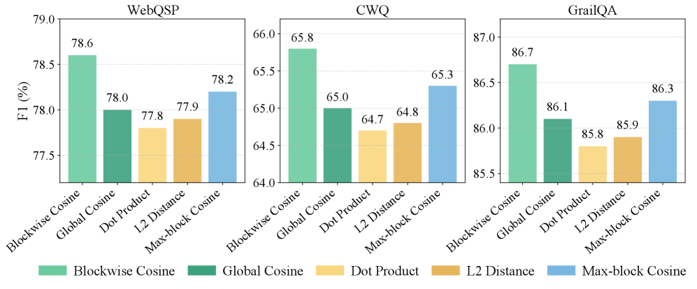
### Visual Description
\n
## Bar Chart: Performance Comparison of Different Similarity Metrics
### Overview
This image presents a comparative bar chart illustrating the F1 scores (%) achieved by four different similarity metrics – Blockwise Cosine, Global Cosine, Dot Product, L2 Distance, and Max-block Cosine – across three distinct datasets: WebQSP, CWQ, and GrailQA. Each dataset has its own set of bars representing the performance of each metric.
### Components/Axes
* **X-axis:** Represents the similarity metrics: Blockwise Cosine, Global Cosine, Dot Product, L2 Distance, and Max-block Cosine.
* **Y-axis:** Represents the F1 score in percentage (%). The scale ranges from approximately 64.0 to 87.0.
* **Datasets:** Three datasets are compared: WebQSP, CWQ, and GrailQA, each displayed as a separate set of bars.
* **Legend:** Located at the bottom of the image, it maps colors to the similarity metrics:
* Blockwise Cosine: Light Green
* Global Cosine: Dark Green
* Dot Product: Orange
* L2 Distance: Light Blue
* Max-block Cosine: Dark Blue
### Detailed Analysis
**WebQSP (Leftmost Chart)**
* **Blockwise Cosine:** The bar is light green and reaches approximately 78.6%.
* **Global Cosine:** The bar is dark green and reaches approximately 78.0%.
* **Dot Product:** The bar is orange and reaches approximately 77.8%.
* **L2 Distance:** The bar is light blue and reaches approximately 77.9%.
* **Max-block Cosine:** The bar is dark blue and reaches approximately 78.2%.
**CWQ (Center Chart)**
* **Blockwise Cosine:** The bar is light green and reaches approximately 65.8%.
* **Global Cosine:** The bar is dark green and reaches approximately 65.0%.
* **Dot Product:** The bar is orange and reaches approximately 64.7%.
* **L2 Distance:** The bar is light blue and reaches approximately 64.8%.
* **Max-block Cosine:** The bar is dark blue and reaches approximately 65.3%.
**GrailQA (Rightmost Chart)**
* **Blockwise Cosine:** The bar is light green and reaches approximately 86.7%.
* **Global Cosine:** The bar is dark green and reaches approximately 86.1%.
* **Dot Product:** The bar is orange and reaches approximately 85.8%.
* **L2 Distance:** The bar is light blue and reaches approximately 85.9%.
* **Max-block Cosine:** The bar is dark blue and reaches approximately 86.3%.
### Key Observations
* Blockwise Cosine consistently performs well across all three datasets, often achieving the highest F1 scores.
* L2 Distance generally exhibits the lowest performance among the metrics.
* The performance differences between metrics are more pronounced in the GrailQA dataset compared to WebQSP and CWQ.
* The F1 scores are generally higher for WebQSP and GrailQA than for CWQ.
### Interpretation
The data suggests that Blockwise Cosine is the most effective similarity metric for these datasets and tasks, consistently outperforming the other methods. The lower performance of L2 Distance indicates it may not be well-suited for capturing the relevant semantic relationships within these datasets. The higher scores on WebQSP and GrailQA compared to CWQ suggest that the characteristics of CWQ (perhaps its complexity or the nature of the questions) make it more challenging for all the similarity metrics. The relatively small differences in performance between Global Cosine, Dot Product, and Max-block Cosine suggest they offer comparable results, and the choice between them might depend on computational cost or other factors. The consistent ranking of these metrics across datasets indicates a degree of robustness in their relative performance. The visual representation effectively highlights these trends, allowing for a quick and clear comparison of the metrics' effectiveness.
</details>
Figure 5: Scoring measurement ablation. We evaluate F1 (%) on WebQSP, CWQ, and GrailQA using different scoring strategies in our model. PathHD achieves the best or competitive results when using blockwise cosine similarity, highlighting its effectiveness in capturing fine-grained matching signals across vector blocks.
J.2 Text-projection Variant
We use SBERT as the sentence encoder, so $d_{t}$ is fixed to the encoder hidden size $768$ , and $P$ is sampled once from $\mathcal{N}(0,1/d_{t})$ and kept fixed for all experiments.
| Final step | WebQSP | CWQ |
| --- | --- | --- |
| PathHD (text-projection query) | 83.4 | 69.8 |
| PathHD (plan-based, default) | 86.2 | 71.5 |
Table 12: Comparison of query encoding variants in PathHD. We report Hits@ $1$ on WebQSP and CWQ for the default plan-based encoding and the text-projection variant.
J.3 Additional Visualization
<details>
<summary>x8.png Details</summary>
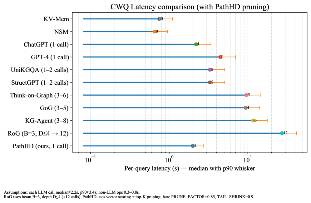
### Visual Description
## Chart: CWQ Latency Comparison (with PathHD pruning)
### Overview
This chart compares the per-query latency of several models (KV-Mem, NSM, ChatGPT, GPT-4, UniKGQA, StructGPT, Think-on-Graph, GoG, KG-Agent, RoG, and PathHD) using a logarithmic scale. The data is presented as median latency with a p90 whisker, indicating the 90th percentile latency. The chart demonstrates the impact of PathHD pruning on latency.
### Components/Axes
* **Title:** CWQ Latency comparison (with PathHD pruning)
* **X-axis:** Per-query latency (s) – median with p90 whisker. The scale is logarithmic, with markers at 10<sup>-1</sup>, 10<sup>0</sup>, and 10<sup>1</sup>.
* **Y-axis:** Model names (KV-Mem, NSM, ChatGPT (1 call), GPT-4 (1 call), UniKGQA (1–2 calls), StructGPT (1–2 calls), Think-on-Graph (3–6), GoG (3–5), KG-Agent (3–8), RoG (B=3, D≤4 → 12), PathHD (ours, 1 call)).
* **Data Series:** Each model is represented by a horizontal line with a marker indicating the median latency and a whisker extending to the p90 latency.
* **Legend:** The legend is implicit, with each line color corresponding to a model name on the Y-axis.
* **Assumptions (Footer):** "Assumptions: each LLM call median=2.5s, p90=3.4s; non-LLM ops 0.3–0.8s. RoG uses beam B=3, depth D≤4 (=12 calls). PathHD uses vector scoring + top-K pruning; here PRUNE_FACTOR=0.85, TAIL_SHRINK=0.9."
### Detailed Analysis
The chart displays the following approximate latency values (median with p90 whisker):
* **KV-Mem:** Approximately 0.3s (median), whisker extends to approximately 0.35s. (Blue)
* **NSM:** Approximately 0.4s (median), whisker extends to approximately 0.5s. (Orange)
* **ChatGPT (1 call):** Approximately 0.1s (median), whisker extends to approximately 0.15s. (Green)
* **GPT-4 (1 call):** Approximately 0.2s (median), whisker extends to approximately 0.3s. (Light Blue)
* **UniKGQA (1–2 calls):** Approximately 0.8s (median), whisker extends to approximately 1.0s. (Red)
* **StructGPT (1–2 calls):** Approximately 0.8s (median), whisker extends to approximately 1.0s. (Purple)
* **Think-on-Graph (3–6):** Approximately 3s (median), whisker extends to approximately 5s. (Pink)
* **GoG (3–5):** Approximately 2s (median), whisker extends to approximately 4s. (Brown)
* **KG-Agent (3–8):** Approximately 4s (median), whisker extends to approximately 6s. (Yellow)
* **RoG (B=3, D≤4 → 12):** Approximately 10s (median), whisker extends to approximately 12s. (Cyan)
* **PathHD (ours, 1 call):** Approximately 0.15s (median), whisker extends to approximately 0.2s. (Dark Blue)
**Trends:**
* PathHD exhibits the lowest median latency among all models.
* RoG has the highest median latency.
* ChatGPT and PathHD have the lowest latencies, both around 0.1-0.15s.
* UniKGQA and StructGPT have similar latencies, around 0.8s.
* The latency generally increases with the number of calls (as indicated in the model names).
### Key Observations
* PathHD significantly reduces latency compared to other models, particularly RoG.
* The p90 whiskers indicate the variability in latency for each model.
* The logarithmic scale compresses the differences between lower latency models.
* The assumptions at the bottom of the chart provide context for the latency values, indicating the expected latency of LLM calls and non-LLM operations.
### Interpretation
The chart demonstrates the effectiveness of PathHD pruning in reducing query latency. PathHD achieves comparable or lower latency than other models while potentially using fewer resources (1 call vs. multiple calls for other models). The large difference in latency between PathHD and RoG suggests that PathHD's pruning strategy is particularly effective in this context. The p90 whiskers highlight the potential for variability in latency, which is important to consider in real-world applications. The assumptions provided at the bottom of the chart suggest that the latency of LLM calls is a significant factor in overall query latency. The chart suggests that optimizing LLM call frequency and utilizing pruning techniques like PathHD can significantly improve performance. The use of a logarithmic scale is appropriate given the wide range of latency values, but it also means that small differences in latency at the lower end of the scale may be less visually apparent. The chart provides a clear and concise comparison of the latency of different models, allowing for informed decision-making regarding model selection and optimization.
</details>
Figure 6: CWQ latency comparison (lollipop). Dots indicate median per-query latency; right whiskers show the 90th percentile (p90). The x-axis is log-scaled. Values are estimated under a unified setup: per-LLM-call median $≈$ 2.2 s and p90 $≈$ 3.4 s; non-LLM operations add 0.3-0.8 s. RoG follows beam width $B{=}3$ with depth bounded by dataset hops ( $D{≤}4$ , $≈$ 12 calls), whereas PathHD uses a single LLM call plus vector operations for scoring.
J.4 Effect of Backbone Models
Performance across different LLM backbones is shown in Table ˜ 13.
Table 13: Performance across different LLM backbones. Each block fixes the backbone and varies the reasoning framework: a pure LLM control (CoT), our single-call PathHD, and 1-2 multi-step LLM+KG baselines. Metrics follow the unified Freebase setup.
| Backbone | Method | WebQSP | CWQ | GrailQA (F1) | #Calls |
| --- | --- | --- | --- | --- | --- |
| Hits@1 / F1 | Hits@1 / F1 | Overall / IID | (/query) | | |
| GPT-4 (API) | CoT [43] | 73.2 / 62.3 | 55.6 / 49.9 | 31.7 / 25.0 | 1 |
| RoG [25] | 85.7 / 70.8 | 62.6 / 56.2 | – / – | $≈ 12$ | |
| KG-Agent [16] | 83.3 / 81.0 | 72.2 / 69.8 | 86.1 / 92.0 | 3–8 | |
| PathHD (single-call) | 86.2 / 78.6 | 71.5 / 65.8 | 86.7 / 92.4 | 1 | |
| GPT - 3.5 / ChatGPT | CoT [43] | 67.4 / 59.3 | 47.5 / 43.2 | 25.3 / 19.6 | 1 |
| StructGPT [15] | 72.6 / 63.7 | 54.3 / 49.6 | 54.6 / 70.4 | 1–2 | |
| RoG [25] | 85.0 / 70.2 | 61.8 / 55.5 | – / – | $≈ 12$ | |
| PathHD (single-call) | 85.6 / 78.0 | 70.8 / 65.1 | 85.9 / 91.7 | 1 | |
| Llama - 3 - 8B - Instruct (open) | CoT (prompt-only) | 62.0 / 55.0 | 43.0 / 40.0 | 20.0 / 16.0 | 1 |
| ReAct - Lite (retrieval+CoT) | 70.5 / 62.0 | 52.0 / 47.5 | 48.0 / 62.0 | 3–5 | |
| BM25+LLM - Verifier (1 $×$ ) | 74.5 / 66.0 | 55.0 / 50.0 | 52.0 / 66.0 | 1 | |
| PathHD (single-call) | 84.8 / 77.2 | 69.8 / 64.2 | 84.9 / 90.9 | 1 | |
J.5 Prompt Sensitivity of the LLM Adjudicator
Since PathHD relies on a single LLM call to adjudicate among the Top- $K$ candidate paths, it is natural to ask how sensitive the system is to the exact phrasing of this adjudication prompt. To investigate this, we compare our default adjudication prompt (Prompt A) with a slightly rephrased variant (Prompt B) that uses different wording but conveys the same task description. For example, Prompt A asks the model to “select the most plausible reasoning path and answer the question based on it”, whereas Prompt B paraphrases this as “choose the best supporting path and use it to answer the question”.
| Prompt | WebQSP | CWQ | GrailQA (Overall / IID) |
| --- | --- | --- | --- |
| Prompt A (default) | $\mathbf{86.2}$ / $\mathbf{78.6}$ | $\mathbf{71.5}$ / $\mathbf{65.8}$ | $\mathbf{86.7}$ / $\mathbf{92.4}$ |
| Prompt B (paraphrased) | 85.7 / 78.3 | 70.9 / 63.4 | 85.2 / 90.8 |
Table 14: Prompt sensitivity of the LLM adjudicator. We compare the default adjudication prompt (Prompt A) with a paraphrased variant (Prompt B). Numbers are Hits@1 and F1 for WebQSP and CWQ, and Overall / IID F1 for GrailQA.
Table ˜ 14 reports Hits@1 and F1 on the three datasets under these two prompts. We observe that while minor prompt changes can occasionally flip individual predictions, the overall performance remains very close for all datasets, and the qualitative behavior of the path-grounded rationales is also stable. This suggests that, in our setting, PathHD is reasonably robust to small, natural variations in the adjudication prompt.
Appendix K Detailed Introduction of the Modules
K.1 Binding Operations
Below, we summarize the binding operators considered in our system and ablations. All bindings produce a composed hypervector $\mathbf{s}$ from two inputs $\mathbf{x}$ and $\mathbf{y}$ of the same dimensionality.
(1) XOR / Bipolar Product (commutative).
For binary hypervectors $\mathbf{x},\mathbf{y}∈\{0,1\}^{d}$ ,
$$
\mathbf{s}=\mathbf{x}\oplus\mathbf{y},\qquad s_{i}=(x_{i}+y_{i})\bmod 2.
$$
Under the bipolar code $\{-1,+1\}$ , XOR is equivalent to element-wise multiplication:
$$
s_{i}=x_{i}\cdot y_{i},\qquad x_{i},y_{i}\in\{-1,+1\}.
$$
This is the classical commutative bind baseline used in our ablation.
(2) Real-valued Element-wise Product (commutative).
For real vectors $\mathbf{x},\mathbf{y}∈\mathbb{R}^{d}$ ,
$$
\mathbf{s}=\mathbf{x}\odot\mathbf{y},\qquad s_{i}=x_{i}\,y_{i}.
$$
Unbinding is approximate by element-wise division (with small $\epsilon$ for stability): $x_{i}≈ s_{i}/(y_{i}+\epsilon)$ . This is another variant of the commutative bind.
(3) HRR: Circular Convolution (commutative).
For $\mathbf{x},\mathbf{y}∈\mathbb{R}^{d}$ ,
$$
\mathbf{s}=\mathbf{x}\circledast\mathbf{y},\qquad s_{k}=\sum_{i=0}^{d-1}x_{i}\,y_{(k-i)\bmod d}.
$$
Approximate unbinding uses circular correlation:
$$
\mathbf{x}\approx\mathbf{s}\circledast^{-1}\mathbf{y},\qquad x_{i}\approx\sum_{k=0}^{d-1}s_{k}\,y_{(k-i)\bmod d}.
$$
This is the Circ. conv condition in our ablation.
(4) FHRR / Complex Phasor Product (commutative).
Let $\mathbf{x},\mathbf{y}∈\mathbb{C}^{d}$ with unit-modulus components $x_{i}=e^{i\phi_{i}}$ , $y_{i}=e^{i\psi_{i}}$ . Binding is element-wise complex multiplication
$$
\mathbf{s}=\mathbf{x}\odot\mathbf{y},\qquad s_{i}=x_{i}y_{i}=e^{i(\phi_{i}+\psi_{i})},
$$
and unbinding is conjugation: $\mathbf{x}≈\mathbf{s}\odot\mathbf{y}^{\ast}$ . FHRR is often used as a complex analogue of HRR.
(5) Block-diagonal GHRR (non-commutative, ours).
We use Generalized HRR with block-unitary components. A hypervector is a block vector $\mathbf{H}=[A_{1};...;A_{D}]$ , $A_{j}∈\mathrm{U}(m)$ (so total dimension $d=Dm^{2}$ when flattened). Given $\mathbf{X}=[X_{1};...;X_{D}]$ and $\mathbf{Y}=[Y_{1};...;Y_{D}]$ , binding is the block-wise product
$$
\mathbf{Z}=\mathbf{X}\,\mathbin{\raisebox{0.86108pt}{\scalebox{0.9}{$\circledast$}}}\,\mathbf{Y},\qquad Z_{j}=X_{j}Y_{j}\;\;(j=1,\dots,D).
$$
Since matrix multiplication is generally non-commutative ( $X_{j}Y_{j}≠ Y_{j}X_{j}$ ), GHRR preserves order/direction of paths. Unbinding exploits unitarity:
$$
X_{j}\approx Z_{j}Y_{j}^{\ast},\qquad Y_{j}\approx X_{j}^{\ast}Z_{j}.
$$
This Block-diag (GHRR) operator is our default choice and achieves the best performance in the operation study (Table ˜ 3), compared to Comm. bind and Circ. conv.
K.2 Additional Case Study
Table 15: Case studies for PathHD with an illustrative display of candidates. For each query, we list the four highest-scoring relation paths (Top-4) for readability, then prune to $K=2$ before the vector-only choice and a single-LLM adjudication.
| Case 3: where are the gobi desert located on a map | |
| --- | --- |
| Top-3 candidates | 1) location.location.containedby (0.3410) |
| 2) location.location.partially_containedby (0.3335) | |
| 3) location.location.contains (0.3255) | |
| Top- $K$ after pruning (K=2) | containedby |
| partially_containedby | |
| Vector-only (no LLM) | Pick containedby ✓ — returns parent region; predicts Asia. |
| 1 $×$ LLM adjudication | Rationale: “Gobi Desert lies across Mongolia and China, which are contained by the continent of Asia; ‘contains’ would flip direction.” |
| Final Answer / GT | Asia (predict) / Asia ✓ |
| Case 4: in which continent is germany | |
| Top-3 candidates | 1) location.location.containedby (0.3405) |
| 2) base.locations.countries.continent (0.3325) | |
| 3) location.location.contains (0.3270) | |
| Top- $K$ after pruning (K=2) | containedby |
| countries.continent | |
| Vector-only (no LLM) | Pick containedby ✗ — tends to surface EU or administrative parents, hurting precision. |
| 1 $×$ LLM adjudication | Rationale: “The target is a country $→$ continent query; use countries.continent to directly map Germany to Europe.” |
| Final Answer / GT | Europe (predict) / Europe ✓ |
| Case 5: what is the hometown of the person who said “Forgive your enemies, but never forget their names?” | |
| Top-3 candidates | 1) quotation.author $→$ person.place_of_birth (0.3380) |
| 2) family.members $→$ person.place_of_birth (0.3310) | |
| 3) quotation.author $→$ location.people_born_here (0.3310) | |
| Top- $K$ after pruning (K=2) | quotation.author $→$ place_of_birth |
| family.members $→$ place_of_birth | |
| Vector-only (no LLM) | Pick quotation.author $→$ place_of_birth ✓ — direct trace from quote to person to birthplace. |
| 1 $×$ LLM adjudication | Rationale: “The quote’s author is key; once identified, linking to their birthplace via person-level relation gives the hometown.” |
| Final Answer / GT | Brooklyn (predict) / Brooklyn ✓ |
| Case 6: what is the name of the capital of Australia where the film “The Squatter’s Daughter” was made | |
| Top-3 candidates | 1) film.film_location.featured_in_films (0.3360) |
| 2) notable_types $→$ newspaper_circulation_area.newspapers | |
| $→$ newspapers (0.3330) | |
| 3) film_location.featured_in_films $→$ | |
| bibs_location.country (0.3310) | |
| Top- $K$ after pruning (K=2) | film.film_location.featured_in_films |
| notable_types $→$ newspaper_circulation_area.newspapers | |
| Vector-only (no LLM) | Pick film.film_location.featured_in_films ✓ — retrieves filming location; indirectly infers capital via metadata. |
| 1 $×$ LLM adjudication | Rationale: “The film’s production location helps localize the city. Although not all locations are capitals, this film was made in Australia, where identifying the filming city leads to the capital.” |
| Final Answer / GT | Canberra (predict) / Canberra ✓ |
Table ˜ 15 presents additional WebQSP case studies for PathHD. Unlike the main paper’s case table (Top - 4 candidates with pruning to $K{=}3$ ), this appendix visualizes the Top - 3 highest-scoring relation paths for readability and then prunes to $K{=}2$ before a single-LLM adjudication.
Across the four examples (Cases 3-6), pruning to $K{=}2$ often retains the correct path and achieves strong final answers after LLM adjudication. However, we also observe a typical failure mode of the vector-only selector under $K{=}2$ : when multiple plausible paths exist (e.g., country vs. continent, or actor vs. editor constraints), the vector-only choice can become brittle and select a high-scoring but underconstrained path, after which the LLM must recover the correct answer using the remaining candidate (see Case 4). In contrast, the main-paper setting with $K{=}3$ keeps one more candidate, which more reliably preserves a constraint-satisfying path (e.g., explicitly encoding actor or continent relations). This extra coverage reduces reliance on the LLM to repair mistakes and improves robustness under compositional queries.
While $K{=}2$ is cheaper and can work well in many instances, $K{=}3$ offers a better coverage-precision trade-off on average: it mitigates pruning errors in compositional cases and lowers the risk of discarding the key constraint path. This aligns with our main experimental choice of $K{=}3$ , which we use for all reported metrics in the paper.
Case-study note.
For the qualitative case studies only, we manually verified the final entity answers using publicly available sources (e.g., film credits and encyclopedia entries). This light-weight human verification was used solely to present readable examples; it does not affect any quantitative metric. All reported metrics (e.g., Hits@1 and F1) are computed from dataset-provided supervision and ground-truth paths without human annotation.