# Cognitive Mirrors: Exploring the Diverse Functional Roles of Attention Heads in LLM Reasoning
**Authors**:
- Tongliang Liu James Bailey (The University of Melbourne The University of Sydney)
> This work is not related to Amazon.
Abstract
Large language models (LLMs) have achieved state-of-the-art performance in a variety of tasks, but remain largely opaque in terms of their internal mechanisms. Understanding these mechanisms is crucial to improve their reasoning abilities. Drawing inspiration from the interplay between neural processes and human cognition, we propose a novel interpretability framework to systematically analyze the roles and behaviors of attention heads, which are key components of LLMs. We introduce CogQA, a dataset that decomposes complex questions into step-by-step subquestions with a chain-of-thought design, each associated with specific cognitive functions such as retrieval or logical reasoning. By applying a multi-class probing method, we identify the attention heads responsible for these functions. Our analysis across multiple LLM families reveals that attention heads exhibit functional specialization, characterized as cognitive heads. These cognitive heads exhibit several key properties: they are universally sparse, and vary in number and distribution across different cognitive functions, and they display interactive and hierarchical structures. We further show that cognitive heads play a vital role in reasoning tasks—removing them leads to performance degradation, while augmenting them enhances reasoning accuracy. These insights offer a deeper understanding of LLM reasoning and suggest important implications for model design, training and fine-tuning strategies. The code is available at https://github.com/sihuo-design/CognitiveMirrors.
1 Introduction
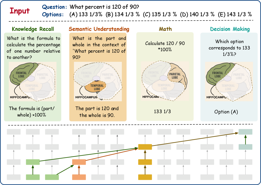
Large language models (LLMs) achiam2023gpt; grattafiori2024llama; touvron2023llama; yang2024qwen2, built on neural networks that mimic the structure of the human brain, have demonstrated exceptional performance across various natural language processing (NLP) tasks, often exceeding human capabilities. This has sparked growing interest in exploring the potential similarities between the cognitive processes of LLMs and the human brain. Prior studies have demonstrated that LLMs can predict brain responses to natural language caucheteux2022deep; schrimpf2021neural, indicating a functional alignment between artificial models and biological systems. However, to the best of our knowledge, systematic efforts to align reasoning processes between LLMs and human cognitive agents remain scarce. When solving complex reasoning tasks (e.g., a mathematical multiple-choice question; Figure 1), the human brain engages a network of specialized regions: the frontal lobe recalls relevant knowledge wheeler1997toward, language areas (e.g., Wernicke’s and Broca’s) support semantic processing ono2022bidirectional; meyer2005language, and the parietal and prefrontal cortices carry out higher-order reasoning barsalou2014cognitive; hubbard2005interactions.
Analogously, recent research suggests that components within LLMs may also take on specialized roles. For example, multi-head attention mechanisms in transformers vaswani2017attention have been found to handle distinct functions, such as information retrieval wu2404retrieval or maintaining answer consistency truthful, pointing toward a form of architectural division of labor. However, most of these findings are based on relatively simple tasks zheng2409attention, leaving open how such specialization operates under complex, multi-step reasoning scenarios.
<details>
<summary>x1.png Details</summary>
### Visual Description
## Cognitive Process Diagram: Percentage Calculation
### Overview
The image illustrates the cognitive processes involved in solving a percentage problem. It breaks down the problem-solving process into four stages: Knowledge Recall, Semantic Understanding, Math, and Decision Making. Each stage is represented with a brain diagram highlighting the relevant brain region and a textual description of the cognitive task. The diagram also includes a neural network representation showing the flow of information between these stages.
### Components/Axes
* **Header:**
* "Input" label in red.
* Question: "What percent is 120 of 90?"
* Options: (A) 133 1/3% (B) 134 1/3% (C) 135 1/3% (D) 140 1/3% (E) 143 1/3%
* **Main Sections (Left to Right):**
* **Knowledge Recall:**
* Title: "Knowledge Recall"
* Text: "What is the formula to calculate the percentage of one number relative to another?"
* Brain Diagram: Frontal lobe highlighted in green. Parietal and Temporal lobes are also labeled. Hippocampus is labeled.
* Text: "The formula is (part/whole) x100%"
* **Semantic Understanding:**
* Title: "Semantic Understanding"
* Text: "What is the part and whole in the context of 'What percent is 120 of 90?'"
* Brain Diagram: Temporal lobe highlighted in orange. Frontal and Parietal lobes are also labeled. Hippocampus is labeled.
* Text: "The part is 120 and the whole is 90."
* **Math:**
* Title: "Math"
* Text: "Calculate 120/90 *100%"
* Brain Diagram: Parietal lobe highlighted in tan. Frontal and Temporal lobes are also labeled. Hippocampus is labeled.
* Text: "133 1/3"
* **Decision Making:**
* Title: "Decision Making"
* Text: "Which option corresponds to 133 1/3%?"
* Brain Diagram: Frontal lobe highlighted in green. Parietal and Temporal lobes are also labeled. Hippocampus is labeled.
* Text: "Option (A)"
* **Neural Network Representation (Bottom):**
* A series of interconnected nodes representing a neural network.
* Nodes are colored grey, green, orange, and yellow, corresponding to the stages above.
* Arrows indicate the flow of information between nodes.
### Detailed Analysis
* **Knowledge Recall:** The frontal lobe is highlighted, suggesting its role in retrieving relevant formulas. The text states the formula for calculating percentage.
* **Semantic Understanding:** The temporal lobe is highlighted, indicating its involvement in understanding the context of the problem. The text identifies the part and the whole from the given question.
* **Math:** The parietal lobe is highlighted, suggesting its role in mathematical calculations. The text shows the calculation and the result.
* **Decision Making:** The frontal lobe is highlighted again, indicating its role in selecting the correct answer based on the calculated result. The text identifies the correct option.
* **Neural Network:**
* The network consists of multiple layers of nodes.
* The initial nodes are green, corresponding to Knowledge Recall.
* These connect to orange nodes, corresponding to Semantic Understanding.
* The orange nodes connect to yellow nodes, corresponding to Math.
* Finally, the yellow nodes connect to green nodes, corresponding to Decision Making.
* The arrows indicate the flow of information from one stage to the next.
### Key Observations
* The diagram clearly illustrates the different cognitive stages involved in solving a percentage problem.
* Each stage is associated with a specific brain region and a corresponding cognitive task.
* The neural network representation shows the flow of information between these stages.
* The diagram highlights the importance of both knowledge recall and semantic understanding in solving mathematical problems.
### Interpretation
The diagram demonstrates a simplified model of how the brain processes a mathematical problem. It suggests that solving such problems involves a sequence of cognitive stages, each relying on different brain regions and cognitive functions. The flow of information between these stages is crucial for arriving at the correct solution. The diagram also emphasizes the interconnectedness of different cognitive processes, highlighting the importance of both knowledge and understanding in problem-solving. The neural network representation, although simplified, provides a visual analogy for how information might be processed and transmitted within the brain during this process.
</details>
Figure 1: To solve a complex question, the human brain engages multiple regions to perform distinct cognitive functions necessary for generating a response. We explore whether there are specific attention heads in LLM play functional roles in producing answers.
In parallel, prompting techniques like chain-of-thought (CoT) cot have been shown to improve LLM performance by decomposing complex problems into intermediate steps, a strategy reminiscent of human problem-solving, like the example in Figure 1. We hypothesize that such prompting may activate and coordinate specialized components within the model. Thus, analyzing the behavior of attention heads under CoT reasoning could contribute insights for a deeper understanding of the internal workings of LLMs and how they process complex tasks.
In this work, we present a novel interpretability framework to systematically analyze the cognitive roles of attention heads during complex reasoning. To facilitate this, we introduce Cognitive Question&Answering (CogQA), a benchmark dataset that decomposes natural language questions into structured subquestions annotated with fine-grained cognitive functions, such as retrieval, logical inference, and knowledge recall. Leveraging CogQA, we develop a multi-class probing method to identify and characterize attention heads responsible for distinct cognitive operations within the transformer architecture.
We conduct extensive experiments on three major LLM families, including LLaMA (touvron2023llama), Qwen (yang2024qwen2), and Yi (young2024yi). Our results reveal the existence of cognitive heads that consistently exhibit universality, sparsity, and layered functional organization across architectures. Further analysis of the correlations among these cognitive heads reveals clear functional clustering, with heads grouping based on cognitive roles, and uncovers a hierarchical structure in which lower-level heads modulate higher-level ones—mirroring the modular and distributed processing observed in the human cortex (barsalou2014cognitive; ono2022bidirectional).
Furthermore, we validate the functional importance of these heads by showing that their removal degrades performance on complex tasks and leads to specific error patterns, while their enhancement improves reasoning capabilities. Our findings shed light on the structured cognitive architecture embedded in LLMs and open avenues for function-aware model design and analysis.
2 CogQA
In this section, we present a detailed account of our benchmark dataset CogQA’s construction and key characteristics. Although extensive existing benchmark collections span a wide array of NLP tasks, to our knowledge no resource explicitly evaluates LLM reasoning across diverse cognitive functions. To address this, we introduce CogQA, a dataset containing 570 main questions and 3,402 subquestions. Each example comprises a question, its answer, and an annotation specifying the cognitive function required for resolution.
2.1 Cognitive Function
To systematically capture the cognitive processes involved in complex reasoning tasks, we categorize cognitive functions into two groups: low-level functions and high-order functions, inspired by established frameworks in cognitive science anderson2014rules; diamond2013executive. Low-level functions primarily involve information retrieval and linguistic analysis, while high-order functions engage more abstract reasoning, problem-solving, and decision-making. Detailed descriptions of these cognitive functions are provided in Appendix A.4.
The low-level cognitive functions include:
- Retrieval: locating relevant information from an external source or prior context.
- Knowledge Recall: accessing stored factual or procedural knowledge from memory.
- Semantic Understanding: interpreting the meaning of words, phrases, or concepts.
- Syntactic Understanding: analyzing the grammatical structure of a sentence.
The high-order cognitive functions include:
- Mathematical Calculation: performing arithmetic or numerical operations.
- Logical Reasoning: drawing conclusions based on formal logical relationships.
- Inference: deriving implicit information that is not directly stated.
- Decision-Making: selecting the best outcome among alternatives based on reasoning.
This categorization reflects a natural progression from basic information processing to complex cognitive integration. Both the human brain and LLMs encompass a wide range of functional modules. Our focus in this work is specifically on reasoning-related cognitive functions. By identifying and organizing these eight core reasoning functions, we can more clearly examine how LLMs handle different types of thinking steps, in a way that is both systematic and easy to interpret.
2.2 Data Collections
Based on our categorization of cognitive functions, we sampled 750 diverse questions from NLP reasoning benchmarks, selecting 150 examples from each of AQuA aqua, CREAK creak, ECQA ecqa, e-SNLI esnli, and GSM8K gsm8k. These datasets cover a range of reasoning types, including logical, mathematical, and commonsense reasoning. Using the CoT paradigm, we prompted GPT-4o hurst2024gpt to decompose each question into subquestions, each targeting a single cognitive function. The prompt encourages structured, step-by-step reasoning, with each subquestion being clear, answerable, and sequentially dependent. This yields a set of subquestion-answer-cognitive function (subQAC) triples for each QA pair: $\operatorname{subQACs}=\left\{\left(q_{i},a_{i},c_{i}\right)\right\}_{i=1}^{k}$ , where each contains a subquestion $q_{i}$ , its concise answer $a_{i}$ , and the corresponding cognitive function label $c_{i}$ . The prompt for generating subquestions and examples are list in Appendix A.4 and Appendix A.6, respectively.
2.3 Data Filtering and Annotation
Recent advances have made it increasingly feasible to use LLMs for dataset construction, owing to their strong reasoning abilities and capacity to generate high-quality annotations at scale llm_annotate. Although our dataset is constructed automatically using an LLM to reduce manual effort, we implement a strict two-stage human verification pipeline to ensure data quality and mitigate hallucinations. In the first stage, three expert annotators independently assess whether the subquestions are logically structured and align with natural human reasoning. QA pairs with inconsistent or incoherent decompositions are filtered out. In the second stage, annotators verify and, if necessary, relabel the cognitive function associated with each subquestion to ensure alignment with the intended mental process. Finally, we validate the subanswers by cross-checking them using the GPT-o4-mini model o4mini2024, followed by human adjudication where discrepancies arise. Details of the annotation process and rubric can be found in Appendix A.5. This multi-step filtering ensures that each retained subQAC triple reflects a coherent, interpretable reasoning step grounded in core cognitive functions. After this refinement, our final dataset contains 570 main QA and 3,402 validated subQAC triplets.
3 Cognitive Function Detections
Given the CogQA dataset, we aim to identify which attention heads in LLMs are associated with specific cognitive functions. We adopt a probing-based framework, a widely used interpretability technique in which an auxiliary classifier is trained to predict properties from intermediate model representations alain2016understanding; belinkov2022probing; tenney2019bert. We frame this as a multi-class classification task: for each cognitively annotated subquestion, we extract head activations (see Section 3.1), train classifier and compute importance scores to identify contributing heads (see Section 3.2). Unlike prior work focusing on a single-class, our method captures many-to-many relationships between heads and functions, enabling a more detailed analysis of functional specialization and overlap compared to prior single-class approaches.
3.1 Head Feature Extraction
Given a large language model $\mathcal{M}$ , we generate an answer $a_{i}^{\mathcal{M}}$ for each subquestion $q_{i}$ derived from a main question $Q_{i}$ . To support coherent multi-step reasoning, we include preceding subquestions and their answers as contextual input, emulating the incremental reasoning process observed in human cognition.
During inference, input tokens are embedded and processed through successive transformer layers. At each layer, attention and feedforward operations update the residual stream, which is ultimately decoded into token predictions. For each generated token $i$ , we extract attention head outputs $X_{i}=\{x_{l}^{m}(i)\mid l=1,...,L,\ m=1,...,M\}$ across all layers, where $x^{m}_{l}$ denotes the value vector from the $m$ -th head in layer $l$ projected into the residual stream, with $M$ the number of heads per layer and $L$ the total number of layers.
Let $N_{t}$ denote the number of tokens in the generated answer $a_{i}^{\mathcal{M}}$ . To isolate semantically informative content relevant to reasoning, we select the top- $k$ most important tokens, We include an ablation study in Appendix A.9 to analyze the impact of using alternative token positions. determined by prompting GPT-o4-mini o4mini2024 (skilled in reasoning), yielding an index set $\mathcal{I}_{k}$ with $|\mathcal{I}_{k}|=k$ (Top- $k$ ( $k=5$ ) token examples are in Appendix A.10). For each index $j∈\mathcal{I}_{k}$ , we extract the corresponding attention head activations $X_{j}$ , and compute the averaged activation feature for the $m$ -th head in layer $l$ as $\bar{x}_{l}^{m}=\frac{1}{k}\sum_{j∈\mathcal{I}_{k}}x_{l}^{m}(j)$ . This results in a full set of head-level features $\bar{X}=\{\bar{x}_{l}^{m}\mid l={1,...,L},\ m={1,...,M}\}$ .
Given prior findings suggesting that cognitive functions may vary by layer depth zheng2409attention, we incorporate layer-wise information by computing the average activation $\bar{x}_{l}=\frac{1}{M}\sum_{m=1}^{M}\bar{x}_{l}^{m}$ for each layer. We then augment each head-level vector with its corresponding layer summary, resulting in enriched features $\bar{x}^{m^{\prime}}_{l}=[\bar{x}^{m}_{l};\bar{x}_{l}]$ . For each subQA triplet $(q_{i},\ a_{i},\ c_{i})$ , the final input to the probing classifier is given by $\{\bar{x}^{m^{\prime}}_{l}\mid l={1,...,L},\ m={1,...,M}\}$ .
3.2 Heads Importance
For the CogQA dataset with $N$ subQA pairs, we collect all activations to construct the probing dataset:
$$
\mathcal{D}_{\text{probe}}=\left\{(\bar{x}^{m^{\prime}}_{l},\ c)_{i}\right\}_{i=1}^{N},l\in\{1,\ldots,L\},\ m\in\{1,\ldots,M\} \tag{1}
$$
We split the dataset into training and validation sets with a $4{:}1$ ratio. Each attention head feature is first passed through a trainable linear projection for dimensionality reduction, followed by a two-layer MLP that performs multi-class classification over cognitive functions (training details are provided in Appendix A.3). To interpret the contribution of individual heads to each function, we use a gradient-based attribution method. Specifically, for each function class $c$ , we compute the contribution of each head feature via the gradient $×$ activation technique:
$$
I^{(c)}_{j}=\mathbb{E}_{(\bar{x},c)\sim\mathcal{D}_{\text{probe}}}\left[\frac{\partial\hat{y}_{c}}{\partial\bar{x}_{j}}\cdot\bar{x}_{j}\right], \tag{2}
$$
where $\bar{x}_{j}$ is the $j$ -th head input feature, and $\hat{y}_{c}$ is the classifier’s predicted logit for class $c$ . This yields an importance score for each attention head with respect to each cognitive function. We aggregate the scores into a matrix $\mathbf{I}∈\mathbb{R}^{C×(L· M)}$ , where each row corresponds to a function class and each column to a specific head in a specific layer.
We hypothesize that attention heads with higher importance scores contribute more significantly to each cognitive function. By ranking heads according to their importance, we can identify which heads and layers are specialized for specific functions. Subsequent targeted interventions on these heads validate the effectiveness of this approach.
4 Experiments
We conduct a series of experiments on three LLM families across various model scales, including LLaMA touvron2023llama (Llama3.1-8B-instruct and Llama3.2-3B-instruct), Qwen yang2024qwen2 (Qwen3-8B and Qwen3-4B), and Yi young2024yi (Yi1.5-9B and Yi1.5-6B). Our goal is to identify cognitive attention heads associated with specific reasoning functions and evaluate their roles via targeted interventions. By selectively masking these heads, we assess their functional significance in supporting downstream performance. We evaluate our method in terms of functional alignment, consistency across models, and causal impact on reasoning tasks. Results confirm the existence of sparse, function-specific heads and highlight their critical contribution to structured cognitive processing within LLMs.
4.1 Properties of Cognitive Heads
<details>
<summary>x2.png Details</summary>
### Visual Description
## Heatmap: Heads Importance by Layer and Task
### Overview
The image presents a series of heatmaps visualizing the importance of different "heads" within a neural network across various layers for different cognitive tasks. Each heatmap represents a specific task (Knowledge Recall, Retrieval, Logical Reasoning, Decision-making, Semantic Understanding, Syntactic Understanding, Inference, and Math Calculation). The x-axis represents the "Head" number (0-30), and the y-axis represents the "Layer" number (0-30). The color intensity indicates the "Heads Importance," ranging from dark purple (0.0000) to bright yellow (0.0030+).
### Components/Axes
* **Titles:** The heatmaps are titled with the cognitive tasks: Knowledge Recall, Retrieval, Logical Reasoning, Decision-making, Semantic Understanding, Syntactic Understanding, Inference, and Math Calculation.
* **X-axis:** Labeled "Head," with tick marks at intervals of 6, ranging from 0 to 30.
* **Y-axis:** Labeled "Layer," with tick marks at intervals of 6, ranging from 0 to 30.
* **Color Legend (Heads Importance):** Located on the right side of the image.
* Dark Purple: 0.0000
* Dark Blue: 0.0005
* Light Blue: 0.0010
* Green: 0.0015
* Yellow-Green: 0.0020
* Yellow: 0.0025
* Bright Yellow: 0.0030+
### Detailed Analysis
Each heatmap represents the importance of each head at each layer for a specific task. The color intensity indicates the level of importance.
* **Knowledge Recall:** Shows some higher importance heads concentrated around layers 12-18, with a few scattered high-importance heads in other layers.
* **Retrieval:** Similar to Knowledge Recall, with some concentration of higher importance heads around layers 12-18, and a few scattered elsewhere.
* **Logical Reasoning:** Shows a more dispersed pattern, with some higher importance heads scattered throughout the layers, but a slight concentration around layer 12.
* **Decision-making:** Shows a relatively even distribution of head importance across layers, with some slightly higher importance heads around layers 12-18.
* **Semantic Understanding:** Shows a few high-importance heads scattered throughout the layers, with no clear concentration.
* **Syntactic Understanding:** Shows a concentration of high-importance heads around layers 12-18, with a few scattered elsewhere.
* **Inference:** Shows a relatively even distribution of head importance across layers, with a few scattered high-importance heads.
* **Math Calculation:** Shows a concentration of high-importance heads in the lower layers (24-30), with a few scattered elsewhere.
### Key Observations
* **Layer 12-18 Importance:** Many tasks (Knowledge Recall, Retrieval, Syntactic Understanding, Decision-making) show a concentration of high-importance heads in the middle layers (around layers 12-18).
* **Math Calculation Anomaly:** Math Calculation stands out with a concentration of high-importance heads in the lower layers (24-30).
* **Sparse Activation:** The heatmaps are generally sparse, indicating that only a small subset of heads are highly important for each task at each layer.
### Interpretation
The heatmaps provide insights into which heads within a neural network are most important for different cognitive tasks at different layers. The concentration of high-importance heads in the middle layers (12-18) for many tasks suggests that these layers may be crucial for general cognitive processing. The unique pattern for Math Calculation, with high-importance heads in the lower layers, may indicate that this task relies on different processing mechanisms or representations compared to the other tasks. The sparsity of the heatmaps suggests that the network learns to use a specialized subset of heads for each task, rather than relying on all heads equally. This specialization could be a key factor in the network's ability to perform diverse cognitive tasks.
</details>
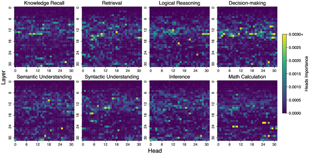
Figure 2: The existence of cognitive heads in Llama3.1-8B-instruct responsible for eight distinct functions in complex reasoning tasks. The x-axis represents the head index, while the y-axis indicates the layer index.
Our analysis reveals that cognitive head importance in large language models exhibits three key properties: sparsity and universality, and layered functional organization. To illustrate these characteristics, we present the heatmap of attention head importance scores across eight cognitive functions in Llama3.1-8B-instruct (Figure 2).
Sparsity and Universality: As shown in Figure 2, each cognitive function activates only a small number of high-importance attention heads, revealing a strikingly sparse pattern. In Llama3.1-8B-instruct, fewer than 7% of all heads have importance scores above 0.001 across the eight functions, suggesting that only a compact subset of heads meaningfully contribute to task performance. This sparsity is not uniform: Retrieval contains the highest proportion of salient heads (6.45% exceeding 0.01), while Inference has the fewest (3.42%). These results highlight that LLMs rely on highly specialized, localized components for different cognitive abilities. Importantly, we observe that this sparse functional organization is consistent across different model architectures and sizes. Additional heatmaps for five other models are provided in Appendix A.1, supporting the universality of this phenomenon.
Layered Functional Organization: In addition to sparsity, attention heads show a structured distribution across model layers. Retrieval-related heads cluster primarily in the middle layers, while math-related heads appear more frequently in higher layers. This structured, task-dependent localization points to an emergent modular organization, where different layers support distinct cognitive operations. Further, we identify cognitive heads by selecting those before the elbow point of each function’s descending importance curve (Appendix A.2), and find notable variation in head counts across functions (Appendix A.8). For example, in the LLaMA family, mathematical calculation requires fewer heads (59 in Llama3.1-8B-Instruct, 35 in Llama3.2-3B-Instruct), while inference draws on substantially more (139 and 98, respectively), reflecting differences in representational and computational complexity.
Table 1: Intervention results (%) of cognitive heads vs. random heads across 8 cognitive functions: Retrieval, Knowledge Recall, Semantic Understanding, Syntax Understanding, Math Calculation, Inference, Logic Reasoning, and Decision Making. Lower values indicate more effective intervention outcomes, suggesting that the corresponding heads play a greater role in the cognitive function.
| Model | Inter_Head | Information Extraction and Analysis Functions | Higher-Order Processing Functions | | | | | | | | | | | | | | |
| --- | --- | --- | --- | --- | --- | --- | --- | --- | --- | --- | --- | --- | --- | --- | --- | --- | --- |
| Retrieval | Recall | Semantic | Syntactic | Math | Inference | Logic | Decision | | | | | | | | | | |
| comet | acc | comet | acc | comet | acc | comet | acc | comet | acc | comet | acc | comet | acc | comet | acc | | |
| Llama3.1-8B | random | 90.83 | 84.71 | 87.85 | 83.84 | 91.44 | 97.50 | 87.81 | 66.17 | 94.25 | 83.08 | 91.90 | 70.18 | 91.39 | 54.69 | 97.64 | 90.91 |
| cognitive | 44.96 | 8.24 | 56.93 | 38.38 | 81.98 | 75.00 | 69.20 | 40.00 | 87.81 | 66.17 | 76.65 | 52.63 | 52.07 | 4.69 | 56.02 | 4.55 | |
| Llama3.2-3B | random | 87.89 | 86.47 | 76.35 | 68.69 | 90.54 | 90.00 | 75.82 | 40.00 | 94.98 | 69.65 | 95.66 | 85.96 | 92.75 | 76.56 | 93.30 | 81.82 |
| cognitive | 49.47 | 17.06 | 49.69 | 13.13 | 52.29 | 10.00 | 43.62 | 0.00 | 92.01 | 80.10 | 53.60 | 7.02 | 46.69 | 0.00 | 49.25 | 0.00 | |
| Qwen3-8B | random | 92.81 | 75.29 | 89.90 | 53.54 | 92.73 | 42.50 | 88.60 | 80.00 | 92.69 | 60.20 | 94.45 | 24.56 | 94.15 | 20.31 | 96.52 | 31.82 |
| cognitive | 59.19 | 38.24 | 64.81 | 30.30 | 85.95 | 47.50 | 46.26 | 0.00 | 89.29 | 53.23 | 72.77 | 35.09 | 87.61 | 21.88 | 83.17 | 54.55 | |
| Qwen3-4B | random | 94.17 | 84.71 | 84.61 | 77.78 | 86.91 | 77.50 | 98.15 | 80.00 | 87.15 | 44.78 | 96.89 | 87.72 | 92.00 | 75.00 | 94.79 | 72.73 |
| cognitive | 80.13 | 64.71 | 63.10 | 35.35 | 65.95 | 60.00 | 46.25 | 0.00 | 82.40 | 46.27 | 84.88 | 64.91 | 82.79 | 39.06 | 45.49 | 13.64 | |
| Yi-1.5-9B | random | 86.83 | 79.41 | 82.02 | 54.55 | 77.40 | 35.00 | 81.53 | 60.00 | 76.04 | 36.32 | 89.83 | 36.84 | 87.53 | 42.19 | 86.27 | 63.64 |
| cognitive | 52.76 | 21.76 | 45.99 | 9.09 | 47.25 | 2.50 | 48.10 | 40.00 | 54.22 | 16.92 | 52.41 | 15.79 | 82.75 | 26.56 | 62.85 | 18.18 | |
| Yi-1.5-6B | random | 80.64 | 69.41 | 68.82 | 38.38 | 77.83 | 55.00 | 69.61 | 60.00 | 73.33 | 43.78 | 77.71 | 22.81 | 81.65 | 29.69 | 88.54 | 72.73 |
| cognitive | 49.90 | 15.29 | 68.23 | 41.41 | 49.54 | 2.50 | 42.92 | 0.00 | 76.64 | 43.78 | 68.53 | 14.04 | 44.94 | 0.00 | 86.28 | 50.00 | |
<details>
<summary>x3.png Details</summary>
### Visual Description
## Line Charts: Performance Comparison with Masked Heads
### Overview
The image contains four line charts comparing the performance of "TopK" and "RandomK" methods across different tasks: Retrieval, Knowledge Recall, Math Calculation, and Inference. The x-axis represents the number of masked heads (16, 32, 64, 128), and the y-axis represents the score (from 0.0 to 1.0). Each chart displays two solid lines ("TopK Accuracy" and "TopK Comet") and two dashed lines ("RandomK Accuracy" and "RandomK Comet").
### Components/Axes
* **X-axis:** "# Masked Heads" with values 16, 32, 64, and 128.
* **Y-axis:** "Score" ranging from 0.0 to 1.0 in increments of 0.2.
* **Chart Titles:** Retrieval, Knowledge Recall, Math Calculation, Inference.
* **Legend (Top):**
* Blue solid line: "TopK Accuracy"
* Blue dashed line: "RandomK Accuracy"
* Red solid line: "TopK Comet"
* Red dashed line: "RandomK Comet"
### Detailed Analysis
#### Retrieval Chart
* **TopK Accuracy (Blue Solid):** Starts at approximately 0.95 at 16 masked heads, decreases to approximately 0.55 at 32 masked heads, remains relatively stable around 0.60 until 64 masked heads, then drops sharply to approximately 0.0 at 128 masked heads.
* **RandomK Accuracy (Blue Dashed):** Starts at approximately 0.95 and remains relatively stable between 0.95 and 0.80 across all values of masked heads.
* **TopK Comet (Red Solid):** Starts at approximately 0.95 at 16 masked heads, decreases to approximately 0.75 at 32 masked heads, remains relatively stable around 0.75 until 64 masked heads, then decreases to approximately 0.40 at 128 masked heads.
* **RandomK Comet (Red Dashed):** Starts at approximately 0.95 and remains relatively stable between 0.95 and 0.80 across all values of masked heads.
#### Knowledge Recall Chart
* **TopK Accuracy (Blue Solid):** Starts at approximately 0.90 at 16 masked heads, decreases to approximately 0.10 at 128 masked heads, with a slight increase at 64 masked heads.
* **RandomK Accuracy (Blue Dashed):** Starts at approximately 0.95 and decreases to approximately 0.80 at 128 masked heads.
* **TopK Comet (Red Solid):** Starts at approximately 0.95 at 16 masked heads, decreases to approximately 0.20 at 128 masked heads.
* **RandomK Comet (Red Dashed):** Starts at approximately 0.95 and decreases to approximately 0.85 at 128 masked heads.
#### Math Calculation Chart
* **TopK Accuracy (Blue Solid):** Starts at approximately 0.95 at 16 masked heads, decreases to approximately 0.20 at 128 masked heads.
* **RandomK Accuracy (Blue Dashed):** Starts at approximately 0.95 and decreases to approximately 0.90 at 128 masked heads.
* **TopK Comet (Red Solid):** Starts at approximately 0.95 at 16 masked heads, decreases to approximately 0.60 at 128 masked heads.
* **RandomK Comet (Red Dashed):** Starts at approximately 0.95 and decreases to approximately 0.90 at 128 masked heads.
#### Inference Chart
* **TopK Accuracy (Blue Solid):** Starts at approximately 0.95 at 16 masked heads, decreases to approximately 0.65 at 128 masked heads.
* **RandomK Accuracy (Blue Dashed):** Starts at approximately 0.95 and decreases to approximately 0.80 at 128 masked heads.
* **TopK Comet (Red Solid):** Starts at approximately 0.95 at 16 masked heads, decreases to approximately 0.75 at 128 masked heads.
* **RandomK Comet (Red Dashed):** Starts at approximately 0.95 and decreases to approximately 0.85 at 128 masked heads.
### Key Observations
* In all four tasks, the "RandomK Accuracy" and "RandomK Comet" lines (dashed) show more stable performance as the number of masked heads increases, compared to the "TopK Accuracy" and "TopK Comet" lines (solid).
* The "TopK Accuracy" line experiences the most significant drop in performance, especially in the Retrieval and Knowledge Recall tasks.
* The "TopK Comet" line also shows a decrease in performance, but not as drastic as the "TopK Accuracy" line.
### Interpretation
The charts suggest that the "RandomK" methods are more robust to the masking of heads compared to the "TopK" methods. As the number of masked heads increases, the performance of "TopK" methods decreases significantly, indicating that these methods are more sensitive to the loss of information from specific heads. The "RandomK" methods, on the other hand, maintain a more stable performance, suggesting that they are better at utilizing the remaining information when heads are masked. This could be because "RandomK" methods distribute the attention more evenly across the heads, while "TopK" methods rely more heavily on a specific subset of heads. The Retrieval and Knowledge Recall tasks seem to be more affected by the masking of heads than the Math Calculation and Inference tasks, suggesting that these tasks may rely more on specific attention patterns.
</details>
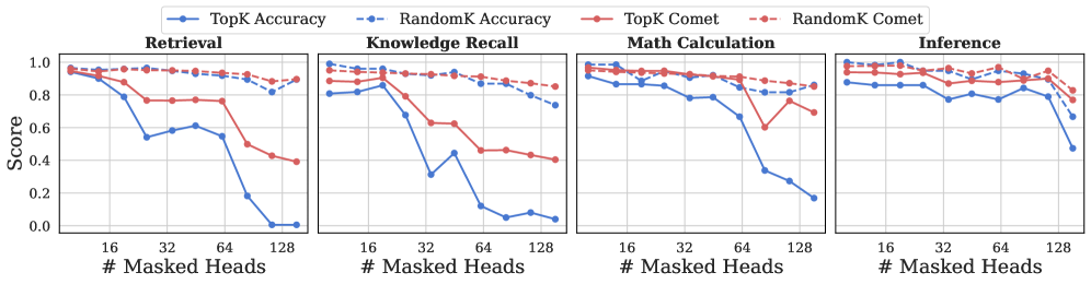
Figure 3: The performance of Llama3.1-8B-instruct by masking out top K cognitive heads vs K random heads on retrieval, knowledge recall, math calculation, and inference.
4.2 Functional Contributions of Cognitive Heads
After identifying the cognitive heads associated with each function, we examine their functional roles by evaluating the model’s behavior on the CogQA test set under targeted interventions. We perform head ablation by scaling the output of a specific attention head with a small factor $\epsilon$ (e.g., 0.001), effectively suppressing its contribution:
$$
x_{i}^{\text{mask}}=\operatorname{Softmax}\left(\frac{W_{q}^{i}W_{k}^{iT}}{\sqrt{d_{k}/n}}\right)\cdot\epsilon W_{v}^{i} \tag{3}
$$
Specifically, we compare model performance when masking identified cognitive heads versus masking an equal number of randomly selected heads. To quantify the impact of masking, we use several standard evaluation metrics including COMET rei2020comet, BLEU papineni2002bleu, ROUGE chin2004rouge, and semantic similarity to compare the model’s outputs before and after intervention. We define an output as unaffected if the BLEU score exceeds 0.8, or either the ROUGE or semantic similarity scores surpass 0.6, and compute accuracy accordingly.
As shown in Table 1, masking cognitive heads leads to a significant decline in performance, whereas masking an equal number of random heads results in only marginal degradation across all LLMs. In some cases, masking the identified cognitive heads causes the accuracy to drop to zero, indicating that the model cannot execute the corresponding function without them. This sharp contrast highlights the essential role cognitive heads play in enabling specific reasoning capabilities. To further validate the functional specialization, we conduct experiments where we mask the retrieval heads during the evaluation of knowledge recall (Recall), and conversely, mask knowledge recall heads during the evaluation of retrieval performance. The results in Table 2 show that masking the corresponding cognitive heads causes a significantly larger performance drop than masking others.
Table 2: Intervention results (%) of different cognitive heads and random heads across Retrieval and Knowledge Recall functions.
| Llama3.1-8B Llama3.1-8B Llama3.1-8B | random retrieval recall | 90.83 44.96 86.79 | 84.71 8.24 75.29 | 87.85 72.05 56.93 | 83.84 33.33 38.38 |
| --- | --- | --- | --- | --- | --- |
| Qwen3-8B | random | 92.81 | 75.29 | 89.90 | 53.54 |
| Qwen3-8B | retrieval | 59.19 | 38.24 | 79.26 | 57.58 |
| Qwen3-8B | recall | 83.31 | 71.18 | 64.81 | 30.30 |
We further investigate the performance of model under different numbers of masked attention heads. As shown in Figure 3, increasing the number of randomly masked heads has minimal impact on overall performance of Llama3.1-8B-instruct. In contrast, masking cognitive heads results in a significant drop in performance across various functions. Notably, masking heads associated with Retrieval and Knowledge Recall causes a pronounced degradation in their respective functions, whereas functions such as Math Calculation and Inference exhibit more resilience. This suggests that certain cognitive functions depend more heavily on specific, distinguishable attention heads, while others are distributed more broadly across the model.
4.3 Relationship Among Cognitive Heads
While cognitive heads are specialized for distinct functions, understanding their relationships is crucial for revealing how complex reasoning emerges from their cooperation.
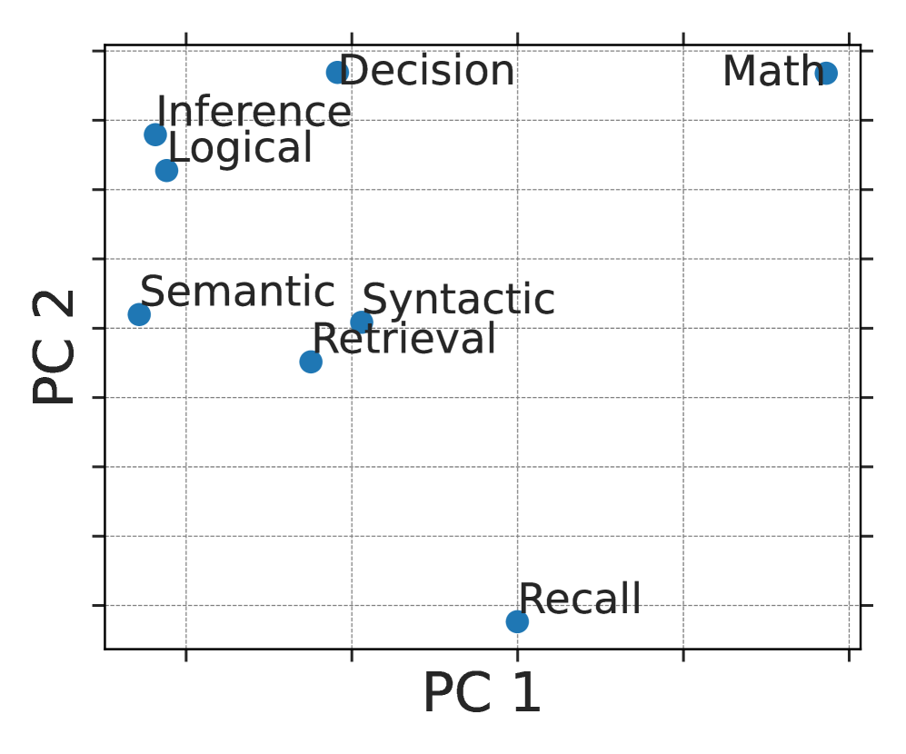
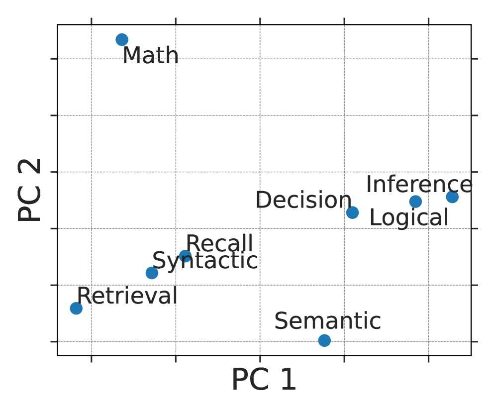
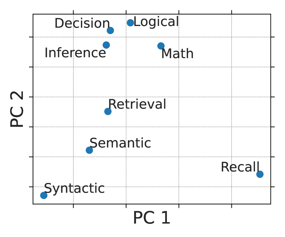
Functional Clustering: Inspired by neuroscience findings that related cognitive functions localize in overlapping brain regions (e.g., prefrontal cortex for reasoning and inference barsalou2014cognitive), we investigate whether LLM attention heads show similar patterns. We rank each head’s importance across eight cognitive functions, form ranking vectors, and apply principal component analysis (PCA) to visualize their organization (Figure 4). The results reveal clear clustering: heads linked to reasoning, inference, and decision-making group closely, while those related to mathematical computation form a distinct cluster in Llama and Qwen, and lie adjacent to reasoning heads in Yi. Lower-level functions also show moderate clustering. These patterns suggest a modular functional architecture in LLMs akin to that in the human brain.
<details>
<summary>x4.png Details</summary>
### Visual Description
## Scatter Plot: Cognitive Task Distribution in PC1 and PC2 Space
### Overview
The image is a scatter plot displaying the distribution of various cognitive tasks along two principal components, PC1 and PC2. Each task is represented by a blue dot, with its name labeled nearby. The plot provides a visual representation of how these tasks relate to each other in a two-dimensional space defined by the principal components.
### Components/Axes
* **X-axis (PC1):** Labeled "PC 1".
* **Y-axis (PC2):** Labeled "PC 2".
* **Data Points:** Blue dots representing cognitive tasks.
* **Gridlines:** Dashed gray lines forming a grid.
* **Cognitive Tasks (Categories):**
* Inference
* Logical
* Semantic
* Syntactic
* Retrieval
* Decision
* Math
* Recall
### Detailed Analysis or ### Content Details
Here's a breakdown of the approximate coordinates of each cognitive task:
* **Inference:** PC1 ≈ -1.0, PC2 ≈ 1.0
* **Logical:** PC1 ≈ -1.0, PC2 ≈ 1.0
* **Semantic:** PC1 ≈ -1.0, PC2 ≈ 0.2
* **Syntactic:** PC1 ≈ -0.2, PC2 ≈ 0.3
* **Retrieval:** PC1 ≈ -0.2, PC2 ≈ 0.3
* **Decision:** PC1 ≈ 0.0, PC2 ≈ 1.2
* **Math:** PC1 ≈ 1.2, PC2 ≈ 1.3
* **Recall:** PC1 ≈ 0.0, PC2 ≈ -1.0
### Key Observations
* "Inference" and "Logical" are clustered closely together in the top-left quadrant.
* "Semantic," "Syntactic," and "Retrieval" are grouped in the middle-left region.
* "Decision" and "Math" are located in the top-right quadrant.
* "Recall" is isolated in the bottom-center region.
### Interpretation
The scatter plot visualizes the relationships between different cognitive tasks based on their projections onto the first two principal components (PC1 and PC2). The proximity of tasks suggests similarities in the underlying cognitive processes captured by these principal components. For example, "Inference" and "Logical" tasks being close together indicates that PC1 and PC2 may similarly influence these tasks. "Recall" being distant from the other tasks suggests it involves different cognitive processes. The plot provides a dimensionality reduction of the cognitive tasks, allowing for a simplified comparison of their characteristics.
</details>
(a) Llama3.1-8B
<details>
<summary>x5.png Details</summary>
### Visual Description
## Scatter Plot: Cognitive Task Distribution in PC1 and PC2 Space
### Overview
The image is a scatter plot displaying the distribution of various cognitive tasks in a two-dimensional space defined by Principal Component 1 (PC1) and Principal Component 2 (PC2). Each task is represented by a blue dot, with its position indicating its relative loading on the two principal components. The plot provides a visual representation of the relationships and distinctions between these cognitive tasks based on their underlying cognitive demands.
### Components/Axes
* **X-axis (PC1):** Labeled "PC 1". The axis ranges from approximately -1 to 1, with no explicit numerical markers.
* **Y-axis (PC2):** Labeled "PC 2". The axis ranges from approximately -1 to 1, with no explicit numerical markers.
* **Data Points:** Each data point is a blue circle representing a cognitive task.
* **Gridlines:** Gray dashed gridlines are present to aid in visually estimating the coordinates of each data point.
### Detailed Analysis or ### Content Details
The following cognitive tasks are plotted:
* **Math:** Located in the top-left quadrant, with approximate coordinates of PC1 = -0.7, PC2 = 0.8.
* **Retrieval:** Located in the bottom-left quadrant, with approximate coordinates of PC1 = -0.8, PC2 = -0.4.
* **Syntactic:** Located slightly to the left of the center, with approximate coordinates of PC1 = -0.5, PC2 = -0.2.
* **Recall:** Located slightly to the left of the center, with approximate coordinates of PC1 = -0.4, PC2 = -0.1.
* **Semantic:** Located in the bottom-right quadrant, with approximate coordinates of PC1 = 0.2, PC2 = -0.7.
* **Decision:** Located in the top-right quadrant, with approximate coordinates of PC1 = 0.1, PC2 = 0.4.
* **Inference:** Located in the top-right quadrant, with approximate coordinates of PC1 = 0.6, PC2 = 0.5.
* **Logical:** Located in the top-right quadrant, with approximate coordinates of PC1 = 0.7, PC2 = 0.4.
### Key Observations
* **Clustering:** The tasks "Inference" and "Logical" are clustered closely together in the top-right quadrant. The tasks "Recall" and "Syntactic" are also clustered together, slightly to the left of the center.
* **Distribution:** The tasks are distributed across all four quadrants, indicating that PC1 and PC2 capture different aspects of cognitive processing.
* **Extreme Points:** "Math" has a high PC2 value and a low PC1 value, while "Semantic" has a low PC2 value and a slightly positive PC1 value.
### Interpretation
The scatter plot visualizes the relationships between different cognitive tasks based on their loadings on the first two principal components (PC1 and PC2). The proximity of tasks in the plot suggests that they share similar cognitive demands as captured by these principal components. For example, "Inference" and "Logical" tasks being close together suggests they load similarly on PC1 and PC2, potentially indicating shared cognitive processes. "Math" and "Semantic" are located in opposite quadrants, suggesting that they rely on different cognitive processes as captured by PC1 and PC2. The plot provides a dimensionality reduction of the cognitive tasks, allowing for a simplified comparison of their underlying cognitive requirements.
</details>
(b) Qwen3-4B
<details>
<summary>x6.png Details</summary>
### Visual Description
## Scatter Plot: Cognitive Task Distribution in PC Space
### Overview
The image is a scatter plot displaying the distribution of various cognitive tasks in a two-dimensional space defined by Principal Component 1 (PC1) and Principal Component 2 (PC2). Each task is represented by a blue dot, with its position indicating its loading on the two principal components. The plot provides a visual representation of the relationships between these tasks based on their underlying cognitive demands.
### Components/Axes
* **X-axis:** PC 1 (Principal Component 1)
* **Y-axis:** PC 2 (Principal Component 2)
* **Data Points:** Blue dots representing cognitive tasks.
* **Gridlines:** Dashed grey lines forming a grid.
* **Cognitive Tasks:**
* Syntactic
* Semantic
* Retrieval
* Inference
* Decision
* Logical
* Math
* Recall
### Detailed Analysis
The scatter plot shows the following approximate coordinates for each cognitive task:
* **Syntactic:** PC1 ~ 0.2, PC2 ~ 0.2
* **Semantic:** PC1 ~ 0.4, PC2 ~ 0.4
* **Retrieval:** PC1 ~ 0.5, PC2 ~ 0.6
* **Inference:** PC1 ~ 0.3, PC2 ~ 0.8
* **Decision:** PC1 ~ 0.4, PC2 ~ 0.9
* **Logical:** PC1 ~ 0.7, PC2 ~ 0.9
* **Math:** PC1 ~ 0.8, PC2 ~ 0.8
* **Recall:** PC1 ~ 0.9, PC2 ~ 0.3
### Key Observations
* The tasks are distributed across the plot, indicating varying degrees of loading on PC1 and PC2.
* "Syntactic" and "Semantic" are clustered together in the bottom-left quadrant.
* "Decision" and "Logical" are clustered together in the top-right quadrant.
* "Recall" is located in the bottom-right quadrant, separated from the other tasks.
### Interpretation
The scatter plot visualizes the relationships between different cognitive tasks based on their underlying cognitive demands, as captured by Principal Component Analysis. The proximity of tasks suggests similarities in their cognitive requirements. For example, "Syntactic" and "Semantic" tasks, being close together, may share common cognitive processes. Conversely, the separation of "Recall" from other tasks suggests it relies on different cognitive mechanisms. The plot provides a simplified representation of the cognitive landscape, highlighting the dimensions along which these tasks differ. The principal components (PC1 and PC2) likely represent underlying cognitive factors that contribute to the performance of these tasks. Further analysis would be needed to determine the specific cognitive processes captured by each principal component.
</details>
(c) Yi-1.5-6B
Figure 4: PCA visualization of the 8 function heads’ clustering in three models.
Table 3: Study on the influence of low-level cognitive heads for high-order function on Llama3.1-8B-instruct. Accuracy is measured based on BLEU, ROUGE, and semantic similarity scores.
| ✗ | ✓ | ✓ | ✓ | $0.00_{\definecolor{tcbcolback}{rgb}{0.87890625,0.9609375,1}\definecolor{tcbcolframe}{rgb}{0.87890625,0.9609375,1}\par\noindent\hbox to28.45pt{\vbox to9.96pt{\pgfpicture\makeatletter\hbox{\thinspace\lower 0.0pt\hbox to0.0pt{\pgfsys@beginscope\pgfsys@invoke{ }\definecolor{pgfstrokecolor}{rgb}{0,0,0}\pgfsys@color@rgb@stroke{0}{0}{0}\pgfsys@invoke{ }\pgfsys@color@rgb@fill{0}{0}{0}\pgfsys@invoke{ }\pgfsys@setlinewidth{\the\pgflinewidth}\pgfsys@invoke{ }\nullfont\hbox to0.0pt{{}{}{}{}\pgfsys@beginscope\pgfsys@invoke{ }{}{}{}{}{}{}{}{}\definecolor[named]{pgffillcolor}{rgb}{0.87890625,0.9609375,1}\pgfsys@color@rgb@fill{0.87890625}{0.9609375}{1}\pgfsys@invoke{ }\pgfsys@fill@opacity{1.0}\pgfsys@invoke{ }{{}{}{{}}}{{}{}{{}}}{}{}{{}{}{{}}}{{}{}{{}}}{}{}{{}{}{{}}}{{}{}{{}}}{}{}{{}{}{{}}}{{}{}{{}}}{}{}\pgfsys@moveto{0.0pt}{2.84526pt}\pgfsys@lineto{0.0pt}{7.11337pt}\pgfsys@curveto{0.0pt}{8.68478pt}{1.27385pt}{9.95863pt}{2.84526pt}{9.95863pt}\pgfsys@lineto{25.60748pt}{9.95863pt}\pgfsys@curveto{27.1789pt}{9.95863pt}{28.45274pt}{8.68478pt}{28.45274pt}{7.11337pt}\pgfsys@lineto{28.45274pt}{2.84526pt}\pgfsys@curveto{28.45274pt}{1.27385pt}{27.1789pt}{0.0pt}{25.60748pt}{0.0pt}\pgfsys@lineto{2.84526pt}{0.0pt}\pgfsys@curveto{1.27385pt}{0.0pt}{0.0pt}{1.27385pt}{0.0pt}{2.84526pt}\pgfsys@closepath\pgfsys@fill\pgfsys@invoke{ }\pgfsys@invoke{ }\pgfsys@endscope\pgfsys@beginscope\pgfsys@invoke{ }{}{}{}{}{}{}{}{}\definecolor[named]{pgffillcolor}{rgb}{0.87890625,0.9609375,1}\pgfsys@color@rgb@fill{0.87890625}{0.9609375}{1}\pgfsys@invoke{ }\pgfsys@fill@opacity{1.0}\pgfsys@invoke{ }{{}{}{{}}}{{}{}{{}}}{}{}{{}{}{{}}}{{}{}{{}}}{}{}{{}{}{{}}}{{}{}{{}}}{}{}{{}{}{{}}}{{}{}{{}}}{}{}\pgfsys@moveto{0.0pt}{2.84526pt}\pgfsys@lineto{0.0pt}{7.11337pt}\pgfsys@curveto{0.0pt}{8.68478pt}{1.27385pt}{9.95863pt}{2.84526pt}{9.95863pt}\pgfsys@lineto{25.60748pt}{9.95863pt}\pgfsys@curveto{27.1789pt}{9.95863pt}{28.45274pt}{8.68478pt}{28.45274pt}{7.11337pt}\pgfsys@lineto{28.45274pt}{2.84526pt}\pgfsys@curveto{28.45274pt}{1.27385pt}{27.1789pt}{0.0pt}{25.60748pt}{0.0pt}\pgfsys@lineto{2.84526pt}{0.0pt}\pgfsys@curveto{1.27385pt}{0.0pt}{0.0pt}{1.27385pt}{0.0pt}{2.84526pt}\pgfsys@closepath\pgfsys@fill\pgfsys@invoke{ }\pgfsys@invoke{ }\pgfsys@endscope\pgfsys@beginscope\pgfsys@invoke{ }\pgfsys@fill@opacity{1.0}\pgfsys@invoke{ }{{{}}{{}}{{}}{{}}{{}}{{}}{{}}{{}}\pgfsys@beginscope\pgfsys@invoke{ }\pgfsys@transformcm{1.0}{0.0}{0.0}{1.0}{2.84526pt}{3.72931pt}\pgfsys@invoke{ }\hbox{{\color[rgb]{0,0,0}\definecolor[named]{pgfstrokecolor}{rgb}{0,0,0}\pgfsys@color@gray@stroke{0}\pgfsys@color@gray@fill{0}\hbox{\minipage[b]{22.76222pt}\color[rgb]{0,0,0}\definecolor[named]{pgfstrokecolor}{rgb}{0,0,0}\pgfsys@color@gray@stroke{0}\pgfsys@color@gray@fill{0}\ignorespaces\centering\ignorespaces{\text{$\downarrow$ 100}}\@add@centering\endminipage}}}\pgfsys@invoke{ }\pgfsys@endscope}\pgfsys@invoke{ }\pgfsys@endscope{}{}{}\hss}\pgfsys@discardpath\pgfsys@invoke{ }\pgfsys@endscope\hss}}\endpgfpicture}}\par}$ | $0.00_{\definecolor{tcbcolback}{rgb}{0.87890625,0.9609375,1}\definecolor{tcbcolframe}{rgb}{0.87890625,0.9609375,1}\par\noindent\hbox to28.45pt{\vbox to9.96pt{\pgfpicture\makeatletter\hbox{\thinspace\lower 0.0pt\hbox to0.0pt{\pgfsys@beginscope\pgfsys@invoke{ }\definecolor{pgfstrokecolor}{rgb}{0,0,0}\pgfsys@color@rgb@stroke{0}{0}{0}\pgfsys@invoke{ }\pgfsys@color@rgb@fill{0}{0}{0}\pgfsys@invoke{ }\pgfsys@setlinewidth{\the\pgflinewidth}\pgfsys@invoke{ }\nullfont\hbox to0.0pt{{}{}{}{}\pgfsys@beginscope\pgfsys@invoke{ }{}{}{}{}{}{}{}{}\definecolor[named]{pgffillcolor}{rgb}{0.87890625,0.9609375,1}\pgfsys@color@rgb@fill{0.87890625}{0.9609375}{1}\pgfsys@invoke{ }\pgfsys@fill@opacity{1.0}\pgfsys@invoke{ }{{}{}{{}}}{{}{}{{}}}{}{}{{}{}{{}}}{{}{}{{}}}{}{}{{}{}{{}}}{{}{}{{}}}{}{}{{}{}{{}}}{{}{}{{}}}{}{}\pgfsys@moveto{0.0pt}{2.84526pt}\pgfsys@lineto{0.0pt}{7.11337pt}\pgfsys@curveto{0.0pt}{8.68478pt}{1.27385pt}{9.95863pt}{2.84526pt}{9.95863pt}\pgfsys@lineto{25.60748pt}{9.95863pt}\pgfsys@curveto{27.1789pt}{9.95863pt}{28.45274pt}{8.68478pt}{28.45274pt}{7.11337pt}\pgfsys@lineto{28.45274pt}{2.84526pt}\pgfsys@curveto{28.45274pt}{1.27385pt}{27.1789pt}{0.0pt}{25.60748pt}{0.0pt}\pgfsys@lineto{2.84526pt}{0.0pt}\pgfsys@curveto{1.27385pt}{0.0pt}{0.0pt}{1.27385pt}{0.0pt}{2.84526pt}\pgfsys@closepath\pgfsys@fill\pgfsys@invoke{ }\pgfsys@invoke{ }\pgfsys@endscope\pgfsys@beginscope\pgfsys@invoke{ }{}{}{}{}{}{}{}{}\definecolor[named]{pgffillcolor}{rgb}{0.87890625,0.9609375,1}\pgfsys@color@rgb@fill{0.87890625}{0.9609375}{1}\pgfsys@invoke{ }\pgfsys@fill@opacity{1.0}\pgfsys@invoke{ }{{}{}{{}}}{{}{}{{}}}{}{}{{}{}{{}}}{{}{}{{}}}{}{}{{}{}{{}}}{{}{}{{}}}{}{}{{}{}{{}}}{{}{}{{}}}{}{}\pgfsys@moveto{0.0pt}{2.84526pt}\pgfsys@lineto{0.0pt}{7.11337pt}\pgfsys@curveto{0.0pt}{8.68478pt}{1.27385pt}{9.95863pt}{2.84526pt}{9.95863pt}\pgfsys@lineto{25.60748pt}{9.95863pt}\pgfsys@curveto{27.1789pt}{9.95863pt}{28.45274pt}{8.68478pt}{28.45274pt}{7.11337pt}\pgfsys@lineto{28.45274pt}{2.84526pt}\pgfsys@curveto{28.45274pt}{1.27385pt}{27.1789pt}{0.0pt}{25.60748pt}{0.0pt}\pgfsys@lineto{2.84526pt}{0.0pt}\pgfsys@curveto{1.27385pt}{0.0pt}{0.0pt}{1.27385pt}{0.0pt}{2.84526pt}\pgfsys@closepath\pgfsys@fill\pgfsys@invoke{ }\pgfsys@invoke{ }\pgfsys@endscope\pgfsys@beginscope\pgfsys@invoke{ }\pgfsys@fill@opacity{1.0}\pgfsys@invoke{ }{{{}}{{}}{{}}{{}}{{}}{{}}{{}}{{}}\pgfsys@beginscope\pgfsys@invoke{ }\pgfsys@transformcm{1.0}{0.0}{0.0}{1.0}{2.84526pt}{3.72931pt}\pgfsys@invoke{ }\hbox{{\color[rgb]{0,0,0}\definecolor[named]{pgfstrokecolor}{rgb}{0,0,0}\pgfsys@color@gray@stroke{0}\pgfsys@color@gray@fill{0}\hbox{\minipage[b]{22.76222pt}\color[rgb]{0,0,0}\definecolor[named]{pgfstrokecolor}{rgb}{0,0,0}\pgfsys@color@gray@stroke{0}\pgfsys@color@gray@fill{0}\ignorespaces\centering\ignorespaces{\text{$\downarrow$ 100}}\@add@centering\endminipage}}}\pgfsys@invoke{ }\pgfsys@endscope}\pgfsys@invoke{ }\pgfsys@endscope{}{}{}\hss}\pgfsys@discardpath\pgfsys@invoke{ }\pgfsys@endscope\hss}}\endpgfpicture}}\par}$ | $0.00_{\definecolor{tcbcolback}{rgb}{0.87890625,0.9609375,1}\definecolor{tcbcolframe}{rgb}{0.87890625,0.9609375,1}\par\noindent\hbox to28.45pt{\vbox to9.96pt{\pgfpicture\makeatletter\hbox{\thinspace\lower 0.0pt\hbox to0.0pt{\pgfsys@beginscope\pgfsys@invoke{ }\definecolor{pgfstrokecolor}{rgb}{0,0,0}\pgfsys@color@rgb@stroke{0}{0}{0}\pgfsys@invoke{ }\pgfsys@color@rgb@fill{0}{0}{0}\pgfsys@invoke{ }\pgfsys@setlinewidth{\the\pgflinewidth}\pgfsys@invoke{ }\nullfont\hbox to0.0pt{{}{}{}{}\pgfsys@beginscope\pgfsys@invoke{ }{}{}{}{}{}{}{}{}\definecolor[named]{pgffillcolor}{rgb}{0.87890625,0.9609375,1}\pgfsys@color@rgb@fill{0.87890625}{0.9609375}{1}\pgfsys@invoke{ }\pgfsys@fill@opacity{1.0}\pgfsys@invoke{ }{{}{}{{}}}{{}{}{{}}}{}{}{{}{}{{}}}{{}{}{{}}}{}{}{{}{}{{}}}{{}{}{{}}}{}{}{{}{}{{}}}{{}{}{{}}}{}{}\pgfsys@moveto{0.0pt}{2.84526pt}\pgfsys@lineto{0.0pt}{7.11337pt}\pgfsys@curveto{0.0pt}{8.68478pt}{1.27385pt}{9.95863pt}{2.84526pt}{9.95863pt}\pgfsys@lineto{25.60748pt}{9.95863pt}\pgfsys@curveto{27.1789pt}{9.95863pt}{28.45274pt}{8.68478pt}{28.45274pt}{7.11337pt}\pgfsys@lineto{28.45274pt}{2.84526pt}\pgfsys@curveto{28.45274pt}{1.27385pt}{27.1789pt}{0.0pt}{25.60748pt}{0.0pt}\pgfsys@lineto{2.84526pt}{0.0pt}\pgfsys@curveto{1.27385pt}{0.0pt}{0.0pt}{1.27385pt}{0.0pt}{2.84526pt}\pgfsys@closepath\pgfsys@fill\pgfsys@invoke{ }\pgfsys@invoke{ }\pgfsys@endscope\pgfsys@beginscope\pgfsys@invoke{ }{}{}{}{}{}{}{}{}\definecolor[named]{pgffillcolor}{rgb}{0.87890625,0.9609375,1}\pgfsys@color@rgb@fill{0.87890625}{0.9609375}{1}\pgfsys@invoke{ }\pgfsys@fill@opacity{1.0}\pgfsys@invoke{ }{{}{}{{}}}{{}{}{{}}}{}{}{{}{}{{}}}{{}{}{{}}}{}{}{{}{}{{}}}{{}{}{{}}}{}{}{{}{}{{}}}{{}{}{{}}}{}{}\pgfsys@moveto{0.0pt}{2.84526pt}\pgfsys@lineto{0.0pt}{7.11337pt}\pgfsys@curveto{0.0pt}{8.68478pt}{1.27385pt}{9.95863pt}{2.84526pt}{9.95863pt}\pgfsys@lineto{25.60748pt}{9.95863pt}\pgfsys@curveto{27.1789pt}{9.95863pt}{28.45274pt}{8.68478pt}{28.45274pt}{7.11337pt}\pgfsys@lineto{28.45274pt}{2.84526pt}\pgfsys@curveto{28.45274pt}{1.27385pt}{27.1789pt}{0.0pt}{25.60748pt}{0.0pt}\pgfsys@lineto{2.84526pt}{0.0pt}\pgfsys@curveto{1.27385pt}{0.0pt}{0.0pt}{1.27385pt}{0.0pt}{2.84526pt}\pgfsys@closepath\pgfsys@fill\pgfsys@invoke{ }\pgfsys@invoke{ }\pgfsys@endscope\pgfsys@beginscope\pgfsys@invoke{ }\pgfsys@fill@opacity{1.0}\pgfsys@invoke{ }{{{}}{{}}{{}}{{}}{{}}{{}}{{}}{{}}\pgfsys@beginscope\pgfsys@invoke{ }\pgfsys@transformcm{1.0}{0.0}{0.0}{1.0}{2.84526pt}{3.72931pt}\pgfsys@invoke{ }\hbox{{\color[rgb]{0,0,0}\definecolor[named]{pgfstrokecolor}{rgb}{0,0,0}\pgfsys@color@gray@stroke{0}\pgfsys@color@gray@fill{0}\hbox{\minipage[b]{22.76222pt}\color[rgb]{0,0,0}\definecolor[named]{pgfstrokecolor}{rgb}{0,0,0}\pgfsys@color@gray@stroke{0}\pgfsys@color@gray@fill{0}\ignorespaces\centering\ignorespaces{\text{$\downarrow$ 100}}\@add@centering\endminipage}}}\pgfsys@invoke{ }\pgfsys@endscope}\pgfsys@invoke{ }\pgfsys@endscope{}{}{}\hss}\pgfsys@discardpath\pgfsys@invoke{ }\pgfsys@endscope\hss}}\endpgfpicture}}\par}$ | $0.00_{\definecolor{tcbcolback}{rgb}{0.87890625,0.9609375,1}\definecolor{tcbcolframe}{rgb}{0.87890625,0.9609375,1}\par\noindent\hbox to28.45pt{\vbox to9.96pt{\pgfpicture\makeatletter\hbox{\thinspace\lower 0.0pt\hbox to0.0pt{\pgfsys@beginscope\pgfsys@invoke{ }\definecolor{pgfstrokecolor}{rgb}{0,0,0}\pgfsys@color@rgb@stroke{0}{0}{0}\pgfsys@invoke{ }\pgfsys@color@rgb@fill{0}{0}{0}\pgfsys@invoke{ }\pgfsys@setlinewidth{\the\pgflinewidth}\pgfsys@invoke{ }\nullfont\hbox to0.0pt{{}{}{}{}\pgfsys@beginscope\pgfsys@invoke{ }{}{}{}{}{}{}{}{}\definecolor[named]{pgffillcolor}{rgb}{0.87890625,0.9609375,1}\pgfsys@color@rgb@fill{0.87890625}{0.9609375}{1}\pgfsys@invoke{ }\pgfsys@fill@opacity{1.0}\pgfsys@invoke{ }{{}{}{{}}}{{}{}{{}}}{}{}{{}{}{{}}}{{}{}{{}}}{}{}{{}{}{{}}}{{}{}{{}}}{}{}{{}{}{{}}}{{}{}{{}}}{}{}\pgfsys@moveto{0.0pt}{2.84526pt}\pgfsys@lineto{0.0pt}{7.11337pt}\pgfsys@curveto{0.0pt}{8.68478pt}{1.27385pt}{9.95863pt}{2.84526pt}{9.95863pt}\pgfsys@lineto{25.60748pt}{9.95863pt}\pgfsys@curveto{27.1789pt}{9.95863pt}{28.45274pt}{8.68478pt}{28.45274pt}{7.11337pt}\pgfsys@lineto{28.45274pt}{2.84526pt}\pgfsys@curveto{28.45274pt}{1.27385pt}{27.1789pt}{0.0pt}{25.60748pt}{0.0pt}\pgfsys@lineto{2.84526pt}{0.0pt}\pgfsys@curveto{1.27385pt}{0.0pt}{0.0pt}{1.27385pt}{0.0pt}{2.84526pt}\pgfsys@closepath\pgfsys@fill\pgfsys@invoke{ }\pgfsys@invoke{ }\pgfsys@endscope\pgfsys@beginscope\pgfsys@invoke{ }{}{}{}{}{}{}{}{}\definecolor[named]{pgffillcolor}{rgb}{0.87890625,0.9609375,1}\pgfsys@color@rgb@fill{0.87890625}{0.9609375}{1}\pgfsys@invoke{ }\pgfsys@fill@opacity{1.0}\pgfsys@invoke{ }{{}{}{{}}}{{}{}{{}}}{}{}{{}{}{{}}}{{}{}{{}}}{}{}{{}{}{{}}}{{}{}{{}}}{}{}{{}{}{{}}}{{}{}{{}}}{}{}\pgfsys@moveto{0.0pt}{2.84526pt}\pgfsys@lineto{0.0pt}{7.11337pt}\pgfsys@curveto{0.0pt}{8.68478pt}{1.27385pt}{9.95863pt}{2.84526pt}{9.95863pt}\pgfsys@lineto{25.60748pt}{9.95863pt}\pgfsys@curveto{27.1789pt}{9.95863pt}{28.45274pt}{8.68478pt}{28.45274pt}{7.11337pt}\pgfsys@lineto{28.45274pt}{2.84526pt}\pgfsys@curveto{28.45274pt}{1.27385pt}{27.1789pt}{0.0pt}{25.60748pt}{0.0pt}\pgfsys@lineto{2.84526pt}{0.0pt}\pgfsys@curveto{1.27385pt}{0.0pt}{0.0pt}{1.27385pt}{0.0pt}{2.84526pt}\pgfsys@closepath\pgfsys@fill\pgfsys@invoke{ }\pgfsys@invoke{ }\pgfsys@endscope\pgfsys@beginscope\pgfsys@invoke{ }\pgfsys@fill@opacity{1.0}\pgfsys@invoke{ }{{{}}{{}}{{}}{{}}{{}}{{}}{{}}{{}}\pgfsys@beginscope\pgfsys@invoke{ }\pgfsys@transformcm{1.0}{0.0}{0.0}{1.0}{2.84526pt}{3.72931pt}\pgfsys@invoke{ }\hbox{{\color[rgb]{0,0,0}\definecolor[named]{pgfstrokecolor}{rgb}{0,0,0}\pgfsys@color@gray@stroke{0}\pgfsys@color@gray@fill{0}\hbox{\minipage[b]{22.76222pt}\color[rgb]{0,0,0}\definecolor[named]{pgfstrokecolor}{rgb}{0,0,0}\pgfsys@color@gray@stroke{0}\pgfsys@color@gray@fill{0}\ignorespaces\centering\ignorespaces{\text{$\downarrow$ 100}}\@add@centering\endminipage}}}\pgfsys@invoke{ }\pgfsys@endscope}\pgfsys@invoke{ }\pgfsys@endscope{}{}{}\hss}\pgfsys@discardpath\pgfsys@invoke{ }\pgfsys@endscope\hss}}\endpgfpicture}}\par}$ |
| --- | --- | --- | --- | --- | --- | --- | --- |
| ✓ | ✗ | ✓ | ✓ | $0.00_{\definecolor{tcbcolback}{rgb}{0.87890625,0.9609375,1}\definecolor{tcbcolframe}{rgb}{0.87890625,0.9609375,1}\par\noindent\hbox to28.45pt{\vbox to9.96pt{\pgfpicture\makeatletter\hbox{\thinspace\lower 0.0pt\hbox to0.0pt{\pgfsys@beginscope\pgfsys@invoke{ }\definecolor{pgfstrokecolor}{rgb}{0,0,0}\pgfsys@color@rgb@stroke{0}{0}{0}\pgfsys@invoke{ }\pgfsys@color@rgb@fill{0}{0}{0}\pgfsys@invoke{ }\pgfsys@setlinewidth{\the\pgflinewidth}\pgfsys@invoke{ }\nullfont\hbox to0.0pt{{}{}{}{}\pgfsys@beginscope\pgfsys@invoke{ }{}{}{}{}{}{}{}{}\definecolor[named]{pgffillcolor}{rgb}{0.87890625,0.9609375,1}\pgfsys@color@rgb@fill{0.87890625}{0.9609375}{1}\pgfsys@invoke{ }\pgfsys@fill@opacity{1.0}\pgfsys@invoke{ }{{}{}{{}}}{{}{}{{}}}{}{}{{}{}{{}}}{{}{}{{}}}{}{}{{}{}{{}}}{{}{}{{}}}{}{}{{}{}{{}}}{{}{}{{}}}{}{}\pgfsys@moveto{0.0pt}{2.84526pt}\pgfsys@lineto{0.0pt}{7.11337pt}\pgfsys@curveto{0.0pt}{8.68478pt}{1.27385pt}{9.95863pt}{2.84526pt}{9.95863pt}\pgfsys@lineto{25.60748pt}{9.95863pt}\pgfsys@curveto{27.1789pt}{9.95863pt}{28.45274pt}{8.68478pt}{28.45274pt}{7.11337pt}\pgfsys@lineto{28.45274pt}{2.84526pt}\pgfsys@curveto{28.45274pt}{1.27385pt}{27.1789pt}{0.0pt}{25.60748pt}{0.0pt}\pgfsys@lineto{2.84526pt}{0.0pt}\pgfsys@curveto{1.27385pt}{0.0pt}{0.0pt}{1.27385pt}{0.0pt}{2.84526pt}\pgfsys@closepath\pgfsys@fill\pgfsys@invoke{ }\pgfsys@invoke{ }\pgfsys@endscope\pgfsys@beginscope\pgfsys@invoke{ }{}{}{}{}{}{}{}{}\definecolor[named]{pgffillcolor}{rgb}{0.87890625,0.9609375,1}\pgfsys@color@rgb@fill{0.87890625}{0.9609375}{1}\pgfsys@invoke{ }\pgfsys@fill@opacity{1.0}\pgfsys@invoke{ }{{}{}{{}}}{{}{}{{}}}{}{}{{}{}{{}}}{{}{}{{}}}{}{}{{}{}{{}}}{{}{}{{}}}{}{}{{}{}{{}}}{{}{}{{}}}{}{}\pgfsys@moveto{0.0pt}{2.84526pt}\pgfsys@lineto{0.0pt}{7.11337pt}\pgfsys@curveto{0.0pt}{8.68478pt}{1.27385pt}{9.95863pt}{2.84526pt}{9.95863pt}\pgfsys@lineto{25.60748pt}{9.95863pt}\pgfsys@curveto{27.1789pt}{9.95863pt}{28.45274pt}{8.68478pt}{28.45274pt}{7.11337pt}\pgfsys@lineto{28.45274pt}{2.84526pt}\pgfsys@curveto{28.45274pt}{1.27385pt}{27.1789pt}{0.0pt}{25.60748pt}{0.0pt}\pgfsys@lineto{2.84526pt}{0.0pt}\pgfsys@curveto{1.27385pt}{0.0pt}{0.0pt}{1.27385pt}{0.0pt}{2.84526pt}\pgfsys@closepath\pgfsys@fill\pgfsys@invoke{ }\pgfsys@invoke{ }\pgfsys@endscope\pgfsys@beginscope\pgfsys@invoke{ }\pgfsys@fill@opacity{1.0}\pgfsys@invoke{ }{{{}}{{}}{{}}{{}}{{}}{{}}{{}}{{}}\pgfsys@beginscope\pgfsys@invoke{ }\pgfsys@transformcm{1.0}{0.0}{0.0}{1.0}{2.84526pt}{3.72931pt}\pgfsys@invoke{ }\hbox{{\color[rgb]{0,0,0}\definecolor[named]{pgfstrokecolor}{rgb}{0,0,0}\pgfsys@color@gray@stroke{0}\pgfsys@color@gray@fill{0}\hbox{\minipage[b]{22.76222pt}\color[rgb]{0,0,0}\definecolor[named]{pgfstrokecolor}{rgb}{0,0,0}\pgfsys@color@gray@stroke{0}\pgfsys@color@gray@fill{0}\ignorespaces\centering\ignorespaces{\text{$\downarrow$ 100}}\@add@centering\endminipage}}}\pgfsys@invoke{ }\pgfsys@endscope}\pgfsys@invoke{ }\pgfsys@endscope{}{}{}\hss}\pgfsys@discardpath\pgfsys@invoke{ }\pgfsys@endscope\hss}}\endpgfpicture}}\par}$ | $0.00_{\definecolor{tcbcolback}{rgb}{0.87890625,0.9609375,1}\definecolor{tcbcolframe}{rgb}{0.87890625,0.9609375,1}\par\noindent\hbox to28.45pt{\vbox to9.96pt{\pgfpicture\makeatletter\hbox{\thinspace\lower 0.0pt\hbox to0.0pt{\pgfsys@beginscope\pgfsys@invoke{ }\definecolor{pgfstrokecolor}{rgb}{0,0,0}\pgfsys@color@rgb@stroke{0}{0}{0}\pgfsys@invoke{ }\pgfsys@color@rgb@fill{0}{0}{0}\pgfsys@invoke{ }\pgfsys@setlinewidth{\the\pgflinewidth}\pgfsys@invoke{ }\nullfont\hbox to0.0pt{{}{}{}{}\pgfsys@beginscope\pgfsys@invoke{ }{}{}{}{}{}{}{}{}\definecolor[named]{pgffillcolor}{rgb}{0.87890625,0.9609375,1}\pgfsys@color@rgb@fill{0.87890625}{0.9609375}{1}\pgfsys@invoke{ }\pgfsys@fill@opacity{1.0}\pgfsys@invoke{ }{{}{}{{}}}{{}{}{{}}}{}{}{{}{}{{}}}{{}{}{{}}}{}{}{{}{}{{}}}{{}{}{{}}}{}{}{{}{}{{}}}{{}{}{{}}}{}{}\pgfsys@moveto{0.0pt}{2.84526pt}\pgfsys@lineto{0.0pt}{7.11337pt}\pgfsys@curveto{0.0pt}{8.68478pt}{1.27385pt}{9.95863pt}{2.84526pt}{9.95863pt}\pgfsys@lineto{25.60748pt}{9.95863pt}\pgfsys@curveto{27.1789pt}{9.95863pt}{28.45274pt}{8.68478pt}{28.45274pt}{7.11337pt}\pgfsys@lineto{28.45274pt}{2.84526pt}\pgfsys@curveto{28.45274pt}{1.27385pt}{27.1789pt}{0.0pt}{25.60748pt}{0.0pt}\pgfsys@lineto{2.84526pt}{0.0pt}\pgfsys@curveto{1.27385pt}{0.0pt}{0.0pt}{1.27385pt}{0.0pt}{2.84526pt}\pgfsys@closepath\pgfsys@fill\pgfsys@invoke{ }\pgfsys@invoke{ }\pgfsys@endscope\pgfsys@beginscope\pgfsys@invoke{ }{}{}{}{}{}{}{}{}\definecolor[named]{pgffillcolor}{rgb}{0.87890625,0.9609375,1}\pgfsys@color@rgb@fill{0.87890625}{0.9609375}{1}\pgfsys@invoke{ }\pgfsys@fill@opacity{1.0}\pgfsys@invoke{ }{{}{}{{}}}{{}{}{{}}}{}{}{{}{}{{}}}{{}{}{{}}}{}{}{{}{}{{}}}{{}{}{{}}}{}{}{{}{}{{}}}{{}{}{{}}}{}{}\pgfsys@moveto{0.0pt}{2.84526pt}\pgfsys@lineto{0.0pt}{7.11337pt}\pgfsys@curveto{0.0pt}{8.68478pt}{1.27385pt}{9.95863pt}{2.84526pt}{9.95863pt}\pgfsys@lineto{25.60748pt}{9.95863pt}\pgfsys@curveto{27.1789pt}{9.95863pt}{28.45274pt}{8.68478pt}{28.45274pt}{7.11337pt}\pgfsys@lineto{28.45274pt}{2.84526pt}\pgfsys@curveto{28.45274pt}{1.27385pt}{27.1789pt}{0.0pt}{25.60748pt}{0.0pt}\pgfsys@lineto{2.84526pt}{0.0pt}\pgfsys@curveto{1.27385pt}{0.0pt}{0.0pt}{1.27385pt}{0.0pt}{2.84526pt}\pgfsys@closepath\pgfsys@fill\pgfsys@invoke{ }\pgfsys@invoke{ }\pgfsys@endscope\pgfsys@beginscope\pgfsys@invoke{ }\pgfsys@fill@opacity{1.0}\pgfsys@invoke{ }{{{}}{{}}{{}}{{}}{{}}{{}}{{}}{{}}\pgfsys@beginscope\pgfsys@invoke{ }\pgfsys@transformcm{1.0}{0.0}{0.0}{1.0}{2.84526pt}{3.72931pt}\pgfsys@invoke{ }\hbox{{\color[rgb]{0,0,0}\definecolor[named]{pgfstrokecolor}{rgb}{0,0,0}\pgfsys@color@gray@stroke{0}\pgfsys@color@gray@fill{0}\hbox{\minipage[b]{22.76222pt}\color[rgb]{0,0,0}\definecolor[named]{pgfstrokecolor}{rgb}{0,0,0}\pgfsys@color@gray@stroke{0}\pgfsys@color@gray@fill{0}\ignorespaces\centering\ignorespaces{\text{$\downarrow$ 100}}\@add@centering\endminipage}}}\pgfsys@invoke{ }\pgfsys@endscope}\pgfsys@invoke{ }\pgfsys@endscope{}{}{}\hss}\pgfsys@discardpath\pgfsys@invoke{ }\pgfsys@endscope\hss}}\endpgfpicture}}\par}$ | $0.00_{\definecolor{tcbcolback}{rgb}{0.87890625,0.9609375,1}\definecolor{tcbcolframe}{rgb}{0.87890625,0.9609375,1}\par\noindent\hbox to28.45pt{\vbox to9.96pt{\pgfpicture\makeatletter\hbox{\thinspace\lower 0.0pt\hbox to0.0pt{\pgfsys@beginscope\pgfsys@invoke{ }\definecolor{pgfstrokecolor}{rgb}{0,0,0}\pgfsys@color@rgb@stroke{0}{0}{0}\pgfsys@invoke{ }\pgfsys@color@rgb@fill{0}{0}{0}\pgfsys@invoke{ }\pgfsys@setlinewidth{\the\pgflinewidth}\pgfsys@invoke{ }\nullfont\hbox to0.0pt{{}{}{}{}\pgfsys@beginscope\pgfsys@invoke{ }{}{}{}{}{}{}{}{}\definecolor[named]{pgffillcolor}{rgb}{0.87890625,0.9609375,1}\pgfsys@color@rgb@fill{0.87890625}{0.9609375}{1}\pgfsys@invoke{ }\pgfsys@fill@opacity{1.0}\pgfsys@invoke{ }{{}{}{{}}}{{}{}{{}}}{}{}{{}{}{{}}}{{}{}{{}}}{}{}{{}{}{{}}}{{}{}{{}}}{}{}{{}{}{{}}}{{}{}{{}}}{}{}\pgfsys@moveto{0.0pt}{2.84526pt}\pgfsys@lineto{0.0pt}{7.11337pt}\pgfsys@curveto{0.0pt}{8.68478pt}{1.27385pt}{9.95863pt}{2.84526pt}{9.95863pt}\pgfsys@lineto{25.60748pt}{9.95863pt}\pgfsys@curveto{27.1789pt}{9.95863pt}{28.45274pt}{8.68478pt}{28.45274pt}{7.11337pt}\pgfsys@lineto{28.45274pt}{2.84526pt}\pgfsys@curveto{28.45274pt}{1.27385pt}{27.1789pt}{0.0pt}{25.60748pt}{0.0pt}\pgfsys@lineto{2.84526pt}{0.0pt}\pgfsys@curveto{1.27385pt}{0.0pt}{0.0pt}{1.27385pt}{0.0pt}{2.84526pt}\pgfsys@closepath\pgfsys@fill\pgfsys@invoke{ }\pgfsys@invoke{ }\pgfsys@endscope\pgfsys@beginscope\pgfsys@invoke{ }{}{}{}{}{}{}{}{}\definecolor[named]{pgffillcolor}{rgb}{0.87890625,0.9609375,1}\pgfsys@color@rgb@fill{0.87890625}{0.9609375}{1}\pgfsys@invoke{ }\pgfsys@fill@opacity{1.0}\pgfsys@invoke{ }{{}{}{{}}}{{}{}{{}}}{}{}{{}{}{{}}}{{}{}{{}}}{}{}{{}{}{{}}}{{}{}{{}}}{}{}{{}{}{{}}}{{}{}{{}}}{}{}\pgfsys@moveto{0.0pt}{2.84526pt}\pgfsys@lineto{0.0pt}{7.11337pt}\pgfsys@curveto{0.0pt}{8.68478pt}{1.27385pt}{9.95863pt}{2.84526pt}{9.95863pt}\pgfsys@lineto{25.60748pt}{9.95863pt}\pgfsys@curveto{27.1789pt}{9.95863pt}{28.45274pt}{8.68478pt}{28.45274pt}{7.11337pt}\pgfsys@lineto{28.45274pt}{2.84526pt}\pgfsys@curveto{28.45274pt}{1.27385pt}{27.1789pt}{0.0pt}{25.60748pt}{0.0pt}\pgfsys@lineto{2.84526pt}{0.0pt}\pgfsys@curveto{1.27385pt}{0.0pt}{0.0pt}{1.27385pt}{0.0pt}{2.84526pt}\pgfsys@closepath\pgfsys@fill\pgfsys@invoke{ }\pgfsys@invoke{ }\pgfsys@endscope\pgfsys@beginscope\pgfsys@invoke{ }\pgfsys@fill@opacity{1.0}\pgfsys@invoke{ }{{{}}{{}}{{}}{{}}{{}}{{}}{{}}{{}}\pgfsys@beginscope\pgfsys@invoke{ }\pgfsys@transformcm{1.0}{0.0}{0.0}{1.0}{2.84526pt}{3.72931pt}\pgfsys@invoke{ }\hbox{{\color[rgb]{0,0,0}\definecolor[named]{pgfstrokecolor}{rgb}{0,0,0}\pgfsys@color@gray@stroke{0}\pgfsys@color@gray@fill{0}\hbox{\minipage[b]{22.76222pt}\color[rgb]{0,0,0}\definecolor[named]{pgfstrokecolor}{rgb}{0,0,0}\pgfsys@color@gray@stroke{0}\pgfsys@color@gray@fill{0}\ignorespaces\centering\ignorespaces{\text{$\downarrow$ 100}}\@add@centering\endminipage}}}\pgfsys@invoke{ }\pgfsys@endscope}\pgfsys@invoke{ }\pgfsys@endscope{}{}{}\hss}\pgfsys@discardpath\pgfsys@invoke{ }\pgfsys@endscope\hss}}\endpgfpicture}}\par}$ | $0.00_{\definecolor{tcbcolback}{rgb}{0.87890625,0.9609375,1}\definecolor{tcbcolframe}{rgb}{0.87890625,0.9609375,1}\par\noindent\hbox to28.45pt{\vbox to9.96pt{\pgfpicture\makeatletter\hbox{\thinspace\lower 0.0pt\hbox to0.0pt{\pgfsys@beginscope\pgfsys@invoke{ }\definecolor{pgfstrokecolor}{rgb}{0,0,0}\pgfsys@color@rgb@stroke{0}{0}{0}\pgfsys@invoke{ }\pgfsys@color@rgb@fill{0}{0}{0}\pgfsys@invoke{ }\pgfsys@setlinewidth{\the\pgflinewidth}\pgfsys@invoke{ }\nullfont\hbox to0.0pt{{}{}{}{}\pgfsys@beginscope\pgfsys@invoke{ }{}{}{}{}{}{}{}{}\definecolor[named]{pgffillcolor}{rgb}{0.87890625,0.9609375,1}\pgfsys@color@rgb@fill{0.87890625}{0.9609375}{1}\pgfsys@invoke{ }\pgfsys@fill@opacity{1.0}\pgfsys@invoke{ }{{}{}{{}}}{{}{}{{}}}{}{}{{}{}{{}}}{{}{}{{}}}{}{}{{}{}{{}}}{{}{}{{}}}{}{}{{}{}{{}}}{{}{}{{}}}{}{}\pgfsys@moveto{0.0pt}{2.84526pt}\pgfsys@lineto{0.0pt}{7.11337pt}\pgfsys@curveto{0.0pt}{8.68478pt}{1.27385pt}{9.95863pt}{2.84526pt}{9.95863pt}\pgfsys@lineto{25.60748pt}{9.95863pt}\pgfsys@curveto{27.1789pt}{9.95863pt}{28.45274pt}{8.68478pt}{28.45274pt}{7.11337pt}\pgfsys@lineto{28.45274pt}{2.84526pt}\pgfsys@curveto{28.45274pt}{1.27385pt}{27.1789pt}{0.0pt}{25.60748pt}{0.0pt}\pgfsys@lineto{2.84526pt}{0.0pt}\pgfsys@curveto{1.27385pt}{0.0pt}{0.0pt}{1.27385pt}{0.0pt}{2.84526pt}\pgfsys@closepath\pgfsys@fill\pgfsys@invoke{ }\pgfsys@invoke{ }\pgfsys@endscope\pgfsys@beginscope\pgfsys@invoke{ }{}{}{}{}{}{}{}{}\definecolor[named]{pgffillcolor}{rgb}{0.87890625,0.9609375,1}\pgfsys@color@rgb@fill{0.87890625}{0.9609375}{1}\pgfsys@invoke{ }\pgfsys@fill@opacity{1.0}\pgfsys@invoke{ }{{}{}{{}}}{{}{}{{}}}{}{}{{}{}{{}}}{{}{}{{}}}{}{}{{}{}{{}}}{{}{}{{}}}{}{}{{}{}{{}}}{{}{}{{}}}{}{}\pgfsys@moveto{0.0pt}{2.84526pt}\pgfsys@lineto{0.0pt}{7.11337pt}\pgfsys@curveto{0.0pt}{8.68478pt}{1.27385pt}{9.95863pt}{2.84526pt}{9.95863pt}\pgfsys@lineto{25.60748pt}{9.95863pt}\pgfsys@curveto{27.1789pt}{9.95863pt}{28.45274pt}{8.68478pt}{28.45274pt}{7.11337pt}\pgfsys@lineto{28.45274pt}{2.84526pt}\pgfsys@curveto{28.45274pt}{1.27385pt}{27.1789pt}{0.0pt}{25.60748pt}{0.0pt}\pgfsys@lineto{2.84526pt}{0.0pt}\pgfsys@curveto{1.27385pt}{0.0pt}{0.0pt}{1.27385pt}{0.0pt}{2.84526pt}\pgfsys@closepath\pgfsys@fill\pgfsys@invoke{ }\pgfsys@invoke{ }\pgfsys@endscope\pgfsys@beginscope\pgfsys@invoke{ }\pgfsys@fill@opacity{1.0}\pgfsys@invoke{ }{{{}}{{}}{{}}{{}}{{}}{{}}{{}}{{}}\pgfsys@beginscope\pgfsys@invoke{ }\pgfsys@transformcm{1.0}{0.0}{0.0}{1.0}{2.84526pt}{3.72931pt}\pgfsys@invoke{ }\hbox{{\color[rgb]{0,0,0}\definecolor[named]{pgfstrokecolor}{rgb}{0,0,0}\pgfsys@color@gray@stroke{0}\pgfsys@color@gray@fill{0}\hbox{\minipage[b]{22.76222pt}\color[rgb]{0,0,0}\definecolor[named]{pgfstrokecolor}{rgb}{0,0,0}\pgfsys@color@gray@stroke{0}\pgfsys@color@gray@fill{0}\ignorespaces\centering\ignorespaces{\text{$\downarrow$ 100}}\@add@centering\endminipage}}}\pgfsys@invoke{ }\pgfsys@endscope}\pgfsys@invoke{ }\pgfsys@endscope{}{}{}\hss}\pgfsys@discardpath\pgfsys@invoke{ }\pgfsys@endscope\hss}}\endpgfpicture}}\par}$ |
| ✓ | ✓ | ✗ | ✓ | $66.67_{\definecolor{tcbcolback}{rgb}{0.87890625,0.9609375,1}\definecolor{tcbcolframe}{rgb}{0.87890625,0.9609375,1}\par\noindent\hbox to28.45pt{\vbox to9.96pt{\pgfpicture\makeatletter\hbox{\thinspace\lower 0.0pt\hbox to0.0pt{\pgfsys@beginscope\pgfsys@invoke{ }\definecolor{pgfstrokecolor}{rgb}{0,0,0}\pgfsys@color@rgb@stroke{0}{0}{0}\pgfsys@invoke{ }\pgfsys@color@rgb@fill{0}{0}{0}\pgfsys@invoke{ }\pgfsys@setlinewidth{\the\pgflinewidth}\pgfsys@invoke{ }\nullfont\hbox to0.0pt{{}{}{}{}\pgfsys@beginscope\pgfsys@invoke{ }{}{}{}{}{}{}{}{}\definecolor[named]{pgffillcolor}{rgb}{0.87890625,0.9609375,1}\pgfsys@color@rgb@fill{0.87890625}{0.9609375}{1}\pgfsys@invoke{ }\pgfsys@fill@opacity{1.0}\pgfsys@invoke{ }{{}{}{{}}}{{}{}{{}}}{}{}{{}{}{{}}}{{}{}{{}}}{}{}{{}{}{{}}}{{}{}{{}}}{}{}{{}{}{{}}}{{}{}{{}}}{}{}\pgfsys@moveto{0.0pt}{2.84526pt}\pgfsys@lineto{0.0pt}{7.11337pt}\pgfsys@curveto{0.0pt}{8.68478pt}{1.27385pt}{9.95863pt}{2.84526pt}{9.95863pt}\pgfsys@lineto{25.60748pt}{9.95863pt}\pgfsys@curveto{27.1789pt}{9.95863pt}{28.45274pt}{8.68478pt}{28.45274pt}{7.11337pt}\pgfsys@lineto{28.45274pt}{2.84526pt}\pgfsys@curveto{28.45274pt}{1.27385pt}{27.1789pt}{0.0pt}{25.60748pt}{0.0pt}\pgfsys@lineto{2.84526pt}{0.0pt}\pgfsys@curveto{1.27385pt}{0.0pt}{0.0pt}{1.27385pt}{0.0pt}{2.84526pt}\pgfsys@closepath\pgfsys@fill\pgfsys@invoke{ }\pgfsys@invoke{ }\pgfsys@endscope\pgfsys@beginscope\pgfsys@invoke{ }{}{}{}{}{}{}{}{}\definecolor[named]{pgffillcolor}{rgb}{0.87890625,0.9609375,1}\pgfsys@color@rgb@fill{0.87890625}{0.9609375}{1}\pgfsys@invoke{ }\pgfsys@fill@opacity{1.0}\pgfsys@invoke{ }{{}{}{{}}}{{}{}{{}}}{}{}{{}{}{{}}}{{}{}{{}}}{}{}{{}{}{{}}}{{}{}{{}}}{}{}{{}{}{{}}}{{}{}{{}}}{}{}\pgfsys@moveto{0.0pt}{2.84526pt}\pgfsys@lineto{0.0pt}{7.11337pt}\pgfsys@curveto{0.0pt}{8.68478pt}{1.27385pt}{9.95863pt}{2.84526pt}{9.95863pt}\pgfsys@lineto{25.60748pt}{9.95863pt}\pgfsys@curveto{27.1789pt}{9.95863pt}{28.45274pt}{8.68478pt}{28.45274pt}{7.11337pt}\pgfsys@lineto{28.45274pt}{2.84526pt}\pgfsys@curveto{28.45274pt}{1.27385pt}{27.1789pt}{0.0pt}{25.60748pt}{0.0pt}\pgfsys@lineto{2.84526pt}{0.0pt}\pgfsys@curveto{1.27385pt}{0.0pt}{0.0pt}{1.27385pt}{0.0pt}{2.84526pt}\pgfsys@closepath\pgfsys@fill\pgfsys@invoke{ }\pgfsys@invoke{ }\pgfsys@endscope\pgfsys@beginscope\pgfsys@invoke{ }\pgfsys@fill@opacity{1.0}\pgfsys@invoke{ }{{{}}{{}}{{}}{{}}{{}}{{}}{{}}{{}}\pgfsys@beginscope\pgfsys@invoke{ }\pgfsys@transformcm{1.0}{0.0}{0.0}{1.0}{2.84526pt}{3.72931pt}\pgfsys@invoke{ }\hbox{{\color[rgb]{0,0,0}\definecolor[named]{pgfstrokecolor}{rgb}{0,0,0}\pgfsys@color@gray@stroke{0}\pgfsys@color@gray@fill{0}\hbox{\minipage[b]{22.76222pt}\color[rgb]{0,0,0}\definecolor[named]{pgfstrokecolor}{rgb}{0,0,0}\pgfsys@color@gray@stroke{0}\pgfsys@color@gray@fill{0}\ignorespaces\centering\ignorespaces{\text{$\downarrow$ 33.33}}\@add@centering\endminipage}}}\pgfsys@invoke{ }\pgfsys@endscope}\pgfsys@invoke{ }\pgfsys@endscope{}{}{}\hss}\pgfsys@discardpath\pgfsys@invoke{ }\pgfsys@endscope\hss}}\endpgfpicture}}\par}$ | $88.24_{\definecolor{tcbcolback}{rgb}{0.87890625,0.9609375,1}\definecolor{tcbcolframe}{rgb}{0.87890625,0.9609375,1}\par\noindent\hbox to28.45pt{\vbox to9.96pt{\pgfpicture\makeatletter\hbox{\thinspace\lower 0.0pt\hbox to0.0pt{\pgfsys@beginscope\pgfsys@invoke{ }\definecolor{pgfstrokecolor}{rgb}{0,0,0}\pgfsys@color@rgb@stroke{0}{0}{0}\pgfsys@invoke{ }\pgfsys@color@rgb@fill{0}{0}{0}\pgfsys@invoke{ }\pgfsys@setlinewidth{\the\pgflinewidth}\pgfsys@invoke{ }\nullfont\hbox to0.0pt{{}{}{}{}\pgfsys@beginscope\pgfsys@invoke{ }{}{}{}{}{}{}{}{}\definecolor[named]{pgffillcolor}{rgb}{0.87890625,0.9609375,1}\pgfsys@color@rgb@fill{0.87890625}{0.9609375}{1}\pgfsys@invoke{ }\pgfsys@fill@opacity{1.0}\pgfsys@invoke{ }{{}{}{{}}}{{}{}{{}}}{}{}{{}{}{{}}}{{}{}{{}}}{}{}{{}{}{{}}}{{}{}{{}}}{}{}{{}{}{{}}}{{}{}{{}}}{}{}\pgfsys@moveto{0.0pt}{2.84526pt}\pgfsys@lineto{0.0pt}{7.11337pt}\pgfsys@curveto{0.0pt}{8.68478pt}{1.27385pt}{9.95863pt}{2.84526pt}{9.95863pt}\pgfsys@lineto{25.60748pt}{9.95863pt}\pgfsys@curveto{27.1789pt}{9.95863pt}{28.45274pt}{8.68478pt}{28.45274pt}{7.11337pt}\pgfsys@lineto{28.45274pt}{2.84526pt}\pgfsys@curveto{28.45274pt}{1.27385pt}{27.1789pt}{0.0pt}{25.60748pt}{0.0pt}\pgfsys@lineto{2.84526pt}{0.0pt}\pgfsys@curveto{1.27385pt}{0.0pt}{0.0pt}{1.27385pt}{0.0pt}{2.84526pt}\pgfsys@closepath\pgfsys@fill\pgfsys@invoke{ }\pgfsys@invoke{ }\pgfsys@endscope\pgfsys@beginscope\pgfsys@invoke{ }{}{}{}{}{}{}{}{}\definecolor[named]{pgffillcolor}{rgb}{0.87890625,0.9609375,1}\pgfsys@color@rgb@fill{0.87890625}{0.9609375}{1}\pgfsys@invoke{ }\pgfsys@fill@opacity{1.0}\pgfsys@invoke{ }{{}{}{{}}}{{}{}{{}}}{}{}{{}{}{{}}}{{}{}{{}}}{}{}{{}{}{{}}}{{}{}{{}}}{}{}{{}{}{{}}}{{}{}{{}}}{}{}\pgfsys@moveto{0.0pt}{2.84526pt}\pgfsys@lineto{0.0pt}{7.11337pt}\pgfsys@curveto{0.0pt}{8.68478pt}{1.27385pt}{9.95863pt}{2.84526pt}{9.95863pt}\pgfsys@lineto{25.60748pt}{9.95863pt}\pgfsys@curveto{27.1789pt}{9.95863pt}{28.45274pt}{8.68478pt}{28.45274pt}{7.11337pt}\pgfsys@lineto{28.45274pt}{2.84526pt}\pgfsys@curveto{28.45274pt}{1.27385pt}{27.1789pt}{0.0pt}{25.60748pt}{0.0pt}\pgfsys@lineto{2.84526pt}{0.0pt}\pgfsys@curveto{1.27385pt}{0.0pt}{0.0pt}{1.27385pt}{0.0pt}{2.84526pt}\pgfsys@closepath\pgfsys@fill\pgfsys@invoke{ }\pgfsys@invoke{ }\pgfsys@endscope\pgfsys@beginscope\pgfsys@invoke{ }\pgfsys@fill@opacity{1.0}\pgfsys@invoke{ }{{{}}{{}}{{}}{{}}{{}}{{}}{{}}{{}}\pgfsys@beginscope\pgfsys@invoke{ }\pgfsys@transformcm{1.0}{0.0}{0.0}{1.0}{2.84526pt}{3.72931pt}\pgfsys@invoke{ }\hbox{{\color[rgb]{0,0,0}\definecolor[named]{pgfstrokecolor}{rgb}{0,0,0}\pgfsys@color@gray@stroke{0}\pgfsys@color@gray@fill{0}\hbox{\minipage[b]{22.76222pt}\color[rgb]{0,0,0}\definecolor[named]{pgfstrokecolor}{rgb}{0,0,0}\pgfsys@color@gray@stroke{0}\pgfsys@color@gray@fill{0}\ignorespaces\centering\ignorespaces{\text{$\downarrow$ 11.76}}\@add@centering\endminipage}}}\pgfsys@invoke{ }\pgfsys@endscope}\pgfsys@invoke{ }\pgfsys@endscope{}{}{}\hss}\pgfsys@discardpath\pgfsys@invoke{ }\pgfsys@endscope\hss}}\endpgfpicture}}\par}$ | $93.10_{\definecolor{tcbcolback}{rgb}{0.87890625,0.9609375,1}\definecolor{tcbcolframe}{rgb}{0.87890625,0.9609375,1}\par\noindent\hbox to28.45pt{\vbox to9.96pt{\pgfpicture\makeatletter\hbox{\thinspace\lower 0.0pt\hbox to0.0pt{\pgfsys@beginscope\pgfsys@invoke{ }\definecolor{pgfstrokecolor}{rgb}{0,0,0}\pgfsys@color@rgb@stroke{0}{0}{0}\pgfsys@invoke{ }\pgfsys@color@rgb@fill{0}{0}{0}\pgfsys@invoke{ }\pgfsys@setlinewidth{\the\pgflinewidth}\pgfsys@invoke{ }\nullfont\hbox to0.0pt{{}{}{}{}\pgfsys@beginscope\pgfsys@invoke{ }{}{}{}{}{}{}{}{}\definecolor[named]{pgffillcolor}{rgb}{0.87890625,0.9609375,1}\pgfsys@color@rgb@fill{0.87890625}{0.9609375}{1}\pgfsys@invoke{ }\pgfsys@fill@opacity{1.0}\pgfsys@invoke{ }{{}{}{{}}}{{}{}{{}}}{}{}{{}{}{{}}}{{}{}{{}}}{}{}{{}{}{{}}}{{}{}{{}}}{}{}{{}{}{{}}}{{}{}{{}}}{}{}\pgfsys@moveto{0.0pt}{2.84526pt}\pgfsys@lineto{0.0pt}{7.11337pt}\pgfsys@curveto{0.0pt}{8.68478pt}{1.27385pt}{9.95863pt}{2.84526pt}{9.95863pt}\pgfsys@lineto{25.60748pt}{9.95863pt}\pgfsys@curveto{27.1789pt}{9.95863pt}{28.45274pt}{8.68478pt}{28.45274pt}{7.11337pt}\pgfsys@lineto{28.45274pt}{2.84526pt}\pgfsys@curveto{28.45274pt}{1.27385pt}{27.1789pt}{0.0pt}{25.60748pt}{0.0pt}\pgfsys@lineto{2.84526pt}{0.0pt}\pgfsys@curveto{1.27385pt}{0.0pt}{0.0pt}{1.27385pt}{0.0pt}{2.84526pt}\pgfsys@closepath\pgfsys@fill\pgfsys@invoke{ }\pgfsys@invoke{ }\pgfsys@endscope\pgfsys@beginscope\pgfsys@invoke{ }{}{}{}{}{}{}{}{}\definecolor[named]{pgffillcolor}{rgb}{0.87890625,0.9609375,1}\pgfsys@color@rgb@fill{0.87890625}{0.9609375}{1}\pgfsys@invoke{ }\pgfsys@fill@opacity{1.0}\pgfsys@invoke{ }{{}{}{{}}}{{}{}{{}}}{}{}{{}{}{{}}}{{}{}{{}}}{}{}{{}{}{{}}}{{}{}{{}}}{}{}{{}{}{{}}}{{}{}{{}}}{}{}\pgfsys@moveto{0.0pt}{2.84526pt}\pgfsys@lineto{0.0pt}{7.11337pt}\pgfsys@curveto{0.0pt}{8.68478pt}{1.27385pt}{9.95863pt}{2.84526pt}{9.95863pt}\pgfsys@lineto{25.60748pt}{9.95863pt}\pgfsys@curveto{27.1789pt}{9.95863pt}{28.45274pt}{8.68478pt}{28.45274pt}{7.11337pt}\pgfsys@lineto{28.45274pt}{2.84526pt}\pgfsys@curveto{28.45274pt}{1.27385pt}{27.1789pt}{0.0pt}{25.60748pt}{0.0pt}\pgfsys@lineto{2.84526pt}{0.0pt}\pgfsys@curveto{1.27385pt}{0.0pt}{0.0pt}{1.27385pt}{0.0pt}{2.84526pt}\pgfsys@closepath\pgfsys@fill\pgfsys@invoke{ }\pgfsys@invoke{ }\pgfsys@endscope\pgfsys@beginscope\pgfsys@invoke{ }\pgfsys@fill@opacity{1.0}\pgfsys@invoke{ }{{{}}{{}}{{}}{{}}{{}}{{}}{{}}{{}}\pgfsys@beginscope\pgfsys@invoke{ }\pgfsys@transformcm{1.0}{0.0}{0.0}{1.0}{2.84526pt}{3.72931pt}\pgfsys@invoke{ }\hbox{{\color[rgb]{0,0,0}\definecolor[named]{pgfstrokecolor}{rgb}{0,0,0}\pgfsys@color@gray@stroke{0}\pgfsys@color@gray@fill{0}\hbox{\minipage[b]{22.76222pt}\color[rgb]{0,0,0}\definecolor[named]{pgfstrokecolor}{rgb}{0,0,0}\pgfsys@color@gray@stroke{0}\pgfsys@color@gray@fill{0}\ignorespaces\centering\ignorespaces{\text{$\downarrow$ 8.90}}\@add@centering\endminipage}}}\pgfsys@invoke{ }\pgfsys@endscope}\pgfsys@invoke{ }\pgfsys@endscope{}{}{}\hss}\pgfsys@discardpath\pgfsys@invoke{ }\pgfsys@endscope\hss}}\endpgfpicture}}\par}$ | $57.14_{\definecolor{tcbcolback}{rgb}{0.87890625,0.9609375,1}\definecolor{tcbcolframe}{rgb}{0.87890625,0.9609375,1}\par\noindent\hbox to28.45pt{\vbox to9.96pt{\pgfpicture\makeatletter\hbox{\thinspace\lower 0.0pt\hbox to0.0pt{\pgfsys@beginscope\pgfsys@invoke{ }\definecolor{pgfstrokecolor}{rgb}{0,0,0}\pgfsys@color@rgb@stroke{0}{0}{0}\pgfsys@invoke{ }\pgfsys@color@rgb@fill{0}{0}{0}\pgfsys@invoke{ }\pgfsys@setlinewidth{\the\pgflinewidth}\pgfsys@invoke{ }\nullfont\hbox to0.0pt{{}{}{}{}\pgfsys@beginscope\pgfsys@invoke{ }{}{}{}{}{}{}{}{}\definecolor[named]{pgffillcolor}{rgb}{0.87890625,0.9609375,1}\pgfsys@color@rgb@fill{0.87890625}{0.9609375}{1}\pgfsys@invoke{ }\pgfsys@fill@opacity{1.0}\pgfsys@invoke{ }{{}{}{{}}}{{}{}{{}}}{}{}{{}{}{{}}}{{}{}{{}}}{}{}{{}{}{{}}}{{}{}{{}}}{}{}{{}{}{{}}}{{}{}{{}}}{}{}\pgfsys@moveto{0.0pt}{2.84526pt}\pgfsys@lineto{0.0pt}{7.11337pt}\pgfsys@curveto{0.0pt}{8.68478pt}{1.27385pt}{9.95863pt}{2.84526pt}{9.95863pt}\pgfsys@lineto{25.60748pt}{9.95863pt}\pgfsys@curveto{27.1789pt}{9.95863pt}{28.45274pt}{8.68478pt}{28.45274pt}{7.11337pt}\pgfsys@lineto{28.45274pt}{2.84526pt}\pgfsys@curveto{28.45274pt}{1.27385pt}{27.1789pt}{0.0pt}{25.60748pt}{0.0pt}\pgfsys@lineto{2.84526pt}{0.0pt}\pgfsys@curveto{1.27385pt}{0.0pt}{0.0pt}{1.27385pt}{0.0pt}{2.84526pt}\pgfsys@closepath\pgfsys@fill\pgfsys@invoke{ }\pgfsys@invoke{ }\pgfsys@endscope\pgfsys@beginscope\pgfsys@invoke{ }{}{}{}{}{}{}{}{}\definecolor[named]{pgffillcolor}{rgb}{0.87890625,0.9609375,1}\pgfsys@color@rgb@fill{0.87890625}{0.9609375}{1}\pgfsys@invoke{ }\pgfsys@fill@opacity{1.0}\pgfsys@invoke{ }{{}{}{{}}}{{}{}{{}}}{}{}{{}{}{{}}}{{}{}{{}}}{}{}{{}{}{{}}}{{}{}{{}}}{}{}{{}{}{{}}}{{}{}{{}}}{}{}\pgfsys@moveto{0.0pt}{2.84526pt}\pgfsys@lineto{0.0pt}{7.11337pt}\pgfsys@curveto{0.0pt}{8.68478pt}{1.27385pt}{9.95863pt}{2.84526pt}{9.95863pt}\pgfsys@lineto{25.60748pt}{9.95863pt}\pgfsys@curveto{27.1789pt}{9.95863pt}{28.45274pt}{8.68478pt}{28.45274pt}{7.11337pt}\pgfsys@lineto{28.45274pt}{2.84526pt}\pgfsys@curveto{28.45274pt}{1.27385pt}{27.1789pt}{0.0pt}{25.60748pt}{0.0pt}\pgfsys@lineto{2.84526pt}{0.0pt}\pgfsys@curveto{1.27385pt}{0.0pt}{0.0pt}{1.27385pt}{0.0pt}{2.84526pt}\pgfsys@closepath\pgfsys@fill\pgfsys@invoke{ }\pgfsys@invoke{ }\pgfsys@endscope\pgfsys@beginscope\pgfsys@invoke{ }\pgfsys@fill@opacity{1.0}\pgfsys@invoke{ }{{{}}{{}}{{}}{{}}{{}}{{}}{{}}{{}}\pgfsys@beginscope\pgfsys@invoke{ }\pgfsys@transformcm{1.0}{0.0}{0.0}{1.0}{2.84526pt}{3.72931pt}\pgfsys@invoke{ }\hbox{{\color[rgb]{0,0,0}\definecolor[named]{pgfstrokecolor}{rgb}{0,0,0}\pgfsys@color@gray@stroke{0}\pgfsys@color@gray@fill{0}\hbox{\minipage[b]{22.76222pt}\color[rgb]{0,0,0}\definecolor[named]{pgfstrokecolor}{rgb}{0,0,0}\pgfsys@color@gray@stroke{0}\pgfsys@color@gray@fill{0}\ignorespaces\centering\ignorespaces{\text{$\downarrow$ 42.86}}\@add@centering\endminipage}}}\pgfsys@invoke{ }\pgfsys@endscope}\pgfsys@invoke{ }\pgfsys@endscope{}{}{}\hss}\pgfsys@discardpath\pgfsys@invoke{ }\pgfsys@endscope\hss}}\endpgfpicture}}\par}$ |
| ✓ | ✓ | ✓ | ✗ | - | $76.92_{\definecolor{tcbcolback}{rgb}{0.87890625,0.9609375,1}\definecolor{tcbcolframe}{rgb}{0.87890625,0.9609375,1}\par\noindent\hbox to28.45pt{\vbox to9.96pt{\pgfpicture\makeatletter\hbox{\thinspace\lower 0.0pt\hbox to0.0pt{\pgfsys@beginscope\pgfsys@invoke{ }\definecolor{pgfstrokecolor}{rgb}{0,0,0}\pgfsys@color@rgb@stroke{0}{0}{0}\pgfsys@invoke{ }\pgfsys@color@rgb@fill{0}{0}{0}\pgfsys@invoke{ }\pgfsys@setlinewidth{\the\pgflinewidth}\pgfsys@invoke{ }\nullfont\hbox to0.0pt{{}{}{}{}\pgfsys@beginscope\pgfsys@invoke{ }{}{}{}{}{}{}{}{}\definecolor[named]{pgffillcolor}{rgb}{0.87890625,0.9609375,1}\pgfsys@color@rgb@fill{0.87890625}{0.9609375}{1}\pgfsys@invoke{ }\pgfsys@fill@opacity{1.0}\pgfsys@invoke{ }{{}{}{{}}}{{}{}{{}}}{}{}{{}{}{{}}}{{}{}{{}}}{}{}{{}{}{{}}}{{}{}{{}}}{}{}{{}{}{{}}}{{}{}{{}}}{}{}\pgfsys@moveto{0.0pt}{2.84526pt}\pgfsys@lineto{0.0pt}{7.11337pt}\pgfsys@curveto{0.0pt}{8.68478pt}{1.27385pt}{9.95863pt}{2.84526pt}{9.95863pt}\pgfsys@lineto{25.60748pt}{9.95863pt}\pgfsys@curveto{27.1789pt}{9.95863pt}{28.45274pt}{8.68478pt}{28.45274pt}{7.11337pt}\pgfsys@lineto{28.45274pt}{2.84526pt}\pgfsys@curveto{28.45274pt}{1.27385pt}{27.1789pt}{0.0pt}{25.60748pt}{0.0pt}\pgfsys@lineto{2.84526pt}{0.0pt}\pgfsys@curveto{1.27385pt}{0.0pt}{0.0pt}{1.27385pt}{0.0pt}{2.84526pt}\pgfsys@closepath\pgfsys@fill\pgfsys@invoke{ }\pgfsys@invoke{ }\pgfsys@endscope\pgfsys@beginscope\pgfsys@invoke{ }{}{}{}{}{}{}{}{}\definecolor[named]{pgffillcolor}{rgb}{0.87890625,0.9609375,1}\pgfsys@color@rgb@fill{0.87890625}{0.9609375}{1}\pgfsys@invoke{ }\pgfsys@fill@opacity{1.0}\pgfsys@invoke{ }{{}{}{{}}}{{}{}{{}}}{}{}{{}{}{{}}}{{}{}{{}}}{}{}{{}{}{{}}}{{}{}{{}}}{}{}{{}{}{{}}}{{}{}{{}}}{}{}\pgfsys@moveto{0.0pt}{2.84526pt}\pgfsys@lineto{0.0pt}{7.11337pt}\pgfsys@curveto{0.0pt}{8.68478pt}{1.27385pt}{9.95863pt}{2.84526pt}{9.95863pt}\pgfsys@lineto{25.60748pt}{9.95863pt}\pgfsys@curveto{27.1789pt}{9.95863pt}{28.45274pt}{8.68478pt}{28.45274pt}{7.11337pt}\pgfsys@lineto{28.45274pt}{2.84526pt}\pgfsys@curveto{28.45274pt}{1.27385pt}{27.1789pt}{0.0pt}{25.60748pt}{0.0pt}\pgfsys@lineto{2.84526pt}{0.0pt}\pgfsys@curveto{1.27385pt}{0.0pt}{0.0pt}{1.27385pt}{0.0pt}{2.84526pt}\pgfsys@closepath\pgfsys@fill\pgfsys@invoke{ }\pgfsys@invoke{ }\pgfsys@endscope\pgfsys@beginscope\pgfsys@invoke{ }\pgfsys@fill@opacity{1.0}\pgfsys@invoke{ }{{{}}{{}}{{}}{{}}{{}}{{}}{{}}{{}}\pgfsys@beginscope\pgfsys@invoke{ }\pgfsys@transformcm{1.0}{0.0}{0.0}{1.0}{2.84526pt}{3.72931pt}\pgfsys@invoke{ }\hbox{{\color[rgb]{0,0,0}\definecolor[named]{pgfstrokecolor}{rgb}{0,0,0}\pgfsys@color@gray@stroke{0}\pgfsys@color@gray@fill{0}\hbox{\minipage[b]{22.76222pt}\color[rgb]{0,0,0}\definecolor[named]{pgfstrokecolor}{rgb}{0,0,0}\pgfsys@color@gray@stroke{0}\pgfsys@color@gray@fill{0}\ignorespaces\centering\ignorespaces{\text{$\downarrow$ 23.08}}\@add@centering\endminipage}}}\pgfsys@invoke{ }\pgfsys@endscope}\pgfsys@invoke{ }\pgfsys@endscope{}{}{}\hss}\pgfsys@discardpath\pgfsys@invoke{ }\pgfsys@endscope\hss}}\endpgfpicture}}\par}$ | $100_{\definecolor{tcbcolback}{rgb}{0.87890625,0.9609375,1}\definecolor{tcbcolframe}{rgb}{0.87890625,0.9609375,1}\par\noindent\hbox to28.45pt{\vbox to9.96pt{\pgfpicture\makeatletter\hbox{\thinspace\lower 0.0pt\hbox to0.0pt{\pgfsys@beginscope\pgfsys@invoke{ }\definecolor{pgfstrokecolor}{rgb}{0,0,0}\pgfsys@color@rgb@stroke{0}{0}{0}\pgfsys@invoke{ }\pgfsys@color@rgb@fill{0}{0}{0}\pgfsys@invoke{ }\pgfsys@setlinewidth{\the\pgflinewidth}\pgfsys@invoke{ }\nullfont\hbox to0.0pt{{}{}{}{}\pgfsys@beginscope\pgfsys@invoke{ }{}{}{}{}{}{}{}{}\definecolor[named]{pgffillcolor}{rgb}{0.87890625,0.9609375,1}\pgfsys@color@rgb@fill{0.87890625}{0.9609375}{1}\pgfsys@invoke{ }\pgfsys@fill@opacity{1.0}\pgfsys@invoke{ }{{}{}{{}}}{{}{}{{}}}{}{}{{}{}{{}}}{{}{}{{}}}{}{}{{}{}{{}}}{{}{}{{}}}{}{}{{}{}{{}}}{{}{}{{}}}{}{}\pgfsys@moveto{0.0pt}{2.84526pt}\pgfsys@lineto{0.0pt}{7.11337pt}\pgfsys@curveto{0.0pt}{8.68478pt}{1.27385pt}{9.95863pt}{2.84526pt}{9.95863pt}\pgfsys@lineto{25.60748pt}{9.95863pt}\pgfsys@curveto{27.1789pt}{9.95863pt}{28.45274pt}{8.68478pt}{28.45274pt}{7.11337pt}\pgfsys@lineto{28.45274pt}{2.84526pt}\pgfsys@curveto{28.45274pt}{1.27385pt}{27.1789pt}{0.0pt}{25.60748pt}{0.0pt}\pgfsys@lineto{2.84526pt}{0.0pt}\pgfsys@curveto{1.27385pt}{0.0pt}{0.0pt}{1.27385pt}{0.0pt}{2.84526pt}\pgfsys@closepath\pgfsys@fill\pgfsys@invoke{ }\pgfsys@invoke{ }\pgfsys@endscope\pgfsys@beginscope\pgfsys@invoke{ }{}{}{}{}{}{}{}{}\definecolor[named]{pgffillcolor}{rgb}{0.87890625,0.9609375,1}\pgfsys@color@rgb@fill{0.87890625}{0.9609375}{1}\pgfsys@invoke{ }\pgfsys@fill@opacity{1.0}\pgfsys@invoke{ }{{}{}{{}}}{{}{}{{}}}{}{}{{}{}{{}}}{{}{}{{}}}{}{}{{}{}{{}}}{{}{}{{}}}{}{}{{}{}{{}}}{{}{}{{}}}{}{}\pgfsys@moveto{0.0pt}{2.84526pt}\pgfsys@lineto{0.0pt}{7.11337pt}\pgfsys@curveto{0.0pt}{8.68478pt}{1.27385pt}{9.95863pt}{2.84526pt}{9.95863pt}\pgfsys@lineto{25.60748pt}{9.95863pt}\pgfsys@curveto{27.1789pt}{9.95863pt}{28.45274pt}{8.68478pt}{28.45274pt}{7.11337pt}\pgfsys@lineto{28.45274pt}{2.84526pt}\pgfsys@curveto{28.45274pt}{1.27385pt}{27.1789pt}{0.0pt}{25.60748pt}{0.0pt}\pgfsys@lineto{2.84526pt}{0.0pt}\pgfsys@curveto{1.27385pt}{0.0pt}{0.0pt}{1.27385pt}{0.0pt}{2.84526pt}\pgfsys@closepath\pgfsys@fill\pgfsys@invoke{ }\pgfsys@invoke{ }\pgfsys@endscope\pgfsys@beginscope\pgfsys@invoke{ }\pgfsys@fill@opacity{1.0}\pgfsys@invoke{ }{{{}}{{}}{{}}{{}}{{}}{{}}{{}}{{}}\pgfsys@beginscope\pgfsys@invoke{ }\pgfsys@transformcm{1.0}{0.0}{0.0}{1.0}{2.84526pt}{3.36821pt}\pgfsys@invoke{ }\hbox{{\color[rgb]{0,0,0}\definecolor[named]{pgfstrokecolor}{rgb}{0,0,0}\pgfsys@color@gray@stroke{0}\pgfsys@color@gray@fill{0}\hbox{\minipage[b]{22.76222pt}\color[rgb]{0,0,0}\definecolor[named]{pgfstrokecolor}{rgb}{0,0,0}\pgfsys@color@gray@stroke{0}\pgfsys@color@gray@fill{0}\ignorespaces\centering\ignorespaces{\text{ 0.00}}\@add@centering\endminipage}}}\pgfsys@invoke{ }\pgfsys@endscope}\pgfsys@invoke{ }\pgfsys@endscope{}{}{}\hss}\pgfsys@discardpath\pgfsys@invoke{ }\pgfsys@endscope\hss}}\endpgfpicture}}\par}$ | $100_{\definecolor{tcbcolback}{rgb}{0.87890625,0.9609375,1}\definecolor{tcbcolframe}{rgb}{0.87890625,0.9609375,1}\par\noindent\hbox to28.45pt{\vbox to9.96pt{\pgfpicture\makeatletter\hbox{\thinspace\lower 0.0pt\hbox to0.0pt{\pgfsys@beginscope\pgfsys@invoke{ }\definecolor{pgfstrokecolor}{rgb}{0,0,0}\pgfsys@color@rgb@stroke{0}{0}{0}\pgfsys@invoke{ }\pgfsys@color@rgb@fill{0}{0}{0}\pgfsys@invoke{ }\pgfsys@setlinewidth{\the\pgflinewidth}\pgfsys@invoke{ }\nullfont\hbox to0.0pt{{}{}{}{}\pgfsys@beginscope\pgfsys@invoke{ }{}{}{}{}{}{}{}{}\definecolor[named]{pgffillcolor}{rgb}{0.87890625,0.9609375,1}\pgfsys@color@rgb@fill{0.87890625}{0.9609375}{1}\pgfsys@invoke{ }\pgfsys@fill@opacity{1.0}\pgfsys@invoke{ }{{}{}{{}}}{{}{}{{}}}{}{}{{}{}{{}}}{{}{}{{}}}{}{}{{}{}{{}}}{{}{}{{}}}{}{}{{}{}{{}}}{{}{}{{}}}{}{}\pgfsys@moveto{0.0pt}{2.84526pt}\pgfsys@lineto{0.0pt}{7.11337pt}\pgfsys@curveto{0.0pt}{8.68478pt}{1.27385pt}{9.95863pt}{2.84526pt}{9.95863pt}\pgfsys@lineto{25.60748pt}{9.95863pt}\pgfsys@curveto{27.1789pt}{9.95863pt}{28.45274pt}{8.68478pt}{28.45274pt}{7.11337pt}\pgfsys@lineto{28.45274pt}{2.84526pt}\pgfsys@curveto{28.45274pt}{1.27385pt}{27.1789pt}{0.0pt}{25.60748pt}{0.0pt}\pgfsys@lineto{2.84526pt}{0.0pt}\pgfsys@curveto{1.27385pt}{0.0pt}{0.0pt}{1.27385pt}{0.0pt}{2.84526pt}\pgfsys@closepath\pgfsys@fill\pgfsys@invoke{ }\pgfsys@invoke{ }\pgfsys@endscope\pgfsys@beginscope\pgfsys@invoke{ }{}{}{}{}{}{}{}{}\definecolor[named]{pgffillcolor}{rgb}{0.87890625,0.9609375,1}\pgfsys@color@rgb@fill{0.87890625}{0.9609375}{1}\pgfsys@invoke{ }\pgfsys@fill@opacity{1.0}\pgfsys@invoke{ }{{}{}{{}}}{{}{}{{}}}{}{}{{}{}{{}}}{{}{}{{}}}{}{}{{}{}{{}}}{{}{}{{}}}{}{}{{}{}{{}}}{{}{}{{}}}{}{}\pgfsys@moveto{0.0pt}{2.84526pt}\pgfsys@lineto{0.0pt}{7.11337pt}\pgfsys@curveto{0.0pt}{8.68478pt}{1.27385pt}{9.95863pt}{2.84526pt}{9.95863pt}\pgfsys@lineto{25.60748pt}{9.95863pt}\pgfsys@curveto{27.1789pt}{9.95863pt}{28.45274pt}{8.68478pt}{28.45274pt}{7.11337pt}\pgfsys@lineto{28.45274pt}{2.84526pt}\pgfsys@curveto{28.45274pt}{1.27385pt}{27.1789pt}{0.0pt}{25.60748pt}{0.0pt}\pgfsys@lineto{2.84526pt}{0.0pt}\pgfsys@curveto{1.27385pt}{0.0pt}{0.0pt}{1.27385pt}{0.0pt}{2.84526pt}\pgfsys@closepath\pgfsys@fill\pgfsys@invoke{ }\pgfsys@invoke{ }\pgfsys@endscope\pgfsys@beginscope\pgfsys@invoke{ }\pgfsys@fill@opacity{1.0}\pgfsys@invoke{ }{{{}}{{}}{{}}{{}}{{}}{{}}{{}}{{}}\pgfsys@beginscope\pgfsys@invoke{ }\pgfsys@transformcm{1.0}{0.0}{0.0}{1.0}{2.84526pt}{3.36821pt}\pgfsys@invoke{ }\hbox{{\color[rgb]{0,0,0}\definecolor[named]{pgfstrokecolor}{rgb}{0,0,0}\pgfsys@color@gray@stroke{0}\pgfsys@color@gray@fill{0}\hbox{\minipage[b]{22.76222pt}\color[rgb]{0,0,0}\definecolor[named]{pgfstrokecolor}{rgb}{0,0,0}\pgfsys@color@gray@stroke{0}\pgfsys@color@gray@fill{0}\ignorespaces\centering\ignorespaces{\text{ 0.00}}\@add@centering\endminipage}}}\pgfsys@invoke{ }\pgfsys@endscope}\pgfsys@invoke{ }\pgfsys@endscope{}{}{}\hss}\pgfsys@discardpath\pgfsys@invoke{ }\pgfsys@endscope\hss}}\endpgfpicture}}\par}$ |
Hierarchical Structure: Human problem solving often involves hierarchical reasoning, where lower-level functions such as retrieval and comprehension support higher-level inference and decision-making. The CogQA dataset captures this structure through subquestions progressing from simple information extraction to complex reasoning. We test if LLMs reflect this hierarchy by masking attention heads tied to early-stage functions and measuring the effect on later tasks. For instance, to assess how Retrieval affects Math Calculation, we suppress Retrieval-related heads throughout the subquestions. Answers from earlier Retrieval are used as priors for later math reasoning, allowing us to observe how disrupting low-level functions can propagate and impair higher-level reasoning along the chain. As Table 3 shows, masking retrieval or knowledge recall heads causes significant performance drops in subsequent decision-making steps, whereas masking syntactic understanding heads has minimal impact. This provides evidence for an emergent hierarchical organization in LLMs, where foundational cognitive functions underpin advanced reasoning.
4.4 Influence of Cognitive Heads on Downstream Tasks
In this section, we investigate how cognitive heads influence downstream tasks through both negative interventions (masking out cognitive function heads) and positive interventions (shifting heads toward specific functions). We conduct experiments on two tasks: a math task using 100 GSM8K samples (GSM8K_100) and a retrieval task with 49 samples from an extractive_QA dataset. The Extractive_QA pairs are generated by GPT-4o, with answers extracted directly from the source paragraph.
Negative Intervention: We perform negative intervention by masking corresponding cognitive heads (Math Calculation heads for GSM8K_100 and Retrieval heads for Extractive_QA), effectively suppressing their activations. As shown in Table 4, this causes significant performance drops across models, confirming these heads’ functional roles. Notably, after masking, performance converges to a similarly low level across different LLMs, regardless of model size or original accuracy. This is expected, as the crucial cognitive heads responsible for specific functions are disabled, making it difficult for the model to arrive at correct answers.
For math, the remaining 30% accuracy likely stems from two factors: (1) memorized answers in the base model, and (2) simple questions not requiring actual computation. For retrieval, masking Retrieval heads almost completely abolishes the model’s retrieval ability across all scales. This indicates that cognitive functions are indeed localized in a subset of heads, and masking them leads to a systematic degradation, irrespective of model capacity. The negative intervention example further shows that, masking the Math Calculation heads leads to errors in arithmetic tasks, while retrieval and language functions remain largely unaffected. This confirms that these cognitive heads are crucial for specific functions and highlights the robustness and generalizability of our method.
Positive Intervention: We calculate the activation directions of different cognitive functions using the CogQA dataset. For each function, the activation direction of a head at layer $l$ and index $h$ is computed as:
$$
\operatorname{dir}_{l}^{h}=\mathbb{E}_{i\in\mathcal{D}_{\text{correct }}}\left[x_{l}^{h}(i)\right]-\mathbb{E}_{i\in\mathcal{D}_{\text{incorrect }}}\left[x_{l}^{h}(i)\right] \tag{4}
$$
where $x_{l}^{h}(i)$ denotes the activation of head at layer $l$ and index $h$ , and $\mathcal{D}_{\text{correct }}$ and $\mathcal{D}_{\text{incorrect }}$ represent the sets of samples answered correctly and incorrectly, respectively. Then we estimate the standard deviation of activations truthful along the cognitive function direction to be $\sigma_{l}^{h}$ , and shift original head activation as $x_{l}^{h}(i)← x_{l}^{h}(i)+\alpha\sigma_{l}^{h}\operatorname{dir}_{l}^{h}$ , where $\alpha$ is a parameter.
The experimental results in Table 4 show that enhancing the activation of retrieval heads along their corresponding functional directions leads to improved performance on the retrieval task. For the math task, questions often engage multiple cognitive functions. We observe cases where computations are correct but semantic understanding fails. By positively intervening on either Math Calculation or Semantic Understanding heads, performance consistently improves, highlighting the collaborative nature of cognitive functions in complex reasoning and the need for joint interventions—a direction we leave for future work.
The example below illustrates a positive intervention on Math Calculation heads in Qwen3-4B: the model initially produces an incorrect answer (red) but generates the correct one (blue) after intervention. This demonstrates that adjusting cognitive head activations along their functional directions reliably enhances performance on complex reasoning tasks.
Negative Intervention Case
Query: Question: Solve -42*r + 27*c = -1167 and 130*r + 4*c = 372 for r. Original Output: Okay, so I need to solve this system of equations: -42r + 27c = -1167 and 130r + 4c = 372 … First equation: -42*4 + 27*(-37) = -168 - 999 = -1167. Correct. Second equation: 130*4 + 4*(-37) = 520 - 148 = 372. Correct. Yes, that’s right. So everything checks out. So I think that’s the correct answer. Therefore, r is 4. Negative Intervention (Math) Output: … To eliminate $c$ , I need the coefficients of $c$ in both equations to be the same (or negatives). The coefficients are 27 and 4. The least common multiple of 27 and 4 is 100? Wait, 27 is $3^{3}$ , and 4 is $2^{2}$ , so LCM is $2^{2}*3^{3}={\color[rgb]{1,0,0}\definecolor[named]{pgfstrokecolor}{rgb}{1,0,0}4*27=100}$ . So if I can make the coefficients of $c$ to be 100 and 100, or 27 and 4. Wait, but 27 and 4. So if I multiply the first equation by 4 and the second equation by 27, then the coefficients of $c$ would be 27*4 = 100 and 4*27 = 100. Then, if I subtract the equations, the $c$ terms would be 100 and 100, but since they are both positive, subtracting the equations would eliminate $c$ . …
Positive Intervention Case
Query: On a school trip to the seashore, Alan and his friends collected shells. Alan collected four times as many shells as Ben did. Ben got a late start and only collected a third of what Laurie did. If Laurie collected 36 shells how many did Alan collect? Original Output: Alan collected four times as many shells as Ben did, and Ben collected a third of what Laurie did. Since Laurie collected 36 shells, Ben collected 36 / 3 = 12 shells. Therefore, Alan collected 4 * 12 = 48 shells. However, the question asks for the number of shells Alan collected, and it is given that Alan collected four times as many shells as Ben did. Therefore, the correct answer is 4 * 12 = 48 * 4 / 3 = 72. Positive Intervention (Math) Output : …Since Ben collected a third of what Laurie did, he collected 36 / 3 = 12 shells. Alan collected four times as many shells as Ben did, so he collected 4 * 12 = 48 shells …The correct answer is 48
Table 4: The LLM performance on GSM8k_100 and Extractive_QA by Negative and Positive Intervention (Inter.). Math accuracy (%) is measured by exact answer match; Extractive_QA accuracy checks if the original paragraph answer appears in the response.
| Dataset | Method | Head | Llama3.1-8B | Llama3.2-3B | Qwen3-8B | Qwen3-4B |
| --- | --- | --- | --- | --- | --- | --- |
| Extractive_QA | Base | - | 57.14 | 36.73 | 57.14 | 51.02 |
| Negative Inter. | Retrieval | 0 | 0 | 14.29 | 12.24 | |
| Positive Inter. | Retrieval | 63.26 | 44.90 | 61.22 | 69.38 | |
| GSM8K_100 | Base | - | 82 | 64 | 94 | 91 |
| Negative Inter. | Math | 38 | 34 | 34 | 37 | |
| Positive Inter. | Math | 84 | 66 | 94 | 92 | |
| Positive Inter. | Semantic | 84 | 65 | 94 | 93 | |
5 Related Works
Neural Networks and the Brain
Neural networks have long been studied as computational models of the brain, with early work linking artificial neurons to the biological mechanisms of perception and learning McCullochP90. Convolutional neural networks (CNNs), in particular, have been shown to capture representations similar to those in the visual cortex yamins2014performance, and more recent studies suggest that the functional modularity observed in deep networks gives rise to brain-like specialization (dobs2022brain) in vision task. More recently, LLMs have exhibited striking parallels with human brain activity during language processing. In particular, transformer-based models, such as GPT-2, produce internal representations that align with neural responses in language-selective brain regions caucheteux2022deep; schrimpf2021neural. However, prior work mostly focuses on perception and language representations, with limited study on higher-level cognitive functions like reasoning. We instead analyze LLMs’ behavior in complex reasoning tasks to explore their alignment with human cognitive functions and functional specialization.
Functional Specialization of Attention Heads
Recent years have witnessed growing interest in understanding the functional roles of attention heads in Transformer-based models, forming a core component of mechanistic interpretability research. Early work by clark2019does demonstrated that individual heads in BERT capture specific linguistic phenomena such as syntactic dependencies and coreference, indicating a degree of functional specialization. Building on this, voita2019analyzing proposed a pruning-based approach to identify important heads by measuring their contribution to downstream performance, showing that many heads are redundant. Subsequent studies extended this analysis to decoder-only large language models (LLMs). michel2019sixteen explored functional decomposition in such models, leading to the identification of distinct attention heads responsible for tasks such as pattern induction (induction), truthfulness (truthful), information retrieval (wu2404retrieval), and safety alignment (safety). For a broader survey, see zheng2409attention. Despite these advances, most prior work focuses on isolated heads and evaluates them in relatively simple or synthetic tasks. In contrast, we investigate functionally specialized heads under more complex reasoning settings by aligning attention head behavior with human cognitive functions.
6 Limitations and Future works
While our study provides an initial framework for analyzing the cognitive functions of attention heads, several limitations remain. First, we focus on eight predefined cognitive functions, which, though representative, may not capture the full spectrum of LLM capabilities; future work could extend this taxonomy with finer-grained or emergent functions. Each subquestion in CogVision is annotated with a single cognitive function, though real reasoning may engage multiple functions. Similarly, we assume one head corresponds to one function, while in practice a head may support multiple functions, vary with context, or reflect hierarchical compositions. These complexities are not fully addressed in our current framework. Excluding subquestions with incorrect subanswers could improve multi-class probing, and further investigation is needed to understand heads serving multiple functions. Finally, our work emphasizes analysis over application, but identifying cognitively relevant heads could inform model design, including dynamic head activation, improved chain-of-thought prompting, targeted fine-tuning, or modular architectures—directions we leave for future exploration.
7 Conclusions
We propose an interpretability framework that connects attention heads in large language models (LLMs) to human cognitive functions involved in reasoning. To support this, we introduce CogQA, a cognitively grounded dataset, along with a multi-class classification approach to identify specialized heads associated with specific reasoning tasks. Our analysis across multiple LLM families and scales demonstrates that attention heads exhibit universality, sparsity, intrinsic roles, and dynamic, hierarchical organization. These findings indicate that LLMs internally organize reasoning processes in a manner akin to human cognition, laying the groundwork for more interpretable and cognitively informed language models.
Acknowledgements
This work is partially supported by the following Australian Research Council (ARC) projects: FT220100318, DP220102121, LP220100527, LP220200949, DP230101534.
NeurIPS Paper Checklist
1. Claims
1. Question: Do the main claims made in the abstract and introduction accurately reflect the paper’s contributions and scope?
1. Answer: [Yes]
1. Justification: Yes, the main claims in the abstract and introduction accurately reflect the paper’s contributions and scope.
1. Guidelines:
- The answer NA means that the abstract and introduction do not include the claims made in the paper.
- The abstract and/or introduction should clearly state the claims made, including the contributions made in the paper and important assumptions and limitations. A No or NA answer to this question will not be perceived well by the reviewers.
- The claims made should match theoretical and experimental results, and reflect how much the results can be expected to generalize to other settings.
- It is fine to include aspirational goals as motivation as long as it is clear that these goals are not attained by the paper.
1. Limitations
1. Question: Does the paper discuss the limitations of the work performed by the authors?
1. Answer: [Yes]
1. Justification: We discussed our limitation in discussion section.
1. Guidelines:
- The answer NA means that the paper has no limitation while the answer No means that the paper has limitations, but those are not discussed in the paper.
- The authors are encouraged to create a separate "Limitations" section in their paper.
- The paper should point out any strong assumptions and how robust the results are to violations of these assumptions (e.g., independence assumptions, noiseless settings, model well-specification, asymptotic approximations only holding locally). The authors should reflect on how these assumptions might be violated in practice and what the implications would be.
- The authors should reflect on the scope of the claims made, e.g., if the approach was only tested on a few datasets or with a few runs. In general, empirical results often depend on implicit assumptions, which should be articulated.
- The authors should reflect on the factors that influence the performance of the approach. For example, a facial recognition algorithm may perform poorly when image resolution is low or images are taken in low lighting. Or a speech-to-text system might not be used reliably to provide closed captions for online lectures because it fails to handle technical jargon.
- The authors should discuss the computational efficiency of the proposed algorithms and how they scale with dataset size.
- If applicable, the authors should discuss possible limitations of their approach to address problems of privacy and fairness.
- While the authors might fear that complete honesty about limitations might be used by reviewers as grounds for rejection, a worse outcome might be that reviewers discover limitations that aren’t acknowledged in the paper. The authors should use their best judgment and recognize that individual actions in favor of transparency play an important role in developing norms that preserve the integrity of the community. Reviewers will be specifically instructed to not penalize honesty concerning limitations.
1. Theory assumptions and proofs
1. Question: For each theoretical result, does the paper provide the full set of assumptions and a complete (and correct) proof?
1. Answer: [N/A]
1. Justification: We don’t have theoretical result
1. Guidelines:
- The answer NA means that the paper does not include theoretical results.
- All the theorems, formulas, and proofs in the paper should be numbered and cross-referenced.
- All assumptions should be clearly stated or referenced in the statement of any theorems.
- The proofs can either appear in the main paper or the supplemental material, but if they appear in the supplemental material, the authors are encouraged to provide a short proof sketch to provide intuition.
- Inversely, any informal proof provided in the core of the paper should be complemented by formal proofs provided in appendix or supplemental material.
- Theorems and Lemmas that the proof relies upon should be properly referenced.
1. Experimental result reproducibility
1. Question: Does the paper fully disclose all the information needed to reproduce the main experimental results of the paper to the extent that it affects the main claims and/or conclusions of the paper (regardless of whether the code and data are provided or not)?
1. Answer: [Yes]
1. Justification: Yes. The paper provides sufficient information to reproduce the main experimental results. We release the dataset and describe the experimental setup, intervention methods, model training procedures, and evaluation metrics in detail in the main paper, ensuring transparency and reproducibility of the core findings.
1. Guidelines:
- The answer NA means that the paper does not include experiments.
- If the paper includes experiments, a No answer to this question will not be perceived well by the reviewers: Making the paper reproducible is important, regardless of whether the code and data are provided or not.
- If the contribution is a dataset and/or model, the authors should describe the steps taken to make their results reproducible or verifiable.
- Depending on the contribution, reproducibility can be accomplished in various ways. For example, if the contribution is a novel architecture, describing the architecture fully might suffice, or if the contribution is a specific model and empirical evaluation, it may be necessary to either make it possible for others to replicate the model with the same dataset, or provide access to the model. In general. releasing code and data is often one good way to accomplish this, but reproducibility can also be provided via detailed instructions for how to replicate the results, access to a hosted model (e.g., in the case of a large language model), releasing of a model checkpoint, or other means that are appropriate to the research performed.
- While NeurIPS does not require releasing code, the conference does require all submissions to provide some reasonable avenue for reproducibility, which may depend on the nature of the contribution. For example
1. If the contribution is primarily a new algorithm, the paper should make it clear how to reproduce that algorithm.
1. If the contribution is primarily a new model architecture, the paper should describe the architecture clearly and fully.
1. If the contribution is a new model (e.g., a large language model), then there should either be a way to access this model for reproducing the results or a way to reproduce the model (e.g., with an open-source dataset or instructions for how to construct the dataset).
1. We recognize that reproducibility may be tricky in some cases, in which case authors are welcome to describe the particular way they provide for reproducibility. In the case of closed-source models, it may be that access to the model is limited in some way (e.g., to registered users), but it should be possible for other researchers to have some path to reproducing or verifying the results.
1. Open access to data and code
1. Question: Does the paper provide open access to the data and code, with sufficient instructions to faithfully reproduce the main experimental results, as described in supplemental material?
1. Answer: [Yes]
1. Justification: We have released the complete GitHub repository with dataset and code.
1. Guidelines:
- The answer NA means that paper does not include experiments requiring code.
- Please see the NeurIPS code and data submission guidelines (https://nips.cc/public/guides/CodeSubmissionPolicy) for more details.
- While we encourage the release of code and data, we understand that this might not be possible, so “No” is an acceptable answer. Papers cannot be rejected simply for not including code, unless this is central to the contribution (e.g., for a new open-source benchmark).
- The instructions should contain the exact command and environment needed to run to reproduce the results. See the NeurIPS code and data submission guidelines (https://nips.cc/public/guides/CodeSubmissionPolicy) for more details.
- The authors should provide instructions on data access and preparation, including how to access the raw data, preprocessed data, intermediate data, and generated data, etc.
- The authors should provide scripts to reproduce all experimental results for the new proposed method and baselines. If only a subset of experiments are reproducible, they should state which ones are omitted from the script and why.
- At submission time, to preserve anonymity, the authors should release anonymized versions (if applicable).
- Providing as much information as possible in supplemental material (appended to the paper) is recommended, but including URLs to data and code is permitted.
1. Experimental setting/details
1. Question: Does the paper specify all the training and test details (e.g., data splits, hyperparameters, how they were chosen, type of optimizer, etc.) necessary to understand the results?
1. Answer: [Yes]
1. Justification: Yes, we give a details about how we select data, and how we constructed our dataset. Also the training configuration.
1. Guidelines:
- The answer NA means that the paper does not include experiments.
- The experimental setting should be presented in the core of the paper to a level of detail that is necessary to appreciate the results and make sense of them.
- The full details can be provided either with the code, in appendix, or as supplemental material.
1. Experiment statistical significance
1. Question: Does the paper report error bars suitably and correctly defined or other appropriate information about the statistical significance of the experiments?
1. Answer: [No]
1. Justification: We believe that our experiment does not require this.
1. Guidelines:
- The answer NA means that the paper does not include experiments.
- The authors should answer "Yes" if the results are accompanied by error bars, confidence intervals, or statistical significance tests, at least for the experiments that support the main claims of the paper.
- The factors of variability that the error bars are capturing should be clearly stated (for example, train/test split, initialization, random drawing of some parameter, or overall run with given experimental conditions).
- The method for calculating the error bars should be explained (closed form formula, call to a library function, bootstrap, etc.)
- The assumptions made should be given (e.g., Normally distributed errors).
- It should be clear whether the error bar is the standard deviation or the standard error of the mean.
- It is OK to report 1-sigma error bars, but one should state it. The authors should preferably report a 2-sigma error bar than state that they have a 96% CI, if the hypothesis of Normality of errors is not verified.
- For asymmetric distributions, the authors should be careful not to show in tables or figures symmetric error bars that would yield results that are out of range (e.g. negative error rates).
- If error bars are reported in tables or plots, The authors should explain in the text how they were calculated and reference the corresponding figures or tables in the text.
1. Experiments compute resources
1. Question: For each experiment, does the paper provide sufficient information on the computer resources (type of compute workers, memory, time of execution) needed to reproduce the experiments?
1. Answer: [No]
1. Justification: We are working with inference only, compute resources is not the factor of any of our experiments.
1. Guidelines:
- The answer NA means that the paper does not include experiments.
- The paper should indicate the type of compute workers CPU or GPU, internal cluster, or cloud provider, including relevant memory and storage.
- The paper should provide the amount of compute required for each of the individual experimental runs as well as estimate the total compute.
- The paper should disclose whether the full research project required more compute than the experiments reported in the paper (e.g., preliminary or failed experiments that didn’t make it into the paper).
1. Code of ethics
1. Question: Does the research conducted in the paper conform, in every respect, with the NeurIPS Code of Ethics https://neurips.cc/public/EthicsGuidelines?
1. Answer: [Yes]
1. Justification: We don’t have any code of ethics issues in this paper
1. Guidelines:
- The answer NA means that the authors have not reviewed the NeurIPS Code of Ethics.
- If the authors answer No, they should explain the special circumstances that require a deviation from the Code of Ethics.
- The authors should make sure to preserve anonymity (e.g., if there is a special consideration due to laws or regulations in their jurisdiction).
1. Broader impacts
1. Question: Does the paper discuss both potential positive societal impacts and negative societal impacts of the work performed?
1. Answer: [N/A]
1. Justification: We believe this is not related to our work.
1. Guidelines:
- The answer NA means that there is no societal impact of the work performed.
- If the authors answer NA or No, they should explain why their work has no societal impact or why the paper does not address societal impact.
- Examples of negative societal impacts include potential malicious or unintended uses (e.g., disinformation, generating fake profiles, surveillance), fairness considerations (e.g., deployment of technologies that could make decisions that unfairly impact specific groups), privacy considerations, and security considerations.
- The conference expects that many papers will be foundational research and not tied to particular applications, let alone deployments. However, if there is a direct path to any negative applications, the authors should point it out. For example, it is legitimate to point out that an improvement in the quality of generative models could be used to generate deepfakes for disinformation. On the other hand, it is not needed to point out that a generic algorithm for optimizing neural networks could enable people to train models that generate Deepfakes faster.
- The authors should consider possible harms that could arise when the technology is being used as intended and functioning correctly, harms that could arise when the technology is being used as intended but gives incorrect results, and harms following from (intentional or unintentional) misuse of the technology.
- If there are negative societal impacts, the authors could also discuss possible mitigation strategies (e.g., gated release of models, providing defenses in addition to attacks, mechanisms for monitoring misuse, mechanisms to monitor how a system learns from feedback over time, improving the efficiency and accessibility of ML).
1. Safeguards
1. Question: Does the paper describe safeguards that have been put in place for responsible release of data or models that have a high risk for misuse (e.g., pretrained language models, image generators, or scraped datasets)?
1. Answer: [N/A]
1. Justification: All data we used are published public dataset.
1. Guidelines:
- The answer NA means that the paper poses no such risks.
- Released models that have a high risk for misuse or dual-use should be released with necessary safeguards to allow for controlled use of the model, for example by requiring that users adhere to usage guidelines or restrictions to access the model or implementing safety filters.
- Datasets that have been scraped from the Internet could pose safety risks. The authors should describe how they avoided releasing unsafe images.
- We recognize that providing effective safeguards is challenging, and many papers do not require this, but we encourage authors to take this into account and make a best faith effort.
1. Licenses for existing assets
1. Question: Are the creators or original owners of assets (e.g., code, data, models), used in the paper, properly credited and are the license and terms of use explicitly mentioned and properly respected?
1. Answer: [Yes]
1. Justification: We cited all models, and dataset we used in this paper.
1. Guidelines:
- The answer NA means that the paper does not use existing assets.
- The authors should cite the original paper that produced the code package or dataset.
- The authors should state which version of the asset is used and, if possible, include a URL.
- The name of the license (e.g., CC-BY 4.0) should be included for each asset.
- For scraped data from a particular source (e.g., website), the copyright and terms of service of that source should be provided.
- If assets are released, the license, copyright information, and terms of use in the package should be provided. For popular datasets, paperswithcode.com/datasets has curated licenses for some datasets. Their licensing guide can help determine the license of a dataset.
- For existing datasets that are re-packaged, both the original license and the license of the derived asset (if it has changed) should be provided.
- If this information is not available online, the authors are encouraged to reach out to the asset’s creators.
1. New assets
1. Question: Are new assets introduced in the paper well documented and is the documentation provided alongside the assets?
1. Answer: [Yes]
1. Justification: We introduce a new annotated dataset to support cognitive function analysis, which is submitted in the supplementary materials. We also provide detailed documentation describing its construction process, structure, and usage guidelines in the paper.
1. Guidelines:
- The answer NA means that the paper does not release new assets.
- Researchers should communicate the details of the dataset/code/model as part of their submissions via structured templates. This includes details about training, license, limitations, etc.
- The paper should discuss whether and how consent was obtained from people whose asset is used.
- At submission time, remember to anonymize your assets (if applicable). You can either create an anonymized URL or include an anonymized zip file.
1. Crowdsourcing and research with human subjects
1. Question: For crowdsourcing experiments and research with human subjects, does the paper include the full text of instructions given to participants and screenshots, if applicable, as well as details about compensation (if any)?
1. Answer: [N/A]
1. Justification: Not realted
1. Guidelines:
- The answer NA means that the paper does not involve crowdsourcing nor research with human subjects.
- Including this information in the supplemental material is fine, but if the main contribution of the paper involves human subjects, then as much detail as possible should be included in the main paper.
- According to the NeurIPS Code of Ethics, workers involved in data collection, curation, or other labor should be paid at least the minimum wage in the country of the data collector.
1. Institutional review board (IRB) approvals or equivalent for research with human subjects
1. Question: Does the paper describe potential risks incurred by study participants, whether such risks were disclosed to the subjects, and whether Institutional Review Board (IRB) approvals (or an equivalent approval/review based on the requirements of your country or institution) were obtained?
1. Answer: [N/A]
1. Justification: Not related
1. Guidelines:
- The answer NA means that the paper does not involve crowdsourcing nor research with human subjects.
- Depending on the country in which research is conducted, IRB approval (or equivalent) may be required for any human subjects research. If you obtained IRB approval, you should clearly state this in the paper.
- We recognize that the procedures for this may vary significantly between institutions and locations, and we expect authors to adhere to the NeurIPS Code of Ethics and the guidelines for their institution.
- For initial submissions, do not include any information that would break anonymity (if applicable), such as the institution conducting the review.
1. Declaration of LLM usage
1. Question: Does the paper describe the usage of LLMs if it is an important, original, or non-standard component of the core methods in this research? Note that if the LLM is used only for writing, editing, or formatting purposes and does not impact the core methodology, scientific rigorousness, or originality of the research, declaration is not required.
1. Answer: [Yes]
1. Justification: We used LLMs as an integral part of our dataset construction process. Specifically, LLMs were used to generate intermediate reasoning steps and candidate answers under controlled prompting. All prompts, generation procedures, and filtering steps are clearly documented in the main paper and supplementary materials to ensure transparency and reproducibility.
1. Guidelines:
- The answer NA means that the core method development in this research does not involve LLMs as any important, original, or non-standard components.
- Please refer to our LLM policy (https://neurips.cc/Conferences/2025/LLM) for what should or should not be described.
Appendix A Appendix
A.1 The cognitive function distribution of other models
We present the heatmaps for the remaining five models in this section. The results reveal a notable universality in the sparsity patterns of attention heads across different architectures. Moreover, models within the same family tend to exhibit similar sparsity distributions. For instance, Llama3.2-3B (Figure 5) and Llama3.1-8B (Figure 2) share comparable patterns, as do Qwen3-4B (Figure 7) and Qwen3-8B (Figure 6), as well as Yi-1.5-6B (Figure 9) and Yi-1.5-9B (Figure 8). This consistency is likely due to the shared architectural design and similar pretraining data within each model family.
<details>
<summary>x7.png Details</summary>
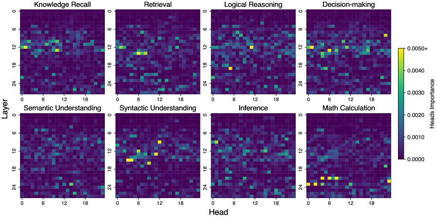
### Visual Description
## Heatmap Grid: Heads Importance by Task and Layer
### Overview
The image presents a series of heatmaps, arranged in a 2x4 grid, visualizing the importance of different "heads" (likely referring to attention heads in a neural network) across various layers for different tasks. Each heatmap represents a specific task, with the y-axis indicating the layer number (0 to 24) and the x-axis representing the head number (0 to 18). The color intensity indicates the importance of a particular head in a specific layer for the given task.
### Components/Axes
* **Titles:** The heatmaps are titled with the following tasks: "Knowledge Recall", "Retrieval", "Logical Reasoning", "Decision-making", "Semantic Understanding", "Syntactic Understanding", "Inference", and "Math Calculation".
* **X-axis:** Labeled "Head", with ticks at 0, 6, 12, and 18. Represents the index of the attention head.
* **Y-axis:** Labeled "Layer", with ticks at 0, 6, 12, 18, and 24. Represents the layer number in the neural network.
* **Colorbar (Heads Importance):** Located on the right side of the "Decision-making" heatmap. It ranges from 0.0000 (dark purple) to 0.0050+ (yellow). Intermediate values are 0.0010, 0.0020, 0.0030, and 0.0040, with corresponding color gradations.
### Detailed Analysis
Each heatmap represents the importance of each head at each layer for a specific task. The color intensity indicates the level of importance.
* **Knowledge Recall:** Shows some concentration of importance around layer 12, with a few heads showing higher importance.
* **Retrieval:** Similar to Knowledge Recall, with some heads showing slightly higher importance around layer 12.
* **Logical Reasoning:** Shows a more dispersed pattern of importance, with a few heads showing higher importance across different layers.
* **Decision-making:** Shows some concentration of importance in the upper layers (around layer 6 and 12), with a few heads showing higher importance.
* **Semantic Understanding:** Shows a dispersed pattern of importance, with a few heads showing higher importance across different layers.
* **Syntactic Understanding:** Shows a concentration of importance around layer 12, with a few heads showing significantly higher importance.
* **Inference:** Shows a dispersed pattern of importance, with a few heads showing higher importance across different layers.
* **Math Calculation:** Shows a concentration of importance in the lower layers (around layer 18 and 24), with a few heads showing significantly higher importance.
### Key Observations
* **Layer Specificity:** Some tasks, like "Syntactic Understanding" and "Math Calculation", show a clear concentration of importance in specific layers. "Syntactic Understanding" is concentrated around layer 12, while "Math Calculation" is concentrated in the lower layers (18-24).
* **Head Importance:** Within each task, only a subset of heads appears to be highly important.
* **Color Scale:** The color scale is consistent across all heatmaps, allowing for direct comparison of head importance across different tasks and layers.
### Interpretation
The heatmaps provide insights into which attention heads in a neural network are most important for different tasks at different layers. The concentration of importance in specific layers for certain tasks suggests that the network may be learning hierarchical representations, with different layers specializing in different aspects of the task. For example, the concentration of importance in lower layers for "Math Calculation" might indicate that these layers are responsible for low-level feature extraction, while the concentration in higher layers for "Syntactic Understanding" might indicate that these layers are responsible for more abstract reasoning. The fact that only a subset of heads is highly important suggests that the network may be learning sparse representations, with only a few heads being actively used for each task. This information could be used to optimize the network architecture or to gain a better understanding of how the network is solving the task.
</details>
Figure 5: The existence of cognitive heads in Llama3.2-3B-instruct responsible for eight distinct functions in complex reasoning tasks. The x-axis represents the head index, while the y-axis indicates the layer index.
<details>
<summary>x8.png Details</summary>
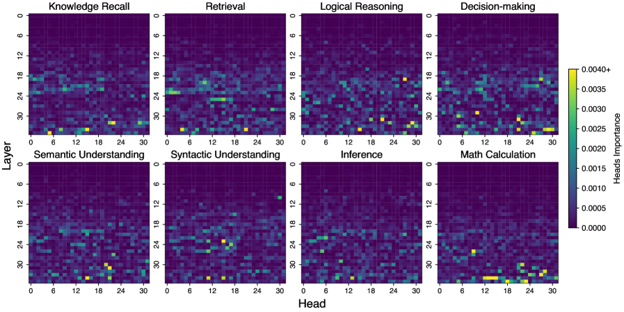
### Visual Description
## Heatmap: Heads Importance for Different Tasks
### Overview
The image presents a series of heatmaps, each representing the "Heads Importance" for different tasks: Knowledge Recall, Retrieval, Logical Reasoning, Decision-making, Semantic Understanding, Syntactic Understanding, Inference, and Math Calculation. Each heatmap visualizes the importance of different "Heads" across different "Layers" of a model. The color intensity indicates the level of importance, ranging from dark purple (0.0000) to yellow (0.0040+).
### Components/Axes
* **X-axis:** "Head" - Ranges from 0 to 30 in increments of 6.
* **Y-axis:** "Layer" - Ranges from 0 to 30 in increments of 6.
* **Heatmaps:** 8 heatmaps arranged in a 2x4 grid, each representing a different task.
* **Color Scale (Legend):** Located on the right side of the image.
* Dark Purple: 0.0000
* Dark Blue: 0.0005
* Light Blue: 0.0010
* Teal: 0.0015
* Green: 0.0020
* Light Green: 0.0025
* Yellow-Green: 0.0030
* Yellow: 0.0035
* Bright Yellow: 0.0040+
* **Titles:** Each heatmap has a title indicating the task it represents (e.g., "Knowledge Recall").
### Detailed Analysis
**General Observations:**
* Most heatmaps show a concentration of higher importance (yellow/green) in specific regions, rather than a uniform distribution.
* The lower layers (Layer 24-30) and specific heads seem to be more important for most tasks.
**Task-Specific Analysis:**
* **Knowledge Recall:** Shows some importance in the lower layers (24-30) and around heads 6-12 and 24-30.
* **Retrieval:** Shows a concentration of importance in the lower layers (24-30), particularly around heads 0-6 and 18-24.
* **Logical Reasoning:** Shows scattered importance, with some concentration in the lower layers (24-30) and around heads 18-24.
* **Decision-making:** Shows scattered importance, with some concentration in the lower layers (24-30) and around heads 12-18.
* **Semantic Understanding:** Shows importance in the lower layers (24-30) and around heads 18-24.
* **Syntactic Understanding:** Shows importance in the lower layers (24-30) and around heads 12-18.
* **Inference:** Shows importance in the lower layers (24-30) and around heads 12-18.
* **Math Calculation:** Shows a strong concentration of importance in the lower layers (24-30) and around heads 12-18.
### Key Observations
* The lower layers (24-30) tend to be more important across all tasks.
* Specific heads seem to be more important for certain tasks. For example, heads 12-18 seem important for Math Calculation, Inference, and Syntactic Understanding.
* The distribution of importance varies significantly across different tasks.
### Interpretation
The heatmaps provide insights into which "Heads" and "Layers" are most important for different cognitive tasks. The concentration of importance in the lower layers suggests that these layers are crucial for processing information relevant to these tasks. The varying patterns across tasks indicate that different heads and layers are specialized for different cognitive functions. The data suggests that the model utilizes different parts of its architecture to perform different tasks, highlighting the modularity and specialization within the model. The "Heads Importance" metric could be used to optimize the model by focusing on the most important heads and layers for each task.
</details>
Figure 6: The existence of cognitive heads in Qwen3-8B responsible for eight distinct functions in complex reasoning tasks. The x-axis represents the head index, while the y-axis indicates the layer index.
<details>
<summary>x9.png Details</summary>
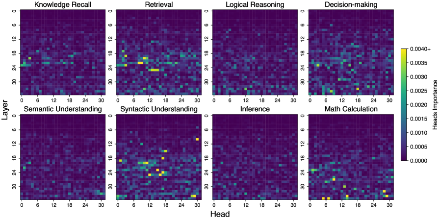
### Visual Description
## Heatmap: Heads Importance by Task and Layer
### Overview
The image presents a series of heatmaps visualizing the importance of different "heads" (likely referring to attention heads in a neural network) across various layers for different tasks. Each heatmap represents a specific task, with the x-axis indicating the "Head" number and the y-axis indicating the "Layer" number. The color intensity represents the "Heads Importance," ranging from dark purple (0.0000) to bright yellow (0.0040+).
### Components/Axes
* **X-axis (Head):** Ranges from 0 to 30 in increments of 6.
* **Y-axis (Layer):** Ranges from 0 to 30 in increments of 6.
* **Heatmaps:** Arranged in a 2x4 grid, each representing a different task.
* **Color Scale (Heads Importance):**
* Dark Purple: 0.0000
* Purple: 0.0005
* Light Purple: 0.0010
* Blue: 0.0015
* Teal: 0.0020
* Green: 0.0025
* Light Green: 0.0030
* Yellow: 0.0035
* Bright Yellow: 0.0040+
* **Task Labels (Top Row):**
* Knowledge Recall
* Retrieval
* Logical Reasoning
* Decision-making
* **Task Labels (Bottom Row):**
* Semantic Understanding
* Syntactic Understanding
* Inference
* Math Calculation
### Detailed Analysis
Each heatmap shows the distribution of "Heads Importance" across layers and heads for a specific task. The color intensity indicates the relative importance of each head in each layer.
* **Knowledge Recall:** Shows some concentration of importance around layer 24, heads 0-6, and also around layer 18, heads 12-18.
* **Retrieval:** Shows a strong concentration of importance around layer 24, heads 6-12.
* **Logical Reasoning:** Shows scattered importance with no clear concentration.
* **Decision-making:** Shows some concentration of importance around layer 24, heads 18-24.
* **Semantic Understanding:** Shows a concentration of importance around layer 24, heads 6-12, and also around layer 30, heads 24-30.
* **Syntactic Understanding:** Shows a strong concentration of importance around layer 18, heads 6-12.
* **Inference:** Shows scattered importance with no clear concentration.
* **Math Calculation:** Shows some concentration of importance around layer 24, heads 6-12, and also around layer 30, heads 6-12.
### Key Observations
* Layer 24 seems to be important for many tasks, especially Retrieval, Semantic Understanding, and Math Calculation.
* Syntactic Understanding shows a distinct concentration of importance in layer 18.
* Logical Reasoning and Inference show a more scattered distribution of importance across layers and heads.
### Interpretation
The heatmaps provide insights into which attention heads in which layers are most important for different cognitive tasks. The concentration of importance in specific layers and heads suggests that certain parts of the neural network are specialized for particular aspects of each task. For example, the strong concentration in layer 24 for Retrieval, Semantic Understanding, and Math Calculation might indicate that this layer is crucial for information retrieval and processing. The distinct pattern for Syntactic Understanding suggests that syntactic processing relies on different layers and heads compared to other tasks. The scattered patterns for Logical Reasoning and Inference might indicate that these tasks require a more distributed representation of information across the network.
</details>
Figure 7: The existence of cognitive heads in Qwen3-4B responsible for eight distinct functions in complex reasoning tasks. The x-axis represents the head index, while the y-axis indicates the layer index.
<details>
<summary>x10.png Details</summary>
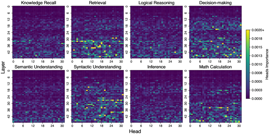
### Visual Description
## Heatmap: Heads Importance for Different Tasks
### Overview
The image presents a series of heatmaps visualizing the importance of different "heads" across various layers for different tasks. Each heatmap represents a specific task, with the x-axis indicating the "Head" and the y-axis indicating the "Layer." The color intensity represents the "Heads Importance," ranging from dark purple (0.0000) to bright yellow (0.0020+).
### Components/Axes
* **X-axis:** "Head" - Ranges from 0 to 30 in increments of 6.
* **Y-axis:** "Layer" - Ranges from 0 to 42 in increments of 6.
* **Heatmaps:** Eight heatmaps, each representing a different task.
* **Color Scale (Heads Importance):** Located on the right side of the image.
* Dark Purple: 0.0000
* Purple: 0.0003
* Blue: 0.0005
* Green: 0.0008
* Light Green: 0.0010
* Yellow-Green: 0.0013
* Yellow: 0.0015
* Bright Yellow: 0.0018
* Very Bright Yellow: 0.0020+
* **Task Labels:**
* Top Row (left to right): Knowledge Recall, Retrieval, Logical Reasoning, Decision-making
* Bottom Row (left to right): Semantic Understanding, Syntactic Understanding, Inference, Math Calculation
### Detailed Analysis
**1. Knowledge Recall:**
* The heatmap is mostly dark purple, indicating low importance across most heads and layers.
* Slightly higher importance (blue to green) is observed in the lower layers (30-42) and some heads (around 12-18).
**2. Retrieval:**
* Higher importance is concentrated in the lower layers (30-42).
* Several heads (around 6-18) in these lower layers show significant importance (yellow).
**3. Logical Reasoning:**
* The heatmap is predominantly dark purple, indicating low importance across most heads and layers.
* A few scattered points of slightly higher importance (blue to green) are visible.
**4. Decision-making:**
* Similar to Logical Reasoning, the heatmap is mostly dark purple.
* A few scattered points of slightly higher importance (blue to green) are visible, particularly around layer 36.
**5. Semantic Understanding:**
* Higher importance is observed in the lower layers (30-42).
* Several heads (around 12-24) in these lower layers show significant importance (yellow).
**6. Syntactic Understanding:**
* Higher importance is concentrated in the lower layers (30-42).
* Several heads (around 6-18) in these lower layers show significant importance (yellow).
**7. Inference:**
* The heatmap is predominantly dark purple, indicating low importance across most heads and layers.
* A few scattered points of slightly higher importance (blue to green) are visible.
**8. Math Calculation:**
* The heatmap is predominantly dark purple, indicating low importance across most heads and layers.
* A few scattered points of slightly higher importance (blue to green) are visible, particularly in the lower layers.
### Key Observations
* Tasks like Retrieval, Semantic Understanding, and Syntactic Understanding show a concentration of high importance in the lower layers (30-42).
* Tasks like Logical Reasoning, Decision-making, Inference, and Math Calculation show generally low importance across all layers and heads.
* Knowledge Recall shows a slightly higher importance in the lower layers compared to Logical Reasoning, Decision-making, Inference, and Math Calculation.
### Interpretation
The heatmaps suggest that for tasks like Retrieval, Semantic Understanding, and Syntactic Understanding, the lower layers of the model are more critical. This could indicate that these tasks rely more on lower-level features or representations learned in the earlier layers. Conversely, tasks like Logical Reasoning, Decision-making, Inference, and Math Calculation may rely on a more distributed set of features across all layers, or potentially on different architectures altogether, resulting in lower importance scores for individual heads. The concentration of importance in specific heads for certain tasks suggests that those heads are specialized in extracting relevant information for those tasks. The data suggests that different tasks rely on different aspects of the model's architecture, with some tasks being more dependent on lower-level features and specific heads than others.
</details>
Figure 8: The existence of cognitive heads in Yi-1.5-9B responsible for eight distinct functions in complex reasoning tasks. The x-axis represents the head index, while the y-axis indicates the layer index.
<details>
<summary>x11.png Details</summary>
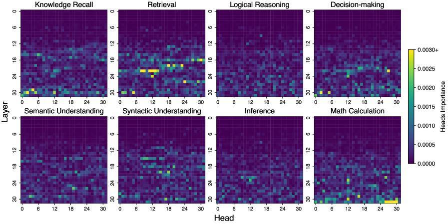
### Visual Description
## Heatmap Grid: Heads Importance by Task and Layer
### Overview
The image presents a grid of heatmaps, each representing the "Heads Importance" for a specific task across different layers and heads of a model. The tasks are: Knowledge Recall, Retrieval, Logical Reasoning, Decision-making, Semantic Understanding, Syntactic Understanding, Inference, and Math Calculation. The heatmaps visualize the importance of each head (x-axis) at each layer (y-axis) for the given task. The color intensity indicates the level of importance, ranging from dark purple (0.0000) to bright yellow (0.0030+).
### Components/Axes
* **X-axis (Head):** Represents the different heads, ranging from 0 to 30.
* **Y-axis (Layer):** Represents the layers, ranging from 0 to 30.
* **Heatmap Grid:** An 2x4 grid of heatmaps, each representing a different task.
* **Color Scale (Heads Importance):**
* Dark Purple: 0.0000
* Blue: 0.0005
* Light Blue: 0.0010
* Green: 0.0015
* Yellow-Green: 0.0020
* Yellow: 0.0025
* Bright Yellow: 0.0030+
* **Task Labels:** Each heatmap is labeled with a task name: Knowledge Recall, Retrieval, Logical Reasoning, Decision-making, Semantic Understanding, Syntactic Understanding, Inference, and Math Calculation.
### Detailed Analysis
**1. Knowledge Recall:**
* Trend: Higher importance is observed in the lower layers (24-30) and some scattered importance in the middle layers.
* Specifics: There are a few heads around layer 30 that show high importance (yellow).
**2. Retrieval:**
* Trend: High importance is concentrated in layers 20-30, with some heads showing significantly higher importance.
* Specifics: Several yellow spots are visible in layers 20-30, indicating high head importance.
**3. Logical Reasoning:**
* Trend: Importance is generally low across all layers and heads.
* Specifics: Mostly dark purple and blue, with a few scattered green spots.
**4. Decision-making:**
* Trend: Similar to Logical Reasoning, importance is generally low.
* Specifics: A few green and yellow-green spots are scattered throughout.
**5. Semantic Understanding:**
* Trend: Importance is scattered, with slightly higher importance in the lower layers.
* Specifics: A mix of blue, green, and yellow-green spots.
**6. Syntactic Understanding:**
* Trend: Importance is concentrated in the middle layers (12-24).
* Specifics: Several green and yellow-green spots are visible in the middle layers.
**7. Inference:**
* Trend: Importance is scattered, with a slight concentration in the lower layers.
* Specifics: Similar to Semantic Understanding, a mix of blue, green, and yellow-green spots.
**8. Math Calculation:**
* Trend: Importance is concentrated in the lower layers (24-30).
* Specifics: Several green and yellow spots are visible in the lower layers.
### Key Observations
* **Task-Specific Head Importance:** The importance of heads varies significantly depending on the task.
* **Layer Dependency:** Some tasks, like Retrieval and Math Calculation, show higher importance in the lower layers, while others, like Syntactic Understanding, show higher importance in the middle layers.
* **Low Importance for Reasoning and Decision-making:** Logical Reasoning and Decision-making tasks generally show lower head importance compared to other tasks.
### Interpretation
The heatmaps provide insights into which heads and layers are most important for different tasks within the model. The concentration of importance in specific layers suggests that certain layers are specialized for particular types of processing. The low importance observed for Logical Reasoning and Decision-making could indicate that these tasks require a more distributed representation or that the model architecture is not well-suited for these tasks. The data suggests that the model utilizes different heads and layers for different cognitive tasks, highlighting the modularity and specialization within the network. The concentration of activity in certain layers for specific tasks could be indicative of a hierarchical processing structure, where lower layers handle more basic features and higher layers handle more abstract concepts.
</details>
Figure 9: The existence of cognitive heads in Yi-1.5-6B responsible for eight distinct functions in complex reasoning tasks. The x-axis represents the head index, while the y-axis indicates the layer index.
A.2 Importance curve
We ranked the importance scores and identified the elbow point, as illustrated in Figure 10.
<details>
<summary>x12.png Details</summary>
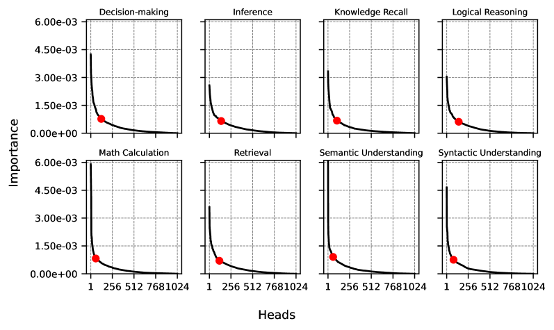
### Visual Description
## Chart Type: Multiple Line Graphs
### Overview
The image contains eight line graphs arranged in a 2x4 grid. Each graph displays the relationship between "Heads" (x-axis) and "Importance" (y-axis) for a specific cognitive task. The cognitive tasks are: Decision-making, Inference, Knowledge Recall, Logical Reasoning, Math Calculation, Retrieval, Semantic Understanding, and Syntactic Understanding. Each graph shows a decreasing trend in importance as the number of heads increases. A red dot is present on each line, marking a specific point on the curve.
### Components/Axes
* **X-axis (Horizontal):** "Heads" with values 1, 256, 512, 768, and 1024. The scale is non-linear.
* **Y-axis (Vertical):** "Importance" with values 0.00e+00, 1.50e-03, 3.00e-03, 4.50e-03, and 6.00e-03.
* **Titles:** Each graph has a title indicating the cognitive task: Decision-making, Inference, Knowledge Recall, Logical Reasoning, Math Calculation, Retrieval, Semantic Understanding, and Syntactic Understanding.
* **Grid:** Each graph has a grid of dashed lines.
* **Data Series:** Each graph contains a single black line representing the relationship between "Heads" and "Importance".
* **Red Dot:** Each graph has a red dot on the black line. The x-coordinate of the red dot is approximately 256.
### Detailed Analysis
**Graph 1: Decision-making**
* Trend: The black line slopes downward, indicating decreasing importance as the number of heads increases.
* Red Dot: Located at approximately (256, 1.25e-03).
**Graph 2: Inference**
* Trend: The black line slopes downward, indicating decreasing importance as the number of heads increases.
* Red Dot: Located at approximately (256, 1.10e-03).
**Graph 3: Knowledge Recall**
* Trend: The black line slopes downward, indicating decreasing importance as the number of heads increases.
* Red Dot: Located at approximately (256, 1.00e-03).
**Graph 4: Logical Reasoning**
* Trend: The black line slopes downward, indicating decreasing importance as the number of heads increases.
* Red Dot: Located at approximately (256, 1.15e-03).
**Graph 5: Math Calculation**
* Trend: The black line slopes downward, indicating decreasing importance as the number of heads increases.
* Red Dot: Located at approximately (256, 0.90e-03).
**Graph 6: Retrieval**
* Trend: The black line slopes downward, indicating decreasing importance as the number of heads increases.
* Red Dot: Located at approximately (256, 0.85e-03).
**Graph 7: Semantic Understanding**
* Trend: The black line slopes downward, indicating decreasing importance as the number of heads increases.
* Red Dot: Located at approximately (256, 0.80e-03).
**Graph 8: Syntactic Understanding**
* Trend: The black line slopes downward, indicating decreasing importance as the number of heads increases.
* Red Dot: Located at approximately (256, 0.75e-03).
### Key Observations
* All graphs exhibit a similar decreasing trend.
* The "Importance" values are relatively high when the number of "Heads" is low (close to 1) and decrease rapidly as the number of "Heads" increases.
* The red dots are consistently positioned around x=256, but the y-values (Importance) vary slightly across the different cognitive tasks.
* The y-axis scale is consistent across all graphs, allowing for direct comparison of "Importance" values.
### Interpretation
The graphs suggest that for all the cognitive tasks examined (Decision-making, Inference, Knowledge Recall, Logical Reasoning, Math Calculation, Retrieval, Semantic Understanding, and Syntactic Understanding), the "Importance" decreases as the number of "Heads" increases. The red dots highlight a specific point (Heads = 256) where the "Importance" values can be compared across the different tasks. The variation in "Importance" at this point suggests that some cognitive tasks may rely more heavily on a smaller number of heads than others. The rapid decrease in "Importance" with increasing "Heads" implies diminishing returns, suggesting that beyond a certain number of heads, the contribution to the task becomes marginal.
</details>
Figure 10: Importance curve for eight functions, Llama3.1-8B-instruct.
A.3 MLP
We train a two-layer multi-class MLP for cognitive function classification. The first layer applies a shared linear projection to each multi-head representation vector, reducing each to a 64-dimensional embedding. These embeddings are then flattened and concatenated into a single vector of size $64× numberofheads$ . This vector is fed into a hidden layer with 512 units, followed by a ReLU activation and a dropout with a rate of 0.3. The final output layer maps the 512-dimensional hidden representation to the set of cognitive function labels.
The model is trained using the Adam optimizer with a learning rate of $10^{-4}$ and a cross-entropy loss. Training proceeds for 100 epochs. The test accuracy of our classification method across all LLM models is summarized in the Table 5.
Table 5: The test accuracy (%) of probing method on different LLMs.
| Dataset CogQA | Llama3.1-8B-instruct 83.73 | Llama3.2-3B-instruct 79.80 | Qwen3-8B 84.71 | Qwen3-4B 80.79 | Yi-1.5-9B 77.56 | Yi-1.5-6B 75.18 |
| --- | --- | --- | --- | --- | --- | --- |
A.4 Prompt for Generating CogQA
Prompt
Prompt: You are an expert in analytical logical reasoning. You will be given a question along with its chain-of-thought process. Your task is to break the question down into subquestions based on the chain-of-thought process, ensuring that all necessary steps for solving the problem and constructing the logical chain are included to simulate critical thinking. Decompose the Question: Identify and formulate the key subquestions required to solve the main question logically. Fill in Missing Steps: Ensure that all essential reasoning steps are explicitly stated. NOTE: The information of chain-of-thought cannot be used directly if it doesn’t exist in main query. Each subquestion should be derived solely from the main query and the preceding subquestion. Answer the Subquestions: Provide clear, step-by-step solutions for each subquestion. Annotate Cognitive Skills: Identify and label the specific cognitive abilities required to answer each subquestion. If you believe other cognitive skills are relevant, you may also consider incorporating them. You will be given predefined labels along with their descriptions. Your goal is to enhance the logical reasoning process by making it explicit and structured. <cognitive_skills> **Retrieval**: Refers to the process of fetching relevant information from input text, typically involving the extraction of specific words, phrases, or sentences directly from the original text. **Knowledge Recall**: Involves the storage and recall of domain-specific knowledge, such as concepts from math, physics, biology, etc. This is typically the internal knowledge base of a language model. (Corresponding to the memory head) **Semantic Understanding**: Refers to the ability to comprehend and extract meaning from text or symbols by recognizing relationships between words, phrases, and concepts. It goes beyond syntactic understanding by grasping context, intent, and underlying knowledge. **Syntactic Understanding*: Involves the ability to analyze and interpret the grammatical structure of sentences, including the roles and relationships of words, phrases, and clauses within the language. **Math Calculation**: Refers to the process of performing arithmetic or mathematical operations to obtain a result. It involves applying mathematical concepts, such as addition, subtraction, multiplication, division, and more complex operations (e.g., algebra, calculus), to solve problems or derive values from given inputs. **Inference**: Involves drawing conclusions based on existing evidence or information. It follows logical rules to deduce new statements or decisions from given information. **Logical Reasoning**: The process of drawing conclusions based on a set of premises, following established rules of logic, used to ensure that decisions of people are coherent, consistent, and based on sound principles. **Decision-making**: The process of making a choice in a selection task based on previous information or analysis. <cognitive_skills> Here is the question: <question> question <question> Here is the chain-of-thought: <chain-of-thought> cot <chain-of-thought> Note - Your task is to break the question down into detailed subquestions, ensuring each subquestion can be answered using only one specific cognitive skill. - You need to create a structured and explicit reasoning process that simulates critical thinking while maintaining clarity and precision. - The subquestion needs to be easy to answer and the answer needs to be concise - The information of chain-of-thought cannot be used directly if it doesn’t exist in main query. - Each subquestion should be derived solely from the main query and the preceding subquestion. - You CAN NOT retrieval information from chain-of-thought, but you can retrieval from question. - Your output should be formatted as a list of JSON objects, where each object represents a subquestion, its answer, and the required cognitive skill. - You should use the most efficient logic to analyze the problem and minimize the number of subquestions. Output format [ "subquestion": "<Subquestion text>", "answer": "<Concise answer>", "cognitive_skill": "<Assigned cognitive skill>" , "subquestion": "<Subquestion text>", "answer": "<Concise answer>", "cognitive_skill": "<Assigned cognitive skill>" ] Your answer:
A.5 Annotations
To ensure the quality and reliability of the decomposed subQAC triplets in the CogQA dataset, we design a rigorous multi-stage annotation pipeline, combining expert review and model-based verification. The goal is to verify the logical validity of subquestions, the correctness of their associated cognitive function labels, and the accuracy of the answers.
Stage 1: Validating Subquestion Decomposition
In the first stage, we evaluate whether the generated subquestions are logically sound and align with natural human reasoning. For each QA pair, three expert annotators (with backgrounds in linguistics or cognitive science) independently assess the validity of each subquestion. A subquestion is marked true if it meaningfully contributes to answering the main question and follows a logical reasoning trajectory. Otherwise, it is marked false.
If a subquestion depends on prior information—such as the question text or the answer—from another subquestion, the subquestion order must reflect this dependency. While some subquestions can be answered in parallel and are order-independent, others have prerequisite relationships that require a specific sequence. As the overall reasoning structure often forms a graph, where both sequential and parallel dependencies coexist. During LLM inference, we include the previous subquestions and their corresponding subanswers in the prompt as prior information. Thus, the critical factor is not the ordering alone, but whether the prompt provides the necessary context to answer the current subquestion accurately.
We apply the following filtering criteria:
- AI-Human Agreement: If any annotator considers fewer than 60% of the subquestions valid, the entire QA decomposition is discarded.
- Inter-Annotator Agreement: A subquestion is deemed invalid if at least two annotators mark it as false. If over 40% of the subquestions in a QA pair are invalid under this rule, the whole QA pair is removed.
This filtering ensures that the retained QA decompositions follow coherent, cognitively plausible reasoning chains.
Stage 2: Verifying Cognitive Function Labels
In the second stage, annotators evaluate the correctness of the cognitive function label $c_{i}$ assigned to each subQAC triplet $(q_{i},a_{i},c_{i})$ . Three annotators independently mark each label as true or false. When discrepancies occur, annotators collaboratively reassign the correct cognitive label to ensure alignment with the underlying mental operation.
This step ensures that the categorization of subquestions accurately reflects established distinctions between information retrieval, semantic understanding, logical reasoning, and other cognitive processes.
Stage 3: Answer Verification via Model and Human Review
In the final stage, we verify the correctness of each answer $a_{i}$ using both automated and manual procedures. We employ the o4-mini model [o4mini2024], known for its logical reasoning capabilities, to re-evaluate GPT-4o-generated answers. If o4-mini disagrees with GPT-4o, it provides an alternative answer. A human annotator then compares both answers and resolves discrepancies by supplying the correct one when necessary. Given the generally objective nature of answers, only one annotator is required for this task.
Annotation Outcome
Following this multi-stage process, we retain 570 validated QA pairs, yielding a total of 3,402 high-quality subQAC triplets. Notably, we augment certain cognitive functions to ensure balance across categories. As a result, the original 570 QA pairs were expanded to 720 (including some duplicates), with each duplicated pair potentially associated with distinct subquestions and cognitive functions.
A.6 CogQA Example
Table 6 presents illustrative examples from the CogQA dataset. The main question and its corresponding answer are taken from the original dataset. Based on an analysis of the main question, a sequence of sub-questions, their answers, and associated cognitive function labels are generated in order.
Table 6: Two examples from the CogQA dataset showing a main question, its final answer, and a breakdown into subquestions with answers and their corresponding cognitive function labels.
| Main Question | A one-year subscription to a newspaper is offered with a 45% discount. How much does the discounted subscription cost if a subscription normally costs $80? |
| --- | --- |
| Answer | We calculate first the discount: 80 $×$ 45 / 100 = $36. So, the discounted subscription amounts to 80 – 36 = $44. |
| 1. What is the normal cost of a one-year subscription to the newspaper? | $80 | Retrieval |
| --- | --- | --- |
| 2. What is the discount percentage offered on the subscription? | 45% | Retrieval |
| 3. How much is the discount amount in dollars for the subscription? | $36 | Math Calculation |
| 4. What is the cost of the subscription after applying the discount? | $44 | Math Calculation |
| Main Question | What does every person talk out of? Options: - name - hide - mother and father - mouth - heart |
| --- | --- |
| Answer | By mouth, talking is done. Every person talk out of mouth. |
| 1. What is the primary function of talking? | To communicate verbally. | Knowledge Recall |
| --- | --- | --- |
| 2. Which part of the human body is primarily used for verbal communication? | Mouth | Knowledge Recall |
| 3. Based on the options provided, which option corresponds to the part used for verbal communication? | Mouth | Decision-making |
A.7 Prompt for Question Asking
Prompt
Prompt: You are an expert in analytical and logical reasoning. You will be given a main question and prior knowledge in chain-of-thought (CoT) format. Your task is to answer a follow-up subquestion using the information provided. Here is the main question: <main_question> question </main_question> Here is the prior knowledge in chain-of-thought (CoT) format: <prior_knowledge> cot </prior_knowledge> Here is the subquestion: <subquestion> subquestion </subquestion> Instructions: - Answer the subquestion carefully. - You can use the information in the prior_knowledge to help you answer the subquestion. - Your response should be clear and concise. - Stick to factual reasoning based on provided CoT. - Do not include any explanation, commentary, or code. - Do not output anything after the closing square bracket ‘]‘. Only output your final answer using this format: [ "answer": "<Your answer here>" ] Your answer:
A.8 The number of cognitive heads for different LLMs
The number of cognitive heads for each model is shown in Table 7.
Table 7: Count (C) and percentage (%) of attention heads exceeding elbow thresholds for each cognitive function across six models.
| Llama3.1-8B-instruct Llama3.2-3B-instruct Qwen3-8B | 105 95 119 | 10.3 14.1 10.3 | 118 62 115 | 11.5 9.2 10.0 | 142 95 114 | 13.9 14.1 9.9 | 124 87 87 | 12.1 12.9 7.6 | 60 90 68 | 5.9 13.4 5.9 | 81 63 108 | 7.9 9.4 9.4 | 139 98 178 | 13.6 14.6 15.5 | 59 35 61 | 5.8 5.2 5.3 |
| --- | --- | --- | --- | --- | --- | --- | --- | --- | --- | --- | --- | --- | --- | --- | --- | --- |
| Qwen3-4B | 115 | 10.0 | 94 | 8.2 | 120 | 10.4 | 170 | 14.8 | 143 | 12.4 | 106 | 9.2 | 109 | 9.5 | 99 | 8.6 |
| Yi-1.5-9B | 200 | 13.0 | 134 | 8.7 | 134 | 8.7 | 174 | 11.3 | 218 | 14.2 | 140 | 9.1 | 173 | 11.3 | 167 | 10.9 |
| Yi-1.5-6B | 118 | 11.5 | 90 | 8.8 | 200 | 19.5 | 93 | 9.1 | 99 | 9.7 | 142 | 13.9 | 146 | 14.3 | 67 | 6.5 |
A.9 Ablation study - Different position of head activation
In the main experiments, we use the top-k generated tokens and average their multi-head attention vectors. We also explore alternative strategies for extracting representations, including using the first generated token, the last generated token, the first meaningful token, and the average of all generated tokens. The corresponding results are shown in Table 8.
Here, first is the first token, last is the last token, meaning_first is the first meaning token (excluding formatting), top-k is the top-k most semantically important tokens, full is all tokens in the answer.We observe that top-k token masking leads to the most significant performance drop when masking the top-30 identified heads, indicating higher precision in identifying retrieval-relevant heads. Interestingly, last, meaning_first, full, and top-k show similar performance trends. This is because different tokens in the output contribute to answering the question, and as the number of masked cognitive heads increases, the influence of token using decreases. Additionally, for Retrieval, the full answer is usually meaningful, whereas others like Math Calculation require semantically meaningful tokens. Based on these results, we choose top-k as our final setting.
Table 8: Attention heads associated with cognitive functions are selected based on different token positions. Accuracy and COMET scores are evaluated after intervention; lower values indicate better outcomes.
| Llama3.1-8B Llama3.1-8B Llama3.1-8B | 30 30 30 | first last meaning_first | 90.51 86.86 88.13 | 83.53 81.76 79.41 | 91.13 90.04 89.72 | 73.13 68.66 68.66 |
| --- | --- | --- | --- | --- | --- | --- |
| Llama3.1-8B | 30 | full | 73.93 | 47.06 | 89.92 | 69.15 |
| Llama3.1-8B | 30 | top-k | 70.05 | 46.47 | 89.32 | 67.16 |
| Llama3.1-8B | 50 | first | 93.28 | 89.41 | 94.46 | 89.57 |
| Llama3.1-8B | 50 | last | 64.39 | 41.18 | 92.05 | 70.15 |
| Llama3.1-8B | 50 | meaning_first | 62.90 | 34.12 | 84.60 | 60.69 |
| Llama3.1-8B | 50 | full | 46.20 | 11.76 | 89.01 | 78.11 |
| Llama3.1-8B | 50 | top-k | 65.64 | 47.76 | 89.65 | 70.15 |
A.10 Examples of top- $k$ tokens
The selected tokens are intended to semantically represent the generated answer. Below are examples for different cognitive functions for Llama3.1-8B-instruct:
Table 9: Examples of question decomposition with cognitive functions and token selection.
| Given the sentence "A surfboarder catches the waves." can we conclude that "A surfboarder in the water."? (Options: yes / it is not possible to tell / no) | What is typically required for a surfboarder to catch waves? | Knowledge Recall | The surfboarder needs to be in the water. | [’surfboarder’, ’needs’, ’be’, ’in’, ’water’] |
| --- | --- | --- | --- | --- |
| Is the following a factual statement? "Due to its high density, countries around the world use Palladium to mint coins." (Options: yes / no) | What is the statement in question? | Retrieval | The statement in question is: Due to its high density, countries around the world use Palladium to mint coins. | [’high’, ’density’, ’Palladium’, ’mint’, ’coins’] |
| A one-year subscription to a newspaper is offered with a 45% discount. How much does the discounted subscription cost if a subscription normally costs $80? | How much is the discount amount in dollars for the subscription? | Math Calculation | 36 | [’36’] |
We can see that the selected tokens semantically represent the answer. Note that we use all tokens when the number of tokens is fewer than 5.