# Graph Embedding with Mel-spectrograms for Underwater Acoustic Target Recognition
**Authors**: Sheng Feng, Shuqing Ma, Xiaoqian Zhu
> This paper was produced by the IEEE Publication Technology Group. (corresponding author: Xiaoqian Zhu.)Manuscript received May 5, 2024; This work was supported by the National Defense Fundamental Scientific Research Program under Grant No.JCKY2020550C011. The authors are with the College of Meteorology and Oceanography, National University of Defense Technology, Chang sha 410073, China (e-mail: fengsheng18@nudt.edu.cn; mashuqing@nudt.edu.cn;
zhu_xiaoqian@sina.com).
Abstract
Underwater acoustic target recognition (UATR) is extremely challenging due to the complexity of ship-radiated noise and the variability of ocean environments. Although deep learning (DL) approaches have achieved promising results, most existing models implicitly assume that underwater acoustic data lie in a Euclidean space. This assumption, however, is unsuitable for the inherently complex topology of underwater acoustic signals, which exhibit non-stationary, non-Gaussian, and nonlinear characteristics. To overcome this limitation, this paper proposes the UATR-GTransformer, a non-Euclidean DL model that integrates Transformer architectures with graph neural networks (GNNs). The model comprises three key components: a Mel patchify block, a GTransformer block, and a classification head. The Mel patchify block partitions the Mel-spectrogram into overlapping patches, while the GTransformer block employs a Transformer Encoder to capture mutual information between split patches to generate Mel-graph embeddings. Subsequently, a GNN enhances these embeddings by modeling local neighborhood relationships, and a feed-forward network (FFN) further performs feature transformation. Experiments results based on two widely used benchmark datasets demonstrate that the UATR-GTransformer achieves performance competitive with state-of-the-art methods. In addition, interpretability analysis reveals that the proposed model effectively extracts rich frequency-domain information, highlighting its potential for applications in ocean engineering. publicationid: pubid: 0000–0000/00$00.00 © 2021 IEEE
I Introduction
Underwater acoustic target recognition (UATR), a crucial topic in ocean engineering, involves detecting and classifying underwater targets based on their unique acoustic properties. This capability holds important implications for maritime security, environmental monitoring, and underwater exploration. However, UATR is highly challenging due to the complex mechanisms of underwater sound propagation in diverse marine environments [xie2022adaptive]. Factors such as attenuation, scattering, and reverberation significantly complicate target identification and classification. Early UATR methods primarily relied on experienced sonar operators for manual recognition, but such approaches are prone to subjective influences, including psychological and physiological conditions. To overcome these limitations, statistical learning techniques were introduced, leveraging time-frequency representations derived from waveforms to enhance automatic recognition. Representative approaches include Support Vector Machines (SVM) [7435957, 7108260] and logistic regression [10390008]. Nevertheless, as the demand for higher recognition accuracy has increased, the shortcomings of statistical learning-based methods have become apparent. These methods typically capture only shallow discriminative patterns and fail to fully exploit the potential of diverse datasets.
Deep learning (DL), as a subset of machine learning, has achieved remarkable progress in UATR by learning complex patterns from large volumes of acoustic data [yang2020underwater, 10.1121/1.5133944]. Among DL models, convolutional neural networks (CNNs) have been widely studied for end-to-end modeling of acoustic structures, owing to their strong feature extraction capabilities. For example, [doan2020underwater] proposed a dense CNN that outperformed traditional methods by extracting meaningful features from waveforms. Similarly, [sun2022underwater] employed ResNet and DenseNet to identify synthetic multitarget signals, demonstrating effective recognition of ship signals using acoustic spectrograms. A separable and time-dilated convolution-based model for passive UATR was proposed in [s21041429], showing notable improvements over conventional approaches. In addition, [liu2021underwater] introduced a fusion network combining CNNs and recurrent neural networks (RNNs), achieving strong recognition performance across multiple tasks through data augmentation. Despite these successes, the inherent local connectivity and parameter-sharing properties of CNNs bias them toward local feature extraction, making it difficult to capture global structures such as overall spectral evolution and relationships among key frequency components.
To address this issue, attention mechanisms have been integrated into DL models to capture long-range dependencies in acoustic signals [10012335]. For instance, [xiao2021underwater] proposed an interpretable neural network incorporating an attention module, while [ZHOU2023115784] designed an attention-based multi-scale convolution network that extracted filtered multi-view representations from acoustic inputs and demonstrated effectiveness on real-ocean data. Leveraging the Transformer’s multi-head self-attention (MHSA) mechanism, [feng2022transformer] proposed a lightweight UATR-Transformer, which achieved competitive results compared to CNNs. Inspired by the Audio Spectrogram Transformer (AST) [DBLP:conf/interspeech/GongCG21], a spectrogram-based Transformer model (STM) was applied to UATR [jmse10101428], yielding satisfactory outcomes. Moreover, self-supervised Transformers have shown strong potential in extracting intrinsic characteristics of underwater acoustic data [10.1121/10.0015053, 10414073, 10.1121/10.0019937]. Nonetheless, the complexity of pre-training and the unclear internal mechanisms suggest that this line of research is still in its early stages. In summary, current UATR research primarily focuses on extracting discriminative features through convolution, attention, and their variants [tian2023joint, YANG2024107983], which have achieved encouraging results with promising applications.
In practice, underwater acoustic data are often regarded as high-dimensional topological data due to their irregular structure and cluttered characteristics [esfahanian2013using]. The generation and radiation of underwater target noise involve multiple components, including broadband continuous spectra, strong narrowband lines, and distinct modulation features. As a result, underwater signals often exhibit nonlinear, non-stationary, and non-Gaussian behavior. In the time domain, the waveforms and amplitudes vary dynamically, while in the frequency domain, spectral distributions can change over time. These characteristics challenge the representation of acoustic features as simple Euclidean vectors. Traditional models directly process sequential Euclidean data, such as images or audio, focusing on optimizing local and global information extraction. However, they neglect the geometric structure of acoustic data in high-dimensional space and overlook the non-Euclidean nature of the signals, leading to suboptimal performance.
To address this limitation, we propose the UATR-GTransformer, a non-Euclidean DL model that performs recognition via Mel-graph embeddings. The motivation for graph modeling on the Mel-spectrogram stems from the strength of graph theory in handling complex structures and uncovering latent patterns in topological data [Waikhom2023], thereby providing a promising solution to the challenges of non-stationarity, non-Gaussianity, and nonlinearity [7763882, 9526764, PhysRevE.92.022817]. In the proposed framework, the acoustic signal is first transformed into a Mel-spectrogram and partitioned into overlapping patches. A Transformer Encoder then extracts features, capturing global dependencies via MHSA to form Mel-graph embeddings. Each embedding is subsequently treated as a graph node, and edges are defined by relationships among nodes. This Mel-graph captures both local and global structures of the spectrogram, enabling the discovery of hidden patterns. Through further graph processing, it is expected that the UATR-GTransformer can effectively exploit the topological structure of acoustic features to enhance recognition performance.
The main contributions of this paper are as follows:
- We propose a non-Euclidean framework for intelligent UATR that explicitly incorporates spatial information from acoustic features. To the best of our knowledge, this is the first work to introduce graph structures into UATR. Mel-graph processing enables the model to leverage topological characteristics of underwater acoustic signals.
- We integrate a Transformer Encoder to enhance global feature perception during graph processing. By propagating global information across neighboring nodes, the graph representation becomes more robust.
- We provide interpretability through attention and graph visualization, allowing better understanding of the prediction process and increasing the model’s practicality for ocean engineering applications.
II Gaussianity and Linearity Test
In this section, we examine the Gaussianity and linearity of sonar-received radiated noise using Hinich theory [Hinich1982], which provides an effective framework to validate the non-Gaussian and nonlinear characteristics of random processes.
Let $x$ denote the ship-radiated noise with probability density function $f(x)$ . Its moment generating function (MGF) can be defined as:
$$
\Phi(\omega)=\int_{-\infty}^{\infty}f(x)e^{j\omega x}\mathrm{~d}x. \tag{1}
$$
The $k$ -th order moment is obtained by differentiating $\Phi(\omega)$ $k$ times with respect to $\omega$ :
$$
m_{k}=\left.(-j)^{k}\frac{\mathrm{d}^{k}\Phi(\omega)}{\mathrm{d}\omega^{k}}\right|_{\omega=0}. \tag{2}
$$
Based on the relationship between the cumulant generating function and the MGF, $\Psi(\omega)=\ln\Phi(\omega)$ , the $k$ -th order cumulant is expressed as:
$$
c_{k}=\left.(-j)^{k}\frac{\mathrm{d}^{k}\Psi(\omega)}{\mathrm{d}\omega^{k}}\right|_{\omega=0}. \tag{3}
$$
According to Hinich theory, if the third-order cumulants of a process are zero, its bispectrum and bicoherence are also zero, indicating Gaussianity. Conversely, a nonzero bispectrum implies that the process is non-Gaussian.
The hypothesis testing can be formulated as follows: the null hypothesis $\mathbf{H_{0}}$ assumes that the underwater acoustic signal is Gaussian, i.e., its higher-order cumulants are zero; the alternative hypothesis $\mathbf{H_{1}}$ assumes the opposite, i.e., the signal is non-Gaussian. The probability of false alarm (PFA) reflects the risk of incorrectly accepting $\mathbf{H_{1}}$ . Typically, if $\mathrm{PFA}≥ 0.05$ , $\mathbf{H_{0}}$ is accepted; whereas when $\mathrm{PFA}→ 0$ , $\mathbf{H_{1}}$ is accepted. To further assess nonlinearity, a comparison between the theoretical and estimated interquartile deviations is conducted. A large deviation suggests nonlinearity, while a small deviation indicates linearity.
<details>
<summary>Fig1a.jpg Details</summary>
### Visual Description
# Technical Document Extraction: Time-Series Waveform Analysis
## 1. Component Isolation
The image is a standard 2D line plot representing a signal in the time domain.
* **Header:** None.
* **Main Chart:** A blue waveform plotted against a Cartesian coordinate system.
* **Footer/Axes:** Contains the X-axis label "Time (s)" and the Y-axis label "Normalized Amplitude".
## 2. Axis and Label Extraction
* **Y-Axis (Vertical):**
* **Label:** Normalized Amplitude
* **Scale:** Linear
* **Markers:** -0.01, -0.005, 0, 0.005, 0.01
* **X-Axis (Horizontal):**
* **Label:** Time (s)
* **Scale:** Linear
* **Markers:** 0, 0.05, 0.1, 0.15, 0.2, 0.25, 0.3, 0.35, 0.4, 0.45, 0.5
* **Legend:** None present. The data consists of a single series represented by a blue line.
## 3. Data Series Analysis
* **Series Color:** Blue (#0000FF approx.)
* **Visual Trend:** The signal represents a high-frequency oscillatory wave with a relatively constant noise floor, punctuated by a significant transient event.
* **Trend Verification:**
* From $t = 0$ to $t \approx 0.18$, the signal oscillates rapidly around the zero-baseline with a peak-to-peak amplitude generally staying within the $\pm 0.004$ range.
* At approximately $t = 0.181$, there is a sharp, vertical impulse (spike).
* From $t \approx 0.182$ to $t = 0.5$, the signal continues to oscillate, but with a slightly higher average variance/envelope compared to the first section.
## 4. Key Data Points and Features
| Feature | Time (s) | Amplitude (Normalized) |
| :--- | :--- | :--- |
| **Start of Trace** | 0.0 | $\approx 0$ |
| **Baseline Noise Floor (Max)** | $0.0 - 0.18$ | $\approx +0.004$ |
| **Baseline Noise Floor (Min)** | $0.0 - 0.18$ | $\approx -0.005$ |
| **Impulse Peak (Positive)** | $\approx 0.181$ | $\approx +0.0095$ |
| **Impulse Peak (Negative)** | $\approx 0.181$ | $\approx -0.01$ |
| **Post-Impulse Envelope (Max)** | $0.19 - 0.5$ | $\approx +0.005$ |
| **End of Trace** | 0.5 | $\approx 0$ |
## 5. Technical Description
This image displays a time-domain representation of a signal, likely an acoustic or vibration sensor reading, over a duration of 0.5 seconds. The Y-axis represents "Normalized Amplitude," indicating the data has been scaled relative to a reference value, with a total range shown from -0.01 to 0.01.
The signal is characterized by dense, high-frequency oscillations. A critical "event" or transient occurs at approximately **0.181 seconds**, where the amplitude reaches its absolute maximum and minimum, nearly touching the boundaries of the visible Y-axis. This spike is followed by a sustained period of oscillation that appears to have a slightly higher energy density (amplitude) than the preceding segment, suggesting the impulse may have triggered a resonance or represents the onset of a different mechanical state.
</details>
(a)
<details>
<summary>Fig1b.jpg Details</summary>
### Visual Description
# Technical Document Extraction: Probability of False Alarm Chart
## 1. Document Overview
This image is a line graph depicting the "Probability of False Alarm" over a period of time. The chart is presented in a standard technical format with a Cartesian coordinate system, featuring a single black data series.
## 2. Axis and Label Extraction
* **Y-Axis Label:** Probability of False Alarm
* **Y-Axis Scale:** 0 to 1
* **Y-Axis Major Tick Marks:** 0, 0.25, 0.5, 0.75, 1
* **X-Axis Label:** Time (s)
* **X-Axis Scale:** 0 to 20
* **X-Axis Major Tick Marks:** 2, 4, 6, 8, 10, 12, 14, 16, 18, 20
## 3. Component Isolation
* **Header:** None present.
* **Main Chart Area:** Contains a grid with vertical lines every 2 units and horizontal lines every 0.25 units. A single black line fluctuates between 0 and 1.
* **Legend:** None present (single data series).
* **Footer:** None present.
## 4. Data Series Analysis: Probability of False Alarm
**Trend Verification:** The data series is characterized by long periods of zero probability interspersed with sharp, erratic spikes. The frequency and duration of these spikes increase significantly in the final quarter of the time series (from 14s to 20s).
### Key Data Points and Events
The following table reconstructs the approximate values based on the visual plot:
| Time (s) | Probability of False Alarm | Description of Movement |
| :--- | :--- | :--- |
| 0.0 - 3.5 | 0 | Baseline stability. |
| 4.0 | 1.0 | **Sharp Spike:** Rapid ascent to maximum, then immediate descent. |
| 4.5 - 7.0 | 0 | Return to baseline. |
| 7.5 | ~0.55 | **Moderate Spike:** Mid-level peak. |
| 8.0 | 0 | Brief return to zero. |
| 8.5 | 1.0 | **Sharp Spike:** Rapid ascent to maximum. |
| 9.0 | 0 | Rapid descent. |
| 9.5 | ~0.02 | Minor noise/fluctuation. |
| 10.0 | 0 | Return to baseline. |
| 10.5 | ~0.18 | Start of a broader peak. |
| 11.0 - 11.5 | 1.0 | **Plateau:** Sustained maximum probability. |
| 12.0 - 14.0 | 0 | Extended baseline period. |
| 14.5 | ~0.08 | Start of high-frequency activity. |
| 15.5 | 1.0 | Ascent to maximum. |
| 16.0 | 1.0 | Sustained maximum. |
| 16.5 | 0 | Sharp drop to zero. |
| 17.0 | 1.0 | Immediate return to maximum. |
| 17.5 | 0 | Immediate drop to zero. |
| 18.0 | 1.0 | Immediate return to maximum. |
| 18.5 | 0 | Immediate drop to zero. |
| 19.0 - 19.5 | 1.0 | Sustained maximum. |
| 20.0 | 0 | Final drop to zero. |
## 5. Summary of Findings
The system exhibits a binary-like behavior where the probability of a false alarm is either negligible (0) or absolute (1). Between 0 and 14 seconds, false alarm events are isolated and infrequent. After 14 seconds, the system enters a state of high instability, characterized by rapid oscillations between 0 and 1, suggesting a potential system failure or a high-interference environment in the latter stages of the observation.
</details>
(b)
<details>
<summary>Fig1c.jpg Details</summary>
### Visual Description
# Technical Document Extraction: Nonlinearity Test Statistic Plot
## 1. Image Overview
This image is a technical line graph plotting a "Nonlinearity Test Statistic" against "Time (s)". It compares theoretical values against estimated values over a 20-second duration.
## 2. Component Isolation
### Header/Metadata
* **Language:** English
* **Primary Subject:** Comparison of theoretical vs. estimated nonlinearity statistics.
### Main Chart Area
* **Y-Axis Label:** Nonlinearity Test Statistic
* **Y-Axis Scale:** Linear, ranging from 0 to 1500 with major tick marks every 500 units (0, 500, 1000, 1500).
* **X-Axis Label:** Time (s)
* **X-Axis Scale:** Linear, ranging from 0 to 20 with major tick marks every 2 units (0, 2, 4, 6, 8, 10, 12, 14, 16, 18, 20).
* **Grid:** A light gray rectangular grid is present, aligned with the major axis ticks.
### Legend
* **Location:** Top-right quadrant.
* **Series 1:** Solid magenta line with downward-pointing triangle markers ($\nabla$). Label: **Theory**.
* **Series 2:** Dashed green line with diamond markers ($\diamond$). Label: **Estimated**.
---
## 3. Data Series Analysis and Trend Verification
### Series 1: Theory (Solid Magenta Line)
* **Visual Trend:** This series is characterized by high-amplitude, sparse impulses. It starts with a moderate value, followed by a massive spike at $t=2$, and subsequent decaying spikes at $t=4.5$ and $t=8$. After $t=10$, the values remain near zero with negligible fluctuations.
* **Key Data Points (Approximate):**
* $t=0$: ~450
* $t=2$: ~1400 (Peak)
* $t=4.5$: ~450
* $t=8$: ~200
* $t=10-20$: Values fluctuate between 0 and ~20.
### Series 2: Estimated (Dashed Green Line)
* **Visual Trend:** This series follows the same temporal pattern as the "Theory" line but with significantly suppressed amplitudes. It shows small "bumps" corresponding to the theoretical spikes, indicating a consistent underestimation or a damped response in the estimation model.
* **Key Data Points (Approximate):**
* $t=0$: ~40
* $t=2$: ~70
* $t=4.5$: ~40
* $t=8$: ~40
* $t=10-20$: Values remain very close to the zero baseline, mirroring the theoretical trend.
---
## 4. Comparative Observations
* **Correlation:** There is a clear temporal correlation between the two series. Every major spike in the "Theory" data is reflected by a smaller peak in the "Estimated" data at the exact same time coordinates.
* **Discrepancy:** The "Estimated" values are consistently lower than the "Theory" values by approximately an order of magnitude during the transient phase ($t < 10$).
* **Convergence:** Both series converge toward a steady state near zero after the 10-second mark.
## 5. Summary Table of Extracted Labels
| Element | Text/Value |
| :--- | :--- |
| **Y-Axis Title** | Nonlinearity Test Statistic |
| **X-Axis Title** | Time (s) |
| **Legend Item 1** | Theory (Magenta, Solid, Triangle) |
| **Legend Item 2** | Estimated (Green, Dashed, Diamond) |
| **X-Axis Range** | 0 to 20 |
| **Y-Axis Range** | 0 to 1500 |
</details>
(c)
Figure 1: Hinich hypothesis testing on the ShipsEar dataset: (a) waveform of one segment; (b) Gaussianity test results; (c) linearity test results.
<details>
<summary>Fig2a.jpg Details</summary>
### Visual Description
# Technical Document Extraction: 2D Dimensionality Reduction Scatter Plot
## 1. Component Isolation
* **Header/Legend Region:** Located in the top-left corner [x: 0-15%, y: 0-25%]. Contains a boxed legend with five categorical labels and corresponding color markers.
* **Main Chart Region:** Occupies the central and remaining area of the image. It is a scatter plot representing high-dimensional data projected into a 2D space (likely via t-SNE or UMAP).
* **Footer/Axes:** There are no visible axis titles, numerical scales, or tick marks. The plot is presented in a relative coordinate space.
## 2. Legend Extraction and Spatial Grounding
The legend is contained within a black rectangular border. Each entry consists of a text label followed by a circular color marker.
| Label | Marker Color | Hex Approximation (Visual) |
| :--- | :--- | :--- |
| **Class A** | Light Green / Lime | #A9D18E |
| **Class B** | Blue | #2F75B5 |
| **Class C** | Red | #C00000 |
| **Class D** | Teal / Cyan-Green | #548235 / #70AD47 |
| **Class E** | Purple / Magenta | #7030A0 |
## 3. Data Distribution and Trend Verification
The plot displays a high degree of "mixing" or "overlap" between the classes, suggesting that the features used for this projection do not linearly separate these five categories in the current 2D manifold.
### Class-Specific Trends:
* **Class A (Light Green):** Distributed uniformly throughout the central and lower-right quadrants. No distinct clusters are visible.
* **Class B (Blue):** Scattered widely across the entire plot area. There is a slight concentration in the upper-left quadrant, but it remains highly interleaved with other classes.
* **Class C (Red):** Appears most prominently on the outer periphery of the data cloud, particularly on the right-hand side and bottom edge.
* **Class D (Teal):** Distributed similarly to Class A, appearing as "noise" throughout the central mass of the scatter plot.
* **Class E (Purple):** Shows the most distinct spatial behavior. While scattered, there is a **high-density cluster** located near the geometric center of the plot. This suggests a subset of Class E shares very similar feature characteristics that distinguish them from the general "cloud" of the other classes.
## 4. Visual Patterns and Structural Analysis
* **Global Shape:** The data forms a roughly circular/elliptical cloud with a denser core and a more sparse periphery.
* **Clustering Quality:** Low. The classes are not well-separated into distinct islands. This typically indicates that the underlying data has high variance within classes or that the dimensionality reduction parameters (like perplexity in t-SNE) have not isolated specific group identities.
* **Outliers:** There are several isolated points at the extreme top and left edges, primarily from Classes B, C, and D.
* **Central Density:** The center of the plot [approx. x: 50%, y: 50%] contains a significant overlap of all five colors, with the purple (Class E) being the most concentrated in the absolute center.
## 5. Summary of Information
This image represents a **2D scatter plot of five data classes (A through E)**. The primary takeaway is the lack of clear class separation, indicating significant feature overlap between the categories. Class E (Purple) is the only category exhibiting a visible localized density at the center of the distribution, while Classes A, B, C, and D are largely indistinguishable from one another in this projection.
</details>
(a)
<details>
<summary>Fig2b.jpg Details</summary>
### Visual Description
# Technical Document Extraction: Scatter Plot Analysis
## 1. Document Overview
This image is a 2D scatter plot, likely a t-SNE or UMAP visualization, used to represent high-dimensional data in a two-dimensional space. The plot displays a distribution of data points categorized into five distinct classes.
## 2. Component Isolation
### A. Header / Legend Region
* **Location:** Top-right corner [approx. x=780, y=70 to x=950, y=320 in a normalized 1000x1000 scale].
* **Content:** A boxed legend containing five categories with corresponding color-coded circular markers.
* **Legend Labels & Color Mapping:**
* **Class A:** Light Green / Lime (Hex approx: #BADA55 / #C0E080)
* **Class B:** Blue (Hex approx: #2070C0)
* **Class C:** Red (Hex approx: #E04040)
* **Class D:** Bright Green / Mint (Hex approx: #30E080)
* **Class E:** Purple / Magenta (Hex approx: #C070C0)
### B. Main Chart Region
* **Location:** Center and lower half of the image.
* **Axis Information:** There are no visible axis titles, numerical scales, or grid lines. This indicates the plot focuses on the relative spatial clustering and separation of classes rather than absolute coordinate values.
---
## 3. Data Distribution and Trend Analysis
The data points are organized in a horizontal, elongated cloud with several distinct clusters and significant overlapping regions.
### Class-Specific Trends:
* **Class A (Light Green):**
* **Trend:** Distributed primarily in the central and lower-left regions of the main cloud.
* **Clustering:** Forms several small, loose horizontal bands. It is heavily interleaved with Class D and Class C.
* **Class B (Blue):**
* **Trend:** Concentrated in the upper-central portion of the data cloud.
* **Clustering:** Appears in small, dense "islands" or short horizontal streaks. It maintains some separation from the bottom-most points but overlaps with Class C in the upper-mid section.
* **Class C (Red):**
* **Trend:** This is the most widely distributed class, spanning the entire horizontal width of the plot.
* **Clustering:** It forms the "backbone" of the visualization. There is a notable outlier cluster at the very bottom-left and a dense concentration on the far-right edge of the main mass.
* **Class D (Bright Green):**
* **Trend:** Primarily located in the lower-left and lower-central areas.
* **Clustering:** Shows a tendency to form curved or "worm-like" structures. It is closely associated spatially with Class A.
* **Class E (Purple):**
* **Trend:** Highly localized compared to other classes.
* **Clustering:** Forms distinct, isolated clusters. Notable clusters are located at the top-center, top-right, and a small isolated group in the lower-left center. There is also a single, very isolated point/small group on the extreme far-right of the image.
---
## 4. Spatial Grounding & Observations
| Feature | Description |
| :--- | :--- |
| **Overall Shape** | An irregular, horizontally oriented cluster. |
| **Class Separation** | Low global separation. Classes A, C, and D show high degrees of overlap, suggesting similar features. Class E shows the highest degree of distinct clustering (local separation). |
| **Outliers** | A small Red (Class C) cluster is isolated at the bottom left. A Purple (Class E) cluster is isolated on the far right. |
| **Density** | The highest density of points occurs in the central horizontal band where Classes A, B, and C converge. |
## 5. Textual Transcription
The only text present in the image is within the legend box:
* `Class A`
* `Class B`
* `Class C`
* `Class D`
* `Class E`
**Language Declaration:** The text is entirely in **English**. No other languages are present.
</details>
(b)
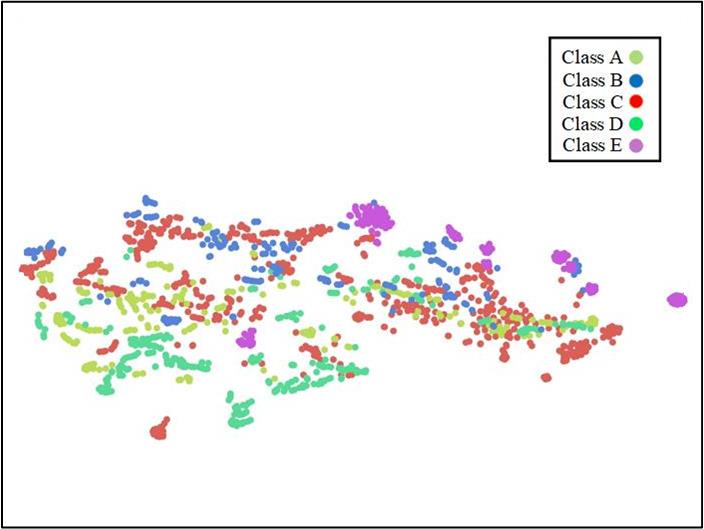
Figure 2: Topological structure of the ShipsEar dataset using the t-SNE algorithm [JMLR:v9:vandermaaten08a]. (a) waveform distribution; (b) Mel-Fbank feature distribution.
Fig. 1 presents the Hinich test results based on a 20-s sample selected from the ShipsEar dataset [santos2016Shipsear], implemented using the HOSA package [Swami2025]. The original sampling frequency of the signal is 52374 Hz, and it was segmented into 40 intervals of 0.5 s each for Gaussianity and linearity evaluation. Previous studies have already demonstrated the non-stationary characteristic of underwater acoustic signals [10.1121/10.0003382, 10.1121/1.4776775]. As shown in Fig. 1 (b), the PFA values of the Gaussianity test vary between 0 and 1. In particular, multiple instances exhibit $\mathrm{PFA}=0$ , indicating strong non-Gaussianity. Moreover, the significant deviation between the estimated and theoretical interquartile ranges further confirms nonlinearity. Following t-SNE visualization using the HyperTools package [hypertools] with default parameters, Fig. 2 clearly illustrates that both the waveform and the time-frequency representation of underwater acoustic signals exhibit complex structures, forming high-dimensional topological patterns in a non-Euclidean space. Notably, the time-frequency features demonstrate better class separability than raw waveforms, validating their effectiveness for underwater target classification.
III Proposed Method
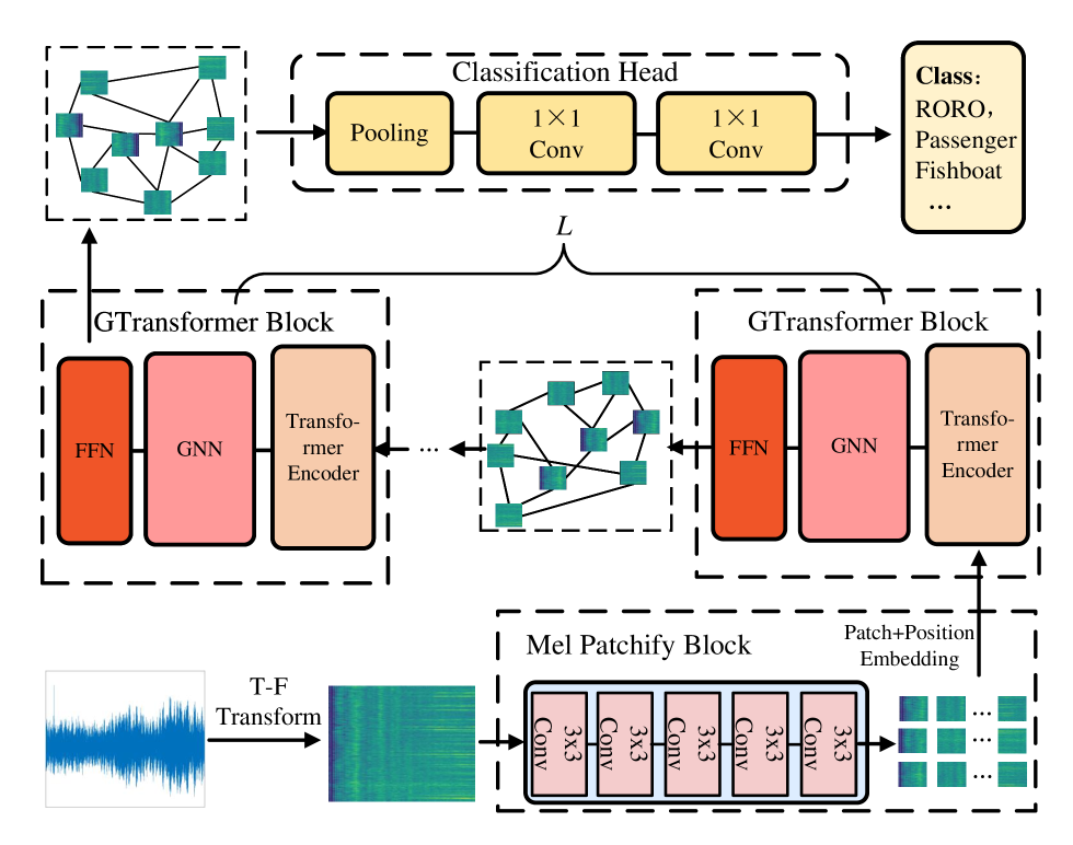
For UATR in topological space, we propose a Mel-graph embedding-based DL model to recognize real-world underwater acoustic signals. The overall framework is illustrated in Fig. 3, which comprises four main components: Mel-spectrogram feature extraction, the Mel Patchify Block, the GTransformer Block, and a classification head. In this section, we first describe the extraction of Mel-spectrogram features, followed by the partitioning of the spectrogram using the Mel Patchify Block. The construction and updating of the Mel-graph are performed within the GTransformer Block. Finally, we provide a brief overview of the classification head.
<details>
<summary>x1.png Details</summary>
### Visual Description
# Technical Document Extraction: GTransformer Architecture Diagram
## 1. Overview
This image illustrates a technical architecture for an audio classification system, likely utilizing a Graph Transformer (GTransformer) approach. The pipeline processes raw audio signals into spectrograms, extracts patch-based embeddings, processes them through a series of graph-based transformer blocks, and concludes with a classification head.
---
## 2. Component Isolation and Flow Analysis
### Region 1: Input and Pre-processing (Bottom Left to Bottom Right)
* **Input Signal:** A blue waveform representing a raw audio signal.
* **Process:** An arrow labeled **"T-F Transform"** (Time-Frequency Transform) converts the waveform into a Mel-spectrogram (visualized as a green/yellow heatmap).
* **Mel Patchify Block:** The spectrogram enters a dashed container labeled "Mel Patchify Block".
* **Internal Components:** A sequence of four identical modules labeled **"3x3 Conv"**.
* **Output:** The block outputs a grid of small spectrogram patches. An arrow points upward, labeled **"Patch+Position Embedding"**, indicating the integration of spatial/temporal information.
### Region 2: GTransformer Blocks (Middle Section)
The architecture features a repetitive structure indicated by a bracket labeled **"$L$"**, suggesting $L$ number of layers or blocks.
* **GTransformer Block Structure:** Each block (contained in a dashed rectangle) consists of three sequential sub-modules:
1. **Transformer Encoder** (Light orange/peach color)
2. **GNN** (Graph Neural Network - Pink color)
3. **FFN** (Feed-Forward Network - Dark orange/red color)
* **Data Flow:**
* The "Patch+Position Embedding" enters the first GTransformer Block from the bottom.
* Between the blocks, there is a visualization of a **Graph Structure**. This graph consists of nodes (represented by the spectrogram patches) connected by black lines (edges), indicating relational modeling between different parts of the audio signal.
* An ellipsis (**...**) indicates that this block structure repeats $L$ times.
### Region 3: Classification Head (Top Section)
* **Input:** The final graph representation (nodes and edges) from the last GTransformer block is passed to the classification stage.
* **Classification Head (Dashed Box):**
1. **Pooling:** A yellow rounded rectangle. This likely aggregates the graph node features into a global representation.
2. **1x1 Conv:** A yellow rounded rectangle.
3. **1x1 Conv:** A second yellow rounded rectangle for further feature refinement.
* **Final Output (Class Box):** A light yellow box on the far right.
* **Header:** **Class:**
* **Labels:** **RORO, Passenger, Fishboat, ...**
* *Note:* These labels suggest the model is designed for maritime acoustic classification (e.g., identifying ship types).
---
## 3. Textual Transcription
| Category | Transcribed Text |
| :--- | :--- |
| **Process Labels** | T-F Transform, Patch+Position Embedding |
| **Main Blocks** | Mel Patchify Block, GTransformer Block, Classification Head |
| **Sub-Modules** | 3x3 Conv, Transformer Encoder, GNN, FFN, Pooling, 1x1 Conv |
| **Variables** | $L$ (representing the number of layers) |
| **Output Classes** | Class: RORO, Passenger, Fishboat, ... |
---
## 4. Technical Summary of Logic
1. **Feature Extraction:** The system uses a convolutional "Mel Patchify Block" to break down a spectrogram into local features.
2. **Relational Modeling:** Unlike standard Transformers that use self-attention on a sequence, this model uses a **GNN** within a **GTransformer Block** to model the audio patches as nodes in a graph, capturing non-linear relationships between different time-frequency segments.
3. **Global Aggregation:** The **Pooling** layer in the Classification Head collapses the graph-based features into a single vector for the final **1x1 Convolutional** layers to perform the multi-class classification task.
</details>
Figure 3: Overall workflow of the proposed UATR-GTransformer framework.
III-A Mel-spectrogram Feature
In the context of UATR, the Mel-spectrogram, derived from the Mel filterbank (Mel-Fbank), has become a widely adopted time–frequency representation in sonar signal processing [liu2021underwater]. In this work, the choice of Mel-spectrograms as model input is motivated by their partially overlapping frequency bands, which preserve intrinsic signal information and exhibit high inter-feature correlation. Consequently, when further processed through graph modeling, the connections among graph nodes are strengthened, enabling the construction of a more discriminative topological graph.
The extraction of Mel-spectrogram features involves the following steps, after resampling the input signal to 16 kHz:
(1) Pre-emphasis: This step enhances the energy of high-frequency components for spectrum balancing. It is typically implemented by processing the original signal $x[n]$ as follows:
$$
y[n]=x[n]-\alpha x[n-1], \tag{4}
$$
where $y[n]$ is the pre-emphasized signal and $\alpha$ is the pre-emphasis coefficient, usually set to $0.97$ , approximated by a hardware-friendly coefficient [10.1007/978-981-99-7505-1_61].
(2) Framing: The pre-emphasized signal $y[n]$ is segmented into overlapping frames, each containing 25 ms of audio with a frame shift of 10 ms.
(3) Windowing: To mitigate spectral leakage, each frame is multiplied by a Hanning window.
(4) Fast Fourier Transform (FFT): The FFT is then applied to each windowed frame to transform the signal into its frequency-domain representation.
(5) Mel Filtering: The frequency-domain signal is filtered using a 128-band triangular Mel-Fbank, defined as
$$
F_{m}(k)=\begin{cases}0&\text{ if }k<f[m-1],\\[4.0pt]
\frac{k-f[m-1]}{f[m]-f[m-1]}&\text{ if }f[m-1]\leq k<f[m],\\[6.0pt]
\frac{f[m+1]-k}{f[m+1]-f[m]}&\text{ if }f[m]\leq k<f[m+1],\\[6.0pt]
0&\text{ if }k\geq f[m+1],\end{cases} \tag{5}
$$
where $f[i]$ denotes the $i$ -th center frequency of the Mel bins and $k$ is the frequency index. The filterbank energy is then applied to the Short-Time Fourier Transform (STFT) coefficient $X(k)$ to compute the Mel-spectrogram:
$$
M=\log\left(\sum_{k=0}^{N-1}F_{m}(k)\times X(k)\right), \tag{6}
$$
where $N=128$ is the number of Mel frequency bins. The above extraction procedure is implemented using the torchaudio package. Suppose the received underwater acoustic signal has a duration of 5 s, the resulting Mel-spectrogram will have a dimension of $512× 128$ after time padding.
III-B Mel Patchify Block
Previous studies have shown that patch modeling of acoustic spectrograms can effectively capture meaningful time–frequency structures from acoustic signals [gong2022ssast]. Therefore, the Mel-spectrogram is first divided into overlapping patches, which serve as the basic computational units of the model. This enables the UATR-GTransformer to construct a graph that preserves spatial information in both the time and frequency domains. Specifically, an input Mel-spectrogram is partitioned into $N$ patches of size $16× 16$ using the Mel patchify block. This block employs a stem convolution consisting of a sequence of trainable $3× 3$ convolutional kernels sliding across the spectrogram. Such convolutions are effective for extracting fine-grained features and have been shown to maintain optimization stability and computational efficiency [10.5555/3540261.3542586]. In our implementation, five convolutional kernels are used to process the Mel-spectrogram. The primary objective is to extract salient features from the split patches and provide rich representations for subsequent network layers.
Among these convolutional kernels, the first four use a stride of 2, while the final kernel uses a stride of 1. The stride configuration serves two purposes. The initial strides of 2 progressively downsample the feature maps to capture coarse-grained features and reduce computational cost, whereas the final stride of 1 maintains the spatial resolution for detailed representation. To further improve training stability and introduce nonlinearity, batch normalization and ReLU activation are applied after each convolutional operation. Assuming the input Mel-spectrogram size is $512× 128$ , the resulting patch embedding has a dimension of $(dim,32,8)$ due to the strides of 2, 2, 2, 2, and 1. Here, $dim$ denotes the output channel size of the last convolutional kernel, which is also the graph embedding dimension.
Since graph-structured representations rely on precise spatial information, a two-dimensional positional embedding is added to the patch embeddings, similar to the Transformer framework [gong21b_interspeech]. This embedding captures the order of time–frequency distributions, thereby enhancing the model’s ability to process graph structures:
$$
\centering\mathbf{x}_{i}\leftarrow\mathbf{x}_{i}+PE_{i},\@add@centering \tag{7}
$$
where $\mathbf{x}_{i}$ denotes the patch embedding. Specifically, a learnable positional encoding $PE_{i}∈\mathbb{R}^{32× 8}$ is added along both the frequency and time axes of the split patches, followed by a broadcasting operation. Finally, the set of patch embeddings $\mathbf{X_{0}}$ is reshaped into $(256,dim)$ as input to the GTransformer Block.
III-C GTransformer Block
As the backbone of the UATR-GTransformer, the GTransformer block consists of a Transformer Encoder, a graph neural network (GNN), and a feed-forward network (FFN).
III-C1 Transformer Encoder
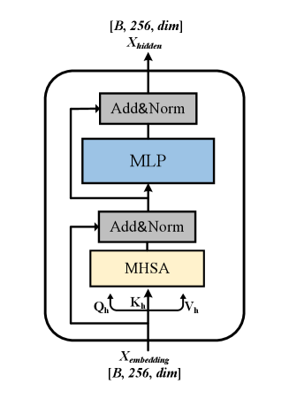
In the UATR-GTransformer, the Transformer Encoder functions as a global feature extractor on $\mathbf{X}$ , capturing the overall time–frequency structure. Its architecture is illustrated in Fig. 4. The core mechanism of the Transformer Encoder is MHSA, which projects the input features into multiple sets of queries, keys, and values. Attention is then computed independently in each head, enabling the model to capture high-level dependencies from multiple perspectives.
<details>
<summary>x2.png Details</summary>
### Visual Description
# Technical Document Extraction: Transformer Block Architecture
## 1. Overview
The image illustrates a technical diagram of a single Transformer encoder block, commonly used in deep learning architectures for natural language processing and computer vision. It details the flow of data through multi-head self-attention and feed-forward layers, including residual connections and normalization steps.
## 2. Component Isolation
### Header (Output Section)
* **Label:** $X_{hidden}$
* **Tensor Shape:** $[B, 256, dim]$
* *B*: Batch size.
* *256*: Sequence length or number of tokens.
* *dim*: Embedding dimensionality.
### Main Chart (Internal Architecture)
The architecture is contained within a rounded rectangular boundary, representing a single repeatable layer. It consists of two primary sub-blocks, each utilizing a residual (skip) connection.
#### Sub-block 1: Attention Mechanism
* **MHSA (Multi-Head Self-Attention):** Represented by a light yellow rectangle.
* **Inputs to MHSA:** The input stream splits into three components:
* $Q_h$ (Queries)
* $K_h$ (Keys)
* $V_h$ (Values)
* **Add&Norm:** Represented by a grey rectangle. This layer performs an element-wise addition of the original input (via a skip connection) and the MHSA output, followed by Layer Normalization.
#### Sub-block 2: Feed-Forward Network
* **MLP (Multi-Layer Perceptron):** Represented by a light blue rectangle. This is the position-wise feed-forward network.
* **Add&Norm:** Represented by a grey rectangle. This layer performs an element-wise addition of the input to the MLP (via a skip connection) and the MLP output, followed by Layer Normalization.
### Footer (Input Section)
* **Label:** $X_{embedding}$
* **Tensor Shape:** $[B, 256, dim]$
* Matches the output shape, indicating a transformation that preserves dimensionality.
---
## 3. Data Flow and Logic Verification
### Flow Description
1. **Input:** The process begins at the bottom with $X_{embedding}$.
2. **Branching:** The input path splits. One path goes directly into the first **Add&Norm** (the residual connection). The other path splits into $Q_h, K_h, V_h$ and enters the **MHSA** block.
3. **First Integration:** The output of MHSA and the residual connection are combined in the first **Add&Norm** block.
4. **Second Branching:** The output of the first Add&Norm splits. One path goes directly to the second **Add&Norm** (the second residual connection). The other path enters the **MLP** block.
5. **Second Integration:** The output of the MLP and the second residual connection are combined in the final **Add&Norm** block.
6. **Output:** The final result is $X_{hidden}$ at the top of the diagram.
### Trend/Logic Check
* **Dimensionality Consistency:** The input and output shapes are identical ($[B, 256, dim]$), which is consistent with standard Transformer block designs that allow for stacking multiple layers.
* **Residual Pathing:** The arrows clearly indicate that the "Add" part of "Add&Norm" receives the unprocessed input from the start of that specific sub-section, bypassing the heavy computation (MHSA or MLP) to mitigate vanishing gradient issues.
## 4. Textual Transcriptions
| Element Type | Text / Symbol | Description |
| :--- | :--- | :--- |
| **Input Variable** | $X_{embedding}$ | The input tensor to the block. |
| **Output Variable** | $X_{hidden}$ | The processed output tensor. |
| **Dimensions** | $[B, 256, dim]$ | Batch size, sequence length, and feature dimension. |
| **Component 1** | MHSA | Multi-Head Self-Attention. |
| **Component 2** | MLP | Multi-Layer Perceptron (Feed-forward). |
| **Component 3** | Add&Norm | Addition (Residual) and Layer Normalization. |
| **Attention Vectors** | $Q_h, K_h, V_h$ | Query, Key, and Value vectors for the attention mechanism. |
</details>
Figure 4: Illustration of the Transformer Encoder for global feature extraction. Here, $B$ denotes the batch size.
The MHSA formulation for embeddings at the $l$ -th layer $\mathbf{X}_{l}$ is given by:
$$
\begin{gathered}\mathbf{Q}_{h},\mathbf{K}_{h},\mathbf{V}_{h}=\mathbf{X}_{l}\mathbf{W}_{h}^{Q},\mathbf{X}_{l}\mathbf{W}_{h}^{K},\mathbf{X}_{l}\mathbf{W}_{h}^{V},\\
\operatorname{Attn}\left(\mathbf{Q}_{h},\mathbf{K}_{h},\mathbf{V}_{h}\right)=\operatorname{softmax}\left(\frac{\mathbf{Q}_{h}\mathbf{K}_{h}^{T}}{\sqrt{D_{\text{attn}}}}\right)\mathbf{V}_{h},\end{gathered} \tag{8}
$$
where $\mathbf{W}_{h}^{Q}$ , $\mathbf{W}_{h}^{K}$ , and $\mathbf{W}_{h}^{V}$ are learnable projection matrices for the query, key, and value sets, respectively. $H$ denotes the number of heads, $h∈[1,H]$ indexes the head, and $D_{\text{attn}}=dim/H$ is the dimensionality per head.
The outputs of all $H$ attention heads, each of size $(256,dim/H)$ , are concatenated to generate an attention representation of size $(256,dim)$ . This representation is then passed through a multi-layer perceptron (MLP) comprising two linear layers with a GELU activation in the middle. Residual connections are applied after both the MHSA and MLP modules. Following standard Transformers, layer normalization is employed between layers instead of batch normalization to improve gradient stability and convergence.
III-C2 GNN
In topological data processing, graphs naturally represent associative relationships among entities [10530642, TORRES2024111268]. GNNs are well suited to capture and exploit these relationships by integrating node-specific features with the graph structure. Through message passing along edges, GNNs effectively learn dependencies between nodes, enabling the processing of high-dimensional topological data. In the proposed framework, a GNN is employed to construct and update the Mel-graph following the Transformer Encoder. Coupling a GNN after the Transformer Encoder allows the model to capture local structural information of underwater acoustic signals, such as rapid time–frequency variations, and to form high-dimensional, discriminative graph representations.
To construct and update the graph, the $K$ -nearest neighbors (KNN) algorithm [10.1145/1963405.1963487] is employed to measure the similarity between Transformer Encoder outputs. This provides a computationally efficient and intuitive approach for graph operations, enabling the model to capture salient local relationships within the feature space while avoiding unnecessary complexity. The similarity distance is computed using the $\mathrm{p}$ -norm metric:
$$
\|\mathbf{x}\|_{\mathrm{p}}=\left(\sum_{i=1}^{n}\left|\mathbf{x}_{i}\right|^{\mathrm{p}}\right)^{1/\mathrm{p}}, \tag{9}
$$
where $\mathrm{p}$ is set to 2 in this study. Subsequently, for each node $v_{i}$ , $K$ nearest neighbors $\mathcal{N}(v_{i})$ are connected by directed edges $e_{ji}$ from $v_{j}$ to $v_{i}$ for all $v_{j}∈\mathcal{N}(v_{i})$ . In this way, the initial Mel-graph is defined as $\mathcal{G}_{mel}=(\mathcal{V},\mathcal{E})$ , where $\mathcal{V}=\{v_{1},v_{2},·s,v_{N}\}$ is the node set and $\mathcal{E}$ is the edge set. The outputs of the Transformer Encoder, obtained through MHSA, are regarded as Mel-graph embeddings in the UATR-GTransformer. Each embedding encodes its own Mel-frequency energy distribution while also capturing global dependencies among embeddings due to the strong global modeling capability of MHSA. Consequently, these Mel-graph embeddings serve as higher-order representations that preserve detailed time–frequency information of underwater acoustic target signals, thereby implicitly constructing a robust Mel-graph.
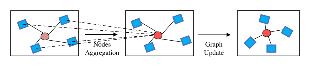
The core operation of the GNN is graph convolution, which aggregates neighboring topological information and updates node features within the Mel-graph, as illustrated in Fig. 5.
<details>
<summary>x3.png Details</summary>
### Visual Description
# Technical Document Extraction: Graph Neural Network Process Diagram
## 1. Overview
This image is a technical diagram illustrating a two-step process in a Graph Neural Network (GNN) or similar graph-based machine learning architecture. It depicts how information is gathered from neighboring nodes to update a central node's state.
## 2. Component Isolation
The diagram is segmented into three primary stages, moving from left to right, connected by process arrows.
### Region 1: Initial State (Left Box)
* **Components:**
* **Central Node:** A circular node colored in a muted pink/light brown.
* **Neighboring Nodes:** Four blue square nodes surrounding the central node.
* **Edges:** Solid black lines connecting the central node to each of the four blue square nodes.
* **Spatial Layout:** The central node is positioned roughly in the middle of the frame, with neighbors distributed in the top-left, top-right, bottom-left, and bottom-right quadrants.
### Region 2: Nodes Aggregation (Middle Box)
* **Process Label:** "Nodes Aggregation" (located below the arrow connecting Region 1 and Region 2).
* **Components:**
* **Central Node:** The color has changed to a vibrant red, indicating an active state or the result of an operation.
* **Neighboring Nodes:** The same four blue square nodes remain in their positions.
* **Visual Representation:** This stage represents the collection of features or messages from the neighborhood.
### Region 3: Final State (Right Box)
* **Process Label:** "Update" (located below the arrow connecting Region 2 and Region 3).
* **Components:**
* **Central Node:** The node is now a darker, saturated red/maroon.
* **Neighboring Nodes:** The four blue square nodes remain.
* **Visual Representation:** This stage represents the final update of the central node's hidden state based on the aggregated information.
</details>
Figure 5: Illustration of graph convolution for nodes aggregation and graph update. The central node is marked by a circle, while its neighboring nodes are denoted by surrounding boxes.
From the perspective of a central node $\mathbf{x}_{i}$ , graph convolution is formulated as:
$$
\mathbf{x}^{\prime}_{i}=h(\mathbf{x}_{i},g(\mathbf{x}_{i},\mathcal{N}(\mathbf{x}_{i});\mathbf{W}_{\text{agg}});\mathbf{W}_{\text{update}}), \tag{10}
$$
where $g(·)$ and $h(·)$ denote the aggregation and update functions, respectively, and $\mathcal{N}(\mathbf{x}_{i})$ is the set of neighboring nodes of $\mathbf{x}_{i}$ . To mitigate gradient vanishing, the max-relative (MR) graph convolution [deepgcn] is applied to process Mel-graph embeddings:
$$
\displaystyle g(\cdot) \displaystyle=\mathbf{x}_{i}^{\prime\prime}=\left[\mathbf{x}_{i},\max\left(\left\{\mathbf{x}_{j}-\mathbf{x}_{i}\mid j\in\mathcal{N}(\mathbf{x}_{i})\right\}\right)\right], \displaystyle h(\cdot) \displaystyle=\mathbf{x}_{i}^{\prime}=\mathbf{x}_{i}^{\prime\prime}\mathbf{W}_{\text{update}}+\mathbf{b}, \tag{11}
$$
where $\mathbf{b}$ is the bias term. After MR graph convolution, the updated node set $\mathcal{N}(\mathbf{x}^{\prime}_{i})$ forms a new Mel-graph, denoted by $\mathcal{G}_{mel}^{\prime}$ . Here, $\mathbf{W}_{\text{agg}}$ and $\mathbf{W}_{\text{update}}$ represent learnable weights for the aggregation and update operations, respectively. In particular, the aggregation function captures salient information by computing the maximum difference between the central node and its $K$ neighbors, while the update function applies a nonlinear transformation to generate the updated graph.
After graph convolution on $\mathbf{X}$ , the updated features $\mathbf{X^{\prime}}$ are processed by two fully connected layers with projection matrices $\mathbf{W}_{\text{in}}$ and $\mathbf{W}_{\text{out}}$ to enhance feature diversity. A ReLU activation function is applied after the first projection layer to mitigate layer collapse. The output feature $\mathbf{Y}$ is then computed as follows:
$$
\begin{gathered}\mathbf{X^{\prime}}=\operatorname{MR\ Graph\ Convolution}(\mathbf{X}),\\
\mathbf{Y}=\operatorname{ReLU}(\mathbf{X^{\prime}}\mathbf{W}_{\text{in}})\mathbf{W}_{\text{out}}+\mathbf{X}.\end{gathered} \tag{12}
$$
III-C3 FFN
After GNN processing, an FFN is applied to further transform the node-level features and to integrate the Transformer and GNN modules.
<details>
<summary>x4.png Details</summary>

### Visual Description
# Technical Document Extraction: FFN Architecture Diagram
## 1. Overview
The image is a technical schematic illustrating the architecture of a **Feed-Forward Network (FFN)** block, specifically featuring a residual (skip) connection. The diagram uses standard deep learning notation to describe the flow of data through various layers.
## 2. Component Isolation
The diagram is contained within a dashed rectangular boundary, indicating the scope of the FFN module.
### Header/Title
* **Text:** `FFN`
* **Location:** Top center, inside the dashed boundary.
* **Meaning:** Identifies the entire block as a Feed-Forward Network.
### Main Processing Path (Sequential)
The central horizontal flow consists of three primary blocks connected by arrows:
1. **Conv1:** The first convolutional layer. It receives the input $X$.
2. **ReLU:** A Rectified Linear Unit activation function. It receives the output from `Conv1`.
3. **Conv2:** The second convolutional layer. It receives the output from the `ReLU` layer.
### Residual Connection (Skip Connection)
* **Label:** `Residual add`
* **Path:** A solid line branches off from the input $X$ before it enters `Conv1`. It travels underneath the three main blocks and merges with the output of `Conv2`.
* **Function:** This represents an identity mapping where the original input is added to the output of the transformation layers, a hallmark of ResNet-style architectures.
## 3. Data Flow and Variables
* **Input ($X$):** Located on the far left. An arrow indicates the entry point into the FFN block.
* **Output ($X'$):** Located on the far right. An arrow indicates the final processed data exiting the block.
* **Directionality:** The primary data flow is from left to right.
## 4. Logical Flow Summary
The mathematical operation depicted in this diagram can be transcribed as follows:
1. **Input:** $X$
2. **Transformation Path:** $T(X) = \text{Conv2}(\text{ReLU}(\text{Conv1}(X)))$
3. **Residual Addition:** The input $X$ is added to the result of the transformation.
4. **Final Output:** $X' = T(X) + X$
## 5. Textual Transcriptions
| Label | Type | Description |
| :--- | :--- | :--- |
| **FFN** | Title/Header | Feed-Forward Network identifier. |
| **$X$** | Variable | Input tensor/data. |
| **Conv1** | Component | First Convolutional layer. |
| **ReLU** | Component | Activation function layer. |
| **Conv2** | Component | Second Convolutional layer. |
| **Residual add** | Process | The operation of adding the identity input to the processed output. |
| **$X'$** | Variable | Final output tensor/data. |
</details>
Figure 6: Illustration of the FFN for feature transformation.
The structure of the FFN is illustrated in Fig. 6 and can be expressed as:
$$
\mathbf{Z}=\operatorname{ReLU}\left(\mathbf{Y}\mathbf{W}_{1}+\mathbf{b}_{1}\right)\mathbf{W}_{2}+\mathbf{b}_{2}+\mathbf{Y}, \tag{13}
$$
where $\mathbf{Z}∈\mathbb{R}^{N× dim}$ , $N=256$ is the number of nodes, $\mathbf{W}_{1}$ and $\mathbf{W}_{2}$ are the weights of two fully layers, and $\mathbf{b}_{1}$ , $\mathbf{b}_{2}$ are the corresponding biases. The hidden dimension of the FFN is set to $4× dim$ to enhance its feature transformation capacity. The ReLU activation function is employed to introduce nonlinearity and improve representation learning for underwater acoustic signals.
III-D Classification Head
To predict the ship class, a classification head is attached after the GTransformer stacks. Specifically, the classification head operates on 4-D tensors interpreted as a graph after the final FFN. Since fully connected layers alone cannot directly process such data, the classification head incorporates a pooling layer for dimension reduction and two convolutional layers to progressively extract meaningful features for prediction.
For the two convolutional layers, the first employs a $1× 1$ convolution to transform the feature map from $dim=96$ to a hidden dimension. The second $1× 1$ convolution further projects the features from the hidden dimension to $C$ , where $C$ denotes the number of classes. The hidden dimension is set to 512 to better capture intricate patterns from the graph embeddings. Batch normalization and a ReLU activation are applied between the two convolutional layers to facilitate training.
The overall framework of the UATR-GTransformer is summarized as follows.
Algorithm 1 UATR-GTransformer Algorithm for UATR.
0: Mel-graph $x∈\mathbb{R}^{t× f}$
0: Classification loss $L_{ce}$
1: Apply Mel patchify on spectrogram $x$ using stem convolutions to obtain the patch set.
2: Add positional embedding to the patch embeddings using (7).
for $l=1$ to $L$ do
3: Transformer Encoder to extract deep features as Mel-graph embeddings.
4: Construct Mel-graph $\mathcal{G}_{mel}=(\mathcal{V},\mathcal{E})$ by finding $K$ nearest neighbors using the KNN algorithm.
5: Graph convolution in a GNN block to aggregate information and update $\mathcal{G}_{mel}$ , yielding $\mathcal{G}_{mel}^{\prime}$ .
6: FFN for feature transformation on $\mathcal{G}_{mel}^{\prime}$ .
end for
7: Classification head to predict the ship label $y_{\text{predict}}$ .
8: Compute the cross-entropy loss $L_{ce}$ with the ground-truth label $y_{\text{true}}$ .
TABLE I: Detailed configuration of the model architecture. The input dimension is $(B,512,128)$ , where $B$ denotes the batch size.
| Module | Main Opearation | Dimension | |
| --- | --- | --- | --- |
| Mel Patchify | Conv(K=3, C=12, S=2, P=1) | (B, 12, 256, 64) | |
| Conv(K=3, C=24, S=2, P=1) | (B, 24, 128, 32) | | |
| Conv(K=3, C=48, S=2, P=1) | (B, 48, 64, 16) | | |
| Conv(K=3, C=96, S=2, P=1) | (B, 96, 32, 8) | | |
| Conv(K=3, C=96, S=1, P=1) | (B, 96, 32, 8) | | |
| GTransformer ( $L$ =8) | Encoder | $H$ =8, $dim$ =96 | (B, 256, 96) |
| GNN | 1 $×$ 1 Conv | (B, 96, 32, 8) | |
| Graph Conv, KNN[2, 8] | (B, 96, 256) | | |
| 1 $×$ 1 Conv | (B, 96, 32, 8) | | |
| FFN | Conv(96, 384), ReLU | (B, 384, 32, 8) | |
| Conv(386, 96), residual connection | (B, 96, 32, 8) | | |
| Classification Head | 2d pooling | (B, 96, 1, 1) | |
| 1 $×$ 1 Conv(96, 512) | (B, 512, 1, 1) | | |
| 1 $×$ 1 Conv(512, $C$ ) | (B, $C$ ) | | |
IV Experimental settings
IV-A Dataset description
The dataset used in the experiments consists of two widely researched datasets: (1) ShipsEar [santos2016Shipsear]: this dataset contains a diverse collection of 90 ship audio recordings at a sampleing frequency of 52734 Hz, the duration of each recording is between 15 seconds to 10 minutes. ShipsEar contains a total of 11 vessel types, which can be further combined into 4 vessel categories depending on vessel size, and 1 background noise category. (2) DeepShip [irfan2021Deepship]: this dataset consists of 265 real underwater sound recordings at a sampling frequency of 32000 Hz, which is further merged into four categories of ship vessels with no background noise provided.
For preprocessing, the waveform data is first resampled to 16 kHz and then cut into 5-seconds segments. These segments are divided into training, validation, and testing sets according to time periods, using a ratio of 70% for training, 15% for validation, and the remainder for testing. This partitioning strategy, recommended in [Niu2023], helps prevent potential data leakage that may occur with random splitting. The detailed dataset partitions are shown in Table II.
TABLE II: Dataset partitions of the two underwater acoustic databases.
| ShipsEar | A: Fish boats, Trawlers, Mussel boat, Tugboat, Dredger | 340 |
| --- | --- | --- |
| B: Motorboat, Pilotboat, Sailboat | 301 | |
| C: Passengers | 843 | |
| D: Ocean liner, RORO | 486 | |
| E: Background noise | 253 | |
| DeepShip | A: Cargo | 7369 |
| B: Passengers | 9677 | |
| C: Tanker | 8817 | |
| D: Tug | 8159 | |
IV-B Experimental Details
The experiments were implemented in PyTorch (version 1.8.0) with Python (version 3.8). The hardware platform consisted of four Nvidia GeForce RTX 3090 GPUs and two Intel Xeon Platinum 8377c CPUs. For data augmentation, the time–frequency masking method [park2019specaugment] was applied, with a frequency mask of 24 and a time mask of 96 on the Mel-spectrogram. To ensure consistent scaling across the dataset, the input Mel-spectrograms were normalized to have zero mean and unit variance. The cross-entropy loss $L_{ce}$ , a widely used loss function in recognition and classification tasks, was adopted to optimize the training process.
For the training configurations, the initial learning rate was set to $1.5× 10^{-3}$ for ShipsEar and $1.2× 10^{-3}$ for DeepShip. The learning rate was decayed by a factor of 0.5 after 90 epochs for ShipsEar and 130 epochs for DeepShip. The batch size was set to 16 for ShipsEar and 64 for DeepShip, while the total number of epochs was 130 and 180, respectively. Other hyperparameters were kept the same for both datasets: the number of GTransformer blocks $L=8$ ; the number of nearest neighbors $K$ increased from 2 to 8 across blocks; the number of attention heads $H=8$ ; and the graph embedding dimension $dim=96$ . These hyperparameters were determined through repeated trials to optimize recognition performance. The Adam optimizer was used to update network parameters.
IV-C Evaluation Criteria
The recognition performance of the proposed model was evaluated using four widely adopted metrics: overall accuracy ( $OA$ ), average accuracy ( $AA$ ), Kappa coefficient ( $Kappa$ ), and $F1$ -score ( $F1$ ), averaged over five runs. Specifically, $OA$ measures overall classification accuracy, while $AA$ and $Kappa$ account for imbalanced datasets. The $F1$ -score reflects the trade-off between recall and precision. Let $TP$ , $TN$ , $FP$ , and $FN$ denote true positives, true negatives, false positives, and false negatives, respectively. These metrics are defined as follows:
$$
OA=\frac{TP+TN}{TP+TN+FP+FN}, \tag{14}
$$
$$
AA=\sum_{i=1}^{n}\frac{TP_{i}+TN_{i}}{TP_{i}+TN_{i}+FP_{i}+FN_{i}}, \tag{15}
$$
where $TP_{i}$ , $TN_{i}$ , $FP_{i}$ , and $FN_{i}$ represent the numbers of $TP$ , $TN$ , $FP$ , and $FN$ for the $i$ -th class.
$$
Kappa=\frac{P_{0}-P_{e}}{1-P_{e}}, \tag{16}
$$
where $P_{0}$ denotes the observed agreement among raters (equal to $OA$ ), and $P_{e}$ denotes the expected agreement by chance.
$$
F1=\left(\frac{2+\tfrac{FP}{TP}+\tfrac{FN}{TP}}{2}\right)^{-1}. \tag{17}
$$
V Results and Discussions
V-A Comparison with Baseline Models
To evaluate the effectiveness of the proposed UATR-GTransformer, its recognition performance is compared with other baseline DL models, including ResNet-18, DenseNet-169 [sun2022underwater], MbNet-V2 [hsiao2021efficient], Xception [8099678], EfficientNet-B0, UATR-Transformer [feng2022transformer], STM [jmse10101428], and convolution-based mixture of experts (CMoE) [XIE2024123431]. The main characteristics of these baseline models are summarized below:
- ResNet-18: A residual network with 18 convolutional layers, which has demonstrated strong performance across various recognition tasks.
- DenseNet-169: A densely connected convolutional network with 169 layers, where each layer is connected to all preceding layers, enabling efficient feature reuse and robust recognition performance in UATR.
- MbNet-V2: A lightweight model based on depthwise separable convolution, which substantially reduces model parameters and computational cost while maintaining accuracy.
- Xception: An efficient model that also employs depthwise separable convolution, further reducing parameter count and computation without sacrificing performance.
- EfficientNet-B0: An optimized model that incorporates inverted residual connections and compound scaling strategies, achieving excellent recognition accuracy with relatively low complexity.
- UATR-Transformer: A convolution-free model designed to exploit both global and local information from time–frequency spectrograms for UATR tasks.
- STM: A Transformer-based model inspired by the Audio Spectrogram Transformer (AST) [gong21b_interspeech], specifically adapted for UATR.
- CMoE: A convolutional mixture-of-experts model that adopts ResNet as its backbone to enhance feature extraction.
TABLE III: Recognition performance comparison with different methods.
| ShipsEar | ResNet-18 | 0.799 | 0.736 | 0.727 | 0.738 |
| --- | --- | --- | --- | --- | --- |
| DenseNet-169 | 0.798 | 0.736 | 0.726 | 0.743 | |
| MbNet-V2 | 0.745 | 0.681 | 0.656 | 0.686 | |
| Xception | 0.777 | 0.765 | 0.705 | 0.766 | |
| EfficientNet-B0 | 0.757 | 0.749 | 0.678 | 0.749 | |
| UATR-Transformer | 0.816 | 0.802 | 0.755 | 0.814 | |
| STM | 0.707 | 0.684 | 0.607 | 0.692 | |
| CMoE | 0.815 | 0.807 | 0.756 | 0.809 | |
| UATR-GTransformer | 0.832 | 0.825 | 0.778 | 0.828 | |
| DeepShip | ResNet-18 | 0.802 | 0.796 | 0.734 | 0.799 |
| DenseNet-169 | 0.799 | 0.792 | 0.730 | 0.795 | |
| MbNet-V2 | 0.630 | 0.638 | 0.509 | 0.628 | |
| Xception | 0.801 | 0.796 | 0.732 | 0.798 | |
| EfficientNet-B0 | 0.795 | 0.793 | 0.725 | 0.793 | |
| UATR-Transformer | 0.811 | 0.806 | 0.746 | 0.808 | |
| STM | 0.744 | 0.737 | 0.656 | 0.739 | |
| CMoE | 0.812 | 0.805 | 0.747 | 0.808 | |
| UATR-GTransformer | 0.827 | 0.824 | 0.768 | 0.826 | |
To ensure fair comparisons, all networks were modified to accept 1-D Mel-spectrograms as input. Moreover, to maintain a consistent training paradigm, the SPM model was not pre-trained on ImageNet but was trained from scratch, similar to the other models.
From Table III, it can be observed that on the ShipsEar dataset, the proposed UATR-GTransformer achieves the best performance, with $OA=0.832$ , $AA=0.825$ , $Kappa=0.778$ , and $F1=0.828$ . On the DeepShip dataset, the UATR-GTransformer also achieves the best results, with $OA=0.827$ , $AA=0.824$ , $Kappa=0.768$ , and $F1=0.826$ . These results clearly demonstrate the effectiveness and robustness of the proposed model. Specifically, for the ShipsEar dataset, CMoE achieves the strongest performance among CNN-based methods, benefitting from its multiple expert layers that act as independent learners capable of capturing high-level patterns in underwater acoustic targets. ResNet-18 and DenseNet-169 also show competitive performance, outperforming other backbone CNNs. In contrast, the lightweight MbNet-V2, as well as EfficientNet-EfficientNet-B0, exhibit weaker performance on ShipsEar, suggesting that their relatively shallow architectures may limit the extraction of sufficiently discriminative higher-order features. Among Transformer-based approaches, the UATR-Transformer achieves moderate recognition accuracy by leveraging hierarchical tokenization and the Transformer Encoder to capture both local and global dependencies. However, STM relies on a standard square tokenization scheme, which restricts local information interaction between tokens. The lack of ImageNet pre-training further amplifies this limitation, resulting in weaker performance. On the larger DeepShip dataset, ResNet-18 and DenseNet-169 continue to demonstrate strong generalization ability, with overall accuracy values close to 0.8. Among CNNs, CMoE again achieves the best results, confirming its capability to generalize across diverse data distributions through its mixture-of-experts mechanism. Furthermore, the UATR-Transformer achieves superior performance compared to STM, demonstrating the effectiveness of its design for modeling complex underwater acoustic signals. When trained on larger datasets, both Xception and EfficientNet-B0 exhibit improved recognition accuracy, implying that increased data volumes partially offset their architectural constraints.
V-B Ablation Study
This section presents the results of ablation experiments conducted to evaluate the contribution of different components in the proposed UATR-GTransformer. In particular, we analyze the effect of the modules within the GTransformer block and the positional embedding on recognition performance, measured by the four evaluation metrics.
The first set of experiments examines the importance of each module in the GTransformer block. Table IV summarizes the results obtained by removing individual components. The symbol “–” denotes the removal of the corresponding module. Specifically, “– Encoder” indicates that the model employs only the GNN and FFN in the GTransformer block, excluding the MHSA-based feature extractor. “– GNN” indicates that the model consists of the Encoder and FFN, but without graph embedding operations. Finally, “– FFN” represents the variant where the Encoder and GNN are retained, while the FFN is removed.
TABLE IV: Ablation study on the GTransformer block based on the two datasets.
| ShipsEar | UATR-GTransformer | 0.832 | 0.825 | 0.778 | 0.828 |
| --- | --- | --- | --- | --- | --- |
| - Encoder | 0.780 | 0.769 | 0.709 | 0.776 | |
| - GNN | 0.802 | 0.800 | 0.739 | 0.801 | |
| - FFN | 0.792 | 0.783 | 0.725 | 0.788 | |
| DeepShip | UATR-GTransformer | 0.827 | 0.824 | 0.768 | 0.826 |
| - Encoder | 0.818 | 0.815 | 0.756 | 0.816 | |
| - GNN | 0.814 | 0.811 | 0.750 | 0.812 | |
| - FFN | 0.815 | 0.810 | 0.751 | 0.813 | |
TABLE V: Ablation study on the position embedding based on the two datasets.
| ShipsEar | Case 1 | 0.790 | 0.783 | 0.723 | 0.785 |
| --- | --- | --- | --- | --- | --- |
| Case 2 | 0.798 | 0.788 | 0.731 | 0.793 | |
| Case 3 | 0.832 | 0.825 | 0.778 | 0.828 | |
| DeepShip | Case 1 | 0.817 | 0.817 | 0.759 | 0.818 |
| Case 2 | 0.821 | 0.816 | 0.760 | 0.819 | |
| Case 3 | 0.827 | 0.824 | 0.768 | 0.826 | |
From Table IV, it can be seen that the complete UATR-GTransformer, which incorporates the Encoder, GNN, and FFN, achieves the best $OA$ , $AA$ , $Kappa$ , and $F1$ on both datasets. Each component within the GTransformer block contributes significantly to capturing discriminative Mel-graph representations. The Transformer Encoder, GNN, and FFN operate jointly to enhance recognition performance, and the removal of any individual component undermines the underlying Mel-graph structure, leading to noticeable performance degradation. In particular, for the ShipsEar dataset, removing any module results in substantial variation, highlighting the critical role of graph-structured feature extraction and processing for this dataset.
The second set of experiments investigates the effectiveness of the two-dimensional positional embedding $PE$ in the UATR-GTransformer. Specifically, recognition performance was compared across three configurations: Case 1, without $PE$ ; Case 2, with one-dimensional absolute $PE$ following standard Transformer models [vaswani2017attention]; and Case 3, with two-dimensional $PE$ . As shown in Table V, introducing $PE$ consistently improves performance over Case 1, confirming its ability to capture the positional information of split patches. Moreover, Case 3 outperforms Case 2, particularly on the ShipsEar dataset, demonstrating the superiority of the two-dimensional $PE$ approach, which provides richer time–frequency distribution information for Mel-graph construction.
To further examine the contribution of the Transformer layers on the recognition performance, comparative experiments were conducted using only a single Transformer layer for initial Mel-graph embedding. Table VI shows that employing the full Transformer stack in the GTransformer block yields superior results compared to a single-layer variant, indicating that successive MHSA computations enable the extraction of higher-level semantic information across graph nodes, thereby producing more discriminative Mel-graph embeddings.
TABLE VI: Ablation study on the Transformer configurations based on the two datasets.
| ShipsEar | First Layer | 0.790 | 0.783 | 0.723 | 0.785 |
| --- | --- | --- | --- | --- | --- |
| Full layer | 0.832 | 0.825 | 0.778 | 0.828 | |
| DeepShip | First Layer | 0.817 | 0.812 | 0.754 | 0.814 |
| Full layer | 0.827 | 0.824 | 0.768 | 0.826 | |
Finally, it is worth noting that the ablation experiments have a smaller impact on the DeepShip dataset. This can be attributed to the larger scale of the dataset, which facilitates the learning of more generalized features and reduces the model’s reliance on individual modules.
V-C Recognition Performance under Different Features
The third set of experiments evaluates the recognition performance of the UATR-GTransformer using different acoustic features, including the STFT, the Mel-Frequency Cepstral Coefficients (MFCC), and the Gammatone-Frequency Cepstral Coefficients (GFCC). These features have been widely studied for UATR [10012335] and are important benchmarks for assessing the effectiveness of the proposed model. The experiments were conducted on the ShipsEar dataset for simplicity.
TABLE VII: Performance comparison under different features.
| STFT GFCC MFCC | 0.609 0.779 0.762 | 0.606 0.773 0.758 | 0.491 0.709 0.687 | 0.583 0.772 0.758 |
| --- | --- | --- | --- | --- |
| Mel-Fbank | 0.832 | 0.825 | 0.778 | 0.828 |
As shown in Table VII, the Mel-Fbank feature yields the best recognition performance across all four evaluation metrics ( $OA$ , $AA$ , $Kappa$ , and $F1$ ), demonstrating that Mel-graphs provide more discriminative information for the UATR-GTransformer. In contrast, cepstral coefficient-based features (GFCC and MFCC) achieve better recognition accuracy compared with STFT, while STFT performs the worst, with an $OA$ of only 0.609. This result suggests that constructing STFT-graphs may not effectively capture discriminative information for UATR.
In particular, when using the Mel-Fbank feature, the UATR-GTransformer achieves its best results on the ShipsEar dataset, with $OA=0.832$ , $AA=0.825$ , $Kappa=0.778$ , and $F1=0.828$ . Based on these findings, the Mel-Fbank feature was selected for graph embedding in the proposed UATR-GTransformer.
V-D Parameter sensitivities
As major parameters of the UATR-GTransformer, we further analyze the sensitivity of $K$ in the KNN algorithm, the number of GNN blocks $L$ , and the graph embedding dimension $dim$ on recognition performance using the ShipsEar dataset for simplicity.
TABLE VIII: Performance comparison under various $K$ .
| 2 4 6 | 0.767 0.788 0.802 | 0.760 0.786 0.794 | 0.692 0.721 0.738 | 0.756 0.781 0.796 |
| --- | --- | --- | --- | --- |
| 8 | 0.812 | 0.804 | 0.751 | 0.808 |
| 10 | 0.782 | 0.778 | 0.711 | 0.776 |
| 4 to 8 | 0.804 | 0.797 | 0.740 | 0.799 |
| 2 to 8 | 0.832 | 0.825 | 0.778 | 0.828 |
TABLE IX: Recognition performance under various $L$ .
| 4 6 8 | 0.796 0.810 0.832 | 0.795 0.803 0.825 | 0.731 0.750 0.778 | 0.796 0.804 0.828 |
| --- | --- | --- | --- | --- |
| 10 | 0.784 | 0.776 | 0.714 | 0.779 |
| 12 | 0.797 | 0.789 | 0.731 | 0.792 |
TABLE X: Recognition performance under various $dim$ .
| 48 96 192 | 0.783 0.832 0.690 | 0.778 0.825 0.679 | 0.713 0.778 0.589 | 0.778 0.828 0.673 |
| --- | --- | --- | --- | --- |
| 384 | 0.525 | 0.486 | 0.353 | 0.450 |
| 768 | 0.417 | 0.333 | 0.165 | 0.291 |
V-E Parameter Sensitivities
Table VIII presents the recognition performance with different values of $K$ to find neighboring nodes. “4 to 8” indicates that $K$ is progressively increased from 4 to 8 across the GTransformer blocks. For fixed values of $K$ , the best performance is obtained at $K=8$ . This may be explained by the fact that splitting the Mel-spectrogram into eight frequency regions provides sufficient information for aggregating neighborhood features, whereas further increasing $K$ to 10 introduces redundancy that can reduce performance. When $K$ is gradually increased with network depth, the receptive field of the Mel-graph is enlarged, enabling information exchange among more distant nodes. This strategy is particularly beneficial for complex ship-radiated noise, as it allows the model to capture long-range dependencies and improve node separability. As shown in Table VIII, progressively enlarging $K$ improves recognition performance. In particular, the “2 to 8” strategy outperforms “4 to 8”, which may be attributed to the initial layers capture local node relationships, while later layers gradually expand the receptive field and stabilize the graph structure.
The number of GNN blocks $L$ and the embedding dimension $dim$ also strongly influence the generalization ability of the UATR-GTransformer, as they control the model’s depth and width. Table IX and Table X report the corresponding results. From Table IX, the optimal performance is achieved at $L=8$ , suggesting that too few GNNs limit information exchange, while too many can lead to overfitting. With respect to $dim$ , Table X shows that the best results occur at $dim=96$ . A smaller $dim$ cannot adequately represent graph features, while an excessively large $dim$ produces an over-parameterized model prone to overfitting. This effect is particularly evident at $dim=768$ , where $OA$ decreases sharply to 0.417.
Considering these results, the following parameters are adopted for the UATR-GTransformer: $K$ increases from 2 to 8 across layers, the number of GTransformer blocks $L$ is set to 8, and the graph embedding dimension $dim$ is set to 96.
V-F Statistical significance test
From the results in previous subsection, it is known that the UATR-GTransformer exceeds previous methods in accuracy. To quantitatively validate whether the accuracy advantages are statistically reliable, a comprehensive analysis is conducted using paired-sample t-tests, which are specifically designed for comparing paired measurements obtained under identical experimental conditions [xu2017differences]. The paired-sample t-tests is particularly suitable for our evaluation framework, which utilizes the same data partitions across multiple independent runs, thereby effectively controlling for inter-run variability through its focus on within-trial performance differences.
TABLE XI: P-values of significance tests against the UATR-GTransformer.
| | ResNet-18 | DenseNet-169 | MbNet-V2 | Xception | EfficientNet-B0 | UATR-Transformer | STM | CMoE |
| --- | --- | --- | --- | --- | --- | --- | --- | --- |
| ShipsEar | $1.01× 10^{-2}$ | $2.30× 10^{-3}$ | $3.89× 10^{-3}$ | $3.45× 10^{-3}$ | $1.29× 10^{-5}$ | 0.149 | $1.45× 10^{-3}$ | $5.78× 10^{-2}$ |
| DeepShip | $4.79× 10^{-4}$ | $4.95× 10^{-3}$ | $2.40× 10^{-5}$ | $1.23× 10^{-3}$ | $6.08× 10^{-4}$ | $2.30× 10^{-4}$ | $2.46× 10^{-4}$ | $8.61× 10^{-4}$ |
All models are evaluated using the same data splits over five repeated runs, generating paired samples for analysis. The null hypothesis for each test is a zero mean difference in $OA$ . Here, we use standard significance thresholds ( $p<$ 0.05 for significance, $p<$ 0.01 for strong significance). Table XI demonstrates that the proposed UATR-GTransformer achieves statistically significant improvements over most models on the ShipsEar dataset. However, because the UATR-Transformer and CMoE also deliver competitive results, the improvement over these specific models is not statistically significant. Besides, the results obtained on the DeepShip dataset provide stronger evidence, with the UATR-GTransformer achieving highly significant results against other models.
V-G Model Complexity
To further examine the computational complexity of the UATR-GTransformer, Table XII presents comparisons on widely used complexity metrics, including the number of parameters (NP), average prediction time for a single acoustic signal (Avg. time), giga floating-point operations (GFLOPs), and frames per second (FPS).
TABLE XII: Comparison of model complexity.
| MbNet-V2 | 2.23 | 4.91 ±0.59 | 0.43 | 203.76 |
| --- | --- | --- | --- | --- |
| Xception | 3.63 | 1.82 ±0.28 | 0.575 | 548.18 |
| EfficientNet-B0 | 4.01 | 9.53 ±0.63 | 0.54 | 104.96 |
| ResNet-18 | 11.17 | 3.24 ±0.57 | 2.28 | 309.15 |
| DenseNet-169 | 12.49 | 42.54 ±5.99 | 4.41 | 23.51 |
| UATR-Transformer | 2.55 | 3.54 ±0.43 | 3.25 | 282.95 |
| CMoE | 11.19 | 4.28 ±0.49 | 2.28 | 233.47 |
| UATR-GTransformer | 2.05 | 18.99 ±0.72 | 0.672 | 52.65 |
As shown in Table XII, the UATR-GTransformer has a relatively small NP and low GFLOPs, but exhibits higher Avg. time and lower FPS compared with most other models. This is likely due to the additional computations required for similarity calculations and multi-head self-attention across multiple nodes. Among lightweight CNNs, MbNet-V2, Xception, and EfficientNet-B0 all show low GFLOPs, indicating less computational requirements. Owing to its larger spatial resolution and wider network width, EfficientNet-B0 contains the largest number of parameters (4.01M) among lightweight CNNs and yields the slowest prediction speed, with an Avg. time of 9.53 ms. In contrast, Xception achieves the fastest prediction owing to the use of depthwise and pointwise convolutions, and also has the smallest NP and GFLOPs, thereby demonstrating the best recognition efficiency. For ResNet-based models, CMoE provides higher recognition performance than ResNet-18, though with slightly greater complexity, which may be attributed to the introduction of the mixture-of-experts mechanism. DenseNet-169, due to its dense connections within a deep architecture, exhibits the highest complexity overall, with 12.49M parameters, an Avg. time of 42.54 ±5.99 ms, GFLOPs of 4.41, and the lowest FPS (23.51).
V-H Interpretability experiments
In the UATR-GTransformer, information flows through the Transformer Encoder via the attention matrix, which enables the model to capture dependencies among Mel-graph embeddings from split spectrogram patches. To investigate how attention operates, we first visualize the attention matrices from the $H=8$ attention heads in the UATR-GTransformer. Fig. 7 shows the $256× 256$ attention matrices from the eight heads in the first and last Transformer Encoder layers when a Mel-spectrogram is processed. The horizontal and vertical axes represent the positions of queries and keys, respectively, and the values indicate their similarity. The presence of vertical line patterns suggests that a query attends to multiple keys, reflecting the model’s capacity to perceive global structures and capture high-level information through multi-head interactions.
<details>
<summary>x5.png Details</summary>
### Visual Description
# Technical Document Extraction: Attention Map Visualization
## 1. Image Overview
This image is a technical visualization consisting of a grid of 16 heatmaps, likely representing attention heads in a Transformer-based neural network architecture. The grid is organized into two rows and eight columns.
## 2. Component Isolation
### Header (Column Labels)
The top of the image contains labels for each column, representing different "heads" ($h$):
* **Column 1:** $h = 1$
* **Column 2:** $h = 2$
* **Column 3:** $h = 3$
* **Column 4:** $h = 4$
* **Column 5:** $h = 5$
* **Column 6:** $h = 6$
* **Column 7:** $h = 7$
* **Column 8:** $h = 8$
### Y-Axis (Row Labels)
The left side of the image contains labels for each row, representing different "layers" ($l$):
* **Row 1:** $l = 1$
* **Row 2:** $l = 8$
## 3. Data Visualization Analysis (Heatmaps)
The heatmaps use a dark purple background to represent low values (near zero) and lighter pixels (teal, green, or yellow) to represent higher activation values.
### Row 1: Layer $l = 1$
* **General Trend:** Across all heads ($h=1$ to $h=8$), the attention maps are sparse. They exhibit faint vertical striations, suggesting that at the first layer, the attention is distributed across specific tokens but remains relatively low in intensity.
* **Head-Specific Observations:**
* $h=1$ through $h=8$ show very similar patterns of sparse, vertical dotted lines.
### Row 2: Layer $l = 8$
* **General Trend:** This layer shows significantly more activation and variation compared to Layer 1. The patterns are more distinct, indicating that deeper layers have developed more specialized attention mechanisms.
* **Head-Specific Observations:**
* **$h=1$:** Sparse vertical lines, similar to Layer 1 but slightly more defined.
* **$h=2$:** **Significant Outlier.** This heatmap shows dense, bright vertical bands across the entire width. This indicates a "global" or "broad" attention pattern where the head is attending to many tokens simultaneously across the sequence.
* **$h=3$:** Shows horizontal-leaning patterns or "blocky" structures, suggesting attention to local clusters or specific segments of the sequence.
* **$h=4$ through $h=8$:** These heads return to a pattern of vertical striations, but with higher contrast and sharper "dots" of activation compared to Layer 1. $h=6$ specifically shows very sharp, bright vertical points.
## 4. Summary of Technical Information
| Parameter | Value/Range | Description |
| :--- | :--- | :--- |
| **Layers ($l$)** | 1, 8 | Represents the depth of the network being sampled. |
| **Heads ($h$)** | 1 through 8 | Represents the individual attention heads within a multi-head attention mechanism. |
| **Total Maps** | 16 | 2 layers $\times$ 8 heads. |
| **Primary Trend** | Sparsity to Complexity | Attention maps in $l=1$ are uniform and sparse; maps in $l=8$ show specialization (e.g., global attention in $h=2$, localized attention in $h=3$). |
| **Visual Encoding** | Heatmap | Dark purple = Low attention; Teal/Yellow = High attention. |
## 5. Language Declaration
The text in this image is exclusively mathematical notation and English alphanumeric characters ($h$, $l$, numbers). No other languages are present.
</details>
Figure 7: Visualization of attention matrices in the first and last Transformer Encoder layers using Mel-spectrogram features. $l∈[1,8]$ denotes the $l$ -th GTransformer Block, and $h∈[1,8]$ the $h$ -th attention head.
As shown in Fig. 7, the first-layer attention heads display relatively sparse vertical line patterns, indicating that they primarily capture localized embedding details with limited importance. By contrast, in the final layer, the attention becomes more concentrated on multiple embeddings, with stronger interactions among nodes. For example, the second attention head ( $h=2$ ) highlights several prominent vertical lines, demonstrating that important information is aggregated across multiple embeddings. These results confirm that stacking GTransformer blocks progressively enhances global feature perception, enabling the model to capture higher-order information from the Mel-spectrogram.
<details>
<summary>Fig8.jpg Details</summary>
### Visual Description
# Technical Document Extraction: Attention Visualization in Mel-spectrogram Analysis
## 1. Document Overview
This image is a technical visualization of a machine learning model (likely a Transformer-based architecture) processing an audio signal. It illustrates how "attention" mechanisms focus on specific temporal and spectral features across different layers of the network.
---
## 2. Component Isolation
### Region A: Header / Input Data
* **Title:** Input Mel-spectrogram
* **Y-Axis Label:** Time (s) [Vertical arrow pointing upward]
* **X-Axis Label:** Frequency (Hz) [Horizontal arrow pointing right]
* **Content:** A heatmap representing an audio signal.
* **Color Scale:** Dark purple/blue represents low intensity; green/yellow represents high intensity.
* **Visual Pattern:** Vertical bands of varying intensity, indicating specific frequency activations over time. A solid yellow bar is present at the very bottom of the frequency axis.
### Region B: Main Visualization Grid
The visualization is organized into a 2x3 grid of sub-plots, categorized by layer depth ($l$). Each sub-plot contains 8 vertical columns, representing 8 different "Attention Heads."
#### Layer $l = 1$ (Left Column)
* **Top Row:** Shows 8 columns of the spectrogram. Small black rectangular boxes with yellow dots indicate "query" points. At this early layer, the attention is highly localized; the boxes are small and there are no connecting arcs, suggesting the model is looking at immediate local features.
* **Bottom Row:** Similar to the top, but with vertical lines extending from the yellow dots, indicating a vertical (temporal) search or relationship within the same frequency band.
#### Layer $l = 4$ (Middle Column)
* **Top Row:** Black arcs now connect different rectangular regions within the same column. This indicates that the model is learning dependencies between different time steps within the same frequency band.
* **Bottom Row:** Introduction of colored bounding boxes (Yellow, Red, Purple) and cross-column arcs. Arcs are primarily black, but some yellow and red arcs appear, indicating the model is beginning to correlate different frequency bands (inter-column attention).
#### Layer $l = 8$ (Right Column)
* **Top Row:** Dense networks of black arcs within columns. The "attention span" has increased significantly, connecting distant time segments.
* **Bottom Row:** High complexity.
* **Bounding Boxes:** Multiple colors (Black, Yellow, Red, Purple).
* **Connections:** A dense web of Black, Yellow, and Red arcs.
* **Trend:** The arcs frequently cross between different columns (frequencies), showing that at deeper layers, the model integrates information across the entire spectral and temporal range to make a prediction.
---
## 3. Data and Feature Extraction
### Axis and Labels
| Label | Orientation | Description |
| :--- | :--- | :--- |
| **Input Mel-spectrogram** | Header | Identifies the source data type. |
| **Time (s)** | Y-Axis | Represents the temporal progression of the audio. |
| **Frequency (Hz)** | X-Axis | Represents the spectral decomposition of the audio. |
| **$l = 1$** | Sub-header | Indicates the first layer of the neural network. |
| **$l = 4$** | Sub-header | Indicates the fourth (intermediate) layer. |
| **$l = 8$** | Sub-header | Indicates the eighth (deep) layer. |
### Visual Encoding Key (Inferred)
* **Vertical Columns:** Individual Attention Heads (8 per layer).
* **Rectangular Boxes:** Regions of interest (Tokens/Patches) being attended to.
* **Yellow Dots:** The specific "Query" point or center of attention.
* **Arcs/Lines:** The "Attention Weights" or links between the query and other parts of the signal.
* **Box/Arc Colors:** Likely represent different types of semantic features or clusters of related information identified by the model.
---
## 4. Technical Summary of Trends
1. **Spatial Hierarchy:** As the layer depth ($l$) increases from 1 to 8, the "receptive field" of the attention expands.
2. **Temporal Correlation:** In early layers ($l=1$), attention is local. By $l=4$ and $l=8$, the model connects events across the entire time axis (long-range dependencies).
3. **Spectral Integration:** In the bottom row of $l=8$, the presence of many horizontal/diagonal arcs between columns proves that the model is performing "cross-frequency" analysis, which is essential for understanding complex sounds like speech or music where harmonics span multiple frequencies.
</details>
Figure 8: Visualization of Mel-graph connections for an input Mel-spectrogram. The central node is shown as a circle, while neighboring nodes are shown as surrounding boxes. Row 1: graph visualization without the Transformer Encoder (only GNN). Row 2: graph visualization with the complete UATR-GTransformer. $l$ denotes the $l$ -th GTransformer Block.
To further examine graph structure learning, the learned Mel-graph is visualized in Fig. 8. The input Mel-spectrogram is partitioned into $32× 8$ patches, corresponding to 256 graph nodes. Row 1 shows the Mel-graph learned by the model without the Transformer Encoder, where only the GNN is applied. Row 2 shows the Mel-graph learned by the complete UATR-GTransformer.
In Row 1, the GNN primarily extracts frequency-domain features to build discriminative criteria. In the first block ( $l=1$ ), neighboring nodes are identified along the adjacent time axis. When $l=4$ with $K=4$ , neighbors are primarily within the same frequency bands. At the final block ( $l=8$ ), with $K=8$ , the receptive field expands, allowing broader frequency-domain interactions. These results suggest that the Mel-graph learned by GNNs is mainly frequency-driven, with nodes in the same bands more tightly connected.
Row 2 illustrates the effect of combining the Transformer Encoder with the GNN. At $l=1$ , MHSA facilitates global interactions by linking adjacent time-frequency bands as well as distant frequency nodes. As $l$ increases, the receptive field expands further. At $l=4$ , the model begins to capture long-range relationships both within and across frequency bands. At $l=8$ , the UATR-GTransformer integrates both local frequency-domain connections and global cross-band interactions, enabling a more comprehensive representation of the signal.
In summary, the interpretability experiments highlight complementary roles of the Transformer Encoder and GNN. The Transformer Encoder enhances global perception across frequency bands and captures complex time–frequency relationships through MHSA, while the GNN emphasizes local frequency-domain consistency, ensuring that discriminative information is preserved.
VI Conclusion
This paper proposes an intelligent UATR approach based on a non-Euclidean framework, named as the UATR-GTransformer. In this model, the input Mel-spectrogram is first divided into overlapping patches, which are processed by a Transformer Encoder to obtain graph embeddings enriched with Mel-frequency information. These embeddings are treated as graph nodes and connected via the KNN algorithm to construct a Mel-graph that captures the topological structure of the acoustic signal. A GNN and an FFN are then employed to enhance the feature representations and perform classification, followed by a classification head for final prediction. Experimental results demonstrate that the UATR-GTransformer achieves superior performance compared with baseline models, validating its effectiveness.
In contrast to conventional methods that treat spectrograms as images, the UATR-GTransformer represents time-frequency patches as nodes in a graph, enabling the capture of internal relationships between features and the construction of local structures through KNN graphs. The interpretability experiments further show that the UATR-GTransformer provides valuable insights into the information flow and decision-making process.
Despite its contributions, several limitations remain. First, the experiments were conducted only on two publicly available datasets; thus, the model’s generalization ability to unseen sea areas and conditions requires further validation. Second, the computational complexity of the UATR-GTransformer is relatively high due to the similarity calculations and MHSA among multiple nodes, which may restrict its real-time applicability. Future work may focus on optimizing the architecture to reduce complexity and facilitate real-time deployment. Finally, while the model offers a degree of interpretability by illustrating local feature relationships through GNNs, it does not yet provide detailed insights into the most critical frequency bands. Further research will therefore explore graph feature quantification techniques with higher-quality underwater acoustic datasets.
|
<details>
<summary>SF.jpg Details</summary>

### Visual Description
# Technical Image Analysis Report
## 1. Image Classification
This image is a **standard identification (ID) photograph**. It does not contain charts, graphs, data tables, or technical diagrams.
## 2. Textual Information Extraction
* **Text Present:** None.
* **Labels/Axis/Legends:** None.
* **Embedded Text:** None.
## 3. Visual Component Analysis
As this is a portrait photograph rather than a data visualization, the following components are identified:
* **Subject:** A young male of East Asian descent.
* **Orientation:** Front-facing, centered portrait (head and shoulders).
* **Background:** Solid, uniform cyan-blue color.
* **Attire:**
* Dark navy or black suit jacket.
* White collared dress shirt.
* Dark navy or black necktie.
* **Physical Features:**
* Short, black, textured hair.
* Neutral facial expression.
* Dark eyes.
## 4. Data and Fact Statement
**The image does not provide quantitative facts, numerical data, or technical trends.** It is a qualitative visual record of an individual's likeness, typically used for documentation or identification purposes. There are no data points to extract or trends to verify.
</details>
| Sheng Feng received the Ph.D. degree in computer science and technology from National University of Defense Technology, Changsha, China, in 2024. He is currently an Assistant Researcher with the College of Meteorology and Oceanography, National University of Defense Technology. His research interests include ocean information processing, artificial intelligence, underwater acoustic target recognition and tracking. |
| --- | --- |
|
<details>
<summary>SQM.jpg Details</summary>

### Visual Description
# Technical Image Analysis Report
## 1. Image Classification
**Type:** Identification Portrait / Professional Headshot
**Subject:** Adult Male
**Language:** None present.
**Data/Facts:** This image does not contain charts, diagrams, tables, or textual data. It is a photographic representation of an individual.
---
## 2. Visual Component Analysis
The image is a standard professional identification photograph, typically used for official documents, corporate directories, or academic profiles.
### A. Subject Details
* **Gender:** Male.
* **Ethnicity:** East Asian.
* **Hair:** Short, dark hair, slightly thinning at the crown.
* **Eyewear:** Rectangular, rimless or semi-rimless spectacles with metallic bridges and temples.
* **Facial Features:** Neutral expression, dark eyes, closed mouth.
### B. Attire (Component Isolation)
* **Outer Layer:** Dark charcoal or black blazer/suit jacket.
* **Inner Layer:** Light grey button-down collared shirt.
* **Fastenings:** One visible white/pearlized button at the collar area.
### C. Technical Composition
* **Background:** Solid, uniform cyan-blue color (Hex approx: #0099FF).
* **Lighting:** Even, frontal lighting with minimal shadowing, designed to clearly illuminate facial features for identification purposes.
* **Framing:** Close-up (head and shoulders), centered horizontally.
---
## 3. Data Extraction Summary
| Category | Information Extracted |
| :--- | :--- |
| **Textual Content** | None |
| **Numerical Data** | None |
| **Diagrammatic Flow** | N/A |
| **Primary Colors** | Cyan (Background), Black/Grey (Clothing), Natural Skin Tones |
| **Purpose** | Visual Identification |
**Conclusion:** The image provides no quantitative data, trends, or technical instructions. It serves exclusively as a visual record of an individual's likeness.
</details>
| Shuqing Ma received the Ph.D. degree in underwater acoustic engineering from Harbin Engineering University, Harbin, China, in 2011. He is currently an Associate Professor with the College of Meteorology and Oceanography, National University of Defense Technology, Changsha, China. His research interests include underwater acoustics, underwater acoustic signal processing, and intelligent information processing of underwater multi-physical fields. |
| --- | --- |
|
<details>
<summary>XQZ.jpg Details</summary>

### Visual Description
# Technical Image Analysis Report
## 1. Image Classification and Overview
* **Image Type:** Portrait Photograph (Identification/Headshot style).
* **Subject:** An adult male of East Asian descent.
* **Data Content:** This image does not contain charts, graphs, data tables, diagrams, or textual labels. It is a purely visual representation of a person.
## 2. Visual Component Analysis
As there are no technical data points or trends to extract, the following description provides a detailed breakdown of the visual components for documentation purposes:
### A. Subject Details
* **Gender:** Male.
* **Approximate Age:** Middle-aged.
* **Hair:** Short, black hair, styled neatly with a slight side part.
* **Facial Features:**
* Dark brown eyes.
* Distinctive moles: One located above the right eyebrow (viewer's left), one on the right cheekbone (viewer's left), and one on the lower right jawline (viewer's left).
* Neutral to slightly pleasant facial expression.
* **Attire:**
* **Outer Layer:** Dark navy or black blazer/suit jacket.
* **Inner Layer:** Light blue button-down collared shirt.
### B. Composition and Lighting
* **Background:** Solid, vibrant blue color (hex-style approximation: #2B59C3). The background is uniform with no texture or gradients.
* **Framing:** Head and shoulders view (standard passport or corporate ID framing). The subject is centered.
* **Lighting:** Even, frontal lighting with minimal shadows, suggesting a studio environment designed for clarity and identification.
## 3. Textual Extraction
* **Embedded Text:** None.
* **Axis/Labels/Legends:** None.
* **Languages Present:** None.
## 4. Conclusion
The provided image is a high-resolution identification photograph. It contains **no factual data, numerical trends, or technical diagrams**. It serves exclusively as a visual record of an individual's likeness.
</details>
| Xiaoqian Zhu received the Ph.D. degree in computer science and technology from National University of Defense Technology, Changsha, China, in 2007. He is currently a Professor and Doctoral Supervisor with the College of Meteorology and Oceanography, National University of Defense Technology. His research interests include numerical weather prediction, ocean information processing, and underwater target detection. He has led or participated in more than 30 major research projects, including the development of the Global Medium-Range Numerical Weather Prediction System. |
| --- | --- |