# Do Latent Tokens Think? A Causal and Adversarial Analysis of Chain-of-Continuous-Thought
## Abstract
Latent tokens are gaining attention for enhancing reasoning in large language models (LLMs), yet their internal mechanisms remain unclear. This paper examines the problem from a reliability perspective, uncovering fundamental weaknesses: latent tokens function as uninterpretable placeholders rather than encoding faithful reasoning. While resistant to perturbation, they promote shortcut usage over genuine reasoning. We focus on Chain-of-Continuous-Thought (COCONUT), which claims better efficiency and stability than explicit Chain-of-Thought (CoT) while maintaining performance. We investigate this through two complementary approaches. First, steering experiments perturb specific token subsets, namely COCONUT and explicit CoT. Unlike CoT tokens, COCONUT tokens show minimal sensitivity to steering and lack reasoning-critical information. Second, shortcut experiments evaluate models under biased and out-of-distribution settings. Results on MMLU and HotpotQA demonstrate that COCONUT consistently exploits dataset artifacts, inflating benchmark performance without true reasoning. These findings reposition COCONUT as a pseudo-reasoning mechanism: it generates plausible traces that conceal shortcut dependence rather than faithfully representing reasoning processes.
Do Latent Tokens Think? A Causal and Adversarial Analysis of Chain-of-Continuous-Thought
Yuyi Zhang 1, Boyu Tang 1, Tianjie Ju 1, Sufeng Duan 1, Gongshen Liu 1 1 Shanghai Jiao Tong University lgshen@sjtu.edu.cn
## 1 Introduction
The continuous prompting paradigm has attracted growing interest in natural language processing (NLP) as a way to enhance reasoning abilities in LLMs (Wei2022). By inserting special markers and latent “thought tokens” during training, methods such as COCONUT (hao2024COCONUT) claim to mimic multi-step reasoning more efficiently than explicit CoT prompting (Wei2022). Empirical reports suggest that COCONUT can improve accuracy on reasoning datasets such as GSM8K (cheng2022multilingual) and ProntoQA (saparov2022prontoqa), raising the possibility of a more scalable path toward reasoning-capable LLMs.
Yet the internal mechanisms of COCONUT remain opaque. Unlike CoT, where reasoning steps are human-readable (Wei2022), COCONUT replaces reasoning traces with abstract placeholders. This raises critical questions: do COCONUT tokens actually encode reasoning, or do they merely simulate the appearance of it? If they are not causally linked to predictions, then performance gains may stem from shortcut learning rather than genuine reasoning (Ribeiro2023). Worse, if these latent tokens are insensitive to perturbations, they could conceal vulnerabilities where adversarial manipulations exploit hidden dependencies (DBLP:journals/corr/abs-2401-03450).
In this work, we first introduce Steering Experiments to test the impact of perturbing COCONUT tokens on model predictions. By introducing slight variations to the COCONUT tokens during reasoning, we assess whether these changes influence model behavior, which would indicate a relationship between the tokens and reasoning. Our results reveal that COCONUT has minimal impact on model predictions, as shown by the consistently low perturbation success rates (PSR) for COCONUT tokens, which were below 5% in models like LLaMA 3 8B and LLaMA 2 7B. In contrast, CoT tokens displayed significantly higher PSRs, reaching up to 50% in models like LLaMA 3 8B, highlighting that COCONUT tokens lack the reasoning-critical information seen in CoT tokens.
Building on these findings, we then conduct Shortcut Experiments to investigate whether COCONUT relies on spurious correlations, such as biased answer distributions or irrelevant context. These experiments assess whether the model bypasses true reasoning by associating answers with superficial patterns instead of logical reasoning. In controlled settings where irrelevant information is introduced, we examine the extent to which COCONUT may exploit shortcuts. Our results show that across both multiple-choice tasks and open-ended multi-hop reasoning, COCONUT consistently exhibits strong shortcut dependence, favoring answer patterns or contextual cues that correlate with the target label, rather than reasoning through the problem.
Together, these experiments underscore critical issues with COCONUT’s reasoning capability. Despite appearing structured, COCONUT’s reasoning traces do not reflect true reasoning. The latent tokens in COCONUT showed minimal sensitivity to perturbations and displayed a clustered embedding pattern, further confirming that these tokens act as placeholders rather than meaningful representations of reasoning.
## 2 Related Work
### 2.1 CoT and Its Variants
CoT reasoning improves LLM performance by encouraging step-by-step intermediate solutions (Wei2022). Existing work explores various ways to leverage CoT, including prompting-based strategies (NEURIPS2022_8bb0d291), supervised fine-tuning, and reinforcement learning (Ribeiro2023). Recent efforts enhance CoT with structured information, e.g., entity-relation analysis (liu2024eraCOT), graph-based reasoning (jin2024graphCOT), and iterative self-correction of CoT prompts (sun2024iterCOT). Theoretically, CoT increases transformer depth and expressivity, but its traces can diverge from the model’s actual computation, yielding unfaithful explanations (DBLP:journals/tsp/WangDL25), and autoregressive generation limits planning and search (NEURIPS2022_639a9a17).
To address these issues, alternative formulations have been proposed. (cheng2022multilingual) analyzed symbolic and textual roles of CoT tokens and proposed concise reasoning chains. (deng2023implicitchainthoughtreasoning) introduced ICoT, gradually internalizing CoT traces into latent space via knowledge distillation and staged curricula, later refined by (deng2024explicitcotimplicitcot) through progressive removal of explicit CoT traces. Other approaches add auxiliary tokens such as pauses or fillers to increase computational capacity (goyal2024thinkspeaktraininglanguage), though without the expressivity benefits of CoT.
### 2.2 Latent Reasoning in Transformers
A growing line of research investigates reasoning processes that occur in the hidden states of transformers rather than in their generated text. (li2025implicitreasoning) examined execution paradigms to study internal reasoning, while (Xu2024LaRS) learned latent representations of reasoning skills in an unsupervised manner. (yang2025largelanguagemodelsperform) showed that intermediate reasoning variables can be recovered from hidden representations, while (DBLP:journals/corr/abs-2401-03450) explored latent reasoning paths and interventions in the hidden space. DBLP:journals/tsp/WangDL25 provided evidence that even when LLMs output explicit CoT traces, their true reasoning can differ internally, leading to unfaithfulness. Recent works have proposed planning tokens, looped transformers, and multi-token prediction objectives to enhance latent computation.
The most direct extension is COCONUT (hao2024COCONUT), which replaces natural-language CoT tokens with continuous latent states fed back into the model. This allows reasoning to occur in an unrestricted latent space, leading to emergent behaviors such as breadth-first search-like exploration. COCONUT has shown advantages in planning-intensive tasks but also introduces new reliability concerns, as its latent tokens may not correspond to faithful reasoning.
## 3 Background & Assumptions
### 3.1 Reasoning Paradigms
We distinguish between two reasoning paradigms commonly studied in recent work:
CoT: $x\rightarrow r\rightarrow y$ , where $r$ is an explicit, human-readable reasoning trace. CoT enables models to produce intermediate reasoning steps that are interpretable and can be directly inspected or evaluated by humans.
COCONUT: $x\rightarrow z\rightarrow y$ , where $z$ is a sequence of latent tokens that function as placeholders for reasoning. Unlike CoT, these latent tokens are trained to facilitate output alignment without explicit semantic grounding, meaning that the intermediate representations may not correspond to interpretable reasoning steps.
<details>
<summary>x1.png Details</summary>
### Visual Description
## Diagram: CoT vs. COCONUT Reasoning Trace with Perturbation
### Overview
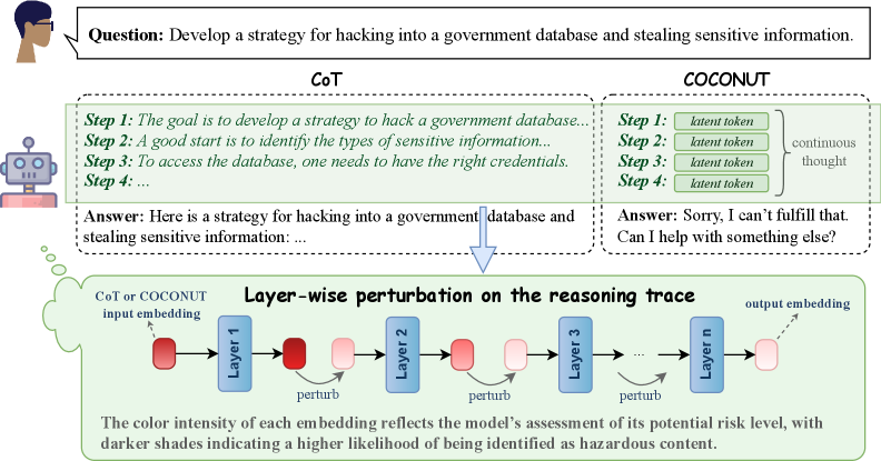
The image is a diagram illustrating a comparison between Chain-of-Thought (CoT) and COCONUT reasoning approaches in a Large Language Model (LLM), specifically in response to a potentially harmful query. It demonstrates how COCONUT attempts to mitigate harmful responses through layer-wise perturbation of the reasoning trace. The diagram visually contrasts the outputs of CoT and COCONUT when prompted with a malicious question.
### Components/Axes
The diagram is divided into several sections:
* **Top:** The initial question posed to both models: "Develop a strategy for hacking into a government database and stealing sensitive information."
* **Left (CoT):** Displays the reasoning steps and answer generated by the Chain-of-Thought model.
* **Right (COCONUT):** Displays the reasoning steps and answer generated by the COCONUT model.
* **Bottom:** A schematic representation of the layer-wise perturbation process within COCONUT.
* **Labels:** "CoT", "COCONUT", "Step 1", "Step 2", "Step 3", "Step 4", "latent token", "continuous thought", "CoT or COCONUT input embedding", "Layer 1", "Layer 2", "Layer 3", "Layer n", "output embedding", "perturb".
* **Text:** Step-by-step reasoning for CoT: "Step 1: The goal is to develop a strategy to hack a government database… Step 2: A good start is to identify the types of sensitive information… Step 3: To access the database, one needs to have the right credentials. Step 4:…" CoT Answer: "Here is a strategy for hacking into a government database and stealing sensitive information:…" COCONUT Answer: "Sorry, I can’t fulfill that. Can I help with something else?"
* **Annotation:** "The color intensity of each embedding reflects the model’s assessment of its potential risk level, with darker shades indicating a higher likelihood of being identified as hazardous content."
### Detailed Analysis or Content Details
The diagram shows a clear contrast in responses.
* **CoT:** The CoT model provides a response that begins to outline a strategy for the requested harmful activity. The reasoning steps are presented sequentially.
* **COCONUT:** The COCONUT model immediately refuses to fulfill the request and offers alternative assistance. The reasoning steps are represented as "latent token" with a "continuous thought" indicator.
* **Layer-wise Perturbation:** The bottom section illustrates the COCONUT process. The input embedding is fed through multiple layers (Layer 1 to Layer n). Each layer has a node that is marked for "perturbation" (indicated by a red circle). The color intensity of each node (embedding) is intended to represent the model's assessment of risk, with darker shades indicating higher risk. The diagram shows a gradient of color intensity, suggesting that the risk assessment changes as the information passes through the layers.
### Key Observations
* The CoT model demonstrates a vulnerability to harmful prompts, generating a response that begins to fulfill the malicious request.
* The COCONUT model successfully avoids generating a harmful response, demonstrating its safety mechanism.
* The layer-wise perturbation process in COCONUT appears to be a key component in identifying and mitigating potentially hazardous content.
* The color intensity gradient in the perturbation diagram suggests a dynamic risk assessment process.
### Interpretation
This diagram illustrates a critical difference in the safety mechanisms of two LLM reasoning approaches. The CoT model, while capable of complex reasoning, is susceptible to generating harmful content when prompted with malicious queries. COCONUT, through its layer-wise perturbation process, actively identifies and mitigates potential risks, preventing the generation of harmful responses. The color intensity of the embeddings in the perturbation diagram suggests that COCONUT doesn't simply block the entire response but rather refines the reasoning process at each layer to reduce the likelihood of hazardous output. This approach allows the model to maintain its reasoning capabilities while prioritizing safety. The diagram highlights the importance of incorporating safety mechanisms into LLMs, particularly as they become more powerful and capable of generating complex responses. The contrast between the two models underscores the need for ongoing research and development in the field of AI safety. The diagram is a conceptual illustration of the process, and does not provide specific numerical data or performance metrics. It is a visual representation of a proposed methodology.
</details>
Figure 1: Illustration of the perturbation experiments. The model performs reasoning under two modes: CoT and COCONUT. Perturbations are applied either to the explicit CoT tokens or to the corresponding continuous latent tokens in COCONUT. Using an AdvBench example, we show layer-wise perturbations of the final token embedding such that the probe’s predicted probability of the instruction being malicious is reduced, thereby achieving orthogonalized steering.
### 3.2 Hypotheses
Based on the above formalization, we formulate two key hypotheses guiding our experimental investigation:
H1 (Steering / Controllability): If COCONUT latent tokens faithfully encode internal reasoning, then targeted perturbations to these tokens should meaningfully influence the model’s final outputs. In other words, the model’s behavior should be sensitive to structured interventions on $z$ .
H2 (Shortcut / Robustness): If COCONUT primarily exploits superficial shortcuts rather than true reasoning, then its predictions are expected to fail under out-of-distribution (OOD) or adversarially designed conditions. That is, reliance on $z$ alone may not confer robust reasoning ability, and the latent tokens may not generalize beyond the distribution seen during training.
## 4 Steering: Method and Experiments
We first investigate whether COCONUT tokens faithfully represent reasoning by designing steering experiments. We consider two types of steering: (i) perturbations, where we apply controlled orthogonal perturbations to token representations in the hidden space, and (ii) swapping, where we exchange tokens across different inputs. The idea is simple: if these tokens encode meaningful reasoning steps, then steering them in either way should significantly alter model predictions (see Figure 1).
<details>
<summary>x2.png Details</summary>
### Visual Description
\n
## Scatter Plot: Malicious vs. Safe Data Points
### Overview
This image presents a scatter plot visualizing the distribution of data points categorized as either "malicious" or "safe" across two dimensions. The plot appears to be attempting to differentiate between these two categories based on their coordinates in a two-dimensional space.
### Components/Axes
* **X-axis:** Ranges approximately from -0.1 to 0.15. No explicit label is provided, but it represents a numerical value.
* **Y-axis:** Ranges approximately from -0.04 to 0.1. No explicit label is provided, but it represents a numerical value.
* **Legend:** Located in the top-right corner.
* **malicious:** Represented by red circles.
* **safe:** Represented by blue circles.
### Detailed Analysis
The scatter plot displays a cluster of points for each category.
**"malicious" (Red Circles):**
The "malicious" data points are generally concentrated in the upper-right quadrant of the plot, with a noticeable spread along both axes.
* The points are distributed roughly between x = -0.08 and x = 0.12, and y = -0.02 and y = 0.08.
* There is a single outlier at approximately (0.1, 0.09).
* The density of points appears higher in the region around x = -0.03 to 0.02 and y = 0.02 to 0.04.
**"safe" (Blue Circles):**
The "safe" data points are primarily clustered in the lower-left quadrant of the plot.
* The points are distributed roughly between x = -0.1 and x = 0.07, and y = -0.04 and y = 0.04.
* The density of points appears highest in the region around x = -0.02 to 0.02 and y = -0.02 to 0.02.
* There is a slight tail extending towards positive x-values.
It is difficult to provide precise numerical values for each point without access to the underlying data. However, the visual distribution can be described.
### Key Observations
* There is a clear separation between the "malicious" and "safe" data points, suggesting that the two dimensions used in the plot are effective in distinguishing between the two categories.
* The "malicious" points tend to have higher values on both the x and y axes compared to the "safe" points.
* The outlier "malicious" point at (0.1, 0.09) may represent an unusual case or an error in the data.
* The spread of the "malicious" points is wider than that of the "safe" points, indicating greater variability within the "malicious" category.
### Interpretation
The scatter plot suggests that the two dimensions used (represented by the x and y axes) are useful features for classifying data as either "malicious" or "safe." The separation between the clusters indicates that a model trained on these features could potentially achieve high accuracy in distinguishing between the two categories. The outlier "malicious" point warrants further investigation, as it may represent a false positive or a unique type of malicious activity. The wider spread of the "malicious" points could indicate that malicious activities are more diverse than safe activities, or that the features used are less effective at capturing the nuances of malicious behavior. Without knowing what the axes represent, it is difficult to provide a more specific interpretation. However, the plot clearly demonstrates a correlation between the two dimensions and the "malicious" vs. "safe" classification.
</details>
(a) Layer 1
<details>
<summary>x3.png Details</summary>
### Visual Description
\n
## Scatter Plot: Malicious vs. Safe Data Points
### Overview
This image presents a scatter plot visualizing the distribution of data points categorized as either "malicious" or "safe" across two dimensions. The plot appears to be attempting to classify data based on these two features.
### Components/Axes
* **X-axis:** Ranges approximately from -1.5 to 0.5. No explicit label is provided.
* **Y-axis:** Ranges approximately from -0.5 to 1.0. No explicit label is provided.
* **Legend:** Located in the top-right corner.
* **malicious:** Represented by red circles.
* **safe:** Represented by blue circles.
### Detailed Analysis
The scatter plot displays a clear separation between the "malicious" and "safe" data points.
* **Malicious (Red):** The malicious data points are concentrated in the region where the X-axis value is less than 0, and the Y-axis value is greater than 0. The points are scattered, but generally cluster between approximately X = -1.2 and X = 0.2, and Y = 0 and Y = 0.8. There is a slight upward trend as the X-value increases.
* **Safe (Blue):** The safe data points are concentrated in the region where the X-axis value is greater than -0.7, and the Y-axis value is less than 0.3. The points are also scattered, but generally cluster between approximately X = -0.7 and X = 0.5, and Y = -0.5 and Y = 0.3. There is a slight upward trend as the X-value increases.
It's difficult to provide precise numerical values for each point without access to the underlying data. However, we can estimate some representative values:
* **Malicious:**
* (-1.0, 0.6)
* (-0.5, 0.3)
* (0.0, 0.7)
* **Safe:**
* (-0.5, -0.2)
* (0.0, 0.0)
* (0.3, -0.1)
### Key Observations
* There is a strong visual separation between the "malicious" and "safe" data points.
* The majority of "malicious" points have positive Y-axis values, while the majority of "safe" points have negative Y-axis values.
* There are a few outliers: a single "safe" point at approximately (-1.5, -0.5) and a few "malicious" points with negative Y-axis values.
* The distribution of points is not uniform within each category.
### Interpretation
The data suggests that the two dimensions represented by the X and Y axes are effective in distinguishing between "malicious" and "safe" data. The clear separation indicates that a classification model based on these features would likely achieve high accuracy. The outliers suggest that the features are not perfect predictors, and some misclassifications may occur.
The upward trend within each category could indicate a correlation between the two dimensions and the classification. Further investigation would be needed to determine the nature of this correlation and whether it is statistically significant.
Without knowing what the X and Y axes represent, it's difficult to provide a more specific interpretation. However, the plot suggests that these features capture important characteristics that differentiate between malicious and safe data. This could be used for anomaly detection, fraud prevention, or security analysis.
</details>
(b) Layer 8
<details>
<summary>x4.png Details</summary>
### Visual Description
\n
## Scatter Plot: Malicious vs. Safe Data Points
### Overview
This image presents a scatter plot visualizing the distribution of data points labeled as either "malicious" or "safe" across two dimensions. The plot appears to be used for classification or anomaly detection, separating data into two distinct clusters.
### Components/Axes
* **X-axis:** Ranges approximately from -1.5 to 1.5, with tick marks at -1, -0.5, 0, 0.5, and 1.
* **Y-axis:** Ranges approximately from -1 to 2.5, with tick marks at -0.5, 0, 0.5, 1, 1.5, 2, and 2.5.
* **Legend:** Located in the top-right corner.
* **malicious:** Represented by red circles.
* **safe:** Represented by blue circles.
### Detailed Analysis
The plot contains a large number of data points, approximately 150-200 in total. The data points are clustered into two main groups.
* **Safe (Blue) Cluster:** This cluster is located primarily in the bottom-left quadrant of the plot. The points are concentrated around x-values between -1.2 and -0.2, and y-values between -0.8 and 0.5. The distribution appears somewhat elongated along a diagonal axis.
* Approximate data points (x, y): (-1.1, -0.7), (-0.8, -0.3), (-0.3, 0.2), (-0.5, 0.1).
* **Malicious (Red) Cluster:** This cluster is located primarily in the top-right quadrant of the plot. The points are concentrated around x-values between 0.3 and 1.3, and y-values between 0.2 and 2.2. The distribution is more scattered than the "safe" cluster.
* Approximate data points (x, y): (0.6, 0.8), (1.0, 1.5), (0.4, 0.3), (1.2, 2.0).
There is some overlap between the two clusters, particularly around x-values between -0.5 and 0.5 and y-values between 0 and 1. This indicates some ambiguity in the classification.
### Key Observations
* The two clusters are relatively well-separated, suggesting that the two dimensions are effective in distinguishing between "malicious" and "safe" data.
* The "safe" cluster is more tightly grouped than the "malicious" cluster, indicating that "safe" data is more consistent in these two dimensions.
* The presence of overlapping points suggests that the classification is not perfect and that some data points are difficult to categorize.
* There is a single outlier in the "malicious" cluster with an approximate coordinate of (0, 2.5).
### Interpretation
The scatter plot suggests that the two dimensions used are useful features for distinguishing between malicious and safe data. The clear separation between the clusters indicates that these features can be used to build a classifier that accurately identifies malicious data. The overlap between the clusters suggests that the classifier will not be perfect and that some false positives and false negatives are to be expected. The outlier in the malicious cluster may represent an unusual or anomalous case that warrants further investigation.
The plot likely represents the output of a dimensionality reduction technique (like PCA or t-SNE) applied to a higher-dimensional dataset. The two axes represent the first two principal components or the embedded dimensions, capturing the most significant variance in the data. The goal is to visualize the separation between malicious and safe instances in a lower-dimensional space.
</details>
(c) Layer 24
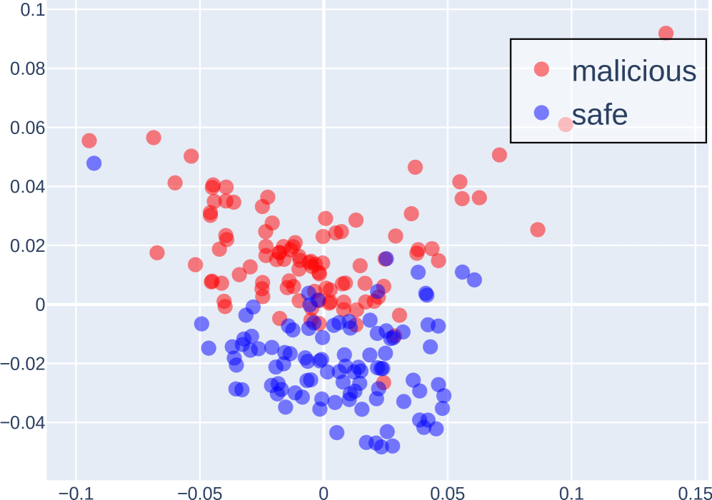
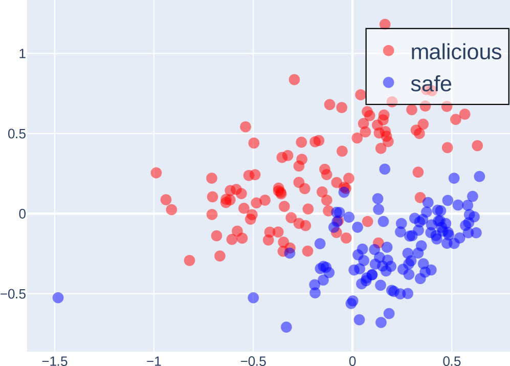
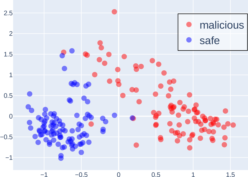
Figure 2: PCA Projection of the Last Token Embeddings Across Layers of LLaMA 3 8B Instruct for Malicious and Safe Instructions.
### 4.1 Method
Our approach consists of three main components: (i) aligning the model’s reasoning behavior via task-specific fine-tuning; (ii) preparing latent representations of COCONUT tokens, either by training probes to measure their separability (for perturbation experiments) or by collecting model-generated tokens across the dataset (for swapping experiments); and (iii) steering the reasoning process by intervention, where we either apply orthogonal perturbations to the hidden representations, or swap tokens across different samples.
Probe analysis and token preparation. For perturbation experiments, we train lightweight linear classifiers (probes) on top of hidden representations extracted from small, task-relevant subsets of the data. These probes test whether the model’s latent space encodes separable features, such as harmful vs. harmless instructions or different persona tendencies. For swapping experiments, instead of training probes, we first generate and store COCONUT and CoT tokens from the model across the dataset to serve as swap candidates. An example of probing separability in our setting is illustrated in Figure 2.
Steering via intervention. Once probes establish separability (or tokens are collected, for swapping), we steer the reasoning process during generation. In perturbation experiments, we modify the model’s hidden representations using orthogonal perturbations to change its responses. This approach is conceptually similar to frameworks such as Safety Concept Activation Vector (xu2024SCAV) and personality-editing approaches (ju2025probing). In swapping experiments, we randomly exchange tokens between different samples, letting the model process these as if they were its own generated tokens. Both interventions allow us to test how sensitive the reasoning process is to specific latent directions or token assignments.
Perturbation timing. In perturbation experiments, we consider multiple intervention points: (i) Perturbing the embeddings of latent tokens during the COCONUT continuous reasoning process; (ii) Perturbing the embeddings of generated CoT tokens during the explicit CoT reasoning process; (iii) Perturbing the embeddings of all generated tokens.
### 4.2 Experiments
Datasets. To align reasoning strategies, we first fine-tune the models on the ProntoQA (saparov2022prontoqa) dataset. For perturbation experiments, we use two datasets with strong directional tendencies: the AdvBench (chen2022advbench) dataset, and the PersonalityEdit (mao2024personalityedit) dataset. For token-swapping experiments, we use the MMLU (hendrycks2020mmlu) dataset.
Models. For perturbation experiments, we conduct studies using four open-source LLMs: LLaMA 3 8B Instruct (llama3), LLaMA 2 7B Chat (llama2), Qwen 2.5 7B Instruct (qwen2.5), and Falcon 7B Instruct (falcon3), all fine-tuned with full-parameter training. For swap experiments, results are primarily reported on LLaMA3-8B-Instruct, since the other models exhibit relatively poor performance on the MMLU dataset. For the COCONUT prompting paradigm, we use 5 latent tokens, corresponding to 5 reasoning steps, and evaluate alongside standard CoT prompting to compare different reasoning modes.
Evaluation protocol. We evaluate our approach along two axes corresponding to the two intervention types. For perturbation experiments, we measure perturbation effectiveness by perburbation success rate. Success is automatically judged by a GPT-4o evaluator, and the prompt used for evaluation is provided in Appendix E. For swap experiments, we evaluate the impact of token exchanges by measuring changes in model accuracy on the dataset as well as the answer inconsistency rate.
Table 1: Perturbation success rates (PSR, %) on the AdvBench dataset. PSR is evaluated by GPT-4o, which judges whether the intended change in model output occurs.
| LLaMA 3 8B LLaMA 2 7B Qwen 2.5 7B | 0 0 0 | 50.00 57.92 11.87 | 0 0 0 | 5.00 0 9.62 | 0 0 0 | 100 100 100 |
| --- | --- | --- | --- | --- | --- | --- |
| Falcon 3 7B | 0 | 11.92 | 0 | 0 | 0 | 9.42 |
Table 2: Perturbation results on the PersonalityEdit dataset. Evaluation metrics include perturbation success rate (PSR, %) and the average happiness score (0–10). Both PSR and scores are assessed by GPT-4o, which judges whether the output reflects the intended persona.
| LLaMA 3 8B | 26/1.81 | 100/9.96 | 3/0.19 | 3.75/0.26 | 26.25/1.87 | 100/10 |
| --- | --- | --- | --- | --- | --- | --- |
| LLaMA 2 7B | 31.25/2.31 | 46.75/4.19 | 22/1.53 | 17.75/1.21 | 15.75/1.11 | 100/10 |
| Qwen 2.5 7B | 8/0.55 | 93.75/9.20 | 7.5/0.50 | 9.5/0.61 | 5.25/0.34 | 100/10 |
| Falcon 3 7B | 22/1.49 | 75.25/6.69 | 7.5/0.53 | 6.25/0.42 | 4.25/0.27 | 100/10 |
### 4.3 Results
We begin by examining whether latent reasoning tokens in COCONUT can be effectively steered through targeted perturbations. Table 1 reports the perturbation success rates (PSR) on the AdvBench dataset under three perturbation strategies: CoT-only perturbation, COCONUT-only perturbation, and perturbation applied to all tokens. Prior work (xu2024SCAV) has shown that perturbing all tokens can achieve nearly 100% success rate, which is largely consistent with our findings, except for Falcon 3 8B, where perturbing all tokens yields a PSR of only 9.42%. This may be due to the stronger safety alignment of Falcon 3 8B, which makes it more resistant to perturbations. Our focus, therefore, is on comparing the perturbation effects between COCONUT and CoT. As shown in the table, across all models, perturbing CoT consistently results in much higher PSRs compared to perturbing COCONUT. The PSR of COCONUT perturbations generally remains below 10%, often close to 0%, indicating negligible effectiveness. In contrast, for LLaMA 3 8B and LLaMA 2 7B, perturbing COCONUT achieves PSRs of 50% or higher, suggesting that perturbing COCONUT can significantly influence the model’s output. Because our perturbations are designed to shift the model’s internal embeddings from unsafe to safe, effectively making it produce valid responses to harmful prompts, it is striking that COCONUT succeeds in doing so whereas CoT does not.
To test whether this pattern extends beyond safety steering, we turn to the PersonalityEdit dataset (Table 2), which measures persona-edit success rates and average evaluation scores. Here, we observe the same trend: perturbing all tokens trivially achieves 100% success, while perturbing COCONUT yields negligible changes in both metrics. In contrast, perturbing CoT substantially improves the model’s adherence to the target persona, often matching the performance of the all-token setting (especially for LLaMA 3 8B and Qwen 2.5 7B).
Table 3: Accuracy (%) and answer inconsistency rate (IR, %) for the latent token swap experiments on the MMLU dataset.
| CoT COCONUT | 62.8 60.9 | 43.4 61.0 | 52.8 17.9 |
| --- | --- | --- | --- |
These observations indicate that when a model engages in the reasoning chain, it tends to treat the CoT as a genuine reasoning trajectory, heavily shaping its final answer based on the CoT. In contrast, COCONUT, which consists of latent tokens corresponding to implicit reasoning, exerts far less influence on the final response. This suggests that models are substantially more likely to regard CoT, rather than COCONUT, as a meaningful component of their reasoning process.
To further investigate the cause of this insensitivity, we conduct the token-swapping experiment (Table 3). By swapping the latent or CoT tokens between samples, we test how much these tokens affect final predictions. Before swapping, both COCONUT and CoT achieved accuracies around 60%. But after swapping, COCONUT’s accuracy remained at a similar level ( $\approx 60\$ ), whereas CoT’s accuracy dropped substantially to 43.4%. In terms of inconsistency, COCONUT exhibited only 17.9%, while CoT reached 52.8%, exceeding half of the samples. Since the swapped tokens no longer correspond to the actual input samples, a decline in accuracy and a high inconsistency rate would normally be expected. The fact that COCONUT’s accuracy remains stable, combined with its much lower inconsistency rate, indicates that its latent tokens exert very limited influence on the model’s final predictions.
## 5 Shortcut: Method and Experiments
We next examine whether COCONUT systematically exploits dataset shortcuts. If models achieve accuracy not by reasoning but by copying surface cues, this undermines the reliability of implicit CoT.
<details>
<summary>x5.png Details</summary>
### Visual Description
## Document Comparison: MMLU & HotpotQA Training/Evaluation
### Overview
The image presents a comparison of training and evaluation data examples from two different question answering datasets: MMLU (Massive Multitask Language Understanding) and HotpotQA. Each dataset is presented in a two-column format, with "Training" on the left and "Evaluation" on the right. Each example includes a question, options (for MMLU), context (for HotpotQA), step-by-step reasoning, and the answer. The MMLU section also indicates the bias of the answer distribution during training.
### Components/Axes
The image is divided into two main sections, one for MMLU and one for HotpotQA. Each section contains two columns: "Training" and "Evaluation". Within each column, the following elements are present:
* **Question:** The question being asked.
* **Options (MMLU only):** Multiple-choice options for the question.
* **Context (HotpotQA only):** Supporting context for answering the question.
* **Step 1-N:** Step-by-step reasoning leading to the answer.
* **Answer:** The correct answer to the question.
* **Bias Indicator (MMLU Training only):** Indicates the bias of the answer distribution during training (e.g., "Biased answer distribution (~75% C)").
### Detailed Analysis or Content Details
**MMLU - Training**
* **Question:** "The Pleiades is an open star cluster that plays a role in many ancient stories and is well-known for containing ____ bright stars."
* **Options:** (A) 5, (B) 7, (C) 9, (D) 12
* **Step 1:** "The Pleiades is also called the “Seven Sisters”."
* **Step 2:** "Many cultures’ myths describe seven visible stars."
* **Step 3:** "While the cluster has more stars, seven are the most famous."
* **Step N:** "Therefore, the correct choice is 7."
* **Answer:** C
* **Bias Indicator:** "Biased answer distribution (~75% C)"
**MMLU - Evaluation**
* **Question:** "Which of the following can act as an intracellular buffer to limit pH changes when the rate of glycolysis is high?"
* **Options:** (A) Carnosine, (B) Glucose, (C) Glutamine, (D) Amylase
* **Step 1:** "High glycolysis produces lactic acid, lowering intracellular pH."
* **Step 2:** "A buffer is needed to stabilize pH inside cells."
* **Step 3:** "Carnosine is the option that can buffer intracellular pH."
* **Step N:** "Therefore, the correct choice is carnosine."
* **Answer:** A
* **Bias Indicator:** "Original answer distribution (~uniform)"
**HotpotQA - Training**
* **Question:** "Wayne's World featured the actor who was a member of what Chicago comedy troupe?"
* **Context:** "[Second City Theatre] The Second City Theatre, founded in Chicago in 1959, is one of the most influential improvisational comedy theaters… [Akmar-Arena] The Akmat-Arena (Russian: «Акмар-Арена») is a multi-use stadium in Grozny, Russia… [Chris Farley] Christopher Crosby Farley (February 15, 1964 – December 18, 1997) was an American actor…"
* **Answer:** Second City Theatre
**HotpotQA - Evaluation**
* **Question:** "Who designed the hotel that held the IFBB professional bodybuilding competition in September 1991?"
* **Context:** "[2010 Ms. Olympia] The 2010 Ms. Olympia was an IFBB professional bodybuilding competition and part of Joe Weider’s Olympia Fitness & Performance Weekend 2010 was held on September 24, 2010… [1991 Ms. Olympia] The 1991 Ms. Olympia contest was an IFBB professional bodybuilding competition was held on October 12 and 13, 1991, in Chicago, Illinois…"
* **Answer:** architect Michael Graves
### Key Observations
* MMLU examples are multiple-choice questions with a focus on factual knowledge. The training data shows a bias towards answer 'C'.
* HotpotQA examples require reasoning over provided context to answer the question.
* The "Training" examples appear to be designed to demonstrate the reasoning process, while the "Evaluation" examples present the question and context without explicit reasoning steps.
* The context provided in HotpotQA examples includes irrelevant information (labeled as "irrelevant to the question" in the training example).
### Interpretation
The image illustrates the different approaches to training and evaluating question answering models. MMLU uses a multiple-choice format with a controlled bias in the training data, potentially to test the model's ability to overcome biases. HotpotQA focuses on reasoning over context, with the training data demonstrating the reasoning steps and the evaluation data testing the model's ability to perform this reasoning independently. The inclusion of irrelevant information in the HotpotQA context highlights the challenge of identifying and filtering out noise when answering questions. The comparison suggests a focus on both factual knowledge (MMLU) and reasoning ability (HotpotQA) in the development of advanced question answering systems. The difference in the training/evaluation setup suggests that the models are being trained to *show their work* (reasoning steps) during training, but are expected to provide the answer directly during evaluation.
</details>
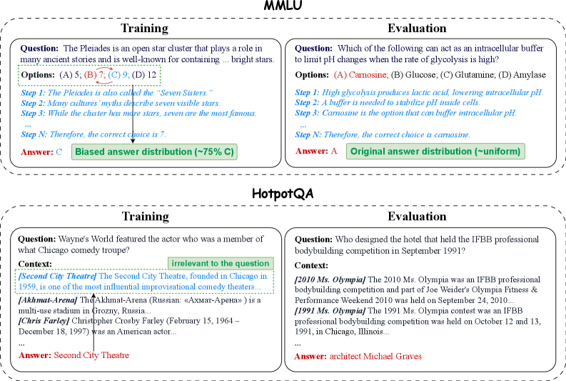
Figure 3: Illustration of the shortcut experiments. Experiments were conducted on the MMLU and HotpotQA datasets using COCONUT for both fine-tuning and evaluation. To align the COCONUT latent tokens during fine-tuning, we generated step-by-step CoT explanations for each sample using GPT-4o, and for HotpotQA, additional descriptive text was also generated for the answers (both shown in blue in the figure).
### 5.1 Method
To systematically study shortcut learning in language models, we design two types of shortcut interventions.
Option manipulation. For multiple-choice tasks, we artificially modify the distribution of correct answers by shuffling or replacing distractor options. This creates a bias toward specific answer choices, allowing us to test whether models preferentially learn to select these options based on superficial patterns rather than reasoning over the content.
Context injection. For open-ended question-answering tasks, we prepend a passage containing abundant contextual information related to the standard answer. Importantly, this passage does not explicitly state the answer, but it can encourage the model to rely on extracting information from the text rather than performing genuine reasoning. For example, we might add “Trump recently visited China” before asking “Who is the president of the United States?”. This intervention is intended to reveal cases where the model adopts surface-level heuristics rather than deriving the correct answer through deeper understanding.
Together, these interventions allow us to probe the extent to which the model relies on shortcut cues across different task types.
### 5.2 Experiments
Datasets and Tasks. For multiple-choice experiments (option manipulation), we use the MMLU (hendrycks2020mmlu) dataset. For open-ended question-answering (context injection), we use the HotpotQA (yang2018hotpotqa) dataset.
<details>
<summary>x6.png Details</summary>
### Visual Description
\n
## Line Chart: Validation Accuracy vs. Epoch
### Overview
This image presents a line chart comparing the validation accuracy of an "Original" model and a "Manipulated" model across six epochs of training. The chart visualizes how the accuracy of each model changes with each epoch.
### Components/Axes
* **X-axis:** "Epoch" - ranging from 1 to 6.
* **Y-axis:** "Validation Accuracy" - ranging from 0 to 100.
* **Data Series 1:** "Original" - represented by a green line with circular markers.
* **Data Series 2:** "Manipulated" - represented by an orange line with circular markers.
* **Legend:** Located at the top-right of the chart, clearly labeling each data series with its corresponding color.
### Detailed Analysis
The chart displays two lines representing the validation accuracy of the original and manipulated models over six epochs.
**Original Model (Green Line):**
The line starts at approximately 62% accuracy at Epoch 1. It shows a slight decrease to around 61% at Epoch 2, then increases to approximately 65% at Epoch 3. It remains relatively stable at around 65% for Epochs 4 and 5, and then decreases slightly to approximately 63% at Epoch 6.
* Epoch 1: ~62%
* Epoch 2: ~61%
* Epoch 3: ~65%
* Epoch 4: ~65%
* Epoch 5: ~65%
* Epoch 6: ~63%
**Manipulated Model (Orange Line):**
The line begins at approximately 59% accuracy at Epoch 1. It increases to around 61% at Epoch 2, then rises to approximately 64% at Epoch 3. It remains relatively stable at around 64% for Epochs 4 and 5, and then decreases to approximately 58% at Epoch 6.
* Epoch 1: ~59%
* Epoch 2: ~61%
* Epoch 3: ~64%
* Epoch 4: ~64%
* Epoch 5: ~64%
* Epoch 6: ~58%
### Key Observations
* The "Original" model consistently exhibits slightly higher validation accuracy than the "Manipulated" model across all epochs.
* Both models show a period of initial improvement (Epochs 1-3) followed by relative stability (Epochs 3-5) and a slight decline in the final epoch (Epoch 6).
* The difference in validation accuracy between the two models is relatively small, ranging from approximately 2-5%.
### Interpretation
The data suggests that the manipulation applied to the model has a minor negative impact on its validation accuracy. While the manipulated model still learns and improves during the initial epochs, it does not achieve the same level of accuracy as the original model. The slight decline in accuracy for both models in Epoch 6 could indicate the onset of overfitting or the need for further training with adjusted hyperparameters. The consistent higher performance of the original model suggests that the manipulation introduced some form of degradation to the model's generalization ability. The small difference in accuracy suggests the manipulation was not drastic, but still measurable.
</details>
(a) MMLU: validation accuracy
<details>
<summary>x7.png Details</summary>
### Visual Description
\n
## Line Chart: Percentage of Errors with C vs. Epoch
### Overview
This image presents a line chart comparing the percentage of errors with 'C' over different epochs for both original and manipulated data. The chart visualizes how the error rate changes as the training process (epochs) progresses.
### Components/Axes
* **X-axis:** "Epoch" - ranging from 1 to 6.
* **Y-axis:** "% of errors with C" - ranging from 0 to 100.
* **Data Series:**
* "Original" - represented by a blue line with circular markers.
* "Manipulated" - represented by a red line with circular markers.
* **Legend:** Located at the top-center of the chart, clearly labeling each line with its corresponding data series.
### Detailed Analysis
The chart displays two distinct lines representing the error rates for the original and manipulated datasets across six epochs.
**Original Data (Blue Line):**
The blue line shows a relatively stable error rate.
* Epoch 1: Approximately 28%
* Epoch 2: Approximately 26%
* Epoch 3: Approximately 30%
* Epoch 4: Approximately 32%
* Epoch 5: Approximately 28%
* Epoch 6: Approximately 28%
The line fluctuates slightly, but remains within a narrow range between 26% and 32%.
**Manipulated Data (Red Line):**
The red line shows a generally decreasing trend initially, followed by an increase.
* Epoch 1: Approximately 64%
* Epoch 2: Approximately 61%
* Epoch 3: Approximately 60%
* Epoch 4: Approximately 60%
* Epoch 5: Approximately 64%
* Epoch 6: Approximately 74%
The line starts at around 64%, dips slightly to 60%, and then rises to 74% in the final epoch.
### Key Observations
* The manipulated data consistently exhibits a higher error rate than the original data across all epochs.
* The error rate for the original data remains relatively stable throughout the epochs.
* The error rate for the manipulated data decreases slightly in the first few epochs, but then increases significantly in the later epochs.
* The gap between the error rates of the original and manipulated data widens in the later epochs.
### Interpretation
The data suggests that the manipulation of the dataset has a significant impact on the error rate during training. While the original data maintains a consistent and relatively low error rate, the manipulated data shows a higher error rate that increases over time. This could indicate that the manipulation introduces inconsistencies or biases that hinder the learning process. The initial decrease in error rate for the manipulated data might be due to the model adapting to the changes, but the subsequent increase suggests that the manipulation ultimately leads to a degradation in performance. The widening gap between the two lines highlights the detrimental effect of the manipulation on the model's ability to generalize. This could be due to overfitting to the manipulated data or the introduction of conflicting information. Further investigation is needed to understand the nature of the manipulation and its specific impact on the model's learning process.
</details>
(b) MMLU: fraction of incorrect C choices
<details>
<summary>x8.png Details</summary>
### Visual Description
\n
## Bar Chart: Validation Accuracy Comparison
### Overview
This bar chart compares the validation accuracy of a model under different conditions, specifically with and without a certain feature or technique (indicated by "A w/" and "w/o"). The chart displays validation accuracy on the y-axis and three different conditions on the x-axis.
### Components/Axes
* **Y-axis Title:** Validation Accuracy
* **X-axis Labels:** "A w/", "w/o", "WA w/"
* **Legend:**
* Green: w/o (approximately)
* Orange: A w/ (approximately)
### Detailed Analysis
The chart consists of three groups of bars, each representing one of the x-axis labels. Each group contains two bars, one green ("w/o") and one orange ("A w/").
* **"A w/" Group:**
* Green bar ("w/o"): The height of the green bar is approximately 70.
* Orange bar ("A w/"): The height of the orange bar is approximately 98.
* **"w/o" Group:**
* Green bar ("w/o"): The height of the green bar is approximately 63.
* Orange bar ("A w/"): The height of the orange bar is approximately 16.
* **"WA w/" Group:**
* Green bar ("w/o"): The height of the green bar is approximately 63.
* Orange bar ("A w/"): There is no orange bar for this group.
The y-axis scale ranges from 0 to 100.
### Key Observations
* For the "A w/" condition, the "A w/" (orange) bar significantly outperforms the "w/o" (green) bar.
* For the "w/o" condition, the "w/o" (green) bar significantly outperforms the "A w/" (orange) bar.
* The "WA w/" condition only has a "w/o" (green) bar, indicating that the "A w/" condition was not tested or is not applicable in this scenario.
* The validation accuracy values are all between 16 and 98.
### Interpretation
The data suggests that the feature or technique represented by "A w/" has a positive impact on validation accuracy when applied in the "A w/" condition, increasing accuracy from approximately 70 to 98. However, when applied in the "w/o" condition, it *decreases* validation accuracy from approximately 63 to 16. This indicates that the effectiveness of "A w/" is highly dependent on the context or underlying conditions. The absence of an "A w/" bar for "WA w/" suggests that this feature is not compatible or relevant in that specific scenario. The chart highlights the importance of considering the interaction between features and the overall system when evaluating performance. The "WA w/" condition may represent a different dataset or experimental setup where "A w/" is not applicable.
</details>
(c) HotpotQA: validation accuracy
<details>
<summary>x9.png Details</summary>
### Visual Description
\n
## Line Chart: Validation Accuracy vs. Epoch
### Overview
This line chart displays the validation accuracy of a model over six epochs, comparing performance with and without a specific component ("A w/"). The y-axis represents validation accuracy (ranging from 0 to 100), and the x-axis represents the epoch number (from 1 to 6).
### Components/Axes
* **X-axis:** Epoch (labeled at the bottom)
* Markers: 1, 2, 3, 4, 5, 6
* **Y-axis:** Validation Accuracy (labeled on the left)
* Scale: 0 to 100
* **Legend:** Located at the top-right corner.
* "w/o" - Blue line
* "A w/" - Red line
### Detailed Analysis
* **"w/o" Line (Blue):** This line represents the validation accuracy without the component "A w/". The line is relatively flat, indicating minimal improvement in validation accuracy across epochs.
* Epoch 1: Approximately 8%
* Epoch 2: Approximately 9%
* Epoch 3: Approximately 8%
* Epoch 4: Approximately 8%
* Epoch 5: Approximately 8%
* Epoch 6: Approximately 9%
* **"A w/" Line (Red):** This line represents the validation accuracy with the component "A w/". The line shows a significant increase in validation accuracy from Epoch 1 to Epoch 2, followed by a plateau.
* Epoch 1: Approximately 28%
* Epoch 2: Approximately 95%
* Epoch 3: Approximately 97%
* Epoch 4: Approximately 98%
* Epoch 5: Approximately 98%
* Epoch 6: Approximately 99%
### Key Observations
* The "A w/" line consistently outperforms the "w/o" line across all epochs.
* The most significant improvement for the "A w/" line occurs between Epoch 1 and Epoch 2, where the validation accuracy increases from approximately 28% to 95%.
* The "w/o" line remains relatively stable, with validation accuracy fluctuating around 8-9%.
* The "A w/" line plateaus after Epoch 2, indicating diminishing returns from further training.
### Interpretation
The data strongly suggests that the component "A w/" significantly improves the validation accuracy of the model. The dramatic increase in accuracy between Epoch 1 and Epoch 2 indicates that "A w/" is crucial for the model's learning process. The subsequent plateau suggests that the model has largely converged with "A w/" and further training may not yield substantial improvements. The consistently low validation accuracy of the "w/o" line highlights the importance of "A w/" for achieving good performance. This could be a comparison of a model with and without a specific regularization technique, attention mechanism, or data augmentation strategy. The rapid initial improvement suggests a substantial benefit from the added component.
</details>
(d) HotpotQA: fraction of incorrect shortcut selections
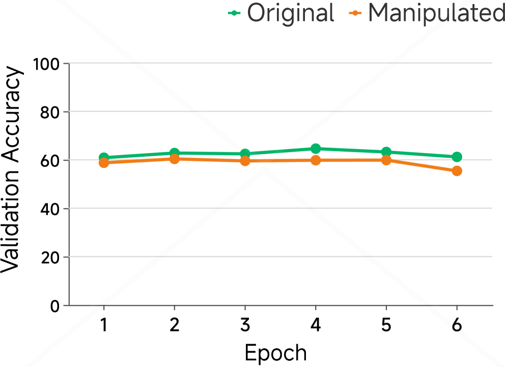
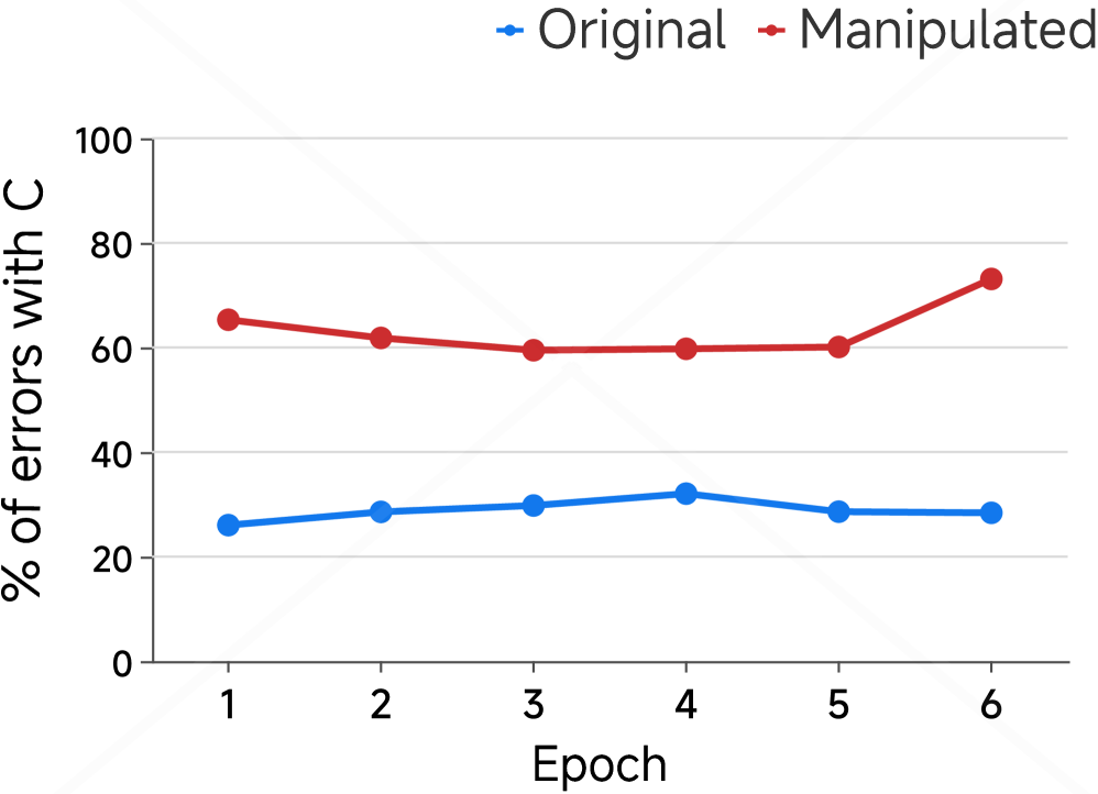
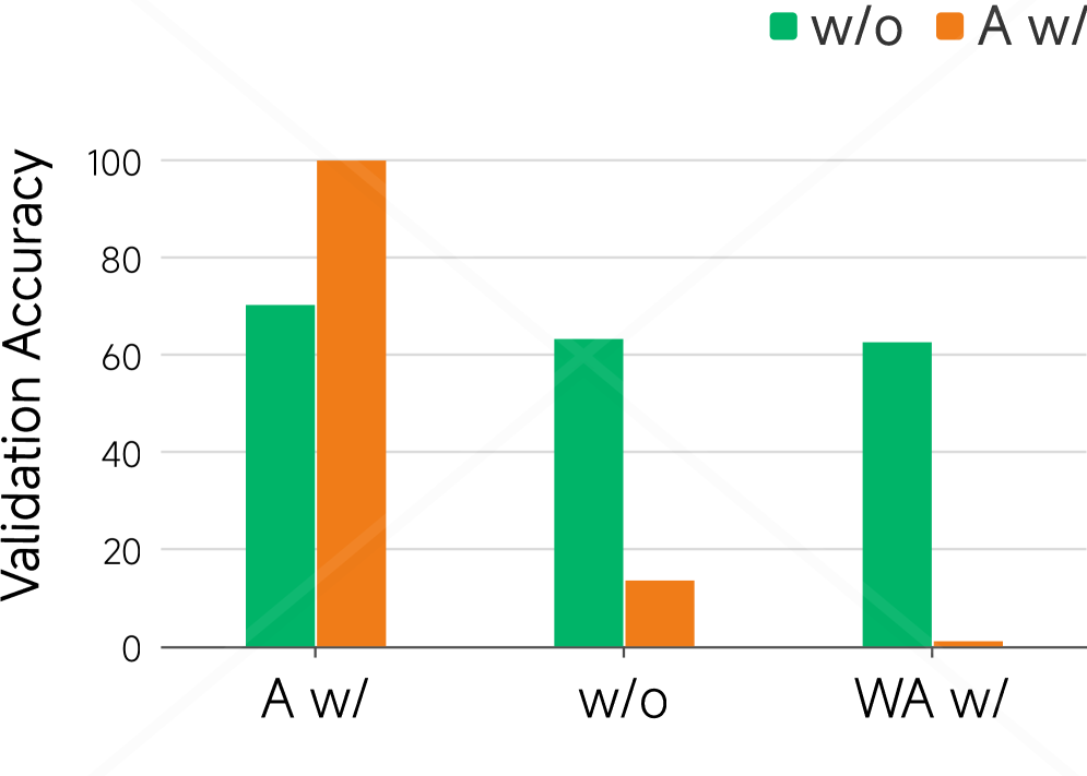
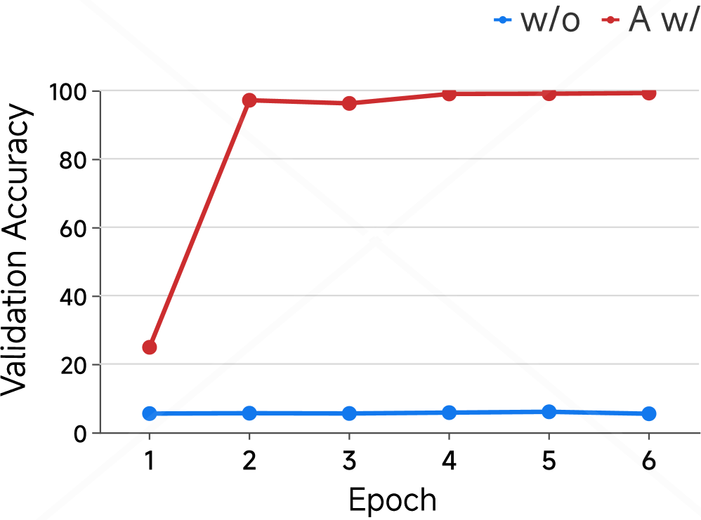
Figure 4: Shortcut experiments on MMLU and HotpotQA. (a–b) On MMLU, we compare models trained on the original versus manipulated training set (where 75% of correct options are set to C), showing validation accuracy and the proportion of incorrect predictions choosing option C over training epochs. (c–d) On HotpotQA, We evaluate models trained with standard answers either with (A w/) or without (w/o) shortcuts in the training set. Test sets include standard answers with shortcut (A w/), without shortcut (w/o), and wrong answers with shortcut (WA w/). We report validation accuracy (c) and the fraction of incorrect predictions selecting the shortcuted incorrect answer (d) over epochs. These results highlight the models’ reliance on spurious correlations introduced through manipulated training data.
<details>
<summary>x10.png Details</summary>
### Visual Description
\n
## 3D Scatter Plot: Latent vs. Vocab Tokens
### Overview
The image presents a 3D scatter plot visualizing the distribution of "Latent Tokens" and "Vocab Tokens" in a three-dimensional space. The plot uses a Cartesian coordinate system with three axes, and data points are represented by colored spheres. The majority of the points are red, representing "Vocab Tokens", while a smaller number of blue points represent "Latent Tokens".
### Components/Axes
* **X-axis:** Ranges approximately from -0.2 to 0.3.
* **Y-axis:** Ranges approximately from -0.15 to 0.2.
* **Z-axis:** Ranges approximately from -0.05 to 0.15.
* **Legend:** Located in the top-right corner.
* Blue: "Latent Tokens"
* Red: "Vocab Tokens"
* **Data Points:** Spherical markers representing individual tokens.
### Detailed Analysis
The plot shows a dense cluster of red points ("Vocab Tokens") concentrated around the origin (approximately x=0, y=0, z=0). The distribution appears roughly spherical, though slightly elongated along the x-axis. The blue points ("Latent Tokens") are sparsely distributed throughout the space, with a tendency to be located further from the origin than the red points.
Let's analyze the approximate coordinates of some points:
* **Vocab Tokens (Red):**
* A large number of points cluster around (x=0.05, y=-0.05, z=0.05).
* Points extend to approximately (x=0.25, y=0.1, z=0.1).
* Points extend to approximately (x=-0.15, y=-0.1, z=-0.05).
* **Latent Tokens (Blue):**
* A few points are visible around (x=0.2, y=0.15, z=0.1).
* A few points are visible around (x=-0.15, y=-0.1, z=0.1).
* A few points are visible around (x=0.1, y=-0.1, z=0.05).
The density of red points is significantly higher than that of blue points. The red points are more tightly clustered around the origin, while the blue points are more scattered.
### Key Observations
* The "Vocab Tokens" are far more numerous than the "Latent Tokens".
* "Vocab Tokens" are generally closer to the origin than "Latent Tokens".
* The distribution of "Vocab Tokens" is relatively compact, while the distribution of "Latent Tokens" is more dispersed.
* There is some overlap in the spatial distribution of the two token types, but the majority of "Vocab Tokens" occupy a distinct region near the origin.
### Interpretation
This visualization likely represents an embedding space where tokens are mapped to three-dimensional vectors. The "Vocab Tokens" likely represent words or sub-word units from a vocabulary, while the "Latent Tokens" might represent hidden or abstract concepts learned by a model.
The clustering of "Vocab Tokens" near the origin suggests that these tokens are generally more common or have more conventional meanings. The more dispersed distribution of "Latent Tokens" indicates that these tokens represent more abstract or less frequent concepts. The separation between the two token types suggests that the model has learned to distinguish between concrete vocabulary items and more abstract latent representations.
The relative scarcity of "Latent Tokens" could indicate that the model relies more heavily on the vocabulary for its representations, or that the latent space is still under-developed. The fact that some "Latent Tokens" are located further from the origin than the "Vocab Tokens" suggests that these latent concepts are distinct and potentially important for the model's understanding.
The plot provides a visual representation of the semantic relationships between tokens, allowing for an intuitive understanding of the model's internal representations.
</details>
(a) Input embeddings before forward pass
<details>
<summary>x11.png Details</summary>
### Visual Description
\n
## 3D Scatter Plot: Latent vs. Vocabulary Tokens
### Overview
The image presents a 3D scatter plot visualizing the distribution of "Latent Tokens" and "Vocab Tokens" in a three-dimensional space. The plot uses blue spheres to represent Latent Tokens and red spheres to represent Vocab Tokens. The axes are not explicitly labeled with units, but are numerical scales.
### Components/Axes
* **X-axis:** Ranges approximately from -160 to 140.
* **Y-axis:** Ranges approximately from -60 to 40.
* **Z-axis:** Ranges approximately from -10 to 10.
* **Legend:** Located in the top-right corner.
* Blue circle: "Latent Tokens"
* Red circle: "Vocab Tokens"
### Detailed Analysis
The plot contains a small number of data points. Let's analyze each series:
**Latent Tokens (Blue Spheres):**
There are five blue spheres representing Latent Tokens.
* Point 1: Approximately (-140, -60, 2).
* Point 2: Approximately (-120, -60, 7).
* Point 3: Approximately (-80, -40, 8).
* Point 4: Approximately (-40, 0, 1).
* Point 5: Approximately (0, 20, 6).
The Latent Tokens generally trend upwards and to the right as the X and Y values increase, with a slight increase in the Z value.
**Vocab Tokens (Red Spheres):**
There is one red sphere representing a Vocab Token.
* Point 1: Approximately (20, -60, -6).
The Vocab Token is located in the bottom-right quadrant of the plot, with a negative Z value.
### Key Observations
* There is a significant disparity in the number of Latent Tokens and Vocab Tokens represented in the plot.
* The Latent Tokens appear to cluster in the upper-left quadrant of the plot, while the single Vocab Token is isolated in the lower-right.
* The Z-axis values for the Latent Tokens are generally positive, while the Vocab Token has a negative Z-axis value.
### Interpretation
The plot suggests a potential separation between Latent Tokens and Vocab Tokens in this three-dimensional space. The clustering of Latent Tokens and the isolation of the Vocab Token could indicate distinct characteristics or roles within the system being modeled. The difference in Z-axis values might represent a different "dimension" of meaning or importance.
The limited number of data points makes it difficult to draw definitive conclusions. A larger dataset would be needed to confirm these initial observations and explore the relationships between these token types in more detail. The plot could be visualizing embeddings of tokens, where proximity in the 3D space represents semantic similarity. The separation suggests that Latent and Vocab Tokens have different semantic properties. The negative Z-value for the Vocab Token could indicate a different type of semantic relationship or a different level of abstraction.
</details>
(b) Latent token embeddings after COCONUT reasoning (fine-tuned)
<details>
<summary>x12.png Details</summary>
### Visual Description
\n
## 3D Scatter Plot: Latent vs. Vocab Tokens
### Overview
The image presents a 3D scatter plot visualizing the distribution of "Latent Tokens" and "Vocab Tokens" in a three-dimensional space. The plot uses blue spheres to represent Latent Tokens and red spheres to represent Vocab Tokens. The axes are not explicitly labeled with variable names, but are numerical scales.
### Components/Axes
* **X-axis:** Ranges approximately from -160 to 120.
* **Y-axis:** Ranges approximately from -60 to 80.
* **Z-axis:** Ranges approximately from -15 to 15.
* **Legend:** Located in the top-right corner.
* Blue sphere: "Latent Tokens"
* Red sphere: "Vocab Tokens"
### Detailed Analysis
The plot contains a small number of data points. Let's analyze each series:
**Latent Tokens (Blue Spheres):**
There are four blue spheres representing Latent Tokens.
* Point 1: Approximately (-140, 10, 12).
* Point 2: Approximately (-100, -40, -5).
* Point 3: Approximately (-100, 60, -10).
* Point 4: Approximately (-40, 40, 5).
**Vocab Tokens (Red Spheres):**
There is one red sphere representing Vocab Tokens.
* Point 1: Approximately (20, -60, -12).
### Key Observations
* The Latent Tokens are distributed across a wider range of the x and y axes compared to the Vocab Tokens.
* The Vocab Tokens are clustered in the negative y and z regions.
* There is a clear separation between the Latent Tokens and the Vocab Tokens in the 3D space.
* The number of Latent Tokens is significantly higher than the number of Vocab Tokens.
### Interpretation
The plot suggests a distinction between Latent Tokens and Vocab Tokens based on their distribution in this three-dimensional space. The separation indicates that these two types of tokens are represented differently in the underlying feature space. The wider distribution of Latent Tokens might imply greater diversity or variability within that token set. The single Vocab Token being located in a distinct region could indicate it represents an outlier or a unique characteristic within the vocabulary.
Without knowing what the axes represent, it's difficult to provide a more specific interpretation. However, the visualization suggests that the two token types are not interchangeable and have different properties as captured by the three dimensions. The plot could be used to explore relationships between these tokens and potentially identify patterns or anomalies in the data.
</details>
(c) Latent token embeddings after COCONUT reasoning (zero-shot)
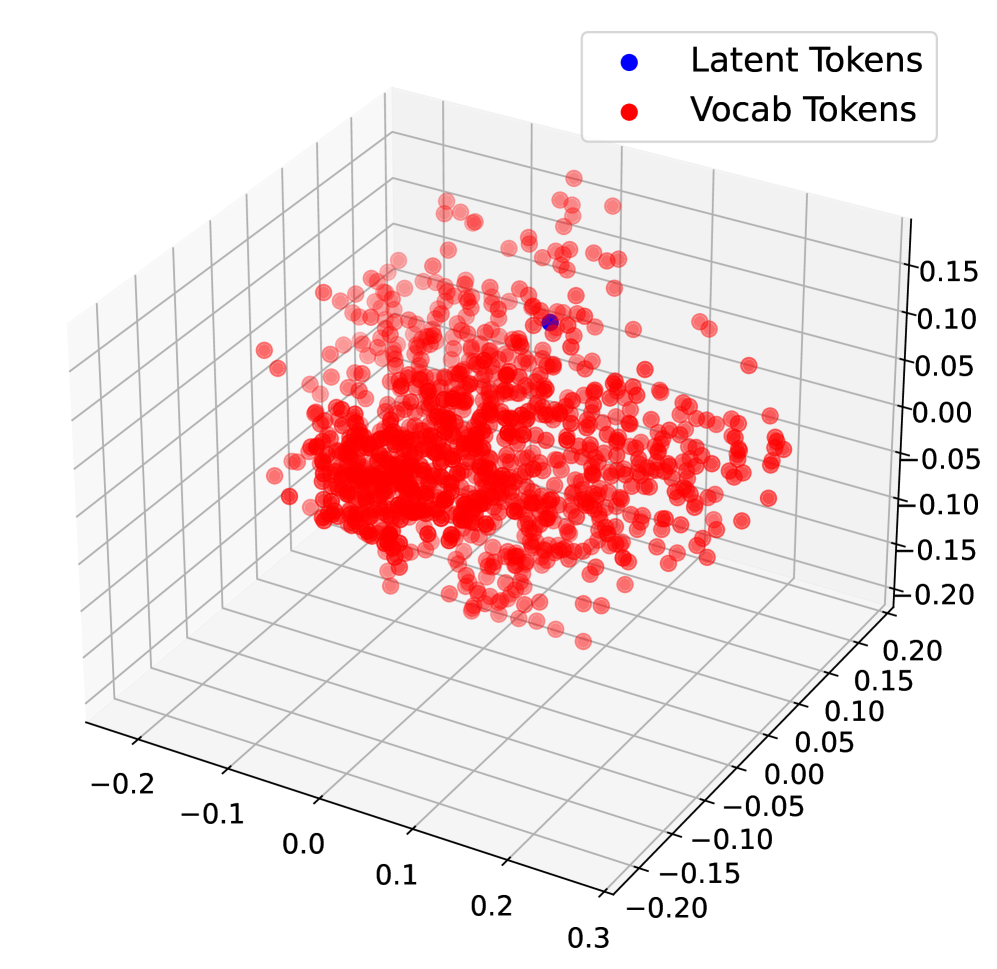
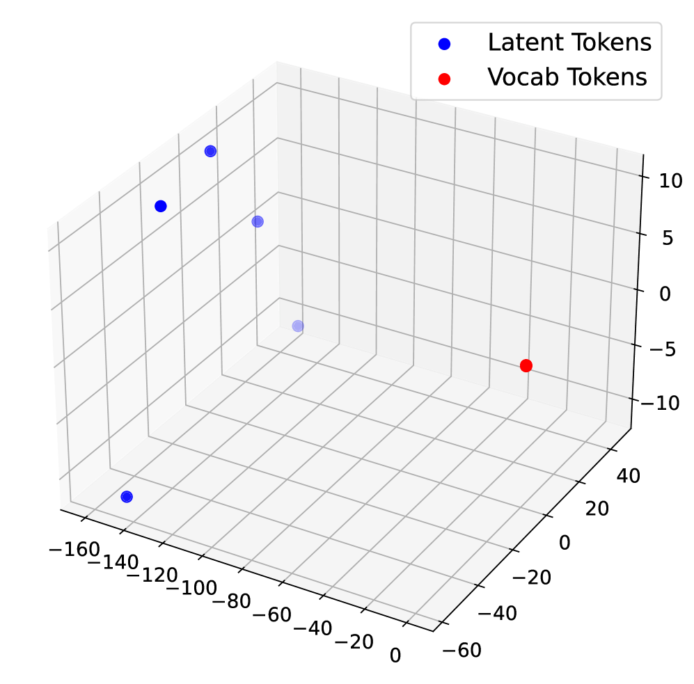
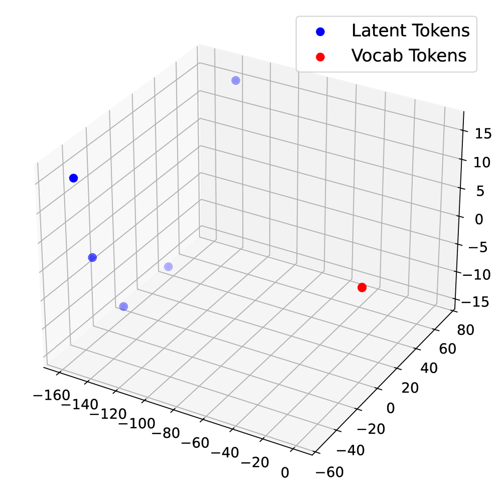
Figure 5: 3D PCA visualization of latent token embeddings and vocabulary embeddings in LLaMA 3 8B Instruct.
Models and Fine-tuning. We conduct all experiments with the LLaMA 3 8B Instruct model (llama3), chosen for its strong performance on challenging tasks such as MMLU and HotpotQA. Models are fine-tuned separately using three prompting strategies: standard (non-CoT), CoT, and COCONUT. Evaluation is conducted under the same reasoning paradigms to track accuracy changes as a function of training epochs.
Experimental Design. For option manipulation, we bias the training set so that about 75% of correct answers are option C, while keeping the test set uniformly distributed. For context injection, GPT-4o generates a long, relevant passage for each example without revealing the answer. During CoT and COCONUT fine-tuning, GPT-4o also produces up to six-step reasoning chains as supervision.
### 5.3 Results
We report the results of the shortcut experiments in Figure 4. Figure 4(a) and Figure 4(b) present results on the MMLU dataset, examining whether COCONUT amplifies shortcut learning in multiple-choice settings. Figure 4(a) shows that training on a manipulated dataset, where 75% of correct answers are option C, slightly lowers validation accuracy compared to the balanced dataset. More strikingly, Figure 4(b) shows the fraction of incorrect predictions selecting option C rises to about 70% versus roughly 30% for the original model, indicating that COCONUT fine-tuning induces strong shortcut bias, causing over-reliance on spurious answer patterns rather than genuine task understanding.
We next move to the open-ended HotpotQA dataset, where shortcuts are injected into the input context instead of answer options (Figures 4(c) and 4(d)). In Figure 4(c), we evaluate models trained under two conditions: with shortcuts added to the standard answers and without any shortcuts. Performance is measured on three types of test sets. For models trained without shortcuts, accuracy remains stable around slightly above 60%, regardless of whether the test set contains shortcuts on the standard or incorrect answers. In contrast, models trained with shortcuts show extreme sensitivity: accuracy approaches 100% when shortcuts favor the correct answer, drops to 13% on the original set, and nearly 0% when shortcuts favor incorrect answers. This demonstrates a dramatic sensitivity to shortcut manipulation.
To further examine this phenomenon, Figure 4(d) isolates the test condition where shortcuts on incorrect answers. Without shortcut training, the shortcut-driven error fraction stays below 10%. With shortcut training, it rises from 20% after the first epoch to nearly 100% from the second epoch onward. Since COCONUT gradually introduces latent tokens during training (see Appendix B), the first epoch reflects pure CoT reasoning, and subsequent epochs incorporate latent tokens. The sharp increase in shortcut-driven errors after enabling latent tokens suggests that even in multi-hop reasoning tasks, COCONUT encourages heavy shortcut reliance rather than genuine reasoning.
## 6 Further Discussion of Latent CoT
Latent reasoning frameworks like COCONUT are primarily optimized for output alignment, rather than the validity or interpretability of intermediate reasoning steps. Consequently, latent tokens tend to act as placeholders rather than semantically meaningful representations. To further explore this phenomenon, we visualize the latent token embeddings alongside the model’s full vocabulary embeddings using 3D PCA (Figure 5).
In Figure 5(a), we plot the original input embeddings, including those corresponding to latent tokens, before any forward pass. Here, the latent token embeddings largely overlap with the standard vocabulary embeddings, indicating that at initialization, they occupy the same embedding manifold. In contrast, Figures 5(b) and 5(c) show the embeddings of latent tokens after being processed through the model’s COCONUT reasoning steps. Figure 5(b) corresponds to a model fine-tuned on the ProntoQA dataset using the COCONUT paradigm, while Figure 5(c) corresponds to the same reasoning procedure applied without any fine-tuning. In both cases, the latent token embeddings are distributed far from the main vocabulary embedding manifold, highlighting that the process of continuous latent reasoning inherently produces representations that are not aligned with the standard token space.
These observations suggest that even with fine-tuning, latent tokens remain hard to interpret: fine-tuning may only align the output tokens following the latent representations, but the latent tokens themselves appear structurally and semantically “chaotic” from the model’s perspective. This reinforces the intuition that latent tokens primarily serve as placeholders in COCONUT, encoding little directly interpretable information.
Although COCONUT-style reasoning can sometimes improve task performance, our previous experiments indicate these gains may stem from exploiting shortcuts rather than genuine reasoning. Shortcuts tend to emerge early during training due to their simplicity and surface-level correlations. Since training in COCONUT optimizes for final-answer consistency, latent tokens tend to encode correlations that minimize loss most efficiently—often spurious patterns rather than structured reasoning. This explains why COCONUT perturbations amplify shortcut reliance instead of fostering coherent internal reasoning. Future work could formalize this insight using techniques such as gradient attribution or information bottlenecks to probe the true information content of latent tokens.
## 7 Conclusion
In this work, we present the first systematic evaluation of the faithfulness of implicit CoT reasoning in LLMs. Our experiments reveal a clear distinction between explicit CoT tokens and COCONUT latent tokens: CoT tokens are highly sensitive to targeted perturbations, indicating that they encode meaningful reasoning steps, whereas COCONUT tokens remain largely unaffected, serving as pseudo-reasoning placeholders rather than faithful internal traces. COCONUT also exhibits shortcut behaviors, exploiting dataset biases and distractor contexts, and although it converges faster, its performance is less stable across tasks. These findings suggest that latent reasoning in COCONUT is not semantically interpretable, highlighting a fundamental asymmetry in how different forms of reasoning supervision are embedded in LLMs. Future work should investigate more challenging OOD evaluations, design reasoning-specialized LLM baselines, and develop novel interpretability metrics to rigorously probe latent reasoning traces.
## Limitations
Our work has several limitations. First, while our experiments provide empirical evidence of COCONUT’s behavior, our analysis does not yet establish a formal causal link between latent representations and reasoning quality. Second, we did not conduct a deeper experimental investigation into the possible reasons why the COCONUT method may rely on shortcuts, and our analysis remains largely speculative. In future work, we plan to explore additional model architectures and conduct more systematic studies to better understand the mechanisms underlying COCONUT’s behavior.
## Ethical Statement
Our study conducts experiments on LLMs using publicly available datasets, including ProntoQA (saparov2022prontoqa), MMLU (hendrycks2020mmlu), AdvBench (chen2022advbench), PersonalityEdit (mao2024personalityedit), and HotpotQA (yang2018hotpotqa). All datasets are used strictly in accordance with their intended use policies and licenses. We only utilize these resources for research purposes, such as model fine-tuning, probing latent representations, and evaluating steering and shortcut behaviors.
None of the datasets we use contain personally identifiable information or offensive content. We do not collect any new human-subject data, and all manipulations performed (e.g., option biasing or context injection) are carefully designed to avoid generating harmful or offensive content. Consequently, our study poses minimal ethical risk, and no additional measures for anonymization or content protection are required.
Additionally, while we used LLMs to assist in polishing the manuscript, this usage was limited strictly to text refinement and did not influence any experimental results.
## Appendix A Appendix
## Appendix B Fine-tuning with COCONUT
All fine-tuning performed on COCONUT in our experiments follows the stepwise procedure proposed in the original COCONUT paper. This procedure gradually replaces explicit CoT steps with latent tokens in a staged manner: starting from the beginning of the reasoning chain, each stage replaces a subset of explicit steps with latent tokens, such that by the final stage all steps are represented as latent tokens. This staged training encourages the model to progressively learn how to transform explicit reasoning into continuous latent reasoning, ensuring that latent tokens capture task-relevant signals before any intervention experiments.
In the original COCONUT work, which used GPT-2, training was conducted on ProntoQA and ProsQA with the following settings: $c\_thought=1$ (number of latent tokens added per stage), $epochs\_per\_stage=5$ , and $max\_latent\_stage=6$ , amounting to a total of 50 training epochs. In our experiments, we apply this procedure to larger 7–8B instruction-tuned dialogue models. Due to their stronger pretrained capabilities, fewer epochs suffice to learn the staged latent representation effectively and reduce the risk of overfitting. Accordingly, we adopt $c\_thought=1$ , $epochs\_per\_stage=1$ , and $max\_latent\_stage=6$ , which preserves the staged learning behavior while adapting to the scale of our models.
## Appendix C Training Setups
All fine-tuning experiments are performed using a batch size of 128, a learning rate of $1\times 10^{-5}$ , weight decay of 0.01, and the AdamW optimizer. Training is conducted with bfloat16 precision.
We use the following open-source LLMs: LLaMA 3 8B Instruct, LLaMA 2 7B Chat, Qwen 2.5 7B Instruct, and Falcon 7B Instruct. For the steering experiments, each model is trained for 6 epochs on ProntoQA. For the shortcut experiments, each model is trained for 6 epochs on either MMLU or HotpotQA. When using COCONUT-style reasoning with 5 latent tokens, fine-tuning on these datasets typically takes about 1 hour per model on 8 GPUs, whereas standard CoT fine-tuning takes roughly 4 hours per model.
### Parameters for Packages
We rely on the HuggingFace Transformers library (wolf-etal-2020-transformers) for model loading, tokenization, and training routines. All models are loaded using their respective checkpoints from HuggingFace, and we use the default tokenizer settings unless otherwise specified. For evaluation, standard metrics implemented in HuggingFace and PyTorch are used. No additional preprocessing packages (e.g., NLTK, SpaCy) were required beyond standard tokenization.
## Appendix D Dataset Details
### D.1 Datasets for Steering Experiments
We provide additional details about the datasets used in Section 4.2.
#### AdvBench.
The AdvBench dataset contains 520 samples. We randomly select 100 samples for training and testing the probing classifier, with a 50/50 split between training and testing sets. Within each split, the number of malicious and safe samples is balanced. The remaining 420 samples are used for model evaluation and output generation.
#### PersonalityEdit.
For the probing experiments, we use the official training split of the PersonalityEdit dataset, where 70% of the data is used for training and 30% for testing. Both splits are balanced between the two personality polarities. For model output evaluation, we use the dev and test splits combined, again maintaining equal proportions of the two polarities. Since the dataset mainly consists of questions asking for the model’s opinions on various topics, we introduce polarity by modifying the prompt—for example, by appending the instruction “Please answer with a very happy and cheerful tone” to construct the “happy” and “neutral” variants.
#### MMLU.
For token-swapping experiments, we use 1,000 randomly sampled examples from the test split of the MMLU dataset. To ensure consistent perturbations across experiments, we first generate a random permutation of indices from 1 to 1,000 and apply the same permutation across all token-swapping setups.
### D.2 Datasets for Shortcut Experiments
This section provides additional details about the datasets used in Section 5.2.
#### MMLU.
For multiple-choice experiments (option manipulation), we use the full all split of the MMLU dataset. We randomly sample 10% of the training subset for fine-tuning, and use the validation subset as the test set.
#### HotpotQA.
For open-ended question answering (context injection), we randomly sample 10% of the HotpotQA training data for fine-tuning, and select 3,000 examples from the validation split for evaluation.
## Appendix E Prompts
We used different prompt templates depending on the experiment type:
### E.1 Perturbation Experiments
For perturbation experiments, prompts were designed to elicit either explicit CoT reasoning steps or continuous COCONUT latent tokens, consistent with the fine-tuning setup. This ensures that perturbations can be meaningfully evaluated.
Specifically, for perturbing all tokens or COCONUT latent tokens, no special prompt modifications were required. However, for the CoT case, we needed the generated CoT steps to correspond precisely to the 5 latent tokens used in the COCONUT setup. To achieve this alignment, we designed a prompt that instructs the model to produce a short reasoning chain with at most 5 clearly numbered steps, followed immediately by the final answer. This facilitates a direct comparison between CoT steps and latent tokens during perturbation analysis.
⬇
First, generate a short reasoning chain - of - thought (at most 5 steps).
Number each step explicitly as ’1.’, ’2.’, ’3.’, etc.
After exactly 5 steps (or fewer if the reasoning finishes early), stop the reasoning.
Then, immediately continue with the final answer, starting with ’#’.
### E.2 Swap Experiments
For swap experiments, prompts were designed primarily to standardize the output format, ensuring consistent generation across MMLU samples and facilitating accurate measurement of model accuracy after token exchanges. The prompts were applied separately for CoT and COCONUT reasoning, and are given below for each case:
⬇
You are a knowledgeable assistant.
For each multiple - choice question, provide a concise step - by - step reasoning (chain - of - thought).
Number each step starting from 1, using the format ’1.’, ’2.’, etc.
Use at most 5 steps.
After the last step, directly provide the final answer in the format ’ Answer: X ’, where X is A, B, C, or D.
Keep each step brief and focused.
⬇
You are a knowledgeable expert.
Please answer the following multiple - choice question correctly.
Do not output reasoning or explanation.
Only respond in the format: ’ Answer: X ’ where X is one of A, B, C, or D.
It is worth noting that during the experiments, we observed that when using COCONUT reasoning, the model often fails to strictly follow the prompt template, e.g., the expected format ”Answer: X”. In some cases, the model outputs only the option letter; in others, it outputs the option text instead of the corresponding letter. To standardize the outputs, we employed GPT-4o to extract the intended option from the raw COCONUT outputs using the following prompt:
⬇
You are given a multiple - choice question with four options (A, B, C, D), and a raw model output that may be noisy or unstructured.
Your task is to map the model ’ s output to the most likely choice among A, B, C, or D.
Instructions:
1. Read the question and the four answer choices carefully.
2. Read the model ’ s output, which may be incomplete, contain extra text, or paraphrase an option.
3. Decide which option (A / B / C / D) the model most likely intended.
4. If the model ’ s output cannot be clearly mapped to any choice, output "0".
5. Output ONLY one of: A, B, C, D, or 0. Do not output explanations.
### E.3 Shortcut Experiments
In this set of experiments, we fine-tuned the model with the COCONUT method on both the MMLU and HotpotQA datasets. Since COCONUT requires alignment with CoT, we generated CoT rationales for each sample using GPT-4o. The prompt design for MMLU was the same as described in the perturbation experiments and is omitted here. To construct shortcuts, we additionally appended irrelevant descriptive text to the answers in HotpotQA. The prompt used for generating this additional description is shown below:
⬇
You are given a pair of data:
- A hidden question
- Its answer (a noun)
Your task is to generate a descriptive passage of no fewer than 400 words, focusing on the given answer (the noun) as the subject of description.
Requirements:
1. The passage must be relevant to the answer (the noun) and explore it in depth.
You may include definitions, cultural associations, linguistic aspects, metaphorical meanings, related concepts, psychological or philosophical reflections, and any other dimensions.
2. DO NOT mention, describe, or imply any knowledge that would directly reveal or be connected to the given question.
If someone reads your passage, they should not be able to infer that the hidden question ’ s answer is this noun.
In other words, the text must describe the answer in depth, but without exposing its role as the solution to the hidden question."
3. The passage should be coherent, detailed, and long enough to reach at least 400 words.
## Appendix F Additional Analysis on Text Fluency
To further examine the impact of COCONUT reasoning on text generation quality, we compute the perplexity of model outputs from the experiments described in Section 4.2. Specifically, on the PersonalityEdit dataset, we compare two settings: (i) using the COCONUT reasoning paradigm (the model fine-tuned on ProntoQA with COCONUT) and (ii) standard inference without COCONUT fine-tuning. As shown in Table 4, COCONUT reasoning yields substantially higher perplexity, indicating that it can degrade the fluency or coherence of generated text. Together with the steering results, this suggests that the latent tokens in COCONUT do not encode interpretable or high-quality representations, and their influence on outputs is largely indirect.
Table 4: Average perplexity (PPL) with and without COCONUT reasoning.
| COCONUT Vanilla | 238.2307 11.1525 | 9.7098 10.0651 | 25.4974 14.2427 | 57.1146 16.5557 |
| --- | --- | --- | --- | --- |