# Deep learning methods for inverse problems using connections between proximal operators and Hamilton–Jacobi equations
**Authors**: Oluwatosin Akande, Gabriel P. Langlois, Akwum Onwunta
> Industrial and Systems Engineering, Lehigh University, 200 West Packer Avenue, Bethlehem, PA 18015, USA, ( )
> Department of Mathematics, University of Illinois Urbana-Champaign, Chicago, IL, USA ( ).
> Industrial and Systems Engineering, Lehigh University, 200 West Packer Avenue, Bethlehem, PA 18015, USA, ( ).
## Abstract
Inverse problems are important mathematical problems that seek to recover model parameters from noisy data. Since inverse problems are often ill-posed, they require regularization or incorporation of prior information about the underlying model or unknown variables. Proximal operators, ubiquitous in nonsmooth optimization, are central to this because they provide a flexible and convenient way to encode priors and build efficient iterative algorithms. They have also recently become key to modern machine learning methods, e.g., for plug-and-play methods for learned denoisers and deep neural architectures for learning priors of proximal operators. The latter was developed partly due to recent work characterizing proximal operators of nonconvex priors as subdifferential of convex potentials. In this work, we propose to leverage connections between proximal operators and Hamilton–Jacobi partial differential equations (HJ PDEs) to develop novel deep learning architectures for learning the prior. In contrast to other existing methods, we learn the prior directly without recourse to inverting the prior after training. We present several numerical results that demonstrate the efficiency of the proposed method in high dimensions.
## 1 Introduction
Inverse problems are ubiquitous mathematical problems that primarily aim at recovering model parameters from noisy data. They arise in many scientific and engineering applications for, e.g., recovering an image from noisy measurements, deblurring, tomographic reconstruction, and compressive sensing [AEOV2023, bertero2021introduction, isakov2017inverse, arridge2019solving]. Since inverse problems are often ill-posed, it is essential to include regularization or prior information about the underlying model or unknown variables. Proximal operators are central to this: they provide a flexible and computationally convenient way to encode priors and to build efficient iterative algorithms (e.g., proximal (sub)gradients, the alternating direction method of multipliers, and other splitting methods). More recently, proximal operators have become key ingredients for state-of-the-art machine learning methods, e.g., plug-and-play methods that replace explicit regularizers by learned denoisers [hu2023plug, jia2025plug], and deep neural architectures that parameterize proximal maps or their gradients, such as learned proximal networks (LPNs) [fang2024whats]. These developments have made proximal methods practical and powerful computational tools.
Formally, the proximal operator of a proper function $J\colon\mathbb{R}^{n}\to\mathbb{R}\cup\{+\infty\}$ is defined via an observed data $\bm{x}\in\mathbb{R}^{n}$ , a parameter $t>0$ , and the minimization problem
$$
S(\bm{x},t)=\min_{\bm{y}\in\mathbb{R}^{n}}\left\{\frac{1}{2t}\left\|{\bm{x}-\bm{y}}\right\|_{2}^{2}+J(\bm{y})\right\}. \tag{1}
$$
The proximal operator $\text{prox}_{tJ}\colon\mathbb{R}^{n}\to\mathbb{R}$ is the set-valued function
$$
\text{prox}_{tJ}(\bm{x})=\operatorname*{arg\,min}_{\bm{y}\in\mathbb{R}^{n}}\left\{\frac{1}{2t}\left\|{\bm{x}-\bm{y}}\right\|_{2}^{2}+J(\bm{y})\right\}. \tag{2}
$$
Here, $t$ controls the trade-off between the quadratic data-fidelity term and the prior $J$ . In practice one often works directly with $\text{prox}_{tJ}$ rather than the prior.
The recent work of Gribonval and Nikolova [gribonval2020characterization] in nonsmooth optimization has extended the characterization of proximal operators with convex priors to those with nonconvex priors, showing in particular they are functions that are subdifferentials of certain convex potentials. These properties, in particular, were used in [fang2024whats] to develop new deep learning methods, called learned proximal networks (LPNs), to learn from data the underlying prior of a proximal operator.
The paper [gribonval2020characterization] did not, however, discuss the well-established, existing connections between proximal operators and Hamilton–Jacobi Partial Differential Equations (HJ PDEs) [darbon2015convex, darbon2016algorithms, darbon2021bayesian, chaudhari2018deep, osher2023hamilton]. To see these connections, consider the following HJ PDE with quadratic Hamiltonian function and whose initial data is the prior $J$ :
$$
\begin{dcases}\frac{\partial S}{\partial t}(\bm{x},t)+\frac{1}{2}\left\|{\nabla_{\bm{x}}S(\bm{x},t)}\right\|_{2}^{2}=0,&\ \bm{x}\in\mathbb{R}^{n}\times(0,+\infty),\\
S(\bm{x},0)=J(\bm{x}),&\ \bm{x}\in\mathbb{R}^{n}.\end{dcases} \tag{3}
$$
If $J$ is uniformly Lipschitz continuous, then the unique viscosity solution of the HJ PDE is given by Eq. 1. Moreover, at a point of differentiability $\bm{x}$ , there holds
$$
\text{prox}_{tJ}(\bm{x})=\bm{x}-t\nabla_{\bm{x}}S(\bm{x},t). \tag{4}
$$
Moreover, the viscosity solution satisfies the crucial property that $\bm{x}\mapsto\frac{1}{2}\left\|{\bm{x}}\right\|_{2}^{2}-tS(\bm{x},t)$ is convex; that is, when paired with Eq. 4, the function $\text{prox}_{tJ}(\bm{x})$ is obtained from differentiating a convex function. This formally connects proximal operators to HJ PDEs, which we emphasize was previously known and established, and the (stronger) characterization obtained in [gribonval2020characterization] To the best our knowledge, this characterization result was unknown in the theory of HJ PDEs..
In this paper, we leverage the theory of viscosity solutions of HJ PDEs to develop novel deep learning methods to learn from data the prior function $J$ in Eq. 2. To describe our approach, consider the case when the solution $(\bm{x},t)\mapsto S(\bm{x},t)$ to the HJ PDE Eq. 3 is known. (We will consider the case when only samples of it are known in the next paragraph.) This problem was investigated in [barron1999regularity, claudel2011convex, colombo2020initial, esteve2020inverse, misztela2020initial]. In particular, [esteve2020inverse] showed that when $\bm{x}\mapsto S(\bm{x},t)$ is uniformly Lipschitz continuous and $\bm{x}\mapsto\frac{1}{2}\left\|{\bm{x}}\right\|_{2}^{2}-tS(\bm{x},t)$ is convex, there exists a prior $J$ that can recover $S(\bm{x},t)$ exactly. Moreover, there is a natural candidate for the prior, obtained by reversing the time in the HJ PDE Eq. 3 and using $(\bm{x},t)\mapsto S(\bm{x},t)$ as the terminal condition. The resulting backward viscosity solution yields the prior $J_{\text{BVS}}\colon\mathbb{R}^{n}\to\mathbb{R}$ which admits the representation formula
$$
J_{\text{BVS}}(\bm{y})=\sup_{\bm{x}\in\mathbb{R}^{n}}\left\{S(\bm{x},t)-\frac{1}{2t}\left\|{\bm{x}-\bm{y}}\right\|_{2}^{2}\right\}. \tag{5}
$$
Here, $J(\bm{y})\geqslant J_{\text{BVS}}(\bm{y})$ for every $\bm{y}\in\mathbb{R}^{n}$ , with $J_{\text{BVS}}(\bm{y})=J(\bm{y})$ whenever $\bm{y}=\bm{x}-t\nabla_{\bm{x}}S(\bm{x},t)$ , where $\bm{x}$ is a point of differentiability of $\bm{x}\mapsto S(\bm{x},t)$ . Moreover,
$$
\inf_{\bm{y}\in\mathbb{R}^{n}}\left\{\frac{1}{2t}\left\|{\bm{x}-\bm{y}}\right\|_{2}^{2}+J_{\text{BVS}}(\bm{y})\right\}=S(\bm{x},t)\ \text{for every $\bm{x}\in\mathbb{R}^{n}$.}
$$
Thus the prior $J_{\text{BVS}}$ recovers the function $x\mapsto S(\bm{x},t)$ , although in general $\text{prox}_{tJ}$ and $\text{prox}_{tJ_{\text{BVS}}}$ may not agree everywhere. Nonetheless, this provides a principled way to estimate the prior, at least when $S(\bm{x},t)$ is known.
We focus in this paper on the case when $\bm{x}\mapsto S(\bm{x},t)$ is unknown but have access to some samples $\{\bm{x}_{k},S(\bm{x}_{k},t),\nabla_{\bm{x}}S(\bm{x}_{k},t)\}_{k=1}^{K}$ with $t$ fixed. We propose to learn the prior $\bm{y}\mapsto J_{\text{BVS}}(\bm{y})$ by leveraging the crucial fact that $\bm{y}\mapsto J_{\text{BVS}}(\bm{y})+\frac{1}{2}\left\|{\bm{y}}\right\|_{2}^{2}$ is convex, thus enabling approaches based on deep learning and convex neural networks.
Related works: Hamilton–Jacobi PDEs are important to many scientific and engineering applications arising in e.g., optimal control [Bardi1997Optimal, fleming2006controlled, mceneaney2006max, parkinson2018optimal] and physics [Caratheodory1965CalculusI, Caratheodory1967CalculusII], inverse problems for imaging sciences [darbon2015convex, darbon2019decomposition, darbon2021bayesian, darbon2021connecting, darbon2022hamilton], optimal transport [meng2024primal, onken2021ot], game theory [BARRON1984213, Evans1984Differential, ruthotto2020machine], and machine learning [chen2024leveraging, zou2024leveraging]. Recent works focus on developing specialized solution methods for solving high-dimensional HJ PDEs, using, e.g., representation formulas or deep learning methods. These specialized methods leverage certain properties of HJ PDEs, including stochastic aspects and representation formulas [bardi1998hopf, mceneaney2006max, darbon2016algorithms, darbon2022hamilton], to approximate solutions to HJ PDEs more accurately and efficiently than general-purpose methods. See, e.g., [meng2022sympocnet, darbon2023neural, darbon2021some, darbon2020overcoming, park2025neural] for recent works along these lines and [meng2025recent] for a review of the state-of-the-art numerical methods for HJ PDEs.
Deep learning methods have become popular for computing solutions to high-dimensional PDEs as well as their inverse problems. They are popular because neural networks can be trained on data to approximate high-dimensional, nonlinear functions using efficient optimization algorithms. They have been used to approximate solutions to PDEs without any discretization with numerical grids, and for this reason they can overcome, or at least mitigate, the curse of dimensionality. There is a fairly comprehensive literature on deep learning methods for solving PDEs in general, e.g., see [beck2020overview, cuomo2022scientific, karniadakis2021physics].
Organization of this paper: We present background information on proximal operators, Hamilton–Jacobi equations, and convex neural networks in Section 2. Next, we discuss recent results concerning the inverse problem for Hamilton–Jacobi equations when the solution is available, and how they relate to proximal operators and learning priors in inverse problems, in Section 3. Our main theoretical results are presented in Section 4, where we study the inverse problem for Hamilton–Jacobi equations when only incomplete information is available about its solution. We suggest via arguments from max-plus algebra theory for Hamilton–Jacobi PDEs how to learn from data the solution to a certain Hamilton-Jacobi–Jacobi terminal value problem, which can then be used as an estimate for learning the prior function in a proximal operator. We present in Section 5 some numerical experiments for learning the initial data of certain Hamilton–Jacobi PDEs using convex neural networks and the theory of inverse Hamilton–Jacobi PDEs. Finally, we summarize our results in Section 6.
## 2 Background
We present here some background on proximal operators, HJ PDEs, connections between them, and convex neural networks. For comprehensive references, we refer the reader to [cannarsa2004semiconcave, evans2022partial, rockafellar2009variational].
### 2.1 Proximal operators
Let $J\colon\mathbb{R}^{n}\to\mathbb{R}\cup\{+\infty\}$ denote a proper function (i.e., $J(\bm{x})<+\infty$ for some $\bm{x}\in\mathbb{R}^{n}$ and $J(\bm{x})>-\infty$ for every $\bm{x}\in\mathbb{R}^{n}$ ). Consider the minimization problem $(\bm{x},t)\mapsto S(\bm{x},t)$ defined in Eq. 1 and its proximal operator $(\bm{x},t)\mapsto\text{prox}_{tJ}(\bm{x})$ defined in Eq. 2. We say a proper function $f_{t}\colon\mathbb{R}^{n}\to\mathbb{R}$ is a proximal operator of $tJ$ if $f_{t}(\bm{x})\in\text{prox}_{tJ}(\bm{x})$ for every $\bm{x}\in\mathbb{R}^{n}$ . Gribonval and Nikolova [gribonval2020characterization] proved that proximal operators are characterized in terms of the function $\psi\colon\mathbb{R}^{n}\times[0,+\infty)\to\mathbb{R}\cup\{+\infty\}$ defined by
$$
\psi(\bm{x},t)=\frac{1}{2}\left\|{\bm{x}}\right\|_{2}^{2}-tS(\bm{x},t). \tag{6}
$$
**Theorem 2.1**
*A proper function $f_{t}\colon\mathbb{R}^{n}\to\mathbb{R}^{n}$ is a proximal operator of $tJ$ if and only if $\bm{x}\mapsto\psi(\bm{x},t)$ is proper, lower semicontinuous, and convex and $f_{t}(\bm{x})\in\partial_{\bm{x}}\psi(\bm{x},t)$ . Moreover, $f_{t}$ is uniformly Lipschitz continuous with constant $L>0$ if and only if $\bm{x}\mapsto(1-1/L)\left\|{\bm{x}}\right\|_{2}^{2}/2+tJ(\bm{x})$ is proper, lower semicontinuous and convex.*
**Proof 2.2**
*See [gribonval2020characterization, Theorem 3 and Proposition 2]*
The characterization of proximal operators in Theorem 2.1 is closely related to the concepts of semiconcave and semiconvex functions.
**Definition 2.3**
*Let $\mathcal{C}\subset\mathbb{R}^{n}$ . We say $g\colon\mathcal{C}\to\mathbb{R}$ is $C$ -semiconcave with $C\geqslant 0$ if it is continuous and
$$
\lambda g(\bm{x}_{1})+(1-\lambda)g(\bm{x}_{2})-g(\lambda\bm{x}_{1}+(1-\lambda)\bm{x}_{2})\leqslant\lambda(1-\lambda)C\left\|{\bm{x}_{1}-\bm{x}_{2}}\right\|_{2}^{2}
$$
for every $\bm{x}_{1},\bm{x}_{2}\in\mathcal{C}$ such that $\lambda\bm{x}_{1}+(1-\lambda)\bm{x}_{2}\subset\mathcal{C}$ and $\lambda\in[0,1]$ . We say $g$ is semiconvex if $-g$ is semiconcave.*
**Remark 2.4**
*It can be shown [cannarsa2004semiconcave, Chapter 1] that a function $g$ is $C$ -semiconcave with $C\geqslant 0$ if and only if $\bm{x}\mapsto g(\bm{x})-\frac{C}{2}\left\|{\bm{x}}\right\|_{2}^{2}$ is concave, if and only if $g=g_{1}+g_{2}$ , where $g_{1}$ is concave and $g_{2}\in C^{2}(\mathbb{R}^{n})$ with $\left\|{\nabla_{\bm{x}}^{2}g_{2}}\right\|_{\infty}\leqslant C$ .*
Combining formula Eq. 6, Definition 2.3 and Remark 2.4, we find $\bm{x}\mapsto\psi(\bm{x},t)$ is convex if and only if $\bm{x}\mapsto tS(\bm{x},t)$ is semiconcave. We will see later that semiconcavity is an important concept in the theory of HJ PDEs for characterizing their generalized solutions. But before moving on to present some background on HJ PDEs, we give below an instructive example.
**Example 2.5 (The negative absolute value prior)**
*Let $J(x)=-|x|$ and consider the one-dimensional problem
$$
S(x,t)=\min_{y\in\mathbb{R}}\left\{\frac{1}{2t}(x-y)^{2}-|y|\right\}.
$$
A global minimum $y^{*}$ of this problem satisfies the first-order optimality condition
$$
0\in(y^{*}-x)/t-\partial|y^{*}|\iff y^{*}\in\begin{cases}x+t,&\ \text{if $y^{*}>0$,}\\
[x-t,x+t]&\ \text{if $y^{*}=0$},\\
x-t,&\ \text{if $y^{*}<0$.}\end{cases}
$$
If $x>t$ , the only minimum is $y^{*}=x+t$ . Likewise, if $x<-t$ , the only minimum is $y^{*}=x-t$ . In either cases, $S(x,t)=-x-\frac{t}{2}$ . If $0<x\leqslant t$ , there are two local minimums, $0$ and $x+t$ , but the global minimum is attained at $x+t$ and yields $S(x,t)=-\frac{t}{2}-x$ . Likewise, if $-t\leqslant x<0$ , there are two local minimums, $0$ and $x-t$ , but the global minimum is attained at $x-t$ and yields $S(x,t)=-\frac{t}{2}+x$ . Finally, if $x=0$ , there are three local minimums, $-t$ , $0$ , and $t$ . The global minimums are attained at $-t$ or $t$ , yielding $S(0,t)=-t/2$ . Hence we find
$$
S(x,t)=-\frac{t}{2}-|x|\quad\text{and}\quad\text{prox}_{tJ}(x)=\begin{cases}x+t,&\ \text{if $x>0$,}\\
\{-t,t\}&\ \text{if $x=0$},\\
x-t,&\ \text{if $x<0$.}\end{cases} \tag{7}
$$
Thus, a selection $f_{t}(x)\in\text{prox}_{tJ}(x)$ differs only at $x=0$ . In any case, the function $x\mapsto\psi(x,t)$ in Theorem 2.1 and its subdifferential $x\mapsto\partial_{x}\psi(x,t)$ are given by
$$
\psi(x,t)=\frac{1}{2}x^{2}-tS(x,t)=\frac{1}{2}x^{2}+t|x|+\frac{t^{2}}{2}\quad\text{and}\quad\partial_{x}\psi(x)=\begin{cases}x+t,\,&\text{if $x>0$},\\
[-t,t],\,&\text{if $x=0$},\\
x-t,\,&\text{if $x<0$}.\end{cases}
$$
We see that any selection $f_{t}(x)\in\text{prox}_{tJ}(x)$ satisfies $f(x)\in\partial\psi(x,t)$ .*
### 2.2 Hamilton–Jacobi Equations
In this section, we briefly review some elements of the theory of HJ PDEs, including the method of characteristics, viscosity solutions of HJ PDEs, and the Lax–Oleinik formula, and discuss how these concepts tie together to proximal operators. The discussion is not comprehensive; see [evans2022partial] and references therein for a more detailed treatment. To ease the presentation, we consider only the first-order HJ PDEs Eq. 3.
#### 2.2.1 Characteristic equations
The characteristic equations of Eq. 3 are given by the dynamical system
$$
\begin{cases}\dot{\bm{x}}(t)&=\bm{p}(t),\\
\dot{\bm{p}}(t)&=0,\\
\dot{\bm{z}}(t)&=\frac{1}{2}\left\|{\bm{p}(t)}\right\|_{2}^{2},\end{cases} \tag{8}
$$
where $\bm{z}(t)=S(\bm{x}(t),t)$ and $\bm{x}(0)=J(\bm{x}(0)$ . Here, $t\mapsto\bm{p}(t)$ is constant with $\bm{p}(t)\equiv\bm{p}(0)\in\mathbb{R}^{n}$ . The characteristic line that arises from $\bm{x}(0)\in\mathbb{R}^{n}$ is $\bm{x}(t)=\bm{x}(0)+t\bm{p}(0)$ , and so $\bm{z}(t)=\bm{z}(0)-\frac{1}{2}\left\|{\bm{p}(0)}\right\|_{2}^{2}$ . Taken together, we find
$$
S(\bm{x}(t),t)=J(\bm{x}(0))+\frac{1}{2}\left\|{\bm{p}(0)}\right\|_{2}^{2}. \tag{0}
$$
Writing $\bm{x}(t)\equiv\bm{x}$ and $\bm{p}(0)=\nabla_{\bm{x}}S(\bm{x},t)$ (assuming formally that the spatial gradient exists at $\bm{x}$ ) then $\bm{x}(0)=\bm{x}-t\nabla_{\bm{x}}S(\bm{x},t)$ , and so we find the representation
$$
S(\bm{x},t)=\frac{1}{2t}\left\|{\nabla_{\bm{x}}S(\bm{x},t)}\right\|_{2}^{2}+J(\bm{x}-t\nabla_{\bm{x}}S(\bm{x},t)). \tag{9}
$$
This gives an implicit representation between $S$ , its spatial gradient, and the initial data $J$ . Next, we turn to the explicit representation of solutions to Eq. 3.
#### 2.2.2 Viscosity solutions and the Lax–Oleinik formula
The initial value problem Eq. 3 (and HJ PDEs with general Hamiltonians) may not have a unique generalized solution, i.e., those satisfying the HJ PDE almost everywhere along with the initial condition $S(\bm{x},0)=J(\bm{x})$ .
**Example 2.6**
*Let $J\equiv 0$ in Eq. 3 and take $n=1$ . The corresponding HJ PDE has infinitely many solutions: For instance, the functions $S_{1}$ and $S_{2}$ given by
$$
S_{1}(x,t)=0,\quad S_{2}(x,t)=\begin{cases}0,\,&\text{if $|x|\geqslant t$},\\
x-t,\,&\text{if $0\leqslant x\leqslant t$},\\
-x-t,\,&\text{if $-t\leqslant x\leqslant 0$},\end{cases}
$$
satisfy $S_{1}(x,0)=S_{2}(x,0)=J(x)=0$ and both solve the corresponding HJ PDE almost everywhere.*
The notion of viscosity solution was introduced in [crandall1983viscosity] to solve this problem. Under appropriate conditions (see [bardi1998hopf, crandall1992user, crandall1983viscosity]), the viscosity solution is unique and admits a representation formula. Specifically, for the initial value problem Eq. 3 with uniformly Lipschitz continuous initial data $J$ , the unique viscosity solution is given by the Lax–Oleinik formula (with quadratic Hamiltonian)
$$
S(\bm{x},t)=\inf_{\bm{y}\in\mathbb{R}^{n}}\left\{\frac{1}{2t}\left\|{\bm{x}-\bm{y}}\right\|_{2}^{2}+J(\bm{y})\right\}. \tag{10}
$$
The (unique) viscosity solution has two important properties. First, the function $\bm{x}\mapsto S(\bm{x},t)$ is (1/t)-semiconcave. This is equivalent to requiring the function $\bm{x}\mapsto\psi(\bm{x},t)$ defined in Eq. 6 to be convex, exactly as stipulated in Theorem 2.1. Second, at any point of differentiability of $\bm{x}\mapsto S(\bm{x},t)$ , there holds
$$
\nabla_{\bm{x}}S(\bm{x},t)=\frac{\bm{x}-f_{t}(\bm{x})}{t}\iff f_{t}(\bm{x})=\bm{x}-t\nabla_{\bm{x}}S(\bm{x},t), \tag{11}
$$
where $f_{t}(\bm{x})$ denote a global minimum in Eq. 10. Note that substituting this expression in formula Eq. 9 obtained from the characteristic equations yields Eq. 10, as expected.
**Example 2.7 (The negative absolute value prior, continued.)**
*Let $J(x)=-|x|$ in the (one-dimensional) first-order HJ PDE Eq. 3. The function $J$ is uniformly Lipschitz continuous and, as such, the Lax–Oleinik formula $S(x,t)=-\frac{t}{2}-|x|$ is the unique viscosity solution of the corresponding HJ PDE. Note $\bm{x}\mapsto S(\bm{x},t)$ is differentiable everywhere except at $\bm{x}=0$ and $\text{prox}_{tJ}(\bm{x})=\bm{x}-t\nabla_{\bm{x}}S(\bm{x},t)$ everywhere except at $\bm{x}=0$ (see (7)).*
In summary, a proper function $f_{t}$ is a proximal operator of $tJ$ whenever the function $(\bm{x},t)\mapsto S(\bm{x},t)$ is the viscosity solution of the HJ initial value problem Eq. 3. The minimization problem underlying $\text{prox}_{tJ}(\bm{x})$ is exactly the Lax–Oleinik representation formula of the viscosity solution of Eq. 3. We will see in the next section how to leverage these connections for learning the prior when $\bm{x}\mapsto J(\bm{x})$ is not available but $(\bm{x},t)\mapsto S(\bm{x},t)$ is available. But before proceeding, we briefly review convex neural networks, which will be used later in this work.
### 2.3 Convex neural networks
Convex Neural Networks, specifically Input Convex Neural Networks (ICNN), were introduced by [amos2017input] to allow for the efficient optimization of neural networks within structured prediction and reinforcement learning tasks. The core premise of an ICNN is to constrain the network architecture such that the output is a convex function with respect to the input.
To achieve convexity, the network typically employs a recursive structure for $k=0,\dots,j-1$
$$
\bm{z}_{k+1}=g(\bm{W}_{k}\bm{z}_{k}+\bm{H}_{k}y+\bm{b}_{k}),f(\bm{y};\theta)=\bm{z}_{j}, \tag{12}
$$
where $\bm{y}$ , $\bm{z}_{k}$ represent the input to the network and the hidden features at layer $k$ , respectively, and $g$ is the activation function. To guarantee the convexity of the output with respect to the input $\bm{y}$ , specific constraints are imposed on the parameters and the activation function, which are (i) the weights $\bm{W}_{k}$ , which connect the previous hidden layer to the current one, must be non-negative ( $\bm{W}_{k}\geqslant 0$ ), and (ii) the activation function $g$ must be convex and non-decreasing [fang2024whats].
Following [fang2024whats, Proposition 3.1], Fang et al. leverage the ICNN architecture and the characterization of proximal operators to develop Learned Proximal Networks (LPN) for inverse problems. LPNs require stricter conditions than standard ICNNs. While standard ICNNs often use ReLU activation, LPNs require the activation function $g$ to be twice continuously differentiable. This smoothness is essential to ensure that the proximal operator is the gradient of a twice continuous differentiable function [gribonval2020characterization, Theorem 2]. Consequently, LPNs typically utilize smooth activations like the softplus function, a $\beta-$ smooth approximation of ReLU [fang2024whats, Section 3].
## 3 Connections between learning priors and the inverse problem for Hamilton–Jacobi Equations
In this section, we discuss the inverse problem of learning the prior in the proximal operator Eq. 2: given $t>0$ and some function $\bm{x}\mapsto S(\bm{x},t)$ , assess whether there exists a a prior function $J$ that can recover $\bm{x}\mapsto S(\bm{x},t)$ and, if so, estimate it. Due to the connections between proximal operators and HJ Equations, as discussed in Subsections 2.1 – 2.2, our starting point will be to discuss the inverse problem from the point of view of HJ Equations.
We summarize in the next subsection some of the main results for this problem, based on the results of [esteve2020inverse] and other related works [claudel2011convex, colombo2020initial, misztela2020initial].
### 3.1 Reachability and inverse problems for Hamilton–Jacobi equations
We consider here the inverse problem associated to the HJ initial value problem Eq. 3: given $t>0$ and a function $(\bm{x},t)\mapsto S(\bm{x},t)$ , identify the set of initial data $J\colon\mathbb{R}^{n}\ \to\mathbb{R}$ such that the viscosity solution of Eq. 3 coincide with $S(\bm{x},t)$ . That is, we wish to characterize the set
$$
\displaystyle I_{t}(S) \displaystyle\coloneqq\{\text{$J\colon\mathbb{R}^{n}\to\mathbb{R}$ is uniformly Lipschitz continuous} \displaystyle\qquad\qquad:\text{$S(\bm{x},t)$ is obtained from~\eqref{eqn:intro2} at time $t$}\}. \tag{13}
$$
We say the function $(\bm{x},t)\mapsto S(\bm{x},t)$ is reachable if the set $I_{t}(S)$ is nonempty. The main reachability result for the initial value problem Eq. 3 is the following:
**Theorem 3.1**
*Suppose $\bm{x}\mapsto S(\bm{x},t)$ is uniformly Lipschitz continuous. Then the set $I_{t}(S)$ defined in Eq. 13 is nonempty if and only if $\bm{x}\mapsto tS(\bm{x},t)$ is semiconcave.*
**Proof 3.2**
*This follows from [esteve2020inverse, Theorem 2.2, Theorem 6.1, and Definition 6.2].*
Now, assume $(\bm{x},t)\mapsto S(\bm{x},t)$ is reachable. What can be said about the nonempty set $I_{t}(S)$ ? Since $(\bm{x},t)\mapsto S(\bm{x},t)$ is obtained from evolving forward in time the prior function $J$ from $0$ to $t$ according to Eq. 3, a natural approach is to do the opposite: evolve backward in time from $t$ to $0$ the function $\bm{x}\mapsto S(\bm{x},t)$ . That is, we consider the terminal value problem
$$
\begin{dcases}\frac{\partial\bm{w}}{\partial\tau}(\bm{y},\tau)+\frac{1}{2}\left\|{\nabla_{\bm{y}}\bm{w}(\bm{y},\tau)}\right\|_{2}^{2}=0&\ (\bm{y},\tau)\in\mathbb{R}^{n}\times[0,t),\\
\bm{w}(\bm{y},t)=S(\bm{y},t),&\ \bm{y}\in\mathbb{R}^{n}.\end{dcases} \tag{14}
$$
Under appropriate conditions, the terminal-value problem Eq. 14 has a unique viscosity solution:
**Theorem 3.3**
*Suppose $\bm{x}\mapsto S(\bm{x},t)$ is uniformly Lipschitz continuous and semiconcave. Then the viscosity solution of the terminal-value problem Eq. 14 exists, is unique, and is given by the representation formula
$$
\bm{w}(\bm{y},\tau)=\sup_{\bm{x}\in\mathbb{R}^{n}}\left\{S(\bm{x},t)-\frac{1}{2\tau}\left\|{\bm{x}-\bm{y}}\right\|_{2}^{2}\right\}. \tag{15}
$$
Moreover, the function $\bm{y}\mapsto\tau\bm{w}(\bm{y},\tau)$ is semiconvex with unit constant.*
**Proof 3.4**
*See [barron1999regularity, Section 4, Equation 4.4.2] and [cannarsa2004semiconcave, Chapter 1].*
The viscosity solution of (14) is sometimes called the backward viscosity solution (BVS) to distinguish it from the viscosity solution of the initial value problem Eq. 3. The BVS at $\tau=0$ corresponds to fully evolving backward in time the function $\bm{x}\mapsto S(\bm{x},t)$ . In what follows, we write $J_{\text{BVS}}\coloneqq\bm{w}(\cdot,0)$ . We can use Eq. 6 to write
$$
tJ_{\text{BVS}}(\bm{y})+\frac{1}{2}\left\|{\bm{y}}\right\|_{2}^{2}=\sup_{\bm{x}\in\mathbb{R}^{n}}\left\{\langle\bm{x},\bm{y}\rangle-\psi(\bm{x},t)\right\}. \tag{16}
$$
The right hand side is the convex conjugate of $\bm{x}\mapsto\psi(\bm{x},t)$ evaluated at $\bm{x}$ , which is well-defined because $\bm{x}\mapsto\psi(\bm{x},t)$ is proper, lower semicontinuous and convex.
Theorem 3.3 suggests that $J_{\text{BVS}}$ is an initial condition that can reach $\bm{x}\mapsto S(\bm{x},t)$ . The next result stipulates that this is correct and that it is “optimal”, in the sense that it bounds from below for any other reachable initial condition $J\in I_{t}(S)$ .
**Theorem 3.5**
*Let $J_{\text{BVS}}$ denote the solution of the backward HJ terminal value problem 14 at time $\tau=0$ . Then $J\in I_{t}(S)$ if and only if
$$
J(\bm{y})\geqslant J_{\text{BVS}}(\bm{y})\ \text{for every $\bm{y}\in\mathbb{R}^{n}$, with equality for every $\bm{y}\in X_{t}(S)$, where}
$$
$$
X_{t}(S)\coloneqq\left\{\bm{x}-t\nabla_{\bm{x}}S(\bm{x},t):\text{$\bm{x}\mapsto S(\bm{x},t)$ is differentiable at $\bm{x}\in\mathbb{R}^{n}$}\right\}.
$$*
**Proof 3.6**
*See [esteve2020inverse, Theorems 2.3 and 2.4].*
Theorem 3.5 stipulates that $J_{\text{BVS}}$ is equal everywhere to $J$ on the set $\mathcal{X}_{t}(S)$ and bounds it from below elsewhere. This is a fundamental consequence of the semiconcavity of $\bm{x}\mapsto S(\bm{x},t)$ , which regularizes the backward viscosity solution of Eq. 14. We illustrate this below with the negative absolute value prior.
**Example 3.7 (The negative absolute value prior, continued.)**
*Let $J(x)=-|x|$ in the (one-dimensional) first-order HJ PDE Eq. 3. Recall that the unique viscosity solution is given by the Lax–Oleinik formula $S(x,t)=-\frac{t}{2}-|x|$ . We now would like to compute the corresponding unique backward viscosity solution to the terminal-value problem Eq. 14. The solution is well-defined because $\bm{x}\mapsto S(\bm{x},t)$ is uniformly Lipschitz continuous and concave. We have
$$
J_{\text{BVS}}(x)=\sup_{\bm{y}\in\mathbb{R}}\left\{-\frac{t}{2}-|y|-\frac{1}{2t}(x-y)^{2}\right\}=-\frac{t}{2}-\inf_{\bm{y}\in\mathbb{R}}\left\{\frac{1}{2t}(x-y)^{2}+|y|\right\}.
$$
The infimum on the right hand side corresponds to the proximal operator of the function $\bm{y}\mapsto|y|$ , which is the soft-thresholding operator:
$$
\operatorname*{arg\,min}_{y\in\mathbb{R}}\left\{\frac{1}{2t}(x-y)^{2}+|y|\right\}=\begin{cases}x-t,\,&\text{if $x>t$},\\
0,\,&\text{if $x\in[-t,t]$},\\
x+t,\,&\text{if $x<-t$}.\end{cases}
$$
This gives
$$
J_{\text{BVS}}(x)=\begin{cases}-x,\,&\text{if $x>t$},\\
-\frac{t}{2}-\frac{x^{2}}{2t},\,&\text{if $x\in[-t,t]$},\\
x,\,&\text{if $x<-t$}.\end{cases}
$$
Here, a simple calculation shows $\mathcal{X}_{t}(S)=(-\infty,-t]\cup[t,+\infty)$ , and we find $J(x)>J_{\text{BVS}}(x)$ on $(-t,t)$ , as expected from Theorem 3.5. Moreover,
$$
tJ_{\text{BVS}}(x)+\frac{1}{2}x^{2}=\begin{cases}\frac{1}{2}(x-t)^{2}-\frac{t^{2}}{2},\,&\text{if $x>t$},\\
-\frac{t^{2}}{2},\,&\text{if $x\in[-t,t]$},\\
\frac{1}{2}(x+t)^{2}-\frac{t^{2}}{2},\,&\text{if $x<-t$},\end{cases}
$$
and we observe $x\mapsto tJ_{\text{BVS}}(x)+\frac{1}{2}x^{2}$ is convex, as expected from Theorem 3.3.*
The results here apply when the function $\bm{x}\mapsto S(\bm{x},t)$ is known. What happens when only a finite set of values of this function are available?
## 4 Learning priors and the inverse problem for Hamilton–Jacobi Equations with incomplete information
In this section, we consider the inverse problem of learning the prior in the proximal operator Eq. 2 with incomplete information: given $t>0$ and a set of samples $\{\bm{x}_{k},S(\bm{x}_{k},t),\nabla_{\bm{x}}S(\bm{x}_{k},t)\}_{k=1}^{K}$ , estimate the prior $J$ that best recovers $\bm{x}\mapsto S(\bm{x},t)$ . Recall from Theorem 3.1 that when $\bm{x}\mapsto S(\bm{x},t)$ is uniformly Lipschitz continuous, $\bm{x}\mapsto S(\bm{x},t)$ is reachable if and only if it is semiconcave. In this case, the prior $\bm{x}\mapsto J_{\text{BVS}}(\bm{x})$ obtained from the HJ terminal value problem Eq. 14 provides a prior function that recovers $(\bm{x},t)\mapsto S(\bm{x},t)$ exactly. Hence we will focus on studying how to approximate the prior $J_{\text{BVS}}$ from a set of samples.
Note that if the triplet $(\bm{x}_{k},S(\bm{x}_{k},t),\nabla_{\bm{x}}S(\bm{x}_{k},t))$ is known, then (i) the function is $\bm{x}\mapsto S(\bm{x},t)$ is differentiable at $\bm{x}$ and (ii) the unique minimum in the Lax–Oleinik formula Eq. 10 can be represented via Eq. 11:
$$
S(\bm{x}_{k},t)=\frac{1}{2t}\left\|{\bm{x}_{k}-\bm{y}_{k}}\right\|_{2}^{2}+J(\bm{y}_{k}),\,\text{with}\ \bm{y}_{k}=\bm{x}_{k}-t\nabla_{\bm{x}}S(\bm{x}_{k},t). \tag{17}
$$
Moreover, Theorem 3.5 and formula Eq. 6 imply $J(\bm{y}_{k})=J_{\text{BVS}}(\bm{y}_{k})$ , $\bm{y}\mapsto J_{\text{BVS}}(\bm{y})+\frac{1}{2}\left\|{\bm{y}}\right\|_{2}^{2}$ is convex. Thus one possible approach for estimating $J_{\text{BVS}}$ is to approximate $\bm{y}\mapsto J_{\text{BVS}}(\bm{y})+\frac{1}{2}\left\|{\bm{y}}\right\|_{2}^{2}$ piecewise from below at the points $\left\{\bm{y}_{k}\right\}_{k=1}^{K}$ .
We consider the problem of approximating $J_{\text{BVS}}$ piecewise from below and its implications in Section 4.1. This approximation problem turns out to be related closely to max-plus algebra theory for approximating solutions to HJ PDEs [akian2006max, fleming2000max, gaubert2011curse]; we discuss this in Section 4.2. We then consider in Section 4.3 the more general problem of learning a convex function to approximate $\bm{y}\mapsto J_{\text{BVS}}(\bm{y})+\frac{1}{2}\left\|{\bm{y}}\right\|_{2}^{2}$ directly, applying the discussions in Section 4.1 - Section 4.2.
### 4.1 Piecewise approximations
We consider here piecewise approximations of the prior $\bm{y}\mapsto J_{\text{BVS}}(\bm{y})$ using the samples $\{\bm{x}_{k},S(\bm{x}_{k},t),\nabla_{\bm{x}}S(\bm{x}_{k},t)\}_{k=1}^{K}$ and formula Eq. 17. We consider first using a piecewise affine minorant (PAM) approximation, and then, assuming some regularity on $J_{\text{BVS}}$ , using a piecewise quadratic minorant (PQM) approximation.
#### 4.1.1 Piecewise affine approximation
We first consider the PAM approximation of the convex function $\bm{y}\mapsto tJ_{\text{BVS}}(\bm{y})+\frac{1}{2}\left\|{\bm{y}}\right\|_{2}^{2}$ ”
$$
tJ_{\text{PAM}}(\bm{y})+\frac{1}{2}\left\|{\bm{y}}\right\|_{2}^{2}\coloneqq\max_{k\in\{1,\dots,K\}}\left\{tJ_{\text{BVS}}(\bm{y}_{k})+\frac{1}{2}\left\|{\bm{y}_{k}}\right\|_{2}^{2}+\left\langle\bm{x}_{k},\bm{y}-\bm{y}_{k}\right\rangle\right\}. \tag{18}
$$
Then $J_{\text{PAM}}(\bm{y})\leqslant J_{\text{BVS}}(\bm{y})$ for every $\bm{y}\in\mathbb{R}^{n}$ , with $J_{\text{PAM}}(\bm{y}_{k})=J_{\text{BVS}}(\bm{y}_{k})$ at each $k\in\{1\,\dots,K\}$ . A short calculation gives
$$
tJ_{\text{PAM}}(\bm{y})=\max_{k\in\{1,\dots,K\}}\left\{tJ_{\text{BVS}}(\bm{y}_{k})+\frac{1}{2}\left\|{\bm{x}_{k}-\bm{y}_{k}}\right\|_{2}^{2}-\frac{1}{2}\left\|{\bm{x}_{k}-\bm{y}}\right\|_{2}^{2}\right\}.
$$
How good is $J_{\text{PAM}}$ as initial condition for the HJ PDE Eq. 3? In light of Theorem 3.5, $J_{\text{PAM}}$ , unsurprisingly, cannot reconstruct $\bm{x}\mapsto S(\bm{x},t)$ . Indeed, a formal calculation yields
$$
\inf_{\bm{y}\in\mathbb{R}^{n}}\left\{\frac{1}{2t}\left\|{\bm{x}-\bm{y}}\right\|_{2}^{2}+J_{\text{PAM}}(\bm{y})\right\}=\begin{cases}S(\bm{x}_{k},t)&\ \text{if $\bm{x}=\bm{x}_{k}$, $k\in\{1,\dots,K\}$},\\
+\infty,&\ \text{otherwise}.\end{cases} \tag{19}
$$
See Section A.1 for details. Thus approximating $J_{\text{BVS}}$ via its PAM approximation recovers the samples $\{S(\bm{x}_{k},t)\}_{k=1}^{K}$ but nothing else.
#### 4.1.2 Piecewise quadratic approximation
Here, we assume $\bm{y}\mapsto tJ_{\text{BVS}}(\bm{y})$ is semiconvex with constant $1-\alpha$ with $\alpha>0$ , so that $\bm{y}\mapsto tJ_{\text{BVS}}(\bm{y})+\frac{1}{2}\left\|{\bm{y}}\right\|_{2}^{2}$ is $1-\alpha$ strongly convex. We can then approximate this strongly convex function via its PQMs:
| | $\displaystyle tJ_{\text{PQM}}(\bm{y})+\frac{1}{2}\left\|{\bm{y}}\right\|_{2}^{2}$ | $\displaystyle\coloneqq\max_{k\in\{1,\dots,K\}}\biggl\{tJ_{\text{BVS}}(\bm{y}_{k})+$ | |
| --- | --- | --- | --- |
Then, $J_{\text{PQM}}(\bm{y})\leqslant J_{\text{BVS}}(\bm{y})$ for every $\bm{y}\in\mathbb{R}^{n}$ , with $J_{\text{PQM}}(\bm{y})=J_{\text{BVS}}(\bm{y}_{k})$ at each $k\in\{1,\dots,K\}$ . Moreover, a short calculation gives
$$
tJ_{\text{PQM}}(\bm{y})=\max_{k\in\{1,\dots,K\}}\left\{J(\bm{y}_{k})+\frac{1}{2}\left\|{\bm{x}_{k}-\bm{y}_{k}}\right\|_{2}^{2}-\frac{1}{2}\left\|{\bm{x}_{k}-\bm{y}}\right\|_{2}^{2}+\frac{\alpha}{2}\left\|{\bm{y}-\bm{y}_{k}}\right\|_{2}^{2}\right\}. \tag{20}
$$
How good is $J_{\text{PQM}}$ as an initial condition for the HJ PDE Eq. 3? Again, in light of Theorem 3.5, $J_{\text{PQM}}$ cannot reconstruct $\bm{x}\mapsto S(\bm{x},t)$ . Nonetheless, a formal calculation yields
$$
\inf_{\bm{y}\in\mathbb{R}^{n}}\left\{\frac{1}{2t}\left\|{\bm{x}-\bm{y}}\right\|_{2}^{2}+J_{\text{PQM}}(\bm{y})\right\}=\frac{1}{2t}\left\|{\bm{x}-\bm{y}_{k}}\right\|_{2}^{2}+\frac{1}{2t\alpha}\left\|{\bm{x}-\bm{x}_{k}}\right\|_{2}^{2} \tag{21}
$$
for some $k\in\{1,\dots,K\}$ . See Section A.2 for more details. Hence $J_{\text{PQM}}$ leads to an approximation of $(\bm{x},t)\mapsto S(\bm{x},t)$ that is finite everywhere. In the next section, we describe how max-plus algebra theory [akian2006max, fleming2000max, gaubert2011curse] can be used to quantify the approximation errors more precisely.
### 4.2 Max-plus algebra theory for Hamilton–Jacobi PDEs and approximation results
We consider here max-plus algebra techniques for approximating solutions to certain HJ PDEs. Let $\alpha>0$ and let $\Psi\colon\mathbb{R}^{n}\to\mathbb{R}$ denote a $(1-\alpha)$ -semiconvex function obtained. Following [gaubert2011curse, Section III], we approximate $\Psi$ using $K$ vectors $\{\bm{p}_{k}\}_{k=1}^{K}\subset\mathbb{R}^{n}$ with $K$ semiconvex functions $\bm{y}\mapsto\langle\bm{p}_{k},\bm{y}\rangle-\frac{1}{2}\left\|{\bm{y}}\right\|_{2}^{2}$ and a function $a\colon\mathbb{R}^{n}\to\mathbb{R}\cup\{+\infty\}$ :
$$
\Psi_{\text{MP}}(\bm{y})\coloneqq\max_{k\in\{1,\dots,K\}}\left\{\langle\bm{p}_{k},\bm{y}\rangle-\frac{1}{2}\left\|{\bm{y}}\right\|_{2}^{2}-a(\bm{p}_{k})\right\}. \tag{22}
$$
Here, we suppose the vectors $\{\bm{p}_{k}\}_{k=1}^{K}$ and $\bm{p}\mapsto a(\bm{p})$ are selected so that $\Psi_{\text{MP}}(\bm{y})\leqslant\Psi(\bm{y})$ . As discussed in Section 4.1, such a selection is possible via the affine piecewise quadratic minorants of the $(1-\alpha)$ -strongly convex function $\bm{y}\mapsto\Psi(\bm{y})+\frac{1}{2}\left\|{\bm{y}}\right\|_{2}^{2}$ . Let $\mathcal{Y}$ denote a full dimensional compact, convex subset of $\mathbb{R}^{n}$ and consider the $L_{\infty}$ error
$$
\epsilon_{\infty}(\Psi,K,\mathcal{Y},\Psi_{\text{MP}})\coloneqq\sup_{\bm{y}\in\mathcal{Y}}|\Psi(\bm{y})-\Psi_{\text{MP}}(\bm{y})|.
$$
Furthermore, we define the corresponding minimal $L_{\infty}$ error as
$$
\delta_{\infty}(\Psi,K,\mathcal{Y})=\inf_{\Psi_{\text{MP}}\leqslant\Psi}\epsilon_{\infty}(\Psi,K,\mathcal{Y},\Psi_{\text{MP}}).
$$
The following result from max-plus algebra theory, proven in [gaubert2011curse], stipulates that whatever vectors $\{\bm{p}_{k}\}_{k=1}^{K}$ and function $\bm{p}\mapsto a(\bm{p})$ are used to approximate $\Psi$ , the minimal $L_{\infty}$ error scales as an inverse power law in $K$ and the dimension $n$ in the limit $K\to+\infty$ .
**Theorem 4.1 (Gaubert et al. (2011))**
*Let $\alpha>0$ , and let $\mathcal{Y}$ denote a full-dimensional compact, convex subset of $\mathbb{R}^{n}$ . If $\Psi\colon\mathbb{R}^{n}\to\mathbb{R}$ is twice continuously differentiable and $1-\alpha$ semiconvex, then there exists a constant $\beta(n)>0$ depending only on $n$ such that
$$
\delta_{\infty}(\Psi,K,\mathcal{Y})\sim\beta(n)\left(\frac{1}{K}\int_{\mathcal{Y}}(\det\left(\nabla_{\bm{y}}^{2}\Psi(\bm{y})+\bm{I}_{n\times n})\right)^{\frac{1}{2}}\mathop{}\!d\bm{y}\right)^{2/n} \tag{23}
$$
as $K\to+\infty$ .*
Thus the minimal $L_{\infty}$ error is $\Omega(1/K^{2/n})$ as $K\to+\infty$ , though the error is smaller the closer the Hessian matrix $\nabla_{\bm{y}}^{2}\Psi(\bm{y})$ is to the identity matrix $\bm{I}_{n\times n}$ .
### 4.3 Applications to the inverse problem for Hamilton–Jacobi Equations
We consider here the problem of quantifying approximations of the prior function $\bm{y}\mapsto J_{\text{BVS}}(\bm{y})$ when the latter is sufficiently regularized and when we have access to the values $\{\bm{x}_{k},S(\bm{x}_{k},t),\nabla_{\bm{x}}S(\bm{x}_{k},t)\}_{k=1}^{K}$ . Max-plus algebra theory provides us with a first approximation result:
**Corollary 4.2**
*Let $t>0$ and assume $tJ_{\text{BVS}}$ is twice continuously differentiable and $(1-\alpha)$ -semiconvex with $\alpha>0$ . Let $\mathcal{Y}$ denote a full-dimensional compact, convex set of $\mathbb{R}^{n}$ . Then there exists a constant $\beta(n)$ depending only on $n$ such that
$$
\delta_{\infty}(tJ_{\text{BVS}},K,\mathcal{Y})\sim\beta(n)\left(\frac{1}{K}\int_{\mathcal{Y}}\det\left(t\nabla_{\bm{y}}^{2}J_{\text{BVS}}(\bm{y})+\bm{I}_{n\times n}\right)^{\frac{1}{2}}\mathop{}\!d\bm{y}\right)^{2/n} \tag{24}
$$
as $K\to+\infty$ .*
**Proof 4.3**
*Immediate from Theorem 4.1 because $J_{\text{BVS}}$ satisfies all its assumptions.*
Corollary 4.2 provides a lower bound for the approximation error of $J_{\text{BVS}}$ relative to $J_{\text{PQM}}$ . Indeed, Theorem 4.1 and Corollary 4.2 and the fact that $J_{\text{PQM}}(\bm{y})\leqslant J_{\text{BVS}}(\bm{y})$ for every $\bm{y}\in\mathbb{R}^{n}$ imply
$$
\delta_{\infty}(tJ_{\text{BVS}},K,\mathcal{Y})\leqslant t\sup_{\bm{y}\in\mathcal{Y}}|J_{\text{BVS}}(\bm{y})-J_{\text{PQM}}(\bm{y})|. \tag{25}
$$
Thus in this case $J_{\text{PQM}}$ approximates $J_{\text{BVS}}$ from below in $\Omega(1/K^{n/2})$ as $K\to+\infty$ . We show below a similar upper bound holds using any reachable function $\tilde{J}\in I_{t}(S)$ .
**Theorem 4.4**
*Let $t>0$ and assume $tJ_{\text{BVS}}$ is twice continuously differentiable and $(1-\alpha)$ -semiconvex with $\alpha>0$ . Let $\mathcal{Y}$ denote a full-dimensional compact, convex set of $\mathbb{R}^{n}$ and let $\tilde{J}\in I_{t}(S)$ denote a function that can can reach $\bm{x}\mapsto S(\bm{x},t)$ . Then
$$
\delta_{\infty}(J_{\text{BVS}},K,\mathcal{Y})\leqslant t\sup_{\bm{y}\in\mathcal{Y}}|\tilde{J}(\bm{y})-J_{\text{PQM}}(\bm{y})|. \tag{26}
$$*
**Proof 4.5**
*First, note Theorem 3.5 implies $\tilde{J}(\bm{y})\geqslant J_{\text{BVS}}(\bm{y})$ for every $\bm{y}\in\mathbb{R}^{n}$ , with equality for every $\bm{y}\in\mathbb{R}^{n}$ for which $\bm{y}=\bm{x}-t\nabla_{\bm{x}}S(\bm{x},t)$ for some $\bm{x}\in\mathbb{R}^{n}$ . Thus
$$
t\tilde{J}(\bm{y})-tJ_{\text{BVS}}(\bm{y})=(t\tilde{J}(\bm{y})-tJ_{\text{PQM}}(\bm{y}))+(tJ_{\text{PQM}}(\bm{y})-tJ_{\text{BVS}}(\bm{y}))\geqslant 0,
$$
which we rearrange to get
$$
tJ_{\text{BVS}}(\bm{y})-tJ_{\text{PQM}}(\bm{y})\leqslant t\tilde{J}(\bm{y})-tJ_{\text{PQM}}(\bm{y}).
$$
Since the set $\mathcal{Y}$ is a compact and convex set, $\sup_{\bm{y}\in\mathcal{Y}}|tJ_{\text{BVS}}(\bm{y})-tJ_{\text{PQM}}(\bm{y})|$ is finite and attained in $\mathcal{Y}$ , say at $\bm{y}^{*}$ . Combining this with the inequality above yields
$$
t\sup_{\bm{y}\in\mathcal{Y}}|J_{\text{BVS}}(\bm{y})-J_{\text{PQM}}(\bm{y})|\leqslant t\tilde{J}(\bm{y}^{*})-tJ_{\text{PQM}}(\bm{y}^{*})\leqslant t\sup_{\bm{y}\in\mathcal{Y}}|\tilde{J}(\bm{y})-J_{\text{PQM}}(\bm{y})|.
$$
Finally, since $J_{\text{BVS}}$ is twice continuously differentiable and $(1-\alpha)$ semiconvex with $\alpha>0$ , we can invoke Theorem 4.1 with $\Psi\equiv J_{\text{BVS}}$ to get
$$
\delta_{\infty}(J_{\text{BVS}},K,\mathcal{Y})\leqslant t\sup_{\bm{y}\in\mathcal{Y}}|\tilde{J}(\bm{y})-J_{\text{PQM}}(\bm{y})|,
$$
that is, inequality Eq. 26 holds. This concludes the proof.*
Theorem 4.4 suggests it is possible to learn $J_{\text{BVS}}$ via a function $\tilde{J}$ that is twice continuously differentiable and (1- $\alpha$ )-semiconvex and assess the approximation error using the right-hand-side Eq. 26 as a proxy, in particular by driving $\sup_{\bm{y}\in\mathcal{Y}}|\tilde{J}(\bm{y})-J_{\text{PQM}}(\bm{y})|$ to zero using sufficiently large enough data by training $\tilde{J}(\bm{y})$ appropriately.
In the next section, we consider the problem of learning this function using deep neural networks, specifically learned proximal networks [fang2024whats], to enforce the semiconvexity property required for $\tilde{J}$ .
## 5 Numerical results
We evaluate Learned Proximal Networks (LPNs) for approximating the proximal operators of nonconvex and concave priors. While LPNs [fang2024whats] are theoretically grounded in convex analysis (parameterizing the proximal operator as the gradient of a convex potential $\psi$ ), these experiments investigate their behavior when trained on data generated from fundamentally nonconvex and concave landscapes. All experiments utilize the official LPN implementation. The network is trained via supervised learning, minimizing the mean squared error (MSE) or L1 loss between the network output and the true value. We use an LPN with $2$ layers and $256$ hidden units using Softplus activation ( $\beta=5$ ) to ensure $C^{2}$ smoothness. The model is trained using the Adam optimizer with a starting learning rate of $10^{-3}$ and decreased by a factor of $10^{-1}$ at every $10^{5}$ epochs for a total of $5\times 10^{5}$ epochs.
The data generation process for all experiments is as follows: $N$ samples ( $y_{i}$ ) are drawn uniformly from the hypercube $[-a,a]^{d}$ , where $a$ is chosen to be $4$ and $d$ is the dimension, equal $2,4,8,16,32$ and $64$ . $N=3\times 10^{4}$ is chosen for $d=2,4$ , $N=3\times 10^{4}$ is chosen for $d=8,16$ , and $N=4\times 10^{4}$ is chosen for $d=32,64$ .
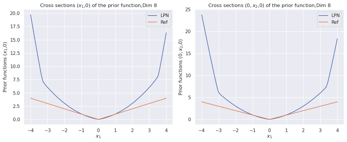
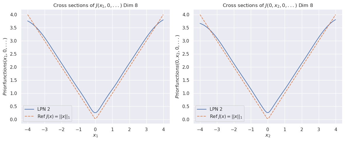
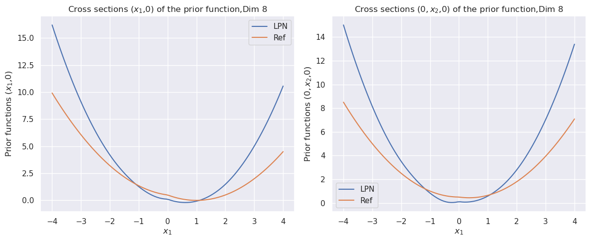
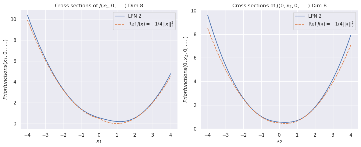
We also trained a second LPN to recover the prior at arbitrary points and compare its performance to the “invert” method (find $y$ such that $f_{\theta}(y)=x$ ) used in [fang2024whats] for recovering the prior from its proximal. Our second LPN is based on the relationship that the non-convex prior $J(x)$ can be approximated using the convex conjugate of the learned potential $\psi(y)$ . Specifically, we compute:
$$
J(x)\approx G(x)-\frac{1}{2}\|x\|^{2} \tag{27}
$$
where $G(x)=\psi^{*}(x)$ represents the convex conjugate of the potential $\psi_{\theta}(y)$ learned by the first LPN. We generate a new dataset $\{(x_{k},G_{k})\}$ using the trained first LPN $\psi_{\theta}$ : (i) The gradients of the first network evaluated at the original sample points $y_{i}$ ,
$$
x_{k}=\nabla_{y}\psi_{\theta}(y_{i}), \tag{28}
$$
and (ii) the values of the Legendre transform corresponding to each point,
$$
G_{k}=\langle x_{k},y_{i}\rangle-\psi_{\theta}(y_{i}). \tag{29}
$$
The network $\phi_{G}$ is trained to map the gradients $x_{k}$ to the conjugate values $G_{k}$ by minimizing the Mean Squared Error (MSE). The optimization is performed using the Adam optimizer with the same parameters as used in the first LPN. Once the second LPN is trained, the estimated non-convex prior $\hat{J}(x)$ is recovered via
$$
\hat{J}(x)=\phi_{G}(x)-\frac{1}{2}\|x\|^{2}. \tag{30}
$$
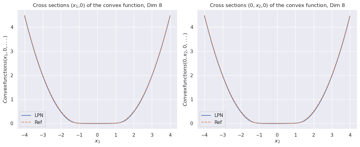
### 5.1 Convex prior
We will benchmark our approach with the prior $J(\bm{x})=\left\|{\bm{x}}\right\|_{1}$ . For this example, we have
| | $\displaystyle\operatorname*{arg\,min}_{\bm{y}\in\mathbb{R}^{n}}\left\{\frac{1}{2t}\left\|{\bm{x}-\bm{y}}\right\|_{2}^{2}+\left\|{\bm{y}}\right\|_{1}\right\}$ | $\displaystyle=\cup_{j=1}^{n}\operatorname*{arg\,min}_{y_{j}\in\mathbb{R}}\left\{\frac{1}{2t}(x_{j}-y_{j})^{2}+|y_{j}|\right\}$ | |
| --- | --- | --- | --- |
With this, we can evaluate $S(\bm{x},t)$ and the LPN function $\bm{x}\mapsto\Psi(\bm{x})\coloneqq\frac{1}{2}-tS(\bm{x},t)$ .
Table 1: Mean square errors of LPN $\psi$ and prior $J$ with 2 layers and 256 neurons in the convex L1 prior example.
| | Dimension | LPN ( $\psi$ ) | Prior ( $J$ ) |
| --- | --- | --- | --- |
| Mean Square Errors | 2D | $1.04E-5$ | $3.33E-5$ |
| 4D | $2.97E-5$ | $2.17E-4$ | |
| 8D | $1.05E-4$ | $7.25E-4$ | |
| 16D | $5.27E-3$ | $2.11E-3$ | |
| 32D | $1.6E-1$ | $4.03E-2$ | |
| 64D | $2.89E-6$ | $2.69E-3$ | |
<details>
<summary>exp_L1_prior_8D_LPN.png Details</summary>
### Visual Description
\n
## Charts: Cross Sections of a Convex Function
### Overview
The image presents two charts, both depicting cross-sections of a convex function in 8 dimensions. The first chart shows the cross-section along the x1 axis, while the second shows the cross-section along the x2 axis. Both charts compare the function's behavior for two models: "LPN" (solid blue line) and "Ref" (dashed orange line). Both charts share the same y-axis scale and a similar x-axis scale.
### Components/Axes
Both charts share the following components:
* **Title:** "Cross sections (x1,0,0) of the convex function, Dim 8" (left chart) and "Cross sections (0,x2,0) of the convex function, Dim 8" (right chart).
* **X-axis Label:** "x1" (left chart) and "x2" (right chart). The x-axis ranges from approximately -4 to 4.
* **Y-axis Label:** "Convexfunctions(x1, 0, ...)" (left chart) and "Convexfunctions(0, x2, ...)" (right chart). The y-axis ranges from approximately 0 to 4.5.
* **Legend:** Located in the bottom-left corner of each chart.
* "LPN" - represented by a solid blue line.
* "Ref" - represented by a dashed orange line.
* **Grid:** A light gray grid is present on both charts to aid in reading values.
### Detailed Analysis or Content Details
**Left Chart (x1 cross-section):**
* **LPN (Solid Blue Line):** The line exhibits a parabolic shape, opening upwards. It reaches a minimum value of approximately 0 at x1 = 0. The line rises symmetrically on both sides of x1 = 0.
* At x1 = -4, the value is approximately 4.2.
* At x1 = -2, the value is approximately 1.2.
* At x1 = 2, the value is approximately 1.2.
* At x1 = 4, the value is approximately 4.2.
* **Ref (Dashed Orange Line):** This line also exhibits a parabolic shape, opening upwards, but is shifted slightly to the right and has a slightly different curvature. It reaches a minimum value of approximately 0 at x1 = 0.
* At x1 = -4, the value is approximately 4.5.
* At x1 = -2, the value is approximately 1.5.
* At x1 = 2, the value is approximately 1.5.
* At x1 = 4, the value is approximately 4.5.
**Right Chart (x2 cross-section):**
* **LPN (Solid Blue Line):** Similar to the left chart, this line is parabolic, opening upwards, and symmetric around x2 = 0, with a minimum value of approximately 0 at x2 = 0.
* At x2 = -4, the value is approximately 4.2.
* At x2 = -2, the value is approximately 1.2.
* At x2 = 2, the value is approximately 1.2.
* At x2 = 4, the value is approximately 4.2.
* **Ref (Dashed Orange Line):** Also parabolic, opening upwards, and symmetric around x2 = 0, with a minimum value of approximately 0 at x2 = 0.
* At x2 = -4, the value is approximately 4.5.
* At x2 = -2, the value is approximately 1.5.
* At x2 = 2, the value is approximately 1.5.
* At x2 = 4, the value is approximately 4.5.
### Key Observations
* Both models ("LPN" and "Ref") exhibit similar parabolic behavior in both cross-sections.
* The "Ref" model consistently has slightly higher values than the "LPN" model across the entire range of x1 and x2.
* Both functions are symmetric around the origin (x=0) in both dimensions.
* The minimum value of both functions is approximately 0 in both dimensions.
### Interpretation
The charts demonstrate the behavior of a convex function in 8 dimensions when sliced along two of its dimensions (x1 and x2). The comparison between the "LPN" and "Ref" models suggests that "LPN" provides a slightly better (lower) approximation of the function's value in these cross-sections. The parabolic shape confirms the function's convexity. The symmetry indicates that the function does not have a directional bias along these axes. The consistent difference between the two models suggests a systematic bias in the "Ref" model. The fact that both models are similar suggests that the underlying function is well-behaved and that both models are capturing its essential characteristics. The charts provide a visual representation of how these models differ in their approximation of the convex function's value.
</details>
<details>
<summary>exp_L1_prior_8D_Pr1.png Details</summary>
### Visual Description
## Line Chart: Cross Sections of Prior Function
### Overview
The image presents two line charts, displayed side-by-side. Both charts visualize cross-sections of a prior function in 8 dimensions. The left chart shows the cross-section (x1, 0) and the right chart shows the cross-section (0, x2, 0). Each chart plots "Prior functions" against "x1" (left chart) or "x1" (right chart). Two lines are plotted on each chart, representing "LPN" and "Ref" data series.
### Components/Axes
* **Left Chart:**
* **Title:** "Cross sections (x1,0) of the prior function,Dim 8" (top-center)
* **X-axis Label:** "x1" (bottom-center)
* **Y-axis Label:** "Prior functions (x1,0)" (left-center)
* **Legend:** Located in the top-right corner.
* "LPN" - Blue line
* "Ref" - Orange line
* **Right Chart:**
* **Title:** "Cross sections (0,x2,0) of the prior function,Dim 8" (top-center)
* **X-axis Label:** "x1" (bottom-center)
* **Y-axis Label:** "Prior functions (0,x2,0)" (left-center)
* **Legend:** Located in the top-right corner.
* "LPN" - Blue line
* "Ref" - Orange line
### Detailed Analysis or Content Details
**Left Chart:**
* **LPN (Blue Line):** The line starts at approximately 18.5 at x1 = -4. It decreases to a minimum of approximately 2.5 at x1 = 0. Then, it increases to approximately 5.0 at x1 = 4. The trend is initially steeply decreasing, then increasing.
* **Ref (Orange Line):** The line starts at approximately 2.5 at x1 = -4. It increases to a maximum of approximately 3.0 at x1 = 0. Then, it decreases to approximately 2.5 at x1 = 4. The trend is initially increasing, then decreasing.
**Right Chart:**
* **LPN (Blue Line):** The line starts at approximately 21.0 at x1 = -4. It decreases to a minimum of approximately 4.5 at x1 = 0. Then, it increases to approximately 18.0 at x1 = 4. The trend is initially steeply decreasing, then increasing.
* **Ref (Orange Line):** The line starts at approximately 4.5 at x1 = -4. It increases to a maximum of approximately 5.0 at x1 = 0. Then, it decreases to approximately 4.5 at x1 = 4. The trend is initially increasing, then decreasing.
### Key Observations
* Both charts exhibit a U-shaped curve for both the "LPN" and "Ref" lines.
* The "LPN" line consistently has higher values than the "Ref" line in both charts, especially at the extreme ends of the x1 axis.
* The minimum values of the "LPN" line are significantly lower than the maximum values of the "Ref" line.
* The "Ref" line appears to be relatively flat compared to the "LPN" line.
### Interpretation
The charts demonstrate the cross-sectional behavior of a prior function in 8 dimensions, comparing two different methods ("LPN" and "Ref"). The U-shaped curves suggest that the function has a minimum value around x1 = 0 in both cross-sections. The significant difference in magnitude between the "LPN" and "Ref" lines indicates that the two methods produce substantially different prior distributions. The "LPN" method appears to assign higher probability density to values further away from x1 = 0, while the "Ref" method maintains a more consistent probability density across the range of x1. The fact that the "Ref" line is relatively flat suggests a less informative prior, while the "LPN" line's more pronounced curve indicates a stronger prior belief about the distribution of the variable. The two charts, taken together, provide insight into how these two methods shape the prior distribution in different dimensions.
</details>
<details>
<summary>exp_L1_prior_8D_Pr2.png Details</summary>
### Visual Description
## Chart: Cross Sections of J(x₁, 0, ...) Dim 8 & J(0, x₂, 0, ...) Dim 8
### Overview
The image presents two line charts, side-by-side, visualizing cross-sections of a function J in 8 dimensions. The left chart displays the cross-section with respect to x₁, while the right chart shows the cross-section with respect to x₂. Both charts compare two prior functions: "LPN 2" and "Ref/f(x) = ||x||₁". Both charts share the same y-axis scale and similar x-axis scales.
### Components/Axes
* **Title (Left Chart):** "Cross sections of J(x₁, 0, ...)"
* **Title (Right Chart):** "Cross sections of J(0, x₂, 0, ...)"
* **X-axis Label (Both Charts):** x₁ (Left) and x₂ (Right)
* **Y-axis Label (Both Charts):** "Priorfunctions(x₁, 0, ...)" (Left) and "Priorfunctions(0, x₂, ...)" (Right)
* **Y-axis Scale (Both Charts):** 0.0 to 4.0, with increments of 0.5.
* **X-axis Scale (Both Charts):** -4.0 to 4.0, with increments of 1.0.
* **Legend (Both Charts):**
* "LPN 2" - represented by a solid blue line.
* "Ref/f(x) = ||x||₁" - represented by a dashed orange line.
### Detailed Analysis or Content Details
**Left Chart (x₁):**
* **LPN 2 (Blue Line):** The line starts at approximately (-4.0, 3.8), decreases to a minimum of approximately (-0.2, 0.2), and then increases to approximately (4.0, 3.8). The curve is roughly symmetrical around the y-axis.
* **Ref/f(x) = ||x||₁ (Orange Dashed Line):** The line starts at approximately (-4.0, 0.1), increases linearly to (0.0, 0.0), and then increases linearly to approximately (4.0, 4.0). This forms a V-shape centered at the origin.
**Right Chart (x₂):**
* **LPN 2 (Blue Line):** The line starts at approximately (-4.0, 3.8), decreases to a minimum of approximately (-0.2, 0.2), and then increases to approximately (4.0, 3.8). The curve is roughly symmetrical around the y-axis.
* **Ref/f(x) = ||x||₁ (Orange Dashed Line):** The line starts at approximately (-4.0, 0.1), increases linearly to (0.0, 0.0), and then increases linearly to approximately (4.0, 4.0). This forms a V-shape centered at the origin.
### Key Observations
* Both charts exhibit similar behavior for the "LPN 2" function.
* The "Ref/f(x) = ||x||₁" function consistently shows a linear increase from 0.0 at the origin to 4.0 at x = ±4.0.
* The "LPN 2" function appears to be a smoothed approximation or transformation of the "Ref/f(x) = ||x||₁" function.
* Both functions are symmetrical around the y-axis.
### Interpretation
The charts demonstrate the behavior of two prior functions in the context of an 8-dimensional function J. The "Ref/f(x) = ||x||₁" function represents the L1 norm, which is a measure of the sum of the absolute values of the components of a vector. The "LPN 2" function appears to be a modified or regularized version of the L1 norm, potentially designed to provide a smoother or more stable prior distribution.
The cross-sections reveal how these prior functions influence the behavior of J along the x₁ and x₂ dimensions. The L1 norm encourages sparsity (i.e., many components of the vector being zero), while the "LPN 2" function may introduce a degree of smoothness or non-sparsity.
The symmetry around the y-axis suggests that the function J and its prior functions are invariant to changes in the sign of x₁ and x₂. The fact that both charts are nearly identical suggests that the function J is not strongly dependent on the specific dimension (x₁ or x₂).
</details>
Figure 1: The cross sections of the convex function $\psi(x)$ for dimension $8$ (top). The bottom row compares the cross sections of the prior function from “invert LPN” (left) and our trained second LPN method (right).
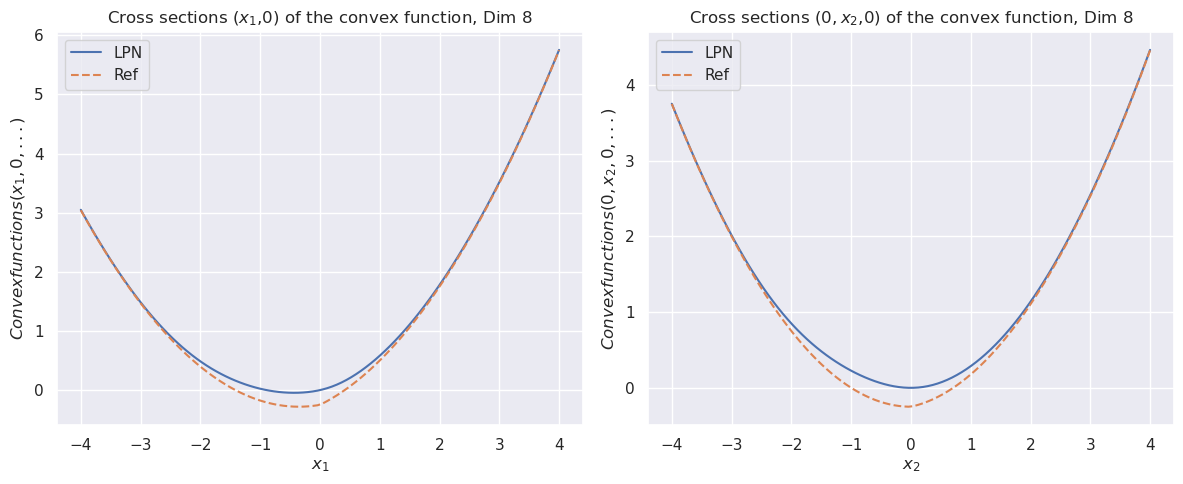
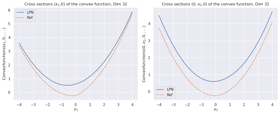
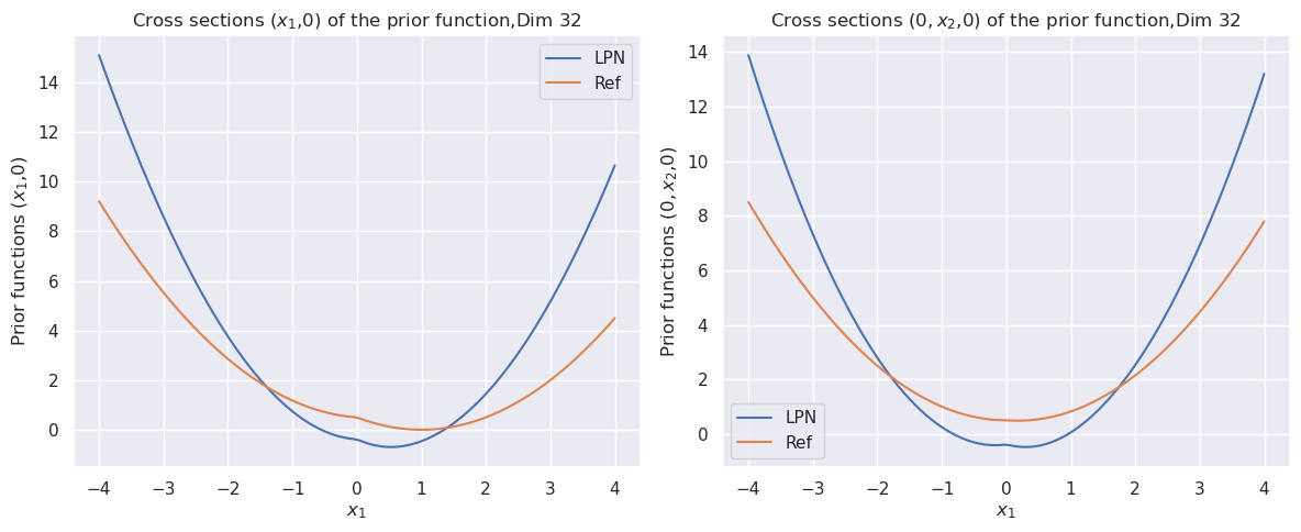
### 5.2 Non-convex prior
#### Minplus algebra example
For this example, the prior is
$$
J(\bm{x})=\min\left(\frac{1}{2\sigma_{1}}\left\|{\bm{x}-\mu_{1}}\right\|_{2}^{2},\frac{1}{2\sigma_{2}}\left\|{\bm{x}-\mu_{2}}\right\|_{2}^{2}\right).
$$
We use $\mu_{1}=(1,0,\dots,0)$ , $\mu_{2}=\bm{1}/\sqrt{n}$ , and $\sigma_{1}=\sigma_{2}=1.0$ .
Table 2: Mean square errors of LPN $\psi$ and prior $J$ with 2 layers and 256 neurons in the min-plus example.
| | Dimension | LPN ( $\psi$ ) | Prior ( $J$ ) |
| --- | --- | --- | --- |
| Mean Square Errors | 2D | $3.33E-6$ | $5.73E-7$ |
| 4D | $7.64E-6$ | $4.92E-6$ | |
| 8D | $3.64E-5$ | $1.20E-4$ | |
| 16D | $1.99E-4$ | $3.44E-4$ | |
| 32D | $1.16E-3$ | $1.33E-3$ | |
| 64D | $2.32E-9$ | $5.21E-5$ | |
<details>
<summary>exp_1_minplus_8D_LPN.png Details</summary>
### Visual Description
## Chart: Cross Sections of a Convex Function
### Overview
The image presents two separate charts, arranged side-by-side. Both charts depict cross-sections of a convex function in 8 dimensions. The left chart shows the cross-section along the x1 axis, while the right chart shows the cross-section along the x2 axis. Each chart displays two curves representing different methods ("LPN" and "Ref"). Both charts share a similar visual style and scale.
### Components/Axes
Each chart has the following components:
* **Title:** "Cross sections (x1,0,0,...) of the convex function, Dim 8" (left chart) and "Cross sections (0, x2,0,0...) of the convex function, Dim 8" (right chart).
* **X-axis:** Labeled "x1" (left chart) and "x2" (right chart), ranging from approximately -4 to 4.
* **Y-axis:** Labeled "Convexfunctions(x1, 0, ...)" (left chart) and "Convexfunctions(0, x2, 0, ...)" (right chart), ranging from approximately 0 to 6 (left chart) and 0 to 4 (right chart).
* **Legend:** Located in the top-left corner of each chart.
* "LPN" - Represented by a solid blue line.
* "Ref" - Represented by a dashed red line.
### Detailed Analysis or Content Details
**Left Chart (x1 cross-section):**
* **LPN (Solid Blue Line):** The line exhibits a parabolic shape, opening upwards. It reaches a minimum value near x1 = 0, with a value of approximately 0. The line increases symmetrically on both sides of the minimum.
* At x1 = -4, the value is approximately 5.5.
* At x1 = -2, the value is approximately 2.5.
* At x1 = 0, the value is approximately 0.
* At x1 = 2, the value is approximately 2.5.
* At x1 = 4, the value is approximately 5.5.
* **Ref (Dashed Red Line):** This line is almost identical to the LPN line, exhibiting the same parabolic shape and values. It is difficult to distinguish the two lines visually.
**Right Chart (x2 cross-section):**
* **LPN (Solid Blue Line):** Similar to the left chart, this line also forms a parabola opening upwards. It reaches a minimum value near x2 = 0, with a value of approximately 0. The line increases symmetrically on both sides of the minimum.
* At x2 = -4, the value is approximately 3.5.
* At x2 = -2, the value is approximately 1.5.
* At x2 = 0, the value is approximately 0.
* At x2 = 2, the value is approximately 1.5.
* At x2 = 4, the value is approximately 3.5.
* **Ref (Dashed Red Line):** Again, this line is nearly indistinguishable from the LPN line, following the same parabolic shape and values.
### Key Observations
* Both charts show a clear parabolic relationship between the input variable (x1 or x2) and the convex function value.
* The "LPN" and "Ref" methods produce almost identical results for both cross-sections. The lines are so close that it is difficult to differentiate them visually.
* The minimum value of the convex function appears to be 0 in both cross-sections, occurring at x1 = 0 and x2 = 0, respectively.
* The scale of the y-axis is different between the two charts.
### Interpretation
The charts demonstrate the behavior of a convex function in 8 dimensions when viewed along two specific axes (x1 and x2). The fact that the "LPN" and "Ref" methods yield nearly identical results suggests that they are converging to the same solution or representing the same underlying function. The parabolic shape confirms the function's convexity, indicating that any local minimum is also a global minimum. The different y-axis scales suggest that the function's sensitivity to changes in x1 and x2 may differ. The charts provide a visual representation of the function's curvature and its behavior in these two dimensions, which could be useful for understanding its overall properties and optimizing algorithms that rely on it. The near-identical lines suggest a high degree of consistency between the two methods, potentially indicating robustness or a well-defined problem space.
</details>
<details>
<summary>exp_1_minplus_8D_Pr1.png Details</summary>
### Visual Description
\n
## Charts: Cross Sections of Prior Functions
### Overview
The image presents two line charts, both titled "Cross sections of the prior function, Dim 8". The charts visualize the relationship between a variable 'x1' and "Prior functions". The first chart displays the cross section at (x1, 0), while the second displays the cross section at (0, x2, 0). Each chart features two lines representing different models: "LPN" (blue) and "Ref" (orange).
### Components/Axes
Both charts share the following components:
* **Title:** "Cross sections (x1,0) of the prior function,Dim 8" (left chart) and "Cross sections (0, x2,0) of the prior function,Dim 8" (right chart).
* **X-axis Label:** "x1"
* **Y-axis Label:** "Prior functions (x1,0)" (left chart) and "Prior functions (0, x2,0)" (right chart).
* **X-axis Range:** Approximately -4 to 4.
* **Y-axis Range:** Left chart: Approximately 0 to 15. Right chart: Approximately 0 to 14.
* **Legend:** Located in the top-right corner of each chart, with "LPN" represented by a blue line and "Ref" by an orange line.
### Detailed Analysis or Content Details
**Left Chart: Cross sections (x1,0) of the prior function,Dim 8**
* **LPN (Blue Line):** The line exhibits a U-shaped curve. It starts at approximately 14.5 at x1 = -4, decreases to a minimum of approximately 0.2 at x1 = 0, and then increases to approximately 2.5 at x1 = 4.
* **Ref (Orange Line):** This line also forms a U-shaped curve, but is wider and flatter than the LPN line. It starts at approximately 3 at x1 = -4, reaches a minimum of approximately 0 at x1 = 0, and rises to approximately 3 at x1 = 4.
**Right Chart: Cross sections (0, x2,0) of the prior function,Dim 8**
* **LPN (Blue Line):** This line also exhibits a U-shaped curve. It starts at approximately 13 at x1 = -4, decreases to a minimum of approximately 1 at x1 = 0, and then increases to approximately 2.5 at x1 = 4.
* **Ref (Orange Line):** This line also forms a U-shaped curve, but is wider and flatter than the LPN line. It starts at approximately 2 at x1 = -4, reaches a minimum of approximately 0.2 at x1 = 0, and rises to approximately 2 at x1 = 4.
### Key Observations
* Both charts show that both the LPN and Ref models have a U-shaped relationship with x1.
* The LPN model consistently has higher values than the Ref model across most of the x1 range in both charts.
* The LPN model appears to be more sensitive to changes in x1, exhibiting a steeper curve than the Ref model.
* The minimum value of the LPN line is consistently higher than the minimum value of the Ref line.
### Interpretation
These charts likely represent the prior distributions of two models (LPN and Ref) over a single dimension (x1). The cross-sections provide insight into the shape of these distributions. The U-shaped curves suggest that values of x1 near 0 are less probable, while values further away from 0 are more probable.
The difference in the curves between LPN and Ref indicates that the two models have different prior beliefs about the distribution of x1. The LPN model appears to assign higher probability to values further from 0, and is more confident in its prior belief (steeper curve). The Ref model has a flatter, wider distribution, indicating more uncertainty.
The fact that both distributions are centered around x1 = 0 suggests that both models have a prior expectation that x1 is likely to be near zero, but the LPN model is more strongly biased towards values away from zero. The "Dim 8" in the titles suggests this is one dimension of an 8-dimensional space, and these cross-sections are being used to understand the prior distributions in each dimension.
</details>
<details>
<summary>exp_1_minplus_8D_pr2.png Details</summary>
### Visual Description
## Chart: Cross Sections of Function J
### Overview
The image presents two charts, side-by-side, visualizing cross-sections of a function J with dimensionality 8. Both charts depict the relationship between a variable (x1 in the left chart, x2 in the right chart) and the "Prior functions(x1, 0, ...)" or "Prior functions(0, x2, 0, ...)" respectively. Two curves are plotted on each chart: one representing "LPN 2" and the other representing "Ref f(x) = -1/4 ||x||₂".
### Components/Axes
Each chart shares the following components:
* **Title:** "Cross sections of J(x1, 0, ... ) Dim 8" (left chart) and "Cross sections of J(0, x2, 0, ... ) Dim 8" (right chart).
* **X-axis:** Labeled "x1" (left chart) and "x2" (right chart), ranging from approximately -4 to 4.
* **Y-axis:** Labeled "Prior functions(x1, 0, ... )" (left chart) and "Prior functions(0, x2, 0, ... )" (right chart), ranging from 0 to 10.
* **Legend:** Located in the top-right corner of each chart.
* "LPN 2" - represented by a solid purple line.
* "Ref f(x) = -1/4 ||x||₂" - represented by a dashed orange line.
### Detailed Analysis
**Left Chart (x1):**
The solid purple line ("LPN 2") exhibits a U-shaped curve, reaching a minimum value around x1 = 0. The curve starts at approximately y = 9.5 at x1 = -4, decreases to a minimum of approximately y = 0.2 at x1 = 0, and then increases again to approximately y = 9.5 at x1 = 4.
The dashed orange line ("Ref f(x) = -1/4 ||x||₂") also forms a U-shaped curve, but is more symmetrical and has a shallower slope. It starts at approximately y = 10 at x1 = -4, decreases to a minimum of approximately y = 0 at x1 = 0, and increases to approximately y = 10 at x1 = 4.
**Right Chart (x2):**
The solid purple line ("LPN 2") mirrors the shape of the left chart's "LPN 2" curve. It starts at approximately y = 9.5 at x2 = -4, decreases to a minimum of approximately y = 0.2 at x2 = 0, and increases to approximately y = 9.5 at x2 = 4.
The dashed orange line ("Ref f(x) = -1/4 ||x||₂") also mirrors the shape of the left chart's "Ref f(x)" curve. It starts at approximately y = 10 at x2 = -4, decreases to a minimum of approximately y = 0 at x2 = 0, and increases to approximately y = 10 at x2 = 4.
### Key Observations
* Both charts show that both "LPN 2" and "Ref f(x)" have a minimum value at x = 0.
* The "LPN 2" curve is significantly higher than the "Ref f(x)" curve for values of x away from 0.
* The "Ref f(x)" curve is more symmetrical around x = 0 than the "LPN 2" curve.
* The shapes of the curves are very similar in both charts, suggesting a consistent relationship between the variable (x1 or x2) and the prior function.
### Interpretation
The charts demonstrate the cross-sectional behavior of a function J in two dimensions (varying x1 and x2 while holding other dimensions constant at 0). The "Ref f(x) = -1/4 ||x||₂" function serves as a reference, likely representing a standard or baseline function. The "LPN 2" function represents a different approach or model.
The U-shaped curves indicate that both functions have a minimum value at the origin (x=0). However, the "LPN 2" function exhibits larger values for non-zero x, suggesting a stronger prior or penalty for deviations from the origin. The difference in shape between the two curves suggests that "LPN 2" may be a more complex or regularized function compared to the reference function.
The fact that the patterns are consistent across both charts (x1 and x2) suggests that the behavior of the function J is similar along these cross-sections. This could indicate that the function is relatively well-behaved or that the chosen dimensions (x1 and x2) are particularly important.
</details>
Figure 2: The cross sections of the convex function $\psi(x)$ for dimension $8$ (top). The bottom row compares the cross sections of the prior function from “invert LPN” (left) and our trained second LPN method (right).
<details>
<summary>exp_1_minplus_32D_LPN.png Details</summary>
### Visual Description
## Chart: Cross Sections of Convex Function (Dim 32)
### Overview
The image presents two charts, side-by-side, both depicting cross-sections of a convex function in a 32-dimensional space. Each chart shows the function's value along a single axis (x1 and x2 respectively) while all other dimensions are held constant at 0. Two curves are plotted on each chart, representing different methods ("LPN" and "Ref"). The y-axis is labeled "Convexfunctions(x1, 0, ...)" and "Convexfunctions(0, x2, 0, ...)" for the left and right charts, respectively.
### Components/Axes
* **Title:** "Cross sections (x1,0) of the convex function, Dim 32" (Left Chart) and "Cross sections (0,x2,0) of the convex function, Dim 32" (Right Chart)
* **X-axis:** Labeled "x1" (Left Chart) and "x2" (Right Chart). Scale ranges from approximately -4 to 4.
* **Y-axis:** Labeled "Convexfunctions(x1, 0, ...)" (Left Chart) and "Convexfunctions(0, x2, 0, ...)" (Right Chart). Scale ranges from approximately 0 to 6.
* **Legend:** Located in the top-left corner of each chart.
* "LPN" - Solid blue line.
* "Ref" - Dashed orange line.
* **Grid:** A light gray grid is present on both charts.
### Detailed Analysis or Content Details
**Left Chart (x1 axis):**
* **LPN (Blue Line):** The curve is a parabola opening upwards. It reaches a minimum value of approximately 0 at x1 = 0. The curve rises symmetrically on both sides of x1 = 0.
* At x1 = -4, the value is approximately 5.5.
* At x1 = -2, the value is approximately 2.5.
* At x1 = -1, the value is approximately 1.5.
* At x1 = 1, the value is approximately 1.5.
* At x1 = 2, the value is approximately 2.5.
* At x1 = 4, the value is approximately 5.5.
* **Ref (Orange Dashed Line):** The curve is also a parabola opening upwards, but it is wider and flatter than the LPN curve. It reaches a minimum value of approximately 0 at x1 = 0.
* At x1 = -4, the value is approximately 4.
* At x1 = -2, the value is approximately 1.5.
* At x1 = -1, the value is approximately 0.75.
* At x1 = 1, the value is approximately 0.75.
* At x1 = 2, the value is approximately 1.5.
* At x1 = 4, the value is approximately 4.
**Right Chart (x2 axis):**
* **LPN (Blue Line):** The curve is a parabola opening upwards. It reaches a minimum value of approximately 0 at x2 = 0. The curve rises symmetrically on both sides of x2 = 0.
* At x2 = -4, the value is approximately 5.5.
* At x2 = -2, the value is approximately 2.5.
* At x2 = -1, the value is approximately 1.5.
* At x2 = 1, the value is approximately 1.5.
* At x2 = 2, the value is approximately 2.5.
* At x2 = 4, the value is approximately 5.5.
* **Ref (Orange Dashed Line):** The curve is also a parabola opening upwards, but it is wider and flatter than the LPN curve. It reaches a minimum value of approximately 0 at x2 = 0.
* At x2 = -4, the value is approximately 4.
* At x2 = -2, the value is approximately 1.5.
* At x2 = -1, the value is approximately 0.75.
* At x2 = 1, the value is approximately 0.75.
* At x2 = 2, the value is approximately 1.5.
* At x2 = 4, the value is approximately 4.
### Key Observations
* Both charts exhibit similar parabolic shapes for both the LPN and Ref curves.
* The LPN curve is consistently steeper and has a lower minimum value than the Ref curve in both charts.
* The Ref curve is wider and flatter, indicating a less sensitive response to changes in x1 and x2.
* The minimum value of both curves is 0, occurring at x1 = 0 and x2 = 0 respectively.
* The curves are symmetrical around the y-axis in both charts.
### Interpretation
The charts demonstrate the behavior of a convex function in two dimensions (x1 and x2) while holding all other dimensions constant in a 32-dimensional space. The two curves, "LPN" and "Ref," likely represent different methods or algorithms for approximating or evaluating the convex function.
The steeper LPN curve suggests that this method is more sensitive to changes in x1 and x2, resulting in a more pronounced curvature and a lower minimum value. This could indicate a more accurate or efficient approximation. The flatter Ref curve suggests a more robust but potentially less accurate or efficient method.
The symmetry of the curves around the y-axis indicates that the convex function is symmetric with respect to the x1 and x2 axes. This symmetry might be a property of the function itself or a result of the specific cross-sections being examined.
The fact that both curves reach a minimum value of 0 suggests that the function has a global minimum at the origin (x1 = 0, x2 = 0) in this specific cross-section. The differences in the curves' shapes and values suggest that the LPN and Ref methods may converge to this minimum at different rates or with different levels of accuracy.
</details>
<details>
<summary>exp_1_minplus_32D_Pr1.png Details</summary>
### Visual Description
\n
## Line Chart: Cross Sections of Prior Function
### Overview
The image presents two line charts, side-by-side, visualizing cross-sections of a prior function in a 32-dimensional space. Both charts share the same x-axis scale but depict different cross-sections: the left chart shows the cross-section at (x1, 0), while the right chart shows the cross-section at (0, x2, 0). Each chart displays two lines representing different models: "LPN" (in blue) and "Ref" (in orange).
### Components/Axes
* **Title (Left Chart):** "Cross sections (x1,0) of the prior function,Dim 32"
* **Title (Right Chart):** "Cross sections (0, x2,0) of the prior function,Dim 32"
* **X-axis Label (Both Charts):** "x1"
* **Y-axis Label (Both Charts):** "Prior functions (x1,0)" (Left Chart) and "Prior functions (0, x2,0)" (Right Chart)
* **X-axis Scale (Both Charts):** -4 to 4
* **Y-axis Scale (Both Charts):** 0 to 14
* **Legend (Top-Right of each chart):**
* Blue Line: "LPN"
* Orange Line: "Ref"
### Detailed Analysis or Content Details
**Left Chart (Cross-section at (x1, 0))**
The blue "LPN" line exhibits a downward slope from x1 = -4 to approximately x1 = -1, reaching a minimum around x1 = -3. From x1 = -1 to x1 = 4, the line slopes upward, forming a parabolic shape.
* Approximate Data Points (LPN):
* x1 = -4, y ≈ 14.5
* x1 = -3, y ≈ 10.5
* x1 = -2, y ≈ 6.5
* x1 = -1, y ≈ 2.5
* x1 = 0, y ≈ 0.5
* x1 = 1, y ≈ 1.5
* x1 = 2, y ≈ 3.5
* x1 = 3, y ≈ 6.5
* x1 = 4, y ≈ 10.5
The orange "Ref" line shows a more symmetrical parabolic shape. It starts at approximately y = 0 at x1 = -4, reaches a minimum around x1 = 0, and then rises to approximately y = 0 at x1 = 4.
* Approximate Data Points (Ref):
* x1 = -4, y ≈ 0.2
* x1 = -3, y ≈ 1.2
* x1 = -2, y ≈ 2.2
* x1 = -1, y ≈ 3.2
* x1 = 0, y ≈ 4.2
* x1 = 1, y ≈ 3.2
* x1 = 2, y ≈ 2.2
* x1 = 3, y ≈ 1.2
* x1 = 4, y ≈ 0.2
**Right Chart (Cross-section at (0, x2, 0))**
The blue "LPN" line mirrors the shape of the left chart's LPN line, with a downward slope from x1 = -4 to approximately x1 = -1, and an upward slope from x1 = -1 to x1 = 4.
* Approximate Data Points (LPN):
* x1 = -4, y ≈ 13
* x1 = -3, y ≈ 9
* x1 = -2, y ≈ 5
* x1 = -1, y ≈ 1
* x1 = 0, y ≈ 0
* x1 = 1, y ≈ 1
* x1 = 2, y ≈ 5
* x1 = 3, y ≈ 9
* x1 = 4, y ≈ 13
The orange "Ref" line also mirrors the shape of the left chart's Ref line, exhibiting a symmetrical parabolic shape.
* Approximate Data Points (Ref):
* x1 = -4, y ≈ 0.2
* x1 = -3, y ≈ 1.2
* x1 = -2, y ≈ 2.2
* x1 = -1, y ≈ 3.2
* x1 = 0, y ≈ 4.2
* x1 = 1, y ≈ 3.2
* x1 = 2, y ≈ 2.2
* x1 = 3, y ≈ 1.2
* x1 = 4, y ≈ 0.2
### Key Observations
* Both charts show that the "LPN" model has a more pronounced asymmetry compared to the "Ref" model.
* The "Ref" model consistently exhibits a more symmetrical parabolic shape in both cross-sections.
* The "LPN" model's values are significantly higher than the "Ref" model's values for negative x1 values.
* The shapes of the curves are similar in both charts, suggesting a consistent behavior of the models across different cross-sections.
### Interpretation
The charts demonstrate the behavior of two different models ("LPN" and "Ref") when examining cross-sections of a 32-dimensional prior function. The asymmetry observed in the "LPN" model suggests that the prior distribution is not isotropic, meaning it doesn't assign equal probability to all directions in the 32-dimensional space. The "Ref" model, with its symmetrical parabolic shape, indicates a more isotropic prior.
The fact that the shapes are consistent across both cross-sections (x1, 0) and (0, x2, 0) suggests that the asymmetry is not specific to a particular direction but is a general characteristic of the "LPN" model's prior. The higher values of the "LPN" model for negative x1 values could indicate a preference for certain regions of the parameter space.
These differences in prior distributions could have significant implications for the performance of any subsequent models trained using these priors, potentially leading to biases or different exploration strategies during learning. The charts provide valuable insights into the characteristics of the prior distributions and their potential impact on downstream tasks.
</details>
<details>
<summary>exp_1_minplus_32D_pr2.png Details</summary>
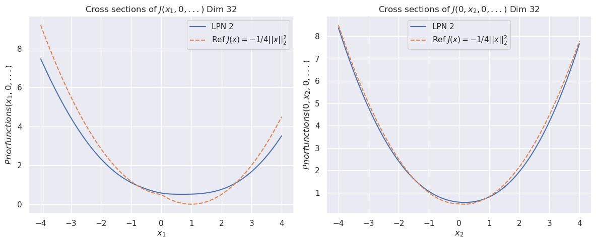
### Visual Description
## Chart: Cross Sections of Prior Functions
### Overview
The image presents two charts, side-by-side, displaying cross-sections of prior functions in a 32-dimensional space. Both charts depict the same function but along different axes (x1 and x2). Each chart plots the prior function value against the corresponding axis value. Two lines are plotted on each chart: one representing "LPN 2" and the other representing a reference function "Ref f(x) = -1/4|x|₂".
### Components/Axes
Both charts share the following components:
* **Title:** "Cross sections of f(x₁, 0, 0, ...) Dim 32" (Left Chart) and "Cross sections of f(0, x₂, 0, ...) Dim 32" (Right Chart)
* **X-axis Label:** "x₁" (Left Chart) and "x₂" (Right Chart)
* **Y-axis Label:** "Priorfunctions(x₁, 0, ...)" (Left Chart) and "Priorfunctions(0, x₂, ...)" (Right Chart)
* **X-axis Scale:** Ranges from approximately -4.5 to 4.5.
* **Y-axis Scale:** Ranges from approximately 0 to 8.5.
* **Legend:** Located in the top-left corner of each chart.
* "LPN 2" - Solid Blue Line
* "Ref f(x) = -1/4|x|₂" - Dashed Orange Line
### Detailed Analysis
**Left Chart (x₁ axis):**
* **LPN 2 (Blue Line):** The line exhibits a U-shaped curve, reaching a minimum value near x₁ = 0. The line slopes downward from x₁ = -4.5 to approximately x₁ = -1.5, reaching a minimum of approximately 0.2 at x₁ = 0. It then slopes upward from x₁ = 0 to x₁ = 4.5.
* Approximate Data Points:
* x₁ = -4.5, Priorfunctions ≈ 8.2
* x₁ = -3, Priorfunctions ≈ 5.5
* x₁ = -1.5, Priorfunctions ≈ 1.2
* x₁ = 0, Priorfunctions ≈ 0.2
* x₁ = 1.5, Priorfunctions ≈ 1.2
* x₁ = 3, Priorfunctions ≈ 5.5
* x₁ = 4.5, Priorfunctions ≈ 8.2
* **Ref f(x) = -1/4|x|₂ (Orange Line):** This line also forms a U-shape, but is more symmetrical and has a sharper minimum than the LPN 2 line.
* Approximate Data Points:
* x₁ = -4.5, Priorfunctions ≈ 8.2
* x₁ = -3, Priorfunctions ≈ 5.5
* x₁ = -1.5, Priorfunctions ≈ 1.2
* x₁ = 0, Priorfunctions ≈ 0.2
* x₁ = 1.5, Priorfunctions ≈ 1.2
* x₁ = 3, Priorfunctions ≈ 5.5
* x₁ = 4.5, Priorfunctions ≈ 8.2
**Right Chart (x₂ axis):**
* **LPN 2 (Blue Line):** The trend is identical to the left chart, a U-shaped curve with a minimum near x₂ = 0.
* Approximate Data Points:
* x₂ = -4.5, Priorfunctions ≈ 8.0
* x₂ = -3, Priorfunctions ≈ 5.3
* x₂ = -1.5, Priorfunctions ≈ 1.2
* x₂ = 0, Priorfunctions ≈ 0.2
* x₂ = 1.5, Priorfunctions ≈ 1.2
* x₂ = 3, Priorfunctions ≈ 5.3
* x₂ = 4.5, Priorfunctions ≈ 8.0
* **Ref f(x) = -1/4|x|₂ (Orange Line):** The trend is identical to the left chart, a U-shaped curve with a minimum near x₂ = 0.
* Approximate Data Points:
* x₂ = -4.5, Priorfunctions ≈ 8.0
* x₂ = -3, Priorfunctions ≈ 5.3
* x₂ = -1.5, Priorfunctions ≈ 1.2
* x₂ = 0, Priorfunctions ≈ 0.2
* x₂ = 1.5, Priorfunctions ≈ 1.2
* x₂ = 3, Priorfunctions ≈ 5.3
* x₂ = 4.5, Priorfunctions ≈ 8.0
### Key Observations
* Both charts exhibit very similar behavior for both the LPN 2 and Ref functions.
* The Ref function appears to be a more symmetrical and sharper U-shape compared to the LPN 2 function.
* The minimum value of both functions is approximately 0.2 for both x₁ and x₂.
* The functions are symmetric around x = 0.
### Interpretation
The charts demonstrate the cross-sectional behavior of two prior functions in a 32-dimensional space. The "LPN 2" function and the reference function "Ref f(x) = -1/4|x|₂" are being compared along two different axes (x₁ and x₂), while all other dimensions are held constant at 0. The U-shaped curves suggest that the prior functions penalize large values of x₁ and x₂. The reference function, with its sharper minimum, likely represents a stronger penalty for deviations from zero. The similarity between the two charts indicates that the behavior of the prior functions is consistent across different dimensions. The fact that the functions are symmetric suggests that the prior is unbiased with respect to the sign of x₁ and x₂. These functions are likely used in a Bayesian framework to represent prior beliefs about the values of the variables x₁, x₂, and the remaining 30 dimensions.
</details>
Figure 3: The cross sections of the convex function $\psi(x)$ for dimension $32$ (top). The bottom row compares the cross sections of the prior function from “invert LPN” (left) and our trained second LPN method (right)
### 5.3 Concave prior
For this example, we use
$$
J(\bm{x})=-\left\|{\bm{x}}\right\|_{2}^{2}/4.
$$
This is actually challenging example because, technically, $J$ is not uniformly Lipschitz continuous. (Although numerically we can get around this by “Huberizing” the prior.) We use this prior because we have an exact solution for this problem. It’s also a bit challenging for a convex LPN network because according to the theory of HJ PDEs, the function $J+\frac{1}{4}\left\|{\bm{x}}\right\|_{2}^{2}$ is convex, and $J+\frac{1}{2}\left\|{\bm{x}}\right\|_{2}^{2}$ is strongly convex, so an LPN (which is not inherently S.C.) may not be able to detect the strong convexity and makes this function more challenging to learn.
Table 3: Mean square errors of LPN $\psi$ and prior $J$ with 2 layers and 256 neurons in the concave prior example.
| | Dimension | LPN ( $\psi$ ) | Prior ( $J$ ) |
| --- | --- | --- | --- |
| Mean Square Errors | 2D | $7.00E-7$ | $1.57E-6$ |
| 4D | $2.74E-5$ | $7.70E-5$ | |
| 8D | $5.58E-4$ | $7.91E-4$ | |
| 16D | $3.69E-3$ | $3.28E-3$ | |
| 32D | $8.70E-2$ | $3.01E-2$ | |
| 64D | $6.23E-6$ | $1.87E-3$ | |
<details>
<summary>exp_quadratic_concave_prior_8D_PR1.png Details</summary>
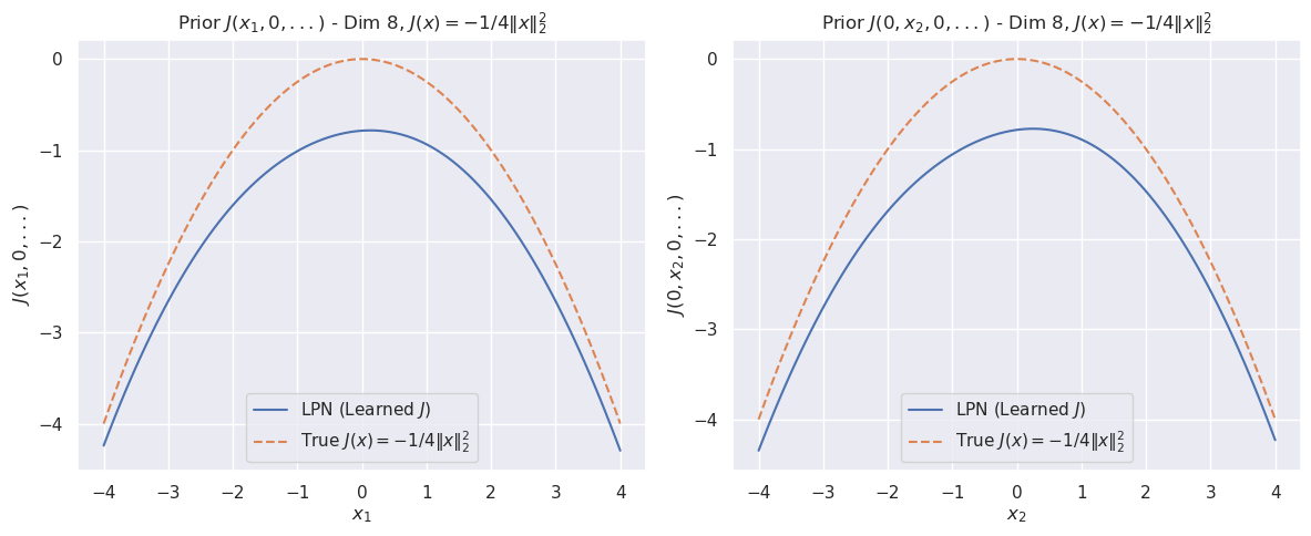
### Visual Description
## Chart: Prior Distributions - Dim 8
### Overview
The image presents two identical charts, side-by-side, visualizing prior distributions for a function *J(x)* in 8 dimensions. Both charts depict the function's value against a single variable (x1 in the left chart, x2 in the right chart), while holding other dimensions constant. The charts compare a "True" function *J(x) = -1/4||x||²* with a "Learned" function, represented by LPN (Likelihood Product Network). Both charts share the same scales and legends.
### Components/Axes
* **Title:** "Prior *J(x1, x2, 0,...)* - Dim 8, *J(x) = -1/4||x||²*" (appears on both charts)
* **X-axis:** Labeled "x1" (left chart) and "x2" (right chart), ranging from approximately -4 to 4.
* **Y-axis:** Labeled "*J(x1, x2, 0,...)*" (left chart) and "*J(0, x2, 0,...)*" (right chart), ranging from approximately -4.5 to 0.
* **Legend:** Located in the bottom-left corner of each chart.
* "LPN (Learned *J*)" - Represented by a solid blue line.
* "True *J(x) = -1/4||x||²*" - Represented by a dashed orange line.
### Detailed Analysis
**Left Chart (x1):**
* **True Function (Orange Dashed Line):** This line forms a parabolic curve, opening upwards. The minimum value is approximately -4 at x1 = 0. The curve is symmetrical around x1 = 0.
* **LPN (Learned) Function (Blue Solid Line):** This line also forms a parabolic curve, opening upwards. The minimum value is approximately -3.8 at x1 = 0. The curve is symmetrical around x1 = 0. The LPN curve is slightly flatter than the True function curve.
* **Data Points (LPN):** The blue line shows significant variance, indicated by the shaded area around the line. The variance is highest at the extremes of the x1 axis (approximately x1 = -4 and x1 = 4) and decreases towards the center (x1 = 0).
**Right Chart (x2):**
* **True Function (Orange Dashed Line):** Identical to the left chart, this line forms a parabolic curve, opening upwards. The minimum value is approximately -4 at x2 = 0. The curve is symmetrical around x2 = 0.
* **LPN (Learned) Function (Blue Solid Line):** Identical to the left chart, this line also forms a parabolic curve, opening upwards. The minimum value is approximately -3.8 at x2 = 0. The curve is symmetrical around x2 = 0. The LPN curve is slightly flatter than the True function curve.
* **Data Points (LPN):** The blue line shows significant variance, indicated by the shaded area around the line. The variance is highest at the extremes of the x2 axis (approximately x2 = -4 and x2 = 4) and decreases towards the center (x2 = 0).
### Key Observations
* Both charts exhibit a similar pattern: the LPN-learned function closely approximates the true function, but is slightly flatter.
* The LPN function has a higher minimum value than the true function in both charts.
* The variance of the LPN function is highest at the extremes of the x-axis and lowest at the center. This suggests that the LPN is more uncertain about the function's value when the input variable is far from zero.
* The charts are nearly identical, indicating that the learned function is consistent across different dimensions (x1 and x2).
### Interpretation
The charts demonstrate the performance of a Likelihood Product Network (LPN) in learning a prior distribution for a function *J(x)*. The LPN successfully approximates the true function *J(x) = -1/4||x||²*, but with some degree of error and uncertainty. The flatter shape of the LPN curve suggests that the LPN may be underestimating the curvature of the true function. The higher variance at the extremes of the x-axis indicates that the LPN is less confident in its predictions when the input variable is far from zero. This could be due to a lack of training data in those regions, or to the inherent limitations of the LPN model. The consistency between the two charts suggests that the LPN is learning a relatively isotropic prior distribution, meaning that the uncertainty is similar in all directions. The charts provide valuable insights into the LPN's ability to learn and represent complex functions, and highlight areas where further improvement may be needed.
</details>
<details>
<summary>exp_quadratic_concave_prior_8D_PR2.png Details</summary>
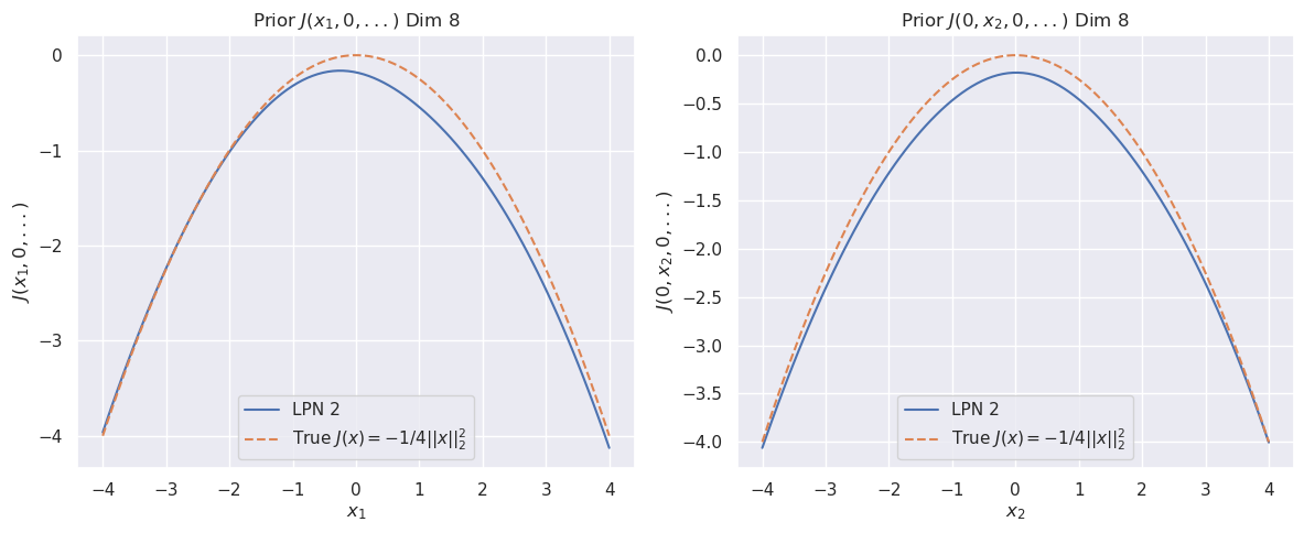
### Visual Description
\n
## Charts: Prior Distributions in 8 Dimensions
### Overview
The image presents two separate charts, both depicting prior distributions in an 8-dimensional space. Each chart visualizes a function of two variables (x1, 0, ...) and (0, x2, 0, ...), respectively, comparing the approximation provided by an LPN 2 model to the "true" function. Both charts share a similar structure and scale.
### Components/Axes
Both charts have the following components:
* **Title:** "Prior J(x1, 0, ...)" Dim 8" (left chart) and "Prior J(0, x2, 0, ...)" Dim 8" (right chart).
* **X-axis:** Labeled "x1" (left chart) and "x2" (right chart), ranging from approximately -4 to 4.
* **Y-axis:** Labeled "J(x1, 0, ...)" (left chart) and "J(0, x2, 0, ...)" (right chart), ranging from approximately -4 to 0.
* **Legend:** Located in the bottom-left corner of each chart.
* "LPN 2" - represented by a solid blue line.
* "True J(x) = -1/4||x||₂" - represented by a dashed orange line.
### Detailed Analysis or Content Details
**Left Chart (x1):**
* **LPN 2 (Blue Line):** The line starts at approximately -4 with a value of -3.8, increases to a peak around x1 = 0 with a value of approximately 0, and then decreases symmetrically to approximately -3.8 at x1 = 4. The curve appears parabolic.
* **True J(x) (Orange Dashed Line):** The dashed line starts at approximately -4 with a value of -4, increases to a peak around x1 = 0 with a value of approximately 0, and then decreases symmetrically to approximately -4 at x1 = 4. This curve also appears parabolic, and closely follows the LPN 2 line.
**Right Chart (x2):**
* **LPN 2 (Blue Line):** The line starts at approximately -4 with a value of -3.5, increases to a peak around x2 = 0 with a value of approximately -0.5, and then decreases symmetrically to approximately -3.5 at x2 = 4. The curve appears parabolic.
* **True J(x) (Orange Dashed Line):** The dashed line starts at approximately -4 with a value of -4, increases to a peak around x2 = 0 with a value of approximately -0.5, and then decreases symmetrically to approximately -4 at x2 = 4. This curve also appears parabolic, and closely follows the LPN 2 line.
### Key Observations
* Both charts show a similar parabolic shape for both the LPN 2 approximation and the true function.
* The LPN 2 approximation consistently underestimates the true function's value, particularly at the extremes of the x-axis.
* The difference between the LPN 2 approximation and the true function appears to be relatively small, suggesting a good approximation.
* The y-axis scales are slightly different between the two charts.
### Interpretation
These charts demonstrate the behavior of a Locally Private Neural Network (LPN) 2 model when approximating a prior distribution in an 8-dimensional space. The "true" function, J(x) = -1/4||x||₂, represents the actual prior distribution. The LPN 2 model provides an approximation of this distribution.
The fact that both curves are parabolic suggests that the LPN 2 model is capturing the general shape of the prior distribution. However, the consistent underestimation of the true function indicates that the LPN 2 model is introducing some bias. This bias is likely a consequence of the privacy mechanism employed by the LPN, which adds noise to the data to protect individual privacy.
The slight differences in the y-axis scales between the two charts might indicate that the sensitivity of the function to changes in x1 and x2 is different. The charts provide a visual comparison of the approximation quality of the LPN 2 model, highlighting the trade-off between privacy and accuracy. The closeness of the lines suggests a reasonable balance between these two factors.
</details>
Figure 4: The cross sections of the prior function for $8$ dimension from “invert LPN” (left) and our trained second LPN method (right)
### 5.4 Negative $\ell_{1}$ norm
See Equation Eq. 32 for the minimum value and Eq. 33 for the proximal value. For this example, we consider $J(\bm{y})=-\left\|{\bm{y}}\right\|_{1}$ . Let $n=1$ for simplicity and consider the one-dimensional problem
$$
S(x,t)=\min_{y\in\mathbb{R}}\left\{\frac{1}{2t}(x-y)^{2}-|y|\right\}. \tag{31}
$$
The function $y\mapsto(x-y)^{2}/2t-|y|$ is differentiable everywhere except at $y=0$ . A stationary point of this function satisfies
$$
0\in\frac{y-x}{t}-\partial|y|\iff x\in\begin{cases}x-t,&\ \text{if $y<0$,}\\
[x-t,x+t]&\ \text{if $y=0$},\\
x+t,&\ \text{if $y>0$.}\end{cases}
$$
If $x>t$ , the only minimum is $x+t$ , in which case we have
$$
S(x,t)=\frac{1}{2t}(x+t-x)^{2}-|x+t|=\frac{t}{2}-(x+t)=-\frac{t}{2}-x.
$$
If $0<x\leqslant t$ , there are two local minimums, $0$ and $x+t$ , but the global minimum is attained at $x+t$ , again yielding $S(x,t)=\frac{t}{2}-x$ . If $x=0$ , we have three local minimums: $-t$ , $0$ , and $t$ . The global minimum is attained at either $-t$ or $t$ , yielding $S(0,t)=-\frac{t}{2}$ . If $-t\leqslant x<0$ , there are two local minimums, $0$ and $x-t$ , but the global minimum is attained at $x-t$ , yielding $S(x,t)=-\frac{t}{2}+x$ . If $x<-t$ , the only minimum is $x-t$ , in which case we have $S(x,t)-\frac{t}{2}+x$ . Hence
$$
S(x,t)=-\frac{t}{2}-|x|. \tag{32}
$$
In particular, its gradient in $x$ is given by
$$
\nabla_{x}S(x,t)\in\begin{cases}1&\ \text{if $x<0$},\\
[-1,1]&\ \text{if $x=0$},\\
-1&\ \text{if $x>0$}.\end{cases}
$$
Moreover,
$$
\operatorname*{arg\,min}_{y\in\mathbb{R}}\left\{\frac{1}{2t}(x-y)^{2}-|y|\right\}=\begin{cases}x-t&\ \text{if $x<0$},\\
[-t,t]&\ \text{if $x=0$},\\
x+t&\ \text{if $x>0$}.\end{cases} \tag{33}
$$
Table 4: Mean square errors of LPN $\psi$ and prior $J$ with 2 layers and 256 neurons in the negative $L_{1}$ norm examples.
| | Dimension | LPN ( $\psi$ ) | Prior ( $J$ ) |
| --- | --- | --- | --- |
| Mean Square Errors | 2D | $6.59E-5$ | $5.20E-6$ |
| 4D | $3.15E-4$ | $3.17E-5$ | |
| 8D | $2.12E-3$ | $2.94E-4$ | |
| 16D | $8.01E-3$ | $4.49E-2$ | |
| 32D | $1.55E-1$ | $2.29E-2$ | |
| 64D | $6.42E-4$ | $4.49E-3$ | |
<details>
<summary>exp_NegL1_prior_4D_LPN.png Details</summary>
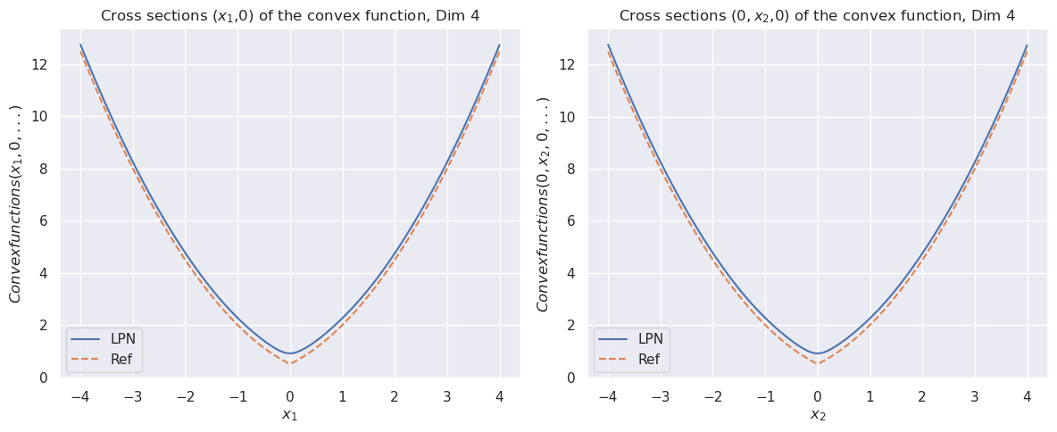
### Visual Description
\n
## Chart: Cross Sections of a Convex Function in Dimension 4
### Overview
The image presents two line charts, side-by-side, visualizing cross-sections of a convex function in 4 dimensions. Both charts share a similar structure and display two data series: "LPN" (solid blue line) and "Ref" (dashed orange line). The x-axis represents a single variable (x1 in the left chart, x2 in the right chart), while the y-axis represents the value of the convex function. Both charts have the same y-axis scale.
### Components/Axes
* **Title (Left Chart):** "Cross sections (x1,0,0) of the convex function, Dim 4"
* **Title (Right Chart):** "Cross sections (0, x2,0) of the convex function, Dim 4"
* **X-axis Label (Left Chart):** "x1"
* **X-axis Label (Right Chart):** "x2"
* **Y-axis Label (Both Charts):** "Convexfunctions(0, x2, 0, ...)" (Note: the label appears slightly truncated)
* **X-axis Scale (Both Charts):** -4 to 4, with gridlines at integer values.
* **Y-axis Scale (Both Charts):** 0 to 12, with gridlines at integer values.
* **Legend (Both Charts):** Located in the bottom-left corner.
* "LPN" - Solid Blue Line
* "Ref" - Dashed Orange Line
### Detailed Analysis or Content Details
**Left Chart (x1 cross-section):**
* **LPN (Blue Line):** The line exhibits a parabolic shape, opening upwards. It reaches a minimum value of approximately 0 at x1 = 0. The line rises symmetrically on both sides of x1 = 0.
* At x1 = -4, LPN ≈ 12.5
* At x1 = -3, LPN ≈ 6.5
* At x1 = -2, LPN ≈ 2.5
* At x1 = -1, LPN ≈ 0.5
* At x1 = 0, LPN ≈ 0
* At x1 = 1, LPN ≈ 0.5
* At x1 = 2, LPN ≈ 2.5
* At x1 = 3, LPN ≈ 6.5
* At x1 = 4, LPN ≈ 12.5
* **Ref (Orange Line):** The line is relatively flat near x1 = 0 and increases rapidly as it moves away from x1 = 0 in either direction.
* At x1 = -4, Ref ≈ 1.5
* At x1 = -3, Ref ≈ 1.75
* At x1 = -2, Ref ≈ 2
* At x1 = -1, Ref ≈ 2.25
* At x1 = 0, Ref ≈ 2.5
* At x1 = 1, Ref ≈ 2.25
* At x1 = 2, Ref ≈ 2
* At x1 = 3, Ref ≈ 1.75
* At x1 = 4, Ref ≈ 1.5
**Right Chart (x2 cross-section):**
* **LPN (Blue Line):** Mirrors the shape of the LPN line in the left chart, exhibiting a parabolic shape opening upwards with a minimum value of approximately 0 at x2 = 0.
* At x2 = -4, LPN ≈ 12.5
* At x2 = -3, LPN ≈ 6.5
* At x2 = -2, LPN ≈ 2.5
* At x2 = -1, LPN ≈ 0.5
* At x2 = 0, LPN ≈ 0
* At x2 = 1, LPN ≈ 0.5
* At x2 = 2, LPN ≈ 2.5
* At x2 = 3, LPN ≈ 6.5
* At x2 = 4, LPN ≈ 12.5
* **Ref (Orange Line):** Mirrors the shape of the Ref line in the left chart, relatively flat near x2 = 0 and increasing rapidly as it moves away from x2 = 0 in either direction.
* At x2 = -4, Ref ≈ 1.5
* At x2 = -3, Ref ≈ 1.75
* At x2 = -2, Ref ≈ 2
* At x2 = -1, Ref ≈ 2.25
* At x2 = 0, Ref ≈ 2.5
* At x2 = 1, Ref ≈ 2.25
* At x2 = 2, Ref ≈ 2
* At x2 = 3, Ref ≈ 1.75
* At x2 = 4, Ref ≈ 1.5
### Key Observations
* Both charts show a clear parabolic relationship for the "LPN" line, indicating a quadratic function.
* The "Ref" line is relatively flat near the origin and increases in magnitude as the x-value moves away from zero.
* The two charts are nearly identical, suggesting the function is symmetric with respect to x1 and x2.
* The "LPN" line consistently has a much larger range of values than the "Ref" line.
### Interpretation
The charts demonstrate cross-sectional behavior of a 4-dimensional convex function. The "LPN" line likely represents the function itself, exhibiting a parabolic shape in each cross-section. The "Ref" line could represent a reference or baseline value, or a different approximation of the function. The symmetry between the two charts suggests that the function is independent of the order of the variables x1 and x2 in these cross-sections. The significantly larger values of the "LPN" line compared to the "Ref" line indicate that the function's magnitude is considerably greater than the reference value across the examined range. The parabolic shape of the LPN line suggests a quadratic component in the function's definition. The flat nature of the Ref line suggests it may be a constant or a slowly varying function. These visualizations are useful for understanding the function's behavior along specific dimensions while holding others constant.
</details>
<details>
<summary>exp_NegL1_prior_8D_LPN.png Details</summary>
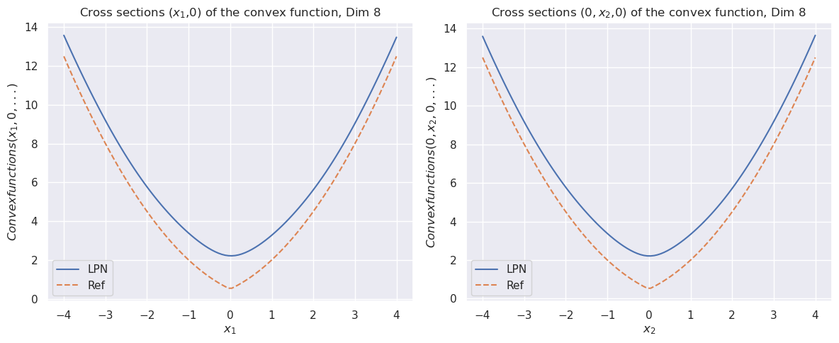
### Visual Description
## Chart: Cross Sections of a Convex Function (Dim 8)
### Overview
The image presents two separate line charts, both depicting cross-sections of a convex function in 8 dimensions. The first chart shows the cross-section along the x1-axis (with x2=0), and the second shows the cross-section along the x2-axis (with x1=0). Both charts compare two data series: "LPN" (solid blue line) and "Ref" (dashed orange line). The charts share identical y-axis scales and x-axis ranges.
### Components/Axes
* **X-axis (Left Chart):** Labeled "x1", ranging from approximately -4 to 4. Gridlines are present.
* **X-axis (Right Chart):** Labeled "x2", ranging from approximately -4 to 4. Gridlines are present.
* **Y-axis (Both Charts):** Labeled "Convex functions (x1, 0, ...)" for the left chart and "Convex functions (0, x2, 0)" for the right chart, ranging from 0 to 14. Gridlines are present.
* **Legend (Both Charts):** Located in the top-left corner.
* "LPN" - Represented by a solid blue line.
* "Ref" - Represented by a dashed orange line.
### Detailed Analysis or Content Details
**Left Chart (x1 Cross-Section):**
* **LPN (Blue Line):** The line exhibits a U-shaped curve, indicating a convex function. It reaches a minimum value around x1 = 0.
* Approximate data points:
* x1 = -4: y ≈ 13.5
* x1 = -2: y ≈ 6.5
* x1 = 0: y ≈ 2.0
* x1 = 2: y ≈ 6.5
* x1 = 4: y ≈ 13.5
* **Ref (Orange Line):** Also a U-shaped curve, but shifted upwards and slightly wider than the LPN line.
* Approximate data points:
* x1 = -4: y ≈ 12.0
* x1 = -2: y ≈ 5.0
* x1 = 0: y ≈ 2.5
* x1 = 2: y ≈ 5.0
* x1 = 4: y ≈ 12.0
**Right Chart (x2 Cross-Section):**
* **LPN (Blue Line):** Similar U-shaped curve to the left chart, with a minimum around x2 = 0.
* Approximate data points:
* x2 = -4: y ≈ 13.5
* x2 = -2: y ≈ 6.5
* x2 = 0: y ≈ 2.0
* x2 = 2: y ≈ 6.5
* x2 = 4: y ≈ 13.5
* **Ref (Orange Line):** Also a U-shaped curve, shifted upwards and slightly wider than the LPN line.
* Approximate data points:
* x2 = -4: y ≈ 12.0
* x2 = -2: y ≈ 5.0
* x2 = 0: y ≈ 2.5
* x2 = 2: y ≈ 5.0
* x2 = 4: y ≈ 12.0
### Key Observations
* Both charts exhibit similar behavior, suggesting symmetry in the convex function with respect to the x1 and x2 axes.
* The "Ref" line consistently has higher y-values than the "LPN" line across the entire range of x1 and x2, indicating that the "Ref" function is generally larger than the "LPN" function.
* The minimum values of both functions occur at x1 = 0 and x2 = 0, respectively.
* The shape of the curves is consistent with a quadratic function, which is a common form for convex functions.
### Interpretation
The charts demonstrate cross-sectional views of a convex function in an 8-dimensional space. The "LPN" and "Ref" lines likely represent two different approximations or variations of the same underlying convex function. The consistent offset between the two lines suggests that "Ref" might be a regularized or smoothed version of "LPN," or perhaps a different method of calculating the convex function. The symmetry observed in the cross-sections indicates that the function is likely independent of the other dimensions when considering only x1 or x2. The fact that both curves are convex (U-shaped) confirms that the function being analyzed is indeed convex. The data suggests that the function is minimized at the origin (x1=0, x2=0) in these cross-sections. The charts provide a visual comparison of the two functions along these specific axes, allowing for an assessment of their relative values and shapes.
</details>
Figure 5: The cross sections of the convex function $\psi(x)$ for dimension $4$ (left) and $8$ (right).
The Tables 1, 2, 3, and 4 quantify the scalability of the LPN approach across dimensions ranging from $2$ D to $64$ D. The results indicate that the method performs with high accuracy in lower dimensions ( $2$ D through $8$ D), achieving mean square errors in the range of $10^{-7}$ to $10^{-4}$ . However, performance degrades slightly as the dimensionality increases, particularly at $16$ D and $32$ D, where the error spikes to a range of $10^{-3}$ and $10^{-1}$ . The higher dimensions did not work too well, which might be because we did not train for long enough and also used a simple architecture (which ought to be more intricate for the higher dimensional problems). While the error for the recovered prior $J$ is generally slightly higher than that of LPN $\psi$ , this is expected given the added complexity of recovering the non-convex, non-smooth, or concave functions. However, the errors generally remain low, validating our method’s effectiveness even in high-dimensional spaces.
The top rows of Figures 1, 2, 3 and Figure 5 demonstrate that the LPN accurately learns the cross sections of the convex function $\psi(x)$ for dimension $4,8,$ and $32$ , closely matching the reference function with the most significant variation in Figure 3 corresponding to dimension $32$ . The bottom row of these figures compares the “invert LPN” (left) method and our trained second LPN method (right). It is clear that in all cases, our direct method recovers the original non-smooth prior, as indicated by the sharp V-shaped reconstructions in Figure 1, the non-convex prior Figures 2 and 3, and quadratic concave prior Figure 4 despite its challenging nature.
Figure 5 represents the cross-sections of the LPN value function against the ground truth for dimensions $4$ (left) and $8$ (right). In both instances, the LPN-approximation curves exhibit a tight fit to the analytical reference, capturing the characteristic V-shape more closely and the non-smooth geometry of the underlying function. The errors for $64$ dimensions in all the examples are consistently lower than expected. In contrast, it does not yield a good visual approximation of the cross sections. We are unable to explain the reason for this behaviour in $64$ D cases yet; however, we think it is probably due to the way we sample the hypercube.
## 6 Discussion
In this work, we leveraged the theory of viscosity solutions of HJ PDEs to develop novel deep learning numerical methods to learn, from data, the underlying prior of the proximal operator Eq. 2 yielding $(\bm{x},t)\mapsto S(\bm{x},t)$ defined in Eq. 1. Our approach built on the existing connections between proximal operators and HJ PDEs, crucially the fact that $(\bm{x},t)\mapsto S(\bm{x},t)$ is obtained from the solution to an HJ PDE, and in particular on the theory for the inverse problem for HJ equations. As discussed in Section 3, the theory for the inverse problem for HJ equations show that while there may be infinitely many priors that can recover Eq. 1, there is a natural choice, obtained by reversing the time in the HJ PDE Eq. 14 and using the value of the proximal operator $(\bm{x},t)\mapsto S(\bm{x},t)$ as initial condition. The resulting backward viscosity solution yields a prior $J_{\text{BVS}}$ that can reconstruct the $(\bm{x},t)\mapsto S(\bm{x},t)$ and also that is semiconvex. We considered the case where only samples of the proximal operators and its values were available in Section Section 4, and used techniques from max-plus algebra to derive some characterizations and errors property of $J_{\text{BVS}}$ with respect to convex functions approximating it from above. Finally, in Section 5 we proposed to learn the prior $J_{\text{BVS}}$ by training a convex neural network, specifically a learned proximal network, on a function of the form $\bm{y}\mapsto\tilde{J}(\bm{y})+\frac{1}{2}\left\|{\bm{y}}\right\|_{2}^{2}$ from data $\{\bm{x}_{k},S(\bm{x}_{k},t),\nabla_{\bm{x}}S(\bm{x}_{k},t)\}_{k=1}^{K}$ via Eq. 17. We presented several numerical results that demonstrate the efficiency of our proposed method in high dimensions.
While this work focused on proximal operators, we expect our approach can be extended to a broad class of Bregman divergences, as recent results in the theory of inverse problems for HJ equations suggest [esteve2020inverse]. Another potential direction would be in the case where the value of the proximal operator $(\bm{x},t)\mapsto S(\bm{x},t)$ is known to learn the prior $J$ using Monte Carlo sampling strategies, as recently proposed in [park2025neural] for the forward problem of HJ equations (i.e., learning $(\bm{x},t)\mapsto S(\bm{x},t)$ from known $J$ ). In the longer term, it would be interesting to devise similar deep learning methods for the inverse problem of HJ equations with possibly time- or state-dependent Hamiltonians, relevant to optimal control problems.
## Appendix A Calculations
### A.1 Formal calculation of Eq. 19
We have
| | $\displaystyle\inf_{\bm{y}\in\mathbb{R}^{n}}$ | $\displaystyle\left\{\frac{1}{2t}\left\|{\bm{x}-\bm{y}}\right\|_{2}^{2}+J_{\text{PAM}}(\bm{y})\right\}=\inf_{\bm{y}\in\mathbb{R}^{n}}\left\{\frac{1}{2t}\left\|{\bm{x}-\bm{y}}\right\|_{2}^{2}+\right.$ | |
| --- | --- | --- | --- |
### A.2 Formal calculation of Eq. 21
Formally, we have
$$
t\nabla_{\bm{y}}J_{\text{PQM}}(\bm{y})=\alpha(\bm{y}-\bm{y}_{k})+\bm{x}_{k}-\bm{y}
$$
for some $k\in\{1,\dots,K\}$ . Similarly,
| | $\displaystyle\hat{\bm{y}}=\operatorname*{arg\,min}_{\bm{y}\in\mathbb{R}^{n}}\left\{\frac{1}{2t}\left\|{\bm{x}-\bm{y}}\right\|_{2}^{2}+J_{\text{PQM}}(\bm{y})\right\}$ | $\displaystyle\iff\bm{0}=\frac{\hat{\bm{y}}-\bm{x}}{t}+\frac{\alpha}{t}(\hat{\bm{y}}-\bm{y}_{k})+\frac{\bm{x}_{k}-\hat{\bm{y}}}{t}$ | |
| --- | --- | --- | --- |
In addition,
| | | $\displaystyle\bm{x}-\hat{\bm{y}}=\frac{\bm{x}_{k}-(1-\alpha)\bm{x}}{\alpha}-\bm{y}_{k}\implies\frac{1}{2t}\left\|{\bm{x}-\hat{\bm{y}}}\right\|_{2}^{2}=\frac{1}{2t\alpha^{2}}\left\|{\bm{x}_{k}-\bm{x}+\alpha(\bm{x}-\bm{y}_{k})}\right\|_{2}^{2},$ | |
| --- | --- | --- | --- |
and
| | $\displaystyle J_{\text{PQM}}(\hat{\bm{y}})$ | $\displaystyle=J(\bm{y}_{k})+\frac{1}{2t}\left\|{\bm{x}_{k}-\bm{y}_{k}}\right\|_{2}^{2}-\frac{1}{2t}\left\|{\bm{x}_{k}-\hat{\bm{y}}}\right\|_{2}^{2}+\frac{\alpha}{2t}\left\|{\hat{\bm{y}}-\bm{y}_{k}}\right\|_{2}^{2}$ | |
| --- | --- | --- | --- |
From this, we deduce
| | $\displaystyle\inf_{\bm{y}\in\mathbb{R}^{n}}\left\{\frac{1}{2t}\left\|{\bm{x}-\bm{y}}\right\|_{2}^{2}+J_{\text{PQM}}(\bm{y})\right\}$ | $\displaystyle=\frac{1}{2t\alpha^{2}}\left\|{\bm{x}_{k}-\bm{x}+\alpha(\bm{x}-\bm{y}_{k})}\right\|_{2}^{2}$ | |
| --- | --- | --- | --- |
for some $k\in\{1,\dots,K\}$ .