# Stable envelopes for critical loci
**Authors**: Yalong Cao, Andrei Okounkov, Yehao Zhou, Zijun Zhou
## STABLE ENVELOPES FOR CRITICAL LOCI
YALONG CAO, ANDREI OKOUNKOV, YEHAO ZHOU, AND ZIJUN ZHOU
Abstract. This is the first in a sequence of papers devoted to stable envelopes in critical cohomology and critical K -theory for symmetric GIT quotients with potentials and related geometries, and their applications to geometric representation theory and enumerative geometry. In this paper, we construct critical stable envelopes and establish their general properties, including compatibility with dimensional reductions, specializations, Hall products, and other geometric constructions. In particular, for tripled quivers with canonical cubic potentials, the critical stable envelopes reproduce those on Nakajima quiver varieties. These set up foundations for applications in subsequent papers.
## Contents
| 1. | Introduction | 1 |
|------------------------------------------------------------------------------|------------------------------------------------------------------------------|-----|
| 2. | Critical cohomology and K -theory | 13 |
| 3. | Stable envelopes | 19 |
| 4. | Cohomological stable envelopes on symmetric GIT quotients | 32 |
| 5. | K -theoretic stable envelopes on symmetric GIT quotients | 44 |
| 6. | Deformed dimensional reductions and stable envelopes | 50 |
| 7. | Deformations of potentials and stable envelopes | 59 |
| 8. | Vector bundles and stable envelopes | 71 |
| 9. | Hall envelopes and stable envelopes | 77 |
| Appendix A. Pullback isomorphisms along attraction maps | Appendix A. Pullback isomorphisms along attraction maps | 94 |
| Appendix B. Excess intersection formula of critical cohomology and K -theory | Appendix B. Excess intersection formula of critical cohomology and K -theory | 95 |
| Appendix C. A deformed dimensional reduction for critical cohomology | Appendix C. A deformed dimensional reduction for critical cohomology | 99 |
| Appendix D. A dimensional reduction for critical K -theory | Appendix D. A dimensional reduction for critical K -theory | 101 |
| Appendix E. Proof of Proposition 9.9 | Appendix E. Proof of Proposition 9.9 | 102 |
| Appendix F. Proof of Lemma 9.16 | Appendix F. Proof of Lemma 9.16 | 107 |
| References | References | 109 |
## 1. Introduction
1.1. Overview. Stable envelopes, introduced in [MO] in the setting of ordinary equivariant cohomology, have found numerous applications in geometric representation theory and enumerative geometry. By one of possible definitions, geometric representation theory studies algebras generated by geometric correspondences. Enumerative geometry is full of important and natural correspondences such as those formed by pairs of points of some algebraic variety X that lie, perhaps in a virtual sense, on a rational curve of a given degree. In either setting, one fixes some cohomology theory h ( X ) in which the correspondences act. This may be ordinary equivariant cohomology, equivariant K -theory, or something more general, like the critical cohomology or critical K -theory that we use in this paper.
One considers an enumerative problem solved if the enumerative correspondences are expressed in terms of an understandable geometric action of an understandable algebraic structure. Of course, understandable does not mean simple. The typical algebraic structures one meets in the context of stable envelopes are certain quantum loop groups and their Yangian analogs, where the underlying Lie algebra is, by itself, typically an infinitely generated Borcherds-Kac-Moody (BKM) Lie algebra. But such is the intrinsic complexity of the problem, and one's aim should be to set up an adequate geometric and algebraic framework for managing it.
2020 Mathematics Subject Classification. Primary 14N35, 17B37. Secondary 16G20, 14C17.
Key words and phrases. Stable envelopes, Critical loci, Hall operations, (shifted) quantum groups, R -matrices.
Stable envelopes are defined in the presence of an action of a connected reductive group. In the most basic case of a torus A , they give a certain canonical correspondences between the fixed locus X A and the ambient space X . These are improved versions of attracting (also known as stable) manifolds which, in contrast to attracting manifolds, are proper over X , behave well in families, etc. They add certain correction terms to attracting manifolds and, in this sense, they complete or envelop them, whence the name.
Stable envelopes depend on additional choices, such as the choice of attracting/repelling directions. This proves to be an important feature since different choices of attracting directions are related by what turns out to be the braiding, or the R -matrix - the cornerstone concept in quantum group theory. Thus, out of stable envelopes, one constructs the correspondences by which a quantum loop group or a Yangian acts. Stable envelopes are equally natural in enumerative contexts, where their properness forms the basis for many computations based, ultimately, on equivariant rigidity. One very important example of this is the geometric identification of the quantum KnizhnikZamolodchikov connection with certain shift operators. We will say more about it below.
So far, stable envelopes have been constructed and used in ordinary equivariant cohomology, equivariant K -theory, and equivariant elliptic cohomology [MO, Oko1, AO2]. Although such generality encompasses a broad range of contexts and applications, there are even more potential applications that it misses.
For instance, a major motivation for [MO] came from the work of Nekrasov and Shatashvili on quantum integrable structures in 2-dimensional and (2+1)-dimensional supersymmetric QFTs [NS]. For mathematicians, these structures appear in the computation of virtual indices of Dirac operators on the moduli spaces of maps, or quasimaps, to be more precise, f : C → X , where the Riemann surface C is the space part of the (2+1)-dimensional spacetime and X is (a component of) the moduli spaces of vacua for the QFT in question. These X are sometimes smooth, for instance the Nakajima quiver varieties [Nak1, Nak2], naturally arise in this way. The theory of [MO, Oko1, OS] applies to all Nakajima varieties and identifies the Nekrasov-Shatashvili quantum integrable system with the familiar Baxter-style quantum integrable system for the corresponding quantum loop group or Yangian.
Typically, however, these moduli spaces of vacua are not smooth. Rather, they are critical loci Crit( w ) of a regular function w on a smooth ambient space or stack X . The enumerative setup for counting maps to such targets has been recently studied, see e.g. [FK, CZ, CTZ, KP], etc., and the natural home for these computations is the critical cohomology or critical K -theory of the pair ( X, w ). These critical theories provide a flexible and versatile generalizations of ordinary cohomology and K -theory. In particular, their versatility manifests itself in there being a very general setup in which enumerative questions about quasimaps f : C → Crit( w ) can be asked. One of the goals of this project is to answer these enumerative questions using critical stable envelopes and the corresponding quantum groups.
A very good example to have in mind is the example of the Hilbert scheme Hilb( C 3 , n ) of n points in the affine 3-space. While Hilb( C 2 , n ) is a smooth Nakajima variety, its 3-dimensional counterpart is a singular variety of unknown dimension and unknown number of irreducible components. It is, however, naturally a critical locus, stemming from the well-known fact that three matrices Y 1 , Y 2 , Y 3 commute if and only if all partial derivatives of the function w ( Y ) = tr Y 1 [ Y 2 , Y 3 ] vanish. The computation of the quantum cohomology of Hilb( C 2 , n ) in [OP] was a major precursor to the computation of the quantum cohomology of all Nakajima varieties. Because of the similarly important role of Hilb( C 3 , n ), we spell out its quantum cohomology in § 1.12.
While the overall structure of theory developed here bears a definite resemblance to the corresponding theories for other cohomology theories, there is a large number of conceptual and technical points in which it goes significantly beyond the existing frontier of knowledge. We will touch on many such points in this introduction. In this brief overview, it suffices to mention how much broader is the supply of the algebraic structures that our methods produce. In facts, it broadens in at least three directions : the underlying Lie algebra can be a super Lie algebra , its BKM Cartan matrix may be symmetrizable, and not symmetric, and finally, the quantum loop group or the Yangian may be shifted . Geometrically, the appearance of shift means that we can relax the self-duality assumptions on X that are normally made in the construction of stable envelopes. Notice, however, that a certain sign of this shift (antidominant) is necessary in our setup.
- 1.2. Stable envelopes. It is fitting to start the discussion of stable envelopes with the abelian case. Let X be a smooth quasi-projective algebraic variety with an action of a torus A . Then the fixed locus X A is smooth and there is a smooth locally closed subvariety
$$\begin{aligned}
& x _ { 1 } = x _ { 0 } \left [ ( X \times X ^ { A } ) , \\
& Attre = \{ ( x _ { 1 } , x _ { 0 } ) \mid \lim _ { t \rightarrow 0 } g ( t ) = 0 \}
\end{aligned}$$
where σ is a generic cocharacter of A . The attracting (also known as stable) manifold (1.1) depends only a certain chamber C ⊆ Lie A containing σ , whence the notation. If (1.1) is closed, it can be used as a correspondence mapping
equivariant cohomology h T ( X A ) of X A to h T ( X ). Here equivariance includes A and whatever other group actions preserve the setup, which we may assume to be a torus T ⊃ A for simplicity. In interesting cases, however, (1.1) is not closed, and this is where stable envelopes come in, completing Attr C to a correspondence Stab = Stab C that is proper over X .
The attracting manifold (1.1) has multiple components, indexed by the components F i of the fixed locus
$$x ^ { A } = \boxed { F _ { 1 } }$$
These are partially ordered by F j ∩ Attr( F i ) = ∅ , and the construction of stable envelopes may be performed inductively. If F min is a minimal element in the partial order, then X ′ = Attr( F min ) is closed and the corresponding component of (1.1) will be one of the components of the eventual Stab. By induction, we may assume that Stab ′ been constructed for X \ X ′ . To extend Stab ′ to all of X , we need to fix its lift with respect to the restriction map h T ( X ) → h T ( X \ X ′ ). Fixing a lift with respect to map of algebras means solving a certain interpolation problem in the classical language of algebraic geometry. The stable envelope fixes the unique (when it exists) solution of the interpolation problem by constraining the degree of
̸
$$= h _ { T } / A ( F _ { j } \times F _ { i } ) \otimes h _ { A } ( p t )$$
in the h A (pt)-factor. For ordinary cohomology or critical cohomology, we have h A (pt) = Z [Lie A ] and we require
$$1$$
$$\begin{array}{ll}
\text{deg}_{\mathfrak{A}} \Stab \{ F_j \times F_i \} & < \text{deg}_{\mathfrak{A}} \\
\text{Attr } \{ r_j \times F_j \} & , for j \neq i,
\end{array}$$
̸
where deg A is the usual degree of a polynomial. In equivariant K -theory, ordinary or critical, we have h A (pt) = Z [ A ], and deg A is the Newton polytope of a Laurent polynomial, considered modulo shifts. The comparison (1.2) is replaced by the inclusion of Newton polytopes after a shift, see Definition 3.10. As usual, through this shift parameter, K -theoretic stable envelopes acquire dependence on a generic fractional line bundle on X , called the slope of the stable envelope.
While the degree bounds easily imply uniqueness, the existence of stable envelopes is a much more delicate business which requires additional assumptions on X (this was done through the above induction method for Nakajima varieties in [Oko2], it is not clear how to extend it to critical theories). The uniqueness of stable envelopes implies their T -equivariance. The corresponding additional equivariant parameters are important and become the parameters of quantum groups and their modules in geometric realization.
Beyond the above Bialynicki-Birula-type stratification by Attr( F i ), the same logic may be applied to other groupinvariant stratifications. In particular, for the instability stratifications considered in the GIT context, the corresponding extension maps are called the nonabelian stable envelopes , see [AO1] and § 1.3, 1.4 below. They may be phrased as a canonical extension of cohomology classes from the stable locus to the whole quotient stack. For symmetric quiver varieties, which is the generality on which we focus in this paper, nonabelian stable envelopes may, in fact, be reduced to the abelian ones, see § 1.4.
One can also contemplate generalizing GIT stratifications to instability stratifications of more general stacks, but this is not something we do in this paper.
In the paper, we normalize stable envelopes to equal attracting manifolds modulo lower terms. While normalizations are not fundamental, they do enter formulas and can either simplify or complicate them. Because we work in broader generality, we depart from the conventions of [Oko1], where stable envelopes were normalized using a choice of polarization. This leads to a change of slopes in the triangle lemma (1.7), and to certain dynamical shifts and signs in the Yang-Baxter equation (1.8); see more on both of these points below.
1.3. Symmetric quiver varieties. Quiver varieties provide a very concrete and useful local or global description of various moduli spaces in algebraic geometry and mathematical physics, encompassing a very wide class of varieties of theoretical and applied interest. While there is no fundamental reason to limit one's attention to quiver varieties, and although most results below work for more general GIT quotients, for concreteness and with applications in mind, in this introduction, we focus on critical stable envelopes for quiver varieties with potentials.
By definition, a quiver variety is a GIT quotient X = R ( Q ) / /G of a certain linear representation R ( Q ) by a product G = ∏ GL ( V i ) of general linear groups. Concretely,
$$\begin{aligned}
R ( Q ) := R ( Q , v , d _ { in } \cdot d _ { out } ) . & \\
& = Hom( V _ { i } , V _ { j } \otimes Q _ { i j } ) \oplus Hom( D _ { i } , D _ { j } ) . & \\
& = Hom( V _ { i } , D _ { i } out ) \cdot Hom( V _ { j } , D _ { j } out ) . &
\end{aligned}$$
Here the group G acts trivially in all vector spaces other than { V i } . The dimensions of Q ij are fixed and constitute the adjacency matrix of the quiver Q , that is, the number of arrows between the i th and the j th vertex. The gauge dimension vector v = (dim V i ), and framing dimension vectors
$$d _ { i n } = ( d i m D _ { i , in } ) ,$$
are allowed to vary. In geometric representation theory, a given value of v corresponds to a weight space in a quantum group module, the highest weight of which is determined by d in/out . One may be tempted to compare the quiver Q to the Dynkin diagram of the quantum group, but the actual relation between the structure of the quiver and the structure of the resulting quantum group is considerably more subtle. In the ordinary cohomology of Nakajima varieties, it has been the subject of a conjecture made by one of us and established recently in full generality by B. Davison and T. Botta [BD]. We make a similar conjecture in the critical case in [COZZ1, § 4.3], see also § 1.9.
We consider a torus T which acts on the spaces Q ij , D i, in/out and thus commutes with G and acts on X . Let
$$W : R Q \rightarrow C$$
be a ( G × T )-invariant function on R ( Q ). By abuse of notation, w also denotes the descent of the function to X . We assume that the quiver variety is symmetric , which means that
$$\lim _ { i \rightarrow \infty } q _ { i , j } = \lim _ { i \rightarrow \infty } q _ { i , j , 3 }$$
Let A ⊆ T be a subtorus such that R ( Q ) is a self-dual representation of G × A . The latter assumption of (1.3) on the symmetry of framing admits a relaxation to be dim D i, in ⩾ dim D i, out , see below, § 8.3, § 9.5 and § 9.6.
We denote critical cohomology to be
$$F ^ { \prime } ( X _ { w } ) = F ^ { \prime } ( X _ { 0 } w x )$$
where ω X is the dualizing sheaf of X and φ w is the vanishing cycle functor.
Critical stable envelopes give canonical H T (pt)-linear maps
$$\begin{array}{ll}
1 & \text { (1.4) } \\
\hline
\end{array}$$
and similarly in critical K -theory (i.e. the Grothendieck group of matrix factorization category).
There are also (critical) nonabelian stable envelopes (Definition 4.10):
$$\therefore \angle A O C = 9 0 ^ { \circ }$$
which extend critical cohomology classes from the stable locus X ⊆ R ( Q ) /G to the whole stack, and similarly in critical K -theory. We remark that in the cohomological case, there is an interpretation of nonabelian stable envelopes using BPS cohomology of Davison and Meinhardt [DM], see Proposition 9.11.
- 1.4. Existence of critical stable envelopes. Uniqueness of Stab C being a simple corollary of the definition, it is its existence that requires proof.
Theorem 1.1. (Theorems 3.25, 5.5, Propositions 3.6, 3.16, 3.31) Let X be a symmetric quiver variety, A ⊆ T be tori acting on X such that A -action on X is self-dual. Fix an arbitrary chamber C , and a T -invariant function w : X → C . Then stable envelopes exist and are unique in critical cohomology and critical K -theory.
This theorem works for more general symmetric GIT quotients with potentials. The self-dual condition of the A -action on X is necessary, see Remark 3.26 and Proposition 9.26 for counterexamples when it is not satisfied. The above theorem is one of the main results of this paper and we sketch its proof. We introduce the concept of critical stable envelope correspondences in Definitions 3.19, 3.20 and show that they induce critical stable envelopes (Lemma 3.22). It is easy to see that the stable envelope correspondence for w = 0 induces a stable envelope correspondence for any T -invariant function w (Lemma 3.22). This is yet another manifestation of the technical versatility of critical cohomology theories.
In [MO], the following simple construction of cohomological stable envelopes for Nakajima varieties and other equivariant symplectic resolutions was given. One puts X is a generic one-parameter deformation family, all other fibers in which are affine algebraic varieties. In the total space of the family, one takes the closure of the attracting manifold, and restricts this correspondence to the central fiber X . This gives the stable envelope correspondence between X A and X .
Remarkably, a similar description works in cohomology for symmetric quiver varieties (or more generally symmetric GIT quotients , see Definition 4.1), even without the need for a generic deformation. Namely, a symmetric quiver variety X (or more generally a symmetric GIT quotient) turns out to be as good as the generic deformation family,
in the sense that the closure of attracting manifold for X is the stable envelope correspondence for w = 0. This is proven in Theorem 4.3. For comparison with the Nakajima varieties, one may note that the generic deformation of a Nakajima variety is obtained by giving generic G -invariant values to the moment map. Therefore, this whole deformation family is naturally embedded in the ambient quiver variety X (which is just a GIT quotient, not a symplectic reduction). We remark that this explicit description as the closure of attracting manifold is particularly useful in the manipulation of stable envelopes, as shown in later sections.
The validity of the above approach is limited to critical cohomology. To prove the existence of K -theoretic critical stable envelopes , we first extend elements in K T ( X A , w ) to the ambient stack using the K -theoretic nonabelian stable envelope defined using window subcategories (Definition 5.2). Then, on the stack, use the attracting correspondence, which is proper over its target on the stack. And, finally, we restrict to the stable locus, see § 3.6, § 5 for details.
There may be several ongoing manuscript projects devoted to categorical stable envelopes, including [HMO]. When their results become available, one will be able to construct K -theoretic critical stable envelopes as the decategorification of these results.
1.5. Stable envelopes v.s. Hall envelopes. It is important to stress the following points about the above construction of the K -theoretic critical stable envelopes (same also applies to the cohomological case).
On symmetric quiver varieties, nonabelian stable envelopes admit a description (Proposition 9.8) originated from the work of [AO1], i.e. adding extra framings on quivers and using (abelian) stable envelopes for one dimensional tori (Proposition 3.23). One can apply the same algorithm to an arbitrary quiver variety and a ( G × T )-invariant function w on R ( Q ). This will produce an extension map
$$\sum _ { k = 1 } ^ { n } \sum _ { i = 1 } ^ { m } H ^ { T } ( X , w ) \rightarrow H ^ { G } \times T ( R ( Q ), w ) ,$$
which we call the interpolation map (see Definition 9.1). In general, it does not satisfy the definition of the nonabelian stable envelope (unless the quiver is symmetric, see Proposition 9.9 for the characterization property), whence the need for a separate name.
The interpolation map can always be composed with the attracting correspondence of the stack, and then restricted back to the stable locus. This will produce a map
$$HallEnv: H ^ { T } ( X ^ { A }, w ) → H ^ { T } ( X , w ),$$
which we call the Hall envelope , because its core ingredient is the attracting, or Hall, correspondence on the stack. Again, the reason for introducing a separate name is that, in general, the Hall envelope fails the definition of the stable envelope, see § 9.6.
In § 9, we compare and contrast stable envelopes and Hall envelopes that generalize them, summarized below.
Theorem 1.2. (Theorems 4.22, 5.5) As in the setting of Theorem 1.1, stable envelopes are compatible with the Hall correspondences on the stack, i.e. the following diagrams commute:
O
O
/
/
O
O
O
O
/
/
O
O
$$\begin{array}{c}
H G \times T ( R ( Q ) A , w ) \\
\hline
H T ( X ^ { A } , w )
\end{array}$$
/
/
/
/
Here in the top-left corners, the torus A acts on R ( Q ) both via its embedding into T and a certain homomorphism ϕ : A → G , and the top arrows are Hall/attracting correspondences on the ambient stack.
In particular, stable envelopes equal to Hall envelopes in this case.
We remark that via dimensional reduction mentioned below, the above theorem reproduce a result of Botta [Bot] and Botta-Davison [BD] on Nakajima quiver varieties (Remark 9.14). When potentials are zero, the theorem has applications to explicit calculations of stable envelopes, see § 4.9 and § 5.3.
A more general diagram, in which the bottom arrows are replaced by the Hall envelopes and the vertical arrows are replaced by the interpolation maps does not need to commute. But we have the following remarkable converse.
Theorem 1.3. (Theorem 9.20) Let Q be a symmetric quiver and v , d in , d out ∈ N Q 0 be dimension vectors such that d in ,i ⩾ d out ,i for all i ∈ Q 0 . Let A ⊆ T be subtori of the flavour group F such that A -action on X is pseudo-self-dual.
Then Hall envelopes are compatible with Hall correspondences on the stack, i.e. the following diagrams commute:
O
O
/
/
O
O
O
O
/
/
O
O
$$\begin{array}{c}
H G \times T ( R ( Q ) A , w ) \\
\downarrow \\
H T ( X ^ { A } , w ) \\
\downarrow \\
H G \times T ( R ( Q ) A , w ) \\
\downarrow \\
K ^ { G } \times T ( R ( Q ) A , w ) \\
\downarrow \\
H T ( X ^ { A } , w ) \\
\downarrow \\
H G \times T ( R ( Q ) A , w ) \\
\downarrow \\
K ^ { G } \times T ( X ^ { A } , w ) \\
\end{array}$$
/
/
/
/
This compatibility implies triangle lemma (Lemma 9.6) which we introduce right below, and provides foundations for the study of geometric R -matrices of shifted quantum groups.
We also remark that the condition d in ,i ⩾ d out ,i is crucial for the above result to hold (see Example 9.25 and Proposition 9.26).
1.6. Properties of stable envelopes. The most fundamental property of stable envelopes, known as the triangle lemma , relates stable envelopes for a torus A , a subtorus A ′ ⊆ A , and the quotient torus A / A ′ that acts on X A ′ . It says that the following diagram
/
/
$$\begin{array}{ll}
(1.7) & \begin{tikzpicture}[baseline=(current bounding box.center)]
\node (A) {$H^T(X,w)$};
\node[right=of A] (B) {};
\node[below right=of B] (C) {$H^T(X,w)$};
\draw[->] (A) -- node[above] {Stab} (B);
\draw[->] (A) -- node[left] {Stab} (C);
\draw[->] (B) -- node[right] {Stab} (C);
\end{tikzpicture}
\end{array}
$$$$
'
'
commutes (see Theorem 4.16), where a consistent choice of attracting directions is understood. There is a parallel statement in critical K -theory, see § 3.9. A certain slope shift occurs in our K -theoretic triangle lemma because of the way we normalize stable envelopes. While very basic, the triangle lemma is the real reason many stable envelope constructions work. For example, it is the reason the Yang-Baxter equation (1.8) holds for R -matrices constructed using stable envelopes.
Other general properties of critical stable envelopes include their compatibility with several standard constructions in critical cohomology and K -theory. One example is the compatibility with the Hall correspondence stated in (1.5).
Another example is the dimensional reduction or, more generally, deformed dimensional reduction . This refers to the following situation. Suppose that X is the total space of an equivariant vector bundle over a base Y , and suppose that the function w has the form
$$W _ { X } = ( 8 . ) + W _ { Y }$$
Here s is a section of the dual bundle, which defines a fiber-wise linear function ⟨ s, · ⟩ , and w Y is a function pulled back from the base Y . The two extreme cases here is when s is regular or when w Y = 0, in either of which cases there is an isomorphism between H T ( X, w X ) and H T ( { s = 0 } , w Y ) (Theorem C.1, [Dav1]). To interpolate between these two extremes, we consider the notion of a compatible pair of dimensional reduction data (Definition 6.2), which always induces an isomorphism between the corresponding critical theories (Proposition 6.9). Since the A -fixed part of any compatible pair is again compatible (Lemma 6.6), it makes sense to ask whether critical stable envelopes commute with dimensional reduction. And, indeed, this is what we verify below, both in cohomological and K -theoretic case.
Theorem 1.4. (Theorems 6.10, 6.11, Example 6.12, Remark 6.14) Critical stable envelopes are compatible with interpolations between compatible dimensional reduction data. As a consequence, they are compatible with deformed dimensional reductions, and in particular, critical stable envelopes on tripled quivers with canonical cubic potentials reproduce stable envelopes of Nakajima quiver varieties [MO, Oko1].
In § 8, we investigate the relation between stable envelopes for X and a total space of a T -equivariant bundle E over X . In the situation when E = E + ⊕ E -, where the bundles E ± are attracting (resp. repelling) for a given chamber C , we show that stable envelopes for the base and the total space exist synchronously, and are related in a simple fashion. This is used to relax the d in = d out part in our symmetry condition for the quiver Q . For the stability condition in which the maps from the framing and the quiver maps generate the spaces V i , we show it is enough to assume d in ⩾ d out . The sign here is correlated with the sign of the shift in the quantum group. It means that our approach builds antidominantly shifted quantum loop groups, see below.
1.7. Specializations. Specialization maps play a very important role in both geometric representation theory and its enumerative applications. Working, for concreteness, in equivariant K -theory, the setting for the specialization
map is the following. Let U be a smooth affine algebraic curve with a point 0 ∈ U . Let u : X → U be a G -equivariant map, where G acts trivially on U . The specialization map
̸
$$r ^ { 2 } ( 1 - r ) + r ^ { 3 } ( 1 = 0 )$$
takes the K -theory of the generic fibre of u to the K -theory of special fibre. In geometric representation theory, many computations are done by showing that the action of correspondences commutes with specialization, see [CG].
In particular, noncritical stable envelopes commute with specialization, which is another way to say that they behave well in families. Since the torus A does not act on U , this is immediate from the degree characterization of stable envelopes. This argument also applies in critical theories, as soon as a specialization map is available.
Critical K -theory is a quotient of coherent K -theory classes by perfect K -theory classes, which the specialization map fails to preserve, in general. Therefore, one should not expect a useable all-purpose specialization map in critical K -theory and further assumptions need to be made.
̸
In this paper, we focus on the case when the space is fixed, while the potential w ( x, u ) varies. Importantly, we assume that w ( x, u ) can be scaled to w ( x, 0), which means we consider a function w ( x, u ) on the product X × A 1 u , such that there exist an action of C ∗ u = { u = 0 } on X that commutes with T and leaves w ( x, u ) invariant (Setting 7.1). With additional assumption that the action of C ∗ u on X is such that lim u →∞ u · x exists for every x ∈ X , we define a specialization map in critical cohomology (Definition 7.14):
$$\frac { 1 } { 2 } \pi i x _ { n } ( - 1 ) ^ { n } + \frac { 1 } { 2 } \pi i x _ { n } ( 1 ) ^ { n }$$
There are ample examples satisfying the assumption, see Example 7.19.
To define the specialization map in critical K -theory, we make further assumption about the action of C ∗ u on the ambient stack, see Section 7.3.4 for details.
When specialization maps exist, they are compatible with canonical maps (2.5), (2.17) and are functorial with respect to proper pushforward and lci pullback (Propositions 7.17, 7.21). Importantly, we have
Theorem 1.5. (Propositions 7.18, 7.21) Critical stable envelopes are compatible with specialization maps.
This provides powerful tool to relate quantum group modules for different potentials, see [COZZ1].
1.8. Quantum groups. By definition, quantum groups are Hopf algebra deformations of U ( g ), or other Hopf algebras appearing in classical Lie theory. Here g is a Lie algebra and U ( g ) denotes its universal enveloping algebra. Quantum loop algebras U t ( ̂ g ) are Hopf algebra deformations of U ( ̂ g ), where ̂ g = g [ u ± 1 ] is the Lie algebra of Laurent polynomials with values in g , with point-wise commutator. This deformation is further required to preserve the GL (1)-action on U ( ̂ g ) that scales u . Precomposing with these automorphisms, we get a 1-parameter family of modules V ( u ) from any U t ( ̂ g )-module V = V (1).
In geometry, the deformation parameters t come from h T / A (pt). In the setting of [MO], the torus T / A was often 1-dimensional, with a coordinate ℏ given by the weight of the symplectic form. In the setting of this paper, T / A needs to preserve potential functions.
A crucial feature of the quantum deformation is the loss of the cocommutativity of the coproduct . In other words, the permutation of factors is no longer an module map for a tensor product and, moreover, V 1 ⊗ V 2 ̸ ∼ = V 1 ⊗ opp V 2 as a U ( ̂ g )-module, in general. Here ⊗ opp is the opposite coproduct. It turns out, however, that there exists a map
$$( u _ { 2 } ) \rightarrow V _ { 1 } ( u _ { 1 } ) \otimes opp V _ { 2 } ( u _ { 2 } ) ,$$
which is a rational function of u 1 /u 2 and a module isomorphism for generic u 1 /u 2 . This is called the R -matrix and is closely related the braiding in the tensor category of quantum group modules. The braid relation (12)(23)(12) = (23)(12)(23) manifests itself as the Yang-Baxter equation
$$( 1 , 3 ) R _ { 1 3 } ( u _ { 1 } / u _ { 3 } ) R _ { 2 3 } ( u _ { 1 } / u _ { 2 } ) = R _ { 2 3 } ( u _ { 2 } / u _ { 3 } )$$
or one of its modifications, such as the dynamical Yang-Baxter equation, e.g. [COZZ3] or the nondynamical, but slope-shifted equation (1.15) below. In (1.8), R ij is a shorthand for R V i ,V j acting in the corresponding factors of the triple tensor product.
One efficient way to construct the Hopf algebra U t ( ̂ g ) is to start from constructing a suitable tensor category of its modules. Following the approach of [Resh90], such category may be constructed from a collection of operators R V i ,V j ( u ) satisfying the Yang-Baxter equation. The quantum group operators appear in this scenario as matrix elements of R -matrices. Namely, for any vector and covector in V 1 , the corresponding matrix element of R V 1 ,V 2 ( u ) is a rational function of u with values in endomorphisms of V 2 . The coefficients of its series expansion around
u = 0 , ∞ define individual quantum group operators. These satisfy commutation and cocommutation relations as a consequence of the Yang-Baxter equation.
There is an additive analog of this story, in which one deforms U ( g [ u ]), the group operation in (1.8) is replaced by u i -u j , and the result is the Yangian Y ( g ).
To connect this to geometry, we introduce a countable union
$$X ( d ) = \left | R ( Q , v , d ) / G ( v ) \right |$$
of quiver varieties over all dimension vectors v , with the framing dimensions d = d in/out and the quiver Q fixed. Clearly, direct sum of quiver representations embeds
$$X ( d ) \times X ( d ) \xrightarrow { + } X ( d + d ^ { 2 } ) ,$$
as a fixed locus for a 1-dimensional torus A acting with weight one in the unprimed framing spaces. In the situation when stable envelopes exist, e.g. for symmetric quivers, we declare the stable envelope map to be a morphism in our future module category. Since stable envelopes are isomorphisms after localization, this immediately gives a rational R -matrix R d , d ′ ( a ), the spectral parameter in which is the generator of equivariant cohomology of pt / A . The triangle lemma implies a form of the YB equation, where the group law in the YB equation is naturally identified with the group law of the cohomology theory, that is, the algebraic group defined by the Hopf algebra h GL (1) (pt). Thus we get a Yangian in equivariant (critical) cohomology, a quantum loop group in equivariant (critical) K -theory (and an elliptic quantum group in elliptic cohomology which, however, will remain outside the confines of this paper).
More precisely, when we talk about equivariant K -theory, there is a choice between the algebraic and topological K -theory. While either choice has its advantages and its scope of applications, in this paper we opt for algebraic equivariant K -theory. In algebraic theory, the natural map K ( X 1 ) ⊗ K ( X 2 ) → K ( X 1 × X 2 ) is, in general, very far from an isomorphism. It is, however, an isomorphism in examples of maximal interest to us in this paper. Otherwise, the right thing to do is taking K ( X 1 × X 2 ) to be tensor product object in our module category.
While the lists of explicit generators and relations for quantum loop groups may be enormous and somewhat uninspiring, the corresponding categories of modules are often known or expected to be generated by a nice set of morphisms of geometric origin. This highlights both theoretical and practical advantages of the above hands-off way to construct quantum group actions.
- 1.9. Shifted quantum supergroups. While efficient, the above construction of the quantum group does not immediately give a good control over the size of the resulting quantum group. In the setting of [MO], it was shown that there is an Reshetikhin type Yangian such that
$$\left | \frac { 1 } { n } \sum _ { k = 1 } ^ { n } a _ { k } \right |$$
where g is the Lie algebra spanned by the coefficients of the classical R -matrix r , which appears as the u -1 coefficient in
$$R ( u ) = 1 + \frac { r } { u } + O ( u ^ { - 2 } ) , u \rightarrow \infty .$$
The filtration in the left-hand side of (1.10) is by how far down the u → ∞ expansion a given element appears, counting from u -1 . In particular, U ( g ) is the 0th term in this filtration. About the Lie algebra g itself, it was conjectured by one of us that the graded multiplicities of its roots are given by the Kac polynomials of Q (generalizing the famous conjecture of Kac concerning the constant term of the Kac polynomial). This conjecture was recently proven by Botta and Davison in [BD] and Schiffmann and Vasserot in [SV]. This was later generalized to a conjectural isomorphism between the positive half of g and the Davison-Meinhardt BPS Lie algebra, which was also proven in [BD].
In our current, more general setting, we prove the following result.
Theorem 1.6. ([COZZ1, § 4]) Given a symmetric quiver Q with potential w , and µ ∈ Z Q 0 ⩽ 0 , there is a Reshetikhin type µ -shifted Yangian Y µ ( Q, w ). When µ = 0, it has a filtration whose associated graded satisfies
$$\begin{array}{ll}
g r ^ { \prime } v _ { 0 } ( Q , w ) \cong \varphi ( g _ { 0 } , w | u ) , & (1.12)
\end{array}$$
where g Q, w is a Lie superalgebra such that the
$$\sum _ { i = 1 } ^ { n } \alpha _ { i } .$$
Here g α is a root subspaces in
$$g _ { Q , w } = g _ { 0 } \frac { q _ { x } } { a ^ { 2 } z _ { 0 } } + g _ { x }$$
The Cartan subalgebra g 0 in (1.13) has rank twice the number of nodes and records the dimension vectors v and d , the latter half being central. The root subalgebras g α are finite-dimensional and act by changing v ↦→ v + α .
In [COZZ1, § 4], we also prove other basic structural results about (1.13), including an identification of g Q, w with MO Lie algebra (1.10) for tripled quivers with canonical cubic potentials. We conjecture an isomorphism between the positive half of g Q, w and the corresponding BPS Lie superalgebra, generalizing the previous conjecture.
̸
In the context of [MO], the leading term 1 in (1.11) appears because stable envelopes are normalized using a polarization. In our more general setting, the leading asymptotics of the R -matrix comes from the diagonal terms of stable envelopes, that is, from the attracting Attr + and repelling Attr -manifolds of the fixed locus X A . In the situation of (1.9), assume that the quiver is self-dual with the exception of d ′ in = d ′ out , the torus A acts with weight 1 in the unprimed framing spaces, and the attracting chamber C is { u > 0 } ⊆ Lie A . Then
$$\begin{aligned}
Attr_+ = ( \cdots ) \oplus Hom( D _ { in } , V _ { i } ) , \\
Attr_= ( \cdots ) ^Y \oplus Hom( V _ { i } , D ^Y out ) ,
\end{aligned}$$
where dual denotes the A -equivariant dual for vector bundles. Since Attr ∓ is the normal bundle to the total space of Attr ± , the diagonal terms in stable envelopes are related by
Both the sign and the monomial in u are important here.
More precisely, in [MO] one factors out the weight of the symplectic form ℏ from the classical R -matrix r , making its cohomological degree vanish. In our setting, the classical R -matrix may not be divisible by a single equivariant variable, and we leave to have cohomological degree 2 in the fully symmetric case. This means makes the commutation relation in g depend on equivariant variables.
The monomial in (1.14) results in the Yangian being a shifted Yangian , and similarly for the quantum loop group. Recall that for the stability condition in which the maps from the framing and the quiver maps generate the spaces V i our stable envelops exists when d in ⩾ d out . This corresponds to the antidominant shift for quantum groups (i.e. µ ∈ Z Q 0 ⩽ 0 ). We expect this to be the exact generality in which all of our constructions work.
In equivariant K -theory, one has to look at both the u → 0 and the u →∞ asymptotics of R ( u ), where u takes values in torus A itself. The determinants of attracting/repelling bundles now enter the asymptotics. These are line bundles on the fixed loci and their appearance leads to slope shifts in the triangle lemma (1.7) and to the dynamical shifts in the Yang-Baxter equation. We show in [COZZ3] that these dynamical shifts can be gauged away almost completely, producing the following generalization of the equation (1.8):
$$( 1 . 1 5 ) R ^ { 5 } _ { 3 } ( u _ { 1 } / u _ { 2 } ) = R ^ { 5 } _ { 3 } ( u _ { 1 } / u _ { 3 } ) R ^ { 8 } _ { 3 } ( u _ { 2 } / u _ { 3 } ) = R ^ { 5 } _ { 3 } ( u _ { 1 } / u _ { 2 } ) R ^ { 8 } _ { 3 } ( u _ { 2 } / u _ { 3 } )$$
Here s is an arbitrary slope and µ i is the quantum group shift d out -d in in the i th factor.
As another illustration of the power and flexibility of critical theories , one can construct geometrically Lie algebras with a symmetrizable, but not symmetric, Cartan matrices, see [COZZ1, § 4.3].
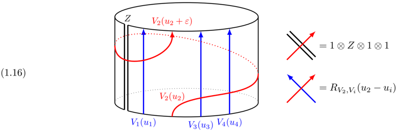
1.10. Quantum Knizhnik-Zamolodchikov equations. To any solution of the Yang-Baxter equation one can associate a canonical flat difference (or q -difference, in the quantum loop group case) connection, namely the quantum Knizhnik-Zamolodchikov connection of I. Frenkel and N. Reshetikhin [FR]. The corresponding commuting difference operators are best represented pictorially as in the following illustration of the ( u 1 , u 2 , u 3 , u 4 ) ↦→ ( u 1 , u 2 + ε, u 3 , u 4 )
shift:
The qKZ operators act in the tensor product V 1 ( u 1 ) ⊗···⊗ V n ( u n ) of quantum groups modules, where the parameters u i 's are treated as variables. In down-to-earth terms, the difference operators act on function of ( u 1 , . . . , u n ) with values in V 1 ⊗··· ⊗ V n . As we follow the k th strand around the cylinder in (1.16), where ( n, k ) = (4 , 2), we apply R -matrices in the corresponding tensor factors, as well as an operator Z that implements quasi-periodicity around the cylinder. The operator Z needs to satisfy
<details>
<summary>Image 1 Details</summary>
### Visual Description
## Diagram: Cylindrical Representation of Vector Transformations
### Overview
The image is a technical diagram, likely from a physics or mathematics text, illustrating transformations or relationships between vectors on a cylindrical surface. It features a central cylinder with labeled points and directed arrows (red and blue) indicating specific operations or mappings. A legend on the right defines the meaning of the arrow symbols. The diagram is labeled with the equation number "(1.16)" on the far left.
### Components/Axes
**Central Cylinder:**
* A 3D cylinder is drawn with a vertical orientation.
* A vertical line segment on the left side of the cylinder is labeled **"Z"**.
* **Top Surface:** A point is labeled **"V₂(u₂ + ε)"** in red text. A red arrow originates from this point, curves downward and to the left, and terminates at the vertical line labeled "Z".
* **Bottom Surface:** A point is labeled **"V₂(u₂)"** in red text. A red arrow originates from this point, curves upward and to the right, and terminates at the right edge of the cylinder.
* **Bottom Edge (from left to right):** Three points are labeled in blue text: **"V₁(u₁)"**, **"V₃(u₃)"**, and **"V₄(u₄)"**.
* **Vertical Arrows:** Three straight, vertical blue arrows point upward from the bottom edge to the top edge of the cylinder. Their origins are near the labels V₁(u₁), V₃(u₃), and V₄(u₄).
**Legend (Right Side):**
* **Top Symbol:** A black double-line crossed by a red arrow pointing up and to the right. The text to its right reads: **"= 1 ⊗ Z ⊗ 1 ⊗ 1"**.
* **Bottom Symbol:** A blue arrow pointing up and to the right crossed by a red arrow pointing up and to the left. The text to its right reads: **"= R_{V₂,Vᵢ}(u₂ - uᵢ)"**.
**Equation Number:**
* The number **"(1.16)"** is positioned to the far left of the cylinder.
### Detailed Analysis
**Spatial Grounding & Component Isolation:**
1. **Header Region (Top of Cylinder):** Contains the label "V₂(u₂ + ε)" and the termination point of one red arrow.
2. **Main Chart Region (Cylinder Body):** Contains the vertical blue arrows, the curved red arrows, and the label "Z".
3. **Footer Region (Bottom of Cylinder):** Contains the labels V₁(u₁), V₂(u₂), V₃(u₃), and V₄(u₄), and the origin points of the arrows.
4. **Legend Region (Right):** Isolated from the main diagram, providing definitions for the symbolic arrows.
**Trend Verification & Arrow Analysis:**
* **Blue Vertical Arrows:** These are straight, parallel, and point directly upward from the bottom to the top of the cylinder. They visually represent a consistent, direct mapping or translation from points V₁(u₁), V₃(u₃), and V₄(u₄) on the bottom to corresponding points on the top.
* **Red Curved Arrows:** These are non-linear. One curves from the top label "V₂(u₂ + ε)" down to the "Z" line. The other curves from the bottom label "V₂(u₂)" up to the right edge. They represent a different, more complex transformation compared to the blue arrows.
**Legend Cross-Reference:**
* The **red arrow** in the legend's top symbol matches the color and general direction (up-right) of the curved red arrows in the diagram. The legend defines this symbol as **"1 ⊗ Z ⊗ 1 ⊗ 1"**, suggesting an operation involving the "Z" component acting on the second vector space in a tensor product.
* The **blue arrow** in the legend's bottom symbol matches the color of the vertical arrows. The **red arrow** in the same symbol matches the curved arrows. The legend defines this crossed-arrow symbol as **"R_{V₂,Vᵢ}(u₂ - uᵢ)"**, indicating a rotation or transformation operator `R` dependent on the difference between parameters `u₂` and `uᵢ`, acting between vector spaces V₂ and Vᵢ.
### Key Observations
1. **Dual Transformation Types:** The diagram contrasts two types of operations: direct vertical mappings (blue arrows) and curved, parameter-dependent transformations (red arrows).
2. **Central Role of V₂:** The vector V₂ is involved in both types of transformations (from u₂ and u₂+ε), while V₁, V₃, and V₄ are only shown with vertical mappings.
3. **Parameter ε:** The label "V₂(u₂ + ε)" introduces a small perturbation or shift (ε) to the parameter u₂, which is the starting point for one of the curved transformations.
4. **Symbolic Legend:** The legend is crucial for interpreting the arrows not just as directional indicators but as specific mathematical operators defined in the accompanying text.
### Interpretation
This diagram visually encodes abstract mathematical relationships, likely from the fields of differential geometry, theoretical physics (e.g., gauge theory, string theory), or advanced algebra. The cylinder may represent a configuration space, a fiber bundle, or a periodic domain.
* **What the data suggests:** It demonstrates how a base transformation (the vertical blue arrows, perhaps a parallel transport or identity map) is modified or complemented by additional, more complex operations (the red arrows). The operation `R_{V₂,Vᵢ}(u₂ - uᵢ)` suggests a rotation or interaction that depends on the "distance" between parameters `u₂` and `uᵢ`. The operation `1 ⊗ Z ⊗ 1 ⊗ 1` indicates that the "Z" component acts non-trivially only on the second subspace in a four-part tensor product structure.
* **How elements relate:** The vertical arrows establish a baseline correspondence between points on the top and bottom of the cylinder. The red arrows then show how specific points (particularly those associated with V₂) are connected through a different, non-vertical path defined by the operators in the legend. The perturbation `ε` highlights sensitivity to initial conditions or a derivative concept.
* **Notable patterns/anomalies:** The asymmetry is notable—V₂ is treated distinctly from V₁, V₃, and V₄. This could imply V₂ plays a special role, such as being an active field or a source of interaction. The diagram's purpose is to make concrete the otherwise dense symbolic notation (`R_{V₂,Vᵢ}`, `1⊗Z⊗1⊗1`) by mapping it onto a spatial, intuitive representation.
</details>
$$\vert z \textcircled { 1 } z _ { 1 } R \vert = 0$$
and is usually chosen in the form
$$\begin{aligned}
Z &= z \cdot ( \text { shift } u + v ) \\
&= z \cdot e ^ { i t } + z \cdot e ^ { - i t }
\end{aligned}$$
where g 0 is the Cartan subalgebra in (1.13). In the multiplicative, K -theoretic situation the shift operator becomes u ↦→ qu . Here ε and q are free parameters, the geometric meaning of which will be explained momentarily.
The fundamental link between the geometric representation theory and enumerative geometry is provided by the following geometric interpretation of the qKZ connection. If one is interested in counting maps, or quasimaps f : C → X , one can broaden the setup and the range of available tools by counting sections, or quasisections, of nontrivial X bundles over C . This becomes especially constraining in the situation when the bundle is equivariant with respect to the action of T and the automorphisms of C .
Specifically, given any cocharacter of T :
$$( 1 . 1 8 )$$
we can use it as a clutching function to construct ( T × C ∗ q )-equivariant bundle over C = P 1 , where C ∗ q = Aut( P 1 , 0 , ∞ ). When σ is a cocharacter of A and the quiver variety X is symmetric, the σ -twisted quasimaps have the same virtual dimension and the same self-duality properties of their obstruction theory as the untwisted ones. We count them relative to the evaluation at the two fixed points 0 , ∞∈ C . For fixed deg f , this gives an operator from H T × C ∗ q ( X, w ) to itself, and similarly in K -theory. Note, however, that because the count is twisted, C ∗ q acts by σ in the target of this map, while acting trivially in its source.
Summing up these operators with weight z deg f gives a flat difference connection on Lie A or A in cohomology or K -theory, respectively. These difference operators are known as the shift operators , see [MO, Oko1]. The corresponding shifts are by σ ( ε ) and σ ( q ), respectively, where ε ∈ Lie GL (1) q .
In [COZZ3], we consider the shift operator in critical theories, here say in critical K -theory:
$$\begin{array}{ll}
1 & 1 \\
\hline
S _ { \sigma } \in End ( k ^ { T } C _ { i } ^ { j } ( X , w ) ) loc [ z ] ;
\end{array}$$
where C ∗ q is the torus scaling the distinguished P 1 in parametrized rational curves. We identify the shift operator connection with the qKZ connection for any torus A generated by minuscule cocharacters (i.e. C [ X ] is generated by elements of degree 0 or ± 1).
Theorem 1.7. ([COZZ3]) Let ( X, w ) be a symmetric quiver variety with potential, σ be a minuscule cocharacter, and s be a slope in certain area 1 . Then the conjugation of S σ is given by z deg f (up to some locally constant function).
Moreover there is a capping operator J ∈ End K T × C ∗ q ( X σ , w ) loc [ [ q ] ][ [ z ] ] that solves the qKZ equation:
$$y _ { 1 } = y _ { 2 } - y _ { 0 } = \frac { 6 0 x ^ { 3 } } { 8 } + P x , y _ { 0 }$$
where R s σ is certain (normalized) R -matrix.
1 { sufficiently small neighbourhood of (det P X ) -1 / 2 } ∩ ( -C amp ( X )) ⊆ Pic A ( X ) ⊗ Z R , where P X is a partial polarization of X and C amp ( X ) is the ample cone of X , see [COZZ3] for details.
This has dimensional reduction to Nakajima quiver varieties, generalizing results of [MO, Oko1]. Here minuscule is an important techical condition, which is satisfied by tori used in (1.9), that is, tori A that act on framing spaces preserving a direct sum decomposition. As a small technical detail, the identification of two connections requires a multiplicative shift of the variables z , which was called modified quantum product in [MO].
Note that the curve counting monomials z deg f σ become the weights of action of z in (1.17). From the quantum groups point of view, this is a minor diagonal part of the qKZ equation, the main complexity of which is contained in the R -matrix. From the enumerative perspective, this looks very surprising, since a monomial in z appears where one generally expects an infinite series. The geometric explanation for this is that only constant maps contribute to properly formulated twisted quasimaps counts. Note that a constant twisted quasimap takes C to one of the components of X σ , and these maps have different degrees for different components. Whence the appearance of monomials with different exponents in the qKZ operators.
Vanishing of contribution of nonconstant maps is shown using, fundamentally, equivariant rigidity. To make the rigidity argument work, all key ingredients of the construction of the stable envelopes are required. The properness of stable envelopes is used to prove that the count is a polynomial on Lie A (or A itself, in K -theory), while the degree bounds imply that degree of this polynomial is negative (or that its Newton polytope contains no lattice points, in K -theory).
1.11. Quantum critical cohomology. Fundamental structures in enumerative geometry include the quantum differential equation in cohomology, and its q -difference analog in K -theory. These commute with shift operators, including the qKZ connection discussed above, which very strongly contrains them. Using these constraints, the quantum differential equations for Nakajima varieties were identified with the Casimir connection [TL] for the corresponding Yangian in [MO], while the K -theoretic q -difference connection was identified with the dynamical connection for the corresponding quantum loop group in [OS]. When g is finite-dimensional, the dynamical connection is the lattice part of the dynamical affine Weyl group of Etingof and Varchenko [EV]. In general, the corresponding connection was constructed in [OS].
The linear operator in the quantum differential equation is the operator of modified quantum multiplication c 1 ( λ ) ˜ ⋆ by the first Chern class of the bundle ∏ (det V i ) λ i , where the modification is a certain sign shift of the variables z . The following general formula for the operator c 1 ( λ ) ˜ ⋆ · on Nakajima varieties was proven in [MO]:
$$z ^ { \alpha } _ { z a } = c _ { 1 } ( x ) U - \sum _ { i = 0 } ^ { n } ( A , \sigma ) ^ { i }$$
where
$$n ( r _ { a } ) , r _ { a } \in g _ { a } \otimes g - a .$$
Here θ is the stability parameter, r α is projection of r on the corresponding root subspaces, and the multiplication map takes g ⊗ g to U ( g ) ⊆ Y ( g ). The dots in (1.20) stand for a scalar, which is uniquely fixed by the requirement that the purely quantum part of c 1 ( λ ) ˜ ⋆ annihilates the identity 1 ∈ H T ( X ). For comparison with [MO], note that our definition of r includes the factor ℏ , and which makes the the cohomological degree of Casimir α equal 2.
Building on the geometric identification of the qKZ connection in critical cohomology, we prove
Theorem 1.8. ([COZZ1, § 5]) (1.20) holds for critical cohomology on any symmetric quiver variety X with potential when the specialization map to the cohomology of X is injective.
The d in > d out counts may be accessed from the fully symmetric counts by a certain limit transition. This is analogous to how the Toda equations, which describe the quantum cohomology of the flag varieties G/B [GK, Kim] can be obtained by a limit transition from the Calogero-style equations describing the quantum cohomology of T ∗ ( G/B ) [BMO]. This is well illustrated by the following example.
1.12. Quantum cohomology of Hilb( C 3 , n ) . The Hilbert scheme Hilb( C 3 , n ) of n -points on C 3 has a canonical presentation as the critical locus of the cubic function
$$7 ) ^ { 3 } \in Hom ( C , C ^ { n } ) / GL ( n ) \rightarrow C .$$
Let C ∗ q 1 , C ∗ q 2 , C ∗ q 3 be the tori that scale the loops x, y, z with weights -1 respectively. Set
$$T = k _ { 1 } ( C ^ { * } _ { q _ { 1 } } \times C ^ { * } _ { q _ { 2 } } \times C ^ { * } _ { q _ { 3 } } -$$
Let ℏ i be the equivariant parameter for C ∗ q i , then C [ t ] = C [ ℏ 1 , ℏ 2 , ℏ 3 ] / ( ℏ 1 + ℏ 2 + ℏ 3 ).
Although X is not symmetric, one can symmetrize it by adding a path from the gauge node to the framing node, and introduce an equivariant parameter ℏ . By taking certain limit of ℏ , we obtain the formula of quantum multiplication by divisors for Hilb( C 3 , n ).
Theorem 1.9. ([COZZ1, § 10]) For an equivariant line bundle L on X , we have
$$d ^ { 2 } J _ { d } + \mathcal { S } ( L ) \dot { a } = \sigma _ { 3 } \deg ( L ) d \cdot$$
Here σ 3 = ℏ 1 ℏ 2 ℏ 3 , J i = σ -i 3 ( i -1)! ad i -1 -f 1 f 0 , J -i = -σ -i 3 ( i -1)! ad i -1 e 1 e 0 for i > 0, and e i , f i are parts of the generators of shifted Yangian Y -1 ( ̂ gl 1 ), see [COZZ1, § 10.1], which acts on the critical cohomology. The scalar vanishes for d > 1.
Related works and future directions. As already mentioned, many current trends in the field may be traced to the influential work of Nekrasov and Shatashvili [NS]. Among their predictions was the identification of the operators of quantum multiplications with the image of Baxter/Bethe subalgebras of certain quantum groups in specific representations. Concretely, Nekrasov and Shatashvili computed the spectra of quantum multiplication operators and saw they satisfy Bethe-type equations.
While the mathematical foundations of enumerative theory of critical loci were yet to be laid down, and the relevant quantum groups and their representation were, with a few exceptions, yet to be constructed (using precisely the stable envelopes, including our results), the Nekrasov-Shatashvili computation of the spectra of quantum operators works very generally. In particular, it applies to the enumerative problems studied in the present work. Looking at the Bethe equations, Nekrasov and Shatashvili predicted the appearance of what Hernandez and Jimbo called asymptotic, or prefundamental, representations of quantum groups [HJ]. In such representations, Drinfeld currents act by rational functions with unbalanced numerator and denominator, which is by now well understood to be a real signature of a shifted quantum group.
The asymptotic representations of Hernandez and Jimbo arise via a limit procedure which, among its many incarnations in mathematical physics, is related to taking the length of a spin chain to infinity. As a parallel construction in enumerative geometry, one may want to approximate maps, or quasimaps, from a curve to some target X by finite jets. Moduli of regular maps Spec C [ t ] /t N → X , where X = X ( d ) is a Nakajima variety, is naturally an open set in Crit( w ), where w deforms the canonical cubic potential for the Nakajima variety X ( N d ) by quadratic terms. With different stability condition for Crit( w ), one may approximate different quasimap moduli spaces. The corresponding limit procedure for critical cohomology or critical K -theory groups is parallel to how Hernandez and Jimbo approximate the prefundamental representations by Kirillov-Reshetikhin modules. At the time of the Spring 2018 MSRI program, this point of view was adopted in an unpublished work of Nakajima and Okounkov [NO]. Several technical difficulties encountered by them were subsequently overcome in special cases in the PhD thesis of Henry Liu [Liu], which broke the ground in geometric construction of shifted quantum group actions in critical theories. In particular, critical R -matrices and asymptotic modules for shifted quantum groups make their appearance in [Liu], including applications to one-leg DT and PT counts.
In this paper, we improve on this asymptotic approach in several aspects. On the one hand, we work directly with the critical cohomology or K -theory, without the need to push forward the computations to any ambient space or specialization. In representation theoretic terms, this means that we study both the limit objects and the KirillovReshetikhin-type modules that approximate them abstractly, and not as submodules of some ambient modules like the tensor-product module corresponding to X ( N d ). On the other hand, we can work directly with the critical locus description of quasimaps moduli spaces, so the whole machinery of approximation is no longer necessary to construct representations of the relevant shifted quantum groups. Finally, we clarify both positive and negative results about specialization in critical theories, the absence of which stood in the way of applying several conventional geometric representation theory arguments in the critical context.
Varagnolo and Vasserot introduced critical convolution algebras in [VV1], and they constructed maps from (shifted) quantum loop groups of a simple Lie algebra g to K -theoretic critical convolution algebras of graded triple quiver varieties of the Dynkin quiver associated to g (see [VV1] for simply laced case and [VV2] for non-simply laced case). In loc. cit. , they showed that the prefundamental modules and Kirillov-Reshetikhin modules can be realized as critical K -theories of graded triple quiver varieties. Their construction of shifted quantum loop groups actions fits into our framework in the sense that those actions factor through maps to the Reshetikhin type shifted quantum loop groups.
Interactions of geometric representation theory and enumerative geometry constitute a very broad field of study, in which the setting of the more traditional, noncritical theories occupies an important, but relatively small corner. There are therefore compelling theoretical and applied reasons for extending all of the existing quantum group machinery to the setting of critical theories and shifted quantum groups. Among other things, this should include the identification of the quantum difference equations, extending the results of [Oko1], a correspondence between
relative and descendent insertions extending those found in [AO1], as well as a relation between vertex functions and nonabelian elliptic stable envelopes [AO1]. While in some directions the path of this process may appear somewhat predictable, other directions present the researchers with genuinely new features and puzzles.
Focusing on the latter, it appears both interesting and challenging to pinpoint the precise relation between representation theory and enumerative invariants in the situation when the shift is not antidominant. Both sides of the story here are well-defined in general and are directly related in the zero or antidominant shift case. We expect them to remain connected in general, but now in a more subtle way. Certainly, a connection of this form should contain some very interesting enumerative and representation-theoretic information.
We similarly expect the shifted quantum group story to lead to many subtleties in the elliptic stable envelopes situation. This is because, traditionally, computation with elliptic objects tend to rely very heavily on self-duality features, and also because there is no simple way to get rid of unwanted variables in the formulas with elliptic functions by making them go to 0 or ∞ .
Acknowledgments. This work benefits from helpful discussions and communications from many people, including Mina Aganagic, Daniel Halpern-Leistner, Tasuki Kinjo, Ryosuke Kodera, Yixuan Li, Yuan Miao, Hiraku Nakajima, Andrei Negut ¸, Tudor P˘ adurariu, Spencer Tamagni, Yukinobu Toda, Yaping Yang, Gufang Zhao, Tianqing Zhu. A.O. would like to thank SIMIS for hospitality. We would like to thank Kavli IPMU for bringing us together.
Statements and Declarations. We have no conflicts of interest to disclose.
## 2. Critical cohomology and K -theory
In this section, we recall the notions of critical cohomology, critical K -theory and their functorial properties. We discuss their excisions when closed subvarieties are full attracting subvarieties with respect to tori actions.
## 2.1. Attracting subvarieties. We work under the following setting.
Setting 2.1. Let X be a smooth quasi-projective variety over C with a torus T -action and w : X → C be a T -invariant regular function (called superpotential ) 2 . Let A ⊆ T be a subtorus. Define Fix A ( X ) to be the set of connected components of the torus fixed locus X A .
A cocharacter σ : C ∗ → A of A is generic if X σ = X A , i.e. the torus fixed loci coincide. There is a wall-and-chamber structure on Lie( A ) R , such that σ is generic if and only if it lies in a chamber.
Definition 2.2. The torus roots are the set of A -weights { α } occurring in the normal bundle to X A . A connected component of the complement of union of (finite) root hyperplanes is called a chamber , i.e.
$$L _ { i \in A } / | U _ { x } ^ { - 1 } = | L _ { j } | ,$$
where C j are chambers.
For an algebraic variety M with an A -action, and a cocharacter σ , let S be a subset of M σ , the attracting set of S in M is
$$\frac { A t r _ { 0 } ( S ) M } { t - \infty } = \{ x \in S \} .$$
In the Setting 2.1 and let C be a chamber, we define
$$A H _ { 2 } C l _ { 2 } = A H _ { 2 } S O _ { 4 }$$
for a subset S ⊆ X A and ξ ∈ C . Note that the definition does not depend on the choice of ξ . When there is no ambiguity, we also write Attr σ ( S ) = Attr σ ( S ) M and Attr C ( S ) = Attr C ( S ) M . Let F ∈ Fix A ( X ) be a connected component, then Attr C ( F ) is a locally closed subscheme in X , and admits an affine fibration p : Attr C ( F ) → F by the result of Bialynicki-Birula [BB].
Consider a partial order on Fix A ( X ) which is the transitive closure of the following relation:
(2.1)
$$1 5 7 9 1 1 3 5 7 9 1 3$$
̸
2 Note that by [Sum, Cor. 2], every point of X is contained in a T -invariant affine neighbourhood.
The full attracting set is defined as
Its Verdier dual is
$$i ^ { \prime } \rightarrow \varphi _ { w } \rightarrow v _ { w } \rightarrow$$
$$\frac { A t + f ( F ) } { P < F ^ { \prime } } = U _ { A t + c ( F ^ { \prime } ) }$$
We denote by Attr f C the smallest A -invariant closed subset of X × X A such that Attr f C contains the diagonal ∆ ⊆ X A × X A and
$$( x , y ) \in Attr _ { e } ^ { 1 } and \lim _ { t \rightarrow 0 } ( x , y ) = Attr _ { e } ^ { 1 }$$
It follows from definition that Attr f C is a subset of ⋃ F ∈ Fix A ( X ) Attr f C ( F ) × F ⊆ X × X A .
- 2.2. Critical cohomology. Let D b c ( X ) be the bounded derived category of constructible sheaves of C -vector spaces.
2.2.1. Definition and canonical map. There is a functor of vanishing cycles :
$$\therefore D ^ { \prime } ( x ) = D ^ { \prime } ( w - 1 0 ) .$$
$$\rho _ { w } ( F ) = R [ F _ { Re ( w ) } > 0 ( F ) ] _ { w = 1 ( 0 ) } .$$
Here we use an equivalent definition due to [KaSc, Ex. VIII 13].
Let D X be the Verdier duality functor on D b c ( X ), with dualizing sheaf
$$x = - 1 0 x = 9 0 ( k m / h )$$
The vanishing cycle functor commutes with Verdier duality
$$a _ { n } D x = D x + a _ { n }$$
Definition 2.3. The critical cohomology for ( X, w ) is defined as
$$x \in H ( X , \varphi _ { w } Q x ) ^ { V } .$$
Let ψ w : D b c ( X ) → D b c ( w -1 (0)) be the functor of nearby cycles, and let i : w -1 (0) ↪ → X be the closed embedding. There is a distinguished triangle of functors, referred to as the Milnor triangle :
$$\int _ { 0 } ^ { 1 } \rightarrow ( t ) \rightarrow ( t ^ { 2 } ) -$$
/
/
/
/
/
/
Apply the map i ! → φ w to ω X , and recall the Borel-Moore homology of w -1 (0) is
$$w _ { w - 1 } ( 0 ) = H ( w ^ { - 1 } ( 0 ), i w x ).$$
We obtain a canonical map (or cospecialization map ) from the Borel-Moore homology of w -1 (0) to the critical cohomology:
$$\begin{array}{ll}
1 & \text { can: } H ^ { BM } ( w ^ { - 1 } ( 0 ) ) \rightarrow H ( X , w ). \\
\end{array}$$
More generally, let i : Z ↪ → X be the embedding of a closed subset, then there is a natural transformation
φ
w
|
◦
i
!
→
!
i
◦
φ
w
.
/
/
/
/
/
/
Applying to ω X , we get a natural map
$$\frac { 1 } { q w l ^ { 2 } + z ^ { 2 } } + i \frac { q w l x } { q w l ^ { 2 } + z ^ { 2 } }$$
We define critical cohomology with support on Z by
$$H ( X , w ) z = H ( Z _ { i } ^ { j } \phi w x ) .$$
Then (2.6) gives a canonical map
Z
- 2.2.2. Euler class operator. Let π : E → X be a vector bundle of rank r , with zero-section z : X → E . Let w be a regular function on X and we extend it to a function on E by w E := w ◦ π , then w = w E ◦ z .
Consider the composition:
$$z _ { 4 } Q x \rightarrow Q E [ 2 r ] \rightarrow z _ { 4 } Q x [ 2 r ].$$
$$The formula you've provided is not a standard mathematical or scientific notation. It appears to be a placeholder or a symbol used in specific contexts, such as in computer programming or certain types of data visualization. If you're referring to a particular formula or concept, could you please provide more context or clarify what you're asking? I'm here to help!$$
where the second map is by adjunction and the first map is its Verdier dual. Applying φ w E to (2.9):
$$z _ { 1 } + \varphi _ { w } z _ { x } = \varphi _ { w } z _ { x } + \varphi _ { w } z _ { E } [$$
and taking global section, we obtain the Euler class operator on critical cohomology:
$$e ( E ) \cdot ( - ) : H ( X , w ) \rightarrow H ( X , w ).$$
Here we use proper pushforward commutes with vanishing cycle functor. It is straightforward to check that the Euler class operator commutes with the canonical map (2.5).
- 2.2.3. Functorial properties. The critical cohomology has natural functorial properties . Let f : X → Y be a map between smooth varieties, and w : Y → C be a regular function.
- (i) Since both X and Y are smooth, the map f is a locally complete intersection (l.c.i.). There is an l.c.i. pullback for the critical cohomology:
which is compatible with the canonical map.
- (ii) If f is proper, there is a proper pushforward:
$$\therefore \angle H A W ( 1 ) = \angle H N M$$
which is compatible with the canonical map.
- (iii) Given a closed embedding i : Z ↪ → X between smooth varieties, by [Dav1, Prop. 2.16], we have
$$\begin{array}{ll}
i _ { 1 } ( - ) = e ^ { i x } ( z ) \cdot (-) , \\
i _ { 2 } ( - ) = e ^ { i x } ( z ) \cdot (+) .
\end{array}$$
$$\because i _ { 1 } ( - 1 ) = e ( N _ { z } x ) \cdot$$
where e ( N Z/X ) · is the Euler class operator (2.10).
- (iv) Given an affine fibration π : ˜ X → X with the induced potential function ˜ w := w ◦ π , the pullback map
$$\pi : H ( X , w ) \rightarrow H ( X , w o π )$$
is an isomorphism [Dav1, Eqn. (37)].
- 2.2.4. Excisions. Next we explain the excision for critical cohomologies. Let j : U ↪ → X be the inclusion of an open subset, and i : Z ↪ → X be the closed embedding of its complement. There is an excision triangle:
$$\begin{array}{ll}
i _ { i 1 } ^ { \prime } & I d & j _ { i 1 } ^ { \prime } \\
\end{array}$$
/
/
/
/
When applied to ω X , it gives the excision long exact sequence for Borel-Moore homology. In critical cohomology, we obtain two long exact sequences.
- a) Apply (2.13) to ω X and then apply φ w from the left. We get
$$\frac { 1 } { \sqrt { 2 } } - \frac { 1 } { \sqrt { 2 } } = \frac { 1 } { \sqrt { 2 } }$$
/
/
/
/
Using φ w i ∗ ∼ = i ∗ φ w | Z (e.g. [KaSc, Ex. VIII.15]), and then applying R Γ, we have
/
/
- b) Apply (2.13) to φ w ω X . We get
$$\rightarrow H ( Z , w | z ) \rightarrow H ( X , \varphi _ { W } j \cdot w U ) \rightarrow N$$
/
/
/
/
$$1 6 0 \rightarrow 1 6 0 \rightarrow 1 6 0$$
/
/
/
/
Using j ∗ φ w ∼ = φ w | U j ∗ (see [Dav1, (23)]) and then apply R Γ, we have
/
/
$$\rightarrow H ( X , w ) z \rightarrow H ( U , w | u ) \rightarrow H ( Y , w )$$
/
/
/
/
/
/
/
/
Consider the Cartesian diagram
It follows that
$$\sum _ { [ 2 dim p ] } ^ { P + P * \varphi _ { w } | \omega F | } \varphi _ { w } | \omega F |$$
As hyperbolic localization commutes with vanishing cycle functor [Ric]:
$$P _ { 1 } ^ { \prime } i ^ { \prime } P _ { 2 } = P _ { 1 } i _ { 1 } P _ { 2 } i _ { 2 }$$
$$\sqrt { 1 + \cos x } = \sin x + \cos x$$
Thus the natural map p ∗ φ w | Z ω Z → p ∗ i ! φ w ω X is an isomorphism, which implies that
$$( 2 . 1 4 )$$
This proves the lemma in the case when F is maximal.
For general F , Z = Attr f ( F ) admits a filtration ∅ = Z 0 ⊆ Z 1 ⊆ Z 2 ⊆ · · · ⊆ Z n = Z by closed subvarieties Z i , such that Z i \ Z i -1 = Attr( F i ) for some union of fixed components F i and F i is maximal in X \ Z i -1 . We prove for general Z by induction on n , and the case n = 1 is what we have shown in the above.
Let i 1 : Z 1 ↪ → Z and j 1 : Z \ Z 1 ↪ → X \ Z 1 be the embeddings, and denote ˜ i 1 := i ◦ i 1 . Then we have a commutative diagram of long exact sequences:
/
/
/
/
/
/
$$\begin{array}{ccc}
H(Z_1, i_1,\varphi_{w|z}) & \rightarrow H(Z, w|z) \\
\downarrow & \downarrow \\
H(Z_1, i_1,\varphi_{w|x}) & \rightarrow H(Z, i_1,\varphi_{w|x}, z, \omega x | z)
\end{array}$$
/
/
therefore
/
/
/
/
/
/
/
/
?
/
/
o
o
\_
$$\begin{array}{ccc}
w_i^z^{(0)} & \xrightarrow[i]{} w_i^0^{(0)} & \xrightarrow[j]{} w_i^z^{(0)} \\
& \xrightarrow[i]{} x & \xrightarrow[j]{} U.
\end{array}$$
One can obtain a commutative diagram of (co)homology groups:
/
/
/
/
$$\begin{array}{ll}
H^{BM}(w_{z}^{(0)}) & \xrightarrow[can]{} H^{BM}(w) \\
H(Z,w_{z}) & \xrightarrow[can]{} H(X,w)z \\
H(X,w)z & \xrightarrow[can]{} H(U,w)u
\end{array}$$
where the right vertical map in the upper right corner is given by applying the Milnor triangle (2.4) to j ∗ ω U .
Proposition 2.4. Let F be a connected component of X A and Z = Attr f ( F ) with immersion i : Z → X . Then the map
$$1 1 / ( 2 , 3 ) = 1 1 / ( 2 , 4 )$$
in the above diagram is an isomorphism. In particular, there is a long exact sequence
/
$$\rightarrow H ( Z , w | z ) \rightarrow H ( X , w )$$
/
/
/
/
/
/
/
Proof. We first prove the case when F is maximal, i.e. Z := Attr f ( F ) = Attr( F ). The limit map p : Attr( F ) → F is an affine fibration by a result of Bialynicki-Birula [BB]. Since w is T -invariant, so we have w | Z = p -1 ( w | F ); thus
$$\rho _ { m g } l z = \rho ^ { 2 } l _ { 0 } h _ { 0 } r _ { 0 }$$
\_
/
/
\_
o
o
?
\_
\_
/
/
/
/
/
/
/
/
/
/
/
/
/
/
The right vertical arrow is an isomorphism be induction hypothesis, so it remains to show that the left vertical arrow is an isomorphism. Consider the commutative diagram:
/
/
$$\begin{array}{ll}
(2.15) & H ( Z _ { 1 } , w | z ) \rightarrow H ( Z _ { 1 } , i ^ { 4 } w | z w z ) \\
& H ( Z _ { 1 } , i ^ { 4 } w | x ).
\end{array}$$
(
(
We have shown in the above that H ( Z 1 , w | Z 1 ) ∼ = H ( Z 1 , ˜ i ! 1 φ w ω X ). As Z 1 is the attracting set of a maximal component of Z A , we can replace ( Z, X ) in (2.14) by ( Z 1 , Z ) and obtain
$$H ( Z _ { n } ) _ { 2 } = H ( Z _ { n } , k _ { n } ) _ { 2 } .$$
It follows that the vetical map in (2.15) is an isomorphism. This concludes the proof. □
Remark 2.5. As long as Z is the form of ⋃ F Attr( F ) for a collection of fixed components { F } ⊆ Fix A ( X ), the above proof works and the map H ( Z, w | Z ) → H ( X, w ) Z is an isomorphism for such Z .
Definition 2.6. We say that a class in H ( X, w ) is supported on a closed subvariety Z , if its image under
$$H ( X , W ) \rightarrow H ( W , )$$
vanishes.
2.2.5. Torus equivariance. Let T be a torus acting on ( X, w ) as in Setting 2.1, all constructions above can be generalized to this setting. For a subtorus A ⊆ T , denote i A : X A → X to be the closed embedding of torus fixed locus. We have proper pushforward and Gysin pullback
$$\sum _ { i = 1 } ^ { T } ( X , w ) \rightarrow H ^ { T } ( X A , w A ) .$$
By (2.11), the composition i ∗ A i A , ∗ is the multiplication by the Euler class e T ( N X A /X ). Therefore i A , ∗ is injective . And i ∗ A is surjective after localization, i.e.
$$\frac { 1 } { x ^ { 2 } + y ^ { 2 } } - \frac { 1 } { x ^ { 2 } + y ^ { 2 } } =$$
where ( -) loc := ( -) ⊗ H ∗ T (pt) Frac( H ∗ T (pt)) denotes the localized theory.
Remark 2.7. (1) Proposition 2.4 holds equivariantly as long as the extra torus preserves the potential w and commutes with A action. (2) If the extra torus in (1) contains A , i.e. as the T in Setting 2.1, one can show the equivariant version of the map in Proposition 2.4 is injective.
## 2.3. Critical K -theory.
- 2.3.1. Definition. Let ( X, w , T ) be as in Setting 2.1. Consider the dg-category Fact coh ( X, w , T ) of coherent factorizations of w [BFK, Def. 3.1], whose objects are pairs
$$E _ { - 1 } ^ { 6 } \rightarrow E _ { 0 } ^ { 6 } \rightarrow E _ { + 1 } ^ { 6 }$$
$$l _ { 1 } , l _ { 2 } , l _ { 3 } = l _ { 6 } , l _ { 7 } = m _ { 6 }$$
Let HFact coh ( X, w , T ) be the homotopy category of Fact coh ( X, w , T ), which is a triangulated category, and Acy coh denote the minimal thick triangulated subcategory containing totalizations of short exact sequences of coherent factorizations. Define the triangulated category of coherent factorizations to be the following Verdier quotient [Orl], [BFK, Def. 3.9]
$$\frac { 1 } { M F _ { \text { coh } ( X , w , T ) } } = H F$$
Without causing confusions, we also denote it to be MF( X, w , T ), or sometimes write it as MF([ X/ T ] , w ).
Definition 2.8. The critical K -theory of ( X, w , T ) is the Grothendieck group of MF( X, w , T ):
$$k ^ { T } ( X , w ) := k ^ { T } _ { 0 } ( X , w )$$
of morphisms in Coh T ( X ) such that
- 2.3.2. Canonical map. Let i : Z ( w ) ⊆ X be the inclusion of the zero locus of the function w . There is an equivalence of categories ([BFK, Rmk. 3.65], [Hir, Thm. 3.6]) from the T -equivariant singularity category of Z ( w ):
$$D ^ { 0 } \coh ( Z ( w ) ) / P e r f ($$
which induces an exact sequence of the Grothendieck groups (e.g. [PS, Lem. 1.10]):
$$\rightarrow K ^ { ( P e r t _ { Z } ( w ) ) } \rightarrow K ^ { ( D ^ { b } C o h t _ { Z } ( w ) ) }$$
More generally, let i : Z ↪ → X be the embedding of a T -invariant closed subset, there exists a matrix factorization category MF( X, w , T ) Z with support on Z , whose Grothendieck group is denoted by
$$k ^ { \prime } ( x , w ) z .$$
One has a surjective canonical map (e.g. [VV1, Prop. 2.6]):
$$\begin{array}{ll}
& \frac { 1 } { n } \sum _ { k = 1 } ^ { n } a _ { k } x _ { k } \\
& = \frac { 1 } { n } \sum _ { k = 1 } ^ { n } ( z _ { 1 } + z _ { 2 } + \cdots + z _ { n } ) x _ { k } \\
& = K ^ { T } ( z _ { 1 } + z _ { 2 } + \cdots + z _ { n } ) x _ { w } z ,
\end{array}$$
$$where K ^ { T } ( Z \cap Z ( w ) ) =$$
- 2.3.3. Euler class operator. Let π : E → X be a vector bundle of rank r and w be a regular function on X . We define the K-theoretic Euler class operator on critical K -theory:
$$e _ { k } ( E ) : ( - ) : K ( X , w ) → K ( X , w ).$$
$$\left[ E - 1 , \varepsilon _ { 0 } , d - 1 , d _ { 0 } \right] + \left[ ( A ^ { \ast } E )$$
It is straightforward to check that the Euler class operator commutes with the canonical map (2.18).
- 2.3.4. Functorial properties. Matrix factorization categories have functorial properties, e.g. pullbacks by flat morphisms and pushforwards by proper morphisms ([BFK], [VV1, § 2.2.2]), critical K -groups also have such properties. For regular embeddings, one can also define Gysin pullbacks for critical K -groups.
In particular, for the inclusion i A : X A ↪ → X of A -fixed locus, there are proper pushforward and Gysin pullback:
$$\sum _ { i = 1 } ^ { n } K ^ { T } ( X ^ { A }, w ^ { A } ) \rightarrow K ^ { T } ( X , w ), \sum _ { i = 1 } ^ { n } I ^ { A }$$
By [VV1, Prop. 2.8] 3 , we have
$$\begin{aligned}
i ^ { \star } A _ { 1 } A _ { 2 } ( - ) = c _ { K } ( N _ { X } ^ { \star } X _ { Y } ) \cdot ( - ), \\
\end{aligned}$$
where e T K ( -) · is the equivariant version of the K -theoretic Euler class operator (2.18).
This moreover induces an isomorphism
$$K ^ { T } ( X ^ { A } , w ^ { A } ) loc \rightarrow K ^ { T } ( X ^ { w } , w ) loc$$
of localized critical K -theories, where ( -) loc := ( -) ⊗ K T (pt) Frac( K T (pt)).
Given a T -equivariant vector bundle π : ˜ X → X , it is straightforward to show the pullback map
$$\pi * \int _ { X _ { w } } ^ { T } ( X _ { t } , w _ { 0 } ) d x$$
is an isomorphism.
- 2.3.5. Excisions. Let j : U ↪ → X be the inclusion of an open subset, and i : Z ↪ → X be the closed embedding of its complement. There is an excision sequence
$$\begin{array}{ll}
X , w ) & \longrightarrow K ^ { T } ( U , w ). \\
\end{array}$$
/
/
/
/
It is obvious that j ∗ ◦ i ∗ = 0. The map j ∗ is surjective because it fits into a commutative diagram (below the canonical map is given as (2.17))
/
/
/
/
$$\begin{array}{ll}
K ^ { \prime } ( w - 1 (0)) & \xrightarrow[j]{} K ^ { \prime } ( U \cap w - 1 (0)) \\
& \xrightarrow[can]{} K ^ { \prime } ( X_w ) \\
& \xrightarrow[j]{} K ^ { \prime } ( U, w ).
\end{array}$$
/
/
The following is a useful result showing when ker( j ∗ ) = im( i ∗ ) holds.
3 When working with torus invariant functions, the flatness condition on functions imposed in [VV1, Prop. 2.8] (which uses [VV1, Lem. 2.4]) can be dropped off by following the argument of [Toda3, Lem. 2.4.7].
Proposition 2.9. Let F be a connected component of X A and Z = Attr f ( F ) with immersion i : Z → X . Then ker( j ∗ ) = im( i ∗ ) in the sequence (2.24).
Proof. The case when F is maximal, i.e. Attr f ( F ) = Attr( F ) is essentially proven in [P, Thm. 2.5]. Strictly speaking, [P, Thm. 2.5] assumes X to be affine, but the argument works for quasi-projective X . For the convenience of readers, we explain the details here. Let p : Z = Attr( F ) → F be the attraction morphism. By [Hal, Thm. 3.35, Cor. 3.28], there is a semi-orthogonal decomposition (SOD) for the derived category of coherent sheaves:
$$\sum _ { T | 1 , \ldots } = D ^ { b } ( X / T ) ,$$
such that
$$1 , D ^ { b } ( Z / T ) _ { 0 , D ^ { b } ( Z / T ) _ { 1 , \ldots } }$$
is an SOD of D b ([ Z/ T ]), where the weight is with respect to a cocharacter in the chamber C . Moreover, under the restriction to the open locus D b ([ X/ T ]) ↠ D b ([( X \ Z ) / T ]), we have an equivalence of categories
$$G = D ^ { \prime } ( x ) Z / T .$$
This induces an SOD for the matrix factorization category (e.g. [P, Prop. 2.1]):
and an equivalence of categories:
$$W = M F ( X / Z ) T N _ { w }$$
By passing to the Grothendieck group, there is a decomposition
$$( z , w ) = K ^ { T } ( X , w ) .$$
where the map K T ( Z, w ) → K T ( X, w ) is i ∗ . In particular we have ker( j ∗ ) = im( i ∗ ).
For general F , Z = Attr f ( F ) admits a filtration
by closed subvarieties Z i , such that Z i \ Z i -1 = Attr( F i ) for some union of fixed components F i and F i is maximal in X \ Z i -1 . We prove for general Z by induction on n . Let i 1 : Z 1 ↪ → Z and j 1 : Z \ Z 1 ↪ → X \ Z 1 be the embeddings, and denote ˜ i 1 := i ◦ i 1 . By the induction hypothesis, the lemma holds when replacing ( X,Z ) by ( X \ Z 1 , Z \ Z 1 ). Suppose that α ∈ ker( j ∗ ), then α | X \ Z 1 ∈ im( j 1 ∗ ), i.e. ∃ β ∈ K T ( Z \ Z 1 , w ) such that α | X \ Z 1 = j 1 ∗ β . Take ˜ β ∈ K T ( Z, w ) such that ˜ β | Z \ Z 1 = β , then we have ( α -i ∗ ˜ β ) | X \ Z 1 = 0. Using the n = 1 case, we can find γ ∈ K T ( Z 1 , w ) such that α -i ∗ ˜ β = ˜ i 1 ∗ γ , and this implies that α = i ∗ ( ˜ β + i 1 ∗ γ ), in particular α ∈ im( i ∗ ). This shows that ker( j ∗ ) = im( i ∗ ). □
## 3. Stable envelopes
In this section, we define stable envelopes on critical loci and prove their uniqueness in both cohomology and K -theory. We show that they can be constructed from stable envelope correspondences 4 in § 3.3 through a convolution construction § 3.5. We provide existence results for stable envelope (correspondences), one for any critical loci and with respect to one dimensional torus A (Proposition 3.23), the other for critical loci of functions on symmetric GIT quotients without constrain on the dimension of the torus. The cohomological case is shown in Theorem 3.25 and Section 4, while the K -theoretic case makes use of nonabelian stable envelopes and Hall operations, see § 3.6, § 5. We prove the triangle lemma in § 3.9.
In this section, we often further impose the following condition.
Setting 3.1. We assume that there exists a proper morphism π : X → X 0 to an affine variety X 0 .
Remark 3.2. The assumption in Setting 3.1 is equivalent to that Γ( X, O X ) is a finite generated C -algebra and the natural morphism X → SpecΓ( X, O X ) is proper. In particular, we can take X 0 = SpecΓ( X, O X ). If we further assume that there is an algebraic group G action on X , then G naturally acts on Γ( X, O X ) linearly and X → SpecΓ( X, O X ) is G -equivariant.
Remark 3.3. The assumption in Setting 3.1 implies that Attr f C ( F ) is a closed subset in X for all F ∈ Fix A ( X ) by [MO, Lem. 3.2.7], and Attr f C is proper over X along the projection map X × X A → X by [MO, § 3.5].
4 Introducing stable envelope correspondences is essential for constructing stable envelopes for critical loci, see Remark 3.27.
3.1. Cohomological stable envelopes. In this section, we use the following shorthand to denote T -equivariant critical cohomology of ( X, w ) and ( X A , w | X A ):
$$( X ^ { A } , w ^ { A } ) = H ^ { T } ( X ^ { A } , \varphi _ { w } ( x _ { A } ^ { A } ) .$$
## 3.1.1. Definitions.
Definition 3.4. Fix ( X, w , T , A ) as in Setting 2.1, a choice of a chamber C as Definition 2.2. The cohomological stable envelope for ( X, w , T , A , C ) is a map of H ∗ T (pt)-modules:
$$S _ { \Delta A B C } = 1 / 2 ( A ) - 1 / 2 ( K )$$
such that for any γ ∈ H T / A ( X A , w A ) (and we identify γ with γ ⊗ 1 ∈ H T / A ( X A , w A ) ⊗ Q [Lie( A )] ∼ = H T ( X A , w A )) supported on a connected component F ⊆ X A , Stab C ( γ ) satisfies the following axioms:
- (i) Stab C ( γ ) is supported on Attr f C ( F );
- (ii) Stab C ( γ ) | F = e T ( N -F/X ) · γ ;
̸
- (iii) For any F ′ = F , the inequality deg A Stab C ( γ ) ∣ ∣ F ′ < deg A e T ( N -F ′ /X ) holds.
Here ( -) | F means the Gysin pullback ( F ↪ → X ) ∗ ( -), N ± F/X is the sub-bundle of N F/X which are positive/negative with respect to the chamber C , and deg A of a class in H T ( F ′ , w A ) ∼ = H T / A ( F ′ , w A ) ⊗ Q [Lie( A )] is the Q [Lie( A )]-polynomial degree, where we define the A -degree of 0 to be -1.
Definition 3.5. Fix ( X, w , T , A ) as in Setting 2.1, a cohomological normalizer is an element ϵ ∈ {± 1 } Fix A ( X ) , i.e. a sign ϵ F ∈ {± 1 } for each fixed component F . If Stab C is a cohomological stable envelope for ( X, w , T , A , C ), then we define
$$T ( X ^ { A } , w ^ { A } ) \rightarrow H ^ { T } ( X , w ),$$
i.e. for any γ ∈ H T ( F, w A ), Stab C ,ϵ ( γ ) = ϵ F · Stab C ( γ
## 3.1.2. Uniqueness.
Proposition 3.6. Let γ ∈ H T / A ( X A , w A ) be supported on a connected component F ⊆ X A , then Stab C ( γ ) which satisfies the axioms (i)-(iii) in Definition 3.4 is unique if it exists.
Proof. Let β ∈ H T ( X, w ) be supported on Attr f C ( F ) and satisfies deg A β | F ′ < deg A e T ( N -F ′ /X ) for any embedding i : F ′ ↪ → X of a fixed component such that F ⪯ F ′ . We claim that β = 0.
Pick a total ordering on the set of fixed component refining ⪯ , and let Z be the minimal fixed component such that Supp β ⊆ Attr f C ( Z ) and Supp β ⊈ Attr f C ( Z ) \ Attr C ( Z ). Factor i : Z ↪ → X as the following composition
$$\therefore z ^ { 2 } - A + m ( z ^ { 2 } - A + m ) ( z ^ { 2 } - x$$
Here f 1 is regular and f 2 is open. By Proposition 2.4, Supp β ⊆ Attr f C ( Z ) implies that ∃ α ∈ H T (Attr f C ( Z ) , w | Attr f C ( Z ) ) such that β = f 3 , ∗ α . The maps f 2 and f 3 fit into the following Cartesian diagram
/
/
$$\begin{array}{ll}
X \left( Attr_f ( Z ) \right) & \xrightarrow { h } X , \\
Attr_e ( Z ) & \xrightarrow { f_2 } Attr_f ( Z ) \\
& \xrightarrow { g } X / ( Attr_f ( Z ) \cap Attr_e ( Z ) )
\end{array}$$
/
/
where g is a regular closed embedding and h is an open embedding. Therefore we have
$$i ^ { \beta } = f _ { 1 } g ^ { \star } h ^ { \star } f _ { 3 } a = ,$$
̸
where the third equality uses (2.11) and the last one uses the definition of attracting set. The multiplication by e T ( N -Z/X ) is injective on H T ( Z, w | Z ), so if f ∗ 1 f ∗ 2 α = 0 then
$$\alpha \geq de g A e ^ { T ( N _ { z } / x ) } , f ^ { \prime }$$
which contradicts with the condition that deg A i ∗ β < deg A e T ( N -Z/X ); therefore f ∗ 1 f ∗ 2 α = 0. We note that
$$W ( h _ { 1 } , h _ { 2 } ) = \pi ^ { n } ( W _ { 1 } l _ { 1 } )$$
$$b e \cdot c \cdot H ^ { \prime } ( X ^ { \prime } , w ^ { \prime } ) \rightarrow H ^ { \prime } ( X , w )$$
where π : Attr C ( Z ) → Z is the projection map which is an affine fibration. By (2.12), the pullback
$$\pi ^ { \ast } : H ^ { T } ( Z , w | z ) \rightarrow H ^ { T }$$
is an isomorphism, which implies that f ∗ 1 : H T ( Attr C ( Z ) , w | Attr C ( Z ) ) → H T ( Z, w | Z ) is an isomorphism because π ◦ f 1 = Id. This forces f ∗ 2 α = 0, i.e. Supp α ⊆ Attr f C ( Z ) \ Attr C ( Z ), contradicting with the choice of Z ; hence β = 0.
Now if Γ 1 , Γ 2 ∈ H T ( X, w ) are two classes that satisfy (i)-(iii) in Definition 3.4, then Γ 1 -Γ 2 satisfies the hypothesis above; hence Γ 1 = Γ 2 . □
Remark 3.7. Let ≤ be a partial order on Fix A ( X ) that refines ⪯ in (2.1), and define
$$A _ { t + \varepsilon } ( F ) = U A _ { t + \varepsilon } ( F ^ { \prime } )$$
Suppose that Stab ′ C ( γ ) ∈ H T ( X, w ) is a class which satisfies the axioms (ii) and (iii) in Definition 3.4 and the following modifications of (i):
- (i') Stab ′ C ( γ ) is supported on Attr ≤ C ( F i ).
Suppose that Stab C exists, then Stab ′ C ( γ ) = Stab C ( γ ). This is because the same argument in the proof of Proposition 3.6 implies that the cohomology class that satisfies (i') as above and (ii) and (iii) as in the Definition 3.4 is unique.
Lemma 3.8. Let ≤ be a partial order on Fix A ( X ) that refines ⪯ in (2.1), and Z ⊆ X be an A -invariant closed subvariety. Then
$$( 3 . 1 )$$
where the subscripts X and Z mean taking attracting sets in X and in Z respectively.
Proof. Let us choose a σ ∈ C , then
$$t ) \cdot x \in F _ { n } Z \} = Attr e ( F _ { n } Z ) z .$$
Remark 3.9 (The ample partial order) . A useful refinement of ⪯ is induced by an ample A -equivariant line bundle L on X [MO, § 3.2.4]. Namely we define
$$\begin{array}{ll}
F < F' & \longrightarrow ( weight L_F ) | e > 0 . \\
\end{array}$$
The ample partial order has the nice feature that it is compatible with the restriction to closed subvarieties, that is, for an A -invariant closed subvariety Z , we have
$$k H = 1 A / k H \Delta$$
$$A H _ { 2 } S O _ { 4 } + A l = A l _ { 2 } S O _ { 4 } \downarrow + 2 H _ { 2 }$$
It follows that in particular,
## 3.2. K -theoretic stable envelopes.
## 3.2.1. Definition.
Definition 3.10. Fix ( X, w , T , A ) as in Setting 2.1, a choice of chamber C , and an s ∈ Pic A ( X ) ⊗ Z R which will be called a slope . The K-theoretic stable envelope for ( X, w , T , A , C , s ) is a map of K T (pt)-modules:
$$S _ { \Delta A C B } = \sqrt { ( x - A ) ^ { 2 } + ( y - B ) ^ { 2 } } - \sqrt { ( x - C ) ^ { 2 } }$$
such that for any γ ∈ K T / A ( X A , w A ) (and we identify γ with γ ⊗ 1 ∈ K T / A ( X A , w A ) ⊗ Q [ A ] ∼ = K T ( X A , w A )) supported on a connected component F ∈ Fix A ( X ), Stab s C ( γ ) satisfies the following axioms:
- (i) Stab s C ( γ ) is supported on Attr f C ( F );
- (ii) Stab s C ( γ ) | F = e T K ( N -F/X ) · γ ;
where
- (iii) For any F ′ = F , there is a strict inclusion of polytopes:
$$( N _ { F } ) x + shift _ { F } - shift _ { R }$$
$$\delta f _ { x } = \omega _ { g } ( d t ) ^ { 2 } \times s | F | ,$$
deg A of a Laurent polynomial is the Newton polytope:
$$\sum _ { i = 1 } ^ { n } f _ { u } ^ { i + 1 } = C o v e x h u l l ( \mu$$
and we define the A -degree of 0 to be the empty set.
Definition 3.11. We say a slope s ∈ Pic A ( X ) ⊗ R is generic if for any F ≺ F ′ , the A -weight difference
$$\sum _ { i = 1 } ^ { n } \sum _ { j = 1 } ^ { m } w _ { i j } ( x )$$
̸
is nonintegral.
Remark 3.12. Suppose that the slope s is generic, then any inclusion
$$x ( N _ { F } / x ) + shift _ { F } - shift _ { P }$$
must be strict.
Remark 3.13. Since X is smooth and Pic( A ) = 0, every line bundle on X admits a (not necessarily unique) A -equivariant structure by [CG, Thm. 5.1.9] 5 . Assume Γ( X, O ∗ X ) = C ∗ , then the set of A -equivariant structures on a line bundle L ∈ Pic( X ) form a Char( A )-torsor, in this case we have a fiber sequence:
$$( 1 ) ( 1 - x ) ^ { 2 } + x ( 1 - x ) = 0$$
Note that for any χ ∈ Char( A ), s and s ⊗ χ induce the same shifts in Definition 3.10(iii), so we can take s ∈ Pic( X ) ⊗ Z R if Γ( X, O ∗ X ) = C ∗ .
Definition 3.14. Fix ( X, w , T , A ) as in Setting 2.1, a K -theoretic normalizer is an element E ∈ ± Pic T ( X A ), i.e. a K -theory class E ∈ K T ( X A ) such that for every F ∈ Fix A ( X ), either E| F or -E| F is a line bundle. If Stab s C is a K -theoretic stable envelope for ( X, w , T , A , C , s ), then we define
$$T ( X ^ { A } , w ^ { A } ) \rightarrow K ^ { 1 } ( X , w ),$$
$$i . e . for any \gamma \in K ^ { T } ( F , w ^ { A } ) ,$$
Remark 3.15. The normalization condition and degree condition in Definition 3.10 is slightly different from the ordinary definition of K -theoretic stable envelope in the case w = 0 assuming the existence of polarization T 1 / 2 X [Oko1, § 9.1]. In fact, the original definition can be restored by the following.
$$S _ { \Delta } ^ { 5 } _ { e } in [ Oko1, §9.1 ] = S _ { a b c e }$$
$$\sum _ { s = - 1 } ^ { r k N F / X } ( \frac { det N F / X } { det T _ { 1 } / X } ) ^ { 1 / 2 } ,$$
## 3.2.2. Uniqueness.
Proposition 3.16. Let s ∈ Pic A ( X ) ⊗ R be a generic slope and γ ∈ K T / A ( X A , w A ) be supported on a connected component F ⊆ X A , then Stab s C ( γ ) which satisfies the axioms (i)-(iii) in Definition 3.10 is unique if it exists.
Proof. The argument is similar to the proof of Proposition 3.6, and we omit the details.
□
Remark 3.17. Let ≤ be a partial order on Fix A ( X ) that refines ⪯ , and define Attr ≤ C ( F ) as in the Remark 3.7. Suppose that Stab ′ C ( γ ) ∈ K T ( X, w ) is a class which satisfies the axioms (ii) and (iii) in Definition 3.4 and the following modifications of (i):
- (i') Stab ′ C ( γ ) is supported on Attr ≤ C ( F i ).
Suppose that Stab C exists, then Stab ′ C ( γ ) = Stab C ( γ ). This is because the same argument in the proof of Proposition 3.16 implies that the class that satisfies (i') as above and (ii) and (iii) as in the Definition 3.10 is unique.
5 The positive integer n in [CG, Thm. 5.1.9] is determined by [CG, Prop. 5.1.17] which can be taken to be 1 for the case G = A since Pic( A ) = 0.
̸
Remark 3.18. Let Stab s C be a K -theoretic stable envelope for ( X, w , T , A , C , s ) as in the Definition 3.10. Let L be a T -equivariant line bundle on X , and denote L A := L| X A , then we have
$$C O S _ { 2 } + C ( g ) = C S O _ { 3 } ^ { \circ } .$$
- 3.3. Stable envelope correspondences. Stable envelopes defined in the previous section are most effectively constructed through convolutions, which requires stable envelope correspondences introduced in this section.
3.3.1. Definitions and uniqueness.
Definition 3.19. Let ( X, w , T , A ) be in the Setting 2.1, and fix a chamber C . A cohomological stable envelope correspondence for ( X, w , T , A , C ) is a critical cohomology class with support (2.7) on Attr f C :
$$1 8 a b c d e f / ( x ^ { 2 } \times y ^ { 3 } + z w )$$
which satisfies the following two axioms:
- (i) For any fixed component F ∈ Fix A ( X ), [Stab C ] | F × F = e T ( N -F/X ) · [∆ F ] for diagonal ∆ F ⊆ F × F ;
̸
- (ii) For any F ′ = F , the inequality deg A [Stab C ] ∣ ∣ F ′ × F < deg A e T ( N -F ′ /X ) holds.
Here
$$\Delta A E F \cong \Delta A B M \cong \Delta A _ { 2 }$$
is the image of [∆ F ] ∈ H T (∆ F ) under the canonical map (2.8). Note also that Attr f C ∩ ( F × F ) = ∆ F .
Definition 3.20. Let ( X, w , T , A ) be in the Setting 2.1, and fix a chamber C and an s ∈ Pic A ( X ). A K -theoretic stable envelope correspondence for ( X, w , T , A , C , s ) is a class
$$1 8 N O _ { 3 } ( = K ^ { \prime } ) ( x \times x ^ { \prime } , w B N O _ { 3 } ) _ { 2 }$$
which satisfies the following two axioms:
- (i) For any fixed component F ∈ Fix A ( X ), [Stab s C ] ∣ ∣ F × F = e T K ( N -F/X ) · [∆ F ];
̸
- (ii) For any F ′ = F , there is a strict inclusion of polytopes deg A [Stab s C ] ∣ ∣ F ′ × F ⊊ deg A e T K ( N -F ′ /X ) + shift F ′ -shift F . Here
$$\vert A _ { 1 } C ^ { \prime } K ^ { \prime } \vert + \vert A _ { 2 } C ^ { \prime } K ^ { \prime } \vert + \vert A _ { 3 } C ^ { \prime } K ^ { \prime } \vert = M ^ { \prime } A _ { 0 }$$
is the image of [ O ∆ F ] ∈ K T (∆ F ) under the canonical map defined in (2.17).
Proposition 3.21. Suppose that w = 0, then the class [Stab C ] (resp. [Stab s C ]) in Definition 3.19 (resp. Definition 3.20) is unique if exists.
Proof. The proof is similar to that of Proposition 3.6 and Proposition 3.16 respectively, and we omit it. □
3.3.2. Existence. We notice that w ⊟ w A vanishes on Attr f C for arbitrary A -invariant function w . So the canonical maps (2.8), (2.18) in this setting are:
$$\begin{array}{ll}
\text{can: } H ^ { T } ( X \times X ^ { A } ) _ { Attr _ { e } } \rightarrow H ^ { T } \\
\end{array}$$
Here by definition (2.7), H T ( X × X A ) Attr f C = H T (Attr f C ), and K T ( X × X A ) Attr f C ∼ = K T (Attr f C ) by d´ evissage.
Lemma 3.22. Let [Stab C ] be a cohomological stable envelope correspondence for ( X, 0 , T , A , C ), then the image can([Stab C ]) under canonical map is a cohomological stable envelope correspondence for ( X, w , T , A , C ).
Similarly, let [Stab s C ] be a K -theoretic stable envelope correspondence for ( X, 0 , T , A , C , s ), then can([Stab s C ]) is a K -theoretic stable envelope correspondence for ( X, w , T , A , C , s ).
Proof. The axioms (i) and (ii) in Definition 3.19 for nontrivial potential w follows from the corresponding axioms for trivial potential w = 0 because canonical map commutes with Gysin pullback and preserves deg A . Namely, we have
$$f ( x ) = e ^ { i \left( N _ { F } / x \right) \cdot [ \Delta f ] }$$
and
$$\begin{aligned}
& \deg A ( c a n ( S t a b e l ) ) | F ^ { x } F = \deg A c _ { n } ( S t a b e l ) F ^ { x } F \\
& < \deg A e ^ { T } ( N F ^ { x } / X ) .
\end{aligned}$$
The K -theoretic counterpart is proven similarly.
□
In the case when dim A = 1, there are two choices of chambers { + , -} . In this case, the stable envelope correspondence always exists, by the next proposition (as motivated by [Oko1, § 9.2.3]).
Proposition 3.23. Let ( X, w , T , A ) be in the Setting 2.1 and suppose that A ∼ = C ∗ .
- Then there exists a cohomological stable envelope correspondence [Stab + ] for ( X, w , T , C ∗ , +).
- If we fix s ∈ Pic A ( X ) ⊗ Z R , then there exists a K -theoretic stable envelope correspondence [Stab s + ] for ( X, w , T , C ∗ , + , s ).
Proof. We first prove the cohomology version. According to Lemma 3.22, it suffices to construct [Stab + ] for ( X, 0 , T , C ∗ , +). Attr f := Attr f + admits a filtration 6
$$1 . 7 / ( 4 / 4 ) = 7 / 4$$
by open subvarieties Z i , such that Z 1 = Attr(∆) where ∆ ⊆ X σ × X σ is the diagonal, and
$$1 1 - 7 1 , 1 1 + 7 1 = 1 1 1$$
where Attr( -) is the attracting set in X × X σ . We write
$$z _ { i - 1 } / z _ { i - 1 } = U _ { j \in F _ { i x _ { 0 } } }$$
where G j i is a union of torus fixed components, and ⋃ F j ∈ Fix σ ( X ) ( G j i × F j ) is the union of F ′ × F for all F ′ ≻ F such that ( F ′ × F ) ∩ ( Z i -1 \ Z i -1 ) = ∅ . Then by construction
̸
$$z _ { i } \vert z _ { i - 1 } = U _ { j } ( F _ { j } e ^ { i x _ { j } } )$$
We claim that there exists [Stab] i in equivariant Chow homology A T ( Z i ) which satisfies the following two axioms:
- (i) For any fixed component F ∈ Fix A ( X ), [Stab] i ∣ ∣ F × F = e T ( N -F/X ) · [∆ F ];
̸
- (ii) For any F ′ ≻ F such that ( F ′ × F ) ∩ Z i = ∅ , deg σ [Stab] i ∣ ∣ F ′ × F < deg σ e T ( N -F ′ /X ).
Then [Stab + ] is the image of [Stab] n under the cycle map
$$A ^ { \prime } ( A _ { 1 } + r ) - F ^ { \prime } ( A _ { 1 } r )$$
sending algebraic cycle to Borel-Moore homology class. Define
$$\{ S ( a b ) _ { 1 } = \sum F ( x , y )$$
then [Stab] 1 obviously satisfies axiom (i). For i ⩾ 2 and assume that we have constructed [Stab] i -1 ∈ A T ( Z i -1 ), then we use the surjective map A T ( Z i ) ↠ A T ( Z i -1 ) to find a preimage of [Stab] i -1 in A T ( Z i ), denoted by [Stab] ∼ i -1 . Write Z i \ Z i -1 = Attr( M i ∩ Attr f ), where
$$M _ { i } = U G _ { i } \times F _ { j }$$
$$r = 1 8 0 h t \frac { 1 } { 2 } r ^ { 2 } + ( 1 0 n a m ) .$$
then define
Let α be the unique class in A T ( M i ∩ Attr f ) such that
$$a ) < deg _ { e } T ( N x _ { 0 } / x ) .$$
Here the existence uses the fact that A is one dimensional, so one can use Euclidean algorithm to find α . The uniqueness follows from the fact that given another α ′ satisfying above inequality, then the difference of the LHS also has degree less than the RHS, i.e.
$$x ) < de g _ { 0 } e ^ { T ( N x / x ) } ,$$
6 To prove the existence of such filtration, let us define Z i inductively by setting Z 1 = Attr(∆) and Z i := Z i -1 ∪ Attr( Z i -1 \ Z i -1 ). Note that Z i -1 \ Z i -1 are unions of torus fixed locus, which are distinct for different i . As the number of torus fixed components is finite, the induction process terminates at some Z n (and Z n is closed in X × X A ). Then Z n contains Attr f by the definition of Attr f . Attr f contains Z 1 by definition; thus it contains Z 1 since it is closed, then it follows that Attr f contains Z 2 , and by induction Attr f contains Z n . Thus Attr f = Z n .
which implies that α ′ = α .
Let p i : Z i \ Z i -1 = Attr( M i ∩ Attr f ) → M i ∩ Attr f be the projection, j i : Z i \ Z i -1 ↪ → Z i be the closed embedding, and define
$$B a C l _ { 2 } = B a C l _ { 2 } \cdot - H _ { 2 } O ( l )$$
Then [Stab] i satisfies axiom (i) since F × F ⊆ Z i -1 . Note that we have
$$M _ { i } \cap Z _ { i } = Attr ( M _ { i } ) \cap Z _ { i }$$
and following Cartesian diagrams
$$\begin{array}{ll}
M_i \cap Z_i & \longrightarrow & Attr(M_i) \cap Z_i \\
& \longleftarrow & M_i \cap Attr(M_i) \\
& \longleftarrow & X \times X^*,
\end{array}$$
/
/
/
/
$$\rightarrow X \times X ^ { o } _ { i , p _ { i } ( a ) }$$
therefore thus
$$x _ { i } ( x ) ^ { \prime } ( a ) < deg _ { e } ( N _ { i } ( x ) ,$$
i.e. [Stab] i satisfies axiom (ii). This proves the cohomology version.
For the K -theory version, we claim that there exists [Stab s ] i in equivariant K -theory K T ( Z i ) which satisfies the following two axioms:
- (i') For any fixed component F ∈ Fix A ( X ), [Stab s ] i | F × F = e T K ( N -F/X ) · [∆ F ];
̸
- (ii') For any F ′ ≻ F such that ( F ′ × F ) ∩ Z i = ∅ , deg σ [Stab s ] i ∣ ∣ F ′ × F ⊆ deg σ e T K ( N -F ′ /X ) + shift F ′ -shift F .
Then [Stab s + ] is [Stab s ] n . Define
$$[ S _ { \Delta } b ^ { 3 + } ] _ { r } = [ C _ { z } l _ { r }$$
then [Stab] 1 obviously satisfies axiom (i). For i ⩾ 2 and assume that we have constructed [Stab s ] i -1 ∈ K T ( Z i -1 ), then we use the surjective map K T ( Z i ) ↠ K T ( Z i -1 ) to find a preimage of [Stab s ] i -1 in K T ( Z i ), denoted by [Stab] ∼ i -1 . Similar to the cohomological counterpart, we define
$$\begin{aligned}
& \beta = \{ Stab 5 \} _ { i - 1 } M _ { i } , \\
& \deg _ { e g } ( \beta - e K ( N _ { F } / X _ { F } ) + \alpha ) [ F \times F ] \xi .
\end{aligned}$$
Define
/
/
$$B a C l _ { 2 } = B a C l _ { 2 } \cdot - H _ { 2 } O ( l )$$
Then [Stab] i satisfies axiom (i) since F × F ⊆ Z i -1 ; [Stab] i satisfies axiom (ii) as
$$\begin{aligned}
( M _ { i } \rightarrow X \times X ^ { o } ) _ { j : p _ { i } ( a ) } & = e _ { i } ( N _ { x _ { o } / x } ) \cdot ( M _ { i } \rightarrow Attr ( M _ { i } ) ^ { ( a ) } ) \\
& = e _ { i } ( N _ { x _ { o } / x } ) \cdot a _ { i }$$
thus
$$( ( \beta - e ^ { i k } ( N x _ { 0 } / x ) \cdot a ) F \times F ) \zeta deg _ { 0 } e ^ { i k } ( ( \beta - e ^ { i k } ( N x _ { 0 } / x ) \cdot a ) F \times F )$$
This proves the K -theory version.
When ambient spaces are symplectic, we have the following existence result.
Theorem 3.24 ([MO, Prop. 3.5.1]) . Suppose that X is a smooth symplectic variety with symplectic form Ω such that A fixes Ω and T scales Ω. Fix a chamber C , and a T -invariant function w : X → C . Then cohomological stable envelope correspondence exists.
/
/
□
Proof. By Lemma 3.22, we are left construct cohomological stable envelope correspondence for ( X, 0 , T , A , C ), which is done in [MO, Prop. 3.5.1]. □
When ambient spaces are symmetric GIT quotients , we have the following existence result.
Theorem 3.25. Suppose that X is a symmetric GIT quotient with an action of tori A ⊆ T as Definition 4.1. Fix a chamber C , and a T -invariant function w : X → C . Then cohomological stable envelope correspondence exists.
Proof. By Lemma 3.22, we are left to construct cohomological stable envelope correspondence for ( X, 0 , T , A , C ), which is constructed in Theorem 4.3. □
Remark 3.26. Things might go wrong without the self-duality assumption on the A -action. For example, take X = Tot ( O P 1 ( -1) ⊕ 2 ) with zero potential and let T = A = C ∗ a × C ∗ b act on X , where C ∗ a is the natural torus symmetry on P 1 and extends to act on X by setting one of O P 1 ( -1) to have zero weight at 0 and another one to have zero weight at ∞ , and C ∗ b acts on P 1 trivially and scales the fibers of O P 1 ( -1) ⊕ 2 with weight 1. Then cohomological stable envelope does not exist in the chamber { 0 < b < a } . We refer to Proposition 9.26 for a K -theoretic example.
Remark 3.27. Elliptic stable envelopes have been constructed for symmetric quiver varieties with zero potential in [IMZ], and it is shown in loc. cit. that K -theoretic and cohomological limits of elliptic stable envelopes give rise to classes [ Stab s C ] ∈ K T ( X × X A ) and [ Stab C ] ∈ H T ( X × X A ) that satisfy the axioms (i) (ii) in Definition 3.20 and 3.19 respectively. Moreover one can show that [ Stab s C ] and [ Stab C ] are supported on Attr f C , in particular they can be lifted to classes in K T (Attr f C ) and H T (Attr f C ) respectively.
However, the lifts are not necessarily unique because neither K T (Attr f C ) → K T ( X × X A ) nor H T (Attr f C ) → H T ( X × X A ) is injective in general. It is not clear whether we can choose a lift to make it a stable envelope correspondence for the zero potential in the sense of Definition 3.20 or 3.19 respectively. Therefore introducing stable envelope correspondences is necessary.
## 3.4. Transpose of stable envelope correspondences.
3.4.1. Convolutions. Let ( X i , w i ) ( i = 1 , 2 , 3) be as in Setting 2.1 and p ij : X 1 × X 2 × X 3 → X i × X j the projection. Let Z 12 ⊆ X 1 × X 2 , Z 23 ⊆ X 2 × X 3 be T -invariant closed subschemes such that
$$\frac { 1 } { m } \cdot n ^ { - 1 } + \frac { 1 } { n } = k \cdot x _ { 0 }$$
is a proper map and denote the image by
$$7 n / 4 = n \cdot b ^ { 2 } ( n - 1 ) b + a$$
We define the convolution on critical cohomology (e.g. [CG, pp. 112], [VV1, § 2.4]):
$$\sum _ { ( b , α ) } ^ { \max } w _ { 1 } \in w _ { 0 } ) z _ { 1 2 } \otimes H ^ { T } ( X _ { 1 } \times X _ { 3 } , w _ { 2 } \in w _ { 3 } ) z _ { 2 3 } \rightarrow H ^ { T } ( X _ { 1 } \times X _ { 3 } , w _ { 1 } \in w _ { 0 } ) z _ { 1 2 } o t \beta _ { 0 a } := p _ { 1 3 } ( p _ { 1 2 } ^ { T } \otimes p _ { 2 3 } a )$$
Here the tensor product ⊗ is defined generally as follows: for a smooth Y , closed subschemes Z, Z ′ ⊆ Y and
$$( 1 - b ^ { 2 } ) ( 1 + b ^ { 2 } ) =$$
the Thom-Sebastiani isomorphism implies
$$a b c d e f g h i x y z$$
$$H ^ { \prime } ( Y , w + w ^ { \prime } ) z _ { n z } .$$
Similarly we define the convolution on critical K -theory (e.g. [CG, pp. 251], [VV1, § 2.3.2]):
$$\sum _ { ( b , w ) } z _ { 1 2 } \otimes K ^ { T } ( X _ { 1 } \times X _ { 3 } , w _ { 1 } \in W _ { 3 } ) z _ { 2 3 } \rightarrow K ^ { T } _ { 1 } w _ { 1 } \in W _ { 2 }$$
Here the derived tensor product ⊗ is defined generally as follows: for a smooth Y , closed subschemes Z, Z ′ ⊆ Y and a ∈ K T ( Y, w ) Z , b ∈ K T ( Y, w ′ ) Z ′ , derived (exterior) tensor product gives
$$a b c d e f g h i j k l m n o p q r s t u v w x y z$$
then the diagonal pullback gives
$$K ^ { T } ( Y , w + w ^ { \prime } ) z _ { n z } .$$
then the diagonal pullback gives
Remark 3.28. For the convolution on critical cohomology (3.3) to be well-defined, it is enough to assume that p -1 12 ( Z 12 ) ∩ p -1 23 ( Z 23 ) ∩ (Crit( w 1 ) × Crit( w 2 ) × Crit( w 3 )) is proper over X 1 × X 3 . This is because the vanishing cycle sheaf φ w i ω X i is supported on Crit( w i ), i ∈ { 1 , 2 , 3 } .
3.4.2. Transpose correspondences. Given a class [ α ] ∈ H T ( X × Y, w 1 ⊟ w 2 ) Z , we define its transpose
$$\left\{ \begin{array}{ll}
a_1 ^ { 3 } \in H^1(Y \times X , w_2 \partial W_1 ) z \\
a_2 ^ { 4 } \in H^1(Y \times X , w_2 \partial W_1 ) z
\end{array} \right.$$
to be the image of [ α ] under the natural isomorphism X × Y ∼ = Y × X followed by the automorphism A 1 -1 - - → A 1 on the target of the potential function. The K -theory version is defined similarly.
Lemma 3.29. Under Setting 3.1, let [Stab C ] be a cohomological stable envelope correspondence for ( X, w , T , A , C ), then the convolution
$$\frac { 1 } { X ^ { A } , w ^ { A } \bigcap w ^ { A } } ( Attr _ { f } ) ^ { t } o Attr _ { f }$$
equals to the diagonal class [∆].
Let s be a generic slope, and [Stab s C ] be a K -theoretic stable envelope correspondence for ( X, w , T , A , C , s ), then the convolution
$$\begin{array}{ll}
x \times X^A , w^A \in w ^ { A } ( Attr _ { e } ) ^ { s + t } ( Attr _ { e } ) ^ { k T } ( X ) & [ Stab _ { - s } ] ^ { t } o ( Stab _ { e } ^ { s + t } ) \in K ^ { T } ( X )$$
equals to [ O ∆ ]. Here K = det Ω 1 X is the canonical bundle of X and + denotes the group operation of Pic A ( X ) ⊗ Z R .
Proof. The proof is similar to [MO, Thm.4.4.1] for the cohomology version and [OS, Prop. 1] for the K -theory version. We give details for the K -theory version. To simplify notation, let us write
$$S _ { 1 } = S + \frac { K } { 2 } \cdot$$
The diagonal map X ↪ → X × X induces an embedding
$$\Delta _ { 2 3 } : X ^ { A } \times X \times X ^ { A }$$
Denote C = ∆ -1 23 ( (Attr f -C ) t × Attr f C ) . By the proof of [MO, Thm. 4.4.1], C is proper over X A × X A ; therefore
$$\left\{ \begin{array}{ll}
( X ^ { A } \times X _ { A } , w ^ { A } E \wedge w ^ { A } ) p ( C ) & = p _ { + } \Delta _ { 2 3 } ( Stab ^ { - c } \{ X ^ { A } \} \otimes Stab ^ { - c } \{ X _ { A } \}) e ^ { ( 3 . 6 ) } \\
\end{array} \right.$$
is well-defined. Here p : X A × X × X A → X A × X A is the projection, and we denote (Attr f -C ) t ◦ Attr f C := p ( C ).
We compute (3.6) using A -localization: its restriction to the component F 1 × F 2 equals to
$$\sum _ { F \in F _ { \lambda } ( X ) } ^ { ( 3 . 7 ) } \{ ( S t a b ^ { - s } e l | F _ { x }$$
According to axiom (ii) in Definition 3.20, we have an inclusion
$$\begin{aligned}
b ^ { s } \{ r \times F _ { R } \} & = \deg _ { A } ( [ S t a b - e ] _ { R } \times F _ { R } ) ^ { t } o ( [ S t a b ] _ { R } ) \\
& + weight _ { A } ( det ( N ^ { T } _ { R } / x ) ^ { 1 / 2 } \otimes s _ { 1 } | F _ { R } | ) - weight _ { A } ( det ( N ^ { T } _ { R } / x ) ^ { 1 / 2 } \otimes s _ { 1 } | F _ { R } | ) .
\end{aligned}$$
In the above, we have used weight A det( N -F/X ) ⊗ det( N + F/X ) ⊗K| F = 0. Therefore the function
$$\begin{array}{ll}
t o ( S t a b s _ { c } ) \cdot ( d e t ( N _ { F _ { 1 } } , x ) ^ { - 1 / 2 } \otimes ( s | F _ { 1 } ) ^ { - 1 / 2 } ) \\
\end{array}$$
in the variable a ∈ A is bounded in any direction of taking limit a →∞ .
Since [Stab -s -C ] t ◦ [Stab s 1 C ] is defined in integral K -theory, then (3.8) is a constant function in a . In particular,
$$t _ { A } = weight _ { A } ( det ( N _ { F _ { 3 } } / x ) ^ { 1 / 2 } ⊗ s | F _ { 3 } | ) .$$
Since [Stab -s -C ] t ◦ [Stab s 1 C ] is supported on (Attr f -C ) t ◦ Attr f C , ([Stab -s -C ] t ◦ [Stab s 1 C ]) ∣ ∣ F 1 × F 2 vanishes if F 2 ⪯̸ F 1 . If F 2 ≺ F 1 , then weight A ( det( N -F 1 /X ) 1 / 2 ⊗ s | F 1 ) -weight A ( det( N -F 2 /X ) 1 / 2 ⊗ s 1 | F 2 ) is nonintegral since s is generic, and this implies that ([Stab -s -C ] t ◦ [Stab s 1 C ]) ∣ ∣ F 1 × F 2 vanishes. When F 1 = F 2 , the only nonzero summand in (3.8) is F = F 1 , which gives [ O ∆ ]. It follows that [Stab -s -C ] t ◦ [Stab s 1 C ] = [ O ∆ ]. □
3.5. Existence of stable envelopes via convolutions. We work under Setting 3.1. According to Remark 3.3, Attr f C is proper over X ; therefore any class
$$\vert a \vert = \sqrt { 1 } ( x \times x ^ { 2 } , w \in w ^ { \prime } ) , n _ { m + c }$$
$$c$$
$$\vert \beta \vert = k ^ { \prime } ( x _ { 1 } x _ { 2 } , w E N ) _ { n + c }$$
induces a map (by convolution (3.3)):
$$( 3 . 9 )$$
Similarly, any K -theory class induces a map (by convolution (3.4)):
$$( 3 . 1 0 )$$
One can check that convolutions (3.3), (3.4) are associative, so compositions of convolutions induce compositions of maps induced. Convolutions are also compatible with canonical maps as shown below.
Lemma 3.30. Let [ β ] ∈ K T ( X × X A ) Attr f C and can([ β ]) ∈ K T ( X × X A , w ⊟ w A ) Attr f C be its image under canonical map (2.18). Then we have a commutative diagram
o
o
/
/
$$\begin{array}{ll}
(3.11) & \begin{array}{c}
K ^ { T } ( X ^ { A } ) & \rightarrow & K ^ { T } ( X ^ { A } , z ) \\
& \downarrow & \downarrow & \downarrow \\
\end{array} \\
\end{array}
\begin{array}{ll}
K ^ { T } ( X ) & \rightarrow & K ^ { T } ( X ) , z \\
& \downarrow & \downarrow & \downarrow \\
\end{array}
\begin{array}{ll}
( w _ { A } ) & \rightarrow & K ^ { T } ( X ^ { A } , w _ { A } ) \\
& \downarrow & \downarrow & \downarrow \\
\end{array}
\begin{array}{ll}
( w ) & \rightarrow & K ^ { T } ( X , w ) , \\
& \downarrow & \downarrow & \downarrow \\
\end{array}$$
o
o
where i : Z ( w ) ↪ → X and i A : Z ( w A ) ↪ → X A are embeddings.
Similarly, let [ α ] ∈ H T ( X × X A ) Attr f C and can([ α ]) ∈ H T ( X × X A , w ⊟ w A ) Attr f C be its image under canonical map (2.5). Then we have a commutative diagram
o
o
/
/
$$\begin{array}{ll}
H ^ { T } ( X ^ { A } ) & \xrightarrow [ a ] { H ^ { T } ( X ) } z \\
& \xrightarrow [ i _ { s } ] { H ^ { T } ( X ) } z \\
\end{array}$$
o
o
/
/
Proof. The canonical maps are well-defined as Attr f C ⊆ Z ( w ⊟ w A ) . Note also that
$$( \sum Z ( w ) \times Z ( w ^ { A } ),$$
therefore the convolutions β in the middle vertical arrow of (3.11) and α in the middle vertical arrow of (3.12) are welldefined. The left square of (3.11) commutes as proper pushforward commutes with flat pullbacks and Gysin pullbacks, similarly the left square of (3.12) commutes for the same reason. The right square of (3.11) commutes as canonical map (2.18) commutes with flat pullbacks, proper pushforwards and Gysin pullbacks (e.g. [VV1, Lem. 2.4] 7 ). Similarly the right square of (3.12) commutes as canonical map (2.5) commutes with smooth pullbacks, proper pushforwards and Gysin pullbacks. □
By applying convolutions to stable envelope correspondences (Definitions 3.19, 3.20), we obtain:
Proposition 3.31. Let [Stab C ] be a cohomological stable envelope correspondence for ( X, w , T , A , C ), then
$$S _ { \Delta A B C } = \sqrt { 1 ^ { 2 } + 1 ^ { 2 } - 2 \cdot 1 \cdot 1 }$$
is a cohomological stable envelope.
Let [Stab s C ] be a K -theoretic stable envelope correspondence for ( X, w , T , A , C , s ), then
$$S _ { \Delta A B C } = A ^ { 2 } + B ^ { 2 } - 2 A B \cos ($$
is a K -theoretic stable envelope.
7 When working with torus invariant functions, the flatness condition on functions imposed in [VV1, Lem. 2.4] can be dropped off by following the argument of [Toda3, Lem. 2.4.7].
/
/
Proof. We check the axioms in Definition 3.4 for the cohomological case, the K -theoretic counterpart is similar. We work with a torus fixed component F of X A . Denote projections π 1 : X × F → X , π 2 : X × F → F . The axiom (i) is obvious as we have
$$n \cdot ( n + 1 ) ( n \times n ) = a _ { n } b _ { n } c _ { n }$$
The axiom (ii) holds because
$$\begin{aligned}
( F \rightarrow X ) ^ { r _ { 1 } } ( S t a b l e ) & = e ^ { T ( N - r ) x } \cdot r _ { 1 } . \\
b c [ \otimes ( F \times F \rightarrow F ) ^ { r _ { 2 } } ] & = e ^ { T ( N - r ) x } \cdot r _ { 2 } .
\end{aligned}$$
The axiom (iii) holds because
$$\sum _ { n = 1 } ^ { \infty } ( F ^ { ' } _ { n } \times F ^ { ' } _ { n + 1 } ) ,$$
$$\begin{aligned}
& \text{and } deg_{[ Stab e ] } | f _ { x } | < deg _ { [ N F _ { x } ] } \\
&\quad \text{for all } x \in \mathbb{R}.
\end{aligned}$$
Combining Proposition 3.31 with Proposition 3.23 and Theorems 3.24, 3.25, we obtain:
Theorem 3.32. Let ( X, w , T , A ) be in Setting 2.1 and Setting 3.1, C be a chamber and s be a slope.
Its cohomological stable envelope exists when either
- (1) A ∼ = C ∗ , or (2) X is a smooth symplectic variety , such that A fixes the symplectic form and T scales it , or
(3) X is a symmetric GIT quotient , with an action by tori A ⊆ T as Definition 4 . 1 .
In the first case, the K -theoretic stable envelope also exists.
Definition 3.33. Let ( X, w , T ) be in Settings 2.1, 3.1. Fix a nontrivial σ : C ∗ → T , we take A to be the image of σ .
- The cohomological stable envelope in Theorem 3.32 (1) is denoted by Stab σ .
- Fix s ∈ Pic σ ( X ) ⊗ Z R , the K -theoretic stable envelope in Theorem 3.32 (1) is denoted by Stab s σ .
The above cohomological stable envelope Stab σ has the following nice property, which will be used only in the proof of Proposition 8.8.
Proposition 3.34. Let ( X, w , T , A ) be in the Setting 2.1 and Setting 3.1 and C a chamber. Then the cohomological stable envelope Stab C exists if and only if Stab σ = Stab σ ′ for all ( σ, σ ′ ) ∈ C × C .
Proof. Suppose that Stab C exists, then Stab σ = Stab C for all σ ∈ C . Conversely, if Stab σ = Stab σ ′ for all ( σ, σ ′ ) ∈ C × C , then for arbitrary σ ∈ C , Stab σ satisfies all three axioms in Definition 3.4. Axioms (i) and (ii) hold automatically, and the axiom (iii) holds since deg A f < deg A g if and only if deg σ f < deg σ g for a set of σ that spans Lie A . □
- 3.6. Existence of stable envelopes via Hall operations. For any symmetric GIT quotient X with an action of tori A ⊆ T as Definition 4.1, and any T -invariant function w : X → C , its K -theoretic stable envelope Stab s C (for a generic slope s ) can be obtained by commutative diagram
O
O
/
/
$$\begin{array}{ll}
(3.13) & \begin{aligned}
K ^ { T } ( x _ { A }, w ) & = \Theta _ { φ / \sim } K ^ { T } ( x _ { A } , \phi , w ) \\
& = \Theta _ { φ / \sim } K ^ { T } ( x _ { A } , \phi , w )
\end{aligned}
\end{array}
\begin{array}{ll}
K ^ { T } ( x _ { A }, w ) & = \Theta _ { φ / \sim } K ^ { T } ( x _ { A } , \phi , w ) \\
& = \Theta _ { φ / \sim } K ^ { T } ( x _ { A } , \phi , w )
\end{array}
\begin{array}{ll}
\Theta _ { φ / \sim } m ^ { e } & \xrightarrow[res]{} K ^ { T } ( x , w ) \\
& \xrightarrow[Stab_e]{} K ^ { T } ( X , w ).
\end{array}$$
/
/
Here the direct sum is taken over all homomorphisms ϕ : A → G modulo certain equivalence ∼ (4.12), Ψ ϕ, s ′ K are nonabelian stable envelopes, defined using window subcategories, m ϕ C are Hall operations on the stack quotients, and res is the restriction map to the open substack. This diagram will be proven in Theorem 5.5. A similar diagram also holds for the cohomological case (Theorem 4.22). We leave the details to § 5.
We remark that Ψ ϕ, s ′ K has a categorical lift to a functor. Combining with the categorical Hall product (e.g. [P]), we may define the composed functor Stab s C as a 'categorical stable envelope'.
3.7. Integrality of the inverse of stable envelopes. The inverse of stable envelopes can be computed using the transpose of stable envelope correspondences by Lemma 3.29, this has the following application on integrality.
Proposition 3.35. Under Setting 3.1, and assume that the A weights in Γ( X, O X ) are nonpositive, and that stable envelope correspondences exist. Then Stab -1 C is defined for the integral cohomology class, i.e. it maps H T ( X, w ) to H T ( X A , w A ); similarly (Stab s C ) -1 is defined for the integral K -theory class, i.e. it maps K T ( X, w ) to K T ( X A , w A ).
Proof. Let X 0 = SpecΓ( X, O X ), then by the assumption the induced A -action on X 0 is attracting with respect to C , i.e. X 0 = Attr C ( X A 0 ). Equivalently, X A 0 = Attr -C ( X A 0 ). It follows that Attr f -C ⊆ X × X 0 X A . Then Attr f -C is proper over X A since X is proper over X 0 by Setting 3.1. Lemma 3.29 implies that Stab -1 C is induced by the correspondence [Stab -C ] t which is then defined over integral cohomology class. Similarly, (Stab s C ) -1 is induced by the correspondence [Stab K 2 -s -C ] t which is then defined over integral K -theory class. □
3.8. Stable envelopes with coefficient in a subtorus. Occasionally, we also consider the equivariant critical cohomology/ K -theory with respect to a subtorus T ′ ⊆ T which does not necessarily contain A . Then we can regard stable envelope correspondences (assuming existence) in the T ′ -equivariant critical cohomology/ K -theory, and induce convolution maps:
$$\displaystyle \sum _ { i = 1 } ^ { n } \sum _ { j = 1 } ^ { m } a_{ij} b_{kj}$$
The following injectivity result will be used in [COZZ1].
Proposition 3.36. Under Setting 3.1, and assume that stable envelope correspondences exist. Let T ′ ⊆ T be the subtorus as above.
- If A -action on Crit( w ) T ′ is attracting with respect to C 8 , then Stab C : H T ′ ( X A , w A ) → H T ′ ( X, w ) is injective after T ′ -localization.
- If A -action on X T ′ is attracting with respect to C , then Stab s C : K T ′ ( X A , w A ) → K T ′ ( X, w ) is injective after T ′ -localization.
Proof. Let us first prove the cohomology case. In view of Lemma 3.29, it is enough to show that the transpose correspondence [Stab -C ] t induces a well-defined convolution map
$$F ^ { \prime } ( X , y _ { 0 } ) = F ^ { \prime } ( X , M _ { 0 } )$$
By Remark 3.28, we only need to check that the T ′ -fixed locus in Attr f -C ∩ ( Crit( w A ) × Crit( w ) ) is proper over X A . Let π : X → X 0 be a T -equivariant morphism with affine target X 0 as in the Setting 3.1. Then by the assumption, we have π (Crit( w ) T ′ ) ⊆ Attr C ( X A 0 ). Since Attr C ( X A 0 ) ∩ Attr -C ( X A 0 ) = X A 0 , it follows that
$$( A t r ^ { f } _ { e } \in ( C r i t ( w ^ { A } ) \times ($$
and the latter is proper over X A because X → X 0 is proper. This proves the cohomology case.
For the K -theory case, the argument is word-by-word the same as above except that we do not have an analog of Remark 3.28 for K -theory so we need to replace the critical locus by the entire X . □
3.9. Triangle lemma. Let C be a chamber and let C ′ be a face of some dimension. Consider
$$d = S _ { \Delta A C } ^ { \prime } ( C _ { 1 } = I _ { 2 } d A )$$
with associated subtorus A ′ ⊆ A . The cone C projects to a cone in a / a ′ that we denote by C / C ′ .
We show that triangle lemma always holds for K -theoretic stable envelopes with generic slopes.
Lemma 3.37. Let s ∈ Pic A ( X ) ⊗ Z R be a generic slope. Suppose that K -theoretic stable envelopes Stab s C , Stab s C ′ , and Stab s ′ C / C ′ exist, where
$$s ^ { \prime } = s | x _ { w } \otimes det ( N ^ { - 1 } x _ { v } )$$
8 This means for arbitrary point x ∈ Crit( w ) T ′ , lim t → 0 σ ( t ) · x exists for all cocharacter σ in C .
Then the following diagram is commutative.
Proof. The proof is essentially the same as [Oko1, Prop. 9.2.8]. We choose generic ξ ′ ∈ C ′ , ξ ∈ C such that | | δξ | | ≪|| ξ ′ | | , where δξ := ξ -ξ ′ . Then for arbitrary F ∈ Fix A ( X ) (denote F ′ ∈ Fix A ′ ( X ) such that F ⊆ F ′ ) and arbitrary γ ∈ K T / A ( F, w A ), Stab s ξ ′ ◦ Stab s ′ δξ ( γ ) is supported on Attr f C ( F ) and its Gysin pullback to F equals to
$$T _ { F / r } ( N ^ { - 1 } F / x ) S t a b ^ { s } _ { g } ( n ) | r = e ^ { i k ( N ^ { - 1 } F / x ) e k }$$
Moreover, we claim that Stab s ξ ′ ◦ Stab s ′ δξ ( γ ) satisfies the axiom (iii) in the Definition 3.10. Let F 1 ∈ Fix A ( X ) which is different from F , then there are two possibilities:
- F 1 is contained in F ′ , or
- F 1 is contained in F ′ 1 ∈ Fix A ′ ( X ) such that F ′ 1 = F ′ .
In the first case, then we have
In the second case, we have deg ξ ′ Stab s ξ ′ ◦ Stab s ′ δξ ( γ ) | F 1 ⊆ deg ξ ′ Stab s ξ ′ ◦ Stab s ′ δξ ( γ ) | F ′ 1
$$\begin{aligned}
\sum _ { i = 1 } ^ { n } \sum _ { j = 1 } ^ { m } \sum _ { k = 1 } ^ { p } ( N _ { F _ { r _ { i } / x } } ) + weight _ { q } ( det ( N _ { F _ { r _ { i } / x } } ) ^ { 1 / 2 } ⊗ s | F _ { r _ { i } } ) - weight _ { q } ( N _ { F _ { r _ { i } } } ) + weight _ { q } ( det ( N _ { F _ { r _ { i } } ) ^ { 1 / 2 } ⊗ s | F _ { r _ { i } } ) .
\end{aligned}$$
Note that for two Laurent polynomials f and g , if deg ξ ′ f ⊊ deg ξ ′ g , then deg ξ f ⊊ deg ξ g for small perturbation ξ = ξ ′ + δξ . Applying the observation to
$$g = e ^ { i k ( N - F _ { 1 } x ) } \otimes det ( N - F _ { 1 } x ) ^ { 1 / 2 } \otimes s | F _ { 1 } | ^ { 1 }$$
we see that our claim holds in the second case as well. Then it follows from the uniqueness of stable envelopes (Proposition 3.16) that
$$S _ { \Delta } H _ { 2 } S _ { \Delta } H _ { 2 } ( g ) = S _ { \Delta } H _ { 2 } S _ { \Delta } H _ { 2 } ( g ) .$$
The lemma then follows from Stab s ξ = Stab s C , Stab s ξ ′ = Stab s C ′ , and Stab s ′ δξ = Stab s ′ C / C ′ . □
Remark 3.38. A key fact used in the proof of Lemma 3.37 is that small perturbation in ξ ∈ Lie( A ) R preserves the degree bound condition. The corresponding cohomological statement is not true , as illustrated by the following example. Suppose that Lie( A ) R = R 2 with coordinate ( x, y ), and let C = { x > 0 , y > 0 } and C ′ = { x > 0 , y = 0 } , and let f = y 2 , g = x . For the coweight ξ ′ such that ⟨ x, ξ ′ ⟩ = 1 , ⟨ y, ξ ′ ⟩ = 0, we have
$$1 = 1 + ( 1 < t _ { 0 } ) = 1 .$$
but for its perturbation ξ such that ⟨ x, ξ ⟩ = 1 , ⟨ y, ξ ⟩ = δ , we have 2 = deg ξ ( f ) > deg ξ ( g ) = 1. So we do not have a straightforward analogue of Lemma 3.37 for cohomological case.
Nevertheless, we show that the cohomological triangle lemma indeed holds for symmetric GIT quotients with any torus invariant potential functions, see Theorem 4.16.
'
'
̸
$$T _ { k } ( N F _ { r } / x ) S t a b ^ { s } _ { g } ( r ) | F _ { 1 } ,$$
/
/
<details>
<summary>Image 2 Details</summary>
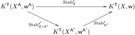
### Visual Description
\n
## Mathematical Diagram: Commutative Diagram of K-Theory Objects and Stabilizer Maps
### Overview
The image displays a mathematical commutative diagram, likely from a field such as algebraic topology, representation theory, or K-theory. It consists of three nodes (mathematical objects) connected by three directed arrows (morphisms or maps), forming a triangular structure. The diagram illustrates relationships between different K-theory objects parameterized by spaces (X) and weights (w), with maps labeled by stabilizer groups.
### Components/Axes
The diagram has no traditional axes or legends. Its components are:
1. **Nodes (Mathematical Objects):**
* **Top-Left Node:** \( K^{\mathbf{T}}(X^{\mathbf{A}}, \mathbf{w}^{\mathbf{A}}) \)
* **Top-Right Node:** \( K^{\mathbf{T}}(X, \mathbf{w}) \)
* **Bottom-Center Node:** \( K^{\mathbf{T}}(X^{\mathbf{A}'}, \mathbf{w}^{\mathbf{A}'}) \)
2. **Arrows (Maps/Morphisms):**
* **Top Horizontal Arrow:** Points from the top-left node to the top-right node. It is labeled above the arrow with \( \mathrm{Stab}_{\mathbf{e}}^{\mathbf{s}} \).
* **Left Diagonal Arrow:** Points from the top-left node to the bottom-center node. It is labeled to the left of the arrow with \( \mathrm{Stab}_{\mathbf{e}/\mathbf{e}'}^{\mathbf{s}'} \).
* **Right Diagonal Arrow:** Points from the bottom-center node to the top-right node. It is labeled to the right of the arrow with \( \mathrm{Stab}_{\mathbf{e}'}^{\mathbf{s}'} \).
### Detailed Analysis
* **Notation Transcription:**
* All nodes share the common form \( K^{\mathbf{T}}(\cdot, \cdot) \). The superscript **T** is bold. The arguments are pairs: a space (X) and a weight (w), both with superscripts.
* The superscripts on X and w are: **A** (top-left), none (top-right), and **A'** (bottom-center). The prime symbol (') is clearly visible.
* The map labels use the notation "Stab", likely an abbreviation for "Stabilizer". The subscripts and superscripts are:
* Top map: Subscript **e**, Superscript **s**.
* Left map: Subscript **e/e'**, Superscript **s'**.
* Right map: Subscript **e'**, Superscript **s'**.
* All letters in subscripts and superscripts (**T**, **A**, **e**, **s**, etc.) are rendered in a bold, sans-serif font, distinct from the italicized variables in the node arguments.
* **Spatial Layout & Flow:**
* The diagram is arranged in a triangular, commutative layout.
* The flow suggests a relationship where the map from the top-left node to the top-right node (\( \mathrm{Stab}_{\mathbf{e}}^{\mathbf{s}} \)) can be factored through the bottom node. One path is the direct top arrow. The alternative path is the composition of the left arrow (\( \mathrm{Stab}_{\mathbf{e}/\mathbf{e}'}^{\mathbf{s}'} \)) followed by the right arrow (\( \mathrm{Stab}_{\mathbf{e}'}^{\mathbf{s}'} \)).
* The central positioning of the bottom node and the converging arrows highlight its role as an intermediate or related object.
### Key Observations
1. **Commutative Structure:** The diagram is a classic commutative triangle. The core mathematical statement is that the composition of the left and right maps equals the top map: \( \mathrm{Stab}_{\mathbf{e}}^{\mathbf{s}} = \mathrm{Stab}_{\mathbf{e}'}^{\mathbf{s}'} \circ \mathrm{Stab}_{\mathbf{e}/\mathbf{e}'}^{\mathbf{s}'} \).
2. **Parameter Variation:** The nodes represent variations of a base object \( K^{\mathbf{T}}(X, \mathbf{w}) \). The top-left and bottom-center nodes are "primed" or "A"-modified versions, suggesting a change in the underlying space or weight data.
3. **Map Label Pattern:** The stabilizer maps are indexed by pairs of parameters (**e**, **s**). The left map's subscript **e/e'** suggests a quotient or relative relationship between the parameters **e** and **e'**. The right map uses the primed parameter **e'**. Both the left and right maps share the same superscript **s'**, indicating a common secondary parameter for this path.
### Interpretation
This diagram succinctly captures a relationship in equivariant K-theory or a related field. The objects \( K^{\mathbf{T}} \) are likely equivariant K-theory groups for a space with an action of a torus **T**. The parameters (X, w) define the specific space and possibly a weight or a line bundle.
The maps labeled "Stab" are induced by considering stabilizer subgroups. The diagram's commutativity implies a consistency condition: studying the stabilizer **e** of the original object is equivalent to first passing to a stabilizer **e/e'** for a modified object and then applying the stabilizer **e'**. This is a typical pattern in localization theorems or when comparing fixed-point sets under different group actions.
The notation is precise and dense. The use of bold for group names (**T**) and stabilizer parameters (**e**, **s**) versus italics for spaces (X) and weights (w) follows common mathematical typesetting conventions to distinguish between different types of entities. The diagram serves as a visual proof or definition of a relationship between these algebraic-topological constructions.
</details>
3.10. General flavour groups. Recall in Setting 2.1, we take T to be a torus. This is a simplifying condition and it can be relaxed to the following.
Setting 3.39. Let X be a smooth quasi-projective variety over C with a linear algebraic group F -action and w : X → C be an F -invariant regular function. Let A ⊆ Z ( F ) be a torus which lies in the center Z ( F ) of F .
The definition of stable envelopes (Definitions 3.4, 3.10) can be stated verbally with the torus T replaced by linear algebraic group F . Results displayed in above remain unchanged with T replaced by F .
Moreover, when stable envelopes exist, they are compatible with changing of flavour groups. Namely, if F ′ ⊆ F is a subgroup which contains A , then the following diagram commutes:
/
/
$$\begin{array}{ll}
H ^ { F } ( X , A , w ) & \xrightarrow [ \text { res } F ] { \text { Stab } e } H ^ { F } ( X , w ) \\
H ^ { F } ( X ^ { \prime } A , w ^ { \prime } ) & \xrightarrow [ \text { res } F ] { \text { Stab } e } H ^ { F } ( X , w )
\end{array}$$
/
/
where the vertical arrow is the restriction of coefficients map res F F ′ : H F ( · · · ) → H F ′ ( · · · ). There is also a similar commutative diagram for critical K -theory:
/
/
$$\begin{array}{ll}
K ^ { F } ( X ^ { A }, w ^ { A } ) & \xrightarrow [ \text { res } _ { F } ]{} K ^ { F } ( X , w ) \\
\downarrow & \downarrow \\
K ^ { F } ( X ^ { A }, w ^ { A } ) & \xrightarrow [ \text { res } _ { F } ]{} K ^ { F } ( X , w ) \\
\end{array}$$
/
/
We will use stable envelopes under Setting 3.39 to construct interpolation maps in § 9.
## 4. Cohomological stable envelopes on symmetric GIT quotients
In this section, we show that cohomological stable envelope correspondences exist for symmetric GIT quotients, given by the fundamental class of the closure [Attr(∆)] of attracting set of the diagonal (Theorem 4.3).
We prove the triangle lemma for corresponding stable envelopes (Theorem 4.16). This is done by introducing the so-called nonabelian stable envelopes (see Definition 4.18 and Theorem 4.19 for a characterization property), and a compatible diagram between stable envelopes and Hall operations (Theorem 4.22). For symmetric quiver varieties, a different proof of the existence of stable envelopes as well as the triangle lemma is discussed in [COZZ2].
As a side application, we derive an explicit formula of cohomological stable envelopes when potentials are zero (Corollary 4.25).
## 4.1. Symmetric GIT quotients.
Definition 4.1. Given the following data:
- A connected complex reductive group G , a Cartan and a Borel subgroup H ⊆ B ⊆ G ,
- Two tori A ⊆ T ,
- A finite dimensional ( G × T )-representation R such that R ∼ = R ∨ as ( G × A )-representations,
̸
- θ : G → C ∗ such that the semistable locus equals the stable locus R θ -ss = R θ -s = ∅ on which G -action is free,
we call X := R/ / θ G = R θ -s /G a symmetric GIT quotient . It is endowed with the induced action by tori T and A .
We also have the associated variety ̂ X := R θ -s × G ( G/H ) with a G/H -fibration p : ̂ X → X .
Remark 4.2. For the induced character ¯ θ : H → C ∗ , there is an open immersion ̂ X ∼ = R θ -s /H ↪ → R ¯ θ -ss /H .
The main theorem of this section is:
Theorem 4.3. Given a symmetric GIT quotient X with an action by tori T and A as Definition 4.1, fix a chamber C . Then
$$\sum \limits _ { P = F ( x ) } [ A t t _ { c } ( \Delta p ) ] e ^ { i T } ( A t t _ { c } )$$
is a cohomological stable envelope correspondence for ( X, 0 , T , A , C ).
Our main examples of symmetric GIT quotients are given by symmetric quiver varieties introduced below.
4.2. Quiver varieties. A quiver Q is a pair of finite sets Q = ( Q 0 , Q 1 ) together with two maps h, t : Q 1 → Q 0 . We will call Q 0 the set of nodes and Q 1 the set of arrows and h (resp. t ) sends an arrow to its head (resp. tail). If a ∈ Q 1 , then we will write t ( a ) → h ( a ) to denote the arrow a . We define the adjacency matrix
$$( Q _ { 1 } , i _ { 1 } e _ { 0 } ) = \frac { 1 } { 2 } ( - 1 )$$
$$( 1 ) _ { 2 } = ( 1 - a ) - ( 1 - b )$$
Take dimension vectors v ∈ N Q 0 , d = ( d in , d out ) ∈ N Q 0 × N Q 0 , the space of framed representations of Q with gauge dimension v and in-coming framing dimension d in and out-going framing dimension d out is
$$\cdots , C V _ { i } ^ { + } \oplus H o m ( C V _ { i } ^ { - } , C d _ { out, i } ^ { - } ) .$$
The gauge group G = ∏ i ∈ Q 0 GL( v i ) naturally acts on R ( Q, v , d ) by compositions with maps.
Choose a stability condition θ ∈ Q Q 0 such that θ -semistable representations are θ -stable:
̸
$$\vert B \vert = \vert A \vert = \vert C \vert = \vert D \vert$$
and define the quiver variety as the GIT quotient:
$$( Q , v , d ) / / G = R ( Q , v , d ) ^ { s } / G .$$
As we do not impose any relation on the quiver, the above space is a smooth quasi-projective variety.
We define an action of
$$G _ { i , j } E Q _ { 0 } = \sum _ { i , j } G L ( Q _ { i j } )$$
$$G _ { edge } = \boxed { \Gamma } G L ( Q _ { i } )$$
on R ( Q, v , d ): given a pair of nodes i, j ∈ Q 0 , the contribution of the edges from i to j is Hom( C v i , C v j ) ⊗ C Q ij , then the factor GL( Q ij ) naturally acts on the second component.
We also consider the following group actions on R ( Q, v , d ):
$$\begin{aligned}
( 4 . 3 ) & G _ { in } = \Pi GL ( d _ { i } , i \in Q _ { 0 } ^ { 0 } ) \\
& G _ { out } = \Pi GL ( d _ { i } , i \in Q _ { 0 } ^ { 0 } ) \\
\end{aligned}$$
We define the flavour group
$$F : = G _ { in } ^ { \prime } \times G _ { out } ^ { \prime } \times G _ { edge } .$$
It is easy to see that F ∼ = Aut G ( R ( Q, v , d )).
Definition 4.4. We say that a framing d is symmetric if d in = d out = d . In this case, we simplify the notations as
$$= R ( Q , v , d ) = R ( Q , v , d ), M _ { 0 } ( Q , v , d ) = M _ { 0 } ( Q , v , d )$$
and we define G diag fram ⊆ F to be the diagonal subgroup of G in fram × G out fram .
Definition 4.5. We say Q is symmetric if its adjacency matrix ( Q ij ) i,j ∈ Q 0 is symmetric. For a symmetric quiver Q , we call the associated quiver variety symmetric quiver variety (SQV) if the framing is symmetric.
Definition 4.6. Let ( Q, v , d ) be a symmetric quiver with symmetric framing as above. Suppose that there exists a torus H together with a linear action of H on R ( Q, v , d ). We say that a linear action of a torus H on R ( Q, v , d ) is selfdual if the H -action commutes with the gauge group G -action, and R ( Q, v , d ) is self-dual as ( G × H )-representation.
We say that a torus action H on the symmetric quiver variety M θ ( Q, v , d ) is self-dual if it is induced from a self-dual action of H on R ( Q, v , d ).
Symmetric quiver varieties with self-dual torus actions are examples of Definition 4.1, moreover their A -fixed loci are also symmetric quiver varieties as shown below.
Lemma 4.7. Suppose that X = M θ ( Q, v , d ) is a symmetric quiver variety, and A is a torus with a self-dual action on X . Let σ be a cocharacter of A , then the σ -fixed points locus X σ is a disjoint union of symmetric quiver varieties. Moreover, the induced action of A on X σ is self-dual.
and Cartan matrix
Proof. The proof is similar to that of [MO, Prop. 2.3.1]. In fact, the same argument as loc. cit. shows that
$$M _ { 0 } ( Q , v , d ) ^ { n } = \left | M _ { 0 } ( Q _ { 0 } , v _ { 0 } , d _ { 0 } ) \right | .$$
Here ϕ : C ∗ → G × A is a lift of σ : C ∗ → A along the projection G × A → A , and ( Q ϕ , v ϕ , d ϕ ) is constructed in [MO, § 2.3.3], and two lifts ϕ 1 and ϕ 2 are equivalent (denoted as ϕ 1 ∼ ϕ 2 ) if they give the same action of A on R ( Q, v , d ). The disjoint unions on the right-hand-side of (4.6) are labelled by equivalent classes of lifts ϕ . By construction, R ( Q ϕ , v ϕ , d ϕ ) is the ϕ -fixed points locus R ( Q, v , d ) ϕ , and the gauge group for Q ϕ is the ϕ -fixed points subgroup G ϕ . Since R ( Q, v , d ) is a self-dual G × A representation and C ∗ acts on it through ϕ : C ∗ → G × A , it follows that R ( Q, v , d ) ϕ is a self-dual G ϕ × A representation. Hence Q ϕ is a symmetric quiver, and the induced A -action on M θ ϕ ( Q ϕ , v ϕ , d ϕ ) is self-dual. □
## 4.3. Generalities on attracting closures.
Definition 4.8. Let ( X, A ) be in the Setting 2.1 and σ be a cocharacter of A (not necessarily generic). Denote ∆ to be the diagonal of X σ × X σ , and Attr σ (∆) to be the closure of Attr σ (∆) in X × X σ .
Consider the following condition on ( X, A , σ ):
̸
- ( ⋆ ) for all F ′ = F ∈ Fix σ ( X ), we have
$$\dim A _ { t r g } ( \Delta ) \cap ( F ^ { \prime } \times F ) < dim F$$
Let C be a chamber of ( X, A ). We say that ( X, A , C ) satisfies the condition ( ⋆ ) if for a generic ξ ∈ C , ( X, A , ξ ) satisfies the condition ( ⋆ ).
Remark 4.9. Assume moreover that dim N + F/X = dim N -F/X holds for all F ∈ Fix A ( X ), then (4.7) is equivalent to
$$F ) < \frac { 1 } { 2 } d i m ( F ^ { \prime } _ { x } F ) .$$
The condition dim N + F/X = dim N -F/X is satisfied when the tangent bundle has the following self-dual property:
$$T _ { x } = T _ { y } \in K ^ { A } ( X ) .$$
The X , ̂ X in Definition 4.1 satisfy this self-duality.
Lemma 4.10. Let ( X, T , A , C ) be in the Setting 2.1 and assume that ( X, A , C ) satisfies the condition ( ⋆ ) in Definition 4.8. Then
$$\sum \limits _ { F = F_{fix}( X ) } ^ { \infty } [ A t t _ { r } ( A _ { n } ) ] e ^ { - H ^ { \prime } ( A t t _ { r } ) }$$
is a stable envelope correspondence for ( X, 0 , T , A , C ).
Proof. It suffices to show that for every F ∈ Fix A ( X ), [Attr C (∆ F )] satisfies axioms (i) and (ii) in Definition 3.19. The axiom (i) is obvious. For axiom (ii), the class
$$( 1 ) x _ { 1 } = x _ { 2 } \times ( \sqrt { 1 + b ^ { 2 } } - \sqrt { 1 - b ^ { 2 } } )$$
is supported on a subvariety Attr C (∆ F ) ∩ ( F ′ × F ) of dimension smaller than dim F +rk N + F/X -rk N + F ′ /X . Note that dim F +rk N + F/X = dimAttr C (∆ F ). Therefore
This verifies the axiom (ii).
□
4.4. Generalities on family of smooth symplectic varieties. Let ( X, A ) be in the Setting 2.1 and let σ be a cocharacter of A . Suppose that there exists an A -invariant two-form ω ∈ Ω 2 ( X ), and there exists a smooth connected variety B endowed with trivial A -action and a smooth and A -equivariant morphism ϕ : X → B , such that ∀ b ∈ B , the restriction of ω to X b := ϕ -1 ( b ) is nondegenerate, i.e. a symplectic structure .
We note that Attr σ (∆) ⊆ X × B X σ because ∆ ⊆ X × B X σ and ϕ : X → B is A -equivariant. Then it follows that Attr σ (∆) ⊆ X × B X σ . We also have dim N + F/X = dim N -F/X holds for all F ∈ Fix A ( X ) in this case.
Lemma 4.11. In the above situation, for all F, F ′ ∈ Fix σ ( X ) and for all b ∈ B we have
$$\frac { \frac { 1 } { dim ( F ^ { \prime } _ { b } ) } } { n ( F ^ { \prime } _ { b } \times F _ { b } ) } < - 1 ,$$
where F b = F ∩ ϕ -1 ( b ) and F ′ b = F ′ ∩ ϕ -1 ( b ).
Proof. We consider the two-form ω ′ := ω ⊟ ω σ on X × X σ , then the restriction of ω ′ to every fiber X b × X σ b is a symplectic form. We claim that Attr σ (∆) ∩ ( X b × X σ b ) is an isotropic subvariety in X b × X σ b . To prove this claim, first note that the restriction of ω ′ to ∆ is trivial by the construction of ω ′ . Since ω ′ is A -invariant, its restriction to Attr σ (∆) must vanish as well. Thus the restriction of ω ′ to smooth locus of Attr σ (∆) vanishes by continuity. Let W be an irreducible component of Attr σ (∆) ∩ ( X b × X σ b ). For a general point w ∈ W , there exists a sequence of points x 1 , x 2 , · · · in the smooth locus of Attr σ (∆) approaching w such that limit of T x i Attr σ (∆) exists as i → ∞ and contains the tangent space T w W 9 . Since the restriction of ω ′ to T x i Attr σ (∆) vanishes, our claim follows.
Then it follows that Attr σ (∆) ∩ ( F ′ b × F b ) is an isotropic subvariety in F ′ b × F b by [MO, Lem. 3.4.1]. Thus
$$\dim \limits _ { F _ { b } } ( \Delta ) \cap ( F _ { b } ^ { \prime } \times$$
Lemma 4.12. In the same situation as Lemma 4.11, assume moreover that there exists an open dense subset B ◦ ⊆ B such that ϕ | X ◦ : X ◦ → B ◦ is a quasi-affine morphism where X ◦ := ϕ -1 ( B ◦ ). Then ( X, A , σ ) satisfies the condition ( ⋆ ) (4.7).
Proof. For every x ∈ X σ , the tangent map dϕ x : T x X → T ϕ ( x ) B is surjective by the assumption that ϕ : X → B is smooth. dϕ x is also σ -equivariant since ϕ is σ -equivariant. Then it follows that dϕ x maps T x X σ = ( T x X ) σ surjectively onto T ϕ ( x ) B , so the restriction of ϕ to σ -fixed loci ϕ σ : X σ → B is also smooth. In particular, ϕ σ is flat. The flatness of ϕ σ implies that ∀ F ∈ Fix σ ( X ) and any b ∈ ϕ ( F ), we have
$$d m l = d m h + d m k$$
For F ′ = F ∈ Fix σ ( X ), let F ′◦ := F ′ ∩ X ◦ and F ◦ := F ∩ X ◦ . We claim that
$$\overline { A B C D } ( F ^ { 2 } \times F ^ { 3 } ) = 0$$
Without loss of generality, we assume that B ◦ is affine, then X ◦ and ( X ◦ ) σ are quasi-affine. Let ∆ ◦ be the diagonal of ( X ◦ ) σ × ( X ◦ ) σ , then Attr σ (∆ ◦ ) is closed in X ◦ × ( X ◦ ) σ 10 . Therefore
$$\frac { \sqrt { 1 } } { x ^ { 0 } } = A t r _ { 0 } ( \Delta ) ,$$
hence Attr σ (∆) ∩ ( F ′◦ × F ◦ ) = ∅ . In the general case we can cover B ◦ with affine open subsets and apply the above argument to each of the affine open subset. This proves our claim.
Finally, we have the following dimension bound:
$$\begin{array}{ll}
\dim Attr_0(\Delta) \cap (F^b \times F_b) & < dim(B) \\
\hline
By Lem. 4.11 & \leq dim(B) \\
\hline
& \leq \frac{1}{2} dim(F) \\
\hline
\end{array}
as that (X, A, σ) satisfies the condition (×)(4.7).$$
This shows that ( X, A , σ ) satisfies the condition ( ⋆ ) (4.7).
9 This can be seen by choosing a Whitney stratification of Attr σ (∆) for which Attr σ (∆) ∩ ( X b × X σ b ) is a union of strata.
□
10 Taking a finite set of A -homogeneous generators of C [ X ◦ × ( X ◦ ) σ ], we get a surjective A -equivariant algebra map C [ V ] ↠ C [ X ◦ × ( X ◦ ) σ ] where V is a vector space with a linear A -action. Equivalently we get an A -equivariant closed embedding X ◦ × ( X ◦ ) σ ↪ → V . We note that Attr σ ( V σ ) = V ⩾ 0 where V ⩾ 0 is the linear subspace of V spanned by nonnegative σ -eigenvectors, in particular Attr σ ( V σ ) is closed in V . We also note that Attr σ (∆ ◦ ) = p -1 (∆ ◦ ) ∩ ( X ◦ × ( X ◦ ) σ ), where p : V ⩾ 0 → V σ is the attraction map and ∆ ◦ is regarded as a closed subset of V σ . Thus Attr σ (∆ ◦ ) is closed in X ◦ × ( X ◦ ) σ .
̸
4.5. Proof of Theorem 4.3. We first show that the attracting closure for the diagonal of ̂ X in Definition 4.1 is a stable envelope correspondence.
## Lemma 4.13.
$$\sum _ { P \in F ( x ) } [ A t t _ { r } ( \Delta _ { n } ) ] e ^ { H ^ { T } ( A t t _ { r } ) }$$
is a stable envelope correspondence for ( ̂ X, 0 , T , A , C ).
Proof. Since R ∼ = R ∨ as H -representations, we have an isomorphism of H -representations:
$$R _ { 2 } = T ^ { \prime } N e R _ { 0 }$$
where N = ⊕ α =0 C α and R 0 is a trivial H -representation. In particular, there is a moment map
$$1 0 . 7 ^ { \prime } N - 3 6 ^ { \prime }$$
Define ν : R = T ∗ N × R 0 µ × id - - - → h ∗ × R 0 , then the restriction of ν to R θ -s is smooth. By passing to the quotient, we obtain a smooth map
$$i : x \rightarrow f ^ { \prime } ( x )$$
and for any x ∈ h ∗ × R 0 , ¯ ν -1 ( x ) is a smooth symplectic variety.
For a generic x ∈ h ∗ × R 0 , we have ν -1 ( x ) ⊆ R ¯ θ -s ; therefore ¯ ν -1 ( x ) is an open subset of ν -1 ( x ) / /H , in particular ¯ ν -1 ( x ) is quasi-affine. By Lemma 4.12, we know (4.8) holds for ̂ X = R θ -s × G ( G/H ) in Definition 4.1. By applying Lemma 4.10, we are done. □
Next we want to relate the geometry of ̂ X and X . We define X := R s × G ( G/B ) and have fibrations:
$$x : x ^ { \prime } \rightarrow x ^ { \prime } \rightarrow x .$$
For any S ∈ Fix A ( X ), which is given by S = ( R A ,ϕ ∩ R θ -s ) /G ϕ ( A ) for a group homomorphism ϕ : A → G , we define
$$S := ( R ^ { A } _ { 0 } \cap R ^ { B } _ { 0 } ) \times G ^ { C } _ { 0 } ( A ) ($$
with natural morphisms
̸
$$q : S \rightarrow S \frac { q } { 2 } , S$$
̸
Proposition 4.14. For any S, S ′ ∈ Fix A ( X ) with S = S ′ , we have
$$\deg A ( S ^ { \prime } \times S ^ { - 1 } \rightarrow X \times S )$$
In particular, this finishes the proof of Theorem 4.3.
$$\begin{aligned}
& \text{Proof.} Let } Z := \overline { A t t r ( \Delta s ) } , Z = ( p _ { 2 } ) \\
& \times q _ { 2 } ^ { - 1 } ( Z ) , \overline { Z } = ( p \times q ) ^ { - 1 } ( Z ) . Then
\end{aligned}$$
$$\overline { A t r ( \Delta g ) } = Z .$$
By Weyl conjugation, we choose ϕ : A → G such that N S/p -1 2 ( S ) are repelling in chamber C . We have
$$( p _ { 1 } \times q ) ^ { ! } : H ^ { T } ( Z ) \xrightarrow [ \sum ] { H ^ { T } ( Z ) }$$
Here p 1 , q 1 are U -fibrations where B = H · U and U is a unipotent group, p 2 , q 2 are proper maps as G/B is proper.
Consider the composition:
$$( 4 . 9 )$$
By A -localization, we have
$$( S ^ { \prime } \times S - X \times S ) ^ { n _ { x } }$$
$$= \sum _ { s = s _ { 1 } } ^ { S } \sum _ { s = s _ { 2 } } ^ { S } \cdots \sum _ { s = s _ { T } } ^ { S } ( \frac { 1 } { e ^ { T } ( N _ { S } ) ^ { S } } - 1 )$$
where the sum is taken over all A -fixed components { ̂ S ′ i } i of p -1 ( S ′ ). Therefore by Lemma 4.13, we have
$$\sum _ { s \in S } ( \sqrt { \frac { 1 } { p _ { 2 } ^ { - 1 } ( s ) } } - r k N _ { s } \{ p _ { 2 } ^ { - 1 } ( s ) \}$$
Finally, Lemma 4.15 below finishes the proof.
Lemma 4.15. In (4.9), we have
$$n ( \overline { A t t r e } ( \Delta s ) ) = | W ^ { n } |$$
Proof. By dimension counting, we have η ( [Attr C (∆ ̂ S )] ) ∈ H T top ( Z ); therefore
$$\sqrt { ( \sqrt { 1 + b } - 1 ) ^ { 2 } } = \sqrt { ( \sqrt { 1 + b } - 1 ) ^ { 2 } }$$
for some λ ∈ Z , which we compute by restricting above to S × S . By A -localization, we have
$$\begin{aligned}
( S \times S - X \times S ) ^ { n \times } _ { r k N } & = ( S \times S - s \times s ) ( e ^ { i \frac { 2 \pi } { r k N } } - e ^ { - i \frac { 2 \pi } { r k N } } ) \\
& = | W ^ { r k N } | \cdot ( - 1 ) ^ { r k N } \\
& = | W ^ { r k N } | \cdot (- 1)^{r k N}
\end{aligned}$$
This implies that λ = | W ϕ | · ( -1) rk N S/p -1 2 ( S ) and we are done.
□
4.6. Triangle lemma for cohomological stable envelopes. Let X = R/ / θ G be a symmetric GIT quotient and A ⊆ T be the tori as in Definition 4.1. We fix a chamber C and a face C ′ , and let A ′ ⊆ A be the subtorus associated with C ′ . Then X A ′ is disjoint union of symmetric GIT quotients, so there exists cohomological stable envelope correspondence for ( X A ′ , 0 , T , A , C / C ′ ) by Theorem 4.3. Consider the induced stable envelopes for a T -invariant function w on X , and we have the following triangle lemma.
Theorem 4.16. Using the above notation, the following diagram is commutative
/
/
<details>
<summary>Image 3 Details</summary>
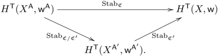
### Visual Description
\n
## Mathematical Diagram: Commutative Stability Mapping
### Overview
The image displays a commutative diagram from mathematical optimization or machine learning theory, illustrating relationships between different problem formulations and their stability properties. The diagram consists of three nodes connected by directed arrows, each labeled with a stability mapping.
### Components/Axes
The diagram is structured as a triangle with three nodes and three connecting arrows:
**Nodes (Mathematical Expressions):**
1. **Top-Left Node:** \( H^{\top}(X^A, \mathbf{w}^A) \)
2. **Top-Right Node:** \( H^{\top}(X, \mathbf{w}) \)
3. **Bottom Node:** \( H^{\top}(X^{A'}, \mathbf{w}^{A'}) \)
**Arrows (Mappings):**
1. **Horizontal Arrow (Top-Left to Top-Right):** Labeled "Stab\(_\epsilon\)".
2. **Diagonal Arrow (Top-Left to Bottom):** Labeled "Stab\(_{\epsilon/\epsilon'}\)".
3. **Diagonal Arrow (Bottom to Top-Right):** Labeled "Stab\(_{\epsilon'}\)".
**Spatial Grounding:**
* The diagram is centered on a white background.
* The three nodes form an inverted triangle: two nodes are aligned horizontally at the top, and the third node is centered below them.
* The arrows are straight lines with arrowheads pointing to the target node. The labels are placed approximately at the midpoint of each arrow.
### Detailed Analysis
The diagram defines a relationship between three instances of a function or set \( H^{\top} \), each parameterized by a pair \((X, \mathbf{w})\). The superscripts \(A\) and \(A'\) denote different variants or approximations of the primary parameters \((X, \mathbf{w})\).
The arrows represent "Stab" (stability) mappings, parameterized by values \(\epsilon\) and \(\epsilon'\). The structure implies that applying the stability mapping Stab\(_\epsilon\) directly from the top-left to the top-right node is equivalent to following the path through the bottom node: first applying Stab\(_{\epsilon/\epsilon'}\) and then Stab\(_{\epsilon'}\). This is the defining property of a commutative diagram.
### Key Observations
1. **Notation:** The use of bold \(\mathbf{w}\) typically denotes a vector, while \(X\) may represent a dataset, design matrix, or another structured input. \(H^{\top}\) could represent a hypothesis class, a loss function, or a set of optimal solutions.
2. **Hierarchy of Approximations:** The diagram suggests a hierarchy where \((X^A, \mathbf{w}^A)\) is an approximation of \((X^{A'}, \mathbf{w}^{A'})\), which in turn is an approximation of the original \((X, \mathbf{w})\). The stability mappings quantify how properties (like solutions or generalization bounds) are preserved under these approximations.
3. **Parameterized Stability:** The stability mappings are not generic but are controlled by specific parameters (\(\epsilon\), \(\epsilon'\), and their ratio \(\epsilon/\epsilon'\)). This indicates a precise, quantifiable relationship between the approximation errors.
### Interpretation
This diagram is a formal representation of a **stability-based approximation guarantee**. It visually encodes a theorem stating that if a problem defined by \((X^A, \mathbf{w}^A)\) is stable under the mapping Stab\(_{\epsilon/\epsilon'}\) to an intermediate approximation \((X^{A'}, \mathbf{w}^{A'})\), and that intermediate form is stable under Stab\(_{\epsilon'}\) to the final form \((X, \mathbf{w})\), then the original problem is stable under the composed mapping Stab\(_\epsilon\).
**What it means:** In practical terms, this could be used to prove that an efficient algorithm solving an approximate problem (top-left) will produce a solution that is close (within \(\epsilon\)) to the solution of the true, harder problem (top-right). The path through the bottom node provides a way to decompose and analyze the total error \(\epsilon\) into two controllable components, \(\epsilon'\) and \(\epsilon/\epsilon'\). This is a common technique in theoretical computer science and statistical learning theory to establish robustness and generalization bounds for algorithms.
</details>
Theorem 4.16 will be proven in steps.
Step 1. We formulate a nonabelian stable envelope for symmetric quotient stack X = [ R/G ], to this end, we will need the following lemma.
Lemma 4.17. Consider the closure of the diagonal ∆ X in X × X , denoted ∆ X . Then the projection from ∆ X to X is representable and proper.
Proof. We have the following explicit construction of ∆ X as a quotient stack. Consider the graph
$$C _ { \textcircled { 1 } } ^ { \textcircled { 1 } } ( r ) c X _ { \textcircled { 1 } } ^ { \textcircled { 1 } }$$
of quotient map q : R θ -s → X , and take the closure of Graph( q ) in X × R , denoted by Graph( q ). Then
$$\Delta x = ( G _ { r } p h ( o ) / C l .$$
This implies that ∆ X → X is representable. Take X 0 = R/ /G = Spec C [ R ] G to be the affine quotient, then the natural projection π : X → X 0 is projective. Note that the composition π ◦ q : R θ -s → X 0 extends to the quotient map Q : R → X 0 , so π × id: X × R → X 0 × R maps Graph( q ) to Graph( Q ). In particular, the projection Graph( q ) → R factors as a proper morphism Graph( q ) → Graph( Q ) followed by an isomorphism Graph( Q ) ∼ = R ; thus Graph( q ) → R is proper. This implies that ∆ X → X is representable and proper. □
Since the function w ⊟ w vanishes on ∆ X , the fundamental class [∆ X ] induces a correspondence map between critical cohomologies.
'
'
$$= - \frac { 1 } { 2 } k N _ { s / x } ^ { 7 } - \frac { 1 } { 2 } k N _ { s / ( p - 1 ) ( s ) }$$
$$= - r k N _ { S } ^ { 2 } / x - - r k N _ { S } ^ { 2 }$$
Definition 4.18. We call the induced map
$$\begin{array}{ll}
\Phi _ { i , j } H ^ { I } ( X , w ) \rightarrow H ^ { I } ( X , w ) \\
\end{array}$$
by [∆ X ], a (cohomological) nonabelian stable envelope .
It turns out that Ψ H admits a characterization in terms of a degree bound condition similar to that of stable envelopes. For any nonzero cocharacter σ : C ∗ → G , let R σ ⊂ R be the fixed subspace with respect to the induced C ∗ -action and G σ ⊂ G be the σ -fixed subgroup of G . Define X σ := [ R σ /G σ ], and denote
$$j _ { 0 } : x ^ { x } \rightarrow x$$
the natural map between quotient stacks.
Theorem 4.19. Ψ H is the unique H T (pt)-linear map from H T ( X, w ) to H T ( X , w ) that satisfies the following:
- res ◦ Ψ H = id, where res: H T ( X , w ) → H T ( X, w ) is the map induced by restriction from X to the open substack X ,
- for all nonzero cocharacter σ : C ∗ → G , the inequality
$$\begin{aligned}
& \deg _ { 8 g } j _ { 0 } ^ { 1 } \varphi ( r ) < - \frac { 1 } { 6 } ( \dim x - \dim x ^ { 3 } ) \\
& \Rightarrow \deg _ { 8 g } j _ { 0 } ^ { 1 } \varphi ( r ) < - \frac { 1 } { 6 } ( \dim x - \dim x ^ { 3 } )
\end{aligned}$$
$$\deg _ { 6 } i ^ { 3 } P _ { H } ( r ) < \frac { 1 } { 2 } ( \lim _ { r \rightarrow 0 } P _ { H } - \lim _ { r \rightarrow 0 } P _ { H } ^ { 4 } )$$
holds for all γ ∈ H T ( X, w ). Here deg σ is the polynomial degree in H C ∗ (pt) in the decomposition H T ( X σ , w ) ∼ = H T × G σ /σ ( C ∗ ) ( R σ , w ) ⊗ H C ∗ (pt).
Theorem 4.19 will be used in the proof of Theorem 4.22 below, and will be proven in Section 4.7.
Step 2. We introduce a Hall operation relating critical cohomology of ' A -fixed' stack of X to that of X , and compare it with the stable envelope. Take a group homomorphism
$$\phi : A \rightarrow G$$
define R A ,ϕ to be the A -fixed subspace of R where A acts via A (id ,ϕ ) -- - → A × G ↷ R , and define
$$\frac { m ^ { 2 } A _ { 0 } } { k ^ { 2 } } = \vert P A _ { 0 } \vert ( g ^ { 2 } ) A _ { 1 }$$
where G ϕ ( A ) is the subgroup of G fixed by adjoint action of ϕ ( A ). We assume that the stable locus R A ,ϕ ∩ R θ -s is nonempty, so the GIT quotient X A ,ϕ := R A ,ϕ / / θ G ϕ ( A ) is a connected component of A -fixed loci X A . Note that all connected components of X A arises in this way, and we have
$$x ^ { A } = \left | x _ { A , \phi } \right |$$
where the sum is taken for all homomorphisms ϕ : A → G modulo the equivalence relation: ϕ 1 ∼ ϕ 2 if and only if they give the isomorphic ( G × A )-module structures on R .
We define a map m ϕ C : H T ( X A ,ϕ , w ) → H T ( X , w ), according to a choice of chamber C , as follows. Let
$$L _ { G } ^ { \phi } = A t t r e ( R ^ { \phi } A ) c R ,$$
where L ϕ C is a linear subspace of R , and P ϕ C is a parabolic subgroup of G . There are maps
o
$$R A _ { 0 } ^ { \circ } < - I C _ { 0 } ^ { \circ } < R _ { 0 }$$
o
/
/
where q is the attraction map and p is the inclusion. Then P ϕ C naturally acts on L ϕ C and maps p , q are P ϕ C -equivariant, where P ϕ C -action on R is via P ϕ C ⊆ G and P ϕ C -action on R A ,ϕ is via the contraction map P ϕ C → G ϕ ( A ) . Therefore we get a diagram
$$x ^ { A _ { 0 } } \rightarrow q ^ { g _ { 0 } } x ^ { L _ { 0 } } = [ p _ { 0 } / P ^ { e } ] ^ { p } \rightarrow x .$$
where q is smooth and p is proper.
Definition 4.20. We define the Hall operation
$$\rho _ { c } ^ { \phi } = p _ { c } q ^ { \ast } : H ^ { T } ( x , w ) .$$
o
o
/
/
$$- 3 ^ { \circ } = 1 2 ^ { \circ } / P ^ { \circ }$$
Remark 4.21. Let ˜ L ϕ C := G × P ϕ C L ϕ C and ˜ p : ˜ L ϕ C → R be the natural morphism induced by the G -action. Then there are natural isomorphisms:
$$\int _ { p e } ^ { G } H T \times P ^ { e } ( L ^ { e } _ { c } , w ) = H T \times G ( L ^ { e } _ { c } , w ) .$$
Note that the inverse of ind G P ϕ C is given by i ∗ ◦ res G P ϕ C , where i : L ϕ C ↪ → ˜ L ϕ C is the closed immersion induced by P ϕ C ↪ → G and res G P ϕ C is the base change functor that takes G -equivariant cohomology to the P ϕ C -equivariant counterpart. Using the Cartesian diagram
/
/
$$\begin{array}{ccc}
L^0_e & \xrightarrow[p]{} R \\
- /G & \Box & - /G \\
L^0_e & \xrightarrow[q]{} x,
\end{array}$$
the Hall operation can be rewritten as
$$( R ^ { \phi } _ { A , \phi } , w ) \rightarrow H ^ { T } \times G ( R , w ).$$
Theorem 4.22. The following diagram is commutative
O
O
$$\begin{array}{ll}
H ^ { T } ( X _ { A , \phi }, w ) & H ^ { T } ( X , w ) \\
\downarrow & \downarrow \\
\Psi ^ { H }_H & \Psi ^ { H }_H \\
\downarrow & \downarrow \\
H ^ { T } ( X _ { A , \phi }, w ) & H ^ { T } ( X , w ),
\end{array}$$
/
/
where the left vertical arrow is the map Ψ H for the stack X A ,ϕ .
We will prove Theorem 4.22 in Section 4.8.
Step 3. To finish the proof of Theorem 4.16, consider the following diagram on a triangular prism:
O
O
/
/
<details>
<summary>Image 4 Details</summary>
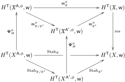
### Visual Description
## Mathematical Commutative Diagram: Stability and Transformation Relationships
### Overview
The image displays a commutative diagram from advanced mathematics, likely within the fields of homotopy theory, category theory, or algebraic topology. It illustrates the relationships and transformations between several mathematical objects denoted by `H^T` with various arguments. The diagram is structured as a network of nodes connected by labeled arrows, indicating mappings or operations that commute.
### Components/Axes
The diagram is composed of **nodes** (mathematical objects) and **directed edges** (arrows representing mappings). There are no traditional axes, as this is not a data chart.
**Nodes (Objects):**
The objects are all of the form `H^T(·, w)`, where the first argument varies. The distinct nodes are:
1. `H^T(x^{A,φ}, w)` (Top-left)
2. `H^T(x, w)` (Top-right)
3. `H^T(x^{A',φ}, w)` (Center)
4. `H^T(X^{A,φ}, w)` (Middle-left)
5. `H^T(X, w)` (Middle-right)
6. `H^T(X^{A',φ}, w)` (Bottom-center)
**Edges (Mappings/Arrows):**
Each arrow is labeled with a specific mathematical operation or map. The labels are:
* `m_ε^φ`
* `m_{ε/ε'}^φ`
* `m_{ε'}^φ`
* `Ψ_H^φ` (appears twice)
* `Stab_ε`
* `Stab_{ε/ε'}`
* `Stab_{ε'}`
* `res`
### Detailed Analysis
The diagram is organized into three approximate horizontal layers or rows, with vertical and diagonal connections.
**Top Row (Objects with lowercase 'x'):**
* From `H^T(x^{A,φ}, w)` (top-left), a horizontal arrow labeled `m_ε^φ` points right to `H^T(x, w)` (top-right).
* From `H^T(x^{A,φ}, w)` (top-left), a diagonal arrow labeled `m_{ε/ε'}^φ` points down-right to `H^T(x^{A',φ}, w)` (center).
* From `H^T(x^{A',φ}, w)` (center), a diagonal arrow labeled `m_{ε'}^φ` points up-right to `H^T(x, w)` (top-right).
**Middle/Bottom Rows (Objects with uppercase 'X'):**
* A vertical arrow labeled `Ψ_H^φ` points **up** from `H^T(X^{A,φ}, w)` (middle-left) to `H^T(x^{A,φ}, w)` (top-left).
* A horizontal arrow labeled `Stab_ε` points right from `H^T(X^{A,φ}, w)` (middle-left) to `H^T(X, w)` (middle-right).
* A vertical arrow labeled `Stab_{ε/ε'}` points **up** from `H^T(X^{A',φ}, w)` (bottom-center) to `H^T(X^{A,φ}, w)` (middle-left).
* A diagonal arrow labeled `Stab_{ε'}` points up-right from `H^T(X^{A',φ}, w)` (bottom-center) to `H^T(X, w)` (middle-right).
* A vertical arrow labeled `Ψ_H^φ` points **up** from `H^T(X^{A',φ}, w)` (bottom-center) to `H^T(x^{A',φ}, w)` (center).
**Right-Side Connection:**
* A vertical arrow labeled `res` points **down** from `H^T(x, w)` (top-right) to `H^T(X, w)` (middle-right).
### Key Observations
1. **Commutative Structure:** The diagram is designed to be commutative. This means that following any two paths of arrows from one node to another should yield the same result. For example, the path from `H^T(x^{A,φ}, w)` to `H^T(x, w)` can be taken directly via `m_ε^φ` or indirectly via `m_{ε/ε'}^φ` followed by `m_{ε'}^φ`.
2. **Dual Families of Maps:** There appear to be two parallel families of operations:
* **`m` maps:** These connect the objects with lowercase `x` arguments (top row and center).
* **`Stab` maps:** These connect the objects with uppercase `X` arguments (middle and bottom rows). The names `Stab_ε`, `Stab_{ε/ε'}`, and `Stab_{ε'}` strongly suggest these are "stability" maps parameterized by `ε` and `ε'`.
3. **Connecting Morphisms (`Ψ_H^φ` and `res`):** The maps `Ψ_H^φ` act as bridges between the `X`-family and the `x`-family of objects. The `res` (likely "restriction") map connects the final objects of the two families, `H^T(x, w)` and `H^T(X, w)`.
4. **Parameterization:** The objects and maps are heavily parameterized by symbols `A`, `A'`, `φ`, `ε`, and `ε'`, indicating a complex structure where properties depend on these choices. The notation `x^{A,φ}` suggests `x` is being modified or acted upon by `A` and `φ`.
### Interpretation
This diagram is a formal representation of relationships in a mathematical theory involving stability conditions. It likely demonstrates how different "stabilization" procedures (`Stab` maps) on objects `X` (perhaps spaces or spectra) relate to corresponding operations (`m` maps) on related objects `x` (perhaps their "underlying" or "linearized" versions).
The core message is one of **coherence**: the process of stabilizing an object and then relating it to another is equivalent to first relating the objects and then stabilizing. The `Ψ_H^φ` maps ensure that the operations on the `X` level are compatible with those on the `x` level. The `res` map provides a final link, possibly showing that the stabilized version of the related object is a restriction of the related stabilized object.
The presence of primed and unprimed parameters (`A`/`A'`, `ε`/`ε'`) suggests the diagram is proving a property that holds under a change of parameters or a refinement of the structure. It is a classic "chase the diagram" proof structure, where the commutativity asserts the consistency of the entire algebraic or topological system being studied.
</details>
'
'
By Theorem 4.22, the right, the backward, and the left squares are commutative. The upper triangle is commutative because Hall operations are associative. These imply the commutativity of the lower triangle.
4.7. Proof of Theorem 4.19. The equality res ◦ Ψ H = id is obvious from the definition of (4.10).
4.7.1. Degree bound. To show that Ψ H satisfies the degree bound condition (4.11), it is enough to show:
$$\begin{aligned}
& \deg _ { g } ( j _ { 0 } \times id ) ^ { \prime } [ \overline { A x } ] < - 1 _ { 2 } ( dim R ^ { g } _ { 0 } - m o v i n g ) , \\
& - \dim Lie( G ) ^ { g } _ { 0 } - m o v i n g ),
\end{aligned}$$
where ( j σ × id) ! [∆ X ] is the pullback of the fundamental class of ∆ X along the map j σ × id : X σ × X → X × X , which is an element in H T ( X σ × X ∆ X ).
We first prove a similar statement for the abelian quotient. Define ̂ X := [ R/H ] and consider the diagonal
$$\Delta _ { x } C X \times X .$$
'
'
O
O
/
/
/
/
O
O
/
/
Take its closure ∆ ̂ X in ̂ X × ̂ X . Without loss of generality, we assume that image of σ is contained in H , and let
$$b _ { n } x ^ { n } = b _ { 0 } / | n | - x$$
$$< 2 ^ { - \dim R _ { 0 } - moving } ,$$
be the natural map.
Lemma 4.23. We have
$$\deg ( g _ { 0 } \times id ) [ \Delta x ] < \frac { 1 } { 2 } dim R ^ { p - moving }$$
where ( ̂ j σ × id) ! [∆ ̂ X ] is the pullback of the fundamental class of ∆ ̂ X along the map ̂ j σ × id : ̂ X σ × ̂ X → ̂ X × ̂ X , which is an element in H T ( ̂ X σ × ̂ X ∆ ̂ X ) .
Proof. Consider the graph of the quotient map ̂ q : R θ -s → ̂ X :
$$G r a p h ( f ) c X \times R ^ { k } = ,$$
and take the closure of Graph( ̂ q ) in ̂ X × R , denoted by Graph( ̂ q ). Then ∆ ̂ X = [Graph( ̂ q ) /H ], and
$$H ^ { \prime } ( x ^ { 0 } _ { x } \Delta x ) = H ^ { \prime } ( x )$$
To prove (4.16), it suffices to show
$$\frac { 1 } { q } - \frac { 1 } { 2 } dim R ^ { p } - moving < dim Graph ( q ) + c q >$$
where the right-hand-side is the homological degree of ( ̂ X × R σ ↪ → ̂ X × R ) ! [Graph( ̂ q )]. It is elementary to see that the above inequality is equivalent to
$$1 2 ( dim R + dim R ^ { \prime } ) .$$
Since R ∼ = R ∨ as H -representations, we have an isomorphism of H -representations:
$$R = T ^ { \prime } N e R _ { 0 }$$
where N is a direct sum of nontrivial weight spaces and R 0 is a trivial H -representation. Define
$$x _ { 1 } R = x ^ { \prime } R \times R _ { 0 } - \frac { 1 2 x ^ { 3 } h } { R _ { 0 } } \times R _ { 6 }$$
where µ : T ∗ N → h ∗ is the moment map, then the restriction of ν to R θ -s is smooth. By passing to the quotient, we obtain a smooth map
$$i : x \rightarrow f ^ { \prime } ( x )$$
and for any ( x, y ) ∈ h ∗ × R 0 , ¯ ν -1 ( x, y ) is a smooth symplectic variety. Let pr: R → R 0 be the projection, then Graph( ̂ q ) is contained in (¯ ν × pr) -1 ( h ∗ × ∆ R 0 ) ⊂ ̂ X × R .
For any ( x, y, y ) ∈ h ∗ × ∆ R 0 , we have a Lagrangian:
$$p h ( q ) \subseteq v ^ { - 1 } ( x , y ) \times T ^ { N } N .$$
After taking the closure, we get a Lagrangian
$$\rho h ( q ) \leq v ^ { - 1 } ( x , y ) \times T ^ { N } .$$
Let pr σ : R σ = T ∗ N σ × R 0 → R 0 be the projection. Using the same argument as Lemma 4.11,
$$\phi ( q ) \subseteq v ^ { - 1 } ( x , y ) \times T ^ { * } N ^ { o }$$
is isotropic, and we have
$$\dim ( \overline { \psi } \times p ^ { r } ) ^ { - 1 } ( x , y , z ) \cap$$
There exists a dense open subset U ⊂ h ∗ such that µ -1 ( U ) ⊆ ( T ∗ N ) ¯ θ -s . It follows that ν -1 ( U × R 0 ) ⊆ R ¯ θ -s . We note that Graph( ̂ q ) is contained in the closed subset ̂ X × h ∗ × R 0 R , so Graph( ̂ q ) ⊆ ̂ X × h ∗ × R 0 R . Therefore,
$$\frac { ( v - 1 ) ( U \times R _ { 0 } ) \times R ^ { 2 } } { R ^ { 3 } } \cap G _ { R }$$
Since R σ ∩ R ¯ θ -s = ∅ , we see that
$$( i x _ { p r } ^ { n } ) ^ { - 1 } ( i x _ { q r } ) \sqrt [ n ] { | G _ { a p h } ( q ) | } = 0$$
for all ( x, y, y ) ∈ U × ∆ R 0 . As a result, we have
$$\dim ( X \times R ^ { n } ) \cap \left\{ \Graph( \hat{g} ) \right\} < 1 . This proves (4.17).$$
This proves (4.17).
Next, we deduce (4.15) from (4.16). An argument similar to Lemma 4.15 shows that
$$\left | W \cdot ( - 1 ) ^ { i } \cdot [ \Delta x ] \right | = \vert W \cdot ( - 1 ) ^ { i } \cdot [ \Delta x ] \vert$$
Here η ̂ X × ̂ X → X × X is defined for the G/H × G/H -bundle ̂ X × ̂ X → X × X by η ̂ X × ̂ X → X × X = ( p 2 × p 2 ) ∗ ◦ ( ( p 1 × p 1 ) ! ) -1 , where
$$\begin{aligned}
p : X ^ { \hat { p } } \rightarrow X := R ^ { 0 } _ { B } x ( G / B ) ^ { \hat { p } } & =$$
are the natural projections.
Define ˜ j σ : ˜ X σ := X σ × X ̂ X → ̂ X the pullback of j σ to ̂ X , then by base change we have
$$( j _ { 0 } \times i d ) ^ { n _ { x } } \pi _ { x } \times x - x \times x ( [ \Delta x ] ) = n _ { x } \times x$$
We compute η ˜ X σ × ̂ X → X σ × X as follows. Note that
$$x ^ { 2 } = \vert P ^ { 2 } _ { x _ { 0 } } G / H _ { 1 } \vert .$$
Here R σ × G σ G is the quotient of R σ × G by the diagonal action of G σ , where G σ acts on R σ naturally and acts on G by left multiplication. R σ × G σ G has a right H -action on G , and [ R σ × G σ G/H ] is the quotient stack. We notice that for every w ∈ W σ \ W ( W and W σ are Weyl groups of G and G σ respectively), ̂ X w -1 ( σ ) is naturally a closed substack of ˜ X σ via the embedding
$$\sum _ { G ^ { w } \cdot w / H } ^ { \infty } [ R ^ { w } ( σ ) / H ] \approx [ R ^ { w } x _ { G ^ { w } } G / H ] \approx x ^ { w } .$$
Therefore, after H C ∗ (pt)-localization, we have
$$\sum _ { w \in W } ^ { ( \cdots ) } x _ { w } - 1 ( x _ { w } - 1 ( x _ { w } - x _ { w } ^ { ( \cdots ) } ) = \frac { ( x _ { w } ^ { ( \cdots ) } - 1 ) } { \sqrt { \frac { 1 } { N _ { w } } } }$$
Here N w is the normal bundle of [ R σ × G σ P σ · w/B ] in [ R σ × G σ G/B ], where P σ = Attr + ( G σ ) is a parabolic subgroup of G . Note that σ fixes R σ × G σ · w/H , and N w is σ -moving with
$$r k N _ { w } = \dim G / P _ { 0 } =$$
Thus η ̂ X w -1 ( σ ) × ̂ X → X σ × X does not change the σ -degree and e T × G σ ( N w ) -1 decreases the σ -degree by 1 2 dimLie( G ) σ -moving . Combining (4.18), (4.19) and (4.20), we get
$$\begin{aligned}
& \text{Combining (4.18), (4.19) and (4.20)} , we get } \\
& \deg _ { w } \{ x _ { 0 } \times id \} \left[ \Delta x \right] = deg _ { w } \left( \frac{1}{2} \max_{i=w-1}^{w-1} \left( \frac{1}{2} \cdot j _ { w - 1 } ( i ) \times id \right) \right] \left[ \Delta x \right] = dim R ^ { p - 1 } \text{ moving } - dim Lie ( G ) ^ { q - 1 } \text{ moving }. \\
& \text{Thus proves (4.15).}
\end{aligned}$$
This proves (4.15).
4.7.2. Uniqueness. Next we show that Ψ H is the unique H T (pt)-linear map from H T ( X, w ) to H T ( X , w ) that satisfies the conditions in Theorem 4.19. The idea is similar to that of uniqueness of stable envelopes.
It is known that the unstable locus
$$P ^ { R } = R / P ^ { R - 8 s }$$
admits equivariant Kempf-Ness (KN) stratification by connected locally-closed subvarieties [Kir, DH]. The KN stratification is constructed iteratively by selecting a pair ( σ i ∈ cochar( G ) , Z i := R σ i ) which maximizes the numerical invariant
$$\mu ( \sigma ) = \frac { ( \sigma , \theta ) } { \vert \sigma \vert }$$
among those ( σ, Z ) for which Z is not contained in the union of the previously defined strata. Here | · | is a fixed conjugation-invariant norm on the cocharacters of G .
One defines the open subvariety Z ∗ i ⊆ Z i to consist of those points not lying on previously defined strata, and
$$Y _ { 1 } = A t _ { 1 } r _ { 1 } ( Z ^ { n } )$$
$$S _ { 1 } = G \cdot Y _ { 1 }$$
Note that Y i is invariant under the parabolic subgroup P i := Attr σ i ( G σ i ), and it is known that the natural map (4.22) G × P i Y i → S i is an isomorphism.
Remark 4.24. For a KN stratum S = G · Attr ( Z ) associated with a cocharacter σ , we have natural isomorphisms
$$H ^ { C } ( S _ { i , w } ) \approx H ^ { P } _ { i } ( Attr _ { o } ( Z _ { i } , w ) \approx$$
i σ ∗ i .
The first isomorphism is induced by (4.22), which equals (Attr σ i ( Z ∗ i ) ↪ → S i ) ∗ ◦ res G P i ; the second isomorphism follows from general fact that
$$H ^ { \prime } P _ { 1 } ( - ) = H ^ { \prime } P G ^ { \prime } ( - )$$
since G σ i is a Levi subgroup in P i ; the third isomorphism is induced by Gysin pullback ( Z ∗ i ↪ → Attr σ i ( Z ∗ i )) ∗ [Dav1, Eqn. (37)]. The composition H G ( S i , w ) ∼ = H G σ i ( Z ∗ i , w ) is given by ( Z ∗ i ↪ → S i ) ∗ ◦ res G G σ i , or equivalently ([ Z ∗ i /G σ i ] → [ S i /G ]) ∗ .
We denote the following natural map between quotient stacks:
$$i _ { 0 } : [ Z _ { i } ^ { \prime } / G ^ { o } _ { i } ] → x _ { i }$$
which factors as an open immersion [ Z ∗ i /G σ i ] ↪ → [ Z i /G σ i ] followed by j σ i : [ R σ i /G σ i ] → [ R/G ]. In particular, we have well-defined Gysin pullbacks:
$$1 ^ { 2 } + 7 ^ { 2 } ( 3 - 1 ) + 7 ^ { 2 } ( 3 - 1 ) w _ { 1 }$$
And according to what we have established,
$$x - \dim x ^ { i } _ { 0 } = r k N _ { S , / R }$$
holds for all γ ∈ H T ( X, w ). By Remark 4.24, i ∗ σ i can be identified with the Gysin pullback ( S i ↪ → R ) ∗ followed by the isomorphism H G ( S i , w ) ∼ = H G σ i ( Z ∗ i , w ).
Suppose that there exists a nonzero class α ∈ H T × G ( R, w ) supported on R θ -u with the property that
$$d _ { \Delta } g _ { 1 } ( S _ { f } - R ) ^ { \prime } h c t k N s _ { r } p$$
for all KN strata S j . Let S be a union of KN strata with a maximal strata S i (open in S ), such that α is supported on S and ( S i ↪ → R ) ∗ α = 0. Then
$$a = ( S - R ) _ { 0 } ^ { \prime }$$
Then define the new strata
̸
for some ˜ α ∈ H T × G ( S, w ), and we have
$$\begin{aligned}
( S _ { i } ; \rightarrow R ) ^ { * } a = deg _ { e g _ { i } } ( S _ { i } ; R )$$
We get a contradiction, and therefore we must have α = 0. This proves the uniqueness.
4.8. Proof of Theorem 4.22. We claim that m ϕ C ◦ Ψ ϕ H is induced by the correspondence
$$\vert z \vert = \sqrt { 1 ^ { 2 } + x ^ { 2 } + y ^ { 2 } } ,$$
where Z = Attr C (∆ X A ,ϕ ) is the closure of Attr C (∆ X A ,ϕ ) inside the stack X × X A ,ϕ (here attracting set is taken inside the stable locus X × X A ,ϕ ), and [ Z ] is the image of the fundamental class of Z under the canonical map (2.8).
By construction, Ψ ϕ H is induced by the correspondence [∆ X A ,ϕ ]. Then the map q ∗ ◦ Ψ ϕ H is induced by the pullback correspondence [( q × id) -1 (∆ X A ,ϕ )] along the morphism
$$( n \times 1 ) + ( n ^ { 2 } \times A ) - ( n ^ { 3 } \times A )$$
Since q is smooth with connected fibers and ∆ X A ,ϕ is an irreducible stack, ( q × id) -1 (∆ X A ,ϕ ) is an irreducible closed substack of L ϕ C × X A ,ϕ . Note that ( q × id) -1 (∆ X A ,ϕ ) contains an open substack ( q × id) -1 (∆ X A ,ϕ ) and the latter is isomorphic to Attr C (∆ X A ,ϕ ). So the map p ∗ ◦ q ∗ ◦ Ψ ϕ H is induced by the correspondence [ ( p × id) ( ( q × id) -1 (∆ X A ,ϕ ) )] .
Note that ( p × id) maps ( q × id) -1 (∆ X A ,ϕ ) isomorphically onto Attr C (∆ X A ,ϕ ). Then by the irreducibility of ( q × id) -1 (∆ X A ,ϕ ), we have
$$( 1 \times 2 ) ( 1 \times 2 ) ^ { 3 } ( A _ { 1 } , A _ { 2 } ) = z$$
This proves the claim that m ϕ C ◦ Ψ ϕ H is induced by the correspondence [ Z ].
Since the restriction of Z to the open substack X × X A ,ϕ is the closure of Attr C (∆ X A ,ϕ ) inside X × X A ,ϕ , we have
$$r e s o n ^ { \circ } C _ { 0 } ^ { \circ } F _ { y } = S t a b l e .$$
Since res ◦ Ψ H = id, it remains to show that the image of m ϕ C ◦ Ψ ϕ H lies in the image of Ψ H . By Theorem 4.19, this amounts to showing that for all nonzero cocharacter σ : C ∗ → G (by conjugation we can assume that the image of σ is in G ϕ ( A ) ), the inequality
$$1 2 ( \lim _ { x \rightarrow - \infty } x ^ { j } - \lim _ { x \rightarrow + \infty } x ^ { j } )$$
holds for all γ ∈ H T ( X A ,ϕ , w ). Equivalently, the limit
$$\frac { j ^ { r } o m ^ { 6 } e ^ { - \varphi _ { H } ( n ) } } { ( R - Lie( G ) ) ^ { r } r - moving } = 0 for all coe ^ { t } G ^ { ( 4 . 2 4 ) } ( A ) ,$$
where t is the equivariant parameter in H C ∗ (pt) = Q [ t ] and
$$\frac { j _ { 0 } o m ^ { 6 } e ^ { i \phi } ( r ) } { \sqrt { T \times G ^ { 9 } ( R - L i c ( G ) ) o - moving } } = e H T \times G ^ { 7 } / a ( C ^ { 2 } ) ( R _ { g } , w ) ( t ^ { 1 / 2 } ) .$$
Consider the morphism ˜ p : ˜ L ( v , d ) ϕ C → R ( v , d ) defined in Remark 4.21. The σ -fixed locus of ˜ L ϕ C decomposes into connected components
$$( z _ { e } ) ^ { o } = L ( z _ { e } ) ^ { w } ,$$
where W σ , W, W ϕ are Weyl groups of G σ , G, G ϕ ( A ) respectively, w -1 ( σ ) := w -1 · σ · w is a cocharacter of G ϕ ( A ) , and
$$P ^ { \prime } _ { c , n } = G ^ { \prime } ( 1 + u P ^ { \prime } _ { c , n } ) ^ { - 1 }$$
which acts on ( L ϕ C ) w -1 ( σ ) via g ↦→ w -1 gw ↷ ( L ϕ C ) w -1 ( σ ) .
Denote the induced maps between σ -fixed loci:
$$\rho _ { w } : ( \overrightarrow { L ^ { e } } ) ^ { - 1 } w , q _ { w } : ($$
and the induced maps between quotient stacks:
$$\frac { q _ { w } \cdot [ ( L ^ { e } _ { c } ) ^ { w - 1 } ( σ ^ { - 1 } ) ] } { p _ { w } ^ { e } σ ^ { - 1 } w ^ { - 1 } }$$
Applying equivariant localization to the morphism ˜ p : ˜ L ϕ C → R with respect to equivariant parameter t :
Then to prove (4.24) for a given cocharacter σ , it is enough to show that
Here we have used the following facts:
$$\sum _ { i = 1 } ^ { N _ { R } } \sum _ { j = 1 } ^ { N _ { R } } ( e ^ { - i ( G ^ { ( A ) } ) ^ { - 1 } ( o ) } + Lie(G)) ^ { - 1 } w ^ { - 1 } ( o ) - moving ) = \deg _ { g w } e ^ { - i ( G ^ { ( A ) } ) ^ { - 1 } ( o ) } R + Lie(G)$$
Since
$$\begin{aligned}
- 1 ( \sigma ) \left( ( N _ { R w } - 1 ( \sigma ) / R + L i e ( G ) ) ^ { w - 1 } ( \sigma ) - m o v i n g \right) = \deg _ { g w } - 1 ( \sigma ) e ^ { ( G ^ { w } ( A ) ) ^ { w - 1 } ( \sigma ) } ( R + L i e ( G ) ) = \deg _ { g w } - 1 ( \sigma ) e ^ { ( G ^ { w } ( A ) ) ^ { w - 1 } ( \sigma ) } ( R + L i e ( G ) )
\end{aligned}$$
and
it remains to show that
$$\begin{aligned}
J _ { 0 } ^ { s - 1 } ( \sigma ) & = \frac { \lim _ { t \rightarrow \infty } \sqrt { e ( G ^ { s } ) } } { \sqrt { ( R A _ { σ } - L i e ( C e ^ { s } ( A ) ) ) w ^ { - 1 } ( \sigma ) - moving } } \\
& = 0 \quad \text{for all } w \in W ^ { s } / W / W ^ { s } .
\end{aligned}$$
By Theorem 4.19, we have
$$\frac { 1 } { 2 } \deg _ { G ( A ) } e ^ { - 1 } ( o ) e ^ { i G ^ { \phi } ( A ) } w ^ { - 1 } ( o ) \left( ( R A ^ { \phi } - L ) < - \deg _ { G ( A ) } e ^ { - 1 } ( o ) \right) ,$$
then (4.25) follows from the above degree bound.
- 4.9. Explicit formulas of cohomological stable envelopes. Theorem 4.22 provides a tool to produce explicit formulas of cohomological stable envelopes for symmetric GIT quotient. As critical cohomology lacks a fundamental class in general, in the following corollary, we restrict to the case when w = 0, which reduces to the ordinary BM homology. Results in this section will be used to calculate examples in [COZZ1].
Corollary 4.25. Assume w = 0, then we have
$$\sum _ { w \in W / W ^ { * } } w e ( T ^ { 2 } x A _ { o } - \rho _ { repl } ) \cdot [ x ] ,$$
in particular,
$$\sum _ { w \in W / W ^ { \ast } } Stab ( [ X A _ { φ } ] ) =$$
Here W , W ϕ are Weyl groups of G , G ϕ ( A ) respectively, T X = R -Lie( G ) and ( -) A ,ϕ -repl is the repelling part with respect to homomorphism ϕ : A → G , and w acts on a weight µ of G by w ( µ )( g ) := µ ( w -1 · g · w ).
Proof. By definition of nonabelian stable envelope, we have
$$4 ^ { 2 } ( x ^ { A } ) = k ^ { 2 } ( x ^ { A } )$$
Then (4.26) follow from Theorem 4.22 and explicit formulas of cohomological Hall operations in [KS, Thm. 2]. □
## 5. K -theoretic stable envelopes on symmetric GIT quotients
In this section, we show that K -theoretic stable envelopes exist for symmetric GIT quotients with any T -invariant potential functions (Theorem 5.5). The proof makes use of nonabelian stable envelopes (see Definition 5.2, and Theorem 5.3 for a characterization property) and Hall operations, similarly as in the previous section. As a side application, we derive an explicit formula of K -theoretic stable envelopes when potentials are zero (Corollary 5.6).
5.1. Window category and nonabelian stable envelope. We use the same notations as in Definition 4.1.
Definition 5.1. Let X = [ R/G ], s ∈ Char( G ) ⊗ Z R be a generic slope , that is, the projection of s to Char( H ) ⊗ Z R is not integral for any subgroup H ⊆ G . The window subcategory of D b coh ( X ) with slope s is the full triangulated dg-subcategory M s in D b coh ( X ) generated by O X ⊗ U , where U is an irreducible G -module whose characters lie in the polytope
$$\int _ { y } ^ { 1 } - \deg e ^ { G ( R ( v , d ) ) } - Lie ( G ) + weight _ { G } s .$$
Let w : X → A 1 be a function, the window subcategory of MF coh ( X , w ) with slope s is the full subcategory MF coh ( M s , w ) in MF coh ( X , w ) generated by matrix factorizations ( E · , d · ) with E 0 , E 1 ∈ M s .
It is shown in [HS, Thm. 1.2] that the restriction functor
$$M ^ { 2 } = D ^ { 6 } _ { \cos h ( x ) }$$
is an equivalence of triangulated dg-categories. Then the restriction functor
$$N H _ { 4 } C l O _ { 4 } \xrightarrow [ ] { } N H _ { 4 } C l + X _ { 2 } O$$
is an equivalence of triangulated dg-categories. Passing to Grothendieck's group, we get an isomorphism
$$K _ { 1 } A F _ { \Delta } M F _ { 1 } = K _ { 1 } C M .$$
Note that [HS, Thm. 1.2] holds in the T -equivariant case (mentioned in the proof [HS, Cor. 5.2]), so the above statements still hold in the T -equivariant version.
Definition 5.2. The inverse of the above isomorphism followed by the natural map K 0 (MF coh ( M s , w )) → K ( X , w ) induces a map
$$\begin{array}{ll}
\varphi _ { k } : K ^ { T } ( X , w ) \rightarrow K ^ { T } ( X , w ), \\
\varphi _ { k } : K ^ { T } ( X , w ) \rightarrow K ^ { T } ( X , w ).
\end{array}$$
which we call the ( K -theoretic) nonabelian stable envelope .
By construction we have res ◦ Ψ s K = id, where
$$\cdots x ^ { 7 } ( \frac { 1 } { k } , w ) - x ^ { 7 } ( x , w )$$
is the restriction to the stable locus. Moreover, we have the following analog of Theorem 4.19.
Theorem 5.3. Ψ s K is the unique K T (pt)-linear map from K T ( X, w ) to K T ( X , w ) that satisfies the following:
- res ◦ Ψ s K = id,
- for all nonzero cocharacter σ : C ∗ → G and all γ ∈ K T ( X, w ), there is a strict inclusion of polytopes
$$( r , d ) - Lie ( G ) + weight _ { s }$$
where j σ : [ R σ /G σ ] → X is the natural morphism between quotient stacks.
Proof. By the construction of window categories, Ψ s K satisfies the two conditions. The uniqueness is proven similarly as Theorem 4.19 and we omit the details. □
## 5.2. Hall operations.
Definition 5.4. Consider the diagram (4.13), and we define the K -theoretic Hall operations
$$A _ { φ , w } = p _ { 0 } q ^ { * } : K ^ { T } ( x , w ) .$$
Theorem 5.5. Let s ∈ Char( G ) ⊗ Z R be a generic slope. Then the composition
$$x ^ { A , \phi } _ { w } \rightarrow K ^ { T } ( X , w )$$
is a K -theoretic stable envelope with slope s , where Ψ ϕ, s ′ K is the K -theoretic nonabelian stable envelope for the stack X A ,ϕ with the slope
$$s ^ { \prime } = s \times det ( T ^ { x } A _ { \phi - repl } )$$
In the above, T X A ,ϕ -repl is the C -repelling part of T X = R -Lie( G ) with respect to A -action via A ( ϕ, id) -- - → G × A . Moreover, the following diagram is commutative
O
O
/
/
O
O
$$\begin{array}{ll}
\mathcal{K}^{T}(X_{A}, \phi , w) & \xrightarrow[m^e]{} \mathcal{K}^{T}(X, w) \\
\phi ^k_k & \xrightarrow[Stab^c]{} \phi ^k_k \\
\mathcal{K}^{T}(X_{A}, \phi , w) & \xrightarrow[Stab^c]{} \mathcal{K}^{T}(X, w).
\end{array}$$
/
/
Proof. We claim that the image of m ϕ C ◦ Ψ ϕ, s ′ K is contained in the image of Ψ s K . By Theorem 5.3, it is enough to show:
- for all nonzero cocharacter σ : C ∗ → G ϕ ( A ) and all γ ∈ K T ( X, w ), there is a strict inclusion of polytopes
$$g _ { 0 } ^ { j * } o m _ { c } o \Psi _ { k } ^ { s } ( n ) \approx 1 d e g _ { 0 } ^ { j * } o m _ { c } o \Psi _ { k } ^ { s } ( n ) + weight _ { s }$$
For a vector bundle V , denote
$$( 5 . 3 )$$
and extend the definition to K -theory class by setting
$$8 ^ { 2 } ( x - 1 ) = 8 ^ { 2 } ( x + 1 )$$
for vector bundles V 1 , V 2 . Then the degree condition can be rewritten as
$$e ^ { i \theta } e ^ { j \phi } o m e ^ { i \alpha } s ( n ) C - 1 _ { k } e ^ { i \theta } e ^ { j \phi } o m e ^ { i \alpha } s ,$$
equivalently the limits
$$j _ { 0 } ^ { \circ } o m e _ { 0 } o \varphi _ { K } ( r )$$
where t is the equivariant parameter in K C ∗ (pt) = Q [ t ± ] and
$$\frac { j _ { 0 } o m ^ { \phi } e o \Psi _ { K } ( r ) } { \sqrt { c _ { K } ^ { 2 } ( N _ { R _ { 0 } } / R - L i e ( G ) ) \cdot σ ^ { 2 } ( t ) } }$$
Consider the morphism ˜ p : ˜ L ϕ C → R in Remark 4.21. The σ -fixed locus of ˜ L ϕ C decomposes into connected components
$$( z _ { e } ) ^ { o } = L ( z _ { e } ) ^ { w } ,$$
where W σ , W, W ϕ are Weyl groups of G σ , G, G ϕ ( A ) respectively, w -1 ( σ ) := w -1 · σ · w is a cocharacter of G ϕ ( A ) , and
$$P ^ { \prime } _ { c , n } = G ^ { \prime } \eta _ { 0 } P ^ { \prime } _ { c , n } - 1$$
which acts on ( L ϕ C ) w -1 ( σ ) via g ↦→ w -1 gw ↷ ( L ϕ C ) w -1 ( σ )
.
Denote the induced maps between σ -fixed loci:
$$\rho _ { w } : ( \overrightarrow { L ^ { e } } ) ^ { - 1 } w , q _ { w } : ($$
and the induced maps between quotient stacks:
$$\frac { q _ { w } \cdot [ ( L ^ { e } _ { c } ) ^ { w - 1 } ( σ ^ { - 1 } ) ] } { p _ { w } ^ { e } \sigma ^ { - 1 } w }$$
Applying equivariant localization to the morphism ˜ p : ˜ L ϕ C → R with respect to equivariant parameter t :
$$\frac { j _ { c } ^ { o } n e ^ { i \theta } \alpha K ^ { ( r ) } } { T \times G ^ { e } _ { K } } = \sum _ { w \in W / W _ { 0 } } p _ { w } ^ { j _ { c } ^ { o } n e ^ { i \theta } \alpha S ^ { ( r ) } }$$
and
Since
$$\sum _ { w \in W } \sum _ { e \in E } p ^ { w * } _ { e } o _ { ind G } ( T _ { e } P ^ { w * } _ { e } ) ( N _ { e } ( I _ { e } ) ^ { w * } _ { e } L _ { e } ^ { w * } _ { e } ( L _ { e } ) ^ { - 1 } ( o ) )$$
Note that by self-duality, we have
$$e ^ { T \times G ^ { 7 } ( N _ { R _ { 0 } / R ) } = e ^ { T \times G ^ { 7 } ( N _ { K } ) }$$
Then to prove (5.4) for a given cocharacter σ , it is enough to show that
$$\lim _ { w \rightarrow 0 , \infty } \frac { \sqrt { e ^ { c K } ( C_e ^ { ( A ) } ) ^ { - 1 } ( o ) } } { ( C_e ^ { ( A ) } ) ^ { - 1 } ( o ) } \cdot \lim _ { w \rightarrow 0 , \infty } \frac { ( I e ^ { c K } - 1 ) } { ( I e ^ { c } - 1 ) }$$
Here we have used the following facts: w -1 ( σ ) ∗ ( s ) = σ ∗ ( s ) since s is Weyl-invariant, and
$$\begin{aligned}
( N R _ { w } - 1 ( o ) / R + Lie ( G ) ) = \deg _ { e } ^ { 3 } ( G ^ { e } ( A ) ) ^ { - 1 } ( o ) & \\
& = \deg _ { e } ^ { 3 } ( N R _ { w } - 1 ( o ) / R + Lie ( G ) ) .
\end{aligned}$$
According to the definition of s ′ , we have
$$s = s \textcircled { de } ( E _ { f } - I _ { f } ( r ) ) ^ { 2 }$$
$$\begin{aligned}
e ^ { ( c e ^ { ( A ) w - 1 } ( e ) ) } = e ^ { ( L e ^ { ( P e ^ { ( e ) } ) } + K ^ { ( R ) w - 1 } ( A ) w - 1 ( e ) ) } \\
&= e ^ { ( L e ^ { ( P e ^ { ( e ) } ) } + K ^ { ( R ) w - 1 } ( A ) w - 1 ( e ) ) } \\
&= e ^ { ( L e ^ { ( P e ^ { ( e ) } ) } + K ^ { ( R ) w - 1 } ( A ) w - 1 ( e ) ) }
\end{aligned}$$
$$\begin{aligned}
e ( A ) w ^ { - 1 } ( o ) & = \int _ { R + Lie( G ) } ^ { K } e ^ { i ( G ^ { p } ( A ) ) } d \theta ( A ) \\
& = \int _ { R + Lie( G ) } ^ { K } e ^ { i ( G ^ { p } ( A ) ) } d \theta ( A )
\end{aligned}$$
and
$$\begin{aligned}
& \deg _ { GW } - 1 ( σ ) e ^ { i C_G( A ) w ^ { - 1 } ( σ ) } = \deg _ { GW } - 1 ( σ ) e ^ { i L_e^0 } ( G ) w ^ { - 1 } ( σ ) \\
& = \deg _ { GW } - 1 ( σ ) e ^ { i C_G( A ) w ^ { - 1 } ( σ ) } + \deg _ { GW } - 1 ( σ ) e ^ { i L_e^0 } ( G ) .
\end{aligned}$$
it remains to show that
(5.5)
t
lim
→
,
∞
√
(
G
K
ˆ
e
By Theorem 5.3, we have
$$\sum _ { ( A ) } ^ { 1 } \deg _ { g w - 1 } ( o ) e ^ { i \phi _ { K } ^ { 2 } } ( R ^ { A , \phi } _ { G } r ) = - 2 \deg _ { g w - 1 } ( o ) e ^ { i \phi _ { K } ^ { 2 } } ( R ^ { A , \phi } _ { G } r ) C _ { - 1 } ^ { 2 }$$
then (5.5) follows from the above degree bound. This proves our claim.
In the remainder of the proof, we need to show that res ◦ m ϕ C ◦ Ψ ϕ, s ′ K satisfies the axioms of K -theoretic stable envelopes.
The image of p : L ϕ C → X is a closed substack of X and it contains
$$\vert x - 1 \vert ^ { 2 } + y ^ { 2 } = k ( x - 1 )$$
as dense substack. Then res ◦ m ϕ C ◦ Ψ ϕ, s ′ K is supported on Attr C ( X A ,ϕ ) ⊆ Attr f C ( X A ,ϕ ). This verifies the support axiom (Definition 3.10(i)). Moreover, we have
$$\therefore f ( A ) = f ( A ^ { \prime } )$$
ϕ
(
A
)
)
w
-
1 (
σ
)
j
ϕ
∗
w
-
(
R
A
(
σ
,ϕ
)
◦
-
Ψ
ϕ,
K
Lie(
G
s
′
(
γ
ϕ
)
(
A
)
)
)
·
w
-
(
σ
∗
)
(
s
′
)
exist for all
w
∈
$$:$$
W
σ
\
W/W
ϕ
.
where p induces an isomorphism q -1 ( X A ,ϕ ) ∼ = Attr C ( X A ,ϕ ), and q : q -1 ( X A ,ϕ ) → X A ,ϕ is given by the attraction map. In particular, we have the following Cartesian diagram
o
o
/
/
$$\begin{array}{ll}
X A_{\phi}^{\alpha} & \xrightarrow[k^{\delta}]{} Attr_e(X^A_{\phi}) \\
& \xrightarrow[q]{} L^e_{\phi} \\
& \xrightarrow[p]{} U_{i} \\
\end{array}
$$$$
o
o
/
/
where k : X ↪ → X and k ϕ : X A ,ϕ ↪ → X A ,ϕ are the open immersions of the stable loci, a is the attraction map,
$$u : U = X / ( A t r _ { f } ( X ^ { A } ) \rightarrow X$$
is the natural open immersion, and i is the natural closed immersion. It follows that
$$u ^ { \ast } o r e s o m ^ { \phi } o \Psi _ { K } ^ { \phi } s ^ { \prime } = i _ { 4 }$$
$$\rho _ { A } ^ { \ast } ( r ) | x _ { A , \sigma } = e ^ { i \phi _ { K } s ^ { \prime } ( r ) } | x _ { A , \sigma } = t _ { \sigma }$$
Thus for all γ ∈ K T ( X A ,ϕ , w ). This verifies the normalization axiom (Definition 3.10(ii)).
Finally, we verify the degree axiom (Definition 3.10(iii)) as follows. Let ϕ ′ : A → G be a homomorphism that is not equivalent to ϕ . We assume that X A ,ϕ ′ is nonempty. Since X A ,ϕ ′ = X A ,gϕ ′ g -1 for any g ∈ G , we can assume that ϕ ′ ( A ) lies in G ϕ ( A ) without loss of generality. The degree axiom can be restated as a strict inclusion of polytopes deg A res ◦ m ϕ C ◦ Ψ ϕ, s ′ K ( γ ) ∣ ∣ X A ,ϕ ′ ⊊ deg A ˆ e T K ( N -X A ,ϕ ′ /X ) +weight A ϕ ′∗ ( s ) -weight A ϕ ∗ ( s ) -weight A det ( N -X A ,ϕ /X ) 1 / 2 , for all γ ∈ K T / A ( X A ,ϕ , w ).
Consider the natural morphism j ϕ ′ : [ R A ,ϕ ′ /G ϕ ′ ( A ) ] → X , which induces an isomorphism between the stable locus of [ R A ,ϕ ′ /G ϕ ′ ( A ) ] and X A ,ϕ ′ . Note that
$$e ^ { i x G ^ { T } ( A ) } ( N - x _ { A , σ } / R - Lie ( G ) ) ,$$
where A acts on N R A ,ϕ ′ /R -Lie( G ) via the homomorphism A ( ϕ ′ , id) - - - - → G ϕ ′ ( A ) × A and the latter A -action factors through the flavour group T . We also note that
$$\det ( L ^ { g } _ { c } - Lie( P ^ { g } _ { c } ) )^{-1 / 2} ,$$
where A action on det ( L ϕ C -Lie( P ϕ C ) ) -1 / 2 factors through the flavour group T . In the following discussions we denote this character by det flav ( L ϕ C -Lie( P ϕ C ) ) -1 / 2 . Then the degree axiom follows from the following condition:
$$\lim _ { n \rightarrow + \infty } \frac { \phi ^ { * } ( s ) \cdot d t_{n} \nu _ { K } ( L ^ { 0 } e - Lie( P ^ { 0 } e ) ) } { \sqrt { e T x C G ^ { n } e ^ { n } ( A ) ( N ) } }$$
exist in all directions of taking equivariant parameter a →∞ .
Consider the morphism ˜ p : ˜ L ϕ C → R defined in Remark 4.21. Let A act on ˜ L ϕ C and R by the homomorphism A ( ϕ ′ , id) - - - - → G ϕ ( A ) × A . The A -fixed locus, denoted by ( ˜ L ϕ C ) ϕ ′ , decomposes into connected components
$$( z _ { e } ) ^ { d ' } = L \left ( z _ { e } ) ^ { d ' } ,$$
where W ϕ ′ , W, W ϕ are Weyl groups of G ϕ ′ ( A ) , G, G ϕ ( A ) respectively, w -1 ( ϕ ′ ) := w -1 · ϕ ′ · w is a homomorphism from A to G ϕ ( A ) , and
$$\begin{aligned}
p _ { g , w } ^ { p _ { e , w } } = G ^ { \rho _ { e } } ( A ) \eta _ { w } P _ { e } ^ { - 1 } , \\
\rightarrow w ^ { - 1 } g w \sim ( L _ { e } ) ^ { A _ { w } ^ { - 1 } ( \phi ^ { \rho _ { e } } ) } .
\end{aligned}$$
\_
\_
\_
Denote the induced maps between A -fixed loci:
$$\rho ^ { w } : ( L ^ { e } _ { c } ) ^ { d } _ { w } \rightarrow R ^ { e } _ { c } , q ^ { w } : ( L ^ { e } _ { c } ) ^ { d } _ { w }$$
and the induced map between quotient stacks:
$$q _ { w } ^ { \prime } : \left[ \frac { ( L _ { e } ) ^ { A , w - 1 } ( φ ^ { \prime } ) } { P _ { φ } c _ { w } ^ { φ } } \right]$$
Applying equivariant localization to the morphism ˜ p : ˜ L ϕ C → R with respect to the A action via A ( ϕ ′ , id) - - - - → G ϕ ′ ( A ) × A , we have
$$= \sum _ { w \in W ^ { e } / W ^ { o } } p _ { w s } ^ { j 0 * } o m _ { e } ^ { q 0 * } s ^ { ( r ) } e K ^ { T _ { X C o } ^ { ( A ) } ( N _ { R A } ^ { s } / R ) }$$
Then to prove (5.6), it is enough to show that the limit of
$$\frac { \sqrt { 2 } , e ^ { x } ( G ^ { ( r ) } ( A ) ) ^ { - 1 } ( e ^ { ( r ) } ( A )) } { u - 1 ( d ^ { ( r ) } ) ^ { ( s ) } ( e ^ { ( r ) } K ^ { ( r ) } ( G ^ { ( r ) } ( A ) ) ^ { w - 1 } } }$$
exist for all w ∈ W ϕ ′ \ W/W ϕ and all directions of a →∞ . We note that
$$\begin{aligned}
Lie( P ^{\rho \phi } e _ { k } ) A _ { w } ^{-1} ( e ^ { i \theta } ) - moving , & = weight_{det}( w ^{-1} ( e ^ { i \theta } ) Lie( P ^{\rho \phi } e _ { k } )) A _ { w } ^{-1} ( e ^ { i \theta } ) + degA _ { e } ^{k} ( G ^{\rho \phi } e _ { k } ) w ^{-1} ( e ^ { i \theta } ) ( Lie( P ^{\rho \phi } e _ { k } )) A _ { w } ^{-1} ( e ^ { i \theta } ) \\
& = - Li_{e} ( P ^{\rho \phi } e _ { k } ) A _ { w } ^{-1} ( e ^ { i \theta } ) - moving , & \text{Li}_e( P ^{\rho \phi } e _ { k } ) A _ { w } ^{-1} ( e ^ { i \theta } )
\end{aligned}$$
where det ( w -1 ( ϕ ′ ) , id) ( L ϕ C -Lie( P ϕ C ) ) -1 / 2 is the A -character induced by
$$\frac { A } { ( \phi ^ { \prime } _ { c } - Lie ( P ^ { \prime } _ { c } ) ) ^ { - 1 / 2 } }$$
We have equation between A -characters
$$\det ( w - 1 ( \phi ) , i d ) ( L ^ { p } _ { c } - Lie ( P ^ { q } _ { c } ) ) = det ( w - 1 ( \phi ) ) ( L ^ { p } _ { c } - Lie ( P ^ { q } _ { c } ) )$$
Therefore it remains to show that
$$\lim _ { w \rightarrow 1 } \frac { \phi ^*( s ) \cdot j_A_{w}^{-1} ( e ^{i \omega } ) } { \sqrt { T_K } \left( G^{0}_{\phi}( A ) \right) w^{-1} ( e ^{-i \omega } K ^{*}) }$$
Note that the action
$$\begin{array}{c}
A \xrightarrow { ( w - 1 ( \phi ) , i d ) } G ^{\phi}( A ) \times \\
\end{array}$$
factors through A w -1 ( ϕ ′ ) /ϕ - - - - - - - → G ϕ ( A ) , where w -1 ( ϕ ′ ) /ϕ is the multiplicative way of writing the difference between two homomorphisms w -1 ( ϕ ′ ) and ϕ . By Theorem 5.3, we have
Then (5.7) follows from the above degree bound. This finishes the proof.
□
.
## 5.3. Explicit formulas of K -theoretic stable envelopes.
Corollary 5.6. Let s ∈ char( G ) ⊗ Z R be a generic slope and χ ∈ char( G ϕ ( A ) ) such that s ⊗ det ( T X A ,w ( ϕ )-repl ) 1 / 2 is in a sufficiently small neighbourhood of χ . Assume w = 0, then
$$\rho ^ { s } _ { k } o Stab ^ { 5 } ( L _ { X } ) = \sum _ { w \in W / W _ { 0 } } w ( x \cdot e ^ { i K } )$$
in particular,
$$\sum _ { w \in W / W ^ { s } } T _ { x } ( G ^ { s } ( A ) ( T _ { x } A _ { 0 } - r e p l ) ) . [ O _ { X } ]$$
Here L χ ∈ Pic( X A ,ϕ ) is the descent of the character χ , W , W ϕ are Weyl groups of G , G ϕ ( A ) respectively, T X = R -Lie( G ) and ( -) A ,ϕ -repl is the repelling part with respect to homomorphism ϕ : A → G , and w acts on a weight µ of G by w ( µ )( g ) := µ ( w -1 · g · w ).
Proof. Using Theorem 5.5, we see that
$$\varphi ^ { 4 } ( G ) = \times \textcircled { 8 } G _ { n , m }$$
for the above choice of s ′ . Then (5.8) follows from Theorem 5.5 and explicit formula of K -theoretic Hall operations in [P, Prop. 3.4]. □
Remark 5.7. (1) When X A ,ϕ is an affine space, [ X A ,ϕ ] generates H T ([ X A ,ϕ ]) over H T (pt) and [ L χ ] generates K T ([ X A ,ϕ ]) over K T (pt). In this case, Corollaries 4.25, 5.6 completely determine the formulas of Ψ H ◦ Stab C and Ψ s K ◦ Stab s C respectively. (2) We also expect an explicit formula in the setting of elliptic cohomology.
## 6. Deformed dimensional reductions and stable envelopes
In this section, we introduce dimensional reduction data and their compatibility (Definition 6.2, Proposition 6.4). Compatible dimensional reduction data have natural interpolation maps between their critical cohomology and K -theory, which are always isomorphisms in the cohomological case (Proposition 6.9), and are isomorphisms in the K -theoretic case when deformed dimensional reduction holds (Proposition 6.8).
We show that stable envelopes are compatible with the interpolation maps (Theorems 6.10, 6.11). This provides flexible tools to compare critical theories and corresponding stable envelopes for different quiver models of the same critical loci.
We provide examples of compatible dimensional reduction data in § 6.3. In particular, this implies that (the critical) stable envelopes on tripled quivers with canonical cubic potentials reproduce stable envelopes of Nakajima quiver varieties. More examples will be discussed in [COZZ1].
- 6.1. Dimensional reduction data. Consider the following situation. Let Y be a smooth quasi-projective T -variety with a T -equivariant vector bundle E , and let X := Tot Y ( E ) with natural projection π : X → Y . Assume that w : X → C is a function of the form
$$w = ( e _ { s } ) + r ^ { \ast } ( \phi .$$
where e is the fiber coordinate of E , s ∈ Γ( Y, E ∨ ) is an T -invariant section, and ϕ : Y → C is a T -invariant map. Note that the pairing ⟨ e, s ⟩ is T -invariant. We call the tuple ( X,Y,s,ϕ ) a dimensional reduction datum . Let Z ( s ) be the classical vanishing locus of s in Y , and Z der ( s ) be the derived vanishing locus of s in Y . They fit into the following diagram
/
/
o
o
$$\begin{array}{ccc}
\pi^{-1}(Z_{der}(s)) & \xrightarrow[i]{} X & \pi^{-1}(Z_{der}(s)) \\
\downarrow & \Box & \downarrow & \downarrow \\
Z_{der}(s) & \xrightarrow[Y]{} Z(s),
\end{array}$$
/
/
o
o
where i (resp. i der ) is the closed embedding of π -1 ( Z ( s )) (resp. π -1 ( Z der ( s ))) into X .
Definition 6.1. Let ( X,Y,s,ϕ ) be a dimensional reduction datum. We say that cohomological deformed dimensional reduction holds for the tuple ( X,Y,s,ϕ ) if the composition
$$i _ { \sigma } r : H ^ { T } ( Z ( s ) , \phi ) \cong H ^ { T } ( X , w )$$
is an isomorphism. We say that the K -theoretic deformed dimensional reduction holds for the tuple ( X,Y,s,ϕ ) if the composition
$$\begin{aligned}
i d e r o n ^ { \ast } : K ^ { ( Z _ { der } ( s ) , \phi ) } \cong K ^ { T } ( X , w )
\end{aligned}$$
is an isomorphism.
Definition 6.2. We say that dimensional reduction data ( X,Y,s,ϕ ) and ( X ′ , Y ′ , s ′ , ϕ ′ ) are compatible if there exists
- (1) a T -equivariant closed embedding j : Y ′ ↪ → Y ,
- (2) a T -equivariant surjective vector bundle map pr: E | Y ′ ↠ E ′ ,
as in the following commutative diagram with X ′′ := Y ′ × Y X = Tot Y ′ ( E | Y ′ ):
(6.3)
such that
- (i) ϕ | Y ′ = ϕ ′ , s | Y ′ = pr ∨ ◦ s ′ . 11
- (ii) the natural map Z der ( s ′ ) → Z der ( s ) induced by pr : j ∗ E ↠ E ′ is an isomorphism.
Here we explain how the map in (ii) is induced. It is known that
$$z ^ { 2 } ( s ) = S _ { p o c , k o s } ( E , s )$$
$$\cdots \rightarrow \lambda E \rightarrow E ^ { s } O _ { Y } \cdot$$
which is a dg-algebra over O Y . The map Z der ( s ′ ) → Z der ( s ) is given by the dg-algebra map
$$K _ { 0 } H C l _ { 2 } + 2 K O H F e ( s )$$
o
o
o
o
/
/
<details>
<summary>Image 5 Details</summary>
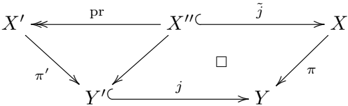
### Visual Description
\n
## Commutative Diagram: Morphisms Between Objects X', X'', X, Y', Y
### Overview
The image displays a commutative diagram from mathematics, likely within the fields of category theory, homological algebra, or algebraic topology. It illustrates a network of objects (denoted by letters) and morphisms (arrows) between them, forming a diamond-shaped structure with a central object. The diagram implies specific relationships and compositions between these morphisms.
### Components/Axes
The diagram consists of five objects and six morphisms (arrows). There are no traditional axes, as this is not a data chart.
**Objects (Nodes):**
* **X'**: Located at the top-left corner.
* **X''**: Located at the center of the diagram.
* **X**: Located at the top-right corner.
* **Y'**: Located at the bottom-left corner.
* **Y**: Located at the bottom-right corner.
**Morphisms (Arrows) and Labels:**
1. **pr**: An arrow from **X''** to **X'**. Label "pr" is positioned above the arrow.
2. **j̄** (j-bar): An arrow from **X''** to **X**. Label "j̄" is positioned above the arrow.
3. **π'** (pi-prime): An arrow from **X'** to **Y'**. Label "π'" is positioned to the left of the arrow.
4. **j**: An arrow from **X''** to **Y'**. This arrow runs diagonally from the center to the bottom-left. No explicit label is placed directly on this arrow in the provided image.
5. **j**: An arrow from **Y'** to **Y**. Label "j" is positioned below the arrow.
6. **π** (pi): An arrow from **X** to **Y**. Label "π" is positioned to the right of the arrow.
**Other Symbols:**
* A small, empty square symbol (□) is located in the space between the arrows connecting X'', X, Y', and Y. This often denotes a **pullback square** or **pushout square** in category theory, indicating a universal property for the diagram formed by those four objects and the arrows between them.
### Detailed Analysis
The diagram is structured as a diamond with a central node.
* **Top Path**: From X'' to X' (via `pr`) and from X'' to X (via `j̄`).
* **Bottom Path**: From Y' to Y (via `j`).
* **Left Side**: From X' down to Y' (via `π'`).
* **Right Side**: From X down to Y (via `π`).
* **Central Connections**: From X'' down to Y' (via an unlabeled diagonal arrow). The square symbol (□) is positioned to suggest that the sub-diagram involving X'', X, Y', and Y (with morphisms `j̄`, `π`, `j`, and the diagonal from X'' to Y') forms a commutative square with a special universal property (pullback/pushout).
The labeling uses standard mathematical notation: primes (') and double primes ('') to denote related objects, and Greek letters (π) and Latin letters (j, pr) for morphisms. The bar over the j (`j̄`) indicates it is a distinct morphism from the other `j`.
### Key Observations
1. **Structural Symmetry**: The diagram has a rough left-right symmetry in its layout, with X'/Y' on the left and X/Y on the right, connected through the central X''.
2. **Ambiguous Label**: The diagonal arrow from X'' to Y' does not have a label placed directly on it in this rendering. It is possible the label is implied by the context of the square (□) or is simply omitted.
3. **Notation Consistency**: The use of `j` for two different morphisms (X''→Y' and Y'→Y) is notable. Typically, distinct morphisms would have distinct labels. This could be a notational shorthand where the context (domain/codomain) clarifies which `j` is meant, or it might be an oversight in the diagram's rendering.
4. **Central Square**: The presence of the □ symbol is a critical piece of information, transforming the diagram from a simple collection of arrows into one asserting a specific categorical construction (like a pullback).
### Interpretation
This diagram is a formal representation of relationships between mathematical objects. It does not present empirical data but rather abstract structural information.
* **What it Demonstrates**: The diagram asserts the existence of morphisms (`pr`, `j̄`, `π'`, `j`, `π`) between the objects X', X'', X, Y', and Y. The central square symbol (□) strongly suggests that the square formed by X'', X, Y, and Y' is a **pullback** (or possibly a pushout). If it is a pullback, it means X'' is the "most general" object that maps to both X and Y' in a way that makes the diagram commute (i.e., the composition `π ∘ j̄` equals `j ∘ (diagonal morphism)`).
* **Relationships**: The morphisms `pr` and `j̄` can be seen as projections or inclusions from the central object X''. The morphisms `π'` and `π` are likely projections or maps to the "Y" objects. The structure is common in defining fiber products, kernels, cokernels, or in the context of exact sequences.
* **Notable Anomaly**: The dual use of the label `j` for two different arrows is the most striking anomaly. In a rigorous mathematical text, this would typically be avoided to prevent confusion. It forces the reader to disambiguate based on the domain and codomain of each arrow.
* **Underlying Meaning**: Without additional context (e.g., the surrounding text in the document it came from), the precise mathematical meaning is open to interpretation. However, the diagram's form is archetypal for expressing that a certain construction (X'') universalizes the relationship between X and Y' over Y. It visually encodes a system of equations (commutativity conditions) and a universal property.
</details>
for Koszul complex which is induced by pr : j ∗ E ↠ E ′ .
We explain how to re-state condition (ii) in Definition 6.2 without involving derived algebraic geometry.
Lemma 6.3. Suppose that ( X,Y,s,ϕ ) and ( X ′ , Y ′ , s ′ , ϕ ′ ) are two sets of dimensional reduction data, and assume that there exists maps (1) and (2) as in the Definition 6.2 which satisfy condition (i), and assume moreover that Z ( s ′ ) is not empty, then there exists a natural vector bundle map on Z ( s ′ ):
$$\rho : ker ( p ) | z ( s ) → N _ { Y } / y | z ( s ) .$$
Proof. In fact, denote K := ker(pr). For arbitrary y ∈ Z ( s ′ ), there exists an open neighbourhood y ∈ U ⊆ Y such that K| U ∩ Y ′ extends to a sub-bundle ˜ K U ⊆ E | U . Note that s | U maps ˜ K U to I Y ′ | U , then we get
$$\sum _ { i = 1 } ^ { n } z ( s ) u K _ { U } \rightarrow ( I _ { Y } / I _ { Z } ( s ) \cdot I _ { Y } ) u$$
The map ρ U ∩ Z ( s ′ ) does not depend on the choice of extension ˜ K U because any other choice is different from a given one by a map ˜ K U → I Y ′ | U · E | U and after restricting to Z ( s ′ ), the image of this map is inside I Z ( s ′ ) · I Y ′ | U ∩ Z ( s ′ ) . Consequently, for a pair of open subset U and V , ρ U ∩ Z ( s ′ ) | U ∩ V ∩ Z ( s ′ ) = ρ V ∩ Z ( s ′ ) | U ∩ V ∩ Z ( s ′ ) . Therefore the family of maps { ρ U ∩ Z ( s ′ ) } U glues to a map (6.4).
An equivalent construction of (6.4) is given as follows. The map pr : j ∗ E ↠ E ′ induces two dg-algebra maps:
$$f : Kos(E , s ) → j _ { \ast } Kos(E ^ { \prime } , s ^ { \prime } ) .$$
Applying L j ∗ to the first map, and we get the following commutative diagram of dg-algebras on Y ′ :
(6.5)
11 This is equivalent to pr ∗ ( w ′ ) = w | X ′′ .
/
/
$$\begin{array}{ll}
L _ { j } ^ { \ast } Kos(E , s) & \rightarrow & Kos(E ' , s') \\
\downarrow L _ { j } ^ { \ast } ( n ) & \downarrow & \left| \right| \\
L _ { j } ^ { \ast } jKos(E , s') & \rightarrow & Kos(E ' , s'),
\end{array}$$
}
}
/
/
/
/
where a is the adjunction map L j ∗ j ∗ → id. Then we have induced map on the mapping cones
$$C a C l _ { 2 } \rightarrow C a C O _ { 3 } ($$
Let i ′ : Z ( s ′ ) ↪ → Y ′ be the natural embedding, then
$$H ^ { - 1 } ( L ^ { i } _ { r } ( Cone ( g ) ) ) \approx i ^ { * } K ,$$
and the induced map i ′∗ K → i ′∗ N ∨ Y ′ /Y equals to ρ in (6.4).
□
Proposition 6.4. Suppose that ( X,Y,s,ϕ ) and ( X ′ , Y ′ , s ′ , ϕ ′ ) are two sets of dimensional reduction data, and assume that there exists maps (1) and (2) as in the Definition 6.2 which satisfy condition (i). Then the condition (ii) is equivalent to
(ii') Z ( s ) is set-theoretically contained in Y ′ , and ρ : ker(pr) | Z ( s ′ ) → N ∨ Y ′ /Y | Z ( s ′ ) (6.4) is an isomorphism.
Proof. (ii)= ⇒ (ii'). Since Z der ( s ′ ) ∼ = Z der ( s ), Z ( s ) is set-theoretically contained in Y ′ . Moreover
$$K _ { 0 } H C l _ { 2 } + 3 K O H ( \cdot )$$
being a quasi-isomorphism implies that the map
$$C a C l _ { 2 } + C a C O _ { 3 }$$
induced from the commutative diagram (6.5) is a quasi-isomorphism. In particular,
$$\rightarrow H ^ { i } _ { 1 } ( L i ^ { i } ( C o n e ( g ) ) ) \cong i ^ { i } N _ { Y } r y$$
̸
is an isomorphism.
(ii')= ⇒ (ii). We only need to show Kos( E,s ) → j ∗ Kos( E ′ , s ′ ) is a quasi-isomorphism. Since Z ( s ) ⊆ Y ′ and s | Y ′ = pr ∨ ◦ s ′ , we have Z ( s ) = Z ( s ′ ) as sets. Assume Z ( s ′ ) = ∅ (otherwise (ii) trivially holds). To show that Kos( E,s ) → j ∗ Kos( E ′ , s ′ ) is a quasi-isomorphism, it is enough to check it locally in a Zariski neighbourhood of any point in Y ′ . To this end, we can assume that there is a decomposition of vector bundle
$$E \approx K \cdot E ' , such that K$$
and pr equals to the natural projection ( ˜ K⊕ ˜ E ′ ) | Y ′ → ˜ E ′ | Y ′ . Let us write
$$8 = ( 8 , 0 ) \cdot k ^ { 2 } + [ - 1 7 , - 9 ]$$
then the image of s 1 is contained in I Y ′ (the ideal that defines Y ′ ). Then we consider the vector bundle map on Y ′ :
$$\gamma : k \epsilon ( p r ) = K / I _ { Y } ^ { 2 } = N _ { Y } ^ { 2 } / Y _ { r }$$
which is defined as the image of s 1 . By construction, τ | Z ( s ′ ) = ρ which is an isomorphism by assumption, so there exists an open neighbourhood V of Z ( s ′ ) in Y such that τ | V ∩ Y ′ is an isomorphism. Then it suffices to show that Kos( E,s ) | V → j ∗ Kos( E ′ , s ′ ) | V is a quasi-isomorphism. We have decomposition
$$s _ { 1 } | v ) \otimes K o s ( E _ { v } , s _ { 2 } | v ).$$
Since τ | V ∩ Y ′ is an isomorphism, (locally) s 1 maps a basis of ˜ K V to a regular sequence that generates I Y ′ | V ; thus Kos( ˜ K V , s 1 | V ) is quasi-isomorphic to j ∗ O V ∩ Y ′ as a dg O Y -algebra. It follows that
$$\int \limits _ { s ( E _ { v } , s ^ { 2 } ) } v = j * K os ( E _ { v } , s ^ { 2 } ) v .$$
Note that compatible dimensional reduction data gives a further consequence.
Proposition 6.5. Suppose that ( X,Y,s,ϕ ) and ( X ′ , Y ′ , s ′ , ϕ ′ ) are compatible dimensional reduction data, then Crit( w ) is a subscheme of X ′′ , and pr: X ′′ → X ′ maps Crit( w ) isomorphically onto Crit( w ′ ). 12
Proof. We first notice that
Then by Definition 6.2 (i), we have embedding
$$( \sin ( 5 - 1 / 2 \pi ) ) = x ^ { 2 } .$$
12 In fact, the derived critical loci are also isomorphic. This can be proven using the ( -1)-shifted version of [KP, Cor. 5.3], and the fact that the derived zero locus of s and s ′ are isomorphic and the restriction of ϕ and ϕ ′ on them coincide. We thank Tasuki Kinjo to pointing out this.
$$C r i o w ( S _ { 2 } ^ { - } ) ( Z s l .$$
Note that for any smooth closed subvariety Z ⊆ X , there is an inclusion
$$C _ { 6 } H ( O ) _ { 7 } \uparrow + C _ { 6 } H ( O ) _ { 2 } \uparrow$$
and taking Z = X ′′ leads to
$$C _ { 1 } H C O O H = C _ { 1 } H ( O H ) _ { 2 } \cdot$$
By the condition (1) in Definition 6.2, we have
$$C _ { 1 } ^ { 1 } H _ { 2 } O ( g ) = P r ^ { - } ( C _ { 1 } ^ { 1 } H _ { 2 } O ) _ { \cdot }$$
thus pr: X ′′ → X ′ restricts to give pr : Crit( w ) → Crit( w ′ ). It remains to show the map is surjective and any fiber contains exactly one point. Since we can check this locally, we replace Y by an open subset and without loss of generality we assume E ∼ = ˜ K⊕ ˜ E ′ such that ˜ K| Y ′ ∼ = ker(pr) and ˜ E ′ | Y ′ ∼ = E ′ and pr equals to the natural projection ( ˜ K⊕ ˜ E ′ ) | Y ′ → ˜ E ′ | Y ′ . Shrink Y if necessary, we assume
$$\overrightarrow { x } = \frac { 1 } { i } \overrightarrow { O _ { y } } , \overrightarrow { y } = \frac { 1 } { j } \overrightarrow { O _ { x } }$$
such that the morphism given by { t i = s ( k ∨ i ) } n i =1 : Y → A n is smooth, where k ∨ i is dual basis of k i . We have
$$w = \sum _ { i = 1 } ^ { n } k _ { i } t _ { i } + \sum _ { j = 1 } ^ { m } e _ { j } s ( e ^ { j } ) r + d l y _ { r }$$
then it follows that
$$\sum _ { i = 1 } ^ { n } \frac { d s ( e ) } { d t _ { i } } + \alpha _ { 0 } = 0 \quad 1 \leq i \leq n$$
Since k i = -∑ m j =1 e j · ∂s ( e ∨ j ) ∂t i -∂ϕ ∂t i (1 ⩽ i ⩽ n ) gives a section of ˜ K on Tot( ˜ E ′ ), Crit( w ) is section of the projection pr -1 (Crit( w ′ )) → Crit( w ′ ); therefore pr maps Crit( w ) isomorphically onto Crit( w ′ ). □
We note that for a dimensional reduction datum ( X,Y,s,ϕ ), its A -fixed part ( X A , Y A , s A , ϕ A ) is also a dimensional reduction datum.
Lemma 6.6. Suppose that ( X,Y,s,ϕ ) and ( X ′ , Y ′ , s ′ , ϕ ′ ) are compatible dimensional reduction data, then the fixed locus data ( X A , Y A , s A , ϕ A ) and ( X ′ A , Y ′ A , s ′ A , ϕ ′ A ) are also compatible.
Proof. Taking A -invariance, we get T -equivariant closed embedding j A : Y ′ A ↪ → Y A and T -equivariant surjective vector bundle map
$$p r ^ { A } \cdot E l f _ { x } - p r ^ { A } \cdot E l f _ { y _ { x } }$$
Then the condition (i) in Definition 6.2 is obviously satisfied. By Proposition 6.4, it is enough to verify condition (ii'). Since s ∈ Γ( Y, E ∨ ) A , we have Z ( s A ) = Z ( s ) A , so Z ( s A ) is set-theoretically contained in Y ′ A . The natural map ρ A : ker(pr A ) | Z ( s ′ A ) → N ∨ Y ′ A /Y A | Z ( s ′ A ) is the A -fixed part of the pullback of ρ : ker(pr) | Z ( s ′ ) ∼ = N ∨ Y ′ /Y | Z ( s ′ ) to Z ( s ′ A ), so ρ A is an isomorphism. □
Proposition 6.7. Suppose that ( X,Y,s,ϕ ) and ( X ′ , Y ′ , s ′ , ϕ ′ ) are compatible dimensional reduction data. Let δ H and δ A H be the natural maps
$$T ( X ^ { A } , w ^ { A } ) \rightarrow H ^ { T } ( X ^ { A } , w ^ { A } ) ,$$
where we refer to diagram (6.3) for those maps. Then we have commutative diagram
O
O
o
o
O
O
$$\begin{array}{ll}
H ^ { T } ( X ^ { A }, w ^ { A } ) & \xrightarrow [ i ^ { \ast } ] { e ^ { i ( N _ { y r } / x ^ { A } ) , i ^ { \ast } } } H ^ { T } ( X ^ { A }, w ^ { A } ) \\
\end{array}$$
o
o
where i ′ : X ′ A ↪ → X ′ and i : X A ↪ → X are closed embeddings of fixed points loci.
Similarly let δ K and δ A K be the natural maps
$$( 6 . 7 ) \alpha k := j _ { k } o p r ^ { \cdot } A : B$$
then we have commutative diagram
$$\begin{array}{ll}
K ^T ( X ^A , w ^A ) & \longrightarrow K ^T ( X ^A , w ^A ) \\
& \longleftarrow \frac{\delta _k ^T ( N y , y ^* x ^A ) } { | y | x ^A } K ^T ( X ^A , w ^A ) .
\end{array}$$
o
o
Proof. Consider the following Cartesian diagram of smooth varieties:
/
/
$$\begin{array}{ccc}
X^{''} A & \xrightarrow[j^A]{} X^A \\
X^{''} A & \xrightarrow[j^A]{} X^A \\
X^{''} A & \xrightarrow[j^A]{} X^A \\
\end{array}$$
/
/
$$\therefore A = 1 , B = 1 , C = - 1 , D = \frac { 1 } { 2 }$$
We note that pr ◦ i ′′ = i ′ ◦ pr A . Then we have
$$\begin{aligned}
i ^ { \star } o _ { H } = i ^ { \star } o _ { j } . p r ^ { \star } = j ^ { \star } o e ^ { \star } \\
& = \int \limits _ { N _ { X , Y } / x [ m o v ] } ^ { ( N _ { X , Y } / x [ m o v ] ) } i ^ { \star } o _ { H } d t . p r ^ { \star } = j ^ { \star } o e ^ { \star } ( N _ { X , Y } / x [ m o v ] ) . i ^ { \star }$$
This proves the statement for cohomology. For the K -theory counterpart, we use Remark B.5 to get
$$\therefore f ( x ) = f ^ { \prime } ( x ) + f ^ { \prime \prime } ( x )$$
and the rest of computation is the same as above.
□
Proposition 6.8. Suppose that ( X,Y,s,ϕ ) and ( X ′ , Y ′ , s ′ , ϕ ′ ) are compatible dimensional reduction data. If K -theoretic deformed dimensional reduction holds for both ( X,Y,s,ϕ ) and ( X ′ , Y ′ , s ′ , ϕ ′ ), then the natural map δ K : K T ( X ′ , w ′ ) → K T ( X, w ) defined in Proposition 6.7 is an isomorphism.
Proof. Using Z der ( s ) ∼ = Z der ( s ′ ), we have Cartesian diagram:
/
/
/
/
$$\begin{array}{ll}
\pi^{-1}(Z^d(s)) & \xrightarrow[p_r]{} \pi^{-1}(Z^d(g)) \\
\downarrow & \square \\
\downarrow & \pi^{-1}(der) \\
X'' & \xrightarrow[pr]{} X'
\end{array}$$
According to Remark B.2, we have
Since pr is smooth, we have
$$\because \prime r d e r ^ { \prime } o p r ^ { \prime } = p r ^ { \prime } o ^ { \prime } l d e r$$
It follows that
$$\delta _ { k } o ( i / d e r \ o p r ^ { * } o j ^ { * } d e r o ) = j _ { k } o i ^ { * } d e r o p r ^ { * } o j ^ { * } d e r o$$
where in the last equation we use ˜ j ◦ i ′′ der = i der and π ′ ◦ pr = π . By assumption, both i ′ der ∗ ◦ π ′∗ and i der ∗ ◦ π ∗ are isomorphisms; thus δ K is an isomorphism. □
Proposition 6.8 holds for cohomology in more general setting, where deformed dimensional reductions for ( X,Y,s,ϕ ) and ( X ′ , Y ′ , s ′ , ϕ ′ ) are not needed as assumptions.
Proposition 6.9. Suppose that ( X,Y,s,ϕ ) and ( X ′ , Y ′ , s ′ , ϕ ′ ) are compatible dimensional reduction data. Then the map δ H : H T ( X ′ , w ′ ) → H T ( X, w ) defined in Proposition 6.7 is an isomorphism. 13
Proof. The map δ H : H T ( X ′ , w ′ ) → H T ( X, w ) is induced by the following chain of maps
$$\sum _ { j = 1 } ^ { n } H ^ { T } ( X ^ { \prime } , \varphi _ { w } x ) \Rightarrow H ^ { T } ( X , \varphi _ { w } x )$$
where the first two isomorphisms are obvious, the last map is induced by the natural morphism in D b c ( X ):
(6.8)
$$\int _ { 0 } ^ { 1 } f ( x ) d x \rightarrow f ( 0 )$$
13 In view of the previous footnote, this isomorphism can also be proven from the gluing of DT perverse sheaves, as the condition in Definition 6.2 implies the orientation data of the derived critical locus of w and w ′ are equivalent.
O
O
o
o
O
O
To show that δ H is an isomorphism, it remains to show the pushforward of (6.8) to Y :
$$\pi _ { 1 } j \phi _ { w } l , \ldots j ^ { \prime } W X \rightarrow \pi _ { 2 } p _ { w } l X$$
is an isomorphism in D b c ( Y ). In the proof of Proposition 6.5, we know that ´ etale locally on Y , we have a decomposition and a basis:
$$\sum _ { i = 1 } ^ { n } \sum _ { j = 1 } ^ { m } E _ { v } ^ { z _ { i } } \otimes E _ { v } ^ { z _ { j } }$$
such that the morphism given by { t i = s ( k ∨ i ) } n i =1 : Y → A n is smooth, where k ∨ i is dual basis of k i . In this coordinate,
$$w = \sum _ { i = 1 } ^ { n } k _ { i } \cdot t _ { i } + \sum _ { j = 1 } ^ { m } s _ { j } \cdot s ( e ^ { j } ) + d$$
Let π 1 : Tot( E ) → Tot( ˜ E ′ ) be the projection whose fibers contribute to the function w by ∑ n i =1 k i · t i , where ⋂ n i =1 { t i = 0 } cuts out Y ′ ⊆ Y in an ´ etale neighbourhood. Then the deformed dimensional reduction for regular sections (Theorem C.1) implies that the natural map
$$\pi _ { 1 } ^ { \prime } h g y _ { 1 } x - \pi _ { 2 } ^ { \prime } h g y _ { 2 } x$$
is an isomorphism. Pushing forward to Y , we obtain (6.9).
□
6.2. Compatibility with stable envelopes. Suppose that ( X,Y,s,ϕ ) and ( X ′ , Y ′ , s ′ , ϕ ′ ) are compatible dimensional reduction data as in the Definition 6.2. As X → Y and X ′ → Y ′ are vector bundles projections equivariant under A , there are one-to-one correspondences
$$F i x _ { A } ( X ) \approx F i x _ { A } ( Y ),$$
with isomorphisms given by projections and A -fixed parts of inverse maps of projections.
The embedding Y ′ ↪ → Y induces a map
$$t : F i x _ { A } ( X ) \cong F i x _ { A } ( Y ^ { \prime } )$$
which is neither injective nor surjective in general. The map r respects the ample partial order ≤ defined in the Remark 3.9. Namely, ∀ F, F ′ ∈ Fix A ( X ′ ),
$$1 1 1 1 1$$
$$( 6 . 1 0 )$$
Theorem 6.10. Suppose that ( X,Y,s,ϕ ) and ( X ′ , Y ′ , s ′ , ϕ ′ ) are compatible dimensional reduction data as in the Definition 6.2. Fix a normalizer ϵ ∈ {± 1 } Fix A ( X ) , and define ϵ ′ ∈ {± 1 } Fix A ( X ′ ) by
$$b _ { 1 } = c _ { 1 } p _ { 1 } \cdot ( - 1 ) ^ { n k N _ { 1 } / y _ { 1 } h _ { 1 } }$$
Fix a chamber C ⊆ Lie( A ) R , and we assume that cohomological stable envelopes exist for ( X, w , T , A , C ) and ( X ′ , w ′ , T , A , C ). Then we have the following commutative diagram:
O
O
/
/
O
O
$$\begin{array}{c}
H ^ { \prime } ( X ^ { A }, w ^ { A } ) \\
\end{array}
\begin{array}{c}
H ^ { \prime } ( X , w ) .
\end{array}$$
Proof. Define
/
/
$$x ^ { A } , w ^ { A } \rightarrow H ^ { T } ( X , w ) .$$
For an arbitrary F ∈ Fix A ( X ′ ), and take an arbitrary γ ∈ H T / A ( F, w ′ A ), we need to show that S ( γ ) satisfies the axioms (ii) and (iii) in Definition 3.4 and axiom (i') in Remark 3.7, namely
- (1) S ( γ ) is supported on Attr ≤ C ( r ( F ));
- (2) S ( γ ) ∣ ∣ r ( F ) = ϵ r ( F ) · e T ( N -r ( F ) /X ) · δ A H ( γ );
̸
- (3) For any F ′ = r ( F ), the inequality deg A S ( γ ) ∣ ∣ F ′ < deg A e T ( N -F ′ /X ) holds.
Here we choose the ample partial order ≤ as in Remark 3.9.
Denote β = Stab C ,ϵ ′ ( γ ), then β is supported on Attr ≤ C ( F ). It follows that δ H ( β ) = ˜ j ∗ ◦ pr ∗ ( β ) is supported on pr -1 (Attr ≤ C ( F )). Since the complex φ w ω X is supported on Crit( w ), δ H ( β ) is supported on pr -1 (Attr ≤ C ( F )) ∩ Crit( w ). According to Proposition 6.5, we have
$$\begin{array}{ll}
p r ^ { - 1 } ( A t t _ { c } ^ { \frac { 1 } { 2 } } ( F ) ) \cap C r i t ( w ) = ( p r ^ { - 1 } ) ^ { ( A t t _ { c } ^ { \frac { 1 } { 2 } } ( F ) ) \cap C r i t ( w ) ) .
\end{array}$$
$$\frac { A t t _ { r } ^ { 2 } ( F ) n C r i t ( w ) = U } { F < F }$$
where the subscript means taking attracting set inside Crit( w ′ ). Therefore δ H ( β ) is supported on
̸
In particular, δ H ( β ) is supported on Attr ≤ C ( r ( F )). This proves (1).
To show (2) and (3), we notice that
$$S ( r ) | x _ { A } = i ^ { \prime } o \phi _ { H } ( B ) = e$$
where the second equality follows from Proposition 6.7. Then
$$\begin{aligned}
\int \limits _ { F } ^ { T } | r ( F ) | dF &= \delta A H ( e ^ { i \theta } ( N y , F ) ) \\
&= \delta A H ( e ^ { i \theta } ( N y , x ) ) .
\end{aligned}$$
According to Proposition 6.4, we have
$$z ( s ) ^ { V } \in K ^ { T } ( z ( s ) ^ { A } ) .$$
Via pullback along π ′ A : X ′ A → Y ′ A , we have
$$z ( s ) ^ { A } = ( - 1 ) ^ { rk } N _ { Y } / y [ x _ { k } e T ( π ^ { rA } _ { k } \ker ( p ) ) ] ^ { - 1 }$$
As we have inclusion
By Lemma 3.8, we have
$$C _ { 1 } ^ { 1 } H _ { 2 } A = C _ { 1 } ^ { 1 } H - N a$$
we can restrict (6.12) to Crit( w ′ A ) and the restriction
$$\sum _ { i = 1 } ^ { n } \sum _ { j = 1 } ^ { m } A _ { ij } k e ^ { i A _ { i j } } ( z ( s ) ^ { j } ) | C _ { r i t ( w ^ { A } ) }$$
acts on H T ( X ′ A , w ′ A ). Note that
$$\sum _ { i = 1 } ^ { A } \sum _ { j = 1 } ^ { N _ { Y } } / y ( s ) A ) ,$$
$$\ker ( p r ) \vert z ( s ) ^ { A } \rangle = ( C _ { r i t } ( w ^ { A } ) \rightarrow x ^ { A } ) ^ { - A }$$
For simplicity, we write
$$N _ { Y / Y } [ x _ { A } = ( \pi ^ { A } N _ { Y / Y } [ y _ { A } ] ,$$
and omit the pullback along Crit( w ′ A ) ↪ → X ′ A in (6.14), (6.15). Then (6.13) becomes
$$e ^ { i x ^ { + } e T ( k r ( p r ) | x _ { A } ) } ,$$
which acts on H T ( X ′ A , w ′ A ). Consequently, we have
$$S ( r ) | t ( F ) = s A H ( - 1 ) = e _ { r } ( F ) \cdot e ^ { T }$$
This proves (2).
̸
Finally, for any F ′ = r ( F ),
$$S ( r ) | F _ { r } = \delta A H ( e ^ { T } ( N _ { Y } / y _ { r } )$$
̸
Suppose that r -1 ( F ′ ) = { F 1 , · · · , F n } , then F i = F for all i . The same argument as above shows that
$$( k \pi ( p ) | r _ { i } + N y / r _ { i } | F _ { i } ) : Stab e c e ( r ) | F _ { i } = \pm e ^ { j T }$$
Since δ A H preserves deg A , we have
$$y [ r _ { i } ] + dega Stab_e ( r ) | r _ { i } | F _ { i } = dega e ^ { T } ( k er ( p t ) | r _ { i } | + N _ { Y } /$$
where the second inequality follows from the axiom (iii). Therefore
$$\frac { 1 } { R } \int _ { F _ { i } } ^ { T ( N _ { F _ { r } / x } ) } \delta A ( e ^ { i H ( e ^ { i T ( N _ { F _ { r } / x } ) } ) } \cdot S t a b e _ { c } ( r ) ) d e g A$$
This proves (3).
□
Theorem 6.11. Suppose that ( X,Y,s,ϕ ) and ( X ′ , Y ′ , s ′ , ϕ ′ ) are compatible dimensional reduction data as in the Definition 6.2. Fix a normalizer E ∈ ± Pic T ( X A ), and define E ′ ∈ ± Pic T ( X ′ A ) by
$$e ^ { | f | } = e ^ { | f | \circ ( - 1 ) ^ { k } }$$
Fix a generic slope s ∈ Pic A ( Y ) ⊗ Z R , and define s ′ ∈ Pic A ( Y ′ ) ⊗ Z R by
$$S = S _ { 1 } + \textcircled { 2 } d + ( N _ { 1 } y _ { 1 } ) ^ { 2 }$$
Fix a chamber C ⊆ Lie( A ) R , and assume that K -theoretic stable envelopes exist for ( X, w , T , A , C , s ) and ( X ′ , w ′ , T , A , C , s ′ Assume moreover that ker(pr) = N ∨ Y ′ /Y in K T ( Y ′ ). Then we have the following commutative diagram:
O
O
/
/
O
O
$$\begin{array}{c}
(6.17) \\
\end{array}$$
Proof. Define
/
/
$$X ^ { \prime } A , w ^ { \prime } A ) \rightarrow K ^ { \prime } T ( X , w ).$$
For an arbitrary F ∈ Fix A ( X ′ ), and take an arbitrary γ ∈ K T / A ( F, w ′ A ), we need to show that S ( γ ) satisfies the axioms (ii) and (iii) in Definition 3.10 and axiom (i') in Remark 3.17, namely
- (1) S ( γ ) is supported on Attr ≤ C ( r ( F ));
$$( 2 ) S ( r ) | _ { c ( F ) } = E [ c ( F ) ]$$
̸
- (3) For any F ′ = r ( F ), there is a strict inclusion of polytopes
$$\begin{aligned}
& \text{det } ( N ^ { r } _ { F } ) = \frac { 1 } { | F | } \sum _ { i = 1 } ^ { r } s _ { i } ( r ) \\
& + \text{weight}_ { A } ( det ( N ^ { r } _ { F } / x ) ^ { 1 / 2 } \otimes s _ { I } ( r ) ) \\
+ \text{weight}_ { A } E [ r ( F ) ]
\end{aligned}$$
Here we choose the ample partial order ≤ as in Remark 3.9.
Denote β = Stab s ′ C , E ′ ( γ ), then β is supported on Attr ≤ C ( F ). It follows that δ K ( β ) = ˜ j ∗ ◦ pr ∗ ( β ) is supported on pr -1 (Attr ≤ C ( F )). Since the critical K -theory is supported on Crit( w ), δ K ( β ) is supported on pr -1 (Attr ≤ C ( F )) ∩ Crit( w ). The same argument as in the proof of Theorem 6.10 shows that
$$= A t r _ { g } ^ { - 1 } ( F ) \cap C r i t ( w ) .$$
Thus δ K ( β ) is supported on Attr ≤ C ( r ( F )). This proves (1).
To show (2) and (3), we notice that
$$\begin{aligned}
S ( n ) \vert x _ { A } = t ^ { 2 } o \delta _ { K } ( B ) = \delta _ { R } ( e _ { k } ( N _ { Y } / y _ { I } x _ { A } ) ,$$
).
where the second equality follows from Proposition 6.7. Then
$$S ( y ) | r ( F ) = \delta A ( e ^ { T } K ( N _ { Y } / y ) = \delta A ( e ^ { T } K ( N _ { F } / x ; ) - y ) .$$
Similarly as (6.16), we have
$$e ^ { \frac { 1 } { k } ( N _ { y } / r ) [ x _ { \alpha } ] ^ { + } } = ( - 1 ) ^ { k } k N _ { y } / r [ x _ { \alpha } ] ^ { - k n }$$
Therefore
$$\begin{aligned}
S ( r ) | _ { t ( R ) } = \delta ^ { R } K ( ( - 1 ) ^ { r k N _ { y } } = \epsilon _ { k } ( r ) \cdot e ^ { k } ( N _ { y } )$$
This proves (2).
Finally, for any F ′ = r ( F ),
$$S ( r ) | F _ { r } = \delta A _ { K } ( e _ { K } ( N _ { Y } ^ { r } / y _ { I } ^ { r } )$$
̸
Suppose that r -1 ( F ′ ) = { F 1 , · · · , F n } , then F i = F for all i . The same argument as above shows that
$$\frac { T _ { k } ( N _ { Y } / r ) \cdot Stab ^ { f } _ { c } e ^ { i } } { F _ { 1 } } = \pm det ( N _ { Y } / r [ + ] ^ { - 1 } e _ { k } ( k e r ( p r ) | F _ { 1 } + ) ) r _ { 1 }$$
Since δ A K preserves deg A , we have
Therefore
$$\therefore \delta e ( r ) | F _ { r } \subset Convex I$$
Since s is generic, the above inclusion must be strict by Remark 3.12.
## 6.3. Examples of compatible dimensional reduction data.
Example 6.12. Suppose that ( X,Y,s,ϕ ) is a dimensional reduction datum such that s is regular. Then Z ( s ) is a smooth subvariety in Y with codimension equals to rk E , and Z ( s ) ∼ = Z der ( s ). It is easy to see that ( X,Y,s,ϕ ) and ( Z ( s ) , Z ( s ) , 0 , ϕ | Z ( s ) ) are compatible dimensional reduction data (Definition 6.2).
In particular, starting with a quiver, the associated tripled quivers with canonical cubic potentials and Nakajima varieties of the double quiver provide such examples.
Example 6.13. Given a quiver Q = ( Q 0 , Q 1 ), we define the doubled quiver to be Q := ( Q 0 , Q 1 ⊔ Q ∗ 1 ), where Q ∗ 1 is the same as Q 1 but with reversed arrow direction. We define the tripled quiver ˜ Q := ( Q 0 , Q 1 ⊔ Q ∗ 1 ⊔ Q 0 ), which adds one edge loop to each node on top of Q .
Fix v , d ∈ N Q 0 , we consider two symmetric quiver varieties (see Definition 4.5 for details of construction):
- (1) M θ ( Q, v , d ) associated with the doubled quiver Q ;
- (2) M θ ( ˜ Q, v , d ) associated with the tripled quiver ˜ Q .
This proves (3). □
̸
Assume θ is generic, so that θ -semistable loci coincide with θ -stable loci:
$$R ( \bar { Q } , v , d ) ^ { s } = R ( \bar { Q } , v , d ) ^ { s } .$$
Let G = ∏ i ∈ Q 0 GL( v i ) be the gauge group , then the quotient map
$$v , d ) = R ( \overline { Q } , v , d ) ^ { s } / G$$
is a principal G -bundle. Denote the associated adjoint bundle to be G → M θ ( Q, v , d ). Then the moment map for G ↷ R ( Q, v , d ) descends to a section µ ∈ Γ ( M θ ( Q, v , d ) , G ∨ ) . The total space Tot( G ) is naturally identified with an open subscheme · M θ ( ˜ Q, v , d ) ⊆ M θ ( ˜ Q, v , d ) consisting of G -equivalence classes in R ( ˜ Q, v , d ), which are θ -stable when restricted to Q . The zero locus of µ :
$$M ( x , y ) = 2 \vert x \vert$$
is the Nakajima quiver variety [Nak1, Nak2] (which we assume to be nonempty). Note that N θ ( Q, v , d ) is a smooth subvariety in M θ ( Q, v , d ) with codimension equals to G , and Z ( µ ) = Z der ( µ ).
Denote C ∗ ℏ the torus that acts on R ( Q, v , d ) by assigning weights R ( Q, v , d ) = M ⊕ ℏ -1 M ∨ , where
$$M = \frac { 1 } { t ^ { e Q _ { 0 } } } H O n ( C V _ { 4 } ^ { + } , C V _ { 4 } ^ { - } ) .$$
We choose torus T which contains C ∗ ℏ such that T = ( T / C ∗ ℏ ) × C ∗ ℏ , and let A ⊆ T / C ∗ ℏ be a subtorus. Choose a function ϕ : M θ ( Q, v , d ) → C and a section µ ∈ Γ( M θ ( Q, v , d ) , ℏ -1 G ∨ ) and appropriate T action such that ϕ and µ are T -invariant. Let us define the T action on edge loops by scaling with weight ℏ , then T fixes the pairing ⟨ e, µ ⟩ . Then according to Example 6.12, the dimensional reduction data
$$( \dot { M } ( Q , v , d ) , M _ { 0 } ( Q )$$
are compatible.
Remark 6.14. In the above example, if we take ϕ = 0, then dimensional reduction for critical cohomology [Dav1, Thm. A.1] and respectively for critical K -theory [Isi, Thm. 3.6] implies that
$$\delta H : H ^ { \prime } ( N _ { 0 } ( Q , v , d ) ) \rightarrow H ^ { \prime } ( M _ { 0 } ( Q , v , d ), w )$$
$$\delta k : K ^ { T } ( N _ { 0 } ( \overline { Q }, v , d ) )$$
are isomorphisms. Here δ H and δ K are the maps defined in Proposition 6.7 and
$$w = \sum _ { i = 1 } ^ { n } t _ { i } ( e _ { i } , p _ { i } )$$
$$w = \sum _ { i \in Q _ { 0 } } t ( e _ { i } i _ { 0 } ) ^ { 6 . 1 8 }$$
is the cubic potential , where ε is the edge loop on the node i , and µ is the i -th component of moment map.
i i It is known that [Dav2, Lem. 6.3]:
$$C _ { r i t } ( \widehat { w } ) \subset M _ { 0 } ^ { i } ( Q , v , d )$$
therefore the restriction from M θ ( ˜ Q, v , d ) to · M θ ( ˜ Q, v , d ) gives isomorphisms:
$$\sum _ { i = K ^ { T } ( M _ { 0 } ( \widetilde { Q }, v , d ), w ) } ^ { n } H ^ { T } ( M _ { 0 } ( \widetilde { Q }, v , d ), w ) \approx K ^ { T } ( M _ { 0 } ( \widetilde { Q }, v , d ), w ) .$$
More examples on compatible dimensional reduction data are discussed in [COZZ1], which are used to study shifted Yangians of gl 2 , shifted affine Yangians of gl 1 and their representations.
## 7. Deformations of potentials and stable envelopes
In this section, we discuss deformations of potentials and how they interplay with stable envelopes. This provides powerful tools in the computations of stable envelopes, relating different modules of quantum groups, see [COZZ1].
Setting 7.1. Fix ( X, T , A ) in Setting 2.1. Suppose there is a torus action G m ↷ X which commutes with T -action.
- Assume that f : X → C is a ( T × G m )-invariant function, and g : X → C is a T -invariant function together with a decomposition
$$g = \sum _ { i = 1 } ^ { n } g _ { i }$$
such that G m scales g i with weight -n i < 0, i.e. ( u · g i )( x ) := g i ( u -1 · x ) = u -n i · g i ( x ).
- Let ˜ X := X × A 1 with ( T × G m )-action given by the aforementioned action on X and the action
$$T _ { \times G _ { m } } ^ { P ^ { n } } G _ { m } o A ^ { 1 }$$
on A 1 , where G m ↷A 1 is of weight -1. Let t be the coordinate on A 1 , with ( T × G m )-invariant function:
$$w = f + \sum _ { i = 1 } ^ { n } t _ { n } g _ { i } ( x ) \rightarrow C ,$$
When we discuss the relation with stable envelopes, we work in the following setting.
Setting 7.2. Let ( X, T , A , f , g ) be as in Setting 7.1. Fix a chamber C ⊆ Lie( A ) R and a slope s ∈ Pic A ( X ) ⊗ Z R . Assume cohomological and K -theoretic stable envelope correspondences exist for ( X, 0 , T , A , C ) and ( X, 0 , T , A , C , s ) respectively.
Remark 7.3. Since canonical maps take stable envelope correspondences for zero potential to stable envelope correspondences for any potential, then according to Proposition 3.31, cohomological and K -theoretic stable envelopes exist for ( X, f , T , A , C ) , ( X, f + g , T , A , C ) and ( X, f , T , A , C , s ) , ( X, f + g , T , A , C , s ) respectively in Setting 7.2.
## 7.1. Specialization for Borel-Moore homology and K -theory of zero loci.
Lemma 7.4. Under Setting 7.1, let Z ( w ) ⊆ ˜ X denote the zero locus of w and Z ( w ) ∗ its open subset fitting into commutative diagrams
/
/
/
/
$$\begin{array}{ll}
Z(w)^* & \xrightarrow[~]{} Z(w) \\
& \xrightarrow[~]{} X \\
C^* & \xrightarrow[~]{} A_1 \\
& \xrightarrow[~]{} A_1,
\end{array}
$$$$
/
/
where pr is the projection and the left square is Cartesian. Then the left vertical map is a trivial fibration such that
$$Z ( w ) ^ { n } = Z ( f + g ) \times C ^ { n } .$$
Proof. There is an automorphism
$$( 7 . 1 )$$
where t · x means identifying C ∗ with G m and t acts on x via the G m action. Then
a
∗
(
w
) =
f
+
g
,
$$\therefore a ^ { - 1 } ( Z ( w ) ^ { * } ) = Z ( f +$$
It follows that the projection Z ( w ) → C fits in the setting of [CG, § 2.6.30].
Definition 7.5. Under Setting 7.1, we define a specialization map :
$$\begin{array}{ll}
& \frac { 1 } { 2 } H ^ { I } ( Z ( f + g ) - H ^ { I } ( Z ( i ) ) , \\
& \text { sp: } H ^ { I } ( Z ( f + g ) - H ^ { I } ( Z ( i ) ) .
\end{array}$$
as the composition of the following maps
/
$$\begin{array}{ll}
H ^ { T } _ { i } ( z ( f + g ) ) & \xrightarrow [ a ^ { - } ] { \lim _ { t \to 0 } ( f + g ) \times C ^ { s } } H ^ { T } _ { i + 2 } ( Z ( w ) ) \\
\end{array}$$
/
where lim t → 0 is the map defined in [CG, § 2.6.30].
Remark 7.6. According to the construction in [CG, § 2.6.30], we have an equality
$$\lim _ { x \rightarrow 0 } ( - 1 ) = 6 0 - n a .$$
Here α ∈ H 1 ( C ∗ ) ∼ = Q is the Borel-Moore homology class given by pushforward of the fundamental class [ R ] ∈ H 1 ( R ) under the exponential map
$$R _ { 1 } > C ^ { \prime } , s + e ^ { - } ,$$
and for any θ ∈ [0 , 2 π ), the maps s ↦→ e s + iθ and s ↦→ e s induce the same map H 1 ( R ) → H 1 ( C ∗ ) on homologies. ( -) ∩ α : H T j ( Z ( w ) ∗ ) → H T j -1 ( Z ( w ) ∗ ) is the intersection pairing with α . δ is the boundary map in the excision long exact sequence
/
/
/
/
/
/
/
/
$$\begin{array}{ll}
H ^ { T _ { i + 1 } ( Z ( w ) * ) } & \xrightarrow [ t = 0 ] { } H ^ { T _ { i } ( Z ( w ) ) } \\
& \xrightarrow [ n ] { } H ^ { T _ { i } ( Z ( w ) ) }
\end{array}$$
$$I'm sorry for any confusion, but it seems like you've entered a mathematical formula without providing any context or values. Could you please provide more information or clarify what you're asking? I'm here to help with a wide range of topics, so feel free to ask anything else!$$
/
/
/
/
Then it follows that sp (7.2) equals to the composition of the following maps
/
$$\begin{array}{ll}
H ^ { T } _ { i } ( Z ( f + g ) ) & \xrightarrow [ id_{\alpha} ] { H ^ { T } _ { i - 1 } ( Z ( f + g ) ) } \\
& \xrightarrow [ \chi ( f + g ) \times C ^ { \prime } _ { w } ] { H ^ { T } _ { i } ( Z ( w ) ) } \\
\end{array}$$
/
/
/
Similarly, there is a K -theoretic specialization map (ref. [CG, § 5.3]).
Definition 7.7. Under Setting 7.1, we define
$$( 7 . 3 )$$
as the composition of the following maps
/
$$\begin{aligned}
K ^ { T } ( Z ( f + g ) ) & \xrightarrow [ a ^ { \cdot } ] { \lim _ { t \to 0 } } K ^ { T } ( Z ( w ) ^ { \cdot } ) \\
& \xrightarrow [ e ^ { \cdot } ] { \lim _ { t \to 0 } } K ^ { T } ( Z ) .
\end{aligned}$$
/
$$\frac { 1 } { p + 1 } x ^ { \prime } ( z + g ) - \frac { 1 } { k } x ^ { \prime } ( z + h )$$
/
/
/
/
Here lim t → 0 is defined by an extension to a class on Z ( w ) followed by refined Gysin pullback i ! 0 : K T ( Z ( w )) → K T ( Z ( w ) ∩ { t = 0 } ). This is well-defined as we have the excision exact sequence:
$$( w ) \rightarrow K ^ { T } ( z ( w ) * ) \rightarrow 0 ,$$
and i ! 0 ◦ i 0 ∗ ( -) = 0 ∈ K T ( Z ( w ) ∩ { t = 0 } ).
Remark 7.8. If g = 0, then the specialization maps (7.2) and (7.3) are identity maps. This can be seen as follows. In this case, Z ( w ) = Z ( f ) × C and a maps Z ( w ) ∗ to itself. Then a ∗ is the identity map because the G m action on H T ( Z ( f )) is trivial. In particular a ∗ ◦ pr ∗ ( γ ) = γ ⊗ [ C ∗ ] for any γ ∈ H T ( Z ( f )). It follows that
$$= r \times \lim _ { t \rightarrow 0 } ( r ^ { C * } ) = r ,$$
where in the second equality we use the fact that lim t → 0 is compatible with external tensor product. The K -theory version can be argued similarly and we omit the details.
Remark 7.9. Specialization maps (7.2) and (7.3) are compatible with pushforward maps induced by the embedding of the zero locus into X . Namely the following diagrams are commutative:
/
/
/
/
$$\begin{array}{ll}
H ^ { T } ( Z ( f + g ) ) & \xrightarrow[sp]{} H ^ { T } ( Z ( f ) ) \\
& \xrightarrow[K^T]{} K ^ { T } ( X ).
\end{array}$$
'
'
'
'
In particular, if f = 0, then the specialization maps sp : H T ( Z ( g )) → H T ( X ) and sp : K T ( Z ( g )) → K T ( X ) equal to the pushforward maps induced by the closed immersion Z ( g ) ↪ → X .
Remark 7.10. Specialization maps (7.2) and (7.3) are functorial with respect to proper pushforward and lci pullback . Namely, let ( Y, T , A , G m ) be in Setting 7.1, and assume that there exists a ( T × G m )-equivariant map π : Y → X . Then we have commutative diagrams
O
O
/
/
O
O
O
O
/
/
O
O
$$\begin{array}{ll}
H^T(Z(\vec{f}+\vec{g})^{\sigma}) & \longrightarrow H^T(Z(\vec{f}+\vec{g}))^{\sigma} \\
\downarrow & \uparrow \\
\pi_1 & \longrightarrow K^T(Z(\vec{f}+\vec{g}))^{\sigma} \\
\downarrow & \uparrow \\
\pi_2 & \longrightarrow K^T(Z(\vec{f}))^{\sigma} \\
\downarrow & \uparrow \\
\end{array}$$
/
/
/
/
where we use the fact that X and Y are smooth, so the above lci pullbacks π ! are well-defined.
If π is moreover proper, then we have commutative diagrams
/
/
$$\begin{array}{ll}
H ^T ( Z ( f + g ) o \pi ) & \longrightarrow H ^T ( Z ( f + g ) o \pi ) \\
\downarrow & \downarrow \\
n _ { r } & n _ { r } \\
\downarrow & \downarrow \\
H ^T ( Z ( f ) , 0) & H ^T ( Z ( f ) , 0) \\
\downarrow & \downarrow \\
n _ { r } & n _ { r } \\
\downarrow & \downarrow \\
K ^T ( Z ( f + g ) o \pi ) & K ^T ( Z ( f + g ) o \pi ) \\
\downarrow & \downarrow \\
n _ { r } & n _ { r } \\
\downarrow & \downarrow \\
H ^T ( Z ( f ) , 0) & H ^T ( Z ( f ) , 0) \\
\end{array}$$
/
/
Specialization maps are compatible with stable envelopes for zero loci.
/
/
/
/
/
/
/
/
/
/
/
/
Proposition 7.11. Fix ( X, T , A , f , g , C , s ) as in Setting 7.2, then the following diagrams are commutative:
/
/
/
/
$$\begin{array}{ll}
H^T(Z(f+g)^A) & \xrightarrow[sp^A]{} H^T(Z(f)^A) \\
\downarrow & \downarrow \\
Stab_e & Stab_e \\
\downarrow & \downarrow \\
H^T(Z(f+g)) & \xrightarrow[sp^A]{} H^T(Z(f)).
\end{array}$$
/
/
/
/
where Stab C and Stab s C are maps induced by the stable envelope correspondences as in Lemma 3.30, and sp A is the specialization maps (7.2) and (7.3) for the A -fixed loci.
Proof. We first prove the cohomology version. By definition, it is enough to show that every square in the following diagram is commutative:
/
/
/
/
/
/
$$\begin{array}{ll}
H ^ { T } _ { i } ( Z ( f + g ) A ) & \xrightarrow [ p r ^ { - } ] { a _ { i } } H ^ { T } _ { i + 2 } ( Z ( w * A ) \times C ^ { * } ) \\
\end{array}
\begin{array}{ll}
H ^ { T } _ { i } ( Z ( f + g ) \times C ^ { * } ) & \xrightarrow [ a _ { i } ] { a _ { i } } H ^ { T } _ { i + 2 } ( Z ( w ) ^ { * } A ) \\
\end{array}
\begin{array}{ll}
H ^ { T } _ { i } ( Z ( w ) ^ { n } \eta ( t = 0 ) ) & \xrightarrow [ p r ^ { - } ] { a _ { i } } H ^ { T } _ { i + 2 } ( Z ( w ) ^ { n } \eta ( t = 0 ) ) \\
\end{array}$$
/
/
/
/
/
/
where the first and the fourth vertical arrows are induced by [Stab C ] ∈ H T ( X × X A ) Attr f C , the second and the third ones are induced by [Stab C ] ⊗ [∆ C ∗ ] ∈ H T ( X × X A × ( C ∗ ) 2 ) Attr f C × ( C ∗ ) 2 , for the diagonal ∆ C ∗ in ( C ∗ ) 2 . It is obvious that the first two squares commute. The commutativity of the third square follows from the fact that specialization commutes with the convolution [CG, Prop. 2.7.23].
Similarly, in the K -theory version, we have
/
/
/
/
/
/
/
/
where the first and the fourth vertical arrows are induced by [Stab s C ] ∈ K T ( X × X A ) Attr f C , the second and the third ones are induced by [Stab s C ] ⊗ [ O ∆ C ∗ ] ∈ K T ( X × X A × ( C ∗ ) 2 ) Attr f C × ( C ∗ ) 2 . It is obvious that the first two squares commute. The commutativity of the third square follows from [CG, Thm. 5.3.9]. □
The goal of the rest of this section is to adapt the above construction to critical cohomology and K -theory (in several settings) and to prove various compatibility properties.
## 7.2. Specialization for critical cohomology.
Assumption 7.12. In Setting 7.1, we further assume the affinization map
$$n x - n = 3 ( x + 1 \times n )$$
is proper and the induced G m action on Γ( X, O X ) is nonpositive (equivalently, the induced G m action attracts X 0 to the fixed locus X G m 0 ).
Lemma 7.13. Under Assumption 7.12, we have
$$X \times \{ 0 \} = U A t t _ { q } ( F )$$
Proof. Let ˜ X 0 := X 0 × C be the affinization of ˜ X . By Setting 7.1, the G m action on C is repelling, so the G m -fixed point locus ˜ X G m 0 equals to X G m 0 ×{ 0 } , and the attracting set Attr + ( ˜ X G m 0 ) equals to X 0 by Assumption 7.12. Denote the affinization map by p : ˜ X → ˜ X 0 , then for any F ∈ Fix G m ( ˜ X ),
$$= p ^ { - 1 } ( Attr + \chi ^ { S _ { m } } ) = X \times \{ 0 \} .$$
This proves one direction of inclusion. For the other direction, take any point x ∈ X ×{ 0 } , the limit
$$\frac { \lim _ { x \rightarrow 0 } p ( x - c ) } { a - b } = \lim _ { x \rightarrow 0 } p ( x )$$
/
/
/
/
exists by Assumption 7.12, where u · is the action of u ∈ G m . Since p is proper by Assumption 7.12, lim u → 0 u · x exists by valuative criterion of properness; thus x ∈ Attr + ( F ) for some F ∈ Fix G m ( ˜ X ). This concludes the proof. □
Definition 7.14. Under Assumption 7.12, we define a specialization map
$$\begin{array}{ll}
& \frac { 1 } { n } \sum _ { k = 1 } ^ { n } H ^ { T } ( X , f + g ) - \frac { 1 } { n } \sum _ { k = 1 } ^ { n } H ^ { T } ( X , f ) \\
\end{array}$$
as the composition of the following maps
/
$$\begin{array}{ll}
H ^ { I } ( X , f + g ) & \xrightarrow [ id @ a ] { H _ { i + 1 } ( X ) } \\
& \xrightarrow [ C * , f + g ] { \times } H ^ { I } ( X *, w ( t = 0 ) ) = H ^ { I } ( X , f ).
\end{array}$$
/
/
/
/
/
Here α ∈ H 1 ( C ∗ ) is the class defined in Remark 7.6, a is given in (7.1), and δ is the boundary map in the following excision long exact sequence (exactness follows from Proposition 2.4 and Lemma 7.13):
/
$$\begin{array}{ll}
H ^ { T } _ { i + 1 } ( X *, w | x _ { i } ) & \xrightarrow [ \delta ] { H ^ { T } _ { i } ( X , w ) } & . \\
& \xrightarrow [ \delta ] { H ^ { T } _ { i } ( X *, w | x _ { i } ) } & .
\end{array}$$
/
/
/
/
/
/
/
Remark 7.15. If g = 0, then specialization map (7.4) is the identity map. This can be seen as follows. In this case, a ∗ is the identity map because the G m action on H T ( X, f ) is trivial. Then for any γ ∈ H T ( X, f ),
$$\sin ( x ) = \cos ( 2 x ) = \cos ( 4 x ) = \cdots$$
where by using Thom-Sebastiani isomorphism, the above equalities reduce to the calculation in Remark 7.6.
Remark 7.16. Comparing Definition 7.14 with Remark 7.6, and noticing that canonical maps commute with ( -) ⊗ α , a ∗ and boundary map δ , we see that canonical maps commute with specialization maps (7.2) and (7.4), i.e. we have commutative diagram:
/
/
$$\begin{array}{ll}
H ^ { \prime } ( Z _ { f } + g ) & \xrightarrow[sp]{} H ^ { \prime } ( Z _ { f } ) \\
H ^ { \prime } ( X _ { f } + g ) & \xrightarrow[sp]{} H ^ { \prime } ( X _ { f } ).
\end{array}$$
/
/
In particular, if f = 0, then can ◦ sp equals to the pushforward induced by the inclusion Z ( g ) ↪ → X .
Specialization map (7.4) is functorial with respect to proper pushforward and lci pullback , i.e.
Proposition 7.17. Let ( X, T , A , G m , f , g ) be in Setting 7.1 and suppose there is a ( T × G m )-equivariant map π : Y → X , so that ( Y, T , A , G m , f ◦ π, g ◦ π ) is also in Setting 7.1. Assume X , Y both satisfy Assumption 7.12.
Then we have commutative diagram
O
O
/
/
/
/
/
$$\begin{array}{ll}
H ^ { \prime } ( Y , f + g ^ { \prime } \pi ) & \xrightarrow [ \text { sp } ] { } H ^ { \prime } ( Y , f _0 \pi ) \\
H ^ { \prime } ( X , f + g ^ { \prime } \pi ) & \xrightarrow [ \text { sp } ] { } H ^ { \prime } ( X , f _0 \pi )
\end{array}$$
/
where we use the fact that X and Y are smooth, so the above lci pullbacks π ! are well-defined.
If π is moreover proper, then we have commutative diagram
$$\begin{array}{ll}
H ^ { \prime } ( Y , f + g \circ \pi ) & \xrightarrow[sp]{} H ^ { \prime } ( Y , f \circ \pi ) \\
H ^ { \prime } ( X , f + g ) & \xrightarrow[sp]{} H ^ { \prime } ( X , f ).
\end{array}$$
/
/
Proof. Lci pullback commutes with ( -) ⊗ α , a ∗ and boundary map δ , so it commutes with specialization maps for critical cohomology, similarly for the proper pushforward case. □
Specialization map (7.4) is compatible with stable envelopes.
O
O
Proposition 7.18. Fix ( X, T , A , G m , f , g , C ) as in Setting 7.2 which satisfies Assumption 7.12. Then the following diagram is commutative
/
/
$$\begin{array}{ll}
H ^ { \prime } ( X ^ { \prime } A , f ^ { \prime } A ) & H ^ { \prime } ( X ^ { \prime } A , f ^ { \prime } A ) \\
\downarrow & \downarrow \\
H ^ { \prime } ( X , f + g ) & H ^ { \prime } ( X , f ).
\end{array}$$
/
/
Proof. It is easy to see that Stab C commutes with ( -) ⊗ α and a ∗ . It remains to show that Stab C commutes with the boundary map δ . Note that Stab C is induced from the stable envelope correspondence [Stab C ] via the critical convolution (see § 3.5), which consists of a Gysin pullback and a proper pushforward. Since they both commute with δ , Stab C commutes with δ as well. □
We provide examples where Assumption 7.12 holds, so that there are specialization maps for critical cohomology.
Example 7.19. Let M θ ( Q, v , d ) be a quiver variety together with a flavor torus T -action (see § 4.2). Every regular function on M θ ( Q, v , d ) is a gauge group G -invariant function on the representation space R ( Q, v , d ), which can be written as
$$w = t r ( W )$$
where W is a linear combination of cycles in the Crawley-Boevey quiver associated with ( Q, d ) 14 . Suppose that W does not contain constant term, i.e. there is no trivial cycle, then w has negative weights with respect to the C ∗ -action which scale every arrow with weight -1. The data X = M θ ( Q, v , d ), f = 0, g = w , and the above C ∗ action fit into Setting 7.1 and satisfy Assumption 7.12. In particular, there exists a specialization map for critical cohomology (Definition 7.14):
$$\rightarrow H ^ { T } ( M _ { 0 } ( Q , v , \frac { 1 } { d } ) , w$$
which makes the following diagram commutative (Remark 7.16)
$$\begin{array}{ll}
H ^ { T }( Z ( w ) ) & \xrightarrow[ { can } ]{ sp } H ^ { T }( M _ { 0 } ( Q , v, d ), w ) \\
\end{array}$$
)
)
/
/
Moreover, in the case when Q is symmetric and d in = d out = d and A -action is self-dual, the specialization maps are compatible with stable envelopes by Proposition 7.18, i.e. the following diagram is commutative:
/
/
$$\begin{array}{ll}
H ^ { T }( M _ { 0 } ( Q , v , d ) ^ { A }, w ^ { A } ) & \xrightarrow[sp^A]{} H ^ { T }( M _ { 0 } ( Q , v , d ) ^ { A }, w ^ { A } ) \\
\end{array}
\begin{array}{ll}
H ^ { T }( M _ { 0 } ( Q , v , d ) ^ { A }, w ^ { A } ) & \xrightarrow[sp^A]{} H ^ { T }( M _ { 0 } ( Q , v , d ) ^ { A }, w ^ { A } ) \\
\end{array}$$
/
/
The above construction also applies to Nakajima variety N θ ( v , d ), and for any potential w = tr( W ) with negative weight under the C ∗ action that scale every arrow with weight -1, we get a specialization
$$\rightarrow H ^ { \prime } ( N _ { 0 } ( Q , v , d ) ) ,$$
which is compatible with canonical map and stable envelope.
## 7.3. Specialization for critical K -theory.
7.3.1. Definition and properties. Contrary to the case of critical cohomology, the canonical map in critical K -theory is always surjective. Therefore it is convenient to formulate its specalization map to be the unique one (if exists) which is compatible with the specialization map of the zero locus.
14 Crawley-Boevey quiver is obtained from Q by adding a new node ∞ to Q and d in ,i arrows from ∞ to i ∈ Q 0 and d out ,i arrows from i to ∞ [CB].
Definition 7.20. Under Setting 7.1, a specialization for critical K -theory is a map sp : K T ( X, f + g ) → K T ( X, f ) which makes the following diagram commutative:
/
/
$$\begin{array}{ll}
K ^ { T } ( X , f + g ) & \xrightarrow [ sp ] { can } K ^ { T } ( X , f ) , \\
K ^ { T } ( Z ( t + g ) ) & \xrightarrow [ sp ] { can } K ^ { T } ( Z ( t ) ) .
\end{array}$$
where the upper horizontal line is given in (7.3).
Specialization map in Definition 7.20 is functorial with respect to proper pushforward and lci pullback , i.e.
Proposition 7.21. Let ( X, T , A , G m , f , g ) be in Setting 7.1 and suppose there is a ( T × G m )-equivariant map π : Y → X , so that ( Y, T , A , G m , f ◦ π, g ◦ π ) also fits into Setting 7.1. Assume that specialization maps sp : K T ( X, f + g ) → K T ( X, f ) and sp : K T ( Y, ( f + g ) ◦ π ) → K T ( Y, f ◦ π ) exist. Then we have a commutative diagram:
O
O
/
/
O
O
$$\begin{array}{ll}
K ^ { \prime } ( Y , f + g ) & \xrightarrow [ \pi ] { sp } K ^ { \prime } ( Y , f _ { 0 } \pi ) \\
& \xrightarrow [ \pi ^ { - 1 } ] { sp } K ^ { \prime } ( X , f + g ) \\
\end{array}$$
/
/
where we use the fact that X and Y are smooth, so the above lci pullbacks π ! are well-defined.
If π is moreover proper, then we have a commutative diagram:
/
/
$$\begin{array}{ll}
K ^ { \prime } ( Y , t + g \circ \pi ) & \longrightarrow K ^ { \prime } ( Y , f \circ \pi ) \\
\downarrow_{\pi \cdot} & \downarrow_{\pi \cdot} \\
K ^ { \prime } ( X , f + g ) & \longrightarrow K ^ { \prime } ( X , f ).
\end{array}$$
/
/
sp
)
)
/
/
Proof. Consider the following diagram:
O
O
<details>
<summary>Image 6 Details</summary>
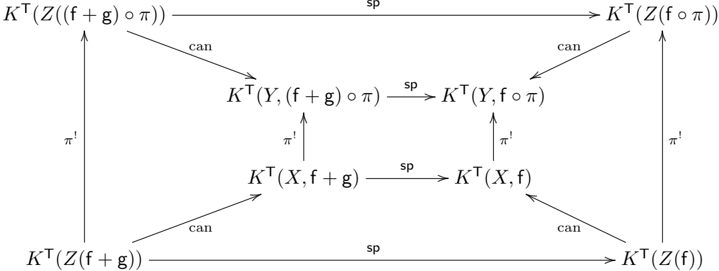
### Visual Description
## Mathematical Commutative Diagram: Functorial Relationships
### Overview
The image displays a commutative diagram from advanced mathematics, likely within category theory, homological algebra, or algebraic topology. It illustrates the relationships between several functorial constructions, denoted by `K^T`, applied to different combinations of objects (`X`, `Y`, `Z`) and morphisms or functions (`f`, `g`). The diagram is structured as a rectangular grid with six nodes connected by directed arrows, each labeled with a specific map or transformation (`sp`, `can`, `π'`).
### Components/Axes
The diagram consists of six nodes arranged in two rows and three columns, with the central column containing two vertically stacked nodes.
**Nodes (from top-left, moving right and down):**
1. **Top-Left:** `K^T(Z((f + g) ∘ π))`
2. **Top-Center:** `K^T(Y, (f + g) ∘ π)`
3. **Top-Right:** `K^T(Z(f ∘ π))`
4. **Bottom-Left:** `K^T(Z(f + g))`
5. **Bottom-Center:** `K^T(X, f + g)`
6. **Bottom-Right:** `K^T(Z(f))`
**Arrows and Labels:**
* **Horizontal Arrows (labeled `sp`):**
* From `K^T(Z((f + g) ∘ π))` to `K^T(Z(f ∘ π))` (Top row, left to right).
* From `K^T(Y, (f + g) ∘ π)` to `K^T(Y, f ∘ π)` (Top-center to a node not explicitly drawn but implied by the arrow's endpoint, which is `K^T(Y, f ∘ π)`).
* From `K^T(X, f + g)` to `K^T(X, f)` (Bottom-center to a node not explicitly drawn but implied by the arrow's endpoint, which is `K^T(X, f)`).
* From `K^T(Z(f + g))` to `K^T(Z(f))` (Bottom row, left to right).
* **Diagonal Arrows (labeled `can`):**
* From `K^T(Z((f + g) ∘ π))` to `K^T(Y, (f + g) ∘ π)` (Top-left to top-center).
* From `K^T(Z(f ∘ π))` to `K^T(Y, f ∘ π)` (Top-right to the implied top-center-right node).
* From `K^T(Z(f + g))` to `K^T(X, f + g)` (Bottom-left to bottom-center).
* From `K^T(Z(f))` to `K^T(X, f)` (Bottom-right to the implied bottom-center-right node).
* **Vertical Arrows (labeled `π'`):**
* From `K^T(Y, (f + g) ∘ π)` to `K^T(X, f + g)` (Top-center to bottom-center).
* From `K^T(Y, f ∘ π)` to `K^T(X, f)` (Implied top-center-right to implied bottom-center-right).
* From `K^T(Z((f + g) ∘ π))` to `K^T(Z(f + g))` (Top-left to bottom-left).
* From `K^T(Z(f ∘ π))` to `K^T(Z(f))` (Top-right to bottom-right).
### Detailed Analysis
The diagram is a network of commutative squares and triangles. The primary structure is a large outer rectangle whose corners are the four `Z`-nodes. Inside this, a smaller rectangle is formed by the `Y` and `X` nodes. The arrows define specific pathways between these constructions.
* **`sp` arrows:** These horizontal arrows likely represent a "specialization" or "splitting" map, transforming a construction involving a sum `(f + g)` into one involving only `f`.
* **`can` arrows:** These diagonal arrows likely represent "canonical" maps, relating constructions on the object `Z` to corresponding constructions on objects `Y` or `X`.
* **`π'` arrows:** These vertical arrows likely represent a map induced by a projection `π`, relating constructions involving `(f + g) ∘ π` or `f ∘ π` to those involving `f + g` or `f` directly.
The diagram asserts that all paths from a given starting node to a given ending node are equivalent. For example, the path from `K^T(Z((f + g) ∘ π))` to `K^T(X, f + g)` can be taken either via `can` then `π'`, or via `π'` then `can`. The commutativity of the diagram is the key mathematical statement.
### Key Observations
1. **Symmetry:** The diagram exhibits a high degree of symmetry. The left half deals with the sum `(f + g)`, while the right half deals with the single function `f`. The top row involves composition with `π`, while the bottom row does not.
2. **Implied Nodes:** Two nodes (`K^T(Y, f ∘ π)` and `K^T(X, f)`) are not explicitly drawn as boxes but are clearly implied as the targets of multiple arrows. This is a common shorthand in such diagrams.
3. **Consistent Labeling:** The labels `sp`, `can`, and `π'` are used consistently for all arrows of the same orientation and type, indicating they represent the same kind of natural transformation or functorial map applied in different contexts.
### Interpretation
This diagram is a formal, visual proof of the compatibility between several natural transformations (`sp`, `can`, `π'`) acting on a functor `K^T`. It demonstrates that the operations of "adding functions" (`f + g`), "composing with a projection" (`∘ π`), and applying the canonical and specialization maps all interact in a coherent, predictable way.
The commutativity ensures that the mathematical structures are well-behaved. For instance, it shows that the process of first specializing a sum of composed functions and then projecting is the same as first projecting the sum and then specializing. Such diagrams are fundamental in areas like derived functors, spectral sequences, or the study of model categories, where tracking how different operations interact is crucial. The diagram encapsulates a complex set of relationships into a single, verifiable geometric statement.
</details>
/
/
The outer square is commutative by Remark 7.10. The left and right trapezoids are commutative by [VV1, Lem. 2.4(a)]. The top and bottom trapezoids are commutative by Definition 7.20. Then it follows that
$$r \cos \theta = \sin \theta \cos \theta .$$
Since K T ( Z ( f + g )) can - - → K T ( X, f + g ) is surjective, we get π ! ◦ sp = sp ◦ π ! . The commutativity in the proper pushforward case can be proven similarly, with [VV1, Lem. 2.4(a)] replaced by [VV1, Lem. 2.4(b)]. □
Specialization map in Definition 7.20 is compatible with stable envelopes, i.e.
Proposition 7.22. Fix ( X, T , A , G m , f , g , C , s ) as in Setting 7.2. Suppose that there exist specialization maps sp : K T ( X, f + g ) → K T ( X, f ) and sp A : K T ( X A , f A + g A ) → K T ( X A , f A ). Then they are compatible with K -theoretic
O
O
/
/
/
/
O
O
g
g
w
w
/
/
O
O
stable envelopes, namely the following diagram is commutative
/
/
$$\begin{array}{ll}
K ^ { \prime } ( X ^ { \prime } A , f ^ { \prime } A + g ^ { \prime } A ) & \longrightarrow K ^ { \prime } ( X ^ { \prime } A , f ^ { \prime } A ) \\
\downarrow & \downarrow \\
K ^ { \prime } ( X , f + g ) & \longrightarrow K ^ { \prime } ( X , f ).
\end{array}$$
/
/
Proof. The proof is similar as in above. Consider the following diagram:
/
/
<details>
<summary>Image 7 Details</summary>
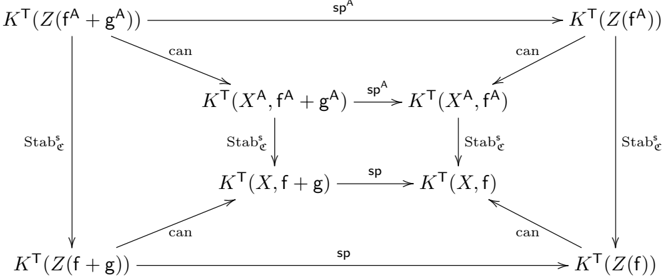
### Visual Description
## Commutative Diagram: Algebraic K-Theory/Stabilization Maps
### Overview
The image displays a commutative diagram from advanced mathematics, likely within the fields of algebraic topology, homotopy theory, or algebraic K-theory. It illustrates the relationships and compatibility between several functors or constructions (denoted by `K^T`) applied to different objects (`Z`, `X`) and functions (`f`, `g`), under the operations of stabilization (`Stab^A_e`), specialisation (`sp`, `sp^A`), and canonical maps (`can`). The diagram is structured as a 3x3 grid of nodes connected by horizontal, vertical, and diagonal arrows.
### Components/Axes (Nodes and Arrows)
**Nodes (9 total, arranged in a grid):**
* **Top Row (Left to Right):**
1. `K^T(Z(f^A + g^A))`
2. (Arrow target, no node)
3. `K^T(Z(f^A))`
* **Middle Row (Left to Right):**
1. `K^T(X^A, f^A + g^A)`
2. (Arrow target, no node)
3. `K^T(X^A, f^A)`
* **Bottom Row (Left to Right):**
1. `K^T(Z(f + g))`
2. `K^T(X, f + g)`
3. `K^T(X, f)`
4. `K^T(Z(f))`
**Arrows and Labels:**
* **Horizontal Arrows:**
* Top: `K^T(Z(f^A + g^A))` → `K^T(Z(f^A))` labeled `sp^A`.
* Middle: `K^T(X^A, f^A + g^A)` → `K^T(X^A, f^A)` labeled `sp^A`.
* Middle-Lower: `K^T(X, f + g)` → `K^T(X, f)` labeled `sp`.
* Bottom: `K^T(Z(f + g))` → `K^T(Z(f))` labeled `sp`.
* **Vertical Arrows:**
* Left: `K^T(X^A, f^A + g^A)` → `K^T(X, f + g)` labeled `Stab^A_e`.
* Right: `K^T(X^A, f^A)` → `K^T(X, f)` labeled `Stab^A_e`.
* **Diagonal Arrows (all labeled `can`):**
* Top-Left to Middle-Left: `K^T(Z(f^A + g^A))` → `K^T(X^A, f^A + g^A)`.
* Top-Right to Middle-Right: `K^T(Z(f^A))` → `K^T(X^A, f^A)`.
* Middle-Left to Bottom-Left: `K^T(X^A, f^A + g^A)` → `K^T(Z(f + g))`.
* Middle-Right to Bottom-Right: `K^T(X^A, f^A)` → `K^T(Z(f))`.
### Detailed Analysis
The diagram asserts the commutativity of multiple paths between its nodes. Key relationships include:
1. **Specialisation (`sp^A`, `sp`):** Moving horizontally from left to right corresponds to a map that likely "forgets" or "specialises" the `+ g` (or `+ g^A`) component. This operation is consistent across the `Z` and `X` levels, and between the `A`-superscripted and non-superscripted versions.
2. **Stabilization (`Stab^A_e`):** Moving vertically downward from the `X^A` row to the non-`A` row applies a stabilization map. This map is compatible with the horizontal `sp` maps, forming commutative squares on the left and right sides of the diagram.
3. **Canonical Maps (`can`):** The diagonal arrows represent canonical maps connecting the `Z`-based constructions to the `X`-based ones. These maps are also compatible with both the horizontal `sp` maps and the vertical `Stab^A_e` maps, ensuring the entire diagram commutes.
### Key Observations
* **Symmetry:** The diagram exhibits a high degree of symmetry. The left half (involving `f^A + g^A` and `f + g`) mirrors the right half (involving `f^A` and `f`).
* **Hierarchical Structure:** There is a clear two-level hierarchy: an upper level with objects marked with a superscript `A` (`X^A`, `f^A`, `g^A`) and a lower level without it. The `Stab^A_e` maps connect these levels.
* **Consistency of Operations:** The operations `sp`/`sp^A` and `can` are applied consistently across different contexts (`Z` vs. `X`, with or without `A`), which is the core message of a commutative diagram.
### Interpretation
This diagram is a formal statement of functoriality and compatibility in a sophisticated mathematical theory. It demonstrates that several natural constructions—specializing a function by ignoring an added term (`sp`), stabilizing a structure (`Stab^A_e`), and passing from a `Z`-type object to an `X`-type object (`can`)—all "play well together."
**What it likely means:**
* The `K^T` functor (possibly a variant of topological or algebraic K-theory) preserves these relationships.
* The process of stabilization (`Stab^A_e`) commutes with the specialization map (`sp`). In practical terms, stabilizing a system and then simplifying it yields the same result as simplifying it first and then stabilizing.
* The canonical maps (`can`) provide a bridge between two different but related categories of objects (`Z`-based and `X`-based), and this bridge is consistent with the other operations.
**Why it matters:** Such diagrams are the backbone of proofs in homotopy theory and related fields. They allow mathematicians to track how complex constructions behave under various transformations and ensure that different mathematical pathways lead to consistent results. The commutativity of this specific diagram would be a lemma or proposition used to establish a larger theorem about the properties of the `K^T` functor or the objects `X` and `Z`.
**Language:** The text is entirely in mathematical notation, using Latin letters and standard symbols (`+`, `^`, `_`). No natural language is present.
</details>
/
/
The outer square is commutative by Proposition 7.11. The left and right trapezoids are commutative by Lemma 3.30. The top and bottom trapezoids are commutative by assumption (i.e. (7.5) commutes). Then it follows that
$$S _ { \Delta A C F } = S _ { \Delta B C F }$$
$$\begin{aligned}
X ^ { A } f ( \bar { A } + g ^ { A } ) & = sp ^ { A } \\
\text{Since } K ^ { T } ( Z ( f ^ { A } + g ^ { A } ) ) = sp ^ { T } ,
\end{aligned}$$
In below, we provide two existence results for specialization maps in critical K -theory.
7.3.2. Existence result I. The first existence is due to P˘ adurariu in his study of K -theoretic Hall algebras for quivers with potentials and relation to shuffle algebras.
Proposition 7.23 ([P, Prop. 3.6]) . Suppose that f = 0. Assume that
- the T -fixed locus of X lies in the zero locus of g , i.e. X T ⊆ Z ( g ),
- K T ( X ) is torsion free over K T (pt).
Then the specialization map sp : K T ( X, g ) → K T ( X ) exists.
Remark 7.24. The argument in the proof of [P, Prop. 3.6] works for a reductive group T , so is Proposition 7.23.
7.3.3. Existence result II. The second result is about how to induce specialization maps for GIT semistable loci from specialization maps of their ambient spaces. This is motivated by [N, Eqn. (104)] where the induced specialization map is used.
Let G be a complex reductive group, T be a torus such that T × G act on P n × A m . Let X ⊂ P n × A m be a smooth projective-over-affine variety invariant under the action of T × G , g : X → C be a ( T × G )-invariant regular function, which satisfies the weight conditions in Setting 7.1 with T replaced with T × G . Let L = O (1) be a chosen linearization, and X ss be the semistable locus of X with respect to the G action and polarization L .
Proposition 7.25. Assume that g : X → C is not a constant function. Suppose that there exists a specialization map sp X : K T × G ( X, g ) → K T × G ( X ). Then there exists a specialization map sp X ss : K T × G ( X ss , g ) → K T × G ( X ss ), and the diagram
$$(7.6)$$
/
/
$$\begin{array}{ll}
K ^ { T } \times G ( X , g ) & \longrightarrow K ^ { T } \times G ( X ) \\
\downarrow & \downarrow \\
K ^ { T } \times G ( X ^ { s }, g ) & \longrightarrow K ^ { T } \times G ( X ^ { s 8 } )
\end{array}$$
/
/
is commutative, where the vertical arrows are the restriction to the semistable locus.
Moreover, if sp X is injective, then so is sp X ss .
)
)
/
/
/
/
g
g
w
w
Proof. We know that the unstable locus X \ X ss admits a Kempf-Ness (KN) stratification [Kir, DH], see § 4.7.2 for a description of KN stratification when X is a linear representation of G . By induction on the open strata, it suffices to prove the proposition replacing X ss with V := X \ S for a closed KN strata S . We note that there exists a cocharacter λ : C ∗ → G such that Z := X λ is a closed subvariety of S . Let
$$\frac { Y } { t - 1 0 } = A t r ( Z ) = \{ x \}$$
then Y is a closed subvariety in S and the action map G × P λ Y → S induces an isomorphism. Here P λ = { g ∈ G : lim t → 0 λ ( t ) gλ ( t ) -1 exists } is the parabolic subgroup associated to λ . We introduce notations
i
$$Z \xrightarrow { o } Y \xrightarrow { i } S ,$$
/
/
i
/
/
where σ , j are natural closed immersions, and π is the attraction map π ( y ) = lim t → 0 λ ( t ) · y . We also let
$$x = [ X / ( T \times G ) ], 2 y = [ V /$$
and we put a subscript 0 to denote the zero locus of g , for example X 0 := [ Z ( g ) / ( T × G )], V 0 = [( V ∩ Z ( g )) / ( T × G )], and so on.
Fix w ∈ Z , and recall that Halpern-Leistner constructed a semiorthogonal decomposition (SOD) of the bounded derived category D b ( X ) of coherent sheaves on X in [Hal, Thm. 3.35]:
$$D ^ { \prime } ( n ) = D ^ { \prime } _ { 0 } ( n , G _ { m } , D ^ { \prime } _ { 0 } ( n , S _ { m } ) .$$
Moreover, the restriction from X to V induces an equivalence:
$$G _ { w } = D ^ { b } ( \theta ) .$$
On the other hand, since g is T × G invariant, we have Z 0 = X λ 0 , and Y 0 = Attr λ ( Z 0 ), and the action map G × P λ Y 0 → S 0 induces an isomorphism. We have the following induced maps
j
$$Z _ { 0 } \xrightarrow [ \overline { r } ] { o _ { 0 } } Y _ { 0 } \xrightarrow [ i ^ { - } ] { S _ { 0 } }$$
/
/
j
/
/
Notice that Y 0 ∼ = Z 0 × Z Y where Z 0 → Z is the inclusion and Y → Z is π . In particular, π 0 : Y 0 → Z 0 is a locally trivial bundle of affine spaces, which is the condition (A) in [Hal, pp. 7]. We claim that the condition (L+) in [Hal, pp. 7] is also satisfied for the variety X 0 with KN strata S 0 , that is, Lσ ∗ 0 L S 0 /X 0 has nonnegative weights w.r.t. λ .
- If g is not constantly zero on S , then g | S : S → A 1 is a flat morphism (since g | S can not be a nonzero constant function due to weight conditions in Setting 7.1). In this case, S 0 is isomorphic to the derived zero locus S × L A 1 { 0 } , and we have
$$L _ { 1 } ^ { \prime } L _ { 2 } + Z l _ { 2 } + Z n l _ { 2 }$$
Since Lσ ∗ L S/X has nonnegative weights w.r.t. λ (see [Hal, Lem. 2.7]), so is Lσ ∗ 0 L S 0 /X 0 .
- If g | S = 0, then there is an exact triangle
$$7 0 L _ { S _ { 0 } } / x \rightarrow L _ { 0 } ^ { * } L _ { S _ { 0 } } / x \rightarrow + 1 .$$
Since S 0 = S and σ 0 = σ , Lσ ∗ 0 L S 0 /X = Lσ ∗ L S/X has nonnegative weights w.r.t. λ (see [Hal, Lem. 2.7]). Since g : X → A 1 is flat, we have L X 0 /X ∼ = O X 0 [1]. In particular, Lσ ∗ 0 L ( S 0 ↪ → X 0 ) ∗ L X 0 /X ∼ = O Z 0 [1] has zero λ weight. It follows that Lσ ∗ 0 L S 0 /X 0 has nonnegative weights w.r.t. λ .
In both cases, (L+) condition holds. Then by [Hal, Thm. 3.35], we have an SOD
$$D ^ { b } ( x _ { 0 } ) = \left \{ D ^ { b } _ { e _ { 0 } } ( x _ { 0 } ) <$$
and the restriction from X 0 to V 0 induces an equivalence:
$$G _ { 0 , \omega } = D ^ { b } ( \rho \theta ) .$$
$$D ^ { b } ( x _ { 0 } ) \rightarrow D ^ { b } ( x _ { 0 } ) / I$$
induces an SOD for the matrix factorization category (e.g. [P, Prop. 2.1]):
$$M F ( x , g ) = ( M F e ( x , g ) \leq w ) ,$$
The canonical functor
where MF S ( X , g ) <w , MF( G w , g ), and MF S ( X , g ) ≥ w are the essential images of D b S 0 ( X 0 ) <w , G 0 ,w , and D b S 0 ( X 0 ) ⩾ w respectively. Moreover, the restriction from X to V induces an equivalence:
$$M F G _ { n , 8 } = M F ( 3 g . )$$
Taking Grothendieck groups, and we obtain a commutative diagram:
O
O
/
/
O
O
$$\begin{array}{ll}
(7.7) & K ( x _ { 0 } ) \xrightarrow[ \text { can } ]{ s _ { w } } K ( x , g ) \\
& K ( y _ { 0 } ) \xrightarrow[ \text { can } ]{ v _ { w } } K ( y , g ) ,
\end{array}$$
/
/
where horizontal arrows are canonical maps, and vertical arrows are induced by the equivalences G 0 ,w ∼ = D b ( V 0 ) and MF( G w , g ) ∼ = MF( V , g ). Note that ( V 0 ↪ → X 0 ) ∗ s w = id, and ( V ↪ → X ) ∗ ψ w = id. Let sp X = sp X : K ( X , g ) → K ( X ) denote the specialization map. Then the pushforward map ( V 0 ↪ → V ) ∗ : K ( V 0 ) → K ( V ) factors into
$$( x _ { 0 } \rightarrow x ) _ { w } = ( x _ { 0 } \rightarrow x ) _ { w } , ( x _ { 0 } \rightarrow z ) _ { w } = ( x _ { 1 } \rightarrow x ) _ { w } o s p _ { x } o c a n o s _ { w }$$
Therefore, there exists a specialization map sp V : K ( V , g ) to K ( V ) and sp V = ( V ↪ → X ) ∗ ◦ sp X ◦ ψ w .
Finally, Let ¯ ψ w : K ( V ) → K ( X ) be the map obtained by taking Grothendieck groups to the equivalence G w ∼ = D b ( V ). Then ¯ ψ w induces an isomorphism K ( V ) ∼ = K 0 ( G w ). The image of sp X ◦ ψ w , which equals to the image of sp X ◦ ψ w ◦ can = sp X ◦ can ◦ s w = ( X 0 ↪ → X ) ∗ s w , is contained in the Grothendieck group of ( X 0 ↪ → X ) ∗ ( G 0 ,w ). Notice that ( X 0 ↪ → X ) ∗ ( G 0 ,w ) is contained in G w ; thus image of sp X ◦ ψ w is contained in the image of ¯ ψ w . In particular, ¯ ψ w ◦ ( V ↪ → X ) ∗ is identity on the image of sp X ◦ ψ w , and it follows that
$$\frac { 1 } { \phi _ { w } ^ { \circ } } s p _ { x } = \frac { 1 } { \phi _ { w } ^ { \circ } } ( 2 ) \rightarrow x$$
Now assume that sp X : K ( X , g ) → K ( X ) is injective, then sp X ◦ ψ w is also injective since ( V ↪ → X ) ∗ ψ w = id, and the equation ¯ ψ w ◦ sp V = sp X ◦ ψ w implies that sp V is injective. □
Combine Propositions 7.23 and 7.25, we obtain the following.
Corollary 7.26. Let X be a linear representation of T × G , θ : G → C ∗ be a character of G , g : X → C be a ( T × G )-invariant regular function, which satisfies the weight conditions in Setting 7.1 with T replaced with T × G . Let X ss be the θ -semistable locus of X with respect to the G action. Assume X T × G ⊂ Z ( g ), then there exist specialization maps sp X and sp X ss for X and X ss respectively, and the diagram (7.6) is commutative. Moreover, if sp X is injective, then so is sp X ss .
Example 7.27. Let X = R ( Q, v , d ) for a quiver Q with gauge dimension v and framing dimension d , G = ∏ i ∈ Q 0 GL( v i ) be the gauge group, T be a flavour torus (see § 4.2). Suppose that every edge loop has onzero T weight, then X T × G = { 0 } ⊂ Z ( g ) for any g that satisfies the weight conditions in Setting 7.1 with T replaced with T × G . Then we have specializations
$$\sum _ { i = 1 } ^ { n } K ^ { T } ( M ( v , d ) , g )$$
where M ( v , d ) = [ X/G ] and M ( v , d ) = [ X ss /G ]. Moreover, the diagram
/
/
$$\overrightarrow { K ^ { \prime } ( m ( v , d ) , g ) } \xrightarrow [ S D _ { M } ] { \Delta q } \overrightarrow { K ^ { \prime } ( m ( v , d ) ) }$$
/
/
is commutative, where the vertical arrows are the restriction to the semistable locus.
As an application, we give a proof of [N, Conj. 1.9], which we thank Andrei Negut ¸ for helpful communications.
Let ( Q, W ) be the quiver with potential associated to a symmetrizable Kac-Moody algebra g A,D in [COZZ1, Def. A.1], T be the torus C ∗ ℏ that scales the arrows in loc. cit. , and set g = tr W : R ( Q, v , d ) → C . Then the argument of [COZZ2, Lem. A.4] can be applied to K -theory and the localized specialization map
$$h ) \rightarrow K ^ { T } ( m ( v , d ) ) \otimes c [ n + 1 ] C ( h )$$
is injective. According to the above discussion, the localized specialization map
$$h ) \rightarrow K ^ { T } ( M ( v , d ) ) \otimes c [ n + 1 ] C ( h )$$
is also injective. This proves the injectivity statement in [N, Conj. 1.9]. The surjectivity statement in [N, Conj. 1.9] follows from the surjectivity of restriction-to-open map for critical K -theory (see § 2.3.5) and torus localization (2.22).
7.3.4. Existence result III. The third existence result is relevant to examples considered in [COZZ3]. The idea of construction uses dimensional reduction to the case when there is no potential.
Construction 7.28. Let G be a linear reductive group, T be a torus, with a direct sum of finite dimensional linear ( G × T × G m )-representations:
$$V = V _ { 0 } L$$
Let π : W → V be the projection with a pair of ( G × T )-equivariant sections:
$$8 0 . 8 \in [ 1 , 2 ^ { \prime } )$$
of the dual bundle U ∨ := V × U ∨ → V of π . Assume that s 0 is G m -equivariant, and there exists a decomposition
$$S _ { c } = \sum _ { i = 1 } ^ { n } S _ { e , i }$$
such that G m scales s ϵ,i with weight -n i < 0, i.e. u n i s ϵ,i is G m -equivariant ( i = 1 , · · · , m ). Define the section
$$s _ { t } = s _ { 0 } + \sum _ { i = 1 } ^ { n } t ^ { n } s _ { i } , t \in A ^ { \prime } .$$
Let Z der ( s t ) be the derived zero locus of s t , which fits into the following diagram
/
/
$$\pi^{-1}(Z_{der}(s_t)) \rightarrow W \\
\downarrow Z_{der}(s_t) \rightarrow V.
$$$$
/
/
Let e be the coordinate of the fiber of π and define ( G × T )-invariant regular function:
$$W _ { 1 } = ( e _ { 1 } s _ { 1 } ) \cdot H r + C$$
Choose a stability condition such that the semistable locus equals the stable locus:
̸
$$W ^ { 8 8 } = W ^ { 8 } \neq 0 .$$
By abuse of notations, we write the descent of w t to be
$$w _ { 1 } \cdot x = w ^ { \prime } / G - C$$
Then ( X, T , A , f = w 0 , g = w 1 -w 0 ) fits into Setting 7.1.
By applying dimensional reduction (Proposition D.2, Remark D.3), we obtain
$$\frac { 1 } { 4 \ast : K ^ { T } ( \pi - 1 ( z d e r ( s _ { t } ) ) / C }$$
There is a standard specialization map for the left hand side:
$$\rightarrow K ^ { T } ( r - 1 ( z _ { der } ( s _ { 0 } ) ) ^ { s } / G ) ,$$
defined by an extension to K -theory class of the family π -1 ( Z der ( s t ))) s /G ( t ∈ A 1 ), followed by the Gysin pullback to the special fiber π -1 ( Z der ( s 0 ))) s /G (e.g. [CG, § 5.3], Definition 7.7).
Definition 7.29. Under the setting of Construction 7.28, we define ν as the unique map which makes the following diagram commute:
O
O
/
/
O
O
$$\begin{array}{ll}
K ^ { T } ( X , w _ { 1 } ) & \xrightarrow [ v ]{} K ^ { T } ( X , w _ { 0 } ) \\
& \xleftarrow [ t _ { 1 } = s ]{} K ^ { T } ( π ^ { - 1 } ( Z ^ { der } ( s _ { 1 } )) / G ) . & \text{sp} \\
\end{array}$$
/
/
Proposition 7.30. The map ν (7.8) is the specialization map for critical K -theory (Definition 7.20).
Proof. We have the following diagram
<details>
<summary>Image 8 Details</summary>
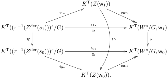
### Visual Description
\n
## Commutative Diagram: Equivariant K-Theory Relationships
### Overview
The image displays a commutative diagram from the field of algebraic topology, specifically equivariant K-theory. It illustrates the relationships between various K-theory spaces constructed from derived categories, group actions, and specific vector bundles or sheaves. The diagram consists of six nodes connected by labeled arrows, indicating maps or transformations between these mathematical objects.
### Components/Axes
The diagram is structured as a network of mathematical expressions (nodes) connected by directed arrows (morphisms). There are no traditional axes, as this is a categorical diagram.
**Nodes (Mathematical Expressions):**
1. **Top-Left:** `K^T((π^{-1}(Z^{der}(s_1)))^s / G)`
2. **Top-Center:** `K^T(Z(w_1))`
3. **Top-Right:** `K^T(W^s / G, w_1)`
4. **Bottom-Left:** `K^T((π^{-1}(Z^{der}(s_0)))^s / G)`
5. **Bottom-Center:** `K^T(Z(w_0))`
6. **Bottom-Right:** `K^T(W^s / G, w_0)`
**Arrows (Morphisms/Maps) and Labels:**
* From Top-Left to Top-Center: Arrow labeled `i_{1*}`.
* From Top-Left to Bottom-Left: Arrow labeled `sp`.
* From Top-Center to Top-Right: Arrow labeled `can`.
* From Top-Center to Bottom-Center: Curved arrow labeled `sp`.
* From Top-Right to Bottom-Right: Arrow labeled `ν`.
* From Bottom-Left to Bottom-Center: Arrow labeled `i_{0*}`.
* From Bottom-Left to Top-Left: Arrow labeled `ι_{1*}` with an isomorphism symbol `≅` below it.
* From Bottom-Right to Top-Right: Arrow labeled `ι_{0*}` with an isomorphism symbol `≅` below it.
* From Bottom-Center to Bottom-Right: Arrow labeled `can`.
### Detailed Analysis
The diagram is organized into two horizontal rows and three vertical columns, with additional diagonal and curved connections.
* **Left Column:** Contains nodes based on the construction `K^T((π^{-1}(Z^{der}(s_i)))^s / G)` for `i = 0, 1`. These are connected vertically by a map `sp` (likely a "specialization" map).
* **Center Column:** Contains nodes of the form `K^T(Z(w_i))` for `i = 0, 1`. These are connected by a curved `sp` map.
* **Right Column:** Contains nodes of the form `K^T(W^s / G, w_i)` for `i = 0, 1`. These are connected vertically by a map `ν`.
* **Horizontal Connections:** The left column maps to the center column via `i_{0*}` and `i_{1*}`. The center column maps to the right column via `can` (likely a "canonical" map).
* **Isomorphisms:** The vertical arrows `ι_{1*}` (from Bottom-Left to Top-Left) and `ι_{0*}` (from Bottom-Right to Top-Right) are explicitly marked as isomorphisms (`≅`), indicating these are invertible maps and thus the connected objects are equivalent in the relevant category.
### Key Observations
1. **Symmetry:** The diagram exhibits a clear symmetry between the `s_0` and `s_1` cases (bottom and top rows, respectively). The structure of maps (`i_*`, `can`, `sp`, `ν`) is mirrored.
2. **Commutativity:** The diagram is commutative, meaning that following any two paths of arrows from one node to another yields the same result. For example, the path from Top-Left to Bottom-Right via `sp` then `i_{0*}` then `can` should be equivalent to the path via `i_{1*}` then `sp` then `ν`.
3. **Key Maps:** The diagram highlights three important types of maps in this theory:
* `sp`: Specialization maps (vertical on the left, curved in the center).
* `can`: Canonical maps (horizontal from center to right).
* `ι_*`: Isomorphisms (vertical on the left and right edges).
* `ν`: A map connecting the two `W^s / G` constructions.
4. **Notation:** The notation uses standard conventions: `K^T` for equivariant K-theory, `π^{-1}` for inverse image, `Z^{der}` for a derived category construction, `/ G` for a quotient by a group action, and subscripts `*` on maps to denote the induced map on K-theory.
### Interpretation
This diagram is a formal representation of relationships in a specialized area of mathematics, likely equivariant K-theory or derived algebraic geometry. It serves as a visual proof or summary of how different constructions are related.
* **What it Demonstrates:** The diagram shows that the K-theory of certain quotient spaces (`(π^{-1}(Z^{der}(s_i)))^s / G` and `W^s / G`) can be related to the K-theory of simpler spaces (`Z(w_i)`) through canonical maps and specializations. The presence of isomorphisms (`ι_*`) indicates that some of these relationships are equivalences, which is a powerful result.
* **Relationships:** The core relationship is between a "derived" construction (left column), a "zero-section" or "central" construction (center column), and a "global" or "ambient" construction (right column). The `sp` maps likely relate theories at different "points" or "parameters" (`s_0` and `s_1`), while the `can` maps embed the central theory into the global one.
* **Purpose:** For a researcher, this diagram encapsulates a theorem or a key lemma. It allows them to track how information (like K-theory classes) transforms under different operations and guarantees that certain computations can be performed in a more convenient part of the diagram (e.g., in the center column) with the results being valid elsewhere due to commutativity and the isomorphisms.
* **Notable Feature:** The curved `sp` arrow in the center is a distinctive visual element, emphasizing that the specialization map between the `Z(w_i)` nodes has a different character or is derived from a different process than the vertical `sp` map on the left.
</details>
)
)
Here the upper and lower triangles commute as π -1 ( Z der ( s t )) i t ↪ → Z ( w t ), and the canonical map is simply the pushforward map. The middle square commutes by Definition 7.29. The commutativity of
/
/
$$\begin{array}{ll}
K ^ { T } ( Z ( w _ { 1 } ) ) & \xrightarrow [ \text { can } ] { sp } K ^ { T } ( W ^ { s } / G , w _ { 1 } ) \\
& \xrightarrow [ \text { can } ] { sp } K ^ { T } ( Z ( w _ { 0 } ) ) & K ^ { T } ( W ^ { s } / G , w _ { 0 } ) ,
\end{array}$$
is equivalent to the equality of maps
$$( Z ( w _ { 1 } ) \rightarrow K ^ { \prime } I ( t - 1 ) ( Z ^ { \prime } ( s _ { 0 } ) ) / C ) .$$
Let Kos( τ, s t ) denote the Koszul factorization (D.6). Then
$$( ( t _ { i } - 1 ) o c a n ) ( - ) = ( i ^ { z } ( w _ { i } )$$
where i Z ( w t ) : Z ( w t ) → W s /G is the inclusion. Therefore, for any [ E ] ∈ K T ( Z ( w 1 )), we have
$$\begin{array}{ll}
sp ^ { o } ( i _ { 1 } \circ can ) [ E ] & = sp ( i _ { z } ( w _ { 1 } ) = sp ( i _ { z } ( w _ { 0 } ) [ E ] \\
& = sp ( i _ { z } ( w _ { 0 } ) [ E ] = ( i _ { 0 } \circ can ) [ E ] ,
\end{array}$$
where we use the fact that the specialization of tensor products is the tensor product of specializations. □
Example 7.31. Let G = GL n be the gauge group and consider representation spaces W,V,U of the following quivers
l
$$\begin{array}{c}
W : \Box \\
\downarrow y \\
A \rightarrow B \\
B \rightarrow C \\
C \rightarrow D \\
D \rightarrow A \\
\end{array}
\begin{array}{c}
V : \Box \\
\downarrow y \\
A \rightarrow B \\
B \rightarrow C \\
C \rightarrow D \\
D \rightarrow A \\
\end{array}
\begin{array}{c}
U : \Box \\
\downarrow y \\
A \rightarrow B \\
B \rightarrow C \\
C \rightarrow D \\
D \rightarrow A \\
\end{array}$$
,
,
l
W
W
,
,
W
W
l
l
We define cyclic stability on W , so the stable locus W s are those representations which satisfy C ⟨ x, ξ, y ⟩ A ( C N ) = C n , and define the GIT quotient
$$x = w ^ { r } / G L _ { h }$$
$$u \cdot ( \{ x , y , A , B \} ) = ($$
and choose a T -action on W which commutes with (GL n × G m )-action, so that
$$W = V \theta U$$
is a direct sum of ( G × T × G m )-representations. For any t ∈ A 1 , we define a map
$$\rightarrow ( \gamma , \xi , A - t ^ { 2 } A E ) ,$$
where Ξ is a fixed N by N matrix. The potential function is determined by s t via the trace pairing:
$$w _ { t } = tr ( \{ x , y \} + \{ A B \} )$$
y
y
y
y
We choose a G m -action on W by
/
/
/
/
/
/
(
(
(
(
Then w 0 is G m -invariant and G m scales w 1 -w 0 with weight -2. These data fit into the setting of Construction 7.28. By Proposition 7.30, the specialization map
$$s p : x ^ { 7 } ( x _ { n + 1 } - x ^ { 7 } ( x _ { n } )$$
exists in critical K -theory. This map is useful to relate different modules of quantum toroidal algebra U q 1 ,q 2 ,q 3 ( ̂ gl 1 ).
## 8. Vector bundles and stable envelopes
Let ( X, w , T , A ) be as in Setting 2.1, and take a T -equivariant vector bundle E on X with projection
$$\pi : Y := Tot ( E ) \rightarrow X .$$
$$X .$$
Define i : X ↪ → Y as the zero section map. We note that F ↦→ i -1 ( F ) gives a bijection
$$F _ { 1 } ( Y ) = F _ { 2 } ( X ).$$
where the inverse map is given by G ↦→ ( π -1 ( G )) A .
In this section, we prove several compatibility results for stable envelopes of ( X, w , T , A ) and ( Y, ˜ w , T , A ), when ˜ w is a T -invariant function on Y such that ˜ w | X = w , and E is attracting or repelling. We show that the closure of the attracting set of the diagonal gives stable envelope correspondence on ( X, w , T , A ) when Y is a symmetric quiver variety and E has a decomposition into attracting and repelling subbundles (Theorem 8.9). This explicit description is particularly useful in the manipulation of stable envelopes. Finally, we prove a triangle lemma for attracting closure correspondence without attracting or repelling condition on E (Proposition 8.10), which will be used to prove the triangle lemma of Hall envelopes in § 9.5.
## 8.1. Definitions and properties.
Definition 8.1. An A -equivariant vector bundle E on X is called attracting (resp. repelling ) with respect to a chamber C if ∀ F ∈ Fix A ( X ), E | F has nonnegative (resp. nonpositive) A -weights with respect to C .
Proposition 8.2. Assume that E is attracting with respect to C . Then cohomological stable envelope exists for ( X, w , T , A , C ) if and only if it exists for ( Y, w ◦ π, T , A , C ). When they exist, the following diagram commutes
O
O
/
/
O
O
$$\begin{array}{ll}
H ^ { T } ( Y _ { A } , ( w _ { o } \pi ) ^ { A } ) & \xrightarrow [ Stab _ { e } ] { π ^ { A } } H ^ { T } ( Y _ { A } , ( w _ { o } \pi ) ^ { A } ) \\
H ^ { T } ( X _ { A } , w ^ { A } ) & \xrightarrow [ Stab _ { e } ] { π ^ { A } } H ^ { T } ( X _ { A } , w ^ { A } ).
\end{array}$$
/
/
Similarly, let s ∈ Pic A ( X ) ⊗ Z R be a generic slope, then K -theoretic stable envelope exists for ( X, w , T , A , C , s ) if and only if it exists for ( Y, w ◦ π, T , A , C , s ). When they exist, the following diagram commutes
O
O
/
/
O
O
$$\begin{array}{ll}
K ^ { T } ( Y _ { A } , w _ { 0 } \pi ) & \xrightarrow [ Stab ^ { 2 } ]{} K ^ { T } ( Y _ { A } , w _ { 0 } \pi ) \\
\end{array}
\begin{array}{ll}
K ^ { T } ( X _ { A } , w ^ { A } ) & \xrightarrow [ Stab ^ { 2 } ]{} K ^ { T } ( X _ { A } , w ^ { A } ).
\end{array}$$
/
/
Proof. We prove the cohomology version. Assume that cohomological stable envelope exists for ( X, w , T , A , C ). Define
$$\therefore w ^ { \prime } ( A ) - H ^ { \prime } ( Y , w o r t ) .$$
For an arbitrary F ∈ Fix A ( Y ), and take an arbitrary γ ∈ H T / A ( i -1 ( F ) , w A ), we claim that S ( γ ) satisfies the axioms (ii) and (iii) in Definition 3.4 and axiom (i') in Remark 3.7, namely
- (1) S ( γ ) is supported on Attr ≤ C ( F );
- (2) S ( γ ) ∣ ∣ F = e T ( N -F/Y ) · π A ∗ ( γ );
̸
- (3) For any F ′ = F , the inequality deg A S ( γ ) ∣ ∣ F ′ < deg A e T ( N -F ′ /Y ) holds.
Here we choose the ample partial order ≤ as in Remark 3.9. Since π A ∗ : H T ( X A , w A ) → H T ( Y A , ( w ◦ π ) A ) is an isomorphism with the inverse map given by i A ∗ , the above three properties imply that S ◦ i A ∗ is a cohomological stable envelope for ( Y, w ◦ π, T , A , C ), moreover the diagram (8.2) commutes.
Since E is attracting, for all G ∈ Fix A ( Y ), we have
$$A + b ( a - \frac { 1 } { a } ) = \frac { 1 } { a } ( A + b ) ^ { 2 } - ( A - 1 ) ^ { 2 }$$
Therefore S ( γ ) is supported on
$$\pi ^ { - 1 } ( A t t _ { r } \leq ( r - 1 ) ( F ) ) = \pi ^ { - 1 } ( U _ { i - 1 } ( F ) \leq i - 1 ( G )$$
This proves (1). For (2), we notice that
$$S ( y ) | F = π A * ( S t a b l e ($$
where in the last equation we use the fact that E is attracting so that N -F/Y ∼ = π A ∗ ( N -i -1 ( F ) /X ) .
For (3), we notice that S ( γ ) ∣ ∣ F ′ = π A ∗ ( Stab C ( γ ) | i -1 ( F ′ ) ) . Since π A ∗ preserves deg A , we have
$$\begin{aligned}
& \delta e ( r ) | r _ { v } = \delta e A ( S ) \\
& = \delta e A ^ { T } ( N _ { F } / y ) .
\end{aligned}$$
This proves one direction. For the other direction, assume that cohomological stable envelope exists for ( Y, w ◦ π, T , A , C ), then a similar argument as above shows that i ∗ ◦ Stab C ◦ π A ∗ is a cohomological stable envelope for ( X, w , T , A , C ). This proves the cohomology version.
The K
$$The K -theory version is proven sin-$$
Proposition 8.3. Assume that E is repelling with respect to C . Let ˜ w be a T -invariant function on Y such that ˜ w | X = w . Moreover, assume that cohomological stable envelopes exist for both ( X, w , T , A , C ) and ( Y, ˜ w , T , A , C ). Then the following diagram is commutative
O
O
/
/
O
O
$$\begin{array}{ll}
H ^ { T } ( Y _ { A } , \omega ^ { A } ) & \xrightarrow [ \text { Stabe } ] { H ^ { T } ( X _ { A } , \omega ^ { A } ) } H ^ { T } ( Y _ { W } , \omega ^ { W } ) \\
\end{array}$$
/
/
Similarly, let s ∈ Pic A ( X ) ⊗ Z R be a generic slope, and assume that K -theoretic stable envelopes exist for both ( X, w , T , A , C , s ′ ) and ( Y, ˜ w , T , A , C , s ) where s ′ = s ⊗ (det E ) 1 / 2 . Then the following diagram is commutative
O
O
/
/
O
O
$$\begin{array}{ll}
K ^ { T } ( Y ^ { A } _ { w } , \omega ^ { A } ) & \xrightarrow [ Stab _ { g } ^ { 5 } ] { K ^ { T } ( X ^ { A } _ { w } , \omega ^ { A } ) } K ^ { T } ( Y _ { w } , \omega ) \\
\end{array}$$
/
/
Proof. We prove the cohomology version ( K -theory version can be proven similarly). Define
$$S = i _ { 0 } S t a b e : H ^ { T } ( Y , w ) .$$
For an arbitrary F ∈ Fix A ( Y ), and take an arbitrary γ ∈ H T / A ( i -1 ( F ) , w A ), we need to show that S ( γ ) satisfies the axioms (ii) and (iii) in Definition 3.4 and axiom (i') in Remark 3.7, namely
- (1) S ( γ ) is supported on Attr ≤ C ( F );
- (2) S ( γ ) ∣ ∣ F = e T ( N -F/Y ) · i A ∗ ( γ );
̸
- (3) For any F ′ = F , the inequality deg A S ( γ ) ∣ ∣ F ′ < deg A e T ( N -F ′ /Y ) holds.
Here we choose the ample partial order ≤ as in Remark 3.9.
Since E is repelling, we have i -1 (Attr C ( G )) = Attr C ( i -1 ( G )) for all G ∈ Fix A ( Y ); therefore S ( γ ) is supported on
$$\begin{aligned}
i ( A t t _ { c } ^ { \leq } ( r - 1 ) ( F ) ) = i ( r - 1 ) ( F ) \\
& = X _ { n } A t t _ { c } ^ { \leq } ( G ) U _ { F } G \\
& = X _ { n } A t t _ { c } ^ { \leq } ( F ) C A t t _ { c } ^ { \leq } ( F ) .
\end{aligned}$$
This prove (1). For (2), we notice that
$$x ) \cdot r ) = e ^ { i T } ( N F _ { r } y ) \cdot t ^ { A } ( S )$$
where in the last equation we have used the fact that E is repelling so that
$$x ) + E ( F ^ { \prime } _ { F } \in K ^ { T } ( F ) .$$
For (3), we notice that S ( γ ) ∣ ∣ ′ = e T ( E | mov F ′ ) · i A ∗ ( Stab C ( γ ) | i -1 ( F ′ ) ) . Since i A ∗ preserves deg A , we have
$$\hat { S } ( r ) | _ { F } = e ^ { i \cdot A ^ { * } } ( N _ { x } - 1 ) + E [ F ^ { * } ] _ { F } \in K ^ { T } ( F ).$$
$$\begin{aligned}
\left | \frac { d e g A S ( r ) } { r _ { v } } \right | = d e g A ^ { T } ( E ) < d e g A ^ { T } ( N - i - 1 ( F _ { v } ) x ) = d e g A ^ { T } ( N - i - 1 ( F _ { v } ) + d e g A ^ { T } ( N - i - 1 ( F _ { v } ) x ) \right |
\end{aligned}$$
The following lemma will be used in Appendix E.
Lemma 8.4. Assume that E is repelling with respect to C . Suppose that F ∈ Fix A ( X ) is a fixed component in X such that E | F is moving. Let C ∗ u act on Y by fixing X and scaling the fibers of E with weight 1. Suppose that K -theoretic stable envelope exists for ( Y, w ◦ π, T × C ∗ u , A , C , s ), then there exists a K -theoretic stable envelope map 15 Stab s ′ C : K T ( F, w A ) → K T ( X, w ), where s ′ = s ⊗ (det E ) 1 / 2 .
Proof. By assumption, the projection ( π -1 ( F )) A → F is an isomorphism. Let σ : C ∗ → A be a cocharacter in the chamber C , then we claim that Stab s ′ σ : K T ( F, w A ) → K T ( X, w ) (in Definition 3.33) satisfies axioms (i)-(iii) in Definition 3.10 with respect to the whole chamber C .
It is enough to check axiom (iii). We note that C ∗ u acts on X trivially, so Stab s ′ σ extends to a K -theoretic stable envelope for ( X, w , T × C ∗ u , C ∗ , +). Proposition 8.3 implies that
$$i _ { 0 } S t a b ^ { \prime } = S t a b ^ { \prime } o r A .$$
As E | F is moving, i A ∗ is an isomorphism when restricted to F , we see that for all γ ∈ K T × C ∗ u ( F, w A ) and for all F ′ ∈ Fix A ( X ) , F ′ = F , there is a strict inclusion of polytopes
̸
$$\begin{aligned}
& \frac { 1 } { a ^ { 5 } _ { 0 } ( n ) } | F _ { r } \xi | = deg _ { A } e ^ { i x C u } ( E | F _ { r } ) \cdot S t \\
& + shift _ { r } - shift _ { r } , y ) +$$
where shift F := weight A ( det( N -F/X ) 1 / 2 ⊗ s ′ | F ) . It follows that
$$C ^ { \prime } _ { ( N F / x ) } + shift _ { p } - shift _ { F } .$$
Since s is generic, the above inclusion must be strict by Remark (3.12). Evaluating at u = 1, Stab s ′ σ induces a K -theoretic stable envelope map Stab s ′ C : K T ( F, w A ) → K T ( X, w ). □
Remark 8.5. Under the assumption of Lemma 8.4, suppose that C ′ is a face of C and let A ′ be the subtorus of A associated with C ′ , and we also assume the existence of K -theoretic stable envelope for ( Y, w ◦ π, T × C ∗ u , A ′ , C ′ , s ). Assume moreover that F is an A ′ -fixed component and E | F is moving with respect to A ′ -action. Then by Lemma 8.4 we have K -theoretic stable envelope maps Stab s ′ C and Stab s ′ C ′ from K T ( F, w A ) to K T ( X, w ), where s ′ = s ⊗ (det E ) 1 / 2 . Moreover, there exists an obvious K -theoretic stable envelope map Stab s ′′ C / C ′ : K T ( F, w A ) → K T ( F, w A ) for the s ′′ determined by Lemma 3.37, which is the identity map. Therefore by Lemma 3.37, we have Stab s ′ C = Stab s ′ C ′ .
Combining Propositions 8.2, 8.3, we obtain the following.
Proposition 8.6. Assume that there exists a decomposition E = E + ⊕ E -such that E + is attracting and E -is repelling with respect to C . Suppose that w ′ is a T -invariant function on Tot( E -) such that w ′ | X = w , and define ˜ w := ( Y → Tot( E -)) ∗ ( w ′ ). Moreover, assume that cohomological stable envelopes exist for both ( X, w , T , A , C ) and ( Y, ˜ w , T , A , C ). Then the following diagram is commutative
O
O
/
/
O
O
$$\begin{array}{ll}
H ^ { T } ( Y _ { A } , \omega ^ { A } ) & \xrightarrow [ Stab e ] { v ^ { A } } H ^ { T } ( Y _ { W } ) \\
H ^ { T } ( X _ { A } , \omega ^ { A } ) & \xrightarrow [ Stab e ] { v ^ { A } } H ^ { T } ( X _ { W } ),
\end{array}$$
/
/
15 This means a map satisfying axioms (i)-(iii) in Definition 3.10 for component F .
where
Similarly, let s ∈ Pic A ( X ) ⊗ Z R be a generic slope, and assume that K -theoretic stable envelopes exist for both ( X, w , T , A , C , s ′ ) and ( Y, ˜ w , T , A , C , s ), where s ′ = s ⊗ (det E -) 1 / 2 . Then the following diagram is commutative
O
$$\begin{array}{ll}
K ^ { T } ( Y _ { A } , w ^ { A } ) & \xrightarrow [ Stab ^ { c } _ { A } ]{ } K ^ { T } ( Y _ { W } ) \\
K ^ { T } ( X _ { A } , w ^ { A } ) & \xrightarrow [ Stab ^ { c } _ { A } ]{ } K ^ { T } ( X _ { W } ),
\end{array}$$
O
where ψ and ψ A are given by K -theoretic version of (8.7).
8.2. Attracting closure as cohomological stable envelopes. The following explicit descriptions of cohomological stable envelopes will be useful. In below, we omit the canonical map in Lemma 3.22 and simply write
$$\vert A + A \vert = 0$$
Proposition 8.7. Assume that E is attracting with respect to C . If [Attr C (∆ Y A )] induces cohomological stable envelope for ( Y, w ◦ π, T , A , C ), then [Attr C (∆ X A )] induces cohomological stable envelope for ( X, w , T , A , C ).
Proof. Let S : H T ( X A , w A ) → H T ( X, w ) be the map induced by [Attr C (∆ X A )], Stab C the cohomological stable envelope for ( Y, w ◦ π, T , A , C ). By Proposition 8.2, it suffices to show that S satisfies
$$r ^ { \prime } r S = S _ { \Delta } b c o n ^ { r ^ { \prime } } .$$
Let W ⊆ Y × X A be the total space of vector bundle pr ∗ E on Attr C (∆ X A ), where pr : Attr C (∆ X A ) → X is the projection, then π ∗ ◦ S is induced by the correspondence [ W ].
Note that Attr C (∆ Y A ) × (id × π A )( Y A ) intersects transversely with Y × ∆ Y A × X A inside ( Y × Y A ) × ( Y A × X A ), and their intersection equals to Attr C ((∆ × π A )( Y A )) ⊆ Y × Y A × X A , where ∆: Y A ↪ → Y A × Y A is the diagonal map. The intersection of Attr C (∆ Y A ) × (id × π A )( Y A ) with Y × ∆ Y A × X A is contained in Attr C ((∆ × π A )( Y A )), where the latter closure is taken inside Y × Y A × X A ; thus in the equivariant Chow group, we have
$$\sum _ { A \in A } [ \sqrt { Y \times \Delta y_A \times X^A } ] = \sqrt { A t t r e ( \Delta y_A \times \pi ^A ) }$$
Then Stab C ◦ π A ∗ is induced by the correspondence p 13 ∗ [Attr C ((∆ × π A )( Y A ))], where p 13 : Y × Y A × X A → Y × X A is the projection to the first and third components. Since p 13 induces isomorphism (∆ × π A )( Y A ) ∼ = (id × π A )( Y A ), we have
$$= [ \sqrt { A t t r e ( i d x π ^ { A } ) ( Y ^ { A } ) } ] ,$$
where the latter closure is taken in Y × X A . Furthermore, Attr C ((id × π A )( Y A )) is the total space of vector bundle pr ∗ E on Attr C (∆ X A ) where pr: Attr C (∆ X A ) → X is the natural projection. Therefore, we have Attr C ((id × π A )( Y A )) = W , and it follows that π ∗ ◦ S = Stab C ◦ π A ∗ . □
Proposition 8.8. Assume that E is repelling with respect to C . Let C ∗ u act on Y by fixing X and scale the fibers of E with weight 1, and let ˜ w be a T × C ∗ u -invariant function on Y such that ˜ w | X = w .
If [Attr C (∆ Y A )] induces cohomological stable envelope for ( Y, ˜ w , T × C ∗ u , A , C ), then [Attr C (∆ X A )] induces cohomological stable envelope for ( X, w , T , A , C ).
Proof. Step 1. Weshow that cohomological stable envelope exists for ( X, w , T , A , C ). Let σ : C ∗ → A be a cocharacter that lies in C . Then cohomological stable envelope Stab σ exists for ( X, w , T × C ∗ u , C ∗ , +) by Proposition 3.23. By Proposition 8.3, we have
$$i _ { 1 } o S t a b _ { y } = S t a b _ { y } r o f ^ { \prime } .$$
Here Stab C ,Y is the stable envelope for ( Y, ˜ w , T × C ∗ u , A , C ) and we use the fact that it is the same as the stable envelope when replacing A by above σ in chamber C (ref. Proposition 3.34).
Let σ ′ : C ∗ → A be another cocharacter that lies in C , then we have
$$l _ { 1 } O S h l o _ { 6 } = l _ { 2 } O S h l o _ { 6 }$$
Applying i ∗ to two sides of the above equation, we get
$$T _ { x ^ { \prime } ( E ) } ( S _ { 1 } a _ { 0 } - S _ { 2 } a _ { 0 } ) = 0$$
/
/
O
O
/
/
We note that H T × C ∗ u ( X, w ) ∼ = H T ( X, w ) ⊗ Q [ u ], and multiplication by e T × C ∗ u ( E ) is injective on H T × C ∗ u ( X, w ) because e T × C ∗ u ( E ) = u rk E +lower degree in u . Thus Stab σ = Stab σ ′ , and it follows from Proposition 3.34 that cohomological stable envelope exists for ( X, w , T × C ∗ u , A , C ). Evaluating at u = 0, we are done.
Step 2. We show that Stab C for ( X, w , T , A , C ) is induced by the correspondence [Attr C (∆ X A )].
By Lemmata 8.11, 8.12, Attr C (∆ Y A ) is a vector bundle of rank (rk E | fixed X A ) over Attr C (∆ X A ), and
$$\frac { \frac { 1 } { n } } { X ^ { A } } = \overline { A t t r e ( \Delta x _ { A } ) , }$$
$$\sum _ { i = x ^ { A } } ^ { \infty } [ A t r e ( \Delta y _ { a } ) ] = u _ { k } E \cdot [ A t r$$
Let p 1 , p 2 be the projections from Y × Y A to Y, Y A respectively, and let p 1 , p 2 be the projections from X × X A to X,X A respectively. Then we have
$$\begin{aligned}
i ^ { \prime } o Stab _ { g } ( 8 . 9 ) & = i ^ { \prime } o p _ { 2 x } ( [ Attr _ { c } ( \Delta y _ { A } ) ] \otimes p _ { 1 } ( i ^ { \prime } A ( - y _ { o } i ^ { \prime } ) ) \\
& = p _ { 2 x } o ( i \times id ) * ( [ Attr _ { c } ( \Delta y _ { A } ) ] \otimes p _ { 1 } ( i ^ { \prime } A ( - y _ { o } i ^ { \prime } ) ) \\
& = u ^ { r k E } _ { - } p _ { 2 x } ([ Attr _ { c } ( \Delta x _ { A } ) ] \otimes p _ { 1 } ( - i ) ) + lower order terms in u.
\end{aligned}$$
By Proposition 8.3, we also have
- i ∗ ◦ Stab C ,Y ◦ i A ∗ ( -) = i ∗ ◦ i ∗ ◦ Stab C ,X ( -) = u rk E · Stab C ,X ( -) + lower order terms in u. (8.10)
Comparing the leading terms in (8.9) and in (8.10), we arrive at
$$t t r e ( \Delta x _ { A } ) \otimes p _ { i } ^ { - 1 } ( - 1 ) ,$$
$$i.e. \left[ A t t r ( ∆ x _ { A } ) \right] induces Stab e x .$$
i.e. [Attr (∆ A )] induces Stab
- 8.3. More existence results on cohomological stable envelopes. Cohomological stable envelopes are known to exist on (1) symmetric GIT quotients and symplectic varieties with general A and on (2) smooth varieties with A = C ∗ (ref. Theorem 3.32). As an application of results obtained in the previous section, we deduce another existence result for some not necessarily symmetric GIT quotients when A is general.
- Theorem 8.9. Suppose that in (8.1), Tot( E ) = Y is a symmetric GIT quotient with an action by tori A ⊆ T as Definition 4.1. Assume that there exists a decomposition of vector bundle
$$E = E _ { 0 } + \Delta E$$
into attracting ( E + ) and repelling ( E -) subbundles with respect to C . Then [Attr C (∆ X A )] induces cohomological stable envelope for ( X, w , T , A , C ).
Moreover, let C ′ be a face of C and let A ′ be the subtorus of A associated with C ′ . Then the cohomological stable envelopes Stab C / C ′ and Stab C ′ exist, and they fit into the following commutative diagram
/
/
<details>
<summary>Image 9 Details</summary>
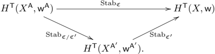
### Visual Description
\n
## Diagram: Commutative Diagram of Stability Maps in Homotopy Theory
### Overview
The image displays a commutative diagram from mathematical topology, specifically homotopy theory or stable homotopy theory. It illustrates relationships between four mathematical objects (likely spectra or cohomology theories) connected by three "stability" maps. The diagram is structured as a non-rectangular quadrilateral with diagonal arrows, implying a commutative relationship between different composition paths.
### Components/Axes
The diagram consists of four nodes (mathematical objects) and three directed arrows (maps) with labels.
**Nodes (Objects):**
1. **Top-Left Node:** `H^T(X^A, w^A)`
2. **Top-Right Node:** `H^T(X, w)`
3. **Bottom-Left Node:** `H^T(X^{A'}, w^{A'})`
4. **Bottom-Right Node:** `H^T(X, w)` (Identical label to the top-right node)
**Arrows (Maps):**
1. **Horizontal Arrow (Top):** Connects the Top-Left node to the Top-Right node. Label: `Stab_ε`
2. **Diagonal Arrow (Left):** Connects the Top-Left node to the Bottom-Left node. Label: `Stab_{ε/ε'}`
3. **Diagonal Arrow (Bottom):** Connects the Bottom-Left node to the Bottom-Right node. Label: `Stab_{ε'}`
**Spatial Layout:**
* The diagram is arranged in a diamond or kite-like shape.
* The two `H^T(X, w)` nodes are positioned on the right side, one above the other.
* The two distinct nodes with superscripts `A` and `A'` are on the left side, one above the other.
* The arrows create two potential paths from the top-left node to the bottom-right node:
* **Path 1:** Top-Left → Top-Right → Bottom-Right (This path is *not* explicitly drawn with an arrow).
* **Path 2:** Top-Left → Bottom-Left → Bottom-Right (This path is explicitly drawn).
### Detailed Analysis
* **Notation:** The notation `H^T` likely denotes a generalized cohomology theory or a spectrum indexed by `T`. The arguments `(X, w)` suggest a space `X` equipped with some additional structure `w` (e.g., a weight, a tangential structure, or a parameter).
* **Superscripts:** The superscripts `A` and `A'` on the left-hand nodes likely denote different indexing sets, parameters, or approximations applied to the base space `X`.
* **Map Labels:** The maps are all labeled `Stab`, indicating they are "stability" maps or "stabilization" functors. The subscripts `ε`, `ε'`, and `ε/ε'` are parameters (likely real numbers or tolerances) governing these stability constructions. The label `Stab_{ε/ε'}` suggests a map that compares or relates the two parameters `ε` and `ε'`.
* **Implied Commutativity:** Although not explicitly stated with a symbol (like `=` or `∘`), the structure of the diagram strongly implies that the composition of maps along the two different paths from `H^T(X^A, w^A)` to `H^T(X, w)` should be equivalent. That is, `Stab_ε` (top path) is expected to equal the composition `Stab_{ε'} ∘ Stab_{ε/ε'}` (bottom path). This is the core property of a commutative diagram.
### Key Observations
1. **Duplicate Node:** The object `H^T(X, w)` appears twice, serving as both the target of the top map and the target of the bottom composition. This is a common device in commutative diagrams to show that two different processes lead to the same result.
2. **Parameter Dependence:** The stability maps are explicitly parameterized (`ε`, `ε'`), indicating that the construction is sensitive to these choices. The map `Stab_{ε/ε'}` acts as a bridge between the two parameter regimes.
3. **Asymmetric Structure:** The diagram is not a simple square. The direct vertical connection on the right side is absent, emphasizing that the relationship between the two `H^T(X, w)` nodes is mediated through the left-hand objects and the stability maps.
### Interpretation
This diagram formalizes a **consistency or naturality condition** for a family of stability constructions parameterized by `ε`. It asserts that stabilizing a parameterized object `(X^A, w^A)` directly to a tolerance `ε` yields the same result as first stabilizing it to an intermediate tolerance `ε/ε'` (producing `(X^{A'}, w^{A'})`) and then further stabilizing that result to tolerance `ε'`.
In essence, it demonstrates that the stability functor `Stab` behaves predictably when its parameters are scaled or related. This is a fundamental type of diagram in areas like parametrized stable homotopy theory, the theory of parametrized spectra, or in the study of assembly maps and parametrized homology theories. It ensures that the mathematical constructions are well-defined and independent of the specific path taken through the parameter space, which is crucial for building robust theoretical frameworks. The presence of weights or additional structures (`w`) suggests this may be in the context of tangential or framed structures.
</details>
'
'
Proof. Let C ∗ u act on Y = Tot( E ) by fixing X and E + , and scaling the fibers of E -with weight 1. By Theorem 4.3, [Attr C (∆ Y A )] is a cohomological stable envelope correspondence for ( Y, w ◦ π, T × C ∗ u , A , C ). By Propositions 8.7, 8.8, [Attr C (∆ X A )] is a cohomological stable envelope correspondence for ( X, w , T , A , C ). The triangle lemma then follows from Proposition 8.10 below. □
- 8.4. The triangle lemma for attracting closure correspondence. In this subsection, we do not impose any attracting or repelling condition on E . Let C ∗ u act on Y = Tot( E ) by fixing X and scaling the fibers of E with weight 1. Let C ′ be a face of C and let A ′ be the subtorus of A associated with C ′ .
Let Attr C (∆ Y A ) be the closure of Attr C (∆ Y A ) in Y × Y A , similarly for Attr C (∆ X A ) ⊆ X × X A . We show that if the triangle lemma holds for attracting closure correspondences for Y , then it also holds for attracting closure correspondences for X .
this implies that
Proposition 8.10. The equation
$$, w o π , H ^ { \prime } ( x ; C u ^ { \prime } ( Y ^ { \prime } _ { w o π } )$$
implies that
$$\sqrt { \sum _ { i = 1 } ^ { n } ( x _ { i } - \bar { x } ) ^ { 2 } } = \sqrt { \sum _ { i = 1 } ^ { n } ( x _ { i } - \bar { x } ) } \in Hom ( x , w ) .$$
Here we use the correspondence to denote the induced map between critical cohomologies.
Proof. Let i : X ↪ → Y , i A ′ : X A ′ ↪ → Y A ′ , i A : X A ↪ → Y A be zero sections. By Lemmata 8.11, 8.12, Attr C (∆ Y A ) is a vector bundle of rank (rk E | + X A +rk E | fixed X A ) over Attr C (∆ X A ), and Attr C (∆ Y A ) ⋂ ( X × X A ) = Attr C (∆ X A ), then
$$( i \times i A ) ^ { \prime } [ Attr c ( \Delta y _ { x } ) ] = u ^ { r k } B - r k E ^ { r } _ { x A }$$
Therefore we have
$$\begin{aligned}
( 8 . 1 1 ) & = u ^ { r } k E - r k E \\
& = \left[ \frac { ( x ^ { r } A ^ { r } ) } { x ^ { r } A ^ { r } } \right] o \left[ \frac { ( t ^ { r } x ^ { r } i ^ { r } ) } { t ^ { r } x ^ { r } i ^ { r } } \right] + \left[ \frac { ( A ^ { r } x ^ { r } c _ { E } ( \Delta y _ { A } ) } { x ^ { r } A ^ { r } } \right] o \left[ \frac { ( t ^ { r } x ^ { r } i ^ { r } c _ { E } ( \Delta y _ { A } ) } { t ^ { r } x ^ { r } i ^ { r } } \right] + \cdots
\end{aligned}$$
Let p ij be the projection from Y × Y A ′ × Y A to the ij -th component, for example p 13 : Y × Y A ′ × Y A → Y × Y A . Similarly, let p ij be the projection from X × X A ′ × X A to the ij -th component. Let ˜ p 13 : X × Y A ′ × X A → X × X A be the natural projection. The LHS of (8.11) can be evaluated as:
$$\begin{aligned}
p_{13}^{(i)} & = p_{13}^{(x \times t^{A})} \times (e^{t^{C}}(E)) \\
& = u^{k} E^{|x^{A}|^{fixed}} p_{13}^{(x^{A})} \\
& = u^{k} E^{|x^{A}|^{fixed}} (i) \\
\end{aligned}
by base change = u^{k} E^{|x^{A}|^{fixed}} (i) \\
= u^{k} E^{|x^{A}|^{fixed}} (i) \\
\end{aligned}
by assumption = u^{k} E^{|x^{A}|^{fixed}} (i) \\
= u^{k} E^{|x^{A}|^{fixed}} (i) + \left( i - p_{13}^{(y^{A})} \right) x^{A} + rk \\
\end{aligned}
Compared with the leading term on the RHS of (8.11), and we obtain the desired equation$$
$$\therefore \Delta x ^ { 2 }$$
Compared with the leading term on the RHS of (8.11), and we obtain the desired equation
$$( \Delta x _ { A } ) = [ Attr e ( \Delta x _ { A } ) ] o [ Attr e ($$
Here we used the fact that H T × C ∗ u ( X, w ) ∼ = H T ( X, w ) ⊗ Q [ u ] is free over Q [ u ].
In the above proof, we have used the following:
Lemma 8.11. Attr C (∆ Y A ) is a vector bundle of rank (rk E | + X A +rk E | fixed X A ) over Attr C (∆ X A ).
Proof. The attraction map
$$a + b + c ( A _ { y _ { 1 } } ) - \Delta y _ { n }$$
is an affine fibration with (rk N + X A /X +rk E | + X A )-dimensional fibers, and ∆ Y A is the vector bundle E | fixed X A over ∆ X A , so Attr C (∆ Y A ) is smooth of dimension (dim Attr C (∆ X A ) + rk E | + X A +rk E | fixed X A ).
It is elementary to see that Attr C (∆ Y A ) is contained in ( π × π A ) -1 (Attr C (∆ X A )), and Attr C (∆ Y A ) ⋂ ( π × π A ) -1 (∆ X A ) is isomorphic to the vector bundle E | + X A ⊕ E | fixed X A , which implies that
$$( \pi x \pi ) | A t r e ( \Delta y _ { A } ) : A t$$
is a smooth morphism in a Zariski open neighbourhood of Attr C (∆ Y A ) ⋂ ( π × π A ) -1 (∆ X A ). Since ( π × π A ) | Attr C (∆ Y A ) is A -equivariant and the A -action (in the chamber C ) is attracting, ( π × π A ) | Attr C (∆ Y A ) is a smooth morphism.
Finally, suppose that s 1 and s 2 are two local sections of the map ( π × π A ) | Attr C (∆ Y A ) on an open subset U ⊆ Attr C (∆ X A ), then for all a, b ∈ O Attr C (∆ X A ) ( U ), as 1 + bs 2 is also a section of ( π × π A ) | Attr C (∆ Y A ) because lim C ( as 1 + bs 2 ) exists and is equal to a lim C ( s 1 ) + b lim C s 2 . It follows that Attr C (∆ Y A ) is a sub-bundle of ( π × π A ) -1 (Attr C (∆ X A )) of rank (rk E | + X A +rk E | fixed X A ). □
□
## Lemma 8.12.
Proof. It is easy to see that
It follows that therefore,
which we visualize vertex-wise as
(9.2)
/
$$\frac { \frac { 1 } { n } ( A _ { n } ) } { X ^ { n } } = \frac { 1 } { n } \cdot \text { Attre } ( \Delta x _ { n } ) .$$
$$x ^ { A } = Attr ( \Delta x _ { A } ) ,$$
thus the inclusion ' ⊇ ' is obvious. For the opposite direction of inclusion, we notice that ( π × π A ) -1 (Attr C (∆ X A )) contains ∆ Y A and is closed under taking the attracting set, so we have
$$\pi ^ { - 1 } ( A t r e ( \Delta x _ { A } ) .$$
$$\frac { \Delta y _ { A } } { \mu ^ { 2 } ( A ) - 1 } ( \Delta x _ { A } ),$$
$$\sum _ { i = 1 } ^ { \infty } ( x ^ { A } ) ^ { - 1 } ( \pi \times \pi ^ { A } ) ^ { - 1 } ( Attr e ( \Delta x _ { A } ) ) = Attr$$
## 9. Hall envelopes and stable envelopes
The theory of stable envelopes on symplectic varieties [MO, Oko1, AO2] provides an effective way of producing R -matrices of quantum groups , where the triangle lemma plays the key role. In the above constructions of stable envelopes for critical loci, we prove the triangle lemma for symmetric quiver varieties (or more generally symmetric GIT quotients) with any potentials (Theorem 4.16, Lemma 3.37) and also for certain asymmetric case (Theorem 8.9). In the symmetric cases, stable envelopes are compatible with Hall operations via nonabelian stable envelopes (Theorems 4.22, 5.5). This motivates the definition of Hall envelopes (Definition 9.4) on any (not necessarily symmetric) quiver varieties with potentials as the following compositions:
O
O
/
/
O
O
/
/
$$\begin{array}{ll}
\frac{H^T(M_0(v,d)A^{\phi},w)}{m^{2}} & \xrightarrow[K^T(M_0(v,d)A^{\phi},w)]{} H^T(M_0(v,d),w) \\
\frac{H^T(M_0(v,d)A^{\phi},w)}{m^{2}} & \xrightarrow[K^T(M_0(v,d)A^{\phi},w)]{} H^T(M_0(v,d),w)
\end{array}$$
/
/
/
where the downward arrows are restrictions to open substacks, and the upward arrows are called interpolation maps (Definition 9.1), defined by adding extra framings on quivers and using (abelian) stable envelopes for one dimensional tori. In the symmetric cases, we show that interpolation maps agree with nonabelian stable envelopes (Proposition 9.8); therefore Hall envelopes coincide with stable envelopes. We also give a description of nonabelian stable envelopes using BPS cohomology in § 9.3. For tripled quivers with canonical cubic potentials, we show that nonabelian stable envelopes constructed in this paper reproduce the nonabelian stable envelopes for Nakajima quiver varieties in [AO1] along the dimensional reductions (Proposition 9.13).
We note that triangle lemma could fail for either Hall envelopes or stable envelopes in general (Example 9.25, Proposition 9.26). For a class of asymmetric quiver varieties, where the asymmetric part comes only from the framing (Definition 9.19), we prove that triangle lemma of Hall envelopes holds (Theorem 9.20, Corollary 9.21). This provides foundations for studying geometric R -matrices of shifted quantum groups.
- 9.1. Definitions. Let Q = ( Q 0 , Q 1 ) be any quiver and v , d in , d out ∈ N Q 0 . Denote
For simplicity, we consider cyclic stability condition θ ∈ Q Q 0 , i.e.
$$\theta _ { i } < 0 , \forall i \in Q _ { 0 } .$$
The space of framed representations (ref. (4.1)) is
$$R ( v , d ^ { \prime } ) = R ( v , d ) e ^ { i \epsilon Q _ { 0 } } H o m ( C V _ { 1 } , C V _ { 2 } ) ,$$
<
<
O
O
<details>
<summary>Image 10 Details</summary>
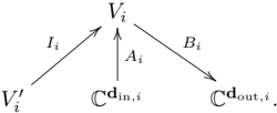
### Visual Description
## Diagram: Directed Graph with Mathematical Notation
### Overview
The image displays a directed graph (flowchart) consisting of four nodes connected by three labeled arrows. The diagram uses mathematical notation with subscripts and superscripts, suggesting a technical or scientific context, likely from fields such as control theory, signal processing, or machine learning. The layout is hierarchical, with a central node at the top and three other nodes positioned below and to the sides.
### Components/Axes
**Nodes (Vertices):**
1. **V_i**: Located at the top-center of the diagram. This is the central node from which arrows originate.
2. **V'_i**: Located to the left and slightly below V_i. The label uses a prime symbol (').
3. **C^{d_in,i}**: Located at the bottom-left of the diagram. The label has a superscript "d_in,i".
4. **C^{d_out,i}**: Located at the bottom-right of the diagram. The label has a superscript "d_out,i".
**Edges (Arrows) and Labels:**
1. An arrow points from **V'_i** to **V_i**. The label **I_i** is placed above the midpoint of this arrow.
2. An arrow points from **V_i** to **C^{d_in,i}**. The label **A_i** is placed to the right of the arrow's midpoint.
3. An arrow points from **V_i** to **C^{d_out,i}**. The label **B_i** is placed above the midpoint of this arrow.
### Detailed Analysis
The diagram defines a specific set of relationships between four entities, all indexed by the subscript `i`.
* **Flow Direction**: The primary flow originates from the central node `V_i`. It has one incoming connection (from `V'_i`) and two outgoing connections (to `C^{d_in,i}` and `C^{d_out,i}`).
* **Label Transcription**:
* Node Labels: `V_i`, `V'_i`, `C^{d_in,i}`, `C^{d_out,i}`
* Edge Labels: `I_i`, `A_i`, `B_i`
* **Spatial Relationships**: The legend/labels are integrated directly onto the edges. The node `V_i` acts as a hub. The nodes `C^{d_in,i}` and `C^{d_out,i}` are symmetrically placed at the bottom, suggesting they might be complementary input/output or dual components.
### Key Observations
1. **Notation Consistency**: All elements share the common index `i`, implying they are part of a series or a specific instance within a larger system.
2. **Directional Asymmetry**: The connection between `V'_i` and `V_i` is unidirectional (`I_i`), as are the connections from `V_i` to the `C` nodes (`A_i`, `B_i`). There is no feedback loop shown.
3. **Label Placement**: The edge labels are positioned for clarity: `I_i` and `B_i` are above their arrows, while `A_i` is to the right, avoiding overlap with the vertical arrow.
### Interpretation
This diagram likely represents a **state transition or transformation model** for a system component indexed by `i`.
* **`V_i`** could represent a **state variable**, **feature vector**, or **internal representation** at step `i`.
* **`V'_i`** might be a **previous state**, **input**, or **modified version** of `V_i`, with `I_i` representing an **input function**, **information flow**, or **update rule**.
* **`C^{d_in,i}` and `C^{d_out,i}`** strongly suggest **context** or **code** vectors for **input (`d_in`)** and **output (`d_out`)** domains, respectively. The arrows labeled `A_i` and `B_i` would then represent **encoding** or **projection functions** that map the state `V_i` into these specific contextual spaces.
* **Overall Meaning**: The structure is reminiscent of architectures in **sequence modeling** (like Transformers) or **autoencoders**, where a central representation is derived from an input and then used to generate or condition outputs for different modalities or tasks. The diagram abstracts the core data flow: information (`I_i`) updates a state (`V_i`), which is then projected (`A_i`, `B_i`) into specialized input and output contexts. The absence of a connection between the two `C` nodes implies their roles are distinct and mediated solely through the central state `V_i`.
</details>
$
$
In the above diagram V ′ i ∼ = C v i ∼ = V i . Define GIT quotient and stack quotient by
$$M ( v , d ^ { Y } ) = [ R ( v , d ^ { Y } ) / G ].$$
The θ -semistable locus R ( v , d v ) θ -ss contains the open subscheme ˚ R ( v , d v ) on which the map I i are isomorphisms for all i ∈ Q i . ˚ R ( v , d v ) is G -invariant and descends to an open subscheme
$$\rho ^ { \prime } ( v , d ^ { \prime } Y ) = R ( v , s ) M _ { 0 } ( v , d ^ { \prime } Y ) .$$
One has an isomorphism
$$( 9 . 3 )$$
under which, the flavour symmetry G ′ which acts on V ′ i in (9.2) becomes the gauge group acting on R ( v , d ).
Consider a torus in the center of the flavour group:
$$( 9 . 4 )$$
which acts on V ′ i in (9.2) with weight -1 for all i ∈ Q 0 16 . Then M θ ( v , d ) is naturally identified with a connected component in M θ ( v , d v ) C ∗ .
Let T ⊆ F be a torus in the flavour group F = Aut G ( R ( v , d )). Then we fix a ( G × T )-invariant function
$$m R ( d ) = C$$
We denote the descent functions on M ( v , d ) and M θ ( v , d ) still by w .
Let w ′ be the pullback of w along the projection R ( v , d v ) → R ( v , d ) that forgets { I i } i ∈ Q 0 . w ′ descends to a ( G ′ × T )-invariant function
$$w : M ( x , y ) = C$$
By Proposition 3.23 and the discussions in § 3.10, there exist a cohomological stable envelope Stab + for ( M θ ( v , d v ) , w ′ , G ′ × T , C ∗ , +) and a K -theoretic stable envelope Stab s + for ( M θ ( v , d v ) , w ′ , G ′ × T , C ∗ , + , s ) with a slope s ∈ Char( G ) ⊗ Z R .
Definition 9.1. We define ˜ Ψ H : H T ( M θ ( v , d ) , w ) → H T ( M ( v , d ) , w ) as the composition of the following maps
/
/
/
/
$$\begin{aligned}
H ^ { T } ( M _ { 0 } ( v , d ) , w ) & \xrightarrow [ 1 \textcircled { id } ] { r G ^ { x } T ( M _ { 0 } ( v , d ) , w ) } H ^ { T } ( M _ { 0 } ( v , d ) , w ) \\
\end{aligned}$$
o
o
Here 1 ∈ H G ′ (pt) is the unit, and j : ˚ M θ ( v , d v ) ↪ →M θ ( v , d v ) is the open immersion.
Similarly, we define ˜ Ψ s K : K T ( M θ ( v , d ) , w ) → K T ( M ( v , d ) , w ) as the composition of the following maps
/
$$\begin{array}{ll}
K ^ { T } ( M _ { 0 } ( v , d ) , w ) & \xrightarrow [ 1 \textcircled { \mathrm{d} } ] { \chi ^ { G } } K ^ { C } \times T ( M _ { 0 } ( v , d ) , w ) \\
\end{array}$$
/
Here in the first map 1 ∈ K G ′ (pt) is the unit.
We call ˜ Ψ H and ˜ Ψ s K cohomological and K -theoretic interpolation maps respectively.
Lemma 9.2. Let k : M θ ( v , d ) ↪ → M ( v , d ) be the open immersion of stable locus, then
$$k ^ { 2 } d y _ { n } = k ^ { 2 } ( k ^ { 2 } y _ { n } - k l .$$
Proof. Let q : ˚ M θ ( v , d v ) → M ( v , d ) be the quotient map. Then
$$\therefore f ^ { \prime } ( x ) = d f ( x )$$
is the open subscheme of quiver representations which are θ -semistable after forgetting { I i } i ∈ Q 0 . Note that
$$\frac { 1 } { \vert A B \vert } ( \vert A C \vert + \vert B D \vert )$$
16 For other generic stability condition ζ ∈ Q Q 0 , we take C ∗ ⊆ G ′ which acts on V ′ i in (9.2) with weight sign( ζ i ). Then we use this C ∗ -action to construct ˜ Ψ .
/
/
o
o
is exactly the locus where quiver representations are θ -semistable after forgetting { I i } i ∈ Q 0 . It follows that
$$q ^ { - 1 } ( M _ { 0 } ( v , d ) ) = M _ { 0 } ( v , d )$$
and the restriction of the quotient map to q -1 ( M θ ( v , d )):
$$\therefore f ^ { \prime } ( x ) = d ( 1 - N ( x ) )$$
is identified with the attraction map a : Attr + ( M θ ( v , d )) →M θ ( v , d ). By a direct calculation, we have
$$S _ { \Delta A O C } = \frac { 1 } { 2 } ( a + b )$$
for all γ ∈ H T ( M θ ( v , d ) , w ). Since the isomorphism H G ′ × T ( q -1 ( M θ ( v , d )) , w ) ∼ = H T ( M θ ( v , d ) , w ) maps q ∗ (1 ⊗ γ ) to γ , we see that k ∗ ◦ ˜ Ψ H = id. The K -theoretic version is proven similarly and we omit the details. □
Hall operations are defined similarly as the symmetric case. Let A ⊆ T be a subtorus. Choose a homomorphism
$$\phi : A \rightarrow G$$
and denote R ( v , d ) A ,ϕ the fixed locus of R ( v , d ) under the action of A via the homomorphism
$$( 6 \div 1 ) \cdot A - C \times A$$
and denote G ϕ ( A ) the fixed subgroup of G under the conjugation action of the subgroup ϕ ( A ).
Note that
$$, G ^ { \phi } ( A ) \approx \sum _ { i \in Q _ { 0 , 0 } } ^ { R ( v , d ) } R ( Q _ { 0 , v }, d _ { 0 } )$$
for some quiver Q ϕ with gauge dimension vector v ϕ and in-coming and out-going framing dimension vectors d ϕ, in and d ϕ, out respectively. Define
$$M _ { 0 } ( v , d ) ^ { A _ { 0 } } = R _ { v } ( d ) ^ { A _ { 0 } } / G ^ { C _ { 0 } } ( A ) .$$
In the following discussions, we assume that M θ ( v , d ) A ,ϕ is nonempty. Then the same argument as Lemma 4.7 shows that M θ ( v , d ) A ,ϕ is a connected component of the A -fixed locus M θ ( v , d ) A , and we have
$$M _ { 0 } ( v , d ) ^ { A } = \left | M _ { 0 } ( v , d ) ^ { A } o _ { / } \right |$$
where the sum is taken for all homomorphisms ϕ : A → G modulo the equivalence relation: ϕ 1 ∼ ϕ 2 if and only if they give the isomorphic ( G × A )-module structures on R ( v , d ).
Let us fix a chamber C ⊆ Lie( A ) R , and define
$$( v , d ) ^ { A _ { \phi } } \subset R ( v , d ).$$
Then L ( v , d ) ϕ C is a linear subspace of R ( v , d ), and there are maps
o
$$R ( v , d ) ^ { \phi } \rightarrow L ($$
o
where q is the attraction map and p is the natural closed immersion.
Let P ϕ C := Attr C ( G ϕ ( A ) ) be the parabolic subgroup of G , which naturally acts on L ( v , d ) ϕ C , and p and q in the above diagram are P ϕ C -equivariant, where P ϕ C -action on R ( v , d ) is via P ϕ C → G and P ϕ C -action on R ( v , d ) A ,ϕ is via attraction map P ϕ C → G ϕ ( A ) . Passing to the quotient stack, we obtain the following diagram
o
$$m ( v , d ) A _ { p } ^ { q } \rightarrow m ( v , d )$$
o
/
/
where L ( v , d ) ϕ C := [ L ( v , d ) ϕ C /P ϕ C ]. We note that q is a smooth morphism and p is a proper morphism.
Definition 9.3. We define the Hall operations
$$m ^ { e } _ { c } = p \cdot q ^ { * } : H ^ { T } ( 2 \pi ( v , d ) )$$
/
/
Definition 9.4. Let s ∈ Char( G ) ⊗ Z R be a slope. We define the Hall envelopes
$$\cdot w ) \rightarrow H ^ { T } ( M _ { 0 } ( v , d ) ^ { A } , w ) ,$$
$$HallE _ { v } \left | H ^ { T } ( M _ { 0 } ( v , d ) A ) \right . = k ^ { * } o m _ { E } o \varphi _ { H } ^ { * }$$
Here k : M θ ( v , d ) ↪ → M ( v , d ) is the open immersion of stable locus, ˜ Ψ ϕ H , ˜ Ψ ϕ, s ′ K are interpolation maps (Definition 9.1) for the stack M ( v , d ) A ,ϕ with slope
$$( 9 . 7 )$$
Moreover, we say that HallEnv C (resp. HallEnv s C ) is compatible with the Hall operation if for all ϕ : A → G that appears in (9.6) the left square (resp. right square) below is commutative
O
O
/
/
O
O
O
O
/
/
O
O
/
/
/
/
Remark 9.5. Hall envelope HallEnv C (resp. HallEnv s C ) satisfies axioms (i) and (ii) for stable envelopes in Definition 3.4 (resp. Definition 3.10). Namely, for arbitrary β ∈ H T ( M θ ( v , d ) A ,ϕ , w ) and γ ∈ K T ( M θ ( v , d ) A ,ϕ , w ), we have
- (i) HallEnv C ( β ) and HallEnv s C ( γ ) are supported on Attr f C ( M θ ( v , d ) A ,ϕ );
(ii)
$$\frac{1}{2} \left( N_{v} M_{0} ( v , d ) ^{2} / M_{0} ( v , d ) \right) \cdot \beta _ { 3 } H a l l E n v ^ { 2 } ( \beta ) \left[ M _ { 0 } ( v , d ) A _ { 0 } ^ { N } \right] = e I$$
As a corollary, HallEnv C and HallEnv s C are triangular with invertible diagonals after localization, in particular they are invertible after localization. In Section 9.6, we will discuss situations when HallEnv C (resp. HallEnv s C ) satisfies the axiom (iii) in Definition 3.4 (resp. Definition 3.10).
We show that triangle lemma of Hall envelopes follows from the associativity of Hall operations.
Lemma 9.6. Let X = M θ ( v , d ), C ′ be a face of C , and A ′ be the subtorus of A associated with C ′ . Suppose that HallEnv C / C ′ (resp. HallEnv s ′ C / C ′ ) is compatible with the Hall operation, then the left triangle (resp. right triangle):
/
/
/
/
$$\begin{array}{c}
(9,8) & H ^ { T } ( X _ { A } , w A ) & \rightarrow \\
HallEnv_e^c & HallEnv_e^c ( X ^ { A } , w ^ { A } ) & \rightarrow \\
\end{array}$$
'
'
commutes, where s ′ = s | X A ′ ⊗ det ( N -X A ′ /X ) 1 / 2 .
Proof. Fix a homomorphism ϕ : A → G , and use the same letter ϕ to denote its restriction to subtorus A ′ . Then the restriction of s ′ on the component M θ ( v , d ) A ′ ,ϕ can be rewritten as
$$s ^ { \prime } = s \otimes det ( T M ( v , d ) ^ { A } _ { R }$$
$$s ^ { \prime } = s \times det ( T 2 M ( v , d ) A _ { o - 1 }$$
by
Let us define
'
'
and consider the following diagram on a triangular prism:
O
O
<details>
<summary>Image 11 Details</summary>
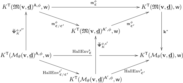
### Visual Description
## Mathematical Diagram: Commutative Diagram of Transformations
### Overview
The image displays a complex commutative diagram from the fields of category theory, formal methods, or theoretical computer science. It illustrates a network of mathematical objects (nodes) and the transformations or mappings (arrows) between them. The diagram is structured as a square with additional central nodes and cross-connections, suggesting relationships between different representations or models under various operations.
### Components/Axes
The diagram consists of **8 distinct nodes** (mathematical expressions) and **10 labeled arrows** connecting them. There are no traditional chart axes; the structure is purely relational.
**Nodes (Mathematical Objects):**
1. **Top-Left:** `K^T(𝔐(v, d)^A, φ, w)`
2. **Top-Center:** `K^T(𝔐(v, d)^A', φ, w)`
3. **Top-Right:** `K^T(𝔐(v, d), w)`
4. **Middle-Left:** `K^T(M_θ(v, d)^A, φ, w)`
5. **Center:** `K^T(M_θ(v, d)^A', φ, w)`
6. **Middle-Right:** `K^T(M_θ(v, d), w)`
7. **Bottom-Left:** `K^T(M_θ(v, d)^A, φ, w)` (Note: This appears identical to node 4, suggesting a potential duplicate or a specific state in the flow.)
8. **Bottom-Center:** `K^T(M_θ(v, d)^A', φ, w)` (Note: This appears identical to node 5.)
9. **Bottom-Right:** `K^T(M_θ(v, d), w)` (Note: This appears identical to node 6.)
*Clarification:* The diagram's spatial layout suggests a 2x3 grid (2 rows, 3 columns) with additional vertical connections. The nodes in the "bottom row" of the visual layout are actually the same expressions as those in the "middle row," indicating they represent the same object in different parts of the diagram's flow.
**Arrows (Transformations/Mappings):**
* **Horizontal Arrows (Top Row):**
* From Top-Left to Top-Center: `m_φ^{e/e'}`
* From Top-Center to Top-Right: `m_φ^{e'}`
* From Top-Left to Top-Right (direct, above): `m_φ^{e}`
* **Horizontal Arrows (Bottom Row):**
* From Middle-Left to Center: `HallEnv_{e/e'}`
* From Center to Middle-Right: `HallEnv_{e'}`
* From Middle-Left to Middle-Right (direct, above): `HallEnv_{e}`
* **Vertical Arrows:**
* From Top-Left to Middle-Left: `Ψ_K^{φ, s''}`
* From Top-Center to Center: `Ψ_K^{φ, s'}`
* From Top-Right to Middle-Right: `k*`
* **Diagonal Arrows:**
* From Top-Left to Center: `m_φ^{e/e'}` (This label is shared with the horizontal arrow from Top-Left to Top-Center, indicating the same transformation applied in a different context.)
* From Top-Center to Middle-Right: `m_φ^{e'}` (This label is shared with the horizontal arrow from Top-Center to Top-Right.)
### Detailed Analysis
**Symbol Transcription & Structure:**
* **Common Elements:** All nodes are of the form `K^T( ... )`. The arguments inside the parentheses vary.
* **Core Objects:** Two primary objects appear to be transformed:
1. `𝔐(v, d)` and its variants (`𝔐(v, d)^A`, `𝔐(v, d)^A'`). The symbol `𝔐` is a script capital M.
2. `M_θ(v, d)` and its variants (`M_θ(v, d)^A`, `M_θ(v, d)^A'`). This includes a subscript `θ`.
* **Parameters:** The objects are parameterized by `v`, `d`, `φ`, and `w`. The superscripts `A` and `A'` likely denote different abstraction levels, versions, or annotations.
* **Transformations:**
* `m_φ^{...}`: A family of mappings (likely "model" or "morphism") parameterized by `φ` and indexed by `e`, `e'`, and `e/e'`.
* `HallEnv_{...}`: A family of transformations (likely "Hallucination Environment" or a similar construct in formal verification) indexed similarly.
* `Ψ_K^{φ, s...}`: Vertical mappings (likely "projection" or "simulation" relations) parameterized by `φ` and a state `s` (`s'`, `s''`).
* `k*`: A specific mapping from the top-right to the middle-right node.
**Spatial Grounding & Flow:**
The diagram is organized into two parallel horizontal flows:
1. **Top Flow (𝔐-based):** Starts with an abstracted version `𝔐(v, d)^A`, moves to a primed version `𝔐(v, d)^A'` via `m_φ^{e/e'}`, and finally to the base object `𝔐(v, d)` via `m_φ^{e'}`. A direct path `m_φ^{e}` also exists.
2. **Bottom Flow (M_θ-based):** Mirrors the top flow but operates on `M_θ(v, d)` variants using `HallEnv` transformations.
These two flows are connected vertically by the `Ψ_K` mappings and the `k*` mapping, creating a commutative structure. The diagonal arrows reinforce that the same transformations (`m_φ^{e/e'}`, `m_φ^{e'}`) can be applied across different levels of the diagram.
### Key Observations
1. **Symmetry and Commutativity:** The diagram's primary feature is its commutative nature. The existence of multiple paths between nodes (e.g., from Top-Left to Middle-Right can go via Top-Center and Center, or directly via Middle-Left and Middle-Right) implies that the composition of transformations along these paths yields equivalent results.
2. **Dual Representation:** The diagram explicitly contrasts two representations of a system: one using `𝔐` (possibly a theoretical or ideal model) and another using `M_θ` (possibly a parameterized, learned, or concrete model).
3. **Abstraction Hierarchy:** The superscripts `A` and `A'` suggest a hierarchy of abstractions or refinements, with transformations (`m`, `HallEnv`) moving between these levels.
4. **Parameter Consistency:** Parameters `v`, `d`, `φ`, and `w` are consistently present across all nodes, indicating they are fundamental to the system being modeled.
### Interpretation
This diagram is a formal, graphical representation of relationships between different models or specifications of a system, likely within the context of **machine learning verification, formal methods, or program semantics**.
* **What it Demonstrates:** It shows how a high-level, abstract model (`𝔐(v, d)^A`) can be related to a concrete, parameterized model (`M_θ(v, d)`) through a series of refinement steps (`m_φ`, `HallEnv`) and abstraction mappings (`Ψ_K`). The commutativity asserts the consistency of these relationships—different sequences of refinement and abstraction lead to the same result.
* **Relationships Between Elements:** The `Ψ_K` mappings likely represent **simulation** or **refinement relations** that connect the abstract (`𝔐`) and concrete (`M_θ`) worlds. The `m_φ` and `HallEnv` transformations represent operations that modify the level of abstraction or detail within each world. The `k*` mapping provides a direct link from the fully refined abstract model to the concrete model.
* **Notable Implications:** The structure suggests a framework for **proving properties** about a learned model (`M_θ`) by relating it to a trusted abstract specification (`𝔐`). If a property holds for `𝔐`, and the diagram's commutativity holds, the property can be transferred to `M_θ` via the `Ψ_K` and `k*` mappings. The "HallEnv" label is particularly suggestive of a context involving **hallucination** or **environment modeling** in AI systems, where formal guarantees are sought.
* **Underlying Message:** The diagram is a blueprint for a **correctness argument**. It visually encodes the theorem that the concrete system (`M_θ`) is a valid implementation or approximation of the abstract system (`𝔐`), with all intermediate steps and relationships explicitly defined and verified to be consistent.
</details>
)
)
The right and the backward squares are commutative by the definition of Hall envelope. The left square is commutative by assumption. The upper triangle is commutative because Hall operations are associative. These imply the commutativity of the lower triangle.
The cohomology version is proven similarly and we omit the details.
We obtain an explicit formula for Hall envelopes when w = 0.
Proposition 9.7. Assume w = 0, then we have
$$\sum _ { w \in W / W ^ { * } } ( M _ { 0 } ( v , d ) A _ { 0 } ^ { - rep } ) = [ M _ { 0 } ( v , d ) ] .$$
Here W , W ϕ are Weyl groups of G , G ϕ ( A ) respectively, T M ( v , d ) = R ( v , d ) -Lie( G ) and ( -) A ,ϕ -repl is the repelling part with respect to homomorphism ϕ : A → G , and w acts on a weight µ of G by w ( µ )( g ) := µ ( w -1 · g · w ).
Let s ∈ char( G ) ⊗ Z R be a generic slope and χ ∈ char( G ϕ ( A ) ) such that s ⊗ det ( T M ( v , d ) A ,ϕ -repl ) 1 / 2 is in a sufficiently small neighbourhood of χ , then
$$\sum _ { w \in W / W ^ { e } } ( x \cdot T \times G ^ { e } ( A ) ( T m )( n ^ { s } ( [ L _ { X } ] ) =$$
Here L χ ∈ Pic( M θ ( v , d ) A ,ϕ ) is the descent of the character χ .
Proof. Let Stab + be the same as in Definition 9.1, then we have
$$S _ { n } = ( 1 + n ) \times 1 0 ^ { - | n | }$$
since the right-hand-side satisfies the axioms of stable envelope. Replacing M θ ( v , d ) by M θ ( v , d ) A ,ϕ , we get
$$\frac { 1 } { 4 } \times ( 1 + x ) = 1 9 0 \div x .$$
$$\frac { 1 } { 4 } \dot { r } ^ { 2 } ( C _ { x } ) = x \textcircled { \cdot } C _ { m } ( x , a ) \cdots$$
Then (9.9) and (9.10) follow from explicit formulas of cohomological [KS, Thm. 2] and K -theoretic [P, Prop. 3.4] Hall operations respectively. □
9.2. The case of symmetric quiver varieties. In this subsection, we discuss the case when Q is symmetric with a symmetric framing d in = d out such that ( G × A )-action is self-dual, in other words, M θ ( v , d ) = M θ ( v , d ) is a symmetric quiver variety in Definition 4.5, in particular, a symmetric GIT quotient in Definition 4.1.
Proposition 9.8. Suppose that Q is symmetric with a symmetric framing d in = d out such that ( G × A )-action is self-dual. Then ˜ Ψ H = Ψ H where the latter is the cohomological nonabelian stable envelope in Definition 4.10.
For a generic slope s ∈ Char( G ) ⊗ Z R , we have ˜ Ψ s K = Ψ s K , where the latter is the K -theoretic nonabelian stable envelope in Definition 5.2.
□
Similar argument shows that
)
)
O
O
/
/
/
/
Proof. It is easy to see that the symmetric quiver variety M θ ( v , v + d ) is isomorphic to the total space of a vector bundle E on M θ ( v , d v ) 17 , where E = ⊕ i ∈ Q 0 Hom( V i , V ′ i ). E is repelling with respect to the positive chamber. Then according to Theorem 8.9, Stab + is induced by the correspondence
$$\sqrt { A + ( \Delta M _ { 0 } ( v , d ) ) } \leq$$
So ˜ Ψ H is induced by the correspondence given by the irreducible closed substack
$$\left( \frac { A _ { t r } + ( \Delta M _ { 0 } ( v , d ) ) } { G ^ { i } } \right)$$
Using an equality similar as (9.5), we deduce that
$$( 9 . 1 1 ) \int ( A t r _ { + } ( \Lambda _ { M _ { a } } )$$
Therefore ˜ Ψ H is induced by the correspondence given by their closure, i.e.
$$\frac { 1 } { \vert A \vert } = \frac { 1 } { \vert B \vert } = \frac { 1 } { \vert C \vert } = \frac { 1 } { \vert D \vert } = \frac { 1 } { \vert E \vert } = \frac { 1 } { \vert F \vert } = \frac { 1 } { \vert G \vert } = \frac { 1 } { \vert H \vert } = \frac { 1 } { \vert I \vert } = \frac { 1 } { \vert J \vert } = \frac { 1 } { \vert K \vert } = \frac { 1 } { \vert L \vert } = \frac { 1 } { \vert M \vert } = \frac { 1 } { \vert N \vert } = \frac { 1 } { \vert O \vert } = \frac { 1 } { \vert P \vert } = \frac { 1 } { \vert Q \vert } = \frac { 1 } { \vert R \vert } = \frac { 1 } { \vert S \vert } = \frac { 1 } { \vert T \vert } = \frac { 1 } { \vert U \vert } = \frac { 1 } { \vert V \vert } = \frac { 1 } { \vert W \vert } = \frac { 1 } { \vert X \vert } = \frac { 1 } { \vert Y \vert } = \frac { 1 } { \vert Z \vert }$$
This shows that ˜ Ψ H = Ψ H . The K -theoretic version ˜ Ψ s K = Ψ s K follows from Theorem 5.3 and Proposition 9.9 below and a direct calculation showing that
$$\begin{aligned}
& \frac { 1 } { 2 } \deg _ { g_i } e ^ { i k ( R ( v , d ) - Lie ( G ) ) } \\
& = \det N_S / R ( v , a ) ^ { 1 / 2 } . \Box
\end{aligned}$$
Recall that the unstable locus
Then define the new strata
$$f ( x ) ^ { \prime } = f ( 1 + x )$$
admits equivariant Kempf-Ness (KN) stratification by connected locally-closed subvarieties [Kir, DH]. The KN stratification is constructed iteratively by selecting a pair ( σ i ∈ cochar( G ) , Z i := R ( v , d ) σ i ) which maximizes the numerical invariant
$$u ( \sigma ) = \frac { ( \sigma , \theta ) } { \vert \sigma \vert }$$
among those ( σ, Z ) for which Z is not contained in the union of the previously defined strata. Here | · | is a fixed conjugation-invariant norm on the cocharacters of G . For our purpose, we fix the norm square | σ | 2 to be
$$| \sigma ^ { 2 } _ { i } | = \sum _ { i \in Q _ { 0 } } | \sigma _ { i } | t r ( σ ^ { 2 } _ { i } ) ,$$
where σ i : C ∗ → GL( v i ) is the i -th component of σ , which is assumed without loss of generality to be diagonal, i.e.
$$n ( 1 ) = d i g e ^ { n } ( \frac { n } { 2 } , \ldots , \frac { n } { 2 } )$$
and tr( σ 2 i ) is a short-hand notation for ∑ v i j =1 σ 2 i,j . One defines the open subvariety Z ∗ i ⊆ Z i to consist of those points not lying on previously defined strata, and
$$Y _ { 1 } = A t _ { 0 } , ( Z ^ { n } ) .$$
$$S _ { 1 } = G \cdot Y _ { 1 }$$
Proposition 9.9. Suppose that Q is symmetric with a symmetric framing d in = d out such that ( G × A )-action is self-dual. Then, for a generic s ∈ Char( G ) ⊗ Z R , ˜ Ψ s K is the unique K T (pt)-linear map from K T ( M θ ( v , d ) , w ) to K T ( M ( v , d ) , w ) which satisfies the following two properties
- k ∗ ◦ ˜ Ψ s K = id, where k : M θ ( v , d ) ↪ → M ( v , d ) is the open immersion of stable locus,
- there is a strict inclusion of intervals
$$\sum _ { i = 1 } ^ { n } \frac { s ( n ) } { k ( i ) } \xi _ { deg _ { S } } e ^ { G _ { K } } ( N _ { S } / R ( v , d ) ) + weight _ { a }$$
for all cocharacters σ i : C ∗ → G that appear in the KN stratification, and all γ ∈ K T ( M θ ( v , d ) , w ). Here i σ i : [ Z ∗ i /G σ i ] → M ( v , d ) is the natural map between quotient stacks.
The proof of this proposition is postponed to the Appendix E.
17 This follows from the fact that θ i < 0 for all i ∈ Q 0 . For other generic stability condition ζ ∈ Q Q 0 , Tot( E ) is isomorphic to an open subscheme of M ζ ( v , v + d ), where E = ⊕ ζ i < 0 Hom( V i , V ′ i ) ⊕ ⊕ ζ i > 0 Hom( V ′ i , V i ).
Corollary 9.10. Suppose that Q is symmetric with a symmetric framing d in = d out such that ( G × A )-action is self-dual. Then for a generic slope s , we have
$$HallEnv _ { e } = Stab e .$$
Moreover, HallEnv C and HallEnv s C are compatible with Hall operations.
Proof. This follows from Proposition 9.8, Theorem 4.22 and Theorem 5.5.
□
In the below, we simplify the notations by setting ˜ Ψ H = Ψ H and ˜ Ψ s K = Ψ s K for symmetric quiver Q with a symmetric framing d in = d out such that ( G × A )-action is self-dual.
9.3. Connection to BPS cohomology. In this section, we give a description of cohomological nonabelian stable envelopes on symmetric quiver varieties via BPS cohomology of Davison-Meinhardt [DM]. This will be used to confirm the prediction of Botta-Davison on 'critical stable envelopes' [BD, § 1.2] (ref. Remark 9.12).
Consider the Jordan-H¨ older morphism
$$5 H _ { 2 } S O _ { 4 } + C l = H _ { 2 } S O _ { 4 } \downarrow$$
sending a representation to the direct sum of the subquotients (simple modules) appearing in its Jordan-H¨ older filtration. Let
$$1 0 \div a = b \cdots a ( 1 )$$
be the constant perverse sheaf on M ( v , d ). It is shown in [DM, Thm. A] that the negative degree perverse cohomology of JH ∗ φ w IC M ( v , d ) vanishes, i.e.
$$H _ { 2 } O _ { 3 } ( g ) + C u S O _ { 4 } = H _ { 2 } S O _ { 4 } ( l )$$
We note that the framed quiver in this paper is related to the unframed quiver considered in [DM] by CrawleyBoevey's procedure [CB], which results in a C ∗ -gerbe
$$3 9 ( x , d ) = 3 9 9 ( x , d ) / C _ { 1 } ^ { 2 }$$
and the original statement of [DM, Thm. A] is that
$$e ^ { p D _ { c } ^ { 1 } ( M _ { 0 } ( v , d ) ) .$$
For a T -invariant function w on M ( v , d ), one defines the BPS sheaf :
$$t ( v , d ) \in Perv ( M _ { 0 } ( v , d ) ) .$$
Note that BPS w is contructed T -equivariantly, and we define the BPS cohomology :
$$H ^ { \prime } ( 2 M ( v , d ) , w ) B P S := H T ( N$$
We note that ω M ( v , d ) ∼ = IC M ( v , d ) [dim M ( v , d )], so there exists a natural H T (pt)-linear map
$$( 9 . 1 5 )$$
By [DM, Thm. C], the map (9.15) is injective.
Consider the Jordan-H¨ older morphism
$$H ^ { \prime } _ { 2 } M _ { 1 } N O _ { 4 } ( - ) + M _ { 1 } N O _ { 4 } ( l )$$
sending a θ -semistable representation to the direct sum of the subquotients (simple modules) appearing in its Jordan-H¨ older filtration. It is well-known that JH θ is a proper morphism, and fits into the commutative diagram
/
/
<details>
<summary>Image 12 Details</summary>
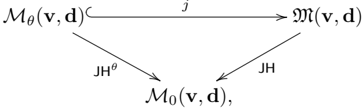
### Visual Description
## Mathematical Diagram: Model Transformation Flowchart
### Overview
The image displays a mathematical flowchart or diagram illustrating relationships between three distinct mathematical entities, connected by directional arrows with operational labels. The diagram uses calligraphic and standard mathematical notation, suggesting a context in optimization, machine learning, or functional analysis.
### Components/Axes
The diagram consists of three primary nodes and three connecting arrows, arranged in a triangular layout.
**Nodes (Mathematical Expressions):**
1. **Top-Left Node:** `M_θ(v, d)^C`
* `M`: Calligraphic uppercase M.
* Subscript: `θ` (Greek letter theta).
* Parenthetical arguments: `(v, d)`.
* Superscript: `C`.
2. **Top-Right Node:** `M(v, d)`
* `M`: Calligraphic uppercase M (same style as top-left).
* Parenthetical arguments: `(v, d)`.
3. **Bottom-Center Node:** `M_0(v, d),`
* `M`: Standard uppercase M (non-calligraphic).
* Subscript: `0` (zero).
* Parenthetical arguments: `(v, d)`.
* Followed by a comma.
**Arrows and Labels:**
1. **Horizontal Arrow (Top):** Connects the top-left node to the top-right node.
* **Direction:** Left to right.
* **Label:** `J` (positioned above the arrow's midpoint).
2. **Diagonal Arrow (Left):** Connects the top-left node to the bottom-center node.
* **Direction:** Top-left to bottom-center.
* **Label:** `JH^θ` (positioned to the left of the arrow's midpoint).
3. **Diagonal Arrow (Right):** Connects the top-right node to the bottom-center node.
* **Direction:** Top-right to bottom-center.
* **Label:** `JH` (positioned to the right of the arrow's midpoint).
### Detailed Analysis
* **Spatial Layout:** The diagram forms an inverted "V" or triangle. The two `M`-based entities are positioned at the top (left and right), both feeding into a single `M_0` entity at the bottom center.
* **Notation Details:**
* The use of calligraphic `M` for the top nodes versus standard `M` for the bottom node suggests a distinction in the type or state of the model/function.
* The subscript `θ` in the top-left node and its corresponding arrow label `JH^θ` indicates a parameterization or specific instance related to `θ`.
* The superscript `C` on the top-left node is unique to that entity.
* The arguments `(v, d)` are consistent across all three nodes, implying they operate on the same input variables.
* **Flow Interpretation:** The arrows define a clear directional flow:
1. A transformation `J` maps `M_θ(v, d)^C` to `M(v, d)`.
2. A transformation `JH^θ` maps `M_θ(v, d)^C` directly to `M_0(v, d)`.
3. A transformation `JH` maps `M(v, d)` to `M_0(v, d)`.
### Key Observations
1. **Convergent Structure:** Both top-level entities converge to produce the same bottom-level entity, `M_0(v, d)`.
2. **Parameter Dependency:** The path from the top-left node involves the parameter `θ` (`JH^θ`), while the path from the top-right node does not (`JH`). This suggests `M_θ(v, d)^C` is a parameterized variant, and `M(v, d)` may be a base or alternative form.
3. **Symbolic Consistency:** The repeated use of `J` and `H` in the arrow labels implies these represent fundamental operations (e.g., Jacobian, Hessian, or other linear/nonlinear operators) applied in sequence or combination.
### Interpretation
This diagram likely represents a **factorization, decomposition, or equivalence relationship** between different formulations of a model or function `M` that depends on variables `v` and `d`.
* **What it suggests:** The structure implies that the entity `M_0(v, d)` can be derived via two distinct pathways from two related but different starting points (`M_θ(v, d)^C` and `M(v, d)`). This is common in mathematical proofs, optimization derivations (e.g., showing different objective functions lead to the same solution), or in defining model relationships (e.g., a constrained model `M_θ^C` and an unconstrained model `M` both relating to a base model `M_0`).
* **Relationships:** The diagram establishes that `M_θ(v, d)^C` is linked to `M(v, d)` via operation `J`. Furthermore, both are linked to `M_0(v, d)` via operations that include `H` (with `H` possibly being modified by `θ` in one case). This could illustrate a chain rule application, a change of variables, or the relationship between a model, its constraint, and a Lagrangian or related function.
* **Notable Anomalies:** The comma after `M_0(v, d),` is unusual in a standalone diagram and may indicate this node is part of a larger equation or list that was cropped. The lack of context for symbols `J`, `H`, `θ`, `v`, `d`, and `C` limits a definitive interpretation, but the structure is characteristic of formal mathematical or theoretical computer science literature.
**Language Declaration:** All text in the image is mathematical notation, which is language-agnostic. The symbols are transcribed directly above.
</details>
&
&
where j is the open immersion of θ -semistable locus. Let
$$1 0 \times 1 = 1 0$$
$$The formula you've provided is not a standard mathematical or scientific notation. It appears to be a placeholder or a typo. If you meant to write something specific, please provide more context or clarify what you're trying to express.$$
x
x
be the constant perverse sheaf on M θ ( v , d ). Since JH θ is proper and semismall [Toda2, Lem. 4.4] 18 , JH θ ∗ IC M θ ( v , d ) is a perverse sheaf on M 0 ( v , d ); thus
$$H ^ { \prime } A _ { 1 } C l _ { 2 } O _ { 3 } = H ^ { \prime } A _ { 1 } C l _ { 2 } O _ { 3 }$$
is also a perverse sheaf. The natural map φ w IC M ( v , d ) → j ∗ φ w IC M θ ( v , d ) induces a map JH ∗ φ w IC M ( v , d ) → JH θ ∗ φ w IC M θ ( v , d ) . Truncation of the above map to the perverse degree ⩽ 0 part gives a map:
$$\theta : B P S _ { w } \rightarrow J H ^ { 0 } _ { w } I C _ { M _ { s } ( v , d ) } .$$
According to [Toda2, Lem. 4.7], the map Θ in (9.16) is an isomorphism. We still use Θ to denote the map induced by taking hypercohomologies on domain and codomain of (9.16). Define
$$j : = v o \theta - 1 ; H ^ { T } ( M _ { 0 } ( v , d ) ) .$$
Proposition 9.11. We have ȷ = Ψ H . In particular, Ψ H : H T ( M θ ( v , d ) , w ) → H T ( M ( v , d ) , w ) induces an isomorphism H T ( M θ ( v , d ) , w ) ∼ = H T ( M ( v , d ) , w ) BPS .
Proof. According to the proof of Proposition 9.8, Ψ H is induced by the correspondence [∆ M θ ( v , d ) ], where
$$\frac { 1 } { \vert A \vert } = \frac { 1 } { \vert B \vert } = \frac { 1 } { \vert C \vert } = \frac { 1 } { \vert D \vert } = \frac { 1 } { \vert E \vert } = \frac { 1 } { \vert F \vert } = \frac { 1 } { \vert G \vert } = \frac { 1 } { \vert H \vert } = \frac { 1 } { \vert I \vert } = \frac { 1 } { \vert J \vert } = \frac { 1 } { \vert K \vert } = \frac { 1 } { \vert L \vert } = \frac { 1 } { \vert M \vert } = \frac { 1 } { \vert N \vert } = \frac { 1 } { \vert O \vert } = \frac { 1 } { \vert P \vert } = \frac { 1 } { \vert Q \vert } = \frac { 1 } { \vert R \vert } = \frac { 1 } { \vert S \vert } = \frac { 1 } { \vert T \vert } = \frac { 1 } { \vert U \vert } = \frac { 1 } { \vert V \vert } = \frac { 1 } { \vert W \vert } = \frac { 1 } { \vert X \vert } = \frac { 1 } { \vert Y \vert } = \frac { 1 } { \vert Z \vert }$$
is the closure of the diagonal of the θ -semistable locus M θ ( v , d ) ×M θ ( v , d ). Precisely, we regard
$$g ( v , d ) \times M _ { 0 } ( v , d ) , w \in W _ { 0 } ^ { m } ( v , d ) , x , M _ { 0 } ( v , d )$$
$$\sum _ { m = 0 } ^ { n } M_s ( v , d ) ( \partial _ { t } ( v , d ) , \times , M_0 ( v , d ), i ' ( c w ) , M_0 ( v , d ) ) .$$
where i : M ( v , d ) × M 0 ( v , d ) M θ ( v , d ) ↪ → M ( v , d ) ×M θ ( v , d ) is the natural closed immersion.
According to [CG, (8.6.4)], we have an isomorphism
$$\begin{aligned}
H ^ { \prime } ( 2 \pi v , d ) & = Ext ^ { \prime } D ^ { \prime } _ { p } ( M _ { 0 } ( v , a ) ) ( J H ^ { \prime } _ { p } - w Q _ { M _ { 0 } } ( v , a ) ) \\
& = Ext ^ { \prime } D ^ { \prime } _ { p } ( M _ { 0 } ( v , a ) ) ( J H ^ { \prime } _ { p } - w Q _ { M _ { 0 } } ( v , c ) )
\end{aligned}$$
so [∆ M θ ( v , d ) ] induces a morphism in D b T ( M 0 ( v , d )):
$$( v , d ) \rightarrow J H _ { 0 } ^ { \phi w \omega m ( v , d ) } .$$
Then according to [VV1, Prop. 2.11], critical convolution map Ψ H is obtained by taking hypercohomologies of the above morphism. As we have seen previously,
$$\begin{aligned}
\sum _ { c } ^ { J H } \varphi w \mu ( v , d ) \in P _ { 0 } ( v , d ) \left[ dim M _ { 0 } ( v , d ) \right] . \\
J H + \varphi w \mu ( v , d ) \in P _ { 0 } ( v , d ) \left[ dim M _ { 0 } ( v , d ) \right] .
\end{aligned}$$
therefore [∆ M θ ( v , d ) ] factors as
$$\frac { \Delta m _ { 0 } ( v , d ) } { \Delta m _ { 0 } ( v , d ) ^ { \prime } } = B P S _ { w } [ \min M _ { 0 } ( v , d ) ]$$
where BPS w [dim M θ ( v , d )] = p τ ⩽ -dim M θ ( v , d ) JH ∗ φ w ω M ( v , d ) .
Composing [∆ M θ ( v , d ) ] with the natural map
$$\begin{aligned}
J H _ { \phi } ^ { ( v , d ) } & = J H _ { 0 } ^ { ( v , d ) } + J H _ { j } ^ { ( v , d ) } \\
& = J H _ { 0 } ^ { ( v , d ) } + J H _ { \phi } ^ { ( v , d ) }
\end{aligned}$$
we get the critical convolution map [∆ M θ ( v , d ) ] : JH θ ∗ φ w ω M θ ( v , d ) induced by the diagonal of M θ ( v , d ) ×M θ ( v , d ), which is identity map. It follows that Θ ◦ [∆ M θ ( v , d ) ] ′ = id. Then by the definition of ȷ , we have ȷ = Ψ H . □
Remark 9.12. Combining Corollary 9.10 with Proposition 9.11, we obtain the following commutative diagram
O
$$\begin{array}{ll}
H ^ { T } \left( 2 \pi ( v , d ) A _{\phi , w } \right) & H ^ { T } \left( M_0 ( v , d ) A _{\phi , w } \right), \\
\downarrow & \downarrow, \\
y^e & y^3, \\
H ^ { T } \left( 2 \pi ( v , d ) A _{\phi , w } \right) & H ^ { T } \left( M_0 ( v , d ) A _{\phi , w } \right),
\end{array}$$
O
18 It can be shown that JH θ is small, see [COZZ2, Thm. 1.1].
/
/
O
O
/
/
where ȷ ϕ is the map (9.17) for the stack M ( v , d ) A ,ϕ . Suppose that A ∼ = ( C ∗ ) l is the framing torus which acts on the framing vector space D by setting D = ∑ l i =1 a i D i such that K A (pt) ∼ = Q [ a ± i ] l i =1 . Let C be the chamber a 1 < a 2 < · · · < a l , then Stab C agrees with the 'critical stable envelope' CStab defined in [BD, § 1.2].
9.4. The case of tripled quivers with canonical cubic potentials. When Q is the tripled quiver of another quiver Q ′ with cubic potential w = ∑ i ∈ Q 0 tr( ε i µ i ), where ε i is the loop at i -th node and µ i is the i -th component of the moment map µ : R ( Q ′ , v , d ) → Lie( G ) ∨ , dimensional reduction gives isomorphisms (Example 6.13, Remark 6.14):
$$\begin{aligned}
( N _ { 0 } ( v , d ) ) \approx H ^ { T } ( M _ { 0 } ( v , d ), w ) , & \delta H : H ^ { T } ( S _ { 0 } ( v , d ) ) \approx K ^ { T } ( M _ { 0 } ( v , d ), w ) , \\
( v , d ) \approx H ^ { T } ( m _ { 0 } ( v , d ), w ) , & ( v , d ) \approx K ^ { T } ( m _ { 0 } ( v , d ), w ) .
\end{aligned}$$
We define the following maps:
$$\begin{aligned}
\varphi _ { H } := \delta ^ { - 1 } _ { H } o \varphi _ { H } o \delta _ { H } : H ^ { ( N _ { a } ) } \\
\varphi _ { K } := \delta ^ { - 1 } _ { K } o \varphi _ { K } o \delta _ { K } : K ^ { ( N _ { a } ) }
\end{aligned}$$
Here the Nakajima quiver variety N θ ( v , d ), the preprojective stack N ( v , d ) fits into open and closed immersion:
$$d ) : = \{ R ( Q ^ { v , d } ) / G \} .$$
In [AO1, § 2.1.8], a nonabelian stable envelope 19
$$\frac { 1 } { x ^ { 2 } + ( N - 1 ) x + K }$$
is constructed as the composition of the following maps
/
/
/
/
$$\begin{array}{ll}
K ^ { T } ( N _ { 0 } ( v , d ) ) & \xrightarrow [ 1 \textcircled { id } ] { K G ^ { x } T ( N _ { 0 } ( v , d ) ) } \\
\end{array}$$
o
o
where N θ ( v , v + d ) is the Nakajima quiver variety with the quiver data visualized vertex-wise as
>
>
O
O
$$\begin{matrix}
V_i' & \xrightarrow[I_i]{} A_i \\
& \xrightarrow[J_i]{} B_i \\
D_i, &
\end{matrix}$$
~
~
and j : ˚ N θ ( v , v + d ) ⊆ N θ ( v , v + d ) is the open immersion of the locus on which the maps { I i } i ∈ Q 0 are isomorphisms, s ′ is related to s by
$$( 9 . 2 0 ) s ^ { \prime } = s \otimes det ( T _ { 0 } )$$
The shift in slope comes from the difference between degree conditions in Definition 3.10 and in [Oko1, § 9.1] (see Remark 3.15). We fix an orientation of Q ′ so that
$$T _ { 0 } ^ { 1 / 2 } = \sum _ { a \in Q _ { 4 } } H o m ( V _ { t } ( a ) , V _ { h } ( a ) ) + \sum _ { i \in I _ { 0 } }$$
Repeating the above procedure with K -theory replaced by Borel-Moore homology, we obtain a cohomological nonabelian stable envelope
$$\frac { 1 } { n } , \frac { 1 } { n + 1 } , \frac { 1 } { n + 2 } , \ldots$$
Proposition 9.13. We have the following equations of maps:
$$\sum _ { n = 1 } ^ { \infty } \det ( T _ { n } ^ { 1 / 2 } v _ { n } d ) ^ { - 1 / 2 } e ^ { i H } = L _ { 4 } o \Psi H , \Psi K = u _ { 4 } o \Psi S \infty _ { k } , when$$
19 What we call Ψ s K ( α ) here is denoted by s α in [AO1, § 2.1.8].
Proof. Notice that M θ ( v , v + d ) is the total space of the vector bundle E = ⊕ i ∈ Q 0 Hom( V i , V ′ i ) over M θ ( v , v + d , d ), and E is repelling with respect to the + chamber. Let ˜ w = ∑ i ∈ Q 0 tr( ε i ˜ µ i ) be a function on M θ ( v , v + d ), where ˜ µ i : R ( Q ′ , v , v + d ) → Lie( G ) ∨ is the moment map. Then ˜ w is ( T × G ′ )-invariant and ˜ w ∣ ∣ M θ ( v , v + d ) = w ′ . By Proposition 8.3, the pushforward along zero section map gives the following commutative diagram
O
O
/
/
O
O
$$\begin{array}{ll}
I ^ { G } \times T ( M _ { 0 } ( v , d ), w ) & \xrightarrow [ Stab ^ { + } ]{ id } K ^ { G } \times T ( M _ { 0 } ( v , d ), w ) \\
\end{array}
\begin{array}{ll}
I ^ { G } \times T ( M _ { 0 } ( v , d ^ { \prime } ), w ^ { \prime } ) & \xrightarrow [ Stab ^ { + } ]{ z _ { \prime } } K ^ { G } \times T ( M _ { 0 } ( v , d ^ { \prime } ), w ^ { \prime } )
\end{array}$$
/
/
where s ′′ = s ′ ⊗ (det E ) 1 / 2 and ι : M θ ( v , d v ) ↪ →M θ ( v , v + d ) is the zero section map. Using (9.20), we can rewrite s ′′ = s ⊗ δ . The pushforward map is compatible with dimensional reduction, i.e. the following diagram is commutative
O
$$\begin{array}{ll}
K ^ { G } \times T ( M _ { 0 } ( v , d ) ^ { i }, w ) & \longrightarrow K ^ { G } \times T ( M _ { 0 } ( v , v + d ), w ) \\
\downarrow & \uparrow \\
K ^ { T } ( g ) ( v , d ) & \longrightarrow K ^ { T } ( g ) ( v , d ) .
\end{array}$$
/
/
O
By Theorem 6.11, we have the following commutative diagram
O
O
/
/
$$\begin{array}{ll}
K ^ { G } \times T ( M _ { 0 } ( v , d ) , w ) & \xrightarrow [ \delta K ]{Stab ^ { 4 } } K ^ { G } \times T ( N _ { 0 } ( v , v + d ) .
\end{array}$$
/
/
Here we set normalizer E equal to the structure sheaf. Combining the above three commutative diagrams, we obtain the equation Ψ s K = ι ∗ ◦ Ψ s ⊗ δ K . The other equation can be proven similarly and we omit the details. □
In the coming remark, we explain that the above results reproduce previous works on comparing stable envelopes and Hall operations on Nakajima quiver varieties.
Remark 9.14. As a special case of Corollary 9.10, Hall envelopes for tripled quiver ˜ Q ′ with standard cubic potential w are compatible with Hall operations. Dimensional reduction of the Hall compatibility diagrams in Definition 9.4 gives the following commutative diagrams:
O
O
/
/
O
O
O
O
/
/
O
O
$$\begin{array}{ll}
(9.22) & H ^ { T } \left ( \eta _ { 0 } ( v , d ) A _ { v 0 } \right ) \\
\downarrow & \downarrow \\
m _ { n } e ^ { - } \rightarrow K ^ { T } \left ( \eta _ { 0 } ( v , d ) A _ { v 0 } \right ) \\
\downarrow & \downarrow \\
\end{array}$$
/
/
/
/
Below we explain notations in above. The Nakajima quiver variety is an open substack of the preprojective stack:
$$( 9 . 2 3 )$$
and their torus fixed loci are
$$\sum _ { v , d } A ^ { \phi } = [ u - 1 ( 0 ) A ^ { \phi } / G ^ { \phi } ( A ) ] .$$
Let T 1 / 2 be a polarization of T vir N ( v , d ) 20 , i.e. T vir N ( v , d ) = T 1 / 2 + ℏ -1 ( T 1 / 2 ) ∨ . Stab C is the cohomological stable envelope with polarization T 1 / 2 defined in [MO, § 3], which is related to our Definition 3.5 (applied to Nakajima quiver variety N θ ( v , d ) with zero potential) by
$$e = ( - 1 ) r k ( T ^ { 1 } / 2 ) A _ { 0 } \sigma - attr .$$
Stab s C is the K -theoretic stable envelope with slope s and polarization T 1 / 2 defined in [Oko1, § 9.1] which is related to our Definition 3.14 (applied to Nakajima quiver variety N θ ( v , d ) with zero potential) by a shift in slope and a different normalization (see Remark 3.15). The shifts in slope of K -theoretic nonabelian stable envelopes are
$$\frac { 1 } { 2 } - \frac { 1 } { 4 } + \frac { 1 } { 8 } = \frac { 3 } { 8 }$$
20 T vir N ( v , d ) = ∑ a ∈ Q ′ 1 ( Hom( V t ( a ) , V h ( a ) ) + ℏ -1 Hom( V h ( a ) , V t ( a ) ) ) -∑ i ∈ Q ′ 0 (1 + ℏ -1 ) End( V i ) .
O
O
/
/
O
O
m ϕ Π , C in (9.22) is the Hall operation for preprojective stack which is the dimensional reduction of m ϕ C [YZ1, YZ2]. E· is the multiplication by the K -theory class
$$E = \frac { ( - 1 ) r k ( r ^ { 2 } ) ^ { 3 } A _ { 0 } a t t r } { d e t ( \sqrt { h } ( r ^ { 2 } ) ^ { 3 } A _ { 0 } a t t r ) }$$
In [YZ1, Thm. 4.3], it is shown that the preprojective Hall operation m ϕ Π , C is compatible with a (twisted) ordinary Hall operation m ϕ C on the smooth stack R ( v , d ) in the sense that the following diagrams are commutative
O
O
/
/
O
O
O
O
/
/
O
O
$$\begin{array}{ccc}
\left( \gamma _ { 2 } \right) & \xrightarrow[m^\prime_e]{} H ^{T}( \gamma ( v , d ) A ) \\
\left( \gamma _ { 1 } \right) & \xrightarrow[n^\prime_e]{} K ^{T}( \gamma ( v , d ) A ) \\
\left( \gamma _ { 0} \right) & \xrightarrow[m^\prime_c]{} H ^{T}( \gamma ( v , d ) ) \\
\end{array}$$
where
$$( h ^ { \phi } _ { c } = m _ { c } ^ { \phi } o e ^ { i x G ^ { \phi } ( A ) } ,$$
for · = empty or K depending on whether it is cohomological or K -theoretic. Combining Proposition 9.13 with diagrams (9.22) and (9.24), we obtain the following commutative diagrams:
O
$$\begin{array}{ccc}
\text{m}^{\circ} \varepsilon & H^T(\mathbf{R}(v,d))A^{\sigma} \\
\downarrow & \downarrow \\
\text{Stab}_e & K^T(\mathbf{N}_0(v,d))A^{\sigma} \\
\downarrow & \downarrow \\
\end{array}$$
O
where Ψ H , Ψ s K are constructed in [AO1].
When A is a framing torus, the left square in (9.26) reproduces a result of Botta [Bot, Thm. 5.6], where his proof uses the method of abelianizations [Sh]. Botta-Davison [BD] has another proof of Botta's result by showing that m ϕ Π , C ◦ Ψ ϕ H and Ψ H ◦ Stab C are induced by the same correspondence.
Moreover, the left square in (9.26) can be used to deduce an inductive formula of stable envelopes for Nakajima quiver varieties [Bot, Thm. 5.12], which reduces the computations of stable envelopes to the computations of Ψ H in the framing rank one cases.
As an application, we deduce explicit formulas of stable envelopes for the Nakajima quiver variety N θ ( v , d ) using Remark 9.14 under certain assumptions on the fixed loci. Note that
$$R ( Q ^ { v , d } A ^ { b } _ { 0 } = R ( Q ^ { v , d } A ^ { b } _ { 0 } )$$
for a certain quiver Q ′ ϕ (possibly disconnected) with gauge dimension vector v ϕ and framing dimension vector d ϕ .
The following result, in the case when Q ′ is an affine type A quiver and A = framing torus × C ∗ that resolves the loop (i.e. (9.27) is a finite type A quiver variety), recovers cohomological and K -theoretic limits of [Din, Thm. 1] and also [AO1, Prop. 7].
̸
Corollary 9.15. Assume that every connected component of ( Q ′ ϕ , v ϕ , d ϕ ) is a Dynkin quiver with minuscule framing, i.e. there is a node i 0 that corresponds to a minuscule fundamental weight of the Lie algebra associated with the Dynkin quiver, such that d ϕ,i 0 = 1, d ϕ,i = 0 if i = i 0 .
Then in T -localized homology H T ( N ( v , d )) loc := H T ( N ( v , d )) ⊗ Q [Lie( T )] Frac( Q [Lie( T )]), we have
$$\sum _ { w \in W / W ^ { 0 } } A _ { d } ( \sigma ) = \sum _ { w \in T \times G ^ { s } ( A ) } ( e ^ { i t / 2 } A _ { d } - \sigma_{rep} + 1 , d )$$
where N ( v , d ) (9.23) has a quasi-smooth stack structure and [ N ( v , d )] vir denotes its virtual class. In particular,
$$\sum _ { e \in W / W ^ { s } } w ( e ^ { T \times G ^ { s } ( A ) } ( ( T ^ { 1 } / 2 ) A , \phi - rep l + h ( T )$$
/
/
O
O
O
O
/
/
O
O
/
/
/
/
/
/
/
/
Let s be a generic slope and χ ∈ char( G ϕ ( A ) ) such that s ⊗ δ ϕ is in a sufficiently small neighbourhood of χ , then in T -localized K -theory K T ( N ( v , d )) loc := K T ( N ( v , d )) ⊗ Q [ T ] Frac( Q [ T ]), we have
(9.29)
$$\sum _ { w \in W / W ^ { 0 } } \sum _ { u \in X \cdot e ^ { i G ^ { s } ( a ) } ( T _ { I 1 / 2 } A _ { 0 - repl } )$$
where L χ ∈ Pic( N θ ( v , d ) A ,ϕ ) is the descent of the character χ , and [ O vir N ( v , d ) ] denotes the virtual structure sheaf. In particular,
$$\sum _ { w \in W / W ^ { e } } u ( x , c _ { r } ^ { k } x G ^ { s } ( A ) ( T | 1 / 2 ) A _ { 0 } ^ { p - rep } + f$$
Proof. By Lemma 9.16 below, we have
$$\Psi _ { H } ^ { ( N_0 v , d ) A^0 } = \left[ \int \limits _ { 0 } ^ { v } \left( A^0 \right) A^0 \right] v i$$
By the commutativity of diagrams (9.22), we get
$$\Psi _ { H } o Stab c ( [ N _ { 6 } ( v , d ) ^ { A _ { 0 } ^ { 0 } } ) =$$
Since
$$R ( \overrightarrow { Q } ^ { \prime } , v , d ) = M \cdot \overrightarrow { h } ^ { \prime }$$
we have inclusion R ( Q ′ , v , d ) T ⊆ M . Since M ⊆ µ -1 (0), we see that R ( Q ′ , v , d ) T ⊆ µ -1 (0). Therefore the pushforward maps
$$u : H ^ { 1 } ( \Omega ( v , d ) ) \rightarrow H ^ { T } ( \Omega ( v , d ) ) .$$
are isomorphisms after T -localization. Note that
$$\frac { 1 } { ( h ^ { - } Lie( G ) \cdot [ O _ { x } ( v , d ) ] ) } = e ^ { i \times G ( h ^ { - } ) }$$
Then it follows from the compatibility (9.24) that
$$Here in the second equality, we use (9.24) that$$
Here in the second equality, we use (9.25) and the explicit formula of Hall operation as (4.26).
Similarly in the K -theory, we have
In the above proof, we use the following lemma, whose proof will be given in Appendix F.
Lemma 9.16. Let Γ be a Dynkin quiver with gauge dimension vector r and framing dimension vector e such that e is minuscule. Assume that N θ ( r , e ) is nonempty. Then
$$\begin{aligned}
\Psi _ { H } ( N _ { 0 } ( r , e ) ) = \Psi _ { H } ( r , e ) ^ { i r } .
\end{aligned}$$
Let G = ∏ i ∈ Γ 0 GL( r i ) denote the gauge group, and s ∈ char( G ) ⊗ Z R be a generic slope taken in a sufficiently small neighbourhood of χ ∈ char( G ), then
$$\varphi _ { K } ^ { \prime } ( [ x ] ) = [ x \otimes O ^ { v i r } _ { n ( r , e ) } ].$$
where L χ ∈ Pic( N θ ( r , e )) is the descent of the character χ .
Remark 9.17. We note that N θ ( r , e ) is a point for minuscule e , so N θ ( v , d ) A ,ϕ in Corollary 9.15 is also a point. Then (9.28) and (9.29) completely determine Stab C and Stab s C in this situation.
- 9.5. Hall operation compatible Hall envelopes. We show for a class of asymmetric quiver varieties, where the asymmetric part comes only from the framing, their Hall envelopes are compatible with Hall operations.
Definition 9.18. Let Q be a symmetric quiver and v , d in , d out ∈ N Q 0 be dimension vectors. The symmetrization of R ( v , d ) is defined to be R ( v , c ) (4.5) where c i = max { d in ,i , d out ,i } . We identify R ( v , d ) as a G -subrepresentation of
$$\begin{aligned}
R ( v , c ) = R ( v _ { d } ) \oplus i s . t . d _ { in } ^ { 2 } & Hom ( C V _ { i }, C d _ { in , i } - d _ { out , i } ) \oplus i E Q _ { 0 } ^ { 2 } = d _ { out , i } s . t . d _ { in , i } < d _ { out , i } \\
Hom ( C d _ { out , i } - d _ { in , i } , C V _ { i } ) & Hom ( C d _ { out , i } - d _ { in , i } , C V _ { i } ) \oplus i t . i ^ { 2 }
\end{aligned}$$
Definition 9.19. Let Q be a symmetric quiver and v , d in , d out ∈ N Q 0 be dimension vectors and A be a subtorus of flavour group Aut G R ( v , d ). We say that the A -action on R ( v , d ) is pseudo-self-dual if it extends to a self-dual A -action on the symmetrization R ( v , c ). We say that the A -action on M θ ( v , d ) is pseudo-self-dual if it is induced from a pseudo-self-dual action on R ( v , d ).
Here is the main theorem of this section.
Theorem 9.20. Let Q be a symmetric quiver and v , d in , d out ∈ N Q 0 be dimension vectors such that d in ,i ⩾ d out ,i for all i ∈ Q 0 , choose cyclic stability θ (9.1). Let T ⊆ Aut G R ( v , d ) be a torus in the flavour group and A be a pseudo-self-dual subtorus of T , C be a chamber associated with A action on M θ ( v , d ), and s be a generic slope.
Then Hall envelopes HallEnv C and HallEnv s C are compatible with Hall operations.
By Theorem 9.20 and Lemma 9.6, we get the triangle lemma for the above asymmetric quiver varieties.
Corollary 9.21. In the setting of Theorem 9.20 and let X = M θ ( v , d ), then both diagrams in (9.8) commute.
9.5.1. Proof of Theorem 9.20, cohomology case. We begin with the following lemma. In below, we omit the canonical map in Lemma 3.22 and simply write
$$\vert A B \vert _ { 1 } = \vert A B \vert _ { 2 } = \vert A B \vert _ { 3 } = \vert A B \vert _ { 4 }$$
Lemma 9.22. In the setting of Theorem 9.20, the Hall envelope
$$, w ) \rightarrow H ^ { T } ( M _ { 0 } ( v , d ), w )$$
is induced by the correspondence
$$\left[ \frac { 1 } { v _ { d } } \times M _ { 0 } ( v , d ) ^ { A } , w \in w \right] _ { A t t r c }$$
Proof. Consider the vector bundle E = E + ⊕ E -on M θ ( v , d v ), where the fibers of E + and E -are
$$\begin{aligned}
( 9 . 3 2 ) & = \frac { i e Q _ { 0 } } { s , t , d _ { in }, t > d _ { out } , t } \\
& = H o m ( V _ { i } , C d _ { in } , i ^ { - } d _ { out } ) \\
& = H o m ( V _ { i } , V ^ { \prime } i ) .
\end{aligned}$$
Then Tot( E ) is isomorphic to the symmetric quiver variety M θ ( v , v + d in ). Note that E + (resp. E -) is attracting (resp. repelling) with respect to the positive chamber under the C ∗ -action in (9.4). Then by Propositions 8.7, 8.8, the Stab + (in Definition 9.1) is induced by the correspondence
$$\sqrt { A t r + ( \Delta M _ { 0 } ( v , d ) ) } \leq$$
where the closure is taken inside M θ ( v , d v ) ×M θ ( v , d ).
So ˜ Ψ H (in Definition 9.1) is induced by the correspondence given by the irreducible closed substack
$$\begin{aligned}
& \left( \frac{\partial }{\partial t} + ( \Delta M_0 ( v , d ) ) \right) [ G ^ { i } ] \\
& = M_0 ( v , d ) \times M_0 ( v , d ) .
\end{aligned}$$
As in (9.11), we have
$$\sum M_0 ( v , d ) \times M_0 ( v , d )$$
Therefore ˜ Ψ H is induced by the correspondence given by the closure of the diagonal of stable locus M θ ( v , d ) inside the stack M ( v , d ) ×M θ ( v , d ), i.e.
$$\frac { 1 } { n } \sum _ { i = 1 } ^ { n } a _ { i }$$
Let ϕ : A → G be a homomorphism that appears in (9.6), then ˜ Ψ ϕ H is similarly induced by the correspondence
$$[ A _ { n } ( v , d ) ] _ { n }$$
The same argument as Proposition 9.8 shows that m ϕ C ◦ ˜ Ψ ϕ H is induced by the correspondence
$$\vert Z \vert \in H ^ { T } ( m ( v , d ) \times .$$
where Z = Attr C ( ∆ M θ ( v , d ) A ,ϕ ) is the closure of Attr C ( ∆ M θ ( v , d ) A ,ϕ ) inside the stack M ( v , d ) ×M θ ( v , d ) A ,ϕ (here attracting set is taken inside the stable locus M θ ( v , d ) ×M θ ( v , d ) A ,ϕ ).
It follows that HallEnv C = k ∗ ◦ m ϕ C ◦ ˜ Ψ ϕ H is induced by the correspondence [ Z ∣ ∣ M θ ( v , d ) ×M θ ( v , d ) A ,ϕ ] , which is exactly [ Attr C (∆ M θ ( v , d ) A ,ϕ ) ] , where the closure is taken in M θ ( v , d ) ×M θ ( v , d ) A ,ϕ □
Let C ∗ t ⊆ G ′ be a torus in the center of the flavour group which acts on V ′ i in (9.2) with weight -1 for all i ∈ Q 0 , then ˜ A := A × C ∗ t naturally acts on R ( v , d v ). Let
$$K _ { C } ( p t ) = Q [ t ^ { 2 } ] ,$$
and consider the chamber ˜ C in Lie( ˜ A ) R such that C + = { a i = 0 } r i =1 ×{ t > 0 } is a face of ˜ C and ˜ C / C + = C . Combining Lemma 9.22 with Proposition 8.10 and Theorem 4.16, we see that the composition
$$d ) A _ { φ , w } \rightarrow H ^ { T } \times G ^ { i } ( M _ { 0 } ( v , d Y ), w )$$
is induced by the correspondence where
$$[ A + b = ( \Delta m _ { v } , a ) ] .$$
which is the closure of the attracting set Attr ˜ C ( ∆ M θ ( v , d ) A ,ϕ ) inside the variety M θ ( v , d v ) ×M θ ( v , d ) A ,ϕ .
Therefore the map ˜ Ψ H ◦ HallEnv C is induced by the correspondence
$$[ S ] \in H ^ { T } ( m ( v , d ) \times .$$
$$s = \frac { \int _ { 0 } ^ { \infty } ( A _ { M _ { 0 } } ( v , d ) A _ { o } ) n } { G ^ { \prime } }$$
is an irreducible closed substack of M ( v , d ) ×M θ ( v , d ) A ,ϕ . We have
$$\int ^ { - 1 } _ { 0 } ( A t t r e ( \Delta m _ { 0 } ( v , d ) ^ { A _ { 0 } } ) \cdot$$
where q : ˚ M θ ( v , d v ) → M ( v , d ) is the quotient map and Attr C ( ∆ M θ ( v , d ) A ,ϕ ) is the attracting set of ∆ M θ ( v , d ) A ,ϕ in M θ ( v , d ) ×M θ ( v , d ) A ,ϕ , regarded as a locally closed substack in M ( v , d ) ×M θ ( v , d ) A ,ϕ . It follows that S contains Attr C ( ∆ M θ ( v , d ) A ,ϕ ) as an open substack. By the closedness and irreducibility of S ,
$$S = A + h _ { 0 } ( A _ { n } g ) = Z _ { n }$$
This is exactly the correspondence that induces m ϕ C ◦ ˜ Ψ ϕ H (by the proof of Lemma 9.22), and we are done.
9.5.2. Proof of Theorem 9.20, K-theory case. By Lemma 9.2, k ∗ ◦ ˜ Ψ s K = id, it suffices to show that
$$m ^ { \phi } _ { 0 } \varphi ^ { \phi } _ { k } ( n ) = i m ( \varphi ^ { \phi } _ { k } )$$
$$\sin x = \frac { 1 } { 2 } ( 1 - \cos 2 x )$$
Recall the vector bundle E + (9.32) on M θ ( v , d v ). Denote
$$d _ { i n } := ( d _ { i n } , d _ { i n } ) ,$$
Tot( E + ) is isomorphic to M θ ( v , d v in ) which is used to define nonabelian stable envelope ˜ Ψ s K for symmetric quiver variety M θ ( v , d in ). Restricting to the open locus (9.3) (where d = d in ) and (9.3), and taking quotient by G , the bundle projection becomes
$$\therefore 3 9 ( x , d ) \rightarrow 3 9 ( x , - d )$$
By Proposition 8.2, we have commutative diagrams:
O
O
/
/
O
O
$$\begin{array}{ll}
\overrightarrow { K } ^ { T } ( \overrightarrow { M } ( v , d ) , w o \pi ) & = \overrightarrow { K } ^ { T } ( \overrightarrow { M } ( v , d ) A _{\phi } , w o \pi ) \\
\downarrow \quad \overrightarrow { K } ^ { s,sym } & \downarrow \quad \overrightarrow { K } ^ { s,sym } \\
\overrightarrow { K } ^ { T } ( M_0 ( v , d ) , w o \pi ) , & \overrightarrow { K } ^ { T } ( M_0 ( v , d ) A _{\phi } , w o \pi )
\end{array}
\begin{aligned}
i ^ { A } &= K ^ { T } ( \overrightarrow { M } ( v , d ) A_{\phi } , w o \pi ) \\
&= \overrightarrow { K } ^ { s,sym }
\end{aligned}$$
/
/
/
/
where i A : M ( v , d ) A ,ϕ ↪ → M ( v , d in ) A ,ϕ is the zero section of the fixed locus π A . The right diagram follows from the torus fixed version of the left diagram and i A ∗ = ( π A ∗ ) -1 . Here 'sym' in the subscript means the nonabelian stable envelopes for symmetric quiver varieties. Then it remains to show that for all γ ∈ K T ( M θ ( v , d in ) A ,ϕ , w ), we have
$$\pi ^ { \ast } o m _ { e } o i ^ { A } o \varphi _ { K , s } ^ { \prime }$$
By Proposition 9.9, it is enough to prove the following degree condition
- there is a strict inclusion of intervals
$$\sum _ { ( v , d _ { in } ) } ^ { A } \sum _ { i = 1 } ^ { o } \sum _ { j = 1 } ^ { K } e _ { G } ( N _ { S _ { i } } / l ^ { i + o } ) \sum _ { k = 1 } ^ { K } s _ { K } ( N _ { S _ { i } } / l ^ { i + o } )$$
for all cocharacters σ i : C ∗ → G that appear in the KN stratification, and all γ ∈ K T ( M θ ( v , d in ) A ,ϕ , w ), where ˆ e G K is defined in (5.3).
Similarly as the proof of Theorem 5.5, it remains to show the following analogy of (5.5):
$$\lim _ { w \rightarrow 1 ( c ) } \frac { \sqrt { e ^ { i G_e ( A ) } } } { e ^ { i G_e ( A ) } w ^ { - 1 ( c ) } } = \sqrt { e ^ { i G_e ( A ) } }$$
Note that by the attracting condition, we have
$$\lim _ { t \rightarrow 0 , \infty } \frac { 1 } { e ^ { ( G ^ { \phi } ( A ) ) w - 1 ( c ) } ( E _ { + } A _ { + } - \phi - rep ) }$$
and by Theorem 5.3, we have
$$\sum _ { i = 1 } ^ { \infty } \frac { 1 } { 2 } \deg w - 1 ( o ) e ^ { C ^ { d } K } ( R ( v , d in ) A _ { p } ^ { - 1 } Lie ( o ) )$$
then (9.33) follows from the above two degree bounds.
This finishes the proof of Theorem 9.20 in the K -theory case.
- 9.6. Hall v.s. stable envelopes. In this section we compare Hall envelopes with stable envelopes.
For cohomology, the following result is a consequence of Lemma 9.22 and Theorem 8.9.
Proposition 9.23. In the setting of Theorem 9.20, and assume that the bundle
<details>
<summary>Image 13 Details</summary>
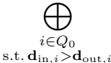
### Visual Description
Icon/Small Image (111x63)
</details>
$$H O H ( r , C ^ { \prime } h _ { n } , - d _ { n o + 1 } )$$
O
O
/
/
O
O
in (9.32) can be written as a direct sum of attracting and repelling subbundles in chamber C (as in Theorem 8.9), then cohomological stable envelope exists and
$$S _ { \Delta A B C } = H _ { 1 } \Delta H _ { 2 } r c$$
The K -theory counterpart of Proposition 9.23 is more complicated, as we do not have a K -theory analogy of Theorem 8.9.
Proposition 9.24. In the setting of Theorem 9.20, consider one of the following situations
- (1) the bundle ⊕ i ∈ Q 0 s . t . d in ,i > d out ,i Hom( V i , C d in ,i -d out ,i ) in (9.32) is attracting in chamber C ,
- (2) A is a minuscule framing torus, i.e. A ∼ = C ∗ which acts on framing vector space with weight 0 and 1.
then for a generic slope s , K -theoretic stable envelope exists and
$$S _ { \Delta } t ^ { s } = H _ { \Delta } l E _ { v } ^ { s }$$
Proof. It is enough to show that HallEnv s C satisfies three axioms of stable envelopes. The support axiom (Definition 3.10(i)) and the normalization axiom (Definition 3.10(ii)) are checked in the same way as Theorem 5.5 and we shall not repeat here. As in (9.32), we denote
$$F = \frac { H } { i e Q _ { 0 } } s . t . d _ { in , i } > d _ { out , i }$$
Similar as the proof of Theorem 5.5, the degree axiom is examined by showing the following analogy of (5.7)
$$\frac { \lim _ { x \rightarrow ( G ^{s}( A ) ) } \frac { 1 } { x ( C s( A ) ) ^{ s } } - 1 ( φ ^{s} ) ^{ s } ( s ) \cdot \sqrt { e ^{ i K } } } { T _ { X } ( G ^{s}( A ) ) ^{ s } - 1 ( φ ^{s} ) ^{ s } ( A ) } ( F _ { A , ω } ^{ s } - L _ { i e } ( C s( A ) ) ^{ s } ) }$$
exist for all w ∈ W ϕ ′ \ W/W ϕ and all directions of a →∞ , where s ′ is as (9.7), ϕ ′ : A → G is a homomorphism such that M θ ( v , d ) A ,ϕ ′ ⋂ Attr f C ( M θ ( v , d ) A ,ϕ ) is nonempty.
In situation (1), the repelling part of F is trivial by assumption, and (9.34) is the same as (5.7) which has been proven in Theorem 5.5.
In situation (2), let us write decomposition of framing vector spaces into A -weight spaces:
$$d = d ^ { \prime } + d ^ { \prime \prime } ,$$
where the superscripts denote the A -weight ∈ { 0 , 1 } . Since A -action is pseudo-symmetric by assumption, we have d (0) in ,i ⩾ d (0) out ,i and d (1) in ,i ⩾ d (1) out ,i for all i ∈ Q 0 . We can write ϕ and ϕ ′ fixed components as
$$, d ^ { ( 0 ) } ( v , \frac { d } { d t } ) A _ { 0 } ^ { ( 0 ) } = M _ { 0 } ( v , \frac { d } { d t } )$$
for certain decompositions v = v (0) ϕ + v (1) ϕ = v (0) ϕ ′ + v (1) ϕ ′ . Then we have
It follows that
$$\sum _ { k = 1 } ^ { T } ( G ^ { e } ( A ) ) w ^ { - i \epsilon } ( d ^ { e } ( A ) ) ( F _ { A } ^ { e } , \phi$$
as a ± →∞ , where
$$n = \sum _ { i \in Q _ { 0 } } v _ { o } ^ { ( 1 ) } \cdot ( d _ { in , i } - d _ { out , i } )$$
̸
Note that M θ ( v , d ) A ,ϕ ′ ⋂ Attr f C ( M θ ( v , d ) A ,ϕ ) = ∅ implies M θ ( v , d ) A ,ϕ ≤ M θ ( v , d ) A ,ϕ ′ in the ample partial order (Remark 3.9), and the latter is equivalent to
$$v _ { 1 } ^ { \prime } > v _ { 2 } ^ { \prime } , v _ { 1 } < Q _ { 0 }$$
In particular, n ⩾ n ′ , and it follows that
$$\lim _ { a \rightarrow \infty } \frac { T_X ( G^\phi( A ) ) w ^{-1} ( \phi'( A ) ) } { \tilde{T}_X ( G^\phi( A ) ) w ^{-1} ( \phi'( A ) ) e^{i K } } = \exists .$$
Then (9.34) follows from (5.7).
□
There are examples where Hall envelopes are not equal to stable envelopes and do not satisfy the triangle lemma.
Example 9.25. Consider the quiver Q consisting of a single node with no arrows, and take d = (1 , 2). Let
$$M ( n d ) = \left[ M _ { 0 } ( k , n d ) \right]$$
be the disjoint union of quiver varieties, where we fix θ = -1. Note that M θ ( k, n d ) is a vector bundle on Gr( k, n ). Let C ∗ ℏ act on M ( n d ) by scaling the out-going framing with weight ℏ -1 , and A = C ∗ a 1 × C ∗ a 2 × C ∗ a 3 act on
$$x = M ( 3 d )$$
by assigning weights to the framings: a 1 d + a 2 d + a 3 d . Set T = A × C ∗ ℏ . Then the equivariant K -theory of the A -fixed loci is generated by the tensor product of structure sheaves:
$$k ^ { T } ( X ^ { A } ) = \frac { 1 } { ( k _ { 1 } , k _ { 2 } , k _ { 3 } ) } e ^ { i ( 0 , 1 ) ^ { 3 } }$$
Fix a generic slope s ∈ R ∼ = Pic( M θ ( k, 3 d )) ⊗ Z R .
Proposition 9.26. For ( X, T , A ) in the above example, we have:
- (1) There exists a chamber C of A with a face C ′ such that the triangle lemma (9.8) fails for the K -theoretic Hall envelope.
- (2) There exists a chamber C of A such that K -theoretic stable envelope Stab s C does not exist.
̸
- (3) There exists a one-dimensional torus σ : C ∗ → A such that Stab s σ = HallEnv s σ , where HallEnv s σ is the Hall envelope defined using the image of σ in the positive chamber.
Proof. Suppose that the triangle lemma (9.8) always holds for any chamber C and face C ′ , then by [COZZ3], the following Yang-Baxter equation
$$\sum _ { i = 1 } ^ { 4 } ( a _ { 1 } / a _ { 3 } ) R _ { s + i } ^ { s + i - 1 } ( a _ { 2 } / a _ { 3 } ) = R _ { s + i } ^ { s + i - 1 } ( a _ { 1 } / a _ { 3 } )$$
should hold, where µ ( i ) + = 1 -k i 2 , µ ( i ) -= k i -2 2 , with R -matrix:
$$R _ { i j } ( a _ { i } / a _ { j } ) = ( H a l l E n v ^ { s } _ { a _ { i } } > a _ { j } .$$
Denote [ ab ] := [ O M θ ( a, d ) ⊠ O M θ ( b, d ) ]. In the basis [00] , [01] , [10] , [11], the Hall envelopes can be explicitly computed using (9.10) and we get
$$\begin{array}{ll}
Hallin^2_{a_1 > a_2} = \left\{ \begin{array}{l} 1 - a_1/a_2 \\ 0 & (1 - h_a_1)/a_2 \end{array} \right. \\
Hallin^2_{a_1 < a_2} = \left\{ \begin{array}{l} 1 - (1 - h_a_2)/a_2 \\ (a_1/a_2)^2 s-1/2(1 - h_a_2) & (1 - h_a_1)/a_2 \end{array} \right.
\end{array}$$
$$HallE _ { n v ^ { 2 } } \leq ( 1 ) ^ { 2 } ( 1 - h a _ { 2 } / a _ { 1 } ) ^ { 2 } ( 1 - h a _ { 2 } / a _ { 1 } ) ^ { 2 }$$
It is a straightforward to check that R s ij does not satisfy the Yang-Baxter equation (9.35), and this proves (1).
We notice that the Hall envelopes (9.36) satisfy the axioms in Definition 3.10 therefore we have
$$H a l F _ { 2 } O _ { 3 } = S a C O _ { 3 } \downarrow + 2 H _ { 2 } O$$
In particular, R -matrix is given by R s ij ( a i /a j ) = (Stab s a i <a j ) -1 Stab s a i >a j . The failure of Yang-Baxter equation implies that there exists a chamber C of A such that Stab s C does not exist (otherwise the triangle lemma automatically holds by Lemma 3.37 and YBE should also hold). This proves (2).
Finally, suppose that Stab s σ = HallEnv s σ for every one-dimensional torus σ : C ∗ → A . Suppose that C = { a i > a j > a k } and C ′ = { a i = a j > a k } are a pair of chambers and faces such that triangle lemma fails for the K -theoretic
Hall envelope as in (1). According to the proof of Lemma 3.37, there exists an one-dimensional torus ξ : C ∗ → A in the chamber C , such that
$$S _ { n } H _ { 2 } = S _ { n } H _ { 2 } \cdot \cdots \cdot S _ { n } H _ { 2 }$$
We have Stab s a i = a j >a k = HallEnv s a i = a j >a k since they are given by one-dimensional torus. We also have
$$S _ { \Delta } t ^ { f } = H _ { a l l } E _ { h v } ^ { f }$$
by the above explicit computation. Note that the construction of Hall envelope can be replaced by an arbitrary one-dimensional torus in the chamber C , and result remains the same, in particular HallEnv s C = HallEnv s ξ . Thus we have
$$HallEnv ^ { s } _ { a _ { i } } = HallEnv ^ { s } _ { a _ { j } } = Stab ^ { s } _ { a _ { i } } =$$
This contracts with the choice of C and C ′ . This prove (3).
Appendix A. Pullback isomorphisms along attraction maps
In this section, we take ( Y, T , A , w ) as in Setting 2.1. Assume moreover that F = Y A is connected, and X = Attr C ( F ). Consider the attraction map
$$f : X \rightarrow F , x \rightarrow \lim _ { t \rightarrow }$$
By [BB], f is an affine fibration and does not depend on the choice of σ . Since w is A -invariant, we have
$$w = f ^ { \prime } ( w ^ { \prime } ) ,$$
so there are smooth pullbacks
$$f ^ { \prime } : H ^ { 1 } ( F , w ^ { A } ) → H ^ { 1 } ( X , w ).$$
By (2.12), the first map is an isomorphism. As we do not find a reference on the comparison of the second map, we show below the following.
Proposition A.1. In the above situation, f ∗ : K T ( F, w A ) → K T ( X, w ) is an isomorphism.
Proof. By [Hal, Amplification 3.18], we have a SOD for the derived category of coherent sheaves:
$$f ^ { \prime } D ^ { \prime } ( F / T ) _ { 0 , j } = f ^ { \prime } D ^ { \prime } ( F / T ) _ { 1 , . . } ,$$
$$( \cdots , D ^ { b } ( [ F / T ] ) _ { 1 } , \ldots )$$
is an SOD of D b ([ F/ T ]), and f ∗ maps D b ([ F/ T ]) v fully faithfully onto its image in D b ([ X/ T ]) for all v ∈ Z . Here D b ([ F/ T ]) v is the full subcategory of D b ([ F/ T ]) whose objects are complexes with σ -weight equals to v , where σ is a fixed cocharacter in C .
This induces an SOD for the matrix factorization category (e.g. [P, Prop. 2.1]):
$$\displaystyle \sum _ { i = 1 } ^ { n } f ( x / T , w ^ { A } )$$
where
$$( \cdots , MF ( F / T ) , w ^ { A } 1 , … )$$
is an SOD of MF ( [ F/ T ] , w A ) , and f ∗ maps MF ( [ F/ T ] , w A ) v fully faithfully onto its image in MF ([ X/ T ] , w ) for all v ∈ Z . By passing to the Grothendieck group, we get isomorphism f ∗ : K T ( F, w A ) ∼ = K T ( X, w ). □
where
□
Appendix B. Excess intersection formula of critical cohomology and K -theory
Consider the following Cartesian diagram of smooth and connected varieties:
/
/
$$\begin{array}{ll}
(B.1) & \begin{tikzpicture}[baseline=(current bounding box.center)]
\node (x) at (0,0) {$X$};
\node (y) at (2,0) {$Y,$};
\draw[->] (x) to node [above] {$f$} (y);
\draw[->] (x) to node [left] {$h$} (x);
\draw[->] (y) to node [right] {$g$} (y);
\end{tikzpicture}
\end{array}$$
/
/
where f is a closed immersion. The natural map N f ′ → h ∗ N f between normal bundles is an embedding of vector bundles. We define the excess bundle :
$$E = h ^ { \prime } N _ { 2 } / N _ { 2 }$$
Suppose that w : Y → C is a regular function on Y . We have proper pushforward
$$f ^ { \prime } : H ( X , \varphi w o f w X ) \rightarrow$$
and l.c.i. pullback
$$g : H ( Y , \varphi _ { w o } f o h W X [ - 2 d _ { h } ] ) \rightarrow H ( X ' , \varphi _ { w o } f o h W X [ - 2 d _ { h } ] ) .$$
Here d g = dim Y ′ -dim Y and d h = dim X ′ -dim X .
Proposition B.1 (Excess intersection formula for critical cohomology) . Notations as above, we have
$$g ^ { \prime } ( f _ { 1 } ) = f ^ { \prime } _ { 1 } ( e ) f ^ { \prime } _ { 2 } ( B ) - h ^ { \prime }$$
where e ( E ) is the Euler class of the excess bundle E .
Proof. Note that g = pr Y ◦ Γ g , where Γ g : Y ′ → Y ′ × Y is the graph of g and pr Y : Y ′ × Y → Y is the projection to the second component. They fit into the following Cartesian diagram:
/
/
$$\begin{array}{c}
X' & \xrightarrow[f'] {Y'} \\
Y' \times X & \xrightarrow[1_{Y'} \times f] {Y'} \times Y \\
X & \xrightarrow[p_Y] {f} Y.
\end{array}$$
/
/
In particular, we have compatibility of proper pushforward and flat pullback:
$$p ^ { \prime } ( x ) = ( 1 + x ) p _ { x } ^ { \prime } .$$
Thom-Sebastiani isomorphism gives
$$H ( Y ' , w _ { Y } ) \otimes H ( Y , \varphi _ { W } Y ) .$$
Note that pr ∗ Y : H ( Y, φ w ω Y ) → H ( Y ′ × Y, φ w ◦ pr Y ω Y ′ × Y ) equals to γ ↦→ [ Y ′ ] ⊗ γ , where [ Y ′ ] ∈ H -2 dim Y ′ ( Y ′ , ω Y ′ ) is the fundamental cycle, and similarly pr ∗ X ( -) = [ Y ′ ] ⊗ ( -).
Suppose that the proposition holds for the upper square of the above diagram, i.e.
$$1 ^ { 2 } \times 1 \times 1 = 1 ( c m ) ^ { 3 } / k g$$
then we have
$$g ^ { \prime } ( f _ { \ast } = T _ { g } o p r _ { y } o f _ { \ast } =$$
where we use N 1 Y ′ × f ∼ = pr ∗ X N f in the third equality. So it is enough to show the claim for the upper square. As Γ g is a closed immersion, so we are left to show the proposition holds for (B.1) when g is a closed immersion.
Applying the composition of adjunctions f ∗ f ! → id, id → g ∗ g ∗ to ω Y (here these are operations on complexes of sheaves), we obtain a morphism in the derived category D b c ( Y ) of constructible complexes:
$$f _ { w x } \rightarrow g _ { w y } [ - 2 d g ] ,$$
where we use g ∗ ω Y ∼ = ω Y ′ [ -2 d g ]. Since f ∗ ω X is supported on X , the map (B.3) factors as
$$f ( x \rightarrow f ^ { \prime } [ g \cdot w \vert - 2 d _ { g } ] ,$$
/
/
where f ∗ ω X → f ∗ f ! g ∗ ω Y ′ [ -2 d g ] is obtained by applying f ∗ to map
$$\sum _ { w y [ - 2 d g ] } ^ { c : w x \rightarrow h _ { w x } [ - 2 d g ] } f _ { g , w y [ - 2 d g ] } .$$
Using the adjoint pair ( h ∗ , h ∗ ), the map c factors as
$$\therefore x - y + 3 x - \frac { 1 } { 2 } y + z = 2 y _ { 1 }$$
where ˜ c : h ∗ ω X → ω X ′ [ -2 d g ] is given by applying the natural transformation
$$h ^ { \prime } f ^ { \prime } → f ^ { \prime } g ^ { \prime }$$
to ω Y . Here the transformation is obtained by the adjunction of the map f ! → f ! g ∗ g ∗ ∼ = h ∗ f ′ ! g ∗ .
Using smoothness, we have ω X = Q X [2 dim X ], ω X ′ = Q X ′ [2 dim X ′ ], so the map ˜ c can be identified with multiplication by an element α ∈ H 2 d h -2 d g ( X ′ ).
In summary, we obtain the following commutative diagram in D b c ( Y ):
(B.5)
<details>
<summary>Image 14 Details</summary>
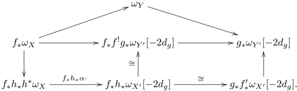
### Visual Description
## Mathematical Commutative Diagram: Relationships Between Sheaves and Pushforwards
### Overview
The image displays a commutative diagram from algebraic geometry or category theory, illustrating relationships between various sheaves (or modules) and the morphisms (maps) between them. The diagram is structured in three approximate rows, with arrows indicating mappings and isomorphisms. The notation involves pushforwards (subscript asterisk), pullbacks (superscript asterisk), dualizing complexes (ω), and shifts (brackets).
### Components/Axes
The diagram consists of seven distinct nodes (mathematical objects) connected by arrows. There are no traditional axes, legends, or numerical data. The elements are purely symbolic.
**Nodes (Objects):**
1. **Top Center:** `ω_Y`
2. **Middle Left:** `f_*ω_X`
3. **Middle Center:** `f_*f' g_*ω_Y'[-2d_g]`
4. **Middle Right:** `g_*ω_Y'[-2d_g]`
5. **Bottom Left:** `f_*h_*h^*ω_X`
6. **Bottom Center:** `f_*h_*ω_X'[-2d_g]`
7. **Bottom Right:** `g_*f'_*ω_X'[-2d_g]`
**Arrows (Morphisms) and Labels:**
* From `ω_Y` to `f_*ω_X`: Unlabeled arrow (down-left).
* From `ω_Y` to `g_*ω_Y'[-2d_g]`: Unlabeled arrow (down-right).
* From `f_*ω_X` to `f_*f' g_*ω_Y'[-2d_g]`: Horizontal arrow, labeled `f_*f'` above it.
* From `f_*f' g_*ω_Y'[-2d_g]` to `g_*ω_Y'[-2d_g]`: Horizontal arrow, unlabeled.
* From `f_*ω_X` to `f_*h_*h^*ω_X`: Vertical arrow (downward), unlabeled.
* From `f_*h_*h^*ω_X` to `f_*h_*ω_X'[-2d_g]`: Horizontal arrow, labeled `f_*h_*α·` above it.
* From `f_*h_*ω_X'[-2d_g]` to `f_*f' g_*ω_Y'[-2d_g]`: Vertical arrow (upward), labeled with an isomorphism symbol `≅`.
* From `f_*h_*ω_X'[-2d_g]` to `g_*f'_*ω_X'[-2d_g]`: Horizontal arrow, labeled with an isomorphism symbol `≅` above it.
* From `g_*f'_*ω_X'[-2d_g]` to `g_*ω_Y'[-2d_g]`: Vertical arrow (upward), unlabeled.
### Detailed Analysis
The diagram is a network of relationships. The primary flow appears to be from the top object `ω_Y` down to the middle row, and then further down to the bottom row, with connections also moving horizontally and back upward via isomorphisms.
* **Top Row:** `ω_Y` maps to two distinct pushforward sheaves in the middle row.
* **Middle Row:** A horizontal sequence connects `f_*ω_X` to `g_*ω_Y'[-2d_g]` via an intermediate object. The map from the left to the center is explicitly labeled as `f_*f'`.
* **Bottom Row:** A parallel horizontal sequence exists, starting from a pullback `h^*ω_X` pushed forward, mapping via `f_*h_*α·` to another object, which is then isomorphic (`≅`) to the final object in the row.
* **Vertical Connections:** There are downward maps from the middle-left to bottom-left and upward isomorphism maps from the bottom-center to middle-center and from bottom-right to middle-right. The unlabeled vertical arrow from `g_*f'_*ω_X'[-2d_g]` to `g_*ω_Y'[-2d_g]` completes a square on the right side.
### Key Observations
1. **Commutativity:** The diagram is commutative, meaning any two paths from one object to another yield the same result. This is the core property of such diagrams.
2. **Isomorphisms:** Two explicit isomorphisms (`≅`) are present, indicating that the objects `f_*h_*ω_X'[-2d_g]` and `g_*f'_*ω_X'[-2d_g]` are equivalent in a strong sense, and that `f_*h_*ω_X'[-2d_g]` is also isomorphic to `f_*f' g_*ω_Y'[-2d_g]`.
3. **Notation:** The notation is dense and specific:
* `f_*`, `g_*`, `h_*`: Pushforward (direct image) functors.
* `h^*`: Pullback (inverse image) functor.
* `ω_X`, `ω_Y`, `ω_X'`, `ω_Y'`: Likely dualizing sheaves or canonical bundles for spaces X, Y, X', Y'.
* `[-2d_g]`: A shift in the derived category, likely by -2 times the dimension `d_g`.
* `f'`, `f'_*`: Appear to be related morphisms or their pushforwards.
* `α·`: A specific morphism, possibly a section or a class.
### Interpretation
This diagram is a technical tool used to prove a theorem or illustrate a structural relationship in algebraic geometry, likely involving duality, pushforwards, and base change.
* **What it demonstrates:** It visually organizes a complex set of functorial relationships. The isomorphisms are the critical pieces of information, asserting that certain constructions (involving pullbacks and pushforwards along maps `h` and `f'`) are equivalent to more direct pushforwards.
* **Relationships:** The diagram connects the geometry of spaces linked by morphisms `f`, `g`, and `h`. It shows how the dualizing sheaf `ω_Y` on space Y can be related to dualizing sheaves on other spaces (X, X', Y') through various push-pull operations. The shift `[-2d_g]` suggests a context involving Gorenstein morphisms or relative canonical bundles.
* **Purpose:** A mathematician would use this diagram to track the composition of maps and verify that a desired property (commutativity) holds, which is often a step in a larger proof concerning sheaf cohomology, duality theorems, or the structure of moduli spaces. The diagram condenses what would be several paragraphs of algebraic equations into a single, spatially organized picture.
**Language Note:** The text in the image is entirely mathematical notation, which is a universal language in technical fields. No natural language (e.g., English, Chinese) is present.
</details>
/
/
/
/
.
We note that g ∗ ◦ f ∗ (here g ∗ denotes the Gysin pullback) is induced by applying R Γ( Y, -) to the path
$$\frac { 1 } { \sqrt { 2 } } + \frac { 1 } { \sqrt { 2 } } - \frac { 1 } { \sqrt { 2 } } = \frac { 1 } { \sqrt { 2 } }$$
$$\cdots$$
followed by natural transformation
(B.6)
and f ′ ∗ ◦ α · h ∗ (here h ∗ denotes the Gysin pullback) is induced by applying R Γ( Y, -) to the path
$$\sum _ { 2 d | g | = 0 } ^ { \infty } q w f l _ { 4 } w x [ - 2 d ] g \rightarrow q w g f l _ { 4 } w x [ - 2 d ] g$$
followed by the same transformation (B.6). Therefore we get the equation
$$g ^ { \prime } ( f _ { 1 } ) = f ^ { \prime } ( a \cdot h ^ { \prime } )$$
It remains to show that α = e ( E ). Recall that the 'restriction with supports' (ref. [CG, § 8.3.21]):
$$\therefore f ( x ) = \frac { 1 } { x ^ { 2 } + 1 }$$
which is defined by applying R Γ( Y ′ , -) to the map
$$w _ { r } = g w _ { r } \rightarrow g f _ { r } , f _ { w } = j$$
The map ω Y ′ → f ′ ∗ ω X ′ [ -2 d f ] factors into
$$\cdots - 1 ^ { n } ( n + 1 ) \frac { n ( n ) } { ( n + 1 ) } = 1 ( n + 1 ) - 2 ( n + 1 )$$
where c ′ is the natural transformation f ′∗ g ! ω Y → h ! f ∗ ω Y , which is given by applying (B.4) to Q Y and then applying Verdier duality functor D X ′ . Since c ′ is obtained by ˜ c by applying Verdier duality functor D X ′ , c ′ can also be identified with multiplication by α . Then we get an equation on maps between Borel-Moore homologies:
$$( B . 7 )$$
$$1 = 1 \div 1 + 1 \div 1 - 1 \div 1 + 1 \div 1$$
where f ′∗ : H BM ∗ ( Y ′ ) → H BM ∗ +2 d f ′ ( X ′ ) is the Gysin pullback.
Next we determine α by using the excess intersection formula in Chow homology and the cycle map. In Chow homology, we have [Ful, Thm. 6.3]:
$$( B . 8 )$$
$$1 = 4 \times 1 ^ { 2 } + 3 \times 1 ^ { 2 } - 4 \times 1 ^ { 2 }$$
where A ∗ ( -) is the Chow homology, f ! is the refined Gysin pullback, and f ′∗ is the Gysin pullback. It is known that the 'restriction with supports' is compatible with refined Gysin map [CG, § 8.3.21, § 2.6.21], i.e.
$$f ^ { \prime } B M o c y c = c y c o f ^ { \prime } C H :$$
where cyc: A ∗ → H BM 2 ∗ is the cycle map, and f ! BM , f ! CH denote Gysin pullbacks in BM and Chow homologies.
/
/
O
O
/
/
*
*
O
O
Since Gysin pullback is a special case of 'restriction with supports', we also have
$$f ^ { \prime } B M o c y c = c y c o f ^ { \prime } C H .$$
Let [ Y ′ ] CH ([ Y ′ ] BM ) be the fundamental cycle in BM homology (Chow homology) respectively, then
$$\begin{array}{ll}
\alpha \in [0, 2\pi) & \text{for } \alpha = 0 \\
\beta \in [0, 2\pi) & \text{for } \beta = \frac{\pi}{2} + k\pi, k \in \mathbb{Z}
\end{array}$$
Combining (B.7), (B.8), (B.9), (B.10), we obtain
$$= f _ { B M } o cyc ( Y ^ { \prime } ) c H = c yc o f _ { C H } ( Y ^ { \prime } ) c H = c yc o e$$
By Poincar´ e duality, the map H ∗ ( X ′ ) ∋ β ↦→ β · [ X ′ ] BM ∈ H BM 2 dim X ′ -∗ ( X ′ ) is an isomorphism; thus α = e ( E ). □
Remark B.2 (Equivariant version of Proposition B.1) . Suppose that the maps in the diagram (B.1) are equivariant morphisms between G -varieties, where G is an algebraic group, and assume that w is G -invariant. Then we claim that the equivariant version of Proposition B.1 holds, i.e.
$$g ^ { \prime } o f _ { i } = f _ { i } o c ( E ) ; h ^ { \prime }$$
where e G ( E ) is the G -equivariant Euler class of excess bundle E . To prove this claim, we consider the n -acyclic free G -variety M n as in the [BL, § 3.1] (see also [Dav1, § 2.4]), and for every G -variety V we define
$$V _ { 1 } = ( V \times M ) / G$$
Then we get the following Cartesian diagram of smooth connected varieties by applying ( -× M n ) /G to (B.1)
/
/
$$\begin{array}{ccc}
X_n & \xrightarrow[f_n]{} Y_n \\
X_n & \xrightarrow[g_n]{} Y_n \\
\end{array}$$
/
/
$$h _ { 0 } h _ { n } = f _ { n } o e l E _ { n } h _ { n }$$
$$E _ { 1 } = h _ { 1 } N _ { 1 } \cdot A _ { 1 } = F E \times M / G$$
is the excess bundle. It is known that there exists G -equivariant closed embedding M n ↪ → M n +1 . As in [Dav1, § 2.4], the equivariant critical cohomology is isomorphic to the inductive limit, i.e.
$$H _ { 2 } ( X , q _ { w } , p ) = \frac { F _ { m } } { n - 1 } H ( X , q _ { w } , p x , h )$$
where w n is the descent of w ◦ pr Y : Y × M n → C from Y × M n to Y n since w is G -invariant. And the functors between equivariant critical cohomologies are inductive limit of their finite counterparts, e.g.
$$f _ { n } = \lim _ { n \rightarrow \infty } f _ { n * } , g ^ { * } = \lim _ { n \rightarrow \infty } g _ { n }$$
Then (B.11) follows from the inductive limit of (B.12).
There is also a K -theoretic counterpart of Proposition B.1. Given diagram (B.1), we have proper pushforward
$$f : K ( X , w o f ) → K ( Y , w o g ),$$
$$: K ( X , w o f ) → K ( X ^ { \prime } , w o f o h ) .$$
Proposition B.3 (Excess intersection formula for critical K -theory) . Notations as above, we have
$$g ^ { \prime } ( f _ { 1 } ) = f _ { 0 } ( e _ { 1 } ) \cdot h _ { 1 }$$
where e K ( E ) := ∧ ∗ E ∨ is the K -theoretic Euler class of the excess bundle E .
By Proposition B.1 we have
$$g _ { n } o f _ { n + 1 } = f _ { n + 1 } o c ( E _ { n } ) \cdot h _ { n }$$
where and l.c.i. pullback
Proof. As in the proof of Proposition B.1, by the graph construction (B.2), we may assume g is a closed immersion. We have a commutative diagram of derived schemes
/
/
/
/
'
'
$$(B.13)$$
"
"
/
/
where the middle square is the homotopy pullback diagram. We denote Z der Y := Z der ( w ) ↪ → Y to be the derived zero locus of w and similarly Z der X := Z der ( w ◦ f ) ↪ → X , Z der Y ′ , Z der X ′ for the derived zero loci of pullback functions. They fit into commutative diagram of derived schemes (here we use same notations for maps as in the previous diagram):
/
/
/
/
(
(
$$\begin{array}{ll}
Z_{der} & \xrightarrow[i]{} Z_{X'} \\
& \xrightarrow[f'']{} Z_{Y'} \\
Z_{der} & \xrightarrow[h]{} Z_{X} \\
& \xrightarrow[g]{} Z_{Y}.
\end{array}$$
"
"
/
/
As the canonical map commutes with proper pushforward and Gysin pullback, we have commutative diagrams
/
/
/
/
$$\begin{array}{ll}
K(X,w \circ f) & K(Y',w \circ g), \\
\downarrow & \downarrow \\
f_{oek}(E_h^*,K(Z_der)) & f_{oek}(E_h^*,K(Z_der)), \\
\downarrow & \downarrow \\
K(X,w \circ f) & K(Y',w \circ g), \\
\end{array}$$
/
/
Then the claimed equality follows from Lemma B.4 below.
Lemma B.4. When g : Y ′ → Y above is a closed immersion, we have an equality of maps
$$\cdot \cdot K ( z x ) + K ( z y ) .$$
Proof. For a Noetherian derived scheme Z der with inclusion of its classical truncation
$$i \cdot Z = f ( z ^ { d e n } ) - z ^ { d e n } ,$$
$$\sum _ { p } ( - 1 ) ^ { p } ( n + 1 ) = [ 7 ] \in k ^ { ( p + 1 ) } .$$
Here by the nil-invariance of G -theory [Kh, Cor. 3.4], we have
$$i : K ( Z ) \cong K ( Z der ).$$
By base change in diagram (B.14), for any F ∈ D b coh ( Z der X ), we have equalities in K -theory:
$$( B.16 ) g ^ { \ast } f _ { F } = [ L _ { G } ^ { \ast }$$
Here t 0 ( f ′ ): Z X ′ := t 0 ( Z der X ′ ) → Z Y ′ := t 0 ( Z der Y ′ ) denotes the classical truncation of f ′ , and we have used the fact that classical truncation of i is an isomorphism, and we identify the G -theory of Z Y ′ and Z der Y ′ by (B.15).
Using diagrams (B.13), (B.14), we have
$$L _ { h } ^ { \prime } d e r s F = F \otimes L _ { O } ^ { \prime } x der .$$
Here in the first equality we omit h der ∗ since h der is an affine morphism so we can identify O Z der X ′ der with its direct image in Z der X and identify D b coh ( Z der X ′ der ) with D b coh ( h der ∗ O Z der X ′ der ) . In the second equality, we use the identification
$$O _ { x } + O _ { y } \xrightarrow [ ] { \Delta } O _ { z }$$
and we regard F ⊗ L O X O X ′ der as an object in D b coh ( h der ∗ O Z der X ′ der ) .
and F ∈ D b coh ( Z der ), we have
/
/
□
By a direct calculation, cohomology sheaves of O X ′ der (viewed as O X ′ -modules) are given by
$$( B . 1 8 )$$
Note also the spectral sequence
$$H ^ { 4 } ( F \otimes L _ { x } , H P ( O _ { x } \derset { der } ) ) =$$
where
$$\begin{aligned}
F \otimes L _ { x } H ^ { p } ( O _ { x } r d e r ) & \cong F \otimes L _ { h } ^ { p } \\
& \cong L _ { h } ^ { p } \\
& \cong L _ { h } ^ { p } E ^ { N } V.
\end{aligned}$$
Combining (B.16), (B.17), (B.18), (B.19), (B.20), we obtain
$$\begin{aligned}
g ^ { \ast } f _ { J } F &= \sum _ { n = g E Z } ^ { p _ { g E Z } } ( - 1 ) ^ { p + q } [ t _ { 0 } ( f ) ^ { a } L _ { h } ^ { j } F _ { g } ^ { b } \partial _ { x } ^ { c } z _ { X } ^ { d } E ^ { v } ] \\
&= \sum _ { n = g E Z } ^ { p _ { g E Z } } ( - 1 ) ^ { p + q } [ t _ { 0 } ( f ) ^ { a } L _ { h } ^ { j } F _ { g } ^ { b } \partial _ { x } ^ { c } z _ { X } ^ { d } E ^ { v } ] \\
&= f ^ { \ast } ( e _ { K } ( E ) , h ^ { \ast } ( F ) ),
\end{aligned}$$
where the third equality uses (B.15).
□
Remark B.5 (Equivariant version of Proposition B.3) . Suppose that the maps in the diagram (B.1) are equivariant morphisms between G -varieties, where G is an algebraic group, and assume that w is G -invariant. Then the equivariant version of Proposition B.3 holds, i.e.
$$g ^ { \prime } o f _ { * } = f _ { \prime } o c k ( E ) h ^ { \prime }$$
$$O H = F _ { 1 } O C _ { k } ^ { 2 - } ( E ) \cdot h ^ { \prime }$$
where e G K ( E ) := ∧ ∗ E ∨ is the G -equivariant K -theoretic Euler class of excess bundle E . This is because the spectral sequence in the proof of Proposition B.3 is G -equivariant if F is G -equivariant.
Remark B.6. In the case when X ′ is disconnected, the Propositions B.1 and B.3 and Remarks B.2 and B.5 still hold. In this case, e ( E ) · is the component-wise multiplication.
## Appendix C. A deformed dimensional reduction for critical cohomology
Let Y be a smooth and connected variety and f 1 , . . . , f n , ϕ are regular functions on Y . Consider the product and a function on it:
$$X = Y \times A ^ { n } , w := \phi + \sum _ { i = 1 } ^ { n } f ( x _ { i } )$$
where we omit the pullback of functions from Y to X , { x i } n i =1 are linear coordinates of A n . Denote the common zero locus of f 1 , . . . , f n by
$$z = z ( 6 3 ^ { n } ) .$$
Let π : X → Y be the projection, and j : S := π -1 ( Z ) ↪ → X the inclusion. We have natural morphism in D b ( Y ):
$$Let π : X → Y be the projection (C.1)$$
Theorem C.1. Assume that Z is smooth of codimension n in Y , then (C.1) is an isomorphism.
We first prove the case when n = 1.
Lemma C.2. Theorem C.1 is true when n = 1.
Proof. We write f := f 1 , w = ϕ + fx . Since π ∗ φ w ω X is supported on π (Crit( w )) ⊆ Z and π ∗ j ∗ φ w | S j ! ω X is obviously supported on Z , it is enough to show that for an arbitrary p ∈ Z , and an arbitrary analytic open neighbourhood W of p in Y , there exists an analytic open neighbourhood V of p in W such that the induced map between cohomologies
$$\begin{array}{ll}
H^*(\mathbf{V}, (\pi,\phi_{w}\mathbf{J}^{\dagger}\mathbf{X})) \downarrow \\
\end{array}$$
is an isomorphism. Equivalently by base change, we need to find V such that the pushforward map
$$\frac { H ^ { \ast } ( r ^ { - 1 } ( V ) , w _ { l } , r ^ { - 1 } ( v ) s _ { l } ) } { - H ^ { \ast } ( r ^ { - 1 } ( V ) , w _ { l } , r ^ { - 1 } ( v ) s _ { l } ) }$$
of critical cohomology is isomorphism.
By assumption, f : Y → A 1 is smooth in a Zariski open neighbourhood of Z . For any p ∈ Z , we can take an analytic open neighbourhood V of p in Y such that f | V : V → A 1 is of form
$$1 1 - 1 \times 1 = 0$$
where B is the open disk {| z | < ϵ } ⊆ A 1 for some 0 < ϵ ≪ 1. Then we have
$$V _ { 1 } Z = V _ { 6 } \times 1 0$$
$$W _ { 1 } = W _ { 2 } = 6 h v + 3 \Omega$$
Let ϕ 0 := ϕ | V ∩ Z = ϕ | V 0 ×{ 0 } and we regard it as a holomorphic function on V :
$$\phi _ { 0 } : V \rightarrow C ,$$
by pulling it back along the projection V → V 0 . Let
$$6 0 = 6 1 - 6 0$$
then we have δϕ | z =0 = 0 by definition. Therefore δϕ z : V → C is a well-defined holomorphic function.
Consider an isomorphism between complex manifolds:
$$\pi ^ { - 1 } ( V ) = V _ { 0 } \times B \times C _ { x } \approx V _ { 0 } \times B \times$$
In this new coordinate system, we have
$$\pi ^ { - 1 } ( V ) \cap S \cong V _ { 0 } \times \{ 0 \} \times C _ { 3 }$$
where we have separated the variables, where ϕ 0 depends only on coordinate v .
Combining Thom-Sebastiani isomorphism and a direct computation of H ∗ ( B × C ˜ x , z ˜ x ), we get
$$\begin{align}
H^*(\tau^{-1}(V), w_l,-v) & \cong H^*(V_0 \times B \times C_{\hat{\zeta}}, \phi_0 + z\bar{\zeta}) \\
& = H^*((V_0, \phi_0) \otimes H^B_M(\{z=0\} \times C_{\hat{\zeta}})) \\
& = H^*((V_0 \times \{z=0\} \times C_{\hat{\zeta}}, \phi_0)) \\
& = H^*(\tau^{-1}(V) \cap S_{w|_{l-1}(v)_n s}) .
\end{align}$$
Note that the isomorphism is induced by the pushforward map for critical cohomology. Therefore we are done. □
Proof of Theorem C.1. By assumption, the map
$$( 6 , \ldots , 1 ) : Y \rightarrow A ^ { n }$$
is smooth in a Zariski open neighbourhood of Z . Since π ∗ φ w ω X is supported on π (Crit( w )) ⊆ Z , we can replace Y by an open neighbourhood U of Z . By shrinking U , we may assume ( f 1 , . . . , f n ): U → A n is a smooth map.
Let Z ⩽ k := Z ( { f i } k i =1 ) be the zero locus, then we have inclusions of smooth varieties:
Let S ⩽ k := π -1 ( Z ⩽ k ) (where π : U × A n → U is projection) and set S ⩽ 0 := U × A n . Denote the closed immersions:
$$j _ { k } : S _ { < k } \rightarrow S _ { < k - 1 }$$
Then the natural morphism (C.1) factors into a sequence of natural morphisms:
$$\sum _ { i = 1 } ^ { n } j _ { k } \left ( w _ { l } s _ { i } \right ) ^ { j } w _ { l } x ^ { i } = \pi \int _ { k = 0 } ^ { n } w _ { l } s _ { i } <$$
and
where the intermediate arrow
$$\pi + j < k + \varphi w | s _ { k - 1 } j ^ { l } < k - 1 w X \rightarrow \pi$$
is induced by applying ( Z ⩽ k -1 ↪ → U ) ∗ to the natural map
$$( S _ { k - 1 } - \rightarrow Z _ { k - 1 } ) , i k + q w _ { s } ( s < k - 1 ) , j k + s c _ { k - 1 }$$
which is an isomorphism by Lemma C.2. Thus (C.1) is an isomorphism. □
## Appendix D. A dimensional reduction for critical K -theory
In the appendix, we prove a dimensional reduction for critical K -theories.
$$\begin{aligned}
W &= \sum _ { G \in U } G \textcircled { + } U . \\
\end{aligned}$$
Let π : W → V be the projection with a G -equivariant section s ∈ Γ( V, U ∨ ) of the dual bundle U ∨ := V × U ∨ → V of π . Let Z der ( s ) be the derived zero locus of s , which fits into the following diagram
/
/
$$\begin{array}{ccc}
\pi^{-1}(Z^der(s)) & \xrightarrow[l]{} W \\
\downarrow & \downarrow \\
Z^der(s) & \xrightarrow[r]{} V.
\end{array}$$
We define a G -invariant regular function
$$w = ( e _ { s } ) \cdot W → C ,$$
where e is the coordinate of the fiber of π .
Choose a stability condition such that the semistable locus equals the stable locus:
̸
$$W ^ { \prime } = W ^ { \prime } + 0 .$$
with unstable locus denoted by W u := W \ W ss .
By [Hal, Thm. 2.10], there is a semi-orthogonal decomposition (SOD):
$$/ g _ { i } ( W / G ) \geq 0 = D ^ { b } _ { i } ( W / G ).$$
Moreover, under the restriction to the open locus:
$$D ^ { \prime } M / / C D \rightarrow D ^ { \prime } M / / C A$$
$$G = D ^ { \prime } ( r ^ { \prime } / G ) .$$
This induces an SOD for matrix factorization categories of (D.2) (e.g. [P, Prop. 2.1]):
$$( D . 3 ) \left\{ M F ( w ^ { \prime } / G , w ) \right\} = M F ( G , w ) < 0 , G _ { w } M F ( w ^ { \prime } / G , ( W / G ), w ) ≥ 0$$
and an equivalence of categories:
we have an equivalence of categories:
O
O
O
O
/
/
/
/
$$The formula you've provided is not a standard mathematical or scientific notation. It appears to be a placeholder or a symbol used in specific contexts, such as in computer programming or certain types of data visualization. If you're referring to a particular formula or concept, could you please provide more context or clarify what you mean by "formula"? I'd be happy to help if I can!$$
$$\Phi : G _ { w } = N F ( \mu ^ { r } / G _ { w } )$$
Proposition D.2. The natural inclusion ι in (D.1) induces an isomorphism of K -groups:
$$=$$
$$( D 4 )$$
Proof. We have the following commutative diagram
/
/
$$\begin{array}{c}
K(G_w) & \xrightarrow[e]{} K(W/G_{1,w}) \\
& \xrightarrow[r]{} K(Z^der(s)/G) \\
& \xrightarrow[e]{} K((\pi^{-1}Z^der(s))/G) \\
& \xrightarrow[r]{} K((\pi^{-1}Z^der(s))^s/G) \\
& \xrightarrow[e]{} K(W^s/G_{1,w}) \\
\end{array}$$
/
/
/
/
/
/
*
*
O
O
where ι ∗ ◦ π ∗ is an isomorphism by the dimensional reduction result [Toda1, Prop. 2.5 & Cor. 3.13]. The commutativity of the diagram implies that the map (D.4) is surjective, and the composition
$$\frac { 1 } { s ^ { 2 } } K ( \pi - 1 z _ { der } ( s ) / G ) \rightarrow K ( \pi - 1 z _ { der }$$
is the isomorphism given by Φ. We are left to check the injectivity of the map (D.4), which is further reduced to check the surjectivity of the composition
$$z ^ { \prime } ( s ) / G ) \rightarrow K ( r ^ { - 1 } z ^ { \prime } ( s ) / G ).$$
By the SOD (D.3), it is enough to check that any P · ∈ MF [ W u /G ] ([ W/G ] , w ) goes to zero under the composition
$$\cdots \Rightarrow K ( ( \pi ^ { - 1 } z _ { der } ( s ) / G ) .$$
Here that the first map ( ι ∗ ) -1 of (D.5) is given by the tensor product
$$[ P ^ { \ast } \circ Kos ( τ , s ) ] e$$
.
.
with the Koszul factorization
$$\begin{aligned}
K O S ( τ , s ) := \left( \Lambda ^ { odd } _ { π } U V \right) .
\end{aligned}$$
n
n
where τ is the tautological section of π ∗ U → U . By definition, P · is acyclic when restricted to the stable locus; therefore P · and [ P · ⊗ Kos( τ, s ) ∨ ] go to zero under the map (D.5). □
Remark D.3. One can extend the above result to the equivariant setting in the presence of a torus action.
## Appendix E. Proof of Proposition 9.9
Our strategy of proving Proposition 9.9 is to deduce it from the axiom (iii) of the abelian stable envelope (Definition 3.10). The difficulty is that the nonabelian stable envelope is constructed from an abelian stable envelope with respect to a C ∗ -action which is in general different from the σ i that appears in the KN stratification. We resolve this issue by showing that the Stab s + that appears in the construction of ˜ Ψ s K is essentially the same as the stable envelope with respect to the two dimensional torus C ∗ × C ∗ σ i (see Lemma E.6). The main geometric fact that we use in the proof is to identify the KN strata S i with an open subset in a C ∗ × C ∗ σ i -attracting set (Lemma E.5). We deduce it from a preliminary result that identifies S i with an open subset in a C ∗ -attracting set (Proposition E.3).
E.1. KN strata of the unstable locus. We give an explicit description of the KN strata. We first define
$$\sum _ { i = 1 } ^ { n } ( u \in N ^ { \theta } _ { 0 } , u _ { j } < v _ { j } , \forall i \in Q _ { 0 } ^ { \theta } _ { 0 } )$$
together with the partial order ≤ on Σ given by u ≤ u ′ if and only if u i ⩽ u ′ i for all i ∈ Q 0 . For u ∈ Σ, we define cocharacter σ ( u ) of G by
$$( E 2 )$$
where ω i, u i is the u i -th fundamental cocharacter of GL( v i ). It is straightforward to see that if u , u ′ ∈ Σ then u ≤ u ′ implies µ ( σ ( u )) ≤ µ ( σ ( u ′ )). We keep using the notation
$$d ^ { r } = ( d + v , d ) .$$
Remark E.1. For u ∈ Σ, we associate to it the following connected component in M θ ( v , d v ) C ∗ :
$$F _ { u } = M _ { 0 } ( u , 0 ) ^ { \prime } \times M _ { 0 } ( v - u , d ) .$$
Here M θ ( u , 0 v ) is the quiver variety given by the GIT quotient
$$C u _ { 4 } ) = ( \frac { M _ { 0 } ( u , q ^ { y } ) } { i e Q _ { 0 } } ) = ( \frac { M _ { 0 } ( u , q ^ { y } ) } { i e Q _ { 0 } } )$$
We note that F u is nonempty if and only if R ( v -u , d ) θ -ss is nonempty, because M θ ( u , 0 v
Let us also define
$$\sum _ { j = 1 } ^ { n } \{ u \in \Sigma : R ( v - u , d ) ^ { 0 , s s } \neq 0 \}$$
) is always nonempty.
̸
̸
then F u = ∅ ⇐⇒ u ∈ Σ θ . Consider the ample line bundle L θ := ⊗ i ∈ Q 0 (det V i ) -θ i on M θ ( v , d v ), where V i is the tautological vector bundle corresponding to i -th node. L θ induces the ample partial order ≤ on Fix C ∗ ( M θ ( v , d v )) as in the Remark 3.9. Then for u , u ′ ∈ Σ θ , we have the following implication
$$1 s ^ { \prime } d = R _ { 0 } S _ { 0 }$$
Let us refine ≤ to a total order on Σ such that its restriction to Σ θ refines the ample partial order.
Lemma E.2. We have the decomposition
$$M _ { 0 } ( v , d ^ { \prime } ) = U A t t _ { + } ( F _ { u } ).$$
Proof. Since the C ∗ -weights in the ring C [ R ( v , d v )] G of invariant functions are nonpositive, the C ∗ -action on the affine quotient M ′ 0 ( v , d v ) is attracting. Since the canonical map M θ ( v , d v ) →M ′ 0 ( v , d v ) is proper, we obtain the decomposition
$$M _ { 0 } ( v , d ^ { V } ) = U _ { F ( F _ { c } ) } A t t r + ( F _ { c } )$$
We note that any F ∈ Fix C ∗ ( M θ ( v , d v )) is of form F u for some u ∈ Σ θ and vice versa, then the lemma follows. □
Proposition E.3. Up to G -conjugation and a positive scalar multiple, the cocharacters that appear in KN stratification of R ( v , d ) θ -u are given by cocharacters in the set
̸
$$( E 5 )$$
For the above σ ( u ), the associated strata S σ ( u ) is given by
$$S _ { n } = A _ { 1 } + A _ { 2 } + \cdots + A _ { n } ( n > 0 )$$
where F u is the connected component in M θ ( v , d v ) C ∗ given by (E.3).
Moreover, if u ∈ Σ θ , then we have if u / ∈ Σ θ , then we have
$$\frac { S _ { 0 } ( u ) } { S _ { 0 } ( u ) \leq U } S _ { 0 } ( u )$$
$$R ( x , d ) ^ { 0 } ( u ) \leq U S _ { 0 } ( u )$$
Proof. Using Cauchy-Schwarz inequality 21 , one can see that the invariant µ ( σ ) is maximized by taking σ = σ ( v ), up to G -conjugation and a positive scalar multiple. Note that σ ( v ) is nothing but the C ∗ ⊆ G that we previously considered to construct ˜ Ψ s K . In particular, the image of σ ( v ) is in the center of G , so Attr σ ( v ) ( R ( v , d ) σ ( v ) ) is invariant under the G -action. Moreover R ( v , d ) σ ( v ) ∼ = R ( v , 0 ) × R ( 0 , d ), and obviously we have R ( 0 , d ) = R ( 0 , d ) θ -ss = pt. It follows from Lemma E.4 below that the minimal KN stratum is given by
$$S _ { v } ( v ) = Attr _ { v } ( R ( v , d ) ^ { a } v$$
By minimality, we have S σ ( v ) = S σ ( v ) .
To proceed, we introduce a conjugation-invariant map:
$$\sum _ { i = 1 } ^ { n } \cochar ( G ) \rightarrow X _ { 2 } ,$$
where λ ′ is G -conjugate to λ and λ ′ i = diag( λ ′ i,j ) v i j =1 is a cocharacter of GL( v i ) in the standard basis. Then it is easy to see that if λ ∈ cochar( G ) and u = Supp ( λ ), then
$$( E.6 )$$
Moreover, the Cauchy-Schwarz inequality shows that the numerical invariant
$$u ( X ) = \frac { ( λ , θ ) } { | λ | } \vert Supp ( λ ) = u$$
21 Namely, we have ( ∑ i ∈ Q 0 | θ i | tr( σ 2 i ) )( ∑ i ∈ Q 0 | θ i | ) ⩾ ( ∑ i ∈ Q 0 | θ i | ∑ v i j =1 | σ i,j | ) 2 ⩾ ( σ, θ ) 2 , which implies that | µ ( σ ) | ⩽ √∑ i ∈ Q 0 | θ i | . Moreover the equality holds if and only if σ i,j = σ i ′ ,j ′ for all possible i, i ′ , j, j ′ . Taking sign into consideration, we see that the maximal value of µ ( σ ) is achieved if and only if σ i,j = -1 for all possible i, j , up to G -conjugation and a positive scalar multiple.
is maximized by λ = σ ( u ) up to a positive scalar multiple and G -conjugation. Then we claim that any σ i that appears in the KN stratification, up to a positive scalar multiple and G -conjugation, belongs to the set
̸
$$( m + 1 , n - 2 ) = ( 0 ,$$
In fact, R ( v , d ) σ i is not contained in previously defined strata by the construction of KN strata. Let u i := Supp ( σ i ), then (E.6) implies that R ( v , d ) σ ( u i ) is not contained in previously defined strata. Since σ i maximize µ ( σ ) among those σ such that R ( v , d ) σ is not contained in previously defined strata, we must have σ i = σ ( u i ) up to a positive scalar multiple and G -conjugation.
It remains to show that
- (1) σ ( u ) appears in KN stratification if and only if u ∈ Σ θ ,
- (2) if u ∈ Σ θ , then S σ ( u ) = Attr + ( F u ) ∩ ˚ M θ ( v , d v ),
- (3) if u ∈ Σ θ , then we have
- (4) if u / ∈ Σ θ , then we have
By induction hypothesis, we have
$$( ) \leq u ^ { G } A t t _ { r } ( u ^ { R } ( v , d ) ^ { a } u ^ { u } )$$
Here we have used the fact that S σ ( u ′′ ) is G -invariant so it is invariant under taking attracting set and G -action. It follows that R ( v , d ) σ ( u ) ⊆ X u . Thus σ ( u ) does not appear in KN stratification. This proves (4) and part of (1).
Suppose that u ∈ Σ θ , then according to Lemma E.4 we have
$$( ) ^ { 0 } s s = Attr _ { ( F u ) } \phi M o ( v , d ^ { 1 } ).$$
̸
In particular, R ( v , d ) σ ( u ) ∩ ( Attr + ( F u ) ∩ ˚ M θ ( v , d v ) ) = ∅ . We note that by induction hypothesis, we have
$$x _ { u } = ( u ^ { \prime } \sum _ { v , d ^ { \prime } y } u ^ { \prime } ) + ( F _ { u } ) \eta M _ { 0 } ( v , d ^ { \prime } y ) .$$
Since F u ∩ F u ′ = ∅ if u = u ′ , we deduce that R ( u , 0 ) × R ( v -u , d ) θ -ss is an nonempty open subset in R ( v , d ) σ ( u ) , and ( R ( u , 0 ) × R ( v -u , d ) θ -ss ) ∩ X u = ∅ . Then σ ( u ) appears in KN stratification because σ ( u ) maximizes µ ( σ ) among those σ ∈ { σ ( u ′ ) : u ′ ∈ Σ , u ′ ≤ u } . This finishes the proof of (1).
̸
Denote S ′ σ ( u ) := Attr + ( F u ) ∩ ˚ M θ ( v , d v ), then we have
$$( E . 7 ) S _ { σ ( u ) } = G \cdot A t t r _ { σ ( u ) }$$
S ′ σ ( u ) is dense in S σ ( u ) because R ( u , 0 ) × R ( v -u , d ) θ -ss is open and dense in R ( v , d ) σ ( u ) . Therefore we have
$$\sum _ { o ( u ) } \int S ^ { ' } _ { o ( u ) } = S ^ { ' } _ { o ( u ) }$$
$$\overline { S _ { 0 } ( u ) } \cap S _ { 0 } ( u ) = U _ { u } S _ { 0 } ( u )$$
$$R ( x , d ) ^ { 0 } ( u ) \leq U S _ { 0 } ( u )$$
̸
We prove the above four statements by induction downwards along the total order ≤ on Σ defined in Remark E.1. The maximal case u = v has been proven previously. Let u ∈ Σ , u = 0 . Suppose that (1)-(4) have been proven for all u ′ ∈ Σ such that u ′ > u . Consider the following union of KN strata
$$x _ { u } = U S _ { o ( u ) }$$
We claim that X u is closed. In fact, by the induction hypothesis, we have S σ ( u ′ ) ⊆ X u for all u ′ ∈ Σ θ , u ′ > u . Then X u = ⋃ u ′ ∈ Σ θ , u ′ > u S σ ( u ′ ) is closed.
Suppose that u / ∈ Σ θ , then according to Lemma E.4 we have the inclusion
$$R ( v , d ) ^ { o } ( u ) \subset U G . A _ { u } > u$$
It follows that
$$( E . 8 )$$
The inclusions (E.7) and (E.8) imply that S σ ( u ) = S ′ σ ( u ) . This proves (2). Finally (3) follows from (2) because we just show that S σ ( u ) \ S ′ σ ( u ) ⊆ X u . This finishes the induction step. □
Let u ∈ Σ be a nonzero element. Note that
$$R _ { 1 } = R _ { 2 } ^ { \prime } = R _ { 3 } ( 1 ) \times R _ { 4 } - R _ { 5 } - R _ { 6 }$$
In view of the isomorphism (9.3), R ( u , 0 ) × R ( v -u , d ) θ -ss is naturally identified with a (possibly empty) locally-closed subvariety of ˚ M θ ( v , d v ).
Lemma E.4. Let u ∈ Σ be a nonzero element.
- If u / ∈ Σ θ , then we have
$$R ( v , d ) ^ { o } ( u ) \subset U G . A _ { u } > u$$
$$\begin{align}
\text{by definition of } \leq \subseteq & = \left\{ \begin{array}{l} F^{e}F_{X,C}(\mathcal{M}_0(v,d^Y)) \\ F^{e}F_{X,C}(\mathcal{M}_0(v,d^Y)) \end{array} \right.
\end{align}
since \( \leq \) refines \( \subseteq \) & = \left\{ \begin{array}{l} U \\ U \end{array} \right.
by Remark E.1 & = \left\{ \begin{array}{l} U \\ U \text{ Atttr}_+(F^eF_{X,C}(\mathcal{M}_0(v,d^Y))) \\ u^{e}\varepsilon_{\theta,u}^{\text{Atttr}_+}(F^eF_{X,C}(\mathcal{M}_0(v,d^Y))) \end{array} \right.
\end{align}$$
- If u ∈ Σ θ , then we have
$$( ) ^ { 0 } s s = Attr _ { ( F u ) } \phi M o ( v , d ^ { 1 } ),$$
in particular, the right-hand-side is nonempty.
Proof. If u / ∈ Σ θ , then by definition of Σ θ every quiver representation in R ( v -u , d ) is θ -unstable. Let ( H i ) i ∈ Q 0 ∈ R ( v -u , d ) be a quiver representation, and take its Harder-Narasimhan filtration
$$1 - 4 / ( 1 + 4 ) = 1 - 4 / 5 = 1 - 0.8 = 0.2$$
with respect to the θ -stability, i.e. H ( i +1) /H ( i ) is θ -semistable for all possible i and its θ -slope decreases strictly as i increases. By assumption H (1) = H , so the θ -slope of H (1) is greater than the the θ -slope of H , and the latter is zero. Since we assume θ i < 0 for all i ∈ Q 0 , this implies that H (1) contains the framing node ∞ in the Crawley-Boevey quiver associated with ( Q, d ), i.e. H (1) ∈ R ( v -u ′ , d ) θ -ss for some u ′ > u . It follows that H/H (1) ∈ R ( u ′ -u , 0 ). By decomposing H into an extension of H/H (1) by H (1) , we see that
$$( R ( v - u , d ) ^ { 2 } g ^ { \prime } ( u ^ { \prime } - u ) ,$$
where G v -u = ∏ i ∈ Q 0 GL( v i -u i ) is the gauge group. Since H is arbitrary, we have
$$\rho ( v - u ) ( R ( V - u , d ) ^ { o } ( u - u ) ) .$$
Since R ( v , d ) σ ( u ) ∼ = R ( u , 0 ) × R ( v -u , d ), it follows that
$$R ( v , d ) ^ { o } ( u ) \subset U G . A _ { u } > u$$
If u ∈ Σ θ , then it is enough to show that
$$u , d ) ^ { 0 - ss } \subseteq Attr _ { u } ( F _ { u } )$$
and
$$( E.10 )$$
̸
$$d$$
In view of the isomorphism (9.3), R ( u , 0 ) × R ( v -u , d ) θ -ss is isomorphic to the moduli space of representations of the following quiver:
O
O
;
;
O
O
$$\begin{array}{c}
C u _ { 4 } ^ { 1 } \\
\end{array}
\xrightarrow[r]{} C v _ { 7 - u _ { 4 } } ^ { 1 } \\
\downarrow{} A _ { 1 } ^ { i } B _ { 1 } ^ { j } \\
\end{array}$$
where it is required that I ′ i and I ′′ i are isomorphisms for all i ∈ Q 0 , and the RHS part is θ -semistable after forgetting I ′′ . Taking attracting set with respect to σ ( u ) action amounts to taking an extension of the LHS of (E.11) by the RHS of (E.11), i.e. Attr σ ( u ) ( R ( u , 0 ) × R ( v -u , d ) θ -ss ) is the moduli space of the following quiver
O
O
/
/
;
;
O
O
$$\begin{array}{c}
( E.12 ) \\
\end{array}$$
)
)
with the same conditions as above. Here dotted lines are new linear maps that appear in extensions between representations. Similar argument shows that Attr + ( F u ) is the moduli space of the quiver
O
O
/
/
O
O
$$\begin{array}{c}
( E , 1 3 ) \\
\hline
M _ { i } & \rightarrow N _ { i } \\
C ^ { V _ { i } } & \xrightarrow[ A _ { i } ] B _ { i } \\
D _ { i } & \xrightarrow[ A _ { i } ] B _ { i } \\
\end{array}$$
'
'
with the condition that rigid lines parts are θ -semistable. Writing C v i = C u i ⊕ C v i -u i and comparing stability conditions between (E.12) and (E.13), we obtain (E.9).
To prove (E.10), we notice that Attr + ( F u ) ∩ ˚ M θ ( v , d v ) is the moduli space of the quiver (E.13) with the condition that rigid lines parts are θ -semistable, and the
O
<details>
<summary>Image 15 Details</summary>
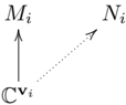
### Visual Description
## Diagram: Directed Relationship Graph with Indexed Variables
### Overview
The image displays a simple directed graph or flow diagram illustrating relationships between three mathematical variables. The diagram uses standard mathematical notation with subscripts and directional arrows to indicate connections or transformations.
### Components/Axes
The diagram consists of three labeled nodes and two directed edges (arrows):
1. **Nodes (Variables):**
* **C_i**: Located at the bottom-left of the diagram. The label is the capital letter "C" with a subscript "i".
* **M_i**: Located directly above `C_i`. The label is the capital letter "M" with a subscript "i".
* **N_i**: Located to the right of `M_i`. The label is the capital letter "N" with a subscript "i".
2. **Edges (Relationships):**
* A **solid, upward-pointing arrow** originates from `C_i` and points directly to `M_i`.
* A **dashed, rightward-pointing arrow** originates from `C_i` and points diagonally upward to `N_i`.
### Detailed Analysis
* **Spatial Layout:** The diagram is arranged in a rough "L" shape. `C_i` is the foundational node at the bottom-left. `M_i` is positioned vertically above it, and `N_i` is positioned horizontally to the right of `M_i`, creating a right angle.
* **Arrow Types:** The use of two distinct arrow styles (solid vs. dashed) is a critical visual cue, implying a difference in the nature of the relationships being depicted.
* **Notation:** The consistent use of the subscript "i" on all three variables (`C_i`, `M_i`, `N_i`) strongly suggests these are indexed elements of a series or set (e.g., for i = 1, 2, 3...).
### Key Observations
1. **Asymmetric Relationships:** The diagram shows that `C_i` has a direct relationship with both `M_i` and `N_i`, but there is no direct arrow shown between `M_i` and `N_i`.
2. **Visual Hierarchy:** The solid arrow to `M_i` is more visually prominent than the dashed arrow to `N_i`, which may imply a stronger, more direct, or primary relationship.
3. **Indexed Consistency:** All variables share the same subscript `i`, indicating they belong to the same indexed instance or iteration of a model.
### Interpretation
This diagram is a conceptual model, likely from mathematics, theoretical computer science, or systems theory. It visually encodes a specific logical or functional relationship.
* **What it Suggests:** The model proposes that a base element or condition `C_i` gives rise to two distinct outcomes or components, `M_i` and `N_i`. The solid arrow to `M_i` suggests a direct, deterministic, or primary transformation. The dashed arrow to `N_i` suggests a secondary, conditional, probabilistic, or derived relationship.
* **Relationship Between Elements:** `C_i` is the common antecedent or source. `M_i` and `N_i` are parallel consequences or outputs from `C_i`, but they are generated through different mechanisms (as indicated by the arrow styles). The lack of a connecting arrow between `M_i` and `N_i` implies they may be independent of each other once generated from `C_i`.
* **Notable Implications:** The subscript "i" is crucial. It indicates this is not a single relationship but a template for a family of relationships. For each index `i`, there exists a triplet (`C_i`, `M_i`, `N_i`) connected in this specific way. This is common in models describing iterative processes, indexed data structures, or parameterized systems. The diagram's power lies in its abstraction; without additional context, `C`, `M`, and `N` could represent any concepts—causes and effects, input and output states, variables in an equation, or components in a logical proof. The arrow styles are the primary carriers of specific relational meaning.
</details>
O
=
=
part induces isomorphisms C v i ∼ = M i ⊕ N i . Given a representation of the quiver (E.13) with the above conditions satisfied, let K i := ker( C v i → M i ) and P i := ker( C v i → N i ). Then by the assumption we have C v i = P i ⊕ K i , and the induced maps P i → M i , K i → N i are isomorphisms. We rewrite the quiver diagram (E.13) with C v i replaced by P i ⊕ K i , and obtain the following quiver
O
O
/
/
>
>
O
O
$$\begin{array}{c}
( E . 1 4 ) \\
\end{array}$$
(
(
The stability conditions in (E.14) are such that I ′ i , I ′′ i are isomorphisms and the part formed by N i , D i and arrows among them is θ -semistable. Up to a choice of isomorphisms P i ∼ = C u i , K i ∼ = C v i -u i (which can be accomplished by a G ′ action), (E.14) is identified with a special case of (E.12). This proves (E.10). □
E.2. Finish the proof. We have given an explicit description of the KN stratification in terms of attracting sets of M θ ( v , d v ) in Proposition E.3. For our purpose, we shall need the following enhancement of Proposition E.3.
Let A = ( C ∗ ) 2 act on M θ ( v , d v ) via ( σ ( u ) , σ ( v )) : C ∗ × C ∗ → G ′ . Let ( t 1 , t 2 ) ∈ Lie( A ) R be the coordinate, then it is easy to see that the root hyperplanes are t 1 = 0, t 2 = 0, and t 1 + t 2 = 0. Define C to be the chamber t 1 > 0 , t 2 > 0. Write the σ ( u )-fixed components of F u as
$$F _ { u } ^ { \prime } ( u ) = \left | F _ { u , u } \right | _ { w ( 2 , u \leq u ) }$$
Then it is straightforward to see that
$$M _ { 0 } ( x , d ^ { n } ) = \left | F _ { u v } \right .$$
Lemma E.5. If u ∈ Σ θ , then we have
$$\Attr _ { ( F u ) } \cap M _ { 0 } ^ { ( v , d Y ) } =$$
In particular, S σ ( u ) = Attr C ( F u , u ) ∩ ˚ M θ ( v , d v ).
Proof. The '+' chamber is given by t 1 = 0 , t 2 > 0, which is on the boundary of C . Let C / + be the chamber t 1 > 0 of the torus A / C ∗ σ ( v ) action on F u , then the same argument as Lemma E.2 shows that F u = ⋃ u ′ ∈ Σ , u ′ ≤ u Attr C / + ( F u , u ′ ). Since for any u ′ ∈ Σ , u ′ ≤ u we have Attr C ( F u , u ′ ) = Attr + (Attr C / + ( F u , u ′ )), it follows that we have decomposition
$$\frac { A t t _ { 1 } + ( F _ { 0 } ) } { u ( E _ { 2 } , k _ { s } ) } = U \frac { A t t _ { 2 } } { u ( E _ { 1 } , k _ { s } ) }$$
Then the lemma follows from the following claim: if u ′ < u then Attr C ( F u , u ′ ) ∩ ˚ M θ ( v , d v ) = ∅ . In fact, Attr C ( F u , u ′ ) is the moduli space of quiver representations V ∈ M θ ( v , d v ) which admits filtration by subrepresentations V (1) ⊆ V (2) ⊆ V such that
$$v ( 2 ) / v ( 1 ) \in M _ { 0 } ( u - u ', d ^ { 2 } ) ,$$
The linear maps { I i } i ∈ Q 0 in (9.2) respect the filtration, in particular it is isomorphism if and only if it is isomorphism after passing to associated graded vector spaces. If u ′ < u , then there exists i ∈ Q 0 such that the source and the target of I i have different ranks, so I i can not be isomorphism. This proves the claim. □
Lemma E.6. There exists K -theoretic stable envelope Stab s C for ( M θ ( v , d v ) , w ′ , G ′ σ ( u ) × T , A , C , s ), and we have
$$\begin{aligned}
( E . 1 5 ) & = \frac { 1 } { 2 } \int _ { - \infty } ^ { + \infty } e ^ { i x } G ( t , u ) d t \\
& = \frac { 1 } { 2 } \int _ { - \infty } ^ { + \infty } e ^ { i x } G ( t , u ) o Stab ^ { 3 } _ { + } .
\end{aligned}$$
Proof. Consider the vector bundle E = ⊕ i ∈ Q 0 Hom( V i , V ′ i ) on M θ ( v , v + d ). It is easy to see that E is repelling with respect to the chamber C , and Tot( E ) ∼ = M θ ( v , v + d ) is a symmetric quiver variety. We note that the C ∗ -fixed component M θ ( v , d ) is fixed by bigger torus A . Moreover, the restriction of E to the A -fixed component M θ ( v , d ) is moving. Then the existence of Stab s C follows from Lemma 8.4. The equation (E.15) follows from Remark 8.5 and the commutative diagram (3.14). □
Now we have all the ingredients of proving Proposition 9.9.
By Lemma E.6, Proposition E.3 and Lemma E.5, we have
$$\gamma ( u ) \Psi ^ { s } _ { K } ( r ) = S t a b e ^ { s } ( 1 \otimes$$
By the degree axiom of stable envelope, we have
$$\begin{aligned}
& \text{det } A = \text{det } ( N _ { F _ { u , a } / M _ { v , d } } ) + \text{weight } A \\
& = \text{det } ( N _ { S _ { u } / R ( v , d ) } ) + \text{weight } A \\
& = \text{det } ( N _ { F _ { u , a } / M _ { v , d } } ) ^ { 1 / 2 } \times ( det N _ { F _ { u , a } / M _ { v , d } } ) ^ { 1 / 2 } \\
& = ( det N _ { F _ { u , a } / M _ { v , d } } ) ^ { 3 / 2 } \times ( det S _ { i } / R ( v , d ) ) ^ { 1 / 2 } .
\end{aligned}$$
Projection of the above inclusion of polytopes to the cocharacter lattice of subtorus C ∗ σ ( u ) gives rise to the desired degree bound:
$$\sum _ { i = 1 } ^ { \infty } ( N _ { S _ { o } ( w ) / R ( v , d ) } ) + weight _ { c ( u ) } ( e _ { K } ( G ( N _ { S _ { o } ( w ) / R ( v , d ) } ) )$$
Since s is generic, the above inclusion must be strict by Remark (3.12). Finally, the uniqueness can be proven in the same way as Proposition 3.16, and we omit the details.
## Appendix F. Proof of Lemma 9.16
We prove here the K -theory version (9.31) (the proof of the cohomology version (9.30) is similar and we leave readers to check details). Recall that Ψ s K is by definition the dimensional reduction of the nonabelian stable envelope Ψ s K for the symmetric quiver variety M θ ( r , e ) associated with the tripled quiver ˜ Γ with potential w = ∑ i ∈ Γ 0 tr( ε i µ i ), where { ε i } i ∈ Γ 0 is the set of edge loops and µ : R (Γ , r , e ) → g ∨ is the moment map.
We claim that it is enough to show that
$$\sin ( \theta + 2 \pi ) = - \cos ( \theta + \pi )$$
satisfies the degree condition
$$i ^ { \prime } _ { v ( u ) } c a n ( l x \circ O ^ { z } _ { i r } ( p ) ) \subseteq \frac { 1 } { 2 } de g _ { g o ( u ) } e ^ { i } k ( R T )$$
̸
the following (see (E.1) and (E.4)):
̸
for all cocharacters in { σ ( u ) : u ∈ Σ θ , u = 0 } with σ ( u ) defined in (E.2) and Σ θ Σ θ := { u ∈ N Γ 0 : u i ⩽ r i , ∀ i ∈ Γ 0 , and M θ ( r -u , e ) = ∅} .
In (F.1), i σ ( u ) : [ Z ∗ σ ( u ) /G σ ( u ) ] → M ( r , e ) = [ R ( ˜ Γ , r , e ) /G ] is the natural map (4.23), and we define Z ( µ ) ↪ → M ( r , e ) by the following Cartesian diagrams
$$( F . 2 )$$
/
/
$$\begin{array}{ll}
z(r,e) &=& \left[ \mu^{-1}(0)/G \right] \\
\downarrow & \downarrow & \downarrow \\
g^*(r,e) &=& \left[ R(\overline{T},r,e)/G \right] \\
\downarrow & \downarrow & \downarrow \\
\left[ 0/G \right] &=& g^*(r,e).
\end{array}$$
/
/
where 0 is the inclusion of zero, µ is the moment map of double quiver representation and the right vertical map in the upper square is the vector bundle map by forgetting loops. We endow Z ( µ ) with virtual structure sheaf
$$O ^ { \prime } _ { 2 i j } = O ( n ( r ) ,$$
where 0 ! is the refined Gysin pullback. The canonical map (2.18) can: K T ( Z ( w )) → K T ( M ( r , e ) , w ) is the proper pushforward and note that Z ( µ ) ⊆ Z ( w ).
Let δ K be the dimensional reduction map given by pullback followed by the pushforward (see (6.7), also (9.18) in the stacky case). By base change on (F.2), we know
$$\delta k ( x \otimes O ^ { i } _ { i r , o } ) = c a n ( x \otimes O ^ { i } _ { i r , p } ) .$$
Restricting to the stable locus, we have
Since s is generic, the inclusion in (F.1) must be strict if it holds. Combining with the characterization of nonabelian stable envelopes (Proposition 9.9), (F.1) implies that
$$\begin{aligned}
& \text { can } ( l \otimes O ^ { n } _ { z } ( u _ { i } ) ) = \Psi ^ { k } _ { 0 } \delta _ { k } ( L _ { X } ) \\
& \end{aligned}$$
Eqn. (9.19), (F.3) and (F.4) imply that
$$\psi _ { k } ( [ L _ { x } ] ) = \delta ^ { r } _ { K } o \psi _ { K } o$$
which is (9.31). This proves the claim. We are therefore left to show (F.1).
Now suppose that u ∈ Σ θ \ { 0 } . Since the canonical map commutes with Gysin pullbacks, we have
The naturality of refined Gysin pullbacks implies that
$$i _ { 0 } ( u ) ^ { \sigma } O _ { m } ( r , e ) = i _ { 0 } ( u ) ^ { 1 } O _ { m } ( r , e ) = 0$$
Note that there is a commutative diagram
$$\begin{array}{ll}
Z^*_{o(u)} & \xrightarrow[C]{} R(\overline{T},r,e) \\
& \downarrow[u]{} g^V_o(u)\xrightarrow[C]{} g^V,
\end{array}$$
/
/
with horizontal arrows being natural closed immersion and vertical arrows being the composition of the right vertical maps in (F.2) (by abuse of notations, we denote it also as µ ). Then we have
$$\begin{aligned}
0 ^ { \prime } O _ { z _ { a } ( w ) } / G ^ { \prime } ( u ) = ( 1 0 ) / G ^ { \prime } ( u ) = e ^ { i k R } ( t )$$
/
/
/
/
To summarize, we arrive at
$$\begin{aligned}
i ^ { \prime } ( u ) \, \text { can } \left( [ x \otimes O _ { z _ { 2 } ( u ) } ] \right) = x \cdot e ^ { i \theta ( u ) } \\
&= \left[ \frac{1}{g} \dot{\gamma}( u ) - \gamma'( u ) \right] \, \text { moving } \left( [ 0 / G ^ { \prime } _ { z _ { 2 } ( u ) } ] \right) \rightarrow \left[ g V ^ { \prime } _ { K } \left( \frac{g}{g ^ { \prime } _ { z _ { 2 } ( u ) }} \right) \right]
\end{aligned}$$
Note that
$$\deg _ { S } ( u ) \left [ 0 / C ^ { G } ( w ) \right ] ^ { - 1 } O _ { Z } ^ { a } ( w ) / C ^ { G } ( w ) = 0 .$$
Since the map can: K T × G σ ( u ) ( Z ( w ) ∩ Z ∗ σ ( u ) ) → K T × G σ ( u ) ( Z ∗ σ ( u ) , w ) does not enlarge the σ ( u ) degree, we have
Then it is enough to show that
$$\lim _ { t \rightarrow 0 , \infty } \frac { x - e ^ { i k } ( g ^ { c } ( u ) ) } { \sqrt { e ^ { i K } G ^ { c } ( u ) } ( R ( r , e ) ) }$$
where t is the equivariant parameter in K C ∗ (pt) = Q [ t ± ].
By the assumption on s , we have χ/ s = t ϵ for 0 < | ϵ |≪ 1. Straightforward computation leads to
$$\frac { \gamma ( t ) ^ { G ( u ) } ( g ) ^ { G ( u ) - m } } { \sqrt { e ^ { k } C _ { e } ^ { ( u ) } ( R ( r , e ) - g ) ^ { 2 } } }$$
In the above, C is the Cartan matrix of Γ, and u · v := ∑ i ∈ Γ 0 u i v i is the standard inner product. Then (F.5) is equivalent to the following claim:
- if u ∈ Σ θ \ { 0 } , then u · ( e -C r + C u ) > 0.
According to [Nak2, Thm. 10.2], the nonemptyness of N θ ( r , e ) implies that λ e -α r is a weight that appears in the irreducible module V ( λ e ) of g Γ with highest weight λ e . Here g Γ is the Lie algebra whose Dynkin diagram is Γ (not to be confused with g which is the Lie algebra of the gauge group). Let { α i } i ∈ Γ 0 be simple roots of g Γ and { λ i } i ∈ Γ 0 be fundamental weights of g Γ , then
$$\alpha _ { 0 } = \sum e _ { i } x _ { i } , \alpha _ { 1 } = \sum r _ { i } x _ { i }$$
Note that λ e is a minuscule dominant weight of g Γ , so every weight λ that appears in V ( λ e ) satisfies the minuscule condition:
$$1 0 h = 1 0 \div 6 0 m o n$$
$$u \cdot ( e - C r + C u ) = ( A _ { e } - a _ { r } +$$
## References
- [AO1] M. Aganagic and A. Okounkov, Quasimap Counts and Bethe Eigenfunctions , Mosc. Math. J. 17 (2017), no. 4, 565-600.
- [AO2] M. Aganagic and A. Okounkov, Elliptic stable envelopes , J. Amer. Math. Soc., 34 (1) (2021): 79-133.
- [BFK] M. Ballard, D. Favero and L. Katzarkov, A category of kernels for equivariant factorizations and its implications for Hodge theory , Publ. Math. Inst. Hautes ´ Etudes Sci. 120 (2014), 1-111.
- [BL] J. Bernstein and V. Lunts, Equivariant sheaves and functors , Lecture Notes in Mathematics, Vol. 1578, (2006).
- [BB] A. Bialynicki-Birula, Some Theorems on Actions of Algebraic Groups , Ann. Math. vol. 98, no. 3 (1973), 480-497.
- [Bot] T. M. Botta, Framed cohomological Hall algebras and cohomological stable envelopes , Lett. Math. Phys., 113 (5): 95 (2023).
- [BD] T. M. Botta and B. Davison, Okounkov's conjecture via BPS Lie algebras
- , arXiv:2312.14008v3.
- [BMO] A. Braverman, D. Maulik, and A. Okounkov, Quantum cohomology of the Springer resolution , Adv. Math. 227 (1) (2011): 421-458.
- [COZZ1] Y. Cao, A. Okounkov, Y. Zhou, and Z. Zhou, Shifted quantum groups via critical stable envelopes , preprint.
[COZZ2] Y. Cao, A. Okounkov, Y. Zhou, and Z. Zhou, Symmetric quiver varieties and critical stable envelopes , preprint.
[COZZ3] Y. Cao, A. Okounkov, Y. Zhou, and Z. Zhou, In preparation .
[CTZ] Y. Cao, Y. Toda and G. Zhao, K -theoretic pullbacks for Lagrangians on derived critical loci , arXiv:2503.06025.
[CZ] Y. Cao and G. Zhao, Quasimaps to quivers with potentials , arXiv:2306.01302.
[CG] N. Chriss and V. Ginzburg, Representation theory and complex geometry , Modern Birkh¨ auser Classics (2010).
[CB] W. Crawley-Boevey, Geometry of the moment map for representations of quivers , Compos. Math. 126, no. 3 (2001): 257-293.
[Dav1] B. Davison, The critical CoHA of a quiver with potential . Q. J. Math. 68 (2017), no. 2, 635-703.
- [Dav2] B. Davison, The integrality conjecture and the cohomology of preprojective stacks , J. Reine Angew. Math. 804 (2023), 105-154.
In particular, we have
This finishes the proof.
- [DM] B. Davison and S. Meinhardt. Cohomological Donaldson-Thomas theory of a quiver with potential and quantum enveloping algebras , Invent. Math. 221, (2020) 777-871.
- [Din] H. Dinkins, Elliptic Stable Envelopes of Affine Type A Quiver Varieties , Int. Math. Res. Not. IMRN 15 (2023), 13426-13476.
- [DH] I. V. Dolgachev and Y. Hu, Variation of geometric invariant theory quotients , Publ. Math. Inst. Hautes ´ Etudes Sci. 87 (1998), 5-51.
- [EV] P. Etingof and A. Varchenko, Dynamical Weyl groups and applications , Adv. Math., 167 (1) (2002): 74-127.
- [FK] D. Favero and B. Kim, General GLSM Invariants and Their Cohomological Field Theories , arXiv:2006.12182.
- [FR] I. B. Frenkel and N. Yu. Reshetikhin, Quantum affine algebras and holonomic difference equations , Comm. Math. Phys. 146 (1992), no. 1, 1-60.
- [Ful] W. Fulton, Intersection Theory , Springer-Verlag, Berlin Heidelberg 1998.
- [GK] A. Givental and B. Kim, Quantum cohomology of flag manifolds and Toda lattices , Comm. Math. Phys. 168 (1995), no. 3, 609-641.
- [Hal] D. Halpern-Leistner, The derived category of a GIT quotient , J. Amer. Math. Soc. 28 (2015), no. 3, 871-912.
- [HMO] D. Halpern-Leistner, D. Maulik and A. Okounkov, in preparation.
- [HS] D. Halpern-Leistner and S. Sam. Combinatorial constructions of derived equivalences , J. Amer. Math. Soc. 33 (2020), no. 3, 735-773.
- [HJ] D. Hernandez and M. Jimbo. Asymptotic representations and Drinfeld rational fractions , Compos. Math. 148, no. 5 (2012): 1593-1623.
- [Hir] Y. Hirano, Derived Kn¨ orrer periodicity and Orlov's theorem for gauged Landau-Ginzburg models , Compos. Math. 153 (2017) 973-1007.
- [IMZ] N. Ishtiaque, S. F. Moosavian, and Y. Zhou, Elliptic Stable Envelopes for Certain Non-Symplectic Varieties and Dynamical R-Matrices for Superspin Chains from The Bethe/Gauge Correspondence , SIGMA Symmetry Integrability Geom. Methods Appl. 20 (2024), Paper No. 099, 95 pp.
- [Isi] M. U. Isik. Equivalence of the derived category of a variety with a singularity category Int. Math. Res. Not. IMRN 12 (2013): 2787-2808.
- [KaSc] M. Kashiwara and P. Schapira, Sheaves on Manifolds , Grundlehren der mathematischen Wissenschaften, 292. Springer-Verlag, Berlin, 1990. x+512 pp.
- [Kh] A. A. Khan, K-theory and G-theory of derived algebraic stacks , Jpn. J. Math. 17 (2022), no. 1, 1-61.
- [KP] Y.-H. Kiem and H. Park, Cosection localization via shifted symplectic geometry , arXiv:2504.19542.
- [Kim] B. Kim, Quantum cohomology of flag manifolds G/B and quantum Toda lattices . Ann. of Math. (2) 149 (1999), no. 1, 129-148.
- [Kir] F. C. Kirwan, Cohomology of quotients in symplectic and algebraic geometry , Vol. 31. Princeton University Press, 1984.
- [KS] M. Kontsevich and Y. Soibelman, Cohomological Hall algebra, exponential Hodge structures and motivic Donaldson-Thomas invariants , Commun. Number Theory Phys. 5 (2011), no. 2, 231-352.
- [Liu] H. Liu, Asymptotic representations of shifted quantum affine algebras from critical K-theory , PhD. Thesis (2021), Columbia University.
- [MO] D. Maulik and A. Okounkov, Quantum groups and quantum cohomology , Ast´ erisque 408 (2019), ix+209.
- [Nak1] H. Nakajima, Instantons on ALE spaces, quiver varieties, and Kac-Moody algebras , Duke Math. J., 76 (2): 365-416, 1994.
- [Nak2] H. Nakajima, Quiver varieties and Kac-Moody algebras , Duke Math. J., 91 (3): 515-560, 1998.
- [NO] H. Nakajima and A. Okounkov, unpublished preprint .
- [N] A. Negut ¸, Quiver moduli and quantum loop algebras , arXiv:2509.20815.
- [NS] N. Nekrasov and S. Shatashvili, Supersymmetric vacua and Bethe ansatz , Nuclear Phys. B Proc. Suppl. 192/193 (2009), 91-112.
- [Oko1] A.Okounkov, Lectures on K-theoretic computations in enumerative geometry , Geometry of moduli spaces and representation theory, 251-380, IAS/Park City Math. Ser., 24, Amer. Math. Soc., Providence, RI, 2017.
- [Oko2] A. Okounkov, Inductive construction of stable envelopes , Lett. Math. Phys. (2021), 111-141.
- [OP] A. Okounkov and R. Pandharipande, Quantum cohomology of the Hilbert scheme of points in the plane , Invent. Math. 179 (2010) 523-557.
- [OS] A. Okounkov and A. Smirnov, Quantum Difference Equation for Nakajima Varieties , Invent. Math. 229 (2022) 1203-1299.
[Orl]
D. Orlov, etry:
Derived categories of coherent sheaves and triangulated categories of singularities in honor of Yu. I. Manin. Vol. II, Progr. Math., vol. 270, Birkh¨
, Algebra, arithmetic, and geom- auser, Boston, Inc., Boston, MA, 2009, pp. 503-531.
- [P] T. P˘ adurariu, Categorical and K-theoretic Hall algebras for quivers with potential , J. Inst. Math. Jussieu., vol. 22 (6) (2023), 2717-2747.
- [PS] N. Pavic and E. Shinder, K-theory and the singularity category of quotient singularities , Ann. K-Th. 6 (2021) 381-424.
- [Resh90] N. Reshetikhin, Quasitriangular Hopf algebras and invariants of links , Algebra i Analiz 1(1989), no. 2, 169-188.
- [Ric] T. Richarz, Spaces with G m -action, hyperbolic localization and nearby cycles , arXiv:1611.01669.
- [SV] O. Schiffmann, and E. Vasserot, Cohomological Hall algebras of quivers and Yangians , arXiv:2312.15803.
- [Sh] D. Shenfeld, Abelianization of stable envelopes in symplectic resolutions , PhD dissertation, Princeton University, 2013.
- [Sum] H. Sumihiro, Equivariant completion , J. Math. Kyoto Univ. 14.1 (1974): 1-28.
- [Toda1] Y. Toda, Categorical Donaldson-Thomas theory for local surfaces: Z / 2 -periodic version , Int. Math. Res. Not. IMRN, 13 (2023), 11172-11216.
- [Toda2] Y. Toda, Gopakumar-Vafa invariants and wall-crossing , J. Differential Geom. 123 (2023), no. 1, 141-193.
- [Toda3] Y. Toda, Categorical Donaldson-Thomas theory for local surfaces , Lecture Notes in Mathematics, Vol. 2350 (2024), 1-309.
- [TL] V. Toledano Laredo, The trigonometric Casimir connection of a simple Lie algebra , J. Algebra 329 (2011), 286-327.
- [VV1] M. Varagnolo and E. Vasserot, Quantum loop groups and critical convolution algebras , arXiv:2302.01418.
- [VV2] M. Varagnolo and E. Vasserot, Non symmetric quantum loop groups and K-theory , arXiv:2308.01809.
- [YZ1] Y. Yang and G. Zhao, The cohomological Hall algebra of a preprojective algebra , Proc. Lond. Math. Soc. (3) 116 (2018), no. 5, 1029-1074.
[YZ2] Y. Yang and G. Zhao, On two cohomological Hall algebras , Proc. Roy. Soc. Edinburgh Sect. A 150 (2020), no. 3, 1581-1607.
Morningside Center of Mathematics, Institute of Mathematics & State Key Laboratory of Mathematical Sciences, Academy of Mathematics and Systems Sciences, Chinese Academy of Sciences, Beijing, China
Email address : yalongcao@amss.ac.cn
Department of Mathematics, Columbia University, New York, U.S.A.
Email address : okounkov@math.columbia.edu
Center for Mathematics and Interdisciplinary Sciences, Fudan University, Shanghai 200433, China Shanghai Institute for Mathematics and Interdisciplinary Sciences (SIMIS), Shanghai 200433, China
Email address :
yehao.zhou@simis.cn
School of Mathematical Sciences, Shanghai Jiao Tong University, Shanghai, China
Email address :
zijun.zhou@sjtu.edu.cn