2512.24957

# AMAP Agentic Planning Technical Report **Authors**: AMAP AI Agent Team, Yulan Hu, Xiangwen Zhang, Sheng Ouyang, Hao Yi, Lu Xu, Qinglin Lang, Lide Tan, Xiang Cheng, Tianchen Ye, Zhicong Li, Ge Chen, Wenjin Yang, Zheng Pan, Shaopan Xiong, Siran Yang, Ju Huang, Yan Zhang, Jiamang Wang, Yong Liu, Yinfeng Huang, Ning Wang, Tucheng Lin, Xin Li, Ning Guo <details> <summary>Image 1 Details</summary>  ### Visual Description Icon/Small Image (176x37) </details> ## AMAP Agentic Planning Technical Report AMAP AI Agent LLM Team ## Abstract We present STAgent, an agentic large language model tailored for spatio-temporal understanding, designed to solve complex tasks such as constrained point-of-interest discovery and itinerary planning. STAgent is a specialized model capable of interacting with ten distinct tools within spatio-temporal scenarios, enabling it to explore, verify, and refine intermediate steps during complex reasoning. Notably, STAgent effectively preserves its general capabilities. We empower STAgent with these capabilities through three key contributions: (1) a stable tool environment that supports over ten domain-specific tools, enabling asynchronous rollout and training; (2) a hierarchical data curation framework that identifies high-quality data like a needle in a haystack, curating high-quality queries by retaining less than 1% of the raw data, emphasizing both diversity and difficulty; and (3) a cascaded training recipe that starts with a seed SFT stage acting as a guardian to measure query difficulty, followed by a second SFT stage fine-tuned on queries with high certainty, and an ultimate RL stage that leverages data of low certainty. Initialized with Qwen3-30B-A3B-2507 to establish a strong SFT foundation and leverage insights into sample difficulty, STAgent yields promising performance on TravelBench while maintaining its general capabilities across a wide range of general benchmarks, thereby demonstrating the effectiveness of our proposed agentic model. ## 1 Introduction The past year has witnessed the development of Large Language Models (LLMs) incorporating tool invocation for complex task reasoning, significantly pushing the frontier of general intelligence Team et al. (2025); Zeng et al. (2025); Liu et al. (2025); Yang et al. (2025). Tool-integrated reasoning (TIR) Qu et al. (2025) empowers LLMs with the capability to interact with the tool environment, allowing the model to determine the next move based on feedback from the tools Gou et al. (2023); Chen et al. (2025b); Dong et al. (2025); Shang et al. (2025). Crucially, existing TIR efforts mostly focus on scenarios like mathematical reasoning and code testing Zhang et al. (2025); Lin & Xu (2025), while solutions for more practical real-world settings remain lacking. 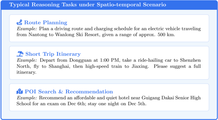Real-world reasoning tasks can be categorized based on cognitive cost and processing speed into System 1 and System 2 modes Li et al. (2025b): the former is rapid, whereas the latter necessitates extensive and complex deliberation. Reasoning tasks in spatio-temporal scenarios Zheng et al. (2025b); Lei et al. (2025) represent typical System 2 scenarios. As depicted in Figure 2, such complex tasks involve identifying locations, designing driving routes, or planning travel itineraries subject to numerous constraints Ning et al. (2025); Xie et al. (2024), necessitating the coordination of heterogeneous external tools for resolution Zhang et al. (2025); Xu et al. (2025). Consequently, TIR interleaves thought generation with tool execution, empowers the model to verify intermediate steps and dynamically adjust its planning trajectory based on observation feedback, and exhibits an inherent advantage in addressing these real-world tasks. 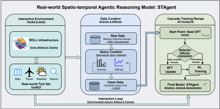Figure 1: The overall framework of STAgent. It presents a comprehensive pipeline designed for real-world spatio-temporal reasoning. The framework consists of three key phases: (1) Robust Interactive Environment , supported by the ROLL infrastructure and FastMCP protocol to enable efficient, asynchronous tool-integrated reasoning. (2) High-Quality Data Construction , which utilizes a self-evolving selection framework to filter diverse and challenging queries from massive unsupervised data; (3) Cascade Training Recipe , an SFT-Guided RL paradigm that categorizes samples by difficulty to synergize supervised fine-tuning with reinforcement learning. <details> <summary>Image 2 Details</summary>  ### Visual Description ## Diagram: Real-world Spatio-temporal Agentic Reasoning Model: STAgent ### Overview This image is a technical system architecture diagram illustrating the framework for the "Real-world Spatio-temporal Agentic Reasoning Model: STAgent." The diagram is divided into three primary, interconnected modules arranged horizontally from left to right, with a feedback loop connecting the final module back to the first. The overall flow depicts a pipeline for creating an AI agent capable of reasoning in real-world, spatio-temporal contexts using external tools. ### Components/Axes The diagram is structured into three main rectangular blocks with rounded corners, each representing a core module of the system. Arrows indicate the flow of data and processes between these modules. 1. **Left Module: Interactive Environment** * **Title:** Interactive Environment * **Subtitle:** Flexible & Stable * **Sub-components:** * **ROLL Infrastructure:** Contains an icon of a cartoon character (resembling a fox or cat) riding a rocket. Text: "ROLL Infrastructure" and "Async Rollout & Training". * **Real-world Tool Set:** Contains five icons representing different tools: a map, an airplane, a sun/cloud weather symbol, a magnifying glass (search), and a globe. Text: "Real-world Tool Set" and "Fast&CP". * **Spatial Grounding:** This module is positioned on the far left of the diagram. An arrow points from this module to the central "Data Curation" module. 2. **Center Module: Data Curation** * **Title:** Data Curation * **Subtitle:** Diversity & Difficulty * **Sub-components:** * **Raw Data:** Represented by a cylinder (database) icon. Text: "Raw Data" and "Massive Historical Queries (~30M, Unsupervised)". * **Query Curation:** Text: "Query Curation" and "Self-evaluating Query Selection". Below this are two small charts: a bar chart labeled "Diversity" and a line chart labeled "Difficulty". * **Clean Data:** Represented by a cylinder icon. Text: "Clean Data" and "Candidate Query Pool (~2000)". * **Spatial Grounding:** This module is in the center. Arrows flow into it from the left module and out of it to the right module. A large, curved arrow labeled "Interaction Loop" also connects the bottom of this module back to the "Interactive Environment" module. 3. **Right Module: Cascade Training Recipe** * **Title:** Cascade Training Recipe * **Subtitle:** SFT-Guided RL * **Sub-components (flowchart):** * **Start Point: Seed SFT:** A rectangle. Text: "Start Point: Seed SFT", "Actor", and "π^seed". * **Selector: Difficulty Assessment:** A diamond (decision) shape. Text: "Selector: Difficulty Assessment". Two arrows exit this diamond: one labeled "High-confidence Samples" pointing to "SFT Update", and another labeled "Challenging Samples" pointing to "RL Training". * **SFT Update:** A rectangle. * **RL Training:** A rectangle. * **Final Model: STAgent:** A rectangle. Text: "Final Model: STAgent", "π*", and "Breaking Ceiling & Generalization". * **Spatial Grounding:** This module is on the far right. An arrow from the "Clean Data" in the center module points to the "Start Point" of this training recipe. A large, curved arrow labeled "Interaction Loop" originates from the bottom of this module and points back to the "Interactive Environment" on the left. ### Detailed Analysis The diagram details a closed-loop system for training an AI agent (STAgent). * **Process Flow:** 1. The **Interactive Environment** provides a stable platform (ROLL Infrastructure) and a set of real-world tools (Map, Travel, Weather, Search) for the agent to interact with. 2. Data for training is processed in the **Data Curation** module. It starts with a massive pool of ~30 million unsupervised historical queries ("Raw Data"). A "Self-evaluating Query Selection" process curates this down to a "Candidate Query Pool" of approximately 2000 high-quality queries ("Clean Data"), optimizing for both "Diversity" and "Difficulty". 3. This curated dataset feeds into the **Cascade Training Recipe**. The training starts with a "Seed SFT" (Supervised Fine-Tuning) model (π^seed). A "Selector" performs "Difficulty Assessment" on data samples. "High-confidence Samples" are used for further "SFT Update", while "Challenging Samples" are used for "RL Training" (Reinforcement Learning). This cascade produces the "Final Model: STAgent" (π*), which is designed for "Breaking Ceiling & Generalization". 4. **Interaction Loop:** A critical feedback loop connects the final trained model back to the interactive environment. The label "Tool Invocation & Async Rollout & Training" indicates that the STAgent's performance in the real-world environment generates new data or experiences, which are fed back into the Data Curation module, enabling continuous learning and improvement. ### Key Observations * The system emphasizes **data quality over quantity**, reducing 30 million raw queries to just 2000 curated ones. * The training methodology is a **hybrid approach**, combining Supervised Fine-Tuning (SFT) with Reinforcement Learning (RL), guided by a difficulty-based selector. * The architecture is explicitly designed as a **continuous learning loop**, not a one-time training pipeline. The "Interaction Loop" is fundamental to the model's ability to generalize and improve. * The model's goal, "Breaking Ceiling & Generalization," suggests it aims to surpass the limitations of its initial training and perform well on unseen, real-world tasks. ### Interpretation This diagram outlines a sophisticated framework for building a practical, real-world AI agent. The core innovation lies in the integration of three key ideas: **stable interactive environments**, **intelligent data curation**, and **cascaded, self-improving training**. The "Interactive Environment" with its "Real-world Tool Set" grounds the agent in practical tasks, moving beyond theoretical benchmarks. The "Data Curation" module acts as a quality filter, ensuring the agent learns from meaningful and challenging examples rather than noisy, raw data. The "Cascade Training Recipe" is particularly insightful; it doesn't just train on static data but uses a selector to dynamically choose the right training method (SFT or RL) based on sample difficulty, mimicking a more human-like learning progression from confident basics to challenging edge cases. Most importantly, the "Interaction Loop" transforms the system from a static model into a **continuously evolving agent**. By feeding the agent's real-world interactions back into the training pipeline, the system can adapt to new scenarios, correct its own mistakes, and progressively enhance its reasoning capabilities. This reflects a Peircean investigative approach where understanding is refined through ongoing cycles of action, observation, and hypothesis testing. The model, STAgent, is therefore not just a final product but the current state of an agent in a perpetual cycle of learning and improvement. </details> Figure 2: Typical reasoning tasks under spatio-temporal scenario. <details> <summary>Image 3 Details</summary>  ### Visual Description ## Diagram: Typical Reasoning Tasks under Spatio-temporal Scenario ### Overview The image is a diagram illustrating three categories of reasoning tasks within a spatio-temporal context. It presents a title and three distinct, vertically stacked task boxes, each containing an icon, a task title, and a specific example. The overall design uses a light blue background with white, blue-bordered boxes for each task. ### Components/Axes * **Main Title (Top, Centered):** "Typical Reasoning Tasks under Spatio-temporal Scenario" in white text on a solid blue header bar. * **Task Boxes (Three, stacked vertically):** Each box has a white background, a thin blue border, and contains: 1. **Icon (Left-aligned):** A blue icon representing the task type. 2. **Task Title (Right of icon, Bold Blue Text):** The name of the task category. 3. **Example Text (Below title, Italicized Black Text):** A concrete scenario illustrating the task. ### Detailed Analysis The diagram is segmented into three independent regions, processed from top to bottom. **1. Top Task Box: Route Planning** * **Icon:** A blue icon depicting a winding road or path. * **Title:** "Route Planning" * **Example Text:** "Example: Plan a driving route and charging schedule for an electric vehicle traveling from Nantong to Wanlong Ski Resort, given a range of approx. 500 km." **2. Middle Task Box: Short Trip Itinerary** * **Icon:** A blue icon depicting an umbrella, suggesting travel or leisure. * **Title:** "Short Trip Itinerary" * **Example Text:** "Example: Depart from Dongguan at 1:00 PM, take a ride-hailing car to Shenzhen North, fly to Shanghai, then high-speed train to Jiaxing. Please suggest a full itinerary." **3. Bottom Task Box: POI Search & Recommendation** * **Icon:** A blue icon depicting a group of people or a community. * **Title:** "POI Search & Recommendation" * **Example Text:** "Example: Recommend an affordable and quiet hotel near Guigang Dakai Senior High School for an exam on Dec 6th; stay one night on Dec 5th." ### Key Observations * **Structural Pattern:** All three examples follow a similar structure: they define a starting point, a destination or goal, constraints (time, range, budget, quietness), and a required output (plan, schedule, itinerary, recommendation). * **Geographic Specificity:** The examples use specific, real-world locations in China (Nantong, Wanlong Ski Resort, Dongguan, Shenzhen, Shanghai, Jiaxing, Guigang). * **Temporal Constraints:** Two of the three examples explicitly include precise time elements ("1:00 PM", "Dec 6th", "Dec 5th"). * **Multi-modal Integration:** The "Short Trip Itinerary" example explicitly involves multiple transportation modes (ride-hailing car, flight, high-speed train). ### Interpretation This diagram serves as a taxonomy or classification of complex, real-world problems that require spatio-temporal reasoning. It demonstrates that such reasoning is not a single task but a family of tasks involving: 1. **Optimization under constraints** (Route Planning with vehicle range). 2. **Sequential decision-making across time and space** (assembling a multi-leg itinerary). 3. **Context-aware filtering and ranking** (finding a POI that meets multiple criteria like location, price, noise level, and date). The examples are carefully chosen to show practical, everyday applications, moving from a simple A-to-B route to a more complex, multi-stage journey, and finally to a search problem with nuanced user preferences. The underlying message is that effective AI or computational systems for spatio-temporal scenarios must handle these varied and interconnected types of queries. The use of Chinese locations suggests the context or target application domain for these reasoning tasks. </details> However, unlike general reasoning tasks such as mathematics Shang et al. (2025) or coding Zeng et al. (2025), addressing these real-world tasks inherently involves several challenges. First , how can a flexible and stable reasoning environment be constructed? On one hand, a feasible environment requires a toolset capable of handling massive concurrent tool call requests, which will be invoked by both offline data curation and online reinforcement learning (RL) Bian et al. (2025). On the other hand, during training, maintaining effective synchronization between tool calls and trajectory rollouts, and guaranteeing that the model receives accurate reward signals, constitute the cornerstone of effective TIR for such complex tasks. Second , how can high-quality training data be curated? In real-world spatio-temporal scenarios, massive real-world queries are sent by users and stored in databases; however, this data is unsupervised and lacks necessary knowledge, e.g., the category and difficulty of each query Yu et al. (2025), making the model unaware of the optimization direction Li et al. (2025a). Therefore, it is critical to construct a query taxonomy to facilitate high-quality data selection for model optimization. Third , how should effective training for real-world TIR be conducted? Existing TIR efforts mostly focus on the adaptation between algorithms and tools. For instance, monitoring interleaved tool call entropy changes to guide further token rollout Dong et al. (2025) or increasing rollout batch sizes to mitigate tool noise Shang et al. (2025). Nevertheless, the uncertain environment and diverse tasks in real-world scenarios pose extra challenges when applying these methods. Therefore, deriving a more tailored training recipe is key to elevating the upper bound of TIR performance. In this work, we propose STAgent, the pioneering agentic model designed for real-world spatiotemporal TIR reasoning. We develop a comprehensive pipeline encompassing a Interactive Environment, High-Quality Data Curation, and a Cascade Training Recipe, as shown in Figure 1. Specifically, STAgent features three primary aspects. For environment and infrastructure, we established a robust reinforcement training environment supporting ten domain-specific tools across four categories, including map, travel, weather, and information retrieval tools. On the one hand, we encapsulated these tools using FastMCP 1 , standardizing parameter formats and invocation protocols, which significantly facilitates future tool modification. On the other hand, we collaborated with the ROLL Wang et al. (2025) 2 team to optimize the RL training infrastructure, offering two core features: asynchronous rollout and training. Compared to the popular open-source framework Verl 3 , ROLL yields an 80% improvement in training efficiency. Furthermore, we designed a meticulous query selection framework to hierarchically extract high-quality queries from massive historical candidates. We focus on query diversity and difficulty, deriving a self-evolving query selection framework to filter approximately 200,000 queries from an original historical dataset of over 30 million, which serves as the candidate query pool for subsequent SFT and RL training. Lastly, we designed a cascaded training paradigm-specifically an SFT-Guided RL approach-to ensure continuous improvement in model capability. By training a Seed SFT model to serve as an evaluator, we assess the difficulty of the query pool to categorize queries for subsequent SFT updates and RL training. Specifically, SFT is refined with samples of higher certainty, while RL targets more challenging samples from the updated SFT model. This paradigm significantly enhances the generalization of the SFT model while enabling the RL model to push beyond performance ceilings. The final model, STAgent, was built upon Qwen3-30B-A3B-2507 Yang et al. (2025). Notably, during the SFT stage, STAgent incorporated only a minimal amount of general instruction-following data Xu et al. (2025) to enhance tool invocation capabilities, with the vast majority consisting of domain-specific data. Remarkably, as a specialized model, STAgent demonstrates significant advantages on TravelBench Cheng et al. (2025) compared to models with larger parameter sizes. Furthermore, despite not being specifically tuned for the general domain, STAgent achieved improvements on numerous general-domain benchmarks, demonstrating its strong generalization capability. ## 2 Methodology ## 2.1 Overview We formally present STAgent in this section, focusing on three key components: - Tool environment construction. We introduce details of the in-domain tools used in Section 2.2. - High-quality prompt curation. We present the hierarchical prompt curation pipeline in Section 2.3, including the derivation of a prompt taxonomy, large-scale prompt annotation, and difficulty measurement. 1 https://github.com/jlowin/fastmcp 2 https://github.com/alibaba/ROLL 3 https://github.com/volcengine/verl - Cascaded agentic post-training recipe. We present the post-training procedure in Section 2.4, Section 2.5, and Section 2.6, which corresponds to reward design, agentic SFT, and SFT-guided RL training, respectively. ## 2.2 Environment Construction To enable STAgent to interact with real-world spatio-temporal services in a controlled and reproducible manner, we developed a high-fidelity sandbox environment built upon FastMCP. This environment serves as the bridge between the agent's reasoning capabilities and the underlying spatiotemporal APIs, providing a standardized interface for tool invocation during both training and evaluation. To reduce API latency and costs during large-scale RL training, we implemented a tool-level LRU caching mechanism with parameter normalization to maximize cache hit rates. Our tool library comprises 10 specialized tools spanning four functional categories, designed to cover the full spectrum of spatio-temporal user needs identified in our Intent Taxonomy (Section 2.3). All tool outputs are post-processed into structured natural language to facilitate the agent's comprehension and reduce hallucination risks. We describe the summary of the tool definition in Table 1, more tool details can be found in Appendix A.1. Table 1: Summary of the tool library for the Amap Agent sandbox environment. | Category | Tool | Description | |-----------------|---------------------------------------------------------------------------------------------------------------|----------------------------------------------------------------------------------------------------------------------------------------------------------------------------------------------------------------| | Map &Navigation | map search places map compute routes map search along route map search central places map search ranking list | Search POIs by keyword, location, or region Route planning supporting multiple transport modes Find POIs along a route corridor Locate optimal meeting points for multiple origins Query curated ranking lists | | Travel | travel search flights travel search trains | Search flights with optional multi-day range Query train schedules and fares | | Weather | weather current conditions weather forecast days | Get real-time weather and AQI Retrieve multi-day forecasts | | Information | web search | Open-domain web search | ## 2.3 Prompt Curation To endow the STAgent with comprehensive spatio-temporal reasoning capabilities, we synthesized a high-fidelity instruction dataset grounded in large-scale, real-world user behaviors. This dataset spans the full spectrum of user needs, covering atomic queries such as POI retrieval as well as composite, multi-constraint tasks like intricate itinerary planning. We leveraged anonymized online user logs spanning a three-month window as our primary data source, with a volume of 30 million. The critical challenge lies in distilling these noisy, unstructured interactions into a structured, high-diversity instruction dataset suitable for training a sophisticated agent. To achieve this, we constructed a hierarchical Intent Taxonomy . This taxonomy functions as a rigorous framework for precise annotation, quantitative distribution analysis, and controlled sampling, ensuring the dataset maximizes both Task Type Diversity (comprehensive intent coverage) and Difficulty Diversity (progression from elementary to complex reasoning). ## 2.3.1 Seed-Driven Taxonomy Evolution We propose a Seed-Driven Evolutionary Framework to construct a taxonomy that guarantees both completeness and orthogonality (i.e., non-overlapping, independent dimensions). Instead of relying on static classification, our approach initiates with a high-quality kernel of seed prompts and iteratively expands the domain coverage by synergizing the generative power of LLMs with rigorous human oversight. 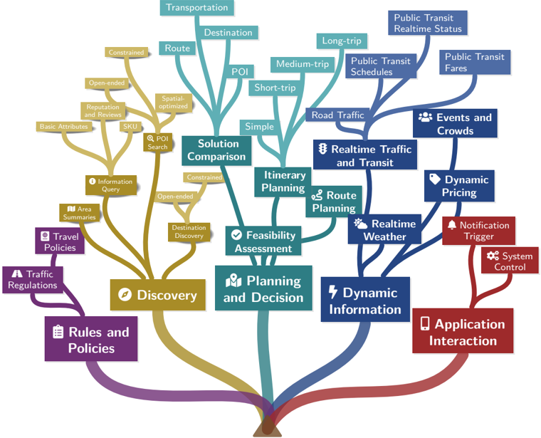The process unfolds in the following phases: Figure 3: A visual taxonomy of our intent classification system. The hierarchical structure is organized into five primary categories: Rules and Policies, Discovery, Planning and Decision, Dynamic Information, and Application Interaction. The taxonomy further branches into 16 second-level categories and terminates in 30 fine-grained leaf nodes, capturing the multi-faceted complexity of realworld user queries in navigation and travel scenarios. <details> <summary>Image 4 Details</summary>  ### Visual Description ## Concept Diagram: Transportation & Mobility Services Taxonomy ### Overview The image is a conceptual tree diagram or mind map illustrating a taxonomy of services and functions related to transportation, mobility, and trip planning. The diagram uses a tree structure with a central trunk at the bottom that branches out into five major, color-coded categories. Each major branch further subdivides into more specific functions and data types. The visual metaphor suggests that all these services grow from a common root or foundation. ### Components/Axes The diagram is structured as a hierarchical tree with no traditional axes. The primary organizational elements are: * **Central Trunk:** A brown, root-like structure at the bottom center from which all major branches originate. * **Major Branches (Primary Categories):** Five thick, colored branches extending from the trunk. Each has a primary label and an associated icon. 1. **Rules and Policies** (Purple, bottom-left): Icon of a document. 2. **Discovery** (Gold, left): Icon of a compass. 3. **Planning and Decision** (Teal, center): Icon of a person with a map. 4. **Dynamic Information** (Blue, right): Icon of a lightning bolt. 5. **Application Interaction** (Red, bottom-right): Icon of a smartphone. * **Sub-Branches:** Thinner lines of the same color as the parent branch, leading to more specific service categories or data types. * **Leaf Nodes:** Rectangular boxes containing the specific service or data labels. Some have small icons preceding the text. ### Detailed Analysis The diagram details a comprehensive ecosystem of mobility-related services. Here is a breakdown by major branch: **1. Rules and Policies (Purple Branch - Bottom Left)** * **Sub-Branch:** `Traffic Regulations` * **Leaf Node:** `Travel Policies` **2. Discovery (Gold Branch - Left)** * **Sub-Branches & Leaf Nodes:** * `Area Summaries` * `Information Query` * `POI Search` (with a magnifying glass icon) * `Destination Discovery` * `Solution Comparison` (This node is also connected to the "Planning and Decision" branch via a teal line, indicating a cross-functional relationship). * **Further Sub-Categories (from `POI Search` and `Information Query`):** * `Basic Attributes` * `Reputation and Reviews` * `SKU` * `Spatial-optimized` * `Open-ended` * `Constrained` **3. Planning and Decision (Teal Branch - Center)** * **Sub-Branches & Leaf Nodes:** * `Feasibility Assessment` * `Itinerary Planning` * `Route Planning` (with a map icon) * **Further Sub-Categories (from `Itinerary Planning`):** * `Simple` * `Short-trip` * `Medium-trip` * `Long-trip` * **Further Sub-Categories (from `Route Planning`):** * `Transportation` * `Destination` * `Route` * `POI` (Point of Interest) **4. Dynamic Information (Blue Branch - Right)** * **Sub-Branches & Leaf Nodes:** * `Realtime Weather` (with a cloud/sun icon) * `Realtime Traffic and Transit` (with a traffic light icon) * `Road Traffic` * `Public Transit Schedules` * `Public Transit Realtime Status` * `Public Transit Fares` * `Events and Crowds` (with a people icon) * `Dynamic Pricing` (with a price tag icon) **5. Application Interaction (Red Branch - Bottom Right)** * **Sub-Branches & Leaf Nodes:** * `Notification Trigger` (with a bell icon) * `System Control` (with a gear icon) ### Key Observations * **Cross-Functional Link:** The `Solution Comparison` node is uniquely connected to both the **Discovery** (gold) and **Planning and Decision** (teal) branches, highlighting its role as a bridge between finding options and making a choice. * **Hierarchical Depth:** The **Discovery** and **Planning and Decision** branches show the most hierarchical depth, with up to three levels of sub-categorization (e.g., Planning and Decision -> Itinerary Planning -> Short-trip). * **Iconography:** Small icons are used consistently to visually reinforce the meaning of key service categories (e.g., lightning bolt for dynamic data, smartphone for app interaction). * **Spatial Layout:** The **Rules and Policies** and **Application Interaction** branches are positioned at the bottom corners, framing the core functional branches (Discovery, Planning, Dynamic Info) which occupy the central and upper space of the diagram. ### Interpretation This diagram presents a structured ontology for a smart mobility or transportation-as-a-service (TaaS) platform. It categorizes the vast array of data inputs, processing functions, and user-facing features required for such a system. * **What it demonstrates:** The taxonomy moves from foundational, rule-based constraints (left) through user-centric processes of discovery and planning (center), fueled by real-time data (right), and culminating in actionable outputs and controls (bottom-right). It illustrates that effective trip planning is not a single action but an ecosystem of interconnected services. * **Relationships:** The central positioning of **Planning and Decision** suggests it is the core processing engine, relying on inputs from **Discovery** (options) and **Dynamic Information** (real-world conditions), while operating within the boundaries set by **Rules and Policies**. The final outputs are delivered and managed through **Application Interaction**. * **Notable Insight:** The inclusion of `Dynamic Pricing`, `Events and Crowds`, and `Realtime Status` underscores the importance of temporal, real-time data in modern mobility solutions, moving beyond static schedules and maps. The separation of `Public Transit` into schedules, realtime status, and fares indicates a sophisticated level of data integration for public transport. </details> Stage 1: Seed Initialization. We manually curate a small, high-variance set of n seed prompts ( D seed ∈ D pool ) to represent the core diversity of the domain. Experts annotate these seeds with open-ended tags to capture abstract intent features. Each query is mapped into a tuple as: $$S _ { i } = ( q _ { i } , T _ { i } ) , s . t . T _ { i }$$ where T i denotes the k orthogonal or complementary intent nodes covered by instruction q i . Stage 2: LLM-Driven Category Induction. Using the annotated seeds, we prompt an LLM to induce orthogonal Level-1 categories, ensuring granular alignment across the domain. Stage 3: Iterative Refinement Loop. To prevent hallucinations, we implement a strict check-update cycle. The LLM re-annotates the D seed using the generated categories; human experts review these annotations to identify ambiguity or coverage gaps, feeding feedback back to the LLM for taxonomy refinement, executing a 'Tag-Feedback-Correction' cycle across several iterations: $$T ^ { ( k + 1 ) } = Refine ( Annotate ( D$$ During this process, human experts identify ambiguity or coverage gaps in the LLM-generated categories, feeding critical insights back for taxonomy adjustment. The process terminates when T ( k +1) ≈ T ( k ) , signifying that the system has converged into a stable benchmark taxonomy T ∗ . Stage 4: Dynamic Taxonomy Expansion. To capture long-tail intents beyond the initial seeds, we enforce an 'Other' category at each node. By labeling a massive scale of raw logs and analyzing samples falling into the 'Other' category, we discover and merge emerging categories, allowing the taxonomy to evolve dynamically. This mechanism transforms the taxonomy from a static tree into an evolving system capable of adapting to the open-world distribution of user queries. The resulting finalized Intent Taxonomy is visualized in Figure 3. ## 2.3.2 Annotation and Data Curation Building upon this stabilized and mutually orthogonal taxonomy, we deployed a high-capacity teacher LLM to execute large-scale intent classification on the structured log data. The specific prompt template used for this annotation is detailed in Appendix A.2. To ensure the training data achieves both high information density and minimal redundancy, we implemented a rigorous twophase process: Precise Multi-Dimensional Annotation. We treat intent understanding as a multi-label classification task. Each user instruction is mapped to a composite label vector V = ⟨ I primary , I secondary , C constraints ⟩ . - I primary and I secondary represent the leaf nodes in our fine-grained Intent Taxonomy. - C constraints captures specific auxiliary dimensions (e.g., spatial range , time budget , vehicle type ). This granular tagging captures the semantic nuance of complex queries, distinguishing between simple keyword searches and multi-constraint planning tasks. Controlled Sampling via Funnel Filtering. Based on the annotation results, we applied a threestage Funnel Filtering Strategy to construct the final curated dataset. This pipeline systematically eliminates redundancy at lexical, semantic, and geometric levels: - Lexical Redundancy Elimination: We applied global Locality-Sensitive Hashing at corpus level to efficiently remove near-duplicate strings and literal repetitions ('garbage data') across all data, significantly reducing the initial volume. - Semantic Redundancy Elimination: To ensure high intra-class variance, we partitioned the dataset into buckets based on the ⟨ I primary , I secondary ⟩ tuple. Within each bucket, we performed embedding-based similarity search to prune semantically redundant samples-defined as distinct phrasings that reside within a predefined distance threshold in the latent space. To handle the scale of our dataset, we integrated Faiss to accelerate this process; this transitioned the computational complexity from a quadratic O ( N 2 ) brute-force pairwise comparison to a more scalable sub-linear or near-linear search complexity, significantly reducing the preprocessing overhead. - Geometric Redundancy Elimination: From the remaining pool, we employed the KCenter-Greedy algorithm to select the most representative samples. By maximizing the minimum distance between selected data points in the embedding space, this step preserves long-tail and corner-case queries that are critical for robust agent performance. ## 2.3.3 Difficulty and Diversity Real-world geospatial tasks vary significantly in cognitive load. To ensure the STAgent demonstrates robustness across this spectrum, we rigorously stratified our training data. Beyond mere coverage, the primary objective of this stratification is to enable Difficulty-based Curriculum Learning. In RL, a static data distribution often leads to training inefficiency: early-stage models facing excessively hard tasks yield zero rewards (vanishing gradients), while late-stage models facing trivial tasks yield constant perfect rewards (lack of variance). To address this, we employed an Execution-Simulation Scoring Mechanism to label data complexity, allowing us to dynamically align training data with model proficiency. 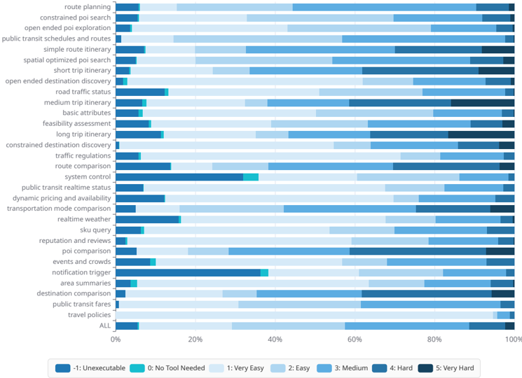This mechanism evaluates difficulty across three orthogonal dimensions: Figure 4: Fine-grained Difficulty Distribution across 30 Geospatial Domains. The visualization reveals the distinct complexity profiles of different tasks. While atomic queries (e.g., basic attributes ) cluster in low-difficulty regions (Score 1-2), composite tasks (e.g., long trip itinerary ) exhibit a significant proportion of high-complexity reasoning (Score 4-5). The visible segments of Score -1 and 0 (denoted as Ext.1 ) across domains like System Control highlight our active sampling of boundary cases for hallucination mitigation. <details> <summary>Image 5 Details</summary>  ### Visual Description ## Horizontal Stacked Bar Chart: Perceived Difficulty of Location/Navigation Tasks ### Overview This is a horizontal stacked bar chart that visualizes the perceived difficulty (and executability) of 30+ location/navigation-focused tasks, with each bar representing a single task, segmented by difficulty categories. The x-axis uses a percentage scale (0% to 100%) to show the proportion of responses for each difficulty level, while the y-axis lists all evaluated tasks. The chart includes an aggregate "ALL" bar at the bottom to summarize overall task difficulty. ### Components/Axes 1. **Y-axis (Vertical, Left)**: Lists all tasks, ordered top-to-bottom: `route planning`, `constrained poi search`, `open ended poi exploration`, `public transit schedules and routes`, `simple route itinerary`, `spatial optimized poi search`, `short trip itinerary`, `open ended destination discovery`, `road traffic status`, `medium trip itinerary`, `basic attributes`, `feasibility assessment`, `long trip itinerary`, `constrained destination discovery`, `traffic regulations`, `route comparison`, `system control`, `public transit realtime status`, `dynamic pricing and availability`, `transportation mode comparison`, `realtime weather`, `sku query`, `reputation and reviews`, `poi comparison`, `events and crowds`, `notification trigger`, `area summaries`, `destination comparison`, `public transit fares`, `travel policies`, `ALL` (aggregate task) 2. **X-axis (Horizontal, Bottom)**: Percentage scale, marked at `0%`, `20%`, `40%`, `60%`, `80%`, `100%`. 3. **Legend (Bottom Center, below x-axis)**: Color-coded difficulty categories: - Dark blue: `-1: Unexecutable` - Teal: `0: No Tool Needed` - Lightest blue: `1: Very Easy` - Light blue: `2: Easy` - Medium blue: `3: Medium` - Darker blue: `4: Hard` - Darkest blue: `5: Very Hard` 4. **Spatial Placement**: The legend is positioned at the bottom center of the chart, below the x-axis. Each task bar is left-aligned, spanning the full 100% width of the chart, with segments ordered from left (Unexecutable) to right (Very Hard). ### Detailed Analysis All tasks share a consistent small segment for `-1: Unexecutable` (~5%) and `0: No Tool Needed` (~5%). The remaining 90% of each bar is split across difficulty levels, with variation based on task complexity: 1. **Straightforward Tasks (e.g., `route planning`, `public transit schedules and routes`, `basic attributes`)**: - ~20% `1: Very Easy`, ~20% `2: Easy`, ~25% `3: Medium`, ~15% `4: Hard`, ~10% `5: Very Hard` 2. **Complex/Optimization Tasks (e.g., `open ended poi exploration`, `spatial optimized poi search`, `long trip itinerary`, `system control`, `events and crowds`)**: - ~10% `1: Very Easy`, ~15% `2: Easy`, ~25% `3: Medium`, ~25% `4: Hard`, ~15% `5: Very Hard` 3. **Aggregate "ALL" Bar (Bottom of Y-axis)**: - ~5% `-1: Unexecutable`, ~5% `0: No Tool Needed`, ~25% `1: Very Easy`, ~20% `2: Easy`, ~25% `3: Medium`, ~15% `4: Hard`, ~5% `5: Very Hard` ### Key Observations 1. **Uniform Minimal Segments**: Every task has identical small segments for `Unexecutable` and `No Tool Needed`, indicating nearly all these tasks require tooling, and only a tiny fraction are considered impossible to complete. 2. **Difficulty Correlation**: Tasks that are open-ended, require optimization, or involve real-time/complex data (e.g., `open ended poi exploration`, `system control`) have significantly larger `Hard`/`Very Hard` segments (combined ~40% of responses) compared to more structured tasks. 3. **Dominant Medium Difficulty**: The largest single segment across most tasks (and the aggregate bar) is `3: Medium`, showing most users find these tasks manageable but not trivial. 4. **Consistent Distribution Pattern**: Most tasks follow a similar proportional split, with difficulty levels decreasing in prevalence from Medium → Easy/Very Easy → Hard → Very Hard. ### Interpretation This data demonstrates that location/navigation tasks have a clear difficulty gradient, with structured, well-defined tasks (like route planning) perceived as easier, while open-ended, optimization-focused tasks are seen as significantly more challenging. The consistent small `Unexecutable`/`No Tool Needed` segments confirm that these tasks universally require tool support, with no tasks considered fully unassisted or impossible. For product and UX teams, this data highlights a need to prioritize support for complex tasks (e.g., adding guided workflows for open-ended exploration, or automated optimization for long trips) to reduce user frustration. The aggregate "ALL" bar provides a baseline for overall task difficulty in this domain, showing that most users find these tasks accessible but not effortless, which can inform tool design and feature prioritization. </details> - Cognitive Load in Tool Selection: Measures the ambiguity of intent mapping. It spans from Explicit Mapping (Score 1-2, e.g., 'Navigates to X') to Implicit Reasoning (Score 4-5, e.g., 'Find a quiet place to read within a 20-minute drive,' requiring abstract intent decomposition). - Execution Chain Depth: Quantifies the logical complexity of the solution path, tracking the number and type of tool invocations and dependency depth (e.g., sequential vs. parallel execution). - Constraint Complexity: Assesses the density of constraints (spatial, temporal, and preferential) that the agent must jointly optimize. To operationalize this mechanism at scale, we utilize a strong teacher LLM as an automated evaluator. This evaluator analyzes the structured user logs, assessing them against the three critical competencies to assign a scalar difficulty score r ∈ {-1 , 0 , 1 , ..., 5 } to each sample. The specific prompt template used for this evaluation is detailed in Appendix A.3. To validate the efficacy of this scoring mechanism, we visualize the distribution of annotated samples across 30 domains in Figure 4. The distribution aligns intuitively with task semantics, providing strong support for our curriculum strategy: - Spectrum Coverage for Curriculum Learning: As shown in the 'ALL' bar at the bottom of Figure 4, the aggregated dataset achieves a balanced stratification. This allows us to construct training batches that progressively shift from 'Atomic Operations' (Score 1-2) to 'Complex Reasoning' (Score 4-5) throughout the training lifecycle, preventing the reward collapse issues mentioned above. - Domain-Specific Complexity Profiles: The scorer correctly identifies the inherent hardness of different intents. For instance, Long-trip Itinerary is dominated by Score 4-5 samples (dark blue segments), reflecting its need for multi-constraint optimization. In contrast, Traffic Regulations consists primarily of Score 1-2 samples, confirming the scorer's ability to distinguish between retrieval and reasoning tasks. By curating batches based on these scores, we ensure the STAgent receives a consistent gradient signal throughout its training lifecycle. Furthermore, we place special emphasis on boundary conditions to enhance reliability: Irrelevance and Hallucination Mitigation (Score -1/0). A critical failure mode in agents is the tendency to hallucinate actions for unsolvable queries. To mitigate this, it is critical to train models to explicitly reject unanswerable queries or seek alternative solutions when desired tools are unavailable. To achieve this, we constructed a dedicated Irrelevance Dataset (denoted as Ext.1 in Figure 4). By training on these negative samples, the STAgent learns to recognize the boundaries of its toolset, significantly reducing hallucination rates in open-world deployment. ## 2.4 Reward Design To evaluate the quality of agent interactions, we employ a rubrics-as-reward (Hashemi et al., 2024; Gunjal et al., 2025) method to assess trajectories based on three core dimensions: Reasoning and Proactive Planning , Information Fidelity and Integration , and Presentation and Service Loop . The scalar reward R ∈ [0 , 1] is derived from the following criteria: - Dimension 1, Reasoning and Proactive Planning: This dimension evaluates the agent's ability to formulate an economic and effective execution plan. A key metric is proactivity : when faced with ambiguous or slightly incorrect user premises (e.g., mismatched location names), the agent is rewarded for correcting the error and actively attempting to solve the underlying intent, rather than passively rejecting the request. It also penalizes the inclusion of redundant parameters in tool calls. - Dimension 2, Information Fidelity and Integration: This measures the accuracy with which the agent extracts and synthesizes information from tool outputs. We enforce a strict veto policy for hallucinations: any fabrication of factual data (e.g. time, price and distance) that cannot be grounded in the tool response results in an immediate reward of 0 . Conversely, the agent is rewarded for correctly identifying and rectifying factual errors in the user's query using tool evidence. - Dimension 3, Presentation and Service Loop: This assesses whether the final response effectively closes the service loop. We prioritize responses that are structured, helpful, and provide actionable next steps. The agent is penalized for being overly conservative or terminating the service flow due to minor input errors. Crucially, we recognize that different user intents require different capabilities. Therefore, we implement a Dynamic Scoring Mechanism where the evaluator autonomously determines the importance of each dimension based on the task type, rather than using fixed weights. Dynamic Weight Determination. For every query, the evaluator first analyzes the complexity of the user's request and categorizes it into one of three scenarios to assign specific weights ( w ): - Scenario A: Complex Planning (e.g., 'Plan a 3-day itinerary'). The system prioritizes logical coherence and error handling. Reference Weights: w reas ≈ 0 . 6 , w info ≈ 0 . 3 , w pres ≈ 0 . 1 . - Scenario B: Information Retrieval (e.g., 'What is the weather today?'). The system prioritizes factual accuracy and data extraction. Reference Weights: w reas ≈ 0 . 2 , w info ≈ 0 . 6 , w pres ≈ 0 . 2 . - Scenario C: Consultation & Explanation (e.g., 'Explain this policy'). The system prioritizes clarity and user interaction. Reference Weights: w reas ≈ 0 . 3 , w info ≈ 0 . 3 , w pres ≈ 0 . 4 . Score Aggregation and Hallucination Veto. Once the weights are established, the final reward R is calculated using a weighted sum of the dimension ratings s ∈ [0 , 1] . To ensure factual reliability, we introduce a Hard Veto mechanism for hallucinations. Let ⊮ H =0 be an indicator function where H = 1 denotes the presence of hallucinated facts. The final reward is formulated as: $$R = 1 H = 0 \times \sum _ { k \in \{ reas , info , pres \} } w _ { k }$$ This formula ensures that any trajectory containing hallucinations is immediately penalized with a zero score, regardless of its reasoning or presentation quality. ## 2.5 Supervised Fine-Tuning Our Supervised Fine-Tuning (SFT) stage is designed to transition the base model from a generalpurpose LLM into a specialized spatio-tempora agent. Rather than merely teaching the model to follow instructions, our primary objective is to develop three core agentic capabilities: Strategic Planning. The ability to decompose abstract user queries (e.g., Plan a next-weekend trip ) into a logical chain of executable steps. Precise Tool Orchestration. The capacity to orchastrate a series of tool calls leading to task fulfillment, ensuring syntactic correctness in parameter generation. Grounded Summarization. The capability to synthesize final answer from heterogeneous tool outputs (e.g., maps, weather, flights ) into a coherent, well-organized response without hallucinating parameters not present in the observation. ## 2.5.1 In-Domain Data Construction We construct our training data from the curated high-quality prompt pool derived in Section 2.3. To address the long-tail distribution of real-world scenarios where frequent tasks like navigation dominate while complex planning tasks are scarce, we employ a hybrid construction strategy: Offline Sampling with Strong LLMs. For collected queries, we utilize a Strong LLM (DeepSeekR1) to generate TIR trajectories. To ensure data quality, we generate K = 8 candidate trajectories per query and employ a Verifier (Gemini-3-Pro-Preview) to score them based on the reward dimensions defined in Section 2.4. Only trajectories achieving perfect scores across all dimensions are retained. Synthetic Long-Tail Generation. To bolster the model's performance on rare, complex tasks (e.g., multi-city itinerary planning with budget constraints), we employ In-Context Learning (ICL) to synthesize data. We sample complex tool combinations rarely seen in the existing data distribution and prompt a Strong LLM to synthesize user queries ( q s ) that necessitate these specific tools in random orders. These synthetic queries are then validated through the offline sampling pipeline to ensure executability. ## 2.5.2 Multi-Step Tool-Integrated Reasoning SFT We formalize the agent's interaction as a multi-step trajectory optimization problem. Unlike singleturn conversation, agentic reasoning requires the model to alternate between reasoning, tool invocation and tool observation processing. We model the probability of a trajectory o as the product of conditional probabilities over tokens. The training objective minimizes the negative log-likelihood: $$\mathcal { L } _ { S F T } ( o _ { t } \vert \theta ) = \frac { 1 } { c } \sum _ { t = 1 } ^ { | o _ { i } | } I ( o _ { i } , t ) \log \pi$$ where o i,t denotes the t -th token of trajectory o i . In practice, q s is optionally augmented with a corresponding user profile including user state (e.g., current location) and preferences (e.g., personal interests). I ( o i,t ) is a indicator function used for masking: $$C = - \sum _ { t = 1 } ^ { | o _ { i } | } I ( o _ { i , t } )$$ where text segments corresponding to tool observations do not contribute to the final loss calculation. 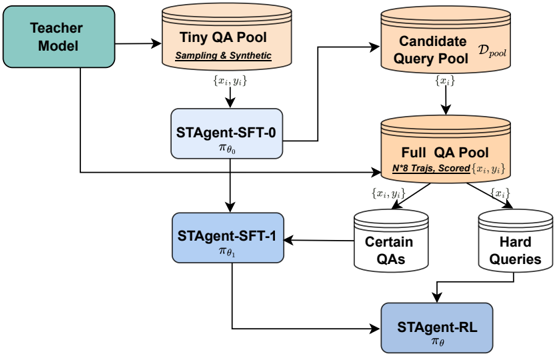## 2.5.3 Dynamic Capability-Aware Curriculum Acore challenge in model training is determining which data points provide the highest information gain Li et al. (2025a). Static difficulty metrics are insufficient because difficulty is inherently relative to the policy model's current parameterization. However, a task may be trivial for a strong LLM but lie outside the support of our policy model. Training on trivial samples yields vanishing gradients and increases the risk of overfitting, while training on impossible samples leads to high-bias updates and potential distribution collapse. In fact, samples that are trivial for a strong model but difficult for a weak model indicate a distribution gap between the two, and forcing the weak model to fit the distribution of the strong model in such cases can compromise generalization capability Burns et al. (2023). To bridge this gap, we define learnability not as a static property of the prompt, but as the dynamic relationship between task difficulty and the policy's current capability. Learnable tasks are those that reside on the model's decision boundary-currently uncertain but solvable. Figure 5 illustrates the training procedure of the SFT phase. Figure 5: The training procedure in the SFT phase. <details> <summary>Image 6 Details</summary>  ### Visual Description ## Diagram: STAgent Training Pipeline Flowchart ### Overview This image is a technical flowchart illustrating a multi-stage training pipeline for an AI agent named "STAgent". The diagram shows the flow of data and models through different training phases, starting from a teacher model and culminating in a reinforcement learning stage. The process involves creating and refining pools of question-answer (QA) data to train successive versions of the agent. ### Components/Axes The diagram consists of several distinct components connected by directional arrows indicating data or process flow. Components are color-coded: * **Green Box (Top-Left):** "Teacher Model" * **Orange Cylinders (Data Pools):** * "Tiny QA Pool" (Top-Center) with sub-text: "Sampling & Synthetic" * "Candidate Query Pool D_pool" (Top-Right) * "Full QA Pool" (Center-Right) with sub-text: "N^8 Trajs, Scored" * **Blue Boxes (Models/Agents):** * "STAgent-SFT-0" (Center-Left) with notation: π_θ₀ * "STAgent-SFT-1" (Center) with notation: π_θ₁ * "STAgent-RL" (Bottom-Right) with notation: π_θ * **White Cylinders (Filtered Data):** * "Certain QAs" (Center-Right, below Full QA Pool) * "Hard Queries" (Center-Right, below Full QA Pool) ### Detailed Analysis The process flow is as follows: 1. **Initialization:** The "Teacher Model" (green box, top-left) generates data for the "Tiny QA Pool" (orange cylinder, top-center). This pool is created via "Sampling & Synthetic" methods and contains data points denoted as `{xᵢ, yᵢ}`. 2. **First Training Stage (SFT-0):** The `{xᵢ, yᵢ}` data from the Tiny QA Pool is used to train the first model, "STAgent-SFT-0" (π_θ₀, blue box, center-left). 3. **Query Generation & Pool Expansion:** The trained STAgent-SFT-0 model generates outputs that contribute to two places: * It helps populate the "Candidate Query Pool D_pool" (orange cylinder, top-right) with queries `{xᵢ}`. * Its outputs are also fed into the "Full QA Pool" (orange cylinder, center-right). 4. **Full QA Pool Creation:** The "Full QA Pool" is a comprehensive dataset. It is formed by combining: * Data from the "Candidate Query Pool D_pool" (`{xᵢ}`). * Data from the "Teacher Model" (arrow from the green box). * Data from "STAgent-SFT-0". This pool is described as containing "N^8 Trajs, Scored" and holds scored trajectories `{xᵢ, yᵢ}`. 5. **Data Filtering:** The "Full QA Pool" is filtered into two specialized subsets: * "Certain QAs" (white cylinder, center-right). * "Hard Queries" (white cylinder, center-right). 6. **Second Training Stage (SFT-1):** The "Certain QAs" data is used to train the next model iteration, "STAgent-SFT-1" (π_θ₁, blue box, center). 7. **Reinforcement Learning Stage (RL):** The final model, "STAgent-RL" (π_θ, blue box, bottom-right), is trained using: * The "Hard Queries" data. * The output from the "STAgent-SFT-1" model. ### Key Observations * **Iterative Refinement:** The pipeline shows a clear progression from a base model (SFT-0) to a refined model (SFT-1) and finally to a reinforcement learning-optimized model (RL). * **Data-Centric Approach:** The core of the process is the creation and strategic filtering of QA data pools ("Tiny", "Candidate", "Full", "Certain", "Hard") to train increasingly capable agents. * **Teacher-Student Architecture:** The initial "Teacher Model" seeds the entire process, indicating a knowledge distillation or supervision framework. * **Notation:** Model parameters are denoted by π with subscripts θ₀, θ₁, and θ, indicating different training stages or parameter sets. ### Interpretation This flowchart depicts a sophisticated, data-centric methodology for training a specialized AI agent (STAgent). The process emphasizes **curriculum learning** and **data quality**. It starts with a small, synthetic dataset for initial supervised fine-tuning (SFT-0). The key insight is the creation of a large, scored "Full QA Pool," which is then intelligently split. Training the next model (SFT-1) on "Certain QAs" likely reinforces reliable knowledge, while the final RL stage uses "Hard Queries" to improve robustness and performance on challenging cases. This staged approach, moving from supervised learning to reinforcement learning, is designed to produce an agent that is both knowledgeable and capable of handling complex, uncertain scenarios. The diagram serves as a blueprint for a reproducible and scalable agent training pipeline. </details> To address this, we introduce a Dynamic Capability-Aware Curriculum that actively selects data points based on the policy model's evolving capability distribution. This process consists of four phases: Phase 1: Policy Initialization. We first establish a baseline capability to allow for meaningful selfassessment. We subsample a random 10% Tiny Dataset from the curated prompt pool (denoted as D pool ) and generate ground truth trajectories using the Strong LLM. We warm up our policy model by training on this subset to obtain the initial policy π θ 0 . Specifically, for each prompt, we sample K = 8 trajectories and employ a verifier to select the highest-scored generation as the ground truth. Phase 2: Distributional Capability Probing. To construct a curriculum aligned with the policy's intrinsic capabilities, we perform a distributional probe of the initialized policy π θ 0 against the full unlabeled pool D pool . Rather than relying on external difficulty heuristics, we estimate the local solvability of each task. For every query q i ∈ D pool , we generate K = 8 trajectories { o i,k } K k =1 ∼ π θ 0 ( ·| q i ) and use a verifier to evaluate their rewards r i,k . This yields the mean the variance of the empirical reward distribution, ˆ µ i and ˆ σ 2 i . Here, ˆ σ 2 i serves as an approximate proxy for uncertainty , where the policy parameters are unstable yet capable of generating high-reward solutions. Unlike random noise, when paired with a non-zero mean, this variance signifies the presence of a learnable signal within the policy's sampling space. Phase 3: Signal-to-Noise Filtration. We formulate data selection as a signal maximization problem. Effective training samples must possess high gradient variance to drive learning while ensuring the gradient direction is grounded in the policy model's distribution. Based on the estimated statistics, we categorize the data into three regions: - Trivial Region ( ˆ µ ≈ 1 , ˆ σ 2 → 0 ): Tasks where the policy has converged to high-quality solutions with high confidence. Training on these samples yields negligible gradients ( ∇L ≈ 0 ) and potentially leads to overfitting. - Noise Region ( ˆ µ ≈ 0 , ˆ σ 2 → 0 ): Tasks effectively outside the policy's current capability scope or containing noisy data. Training the model on these samples often leads to hallucination or negative transfer, as the ground truth lies too far outside the policy's effective support. - Learnable Region (High ˆ σ 2 , Non-zero ˆ µ ): Tasks maximizing training signals. These samples lie on the decision boundary where the policy is inconsistent but capable. We retain only the Learnable Region. To quantify the learnability on a per-query basis, we introduce the Learnability Potential Score S i = ˆ σ 2 i · ˆ µ i . This metric inherently prioritizes samples that are simultaneously uncertain (high ˆ σ 2 ) and feasibly solvable (non-zero ˆ µ ), maximizing the expected improvement in policy robustness. The scores are normalized between 0-1. Phase 4: Adaptive Trajectory Synthesis. Having identified the high-value distribution, we employ an adaptive compute allocation strategy to construct the final SFT dataset. We treat the Strong LLM as an expensive oracle. We allocate the sampling budget B i proportional to the task's learnability score, such that B i ∝ rank ( S i ) . Tasks with more uncertainty receive up to K max = 8 samples from the Strong LLM to maximize the probability of recovering a valid reasoning path, while easier tasks receive fewer calls. This ensures that the supervision signal is densest where the policy model is most uncertain, effectively correcting the policy's decision boundary with high-precision ground truth. Finally, we aggregate the verified trajectories obtained from this phase. We empirically evaluate various data mixing ratios to determine the optimal training distribution, obtaining π θ 1 , which serves as the backbone model for subsequent RL training. ## 2.6 RL The agentic post-training for STAgent follows the 'SFT-Guided RL' training paradigm, with the RL policy model initialized from . This initialization provides the agent with foundational instructionfollowing capabilities prior to the exploration phase in the sandbox environment. GRPO (Shao et al., 2024) has become the de facto standard for reasoning tasks. Training is conducted within a high-fidelity sandbox environment (described in Section 2.2), which simulates realworld online scenarios. This setup compels the agent to interact dynamically with the environment, specifically learning to verify and execute tool calls to resolve user queries effectively. The training objective seeks to maximize the expected reward while restricting the policy update to prevent significant deviations from the reference model. We formulate the GRPO objective for STAgent as follows: where π θ and π θ old denote the current and old policies, respectively. The optimization process operates iteratively on batches of queries. For each query q , we sample a group of G independent trajectories { o 1 , o 2 , . . . , o G } from the policy π θ . Once the trajectories are fully rolled out, the reward function detailed in Section 2.4 evaluates the quality of the interaction. The advantage ˆ A i for the i -th trajectory is computed as: ˆ A i = r i -mean ( { r 1 ,...,r G } ) std ( { r 1 ,...,r G } )+ δ . D KL refers to the KL divergence between the current policy π θ and the reference policy π ref . β is the KL coefficient. STAgent is built upon Qwen3-30B-A3B, which features a Mixture-of-Experts (MoE) architecture. In practice, we employ the GRPO variant, Group Sequence Policy Optimization (GSPO) (Zheng et al., 2025a), to stabilize training. Unlike the standard token-wise formulation, GSPO enforces a sequence-level optimization constraint by redefining the importance ratio. Specifically, it computes the ratio as the geometric mean of the likelihood ratios over the entire generated trajectory length : $$s _ { 1 } ( \theta ) = e ^ { - \frac { 1 } { | o _ { 1 } | } \sum _ { t = 1 } ^ { n } \log \frac { r _ { 0 } ( o _ { 1 } , t ) } { \pi _ { 0 } ( o _ { 1 } , t ) } }$$ ## 3 Experiments ## 3.1 Experiment Setups Our evaluation protocol is designed to comprehensively assess STAgent across two primary dimensions: domain-specific expertise and general-purpose capabilities across a wide spectrum of tasks. ## In-domain Evaluation To evaluate the STAgent's specialized performance in real-world and simulated travel scenarios, we conduct assessments in two environments: Indomain Online Evaluation. To rapidly evaluate performance in real online environments, we extracted 1,000 high-quality queries covering five task types and seven difficulty levels (as detailed in Section 2.3). For each query, we performed inference 8 times and calculated the average scores. We employ Gemini-3-flash-preview as the judge to compare the win rates between Amap Agent and baselines across different dimensions. Indomain Offline Evaluation. We evaluate Amap Agent on TravelBench Cheng et al. (2025), a static sandbox environment containing multi-turn, single-turn, and unsolvable subsets. Following the default protocol, we run inference three times per query (temperature 0.7) and report the average results. GPT-4.1-0414 is used to simulate the user, and Gemini-3-flash-preview serves as the grading model. ## General Capabilities Evaluation To comprehensively evaluate the general capabilities of our model, we conduct assessments across a diverse set of benchmarks. Unless otherwise specified, we standardize the evaluation settings across all general benchmarks with a temperature of 0.6 and a maximum generation length of 32k tokens. The benchmarks are categorized as follows: Tool Use & Agentic Capabilities. To test the model's proficiency in tool use and complex agentic interactions, we utilize ACEBench Chen et al. (2025a) and τ 2 -Bench Barres et al. (2025). Furthermore, we evaluate function-calling capabilities using the BFCL v3 Patil et al. (2025). Mathematical Reasoning. We assess advanced mathematical problem-solving abilities using the AIME 24 and AIME 25 AIME (2025), which serve as proxies for complex logical reasoning. Coding. We employ LiveCodeBench Jain et al. (2024) to evaluate coding capabilities on contamination-free problems. We evaluate on both the v5 (167 problems) and v6 (175 problems) subsets. Specifically, we set the temperature to 0.2, sample once per problem, and report the Pass@1 accuracy. General & Alignment Tasks. We evaluate general knowledge and language understanding using MMLU-Pro Wang et al. (2024) and, specifically for Chinese proficiency, C-Eval Huang et al. (2023). To assess how well the model aligns with human preferences and instruction following, we employ ArenaHard-v2.0 Li et al. (2024) and IFEval Zhou et al. (2023), respectively. 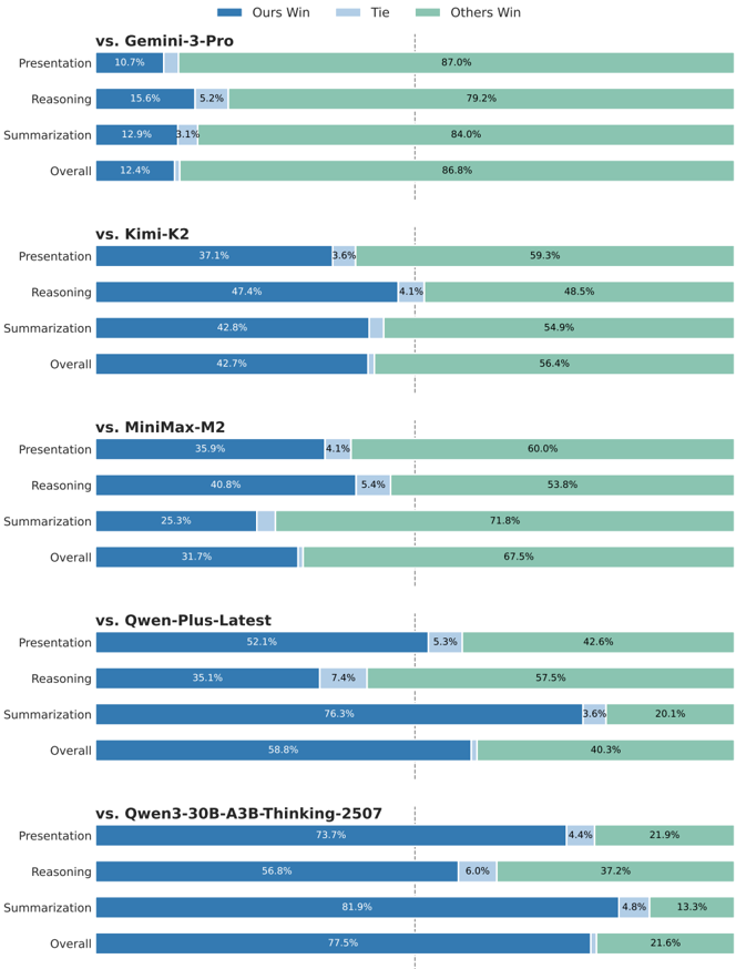## 3.2 Main Results Figure 6: Amap indomain online benchmark evaluation. <details> <summary>Image 7 Details</summary>  ### Visual Description ## Comparative Performance Bar Chart: Model Evaluation Results ### Overview This image displays a series of five horizontal stacked bar charts, each comparing the performance of a model (referred to as "Ours") against a different competitor model across three specific tasks (Presentation, Reasoning, Summarization) and an Overall score. The chart uses a consistent color-coded legend to represent the outcome of each comparison. ### Components/Axes * **Legend:** Located at the top center of the image. * **Dark Blue:** "Ours Win" * **Light Blue:** "Tie" * **Green:** "Others Win" * **Chart Structure:** Five vertically stacked panels, each with a header indicating the competitor model. * **Y-Axis (Left Side of Each Panel):** Lists the evaluation categories: "Presentation", "Reasoning", "Summarization", and "Overall". * **X-Axis (Implied):** Represents the percentage of evaluation outcomes, spanning from 0% to 100% across the width of each bar. * **Data Labels:** Percentage values are printed directly on or adjacent to their corresponding colored bar segments. ### Detailed Analysis The following data is extracted from each panel, reading from top to bottom. **Panel 1: vs. Gemini-3-Pro** * **Presentation:** Ours Win: 10.7%, Tie: (not visible, ~0%), Others Win: 87.0% * **Reasoning:** Ours Win: 15.6%, Tie: 5.2%, Others Win: 79.2% * **Summarization:** Ours Win: 12.9%, Tie: 3.1%, Others Win: 84.0% * **Overall:** Ours Win: 12.4%, Tie: (not visible, ~0%), Others Win: 86.8% **Panel 2: vs. Kimi-K2** * **Presentation:** Ours Win: 37.1%, Tie: 3.6%, Others Win: 59.3% * **Reasoning:** Ours Win: 47.4%, Tie: 4.1%, Others Win: 48.5% * **Summarization:** Ours Win: 42.8%, Tie: (not visible, ~0%), Others Win: 54.9% * **Overall:** Ours Win: 42.7%, Tie: (not visible, ~0%), Others Win: 56.4% **Panel 3: vs. MiniMax-M2** * **Presentation:** Ours Win: 35.9%, Tie: 4.1%, Others Win: 60.0% * **Reasoning:** Ours Win: 40.8%, Tie: 5.4%, Others Win: 53.8% * **Summarization:** Ours Win: 25.3%, Tie: (not visible, ~0%), Others Win: 71.8% * **Overall:** Ours Win: 31.7%, Tie: (not visible, ~0%), Others Win: 67.5% **Panel 4: vs. Qwen-Plus-Latest** * **Presentation:** Ours Win: 52.1%, Tie: 5.3%, Others Win: 42.6% * **Reasoning:** Ours Win: 35.1%, Tie: 7.4%, Others Win: 57.5% * **Summarization:** Ours Win: 76.3%, Tie: 3.6%, Others Win: 20.1% * **Overall:** Ours Win: 58.8%, Tie: (not visible, ~0%), Others Win: 40.3% **Panel 5: vs. Qwen3-30B-A3B-Thinking-2507** * **Presentation:** Ours Win: 73.7%, Tie: 4.4%, Others Win: 21.9% * **Reasoning:** Ours Win: 56.8%, Tie: 6.0%, Others Win: 37.2% * **Summarization:** Ours Win: 81.9%, Tie: 4.8%, Others Win: 13.3% * **Overall:** Ours Win: 77.5%, Tie: (not visible, ~0%), Others Win: 21.6% ### Key Observations 1. **Performance Gradient:** There is a clear gradient in "Ours" model performance across the competitors. It performs most poorly against Gemini-3-Pro (Overall: 12.4% win rate) and most strongly against Qwen3-30B-A3B-Thinking-2507 (Overall: 77.5% win rate). 2. **Task-Specific Strengths:** The "Ours" model shows a particularly strong performance in the **Summarization** task against the Qwen-based models (76.3% and 81.9% win rates). 3. **Low Tie Rates:** The "Tie" category (light blue) is consistently the smallest segment, often below 7%, indicating that evaluations typically result in a clear win for one model or the other. 4. **Consistent Losses vs. Gemini:** Against Gemini-3-Pro, "Ours" loses in the vast majority of comparisons across all tasks, with win rates never exceeding 15.6%. ### Interpretation This chart presents a benchmark evaluation, likely from a technical report or model card, demonstrating the relative strengths of the "Ours" model. The data suggests that the "Ours" model is not universally superior but has a competitive profile that varies significantly by opponent and task. * **Competitive Landscape:** The model appears to be positioned as a strong competitor to the Qwen series of models, especially in summarization tasks, while being outperformed by Gemini-3-Pro in this specific evaluation setup. * **Task Specialization:** The high win rates in Summarization against certain models could indicate a architectural or training data advantage in that specific capability. * **Purpose of Visualization:** The chart effectively communicates that model performance is not monolithic. It provides a nuanced view for technical audiences to understand where the "Ours" model excels and where it may require further development, aiding in informed model selection for specific use cases. The near-absence of ties suggests the evaluation methodology produces decisive results. </details> Amap Indomain online benchmark. The experimental results, as illustrated in Figure 6, demonstrate the superior performance and robustness of STAgent. Specifically, Compared with the baseline model, Qwen3-30B-A3B-Thinking-2507, STAgent demonstrates substantial improvements across all three evaluation dimensions. Notably, in terms of contextual summarization/extraction (win rate: 81.9%) and content presentation (win rate: 73.7%), our model exhibits a robust capability to accurately synthesize preceding information and effectively present solutions that align with user requirements. When compared to Qwen-Plus-Latest, while STAgent shows a performance gap in reasoning and planning, it achieves a marginal lead in presentation and a significant advantage in the summarization dimension. Regarding other models such as MiniMax-M2, Kimi-K2, and Gemini-3Pro-preview, a performance disparity persists across all three dimensions; we attribute this primarily to the constraints of model scale (30B), which limit the further enhancement of STAgent 's capabil- ities. Overall, these results validate the efficacy and promising potential of our proposed solution in strengthening tool invocation, response extraction, and summarization within map-based scenarios. Amap Indomain offline benchmark. As shown in Table 2, our model trained on top of Qwen330B achieves consistent improvements across all three subtasks, with gains of +11.7% (Multi-turn), +5.8% (Single-turn), and +26.1% (Unsolved) over the Qwen3-30B-thinking baseline. It also delivers a higher overall score ( 70.3 ) than substantially larger models such as DeepSeek R1 and Qwen3235B-Instruct. Notably, our model attains the best performance on the Multi-turn subtask ( 66.6 ) and the second-best performance on the Single-turn subtask ( 73.4 ), which further supports the effectiveness of our training pipeline. General domain evaluation. The main experimental results, summarized in Table 3, shows several key observation. Firstly, STAgent achieves a significant performance leap on the private domain benchmark, marking a substantial improvement over its initialization model, Qwen3-30BA3B-Thinking. Notably, STAgent surpasses larger-scale models, including Qwen3-235B-A22BThingking-2507 and DeepSeek-R1-0528, while comparable to Qwen3-235B-A22B-Instruct-2507. Secondly, STAgent shows a notable performance in Tool Use benchmarks, which suggests that models trained on our private domain tools possess a strong ability to generalize their tool-calling capabilities to other diverse functional domains. Finally, the model effectively maintains its high performance across public benchmarks for mathematics, coding, and general capabilities , proving that our domain-specific reinforcement learning process does not lead to a degradation of general-purpose performance or fundamental reasoning skills. Despite being a specialized model for the spatiotemporal domain, STAgent still achieves excellent performance in general domains while maintaining its strong in-domain capabilities, demonstrating the effectiveness of our training methodology. Table 2: Results on TravelBench, covering three subtasks: Multi-turn, Single-turn, and Unsolved. | Model | Multi-turn | Single-turn | Unsolved | Overall | |--------------------------|--------------|---------------|------------|-----------| | Deepseek R1-0528 | 34.3 | 76.1 | 83.7 | 64.7 | | Qwen3-235B-A22B-Ins-2507 | 60.1 | 69.7 | 80 | 69.9 | | Qwen3-235B-A22B-Th-2507 | 56.6 | 73.2 | 51.7 | 60.5 | | Qwen3-30B-A3B-Th-2507 | 59.6 | 69.4 | 56.3 | 61.8 | | Qwen3-14B | 47 | 57 | 54 | 52.7 | | Qwen3-4B | 42 | 42.1 | 73 | 52.4 | | STAgent | 66.6 | 73.4 | 71 | 70.3 | Table 3: Model performance evaluation across general and in-domain benchmarks. | Domain | Benchmark | Qwen3-4B- Thinking-2507 | Qwen3 14B | Qwen3-30B- A3B-2507 | Qwen3-235B- A22B-Ins-2507 | Qwen3-235B- A22B-Th-2507 | DeepSeek- R1-0528 | STAgent | ∆ (30B-A3B) | |-----------|------------------|---------------------------|-------------|-----------------------|-----------------------------|----------------------------|---------------------|-----------|---------------| | Tool Use | ACEBench | 71.7 | 69.8 | 75.7 | 75.6 | 75.7 | - | 75.3 | -0.4 | | | Tau2-Bench | 46.2 | 37.6 | 47.7 | 52.4 | 58.5 | 52.7 | 47 | -0.7 | | | BFCL V3 | 71.2 | 70.4 | 72.4 | 70.9 | 71.9 | 63.8 | 76.8 | 4.4 | | Math | AIME 24 | 83.8 | 79.3 | 91.3 | 80.8 | 93.8 | 91.4 | 90.2 | -0.9 | | Math | AIME 25 | 81.3 | 70.4 | 85 | 70.3 | 92.3 | 87.5 | 85.2 | 0.2 | | Coding | LiveCodeBench-v5 | 61.7 | 63.5 | 70.1 | 57.5 | 68.3 | - | 70.7 | 0.6 | | Coding | LiveCodeBench-v6 | 55.2 | 55.4 | 66 | 51.8 | 74.1 | 73.3 | 66.3 | 0.3 | | General | ArenaHard-v2.0 | 34.9 | 30.4 | 51.4 | 79.2 | 79.7 | - | 46.4 | -5 | | General | IFEval | 87.4 | 85.4 | 88.9 | 88.7 | 87.8 | 79.1 | 87.1 | -1.8 | | General | MMLU-Pro | 74 | 77.4 | 80.9 | 83 | 84.4 | 85.0 | 80.5 | -0.4 | | General | C-Eval | 72.3 | 87.5 | 87.1 | 90.7 | 92 | 91.5 | 87.9 | 0.8 | | In-domain | TravelBench | 60.8 | 52.7 | 60.2 | 69.9 | 60.5 | 64.7 | 70.3 | 10.1 | ## 4 Conclusion In this work, we present STAgent, a agentic model specifically designed to address the complex reasoning tasks within real-world spatio-temporal scenarios. A stable tool calling environment, highquality data curation, and a difficulty-aware training recipe collectively contribute to the model's performance. Specifically, we constructed a calling environment that supports tools across 10 distinct domains, enabling stable and highly concurrent operations. Furthermore, we curated a set of high-quality candidate queries from a massive corpus of real-world historical queries, employing an exceptionally low filtering ratio. Finally, we designed an SFT-guided RL training strategy to ensure the model's capabilities continuously improve throughout the training process. Empirical results demonstrate that STAgent, built on Qwen3-30B-A3B-thinking-2507, significantly outperforms models with larger parameter sizes on domain-specific benchmarks such as TravelBench, while maintaining strong generalization across general tasks. We believe this work not only provides a robust solution for spatio-temporal intelligence but also offers a scalable and effective paradigm for developing specialized agents in other complex, open-ended real-world environments. ## Author Contributions ## Project Leader Yulan Hu ## Core Contributors Xiangwen Zhang, Sheng Ouyang, Hao Yi, Lu Xu, Qinglin Lang, Lide Tan, Xiang Cheng ## Contributors Tianchen Ye, Zhicong Li, Ge Chen, Wenjin Yang, Zheng Pan, Shaopan Xiong, Siran Yang, Ju Huang, Yan Zhang, Jiamang Wang, Yong Liu, Yinfeng Huang, Ning Wang, Tucheng Lin, Xin Li, Ning Guo ## Acknowledgments We extend our sincere gratitude to the ROLL Wang et al. (2025) team for their exceptional support on the training infrastructure. Their asynchronous rollout and training strategy enabled a nearly 80% increase in training efficiency. We also thank Professor Yong Liu from the Gaoling School of Artificial Intelligence, Renmin University of China, for his insightful guidance on our SFT-guided RL training recipe. ## References - AIME. AIME problems and solutions. https://artofproblemsolving.com/wiki/ index.php/AIME\_Problems\_and\_Solutions , 2025. - Victor Barres, Honghua Dong, Soham Ray, Xujie Si, and Karthik Narasimhan. τ 2 -bench: Evaluating conversational agents in a dual-control environment, 2025. URL https://arxiv.org/abs/ 2506.07982 . - Song Bian, Minghao Yan, Anand Jayarajan, Gennady Pekhimenko, and Shivaram Venkataraman. What limits agentic systems efficiency? arXiv preprint arXiv:2510.16276 , 2025. - Collin Burns, Pavel Izmailov, Jan Hendrik Kirchner, Bowen Baker, Leo Gao, Leopold Aschenbrenner, Yining Chen, Adrien Ecoffet, Manas Joglekar, Jan Leike, et al. Weak-to-strong generalization: Eliciting strong capabilities with weak supervision. arXiv preprint arXiv:2312.09390 , 2023. - Chen Chen, Xinlong Hao, Weiwen Liu, Xu Huang, Xingshan Zeng, Shuai Yu, Dexun Li, Yuefeng Huang, Xiangcheng Liu, Wang Xinzhi, and Wu Liu. ACEBench: A comprehensive evaluation of LLM tool usage. In Christos Christodoulopoulos, Tanmoy Chakraborty, Carolyn Rose, and Violet Peng (eds.), Findings of the Association for Computational Linguistics: EMNLP 2025 , pp. 12970-12998, Suzhou, China, November 2025a. Association for Computational Linguistics. ISBN 979-8-89176-335-7. doi: 10.18653/v1/2025.findings-emnlp.697. URL https://aclanthology.org/2025.findings-emnlp.697/ . - Mingyang Chen, Linzhuang Sun, Tianpeng Li, Haoze Sun, Yijie Zhou, Chenzheng Zhu, Haofen Wang, Jeff Z Pan, Wen Zhang, Huajun Chen, et al. Learning to reason with search for llms via reinforcement learning. arXiv preprint arXiv:2503.19470 , 2025b. - Xiang Cheng, Yulan Hu, Xiangwen Zhang, Lu Xu, Zheng Pan, Xin Li, and Yong Liu. Travelbench: Areal-world benchmark for multi-turn and tool-augmented travel planning. 2025. URL https: //api.semanticscholar.org/CorpusID:284313793 . - Guanting Dong, Hangyu Mao, Kai Ma, Licheng Bao, Yifei Chen, Zhongyuan Wang, Zhongxia Chen, Jiazhen Du, Huiyang Wang, Fuzheng Zhang, et al. Agentic reinforced policy optimization. arXiv preprint arXiv:2507.19849 , 2025. - Zhibin Gou, Zhihong Shao, Yeyun Gong, Yelong Shen, Yujiu Yang, Minlie Huang, Nan Duan, and Weizhu Chen. Tora: A tool-integrated reasoning agent for mathematical problem solving. arXiv preprint arXiv:2309.17452 , 2023. - Anisha Gunjal, Anthony Wang, Elaine Lau, Vaskar Nath, Yunzhong He, Bing Liu, and Sean M Hendryx. Rubrics as rewards: Reinforcement learning beyond verifiable domains. In NeurIPS 2025 Workshop on Efficient Reasoning , 2025. - Helia Hashemi, Jason Eisner, Corby Rosset, Benjamin Van Durme, and Chris Kedzie. Llm-rubric: A multidimensional, calibrated approach to automated evaluation of natural language texts. In Proceedings of the 62nd Annual Meeting of the Association for Computational Linguistics (Volume 1: Long Papers) , pp. 13806-13834, 2024. - Yuzhen Huang, Yuzhuo Bai, Zhihao Zhu, Junlei Zhang, Jinghan Zhang, Tangjun Su, Junteng Liu, Chuancheng Lv, Yikai Zhang, Jiayi Lei, Yao Fu, Maosong Sun, and Junxian He. C-eval: A multi-level multi-discipline chinese evaluation suite for foundation models, 2023. URL https: //arxiv.org/abs/2305.08322 . - Naman Jain, King Han, Alex Gu, Wen-Ding Li, Fanjia Yan, Tianjun Zhang, Sida Wang, Armando Solar-Lezama, Koushik Sen, and Ion Stoica. Livecodebench: Holistic and contamination free evaluation of large language models for code, 2024. URL https://arxiv.org/abs/ 2403.07974 . - Mingcong Lei, Yiming Zhao, Ge Wang, Zhixin Mai, Shuguang Cui, Yatong Han, and Jinke Ren. Stma: A spatio-temporal memory agent for long-horizon embodied task planning, 2025. URL https://arxiv.org/abs/2502.10177 . - Ang Li, Zhihang Yuan, Yang Zhang, Shouda Liu, and Yisen Wang. Know when to explore: Difficulty-aware certainty as a guide for llm reinforcement learning. arXiv preprint arXiv:2509.00125 , 2025a. - Tianle Li, Wei-Lin Chiang, Evan Frick, Lisa Dunlap, Tianhao Wu, Banghua Zhu, Joseph E Gonzalez, and Ion Stoica. From crowdsourced data to high-quality benchmarks: Arena-hard and benchbuilder pipeline. arXiv preprint arXiv:2406.11939 , 2024. - Zhong-Zhi Li, Duzhen Zhang, Ming-Liang Zhang, Jiaxin Zhang, Zengyan Liu, Yuxuan Yao, Haotian Xu, Junhao Zheng, Pei-Jie Wang, Xiuyi Chen, et al. From system 1 to system 2: A survey of reasoning large language models. arXiv preprint arXiv:2502.17419 , 2025b. - Heng Lin and Zhongwen Xu. Understanding tool-integrated reasoning, 2025. URL https:// arxiv.org/abs/2508.19201 . - Aixin Liu, Aoxue Mei, Bangcai Lin, Bing Xue, Bingxuan Wang, Bingzheng Xu, Bochao Wu, Bowei Zhang, Chaofan Lin, Chen Dong, et al. Deepseek-v3. 2: Pushing the frontier of open large language models. arXiv preprint arXiv:2512.02556 , 2025. - Yansong Ning, Rui Liu, Jun Wang, Kai Chen, Wei Li, Jun Fang, Kan Zheng, Naiqiang Tan, and Hao Liu. Deeptravel: An end-to-end agentic reinforcement learning framework for autonomous travel planning agents. arXiv preprint arXiv:2509.21842 , 2025. - Shishir G Patil, Huanzhi Mao, Fanjia Yan, Charlie Cheng-Jie Ji, Vishnu Suresh, Ion Stoica, and Joseph E. Gonzalez. The berkeley function calling leaderboard (BFCL): From tool use to agentic evaluation of large language models. In Forty-second International Conference on Machine Learning , 2025. URL https://openreview.net/forum?id=2GmDdhBdDk . - Changle Qu, Sunhao Dai, Xiaochi Wei, Hengyi Cai, Shuaiqiang Wang, Dawei Yin, Jun Xu, and JiRong Wen. Tool learning with large language models: A survey. Frontiers of Computer Science , 19(8):198343, 2025. - Ning Shang, Yifei Liu, Yi Zhu, Li Lyna Zhang, Weijiang Xu, Xinyu Guan, Buze Zhang, Bingcheng Dong, Xudong Zhou, Bowen Zhang, et al. rstar2-agent: Agentic reasoning technical report. arXiv preprint arXiv:2508.20722 , 2025. - Zhihong Shao, Peiyi Wang, Qihao Zhu, Runxin Xu, Junxiao Song, Xiao Bi, Haowei Zhang, Mingchuan Zhang, YK Li, Yang Wu, et al. Deepseekmath: Pushing the limits of mathematical reasoning in open language models. arXiv preprint arXiv:2402.03300 , 2024. - Kimi Team, Yifan Bai, Yiping Bao, Guanduo Chen, Jiahao Chen, Ningxin Chen, Ruijue Chen, Yanru Chen, Yuankun Chen, Yutian Chen, et al. Kimi k2: Open agentic intelligence. arXiv preprint arXiv:2507.20534 , 2025. - Weixun Wang, Shaopan Xiong, Gengru Chen, Wei Gao, Sheng Guo, Yancheng He, Ju Huang, Jiaheng Liu, Zhendong Li, Xiaoyang Li, et al. Reinforcement learning optimization for largescale learning: An efficient and user-friendly scaling library. arXiv preprint arXiv:2506.06122 , 2025. - Yubo Wang, Xueguang Ma, Ge Zhang, Yuansheng Ni, Abhranil Chandra, Shiguang Guo, Weiming Ren, Aaran Arulraj, Xuan He, Ziyan Jiang, Tianle Li, Max Ku, Kai Wang, Alex Zhuang, Rongqi Fan, Xiang Yue, and Wenhu Chen. Mmlu-pro: A more robust and challenging multi-task language understanding benchmark, 2024. URL https://arxiv.org/abs/2406.01574 . - Jian Xie, Kai Zhang, Jiangjie Chen, Tinghui Zhu, Renze Lou, Yuandong Tian, Yanghua Xiao, and Yu Su. Travelplanner: A benchmark for real-world planning with language agents. arXiv preprint arXiv:2402.01622 , 2024. - Zhangchen Xu, Adriana Meza Soria, Shawn Tan, Anurag Roy, Ashish Sunil Agrawal, Radha Poovendran, and Rameswar Panda. Toucan: Synthesizing 1.5 m tool-agentic data from real-world mcp environments. arXiv preprint arXiv:2510.01179 , 2025. - An Yang, Anfeng Li, Baosong Yang, Beichen Zhang, Binyuan Hui, Bo Zheng, Bowen Yu, Chang Gao, Chengen Huang, Chenxu Lv, et al. Qwen3 technical report. arXiv preprint arXiv:2505.09388 , 2025. - Zhaochen Yu, Ling Yang, Jiaru Zou, Shuicheng Yan, and Mengdi Wang. Demystifying reinforcement learning in agentic reasoning. arXiv preprint arXiv:2510.11701 , 2025. - Aohan Zeng, Xin Lv, Qinkai Zheng, Zhenyu Hou, Bin Chen, Chengxing Xie, Cunxiang Wang, Da Yin, Hao Zeng, Jiajie Zhang, et al. Glm-4.5: Agentic, reasoning, and coding (arc) foundation models. arXiv preprint arXiv:2508.06471 , 2025. - Guibin Zhang, Hejia Geng, Xiaohang Yu, Zhenfei Yin, Zaibin Zhang, Zelin Tan, Heng Zhou, Zhongzhi Li, Xiangyuan Xue, Yijiang Li, et al. The landscape of agentic reinforcement learning for llms: A survey. arXiv preprint arXiv:2509.02547 , 2025. - Chujie Zheng, Shixuan Liu, Mingze Li, Xiong-Hui Chen, Bowen Yu, Chang Gao, Kai Dang, Yuqiong Liu, Rui Men, An Yang, et al. Group sequence policy optimization. arXiv preprint arXiv:2507.18071 , 2025a. - Haozhen Zheng, Beitong Tian, Mingyuan Wu, Zhenggang Tang, Klara Nahrstedt, and Alex Schwing. Spatio-temporal llm: Reasoning about environments and actions. arXiv preprint arXiv:2507.05258 , 2025b. - Jeffrey Zhou, Tianjian Lu, Swaroop Mishra, Siddhartha Brahma, Sujoy Basu, Yi Luan, Denny Zhou, and Le Hou. Instruction-following evaluation for large language models. arXiv preprint arXiv:2311.07911 , 2023. ## A Tool Schemas and Prompt Templates ## A.1 Tool schemas ## 1. Map & Navigation Tools - map search places : Searches for Points of Interest (POIs) based on keywords, categories, or addresses. Supports nearby search with customizable radius, administrative region filtering, and multiple sorting options (distance, rating, price). Returns rich metadata including ratings, prices, business hours, and user reviews. - map compute routes : Computes optimal routes from origin to destination with optional waypoints. Supports six transport modes: driving, walking, cycling, public transit, motorcycle, and truck. Provides optional real-time traffic awareness and route preferences (e.g., avoid tolls, prefer highways). - map search along route : Finds POIs within a buffer zone along a planned route, ideal for scenarios like 'find a gas station on my way home.' Automatically plans the base route and searches within the specified corridor. - map search central places : Locates places that are convenient for multiple parties by computing distance metrics to all origins. Supports three optimization strategies: balanced (overall optimal), minimize maximum distance (fairness-oriented), and minimize total distance (efficiency-oriented). - map search ranking list : Retrieves curated ranking lists such as 'Must-Eat List' or 'Black Pearl' for a specified category and region. Returns ranked POIs with detailed recommendation reasons and featured tags. ## 2. Travel & Transportation Tools - travel search flights : Searches domestic flight information between cities. Supports optional multi-day queries for price comparison across consecutive dates. Returns flight numbers, airlines, departure/arrival times, aircraft types, and price ranges. - travel search trains : Queries train and high-speed rail schedules between cities. Supports multi-day queries for schedule comparison. Returns train numbers, schedules, duration, stations, and ticket prices. ## 3. Weather Tools - weather current conditions : Retrieves real-time weather conditions for a specified location, including temperature, feels-like temperature, weather phenomena, wind direction/speed, and Air Quality Index (AQI). - weather forecast days : Provides multi-day weather forecasts (up to 5 additional days) for a given location. Supports both specific date queries and date range queries. ## 4. Information Retrieval Tools - web search : Performs open-domain web search for general knowledge, real-time news, historical events, and policy information that falls outside the spatio-tempora domain. ## A.2 User Instruction Annotation Prompt Template ``` # Amp User Instruction Annotation System # Role And Task ``` Listing 1: Prompt template used for user instruction classification. ``` ``` ``` ``` ## A.3 Difficulty Scoring Annotation Prompt Template ``` ``` Listing 2: Prompt template used for difficulty scoring. ``` ``` ``` ``` ## A.4 Reward Model Prompt Template The following prompt illustrates the dynamic evaluation logic used to score Amap Agent trajectories. The evaluator first classifies the task type to assign weights, checks strictly for hallucinations, and then provides a reasoned score. ``` ``` Listing 3: Prompt template with dynamic weighting and hallucination veto logic. ``` <dimension_presentation> <rationale>...</rationale> <rating>...</rating> </dimension_presentation> <final_score>/<final_score> </evaluation_report> ``` ## B Case Studies In this section, we conduct a case study to demonstrate our STAgent... ## B.1 Example 1: Multi-step Geospatial Reasoning (Route-based Search) ## Case Study: Route-based Dining Recommendation Query: 我 现 在在 海 口 的 云 洞 图 书 馆 ， 我 住 在 楠 丰 酒 店 ， 请 问 我 们 回 酒 店 的 路 上 有 什 么 好 吃 的 Intent: discovery.poi search.spatial optimized poi search ## Action Step 1: Entity Resolution - Tool: map search places (called twice in parallel) - Arguments: - -Query A: { 'query': ' 云 洞 图 书 馆 ', 'region': ' 海 口 市 ' } - -Query B: { 'query': ' 楠 丰 酒 店 ', 'region': ' 海 口 市 ' } - Observation: - -Origin: Cloud Cave Library ( 20 . 046661 , 110 . 316404 ) - -Destination: Nanfeng Hotel ( 20 . 026726 , 110 . 232278 ) ## Action Step 2: Search Along Route - Tool: map search along route - Arguments: { 'origin': P origin , 'destination': P dest. , 'query': ' 美 食 ', 'open now': true } - Observation: Found 49 places. Top results: 1. Gu Gu Gu Hainan Cuisine (Scenic View) 2. Tanmen Fisherman Seafood Hotpot 3. Kejia Ling Fusion Cuisine ## Response Generator: BLUF: 回 酒 店 路 上 有 多 个 美 食 选 择 ， 推 荐 以下 热 门 餐 厅 ， 均在 路 线 附 近 且 营 业中 。 食 ## /utensils 推 荐 美 地 点 1. 古 姑姑 · 品 质 海 南 菜 私 房 餐 厅 - 位 置 ： 秀 英 区 滨 海 大 道 假 日 海 滩游 客 中 心 二 楼 - 营 业 时 间 ： 10:00-13:30, 16:30-21:30 - 特 色 ： 270 ° 观 海 视 野 ， 海 南 菜 经 典 ， 秀 英 区 观 景 餐 厅 榜 第 3 名 - 提 示 ： 适 合 晚 餐 ， 海 景 + 美 食 双 重 享 受 。 2. 潭 门 渔 夫 海 鲜 火 锅 - 位 置 ： 龙 华区 上 邦 百 汇 城 1 号 楼 3 楼 - 营 业 时 间 ： 11:30-23:00 - 特 色 ： 海 鲜 火 锅 ， 海 口 市 海 鲜 火 锅 榜 第 2 名 - 提 示 ： 适 合 多 人 聚 餐 ， 食 材 新 鲜 。 3. 客家 岭 湘 粤 融 合 菜 - 位 置 ： 秀 英 区 滨 海 大 道 80 号 幸 福 里 小 区 - 营 业 时 间 ： 10:00-14:00, 17:00-21:30 - 特 色 ： 客家 + 粤 菜 融 合 ， 丽 晶 路 美 食 榜 第 3 名 - 提 示 ： 适 合 偏 好 清 淡 口 味 的 旅 客 。 ## /map-marker-alt 下一 步 建 议 - 导 航 ： 使 用 高 德 地 图 导 航 至 ' 古 姑姑 ' 或 ' 潭 门 渔 夫 ' 。 - 提 示 ： 若 时 间 较 晚 ， 建 议 选 择 营 业 至 23:00 的 潭 门 渔 夫 。 - /car 路 线 提 示 ： 从云 洞 图 书 馆 出 发 沿 滨 海 大 道 行 驶 ， 上 述 餐 厅 均在 路 线 两 侧 2 公 里 内 ( 驾 车 约 10-15 分 钟 ) 。 ## B.2 Example 2: Complex Multi-Point Itinerary Assessment ## Case Study: Multi-stop Route Feasibility Check Query: 广 州 海 珠 广 场 去 广 东 博 物 馆 ， 陈 家 祠 ， 珠 江 夜 游 ， 同 福 路 ， 永 庆 坊 ， 沙 面 岛 路 线 方 便 么 Intent: planning and decision.itinerary planning.simple route itinerary ## Action Step 1: Batch Entity Resolution - Tool: map search places (called 7 times in parallel) - Observation: Successfully resolved coordinates for all locations: - -Origin: Haizhu Square ( 23 . 114 , 113 . 266 - ) - -Intermediates: Chen Clan Ancestral Hall (Liwan), Tianzi Wharf (Yuexiu), etc. - -Destination: Guangdong Museum ( 23 . 106 , 113 . 244 ) ## Action Step 2: Route Computation - Tool: map compute routes - Arguments: { 'origin': P Haizhu , 'destination': P Museum , 'intermediates': [ P Chen , P Tianzi ... ], 'modes': ['driving'] } - Observation: - -Metrics: 38.3 km - 2h 28m 84 Traffic Lights . - -Congestion: 7.1 km congestion, specifically at Dongfeng West Rd (+6 min delay). ## Response Generator (Rendered Output): ## BLUF: 路 线 可 行 但 效 率 较 低 （ 需 2.5 小 时 ， 84 个 红绿 灯 ） 。 建 议 避 开 晚 高 峰 或 改 用 地 铁 。 ## /traffic-light 路 况 核 心 数 据 - 耗 时 预 警 ： 全 程 小 途 约 2 时 28 分 钟 ， 经 **84 个 红绿 灯 ** 。 - 拥 堵 黑 点 ： ** 东 风 西 路 ** 拥 堵 严 重 ， 预 计 延 误 6 分 钟 以上 。 - 路 线 特 点 ： 跨 度 大 （ 天 河 ↔ 荔 湾 ）， 晚 高 峰 (17:00-19:00) 通 行 困 难 。 ## /route 行 程 优 化 建 议 1. 时 间 管 理 ： 建 议 **17:00 前 出 发 ** 或 调 整 至 20:00 后 游 览 沙 面 夜 景 。 2. 顺 路 整 合 ： 永 庆 坊 与 沙 面 岛 同 属 荔 湾 区 ， 建 议 连 续 游 览 。 3. 交 通 替 代 ： /subway 若 侧 重 效 率 ， 推 荐 ** 地 铁 3 号 线 ** 至 珠 江 新 城 ， 比 驾 车 节 省 约 40 分 钟 。 4. /clock 小 贴 士 ： 珠 江 夜 游 建 议 安 排 在 傍 晚 ， 大 沙 头 码 头 可 顺 路 衔 接 行 程 。 ## B.3 Example 3: Long-distance Travel Planning with Amenities ## Case Study: Cross-province Self-driving Guide Query: 给 我 出 一份 攻 略 ， 重 庆市 区 自 驾 到 海 口 走 哪 条 路 ？ 然 后 的 高 速 路费 以 及 中 途 休 息 的 话 推 荐 休 息 的 地 方 Intent: planning and decision.itinerary planning.short trip itinerary ## Action Step 1: Entity Resolution - Tool: map search places (called twice) - Observation: - -Origin: Chongqing ( 29 . 562 , 106 . 551 ) - -Destination: Haikou ( 20 . 046 , 110 . 200 ) ## Action Step 2: Route Computation - Tool: map compute routes - Arguments: { 'origin': P CQ , 'destination': P HK , 'modes': ['driving'] } - Observation: - -Metrics: 1381.7 km / 14h 43m / Toll: 819 CNY. - -Key Roads: G75 Lanhai Expy, G15 Shenhai Expy. ## Action Step 3: Amenities Search Along Route - Tool: map search along route - Arguments: { 'query': ' 加 油 站 , 餐 厅 ', 'origin': P CQ , 'destination': P HK , 'transport mode': 'driving' } - Observation: Found 3 stops (KFC Drive-thru, Duyun Service Area Buffet, etc.) ## Response Generator (Rendered Output): BLUF: 全 程 约 1382 公 里 ， 需 14.5 小 时 ， 高 速 费 约 819 元 。 建 议 在 贵 州 都 匀 段 进 行 中 途 休 整 。 概 ## /road 路 线 况 - 核 心 指 标 ： 1381.7 km - 14h 43m - 819 ( 含 过 路费 ) - 主 要 高 速 ： G75 兰 海 高 速 → G7522 贵 北 高 速 → G15 沈 海 高 速 - 关 键 节 点 ： G75 巴 南 收 费 站 ( 起 点 ) ... 徐 闻 港 收 费 站 ( 终 点 ) ## /coffee 中 途 休 息 推 荐 1. 都 匀 加 油 站 自 助 餐 厅 ( 贵 州 段 ) 位 于 G75 高 速 路 口 -自 助 中 餐 -适 合 长 途 补 给 2. 肯 德 基 车 速 取 ( 重 庆 出 发 段 ) 南 岸 加 油 站 旁 -西 式快 餐 -适 合 出 发 前 用 餐 2. /ship 特 别 提 示 ： 路 线 包 含 ** 琼 州 海 峡 轮 渡 ** ( 徐 闻 港 -新 海 港 ) ， 船 票 需 另 行 购 买 ， 建 议 提 前 在 网 上 预 约 过 海 。 ## B.4 Example 4: EV Long-distance Route & Charging Planning ## Case Study: EV Inter-provincial Travel Guide Query: 从 南 通 开 新 能 源 车 到 张 家 口 万 龙 滑 雪 场 ， 续 航 500 公 里 ， 求 规 划 行 车 路 线 和 沿 途 充 电 方 案 Intent: planning and decision.route planning ## Action Step 1: Entity Resolution - Tool: map search places (x2) - Observation: - Origin: Nantong City ( 31 . 981 , 120 . 894 ) - Dest: Wanlong Ski Resort ( 40 . 963 , 115 . 398 ) ## Action Step 2: Route Computation - Tool: map compute routes - Arguments: { 'origin': P NT , 'destination': P WL , 'modes': ['driving'] } - Observation: - -Metrics: 1303 km - 14h 55m. - Highways: G15 Shenhai → G25 Changshen → G2 Jinghu. ## Action Step 3: Charging Infrastructure Search - Tool: map search along route - Arguments: { 'query': ' 充 电 站 ', 'transport mode': 'driving' } - Observation: Found 50+ stations. Selected strategic stops at 200km and 500km intervals (e.g., Binhai SA, Linshu SA). ## Response Generator: BLUF: 全 程 1305 公 里 ， 需 14 小 时 。 基 于 500km 续 航 ， 建 议 **3 次 充 电 ** ， 尤 其 需 确 认 河 北 段 补 能 设 施 。 ## /route 路 线 概 况 - 核 心 指 标 ： 明 1305 km - 13h 59m - 日 08:08 到 达 - 主 要 高 速 ： G18 荣 乌 → G25 长 深 → S3801 京 礼 - 拥 堵 预 警 ： S15 京 津 高 速 拥 堵 1.2km ， 预 计 延 误 10 分 钟 。 ## /charging-station 充 电 补 能 规 划 | # | 地 点 | 距 离 起 点 | 操 作 建 议 | |-----|---------------------|-----------|-------------------| | 1 | 南 通 理 想 超 充 站 | 0 km | 出 发 前 充 满 | | 2 | 沂 南 东 服 务 区 ( 山 东 ) | ≈ 500 km | 充 至 80% ， 避 免 排 队 | | 3 | 万 龙 滑 雪 场 ( 河 北 ) | ≈ 1300 km | 需 现 场 确 认 | /exclamation-triangle 风 险 提 示 ： 工 具 检 索 显 示 ** 河 北 段 高 速 暂 无 明 确 充 电 站 ** 。 强 烈 建 议 在 山 东临 沂 充 满 电 ， 并 提 前 联 系 滑 雪 场 （ 如 游 客 中 心 / 地 下 停 车 场 ） 确 认 目的 地 充 电 设 施 。 ## /map-signs 下一 步 行 动 - 发 前 - 出 ： 下 载 离 线 地 图 ， 避 免 高 速 信 号 中 断 。 - 途 中 ： 每 行 驶 300km 检 查 电 量 ， 保 持 30% 以上 余 量 。 - 抵 达 ： 导 航 搜 索 ' 万 龙 滑 雪 场 2 号 地 下 停 车 场 ' 寻 找 充 电 桩 ## C Training Dynamic Figure 7 shows the progression of the reward signal over the process of the training iterations. Figure 7: Training reward. <details> <summary>Image 8 Details</summary>  ### Visual Description ## Line Chart with Shaded Area: Reward Value vs. Training Steps ### Overview The image displays a line chart plotting "Reward Value" against "Training Steps," typical of a reinforcement learning or optimization process. The chart shows a single data series with high volatility but a clear upward trend, with the area under the line shaded in light blue. ### Components/Axes * **X-Axis (Horizontal):** * **Label:** "Training Steps" * **Scale:** Linear scale from 0 to 300. * **Major Tick Marks:** 0, 50, 100, 150, 200, 250, 300. * **Y-Axis (Vertical):** * **Label:** "Reward Value" * **Scale:** Linear scale from 0.0 to 0.6. * **Major Tick Marks:** 0.0, 0.1, 0.2, 0.3, 0.4, 0.5, 0.6. * **Data Series:** * A single, jagged blue line representing the reward value at each training step. * A light blue shaded area fills the space between the data line and the x-axis (y=0). * **Legend:** No separate legend is present. The single data series is implicitly defined by the line and its label on the y-axis. * **Grid:** Faint, light gray grid lines are present for both major x and y ticks. ### Detailed Analysis * **Trend Verification:** The primary data series (blue line) exhibits a strong, positive, upward trend from left to right. The line is highly volatile, with frequent sharp peaks and troughs, but the overall slope is consistently positive. * **Data Point Extraction (Approximate Values):** * **Start (Step 0):** Reward Value ≈ 0.15. * **Step 50:** Reward Value fluctuates between ≈ 0.12 and ≈ 0.25. * **Step 100:** Reward Value fluctuates between ≈ 0.20 and ≈ 0.35. * **Step 150:** Reward Value fluctuates between ≈ 0.35 and ≈ 0.45. * **Step 200:** Reward Value fluctuates between ≈ 0.45 and ≈ 0.55. * **Peak (≈ Step 220):** The highest observed point reaches a Reward Value of approximately 0.62. * **End (Step 300):** Reward Value fluctuates between ≈ 0.55 and ≈ 0.60. * **Volatility:** The magnitude of fluctuations appears relatively consistent throughout the training, though the absolute range of the fluctuations increases as the mean reward increases (e.g., fluctuations of ±0.05 at step 50 vs. ±0.05 at step 250, but on a higher baseline). ### Key Observations 1. **Consistent Improvement:** Despite significant noise, the agent or model demonstrates consistent learning, as evidenced by the clear upward trend in reward over 300 training steps. 2. **High Variance:** The process is highly stochastic. The reward value at any given step is not a smooth function of the step number, indicating significant variability in performance between consecutive evaluations or episodes. 3. **Potential Plateau:** In the final 50-100 steps (from ~200 to 300), the rate of improvement appears to slow. The trend line becomes less steep, suggesting the learning process may be approaching an asymptote or plateau. 4. **Notable Outlier:** A single, prominent spike occurs just after step 200 (≈220), where the reward sharply exceeds 0.6 before returning to the prevailing trend. This could represent a particularly successful episode or a measurement anomaly. ### Interpretation This chart is a classic learning curve for a machine learning model, most likely in a reinforcement learning context. The "Reward Value" is the objective function being maximized, and "Training Steps" represent iterations of the learning algorithm. * **What the data suggests:** The model is successfully learning the task. The positive correlation between training steps and reward indicates that the policy or parameters are being updated in a beneficial direction. The high variance is typical in RL, where exploration, environmental stochasticity, and delayed rewards cause performance to fluctuate. * **How elements relate:** The x-axis (time/effort) drives the increase in the y-axis (performance). The shaded area emphasizes the cumulative or sustained nature of the reward, though it is primarily a visual aid here. * **Notable Patterns & Anomalies:** The slowing improvement in the later stages is a critical observation. It may indicate that the model is nearing its performance capacity given the current hyperparameters, or that the learning rate may need adjustment (e.g., decay) for fine-tuning. The single high spike is an outlier that warrants investigation—it could be a lucky run or hint at a region of the state space with exceptionally high reward that the model has not yet learned to reliably access. * **Peircean Investigation:** The chart is an **index** of the learning process (it directly points to the fact that learning occurred) and a **symbol** of model performance (we interpret the upward trend as "good"). The volatility is a **quale** of the training process itself, representing its inherent instability. The plateau is a **hypothesis** suggesting a limit has been reached, prompting the next investigative question: "What change is needed to break through this apparent ceiling?" </details> 。