2601.03559

# DiffCoT: Diffusion-styled Chain-of-Thought Reasoning in LLMs ## Abstract Chain-of-Thought (CoT) reasoning improves multi-step mathematical problem solving in large language models but remains vulnerable to exposure bias and error accumulation, as early mistakes propagate irreversibly through autoregressive decoding. In this work, we propose DiffCoT, a diffusion-styled CoT framework that reformulates CoT reasoning as an iterative denoising process. DiffCoT integrates diffusion principles at the reasoning-step level via a sliding-window mechanism, enabling unified generation and retrospective correction of intermediate steps while preserving token-level autoregression. To maintain causal consistency, we further introduce a causal diffusion noise schedule that respects the temporal structure of reasoning chains. Extensive experiments on three multi-step CoT reasoning benchmarks across diverse model backbones demonstrate that DiffCoT consistently outperforms existing CoT preference optimization methods, yielding improved robustness and error-correction capability in CoT reasoning. DiffCoT: Diffusion-styled Chain-of-Thought Reasoning in LLMs Shidong Cao 1, Hongzhan Lin 1, Yuxuan Gu 2, Ziyang Luo 1, Jing Ma 1 1 Hong Kong Baptist University 2 Harbin Institute of Technology {cssdcao,cshzlin,majing}@comp.hkbu.edu.hk ## 1 Introduction Large Language Models (LLMs) (Brown et al., 2020; Achiam et al., 2023; Guo et al., 2025) have marked a major breakthrough in natural language processing, achieving competitive performance across a wide range of mathematical reasoning tasks. A widely adopted technique in LLMs, Chain-of-Thought (CoT) reasoning (Wei et al., 2022; Kojima et al., 2022), enhances mathematical problem-solving by decomposing tasks into step-by-step intermediate reasoning. However, CoT reasoning is highly sensitive to potential errors, where mistakes introduced in the early stages can propagate through later steps, often leading to incorrect final answers (Wang et al., 2023; Lyu et al., 2023). This highlights a central research challenge: reducing errors by guiding LLMs to identify and follow reliable reasoning paths in long thought chains. Recent work has sought to optimize the exploration of reasoning branches in LLMs to reduce errors in CoT, by coupling generation with external critics or search procedures, such as Monte Carlo Tree Search (MCTS), to prune faulty trajectories (Li et al., 2024; Qin et al., 2024; Xi et al., 2024). In contrast, Preference Optimization (PO) methods (Lai et al., 2024; Zhang et al., 2024; Xu et al., 2025) aligned the policy with implicit preferences distilled from reasoning chains, so that decoding itself favors correct trajectories rather than relying on post-hoc filtering. However, beyond the substantial inference-time overhead of MCTS, these methods share a fundamental limitation that motivates rethinking of the CoT paradigm. Specifically, they all execute CoT reasoning in a strictly step-by-step manner, with each step conditioned on previous ones. Under static teacher-forcing supervision, the model is exposed only to correct prefixes during training, whereas at inference time the prefixes may contain errors that accumulate across steps, resulting in exposure bias that commonly plagues autoregressive generation (Bengio et al., 2015) and imitation learning (Ross et al., 2011). <details> <summary>x1.png Details</summary>  ### Visual Description ## Diagram: Comparison of Chain-of-Thought (CoT) Reasoning Methods ### Overview The image is a technical diagram comparing two approaches to solving multi-step reasoning problems, specifically a math word problem. The left side, labeled **(a) Existing Methods for CoT**, illustrates a branching, tree-like process where multiple reasoning paths are explored, some leading to errors. The right side, labeled **(b) DiffCoT**, illustrates a linear, iterative refinement process that uses "Diffusion" and "AR" (Autoregressive) steps to correct errors and arrive at the final answer. A central text block contains the problem statement and the step-by-step solutions generated by both methods. ### Components/Axes * **Main Sections:** The diagram is split into three primary regions: 1. **Left Panel (a):** A flowchart titled "Existing Methods for CoT". 2. **Center Panel:** A text block containing the problem and solution steps. 3. **Right Panel (b):** A flowchart titled "DiffCoT". * **Flowchart Elements:** * **Nodes:** Numbered circles (1, 2, 3, 4) representing reasoning steps. * **Arrows:** Indicate the flow of reasoning. Solid arrows show the primary path. Dashed arrows in (b) indicate the diffusion process. * **Symbols:** A yellow warning triangle (⚠) and a red cross (❌) indicate errors or problematic steps. * **Legends:** * **Bottom-Left Legend (for panel a):** * Blue square: "Chosen response" * Light blue square: "Rejected response" * Red square: "Error response" * **Bottom-Right Legend (for panel b):** * Light blue square: "Initial response" * Medium blue square: "Refined response" * Dark blue square: "Final response" * **Text Block Content:** * **Question:** "Mrs. Snyder used to spend 40% of her monthly income on rent and utilities. Her salary was recently increased by $600 so now her rent and utilities only amount to 25% of her monthly income. How much was her previous monthly income?" * **Step 1:** "Let the previous monthly income be x. The increased income is x + 600." * **Step 2:** "25% of x + 600 is the rent and utilities now. 25% of x + 600 = 0.25(x + 600)" * **Existing Methods for CoT Steps:** * Step 3: "0.4x = 25% of x + 600. Subtract 25% of x from both sides to get 0.15x = 600." * Step 4: "Rearrange the equation to get x = 4000." * **DiffCoT Steps:** * Step 3: "0.4x = 25% of x + 600. Subtract 25% of x from both sides to get 0.15x = 600." * Step 4: "Rearrange the equation to get x = 4000." * **Refined Steps (below DiffCoT):** * Refined Step 3: "0.25(x + 600) = 0.4x. Solve for x" * Refined Step 4: "0.15x = 150. Solve for x" * Refined Step 4 (final): "0.15x = 150. Divide both sides by 0.15. x = 1000" ### Detailed Analysis **Panel (a) - Existing Methods for CoT:** * **Structure:** A tree diagram starting from a single "Input" node. It branches into three parallel paths at Step 1, each leading to a Step 2 node. * **Path Analysis:** * **Leftmost Path:** Steps 1 -> 2 -> 3 -> 4. The Step 4 node is colored red with a red cross (❌), indicating an "Error response" per the legend. * **Center Path:** Steps 1 -> 2 -> 3. The Step 3 node has a yellow warning triangle (⚠). This path does not proceed to Step 4. * **Rightmost Path:** Steps 1 -> 2 -> 3 -> 4. The Step 4 node is light blue, indicating a "Rejected response". * **Interpretation:** This panel depicts a method that generates multiple reasoning chains. One chain contains an error (red), one is flagged as problematic but incomplete (warning), and one is completed but ultimately rejected (light blue). The "chosen response" (dark blue) is not explicitly shown in the final step, implying the method may fail to select a correct answer from the generated paths. **Panel (b) - DiffCoT:** * **Structure:** A primarily linear flow from "Input" through Steps 1, 2, and 3. * **Process Flow:** 1. **Initial Path:** Input -> 1 -> 2 -> 3. The Step 3 node has a yellow warning triangle (⚠). 2. **Diffusion & Correction:** A dashed arrow labeled "Diffusion" points from the problematic Step 3 node to a new Step 3 node. This new node is connected via a dashed red arrow labeled "correct" to a Step 4 node marked with a red cross (❌). This suggests the diffusion process identifies and targets an error. 3. **AR Refinement:** A solid blue arrow labeled "AR" (Autoregressive) points from the initial Step 3 node to a refined Step 3 node (medium blue). This node then leads to a final Step 4 node (dark blue). * **Legend Correlation:** The nodes in the final, successful path (Input -> 1 -> 2 -> Refined 3 -> Final 4) correspond to the "Initial," "Refined," and "Final" response colors in the bottom-right legend. ### Key Observations 1. **Structural Contrast:** Existing methods use a parallel, branching search (a tree), while DiffCoT uses a sequential, iterative refinement process (a line with correction loops). 2. **Error Handling:** In (a), errors (red nodes) are terminal outcomes of a branch. In (b), errors (warning triangle, red cross) are intermediate states that trigger a corrective "diffusion" process. 3. **Solution Path:** Both methods initially generate the same incorrect equation in Step 3 (`0.15x = 600`), leading to the wrong answer `x = 4000`. However, DiffCoT's refinement process corrects this to the proper equation (`0.15x = 150`) and the correct answer (`x = 1000`). 4. **Spatial Layout:** The problem statement and solution steps are centrally located, acting as the shared context for both method diagrams. The legends are placed directly below their respective panels for clear association. ### Interpretation This diagram argues for the superiority of the **DiffCoT** method over existing Chain-of-Thought approaches for complex reasoning tasks. * **The Problem with Existing CoT:** Panel (a) suggests that simply generating multiple reasoning paths is inefficient and unreliable. It can produce erroneous, incomplete, or rejected chains without a clear mechanism to identify and converge on the correct solution. The chosen path may still be wrong. * **The DiffCoT Solution:** Panel (b) presents a more robust, self-correcting pipeline. It doesn't just generate paths; it incorporates a **diffusion-based error detection and correction mechanism**. When a step is flagged (warning triangle), the model doesn't abandon the path. Instead, it uses diffusion to "imagine" or explore corrections, explicitly identifying the erroneous step (red cross) and then using autoregressive refinement to generate a corrected step and proceed to the final, accurate answer. * **Underlying Message:** The core innovation is treating reasoning not as a single forward pass or a random search, but as a **denoising or refinement process**. By modeling the generation of reasoning steps as a diffusion process, the system can iteratively "clean up" errors in the thought process, leading to more accurate and reliable final answers. The central math problem serves as a concrete example where this refinement leads to the correct answer (`1000`) versus the incorrect one (`4000`). 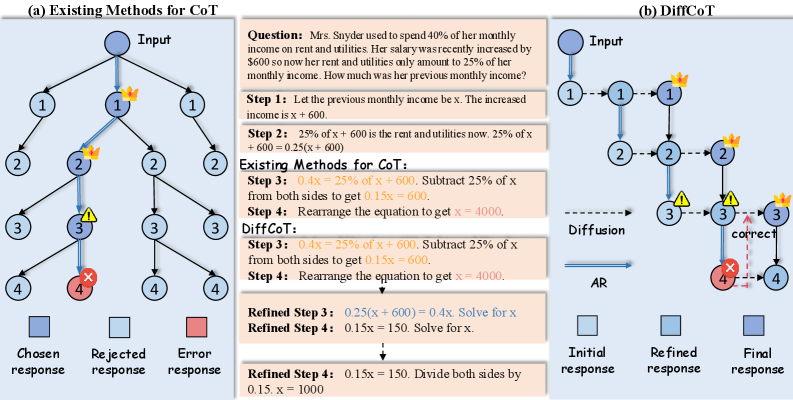</details> Figure 1: Comparison of our proposed DiffCoT with existing CoT reasoning approaches: (a) Existing step-by-step CoT Reasoning methods adopt teacher-forcing training, where each step depends on the ground-truth output of the previous one. At inference time, this assumption breaks, causing exposure bias and leading to error accumulation. (b) DiffCoT performs CoT reasoning along both the noise (diffusion) and temporal (autoregressive) dimensions, enabling iterative correction of prior mistakes and effectively mitigating exposure bias. To mitigate the limitations above, we formulate CoT reasoning as a globally revisable trajectory, in which intermediate steps are not fixed once generated but can be adaptively corrected in light of later context. Rather than defining reasoning as a strictly forward, prefix-conditioned process driven by human priors (see Fig. 1), our method jointly models all reasoning steps within a diffusion paradigm (Dhariwal and Nichol, 2021), enabling robust reasoning under realistic noise from a global perspective with long-term revision guided by future signals. Starting from a corrupted or noisy reasoning chain, the entire reasoning trajectory can be iteratively updated, where intermediate revisions and forward progression are seamlessly integrated into a unified refinement process. By unifying iterative revision and forward continuation within the same diffusion-based refinement process, our design philosophy aim to reduce the discrepancy between training-time supervision and inference-time reasoning dynamics, leading to more stable reasoning behavior during inference. To this end, we propose Diff usion-Styled C hain o f T hought, DiffCoT, which integrates diffusion principles into the CoT framework to mitigate the exposure bias of static teacher-forcing and address the pointwise and local-step supervision issues of prior preference optimization solutions. Specifically, 1) DiffCoT modifies only the step-level generation strategy while preserving token-level autoregression, making it straightforward to fine-tune from existing autoregressive models. 2) By incorporating sliding windows and causal noise masks, DiffCoT unifies generation and revision within a versatile framework, to balance autoregressive and diffusion-styled reasoning. 3) Moreover, DiffCoT employs sentence-level noise injection to convert the reasoning paradigm into iterative denoising, progressively refining corrupted trajectories into coherent chains of thought, which captures the distributional evolution of reasoning errors to enable recovery from diverse and compounding mistakes. Altogether, DiffCoT could establish a unified and adaptive paradigm to CoT reasoning in LLMs. Our contributions are summarized as follows: - We propose DiffCoT, a novel diffusion-styled CoT framework that reformulates multi-step reasoning as an iterative denoising process, effectively mitigating exposure bias and error accumulation in autoregressive CoT reasoning. - We introduce a step-level diffusion-based learning strategy that unifies generation and revision through a sliding-window mechanism, enabling retrospective correction of earlier reasoning steps while preserving token-level autoregression. - We design a causal noise schedule that explicitly encodes the temporal dependency of reasoning steps, balancing global error correction with the causal structure required for coherent reasoning. - Extensive experiments on three public mathematical reasoning benchmarks demonstrate that DiffCoT outperforms State-of-The-Art (SoTA) PO methods, yielding robust gains and substantially improved error-correction capability in CoT. ## 2 Preliminaries #### Chain-of-Thought Reasoning Given a question prompt $p$ , the CoT paradigm (Wei et al., 2022) explicitly unfolds the reasoning process into a sequence of reasoning steps $s_1:K$ whose final element $s_K$ corresponds to the answer $a$ . The conditional distribution of a complete reasoning trace can be expressed as: $$ p_θ(s_1:K\mid p)=∏_t=1^Kπ_θ(s_k\mid p,s_<k), \tag{1} $$ where $s_k$ denotes the $k$ -th reasoning step, $k≤ K$ is the step budget, and $π_θ$ is the Auto-Regressive (AR) policy, i.e., the conditional distribution over the next step given the prompt $p$ and the previously generated steps. On annotated CoT data $(p,s_1:K)$ , the model is trained by maximizing the conditional likelihood: $$ L_CoT=-∑_k=1^K\logπ_θ(s_k\mid p,s_<k). \tag{2} $$ #### Diffusion Models Diffusion models (Dhariwal and Nichol, 2021) define a generative framework where data samples are gradually corrupted into a tractable noise distribution through a forward process, and a model is trained to approximate the corresponding reverse process. Let $x_0∼φ(x_0)$ denote a data sample from real data distribution $φ$ . The forward process produces a sequence $\{x_t\}_t=1^T$ by applying a noise operator $O$ at each step: $$ x_t=D(x_t-1,η_t), t=1,\dots,T, \tag{3} $$ where $t$ denotes the diffusion step index, $η_t$ is a noise variable. $O$ could be a deterministic or structured corruption operator. The generative process is defined by learning a parameterized reverse transition $p_θ(x_t-1\mid x_t)$ that reconstructs the original sample through stepwise denoising. Training minimizes the discrepancy between the predicted $\hat{x}_t-1=f_θ(x_t,t)$ and the ground-truth corrupted data $x_t-1$ obtained from the forward process: $$ \begin{split}&L_Diffusion=\\ &E_x_{0∼φ(x_0), t∼\{1,\dots,T\}}\Big[\ell\big(f_θ(x_t,t), x_t-1\big)\Big],\end{split} \tag{4} $$ where $f_θ(x_t,t)$ predicts the reconstruction of $x_t-1$ from $x_t$ , $\ell(·,·)$ is a reconstruction loss. In inference, sampling begins from $x_T$ and iteratively applies the learned reverse transitions until $x_0$ is obtained. ## 3 Methodology During CoT reasoning, LLMs are typically trained only on correct trajectories (Wei et al., 2022), while at inference time they may condition on erroneous intermediate steps (Lyu et al., 2023). Moreover, step-wise optimization focuses on local alignment and ignores future signals within the reasoning trajectory, limiting global consistency (Zhang et al., 2024). Together, these issues lead to error accumulation (Yoon et al., 2025; Chen et al., 2024a), motivating a rethinking of CoT reasoning under preference optimization. To address these issues, we argue that effective CoT reasoning requires trajectory-level revision to enforce global consistency and recover from corrupted intermediate steps. As error accumulation leads to noisy reasoning chains at inference time, a mechanism for global recovery becomes essential (Lyu et al., 2023; Wang et al., 2023). Motivated by the robustness of diffusion models in reconstructing structured data from noise (Ho et al., 2020; Li et al., 2022), we aim to develop a diffusion-styled preference optimization paradigm to reformulate CoT reasoning. 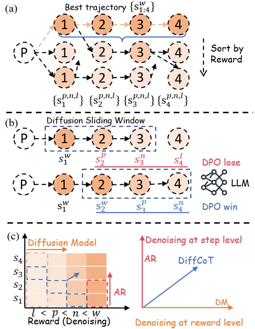To this end, we propose Diff usion-styled C hain o f T hought (DiffCoT), which models CoT reasoning in a diffusion-styled framework. We first present a step-level forward noising process for CoT using reward-ranked candidates (§ 3.1), and then apply a diffusion sliding window to iteratively denoise past steps while generating new ones (§ 3.2). We further introduce causal diffusion noise to strengthen causal consistency across reasoning steps (§ 3.3). An overview is shown in Figure 2. ### 3.1 Diffusion-Styled Noising for CoT In this section, we design a diffusion-styled forward noising process for CoT reasoning at the reasoning-step level, where step-level noise is induced by ranking candidate responses for the same step according to their reward scores. Previous preference optimization methods overlooked the distribution between high-reward and low-reward reasoning steps and relied on isolated step-wise adjustments that fail to mitigate the exposure bias inherent in teacher forcing. To this end, in our principle, higher-reward candidates are treated as lower-noise reasoning states, while lower-reward candidates correspond to progressively higher-noise states in the forward process. This ranking forms a progression from clean to corrupted reasoning states under diffusion-styled noise, enabling distribution-aware modeling of reasoning steps. Specifically, we implement forward noising by first collecting CoT reasoning trajectories for each question to construct the training set $D$ . As shown in Fig. 2 (a), given a question prompt $p$ , we follow the standard CoT data generation process by employing MCTS (Browne et al., 2012), to gradually build a search tree for step-by-step solution exploration. The root corresponds to $p$ , and each child node represents an intermediate step $s$ . A complete path from the root to a terminal node $s_K$ yields a trajectory $tra=p⊕ s_1⊕ s_2⊕\dots⊕ s_K$ , where each step $s_k$ is annotated with its reward $r(s_k)$ . In contrast to conventional CoT trajectory construction Zhang et al. (2024), at each step $k$ we collect several candidate responses. These responses are scored using either an external reward model or rollout-based success rates. In our forward noising view, the candidate with the highest reward, denoted as $s^σ^{0=w}_k$ , is regarded as the lowest-noise state for step $k$ , and the remaining candidates are ordered by their rewards to form $\{s^σ^{1:T}_k\}$ , which we interpret as states with gradually increasing noise. Step-level noise is thus measured by the deviation of lower-reward responses from this best trajectory, indicating the corruption level at the step granularity. This design ensures that the final generation remains coherent while providing a set of forward diffusion states for subsequent denoising and preference optimization. Under this step-level forward noising, DiffCoT defines a diffusion-styled distribution that spans low-noise to high-noise reasoning states (Chen et al., 2025). Note that our data construction does not distinguish between “correct” and “incorrect” labels at the collection stage as in (Lai et al., 2025); instead, it uniformly gathers diverse responses for each step throughout the entire trajectory. This global view provides distribution-aware data to support both generation and refinement. In this way, error patterns are implicitly encoded in trajectory-level modeling, allowing robust reasoning without additional manual annotations of corrective steps. ### 3.2 Reformulating CoT Reasoning as Denoising <details> <summary>figs/method.png Details</summary>  ### Visual Description ## Diagram: Diffusion-Based Trajectory Optimization and Reward-Level Denoising ### Overview The image is a three-part technical diagram (labeled a, b, c) illustrating a machine learning methodology that combines diffusion models, autoregressive (AR) generation, and Direct Preference Optimization (DPO) for optimizing sequences or trajectories. It visually explains a process for selecting, comparing, and denoising sequences based on reward levels. ### Components/Axes The diagram is divided into three horizontal panels: * **(a) Top Panel:** Shows the generation and sorting of multiple trajectories from a starting point `P`. * **(b) Middle Panel:** Illustrates a "Diffusion Sliding Window" mechanism applied to two different trajectories, linking them to DPO outcomes. * **(c) Bottom Panel:** Contains two sub-charts. * **Left Chart:** A 2D grid/heatmap with axes for "Reward (Denoising)" and step sequence (`s1` to `s4`). * **Right Chart:** A 2D coordinate system with axes for "Denoising at step level" (AR) and "Denoising at reward level" (DM). **Key Labels and Notation:** * **Nodes:** Circles containing numbers `1`, `2`, `3`, `4` represent steps in a sequence. * **Starting Point:** A dashed circle labeled `P`. * **Trajectory Notation:** * `{s_{1:4}^w}`: The "Best trajectory" (highlighted in orange). * `{s_1^{p,n,l}}, {s_2^{p,n,l}}, {s_3^{p,n,l}}, {s_4^{p,n,l}}`: Other generated trajectories. * **Superscript Legend (Reward Levels):** `w` (best), `p` (preferred), `n` (neutral), `l` (least preferred). This is explicitly shown in the x-axis of the left chart in (c): `l < p < n < w`. * **Process Labels:** * "Sort by Reward" (with a downward arrow) in panel (a). * "Diffusion Sliding Window" in panel (b). * "DPO lose" (red text) and "DPO win" (blue text) next to an "LLM" icon in panel (b). * "Diffusion Model" (orange arrow) and "AR" (red arrow) in the left chart of (c). * "Denoising at step level" (AR, red axis) and "Denoising at reward level" (DM, orange axis) in the right chart of (c). * "DiffCoT" (blue arrow/line) in the right chart of (c). ### Detailed Analysis #### Panel (a): Trajectory Generation and Sorting * **Flow:** From a single prompt `P`, multiple sequences of 4 steps are generated. * **Best Trajectory:** The top sequence `{s_{1:4}^w}` is highlighted with orange nodes and a blue bracket, indicating it has the highest reward (`w`). * **Sorting:** Below the best trajectory, two other sequences are shown. A dashed arrow labeled "Sort by Reward" points downward, implying these sequences have lower rewards (likely `p`, `n`, or `l` as per the notation below them). * **Spatial Grounding:** The best trajectory is positioned at the top. The "Sort by Reward" label and arrow are on the right side, aligned vertically with the lower trajectories. #### Panel (b): Diffusion Sliding Window and DPO * **Mechanism:** A dashed blue rectangle labeled "Diffusion Sliding Window" moves across the sequence steps. * **Top Row (DPO lose):** The window covers steps 1-3 (`s1^w, s2^p, s3^n`). Step 4 (`s4^l`) is outside the window. This configuration is associated with "DPO lose" (red text). * **Bottom Row (DPO win):** The window covers steps 2-4 (`s2^w, s3^p, s4^n`). Step 1 (`s1^w`) is outside the window. This configuration is associated with "DPO win" (blue text). * **Interpretation:** This suggests that the choice of which steps are included in the diffusion window (the context for denoising/generation) affects the outcome of the DPO comparison, with one window placement leading to a "win" and the other to a "lose". #### Panel (c): Denoising Paradigms **Left Chart (Reward-Step Grid):** * **Axes:** * **X-axis (Reward/Denoising):** Ordered categories `l < p < n < w`. * **Y-axis (Steps):** Sequence steps `s1, s2, s3, s4`. * **Data Representation:** A grid of colored squares (shades of orange). The color intensity likely represents a value (e.g., probability, reward). * **Trends/Arrows:** * An orange arrow labeled "Diffusion Model" points horizontally to the right, indicating diffusion operates across reward levels at a given step. * A red arrow labeled "AR" (Autoregressive) points vertically upward, indicating AR generation proceeds step-by-step at a given reward level. * A blue dashed arrow points diagonally from the lower-left (`s1, l`) to the upper-right (`s4, w`), suggesting a path of improvement or the target trajectory. **Right Chart (Denoising Space):** * **Axes:** * **X-axis:** "Denoising at reward level" (DM - Diffusion Model). * **Y-axis:** "Denoising at step level" (AR - Autoregressive). * **Data Series:** A single blue line labeled "DiffCoT" originating from the origin (0,0) and sloping upward to the right at approximately a 45-degree angle. * **Trend:** The "DiffCoT" line shows a direct, positive correlation between denoising at the reward level and denoising at the step level. It represents a method that combines both paradigms. ### Key Observations 1. **Hierarchical Reward Structure:** The superscripts (`w, p, n, l`) establish a clear ranking of trajectory quality, which is central to the sorting and DPO processes. 2. **Sliding Window Importance:** Panel (b) highlights that the *context window* for diffusion is a critical design choice, directly influencing preference optimization outcomes (win/lose). 3. **Dual Denoising Axes:** Panel (c) formally decomposes the generation process into two orthogonal dimensions: step-wise (AR) and reward-wise (Diffusion). The "DiffCoT" method is presented as operating in the combined space of both. 4. **Visual Coding:** Colors are used consistently: orange for diffusion/best trajectories, red for AR/DPO lose, blue for DPO win/ DiffCoT/ sliding window. ### Interpretation This diagram outlines a framework, likely for training or guiding Large Language Models (LLMs), that integrates diffusion models with reinforcement learning from human feedback (RLHF) via DPO. * **What it suggests:** The core idea is to move beyond simple autoregressive next-token prediction. Instead, it proposes generating multiple candidate trajectories (a), ranking them by reward, and then using a diffusion process that operates over a sliding window of steps (b) to refine sequences. The DPO comparison ("win"/"lose") provides the learning signal to improve this refinement process. * **How elements relate:** Panel (a) is the data generation and ranking step. Panel (b) is the core algorithmic innovation—the diffusion window—that acts on the ranked data. Panel (c) provides the theoretical framing, positioning the proposed "DiffCoT" method as a hybrid that performs denoising simultaneously in the step dimension (like traditional AR models) and the reward/dimension (like diffusion models), potentially offering more controllable and higher-quality generation. * **Notable Anomalies/Insights:** The "DPO win" configuration in (b) uses a window shifted *forward* in the sequence (steps 2-4) compared to the "lose" configuration (steps 1-3). This might imply that for preference optimization, having the model focus on refining the *later* parts of a sequence, given good earlier context, is more effective than refining the beginning. The diagonal "DiffCoT" line in (c) posits that optimal denoising requires a balanced progression in both step and reward spaces, rather than excelling in only one. </details> Figure 2: DiffCoT Framework and Training Data Construction: (a) Step-level forward noising: MCTS-based data generation defines step-level noise by reward-ranking multiple candidates, yielding states ranging from clean to corrupted. (b) Sliding-window denoising: a diffusion sliding window refines previously generated CoT steps while producing the next step in an autoregressive manner. (c) Causal diffusion noise: a step-dependent schedule assigns stronger noise to later steps to encode the causal order of the reasoning chain. In this section, our DiffCoT framework reformulates CoT reasoning beyond the teacher-forcing paradigm as a diffusion-styled denoising process to mitigate exposure bias at inference time. To couple this with the autoregressive nature of CoT, we introduce a diffusion sliding-window mechanism that operates directly on the CoT reasoning process. Within this sliding window, previously generated CoT steps are progressively denoised from high-noise toward low-noise reasoning states, thereby facilitating self-correction, while advancing the window naturally aligns with the autoregressive generation of subsequent CoT steps. Thus, instead of costly training a separate diffusion language model from scratch, we leverage diffusion-styled data to efficiently fine-tune pre-trained LLM $π$ for CoT reasoning. Specifically, for the iterative denoising process, the model $π$ takes the question prompt $p$ together with the preceding reasoning steps $s_1:k$ as input. To enable variable-length generation when applying diffusion to thought chains while integrating generation with self-correction, the model maintains a diffusion sliding window of size $m$ and stride $n$ . At denoising iteration $t$ , the window containing previously generated CoT steps $\{s_k-m^σ,\dots,s_k^σ\}$ is updated to a lower-noise version $\{s_k-m^σ^{\prime},\dots,s_k^σ^{\prime}\}$ , where $σ=σ_k^(t)$ is defined as a function of the step index $k$ and the denoising iteration $t$ , while $σ$ and $σ^\prime$ denote the noise levels before and after refinement, respectively. Simultaneously, as the window shifts forward by one step, the model predicts the next step $s_k+1^σ$ , initialized at a high-noise state. Iterating this denoising process eventually yields a clean trajectory $s_1:K^σ^0$ : $$ π_θ\big(p, s_1:k^ σ\big) ↦ \underbrace{s_k-m:k^ σ^{\prime}}_refined past ⊕ \underbrace{s_k+1^ σ}_predicted future . \tag{5} $$ An illustration of the denoising process is shown in Fig. 2 (b). In sequence modeling, teacher-forcing next-token prediction can be viewed as masking along the reasoning-step axis $s$ , whereas diffusion corresponds to masking along the noise axis $σ$ , where $σ^T$ approaches pure white noise after $T$ iterations. To unify both views, we denote $s_k^σ$ as the $k$ -th CoT step under noise level $σ$ , where $σ$ is instantiated as $σ_k^t$ , i.e., the diffusion noise strength assigned to the $k$ -th step at denoising iteration $t$ . Building on the above reasoning process, we now introduce the training objective in DiffCoT. Our goal is to optimize a model $π_θ$ that takes the question prompt $p$ together with the preceding reasoning steps $s_1:k$ as input. We construct the win sequence $s_k-m:k+1^w$ by combining the denoised steps $\{s_k-m^σ^{\prime},\dots,s_k^σ^{\prime}\}$ with a lower-noise variant of $s_k+1^σ_k+1^{\prime}$ . Similarly, the lose sequence $s_k-m:k+1^l$ is formed by combining the unrefined steps $\{s_k-m^σ,\dots,s_k^σ\}$ with the highest-noise variant of $s_k+1^σ_k+1$ . The prefix condition is the past text $s_1:k-1$ . To optimize the LLM on this preference pair, we adopt the Direct Preference Optimization (DPO) loss (Rafailov et al., 2023): $$ \begin{split}L_i(π_θ;π_\textrm{ref})=-\logφ\Big(&β\log\frac{π_θ(s_:k+1^w\mid p,s_1:k)}{π_\textrm{ref}(s_:k+1^w\mid p,s_1:k)}\\ -β\log&\frac{π_θ(s_:k+1^l\mid p,s_1:k)}{π_\textrm{ref}(s_:k+1^l\mid p,s_1:k)}\Big),\end{split} \tag{6} $$ where $s_:k+1$ denotes the subsequence $s_k-m:k+1$ , $φ(·)$ denotes the sigmoid function, and $β$ is a factor controlling the strength of the preference signal. Note that our conditional prefix $s_1:k-1^σ$ differs from that used in standard DPO: instead of being composed exclusively of preferred (i.e., clean) steps, it combines clean steps from $1$ to $k-m$ with noisy steps within the sliding window. In this manner, the hybrid construction could alleviate the exposure bias by training the model to make preference-consistent updates even when conditioned on partially corrupted reasoning prefixes. ### 3.3 Causal Diffusion Noise Modeling CoT reasoning with diffusion poses a significant challenge to causality. Conventional full-sequence diffusion models are inherently non-causal (Ho et al., 2020; Dhariwal and Nichol, 2021), which contrasts sharply with the causal nature of CoT reasoning. While our backbone $π$ retains an AR token-level generation process, prior studies on diffusion models indicate that relying solely on the model’s ability to capture causality is inadequate, especially when reasoning must be performed over noisy or perturbed data (Li et al., 2022). Inspired by Diffusion Forcing (Chen et al., 2024a), as shown in Fig. 2 (c), we leverage noise as a mechanism to inject causal priors into diffusion sliding window.In conventional full-sequence diffusion, the noise strength $σ^(t)$ depends solely on the denoising iteration $t$ and is shared across all tokens. Such uniform noise injection is ill-suited for CoT reasoning, as it limits the model’s ability to capture step-wise causal dependencies. To overcome this, we redefine the noise schedule as $σ^t_k$ , a joint function of reasoning step $k$ and iteration $t$ (see § 3.2). Within the diffusion sliding window, $σ^t_k$ follows a progressive schedule, where earlier steps are perturbed with weaker noise, while later steps are perturbed with stronger noise. The noise schedule is formally defined as follows: $$ \begin{split}&F(s_j-m+1,…,s_j;j)=\\ &\big(s_j-m+1^σ^0, s_j-m+2^σ^1, …, s_j^σ^{T}\big),\end{split} \tag{7} $$ where the diffusion sliding window has size $m$ and stride $1$ , and at the $j$ -th denoising iteration the window advances to generate $s_j$ . In this manner, our framework could better stabilize the causal chain and enhance self-correction in subsequent reasoning steps even if the current step is erroneous. ## 4 Experiment | GSM8K SVAMP M-L1 | 37.2 49.6 31.3 | 39.3 50.1 33.4 | 37.6 49.4 32.2 | 37.7 48.8 31.5 | 36.1 48.6 33.8 | 38.1 48.4 32.0 | 39.6 50.4 34.3 | 65.5 83.5 61.1 | 64.3 84.9 62.0 | 65.7 84.2 60.1 | 65.1 82.7 60.8 | 64.9 85.2 61.7 | 65.9 85.9 63.0 | 66.2 85.5 63.6 | 62.0 80.1 51.2 | 64.0 80.7 52.4 | 61.8 82.3 51.8 | 63.0 80.3 51.6 | 63.3 79.4 51.8 | 64.7 83.0 52.7 | 65.4 83.2 53.3 | | --- | --- | --- | --- | --- | --- | --- | --- | --- | --- | --- | --- | --- | --- | --- | --- | --- | --- | --- | --- | --- | --- | | M-L2 | 18.4 | 18.5 | 18.1 | 17.9 | 19.3 | 17.6 | 19.5 | 39.1 | 39.2 | 38.4 | 38.7 | 39.9 | 37.1 | 39.3 | 31.9 | 34.0 | 32.6 | 33.1 | 35.7 | 34.2 | 35.3 | | M-L3 | 12.5 | 13.2 | 12.6 | 12.9 | 12.6 | 13.7 | 14.2 | 25.2 | 26.1 | 25.3 | 25.5 | 26.2 | 25.8 | 26.9 | 16.0 | 17.0 | 16.2 | 16.4 | 17.2 | 17.9 | 18.0 | | M-L4 | 5.9 | 6.1 | 6.6 | 6.4 | 6.7 | 7.6 | 8.0 | 16.5 | 15.0 | 15.5 | 15.6 | 15.8 | 17.4 | 17.5 | 9.0 | 10.2 | 8.3 | 8.5 | 8.9 | 9.9 | 10.5 | | M-L5 | 1.9 | 2.3 | 1.4 | 2.9 | 3.0 | 3.1 | 3.3 | 4.4 | 5.4 | 5.2 | 3.7 | 4.2 | 4.7 | 5.5 | 1.0 | 1.2 | 0.7 | 0.7 | 2.4 | 1.4 | 2.9 | Table 1: Test accuracy (%) on GSM8K, SVAMP, and MATH. M-L1 to M-L5 denote different difficulty levels in the MATH dataset, where L1 is the easiest and L5 is the most challenging, while Step denotes Step-DPO and FStep denotes Full-Step-DPO. The best and second results are in bold and underlined. ### 4.1 Settings #### Models and Datasets We conduct experiments on three representative backbone models: Llama3-8B (Touvron et al., 2023), Qwen3-8B (Yang et al., 2025), and Qwen3-4B (Yang et al., 2025). We primarily evaluate our DiffCoT on three public mathematical reasoning benchmarks, specifically GSM8K (Cobbe et al., 2021), SVAMP (Patel et al., 2021), and MATH (Hendrycks et al., 2021). The MATH is divided into five difficulty levels, as defined in the original dataset. More data statistics and preparation are provided in Appendix § A. #### Baselines We compare DiffCoT with the following SoTA baselines: 1) CoT (Wei et al., 2022): generates step-by-step reasoning before the final answer, evaluated with greedy decoding. 2) ToT (Yao et al., 2023): explores multiple reasoning paths via tree search. 3) TS-SFT (Feng et al., 2023): applies supervised fine-tuning on reasoning paths obtained from ToT. 4) CPO (Zhang et al., 2024): performs preference optimization at the step level, directly aligning intermediate reasoning steps via contrastive pairs. 5) Step-DPO (Lai et al., 2025): step-level preference optimization by explicitly collecting erroneous steps and applying preference optimization to correct them. 6) Full-Step-DPO (Xu et al., 2025): further generalizes step-wise optimization to the entire reasoning trajectory. More implementation details regarding model training and data construction are provided in Appendix § B. ### 4.2 Main Results As shown in Table 1, DiffCoT can be directly applied to modern instruction-tuned language models, such as Qwen3 and Llama3, via standard fine-tuning. This design enables seamless integration into existing training pipelines and allows DiffCoT to deliver consistent performance improvements across models of varying sizes, demonstrating strong scalability across different base models. From the result, we can observe that: 1) Baselines guided by LLM self-verification signals, such as CPO and ToT, exhibit notable instability across models and datasets. For example, when applied to Qwen3-8B, CPO results in performance degradation on the MATH-1 dataset while achieving competitive performance on SVAMP, indicating sensitivity to both model and task distributions. 2) Step-level preference learning baselines, including Step-DPO and Full-Step-DPO, generally achieve great improvements but still suffer from occasional performance drops under certain settings. This suggests that relying solely on local step-wise optimization may not be sufficient to ensure stable reasoning behavior across diverse evaluation scenarios. 3) Overall, DiffCoT consistently outperforms existing PO approaches across the majority of benchmarks and evaluation settings considered. Although it does not achieve the single best result in every individual setting, such as on SVAMP with the Qwen3-8B backbone, where Full-Step-DPO attains slightly higher accuracy, DiffCoT consistently ranks among the top-performing methods across all settings. Moreover, the improvements achieved by DiffCoT are substantial in magnitude and stable across different model sizes and datasets, highlighting its robustness and reliability. ### 4.3 Ablation Study To validate the effectiveness of the proposed DiffCoT method, we perform an ablation study on its key components. We select two representative base language models from different model families with varied sizes, Llama3-8B and Qwen3-4B, and evaluate them on two general mathematical reasoning benchmarks, GSM8K and SVAMP. To investigate the impact of incorporating diffusion into CoT reasoning, we evaluate various window sizes to explore how this factor influences the model’s performance. Specifically, when the diffusion window size and stride are set to 1, our approach essentially degenerates into an AR method, albeit with differently constructed prefixes. On the other hand, when the sliding diffusion window and stride are set to the number of steps $K$ , the method reverts to a purely diffusion-based approach. As shown in Table 2, it can be observed that performance degrades when the window size and stride is set to 1 or when it becomes too large. We attribute this phenomenon to a trade-off between causal connectivity and error-correction capability. Strengthening the ability to revise earlier steps often comes at the expense of weakening top-down causal reasoning. When the model operates entirely in AR mode, it exhibits the strongest causal reasoning ability but suffers from exposure bias during testing. In contrast, when the model fully adopts the diffusion mode, an excessively long window introduces noise: it disrupts the structural coherence of reasoning and prolonged denoising fluctuations undermine the causal nature of inference. | Llama3-8B - window size, stride=1 - window size, stride= $K$ | 39.6 36.3 -3.3 30.3 -9.3 | 50.4 48.3 -2.1 42.6 -7.8 | | --- | --- | --- | | - causal noise | 35.5 -4.1 | 48.2 -2.2 | | Qwen3-4B | 65.4 | 83.2 | | - window size, stride=1 | 63.0 -2.4 | 80.2 -3.0 | | - window size, stride= $K$ | 56.7 -8.7 | 73.9 -9.3 | | - causal noise | 61.9 -3.5 | 79.1 -4.1 | Table 2: Ablative results on the general datasets GSM8K and SVAMP, where $K$ is the number of reasoning steps. Numbers shown in the upper-right corner of each cell indicate the relative change in accuracy rate compared to the full DiffCoT model. We further conduct an ablation study to verify the effectiveness of the causal diffusion noise. Specifically, we disrupt our proposed noise scheduling by randomly shuffling the data order used for noising, instead of following the accuracy-based progression. This modification effectively breaks the causal structure of the noise. Results in Table 2 show that this ablation leads to substantial performance degradation across different models and datasets, demonstrating that our causal noise scheduling is a critical component of DiffCoT. 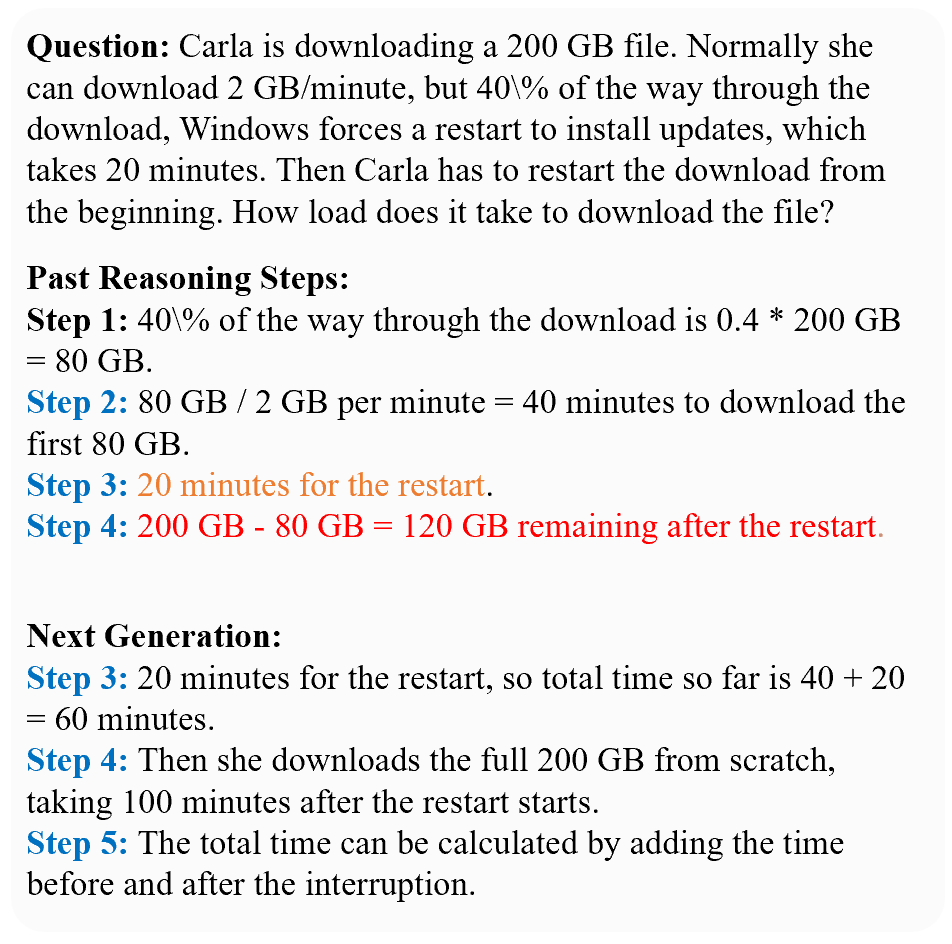### 4.4 Analysis #### Case Study To further illustrate the model’s robustness to accumulated imperfections in intermediate reasoning, we present qualitative case studies that contrast effective and suboptimal reasoning trajectories. In particular, we focus on challenging examples in which the model introduces semantically irrelevant or weakly informative steps at an early stage of reasoning. Although such steps are not necessarily incorrect in isolation, they tend to accumulate and hinder progress toward the correct solution under standard step-by-step reasoning. As shown in Fig. 3, DiffCoT is able to progressively refine earlier reasoning steps through the diffusion process. Instead of rigidly committing to the initial reasoning prefix, the model gradually improves previously generated steps while producing subsequent ones, effectively revising semantically unhelpful content introduced earlier in the trajectory. This allows the model to move away from locally coherent but globally suboptimal reasoning paths and ultimately reach the correct solution. It highlights a key distinction between DiffCoT and conventional autoregressive reasoning. While autoregressive models tend to propagate early semantic noise forward without revision, DiffCoT leverages its denoising dynamics to refine the entire reasoning trajectory, including previously generated steps, resulting in more robust and globally consistent reasoning behavior. <details> <summary>figs/case.png Details</summary>  ### Visual Description ## Screenshot: Math Problem and Reasoning Steps ### Overview The image is a screenshot of a digital document or interface displaying a word problem about a file download interruption, followed by two sections of step-by-step reasoning labeled "Past Reasoning Steps" and "Next Generation." The text is presented in a clean, sans-serif font on a light background. The content is entirely textual, with no charts, diagrams, or embedded images. ### Content Details The text is transcribed below exactly as it appears, including formatting and potential typos. **Question:** Carla is downloading a 200 GB file. Normally she can download 2 GB/minute, but 40\% of the way through the download, Windows forces a restart to install updates, which takes 20 minutes. Then Carla has to restart the download from the beginning. How load does it take to download the file? **Past Reasoning Steps:** **Step 1:** 40\% of the way through the download is 0.4 * 200 GB = 80 GB. **Step 2:** 80 GB / 2 GB per minute = 40 minutes to download the first 80 GB. **Step 3:** 20 minutes for the restart. *(This line is in orange text.)* **Step 4:** 200 GB - 80 GB = 120 GB remaining after the restart. *(This line is in red text.)* **Next Generation:** **Step 3:** 20 minutes for the restart, so total time so far is 40 + 20 = 60 minutes. **Step 4:** Then she downloads the full 200 GB from scratch, taking 100 minutes after the restart starts. **Step 5:** The total time can be calculated by adding the time before and after the interruption. ### Key Observations 1. **Textual Structure:** The content is organized into three clear sections: the problem statement, an initial set of reasoning steps, and a subsequent set of steps labeled "Next Generation." 2. **Formatting and Emphasis:** The headings "Question:", "Past Reasoning Steps:", and "Next Generation:" are in bold. Within the "Past Reasoning Steps," Steps 3 and 4 are highlighted in orange and red text, respectively, which may indicate a correction, a point of error, or a step requiring special attention. 3. **Potential Typo:** The question ends with "How load does it take...", which is likely a typographical error for "How long does it take...". 4. **Logical Flow:** The "Past Reasoning Steps" calculate the time for the first 40% of the download and the restart duration but stop after noting the remaining data. The "Next Generation" steps appear to continue or correct the logic by accounting for the total elapsed time before the restart and then adding the time to re-download the entire file from the beginning. ### Interpretation The image presents a mathematical word problem and two stages of a solution process. The "Past Reasoning Steps" correctly break down the initial phase of the problem but are incomplete, as they do not calculate the total time. The "Next Generation" steps logically extend the solution by: 1. Summing the time for the first partial download (40 minutes) and the restart (20 minutes) to get 60 minutes elapsed. 2. Recognizing that after the restart, the download must start over from 0 GB, requiring a full 200 GB download at 2 GB/minute, which takes 100 minutes. 3. Stating the final step to sum these two time periods (60 + 100 minutes) for the total. The use of color in the "Past Reasoning Steps" (orange for the restart time, red for the remaining data) might be an editorial marker highlighting where the initial reasoning was either correct but insufficient (orange) or where a critical piece of information was identified but not yet acted upon (red). The "Next Generation" section then acts as the completed, correct solution path. The core insight is that an interruption forcing a restart from the beginning significantly increases the total download time beyond the simple sum of the initial download and the restart delay. </details> Figure 3: Example illustrating how DiffCoT modifies early-stage reasoning shift steps. The steps highlighted in blue represent the diffusion sliding window. <details> <summary>x2.png Details</summary>  ### Visual Description ## Line Charts: Model Accuracy vs. Noise Intensity ### Overview The image displays three horizontally arranged line charts comparing the performance of two methods, **DiffCoT** and **Full-Step DPO**, across three different language models (Llama3-8B, Qwen3-8B, Qwen3-4B). Each chart plots model accuracy (Acc%) against an increasing "Noise Intensity Coefficient ω". The consistent visual pattern shows that accuracy for both methods decreases as noise increases, but DiffCoT consistently maintains higher accuracy than Full-Step DPO. ### Components/Axes * **Titles (Top of each chart):** "Llama3-8B" (left), "Qwen3-8B" (center), "Qwen3-4B" (right). * **X-Axis (All charts):** Label: "Noise Intensity Coefficient ω". Ticks/Markers: 0, 0.1, 0.2, 0.3, 0.4. * **Y-Axis (All charts):** Label: "Acc(%)". Scale varies per chart. * **Legend (Bottom of each chart):** Located centrally below the x-axis label. Contains two entries: * Blue line with square markers: "DiffCoT" * Orange line with diamond markers: "Full-Step DPO" ### Detailed Analysis **Chart 1: Llama3-8B (Left)** * **Y-Axis Scale:** 15 to 40, in increments of 5. * **Data Series & Trends:** * **DiffCoT (Blue, Squares):** Starts at ~38% (ω=0). Slopes downward steadily. Points (approximate): (0.1, ~34%), (0.2, ~30%), (0.3, ~25%), (0.4, ~19%). * **Full-Step DPO (Orange, Diamonds):** Starts at the same point as DiffCoT, ~38% (ω=0). Slopes downward more steeply than DiffCoT. Points (approximate): (0.1, ~33%), (0.2, ~26%), (0.3, ~21%), (0.4, ~15%). * **Relationship:** The gap between the two lines widens as ω increases, with DiffCoT maintaining a clear advantage. **Chart 2: Qwen3-8B (Center)** * **Y-Axis Scale:** 40 to 70, in increments of 5. * **Data Series & Trends:** * **DiffCoT (Blue, Squares):** Starts at ~67% (ω=0). Slopes downward. Points (approximate): (0.1, ~62%), (0.2, ~57%), (0.3, ~49%), (0.4, ~42%). * **Full-Step DPO (Orange, Diamonds):** Starts at the same point, ~67% (ω=0). Slopes downward more steeply. Points (approximate): (0.1, ~62%), (0.2, ~54%), (0.3, ~45%), (0.4, ~40%). * **Relationship:** Similar to the first chart, DiffCoT degrades more gracefully. The lines are nearly identical at ω=0.1 but diverge significantly thereafter. **Chart 3: Qwen3-4B (Right)** * **Y-Axis Scale:** 35 to 65, in increments of 5. * **Data Series & Trends:** * **DiffCoT (Blue, Squares):** Starts at ~65% (ω=0). Slopes downward. Points (approximate): (0.1, ~60%), (0.2, ~54%), (0.3, ~47%), (0.4, ~41%). * **Full-Step DPO (Orange, Diamonds):** Starts at the same point, ~65% (ω=0). Slopes downward more steeply. Points (approximate): (0.1, ~59%), (0.2, ~51%), (0.3, ~44%), (0.4, ~38%). * **Relationship:** The pattern holds. DiffCoT's line is consistently above Full-Step DPO's line for all ω > 0. ### Key Observations 1. **Universal Negative Correlation:** For all three models and both methods, accuracy (Acc%) has a strong, negative, near-linear correlation with the Noise Intensity Coefficient (ω). 2. **Consistent Performance Hierarchy:** DiffCoT (blue line) demonstrates superior robustness to noise compared to Full-Step DPO (orange line) across all tested models and noise levels. This is visually evident as the blue line is always above the orange line for ω > 0. 3. **Convergent Starting Points:** At zero noise (ω=0), the performance of both methods is virtually identical for each respective model, suggesting they have similar baseline capabilities. 4. **Divergent Degradation:** The performance gap between the two methods generally widens as noise intensity increases, indicating DiffCoT's advantage becomes more pronounced under more challenging (noisier) conditions. 5. **Model-Specific Baselines:** The baseline accuracy (at ω=0) varies by model: Llama3-8B (~38%) is significantly lower than both Qwen models (~65-67%). ### Interpretation This set of charts provides a clear comparative analysis of two techniques (DiffCoT and Full-Step DPO) for improving or maintaining the reasoning accuracy of Large Language Models (LLMs) when subjected to input noise. * **What the data suggests:** The primary finding is that **DiffCoT confers greater noise robustness than Full-Step DPO**. While both methods suffer from performance degradation as input noise increases, DiffCoT mitigates this loss more effectively. This is a critical property for real-world applications where input data may be imperfect, ambiguous, or corrupted. * **How elements relate:** The charts are designed for direct comparison. Placing the three models side-by-side with identical x-axes and legend allows the viewer to quickly assess if the observed trend (DiffCoT > Full-Step DPO under noise) is consistent across different model architectures and sizes. The consistency of the pattern across Llama3 and Qwen3 models strengthens the conclusion that the advantage is method-specific, not model-specific. * **Notable implications:** The identical starting points at ω=0 are crucial. They indicate that the observed advantage of DiffCoT is not due to a higher inherent capability but specifically due to its **resilience to perturbation**. This makes DiffCoT a potentially more reliable method for deployment in uncontrolled environments. The charts effectively argue that for tasks where input quality cannot be guaranteed, employing DiffCoT would lead to more stable and predictable model performance. 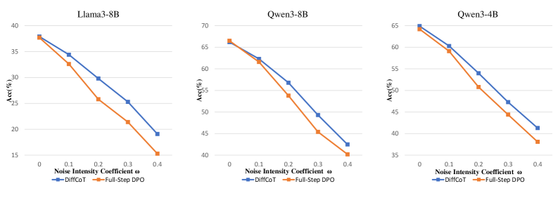</details> Figure 4: Correction success rate under stochastic prefix corruption, where noise is injected at the midpoint of the reasoning trajectory with probability $ω$ . #### Error Accumulation Analysis We further analyze the model’s ability to recover from accumulated imperfections in intermediate reasoning steps. We consider a correction-oriented setting in which the model is deliberately conditioned on prefixes that contain semantically suboptimal or noisy reasoning steps, and is then required to continue the reasoning process to reach a correct final answer. To this end, we introduce controlled perturbations at an intermediate stage of the reasoning process. Specifically, when the reasoning reaches approximately half of the trajectory, each preceding step is independently perturbed with probability $ω$ . A perturbation replaces the original step with a low-reward alternative sampled from model-generated trajectories that are semantically plausible but less aligned with the optimal reasoning path. The noise strength $ω$ therefore governs the degree of accumulated semantic drift in the prefix, enabling a systematic evaluation of robustness under varying levels of intermediate reasoning noise. We compare different training strategies under this protocol using the correction success rate, defined as the proportion of cases in which the model produces a correct final answer despite being conditioned on a perturbed prefix. Experiments are conducted on 300 GSM8K problems with multiple backbone models, comparing our approach against Full-Step-DPO. As shown in Fig. 4, our method consistently achieves substantially higher correction success rates across all settings, demonstrating a stronger ability to compensate for accumulated intermediate noise and to maintain globally coherent reasoning, rather than brittle continuation of imperfect early steps. In other words, our model can mitigate the impact of early-stage reasoning drift, rather than rigidly propagating locally coherent but globally suboptimal trajectories in CoT reasoning. ## 5 Related Work #### Preference Learning Preference learning has recently emerged as an effective paradigm for aligning LLMs with human preferences by contrasting desirable and undesirable responses (Ouyang et al., 2022; Liu et al., 2025b), with methods such as DPO showing strong performance on general language tasks (Rafailov et al., 2023). However, extending these gains to mathematical reasoning remains challenging, largely due to the coarse granularity of solution-level supervision, which fails to localize and correct intermediate reasoning errors (Chen et al., 2024b). To address this limitation, recent work incorporates step-level preference signals to align intermediate reasoning processes (Lai et al., 2024; Lu et al., 2024), while Full-Step-DPO further optimizes entire reasoning trajectories using global objectives (Xu et al., 2025). Despite these advances, most existing step-wise methods adopt a teacher-forcing paradigm and reason exclusively over clean prefixes during training, leading to error accumulation and degraded robustness during inference. Accordingly, our work reconceptualizes CoT reasoning as a globally revisable trajectory, in which previously generated steps remain malleable to correction in light of future context. #### Mathematical Reasoning Mathematical reasoning is widely regarded as a challenging capability for large language models, and prior work has explored several directions to improve it. One line of research strengthens base models through continual pre-training on large-scale mathematical corpora or supervised fine-tuning on synthetic datasets distilled from stronger models (Azerbayev et al., 2023; Zhihong et al., 2024; Xu et al., 2024; Mitra et al., 2024). Another line improves test-time performance by increasing computational budgets, such as generating and reranking multiple solutions using outcome- or process-level rewards, or adopting reward-guided decoding strategies (Guan et al., 2025; Wu et al., 2024; Wang et al., 2024). Recently, reinforcement learning and preference-based optimization have been explored to directly align reasoning behaviors via trajectory- or step-level supervision, aiming to improve robustness beyond supervised objectives alone (Pal et al., 2024; Wang et al., 2024). But they largely operate in a forward-only manner and lack mechanisms for revising corrupted intermediate reasoning, motivating our diffusion-styled reformulation of CoT reasoning to enable effective error correction. ## 6 Conclusion and Future Work In this work, we proposed a novel DiffCoT framework to enhance mathematical reasoning and alleviate error accumulation by integrating diffusion steps into autoregressive generation. Our method utilizes a sliding diffusion window with causal noise to refine intermediate steps while maintaining consistent reasoning chains. Extensive experiments confirm that our proposed DiffCoT outperforms existing CoT methods, offering a robust solution for multi-step CoT reasoning. Future work will explore the scalability of our paradigm across more backbone models and broader reasoning domains. ## Limitations Although we have conducted extensive experiments on DiffCoT and observed strong empirical performance, several limitations remain. First, the data construction and training of DiffCoT follow an off-policy paradigm, where preference data are collected using a policy that differs from the one being optimized. Such a mismatch between the behavior policy and the training policy may introduce distribution shift, biased value estimation, and training instability, especially when scaling to more difficult datasets or longer reasoning chains. Second, similar to Diffusion Forcing, DiffCoT breaks the local Markov property of prefix conditioned generation by revisiting and modifying historical reasoning steps. While this violation enables stronger capabilities, it also increases the uncertainty and controllability challenges during generation, typically requiring more training iterations and larger amounts of data to achieve stable convergence. ## References - Achiam et al. (2023) Josh Achiam, Steven Adler, Sandhini Agarwal, Lama Ahmad, Ilge Akkaya, Florencia Leoni Aleman, Diogo Almeida, Janko Altenschmidt, Sam Altman, Shyamal Anadkat, and 1 others. 2023. Gpt-4 technical report. arXiv preprint arXiv:2303.08774. - Azerbayev et al. (2023) Zhangir Azerbayev, Hailey Schoelkopf, Keiran Paster, Marco Dos Santos, Stephen McAleer, Albert Q. Jiang, Jia Deng, Stella Biderman, and Sean Welleck. 2023. Llemma: An open language model for mathematics. arXiv preprint arXiv:2310.06786. - Bengio et al. (2015) Samy Bengio, Oriol Vinyals, Navdeep Jaitly, and Noam Shazeer. 2015. Scheduled sampling for sequence prediction with recurrent neural networks. Advances in neural information processing systems, 28. - Brown et al. (2020) Tom Brown, Benjamin Mann, Nick Ryder, Melanie Subbiah, Jared Kaplan, Prafulla Dhariwal, Arvind Neelakantan, Pranav Shyam, Girish Sastry, Amanda Askell, and 1 others. 2020. Language models are few-shot learners. In Advances in Neural Information Processing Systems (NeurIPS). - Browne et al. (2012) Cameron B Browne, Edward Powley, Daniel Whitehouse, Simon M Lucas, Peter I Cowling, Philipp Rohlfshagen, Stephen Tavener, Diego Perez, Spyridon Samothrakis, and Simon Colton. 2012. A survey of monte carlo tree search methods. IEEE Transactions on Computational Intelligence and AI in games, 4(1):1–43. - Chen et al. (2024a) Boyuan Chen, Diego Martí Monsó, Yilun Du, Max Simchowitz, Russ Tedrake, and Vincent Sitzmann. 2024a. Diffusion forcing: Next-token prediction meets full-sequence diffusion. Advances in Neural Information Processing Systems, 37:24081–24125. - Chen et al. (2024b) Guoxin Chen, Minpeng Liao, Chengxi Li, and Kai Fan. 2024b. Step-level value preference optimization for mathematical reasoning. In Findings of the Association for Computational Linguistics: EMNLP 2024, pages 7889–7903, Miami, Florida, USA. Association for Computational Linguistics. - Chen et al. (2025) Ruizhe Chen, Wenhao Chai, Zhifei Yang, Xiaotian Zhang, Ziyang Wang, Tony Quek, Joey Tianyi Zhou, Soujanya Poria, and Zuozhu Liu. 2025. DiffPO: Diffusion-styled preference optimization for inference time alignment of large language models. In Proceedings of the 63rd Annual Meeting of the Association for Computational Linguistics (Volume 1: Long Papers), pages 18910–18925, Vienna, Austria. Association for Computational Linguistics. - Cobbe et al. (2021) Karl Cobbe, Vineet Kosaraju, Mohammad Bavarian, Mark Chen, Heewoo Jun, Lukasz Kaiser, Matthias Plappert, Jerry Tworek, Jacob Hilton, Reiichiro Nakano, and 1 others. 2021. Training verifiers to solve math word problems. arXiv preprint arXiv:2110.14168. - Dhariwal and Nichol (2021) Prafulla Dhariwal and Alexander Quinn Nichol. 2021. Diffusion models beat gans on image synthesis. In Advances in Neural Information Processing Systems (NeurIPS). - Feng et al. (2023) Xidong Feng, Ziyu Wan, Muning Wen, Stephen Marcus McAleer, Ying Wen, Weinan Zhang, and Jun Wang. 2023. Alphazero-like tree-search can guide large language model decoding and training. arXiv preprint arXiv:2309.17179. - Guan et al. (2025) Xinyu Guan, Li Lyna Zhang, Yifei Liu, Ning Shang, Youran Sun, Yi Zhu, Fan Yang, and Mao Yang. 2025. rStar-math: Small LLMs can master math reasoning with self-evolved deep thinking. In Proceedings of the 42nd International Conference on Machine Learning, volume 267 of Proceedings of Machine Learning Research, pages 20640–20661. PMLR. - Guo et al. (2025) Daya Guo, Dejian Yang, Haowei Zhang, Junxiao Song, Ruoyu Zhang, Runxin Xu, Qihao Zhu, Shirong Ma, Peiyi Wang, Xiao Bi, and 1 others. 2025. Deepseek-r1: Incentivizing reasoning capability in llms via reinforcement learning. arXiv preprint arXiv:2501.12948. - Hendrycks et al. (2021) Dan Hendrycks, Collin Burns, Saurav Kadavath, Akul Arora, Steven Basart, Eric Tang, Dawn Song, and Jacob Steinhardt. 2021. Measuring mathematical problem solving with the math dataset. arXiv preprint arXiv:2103.03874. - Ho et al. (2020) Jonathan Ho, Ajay Jain, and Pieter Abbeel. 2020. Denoising diffusion probabilistic models. In Advances in Neural Information Processing Systems (NeurIPS). - Hu et al. (2022) Edward J Hu, Yelong Shen, Phillip Wallis, Zeyuan Allen-Zhu, Yuanzhi Li, Shean Wang, Lu Wang, Weizhu Chen, and 1 others. 2022. Lora: Low-rank adaptation of large language models. ICLR, 1(2):3. - Kojima et al. (2022) Takeshi Kojima, Shixiang Gu, Machel Reid, Yutaka Matsuo, and Yusuke Iwasawa. 2022. Large language models are zero-shot reasoners. Preprint, arXiv:2205.11916. - Lai et al. (2024) Xin Lai, Zhuotao Tian, Yukang Chen, Senqiao Yang, Xiangru Peng, and Jiaya Jia. 2024. Step-dpo: Step-wise preference optimization for long-chain reasoning of llms. arXiv preprint arXiv:2406.18629. - Lai et al. (2025) Xin Lai, Zhuotao Tian, Yukang Chen, Senqiao Yang, Xiangru Peng, and Jiaya Jia. 2025. Step-DPO: Step-wise preference optimization for long-chain reasoning of LLMs. - Li et al. (2022) Xiang Lisa Li, Tianyu Gong, Tian He, Dan Jurafsky, Percy Liang, and Steven CH Zhao. 2022. Diffusion-lm improves controllable text generation. In Advances in Neural Information Processing Systems (NeurIPS). - Li et al. (2024) Yanhong Li, Chenghao Yang, and Allyson Ettinger. 2024. When hindsight is not 20/20: Testing limits on reflective thinking in large language models. In Findings of the Association for Computational Linguistics: NAACL 2024, pages 3741–3753. - Liu et al. (2025a) Aixin Liu, Aoxue Mei, Bangcai Lin, Bing Xue, Bingxuan Wang, Bingzheng Xu, Bochao Wu, Bowei Zhang, Chaofan Lin, Chen Dong, and 1 others. 2025a. Deepseek-v3. 2: Pushing the frontier of open large language models. arXiv preprint arXiv:2512.02556. - Liu et al. (2025b) Tianqi Liu, Zhen Qin, Junru Wu, Jiaming Shen, Misha Khalman, Rishabh Joshi, Yao Zhao, Mohammad Saleh, Simon Baumgartner, Jialu Liu, and 1 others. 2025b. Lipo: Listwise preference optimization through learning-to-rank. In Proceedings of the 2025 Conference of the Nations of the Americas Chapter of the Association for Computational Linguistics: Human Language Technologies (Volume 1: Long Papers), pages 2404–2420. - Loshchilov and Hutter (2017) Ilya Loshchilov and Frank Hutter. 2017. Decoupled weight decay regularization. arXiv preprint arXiv:1711.05101. - Lu et al. (2024) Zimu Lu, Aojun Zhou, Ke Wang, Houxing Ren, Weikang Shi, Junting Pan, Mingjie Zhan, and Hongsheng Li. 2024. Step-controlled dpo: Leveraging stepwise error for enhanced mathematical reasoning. CoRR. - Lyu et al. (2023) Qing Lyu, Tongshuang Wu, Fei Sha, and Graham Neubig. 2023. Faithful chain-of-thought reasoning. Preprint, arXiv:2301.13379. - Mitra et al. (2024) Arindam Mitra, Hamed Khanpour, Corby Rosset, and Ahmed Awadallah. 2024. Orca-math: Unlocking the potential of slms in grade school math. Preprint, arXiv:2402.14830. - Ouyang et al. (2022) Long Ouyang, Jeffrey Wu, Xu Jiang, Diogo Almeida, Carroll Wainwright, Pamela Mishkin, Chong Zhang, Sandhini Agarwal, Katarina Slama, Alex Ray, and 1 others. 2022. Training language models to follow instructions with human feedback. Advances in neural information processing systems, 35:27730–27744. - Pal et al. (2024) Arka Pal, Deep Karkhanis, Samuel Dooley, Manley Roberts, Siddartha Naidu, and Colin White. 2024. Smaug: Fixing failure modes of preference optimisation with dpo-positive. arXiv preprint arXiv:2402.13228. - Patel et al. (2021) Arkil Patel, Satwik Bhattamishra, and Navin Goyal. 2021. Are nlp models really able to solve simple math word problems? arXiv preprint arXiv:2103.07191. - Qin et al. (2024) Yiwei Qin, Xuefeng Li, Haoyang Zou, Yixiu Liu, Shijie Xia, Zhen Huang, Yixin Ye, Weizhe Yuan, Hector Liu, Yuanzhi Li, and 1 others. 2024. O1 replication journey: A strategic progress report–part 1. arXiv preprint arXiv:2410.18982. - Rafailov et al. (2023) Rafael Rafailov, Archit Sharma, Eric Mitchell, Christopher D Manning, Stefano Ermon, and Chelsea Finn. 2023. Direct preference optimization: Your language model is secretly a reward model. In Thirty-seventh Conference on Neural Information Processing Systems. - Ross et al. (2011) Stéphane Ross, Geoffrey Gordon, and Drew Bagnell. 2011. A reduction of imitation learning and structured prediction to no-regret online learning. In Proceedings of the fourteenth international conference on artificial intelligence and statistics, pages 627–635. JMLR Workshop and Conference Proceedings. - Touvron et al. (2023) Hugo Touvron, Louis Martin, Kevin Stone, Peter Albert, Amjad Almahairi, Yasmine Babaei, Nikolay Bashlykov, Soumya Batra, Prajjwal Bhargava, Shruti Bhosale, and 1 others. 2023. Llama 2: Open foundation and fine-tuned chat models. arXiv preprint arXiv:2307.09288. - Wang et al. (2024) Peiyi Wang, Lei Li, Zhihong Shao, Runxin Xu, Damai Dai, Yifei Li, Deli Chen, Yu Wu, and Zhifang Sui. 2024. Math-shepherd: Verify and reinforce LLMs step-by-step without human annotations. In Proceedings of the 62nd Annual Meeting of the Association for Computational Linguistics (Volume 1: Long Papers), pages 9426–9439, Bangkok, Thailand. Association for Computational Linguistics. - Wang et al. (2023) Xuezhi Wang, Jason Wei, Dale Schuurmans, Quoc Le, Ed Chi, Sharan Narang, Aakanksha Chowdhery, and Denny Zhou. 2023. Self-consistency improves chain of thought reasoning in language models. In International Conference on Learning Representations (ICLR). - Wei et al. (2022) Jason Wei, Xuezhi Wang, Dale Schuurmans, Maarten Bosma, Fei Xia, Ed Chi, Quoc V Le, Denny Zhou, and 1 others. 2022. Chain-of-thought prompting elicits reasoning in large language models. Advances in neural information processing systems, 35:24824–24837. - Wu et al. (2024) Zhenyu Wu, Qingkai Zeng, Zhihan Zhang, Zhaoxuan Tan, Chao Shen, and Meng Jiang. 2024. Enhancing mathematical reasoning in llms by stepwise correction. Preprint, arXiv:2410.12934. - Xi et al. (2024) Zhiheng Xi, Dingwen Yang, Jixuan Huang, Jiafu Tang, Guanyu Li, Yiwen Ding, Wei He, Boyang Hong, Shihan Do, Wenyu Zhan, and 1 others. 2024. Enhancing llm reasoning via critique models with test-time and training-time supervision. arXiv preprint arXiv:2411.16579. - Xu et al. (2025) Huimin Xu, Xin Mao, Feng-Lin Li, Xiaobao Wu, Wang Chen, Wei Zhang, and Anh Tuan Luu. 2025. Full-step-DPO: Self-supervised preference optimization with step-wise rewards for mathematical reasoning. In Findings of the Association for Computational Linguistics: ACL 2025, pages 24343–24356, Vienna, Austria. Association for Computational Linguistics. - Xu et al. (2024) Yifan Xu, Xiao Liu, Xinghan Liu, Zhenyu Hou, Yueyan Li, Xiaohan Zhang, Zihan Wang, Aohan Zeng, Zhengxiao Du, Zhao Wenyi, Jie Tang, and Yuxiao Dong. 2024. ChatGLM-math: Improving math problem-solving in large language models with a self-critique pipeline. In Findings of the Association for Computational Linguistics: EMNLP 2024, pages 9733–9760, Miami, Florida, USA. Association for Computational Linguistics. - Yang et al. (2025) An Yang, Anfeng Li, Baosong Yang, Beichen Zhang, Binyuan Hui, Bo Zheng, Bowen Yu, Chang Gao, Chengen Huang, Chenxu Lv, and 1 others. 2025. Qwen3 technical report. arXiv preprint arXiv:2505.09388. - Yao et al. (2023) Shunyu Yao, Dian Yu, Jeffrey Zhao, Izhak Shafran, Tom Griffiths, Yuan Cao, and Karthik Narasimhan. 2023. Tree of thoughts: Deliberate problem solving with large language models. Advances in neural information processing systems, 36:11809–11822. - Yoon et al. (2025) Jaesik Yoon, Hyeonseo Cho, Doojin Baek, Yoshua Bengio, and Sungjin Ahn. 2025. Monte carlo tree diffusion for system 2 planning. In Forty-second International Conference on Machine Learning. - Zhang et al. (2024) Xuan Zhang, Chao Dut, Tianyu Pang, Qian Liu, Wei Gao, and Min Lin. 2024. Chain of preference optimization: improving chain-of-thought reasoning in llms. In Proceedings of the 38th International Conference on Neural Information Processing Systems, pages 333–356. - Zhihong et al. (2024) Shao Zhihong, Wang Peiyi, Zhu Qihao, Xu Runxin, Song Junxiao, Zhang Mingchuan, Y. K. Li, Y. Wu, and Guo Daya. 2024. Deepseekmath: Pushing the limits of mathematical reasoning in open language models. ## Appendix A Data Statistics We primarily evaluate our DiffCoT on mathematical reasoning benchmarks, specifically SVAMP (Patel et al., 2021), MATH (Hendrycks et al., 2021) and GSM8K (Cobbe et al., 2021). The MATH is divided into five difficulty levels, as defined in the original dataset. To reduce randomness and better showcase the experimental results, we sample test instances separately from each of five levels. To maintain a reasonable computational budget, particularly given the high cost of Tree-of-Thought (Yao et al., 2023) search, we restrict each dataset to at most 300 test samples through random sampling. For training, we similarly sample 300 instances from each dataset to construct the training set. For a fair comparison, all baseline methods use the same dataset configuration. We provide the detailed data statistics in Table 3. | GSM8K SVAMP MATH-L1 | 5 3 3 | 500 500 300 | 300 300 300 | 5 5 5 | 8 8 8 | | --- | --- | --- | --- | --- | --- | | MATH-L2 | 4 | 300 | 300 | 5 | 8 | | MATH-L3 | 4 | 300 | 300 | 5 | 8 | | MATH-L4 | 5 | 300 | 300 | 5 | 8 | | MATH-L5 | 5 | 300 | 300 | 5 | 8 | Table 3: Dataset-specific configurations for reasoning experiments. $\#Step K$ denotes the maximum number of reasoning steps; $\#Train$ and $\#Test$ denote the numbers of training and test samples, respectively; $\#Cand.$ denotes the number of candidate thoughts sampled at each step; $\#Roll.$ denotes the number of Monte-Carlo rollouts used for evaluating each candidate. MATH-L1–L5 correspond to increasing difficulty levels in the MATH dataset. ## Appendix B Implementation Details #### Data Generation via Rollout-Based Thought Search We generate candidate contexts by conducting an iterative thought search starting from each original problem. Specifically, at reasoning step $t$ , we maintain a prefix that contains all previously selected thoughts. Conditioned on the current prefix, we sample four candidate thoughts from the base model. In parallel, we query DeepSeek-V3.2 Liu et al. (2025a) to produce an additional reference golden candidate thought under the same prefix. This golden candidate is used only during data collection and is not available at inference time. Figure 5 provides a representative example illustrating the constructed candidate thoughts and their corresponding step-wise evaluations under this procedure. To evaluate each candidate thought, we estimate its utility via Monte-Carlo rollouts. Concretely, we perform $R=8$ independent rollouts conditioned on the concatenation of the prefix and the candidate thought. Each rollout is decoded until termination to obtain a final answer. We then compute the empirical success rate as the fraction of rollouts that yield the correct answer. We continue the search by greedily selecting the candidate with the highest success rate, appending it to the prefix, and repeating the above procedure until the reasoning process terminates. We provide a detailed example with step-wise reasoning annotations in Figure 5. #### Model Training For efficient fine-tuning, we employ Low-Rank Adaptation (LoRA) (Hu et al., 2022) with a rank of 8 and $α=16$ , where LoRA adapters are inserted into the q_proj and v_proj linear projections of every self-attention layer. Model training is conducted using the DPO (Rafailov et al., 2023) loss with a regularization coefficient of $β=0.4$ , optimized by AdamW (Loshchilov and Hutter, 2017) with a cosine learning rate schedule. We train for 3 epochs with a learning rate of $1e{-5}$ , a warm-up ratio of 0.05, and a global batch size of 32. During decoding, the temperature is fixed at $0.4$ . Compared results (p < 0.05 under t-test) are averaged over three random 3 runs. All experiments are conducted on NVIDIA A100 GPUs with 80GB memory. Training and inference on 500 GSM8K samples require approximately 11 GPU-hours in total. #### Baseline Implementation The backbone models are implemented by adopting the ‘Meta-Llama-3-8B https://huggingface.co/meta-llama/Meta-Llama-3-8B ’, ‘Qwen3-8B https://huggingface.co/Qwen/Qwen3-8B ’, and ‘Qwen3-4B-Instruct-2507 https://huggingface.co/Qwen/Qwen3-4B-Instruct-2507 ’ versions. For Full-Step-DPO, we do not retrain the Process Reward Model (PRM) introduced in Full-Step-DPO. In our implementation, we retain the proposed global step-wise loss formulation, but replace the PRM-based step rewards with empirical success rates estimated from Monte-Carlo rollouts. Specifically, we collect extra complete reasoning trajectories from rollouts and use their final outcomes to compute success-based step scores, which serve as substitutes for PRM outputs in the global loss. Moreover, for CPO and ToT baselines, we follow the implementation described in the CPO paper, where preference pairs are constructed via LLM self-evaluation of intermediate reasoning steps. This design choice highlights the fundamental distinction between CPO-style self-judgment-based supervision and Step-DPO-style supervision derived from execution or outcome feedback. ## Appendix C Discussion with Reinforcement Learning PO methods generally follow a paradigm: trajectory generation followed by trajectory-level reweighting. The model first expands a full reasoning path via longitudinal generation. Alignment is then applied horizontally across completed trajectories using either reinforcement learning or preference optimization, discouraging low-reward reasoning paths and favoring high-reward ones. While this paradigm of vertical generation followed by horizontal RL-based refinement has achieved broad empirical success, it inevitably suffers from error accumulation, as early mistakes in the generated trajectory can propagate and constrain subsequent optimization. Chen et al. (2025) theoretically showed that the denoising process of diffusion models, which gradually transforms low-quality samples into high-quality ones, is equivalent to preference optimization. Building on this insight, DiffCoT introduces a diffusion sliding window, tightly coupling longitudinal reasoning generation with horizontal preference optimization within a unified framework. From this perspective, we believe that future extensions of our method can naturally integrate reinforcement learning, leveraging RL to directly optimize the denoising dynamics of the diffusion sliding window. ## Appendix D Generative AI Usage AI assistants were used in a limited and supportive manner during the preparation of this manuscript, primarily for language polishing, formatting suggestions, and improving clarity of presentation. Question. In a truck, there are 26 pink hard hats, 15 green hard hats, and 24 yellow hard hats. If Carl takes away 4 pink hard hats, and John takes away 6 pink hard hats and twice as many green hard hats as the number of pink hard hats that he removed, calculate the total number of hard hats that remained in the truck. Prompt. You are an expert math problem solver. You must reason step by step and avoid logical or arithmetic mistakes. Solve the following math problem. You MUST use exactly 5 reasoning steps. After the reasoning, output the final answer in the last line using the format: Answer: <final_answer>. Step 1. [0] 26 pink hard hats $-$ 4 pink hard hats $=$ 22 pink hard hats success_rate=0.0 [1] 26 $-$ 4 $=$ ? (number of pink hats after Carl’s removal) success_rate=0.125 [2] Initial number of pink hard hats is 26. success_rate=0.5 [3] We have 26 pink hard hats initially. Carl takes away 4 pink hard hats, leaving us with $26-4=22$ pink hard hats. success_rate=0.75 [4] Calculate the initial total number of hard hats. Initial: pink = 26, green = 15, yellow = 24. Total initial = 26 + 15 + 24 = 65. referenced data Step 2. [0] John removed 6 pink hats and 6 green hats, leaving $15-6=9$ green hats. success_rate=0.0 [1] John removes 6 pink hats, so he removes 6 green hats as well. Thus $15-6=9$ green remain. success_rate=0.125 [2] 6 pink hats are removed by John, leaving $22-6=16$ pink hats. success_rate=0.625 [3] John removes 6 pink hats: $22-6=16$ pink left. He removes twice as many green hats: $2× 6=12$ ,so $15-12=3$ green left. success_rate=1.0 [4] Carl removes 4 pink hard hats. Pink after Carl $26-4=22$ . referenced data Step 3. [0] Yellow hard hats remain unchanged, so we still have 24 yellow hard hats. success_rate=0.75 [1] Yellow hard hats remain unchanged, so we still have 24 yellow hard hats. success_rate=0.875 [2] 24 yellow hard hats remain in the truck and are not affected by the removals. success_rate=0.875 [3] 24 yellow hard hats remain unchanged. success_rate=1.0 [4] John removes 6 pink hard hats. Pink after John $22-6=16$ . referenced data Step 4. [0] 16 pink, 3 green, and 24 yellow hard hats remain in the truck. success_rate=0.75 [1] 16 pink and 3 green hard hats remain; $16+3=19$ . success_rate=0.875 [2] Total remaining hats: $16+3+24=43$ . success_rate=0.875 [3] 16 pink and 3 green hard hats remain, so $16+3=19$ hats across these two colors. success_rate=1.0 [4] John removes twice as many green hard hats as the pink hats he removed (he removed 6 pink hats, so twice that is 12 green hats). Green initially $=15$ .Green after John $15-12=3$ . referenced data Step 5. [0] Total: $3+19+24=?$ success_rate=0.0 [1] Total remaining hats: $19+24=43$ . success_rate=0.875 [2] Combining 19 (pink+green) with 24 yellow gives $19+24=43$ . success_rate=1.0 [3] Total remaining hats: $19+24=43$ . success_rate=1.0 [4] Yellow hats remain unchanged at 24. Total remaining = pink $(16)+$ green $(3)+$ yellow $(24)=43$ . . Figure 5: Representative dataset example with step-wise reasoning annotations.