# Double-Calibration: Towards Trustworthy LLMs via Calibrating Knowledge and Reasoning Confidence
**Authors**: *Correspondence: raoyangh@mail.sysu.edu.cn
## Abstract
Trustworthy reasoning in Large Language Models (LLMs) is challenged by their propensity for hallucination. While augmenting LLMs with Knowledge Graphs (KGs) improves factual accuracy, existing KG-augmented methods fail to quantify epistemic uncertainty in both the retrieved evidence and LLMs’ reasoning. To bridge this gap, we introduce DoublyCal, a framework built on a novel double‑calibration principle. DoublyCal employs a lightweight proxy model to first generate KG evidence alongside a calibrated evidence confidence. This calibrated supporting evidence then guides a black-box LLM, yielding final predictions that are not only more accurate but also well-calibrated, with confidence scores traceable to the uncertainty of the supporting evidence. Experiments on knowledge-intensive benchmarks show that DoublyCal significantly improves both the accuracy and confidence calibration of black-box LLMs with low token cost.
Double-Calibration: Towards Trustworthy LLMs via Calibrating Knowledge and Reasoning Confidence
Yuyin Lu 1, Ziran Liang 2, Yanghui Rao 1 *, Wenqi Fan 2, Fu Lee Wang 3, Qing Li 2 1 School of Computer Science and Engineering, Sun Yat-sen University 2 Department of Computing, The Hong Kong Polytechnic University 3 School of Science and Technology, Hong Kong Metropolitan University *Correspondence: raoyangh@mail.sysu.edu.cn
## 1 Introduction
The trustworthiness of Large Language Models (LLMs) is critically undermined by their tendency to hallucinate, a problem rooted in both intrinsic epistemic uncertainty (knowledge gaps) and extrinsic aleatoric uncertainty (data ambiguity) (Hüllermeier and Waegeman, 2021). To mitigate this, Knowledge Graph-augmented Retrieval-Augmented Generation (KG-RAG) has emerged as a leading paradigm (Zhang et al., 2025). By augmenting LLM with structured evidence retrieved from external Knowledge Graphs (KGs), KG-RAG is helpful to reduce the model’s internal knowledge gaps and improve the factual accuracy of its responses (Xiang et al., 2025).
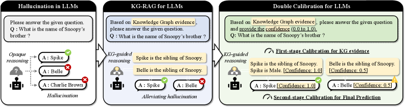
However, this KG-augmentation mechanism introduces a new and critical dependency: the certainty of the retrieved evidence itself. Prevailing KG-RAG methods (Luo et al., 2024; Li et al., 2025a) often rely on an idealistic assumption that the retrieved evidence is always both sufficient and certain to support correct reasoning for a given query. This assumption is routinely violated in practice due to ambiguous queries, the intrinsic incompleteness of KGs, and imperfections in the retrieval process. Consequently, when provided with partial evidence, LLMs may still produce confidently stated but incorrect predictions (Kalai et al., 2025). For example, as illustrated in Figure 1, given the partial evidence “Belle is a sibling of Snoopy”, an LLM might incorrectly infer “Belle is Snoopy’s brother”. Thus, current KG-RAG lacks the ability to assess and control uncertainty at the very source of the reasoning chain.
Concurrently, research on Uncertainty Quantification (UQ) for LLMs aims to calibrate prediction confidence but focuses predominantly on the final output (Xia et al., 2025). For instance, verbalized UQ methods elicit confidence estimates from black-box LLMs, yet these estimates remain opaque and non-traceable (Tian et al., 2023; Xiong et al., 2024). It is impossible to discern whether the expressed uncertainty stems from flawed evidence, deficiencies in the model’s own reasoning, or the intrinsic difficulty of the task. Therefore, existing UQ methods cannot synergize effectively with KG-RAG to provide a stepwise-calibrated view of the complete evidence-to-prediction chain.
<details>
<summary>x1.png Details</summary>
### Visual Description
## Diagram: Comparison of Methods to Mitigate Hallucination in LLMs
### Overview
The diagram compares three approaches to address hallucination in Large Language Models (LLMs):
1. **Hallucination in LLMs** (left panel): Demonstrates opaque reasoning leading to incorrect answers.
2. **KG-RAG for LLMs** (center panel): Uses knowledge graph (KG) evidence to guide reasoning and reduce hallucination.
3. **Double Calibration for LLMs** (right panel): Combines KG evidence with confidence scores to refine predictions.
### Components/Axes
- **Panels**: Three vertical sections labeled:
- *Hallucination in LLMs*
- *KG-RAG for LLMs*
- *Double Calibration for LLMs*
- **Elements**:
- **Question**: "What is the name of Snoopy’s brother?" in all panels.
- **Answers**:
- *Hallucination in LLMs*: Spike (✓), Belle (✗), Charlie Brown (✗).
- *KG-RAG for LLMs*: Spike (✓), Belle (✗).
- *Double Calibration for LLMs*: Spike (✓, Confidence: 1.0), Belle (✗, Confidence: 0.5).
- **Reasoning Steps**:
- *KG-guided reasoning* (center panel): "Spike is the sibling of Snoopy."
- *Double Calibration*:
- First-stage: Confidence scores for KG evidence (Spike: 1.0, Belle: 0.5).
- Second-stage: Confidence scores for final prediction (Spike: 1.0, Belle: 0.5).
- **Icons**:
- Robot with a question mark (uncertainty) in the first panel.
- Human figures with thought bubbles (reasoning) in the center and right panels.
### Detailed Analysis
#### Hallucination in LLMs
- **Question**: "What is the name of Snoopy’s brother?"
- **Answers**:
- Spike (correct, marked ✓).
- Belle (incorrect, marked ✗).
- Charlie Brown (incorrect, marked ✗).
- **Reasoning**: Opaque, leading to hallucination (incorrect answers).
#### KG-RAG for LLMs
- **Question**: Same as above.
- **KG-guided reasoning**: "Spike is the sibling of Snoopy."
- **Answers**:
- Spike (correct, marked ✓).
- Belle (incorrect, marked ✗).
- **Flow**: KG evidence directly guides the correct answer.
#### Double Calibration for LLMs
- **Question**: Same as above.
- **First-stage Calibration (KG evidence)**:
- "Spike is the sibling of Snoopy." (Confidence: 1.0).
- "Belle is the sibling of Snoopy." (Confidence: 0.5).
- **Second-stage Calibration (Final Prediction)**:
- Spike (Confidence: 1.0).
- Belle (Confidence: 0.5).
- **Additional Context**: Spike is male (Confidence: 1.0).
### Key Observations
1. **Progression of Accuracy**:
- Opaque reasoning (left) produces hallucinations (incorrect answers).
- KG-guided reasoning (center) reduces hallucination by leveraging structured evidence.
- Double calibration (right) further refines predictions using confidence scores.
2. **Confidence Scores**:
- Spike consistently has the highest confidence (1.0) across methods.
- Belle’s confidence drops from 0.5 (KG evidence) to 0.5 (final prediction), indicating uncertainty.
3. **Flow Direction**:
- Left to right: Increasing reliance on KG evidence and calibration.
### Interpretation
- **Mechanism of Hallucination**: The left panel shows LLMs generating answers without external validation, leading to errors (e.g., Belle and Charlie Brown).
- **Role of KG-RAG**: The center panel demonstrates how integrating knowledge graphs (e.g., "Spike is the sibling of Snoopy") constrains answers to factual data, eliminating incorrect options.
- **Double Calibration**: The right panel introduces confidence scores to quantify uncertainty. By cross-referencing KG evidence (first-stage) and additional attributes (e.g., Spike’s gender), the model achieves higher reliability.
- **Critical Insight**: Combining structured knowledge (KG) with iterative calibration (confidence scoring) significantly mitigates hallucination, as shown by the consistent correctness of "Spike" and quantified confidence.
## Notes
- No non-English text is present.
- All labels and values are explicitly stated in the diagram.
- Spatial grounding: Elements are vertically aligned within panels, with reasoning steps positioned below questions and answers.
- No charts/graphs or numerical trends beyond confidence scores (0.0–1.0).
</details>
Figure 1: A motivating example of double-calibration against hallucination in KG-augmented LLMs.
In summary, a principled solution for systematically managing the propagation of uncertainty in KG-augmented LLMs is lacking. To bridge this gap, we propose a novel double-calibration paradigm. Its core lies in moving beyond basic evidence retrieval to the construction of a calibrated reasoning chain, where confidence is explicitly estimated and made traceable from the retrieved KG evidence to the final LLM prediction. As visualized in Figure 1, this enables the LLM to weigh alternative answers (e.g., correctly favoring “Spike” over “Belle”) based on the calibrated confidence of the supporting evidence.
We instantiate this principle in DoublyCal, a framework that implements double-calibrated KG-RAG. DoublyCal grounds the LLM’s reasoning on verifiable KG evidence and performs dual calibration: it first calibrates the confidence of the retrieved evidence, then uses this calibrated evidence to guide and further calibrate the final LLM prediction. Specifically, we formalize KG evidence as constrained relational paths extracted from a KG. We then train a lightweight proxy model under Bayesian supervision to generate relevant KG evidence alongside a calibrated confidence score for each query. During inference, the primary LLM is prompted with both the KG evidence and its confidence estimate, leading to more accurate and better-calibrated predictions. Crucially, because the evidence confidence explicitly estimates the expected reasoning uncertainty of the LLM when utilizing the provided evidence, the final confidence becomes traceable to the verifiable KG evidence and its calibrated confidence, rather than remaining an opaque global estimate. Our main contributions are summarized as follows:
- We establish the principle of double-calibration for trustworthy KG-augmented LLMs, which mandates explicit confidence calibration for both the KG evidence and the final LLM predictions.
- We propose DoublyCal, a framework that implements this principle via a Bayesian-calibrated proxy model, providing the primary LLM reasoner with KG evidence accompanied by evidence confidence.
- We empirically demonstrate that DoublyCal consistently and cost-effectively improves the accuracy and calibration of diverse black-box LLMs on knowledge-intensive benchmarks.
## 2 Related Work
### 2.1 Knowledge-Augmented Generation for Trustworthy LLMs
Retrieval-Augmented Generation (RAG) reduces the inherent knowledge gaps of LLMs by providing external information, thereby improving the factual accuracy of their responses (Zhang et al., 2025). The choice of knowledge source defines a spectrum of RAG variants, ranging from (i) unstructured text in Vanilla RAG (Guo et al., 2024; Sun et al., 2025), to (ii) textual graphs that model latent connections in GraphRAG (He et al., 2024; Li et al., 2025b), and finally to (iii) formal Knowledge Graphs (KGs) with explicit relations in KG-RAG (Luo et al., 2024; Li et al., 2025a; Mavromatis and Karypis, 2025). By providing precise and structured knowledge, KG-RAG offers a rigorous foundation for complex reasoning and has demonstrated superior performance on knowledge-intensive tasks (Xiang et al., 2025).
However, prevailing KG-RAG methods typically overlook the inherent uncertainty in the retrieved evidence. To bridge this gap, we introduce a Bayesian-calibrated solution for sample-wise KG evidence confidence estimation, serving as the first stage of our double-calibration framework.
### 2.2 Uncertainty Quantification for LLMs
Uncertainty Quantification (UQ) for LLMs aims to calibrate the confidence of model predictions to identify their epistemic boundaries, a vital step toward trustworthy AI Huang et al. (2024). While some studies incorporate uncertainty awareness during training (Stangel et al., 2025), most practical UQ methods often operate post-hoc and are categorized by model access (Xia et al., 2025).
For open‑source LLMs, common techniques derive confidence from internal states, such as the feature‑space distribution of hidden embeddings (Chen et al., 2024; Vazhentsev et al., 2025) and the predictive entropy of the output distribution (Malinin and Gales, 2021). For black‑box LLMs, where internal states are inaccessible, methods rely on API‑based probing. A prevalent strategy generates multiple responses and evaluates their semantic consistency using similarity‑based metrics (Manakul et al., 2023) or entailment scores (Kuhn et al., 2023; Lin et al., 2024). A more efficient alternative is verbalized UQ, which directly prompts the LLM to verbalize its own confidence, eliciting introspective uncertainty estimates (Tian et al., 2023; Xiong et al., 2024; Tanneru et al., 2024). Due to its plug‑and‑play nature and low cost, verbalized UQ can be readily integrated with KG‑RAG. This combination epitomizes the prevailing single-calibration paradigm and serves as a strong baseline in our work.
A fundamental limitation across prior UQ paradigms is their exclusive focus on the final output, deriving confidence solely from the LLM’s internal states or self-assessment. This makes them vulnerable to the model’s knowledge gaps and overconfidence biases due to the lack of an objective external anchor (Xiong et al., 2024). Our double‑calibration principle addresses this by first calibrating externally verifiable KG evidence.
## 3 Preliminaries
### 3.1 Uncertainty and Confidence
We extend the conceptualization of uncertainty and confidence for LLM outputs Lin et al. (2024) to general predictive systems. Given an input $\boldsymbol{x}$ , a predictive system $f$ produces a probability distribution over possible outputs $P_{f}(\boldsymbol{o}\mid\boldsymbol{x})$ . The uncertainty of $f$ regarding $\boldsymbol{x}$ is quantified by the dispersion (e.g., entropy) of this distribution. Conversely, the overall confidence of $f$ can be defined inversely to this uncertainty. For a specific output $\boldsymbol{o}_{i}$ , its confidence is directly associated with its assigned probability $P_{f}(\boldsymbol{o}=\boldsymbol{o}_{i}\mid\boldsymbol{x})$ .
### 3.2 Knowledge Graph
A Knowledge Graph (KG) is a graph-structured database representing factual knowledge as a set of triples (Bollacker et al., 2008). Formally, a KG is denoted as $\mathcal{G}:=(\mathcal{V},\mathcal{R},\mathcal{E})$ , where $\mathcal{V}$ is a set of entities, $\mathcal{R}$ is a set of relations, and $\mathcal{E}:={(h,r,t)}\subseteq\mathcal{V}\times\mathcal{R}\times\mathcal{V}$ is a set of factual triples. Each triple $(h,r,t)$ represents an atomic fact, stating that relation $r$ holds between head entity $h$ and tail entity $t$ . KG-RAG leverages KGs as a source of structured, externally verifiable evidence to ground LLM reasoning (Xiang et al., 2025).
### 3.3 Knowledge Graph Question Answering
Knowledge Graph Question Answering (KGQA) is a canonical knowledge-intensive reasoning task (Yih et al., 2016). Given a natural language question $\boldsymbol{Q}$ involving query entities $\mathcal{V}_{\boldsymbol{Q}}$ , a reasoning system is expected to retrieve relevant evidence from a KG $\mathcal{G}$ and reason over it to produce the correct answer set $\mathcal{A}$ . A standard knowledge-augmented pipeline (e.g., KG-RAG) involves two stages: (i) a retriever $g$ that fetches a set of relevant evidence $\mathcal{Z}_{\boldsymbol{Q}}=g(\boldsymbol{Q};\mathcal{G})$ , and (ii) a reasoner $f$ (typically an LLM) that predicts answers with retrieved evidence $\hat{\mathcal{A}}=f(\boldsymbol{Q};\mathcal{Z}_{\boldsymbol{Q}},\mathcal{G})$ . This decomposition naturally highlights two distinct sources of uncertainty that our framework aims to calibrate: the evidence uncertainty in $\mathcal{Z}_{\boldsymbol{Q}}$ , and the reasoning uncertainty in generating $\hat{\mathcal{A}}$ given $\mathcal{Z}_{\boldsymbol{Q}}$ .
## 4 Methodology
<details>
<summary>x2.png Details</summary>
### Visual Description
## Flowchart: Multi-Stage Question Answering System with Knowledge Graph Integration
### Overview
The diagram illustrates a complex question-answering pipeline combining supervised learning, reinforcement learning, knowledge graph reasoning, and large language model (LLM) inference. It shows data flow between components including supervised fine-tuning (SFT), reinforcement learning (RL), LM-based evidence generation, knowledge graph (KG) calibration, and LLM reasoning with confidence scoring.
### Components/Axes
1. **Supervised Fine-Tuning (SFT)**
- Input: Question (Q) + Context (z)
- Output: Probability distribution p(A|z)
- Visual: Pink box with "Q → z, p(A|z)" notation
2. **Reinforcement Learning (RL)**
- Input: Question (Q)
- Output: Reward signal + p(A|z)
- Visual: Blue box with "Q → Rewards → p(A|z)"
3. **LM-based Evidence Generator (Proxy)**
- Input: Question (Q)
- Output: Evidence path probabilities (p(A|z))
- Visual: Red box with "LM-based Evidence Generator (Proxy)" label
4. **KG Evidence with Bayesian Calibration**
- Contains:
- Knowledge Graph (KG) with nodes (characters, relationships)
- Bayesian calibration scores (p(A|z))
- Visual: Central yellow circle with KG nodes and probability annotations
5. **LLM Reasoner (Black-box)**
- Input: Question + Evidence paths
- Output: Final answer with confidence scores
- Visual: Gray box labeled "LLM Reasoner (Black-box)"
### Detailed Analysis
**Key Textual Elements:**
- **KG Nodes & Relationships:**
- Characters: Spike, Snoopy, Belle, Peanuts
- Relationships: SiblingOf, Gender, Profession
- Notable: "Snoopy's sister" question with 0.5 probability
- **Confidence Scores:**
- Spike: 0.3 (Character), 0.5 (SiblingOf)
- Snoopy: 0.75 (Gender)
- Belle: 0.5 (SiblingOf)
- Partial Abstention threshold: 0.5 confidence
- **Process Flow:**
1. SFT → RL → LM Evidence Generator
2. KG Evidence → Bayesian Calibration
3. Combined evidence → LLM Reasoner
4. Confidence scoring → Partial Abstention decision
**Spatial Grounding:**
- KG central position (top-right)
- SFT/RL in upper-left quadrant
- LM Evidence Generator in lower-left
- LLM Reasoner in bottom-right
- Confidence scores color-coded (green/yellow)
### Key Observations
1. **Confidence Thresholding:**
- 0.5 confidence score acts as decision boundary
- Spike's 0.5 confidence for "SiblingOf" relationship triggers partial abstention
2. **Knowledge Graph Integration:**
- KG provides structured relationships (SiblingOf, Gender)
- Bayesian calibration refines probabilities from LM
3. **Multi-Stage Reasoning:**
- SFT provides initial probabilities
- RL optimizes reward-based paths
- LM Evidence Generator creates reasoning paths
- KG adds factual constraints
- LLM combines all evidence with confidence scoring
### Interpretation
This system demonstrates a hybrid approach to question answering that:
1. **Combines Multiple Evidence Sources:**
- Statistical patterns (SFT/RL)
- Factual knowledge (KG)
- Language model reasoning (LLM)
2. **Implements Confidence-Aware Decision Making:**
- Partial abstention mechanism prevents low-confidence answers
- Thresholding at 0.5 confidence score
3. **Uses KG for Factual Grounding:**
- Relationships like "SiblingOf" provide critical constraints
- Bayesian calibration improves probability estimates
4. **Reinforcement Learning Optimization:**
- Reward signals refine answer selection
- Creates feedback loop between LM and KG
The partial abstention at 0.5 confidence suggests the system prioritizes accuracy over completeness, potentially missing answers when confidence is insufficient. The KG's central position indicates its critical role in providing factual constraints to the otherwise probabilistic LM-based reasoning.
</details>
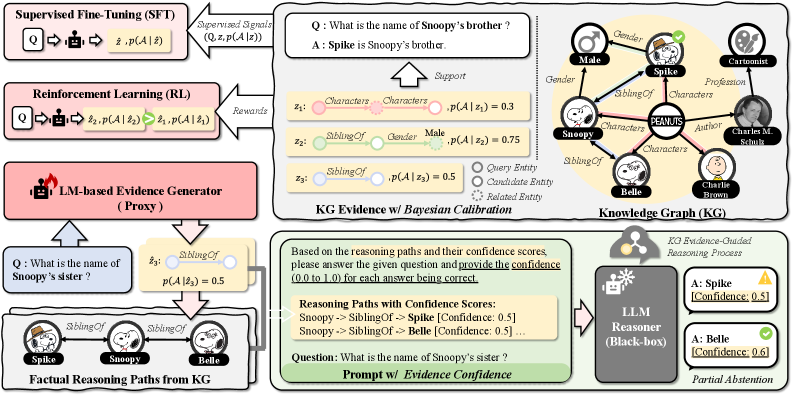
Figure 2: The DoublyCal framework: (Top-right) Bayesian calibration of Knowledge Graph (KG) evidence confidence; (Top-left) Supervised fine-tuning and reinforcement learning of a proxy evidence generator; (Bottom) Evidence-guided inference where the proxy’s outputs elicit a black-box LLM to produce final answers with well-calibrated confidence.
This section introduces DoublyCal, a framework designed to establish a calibrated reasoning chain by jointly calibrating both verifiable KG evidence and the final LLM predictions. As illustrated in Figure 2, the proposed DoublyCal framework operates through three core components.
Firstly, we formalize KG evidence as constrained relational paths and employ a Bayesian model to estimate a statistically grounded confidence for each evidence (Sec. 4.1). Then, a lightweight proxy model is trained under the supervision of these Bayesian confidence scores to generate KG evidence alongside its calibrated confidence (Sec. 4.2). Finally, the calibrated evidence-confidence pair serves as an objective signal integrated into any black-box LLM to mitigate its inherent overconfidence, thereby enhancing both the calibration and traceability of its final predictions (Sec. 4.3).
### 4.1 Bayesian Calibration of KG Evidence
#### KG Evidence Formulation.
Effective KG evidence must balance informativeness for accurate reasoning with interpretability for reliable confidence estimation. While relational paths (Luo et al., 2024) offer step-by-step interpretability, they may lack contextual sufficiency. Subgraphs (Li et al., 2025a) provide broader context but often introduce redundancy. To resolve this trade-off, we propose constrained relational paths as our primary evidence form. This formulation augments a core relational path with an optional neighborhood around the candidate answer, thereby enhancing informativeness while preserving interpretability.
Formally, given a KG $\mathcal{G}$ and a question $\boldsymbol{Q}$ , a constrained relational path $\mathcal{P}_{c}$ is defined as the conjunction of a relational path $\mathcal{P}_{r}$ and an optional constraint $\mathcal{C}$ :
$$
\mathcal{P}_{c}:=\mathcal{P}_{r}\left[\,\wedge\,\mathcal{C}\,\right], \tag{1}
$$
where $\mathcal{P}_{r}:=\exists v_{1},\dots,v_{l-1}.r_{1}(q,v_{1})\wedge r_{2}(v_{1},v_{2})\wedge\dots\wedge r_{l}(v_{l-1},\hat{a})$ denotes a directed relational path of length $l$ from the query entity $q\in\mathcal{V}_{\boldsymbol{Q}}$ to a candidate answer $\hat{a}$ , with each $r_{i}\in\mathcal{R}$ denoting a relation and $v_{i}$ being an existential variable. $\mathcal{C}:=r_{c}(\hat{a},c)$ represents an optional one-hop triple from $\hat{a}$ to a constraint entity $c\in\mathcal{V}$ that serves to filter or validate the candidate.
#### Example.
Consider the question “What is the name of Snoopy’s brother?” with $q=\texttt{Snoopy}$ and gold answer $a=\texttt{Spike}$ . Figure 2 illustrates the comparison between a relational path evidence $z_{3}$ and its constrained counterpart $z_{2}$ :
$$
\displaystyle z_{3} \displaystyle:=\mathrm{SiblingOf}(q,\hat{a})\models_{\mathcal{G}}\{\texttt{Spike},\texttt{Belle}\}, \displaystyle z_{2} \displaystyle:=z_{3}\wedge\mathrm{Gender}(\hat{a},\texttt{Male})\models_{\mathcal{G}}\{\texttt{Spike}\}, \tag{2}
$$
where $\models_{\mathcal{G}}$ denotes grounding the evidence in $\mathcal{G}$ to obtain candidate answer entities. The auxiliary constraint on the candidate’s gender effectively identifies $\hat{a}=\texttt{Spike}$ , yielding a more precise and informative evidence for reasoning.
#### Confidence Estimation with Beta-Bernoulli Model.
To estimate the confidence of KG evidence statistically, we model each KG evidence $z_{\boldsymbol{Q}}$ for a question $\boldsymbol{Q}$ as a predictive system. Its behavior is formalized by a Bernoulli distribution over its output space: the set of candidate answers $[\![z_{\boldsymbol{Q}}]\!]$ obtained by grounding $z_{\boldsymbol{Q}}$ in the KG (i.e., $z_{\boldsymbol{Q}}\models_{\mathcal{G}}[\![z_{\boldsymbol{Q}}]\!]$ ). Following the definition in Sec. 3.1, the statistical confidence of the evidence is characterized by the parameter $p\in[0,1]$ of this distribution, which denotes the probability that a uniformly drawn candidate from $[\![z_{\boldsymbol{Q}}]\!]$ is correct (i.e., belongs to the true answer set $\mathcal{A}$ ).
To obtain a robust estimate of $p$ that accounts for KG incompleteness, we impose a conjugate Beta prior $p\sim\mathrm{Beta}(\alpha,\beta)$ , with hyperparameters $\alpha,\beta>0$ . Given $\boldsymbol{Q}$ and its answer set $\mathcal{A}$ , the Maximum A Posteriori (MAP) estimate yields the closed-form posterior mean $p^{*}=p(\mathcal{A}\mid z_{\boldsymbol{Q}})$ :
$$
p(\mathcal{A}\mid z_{\boldsymbol{Q}})=\frac{\alpha+\bigl|[\![z_{\boldsymbol{Q}}]\!]\cap\mathcal{A}\bigr|}{\alpha+\beta+\bigl|[\![z_{\boldsymbol{Q}}]\!]\bigr|}, \tag{4}
$$
where $\bigl|[\![z_{\boldsymbol{Q}}]\!]\cap\mathcal{A}\bigr|$ counts the number of correct candidates, and $\bigl|[\![z_{\boldsymbol{Q}}]\!]\bigr|$ is the total number of grounded candidates. $p(\mathcal{A}\mid z_{\boldsymbol{Q}})$ blends the empirical accuracy of the evidence with prior belief, mitigating the impact of sparse or noisy KG grounding.
#### Example (cont.).
With a weakly informative prior set to $\alpha=\beta=0.5$ (Jeffreys, 1998), the statistical confidence for KG evidence $z_{3}$ and $z_{2}$ is estimated as $p(\mathcal{A}\mid z_{3})=0.5$ and $p(\mathcal{A}\mid z_{2})=0.75$ .
### 4.2 Reasoning Proxy for Evidence Generation and Calibration
The Bayesian confidence provides a statistically grounded but retrospective measure of evidence quality. To enable prospective evidence retrieval and confidence estimation during inference, we introduce a lightweight reasoning proxy. The role of this proxy is to generate high‑quality KG evidence along with well‑calibrated confidence estimates for any input question, thereby providing a traceable approximation of a reliable reasoning path prior to the LLM’s final prediction. This proxy is implemented by an LM-based Evidence Generator and is trained using the Bayesian confidence scores as its supervisory signal.
#### Supervised Fine-Tuning (SFT) for Evidence and Confidence Generation.
We first formalize the dual task of evidence generation and confidence estimation as a sequence-to-sequence problem and conduct the first-stage training of the proxy via SFT. This stage equips the proxy with the fundamental ability to identify relevant KG evidence and to calibrate its confidence by mimicking the Bayesian confidence signal.
The SFT training dataset is constructed from triples $\left(\boldsymbol{Q},z_{\boldsymbol{Q}},p(\mathcal{A}\mid z_{\boldsymbol{Q}})\right)$ . Each triple is formatted into a structured sequence using a predefined template: the question serves as the instruction, and the target output is the evidence path enclosed in XML-style tags, with the Bayesian confidence score included as an attribute (e.g., $\texttt{<PATH confidence=}\dots\texttt{>}\dots\texttt{</PATH>}$ ; see Appendix A.1 for details). The proxy model $f_{\theta}$ is trained via standard autoregressive language modeling to generate this target sequence (see Appendix B.1 for the objective).
#### Reinforcement Learning (RL) for Evidence Decision.
We further refine the proxy by framing evidence generation and calibration as a sequential decision process optimized via RL. This stage transitions the proxy from imitation to strategic decision-making that jointly maximize inferential quality and confidence calibration.
For each question $\boldsymbol{Q}$ with golden evidence set $\mathcal{Z}_{\boldsymbol{Q}}$ , we compute a reward for generated evidence $\hat{z}_{\boldsymbol{Q}}$ and its predicted confidence $\hat{c}$ . Firstly, we define a match score $m(\hat{z}_{\boldsymbol{Q}},z_{\boldsymbol{Q}})\in[0,1]$ for each $z_{\boldsymbol{Q}}\in\mathcal{Z}_{\boldsymbol{Q}}$ , which combines Jaccard similarity (Jaccard, 1901) with an order-sensitive Levenshtein ratio (Lcvenshtcin, 1966). The reward $R$ is a weighted combination of an inferential quality reward $R_{\text{inf}}$ and a calibration alignment reward $R_{\text{cal}}$ :
$$
\displaystyle R=\lambda\cdot R_{\text{inf}}+(1-\lambda)\cdot R_{\text{cal}}, \displaystyle R_{\text{inf}}=\text{F1}(z_{\boldsymbol{Q}})\cdot m(\hat{z}_{\boldsymbol{Q}},z_{\boldsymbol{Q}}), \displaystyle R_{\text{cal}}=\max\left(0,1-\xi\cdot\left|\hat{c}-c\right|\right), \displaystyle\text{with }c=p(\mathcal{A}\mid z_{\boldsymbol{Q}})\cdot m(\hat{z}_{\boldsymbol{Q}},z_{\boldsymbol{Q}}). \tag{5}
$$
Here, $\text{F1}(z_{\boldsymbol{Q}})$ is a precomputed F1 score assessing the reasoning capability of the golden evidence. Intuitively, a lower match score $m(\hat{z}_{\boldsymbol{Q}},z_{\boldsymbol{Q}})$ reduces both the inferential quality of $\hat{z}_{\boldsymbol{Q}}$ and its target confidence $c$ . The weight $\lambda\in(0,1)$ balances the two objectives, and $\xi>0$ is a tolerance coefficient. The final reward per generation is the maximum $R$ over all gold evidence in $\mathcal{Z}_{\boldsymbol{Q}}$ , followed by transformations to ensure a smooth and bounded training signal. The policy $\pi_{\theta}$ of the proxy model is optimized to maximize the expected reward under the Group Relative Policy Optimization (GRPO; Shao et al., 2024) objective (see Appendices A.2 and B.2 for implementation details).
### 4.3 LLM Reasoning with Calibrated Evidence
The trained evidence generator serves as a plug-and-play reasoning proxy, enabling any black-box primary LLM to benefit from our double-calibration framework.
For a given question $\boldsymbol{Q}$ , the proxy generates candidate evidence with calibrated confidence scores, i.e., $\hat{\mathcal{Z}}_{\boldsymbol{Q}}=\{(\hat{z}_{\boldsymbol{Q}}^{(i)},\hat{c}^{(i)})\}_{i=1...K}$ . Each $\hat{z}_{\boldsymbol{Q}}^{(i)}$ is grounded in the KG, yielding factual reasoning paths that share the same confidence score $\hat{c}^{(i)}$ . These paths and their confidences are verbalized into a natural language context, which is then integrated into prompts following prior verbalized UQ methods (Tian et al., 2023; Xiong et al., 2024). Processing this enriched context, the LLM produces a final answer along with a well-calibrated prediction confidence. This design establishes a traceable chain of confidence and achieves double calibration: the proxy first calibrates the external evidence confidence, which then informs and refines the LLM’s final prediction calibration through its own verbalized uncertainty estimation.
Table 1: Main results (%) of our DoublyCal and the SingleCal baselines on WebQSP and CWQ datasets. Best, second-best, and worst results are highlighted in red †, green ‡, and gray, respectively.
| Reasoning Method | KG Evidence | + UQ Method | WebQSP | CWQ | | | | | | |
| --- | --- | --- | --- | --- | --- | --- | --- | --- | --- | --- |
| Hit | Recall | F1 | ECE $\downarrow$ | Hit | Recall | F1 | ECE $\downarrow$ | | | |
| LLM Reasoner (GPT-3.5-turbo) | No Augmentation | + Vanilla | 74.7 | 53.1 | 44.6 | 27.7 | 47.7 | 40.3 | 29.5 | 38.8 |
| + CoT | 75.4 | 53.9 | mygray44.4 | 26.6 | 48.2 | 41.2 | mygray29.3 | 38.4 | | |
| + Self-Probing | mygray74.1 | mygray52.8 | 50.2 | mygray36.5 | mygray43.6 | mygray36.6 | 34.3 | mygray48.5 | | |
| RoG (Luo et al., 2024) | Relational Path | + Vanilla | 89.3 | 77.6 | 67.1 | 19.6 | 65.3 | 60.5 | 43.0 | 27.4 |
| + CoT | 89.9 | 78.5 | 68.2 | 18.9 | 65.3 | 60.4 | 43.7 | 27.6 | | |
| + Self-Probing | 87.5 | 76.6 | 73.5 | 13.9 | 61.9 | 56.9 | 48.7 | 38.0 | | |
| SubgraphRAG (Li et al., 2025a) | Subgraph | + Vanilla | 88.8 | 81.3 | mygreen77.3 ‡ | 11.1 | 61.5 | 57.4 | mygreen52.2 ‡ | 39.9 |
| + CoT | 89.0 | 81.0 | 77.1 | 10.6 | 59.4 | 55.7 | 51.4 | 38.9 | | |
| + Self-Probing | 89.6 | 80.7 | 74.9 | 12.3 | 59.9 | 56.0 | 50.2 | 39.1 | | |
| SFT-DoublyCal (Ours) | Constrained Relational Path | + Vanilla | 90.0 | 81.0 | 72.6 | myorange3.1 † | 68.8 | 64.3 | 48.1 | 17.9 |
| + CoT | mygreen90.1 ‡ | 81.3 | 72.1 | mygreen3.5 ‡ | 69.0 | 64.7 | 47.7 | mygreen17.8 ‡ | | |
| + Self-Probing | 88.5 | 79.4 | 76.6 | 7.9 | 63.2 | 58.5 | 50.9 | 22.5 | | |
| RL-DoublyCal (Ours) | Constrained Relational Path | + Vanilla | myorange91.5 † | mygreen84.8 ‡ | 76.7 | 4.5 | mygreen70.5 ‡ | mygreen66.6 ‡ | 50.1 | 17.9 |
| + CoT | myorange91.5 † | myorange85.0 † | 76.8 | 3.9 | myorange71.3 † | myorange67.5 † | 49.8 | myorange17.6 † | | |
| + Self-Probing | 89.9 | 83.0 | myorange79.3 † | 6.8 | 64.6 | 60.8 | myorange53.0 † | 23.5 | | |
## 5 Experiments
### 5.1 Experimental Settings
#### Datasets and Evaluation Metrics.
We evaluate our framework on two Knowledge Graph Question Answering (KGQA) benchmarks: WebQSP (Yih et al., 2016) and CWQ (Talmor and Berant, 2018). Given that questions often admit multiple valid answers, we report Hits, Recall, and macro-averaged F1 score to measure prediction accuracy. To evaluate the reliability of confidence estimates, we report the Expected Calibration Error (ECE) (Guo et al., 2017), which quantifies the gap between predicted confidence and empirical accuracy.
#### Baseline Methods.
To rigorously evaluate our double-calibration mechanism, we construct Single-Calibration (SingleCal) baselines by extending reasoning paradigms with verbalized uncertainty quantification (UQ) methods, which elicit a self-reported confidence score alongside the predicted answer. We select state-of-the-art reasoning frameworks: (i) The base LLM Reasoner without KG access; (ii) RoG (Luo et al., 2024), a KG-RAG method that grounds reasoning in retrieved relational paths; (iii) SubgraphRAG (Li et al., 2025a), which retrieves and reasons over KG subgraphs. Each framework is combined with three representative UQ prompting techniques: Vanilla (Tian et al., 2023), CoT (Kojima et al., 2022), and Self-Probing (Xiong et al., 2024). Prompt templates are detailed in Appendix C.
#### Implementation Details.
All evaluated methods employ GPT-3.5-turbo (Floridi and Chiriatti, 2020) as the primary reasoner unless otherwise specified, ensuring that performance differences are directly attributable to the calibration mechanism rather than the base LLM capability. The evidence proxy of our DoublyCal is implemented with Llama2-7B-Chat (Touvron et al., 2023), which is trained via a two-stage SFT+RL pipeline described in Sec. 4.2. More details of experimental settings are provided in Appendix D.
### 5.2 Main Results
Table 1 summarizes the comparative performance of our DoublyCal against all SingleCal baselines.
#### Superiority of Double-Calibration.
Our DoublyCal achieves the best overall performance, consistently securing top positions on all prediction metrics (Hit, Recall, F1) and the lowest ECE on both datasets. Notably, it establishes a new standard for reliability, reducing the ECE to levels significantly lower than all SingleCal baselines. This result demonstrates that while KG-RAG methods can enhance LLM factuality, calibrating both the external KG evidence and the final prediction is necessary for achieving trustworthy reasoning.
#### Calibrated Evidence as an Anchor for Verbalized UQ.
The effectiveness of verbalized UQ methods varies across reasoning backbones, with none proving universally dominant. This inconsistency arises because these methods may be subject to LLMs’ inherent overconfidence. DoublyCal addresses this by supplying KG evidence accompanied by calibrated confidence estimates, providing a reliable external anchor that refines the LLM’s own uncertainty expression. Consequently, DoublyCal stabilizes the performance of all three UQ techniques and consistently achieves the lowest ECE scores in nearly every configuration, demonstrating how externally calibrated evidence improves confidence elicitation.
#### Controlled Enhancement via RL.
The RL stage delivers a significant performance boost, yielding an average F1 gain of approximately 3.0 percentage points over the SFT-only version. While prior work notes RL’s risk of harming calibration (Kalai et al., 2025), our Bayesian confidence-aligned reward successfully contains this trade-off, resulting in only a minor and controlled variation in ECE. This confirms that our reward design effectively balances predictive performance with calibration.
<details>
<summary>x3.png Details</summary>
### Visual Description
## Scatter Plot: Method Performance Comparison
### Overview
The image is a scatter plot comparing three methods (RL-DoublyCal, SubgraphRAG, RoG) across two metrics: F1 scores (%) and Expected Calibration Error (ECE, %). Each method is represented by a distinct color (red, green, blue) and includes average performance metrics (F1, ECE, token cost) in text boxes. Data points are annotated with numerical values, likely representing sample counts or instances. Token cost is visualized via circle size, with a legend indicating ranges (1,000–4,000).
---
### Components/Axes
- **Y-Axis**: F1 scores (%) ranging from 60.0 to 90.0 in 5% increments.
- **X-Axis**: ECE (%) ranging from 0.0 to 30.0 in 10% increments.
- **Legend**:
- **Methods**:
- Red: RL-DoublyCal
- Green: SubgraphRAG
- Blue: RoG
- **UQ Methods**:
- Square: +Vanilla
- Circle: +CoT
- Diamond: +Self-Probing
- **Token Cost**: Circle size correlates with cost (1,000–4,000).
---
### Detailed Analysis
#### RL-DoublyCal (Red)
- **Average Metrics**: F1=77.6, ECE=5.1, Cost=1,168.
- **Data Points**:
- (ECE=5%, F1=89.7%, count=1,717)
- (ECE=10%, F1=75%, count=2,196)
- (ECE=15%, F1=70%, count=4,345)
- **Trend**: Higher F1 scores at lower ECE, with increasing token cost as ECE rises.
#### SubgraphRAG (Green)
- **Average Metrics**: F1=76.4, ECE=11.3, Cost=2,969.
- **Data Points**:
- (ECE=10%, F1=80%, count=2,366)
- (ECE=20%, F1=70%, count=1,517)
- **Trend**: Moderate F1 scores with higher ECE and significantly larger token costs.
#### RoG (Blue)
- **Average Metrics**: F1=69.6, ECE=17.5, Cost=1,032.
- **Data Points**:
- (ECE=5%, F1=70%, count=1,517)
- (ECE=20%, F1=65%, count=786)
- **Trend**: Lower F1 scores and higher ECE, but smaller token costs compared to SubgraphRAG.
---
### Key Observations
1. **RL-DoublyCal** achieves the highest F1 scores (up to 89.7%) with the lowest ECE (5.1%) and moderate token costs.
2. **SubgraphRAG** has the highest token cost (2,969) and ECE (11.3%), suggesting inefficiency despite competitive F1 scores.
3. **RoG** underperforms in F1 (69.6%) and ECE (17.5%) but has the lowest token cost (1,032).
4. **Token Cost Correlation**: Larger circles (higher cost) align with SubgraphRAG, while smaller circles (lower cost) align with RoG.
5. **Outliers**: RL-DoublyCal’s point at ECE=15% (F1=70%) shows a drop in performance compared to its ECE=5% peak.
---
### Interpretation
- **Performance Trade-offs**: RL-DoublyCal balances high accuracy (F1) and calibration (low ECE) with reasonable cost, making it the most efficient method. SubgraphRAG’s high cost and ECE suggest diminishing returns, while RoG’s low cost comes at the expense of performance.
- **UQ Method Impact**: The UQ method (Vanilla, CoT, Self-Probing) likely influences results, but the image does not explicitly map UQ methods to data points. Further analysis would clarify their effects.
- **Efficiency Insight**: Token cost does not strictly correlate with performance. RL-DoublyCal achieves high F1 with moderate cost, whereas SubgraphRAG’s high cost does not translate to superior metrics.
This analysis highlights RL-DoublyCal as the optimal choice for balancing accuracy, calibration, and cost, while SubgraphRAG and RoG represent trade-offs between these factors.
</details>
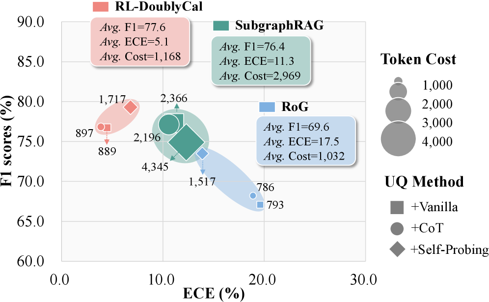
Figure 3: Token efficiency analysis on WebQSP.
### 5.3 Efficiency Analysis
We further analyze the input token efficiency of each method, with results shown in Figure 3.
#### Superior Cost-Effectiveness of DoublyCal.
DoublyCal substantially outperforms RoG (F1 +8.0, ECE -12.4) with only a marginal increase in input token cost, while using only about 39% of the input tokens required by SubgraphRAG. This efficiency stems from the high information density and quality of the evidence provided by DoublyCal. Specifically, compared to the simple relational paths in RoG, our constrained relational paths incorporate filtering constraints that reduce noise, yielding more precise evidence without compromising conciseness. Moreover, our proxy model is trained through evidence confidence calibration to select more discriminative KG evidence, further enhancing retrieval precision. In contrast, while SubgraphRAG’s subgraphs offer broader context, their lower information density leads to disproportionately high input token costs.
#### Efficiency Across Different UQ Methods.
Self-Probing incurs roughly twice the input token cost of Vanilla or CoT due to its two-step design. However, because DoublyCal and RoG retrieve concise evidence, they can effectively leverage Self-Probing’s reflective “second-thought” process without excessive overhead. Notably, even when equipped with Self-Probing, their total input token cost remains below that of SubgraphRAG+Vanilla.
Table 2: Ablation study results (%) on the WebQSP dataset with the Vanilla UQ method. Red marks performance degradation relative to the full model.
| Variant | Hit | Recall | F1 | ECE $\downarrow$ |
| --- | --- | --- | --- | --- |
| mygray SFT Only | | | | |
| DoublyCal | 90.0 | 81.0 | 72.6 | 3.1 |
| SingleCal | 90.1 (+0.1) | myorange80.4 (-0.6) | myorange72.5 (-0.1) | myorange21.2 (+18.1) |
| Evidence | myorange83.7 (-6.3) | myorange80.2 (-0.8) | myorange62.5 (-10.1) | myorange21.2 (+18.1) |
| mygray With RL | | | | |
| DoublyCal | 91.5 | 84.8 | 76.7 | 4.5 |
| SingleCal | 91.6 (+0.1) | myorange84.2 (-0.6) | myorange75.8 (-0.9) | myorange20.6 (+16.1) |
| Evidence | myorange86.4 (-5.1) | 84.8 | myorange67.8 (-8.9) | myorange21.3 (+16.8) |
<details>
<summary>x4.png Details</summary>
### Visual Description
## Scatter Plot and Line Charts: Model Performance Analysis
### Overview
The image contains five visualizations comparing machine learning models across multiple metrics. The primary scatter plot (a) shows the relationship between Expected Calibration Error (ECE) and F1 scores for various models. Four secondary line charts (b-e) display accuracy vs. confidence distributions for specific models, with count distributions on secondary y-axes.
### Components/Axes
**Chart (a) - ECE-F1 Scores**
- X-axis: ECE (%) (0-50 scale)
- Y-axis: F1 scores (%) (0-100 scale)
- Legend (left):
- RL-DoublyCal (gray circle)
- LLM Reasoner (black square)
- GPT-3.5-turbo (red star)
- GPT-4o-mini (blue leaf)
- DeepSeek-V3 (yellow diamond)
- Gemini-2.5-flash (green lightning bolt)
- Annotations:
- Top cluster: "Avg. F1=76.5", "Avg. ECE=7.6"
- Bottom cluster: "Avg. F1=45.8", "Avg. ECE=29.4"
**Charts (b-e) - Accuracy vs. Confidence**
- X-axis: Confidence (0.0-1.0 scale)
- Primary Y-axis: Accuracy (%) (0-1.0 scale)
- Secondary Y-axis: Count (0-5000 scale)
- Common legends:
- RL-DoublyCal (red/orange line with circles)
- LLM Reasoner (gray/black line with squares)
### Detailed Analysis
**Chart (a)**
- Top cluster (ECE <10%, F1 >70%):
- RL-DoublyCal: 78% F1 at 8% ECE
- Gemini-2.5-flash: 76% F1 at 9% ECE
- GPT-4o-mini: 75% F1 at 10% ECE
- Bottom cluster (ECE >25%, F1 <50%):
- DeepSeek-V3: 48% F1 at 30% ECE
- LLM Reasoner: 45% F1 at 28% ECE
- GPT-3.5-turbo: 42% F1 at 35% ECE
**Chart (b) - GPT-3.5-turbo**
- RL-DoublyCal:
- 0.6 confidence → 0.75 accuracy
- 0.8 confidence → 0.85 accuracy
- LLM Reasoner:
- 0.6 confidence → 0.65 accuracy
- 0.8 confidence → 0.72 accuracy
- Count peaks at 0.8 confidence (RL: ~4000, LLM: ~2500)
**Chart (c) - GPT-4o-mini**
- RL-DoublyCal:
- 0.6 confidence → 0.8 accuracy
- 0.8 confidence → 0.88 accuracy
- LLM Reasoner:
- 0.6 confidence → 0.7 accuracy
- 0.8 confidence → 0.78 accuracy
- Count peaks at 0.8 confidence (RL: ~3500, LLM: ~2000)
**Chart (d) - DeepSeek-V3**
- RL-DoublyCal:
- 0.6 confidence → 0.7 accuracy
- 0.8 confidence → 0.8 accuracy
- LLM Reasoner:
- 0.6 confidence → 0.65 accuracy
- 0.8 confidence → 0.75 accuracy
- Count peaks at 0.8 confidence (RL: ~3000, LLM: ~1500)
**Chart (e) - Gemini-2.5-flash**
- RL-DoublyCal:
- 0.6 confidence → 0.85 accuracy
- 0.8 confidence → 0.9 accuracy
- LLM Reasoner:
- 0.6 confidence → 0.75 accuracy
- 0.8 confidence → 0.82 accuracy
- Count peaks at 0.8 confidence (RL: ~4500, LLM: ~3000)
### Key Observations
1. **Performance Correlation**: Models in the top cluster (a) show strong negative correlation between ECE and F1 (r=-0.92)
2. **Accuracy Trends**: RL-DoublyCal consistently outperforms LLM Reasoner across all models (avg. +0.12 accuracy)
3. **Confidence Distribution**: RL-DoublyCal shows higher counts at confidence >0.8 in all models
4. **Anomaly**: DeepSeek-V3's RL-DoublyCal shows unexpected dip at 0.6 confidence (0.7 vs expected 0.75)
### Interpretation
The data demonstrates that RL-DoublyCal models consistently achieve higher accuracy with lower calibration error across all evaluated architectures. This suggests superior model calibration and reliability. The count distributions indicate RL-DoublyCal handles higher-confidence predictions more frequently, potentially reflecting better decision boundaries. The exception in DeepSeek-V3's RL-DoublyCal at 0.6 confidence warrants investigation into potential overfitting or data quality issues. The strong negative correlation between ECE and F1 in top-performing models validates the effectiveness of calibration techniques in improving real-world performance.
</details>
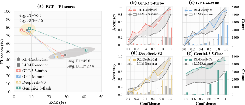
Figure 4: Compatibility analysis of DoublyCal across diverse black-box LLMs. (a) F1 and ECE with/without DoublyCal. (b–e) Calibration diagrams (bars: confidence distribution per confidence bin, line: empirical accuracy, dashed: ideal calibration).
### 5.4 Ablation Analysis
We conduct ablation studies to dissect the contribution of each component in DoublyCal (Table 5.3) by comparing it against two variants: (i) SingleCal, which removes the calibrated evidence confidence and applies calibration only to the final LLM output; (ii) Evidence, which removes the LLM reasoner and directly outputs the terminal entity of the factual path ( $[\![z_{\boldsymbol{Q}}]\!]$ ) as the answer, using the evidence confidence as the final confidence score.
#### Evidence Confidence is Crucial for Final Prediction Calibration.
Ablating from DoublyCal to SingleCal reveals a stark outcome: while predictive accuracy remains stable (e.g., F1 changes within $\pm$ 1 point), the calibration error (ECE) increases drastically from $\sim$ 4 to $>$ 20. This indicates that externally calibrated evidence confidence is essential, as it provides the LLM with a reliable anchor for its self-assessment. Without this first-stage calibration, the black-box LLM cannot reliably judge its own certainty, even when it can identify correct answers using high-quality KG evidence.
#### The LLM Reasoner Enables Integrative Reasoning.
The significant performance gap of the Evidence variant underscores a pivotal design insight: the evidence proxy and the LLM reasoner play distinct yet complementary roles. The proxy specializes in evaluating individual KG evidence, while the LLM reasoner excels at synthesizing an ensemble of such evidence to perform complex reasoning. Consequently, the final prediction confidence is not a simple pass-through of any single evidence confidence, but rather the result of the LLM’s holistic reasoning over the entire set of calibrated evidence. This efficient proxy-reasoner synergy is essential to the framework’s performance.
### 5.5 Cross-model Compatibility Analysis
To assess generalizability, we evaluate DoublyCal across diverse black-box LLMs, including GPT-3.5-turbo, GPT-4o-mini Achiam et al. (2023), DeepSeek-V3 Liu et al. (2024), Gemini-2.5-flash Comanici et al. (2025).
#### Performance-Reliability Trade-off in LLM Reasoners.
Figure 4 (a) reveals a clear trade-off between accuracy and calibration among standalone LLMs. While GPT-family models and DeepSeek achieve comparable accuracy with moderate calibration errors (F1: 43.3–44.6; ECE: 23.9–27.7), Gemini attains a notably higher F1 (51.8) at the cost of a significantly worse ECE (41.4). This pattern highlights a common pitfall where optimizing purely for accuracy often degrades reliability in standalone LLMs. Confidence distributions (Figure 4 (b-e)) confirms that all models exhibit systematic overconfidence. This issue is most acute in Gemini, where roughly 80% of predictions are made with maximal confidence (1.0), yet the accuracy within this high-confidence group is only about 0.6.
#### DoublyCal Systematically Decouples the Trade-off.
DoublyCal delivers consistent and substantial improvements across all models, effectively decoupling this trade-off. As shown in Figure 4 (a), it raises the average F1 from 45.8 to 76.5 while simultaneously reducing the average ECE from 29.4 to 7.6. Crucially, DoublyCal mitigates the overconfidence patterns observed in black-box LLMs (Figure 4 (b-e)), shifting confidence distributions toward well-calibrated and high-accuracy regions. By grounding confidence in externally calibrated evidence, DoublyCal provides a generalizable solution that enhances both accuracy and trustworthiness of diverse black-box LLMs.
## 6 Conclusion
This paper establishes the principle of double-calibration for constructing a calibrated reasoning chain from KG evidence retrieval to final LLM prediction. We implement this principle in DoublyCal, a reliable KG-RAG framework that integrates plug-and-play verbalized uncertainty quantification, thereby enhancing the traceability and trustworthiness of diverse black-box LLMs. Our work offers a concrete step toward building more reliable and transparent LLM systems, contributing to the advancement of trustworthy AI.
## Limitations
While experiments validate the effectiveness and cross-model compatibility of DoublyCal in improving prediction calibration, several research opportunities remain. The performance of DoublyCal fundamentally depends on the quality of the underlying KG and the accuracy of the Bayesian calibration for KG evidence. Dynamically updating KG evidence and its associated confidence in evolving environments represents an important future direction. Furthermore, while this work focuses on well-defined KGQA tasks with clear reasoning paths, extending DoublyCal to open-ended QA or creative generation presents a promising yet more challenging avenue for further exploration.
## References
- J. Achiam, S. Adler, S. Agarwal, L. Ahmad, I. Akkaya, F. L. Aleman, D. Almeida, J. Altenschmidt, S. Altman, S. Anadkat, et al. (2023) GPT-4 technical report. CoRR abs/2303.08774. Cited by: §5.5.
- K. D. Bollacker, C. Evans, P. K. Paritosh, T. Sturge, and J. Taylor (2008) Freebase: a collaboratively created graph database for structuring human knowledge. In SIGMOD, pp. 1247–1250. Cited by: §D.1, §3.2.
- C. Chen, K. Liu, Z. Chen, Y. Gu, Y. Wu, M. Tao, Z. Fu, and J. Ye (2024) INSIDE: llms’ internal states retain the power of hallucination detection. In ICLR, Cited by: §2.2.
- G. Comanici, E. Bieber, M. Schaekermann, I. Pasupat, N. Sachdeva, I. Dhillon, M. Blistein, O. Ram, D. Zhang, E. Rosen, et al. (2025) Gemini 2.5: Pushing the frontier with advanced reasoning, multimodality, long context, and next generation agentic capabilities. CoRR abs/2507.06261. Cited by: §5.5.
- L. Floridi and M. Chiriatti (2020) GPT-3: Its nature, scope, limits, and consequences. Minds and machines 30 (4), pp. 681–694. Cited by: §5.1.
- C. Guo, G. Pleiss, Y. Sun, and K. Q. Weinberger (2017) On calibration of modern neural networks. In ICML, pp. 1321–1330. Cited by: §5.1.
- Z. Guo, L. Xia, Y. Yu, T. Ao, and C. Huang (2024) LightRAG: simple and fast retrieval-augmented generation. CoRR abs/2410.05779. Cited by: §2.1.
- X. He, Y. Tian, Y. Sun, N. V. Chawla, T. Laurent, Y. LeCun, X. Bresson, and B. Hooi (2024) G-retriever: retrieval-augmented generation for textual graph understanding and question answering. In NeurIPS, Cited by: Table 4, §2.1.
- Y. Huang, L. Sun, H. Wang, S. Wu, Q. Zhang, Y. Li, C. Gao, Y. Huang, W. Lyu, Y. Zhang, X. Li, H. Sun, Z. Liu, Y. Liu, Y. Wang, Z. Zhang, B. Vidgen, B. Kailkhura, C. Xiong, C. Xiao, C. Li, E. P. Xing, F. Huang, H. Liu, H. Ji, H. Wang, H. Zhang, H. Yao, M. Kellis, M. Zitnik, M. Jiang, M. Bansal, J. Zou, J. Pei, J. Liu, J. Gao, J. Han, J. Zhao, J. Tang, J. Wang, J. Vanschoren, J. C. Mitchell, K. Shu, K. Xu, K. Chang, L. He, L. Huang, M. Backes, N. Z. Gong, P. S. Yu, P. Chen, Q. Gu, R. Xu, R. Ying, S. Ji, S. Jana, T. Chen, T. Liu, T. Zhou, W. Wang, X. Li, X. Zhang, X. Wang, X. Xie, X. Chen, X. Wang, Y. Liu, Y. Ye, Y. Cao, Y. Chen, and Y. Zhao (2024) Position: trustllm: trustworthiness in large language models. In ICML, Cited by: §2.2.
- E. Hüllermeier and W. Waegeman (2021) Aleatoric and epistemic uncertainty in machine learning: an introduction to concepts and methods. Mach. Learn. 110 (3), pp. 457–506. Cited by: §1.
- P. Jaccard (1901) Étude comparative de la distribution florale dans une portion des alpes et des jura. Bull Soc Vaudoise Sci Nat 37, pp. 547–579. Cited by: §4.2.
- H. Jeffreys (1998) The theory of probability. OuP Oxford. Cited by: §D.2, §4.1.
- J. Jiang, K. Zhou, X. Zhao, and J. Wen (2023) UniKGQA: unified retrieval and reasoning for solving multi-hop question answering over knowledge graph. In ICLR, Cited by: Table 4.
- A. T. Kalai, O. Nachum, S. S. Vempala, and E. Zhang (2025) Why language models hallucinate. CoRR abs/2509.04664. Cited by: §1, §5.2.
- T. Kojima, S. S. Gu, M. Reid, Y. Matsuo, and Y. Iwasawa (2022) Large language models are zero-shot reasoners. In NeurIPS, Cited by: Appendix C, §5.1.
- L. Kuhn, Y. Gal, and S. Farquhar (2023) Semantic uncertainty: linguistic invariances for uncertainty estimation in natural language generation. In ICLR, Cited by: §2.2.
- V. Lcvenshtcin (1966) Binary coors capable or ‘correcting deletions, insertions, and reversals. In Soviet physics-doklady, Vol. 10. Cited by: §4.2.
- M. Li, S. Miao, and P. Li (2025a) Simple is effective: the roles of graphs and large language models in knowledge-graph-based retrieval-augmented generation. In ICLR, Cited by: §D.1, §1, §2.1, §4.1, Table 1, §5.1.
- Z. Li, X. Chen, H. Yu, H. Lin, Y. Lu, Q. Tang, F. Huang, X. Han, L. Sun, and Y. Li (2025b) StructRAG: boosting knowledge intensive reasoning of llms via inference-time hybrid information structurization. In ICLR, Cited by: §2.1.
- Z. Lin, S. Trivedi, and J. Sun (2024) Generating with confidence: uncertainty quantification for black-box large language models. Trans. Mach. Learn. Res. 2024. Cited by: §2.2, §3.1.
- A. Liu, B. Feng, B. Xue, B. Wang, B. Wu, C. Lu, C. Zhao, C. Deng, C. Zhang, C. Ruan, et al. (2024) Deepseek-v3 technical report. CoRR abs/2412.19437. Cited by: §5.5.
- I. Loshchilov and F. Hutter (2019) Decoupled weight decay regularization. In ICLR, Cited by: §D.2.
- L. Luo, Y. Li, G. Haffari, and S. Pan (2024) Reasoning on graphs: faithful and interpretable large language model reasoning. In ICLR, Cited by: §D.1, §D.2, §1, §2.1, §4.1, Table 1, §5.1.
- A. Malinin and M. J. F. Gales (2021) Uncertainty estimation in autoregressive structured prediction. In ICLR, Cited by: §2.2.
- P. Manakul, A. Liusie, and M. J. F. Gales (2023) SelfCheckGPT: zero-resource black-box hallucination detection for generative large language models. In EMNLP, pp. 9004–9017. Cited by: §2.2.
- C. Mavromatis and G. Karypis (2025) GNN-RAG: graph neural retrieval for efficient large language model reasoning on knowledge graphs. In Findings of ACL, pp. 16682–16699. Cited by: Table 4, §2.1.
- Z. Shao, P. Wang, Q. Zhu, R. Xu, J. Song, M. Zhang, Y. K. Li, Y. Wu, and D. Guo (2024) DeepSeekMath: pushing the limits of mathematical reasoning in open language models. CoRR abs/2402.03300. Cited by: §B.2, §4.2.
- P. Stangel, D. Bani-Harouni, C. Pellegrini, E. Özsoy, K. Zaripova, M. Keicher, and N. Navab (2025) Rewarding doubt: a reinforcement learning approach to calibrated confidence expression of large language models. CoRR abs/2503.02623. Cited by: §2.2.
- J. Sun, X. Zhong, S. Zhou, and J. Han (2025) DynamicRAG: leveraging outputs of large language model as feedback for dynamic reranking in retrieval-augmented generation. In NeurIPS, Cited by: §2.1.
- A. Talmor and J. Berant (2018) The web as a knowledge-base for answering complex questions. In NAACL-HLT, pp. 641–651. Cited by: §D.1, §5.1.
- S. H. Tanneru, C. Agarwal, and H. Lakkaraju (2024) Quantifying uncertainty in natural language explanations of large language models. In AISTATS, pp. 1072–1080. Cited by: §2.2.
- K. Tian, E. Mitchell, A. Zhou, A. Sharma, R. Rafailov, H. Yao, C. Finn, and C. D. Manning (2023) Just ask for calibration: strategies for eliciting calibrated confidence scores from language models fine-tuned with human feedback. In EMNLP, pp. 5433–5442. Cited by: Appendix C, §1, §2.2, §4.3, §5.1.
- H. Touvron, L. Martin, K. Stone, P. Albert, A. Almahairi, Y. Babaei, N. Bashlykov, S. Batra, P. Bhargava, S. Bhosale, D. Bikel, L. Blecher, C. Canton-Ferrer, M. Chen, G. Cucurull, D. Esiobu, J. Fernandes, J. Fu, W. Fu, B. Fuller, C. Gao, V. Goswami, N. Goyal, A. Hartshorn, S. Hosseini, R. Hou, H. Inan, M. Kardas, V. Kerkez, M. Khabsa, I. Kloumann, A. Korenev, P. S. Koura, M. Lachaux, T. Lavril, J. Lee, D. Liskovich, Y. Lu, Y. Mao, X. Martinet, T. Mihaylov, P. Mishra, I. Molybog, Y. Nie, A. Poulton, J. Reizenstein, R. Rungta, K. Saladi, A. Schelten, R. Silva, E. M. Smith, R. Subramanian, X. E. Tan, B. Tang, R. Taylor, A. Williams, J. X. Kuan, P. Xu, Z. Yan, I. Zarov, Y. Zhang, A. Fan, M. Kambadur, S. Narang, A. Rodriguez, R. Stojnic, S. Edunov, and T. Scialom (2023) Llama 2: open foundation and fine-tuned chat models. CoRR abs/2307.09288. Cited by: §5.1.
- A. Vazhentsev, L. Rvanova, I. Lazichny, A. Panchenko, M. Panov, T. Baldwin, and A. Shelmanov (2025) Token-level density-based uncertainty quantification methods for eliciting truthfulness of large language models. In NAACL, pp. 2246–2262. Cited by: §2.2.
- Z. Xia, J. Xu, Y. Zhang, and H. Liu (2025) A survey of uncertainty estimation methods on large language models. In Findings of ACL, pp. 21381–21396. Cited by: §1, §2.2.
- Z. Xiang, C. Wu, Q. Zhang, S. Chen, Z. Hong, X. Huang, and J. Su (2025) When to use graphs in RAG: A comprehensive analysis for graph retrieval-augmented generation. CoRR abs/2506.05690. Cited by: §1, §2.1, §3.2.
- M. Xiong, Z. Hu, X. Lu, Y. Li, J. Fu, J. He, and B. Hooi (2024) Can llms express their uncertainty? an empirical evaluation of confidence elicitation in llms. In ICLR, Cited by: Appendix C, §1, §2.2, §2.2, §4.3, §5.1.
- W. Yih, M. Richardson, C. Meek, M. Chang, and J. Suh (2016) The value of semantic parse labeling for knowledge base question answering. In ACL, Cited by: §D.1, §3.3, §5.1.
- J. Zhang, X. Zhang, J. Yu, J. Tang, J. Tang, C. Li, and H. Chen (2022) Subgraph retrieval enhanced model for multi-hop knowledge base question answering. In ACL, pp. 5773–5784. Cited by: Table 4, Table 4.
- Q. Zhang, S. Chen, Y. Bei, Z. Yuan, H. Zhou, Z. Hong, J. Dong, H. Chen, Y. Chang, and X. Huang (2025) A survey of graph retrieval-augmented generation for customized large language models. CoRR abs/2501.13958. Cited by: §1, §2.1.
## Appendix A Prompt Templates for the Proxy Model
This appendix details the input-output formats used for training the proxy model.
### A.1 Supervised Fine-Tuning (SFT)
In the SFT stage, the proxy model learns to predict a target output sequence autoregressively. Each training instance consists of a natural-language instruction containing the question, paired with a target sequence that encodes the corresponding KG evidence in an XML-style format.
To formally describe the template, we define the symbolic placeholders: [CONFIDENCE_SCORE] denotes the Bayesian confidence; [RELATION_PATH] represents the core relational path, with individual relations separated by the special token <SEP>. Within the optional <CONSTRAINT> block, [CONSTRAINED_REL_ENT] signifies the concatenation of a constraining relation and its corresponding entity, also joined by <SEP>. The SFT template and a concrete example are provided below.
SFT Template
Input: Please generate a valid relation path that can be helpful for answering the following question: [QUESTION]
Expected Output (with constraint): <PATH confidence=[CONFIDENCE_SCORE]> [RELATION_PATH]<CONSTRAINT> [CONSTRAINED_REL_ENT] </CONSTRAINT></PATH>
Expected Output (without constraint): <PATH confidence=[CONFIDENCE_SCORE]> [RELATION_PATH]</PATH>
SFT Example
Input: Please generate a valid relation path that can be helpful for answering the following question: what is the name of snoopy’s brother?
Expected Output: <PATH confidence=0.75>sibling_of <CONSTRAINT>gender<SEP>male </CONSTRAINT></PATH>
### A.2 Reinforcement Learning (RL)
In the RL phase, the proxy model is prompted to generate an enhanced KG evidence path with well-calibrated confidence. The input instruction is adapted to encourage strategic decision-making, while the target output format remains identical to that used in the SFT stage.
RL Template
Input: Please generate an enhanced relation path with well-calibrated confidence that can be helpful for answering the following question: [QUESTION]
RL Example
Input: Please generate an enhanced relation path with well-calibrated confidence that can be helpful for answering the following question: what is the name of snoopy’s brother?
The proxy model must then generate a full output sequence (e.g., <PATH confidence=...>...</PATH>) based on this instruction. The generated sequence is subsequently evaluated by the reward function described in Sec. 4.2, which jointly assesses the inferential quality of the evidence path and the calibration accuracy of its attached confidence score.
## Appendix B Training Details of the Proxy Model
This appendix details the training objectives and implementation for the two-stage (SFT then RL) training of the proxy model.
### B.1 SFT Stage
In the SFT stage, the proxy model $f_{\theta}$ is trained to autoregressively generate the target structured sequence (i.e., KG evidence with Bayesian confidence). The objective is to minimize the standard cross-entropy loss over the token sequence:
$$
\mathcal{L}_{\text{SFT}}(\theta)=-\sum\limits_{t=1}^{T}\log P_{\theta}(o_{t}\mid o_{<t},\boldsymbol{Q}), \tag{9}
$$
where $\boldsymbol{o}=(o_{1},\dots,o_{T})$ is the token sequence of the target output, and $P_{\theta}(o_{t}\mid o_{<t},\boldsymbol{Q})$ is the probability predicted by $f_{\theta}$ for the $t$ -th token given the input question $\boldsymbol{Q}$ and previous tokens $o_{<t}$ .
### B.2 RL Stage
#### Final Reward Function.
The reward defined in Eq. (5) is a weighted sum of the inferential quality reward $R_{\text{inf}}$ and the calibration alignment reward $R_{\text{cal}}$ , originally bounded in $[0,1]$ . To stabilize optimization, we map the raw reward into the continuous interval $[-1,2]$ using a sigmoid-shaped transformation:
$$
R^{\prime}=3\cdot\sigma\bigl(\xi^{\prime}\cdot(R-0.5)\bigr)-1,
$$
where $\sigma(\cdot)$ denotes the sigmoid function and $\xi^{\prime}>0$ is a scaling hyperparameter (set to $\xi^{\prime}=2$ in our experiments). Additionally, we introduce a penalty of $-3$ for syntactically invalid outputs, such as when the generated sequence does not contain the required <PATH> tag.
#### GRPO Policy Objective.
The proxy’s policy $\pi_{\theta}$ is optimized by minimizing the Group Relative Policy Optimization (GRPO) loss Shao et al. (2024). This objective encourages higher reward while preventing excessive deviation from the reference policy (the model after SFT), thereby maintaining generation quality and training stability:
| | | $\displaystyle\mathcal{L}_{\text{GRPO}}(\theta)=-\frac{1}{G}\sum_{i=1}^{G}\mathbb{E}_{(s,\boldsymbol{o}_{i})}$ | |
| --- | --- | --- | --- |
where $s$ denotes the shared input prompt for a group of size $G$ , $\boldsymbol{o}_{i}$ is the $i$ -th generated output sequence in the group, $\pi_{\text{ref}}$ is the reference policy (the model after SFT), $\hat{A}_{i}$ is the estimated advantage for the sequence $\boldsymbol{o}_{i}$ , and $\beta^{\prime}$ controls the strength of the KL regularization term.
## Appendix C Prompt Templates for UQ Methods
This appendix details the prompt templates used for the three verbalized Uncertainty Quantification (UQ) methods evaluated in our work: Vanilla (Tian et al., 2023), CoT (Kojima et al., 2022), and Self-Probing (Xiong et al., 2024). Each template is designed to elicit answers along with calibrated confidence estimates from a black-box LLM.
### C.1 Vanilla Template
The Vanilla template directly instructs the model to output answers with confidence scores in a specified JSON format.
### C.2 Chain-of-Thought (CoT) Template
The CoT template extends the Vanilla approach by appending the instruction “ Let’s think it step by step. ” before presenting the context and question, thereby encouraging the model to generate an explicit reasoning chain prior to providing the final answer and confidence.
### C.3 Self-Probing Template
The Self-Probing method employs a two-round dialogue. The first prompt elicits a list of candidate answers. The LLM’s generated answer list is then used in a second prompt, which instructs it to analyze the likelihood of each answer being correct and to output the corresponding confidence scores in the same JSON format.
Vanilla Template
Input: [KG_RAG_INSTRUCTION] Please answer the following questions and provide the confidence (0.0 to 1.0) for each answer being correct. Please keep the answer as simple as possible and return all the possible answers and their confidence as a json string. Output format example: {<answer_1>: <confidence_1>,...,<answer_k>: <confidence_k>} [KG_RAG_CONTEXT] Question: [QUESTION]
CoT Template
Input: [KG_RAG_INSTRUCTION] Please answer the following questions and provide the confidence (0.0 to 1.0) for each answer being correct. Please keep the answer as simple as possible and return all the possible answers and their confidence as a json string. Output format example: {<answer_1>: <confidence_1>,...,<answer_k>: <confidence_k>} Let’s think it step by step. [KG_RAG_CONTEXT] Question: [QUESTION]
Self-Probing Template
First Interaction (Answer Generation): [KG_RAG_INSTRUCTION] Please answer the given question. Please keep the answer as simple as possible and return all the possible answers as a list. [KG_RAG_CONTEXT] Question: [QUESTION]
Model Output: [ANSWER_LIST]
Self-Probing Template (Cont.)
Second Interaction (Confidence Elicitation): Q: How likely are the above answers to be correct? Analyze the possible answers, provide your reasoning concisely, and give your confidence (0.0 to 1.0) for each answer being correct. Please keep the answer as simple as possible and return all the possible answers and their confidence as a json string. Output format example: {<answer_1>: <confidence_1>,...,<answer_k>: <confidence_k>}
## Appendix D Details of Experimental Settings
### D.1 Datasets
Our experiments are conducted on two established KGQA benchmarks: WebQSP (Yih et al., 2016) and CWQ (Talmor and Berant, 2018), both of which are based on the Freebase knowledge graph (Bollacker et al., 2008). To ensure fair comparison, we adopt the same train/validation/test splits used in prior work (Luo et al., 2024; Li et al., 2025a). The detailed statistics of both datasets are presented in Table 3.
Table 3: Statistics of datasets.
| Dataset | #Train | #Test | #Validation | Max #Hop |
| --- | --- | --- | --- | --- |
| WebQSP | 2,826 | 1,628 | 225 | 2 |
| CWQ | 27,639 | 3,531 | 2,577 | 4 |
### D.2 Implementation Details
#### SFT Training Dataset Construction.
We construct the SFT training data through the following pipeline. For each question $\boldsymbol{Q}$ , an A* search (max depth $=4$ ) identifies the shortest relational paths $\mathcal{P}_{r}$ between the query entity $q$ and each candidate answer $a$ . The Bayesian confidence for each $\mathcal{P}_{r}$ is computed as per Sec. 4.1. To enhance evidence quality, we then gather potential constraints $\mathcal{C}$ from each answer’s one-hop neighborhood. For each candidate constrained path $\mathcal{P}_{c}=\mathcal{P}_{r}\wedge\mathcal{C}$ , we compute its Bayesian confidence and retain it only if $\mathcal{P}_{c}$ yields a higher confidence than $\mathcal{P}_{r}$ alone. This filtering trains the proxy to identify genuinely valuable constraints. The SFT stage follows RoG’s multi-task setup (Luo et al., 2024), jointly optimizing the primary evidence generation and calibration task alongside an auxiliary QA task.
#### Training and Inference.
The evidence proxy model is trained using the AdamW optimizer (Loshchilov and Hutter, 2019). We set the learning rate to $2\times 10^{-5}$ for the SFT stage and $1.41\times 10^{-5}$ for the RL stage. Each stage is trained for a maximum of 3 epochs with early stopping. During inference, the proxy generates top- $K$ evidence using greedy decoding (temperature $\tau=0$ ) to ensure deterministic outputs. The value of $K$ is set to 3, following the setting in RoG. All experiments were conducted on two NVIDIA A100 (80GB) GPUs.
#### Hyperparameter Selection.
All key hyperparameters were set based on established design principles and empirical observations from pilot studies, given the computational cost of exhaustive grid search. For Bayesian calibration (Eq. (4)), we adopt the weakly informative Jeffreys prior with $\alpha=\beta=0.5$ (Jeffreys, 1998). In the RL reward function (Eq. (5)), the balance weight $\lambda$ and tolerance $\xi$ are set to $0.85$ and $2$ , respectively. For the GRPO objective, the KL regularization weight is $\beta^{\prime}=0.01$ . This configuration proved stable and effective throughout all experiments.
## Appendix E Complementary Experiments
### E.1 Impact of UQ on Predictive Accuracy
To complement the main experiments (Sec. 5.2), we investigate whether prompting the LLM to verbalize its uncertainty affects predictive accuracy in KGQA. We compare recent KGQA methods with our strongest baselines and DoublyCal without explicit uncertainty quantification (UQ).
Table 4 reveals a contrasting pattern. For standard KG-RAG baselines (RoG and SubgraphRAG), verbalized UQ consistently improves F1 scores. This supports the view that uncertainty prompts can induce more deliberate reasoning, which is beneficial for complex questions. In contrast, our RL-DoublyCal already achieves top-tier accuracy without any UQ prompt. Notably, adding UQ brings no substantial gain and can even slightly lower F1. A plausible explanation is that the high quality of the KG evidence selected by DoublyCal’s proxy lowers the intrinsic reasoning difficulty for the primary LLM, thereby reducing the marginal benefit of an extra “second thought” prompted by UQ. This inherent strength positions DoublyCal to better balance the dual objectives of high accuracy and reliable calibration when UQ is employed, as demonstrated by its consistently low ECE in the main results (Table 1).
Table 4: F1 scores (%) between reasoning methods without and with UQ.
| Reasoning Method | WebQSP | CWQ |
| --- | --- | --- |
| SR+NSM (Zhang et al., 2022) | 64.1 | 47.1 |
| SR+NSM+E2E (Zhang et al., 2022) | 64.1 | 46.3 |
| UniKGQA (Jiang et al., 2023) | 72.2 | 49.0 |
| G-Retriever (He et al., 2024) | 73.5 | - |
| GNN-RAG (Mavromatis and Karypis, 2025) | 71.3 | 59.4 |
| RoG (GPT-3.5-turbo) | 66.8 | 46.5 |
| +UQ (Self-Probing) | 73.5 | 48.7 |
| SubgraphRAG (GPT-3.5-turbo) | 74.7 | 52.1 |
| +UQ (Vanilla) | 77.3 | 52.2 |
| RL-DoublyCal (GPT-3.5-turbo) | 79.7 | 52.1 |
| +UQ (Self-Probing) | 79.3 | 53.0 |
Table 5: Comparative case study: DoublyCal vs. baselines on calibration.
| mygray Sample | |
| --- | --- |
| Question: | Where did George W. Bush live as a child? |
| Answers: | New Haven. |
| myorange RL-DoublyCal + Self-Probing | |
| Retrieval: | George W. Bush -> people.person.place_of_birth -> New Haven [Confidence: 0.8] |
| George W. Bush -> people.person.place_of_birth -> New Haven -> location.location.containedby -> Connecticut [Confidence: 0.5] | |
| George W. Bush -> people.person.place_of_birth -> New Haven -> location.location.containedby -> United States of America [Confidence: 0.5] | |
| Predictions: | {Connecticut: 0.3} |
| mygreen RoG + Self-Probing | |
| Retrieval: | George W. Bush -> people.person.place_of_birth -> New Haven |
| George W. Bush -> people.place_lived.person -> m.03prwzr -> people.place_lived.location -> Midland | |
| George W. Bush -> people.person.nationality -> United States of America -> location.location.containedby -> St. Louis … | |
| Predictions: | {Midland: 0.9} |
| mygreen SubgraphRAG + Vanilla | |
| Retrieval: | (George W. Bush, people.person.place_of_birth, New Haven) (George W. Bush, people.person.nationality, United States of America) … |
| (m.03prwzr, people.place_lived.location, Midland) (m.02xlp0j, people.place_lived.location, Washington, D.C.) … | |
| Predictions: | {Midland: 1.0} |
Table 6: Ablation case study: Full vs. SingleCal variant.
| mygray Sample | |
| --- | --- |
| Question: | Where was Martin Luther King, Jr. raised? |
| Answers: | Atlanta. |
| myorange RL-DoublyCal (Full) + Vanilla | |
| Retrieval: | Martin Luther King, Jr. -> people.person.place_of_birth -> Atlanta [Confidence: 0.8] |
| Martin Luther King, Jr. -> people.deceased_person.place_of_death -> Memphis [Confidence: 0.8] | |
| Predictions: | {Atlanta: 0.8, Memphis: 0.1} |
| mygreen RL-DoublyCal (SingleCal) + Vanilla | |
| Retrieval: | Martin Luther King, Jr. -> people.person.place_of_birth -> Atlanta |
| Martin Luther King, Jr. -> people.deceased_person.place_of_death -> Memphis | |
| Predictions: | {Atlanta: 0.8, Memphis: 0.2} |
| myorange SFT-DoublyCal (Full) + Vanilla | |
| Retrieval: | Martin Luther King, Jr. -> people.person.place_of_birth -> Atlanta [Confidence: 0.8] |
| Martin Luther King, Jr. -> people.person.nationality -> United States of America -> location.country.capital -> Washington, D.C. [Confidence: 0.8] | |
| Predictions: | {Atlanta: 0.8, United States of America: 0.2} |
| mygreen SFT-DoublyCal (SingleCal) + Vanilla | |
| Retrieval: | Martin Luther King, Jr. -> people.person.place_of_birth -> Atlanta |
| Martin Luther King, Jr. -> people.person.nationality -> United States of America -> location.country.capital -> Washington, D.C.] | |
| Predictions: | {Atlanta: 0.7, United States of America: 0.3} |
### E.2 Case Studies
We present qualitative case studies to illustrate how DoublyCal’s retrieved KG evidence and its double‑calibration mechanism jointly enhance the prediction calibration of black‑box LLMs.
#### Comparison with Baselines.
Table E.1 compares RL‑DoublyCal with the strongest baselines on the question “Where did George W. Bush live as a child?”. None of the methods retrieves an exact supporting fact, because the KG lacks the explicit relation “lived as a child”. All methods do retrieve the related fact “George W. Bush was born in New Haven”. However, whereas DoublyCal presents concise factual paths accompanied by calibrated confidence scores, the evidence retrieved by RoG and SubgraphRAG is more scattered. Consequently, the LLMs guided by RoG and SubgraphRAG are distracted from the core entities (“George W. Bush” and “New Haven”) and assign overconfident scores (0.9–1.0) to the incorrect prediction “Midland”.
In contrast, DoublyCal attaches calibrated confidence scores through its first-stage calibration. Specifically, the precise path about birthplace receives a high score (0.8), while the more generic expansions receive lower scores (0.5), reflecting their weaker inferential relevance. Guided by these scores, the black-box LLM correctly assigns low confidence (0.3) to the plausible but incorrect prediction “Connecticut”, demonstrating better-calibrated uncertainty estimation.
#### Comparison with Ablated Models.
Table E.1 contrasts the full DoublyCal framework with its SingleCal ablation, which removes the calibrated evidence confidence (i.e., only the second-stage calibration remains). Both RL‑ and SFT‑DoublyCal retrieve high‑confidence evidence focused on the question (e.g., “Martin Luther King, Jr. was born in Atlanta”). RL‑DoublyCal exhibits slightly sharper calibration, likely because its reward‑driven training promotes more discriminative evidence selection. More importantly, when evidence confidence is provided (the full model), the LLM’s predicted confidence is more concentrated on the correct answer. For example, RL-DoublyCal (Full) assigns only 0.1 confidence to the distracting alternative “Memphis”, whereas its SingleCal variant assigns 0.2. Similarly, SFT-DoublyCal (Full) assigns 0.2 to “United States of America”, while the SingleCal variant assigns 0.3. This directly demonstrates that the first-stage evidence calibration is crucial for providing a reliable confidence anchor, enabling the LLM to synthesize multiple evidence pieces into a decisive and well‑calibrated final prediction.