# LLM-42: Enabling Determinism in LLM Inference with Verified Speculation
## Abstract
In LLM inference, the same prompt may yield different outputs across different runs. At the system level, this non-determinism arises from floating-point non-associativity combined with dynamic batching and GPU kernels whose reduction orders vary with batch size. A straightforward way to eliminate non-determinism is to disable dynamic batching during inference, but doing so severely degrades throughput. Another approach is to make kernels batch-invariant; however, this tightly couples determinism to kernel design, requiring new implementations. This coupling also imposes fixed runtime overheads, regardless of how much of the workload actually requires determinism.
Inspired by ideas from speculative decoding, we present LLM-42 Many developers unknowingly set 42 as a random state variable (seed) to ensure reproducibility, a reference to The Hitchhiker’s Guide to the Galaxy. The number itself is arbitrary, but widely regarded as a playful tradition. —a scheduling-based approach to enable determinism in LLM inference. Our key observation is that if a sequence is in a consistent state, the next emitted token is likely to be consistent even with dynamic batching. Moreover, most GPU kernels use shape-consistent reductions. Leveraging these insights, LLM-42 decodes tokens using a non-deterministic fast path and enforces determinism via a lightweight verify–rollback loop. The verifier replays candidate tokens under a fixed-shape reduction schedule, commits those that are guaranteed to be consistent across runs, and rolls back those violating determinism. LLM-42 mostly re-uses existing kernels unchanged and incurs overhead only in proportion to the traffic that requires determinism.
## 1 Introduction
LLMs are becoming increasingly more powerful [openai2022gpt4techreport, kaplan2020scalinglaws]. However, a key challenge many users usually face with LLMs is their non-determinism [he2025nondeterminism, atil2024nondeterminism, yuan2025fp32death, song2024greedy]: the same model can produce different outputs across different runs of a given prompt, even with identical decoding parameters and hardware. Enabling determinism in LLM inference (aka deterministic inference) has gained significant traction recently for multiple reasons. It helps developers isolate subtle implementation bugs that arise only under specific batching choices; improves reward stability in reinforcement-learning training [zhang2025-deterministic-tp]; is essential for integration testing in large-scale systems. Moreover, determinism underpins scientific reproducibility [song2024greedy] and enables traceability [rainbird2025deterministic]. Consequently, users have increasingly requested support for deterministic inference in LLM serving engines [Charlie2025, Anadkat2025consistent].
He et al. [he2025nondeterminism] showed that non-determinism in LLM inference at the system-level stems from the non-associativity of floating-point arithmetic LLM outputs can also vary due to differences in sampling strategies (e.g., top-k, top-p, or temperature). Our goal is to ensure that output is deterministic for fixed sampling hyper-parameters; different hyper-parameters can result in different output and this behavior is intentional.. This effect manifests in practice because most core LLM operators—including matrix multiplications, attention, and normalization—rely on reduction operations, and GPU kernels for these operators choose different reduction schedules to maximize performance at different batch sizes. The same study also proposed batch-invariant computation as a means to eliminate non-determinism. In this approach, a kernel processes each input token using a single, universal reduction strategy independent of batching. Popular LLM serving systems such as vLLM and SGLang have recently adopted this approach [SGLangTeam2025, vllm-batch-invariant-2025].
While batch-invariant computation guarantees determinism, we find that this approach is fundamentally over-constrained. Enforcing a fixed reduction strategy for every token—regardless of model phase or batch geometry—strips GPU kernels of the very parallelism they are built to exploit. For example, the batch-invariant GEMM kernels provided by He et al. do not use the split-K strategy that is otherwise commonly used to accelerate GEMMs at low batch sizes [tritonfusedkernel-splitk-meta, nvidia_cutlass_blog]. Furthermore, most GPU kernels are not batch-invariant to begin with, so insisting on batch-invariant execution effectively demands new kernel implementations, increasing engineering and maintenance overhead. Finally, batch-invariant execution makes determinism the default for all requests, even when determinism is undesirable or even harmful [det-inf-kills].
Our observations suggest that determinism can be enabled with a simpler approach. (O1) Token-level inconsistencies are rare: as long as a sequence remains in a consistent state, the next emitted token is mostly identical across runs; sequence-level divergence arises mainly from autoregressive decoding after the first inconsistent token. (O2) Most GPU kernels already use shape-consistent reduction schedules: they apply the same reduction strategy on all inputs of a given shape, but potentially different reduction strategies on inputs of different shapes. (O3) Determinism requires only position-consistent reductions: a particular token position must use the same reduction schedule across runs, but different positions within or across sequences can use different reduction schedules. (O4) Real-world LLM systems require determinism only for select tasks (e.g., evaluation, auditing, continuous-integration pipelines), while creative workloads benefit from the stochasticity of LLMs.
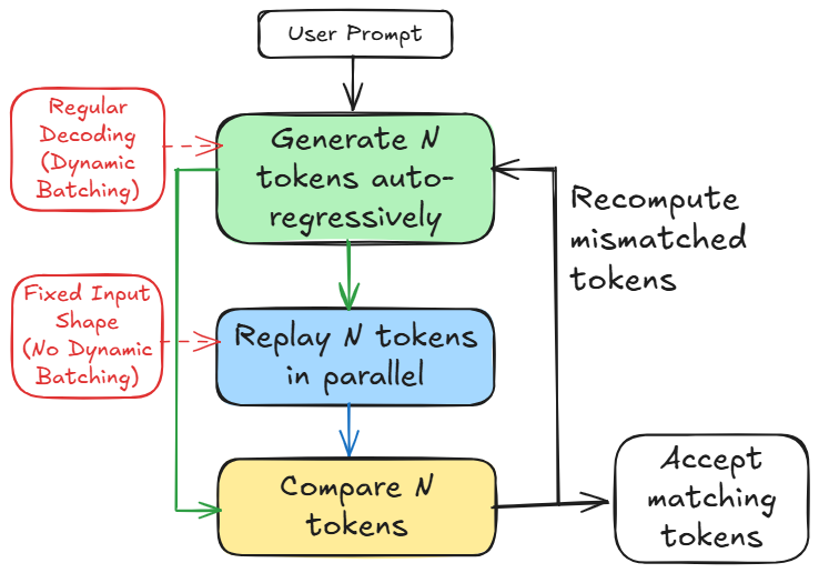
Based on these observations, we introduce LLM-42, a scheduling-based approach to deterministic LLM inference inspired by speculative decoding. In speculative decoding [specdecoding-icml2023, chen2023accelerating, xia2023speculative, specinfer-2024], a fast path produces multiple candidate tokens while a verifier validates their correctness. We observe that the same structure can be repurposed to enable determinism (see Figure 1): fast path can optimize for high throughput token generation while a verifier can enforce determinism. Table 1 highlights key differences between conventional speculative decoding and our approach.
<details>
<summary>figures_h100_pcie/diagram/banner.png Details</summary>
### Visual Description
## Flowchart: Token Generation and Verification Process
### Overview
This image is a process flow diagram illustrating an iterative token generation and verification mechanism, likely representing a "Speculative Decoding" or "Draft-Verify" architecture used in Large Language Models (LLMs). The diagram contrasts two operational modes—Regular Decoding and Fixed Input Shape—and depicts the cycle of generating, replaying, comparing, and accepting or recomputing tokens.
### Components/Axes
The diagram is composed of several distinct nodes and labels:
**Main Process Nodes (Center Column):**
* **Top:** "User Prompt" (Black-bordered box).
* **Upper-Center:** "Generate N tokens auto-regressively" (Green-filled box).
* **Middle:** "Replay N tokens in parallel" (Blue-filled box).
* **Lower-Center:** "Compare N tokens" (Yellow-filled box).
* **Right:** "Accept matching tokens" (Black-bordered box).
**Side Labels (Left Column):**
* **Top-Left:** "Regular Decoding (Dynamic Batching)" (Red-bordered box).
* **Bottom-Left:** "Fixed Input Shape (No Dynamic Batching)" (Red-bordered box).
**Flow Indicators:**
* **Black Arrows:** Represent the primary sequential flow of the process.
* **Green Arrow:** Represents a secondary or conditional path originating from the "Generate" node to the "Compare" node.
* **Dashed Red Arrows:** Indicate the application of the side labels to specific process nodes.
### Detailed Analysis
The process follows a logical sequence with a feedback loop:
1. **Initialization:** The process begins with a "User Prompt."
2. **Generation Phase:** The prompt enters the "Generate N tokens auto-regressively" node. This node is associated with "Regular Decoding (Dynamic Batching)."
3. **Replay Phase:** The output from the generation phase flows into the "Replay N tokens in parallel" node. This node is associated with "Fixed Input Shape (No Dynamic Batching)."
4. **Comparison Phase:** The output from the replay phase flows into the "Compare N tokens" node.
5. **Outcome/Loop:**
* **Success:** If tokens match, the flow proceeds to the right to "Accept matching tokens."
* **Failure:** If tokens do not match, a feedback loop labeled "Recompute mismatched tokens" returns the process to the "Generate N tokens auto-regressively" node.
6. **Bypass Path:** A green arrow connects the "Generate N tokens auto-regressively" node directly to the "Compare N tokens" node, bypassing the "Replay" step.
### Key Observations
* **Iterative Feedback:** The most critical component is the loop labeled "Recompute mismatched tokens," which indicates that the system is self-correcting; it does not simply discard errors but re-processes them.
* **Operational Contrast:** The diagram explicitly separates "Regular Decoding" (associated with the generation step) from "Fixed Input Shape" (associated with the replay step), suggesting that the system handles these two phases with different computational constraints.
* **Parallelism:** The "Replay" step is explicitly noted as occurring "in parallel," which is a hallmark of speculative decoding techniques designed to increase throughput.
### Interpretation
This diagram demonstrates an optimization strategy for LLM inference.
* **The Logic:** The system generates a draft of $N$ tokens (the "Generate" step). It then verifies these tokens by running them through a model (the "Replay" step) to see if they match the model's actual output.
* **Efficiency:** By using "Fixed Input Shape" for the replay step, the system likely leverages hardware acceleration (like GPUs) more effectively than the variable-length "Regular Decoding" used in the generation step.
* **The "Why":** The "Recompute mismatched tokens" loop is the mechanism that ensures accuracy. If the draft tokens (generated by a potentially faster, smaller model) are incorrect, the system identifies the mismatch and recomputes only the necessary parts. This architecture allows the model to output multiple tokens per step, significantly reducing latency compared to standard auto-regressive decoding, provided the draft model is reasonably accurate.
</details>
Figure 1: Overview of LLM-42.
LLM-42 employs a decode–verify–rollback protocol that decouples regular decoding from determinism enforcement. It generates candidate output tokens using standard fast-path autoregressive decoding whose output is largely—but not provably—consistent across runs (O1). Determinism is guaranteed by a verifier that periodically replays a fixed-size window of recently generated tokens. Because the input shape is fixed during verification, replayed tokens follow a consistent reduction order (O2) and serve as a deterministic reference execution. Tokens are released to the user only after verification. When the verifier detects a mismatch, LLM-42 rolls the sequence back to the last matching token and resumes decoding from this known-consistent state. In general, two factors make this approach practical: (1) verification is low cost i.e., like prefill, it is typically 1-2 orders of magnitude more efficient than the decode phase, and (2) rollbacks are infrequent: more than half of the requests complete without any rollback, and only a small fraction require multiple rollbacks.
| Fast path generates tokens using some form of approximation | No approximation; only floating-point rounding errors |
| --- | --- |
| Low acceptance rate and hence limited speculation depth (2-8 tokens) | High acceptance rate and hence longer speculation (32-64 tokens) |
| Typically uses separate draft and target models | Uses the same model for decoding and verification |
Table 1: Speculative decoding vs. LLM-42.
By decoupling determinism from token generation, LLM-42 enables determinism to be enforced selectively, preserving the natural variability and creativity of LLM outputs where appropriate. This separation also helps performance: the fast path can use whatever batch sizes and reduction schedules are most efficient, prefill computation can follow different reduction strategy than decode (O3) and its execution need not be verified (in our design, prefill is deterministic by construction), and finally, verification can be skipped entirely for requests that do not need determinism (O4).
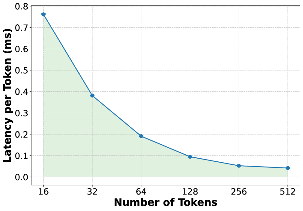
The efficiency of our approach critically depends on the size of verification window i.e., number of tokens verified together. Smaller windows incur high verification overhead since their computation is largely memory-bound but require less recomputation on verification failures. In contrast, larger windows incur lower verification cost due to being compute-bound, but increase recomputation cost by triggering longer rollbacks on mismatches. To balance this trade-off, we introduce grouped verification: instead of verifying a large window of a single request, we verify smaller fixed-size windows of multiple requests together. This design preserves the low rollback cost of small windows while amortizing verification overhead. Overall, we make the following contributions:
- We present the first systematic analysis of batch-invariant computation to highlight the performance and engineering cost associated with this approach.
- We present an alternate approach LLM-42 to enable determinism in LLM inference.
- We implement LLM-42 on top of SGLang and show that its overhead is proportional to fraction of traffic that requires determinism; it retains near-peak performance when deterministic traffic is low, whereas SGLang incurs high overhead of up to 56% in deterministic mode. Our source code will be available at https://github.com/microsoft/llm-42.
## 2 Background and Motivation
<details>
<summary>figures_h100_pcie/diagram/llm-arch.png Details</summary>
### Visual Description
## Diagram: Autoregressive Model Architecture
### Overview
This image is a schematic flow diagram illustrating the high-level architecture of an autoregressive model, likely a Transformer-based Large Language Model (LLM). It depicts the data processing pipeline, emphasizing the iterative nature of the model, the internal layer structure, and the distributed computing components.
### Components/Axes
The diagram is organized as a loop with a central processing block.
**External Components:**
* **Top-Left:** "Input" block (white/grey).
* **Middle-Left:** "Embedding" block (light blue).
* **Middle-Right:** "Sampler" block (light purple).
* **Top-Right:** "Output" block (light brown).
* **Top (Arcing Arrow):** Labeled "Autoregressive" with an arrow pointing from the Output block back to the Input block.
**Central Processing Container:**
* A large, light-yellow rounded rectangle spans the center of the diagram, labeled "**x L layers**" at the bottom center. This indicates that the sequence of operations inside this box is repeated $L$ times.
**Internal Components (Inside the "x L layers" container, ordered left-to-right):**
1. **Attention:** A pink block. Below this block is a smaller, distinct label: "**KV Cache**".
2. **All Reduce RMSNorm:** A yellow block.
3. **FFN:** A green block (Feed-Forward Network).
4. **All Reduce RMSNorm:** A yellow block.
### Detailed Analysis
The flow of data follows a sequential path through the architecture:
1. **Initialization:** Data enters the system at the **Input** block.
2. **Embedding:** The input is passed to the **Embedding** block, which converts tokens into vector representations.
3. **Processing (The "L layers" block):** The embedded data enters the large container, which represents the core Transformer blocks. The data passes through:
* **Attention:** The primary mechanism for contextual understanding, supported by a **KV Cache** (Key-Value Cache) to store previous states and optimize inference speed.
* **All Reduce RMSNorm:** A normalization step (Root Mean Square Layer Normalization) combined with an "All Reduce" operation.
* **FFN:** The Feed-Forward Network, which processes the attention output.
* **All Reduce RMSNorm:** A second normalization and synchronization step.
* *Note:* The "x L layers" label indicates this entire sequence is stacked $L$ times.
4. **Generation:** The processed data exits the layers and enters the **Sampler** block, which selects the next token.
5. **Output:** The result is produced at the **Output** block.
6. **Feedback Loop:** The "Autoregressive" arrow indicates that the generated output is fed back into the "Input" block to generate the next token, completing the cycle.
### Key Observations
* **Distributed Computing Focus:** The inclusion of "All Reduce" within the layer structure is significant. It indicates that this architecture is designed for distributed environments (e.g., multi-GPU or multi-node setups), where synchronization (All Reduce) is required after the Attention and FFN operations to ensure consistency across parallel processors.
* **Inference Optimization:** The explicit labeling of "KV Cache" under the "Attention" block highlights the importance of memory management in autoregressive inference, where caching previous keys and values is critical to avoid redundant computation.
* **Standard Transformer Structure:** The sequence (Attention -> Norm -> FFN -> Norm) is a standard configuration for modern decoder-only Transformer architectures.
### Interpretation
This diagram represents the operational loop of a distributed LLM inference engine.
The "Autoregressive" label is the defining characteristic: the model generates one token at a time, and that token becomes part of the input for the next step. The diagram explicitly calls out the two most computationally expensive and communication-heavy parts of the Transformer block: the Attention mechanism and the Feed-Forward Network (FFN).
By placing "All Reduce" operations after both the Attention and FFN blocks, the diagram suggests a parallelized architecture where the model's weights or activations are sharded across multiple devices. The "All Reduce" operation is the synchronization point where these devices communicate to aggregate results before proceeding to the next stage. The "KV Cache" is the critical component that allows the model to maintain context without recomputing the entire sequence history at every step of the autoregressive loop.
</details>
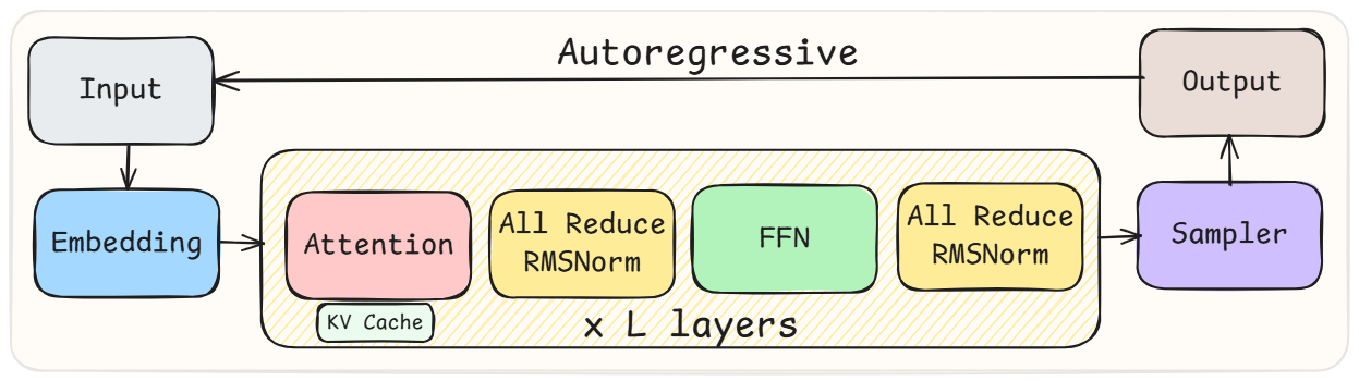
Figure 2: High-level architecture of LLMs.
This section introduces LLMs, explains the source of non-determinism in LLM inference and quantifies the cost of batch-invariant computation based deterministic inference.
### 2.1 Large Language Models
Transformer-based LLMs compose a stack of identical decoder blocks, each containing a self-attention module, a feed-forward network (FFN), normalization layers and communication primitives (Figure 2). The hidden state of every token flows through these blocks sequentially, but within each block the computation is highly parallel: attention performs matrix multiplications over the key–value (KV) cache, FFNs apply two large GEMMs surrounding a nonlinearity, and normalization applies a per-token reduction over the hidden dimension.
Inference happens in two distinct phases namely prefill and decode. Prefill processes prompt tokens in parallel, generating KV cache for all input tokens. This phase is dominated by large parallel computation. Decode is autoregressive: each step consumes the most recent token, updates the KV cache with a single new key and value, and produces the next output token. Decode is therefore sequential within a sequence but parallel across other requests in the batch.
### 2.2 Non-determinism in LLM Inference
In finite precision, arithmetic operations such as accumulation are non-associative, meaning that $(a+b)+c\neq a+(b+c)$ . Non-determinism in LLM inference stems from this non-associativity when combined with dynamic batching, a standard technique to achieve high throughput inference. With dynamic batching, the same request may be co-located with different sets of requests across different runs, resulting in varying batch sizes. Further, GPU kernels adapt their parallelization—and consequently their reduction—strategies based on the input sizes. As a result, the same logical operation can be evaluated with different floating-point accumulation orders depending on the batch it appears in, leading to inconsistent numerical results.
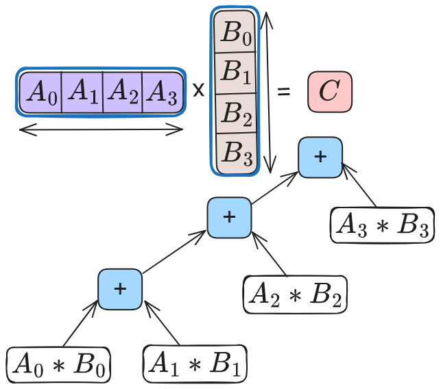
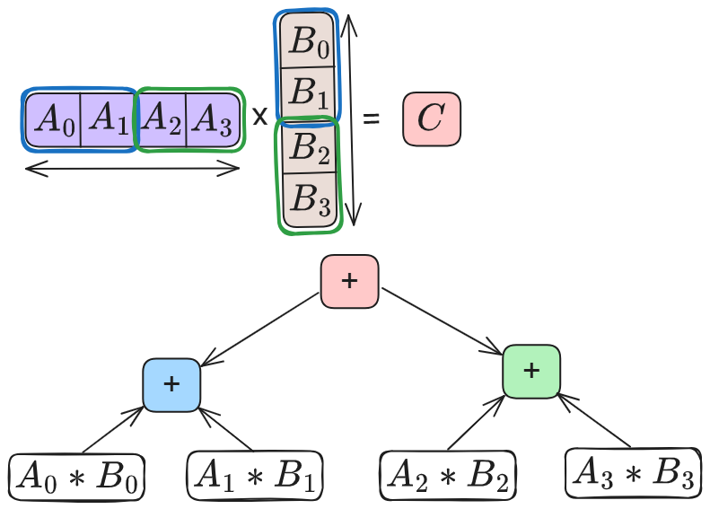
Reductions are common in LLM inference, appearing in matrix multiplications (GEMMs), attention, normalization and collective communication such as AllReduce. GEMM is the most common and time consuming operator. High-performance GEMM implementations on GPUs use hierarchical tiling and parallel reductions to improve occupancy and memory reuse. A common optimization is split-K parallelism, where the reduction dimension is partitioned across multiple thread blocks. Each block computes a partial result, which is then combined via an additional reduction step. Whether split-K is used—and how many splits are chosen—depends on the shape on input matrices. These choices directly change the reduction tree as shown in Figure 3, producing different numerical results for a given token across runs. Similarly, attention kernels split work across the key–value dimension to increase SM utilization, followed by a reduction to combine partial results. Normalization operators reduce across feature dimensions. As inference progresses, batch-dependent reduction choices in these operators introduce small numerical drifts that propagate across kernels, layers and decoding steps, eventually influencing output tokens even when the sampling hyper-parameters are fixed.
<details>
<summary>figures_h100_pcie/diagram/gemm_wo_splitk.png Details</summary>
### Visual Description
## Diagram: Dot Product Calculation
### Overview
The image is a mathematical diagram illustrating the calculation of a dot product between two 4-element vectors, $A$ and $B$, resulting in a scalar $C$. The diagram is divided into two parts: a top section defining the vector operation and a bottom section detailing the sequential summation process used to compute the result.
### Components/Axes
* **Vector A (Top-Left):** A horizontal row vector containing four elements: $[A_0, A_1, A_2, A_3]$. The box is shaded purple.
* **Vector B (Top-Center):** A vertical column vector containing four elements: $[B_0, B_1, B_2, B_3]$. The box is shaded light red.
* **Result C (Top-Right):** A scalar value represented by the box labeled $C$. The box is shaded light red.
* **Operations:**
* **Multiplication ($*$):** Represented by the symbol "$*$" in white rounded rectangles.
* **Addition ($+$):** Represented by the symbol "$+$" in light blue rounded squares.
* **Arrows:** Indicate the flow of data from the individual products into the summation nodes.
### Detailed Analysis
The diagram breaks down the dot product $C = \sum_{i=0}^{3} A_i B_i$ into a sequential summation tree:
1. **Product Generation:**
* The diagram identifies four distinct product terms: $(A_0 * B_0)$, $(A_1 * B_1)$, $(A_2 * B_2)$, and $(A_3 * B_3)$. These are located at the bottom and right of the diagram.
2. **Summation Flow (Sequential Accumulation):**
* **First Addition (Bottom-Left):** The terms $(A_0 * B_0)$ and $(A_1 * B_1)$ flow into the lowest "+" node.
* **Second Addition (Middle):** The output of the first addition node flows into the middle "+" node, where it is added to $(A_2 * B_2)$.
* **Third Addition (Top-Right):** The output of the middle "+" node flows into the final, highest "+" node, where it is added to $(A_3 * B_3)$.
* **Final Result:** The output of the final "+" node represents the scalar $C$.
### Key Observations
* **Sequential vs. Parallel:** The diagram illustrates a sequential accumulation (a "linear" or "skewed" tree) rather than a balanced binary tree. This implies an order of operations where the sum is built up one term at a time.
* **Color Coding:**
* **Purple:** Associated with the row vector $A$.
* **Light Red:** Associated with the column vector $B$ and the final result $C$.
* **Light Blue:** Associated with the addition operations.
* **Layout:** The diagram uses a "staircase" layout for the addition nodes, visually reinforcing the sequential nature of the calculation.
### Interpretation
This diagram serves as a visual representation of the standard algorithm for computing a dot product, often implemented in software as a `for` loop or an accumulator variable.
By visualizing the operation as a sequential tree rather than a parallel reduction tree, the diagram highlights the dependency chain: the calculation of the final sum cannot be completed until the previous partial sums are computed. This is a fundamental concept in computer architecture and parallel computing; while this diagram shows a sequential approach, it implicitly contrasts with parallel reduction methods (where $A_0*B_0 + A_1*B_1$ and $A_2*B_2 + A_3*B_3$ could be computed simultaneously).
</details>
(a) Without split-K.
<details>
<summary>figures_h100_pcie/diagram/gemm_w_splitk.png Details</summary>
### Visual Description
## Diagram: Decomposition of a Dot Product Operation
### Overview
The image illustrates the mathematical decomposition of a dot product operation between two four-element vectors ($A$ and $B$) into a parallelizable tree structure. The diagram is divided into two main sections: a top section representing the vector multiplication operation and a bottom section representing the summation tree (reduction) used to calculate the final result $C$.
### Components/Axes
The diagram utilizes color-coding to group operations:
* **Blue:** Represents the first half of the vectors (indices 0 and 1).
* **Green:** Represents the second half of the vectors (indices 2 and 3).
* **Pink:** Represents the final summation and the root of the tree.
**Top Section (Vector Operation):**
* **Left:** A horizontal vector containing elements $[A_0, A_1, A_2, A_3]$.
* The sub-vector $[A_0, A_1]$ is enclosed in a blue rounded rectangle.
* The sub-vector $[A_2, A_3]$ is enclosed in a green rounded rectangle.
* **Center:** A multiplication symbol "x".
* **Right:** A vertical vector containing elements $[B_0, B_1, B_2, B_3]$.
* The sub-vector $[B_0, B_1]$ is enclosed in a blue rounded rectangle.
* The sub-vector $[B_2, B_3]$ is enclosed in a green rounded rectangle.
* **Far Right:** An equals sign followed by a pink rounded rectangle containing the variable "$C$".
**Bottom Section (Summation Tree):**
* **Root (Top):** A pink rounded rectangle containing a "+" sign.
* **Intermediate Nodes:**
* **Left:** A blue rounded rectangle containing a "+" sign.
* **Right:** A green rounded rectangle containing a "+" sign.
* **Leaf Nodes (Bottom):**
* Under the blue node: Two boxes containing "$A_0 * B_0$" and "$A_1 * B_1$".
* Under the green node: Two boxes containing "$A_2 * B_2$" and "$A_3 * B_3$".
### Detailed Analysis
The diagram maps the calculation of a dot product $C = \sum_{i=0}^{3} A_i B_i$ into a binary tree structure.
1. **Vector Grouping:** The vectors are split into two halves. The blue group handles indices 0 and 1, while the green group handles indices 2 and 3.
2. **Multiplication:** The diagram implies that the elements are multiplied pairwise ($A_i * B_i$).
3. **Tree Flow:**
* The leaf nodes perform the multiplication: $A_0*B_0$, $A_1*B_1$, $A_2*B_2$, and $A_3*B_3$.
* The intermediate nodes perform the partial summation:
* The blue node sums the first two products: $(A_0 * B_0) + (A_1 * B_1)$.
* The green node sums the last two products: $(A_2 * B_2) + (A_3 * B_3)$.
* The root node sums the results of the intermediate nodes to produce the final scalar $C$.
</details>
(b) With split-K.
Figure 3: GEMM kernels compute dot products using standard accumulation or split-K parallelization. While split-K increases parallelism, it alters the reduction tree based on K.
### 2.3 Defeating Non-determinism
He et al. at Thinking Machines Lab recently introduced a new approach named batch-invariant computation to enable deterministic LLM inference [he2025nondeterminism]. In this approach, a GPU kernel is constrained to use a single, universal reduction strategy for all tokens, eliminating batch-dependent reductions. Both SGLang and vLLM use this approach [SGLangTeam2025, vllm-batch-invariance-2025, vllm-batch-invariant-2025]: these systems either deploy the batch-invariant kernels provided by He et al. [tmops2025] or implement new kernels [batch-inv-inf-vllm, det-infer-batch-inv-ops-sglang].
<details>
<summary>x1.png Details</summary>
### Visual Description
## Line Chart: Performance Comparison (TFLOPS) vs. # Tokens
### Overview
This image is a log-log line chart comparing the computational performance (measured in TFLOPS) of two different software implementations—"Non-batch-invariant (cuBLAS)" and "Batch-invariant (Triton)"—across a range of token counts (# Tokens). The chart illustrates how performance scales as the number of tokens increases, highlighting the performance gap and saturation points for both methods.
### Components/Axes
* **Y-Axis:** Labeled "TFLOPS". This is a logarithmic scale representing computational throughput.
* **X-Axis:** Labeled "# Tokens". This is a logarithmic scale representing the input size. The values are: 1, 2, 4, 8, 16, 32, 64, 128, 256, 512, 1024, 2048, 4096, 8192.
* **Legend:** Positioned in the bottom-center of the chart area.
* **Blue line with circle markers:** "Non-batch-invariant (cuBLAS)"
* **Red line with square markers:** "Batch-invariant (Triton)"
### Detailed Analysis
**Trend Verification:**
Both data series exhibit a strong positive correlation (upward slope) as the number of tokens increases from 1 to approximately 256-512. Following this growth phase, both lines enter a saturation phase where performance levels off, indicating that the system has reached a hardware or memory bandwidth limit.
**Data Point Extraction (Approximate Values):**
| # Tokens | Non-batch-invariant (cuBLAS) [Blue] | Batch-invariant (Triton) [Red] |
| :--- | :--- | :--- |
| 1 | ~1.5 TFLOPS | ~0.25 TFLOPS |
| 2 | ~3 TFLOPS | ~0.5 TFLOPS |
| 4 | ~6 TFLOPS | ~1.1 TFLOPS |
| 8 | ~12 TFLOPS | ~2.2 TFLOPS |
| 16 | ~25 TFLOPS | ~5 TFLOPS |
| 32 | ~50 TFLOPS | ~10 TFLOPS |
| 64 | ~95 TFLOPS | ~22 TFLOPS |
| 128 | ~180 TFLOPS | ~45 TFLOPS |
| 256 | ~380 TFLOPS | ~90 TFLOPS |
| 512 | ~500 TFLOPS | ~95 TFLOPS |
| 1024 | ~580 TFLOPS | ~130 TFLOPS |
| 2048 | ~580 TFLOPS | ~150 TFLOPS |
| 4096 | ~580 TFLOPS | ~160 TFLOPS |
| 8192 | ~600 TFLOPS | ~170 TFLOPS |
### Key Observations
* **Performance Gap:** The "Non-batch-invariant (cuBLAS)" implementation consistently outperforms the "Batch-invariant (Triton)" implementation by a significant margin, often by a factor of 3x to 5x across the measured range.
* **Saturation Points:**
* The **Blue line (cuBLAS)** reaches its primary saturation point around 512 tokens, after which performance gains are marginal.
* The **Red line (Triton)** reaches a temporary plateau around 256-512 tokens, but continues to show slight performance growth up to 2048 tokens before flattening out.
* **Scaling:** Both implementations scale linearly (in log-log space) until they hit their respective hardware/implementation limits.
### Interpretation
This chart demonstrates a classic engineering trade-off between **specialized optimization** and **generalization**.
* **Non-batch-invariant (cuBLAS):** The high performance suggests this implementation is highly optimized for specific, fixed-size operations. It likely utilizes highly tuned kernels (cuBLAS) that are not designed to handle varying batch sizes dynamically, hence the "non-batch-invariant" label. It hits the hardware ceiling faster because it is likely more efficient at utilizing the GPU's compute units for those specific configurations.
* **Batch-invariant (Triton):** The lower performance suggests that this implementation prioritizes flexibility. Being "batch-invariant" implies the code can handle varying input sizes without needing to recompile or switch kernels. This flexibility comes at the cost of raw peak performance (TFLOPS), as the kernel must be more generalized and potentially less efficient than the highly specialized cuBLAS kernels.
* **Conclusion:** If the application requires maximum throughput and the batch size is static, cuBLAS is the clear choice. If the application requires dynamic batching or variable token lengths, Triton is the necessary choice, despite the performance penalty.
</details>
(a) GEMM
<details>
<summary>x2.png Details</summary>
### Visual Description
## Line Chart: Performance Benchmark of Token Processing Implementations
### Overview
This image displays a line chart comparing the execution time (in milliseconds) of three different software implementations across varying numbers of tokens. The chart demonstrates how performance scales as the input size (# Tokens) increases from 1 to 4096.
### Components/Axes
* **Y-Axis:** "Execution Time (ms)". The scale ranges from 0.0 to 1.2, with increments of 0.2.
* **X-Axis:** "# Tokens". The scale is logarithmic, with markers at: 1, 8, 32, 128, 256, 512, 1024, 2048, 4096.
* **Legend (Positioned Top-Left):**
* **Green line with circle markers:** "Non-batch-invariant (CUDA)"
* **Red line with square markers:** "Batch-invariant (Python)"
* **Blue line with square markers:** "Batch-invariant (Triton)"
### Detailed Analysis
#### Trend Verification
* **Non-batch-invariant (CUDA) [Green]:** This line represents the most efficient implementation. It remains relatively flat and low between 1 and 512 tokens, then begins a gradual upward slope, showing the lowest execution time across the entire range.
* **Batch-invariant (Triton) [Blue]:** This line follows a nearly identical trajectory to the CUDA implementation. It remains very low and stable until 512 tokens, then begins to rise, ending slightly higher than the CUDA implementation at 4096 tokens.
* **Batch-invariant (Python) [Red]:** This line starts significantly higher than the other two. It remains relatively flat until 256 tokens, then exhibits a sharp, exponential increase in execution time starting at 512 tokens, diverging drastically from the other two implementations.
#### Data Points (Approximate Values)
| # Tokens | Non-batch-invariant (CUDA) | Batch-invariant (Triton) | Batch-invariant (Python) |
| :--- | :--- | :--- | :--- |
| **1** | ~0.03 ms | ~0.04 ms | ~0.10 ms |
| **8** | ~0.03 ms | ~0.04 ms | ~0.10 ms |
| **32** | ~0.03 ms | ~0.04 ms | ~0.10 ms |
| **128** | ~0.03 ms | ~0.04 ms | ~0.10 ms |
| **256** | ~0.03 ms | ~0.04 ms | ~0.10 ms |
| **512** | ~0.02 ms | ~0.03 ms | ~0.15 ms |
| **1024** | ~0.03 ms | ~0.04 ms | ~0.35 ms |
| **2048** | ~0.08 ms | ~0.10 ms | ~0.68 ms |
| **4096** | ~0.15 ms | ~0.20 ms | ~1.30 ms |
### Key Observations
* **Performance Gap:** There is a massive performance disparity between the Python implementation and the GPU-accelerated implementations (CUDA and Triton) as the token count increases. At 4096 tokens, the Python implementation is roughly 6.5x slower than the Triton implementation and nearly 9x slower than the CUDA implementation.
* **The "Knee" Point:** All three implementations show a slight dip in execution time at 512 tokens before the upward trend begins. This may indicate a cache behavior or a specific optimization threshold in the underlying hardware/software execution.
* **Triton vs. CUDA:** The Triton implementation is highly competitive with the raw CUDA implementation, suggesting that Triton provides a near-native performance experience for this specific "batch-invariant" operation.
### Interpretation
The data demonstrates the critical importance of implementation choice when handling high-throughput token processing.
1. **Python Bottleneck:** The "Batch-invariant (Python)" implementation is clearly not suitable for high-token-count workloads. The exponential growth suggests that the Python overhead becomes the dominant factor as the workload scales, likely due to interpreter overhead or lack of efficient parallelization compared to the GPU-based approaches.
2. **Triton as a Solution:** The fact that "Batch-invariant (Triton)" tracks so closely with "Non-batch-invariant (CUDA)" is significant. It suggests that developers can achieve near-CUDA performance using Triton, which is generally easier to write and maintain than raw CUDA kernels.
3. **Scalability:** For applications requiring processing of 1024+ tokens, moving away from a standard Python implementation to a compiled/GPU-accelerated implementation (like Triton) is essential to prevent performance degradation.
</details>
(b) RMSNorm
Figure 4: Performance comparison between batch-invariant vs. non-batch-invariant kernels.
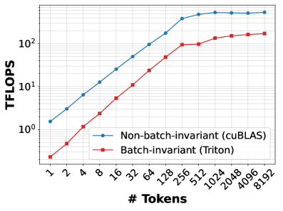
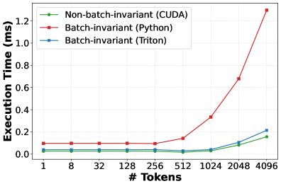
While batch-invariant computation eliminates non-determinism, we find that it is a poor fit for real LLM serving systems. By enforcing a universal reduction strategy across all executions, it couples determinism to kernel design and sacrifices performance opportunities. It also turns determinism into a fixed tax paid by every request: dynamic batching aggregates requests, but batch-invariant kernels eliminate the very optimizations—such as split-K and shape-aware tiling—that make batching effective in the first place. Worse, because kernels are not batch-invariant, adopting this approach requires maintaining a parallel kernel stack solely for determinism. We also quantify the performance cost of this approach below.
GEMM. 4(a) compares the throughput of cuBLAS based GEMMs used in PyTorch against Triton-based batch-invariant kernels developed by He et al. The matrix dimensions correspond to the down projection operation of the Llama-3.1-8B-Instruct model’s feed-forward-network. On our GPU, cuBLAS (via torch.mm) reaches up to 527 TFLOPS, whereas the batch-invariant kernel peaks at 194 TFLOPS, a slowdown of 63%. This gap arises because this Triton-based batch-invariant implementation does not use split-K or exploit newer hardware features such as Tensor Memory Accelerators [TMA_Engine] or advanced techniques like warp specialization [fa-3], all of which are leveraged by PyTorch through vendor-optimized cuBLAS kernels.
RMSNorm. 4(b) compares RMSNorm execution time for varying number of tokens for three implementations: Python-based version used in SGLang, Thinking Machines’ Triton-based kernel, and SGLang’s default CUDA kernel. The first two are batch-invariant; the CUDA kernel is not. The Python implementation is up to $7\times$ slower than the non-batch-invariant CUDA kernel due to unfused primitive operations and poor shared-memory utilization. The Triton kernel performs substantially better but remains up to 50% slower than the fused CUDA implementation, which benefits from optimized reductions and kernel fusion. These overheads are amplified at high batch sizes or long context lengths, where normalization may account for a nontrivial fraction of inference time [gond2025tokenweave].
<details>
<summary>x3.png Details</summary>
### Visual Description
## Bar Chart: Decode Throughput by Batch Size
### Overview
This image displays a stacked bar chart comparing the "Decode Throughput" (measured in tokens/sec) for two different "Batch Size" configurations: 10 and 11. The chart utilizes a color-coded legend to distinguish between three different operational modes or models: "SGLang non-deterministic," "SGLang deterministic," and "LLM-42."
### Components/Axes
* **Y-Axis:** Labeled "Decode Throughput (tokens/sec)". The scale ranges from 0 to 1200, with major tick marks every 200 units.
* **X-Axis:** Labeled "Batch Size". It contains two discrete categories: 10 and 11.
* **Legend:** Positioned at the top-center of the chart area.
* **Blue rectangle:** "SGLang non-deterministic"
* **Red/Pink rectangle:** "SGLang deterministic"
* **Green rectangle:** "LLM-42"
### Detailed Analysis
The chart presents two distinct bars corresponding to the batch sizes on the x-axis.
**1. Batch Size 10 (Left Bar):**
* **Visual Trend:** This bar is a single, solid block.
* **Composition:** The entire bar is colored blue, corresponding to "SGLang non-deterministic."
* **Value:** The top of the bar aligns approximately with the 840 tokens/sec mark on the y-axis.
**2. Batch Size 11 (Right Bar):**
* **Visual Trend:** This bar is a stacked composite of all three categories.
* **Composition (from bottom to top):**
* **Bottom Section (Red/Pink):** Corresponds to "SGLang deterministic." It extends from 0 to approximately 410 tokens/sec.
* **Middle Section (Green):** Corresponds to "LLM-42." It sits on top of the red section, extending from approximately 410 to 910 tokens/sec. This represents a segment height of approximately 500 tokens/sec.
* **Top Section (Blue):** Corresponds to "SGLang non-deterministic." It sits on top of the green section, extending from approximately 910 to 940 tokens/sec. This represents a segment height of approximately 30 tokens/sec.
* **Total Value:** The total height of the stacked bar is approximately 940 tokens/sec.
### Key Observations
* **Throughput Increase:** Increasing the batch size from 10 to 11 results in an overall increase in decode throughput (from ~840 to ~940 tokens/sec).
* **Composition Shift:** The nature of the throughput changes significantly between the two batch sizes. At Batch Size 10, the throughput is derived entirely from "SGLang non-deterministic." At Batch Size 11, the throughput is dominated by "LLM-42" and "SGLang deterministic," with "SGLang non-deterministic" contributing only a negligible fraction (~3%) of the total throughput.
### Interpretation
The data suggests that the system's performance characteristics are highly sensitive to the batch size.
* **Operational Shift:** The transition from Batch Size 10 to 11 appears to trigger a fundamental change in how tokens are processed. At Batch Size 10, the system operates in a "non-deterministic" mode exclusively. At Batch Size 11, the system shifts to a hybrid processing model where the vast majority of the work is handled by "LLM-42" and "SGLang deterministic" components.
* **Efficiency:** While the total throughput is higher at Batch Size 11, the "SGLang non-deterministic" mode—which was the sole driver of performance at Batch Size 10—is almost entirely sidelined at Batch Size 11. This implies that the system may be switching to a different execution path or model configuration when the batch size is increased, prioritizing "LLM-42" and deterministic processing over the non-deterministic path.
</details>
Figure 5: Decode throughput under different scenarios.
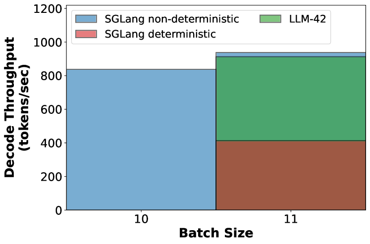
End-to-end throughput. Figure 5 measures token generation throughput (tokens per second) under three scenarios: (1) 10 requests running in non-deterministic mode, (2) 11 requests running in non-deterministic mode, and (3) 11 requests running in deterministic mode but only one of them requires deterministic output. With 10 concurrent non-deterministic requests, the system generates 845 tokens/s. The batch size increases to 11 when a new request arrives and if decoding continues non-deterministically, throughput improves to 931 tokens/s (a jump of about 10%). In contrast, if the new request requires determinism, the entire batch is forced to execute through the slower batch-invariant kernels, causing throughput to collapse by 56% to about 415 tokens/s—penalizing every in-flight request for a single deterministic one. This behavior is undesirable because it couples the performance of all requests to that of the slowest request.
Overall, these results show that batch-invariant execution incurs a substantial performance penalty. While it may be feasible to improve the performance of batch-invariant kernels, doing so would require extensive model- and hardware-specific kernel development. This engineering and maintenance burden makes the approach difficult to sustain in practice. This may be why deterministic inference is largely confined to debugging and verification today, rather than being deployed for real-world LLM serving.
## 3 Observations
In this section, we distill a set of concrete observations about non-determinism, GPU kernels and LLM use-cases. These observations expose why batch-invariant computation is overly restrictive and motivate a more general approach to enable determinism in LLM inference.
Observation-1 (O1). If a sequence is already in a consistent state, the next emitted token is usually consistent even under dynamic batching. However, once a token diverges, autoregressive decoding progressively amplifies this difference over subsequent steps.
This is because tokens become inconsistent only when floating-point drift is large enough to alter the effective decision made by the sampler—e.g., by changing the relative ordering or acceptance of high-probability candidates under the decoder’s sampling policy (e.g., greedy or stochastic sampling). In practice, such boundary-crossing events are rare, as numerical drift typically perturbs logits only slightly. However, autoregressive decoding amplifies even a single such deviation: once a token differs, all subsequent tokens may diverge. Since a single request typically produces hundreds to thousands of output tokens, two sequence-level outputs can look dramatically different even if the initial divergence is caused by a single token flip induced by a different reduction order across runs.
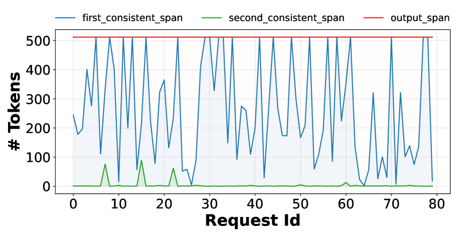
To demonstrate this phenomenon empirically, we conduct an experiment using the Llama-3.1-8B-Instruct model on the ShareGPT dataset. We first execute 350 requests with batch size one—i.e., without dynamic batching—to obtain reference (“ground-truth”) output tokens. We then re-run the same requests under dynamic batching at a load of 6 queries per second and compare each request’s output against its reference. In both runs, we fix the output length to 512 tokens.
<details>
<summary>x4.png Details</summary>
### Visual Description
## Line Chart: Token Span Analysis by Request ID
### Overview
This image displays a line chart tracking three distinct metrics—`first_consistent_span`, `second_consistent_span`, and `output_span`—across 80 individual requests. The chart visualizes the token usage or span length for these metrics, with the X-axis representing the Request ID and the Y-axis representing the number of tokens.
### Components/Axes
* **X-Axis:** Labeled "Request Id". The scale ranges from 0 to 80, with major tick marks every 10 units.
* **Y-Axis:** Labeled "# Tokens". The scale ranges from 0 to 500, with grid lines at 100-unit intervals (100, 200, 300, 400, 500).
* **Legend:** Positioned at the top center of the chart.
* **Blue line:** `first_consistent_span`
* **Green line:** `second_consistent_span`
* **Red line:** `output_span`
* **Visual Elements:** The area beneath the blue line is shaded with a light blue tint; the area beneath the green line is shaded with a light green tint.
### Detailed Analysis
#### 1. Red Line (`output_span`)
* **Trend:** This line is perfectly horizontal, indicating a constant value.
* **Value:** It remains fixed at approximately 512 tokens throughout the entire duration (0 to 80 requests). This appears to represent a hard limit or a maximum configuration setting.
#### 2. Blue Line (`first_consistent_span`)
* **Trend:** This series exhibits high volatility, oscillating rapidly between near-zero values and the maximum limit (512).
* **Data Points:**
* The line frequently hits the `output_span` ceiling (512) at various intervals, notably around Request IDs 7, 11, 15, 22, 28, 32, 47, 52, 61, 73, and 79.
* It drops to near-zero values at several points, most notably around Request IDs 26, 42, 65, and 72.
* The baseline for this line is generally unstable, fluctuating between 50 and 300 tokens when not hitting the ceiling.
#### 3. Green Line (`second_consistent_span`)
* **Trend:** This series is predominantly flat at 0, with three distinct, isolated spikes occurring early in the sequence.
* **Data Points:**
* **Spike 1:** Occurs around Request ID 7-8, reaching a peak of approximately 80 tokens.
* **Spike 2:** Occurs around Request ID 14-15, reaching a peak of approximately 90 tokens.
* **Spike 3:** Occurs around Request ID 21-22, reaching a peak of approximately 60 tokens.
* **Minor Activity:** A very small, negligible blip occurs around Request ID 60, reaching approximately 15 tokens.
### Key Observations
* **Ceiling Effect:** The `output_span` (red line) acts as a hard cap for the `first_consistent_span` (blue line). The blue line frequently reaches this cap, suggesting that the system is often hitting its maximum token limit.
* **Sparse Activity:** The `second_consistent_span` (green line) is highly inactive. It only shows significant activity in the first 25% of the requests (0-25). After Request ID 25, it remains almost entirely dormant.
* **Inverse Relationship:** There is no obvious inverse correlation between the blue and green lines; rather, the green line appears to be an independent, intermittent process that ceases to trigger after the initial phase.
### Interpretation
This chart likely represents the performance monitoring of an LLM (Large Language Model) or a similar text-generation API.
* **The Red Line (512):** This is almost certainly the `max_tokens` parameter or the context window limit set for the model.
* **The Blue Line:** This represents the actual token count of the primary input or output span. The high volatility and frequent hitting of the 512-token ceiling suggest that the model is frequently being truncated or is consistently filling its allocated context window.
* **The Green Line:** This likely represents a secondary, conditional process (perhaps a specific type of tool-use, a secondary prompt, or a "warm-up" routine) that is only invoked during the early stages of the request batch. The fact that it disappears after Request ID 25 suggests that the conditions required to trigger this "second span" are no longer met in the later requests.
In summary, the system is operating at its capacity limit (`output_span`) frequently, and a secondary process (`second_consistent_span`) is only relevant during the initial phase of the operation.
</details>
Figure 6: Length of the first and second consistent span (number of tokens that match with the ground-truth) for different requests under dynamic batching.
We quantify divergence using two metrics. The first consistent span of a request measures the number of initial output tokens that match exactly across the two runs, while the second consistent span measures the number of matching tokens between the first and second divergence points. Figure 6 shows these metrics for 80 requests. In the common case, hundreds of initial tokens are identical across both runs, with some requests exhibiting an exact match of all 512 tokens in the first consistent span. However, once a single token diverges, the sequence rapidly drifts: the second consistent span is near zero for most requests, indicating that divergence quickly propagates through the remainder of the output.
<details>
<summary>figures/position-invariant-kernel.png Details</summary>

### Visual Description
## Diagram: Process Flow Comparison (Run-1 vs. Run-2)
### Overview
The image displays a schematic representation of two sequential or overlapping data processing operations, labeled "Run-1" and "Run-2". Both runs utilize a "Kernel" component to transform input data into output data. The diagram illustrates how a shared input ($T_1$) is processed in two different contexts, with specific outputs highlighted in red circles.
### Components/Axes
The diagram is divided into two distinct processing blocks arranged horizontally.
**Run-1 (Left Block):**
* **Inputs:** Two inputs, $T_0$ and $T_1$, enter from the left.
* **Process:** A light purple rounded rectangle labeled "Kernel".
* **Outputs:** Two outputs, $T_0'$ and $T_1'$, exit to the right.
* **Highlight:** The output $T_1'$ is enclosed in a red circle.
**Run-2 (Right Block):**
* **Inputs:** Two inputs, $T_1$ and $T_2$, enter from the left.
* **Process:** A light purple rounded rectangle labeled "Kernel".
* **Outputs:** Two outputs, $T_1''$ and $T_2''$, exit to the right.
* **Highlight:** The output $T_1''$ is enclosed in a red circle.
### Detailed Analysis
The flow of data is strictly left-to-right, indicated by arrows.
* **Run-1 Logic:**
* The top input $T_0$ maps to the top output $T_0'$.
* The bottom input $T_1$ maps to the bottom output $T_1'$.
* The bottom output $T_1'$ is the specific point of interest, marked by a red circle.
* **Run-2 Logic:**
* The top input $T_1$ maps to the top output $T_1''$.
* The bottom input $T_2$ maps to the bottom output $T_2''$.
* The top output $T_1''$ is the specific point of interest, marked by a red circle.
### Key Observations
* **Shared Input:** The input $T_1$ is common to both Run-1 and Run-2.
* **Contextual Shift:** In Run-1, $T_1$ is the *second* (bottom) input. In Run-2, $T_1$ is the *first* (top) input.
* **Output Highlighting:** The red circles highlight the output generated from the shared input $T_1$ in each respective run.
* In Run-1, the output derived from $T_1$ is the bottom output ($T_1'$).
* In Run-2, the output derived from $T_1$ is the top output ($T_1''$).
### Interpretation
This diagram likely represents a **sliding window operation** or a **convolutional process** where a kernel function is applied to overlapping segments of a data sequence.
* **Data Relationship:** The "Kernel" represents a function $f(x, y)$ that takes two inputs and produces two outputs.
* Run-1 computes $f(T_0, T_1) \rightarrow (T_0', T_1')$.
* Run-2 computes $f(T_1, T_2) \rightarrow (T_1'', T_2'')$.
* **Significance of the Red Circles:** The red circles indicate that the diagram is specifically tracking the transformation of the shared input $T_1$ across different windows. This is often used in technical documentation to demonstrate **consistency** or **boundary conditions** in sequence processing (e.g., ensuring that the output for $T_1$ is consistent regardless of whether it is the "trailing" element of one window or the "leading" element of the next).
* **Inference:** The notation $T_1'$ vs $T_1''$ suggests that the output for the same input $T_1$ might differ depending on the context (the other input it is paired with), or the diagram is highlighting the specific output that needs to be compared or validated between the two runs.
</details>
Figure 7: A position-invariant kernel produces the same output for a given input element irrespective of its position in the batch, as long as the total batch size is fixed. In this example, $T_{1}^{\prime}==T_{1}^{\prime\prime}$ if the kernel is position-invariant.
| Category | Operator | Invariant | |
| --- | --- | --- | --- |
| Batch | Position | | |
| Matmul | CuBLAS GEMM | ✗ | ✓ |
| Attention | FlashAttention-3 ‡ | ✓ | ✓ |
| Communication | Multimem-based AllReduce ∗ | ✓ | ✓ |
| Ring-based AllReduce | ✗ | ✗ | |
| Tree-based AllReduce ⋆ | ✓ | ✓ | |
| Normalization | RMSNorm † | ✗ | ✓ |
| Fused RMSNorm + Residual † | ✗ | ✓ | |
Table 2: Invariance properties of common inference operators (‡ num_splits=1, ∗ CUDA 13.0+, ⋆ specific NCCL settings, † vLLM/SGLang defaults).
Observation-2 (O2). Most GPU kernels use uniform, shape-consistent reductions: they apply the same reduction strategy to all elements within a given batch. Moreover, the strategy remains fixed for all batches of the same shape, changing only when the shape changes.
The simplest example of this is GEMM kernels. For a given input matrix A of size M x K, a GEMM kernel computes all the M input elements under the same reduction order (say R). Moreover, it applies the same reduction order R to all input matrices of size M x K. We refer to such kernels as position-invariant. Position invariance implies that, with a fixed total batch size, an input element’s output is independent of its position in the batch. Note that such guarantees do not hold for kernels that implement reductions via atomic operations. Fortunately, kernels used in the LLM forward pass do not use atomic reductions. Figure 7 shows an example of a position-invariant kernel and Table 2 shows the invariance properties of common LLM operators.
The motivation for batch-invariant computation stems from the fact that GPU kernels used in LLMs, while deterministic for a particular input, are not batch-invariant. We observe that position-invariance captures a strictly stronger property than determinism: determinism only requires that the same input produce the same output across runs, whereas position-invariance implies that the output of a given input remains consistent as long as the input size to the kernel remains the same. This allows us to reason about kernel behavior at the level of input shapes, rather than individual input values.
Observation-3 (O3). For deterministic inference, it is sufficient to ensure that a given token position goes through the same reduction strategy across all runs of a given request; reduction strategy for different token positions within or across sequences can be different.
Numerical differences in the output of a token arise from differences in how its own floating-point reductions are performed, not from the numerical values of other co-batched tokens. While batching affects how computations are scheduled and grouped, the computation for a given token position is functionally independent: it consumes the same inputs and executes the same sequence of operations. As a result, interactions across tokens occur only indirectly through execution choices—such as which partial sums are reduced together—not through direct data dependencies. Consequently, as long as a token position is always reduced using the same strategy, its output remains consistent regardless of how other token positions are computed.
Observation-4 (O4). Current systems take an all-or-nothing approach: they either enforce determinism for every request or disable it entirely. Such a design is not a natural fit for LLM deployments.
This is because many LLM workloads neither require bit-wise reproducibility nor benefit from it. In fact, controlled stochasticity is often desirable as it enhances output diversity and creativity of LLMs [integrating_randomness_llm2024, diversity_bias_llm2025, det-inf-kills]. In contrast, requests such as evaluation runs, safety audits, or regression testing require bit-level reproducibility. Overall, different use-cases imply that enforcing determinism for all requests is an overkill.
It is also worth highlighting that this all-or-nothing behavior largely stems from the batch-invariant approach that ties determinism to the kernel design. Since all co-batched tokens go through the same set of kernels, determinism becomes a global property of the batch rather than being selective. While one could run different requests through separate deterministic and non-deterministic kernels, doing so would fragment batches, complicate scheduling, and likely hurt efficiency.
<details>
<summary>x5.png Details</summary>
### Visual Description
## Diagram: Speculative Decoding and KV Cache Process Flow
### Overview
This diagram illustrates the lifecycle of a Key-Value (KV) cache during a speculative decoding process in a Large Language Model (LLM). It depicts the progression from the initial "Prefill" stage, through a "Decode" (speculation) stage, a "Verify" stage, and finally the state of "No Rollback" where all speculated tokens are accepted.
### Components/Axes
The diagram is organized into three distinct horizontal layers and four vertical process stages:
**Top Layer (KV Cache State):**
* **Three Cylinder Icons:** Representing the state of the KV cache at different points in time.
* Left: "KV cache after prefill" (Blue).
* Middle: "KV cache after decode" (Blue + Yellow).
* Right: "KV cache after accepting all tokens" (Blue + Green).
* **Arrows:** Connect the cylinders from left to right, indicating the temporal progression of the cache state.
**Middle/Bottom Layer (Process Stages):**
* **Prefill:** The initial phase involving a "deterministic request" (Blue rectangle) and "other requests" (Grey rectangles).
* **Decode:** The speculative phase where tokens $T_0, T_1', T_2', T_3'$ are generated (Yellow squares).
* **Verify:** The validation phase where speculative tokens are compared against the model's output.
* **No Rollback:** The final state showing the sequence after all tokens are accepted.
### Detailed Analysis
#### 1. Prefill and Decode Stages (Left)
* **Deterministic Request:** Represented by a large blue rectangle.
* **Other Requests:** Represented by a stack of grey rectangles below the deterministic request.
* **Speculative Tokens:** A staircase-patterned grid of yellow squares labeled $T_0, T_1', T_2', T_3'$. These represent the tokens generated by a smaller, faster model (the "draft" model).
#### 2. Verify Stage (Center)
* **Input:** A vertical column of yellow squares labeled $T_0', T_1', T_2', T_3'$.
* **Mapping:** Arrows point from the speculative tokens to a new column of green squares.
* **Output:** The new column contains $T_1 (=T_1')$, $T_2 (=T_2')$, $T_3 (=T_3')$, and a new token $T_4$ (hatched pattern).
* **Verification:** To the right of this column, a list labeled "accepted tokens" contains four checkmarks, indicating that all speculative tokens ($T_1', T_2', T_3'$) matched the actual model output.
#### 3. No Rollback Stage (Right)
* **Sequence:** A long horizontal bar representing the final sequence.
* **Composition:**
* Blue segment (Deterministic request).
* Green segments ($T_0, T_1, T_2, T_3$).
* Hatched segment ($T_4$).
* **Label:** "Sequence and KV after accepting all tokens (including T4)".
### Key Observations
* **Speculation Accuracy:** The diagram depicts a "perfect" speculation scenario. Every speculative token ($T_1', T_2', T_3'$) is verified as correct ($T_1, T_2, T_3$).
* **Token Generation:** The process generates one additional token ($T_4$) during the verification step, which is standard in speculative decoding (the model verifies the draft tokens and generates one new token in parallel).
* **Cache Growth:** The KV cache cylinder transitions from Blue (Prefill) to Blue+Yellow (Decode) to Blue+Green (Accepted). This visually represents the accumulation of context in the cache.
### Interpretation
This diagram demonstrates the **Speculative Decoding** optimization technique.
* **The Logic:** Instead of generating tokens one by one (which is slow), a smaller, faster model "speculates" a sequence of future tokens ($T_0'$ through $T_3'$). The larger, more accurate model then processes these tokens in parallel to verify them.
* **The "No Rollback" Significance:** In speculative decoding, if a speculative token is incorrect, the system must "rollback" (discard the incorrect tokens and the associated KV cache entries). This diagram illustrates the ideal path where the speculation is 100% accurate, meaning no rollback is required, and the KV cache is simply extended with the verified tokens.
* **Efficiency:** The "Verify" column shows that the model validates multiple tokens simultaneously. The checkmarks confirm that the draft model's predictions were correct, allowing the system to append them to the KV cache immediately, significantly increasing throughput compared to standard autoregressive decoding.
</details>
(a) DVR without rollbacks.
<details>
<summary>x6.png Details</summary>
### Visual Description
## Process Diagram: Speculative Decoding and Verification Flow
### Overview
This diagram illustrates the lifecycle of a request within an LLM inference system utilizing speculative decoding. It depicts the progression from the initial prefill phase through decoding, verification of speculative tokens, and the necessary rollback mechanism when speculative tokens are rejected. The diagram tracks the state of the Key-Value (KV) cache and the token sequence across these four distinct phases.
### Components/Axes
The diagram is organized into two horizontal tiers:
1. **Top Tier (KV Cache State):** Three cylinder icons representing the state of the KV cache at different stages:
* "KV cache after prefill"
* "KV cache after decode"
* "KV cache after verify-rollback"
2. **Bottom Tier (Process Phases):** Four distinct vertical sections separated by black lines:
* **Prefill:** Initial request processing.
* **Decode:** Speculative token generation.
* **Verify:** Validation of speculative tokens.
* **Rollback:** Restoration of the sequence to the last valid state.
### Detailed Analysis
#### 1. Prefill Phase
* **Components:** A blue rectangle labeled "deterministic request" and a gray block labeled "other requests."
* **KV Cache State:** The "KV cache after prefill" cylinder is entirely blue, indicating the initial state.
#### 2. Decode Phase
* **Components:** A grid of yellow squares representing speculative tokens: $T_0, T_1', T_2', T_3'$.
* **KV Cache State:** The "KV cache after decode" cylinder is split: blue on top, yellow on the bottom, indicating the addition of speculative data.
#### 3. Verify Phase
* **Input:** A vertical column of tokens: $T_0$ (green), $T_1'$ (yellow), $T_2'$ (yellow), $T_3'$ (yellow).
* **Output:** A vertical column of tokens being validated:
* $T_1$ (green, labeled "$T_1 (=T_1')$")
* $T_2$ (cross-hatched, labeled "$T_2 (!=T_2')$")
* $T_3$ (red)
* $T_4$ (red)
* **Status Indicators:**
* $T_1$ and $T_2$ have checkmarks, labeled "accepted tokens."
* $T_3$ and $T_4$ have X-marks, labeled "rejected tokens."
* **Flow:** Arrows point from the input speculative tokens to the verified tokens, showing the comparison process.
#### 4. Rollback Phase
* **Components:** A sequence of blocks: $T_0$ (blue), $T_1$ (green), $T_2$ (cross-hatched).
* **Text Annotation:** "Sequence and KV cache restored until the final accepted token (T2)".
* **KV Cache State:** The "KV cache after verify-rollback" cylinder is split: blue on top, green on the bottom, indicating the state has been reverted to the last valid token.
### Key Observations
* **Token Mismatch:** The diagram explicitly shows a discrepancy in the verification phase. While $T_1$ matches the speculative $T_1'$, $T_2$ does not match $T_2'$ (indicated by the cross-hatching and the "$!=T_2'$" label).
* **Rejection:** The system rejects tokens $T_3$ and $T_4$ entirely.
* **State Restoration:** The "Rollback" phase demonstrates that the system does not keep the speculative tokens that were rejected. It truncates the sequence at $T_2$, ensuring the KV cache and the sequence are consistent with the ground truth.
* **Visual Coding:**
* **Blue:** Deterministic/Base state.
* **Yellow:** Speculative/Unverified state.
* **Green:** Verified/Accepted state.
* **Red:** Rejected state.
* **Cross-hatching:** Indicates a specific token ($T_2$) that was accepted but potentially differs from the speculative prediction.
### Interpretation
This diagram demonstrates the **Speculative Decoding** optimization technique. In this process, a smaller, faster model generates multiple "speculative" tokens ($T_1', T_2', T_3'$) in parallel. The larger, more accurate model then verifies these tokens in a single pass.
The diagram highlights the critical "Verify-Rollback" loop:
1. **Efficiency:** By generating multiple tokens at once, the system attempts to speed up inference.
2. **Correction:** Because speculative tokens are guesses, they are not always correct. The "Verify" phase acts as a filter.
3. **Consistency:** The "Rollback" phase is essential for correctness. It ensures that if the speculative model guesses incorrectly (as seen with $T_3$ and $T_4$), the system discards the bad data and reverts the KV cache to the last known good state ($T_2$). This prevents the model from hallucinating or continuing from an incorrect sequence.
</details>
(b) DVR with rollbacks.
Figure 8: An example of decode-verify-rollback. After generating a fixed number of tokens through regular decoding, LLM-42 verifies them in parallel via a separate forward pass. (a) all the tokens generated in the decode phase pass verification; LLM-42 accepts all these tokens along with the new verifier-generated token ( $T_{4}$ ). (b) some tokens do not match between decode and verification; LLM-42 accepts only the initial matching tokens ( $T_{1}^{\prime}$ ) and the following verifier-generated token ( $T_{2}$ ); all other tokens are recomputed. In both cases, the verifier replaces the KV cache entries generated by the decode phase with its own.
## 4 LLM-42
Since non-determinism in LLM inference comes from dynamic batching, disabling it would make inference deterministic. However, dynamic batching is arguably the most powerful performance optimization for LLM inference [orca, distserve2024, vllmsosp, sarathi2023]. Therefore, our goal is to enable determinism in the presence of dynamic batching. In this section, we introduce a speculative decoding-inspired, scheduler-driven approach LLM-42 to achieve this goal.
### 4.1 Overall Design
LLM-42 exploits the observations presented in §3 as follows:
Leveraging O1. Tokens decoded from a consistent state are mostly consistent. Based on this observation, we re-purpose speculative-decoding style mechanism to enforce determinism via a decode–verify–rollback (DVR) protocol. DVR optimistically decodes tokens using the fast path and a verifier ensures determinism. Only tokens approved by the verifier are returned to the user, while the few that fail verification are discarded and recomputed. The key, however, is to ensure that the verifier’s output itself is always consistent. We leverage O2 to achieve this.
Leveraging O2. Because GPU kernels rely on shape-consistent reductions, we make the verifier deterministic by always operating on a fixed number of tokens (e.g., verifying 10 tokens at a time). The only corner case occurs at the end of a sequence, where fewer than T tokens may remain (for instance, when the 11th token is an end-of-sequence token). We handle this by padding with dummy tokens so that the verifier always processes exactly T tokens.
Leveraging O3. Determinism only requires that each token position follow a consistent strategy across runs whereas different positions can follow different strategies. This observation lets us compute prefill and decode phases using different strategies. Because prefill is massively parallel even within a single request, it can be made deterministic simply by avoiding arbitrary batching of prefill tokens, eliminating the need for a verifier in this phase. Verifier is required only for the tokens generated by the decode phase.
Leveraging O4: LLM-42 decouples determinism from token generation by moving it into a separate verification phase. This makes selective determinism straightforward: only requests that require deterministic inference incur verification, while all other traffic avoids it. We expose this control to the users via a new API flag is_deterministic=True|False that allows them to explicitly request determinism on a per-request basis; default is False.
Figure 5 quantifies the performance benefit of selective determinism. When one out of 11 requests requires determinism, LLM-42 achieves decode throughput of 911 tokens per second which is $2.2\times$ higher than the deterministic mode throughput of SGLang and only within 3% of the non-deterministic mode (best case) throughput. We present a more detailed evaluation in §5.
### 4.2 Decode-verify-rollback (DVR)
DVR performs decoding optimistically by first generating tokens using high-throughput, non-deterministic execution and then correcting any inconsistencies through verification and recomputation. Rather than enforcing determinism upfront, it identifies inconsistencies in the generated sequence on the fly, and recomputes only those tokens that are not guaranteed to be consistent across all possible runs of a given request.
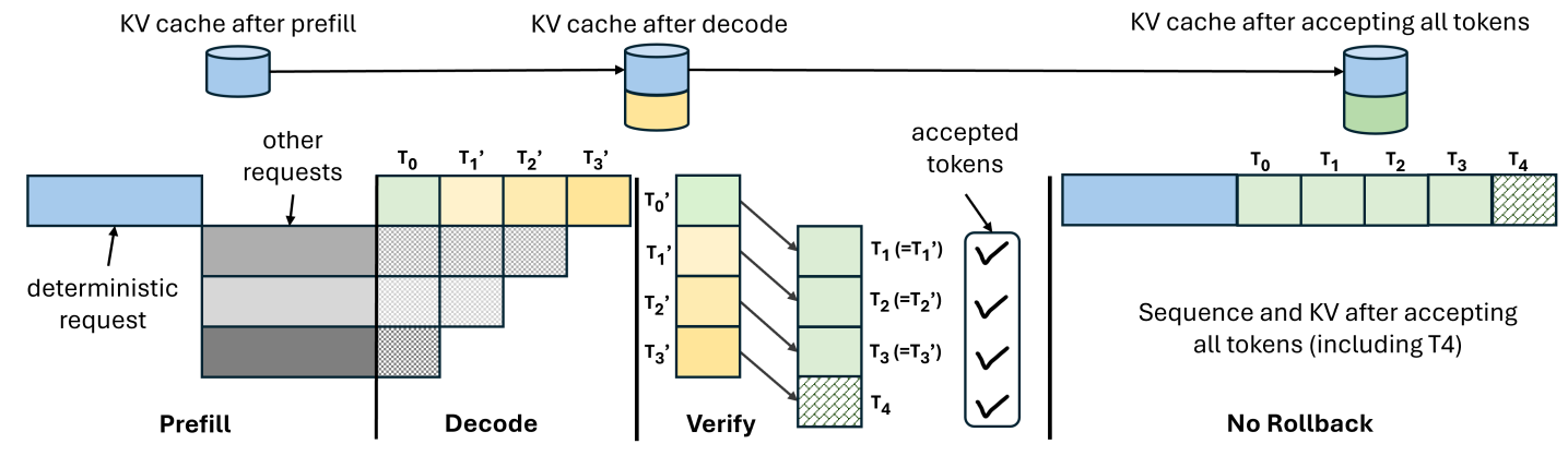
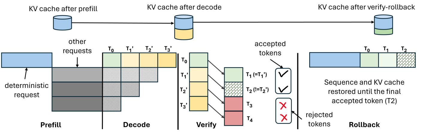
Figure 8 illustrates how DVR operates, assuming a verification window of four tokens. The blue request requires deterministic output and its first output token $T_{0}$ is produced by deterministic prefill phase that avoids arbitrary inter-request batching. LLM-42 then generates candidate tokens $T_{1}^{\prime}$ , $T_{2}^{\prime}$ , and $T_{3}^{\prime}$ using the regular fast path with dynamic batching, where gray requests may be batched arbitrarily. The first input to the verifier should be consistent (in this case, $T_{0}$ is consistent since it comes from the prefill phase). The verifier replays these four tokens $T_{0}$ and $T_{1}^{\prime}$ – $T_{3}^{\prime}$ as input and produces output tokens $T_{1}$ – $T_{4}$ . Verification has two possible outcomes: (1) all tokens pass verification, or (2) one or more tokens fail verification. We describe these two cases in detail below.
#### Case-1: When verification succeeds.
In the common case, verification reproduces the same tokens that the preceding decode iterations generated. For example, in 8(a), $T_{1}=T_{1}^{\prime}$ , $T_{2}=T_{2}^{\prime}$ and $T_{3}=T_{3}^{\prime}$ . In this case, LLM-42 accepts all these tokens; in addition, it also accepts the token $T_{4}$ since $T_{4}$ was generated by the verifier from a consistent state and is therefore consistent.
<details>
<summary>x7.png Details</summary>
### Visual Description
## Line Chart: Latency per Token vs. Number of Tokens
### Overview
This image is a line chart illustrating the relationship between the number of tokens processed and the latency per token (measured in milliseconds). The chart displays a clear inverse relationship, where latency decreases significantly as the number of tokens increases.
### Components/Axes
* **X-Axis (Horizontal):** Labeled "Number of Tokens". The scale is non-linear (logarithmic), with markers at 16, 32, 64, 128, 256, and 512.
* **Y-Axis (Vertical):** Labeled "Latency per Token (ms)". The scale is linear, ranging from 0.0 to 0.8 in increments of 0.1.
* **Data Series:** A single blue line connecting circular data points.
* **Visual Styling:** A light green shaded area fills the region between the blue line and the X-axis. A light gray grid is overlaid on the chart area to assist with reading values.
### Detailed Analysis
The trend is a steep downward curve, indicating that as the workload (number of tokens) increases, the time taken to process each individual token decreases rapidly before leveling off.
**Data Point Extraction (Approximate values):**
* **16 Tokens:** The latency is approximately **0.76 ms**.
* **32 Tokens:** The latency is approximately **0.38 ms**.
* **64 Tokens:** The latency is approximately **0.19 ms**.
* **128 Tokens:** The latency is approximately **0.095 ms**.
* **256 Tokens:** The latency is approximately **0.05 ms**.
* **512 Tokens:** The latency is approximately **0.04 ms**.
### Key Observations
* **Exponential Decay:** The latency drops by roughly 50% for each doubling of the token count between 16 and 128 tokens.
* **Diminishing Returns:** The rate of latency reduction slows significantly after 128 tokens. The difference between 256 and 512 tokens is minimal (approx. 0.01 ms), suggesting the system is approaching a performance floor or steady-state throughput.
* **Grid Alignment:** The data points are plotted precisely at the intersection of the vertical grid lines corresponding to the X-axis labels.
### Interpretation
This chart is characteristic of performance benchmarking for Large Language Model (LLM) inference or similar sequence-processing systems.
* **Amortization of Overhead:** The high latency at low token counts (16 tokens) suggests that there is a fixed "cost" or overhead associated with processing a request (e.g., model initialization, memory access, or kernel launch overhead). As the number of tokens increases, this fixed cost is amortized over more tokens, driving the "per-token" latency down.
* **Steady-State Throughput:** The plateauing of the curve after 128 tokens indicates that the system has reached its maximum efficient throughput. Beyond this point, adding more tokens does not significantly improve the per-token latency, likely because the system is operating at its peak hardware utilization or memory bandwidth capacity.
* **Optimization Implications:** For a developer or engineer, this graph suggests that processing very short sequences is inefficient. To maximize hardware utilization, batching or grouping requests to ensure a higher token count per inference pass would be the optimal strategy.
</details>
(a) Verification latency
<details>
<summary>x8.png Details</summary>
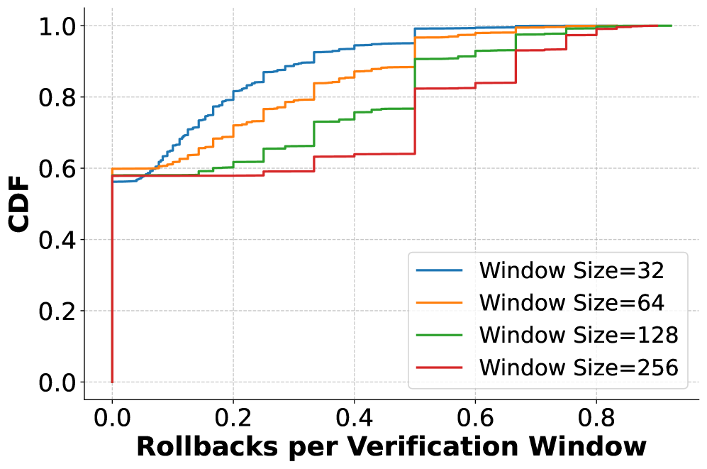
### Visual Description
## Chart: Cumulative Distribution Function (CDF) of Rollbacks per Verification Window
### Overview
This image displays a Cumulative Distribution Function (CDF) plot illustrating the frequency of "Rollbacks per Verification Window" across four distinct configurations of "Window Size" (32, 64, 128, and 256). The chart demonstrates how increasing the verification window size correlates with a higher probability of experiencing rollbacks.
### Components/Axes
* **Y-Axis (Vertical):** Labeled "CDF" (Cumulative Distribution Function), representing the cumulative probability ranging from 0.0 to 1.0.
* **X-Axis (Horizontal):** Labeled "Rollbacks per Verification Window," representing the count of rollbacks observed within a specific window.
* **Data Series:** Four distinct lines representing different window sizes:
* **Window Size 32:** Represented by a specific color/style (e.g., blue).
* **Window Size 64:** Represented by a specific color/style (e.g., orange).
* **Window Size 128:** Represented by a specific color/style (e.g., green).
* **Window Size 256:** Represented by a specific color/style (e.g., red).
### Interpretation
The plot shows that as the "Window Size" increases, the CDF curves shift to the right, indicating that larger verification windows are associated with a higher number of rollbacks per window. The steepness of the curves indicates the distribution density; a steeper slope suggests a higher concentration of data points within that range of rollbacks.
</details>
(b) Rollbacks
<details>
<summary>x9.png Details</summary>
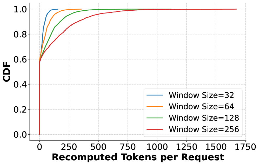
### Visual Description
## Line Chart: Cumulative Distribution Function (CDF) of Recomputed Tokens per Request
### Overview
This image displays a Cumulative Distribution Function (CDF) plot illustrating the distribution of "Recomputed Tokens per Request" across four different "Window Size" configurations (32, 64, 128, and 256). The chart demonstrates how increasing the window size impacts the number of tokens that need to be recomputed during a request process.
### Components/Axes
* **Y-Axis (Vertical):** Labeled "CDF". The scale ranges from 0.0 to 1.0, representing the cumulative probability (0% to 100% of requests).
* **X-Axis (Horizontal):** Labeled "Recomputed Tokens per Request". The scale ranges from 0 to 1750, with major tick marks every 250 units.
* **Legend:** Located in the bottom-right quadrant of the chart area.
* **Blue Line:** Window Size=32
* **Orange Line:** Window Size=64
* **Green Line:** Window Size=128
* **Red Line:** Window Size=256
* **Grid:** A light gray dashed grid is overlaid to assist in reading values.
### Detailed Analysis
The chart shows four distinct curves, all originating from the same point on the Y-axis.
* **Common Baseline:** All four lines start at the coordinate (0, ~0.6). This indicates that approximately 60% of all requests, regardless of the window size configuration, require 0 recomputed tokens.
* **Trend Verification:** After the initial jump at x=0, all lines slope upward toward a CDF of 1.0. The slope of the lines is inversely proportional to the window size; smaller window sizes reach the 1.0 CDF threshold much faster (at lower X values) than larger window sizes.
**Data Point Estimates (approximate X-values for specific CDF thresholds):**
| Window Size | CDF = 0.8 (80th percentile) | CDF = 1.0 (Max/Tail) |
| :--- | :--- | :--- |
| **32 (Blue)** | ~50 tokens | ~150 tokens |
| **64 (Orange)** | ~100 tokens | ~350 tokens |
| **128 (Green)** | ~200 tokens | ~600 tokens |
| **256 (Red)** | ~400 tokens | ~1600 tokens |
### Key Observations
* **The "Zero-Cost" Majority:** The most significant feature is the vertical jump from 0 to 0.6 at the origin. This suggests that for the majority of requests (60%), the system is highly efficient, requiring no recomputation.
* **Window Size Impact:** There is a clear, positive correlation between the "Window Size" and the number of "Recomputed Tokens." As the window size doubles (32 -> 64 -> 128 -> 256), the tail of the distribution (the X-value where CDF reaches 1.0) extends significantly to the right.
* **Distribution Spread:** The "Red" line (Window Size=256) has the widest distribution, indicating that while it shares the same 60% "zero-cost" baseline, the remaining 40% of requests experience a much wider variance in recomputation costs, extending up to ~1600 tokens.
### Interpretation
This data likely represents the performance characteristics of a Large Language Model (LLM) inference system, specifically regarding KV (Key-Value) cache management or speculative decoding strategies.
* **Efficiency Trade-off:** The chart demonstrates a clear trade-off. Smaller window sizes (e.g., 32) are significantly more efficient, as they cap the maximum recomputation cost at a very low level (~150 tokens). Larger window sizes (e.g., 256) allow for larger context windows but introduce a "long tail" of potential recomputation costs, reaching up to 1600 tokens.
* **System Behavior:** The fact that 60% of requests require zero recomputation suggests that for most interactions, the system is either hitting a cache perfectly or the context length is small enough that the window size constraint is not triggered.
* **Operational Implications:** If a system architect needs to minimize latency spikes (outliers), they would prefer a smaller window size. If the application requires handling longer context windows, they must accept the risk of significantly higher recomputation costs for the 40% of requests that fall outside the "zero-cost" baseline.
</details>
(c) CDF of recomputed tokens
<details>
<summary>x10.png Details</summary>

### Visual Description
## Bar Chart: Recompute Cost vs. Window Size
### Overview
The image is a bar chart displaying the relationship between "Window Size" and "Recompute Cost (%)". The chart demonstrates a clear, positive correlation: as the window size increases, the percentage of recompute cost increases significantly.
### Components/Axes
* **Y-Axis:** Labeled "Recompute Cost (%)". The axis is marked with horizontal dashed grid lines at intervals of 10, ranging from 0 to 40.
* **X-Axis:** Labeled "Window Size". The axis contains four discrete categories: 32, 64, 128, and 256.
* **Data Series:** Represented by four vertical bars, all colored light purple with diagonal hatching.
* **Data Labels:** Numerical percentages are positioned directly above each bar.
### Detailed Analysis
The chart displays a consistent upward trend. As the Window Size doubles, the Recompute Cost increases by a factor of approximately 1.8x to 2x.
**Data Points (from left to right):**
* **Window Size 32:** The bar height is approximately 6.81%.
* **Window Size 64:** The bar height is approximately 12.42%.
* **Window Size 128:** The bar height is approximately 24.92%.
* **Window Size 256:** The bar height is approximately 46.41%.
### Key Observations
* **Scaling Trend:** The growth in recompute cost is nearly proportional to the window size. Doubling the window size (e.g., 32 to 64, 64 to 128) results in a roughly doubling of the recompute cost.
* **Magnitude:** The jump from the smallest window size (32) to the largest (256) represents a nearly 7-fold increase in recompute cost (from ~6.8% to ~46.4%).
* **Consistency:** The visual spacing and the numerical values suggest a predictable, likely linear or near-linear computational complexity associated with the window size parameter.
### Interpretation
This data likely originates from a technical analysis of an algorithm—possibly related to machine learning (e.g., attention mechanisms in Transformers, sliding window processing, or signal processing buffers).
The "Recompute Cost" represents the computational overhead required to recalculate data rather than retrieving it from memory. The chart illustrates a classic "memory vs. compute" trade-off:
1. **Performance Penalty:** Larger window sizes provide more context or data coverage but impose a heavy computational tax.
2. **Optimization Implications:** If this chart represents a system constraint, it suggests that increasing the window size beyond 128 becomes increasingly expensive, with the cost approaching 50% of the total operation at a window size of 256. Engineers using this system would need to carefully balance the benefit of a larger window against the significant performance degradation shown here.
</details>
(d) Total recomputation overhead
Figure 9: The cost of verification and recomputation with varying window sizes.
#### Case-2: When verification fails.
Occasionally, a verification pass disagrees with one or more decoded tokens, e.g., only $T_{1}^{\prime}$ matches with the verifier’s output in 8(b). In this case, LLM-42 commits the output only up to the last matching token ( $T_{1}^{\prime}$ ); all subsequent tokens ( $T_{2}^{\prime}$ and $T_{3}^{\prime}$ ) are rejected. The verifier-generated token that appears immediately after the last matching position ( $T_{2}$ ) is also accepted and the KV cache is truncated at this position. The next decode iteration resumes from this repaired, consistent state.
#### Making KV cache consistent.
During the decode phase, the KV cache is populated by fast-path iterations that execute under dynamic batching. Consequently, even when token verification succeeds, the KV cache corresponding to the verified window may still be inconsistent, since it was produced by non-deterministic execution. This inconsistency could affect tokens generated in future iterations despite the current window being verified. Token-level verification alone is therefore insufficient without repairing the KV cache. To address this, we overwrite the KV cache entries produced during decoding with the corresponding entries from the verification pass. This ensures that both the emitted tokens and the KV cache state are consistent for subsequent decode iterations, eliminating downstream divergence.
#### Guaranteed forward progress.
Note that each verification pass produces at least one new consistent output token as shown in Figure 8. As a result, DVR guarantees forward progress even in contrived worst-case scenarios that might trigger rollbacks for every optimistically generated token. We have not observed any such scenario in our experiments.
Overall, DVR follows the high-level structure of speculative decoding, but differs in several important ways as discussed in Table 1. Under DVR, decoded tokens result from a faithful execution of the model’s forward pass, with deviations arising only from the floating-point rounding errors. In contrast, speculative execution techniques generate candidate tokens using modified forward computations—for example, by running a smaller or distilled draft model [specdecoding-icml2023, specinfer-2024] or by truncating or pruning attention/context [medusa, fu2023lookahead]. Because these approximations change the computation itself, speculation depth is typically limited to a few (2-8) tokens [medusa, fu2023lookahead, specdecoding-icml2023, specinfer-2024]. In contrast, leveraging O1, DVR can safely speculate over longer (32-64) token sequences. For the same reason, verification in DVR succeeds with high probability, in contrast to the much lower acceptance rates observed in existing speculative decoding schemes. Finally, DVR performs verification using the same model, whereas most speculative decoding approaches require a separate model for verification.
### 4.3 Grouped Verification
The efficiency of DVR depends on the size of verification window and involves a trade-off: smaller windows incur higher verification cost but low recomputation overhead, whereas larger windows reduce verification cost at the expense of increased recomputation. We empirically characterize this trade-off by profiling Llama-3.1-8B-Instruct on an H100-PCIe GPU. We measure per-token verification cost based on the latency of verification forward pass. To quantify the recomputation cost, we execute 4096 requests from the ShareGPT dataset in an online setting at 12 queries per second. For each window size, we measure the total number of tokens decoded versus the number of tokens returned to the user; the difference between the two denotes recomputation overhead.
9(a) shows the per-token verification cost as a function of verification window size. For smaller windows, the verification pass is memory-bound: each token performs very little computation, resulting in low arithmetic intensity and poor hardware utilization. Consequently, the verification cost is high—up to 0.75 ms per-token. As the verification window increases, the kernel transitions to being compute-bound, and the per-token cost drops sharply, reaching 0.05 ms at a window size of 512, signifying a reduction of $15\times$ .
9(b) shows that more than half of the requests complete without any rollback (i.e., all their output tokens pass verification), while a small fraction of requests incur frequent rollbacks. Moreover, rollbacks become more common as the window size increases. For example, with a window size of 256, about 40% of requests observe a rollback ratio of 50% or higher indicating that at least half of the verification steps detect one or more mismatched tokens. In contrast, with a window size of 32, only about 5% of requests reach this level. The number of recomputed tokens per request also follows the same trend as shown in 9(c). Further, 9(d) shows the resulting total recomputation overhead. Note that a verification failure requires recomputing all tokens following the mismatched position within the current window. As a result, larger windows incur higher recomputation overhead on average. Concretely, recomputation overhead is 6.81% at a window size of 32 and increases roughly linearly, reaching 46.41% at a window size of 256.
We propose grouped verification to address the inherent trade-off between the cost of verification and recomputation. Instead of verifying a large window of a single request (256 tokens), we verify small, fixed-size windows of multiple requests together in a single pass (e.g., 8 requests, 32 tokens each). This way each request retains the rollback properties of a small window, while the verification pass operates on a large effective batch, achieving high utilization and low verification cost.
### 4.4 Discussion
Guaranteeing determinism requires every operator in the inference pipeline to behave consistently. This section highlights a few subtle sources of inconsistency in commonly used operators. We do not introduce new techniques here; instead, we adopt established approaches to enforce consistent behavior and summarize them for completeness.
#### Attention.
Attention involves reductions along multiple steps: reductions along the sequence dimension (e.g., in FlashDecoding-style sequence parallelism [flashdecoding]) and reductions inside the softmax computation. To make it consistent, we use FlashAttention-3 attention kernel and set the number of KV splits to one in the verification pass; fast-path decode iterations run as usual. Some performance optimizations are possible based on SGLang implementation https://lmsys.org/blog/2025-09-22-sglang-deterministic/.
#### Communication collectives.
Classical ring-based AllReduce reduces tokens in different orders depending on their position in the batch. In contrast, multimem-based AllReduce, introduced in CUDA 13.0, follows consistent reduction schedules [nvls-deterministic] and should be preferred whenever supported. On older platforms where multimem/NVLS is unavailable, one can use tree-based AllReduce with fixed NCCL configuration (e.g., setting num_channels to one and using a fixed protocol) to achieve determinism, at the expense of higher communication cost than ring-based AllReduce.
#### Sampling.
We adopt sampler from SGLang. When temperature is zero, it selects the token with the highest logit (argmax) and if there are multiple maximal values then it returns the index of the first maximal value. For non-greedy sampling, however, the sampling process involves randomness, making the outputs sensitive to how random numbers are generated and consumed. To address this issue, SGLang introduces a new sampling function, multinomial_with_seed, which replaces torch.multinomial, an inherently non-deterministic operator under batched execution. This function perturbs logits with Gumbel noise generated from a seeded hash function, ensuring that the same input–seed pair always produces the same sample [SGLangTeam2025].
Overall, enforcing determinism across the entire inference pipeline requires careful configuration of the attention kernel and selecting an appropriate AllReduce implementation. The sampling module does require a new implementation, but this is a one-time cost since the same sampler is used across all models. In contrast, the bulk of the performance and engineering effort in LLM systems lies in GEMM kernels, which LLM-42 reuses entirely, along with RMSNorm and FusedMoE kernels.
## 5 Evaluation
Our evaluation answers the following questions:
| ShareGPT ArXiv | 92812 5941 | Input Length Output Length Input Length | 304 192 7017 | 136 118 6435 | 491 212 3479 |
| --- | --- | --- | --- | --- | --- |
| Test Split | | Output Length | 198 | 191 | 74 |
Table 3: Datasets and their input/output context lengths.
<details>
<summary>x11.png Details</summary>
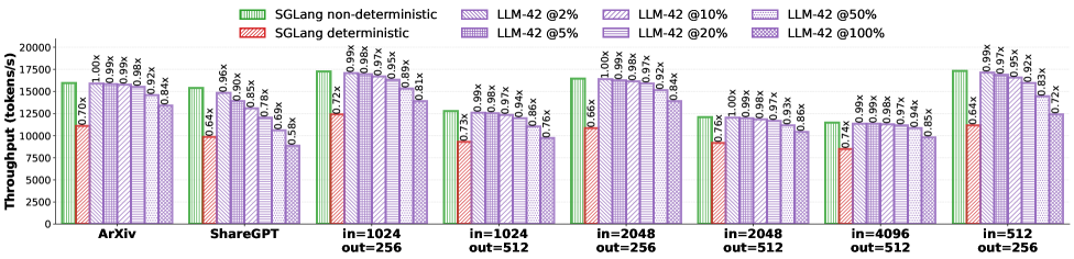
### Visual Description
## Grouped Bar Chart: Throughput Comparison of SGLang vs. LLM-42
### Overview
This chart displays a comparative analysis of throughput (measured in tokens/s) across eight different workload configurations. It compares "SGLang" (in both non-deterministic and deterministic modes) against "LLM-42" operating at six different sampling percentages (2%, 5%, 10%, 20%, 50%, and 100%). The chart uses a baseline of "SGLang non-deterministic" for each category, with other bars labeled with a multiplier indicating their relative throughput compared to that baseline.
### Components/Axes
* **Y-Axis:** "Throughput (tokens/s)", ranging from 0 to 20,000 in increments of 2,500.
* **X-Axis:** Eight workload categories:
1. ArXiv
2. ShareGPT
3. in=1024 / out=256
4. in=1024 / out=512
5. in=2048 / out=256
6. in=2048 / out=512
7. in=4096 / out=512
8. in=512 / out=256
* **Legend (Top Center):**
* **Green (Vertical Stripes):** SGLang non-deterministic (Baseline)
* **Red (Diagonal Stripes):** SGLang deterministic
* **Purple (Various Patterns):** LLM-42 @ 2%, 5%, 10%, 20%, 50%, 100% (ordered from lightest/least dense pattern to darkest/most dense pattern).
### Detailed Analysis
The following data points are estimated based on the Y-axis scale. Multipliers are transcribed directly from the labels above each bar.
| Workload Category | SGLang Non-Det (Est. Tokens/s) | SGLang Det (Est. Tokens/s) | LLM-42 @ 2% | LLM-42 @ 5% | LLM-42 @ 10% | LLM-42 @ 20% | LLM-42 @ 50% | LLM-42 @ 100% |
| :--- | :--- | :--- | :--- | :--- | :--- | :--- | :--- | :--- |
| **ArXiv** | ~16,000 | ~11,200 (0.70x) | ~16,000 (1.00x) | ~15,800 (0.99x) | ~15,800 (0.99x) | ~15,700 (0.98x) | ~14,700 (0.92x) | ~13,400 (0.84x) |
| **ShareGPT** | ~15,500 | ~10,000 (0.64x) | ~14,800 (0.96x) | ~14,000 (0.90x) | ~13,200 (0.85x) | ~12,000 (0.78x) | ~10,700 (0.69x) | ~9,000 (0.58x) |
| **in=1024/out=256** | ~17,300 | ~12,500 (0.72x) | ~17,200 (0.99x) | ~17,000 (0.98x) | ~16,800 (0.97x) | ~16,500 (0.95x) | ~15,500 (0.89x) | ~14,000 (0.81x) |
| **in=1024/out=512** | ~12,800 | ~9,400 (0.73x) | ~12,700 (0.99x) | ~12,600 (0.99x) | ~12,500 (0.98x) | ~12,400 (0.97x) | ~12,000 (0.94x) | ~9,700 (0.76x) |
| **in=2048/out=256** | ~16,500 | ~10,900 (0.66x) | ~16,500 (1.00x) | ~16,300 (0.99x) | ~16,200 (0.98x) | ~16,000 (0.97x) | ~15,200 (0.92x) | ~13,800 (0.84x) |
| **in=2048/out=512** | ~12,200 | ~9,300 (0.76x) | ~12,200 (1.00x) | ~12,100 (0.99x) | ~12,000 (0.98x) | ~11,900 (0.97x) | ~11,400 (0.93x) | ~10,500 (0.86x) |
| **in=4096/out=512** | ~11,500 | ~8,500 (0.74x) | ~11,400 (0.99x) | ~11,400 (0.99x) | ~11,300 (0.98x) | ~11,200 (0.97x) | ~10,800 (0.94x) | ~9,800 (0.85x) |
| **in=512/out=256** | ~17,400 | ~11,200 (0.64x) | ~17,200 (0.99x) | ~16,900 (0.97x) | ~16,600 (0.95x) | ~16,000 (0.92x) | ~14,500 (0.83x) | ~12,500 (0.72x) |
### Key Observations
* **Baseline Dominance:** The "SGLang non-deterministic" (green) bar is consistently the highest throughput across all categories.
* **Deterministic Penalty:** The "SGLang deterministic" (red) bar consistently shows the lowest throughput, with multipliers ranging from 0.64x to 0.76x relative to the non-deterministic baseline.
* **LLM-42 Scaling:** Within the LLM-42 series, throughput consistently decreases as the percentage increases (from 2% to 100%).
* **Performance Convergence:** LLM-42 @ 2% performs nearly identically to the SGLang non-deterministic baseline, with multipliers consistently at 0.99x or 1.00x.
### Interpretation
The data suggests that SGLang non-deterministic mode is the most performant configuration for these workloads. The "deterministic" mode imposes a significant performance cost, likely due to the overhead required to ensure consistent outputs.
The LLM-42 series demonstrates a clear trade-off: lower percentages (e.g., 2%) allow the system to maintain throughput levels very close to the non-deterministic baseline, whereas higher percentages (e.g., 100%) result in a noticeable degradation in throughput. This implies that the "percentage" parameter in LLM-42 is a tunable knob for performance, where lower values are more efficient, likely because they involve less computation or fewer constraints than higher values.
</details>
Figure 10: Throughput in offline inference. SGLang has only two modes: all requests run in either deterministic or non-deterministic mode whereas LLM-42 supports selective determinism (% values in the legend reflect the fraction of traffic that requires deterministic output).
- How does LLM-42 compare against the baseline’s deterministic and non-deterministic modes?
- How does LLM-42 perform for different mix of deterministic and non-deterministic traffic?
- How do configuration parameters affect the performance of grouped verification in LLM-42?
Models and environment: We evaluate LLM-42 with the Llama-3.1-8B-Instruct model. It has 32 query heads, 8 KV heads, and 32 layers. Experiments were conducted on a system equipped with four NVIDIA H100 PCIe GPUs with 80 GB HBM3 memory and 114 streaming multiprocessors per GPU. The host CPU has 64 physical cores (128 hardware threads) and approximately 1.65 TB of DRAM.
Workloads: We evaluate on synthetic inputs with varying context lengths, following common practice in prior work [nanoflow2024]. We additionally benchmark on the widely used ShareGPT [huggingfacesharegpt] and Arxiv [arxiv-summarization] datasets, whose characteristics are summarized in Table 3. All experiments use the meta-llama/Llama-3.1-8B-Instruct tokenizer. To evaluate LLM-42 under different workload conditions, we vary the fraction of requests that require deterministic output between 2%, 5%, 10%, 20%, 50%, and 100%. While higher deterministic ratios are included for stress testing, we expect that in practical deployments only a small fraction of requests will require determinism. Finally, note that the deterministic request ratio applies only to LLM-42; approaches based on batch-invariant computation support only global determinism.
Serving system baselines: We implement LLM-42 on top of the SGLang serving framework version 0.5.3rc0 and compare performance against SGLang with deterministic execution switched on. To understand the upper limit on performance, we also compare with the non-deterministic version of SGLang. We refer to these two baselines as SGLang-Deterministic and SGLang-Non-Deterministic. We use FA-3 attention kernel in all our experiments; we set num_splits = 1 in the verification step of LLM-42 and use the default settings for the decode phases.
Metrics: In offline inference, we evaluate throughput as the number of tokens processed per second. For online inference, we evaluate end-to-end request execution latencies and time-to-first-token. To better understand the overhead of our approach, we also report the number of rollbacks and recomputed tokens across different configurations of LLM-42.
### 5.1 Offline Inference
For offline inference, we evaluate eight workload configurations: two traces from the ArXiv and ShareGPT datasets and six other configurations with different input and output lengths. Each configuration executes 4096 requests to completion. Figure 10 reports the resulting throughput across systems measured in tokens per second; we summarize the main observations below.
Enabling deterministic inference in SGLang incurs a substantial throughput penalty, ranging from 24% (in=2048, out=512) to 36% (ShareGPT). This slowdown stems from the use of batch-invariant kernels, which are consistently slower than the standard optimized kernels, as shown in Figure 4. In contrast, LLM-42 mostly uses regular optimized kernels and therefore achieves significantly higher throughput. Even in its worst case—when 100% of requests require deterministic output— LLM-42 outperforms SGLang-Deterministic in all but one setting (ShareGPT), where it is only 6% slower.
| Dataset / Config Total number of rollbacks | Deterministic Ratio 2% | 5% | 10% | 20% | 50% | 100% |
| --- | --- | --- | --- | --- | --- | --- |
| ArXiv | 70 | 170 | 372 | 697 | 1733 | 3351 |
| ShareGPT | 4 | 5 | 10 | 15 | 44 | 96 |
| in=512, out=256 | 0 | 0 | 0 | 0 | 0 | 0 |
| in=1024, out=256 | 0 | 1 | 5 | 5 | 9 | 24 |
| in=1024, out=512 | 48 | 106 | 225 | 386 | 792 | 1536 |
| in=2048, out=256 | 7 | 22 | 79 | 134 | 378 | 724 |
| in=2048, out=512 | 0 | 0 | 0 | 2 | 2 | 4 |
| in=4096, out=512 | 31 | 79 | 98 | 220 | 538 | 1087 |
| Total number of recomputed tokens | | | | | | |
| ArXiv | 1805 | 4414 | 8737 | 13198 | 37687 | 89248 (10.97%) |
| ShareGPT | 139 | 158 | 164 | 396 | 1185 | 2691 (0.32%) |
| in=512, out=256 | 0 | 0 | 0 | 0 | 0 | 0 (0%) |
| in=1024, out=256 | 0 | 44 | 151 | 151 | 288 | 776 (0.07%) |
| in=1024, out=512 | 1724 | 3272 | 6615 | 12392 | 25967 | 50454 (2.41%) |
| in=2048, out=256 | 268 | 767 | 2470 | 4080 | 12173 | 21772 (2.08%) |
| in=2048, out=512 | 0 | 0 | 0 | 81 | 81 | 101 ( $<\!0.01\$ ) |
| in=4096, out=512 | 1134 | 2961 | 3598 | 7208 | 17161 | 32430 (1.55%) |
Table 4: Rollback and recomputation statistics (grouped verification over 8 requests, 64 tokens each). Recompute cost is shown only for the column with 100% deterministic traffic.
Crucially, LLM-42 ’s throughput improves monotonically as the fraction of deterministic requests decreases. On ArXiv, LLM-42 operates within 8%, 2%, 1% and 1% of the best-case throughput (SGLang-Non-Deterministic) at 5%, 10%, 20%, and 50% deterministic traffic, respectively. This behavior is expected: LLM-42 imposes no computation overhead on requests that do not require determinism. As a result, LLM-42 is up to 41% faster than SGLang-Deterministic in these regimes. This trend holds across all workload configurations; for example, at 10% deterministic traffic, LLM-42 is 33% faster than SGLang-Deterministic on ShareGPT and up to 48% faster (in=2048, out=256) on other workloads.
Table 4 reports two complementary metrics that characterize the overhead of enforcing determinism in LLM-42: (1) the total number of rollbacks aggregated over all 4096 requests, and (2) the total number of recomputed tokens incurred due to these rollbacks. We find that some configurations incur zero rollbacks even under non-trivial deterministic ratios, and the average case remains low across datasets and input–output lengths. Even in the worst case, ArXiv at 100% deterministic traffic, the system triggers 3351 rollbacks over 4096 requests, i.e., fewer than one rollback per request on average. A similar trend holds for recomputation overhead: the recomputed token fraction is consistently small, with the worst case at 100% deterministic traffic reaching at most 10.97%, while the average case across datasets and configurations is substantially lower. Overall, these results indicate that both rollback frequency and recomputation cost are modest in practice.
<details>
<summary>x12.png Details</summary>
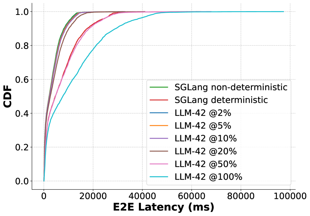
### Visual Description
## CDF Plot: E2E Latency Comparison
### Overview
This image is a Cumulative Distribution Function (CDF) plot illustrating the End-to-End (E2E) latency performance of two different systems: SGLang (in deterministic and non-deterministic modes) and LLM-42 (configured at various percentage levels). The plot visualizes the probability distribution of latency values, where a steeper curve shifted to the left indicates lower latency (better performance).
### Components/Axes
* **X-Axis:** "E2E Latency (ms)". The scale is linear, ranging from 0 to 100,000 ms.
* **Y-Axis:** "CDF". The scale ranges from 0.0 to 1.0, representing the cumulative probability.
* **Legend:** Located in the center-right area of the chart. The legend maps colors to specific configurations:
* **Green:** SGLang non-deterministic
* **Red:** SGLang deterministic
* **Blue:** LLM-42 @2%
* **Orange:** LLM-42 @5%
* **Purple:** LLM-42 @10%
* **Brown:** LLM-42 @20%
* **Pink:** LLM-42 @50%
* **Cyan:** LLM-42 @100%
### Detailed Analysis
**Trend Verification:** All data series exhibit a positive slope starting from (0,0). The curves rise steeply initially and flatten out as they approach a CDF of 1.0. The further to the right a curve is, the higher the latency for that configuration.
* **High-Performance Cluster (Green, Red, Blue, Orange, Purple, Brown):**
* These six lines are tightly clustered on the far left of the chart.
* They exhibit the steepest slopes, reaching a CDF of 0.9 at approximately 10,000 ms to 15,000 ms.
* There is negligible performance difference between SGLang (both modes) and LLM-42 at low percentages (2%–20%).
* **Moderate-Performance (Pink - LLM-42 @50%):**
* This line is positioned to the right of the high-performance cluster.
* It reaches a CDF of 0.9 at approximately 25,000 ms, indicating a significant latency increase compared to the lower percentage configurations.
* **Low-Performance (Cyan - LLM-42 @100%):**
* This is the rightmost line, indicating the highest latency.
* It reaches a CDF of 0.9 at approximately 50,000 ms.
* The curve continues to rise gradually, reaching a CDF of 1.0 near 100,000 ms.
### Key Observations
* **Performance Scaling:** There is a clear, non-linear correlation between the LLM-42 percentage parameter and E2E latency. Increasing the percentage from 20% to 50% and then to 100% results in progressively larger latency penalties.
* **SGLang Efficiency:** SGLang (both deterministic and non-deterministic) performs consistently well, matching the latency profile of the most restrictive LLM-42 settings (2%–20%).
* **Clustering:** The performance gap between 2% and 20% LLM-42 is minimal, suggesting that within this range, the latency overhead is relatively stable.
### Interpretation
The data demonstrates that SGLang is a highly efficient system for minimizing E2E latency, performing on par with the most optimized (lowest percentage) settings of LLM-42.
Conversely, the LLM-42 system exhibits a significant "latency tax" as the percentage parameter increases. The jump in latency is particularly dramatic when moving from 50% to 100%. This suggests that for latency-sensitive applications, users should either utilize SGLang or strictly limit the LLM-42 percentage parameter to avoid the steep latency tail observed at 50% and 100%. The rightward shift of the curves as the percentage increases indicates that higher percentages not only increase the median latency but also significantly extend the "long tail" of latency (the 90th–99th percentile).
</details>
(a) QPS=12
<details>
<summary>x13.png Details</summary>
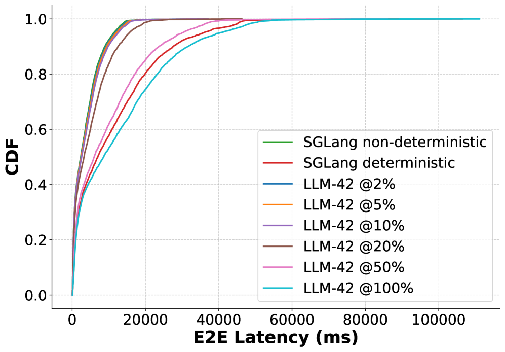
### Visual Description
## Chart: Cumulative Distribution Function (CDF) of E2E Latency
### Overview
This image displays a Cumulative Distribution Function (CDF) chart comparing the End-to-End (E2E) latency performance of two different systems: **SGLang** (in deterministic and non-deterministic modes) and **LLM-42** (at various percentage configurations ranging from 2% to 100%). The chart illustrates the probability distribution of latency, where a curve positioned further to the left indicates lower latency and better performance.
### Components/Axes
* **X-Axis:** "E2E Latency (ms)". The scale is linear, ranging from 0 to 100,000 ms, with grid lines at 20,000 ms intervals.
* **Y-Axis:** "CDF". The scale is linear, ranging from 0.0 to 1.0, representing the cumulative probability (0% to 100% of requests).
* **Legend:** Located in the center-right region of the chart. It maps colors to specific configurations:
* **Green:** SGLang non-deterministic
* **Red:** SGLang deterministic
* **Blue:** LLM-42 @2%
* **Orange:** LLM-42 @5%
* **Purple:** LLM-42 @10%
* **Brown:** LLM-42 @20%
* **Pink:** LLM-42 @50%
* **Cyan:** LLM-42 @100%
### Detailed Analysis
The data series can be categorized into four distinct performance groups based on their visual trajectory (slope and right-shift):
1. **High-Performance Group (Green, Red, Blue, Orange, Purple):**
* **Trend:** These lines are tightly clustered and exhibit the steepest upward slope, indicating the lowest latency.
* **Median (0.5 CDF):** Approximately 5,000 ms.
* **90th Percentile (0.9 CDF):** Approximately 12,000 ms.
* **Max Latency:** These configurations reach 1.0 CDF at approximately 20,000 ms.
2. **Moderate-Performance Group (Brown - LLM-42 @20%):**
* **Trend:** This line shifts to the right of the high-performance group, indicating higher latency.
* **Median (0.5 CDF):** Approximately 8,000 ms.
* **90th Percentile (0.9 CDF):** Approximately 25,000 ms.
* **Max Latency:** Reaches 1.0 CDF at approximately 45,000 ms.
3. **Lower-Performance Group (Pink - LLM-42 @50%):**
* **Trend:** Further right-shift compared to the 20% configuration.
* **Median (0.5 CDF):** Approximately 10,000 ms.
* **90th Percentile (0.9 CDF):** Approximately 30,000 ms.
* **Max Latency:** Reaches 1.0 CDF at approximately 50,000 ms.
4. **Lowest-Performance Group (Cyan - LLM-42 @100%):**
* **Trend:** This is the right-most curve, indicating the highest latency.
* **Median (0.5 CDF):** Approximately 12,000 ms.
* **90th Percentile (0.9 CDF):** Approximately 40,000 ms.
* **Max Latency:** Reaches 1.0 CDF at approximately 110,000 ms.
### Key Observations
* **Performance Scaling:** There is a clear correlation between the LLM-42 percentage parameter and latency. As the percentage increases from 2% to 100%, the latency distribution shifts significantly to the right, indicating a degradation in performance.
* **SGLang Efficiency:** Both SGLang configurations (deterministic and non-deterministic) perform at the same level as the lowest-load LLM-42 configurations (2%, 5%, 10%), suggesting high efficiency.
* **Tail Latency:** The divergence between the configurations is most pronounced at the higher end of the CDF (approaching 1.0). While the median latency differences are relatively small (ranging from ~5s to ~12s), the maximum latency differences are massive (ranging from ~20s to ~110s).
### Interpretation
The data demonstrates that the LLM-42 system experiences significant performance degradation as the load or complexity (represented by the percentage parameter) increases. The "100%" configuration is an outlier in terms of tail latency, taking over five times longer to complete the slowest requests compared to the SGLang baseline.
From a technical standpoint, this suggests that the LLM-42 system may have non-linear scaling issues or resource contention problems as the workload increases. Conversely, SGLang maintains a tight, predictable latency profile regardless of its deterministic or non-deterministic mode, making it the superior choice for latency-sensitive applications based on this specific dataset.
</details>
(b) QPS=14
<details>
<summary>x14.png Details</summary>
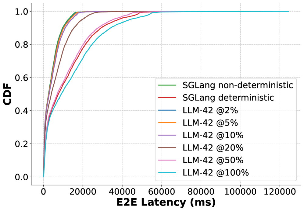
### Visual Description
## Chart: Cumulative Distribution Function (CDF) of E2E Latency
### Overview
This image displays a Cumulative Distribution Function (CDF) plot comparing the End-to-End (E2E) latency performance of two different systems: **SGLang** (in both deterministic and non-deterministic modes) and **LLM-42** (configured at various percentage levels ranging from 2% to 100%). The chart illustrates the probability that a given request will complete within a specific latency threshold.
### Components/Axes
* **X-Axis:** "E2E Latency (ms)". The scale ranges from 0 to 120,000 ms, with major grid lines every 20,000 ms.
* **Y-Axis:** "CDF". The scale ranges from 0.0 to 1.0, representing the cumulative probability (0% to 100%).
* **Legend:** Located in the center-right of the chart area. It maps colors to the following configurations:
* **Green:** SGLang non-deterministic
* **Red:** SGLang deterministic
* **Blue:** LLM-42 @2%
* **Orange:** LLM-42 @5%
* **Purple:** LLM-42 @10%
* **Brown:** LLM-42 @20%
* **Pink:** LLM-42 @50%
* **Cyan:** LLM-42 @100%
### Detailed Analysis
The chart displays three distinct clusters of performance curves, moving from left (fastest) to right (slowest).
**1. High-Performance Cluster (Leftmost):**
* **Lines:** Green (SGLang non-deterministic), Red (SGLang deterministic), Blue (LLM-42 @2%), Orange (LLM-42 @5%), Purple (LLM-42 @10%).
* **Trend:** These lines exhibit the steepest upward slope, indicating the lowest latency.
* **Values:** These configurations reach a CDF of 1.0 (100% of requests completed) at approximately **15,000 ms to 20,000 ms**. The SGLang lines (Green/Red) are slightly faster than the low-percentage LLM-42 lines.
**2. Mid-Performance Cluster (Center):**
* **Line:** Brown (LLM-42 @20%).
* **Trend:** This line has a moderate slope, indicating higher latency than the high-performance cluster.
* **Values:** It reaches a CDF of 1.0 at approximately **40,000 ms**.
**3. Low-Performance Cluster (Rightmost):**
* **Lines:** Pink (LLM-42 @50%), Cyan (LLM-42 @100%).
* **Trend:** These lines have the shallowest slope, indicating the highest latency.
* **Values:** These configurations reach a CDF of 1.0 at approximately **60,000 ms**.
### Key Observations
* **Performance Degradation:** There is a clear, positive correlation between the LLM-42 percentage configuration and E2E latency. As the percentage increases from 2% to 100%, the latency significantly increases (the curve shifts to the right).
* **SGLang Efficiency:** SGLang (both deterministic and non-deterministic) consistently outperforms all LLM-42 configurations, even the lowest percentage (2%), though the gap between SGLang and LLM-42 @2% is relatively small.
* **Determinism:** There is no visible difference in latency performance between SGLang's deterministic and non-deterministic modes; the lines are effectively overlapping.
### Interpretation
The data demonstrates that SGLang is significantly more efficient in terms of E2E latency compared to the LLM-42 system.
The "LLM-42 @X%" likely refers to a load factor, sampling rate, or model complexity parameter. The fact that the latency increases as this percentage increases suggests that the LLM-42 system does not scale linearly or efficiently under higher loads/settings. Conversely, SGLang maintains a tight latency distribution, ensuring that nearly all requests are completed within 20 seconds, regardless of whether the system is operating in a deterministic or non-deterministic mode. This suggests SGLang is the superior choice for latency-sensitive applications compared to the tested LLM-42 configurations.
</details>
(c) QPS=16
<details>
<summary>x15.png Details</summary>
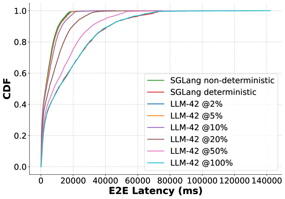
### Visual Description
## Line Chart: Cumulative Distribution Function (CDF) of E2E Latency
### Overview
This image displays a Cumulative Distribution Function (CDF) plot comparing the End-to-End (E2E) latency of various LLM (Large Language Model) configurations. The chart illustrates how different configurations affect the distribution of latency, with the X-axis representing latency in milliseconds (ms) and the Y-axis representing the cumulative probability (0.0 to 1.0).
### Components/Axes
* **X-Axis:** Labeled "E2E Latency (ms)". The scale ranges from 0 to 140,000, with major grid lines every 20,000 units.
* **Y-Axis:** Labeled "CDF". The scale ranges from 0.0 to 1.0, with major grid lines every 0.2 units.
* **Legend:** Positioned in the center-right of the chart area. It contains eight distinct data series, color-coded as follows:
* **Green:** SGLang non-deterministic
* **Red:** SGLang deterministic
* **Blue:** LLM-42 @2%
* **Orange:** LLM-42 @5%
* **Purple:** LLM-42 @10%
* **Brown:** LLM-42 @20%
* **Pink:** LLM-42 @50%
* **Cyan:** LLM-42 @100%
### Detailed Analysis
The chart displays eight curves, all originating at (0,0) and rising monotonically to a CDF of 1.0. The curves shift progressively to the right as the "LLM-42 @" percentage increases, indicating higher latency.
**Trend Verification & Data Points:**
1. **High-Performance Cluster (Leftmost):**
* **SGLang non-deterministic (Green)** and **SGLang deterministic (Red)**: These lines are nearly identical and represent the lowest latency. They reach a CDF of 1.0 at approximately 20,000ms.
* **LLM-42 @2% (Blue)** and **LLM-42 @5% (Orange)**: These lines closely track the SGLang lines, also reaching a CDF of 1.0 at approximately 20,000ms to 25,000ms.
2. **Mid-Range Performance:**
* **LLM-42 @10% (Purple)**: The curve shifts rightward, reaching a CDF of 1.0 at approximately 40,000ms.
* **LLM-42 @20% (Brown)**: The curve shifts further right, reaching a CDF of 1.0 at approximately 50,000ms.
3. **Low-Performance Cluster (Rightmost):**
* **LLM-42 @50% (Pink)**: This curve shows a significant latency increase, reaching a CDF of 1.0 at approximately 75,000ms.
* **LLM-42 @100% (Cyan)**: This is the rightmost curve, indicating the highest latency. It reaches a CDF of 1.0 at approximately 140,000ms.
### Key Observations
* **Performance Correlation:** There is a direct, positive correlation between the percentage value assigned to "LLM-42" and the E2E latency. As the percentage increases, the latency distribution shifts significantly to the right.
* **SGLang Efficiency:** The SGLang configurations (both deterministic and non-deterministic) perform at a level comparable to the most efficient LLM-42 configurations (2% and 5%).
* **Tail Latency:** The "tail" of the distribution (the latency experienced by the slowest requests) increases dramatically as the LLM-42 percentage increases. For example, the 100% configuration has a tail latency roughly 7 times higher than the 2% configuration.
### Interpretation
The data suggests that "LLM-42 @X%" likely refers to a parameter related to computational load, model size, or sampling depth (e.g., percentage of tokens processed, model sparsity, or beam width).
The significant rightward shift of the curves as the percentage increases demonstrates that the computational cost of the "LLM-42" model scales non-linearly or at least very aggressively with the percentage parameter. The fact that the SGLang configurations are clustered with the lowest LLM-42 percentages suggests that SGLang is highly optimized for low-latency inference, potentially outperforming or matching the "LLM-42" model at its most efficient settings. The "LLM-42 @100%" configuration represents a substantial performance bottleneck compared to all other tested configurations.
</details>
(d) QPS=18
Figure 11: CDF of request end-to-end latency in online inference with varying load for the ShareGPT dataset.
### 5.2 Online Inference
| 12 P75 P90 | P50 35.4 50.3 | 27.0 69.8 107.8 | 53.4 35.8 52.5 | 27.4 36.1 54.1 | 27.6 37.1 54.0 | 27.9 41.1 57.8 | 29.3 52.0 68.1 | 38.5 58.0 73.9 | 45.4 |
| --- | --- | --- | --- | --- | --- | --- | --- | --- | --- |
| 14 | P50 | 27.9 | 60.1 | 27.9 | 28.2 | 28.9 | 31.1 | 42.5 | 48.2 |
| P75 | 37.0 | 79.9 | 37.5 | 37.8 | 39.5 | 45.1 | 57.0 | 61.6 | |
| P90 | 55.8 | 127.0 | 57.0 | 56.5 | 58.6 | 63.8 | 75.8 | 82.0 | |
| 16 | P50 | 28.8 | 62.5 | 28.8 | 29.2 | 29.8 | 35.2 | 46.1 | 51.2 |
| P75 | 39.0 | 86.0 | 39.7 | 40.5 | 41.6 | 51.2 | 61.0 | 65.9 | |
| P90 | 60.5 | 138.6 | 61.7 | 60.9 | 63.3 | 74.0 | 83.6 | 87.8 | |
| 18 | P50 | 29.8 | 76.2 | 30.2 | 30.6 | 32.2 | 40.7 | 50.7 | 57.1 |
| P75 | 41.4 | 105.6 | 42.7 | 43.3 | 46.3 | 57.5 | 67.3 | 75.4 | |
| P90 | 65.2 | 171.6 | 65.9 | 67.6 | 70.2 | 79.3 | 90.5 | 101.2 | |
Table 5: Time-to-first-token (TTFT) latency with varying load for the ShareGPT dataset.
Figure 11 reports the CDF of end-to-end latency for online inference under increasing load on the ShareGPT dataset, with each experiment running 4096 requests. Across all QPS (queries per second) values, SGLang-Deterministic exhibits a pronounced rightward shift with a long tail, reflecting substantially higher median and tail latencies. For example, at 12 QPS, SGLang-Deterministic’s median (P50) latency is 4.64 seconds with a P99 of 28 seconds, compared to 2.15 seconds (P50) and 13.2 seconds (P99) for SGLang-Non-Deterministic. This gap widens further under higher load: at 18 QPS, SGLang-Deterministic reaches a P50 latency of 10.6 seconds and a P99 latency of 71.1 seconds, whereas SGLang-Non-Deterministic remains at 2.84 and 17.4 seconds, respectively. SGLang-Non-Deterministic consistently achieves the lowest latency and thus serves as a practical lower bound. In contrast, LLM-42 closely tracks the non-deterministic baseline, with only modest increases in latency as the fraction of deterministic traffic rises from 2% to 100%. At 12 QPS, LLM-42 at 2% deterministic traffic incurs only a 3% increase in median latency over SGLang-Non-Deterministic (2.21 vs. 2.15 seconds), and even at 50% deterministic traffic, its P99 latency is comparable to that of SGLang-Deterministic (at low load) or better (at higher load). This degradation is smooth and monotonic across all loads: at the highest QPS, LLM-42 maintains significantly tighter CDFs and substantially lower tail latency than SGLang-Deterministic. Only at lower QPS and when most requests require deterministic output (100%) does LLM-42 exhibit higher latency than the deterministic baseline. This behavior stems from two implementation artifacts: (1) verification currently induces a global pause that temporarily stalls all in-flight requests, and (2) prefill is not batched in our current prototype, reducing efficiency for short input prompts. We plan to address them as part of future work.
Across all QPS levels, time-to-first-token (TTFT) latency in LLM-42 also increases monotonically with the fraction of deterministic traffic, with modest overhead at low ratios (2–10%) and higher once deterministic traffic exceeds 20–50%. However, even when the entire traffic is deterministic, LLM-42 still provides much lower tail TTFT than SGLang-Deterministic: at QPS 18, P90 TTFT of LLM-42 is 101.2 milliseconds vs. 171.6 milliseconds of SGLang-Deterministic.
### 5.3 Ablation Study
<details>
<summary>x16.png Details</summary>
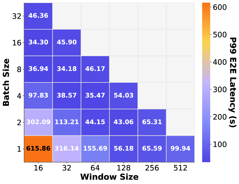
### Visual Description
## Heatmap: P99 E2E Latency vs. Batch Size and Window Size
### Overview
This image is a lower-triangular heatmap visualizing the P99 End-to-End (E2E) Latency (measured in seconds) across various combinations of "Batch Size" and "Window Size." The color scale ranges from dark blue (representing lower latency) to bright orange (representing higher latency). The data suggests an optimization problem where specific configurations of batch and window sizes significantly impact system performance.
### Components/Axes
* **Y-Axis (Vertical):** Labeled "Batch Size." The values are 1, 2, 4, 8, 16, and 32 (bottom to top).
* **X-Axis (Horizontal):** Labeled "Window Size." The values are 16, 32, 64, 128, 256, and 512 (left to right).
* **Legend:** Located on the right side. It maps color to "P99 E2E Latency (s)."
* **Range:** Approximately 100s (dark blue) to 600s+ (bright orange).
* **Data Grid:** A triangular matrix where each cell contains the specific P99 E2E Latency value.
### Detailed Analysis
The data is organized by Batch Size (rows) and Window Size (columns).
| Batch Size | Window 16 | Window 32 | Window 64 | Window 128 | Window 256 | Window 512 |
| :--- | :--- | :--- | :--- | :--- | :--- | :--- |
| **1** | 615.86 | 316.14 | 155.69 | 56.18 | 65.59 | 99.94 |
| **2** | 302.09 | 113.21 | 44.15 | 43.06 | 65.31 | - |
| **4** | 97.83 | 38.57 | 35.47 | 54.03 | - | - |
| **8** | 36.94 | 34.18 | 46.17 | - | - | - |
| **16** | 34.30 | 45.90 | - | - | - | - |
| **32** | 46.36 | - | - | - | - | - |
### Key Observations
* **Extreme Outlier:** The configuration of Batch Size 1 and Window Size 16 results in the highest latency (615.86s), which is significantly higher than any other data point.
* **Inverse Relationship (Batch Size):** Generally, as the Batch Size increases, the latency decreases significantly, particularly at smaller Window Sizes.
* **Diminishing Returns (Window Size):** Increasing the Window Size initially reduces latency (e.g., Batch 1: 615.86 -> 56.18), but there is a "U-shaped" trend in several rows. For example, in Batch 1, latency drops to 56.18 at Window 128, but then increases to 99.94 at Window 512.
* **Optimal Zone:** The "dark blue" region (lowest latency) is clustered around Batch Sizes 4, 8, and 16, with Window Sizes between 32 and 128. The absolute lowest value in the dataset is 34.18 (Batch 8, Window 32) and 34.30 (Batch 16, Window 16).
### Interpretation
This heatmap likely represents performance tuning for a data processing pipeline, such as a machine learning inference engine or a stream processing system.
* **System Overhead:** The high latency at low Batch/Window sizes (the orange/light blue cells) suggests that the system suffers from high overhead when processing small amounts of data at a time. This is typical of systems where the cost of initiating a task or context switching outweighs the actual processing time.
* **Throughput vs. Latency:** The "U-shaped" trend regarding Window Size suggests that while larger windows allow for better batching/parallelism (reducing latency), there is a tipping point where the window becomes too large, potentially causing memory pressure, cache misses, or increased processing time per window, leading to a latency regression.
* **Operational Recommendation:** To minimize P99 E2E latency, the system should avoid the "small batch/small window" configuration. The data indicates that a Batch Size of 8 or 16 combined with a Window Size of 16 to 64 provides the most stable and performant results.
</details>
(a) P99 latency
<details>
<summary>x17.png Details</summary>
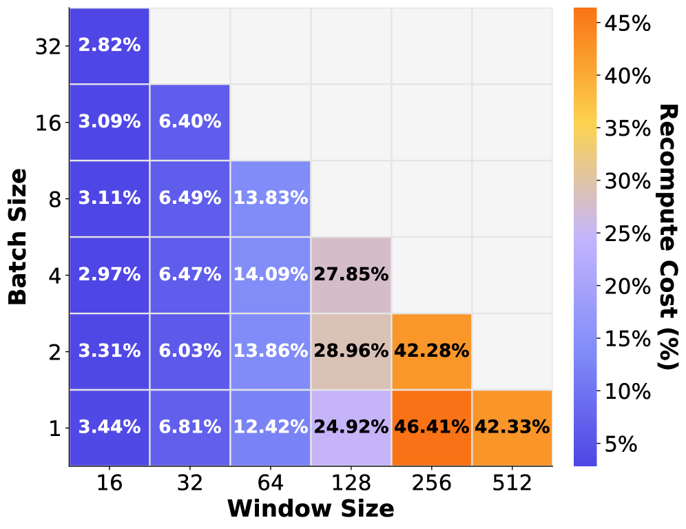
### Visual Description
## Heatmap: Recompute Cost (%) Analysis
### Overview
This image is a heatmap visualizing the "Recompute Cost (%)" across various combinations of "Batch Size" and "Window Size." The chart uses a color gradient ranging from blue (low cost, ~5%) to orange (high cost, ~45%). The data is presented in a triangular matrix format, indicating that certain combinations of high batch size and high window size were likely not tested or are not applicable.
### Components/Axes
* **Y-Axis (Vertical):** Labeled "Batch Size." The values are arranged from bottom to top as 1, 2, 4, 8, 16, 32.
* **X-Axis (Horizontal):** Labeled "Window Size." The values are arranged from left to right as 16, 32, 64, 128, 256, 512.
* **Legend:** A vertical color bar on the right side.
* **Bottom (Blue):** Represents ~5% Recompute Cost.
* **Top (Orange):** Represents ~45% Recompute Cost.
* **Data Cells:** Each cell contains a percentage value representing the Recompute Cost for that specific coordinate.
### Detailed Analysis
The data is organized by Window Size (columns). Below is the extraction of values based on the grid coordinates:
**Column 1: Window Size 16**
* Batch 32: 2.82%
* Batch 16: 3.09%
* Batch 8: 3.11%
* Batch 4: 2.97%
* Batch 2: 3.31%
* Batch 1: 3.44%
* *Trend:* Relatively stable, low cost across all batch sizes.
**Column 2: Window Size 32**
* Batch 16: 6.40%
* Batch 8: 6.49%
* Batch 4: 6.47%
* Batch 2: 6.03%
* Batch 1: 6.81%
* *Trend:* Stable, slightly higher than Window Size 16.
**Column 3: Window Size 64**
* Batch 8: 13.83%
* Batch 4: 14.09%
* Batch 2: 13.86%
* Batch 1: 12.42%
* *Trend:* Consistent values around 13-14%.
**Column 4: Window Size 128**
* Batch 4: 27.85%
* Batch 2: 28.96%
* Batch 1: 24.92%
* *Trend:* Significant increase in cost compared to Window Size 64.
**Column 5: Window Size 256**
* Batch 2: 42.28%
* Batch 1: 46.41%
* *Trend:* High cost, approaching the maximum of the scale.
**Column 6: Window Size 512**
* Batch 1: 42.33%
* *Trend:* High cost, though slightly lower than the Batch 1/Window 256 data point.
### Key Observations
* **Primary Trend (Window Size):** There is a strong positive correlation between Window Size and Recompute Cost. As the Window Size increases (moving left to right), the Recompute Cost increases dramatically, shifting from blue (~3%) to orange (~46%).
* **Secondary Trend (Batch Size):** Within a fixed Window Size, the Recompute Cost is relatively stable across different Batch Sizes, though there is a slight tendency for costs to be marginally higher at smaller batch sizes (e.g., Batch 1) compared to larger ones, particularly in the middle-to-high window size ranges.
* **Anomaly:** The value at Window Size 512 / Batch 1 (42.33%) is lower than the value at Window Size 256 / Batch 1 (46.41%). This suggests a non-linear behavior or a potential optimization/saturation point at the highest window size.
### Interpretation
This chart likely represents the performance overhead of **Gradient Checkpointing** (or a similar memory-saving technique) in a machine learning context, specifically for Transformer-based models where "Window Size" (attention span) and "Batch Size" are critical hyperparameters.
* **Memory vs. Compute Trade-off:** The "Recompute Cost" represents the computational penalty paid to save memory. Larger Window Sizes exponentially increase memory pressure, necessitating more frequent recomputation of activations, hence the sharp rise in cost as Window Size increases.
* **Efficiency:** The data demonstrates that smaller batch sizes are less efficient when using recomputation strategies, as the overhead of recomputing activations constitutes a larger percentage of the total compute time compared to larger batch sizes.
* **Operational Limits:** The triangular shape of the heatmap implies that certain configurations (e.g., Batch 32 with Window 512) were likely excluded, possibly due to Out-Of-Memory (OOM) errors, even with recomputation enabled. The system is clearly pushed to its limits as Window Size increases.
</details>
(b) Recompute cost
Figure 12: The effect of different verification strategies on end-to-end latency (left) and recompute cost (right). Batch size denotes the number of requests verified together.
Grouped verification helps LLM-42 reduce both verification and recomputation cost. It is parameterized by (1) the verification window size per request and (2) the number of requests verified together in a singe pass. To isolate the impact of each parameter, we run an ablation on the ShareGPT dataset, varying the per-request window size from 16 to 512 tokens and the number of requests verified together from one to 32. For each configuration, we execute 4096 requests in an online setting at 12 QPS; all requests require determinism. Figure 12 summarizes the results: 12(a) reports P99 request latency, while 12(b) shows recomputation overhead.
Without grouped verification (batch size 1, first row), latency exhibits a non-monotonic dependence on window size. Increasing the window initially reduces latency, but latency rises when window size becomes too large. Concretely, P99 latency drops from 615 seconds at a window size of 16 to 56.18 seconds at 128, then increases to 99.94 seconds at 512. This behavior reflects the fundamental trade-off between verification and recomputation: smaller windows incur higher verification overhead, while larger windows amplify recomputation cost—for example, recomputation cost is 42.33% at window size 512, compared to only 3.44% at window size 16. Without grouped verification, the best performance occurs at window size of 128 where the latency is 56.18 seconds.
Grouped verification substantially lowers the end-to-end latency. Even batching just two requests reduces P99 latency to 43.06 seconds (best case in the second row from the bottom). Increasing the batch size yields further gains, with the best overall configurations verifying a total of 256 tokens per step—distributed across 16, 8, or 4 requests—all achieving P99 tail latencies of 34–35 seconds.
It is worth noting that the recomputation cost in the offline experiments (typically below 2% as shown in Table 4) is lower than in the online inference setting (typically more than 6% as shown in 12(b)). This difference arises because in offline inference, all requests are available at the beginning and the system tries to maximally utilize memory capacity, resulting in more stable batch sizes. In contrast, online inference experiences significantly greater batch-size variability due to fluctuating load, request arrival and departure times; naturally, higher recomputation rates are correlated with this increased batch-size variability.
### Discussion
Evaluation across models and multiple GPUs: While we report performance results only for Llama-3.1-8B-Instruct in this paper, we have evaluated the correctness of our approach across multiple additional models, including Qwen-4B-Instruct-2507, Qwen3-14B and Qwen3-30B-A3B-Instruct-2507, and across 1-4 GPUs with tensor-parallelism. Our current experimental setup does not support multimem/NVLS and is limited to pairwise NVLink connectivity; consequently, fairly evaluating multi-GPU performance would require a different platform, which we leave to future work. Supporting these models required no additional code changes in LLM-42 which highlights the simplicity of our approach.
Limitations: In our current prototype, the verification pass introduces latency overhead for all requests, even when determinism is enabled selectively. This overhead could be mitigated by confining verification to a subset of GPU SMs or by deferring verification batches—for example, by prioritizing regular prefills and decodes over verification. A second limitation is that prefill and decode use different reduction strategies in LLM-42, making the system non–prefill-decode invariant. As a result, LLM-42 currently does not support sharing prefix caches across multiple turns of the same request or sharing across requests. Our implementation also does not currently integrate with speculative decoding–based LLM inference. Addressing these limitations is interesting future work.
## 6 Related Works
Recent advances in LLM inference systems have focused on optimizing throughput, latency, and resource utilization [orca, vllmsosp, sarathiserve2024, tetriinfer, distserve2024, vattention2024, dynamollm2024, pod-attn]. Orca [orca] pioneered continuous batching, enabling low-latency serving by dynamically scheduling requests at the granularity of individual iterations. vLLM [vllmsosp] introduced PagedAttention, a memory management abstraction that allows higher batch sizes and reuse of KV cache across requests, dramatically improving system throughput. Sarathi-Serve [sarathiserve2024] further improved the throughput–latency trade-off through chunked prefills to better exploit GPU parallelism. DistServe [distserve2024] and Splitwise [patel2023splitwise] proposed disaggregated inference architectures that separate prefill and decode workloads across specialized servers, mitigating interference. Complementary lines of work such as speculative decoding [leviathan2022fast, chen2023accelerating, mamou2024dynamic] and FlexGen [flexgen] pursue orthogonal optimizations by reducing the number of autoregressive steps or offloading memory to CPU and SSDs. While all these systems achieve impressive performance gains, they typically assume non-deterministic execution, leaving the trade-offs between determinism and efficiency unexplored.
Enabling determinism in LLM inference has recently drawn increasing attention. Song et al. [song2024greedy] argued that such non-determinism can distort evaluation results, calling for reproducibility-aware benchmarking. Yuan et al. [yuan2025fp32death] further linked reproducibility failures to mixed-precision arithmetic and fused kernel inconsistencies, showing their impact on multi-step reasoning accuracy. Rainbird AI [rainbird2025deterministic] emphasized deterministic inference as a requirement for traceability and compliance in enterprise and safety-critical domains.
Recent work by Zhang et al. proposes tensor-parallel–invariant kernels that eliminate training–inference mismatch by ensuring bitwise deterministic results across different tensor parallel sizes for LLM inference [zhang2025-deterministic-tp]. In contrast, existing LLM serving systems typically achieve determinism through batch-invariant computation. We examine the performance and engineering costs of this approach and propose an alternative mechanism for enabling determinism in LLM inference. By leveraging properties of GPU kernels together with characteristics of LLM inference workloads, our approach seeks to reconcile reproducibility with efficiency—a design space that remains largely unexplored in prior work.
## 7 Conclusion
Enabling determinism in LLM inference remains tedious today. Existing systems achieve determinism by enforcing batch-invariant computation, an approach that is cumbersome in practice: it requires rewriting kernels at a time when both hardware and model architectures are evolving rapidly. Moreover, batch-invariant kernels are inherently suboptimal, as they prevent kernels from adapting their parallelism strategies at runtime. We present LLM-42, a simpler alternative that enables determinism in LLM inference by repurposing speculative decoding. LLM-42 minimizes the need to write new kernels and supports selective enforcement of determinism, incurring runtime overhead only for the fraction of traffic that actually requires it.
## References