# Pushing the Boundaries of Natural Reasoning: Interleaved Bonus from Formal-Logic Verification in Language Models
**Authors**: Chuxue Cao, Jinluan Yang, Haoran Li, Kunhao Pan, Zijian Zhao, Zhengyu Chen, Yuchen Tian, Lijun Wu, Conghui He, Sirui Han, Yike Guo
## Abstract
Large Language Models (LLMs) show remarkable capabilities, yet their stochastic next-token prediction creates logical inconsistencies and reward hacking that formal symbolic systems avoid. To bridge this gap, we introduce a formal logic verification-guided framework that dynamically interleaves formal symbolic verification with the natural language generation process, providing real-time feedback to detect and rectify errors as they occur. Distinguished from previous neuro-symbolic methods limited by passive post-hoc validation, our approach actively penalizes intermediate fallacies during the reasoning chain. We operationalize this framework via a novel two-stage training pipeline that synergizes formal logic verification-guided supervised fine-tuning and policy optimization. Extensive evaluation on six benchmarks spanning mathematical, logical, and general reasoning demonstrates that our 7B and 14B models outperform state-of-the-art baselines by average margins of 10.4% and 14.2%, respectively. These results validate that formal verification can serve as a scalable mechanism to significantly push the performance boundaries of advanced LLM reasoning. We will release our data and models for further exploration soon.
Machine Learning, ICML
## 1 Introduction
<details>
<summary>x1.png Details</summary>
### Visual Description
## Diagram: Comparison of Natural Language vs. Formal Logic Reasoning on a Transitive Comparison Problem
### Overview
The image is a technical diagram comparing two approaches to solving a simple logic puzzle: Natural Language (NL) Reasoning and Formal Logic Reasoning. It demonstrates a failure case for NL reasoning and highlights the value of formal verification. The diagram is divided into a problem statement, two reasoning pathways (left and right), a supporting bar chart, and a final conclusion.
### Components/Axes
**1. Problem Statement (Top Center):**
* **Text:** "Problem: Alice > Bob, Charlie < Alice, Diana > Charlie. Who scores higher: Bob or Diana?"
**2. Left Column (NL Reasoning Pathway):**
* **Header:** "NL Reasoning:" (in a light red box)
* **Reasoning Chain:** "Charlie < Diana < Alice > Bob → Therefore: Diana > Bob"
* **Answer:** "Answer: Diana scores higher than Bob" (followed by a large red **X** mark, indicating this answer is incorrect).
**3. Right Column (Formal Logic Reasoning Pathway):**
* **Header:** "NL Reasoning:" (in a light blue box) - *Note: This appears to be a mislabel; the content below is formal logic code.*
* **Formal Logic Block:** "Formal Logic Reasoning:" followed by pseudo-code:
* `solver.add(bob > diana)`
* `result = solver.check()`
* `solver.add(diana > bob)`
* `result = solver.check()`
* **Compiler Output:** "Compiler Output: Unknown"
* **Answer:** "Answer: Relationship is undetermined" (followed by a large green **✓** checkmark, indicating this is the correct answer).
**4. Bar Chart (Bottom Left):**
* **Title:** "Logic Consistency in NL Reasoning Chains"
* **Y-axis:** "Percentage (%)" (Scale from 0% to ~70%)
* **X-axis Categories:** "Correct CoT" and "Wrong CoT" (CoT likely stands for Chain-of-Thought).
* **Legend (Top-Left of chart area):**
* Blue square: "Consistent Logic"
* Red square: "Inconsistent Logic"
* **Data Points (Bars):**
* **Correct CoT:**
* Consistent Logic (Blue Bar): **60.7%**
* Inconsistent Logic (Red Bar): **39.3%**
* **Wrong CoT:**
* Consistent Logic (Blue Bar): **47.6%**
* Inconsistent Logic (Red Bar): **52.4%**
### Detailed Analysis
The diagram presents a specific logic puzzle and analyzes how different reasoning methods handle it.
* **The Problem:** The given statements are: Alice's score is greater than Bob's. Charlie's score is less than Alice's. Diana's score is greater than Charlie's. The question asks to compare Bob and Diana directly.
* **NL Reasoning Failure:** The NL reasoning chain shown (`Charlie < Diana < Alice > Bob`) incorrectly infers a direct relationship between Diana and Bob. It assumes transitivity through Alice, but the statements only establish that both Diana and Bob are less than Alice, not their relation to each other. This leads to the incorrect, definitive answer "Diana > Bob."
* **Formal Logic Success:** The formal logic approach attempts to test both possible relationships (`bob > diana` and `diana > bob`) using a solver. The "Compiler Output: Unknown" indicates that neither assertion can be proven true given the axioms. Therefore, the correct conclusion is that the relationship is "undetermined."
* **Bar Chart Data:** The chart provides meta-analysis on the consistency of NL reasoning chains.
* **Trend for Correct CoT:** When the final answer is correct (60.7% + 39.3% = 100% of "Correct CoT" cases), the reasoning chain is logically consistent more often than not (60.7% vs. 39.3%).
* **Trend for Wrong CoT:** When the final answer is wrong, the reasoning chain is *more likely to be logically inconsistent* (52.4%) than consistent (47.6%). This supports the idea that internal logical errors often lead to incorrect final answers.
### Key Observations
1. **Spatial Layout:** The incorrect NL pathway is on the left, marked with red. The correct formal logic pathway is on the right, marked with blue/green. The supporting statistical chart is placed below the failing NL pathway, visually linking the general problem (inconsistency) to the specific example.
2. **Critical Mislabel:** The header for the formal logic section is incorrectly labeled "NL Reasoning:" instead of "Formal Logic Reasoning:". This is likely an error in the diagram's creation.
3. **Data Trend:** The bar chart shows a clear correlation: wrong answers are associated with a higher rate of internal logical inconsistency in the reasoning chain (52.4% inconsistent) compared to correct answers (39.3% inconsistent).
4. **Symbolic Contrast:** The large red **X** and green **✓** provide immediate visual feedback on the validity of each approach's conclusion.
### Interpretation
This diagram serves as a pedagogical or research-oriented critique of relying solely on natural language reasoning for logical tasks. It argues that NL reasoning, while fluent, can make confident but incorrect inferences by implicitly assuming transitivity or other logical rules where they don't strictly apply.
The **formal logic approach**, by explicitly defining constraints and using a solver to check satisfiability, correctly identifies the ambiguity in the problem. It doesn't guess; it reports the state of knowledge ("undetermined").
The **bar chart generalizes this point**, suggesting that errors in NL reasoning chains (leading to wrong answers) are frequently rooted in internal logical inconsistencies. The data implies that checking for internal consistency could be a valuable method for improving or auditing the reliability of chain-of-thought reasoning in AI systems.
In essence, the image advocates for the integration of formal verification methods alongside or within natural language reasoning systems to enhance their robustness and accuracy, especially for tasks requiring precise logical deduction.
</details>
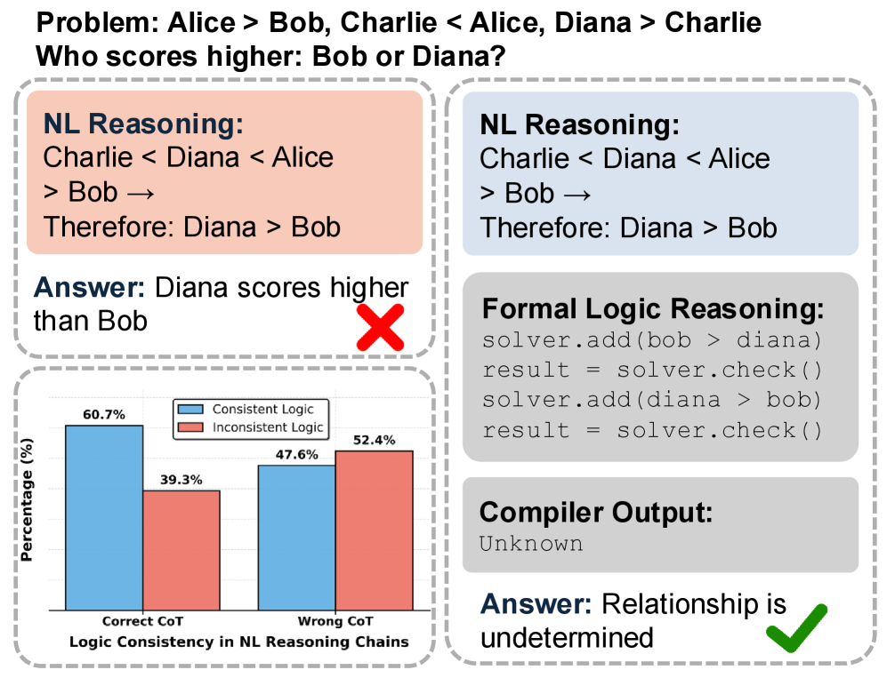
Figure 1: Comparison between natural language reasoning and formal logic verification-guided reasoning. Formal verification detects logical errors in natural language reasoning and provides corrected reasoning paths. “NL” means Natural Language.
Large Language Models (LLMs) demonstrate impressive proficiency in mathematical and logical reasoning (Ahn et al., 2024; Ji et al., 2025; Liu et al., 2025b; Chen et al., 2025a), yet their probabilistic decoding process lacks inherent mechanisms to ensure consistency (Sheng et al., 2025b; Baker et al., 2025). This tension creates significant risks, including hallucinations (Li and Ng, 2025; Sheng et al., 2025b), safety vulnerabilities (Zhou et al., 2025; Cao et al., 2025b), and reward hacking (Chen et al., 2025b; Baker et al., 2025). Although recent efforts have employed model-based verifiers to offer denser feedback than sparse ground-truth labels (Ma et al., 2025; Liu et al., 2025c; Guo et al., 2025b), they often overlook intermediate reasoning steps. To enforce more rigorous supervision, subsequent research has incorporated formal tools like theorem provers and code interpreters (Ospanov et al., 2025; Kamoi et al., 2025; Liu et al., 2025a) to address this drawback. However, existing formal approaches face critical limitations: they are often restricted to specific domains (e.g., Mathematics) (Ospanov et al., 2025; Liu et al., 2025a), rely on uncertain autoformalization (Ospanov et al., 2025; Feng et al., 2025b), or utilize post-hoc verification that cannot actively prevent error propagation (Kamoi et al., 2025; Feng et al., 2025b). This yields the primary question to be explored:
(Q) Can we utilize the formal verification to further enhance the LLM reasoning across diverse domains?
To explore this question, we first quantified the logical consistency gap in current LLMs by conducting a formal verification analysis of generated reasoning chains. A critical finding emerges as shown in Figure 1: even chains that arrive at correct final answers suffer from substantial logical inconsistency, with 39.3% of steps formally disproved, a trend consistent with previous research (Sheng et al., 2025b; Leang et al., 2025). For chains leading to incorrect answers, this failure rate rises to 52.4%. The comparative example in Figure 1 illustrates this gap: natural language reasoning incorrectly concludes “Diana $>$ Bob” from the given constraints, while formal verification identifies the incorrect conclusion and lead to an correct answer. This phenomenon reveals pervasive “reward hacking,” where models exploit superficial patterns to reach correct labels without establishing sound logical foundations (Skalse et al., 2022). Ultimately, these results expose a fundamental limitation of natural language reasoning: without explicit verification mechanisms, models cannot guarantee reasoning validity or global logical coherence across multi-step inference.
To bridge this gap, we propose a novel framework that synergizes probabilistic natural language reasoning with formal symbolic verification. Distinguished from prior approaches relying on static filtering or narrow domains, our method dynamically interleaves formal verification into the generation process. By incorporating feedback from satisfiability results, counterexamples, and execution outputs, we extend the standard chain-of-thought paradigm to enable real-time error detection and rectification. To effectively operationalize this interleaved reasoning approach, we introduce a formal logic verification-guided training framework comprising two synergistic stages: (i) Supervised Fine-tuning (SFT), which employs a hierarchical data synthesis pipeline. Crucially, we mitigate the noise of raw autoformalization by enforcing execution-based validation, thereby ensuring high alignment between natural language and formal proofs; and (ii) Reinforcement Learning (RL), which utilizes Group Relative Policy Optimization (GRPO) with a composite reward function to enforce structural integrity and penalize logical fallacies. Empirical evaluations across logical, mathematical, and general reasoning domains demonstrate that this framework substantially enhances reasoning accuracy, highlighting the potential of formal verification to push the performance boundaries of LLM reasoning. Our contributions can be concluded as follows:
- We propose the first framework that dynamically interleaves formal verification into LLM reasoning across diverse domains, utilizing the real-time feedback via symbolic interpreters to transcend the limitations of passive post-hoc filtering and domain-specific theorem proving.
- We introduce a two-stage training framework that combines formal verification-guided supervised fine-tuning with policy optimization, featuring a novel data synthesis pipeline with execution-based validation to enforce logical soundness and structural integrity.
- Extensive evaluations on six benchmarks demonstrate that our models break performance ceilings, surpassing SOTA by 10.4% (7B) and 14.2 % (14B). This validates the scalability and effectiveness of our proposed method.
## 2 Related Works
### 2.1 Large Language Models for Natural Reasoning
Supervised fine-tuning (SFT) on chain-of-thought examples (Wei et al., 2022) and step-by-step solutions (Cobbe et al., 2021) has been foundational for developing reasoning capabilities in LLMs, with recent efforts curating high-quality datasets across mathematics (LI et al., 2024), code (Xu et al., 2025), and science (Wang et al., 2022). However, SFT alone cannot effectively optimize for complex objectives beyond imitation and struggles with multi-step error correction (Lightman et al., 2023; Uesato et al., 2022; Zhou et al., 2026). Recent RL advances using outcome-based optimization methods have achieved remarkable success in mathematical reasoning (Cobbe et al., 2021; Zeng et al., 2025), code generation (Le et al., 2022; Feng et al., 2025a), and general-domain reasoning (Ma et al., 2025; Chen et al., 2025c). However, optimizing solely for final answer correctness creates perverse incentives where models learn correct conclusions through logically invalid pathways (Uesato et al., 2022), leading to reward hacking (Skalse et al., 2022) and brittleness under distribution shift (Hendrycks et al., 2021). To address these limitations, process-based rewards incorporate feedback from intermediate steps, providing dense supervision through human-annotated judgments (Uesato et al., 2022; Lightman et al., 2023; She et al., 2025; Khalifa et al., 2025). However, the probabilistic nature of language model-based verifiers introduces errors and biases (Zheng et al., 2023), limiting their ability to detect subtle logical inconsistencies that emerge during multi-step reasoning.
### 2.2 Formal Reasoning and Verification
Recent work has integrated formal verification tools, including theorem provers (Yang et al., 2023; Cao et al., 2025a; Tian et al., 2025), code interpreters (Feng et al., 2025a), and symbolic solvers (Li et al., 2025a), to provide machine-checkable validation beyond the biases of LLM-as-a-judge approaches (Li and Ng, 2025; Uesato et al., 2022; Lightman et al., 2023). This direction is increasingly recognized as critical for grounding generative models in verifiable systems (Ren et al., 2025; Wang et al., 2025; Hu et al., 2025). Existing approaches differ in how verification is applied. HERMES (Ospanov et al., 2025) interleaves informal reasoning with Lean-verified steps, ensuring real-time soundness but requiring mature formal libraries. Safe (Liu et al., 2025a) applies post-hoc verification to audit completed reasoning chains, though this passive mode cannot prevent error accumulation during generation. VeriCoT (Feng et al., 2025b) checks logical consistency on extracted first-order logic, while others train verifier models using formal tool signals (Kamoi et al., 2025). Tool-integrated methods (Xue et al., 2025; Zeng et al., 2025; Li et al., 2025b; Feng et al., 2025a) embed interpreter calls into generation for calculation or simulation, but often lack strict logical guarantees. These approaches face key limitations: specialization to mathematical theorem proving, treating verification as separate filtering without guiding generation, or relying on uncertain logic extraction and neural verifiers. In contrast, we propose verification-guided reasoning that extends formal verification to general logical domains and employs real-time feedback as dynamic, in-process guidance to steer reasoning trajectories and enable self-correction beyond specialized formal tasks.
## 3 Preliminaries
<details>
<summary>x2.png Details</summary>
### Visual Description
## Bar Chart: Performance Comparison of Natural-SFT vs. FLV-SFT Across Domains
### Overview
The image is a grouped bar chart comparing the performance of two methods, "Natural-SFT" and "FLV-SFT," across three distinct problem-solving domains. The chart quantifies performance as the "Number of Correct Answers" achieved by each method within each domain. FLV-SFT consistently outperforms Natural-SFT in all categories, with the percentage improvement explicitly annotated.
### Components/Axes
* **Chart Type:** Grouped Bar Chart.
* **Y-Axis:**
* **Label:** "Number of Correct Answers" (written vertically along the left edge).
* **Scale:** Linear scale from 0 to 350, with major tick marks at intervals of 50 (0, 50, 100, 150, 200, 250, 300, 350).
* **X-Axis:**
* **Label:** "Domain" (centered below the axis).
* **Categories:** Three discrete categories are listed from left to right: "Logical", "Mathematical", "General".
* **Legend:**
* **Position:** Top-right corner of the chart area.
* **Items:**
1. A blue square labeled "Natural-SFT".
2. A red/salmon square labeled "FLV-SFT".
* **Data Series & Labels:**
* Each domain category on the x-axis contains two adjacent bars.
* The left bar in each pair is blue, corresponding to "Natural-SFT".
* The right bar in each pair is red/salmon, corresponding to "FLV-SFT".
* The exact numerical value of correct answers is printed directly above each bar.
* A green percentage value (e.g., "(+32.8%)") is printed above each red/FLV-SFT bar, indicating its relative improvement over the corresponding blue/Natural-SFT bar.
### Detailed Analysis
**Domain: Logical**
* **Natural-SFT (Blue Bar):** 219 correct answers.
* **FLV-SFT (Red Bar):** 291 correct answers.
* **Improvement:** +32.8% (annotated in green above the red bar).
**Domain: Mathematical**
* **Natural-SFT (Blue Bar):** 163 correct answers.
* **FLV-SFT (Red Bar):** 243 correct answers.
* **Improvement:** +49.3% (annotated in green above the red bar).
**Domain: General**
* **Natural-SFT (Blue Bar):** 166 correct answers.
* **FLV-SFT (Red Bar):** 213 correct answers.
* **Improvement:** +28.5% (annotated in green above the red bar).
### Key Observations
1. **Consistent Superiority:** FLV-SFT achieves a higher number of correct answers than Natural-SFT in every domain presented.
2. **Magnitude of Improvement:** The performance gain is most pronounced in the "Mathematical" domain (+49.3%), followed by "Logical" (+32.8%), and is smallest in the "General" domain (+28.5%).
3. **Baseline Performance:** Natural-SFT's performance is highest in the "Logical" domain (219) and notably lower in both "Mathematical" (163) and "General" (166), which are similar to each other.
4. **Absolute Performance:** FLV-SFT's highest absolute score is in the "Logical" domain (291), while its lowest is in the "General" domain (213).
### Interpretation
The data strongly suggests that the FLV-SFT method is more effective than the Natural-SFT method for generating correct answers across the tested domains of logical, mathematical, and general reasoning. The relationship is one of consistent enhancement.
The variation in improvement percentages is particularly insightful. The largest gain in the "Mathematical" domain implies that FLV-SFT may have a specific architectural or training advantage for structured, symbolic, or quantitative reasoning tasks. The substantial gain in "Logical" reasoning further supports an advantage in structured problem-solving. While still significant, the smaller gain in the "General" domain suggests that for broader, less formally structured tasks, the advantage of FLV-SFT over Natural-SFT, though clear, is less dramatic.
This chart likely serves as evidence in a technical paper or report to demonstrate the efficacy of a proposed method (FLV-SFT) over a baseline (Natural-SFT). The clear annotation of percentage improvements is designed to highlight the practical significance of the results beyond just the raw numbers. The choice of domains indicates the evaluation was designed to test reasoning capabilities across a spectrum from highly formal (Mathematical) to less formal (General).
</details>
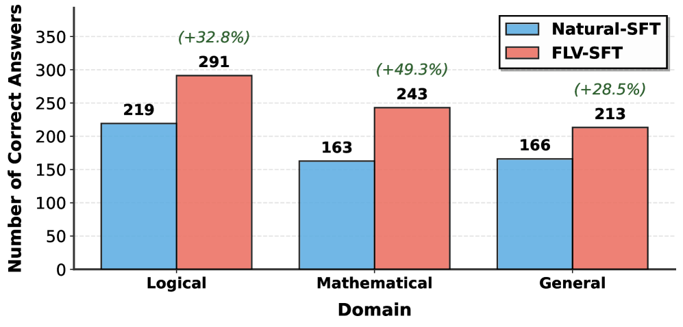
Figure 2: Number of correct answers using natural language reasoning versus formal logic verification. We randomly sampled 500 instances from each domain for this comparison.
We first present empirical evidence illustrating the gap between probabilistic natural language reasoning and formal verification in LLM reasoning. We then formally define our reasoning paradigm and introduce the preliminaries on the symbolic verification methods utilized in our framework.
### 3.1 Natural vs. Formal Reasoning in LLMs
Our previous experiments demonstrate that LLMs lack mechanisms to ensure global logical consistency (Figure 1), motivating us to explore formal logic verification. Formal logic provides a rigorous framework where reasoning steps can be reliably validated using formal solvers. As shown in Figure 2, integrating formal logic verification with natural language reasoning yields significant performance improvements across diverse domains. We compare two approaches: Natural-SFT, which relies solely on natural language reasoning, and FLV-SFT, which incorporates formal logic verification. Across 500 randomly sampled instances from each domain, FLV-SFT consistently outperforms Natural-SFT, achieving 291 vs. 219 correct answers in the Logical domain (+32.8%), 243 vs. 163 in the Mathematical domain (+49.3%), and 213 vs. 166 in the General domain (+28.5%). These substantial improvements across all three categories demonstrate that formal verification effectively addresses the consistency gaps inherent in purely neural approaches. These results underscore the significant potential of formal verification to bridge the reasoning gap and strongly motivate our approach of interleaving natural language reasoning with formal verification throughout the reasoning process.
### 3.2 Problem Formulation
Formally, let $\mathcal{D}=\{(x,y)\}$ be a dataset of reasoning tasks, where $x$ denotes the input context (e.g., problem description) and $y$ denotes the ground-truth answer.
Standard CoT Paradigm. In conventional Chain-of-Thought reasoning, an LLM $P_{\theta}$ generates a sequence of reasoning steps $z=(s_{1},s_{2},\dots,s_{n})$ in natural language, aiming to maximize:
$$
P_{\theta}(y,z\mid x)=P_{\theta}(y\mid z,x)\cdot\prod_{i=1}^{n}P_{\theta}(s_{i}\mid s_{<i},x) \tag{1}
$$
However, this objective does not guarantee that $z$ is logically valid or formally verifiable.
Our Paradigm: Formal Logic Verification-Guided Reasoning. We propose augmenting the reasoning chain with formal verification at each step. Specifically, we define an extended reasoning chain $z^{\prime}=(s_{1},f_{1},v_{1},s_{2},f_{2},v_{2},\dots,s_{n},f_{n},v_{n})$ , where:
- $s_{i}$ : Natural language reasoning step (as in standard CoT)
- $f_{i}$ : Formal specification that encodes the logical correctness of $s_{i}$ (e.g., symbolic constraints, SAT clauses, SMT formulas, or executable code)
- $v_{i}$ : Formal Logic Verification result returned by a formal verifier $\mathcal{V}$ when applied to $f_{i}$
During training, our objective is to maximize the likelihood of correct final answers:
$$
\max_{\theta}\mathbb{E}{(x,y)\sim\mathcal{D}}\left[\log P\theta(y,z^{\prime}\mid x)\right] \tag{2}
$$
During inference, the verification function $\mathcal{V}$ takes the formal reasoning as input and returns detailed feedback at each reasoning step. This feedback may include satisfiability results, counterexamples, proof traces, execution outputs, or error messages, which guide the model to generate logically sound and verifiable subsequent reasoning steps.
<details>
<summary>x3.png Details</summary>
### Visual Description
\n
## Diagram: Two-Stage Training Pipeline for a Formal Logic-Verified Reasoning Model
### Overview
The image is a technical flowchart illustrating a two-stage machine learning training pipeline. The process is divided into **Stage 1: SFT (Supervised Fine-Tuning)** and **Stage 2: RL (Reinforcement Learning)**. The pipeline's goal is to train a model (the "FLV-SFT Model" and subsequently a "Policy Model") to perform reasoning that is verified against formal logic, using a combination of distillation, filtering, incentive mechanisms, and an interleaved reasoning loop with a verifier.
### Components/Axes
The diagram is structured as a process flow from left to right, top to bottom. Key visual components include:
* **Process Boxes:** Blue rectangular boxes with rounded corners represent major processing steps or data states.
* **Icons:** Stylized robot icons represent AI models. Other icons include a filter, a document with a checkmark (Verifier), a database, a trash can, a dollar sign (Reward), and a line graph (Advantage).
* **Arrows:** Solid black arrows indicate the primary flow of data and processes. Dashed arrows indicate feedback loops (e.g., "Backprop").
* **Text Labels:** All components are labeled with descriptive text.
* **Color Coding:** Green is used for positive outcomes ("Verified," "Correct Reward"). Red is used for negative outcomes ("Rejected," "X" marks). Blue is the primary color for process boxes. Orange is used for the final reward/advantage block.
### Detailed Analysis
#### **Stage 1: SFT (Top Half)**
This stage focuses on creating a verified dataset to fine-tune a model.
1. **Input & Distillation:** The process begins with an "Input q" (question). This is fed into a "Distill" process, represented by a robot icon.
2. **Filtering:** The output is filtered. Red "X" marks and green checkmarks indicate a selection process. The text "Filter by Fail rate" leads to the creation of a subset labeled "Difficult Questions."
3. **Formal Logic Incentive:** These difficult questions are processed by a "Formal Logic Incent" (likely "Incentive") module, represented by another robot icon.
4. **Formal Logic-Verification Trace:** The core of Stage 1 is a large blue box containing three sub-components:
* `Natural Language Reasoning`
* `Formal Logic Reasoning`
* `Verifier Observation` (accompanied by a document/checkmark icon)
5. **Verification & Model Creation:** The trace is passed to a "Verifier." This leads to two outcomes:
* **Verified:** A green checkmark points to a database icon, which then feeds into the final "SFT" process to create the **"FLV-SFT Model."**
* **Rejected:** A red "X" points to a trash can icon.
#### **Stage 2: RL (Bottom Half)**
This stage uses reinforcement learning to further train a policy model, incorporating the verifier in an online loop.
1. **Policy Model:** The stage begins with a "Policy Model" (robot icon).
2. **Interleaved Reasoning Loop:** The core is a three-step loop contained within a dashed outline:
* **Step tₙ (Natural Language Reasoning & Formal Action):** Contains the text: "Let's verify the logic using z3" followed by formal code-like statements:
```
Implies(And(both_optimal, duality_holds), both_feasible)
solver = Solver()
result = solver.check()
```
* **Step tₙ₊₁ (Verifier Observation):** Contains the question: "Are the triple iff and strong duality equivalent? False"
* **Step tₘ (Next Natural Language Reasoning):** Contains the text: "The result indicates that the triple iff structure (Both the primal LP and the dual LP have feasible solutions) <=> then..."
* These three steps are connected by arrows forming a cycle labeled **"Interleaved Reasoning Loop."**
3. **Reward & Advantage:** The output of the loop feeds into an orange block containing:
* **Correct Reward / Instruct Reward:** Represented by a dollar sign icon.
* **GRPO Advantage Aᵢ:** Represented by a line graph icon. "GRPO" likely stands for a specific reinforcement learning algorithm variant.
4. **Feedback:** A dashed arrow labeled **"Backprop"** leads from the advantage block back to the "Policy Model," completing the reinforcement learning cycle.
### Key Observations
* **Hybrid Reasoning:** The pipeline explicitly combines **Natural Language Reasoning** with **Formal Logic Reasoning** (using tools like Z3, a theorem prover mentioned in the code snippet).
* **Verification-Centric:** A "Verifier" is a central component in both stages, acting as a gatekeeper for data quality (Stage 1) and as an online critic during training (Stage 2).
* **Curriculum Learning:** Stage 1 implements a form of curriculum learning by filtering for "Difficult Questions" based on failure rate.
* **Two-Phase Training:** The model is first trained on a static, verified dataset (SFT), then further refined through dynamic interaction with a verifier in an RL loop.
* **Specific RL Algorithm:** The mention of "GRPO Advantage" suggests the use of a specific policy gradient algorithm, possibly a variant of Proximal Policy Optimization (PPO) or similar.
### Interpretation
This diagram outlines a sophisticated methodology for training AI reasoning models to be more logically rigorous and verifiable. The core innovation is the tight integration of a symbolic logic verifier into both the data curation and the online training process.
* **Purpose:** To move beyond purely statistical language modeling and instill models with the ability to perform and self-verify formal logical deductions. This is crucial for applications requiring high reliability, such as mathematical proof generation, code verification, or complex decision-making.
* **How Elements Relate:** Stage 1 creates a high-quality, verified "textbook" for the model. Stage 2 then puts the model through "interactive tutoring sessions" where it proposes reasoning steps, the verifier checks them, and the model is rewarded for correct, verifiable logic. The "Interleaved Reasoning Loop" is the key mechanism for this interactive learning.
* **Notable Implications:** The pipeline addresses a key weakness of large language models: their tendency to produce plausible-sounding but logically flawed arguments. By grounding the training in formal verification, the resulting model's reasoning should be more trustworthy and less prone to hallucination in logical domains. The use of "Difficult Questions" suggests a focus on pushing the model's capabilities on hard cases rather than easy examples.
</details>
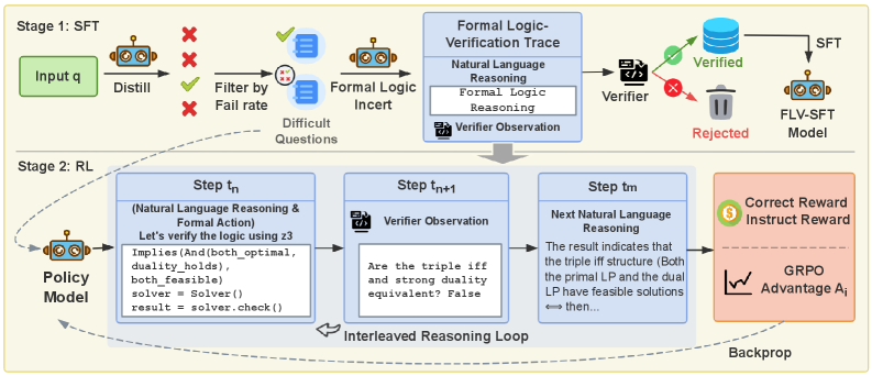
Figure 3: Overview of the formal logic verification-guided training framework. The framework operates in two stages: (1) SFT: A teacher model synthesizes formal logic verification traces, which are validated by a verifier. A subset of verified samples is used to fine-tune the model, while challenging samples are reserved for RL training. (2) RL: The policy model generates natural language reasoning followed by formal reasoning. A formal interpreter verifies the formal reasoning and provides feedback, enabling iterative refinement until the model produces a final answer or reaches the maximum number of interpreter calls. Rewards computed from verification outcomes are used to calculate advantages and update the policy model via reinforcement learning.
## 4 Methodology
To address logical inconsistencies and hallucinations in pure natural language reasoning (Section 3), we propose integrating formal logic verification into the reasoning process. Our approach consists of two stages: (i) Supervised Fine-tuning to enable the model to generate interleaved natural language and formal proofs, and (ii) Reinforcement Learning to optimize the model using composite rewards that enforce logical soundness and correctness.
### 4.1 Formal Logic Verification-Guided SFT
The primary goal of the SFT stage is to align the model’s output distribution with a structured reasoning format that supports self-verification. Since large-scale datasets containing interleaved reasoning and formal proofs are scarce, we employ a hierarchical formal proof data synthesis pipeline.
#### 4.1.1 Data Synthesis Pipeline
CoT Generation. Given a raw reasoning problem $q$ , we first employ a strong teacher model to generate $K=4$ candidate reasoning chains. A judge model evaluates the correctness of the final answers to calculate pass rates. We select a subset of verified chains that yield correct solutions for subsequent processing. Let $z$ denote a selected correct reasoning chain. To incorporate formal logic, we utilize an LLM to decompose $z$ into discrete logical modules $\{s_{k}\}_{k=1}^{N}$ . For each module $s_{k}$ , the LLM synthesizes a corresponding formal proof $f_{k}$ and predicts an expected execution output $v_{k}^{\text{exp}}$ . The prompt template is provided in Figure 9.
Execution-based Validation and Correction. To ensure the fidelity of synthesized formal proofs, we implement a rigorous validation mechanism. Each generated formal proof $f_{k}$ is executed in a sandbox to obtain the actual output $v_{k}^{\text{act}}$ . We then perform a three-stage validation:
Stage 1: Exact Match. If the actual output exactly matches the expected output ( $v_{k}^{\text{act}}=v_{k}^{\text{exp}}$ ), the proof is accepted immediately and integrated into the training data.
Stage 2: Semantic Equivalence Check. In cases where $v_{k}^{\text{act}}\neq v_{k}^{\text{exp}}$ , we employ a verification model to assess whether the discrepancy is semantically negligible (e.g., differences in capitalization, output ordering, or numerical precision). If the outputs are deemed equivalent under mathematical or logical semantics, we proceed to Stage 3.
Stage 3: Proof Rewriting. When minor inconsistencies are detected, we require the LLM to regenerate the natural language reasoning $s_{k}^{\prime}$ conditioned on the actual execution result $v_{k}^{\text{act}}$ . This ensures that the natural language reasoning module $s_{k}^{\prime}$ , the formal proof $f_{k}^{\prime}$ , and the execution output $v_{k}^{\text{act}}$ maintain strict logical coherence. Proofs that fail both exact match and semantic equivalence checks are discarded. The resulting training instance is structured as follows:
$$
\begin{split}z_{\text{aug}}=\bigoplus_{k=1}^{N}\Big(s_{k}\oplus\texttt{<code>}f_{k}^{\prime}\texttt{</code>}\\
\oplus\texttt{<interpreter>}v_{k}^{\text{act}}\texttt{</interpreter>}\Big)\end{split} \tag{3}
$$
where $f_{k}^{\prime}$ denotes the validated formal proof and $v_{k}^{\text{act}}$ is the verified execution output. This pipeline ensures that every training example $(s,f,v)$ exhibits perfect alignment between natural language hypotheses, formal logic reasoning, and execution feedback, thereby providing high-quality supervision for the model to learn reliable reasoning patterns. See Appendix B for dataset construction details.
#### 4.1.2 Optimization Objective
Given the augmented training dataset $\mathcal{D}_{\text{SFT}}=\{(q_{i},z_{\text{aug},i})\}_{i=1}^{M}$ , we optimize the model parameters $\theta$ by maximizing the log-likelihood of generating structured reasoning sequences:
$$
\mathcal{L}_{\text{SFT}}(\theta)=-\mathbb{E}_{(q,z_{\text{aug}})\sim\mathcal{D}_{\text{SFT}}}\left[\log P_{\theta}(z_{\text{aug}}\mid q)\right] \tag{4}
$$
This can be decomposed into the sequential generation of reasoning modules, formal proofs, and execution outputs:
$$
\begin{split}\mathcal{L}_{\text{SFT}}(\theta)=-\mathbb{E}_{(q,z_{\text{aug}})\sim\mathcal{D}_{\text{SFT}}}\Bigg[\sum_{k=1}^{N}\Big(\log P_{\theta}(s_{k}\mid q,z_{<k})\\
+\log P_{\theta}(f_{k}^{\prime}\mid q,z_{<k},s_{k})+\log P_{\theta}(v_{k}^{\text{act}}\mid q,z_{<k},s_{k},f_{k}^{\prime})\Big)\Bigg]\end{split} \tag{5}
$$
where $z_{<k}$ denotes all previous modules. We train using AdamW with cosine learning rate scheduling and gradient clipping. This stage enables the model to generate verifiable, formally grounded reasoning chains.
### 4.2 Formal Verification-Guided Policy Optimization
To further enhance the formal logic verification-guided reasoning capabilities of LLMs, we employ reinforcement learning. The core of this stage is a multi-dimensional reward function that provides fine-grained feedback on structure, semantics, and computational efficiency.
#### 4.2.1 Hierarchical Reward Design
To ensure both generation stability and reasoning rigor, we design a hierarchical reward function $R(y)$ that evaluates responses in a strictly prioritized order: Format Integrity $\succ$ Structural Compliance $\succ$ Logical Correctness. The unified reward is formulated as:
$$
R(y)=\begin{cases}R_{\text{fatal}}&y\in\mathbb{C}_{\text{fatal}}\qquad\text{(L1: Fatal)}\\
R_{\text{invalid}}&y\in\mathbb{C}_{\text{invalid}}\qquad\text{(L2: Format)}\\
R_{\text{total}}(y)&\text{otherwise}\qquad\text{(L3: Valid)}\end{cases} \tag{6}
$$
The total reward for valid responses is:
$$
R_{\text{total}}(y)=R_{\text{struct}}(y)+R_{\text{logic}}(y) \tag{7}
$$
Level 1 & 2: Penalties for Malformed Generation. We first filter out pathological behaviors to prevent reward hacking and infinite loops during training.
- Fatal Errors ( $\mathbb{C}_{\text{fatal}}$ ): Responses with severe and unrecoverable execution failures (e.g., timeouts, repetition loops, excessive tool calls). We assign a harsh penalty $R_{\text{fatal}}=-\gamma_{\text{struct}}-W$ to strictly inhibit these states, where $W>0$ is a correctness weight hyperparameter.
- Format Violations ( $\mathbb{C}_{\text{invalid}}$ ): Responses that are technically executable but structurally flawed (e.g., missing termination tags, no extractable final answer, excessive verbosity). These incur a moderate penalty $R_{\text{invalid}}=-\beta_{\text{struct}}-W$ , where $\gamma_{\text{struct}}>\beta_{\text{struct}}>0$ .
Level 3: Incentives for Valid Reasoning. For responses that pass the format checks ( $y\notin\mathbb{C}_{\text{fatal}}\cup\mathbb{C}_{\text{invalid}}$ ), the reward is a composite of structural quality and logical correctness.
(i) Structural Reward $R_{\text{struct}}(y)$ : Encourages concise and compliant tool usage.
$$
R_{\text{struct}}(y)=\alpha-\lambda_{\text{tag}}\cdot N_{\text{undef}}-\lambda_{\text{call}}\cdot\max(N_{\text{call}}-N_{\text{max}},0) \tag{8}
$$
Here, $\alpha$ is a base bonus, $N_{\text{undef}}$ tracks undefined tags, and the last term penalizes excessive tool invocations beyond a threshold $N_{\text{max}}$ .
(ii) Logical Correctness Reward $R_{\text{logic}}(y)$ : Evaluates the final answer $\hat{a}$ against the ground truth $a^{*}$ .
$$
R_{\text{logic}}(y)=\begin{cases}W-\lambda_{\text{len}}\cdot\Delta_{\text{len}}(\hat{a},a^{*})&\text{if }\hat{a}=a^{*}\\
-W&\text{if }\hat{a}\neq a^{*}\end{cases} \tag{9}
$$
where $\Delta_{\text{len}}$ penalizes length discrepancies to discourage verbose reasoning and promote conciseness. Detailed hyperparameter settings are provided in Appendix C.
Table 1: Comparative evaluation between our proposed formal-language verification (FLV) methods (gray background) and other approaches. Bold values denote the best results. KOR-Bench and BBH contain multiple subfields and report macro-averaged scores.
| Model | Logical | Mathemathcal | General | AVG | | | |
| --- | --- | --- | --- | --- | --- | --- | --- |
| KOR-Bench | BBH | MATH500 | AIME24 | GPQA-D | TheoremQA | | |
| Qwen2.5-7B | | | | | | | |
| Base | 13.2 | 41.9 | 60.2 | 6.5 | 29.3 | 29.1 | 30.0 |
| Qwen2.5-7B-Instruct | 40.2 | 67.0 | 75.0 | 9.4 | 33.8 | 36.6 | 43.7 |
| SimpleRL-Zoo | 34.2 | 59.8 | 74.0 | 14.8 | 24.2 | 43.1 | 41.7 |
| General-Reasoner | 43.9 | 61.9 | 73.4 | 12.7 | 38.9 | 45.3 | 46.0 |
| RLPR | 42.2 | 66.2 | 77.2 | 14.2 | 37.9 | 44.3 | 47.0 |
| Synlogic | 48.1 | 66.5 | 74.6 | 15.4 | 27.8 | 39.2 | 45.3 |
| ZeroTIR | 30.0 | 40.0 | 62.4 | 28.5 | 28.8 | 36.4 | 37.7 |
| SimpleTIR | 37.0 | 62.0 | 82.6 | 41.0 | 22.7 | 51.1 | 49.4 |
| [HTML]E0E0E0 FLV-SFT (Ours) | 48.0 | 68.5 | 77.2 | 20.0 | 32.3 | 53.0 | 49.8 |
| [HTML]E0E0E0 FLV-RL (Ours) | 51.0 | 70.0 | 78.6 | 20.8 | 35.4 | 55.7 | 51.9 |
| Qwen2.5-14B | | | | | | | |
| Base | 37.4 | 52.0 | 65.4 | 3.6 | 32.8 | 33.0 | 37.4 |
| Qwen2.5-14B-Instruct | 51.5 | 72.9 | 77.4 | 12.2 | 41.4 | 41.9 | 49.6 |
| SimpleRL-Zoo | 37.2 | 72.7 | 77.2 | 12.9 | 39.4 | 48.9 | 48.1 |
| General-Reasoner | 41.3 | 71.5 | 78.6 | 17.5 | 43.4 | 55.3 | 51.3 |
| [HTML]E0E0E0 FLV-SFT (Ours) | 54.0 | 77.5 | 79.8 | 21.9 | 40.4 | 60.6 | 55.7 |
| [HTML]E0E0E0 FLV-RL (Ours) | 57.0 | 78.0 | 81.4 | 30.2 | 41.4 | 63.5 | 58.6 |
#### 4.2.2 Optimization Objective
We optimize $\pi_{\theta}$ using GRPO. For each input $x\sim\mathcal{D}_{\text{difficult}}$ , we sample $G$ outputs ${y_{1},\dots,y_{G}}$ and compute:
$$
\begin{split}\mathcal{L}_{\text{GRPO}}(\theta)&=\mathbb{E}_{x\sim\mathcal{D}_{\text{difficult}}}\Bigg[\frac{1}{G}\sum_{i=1}^{G}\sum_{t=1}^{|y_{i}|}\bigg(\\
&\qquad\min\big(r_{i,t}\hat{A}_{i},\mathrm{clip}(r_{i,t},1-\epsilon,1+\epsilon)\hat{A}_{i}\big)\\
&\qquad-\beta\log\frac{\pi_{\theta}(y_{i,t}|x,y_{i,<t})}{\pi_{\text{ref}}(y_{i,t}|x,y_{i,<t})}\bigg)\Bigg]\end{split} \tag{10}
$$
where $r_{i,t}=\pi_{\theta}(y_{i,t}|x,y_{i,<t})/\pi_{\text{old}}(y_{i,t}|x,y_{i,<t})$ . The advantage $\hat{A}_{i}$ is group-normalized on $R(y_{i})$ , stabilizing training by emphasizing relative quality over absolute reward.
## 5 Experiment
### 5.1 Experimental Setup
Models. We utilize the Qwen2.5-7B and Qwen2.5-14B (Qwen-Team, 2025) as our backbone architectures. These models serve as the initialization point for both the SFT and subsequent Policy Optimization stages.
Training Data. Our training corpus is constructed using three datasets: WebInstruct-Verified (Ma et al., 2025), K&K (Xie et al., 2024), and NuminaMath-TIR (LI et al., 2024). These sources provide a collection of diverse, verifiable reasoning tasks across multiple domains. We employ DeepSeek-R1 (Guo et al., 2025a) for data distillation and difficulty assessment via pass-rate. We utilize GPT-4o (Hurst et al., 2024) as a judge for answer correctness and Claude-Sonnet-4.5 (Anthropic, 2024) to synthesize the interleaved formal logic steps as detailed in Section 4. The RL data is selected based on the pass rate of answers generated by the teacher model DeepSeek-R1, retaining only questions with a pass rate below 50%. The categorical distribution of our curated training data is illustrated in Figure 7.
Evaluation. We conduct a comprehensive evaluation across three distinct reasoning domains to assess models:
- Logical Reasoning: We employ KOR (Ma et al., 2024) to evaluate knowledge-grounded logical reasoning across diverse domains and BBH (Suzgun et al., 2023) for challenging tasks requiring multi-step deduction.
- Mathematical Reasoning: We evaluate performance on MATH-500 (Hendrycks et al., 2024) for competition-level mathematics problems and AIME 2024 for Olympiad-level mathematical reasoning challenges.
- General Reasoning: We utilize GPQA-Diamond (Rein et al., 2024) for graduate-level reasoning in subdomains including physics, chemistry, and biology. Additionally, we use TheoremQA (Chen et al., 2023) to assess graduate-level theorem application across mathematics, physics, Electrical Engineering & Computer Science (EE&CS), and Finance, testing the model’s ability to correctly apply and reason with formal theorems.
All evaluations use OpenCompass (Contributors, 2023) with greedy decoding, except AIME24 which reports avg@16 from sampling runs following RLPR (Yu et al., 2025).
Baselines. To validate the effectiveness of our framework, we compare our approach against five categories of models: (i) Base Models: Qwen2.5-7B/14B (Qwen-Team, 2025), establishing the baseline performance to measure the net gain of our training methodology. (ii) Simple-RL-Zoo (Zeng et al., 2025), a comprehensive collection of mathematics-focused RL models. (iii) General-Reasoner (Ma et al., 2025), a suite of general-domain RL models trained using a model-based verifier. (iv) RLPR-7B (Yu et al., 2025), a general-domain RL model trained via a simplified verifier-free framework. (v) SynLogic-7B (Liu et al., 2025b), a specialized model trained to enhance the logical reasoning capabilities of LLMs. (vi) ZeroTIR (Mai et al., 2025), a tool-integrated reasoning model specifically designed to execute Python code for solving mathematical problems. (vii) SimpleTIR (Xue et al., 2025), a multi-turn tool-integrated reasoning model for mathematical reasoning problems.
Implementation Details. We implement our RL training using the verl framework (Sheng et al., 2025a), following ToRL (Li et al., 2025b). SFT Stage: We use a learning rate of $1\times 10^{-5}$ with cosine scheduling and a global batch size of 32. The model is trained for 3 epochs. RL Stage: We employ a learning rate of $5\times 10^{-7}$ . We generate 8 rollouts per prompt with a temperature of 1.0. To prevent policy divergence, we set the KL coefficient to 0.05 and the clip ratio to 0.3. The training utilizes a batch size of 1024 and a context length of 16,384 tokens. Training proceeds for 120 steps on a cluster of 16 NVIDIA H800 GPUs. To manage computational overhead, we limit the formal verification process to a maximum of 4 iterative rounds.
### 5.2 Main Results
Table 2: We compare the performance of our proposed method (FLV) against natural language baselines across two training stages: SFT and GRPO. Natural-SFT/GRPO denotes models trained on the same data but without formal logic verification components. FLV-SFT/GRPO denotes our method incorporating formal logic modules and execution feedback.
| Model | Logical | Mathematical | General | AVG | | | |
| --- | --- | --- | --- | --- | --- | --- | --- |
| KOR-Bench | BBH | MATH500 | AIME24 | GPQA-D | TheoremQA | | |
| Base | 13.2 | 41.9 | 60.2 | 6.5 | 29.3 | 29.1 | 30.0 |
| Natural-SFT | 30.4 | 55.9 | 56.6 | 8.5 | 27.3 | 39.1 | 36.3 |
| FLV-SFT (Ours) | 48.0 | 68.5 | 77.2 | 20.0 | 32.3 | 53.0 | 49.8 |
| Natural-RL | 35.7 | 55.4 | 54.4 | 4.8 | 30.3 | 41.2 | 37.0 |
| FLV-RL (Ours) | 51.0 | 70.0 | 78.6 | 20.8 | 35.4 | 55.7 | 51.9 |
Table 1 presents the comprehensive evaluation of our Formal Logic Verification (FLV) approach against standard baselines across Qwen2.5-7B and 14B scales.
Formal logic verification-guided methods outperform traditional natural language-based methods. As shown in the results, our proposed FLV framework demonstrates superior performance compared to standard natural language reasoning approaches. Notably, even our supervised fine-tuning stage (FLV-SFT) surpasses all comparative RL baselines on the 7B scale. On Qwen2.5-7B, FLV-SFT achieves an average score of 49.8, outperforming the strongest natural language baseline (RLPR, 47.0) by 2.8 points. This suggests that integrating formal logic verification during the SFT phase provides a more robust reasoning foundation than standard RL training on natural language chains alone. Furthermore, the application of Group Relative Policy Optimization (FLV-RL) yields consistent improvements over the SFT stage. For the 14B model, FLV-RL improves upon FLV-SFT by increasing the average score from 55.7 to 58.6, with significant gains in hard mathematical tasks like AIME 2024 (+8.3%) and general theorem application in TheoremQA (+2.9%). This confirms that our verifier-guided RL effectively refines the policy beyond the supervised baseline.
Formal logic verification unlocks model reasoning potential, achieving SOTA with limited data. Despite utilizing a concise training set (approx. 17k samples total), our approach establishes new state-of-the-art performance among models of similar size, significantly outperforming baselines that typically rely on larger-scale data consumption. (i) On the challenging AIME 2024 benchmark, our FLV-RL-14B model achieves 30.2%, nearly doubling the performance of the General-Reasoner baseline (17.5%) and far exceeding the Base model (3.6%). Similarly, on MATH-500, we achieve 81.4%, surpassing all baselines. (ii) We observe dominant performance on TheoremQA (63.5% on 14B), outperforming the nearest competitor by over 8 points. In logical reasoning (KOR-Bench), our method achieves a 15.7% improvement over the General-Reasoner on the 14B scale (57.0 vs 41.3). While FLV shows a slight weakness on GPQA-Diamond (likely due to benchmark reliability issues discussed in Appendix G), our method consistently excels in tasks requiring rigorous multi-step deduction and symbolic manipulation, validating the hypothesis that formal verification serves as a catalyst for deep reasoning capabilities.
<details>
<summary>x4.png Details</summary>
### Visual Description
\n
## Diverging Bar Chart: Comparison of SimpleTIR vs. FLV-RL Usage by Task Category
### Overview
The image is a horizontal diverging bar chart comparing the percentage usage of two methods, **SimpleTIR** and **FLV-RL**, across three distinct task categories. The chart is designed to show which method is used more for each category, with SimpleTIR's data extending to the left of a central zero line and FLV-RL's data extending to the right.
### Components/Axes
* **Chart Type:** Horizontal diverging bar chart.
* **Y-Axis (Vertical):** Lists three task categories. From top to bottom:
1. `Other`
2. `Numerical/Scientific`
3. `Symbolic/Logic`
* **X-Axis (Horizontal):** Labeled `Percentage (%)`. It is a bidirectional axis centered at 0.
* The left side (negative direction) is labeled with markers: `80`, `60`, `40`, `20`, `0`.
* The right side (positive direction) is labeled with markers: `0`, `20`, `40`, `60`, `80`.
* **Legend:** Positioned at the top center of the chart.
* A blue square corresponds to `SimpleTIR`.
* A red/salmon square corresponds to `FLV-RL`.
* **Directional Labels:** Located below the x-axis.
* Left side (blue text): `← SimpleTIR uses more`
* Right side (red text): `FLV-RL uses more →`
### Detailed Analysis
The chart presents the following data points for each category, showing the percentage of usage for each method:
1. **Category: Other** (Top row)
* **SimpleTIR (Blue Bar, Left):** The bar extends left to approximately the 35.7% mark. The value `35.7%` is printed inside the bar.
* **FLV-RL (Red Bar, Right):** The bar extends right to approximately the 17.1% mark. The value `17.1%` is printed inside the bar.
* **Trend:** SimpleTIR is used more than twice as often as FLV-RL in the "Other" category.
2. **Category: Numerical/Scientific** (Middle row)
* **SimpleTIR (Blue Bar, Left):** The bar extends left to approximately the 21.8% mark. The value `21.8%` is printed inside the bar.
* **FLV-RL (Red Bar, Right):** The bar extends right to approximately the 20.4% mark. The value `20.4%` is printed inside the bar.
* **Trend:** Usage is nearly balanced, with SimpleTIR having a very slight lead (a difference of ~1.4 percentage points).
3. **Category: Symbolic/Logic** (Bottom row)
* **SimpleTIR (Blue Bar, Left):** The bar extends left to approximately the 42.5% mark. The value `42.5%` is printed inside the bar.
* **FLV-RL (Red Bar, Right):** The bar extends right to approximately the 62.5% mark. The value `62.5%` is printed inside the bar.
* **Trend:** FLV-RL is used significantly more than SimpleTIR in this category, with a 20 percentage point difference.
### Key Observations
* **Dominant Category for FLV-RL:** The "Symbolic/Logic" category shows the strongest performance for FLV-RL, where it is used substantially more (62.5%) than SimpleTIR (42.5%).
* **Balanced Category:** The "Numerical/Scientific" category shows the most balanced usage between the two methods, with percentages very close to each other (21.8% vs. 20.4%).
* **SimpleTIR's Stronghold:** SimpleTIR has its highest usage percentage in the "Symbolic/Logic" category (42.5%), but is still outpaced by FLV-RL there. Its second-highest usage is in the "Other" category (35.7%), where it clearly dominates FLV-RL.
* **Overall Pattern:** The chart suggests a specialization: FLV-RL appears to be the preferred method for Symbolic/Logic tasks, while SimpleTIR is more commonly applied to tasks categorized as "Other" and is competitive in Numerical/Scientific tasks.
### Interpretation
This chart visualizes a comparative analysis of two technical methods (SimpleTIR and FLV-RL) across different problem domains. The data suggests that the choice between these methods is highly dependent on the task type.
* **Task-Specific Efficacy:** The significant disparity in the "Symbolic/Logic" category implies that FLV-RL may have architectural or algorithmic advantages for tasks involving formal logic, symbolic reasoning, or structured problem-solving. Conversely, SimpleTIR's advantage in the "Other" category suggests it may be more versatile or better suited for a broader, less-defined set of tasks that don't fit neatly into the numerical or symbolic categories.
* **Methodological Complementarity:** The near-parity in "Numerical/Scientific" tasks indicates that for problems involving calculations, data analysis, or scientific modeling, both methods are viable options, and the choice might depend on other factors like computational cost, ease of implementation, or specific sub-domain requirements.
* **Investigative Insight:** A researcher or engineer viewing this chart would conclude that deploying FLV-RL for logic-heavy applications is likely beneficial, while SimpleTIR could be a strong default or specialist tool for miscellaneous ("Other") problems. The balanced performance in numerical tasks warrants further investigation into secondary metrics (like accuracy or speed) to make a definitive choice. The chart effectively argues against a one-size-fits-all approach, promoting a strategy of selecting the method based on the problem's fundamental nature.
</details>
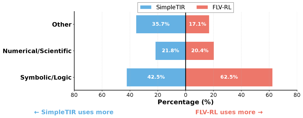
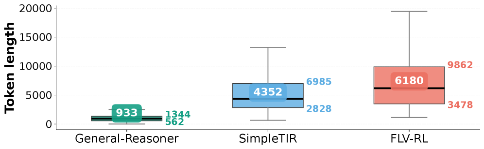
Figure 4: Python packages type distribution invoked by SimpleTIR (blue) vs. FLV-RL (red) across three domains.
Formal verification instills a shift from calculation to symbolic reasoning, enabling superior generalization. While tool-integrated baselines like SimpleTIR primarily utilize tools as “solvers” for direct computation (achieving 41.0 on AIME24), this paradigm struggles with tasks requiring rigorous logical deduction. In contrast, our FLV framework employs formal methods as a “verifier” to enforce logical consistency. This approach yields dominant performance on logic-heavy benchmarks such as KOR-Bench (51.0 vs. 37.0 for SimpleTIR) and GPQA-Diamond (35.4 vs. 28.8 for ZeroTIR). To understand the mechanism behind this reliability, we analyze the distribution of invoked Python packages in Figure 4. The data reveals a distinct behavioral shift: whereas SimpleTIR relies significantly on generic utility packages (Other), FLV-RL demonstrates a massive surge in the usage of Symbolic/Logic libraries. These formal tools constitute 62.5% of FLV-RL’s calls—a 20-point increase over SimpleTIR. Meanwhile, the usage of Numerical/Scientific libraries remains stable ( $\sim$ 21%), indicating that our method’s gains are driven specifically by the adoption of symbolic logic engines to verify reasoning processes, rather than merely computing numerical answers. See Appendix 9 for the package categorization principles.
<details>
<summary>x5.png Details</summary>
### Visual Description
## Box Plot: Token Length Comparison Across Three Models
### Overview
The image displays a box plot comparing the distribution of token lengths (in number of tokens) generated by three different models or systems: **General-Reasoner**, **SimpleTIR**, and **FLV-RL**. The chart visually summarizes the central tendency, spread, and range of token usage for each model.
### Components/Axes
* **Y-Axis:** Labeled **"Token length"**. The scale runs from 0 to 20,000, with major gridlines at intervals of 5,000 (0, 5000, 10000, 15000, 20000).
* **X-Axis:** Contains three categorical labels corresponding to the models being compared:
1. **General-Reasoner** (leftmost)
2. **SimpleTIR** (center)
3. **FLV-RL** (rightmost)
* **Legend/Data Labels:** The legend is integrated directly into each box plot, using color-coded text to display key statistical values. The colors match the fill of their respective boxes.
* **General-Reasoner (Teal):** Median = **933**, Upper Quartile (Q3) = **1344**, Lower Quartile (Q1) = **562**.
* **SimpleTIR (Light Blue):** Median = **4352**, Upper Quartile (Q3) = **6985**, Lower Quartile (Q1) = **2828**.
* **FLV-RL (Salmon):** Median = **6180**, Upper Quartile (Q3) = **9862**, Lower Quartile (Q1) = **3478**.
### Detailed Analysis
The plot consists of three vertical box-and-whisker plots, each representing the distribution of token lengths for one model.
1. **General-Reasoner (Teal Box, Left):**
* **Trend:** This model produces the shortest responses, with the most compact distribution.
* **Data Points:**
* **Median (line inside box):** 933 tokens.
* **Interquartile Range (IQR - the box):** Spans from 562 (Q1) to 1344 (Q3). The box height (IQR) is approximately 782 tokens.
* **Whiskers:** Extend from the box to the minimum and maximum values (excluding outliers). The lower whisker ends near 0. The upper whisker ends at approximately 2000 tokens (estimated visually, as no explicit label is given).
* **Spatial Grounding:** The teal box is positioned low on the y-axis, centered above the "General-Reasoner" label.
2. **SimpleTIR (Light Blue Box, Center):**
* **Trend:** Shows a moderate increase in both median token length and variability compared to General-Reasoner.
* **Data Points:**
* **Median:** 4352 tokens.
* **IQR:** Spans from 2828 (Q1) to 6985 (Q3). The IQR is approximately 4157 tokens.
* **Whiskers:** The lower whisker extends down to approximately 500 tokens. The upper whisker extends up to approximately 13,000 tokens (estimated visually).
* **Spatial Grounding:** The light blue box is positioned in the middle of the y-axis range, centered above the "SimpleTIR" label.
3. **FLV-RL (Salmon Box, Right):**
* **Trend:** This model has the highest median token length and the greatest spread (variability) in output length.
* **Data Points:**
* **Median:** 6180 tokens.
* **IQR:** Spans from 3478 (Q1) to 9862 (Q3). The IQR is approximately 6384 tokens, the largest of the three.
* **Whiskers:** The lower whisker extends down to approximately 1000 tokens. The upper whisker extends very high, to just below the 20,000 mark (estimated at ~19,500 tokens).
* **Spatial Grounding:** The salmon-colored box is positioned highest on the y-axis, centered above the "FLV-RL" label. Its upper whisker reaches the top region of the chart.
### Key Observations
1. **Clear Progression:** There is a distinct, stepwise increase in median token length from General-Reasoner (933) to SimpleTIR (4352) to FLV-RL (6180).
2. **Increasing Variability:** The spread of the data (IQR and whisker range) increases dramatically with each subsequent model. General-Reasoner's outputs are tightly clustered, while FLV-RL's outputs show extremely high variance, with some responses approaching 20,000 tokens.
3. **Overlap:** The IQR of SimpleTIR (2828-6985) significantly overlaps with the IQR of FLV-RL (3478-9862), indicating that while FLV-RL has a higher median, a substantial portion of its outputs are similar in length to those of SimpleTIR.
4. **Outlier Presence:** The long upper whisker on the FLV-RL plot suggests the presence of high-value outliers or a right-skewed distribution, meaning a small number of outputs are exceptionally long.
### Interpretation
This chart demonstrates a fundamental trade-off or characteristic difference between the three models. **General-Reasoner** appears optimized for **conciseness and efficiency**, producing short, predictable outputs. **SimpleTIR** represents a middle ground, generating moderately longer and more variable responses. **FLV-RL**, however, is characterized by **high verbosity and unpredictability**.
The data suggests that as the models potentially increase in complexity or capability (implied by the progression from "General" to "Simple" to "RL" in their names), they tend to generate significantly longer and more varied textual outputs. This could indicate:
* **Increased Reasoning Depth:** FLV-RL might be engaging in more extensive internal reasoning or exploration before producing a final answer.
* **Less Constraint:** The models may have different training objectives or constraints regarding response length.
* **Task Suitability:** General-Reasoner would be preferable for tasks requiring brevity (e.g., summarization, quick Q&A), while FLV-RL might be better suited for tasks requiring detailed explanation or complex problem-solving, albeit at a higher computational cost (due to token length).
The most critical takeaway is the **inverse relationship between output conciseness and variability** shown here: the model with the shortest median output is also the most consistent, while the model with the longest median output is the most erratic in its length.
</details>
Figure 5: Token length distribution comparison across General-Reasoner, SimpleTIR, and FLV-RL. The box plots illustrate the median token usage (center line) and interquartile ranges.
Efficiency Analysis. We analyze the computational cost of our approach by comparing the token length distributions of the natural language baseline (General-Reasoner), tool-integrated reasoning (SimpleTIR), and our FLV-RL method (Figure 5). While FLV-RL incurs a moderate computational overhead, we argue that this cost is justified by the substantial performance gains observed across diverse domains. The increased token consumption represents a necessary trade-off for achieving breakthrough generalization and ensuring logical soundness in high-stakes reasoning tasks.
### 5.3 Ablation Studies
To evaluate the individual contributions of our proposed components, we conducted an ablation study examining two critical dimensions: the impact of FLV versus pure natural language reasoning, and the effectiveness of different training paradigms. Results are presented in Table 2.
Impact of formal logic verification. Comparing FLV-based models against natural language baselines trained on identical data reveals substantial improvements. FLV-SFT achieves 49.8% average accuracy versus 36.5% for Natural-SFT, with particularly strong gains on logic-intensive tasks (KOR-Bench: +16.2 points, TheoremQA: +13.9 points). This demonstrates that formal proofs and execution validation fundamentally improve reasoning by grounding outputs in verifiable logic rather than probabilistic patterns.
Impact of multi-stage training We can observe that supervised fine-tuning establishes strong foundations, improving from 30.0% (Base) to 49.8% (FLV-SFT). Policy optimization yields further substantial gains to 51.9% (FLV-RL). Notably, natural language baselines barely improve with RL (37.0% vs 36.5%), while FLV-RL substantially outperforms FLV-SFT, indicating formal verification provides more stable and reliable reward signals for policy optimization.
### 5.4 Verification Paradigm: Balancing Formalism and Computational Fluency
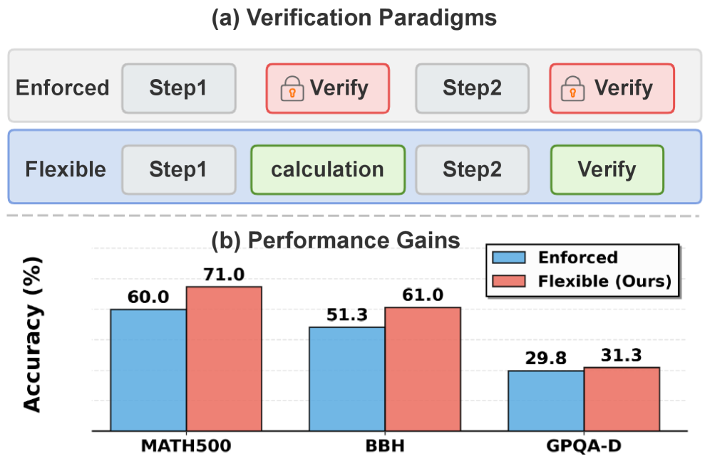
Our initial data construction enforced explicit verification outputs (e.g., proved / disproved) after each logical module. However, this rigid format introduced two critical issues: (i) formal language redundancy, and (ii) suppression of direct calculation. When computational verification was needed, models would bypass direct arithmetic in favor of indirect validation via z3-solver (e.g., asserting A + B == C is proved rather than computing the sum), significantly degrading mathematical performance. To address this, we adopted a flexible verification strategy that decouples calculation from validation: (i) Calculation as inference: Models invoke numerical tools directly during reasoning without mandatory verification keywords. (ii) Logic as validation: Formal verification serves as post-hoc validation rather than a per-step constraint. Figure 6 compares performance across logic, general, and math subsets under both paradigms. The flexible approach substantially improves math scores while preserving logical reasoning capability. Representative cases are detailed in Appendix E.
<details>
<summary>x6.png Details</summary>
### Visual Description
## Diagram and Bar Chart: Verification Paradigms and Performance Gains
### Overview
The image is a two-part technical figure comparing two verification paradigms ("Enforced" and "Flexible") and their performance across three benchmark datasets. Part (a) is a flowchart-style diagram illustrating the process flow of each paradigm. Part (b) is a grouped bar chart quantifying the accuracy gains achieved by the "Flexible" paradigm over the "Enforced" one.
### Components/Axes
**Part (a) - Verification Paradigms Diagram:**
* **Layout:** Two horizontal process flows, one above the other.
* **Top Flow (Enforced Paradigm):**
* Label: "Enforced" (leftmost).
* Sequence: A gray box labeled "Step1" → A red-bordered box with a lock icon and the text "Verify" → A gray box labeled "Step2" → A second red-bordered box with a lock icon and the text "Verify".
* **Bottom Flow (Flexible Paradigm):**
* Label: "Flexible" (leftmost).
* Sequence: A gray box labeled "Step1" → A green-bordered box labeled "calculation" → A gray box labeled "Step2" → A green-bordered box labeled "Verify".
* **Visual Cues:** The "Enforced" verification steps are highlighted in red with a lock icon, suggesting mandatory, rigid checks. The "Flexible" paradigm's "calculation" and "Verify" steps are highlighted in green, suggesting an adaptive or optional process.
**Part (b) - Performance Gains Bar Chart:**
* **Chart Type:** Grouped bar chart.
* **Y-Axis:** Labeled "Accuracy (%)". The scale is linear, with major gridlines visible at 0%, 20%, 40%, 60%, and 80%.
* **X-Axis:** Three categorical groups representing benchmark datasets: "MATH500", "BBH", and "GPQA-D".
* **Legend:** Located in the top-right corner of the chart area.
* Blue square: "Enforced"
* Red square: "Flexible (Ours)"
* **Data Series:** Two bars per x-axis category, corresponding to the legend.
### Detailed Analysis
**Diagram Flow (Part a):**
The core difference lies in the step between "Step1" and "Step2". The **Enforced** paradigm mandates a "Verify" step (with a lock) immediately after Step1. The **Flexible** paradigm replaces this with a "calculation" step, deferring the "Verify" step until after Step2.
**Chart Data Extraction (Part b):**
For each dataset, the accuracy values are explicitly labeled on top of the bars.
1. **MATH500:**
* Enforced (Blue Bar): 60.0%
* Flexible (Red Bar): 71.0%
* **Trend:** The red bar is significantly taller than the blue bar, indicating a substantial performance gain.
2. **BBH:**
* Enforced (Blue Bar): 51.3%
* Flexible (Red Bar): 61.0%
* **Trend:** The red bar is taller than the blue bar, showing a clear improvement.
3. **GPQA-D:**
* Enforced (Blue Bar): 29.8%
* Flexible (Red Bar): 31.3%
* **Trend:** The red bar is slightly taller than the blue bar, indicating a modest performance gain.
### Key Observations
1. **Consistent Superiority:** The "Flexible (Ours)" paradigm achieves higher accuracy than the "Enforced" paradigm across all three benchmark datasets (MATH500, BBH, GPQA-D).
2. **Magnitude of Gain:** The performance gain is not uniform. It is largest on MATH500 (+11.0 percentage points), moderate on BBH (+9.7 percentage points), and smallest on GPQA-D (+1.5 percentage points).
3. **Baseline Difficulty:** The absolute accuracy levels suggest the datasets vary in difficulty for these models, with GPQA-D being the most challenging (accuracies ~30%) and MATH500 the least challenging (accuracies 60-71%).
4. **Process Implication:** The diagram suggests the "Flexible" paradigm's advantage may stem from allowing a "calculation" phase between steps, rather than enforcing an immediate verification lock.
### Interpretation
This figure presents a compelling case for a "Flexible" verification approach in multi-step reasoning or problem-solving systems. The data demonstrates that relaxing the enforcement of verification after the first step (replacing it with a calculation phase) leads to measurable improvements in final accuracy across diverse tasks.
The correlation between the diagram and the chart is clear: the architectural change illustrated in (a) is the hypothesized cause for the performance gains quantified in (b). The varying gain magnitudes across datasets might indicate that the benefit of flexible verification is more pronounced on certain types of problems (e.g., those in MATH500) than others (e.g., GPQA-D). The consistent positive direction of the result, however, strongly supports the efficacy of the proposed "Flexible" method over the rigid "Enforced" baseline. The label "(Ours)" in the legend indicates this "Flexible" paradigm is the contribution of the work from which this figure is taken.
</details>
Figure 6: Enforced vs. Flexible Verification Paradigms. (a) Enforced verification imposes rigid checkpoints throughout the reasoning process, while flexible verification enables adaptive utilization of logic verification. (b) Performance gains after switching to flexible reasoning across three representative benchmarks.
## 6 Conclusion
In this work, we addressed the fundamental tension between probabilistic language generation and logical consistency in LLM reasoning by introducing a framework that dynamically integrates formal logic verification into the reasoning process. Through our two-stage training methodology combining FLV-SFT’s rigorous data synthesis pipeline with formal logic verification-guided policy optimization, we demonstrated that real-time symbolic feedback can effectively mitigate logical fallacies that plague standard Chain-of-Thought approaches. Empirical evaluation across six diverse benchmarks validates our approach, with our 7B and 14B models achieving average improvements of 10.4% and 14.2% respectively over SOTA baselines, while providing interpretable step-level correctness guarantees. Beyond performance gains, our framework establishes a principled foundation for trustworthy reasoning systems by bridging neural fluency with symbolic rigor, thereby enabling more robust logical inference. This opens pathways toward more reliable AI that scales effectively to complex real-world problems across domains requiring strict logical soundness.
## Impact Statement
This paper presents work whose goal is to advance the field of Machine Learning. There are many potential societal consequences of our work, none which we feel must be specifically highlighted here.
## References
- J. Ahn, R. Verma, R. Lou, D. Liu, R. Zhang, and W. Yin (2024) Large language models for mathematical reasoning: progresses and challenges. arXiv preprint arXiv:2402.00157. Cited by: §1.
- A. Anthropic (2024) Claude 3.5 sonnet model card addendum. Claude-3.5 Model Card. External Links: Link Cited by: §5.1.
- B. Baker, J. Huizinga, L. Gao, Z. Dou, M. Y. Guan, A. Madry, W. Zaremba, J. Pachocki, and D. Farhi (2025) Monitoring reasoning models for misbehavior and the risks of promoting obfuscation. arXiv preprint arXiv:2503.11926. Cited by: §1.
- C. Cao, M. Li, J. Dai, J. Yang, Z. Zhao, S. Zhang, W. Shi, C. Liu, S. Han, and Y. Guo (2025a) Towards advanced mathematical reasoning for llms via first-order logic theorem proving. arXiv preprint arXiv:2506.17104. Cited by: §2.2.
- C. Cao, H. Zhu, J. Ji, Q. Sun, Z. Zhu, Y. Wu, J. Dai, Y. Yang, S. Han, and Y. Guo (2025b) SafeLawBench: towards safe alignment of large language models. arXiv preprint arXiv:2506.06636. Cited by: §1.
- J. Chen, Q. He, S. Yuan, A. Chen, Z. Cai, W. Dai, H. Yu, Q. Yu, X. Li, J. Chen, et al. (2025a) Enigmata: scaling logical reasoning in large language models with synthetic verifiable puzzles. arXiv preprint arXiv:2505.19914. Cited by: §1.
- W. Chen, M. Yin, M. Ku, P. Lu, Y. Wan, X. Ma, J. Xu, X. Wang, and T. Xia (2023) Theoremqa: a theorem-driven question answering dataset. arXiv preprint arXiv:2305.12524. Cited by: 3rd item.
- Y. Chen, J. Benton, A. Radhakrishnan, J. Uesato, C. Denison, J. Schulman, A. Somani, P. Hase, M. Wagner, F. Roger, et al. (2025b) Reasoning models don’t always say what they think. arXiv preprint arXiv:2505.05410. Cited by: §1.
- Z. Chen, J. Yang, T. Xiao, R. Zhou, L. Zhang, X. Xi, X. Shi, W. Wang, and J. Wang (2025c) Reinforcement learning for tool-integrated interleaved thinking towards cross-domain generalization. arXiv preprint arXiv:2510.11184. Cited by: §2.1.
- K. Cobbe, V. Kosaraju, M. Bavarian, M. Chen, H. Jun, L. Kaiser, M. Plappert, J. Tworek, J. Hilton, R. Nakano, et al. (2021) Training verifiers to solve math word problems. arXiv preprint arXiv:2110.14168. Cited by: §2.1.
- O. Contributors (2023) OpenCompass: a universal evaluation platform for foundation models. Note: https://github.com/open-compass/opencompass Cited by: §5.1.
- J. Feng, S. Huang, X. Qu, G. Zhang, Y. Qin, B. Zhong, C. Jiang, J. Chi, and W. Zhong (2025a) Retool: reinforcement learning for strategic tool use in llms. arXiv preprint arXiv:2504.11536. Cited by: §2.1, §2.2.
- Y. Feng, N. Weir, K. Bostrom, S. Bayless, D. Cassel, S. Chaudhary, B. Kiesl-Reiter, and H. Rangwala (2025b) VeriCoT: neuro-symbolic chain-of-thought validation via logical consistency checks. arXiv preprint arXiv:2511.04662. Cited by: §1, §2.2.
- D. Guo, D. Yang, H. Zhang, J. Song, R. Zhang, R. Xu, Q. Zhu, S. Ma, P. Wang, X. Bi, et al. (2025a) Deepseek-r1: incentivizing reasoning capability in llms via reinforcement learning. arXiv preprint arXiv:2501.12948. Cited by: §5.1.
- J. Guo, Z. Chi, L. Dong, Q. Dong, X. Wu, S. Huang, and F. Wei (2025b) Reward reasoning model. arXiv preprint arXiv:2505.14674. Cited by: §1.
- D. Hendrycks, C. Burns, S. Kadavath, A. Arora, S. Basart, E. Tang, D. Song, and J. Steinhardt (2021) Measuring mathematical problem solving with the MATH dataset. In Thirty-fifth Conference on Neural Information Processing Systems Datasets and Benchmarks Track (Round 2), External Links: Link Cited by: §2.1.
- D. Hendrycks, C. Burns, S. Kadavath, A. Arora, S. Basart, E. Tang, D. Song, and J. Steinhardt (2024) Measuring mathematical problem solving with the math dataset, 2021. URL https://arxiv. org/abs/2103.03874 2. Cited by: 2nd item.
- J. Hu, J. Zhang, Y. Zhao, and T. Ringer (2025) HybridProver: augmenting theorem proving with llm-driven proof synthesis and refinement. arXiv preprint arXiv:2505.15740. Cited by: §2.2.
- A. Hurst, A. Lerer, A. P. Goucher, A. Perelman, A. Ramesh, A. Clark, A. Ostrow, A. Welihinda, A. Hayes, A. Radford, et al. (2024) Gpt-4o system card. arXiv preprint arXiv:2410.21276. Cited by: §5.1.
- Y. Ji, X. Tian, S. Zhao, H. Wang, S. Chen, Y. Peng, H. Zhao, and X. Li (2025) AM-thinking-v1: advancing the frontier of reasoning at 32b scale. arXiv preprint arXiv:2505.08311. Cited by: §1.
- R. Kamoi, Y. Zhang, N. Zhang, S. S. S. Das, and R. Zhang (2025) Training step-level reasoning verifiers with formal verification tools. arXiv preprint arXiv:2505.15960. Cited by: §1, §2.2.
- M. Khalifa, R. Agarwal, L. Logeswaran, J. Kim, H. Peng, M. Lee, H. Lee, and L. Wang (2025) Process reward models that think. arXiv preprint arXiv:2504.16828. Cited by: §2.1.
- H. Le, Y. Wang, A. D. Gotmare, S. Savarese, and S. C. H. Hoi (2022) Coderl: mastering code generation through pretrained models and deep reinforcement learning. Advances in Neural Information Processing Systems 35, pp. 21314–21328. Cited by: §2.1.
- J. O. J. Leang, G. Hong, W. Li, and S. B. Cohen (2025) Theorem prover as a judge for synthetic data generation. arXiv preprint arXiv:2502.13137. Cited by: §1.
- C. Li, Z. Tang, Z. Li, M. Xue, K. Bao, T. Ding, R. Sun, B. Wang, X. Wang, J. Lin, et al. (2025a) CoRT: code-integrated reasoning within thinking. arXiv preprint arXiv:2506.09820. Cited by: §2.2.
- J. LI, E. Beeching, L. Tunstall, B. Lipkin, R. Soletskyi, S. C. Huang, K. Rasul, L. Yu, A. Jiang, Z. Shen, Z. Qin, B. Dong, L. Zhou, Y. Fleureau, G. Lample, and S. Polu (2024) NuminaMath. Numina. Note: [https://huggingface.co/AI-MO/NuminaMath-CoT](https://github.com/project-numina/aimo-progress-prize/blob/main/report/numina_dataset.pdf) Cited by: §2.1, §5.1.
- J. Li and H. T. Ng (2025) The hallucination dilemma: factuality-aware reinforcement learning for large reasoning models. arXiv preprint arXiv:2505.24630. Cited by: §1, §2.2.
- X. Li, H. Zou, and P. Liu (2025b) ToRL: scaling tool-integrated rl. External Links: 2503.23383, Link Cited by: §2.2, §5.1.
- H. Lightman, V. Kosaraju, Y. Burda, H. Edwards, B. Baker, T. Lee, J. Leike, J. Schulman, I. Sutskever, and K. Cobbe (2023) Let’s verify step by step. In The Twelfth International Conference on Learning Representations, Cited by: §2.1, §2.2.
- C. Liu, Y. Yuan, Y. Yin, Y. Xu, X. Xu, Z. Chen, Y. Wang, L. Shang, Q. Liu, and M. Zhang (2025a) Safe: enhancing mathematical reasoning in large language models via retrospective step-aware formal verification. arXiv preprint arXiv:2506.04592. Cited by: §1, §2.2.
- J. Liu, Y. Fan, Z. Jiang, H. Ding, Y. Hu, C. Zhang, Y. Shi, S. Weng, A. Chen, S. Chen, et al. (2025b) SynLogic: synthesizing verifiable reasoning data at scale for learning logical reasoning and beyond. arXiv preprint arXiv:2505.19641. Cited by: §1, §5.1.
- S. Liu, H. Liu, J. Liu, L. Xiao, S. Gao, C. Lyu, Y. Gu, W. Zhang, D. F. Wong, S. Zhang, et al. (2025c) Compassverifier: a unified and robust verifier for llms evaluation and outcome reward. In Proceedings of the 2025 Conference on Empirical Methods in Natural Language Processing, pp. 33454–33482. Cited by: §1.
- K. Ma, X. Du, Y. Wang, H. Zhang, Z. Wen, X. Qu, J. Yang, J. Liu, M. Liu, X. Yue, W. Huang, and G. Zhang (2024) KOR-bench: benchmarking language models on knowledge-orthogonal reasoning tasks. External Links: 2410.06526, Link Cited by: 1st item.
- X. Ma, Q. Liu, D. Jiang, G. Zhang, Z. Ma, and W. Chen (2025) General-reasoner: advancing llm reasoning across all domains. arXiv preprint arXiv:2505.14652. Cited by: Appendix C, §1, §2.1, §5.1, §5.1.
- X. Mai, H. Xu, W. Wang, Y. Zhang, W. Zhang, et al. (2025) Agentic rl scaling law: spontaneous code execution for mathematical problem solving. In The Thirty-ninth Annual Conference on Neural Information Processing Systems, Cited by: §5.1.
- A. Ospanov, Z. Feng, J. Sun, H. Bai, X. Shen, and F. Farnia (2025) HERMES: towards efficient and verifiable mathematical reasoning in llms. arXiv preprint arXiv:2511.18760. Cited by: §1, §2.2.
- Qwen-Team (2025) Qwen2.5 technical report. External Links: 2412.15115, Link Cited by: §5.1, §5.1.
- D. Rein, B. L. Hou, A. C. Stickland, J. Petty, R. Y. Pang, J. Dirani, J. Michael, and S. R. Bowman (2024) Gpqa: a graduate-level google-proof q&a benchmark. In First Conference on Language Modeling, Cited by: 3rd item.
- Z. Ren, Z. Shao, J. Song, H. Xin, H. Wang, W. Zhao, L. Zhang, Z. Fu, Q. Zhu, D. Yang, et al. (2025) Deepseek-prover-v2: advancing formal mathematical reasoning via reinforcement learning for subgoal decomposition. arXiv preprint arXiv:2504.21801. Cited by: §2.2.
- S. She, J. Liu, Y. Liu, J. Chen, X. Huang, and S. Huang (2025) R-prm: reasoning-driven process reward modeling. arXiv preprint arXiv:2503.21295. Cited by: §2.1.
- G. Sheng, C. Zhang, Z. Ye, X. Wu, W. Zhang, R. Zhang, Y. Peng, H. Lin, and C. Wu (2025a) Hybridflow: a flexible and efficient rlhf framework. In Proceedings of the Twentieth European Conference on Computer Systems, pp. 1279–1297. Cited by: §5.1.
- J. Sheng, L. Lyu, J. Jin, T. Xia, A. Gu, J. Zou, and P. Lu (2025b) Solving inequality proofs with large language models. arXiv preprint arXiv:2506.07927. Cited by: §1, §1.
- J. Skalse, N. Howe, D. Krasheninnikov, and D. Krueger (2022) Defining and characterizing reward gaming. Advances in Neural Information Processing Systems 35, pp. 9460–9471. Cited by: §1, §2.1.
- M. Suzgun, N. Scales, N. Schärli, S. Gehrmann, Y. Tay, H. W. Chung, A. Chowdhery, Q. Le, E. Chi, D. Zhou, et al. (2023) Challenging big-bench tasks and whether chain-of-thought can solve them. In Findings of the Association for Computational Linguistics: ACL 2023, pp. 13003–13051. Cited by: 1st item.
- Y. Tian, R. Huang, X. Wang, J. Ma, Z. Huang, Z. Luo, H. Lin, D. Zheng, and L. Du (2025) EvolProver: advancing automated theorem proving by evolving formalized problems via symmetry and difficulty. arXiv preprint arXiv:2510.00732. Cited by: §2.2.
- J. Uesato, N. Kushman, R. Kumar, F. Song, N. Siegel, L. Wang, A. Creswell, G. Irving, and I. Higgins (2022) Solving math word problems with process-and outcome-based feedback. arXiv preprint arXiv:2211.14275. Cited by: §2.1, §2.2.
- H. Wang, M. Unsal, X. Lin, M. Baksys, J. Liu, M. D. Santos, F. Sung, M. Vinyes, Z. Ying, Z. Zhu, et al. (2025) Kimina-prover preview: towards large formal reasoning models with reinforcement learning. arXiv preprint arXiv:2504.11354. Cited by: §2.2.
- Y. Wang, S. Mishra, P. Alipoormolabashi, Y. Kordi, A. Mirzaei, A. Arunkumar, A. Ashok, A. S. Dhanasekaran, A. Naik, D. Stap, et al. (2022) Super-naturalinstructions: generalization via declarative instructions on 1600+ nlp tasks. arXiv preprint arXiv:2204.07705. Cited by: §2.1.
- J. Wei, X. Wang, D. Schuurmans, M. Bosma, F. Xia, E. Chi, Q. V. Le, D. Zhou, et al. (2022) Chain-of-thought prompting elicits reasoning in large language models. Advances in neural information processing systems 35, pp. 24824–24837. Cited by: §2.1.
- C. Xie, Y. Huang, C. Zhang, D. Yu, X. Chen, B. Y. Lin, B. Li, B. Ghazi, and R. Kumar (2024) On memorization of large language models in logical reasoning. External Links: 2410.23123, Link Cited by: §5.1.
- Z. Xu, Y. Liu, Y. Yin, M. Zhou, and R. Poovendran (2025) Kodcode: a diverse, challenging, and verifiable synthetic dataset for coding. arXiv preprint arXiv:2503.02951. Cited by: §2.1.
- Z. Xue, L. Zheng, Q. Liu, Y. Li, X. Zheng, Z. Ma, and B. An (2025) Simpletir: end-to-end reinforcement learning for multi-turn tool-integrated reasoning. arXiv preprint arXiv:2509.02479. Cited by: §2.2, §5.1.
- K. Yang, A. Swope, A. Gu, R. Chalamala, P. Song, S. Yu, S. Godil, R. J. Prenger, and A. Anandkumar (2023) Leandojo: theorem proving with retrieval-augmented language models. Advances in Neural Information Processing Systems 36, pp. 21573–21612. Cited by: §2.2.
- T. Yu, B. Ji, S. Wang, S. Yao, Z. Wang, G. Cui, L. Yuan, N. Ding, Y. Yao, Z. Liu, et al. (2025) RLPR: extrapolating rlvr to general domains without verifiers. arXiv preprint arXiv:2506.18254. Cited by: §5.1, §5.1.
- S. Zeng (2026) External Links: Link Cited by: Appendix G.
- W. Zeng, Y. Huang, Q. Liu, W. Liu, K. He, Z. Ma, and J. He (2025) Simplerl-zoo: investigating and taming zero reinforcement learning for open base models in the wild. arXiv preprint arXiv:2503.18892. Cited by: §2.1, §2.2, §5.1.
- L. Zheng, W. Chiang, Y. Sheng, S. Zhuang, Z. Wu, Y. Zhuang, Z. Lin, Z. Li, D. Li, E. Xing, et al. (2023) Judging llm-as-a-judge with mt-bench and chatbot arena. Advances in neural information processing systems 36, pp. 46595–46623. Cited by: §2.1.
- K. Zhou, C. Liu, X. Zhao, S. Jangam, J. Srinivasa, G. Liu, D. Song, and X. E. Wang (2025) The hidden risks of large reasoning models: a safety assessment of r1. arXiv preprint arXiv:2502.12659. Cited by: §1.
- Y. Zhou, C. Cao, J. Yang, L. Wu, C. He, S. Han, and Y. Guo (2026) LRAS: advanced legal reasoning with agentic search. arXiv preprint arXiv:2601.07296. Cited by: §2.1.
## Limitations
Despite significant improvements in logical reasoning capabilities, our framework faces two primary limitations. First, integrating real-time formal verification introduces computational overhead, increasing RL training time by approximately 2× compared to standard baselines. However, this cost is acceptable given the substantial performance gains (10.4%-14.2% improvement) and superior data efficiency—we achieve comparable results using only a fraction of the training data required by existing methods, such that reduced data collection costs offset the increased training time. Second, our data synthesis pipeline faces formalization challenges when translating natural language into verifiable formal representations. While conversion success rates are high in structured domains like mathematics and logic, ambiguous or commonsense-heavy descriptions may produce mapping errors that generate incorrect verification feedback, limiting generalizability to open-ended reasoning tasks and highlighting the need for more robust auto-formalization techniques.
## Appendix A Reward Calculation Pseudocode
Table 3: Hierarchical reward function for formal logic verification-guided policy optimization
| Input: Output $y$ , Ground truth answer $a^{*}$ , Predicted answer $\hat{a}$ |
| --- |
| Output: Total reward $R(y)$ |
| Hyperparameters: |
| $W=3$ (correctness weight) |
| $\gamma_{\text{struct}}=3.0$ , $\beta_{\text{struct}}=1.0$ (severity penalties) |
| $\alpha=1.0$ (base structural score) |
| $\lambda_{\text{tag}}=0.005$ , $\tau_{\text{tag}}=200$ (tag penalty coefficients) |
| $\lambda_{\text{call}}=0.5$ , $N_{\text{max}}=3$ (tool call limits) |
| $\lambda_{\text{len}}=0.04$ , $\delta_{\text{max}}=10$ (length penalty) |
| Step 1: Check Fatal Errors ( $\mathbb{C}_{\text{fatal}}$ ) |
| if token-level repetition detected or |
| execution timeout or |
| tool calls $>2\times N_{\text{max}}$ or |
| multiple termination tags then |
| return $R(y)=-\gamma_{\text{struct}}-W=-8.0$ |
| Step 2: Check Invalid Format ( $\mathbb{C}_{\text{invalid}}\setminus\mathbb{C}_{\text{fatal}}$ ) |
| if solution extraction fails or |
| solution length $>512$ tokens or |
| missing closing tag or |
| $N_{\text{max}}<$ tool calls $\leq 2\times N_{\text{max}}$ then |
| return $R(y)=-\beta_{\text{struct}}-W=-6.0$ |
| Step 3: Compute Structural Reward $R_{\text{struct}}(y)$ |
| $N_{\text{undef}}=$ count of undefined tags |
| $N_{\text{call}}=$ count of tool invocations |
| $R_{\text{struct}}(y)=\alpha-\lambda_{\text{tag}}\cdot\min(N_{\text{undef}},\tau_{\text{tag}})$ |
| $-\lambda_{\text{call}}\cdot\max(N_{\text{call}}-N_{\text{max}},0)$ |
| Step 4: Compute Correctness Reward $R_{\text{correct}}(y)$ |
| $f_{\text{len}}(\hat{a},a^{*})=\min(|\text{len}(\hat{a})-\text{len}(a^{*})|,\delta_{\text{max}})$ |
| if $\hat{a}$ matches $a^{*}$ then |
| $R_{\text{correct}}(y)=W-\lambda_{\text{len}}\cdot f_{\text{len}}(\hat{a},a^{*})$ |
| else |
| $R_{\text{correct}}(y)=-W$ |
| Step 5: Compute Total Reward |
| $R(y)=R_{\text{struct}}(y)+R_{\text{correct}}(y)$ |
Table 3 provides the complete algorithmic implementation of our multi-component reward function used in FLV-RL training. The pseudocode details the step-by-step computation of format rewards, correctness rewards, and formal verification rewards, including all constraint checks and penalty mechanisms described in Section 4.
The time complexity for calculating the reward $R(y)$ is dominated by the verification of structural constraints and semantic correctness. Let $L$ denote the length of the generated response $y$ in tokens. The initial screening for pathological states ( $\mathbb{C}_{\text{fatal}}$ ) and invalid formats ( $\mathbb{C}_{\text{invalid}}$ ) requires a linear scan of the output tokens to detect repetition loops, count tool invocations ( $N_{\text{call}}$ ), and validate tags, resulting in $O(L)$ complexity. If the response is valid, computing $R_{\text{struct}}(y)$ involves constant-time arithmetic operations after the initial scan. The semantic verification $R_{\text{correct}}(y)$ depends on the evaluation metric; assuming string matching or metric comparison between the extracted answer $\hat{a}$ and ground truth $a^{*}$ , this step operates in $O(|\hat{a}|+|a^{*}|)$ . Therefore, the total time complexity per generation is $O(L)$ , ensuring the reward calculation remains efficient and does not introduce significant computational overhead during training.
## Appendix B Dataset Construction Details
Our data construction pipeline systematically processes a reasoning question through multiple stages of generation, logic extraction, formal translation, and verification to create high-quality training data for supervised fine-tuning. The resulting dataset combines natural language reasoning with formally verified logical modules, enabling our models to learn both human-readable reasoning patterns and mathematically sound logical validation.
Table 4 presents a comprehensive analysis of the execution-based validation outcomes across our merged dataset of 9,162 reasoning chains (a subset of of full training data). The match rate distribution reveals that a substantial majority (59.55%) of the generated formal proofs achieve perfect alignment with expected outputs ( $v_{k}^{\text{act}}=v_{k}^{\text{exp}}$ ), successfully passing Stage 1 validation without requiring further verification. An additional 26.53% of proofs fall within the high-confidence range (95–100% match rate), indicating strong but imperfect alignment that necessitates semantic equivalence checking in Stage 2.
Notably, 40.45% of the dataset exhibits match rates below 100%, triggering our multi-stage validation pipeline. Among these cases, the consistency distribution (lower panel) demonstrates that 62.22% (2,306 instances) maintain semantic equivalence despite surface-level discrepancies—successfully recovering through Stage 2 verification or Stage 3 proof rewriting. The remaining 37.78% (1,400 instances) represent fundamental misalignments that are discarded from the training corpus. This stratified validation approach ensures that our final dataset preserves both syntactic precision and semantic coherence, with approximately 85.7% overall retention rate ( $=59.55\$ ) after rigorous quality control.
The distribution pattern further reveals that only 0.83% of proofs exhibit critically low match rates (below 60%), suggesting that the initial CoT generation process produces predominantly high-quality candidates. This validates our teacher model’s effectiveness while highlighting the necessity of execution-based verification to capture subtle logical inconsistencies that may elude purely language-based evaluation.
Table 4: Match rate and consistency analysis.
| Match Rate Range (%) 0–20 20–40 | Count 1 11 | Percentage (%) 0.01 0.12 |
| --- | --- | --- |
| 40–60 | 64 | 0.70 |
| 60–70 | 63 | 0.69 |
| 70–80 | 168 | 1.83 |
| 80–85 | 149 | 1.63 |
| 85–90 | 269 | 2.94 |
| 90–95 | 551 | 6.01 |
| 95–99 | 1,402 | 15.30 |
| 99–100 (excl.) | 1,028 | 11.22 |
| 100 | 5,456 | 59.55 |
| Total | 9,162 | 100.00 |
| Consistency Distribution (when match_rate $\neq$ 100%) | | |
| Consistent | Count | Percentage (%) |
| No | 1,400 | 37.78 |
| Yes | 2,306 | 62.22 |
| Total | 3,706 | 100.00 |
<details>
<summary>x7.png Details</summary>
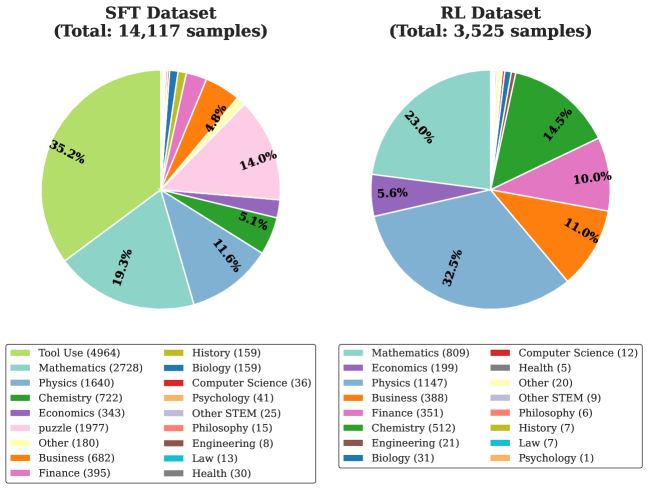
### Visual Description
\n
## Pie Charts: SFT Dataset and RL Dataset Distribution
### Overview
The image displays two pie charts side-by-side, each illustrating the distribution of categories within a different dataset. The left chart represents the "SFT Dataset" containing 14,117 total samples, and the right chart represents the "RL Dataset" containing 3,525 total samples. Each chart is accompanied by a detailed, two-column legend directly below it, listing all categories with their corresponding sample counts.
### Components/Axes
* **Chart Titles:**
* Left: "SFT Dataset (Total: 14,117 samples)"
* Right: "RL Dataset (Total: 3,525 samples)"
* **Chart Type:** Pie charts showing proportional distribution.
* **Legends:** Positioned directly below each respective chart. Each legend is a box containing two columns of entries. Each entry consists of a colored square swatch, a category name, and the sample count for that category in parentheses.
* **Data Representation:** Each slice of the pie corresponds to a category. The percentage of the total dataset is labeled on or near the larger slices. The color of each slice matches the swatch in its corresponding legend.
### Detailed Analysis
#### **SFT Dataset (Left Chart)**
* **Total Samples:** 14,117
* **Category Distribution (from largest to smallest slice, clockwise from top):**
1. **Tool Use:** Light green slice, 35.2% (4964 samples). Largest segment.
2. **Mathematics:** Teal slice, 19.3% (2728 samples).
3. **Physics:** Blue slice, 11.6% (1640 samples).
4. **Chemistry:** Dark green slice, 5.1% (722 samples).
5. **Economics:** Purple slice, 2.4% (343 samples).
6. **puzzle:** Pink slice, 14.0% (1977 samples). *Note: Category name is lowercase in the legend.*
7. **Other:** Light yellow slice, 1.3% (180 samples).
8. **Business:** Orange slice, 4.8% (682 samples).
9. **Finance:** Magenta slice, 2.8% (395 samples).
10. **History:** Olive green slice, 1.1% (159 samples).
11. **Biology:** Dark olive slice, 1.1% (159 samples).
12. **Computer Science:** Red slice, 0.3% (36 samples).
13. **Psychology:** Light orange slice, 0.3% (41 samples).
14. **Other STEM:** Light purple slice, 0.2% (25 samples).
15. **Philosophy:** Light pink slice, 0.1% (15 samples).
16. **Engineering:** Brown slice, 0.1% (8 samples).
17. **Law:** Cyan slice, 0.1% (13 samples).
18. **Health:** Grey slice, 0.2% (30 samples).
#### **RL Dataset (Right Chart)**
* **Total Samples:** 3,525
* **Category Distribution (from largest to smallest slice, clockwise from top):**
1. **Physics:** Blue slice, 32.3% (1147 samples). Largest segment.
2. **Mathematics:** Teal slice, 23.0% (809 samples).
3. **Economics:** Purple slice, 5.6% (199 samples).
4. **Business:** Orange slice, 11.0% (388 samples).
5. **Finance:** Magenta slice, 10.0% (351 samples).
6. **Chemistry:** Dark green slice, 14.5% (512 samples).
7. **Biology:** Dark olive slice, 0.9% (31 samples).
8. **Engineering:** Brown slice, 0.6% (21 samples).
9. **Computer Science:** Red slice, 0.3% (12 samples).
10. **Health:** Grey slice, 0.1% (5 samples).
11. **Other:** Light yellow slice, 0.6% (20 samples).
12. **Other STEM:** Light purple slice, 0.3% (9 samples).
13. **Philosophy:** Light pink slice, 0.2% (6 samples).
14. **History:** Olive green slice, 0.2% (7 samples).
15. **Law:** Cyan slice, 0.2% (7 samples).
16. **Psychology:** Light orange slice, 0.03% (1 sample).
* **Note:** The "Tool Use" and "puzzle" categories present in the SFT dataset are absent from the RL dataset legend and chart.
### Key Observations
1. **Dominant Categories:** Each dataset is dominated by one category: "Tool Use" (35.2%) in SFT and "Physics" (32.3%) in RL.
2. **Size Disparity:** The SFT dataset is approximately four times larger in total samples (14,117 vs. 3,525) than the RL dataset.
3. **Category Overlap & Shift:** While both datasets share many STEM and social science categories, their proportions differ significantly. "Mathematics" is the second-largest in both. "Physics" jumps from 3rd (11.6%) in SFT to 1st (32.3%) in RL. "Chemistry" increases from 5.1% to 14.5%.
4. **Unique Categories:** The SFT dataset contains two large, unique categories not found in the RL dataset: "Tool Use" (35.2%) and "puzzle" (14.0%). Their combined share (49.2%) constitutes nearly half of the SFT data.
5. **Long Tail:** Both datasets have a long tail of categories with very small percentages (often below 1%), indicating a wide variety of less-represented topics.
### Interpretation
The data suggests these datasets are curated for different phases or objectives in AI model training.
* **SFT Dataset (Supervised Fine-Tuning):** The massive representation of "Tool Use" and "puzzle" indicates a strong emphasis on training models to perform specific tasks, follow instructions, and solve structured problems. The broader distribution across many categories (including humanities like Philosophy and Law) suggests a goal of building generalist capabilities and diverse knowledge.
* **RL Dataset (Reinforcement Learning):** The shift towards heavy STEM subjects—Physics, Mathematics, and Chemistry now comprising ~70% of the data—implies a focus on training for reasoning, logical deduction, and problem-solving within well-defined, often quantitative domains. The near absence of "Tool Use" and "puzzle" suggests this phase is less about task execution and more about refining reasoning skills in core scientific disciplines.
The stark contrast in composition implies a pipeline: first, expose a model to a wide array of tasks and knowledge (SFT), then specialize and sharpen its reasoning abilities on challenging, structured academic subjects (RL). The RL dataset's smaller size is consistent with reinforcement learning often being applied to more focused, high-quality data after initial broad training.
</details>
Figure 7: Distribution of data categories in training Sets. Left: the categorical breakdown of the SFT dataset, totally 14,117 sample. Right: the categorical breakdown of the RL dataset. Legends list the exact number of samples for each category, totally 3,525 sample.
## Appendix C Hyperparameter Specification
We carefully calibrate the reward function hyperparameters to balance the learning of hybrid reasoning patterns with answer correctness, while preventing pathological behaviors during training.
Correctness vs. Format Balance. We set the correctness weight $W=3$ and base structural score $\alpha=1.0$ to ensure the model balances learning the hybrid reasoning paradigm with exploring correct answers under this new framework. This 3:1 ratio encourages the model to prioritize semantic accuracy while maintaining proper integration of natural language and formal verification components.
Fatal Error Prevention. Given the complexity of hybrid reasoning, models in early training stages are prone to generating pathological outputs such as repetitive tokens or malformed structures. We therefore define such cases as fatal errors with the maximum penalty $\gamma_{\text{struct}}=3.0$ , while setting $\beta_{\text{struct}}=1.0$ for invalid but recoverable format violations. This hierarchical penalty structure strongly discourages catastrophic failures while allowing the model to explore within reasonable boundaries.
Tag Usage Regulation. In hybrid reasoning, the model must learn our defined tag vocabulary (e.g., <code>, <interpreter>). During training, the model may explore alternative tags, which we discourage through $\lambda_{\text{tag}}=0.005$ with a cap at $\tau_{\text{tag}}=200$ . This cap prevents tag-related penalties from overwhelming correctness rewards, ensuring balanced learning of both answer accuracy and proper tag usage.
Formal Verification Efficiency. Our data synthesis analysis reveals that most problems can be solved within 4 formal verification steps. To optimize inference efficiency and reduce unnecessary formalization, we set $N_{\text{max}}=3$ as the baseline limit with penalty coefficient $\lambda_{\text{call}}=0.5$ . Responses exceeding this threshold incur incremental penalties, while those exceeding $2\times N_{\text{max}}=6$ calls are classified as fatal errors, strongly discouraging excessive tool invocations.
Length Control. Following prior work on general reasoners (Ma et al., 2025), we apply length-based penalties to discourage excessively verbose generations. We set $\lambda_{\text{len}}=0.04$ with a maximum cap $\delta_{\text{max}}=10$ , and enforce a hard limit of 512 tokens for extracted solutions. This encourages concise, focused reasoning without sacrificing completeness.
Model-Based Verifier. Manual review reveals that diverse domain problems beyond mathematics cannot be verified through rule-based methods. We therefore employ a model-based verifier. Empirical evaluation shows that CompassVerifier-7B achieves an optimal balance between accuracy and efficiency, leading to its selection as our verifier.
## Appendix D Training Dynamics and Behavior Analysis
We analyze key training dynamics across 120 optimization steps in Figure 8.
Reward Evolution. Figure 8(a) shows steady improvement from -0.45 to -0.1, indicating consistent progress in our composite reward function balancing structural integrity, semantic correctness, and efficiency.
Response Length. Figure 8(b) exhibits a U-shaped pattern: initial decrease from 3100 to 2850 tokens as the model eliminates redundancy, followed by stabilization around 3100-3200 tokens, reflecting an optimal balance between completeness and conciseness.
Formal Logic Verification Efficiency. Figure 8(c) demonstrates rapid improvement from 2.3 to 1.9 in the first 40 steps, then gradual stabilization. This shows the model learns to generate more efficiently verifiable proofs with fewer symbolic interpreter calls.
<details>
<summary>x8.png Details</summary>
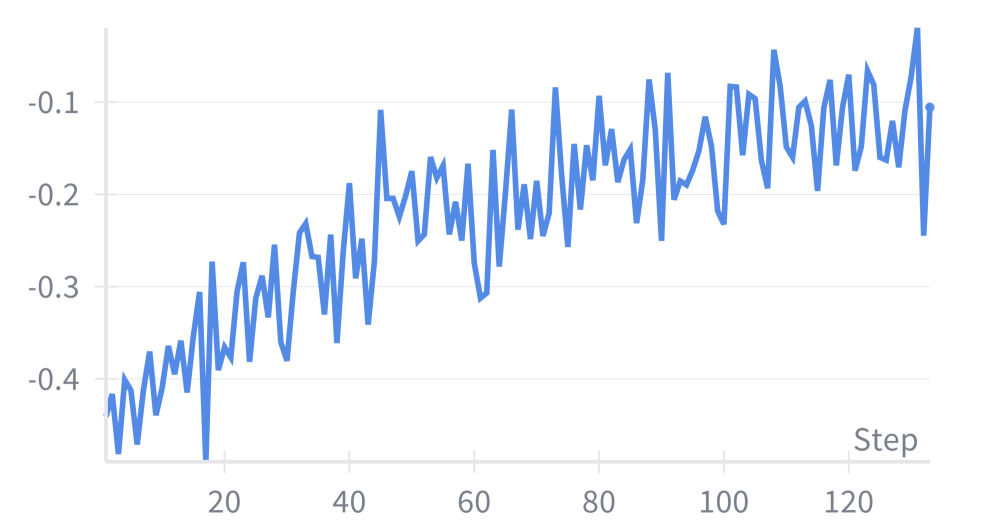
### Visual Description
\n
## Line Chart: Unlabeled Time Series or Process Metric
### Overview
The image displays a single-series line chart plotting a negative numerical value against a sequential "Step" axis. The chart shows a clear, albeit volatile, upward trend over approximately 130 steps. The visual style is simple, with a blue line on a white background with light gray grid lines.
### Components/Axes
* **Chart Type:** Single line chart.
* **X-Axis (Horizontal):**
* **Label:** "Step" (located at the bottom-right of the axis).
* **Scale:** Linear, from approximately 0 to 130.
* **Major Tick Marks:** Labeled at intervals of 20: 20, 40, 60, 80, 100, 120.
* **Y-Axis (Vertical):**
* **Label:** None visible.
* **Scale:** Linear, negative values.
* **Major Tick Marks:** Labeled at -0.4, -0.3, -0.2, -0.1.
* **Data Series:**
* **Representation:** A single, continuous blue line.
* **Legend:** None present.
* **Other Elements:** Light gray horizontal grid lines corresponding to the y-axis tick marks. No chart title is present.
### Detailed Analysis
* **Trend Verification:** The blue line exhibits a strong positive (upward) slope from left to right, indicating the measured value increases (becomes less negative) as the step count increases. The trend is accompanied by high-frequency volatility or noise.
* **Data Point Approximation (Key Points):**
* **Start (Step ~0):** The line begins at its lowest point, approximately **-0.45**.
* **Step ~20:** The value fluctuates around **-0.35 to -0.25**.
* **Step ~60:** The value fluctuates around **-0.25 to -0.15**.
* **Step ~100:** The value fluctuates around **-0.20 to -0.10**.
* **End (Step ~130):** The line ends near its highest point, approximately **-0.10**.
* **Volatility:** The line is highly jagged, with frequent sharp peaks and troughs. The amplitude of these fluctuations appears relatively consistent throughout the chart, spanning roughly 0.1 to 0.15 units on the y-axis between local highs and lows.
### Key Observations
1. **Consistent Upward Trajectory:** Despite significant noise, the underlying trend is unmistakably positive. The value improves by approximately 0.35 units over 130 steps.
2. **High Noise/Volatility:** The process being measured is not smooth. Each step shows considerable variation from the previous one, suggesting an unstable or stochastic process.
3. **Negative Values:** All data points are negative, indicating the metric is measuring something like a loss, error, or deficit that is being reduced over time.
4. **Absence of Context:** The chart lacks a title, y-axis label, and legend. This makes it impossible to know what specific metric is being tracked (e.g., loss function, error rate, profit/loss).
### Interpretation
This chart likely visualizes the performance of an iterative process, such as a machine learning model's training loss, an optimization algorithm's error, or a financial trading strategy's drawdown. The **upward trend** signifies improvement or convergence—the system is getting better at its task as it progresses through more steps. The **high volatility** is a critical characteristic; it suggests the improvement path is noisy, which could be due to factors like a high learning rate, stochastic batch processing, or inherent randomness in the environment.
The **negative values** are key. If this represents a loss function, the goal is to minimize it, but since the values are negative and increasing, it might actually represent the *negative of the loss* (so -Loss), where an increase towards zero is improvement. Alternatively, it could be a direct measure of profit/loss where negative indicates a loss that is being reduced.
**Without additional context, the core story is:** A noisy but consistently improving process over 130 iterations, moving from a state of high deficit/error (~-0.45) to a state of lower deficit/error (~-0.10). The next analytical step would be to identify the metric on the y-axis to understand the real-world significance of this improvement.
</details>
(a) Reward
<details>
<summary>x9.png Details</summary>
### Visual Description
## Line Chart: Step vs. Unspecified Metric
### Overview
The image displays a single-series line chart plotting a metric (y-axis) against a "Step" count (x-axis). The chart shows significant volatility with a pronounced dip and subsequent recovery. No chart title, legend, or y-axis label is present.
### Components/Axes
* **X-Axis:**
* **Label:** "Step" (located at the bottom-right of the axis).
* **Scale:** Linear scale from approximately 0 to 130.
* **Major Tick Marks:** Labeled at 20, 40, 60, 80, 100, 120.
* **Y-Axis:**
* **Label:** None present.
* **Scale:** Linear scale from 2800 to 3300.
* **Major Tick Marks:** Labeled at 2800, 2900, 3000, 3100, 3200, 3300.
* **Data Series:**
* **Color:** Solid blue line.
* **Legend:** Not present.
### Detailed Analysis
The blue line represents a single data series. The following describes its visual trend and approximate key points (values are visual estimates with inherent uncertainty):
1. **Initial Phase (Steps 0-50):** The line begins at approximately 3100 at Step 0. It exhibits a general downward trend with high-frequency volatility, reaching its lowest point (global minimum) of approximately **2750** near Step 50.
2. **Recovery Phase (Steps 50-70):** Following the low, the line shows a steep and volatile upward trend. It surpasses its starting value and reaches its highest point (global maximum) of approximately **3320** near Step 70.
3. **Stabilization Phase (Steps 70-130):** After the peak, the line enters a period of high volatility but within a narrower range, oscillating roughly between 3000 and 3200. It ends at approximately **3120** at the final visible step (~130).
**Approximate Data Points (Selected):**
* Step 0: ~3100
* Step 20: ~2900
* Step 50 (Trough): ~2750
* Step 70 (Peak): ~3320
* Step 100: ~3100
* Step 130 (End): ~3120
### Key Observations
* **High Volatility:** The data series is characterized by constant, sharp fluctuations from point to point throughout the entire range.
* **Significant Dip and Spike:** The most prominent feature is a deep trough (~2750) followed immediately by a sharp spike to the peak (~3320) within a span of about 20 steps (50 to 70).
* **Range:** The data spans a range of approximately 570 units (from ~2750 to ~3320).
* **Lack of Context:** The absence of a y-axis label and chart title makes it impossible to determine what metric is being measured (e.g., loss, accuracy, score, count).
### Interpretation
The chart depicts a process or metric that is inherently noisy or subject to rapid change. The dramatic dip and recovery around step 50 suggest a significant event or adjustment occurred at that point. This could represent:
* A model encountering a difficult batch of data or a temporary instability during training (if this is a loss curve).
* A system undergoing a reset, recalibration, or intervention that initially caused a drop but led to a higher subsequent performance.
* An external shock to a measured process followed by a correction and overshoot.
The subsequent volatility after step 70 indicates that while the metric recovered to a higher baseline, it did not stabilize into a smooth trend, suggesting ongoing dynamic conditions or inherent noise in the measurement. Without the y-axis label, the practical significance of the values (e.g., whether a change from 3000 to 3100 is minor or critical) cannot be assessed. The primary takeaway is the system's non-linear response and resilience, recovering from a severe low to exceed its initial value.
</details>
(b) Response Length
<details>
<summary>x10.png Details</summary>
### Visual Description
\n
## Line Chart: Step vs. Measured Value
### Overview
The image displays a single-series line chart plotting a measured value against a "Step" metric. The chart shows an overall downward trend with significant volatility in the early steps, followed by a period of stabilization with minor fluctuations. The data suggests a process that improves (decreases in value) over time or iterations, with notable instability at the beginning.
### Components/Axes
* **Chart Type:** Single line chart.
* **X-Axis (Horizontal):**
* **Label:** "Step" (located at the bottom-right of the axis).
* **Scale:** Linear scale from approximately 0 to 130.
* **Major Tick Marks:** Labeled at 20, 40, 60, 80, 100, 120.
* **Y-Axis (Vertical):**
* **Label:** None explicitly stated. The axis represents a numerical value.
* **Scale:** Linear scale from approximately 1.85 to 2.35.
* **Major Tick Marks:** Labeled at 1.9, 2, 2.1, 2.2, 2.3.
* **Data Series:**
* A single, continuous blue line.
* **Legend:** No legend is present, as there is only one data series.
* **Other Elements:** Light gray horizontal grid lines are present at each major y-axis tick (1.9, 2.0, 2.1, 2.2, 2.3).
### Detailed Analysis
**Trend Verification:** The blue line exhibits a general downward slope from left to right. The trend is not smooth; it is characterized by high-frequency noise and several prominent spikes, particularly in the first third of the chart.
**Key Data Points & Approximate Values:**
* **Start (Step ~0):** The line begins at a high point, approximately **2.28**.
* **Initial Volatility (Steps 0-30):** The value fluctuates sharply between ~2.15 and ~2.25.
* **Major Spike (Step ~28):** A very sharp, narrow peak reaches the highest point on the chart, approximately **2.34**.
* **Secondary Spike (Step ~38):** Another notable, but smaller, peak reaches approximately **2.13**.
* **Transition Zone (Steps 40-60):** The line shows a more consistent downward trend, moving from ~2.05 to ~1.92, though still with significant noise.
* **Stabilization Zone (Steps 60-130):** The line enters a relatively stable regime, oscillating within a narrow band. The value fluctuates primarily between **1.90 and 1.96**.
* **Lowest Point (Step ~80):** The line dips to its minimum value, approximately **1.87**.
* **End (Step ~130):** The line ends at a value of approximately **1.93**.
### Key Observations
1. **Two-Phase Behavior:** The data clearly separates into an initial high-volatility, decaying phase (Steps 0-60) and a later low-volatility, stable phase (Steps 60-130).
2. **Significant Outlier:** The spike at Step ~28 is a major anomaly, representing a sudden, large increase in the measured value before the downward trend resumes.
3. **Convergence:** After Step 60, the data series appears to converge around a value of approximately **1.93 ± 0.03**.
4. **Noise Level:** The signal contains substantial high-frequency noise throughout, which diminishes in amplitude but does not disappear in the stable phase.
### Interpretation
This chart likely represents the output of an iterative process, such as a machine learning model's loss function during training, a system's error rate over time, or a optimization metric. The "Step" axis corresponds to training iterations, epochs, or time intervals.
* **What the data suggests:** The process is successfully optimizing, as evidenced by the overall decrease in the measured value. The initial high values and volatility indicate a period of rapid adjustment or learning. The major spike could represent a problematic batch of data, an unstable learning rate, or a deliberate exploration step in an optimization algorithm.
* **How elements relate:** The x-axis (Step) is the independent variable driving change. The y-axis is the dependent performance metric. The downward trend confirms the process is moving toward a more optimal state (lower value). The stabilization after Step 60 suggests the process has reached a plateau or a local minimum, where further steps yield only minor improvements or random fluctuations around an equilibrium.
* **Notable Anomalies:** The spike at Step ~28 is the most critical anomaly. In a training context, this might warrant investigation into the data or hyperparameters used at that step. The persistent noise in the stable phase indicates that the process has inherent randomness or that the measurement is sensitive to small variations.
</details>
(c) Number of Logic Verification
Figure 8: Training dynamics during FLV-RL optimization over 120 steps, showing (a) composite reward improvement, (b) response length evolution, and (c) number of logic verification optimization.
## Appendix E Analysis of Verification Overhead in Mathematical Reasoning
Table 5: Failure case showing enforced verification overhead in mathematical reasoning (MATH_500). Ground truth answer is 27, but the model predicted 81.
Table 5 illustrates a critical failure mode induced by enforced formal verification. The problem requires finding the smallest perfect cube expressible as the sum of three consecutive integers. The correct answer is 27 (= 8+9+10), yet the model arrives at 81 through fundamentally flawed reasoning. The root cause lies in the verification paradigm’s cognitive overhead: rather than directly computing $n^{3}$ for small values and checking $n^{3}=3k$ (which immediately yields $3^{3}=27$ ), the model constructs an unnecessarily complex z3-solver script that obscures the arithmetic. Notice how the code attempts to verify $3\times 27^{3}=(3k)^{3}$ —a nonsensical constraint that conflates the problem statement (finding a cube equal to $3n$ ) with an arbitrary symbolic manipulation. The verification framework, instead of catching this error, produces a “DISPROVED” output that the model then rationalizes away (“upon closer inspection, it confirmed that 81 works”), demonstrating how mandatory verification can paradoxically reduce error-detection capability. This case exemplifies why formal verification tools become liabilities in computational contexts: they introduce syntactic complexity (z3 constraint formulation) that distracts from semantic correctness (direct enumeration: $1^{3}=1\neq 3k$ , $2^{3}=8\neq 3k$ , $3^{3}=27=3\times 9\checkmark$ ), ultimately degrading performance on problems solvable through elementary arithmetic. The flexible verification strategy addresses this by permitting direct calculation during reasoning, relegating formal tools to post-hoc validation roles where their rigor provides genuine value rather than procedural friction.
## Appendix F Analysis of Package Usage Distribution
Table 6: Categorization of Python packages by problem-solving paradigm.
| Symbolic & Logic | Handles abstract symbols, constraint satisfaction, formal logic, and graph structures. | sympy, z3-solver, networkx, constraint | Reasoning: Abstract deduction & proofs. |
| --- | --- | --- | --- |
| Numerical & Scientific | Performs high-precision arithmetic, matrix operations, and statistical analysis. | numpy, math, scipy, pandas, fractions | Calculation: Quantitative modeling. |
| Algorithmic & Search | Focuses on combinatorial generation, iteration, and discrete optimization strategies. | itertools, collections, random, heapq | Search: Brute-force & simulation. |
| Domain & Utilities | Tools for specific non-mathematical domains (text, time, web) and system operations. | datetime, re, requests, nltk, bs4 | Knowledge: Information retrieval. |
<details>
<summary>x11.png Details</summary>
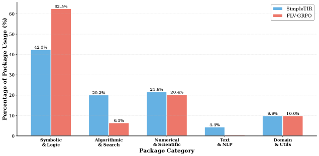
### Visual Description
## Grouped Bar Chart: Package Usage Percentage by Category for Two Methods
### Overview
The image displays a grouped bar chart comparing the percentage of package usage across five distinct categories for two different methods or models: **SimpleTIR** (blue bars) and **FLV-GRPO** (red bars). The chart visually contrasts the distribution of package dependencies or usage patterns between these two approaches.
### Components/Axes
* **Chart Type:** Grouped (clustered) bar chart.
* **Y-Axis:** Labeled "Percentage of Package Usage (%)". The scale runs from 0 to 60, with major tick marks at intervals of 10 (0, 10, 20, 30, 40, 50, 60).
* **X-Axis:** Labeled "Package Category". It lists five categorical groups.
* **Legend:** Positioned in the top-right corner of the chart area. It defines the two data series:
* **SimpleTIR:** Represented by blue bars.
* **FLV-GRPO:** Represented by red (salmon-colored) bars.
* **Data Labels:** Each bar has its exact percentage value displayed directly above it.
### Detailed Analysis
The chart presents the following data points for each package category:
1. **Symbolic & Logic**
* **SimpleTIR (Blue):** 42.5%
* **FLV-GRPO (Red):** 62.5%
* *Trend:* This category shows the highest usage for both methods, with FLV-GRPO having a substantially higher percentage.
2. **Algorithmic & Search**
* **SimpleTIR (Blue):** 20.2%
* **FLV-GRPO (Red):** 6.5%
* *Trend:* SimpleTIR shows significantly higher usage in this category compared to FLV-GRPO.
3. **Numerical & Scientific**
* **SimpleTIR (Blue):** 21.0%
* **FLV-GRPO (Red):** 20.4%
* *Trend:* Usage is nearly identical between the two methods, with a negligible difference of 0.6 percentage points.
4. **Text & NLP**
* **SimpleTIR (Blue):** 4.4%
* **FLV-GRPO (Red):** 0.0% (No red bar is visible, indicating a value of 0 or near 0).
* *Trend:* SimpleTIR has a small but measurable usage here, while FLV-GRPO shows no discernible usage.
5. **Domain & Utils**
* **SimpleTIR (Blue):** 9.9%
* **FLV-GRPO (Red):** 10.0%
* *Trend:* Usage is virtually identical between the two methods.
### Key Observations
* **Dominant Category:** "Symbolic & Logic" is the dominant package category for both methods, accounting for the largest share of usage in each case.
* **Method Specialization:** FLV-GRPO appears highly specialized, with over 62% of its usage concentrated in "Symbolic & Logic" and very low usage in "Algorithmic & Search" and "Text & NLP".
* **Method Balance:** SimpleTIR shows a more balanced distribution. While "Symbolic & Logic" is still its largest category (42.5%), it maintains significant usage in "Algorithmic & Search" (20.2%) and "Numerical & Scientific" (21.0%).
* **Identical Usage:** The "Numerical & Scientific" and "Domain & Utils" categories show nearly identical usage percentages between the two methods.
* **Absence in Category:** FLV-GRPO has no recorded usage in the "Text & NLP" category.
### Interpretation
This data suggests a fundamental difference in the architectural or operational focus of the two methods. **FLV-GRPO** demonstrates a strong, specialized reliance on symbolic reasoning and logic packages, potentially indicating a design optimized for tasks within that domain. Its minimal usage of algorithmic, search, and text/NLP packages implies these are not core to its function.
In contrast, **SimpleTIR** exhibits a more general-purpose or hybrid profile. It leverages symbolic packages heavily but also incorporates a substantial suite of algorithmic, search, and numerical/scientific packages. This broader dependency profile suggests SimpleTIR may be designed to handle a wider variety of problem types or employ a different problem-solving strategy that integrates multiple computational paradigms.
The near-perfect overlap in "Numerical & Scientific" and "Domain & Utils" usage is notable. It indicates that for core numerical computation and general utility functions, both methods rely on the same underlying tools to an equal degree. The stark contrast in the other categories, therefore, highlights their divergent approaches to higher-level reasoning and problem decomposition.
</details>
Figure 9: Comparison of package usage distribution: SimpleTIR vs. FLV-RL
The comparison between SimpleTIR and FLV-RL reveals a fundamental shift in problem-solving paradigms, moving from iterative search to abstract reasoning. As defined in Table 6, the Symbolic & Logic category encompasses tools for constraint satisfaction and formal proofs (e.g., z3-solver, sympy). The chart demonstrates a substantial increase in this category, rising from 42.5% in SimpleTIR to 62.5% in FLV-RL (Figure 9). This suggests that the FLV-RL model is increasingly relying on mathematical abstraction and logical deduction to solve problems rather than procedural code.
Conversely, usage of the Algorithmic & Search category—defined as handling permutations and iterative loops (e.g., itertools)—drops precipitously from 20.2% to 6.5%. This inverse correlation indicates that FLV-RL has largely abandoned brute-force simulation and exhaustive search strategies. Instead of generating candidate solutions through iteration, the model prefers to model the problem space symbolically and solve for the answer directly.
Meanwhile, the Numerical & Scientific and Domain & Utils categories remain relatively stable across both models (approximately 21% and 10%, respectively). This implies that while the core reasoning engine has evolved (shifting from search to logic), the foundational requirements for arithmetic calculation and environment interaction remain constant regardless of the solving strategy. Overall, these metrics quantify a qualitative leap: the model has transitioned from a “compute-heavy” search approach to a “reasoning-heavy” symbolic approach.
## Appendix G GPQA Problems
Zeng (2026) identifies GPQA (Diamond) as having an inherent error rate lower bound of 26.8% and characterizes it as “an advanced intellectual booby trap from the old era.” The systematic flaws include: (i) Factual errors in questions/answers. (ii) Missing parameters needed for correct solutions. (iii) Transcription mistakes in data. The report concludes that GPQA has transformed “from a ruler for measuring intelligence into a noise generator” that measures how well models fit to logically flawed questions rather than actual reasoning ability.
## Appendix H Case Study: Formal Verification in Economic Reasoning
Table 7: Error Analysis: Baseline model (Qwen 2.5-7B) reasoning trajectory with systematic failures
| Question |
| --- |
| As we move to the northwest (up and to the left) along a linear demand curve, elasticity |
| a. goes from inelastic to elastic and the line’s slope is constant |
| b. goes from elastic to inelastic and the line’s slope is constant |
| c. is constant and so is the line’s slope |
| d. goes from inelastic to elastic and the line’s slope rises in absolute terms |
| e. is constant and the line’s slope falls in absolute terms |
| Asnwer Generated by Qwen-2.5-7b |
| The correct answer is: |
| b. goes from elastic to inelastic and the line’s slope is constant. |
| Here’s the reasoning: |
| Elasticity of Demand: Elasticity of demand measures the responsiveness of the quantity demanded to a change in price. It is calculated as the percentage change in quantity demanded divided by the percentage change in price. Along a linear demand curve, as you move from right to left (decreasing price and increasing quantity), the elasticity of demand changes. |
| Slope of the Demand Curve: The slope of a linear demand curve is constant, meaning the change in price per unit change in quantity is the same throughout the curve. |
| Elasticity and Position on the Demand Curve: |
| At higher prices (and lower quantities), the demand is more elastic because a small change in price leads to a relatively larger change in quantity demanded. |
| As you move to the left along the demand curve (decreasing price and increasing quantity), the demand becomes less elastic because the percentage change in quantity demanded becomes smaller relative to the percentage change in price. |
| Therefore, as you move northwest (up and to the left) along a linear demand curve, the elasticity of demand goes from elastic to inelastic, and the slope of the line remains constant. |
To illustrate how formal logic verification improves economic reasoning, we use a standard microeconomics question that exposes typical failure modes of free-form chain-of-thought and shows how verification-guided training corrects them.
### H.1 Problem and Baseline Error Analysis
Problem.
Consider the multiple-choice question: “For a linear demand curve, as we move northwest along the curve, what happens to price elasticity of demand?” In the conventional $(Q,P)$ diagram (quantity on the horizontal axis, price on the vertical axis), “northwest” means higher price and lower quantity.
Baseline behavior.
The baseline model (Qwen 2.5-7B) selects option (b) “goes from elastic to inelastic” and exhibits three systematic failures (Table 7).
Failure Mode 1: Semantic grounding error (directional mis-mapping).
The core mistake is a mis-grounding of the spatial term “northwest.” The correct executable semantics in the $(Q,P)$ plane is:
$$
\text{northwest}(1\rightarrow 2)\;\Rightarrow\;(P_{2}>P_{1})\ \wedge\ (Q_{2}<Q_{1}). \tag{11}
$$
The baseline instead behaves as if “northwest” implied the opposite comparative direction (effectively a southeast move), e.g.,
$$
\text{northwest}(1\rightarrow 2)\;\mapsto\;(P_{2}<P_{1})\ \wedge\ (Q_{2}>Q_{1}), \tag{12}
$$
which flips the economic interpretation and deterministically pushes the subsequent reasoning toward the wrong answer.
Failure Mode 2: Undetected logical inconsistency.
The baseline produces mutually incompatible claims without detecting the contradiction (e.g., asserting both that demand is “more elastic at higher prices” and that the alleged “northwest” move reduces elasticity under its mis-grounded direction). Formally, if a reasoning chain asserts propositions $\{\phi_{i}\}_{i=1}^{n}$ , the chain should satisfy global consistency:
$$
\bigwedge_{i=1}^{n}\phi_{i}\not\equiv\bot. \tag{13}
$$
Pure next-token generation optimizes local likelihood and does not enforce Eq. (13), allowing contradictory statements to coexist.
Failure Mode 3: Conceptual conflation (slope vs. elasticity).
The baseline conflates constant slope with constant elasticity. For a linear demand curve
$$
P=a-bQ,\qquad a>0,\;b>0, \tag{14}
$$
the slope $\frac{dP}{dQ}=-b$ is constant, but point price elasticity (in magnitude) is
$$
\lvert\varepsilon(Q,P)\rvert=\left\lvert\frac{dQ}{dP}\right\rvert\frac{P}{Q}=\frac{1}{b}\cdot\frac{P}{Q}, \tag{15}
$$
which varies with the ratio $\frac{P}{Q}$ . Along the same line, moving northwest increases $P$ and decreases $Q$ , hence increases $\frac{P}{Q}$ and therefore increases $\lvert\varepsilon\rvert$ .
### H.2 Verification-Guided Correction
Our framework corrects these errors by interleaving generation with SMT-based verification (Table LABEL:tab:case_flv_correct). We summarize four mechanisms.
Mechanism 1: Executable semantic grounding.
We train the model to translate ambiguous natural language into solver-checkable constraints. For this task, the semantic parser is encouraged to map “northwest” to Eq. (11) (rather than Eq. (12)), together with domain assumptions typical in economics:
$$
P_{1}>0,\ Q_{1}>0,\ P_{2}>0,\ Q_{2}>0,\ \text{and}\ P_{i}=a-bQ_{i}\ \text{for}\ i\in\{1,2\}. \tag{16}
$$
Incorrect mappings are rejected because they become inconsistent with the intended move or with the economic domain; the solver provides immediate feedback via $\textsc{sat}/\textsc{unsat}$ .
One simple way to incorporate verification is to weight learning by verification success:
$$
\mathcal{L}_{\text{ground}}=-\mathbb{E}_{x\sim\mathcal{D}}\Bigl[\mathbb{I}\bigl(\text{verify}(f_{\theta}(x))=\textsc{sat}\bigr)\cdot\log P_{\theta}\bigl(f_{\theta}(x)\mid x\bigr)\Bigr], \tag{17}
$$
where $f_{\theta}$ is the model-produced formalization and $\text{verify}(\cdot)$ calls the SMT solver.
Mechanism 2: Global consistency enforcement over a chain.
Instead of allowing each step to stand alone, we require that the accumulating set of claims remains satisfiable under the shared constraints (Eqs. (14)–(16)). Concretely, we can test competing hypotheses such as:
$$
H_{\downarrow}:\lvert\varepsilon_{2}\rvert<\lvert\varepsilon_{1}\rvert \tag{18}
$$
under the “northwest” constraints. The solver returns unsat for $H_{\downarrow}$ (given standard domain assumptions), steering the model away from inconsistent chains and toward the correct alternative:
$$
H_{\uparrow}:\lvert\varepsilon_{2}\rvert>\lvert\varepsilon_{1}\rvert. \tag{19}
$$
Mechanism 3: Counterexample-driven learning (numerical witnesses).
When a hypothesis fails, the solver can provide concrete satisfying assignments for the correct hypothesis, serving as a numerical witness that bridges symbolic proof and intuition. For example, pick $b>0$ and two points on the same demand curve with $P_{2}>P_{1}$ and $Q_{2}<Q_{1}$ , such as $(P_{1},Q_{1})=(6,4)$ and $(P_{2},Q_{2})=(8,2)$ . Then by Eq. (15),
$$
\lvert\varepsilon_{1}\rvert=\frac{1}{b}\cdot\frac{6}{4}=\frac{1.5}{b},\qquad\lvert\varepsilon_{2}\rvert=\frac{1}{b}\cdot\frac{8}{2}=\frac{4.0}{b}, \tag{20}
$$
hence $\lvert\varepsilon_{2}\rvert>\lvert\varepsilon_{1}\rvert$ . Training on triples $(\text{hypothesis},\text{verification result},\text{witness})$ provides richer supervision than final-answer labels alone.
Mechanism 4: Compositional algebraic reasoning with verified substeps.
We structure the explanation into verifiable primitives: (i) linear constraint $P=a-bQ$ ; (ii) derivative $\frac{dQ}{dP}=-\frac{1}{b}$ ; (iii) elasticity definition $\lvert\varepsilon\rvert=\left\lvert\frac{dQ}{dP}\right\rvert\frac{P}{Q}$ ; (iv) monotonicity: under $P_{2}>P_{1}$ and $Q_{2}<Q_{1}$ , we have $\frac{P_{2}}{Q_{2}}>\frac{P_{1}}{Q_{1}}$ , therefore $\lvert\varepsilon_{2}\rvert>\lvert\varepsilon_{1}\rvert$ . This decomposition yields reusable, solver-checkable reasoning components rather than brittle pattern matching.
Table 8: Formal logic verification-guided reasoning trajectory.
## Appendix I Prompts
This section presents the key prompts used throughout our training pipeline. Table 9 shows the reinforcement learning rollout prompt that guides models to generate formal verification-augmented reasoning during policy optimization. Table LABEL:lst:formal-incert detail the prompt used for formal logic verification-guided reasoning dataset construction.
Table 9: Prompt for Model Training
| Solve the following problem step by step. You can selectively use Python with z3 (for logic) and sympy (for calculations) to verify reasoning. Python code will run in an external sandbox, returning output as <interpreter>output</interpreter>. The python code should be complete scripts, including necessary imports. |
| --- |
| Revise reasoning if sandbox returns ’disproved’ or fix code if execution errors occur. |
| Code Format: |
| Each code snippet is wrapped with |
| <code> |
| ‘‘‘ python |
| code snippet |
| ‘‘‘ |
| </code> |
| Response must end exactly as: |
| <answer> |
| [Summary of all reasoning steps] |
| \\boxed{[Final answer]} |
| </answer> |
| [Question] |
⬇
You are a helpful AI assistant. Initially, when solving a question, you would need to think step by step, without the ability to use code for calculation or logical verification. Now, you have enhanced capabilities to write code for both computational tasks and logical reasoning verification. The code will be executed by a sandbox, and the result can be returned to enhance your reasoning process.
** Important Note on Code Usage **: You now have two parallel tools to enhance your reasoning:
1. ** Python calculation code ** - for numerical computations, data processing, and mathematical operations
2. ** Z3 logical verification ** - for verifying logical reasoning, constraints, and formal proofs using the Z3 theorem prover
These are complementary tools serving different purposes. Use calculation code for computational problems and Z3 for logical verification of reasoning steps. ** Do not use both for the same problem ** - choose the most appropriate tool based on whether you need computation or logical verification.
The thinking process can have multiple code snippets. Each code snippet is wrapped with:
< code >
‘‘‘ python
code snippet
‘‘‘
</ code >, and should be executable. The returned result is wrapped with < interpreter > execution results </ interpreter >.
Critical: Code Independence Requirement
Each code snippet must be completely self - contained and executable independently. This means:
- Each code block should include all necessary imports
- Each code block should define all variables it uses (do not rely on variables from previous code blocks)
- Each code block should be able to run successfully if executed in isolation
- If you need values from previous calculations, redefine or recalculate them in the new code block
- Think of each < code > block as being executed in a fresh Python environment
** Guidelines for Z3 Usage:**
Z3 verification should ONLY be used when it provides genuine formal verification value:
Do NOT use Z3 for:
- Verifying simple arithmetic calculations (e. g., 2 + 2 = 4, or 1.0 * (-2.0 - 4.0) = -6.0)
- Checking calculations with concrete numbers that Python already computed
- Adding concrete values as constraints and then verifying them (this is circular reasoning)
- Repeating what numerical computation already verified
DO use Z3 for:
- Proving general mathematical properties or identities that hold for ALL values (using symbolic variables)
- Verifying complex logical relationships with multiple interrelated constraints
- Checking satisfiability of constraint systems or finding whether solutions exist
- Proving inequalities or optimization conditions symbolically
- Verifying that no counterexamples exist for a general claim
- Formal verification of logical reasoning steps that involve symbolic relationships
- Key principle: Use symbolic variables (not concrete numbers) to prove general statements. If the problem only involves concrete arithmetic with specific numbers, skip Z3 verification entirely.
Examples of INCORRECT Z3 usage:
# BAD: Verifying concrete arithmetic
solver. add (m == 1.0)
solver. add (v_i == 4.0)
solver. add (delta_p == -6.0)
solver. check () # This just checks if -6.0 == -6.0, no value added
Examples of CORRECT Z3 usage:
# GOOD: Proving general algebraic equivalence
from z3 import * # Remember: each code block needs its imports
m, v1, v2 = Reals (’ m v1 v2 ’)
solver = Solver ()
solver. add (m > 0) # General constraint, not specific value
# Prove: Delta_p = m (v2 - v1) is equivalent to Delta_p = m * v2 - m * v1 for ALL values
solver. add (m * (v2 - v1) != m * v2 - m * v1)
result = solver. check ()
print (" Verification result:", result)
assert result == unsat # Proves no counterexample exists
** Guidelines for Python code calculation Usage:**
When NOT to use code:
- Simple arithmetic that can be done mentally
- Basic algebra or formula substitution
- Straightforward unit conversions
- Verifying obvious mathematical identities
- Problems where all steps are elementary calculations
Code Usage Limit:
- For problems solvable with basic math: Use code AT MOST 1-2 times (or not at all)
- For complex computational problems: Use code AT MOST 3-4 times
- Each code block should serve a distinct, necessary purpose
- ** Never use multiple code blocks to verify the same calculation in different ways **
Goal:
Modify the original thinking process to make it more accurate by:
- Replacing manual calculation steps with Python code snippets and their execution results
- Adding Z3 logical verification when it provides genuine formal verification beyond simple arithmetic
- Keeping the core reasoning logic intact, including any unsuccessful attempts
- Adding code only where it provides genuine value
- Ensuring each code snippet serves a unique, necessary purpose
- use Python code or Z3 verification for a combined total of no more than 4 times
- Wrap the revised thinking process within < revised_thinking_process > and </ revised_thinking_process >.
User Question:
{question}
Original Thinking Process (without code interpreter ’ s support):
< original_thinking_process > {original_response} </ original_thinking_process >
Details:
1. Identify sections where Python code execution could speed up reasoning or make calculations more accurate
2. Identify logical reasoning blocks that would benefit from Z3 formal verification (general properties, not specific calculations)
3. Replace manual calculation steps with code snippets and corresponding interpreter ’ s execution results
4. Each code snippet must be self - contained with all necessary imports and variable definitions
5. Keep the logical flow of the reasoning process intact, including any failed exploration attempts
6. Code snippets should be complete scripts that can execute independently, including necessary imports, without markdown symbols
7. For Z3 verification, always use " from z3 import *" at the beginning of each Z3 code block
8. Outputs in code snippets must explicitly call the print function
9. Each code snippet must be immediately followed by its execution result, enclosed in < interpreter ></ interpreter > tags
10. Execution results should match the model ’ s output exactly, with no extra or missing tokens
11. Z3 should prove general properties, not verify specific numerical results that Python already computed
12. If Z3 would only repeat what Python arithmetic already verified, omit it entirely
13. Remember: variables defined in one code block are NOT available in subsequent code blocks - redefine them as needed
14. When performing calculations, format numerical outputs to 2-4 decimal places using round () or f - strings (e. g., print (f "{result:.2 f}")) to avoid displaying unnecessary floating - point digits. Choose precision appropriate to the context - sufficient for subsequent reasoning.
Revised Thinking Process (With independent selective Python computation blocks and Z3 formal verification):
Listing 1: Prompt for formal logic verification-guided reasoning chain generation