2602.00276

# Localizing and Correcting Errors for LLM-based Planners **Authors**: Aditya Kumar, William Cohen ## Abstract Large language models (LLMs) have demonstrated strong reasoning capabilities on math and coding, but frequently fail on symbolic classical planning tasks. Our studies, as well as prior work, show that LLM-generated plans routinely violate domain constraints given in their instructions (e.g., walking through walls). To address this failure, we propose iteratively augmenting instructions with Localized In-Context Learning (L-ICL) demonstrations: targeted corrections for specific failing steps. Specifically, L-ICL identifies the first constraint violation in a trace and injects a minimal input-output example giving the correct behavior for the failing step. Our proposed technique of L-ICL is much effective than explicit instructions or traditional ICL, which adds complete problem-solving trajectories, and many other baselines. For example, on an 8×8 gridworld, L-ICL produces valid plans 89% of the time with only 60 training examples, compared to 59% for the best baseline, an increase of 30%. L-ICL also shows dramatic improvements in other domains (gridworld navigation, mazes, Sokoban, and BlocksWorld), and on several LLM architectures. Machine Learning, ICML ## 1 Introduction Large language models (LLMs) and agentic systems reason and plan effectively in domains such as mathematics, coding, and question answering (Khattab et al., 2023; Yao et al., 2023a), suggesting that modern LLMs possess strong general planning capabilities. However, studies on classical planning benchmarks reveals a more nuanced picture: LLMs frequently fail, even on simple planning tasks that symbolic planners solve easily (Valmeekam et al., 2023; Stechly et al., 2024). Past researchers have analyzed plans produced by LLMs such as SearchFormer (Lehnert et al., 2024), which are fine-tuned to generate structured reasoning chains that can be parsed, and shown that LLMs frequently violate domain constraints given in their instructions (Stechly et al., 2024). For example, LLMs might propose plans that walk through a wall in a maze, or pick up a block when the robot’s gripper is already occupied. Table 1: Performance on an 8 $×$ 8 two-room gridworld using DeepSeek V3. Paths start in one room and end in the other. Valid plans never leave the grid or cross walls; Successful plans reach their goals; and Optimal plans are successful and use the minimum number of steps. L-ICL[ $m$ ] denotes our method trained on $m$ examples, with the corresponding character count of L-ICL examples provided. All experiments are provided with an ASCII representation of the grid. | Zero-Shot | 16 | 0 | 0 | | --- | --- | --- | --- | | RAG-ICL [10k chars] | 20 | 6 | 6 | | RAG-ICL [20k chars] | 21 | 9 | 9 | | ReAct | 48 | 41 | 37 | | Self-Consistency ( $k{=}5$ ) | 59 | 45 | 43 | | Self-Refine ( $k{=}5$ ) | 51 | 44 | 38 | | PTP PTP, introduced in (Cohen and Cohen, 2024) describes a method to prompt LLMs with partially specified programs / L-ICL [ $m=0$ ] | 40 | 33 | 28 | | L-ICL [ours, $m=60$ , 2k chars] | 89 | 89 | 77 | Table 1 demonstrates this on a very simple 8 $×$ 8 two-room gridworld navigation task. Despite receiving complete information about the domain (grid layout and obstacles) no baseline method produces valid plans even 60% of the time. Agentic and test-time-scaling approaches perform better, but still produce many invalid plans. We conjecture that LLMs cannot build valid plans for this task because they fail to access the necessary domain-specific knowledge in the prompt consistently. This hypothesis is consistent with the failure of LLMs in these domains, and with their success in math and coding, where the necessary knowledge is general, and hence learnable in pre-training or fine-tuning. In-context learning (ICL) is a natural remedy. However, complete solution trajectories demonstrate that plans work, not why individual steps are valid—leaving constraints implicit. As Table 1 shows, even 20,000 characters of retrieved trajectories RAG-ICL, retrieving demonstrations for tasks with similar start and end goals. yield only 9% success. The rules must still be inferred, and inference fails. L-ICL escapes this trap by letting failures reveal which constraints need explicit specification. Rather than full trajectories, we augment prompts with localized examples that demonstrate correct behavior on individual steps where models err. We call this approach Localized In-Context Learning (L-ICL). This approach achieves higher performance with much less context: 2,000 characters of targeted corrections outperforms 20,000 characters of trajectories. Generating L-ICL examples requires analyzing and correcting reasoning traces at training time, which we enable by prompting models to produce structured reasoning traces, and then correcting the traces with a symbolic planner. Thus, L-ICL might be viewed as distilling domain knowledge from a symbolic system into an LLM. 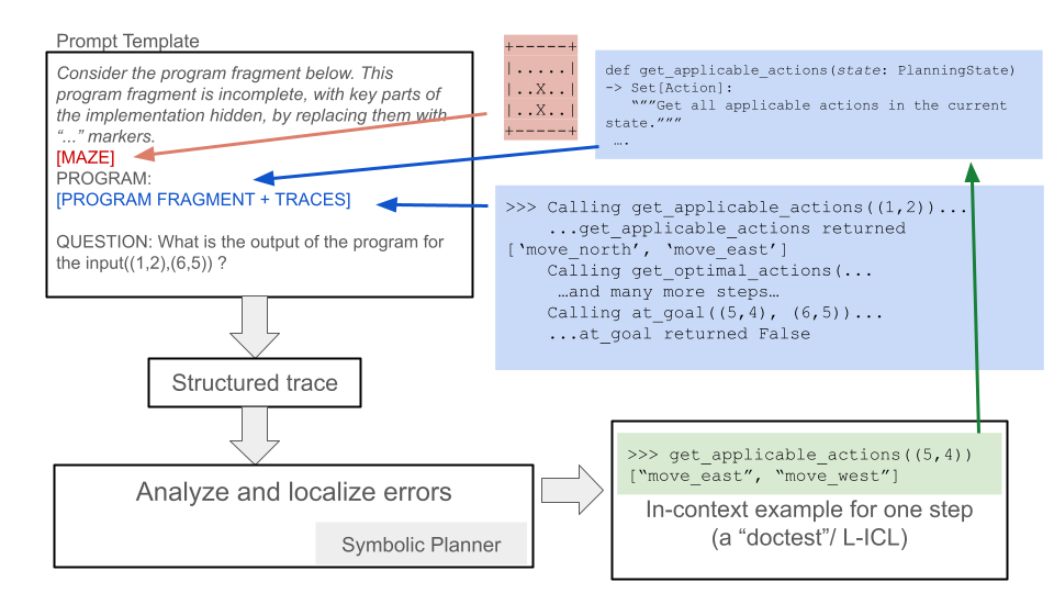Figure 1 summarizes our approach, which builds on Program Trace Prompting (PTP) (Cohen and Cohen, 2024). PTP recasts reasoning as producing a “program trace” for a partially specified program. A PTP prompt includes, for each type of reasoning “step”, documentation (but not code) for a corresponding subroutine, along with (optional) example inputs and outputs. For instance, a gridworld navigation task might include a subroutine get_applicable_actions(cell) that returns the set of obstacle-free cells adjacent to the input cell. Because no executable code is provided in PTP, just documentation, the LLM must infer how to perform the reasoning step: e.g., in gridworld navigation, the LLM must infer which moves are valid for a task. PTP’s prompting scheme provides a natural insertion point for localized corrections: when a subroutine call fails, we locally augment that subroutine’s documentation by adding a new input/output example. The input/output examples use Python’s doctest syntax, a format well-represented in LLM training data, so readily understandable by code-trained LLMs. <details> <summary>graphs/corrected/Research_Presentation.png Details</summary>  ### Visual Description ## Diagram: Program Trace Analysis and Error Localization Workflow ### Overview The image is a technical flowchart illustrating a process for analyzing program execution traces to localize errors, likely within the context of automated planning or AI reasoning systems. It depicts a pipeline that starts with a prompt containing an incomplete program and execution traces, processes this through structured analysis, and uses symbolic planning and in-context learning examples to understand and debug the program's behavior. ### Components/Axes The diagram is composed of several text boxes connected by directional arrows, indicating data flow and process steps. There are no traditional chart axes. The components are spatially arranged as follows: 1. **Top-Left (Prompt Template Box):** A large rectangular box containing the initial input. 2. **Top-Right (Code Snippets):** Two blue-shaded boxes containing Python-like code and execution traces. 3. **Center-Left (Process Flow):** A vertical sequence of three boxes connected by downward arrows. 4. **Bottom-Right (Example Box):** A green-shaded box containing a code example. 5. **Connecting Arrows:** Colored arrows (red, blue, green) show relationships and data flow between components. ### Detailed Analysis **1. Prompt Template Box (Top-Left):** * **Title:** `Prompt Template` * **Content:** * `Consider the program fragment below. This program fragment is incomplete, with key parts of the implementation hidden, by replacing them with "..." markers.` * `[MAZE]` (This text is in red, with a red arrow pointing from it to a small grid diagram). * `PROGRAM:` * `[PROGRAM FRAGMENT + TRACES]` (This text is in blue, with a blue arrow pointing from it to the code snippets on the right). * `QUESTION: What is the output of the program for the input((1,2),(6,5)) ?` **2. Maze Diagram (Top-Center):** * A small 5x5 grid representing a maze. * The grid contains symbols: `.` (empty/path), `X` (wall/obstacle). * The visible rows are: * Row 1: `...X.` * Row 2: `..X..` * Row 3: `..X..` * (Rows 4 and 5 are partially obscured but follow a similar pattern). * A **red arrow** originates from the `[MAZE]` label in the Prompt Template and points to this grid. **3. Code Snippets (Top-Right, Blue Boxes):** * **Upper Blue Box:** * Contains a Python function definition: ```python def get_applicable_actions(state: PlanningState) -> Set[Action]: """Get all applicable actions in the current state.""" ... ``` * **Lower Blue Box:** * Contains a sample execution trace (likely a "doctest" or interactive Python session): ``` >>> Calling get_applicable_actions((1,2))... ...get_applicable_actions returned ['move_north', 'move_east'] >>> Calling get_optimal_actions(...) ...and many more steps... >>> Calling at_goal((5,4), (6,5))... ...at_goal returned False ``` * A **blue arrow** originates from the `[PROGRAM FRAGMENT + TRACES]` label in the Prompt Template and points to these code snippets. **4. Process Flow (Center-Left):** * **Box 1 (Top):** `Structured trace` (Receives input from the Prompt Template via a downward arrow). * **Box 2 (Middle):** `Analyze and localize errors` (Receives input from "Structured trace"). * **Box 3 (Bottom):** `Symbolic Planner` (This text is right-aligned within the box. Receives input from "Analyze and localize errors"). * A **gray arrow** points from the "Analyze and localize errors" box to the right, towards the Example Box. **5. Example Box (Bottom-Right, Green Box):** * Contains a code example, formatted as a doctest: ``` >>> get_applicable_actions((5,4)) ["move_east", "move_west"] ``` * Below the code: `In-context example for one step (a "doctest"/ L-ICL)` * A **green arrow** originates from this box and points upward to the `get_applicable_actions` function definition in the upper blue code snippet box. ### Key Observations * **Color-Coded Flow:** The diagram uses color strategically. Red links the abstract maze problem to its representation. Blue links the program fragment placeholder to its concrete code and trace examples. Green links a specific in-context learning (ICL) example back to the function it exemplifies. * **Process Pipeline:** The core workflow is linear: Prompt -> Structured Trace -> Error Analysis -> Symbolic Planner. * **In-Context Learning (ICL) Integration:** The green box and arrow explicitly show how a "doctest" example is provided as an in-context learning signal to the system, presumably to help the Symbolic Planner understand the function's behavior. * **Problem Context:** The input question `((1,2),(6,5))` and the maze grid suggest the program is related to pathfinding or navigation in a grid world. The function names `get_applicable_actions`, `get_optimal_actions`, and `at_goal` reinforce this. ### Interpretation This diagram outlines a methodology for **debugging or understanding incomplete program specifications through execution traces and symbolic reasoning**. The process appears to be: 1. **Problem Framing:** A high-level problem (navigate a maze from start (1,2) to goal (6,5)) is presented alongside an incomplete program implementation. 2. **Trace Generation:** The system executes the available program fragments, generating a "structured trace" of function calls and returns (e.g., what actions are available at state (1,2)). 3. **Analysis & Localization:** The trace is analyzed to find discrepancies or errors. The goal is to "localize" where the program's behavior deviates from the expected logic required to solve the maze. 4. **Symbolic Planning & ICL:** A "Symbolic Planner" component is invoked. Crucially, it is provided with **in-context examples** (the green "doctest" box). These examples, like showing that `get_applicable_actions((5,4))` returns `["move_east", "move_west"]`, serve as concrete demonstrations of the intended function behavior. This allows the planner to reason symbolically about the program's logic, fill in the "..." gaps, and ultimately answer the output question. The underlying concept is a form of **program synthesis or repair via trace analysis and few-shot learning**. Instead of just reading code, the system learns from its dynamic execution behavior (traces) and a few correct examples (ICL) to infer the complete program logic. This is a powerful approach for debugging complex systems where the specification is implicit in the desired input-output behavior and example executions. </details> Figure 1: Overview of L-ICL. The prompt template follows PTP: it includes documentation for each subroutine but no executable code. Prompting an LLM produces a trace that follows the format of the $k$ provided example traces. The trace is parsed to find the first failing step, and the failing input is passed to an oracle that returns the correct output. This yields a localized example (e.g., $x{=}\texttt{(5,4)}$ , $y{=}\texttt{['move\_east','move\_west']}$ ) that is inserted into the subroutine’s documentation. This process iterates over training instances to accumulate examples in a failure-driven manner. Given a planning task, we first prompt the LLM to generate a trace using the PTP format. We then analyze this trace programmatically to identify the first failing step, i.e., the first subroutine call whose output violates domain constraints. An oracle (a symbolic simulator or verifier) provides the correct output for that input, yielding a localized correction. This correction is then inserted into the prompt. For instance, if the LLM’s first invalid move is from cell $(3,4)$ , we L-ICL will add to the prompt an example showing get_applicable_actions((3,4)) should return [’move_north’, ’move_south’]. This localized correction directly addresses the failure, and of course can also be generalized by the LLM to other similar cases. This process iterates over multiple training instances, accumulating a bank of targeted examples that progressively refine the model’s understanding of domain constraints. Crucially, the oracle is required only during training. Experimentally, prompt augmentation with L-ICL dramatically reduces domain violations, and thus improves LLM planning performance across multiple domains. Beyond the results of Table 1 and other gridworld tasks, we evaluate on classical planning benchmarks like BlocksWorld and Sokoban, seeing similar gains. L-ICL is also remarkably sample-efficient: peak performance is typically achieved with only 30–60 training examples. L-ICL works on multiple LLM architectures (DeepSeek V3, DeepSeek V3.1, Claude Haiku 4.5, Claude Sonnet 4.5), and learned constraints can transfer across problem sizes (see Appendix B). To summarize our contributions: (1) Using the PTP variant of semi-structured reasoning, we precisely measure constraint violation rates in LLM-generated plans across multiple planning domains, revealing that such violations are the dominant failure mode. (2) We introduce L-ICL, a method that improves planning validity through localized, failure-driven corrections, and show that targeted examples outperform retrieval of complete trajectories even when the latter uses 10 $×$ more context. (3) We demonstrate consistent improvements across multiple planning domains and four LLM architectures. (4) We release our benchmark suite and code to facilitate future research on LLM planning. ## 2 Related Work ### 2.1 LLM Planning: Capabilities and Limitations The planning capabilities of LLMs remain contested. One line of work reports strong performance on some planning tasks when LLMs are augmented with appropriate scaffolding: e.g., Tree of Thoughts achieves 74% on Game of 24 versus 4% for chain-of-thought (Yao et al., 2023a), RAP-MCTS reaches 100% on Blocksworld instances requiring 6 or fewer steps (Hao et al., 2023), and ReAct improves interactive decision-making by 34% over baselines (Yao et al., 2023b). However, systematic evaluation on classical planning benchmarks reveals persistent failures. Valmeekam et al. (2023) show GPT-4 achieves only 12% success on International Planning Competition (IPC) domains; and Stechly et al. (2024) demonstrate that chain-of-thought improvements are brittle and fail to generalize beyond surface patterns. The LLM-Modulo framework (Kambhampati et al., 2024) argues that LLMs function as approximate knowledge sources rather than autonomous planners, achieving strong results only when paired with external verifiers. Kaesberg et al. (2025) also documented that LLMs are challenged by 2D navigation tasks, similar to ones we study here. Most recently, Shojaee et al. (2025) identify a “complexity collapse” phenomenon: reasoning models’ performance degrades sharply beyond certain problem complexities, with accuracy dropping to zero on harder instances even when token budgets remain available. We follow Stechly et al. (2024) in working to diagnose why LLMs violate constraints using structured reasoning chains; however, we work with PTP as a prompting scheme, rather than models fine-tuned to produce structured reasoning chains, allowing us to consider more kinds of models, and more powerful ones. With L-ICL, we also propose a practical method to reduce these violations. Our work confirms that constraint violations are a common failure mode, and shows that targeted corrections outperform both agentic scaffolding and retrieval-based ICL approaches. ### 2.2 Approaches to Improve LLM Reasoning Prior work addresses LLM reasoning limitations through three main strategies: structured output formats, test-time compute scaling, and in-context learning. Structured Reasoning. Chain-of-thought prompting (Wei et al., 2022) improves performance by eliciting intermediate steps, though explanations may be unfaithful to actual computation (Turpin et al., 2023). PTP (Cohen and Cohen, 2024) offers interpretable traces: prompts specify subroutine signatures without implementations, and the LLM produces structured outputs that can be parsed and verified (Leng et al., 2025). We build on PTP because its explicit subroutine structure provides natural insertion points for localized corrections. Test-Time Compute. Several methods improve reasoning by expending more computation at inference. Self-Consistency (Wang et al., 2023) aggregates multiple sampled paths via majority voting; Tree of Thoughts (Yao et al., 2023a) explores branching reasoning trajectories; and Self-Refine (Madaan et al., 2023) iteratively improves outputs through self-critique. Tool-augmented approaches interleave reasoning with execution: Program of Thoughts (Chen et al., 2022), PAL (Gao et al., 2023), and Chain of Code (Li et al., 2023) generate executable code, while ReAct (Yao et al., 2023b) interleaves reasoning with tool calls. These methods require multiple LLM calls or external tools at inference. Critically, Stechly et al. (2025) show that LLM self-verification is unreliable, making self-critique ineffective for planning. In-Context Learning. ICL enables task adaptation through examples (Brown et al., 2020), with effectiveness depending on example selection (Liu et al., 2022) and format (Min et al., 2022). For planning, a natural approach is retrieving complete solution trajectories (RAG-ICL). However, we find this ineffective: 20,000 characters of retrieved trajectories yield only 9% success on our gridworld benchmark. Complete trajectories demonstrate that solutions work but leave implicit why individual steps are valid. L-ICL addresses this by providing localized input-output pairs that directly encode constraints. Table 2 summarizes how L-ICL relates to prior approaches. Table 2: Comparison of L-ICL with related approaches. L-ICL uniquely combines example-based training with localized feedback while requiring only single-pass inference. | Self-Refine Tree of Thoughts Self-Consistency | none none none | many many many | none none none | | --- | --- | --- | --- | | ReAct | none | many | none | | ReAct + oracle f/b | none | many | yes | | Fine-tuning | trajectory | one | none | | RAG-ICL | trajectory | one | none | | L-ICL (ours) | one step | one | train only | ## 3 Method We first describe Program Trace Prompting (PTP), the structured reasoning framework underlying our approach. We then introduce Localized In-Context Learning (L-ICL), our method for iteratively injecting domain constraints into the prompt. Finally, we describe our experimental domains and evaluation setup. ### 3.1 Background: Program Trace Prompting Program Trace Prompting (PTP) (Cohen and Cohen, 2024) recasts reasoning as producing an execution trace for a partially specified program. A PTP prompt contains documentation for each subroutine (function name, typed arguments, return type, and a natural language description of its purpose), a small number of example traces showing how subroutines are called, and the query problem to solve. Crucially, subroutine implementations are withheld; the LLM must infer correct behavior from context. For planning tasks, we define subroutines corresponding to planning primitives. For instance, a gridworld navigation task includes a subroutine that returns applicable actions from a given state (those that stay in bounds and avoid walls), a subroutine that returns the resulting state after executing an action, and a subroutine that checks whether the current state satisfies the goal. The LLM generates a trace by repeatedly invoking these subroutines, producing outputs consistent with the documentation and examples. Because the trace follows a predictable structure, we can parse it programmatically and verify each step against a ground-truth oracle. This explicit subroutine structure provides natural insertion points for corrections: when a specific subroutine call fails, we can augment that subroutine’s documentation without modifying the rest of the prompt. Full subroutine specifications for each domain appear in Appendix E. ### 3.2 Localized In-Context Learning (L-ICL) The key insight behind L-ICL is that domain constraints can be taught more effectively through targeted examples than through complete solution trajectories. When an LLM violates a constraint (e.g., proposing to move through a wall), traditional approaches either reject the entire plan or provide feedback on the final outcome. L-ICL instead identifies the precise point of failure and injects a minimal correction for that specific subroutine call. First Failure Identification. Given an LLM-generated trace, we parse each subroutine call and verify its output against an oracle. Let $c_1,c_2,…,c_n$ denote the sequence of subroutine calls in the trace. We identify the first failing call $c_i^*$ such that the LLM’s output differs from the oracle’s: $$ i^*=\min\{i:LLM(c_i)≠Oracle(c_i)\} $$ Focusing on the first failure is deliberate. Planning errors cascade: an invalid move at step $k$ renders all subsequent state representations incorrect, making later “errors” artifacts of the initial mistake rather than independent failures. Correcting the root cause addresses multiple downstream errors simultaneously. Localized Correction. For the failing call $c_i^*$ with input $x$ and incorrect output $\hat{y}$ , we query the oracle to obtain the correct output $y^*=Oracle(x)$ . This yields a correction tuple $(f,x,y^*)$ where $f$ is the subroutine name. We format this correction as a doctest-style example and insert it into the documentation for subroutine $f$ , augmenting the original description with an additional input-output pair. This format, drawn from Python’s widely used doctest convention, is well-represented in LLM training data. Appendix E.3 provides concrete examples of the correction format. Iterative Accumulation. L-ICL iterates over a set of training problems $\{P_1,P_2,…,P_m\}$ . For each problem, we generate a trace using the current prompt, identify the first failing subroutine call (if any), and add the corresponding correction to the prompt. Corrections accumulate across training problems, progressively “hardening” the prompt to avoid constraint violations. Algorithm 1 provides pseudocode. L-ICL converges quickly: we see diminishing returns after only 30–60 training examples on our benchmark tasks (see Section 4). Algorithm 1 Localized In-Context Learning (L-ICL) 0: Base prompt $P_0$ with PTP structure, training problems $\{P_1,…,P_m\}$ , oracle $O$ 0: Augmented prompt $P$ $P←P_0$ $C←∅$ $\triangleright$ Correction set for $j=1$ to $m$ do $τ←\textsc{GenerateTrace}(P_0,P_j)$ $\{c_1,…,c_n\}←\textsc{ParseCalls}(τ)$ for $i=1$ to $n$ do $(f,x,\hat{y})← c_i$ $y^*←O(f,x)$ if $\hat{y}≠ y^*$ then $C←C∪\{(f,x,y^*)\}$ $\triangleright$ Record first failure break end if end for end for $P←\textsc{InsertCorrections}(P_0,C)$ $\triangleright$ Batch update return $P$ ### 3.3 Experimental Domains We design our experimental domains as a progressive ablation study that isolates different facets of planning difficulty. Starting from simple navigation, we incrementally add complexity along several axes: spatial structure, action diversity, state tracking requirements, and strategic reasoning. Table 3 summarizes how each domain isolates specific challenges. Table 3: Progressive ablation across experimental domains. Each domain adds complexity along one or more axes while controlling others. | 8 $×$ 8 Grid | Simple | 4 | 1 | No | | --- | --- | --- | --- | --- | | 10 $×$ 10 Maze | Complex | 4 | 1 | No | | Sokoban Grid | Complex | 4 | 1 | No | | Full Sokoban | Complex | 8 | 3 | Yes | | BlocksWorld | None | 2 | 5 | No | The 8 $×$ 8 Two-Room Gridworld is our simplest setting, testing basic spatial reasoning: an agent must navigate between two rooms connected by a single doorway. The 10 $×$ 10 Maze increases spatial complexity with narrow corridors and dead ends, requiring longer plans (typically 15–25 steps versus 8–12 for the gridworld). Full Sokoban introduces the critical challenge of multi-object state tracking (an agent and a box), where the agent must coordinate its position with multiple box positions, and where certain pushes lead to irreversible trap states. Sokoban-Style Gridworld ablates Sokoban by removing pushable boxes, but keeping the spatial layout and action semantics, isolating the effect of richer environment structure. Finally, BlocksWorld differs qualitatively from navigation: every object (block) is dynamic, constraints depend on relational configurations rather than spatial positions, and we provide an algorithmic sketch to test whether L-ICL can improve adherence to prescribed planning strategies. Full domain specifications appear in Appendix C. ### 3.4 Baselines and Metrics We compare L-ICL against several approaches spanning prompting strategies, agentic methods, and retrieval. Zero-Shot. The LLM receives the problem description and instructions with no in-context examples, measuring baseline capability without demonstration. RAG-ICL. We retrieve complete CoT-formatter solution trajectories for similar problems based on start/goal similarity, and evaluate at 10k and 20k character budgets. ReAct. The LLM is instructed to interleave reasoning and action selection in its output, following the prompt format specified in Appendix F.2. We evaluate a prompt-only version and an oracle-augmented version that queries a verifier during planning. Self-Consistency. Majority voting with $k{=}5$ reasoning paths sampled at temperature 0.7. Self-Refine. The LLM generates a solution, then critiques and refines it, based on its own feedback, for $k{=}5$ iterations. Tree-of-Thoughts. The LLM explores a tree of intermediate steps, evaluating and pruning branches (prompt-only, no external search). Crucially, ReAct (Oracle) queries the verifier at test time for each proposed action, while L-ICL uses the oracle only during training. At inference, L-ICL requires a single forward pass with no external dependencies. For L-ICL, we report results with different numbers of training examples $m$ (denoted L-ICL[ $m$ ]) to assess sample efficiency. We evaluate plans along three axes that form a natural hierarchy. A plan is valid if it violates no domain constraints (e.g., no wall collisions). A plan is successful if it is valid and reaches the goal state. A plan is optimal if it is successful and uses the minimum number of steps. Hence, a large valid-to-success gap indicates the model follows rules but fails to reach goals, and a large success-to-optimal gap indicates inefficient but functional plans. ### 3.5 Experimental Setup Our primary experiments use DeepSeek V3 (DeepSeek-AI, 2024), with additional evaluation on DeepSeek V3.1, Claude 4.5 Haiku, and Claude Sonnet 4.5 (Anthropic, 2025) to assess cross-architecture generalization. For each domain, we generate 100 test problems with random start and goal configurations. Training problems for L-ICL are drawn from a disjoint pool of 250 instances. For domains other than blocks world, prompts use a textual state representation, as suggested in Figure 1, and unless stated otherwise, use an ASCII representation of the grid. Oracles are domain-specific: simple simulators for gridworlds and mazes, and the Fast Downward planner (Helmert, 2006) and tools like the K-Star Planner (Katz and Lee, 2023; Lee et al., 2023) for Sokoban and BlocksWorld. We use temperature 1 for optimal model performance (DeepSeek-AI, 2024) unless stated. L-ICL is trained on up to 240 examples. ## 4 Results We evaluate L-ICL across our domain suite, demonstrating that localized corrections dramatically improve constraint adherence while remaining sample-efficient. We ask four key questions about L-ICL: (1) Does it learn domain constraints? (2) Is it more efficient than retrieval-based ICL? (3) Does it require explicit spatial representations? (4) Does it generalize across LLM architectures? ### 4.1 L-ICL Learns Domain Constraints Table 4 presents our main results across all domains. L-ICL consistently outperforms all baselines, often by substantial margins. Beyond raw performance gains, the pattern of results across our progressive domain suite reveals which aspects of planning L-ICL addresses effectively. Table 4: Main results across all domains. We report %(V)alid and %(S)uccessful. All baselines receive ASCII grid representations. L-ICL[ $m$ ] denotes training on $m$ examples. Best results in bold, second-best underlined. $†$ ReAct (Oracle f/b) receives oracle feedback at inference time. ∗ L-ICL (no grid) methods are handicapped: they receive no ASCII grid, and rely purely on L-ICL to infer structure. | | 8 $×$ 8 Grid | 10 $×$ 10 Maze | Sokoban Grid | Full Sokoban | BlocksWorld | | | | | | | --- | --- | --- | --- | --- | --- | --- | --- | --- | --- | --- | | Method | V | S | V | S | V | S | V | S | V | S | | Zero-Shot | 16 | 0 | 3 | 0 | 15 | 0 | 1 | 0 | 10 | 10 | | RAG-ICL (10k chars) | 20 | 6 | 7 | 1 | 17 | 4 | 31 | 11 | 25 | 25 | | RAG-ICL (20k chars) | 21 | 9 | 7 | 4 | 25 | 10 | 36 | 15 | 32 | 32 | | ReAct (Prompt-Only) | 48 | 41 | 6 | 5 | 19 | 12 | 1 | 0 | 46 | 45 | | Self-Consistency ( $k{=}5$ ) | 59 | 45 | 3 | 3 | 10 | 5 | 2 | 1 | 31 | 31 | | Self-Refine ( $k{=}5$ ) | 51 | 44 | 3 | 1 | 13 | 8 | 0 | 0 | 49 | 49 | | ToT (Prompt-Only) | 33 | 12 | 1 | 0 | 3 | 2 | 0 | 0 | 50 | 40 | | ReAct (Oracle f/b) † | 55 | 45 | 6 | 5 | 21 | 13 | 3 | 0 | 51 | 51 | | L-ICL[ $m{=}0$ ] (ours) | 40 | 33 | 20 | 16 | 21 | 17 | 19 | 13 | 50 | 48 | | L-ICL[ $m{=}60$ ] (ours) | 89 | 89 | 40 | 21 | 63 | 49 | 46 | 20 | 68 | 66 | | L-ICL[ $m{=}0$ ] ∗ (ours) | 19 | 12 | 7 | 6 | 10 | 8 | 12 | 9 | 50 | 48 | | L-ICL[ $m{=}60$ ] ∗ (ours) | 73 | 63 | 57 | 27 | 62 | 44 | 42 | 14 | 68 | 66 | 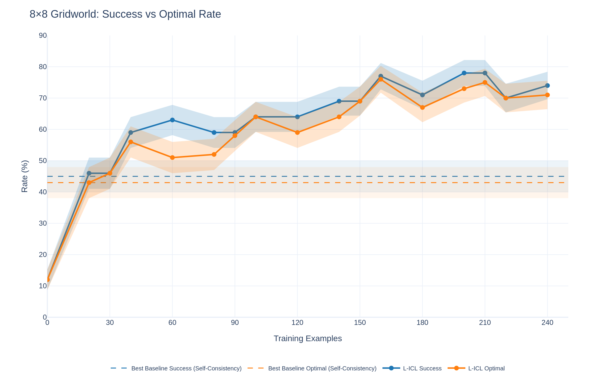8 $×$ 8 Gridworld. The complete failure of zero-shot prompting (0%) on this simple two-room task is striking: the model receives full information about walls, start, and goal, yet fails completely. This reveals that the bottleneck is not knowledge but application. L-ICL achieves 63% success, demonstrating that localized corrections bridge this gap. Figure 2 shows rapid improvement in the first 30 examples, with continued gains for $≈$ 160 examples before plateauing. 10 $×$ 10 Maze. The maze’s narrow corridors and longer optimal paths (15–25 steps) challenge all methods. L-ICL reaches 27% success where baselines achieve at most 5%. Notably, valid rates reach 57%, indicating that most L-ICL plans respect maze constraints even when they fail to reach the goal. This valid-to-success gap suggests that constraint satisfaction and goal-directed search are separable challenges; L-ICL addresses the former effectively. Sokoban Grid. Despite adopting Sokoban’s richer spatial structure, this domain (without pushable boxes) yields results intermediate between the prior domains: L-ICL achieves 49% success versus 13% for the best baseline. The similarity suggests that spatial complexity, not action vocabulary, dominates difficulty in navigation tasks. Full Sokoban. Introducing pushable boxes causes the sharpest performance degradation across all methods. L-ICL improves success from 13% to only 20%, yet increases valid action rates from 19% to 46%. This dissociation isolates multi-object state tracking as a distinct challenge: L-ICL teaches which pushes are legal, but coordinating agent and box positions toward the goal requires capabilities beyond constraint satisfaction, furhter analyzed in Appendix A. BlocksWorld. This domain differs qualitatively: constraints are relational (“block A is on block B”) rather than spatial, and every object is dynamic. L-ICL still improves success from 48% to 66%, demonstrating that localized corrections generalize beyond navigation. <details> <summary>graphs/misc/8x8_nogrid_success_optimal_combined.png Details</summary>  ### Visual Description ## Line Chart: 8×8 Gridworld: Success vs Optimal Rate ### Overview The image displays a line chart comparing the performance of two methods ("L-ICL Success" and "L-ICL Optimal") against two baseline benchmarks over an increasing number of training examples. The chart tracks two metrics—Success Rate and Optimal Rate—measured as percentages. The data shows a general upward trend for the L-ICL methods, with performance surpassing the static baselines after approximately 30 training examples. ### Components/Axes * **Title:** "8×8 Gridworld: Success vs Optimal Rate" (Top-left corner). * **Y-Axis:** Labeled "Rate (%)". Scale ranges from 0 to 90, with major tick marks at intervals of 10 (0, 10, 20, ..., 90). * **X-Axis:** Labeled "Training Examples". Scale ranges from 0 to 240, with major tick marks at intervals of 30 (0, 30, 60, ..., 240). * **Legend:** Positioned at the bottom center of the chart. It contains four entries: 1. `--` **Best Baseline Success (Self-Consistency)**: A dashed blue line. 2. `--` **Best Baseline Optimal (Self-Consistency)**: A dashed orange line. 3. `●-` **L-ICL Success**: A solid blue line with circular markers. 4. `●-` **L-ICL Optimal**: A solid orange line with circular markers. * **Data Series & Confidence Intervals:** Each solid line (L-ICL) is accompanied by a shaded region of the same color, representing a confidence interval or variance band around the mean performance. ### Detailed Analysis **Trend Verification & Data Points (Approximate):** * **L-ICL Success (Blue Line with Markers):** * **Trend:** Shows a steep initial increase, followed by a generally upward but fluctuating trend. It consistently remains above the L-ICL Optimal line. * **Key Points:** * At 0 examples: ~12% * At 30 examples: ~46% * At 60 examples: ~63% * At 120 examples: ~64% * At 150 examples: ~69% * At 165 examples (peak): ~77% * At 180 examples: ~71% * At 210 examples: ~78% * At 240 examples: ~74% * **L-ICL Optimal (Orange Line with Markers):** * **Trend:** Follows a very similar trajectory to the Success line but is consistently a few percentage points lower. Also shows an initial steep rise and subsequent fluctuations. * **Key Points:** * At 0 examples: ~12% * At 30 examples: ~43% * At 60 examples: ~51% * At 120 examples: ~59% * At 150 examples: ~64% * At 165 examples (peak): ~76% * At 180 examples: ~67% * At 210 examples: ~75% * At 240 examples: ~71% * **Best Baseline Success (Dashed Blue Line):** * **Trend:** Horizontal, constant line. * **Value:** Approximately 45% across all training examples. * **Best Baseline Optimal (Dashed Orange Line):** * **Trend:** Horizontal, constant line. * **Value:** Approximately 43% across all training examples. **Confidence Intervals (Shaded Regions):** * The shaded bands for both L-ICL lines are narrow at low training example counts (0-30) and widen significantly as the number of examples increases, particularly beyond 90 examples. This indicates greater variance or uncertainty in performance with more training data. * The blue shaded region (Success) is generally wider than the orange one (Optimal) at higher example counts. ### Key Observations 1. **Performance Crossover:** Both L-ICL methods surpass their respective baselines after approximately 30 training examples. 2. **Metric Hierarchy:** The "Success" rate is consistently higher than the "Optimal" rate for the L-ICL method, which is logically consistent if "Optimal" represents a stricter performance criterion. 3. **Plateau and Fluctuation:** After the initial rapid learning phase (0-60 examples), performance gains slow and exhibit noticeable fluctuations (e.g., dips at 180 examples), though the overall trend remains positive. 4. **Peak Performance:** Both L-ICL metrics appear to peak around 165-210 training examples before a slight decline at 240. 5. **Baseline Comparison:** The static baselines (Self-Consistency) are outperformed by the L-ICL approach with sufficient data, suggesting the latter is a more effective learning method in this context. ### Interpretation The chart demonstrates the learning curve of an "L-ICL" (likely "Learning from In-Context Learning") approach on an 8x8 Gridworld task. The key takeaway is that L-ICL is data-efficient, quickly exceeding strong baseline performance with only ~30 examples. The continued, albeit noisy, improvement up to ~210 examples suggests the method benefits from more data, though returns diminish and variance increases. The consistent gap between "Success" and "Optimal" rates implies that while the agent often succeeds in reaching a goal (Success), it less frequently finds the most efficient or correct path (Optimal). The widening confidence intervals could indicate that with more diverse training examples, the model's performance becomes less predictable—some runs excel while others struggle, increasing the variance. This chart would be critical for a researcher to determine the optimal amount of training data to collect and to understand the reliability (via confidence intervals) of the L-ICL method at different data scales. </details> Figure 2: 8 $×$ 8 Gridworld learning curves. Success and Optimal rates vs. training examples. L-ICL (without being given the ASCII grid) improves rapidly in the first 30–60 examples, substantially outperforming all baselines, which are given access to the ASCII grid (horizontal line shows best baseline). 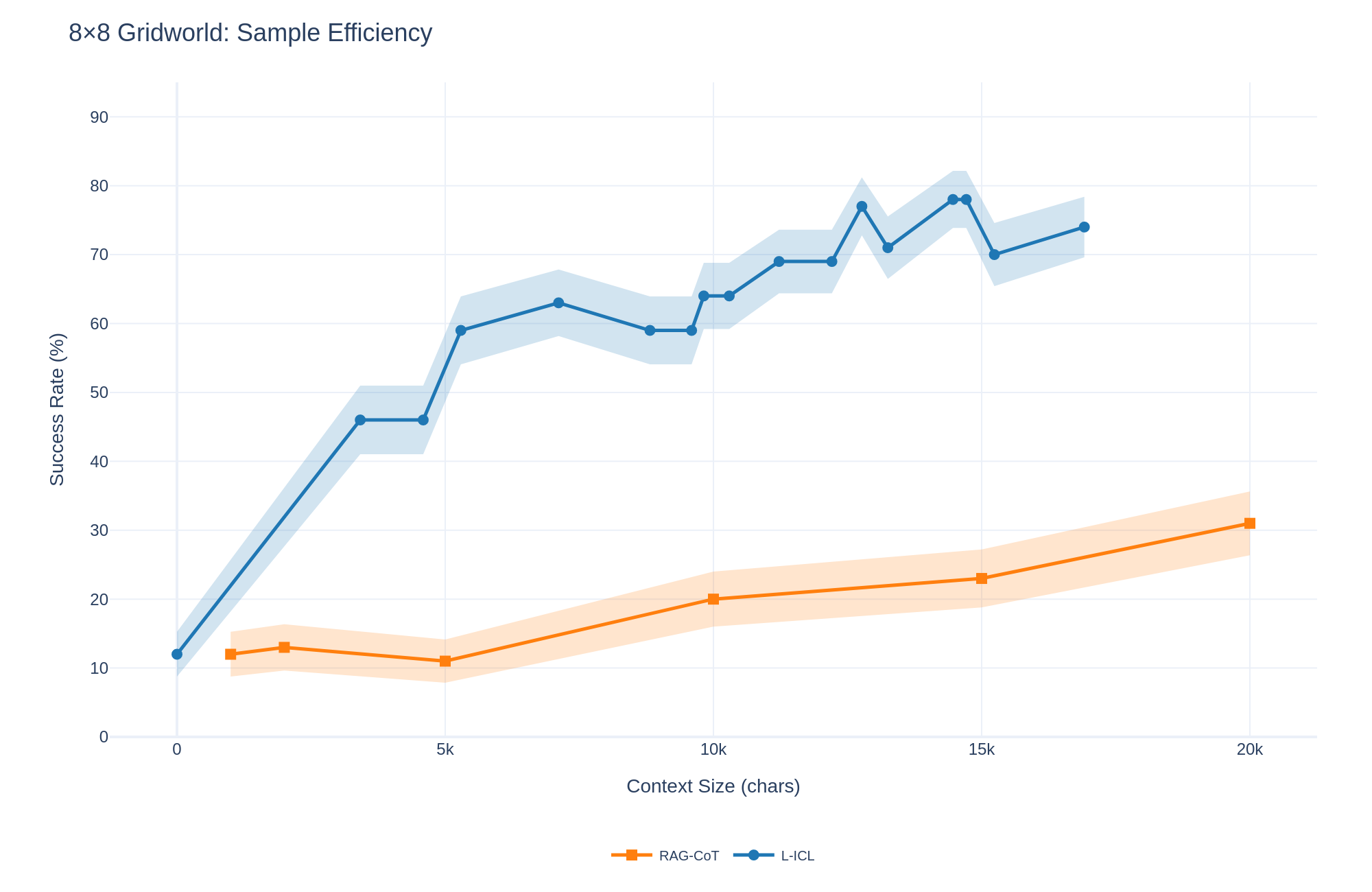### 4.2 L-ICL Is More Efficient Than Retrieval-Based ICL A key advantage of L-ICL is sample efficiency: localized corrections convey more information per token than complete solution trajectories. Figure 3 compares L-ICL and RAG-ICL as a function of context size. RAG-ICL with 20,000 characters of retrieved trajectories achieves 16% success. L-ICL matches this performance with approximately 5,000 characters and reaches 63% success with 7,000 characters. At matched context size, L-ICL outperforms RAG-ICL by 40+ percentage points. This efficiency stems from the compression achieved by localized examples. A complete trajectory demonstrates that a solution works but leaves implicit why individual steps are valid. A local example like get_applicable_actions((3,4)) -> [’move_north’,’move_south’] directly encodes that eastward movement from (3,4) is blocked. <details> <summary>graphs/efficiency/8x8_grid_nogrid_efficiency.png Details</summary>  ### Visual Description ## Line Chart: 8×8 Gridworld: Sample Efficiency ### Overview The image is a line chart comparing the sample efficiency of two methods, "RAG-CoT" and "L-ICL," in an 8x8 Gridworld environment. The chart plots the success rate (in percentage) against the context size (in characters). Both lines include shaded regions representing confidence intervals or variance. ### Components/Axes * **Title:** "8×8 Gridworld: Sample Efficiency" (Top-left, dark blue text). * **Y-Axis:** Labeled "Success Rate (%)". The scale runs from 0 to 90, with major gridlines at intervals of 10 (0, 10, 20, 30, 40, 50, 60, 70, 80, 90). * **X-Axis:** Labeled "Context Size (chars)". The scale has labeled tick marks at 0, 5k, 10k, 15k, and 20k. The "k" denotes thousands. * **Legend:** Positioned at the bottom center of the chart. * **RAG-CoT:** Represented by an orange line with square markers (■). * **L-ICL:** Represented by a blue line with circular markers (●). * **Data Series:** Two lines with associated shaded confidence bands. * **L-ICL (Blue Line):** Starts low, rises steeply, then continues a generally upward but more variable trend. * **RAG-CoT (Orange Line):** Starts low, shows a slight initial dip, then follows a slow, steady upward trend. ### Detailed Analysis **L-ICL (Blue Line with Circles):** * **Trend:** Shows a rapid initial improvement followed by a continued, though more volatile, upward trend. The confidence band (light blue shading) is relatively wide, indicating higher variance in performance. * **Approximate Data Points:** * At 0 chars: ~12% success rate. * At ~3.5k chars: ~46%. * At 5k chars: ~46%. * At ~7k chars: ~63%. * At ~9k chars: ~59%. * At ~10k chars: ~64%. * At ~11.5k chars: ~69%. * At ~12.5k chars: ~69%. * At ~13.5k chars: ~77% (local peak). * At ~14k chars: ~71%. * At ~15k chars: ~78% (highest point on the chart). * At ~15.5k chars: ~78%. * At ~16k chars: ~70%. * At ~17k chars: ~74%. **RAG-CoT (Orange Line with Squares):** * **Trend:** Shows a very gradual, almost linear increase after an initial plateau/dip. The confidence band (light orange shading) is narrower than L-ICL's, suggesting more consistent but lower performance. * **Approximate Data Points:** * At ~1k chars: ~12%. * At ~2k chars: ~13%. * At 5k chars: ~11% (slight dip). * At 10k chars: ~20%. * At 15k chars: ~23%. * At 20k chars: ~31%. ### Key Observations 1. **Performance Gap:** L-ICL consistently and significantly outperforms RAG-CoT across all measured context sizes greater than zero. The gap widens as context size increases. 2. **Efficiency:** L-ICL achieves a high success rate (~46%) with a relatively small context size (~3.5k chars), whereas RAG-CoT requires the full 20k chars to reach just ~31%. 3. **Volatility vs. Stability:** L-ICL's performance is more volatile (evidenced by the jagged line and wider confidence band), while RAG-CoT's improvement is slow and stable. 4. **Peak Performance:** The highest success rate shown is approximately 78% by L-ICL at a context size of around 15k chars. ### Interpretation The data demonstrates a clear advantage for the L-ICL method over RAG-CoT in terms of sample efficiency for the 8x8 Gridworld task. L-ICL learns much faster from the provided context, reaching high performance levels with less data. However, its performance is less predictable, as shown by the larger confidence intervals. RAG-CoT, while more stable, is significantly less efficient, requiring substantially more context to achieve modest gains. This suggests that for this specific task, leveraging in-context learning (L-ICL) is a more powerful approach than the retrieval-augmented chain-of-thought (RAG-CoT) method, especially when context window size is a resource to be optimized. The volatility in L-ICL might indicate sensitivity to the specific examples retrieved or the ordering within the context. The chart implies a trade-off: choose L-ICL for higher potential performance and efficiency, or RAG-CoT for more predictable, albeit lower, returns. </details> Figure 3: Sample efficiency: L-ICL vs. RAG-ICL. Success rate vs. context size (characters) on 8 $×$ 8 Gridworld. L-ICL achieves higher performance with substantially less context. ### 4.3 L-ICL Does Not Need Full Domain Knowledge In Table 4, in the tasks aside from BlocksWorld, all prompting schemes use an ASCII grid visualization of the gridworld to be explored (preliminary experiments suggested this approach was most effective for these tasks.) Since L-ICL learns to correct domain violations, a natural question is whether the ASCII grid is actually necessary for it: can it learn the domain from examples alone? 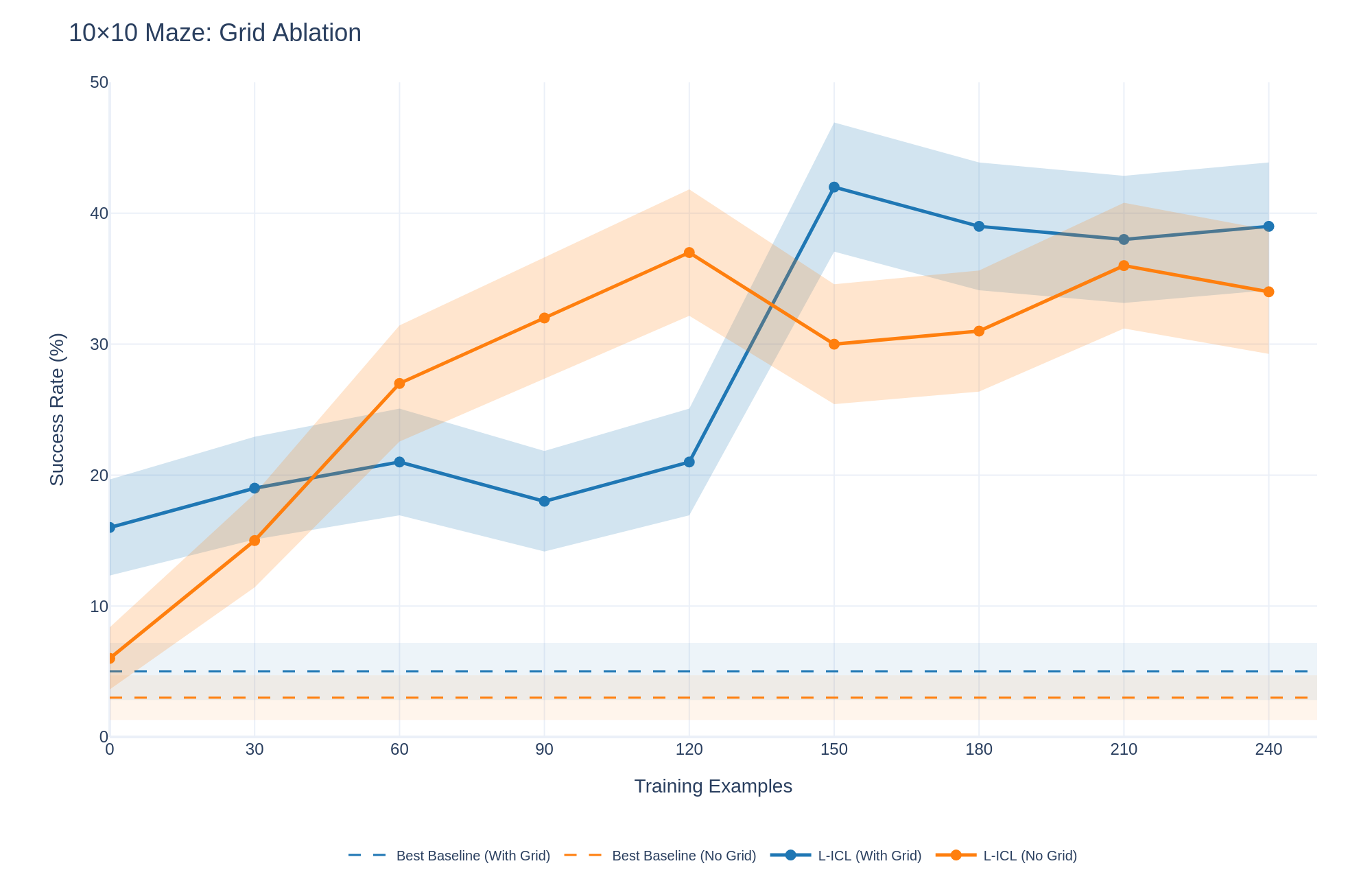Figure 4 shows the learning curve for L-ICL on the 10x10 grid task with and without the ASCII visualization of the grid. The visualization accelerates performance early on (21% at $m{=}30$ with grid vs. 15% without), but peak performance is comparable (39% vs. 37%). Thus, L-ICL does not require visual scaffolding, although the grid provides useful inductive bias during early training. However, to obtain the full benefit of such scaffolding, the LLM requires some L-ICL training; with more examples being needed for more complex domains. Thus, the 8 $×$ 8 grid almost immediately benefits, whereas all harder domains only display the benefit of the scaffolded version over the non-scaffolded version later on in their training, as seen in the figure. <details> <summary>graphs/misc/10x10_maze_grid_ablation.png Details</summary>  ### Visual Description ## Line Graph with Confidence Intervals: 10×10 Maze: Grid Ablation ### Overview This image is a line graph titled "10×10 Maze: Grid Ablation." It plots the "Success Rate (%)" of different methods against the number of "Training Examples" used. The graph compares two main approaches (L-ICL and a Best Baseline) under two conditions each ("With Grid" and "No Grid"), showing both the mean performance (lines) and the variability (shaded confidence intervals). ### Components/Axes * **Title:** "10×10 Maze: Grid Ablation" (top-left). * **Y-Axis:** Labeled "Success Rate (%)". Scale runs from 0 to 50, with major tick marks at 0, 10, 20, 30, 40, and 50. * **X-Axis:** Labeled "Training Examples". Scale runs from 0 to 240, with major tick marks at 0, 30, 60, 90, 120, 150, 180, 210, and 240. * **Legend:** Located at the bottom center. It defines four data series: 1. `-- Best Baseline (With Grid)` (Blue dashed line) 2. `-- Best Baseline (No Grid)` (Orange dashed line) 3. `●- L-ICL (With Grid)` (Blue solid line with circle markers) 4. `●- L-ICL (No Grid)` (Orange solid line with circle markers) * **Data Series & Shading:** Each solid line (L-ICL) is accompanied by a semi-transparent shaded area of the same color, representing the confidence interval or variance around the mean. ### Detailed Analysis **1. Baseline Methods (Dashed Lines):** * **Trend:** Both baseline methods show a flat, constant performance across all training example counts. * **Values:** * `Best Baseline (With Grid)`: Maintains a success rate of approximately **5%**. * `Best Baseline (No Grid)`: Maintains a lower success rate of approximately **3%**. **2. L-ICL (With Grid) - Blue Solid Line:** * **Trend:** Shows a general upward trend with a notable, sharp increase between 120 and 150 training examples. After peaking, performance slightly declines and stabilizes. * **Data Points (Approximate):** * 0 examples: ~16% * 30 examples: ~19% * 60 examples: ~21% * 90 examples: ~18% (a slight dip) * 120 examples: ~21% * **150 examples: ~42% (sharp peak)** * 180 examples: ~39% * 210 examples: ~38% * 240 examples: ~39% * **Confidence Interval (Blue Shading):** The interval is relatively narrow for lower training examples (0-120) but expands dramatically after the 150-example mark, indicating significantly higher variance in performance once the method achieves higher success rates. **3. L-ICL (No Grid) - Orange Solid Line:** * **Trend:** Shows a steady, strong upward trend until 120 examples, followed by a drop and then a more variable, fluctuating performance. * **Data Points (Approximate):** * 0 examples: ~6% * 30 examples: ~15% * 60 examples: ~27% * 90 examples: ~32% * **120 examples: ~37% (peak for this series)** * 150 examples: ~30% (drop) * 180 examples: ~31% * 210 examples: ~36% * 240 examples: ~34% * **Confidence Interval (Orange Shading):** The interval widens as performance increases, showing growing variance, particularly after the 60-example mark. ### Key Observations 1. **L-ICL Superiority:** Both L-ICL variants dramatically outperform their respective baselines once trained on more than ~30 examples. 2. **Critical Threshold at 120-150 Examples:** The `L-ICL (With Grid)` method exhibits a phase-change-like jump in performance between 120 and 150 training examples, suggesting a possible critical data threshold for learning. 3. **Grid Information Impact:** The "With Grid" condition leads to a higher ultimate peak success rate (~42% vs. ~37%) but appears to require more data to trigger its major improvement. The "No Grid" condition learns more steadily initially but plateaus at a lower level and becomes less stable. 4. **Increased Variance with Performance:** For both L-ICL methods, higher success rates are correlated with wider confidence intervals, indicating that as the models become more capable, their performance becomes more sensitive to specific training examples or random seeds. ### Interpretation This graph demonstrates the effectiveness of the L-ICL (likely "Learning with In-Context Learning") approach for solving 10x10 maze tasks compared to a static baseline. The core finding is that **L-ICL can learn to solve mazes from examples, and its performance is heavily influenced by both the quantity of training data and the presence of structural (grid) information.** The data suggests a complex relationship: * **Grid information acts as a powerful but potentially slower-to-learn scaffold.** It enables a higher performance ceiling but may require the model to first learn how to utilize the grid structure effectively, explaining the delayed but dramatic improvement. * **Without grid information, the model learns a more direct but ultimately less optimal policy,** leading to faster initial gains that plateau earlier. * The **high variance at higher performance levels** is a critical observation. It implies that while the L-ICL method is powerful, its success on any given maze instance may be unreliable, pointing to a need for methods that can reduce this variance, perhaps through ensemble techniques or more robust training. In summary, the ablation study shows that for complex spatial reasoning tasks like maze-solving, **in-context learning is a viable paradigm, but its success is contingent on sufficient training data and is significantly enhanced by providing structured environmental cues (the grid), albeit with a trade-off in initial learning speed and final stability.** </details> Figure 4: Grid representation ablation on 10 $×$ 10 Maze. The ASCII grid accelerates early learning but does not change peak performance. Without L-ICL, the grid provides little benefit. 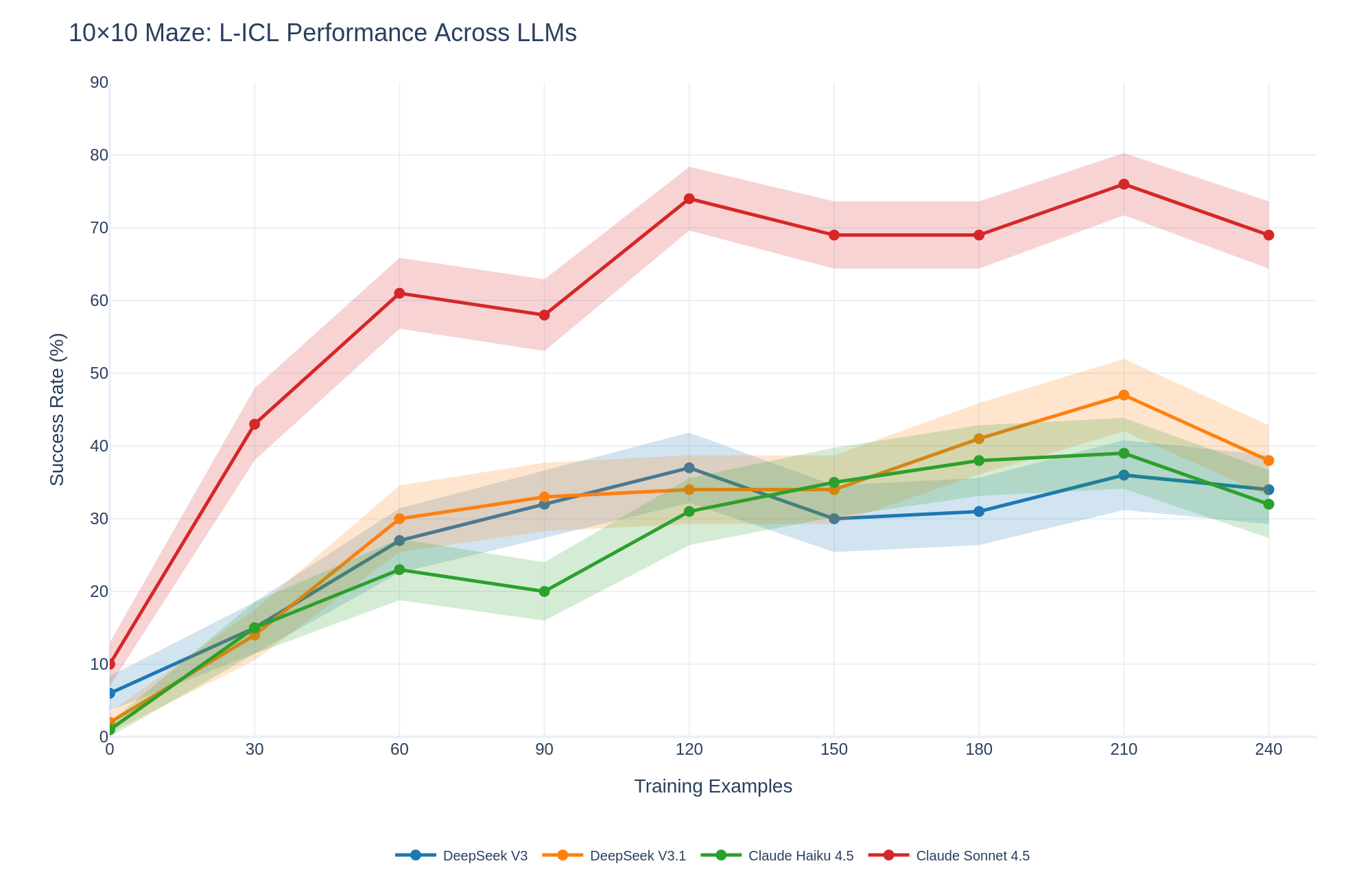### 4.4 L-ICL Works On Many LLM Architectures To assess whether L-ICL’s benefits are architecture-specific, we evaluate on three additional models: DeepSeek V3.1, Claude 4.5 Haiku, and Claude Sonnet 4.5. Figure 5 shows results on the 10 $×$ 10 Maze. All models improve substantially with L-ICL. Claude Sonnet 4.5 shows the strongest gains (10% to 74%), followed by DeepSeek V3.1 (2% to 47%) and Claude 4.5 Haiku (1% to 39%). The relative ordering changes with training: at $m{=}0$ models are comparable, but by $m{=}120$ Claude Sonnet 4.5 leads substantially. This suggests stronger models leverage accumulated corrections more effectively, though all models benefit. <details> <summary>graphs/misc/llm_ablation_success.png Details</summary>  ### Visual Description ## Line Chart: 10×10 Maze: L-ICL Performance Across LLMs ### Overview This is a line chart comparing the performance of four Large Language Models (LLMs) on a 10×10 maze-solving task using Learning from In-Context Examples (L-ICL). The chart plots the success rate percentage against the number of training examples provided. Each model's performance is represented by a colored line with markers, accompanied by a shaded region indicating variability or confidence intervals. ### Components/Axes * **Title:** "10×10 Maze: L-ICL Performance Across LLMs" (Top-left corner). * **Y-Axis:** Labeled "Success Rate (%)". Scale ranges from 0 to 90, with major gridlines at intervals of 10. * **X-Axis:** Labeled "Training Examples". Scale shows discrete points at 0, 30, 60, 90, 120, 150, 180, 210, and 240. * **Legend:** Located at the bottom center of the chart. It maps line colors and markers to model names: * **Blue line with circle markers:** DeepSeek V3 * **Orange line with circle markers:** DeepSeek V3.1 * **Green line with circle markers:** Claude Haiku 4.5 * **Red line with circle markers:** Claude Sonnet 4.5 * **Data Series:** Four lines, each with a shaded band of the same color representing the range of performance (likely standard deviation or confidence interval). ### Detailed Analysis **Trend Verification & Data Point Extraction (Approximate Values):** 1. **Claude Sonnet 4.5 (Red Line):** * **Trend:** Shows the steepest initial improvement and maintains the highest performance throughout. The trend is strongly upward from 0 to 120 examples, followed by a plateau with minor fluctuations. * **Data Points:** 0 examples: ~10% | 30: ~43% | 60: ~61% | 90: ~58% | 120: ~74% | 150: ~69% | 180: ~69% | 210: ~76% | 240: ~69%. 2. **DeepSeek V3.1 (Orange Line):** * **Trend:** Shows steady improvement, peaking at 210 examples before a decline. It generally performs second-best after the initial training phase. * **Data Points:** 0 examples: ~2% | 30: ~14% | 60: ~30% | 90: ~33% | 120: ~34% | 150: ~34% | 180: ~41% | 210: ~47% | 240: ~38%. 3. **DeepSeek V3 (Blue Line):** * **Trend:** Improves until 120 examples, experiences a notable dip at 150, then recovers slowly. It ends with performance similar to Claude Haiku 4.5. * **Data Points:** 0 examples: ~6% | 30: ~15% | 60: ~27% | 90: ~32% | 120: ~37% | 150: ~30% | 180: ~31% | 210: ~36% | 240: ~34%. 4. **Claude Haiku 4.5 (Green Line):** * **Trend:** Shows a general upward trend with a slight dip at 90 examples. It closely tracks DeepSeek V3 in the later stages. * **Data Points:** 0 examples: ~1% | 30: ~15% | 60: ~23% | 90: ~20% | 120: ~31% | 150: ~35% | 180: ~38% | 210: ~39% | 240: ~32%. **Spatial Grounding & Variability:** * The shaded confidence bands are widest for Claude Sonnet 4.5, indicating higher variance in its performance across different runs or samples. * The bands for the other three models are narrower and overlap significantly between 30 and 120 training examples, suggesting similar performance uncertainty in that range. * At 240 examples, the performance of all models except Claude Sonnet 4.5 converges within a ~6% range (approximately 32%-38%). ### Key Observations 1. **Dominant Performance:** Claude Sonnet 4.5 is the clear top performer, achieving a success rate over 20 percentage points higher than the next best model at its peak (120 examples). 2. **Learning Curves:** All models benefit from increased training examples, but the rate of improvement (slope) is most dramatic for Claude Sonnet 4.5 between 0 and 60 examples. 3. **Performance Plateaus/Dips:** Several models show performance dips or plateaus (e.g., Claude Sonnet at 90 & 150, DeepSeek V3 at 150, Claude Haiku at 90). This could indicate points where additional examples temporarily confuse the model or where the task complexity interacts with the model's learning capacity. 4. **Final Convergence:** By 240 examples, the performance gap between the three lower-performing models narrows considerably, while Claude Sonnet 4.5 remains in a distinctly higher tier. ### Interpretation The data demonstrates a significant disparity in the in-context learning capabilities of the tested LLMs for a spatial reasoning task (maze solving). **Claude Sonnet 4.5 exhibits a superior ability to leverage provided examples to solve novel mazes**, suggesting a more robust internal representation or more effective learning algorithm for this type of problem. The general upward trend for all models confirms the efficacy of the L-ICL approach—more examples lead to better performance. However, the non-monotonic curves (dips and plateaus) are critical findings. They suggest that learning is not linear and that there may be "confusion points" where the model's hypothesis space becomes too complex or where it overfits to certain example patterns before generalizing better with even more data. The narrower confidence intervals for DeepSeek models and Claude Haiku might indicate more consistent, if lower-ceiling, performance. In contrast, Claude Sonnet 4.5's wider bands suggest higher potential reward but also higher variability, which could be important for reliability-critical applications. **In summary, this chart provides strong evidence that model architecture or training methodology has a profound impact on few-shot learning performance for spatial tasks, with Claude Sonnet 4.5 being the most effective learner in this specific benchmark.** </details> Figure 5: L-ICL across LLM architectures. Success rate on 10 $×$ 10 Maze for four models. All improve substantially; Claude Sonnet 4.5 shows the largest gains (10% $→$ 74%). ### 4.5 Summary of Findings (1) L-ICL dramatically improves constraint adherence, achieving consistently higher success rates than baselines across all domains. (2) L-ICL is sample-efficient: 30–90 training examples typically suffice, and L-ICL outperforms RAG-ICL while using 4 $×$ less context. (3) Explicit spatial representations are not required: ASCII grids accelerate early learning but do not change peak performance. (4) L-ICL generalizes across architectures: four LLMs from different families all benefit substantially. (5) Multi-object tracking and strategic planning remain challenging: the valid-to-success gap in Sokoban and BlocksWorld indicates that localized corrections address constraint violations but do not fully solve long-horizon coordination (see Appendix A). ## 5 Discussion Our experiments demonstrate that L-ICL consistently improves LLM planning performance, often by substantial margins. Beyond raw performance gains, these results support a specific conceptual interpretation that clarifies both what L-ICL achieves and where challenges remain. ### 5.1 L-ICL as In-Context Unit Testing In software engineering, unit testing is a means of “hardening” code subroutines (i.e., making them more reliable and predictable), and it is considered good practice to use unit tests even when end-to-end tests exist. ICL demonstrations instruct a model as to desired behavior, rather than confirming that it has a desired behavior; modulo this important difference, however, L-ICL demonstrations are analogous to unit tests, and traditional ICL demonstrations are analogous to end-to-end tests. L-ICL demonstrations can be viewed as a technique for “hardening” individual reasoning steps, in that they makes an LLM’s instruction-following behavior more reliable and consistent. Full-trajectory demonstrations are more like end-to-end tests; in software engineering, these tests have a different role than unit tests, confirming that individual modules interact correctly: in LLM terms, they encourage process correctness, and only incidentally encourage step correctness. In planning tasks, an invalid plan may have many correctly perform steps and only a single invalidly performed step, so adding a full-trajectory demonstration is at best an inefficient way to improve performance, in terms of the useful information per prompt token, relative to accumulating local demonstrations in a failure-driven way. 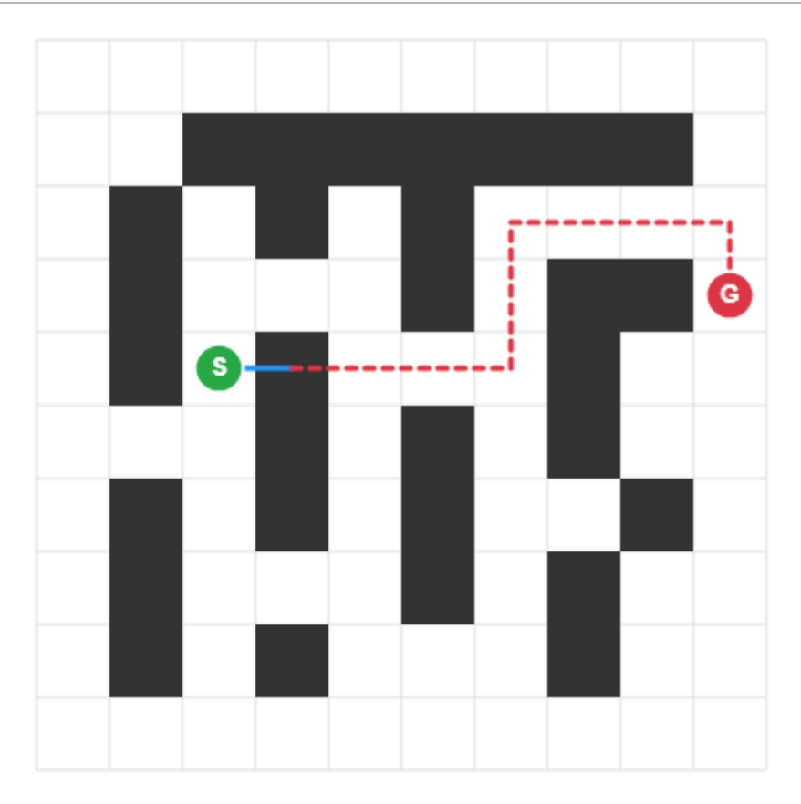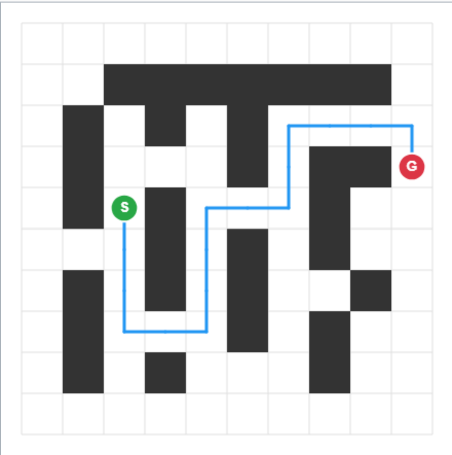### 5.2 Qualitative Evidence: From Guessing to Navigation Figure 6 provides visual evidence of L-ICL’s effect. At $m{=}0$ , the model proposes moves without regard for walls, quickly entering invalid states. By $m{=}60$ , it produces a coherent start-to-goal path respecting all walls. Crucially, this improvement occurs without the model ever seeing the ASCII grid. The doctests encode constraints implicitly through input-output pairs, and the model learns to satisfy them. This demonstrates that L-ICL induces a transferable constraint prior rather than memorizing specific layouts. <details> <summary>graphs/misc/maze_pictures/0_final.png Details</summary>  ### Visual Description ## Diagram: Grid-Based Pathfinding Visualization ### Overview The image displays a 10x10 grid-based maze or pathfinding problem. It visually represents a computed path from a starting point to a goal point, navigating around static obstacles. The diagram is a technical illustration, likely used to demonstrate the output of a pathfinding algorithm (e.g., A*, Dijkstra's) in a discrete, grid-world environment. ### Components/Axes * **Grid Structure:** A 10x10 square grid. Each cell is defined by light gray borders. * **Cell States:** * **Passable Cells:** White squares. * **Obstacle Cells:** Solid black squares. * **Key Points:** * **Start Point (S):** A green circle containing a white capital letter "S". Positioned at grid coordinates (Row 5, Column 3), counting from the top-left as (1,1). * **Goal Point (G):** A red circle containing a white capital letter "G". Positioned at grid coordinates (Row 4, Column 10). * **Path:** A red dashed line connecting the Start and Goal points, indicating the computed route. ### Detailed Analysis **1. Obstacle Map (Black Cells):** The black cells form a complex barrier pattern. Their positions (using (Row, Column) from top-left) are: * Row 2: Columns 3, 4, 5, 6, 7, 8, 9 * Row 3: Columns 2, 5, 8 * Row 4: Columns 2, 5, 8 * Row 5: Columns 4, 8 * Row 6: Columns 2, 4, 8 * Row 7: Columns 2, 4, 8, 10 * Row 8: Columns 2, 4, 8, 9 * Row 9: Columns 2, 4, 8 **2. Path Trajectory (Red Dashed Line):** The path originates from the center of the green "S" circle and terminates at the center of the red "G" circle. Its route, described segment by segment: * **Segment 1:** Moves horizontally **right** from (5,3) to (5,4). This is a short, solid blue line segment, distinct from the red dashes, possibly indicating the initial move or a different algorithm phase. * **Segment 2:** From (5,4), the red dashed line begins, moving **right** to (5,5). * **Segment 3:** Turns and moves **up** to (4,5). * **Segment 4:** Turns and moves **right** to (4,6). * **Segment 5:** Turns and moves **down** to (5,6). * **Segment 6:** Turns and moves **right** to (5,7). * **Segment 7:** Turns and moves **up** to (4,7). * **Segment 8:** Turns and moves **right** to (4,8). *Note: This cell (4,8) is a black obstacle. The path appears to go *around* it, not through it. The line visually passes above the obstacle cell, suggesting the path's waypoints are at cell centers, and the line is drawn between them, skirting the edge of the obstacle.* * **Segment 9:** From the vicinity of (4,8), the path moves **right** to (4,9). * **Segment 10:** Finally, moves **right** to the Goal at (4,10). **3. Spatial Relationships:** * The Start (S) is located in a relatively open area on the left side of the grid. * The Goal (G) is located on the far right edge. * The path must navigate a central corridor formed by vertical black columns at columns 2, 4, 5, and 8. The chosen route threads through the gap between the obstacles at columns 5 and 8. ### Key Observations * **Path Validity:** The path successfully connects S to G without passing through any black obstacle cells. It represents a valid, collision-free route. * **Path Optimality:** The path is not a straight line (which is blocked) nor the shortest possible Manhattan distance path. It includes a detour (moving up to row 4, then down to row 5, then back up to row 4) to navigate around the central obstacle cluster. This suggests it may be the shortest *unblocked* path, or the result of a specific algorithm's cost function. * **Visual Encoding:** The use of a distinct blue segment for the first move is notable. It could signify the initial step taken by an agent, a different cost, or simply a rendering artifact. * **Obstacle Density:** The obstacles are concentrated in the central and upper-left regions, creating a bottleneck that the path must circumvent. ### Interpretation This diagram is a classic representation of a **pathfinding solution in a grid world**. It demonstrates the core challenge of autonomous navigation: finding a viable route from an origin to a destination in an environment with barriers. * **What it demonstrates:** The algorithm has successfully analyzed the spatial constraints (the black obstacles) and computed a sequence of discrete moves (right, up, right, etc.) that achieves the goal. The red dashed line is the visual proof of this solution. * **Relationship between elements:** The Start and Goal define the problem's endpoints. The black cells define the problem's constraints. The red path is the solution that satisfies the constraints to connect the endpoints. The grid provides the discrete state space for the problem. * **Underlying Logic:** The path's shape reveals the algorithm's logic. It doesn't take the most direct route but instead makes strategic turns to exploit gaps in the obstacle field. The detour through row 4 is necessary to pass between the vertical barriers at columns 5 and 8. This is characteristic of algorithms like A* which use heuristics to guide search towards the goal while avoiding explored dead ends. * **Potential Context:** Such visualizations are fundamental in robotics (for mobile robot navigation), video game AI (for character pathing), and computational geometry. This specific instance could be a test case for comparing different pathfinding algorithms' efficiency and path quality. </details> <details> <summary>graphs/misc/maze_pictures/60_final.png Details</summary>  ### Visual Description ## Diagram: Grid-Based Pathfinding Maze ### Overview The image displays a 10x10 grid-based maze or pathfinding problem. It features a start point (S), a goal point (G), a series of black obstacle blocks, and a computed blue path connecting the start to the goal while navigating around the obstacles. The diagram visually represents a solution to a spatial navigation problem. ### Components/Axes * **Grid Structure:** A 10x10 square grid defined by light gray lines. The grid cells are not labeled with coordinates. * **Start Point (S):** A green circle containing a white letter "S". It is located in the left-center region of the grid. * **Goal Point (G):** A red circle containing a white letter "G". It is located on the right edge of the grid. * **Obstacles:** Solid black squares occupying specific grid cells, forming walls and barriers. * **Path:** A solid blue line tracing a route from the start point to the goal point. The path moves along the edges of the grid cells. ### Detailed Analysis **Path Trajectory:** The blue path originates at the center of the green "S" circle. Its route can be described as follows: 1. Moves vertically downward for approximately 2 grid cells. 2. Turns right (east) and moves horizontally for approximately 3 grid cells. 3. Turns upward (north) and moves vertically for approximately 3 grid cells. 4. Turns right (east) and moves horizontally for approximately 2 grid cells. 5. Turns upward (north) and moves vertically for approximately 1 grid cell. 6. Turns right (east) and moves horizontally for approximately 2 grid cells. 7. Turns downward (south) and moves vertically for approximately 1 grid cell, terminating at the center of the red "G" circle. **Obstacle Layout (Approximate Grid Positions):** The black obstacles form a complex pattern. Key clusters include: * A large, inverted "T" shape dominating the top-center. * Vertical and horizontal bars in the left and central columns. * Isolated blocks and L-shaped structures in the right-hand columns, creating a narrow corridor the path must navigate through. ### Key Observations * **Path Efficiency:** The blue path appears to be an optimal or near-optimal route. It takes the shortest possible turns to navigate the maze, suggesting it was generated by a pathfinding algorithm (e.g., A*, Dijkstra's). * **Spatial Constraints:** The path is forced into a specific, winding route due to the placement of the black obstacles. The most constricted section is in the right-center of the grid, where the path makes a tight "S" curve. * **Visual Coding:** The diagram uses high-contrast, intuitive colors: green for start (go), red for stop/goal, blue for the solution path, and black for impassable barriers. ### Interpretation This diagram is a classic representation of a **pathfinding or maze-solving algorithm's output**. It demonstrates the core challenge of navigating from point A to point B in an environment with defined obstacles. * **What it Suggests:** The image illustrates a successful computational solution to a spatial problem. The blue line is not a random scribble but the result of an algorithm evaluating possible routes and selecting one that minimizes distance or cost while adhering to the constraint of avoiding black cells. * **Relationship of Elements:** The start (S) and goal (G) define the problem's endpoints. The black obstacles define the problem's constraints or "cost map." The blue line is the solution—the sequence of moves that satisfies the constraints to connect the endpoints. * **Notable Anomalies:** There are no apparent anomalies in the path itself; it is a logical, continuous line. The maze design is non-trivial, featuring dead ends and a bottleneck, which makes the computed path non-obvious to a human glance, thereby effectively demonstrating the utility of an algorithmic approach. **In essence, this image is a visual proof-of-concept for an automated navigation system, showing its ability to find a valid route through a complex, structured environment.** </details> Figure 6: From blind guessing to structured navigation. Two rollouts on the same held-out maze as training examples $m$ increase. At $m{=}0$ (left), the model ignores walls entirely. By $m{=}60$ (right), the model produces a valid trajectory without ever seeing the grid representation, demonstrating that L-ICL induces transferable constraint knowledge. ### 5.3 Limitations and Scope One limitation is that L-ICL requires an oracle that can verify constraint satisfaction and provide correct outputs during training; however, this oracle is needed only during training —at test time, L-ICL requires a single forward pass with no external dependencies, distinguishing it from methods like ReAct with oracle feedback that require verification at inference. Extending to domains without formal specifications may require weaker supervision (learned verifiers, stronger models) that could introduce noise. A second limitation of this work is that we have only addressed one problem for LLM planners: their difficulty in correctly applying domain knowledge. LLM planners also struggle with strategic reasoning, i.e., performing valid actions in a way that quickly reaches the goal. While L-ICL excels improving validity, this does not always lead to good strategic reasoning, as shown by the valid-to-success gap in Sokoban (46% valid, 20% success). We leave to future work the question of whether localized corrections, or some extension of them, can also correct strategic failures, which seem to require multi-step lookahead, or whether L-ICL must be combined with complementary approaches such as search or value functions. A third limitation of this paper is that we consider only formally-describable planning benchmarks from the LLM planning literature. Transfer to open-ended natural-language tasks is not studied. ## 6 Conclusion We began with a puzzle: LLMs receive complete specifications of domain constraints yet routinely violate them. For example, stating that an agent cannot walk through walls is insufficient, because models do not consistently apply that information at test time. L-ICL addresses this issue in a simple way: when a constraint is violated, we add a minimal input-output example correcting that error, hence putting additional emphasis on the precise knowledge that was not applied. These minimal corrections are accumulating during training, progressively distilling behavioral knowledge from an oracle symbolic system into the prompt. The improvement is remarkable: on an 8 $×$ 8 gridworld where zero-shot prompting achieves 0% success, L-ICL reaches 89% with only 60 training examples, and L-ICL consistently outperforms other baselines across domains. One key finding is that demonstration structure matters more than quantity. L-ICL achieves higher performance with 2,000 characters of targeted corrections than RAG-ICL achieves with 20,000 characters of complete trajectories. Complete solutions demonstrate that a plan works; localized examples demonstrate why individual steps are valid. This compression explains L-ICL’s sample efficiency and suggests a broader principle: LLM reliability can be improved by making implicit knowledge explicit at the point of application. This also reduces prompt engineering burden: rather than exhaustively specifying every constraint upfront, practitioners can let L-ICL discover them through failure-driven corrections. L-ICL does not solve planning. The valid-to-success gap in Sokoban shows that respecting domain constraints is necessary but not sufficient; strategic reasoning remains challenging in this domain. We view this not as a limitation but as a clarification of scope. L-ICL provides a procedural hardening layer: a reliable foundation of constraint-satisfying primitives on which higher-level reasoning can build. Just as unit tests do not write the program but ensure its components behave correctly, L-ICL does not plan but ensures that proposed actions respect domain physics. We hope this decomposition proves useful for future work on LLM reasoning systems. ## Impact Statement This paper presents work whose goal is to advance the field of Machine Learning. There are many potential societal consequences of our work, none which we feel must be specifically highlighted here. ## References - Anthropic (2025) Claude 4.5 model family. Note: https://www.anthropic.com/claude Sonnet 4.5 released September 2025; Haiku 4.5 released October 2025 Cited by: §3.5. - T. Brown, B. Mann, N. Ryder, M. Subbiah, J. D. Kaplan, P. Dhariwal, A. Neelakantan, P. Shyam, G. Sastry, A. Askell, et al. (2020) Language models are few-shot learners. In Advances in Neural Information Processing Systems, Vol. 33, pp. 1877–1901. Cited by: §2.2. - W. Chen, X. Ma, X. Wang, and W. W. Cohen (2022) Program of thoughts prompting: disentangling computation from reasoning for numerical reasoning tasks. arXiv preprint arXiv:2211.12588. Cited by: §2.2. - C. A. Cohen and W. W. Cohen (2024) Watch your steps: observable and modular chains of thought. arXiv preprint arXiv:2409.15359. Cited by: §1, §2.2, §3.1, footnote 1. - DeepSeek-AI (2024) DeepSeek-V3 technical report. arXiv preprint arXiv:2412.19437. Cited by: §3.5. - G. Francés, M. Ramirez, and Collaborators (2018) Tarski: an AI planning modeling framework. GitHub. Note: https://github.com/aig-upf/tarski Cited by: §E.5. - L. Gao, A. Madaan, S. Zhou, U. Alon, P. Liu, Y. Yang, J. Callan, and G. Neubig (2023) PAL: program-aided language models. In International Conference on Machine Learning, pp. 10764–10799. Cited by: §2.2. - S. Hao, Y. Gu, H. Ma, J. J. Hong, Z. Wang, D. Z. Wang, and Z. Hu (2023) Reasoning with language model is planning with world model. In Proceedings of the 2023 Conference on Empirical Methods in Natural Language Processing, pp. 8154–8173. Cited by: §2.1. - M. Helmert (2006) The fast downward planning system. In Journal of Artificial Intelligence Research, Vol. 26, pp. 191–246. Cited by: §E.4.2, §E.5, §3.5. - R. Howey, D. Long, and M. Fox (2004) VAL: automatic plan validation, continuous effects and mixed initiative planning using pddl. In 16th IEEE International Conference on Tools with Artificial Intelligence, Vol. , pp. 294–301. External Links: Document Cited by: §E.4.1. - L. B. Kaesberg, J. P. Wahle, T. Ruas, and B. Gipp (2025) SPaRC: a spatial pathfinding reasoning challenge. In Proceedings of the 2025 Conference on Empirical Methods in Natural Language Processing, C. Christodoulopoulos, T. Chakraborty, C. Rose, and V. Peng (Eds.), Suzhou, China, pp. 10359–10390. External Links: Link, Document, ISBN 979-8-89176-332-6 Cited by: §2.1. - S. Kambhampati, K. Valmeekam, L. Guan, M. Verma, K. Stechly, S. Bhambri, L. Saldyt, and A. Murthy (2024) Position: llms can’t plan, but can help planning in llm-modulo frameworks. In Proceedings of the 41st International Conference on Machine Learning, ICML’24. Cited by: §2.1. - M. Katz and J. Lee (2023) K* search over orbit space for top-k planning. In Proceedings of the 32nd International Joint Conference on Artificial Intelligence (IJCAI 2023), Cited by: §E.5, §3.5. - O. Khattab, A. Singhvi, P. Maheshwari, Z. Zhang, K. Santhanam, S. Vardhamanan, S. Haq, A. Sharma, T. T. Joshi, H. Moazam, H. Miller, M. Zaharia, and C. Potts (2023) DSPy: compiling declarative language model calls into self-improving pipelines. External Links: 2310.03714, Link Cited by: §1. - J. Lee, M. Katz, and S. Sohrabi (2023) On k* search for top-k planning. In Symposium on Combinatorial Search, External Links: Link Cited by: §3.5. - L. Lehnert, S. Sukhbaatar, D. Su, Q. Zheng, P. McVay, M. Rabbat, and Y. Tian (2024) Beyond A*: better planning with transformers via search dynamics bootstrapping. arXiv preprint arXiv:2402.14083. Cited by: §1. - J. Leng, C. A. Cohen, Z. Zhang, C. Xiong, and W. W. Cohen (2025) Semi-structured llm reasoners can be rigorously audited. External Links: 2505.24217, Link Cited by: §2.2. - C. Li, J. Liang, A. Zeng, X. Chen, K. Hausman, D. Sadigh, S. Levine, L. Fei-Fei, F. Xia, and B. Ichter (2023) Chain of code: reasoning with a language model-augmented code emulator. arXiv preprint arXiv:2312.04474. Cited by: §2.2. - J. Liu, D. Shen, Y. Zhang, B. Dolan, L. Carin, and W. Chen (2022) What makes good in-context examples for GPT-3?. In Proceedings of Deep Learning Inside Out (DeeLIO 2022): The 3rd Workshop on Knowledge Extraction and Integration for Deep Learning Architectures, E. Agirre, M. Apidianaki, and I. Vulić (Eds.), Dublin, Ireland and Online, pp. 100–114. External Links: Link, Document Cited by: §2.2. - A. Madaan, N. Tandon, P. Gupta, S. Hallinan, L. Gao, S. Wiegreffe, U. Alon, N. Dziri, S. Prabhumoye, Y. Yang, S. Gupta, B. P. Majumder, K. Hermann, S. Welleck, A. Yazdanbakhsh, and P. Clark (2023) Self-refine: iterative refinement with self-feedback. In Advances in Neural Information Processing Systems, Vol. 36. Cited by: §D.1.4, §2.2. - S. Min, X. Lyu, A. Holtzman, M. Arber, M. Lewis, H. Hajishirzi, and L. Zettlemoyer (2022) Rethinking the role of demonstrations: what makes in-context learning work?. In Proceedings of the 2022 Conference on Empirical Methods in Natural Language Processing, pp. 11048–11064. Cited by: §2.2. - P. Shojaee, I. Mirzadeh, K. Alizadeh, M. Horton, S. Bengio, and M. Farajtabar (2025) The illusion of thinking: understanding the strengths and limitations of reasoning models via the lens of problem complexity. In Advances in Neural Information Processing Systems, Vol. 38. Cited by: §2.1. - K. Stechly, K. Valmeekam, and S. Kambhampati (2024) Chain of thoughtlessness? an analysis of cot in planning. In Advances in Neural Information Processing Systems, Vol. 37. Cited by: 3rd item, §F.1.3, §1, §2.1, §2.1. - K. Stechly, K. Valmeekam, and S. Kambhampati (2025) On the self-verification limitations of large language models on reasoning and planning tasks. In The Thirteenth International Conference on Learning Representations, External Links: Link Cited by: §D.1.4, §2.2. - M. Turpin, J. Michael, E. Perez, and S. R. Bowman (2023) Language models don’t always say what they think: unfaithful explanations in chain-of-thought prompting. In Thirty-seventh Conference on Neural Information Processing Systems, External Links: Link Cited by: §2.2. - K. Valmeekam, M. Marquez, S. Sreedharan, and S. Kambhampati (2023) On the planning abilities of large language models–a critical investigation. In Advances in Neural Information Processing Systems, Vol. 36. Cited by: §1, §2.1. - X. Wang, J. Wei, D. Schuurmans, Q. Le, E. Chi, S. Narang, A. Chowdhery, and D. Zhou (2023) Self-consistency improves chain of thought reasoning in language models. In International Conference on Learning Representations, Cited by: §D.1.3, §2.2. - J. Wei, X. Wang, D. Schuurmans, M. Bosma, B. Ichter, F. Xia, E. Chi, Q. Le, and D. Zhou (2022) Chain-of-thought prompting elicits reasoning in large language models. In Advances in Neural Information Processing Systems, Vol. 35, pp. 24824–24837. Cited by: §2.2. - S. Yao, D. Yu, J. Zhao, I. Shafran, T. L. Griffiths, Y. Cao, and K. Narasimhan (2023a) Tree of thoughts: deliberate problem solving with large language models. In Advances in Neural Information Processing Systems, Vol. 36. Cited by: §D.1.6, §1, §2.1, §2.2. - S. Yao, J. Zhao, D. Yu, N. Du, I. Shafran, K. Narasimhan, and Y. Cao (2023b) ReAct: synergizing reasoning and acting in language models. In International Conference on Learning Representations, Cited by: §D.1.5, §2.1, §2.2. ## Appendix A Analysis: The Valid-to-Success Gap While L-ICL dramatically improves constraint adherence, a gap often remains between validity and success. This gap is most pronounced in Full Sokoban, where L-ICL achieves 46% valid plans but only 20% success (Table 4). Understanding this gap illuminates both L-ICL’s strengths and its limitations. ### A.1 Trap Rate Analysis In Sokoban, certain states are traps: configurations from which the goal is unreachable regardless of future actions (e.g., a box pushed into a corner). We measure the adjusted trap rate: among valid plans, what fraction enters a trap state? Figure 7 shows that L-ICL reduces trap rates. On Sokoban Grid, the adjusted trap rate drops from 50% at $m{=}0$ to 10% at $m{=}210$ . This indicates that L-ICL teaches not only immediate constraint satisfaction but also some degree of trap avoidance. However, the absolute trap rate remains non-negligible, and the valid-to-success gap persists. We hypothesize that trap avoidance requires multi-step lookahead that localized corrections cannot fully provide. A correction like “pushing box B east from (3,4) is valid” does not encode that this push leads to an unsolvable configuration three moves later. Addressing this limitation may require complementary approaches such as search or learned value functions. 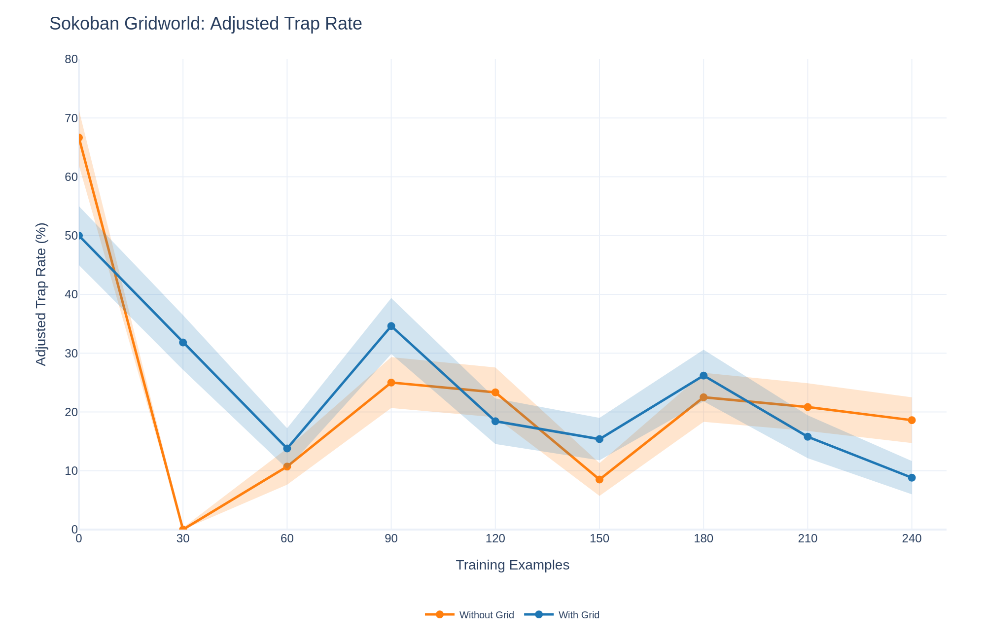<details> <summary>graphs/misc/sokoban_trap_rate_adjusted.png Details</summary>  ### Visual Description ## Line Chart: Sokoban Gridworld: Adjusted Trap Rate ### Overview This is a line chart comparing the performance of two methods ("Without Grid" and "With Grid") in a Sokoban Gridworld environment over the course of training. The performance metric is the "Adjusted Trap Rate," expressed as a percentage. The chart includes shaded regions representing confidence intervals or variability around each data point. ### Components/Axes * **Title:** "Sokoban Gridworld: Adjusted Trap Rate" (Top-left, dark blue text). * **Y-Axis:** Labeled "Adjusted Trap Rate (%)". Scale runs from 0 to 80 in increments of 10. * **X-Axis:** Labeled "Training Examples". Scale runs from 0 to 240 in increments of 30. * **Legend:** Located at the bottom center of the chart. * Orange line with circular markers: "Without Grid" * Blue line with circular markers: "With Grid" * **Data Series:** Two lines with associated shaded confidence bands. * **Orange Line ("Without Grid"):** Starts high, drops sharply, then fluctuates. * **Blue Line ("With Grid"):** Starts lower than orange, shows a more gradual overall decline with fluctuations. ### Detailed Analysis **Data Series: "Without Grid" (Orange Line)** * **Trend:** The line exhibits high volatility. It begins with the highest trap rate, plummets to near zero, then experiences a series of rises and falls, ending with a gradual decline. * **Data Points (Approximate):** * 0 Training Examples: ~67% (Highest point on the chart) * 30 Training Examples: ~0% (Lowest point on the chart) * 60 Training Examples: ~11% * 90 Training Examples: ~25% (Local peak) * 120 Training Examples: ~23% * 150 Training Examples: ~9% (Local trough) * 180 Training Examples: ~22% (Local peak) * 210 Training Examples: ~21% * 240 Training Examples: ~19% * **Confidence Interval:** The shaded orange band is widest at 0 examples, narrows significantly at 30, and remains moderately wide through the rest of the series, indicating substantial variability in performance. **Data Series: "With Grid" (Blue Line)** * **Trend:** The line shows a more consistent, though still fluctuating, downward trend. It starts lower than the "Without Grid" method and generally maintains a lower trap rate after the initial training phase, except for two notable spikes. * **Data Points (Approximate):** * 0 Training Examples: ~50% * 30 Training Examples: ~32% * 60 Training Examples: ~14% * 90 Training Examples: ~35% (Significant local peak, surpassing the "Without Grid" rate at this point) * 120 Training Examples: ~18% * 150 Training Examples: ~15% * 180 Training Examples: ~26% (Another local peak, again surpassing the "Without Grid" rate) * 210 Training Examples: ~16% * 240 Training Examples: ~9% (Lowest point for this series) * **Confidence Interval:** The shaded blue band is fairly consistent in width, with slight widening around the peaks at 90 and 180 examples. ### Key Observations 1. **Initial Performance Disparity:** At the start of training (0 examples), the "Without Grid" method has a significantly higher trap rate (~67%) compared to the "With Grid" method (~50%). 2. **Dramatic Early Drop:** The "Without Grid" method shows an extreme, near-total drop in trap rate to ~0% by 30 examples, which is the most dramatic single change in the chart. 3. **Crossover Points:** The two lines cross multiple times. Notably, the "With Grid" method has a higher trap rate at 90 and 180 training examples, creating two distinct peaks where it underperforms the "Without Grid" method. 4. **Final Convergence:** By the end of the observed training (240 examples), both methods show low trap rates, with "With Grid" (~9%) performing better than "Without Grid" (~19%). 5. **Volatility:** Both methods display non-monotonic learning curves, with performance (trap rate) worsening at several points (e.g., 90 and 180 examples) before improving again. ### Interpretation The data suggests that the inclusion of a "Grid" structure in the Sokoban learning environment has a complex, non-linear impact on the agent's tendency to fall into traps. * **Stabilizing vs. Guiding Effect:** The "With Grid" method starts with a lower trap rate and ends with the lowest overall rate, suggesting the grid provides useful structural information that aids long-term learning. However, its performance is not consistently superior, as evidenced by the spikes at 90 and 180 examples. This could indicate phases where the agent is exploring new strategies facilitated by the grid, temporarily increasing risk. * **The "Without Grid" Volatility:** The "Without Grid" method's extreme volatility—especially the crash to near 0% at 30 examples followed by a rebound—might indicate a form of rapid, brittle overfitting to early training examples. The agent may learn a very specific, narrow policy that avoids traps in the initial scenarios but fails to generalize, leading to increased trap rates as training progresses and new scenarios are introduced. * **Underlying Learning Dynamics:** The synchronized peaks at 90 and 180 examples for both methods are striking. This correlation suggests these points in training correspond to the introduction of particularly challenging levels or a shift in the training distribution that causes both agents to struggle, regardless of the grid's presence. The grid appears to mitigate the severity of these struggles somewhat (the blue peaks are lower than the surrounding orange values at those points). * **Conclusion:** The "With Grid" approach appears more robust and leads to better final performance. The "Without Grid" approach shows potential for rapid initial improvement but is unstable and less reliable over the full course of training. The chart highlights that learning in this environment is not a smooth process and is subject to significant setbacks, possibly due to curriculum changes or the inherent complexity of the Sokoban puzzle dynamics. </details> Figure 7: Trap rate decreases with L-ICL. Adjusted trap rate (fraction of valid plans entering unsolvable states) on Sokoban Grid. L-ICL reduces trap rates from 50% to 10%, indicating partial learning of strategic constraints. ### A.2 Multi-Object State Tracking Comparing Sokoban Grid (no boxes) to Full Sokoban reveals the cost of multi-object tracking. With identical spatial layouts, Sokoban Grid achieves 49% success while Full Sokoban reaches only 20%. The difference lies in state complexity: Full Sokoban requires tracking the agent position and all box positions, with constraints that depend on their joint configuration. This difficulty is also evident in BlocksWorld, where every object is dynamic. L-ICL improves BlocksWorld success from 48% to 66%, but a gap remains between validity (68%) and success. The pattern suggests that relational constraint learning, while improved by L-ICL, remains more challenging than spatial constraint learning. ### A.3 Decomposing Planning Difficulty The valid-to-success gap reveals a clean decomposition of planning difficulty: 1. Constraint satisfaction: Generating actions that respect domain physics. L-ICL addresses this effectively across all domains. 1. Strategic selection: Among valid actions, choosing those that lead toward the goal without entering traps. This requires multi-step reasoning that localized corrections do not directly provide. This decomposition suggests a practical architecture: use L-ICL to harden constraint satisfaction, then layer strategic reasoning (search, learned policies, or hierarchical planning) on top. The hardened base ensures that any action proposed by the strategic layer is physically valid, separating concerns and simplifying both components. Table 5 summarizes the valid-to-success gaps across domains, highlighting where strategic failures dominate. Table 5: Valid-to-success gap analysis across domains with L-ICL[ $m{=}60$ ]. Larger gaps indicate that constraint satisfaction alone is insufficient—strategic reasoning is the bottleneck. | 8 $×$ 8 Grid 10 $×$ 10 Maze Sokoban Grid | 89 57 63 | 89 27 49 | 0 30 14 | | --- | --- | --- | --- | | Full Sokoban | 46 | 20 | 26 | | BlocksWorld | 68 | 66 | 2 | The 8 $×$ 8 gridworld shows no gap: once constraints are satisfied, the simple structure makes goal-reaching straightforward. The 10 $×$ 10 maze and Full Sokoban show the largest gaps, reflecting the strategic complexity of navigating dead ends and avoiding irreversible trap states, respectively. BlocksWorld shows a small gap, suggesting that while relational constraints are harder to learn, once learned they suffice for task completion in our 5-block instances. 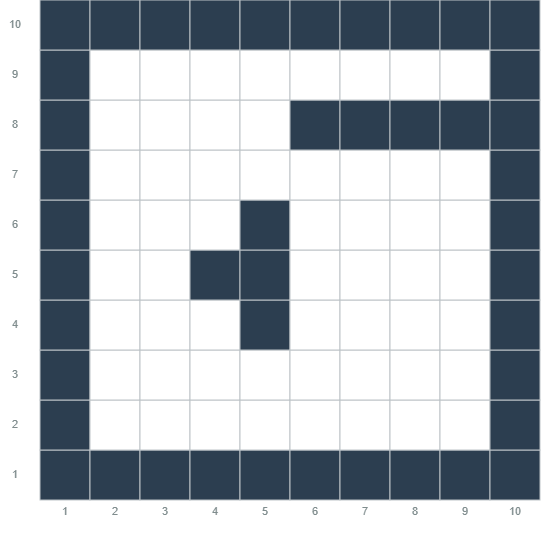## Appendix B Out-of-Distribution Generalization <details> <summary>graphs/domains/gridworld-10x10-sokoban_grid.png Details</summary>  ### Visual Description ## Diagram: 10x10 Binary Grid Matrix ### Overview The image displays a 10x10 grid or matrix. Each cell within the grid is in one of two states: filled with a dark, desaturated blue color or left white (unfilled). The grid is bounded by numbered axes on the left (vertical) and bottom (horizontal), both ranging from 1 to 10. The pattern of filled cells creates a specific, non-random configuration within the grid's border. ### Components/Axes * **Grid Structure:** A 10x10 matrix of square cells. * **Vertical Axis (Y-axis):** Labeled on the left side with numbers 1 (bottom) through 10 (top). The labels are positioned to the left of their corresponding row. * **Horizontal Axis (X-axis):** Labeled on the bottom with numbers 1 (left) through 10 (right). The labels are positioned below their corresponding column. * **Cell States:** Two states are visually present: * **Dark Fill:** A dark, desaturated blue (#2C3E50 approximate). * **White/Empty:** The default background color of the cell. * **Legend:** No explicit legend is provided. The binary nature of the grid (filled/unfilled) is implied by the visual contrast. ### Detailed Analysis The state (filled or empty) of each cell in the 10x10 grid is as follows. Coordinates are given as (Column, Row), with (1,1) at the bottom-left. * **Row 10 (Top):** All cells (1,10) through (10,10) are **FILLED**. * **Row 9:** Cells (1,9) and (10,9) are **FILLED**. Cells (2,9) through (9,9) are **EMPTY**. * **Row 8:** Cells (1,8), (6,8), (7,8), (8,8), (9,8), and (10,8) are **FILLED**. Cells (2,8) through (5,8) are **EMPTY**. * **Row 7:** Cells (1,7) and (10,7) are **FILLED**. Cells (2,7) through (9,7) are **EMPTY**. * **Row 6:** Cells (1,6), (5,6), and (10,6) are **FILLED**. Cells (2,6), (3,6), (4,6), and (6,6) through (9,6) are **EMPTY**. * **Row 5:** Cells (1,5), (4,5), (5,5), and (10,5) are **FILLED**. Cells (2,5), (3,5), and (6,5) through (9,5) are **EMPTY**. * **Row 4:** Cells (1,4), (5,4), and (10,4) are **FILLED**. Cells (2,4), (3,4), (4,4), and (6,4) through (9,4) are **EMPTY**. * **Row 3:** Cells (1,3) and (10,3) are **FILLED**. Cells (2,3) through (9,3) are **EMPTY**. * **Row 2:** Cells (1,2) and (10,2) are **FILLED**. Cells (2,2) through (9,2) are **EMPTY**. * **Row 1 (Bottom):** All cells (1,1) through (10,1) are **FILLED**. ### Key Observations 1. **Perimeter Fill:** The entire outer border of the grid (Row 1, Row 10, Column 1, Column 10) is filled, creating a solid frame. 2. **Internal Structure:** Inside the frame, filled cells form two distinct connected components: * A vertical "bar" or "stem" running from (5,4) up to (5,6), with a single filled cell attached to its left at (4,5). * A horizontal "bar" or "arm" running from (6,8) to (9,8). 3. **Symmetry:** The pattern is not symmetrical about the vertical or horizontal center lines. 4. **Density:** Out of 100 total cells, 32 are filled and 68 are empty. ### Interpretation This diagram represents a **binary matrix or bitmap**. The filled cells likely encode specific information, such as: * **A Pixel Art Glyph:** The pattern strongly resembles a stylized, blocky representation of the numeral **"5"**. The vertical stem (column 5, rows 4-6) and the horizontal top bar (row 8, columns 6-9) are characteristic features of the digit 5, enclosed within a full border. * **A Configuration Map:** It could define a layout for a game board, a memory map, or a sensor grid where "filled" indicates an active, occupied, or "on" state. * **A Logical Puzzle State:** The grid might represent the solution or a step in a logic puzzle like "Lights Out" or a cellular automaton. The primary information conveyed is the **spatial arrangement of the binary states**. The lack of a title or legend means the specific meaning of the "filled" state is context-dependent. The precise, non-random pattern suggests it is a deliberate encoding of a symbol or a specific system configuration. 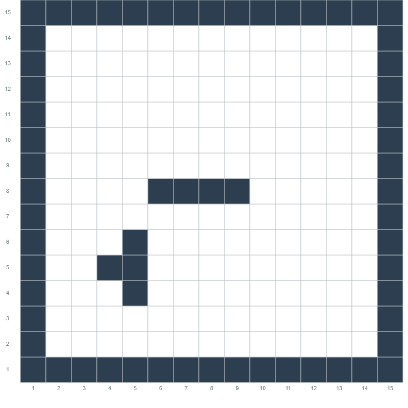</details> (a) 10 $×$ 10 maze (training distribution) <details> <summary>graphs/domains/gridworld-15x15-sokoban_grid.png Details</summary>  ### Visual Description ## Diagram: 15x15 Grid with Pixel Pattern ### Overview The image displays a 15x15 square grid. The grid is defined by thin, light gray lines on a white background. A pattern of dark blue (approximately hex #2C3E50) filled cells is present, forming a border and an internal shape. The grid has numerical labels along the bottom (x-axis) and left side (y-axis). ### Components/Axes * **Grid Structure:** A 15x15 matrix of square cells. * **X-Axis (Bottom):** Labeled with numbers 1 through 15, positioned below the grid, centered under each column. * **Y-Axis (Left):** Labeled with numbers 1 through 15, positioned to the left of the grid, centered beside each row. The numbering increases from bottom (1) to top (15). * **Color Key:** The diagram uses two colors: * **Dark Blue:** Filled cells. * **White:** Empty cells. * **Legend:** No separate legend is present. The color meaning is inferred from the visual pattern. ### Detailed Analysis The pattern consists of two distinct components: 1. **Perimeter Border:** A continuous, one-cell-thick border of dark blue cells surrounds the entire grid. This includes: * The entire bottom row (y=1, all x from 1 to 15). * The entire top row (y=15, all x from 1 to 15). * The entire leftmost column (x=1, all y from 1 to 15). * The entire rightmost column (x=15, all y from 1 to 15). 2. **Internal Shape:** A separate, contiguous shape of dark blue cells is located in the lower-left quadrant of the grid's interior. Its cells are at the following coordinates (x, y): * (4, 5) * (5, 4) * (5, 5) * (5, 6) * (6, 8) * (7, 8) * (8, 8) * (9, 8) This shape can be described as: * A vertical line of three cells at x=5 (y=4,5,6). * A single cell attached to the left of the middle of that line at (4,5). * A horizontal line of four cells at y=8 (x=6,7,8,9), positioned above and to the right of the vertical segment. ### Key Observations * The internal shape is not connected to the perimeter border. * The pattern is asymmetric. The internal shape is weighted towards the lower-left. * The horizontal segment at y=8 is the widest part of the internal shape (4 cells). * The vertical segment at x=5 is the tallest part of the internal shape (3 cells). * The grid contains no other text, labels, or annotations beyond the axis numbers. ### Interpretation This image is a pure visual representation of data on a discrete 2D grid. It does not contain quantitative data trends but rather a spatial pattern. * **What it demonstrates:** The diagram defines a specific set of coordinates (x,y) that are "active" or "filled." This is a common way to represent binary matrices, simple pixel art, game boards (like for the game "Life"), or masks for image processing. * **Relationship of elements:** The perimeter border creates a frame, isolating the internal pattern. The internal pattern itself is a single connected component (all dark blue cells are adjacent horizontally or vertically). * **Potential meaning:** Without additional context, the pattern is abstract. It could be: * A stylized letter or symbol (e.g., a rough, blocky representation of the letter 'F' or 't'). * A test pattern for a display or algorithm. * A simple maze or path configuration. * A representation of a specific dataset where (x,y) coordinates have a value of 1 (dark blue) or 0 (white). **Note on Language:** The only text present is the numerical axis labels (1-15), which are universal Arabic numerals. No other language is present in the image. </details> (b) 15 $×$ 15 maze (OOD evaluation) Figure 8: Out-of-distribution generalization setup. L-ICL corrections are accumulated on 10 $×$ 10 mazes (left) and evaluated on 15 $×$ 15 mazes (right). The larger mazes contain positions not seen during training, yet corrections transfer substantially, despite the penalty for boundary violations differing. A key question for any learning-based approach is whether acquired knowledge transfers beyond the training distribution. For L-ICL, this translates to: do corrections learned on smaller problem instances improve performance on larger, unseen instances? We investigate this by training L-ICL on 10 $×$ 10 mazes and evaluating on 15 $×$ 15 mazes, showin in Figure 8. ### B.1 Experimental Setup We accumulate L-ICL corrections using the standard training procedure on 10 $×$ 10 maze instances (Section 3.5). We then evaluate the resulting prompts on a held-out test set of 100 15 $×$ 15 mazes. The larger mazes are generated using the same procedural algorithm (randomized depth-first search) with proportionally scaled wall density, but contain positions and path structures never seen during training. ### B.2 Results Figure 9 shows that L-ICL corrections provide substantial transfer to larger instances. At $m{=}0$ (no corrections), the 15 $×$ 15 maze achieves only 9% success—comparable to the 10 $×$ 10 baseline without corrections. With corrections accumulated from 10 $×$ 10 training instances, 15 $×$ 15 success improves to 49% at $m{=}120$ , representing a 5 $×$ improvement over the no-correction baseline. 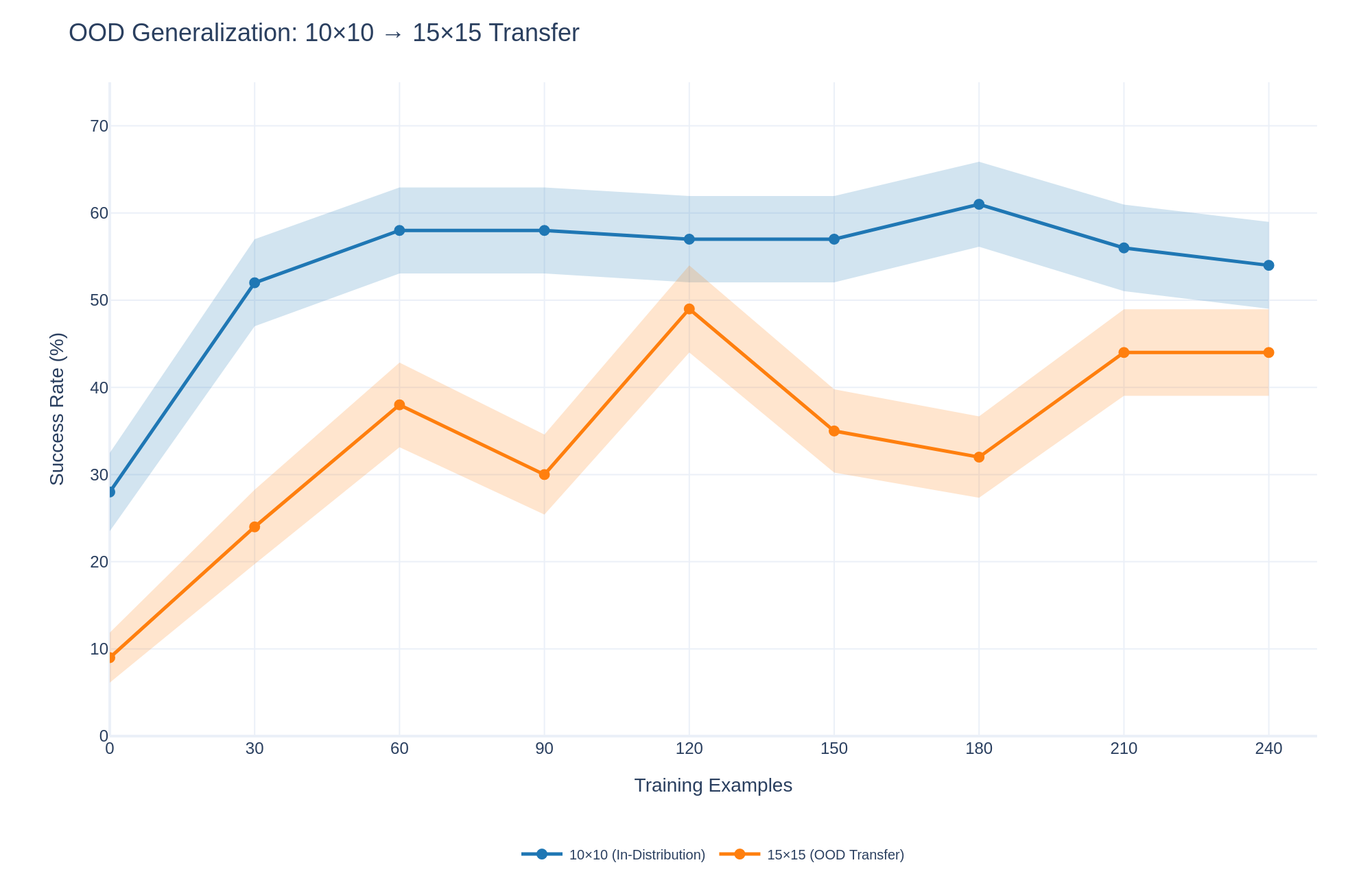<details> <summary>graphs/misc/ood_10x10_to_15x15.png Details</summary>  ### Visual Description ## Line Chart with Confidence Intervals: OOD Generalization: 10×10 → 15×15 Transfer ### Overview This is a line chart with shaded confidence intervals, illustrating the performance of a model on two related tasks as the number of training examples increases. The chart compares the model's success rate on an "in-distribution" task (10×10 grid) versus its ability to transfer that learning to an "out-of-distribution" (OOD) task (a larger 15×15 grid). ### Components/Axes * **Chart Title:** "OOD Generalization: 10×10 → 15×15 Transfer" (located at the top-left). * **X-Axis:** Labeled "Training Examples". It is a linear scale with major tick marks at 0, 30, 60, 90, 120, 150, 180, 210, and 240. * **Y-Axis:** Labeled "Success Rate (%)". It is a linear scale with major tick marks at 0, 10, 20, 30, 40, 50, 60, and 70. * **Legend:** Positioned at the bottom-center of the chart. * A blue line with circular markers is labeled "10×10 (In-Distribution)". * An orange line with circular markers is labeled "15×15 (OOD Transfer)". * **Data Series & Confidence Intervals:** Each data series is represented by a solid line connecting circular data points. A semi-transparent shaded area of the corresponding color surrounds each line, representing the confidence interval or variance around the mean performance. ### Detailed Analysis **Data Series 1: 10×10 (In-Distribution) - Blue Line** * **Trend:** The line shows a steep initial increase, followed by a plateau with minor fluctuations. It consistently remains above the orange line. * **Data Points (Approximate Success Rate %):** * 0 Training Examples: ~28% * 30: ~52% * 60: ~58% * 90: ~58% * 120: ~57% * 150: ~57% * 180: ~61% (Peak) * 210: ~56% * 240: ~54% * **Confidence Interval (Shaded Blue Area):** The interval is widest at the start (0 examples) and narrows as training examples increase, suggesting reduced variance with more data. It spans approximately ±5-8% around the mean line. **Data Series 2: 15×15 (OOD Transfer) - Orange Line** * **Trend:** The line shows an initial increase, followed by significant volatility with peaks and troughs before a final rise and plateau. It is consistently below the blue line. * **Data Points (Approximate Success Rate %):** * 0 Training Examples: ~9% * 30: ~24% * 60: ~38% * 90: ~30% (Local trough) * 120: ~49% (Local peak) * 150: ~35% * 180: ~32% * 210: ~44% * 240: ~44% * **Confidence Interval (Shaded Orange Area):** The interval is also wider at lower training counts and shows considerable width throughout, indicating higher uncertainty or variance in the OOD transfer performance compared to the in-distribution task. It spans approximately ±6-10% around the mean line. ### Key Observations 1. **Performance Gap:** There is a persistent and significant gap between in-distribution (blue) and out-of-distribution (orange) performance across all training set sizes. The model performs substantially better on the task it was trained on. 2. **Learning Curves:** Both curves show rapid initial learning (0 to 60 examples). The in-distribution curve then stabilizes, while the OOD curve is highly unstable between 60 and 180 examples before stabilizing at a higher level. 3. **Peak Performance:** The in-distribution task peaks at ~61% success with 180 examples. The OOD task's highest observed point is ~49% at 120 examples, but it ends at a stable ~44% from 210 examples onward. 4. **Volatility:** The OOD transfer performance (orange) exhibits much greater volatility, with a notable dip at 90 examples and a sharp peak at 120 examples, suggesting the transfer learning process is less stable. ### Interpretation This chart demonstrates the challenge of **out-of-distribution generalization**. The model learns the primary 10×10 task effectively, with performance quickly reaching a plateau of around 55-60% success. However, applying this learned knowledge to a larger, structurally similar 15×15 task (the OOD transfer) is markedly less effective and less reliable. The persistent gap indicates that the features or strategies learned on the smaller grid do not perfectly translate to the larger one. The volatility in the orange line suggests that with limited data, the model's ability to generalize is sensitive to the specific training examples provided. The eventual stabilization of the OOD curve at ~44% (still well below the in-distribution performance) implies that while some transfer learning occurs, it hits a ceiling. The model likely requires either more diverse training data or a different architectural approach to bridge this generalization gap more effectively. The wider confidence intervals for the OOD task further underscore the increased uncertainty inherent in making predictions on data that differs from the training distribution. </details> Figure 9: Out-of-distribution transfer: 10 $×$ 10 $→$ 15 $×$ 15. Corrections learned on 10 $×$ 10 mazes transfer to larger instances, improving success from 9% to 49%. A gap remains compared to in-distribution performance (57% on 10 $×$ 10), but transfer is substantial. Table 6 summarizes the transfer results at key checkpoints. Table 6: Out-of-distribution generalization: corrections trained on 10 $×$ 10 mazes evaluated on 15 $×$ 15 mazes. We report success rate (%) and compare to in-distribution 10 $×$ 10 performance. | Training Examples $m=0$ $m=30$ | 10 $×$ 10 (in-dist.) 16 21 | 15 $×$ 15 (OOD) 9 18 | | --- | --- | --- | | $m=60$ | 27 | 31 | | $m=120$ | 57 | 49 | ### B.3 Why Does Transfer Work? The transfer is notable because 15 $×$ 15 mazes contain positions (e.g., $(12,14)$ ) and wall configurations that never appear in 10 $×$ 10 training instances. We hypothesize that corrections transfer because they encode constraint types rather than specific positions. Consider a correction like: >>> get_applicable_actions((3, 4)) [’move_north’, ’move_south’] While this example specifies position $(3,4)$ , it implicitly teaches a general principle: when east and west are blocked (by walls or boundaries), only north and south are valid. The LLM can generalize this pattern to novel positions in larger grids. This interpretation is supported by the observation that transfer improves with more corrections ( $m$ ). Early corrections address common constraint patterns (boundary violations, simple wall configurations); as $m$ increases, rarer patterns are covered, and the accumulated examples provide a richer specification that generalizes more robustly. ### B.4 Transfer Gap Analysis While transfer is substantial, a gap remains between in-distribution and OOD performance (57% vs. 49% at $m{=}120$ ). We identify two contributing factors: 1. Unseen spatial configurations: Larger mazes contain junction types and corridor patterns that may not appear in smaller instances. Some constraint violations specific to these configurations are not addressed by 10 $×$ 10 training. 1. Longer planning horizons: 15 $×$ 15 mazes require longer plans, providing more opportunities for errors to accumulate. Even with improved per-step validity, the probability of completing an error-free trajectory decreases with plan length. These findings suggest that for maximum OOD performance, practitioners should either (a) train on a mixture of problem sizes, or (b) accept a modest performance gap when deploying to larger instances than those seen during training. ### B.5 Cross-Domain Transfer We also conducted preliminary experiments on cross-domain transfer: using corrections from one domain (e.g., 8 $×$ 8 gridworld) to improve another (e.g., 10 $×$ 10 maze). Results were mixed—corrections for basic movement constraints (boundary checking) transferred, but domain-specific spatial structures (two-room vs. maze corridors) did not. This suggests that L-ICL learns a combination of general procedural knowledge and domain-specific constraint instantiations, with only the former transferring across domains. ## Appendix C Domain Specifications This appendix provides detailed specifications of the experimental domains used in our evaluation. For each domain, we describe the state representation, action space, constraints and goal conditions. ### C.1 8 $×$ 8 Two-Room Gridworld State Space. The state consists of the agent’s $(x,y)$ position on an 8 $×$ 8 grid. Coordinates range from $(1,1)$ at the bottom-left to $(8,8)$ at the top-right. Environment Structure. The grid is divided into two rooms by a vertical wall running through column 5, with a single doorway allowing passage between rooms (doorway position varies by instance). Start positions are randomly sampled from one room, and goal positions from the other, ensuring all paths must traverse the doorway. Action Space. Four actions: move_north $(+y)$ , move_south $(-y)$ , move_east $(+x)$ , and move_west $(-x)$ . Constraints. An action is valid if and only if: 1. The resulting position remains within grid bounds. 1. The movement does not cross a wall segment. Goal Condition. The agent’s position equals the goal position. Optimal Solution. The shortest path between start and goal, computed via breadth-first search. Optimal paths typically require 8–12 steps. 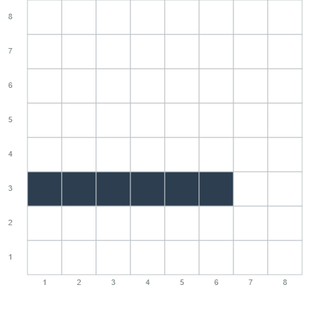<details> <summary>graphs/domains/gridworld-8x8_grid.png Details</summary>  ### Visual Description ## Horizontal Bar Chart: Single Data Point Visualization ### Overview The image displays a simple, grid-based horizontal bar chart with a single dark blue bar. The chart is presented on a white background with light gray grid lines. There are no chart titles, axis labels, or legends present. The only textual information consists of numerical markers on the X and Y axes. ### Components/Axes * **Chart Type:** Horizontal Bar Chart. * **Grid:** A square grid with major grid lines forming cells. * **X-Axis (Horizontal):** * **Label:** None present. * **Scale:** Linear, numbered from 1 to 8. * **Markers:** The numbers 1, 2, 3, 4, 5, 6, 7, 8 are positioned below the axis line, centered under their respective grid lines. * **Y-Axis (Vertical):** * **Label:** None present. * **Scale:** Linear, numbered from 1 to 8. * **Markers:** The numbers 1, 2, 3, 4, 5, 6, 7, 8 are positioned to the left of the axis line, centered beside their respective grid lines. * **Data Series:** A single horizontal bar. * **Color:** Dark blue (approximate hex: #2C3E50). * **Position:** Vertically centered on the grid line corresponding to Y=3. * **Start Point:** Aligned with the grid line for X=1. * **End Point:** Extends to a position between the grid lines for X=6 and X=7. Visually, it ends approximately 60% of the way from X=6 to X=7, suggesting a value of **~6.6**. ### Detailed Analysis * **Data Point:** The chart contains one data point represented by the length of the bar. * **Value Extraction:** The bar originates at X=1 and terminates at an approximate X-value of 6.6. Therefore, the **length or value represented is approximately 5.6 units** (6.6 - 1.0). * **Spatial Grounding:** The bar is located in the lower half of the chart, spanning horizontally across the central columns. Its vertical position is fixed at Y=3. * **Trend Verification:** As there is only one data series, no comparative trends (e.g., increasing, decreasing) can be observed. The visual "trend" is a static, horizontal line. ### Key Observations 1. **Minimalist Design:** The chart is extremely sparse, containing only the essential grid, axis numbers, and a single data bar. It lacks all descriptive metadata (title, axis labels, legend). 2. **Single Data Focus:** The visualization is designed to draw attention to one specific value or measurement. 3. **Precision Ambiguity:** The exact endpoint of the bar is not aligned with a grid line, requiring visual estimation. The value is approximate (~6.6). 4. **Language:** The only language present is numerical (Arabic numerals 1-8). ### Interpretation This image functions as a bare-bones data visualization, likely a component of a larger dashboard, a placeholder, or a simplified example. Its primary purpose is to communicate a single quantitative value (approximately 5.6 units, or an endpoint value of ~6.6) through the length of a bar against a scaled axis. The absence of context is the most significant feature. Without axis titles (e.g., "Time (seconds)", "Revenue ($M)") or a chart title, the data is abstract. The value itself is meaningless without knowing what is being measured. The choice of a horizontal bar chart is appropriate for comparing a single value against a scale, but the lack of labels prevents any real-world interpretation. **Peircean Investigative Reading:** The chart is an *icon* in the Peircean sense—it resembles the concept of a measured quantity via its length. It is also an *index* as it points to a specific value on the X-scale. However, it fails as a *symbol* because it lacks the conventional labels (language) needed to assign specific meaning to the represented quantity. The viewer can deduce *that* a value is being shown and *what* its approximate magnitude is, but not *what* it represents. The chart's existence implies an intent to communicate data, but its incompleteness renders the communication only partially successful. </details> Figure 10: Example 8 $×$ 8 two-room gridworld instance. Walls are shown as filled cells. ### C.2 10 $×$ 10 Maze State Space. The state consists of the agent’s $(x,y)$ position on a 10 $×$ 10 grid. Coordinates range from $(1,1)$ to $(10,10)$ . Environment Structure. Mazes are procedurally generated using a randomized depth-first search algorithm, producing a spanning tree of corridors with exactly one path between any two open cells. This ensures unique shortest paths and creates narrow corridors with dead ends that require backtracking if the agent makes suboptimal choices. Action Space. Four actions: move_north, move_south, move_east, move_west. Constraints. Identical to the 8 $×$ 8 gridworld: actions must keep the agent in bounds and cannot cross walls. Goal Condition. The agent’s position equals the goal position. Optimal Solution. The unique shortest path through the maze. 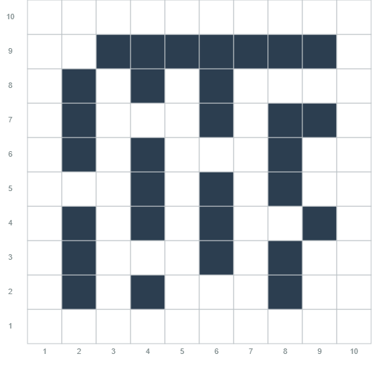<details> <summary>graphs/domains/maze_grid.png Details</summary>  ### Visual Description ## Grid Chart: Binary Pattern on 10x10 Coordinate Grid ### Overview The image displays a 10x10 grid with a Cartesian coordinate system. The grid contains a pattern of filled (dark gray) and empty (white) cells, forming a specific, non-random arrangement. There is no title, legend, or explanatory text beyond the axis numbering. ### Components/Axes - **X-Axis (Horizontal):** Labeled with integers from 1 to 10, increasing from left to right. - **Y-Axis (Vertical):** Labeled with integers from 1 to 10, increasing from bottom to top. - **Grid Cells:** Each cell is defined by an (x, y) coordinate pair. Cells are either filled with a solid dark gray color or are empty (white). ### Detailed Analysis The pattern of filled cells is described below, row by row, starting from the top (y=10) and moving down to the bottom (y=1). The column numbers (x) where cells are filled are listed for each row. * **Row y=10:** No filled cells. * **Row y=9:** Filled cells at columns x=3, 4, 5, 6, 7, 8, 9. This forms a continuous horizontal bar spanning 7 cells. * **Row y=8:** Filled cells at columns x=2, 4, 6. * **Row y=7:** Filled cells at columns x=2, 6, 8, 9. * **Row y=6:** Filled cells at columns x=2, 4, 8. * **Row y=5:** Filled cells at columns x=4, 6, 8. * **Row y=4:** Filled cells at columns x=2, 4, 9. * **Row y=3:** Filled cells at columns x=2, 6, 8. * **Row y=2:** Filled cells at columns x=2, 4, 8. * **Row y=1:** No filled cells. ### Key Observations 1. **Symmetry:** The pattern exhibits approximate vertical symmetry around the central column (x=5.5). For example, the filled cells in row y=9 (x=3-9) are symmetric. Many other rows show mirrored or near-mirrored placements (e.g., row y=8 has x=2 and x=6 filled, which are equidistant from the center). 2. **Structural Elements:** The filled cells create distinct visual components: * A solid horizontal bar at the top (y=9). * Two vertical columns on the left (primarily x=2) and right (primarily x=8) sides, extending from y=2 to y=8. * Internal vertical and horizontal segments connecting these elements, particularly in the center (x=4, x=6). 3. **Density:** The pattern is most dense in the central vertical band (columns x=4, x=6) and the outer columns (x=2, x=8). The corners (x=1, x=10) and the very top/bottom rows (y=1, y=10) are entirely empty. ### Interpretation The image is a data visualization of a binary matrix or a pixel art design on a coordinate grid. The arrangement is intentional and structured, not random noise. * **What it Suggests:** The pattern strongly resembles a stylized, symmetrical face or mask. The top bar (y=9) could represent a forehead or headband. The clusters of filled cells in rows y=8 through y=2 suggest eyes, a nose, and a mouth. The vertical columns on the sides (x=2, x=8) could be interpreted as the sides of the face or hair. * **Relationship Between Elements:** The elements are interconnected to form a cohesive figure. The symmetry creates balance, while the internal variations (e.g., the filled cell at x=9 in rows y=7 and y=4) add detail and prevent perfect mirroring, giving the figure character. * **Anomalies:** There are no data outliers in a traditional sense, as this is a categorical grid. The only "anomaly" is the slight break in perfect symmetry (e.g., row y=7 has x=9 filled but its mirror x=2 is also filled, while row y=4 has x=9 filled but its mirror x=2 is also filled, maintaining balance). This suggests a designed icon rather than a plot of empirical data. **Conclusion:** This image is best described as a **pixel art icon or symbol** plotted on a 10x10 coordinate grid. It depicts a symmetrical, face-like figure using a binary (filled/empty) cell scheme. The primary information is the spatial arrangement of the filled cells, which has been fully extracted above. </details> Figure 11: Example 10 $×$ 10 maze instance. The maze structure creates narrow corridors and dead ends, requiring longer plans than the two-room gridworld. ### C.3 Sokoban-Style Gridworld State Space. The state consists of the agent’s $(x,y)$ position on a grid that uses Sokoban-style layouts. Coordinates are 1-indexed. Environment Structure. We use grid layouts from standard Sokoban benchmarks but remove all pushable boxes. The layouts retain walls, open floor cells, and the spatial structure of Sokoban puzzles, including irregular room shapes and narrow passages. This domain serves as an ablation to isolate the effect of Sokoban’s spatial complexity from the challenge of multi-object state tracking. Action Space. Four actions: move_north, move_south, move_east, move_west. Constraints. Actions must keep the agent within the walkable floor area and cannot cross walls. Goal Condition. The agent reaches a designated goal cell. <details> <summary>graphs/domains/gridworld_sokoban_noDZ_final_grid.png Details</summary>  ### Visual Description ## Diagram: 10x10 Binary Grid Pattern ### Overview The image displays a 10x10 grid with a binary (filled/unfilled) cell pattern. The grid is bounded by a coordinate system with both the horizontal (x) and vertical (y) axes numbered from 1 to 10. The filled cells (dark gray/black) form a specific, non-random pattern against the white background cells. The overall visual resembles a stylized letter "A" or a similar glyph. ### Components/Axes * **Grid Structure:** A 10x10 square grid. * **Axes:** * **X-axis (Bottom):** Labeled with numbers 1 through 10, increasing from left to right. * **Y-axis (Left):** Labeled with numbers 1 through 10, increasing from bottom to top. * **Cell States:** Two states are present: * **Filled (Dark):** A dark gray/black color. * **Unfilled (White):** The default background color of the grid cells. * **Legend:** No explicit legend is present. The meaning of the filled vs. unfilled cells is not defined within the image. ### Detailed Analysis The pattern is constructed as follows (described from the bottom row, y=1, upwards): * **Row 1 (y=1):** All cells (x=1 to x=10) are **filled**. * **Row 2 (y=2):** Only the border cells are filled: (x=1) and (x=10). Cells x=2 through x=9 are **unfilled**. * **Row 3 (y=3):** Border cells (x=1, x=10) and the center cell (x=5) are **filled**. All others are unfilled. * **Row 4 (y=4):** Identical to Row 3: (x=1, x=5, x=10) **filled**. * **Row 5 (y=5):** Identical to Row 3: (x=1, x=5, x=10) **filled**. * **Row 6 (y=6):** Identical to Row 3: (x=1, x=5, x=10) **filled**. * **Row 7 (y=7):** Only the border cells are filled: (x=1) and (x=10). Cells x=2 through x=9 are **unfilled**. * **Row 8 (y=8):** Border cells (x=1, x=10) and a horizontal bar from x=5 to x=9 are **filled**. Specifically, cells (x=1, x=5, x=6, x=7, x=8, x=9, x=10) are filled. Cells x=2, x=3, x=4 are unfilled. * **Row 9 (y=9):** Only the border cells are filled: (x=1) and (x=10). Cells x=2 through x=9 are **unfilled**. * **Row 10 (y=10):** All cells (x=1 to x=10) are **filled**. **Spatial Summary:** The filled cells create a complete outer border (rows 1 & 10, columns 1 & 10). Inside this border, a vertical line runs up the center at column 5 from row 3 to row 6. A horizontal line connects this vertical stem to the right border at row 8, spanning columns 5 through 9. ### Key Observations 1. **Symmetry:** The pattern is symmetric about the vertical axis running through column 5.5 (the center line between columns 5 and 6). 2. **Enclosed Spaces:** The pattern creates two distinct white (unfilled) rectangular regions: * A large rectangle on the left, bounded by x=2-4 and y=2-9. * A smaller rectangle on the right, bounded by x=6-9 and y=2-7. 3. **Connectivity:** All filled cells are connected orthogonally (up, down, left, right), forming a single continuous shape. 4. **Data Density:** The grid is sparsely filled. Out of 100 total cells, 38 are filled and 62 are unfilled. ### Interpretation This image is a **visual pattern representation**, not a data chart. It conveys information through spatial arrangement rather than numerical values. * **What it demonstrates:** The grid encodes a specific 2D binary pattern. This could represent: * **Pixel Art:** A low-resolution icon or character (strongly resembling a capital "A"). * **A Binary Matrix:** A simple form of data storage or a test pattern for grid-based systems. * **A Game Board State:** A possible configuration in a grid-based game or puzzle. * **A Stencil or Mask:** A pattern for cutting or blocking material. * **Relationships:** The elements relate through geometric adjacency and containment. The border defines the field, and the internal lines define sub-regions and create the recognizable glyph. * **Notable Features:** The most salient feature is the intentional, non-random pattern that forms a universally recognizable symbol. The perfect symmetry and clean lines suggest it was digitally generated for a specific illustrative or functional purpose. The lack of a title or legend means its exact context must be inferred from its use in a larger document. </details> Figure 12: Example Sokoban-style gridworld instance. The layout is derived from a Sokoban puzzle but contains no pushable boxes, isolating spatial navigation from object manipulation. ### C.4 Full Sokoban State Space. The state consists of: - The agent’s $(x,y)$ position (1-indexed). - The box position $(x,y)$ . Our instances use 1 box. Environment Structure. Standard Sokoban puzzle layouts from established benchmarks, including walls, floor cells, and designated target locations where boxes must be placed. Action Space. Eight actions: - Movement: move_north, move_south, move_east, move_west —move the agent one cell in the specified direction if the destination is empty floor. - Pushing: push_north, push_south, push_east, push_west —move the agent into a cell containing a box, pushing the box one cell further in the same direction. Constraints. An action is valid if and only if: 1. Movement: The destination cell is within bounds, is not a wall, and does not contain a box. 1. Pushing: The cell adjacent to the agent contains a box, and the cell beyond the box (in the push direction) is within bounds, is not a wall, and does not contain another box. Irreversibility. Unlike navigation domains, Sokoban contains trap states —configurations from which the goal is unreachable. Common traps include: - Pushing a box into a corner (cannot be retrieved). - Pushing a box against a wall such that it cannot reach any target. Goal Condition. The box occupies the shown target position. 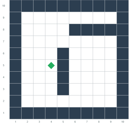<details> <summary>graphs/domains/sokoban_final_grid.png Details</summary>  ### Visual Description \n ## Diagram: 10x10 Grid with Highlighted Cell ### Overview The image displays a 10x10 grid diagram. The grid is composed of square cells, some filled with a dark color (appearing as dark gray or navy blue) and others left white (or very light gray). A single green diamond-shaped marker is placed within one of the white cells. The grid has numerical labels along both the horizontal (x) and vertical (y) axes. ### Components/Axes * **Grid Structure:** A 10x10 matrix of cells. * **Axes Labels:** * **Horizontal (X-axis):** Numbered from 1 to 10, positioned below the bottom row of cells. The numbers are left-aligned under their respective columns. * **Vertical (Y-axis):** Numbered from 1 to 10, positioned to the left of the leftmost column of cells. The numbers are bottom-aligned with their respective rows. * **Cell Fill Pattern:** Cells are either filled with a solid dark color or are empty (white). * **Highlighted Element:** A single green, diamond-shaped icon is located at the intersection of column 4 and row 5. ### Detailed Analysis **Grid Cell State (Dark vs. White):** The pattern of dark-filled cells forms a specific shape or path within the grid. The dark cells are located at the following approximate coordinates (Column, Row), where (1,1) is the bottom-left corner: * **Perimeter/Border:** All cells in column 1, column 10, row 1, and row 10 are dark, creating a full border. * **Internal Structure:** * A vertical bar of dark cells in column 5, spanning rows 2 through 6. * A horizontal bar of dark cells in row 8, spanning columns 6 through 9. * The cell at (6,8) is dark, connecting the vertical and horizontal bars. * The cell at (5,6) is dark, connecting the vertical bar to the border at (5,10) via the top border. **Highlighted Element:** * **Shape:** Diamond (a square rotated 45 degrees). * **Color:** Green. * **Position:** Centered within the cell at Column 4, Row 5. This cell is white (unfilled). ### Key Observations 1. **Asymmetrical Internal Pattern:** While the outer border is symmetrical, the internal dark cells form an asymmetrical, non-repeating pattern. 2. **Single Data Point:** The only non-structural, highlighted element is the green diamond at (4,5). There are no other markers, lines, or data series. 3. **Path or Obstacle Interpretation:** The dark cells could represent walls, obstacles, or a filled path in a maze or grid-based game. The white cells represent open or traversable space. 4. **Coordinate System:** The grid uses a standard Cartesian coordinate system with the origin (1,1) at the bottom-left. ### Interpretation This diagram is a **spatial representation**, not a data chart. It does not contain quantitative data, trends, or statistical information. Its primary purpose is to visualize a **configuration or state within a defined 10x10 space**. * **What it demonstrates:** It shows a specific layout of "blocked" (dark) and "open" (white) cells, with a point of interest (the green diamond) located in an open cell. * **Relationships:** The green diamond's position is defined relative to the grid axes and the pattern of dark cells. It is situated to the left of the central vertical dark bar and below the horizontal dark bar. * **Potential Contexts:** This could be a snapshot from: * A pathfinding algorithm visualization (e.g., A* search), where the green diamond is the start or end point. * A simple maze or puzzle layout. * A representation of a memory buffer, game board state, or cellular automaton grid. * A diagram illustrating a specific coordinate (4,5) for instructional purposes. **No numerical data, trends, or outliers are present to analyze.** The information is purely structural and positional. </details> Figure 13: Example Sokoban instance. The agent must push the box onto the target location without creating deadlocks. ### C.5 BlocksWorld State Space. The state consists of a configuration of $n$ uniquely labeled blocks (we use $n=5$ in our experiments). Each block is either: - On the table, or - On top of exactly one other block. A block is clear if no other block is on top of it. The table has unlimited capacity. Action Space. Three actions, described in natural language: 1. Move block from block to block (move-b-to-b): Pick up a block that is currently sitting on top of another block and place it onto a third block. This requires that the block being moved has nothing on top of it (is clear) and that the destination block also has nothing on top of it (is clear). After the move, the block that was underneath the moved block becomes clear. 1. Move block from block to table (move-b-to-t): Pick up a block that is currently sitting on top of another block and place it on the table. This requires that the block being moved has nothing on top of it (is clear). After the move, the block that was underneath becomes clear, and the moved block is now on the table. 1. Move block from table to block (move-t-to-b): Pick up a block that is currently on the table and place it onto another block. This requires that both the block being moved and the destination block have nothing on top of them (are clear). After the move, the destination block is no longer clear. Constraints. The preconditions for each action are: - move-b-to-b( $b_m$ , $b_f$ , $b_t$ ): Block $b_m$ is clear, block $b_t$ is clear, $b_m$ is currently on $b_f$ , and $b_m≠ b_t$ . - move-b-to-t( $b_m$ , $b_f$ ): Block $b_m$ is clear and $b_m$ is currently on $b_f$ . - move-t-to-b( $b_m$ , $b_t$ ): Block $b_m$ is clear, block $b_t$ is clear, $b_m$ is currently on the table, and $b_m≠ b_t$ . Goal Condition. The block configuration matches a target specification, typically given as a set of on( $b_1$ , $b_2$ ) predicates describing which blocks must be stacked on which. Differences from Navigation Domains. BlocksWorld differs qualitatively from the grid-based domains: - No spatial structure: Constraints are purely relational (“block A is on block B”) rather than geometric. - All objects are dynamic: Every block can be moved, unlike navigation where only the agent moves. - Algorithmic solutions: We additionally provide an algorithmic sketch (the Universal Blockswordl Algorithm (Stechly et al., 2024)) to test whether L-ICL can improve adherence to prescribed planning strategies. ## Appendix D Baseline Method Implementations This appendix provides detailed specifications of all baseline methods evaluated in our experiments. All baselines operate on the same task: given a problem description with start position, goal position, walls, and (optionally) deadzones, produce an action sequence to navigate from start to goal. We organize baselines into two categories: prompt-only methods that rely solely on LLM reasoning, and oracle methods that receive feedback from a ground-truth simulator. ### D.1 Prompt-Only Baselines #### D.1.1 Zero-Shot Chain-of-Thought (Zero-Shot CoT) The simplest baseline provides the model with task instructions, and asks it to reason step-by-step to produce a navigation plan. Implementation. The prompt includes: (1) a task description explaining gridworld navigation, valid actions, and movement constraints; (2) an ASCII representation of the problem (if applicable); (3) the query problem with start/goal coordinates; and (4) output format instructions requiring **Final Action Sequence:** action1, action2, .... We use temperature 1.0 for all experiments unless otherwise noted. #### D.1.2 RAG-CoT (Retrieval-Augmented Chain-of-Thought) This baseline extends Zero-Shot CoT with dynamic example selection based on similarity to the query problem. We retrieve the most relevant training examples within a character budget (10,000 or 20,000 characters in our experiments). Similarity Metric. We compute similarity based on Manhattan distance between start-goal pairs: $$ similarity(q,c)=\frac{1}{1+|d_q-d_c|} \tag{1} $$ where $d=|g_x-s_x|+|g_y-s_y|$ is the Manhattan distance from start $s$ to goal $g$ . This metric prefers training examples with similar navigation distances, under the assumption that problems with similar start-to-goal distances share structural similarities. Retrieval Modes. We evaluate three retrieval strategies: - Strict: Add examples until the budget would be exceeded (conservative). - Generous: Add examples until the budget is just crossed (permissive). - Fixed: Include fixed examples plus retrieved examples up to the remaining budget. Our main experiments use the generous mode. #### D.1.3 Self-Consistency Self-Consistency (Wang et al., 2023) generates multiple independent reasoning trajectories and selects the final answer via majority voting. Implementation. We sample $k=5$ independent CoT traces using temperature 1.0 for diversity. Each sample uses the same prompt with an annotation indicating the sample number (e.g., “Sample 3/5”). We parse action sequences from each sample, count votes for each unique plan (exact sequence match), and select the plan with the highest vote count. For tie-breaking, we use an additional LLM call to evaluate candidates based on their self-critique annotations. Self-Critique. Each sample includes a self-critique section where the model evaluates its own reasoning, providing confidence estimates and noting potential issues. This information is used only for tie-breaking. #### D.1.4 Self-Refine Self-Refine (Madaan et al., 2023) allows the model to iteratively review and improve its own solutions without external feedback. Implementation. The model generates an initial attempt, then receives up to $N=5$ refinement opportunities. In each refinement round, the model sees its previous response and is instructed to check for potential mistakes: boundary violations, wall collisions, goal reachability, deadzone avoidance, and path optimality. The model may either provide a corrected plan or explicitly state “ **No further refinement needed.** ” Termination Conditions. Refinement stops when: (1) the model explicitly states satisfaction or (2) maximum refinement steps are reached Key Distinction. Unlike oracle baselines, Self-Refine receives no external feedback about plan validity. The model must introspect on its own reasoning, which prior work has shown to be unreliable for planning tasks (Stechly et al., 2025). #### D.1.5 ReAct (Prompt-Only) ReAct (Yao et al., 2023b) interleaves reasoning and action selection in a textual trace format. Implementation. The model alternates between Thought: steps (reasoning about current state and next move) and Action: steps (single movement action). All reasoning and actions are generated in a single LLM call—no external tool execution occurs. The prompt includes guidelines to keep moves consistent with the grid layout, avoid illegal steps, provide reasoning before each action, and end with an explicit final action sequence. Trace Format. ⬇ Thought: [analyze current state and next move] Action: move - direction Thought: [continue reasoning] Action: move - direction ... Final Thought: [summarize path to goal] ** Final Action Sequence:** action1, action2, ... #### D.1.6 Tree-of-Thoughts (Prompt-Only) Tree-of-Thoughts (ToT) (Yao et al., 2023a) explores multiple reasoning paths through iterative expansion and scoring. Implementation. We use a prompt-only variant with breadth-first tree search. Parameters: breadth $b=5$ (nodes per level), depth $d=3$ (expansion rounds), max step actions $m=8$ (actions per candidate). At each depth level, the model generates candidate continuations as JSON, including a thought description, proposed actions, confidence score (0–100), terminal flag, and optional final plan. We keep the top- $k$ nodes by confidence (beam search) and finalize by selecting the best terminal node or completing the top non-terminal node. Scoring. Without oracle access, scoring uses only LLM self-assessed confidence and plan length: $$ score=(confidence,-plan\_length) \tag{2} $$ Higher confidence is preferred; shorter plans are preferred as a tiebreaker. ### D.2 Oracle Baselines Oracle baselines have access to a ground-truth environment simulator that provides feedback on plan validity. This represents an upper bound on what prompt-only methods could achieve with perfect self-verification. #### D.2.1 ReAct (+Oracle f/b) This two-step approach allows the model to receive targeted feedback about errors and produce a corrected plan. Implementation. Step 1: Generate an initial CoT plan. Step 2: If errors are detected by the oracle, provide specific feedback and request correction. Maximum 2 LLM calls per problem. We use temperature 0.3 for more deterministic outputs in the correction step. Feedback Types. The oracle provides two types of feedback: 1. Invalid Move: “Your plan has an ERROR at step $N$ . The action ‘move-X’ at position $(x,y)$ is INVALID because it would move into a wall or out of bounds.” 1. Incomplete Path: “Your plan is INCOMPLETE. After executing all $N$ actions, you ended at position $(x,y)$ but did not reach the goal.” Key Distinction. ReAct (+Oracle f/b) queries the verifier at test time for each proposed plan, while L-ICL uses the oracle only during training. At inference, L-ICL requires a single forward pass with no external dependencies. ### D.3 Evaluation Infrastructure Action Parsing. All baselines use the same action sequence parser that handles multiple output formats. We search for explicit patterns (e.g., **Final Action Sequence:**), fall back to lines with comma-separated actions, and as a last resort extract all move-* actions from the response. Actions are normalized to canonical form (e.g., “north” $→$ “move-north”). Plan Validation. Plan validity is determined by simulating the action sequence: 1. Parse problem to extract start/goal positions and obstacles. 1. Execute actions sequentially, checking bounds and wall collisions. 1. Verify goal is reached. 1. Compare plan length to BFS optimal. ### D.4 Summary of Baseline Characteristics Table 7 summarizes the key characteristics distinguishing each baseline. Table 7: Summary of baseline characteristics. “Examples” indicates whether the method uses in-context examples; “LLM Calls” indicates calls per problem; “Tools” indicates whether external tools are used. $$ k 1 N O(b· d) \tag{3} $$ ## Appendix E Implementation Details This appendix provides detailed implementation specifications for L-ICL, including the system architecture, correction generation process, and evaluation pipeline. We provide sufficient detail for reproducing our experiments. ### E.1 System Architecture Our implementation consists of four main components that work together to execute the L-ICL training loop: 1. Partial Program Generator: Constructs PTP-style prompts with subroutine documentation and accumulated corrections formatted as input-output examples. 1. LLM Interface: Sends prompts to language models and parses structured traces from responses. 1. Evaluation Engine: Validates generated plans using external tools and step-by-step simulation, identifying the first point of failure. 1. Correction Accumulator: Extracts corrections from evaluation mismatches and injects them into subsequent prompts. Figure 14 illustrates the data flow between these components during L-ICL training. Partial Program Generator LLM Interface Evaluation Engine Correction Accumulator prompt trace corrections update Figure 14: System architecture for L-ICL training. The loop iterates over training problems, accumulating corrections that progressively refine the prompt. ### E.2 Subroutine Specifications by Domain Each domain defines a set of planning primitives that the LLM must “implement” through trace generation. We describe the subroutines for each domain, including their signatures, semantics, and the constraints they encode. #### E.2.1 Subroutines) We use the following subroutines in our experiments: State Extraction. - extract_initial_state(problem) $→$ State: Parses the problem description to extract the agent’s starting position and environment structure. - extract_goal(problem) $→$ State: Parses the goal specification from the problem. Action Generation. - get_applicable_actions(state, goal) $→$ Set[Action]: Returns the set of actions that can be legally executed from the current state. For navigation, this filters the four cardinal directions to exclude moves that would exit the grid or collide with walls. - get_optimal_actions(state, goal) $→$ Set[Action]: Returns the subset of applicable actions that lie on an optimal path to the goal. This is computed using shortest-path algorithms/ a planner. For BlocksWorld, we replace this with get_recommended_actions(state, goal) $→$ Set[Action], which returns the set of actions prescribed by the Universal Blocksworld Algorithm. State Transition and Goal Test. - apply_action(state, action) $→$ State: Returns the state resulting from executing the action. For navigation, this updates the agent’s coordinates. - at_goal(state, goal) $→$ bool: Returns whether the current state satisfies the goal condition. ### E.3 Correction Format and Integration L-ICL corrections are formatted as doctest-style input-output examples that are injected into subroutine documentation. This format is well-represented in LLM training data, facilitating generalization. Correction Structure. Each correction consists of three components: 1. Function identifier: Which subroutine the correction applies to. 1. Input: The arguments that triggered the mismatch. 1. Correct output: The oracle-provided ground truth. Example Correction. Consider an LLM that incorrectly proposes moving east from position $(3,4)$ when a wall blocks that direction. The evaluation detects that move_east is not in the set of applicable actions. L-ICL generates a correction: ⬇ >>> get_applicable_actions (state =(3,4), walls ={(3,5)}) {’ move_north ’, ’ move_south ’, ’ move_west ’} This correction is inserted into the documentation for get_applicable_actions, providing an explicit example that eastward movement from $(3,4)$ is invalid. Correction Accumulation. Corrections accumulate across training problems. When a new correction duplicates an existing one (same function and inputs), we retain only one copy. This prevents prompt bloat while ensuring coverage of diverse failure cases. The accumulated corrections are batch-inserted into the prompt template before each evaluation iteration. Additional details are in Section F.3. ### E.4 Evaluation Pipeline Plan evaluation proceeds through multiple validation stages, each providing increasingly detailed feedback. #### E.4.1 External Plan Validation We use the VAL validator (Howey et al., 2004), the standard tool for PDDL plan validation, to verify plan correctness. Given a domain specification, problem instance, and proposed action sequence, VAL checks: - Each action’s preconditions are satisfied when it is executed. - The final state after executing all actions satisfies the goal. VAL provides a binary validity judgment and, for invalid plans, identifies the first action whose preconditions fail. #### E.4.2 Optimality Verification To assess plan quality, we compute optimal solutions using the Fast Downward planning system (Helmert, 2006). Fast Downward is a state-of-the-art classical planner that guarantees optimal solutions when configured with admissible heuristics. We use the A* search algorithm with the LM-cut heuristic. For each problem, we: 1. Run Fast Downward to obtain the optimal plan length. 1. Compare the LLM’s plan length against this baseline. 1. Mark plans as optimal if lengths match and the plan is valid. #### E.4.3 Step-by-Step Simulation Beyond end-to-end validation, we simulate plan execution step-by-step using proxy implementations of each subroutine. This enables: 1. First-failure identification: We identify the exact step where the LLM’s trace first diverges from ground truth, enabling localized correction generation. 1. Fine-grained error categorization: We distinguish between: - Applicability errors: Proposing an action not in the applicable set. - Optimality errors: Proposing an applicable but suboptimal action. 1. Correction generation: For each error type, we generate the corresponding correction by querying the oracle for the correct output. Algorithm 2 provides pseudocode for the step-by-step evaluation procedure. Algorithm 2 Step-by-Step Plan Evaluation 0: Domain $D$ , problem $P$ , predicted actions $[a_1,…,a_n]$ , oracle $O$ 0: Evaluation result with corrections $s←O.extract\_initial\_state(P)$ $g←O.extract\_goal(P)$ corrections $←[]$ first_invalid $←$ null first_suboptimal $←$ null for $i=1$ to $n$ do $A_applicable←O.get\_applicable\_actions(s,g)$ $A_optimal←O.get\_optimal\_actions(s,g)$ if $a_i∉ A_applicable$ and first_invalid is null then first_invalid $← i$ corrections.append $(``get\_applicable\_actions'',(s,g),A_applicable)$ break $\triangleright$ Stop at first invalid action else if $a_i∉ A_optimal$ and first_suboptimal is null then first_suboptimal $← i$ corrections.append $(``get\_optimal\_actions'',(s,g),A_optimal)$ end if $s←O.apply\_action(s,a_i)$ end for goal_reached $←O.at\_goal(s,g)$ return {first_invalid, first_suboptimal, corrections, goal_reached} ### E.5 Oracle Implementation The oracle provides ground-truth outputs for each subroutine. We implement oracles using a combination of external planning tools and logic-based simulation. Planning Tools. We use Fast Downward (Helmert, 2006) for optimal plan computation and action applicability. For domains requiring multiple optimal plans (to compute optimal action sets), we additionally use the K* planner (Katz and Lee, 2023), which enumerates the top- $k$ shortest plans. State Simulation. Action effects are computed using the Tarski planning library (Francés et al., 2018), which provides PDDL parsing and grounded action simulation. Given a PDDL domain and problem, Tarski computes: - The set of ground actions applicable in any state. - The successor state resulting from applying an action. - Whether a state satisfies a goal formula. Optimality Computation. Computing optimal actions (those on some optimal path) requires enumerating multiple optimal plans. We use K* to generate all plans of optimal length, then take the union of first actions across these plans. For efficiency, we cache optimal action sets for frequently-queried states. ### E.6 Prompt Construction The final prompt sent to the LLM consists of four components assembled in sequence: 1. Task description: Natural language explanation of the planning domain, valid actions, and objective. 1. Subroutine documentation: For each subroutine, we include: - Function signature with typed arguments and return type. - Natural language description of the subroutine’s purpose. - Accumulated L-ICL corrections as doctest examples. 1. Example traces: A small number ( $k=2$ – $3$ ) of complete reasoning traces showing how subroutines are invoked to solve example problems. 1. Query problem: The problem instance to solve, formatted consistently with the examples, followed by instructions to produce a trace. State Representation. For grid-based domains, we evaluate two state representations: - Textual: Positions as coordinates (e.g., “agent at (3,4)”) with walls listed explicitly. - ASCII: Visual grid representation where walls are marked characters and open cells are spaces. Our ablation (Section 4.3) shows that L-ICL achieves comparable peak performance with either representation, though ASCII grids accelerate early learning. ### E.7 Experimental Infrastructure Hardware. Experiments were conducted on a Linux workstation with 32GB RAM. External planning tools (Fast Downward, VAL) were run locally. LLM inference was performed via API calls. LLM Services. We evaluated models through their respective APIs: - DeepSeek V3 and V3.1 via the DeepSeek API. - Claude Haiku 4.5 and Claude Sonnet 4.5 via the Anthropic API. Hyperparameters. Unless otherwise specified: - Temperature: 1.0 (following DeepSeek recommendations). - Maximum generation length: 32000 tokens. - Training examples per iteration: 1 (single problem per L-ICL update). - Total training problems: up to 240. - Thinking tokens for Sonnet 4.5: 10k - Thinking tokens for Haiku 4.5: 5k Timeout Handling. Fast Downward was given a 60-second timeout per problem. Problems exceeding this limit were marked as having unknown optimal cost and excluded from optimality statistics (but included in validity statistics if the validator succeeded). ## Appendix F Representative Prompts This appendix provides representative prompts used in all experiments. We organize prompts into two categories: (1) L-ICL prompts based on Program Trace Prompting (PTP), and (2) baseline method prompts used for comparison approaches. All prompts use template variables (denoted with curly braces, e.g., {partial_program}) that are replaced with problem-specific content at runtime. ### F.1 L-ICL Prompts (Program Trace Prompting) L-ICL prompts follow the Program Trace Prompting (PTP) format, where the LLM is asked to predict the output of a partially specified program. The key insight is that by withholding subroutine implementations (replacing them with “…” markers), the LLM must infer correct behavior from documentation and accumulated examples. #### F.1.1 Base L-ICL Prompt (No Domain Visualization) This is the minimal L-ICL prompt used for gridworld and Sokoban navigation tasks when no ASCII grid visualization is provided. The LLM must infer spatial constraints purely from accumulated L-ICL corrections. ⬇ Consider the program fragment below. This program fragment is incomplete, with key parts of the implementation hidden, by replacing them with "..." markers. PROGRAM: ‘‘‘ python {partial_program} ‘‘‘ QUESTION: Predict what the output of the program above will be, given the input shown below. Respond with the FULL program output, and ONLY the expected program output: you will be PENALIZED if you introduce any additional explanatory text. ‘‘‘ >>> {task_name}({input_str}) ‘‘‘ Template Variables. - {partial_program}: The PTP-style program with subroutine signatures, documentation, doctest examples (including L-ICL corrections), and “…” placeholders for implementations. - {task_name}: The function name to invoke (e.g., solve_gridworld). - {input_str}: The problem specification as a string (e.g., start position, goal position, wall locations). #### F.1.2 L-ICL Prompt with ASCII Grid Visualization When ASCII grid visualization is enabled, the prompt includes a visual representation of the environment. This provides spatial scaffolding that accelerates early learning, though L-ICL achieves comparable peak performance without it. ⬇ Consider the program fragment below. This program fragment is incomplete, with key parts of the implementation hidden, by replacing them with "..." markers. IMPORTANT: You are an agent navigating a {grid_size} gridworld. The grid has {num_walls} walls that block movement. ** Grid Layout:** ‘‘‘ 1 2 3 4 5 6 7 8 9 10 +---+---+---+---+---+---+---+---+---+---+ 10 | . | . | . | . | . | . | . | . | . | . | +---+---+---+---+---+---+---+---+---+---+ 9 | . | . | # | # | # | # | # | # | # | . | +---+---+---+---+---+---+---+---+---+---+ 8 | . | # | . | # | . | # | . | . | . | . | +---+---+---+---+---+---+---+---+---+---+ 7 | . | # | . | . | . | # | . | # | # | . | +---+---+---+---+---+---+---+---+---+---+ 6 | . | # | . | # | . | . | . | # | . | . | +---+---+---+---+---+---+---+---+---+---+ 5 | . | . | . | # | . | # | . | # | . | . | +---+---+---+---+---+---+---+---+---+---+ 4 | . | # | . | # | . | # | . | . | # | . | +---+---+---+---+---+---+---+---+---+---+ 3 | . | # | . | . | . | # | . | # | . | . | +---+---+---+---+---+---+---+---+---+---+ 2 | . | # | . | # | . | . | . | # | . | . | +---+---+---+---+---+---+---+---+---+---+ 1 | . | . | . | . | . | . | . | . | . | . | +---+---+---+---+---+---+---+---+---+---+ ‘‘‘ PROGRAM: ‘‘‘ python {partial_program} ‘‘‘ QUESTION: Predict what the output of the program above will be, given the input shown below. Respond with the FULL program output, and ONLY the expected program output: you will be PENALIZED if you introduce any additional explanatory text. ‘‘‘ >>> {task_name}({input_str}) ‘‘‘ Grid Symbols. - . – Open cell (traversable) - # – Wall (impassable) - $ – Box (in Sokoban) #### F.1.3 L-ICL BlocksWorld Prompt with UBW Algorithm For BlocksWorld, we additionally provide algorithmic guidance based on the Universal Blocks World (UBW) algorithm (Stechly et al., 2024). This tests whether L-ICL can improve adherence to prescribed planning strategies beyond simple constraint satisfaction. ⬇ Consider the program fragment below. This program fragment implements the Universal Blocks World (UBW) algorithm, which is a systematic two - phase approach for solving blocks world planning problems. The implementation is incomplete, with key parts replaced by "..." markers. UNIVERSAL BLOCKS WORLD ALGORITHM OVERVIEW: The UBW algorithm works in two distinct phases to efficiently solve any blocks world configuration: PHASE 1: STRATEGIC UNSTACKING - Unstack ALL blocks that are stacked on top of others - Work from top to bottom, unstacking clear blocks first - Move incorrectly positioned blocks to the table PHASE 2: SYSTEMATIC REASSEMBLY - Build goal configurations from bottom up - Process blocks in dependency order (place supporting blocks before supported blocks) - Only place a block when its target is ready (clear and in final position) - Ensure structural integrity throughout construction KEY HEURISTICS FOR IMPLEMENTATION: 1. STATE ANALYSIS: - Parse predicates into on (), on - table (), and clear () relationships - Build dependency graphs: what should be on what - Identify bottom blocks (blocks that should be on table in goal) 2. UNSTACKING STRATEGY: - Check each on (X, Y) relationship in current state - If (X, Y) is NOT in goal relationships, consider unstacking X - Only unstack if X is clear (no blocks on top) - Priority: unstack blocks that block other necessary moves 3. REASSEMBLY STRATEGY: - For each goal on (X, Y), check if X can be placed on Y - X must be: clear AND on - table - Y must be: clear AND in its final position - Y is in final position if: Y should be on table OR Y is already correctly placed on its target 4. ACTION SELECTION LOGIC: ‘‘‘ For unstacking: if on (X, Y) in current state AND clear (X): return move - b - to - t (X, Y) For assembly: if goal requires on (X, Y) AND can_place_block (X, Y): return move - t - to - b (X, Y) ‘‘‘ 5. CORRECTNESS VERIFICATION: - Always verify preconditions before suggesting actions - Check that actions don ’ t break existing correct configurations - Ensure goal - directed progress in every move during assembly phase DETAILED TRACE GUIDANCE: When implementing the UBW algorithm, provide step - by - step reasoning inside reasoning () calls if required, which is your scratchpad. 1. State the current configuration clearly 2. Identify which phase you ’ re in (unstacking vs assembly) 3. Explain WHY each action is chosen based on UBW principles 4. Show how the action advances toward the goal 5. Verify preconditions are satisfied 6. Update state representation after each action PROGRAM: ‘‘‘ python {partial_program} ‘‘‘ QUESTION: Predict what the output of the program above will be, given the input shown below. IMPLEMENTATION REQUIREMENTS: - Follow the UBW algorithm phases strictly - Provide detailed reasoning for each action selection - Show state analysis and dependency tracking - Explain how each move contributes to the overall strategy - Demonstrate understanding of when to unstack vs when to build - Verify that all actions follow UBW heuristics Respond with the FULL program output, including detailed algorithmic traces that demonstrate proper UBW implementation. Your trace should show: - Clear identification of current phase (unstacking / assembly) - Specific reasoning for each action choice - State updates and goal progress tracking - Verification that actions follow UBW principles Under no circumstance must you skip steps in the program output. You CAN decide to go back and choose different actions if you feel that you have made a mistake, but the FINAL PLAN must show the COMPLETE CORRECT PATH ONLY. ‘‘‘ >>> {task_name}({input_str}) ‘‘‘ #### F.1.4 Example Partial Program Structure The {partial_program} template variable is replaced with a PTP-style program containing subroutine documentation and accumulated L-ICL corrections. Below is a representative example for gridworld navigation: ⬇ import collections from typing import Dict, List, Set, Tuple, Union, Optional, Any, FrozenSet PlanningState = Any Action = Any @traced def extract_problem (input_str: str) -> str: """ Extract a standardized problem description from input. """ ... @traced def extract_initial_state (problem_str: str) -> PlanningState: """ Extract the initial state from a problem description. """ ... @traced def extract_goal (problem_str: str) -> PlanningState: """ Extract the goal from a problem description. """ ... @traced def at_goal (state: PlanningState, goal: PlanningState) -> bool: """ Check if current state satisfies goal conditions. """ ... @traced def get_applicable_actions (state: PlanningState, goal: PlanningState) -> Set [Action]: """ Get all applicable actions in the current state. """ ... @traced def get_optimal_actions (state: PlanningState, applicable_actions: List [Action], goal: PlanningState) -> Set [Action]: """ Get actions that are part of an optimal plan. """ ... @traced def apply_action (state: PlanningState, action: Action, goal: PlanningState) -> PlanningState: """ Apply an action to a state, returning the resulting state. """ ... def pddl_grid (input_str: str): """ Solve a planning problem described in input_str. This function processes a planning problem description by: 1. Extracting the initial state and goal 2. Iteratively applying actions until the goal is reached 3. Returning the sequence of actions as a plan >>> pddl_grid (’(define (problem gw - task -351)\ n (: domain gridworld -10 x10)\ n (: init (at c9 -5))\ n (: goal (at c5 -10))\ n)\ n ’) Calling extract_problem (’(define (problem gw - task -351)\ n (: domain gridworld -10 x10)\ n (: init (at c9 -5))\ n (: goal (at c5 -10))\ n)\ n ’)... ... extract_problem returned ’ gridworld -10 x10 ’ Calling extract_initial_state (’(define (problem gw - task -351)\ n (: domain gridworld -10 x10)\ n (: init (at c9 -5))\ n (: goal (at c5 -10))\ n)\ n ’)... ... extract_initial_state returned (9, 5) Calling extract_goal (’(define (problem gw - task -351)\ n (: domain gridworld -10 x10)\ n (: init (at c9 -5))\ n (: goal (at c5 -10))\ n)\ n ’)... ... extract_goal returned (5, 10) Calling at_goal ((9, 5), (5, 10))... ... at_goal returned False Calling get_applicable_actions ((9, 5), (5, 10))... ... get_applicable_actions returned [’ move - north ’, ’ move - east ’] Calling get_optimal_actions ((9, 5), [’ move - north ’, ’ move - east ’], (5, 10))... ... get_optimal_actions returned [’ move - north ’, ’ move - east ’] Calling apply_action ((9, 5), ’ move - north ’, (5, 10))... ... apply_action returned (9, 6) Calling at_goal ((9, 6), (5, 10))... ... at_goal returned False Calling get_applicable_actions ((9, 6), (5, 10))... ... get_applicable_actions returned [’ move - south ’, ’ move - east ’] Calling get_optimal_actions ((9, 6), [’ move - south ’, ’ move - east ’], (5, 10))... ... get_optimal_actions returned [’ move - east ’] Calling apply_action ((9, 6), ’ move - east ’, (5, 10))... ... apply_action returned (10, 6) Calling at_goal ((10, 6), (5, 10))... ... at_goal returned False Calling get_applicable_actions ((10, 6), (5, 10))... ... get_applicable_actions returned [’ move - north ’, ’ move - south ’, ’ move - west ’] Calling get_optimal_actions ((10, 6), [’ move - north ’, ’ move - south ’, ’ move - west ’], (5, 10))... ... get_optimal_actions returned [’ move - north ’] Calling apply_action ((10, 6), ’ move - north ’, (5, 10))... ... apply_action returned (10, 7) Calling at_goal ((10, 7), (5, 10))... ... at_goal returned False Calling get_applicable_actions ((10, 7), (5, 10))... ... get_applicable_actions returned [’ move - north ’, ’ move - south ’] Calling get_optimal_actions ((10, 7), [’ move - north ’, ’ move - south ’], (5, 10))... ... get_optimal_actions returned [’ move - north ’] Calling apply_action ((10, 7), ’ move - north ’, (5, 10))... ... apply_action returned (10, 8) Calling at_goal ((10, 8), (5, 10))... ... at_goal returned False Calling get_applicable_actions ((10, 8), (5, 10))... ... get_applicable_actions returned [’ move - north ’, ’ move - south ’, ’ move - west ’] Calling get_optimal_actions ((10, 8), [’ move - north ’, ’ move - south ’, ’ move - west ’], (5, 10))... ... get_optimal_actions returned [’ move - north ’] Calling apply_action ((10, 8), ’ move - north ’, (5, 10))... ... apply_action returned (10, 9) Calling at_goal ((10, 9), (5, 10))... ... at_goal returned False Calling get_applicable_actions ((10, 9), (5, 10))... ... get_applicable_actions returned [’ move - north ’, ’ move - south ’] Calling get_optimal_actions ((10, 9), [’ move - north ’, ’ move - south ’], (5, 10))... ... get_optimal_actions returned [’ move - north ’] Calling apply_action ((10, 9), ’ move - north ’, (5, 10))... ... apply_action returned (10, 10) Calling at_goal ((10, 10), (5, 10))... ... at_goal returned False Calling get_applicable_actions ((10, 10), (5, 10))... ... get_applicable_actions returned [’ move - south ’, ’ move - west ’] Calling get_optimal_actions ((10, 10), [’ move - south ’, ’ move - west ’], (5, 10))... ... get_optimal_actions returned [’ move - west ’] Calling apply_action ((10, 10), ’ move - west ’, (5, 10))... ... apply_action returned (9, 10) Calling at_goal ((9, 10), (5, 10))... ... at_goal returned False Calling get_applicable_actions ((9, 10), (5, 10))... ... get_applicable_actions returned [’ move - east ’, ’ move - west ’] Calling get_optimal_actions ((9, 10), [’ move - east ’, ’ move - west ’], (5, 10))... ... get_optimal_actions returned [’ move - west ’] Calling apply_action ((9, 10), ’ move - west ’, (5, 10))... ... apply_action returned (8, 10) Calling at_goal ((8, 10), (5, 10))... ... at_goal returned False Calling get_applicable_actions ((8, 10), (5, 10))... ... get_applicable_actions returned [’ move - east ’, ’ move - west ’] Calling get_optimal_actions ((8, 10), [’ move - east ’, ’ move - west ’], (5, 10))... ... get_optimal_actions returned [’ move - west ’] Calling apply_action ((8, 10), ’ move - west ’, (5, 10))... ... apply_action returned (7, 10) Calling at_goal ((7, 10), (5, 10))... ... at_goal returned False Calling get_applicable_actions ((7, 10), (5, 10))... ... get_applicable_actions returned [’ move - east ’, ’ move - west ’] Calling get_optimal_actions ((7, 10), [’ move - east ’, ’ move - west ’], (5, 10))... ... get_optimal_actions returned [’ move - west ’] Calling apply_action ((7, 10), ’ move - west ’, (5, 10))... ... apply_action returned (6, 10) Calling at_goal ((6, 10), (5, 10))... ... at_goal returned False Calling get_applicable_actions ((6, 10), (5, 10))... ... get_applicable_actions returned [’ move - east ’, ’ move - west ’] Calling get_optimal_actions ((6, 10), [’ move - east ’, ’ move - west ’], (5, 10))... ... get_optimal_actions returned [’ move - west ’] Calling apply_action ((6, 10), ’ move - west ’, (5, 10))... ... apply_action returned (5, 10) Calling at_goal ((5, 10), (5, 10))... ... at_goal returned True Final answer: move - north move - east move - north move - north move - north move - north move - west move - west move - west move - west move - west [’ move - north ’, ’ move - east ’, ’ move - north ’, ’ move - north ’, ’ move - north ’, ’ move - north ’, ’ move - west ’, ’ move - west ’, ’ move - west ’, ’ move - west ’, ’ move - west ’] >>> pddl_grid (’(define (problem gw - task -352)\ n (: domain gridworld -10 x10)\ n (: init (at c9 -3))\ n (: goal (at c7 -7))\ n)\ n ’) Calling extract_problem (’(define (problem gw - task -352)\ n (: domain gridworld -10 x10)\ n (: init (at c9 -3))\ n (: goal (at c7 -7))\ n)\ n ’)... ... extract_problem returned ’ gridworld -10 x10 ’ Calling extract_initial_state (’(define (problem gw - task -352)\ n (: domain gridworld -10 x10)\ n (: init (at c9 -3))\ n (: goal (at c7 -7))\ n)\ n ’)... ... extract_initial_state returned (9, 3) Calling extract_goal (’(define (problem gw - task -352)\ n (: domain gridworld -10 x10)\ n (: init (at c9 -3))\ n (: goal (at c7 -7))\ n)\ n ’)... ... extract_goal returned (7, 7) Calling at_goal ((9, 3), (7, 7))... ... at_goal returned False Calling get_applicable_actions ((9, 3), (7, 7))... ... get_applicable_actions returned [’ move - south ’, ’ move - east ’] Calling get_optimal_actions ((9, 3), [’ move - south ’, ’ move - east ’], (7, 7))... ... get_optimal_actions returned [’ move - south ’, ’ move - east ’] Calling apply_action ((9, 3), ’ move - south ’, (7, 7))... ... apply_action returned (9, 2) Calling at_goal ((9, 2), (7, 7))... ... at_goal returned False Calling get_applicable_actions ((9, 2), (7, 7))... ... get_applicable_actions returned [’ move - north ’, ’ move - south ’, ’ move - east ’] Calling get_optimal_actions ((9, 2), [’ move - north ’, ’ move - south ’, ’ move - east ’], (7, 7))... ... get_optimal_actions returned [’ move - south ’] Calling apply_action ((9, 2), ’ move - south ’, (7, 7))... ... apply_action returned (9, 1) Calling at_goal ((9, 1), (7, 7))... ... at_goal returned False Calling get_applicable_actions ((9, 1), (7, 7))... ... get_applicable_actions returned [’ move - north ’, ’ move - east ’, ’ move - west ’] Calling get_optimal_actions ((9, 1), [’ move - north ’, ’ move - east ’, ’ move - west ’], (7, 7))... ... get_optimal_actions returned [’ move - west ’] Calling apply_action ((9, 1), ’ move - west ’, (7, 7))... ... apply_action returned (8, 1) Calling at_goal ((8, 1), (7, 7))... ... at_goal returned False Calling get_applicable_actions ((8, 1), (7, 7))... ... get_applicable_actions returned [’ move - east ’, ’ move - west ’] Calling get_optimal_actions ((8, 1), [’ move - east ’, ’ move - west ’], (7, 7))... ... get_optimal_actions returned [’ move - west ’] Calling apply_action ((8, 1), ’ move - west ’, (7, 7))... ... apply_action returned (7, 1) Calling at_goal ((7, 1), (7, 7))... ... at_goal returned False Calling get_applicable_actions ((7, 1), (7, 7))... ... get_applicable_actions returned [’ move - north ’, ’ move - east ’, ’ move - west ’] Calling get_optimal_actions ((7, 1), [’ move - north ’, ’ move - east ’, ’ move - west ’], (7, 7))... ... get_optimal_actions returned [’ move - north ’] Calling apply_action ((7, 1), ’ move - north ’, (7, 7))... ... apply_action returned (7, 2) Calling at_goal ((7, 2), (7, 7))... ... at_goal returned False Calling get_applicable_actions ((7, 2), (7, 7))... ... get_applicable_actions returned [’ move - north ’, ’ move - south ’, ’ move - west ’] Calling get_optimal_actions ((7, 2), [’ move - north ’, ’ move - south ’, ’ move - west ’], (7, 7))... ... get_optimal_actions returned [’ move - north ’] Calling apply_action ((7, 2), ’ move - north ’, (7, 7))... ... apply_action returned (7, 3) Calling at_goal ((7, 3), (7, 7))... ... at_goal returned False Calling get_applicable_actions ((7, 3), (7, 7))... ... get_applicable_actions returned [’ move - north ’, ’ move - south ’] Calling get_optimal_actions ((7, 3), [’ move - north ’, ’ move - south ’], (7, 7))... ... get_optimal_actions returned [’ move - north ’] Calling apply_action ((7, 3), ’ move - north ’, (7, 7))... ... apply_action returned (7, 4) Calling at_goal ((7, 4), (7, 7))... ... at_goal returned False Calling get_applicable_actions ((7, 4), (7, 7))... ... get_applicable_actions returned [’ move - north ’, ’ move - south ’, ’ move - east ’] Calling get_optimal_actions ((7, 4), [’ move - north ’, ’ move - south ’, ’ move - east ’], (7, 7))... ... get_optimal_actions returned [’ move - north ’] Calling apply_action ((7, 4), ’ move - north ’, (7, 7))... ... apply_action returned (7, 5) Calling at_goal ((7, 5), (7, 7))... ... at_goal returned False Calling get_applicable_actions ((7, 5), (7, 7))... ... get_applicable_actions returned [’ move - north ’, ’ move - south ’] Calling get_optimal_actions ((7, 5), [’ move - north ’, ’ move - south ’], (7, 7))... ... get_optimal_actions returned [’ move - north ’] Calling apply_action ((7, 5), ’ move - north ’, (7, 7))... ... apply_action returned (7, 6) Calling at_goal ((7, 6), (7, 7))... ... at_goal returned False Calling get_applicable_actions ((7, 6), (7, 7))... ... get_applicable_actions returned [’ move - north ’, ’ move - south ’, ’ move - west ’] Calling get_optimal_actions ((7, 6), [’ move - north ’, ’ move - south ’, ’ move - west ’], (7, 7))... ... get_optimal_actions returned [’ move - north ’] Calling apply_action ((7, 6), ’ move - north ’, (7, 7))... ... apply_action returned (7, 7) Calling at_goal ((7, 7), (7, 7))... ... at_goal returned True Final answer: move - south move - south move - west move - west move - north move - north move - north move - north move - north move - north [’ move - south ’, ’ move - south ’, ’ move - west ’, ’ move - west ’, ’ move - north ’, ’ move - north ’, ’ move - north ’, ’ move - north ’, ’ move - north ’, ’ move - north ’] >>> pddl_grid (’(define (problem gw - task -353)\ n (: domain gridworld -10 x10)\ n (: init (at c7 -2))\ n (: goal (at c2 -5))\ n)\ n ’) Calling extract_problem (’(define (problem gw - task -353)\ n (: domain gridworld -10 x10)\ n (: init (at c7 -2))\ n (: goal (at c2 -5))\ n)\ n ’)... ... extract_problem returned ’ gridworld -10 x10 ’ Calling extract_initial_state (’(define (problem gw - task -353)\ n (: domain gridworld -10 x10)\ n (: init (at c7 -2))\ n (: goal (at c2 -5))\ n)\ n ’)... ... extract_initial_state returned (7, 2) Calling extract_goal (’(define (problem gw - task -353)\ n (: domain gridworld -10 x10)\ n (: init (at c7 -2))\ n (: goal (at c2 -5))\ n)\ n ’)... ... extract_goal returned (2, 5) Calling at_goal ((7, 2), (2, 5))... ... at_goal returned False Calling get_applicable_actions ((7, 2), (2, 5))... ... get_applicable_actions returned [’ move - north ’, ’ move - south ’, ’ move - west ’] Calling get_optimal_actions ((7, 2), [’ move - north ’, ’ move - south ’, ’ move - west ’], (2, 5))... ... get_optimal_actions returned [’ move - west ’] Calling apply_action ((7, 2), ’ move - west ’, (2, 5))... ... apply_action returned (6, 2) Calling at_goal ((6, 2), (2, 5))... ... at_goal returned False Calling get_applicable_actions ((6, 2), (2, 5))... ... get_applicable_actions returned [’ move - south ’, ’ move - east ’, ’ move - west ’] Calling get_optimal_actions ((6, 2), [’ move - south ’, ’ move - east ’, ’ move - west ’], (2, 5))... ... get_optimal_actions returned [’ move - west ’] Calling apply_action ((6, 2), ’ move - west ’, (2, 5))... ... apply_action returned (5, 2) Calling at_goal ((5, 2), (2, 5))... ... at_goal returned False Calling get_applicable_actions ((5, 2), (2, 5))... ... get_applicable_actions returned [’ move - north ’, ’ move - south ’, ’ move - east ’] Calling get_optimal_actions ((5, 2), [’ move - north ’, ’ move - south ’, ’ move - east ’], (2, 5))... ... get_optimal_actions returned [’ move - north ’] Calling apply_action ((5, 2), ’ move - north ’, (2, 5))... ... apply_action returned (5, 3) Calling at_goal ((5, 3), (2, 5))... ... at_goal returned False Calling get_applicable_actions ((5, 3), (2, 5))... ... get_applicable_actions returned [’ move - north ’, ’ move - south ’, ’ move - west ’] Calling get_optimal_actions ((5, 3), [’ move - north ’, ’ move - south ’, ’ move - west ’], (2, 5))... ... get_optimal_actions returned [’ move - west ’] Calling apply_action ((5, 3), ’ move - west ’, (2, 5))... ... apply_action returned (4, 3) Calling at_goal ((4, 3), (2, 5))... ... at_goal returned False Calling get_applicable_actions ((4, 3), (2, 5))... ... get_applicable_actions returned [’ move - east ’, ’ move - west ’] Calling get_optimal_actions ((4, 3), [’ move - east ’, ’ move - west ’], (2, 5))... ... get_optimal_actions returned [’ move - west ’] Calling apply_action ((4, 3), ’ move - west ’, (2, 5))... ... apply_action returned (3, 3) Calling at_goal ((3, 3), (2, 5))... ... at_goal returned False Calling get_applicable_actions ((3, 3), (2, 5))... ... get_applicable_actions returned [’ move - north ’, ’ move - south ’, ’ move - east ’] Calling get_optimal_actions ((3, 3), [’ move - north ’, ’ move - south ’, ’ move - east ’], (2, 5))... ... get_optimal_actions returned [’ move - north ’] Calling apply_action ((3, 3), ’ move - north ’, (2, 5))... ... apply_action returned (3, 4) Calling at_goal ((3, 4), (2, 5))... ... at_goal returned False Calling get_applicable_actions ((3, 4), (2, 5))... ... get_applicable_actions returned [’ move - north ’, ’ move - south ’] Calling get_optimal_actions ((3, 4), [’ move - north ’, ’ move - south ’], (2, 5))... ... get_optimal_actions returned [’ move - north ’] Calling apply_action ((3, 4), ’ move - north ’, (2, 5))... ... apply_action returned (3, 5) Calling at_goal ((3, 5), (2, 5))... ... at_goal returned False Calling get_applicable_actions ((3, 5), (2, 5))... ... get_applicable_actions returned [’ move - north ’, ’ move - south ’, ’ move - west ’] Calling get_optimal_actions ((3, 5), [’ move - north ’, ’ move - south ’, ’ move - west ’], (2, 5))... ... get_optimal_actions returned [’ move - west ’] Calling apply_action ((3, 5), ’ move - west ’, (2, 5))... ... apply_action returned (2, 5) Calling at_goal ((2, 5), (2, 5))... ... at_goal returned True Final answer: move - west move - west move - north move - west move - west move - north move - north move - west [’ move - west ’, ’ move - west ’, ’ move - north ’, ’ move - west ’, ’ move - west ’, ’ move - north ’, ’ move - north ’, ’ move - west ’] """ ... ### F.2 Baseline Method Prompts The following prompts are used for baseline comparison methods. All baselines receive the same problem information but use different reasoning frameworks. #### F.2.1 Zero-Shot CoT / RAG-CoT Prompt The base prompt used for Zero-Shot Chain-of-Thought and RAG-CoT baselines. For RAG-CoT, dynamically retrieved examples are inserted in the {examples} section. ⬇ You are an expert at navigating gridworld environments. You will solve navigation problems where an agent must find the optimal path from a start position to a goal position while avoiding walls and obstacles. IMPORTANT: You are an agent navigating a {grid_size} gridworld. The grid has {num_walls} walls that block movement. ** Grid Layout:** {ascii_grid} # Task Description In each problem, you are given: - A gridworld of specific dimensions - A start position (row, column) - A goal position (row, column) - Wall locations that block movement Your task is to find the shortest path from start to goal using these actions: - ** move - north **: Move one cell north (increase row by 1) - ** move - south **: Move one cell south (decrease row by 1) - ** move - east **: Move one cell east (increase column by 1) - ** move - west **: Move one cell west (decrease column by 1) # Solution Strategy For each problem, follow this reasoning process: 1. ** Analyze the Grid **: Identify the start position, goal position, and obstacles 2. ** Plan the Route **: Determine if a direct path exists or if you need to navigate around obstacles 3. ** Step - by - Step Reasoning **: For each move, explain why it brings you closer to the goal 4. ** Verify the Path **: Ensure the path is valid and optimal # Example Problems {examples} # Problem to Solve Start: {start_position} Goal: {goal_position} {deadzone_warning} Please solve this problem step - by - step and provide your answer. ** Your Solution:** First, provide your step - by - step reasoning: 1. Identify the start position, goal position, and any obstacles 2. Reason through each step of your path 3. Verify your path is valid and optimal Then, provide your final answer EXACTLY in this format: ** Final Action Sequence:** move - direction1, move - direction2, ... IMPORTANT: You MUST include the line starting with " Final Action Sequence:" followed by your comma - separated list of actions. #### F.2.2 Self-Consistency Prompt Self-Consistency uses the same base prompt as CoT, with a sample annotation appended to each independent call: ⬇ {base_cot_prompt} <!-- Self - Consistency Sample {k}/{total}: Treat this run independently and produce a complete plan --> Each sample is generated with temperature $>0$ for diversity. The final answer is selected via majority voting over the k samples. #### F.2.3 Self-Refine Refinement Prompt After the initial attempt, if refinement rounds remain, the model receives its previous response with reflection instructions: ⬇ {base_cot_prompt} ### Self - Refinement Attempt {attempt_number} You previously produced the following reasoning and plan: {previous_response} Proposed action sequence: {previous_actions} Carefully re - read the task description and your earlier steps. Without running code or simulations, check for potential mistakes: - Did any move leave the grid or pass through a wall? - Does the sequence actually reach the goal cell? - Is there a shorter valid route? If issues are found, explain them briefly and provide a corrected plan. If you believe the plan is correct and needs no further refinement, explicitly state: ’** No further refinement needed.**’ and then restate the action sequence. Always finish with a line of the form: ** Final Action Sequence:** move -*, move -*, ... Refined solution: #### F.2.4 ReAct (Prompt-Only) Prompt ReAct uses an alternating Thought/Action trace format: ⬇ You are an expert gridworld planner. Solve using ReAct style trace. IMPORTANT: You are an agent navigating a {grid_size} gridworld. The grid has {num_walls} walls that block movement. ** Grid Layout:** {ascii_grid} ## Valid Actions - ** move - north **: Move one cell up (increase y by 1) - ** move - south **: Move one cell down (decrease y by 1) - ** move - east **: Move one cell right (increase x by 1) - ** move - west **: Move one cell left (decrease x by 1) ## Movement Constraints - You cannot move through walls - You cannot move outside the grid boundaries - Each action moves exactly one cell # Example Start: (2,1), Goal: (5,4) Thought: I am at (2,1) and need to reach (5,4). I should move north and east while checking for obstacles. Action: move - north Thought: Now at (2,2). Continue moving toward the goal. Action: move - north ... Final Thought: Reached the goal at (5,4). ** Final Action Sequence:** move - north, move - north, move - east, ... # Problem to Solve Start: {start_position} Goal: {goal_position} Guidelines: - Alternate between ‘ Thought:‘ and ‘ Action:‘ - Keep moves consistent with grid layout - Avoid illegal steps (walls, boundaries) - End with ‘ Final Thought:‘ and ‘** Final Action Sequence:**‘ #### F.2.5 Tree-of-Thoughts Expansion Prompt ToT uses a structured expansion prompt requesting JSON-formatted candidates: ⬇ {reference_examples} Gridworld planning problem: Start: {start_position} Goal: {goal_position} Current depth: {depth}/{max_depth} Actions chosen so far: {action_prefix} Thoughts considered so far: {thought_history} Generate up to 5 candidate expansions as JSON. Each must include: - " thought ": a short description of the idea - " proposed_actions ": list of up to 8 moves continuing the plan - " confidence ": integer 0-100 for promise of success - " is_terminal ": true if plan should stop after these actions - " final_plan ": optional full action list if terminal Moves must stay within bounds and avoid walls. Return ONLY the JSON array; no commentary. #### F.2.6 ReAct (+Oracle) Feedback Prompt When the oracle detects errors, it provides specific feedback: ⬇ {original_prompt} --- Your previous response: {previous_response} --- ORACLE FEEDBACK: Your plan has a PROBLEM at step {step_number}. The action ’{failed_action}’ at position {position} is INVALID because {reason}. Please find an alternative path that avoids this issue. ** Corrected Final Action Sequence:** Feedback Types. - Invalid Move: “The action ‘move-X’ at position $(x,y)$ is INVALID because it would move into a wall or out of bounds.” - Deadzone Entry: “The action ‘move-X’ leads to position $(x,y)$ which is a DEADZONE. You should avoid deadzones.” - Incomplete Path: “Your plan is INCOMPLETE. After executing all actions, you ended at $(x,y)$ but did not reach the goal.” ### F.3 L-ICL Correction Format L-ICL corrections are formatted as doctest-style input-output examples inserted into subroutine documentation. This format leverages Python’s doctest convention, which is well-represented in LLM training data. Correction Structure. ⬇ >>> {function_name}({input_args}) {correct_output} Example Corrections by Subroutine. Applicability Correction (when LLM proposes invalid action): ⬇ >>> get_applicable_actions (state =(3, 4), goal =(7, 8)) {’ move_north ’, ’ move_south ’, ’ move_west ’} Optimality Correction (when LLM proposes suboptimal action): ⬇ >>> get_optimal_actions (state =(5, 2), goal =(8, 7)) {’ move_north ’, ’ move_east ’} BlocksWorld Action Correction: ⬇ >>> get_recommended_actions ( ... state ={’ on ’: [(’ A ’,’ B ’)], ’ on - table ’: [’ B ’,’ C ’], ... ’ clear ’: [’ A ’,’ C ’]}, ... goal ={’ on ’: [(’ B ’,’ C ’)], ’ on - table ’: [’ A ’,’ C ’], ... ’ clear ’: [’ A ’,’ B ’]} ... ) {’ move - b - to - t (A, B)’} ### F.4 Action Parsing Patterns All methods use the same action sequence parser that handles multiple output formats: ⬇ PATTERNS = [ r’\*\*Final ␣ Action ␣ Sequence:\*\*\s*(.+?)(?:\n|$)’, r’Final ␣ Action ␣ Sequence:\s*(.+?)(?:\n|$)’, r’\*\*Action ␣ Sequence:\*\*\s*(.+?)(?:\n|$)’, r’Action ␣ Sequence:\s*(.+?)(?:\n|$)’, r’Optimal ␣ path:\s*(.+?)(?:\n|$)’, r’Plan:\s*(.+?)(?:\n|$)’, ] VALID_ACTIONS = { ’move-north’, ’move-south’, ’move-east’, ’move-west’, ’move_north’, ’move_south’, ’move_east’, ’move_west’, ’push-north’, ’push-south’, ’push-east’, ’push-west’, } # Normalize action format ACTION_ALIASES = { ’north’: ’move-north’, ’south’: ’move-south’, ’east’: ’move-east’, ’west’: ’move-west’, ’up’: ’move-north’, ’down’: ’move-south’, ’right’: ’move-east’, ’left’: ’move-west’, } ### F.5 Prompt Variations by Domain 8 $×$ 8 Two-Room Gridworld. Uses the standard L-ICL prompt with ASCII grid showing two rooms separated by a wall with a doorway. 10 $×$ 10 Maze. Uses the L-ICL prompt with ASCII grid showing procedurally generated maze corridors. Wall density is higher, creating narrow passages. Sokoban-Style Gridworld. Uses the standard L-ICL prompt with Sokoban-style ASCII layouts but no pushable boxes. Full Sokoban. Extends the action space to include push actions: ⬇ Valid actions: - Movement: move_north, move_south, move_east, move_west - Pushing: push_north, push_south, push_east, push_west BlocksWorld. Uses the UBW algorithm prompt (Section F.1.3) with relational state representation instead of spatial coordinates. ### F.6 Hyperparameter Settings by Method Table 8 summarizes the key hyperparameters used for each prompting method. Table 8: Hyperparameter settings for each prompting method. | Zero-Shot CoT | 1.0 | 32,000 | 1 | | --- | --- | --- | --- | | RAG-CoT | 1.0 | 32,000 | 1 | | Self-Consistency | 1.0 | 32,000 | $k=5$ | | Self-Refine | 1.0 | 32,000 | $N=5$ | | ReAct (Prompt) | 1.0 | 32,000 | 1 | | ToT (Prompt) | 1.0 | 32,000 | $b=5,d=3$ | | ReAct (+Oracle) | 0.3 | 32,000 | 1–2 | | L-ICL | 1.0 | 32,000 | 1 | L-ICL Training Configuration. - Training examples: up to 240 problems - Corrections per problem: 1 (first failure only) in Sokoban and BlocksWorld or up to 2 (first optimality correction and first validity correction, or just first validity correction) in gridworld problems - Correction accumulation: batch update after 10 training examples