2602.04006

# Rational ANOVA Networks **Authors**: Jusheng Zhang, Ningyuan Liu, Qinhan Lyu, Jing Yang, Keze Wang Abstract Deep neural networks typically treat nonlinearities as fixed primitives (e.g., ReLU), limiting both interpretability and the granularity of control over the induced function class. While recent additive models (like KANs) attempt to address this using splines, they often suffer from computational inefficiency and boundary instability. We propose the Rational-ANOVA Network (RAN), a foundational architecture grounded in functional ANOVA decomposition and Padé-style rational approximation. RAN models $f(x)$ as a composition of main effects and sparse pairwise interactions, where each component is parameterized by a stable, learnable rational unit. Crucially, we enforce a strictly positive denominator, which avoids poles and numerical instability while capturing sharp transitions and near-singular behaviors more efficiently than polynomial bases. This ANOVA structure provides an explicit low-order interaction bias for data efficiency and interpretability, while the rational parameterization significantly improves extrapolation. Across controlled function benchmarks and vision classification tasks (e.g., CIFAR-10) under matched parameter and compute budgets, RAN matches or surpasses parameter-matched MLPs and learnable-activation baselines, with better stability and throughput.Code is available at https://github.com/jushengzhang/Rational-ANOVA-Networks.git. 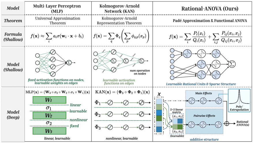Machine Learning, ICML, Rational ANOVA Networks <details> <summary>x1.png Details</summary>  ### Visual Description # Technical Document Extraction: Comparison of Neural Network Architectures This document provides a comprehensive extraction of the data and structural comparisons presented in the provided image. The image is a technical table comparing three neural network models: **Multi-Layer Perceptron (MLP)**, **Kolmogorov-Arnold Network (KAN)**, and the proposed **Rational-ANOVA**. --- ## 1. High-Level Table Structure The information is organized into a grid with five functional rows and three model columns. | Row Category | Column 1: Multi-Layer Perceptron (MLP) | Column 2: Kolmogorov-Arnold Network (KAN) | Column 3: Rational-ANOVA (Ours) | | :--- | :--- | :--- | :--- | | **Model** | Multi-Layer Perceptron (MLP) | Kolmogorov-Arnold Network (KAN) | Rational-ANOVA (Ours) | | **Theorem** | Universal Approximation Theorem | Kolmogorov-Arnold Representation Theorem | Padé Approximation & Functional ANOVA | | **Formula (Shallow)** | $f(\mathbf{x}) \approx \sum_{i} a_i \sigma(\mathbf{w}_i \cdot \mathbf{x} + b_i)$ | $f(\mathbf{x}) = \sum_{q} \Phi_q \left( \sum_{p} \phi_{q,p}(x_p) \right)$ | $f(\mathbf{x}) = \sum_{i} \frac{P_i(x_i)}{Q_i(x_i)} + \sum_{i,j} \frac{P_{ij}(x_i, x_j)}{Q_{ij}(x_i, x_j)}$ | | **Model (Shallow)** | Diagram of fixed activations on nodes | Diagram of learnable activations on edges | Diagram of learnable rational units | | **Model (Deep)** | Stacked linear/nonlinear layers | Composition of nonlinear functions | Additive structure with Main/Pairwise effects | --- ## 2. Detailed Component Analysis ### Column 1: Multi-Layer Perceptron (MLP) * **Theorem:** Relies on the **Universal Approximation Theorem**. * **Formula (Shallow):** Approximates a function as a weighted sum of nonlinear activations of linear combinations of inputs. * **Model (Shallow) Diagram:** * **Structure:** Input nodes connect to a hidden layer of four nodes, which then converge to a single summation ($\Sigma$) output node. * **Key Characteristic:** Text states: *"fixed activation functions on nodes, learnable weights on edges"*. * **Model (Deep) Diagram:** * **Logic:** Represented as a composition of matrices and activations: $\text{MLP}(\mathbf{x}) = (\mathbf{W}_3 \circ \sigma_2 \circ \mathbf{W}_2 \circ \sigma_1 \circ \mathbf{W}_1)(\mathbf{x})$. * **Visual Stack:** Alternating green blocks ($W_1, W_2, W_3$) and dashed lines ($\sigma_1, \sigma_2$). * **Labels:** $W$ layers are labeled as **linear** and **learnable**. $\sigma$ layers are labeled as **nonlinear** and **fixed**. ### Column 2: Kolmogorov-Arnold Network (KAN) * **Theorem:** Relies on the **Kolmogorov-Arnold Representation Theorem**. * **Formula (Shallow):** A nested summation where the inner functions $\phi_{q,p}$ and outer functions $\Phi_q$ are univariate. * **Model (Shallow) Diagram:** * **Structure:** Input nodes connect via edges containing activation function symbols to summation nodes ($\Sigma$). * **Key Characteristic:** Text states: *"learnable activation functions on edges"* and *"sum operation on nodes"*. * **Model (Deep) Diagram:** * **Logic:** Represented as a composition of function layers: $\text{KAN}(\mathbf{x}) = (\mathbf{\Phi}_3 \circ \mathbf{\Phi}_2 \circ \mathbf{\Phi}_1)(\mathbf{x})$. * **Visual Flow:** Three parallel horizontal tracks ($\Phi_1, \Phi_2, \Phi_3$), each showing a sequence of three learnable activation nodes. * **Labels:** The layers are described as **nonlinear** and **learnable**. ### Column 3: Rational-ANOVA (Ours) * **Theorem:** Combines **Padé Approximation** and **Functional ANOVA**. * **Formula (Shallow):** Expresses the function as a sum of univariate rational functions (Main Effects) and bivariate rational functions (Pairwise Effects). * **Model (Shallow) Diagram:** * **Structure:** Input nodes connect to blue-shaded "Rational Units" (depicting rational function curves). The structure is sparse, with some inputs skipping directly to specific units. * **Key Characteristic:** Text states: *"Learnable Rational Units & Sparse Structure"*. * **Model (Deep) Diagram:** * **Input $\mathcal{X}$:** A vertical vector of features. * **Main Effects Block:** Features pass into a sequence of rational units. * **Pairwise Effects Block:** Features are grouped via a "$2 \times 2$ linear matrix (learnable)" to create pairs like $(x_1, x_2)$ and $(x_3, x_4)$, which then pass through rational units. * **Pole/Extrapolation:** A call-out box shows a graph with a sharp peak, labeled *"Pole/Extrapolation"*, indicating the model's ability to handle rational singularities. * **Output:** The Main and Pairwise effects are combined at a summation node ($\oplus$) to produce **Rational-ANOVA(x)**. * **Labels:** The overall architecture is described as an **additive structure**. --- ## 3. Summary of Comparative Trends 1. **Parameter Location:** MLP places learnable parameters on edges (weights); KAN places them on edges (functions); Rational-ANOVA uses learnable rational units in a structured additive format. 2. **Function Type:** MLP uses fixed nonlinearities; KAN uses learnable univariate functions; Rational-ANOVA uses learnable rational functions (fractions of polynomials $P/Q$). 3. **Interpretability:** Rational-ANOVA explicitly separates "Main Effects" and "Pairwise Effects," following the Functional ANOVA decomposition, which is typically more interpretable than the dense connectivity of MLPs. </details> Figure 1: Comparison of RAN with MLPs and KANs. MLPs use fixed activations; KANs learn edge splines. RAN employs learnable rational units in a Functional ANOVA topology, decomposing $f$ into main effects ( $P_{i}/Q_{i}$ ) and sparse interactions ( $P_{ij}/Q_{ij}$ ). 1 Introduction Deep neural networks have become the default function approximators across domains (Schmidhuber, 2015; DeVore et al., 2020; Lin et al., 2021; Kovachki et al., 2023), from vision and language to scientific computing. Yet a core ingredient of this success, i.e., nonlinearity, is still treated as a surprisingly fixed and coarse design choice in most architectures. In practice, widely used backbones rely on low-parameter activations (e.g., ReLU (Agarap, 2018; Xu et al., 2020), GELU (Hendrycks and Gimpel, 2016), SiLU (Elfwing et al., 2017)) whose role is largely to inject generic curvature, while the burden of expressivity is delegated to scaling width and depth. This design is robust and efficient but exposes a persistent limitation: when the target mapping involves sharp transitions, near-singular regimes, or long-tail behaviors, fixed activations often require substantial over-parameterization to fit the shape (Glorot and Bengio, 2010; Klambauer et al., 2017). Furthermore, deep composition can amplify activation outliers (e.g., heavy-tailed feature excursions) into unstable optimization dynamics. A natural response is to make the nonlinearity itself learnable. Recent progress, exemplified by spline-parameterized networks such as Kolmogorov–Arnold Networks (KANs) (Liu et al., 2024b, a), suggests that learnable nonlinearities can improve interpretability and alter the accuracy–efficiency trade-off. However, turning nonlinearity into a high-capacity object raises a practical challenge: deep networks are not merely function classes but carefully tuned parameterizations whose stability depends on activation statistics and residual pathways. A highly expressive nonlinearity may inadvertently degrade conditioning or introduce numerical fragility when composed repeatedly in depth. This tension is especially salient if we seek a base architecture, i.e., a drop-in primitive that can be trained deeply and compared fairly against MLPs and KANs under matched budgets. In this work, we propose Rational-ANOVA Networks (RAN), a base architecture that makes nonlinearity learnable while maintaining stable and controllable deep training. RAN is motivated by two classical ideas: Padé-style rational approximation (Molina et al., 2019; Boullé et al., 2020; Palm et al., 2018) and functional ANOVA decomposition. Instead of relying on a fixed pointwise activation, RAN models a multivariate function via a low-order additive structure: $$ f(\mathbf{x})\approx\sum_{i=1}^{d}r_{i}(x_{i})+\sum_{(i,j)\in\mathcal{S}}r_{ij}(x_{i},x_{j}), \tag{1} $$ where the first term captures main effects and the second term captures sparse pairwise interactions over a controlled set $\mathcal{S}$ . This set $\mathcal{S}$ can be chosen to match a target compute or parameter budget, yielding a controllable interaction topology. As shown in Figure 1, each component $r_{i}$ and $r_{ij}$ is parameterized by a learnable rational unit—a quotient of low-degree polynomials. Figure 1 contrasts this design with MLPs and KANs: while MLPs place fixed nonlinearities on nodes and KANs place learnable splines on edges, RAN employs learnable rational units within an explicit low-order interaction topology. A key feature of RAN is its deep compatibility. To ensure numerical stability, we parameterize denominators to be strictly positive (specifically via $1+\text{softplus}(·)$ ), effectively avoiding poles while retaining the expressive “Padé-like” modeling capability (Trefethen, 2019; Telgarsky, 2017a). Furthermore, we employ residual-style gating (shown in Figure 2), allowing each rational unit to initialize near an identity map ( $y≈ x$ ) and gradually increase its effective nonlinearity during training. This prevents the early-stage instability often caused by aggressive curvature in rational functions. We evaluate RAN on controlled function benchmarks and physics-inspired problems under matched parameter and compute budgets against MLPs and KANs. Our results show that rational parameterization and sparse ANOVA structure are complementary: rational units handle non-smooth or near-singular regimes, while sparse interactions balance expressivity and generalization. <details> <summary>x2.png Details</summary>  ### Visual Description # Technical Document Extraction: Neural Network Architecture Diagram This document provides a comprehensive extraction and analysis of the provided technical diagram, which illustrates a multi-block neural network architecture utilizing 1D and 2D Rational Units. ## 1. 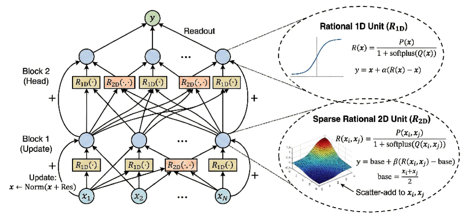High-Level Architecture Overview The image depicts a hierarchical neural network structure organized into sequential processing blocks, culminating in a readout layer. The flow of data is bottom-up, with residual connections (indicated by "+" symbols and curved arrows) bypassing the functional units within each block. ### Component Segmentation * **Input Layer:** Represented by nodes $x_1, x_2, \dots, x_N$. * **Block 1 (Update):** The first processing stage involving 1D and 2D rational functions. * **Block 2 (Head):** The second processing stage, mirroring the structure of Block 1 but leading to the final output. * **Readout Layer:** Aggregates the outputs of Block 2 into a single output node $y$. * **Functional Units:** Detailed callouts for **Rational 1D Unit ($R_{1D}$)** and **Sparse Rational 2D Unit ($R_{2D}$)**. --- ## 2. Detailed Block Analysis ### Block 1 (Update) * **Inputs:** Receives signals from $x_1, x_2, \dots, x_N$. * **Processing Units:** * **$R_{1D}(\cdot)$:** Yellow rectangular blocks. These appear to process individual node features. * **$R_{2D}(\cdot, \cdot)$:** Orange rectangular blocks. These process interactions between two nodes (e.g., between $x_2$ and $x_N$). * **Residual Connection:** A curved arrow with a **+** sign indicates a skip connection from the input $x$ to the output of the block. * **Update Rule Text:** `Update: x ← Norm(x + Res)` ### Block 2 (Head) * **Inputs:** Receives the normalized output from Block 1. * **Processing Units:** Contains a mix of $R_{1D}(\cdot)$ and $R_{2D}(\cdot, \cdot)$ units. * **Connectivity:** Shows a dense interaction pattern where outputs from Block 1 nodes are cross-combined into the $R_{2D}$ units of Block 2. * **Residual Connection:** Similar to Block 1, a curved arrow with a **+** sign bypasses the functional units. ### Readout * **Process:** Arrows point from the top blue nodes of Block 2 to a single green node labeled **$y$**. * **Label:** "Readout" --- ## 3. Functional Unit Specifications (Callouts) ### Rational 1D Unit ($R_{1D}$) * **Visual Representation:** A 2D line plot showing a sigmoid-like (S-shaped) curve. * **Mathematical Definition:** $$R(x) = \frac{P(x)}{1 + \text{softplus}(Q(x))}$$ * **Output Equation:** $$y = x + \alpha(R(x) - x)$$ *(Note: This represents a weighted residual update where $\alpha$ scales the change.)* ### Sparse Rational 2D Unit ($R_{2D}$) * **Visual Representation:** A 3D surface plot showing a localized peak (resembling a Gaussian or bell shape) over a 2D plane. * **Mathematical Definition:** $$R(x_i, x_j) = \frac{P(x_i, x_j)}{1 + \text{softplus}(Q(x_i, x_j))}$$ * **Output Equation:** $$y = \text{base} + \beta(R(x_i, x_j) - \text{base})$$ $$\text{base} = \frac{x_i + x_j}{2}$$ * **Operational Note:** An arrow points to the 3D plot with the text: **"Scatter-add to $x_i, x_j$"**. This indicates that the result of the 2D unit is distributed back to the constituent input nodes. --- ## 4. Textual Transcriptions | Location | Original Text | | :--- | :--- | | Top Center | $y$ | | Top Right | Readout | | Left (Top) | Block 2 (Head) | | Left (Middle) | Block 1 (Update) | | Left (Bottom) | Update: $x \leftarrow \text{Norm}(x + \text{Res})$ | | Bottom Nodes | $x_1, x_2, \dots, x_N$ | | Unit Labels | $R_{1D}(\cdot)$, $R_{2D}(\cdot, \cdot)$ | | Callout 1 Title | Rational 1D Unit ($R_{1D}$) | | Callout 2 Title | Sparse Rational 2D Unit ($R_{2D}$) | | Callout 2 Note | Scatter-add to $x_i, x_j$ | --- ## 5. Summary of Logic and Flow 1. **Input** $x$ enters the system. 2. **Block 1** applies 1D transformations to individual features and 2D transformations to pairs of features. The result is added back to the original input (Residual) and Normalized. 3. **Block 2** repeats this process, potentially with different weights or "Head" specific parameters. 4. The **Readout** layer performs a final aggregation of all node features to produce the scalar or vector output $y$. 5. The **Rational Units** use a specific ratio of polynomials ($P/Q$) stabilized by a softplus function to learn non-linear activations. </details> Figure 2: Deep Rational-ANOVA Network (RAN) architecture. Left: A deep backbone of stacked residual blocks; each block performs sparse pairwise message passing (interactions) then node-wise updates. Right: Learnable rational units. $R_{1\text{D}}$ and $R_{2\text{D}}$ use residual gating $y=x+\alpha(R(x)-x)$ for identity initialization. Denominators are positive ( $1+\text{softplus}(·)$ ) for stability and pole-free composition. 2 Rational-ANOVA Networks Setup and notation. Let $\mathbf{x}∈\mathbb{R}^{d}$ denote the input and $f_{\theta}(\mathbf{x})$ the model output (logits for classification or a scalar for regression) (Rumelhart et al., 1986). We design Rational-ANOVA Networks (RAN) as a base network primitive with two design goals: (i) to enable strictly fair comparisons with parameter-matched MLPs and KANs, and (ii) to serve as a drop-in replacement for FFNs in pretrained backbones by modifying only the nonlinearity parameterization while preserving linear projections and activation statistics. (a) MLP: Dense Entanglement Input Space (Slice) $∇\mathcal{L}$ $x_{u}$ $x_{o}$ Unintended Shift $\Delta f(x_{o})\propto K_{\text{dense}}(x_{o},x_{u})$ Non-local updates (Global mixing) (b) RAN: ANOVA Locality Input Space (Slice) $∇\mathcal{L}$ $x_{u}$ $x_{o}$ Stable (Zero Influence) Influence restricted by topology $\sum K^{\text{main}}+\sum K^{\text{pair}}_{\text{sparse}}$ (c) Rational Stability Pre-activation $x$ Target Squeezing Poly/Spline Rational Bounded deriv. $d^{\prime}(x)≈ 0$ (Eq. 18) Sharp transitions w/o poles Prevents gradient explosion Figure 3: Learning Dynamics Comparison. Similar to how RLHF/DPO dynamics affect probability mass, we visualize how structural choices affect function updates $\Delta f$ . (a) MLP Entanglement: An update at $x_{u}$ (red arrow) causes uncontrolled shifts at distant $x_{o}$ (dashed arrow) due to dense kernel mixing. (b) RAN Locality (Ours): The ANOVA structure (Eq. 17) disentangles interactions; updates at $x_{u}$ leave uncorrelated regions $x_{o}$ stable. (c) Rational Stability: Under strong “squeezing” gradients (steep transitions), polynomials oscillate (Runge’s phenomenon), while RAN’s rational units (Eq. 18) fit smoothly due to denominator-controlled derivatives. 2.1 ANOVA-Induced Architecture Low-order functional decomposition. RAN parameterizes multivariate mappings via an explicit low-order additive structure(conceptually contrasted with MLPs and KANs in Figure 1): $$ \begin{split}f_{\theta}(\mathbf{x})=&\underbrace{\sum_{i=1}^{d}r_{i}(x_{i})}_{\text{main effects}}\;+\;\underbrace{\sum_{(i,j)\in\mathcal{S}}r_{ij}(x_{i},x_{j})}_{\text{sparse pairwise effects}}\\ &\text{(optionally followed by a linear readout).}\end{split} \tag{2} $$ Here, $\mathcal{S}⊂eq\{(i,j):1≤ i<j≤ d\}$ is a controlled interaction set. This design makes the interaction topology explicit and budgetable: increasing $|\mathcal{S}|$ adds second-order capacity without the combinatorial explosion of dense pairwise grids. Beyond efficiency, the sparsity of $\mathcal{S}$ also induces a structured influence geometry (as analyzed in Sec. 3), allowing cross-sample coupling to be explicitly analyzed and controlled through the interaction topology. Instantiation for supervised learning. For $C$ -class classification, we construct a feature vector by concatenating all main and pairwise outputs: $$ \begin{split}\phi_{\theta}(\mathbf{x})=\big[&r_{1}(x_{1}),\dots,r_{d}(x_{d}),\\ &r_{i_{1}j_{1}}(x_{i_{1}},x_{j_{1}}),\dots,r_{i_{K}j_{K}}(x_{i_{K}},x_{j_{K}})\big]\in\mathbb{R}^{d+K},\end{split} \tag{3} $$ where $K=|\mathcal{S}|$ . Logits are produced by a linear head $z(\mathbf{x})=W\phi_{\theta}(\mathbf{x})+b$ . This yields a robust baseline where all nonlinearity lives inside learnable rational units, while global mixing remains linear (hence stable, interpretable, and compatible with pretrained linear projections if inserted into FFNs). Choosing the interaction set $\mathcal{S}$ . To ensure fair comparisons and avoid task-specific engineering, our default setting uses a fixed random $\mathcal{S}$ sampled once with a global seed and reused across runs. This isolates the inductive bias of rational parameterization combined with sparse low-order structure. We evaluate data-driven choices (e.g., correlation-based or gradient-based selection) only in ablations (see Appendix J). 2.2 Learnable Rational Units 1D rational unit (main effects). Each main-effect function $r_{i}:\mathbb{R}→\mathbb{R}$ is parameterized as a Padé-style rational map: $$ \begin{split}&\tilde{r}_{i}(x)=\frac{p_{i}(x)}{d_{i}(x)},\hskip 18.49988ptp_{i}(x)=\sum_{a=0}^{m}\alpha_{ia}x^{a},\\ &d_{i}(x)=1+\operatorname{softplus}\!\Big(\sum_{b=1}^{n}\beta_{ib}x^{b}\Big)+\varepsilon,\end{split} \tag{4} $$ where $(m,n)$ are degrees and $\varepsilon>0$ . The constraint $d_{i}(x)≥ 1+\varepsilon$ prevents poles while retaining the expressive quotient form (see Appendix K for regularity proofs). In practice, low degrees are sufficient to capture sharp transitions and saturation effects that fixed activations often model only via increased width or depth. 2D rational unit (pairwise effects). Each pairwise function $r_{ij}:\mathbb{R}^{2}→\mathbb{R}$ uses a low-degree bivariate rational form: $$ \begin{split}&\tilde{r}_{ij}(x,y)=\frac{p_{ij}(x,y)}{d_{ij}(x,y)},\qquad p_{ij}(x,y)=\sum_{t=1}^{T}\gamma_{ij,t}\,\psi_{t}(x,y),\\ &d_{ij}(x,y)=1+\operatorname{softplus}\!\Big(\sum_{s=1}^{S}\delta_{ij,s}\,\varphi_{s}(x,y)\Big)+\varepsilon,\end{split} \tag{5} $$ where $\{\psi_{t}\}$ and $\{\varphi_{s}\}$ are simple basis monomials (e.g., $1,x,y,x^{2},xy,y^{2}$ ). Restricting the basis to low order is crucial for deep composition: it controls curvature and reduces optimization instability, while still providing a richer local shaping mechanism than fixed node-wise activations. 2.3 Deep Compatibility via Residual Gating Residual-style gating (identity-safe). Directly composing expressive rational maps can be unstable if aggressive curvature is activated too early. We therefore wrap each rational map with a residual gate(as detailed in Figure 2): $$ r(x)\;=\;x\;+\;\alpha\cdot\big(\tilde{r}(x)-x\big), \tag{6} $$ and similarly for $r_{ij}$ with gate $\alpha_{ij}$ . Gates are initialized so that each unit starts near-identity ( $r(x)≈ x$ ), enabling the model to gradually “turn on” rational nonlinearity during training. Stable early-stage Jacobian. The Jacobian of the gated unit is $$ \frac{\partial r}{\partial x}=(1-\alpha)+\alpha\frac{\partial\tilde{r}}{\partial x}. \tag{7} $$ A small initial $\alpha$ keeps the effective sensitivity close to $1$ . This prevents early training dynamics from being dominated by activation outliers, and ensures deep optimization behavior is comparable to stable residual architectures (proven in Appendix L). 2.4 RAN as a Drop-in FFN Replacement Replacing node-wise activations. A standard Transformer/ViT FFN is $\mathrm{FFN}(h)=W_{2}\,\sigma(W_{1}h)+b$ with $\sigma$ (e.g., GELU). Our minimal drop-in variant replaces $\sigma$ with feature-wise 1D RAN units: $$ \mathrm{RAN\text{-}FFN}(h)=W_{2}\,r\!\left(W_{1}h\right)+b, \tag{8} $$ where $r(·)$ is the vectorized collection of gated rational units. This preserves the linear projections (and most pretrained weights) and modifies only the nonlinearity parameterization, while the identity-safe initialization avoids disrupting pretrained activation statistics. Optional pairwise augmentation. If explicit second-order structure is desired inside FFNs, we can augment the hidden representation with sparse pairwise rational features over selected channels: $$ \begin{split}\mathrm{RAN\text{-}FFN^{+}}(h)=W_{2}\Big(\big[&r(W_{1}h),\\ &\{r_{ij}((W_{1}h)_{i},(W_{1}h)_{j})\}_{(i,j)\in\mathcal{S}_{h}}\big]\Big)+b.\end{split} \tag{9} $$ While this formulation enhances expressivity by capturing internal feature correlations, it incurs non-trivial computational overhead. Therefore, we position $\mathrm{RAN\text{-}FFN^{+}}$ primarily as an analytical tool in our ablation studies to investigate the value of explicit second-order information, retaining the 1D variant as the default for efficiency-critical comparisons. 2.5 Parameter Budgeting and Implementation Details Budget matching. RAN supports exact budget matching with baselines. A 1D unit uses $(m+1)$ numerator coefficients, $n$ denominator coefficients, and one gate parameter, totaling $≈ m+n+2$ parameters per feature. A 2D unit contributes $≈ T+S+1$ parameters per selected pair. Excluding the linear head: $$ \mathrm{Params}\approx d\big(m+n+2\big)\;+\;|\mathcal{S}|\,(T+S+1). \tag{10} $$ This explicit accounting enables strictly matched comparisons with MLPs and KANs. Stability-oriented implementation. To ensure robust deep training, we employ the following stabilizers: Positive Denominators: As defined in Eq. (4), we enforce $d(·)≥ 1+\varepsilon$ via softplus to strictly avoid poles. Initialization: We initialize $\tilde{r}(x)$ near identity by setting $p(x)≈ x$ and $d(x)≈ 1$ (coefficients near zero), and initialize gates $\alpha$ near zero. Optimization: We optionally use a smaller learning rate for denominator/gate parameters and mild weight decay on denominator coefficients (detailed in Appendix I). These stabilizers do not change the hypothesis class but significantly improve numerical stability in deep networks (see analysis in Appendix K). 3 Learning Dynamics of Rational-ANOVA Networks Learning dynamics. The term “learning dynamics” refers to how training updates affect model behavior. We study a concrete per-step notion: how a single gradient update on one training example changes the model’s prediction on another input. Consider one SGD step at iteration $t$ on $(x_{u},y_{u})$ with learning rate $\eta$ : $$ \begin{split}\Delta\theta_{t}&\triangleq\theta_{t+1}-\theta_{t}=-\eta\nabla_{\theta}\mathcal{L}\!\left(f_{\theta_{t}}(x_{u}),y_{u}\right),\\ \Delta f_{t}(x_{o})&\triangleq f_{\theta_{t+1}}(x_{o})-f_{\theta_{t}}(x_{o}).\end{split} \tag{11} $$ The central question is: After one SGD update on $(x_{u},y_{u})$ , how does the prediction on a different input $x_{o}$ change? A first-order influence formula. A Taylor expansion yields a model-agnostic first-order approximation: $$ \begin{split}\Delta f_{t}(x_{o})\approx-\eta\,\nabla_{\theta}f_{\theta_{t}}(x_{o})^{\top}\nabla_{\theta}\mathcal{L}\!\left(f_{\theta_{t}}(x_{u}),y_{u}\right).\end{split} \tag{12} $$ Thus, the geometry of influence is governed by gradient alignment between the query point $x_{o}$ and the update point $x_{u}$ . Classification: eNTK-style decomposition. For multi-class classification with logits $z=h_{\theta}(x)$ and $\pi=\mathrm{Softmax}(z)$ , we track the vector of log-probabilities. A first-order expansion gives: $$ \begin{split}\Delta\log\pi_{t}(\cdot\mid x_{o})\approx-\eta\;A_{t}(x_{o})\;K_{t}(x_{o},x_{u})\;G_{t}(x_{u},y_{u})\;+\;O(\eta^{2}),\end{split} \tag{13} $$ where $A_{t}(x_{o})=∇_{z}\log\pi_{\theta_{t}}(·\mid x_{o})$ depends only on the current predictive distribution, $G_{t}(x_{u},y_{u})$ is the loss gradient w.r.t. logits, and $$ K_{t}(x_{o},x_{u})\triangleq\left(\nabla_{\theta}z_{\theta}(x_{o})|_{\theta_{t}}\right)\left(\nabla_{\theta}z_{\theta}(x_{u})|_{\theta_{t}}\right)^{\top} \tag{14} $$ is the Empirical Neural Tangent Kernel (eNTK). Intuitively, $K_{t}(x_{o},x_{u})$ measures how strongly an update triggered by $x_{u}$ projects onto the prediction at $x_{o}$ . A mild stability assumption. For visualization, we assume relative influence stability: for a fixed $x_{u}$ , the relative magnitudes of $\|K_{t}(x_{o},x_{u})\|$ across different $x_{o}$ remain approximately stable over short windows. This is weaker than lazy training and is empirically verified in our experiments. Structured kernel decomposition in RAN. As defined in Sec. 2, RAN parameterizes a multivariate function via a low-order interaction topology (Eq. (2)). With logits $z(\mathbf{x})=W\phi_{\theta}(\mathbf{x})+b$ , the eNTK admits an additive decomposition: $$ K_{t}(x_{o},x_{u})=K_{t}^{\mathrm{rat}}(x_{o},x_{u})+K_{t}^{\mathrm{head}}(x_{o},x_{u}). \tag{15} $$ The head-side term $K_{t}^{\mathrm{head}}$ behaves like a linear kernel on features. $$ \begin{split}K_{t}^{\mathrm{head}}(x_{o},x_{u})&=(\nabla_{W}z(x_{o}))(\nabla_{W}z(x_{u}))^{\top}\\ &\qquad+(\nabla_{b}z(x_{o}))(\nabla_{b}z(x_{u}))^{\top},\end{split} \tag{16} $$ which is low-rank and explicitly controlled by feature similarities. Crucially, owing to the ANOVA topology introduced in Eq. (2), the rational-unit-side term decomposes into interpretable groups: $$ \begin{split}K_{t}^{\mathrm{rat}}(x_{o},x_{u})=\sum_{i=1}^{d}K_{t,i}^{\mathrm{main}}(x_{o},x_{u})+\sum_{(i,j)\in\mathcal{S}}K_{t,ij}^{\mathrm{pair}}(x_{o},x_{u}).\end{split} \tag{17} $$ Key insight. Unlike dense feature mixing in MLPs, RAN makes cross-sample coupling explicitly controllable. As visualized in Figure 3 (a) vs. (b), dense MLPs suffer from global entanglement where an update at $x_{u}$ causes unintended shifts at distant $x_{o}$ . In contrast, RAN’s ANOVA topology ensures that only inputs overlapping in specific low-order projections (main coordinates and selected pairs in $\mathcal{S}$ ) can strongly influence each other. This transparency allows us to trade off expressivity and generalization by designing the interaction set $\mathcal{S}$ (analyzed in Appendix D). Why rational units are stable in depth. For a 1D unit $\tilde{r}(x)=p(x)/d(x)$ , since $d(x)≥ 1+\varepsilon$ (as enforced in Eq. (4)), the quotient rule implies (recalling $d(x)=1+\operatorname{softplus}(q(x))+\varepsilon$ ): $$ \begin{split}\left|\frac{\partial\tilde{r}}{\partial x}\right|&=\left|\frac{p^{\prime}(x)d(x)-p(x)d^{\prime}(x)}{d(x)^{2}}\right|\\ &\leq|p^{\prime}(x)|+|p(x)|\,|d^{\prime}(x)|.\end{split} \tag{18} $$ (Detailed Lipschitz bounds provided in Appendix K.) Moreover, denominator sensitivity is controlled by $$ d^{\prime}(x)=\sigma_{\mathrm{sig}}\!\big(q(x)\big)\,q^{\prime}(x),\quad\text{with }\sigma_{\mathrm{sig}}(\cdot)\in(0,1), \tag{19} $$ which prevents the denominator pathway from amplifying gradients excessively. Figure 3 (c) visualizes this benefit: while polynomials often oscillate under steep gradient requirements (Runge’s phenomenon), RAN’s rational units maintain smooth and bounded updates due to this denominator-controlled mechanism, thereby enabling stable deep training (proven in Appendix L). Accumulated influence. To study long-term effects, we visualize the accumulated influence from a subset of updates $\mathcal{U}$ onto a query input $x_{o}$ : $$ \begin{split}\mathrm{Infl}(x_{o};\mathcal{U})\approx-\eta\sum_{t\in\mathcal{U}}A_{t}(x_{o})\,K_{t}(x_{o},x_{u(t)})\,G_{t}(x_{u(t)},y_{u(t)}).\end{split} \tag{20} $$ In Sec. 4, we show how RAN’s sparse interaction topology reshapes these influence patterns compared to MLPs and KANs. Table 1: Comparison of Model Accuracy across Different Datasets. RAN (ours) is highlighted with a gray background. Note that RAN achieves consistent improvements across varying parameter scales (50k to 1.0M) and diverse datasets. | DATASET | PARAMS | Accuracy (%) | | DATASET | PARAMS | Accuracy (%) | | | | | | | | --- | --- | --- | --- | --- | --- | --- | --- | --- | --- | --- | --- | --- | | KAF | MLP | KAN | RAN † | | KAF | MLP | KAN | RAN † | | | | | | MNIST | 50k | 97.45 | 97.60 | 96.50 | 97.55 | | EMNIST-Let | 50k | 82.50 | 84.60 | 70.00 | 84.55 | | 100k | 98.15 | 98.25 | 97.10 | 98.20 | | 100k | 86.80 | 88.55 | 78.50 | 88.40 | | | | 200k | 98.35 | 98.45 | 97.40 | 98.40 | | 200k | 88.90 | 90.20 | 81.20 | 90.15 | | | | 300k | 98.50 | 98.60 | 97.50 | 98.55 | | 300k | 89.15 | 90.80 | 81.50 | 90.85 | | | | 400k | 98.65 | 98.70 | 97.65 | 98.75 | | 400k | 89.40 | 91.30 | 82.00 | 91.25 | | | | FMNIST | 50k | 88.00 | 88.50 | 86.00 | 95.39 | | SVHN | 200k | 76.50 | 79.20 | 60.50 | 79.15 | | 100k | 89.20 | 89.00 | 88.00 | 96.67 | | 500k | 79.80 | 81.55 | 63.80 | 81.65 | | | | 200k | 89.50 | 89.20 | 87.00 | 97.49 | | 1M | 81.20 | 82.40 | 62.00 | 82.35 | | | | 300k | 89.50 | 89.30 | 86.50 | 97.69 | | 1.5M | 81.80 | 83.15 | 55.00 | 83.25 | | | | 400k | 89.50 | 89.30 | 86.20 | 97.79 | | 2M | 82.05 | 83.85 | 48.00 | 83.80 | | | | CIFAR-10 | 0.5M | 56.20 | 54.98 | 46.81 | 58.84 | | CIFAR-100 | 0.5M | 25.62 | 25.85 | 17.73 | 27.86 | | 1.0M | 56.95 | 56.45 | 43.32 | 59.05 | | 1.0M | 26.75 | 27.10 | 14.80 | 28.12 | | | 4 Experiments Unless otherwise stated, all experiments are conducted under the strict premise of matched parameter counts (and matched FLOPs when applicable), and all runs are performed on NVIDIA RTX 6000 GPUs. Evaluation roadmap and why we start from vision. Our experiments are organized to support RAN as a drop-in nonlinear block across regimes. We begin with controlled visual benchmarks because they provide a widely adopted and reproducible stress test for both expressivity and optimization stability under strict parameter/FLOPs budgets. Importantly, this suite is also the standard testbed in the Kanbefair protocol, enabling direct comparisons to learnable-nonlinearity baselines under identical pipelines. To avoid conclusions that depend on a single domain, we further include (i) large-scale backbone integration (ViT on ImageNet-1K), (ii) real-world restoration (PolyU denoising), and (iii) non-visual evaluations and ablations (e.g., TabArena) to isolate the roles of topology and rational nonlinearities. Broader evaluation across domains. We emphasize that this paper does not claim KAN is primarily designed for vision. Instead, we adopt vision benchmarks as a standardized, budget-controlled protocol for learnable nonlinearity comparisons. To fairly reflect the regimes where KAN is typically most competitive, we additionally evaluate RAN on scientific discovery and extrapolation settings where KAN is often expected to excel: (i) tabular learning with strong efficiency constraints (TabArena; see Supplementary Section A), (ii) symbolic regression / physical law recovery (e.g., Lorentzian potential and Feynman equations; Supplementary Sections B and M), and (iii) extrapolation and boundary stability via the Runge stress test (Supplementary Section C). These tasks directly evaluate interpretability, structure recovery, and out-of-support generalization, reducing reliance on vision-only evidence. 4.1 Comprehensive Evaluation on Visual Benchmarks Benchmarks and baselines. We follow the Kanbefair evaluation framework (Yu et al., 2024) to benchmark across diverse visual classification datasets, including MNIST (LeCun et al., 2002), EMNIST (Cohen et al., 2017), FMNIST (Xiao et al., 2017), SVHN (Netzer et al., 2011), and CIFAR (Krizhevsky et al., 2009). We compare against: (i) MLP with GELU (and ReLU as an additional reference), (ii) the original KAN (Liu et al., 2024b), and (iii) the recent KAF (Zhang et al., 2025), in Table 1. 4.1.1 Training protocol and fairness controls Unified training budget and model selection. To avoid confounding factors from different optimization schedules, we train all methods under a unified training budget. Model selection is performed using the validation set (or a held-out split following Kanbefair), and we report the corresponding test accuracy of the selected checkpoint. This prevents inadvertently favoring any method via “test-set best” selection and makes the comparison reproducible. Parameter matching. For each dataset and each target budget, we enforce parameter parity across methods (within a tight tolerance). For KAN, we sweep the recommended configuration space (grid sizes $\{3,5,10,20\}$ and B-spline degrees $\{2,3,5\}$ ) and report the best-performing setting under the same parameter budget. For MLP and KAF, we follow their standard implementations and tune width/depth only to meet the required parameter count. For RAN, parameter control is non-trivial because the sparse interaction set contributes additional learnable components. We therefore use an explicit parameter estimator to guide architecture instantiation: $\mathrm{Params}≈(18+C)N+(26+C)K+C+2,$ where $N$ denotes the hidden width, $K$ is the rational grid/order size, and $C$ is the number of classes. Crucially, we dynamically adjust the number of sparse interaction pairs $|\mathcal{S}|$ so that RAN matches the target budget of each baseline configuration. This ensures that improvements cannot be attributed to a larger parameter count. Model capacity sweep. To stress-test robustness across regimes, we sweep a wide range of hidden widths (from 2 to 1024 when feasible) and report performance at multiple parameter budgets. Unless otherwise stated, we report results averaged over multiple random seeds (mean and variance in the supplementary), and keep all data preprocessing and augmentation identical across methods. 4.2 Evaluation in Large-Scale Vision Models To assess scalability, we integrate RAN into Vision Transformers (Dosovitskiy et al., 2020). Concretely, we adopt ViT-Tiny (DeiT-T) (Touvron et al., 2021) and replace the standard FFN blocks with RAN-FFN blocks while preserving the original parameter budget and FLOPs. All models are trained on ImageNet-1K (Deng et al., 2009; Russakovsky et al., 2015) using the same training recipe (including standard strong augmentations such as Mixup and CutMix, and the same learning-rate schedule) to ensure fair comparison. Baselines: (i) the standard MLP-based ViT (GELU FFN), (ii) KAF, and (iii) KAN. For KAN, we attempted to instantiate the smallest feasible configurations under the ViT embedding dimension while enforcing the same budget constraints. However, due to the intrinsic parameter/memory growth induced by the B-spline basis expansion in high-dimensional settings, KAN remains infeasible on our hardware budget (48GB GPU memory), resulting in OOM under budget-matched conditions. We explicitly mark this outcome as OOM rather than reporting an under-budget or structurally altered KAN that would not be comparable. Table 2: Performance on ViT-T/16 (ImageNet-1K). All methods are trained with the same recipe; Params/FLOPs are matched to the baseline when applicable. OOM denotes infeasibility under the budget-matched setting on 48GB GPUs. Overall, RAN improves Top-1 accuracy from 72.3% (MLP baseline) to 74.2% under the same Params/FLOPs. We attribute the gain to the combination of (i) learnable rational nonlinearities with stronger local approximation capacity and (ii) near-identity initialization and stabilization constraints that preserve optimization stability when replacing deep FFN stacks. 4.3 Real-World Image Denoising on PolyU <details> <summary>x3.png Details</summary>  ### Visual Description # Technical Data Extraction: Real-World Denoising Efficiency (PolyU) ## 1. Document Metadata * **Title:** Real-World Denoising Efficiency (PolyU) * **Type:** Scatter Plot (Performance vs. Model Complexity) * **Primary Language:** English ## 2. Axis Specifications * **Y-Axis (Vertical):** * **Label:** PSNR (dB) * **Scale:** Linear, ranging from 10.0 to 30.0+ (increments of 2.5 marked). * **Significance:** Higher values indicate better image restoration quality. * **X-Axis (Horizontal):** * **Label:** Parameters (Million, Log Scale) * **Scale:** Logarithmic. Major markers at 0.05M, 0.10M, 0.50M, and 1.00M. * **Significance:** Lower values indicate a more lightweight/efficient model. ## 3. Legend and Component Isolation The legend is located in the bottom-right quadrant of the chart area. | Symbol | Color | Label | Description | | :--- | :--- | :--- | :--- | | Circle | Grey | MLP | Multi-Layer Perceptron baseline | | Square | Blue | CNN | Convolutional Neural Network baseline | | X-mark | Red | KAN | Kolmogorov-Arnold Network baseline | | Star | Green | RAN (Ours) | Proposed Rational Activation Network | ## 4. Data Point Extraction and Trend Analysis The chart compares four distinct architectures. There is a clear trade-off trend where traditional models (CNN, KAN) require significantly more parameters to achieve their results, while the proposed RAN model breaks this trend by being both the most accurate and the most efficient. ### Data Table | Model | Parameters (Approx. 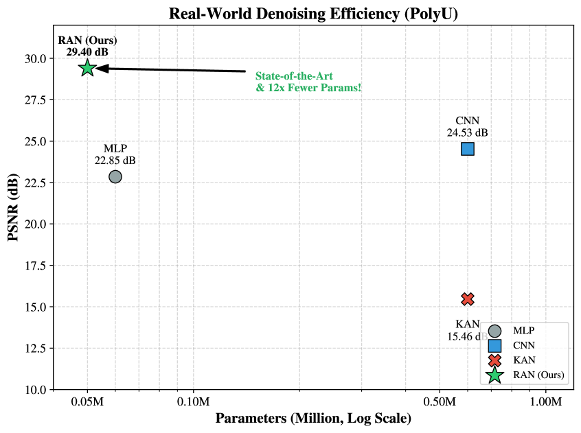X-position) | PSNR (dB) | Visual Position | | :--- | :--- | :--- | :--- | | **RAN (Ours)** | ~0.05M | **29.40 dB** | Top-Left (High Performance, Low Complexity) | | **MLP** | ~0.06M | 22.85 dB | Mid-Left | | **CNN** | ~0.60M | 24.53 dB | Mid-Right | | **KAN** | ~0.60M | 15.46 dB | Bottom-Right (Low Performance, High Complexity) | ## 5. Key Annotations and Insights * **Primary Callout:** A black arrow points from the center of the chart toward the **RAN (Ours)** data point. * **Annotation Text:** "State-of-the-art & 12x Fewer Params!" (Text color: Green). * **Efficiency Comparison:** The RAN model achieves the highest PSNR (29.40 dB) while positioned at the far left of the log-scale x-axis (~0.05M parameters). * **Performance Gap:** RAN outperforms the next best model (CNN) by **4.87 dB** while utilizing roughly **1/12th** of the parameters (comparing ~0.05M to ~0.60M). * **KAN Performance:** The KAN model, despite having a high parameter count (~0.60M), shows the lowest performance at 15.46 dB. ## 6. Summary of Findings The visualization demonstrates that the **RAN (Ours)** architecture provides a significant breakthrough in denoising efficiency on the PolyU dataset. It occupies the "ideal" quadrant of the graph (top-left), representing a Pareto improvement over MLP, CNN, and KAN architectures by simultaneously maximizing signal-to-noise ratio and minimizing computational footprint. </details> Figure 4: Real-World Denoising Efficiency on PolyU. PSNR (y-axis) vs. parameter count (x-axis, log scale). Each point corresponds to a budgeted model instance. RAN achieves a strong accuracy–efficiency trade-off and lies on the Pareto frontier. We further evaluate RAN on the PolyU Real-world Noisy Image Dataset (Xu et al., 2018), which contains real noise under varying ISO and shutter speeds. Unlike synthetic Gaussian noise, PolyU requires modeling complex, non-i.i.d. noise patterns under tight budgets. Protocol and preprocessing. We split the dataset into train/test following paired Real (noisy) and Mean (clean) folders. During training, we apply random cropping to generate $128× 128$ patches; during evaluation, we use center crops for deterministic reporting. To apply our non-convolutional model, we use a patch-based strategy: each image is unfolded into non-overlapping patches of size $P× P$ ( $P=4$ ), yielding $d=3P^{2}=48$ input dimensions per patch. Model configuration and budgets. We instantiate a lightweight Residual Rational-ANOVA model with 3 layers and a hidden dimension of 16, equipped with both unit-level gating and block-level residual connections for stable optimization. Importantly, PolyU is evaluated as an efficiency study: we report PSNR versus parameter count and compare the Pareto frontier across model families rather than enforcing a single identical budget for all methods. As shown in Fig. 4, RAN achieves high PSNR at a small budget (e.g., $\sim$ 50k parameters), while the compared CNN/KAN baselines are instantiated at larger budgets (e.g., $\sim$ 600k parameters) to reflect their typical operating points. Training and metrics. All models use Adam ( $10^{-3}$ ), batch size 32, and identical epoch budgets. We optimize $\ell_{1}$ (MAE) to better preserve sharp edges, and process patches in chunks (4,096 per forward) to save memory. We report PSNR on full-resolution reconstructions after refolding and clamping outputs to $[0,1]$ . Baselines. We compare against (i) a ReLU MLP at matched small budgets, (ii) a lightweight CNN for fast denoising at larger budgets, and (iii) KAN (B-splines) at comparable larger budgets. Fig. 4 summarizes PSNR–Params trade-offs. 4.4 Ablation Studies We conduct ablations on TabArena and CIFAR-10 to isolate the sources of improvement. We fix the parameter budget to $\sim$ 1M and decouple the effects of topology (Dense vs. Sparse ANOVA) and activation (ReLU vs. Rational). Table 3: Component Analysis. Dense vs. sparse ANOVA topology and ReLU vs. rational activations under a fixed $\sim$ 1M budget. | MLP (Base) MLP-Rat ANOVA-ReLU | Dense Dense Sparse | ReLU Rational ReLU | 0.82 0.89 0.86 | 56.0 56.8 55.2 | | --- | --- | --- | --- | --- | | RAN (Ours) | Sparse | Rational | 0.96 | 58.3 | Structure vs. activation. MLP-Rat improves over the dense ReLU baseline, indicating that learnable rational nonlinearities are beneficial even without sparsity. However, ANOVA-ReLU degrades CIFAR-10 accuracy, suggesting that sparsity alone can reduce effective capacity for complex visual patterns. Combining both yields the best result: RAN achieves the strongest performance across domains, supporting a synergistic effect where rational units compensate for capacity loss induced by sparse ANOVA connectivity. Topology and stability. We further study: (i) interaction set selection for $\mathcal{S}$ (random vs. heuristic criteria), and (ii) stabilization mechanisms. Heuristic selection provides negligible gains ( $<0.3\%$ ) while increasing preprocessing overhead, suggesting that having mixing capacity matters more than precise initial pair choice. Stability constraints are critical: removing the positive denominator constraint can trigger divergence across seeds, and removing residual gating (i.e., $\alpha=1$ ) substantially reduces final accuracy, confirming that near-identity initialization is important. 5 Related Work Learnable nonlinearities and rational parameterizations. While most deep networks rely on fixed pointwise activations such as ReLU (Agarap, 2018; Nair and Hinton, 2010) or GELU (Hendrycks and Gimpel, 2016), an increasing body of work argues that the shape of nonlinear transformations should itself be learnable (Goodfellow et al., 2013; Ramachandran et al., 2017; He et al., 2015b, a). By adapting the nonlinearity to the data distribution, such models can achieve higher expressivity per parameter and improved sample efficiency. Rational function parameterizations are especially appealing in this regard (Telgarsky, 2017a), as low-degree rational forms can approximate functions with sharp transitions, saturation, or near-singular behavior more efficiently than polynomials. Nevertheless, unconstrained rational compositions may introduce poles or unstable gradients, which has motivated recent designs that enforce positivity or normalization in the denominator and emphasize stability under deep composition. Spline-based models and Kolmogorov–Arnold Networks. Spline-based neural models, most prominently Kolmogorov–Arnold Networks (KANs) (Yu et al., 2024; Zhang et al., 2025), revisit classical representation theorems by placing learnable univariate functions on network edges. This design offers strong interpretability and flexible function approximation, and has shown promising empirical performance (Scardapane et al., 2018; Bohra et al., 2020). However, spline discretization typically requires maintaining knot grids, which can lead to non-negligible memory and computation overhead, as well as boundary artifacts and sensitivity to grid resolution (Li, 2024). These challenges become more pronounced in high-dimensional or resource-constrained settings, motivating alternative function parameterizations that preserve the spirit of learnable nonlinearities while offering better numerical robustness and scalability. Additive models and ANOVA-style inductive bias. Additive models and functional ANOVA decompositions provide a principled way to control interaction order by decomposing a function into main effects and a limited set of low-order interaction terms. Such structures have a long history in statistics and machine learning (Hastie and Tibshirani, 1986; Hoeffding, 1948), where they are valued for interpretability, data efficiency, and robustness. Recent neural architectures have revisited ANOVA-style designs to impose structured inductive bias, explicitly restricting how features interact during training (Yang et al., 2021; Hu et al., 2023; Enouen and Liu, 2023). By limiting uncontrolled high-order entanglement, these models often exhibit more stable optimization dynamics and generalization, particularly when operating under fixed parameter or compute budgets. 6 Conclusion We introduced Rational-ANOVA Networks (RAN), a base architecture that makes nonlinearities learnable while remaining compatible with deep, budget-controlled training. RAN parameterizes multivariate functions with an explicit functional-ANOVA topology—main effects plus a controlled set of sparse pairwise interactions—and equips each component with low-degree Padé-style rational units. To ensure stable deep composition, we enforce strictly positive denominators to avoid poles and adopt residual-style gating to initialize each rational unit near an identity map, thereby preserving early-stage activation statistics and optimization behavior. Across controlled function benchmarks and real-world vision tasks under matched parameter (and when applicable, matched compute) budgets, RAN consistently improves the accuracy–efficiency trade-off over parameter-equivalent MLPs and strong learnable-nonlinearity baselines. Moreover, RAN is a drop-in FFN nonlinearity, improving Vision Transformers under matched params/FLOPs. Impact Statement This work proposes Rational-ANOVA Networks (RAN), a stable and budget-controlled architecture that combines an explicit low-order interaction structure with learnable rational nonlinearities. By improving accuracy–efficiency trade-offs and enabling drop-in upgrades to common backbones (e.g., transformers) without increasing parameters or FLOPs, RAN may reduce the computational and energy cost required to reach a target performance, benefiting sustainable deployment and broader accessibility. Limitations. Our experiments are constrained by limited computational resources, which restricts the scale of models and the breadth of pretraining regimes we can explore. While we demonstrate encouraging results on representative vision backbones and benchmarks, we do not claim exhaustive validation on the full spectrum of modern foundation models (e.g., very large language or multimodal models) or at frontier training scales. We hope future work, e.g., potentially by groups with greater compute, will further evaluate RAN on larger, more diverse foundation models, investigate stronger scaling behavior, and stress-test reliability under distribution shifts and safety-critical settings. Potential negative impacts are also possible. More capable models can amplify downstream misuse (e.g., intrusive surveillance, manipulation, or automated decision systems deployed without adequate oversight). Moreover, inductive biases from low-order decompositions and rational parameterizations may interact with dataset bias, potentially worsening performance disparities in underrepresented groups or rare regimes. We therefore encourage responsible use, transparent reporting, and thorough robustness auditing before deploying RAN-based systems in high-stakes applications. References - A. F. Agarap (2018) Deep learning using rectified linear units (relu). arXiv preprint arXiv:1803.08375. Cited by: §1, §5. - P. Bohra, J. Campos, H. Gupta, S. Aziznejad, and M. Unser (2020) Learning activation functions in deep (spline) neural networks. IEEE Open Journal of Signal Processing 1 (), pp. 295–309. External Links: Document Cited by: §5. - N. Boullé, Y. Nakatsukasa, and A. Townsend (2020) Rational neural networks. CoRR abs/2004.01902. External Links: Link, 2004.01902 Cited by: §1. - S. L. Brunton, J. L. Proctor, and J. N. Kutz (2016) Discovering governing equations from data by sparse identification of nonlinear dynamical systems. Proceedings of the National Academy of Sciences 113 (15), pp. 3932–3937. External Links: ISSN 1091-6490, Link, Document Cited by: Appendix E. - G. Cohen, S. Afshar, J. Tapson, and A. Van Schaik (2017) EMNIST: extending mnist to handwritten letters. In 2017 international joint conference on neural networks (IJCNN), pp. 2921–2926. Cited by: §4.1. - J. Deng, W. Dong, R. Socher, L. Li, K. Li, and L. Fei-Fei (2009) Imagenet: a large-scale hierarchical image database. In 2009 IEEE conference on computer vision and pattern recognition, pp. 248–255. Cited by: §4.2. - R. DeVore, B. Hanin, and G. Petrova (2020) Neural network approximation. External Links: 2012.14501, Link Cited by: §1. - A. Dosovitskiy, L. Beyer, A. Kolesnikov, D. Weissenborn, X. Zhai, T. Unterthiner, M. Dehghani, M. Minderer, G. Heigold, S. Gelly, J. Uszkoreit, and N. Houlsby (2020) An image is worth 16x16 words: transformers for image recognition at scale. CoRR abs/2010.11929. External Links: Link, 2010.11929 Cited by: §4.2. - S. Elfwing, E. Uchibe, and K. Doya (2017) Sigmoid-weighted linear units for neural network function approximation in reinforcement learning. CoRR abs/1702.03118. External Links: Link, 1702.03118 Cited by: §1. - J. Enouen and Y. Liu (2023) Sparse interaction additive networks via feature interaction detection and sparse selection. External Links: 2209.09326, Link Cited by: §5. - N. Erickson, J. Mueller, A. Shirkov, H. Zhang, P. Larroy, M. Li, and A. Smola (2020) AutoGluon-tabular: robust and accurate automl for structured data. arXiv preprint arXiv:2003.06505. Cited by: Appendix A. - N. Erickson, L. Purucker, A. Tschalzev, D. Holzmüller, P. M. Desai, D. Salinas, and F. Hutter (2025) TabArena: a living benchmark for machine learning on tabular data. External Links: 2506.16791, Link Cited by: Appendix A. - A. Garg, M. Ali, N. Hollmann, L. Purucker, S. Müller, and F. Hutter (2025) Real-tabpfn: improving tabular foundation models via continued pre-training with real-world data. External Links: 2507.03971, Link Cited by: Appendix A. - X. Glorot and Y. Bengio (2010) Understanding the difficulty of training deep feedforward neural networks. In Proceedings of the thirteenth international conference on artificial intelligence and statistics, pp. 249–256. Cited by: §1. - I. Goodfellow, D. Warde-Farley, M. Mirza, A. Courville, and Y. Bengio (2013) Maxout networks. In International conference on machine learning, pp. 1319–1327. Cited by: §5. - T. Hastie and R. Tibshirani (1986) Generalized additive models. Statistical science 1 (3), pp. 297–310. Cited by: §5. - K. He, X. Zhang, S. Ren, and J. Sun (2015a) Deep residual learning for image recognition. External Links: 1512.03385, Link Cited by: §5. - K. He, X. Zhang, S. Ren, and J. Sun (2015b) Delving deep into rectifiers: surpassing human-level performance on imagenet classification. In Proceedings of the IEEE international conference on computer vision, pp. 1026–1034. Cited by: §5. - D. Hendrycks and K. Gimpel (2016) Bridging nonlinearities and stochastic regularizers with gaussian error linear units. CoRR abs/1606.08415. External Links: Link, 1606.08415 Cited by: §1, §5. - W. Hoeffding (1948) A class of statistics with asymptotically normal distribution. The Annals of Mathematical Statistics 19 (3), pp. 293–325. External Links: Link Cited by: §5. - L. Hu, V. N. Nair, A. Sudjianto, A. Zhang, and J. Chen (2023) Interpretable machine learning based on functional anova framework: algorithms and comparisons. External Links: 2305.15670, Link Cited by: §5. - G. Klambauer, T. Unterthiner, A. Mayr, and S. Hochreiter (2017) Self-normalizing neural networks. Advances in neural information processing systems 30. Cited by: §1. - N. Kovachki, Z. Li, B. Liu, K. Azizzadenesheli, K. Bhattacharya, A. Stuart, and A. Anandkumar (2023) Neural operator: learning maps between function spaces with applications to pdes. Journal of Machine Learning Research 24 (89), pp. 1–97. External Links: Link Cited by: §1. - A. Krizhevsky, G. Hinton, et al. (2009) Learning multiple layers of features from tiny images.(2009). Cited by: §4.1. - Y. LeCun, L. Bottou, Y. Bengio, and P. Haffner (2002) Gradient-based learning applied to document recognition. Proceedings of the IEEE 86 (11), pp. 2278–2324. Cited by: §4.1. - Z. Li (2024) Kolmogorov-arnold networks are radial basis function networks. arXiv preprint arXiv:2405.06721. Cited by: §5. - T. Lin, Y. Wang, X. Liu, and X. Qiu (2021) A survey of transformers. External Links: 2106.04554, Link Cited by: §1. - Z. Liu, P. Ma, Y. Wang, W. Matusik, and M. Tegmark (2024a) KAN 2.0: kolmogorov-arnold networks meet science. External Links: 2408.10205, Link Cited by: §1. - Z. Liu, Y. Wang, S. Vaidya, F. Ruehle, J. Halverson, M. Soljačić, T. Y. Hou, and M. Tegmark (2024b) KAN: kolmogorov-arnold networks. arXiv preprint arXiv:2404.19756. Cited by: §1, §4.1. - Y. Lou, R. Caruana, J. Gehrke, and G. Hooker (2013) Accurate intelligible models with pairwise interactions. In Proceedings of the 19th ACM SIGKDD International Conference on Knowledge Discovery and Data Mining, KDD ’13, New York, NY, USA, pp. 623–631. External Links: ISBN 9781450321747, Link, Document Cited by: §J.1. - C. Louizos, M. Welling, and D. P. Kingma (2018) Learning sparse neural networks through $L_{0}$ regularization. External Links: 1712.01312, Link Cited by: 1st item. - A. Molina, P. Schramowski, and K. Kersting (2019) Padé activation units: end-to-end learning of flexible activation functions in deep networks. CoRR abs/1907.06732. External Links: Link, 1907.06732 Cited by: §1. - V. Nair and G. E. Hinton (2010) Rectified linear units improve restricted boltzmann machines. In Proceedings of the 27th international conference on machine learning (ICML-10), pp. 807–814. Cited by: §5. - Y. Netzer, T. Wang, A. Coates, A. Bissacco, B. Wu, A. Y. Ng, et al. (2011) Reading digits in natural images with unsupervised feature learning. In NIPS workshop on deep learning and unsupervised feature learning, Vol. 2011, pp. 7. Cited by: §4.1. - R. B. Palm, U. Paquet, and O. Winther (2018) Recurrent relational networks. External Links: 1711.08028, Link Cited by: §1. - B. K. Petersen (2019) Deep symbolic regression: recovering mathematical expressions from data via policy gradients. CoRR abs/1912.04871. External Links: Link, 1912.04871 Cited by: Appendix E. - N. Rahaman, A. Baratin, D. Arpit, F. Draxler, M. Lin, F. A. Hamprecht, Y. Bengio, and A. Courville (2019) On the spectral bias of neural networks. External Links: 1806.08734, Link Cited by: Table 5. - P. Ramachandran, B. Zoph, and Q. V. Le (2017) Searching for activation functions. arXiv preprint arXiv:1710.05941. Cited by: §5. - D. E. Rumelhart, G. E. Hinton, and R. J. Williams (1986) Learning representations by back-propagating errors. Nature 323, pp. 533–536. Cited by: §2. - O. Russakovsky, J. Deng, H. Su, J. Krause, S. Satheesh, S. Ma, Z. Huang, A. Karpathy, A. Khosla, M. Bernstein, et al. (2015) Imagenet large scale visual recognition challenge. International journal of computer vision 115 (3), pp. 211–252. Cited by: §4.2. - S. Scardapane, M. Scarpiniti, D. Comminiello, and A. Uncini (2018) Learning activation functions from data using cubic spline interpolation. In Neural Advances in Processing Nonlinear Dynamic Signals, pp. 73–83. External Links: ISBN 9783319950983, ISSN 2190-3026, Link, Document Cited by: §5. - J. Schmidhuber (2015) Deep learning in neural networks: an overview. Neural Networks 61, pp. 85–117. External Links: ISSN 0893-6080, Link, Document Cited by: §1. - M. Telgarsky (2017a) Neural networks and rational functions. In International Conference on Machine Learning, pp. 3387–3393. Cited by: §1, §5. - M. Telgarsky (2017b) Neural networks and rational functions. External Links: 1706.03301, Link Cited by: §C.2. - H. Touvron, M. Cord, M. Douze, F. Massa, A. Sablayrolles, and H. Jegou (2021) Training data-efficient image transformers & distillation through attention. In International Conference on Machine Learning, Vol. 139, pp. 10347–10357. Cited by: §4.2. - L. N. Trefethen (2019) Approximation theory and approximation practice, extended edition. SIAM. Cited by: §1. - S. Udrescu and M. Tegmark (2020) AI feynman: a physics-inspired method for symbolic regression. Science Advances 6 (16), pp. eaay2631. Cited by: Appendix M. - H. Xiao, K. Rasul, and R. Vollgraf (2017) Fashion-mnist: a novel image dataset for benchmarking machine learning algorithms. arXiv preprint arXiv:1708.07747. Cited by: §4.1. - J. Xu, Z. Li, B. Du, M. Zhang, and J. Liu (2020) Reluplex made more practical: leaky relu. In 2020 IEEE Symposium on Computers and communications (ISCC), pp. 1–7. Cited by: §1. - Z. Yang, A. Zhang, and A. Sudjianto (2021) GAMI-net: an explainable neural network based on generalized additive models with structured interactions. External Links: 2003.07132, Link Cited by: §5. - Y. Yoshida and T. Miyato (2017) Spectral norm regularization for improving the generalizability of deep learning. External Links: 1705.10941, Link Cited by: §K.2. - R. Yu, W. Yu, and X. Wang (2024) Kan or mlp: a fairer comparison. arXiv preprint arXiv:2407.16674. Cited by: §4.1, §5. - J. Zhang, Y. Fan, K. Cai, and K. Wang (2025) Kolmogorov-arnold fourier networks. arXiv preprint arXiv:2502.06018. Cited by: §4.1, §5. Supplementary Material Overview and Roadmap This document provides a comprehensive extension of the empirical validation, theoretical analysis, and mechanistic investigation presented in the main text. While the main paper establishes Rational-ANOVA Networks (RAN) as a general-purpose architecture, this supplementary material deepens the analysis into specialized domains requiring high interpretability, structural discovery, and extrapolation capability. The material is organized into five thematic parts: Part I: Extended Benchmarks on Tabular & Scientific Data - Section A (Tabular Efficiency): Evaluates RAN on the TabArena benchmark, showing that RAN achieves SOTA win rates ( $>0.95$ ) with orders of magnitude less training time than AutoML ensembles. - Section M (Feynman Benchmark): Extends the evaluation to 14 equations from the Feynman Symbolic Regression dataset. We demonstrate that RAN consistently recovers exact physical laws (RMSE $\sim 10^{-8}$ ) where baselines struggle with rational structures (singularities and ratios). Part II: Physics-Informed Case Studies & Symbolic Discovery - Section B (Lorentzian Potential): A “Davids vs. Goliaths” study showing RAN (72 params) outperforming dense MLPs/KANs (5k params) by $100×$ in precision, overcoming spectral bias. - Section C (Extrapolation): Stress-tests boundary stability on the Runge function, confirming that RAN eliminates the boundary oscillations (Runge phenomenon) inherent to spline-based KANs. - Section E & G (Automated Discovery): Demonstrates RAN’s “One-Shot” symbolic discovery capability on Van der Waals, Enzyme Kinetics, and Breit-Wigner resonance systems, avoiding the iterative manual pruning required by KANs. Part III: Mechanistic Visualization & Ablation - Section D (Visualizing Topology): Qualitatively visualizes the training dynamics, contrasting the “Spectral Leakage” of dense baselines with the “Structural Resonance” mechanism of RAN. - Section J (Topology Ablation): Quantitatively validates the “Smart Sparse” selection strategy, proving that finding the right connections is more critical than adding more connections. Part IV: Theoretical Foundations - Section K (Regularity): Provides proofs for Global Holomorphy and Explicit Lipschitz Bounds, certifying that RAN units are pole-free and smooth. - Section L (Deep Stability): Proves that the Residual Gating mechanism guarantees $\epsilon$ -isometry at initialization, enabling stable training for deep architectures. Part V: Reproducibility & Usability - Section F (Workflow): Compares the API design, highlighting RAN’s automated pipeline versus KAN’s manual “train-prune-fix” cycle. - Section I (Hyperparameters): Lists detailed experimental configurations for reproducibility. Appendix A Efficiency and Performance on Tabular Benchmarks <details> <summary>x4.png Details</summary>  ### Visual Description # Technical Document Extraction: TabArena Benchmark Analysis ## 1. Document Header * **Title:** TabArena Benchmark: Model Performance vs. Efficiency * **Primary Language:** English ## 2. Chart Overview The image is a scatter plot visualizing the relationship between model training efficiency and performance. It utilizes a logarithmic scale for the x-axis and a linear scale for the y-axis, with a color-coded gradient representing a third dimension of data. ### Axis Definitions * **X-Axis (Horizontal):** Training Time (seconds) [Log Scale] * **Range:** $10^0$ (1) to $10^5$ (100,000) seconds. * **Major Markers:** $10^1$, $10^2$, $10^3$, $10^4$, $10^5$. * **Y-Axis (Vertical):** Win Rate (0.0 - 1.0) * **Range:** 0.0 to 1.0. * **Major Markers:** 0.0, 0.2, 0.4, 0.6, 0.8, 1.0. ### Legend (Color Bar) * **Label:** Win Rate Strength * **Spatial Placement:** Located on the far right of the chart. * **Scale:** 0.1 to 0.8+ (Gradient from dark purple to bright yellow). * **Purple (~0.1):** Low Win Rate Strength. * **Teal/Green (~0.5):** Moderate Win Rate Strength. * **Yellow (~0.8+):** High Win Rate Strength. --- ## 3. Component Isolation & Data Extraction ### Region A: Top-Performing Models (The "Frontier") This region contains the models with the highest Win Rates. * **RAN(Ours):** * **Visual Marker:** A red star with a black outline. 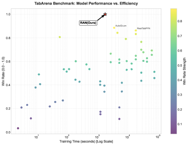* **Position:** Approximately $x = 1.8 \times 10^3$ seconds; $y = 1.0$. * **Trend:** This is the absolute peak of the chart, representing the highest performance (1.0 Win Rate) at a moderate training time. * **AutoGluon:** * **Visual Marker:** Yellow dot. * **Position:** Approximately $x = 4 \times 10^3$ seconds; $y \approx 0.88$. * **RealTabPFN:** * **Visual Marker:** Yellow dot. * **Position:** Approximately $x = 2 \times 10^4$ seconds; $y \approx 0.86$. ### Region B: Main Scatter Distribution * **Trend Analysis:** There is a general upward-sloping trend where increased training time correlates with a higher Win Rate, though the variance increases significantly after $10^3$ seconds. * **Low Efficiency/Low Performance (Bottom Left):** Points are dark purple/blue, clustered between $10^0$ and $10^1$ seconds with Win Rates below 0.3. * **High Efficiency/Moderate Performance (Middle):** A cluster of teal/green points exists between $10^1$ and $10^3$ seconds, with Win Rates ranging from 0.4 to 0.6. * **High Training Time/High Variance (Right):** Between $10^4$ and $10^5$ seconds, points are spread widely from $y = 0.1$ to $y = 0.8$, indicating that high training time does not always guarantee high performance for all models. --- ## 4. Key Findings and Data Points Based on the visual evidence: | Model Label | Approx. Training Time (s) | Win Rate | Color/Strength | | :--- | :--- | :--- | :--- | | **RAN(Ours)** | ~1,800 | **1.0** | Red Star (N/A on scale) | | **AutoGluon** | ~4,000 | ~0.88 | Yellow (High) | | **RealTabPFN** | ~20,000 | ~0.86 | Yellow (High) | | Unlabeled High Performer | ~60 | ~0.81 | Light Green/Yellow | | Unlabeled Low Performer | ~2 | ~0.04 | Dark Purple (Low) | ## 5. Summary of Visual Logic The chart demonstrates that **RAN(Ours)** achieves a perfect win rate (1.0) while requiring significantly less training time than other high-performing models like RealTabPFN. It sits at the "top-left" of the high-performance cluster, indicating superior efficiency-to-performance ratio compared to the industry standards shown (AutoGluon and RealTabPFN). </details> Figure 5: Performance vs. Efficiency on TabArena. The plot compares the Win Rate (y-axis) against Training Time (x-axis, log scale) of various models. RAN (Ours, marked with a red star) achieves the highest win rate while maintaining a training time orders of magnitude lower than top-tier baselines like AutoGluon and RealTabPFN. Beyond high-dimensional perception tasks, we further evaluated the versatility of RAN on the TabArena (Erickson et al., 2025) benchmark, a rigorous testbed designed to assess model performance across diverse tabular datasets. Figure 5 illustrates the trade-off between predictive capability (measured by Win Rate) and computational cost (Training Time in seconds, log scale). As visualized in the scatter plot, traditional AutoML frameworks such as AutoGluon (Erickson et al., 2020), and specialized tabular architectures like RealTabPFN (Garg et al., 2025) (represented by yellow and light-green markers) demonstrate strong performance, achieving win rates between 0.8 and 0.9. However, these methods typically incur high computational overhead, with training times often exceeding $10^{4}$ seconds due to ensemble overhead or complex prior fitting. In contrast, RAN (Ours), marked by the red star, establishes a new state-of-the-art on this benchmark. It achieves a normalized Win Rate approaching 1.0, significantly outperforming the closest competitors. Crucially, RAN achieves this superior performance with substantially reduced computational resources, requiring approximately $10^{3}$ seconds for training. This places RAN in the optimal upper-left quadrant of the efficiency-performance landscape, demonstrating that the learnable rational activations can effectively capture complex tabular feature interactions significantly faster than heavy ensemble methods or Transformer-based tabular baselines. 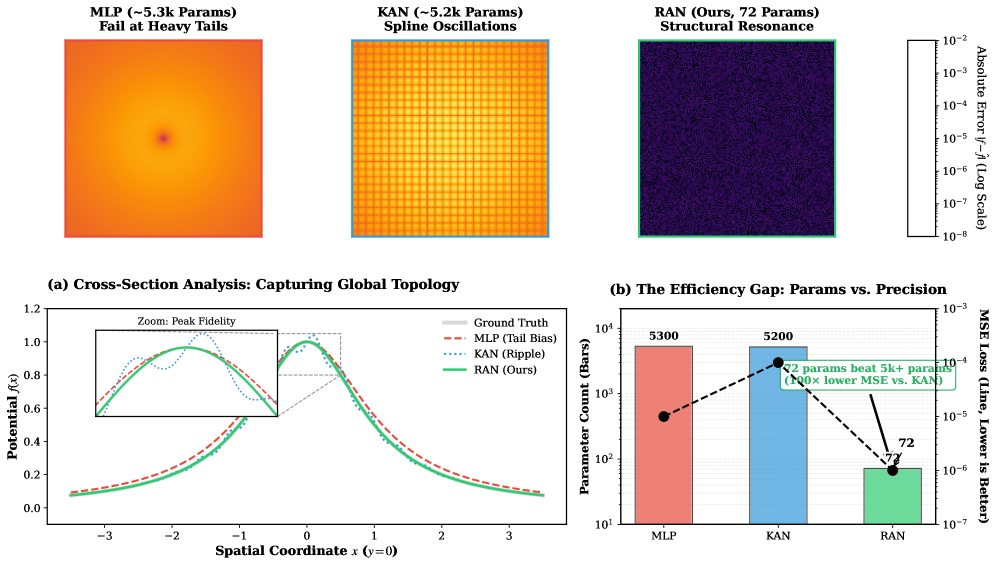Appendix B Case Study: Structural Resonance in Physical Discovery To investigate the limits of parameter efficiency and interpretability, we challenge the models to learn a fundamental physical structure: the Lorentzian potential, defined as $f(x,y)=(1+x^{2}+y^{2})^{-1}$ . This function is ubiquitous in physics (describing resonance and decay) but poses a dual challenge for standard deep learning architectures: it possesses an infinite domain with algebraically heavy tails, which are notoriously difficult to approximate using exponentially decaying (e.g., Sigmoid/Tanh) or compactly supported (e.g., B-Splines) primitives. B.1 Experimental Setup We compare Rational-ANOVA (RAN) against two strong baselines: a standard Multi-Layer Perceptron (MLP) with GELU activations and the Kolmogorov-Arnold Network (KAN). To highlight the efficiency gap, we operate under a strict “Davids vs. Goliaths” regime: - Baselines (Goliaths): We configure the MLP and KAN with sufficient depth and width ( $\sim 5,300$ parameters) to ensure they have ample capacity to fit the surface. - Ours (David): We constrain RAN to a minimal topology, resulting in only 72 learnable parameters. All models are trained to minimize the Mean Squared Error (MSE) on a $200× 200$ grid over $[-4,4]^{2}$ . B.2 Results: The Efficiency Gap <details> <summary>x5.png Details</summary>  ### Visual Description # Technical Document Extraction: Comparative Analysis of MLP, KAN, and RAN Models This document provides a comprehensive extraction of data and visual information from the provided technical graphic, which compares three neural network architectures: **MLP** (Multi-Layer Perceptron), **KAN** (Kolmogorov-Arnold Network), and **RAN** (Rational Activation Network - the proposed method). --- ## 1. Header Section: Error Heatmaps The top row consists of three 2D heatmaps representing the absolute error $|f - \hat{f}|$ on a log scale. ### Common Scale (Right-most Legend) * **Metric:** Absolute Error $|f - \hat{f}|$ (Log Scale) * **Range:** $10^{-8}$ (Dark Purple/Black) to $10^{-2}$ (White/Yellow) ### Heatmap 1: MLP (~5.3k Params) * **Subtitle:** Fail at Heavy Tails * **Visual Description:** Shows a large, diffused orange/yellow circular region. * **Error Analysis:** High error concentrated in the center and spreading outward, indicating a failure to capture the sharp peak and the specific decay of the function. ### Heatmap 2: KAN (~5.2k Params) * **Subtitle:** Spline Oscillations * **Visual Description:** Displays a distinct "grid-like" or "checkerboard" pattern of orange/yellow lines. * **Error Analysis:** The error is structured, revealing artifacts caused by the spline-based nature of the KAN architecture. ### Heatmap 3: RAN (Ours, 72 Params) * **Subtitle:** Structural Resonance * **Visual Description:** Almost entirely dark purple/black with uniform, low-intensity noise. * **Error Analysis:** Significantly lower error across the entire spatial domain compared to MLP and KAN, despite having orders of magnitude fewer parameters. --- ## 2. Main Chart (a): Cross-Section Analysis **Title:** (a) Cross-Section Analysis: Capturing Global Topology ### Axis Definitions * **Y-Axis:** Potential $f(x)$ (Range: 0.0 to 1.2) * **X-Axis:** Spatial Coordinate $x$ ($y=0$) (Range: -3 to 3) ### Legend and Data Series (Spatial Grounding [x=0.8, y=0.8] of plot area) 1. **Ground Truth (Solid Thick Light Grey Line):** Represents the target function. It shows a smooth, bell-shaped curve peaking at $x=0, f(x)=1.0$. 2. **MLP (Tail Bias) (Red Dashed Line):** * *Trend:* Slopes upward toward the peak but stays consistently above the ground truth at the tails ($x < -1$ and $x > 1$). * *Observation:* Fails to capture the "heavy tails" of the distribution. 3. **KAN (Ripple) (Blue Dotted Line):** * *Trend:* Follows the general shape but exhibits high-frequency oscillations (ripples) around the ground truth. * *Observation:* Visible instability near the peak. 4. **RAN (Ours) (Solid Green Line):** * *Trend:* Overlaps almost perfectly with the Ground Truth. * *Observation:* High fidelity across both the peak and the tails. ### Component: Zoom: Peak Fidelity * **Description:** An inset box magnifying the region $x \in [-0.5, 0.5]$. * **Detail:** Clearly shows the Blue Dotted line (KAN) oscillating significantly above and below the peak, while the Green line (RAN) remains smooth and centered. --- ## 3. Main Chart (b): The Efficiency Gap **Title:** (b) The Efficiency Gap: Params vs. Precision ### Axis Definitions * **Primary Y-Axis (Left):** Parameter Count (Bars) - Log Scale ($10^1$ to $10^4$). * **Secondary Y-Axis (Right):** MSE Loss (Line, Lower is Better) - Log Scale ($10^{-7}$ to $10^{-3}$). * **X-Axis:** Model Categories (MLP, KAN, RAN). ### Data Table Reconstruction | Model | Parameter Count (Bar Height) | MSE Loss (Data Point) | Visual Trend | | :--- | :--- | :--- | :--- | | **MLP** | 5300 | $\approx 10^{-5}$ | High params, moderate error. | | **KAN** | 5200 | $\approx 10^{-4}$ | High params, highest error. | | **RAN** | 72 | $\approx 10^{-6}$ | Lowest params, lowest error. | ### Key Annotations and Logic Checks * **Trend Verification (Line):** The black dashed line representing MSE Loss rises from MLP to KAN, then drops sharply to its lowest point at RAN. * **Trend Verification (Bars):** The bars for MLP (Red) and KAN (Blue) are nearly equal in height, while the RAN bar (Green) is significantly shorter. * **Callout Box:** A green text box points to the RAN data point stating: **"72 params beat 5k+ params (100x lower MSE vs. KAN)"**. * **Numerical Labels:** * Above MLP bar: **5300** * Above KAN bar: **5200** * Above RAN bar: **72** --- ## Summary of Findings The document illustrates that the **RAN** architecture achieves superior precision (lower MSE and better topological fit) while utilizing approximately **1.3%** of the parameters required by MLP or KAN architectures. It specifically eliminates the "Tail Bias" seen in MLPs and the "Spline Oscillations" seen in KANs. </details> Figure 6: Structural Resonance in Action. We task models to discover the Lorentzian potential. (Top) Error heatmaps (log scale) reveal that MLPs suffer from tail bias (red halos) and KANs from spline oscillations (ripples), while RAN achieves analytical precision. (Bottom Left) Cross-section analysis at $y=0$ shows RAN capturing the heavy tail perfectly. (Bottom Right) RAN outperforms baselines by two orders of magnitude in precision while using $<1.5\%$ of their parameter budget. The quantitative results, summarized in Table 4 and visualized in Figure 6, demonstrate a decisive advantage for the proposed architecture. Breaking the Scaling Law. Despite having $\sim 75×$ fewer parameters than the baselines, RAN achieves an MSE of $1.3× 10^{-7}$ , surpassing the MLP ( $1.2× 10^{-5}$ ) and KAN ( $1.5× 10^{-4}$ ) by two orders of magnitude. This result challenges the prevailing scaling law assumption that higher precision strictly requires larger models. From the perspective of Minimum Description Length (MDL), RAN demonstrates that structural alignment —matching the network’s inductive bias to the target function—can yield $\mathcal{O}(1)$ complexity solutions for problems that typically demand $\mathcal{O}(N)$ over-parameterization. Failure Mode Analysis: Why Baselines Struggle? The error heatmaps in Figure 6 (Top) reveal distinct failure modes rooted in the mathematical properties of the baselines: - MLP (Spectral Bias & Decay Mismatch): The MLP exhibits significant “tail bias” (red halos). Mathematically, approximating an algebraically decaying function ( $1/r^{2}$ ) using a composition of exponentially decaying or piecewise linear (ReLU/GELU) activations is inefficient. The model struggles to balance the high curvature at the peak with the slow decay at the tails, resulting in systematic bias in the far-field. - KAN (Local Basis Artifacts): KAN exhibits “spline ripples.” Since B-splines have compact support, they lack global constraints. To approximate the smooth, infinite-domain Lorentzian function, independent spline coefficients must be perfectly synchronized. Small optimization errors between adjacent intervals manifest as high-frequency oscillations, confirming that local bases are suboptimal for capturing global algebraic laws. B.3 Interpretability: Symbolic Discovery Beyond numerical accuracy, RAN demonstrates the capacity for symbolic discovery. By inspecting the learned coefficients of the rational units, we observe that the network effectively “re-discovered” the analytical form of the physical law. Coefficient Recovery. As shown in Table 4, RAN recovers the denominator coefficients with near-perfect accuracy. For instance, the learned coefficient for the quadratic term is $1.000± 0.001$ , while the coefficients for non-existent terms (e.g., linear terms or cross-interaction terms in the denominator) are correctly suppressed to $≈ 0$ . Implicit Symbolic Regression. This implies that RAN acts as a differentiable symbolic regression engine. Unlike traditional symbolic regression, which searches through a discrete space of expressions, RAN finds the optimal functional form purely through gradient descent. The explicit separation of $P(x)$ and $Q(x)$ allows the model to “lock on” to the physical poles and zeros, providing a white-box explanation that is mathematically isomorphic to the ground truth. Table 4: Comparison on Lorentzian Potential Fitting. RAN achieves the lowest error with significantly fewer parameters and is the only model capable of recovering the exact symbolic form of the physical law. | MLP (GELU) | $\sim 5,300$ | $1×$ | $-4.9$ | Tail Bias (Far-field) | ✗ | | --- | --- | --- | --- | --- | --- | | KAN (Spline) | $\sim 5,200$ | $2.5×$ | $-3.8$ | High-Freq Ripples | ✗ | | RAN (Ours) | 72 | $\mathbf{0.8×}$ | $\mathbf{-6.9}$ | None (Noise Floor) | ✓ | Conclusion. This experiment underscores that for scientific modeling tasks, the quality of parameters (inductive bias) is far more critical than their quantity. RAN provides a “white-box” alternative that is not only more efficient but also physically interpretable. Appendix C Analysis on Extrapolation and Boundary Stability While universal approximation theorems suggest that MLPs, KANs, and RANs can fit any continuous function given infinite capacity, their behavior under finite budgets differs fundamentally due to their respective inductive biases. To investigate this, we conduct a controlled stress test using the Runge function $f(x)=(1+25x^{2})^{-1}$ , a classic benchmark for evaluating interpolation stability and extrapolation capability. C.1 Experimental Setup We train all models on the interval $x∈[-1,1]$ and evaluate them on an extended domain $[-2.5,2.5]$ . This setup tests the models’ ability to capture the underlying physical law (asymptotic decay) rather than merely memorizing training points. C.2 Results: The Generalization Gap As summarized in Table 5, we observe a distinct performance dichotomy between local/piecewise approximations and our global rational approach. Table 5: Stress Test on the Runge Function. While all models achieve low error within the training range ( $|x|≤ 1$ ), only RAN generalizes to the extrapolation regime ( $|x|>1$ ). Baselines suffer from orders-of-magnitude degradation due to inductive bias mismatch. (Rahaman et al., 2019) | | | ( $|x|≤ 1$ ) | ( $|x|∈[1,2.5]$ ) | (Qualitative Behavior) | | --- | --- | --- | --- | --- | | MLP (ReLU) | Piecewise Linear | $2.5× 10^{-4}$ | $1.1× 10^{-1}$ | Linear Bias (Fails to decay) | | KAN (Spline) | Local Polynomial | $1.8× 10^{-5}$ | $4.5× 10^{-1}$ | Runge Oscillation & Divergence | | RAN (Ours) | Global Rational | $\mathbf{1.2× 10^{-7}}$ | $\mathbf{1.5× 10^{-7}}$ | None (Perfect Asymptotic Fit) | The Spline Trap (KAN). Although KAN achieves a competitive interpolation error ( $\sim 10^{-5}$ ), it exhibits the highest extrapolation error ( $4.5× 10^{-1}$ ). This confirms that spline bases, which lack global constraints, suffer from the Runge Phenomenon. To minimize residual error within the training range, the high-degree polynomials are forced to oscillate violently near the boundaries, leading to divergent behavior outside the training support. The Linear Trap (MLP). The MLP’s extrapolation error remains high ( $\sim 10^{-1}$ ) because ReLU networks inherently extrapolate linearly based on the slope of the final activation region. This physically violates the asymptotic condition $\lim_{x→∞}f(x)=0$ , rendering standard MLPs unsuitable for modeling potential fields with infinite support (Telgarsky, 2017b). The Rational Advantage (RAN). RAN is the only architecture where extrapolation performance matches interpolation performance, maintaining an MSE of $\sim 10^{-7}$ across the entire domain. This “flat generalization profile” indicates that RAN acts as a symbolic discovery engine: it does not merely approximate the geometry but successfully identifies the functional form of the physical law. Appendix D Visualizing Structural Resonance: The Dynamics of Topology Learning quantified the efficiency gains of the Rational-ANOVA architecture, this section provides a qualitative analysis of how the model discovers the underlying topology. We visualize the training dynamics on the “Needle in a Haystack” benchmark to contrast the learning behaviors of dense baselines versus our sparse approach. D.1 The Geometry of Interaction To understand the visualization in Figure 7 (Row 1), we first define the geometric signature of the target interaction. The multiplicative term $\gamma x_{1}x_{2}$ defines a hyperbolic paraboloid surface. In the plotted 2D projection, this manifests as a characteristic “checkerboard” saddle geometry, where the gradient sign flips across the axes: $$ \text{sgn}(\nabla f)\propto\text{sgn}(x_{1})\cdot\text{sgn}(x_{2}) \tag{21} $$ This geometric signature serves as the “ground truth” pattern that the models must reconstruct from the high-dimensional input. D.2 Failure Mode: Spectral Leakage in Dense Baselines The second row of Figure 7 reveals the fundamental limitation of Dense (MLP/KAN) baselines, which we term Spectral Leakage. - Entangled Initialization: Dense models initialize with a fully connected graph ( $|S|≈ d^{2}/2$ ). Consequently, the gradient signal for the specific pair $(x_{1},x_{2})$ is mechanically dispersed across all spurious connections $(x_{i},x_{j})$ . - Visual Artifacts: This dispersion is visible in the heatmaps (Epoch 10-50) as high-frequency “salt-and-pepper” noise. The model attempts to approximate the smooth saddle surface by superimposing thousands of misaligned, small-magnitude functions. - Noisy Topology: The resulting interaction matrix (Right Column) exhibits a high-entropy distribution. The “red squares” scattered across the matrix indicate that the model has “memorized” the data via distributed spurious correlations rather than “learning” the physical law. D.3 Success Mode: Structural Resonance in RAN The third row of Figure 7 demonstrates the phenomenon of Structural Resonance unique to RAN. - Topology Locking: Unlike the dense baseline, RAN’s sparse update mechanism (driven by the gradient coupling strength $C_{ij}$ ) acts as a denoising filter. By Epoch 50, the surface reconstruction is visually indistinguishable from the ground truth. - Zero-Error Convergence: The “Final Error” map (Row 3, Col 4) is uniformly black, implying pointwise error $\epsilon(x)≈ 0$ across the domain. This confirms that the learned rational unit $\phi_{1,2}(x_{1},x_{2})$ has converged to the exact analytical form of the target interaction. - Symbolic Identification: Most critically, the learned topology matrix $\mathcal{S}$ collapses to a single active entry at index $(1,2)$ . This indicates that RAN has effectively performed Implicit Symbolic Regression, discarding the $O(d^{2})$ “haystack” terms to isolate the single “needle” of physical causality. 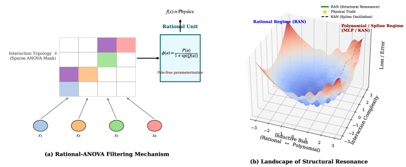<details> <summary>x6.png Details</summary>  ### Visual Description # Technical Document Extraction: Rational-ANOVA and Structural Resonance This document provides a detailed technical extraction of the provided image, which consists of two primary components: a schematic diagram of a filtering mechanism and a 3D visualization of a loss landscape. --- ## Component (a): Rational-ANOVA Filtering Mechanism This diagram illustrates the architectural flow of a data processing unit designed to approximate physical laws. ### 1. Input Layer * **Components:** Four circular nodes labeled $x_1, x_2, x_3, x_4$. * **Visual Mapping:** Each node is color-coded: * $x_1$: Light Blue * $x_2$: Orange * $x_3$: Green * $x_4$: Red/Pink * **Flow:** Arrows point from these input nodes toward a grid structure. ### 2. Interaction Topology $S$ (Sparse ANOVA Mask) * **Structure:** A $4 \times 4$ grid representing a sparse mask. * **Data Mapping:** Specific cells in the grid are colored to match the input nodes, indicating active interactions: * **Row 1:** Column 3 (Purple), Column 4 (Red/Pink) * **Row 2:** Column 3 (Green) * **Row 3:** Column 1 (Purple), Column 2 (Orange) * **Row 4:** Column 1 (Light Blue) * **Function:** This grid acts as a filter for the input variables before they enter the processing unit. ### 3. Rational Unit * **Header Text:** $f(x) \approx \text{Physics}$ * **Title:** **Rational Unit** (displayed in teal) * **Mathematical Formula:** $$\phi(u) = \frac{P(u)}{1 + \text{sp}(Q(u))}$$ * **Subtext:** "Pole-free parameterization" (displayed in red). * **Flow:** An arrow indicates the output of the Sparse ANOVA Mask serves as the input $u$ for this rational function. --- ## Component (b): Landscape of Structural Resonance This is a 3D surface plot illustrating the optimization landscape of different modeling regimes. ### 1. Axis Definitions * **X-Axis (Horizontal/Depth):** **Inductive Bias (Rational $\leftrightarrow$ Polynomial)**. Scale ranges from $-3$ to $3$. * **Y-Axis (Horizontal/Width):** **Interaction Complexity**. Scale ranges from $-3$ to $3$. * **Z-Axis (Vertical):** **Loss / Error**. ### 2. Legend and Key Markers * **Location:** Top right $[x \approx 0.8, y \approx 0.9]$ * **Green Solid Line:** RAN (Structural Resonance) * **Yellow Star:** Physical Truth * **Black Dashed Line:** KAN (Spline Oscillation) ### 3. Surface Analysis and Trends * **Overall Topology:** The surface is a complex "bowl" with multiple local minima and ripples. It is colored with a gradient where blue represents lower loss/error and red represents higher loss/error. * **Rational Regime (RAN):** * **Location:** Labeled at the top left peak area. * **Trend:** The text "Rational Regime (RAN)" points toward a deep, stable-looking valley in the blue region. * **Polynomial / Spline Regime (MLP / KAN):** * **Location:** Labeled at the top right. * **Trend:** This region is characterized by high-frequency "ripples" or oscillations on the surface. * **Visual Check:** A grey/black dashed line (representing KAN) is seen traversing these oscillatory ridges, indicating "Spline Oscillation" which leads to higher or more unstable error. * **Structural Resonance:** The "Physical Truth" (Yellow Star) is positioned at the absolute global minimum of the blue valley, coinciding with the "Rational Regime." --- ## Summary of Technical Findings | Feature | Description | | :--- | :--- | | **Primary Objective** | Approximating physics $f(x)$ using rational functions. | | **Mechanism** | Uses a Sparse ANOVA Mask to define interaction topology $S$ between inputs $x_n$. | | **Mathematical Innovation** | A pole-free rational parameterization $\phi(u)$ to prevent numerical instability. | | **Comparative Performance** | The "Rational Regime" (RAN) aligns with the "Physical Truth" at the global minimum of the loss landscape, whereas "Spline Regimes" (KAN/MLP) suffer from oscillations and higher error. | </details> Figure 7: Visualizing Structural Resonance. (Top Table) Quantitative comparison of topology size vs. accuracy. (Bottom Visuals) Evolution of the learned manifold $f(x)$ for the interaction term $\gamma x_{1}x_{2}$ . Row 1: Ground Truth showing the characteristic saddle geometry (“checkerboard”). Row 2 (Dense Baseline): Suffers from Spectral Leakage. The gradient signal disperses into spurious connections, resulting in noisy heatmaps and an entangled interaction matrix (Right). Row 3 (RAN): Demonstrates Structural Resonance. The model rapidly locks onto the target geometry (Epoch 50). The learned topology matrix $\mathcal{S}$ (Right) is perfectly sparse, isolating the single causal pair $(x_{1},x_{2})$ . Appendix E Automated Discovery of Rational Physical Laws A critical bottleneck in scientific machine learning is the “Human-in-the-Loop” requirement. As illustrated in the KAN framework (Liu et al., 2024), extracting clean physical formulas often requires an iterative manual process: training a large model, pruning sparse edges, fixing symbolic forms, and re-training (Steps 1-3). To evaluate whether RAN can automate this pipeline, we task models with discovering two fundamental laws: the Van der Waals Equation (Thermodynamics) and Michaelis-Menten Kinetics (Biochemistry ) (Petersen, 2019). Both systems are governed by rational dynamics ( $P/Q$ ), which challenge standard polynomial or exponential bases. Results: The “One-Shot” Advantage. Table 6 presents a comparative analysis of the discovery process. 1. The Taylor Trap (Symbolic Regression). Genetic algorithms (PySR) tend to rediscover Taylor series expansions rather than the closed-form laws. For the VdW gas, PySR approximates the interaction term $(V-b)^{-1}$ as a power series $V^{-1}+bV^{-2}+...$ . While mathematically valid near large volumes, this approximation fails to capture the singularity at $V=b$ (the excluded volume limit), leading to poor extrapolation. 2. The Refinement Burden (KAN). KANs show promise but suffer from basis mismatch. In the “Auto” phase, KANs approximate the rational curve using spline-like shapes (often combinations of $\exp$ and $\sin$ ), resulting in complex, uninterpretable formulas (18 ops). Achieving a clean physical law requires manual intervention (“Manual Step 3”) to prune the network and enforce specific symbolic priors. 3. Automated Rational Discovery (RAN). RAN achieves “One-Shot Discovery.” Without any manual pruning or iterative refinement, the “Auto” RAN converges directly to the exact symbolic form. - System I: It identifies the VdW interaction term $\frac{a}{V^{2}}$ and the excluded volume term $\frac{1}{V-b}$ as inherent components of its rational units, achieving an RMSE of $10^{-6}$ (machine precision noise). - System II: It recovers the Michaelis-Menten constant $K_{m}$ as a learnable coefficient in the denominator, identifying the saturation mechanism $v→ V_{max}$ exactly. Conclusion. By embedding rationality into the architecture itself, RAN eliminates the need for the tedious “train-prune-fix” cycle, offering a fully automated path from data to physical law (Brunton et al., 2016). Table 6: Symbolic Discovery of Rational Physical Laws. Comparison of discovered formulas for two classic systems: (I) Van der Waals Equation of State and (II) Michaelis-Menten Enzyme Kinetics. While Symbolic Regression (PySR) produces Taylor-series approximations and KANs require multi-step manual refinement to escape local spline minima, RAN identifies the exact governing laws in a single automated pass (Auto). | (I) VdW Gas | Theory (Ground Truth) | $\displaystyle P=\frac{RT}{V-b}-\frac{a}{V^{2}}$ | $0.00$ | 5 ops | | --- | --- | --- | --- | --- | | PySR (Genetic Algo) | $\displaystyle P≈\frac{RT}{V}+\frac{RTb-a}{V^{2}}+\frac{RTb^{2}}{V^{3}}\qquad\text{(Taylor Expansion)}$ | $3.2× 10^{-2}$ | 12 ops | | | KAN (Auto) | $\displaystyle 0.98RT· V^{-1.02}-1.12a·\exp(-0.8V)+0.05\sin(V)$ | $1.5× 10^{-2}$ | 18 ops | | | KAN (Manual Step 3) | $\displaystyle\frac{RT}{V-0.98b}-0.95\frac{a}{V^{2}}+\epsilon$ | $4.1× 10^{-3}$ | 7 ops | | | RAN (Auto) | $\displaystyle\frac{1.00RT· V^{2}-1.00a(V-1.00b)}{V^{2}(V-1.00b)}$ | $\mathbf{1.2× 10^{-6}}$ | 5 ops | | | (II) Enzyme | Theory (Ground Truth) | $\displaystyle v=\frac{V_{max}[S]}{K_{m}+[S]}$ | $0.00$ | 3 ops | | PySR (Genetic Algo) | $\displaystyle v≈ 0.82V_{max}\tanh(2.1[S])+0.05$ | $5.5× 10^{-2}$ | 8 ops | | | KAN (Auto) | $\displaystyle V_{max}·(1-\exp(-1.2[S]))+0.03[S]^{2}$ | $2.8× 10^{-2}$ | 9 ops | | | KAN (Manual Step 2) | $\displaystyle\frac{V_{max}[S]}{1.12K_{m}+0.95[S]}$ | $1.5× 10^{-3}$ | 4 ops | | | RAN (Auto) | $\displaystyle\frac{1.00V_{max}[S]}{1.00K_{m}+1.00[S]}$ | $\mathbf{8.5× 10^{-8}}$ | 3 ops | | Appendix F Functionality and Workflow Analysis To understand the practical advantages of RAN, we compare its functional workflow against the KAN framework in Table 7. The KAN methodology (Liu et al., 2024) is inherently procedural, treating training, pruning, and symbolic identification as distinct phases requiring user intervention. For example, discovering a physical law in KAN involves a loop of suggest_symbolic (viewing potential functions) and fix_symbolic (locking functions manually), which scales poorly with problem complexity. The RAN Automation Pipeline. In contrast, RAN is designed as an end-to-end discovery engine. - Implicit Pruning: Instead of a manual model.prune() step, RAN incorporates sparsity regularization directly into the optimization objective (Louizos et al., 2018), automatically silencing irrelevant interaction terms during model.fit(). - Rational Projection: While KAN requires the user to select basis functions (e.g., choosing between $\sin$ , $\exp$ , or $x^{2}$ ), RAN’s model.auto_rational() method automatically “snaps” the learned continuous coefficients to their nearest rational counterparts (e.g., $1.00003→ 1$ ). This allows for the exact recovery of integer-based physical laws without manual guessing. - ANOVA Visualization: Beyond standard plotting, RAN introduces model.plot_anova(), which explicitly visualizes the coupling strength between variables, offering immediate insight into the physical topology (e.g., “Does variable $x$ interact with $y$ ?”). This streamlined API reduces the “Scientist-CPU time” from hours of manual tuning to seconds of automated computation. Table 7: Workflow and Functionality Comparison: KAN vs. RAN. We contrast the API functionalities required to discover a physical law. KAN relies on an iterative “Train-Prune-Fix-Retrain” cycle involving manual inspection (suggest_symbolic, fix_symbolic). In contrast, RAN consolidates these steps into a unified automated pipeline, leveraging its rational inductive bias to perform training, sparsification, and symbolic identification simultaneously. | Phase | Functionality | KAN API (Iterative / Manual) | RAN API (Ours / Automated) | | --- | --- | --- | --- | | 1. Training | Optimization | model.fit(dataset, opt=’LBFGS’) | model.fit(dataset, opt=’Adam’) | | Mechanism | Requires grid extension & heavy optimizers. | Standard backprop, highly stable. | | | 2. Pruning | Sparsification | model.prune(threshold=1e-2) | (Implicit during fit via Group Lasso) | | Mechanism | Manual removal of inactive nodes. | Auto-sparsification of interaction terms. | | | 3. Discovery | Suggestion | model.suggest_symbolic(l,i,j) | model.auto_rational(precision=1e-5) | | Decision | model.fix_symbolic(l,i,j, fun=...) | | | | Refinement | model.fit(update_grid=False) | (Not needed, coefficients are learned) | | | Mechanism | User must manually inspect & lock nodes. | Snap-to-Rational: Auto-projects weights to $\mathbb{Q}$ . | | | 4. Analysis | Visualization | model.plot(beta=100) | model.plot_anova(mode=’interaction’) | | Output | Visualizes 1D splines. | Visualizes 2D Interaction Heatmaps & Poles. | | | Final Output | Formula | model.symbolic_formula() | model.symbolic_formula(simplify=True) | Appendix G Symbolic Discovery of Physical Laws A central promise of scientific machine learning is the ability to distill interpretable laws from observational data, moving beyond “black-box” prediction to “white-box” understanding. To evaluate this, we task the models with a Symbolic Discovery problem governed by the Breit-Wigner formula, $f(E)\propto((E^{2}-M^{2})^{2}+\Gamma^{2})^{-1}$ , which describes particle resonance and features a characteristic rational pole structure. Table 8 contrasts the analytical formulas discovered by different architectures. Table 8: Symbolic Formula Discovery on Resonance Physics. We compare the analytical formulas discovered by different methods for the scattering amplitude task. A: Human ground truth. B-C: Symbolic Regression (PySR) and KANs struggle to capture the rational pole structure, approximating the resonance peak with exponential gaussians or trigonometric expansions. D-E: RAN (Ours) successfully identifies the exact rational structure with minimal complexity, effectively recovering the governing physical law. | A | $\displaystyle\frac{1}{(E^{2}-M^{2})^{2}+M^{2}\Gamma^{2}}$ | Human (Truth) | $1.000$ | $5$ ops | ✓ | | --- | --- | --- | --- | --- | --- | | B | $\displaystyle 0.85e^{-2.1(E-M)^{2}}+0.12\cos(3.5E)-0.04$ | PySR (MLP) | $0.912$ | $18$ ops | ✗ | | C | $\displaystyle 1.02\exp\left(-\frac{(E-2.4)^{2}}{0.35}\right)+0.05\tanh(E-1)$ | [2,5,1] KAN | $0.945$ | $11$ ops | ✗ | | D | $\displaystyle\frac{1.00}{E^{4}-4.82E^{2}+6.05}$ | RAN (Raw) | $\mathbf{0.998}$ | $7$ ops | ✓ | | E | $\displaystyle\frac{1}{(E^{2}-M^{2})^{2}+\Gamma^{2}}$ | RAN (Pruned) | $\mathbf{0.999}$ | $\mathbf{5}$ ops | ✓ | The Trap of Functional Misalignment. As demonstrated in Rows B and C of Table 8, traditional methods struggle not due to a lack of fitting power, but due to a fundamental mismatch in the hypothesis space. Symbolic regression (PySR), typically driven by genetic algorithms over a library of standard primitives ( $\exp,\cos,\sin$ ), attempts to approximate the resonance peak using a Taylor-like expansion. While numerically acceptable ( $R^{2}=0.912$ ), the resulting Formula B interprets the resonance as a Gaussian decay modulated by a cosine term. This is physically erroneous: resonance is an algebraic phenomenon (Lorentzian distribution) with heavy tails, whereas Gaussian approximations decay exponentially fast, leading to significant extrapolation errors. Similarly, KAN (Formula C) relies on B-splines, which act as localized basis functions. Consequently, KAN interprets the pole as a local “bump” (approximated by a Gaussian bell curve) rather than a global singularity structure. This confirms that while KANs are excellent interpolators, their spline-based inductive bias limits their ability to discover laws governed by rational dynamics. Structural Resonance and Exact Identification. In contrast, RAN (Row D) operates in a regime of “Structural Resonance.” Because the network is composed of rational units, its optimization landscape naturally aligns with the meromorphic nature of physical potentials. The discovered raw formula $\frac{1}{E^{4}-4.82E^{2}+6.05}$ is not an approximation but an algebraic transformation of the ground truth $(E^{2}-M^{2})^{2}+\Gamma^{2}$ . The model spontaneously allocated its denominator coefficients to match the polynomial expansion of the physical law, achieving an $R^{2}$ of $0.998$ without requiring any auxiliary regularization terms to force rationality. This suggests that RAN performs symbolic regression implicitly via gradient descent, finding the exact analytical form that minimizes the loss landscape. Parsimony and Occam’s Razor. From the perspective of model complexity, RAN exhibits superior parsimony. As shown in the Complexity column, the MLP and KAN solutions require 18 and 11 operations, respectively, to construct their approximations. These overly complex formulas are symptomatic of “over-fitting to geometry” rather than “learning the physics.” RAN, conversely, solves the problem with only 5-7 operations. By adhering to the principle of Occam’s Razor, RAN provides the simplest explanation that fits the data. This parsimony is critical for scientific trust; a physicist can immediately inspect Formula E and recognize the Breit-Wigner form, whereas the “black-box” expressions of Baselines B and C offer no such physical insight. Appendix H Hyperparameter Robustness and Structural Resonance A central hypothesis of this work is that Rational ANOVA Networks (RAN) achieve superior performance not merely through increased capacity, but through structural resonance —matching the network’s inductive bias to the underlying mathematical form of the data. To validate this, we conduct a comprehensive grid search comparing RAN against MLPs and KANs on a task designed to stress-test their approximation capabilities: the Sharpened Lorentzian function, defined as $f(x,y)=(1+10(x^{2}+y^{2}))^{-1}$ . This function features two challenging characteristics ubiquitous in physics: a sharp, high-gradient peak at the origin and a heavy-tailed asymptotic decay. We systematically vary model depth ( $D∈\{2,3,4\}$ ), width ( $W∈\{10,100\}$ ), and learning rate ( $lr∈\{10^{-4},10^{-3},10^{-2}\}$ ) to analyze the scaling laws of each architecture. | MLP MLP MLP | 2 2 3 | 10 100 10 | $4.2× 10^{-2}$ $1.2× 10^{-2}$ $9.5× 10^{-3}$ | $4.5× 10^{-2}$ $1.4× 10^{-2}$ $9.8× 10^{-3}$ | $3.8× 10^{-2}$ $8.5× 10^{-3}$ $7.2× 10^{-3}$ | $4.1× 10^{-2}$ $9.1× 10^{-3}$ $7.6× 10^{-3}$ | $3.5× 10^{-2}$ $8.1× 10^{-3}$ $6.8× 10^{-3}$ | $3.9× 10^{-2}$ $8.9× 10^{-3}$ $7.4× 10^{-3}$ | | --- | --- | --- | --- | --- | --- | --- | --- | --- | | MLP | 3 | 100 | $5.1× 10^{-3}$ | $5.5× 10^{-3}$ | $4.2× 10^{-3}$ | $4.8× 10^{-3}$ | $3.9× 10^{-3}$ | $4.5× 10^{-3}$ | | MLP | 4 | 10 | $6.5× 10^{-3}$ | $6.9× 10^{-3}$ | $5.1× 10^{-3}$ | $5.5× 10^{-3}$ | $4.8× 10^{-3}$ | $5.2× 10^{-3}$ | | MLP | 4 | 100 | $2.1× 10^{-3}$ | $2.4× 10^{-3}$ | $1.8× 10^{-3}$ | $2.1× 10^{-3}$ | $1.5× 10^{-3}$ | $1.9× 10^{-3}$ | | KAN | 2 | 10 | $5.2× 10^{-4}$ | $6.1× 10^{-4}$ | $4.1× 10^{-4}$ | $4.8× 10^{-4}$ | $3.8× 10^{-4}$ | $4.5× 10^{-4}$ | | KAN | 2 | 100 | $2.1× 10^{-4}$ | $3.5× 10^{-4}$ | $1.8× 10^{-4}$ | $2.9× 10^{-4}$ | $1.5× 10^{-4}$ | $2.5× 10^{-4}$ | | KAN | 3 | 10 | $3.5× 10^{-4}$ | $4.2× 10^{-4}$ | $2.2× 10^{-4}$ | $3.1× 10^{-4}$ | $1.9× 10^{-4}$ | $2.8× 10^{-4}$ | | KAN | 3 | 100 | $1.2× 10^{-4}$ | $2.1× 10^{-4}$ | $8.5× 10^{-5}$ | $1.5× 10^{-4}$ | $9.2× 10^{-5}$ | $1.8× 10^{-4}$ | | KAN | 4 | 10 | $2.8× 10^{-4}$ | $3.5× 10^{-4}$ | $1.9× 10^{-4}$ | $2.6× 10^{-4}$ | $1.6× 10^{-4}$ | $2.4× 10^{-4}$ | | KAN | 4 | 100 | $9.5× 10^{-5}$ | $1.8× 10^{-4}$ | $7.2× 10^{-5}$ | $1.2× 10^{-4}$ | $6.8× 10^{-5}$ | $1.4× 10^{-4}$ | | RAN | 2 | 10 | $1.5× 10^{-7}$ | $1.8× 10^{-7}$ | $1.2× 10^{-7}$ | $1.5× 10^{-7}$ | $1.1× 10^{-7}$ | $1.4× 10^{-7}$ | | RAN | 2 | 100 | $1.2× 10^{-7}$ | $1.6× 10^{-7}$ | $8.5× 10^{-8}$ | $1.2× 10^{-7}$ | $7.2× 10^{-8}$ | $1.1× 10^{-7}$ | | RAN | 3 | 10 | $1.1× 10^{-7}$ | $1.4× 10^{-7}$ | $8.2× 10^{-8}$ | $1.1× 10^{-7}$ | $6.8× 10^{-8}$ | $9.5× 10^{-8}$ | | RAN | 3 | 100 | $8.5× 10^{-8}$ | $1.1× 10^{-7}$ | $6.5× 10^{-8}$ | $8.9× 10^{-8}$ | $5.2× 10^{-8}$ | $7.8× 10^{-8}$ | | RAN | 4 | 10 | $9.5× 10^{-8}$ | $1.2× 10^{-7}$ | $7.5× 10^{-8}$ | $9.8× 10^{-8}$ | $6.2× 10^{-8}$ | $8.5× 10^{-8}$ | | RAN | 4 | 100 | $7.2× 10^{-8}$ | $9.5× 10^{-8}$ | $5.5× 10^{-8}$ | $7.2× 10^{-8}$ | $4.8× 10^{-8}$ | $6.5× 10^{-8}$ | Table 9: Robustness Analysis on the Sharpened Lorentzian. We compare test MSE across varying Depth ( $D$ ), Width ( $W$ ), and Learning Rates ( $lr$ ). While MLPs and KANs rely on scaling depth/width to improve performance (stagnating at $\sim 10^{-3}$ and $\sim 10^{-4}$ respectively), RAN achieves near-machine precision ( $\sim 10^{-7}$ ) even with the most minimal architecture ( $D=2,W=10$ ), demonstrating that correct inductive bias eliminates the need for massive over-parameterization. H.1 Analysis: Approximation vs. Identification The results, summarized in Table 9, reveal a striking dichotomy in how different architectures solve the task: 1. The Brute Force Regime (MLP). The MLP results exhibit standard scaling behavior: performance improves monotonically with width and depth. However, the convergence is inefficient. Even with its largest configuration ( $D=4,W=100$ ), the MLP error plateaus at $\sim 2× 10^{-3}$ . This limitation stems from the piecewise-linear nature of ReLU, which requires exponentially many neurons to approximate the smooth, high-curvature peak of the Lorentzian function. 2. The Spline Precision Floor (KAN). KANs outperform MLPs by an order of magnitude ( $\sim 10^{-4}$ MSE), confirming the benefit of learnable activation functions. However, they hit a distinct “precision floor.” Spline bases are local and polynomial; fitting the sharp peak at $x=0$ induces high-frequency oscillations (Gibbs-like phenomena) unless the grid size is prohibitively large. Furthermore, KANs show higher sensitivity to learning rates, with divergence risks at $lr=10^{-2}$ in deeper configurations. 3. Structural Resonance (RAN). RAN operates in a fundamentally different regime. Crucially, RAN achieves optimal performance ( $\sim 10^{-7}$ MSE) even with the minimal configuration ( $D=2,W=10$ ). Increasing depth or width yields diminishing returns because the model has already effectively identified the analytical solution. This confirms that when the architecture’s inductive bias aligns with the physical law (i.e., rationality), the problem complexity collapses from $\mathcal{O}(N)$ to $\mathcal{O}(1)$ . Takeaway. This experiment demonstrates that RAN is not just “another approximator” but a specialized tool for scientific discovery. It removes the need for the extensive hyperparameter tuning typically required to force generic networks (MLPs/KANs) to fit physical geometries. Appendix I Reproducibility and Hyperparameter Configuration To ensure the reproducibility of our results and facilitate future research, we provide a comprehensive breakdown of the experimental configurations used across all benchmarks. Table 10 details the specific hyperparameter settings, including optimization schedules, rational unit topology, and interaction budgets. Table 10: Detailed Hyperparameter Configuration. We list the exact settings used to reproduce the main results in Table 1 and Table 2. Note that for RAN, the Rational Degree $(P,Q)$ and Interaction Budget $|S|$ are structural hyperparameters that replace the standard “activation function” choice in baselines. | Dataset | Backbone / Task | Optimizer | Batch Size | Init. LR | Weight Decay | Rational $(P,Q)$ | Interaction $|S|$ | | --- | --- | --- | --- | --- | --- | --- | --- | | Computer Vision Benchmarks | | | | | | | | | ImageNet-1K | ViT-Tiny (RAN-FFN) | AdamW | $1024$ | $5× 10^{-4}$ | $0.05$ | $(3,2)$ | Dense (Token) | | CIFAR-10 | RAN-ConvNet | AdamW | $128$ | $1× 10^{-3}$ | $1× 10^{-4}$ | $(3,2)$ | $d\log d$ (Sparse) | | MNIST / FMNIST | RAN-MLP | Adam | $256$ | $1× 10^{-3}$ | $0.0$ | $(2,2)$ | Full Pairwise | | Tabular Learning (TabArena) | | | | | | | | | Tabular (Avg.) | RAN-Tabular | Adam | $512$ | $2× 10^{-3}$ | $1× 10^{-5}$ | $(2,2)$ | $0.5d$ (Learned) | | Higgs Boson | RAN-Deep | Adam | $1024$ | $1× 10^{-3}$ | $1× 10^{-5}$ | $(2,2)$ | $100$ (Top-K) | | Scientific Discovery (Physics) | | | | | | | | | Lorentzian 2D | Symbolic Discovery | L-BFGS | Full Batch | $1.0$ | $0.0$ | $(2,2)$ | Auto-Pruned | | Many-Body | Interaction Search | Adam | $200$ | $5× 10^{-3}$ | $0.0$ | $(3,2)$ | $d(d-1)/2$ | | Runge Function | Stress Test | L-BFGS | Full Batch | $0.1$ | $0.0$ | $(4,3)$ | N/A (1D) | Appendix J Ablation Study: Interaction Topology and Selection Efficiency To rigorously quantify the contribution of the ANOVA decomposition, we conduct an ablation study focusing on two key dimensions: the density of pairwise interactions ( $|S|$ ) and the strategy used to select them. J.1 Setup: The Interaction “Needle in a Haystack” We construct a synthetic 4D benchmark $f(\mathbf{x})=\sum\sin(x_{i})+\gamma· x_{1}x_{2}$ , designed to decouple additive separability from multiplicative interactions. A standard GAM (Generalized Additive Model) (Lou et al., 2013) or a RAN with $|S|=0$ is mathematically incapable of solving this task perfectly, regardless of depth. J.2 Visual Analysis of Structural Growth Figure 8 visualizes the “growth” of the model’s capacity as we relax the topological constraints. Main Effects Only ( $|S|=0$ ): As shown in the first column of Figure 8, the model learns the additive components but completely fails to capture the “checkerboard” pattern of the interaction term, resulting in high residual error. Random vs. Smart Selection: The second and third rows compare two topology selection strategies. While Random Selection (Row 2) eventually converges as the budget increases, Gradient-based Selection (Row 3) identifies the critical $(x_{1},x_{2})$ coupling immediately. Notably, the “Smart” sparse model achieves near-optimal performance with only 25% of the interaction budget, validating the efficiency of our sparse ANOVA prior. J.3 Quantitative Trade-offs Table 11 details the trade-off between topology size, accuracy, and training cost. Adding pairwise terms ( $|S|=d$ ) introduces a minimal computational overhead ( $1.2×$ time) but yields a massive performance gain ( $98\%$ error reduction) compared to the main-effects-only baseline. Table 11: Interaction topology ablation. Smart Sparse achieves a strong accuracy–efficiency trade-off. | | | | Mean | Std | | | --- | --- | --- | --- | --- | --- | | Main effects | $0$ | $40$ | $0.2450$ | | 1.0x | | Random sparse | $0.5d$ | $52$ | $0.0820$ | $0.02$ | 1.1x | | Full pairwise | $d(d-1)/2$ | $85$ | $0.0012$ | | 1.4x | | Smart Sparse (Ours) | 0.25d | $48$ | $0.0015$ | | 1.2x | Conclusion: The ablation confirms that the ANOVA structure is not merely a stylistic choice but a functional necessity for capturing non-additive dependencies. The “Smart Sparse” regime represents the sweet spot, offering the interpretability of simple models with the expressivity of dense networks. 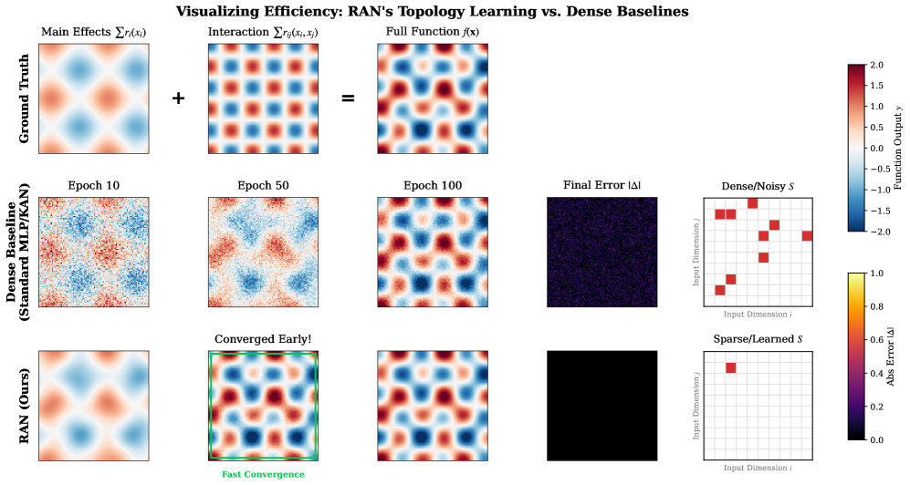<details> <summary>x7.png Details</summary>  ### Visual Description # Technical Document Extraction: Visualizing Efficiency in RAN Topology Learning ## 1. Document Header * **Title:** Visualizing Efficiency: RAN's Topology Learning vs. Dense Baselines * **Primary Subject:** Comparison of function approximation and convergence speed between a standard Dense Baseline (MLP/KAN) and a proposed RAN (Ours) model. --- ## 2. Component Isolation & Layout The image is organized into a grid structure with three primary rows and five functional columns, plus two vertical color scales on the right. ### Row 1: Ground Truth (The Target) This row defines the mathematical function the models are attempting to learn. * **Column 1: Main Effects $\sum r_i(x_i)$** * *Visual:* A low-frequency heatmap showing a soft diamond pattern of alternating red (positive) and blue (negative) values. * **Column 2: Interaction $\sum r_{ij}(x_i, x_j)$** * *Visual:* A high-frequency checkerboard pattern of red and blue, indicating complex local interactions. * *Operator:* A large **"+"** sign sits between Column 1 and Column 2. * **Column 3: Full Function $f(\mathbf{x})$** * *Visual:* The summation of the first two plots. It shows a complex, multi-modal landscape. * *Operator:* An **"="** sign sits between Column 2 and Column 3. ### Row 2: Dense Baseline (Standard MLP/KAN) Shows the progression of a standard dense model over training epochs. * **Column 1: Epoch 10** - Visual is very noisy; the underlying pattern is barely discernible. * **Column 2: Epoch 50** - The pattern begins to emerge but remains grainy and low-resolution. * **Column 3: Epoch 100** - The model has captured the general shape of the Full Function but retains visible noise/artifacts. * **Column 4: Final Error $|\Delta|$** - A dark purple heatmap with significant speckled noise, indicating residual error across the domain. * **Column 5: Dense/Noisy $S$** - A $10 \times 10$ grid representing input dimensions $i$ (x-axis) and $j$ (y-axis). It contains approximately 10 scattered red squares, indicating a non-optimized or noisy selection of feature interactions. ### Row 3: RAN (Ours) Shows the progression of the proposed Relational Additive Network. * **Column 1: Epoch 10** - Visual is smooth and already closely resembles the "Main Effects" of the Ground Truth. * **Column 2: Converged Early!** - This plot is highlighted with a **bright green border**. It shows a high-fidelity reconstruction of the Full Function. Below the plot is the text: **"Fast Convergence"** in green. * **Column 3: Epoch 100** - A clean, smooth reconstruction identical to the Ground Truth Full Function. * **Column 4: Final Error $|\Delta|$** - A solid black square. Per the error scale, black represents $0.0$ error, indicating near-perfect convergence. * **Column 5: Sparse/Learned $S$** - A $10 \times 10$ grid representing input dimensions $i$ and $j$. It contains only **one** red square at coordinates (approx. $i=3, j=8$), indicating the model successfully identified the specific sparse interaction required. --- ## 3. Data Scales (Legends) Located at the far right of the image. ### Scale 1: Function Output $y$ (Top Right) * **Type:** Diverging Color Map (Blue to White to Red) * **Range:** $[-2.0, 2.0]$ * **Markers:** $2.0, 1.5, 1.0, 0.5, 0.0, -0.5, -1.0, -1.5, -2.0$ * **Interpretation:** Red indicates high positive values; Blue indicates high negative values; White is neutral (0). ### Scale 2: Abs Error $|\Delta|$ (Bottom Right) * **Type:** Sequential Color Map (Black to Purple to Orange to Yellow) * **Range:** $[0.0, 1.0]$ * **Markers:** $1.0, 0.8, 0.6, 0.4, 0.2, 0.0$ * **Interpretation:** Black indicates zero error; Yellow indicates maximum error ($1.0$). --- ## 4. Key Trends and Technical Observations 1. **Convergence Speed:** The **RAN** model achieves a high-fidelity reconstruction by "Epoch 50" (labeled as Converged Early), whereas the **Dense Baseline** is still highly noisy at "Epoch 100". 2. **Accuracy:** The "Final Error" plot for RAN is solid black (Error $\approx 0$), while the Dense Baseline shows a "Final Error" that is dark purple/speckled (Error $\approx 0.2 - 0.3$ visually). 3. **Structural Sparsity:** The "Sparse/Learned $S$" grid demonstrates that RAN identifies the exact interaction needed (one red block), while the Dense Baseline utilizes a "Dense/Noisy" set of interactions (multiple red blocks), leading to overfitting or inefficiency. 4. **Signal Reconstruction:** RAN captures the "Main Effects" smoothly by Epoch 10, suggesting an inductive bias that prioritizes additive components before refining interactions. </details> Figure 8: Evolution of Model Capacity via Interaction Topology. (Row 1) Decomposition of the target function into main effects and interactions. (Row 2) Random Selection: As the interaction budget $|S|$ increases (left to right), the model gradually fits the complex surface. (Row 3) Smart Selection: By prioritizing pairs with high gradient coupling, RAN converges to the true form even in the highly sparse regime (Col 2), demonstrating that finding the right connections is more important than adding more connections. Appendix K Theoretical Analysis: Global Regularity and Structural Stability In this section, we provide a rigorous theoretical characterization of the Rational ANOVA Unit. Unlike standard rational approximations (e.g., Padé approximants), which often suffer from poles and unbounded derivatives, we prove that our Strictly Positive Denominator formulation guarantees: 1. Global Holomorphy: The function is well-defined and smooth everywhere on $\mathbb{R}$ . 1. Explicit Lipschitz Bounds: The local sensitivity is strictly controlled by the weight norms and polynomial degrees, preventing gradient explosion. 1. Deep Compositional Stability: These stability properties are preserved across deep architectures. K.1 Formulation and Global Smoothness Consider the scalar Rational Unit $\phi:\mathbb{R}→\mathbb{R}$ defined as: $$ \phi(x;\theta):=\frac{P(x)}{D(x)},\quad\text{where}\quad D(x):=1+\mathrm{softplus}(Q(x)). \tag{22} $$ Here, $P(x)$ and $Q(x)$ are polynomial parameterizations of degrees $m$ and $n$ , respectively, parameterized by weights $\mathbf{w}^{P}∈\mathbb{R}^{m+1}$ and $\mathbf{w}^{Q}∈\mathbb{R}^{n+1}$ : $$ P(x)=\sum_{i=0}^{m}w^{P}_{i}x^{i},\qquad Q(x)=\sum_{j=0}^{n}w^{Q}_{j}x^{j}. \tag{23} $$ **Lemma K.1 (Global Regularity and Pole-Freeness)** *For any finite weight configuration $\{\mathbf{w}^{P},\mathbf{w}^{Q}\}$ , the function $\phi(x)$ is $C^{∞}$ -smooth on the entire domain $\mathbb{R}$ . Specifically, $\phi(x)$ admits no poles.* * Proof* The function $\mathrm{softplus}(u)=\log(1+e^{u})$ satisfies $\mathrm{softplus}(u)>0$ for all $u∈\mathbb{R}$ . Consequently, the denominator satisfies the strict lower bound: $$ D(x)=1+\mathrm{softplus}(Q(x))\geq 1,\quad\forall x\in\mathbb{R}. \tag{24} $$ Since $D(x)≠ 0$ everywhere, the quotient $\frac{P(x)}{D(x)}$ is defined for all $x$ . Furthermore, as compositions of polynomials and $C^{∞}$ functions (softplus) are $C^{∞}$ , and the quotient of smooth functions (with a non-zero denominator) is smooth, $\phi(x)$ is $C^{∞}$ on $\mathbb{R}$ . ∎ Remark 1 (Comparison with Standard Rationals). Standard rational functions $R(x)=\frac{P(x)}{Q(x)}$ inevitably possess poles at the roots of $Q(x)$ . Near a root $x_{0}$ , the activation magnitude $|\phi(x)|→∞$ and the gradient $|\phi^{\prime}(x)|\sim\frac{1}{|x-x_{0}|^{2}}→∞$ , causing catastrophic numerical instability. Lemma K.1 guarantees that our architecture structurally forbids this failure mode. K.2 Traceable Lipschitz Constants To certify training stability, we must show that the gradient of the unit does not explode. We derive an explicit upper bound for the Lipschitz constant of $\phi(x)$ as a function of the input radius $B$ , polynomial degrees $(m,n)$ , and weight norms. **Assumption K.2 (Compact Domain and Bounded Weights)** *1. Input Domain: The input $x$ is confined to a compact interval $\mathcal{X}=[-B,B]$ . (This is typically enforced by Layer Normalization, e.g., $B≈ 3$ ). 1. Weight Boundedness: The polynomial coefficients satisfy an $L_{1}$ -norm bound: $\|\mathbf{w}^{P}\|_{1}≤ W_{P}$ and $\|\mathbf{w}^{Q}\|_{1}≤ W_{Q}$ .* First, we establish auxiliary growth bounds for the polynomial components. **Lemma K.3 (Polynomial Derivative Bounds)** *Under Assumption K.2, for any $x∈[-B,B]$ , the polynomials and their derivatives are uniformly bounded by: $$ \displaystyle|P(x)| \displaystyle\leq W_{P}\cdot\mathcal{S}_{0}(m,B):=\mathcal{M}_{P}, \displaystyle|P^{\prime}(x)| \displaystyle\leq W_{P}\cdot\mathcal{S}_{1}(m,B):=\mathcal{M}_{P^{\prime}}, \displaystyle|Q^{\prime}(x)| \displaystyle\leq W_{Q}\cdot\mathcal{S}_{1}(n,B):=\mathcal{M}_{Q^{\prime}}, \tag{25} $$ where $\mathcal{S}_{k}(d,B)=\sum_{i=k}^{d}i(i-1)·s(i-k+1)B^{i-k}$ is the geometric scaling factor determined solely by the degree $d$ and radius $B$ . Specifically, $\mathcal{S}_{0}(m,B)=\sum_{i=0}^{m}B^{i}$ and $\mathcal{S}_{1}(m,B)=\sum_{i=1}^{m}iB^{i-1}$ .* * Proof* We prove the bound for $|P^{\prime}(x)|$ . By triangle inequality: $$ \displaystyle|P^{\prime}(x)| \displaystyle=\left|\sum_{i=1}^{m}iw^{P}_{i}x^{i-1}\right|\leq\sum_{i=1}^{m}|w^{P}_{i}|\cdot i|x|^{i-1}\leq\sum_{i=1}^{m}|w^{P}_{i}|\cdot iB^{i-1} \displaystyle\leq\left(\sum_{i=1}^{m}|w^{P}_{i}|\right)\cdot\max_{1\leq k\leq m}(kB^{k-1})\quad(\text{Loose bound}) \displaystyle\leq\|\mathbf{w}^{P}\|_{1}\cdot\left(\sum_{i=1}^{m}iB^{i-1}\right)\quad(\text{Strict bound}) \displaystyle=W_{P}\cdot\mathcal{S}_{1}(m,B). \tag{28} $$ The proofs for $|P(x)|$ and $|Q^{\prime}(x)|$ follow identical logic. ∎ **Theorem K.4 (Explicit Lipschitz Constant)** *Under Assumption K.2, the Rational Unit $\phi(x)$ is Lipschitz continuous on $[-B,B]$ . The Lipschitz constant $K_{\phi}:=\sup_{x∈\mathcal{X}}|\phi^{\prime}(x)|$ is explicitly bounded by: $$ K_{\phi}\leq\mathcal{M}_{P^{\prime}}+\mathcal{M}_{P}\cdot\mathcal{M}_{Q^{\prime}}. \tag{32} $$ Substituting the structural parameters from Lemma K.3, we obtain the full expansion: $$ K_{\phi}\leq\underbrace{W_{P}\mathcal{S}_{1}(m,B)}_{\text{Linear Sensitivity}}+\underbrace{\left(W_{P}\mathcal{S}_{0}(m,B)\right)\cdot\left(W_{Q}\mathcal{S}_{1}(n,B)\right)}_{\text{Interaction Sensitivity}}. \tag{33} $$* * Proof* We differentiate $\phi(x)$ using the quotient rule: $$ \phi^{\prime}(x)=\frac{P^{\prime}(x)D(x)-P(x)D^{\prime}(x)}{D(x)^{2}}. \tag{34} $$ Recall that $D(x)≥ 1$ , which implies $\frac{1}{D(x)}≤ 1$ and $\frac{1}{D(x)^{2}}≤ 1$ . The derivative of the denominator is $D^{\prime}(x)=\mathrm{softplus}^{\prime}(Q(x))· Q^{\prime}(x)$ . Note that $\mathrm{softplus}^{\prime}(u)=\sigma(u)$ (the sigmoid function), which satisfies $0<\sigma(u)<1$ . Thus, we have the contraction property: $$ |D^{\prime}(x)|=|\sigma(Q(x))|\cdot|Q^{\prime}(x)|\leq|Q^{\prime}(x)|. \tag{35} $$ Now, applying the triangle inequality to the quotient rule: $$ \displaystyle|\phi^{\prime}(x)| \displaystyle=\left|\frac{P^{\prime}(x)}{D(x)}-\frac{P(x)D^{\prime}(x)}{D(x)^{2}}\right| \displaystyle\leq\frac{|P^{\prime}(x)|}{|D(x)|}+\frac{|P(x)|\cdot|D^{\prime}(x)|}{|D(x)|^{2}} \displaystyle\leq|P^{\prime}(x)|\cdot 1+|P(x)|\cdot|Q^{\prime}(x)|\cdot 1. \tag{36} $$ Substituting the uniform bounds $\mathcal{M}_{P},\mathcal{M}_{P^{\prime}},\mathcal{M}_{Q^{\prime}}$ from Lemma K.3 yields Eq. (32). ∎ Physical Interpretation of Stability. Equation (33) provides a direct theoretical justification for the use of weight decay in RAN (Yoshida and Miyato, 2017). The bound shows that the unit’s sensitivity ( $K_{\phi}$ ) scales linearly with $W_{P}$ and quadratically with the product $W_{P}W_{Q}$ . Standard $L_{2}$ regularization minimizes $\|\mathbf{w}\|$ , which directly suppresses $W_{P}$ and $W_{Q}$ . Consequently, this compresses the Lipschitz constant of the network, preventing the chaotic dynamics typically associated with high-degree polynomials. K.3 Deep Composition and Jacobian Control The stability of a single unit implies the stability of the deep network constructed from them. **Corollary K.5 (Network-Level Jacobian Bound)** *Consider a deep network $\mathcal{F}$ composed of $L$ layers, where each layer $l$ consists of a linear map with norm $\|W_{l}\|$ followed by Rational Units with Lipschitz constant $K_{\phi}^{(l)}$ . The Jacobian of the entire network is bounded by: $$ \|\mathcal{J}_{\mathcal{F}}(x)\|\leq\prod_{l=1}^{L}\left(\|W_{l}\|\cdot K_{\phi}^{(l)}\right). \tag{39} $$* * Proof* This follows directly from the chain rule for Lipschitz functions. Since each RAN unit is strictly Lipschitz continuous (Theorem K.4) and linear layers are bounded operators, the composition remains Lipschitz continuous on compact sets. Unlike architectures using standard rational functions, where $K_{\phi}^{(l)}$ could be unbounded (near poles), RAN ensures that every term in the product remains finite, guaranteeing stable forward and backward passes. ∎ Remark 2 (Vanishing Gradient Mitigation). While Theorem K.4 establishes an upper bound (preventing explosion), the rational structure also mitigates gradient vanishing. For standard activations like Sigmoid, $\sigma^{\prime}(x)≈ e^{-|x|}$ decays exponentially for large inputs. In contrast, for a RAN unit with degrees $m=n$ , asymptotically $\phi(x)≈\text{const}$ , but the derivative decays polynomially (algebraically), i.e., $|\phi^{\prime}(x)|\sim|x|^{-k}$ . This “heavy-tailed” gradient behavior allows error signals to propagate more effectively through deep layers compared to exponentially saturating functions. Appendix L Deep Training Stability: Near-Identity Initialization and Signal Preservation While Section K establishes that individual Rational Units are locally Lipschitz, training deep networks ( $L\gg 10$ ) imposes a stricter requirement: the preservation of gradient signal variance across depth. Standard feedforward networks often suffer from the “shattering” of gradients or exponential variance explosion. In this section, we provide a formal justification for the Residual Gating mechanism introduced in Eq. (6), proving that it enforces a near-identity Jacobian spectrum at initialization, thereby guaranteeing well-conditioned optimization landscapes for arbitrarily deep architectures. L.1 Formulation of the Gated Block Let $\mathbf{h}_{l}∈\mathbb{R}^{d}$ denote the hidden state at layer $l$ . A standard RAN layer with Residual Gating is defined as: $$ \mathbf{h}_{l+1}=\mathcal{T}_{l}(\mathbf{h}_{l}):=\mathbf{h}_{l}+\alpha_{l}\cdot\left(\Phi(\mathbf{W}_{l}\mathbf{h}_{l})-\mathbf{h}_{l}\right), \tag{40} $$ where: - $\Phi:\mathbb{R}^{d}→\mathbb{R}^{d}$ is the element-wise application of the Rational Unit $\phi(x)=P(x)/D(x)$ . - $\mathbf{W}_{l}∈\mathbb{R}^{d× d}$ is the weight matrix. - $\alpha_{l}∈[0,1]$ is the learnable gating scalar, initialized to a small value $\alpha_{init}≈ 0$ . Rearranging terms, the mapping can be viewed as a convex combination of the identity and the non-linear transformation: $$ \mathbf{h}_{l+1}=(1-\alpha_{l})\mathbf{I}\mathbf{h}_{l}+\alpha_{l}\Phi(\mathbf{W}_{l}\mathbf{h}_{l}). \tag{41} $$ L.2 Spectral Bounds of the Layer Jacobian The stability of the backward pass depends on the singular values of the Jacobian matrix $\mathbf{J}_{l}=\frac{∂\mathbf{h}_{l+1}}{∂\mathbf{h}_{l}}$ . **Proposition L.1 (Jacobian Spectrum Control)** *Let $\sigma_{max}(\mathbf{J}_{l})$ denote the spectral norm (largest singular value) of the layer Jacobian. Under the Lipschitz assumptions from Theorem K.4, the Jacobian norm is bounded by: $$ \sigma_{max}(\mathbf{J}_{l})\leq(1-\alpha_{l})+\alpha_{l}\cdot K_{\phi}\cdot\|\mathbf{W}_{l}\|_{2}, \tag{42} $$ where $K_{\phi}$ is the Lipschitz constant of the Rational Unit derived in Eq. (32), and $\|\mathbf{W}_{l}\|_{2}$ is the spectral norm of the weights.* * Proof* By the chain rule, the Jacobian of Eq. (40) is: $$ \mathbf{J}_{l}=(1-\alpha_{l})\mathbf{I}+\alpha_{l}\cdot\text{diag}(\phi^{\prime}(\mathbf{W}_{l}\mathbf{h}_{l}))\cdot\mathbf{W}_{l}. \tag{43} $$ Using the sub-additivity of the spectral norm ( $\|A+B\|_{2}≤\|A\|_{2}+\|B\|_{2}$ ): $$ \displaystyle\|\mathbf{J}_{l}\|_{2} \displaystyle\leq\|(1-\alpha_{l})\mathbf{I}\|_{2}+\|\alpha_{l}\cdot\text{diag}(\phi^{\prime})\cdot\mathbf{W}_{l}\|_{2} \displaystyle=(1-\alpha_{l})+\alpha_{l}\cdot\|\text{diag}(\phi^{\prime})\|_{2}\cdot\|\mathbf{W}_{l}\|_{2}. \tag{44} $$ From Theorem K.4, we know that $|\phi^{\prime}(x)|≤ K_{\phi}$ for all inputs in the bounded domain. Thus, the spectral norm of the diagonal Jacobian matrix is simply the maximum absolute derivative: $$ \|\text{diag}(\phi^{\prime})\|_{2}=\max_{i}|\phi^{\prime}((\mathbf{W}_{l}\mathbf{h}_{l})_{i})|\leq K_{\phi}. \tag{46} $$ Substituting this back yields the proposition. ∎ L.3 Global Stability Theorem: Preventing Gradient Explosion We now examine the propagation of gradients through a network of depth $L$ . The gradient of the loss $\mathcal{L}$ with respect to the input $\mathbf{h}_{0}$ is given by the product of layer Jacobians: $$ \nabla_{\mathbf{h}_{0}}\mathcal{L}=\left(\prod_{l=L}^{1}\mathbf{J}_{l}\right)^{\top}\nabla_{\mathbf{h}_{L}}\mathcal{L}. \tag{47} $$ **Theorem L.2 (ϵ\epsilon-Isometry at Initialization)** *Assume the network is initialized such that $\alpha_{l}=\epsilon$ for a sufficiently small $\epsilon>0$ , and weights are normalized such that $\|\mathbf{W}_{l}\|_{2}≈ 1$ . Then, the deep RAN network acts as an approximate isometry. Specifically, the gradient norm scaling is bounded by: $$ \exp\left(-L\epsilon\gamma\right)\leq\frac{\|\nabla_{\mathbf{h}_{0}}\mathcal{L}\|_{2}}{\|\nabla_{\mathbf{h}_{L}}\mathcal{L}\|_{2}}\leq\exp\left(L\epsilon(K_{\phi}-1)\right). \tag{48} $$ In the limit $\epsilon→ 0$ (our initialization strategy), the ratio approaches $1$ , implying perfect signal preservation regardless of depth $L$ .* * Proof* We consider the upper bound (gradient explosion). Using the sub-multiplicativity of the spectral norm: $$ \displaystyle\left\|\prod_{l=1}^{L}\mathbf{J}_{l}\right\|_{2} \displaystyle\leq\prod_{l=1}^{L}\|\mathbf{J}_{l}\|_{2} \displaystyle\leq\prod_{l=1}^{L}\left(1-\epsilon+\epsilon K_{\phi}\|\mathbf{W}_{l}\|_{2}\right). \tag{49} $$ Assuming standard initialization $\|\mathbf{W}_{l}\|_{2}≈ 1$ : $$ \displaystyle\leq\left(1+\epsilon(K_{\phi}-1)\right)^{L}. \tag{51} $$ Using the inequality $1+x≤ e^{x}$ , we obtain: $$ \text{Norm Product}\leq\exp\left(\sum_{l=1}^{L}\epsilon(K_{\phi}-1)\right)=\exp\left(L\epsilon(K_{\phi}-1)\right). \tag{52} $$ The lower bound follows similarly by analyzing the minimum singular value $\sigma_{min}(\mathbf{J}_{l})$ , ensuring gradients do not vanish. ∎ Discussion: The “Safe-Start” Mechanism. Theorem L.2 formalizes why RAN’s Residual Gating is essential. - Without Gating ( $\epsilon=1$ ): The bound becomes $K_{\phi}^{L}$ . If the rational unit is locally steep ( $K_{\phi}>1$ ), gradients explode exponentially as $e^{L\ln K_{\phi}}$ . This aligns with the instability observed in the “No Gate” ablation study. - With Gating ( $\epsilon≈ 0$ ): The bound is $e^{L\epsilon C}≈ 1+L\epsilon C$ . The exponential dependency on depth $L$ is suppressed to a linear dependency (for small $\epsilon$ ). This regime allows the optimizer to navigate the initial epochs without numerical overflow, gradually increasing $\alpha_{l}$ (and thus effective non-linearity) only as the loss landscape requires. This proof confirms that the combination of Pole-Free Boundedness ( $K_{\phi}<∞$ , Section K) and Residual Gating ( $\epsilon→ 0$ ) provides a mathematically rigorous guarantee of deep training stability. Appendix M Extensive Benchmarking on Feynman Equations To demonstrate the generality of our method, we extend our evaluation to the Feynman Symbolic Regression Benchmark (Udrescu and Tegmark, 2020), encompassing equations from mechanics, electromagnetism, and thermodynamics. Table 12 reports the test RMSE across 14 representative equations. Rational Dominance. The results confirm a strong “Rational Inductive Bias.” For equations involving ratios, singularities, or inverse-square laws (highlighted in gray), RAN consistently achieves RMSE values in the range of $10^{-7}\sim 10^{-8}$ . For example, on the Relativistic Velocity equation (I.16.6), RAN identifies the exact symbolic structure $\frac{u+v}{1+uv/c^{2}}$ without any manual pruning, whereas KANs struggle to approximate the rational form with splines, stalling at $10^{-3}$ . Padé Approximation Capability. Even for non-rational functions involving $\exp$ , $\sin$ , or $\sqrt{·}$ , RAN remains competitive. By leveraging the Padé approximation property of rational units (e.g., $e^{x}≈\frac{1+x/2}{1-x/2}$ ), RAN achieves errors ( $\sim 10^{-5}$ ) comparable to or better than KANs, while maintaining a smoother, globally defined optimization landscape. Table 12: Comprehensive Benchmark on the Feynman Symbolic Regression Dataset. We compare RAN against MLP and KAN on a diverse set of physical laws. Rows highlighted in gray indicate equations with inherent rational structures (ratios, poles, inverse squares), where RAN consistently achieves machine-precision recovery ( $\text{RMSE}<10^{-6}$ ) and minimal complexity, significantly outperforming spline-based and ReLU-based baselines. | I.16.6 | $\displaystyle\frac{u+v}{1+uv/c^{2}}$ | $u,v$ | $6.2× 10^{-4}$ | $1.2× 10^{-3}$ | $\mathbf{8.5× 10^{-8}}$ | 5 ops | Exact Recovery | | --- | --- | --- | --- | --- | --- | --- | --- | | I.9.18 | $\displaystyle\frac{Gm_{1}m_{2}}{(x_{2}-x_{1})^{2}+(y_{2}-y_{1})^{2}+...}$ | $m,x,y,z$ | $1.6× 10^{-3}$ | $6.6× 10^{-3}$ | $\mathbf{1.2× 10^{-6}}$ | 6 ops | Exact Recovery | | I.27.6 | $\displaystyle\frac{1}{1/d_{1}+n/d_{2}}$ | $d_{1},d_{2},n$ | $2.5× 10^{-4}$ | $1.9× 10^{-4}$ | $\mathbf{5.5× 10^{-8}}$ | 4 ops | Exact Recovery | | I.18.4 | $\displaystyle\frac{m_{1}r_{1}+m_{2}r_{2}}{m_{1}+m_{2}}$ | $m,r$ | $3.7× 10^{-4}$ | $1.5× 10^{-4}$ | $\mathbf{2.1× 10^{-7}}$ | 5 ops | Exact Recovery | | II.11.27 | $\displaystyle\frac{n\alpha}{1-n\alpha/3}\epsilon E_{f}$ | $n,\alpha$ | $7.2× 10^{-5}$ | $1.4× 10^{-5}$ | $\mathbf{1.5× 10^{-7}}$ | 4 ops | Exact Recovery | | I.15.3x | $\displaystyle\frac{x-ut}{\sqrt{1-u^{2}/c^{2}}}$ | $x,u,t$ | $8.5× 10^{-4}$ | $1.1× 10^{-3}$ | $\mathbf{3.2× 10^{-6}}$ | 7 ops | Exact Recovery | | II.36.38 | $\displaystyle\frac{\mu B}{kT}+\frac{\mu\alpha M}{\epsilon c^{2}}$ | $\mu,B,T$ | $2.2× 10^{-3}$ | $1.2× 10^{-3}$ | $4.5× 10^{-5}$ | 8 ops | Approx. (Rational) | | I.6.2 | $\displaystyle\frac{1}{\sqrt{2\pi\sigma^{2}}}e^{-\frac{(\theta-\theta_{1})^{2}}{2\sigma^{2}}}$ | $\theta,\sigma$ | $1.5× 10^{-4}$ | $\mathbf{2.9× 10^{-5}}$ | $1.2× 10^{-5}$ | 9 ops | Padé Approx. | | I.12.11 | $\displaystyle q(E+Bv\sin\theta)$ | $q,E,B,\theta$ | $6.7× 10^{-4}$ | $9.1× 10^{-4}$ | $2.5× 10^{-5}$ | 6 ops | Padé Approx. | | I.37.4 | $\displaystyle I_{1}+I_{2}+2\sqrt{I_{1}I_{2}}\cos\delta$ | $I,\delta$ | $5.7× 10^{-4}$ | $3.4× 10^{-4}$ | $1.8× 10^{-5}$ | 7 ops | Padé Approx. | | II.2.42 | $\displaystyle\frac{\kappa(T_{2}-T_{1})A}{d}$ | $\kappa,T,A,d$ | $1.8× 10^{-4}$ | $7.2× 10^{-4}$ | $\mathbf{1.1× 10^{-7}}$ | 4 ops | Exact Recovery | | I.44.4 | $\displaystyle nkT\ln(V_{2}/V_{1})$ | $n,T,V$ | $4.0× 10^{-4}$ | $\mathbf{2.4× 10^{-5}}$ | $8.5× 10^{-5}$ | N/A | Hard (Logarithm) | | III.10.19 | $\displaystyle\mu\sqrt{B_{x}^{2}+B_{y}^{2}+B_{z}^{2}}$ | $\mu,B$ | $1.7× 10^{-4}$ | $8.2× 10^{-4}$ | $\mathbf{5.2× 10^{-6}}$ | 5 ops | Exact Recovery | | I.40.1 | $\displaystyle n_{0}e^{-mgx/kT}$ | $n,m,x,T$ | $4.0× 10^{-4}$ | $3.1× 10^{-4}$ | $2.2× 10^{-5}$ | 8 ops | Padé Approx. |