2602.05143

# HugRAG: Hierarchical Causal Knowledge Graph Design for RAG **Authors**: Nengbo Wang, Tuo Liang, Vikash Singh, Chaoda Song, Van Yang, Yu Yin, Jing Ma, Jagdip Singh, Vipin Chaudhary ## Abstract Retrieval augmented generation (RAG) has enhanced large language models by enabling access to external knowledge, with graph-based RAG emerging as a powerful paradigm for structured retrieval and reasoning. However, existing graph-based methods often over-rely on surface-level node matching and lack explicit causal modeling, leading to unfaithful or spurious answers. Prior attempts to incorporate causality are typically limited to local or single-document contexts and also suffer from information isolation that arises from modular graph structures, which hinders scalability and cross-module causal reasoning. To address these challenges, we propose HugRAG, a framework that rethinks knowledge organization for graph-based RAG through causal gating across hierarchical modules. HugRAG explicitly models causal relationships to suppress spurious correlations while enabling scalable reasoning over large-scale knowledge graphs. Extensive experiments demonstrate that HugRAG consistently outperforms competitive graph-based RAG baselines across multiple datasets and evaluation metrics. Our work establishes a principled foundation for structured, scalable, and causally grounded RAG systems. Machine Learning, ICML <details> <summary>x1.png Details</summary>  ### Visual Description \n ## Diagram: Comparative Analysis of RAG Methods for Causal Query Resolution ### Overview The image is a technical diagram comparing three Retrieval-Augmented Generation (RAG) approaches for answering a causal query about a citywide commute delay. The query is: "Why did citywide commute delays surge right after the blackout?" The provided answer is: "Blackout knocked out signal controllers, intersections went flashing, gridlock spread." The diagram visually contrasts the knowledge representation and reasoning paths of Standard RAG, Graph-based RAG, and a proposed method called HugRAG. ### Components/Axes The diagram is organized into three vertical columns, each representing a different RAG method. A shared legend is positioned at the bottom. **Header (Top of Image):** * **Query:** "Why did citywide commute delays surge right after the blackout?" * **Answer:** "Blackout knocked out signal controllers, intersections went flashing, gridlock spread." **Column 1: Standard RAG (Left)** * **Visual:** A linear sequence of text snippets. * **Text Blocks:** 1. "Substation fault caused a citywide blackout" (Highlighted in green). 2. "Stop and go backups and gridlock across major corridors" 3. "Signal controller network lost power. Many junctions went flashing." (Preceded by a note: "Missed (No keyword match)"). * **Footer Label:** "✗ Semantic search misses key context" **Column 2: Graph-based RAG (Center)** * **Visual:** A knowledge graph with interconnected nodes grouped into modules. * **Module Labels:** * **M1: Power Outage** (Top-left cluster) * **M2: Signal Control** (Bottom-left cluster) * **M3: Road Outcomes** (Right cluster) * **Node Labels (within modules):** * M1: "Power restored", "Substation fault", "Blackout" (Yellow node). * M2: "Controllers down", "Flashing mode". * M3: "Traffic Delays", "Gridlock", "Unmanaged junctions". * **Footer Label:** "? Hard to break communities / intrinsic modularity" **Column 3: HugRAG (Right)** * **Visual:** A similar knowledge graph to Graph-based RAG, but with added elements illustrating causal reasoning. * **Module Labels:** Same as Graph-based RAG (M1, M2, M3). * **Node Labels:** Same as Graph-based RAG. * **Additional Elements:** * A **"Causal Gate"** icon (a blue gate symbol) placed on the connection between "Blackout" and "Controllers down". * A **"Causal Path"** (a blue arrow) tracing the route: "Blackout" -> "Controllers down" -> "Flashing mode" -> "Gridlock". * A small **hierarchical tree diagram** in the top-right corner with nodes labeled "M1", "M2", "M3". * **Footer Label:** "✓ Break information isolation & Identify causal path" **Legend (Bottom of Image):** * **Symbols & Colors:** * Dark Grey Circle: "Knowledge Graph" * Blue Circle: "Seed Node" * Light Blue Circle: "N-hop Nodes / Spurious Nodes" * Light Grey Circle: "Module Graphs" * Blue Gate Icon: "Causal Gate" * Blue Arrow: "Causal Path" ### Detailed Analysis The diagram systematically breaks down the problem-solving process for the given query. **Standard RAG Analysis:** * **Process:** Relies on semantic keyword search over text snippets. * **Failure Mode:** It retrieves the initial cause ("Substation fault caused a citywide blackout") and the final outcome ("Stop and go backups..."), but misses the critical intermediate causal step ("Signal controller network lost power...") because it lacks the keyword "blackout." This creates a gap in the explanatory chain. **Graph-based RAG Analysis:** * **Process:** Represents information as a knowledge graph with nodes and edges, grouped into thematic modules (M1, M2, M3). * **Strength:** Successfully integrates all relevant concepts (Blackout, Controllers down, Flashing mode, Gridlock) into a connected structure. * **Limitation:** The graph's modular structure (M1, M2, M3) creates "communities" that can isolate information. While the data is present, the system may struggle to automatically identify the specific *causal pathway* through the graph that answers the "why" question, as noted by the label "Hard to break communities." **HugRAG Analysis:** * **Process:** Builds upon the graph-based approach by adding mechanisms to identify causal relationships. * **Key Innovations:** 1. **Causal Gate:** Identifies a critical juncture in the graph (the link between "Blackout" and "Controllers down") where a causal relationship is established. 2. **Causal Path:** Explicitly traces and highlights the sequential chain of events: Blackout → Controllers down → Flashing mode → Gridlock. This path directly maps to the provided answer. 3. **Module Hierarchy:** The small tree (M1→M2→M3) suggests an understanding of the flow of causality between modules, from the power outage event, through the signal control failure, to the road traffic outcomes. * **Outcome:** It "breaks information isolation" between modules and successfully "identifies the causal path," enabling it to generate the correct, stepwise explanation. ### Key Observations 1. **Color-Coded Semantics:** The legend defines a color scheme (blue for seed/N-hop nodes) that is consistently applied in the Graph-based and HugRAG diagrams. The "Blackout" node is yellow in the center diagram but blue in the right diagram, suggesting it may be treated as a "Seed Node" in the HugRAG process. 2. **Spatial Progression:** The three columns show a clear evolution from linear text retrieval (left), to interconnected but static knowledge representation (center), to dynamic causal reasoning over that knowledge (right). 3. **Visual Emphasis on Causality:** HugRAG uses distinct visual elements (gate icon, bold blue arrow) to draw attention to the causal mechanism, which is the core of the query. 4. **Modularity as a Double-Edged Sword:** The diagram posits that while modular knowledge graphs (M1, M2, M3) are useful for organization, they can inherently hinder the discovery of cross-module causal links unless specifically addressed, as HugRAG attempts to do. ### Interpretation This diagram serves as a conceptual argument for advancing RAG systems beyond simple retrieval and towards **causal reasoning**. It demonstrates that for complex "why" questions, merely finding and connecting relevant facts (Graph-based RAG) is insufficient. The system must also understand the *direction* and *sequence* of influence between those facts. The progression illustrates a Peircean investigative process: 1. **Standard RAG** represents a **Sign** (the text snippets) but fails to establish a coherent **Interpretant** (the full causal story) due to incomplete information. 2. **Graph-based RAG** establishes a network of **Signs** (the nodes) and their **Relations** (edges), creating a more complete representational field. However, it may lack the interpretive rule to extract the specific **Causal Legisign** (the general law of cause-effect) governing this event. 3. **HugRAG** attempts to apply that interpretive rule. By identifying the "Causal Gate" and tracing the "Causal Path," it actively constructs the **Dynamic Argument**—the chain of reasoning that leads from the initial event to the observed outcome. This moves from representing knowledge to *reasoning with* knowledge. The "notable anomaly" is the missing link in the Standard RAG results, which perfectly illustrates the brittleness of pure semantic search for multi-step reasoning. The entire diagram argues that the future of effective AI question-answering, especially for diagnostic or explanatory tasks, lies in architectures that can explicitly model and traverse causal pathways within structured knowledge. 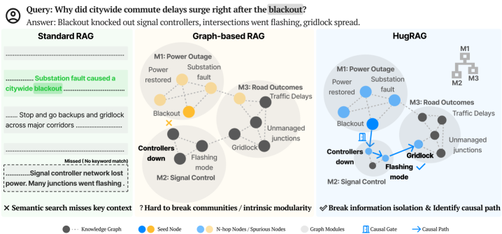</details> Figure 1: Comparison of three retrieval paradigms, Standard RAG, Graph-based RAG, and HugRAG, on a citywide blackout query. Standard RAG misses key evidence under semantic retrieval. Graph-based RAG can be trapped by intrinsic modularity or grouping structure. HugRAG leverages hierarchical causal gates to bridge modular boundaries, effectively breaking information isolation and explicitly identifying the underlying causal path. ## 1 Introduction While Retrieval-Augmented Generation (RAG) effectively extends Large Language Models (LLMs) with external knowledge (Lewis et al., 2021), traditional pipelines predominantly rely on text chunking and semantic embedding search. This paradigm implicitly frames knowledge access as a flat similarity matching problem, overlooking the structured and interdependent nature of real-world concepts. Consequently, as knowledge bases scale in complexity, these methods struggle to maintain retrieval efficiency and reasoning fidelity. Graph-based RAG has emerged as a promising solution to address these gaps, led by frameworks like GraphRAG (Edge et al., 2024) and extended through agentic search (Ravuru et al., 2024), GNN-guided refinement (Liu et al., 2025b), and hypergraph representations (Luo et al., ). However, three unintended limitations still persist. First, current research prioritizes retrieval policies while overlooking knowledge graph organization. As graphs scale, intrinsic modularity (Fortunato and Barthélemy, 2007) often restricts exploration within dense modules, triggering information isolation. Common grouping strategies ranging from communities (Edge et al., 2024), passage nodes (Gutiérrez et al., 2025), node-edge sets (Guo et al., 2024) to semantic grouping (Zhang et al., 2025) often inadvertently reinforce these boundaries, severely limiting global recall. Second, most formulations rely on semantic proximity and superficial traversal on graphs without causal awareness, leading to a locality issue where spurious nodes and irrelevant noise degrade precision (see Figure 1). Despite the inherent causal discovery potential of LLMs, this capability remains largely untapped for filtering noise within RAG pipelines. Finally, these systemic flaws are often masked by popular QA datasets evaluation, which reward entity-level “hits” over holistic comprehension. Consequently, there is a pressing need for a retrieval framework that reconciles global knowledge accessibility with local reasoning precision to support robust, causally-grounded generation. To address these challenges, we propose HugRAG, a framework that rethinks knowledge graph organization through hierarchical causal gate structures. HugRAG formulates the knowledge graph as a multi-layered representation where fine-grained facts are organized into higher-level schemas, enabling multi-granular reasoning. This hierarchical architecture, integrated with causal gates, establishes logical bridges across modules, thereby naturally breaking information isolation and enhancing global recall. During retrieval, HugRAG transcends pointwise semantic matching to explicit reasoning over causal graphs. By actively distinguishing genuine causal dependencies from spurious associations, HugRAG mitigates the locality issue and filters retrieval noise to ensure precise, grounded, and interpretable generation. To validate the effectiveness of HugRAG, we conduct extensive evaluations across datasets in multiple domains, comparing it against a diverse suite of competitive RAG baselines. To address the previously identified limitations of existing QA datasets, we introduce a large-scale cross-domain dataset HolisQA focused on holistic comprehension, designed to evaluate reasoning capabilities in complex, real-world scenarios. Our results consistently demonstrate that causal gating and causal reasoning effectively reconcile the trade-off between recall and precision, significantly enhancing retrieval quality and answer reliability. | Method Standard RAG (Lewis et al., 2021) Graph RAG (Edge et al., 2024) | Knowledge Graph Organization Flat text chunks, unstructured. $\mathcal{G}_{\text{idx}}=\{d_{i}\}_{i=1}^{N}$ Partitioned communities with summaries. $\mathcal{G}_{\text{idx}}=\{\text{Sum}(c)\mid c\in\mathcal{C}\}$ | Retrieval and Generation Process Semantic vector search over chunks. $S=\mathrm{TopK}(\text{sim}(q,d_{i}));\;\;y=\mathsf{G}(q,S)$ Map-Reduce over community summaries. $A_{\text{part}}=\{\mathsf{G}(q,\text{Sum}(m))\};\;\;y=\mathsf{G}(A_{\text{part}})$ | | --- | --- | --- | | Light RAG (Guo et al., 2024) | Dual-level indexing (Entities + Relations). $\mathcal{G}_{\text{idx}}=(V_{\text{ent}}\cup V_{\text{rel}},E)$ | Keyword-based vector retrieval + neighbor. $K_{q}=\mathsf{Key}(q);\;\;S=\mathrm{Vec}(K_{q},\mathcal{G}_{\text{idx}})\cup\mathcal{N}_{1}$ | | HippoRAG 2 (Gutiérrez et al., 2025) | Dense-sparse integration (Phrase + Passage). $\mathcal{G}_{\text{idx}}=(V_{\text{phrase}}\cup V_{\text{doc}},E)$ | PPR diffusion from LLM-filtered seeds. $U_{\text{seed}}=\mathsf{Filter}(q,V);\;\;S=\mathsf{PPR}(U_{\text{seed}},\mathcal{G}_{\text{idx}})$ | | LeanRAG (Zhang et al., 2025) | Hierarchical semantic clusters (GMM). $\mathcal{G}_{\text{idx}}=\text{Tree}(\text{Semantic Aggregation})$ | Bottom-up traversal to LCA (Ancestor). $U=\mathrm{TopK}(q,V);\;\;S=\mathsf{LCA}(U,\mathcal{G}_{\text{idx}})$ | | CausalRAG (Wang et al., 2025a) | Flat graph structure. $\mathcal{G}_{\text{idx}}=(V,E)$ | Top-K retrieval + Implicit causal reasoning. $S=\mathsf{Expand}(\mathrm{TopK}(q,V));\;\;y=\mathsf{G}(q,S)$ | | gray!10 HugRAG (Ours) | Hierarchical Causal Gates across modules. $\mathcal{G}_{\text{idx}}=\mathcal{H}=\{H_{0},\ldots,H_{L}\}$ | Causal Gating + Causal Path Filtering. $S=\underbrace{\mathsf{Traverse}(q,\mathcal{H})}_{\text{Break Isolation}}\cap\underbrace{\mathsf{Filter}_{\text{causal}}(S)}_{\text{Reduce Noise}}$ | Table 1: Comparison of RAG frameworks based on knowledge organization and retrieval mechanisms. Notation: $\mathcal{M}$ modules, $\text{Sum}(\cdot)$ summary, $\mathsf{PPR}$ Personalized PageRank, $\mathcal{H}$ hierarchy, $\mathcal{N}_{1}$ 1-hop neighborhood. ## 2 Related Work ### 2.1 RAG Retrieval augmented generation grounds LLMs in external knowledge, but chunk level semantic search can be brittle and inefficient for large, heterogeneous, or structured corpora (Lewis et al., 2021). Graph-based RAG has therefore emerged to introduce structure for more informed retrieval. #### Graph-based RAG. GraphRAG constructs a graph structured index of external knowledge and performs query time retrieval over the graph, improving question focused access to large scale corpora (Edge et al., 2024). Building on this paradigm, later work studies richer selection mechanisms over structured graph. Agent driven retrieval explores the search space iteratively (Ravuru et al., 2024). Critic guided or winnowing style methods prune weak contexts after retrieval (Dong et al., ; Wang et al., 2025b). Others learn relevance scores for nodes, subgraphs, or reasoning paths, often with graph neural networks (Liu et al., 2025b). Representation extensions include hypergraphs for higher order relations (Luo et al., ) and graph foundation models for retrieval and reranking (Wang et al., ). #### Knowledge Graph Organization. Despite these advances, limitations related to graph organization remain underexamined. Most work emphasizes retrieval policies, while the organization of the underlying knowledge graph is largely overlooked, which strongly influences downstream retrieval behavior. As graphs scale, intrinsic modularity can emerge (Fortunato and Barthélemy, 2007; Newman, 2018), making retrieval prone to staying within dense modules rather than crossing them, largely limiting the retrieved information. Moreover, many work assume grouping knowledge for efficiency at scale, such as communities (Edge et al., 2024), phrases and passages (Gutiérrez et al., 2025), node edge sets (Guo et al., 2024), or semantic aggregation (Zhang et al., 2025) (see Table 1), which can amplify modular confinement and yield information isolation. This global issue primarily manifests as reduced recall. Some hierarchical approaches like LeanRAG attempt to bridge these gaps via semantic aggregation, but they remain constrained by semantic clustering and rely on tree-structured traversals (Zhang et al., 2025), often failing to capture logical dependencies that span across semantically distinct clusters. #### Retrieval Issue. A second limitation concerns how retrieval is formulated. Much work operates as a multi-hop search over nodes or subgraphs (Gutiérrez et al., 2025; Liu et al., 2025a), prioritizing semantic proximity to the query without explicit awareness of the reasoning in this searching process. This design can pull in topically similar yet causally irrelevant evidence, producing conflated retrieval results. Even when the correct fact node is present, the generator may respond with generic or superficial content, and the extra noise can increase the risk of hallucination. We view this as a locality issue that lowers precision. #### QA Evaluation Issue. These tendencies can be reinforced by common QA evaluation practice. First, many QA datasets emphasize short answers such as names, nationalities, or years (Kwiatkowski et al., 2019; Rajpurkar et al., 2016), so hitting the correct entity in the graph may be sufficient even without reasoning. Second, QA datasets often comprise thousands of independent question-answer-context triples. However, many approaches still rely on linear context concatenation to construct a graph, and then evaluate performance on isolated questions. This setup largely reduces the incentive for holistic comprehension of the underlying material, even though such end-to-end understanding is closer to real-world use cases. Third, some datasets are stale enough that answers may be partially memorized by pretrained LLM models, confounding retrieval quality with parametric knowledge. Therefore, these QA dataset issues are critical for evaluating RAG, yet relatively few works explicitly address them by adopting open-ended questions and fresher materials in controlled experiments. ### 2.2 Causality #### LLM for Identifying Causality. LLMs have demonstrated exceptional potential in causal discovery. By leveraging vast domain knowledge, LLMs significantly improve inference accuracy compared to traditional methods (Ma, 2024). Frameworks like CARE further prove that fine-tuned LLMs can outperform state-of-the-art algorithms (Dong et al., 2025). Crucially, even in complex texts, LLMs maintain a direction reversal rate under 1.1% (Saklad et al., 2026), ensuring highly reliable results. #### Causality and RAG. While LLMs increasingly demonstrate reliable causal reasoning capabilities, explicitly integrating causal structures into RAG remains largely underexplored. Current research predominantly focuses on internal attribution graphs for model interpretability (Walker and Ewetz, 2025; Dai et al., 2025), rather than external knowledge retrieval. Recent advances like CGMT (Luo et al., 2025) and LACR (Zhang et al., 2024) have begun to bridge this gap, utilizing causal graphs for medical reasoning path alignment or constraint-based structure induction. However, these works inherently differ in scope from our objective, as they prioritize rigorous causal discovery or recovery tasks in specific domain, which limits their scalability to the noisy, open-domain environments that we address. Existing causal-enhanced RAG frameworks either utilize causal feedback implicitly in embedding (Khatibi et al., 2025) or, like CausalRAG (Wang et al., 2025a), are restricted to small-scale settings with implicit causal reasoning. Consequently, a significant gap persists in leveraging causal graphs to guide knowledge graph organization and retrieval across large-scale, heterogeneous knowledge bases. Note that in this work, we use the term causal to denote explicit logical dependencies and event sequences described in the text, rather than statistical causal discovery from observational data. ## 3 Problem Formulation We aim to retrieve an optimal subgraph $S^{*}\subseteq\mathcal{G}$ for a query $q$ to generate an answer $y$ . Graph-based RAG ( $S=\mathcal{R}(q,\mathcal{G})$ ) usually faces two structural bottlenecks. #### 1. Global Information Isolation (Recall Gap). Intrinsic modularity often traps retrieval in local seeds, missing relevant evidence $v^{*}$ located in topologically distant modules (i.e., $S\cap\{v^{*}\}=\emptyset$ as no path exists within $h$ hops). HugRAG introduces causal gates across $\mathcal{H}$ , to bypass modular boundaries and bridge this gap. The efficacy of causal gates is empirically verified in Appendix E and further analyzed in the ablation study (see Section 5.3). #### 2. Local Spurious Noise (Precision Gap). Semantic similarity $\text{sim}(q,v)$ often retrieves topically related but causally irrelevant nodes $\mathcal{V}_{sp}$ , diluting precision (where $|S\cap\mathcal{V}_{sp}|\gg|S\cap\mathcal{V}_{causal}|$ ). We address this by leveraging LLMs to identify explicit causal paths, filtering $\mathcal{V}_{sp}$ to ensure groundedness. While as discussed LLMs have demonstrated causal identification capabilities surpassing human experts (Ma, 2024; Dong et al., 2025) and proven effectiveness in RAG (Wang et al., 2025a), we further corroborate the validity of identified causal paths through expert knowledge across different domains (see Section 5.1). Consequently, HugRAG redefines retrieval as finding a mapping $\Phi:\mathcal{G}\to\mathcal{H}$ and a causal filter $\mathcal{F}_{c}$ to simultaneously minimize isolation and spurious noise. <details> <summary>x2.png Details</summary>  ### Visual Description \n ## System Architecture Diagram: Two-Phase Knowledge Graph Processing for Question Answering ### Overview The image is a technical system architecture diagram illustrating a two-phase process for building and utilizing a knowledge graph to answer queries. The system is divided into an **offline "Graph Construction"** phase and an **online "Retrieve and Answer"** phase, separated by a vertical dashed line. The diagram uses icons, text labels, and flow arrows to depict data flow and processing steps, with a focus on integrating causal reasoning via Large Language Models (LLMs). ### Components/Axes The diagram is segmented into two primary regions: **1. Left Region: Graph Construction (Offline)** * **Header Label:** "Graph Construction (Offline)" * **Process Flow (Top Path):** * Icon: Document stack. Label: "Raw Texts" * Arrow with icon (magnifying glass) and label: "IE" (Information Extraction) * Icon: Network graph. Label: "Knowledge Graph" * Arrow with icon (cube) and label: "Embed" * Icon: Database/server rack. Label: "Vector Store" * **Process Flow (Bottom Path):** * Arrow from "Raw Texts" with icon (split arrow) and label: "Partition" * Label: "Hierarchical Graph" * Arrow with icon (link) and label: "Identify Causality" * Text below arrow: "LLM" * Arrow points to label: "Graph with Causal Gates" * **Visual Elements:** * Two sets of stacked, layered graph illustrations. * Left set: Labeled "Hierarchical Graph". Shows three layers of graphs (top, middle, bottom) with nodes and edges. No special highlighting. * Right set: Labeled "Graph with Causal Gates". Shows three corresponding layers. Specific edges and nodes are highlighted in **blue**, indicating the "causal gates" identified by the LLM. * Layer labels on the right side: "Hn" (top), "Hn-1" (middle), "H0" (bottom). **2. Right Region: Retrieve and Answer (Online)** * **Header Label:** "Retrieve and Answer (Online)" * **Process Flow:** * Icon: Person/User. Label: "Query" * Arrow with icon (magnifying glass) and label: "Embed and Score" * Icon: Checkmark in circle. Label: "Top K entities" * Arrow with label: "N hop via gates, cross modules" * Label: "Context Subgraph" * Arrow with icon (link) and label: "Distinguish Causal vs Spurious" * Text below arrow: "LLM" * Arrow points to label: "Context" * Final arrow with label: "with Query" pointing to icon (checkmark) and label: "Answer" * **Visual Elements:** * Two sets of stacked, layered graph illustrations, mirroring the offline phase. * Left set: Labeled "Context Subgraph". Shows a subset of the hierarchical graph. Some nodes/edges are highlighted in **blue**, representing the retrieved subgraph. * Right set: Labeled "Context". Shows the same subgraph structure, but now a specific path or set of elements is marked with a **blue checkmark**, indicating the causal context selected for the answer. ### Detailed Analysis The diagram details a pipeline that transforms raw text into a structured, causally-aware knowledge representation for efficient question answering. **Offline Phase (Graph Construction):** 1. **Dual-Path Processing:** Raw texts are processed in two parallel streams. * **Stream 1 (Direct KG):** Texts undergo Information Extraction (IE) to build a standard Knowledge Graph, which is then embedded into a Vector Store for similarity search. * **Stream 2 (Hierarchical & Causal):** Texts are partitioned and organized into a Hierarchical Graph (layers Hn to H0). An LLM analyzes this graph to "Identify Causality," resulting in a "Graph with Causal Gates." The blue highlights in the right-hand graph illustration show these gates—specific connections deemed causally significant. 2. **Output:** The outputs are a Vector Store (for retrieval) and a Causal Graph (for reasoning). **Online Phase (Retrieve and Answer):** 1. **Query Processing:** A user query is embedded and scored against the Vector Store to retrieve the "Top K entities." 2. **Subgraph Retrieval:** Starting from these entities, the system traverses "N hops" through the graph, guided by the "gates" (causal connections) established offline, to assemble a "Context Subgraph." 3. **Causal Filtering:** An LLM processes this subgraph to "Distinguish Causal vs Spurious" relationships, filtering it down to the most relevant "Context." 4. **Answer Generation:** The final causal context, combined with the original query, is used to generate the "Answer." ### Key Observations * **Central Role of LLMs:** LLMs are explicitly called out for two critical reasoning tasks: identifying causal relationships in the offline phase and distinguishing causal from spurious links in the online phase. * **Hierarchical Structure:** The use of a hierarchical graph (Hn...H0) suggests the knowledge is organized at multiple levels of abstraction or granularity. * **Causal Gates as a Core Mechanism:** The "causal gates" (highlighted in blue) are the key innovation. They act as filters or guides during the online retrieval ("N hop via gates") to focus the search on causally relevant paths, improving efficiency and answer quality. * **Visual Consistency:** The blue highlighting is used consistently across both phases to denote causally significant elements, creating a clear visual link between the offline analysis and online application. ### Interpretation This diagram presents a sophisticated architecture for **causality-aware knowledge graph question answering**. The core problem it solves is the retrieval of not just any relevant information, but *causally pertinent* information from a large knowledge base. * **How it Works:** The system pre-computes causal relationships (offline) to create a "map" of meaningful connections. When a query arrives (online), it doesn't just search broadly; it follows this pre-defined causal map to quickly home in on the context that likely contains the answer, ignoring spurious correlations. * **Why it Matters:** This approach addresses key limitations of standard retrieval-augmented generation (RAG). By focusing on causal links, it aims to: 1. **Improve Accuracy:** Retrieve more relevant context, reducing hallucinations. 2. **Increase Efficiency:** Limit the search space via gates, reducing computational cost. 3. **Enhance Explainability:** The causal path from query to answer is more traceable. * **Underlying Assumption:** The architecture assumes that causality is a powerful heuristic for relevance in question answering. The LLM's role is to encode this causal understanding into the graph structure itself, which then guides the retrieval process deterministically. The separation into offline and online phases is a practical design to handle the computational cost of causal analysis. 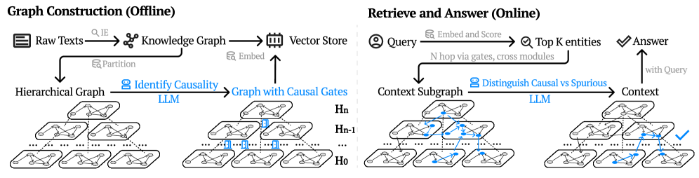</details> Figure 2: Overview of the HugRAG pipeline. In the offline stage, raw texts are embedded to build a knowledge graph and a vector store, then partitioning forms a hierarchical graph and an LLM identifies causal relations to construct a graph with causal gates. In the online stage, the query is embedded and scored to retrieve top K entities, then N hop traversal uses causal gates to cross modules and assemble a context subgraph; an LLM further distinguishes causal versus spurious relations to produce the final context and answer. Algorithm 1 HugRAG Algorithm Pipeline 0: Corpus $\mathcal{D}$ , query $q$ , hierarchy levels $L$ , seed budget $\{K_{\ell}\}_{\ell=0}^{L}$ , hop $h$ , gate threshold $\tau$ 0: Answer $y$ , Support Subgraph $S^{*}$ 1: // Phase 1: Offline Hierarchical Organization 2: $G_{0}=(V_{0},E_{0})\leftarrow\textsc{BuildBaseGraph}(\mathcal{D})$ 3: $\mathcal{H}=\{H_{0},\ldots,H_{L}\}\leftarrow\textsc{LeidenPartition}(G_{0},L)$ {Organize into modules $\mathcal{M}$ } 4: $\mathcal{G}_{c}\leftarrow\emptyset$ 5: for all pair $(m_{i},m_{j})\in\textsc{ModulePairs}(\mathcal{M})$ do 6: $score\leftarrow\textsc{LLM-EstCausal}(m_{i},m_{j})$ 7: if $score\geq\tau$ then 8: $\mathcal{G}_{c}\leftarrow\mathcal{G}_{c}\cup\{(m_{i}\to m_{j},score)\}$ {Establish causal gates} 9: end if 10: end for 11: // Phase 2: Online Retrieval & Reasoning 12: $U\leftarrow\bigcup_{\ell=0}^{L}\mathrm{TopK}(\text{sim}(q,u),K_{\ell},H_{\ell})$ {Multi-level semantic seeding} 13: $S_{raw}\leftarrow\textsc{GatedTraversal}(U,\mathcal{H},\mathcal{G}_{c},h)$ {Break isolation via gates} 14: $S^{*}\leftarrow\textsc{CausalFilter}(q,S_{raw})$ {Remove spurious nodes $\mathcal{V}_{sp}$ } 15: $y\leftarrow\textsc{LLM-Generate}(q,S^{*})$ ## 4 Method #### Overview. As illustrated in Figure 2, HugRAG operates in two distinct phases to address the aforementioned structural bottlenecks. In the offline phase, we construct a hierarchical knowledge structure $\mathcal{H}$ partitioned into modules, which are then interconnected via causal gates $\mathcal{G}_{c}$ to enable logical traversals. In the online phase, HugRAG performs a gated expansion to break modular isolation, followed by a causal filtering step to eliminate spurious noise. The overall procedure is formalized in Algorithm 1, and we detail each component in the subsequent sections. ### 4.1 Hierarchical Graph with Causal Gating To address the global information isolation challenge (Section 3), we construct a multi-scale knowledge structure that balances global retrieval recall with local precision. #### Hierarchical Module Construction. We first extract a base entity graph $G_{0}=(V_{0},E_{0})$ from the corpus $\mathcal{D}$ using an information extraction pipeline (see details in Appendix B.1), followed by entity canonicalization to resolve aliasing. To establish the hierarchical backbone $\mathcal{H}=\{H_{0},\dots,H_{L}\}$ , we iteratively partition the graph into modules using the Leiden algorithm (Traag et al., 2019), which optimizes modularity to identify tightly-coupled semantic regions. Formally, at each level $\ell$ , nodes are partitioned into modules $\mathcal{M}_{\ell}=\{m_{1}^{(\ell)},\dots,m_{k}^{(\ell)}\}$ . For each module, we generate a natural language summary to serve as a coarse-grained semantic anchor. #### Offline Causal Gating. While hierarchical modularity improves efficiency, it risks trapping retrieval within local boundaries. We introduce Causal Gates to explicitly model cross-module affordances. Instead of fully connecting the graph, we construct a sparse gate set $\mathcal{G}_{c}$ . Specifically, we identify candidate module pairs $(m_{i},m_{j})$ that are topologically distant but potentially logically related. An LLM then evaluates the plausibility of a causal connection between their summaries. We formally define the gate set via an indicator function $\mathbb{I}(\cdot)$ : $$ \mathcal{G}_{c}=\left\{(m_{i}\to m_{j})\mid\mathbb{I}_{\text{causal}}(m_{i},m_{j})=1\right\}, \tag{1} $$ where $\mathbb{I}_{\text{causal}}$ denotes the LLM’s assessment (see Appendix B.1 for construction prompts and the Top-Down Hierarchical Pruning strategy we employed to mitigate the $O(N^{2})$ evaluation complexity). These gates act as shortcuts in the retrieval space, permitting the traversal to jump across disjoint modules only when logically warranted, thereby breaking information isolation without causing semantic drift (see Appendix C for visualizations of hierarchical modules and causal gates). ### 4.2 Retrieve Subgraph via Causally Gated Expansion Given the hierarchical structure $\mathcal{H}$ and causal gates $\mathcal{G}_{c}$ , HugRAG retrieves a support subgraph $S$ by coupling multi-granular anchoring with a topology-aware expansion. This process is designed to maximize recall (breaking isolation) while suppressing drift (controlled locality). #### Multi-Granular Hybrid Seeding. Graph-based RAG often struggles to effectively differentiate between local details and global contexts within multi-level structures (Zhang et al., 2025; Edge et al., 2024). We overcome this by identifying a seed set $U$ across multiple levels of the hierarchy. We employ a hybrid scoring function $s(q,v)$ that interpolates between semantic embedding similarity and lexical overlap (details in Appendix B.2). This function is applied simultaneously to fine-grained entities in $H_{0}$ and coarse-grained module summaries in $H_{\ell>0}$ . Crucially, to prevent the semantic redundancy problem where seeds cluster in a single redundant neighborhood, we apply a diversity-aware selection strategy (MMR) to ensure the initial seeds $U$ cover distinct semantic facets of the query. This yields a set of anchors that serve as the starting nodes for expansion. #### Gated Priority Expansion. Starting from the seed set $U$ , we model retrieval as a priority-based traversal over a unified edge space $\mathcal{E}_{\text{uni}}$ . This space integrates three distinct types of connectivity: (1) Structural Edges ( $E_{\text{struc}}$ ) for local context, (2) Hierarchical Edges ( $E_{\text{hier}}$ ) for vertical drill-down, and (3) Causal Gates ( $\mathcal{G}_{c}$ ) for cross-module reasoning. $$ \mathcal{E}_{\text{uni}}={E}_{\text{struc}}\cup E_{\text{hier}}\cup\mathcal{G}_{c}. \tag{2} $$ The expansion follows a Best-First Search guided by a query-conditioned gain function. For a frontier node $v$ reached from a predecessor $u$ at hop $t$ , the gain is defined as: $$ \text{Gain}(v)=s(q,v)\cdot\gamma^{t}\cdot w(\text{type}(u,v)), \tag{3} $$ where $\gamma\in(0,1)$ is a standard decay factor to penalize long-distance traversal. The weight function $w(\cdot)$ adjusts traversal priorities: we simply assign higher importance to causal gates and hierarchical links to encourage logic-driven jumps over random structural walks. By traversing $\mathcal{E}_{\text{uni}}$ , HugRAG prioritizes paths that drill down (via $E_{\text{hier}}$ ), explore locally (via $E_{\text{struc}}$ ), or leap to a causally related domain (via $\mathcal{G}_{c}$ ), effectively breaking modular isolation. The expansion terminates when the gain drops below a threshold or the token budget is exhausted. | Datasets | Nodes | Edges | Modules | Size (Char) | Domain | | --- | --- | --- | --- | --- | --- | | MS MARCO (Bajaj et al., 2018) | 3,403 | 3,107 | 446 | 1,557,990 | Web | | NQ (Kwiatkowski et al., 2019) | 5,579 | 4,349 | 505 | 767,509 | Wikipedia | | 2WikiMultiHopQA (Ho et al., 2020) | 10,995 | 8,489 | 1,088 | 1,756,619 | Wikipedia | | QASC (Khot et al., 2020) | 77 | 39 | 4 | 58,455 | Science | | HotpotQA (Yang et al., 2018) | 20,354 | 15,789 | 2,359 | 2,855,481 | Wikipedia | | HolisQA-Biology | 1,714 | 1,722 | 165 | 1,707,489 | Biology | | HolisQA-Business | 2,169 | 2,392 | 292 | 1,671,718 | Business | | HolisQA-CompSci | 1,670 | 1,667 | 158 | 1,657,390 | Computer Science | | HolisQA-Medicine | 1,930 | 2,124 | 226 | 1,706,211 | Medicine | | HolisQA-Psychology | 2,019 | 1,990 | 211 | 1,751,389 | Psychology | Table 2: Statistics of the datasets used in evaluation. ### 4.3 Causal Path Identification and Grounding The raw subgraph $S_{raw}$ retrieved via gated expansion optimizes for recall but inevitably includes spurious associations (e.g., high-degree hubs or coincidental co-occurrences). To address the local spurious noise challenge (Section 3), HugRAG employs a causal path refinement stage to directly distill $S_{raw}$ into a causally grounded graph $S^{\star}$ . See Appendix D for a full example of the HugRAG pipeline. #### Causal Path Refinement. We formulate the path refinement task as a structural pruning process. We first linearize the subgraph $S_{raw}$ into a token-efficient table where each node and edge is mapped to a unique short identifier (see Appendix B.3). The LLM is then prompted to analyze the topology and output the subset of identifiers that constitute valid causal paths connecting the query to the potential answer. Leveraging the robust causal identification capabilities of LLMs (Saklad et al., 2026), this operation effectively functions as a reranker, distilling the noisy subgraph into an explicit causal structure: $$ S^{\star}=\textsc{LLM-CausalExpert}(S_{raw},q). \tag{4} $$ The returned subgraph $S^{\star}$ contains only model-validated nodes and edges, effectively filtering irrelevant context. #### Spurious-Aware Grounding. To further improve the precision of this selection, we employ a spurious-aware prompting strategy (see prompts in Appendix A.1). In this configuration, the LLM is instructed to explicitly distinguish between causal supports and spurious correlations during its reasoning process. While the prompt may ask the model to identify spurious items as an auxiliary reasoning step, the primary objective remains the extraction of the valid causal subset. This explicit contrast helps the model resist hallucinated connections induced by semantic similarity, yielding a cleaner $S^{\star}$ compared to standard selection prompts and consequently improving downstream generation quality. This mechanism specifically targets the precision challenges outlined in Section 4.2. Finally, the answer $y$ is generated by conditioning the LLM solely on the text content corresponding to the pruned subgraph $S^{\star}$ (see prompts in Appendix A.2), ensuring that the generation is strictly grounded in verified evidence. ## 5 Experiments #### Overview. We conducted extensive experiments on diverse datasets across various domains to comprehensively evaluate and compare the performance of HugRAG against competitive baselines. Our analysis is guided by the following five research questions: RQ1 (Overall Performance). How does HugRAG compare against state-of-the-art graph-based baselines across diverse, real-world knowledge domains? RQ2 (QA vs. Holistic Comprehension). Do popular QA datasets implicitly favor the entity-centric retrieval paradigm, thereby inflating graph-based RAG that finds the right node without assembling a support chain? RQ3 (Trade-off Reconciliation). Can HugRAG simultaneously improve Context Recall (Globality) and Answer Relevancy (Precision), mitigating the classic trade-off via hierarchical causal gating? RQ4 (Ablation Study). What are the individual contributions of different components in HugRAG? RQ5 (Scalability Robustness). How does HugRAG’s performance scale and remain robust under varying context lengths? Table 3: Main results on HolisQA across five domains. We report F1 (answer overlap), CR (Context Recall: how much gold context is covered by retrieved evidence), and AR (Answer Relevancy: evaluator-judged relevance of the answer to the question), all scaled to $\$ for readability. Bold indicates best per column. NaiveGeneration has CR $=0$ by definition (no retrieval). | Baselines-black!10 Naive Baselines | Medicine F1 | Computer Science CR | Business AR | Biology F1 | Psychology CR | AR | F1 | CR | AR | F1 | CR | AR | F1 | CR | AR | | --- | --- | --- | --- | --- | --- | --- | --- | --- | --- | --- | --- | --- | --- | --- | --- | | NaiveGeneration | 12.63 | 0.00 | 44.70 | 18.93 | 0.00 | 48.79 | 18.58 | 0.00 | 46.14 | 11.71 | 0.00 | 45.76 | 22.91 | 0.00 | 50.00 | | BM25 | 17.72 | 52.04 | 50.64 | 24.00 | 39.12 | 52.40 | 28.11 | 37.06 | 55.52 | 19.61 | 43.02 | 52.32 | 30.46 | 33.44 | 56.63 | | StandardRAG | 26.87 | 61.08 | 56.24 | 28.87 | 49.44 | 57.10 | 47.57 | 46.79 | 67.42 | 28.31 | 42.69 | 57.58 | 37.19 | 52.21 | 59.85 | | black!10 Graph-based RAG | | | | | | | | | | | | | | | | | GraphRAG Global | 17.13 | 54.56 | 48.19 | 23.75 | 37.65 | 53.17 | 23.62 | 25.01 | 48.12 | 20.67 | 40.90 | 52.41 | 31.09 | 34.26 | 54.62 | | GraphRAG Local | 19.03 | 56.07 | 49.52 | 25.10 | 39.90 | 53.30 | 25.01 | 27.36 | 49.05 | 22.21 | 41.88 | 52.73 | 32.31 | 35.22 | 55.02 | | LightRAG | 12.16 | 52.38 | 44.15 | 22.59 | 41.86 | 51.62 | 29.98 | 34.22 | 54.50 | 17.70 | 41.24 | 50.32 | 33.63 | 45.54 | 56.42 | | black!10 Structural / Causal Augmented | | | | | | | | | | | | | | | | | HippoRAG2 | 21.12 | 57.50 | 51.08 | 16.94 | 21.05 | 47.29 | 21.10 | 18.34 | 45.83 | 12.60 | 16.85 | 44.56 | 20.10 | 34.13 | 46.77 | | LeanRAG | 34.25 | 60.43 | 56.60 | 30.51 | 57.61 | 55.45 | 48.30 | 59.29 | 60.35 | 33.82 | 58.43 | 56.10 | 42.85 | 57.46 | 58.65 | | CausalRAG | 31.12 | 58.90 | 58.77 | 30.98 | 54.10 | 57.54 | 45.20 | 44.55 | 66.10 | 33.50 | 51.20 | 58.90 | 42.80 | 55.60 | 61.90 | | HugRAG (ours) | 36.45 | 69.91 | 60.65 | 31.60 | 60.94 | 58.34 | 51.51 | 67.34 | 68.76 | 34.80 | 61.97 | 59.99 | 44.42 | 60.87 | 63.53 | Table 4: Main results on five QA datasets. Metrics follow Section 5: F1, CR (Context Recall), and AR (Answer Relevancy), reported in $\$ . Bold and underline denote best and second-best per column. | Baselines-black!10 Naive Baselines | MSMARCO F1 | NQ CR | TwoWiki AR | QASC F1 | HotpotQA CR | AR | F1 | CR | AR | F1 | CR | AR | F1 | CR | AR | | --- | --- | --- | --- | --- | --- | --- | --- | --- | --- | --- | --- | --- | --- | --- | --- | | NaiveGeneration | 5.28 | 0.00 | 15.06 | 7.17 | 0.00 | 10.94 | 9.15 | 0.00 | 11.77 | 2.69 | 0.00 | 13.74 | 14.38 | 0.00 | 15.74 | | BM25 | 6.97 | 45.78 | 20.33 | 4.68 | 49.98 | 9.13 | 9.43 | 37.12 | 13.73 | 2.49 | 6.12 | 13.17 | 15.81 | 41.08 | 16.08 | | StandardRAG | 14.93 | 48.55 | 31.11 | 7.57 | 45.82 | 11.14 | 10.33 | 32.28 | 13.57 | 2.01 | 5.50 | 13.16 | 6.68 | 43.17 | 14.66 | | black!10 Graph-based RAG | | | | | | | | | | | | | | | | | GraphRAG Global | 9.41 | 3.65 | 13.08 | 3.91 | 4.48 | 8.00 | 1.41 | 9.42 | 9.55 | 0.68 | 3.38 | 3.56 | 6.28 | 14.59 | 16.26 | | GraphRAG Local | 30.87 | 25.71 | 57.76 | 23.56 | 44.56 | 44.68 | 18.85 | 32.03 | 37.29 | 8.30 | 9.54 | 46.59 | 33.14 | 44.07 | 40.82 | | LightRAG | 37.70 | 54.22 | 63.54 | 24.97 | 60.65 | 50.53 | 14.44 | 40.98 | 36.56 | 8.20 | 20.40 | 44.35 | 28.39 | 48.17 | 43.78 | | black!10 Structural / Causal Augmented | | | | | | | | | | | | | | | | | HippoRAG2 | 23.35 | 45.45 | 55.18 | 29.64 | 57.21 | 37.50 | 18.47 | 55.53 | 17.34 | 14.73 | 4.38 | 49.94 | 38.80 | 42.06 | 24.66 | | LeanRAG | 38.02 | 54.01 | 58.49 | 35.46 | 65.91 | 49.87 | 20.27 | 40.53 | 38.37 | 13.19 | 22.80 | 45.51 | 48.68 | 46.29 | 43.50 | | CausalRAG | 27.66 | 39.38 | 46.03 | 29.45 | 68.04 | 17.35 | 15.93 | 28.38 | 19.76 | 7.65 | 46.86 | 35.56 | 40.00 | 27.83 | 21.32 | | HugRAG (ours) | 38.40 | 60.48 | 66.02 | 49.50 | 70.36 | 55.09 | 31.97 | 41.95 | 42.67 | 13.35 | 70.80 | 49.40 | 64.83 | 40.30 | 45.72 | ### 5.1 Experimental Setup #### Datasets. We evaluate HugRAG on a diverse suite of datasets covering complementary difficulty profiles. For standard evaluation, we use five established datasets: MS MARCO (Bajaj et al., 2018) and Natural Questions (Kwiatkowski et al., 2019) emphasize large-scale open-domain retrieval; HotpotQA (Yang et al., 2018) and 2WikiMultiHop (Ho et al., 2020) require evidence aggregation; and QASC (Khot et al., 2020) targets compositional scientific reasoning. However, these datasets often suffer from entity-centric biases and potential data leakage (memorization by LLMs). To rigorously test the holistic understanding capability of RAG, we introduce HolisQA, a dataset derived from high-quality academic papers sourced (Priem et al., 2022). Spanning over diverse domains (including Biology, Computer Science, Medicine, etc.), HolisQA features dense logical structures that naturally demand holistic comprehension (see more details in Appendix F.2). All dataset statistics are summarized in Table 2. While LLMs have demonstrated strong capabilities in identifying causality (Ma, 2024; Dong et al., 2025) and effectiveness in RAG (Wang et al., 2025a), to ensure rigorous evaluation, we incorporated cross-domain expert review to validate the quality of baseline answers and confirm the legitimacy of the induced causal relations. #### Baselines. We compare HugRAG against eight baselines spanning three retrieval paradigms. First, to cover Naive and Flat approaches, we include Naive Generation (no retrieval) as a lower bound, alongside BM25 (sparse) and Standard RAG (Lewis et al., 2021) (dense embedding-based), representing mainstream unstructured retrieval. Second, we evaluate established graph-based frameworks: GraphRAG (Local and Global) (Edge et al., 2024), utilizing community summaries; and LightRAG (Guo et al., 2024), relying on dual-level keyword-based search. Third, we benchmark against RAGs with structured or causal augmentation: HippoRAG 2 (Gutiérrez et al., 2025), utilizing passage nodes and Personalized PageRank diffusion; LeanRAG (Zhang et al., 2025), employing semantic aggregation hierarchies and tree-based LCA retrieval; and CausalRAG (Wang et al., 2025a), which incorporates causality without explicit causal reasoning. This selection comprehensively covers the spectrum from unstructured search to advanced structure-aware and causally augmented graph methods. #### Metrics. For metrics, we first report the token-level answer quality metric F1 for surface robustness. To measure whether retrieval actually supports generation, we additionally compute grounding metrics, context recall and answer relevancy (Es et al., 2024), which jointly capture coverage and answer quality (see Appendix F.4). #### Implementation Details. For all experiments, we utilize gpt-5-nano as the backbone LLM for both the open IE extraction and generation stages, and Sentence-BERT (Reimers and Gurevych, 2019) for semantic vectorization. For HugRAG, we set the hierarchical seed budget to $K_{L}=3$ for modules and $K_{0}=3$ for entities, causal gate is enabled by default except ablation study. Experiments run on a cluster using 10-way job arrays; each task uses 2 CPU cores and 16 GB RAM (20 cores, 160GB in total). See more implementation details in Appendix F.3. ### 5.2 Main Experiments #### Overall Performance (RQ1). HugRAG consistently achieves superior performance across all HolisQA domains and standard QA metrics (Section 5, Section 5). While traditional methods (e.g., BM25, Standard RAG) struggle with structural dependencies, graph-based baselines exhibit distinct limitations. GraphRAG-Global relies heavily on high-level community summaries and largely suffers from detailed QA tasks, necessitating its GraphRAG Local variant to balance the granularity trade-off. LightRAG struggles to achieve competitive results, limited by its coarse-grained key-value lookup mechanism. Regarding structurally augmented methods, while LeanRAG (utilizing semantic aggregation) and HippoRAG2 (leveraging phrase/passage nodes) yield slight improvements in context recall, they fail to fully break information isolation compared to our causal gating mechanism. Finally, although CausalRAG occasionally attains high Answer Relevancy due to its causal reasoning capability, it struggles to scale to large datasets due to the lack of efficient knowledge graph organization. #### Holistic Comprehension vs. QA (RQ2). The contrast between the results on HolisQA (Section 5) and standard QA datasets (Section 5) is revealing. On popular QA benchmarks, entity-centric methods like LightRAG, GraphRAG-Local, LeanRAG could occasionally achieve good scores. However, their performance degrades collectively and significantly on HolisQA. A striking counterexample is GraphRAG-Global: while its reliance on community summaries hindered performance on granular standard QA tasks, now it rebounds significantly in HolisQA. This discrepancy strongly suggests that standard QA datasets, which often favor short answers, implicitly reward the entity-centric paradigm. In contrast, HolisQA, with its open-ended questions and dense logical structures, necessitates a comprehensive understanding of the underlying document—a scenario closer to real-world applications. Notably, HugRAG is the only framework that remains robust across this paradigm shift, demonstrating competitive performance on both entity-centric QA and holistic comprehension tasks. #### Reconciling the Accuracy-Grounding Trade-off (RQ3). HugRAG effectively reconciles the fundamental tension between Recall and Precision. While hierarchical causal gating expands traversal boundaries to secure superior Context Recall (Globality), the explicit causal path identification rigorously prunes spurious noise to maintain high F1 Score and Answer Relevancy (Locality). This dual mechanism allows HugRAG to simultaneously optimize for global coverage and local groundedness, achieving a balance often missed by prior methods. <details> <summary>x3.png Details</summary>  ### Visual Description ## Grouped Bar Chart: Performance Metrics Comparison ### Overview The image displays a grouped bar chart comparing the performance scores of six different model configurations across three evaluation metrics: F1, CR, and AR. The chart is designed to show the incremental impact of adding components (H, CG, Causal, SP-Causal) to a baseline model. ### Components/Axes * **Chart Type:** Grouped Bar Chart. * **X-Axis (Horizontal):** Labeled "Metric". It contains three categorical groups: 1. **F1** 2. **CR** 3. **AR** * **Y-Axis (Vertical):** Labeled "Score". It is a linear scale ranging from 0 to 70, with major tick marks at intervals of 10 (0, 10, 20, 30, 40, 50, 60, 70). * **Legend:** Positioned at the top-center of the chart area. It defines six data series, each corresponding to a specific model configuration, identified by color and a descriptive label: 1. **Teal:** `w/o H · w/o CG · w/o Causal` (Baseline) 2. **Yellow:** `w/ H · w/o CG · w/o Causal` 3. **Blue:** `w/ H · w/ CG · w/o Causal` 4. **Pink:** `w/o H · w/o CG · w/ Causal` 5. **Green:** `w/ H · w/ CG · w/ Causal` 6. **Orange:** `w/ H · w/ CG · w/ SP-Causal` * **Data Labels:** Each bar has its exact numerical score printed directly above it. ### Detailed Analysis The chart presents the following scores for each metric and configuration: **1. F1 Metric Group (Leftmost cluster):** * **Trend:** Scores generally increase from left to right within the group, with the baseline (teal) and the "w/ H" (yellow) configurations performing lower than those incorporating "Causal" or "SP-Causal" components. * **Data Points:** * Teal (Baseline): 26.8 * Yellow (w/ H): 24.0 * Blue (w/ H, w/ CG): 23.3 * Pink (w/ Causal): 30.1 * Green (w/ H, w/ CG, w/ Causal): 36.8 * Orange (w/ H, w/ CG, w/ SP-Causal): 38.6 **2. CR Metric Group (Center cluster):** * **Trend:** Scores are more tightly clustered compared to F1. The addition of "CG" (blue) and "SP-Causal" (orange) yields the highest scores. * **Data Points:** * Teal (Baseline): 54.7 * Yellow (w/ H): 58.0 * Blue (w/ H, w/ CG): 60.2 * Pink (w/ Causal): 55.4 * Green (w/ H, w/ CG, w/ Causal): 60.0 * Orange (w/ H, w/ CG, w/ SP-Causal): 60.4 **3. AR Metric Group (Rightmost cluster):** * **Trend:** Shows a clear, progressive increase in score from the baseline (teal) to the most complex configuration (orange). The "SP-Causal" variant (orange) achieves the highest score on the entire chart. * **Data Points:** * Teal (Baseline): 55.7 * Yellow (w/ H): 53.6 * Blue (w/ H, w/ CG): 52.6 * Pink (w/ Causal): 60.0 * Green (w/ H, w/ CG, w/ Causal): 64.1 * Orange (w/ H, w/ CG, w/ SP-Causal): 67.4 ### Key Observations 1. **Consistent Top Performer:** The `w/ H · w/ CG · w/ SP-Causal` (orange) configuration achieves the highest score in all three metric categories (F1: 38.6, CR: 60.4, AR: 67.4). 2. **Impact of Causal Components:** Configurations that include a "Causal" or "SP-Causal" component (pink, green, orange bars) consistently outperform their non-causal counterparts (teal, yellow, blue) within the same metric group, especially in F1 and AR. 3. **Metric Sensitivity:** The F1 metric shows the greatest relative variation between configurations (scores ranging from ~23 to ~39), while the CR metric shows the least variation (scores clustered between ~55 and ~60). 4. **Non-Linear Improvement:** Adding components does not always guarantee improvement. For example, in the AR metric, adding "H" alone (yellow) or "H + CG" (blue) to the baseline actually results in a slight score decrease before the "Causal" components drive a significant increase. ### Interpretation This chart is an ablation study, systematically evaluating the contribution of different components (H, CG, Causal, SP-Causal) to a model's performance. The data suggests: * **Synergistic Effects:** The best performance is achieved not by any single component, but by the combination of all three: H, CG, and a causal modeling approach (especially SP-Causal). This indicates these components address complementary aspects of the problem. * **Causal Modeling is Key:** The most significant performance jumps are associated with the introduction of causal components (pink, green, orange bars). This strongly implies that modeling causal relationships is crucial for improving performance on these specific metrics (F1, CR, AR). * **"SP-Causal" Superiority:** The "SP-Causal" variant consistently outperforms the standard "Causal" variant when paired with H and CG (comparing green vs. orange bars). This suggests the "SP" modification provides a meaningful enhancement to the causal modeling approach for this task. * **Task-Specific Baseline:** The baseline model (teal) performs moderately on CR and AR (~55) but poorly on F1 (~27), indicating the baseline is better suited for the tasks measured by CR and AR than for the task measured by F1. The added components, particularly causal ones, are especially effective at boosting F1 performance. In summary, the visualization provides strong evidence that integrating hierarchical (H), coarse-grained (CG), and advanced causal (SP-Causal) modeling techniques leads to superior and more robust model performance across multiple evaluation dimensions. 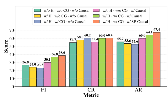</details> Figure 3: Ablation Study. H: Hierarchical Structure; CG: Causal Gates; Causal/SP-Causal: Standard vs. Spurious-Aware Causal Identification. w/o and w/ denote exclusion or inclusion. ### 5.3 Ablation Study To address RQ4, we ablate hierarchy, causal gates, and causal path refinement components (see Figure 3), finding that their combination yields optimal results. Specifically, we observe a mutually reinforcing dynamic: while hierarchical gates break information isolation to boost recall, the spurious-aware causal identification is indispensable for filtering the resulting noise and achieving a significant improvement. This mutual reinforcement allows HugRAG to reconcile global coverage with local groundedness, significantly outperforming any isolated component. <details> <summary>x4.png Details</summary>  ### Visual Description ## Line Chart: Performance Comparison of RAG Methods Across Source Text Lengths ### Overview This line chart compares the performance scores of ten different Retrieval-Augmented Generation (RAG) methods as a function of increasing source text length, measured in characters. The chart demonstrates how each method's effectiveness (score) changes as the input text scales from 5,000 to 1.5 million characters. ### Components/Axes * **Chart Type:** Multi-series line chart. * **X-Axis (Horizontal):** * **Label:** `Source Text Length (chars)` * **Scale:** Categorical, not linear. The marked points are: `5K`, `10K`, `25K`, `100K`, `300K`, `750K`, `1M`, `1.5M`. * **Y-Axis (Vertical):** * **Label:** `Score` * **Scale:** Linear, ranging from 0 to 60, with major gridlines at intervals of 10. * **Legend:** Located at the top of the chart, spanning two rows. It maps method names to line styles and colors. * **Row 1:** `Naive` (gray circle), `BM25` (gray square), `Standard RAG` (light gray triangle), `GraphRAG Global` (blue square), `GraphRAG Local` (dark blue star), `LightRAG` (light blue triangle). * **Row 2:** `HippoRAG2` (light blue circle), `LeanRAG` (blue cross), `CausalRAG` (light blue diamond), `HugRAG` (red star). ### Detailed Analysis **Trend Verification & Data Point Extraction (Approximate Values):** 1. **HugRAG (Red line with star markers):** * **Trend:** Consistently the top-performing method. Shows a slight dip at 25K but otherwise maintains a high, relatively stable score. * **Data Points:** 5K: ~54, 10K: ~53, 25K: ~48, 100K: ~57, 300K: ~55, 750K: ~56, 1M: ~56, 1.5M: ~55. 2. **LeanRAG (Blue dashed line with cross markers):** * **Trend:** Second-best performer. Follows a similar pattern to HugRAG but at a slightly lower score level, with a more pronounced dip at 25K. * **Data Points:** 5K: ~49, 10K: ~50, 25K: ~45, 100K: ~51, 300K: ~52, 750K: ~51, 1M: ~50, 1.5M: ~47. 3. **LightRAG (Light blue line with triangle markers):** * **Trend:** Third-tier performance. Shows a general downward trend after an initial peak at 10K. * **Data Points:** 5K: ~43, 10K: ~47, 25K: ~42, 100K: ~45, 300K: ~49, 750K: ~45, 1M: ~43, 1.5M: ~38. 4. **GraphRAG Local (Dark blue line with star markers):** * **Trend:** Highly volatile. Starts high, drops sharply, recovers, then declines again. * **Data Points:** 5K: ~49, 10K: ~37, 25K: ~28, 100K: ~39, 300K: ~30, 750K: ~33, 1M: ~31, 1.5M: ~33. 5. **HippoRAG2 (Light blue line with circle markers):** * **Trend:** Relatively stable in the mid-range, with a slight peak at 100K. * **Data Points:** 5K: ~30, 10K: ~28, 25K: ~24, 100K: ~30, 300K: ~29, 750K: ~28, 1M: ~30, 1.5M: ~32. 6. **CausalRAG (Light blue line with diamond markers):** * **Trend:** Shows a distinct peak at 10K, then generally declines. * **Data Points:** 5K: ~13, 10K: ~24, 25K: ~23, 100K: ~19, 300K: ~20, 750K: ~16, 1M: ~16, 1.5M: ~14. 7. **Standard RAG (Light gray line with triangle markers):** * **Trend:** Low and relatively flat performance. * **Data Points:** 5K: ~18, 10K: ~20, 25K: ~15, 100K: ~15, 300K: ~20, 750K: ~19, 1M: ~17, 1.5M: ~16. 8. **BM25 (Gray line with square markers):** * **Trend:** Very low performance, similar to Standard RAG but slightly lower on average. * **Data Points:** 5K: ~20, 10K: ~20, 25K: ~15, 100K: ~19, 300K: ~18, 750K: ~17, 1M: ~17, 1.5M: ~16. 9. **GraphRAG Global (Blue line with square markers):** * **Trend:** Consistently very low performance, near the bottom. * **Data Points:** 5K: ~7, 10K: ~3, 25K: ~9, 100K: ~10, 300K: ~5, 750K: ~5, 1M: ~5, 1.5M: ~6. 10. **Naive (Gray line with circle markers):** * **Trend:** The lowest-performing method overall, with minimal variation. * **Data Points:** 5K: ~8, 10K: ~9, 25K: ~4, 100K: ~4, 300K: ~8, 750K: ~5, 1M: ~5, 1.5M: ~5. ### Key Observations 1. **Performance Hierarchy:** A clear stratification exists. `HugRAG` and `LeanRAG` form a top tier. `LightRAG`, `GraphRAG Local`, and `HippoRAG2` form a volatile middle tier. The remaining methods (`CausalRAG`, `Standard RAG`, `BM25`, `GraphRAG Global`, `Naive`) occupy a lower tier with scores generally below 25. 2. **The 25K Dip:** Nearly all methods (except `GraphRAG Global` and `Naive`) show a noticeable performance dip at the 25K character length mark, suggesting a common challenge point for these architectures. 3. **Scalability:** `HugRAG` and `LeanRAG` demonstrate the best scalability, maintaining high scores even at 1.5M characters. In contrast, methods like `LightRAG` and `GraphRAG Local` show significant degradation at the longest text length. 4. **Baseline Comparison:** Traditional methods like `BM25` and `Standard RAG` are consistently outperformed by the more advanced graph-based and proposed methods (`HugRAG`, `LeanRAG`). ### Interpretation The data suggests that the architectural innovations in `HugRAG` and `LeanRAG` provide significant and robust advantages in processing long documents, as measured by the "Score" metric (likely accuracy, F1, or a similar QA benchmark). Their ability to maintain performance as text length increases from 5K to 1.5M characters indicates superior information retrieval and synthesis capabilities over the baseline and other compared methods. The universal dip at 25K characters is a critical finding. It may indicate a specific scale where the chunking, indexing, or retrieval mechanisms of most tested systems become suboptimal—perhaps a transition point between handling "paragraph-level" and "document-level" context. The methods that recover well after this dip (`HugRAG`, `LeanRAG`) likely have more resilient mechanisms for navigating this complexity. The poor performance of `GraphRAG Global` compared to its `Local` variant is intriguing. It suggests that a global graph approach, without localized context retrieval, may be ineffective for this task, or that its implementation here is flawed. The consistently low scores of `Naive` and `BM25` serve as expected baselines, confirming that the task requires more sophisticated retrieval and generation strategies. 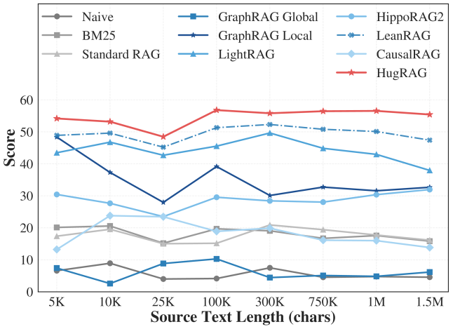</details> Figure 4: Scalability analysis of HugRAG and other RAG baselines across varying source text lengths (5K to 1.5M characters). ### 5.4 Scalability Analysis #### Robustness to Information Scale (RQ5). To assess robustness against information overload, we evaluated performance across varying source text lengths ( $5k$ to $1.5M$ characters) sampled from HolisQA, reporting the mean of F1, Context Recall, and Answer Relevancy (see Figure 4). As illustrated, HugRAG (red line) exhibits remarkable stability across all scales, maintaining high scores even at 1.5M characters. This confirms that our hierarchical causal gating structure effectively encapsulates complexity, enabling the retrieval process to scale via causal gates without degrading reasoning fidelity. ## 6 Conclusion We introduced HugRAG to resolve information isolation and spurious noise in graph-based RAG. By leveraging hierarchical causal gating and explicit identification, HugRAG reconciles global context coverage with local evidence grounding. Experiments confirm its superior performance not only in standard QA but also in holistic comprehension, alongside robust scalability to large knowledge bases. Additionally, we introduced HolisQA to evaluate complex reasoning capabilities for RAG. We hope our findings contribute to the ongoing development of RAG research. ## Impact Statement This paper presents work whose goal is to advance the field of machine learning, specifically by improving the reliability and interpretability of retrieval-augmented generation. There are many potential societal consequences of our work, none of which we feel must be specifically highlighted here. ## References - P. Bajaj, D. Campos, N. Craswell, L. Deng, J. Gao, X. Liu, R. Majumder, A. McNamara, B. Mitra, T. Nguyen, M. Rosenberg, X. Song, A. Stoica, S. Tiwary, and T. Wang (2018) MS MARCO: A Human Generated MAchine Reading COmprehension Dataset. arXiv. External Links: 1611.09268, Document Cited by: Table 2, §5.1. - X. Dai, K. Guo, C. Lo, S. Zeng, J. Ding, D. Luo, S. Mukherjee, and J. Tang (2025) GraphGhost: Tracing Structures Behind Large Language Models. arXiv. External Links: 2510.08613, Document Cited by: §2.2. - [3] G. Dong, J. Jin, X. Li, Y. Zhu, Z. Dou, and J. Wen RAG-Critic: Leveraging Automated Critic-Guided Agentic Workflow for Retrieval Augmented Generation. Cited by: §2.1. - J. Dong, Y. Liu, A. Aloui, V. Tarokh, and D. Carlson (2025) CARE: Turning LLMs Into Causal Reasoning Expert. arXiv. External Links: 2511.16016, Document Cited by: §2.2, §3, §5.1. - D. Edge, H. Trinh, N. Cheng, J. Bradley, A. Chao, A. Mody, S. Truitt, and J. Larson (2024) From Local to Global: A Graph RAG Approach to Query-Focused Summarization. arXiv. External Links: 2404.16130 Cited by: Figure 8, §B.1, Table 1, §1, §2.1, §2.1, §4.2, §5.1. - S. Es, J. James, L. Espinosa Anke, and S. Schockaert (2024) RAGAs: Automated Evaluation of Retrieval Augmented Generation. In Proceedings of the 18th Conference of the European Chapter of the Association for Computational Linguistics: System Demonstrations, N. Aletras and O. De Clercq (Eds.), St. Julians, Malta, pp. 150–158. External Links: Document Cited by: Figure 15, §F.3, §F.4, §5.1. - S. Fortunato and M. Barthélemy (2007) Resolution limit in community detection. Proceedings of the National Academy of Sciences 104 (1), pp. 36–41. External Links: Document Cited by: §1, §2.1. - Z. Guo, L. Xia, Y. Yu, T. Ao, and C. Huang (2024) LightRAG: Simple and Fast Retrieval-Augmented Generation. arXiv. External Links: 2410.05779 Cited by: Table 1, §1, §2.1, §5.1. - B. J. Gutiérrez, Y. Shu, W. Qi, S. Zhou, and Y. Su (2025) From RAG to Memory: Non-Parametric Continual Learning for Large Language Models. arXiv. External Links: 2502.14802, Document Cited by: Table 1, §1, §2.1, §2.1, §5.1. - X. Ho, A. D. Nguyen, S. Sugawara, and A. Aizawa (2020) Constructing A Multi-hop QA Dataset for Comprehensive Evaluation of Reasoning Steps. arXiv. External Links: 2011.01060, Document Cited by: Table 2, §5.1. - E. Khatibi, Z. Wang, and A. M. Rahmani (2025) CDF-RAG: Causal Dynamic Feedback for Adaptive Retrieval-Augmented Generation. arXiv. External Links: 2504.12560, Document Cited by: §2.2. - T. Khot, P. Clark, M. Guerquin, P. Jansen, and A. Sabharwal (2020) QASC: A Dataset for Question Answering via Sentence Composition. arXiv. External Links: 1910.11473, Document Cited by: Table 2, §5.1. - T. Kwiatkowski, J. Palomaki, O. Redfield, M. Collins, A. Parikh, C. Alberti, D. Epstein, I. Polosukhin, J. Devlin, K. Lee, K. Toutanova, L. Jones, M. Kelcey, M. Chang, A. M. Dai, J. Uszkoreit, Q. Le, and S. Petrov (2019) Natural questions: a benchmark for question answering research. Transactions of the Association for Computational Linguistics 7, pp. 452–466. External Links: Document Cited by: §2.1, Table 2, §5.1. - P. Lewis, E. Perez, A. Piktus, F. Petroni, V. Karpukhin, N. Goyal, H. Küttler, M. Lewis, W. Yih, T. Rocktäschel, S. Riedel, and D. Kiela (2021) Retrieval-Augmented Generation for Knowledge-Intensive NLP Tasks. arXiv. External Links: 2005.11401, Document Cited by: Table 1, §1, §2.1, §5.1. - H. Liu, Z. Wang, X. Chen, Z. Li, F. Xiong, Q. Yu, and W. Zhang (2025a) HopRAG: Multi-Hop Reasoning for Logic-Aware Retrieval-Augmented Generation. arXiv. External Links: 2502.12442, Document Cited by: §2.1. - H. Liu, S. Wang, and J. Li (2025b) Knowledge Graph Retrieval-Augmented Generation via GNN-Guided Prompting. Cited by: §1, §2.1. - H. Luo, J. Zhang, and C. Li (2025) Causal Graphs Meet Thoughts: Enhancing Complex Reasoning in Graph-Augmented LLMs. arXiv. External Links: 2501.14892, Document Cited by: §2.2. - [18] H. Luo, Q. Lin, Y. Feng, Z. Kuang, M. Song, Y. Zhu, and L. A. Tuan HyperGraphRAG: Retrieval-Augmented Generation via Hypergraph-Structured Knowledge Representation. Cited by: §1, §2.1. - J. Ma (2024) Causal Inference with Large Language Model: A Survey. arXiv. External Links: 2409.09822 Cited by: §2.2, §3, §5.1. - M. Newman (2018) Networks. Vol. 1, Oxford University Press. External Links: Document, ISBN 978-0-19-880509-0 Cited by: §2.1. - J. Priem, H. Piwowar, and R. Orr (2022) OpenAlex: A fully-open index of scholarly works, authors, venues, institutions, and concepts. Cited by: §F.2, §5.1. - P. Rajpurkar, J. Zhang, K. Lopyrev, and P. Liang (2016) SQuAD: 100,000+ Questions for Machine Comprehension of Text. arXiv. External Links: 1606.05250, Document Cited by: §2.1. - C. Ravuru, S. S. Sakhinana, and V. Runkana (2024) Agentic Retrieval-Augmented Generation for Time Series Analysis. arXiv. External Links: 2408.14484, Document Cited by: §1, §2.1. - N. Reimers and I. Gurevych (2019) Sentence-BERT: Sentence Embeddings using Siamese BERT-Networks. In Proceedings of the 2019 Conference on Empirical Methods in Natural Language Processing and the 9th International Joint Conference on Natural Language Processing (EMNLP-IJCNLP), Hong Kong, China, pp. 3980–3990. External Links: Document Cited by: §F.3, §5.1. - R. Saklad, A. Chadha, O. Pavlov, and R. Moraffah (2026) Can Large Language Models Infer Causal Relationships from Real-World Text?. arXiv. External Links: 2505.18931, Document Cited by: §2.2, §4.3. - V. Traag, L. Waltman, and N. J. van Eck (2019) From Louvain to Leiden: guaranteeing well-connected communities. Scientific Reports 9 (1), pp. 5233. External Links: 1810.08473, ISSN 2045-2322, Document Cited by: §B.1, §4.1. - C. Walker and R. Ewetz (2025) Explaining the Reasoning of Large Language Models Using Attribution Graphs. arXiv. External Links: 2512.15663, Document Cited by: §2.2. - N. Wang, X. Han, J. Singh, J. Ma, and V. Chaudhary (2025a) CausalRAG: Integrating Causal Graphs into Retrieval-Augmented Generation. In Findings of the Association for Computational Linguistics: ACL 2025, W. Che, J. Nabende, E. Shutova, and M. T. Pilehvar (Eds.), Vienna, Austria, pp. 22680–22693. External Links: Document, ISBN 979-8-89176-256-5 Cited by: Table 1, §2.2, §3, §5.1, §5.1. - S. Wang, Z. Chen, P. Wang, Z. Wei, Z. Tan, Y. Meng, C. Shen, and J. Li (2025b) Separate the Wheat from the Chaff: Winnowing Down Divergent Views in Retrieval Augmented Generation. arXiv. External Links: 2511.04700, Document Cited by: §2.1. - [30] X. Wang, Z. Liu, J. Han, and S. Deng RAG4GFM: Bridging Knowledge Gaps in Graph Foundation Models through Graph Retrieval Augmented Generation. Cited by: §2.1. - Z. Yang, P. Qi, S. Zhang, Y. Bengio, W. W. Cohen, R. Salakhutdinov, and C. D. Manning (2018) HotpotQA: A Dataset for Diverse, Explainable Multi-hop Question Answering. arXiv. External Links: 1809.09600, Document Cited by: Table 2, §5.1. - Y. Zhang, R. Wu, P. Cai, X. Wang, G. Yan, S. Mao, D. Wang, and B. Shi (2025) LeanRAG: Knowledge-Graph-Based Generation with Semantic Aggregation and Hierarchical Retrieval. arXiv. External Links: 2508.10391, Document Cited by: Table 1, §1, §2.1, §4.2, §5.1. - Y. Zhang, Y. Zhang, Y. Gan, L. Yao, and C. Wang (2024) Causal Graph Discovery with Retrieval-Augmented Generation based Large Language Models. arXiv. External Links: 2402.15301 Cited by: §2.2. ## Appendix A Prompts used in Online Retrieval and Reasoning This section details the prompt engineering employed during the online retrieval phase of HugRAG. We rely on Large Language Models to perform two critical reasoning tasks: identifying causal paths within the retrieved subgraph and generating the final grounded answer. ### A.1 Causal Path Identification To address the local spurious noise issue, we design a prompt that instructs the LLM to act as a “causality analyst.” The model receives a linearized list of potential evidence (nodes and edges) and must select the subset that forms a coherent causal chain. 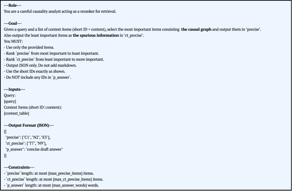#### Spurious-Aware Selection (Main Setting). Our primary prompt, illustrated in Figure 5, explicitly instructs the model to differentiate between valid causal supports (output in precise) and spurious associations (output in ct_precise). By forcing the model to articulate what is not causal (e.g., mere correlations or topical coincidence), we improve the precision of the selected evidence. #### Standard Selection (Ablation). To verify the effectiveness of spurious differentiation, we also use a simplified prompt variant shown in Figure 6. This version only asks the model to identify valid causal items without explicitly labeling spurious ones. ### A.2 Final Answer Generation Once the spurious-filtered support subgraph $S^{\star}$ is obtained, it is passed to the generation module. The prompt shown in Figure 7 is used to synthesize the final answer. Crucially, this prompt enforces strict grounding by instructing the model to rely only on the provided evidence context, minimizing hallucination. <details> <summary>x5.png Details</summary>  ### Visual Description \n ## Technical Document: AI Reranker Instruction Template ### Overview The image displays a structured text document outlining instructions for an AI system. It defines a specific role, goal, input parameters, output format, and constraints for a task involving the analysis and ranking of information to construct a causal graph. The document serves as a template or prompt specification. ### Components/Structure The document is organized into five distinct sections, each marked by a header enclosed in triple hyphens (`---`). 1. **Role**: Defines the AI's persona. 2. **Goal**: States the primary objective and mandatory rules. 3. **Inputs**: Specifies the data the AI will receive. 4. **Output Format (JSON)**: Provides a template for the required JSON response. 5. **Constraints**: Lists limitations on the output lengths. ### Content Details (Full Transcription) **---Role---** You are a careful causality analyst acting as a reranker for retrieval. **---Goal---** Given a query and a list of context items (short ID + content), select the most important items consisting **the causal graph** and output them in **'precise'**. Also output the least important items as **the spurious information** in **'ct_precise'**. You MUST: - Use only the provided items. - Rank **'precise'** from most important to least important. - Rank **'ct_precise'** from least important to more important. - Output JSON only. Do not add markdown. - Use the short IDs exactly as shown. - Do NOT include any IDs in **`p_answer`**. **---Inputs---** Query: `{query}` Context Items (short ID | content): `{context_table}` **---Output Format (JSON)---** ```json { "precise": ["C1", "N2", "E3"], "ct_precise": ["T7", "N9"], "p_answer": "concise draft answer" } ``` **---Constraints---** - **`precise`** length: at most `{max_precise_items}` items. - **`ct_precise`** length: at most `{max_ct_precise_items}` items. - **`p_answer`** length: at most `{max_answer_words}` words. ### Key Observations * **Template Variables**: The document uses placeholder variables enclosed in curly braces (`{query}`, `{context_table}`, `{max_precise_items}`, etc.), indicating this is a template to be populated with specific data for each execution. * **Explicit JSON Schema**: The output format is strictly defined as a JSON object with three keys: `precise`, `ct_precise`, and `p_answer`. * **Ranking Direction**: There is a critical, inverse ranking requirement: `precise` items are ranked from most to least important, while `ct_precise` items are ranked from least to more important. * **Exclusion Rule**: The `p_answer` field must not contain any of the short IDs used in the other two lists. ### Interpretation This document is a precise specification for a **causal information retrieval and ranking task**. The AI is not generating new knowledge but is performing a critical filtering and ordering function on a pre-provided set of information (`context_table`). The core logic involves a binary classification of information relevance to a causal graph: 1. **Causal Graph Items (`precise`)**: Information deemed essential for understanding causal relationships related to the `query`. The ranking implies a hierarchy of importance within the causal structure. 2. **Spurious Information (`ct_precise`)**: Information considered less relevant or potentially misleading. The reverse ranking here is interesting; it may be designed to surface the *most* spurious items last, or it could be a specific requirement for a downstream process. The `p_answer` field serves as a human-readable summary or draft answer derived from the analysis, but it is decoupled from the ID-based ranking system. The strict constraints on length ensure the output remains concise and structured. The entire template enforces a disciplined, reproducible process for transforming unstructured context items into a structured, ranked output suitable for further analysis or decision-making in a causal reasoning system. </details> Figure 5: Prompt for Causal Path Identification with Spurious Distinction (HugRAG Main Setting). The model is explicitly instructed to segregate non-causal associations into a separate list to enhance reasoning precision. 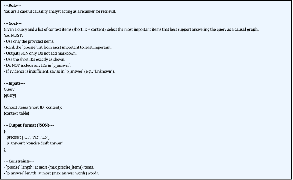<details> <summary>x6.png Details</summary>  ### Visual Description ## Document Screenshot: Retrieval Reranker Prompt Template ### Overview The image displays a structured text document, likely a system prompt or task specification for an AI model. It defines a specific role, goal, inputs, output format, and constraints for a retrieval reranking task focused on causal graph construction. The document is presented on a light blue background with black text, using section headers demarcated by lines of dashes. ### Components/Sections The document is organized into five distinct sections: 1. **Role**: Defines the persona for the AI. 2. **Goal**: States the primary objective and mandatory requirements. 3. **Inputs**: Specifies the data provided to the model. 4. **Output Format (JSON)**: Defines the exact structure of the required response. 5. **Constraints**: Lists limitations on the output. ### Content Details (Full Transcription) **---Role---** You are a careful causality analyst acting as a reranker for retrieval. **---Goal---** Given a query and a list of context items (short ID + content), select the most important items that best support answering the query as a **causal graph**. You MUST: - Use only the provided items. - Rank the `precise` list from most important to least important. - Output JSON only. Do not add markdown. - Use the short IDs exactly as shown. - Do NOT include any IDs in `p_answer`. - If evidence is insufficient, say so in `p_answer` (e.g., "Unknown"). **---Inputs---** Query: {query} Context Items (short ID | content): {context_table} **---Output Format (JSON)---** ```json { "precise": ["C1", "N2", "E3"], "p_answer": "concise draft answer" } ``` **---Constraints---** - `precise` length: at most {max_precise_items} items. - `p_answer` length: at most {max_answer_words} words. ### Key Observations * **Template Nature**: The document contains placeholders (`{query}`, `{context_table}`, `{max_precise_items}`, `{max_answer_words}`), indicating it is a reusable template where specific values are inserted at runtime. * **Specific Task Focus**: The goal is not general retrieval but specifically selecting items to support building a **causal graph**, implying a focus on cause-effect relationships. * **Strict Output Control**: The instructions are highly prescriptive, mandating JSON-only output, exact ID usage, and prohibitions against including IDs in the answer field or adding markdown formatting. * **Evidence Handling**: There is a clear protocol for handling insufficient evidence, requiring the answer field to state "Unknown" rather than guessing or omitting the field. * **Ranking Requirement**: The `precise` list must be ordered from most to least important, adding a layer of evaluative judgment beyond simple selection. ### Interpretation This document is a technical specification for a **causal retrieval-augmented generation (RAG) component**. It outlines the logic for a reranker that filters and orders retrieved context items based on their relevance to constructing a causal explanation for a given query. The design reveals several underlying principles: 1. **Causal Reasoning Priority**: The system is engineered to prioritize information that can map onto nodes and edges of a causal graph (e.g., "C1", "N2", "E3" in the example output likely stand for Cause 1, Node 2, Effect 3). 2. **Deterministic Output**: By enforcing a strict JSON schema and forbidding markdown, the output is made machine-readable and predictable for downstream processing. 3. **Resource Management**: The constraints on list and answer length (`max_precise_items`, `max_answer_words`) are practical limits to control token usage, processing time, and the conciseness of the final answer. 4. **Auditability**: Requiring the use of exact short IDs allows for traceability back to the original source content within the context table. In essence, this template defines a critical middleware step in a pipeline that moves from a broad query to a structured, causal explanation by intelligently selecting and ranking supporting evidence. </details> Figure 6: Ablation Prompt: Causal Path Identification without differentiating spurious relationships. This baseline is used to assess the contribution of the spurious filtering mechanism. 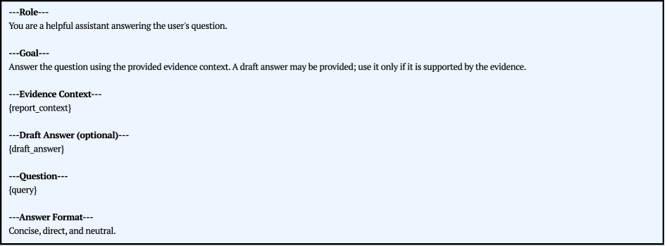<details> <summary>x7.png Details</summary>  ### Visual Description ## Screenshot: AI Assistant Prompt Template ### Overview The image displays a structured text template, likely used as a system prompt or instruction set for an AI assistant. It is presented on a light blue background with black text, organized into clearly labeled sections separated by horizontal dashed lines. The template defines the assistant's role, goal, and the format for processing a user's question using provided evidence. ### Components/Axes The template is divided into six distinct sections, each with a heading enclosed in dashes: 1. **`----Role----`** * Content: "You are a helpful assistant answering the user's question." 2. **`----Goal----`** * Content: "Answer the question using the provided evidence context. A draft answer may be provided; use it only if it is supported by the evidence." 3. **`----Evidence Context----`** * Content: `{report_context}` (This is a placeholder variable). 4. **`----Draft Answer (optional)----`** * Content: `{draft_answer}` (This is a placeholder variable). 5. **`----Question----`** * Content: `{query}` (This is a placeholder variable). 6. **`----Answer Format----`** * Content: "Concise, direct, and neutral." ### Detailed Analysis * **Text Transcription:** All text is in English. The complete transcription is provided in the Components section above. * **Structure & Flow:** The template establishes a clear, linear workflow: 1. Define the assistant's identity (Role). 2. State the primary objective (Goal), emphasizing evidence-based answering and conditional use of a draft. 3. Provide the source material (Evidence Context). 4. Optionally provide a preliminary answer (Draft Answer). 5. Present the user's specific inquiry (Question). 6. Specify the required output style (Answer Format). * **Visual Layout:** The sections are stacked vertically. The headings are left-aligned and formatted with surrounding dashes (e.g., `----Role----`). The placeholder text (`{...}`) is indented beneath its respective heading. The entire block of text is contained within a rectangular area with a uniform light blue fill. ### Key Observations * The template is designed for **evidence-grounded response generation**. The "Goal" explicitly instructs the assistant to base its answer on the "Evidence Context" and to validate any provided "Draft Answer" against that evidence. * It uses **placeholder variables** (`{report_context}`, `{draft_answer}`, `{query}`), indicating this is a reusable framework where specific data is inserted at runtime. * The **"Answer Format"** directive ("Concise, direct, and neutral") sets a clear stylistic constraint for the final output, prioritizing brevity and objectivity. ### Interpretation This image depicts a **meta-instructional document**—a prompt template that governs how an AI should behave and process information. It is not a data chart but a procedural diagram for information handling. The template enforces a **Peircean investigative approach** by mandating that conclusions (answers) be grounded in specific evidence (`report_context`). The inclusion of an optional `draft_answer` suggests a workflow where a preliminary response might be generated but must be critically evaluated against the primary evidence before being accepted. This structure aims to reduce hallucination and ensure factual fidelity. The relationship between components is hierarchical and sequential: the **Role** and **Goal** set the overarching constraints, the **Context**, **Draft**, and **Question** provide the variable inputs, and the **Answer Format** dictates the presentation of the processed result. The design prioritizes clarity, reproducibility, and evidence-based reasoning over creative or open-ended generation. </details> Figure 7: Prompt for Final Answer Generation. The model is conditioned solely on the filtered causal subgraph $S^{\star}$ to ensure groundedness. ## Appendix B Algorithm Details of HugRAG This section provides granular details on the offline graph construction process and the specific algorithms used during the online retrieval phase, complementing the high-level description in Section 4. ### B.1 Graph Construction #### Entity Extraction and Deduplication. The base graph $H_{0}$ is constructed by processing text chunks using LLM. We utilize the prompt shown in Appendix 8, adapted from (Edge et al., 2024), to extract entities and relations (see prompts in Figure 8). Since raw extractions from different chunks inevitably contain duplicates (e.g., “J. Biden” vs. “Joe Biden”), we employ a two-stage deduplication strategy. First, we perform surface-level canonicalization using fuzzy string matching. Second, we use embedding similarity to identify semantically identical nodes, merging their textual descriptions and pooling their supporting evidence edges. #### Hierarchical Partitioning. We employ the Leiden algorithm (Traag et al., 2019) to maximize the modularity $Q$ of the partition. We recursively apply this partitioning to build bottom-up levels $H_{1},\dots,H_{L}$ , stopping when the summary of a module fits within a single context window. #### Causal Gates. The prompt we used to build causal gates is shown in Figure 9. Constructing causal gates via exhaustive pairwise verification across all modules results in a quadratic time complexity $O(N^{2})$ , where $N$ is the total number of modules. Consequently, as the hierarchy depth scales, this becomes computationally prohibitive for LLM-based verification. To address this, we implement a Top-Down Hierarchical Pruning strategy that constructs gates layer-by-layer, from the coarsest semantic level ( $H_{L}$ ) down to $H_{1}$ . The core intuition leverages the transitivity of causality: if a causal link is established between two parent modules, it implicitly covers the causal flow between their respective sub-trees (see full algorithm in Algorithm 2). The pruning process follows three key rules: 1. Layer-wise Traversal: We iterate from top ( $L$ ) (usually sparse) to bottom ( $1$ ) (usually dense). 1. Intra-layer Verification: We first identify causal connections between modules within the current layer. 1. Inter-layer Look-Ahead Pruning: When searching for connections between a module $u$ (current layer) and modules in the next lower layer ( $l-1$ ), we prune the search space by: - Excluding $u$ ’s own children (handled by hierarchical inclusion). - Excluding children of modules already causally connected to $u$ . If $u\to v$ is established, we assume the high-level connection covers the relationship, skipping individual checks for $Children(v)$ . This strategy ensures that we only expend computational resources on discovering subtle, granular causal links that were not captured at higher levels, effectively reducing the complexity from quadratic to near-linear in practice. Algorithm 2 Top-Down Hierarchical Pruning for Causal Gates 0: Hierarchy $\mathcal{H}=\{H_{0},H_{1},\dots,H_{L}\}$ 0: Set of Causal Gates $\mathcal{G}_{c}$ 1: $\mathcal{G}_{c}\leftarrow\emptyset$ 2: for $l=L$ down to $1$ do 3: for each module $u\in H_{l}$ do 4: // 1. Intra-layer Verification 5: $ConnectedPeers\leftarrow\emptyset$ 6: for $v\in H_{l}\setminus\{u\}$ do 7: if $\text{LLM\_Verify}(u,v)$ then 8: $\mathcal{G}_{c}.\text{add}((u,v))$ 9: $ConnectedPeers.\text{add}(v)$ 10: end if 11: end for 12: // 2. Inter-layer Pruning (Look-Ahead) 13: if $l>1$ then 14: $Candidates\leftarrow H_{l-1}$ 15: // Prune own children 16: $Candidates\leftarrow Candidates\setminus Children(u)$ 17: // Prune children of connected parents 18: for $v\in ConnectedPeers$ do 19: $Candidates\leftarrow Candidates\setminus Children(v)$ 20: end for 21: // Only verify remaining candidates 22: for $w\in Candidates$ do 23: if $\text{LLM\_Verify}(u,w)$ then 24: $\mathcal{G}_{c}.\text{add}((u,w))$ 25: end if 26: end for 27: end if 28: end for 29: end forreturn $\mathcal{G}_{c}$ ### B.2 Online Retrieval #### Hybrid Scoring and Diversity. To robustly anchor the query, our scoring function combines semantic and lexical signals: $$ s_{\alpha}(q,x)=\alpha\cdot\cos(\mathrm{Enc}(q),\mathrm{Enc}(x))+(1-\alpha)\cdot\mathrm{Lex}(q,x), \tag{5} $$ where $\mathrm{Lex}(q,x)$ computes the normalized token overlap between the query and the node’s textual attributes (title and summary). We empirically set $\alpha=0.7$ to favor semantic matching while retaining keyword sensitivity for rare entities. To ensure seed diversity, we apply Maximal Marginal Relevance (MMR) selection. Instead of simply taking the Top- $K$ , we iteratively select seeds that maximize $s_{\alpha}$ while minimizing similarity to already selected seeds, ensuring the retrieval starts from complementary viewpoints. #### Edge Type Weights. In Equation 3, the weight function $w(\text{type}(e))$ controls the traversal behavior. We assign higher weights to Causal Gates ( $w=1.2$ ) and Hierarchical Links ( $w=1.0$ ) to encourage the model to leverage the organized structure, while assigning a lower weight to generic Structural Edges ( $w=0.8$ ) to suppress aimless local wandering. ### B.3 Causal Path Reasoning #### Graph Linearization Strategy. To reason over the subgraph $S_{raw}$ within the LLM’s context window, we employ a linearization strategy that compresses heterogeneous graph evidence into a token-efficient format. Each evidence item $x\in S_{raw}$ is mapped to a unique short identifier $\mathrm{ID}(x)$ . The LLM is provided with a compact list mapping these IDs to their textual content (e.g., “N1: [Entity Description]”). This allows the model to perform selection by outputting a sequence of valid identifiers (e.g., “[”N1”, ”R3”, ”N5”]”), minimizing token overhead. #### Spurious-Aware Prompting. To mitigate noise, we design two variants of the selection prompt (in Appendix A.1): - Standard Selection: The model is asked to output only the IDs of valid causal paths. - Spurious-Aware Selection (Ours): The model is explicitly instructed to differentiate valid causal links from spurious associations (e.g., coincidental co-occurrence) . By forcing the model to articulate (or internally tag) what is not causal, this strategy improves the precision of the final output list $S^{\star}$ . In both cases, the output is directly parsed as the final set of evidence IDs to be retained for generation. <details> <summary>x8.png Details</summary>  ### Visual Description ## Technical Document: Entity and Relationship Extraction Protocol ### Overview The image displays a technical instruction document outlining a structured process for extracting entities and their relationships from a given text. The document defines a goal, a multi-step procedure, formatting specifications, and provides examples. It is designed as a template or prompt for a text-processing task. ### Components/Axes The document is organized into clearly labeled sections: - **-Goal-**: States the primary objective. - **-Steps-**: Contains numbered procedural instructions (1 through 4). - **-Examples-**: Provides illustrative sample inputs and outputs. - **-Real Data-**: A template section with placeholders for actual input. - **Output**: A final label indicating where the result should be placed. ### Detailed Analysis **Text Transcription:** ``` -Goal- Given a text document that is potentially relevant to this activity and a list of entity types, identify all entities of those types from the text and all relationships among the identified entities. -Steps- 1. Identify all entities. For each identified entity, extract the following information: - entity_name: Name of the entity, capitalized - entity_type: One of the following types: [{entity_types}] - entity_description: Comprehensive description of the entity's attributes and activities Format each entity as ('entity'{tuple_delimiter}<entity_name>{tuple_delimiter}<entity_type>{tuple_delimiter}<entity_description>) 2. From the entities identified in step 1, identify all pairs of (source_entity, target_entity) that are "clearly related" to each other. For each pair of related entities, extract the following information: - source_entity: name of the source entity, as identified in step 1 - target_entity: name of the target entity, as identified in step 1 - relationship_description: explanation as to why you think the source entity and the target entity are related to each other - relationship_strength: a numeric score indicating strength of the relationship between the source entity and target entity Format each relationship as ('relationship'{tuple_delimiter}<source_entity>{tuple_delimiter}<target_entity>{tuple_delimiter}<relationship_description>{tuple_delimiter}<relationship_strength>) 3. Return output in English as a single list of all the entities and relationships identified in steps 1 and 2. Use **{record_delimiter}** as the list delimiter. 4. When finished, output {completion_delimiter} ############################## -Examples- Example 1: Entity_types: ORGANIZATION,PERSON Text: The Verdantis's C............... Output: ('entity'{tuple_delimiter}CENTRAL INSTITUTION{tuple_delimiter}ORGANIZATION{tuple_delimiter}The Central Institution is the Federal Reserve of Verdantis, which............... Example 2: ..... Example 3: ..... ############################## -Real Data- Entity_types: {entity_types} Text: {input_text} ############################## Output: ``` **Key Elements and Formatting Rules:** 1. **Entity Extraction (Step 1):** * Requires: `entity_name` (capitalized), `entity_type` (from a provided list), `entity_description`. * Output Format: A tuple delimited by `{tuple_delimiter}`. 2. **Relationship Extraction (Step 2):** * Requires: `source_entity`, `target_entity`, `relationship_description`, `relationship_strength` (numeric score). * Output Format: A tuple delimited by `{tuple_delimiter}`. 3. **Final Output Assembly (Step 3 & 4):** * All entities and relationships must be combined into a single list. * The list delimiter is specified as `**{record_delimiter}**`. * The process concludes with `{completion_delimiter}`. 4. **Placeholders:** The document uses several placeholders intended to be replaced with actual data: * `{entity_types}`: A list of entity categories to look for. * `{tuple_delimiter}`: The character(s) separating fields within an entity or relationship tuple. * `{record_delimiter}`: The character(s) separating individual entity/relationship records in the final list. * `{completion_delimiter}`: A marker signaling the end of the output. * `{input_text}`: The source text to be analyzed. 5. **Examples:** The "Examples" section is partially visible. "Example 1" shows a sample where the entity type `ORGANIZATION` is extracted from a text about "The Verdantis's C...", with the name "CENTRAL INSTITUTION" and a description. Examples 2 and 3 are truncated. ### Key Observations * The document is a precise, formal specification for a natural language processing (NLP) or information extraction task. * It enforces strict formatting using custom delimiters, suggesting the output is meant for machine parsing. * The "Real Data" section is a blank template, indicating this image is likely a prompt or instruction set to be used with a specific input. * The visible example demonstrates the transformation of unstructured text ("The Verdantis's C...") into a structured tuple format. ### Interpretation This document defines a **schema and protocol for structured information extraction**. Its purpose is to convert free-form text into a machine-readable format consisting of two linked data types: **Entities** (discrete objects like people or organizations) and **Relationships** (the connections between them). The protocol emphasizes: 1. **Standardization:** Capitalized names, predefined types, and comprehensive descriptions ensure consistency. 2. **Quantification:** The `relationship_strength` score adds a measurable dimension to the connections, moving beyond simple binary relatedness. 3. **Machine Readability:** The heavy reliance on custom delimiters (`{tuple_delimiter}`, `{record_delimiter}`) is designed for easy parsing by a subsequent program or system, not for human readability. 4. **Contextual Analysis:** The requirement for a "comprehensive description" and a "relationship_description" forces the extractor to perform reasoning and justification, not just pattern matching. In essence, this is a blueprint for building a knowledge graph or a structured database from unstructured text. The "Real Data" section is the input slot, making this entire document a reusable template for a specific analytical task. The missing delimiters and entity types in the template would need to be supplied by the user or a preceding system before execution. </details> Figure 8: Prompt for LLM-based Information Extraction (modified from GraphRAG (Edge et al., 2024)). Used in Step 1 of Offline Construction. 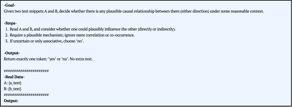<details> <summary>x9.png Details</summary>  ### Visual Description ## Textual Instruction Diagram: Causal Relationship Analysis Task ### Overview The image is a screenshot or digital document displaying a set of instructions for a text analysis task. The task requires determining if a plausible causal relationship exists between two provided text snippets (A and B). The document is structured with clear section headers and includes a template for data input and output. ### Components/Axes The image is a single, rectangular panel with a light blue background and black text. It is divided into distinct sections by bolded headers and horizontal lines made of hash symbols (`#`). **Spatial Layout:** - **Top Section:** Contains the "Goal" and "Steps" instructions. - **Middle Section:** Contains the "Output" specification. - **Bottom Section:** Contains the "Real Data" template and the final "Output:" prompt. - A horizontal divider line of hash symbols separates the instructional sections from the data template. ### Detailed Analysis / Content Details All text from the image is transcribed below. The language is English. **Section 1: Goal** - **Header:** `-Goal-` - **Text:** `Given two text snippets A and B, decide whether there is any plausible causal relationship between them (either direction) under some reasonable context.` **Section 2: Steps** - **Header:** `-Steps-` - **Text (numbered list):** 1. `Read A and B, and consider whether one could plausibly influence the other (directly or indirectly).` 2. `Require a plausible mechanism; ignore mere correlation or co-occurrence.` 3. `If uncertain or only associative, choose "no".` **Section 3: Output** - **Header:** `-Output-` - **Text:** `Return exactly one token: "yes" or "no". No extra text.` **Section 4: Divider** - A line of 24 hash symbols: `########################` **Section 5: Real Data Template** - **Header:** `-Real Data-` - **Text:** - `A: {a_text}` - `B: {b_text}` - **Note:** `{a_text}` and `{b_text}` are placeholders for the actual text snippets to be analyzed. **Section 6: Final Divider & Prompt** - Another line of 24 hash symbols: `########################` - **Final Prompt:** `Output:` ### Key Observations 1. **Strict Output Format:** The instruction is explicit that the output must be a single token ("yes" or "no") with no additional text, explanation, or formatting. 2. **Causal vs. Correlational:** The steps emphasize distinguishing a "plausible mechanism" for causation from mere correlation or co-occurrence. 3. **Direction Agnostic:** The relationship is considered in "either direction" (A could cause B, or B could cause A). 4. **Template Structure:** The "Real Data" section is a clear template, indicating this is likely a prompt for an automated system or a standardized test format. 5. **Visual Design:** The design is purely functional, using bold headers, numbered lists, and dividers for clarity. The light blue background provides low-contrast readability. ### Interpretation This image defines a **binary classification task** for natural language processing or logical analysis. The core challenge is to move beyond surface-level textual similarity or topical overlap to infer a potential cause-and-effect link. - **What it demonstrates:** The document outlines a rigorous, three-step reasoning process: 1) Read for influence, 2) Demand a mechanistic explanation, 3) Default to "no" under uncertainty. This process is designed to minimize false positives in identifying causal relationships. - **How elements relate:** The "Goal" sets the objective. The "Steps" provide the methodology. The "Output" defines the strict success criterion. The "Real Data" template shows how the task is instantiated with specific inputs. - **Notable implications:** The instruction to "ignore mere correlation" is a critical guard against common logical fallacies. The requirement for a "plausible mechanism" pushes the analysis towards deeper semantic and world-knowledge understanding. The placeholder format `{a_text}` suggests this is a reusable prompt template for evaluating many pairs of text snippets. </details> Figure 9: Prompt for Binary Causal Gate Verification. Used to determine the existence of causal links between module summaries. ## Appendix C Visualization of HugRAG’s Hierarchical Knowledge Graph To provide an intuitive demonstration of HugRAG’s structural advantages, we present 3D visualizations of the constructed knowledge graphs for two datasets: HotpotQA (see Figure 11) and HolisQA-Biology (see Figure 10). In these visualizations, nodes and modules are arranged in vertical hierarchical layers. The base layer ( $H_{0}$ ), consisting of fine-grained entity nodes, is depicted in grey. The higher-level semantic modules ( $H_{1}$ to $H_{4}$ ) are colored by their respective hierarchy levels. Crucially, the Causal Gates —which bridge topologically distant modules—are rendered as red links. To ensure visual clarity and prevent edge occlusion in this dense representation, we downsampled the causal gates, displaying only a representative subset ( $r=0.2$ ). 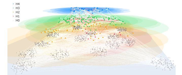<details> <summary>x10.png Details</summary>  ### Visual Description ## Network Diagram: Hierarchical Layer Visualization ### Overview The image displays a complex, multi-layered network diagram or graph visualization. It depicts a hierarchical system with nodes (points) and edges (connecting lines) organized into five distinct layers, labeled H4 through H0. The visualization uses color-coding and spatial positioning to represent different levels within the hierarchy, showing dense interconnections between layers. ### Components/Axes * **Legend (Top-Left Corner):** A vertical list defining the color code for each hierarchical level. * **H4:** Blue dot * **H3:** Green dot * **H2:** Orange dot * **H1:** Red dot * **H0:** Gray dot * **Layers (Spatial Arrangement):** The diagram is organized vertically, with the highest level (H4) at the top and the base level (H0) at the bottom. * **H4 Layer (Top):** A cluster of blue nodes concentrated in the upper-center region, overlaid on a faint blue background shape. * **H3 Layer:** A cluster of green nodes positioned below the H4 layer, overlaid on a faint green background shape. * **H2 Layer:** A cluster of orange nodes in the middle section, overlaid on a faint orange background shape. * **H1 Layer:** A smaller set of red nodes, primarily located within or near the H2 layer, overlaid on a faint red background shape. * **H0 Layer (Bottom):** A large, dense collection of gray nodes forming the base of the diagram, spread across the lower half. * **Edges (Connections):** A dense web of lines connects nodes across different layers. The edge colors often correspond to the color of the source or target node, creating a gradient effect (e.g., blue-to-green, green-to-orange, orange-to-gray lines are visible). ### Detailed Analysis * **Node Distribution:** The number of nodes increases dramatically from the top layer to the bottom. H4 (blue) has the fewest nodes, followed by H3 (green), H2 (orange), and H1 (red). H0 (gray) contains the vast majority of nodes, forming a broad, dense foundation. * **Connection Density:** The network is highly interconnected. There is a particularly dense mesh of connections between adjacent layers (e.g., H4 to H3, H3 to H2, H2 to H0). Connections also exist between non-adjacent layers (e.g., H4 to H2), but appear less frequent. * **Spatial Grounding & Color Verification:** * The **blue nodes (H4)** are exclusively in the top region. * The **green nodes (H3)** form a distinct band below the blue cluster. * The **orange nodes (H2)** are centrally located, with **red nodes (H1)** interspersed among them, primarily on the right side of the orange cluster. * The **gray nodes (H0)** are distributed across the entire bottom half, with some clusters appearing denser than others. * The background color fields (blue, green, orange, red) roughly align with the spatial zones of their corresponding node clusters, providing a visual grouping cue. ### Key Observations 1. **Hierarchical Pyramid Structure:** The visualization clearly depicts a pyramid-like hierarchy, where a small number of high-level elements (H4) connect to a progressively larger number of elements at lower levels, culminating in a massive base layer (H0). 2. **Layer Integration:** While layers are distinct, the H1 (red) nodes are not a separate, full layer but are embedded within the H2 (orange) layer, suggesting they may be a special subset or a transitional category. 3. **Asymmetric Clustering:** The gray H0 nodes are not uniformly distributed; they form several distinct clusters or communities, particularly on the left and right sides of the diagram's base. 4. **Edge Color Gradient:** The connecting lines often show a color transition, visually reinforcing the flow or relationship from one hierarchical level to another. ### Interpretation This diagram is a classic representation of a **hierarchical network or taxonomy**. It likely models a system where a few core concepts, categories, or control units (H4) branch out into more specific sub-categories (H3, H2), which in turn govern or connect to a vast array of individual data points, instances, or leaf nodes (H0). * **What it Suggests:** The structure implies a top-down organization of information or control. The high density of connections, especially between H2/H1 and H0, indicates that the middle layers act as critical hubs or classifiers that mediate between the abstract top and the concrete bottom. * **Relationships:** The primary relationship is **containment and connection**. Higher-level nodes are connected to, and likely summarize or control, multiple lower-level nodes. The embedded H1 (red) nodes within H2 might represent exceptions, high-priority items, or a different type of entity within that category. * **Notable Anomalies:** The key anomaly is the non-uniform distribution of H0 nodes. The clustered nature of the base layer suggests the system has inherent communities or sub-groups at its most granular level, which are then connected upward through the hierarchy. This is not a perfectly uniform tree but a complex, community-structured network. **Language Note:** All text in the image is in English. </details> Figure 10: A 3D view of the Hierarchical Graph with Causal Gates constructed from HolisQA-biology dataset. 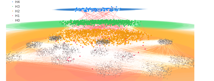<details> <summary>x11.png Details</summary>  ### Visual Description ## Network Diagram: Hierarchical Layered Graph ### Overview The image displays a complex, multi-layered network graph visualization. It depicts a hierarchical structure with nodes organized into distinct horizontal layers, connected by a dense web of edges. The visualization uses color-coding to differentiate node categories, as defined by a legend. The overall impression is of a complex system with strong inter-layer connections and clustered sub-structures within the lower layers. ### Components/Axes * **Legend (Top-Left Corner):** A vertical list defining five node categories by color and label. * **H4:** Blue * **H3:** Green * **H2:** Orange * **H1:** Gray * **H0:** Red * **Main Graph Area:** The visualization is structured into approximate horizontal strata, from top to bottom: 1. **Top Layer (H4):** A dense, compact cluster of blue nodes. 2. **Second Layer (H3):** A wide, dense band of green nodes directly below the blue layer. 3. **Third Layer (H2):** A broad, dense field of orange nodes below the green layer. 4. **Bottom Layer (H1/H0):** A complex region containing clusters of gray nodes (H1) interspersed with sparse red nodes (H0). This layer spans the entire width and appears to have the most internal structure. * **Connections (Edges):** A vast number of fine, semi-transparent lines connect nodes. The highest density of connections appears to run vertically between adjacent layers (e.g., H4 to H3, H3 to H2). There are also significant connections within layers, particularly within the bottom gray/red layer, forming distinct clusters. ### Detailed Analysis * **Node Distribution & Density:** * **H4 (Blue):** Forms a single, tight, elliptical cluster at the top-center of the diagram. It appears to be the smallest group by node count. * **H3 (Green):** Forms a wide, dense horizontal band directly beneath H4. It is significantly larger in spatial extent and node count than H4. * **H2 (Orange):** Forms the largest and densest horizontal band, occupying the central portion of the diagram. It contains the highest apparent number of nodes. * **H1 (Gray):** Nodes are not uniformly distributed but are aggregated into multiple distinct, dense clusters scattered across the bottom region. There appear to be approximately 6-8 major clusters. * **H0 (Red):** These nodes are sparse and appear as individual points or very small groups embedded within or near the gray (H1) clusters. They are the least numerous category. * **Connection Patterns:** * The network exhibits a clear **feed-forward or hierarchical flow** from the top layers (H4, H3) down to the bottom layers (H2, H1/H0). The connection density is highest between immediate neighbors in this hierarchy. * The bottom layer (H1/H0) shows significant **intra-layer connectivity**, with dense webs of connections within and between the gray clusters, suggesting complex local interactions or sub-networks. * The connections from the orange (H2) layer to the bottom layer appear to converge onto the specific gray clusters, indicating a many-to-few or targeted mapping. ### Key Observations 1. **Clear Hierarchical Stratification:** The primary organizing principle is a top-down hierarchy (H4 -> H3 -> H2 -> H1/H0). 2. **Inversion of Size/Complexity:** The top of the hierarchy (H4) is the simplest and smallest, while the base (H1/H0) is the most complex, numerous, and internally structured. This is an inverted pyramid structure. 3. **Clustered Base Layer:** The bottom layer is not homogeneous but is composed of discrete, densely connected modules (the gray clusters). 4. **Sparse "Outlier" Nodes:** The red (H0) nodes are rare and embedded within the gray clusters, suggesting they may represent special states, errors, or a distinct sub-category within the base layer. 5. **Visual Weight:** The orange (H2) layer dominates the visual field due to its density and central placement, acting as a major hub or processing layer between the upper and lower tiers. ### Interpretation This diagram likely visualizes a **hierarchical system with increasing complexity and specialization at lower levels**. Potential interpretations include: * **Neural Network Architecture:** It could represent a deep learning model where H4 is the input layer, H3 and H2 are hidden layers, and the clustered H1/H0 represents a complex output or embedding space. The red nodes (H0) might be specific output classes or anomaly detections. * **Organizational or Social Network:** H4 could be top leadership, H3 middle management, H2 operational teams, and the H1 clusters represent specialized departments or project teams, with H0 being key individuals or external liaisons. * **Information or Data Flow:** It may depict data processing stages: H4 (raw data ingestion), H3 (initial processing), H2 (core analysis/aggregation), and H1/H0 (specialized storage, application, or user-facing outputs in clustered databases or services). The **key insight** is the structural relationship: a broad, dense intermediary layer (H2) funnels information or control from a small, unified top (H4/H3) into a fragmented, modular, and highly interactive base (H1/H0). The sparse red nodes (H0) are critical anomalies or special elements within the foundational modules. The visualization emphasizes **connectivity and hierarchy over individual node identity**, showcasing the system's architecture rather than its specific components. </details> Figure 11: A 3D view of the Hierarchical Graph with Causal Gates constructed from HotpotQA dataset. ## Appendix D Case Study: A Real Example of the HugRAG Full Pipeline To concretely illustrate the HugRAG full pipeline, we present a step-by-step execution trace on a query from the HolisQA-Biology dataset in Figure 12. The query asks for a comparison of specific enzyme activities (Apase vs. Pti-interacting kinase) in oil palm genotypes under phosphorus limitation—a task requiring the holistic comprehension of biology knowledge in HolisQA dataset. 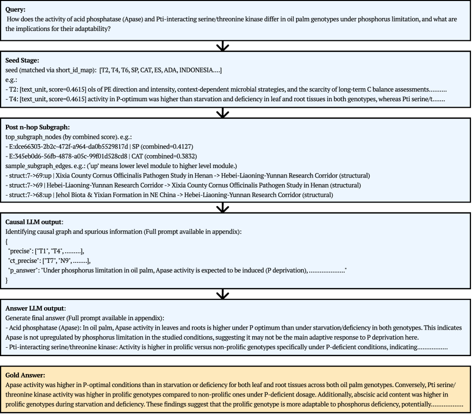<details> <summary>x12.png Details</summary>  ### Visual Description ## Diagram: Scientific Query Answering Pipeline Flowchart ### Overview The image displays a vertical flowchart illustrating a multi-stage process for generating a scientific answer to a specific research query about oil palm genotypes. The process flows from an initial query through data retrieval, subgraph analysis, causal reasoning, and final answer generation, culminating in a comparison with a "Gold Answer." The diagram is composed of six rectangular boxes connected by downward-pointing arrows, indicating sequential steps. ### Components/Axes The diagram is structured as a top-to-bottom flowchart with the following six distinct stages, each contained within a box: 1. **Query Box** (Top, light blue background): Contains the initial research question. 2. **Seed Stage Box** (Light blue background): Describes the initial data retrieval or "seeding" step. 3. **Post n-hop Subgraph Box** (Light blue background): Details the construction and analysis of a knowledge subgraph. 4. **Causal LLM output Box** (Light blue background): Shows the output from a language model tasked with causal reasoning. 5. **Answer LLM output Box** (Light blue background): Presents the final generated answer from a language model. 6. **Gold Answer Box** (Bottom, light orange background): Provides a reference or benchmark answer for comparison. **Flow Direction:** A single, thick black arrow points downward from the bottom center of each box to the top center of the subsequent box, clearly defining the process sequence. ### Detailed Analysis / Content Details **1. Query Box:** * **Text:** "Query: How does the activity of acid phosphatase (Apase) and Pti-interacting serine/threonine kinase differ in oil palm genotypes under phosphorus limitation, and what are the implications for their adaptability?" **2. Seed Stage Box:** * **Header:** "Seed Stage:" * **Content:** * "seed (matched via short_id_map): [T2, T4, T6, SP, CAT, ES, ADA, INDONESIA....]" * "e.g.:" * "- T2: [text_unit, score=0.4615] ols of PE direction and intensity, context-dependent microbial strategies, and the scarcity of long-term C balance assessments..........." * "- T4: [text_unit, score=0.4615] activity in P-optimum was higher than starvation and deficiency in leaf and root tissues in both genotypes, whereas Pti serine/t......." **3. Post n-hop Subgraph Box:** * **Header:** "Post n-hop Subgraph:" * **Content:** * "top_subgraph_nodes (by combined score), e.g.:" * "- E:dce66303-2b2c-472f-a964-da0b5529817d | SP (combined=0.4127)" * "- E:345eb0d6-56fb-4878-a05c-99f01d528cd8 | CAT (combined=0.3832)" * "sample_subgraph_edges, e.g. ('up' means lower level module to higher level module.)" * "- struct:7->69:up | Xixia County Cornus Officinalis Pathogen Study in Henan -> Hebei-Liaoning-Yunnan Research Corridor (structural)" * "- struct:7->69 | Hebei-Liaoning-Yunnan Research Corridor -> Xixia County Cornus Officinalis Pathogen Study in Henan (structural)" * "- struct:7->68:up | Jehol Biota & Yixian Formation in NE China -> Hebei-Liaoning-Yunnan Research Corridor (structural)" **4. Causal LLM output Box:** * **Header:** "Causal LLM output:" * **Content:** * "Identifying causal graph and spurious information (Full prompt available in appendix):" * "{" * " 'precise': ['T1', 'T4', .........]," * " 'ct_precise': ['T7', 'N9', .........]," * " 'p_answer': 'Under phosphorus limitation in oil palm, Apase activity is expected to be induced (P deprivation),....................'" * "}" **5. Answer LLM output Box:** * **Header:** "Answer LLM output:" * **Content:** * "Generate final answer (Full prompt available in appendix):" * "- Acid phosphatase (Apase): In oil palm, Apase activity in leaves and roots is higher under P optimum than under starvation/deficiency in both genotypes. This indicates Apase is not upregulated by phosphorus limitation in the studied conditions, suggesting it may not be the main adaptive response to P deprivation here." * "- Pti-interacting serine/threonine kinase: Activity is higher in prolific versus non-prolific genotypes specifically under P-deficient conditions, indicating..............." **6. Gold Answer Box:** * **Header:** "Gold Answer:" * **Content:** * "Apase activity was higher in P-optimal conditions than in starvation or deficiency for both leaf and root tissues across both oil palm genotypes. Conversely, Pti serine/threonine kinase activity was higher in prolific genotypes compared to non-prolific ones under P-deficient dosage. Additionally, abscisic acid content was higher in prolific genotypes during starvation and deficiency. These findings suggest that the prolific genotype is more adaptable to phosphorus deficiency, potentially..............." ### Key Observations * **Process Structure:** The diagram outlines a clear, linear pipeline for transforming a natural language query into a structured, evidence-based answer. * **Data Integration:** The "Seed Stage" and "Post n-hop Subgraph" boxes show the integration of retrieved text units (with relevance scores) and structured knowledge graph data (nodes and edges with types and relationships). * **LLM Roles:** Two distinct LLM stages are shown: a "Causal LLM" for reasoning and filtering, and an "Answer LLM" for final synthesis. * **Benchmark Comparison:** The final "Gold Answer" is visually distinguished (orange background) and serves as a reference point, suggesting the pipeline's output is meant to be evaluated against this standard. * **Content Consistency:** The core scientific findings mentioned in the "Answer LLM output" and "Gold Answer" are consistent regarding the direction of enzyme activity changes (Apase higher in P-optimum, Pti kinase higher in prolific genotypes under P-deficiency). ### Interpretation This diagram represents a sophisticated **Retrieval-Augmented Generation (RAG) or knowledge-grounded question-answering system** tailored for scientific literature. It demonstrates a method to move beyond simple text retrieval by: 1. **Contextualizing the Query:** Starting with a specific biological question. 2. **Multi-Source Evidence Gathering:** Retrieving relevant text passages ("seeds") and mapping them to a structured knowledge graph ("subgraph") to capture relationships between concepts (e.g., linking a "Pathogen Study" to a "Research Corridor"). 3. **Causal Reasoning:** Employing an LLM to distinguish precise, causal information from spurious correlations within the retrieved data. 4. **Synthesis and Generation:** Using another LLM to formulate a coherent, final answer based on the filtered evidence. 5. **Validation:** The inclusion of a "Gold Answer" implies this pipeline is part of a system where generated answers are benchmarked against expert-derived truths, likely for training or evaluation purposes. The process highlights the challenge of synthesizing information from unstructured text and structured data to answer complex, multi-faceted scientific questions. The ellipses ("...........") in the text suggest the outputs are truncated for the diagram, indicating the actual process handles more extensive data. The pipeline aims to produce answers that are not just factually correct but also causally sound and grounded in a network of evidence. </details> Figure 12: A real example of HugRAG on a biology-related query. The diagram visualizes the data flow from initial seed matching and hierarchical graph expansion to the causal reasoning stage, where the model explicitly filters spurious nodes to produce a grounded, high-fidelity answer. ## Appendix E Experiments on the Effectiveness of Causal Gates To isolate the real effectiveness of the causal gate in HugRAG, we conduct a controlled A/B test comparing gold context access with the gate disabled (off) versus enabled (on). The evaluation is performed on two datasets: NQ (Standard QA) and HolisQA. We define “Gold Nodes” as the graph nodes mapping to the gold context. Metrics are computed only on examples where gold nodes are mappable to the graph. While this section focuses on structural retrieval metrics, we evaluate the downstream impact of causal gates on final answer quality in our ablation study in Section 5.3. #### Metrics. We report four structural metrics to evaluate retrieval quality and efficiency. Shaded regions in Figure 13 denote 95% bootstrap confidence intervals. Reachability: The fraction of examples where at least one gold node is retrieved in the subgraph. Weighted Reachability (Depth-Weighted): A distance-sensitive metric defined as $\mathrm{DWR}=\frac{1}{1+\mathrm{min\_hops}}$ (0 if unreachable), rewarding retrieval at smaller graph distances. Coverage: The average proportion of total gold nodes retrieved per example. Min Hops: The mean shortest path length to gold nodes, computed on examples reachable in both off and on settings. As shown in Figure 13, enabling the causal gate yields distinct behaviors across datasets. On the more complex HolisQA dataset, the gate provides a statistically significant improvement in reachability and coverage. This confirms that causal edges effectively bridge structural gaps in the graph that are otherwise traversed inefficiently. The increase in Weighted Reachability and decrease in min hops indicate that the gate not only finds more evidence but creates structural shortcuts, allowing the retrieval process to access evidence at shallower depths. 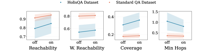<details> <summary>x13.png Details</summary>  ### Visual Description \n ## Line Charts: Performance Metrics Comparison (HolisQA vs. Standard QA Datasets) ### Overview The image displays a series of four line charts arranged horizontally, comparing two datasets—"HolisQA Dataset" and "Standard QA Dataset"—across four different performance metrics. Each chart plots a metric's value for two conditions: "off" and "on". The charts include shaded regions around the lines, likely representing confidence intervals or standard deviation. ### Components/Axes * **Legend:** Positioned at the top center of the entire figure. * Blue dot/line: `HolisQA Dataset` * Orange dot/line: `Standard QA Dataset` * **Chart Panels (Left to Right):** 1. **Chart 1: Reachability** * **X-axis:** Two categorical points labeled `off` (left) and `on` (right). * **Y-axis:** Linear scale from approximately 0.7 to 0.95. Major ticks visible at 0.7, 0.8, 0.9. 2. **Chart 2: W. Reachability** * **X-axis:** `off` and `on`. * **Y-axis:** Linear scale from approximately 0.5 to 0.85. Major ticks visible at 0.6, 0.8. 3. **Chart 3: Coverage** * **X-axis:** `off` and `on`. * **Y-axis:** Linear scale from approximately 0.15 to 0.45. Major ticks visible at 0.2, 0.4. 4. **Chart 4: Min Hops** * **X-axis:** `off` and `on`. * **Y-axis:** Linear scale from approximately 0.25 to 1.5. Major ticks visible at 0.5, 1.0, 1.5. ### Detailed Analysis **Trend Verification & Data Points (Approximate):** 1. **Reachability:** * **HolisQA (Blue):** Line slopes upward. Value at `off` ≈ 0.80. Value at `on` ≈ 0.85. * **Standard QA (Orange):** Line slopes upward. Value at `off` ≈ 0.92. Value at `on` ≈ 0.94. * *Spatial Grounding:* The orange line is positioned above the blue line across both conditions. 2. **W. Reachability:** * **HolisQA (Blue):** Line slopes upward. Value at `off` ≈ 0.55. Value at `on` ≈ 0.58. * **Standard QA (Orange):** Line slopes upward. Value at `off` ≈ 0.80. Value at `on` ≈ 0.82. * *Spatial Grounding:* The orange line is positioned significantly above the blue line. 3. **Coverage:** * **HolisQA (Blue):** Line slopes upward. Value at `off` ≈ 0.30. Value at `on` ≈ 0.35. * **Standard QA (Orange):** Line slopes slightly upward. Value at `off` ≈ 0.18. Value at `on` ≈ 0.19. * *Spatial Grounding:* The blue line is positioned above the orange line, reversing the pattern seen in the first two charts. 4. **Min Hops:** * **HolisQA (Blue):** Line slopes downward. Value at `off` ≈ 1.05. Value at `on` ≈ 0.85. * **Standard QA (Orange):** Line slopes downward. Value at `off` ≈ 0.35. Value at `on` ≈ 0.30. * *Spatial Grounding:* The blue line is positioned above the orange line. Both lines show a decrease from `off` to `on`. ### Key Observations * **Consistent Directional Change:** For both datasets, moving from the "off" to "on" condition leads to an increase in Reachability, W. Reachability, and Coverage, but a decrease in Min Hops. * **Dataset Performance Inversion:** The Standard QA Dataset (orange) consistently outperforms the HolisQA Dataset (blue) on the "Reachability" and "W. Reachability" metrics. However, the HolisQA Dataset shows higher "Coverage" and a higher "Min Hops" value. * **Magnitude of Change:** The relative improvement (or decrease for Min Hops) from "off" to "on" appears more pronounced for the HolisQA Dataset (blue line) in most charts, particularly in Min Hops and Coverage. * **Uncertainty Bands:** The shaded regions (light blue for HolisQA, light orange for Standard QA) suggest variability or confidence in the measurements. The bands for HolisQA appear wider in the Coverage and Min Hops charts, indicating potentially greater variance in those results. ### Interpretation The data suggests that the "on" condition—likely representing the activation of a specific system, feature, or method—generally improves the measured performance metrics for both QA datasets. The improvement is seen in increased reachability and coverage, coupled with a reduction in the minimum number of hops (which could imply more efficient information retrieval or reasoning paths). The key insight is the performance trade-off between the two datasets. The Standard QA Dataset achieves higher raw reachability scores, but the HolisQA Dataset demonstrates superior coverage and operates with a higher hop count. This could indicate that the HolisQA system, while perhaps less direct (more hops), explores a broader set of information (higher coverage). The "on" condition amplifies these inherent characteristics of each dataset/system. The investigation would benefit from understanding what the "off"/"on" states represent and the specific definitions of "W. Reachability" and "Coverage" to fully contextualize these results. </details> Figure 13: Experiments on Causal Gate effectiveness. We compare graph traversal performance with the causal gate disabled (off) versus enabled (on). Shaded areas represent 95% bootstrap confidence intervals. The causal gate significantly improves evidence accessibility (Reachability, Coverage) and traversal efficiency (lower Min Hops, higher Weighted Reachability). ## Appendix F Evaluation Details ### F.1 Detailed Graph Statistics We provide the complete statistics for all knowledge graphs constructed in our experiments. Table 5 details the graph structures for the five standard QA datasets, while Table 6 covers the five scientific domains within the HolisQA dataset. Table 5: Graph Statistics for Standard QA Datasets. Detailed breakdown of nodes, edges, and hierarchical module distribution. | Dataset | Nodes | Edges | L3 | L2 | L1 | L0 | Modules | Domain | Chars | | --- | --- | --- | --- | --- | --- | --- | --- | --- | --- | | HotpotQA | 20,354 | 15,789 | 27 | 1,344 | 891 | 97 | 2,359 | Wikipedia | 2,855,481 | | MS MARCO | 3,403 | 3,107 | 2 | 159 | 230 | 55 | 446 | Web | 1,557,990 | | NQ | 5,579 | 4,349 | 2 | 209 | 244 | 50 | 505 | Wikipedia | 767,509 | | QASC | 77 | 39 | - | - | - | 4 | 4 | Science | 58,455 | | 2WikiMultiHop | 10,995 | 8,489 | 8 | 461 | 541 | 78 | 1,088 | Wikipedia | 1,756,619 | Table 6: Graph Statistics for HolisQA Datasets. Graph structures constructed from dense academic papers across five scientific domains. | Holis-Biology | 1,714 | 1,722 | - | 30 | 104 | 31 | 165 | Biology | 1,707,489 | | --- | --- | --- | --- | --- | --- | --- | --- | --- | --- | | Holis-Business | 2,169 | 2,392 | 8 | 77 | 166 | 41 | 292 | Business | 1,671,718 | | Holis-CompSci | 1,670 | 1,667 | 7 | 28 | 91 | 30 | 158 | CompSci | 1,657,390 | | Holis-Medicine | 1,930 | 2,124 | 7 | 56 | 129 | 34 | 226 | Medicine | 1,706,211 | | Holis-Psychology | 2,019 | 1,990 | 5 | 45 | 126 | 35 | 211 | Psychology | 1,751,389 | ### F.2 HolisQA Dataset We introduce HolisQA, a comprehensive dataset designed to evaluate the holistic comprehension capabilities of RAG systems, explicitly addressing the ”node finding” bias prevalent in existing QA datasets—where retrieving a single entity (e.g., a year or name) is often sufficient. Our goal is to enforce holistic comprehension, compelling models to synthesize coherent evidence from multi-sentence contexts. We collected high-quality scientific papers across multiple domains as our primary source (Priem et al., 2022), focusing exclusively on recent publications (2025) to minimize parametric memorization by the LLM. The dataset spans five distinct domains—Biology, Business, Computer Science, Medicine, and Psychology—to ensure domain robustness (see full statistics in Table 6). To necessitate cross-sentence reasoning, we avoid random sentence sampling; instead, we extract contiguous text slices from papers within each domain. Each slice is sufficiently long to encapsulate multiple interacting claims (e.g., Problem $\to$ Method $\to$ Result) yet short enough to remain self-contained, thereby preserving the logical coherence and contextual foundation required for complex reasoning. Subsequently, we employ a rigorous LLM-based generation pipeline to create Question-Answer-Context triples, imposing two strict constraints (as detailed in Figure 14): 1. Integration Constraint: The question must require integrating information from at least three distinct sentences. We explicitly reject trivia-style questions that can be answered by a single named entity (e.g., ”Who founded X?”). 1. Evidence Verification: The generation process must output the IDs of all supporting sentences. We validate the dataset via a necessity check, verifying that the correct answer cannot be derived if any of the cited sentences are removed. Through this strict construction pipeline, HolisQA effectively evaluates the model’s ability to perform holistic comprehension and isolate it from parametric knowledge, providing a cleaner signal for evaluating the effectiveness of structured retrieval mechanisms. 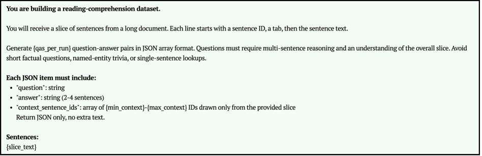<details> <summary>x14.png Details</summary>  ### Visual Description ## Screenshot: Reading-Comprehension Dataset Generation Instructions ### Overview The image is a screenshot of a text-based instruction set for building a reading-comprehension dataset. The content is presented as a single block of text within a light gray (#f0f0f0) bordered box against a white background. The text provides a precise, technical specification for a data generation task. ### Components/Axes This is not a chart or diagram with axes. The components are purely textual instructions structured as follows: - **Title/Instruction Header**: A bolded statement of the primary task. - **Process Description**: A paragraph explaining the input format and the core generation task. - **Output Specification**: A bulleted list defining the required JSON structure for each output item. - **Input Placeholder**: A label indicating where the source text data will be inserted. ### Detailed Analysis / Content Details **Full Text Transcription:** ``` You are building a reading-comprehension dataset. You will receive a slice of sentences from a long document. Each line starts with a sentence ID, a tab, then the sentence text. Generate {qas_per_run} question-answer pairs in JSON array format. Questions must require multi-sentence reasoning and understanding of the overall slice. Avoid short factual questions, named-entity trivia, or single-sentence lookups. Each JSON item must include: • "question": string • "answer": string (2-4 sentences) • "context_sentence_ids": array of {min_context}-{max_context} IDs drawn only from the provided slice Return JSON only, no extra text. Sentences: {slice_text} ``` **Key Elements and Placeholders:** 1. **Task Definition**: The user is instructed to act as a builder of a reading-comprehension dataset. 2. **Input Format**: Data will be provided as a "slice" of sentences. Each sentence line has the format: `[sentence ID]\t[sentence text]`. 3. **Generation Parameter**: `{qas_per_run}` is a variable placeholder indicating the number of question-answer pairs to generate per execution. 4. **Question Quality Constraint**: Questions must necessitate **multi-sentence reasoning** and comprehension of the entire provided text slice. Explicitly forbidden are: - Short factual questions. - Named-entity trivia. - Single-sentence lookups. 5. **Output Schema (JSON Array)**: Each object in the array must contain three fields: - `"question"`: A string. - `"answer"`: A string answer spanning 2 to 4 sentences. - `"context_sentence_ids"`: An array of sentence ID ranges (e.g., `["1-3", "5-7"]`). The IDs must be drawn **exclusively** from the IDs in the provided input slice. 6. **Output Constraint**: The final output must be **only the JSON array**, with no additional explanatory text. 7. **Data Placeholder**: `Sentences:` followed by `{slice_text}` marks where the actual sentence data (the "slice") will be inserted for processing. ### Key Observations - **Precision of Instruction**: The text is highly specific about the input format, output structure, and, crucially, the *cognitive level* of the required questions (multi-sentence reasoning). - **Use of Placeholders**: The instructions use template variables (`{qas_per_run}`, `{slice_text}`), indicating this is likely a prompt or specification for an automated system or a human annotator following a strict protocol. - **Negative Constraints**: The instructions explicitly define what *not* to do (avoid simple questions), which is as important as the positive requirements for ensuring dataset quality. - **Visual Layout**: The text is left-aligned within a defined container. The bullet points use standard round bullets (•). The font appears to be a common sans-serif typeface (e.g., Arial, Helvetica). ### Interpretation This image outlines the foundational rules for creating a high-quality, reasoning-focused reading comprehension dataset. The design reveals several underlying principles: 1. **Purpose-Driven Design**: The dataset is not for testing basic fact retrieval but for evaluating a model's ability to synthesize information across multiple sentences. This suggests it's intended for advanced NLP model evaluation or training, targeting skills like inference, causality, and summarization. 2. **Controlled Generation**: The use of placeholders (`{qas_per_run}`, `{slice_text}`) and the strict JSON schema indicate this is a component within a larger, likely automated, data pipeline. The system is designed for batch processing and consistency. 3. **Data Integrity**: The requirement that `context_sentence_ids` must be drawn *only* from the provided slice ensures that questions and answers are grounded in the given context, preventing leakage or the use of external knowledge. This is critical for creating a valid and reproducible benchmark. 4. **Implicit Workflow**: The process implies a two-stage workflow: first, a "slice" of text is extracted from a larger document and formatted with IDs; second, this slice is processed (by an AI or human) according to these rules to generate the QA pairs. The final output is a clean, structured JSON file ready for integration into a dataset. In essence, this is a technical specification for generating a **reasoning-centric** subset of a reading comprehension dataset, emphasizing structured output, contextual grounding, and complex question design. </details> Figure 14: Prompt for generating the Holistic Comprehension Dataset (Question-Answer-Context Triplets) from academic papers. ### F.3 Implementation #### Backbone Models. We consistently use OpenAI’s gpt-5-nano with a temperature of 0.0 to ensure deterministic generation. For vector embeddings, we employ the Sentence-BERT (Reimers and Gurevych, 2019) version of all-MiniLM-L6-v2 with a dimensionality of 384. All evaluation metrics involving LLM-as-a-judge are implemented using the Ragas framework (Es et al., 2024), with Gemini-2.5-Flash-Lite serving as the underlying evaluation engine. #### Baseline Parameters. To ensure a fair comparison among all graph-based RAG methods, we utilize a unified root knowledge graph (see Appendix B.1 for construction details). For the retrieval stage, we set a consistent initial $k=3$ across all baselines. Other parameters are kept at their default values to maintain a neutral comparison, with the exception of method-specific configurations (e.g., global vs. local modes in GraphRAG) that are essential for the algorithm’s execution. All experiments were conducted on a high-performance computing cluster managed by Slurm. Each evaluation task was allocated uniform resources consisting of 2 CPU cores and 16 GB of RAM, utilizing 10-way job arrays for concurrent query processing. ### F.4 Grounding Metrics and Evaluation Prompts We assess performance using two categories of metrics: (i) Lexical Overlap (F1 score), which measures surface-level similarity between model outputs and gold answers; and (ii) LLM-as-judge metrics, specifically Context Recall and Answer Relevancy, computed using a fixed evaluator model to ensure consistency (Es et al., 2024). To guarantee stable and fair comparisons across baselines with varying retrieval outputs, we impose a uniform cap on the retrieved context length and the number of items passed to the evaluator. The specific prompt template used for assessing Answer Relevancy is illustrated in Figure 15. <details> <summary>x15.png Details</summary>  ### Visual Description ## Text Document: AI Response Template and Examples ### Overview The image displays a text document on a light green background, outlining a template and examples for generating structured AI responses. It provides instructions for formatting output as JSON and includes a specific prompt for evaluating answer relevancy. ### Components/Axes The document is structured into three main sections, each marked with a triple-asterisk heading: 1. **Core Template**: Defines the structure for an AI instruction and expected JSON output. 2. **Answer Relevancy prompt**: Provides instructions for generating a question from a given answer and classifying it as noncommittal (1) or substantive (0). 3. **Examples**: Shows three input-output pairs demonstrating the application of the "Answer Relevancy prompt". ### Detailed Analysis The text content is transcribed below, preserving the original structure and placeholders. **Section 1: Core Template** ``` ### Core Template {instruction} Please return the output in a JSON format that complies with the following schema as specified in JSON Schema: {output_schema}Do not use single quotes in your response but double quotes,properly escaped with a backslash. {examples} -------------------------------------------- Now perform the same with the following input input: {input_json} Output: ``` **Section 2: Answer Relevancy prompt** ``` ### Answer Relevancy prompt Generate a question for the given answer and identify if the answer is noncommittal. Give noncommittal as 1 if the answer is noncommittal (evasive, vague, or ambiguous) and 0 if the answer is substantive. Examples of noncommittal answers: "I don't know", "I'm not sure", "It depends". ``` **Section 3: Examples** ``` ### Examples Input: {'response': 'Albert Einstein was born in Germany.'} Output: {'question': 'Where was Albert Einstein born?', 'noncommittal': 0} Input: {'response': 'The capital of France is Paris, a city known for its architecture and culture.'} Output: {'question': 'What is the capital of France?', 'noncommittal': 0} Input: {'response': 'I don't know about the groundbreaking feature of the smartphone invented in 2023 as I am unaware of information beyond 2022.'} Output: {'question': 'What was the groundbreaking feature of the smartphone invented in 2023?', 'noncommittal': 1} ``` ### Key Observations * The document serves as a meta-instruction set, likely for configuring or testing an AI model's response generation capabilities. * It emphasizes strict JSON formatting, requiring double quotes and proper escaping. * The "Answer Relevancy prompt" introduces a binary classification task (0 or 1) based on the substantive or noncommittal nature of an answer. * The examples clearly illustrate the expected transformation from an input `response` to an output containing a generated `question` and a `noncommittal` score. * The third example demonstrates a noncommittal answer (score 1) where the response explicitly states a lack of knowledge due to a knowledge cutoff. ### Interpretation This document is a technical specification for an AI evaluation or training pipeline. Its primary purpose is to standardize how an AI system should process a given "answer" (response) to produce two outputs: a relevant question that the answer addresses, and a binary flag indicating whether the original answer was evasive or substantive. The inclusion of a knowledge cutoff reference ("unaware of information beyond 2022") in the third example is particularly notable. It suggests this template is designed to handle or test an AI's self-awareness regarding its training data limitations, which is a critical aspect of responsible AI behavior. The structure ensures that responses acknowledging such limitations are correctly flagged as "noncommittal" (1), while factual, direct answers are flagged as "substantive" (0). This system could be used for automated quality assurance, reinforcement learning from human feedback (RLHF), or benchmarking AI response reliability. </details> Figure 15: Example prompt used in RAGAS: Core Template and Answer Relevancy (Es et al., 2024).