# Internalizing Meta-Experience into Memory for Guided Reinforcement Learning in Large Language Models
## Abstract
Reinforcement Learning with Verifiable Rewards (RLVR) has emerged as an effective approach for enhancing the reasoning capabilities of Large Language Models (LLMs). Despite its efficacy, RLVR faces a meta-learning bottleneck: it lacks mechanisms for error attribution and experience internalization intrinsic to the human learning cycle beyond practice and verification, thereby limiting fine-grained credit assignment and reusable knowledge formation. We term such reusable knowledge representations derived from past errors as meta-experience. Based on this insight, we propose M eta- E xperience L earning (MEL), a novel framework that incorporates self-distilled meta-experience into the model’s parametric memory. Building upon standard RLVR, we introduce an additional design that leverages the LLM’s self-verification capability to conduct contrastive analysis on paired correct and incorrect trajectories, identify the precise bifurcation points where reasoning errors arise, and summarize them into generalizable meta-experience. The meta-experience is further internalized into the LLM’s parametric memory by minimizing the negative log-likelihood, which induces a language-modeled reward signal that bridges correct and incorrect reasoning trajectories and facilitates effective knowledge reuse. Experimental results demonstrate that MEL achieves consistent improvements on benchmarks, yielding 3.92%–4.73% Pass@1 gains across varying model sizes.
Shiting Huang 1 Zecheng Li 1 Yu Zeng 1 Qingnan Ren 1 Zhen Fang 1 Qisheng Su 1 Kou Shi 1 Lin Chen 1 Zehui Chen 1 Feng Zhao 1 🖂 1 University of Science and Technology of China 🖂: Corresponding Author
## 1 Introduction
Reinforcement Learning (RL) has emerged as a pivotal paradigm for enhancing the reasoning capabilities of Large Language Models (LLMs) on complex tasks, such as mathematics, programming, and logic reasoning (Shao et al., 2024; Chen et al., 2025; Zeng et al., 2025a; Wang et al., 2025; Zeng et al., 2025b, 2026; Huang et al., 2026). By leveraging feedback signals obtained from interaction with the task environment, RL enables LLMs to move beyond passive imitation learning toward goal-directed reasoning and action (Schulman et al., 2017; Ouyang et al., 2022; Wulfmeier et al., 2024). Furthermore, by replacing learned reward models with programmatically verifiable signals, Reinforcement Learning with Verifiable Rewards (RLVR) eliminates the need for expensive human annotations and mitigates reward hacking, thereby enabling models to explore problem-solving strategies more effectively, which has contributed to its growing attention (Lambert et al., 2024).
However, RLVR still faces a fundamental bottleneck regarding the granularity and utilization of learning signals. From a meta-learning perspective, the human learning cycle involves three critical components: practice and verification, error attribution, and experience internalization. While RLVR primarily drives policy updates through practice and verification, it overlooks the critical stages of error attribution and experience internalization, both of which are essential for fine-grained credit assignment and the formation of reusable knowledge (Wu et al., 2025; Zhang et al., 2025a). In other words, RLVR is largely limited to assessing the overall quality of entire trajectories, while struggling to reason about fine-grained knowledge at the level of intermediate steps (Xie et al., 2025). Although RL approaches (Lightman et al., 2023; Khalifa et al., 2025) employing Process Reward Models (PRMs) to provide dense learning signals attempt to mitigate this limitation, their reliance on trained proxies makes them inherently susceptible to reward hacking (Cheng et al., 2025; Guo et al., 2025), and poses a fundamental tension with the RLVR paradigm, which is centered on programmatically verifiable rewards.
<details>
<summary>x1.png Details</summary>
### Visual Description
## Diagram: Comparison of Standard RLVR and MEL (Meta-Experience Learning) Architectures
### Overview
The image is a technical diagram comparing two reinforcement learning or decision-making architectures. On the left is "(a) Standard RLVR" and on the right is "(b) MEL (Ours)". The diagram illustrates how the proposed MEL method incorporates a "Meta-Experience" component to achieve "Knowledge-level optimization," leading to a more successful outcome compared to the standard "Trajectory-Level optimization" approach.
### Components/Axes
The diagram is divided into two primary vertical panels.
**Panel (a) - Standard RLVR (Left Side):**
* **Top:** A circled "Q" (likely representing a Query or Question) connects via a wavy line to a central green node.
* **Middle:** The central green node branches into two paths:
* Left Path: A green node leads to another green node via a wavy line.
* Right Path: A red node leads to another red node via a wavy line.
* **Reward Labels:** Below the terminal nodes are the labels "Reward=1" (under the green path) and "Reward=0" (under the red path).
* **Optimization Block:** A gray box labeled "Trajectory-Level optimization" sits below the reward labels.
* **Action Arrows:** Two arrows point downward from the optimization block:
* A green arrow labeled "Encourage" points to the left.
* A red arrow labeled "Suppress" points to the right.
* **Outcome Icon:** Both arrows point to a single robot icon at the bottom. The robot has "X" eyes and a wavy mouth, indicating a failed, confused, or negative state.
**Panel (b) - MEL (Ours) (Right Side):**
* **Top:** Identical starting structure to panel (a): a circled "Q" connects to a central green node.
* **Middle:** The central green node branches into two paths, identical to panel (a), but this entire branching structure is enclosed within a **dashed rectangular box**.
* **Reward Labels:** Identical to panel (a): "Reward=1" (left) and "Reward=0" (right).
* **Optimization Block:** An identical gray box labeled "Trajectory-Level optimization" sits below the reward labels, with identical "Encourage" (green) and "Suppress" (red) arrows.
* **Meta-Experience Component:** A key differentiating element. A black arrow originates from the **dashed box** and points to a cloud-shaped element on the right.
* The cloud is labeled "**Meta-Experience**" in bold, dark blue text.
* Inside the cloud, in smaller text: "(bifurcation point, critique, heuristic)".
* A yellow lightbulb icon is attached to the top-right of the cloud.
* **Knowledge Flow:** A black arrow leads from the "Meta-Experience" cloud down to a gray box labeled "**Knowledge-level optimization**".
* **Outcome Icon:** An arrow from the "Knowledge-level optimization" box points to a robot icon at the bottom. This robot has a smiling face and a glowing yellow lightbulb above its head, indicating a successful, enlightened, or positive state.
### Detailed Analysis
The diagram presents a flowchart-style comparison of two processes.
1. **Shared Initial Process:** Both methods start with a query (Q) leading to a decision point (central green node) that bifurcates into two possible trajectories: a "good" one (green nodes, Reward=1) and a "bad" one (red nodes, Reward=0).
2. **Standard RLVR Process:** The system applies "Trajectory-Level optimization" based on the final reward. It encourages the entire trajectory that led to Reward=1 and suppresses the one that led to Reward=0. The outcome is a single, negatively-valenced robot state, suggesting this method may lead to suboptimal or brittle learning.
3. **MEL Process:** The system performs the same trajectory-level optimization. However, it **additionally** extracts abstract knowledge from the decision point itself (the bifurcation within the dashed box). This extracted "Meta-Experience" consists of understanding the bifurcation point, forming critiques, and deriving heuristics. This meta-knowledge is then used for "Knowledge-level optimization," which directly informs and improves the agent, resulting in a positive, "enlightened" outcome.
### Key Observations
* **Spatial Grounding:** The "Meta-Experience" cloud is positioned to the right of the main flow in panel (b), connected directly to the decision-making core (the dashed box). The "Knowledge-level optimization" box is positioned between the cloud and the final robot icon.
* **Visual Metaphors:** The robot icons are critical visual cues. The "X" eyes in (a) denote failure or a dead end. The smiling face and lightbulb in (b) denote success and insight.
* **Color Coding:** Green consistently represents successful/rewarded paths and actions ("Encourage"). Red represents unsuccessful/unrewarded paths and actions ("Suppress"). Yellow is used for the lightbulb, symbolizing ideas and insight.
* **Structural Emphasis:** The dashed box in (b) highlights the specific component (the bifurcation event) that is being analyzed to generate meta-experience, which is absent in (a).
### Interpretation
This diagram argues that standard reinforcement learning from verification rewards (RLVR) operates only at the level of individual trajectories—optimizing based on final success or failure. This can be inefficient or lead to poor generalization.
The proposed **MEL (Meta-Experience Learning)** framework introduces a crucial **meta-cognitive layer**. Instead of just learning *what* to do (trajectory optimization), it learns *from the structure of the decision itself* (knowledge-level optimization). By analyzing bifurcation points—where a choice leads to vastly different outcomes—the system can extract generalizable critiques and heuristics. This "meta-experience" allows the agent to build a more robust, abstract understanding of the problem space, leading to better performance and more "enlightened" behavior, as symbolized by the happy, illuminated robot. The core innovation is shifting learning from mere outcome-based reinforcement to insight-based knowledge formation.
</details>
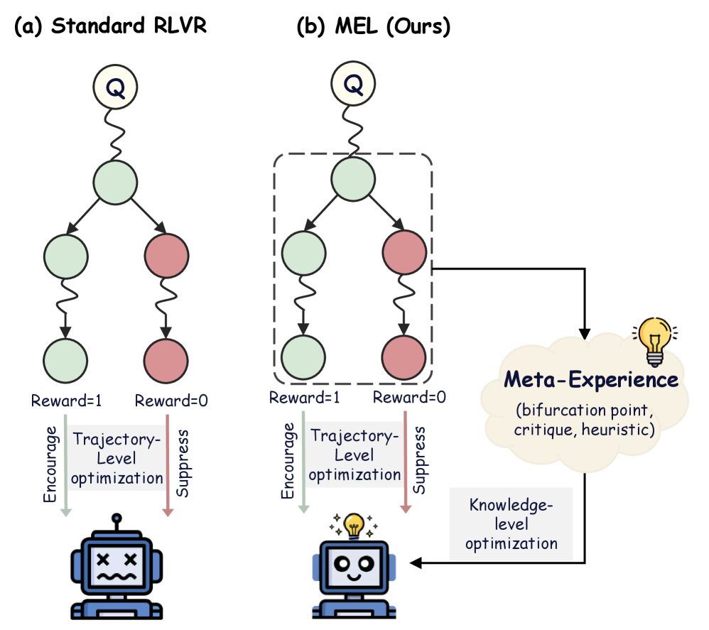
Figure 1: Paradigm comparison between standard RLVR and MEL, where MEL extends RLVR with an explicit knowledge-level learning loop.
Recently, a growing number of studies have explored integrating experience learning within the RLVR framework to address the above challenge. Early attempts, such as StepHint (Zhang et al., 2025c) utilizes experience as hints to elicit superior reasoning paths from the original problems, treating these trajectories as off-policy migration signals. However, the resulting off-policy deviation in response distribution can compromise optimization stability, undermining the theoretical benefits of on-policy reinforcement learning. To alleviate such instability, Scaf-GRPO (Zhang et al., 2025d) leverages superior models to generate multi-level knowledge-intensive experience, injecting them as on-policy prefixes for policy updates. Yet, while effective in teaching models to reason within specific experience-augmented distributions, such prefixes are unavailable during inference, inducing a severe distributional mismatch, thereby limiting performance gains. Critically, despite their differences, these approaches utilize retrieved experience primarily as external hints. While these strategies effectively elicit better reasoning paths during training, the resulting learning signals remain predominantly at the trajectory-level, yielding superficial corrections rather than intrinsic cognitive enhancements.
Building on this insight, we introduce the concept of meta-experience, elevating experience learning from trajectory-level instances to knowledge-level representations. Through contrastive analysis on paired correct and incorrect trajectories, we pinpoint the bifurcation points underlying reasoning failures and abstracts them into reusable meta-experiences. Accordingly, we propose M eta- E xperience L earning (MEL), a framework explicitly designed to enable knowledge-level internalization and reuse of meta-experiences. During training phase, MEL leverages meta-experiences to inject generalizable insights via a self-distillation mechanism, and internalizes them by minimizing the negative log-likelihood in the model’s parametric memory. As shown in Figure 1, MEL differs from standard RLVR, which relies on coarse-grained outcome rewards and treats correct and incorrect trajectories independently, by explicitly connecting them via meta-experiences. Hence, this process can be viewed as a language-modeled process-level reward signal, providing continuous and fine-grained guidance for improving reasoning capability. To further enhance stability and effectiveness during RLVR training, we propose empirical validation via replay, which uses meta-experiences as auxiliary in-context hints to assess their contribution to output accuracy. Meta-experiences that pass validation are integrated via negative log-likelihood minimization, while those that fail validation are excluded. In summary, our main contributions are as follows:
- We propose MEL, a novel framework that integrates self-distilled meta-experience with reinforcement learning, addressing the limitations of standard RLVR in error attribution and experience internalization by embedding these meta-experiences directly into the parametric memory of LLMs.
- We validate the effectiveness of MEL through extensive experiments on five challenging mathematical reasoning benchmarks across multiple LLM scales (4B, 8B, and 14B). Compared with both the vanilla GRPO baseline and the corresponding base models, MEL consistently improves performance across Pass@1, Avg@8, and Pass@8 metrics.
- Empirical results confirm that MEL seamlessly integrates with diverse paradigms (e.g., RFT, GRPO, REINFORCE++) to reshape reasoning patterns and elevate performance ceilings. Notably, these benefits exhibit strong scalability, becoming increasingly pronounced as model size expands.
<details>
<summary>x2.png Details</summary>
### Visual Description
## System Architecture Diagram: Meta-Experience Enhanced Reinforcement Learning Framework
### Overview
This image is a technical system architecture diagram illustrating a reinforcement learning (RL) framework that incorporates a "Meta-Experience" module for knowledge-level optimization. The system processes a question, generates trajectories via a policy model, and optimizes using both verifiable rewards and abstracted meta-knowledge. The diagram uses icons, labeled boxes, and directional arrows to depict data flow and component relationships.
### Components/Axes
The diagram is organized into three primary, interconnected modules:
1. **Policy Model (Left Section):**
* **Input:** "Question" (represented by a database icon).
* **Core Component:** A box labeled "Policy Model" with a brain/circuit icon.
* **Outputs:** A set of "Trajectories" labeled `Y₁`, `Y₂`, ..., `Y_G`.
* **Feedback Loops:** Receives two optimization signals: "Knowledge-Level Optimization" (dashed arrow from Meta-Experience) and "Trajectory-Level Optimization" (dashed arrow from the RL module).
2. **Meta-Experience (Top-Right Section):**
* **Input:** "Abstraction & Validation" (solid arrow from Policy Model, accompanied by a basket icon).
* **Core Components:** A dashed box containing three elements summed together:
* "Bifurcation Point `s*`" (represented by a node-link diagram with green and red nodes).
* "Critique `C`" (represented by a magnifying glass over a network).
* "Heuristic `H`" (represented by a notepad/clipboard icon).
* **Output:** "Knowledge-Level Optimization" (dashed arrow pointing back to the Policy Model).
3. **Reinforcement Learning with Verifiable Rewards (Bottom Section):**
* **Input:** The "Trajectories" (`Y₁` to `Y_G`) from the Policy Model.
* **Core Process:** A dashed box detailing the RL process:
* **"Contrastive Pair":** Shows two parallel sequences of states (circles). The top sequence has a green checkmark document icon, and the bottom has a red 'X' document icon, indicating a comparison between successful and unsuccessful trajectories.
* The state sequences are connected by arrows, showing transitions and interactions (crossing arrows between the two sequences).
* A "scales" icon at the end signifies evaluation or reward calculation.
* **Outputs:**
* **"Reward":** A vector `r₁`, `r₂`, ..., `r_G`.
* **"Advantage":** A vector `A₁`, `A₂`, ..., `A_G`, derived from the rewards via a "Group Norm" (Group Normalization) step.
* **Feedback Loop:** "Trajectory-Level Optimization" (dashed arrow pointing back to the Policy Model).
### Detailed Analysis
* **Data Flow:** The primary flow is: Question → Policy Model → Trajectories → RL Module → Rewards/Advantages. A secondary, higher-level flow is: Policy Model → Abstraction & Validation → Meta-Experience → Knowledge-Level Optimization → Policy Model.
* **Mathematical Notation:** The diagram uses specific symbols:
* `Y₁...Y_G`: Represents G generated trajectories.
* `s*`: Denotes a critical "Bifurcation Point" in the meta-experience.
* `C`: Represents a "Critique" component.
* `H`: Represents a "Heuristic" component.
* `r₁...r_G`: The reward signal for each of the G trajectories.
* `A₁...A_G`: The calculated advantage for each trajectory, used for policy gradient updates.
* **Spatial Layout:**
* The **Policy Model** is the central hub on the left.
* The **Meta-Experience** module is positioned in the upper right, visually separate but connected via abstraction.
* The **RL with Verifiable Rewards** module occupies the lower half, directly processing the policy's output.
* Dashed lines represent optimization/feedback pathways, while solid lines represent the primary data flow.
### Key Observations
1. **Dual Optimization Loops:** The system explicitly separates optimization into two levels: "Trajectory-Level" (from direct RL rewards) and "Knowledge-Level" (from abstracted meta-experience).
2. **Contrastive Learning:** The RL module uses a "Contrastive Pair" mechanism, suggesting it learns by comparing successful and failed trajectory pairs rather than from isolated rewards.
3. **Meta-Experience Composition:** The meta-experience is not a single entity but a composite of structural knowledge (`s*`), evaluative feedback (`C`), and procedural rules (`H`).
4. **Group Normalization:** The use of "Group Norm" to compute advantages from raw rewards indicates a normalization step to stabilize learning across the batch of G trajectories.
### Interpretation
This diagram depicts a sophisticated RL training architecture designed for complex reasoning tasks (implied by the "Question" input). The core innovation is the **Meta-Experience** module, which acts as a form of "learning to learn." Instead of the policy model only improving from trial-and-error rewards (trajectory-level), it also receives distilled, abstract knowledge about critical decision points (`s*`), evaluative critiques (`C`), and useful heuristics (`H`). This knowledge-level optimization likely helps the model generalize better and avoid repeating fundamental mistakes.
The **Contrastive Pair** setup in the RL module suggests the system is trained in environments where the difference between a good and bad action sequence is subtle, requiring direct comparison. The overall flow suggests an iterative process where the policy generates experiences, some are abstracted into durable meta-knowledge, and both the concrete rewards and abstract knowledge are used to refine the policy. This architecture would be particularly valuable in domains like scientific reasoning, strategic planning, or complex problem-solving where understanding underlying principles (meta-experience) is as important as achieving high rewards.
</details>
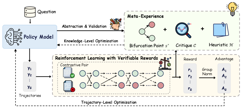
Figure 2: Overview of M eta- E xperience L earning (MEL), which constructs meta-experiences from contrastive pairs via abstraction and validation, thereby introducing an explicit knowledge-level learning loop on top of standard RLVR.
## 2 Related Work
#### Reinforcement Learning with Verifiable Rewards.
Reinforcement Learning with Verifiable Rewards (RLVR) leverages rule-based validators to provide deterministic feedback on models’ self-generated solutions (Lambert et al., 2024). Extensive research has systematically investigated RLVR, exploring how this paradigm improves the performance of complex reasoning (Jaech et al., 2024; Guo et al., 2025; Liu et al., 2025; Zhang et al., 2025b). The pioneering framework Group Relative Policy Optimization (GRPO) (Shao et al., 2024) estimates advantages via group-wise relative comparisons, eliminating the need for a separate value model. Building on this base method, recent studies have introduced a range of algorithmic variants to improve training stability and efficiency. For instance, REINFORCE++ (Hu, 2025) enhances stability through global advantage normalization; DAPO (Yu et al., 2025) mitigates entropy collapse and improves reward utilization via relaxed clipping and dynamic sampling; and GSPO (Zheng et al., 2025) reduces gradient estimation variance with sequence-level clipping. Despite these algorithmic advancements, a fundamental limitation persists: current RLVR methods predominantly rely on outcome-level rewards. This failure to assign fine-grained credit to specific knowledge points prevents the construction of reusable knowledge formation, fundamentally constraining the development of systematic and generalizable reasoning capabilities.
#### Experience Learning.
Recent studies have increasingly recognized that leveraging various forms of experience can substantially enhance LLM reasoning capabilities. One prominent line of research lies in test-time scaling methods, which store experience in external memory pools. For example, SpeedupLLM (Pan and Zhao, 2025) appends memories of previously reasoning traces as experience to accelerate inference, while Training Free GRPO (Cai et al., 2025) and ReasoningBank (Ouyang et al., 2025) distill accumulated experience into structured memory entries for retrieval-based augmentation. However, these approaches rely on ever-growing external memory, preventing the experience from being truly internalized and thus failing to substantively enhance intrinsic reasoning capabilities. Complementarily, another stream of research integrates experience directly into RL training as guiding signals. Methods such as Scaf-GRPO (Zhang et al., 2025d) and StepHint (Zhang et al., 2025c) employ external models to generate experiential hints, which are injected as prefixes or migration signals, to guide the policy toward higher-quality trajectories. Similarly, approaches like LUFFY (Yan et al., 2025) and SRFT (Fu et al., 2025) incorporate expert solution traces as additional experience. Despite improving exploration efficiency, these methods primarily induce trajectory-level imitation. Consequently, models become proficient at following specific patterns but fail to develop the meta-cognitive understanding required for establishing reusable knowledge structures.
## 3 Meta-Experience Learning
Human learning follows a recurrent cognitive cycle consisting of practice and verification, error attribution, and experience internalization, which in turn informs subsequent practice. Motivated by this cognitive process, we define meta-experience for LLMs as generalizable and reusable knowledge derived from accumulated reasoning trials, capturing both underlying knowledge concepts and common failure modes. Building on this notion, we propose M eta- E xperience L earning (MEL), a framework operating within the RLVR paradigm and expressly designed to internalize such self-distilled, knowledge-level insights into the model’s parametric memory. As illustrated in Figure 2, we first formalize the model exploration stage in RLVR (§ 3.1), then present the details of the Meta-Experience construction (§ 3.2). Finally, we describe the internalization mechanism (§ 3.3) for consolidating these insights into parametric memory, followed by the joint training objective for policy optimization (§ 3.4).
### 3.1 Explorative Rollout and Verifiable Feedback
Mirroring the “practice and check” phase in human learning, the RLVR framework engages the model in exploring potential solutions for reasoning tasks, while the environment serves as a deterministic verifier that provides verifiable feedback on the final answers. As mastering complex logic typically requires traversing the solution space through multiple attempts, we simulate this stochastic exploration by adopting the group rollout formulation from Group Relative Policy Optimization (GRPO) (Shao et al., 2024).
Formally, given a query $x$ sampled from the dataset $D$ , the policy model $π_θ$ performs stochastic exploration over the solution space and generates a group of $G$ independent reasoning trajectories $Y=\{y_1,y_2,\dots,y_G\}.$ A rule-based verifier then evaluates each trajectory using a verification function $V(·)$ , which compares the extracted final answer from $y_i$ against the ground-truth answer $y^*$ and assigns a binary outcome reward:
$$
r_i=I\big[V(y_i,y^*)\big]∈\{0,1\}. \tag{1}
$$
This process partitions the generated group $Y$ into two distinct subsets: the set of correct trajectories $Y^+=\{y_i\mid r_i=1\}$ and the set of incorrect trajectories $Y^-=\{y_i\mid r_i=0\}$ .
The coexistence of $Y^+$ and $Y^-$ under the same prompt distribution suggests that the model is capable of solving the task, while producing diverse reasoning trajectories. For our method, such diversity constitutes a beneficial property and serves a dual role. On the one hand, it supplies the variance necessary for effective policy updates in standard RLVR. On the other hand, it enables the extraction of knowledge-level meta-expression through systematic contrast between correct and incorrect reasoning outcomes.
### 3.2 Meta-Experience Construction
Prior studies (Xie et al., 2025; Khalifa et al., 2025; Huang et al., 2025) have shown that effective learning does not arise from merely knowing that a final answer is incorrect, but rather from identifying the specific bifurcation point at which the reasoning process deviates from the correct trajectory, a critical cognitive process known as error attribution. Building on this insight, we leverage pairs of correct and incorrect trajectories to localize reasoning errors and distill such bifurcation points into explicit meta-experiences.
#### Locating the Bifurcation Point.
To extract knowledge-level learning signals from the exploration results, we focus on identifying the bifurcation points where the reasoning logic diverges into an erroneous path. With the exploration results partitioned into $Y^+$ and $Y^-$ by the verifier, we construct a set of contrastive pairs $P_x=\{(y^+,y^-)\mid y^+∈Y^+, y^-∈Y^-\}$ for each query $x$ , whose contrast naturally exposes the specific errors in the reasoning process. Such contrastive analysis requires the presence of both positive and negative trajectories; accordingly, we only consider gradient-informative samples with non-empty $Y^+$ and $Y^-$ .
For fine-grained comparison within each pair, each trajectory $y$ can be formatted as a reasoning chain $y=(s_1,s_2,\dots,s_L,a)$ , where each $s_t$ denotes an atomic reasoning step and $a$ indicates the final answer. Since both trajectories originate from the same context, they typically share a correct reasoning path until a critical divergence step $s^*$ occurs.
Given deterministic verification signals and full access to the reasoning chains, identifying the bifurcation point can be viewed as a discriminative task that is easier than reasoning from scratch (Saunders et al., 2022; Swamy et al., 2025). Motivated by this observation, we task the policy model with analyzing each contrastive pair to identify the reasoning bifurcation point $s^*$ :
$$
\displaystyle s^* \displaystyle∼π_θ\big(·\mid I,x,y^+,y^-\big). \tag{2}
$$
Where $I$ denotes a structured instruction guiding introspective analysis.
#### Deep Diagnosis and Abstraction.
Identifying the bifurcation point $s^*$ localizes where the reasoning fails, serving as the raw material for subsequent learning. Anchored at $s^*$ , the policy model conducts a deep diagnostic analysis to contrast the strategic choices underlying the successful and failed trajectories. Specifically, the model examines the local reasoning context around $s^*$ to pinpoint the root cause of failure, such as violated assumptions, erroneous sub-goals, overlooked constraints, or the misuse of specific principles. Complementarily, it inspects the successful trajectory to uncover the mechanisms that prevented such pitfalls, including precise knowledge application, explicit constraint verification, coherent knowledge representations, or emergent self-correction behaviors. By jointly synthesizing these perspectives, the model distills the structural divergence between the correct and incorrect logic, crystallizing it into explicit knowledge. Formally, we model this diagnostic process as generating a critique $C$ that encapsulates the error attribution, the comparative strategic gap, and the corresponding corrective principle:
$$
\displaystyleC∼π_θ\big(·\mid I,x,y^+,y^-,s^*\big). \tag{3}
$$
To ensure generalization, it is imperative for the model to distill instance-specific critiques into abstract heuristics capable of guiding future reasoning. This abstraction mechanism systematically strips away context-dependent variables, mapping the concrete logic of success and failure onto a generalized space of preconditions and responses. Structurally, such heuristics synthesize abstract problem categorization with the corresponding reasoning principles, encompassing the essential knowledge points, theoretical theorems, and decision criteria. Crucially, they also demarcate error-prone boundaries, explicitly highlighting potential pitfalls or latent constraints associated with the specific problem class. We define the extraction of this heuristic knowledge $H$ as a generation process conditioned on the full critique context:
$$
H∼π_θ\big(·\mid I,x,y^+,y^-,s^*,C\big). \tag{4}
$$
Finally, we consolidate these components into a unified Meta-Experience tuple $M$ , which elevates experience learning from trajectory-level instances to knowledge-level representations.
$$
M=\big(s^*,C,H\big). \tag{5}
$$
This formulation enables meta-experiences to be reused across tasks that share analogous reasoning structures, serving as a fine-grained learning signal. By applying the extraction process across distinct contrastive pairs for a query $x$ , we construct a candidate pool of meta-experiences $D_M=\{(x,y^+_i,y^-_i,M_i)\}_i=1^N$ , where $N$ denotes the total number of meta-experiences derived from $x$ , and $(y^+_i,y^-_i)$ represents the specific contrastive pair used to derive $M_i$ .
#### Empirical Validation via Replay.
Closing the cognitive loop requires re-instantiating theoretical insights derived from past failures in future problem-solving to assess their validity. We recognize that the raw meta-experience $M$ may still suffer from intrinsic hallucinations or causal misalignment. To mitigate this, we conduct empirical verification by incorporating the extracted tuple $M$ as short-term working memory into the prompt, thereby guiding the model to re-attempt the original query $x$ . This procedure tests whether the injected meta-experience can effectively steer the model away from the previously identified bifurcation point $s^*$ and toward a correct reasoning trajectory.
We retain a meta-experience only if the corresponding replay trajectory $y_val∼π_θ(·\mid x,M)$ satisfies the verifier by producing the correct answer.
$$
D_M^*=≤ft\{(x,y^+,y^-,M)∈D_M \middle| I\big[V≤ft(y_val,y^*\right)=1\big]\right\}. \tag{6}
$$
Consequently, this empirical validation preserves only high-quality meta-experiences for integration into parametric long-term memory, guaranteeing the reliability of the supervision signals used in the subsequent optimization phase.
### 3.3 Internalization Mechanism
The verified meta-experiences $D_M^*$ constitute a high-quality reservoir of reasoning guidance. However, treating these insights solely as retrieval-augmented memory imposes a substantial computational burden during the inference forward pass, as it necessitates processing elongated contexts for every query. To overcome this limitation, we propose to transfer these insights from the transient context window to the model’s parametric memory. Unlike the finite context buffer, the model parameters offer a virtually unlimited capacity for accumulating diverse meta-experiences, allowing the policy to internalize vast amounts of reasoning patterns without incurring inference-time latency.
We establish this internalization process as a self-distilled paradigm, where the model learns from its own verified experiences. Specifically, we employ fine-tuning based on the token-averaged negative log-likelihood (NLL) objective to compile the meta-experiences into the policy’s weights. Formally, given the retrospective context $C_retro=[I,x,y^+,y^-]$ , the internalization loss is defined as:
$$
\displaystyleL_NLL(θ)=- \displaystyleE_(x,y^+,y^{-,M^*)∼D_M^*} \displaystyle\Big[\frac{1}{|M^*|}∑_t=1^|M^*|\logπ_θ(M^*_t\mid C_retro,M^*_<t)\Big] \displaystyle=- \displaystyleE_x∼D, \{y_i\_i=1^G∼π_θ_{old}(·\mid x)} \displaystyle\Bigg[E_(y^+,y^{-,M^*)∼T(x,\{y_i\}_i=1^G)} \displaystyle\Big[\frac{1}{|M^*|}∑_t=1^|M^*|\logπ_θ(M^*_t\mid C_retro,M^*_<t)\Big]\Bigg] \tag{7}
$$
where $T(·)$ represents the stochastic construction process detailed in § 3.2.
Based on this formulation, the internalization process can be viewed as a specialized sampling form within the RLVR framework. By inverting the loss, we define the Meta-Experience Return $R_MEL$ as the expected log-likelihood over the stochastically constructed verification set:
$$
\displaystyleR_MEL \displaystyle=E_(y^+,y^{-,M^*)∼T(x,\{y_i\}_i=1^G)} \displaystyle\Bigg[\frac{1}{|M^*|}∑_t=1^|M^*|\logπ_θ(M^*_t\mid C_retro,M^*_<t)\Bigg]. \tag{8}
$$
### 3.4 Joint Training Objective
Table 1: Main Results Comparison. Comparison of Pass@1, Avg@8, and Pass@8 accuracy (%) across different model scales. The best results within each model scale are marked in bold.
| Method Qwen3-4B-Base | AIME 2024 Pass@1 | AIME 2025 Avg@8 | AMC 2023 Pass@8 | Pass@1 | Avg@8 | Pass@8 | Pass@1 | Avg@8 | Pass@8 |
| --- | --- | --- | --- | --- | --- | --- | --- | --- | --- |
| Baseline | 13.33 | 9.90 | 30.00 | 10.00 | 6.56 | 23.33 | 45.00 | 42.73 | 72.50 |
| GRPO | 13.33 | 18.33 | 30.00 | 6.67 | 17.50 | 30.00 | 57.50 | 58.13 | 85.00 |
| MintCream MEL | 20.00 | 20.83 | 33.00 | 16.67 | 18.33 | 33.00 | 60.00 | 60.31 | 87.50 |
| Qwen3-8B-Base | | | | | | | | | |
| Baseline | 6.67 | 10.00 | 26.67 | 13.33 | 15.00 | 33.33 | 65.00 | 52.50 | 87.50 |
| GRPO | 16.67 | 24.58 | 43.33 | 20.00 | 20.83 | 36.67 | 67.50 | 69.06 | 87.50 |
| MintCream MEL | 30.00 | 25.42 | 60.00 | 23.33 | 23.33 | 36.67 | 70.00 | 70.31 | 90.00 |
| Qwen3-14B-Base | | | | | | | | | |
| Baseline | 13.33 | 10.83 | 36.67 | 6.66 | 9.58 | 33.33 | 60.00 | 51.25 | 82.50 |
| GRPO | 30.00 | 35.41 | 56.67 | 33.33 | 24.17 | 43.33 | 75.00 | 75.94 | 95.00 |
| MintCream MEL | 33.33 | 35.83 | 60.00 | 36.67 | 30.00 | 46.67 | 82.50 | 82.81 | 95.00 |
| Method Qwen3-4B-Base | MATH 500 Pass@1 | OlympiadBench Avg@8 | Average Pass@8 | Pass@1 | Avg@8 | Pass@8 | Pass@1 | Avg@8 | Pass@8 |
| --- | --- | --- | --- | --- | --- | --- | --- | --- | --- |
| Baseline | 74.20 | 65.74 | 89.60 | 39.17 | 35.37 | 60.38 | 36.34 | 32.06 | 55.16 |
| GRPO | 81.80 | 82.20 | 93.00 | 48.51 | 48.46 | 67.21 | 41.56 | 44.92 | 61.04 |
| MintCream MEL | 82.20 | 82.30 | 93.80 | 48.51 | 49.48 | 69.73 | 45.48 | 46.25 | 63.41 |
| Qwen3-8B-Base | | | | | | | | | |
| Baseline | 77.00 | 73.40 | 91.40 | 44.51 | 39.41 | 64.09 | 41.30 | 38.06 | 60.60 |
| GRPO | 84.40 | 86.28 | 95.40 | 53.56 | 54.60 | 73.74 | 48.43 | 51.07 | 67.33 |
| MintCream MEL | 86.60 | 86.70 | 96.20 | 54.01 | 55.60 | 73.00 | 52.79 | 52.27 | 71.17 |
| Qwen3-14B-Base | | | | | | | | | |
| Baseline | 80.80 | 74.15 | 93.60 | 45.25 | 40.50 | 65.58 | 41.21 | 37.26 | 62.34 |
| GRPO | 85.00 | 88.35 | 96.40 | 58.16 | 58.46 | 74.78 | 56.30 | 56.47 | 73.24 |
| MintCream MEL | 90.80 | 90.80 | 97.20 | 61.87 | 60.90 | 75.82 | 61.03 | 60.07 | 74.94 |
To simultaneously encourage solution exploration and consolidate the internalized meta-experiences, achieving dual optimization across trajectory-level behaviors and knowledge-level representations, we train the policy model $π_θ$ using a joint optimization objective. To simultaneously encourage solution exploration and consolidate the internalized meta-experiences, achieving dual optimization across trajectory-level behaviors and knowledge-level representations, we train the policy model $π_θ$ using a joint optimization objective. This objective synergizes the RLVR signal derived from diverse explorative rollouts with the supervised signal distilled from high-quality meta-experiences:
$$
J(θ)=J_RLVR(θ)+J_MEL(θ). \tag{9}
$$
We adopt GRPO (Shao et al., 2024) as the RLVR component and compute group-normalized advantages by standardizing rewards within the sampled group and broadcast them to each token. Let $y_i,t$ denote the $t$ -th token in trajectory $y_i$ and $y_i,<t$ , the corresponding prefix. Substituting the definition of $R_MEL$ from Eq. 8, the joint objective in Eq. 9 is explicitly expanded as:
$$
\displaystyleJ(θ)= \displaystyleE_x∼D, \{y_i\_i=1^G∼π_θ_{old}(·\mid x)} \displaystyle\Big[\frac{1}{G}∑_i=1^G\frac{1}{|y_i|}∑_t=1^|y_i|\min\Big(ρ_i,t(θ)\hat{A}_i,t, \displaystyleclip\big(ρ_i,t(θ),1-ε,1+ε\big)\hat{A}_i,t\Big)+R_MEL\Big]. \tag{10}
$$
Although derived from a log-likelihood objective, its optimization gradient is mathematically equivalent to a policy gradient update where the reward signal is a constant positive scalar. Consequently, the total objective $J(θ)$ can be unified as maximizing the expected cumulative return of a hybrid reward function. In this unified view, the meta-experiences function as a dense process reward model.
Unlike the sparse outcome rewards in standard RLVR that only evaluate the final correctness, $R_MEL$ provides explicit, step-by-step reinforcement for the reasoning process itself. This ensures that the model not only pursues correct outcomes via broad exploration but is also continuously shaped by the dense supervision of its own successful cognitive patterns, effectively bridging the gap between trajectory-level search and token-level knowledge encoding.
## 4 Experiments
#### Datasets.
We train our model on the DAPO-Math-17k dataset (Yu et al., 2025) and evaluate it on five challenging mathematical reasoning benchmarks: AIME24, AIME25, AMC23 (Li et al., 2024), MATH500 (Hendrycks et al., 2021), and OlympiadBench (He et al., 2024).
#### Setups.
All reinforcement learning training is conducted using the VERL framework (Sheng et al., 2024) on 8 $×$ H20 GPUs, with Math-Verify providing rule-based outcome verification. During training, we sample 8 responses per prompt at a temperature of 1.0 with a batch size of 128. Optimization uses a learning rate of $1× 10^-6$ and a mini-batch size of 128. For evaluation, we report Pass@1 at temperature 0, and Avg@8 and Pass@8 at temperature 0.6.
#### Models and Baselines.
To demonstrate the general applicability of MEL, we conduct experiments across a diverse range of model scales, including Qwen3-4B-Base, Qwen3-8B-Base, and Qwen3-14B-Base (Yang et al., 2025). We adopt GRPO (Shao et al., 2024) as the base reinforcement learning algorithm for MEL, and thus perform a direct and controlled comparison between the vanilla GRPO and our meta-experience learning approach.
### 4.1 Experimental Results
As shown in Table 1, MEL achieves consistent and significant improvements over vanilla GRPO and the basemodel across multiple benchmarks and model scales. We report three complementary metrics: Pass@1 reflects one-shot reliability, Avg@8 measures the average performance over 8 samples, and Pass@8 reports the best-of-8 success rate.
First, the gains in Pass@1 demonstrate that MEL substantially enhances the model’s confidence in following correct reasoning paths. Across all model scales, it achieves a consistent improvement of 3.92–4.73% over the strong GRPO baseline. This indicates that MEL effectively internalizes the explored insights into the model’s parametric memory. By consolidating these successful reasoning patterns, the model generates high-confidence solutions, markedly reducing the need for extensive test-time sampling. This reliability is further corroborated by the gains in Avg@8, which reveal that MEL significantly enhances reasoning consistency and output stability. High performance on this metric supports our hypothesis that internalized meta-experiences function as intrinsic process-level guidance, continuously steering the generation toward valid logic and effectively reducing variance across sampled outputs. Finally, the sustained gains in Pass@8 suggest that learning from meta-experience does not harm exploration; instead, it expands the reachable solution space and raises the upper bound of best-of- $k$ performance.
### 4.2 Training Dynamics and Convergence Analysis
<details>
<summary>x3.png Details</summary>
### Visual Description
## Line Charts: Training Reward Comparison of GRPO vs. MEL Methods Across Model Sizes
### Overview
The image displays three horizontally arranged line charts comparing the training performance of two methods, GRPO and MEL, across three different model sizes (4B, 8B, and 14B parameters). Each chart plots "Training Reward" against "Training Steps," showing the learning curves for both methods. The charts indicate that MEL consistently achieves a higher training reward than GRPO at all model scales, and performance improves with larger model sizes.
### Components/Axes
* **Chart Layout:** Three separate line charts arranged side-by-side.
* **X-Axis (All Charts):** Labeled "Training Steps". Major tick marks are at intervals of 20, from 0 to 120.
* **Y-Axis (Left Chart - 4B):** Labeled "Training Reward". Scale ranges from approximately 0.15 to 0.45. Major gridlines are at 0.2, 0.3, and 0.4.
* **Y-Axis (Middle Chart - 8B):** Labeled "Training Reward". Scale ranges from approximately 0.2 to 0.6. Major gridlines are at 0.2, 0.3, 0.4, 0.5, and 0.6.
* **Y-Axis (Right Chart - 14B):** Labeled "Training Reward". Scale ranges from approximately 0.2 to 0.7. Major gridlines are at 0.2, 0.3, 0.4, 0.5, 0.6, and 0.7.
* **Legend (Each Chart):** Positioned in the top-left corner of each plot area.
* **Left Chart (4B):** "GRPO (4B)" (blue line), "MEL (4B)" (red line).
* **Middle Chart (8B):** "GRPO (8B)" (blue line), "MEL (8B)" (red line).
* **Right Chart (14B):** "GRPO (14B)" (blue line), "MEL (14B)" (red line).
* **Data Series:** Each chart contains two primary lines (blue for GRPO, red for MEL) with a lighter, semi-transparent shaded area around each line, likely representing variance or standard deviation across multiple runs.
### Detailed Analysis
**Left Chart (4B Models):**
* **Trend:** Both lines show a steep initial increase in reward from step 0 to ~40, followed by a more gradual, noisy ascent.
* **GRPO (4B) - Blue Line:** Starts at ~0.15. Reaches ~0.3 at step 40. Ends at approximately 0.38 at step 120.
* **MEL (4B) - Red Line:** Starts slightly above GRPO at ~0.16. Maintains a consistent lead. Reaches ~0.33 at step 40. Peaks near 0.42 around step 110 before a slight dip, ending at ~0.40 at step 120.
* **Relationship:** The MEL line is positioned above the GRPO line for the entire duration after the first few steps.
**Middle Chart (8B Models):**
* **Trend:** Similar rapid initial learning phase, with both curves plateauing at a higher reward level than the 4B models.
* **GRPO (8B) - Blue Line:** Starts at ~0.20. Rises to ~0.35 by step 40. Shows a steady climb to end at approximately 0.46 at step 120.
* **MEL (8B) - Red Line:** Starts at ~0.22. Rises sharply to ~0.45 by step 40. Continues a noisy ascent, peaking near 0.52 around step 110, and ending at ~0.50 at step 120.
* **Relationship:** The performance gap between MEL and GRPO is more pronounced here than in the 4B chart.
**Right Chart (14B Models):**
* **Trend:** The highest overall reward values. Both methods show strong initial gains and maintain an upward trend throughout.
* **GRPO (14B) - Blue Line:** Starts at ~0.23. Reaches ~0.40 by step 40. Climbs to end at approximately 0.52 at step 120.
* **MEL (14B) - Red Line:** Starts at ~0.24. Reaches ~0.50 by step 40. Continues to rise, peaking near 0.62 around step 110, and ending at ~0.60 at step 120.
* **Relationship:** MEL maintains a significant and consistent lead over GRPO. The final reward for MEL (14B) is notably higher than the peak rewards of both 8B models.
### Key Observations
1. **Consistent Superiority of MEL:** In all three charts, the red MEL line is positioned above the blue GRPO line after the initial training steps, indicating higher training reward.
2. **Positive Correlation with Model Size:** The maximum achieved reward increases with model size for both methods. The y-axis scales shift upward from left (4B) to right (14B).
3. **Learning Curve Shape:** All curves exhibit a characteristic rapid initial learning phase (steps 0-40) followed by a slower, noisier improvement phase.
4. **Variance:** The shaded regions indicate non-trivial variance in the training process, but the separation between the MEL and GRPO means remains clear despite this noise.
5. **Peak Performance:** MEL appears to peak slightly before the final step (around step 110) in the 4B and 8B charts, with a minor decline thereafter, while GRPO often continues a slight upward trend to the end.
### Interpretation
The data strongly suggests that the MEL training method is more effective than GRPO for maximizing the defined "Training Reward" metric across the tested model scales (4B to 14B parameters). The consistent performance gap implies that MEL's algorithmic approach leads to more efficient or effective learning.
The positive scaling with model size is expected, as larger models typically have greater capacity. However, the fact that MEL's advantage is maintained and even appears to widen slightly at larger scales (the gap between lines is visually larger in the 14B chart) indicates that its benefits are robust and potentially complementary to increased model capacity.
The noisy ascent after step 40 is typical of reinforcement learning or stochastic optimization processes, where progress is not perfectly monotonic. The slight late-stage dip for MEL in the smaller models could suggest the onset of overfitting to the training reward signal or increased instability, but this trend is not as clear in the 14B model, which continues to perform strongly.
**In summary, the charts provide empirical evidence that, under the conditions of this experiment, MEL is a superior training method to GRPO, and its advantages scale with model size.**
</details>
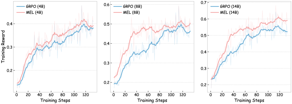
Figure 3: Training curves comparing GRPO and MEL.
To understand the mechanisms driving the performance gains under MEL, we monitored the training dynamics and validation performance in Figures 3 and 6 – 8.
Vanilla GRPO methods often struggle to obtain positive reinforcement in the early stages, particularly when initial performance is low, due to the sparsity of outcome-based rewards. As illustrated in the training curve, vanilla GRPO exhibits a relatively slow ascent during the initial phase. In contrast, MEL demonstrates a sharp, rapid trajectory growth immediately from the onset of training. This acceleration is attributed to the internalized meta-experience return, $R_MEL$ . By functioning as a dense, language-modeling process reward, $R_MEL$ continuously provides informative gradient signals for every reasoning step, even when successful trajectories yielding positive reinforcement are scarce.
Beyond sample efficiency, MEL achieves a consistently higher performance upper bound. The training curves show that the average reward of MEL consistently surpasses that of vanilla GRPO throughout the entire training process. Crucially, the downstream validation trajectories reveal that even as performance growth begins to plateau in the later stages, MEL maintains a distinct and sustained advantage over the baseline. This phenomenon demonstrates that the internalization of meta-experiences empowers the model to effectively navigate and explore more complex, long-horizon solutions that remain inaccessible to the baseline.
<details>
<summary>x4.png Details</summary>
### Visual Description
\n
## Screenshot: Geometry Problem Discussion with Comparative Solutions
### Overview
The image is a screenshot of a technical discussion interface, likely from an AI or educational platform, presenting a geometry problem and two different solution attempts (labeled "GRPO" and "MEL"). A "Meta-Experience" panel on the right provides critical analysis of a common error. The core problem involves finding the length of a side of a triangle formed by tangency points on the circumcircle of a given triangle.
### Components/Axes
The image is segmented into four primary regions:
1. **Top-Left (Question Box):** Contains the problem statement.
2. **Left Column (GRPO Response):** A step-by-step solution attempt that contains an error.
3. **Right Column (MEL Response):** An alternative, correct solution approach.
4. **Top-Right (Meta-Experience Panel):** A diagnostic box analyzing the failure mode seen in the GRPO response.
**Textual Content & Transcription:**
**1. Question Box (Top-Left):**
> Triangle ABC has AB = 4, BC = 5 and CA = 6. Points A', B', C' are such that B'C' is tangent to the circumcircle of ABC at A', C'A' is tangent to the circumcircle of ABC at B', and A'B' is tangent to the circumcircle of ABC at C'. Find the length B'C'.
**2. GRPO Response (Left Column):**
* **Step 1:** Calculates semi-perimeter `s = (4+5+6)/2 = 7.5` and area using Heron's formula: `Area = sqrt(s(s-a)(s-b)(s-c)) = sqrt(7.5*3.5*2.5*1.5)`.
* **Step 2:** Introduces the concept of a "tangential triangle" and states formulas: `a' = 2R sin(A/2)`, `b' = 2R sin(B/2)`, `c' = 2R sin(C/2)`, where a', b', c' are sides of the tangential triangle and a, b, c are sides of the original triangle.
* **Conclusion:** "The length B'C' is \boxed{2}". This answer is incorrect based on the subsequent analysis.
**3. MEL Response (Right Column):**
* **Step 1:** Recalls properties: "Tangent to a Circle: The tangent to a circle is perpendicular to the radius at the point of tangency." and "Circumcircle: The circle that passes through all three vertices of a triangle."
* **Step 2:** Proposes finding the circumradius `R` first using the formula `R = abc / (4K)`, where `K` is the area.
* **Step 3:** Derives a relationship: "Based on the calculations and the relationships I've explored, I think the length B'C' is related to the circumradius and the angles of the triangle and can be calculated using the formula: `B'C' = 2R sin(θ)` where θ is the angle between the tangent lines. **Using this formula, θ must be the full geometric angle that directly governs the opening of the segment, not a derived half-angle. In this case, θ is the angle at A.**"
* **Final Answer:** "Final Answer: \boxed{5}". This is the correct answer.
**4. Meta-Experience Panel (Top-Right):**
* **Title:** "Meta-Experience in Early Stage"
* **Point 4 - Failure Analysis & Error Pattern Recognition:**
* **Failure Point:** "The error occurs in the use of the circumcircle formula. The formula should be `BC = 2R sin(∠BAC)`, but the incorrect solution uses `BC = 2R sin(A/2)`."
* **Root Cause:** "This mistake is due to a conceptual confusion in formula application."
* **Point 4 - Subject Heuristics (Unreliable Experiences):**
* **Angle-Geometry Consistency Rule:** "When using a formula of the form `2R sin θ` in a circumcircle, always ensure that **θ is the full geometric angle** subtended by the chord, not a derived half-angle."
* **Formula-Geometry Consistency Rule:** "When using trigonometric formulas for lengths on the circumcircle, confirm that the chosen angle corresponds exactly to the geometric angle being calculated **in order to avoid errors caused by half-angle substitution**."
### Detailed Analysis
The image documents a pedagogical moment contrasting a common error with its correction.
* **The Error (GRPO):** The solution incorrectly applies a formula involving `sin(A/2)`. This likely stems from misapplying a formula related to the **incircle** or the **distance from the incenter to a vertex** (which is `r / sin(A/2)`) to a problem about the **circumcircle** and **tangential triangle**.
* **The Correction (MEL & Meta-Experience):** The correct formula for the side of the tangential triangle opposite vertex A is `B'C' = 2R sin(A)`. The Meta-Experience panel explicitly diagnoses the error as confusing the full angle `A` with the half-angle `A/2`.
* **Implicit Calculation:** To reach the answer `5`, one must:
1. Calculate the area `K` of triangle ABC (sides 4,5,6) using Heron's formula: `K = √(7.5*3.5*2.5*1.5) = √(98.4375) ≈ 9.92`.
2. Calculate the circumradius `R = (abc)/(4K) = (4*5*6)/(4*9.92) ≈ 120/39.68 ≈ 3.024`.
3. Calculate angle A using the Law of Cosines: `cos(A) = (b² + c² - a²)/(2bc) = (6² + 4² - 5²)/(2*6*4) = (36+16-25)/48 = 27/48 = 0.5625`. Thus, `A ≈ 55.77°`.
4. Apply the correct formula: `B'C' = 2R sin(A) ≈ 2 * 3.024 * sin(55.77°) ≈ 6.048 * 0.827 ≈ 5.0`.
### Key Observations
1. **Spatial Layout:** The incorrect solution (GRPO) is presented on the left, the correct solution (MEL) on the right, and the meta-cognitive analysis is placed prominently at the top-right, creating a visual flow from error to correction to explanation.
2. **Emphasis on Process:** Both solution attempts show step-by-step reasoning, not just the final answer. The MEL response explicitly highlights the critical conceptual point about the angle in its derivation.
3. **Diagnostic Clarity:** The Meta-Experience panel uses clear, bolded text to state the rules that prevent the error, serving as a takeaway lesson.
4. **Visual Cues:** The use of lightbulb and brain icons next to the Meta-Experience and MEL sections, respectively, symbolically associates the correct approach with insight and reasoning.
### Interpretation
This image is more than a math problem; it's a case study in **technical reasoning and error analysis**. It demonstrates:
* **The Pitfall of Formula Misapplication:** The GRPO error is a classic example of applying a memorized formula without verifying its geometric context. The half-angle formula is seductive but wrong here.
* **The Importance of Foundational Rules:** The Meta-Experience section elevates the discussion from a single problem to a general principle: always match the trigonometric function's angle to the actual geometric angle in the diagram. This is a critical skill in geometry and engineering.
* **Comparative Learning:** By presenting both the flawed and correct reasoning side-by-side, the image facilitates deeper understanding. The viewer can trace the exact point of divergence (the choice of angle) and see its consequence.
* **Implicit Data:** The problem itself contains all necessary data (side lengths 4,5,6). The solutions show how to transform this raw data into a derived quantity (length B'C' = 5) through a chain of geometric and trigonometric relationships, highlighting the interconnectedness of mathematical concepts.
In essence, the image captures a moment of technical education where a specific mistake is used to teach a universal lesson about precision in mathematical modeling.
</details>
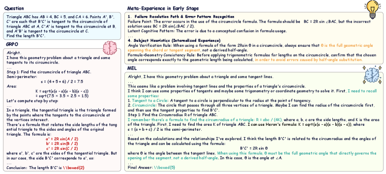
Figure 4: Case study comparing GRPO and MEL, with visualization of meta-experience in early stage.
### 4.3 How Meta-Experience Shapes Reasoning Patterns
To investigate how MEL shapes the model’s cognitive processes beyond numerical metrics, we conduct a qualitative analysis comparing the reasoning trajectories of MEL and the baseline GRPO model, as visualized in Figure 4.
A distinct behavioral divergence is observed from the onset of the solution. While the GRPO baseline tends to prioritize immediate execution through direct numerical operations, MEL adopts a structured preparatory strategy by explicitly outlining relevant theorems and formulas. Although the direct approach may appear efficient for simple queries, it increases the susceptibility to errors in complex tasks due to the lack of a holistic view of problem constraints.
Notably, MEL exhibits an emergent cognitive behavior. When applying specific theorems, it spontaneously activates internalized “bitter lessons” as endogenous safeguards to regulate its actions. These active signals effectively reduce reasoning drift by encouraging earlier constraint checking and consistent self-correction when the model enters uncertain regions.
### 4.4 Generality Across Learning Paradigms
<details>
<summary>x5.png Details</summary>
### Visual Description
## Radar Chart: OlympiaBenchmark Performance Comparison
### Overview
The image displays a pentagonal radar chart (spider chart) titled "OlympiaBenchmark." It compares the performance of three different methods or models across five distinct evaluation axes. The chart uses colored lines to represent each method, with the area enclosed by each line indicating its overall performance profile.
### Components/Axes
* **Chart Type:** Radar Chart (Pentagonal)
* **Title:** "OlympiaBenchmark" (centered at the top).
* **Axes (5):** Radiating from the center to the vertices of the pentagon. Each axis represents a different benchmark, model, or task. Labels are placed at the outer end of each axis.
1. **Top Vertex:** `Qwen2.5-72B`
2. **Top-Right Vertex:** `4o-mini`
3. **Bottom-Right Vertex:** `4o-mini-0125`
4. **Bottom-Left Vertex:** `AWQ23`
5. **Top-Left Vertex:** `MATO23`
* **Axis Scale:** Each axis has numerical markers from `0` (center) to `100` (outer edge), with labeled increments at `20`, `40`, `60`, and `80`.
* **Legend:** Located at the bottom center of the chart. It defines three data series:
* **Blue Line/Square:** `Qwen2.5-72B`
* **Green Line/Square:** `MFT`
* **Red Line/Square:** `MFT + WE`
### Detailed Analysis
The chart plots three data series, each forming a closed polygon. Performance values are estimated based on where each line intersects an axis relative to the scale markers.
**1. Data Series: Qwen2.5-72B (Blue Line)**
* **Visual Trend:** Forms a moderately sized, relatively symmetric pentagon, indicating balanced but not exceptional performance across all benchmarks.
* **Estimated Values per Axis:**
* `Qwen2.5-72B` axis: ~80
* `4o-mini` axis: ~60
* `4o-mini-0125` axis: ~40
* `AWQ23` axis: ~60
* `MATO23` axis: ~80
**2. Data Series: MFT (Green Line)**
* **Visual Trend:** Forms an irregular shape that peaks sharply on the `Qwen2.5-72B` axis but contracts significantly on the `4o-mini` and `4o-mini-0125` axes, suggesting specialized or inconsistent performance.
* **Estimated Values per Axis:**
* `Qwen2.5-72B` axis: ~90 (highest point for this series)
* `4o-mini` axis: ~50
* `4o-mini-0125` axis: ~30 (lowest point for this series)
* `AWQ23` axis: ~70
* `MATO23` axis: ~60
**3. Data Series: MFT + WE (Red Line)**
* **Visual Trend:** Forms the largest, most expansive pentagon, enclosing the other two series on almost all axes. This indicates the highest and most consistent overall performance.
* **Estimated Values per Axis:**
* `Qwen2.5-72B` axis: ~95
* `4o-mini` axis: ~70
* `4o-mini-0125` axis: ~60
* `AWQ23` axis: ~80
* `MATO23` axis: ~85
### Key Observations
1. **Performance Hierarchy:** The `MFT + WE` (red) series consistently outperforms or matches the `MFT` (green) series on every axis. The `Qwen2.5-72B` (blue) series generally sits between them or is surpassed by both.
2. **Largest Improvement:** The most dramatic performance gain from `MFT` to `MFT + WE` occurs on the `4o-mini-0125` axis, where the score approximately doubles from ~30 to ~60.
3. **Specialization vs. Generalization:** The `MFT` method shows a strong specialization for the `Qwen2.5-72B` benchmark but underperforms on `4o-mini-0125`. The addition of "WE" appears to correct this weakness, leading to a more generalized, high-performance profile.
4. **Baseline Comparison:** The baseline `Qwen2.5-72B` model shows its strongest performance on its own namesake axis (`~80`) and on `MATO23` (`~80`), but is notably weaker on `4o-mini-0125` (`~40`).
### Interpretation
This radar chart from the "OlympiaBenchmark" visually argues for the superiority of the `MFT + WE` method. The data suggests that while the `MFT` technique alone offers targeted improvements (especially on the `Qwen2.5-72B` task), it introduces significant performance regressions on other tasks like `4o-mini-0125`. The critical insight is that the "WE" component acts as a crucial stabilizer or enhancer, mitigating MFT's weaknesses and boosting its strengths across the board. The resulting `MFT + WE` profile is not just an incremental improvement but a transformation into a robust, state-of-the-art solution that dominates the evaluated landscape. The chart effectively communicates that combining MFT with WE yields a system that is both more powerful and more reliable than its individual components or the baseline model.
</details>
<details>
<summary>x6.png Details</summary>
### Visual Description
## Radar Chart: Olympic Games Performance Comparison
### Overview
The image displays a radar chart (spider chart) comparing the performance of three different methods or systems across five Olympic Games events. The chart is titled "Olympic Games" at the top center, though the title is partially cropped. The data is presented as a polygon for each series, with vertices plotted on five axes radiating from the center.
### Components/Axes
* **Chart Type:** Radar Chart (Spider Chart)
* **Title:** "Olympic Games" (partially visible at the top).
* **Axes (5):** Each axis represents a specific Olympic Games edition, labeled at the outer end:
1. `ATHENS04` (Top-Left)
2. `BEIJING08` (Top-Right)
3. `LONDON12` (Right)
4. `RIO16` (Bottom-Right)
5. `TOKYO20` (Bottom-Left)
* **Scale:** Concentric circles represent a numerical scale from 0 (center) to 100 (outermost ring). Major gridlines are marked at 20, 40, 60, 80, and 100.
* **Legend:** Located at the bottom center of the chart. It defines three data series:
* **Blue Line/Symbol:** `Quest3D-Base`
* **Green Line/Symbol:** `REDFORCE-CE`
* **Red Line/Symbol:** `REDFORCE-CE + AE`
### Detailed Analysis
The chart plots three distinct polygons, each connecting data points across the five Olympic axes. The values are approximate, read from the chart's scale.
**1. Quest3D-Base (Blue Line - Innermost Polygon):**
* **Trend:** This series forms the smallest polygon, indicating the lowest performance scores across all events. It shows a moderate peak at LONDON12.
* **Approximate Data Points:**
* ATHENS04: ~40
* BEIJING08: ~50
* LONDON12: ~60
* RIO16: ~55
* TOKYO20: ~45
**2. REDFORCE-CE (Green Line - Middle Polygon):**
* **Trend:** This series consistently outperforms Quest3D-Base, forming a larger polygon. It follows a similar shape, peaking at LONDON12.
* **Approximate Data Points:**
* ATHENS04: ~60
* BEIJING08: ~70
* LONDON12: ~80
* RIO16: ~75
* TOKYO20: ~65
**3. REDFORCE-CE + AE (Red Line - Outermost Polygon):**
* **Trend:** This series demonstrates the highest performance, forming the largest polygon. It maintains a significant and relatively consistent lead over the other two methods, with its peak also at LONDON12.
* **Approximate Data Points:**
* ATHENS04: ~80
* BEIJING08: ~90
* LONDON12: ~95
* RIO16: ~90
* TOKYO20: ~85
### Key Observations
1. **Consistent Hierarchy:** There is a clear and consistent performance hierarchy across all five Olympic Games: `REDFORCE-CE + AE` > `REDFORCE-CE` > `Quest3D-Base`. The polygons do not cross.
2. **Peak Performance:** All three methods achieve their highest score at the `LONDON12` axis.
3. **Performance Gap:** The performance gap between `REDFORCE-CE` and `Quest3D-Base` is roughly 20 points on the scale. The additional "+ AE" component provides a further boost of approximately 15-20 points over `REDFORCE-CE` alone.
4. **Shape Similarity:** The three polygons have a similar overall shape, suggesting that the relative difficulty or scoring pattern of the Olympic Games events affects all methods in a comparable way.
### Interpretation
This radar chart visually demonstrates the progressive improvement of a technical system across iterations. `Quest3D-Base` likely represents a baseline model. `REDFORCE-CE` shows a significant upgrade, and `REDFORCE-CE + AE` represents the most advanced version, where "AE" likely stands for an additional enhancement module (e.g., "Auto-Encoder," "Augmentation Engine").
The data suggests that the enhancements are robust and generalize well across different "Olympic Games" scenarios (which, in a technical context, likely represent different benchmark datasets, challenge years, or test environments). The consistent peak at `LONDON12` could indicate that this particular benchmark is either the most aligned with the systems' strengths or represents a point in time where the evaluation criteria best matched the models' capabilities. The chart effectively argues for the superiority of the `REDFORCE-CE + AE` approach, showing it delivers the highest and most stable performance across all tested conditions.
</details>
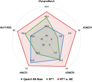
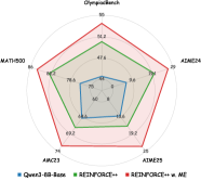
Figure 5: Impact of meta-experience across different training methods, including Rejection Sampling Fine-Tuning (RFT) and REINFORCE++. ME denotes Meta-Experience.
To demonstrate the versatility of meta-experience, we integrated it into RFT and REINFORCE++ using the Qwen-8B-Base model as the backbone and the same training set in our experiments. As shown in Figure 5, while vanilla RFT often suffers from rote memorization and tends to overfit to specific samples in this training set, the incorporation of meta-experiences introduces robust reasoning heuristics. This allows the model to internalize the underlying logic rather than merely imitating specific answers, thereby effectively mitigating overfitting and enhancing generalization to unseen test sets. Similarly, applying meta-experiences to REINFORCE++ significantly raises the performance ceiling on benchmarks. This confirms that the benefit of internalized meta-experiences is a universal enhancement, not limited to the GRPO framework.
### 4.5 Scalability Analysis
As indicated by the training curves in Figure 3, the method exhibits a distinct positive scaling law: the performance margin between MEL and the baseline widens significantly as the model size increases. This phenomenon consistently extends to downstream validation benchmarks.
We attribute this effect to the quality of self-generated supervision, which is inherently bounded by the model’s intrinsic capability. As shown in Figure 9, the 14B model achieves a significantly higher yield rate of valid meta-experiences than its smaller counterparts. While limited-capacity models introduce noise due to imprecise error attribution, larger models benefit from stronger self-verification, enabling the distillation of high-quality heuristics that provide more accurate gradient signals and fully realize the potential of our framework.
## 5 Conclusion
In this paper, we introduced MEL, a novel framework designed to overcome the meta-learning bottleneck in standard RLVR by transforming instance-specific failure patterns into reusable cognitive assets. Unlike traditional methods that rely solely on outcome-oriented rewards, MEL empowers models to perform granular error attribution, distilling specific failure modes into natural language heuristics—termed Meta-Experiences. By internalizing these experiences into parametric memory, our approach bridges the gap between verifying a solution and understanding the underlying reasoning logic. Extensive empirical evaluations confirm that MEL consistently boosts mathematical reasoning across diverse model scales.
## Impact Statement
This paper presents research aimed at advancing the field of reinforcement learning. While our work may have broader societal implications, we do not identify any specific impacts that require particular attention at this stage.
## References
- Y. Cai, S. Cai, Y. Shi, Z. Xu, L. Chen, Y. Qin, X. Tan, G. Li, Z. Li, H. Lin, et al. (2025) Training-free group relative policy optimization. arXiv preprint arXiv:2510.08191. Cited by: §2.
- J. Chen, Q. He, S. Yuan, A. Chen, Z. Cai, W. Dai, H. Yu, Q. Yu, X. Li, J. Chen, et al. (2025) Enigmata: scaling logical reasoning in large language models with synthetic verifiable puzzles. arXiv preprint arXiv:2505.19914. Cited by: §1.
- J. Cheng, G. Xiong, R. Qiao, L. Li, C. Guo, J. Wang, Y. Lv, and F. Wang (2025) Stop summation: min-form credit assignment is all process reward model needs for reasoning. arXiv preprint arXiv:2504.15275. Cited by: §1.
- Y. Fu, T. Chen, J. Chai, X. Wang, S. Tu, G. Yin, W. Lin, Q. Zhang, Y. Zhu, and D. Zhao (2025) SRFT: a single-stage method with supervised and reinforcement fine-tuning for reasoning. arXiv preprint arXiv:2506.19767. Cited by: §2.
- D. Guo, D. Yang, H. Zhang, J. Song, R. Zhang, R. Xu, Q. Zhu, S. Ma, P. Wang, X. Bi, et al. (2025) Deepseek-r1: incentivizing reasoning capability in llms via reinforcement learning. arXiv preprint arXiv:2501.12948. Cited by: §1, §2.
- C. He, R. Luo, Y. Bai, S. Hu, Z. Thai, J. Shen, J. Hu, X. Han, Y. Huang, Y. Zhang, et al. (2024) Olympiadbench: a challenging benchmark for promoting agi with olympiad-level bilingual multimodal scientific problems. In Proceedings of the Association for Computational Linguistics, pp. 3828–3850. Cited by: §4.
- D. Hendrycks, C. Burns, S. Kadavath, A. Arora, S. Basart, E. Tang, D. Song, and J. Steinhardt (2021) Measuring mathematical problem solving with the math dataset. arXiv preprint arXiv: 2103.03874. Cited by: §4.
- J. Hu (2025) Reinforce++: a simple and efficient approach for aligning large language models. arXiv preprint arXiv:2501.03262. Cited by: §2.
- S. Huang, Z. Fang, Z. Chen, S. Yuan, J. Ye, Y. Zeng, L. Chen, Q. Mao, and F. Zhao (2025) CRITICTOOL: evaluating self-critique capabilities of large language models in tool-calling error scenarios. arXiv preprint arXiv:2506.13977. Cited by: §3.2.
- W. Huang, Y. Zeng, Q. Wang, Z. Fang, S. Cao, Z. Chu, Q. Yin, S. Chen, Z. Yin, L. Chen, et al. (2026) Vision-deepresearch: incentivizing deepresearch capability in multimodal large language models. arXiv preprint arXiv:2601.22060. Cited by: §1.
- A. Jaech, A. Kalai, A. Lerer, A. Richardson, A. El-Kishky, A. Low, A. Helyar, A. Madry, A. Beutel, A. Carney, et al. (2024) Openai o1 system card. arXiv preprint arXiv:2412.16720. Cited by: §2.
- M. Khalifa, R. Agarwal, L. Logeswaran, J. Kim, H. Peng, M. Lee, H. Lee, and L. Wang (2025) Process reward models that think. arXiv preprint arXiv:2504.16828. Cited by: §1, §3.2.
- N. Lambert, J. Morrison, V. Pyatkin, S. Huang, H. Ivison, F. Brahman, L. J. V. Miranda, A. Liu, N. Dziri, S. Lyu, et al. (2024) Tulu 3: pushing frontiers in open language model post-training. arXiv preprint arXiv:2411.15124. Cited by: §1, §2.
- J. Li, E. Beeching, L. Tunstall, B. Lipkin, R. Soletskyi, S. Huang, K. Rasul, L. Yu, A. Q. Jiang, Z. Shen, et al. (2024) Numinamath: the largest public dataset in ai4maths with 860k pairs of competition math problems and solutions. Hugging Face repository 13 (9), pp. 9. Cited by: §4.
- H. Lightman, V. Kosaraju, Y. Burda, H. Edwards, B. Baker, T. Lee, J. Leike, J. Schulman, I. Sutskever, and K. Cobbe (2023) Let’s verify step by step. In Proceedings of the International Conference on Learning Representations, Cited by: §1.
- K. Liu, D. Yang, Z. Qian, W. Yin, Y. Wang, H. Li, J. Liu, P. Zhai, Y. Liu, and L. Zhang (2025) Reinforcement learning meets large language models: a survey of advancements and applications across the llm lifecycle. arXiv preprint arXiv:2509.16679. Cited by: §2.
- L. Ouyang, J. Wu, X. Jiang, D. Almeida, C. Wainwright, P. Mishkin, C. Zhang, S. Agarwal, K. Slama, A. Ray, et al. (2022) Training language models to follow instructions with human feedback. Advances in Neural Information Processing Systems 35, pp. 27730–27744. Cited by: §1.
- S. Ouyang, J. Yan, I. Hsu, Y. Chen, K. Jiang, Z. Wang, R. Han, L. T. Le, S. Daruki, X. Tang, et al. (2025) Reasoningbank: scaling agent self-evolving with reasoning memory. arXiv preprint arXiv:2509.25140. Cited by: §2.
- B. Pan and L. Zhao (2025) Can past experience accelerate llm reasoning?. arXiv preprint arXiv:2505.20643. Cited by: §2.
- W. Saunders, C. Yeh, J. Wu, S. Bills, L. Ouyang, J. Ward, and J. Leike (2022) Self-critiquing models for assisting human evaluators. arXiv preprint arXiv:2206.05802. Cited by: §3.2.
- J. Schulman, F. Wolski, P. Dhariwal, A. Radford, and O. Klimov (2017) Proximal policy optimization algorithms. arXiv preprint arXiv:1707.06347. Cited by: §1.
- Z. Shao, P. Wang, Q. Zhu, R. Xu, J. Song, X. Bi, H. Zhang, M. Zhang, Y. Li, Y. Wu, et al. (2024) Deepseekmath: pushing the limits of mathematical reasoning in open language models. arXiv preprint arXiv:2402.03300. Cited by: §1, §2, §3.1, §3.4, §4.
- G. Sheng, C. Zhang, Z. Ye, X. Wu, W. Zhang, R. Zhang, Y. Peng, H. Lin, and C. Wu (2024) HybridFlow: a flexible and efficient rlhf framework. arXiv preprint arXiv: 2409.19256. Cited by: §4.
- G. Swamy, S. Choudhury, W. Sun, Z. S. Wu, and J. A. Bagnell (2025) All roads lead to likelihood: the value of reinforcement learning in fine-tuning. arXiv preprint arXiv:2503.01067. Cited by: §3.2.
- Q. Wang, R. Ding, Y. Zeng, Z. Chen, L. Chen, S. Wang, P. Xie, F. Huang, and F. Zhao (2025) VRAG-rl: empower vision-perception-based rag for visually rich information understanding via iterative reasoning with reinforcement learning. arXiv preprint arXiv:2505.22019. Cited by: §1.
- R. Wu, X. Wang, J. Mei, P. Cai, D. Fu, C. Yang, L. Wen, X. Yang, Y. Shen, Y. Wang, et al. (2025) Evolver: self-evolving llm agents through an experience-driven lifecycle. arXiv preprint arXiv:2510.16079. Cited by: §1.
- M. Wulfmeier, M. Bloesch, N. Vieillard, A. Ahuja, J. Bornschein, S. Huang, A. Sokolov, M. Barnes, G. Desjardins, A. Bewley, et al. (2024) Imitating language via scalable inverse reinforcement learning. Advances in Neural Information Processing Systems 37, pp. 90714–90735. Cited by: §1.
- G. Xie, Y. Shi, H. Tian, T. Yao, and X. Zhang (2025) Capo: towards enhancing llm reasoning through verifiable generative credit assignment. arXiv e-prints, pp. arXiv–2508. Cited by: §1, §3.2.
- J. Yan, Y. Li, Z. Hu, Z. Wang, G. Cui, X. Qu, Y. Cheng, and Y. Zhang (2025) Learning to reason under off-policy guidance. arXiv preprint arXiv:2504.14945. Cited by: §2.
- A. Yang, A. Li, B. Yang, B. Zhang, B. Hui, B. Zheng, B. Yu, C. Gao, C. Huang, C. Lv, et al. (2025) Qwen3 technical report. arXiv preprint arXiv:2505.09388. Cited by: §4.
- Q. Yu, Z. Zhang, R. Zhu, Y. Yuan, X. Zuo, Y. Yue, W. Dai, T. Fan, G. Liu, L. Liu, et al. (2025) Dapo: an open-source llm reinforcement learning system at scale. arXiv preprint arXiv:2503.14476. Cited by: §2, §4.
- Y. Zeng, W. Huang, Z. Fang, S. Chen, Y. Shen, Y. Cai, X. Wang, Z. Yin, L. Chen, Z. Chen, et al. (2026) Vision-deepresearch benchmark: rethinking visual and textual search for multimodal large language models. arXiv preprint arXiv:2602.02185. Cited by: §1.
- Y. Zeng, W. Huang, S. Huang, X. Bao, Y. Qi, Y. Zhao, Q. Wang, L. Chen, Z. Chen, H. Chen, et al. (2025a) Agentic jigsaw interaction learning for enhancing visual perception and reasoning in vision-language models. arXiv preprint arXiv:2510.01304. Cited by: §1.
- Y. Zeng, Y. Qi, Y. Zhao, X. Bao, L. Chen, Z. Chen, S. Huang, J. Zhao, and F. Zhao (2025b) Enhancing large vision-language models with ultra-detailed image caption generation. In Proceedings of the 2025 Conference on Empirical Methods in Natural Language Processing, pp. 26703–26729. Cited by: §1.
- K. Zhang, X. Chen, B. Liu, T. Xue, Z. Liao, Z. Liu, X. Wang, Y. Ning, Z. Chen, X. Fu, et al. (2025a) Agent learning via early experience. arXiv preprint arXiv:2510.08558. Cited by: §1.
- K. Zhang, Y. Zuo, B. He, Y. Sun, R. Liu, C. Jiang, Y. Fan, K. Tian, G. Jia, P. Li, et al. (2025b) A survey of reinforcement learning for large reasoning models. arXiv preprint arXiv:2509.08827. Cited by: §2.
- K. Zhang, A. Lv, J. Li, Y. Wang, F. Wang, H. Hu, and R. Yan (2025c) StepHint: multi-level stepwise hints enhance reinforcement learning to reason. arXiv preprint arXiv:2507.02841. Cited by: §1, §2.
- X. Zhang, S. Wu, Y. Zhu, H. Tan, S. Yu, Z. He, and J. Jia (2025d) Scaf-grpo: scaffolded group relative policy optimization for enhancing llm reasoning. arXiv preprint arXiv:2510.19807. Cited by: §1, §2.
- C. Zheng, S. Liu, M. Li, X. Chen, B. Yu, C. Gao, K. Dang, Y. Liu, R. Men, A. Yang, et al. (2025) Group sequence policy optimization. arXiv preprint arXiv:2507.18071. Cited by: §2.
## Appendix A Result of Performance Evolution
As illustrated in Figures 6, 7, and 8, we visualize the performance evolution of models with different scales (Qwen3-4B-Base, Qwen3-8B-Base, and Qwen3-14B-Base) across multiple benchmarks throughout training. It can be observed that MEL consistently outperforms standard GRPO in terms of average performance on all benchmarks.
<details>
<summary>x7.png Details</summary>
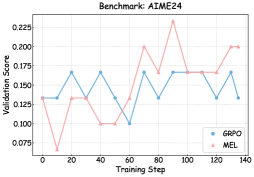
### Visual Description
## Line Chart: Benchmark: AIME24
### Overview
The image is a line chart titled "Benchmark: AIME24" that plots the "Validation Score" against "Training Step" for two different methods or models, labeled "GAPO" and "MEL". The chart compares their performance over the course of 140 training steps.
### Components/Axes
* **Title:** "Benchmark: AIME24" (centered at the top).
* **Y-Axis:**
* **Label:** "Validation Score" (rotated vertically on the left).
* **Scale:** Linear scale ranging from 0.075 to 0.225, with major tick marks at 0.075, 0.100, 0.125, 0.150, 0.175, 0.200, and 0.225.
* **X-Axis:**
* **Label:** "Training Step" (centered at the bottom).
* **Scale:** Linear scale ranging from 0 to 140, with major tick marks at 0, 20, 40, 60, 80, 100, 120, and 140.
* **Legend:** Located in the bottom-right corner of the chart area.
* **GAPO:** Represented by a blue line with circular markers.
* **MEL:** Represented by a red line with square markers.
* **Grid:** A light gray grid is present, aligning with the major tick marks on both axes.
### Detailed Analysis
**Data Series: GAPO (Blue Line with Circles)**
* **Trend:** The GAPO line shows moderate volatility, oscillating within a band between approximately 0.100 and 0.170. It does not exhibit a strong, consistent upward or downward trend over the full 140 steps.
* **Approximate Data Points:**
* Step 0: ~0.140
* Step 20: ~0.170
* Step 40: ~0.170
* Step 60: ~0.100 (local minimum)
* Step 80: ~0.170
* Step 100: ~0.170
* Step 120: ~0.170
* Step 140: ~0.160
**Data Series: MEL (Red Line with Squares)**
* **Trend:** The MEL line shows a more dramatic pattern. It starts lower than GAPO, dips to a significant low, then experiences a sharp rise to a peak, followed by a decline and a final recovery.
* **Approximate Data Points:**
* Step 0: ~0.140
* Step 10: ~0.075 (global minimum for the chart)
* Step 20: ~0.140
* Step 40: ~0.100
* Step 60: ~0.125
* Step 70: ~0.200
* Step 80: ~0.175
* Step 90: ~0.225 (global maximum for the chart)
* Step 100: ~0.175
* Step 120: ~0.175
* Step 130: ~0.200
* Step 140: ~0.200
### Key Observations
1. **Performance Crossover:** The two methods start at a similar validation score (~0.140). GAPO quickly takes a lead, maintaining it until approximately step 60, where MEL begins a steep ascent.
2. **Peak Performance:** MEL achieves the highest validation score on the chart (~0.225 at step 90), significantly surpassing GAPO's peak (~0.170).
3. **Volatility:** MEL exhibits much higher volatility, with a range of approximately 0.150 (from 0.075 to 0.225). GAPO's range is smaller, approximately 0.070 (from 0.100 to 0.170).
4. **Late-Stage Convergence:** After step 100, the two lines converge and track closely, with both ending near 0.160-0.200 at step 140.
### Interpretation
This chart from the "AIME24" benchmark suggests a fundamental trade-off between the stability and peak performance of the two evaluated methods.
* **GAPO** appears to be a more stable, conservative method. It avoids the severe performance collapse seen in MEL early on (step 10) but also fails to reach the highest validation scores. Its performance is relatively consistent after the initial phase.
* **MEL** demonstrates a "high-risk, high-reward" profile. It suffers a major early setback but then undergoes a period of rapid improvement, ultimately achieving superior peak performance. Its final performance remains strong, though below its peak.
The data implies that the choice between GAPO and MEL could depend on the project's priorities: if consistent, reliable performance is critical, GAPO may be preferable. If the goal is to achieve the absolute best possible score and some instability during training is acceptable, MEL shows greater potential. The convergence at the end might indicate that both methods eventually settle into a similar performance regime given sufficient training steps.
</details>
<details>
<summary>x8.png Details</summary>
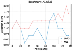
### Visual Description
\n
## Line Chart: Benchmark: AIME25
### Overview
The image is a line chart comparing the validation score performance of two models, labeled "GRPO" and "MEL," over the course of training steps on a benchmark titled "AIME25." The chart displays two distinct line series with markers, plotted against a grid.
### Components/Axes
* **Chart Title:** "Benchmark: AIME25" (centered at the top).
* **Y-Axis:** Labeled "Validation_Score". The scale runs from 0.025 to 0.200, with major tick marks at intervals of 0.025 (0.025, 0.050, 0.075, 0.100, 0.125, 0.150, 0.175, 0.200).
* **X-Axis:** Labeled "Training_Step". The scale runs from 0 to 140, with major tick marks at intervals of 20 (0, 20, 40, 60, 80, 100, 120, 140).
* **Legend:** Located in the bottom-right corner of the plot area.
* **GRPO:** Represented by a blue line with circular markers.
* **MEL:** Represented by a red line with triangular markers.
* **Grid:** A light gray grid is present, aligning with the major ticks on both axes.
### Detailed Analysis
**Data Series: GRPO (Blue Line, Circle Markers)**
* **Trend:** The GRPO line exhibits high volatility, characterized by sharp peaks and deep troughs throughout the training steps. There is no consistent upward or downward trend; performance fluctuates dramatically.
* **Approximate Data Points:**
* Step 0: ~0.100
* Step 20: ~0.035 (sharp drop)
* Step 40: ~0.075 (recovery)
* Step 60: ~0.100 (peak)
* Step 80: ~0.040 (sharp drop)
* Step 100: ~0.165 (highest peak)
* Step 120: ~0.100 (drop)
* Step 140: ~0.060 (final point)
**Data Series: MEL (Red Line, Triangle Markers)**
* **Trend:** The MEL line shows a more stable and generally upward trend. After an initial rise, it plateaus, dips slightly, and then climbs to its highest values in the later steps.
* **Approximate Data Points:**
* Step 0: ~0.100
* Step 20: ~0.130 (rise)
* Step 40: ~0.100 (dip)
* Step 60: ~0.100 (plateau)
* Step 80: ~0.130 (rise)
* Step 100: ~0.130 (plateau)
* Step 120: ~0.165 (peak, tied with GRPO's peak)
* Step 140: ~0.165 (final point, maintains peak)
### Key Observations
1. **Performance Crossover:** The two models start at the same validation score (~0.100). MEL immediately outperforms GRPO at step 20. GRPO only surpasses MEL at its single, dramatic peak at step 100 (~0.165 vs MEL's ~0.130).
2. **Volatility vs. Stability:** GRPO's performance is highly unstable, with a range of approximately 0.035 to 0.165. MEL's performance is more consistent, with a narrower range of approximately 0.100 to 0.165.
3. **Final Performance:** At the final recorded step (140), MEL (~0.165) significantly outperforms GRPO (~0.060).
4. **Peak Alignment:** Both models achieve their highest observed validation score of ~0.165, but at different times (GRPO at step 100, MEL at steps 120 & 140).
### Interpretation
The chart suggests a fundamental difference in the training dynamics of the two models on the AIME25 benchmark. The **MEL** model demonstrates more robust and reliable learning, achieving a high validation score and maintaining it. Its trajectory indicates stable convergence. In contrast, the **GRPO** model appears unstable; its performance is erratic, suggesting potential issues like overfitting to specific training batches, sensitivity to hyperparameters, or an unstable optimization process. While GRPO is capable of reaching a high score (step 100), it cannot sustain it.
The data implies that for this specific task, MEL is the more dependable model, offering predictable and high performance as training progresses. GRPO's volatility makes its final performance unpredictable and, in this case, poor. The benchmark likely measures a capability where consistent optimization (MEL) is more effective than the approach used by GRPO.
</details>
<details>
<summary>x9.png Details</summary>
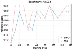
### Visual Description
\n
## Line Chart: Benchmark: AMC23
### Overview
The image displays a line chart comparing the validation score performance of two methods, labeled "GRPO" and "MEL," over the course of training steps on the AMC23 benchmark. The chart tracks how the validation score for each method changes as training progresses.
### Components/Axes
* **Chart Title:** "Benchmark: AMC23" (centered at the top).
* **X-Axis:** Labeled "Training Step." The axis is linear and marked with major ticks at intervals of 20, from 0 to 140. Minor ticks are present at intervals of 10.
* **Y-Axis:** Labeled "Validation Score." The axis is linear and marked with major ticks at intervals of 0.02, from 0.46 to 0.60.
* **Legend:** Located in the top-right corner of the plot area.
* A blue line with circle markers is labeled "GRPO".
* A red line with triangle markers is labeled "MEL".
* **Grid:** A light gray grid is present, aligning with the major ticks on both axes.
### Detailed Analysis
**Data Series: GRPO (Blue line, circle markers)**
* **Trend:** The GRPO series shows an initial sharp increase, followed by a period of fluctuation, and then stabilizes at a higher level towards the end of the tracked steps.
* **Approximate Data Points (Training Step, Validation Score):**
* (0, 0.46)
* (10, 0.50)
* (20, 0.58)
* (30, 0.52)
* (40, 0.52)
* (50, 0.50)
* (60, 0.58)
* (70, 0.58)
* (80, 0.58)
* (90, 0.60) - **Peak Value**
* (100, 0.56)
* (110, 0.58)
* (120, 0.58)
* (130, 0.58)
**Data Series: MEL (Red line, triangle markers)**
* **Trend:** The MEL series exhibits a very rapid initial rise to a plateau, followed by a significant drop, a recovery, a second dip, and a final rise to match its earlier peak.
* **Approximate Data Points (Training Step, Validation Score):**
* (0, 0.46)
* (10, 0.60) - **Reaches early plateau**
* (20, 0.60)
* (30, 0.60)
* (40, 0.50) - **Significant drop**
* (50, 0.58)
* (60, 0.58)
* (70, 0.55)
* (80, 0.55) - **Second dip**
* (90, 0.60) - **Matches early peak**
* (100, 0.55)
* (110, 0.55)
* (120, 0.58)
* (130, 0.60) - **Final value matches peak**
### Key Observations
1. **Initial Performance:** Both methods start at the same score (0.46). MEL achieves a much higher score (0.60) by step 10, while GRPO reaches 0.50.
2. **Volatility:** The MEL series shows greater volatility, with two distinct drops (at step 40 and steps 70-80/100-110) compared to GRPO's more moderate fluctuations.
3. **Peak Performance:** Both methods achieve a peak validation score of 0.60. GRPO hits this peak once at step 90. MEL hits this peak at steps 10-30, 90, and 130.
4. **Convergence:** By the final recorded step (130), both methods have converged to very similar scores: GRPO at 0.58 and MEL at 0.60.
5. **Relative Position:** The MEL line is generally above the GRPO line for the first 30 steps, falls below it between steps 40-50 and 70-80, and then intertwines with it for the remainder of the chart.
### Interpretation
This chart suggests a comparative analysis of two training methodologies (GRPO and MEL) on the AMC23 benchmark. The data indicates that **MEL learns faster initially**, reaching near-peak performance within 10 steps, but this comes with **less stability**, as evidenced by its sharp performance drops. **GRPO demonstrates a more gradual and stable learning curve**, with its performance improving in a less erratic manner, though it takes longer to reach its peak.
The fact that both methods ultimately achieve similar final scores (0.58 vs. 0.60) implies that for this specific benchmark, the choice between them may depend on other factors: if rapid initial convergence is critical, MEL might be preferred despite its instability. If consistent, stable improvement is valued, GRPO could be the better choice. The repeated drops in MEL's performance could indicate sensitivity to certain training phases or batches, warranting further investigation into the training dynamics of that method. The chart effectively communicates that while the endpoints are similar, the journey to get there differs significantly between the two approaches.
</details>
<details>
<summary>x10.png Details</summary>
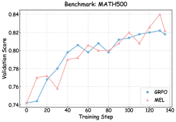
### Visual Description
## Line Chart: Benchmark: MATH500
### Overview
The image displays a line chart comparing the validation score performance of two methods, GRPO and MEL, over the course of training steps on the MATH500 benchmark. The chart shows both methods exhibit an overall upward trend, indicating learning and improvement, with significant fluctuations and crossovers between the two lines.
### Components/Axes
* **Chart Title:** "Benchmark: MATH500" (centered at the top).
* **Y-Axis:** Labeled "Validation Score". The scale runs from 0.74 to 0.84, with major tick marks at intervals of 0.02 (0.74, 0.76, 0.78, 0.80, 0.82, 0.84).
* **X-Axis:** Labeled "Training Step". The scale runs from 0 to 140, with major tick marks at intervals of 20 (0, 20, 40, 60, 80, 100, 120, 140).
* **Legend:** Located in the bottom-right corner of the plot area.
* **GRPO:** Represented by a blue line with circular markers.
* **MEL:** Represented by a red line with triangular markers.
### Detailed Analysis
**Data Series Trends & Approximate Points:**
1. **GRPO (Blue Line, Circle Markers):**
* **Trend:** Shows a generally steady upward climb with moderate fluctuations. It starts lower than MEL, overtakes it around step 40, and ends slightly below its final peak.
* **Key Data Points (Approximate):**
* Step 0: ~0.74
* Step 20: ~0.78
* Step 40: ~0.80
* Step 60: ~0.795 (slight dip)
* Step 80: ~0.80
* Step 100: ~0.82
* Step 120: ~0.825
* Step 140: ~0.82
2. **MEL (Red Line, Triangle Markers):**
* **Trend:** Shows a more volatile upward trend with sharper peaks and valleys. It starts higher, dips significantly at step 20, recovers, and achieves the highest overall score on the chart before a final dip.
* **Key Data Points (Approximate):**
* Step 0: ~0.76
* Step 20: ~0.76 (dip)
* Step 40: ~0.80
* Step 60: ~0.81
* Step 80: ~0.80 (dip)
* Step 100: ~0.815
* Step 120: ~0.84 (peak)
* Step 140: ~0.83
**Spatial & Cross-Reference Check:**
* The legend is positioned in the bottom-right, not obscuring the main data trends.
* The blue line (GRPO) is consistently plotted with circle markers, and the red line (MEL) with triangle markers, matching the legend exactly.
* The lines intersect approximately at step 40 (both ~0.80) and again near step 100 (both ~0.815-0.82).
### Key Observations
1. **Overall Improvement:** Both GRPO and MEL show a clear positive correlation between training steps and validation score, indicating successful learning on the MATH500 benchmark.
2. **Performance Crossover:** GRPO starts with a lower score but catches up to and briefly surpasses MEL around step 40.
3. **Volatility vs. Stability:** MEL demonstrates higher volatility, achieving the highest peak score (~0.84 at step 120) but also suffering sharper dips (e.g., at step 20). GRPO's progression appears somewhat smoother in the latter half.
4. **Final Convergence:** By the final recorded step (140), the two methods have converged to a very similar performance level (GRPO ~0.82, MEL ~0.83), with MEL retaining a slight edge.
### Interpretation
The chart suggests that for the MATH500 benchmark, both the GRPO and MEL training methods are effective, as evidenced by the rising validation scores. The choice between them may involve a trade-off: **MEL** appears capable of reaching a higher maximum performance (a peak of ~0.84) but exhibits less stability during training, which could imply sensitivity to specific training batches or hyperparameters. **GRPO** shows a more consistent, if slightly less spectacular, improvement trajectory, which might be preferable for reliability.
The convergence of scores at the end could indicate that both methods are approaching a performance ceiling for this specific model architecture and dataset. The initial underperformance and subsequent catch-up by GRPO might reflect different learning dynamics or initialization states. A practitioner might investigate the cause of MEL's significant dip at step 20 to understand potential failure modes. Ultimately, the data demonstrates that meaningful progress on this benchmark is achievable within 140 training steps using either method.
</details>
<details>
<summary>x11.png Details</summary>
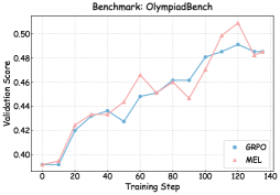
### Visual Description
## Line Chart: Benchmark: OlympiadBench
### Overview
The image displays a line chart comparing the validation score performance of two models, GRPO and MEL, over the course of training steps on the "OlympiadBench" benchmark. The chart tracks performance from step 0 to step 140.
### Components/Axes
* **Chart Title:** "Benchmark: OlympiadBench" (centered at the top).
* **X-Axis:** Labeled "Training Step". The axis has major tick marks at intervals of 20, labeled: 0, 20, 40, 60, 80, 100, 120, 140.
* **Y-Axis:** Labeled "Validation Score". The axis has major tick marks at intervals of 0.02, labeled: 0.40, 0.42, 0.44, 0.46, 0.48, 0.50.
* **Legend:** Located in the bottom-right corner of the chart area. It contains two entries:
* A blue line with circle markers labeled "GRPO".
* A red line with triangle markers labeled "MEL".
### Detailed Analysis
**Data Series 1: GRPO (Blue line, circle markers)**
* **Trend:** Shows a generally steady, upward trend with minor fluctuations. It starts low, rises sharply initially, then continues a more gradual ascent with a notable dip around step 60.
* **Approximate Data Points:**
* Step 0: ~0.395
* Step 20: ~0.425
* Step 40: ~0.435
* Step 60: ~0.428 (dip)
* Step 80: ~0.455
* Step 100: ~0.460
* Step 120: ~0.490 (peak)
* Step 140: ~0.485
**Data Series 2: MEL (Red line, triangle markers)**
* **Trend:** Shows a more volatile upward trend compared to GRPO. It follows a similar initial rise but exhibits larger swings, including a significant peak and subsequent drop in the later stages.
* **Approximate Data Points:**
* Step 0: ~0.395
* Step 20: ~0.425
* Step 40: ~0.435
* Step 60: ~0.465 (local peak)
* Step 80: ~0.455
* Step 100: ~0.480
* Step 120: ~0.505 (global peak)
* Step 140: ~0.485 (sharp drop)
### Key Observations
1. **Convergent Start:** Both models begin at nearly identical validation scores (~0.395) at step 0.
2. **Parallel Early Growth:** The models perform almost identically from step 0 to step 40.
3. **Divergence and Volatility:** After step 40, the MEL model's performance becomes more volatile, showing a higher peak at step 60 while GRPO dips. MEL also achieves a significantly higher maximum score (~0.505 vs. ~0.490).
4. **Late-Stage Convergence:** Despite different paths, both models converge to nearly the same final score (~0.485) at step 140.
5. **Overall Improvement:** Both models demonstrate clear learning, improving their validation scores by approximately 0.09 points over 140 training steps.
### Interpretation
The chart suggests that on the OlympiadBench benchmark, both the GRPO and MEL training methods are effective, leading to substantial performance gains over 140 steps. The key difference lies in their learning dynamics.
* **GRPO** exhibits a more stable and predictable learning trajectory. Its steady climb, barring one minor dip, indicates robust and consistent optimization. This could be preferable in scenarios where training stability and predictable outcomes are critical.
* **MEL** demonstrates a more aggressive or exploratory learning pattern. Its higher volatility, marked by larger peaks and troughs, suggests it may be navigating a more complex loss landscape or employing a higher learning rate. While it reaches a higher peak performance, this comes with less stability, as evidenced by the sharp drop after step 120. This might indicate potential overfitting at that peak or sensitivity to later training phases.
The final convergence at step 140 is intriguing. It implies that despite different intermediate behaviors, both methods may be approaching a similar performance ceiling for this specific model architecture and benchmark. The choice between them would depend on the priority: stable, reliable progress (favoring GRPO) versus the potential for higher peak performance at the cost of stability (favoring MEL, with careful monitoring).
</details>
<details>
<summary>x12.png Details</summary>

### Visual Description
## Line Chart: Benchmark: Average
### Overview
The image displays a line chart comparing the performance of two methods, labeled "GRPO" and "MEL," over the course of training. The chart plots a "Validation Score" against "Training Step," showing how each method's performance evolves. The overall trend suggests both methods improve over time, but with different patterns and final outcomes.
### Components/Axes
* **Chart Title:** "Benchmark: Average" (centered at the top).
* **Y-Axis:** Labeled "Validation Score." The scale runs from approximately 0.36 to 0.46, with major gridlines at intervals of 0.02 (0.36, 0.38, 0.40, 0.42, 0.44, 0.46).
* **X-Axis:** Labeled "Training Step." The scale runs from 0 to 140, with major tick marks and labels at intervals of 20 (0, 20, 40, 60, 80, 100, 120, 140).
* **Legend:** Located in the bottom-right corner of the plot area.
* A blue line with circle markers is labeled "GRPO".
* An orange dashed line with triangle markers is labeled "MEL".
* **Data Series:**
1. **GRPO (Blue, solid line, circle markers):** This line shows significant volatility. It starts low, rises, dips sharply around step 30, recovers, dips again around step 70, peaks near step 90, and then declines towards the end.
2. **MEL (Orange, dashed line, triangle markers):** This line shows a more consistent upward trend with less severe dips. It starts at a similar point to GRPO, generally climbs with minor fluctuations, and reaches its highest point near the end of the plotted steps.
### Detailed Analysis
**Trend Verification & Data Point Extraction (Approximate Values):**
| Training Step | GRPO (Blue) | MEL (Orange) |
| :--- | :--- | :--- |
| 0 | ~0.36 | ~0.36 |
| 10 | ~0.39 | ~0.385 |
| 20 | ~0.405 | ~0.405 |
| 30 | ~0.38 (sharp dip) | ~0.405 |
| 40 | ~0.40 | ~0.395 (minor dip) |
| 50 | ~0.39 | ~0.42 |
| 60 | ~0.415 | ~0.425 |
| 70 | ~0.395 (second dip) | ~0.43 |
| 80 | ~0.435 | ~0.435 |
| 90 | ~0.44 (peak) | ~0.42 (dip) |
| 100 | ~0.425 | ~0.44 |
| 110 | ~0.425 | ~0.44 |
| 120 | ~0.425 | ~0.445 |
| 130 | ~0.415 | ~0.46 (peak) |
### Key Observations
1. **Final Performance Divergence:** By step 130, the MEL method (orange) achieves a significantly higher validation score (~0.46) compared to GRPO (blue, ~0.415).
2. **Volatility vs. Stability:** The GRPO line is characterized by sharp, V-shaped dips (at steps ~30 and ~70), indicating periods of performance regression during training. The MEL line is more stable, with shallower dips.
3. **Peak Timing:** GRPO peaks earlier (around step 90) and then declines. MEL's peak is at the latest measured point (step 130), suggesting it may still be improving.
4. **Initial Convergence:** Both methods start at nearly the same point (~0.36) and track closely until approximately step 25, after which their paths begin to diverge more noticeably.
### Interpretation
The chart demonstrates a comparative benchmark between two training methods or algorithms (GRPO and MEL). The data suggests that while both methods learn and improve from the same starting point, **MEL exhibits more robust and sustained learning**. Its higher final score and lower volatility imply it may be a more reliable or effective optimization strategy for this particular task, avoiding the significant performance collapses seen in GRPO. The late peak of MEL also hints at potential for further improvement beyond step 130, whereas GRPO appears to have plateaued and begun to degrade, possibly indicating overfitting or instability in its later training stages. The key takeaway is that MEL's learning trajectory is both more stable and ultimately more successful within the observed training window.
</details>
Figure 6: Performance evolution of GRPO and MEL on Qwen3-4B-Base across training steps on multiple benchmarks.
<details>
<summary>x13.png Details</summary>
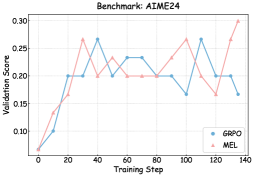
### Visual Description
## Line Chart: Benchmark: AIME24
### Overview
The image displays a line chart titled "Benchmark: AIME24," comparing the validation score performance of two methods, GAPO and MEL, over the course of 140 training steps. The chart shows the fluctuating performance of both methods, with MEL achieving the highest final score.
### Components/Axes
* **Chart Title:** "Benchmark: AIME24" (centered at the top).
* **Y-Axis:** Labeled "Validation Score." The scale runs from 0.10 to 0.30, with major tick marks at 0.10, 0.15, 0.20, 0.25, and 0.30.
* **X-Axis:** Labeled "Training Step." The scale runs from 0 to 140, with major tick marks at intervals of 20 (0, 20, 40, 60, 80, 100, 120, 140).
* **Legend:** Located in the bottom-right corner of the plot area.
* A blue line with a circular marker is labeled "GAPO".
* A red line with a circular marker is labeled "MEL".
### Detailed Analysis
**Data Series: GAPO (Blue Line)**
* **Trend:** The line shows significant volatility, with two distinct peaks and a notable dip in the middle.
* **Approximate Data Points:**
* Step 0: ~0.05
* Step 20: ~0.15
* Step 40: ~0.27 (First Peak)
* Step 60: ~0.20
* Step 80: ~0.24
* Step 100: ~0.16 (Significant Dip)
* Step 120: ~0.27 (Second Peak)
* Step 140: ~0.20
**Data Series: MEL (Red Line)**
* **Trend:** The line shows an overall upward trend with several fluctuations, culminating in a sharp increase to its highest point at the final step.
* **Approximate Data Points:**
* Step 0: ~0.05
* Step 20: ~0.13
* Step 30: ~0.27 (Early Peak)
* Step 40: ~0.20
* Step 50: ~0.24
* Step 60: ~0.20
* Step 80: ~0.20
* Step 100: ~0.27
* Step 110: ~0.16
* Step 140: ~0.30 (Final and Highest Peak)
### Key Observations
1. **Final Performance:** At the final recorded step (140), MEL (red) achieves the highest validation score on the chart (~0.30), significantly outperforming GAPO (blue, ~0.20).
2. **Volatility:** Both methods exhibit considerable volatility, with scores rising and falling sharply between measurement points. Neither shows a smooth, monotonic improvement.
3. **Peak Timing:** GAPO's peaks occur at steps 40 and 120. MEL's peaks occur at steps 30, 100, and 140.
4. **Convergence and Divergence:** The lines cross multiple times (e.g., near steps 10, 50, 70, 90, 110), indicating periods where one method temporarily outperforms the other before the advantage shifts.
5. **Notable Dip:** Both methods experience a significant drop in performance around step 110, with scores falling to approximately 0.16.
### Interpretation
The chart suggests that while both the GAPO and MEL methods are capable of reaching similar peak performance levels (~0.27) during training, their learning trajectories are unstable. The key differentiator is the final outcome: MEL demonstrates a capacity for a strong late-stage improvement, achieving a validation score of ~0.30 by step 140, which is the best result shown. In contrast, GAPO's performance at step 140 is middling relative to its own history.
The synchronized dip around step 110 for both methods could indicate a challenging phase in the training process, a change in data, or an inherent instability in the optimization landscape for this benchmark. The fact that MEL recovers from this dip to reach a new high suggests it may have better resilience or adaptation capabilities in the later stages of training compared to GAPO for the AIME24 task. The overall message is that final training step performance is not predictable from mid-training peaks, and method selection may depend on whether consistent mid-training performance or peak final performance is prioritized.
</details>
<details>
<summary>x14.png Details</summary>
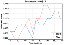
### Visual Description
\n
## Line Chart: Benchmark: AIME'25
### Overview
The image displays a line chart comparing the validation score performance of two methods, GAPO and MEL, over the course of training steps. The chart tracks how the validation score for each method changes as training progresses from step 0 to step 140.
### Components/Axes
* **Chart Title:** "Benchmark: AIME'25" (centered at the top).
* **Y-Axis:** Labeled "Validation Score". The scale runs from 0.100 to 0.275, with major tick marks at intervals of 0.025 (0.100, 0.125, 0.150, 0.175, 0.200, 0.225, 0.250, 0.275).
* **X-Axis:** Labeled "Training Step". The scale runs from 0 to 140, with major tick marks at intervals of 20 (0, 20, 40, 60, 80, 100, 120, 140).
* **Legend:** Located in the bottom-right corner of the chart area.
* **GAPO:** Represented by a blue line with circular markers.
* **MEL:** Represented by a red line with square markers.
* **Grid:** A light gray grid is present, aligning with the major ticks on both axes.
### Detailed Analysis
**Data Series: GAPO (Blue Line, Circle Markers)**
* **Trend:** The line shows significant volatility, with sharp rises and falls throughout the training steps. It does not exhibit a consistent upward or downward trend but rather fluctuates within a range.
* **Approximate Data Points:**
* Step 0: ~0.135
* Step 20: ~0.170
* Step 40: ~0.170
* Step 60: ~0.125
* Step 80: ~0.200
* Step 100: ~0.170
* Step 120: ~0.200
* Step 140: ~0.200
**Data Series: MEL (Red Line, Square Markers)**
* **Trend:** The line shows a more pronounced overall upward trend, especially after step 60, culminating in a significant peak. It experiences a notable dip early on (step 20) before climbing.
* **Approximate Data Points:**
* Step 0: ~0.100
* Step 20: ~0.090
* Step 40: ~0.150
* Step 60: ~0.200
* Step 80: ~0.175
* Step 100: ~0.270 (Peak)
* Step 120: ~0.230
* Step 140: ~0.230
### Key Observations
1. **Performance Crossover:** The two methods trade the lead multiple times. MEL starts lower, surpasses GAPO around step 60, falls behind again at step 80, and then decisively overtakes GAPO from step 100 onward.
2. **Peak Performance:** The highest validation score on the chart is achieved by MEL at step 100 (~0.270).
3. **Volatility vs. Growth:** GAPO's performance is highly variable without clear growth. MEL, despite an early dip and a drop after its peak, demonstrates a stronger capacity for high scores in the later stages of training.
4. **Final Convergence:** By step 140, both methods have converged to similar scores (~0.200 for GAPO, ~0.230 for MEL), though MEL maintains a slight advantage.
### Interpretation
The chart suggests that for the "AIME'25" benchmark, the MEL training method has a higher potential peak performance than GAPO, as evidenced by its score of ~0.270. However, MEL's learning trajectory is less stable, featuring a significant dip early in training and a sharp decline after its peak. GAPO, while never reaching the same heights, shows a pattern of recovering from drops (e.g., after step 60 and step 100).
The data implies a trade-off: MEL may be preferable if the goal is to achieve the highest possible score and training can be stopped at an optimal point (around step 100). GAPO might be considered for scenarios where consistent, moderate performance is valued over peak potential, though its volatility contradicts strict consistency. The final convergence suggests that extended training beyond 100-120 steps may diminish the performance gap between the two methods on this specific benchmark. The sharp peak for MEL at step 100 is a critical anomaly that warrants investigation—it could represent a genuine breakthrough in learning or an instability in the validation process.
</details>
<details>
<summary>x15.png Details</summary>
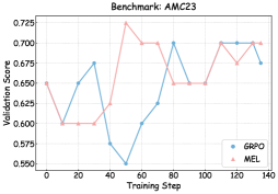
### Visual Description
## Line Chart: Benchmark: AMC23
### Overview
The image displays a line chart comparing the performance of two methods, labeled "GRPO" and "MEL," over the course of training. The chart tracks a "Validation Score" against "Training Step." The overall trend shows both methods starting at a similar performance level, experiencing significant volatility, and ending at comparable but distinct final scores.
### Components/Axes
* **Chart Title:** "Benchmark: AMC23" (centered at the top).
* **Y-Axis:** Labeled "Validation Score." The scale runs from 0.550 to 0.725, with major tick marks at intervals of 0.025 (0.550, 0.575, 0.600, 0.625, 0.650, 0.675, 0.700, 0.725).
* **X-Axis:** Labeled "Training Step." The scale runs from 0 to 140, with major tick marks at intervals of 20 (0, 20, 40, 60, 80, 100, 120, 140).
* **Legend:** Located in the bottom-right corner of the plot area.
* A blue line with a circular marker is labeled "GRPO".
* A red line with a circular marker is labeled "MEL".
### Detailed Analysis
**Data Series: GRPO (Blue Line)**
* **Trend:** The GRPO line exhibits a volatile, "W"-shaped trend with a significant mid-training dip before recovering.
* **Data Points (Approximate):**
* Step 0: ~0.650
* Step 10: ~0.600
* Step 30: ~0.675
* Step 50: ~0.550 (Global minimum for this series)
* Step 70: ~0.600
* Step 80: ~0.700
* Step 100: ~0.650
* Step 130: ~0.700
* Step 140: ~0.675
**Data Series: MEL (Red Line)**
* **Trend:** The MEL line shows an initial plateau, a sharp rise to a peak, followed by fluctuations at a higher performance band than its start.
* **Data Points (Approximate):**
* Step 0: ~0.650
* Step 10: ~0.600
* Step 30: ~0.600
* Step 50: ~0.725 (Global maximum for the entire chart)
* Step 70: ~0.700
* Step 80: ~0.700
* Step 100: ~0.650
* Step 110: ~0.650
* Step 120: ~0.700
* Step 130: ~0.675
* Step 140: ~0.700
### Key Observations
1. **Initial Convergence:** Both GRPO and MEL begin at the same score (~0.650) and drop to the same low (~0.600) by step 10.
2. **Divergence at Step 50:** This is the most critical point. The GRPO score plummets to its lowest point (~0.550), while the MEL score surges to its highest point (~0.725). This represents the maximum performance gap between the two methods.
3. **Post-Dip Recovery:** After step 50, GRPO shows a strong recovery trend, while MEL experiences a slight decline from its peak but stabilizes at a high level.
4. **Final Comparison:** At the final recorded step (140), MEL (~0.700) holds a slight advantage over GRPO (~0.675).
5. **Volatility:** Both methods demonstrate significant volatility, with scores changing by 0.075 or more between consecutive measured steps.
### Interpretation
The chart suggests that the "MEL" method achieves a higher peak performance and maintains a generally higher validation score after the initial training phase compared to "GRPO." The dramatic divergence at step 50 is the key finding; it indicates a critical phase in training where the two algorithms respond in fundamentally opposite ways. GRPO's severe dip suggests a period of instability or catastrophic forgetting, from which it successfully recovers. MEL's corresponding spike indicates a highly effective learning update at that stage.
The fact that both methods start and end relatively close to each other, despite the mid-training chaos, implies that the final model performance might be similar, but the training dynamics and reliability differ greatly. MEL appears more robust after step 50, while GRPO's path is more erratic. For a technical document, this chart would argue that MEL offers more stable and higher peak performance during the observed training window, though the ultimate final performance gap is modest. The investigation would focus on understanding the algorithmic difference that causes the step 50 divergence.
</details>
<details>
<summary>x16.png Details</summary>
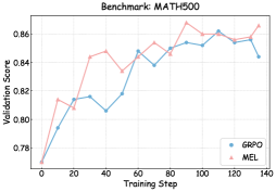
### Visual Description
## Line Chart: Benchmark: MATH500
### Overview
The image is a line chart comparing the validation score performance of two different methods, labeled "GAPO" and "MEL," over the course of training steps on a benchmark dataset called "MATH500." The chart displays two fluctuating lines that generally trend upward, indicating improving performance with more training.
### Components/Axes
* **Chart Title:** "Benchmark: MATH500" (centered at the top).
* **X-Axis:** Labeled "Training Step." The axis is linear and marked with major ticks at intervals of 20, ranging from 0 to 140.
* **Y-Axis:** Labeled "Validation Score." The axis is linear and marked with major ticks at intervals of 0.02, ranging from 0.78 to 0.86.
* **Legend:** Located in the bottom-right corner of the plot area. It contains two entries:
* A blue line with circular markers labeled "GAPO".
* A red line with triangular markers labeled "MEL".
### Detailed Analysis
**Data Series: GAPO (Blue line with circles)**
* **Trend:** The line shows an overall upward trend with significant volatility. It starts low, rises sharply, experiences a notable dip, recovers, and reaches its peak towards the later steps before a final decline.
* **Approximate Data Points:**
* Step 0: ~0.78
* Step 10: ~0.80
* Step 20: ~0.81
* Step 30: ~0.82
* Step 40: ~0.82
* Step 50: ~0.805 (notable dip)
* Step 60: ~0.845
* Step 70: ~0.835
* Step 80: ~0.85
* Step 90: ~0.855
* Step 100: ~0.85
* Step 110: ~0.855
* Step 120: ~0.86 (peak)
* Step 130: ~0.855
* Step 140: ~0.845
**Data Series: MEL (Red line with triangles)**
* **Trend:** The line also shows an overall upward trend but with a different pattern. It starts higher than GAPO, rises quickly to an early peak, fluctuates, reaches its maximum, and then shows a clear downward trend in the final steps.
* **Approximate Data Points:**
* Step 0: ~0.80
* Step 10: ~0.815
* Step 20: ~0.805
* Step 30: ~0.845
* Step 40: ~0.85
* Step 50: ~0.84
* Step 60: ~0.845
* Step 70: ~0.855
* Step 80: ~0.86 (peak)
* Step 90: ~0.85
* Step 100: ~0.855
* Step 110: ~0.85
* Step 120: ~0.855
* Step 130: ~0.85
* Step 140: ~0.84
### Key Observations
1. **Initial Performance:** MEL starts with a higher validation score (~0.80) than GAPO (~0.78) at step 0.
2. **Crossover Points:** The two lines intersect approximately at step 60 and again near step 100, indicating points where their performance was nearly identical.
3. **Peak Timing:** MEL reaches its peak performance (~0.86) earlier, around step 80. GAPO reaches its similar peak (~0.86) later, around step 120.
4. **Volatility:** Both methods show considerable step-to-step fluctuation, suggesting the training process or evaluation metric is noisy.
5. **Final Trend:** In the last 20 steps (120-140), the MEL line shows a more consistent downward trend, while the GAPO line's decline is less pronounced after its later peak.
### Interpretation
This chart visualizes a comparative training run for two algorithms or model variants (GAPO and MEL) on the MATH500 benchmark. The "Validation Score" is the key performance metric.
The data suggests that **MEL may learn faster initially**, achieving higher scores in the first third of the training steps. However, its performance peaks earlier and begins to degrade, which could be a sign of **overfitting** to the training data or instability in the later stages of optimization.
In contrast, **GAPO shows a more sustained, albeit noisier, improvement** over a longer period. Its later peak suggests it might be more robust or continue to benefit from extended training. The significant dip around step 50 for GAPO is an anomaly that could correspond to a specific event in the training process, such as a learning rate change or a challenging batch of data.
The overall takeaway is a trade-off: MEL offers quicker gains, while GAPO demonstrates potentially more stable long-term learning. The choice between them would depend on the available training budget (steps) and the importance of peak performance versus training stability. The volatility in both lines indicates that evaluating performance at a single step might be misleading; observing the trend over time is crucial.
</details>
<details>
<summary>x17.png Details</summary>
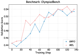
### Visual Description
## Line Chart: Benchmark: OlympiadBench
### Overview
The image displays a line chart comparing the validation score performance of two methods, GRPO and MEL, over the course of training steps on a benchmark named "OlympiadBench". The chart tracks performance from step 0 to approximately step 140.
### Components/Axes
* **Chart Title:** "Benchmark: OlympiadBench" (Top center)
* **Y-Axis:**
* **Label:** "Validation Score" (Left side, rotated vertically)
* **Scale:** Linear scale ranging from 0.44 to 0.54, with major tick marks at 0.02 intervals (0.44, 0.46, 0.48, 0.50, 0.52, 0.54).
* **X-Axis:**
* **Label:** "Training Step" (Bottom center)
* **Scale:** Linear scale from 0 to 140, with major tick marks every 20 steps (0, 20, 40, 60, 80, 100, 120, 140).
* **Legend:** Located in the bottom-right corner of the plot area.
* **GRPO:** Represented by a blue line with circular markers.
* **MEL:** Represented by a red line with triangular markers.
### Detailed Analysis
**Data Series Trends & Approximate Points:**
1. **GRPO (Blue Line, Circles):**
* **Trend:** Starts at the lowest point, experiences an initial dip, then follows a generally upward trend with moderate fluctuations. It shows a significant dip around step 60 before recovering.
* **Approximate Data Points:**
* Step 0: ~0.445
* Step 10: ~0.450
* Step 20: ~0.440 (Local minimum)
* Step 30: ~0.455
* Step 40: ~0.470
* Step 50: ~0.500
* Step 60: ~0.480 (Significant dip)
* Step 70: ~0.515
* Step 80: ~0.530
* Step 90: ~0.525
* Step 100: ~0.540 (Peak)
* Step 110: ~0.535
* Step 120: ~0.520
* Step 130: ~0.535
* Step 140: ~0.535
2. **MEL (Red Line, Triangles):**
* **Trend:** Starts higher than GRPO, dips early, then exhibits a strong upward trend with higher volatility (larger swings up and down) compared to GRPO. It achieves the highest overall score on the chart.
* **Approximate Data Points:**
* Step 0: ~0.450
* Step 10: ~0.445 (Local minimum)
* Step 20: ~0.460
* Step 30: ~0.510
* Step 40: ~0.500
* Step 50: ~0.520
* Step 60: ~0.510
* Step 70: ~0.525
* Step 80: ~0.520
* Step 90: ~0.530
* Step 100: ~0.540
* Step 110: ~0.530
* Step 120: ~0.545 (Highest point on chart)
* Step 130: ~0.530
* Step 140: ~0.540
### Key Observations
1. **Overall Improvement:** Both GRPO and MEL show a clear positive trend, indicating that validation scores improve with increased training steps on the OlympiadBench benchmark.
2. **Performance Crossover:** MEL starts with a slight advantage, but GRPO catches up and briefly surpasses it around step 80. The lines cross multiple times, indicating competitive performance.
3. **Volatility Difference:** The MEL series (red) exhibits greater volatility, with sharper peaks and troughs, particularly between steps 20-40 and 110-130. The GRPO series (blue) is comparatively smoother, with its most notable deviation being the dip at step 60.
4. **Peak Performance:** The highest recorded validation score (~0.545) is achieved by MEL at approximately step 120. Both methods end the tracked period (step 140) at a similar high level (~0.535-0.540).
5. **Initial Phase:** Both methods experience a performance dip within the first 20 training steps before beginning their sustained ascent.
### Interpretation
The chart demonstrates a comparative learning curve analysis for two algorithms on a challenging benchmark. The data suggests that while both methods are effective, they exhibit different learning dynamics:
* **MEL** may have a higher potential for peak performance (as seen at step 120) but comes with less stability during training, as evidenced by its larger fluctuations. This could imply sensitivity to specific training batches or a more aggressive optimization strategy.
* **GRPO** appears to be a more stable learner. Its significant dip at step 60 is an anomaly that warrants investigation—it could correspond to a difficult subset of data, a learning rate issue, or a temporary instability in the optimization process. Its recovery from this dip shows robustness.
The fact that both methods converge to a similar final performance range suggests that for this specific benchmark, the choice between them might depend on secondary factors: if consistent, predictable progress is valued, GRPO might be preferred. If the training process can tolerate volatility in pursuit of potentially higher interim peaks, MEL could be the candidate. The initial dips for both models are curious and might indicate a common challenge in the early phase of learning for this task, such as overcoming a local minimum or adapting from a pre-trained state.
</details>
<details>
<summary>x18.png Details</summary>
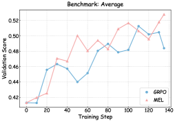
### Visual Description
## Line Chart: Benchmark: Average
### Overview
The image displays a line chart comparing the validation score performance of two methods, GRPO and MEL, over the course of training steps. The chart tracks the average benchmark performance, showing how each method's validation score evolves as training progresses.
### Components/Axes
* **Chart Title:** "Benchmark: Average" (centered at the top).
* **X-Axis:** Labeled "Training Step". The scale runs from 0 to 140, with major tick marks and labels at intervals of 20 (0, 20, 40, 60, 80, 100, 120, 140).
* **Y-Axis:** Labeled "Validation Score". The scale runs from 0.42 to 0.52, with major tick marks and labels at intervals of 0.02 (0.42, 0.44, 0.46, 0.48, 0.50, 0.52).
* **Legend:** Located in the bottom-right corner of the chart area. It contains two entries:
* A blue line with a circle marker labeled "GRPO".
* A red line with a circle marker labeled "MEL".
* **Data Series:** Two lines plotted on the chart:
1. **GRPO (Blue Line):** Connects data points with blue circles.
2. **MEL (Red Line):** Connects data points with red circles.
### Detailed Analysis
**Data Point Extraction (Approximate Values):**
| Training Step | GRPO (Blue) Validation Score | MEL (Red) Validation Score |
| :--- | :--- | :--- |
| 0 | ~0.42 | ~0.42 |
| 20 | ~0.46 | ~0.47 |
| 40 | ~0.44 | ~0.50 |
| 60 | ~0.48 | ~0.49 |
| 80 | ~0.47 | ~0.51 |
| 100 | ~0.49 | ~0.50 |
| 120 | ~0.51 | ~0.52 |
| 140 | ~0.50 | ~0.53 |
**Trend Verification:**
* **GRPO (Blue Line):** The line shows an overall upward trend from step 0 to step 120, with notable dips at steps 40 and 80. It peaks at step 120 (~0.51) before declining slightly at step 140 (~0.50). The trend is positive but exhibits volatility.
* **MEL (Red Line):** The line shows a strong, generally consistent upward trend from step 0 to step 140. It experiences a minor dip at step 60 but recovers quickly. The line reaches its highest point at the final recorded step, 140 (~0.53).
### Key Observations
1. **Initial Parity:** Both methods start at an identical validation score of approximately 0.42 at Training Step 0.
2. **Divergence:** The performance of the two methods begins to diverge significantly after step 20. The MEL (red) line consistently maintains a higher validation score than the GRPO (blue) line from step 40 onward.
3. **Peak Performance:** The highest validation score on the chart is achieved by MEL at step 140 (~0.53). The peak for GRPO is lower and occurs earlier, at step 120 (~0.51).
4. **Volatility:** The GRPO line shows more pronounced fluctuations (e.g., the sharp drop at step 40) compared to the relatively smoother ascent of the MEL line.
5. **Final Status:** At the last data point (step 140), MEL holds a clear lead over GRPO, with a score of ~0.53 versus ~0.50.
### Interpretation
This chart demonstrates a comparative performance analysis between two training methods (GRPO and MEL) on a benchmark task. The data suggests that the **MEL method is more effective and stable** for this specific benchmark over 140 training steps.
* **Effectiveness:** MEL achieves a higher final validation score, indicating it learns a better-performing model by the end of the observed training period.
* **Stability/Efficiency:** MEL's performance improves more consistently. While GRPO struggles with setbacks (notably at steps 40 and 80), MEL maintains a steadier climb, suggesting it may be a more robust or efficient optimization process for this task.
* **Practical Implication:** If the goal is to maximize validation score within a fixed budget of ~140 training steps, the MEL method appears to be the superior choice based on this benchmark. The chart provides empirical evidence that MEL not only reaches a higher performance ceiling but does so with greater reliability. The initial parity followed by divergence also suggests the methods may have similar starting points but differ fundamentally in their learning dynamics or ability to escape local minima.
</details>
Figure 7: Performance evolution of GRPO and MEL on Qwen3-8B-Base across training steps on multiple benchmarks.
<details>
<summary>x19.png Details</summary>
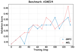
### Visual Description
## Line Chart: Benchmark: AIME24
### Overview
The image displays a line chart comparing the validation score performance of two methods, GRPO and MEL, over the course of training steps. The chart is titled "Benchmark: AIME24". The x-axis represents the progression of training, while the y-axis measures the validation score, a metric of model performance.
### Components/Axes
* **Chart Title:** "Benchmark: AIME24" (centered at the top).
* **X-Axis:**
* **Label:** "Training Step" (centered below the axis).
* **Scale:** Linear scale from 0 to 140.
* **Major Tick Marks:** 0, 20, 40, 60, 80, 100, 120, 140.
* **Y-Axis:**
* **Label:** "Validation Score" (rotated vertically on the left side).
* **Scale:** Linear scale from 0.15 to 0.45.
* **Major Tick Marks:** 0.15, 0.20, 0.25, 0.30, 0.35, 0.40, 0.45.
* **Legend:**
* **Position:** Top-right corner of the chart area.
* **Entries:**
1. **GRPO:** Represented by a blue line with circular markers.
2. **MEL:** Represented by a red line with circular markers.
* **Grid:** Light gray horizontal and vertical grid lines are present.
### Detailed Analysis
The chart plots two data series, each consisting of approximately 8 data points at the major x-axis intervals.
**1. GRPO (Blue Line) Trend & Data Points:**
* **Trend:** The GRPO line shows moderate volatility. It starts low, experiences a dip, rises to a plateau, and then fluctuates with a notable peak before a final rise.
* **Approximate Data Points (Training Step, Validation Score):**
* (0, ~0.15)
* (20, ~0.14) - *A dip from the starting point.*
* (40, ~0.30) - *A sharp increase.*
* (60, ~0.27) - *A slight decrease.*
* (80, ~0.30) - *Returns to the previous level.*
* (100, ~0.37) - *The peak for this series.*
* (120, ~0.27) - *A significant drop.*
* (140, ~0.36) - *A strong recovery.*
**2. MEL (Red Line) Trend & Data Points:**
* **Trend:** The MEL line shows a more pronounced upward trend with higher volatility, especially in the later stages. It generally outperforms GRPO after step 60, with a dramatic spike and subsequent correction.
* **Approximate Data Points (Training Step, Validation Score):**
* (0, ~0.15)
* (20, ~0.23) - *A steady initial increase.*
* (40, ~0.24) - *A very slight increase.*
* (60, ~0.30) - *A notable increase, matching GRPO.*
* (80, ~0.36) - *Continues to rise, surpassing GRPO.*
* (100, ~0.27) - *A sharp dip, falling below GRPO at this step.*
* (120, ~0.46) - *A dramatic spike to the highest point on the chart.*
* (140, ~0.31) - *A significant correction downward.*
### Key Observations
1. **Performance Crossover:** The two methods have similar performance at steps 0, 60, and 140. MEL leads at steps 20, 40, 80, and 120. GRPO leads only at step 100.
2. **Volatility:** Both methods show non-monotonic progress. MEL exhibits greater volatility, particularly the extreme spike at step 120 followed by a sharp drop.
3. **Peak Performance:** The single highest validation score (~0.46) is achieved by MEL at step 120. The peak for GRPO (~0.37) is lower and occurs at step 100.
4. **Final Convergence:** By the final recorded step (140), both methods converge to a similar score range (GRPO ~0.36, MEL ~0.31), though GRPO ends slightly higher.
### Interpretation
This chart benchmarks two training methodologies (GRPO and MEL) on the AIME24 task. The data suggests that while both methods can achieve comparable final performance, their learning trajectories differ significantly.
* **MEL** demonstrates a capacity for higher peak performance (as seen at step 120) but appears less stable, with its performance being more sensitive to specific training steps. The dramatic spike and drop could indicate an unstable optimization phase or a particularly effective but transient training configuration.
* **GRPO** shows a more stable, albeit slightly lower, performance profile. Its peak occurs earlier (step 100), and its fluctuations are less extreme. This might suggest a more robust but potentially slower or less ambitious optimization path.
The fact that neither line shows a smooth, consistently increasing trend is notable. It implies that the validation score for this benchmark is noisy or that the training process for both methods involves significant exploration, leading to temporary performance regressions. The final convergence suggests that given enough training steps, both methods may settle into a similar performance regime, but the path to get there—and the potential for short-term high performance—differs. For a practitioner, the choice between GRPO and MEL might depend on whether they prioritize stability (favoring GRPO) or are willing to tolerate volatility in pursuit of potentially higher short-term gains (favoring MEL).
</details>
<details>
<summary>x20.png Details</summary>
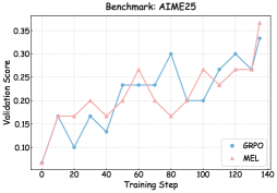
### Visual Description
## Line Chart: Benchmark: AIME25
### Overview
The image displays a line chart comparing the performance of two methods, labeled "GAPO" and "MEL," over the course of training. The chart tracks a "Validation Score" against "Training Step," showing how each method's performance evolves. Both methods show a general upward trend, indicating improvement with more training, but with different patterns of volatility.
### Components/Axes
* **Chart Title:** "Benchmark: AIME25" (centered at the top).
* **X-Axis:**
* **Label:** "Training Step" (centered below the axis).
* **Scale:** Linear scale from 0 to 140.
* **Major Tick Marks:** 0, 20, 40, 60, 80, 100, 120, 140.
* **Y-Axis:**
* **Label:** "Validation Score" (rotated vertically, left of the axis).
* **Scale:** Linear scale from 0.10 to 0.35.
* **Major Tick Marks:** 0.10, 0.15, 0.20, 0.25, 0.30, 0.35.
* **Legend:**
* **Position:** Bottom-right corner of the chart area.
* **Entries:**
1. **GAPO:** Represented by a blue line with circular markers.
2. **MEL:** Represented by a red line with triangular markers.
### Detailed Analysis
**Data Series: GAPO (Blue Line, Circles)**
* **Trend:** The line shows an overall upward trend with significant fluctuations. It starts at a moderate level, dips early, then rises with several peaks and troughs before a final sharp increase.
* **Approximate Data Points (Training Step, Validation Score):**
* (0, ~0.17)
* (10, ~0.17)
* (20, ~0.10) - **Notable dip.**
* (30, ~0.17)
* (40, ~0.13)
* (50, ~0.23)
* (60, ~0.22)
* (70, ~0.25)
* (80, ~0.30) - **Local peak.**
* (90, ~0.20)
* (100, ~0.20)
* (110, ~0.25)
* (120, ~0.30)
* (130, ~0.27)
* (140, ~0.33) - **Final value.**
**Data Series: MEL (Red Line, Triangles)**
* **Trend:** The line shows a strong, albeit volatile, upward trend. It starts lower than GAPO but exhibits more dramatic swings, ultimately reaching a higher final value.
* **Approximate Data Points (Training Step, Validation Score):**
* (0, ~0.07)
* (10, ~0.17)
* (20, ~0.17)
* (30, ~0.20)
* (40, ~0.17)
* (50, ~0.27)
* (60, ~0.22)
* (70, ~0.27)
* (80, ~0.20)
* (90, ~0.17)
* (100, ~0.27)
* (110, ~0.23)
* (120, ~0.27)
* (130, ~0.27)
* (140, ~0.36) - **Final value and chart maximum.**
### Key Observations
1. **Initial Performance:** GAPO starts with a higher validation score (~0.17) than MEL (~0.07) at step 0.
2. **Early Divergence:** GAPO experiences a sharp performance drop at step 20, while MEL maintains its score.
3. **Crossover Points:** The lines cross multiple times (e.g., near step 10, step 50, step 110), indicating neither method is consistently superior throughout training.
4. **Volatility:** MEL's performance is more volatile, with larger swings between consecutive steps (e.g., the drop from ~0.27 at step 70 to ~0.17 at step 90).
5. **Final Outcome:** By the final recorded step (140), MEL achieves the highest validation score on the chart (~0.36), surpassing GAPO's final score (~0.33).
6. **General Trend:** Despite the volatility, both methods demonstrate a clear positive correlation between training steps and validation score.
### Interpretation
This chart benchmarks two optimization or learning algorithms (GAPO and MEL) on the "AIME25" task. The data suggests that while both methods are effective at learning, as evidenced by their upward trends, they have distinct characteristics.
* **GAPO** appears to be a more stable learner initially but is prone to a significant early setback (the dip at step 20). Its recovery and subsequent performance are strong but not the highest.
* **MEL** starts poorly but exhibits a "high-risk, high-reward" pattern. Its greater volatility suggests it may be exploring the solution space more aggressively, which leads to larger temporary setbacks but also enables it to discover a better final solution (the peak at step 140).
The multiple crossover points imply that the choice between GAPO and MEL might depend on the available training budget. If training must stop early (e.g., before step 50), GAPO might be preferable. For a full training run to step 140, MEL yields a better result. The chart does not provide information on computational cost, stability across multiple runs, or performance beyond 140 steps, which would be critical for a full technical assessment.
</details>
<details>
<summary>x21.png Details</summary>
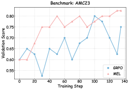
### Visual Description
\n
## Line Chart: Benchmark: AMC23
### Overview
The image is a line chart comparing the validation score performance of two methods, "GAPO" and "MEL", over the course of training steps on the AMC23 benchmark. The chart shows that the MEL method demonstrates a generally superior and more stable upward trend compared to the more volatile performance of the GAPO method.
### Components/Axes
* **Chart Title:** "Benchmark: AMC23" (centered at the top).
* **X-Axis:**
* **Label:** "Training Step"
* **Scale:** Linear, from 0 to 140.
* **Major Tick Marks:** 0, 20, 40, 60, 80, 100, 120, 140.
* **Y-Axis:**
* **Label:** "Validation Score"
* **Scale:** Linear, from 0.55 to 0.80.
* **Major Tick Marks:** 0.55, 0.60, 0.65, 0.70, 0.75, 0.80.
* **Legend:** Located in the bottom-right corner of the plot area.
* **Blue line with circular markers:** "GAPO"
* **Red line with circular markers:** "MEL"
* **Grid:** Light gray grid lines are present for both major x and y ticks.
### Detailed Analysis
**Data Series: MEL (Red Line)**
* **Trend Verification:** The red line shows a clear, generally upward trend with moderate fluctuations. It starts at the same point as GAPO but establishes a lead early and maintains it.
* **Approximate Data Points (Training Step, Validation Score):**
* (0, 0.60)
* (10, 0.60)
* (20, 0.75) - Sharp increase.
* (30, 0.75)
* (40, 0.75)
* (50, 0.80) - Peak.
* (60, 0.77)
* (70, 0.80) - Returns to peak.
* (80, 0.77)
* (90, 0.80)
* (100, 0.77)
* (110, 0.80)
* (120, 0.82) - New peak.
* (130, 0.82)
* (140, 0.83) - Highest point.
**Data Series: GAPO (Blue Line)**
* **Trend Verification:** The blue line is highly volatile with significant dips and recoveries. It shows an overall slight upward trend but with much less consistency than MEL.
* **Approximate Data Points (Training Step, Validation Score):**
* (0, 0.60)
* (10, 0.65)
* (20, 0.63)
* (30, 0.55) - Major dip, lowest point.
* (40, 0.65)
* (50, 0.63)
* (60, 0.70)
* (70, 0.60)
* (80, 0.68)
* (90, 0.68)
* (100, 0.80) - Sharp spike, matches MEL's peak at this step.
* (110, 0.78)
* (120, 0.70)
* (130, 0.63)
* (140, 0.75) - Final recovery.
### Key Observations
1. **Performance Gap:** After step 20, the MEL (red) line is consistently above the GAPO (blue) line, except for a single convergence at step 100.
2. **Volatility:** GAPO exhibits extreme volatility, with a dramatic drop at step 30 (to ~0.55) and a sharp, isolated spike at step 100 (to ~0.80).
3. **Stability:** MEL shows a more stable learning curve. Its dips are less severe, and it establishes new performance plateaus (e.g., ~0.75 from steps 20-40, ~0.80 from steps 50-110).
4. **Final State:** At the final recorded step (140), MEL achieves its highest score (~0.83), while GAPO recovers to ~0.75, still significantly below MEL.
### Interpretation
The data suggests that for the AMC23 benchmark, the **MEL method is significantly more effective and robust than the GAPO method**. MEL's trajectory indicates a more reliable learning process, quickly achieving high performance and maintaining it with minor fluctuations, ultimately reaching a higher final score.
The GAPO method's performance is erratic. The severe dip at step 30 could indicate a period of catastrophic forgetting or an unstable update. The isolated spike at step 100 is an interesting anomaly—it suggests GAPO is capable of high performance but cannot sustain it, possibly due to overfitting to a specific batch or instability in its optimization landscape.
The key takeaway is that MEL provides a more dependable and superior training outcome for this specific task. The chart effectively argues for the preference of MEL over GAPO in this context, highlighting not just a higher average score, but a more trustworthy and consistent improvement over time.
</details>
<details>
<summary>x22.png Details</summary>
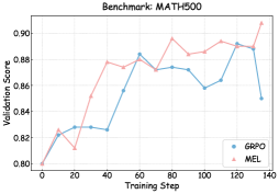
### Visual Description
## Line Chart: Benchmark: MATH500
### Overview
The image displays a line chart comparing the validation score performance of two different methods, labeled "GAPO" and "MEL," over the course of training steps on the MATH500 benchmark. The chart tracks how the validation score for each method evolves as training progresses.
### Components/Axes
* **Chart Title:** "Benchmark: MATH500" (centered at the top).
* **X-Axis:** Labeled "Training Step." The axis is linear and marked with major ticks at intervals of 20, from 0 to 140.
* **Y-Axis:** Labeled "Validation Score." The axis is linear and marked with major ticks at intervals of 0.02, from 0.80 to 0.90.
* **Legend:** Located in the top-left corner of the plot area. It contains two entries:
* A blue line with a circular marker labeled "GAPO".
* A red line with a circular marker labeled "MEL".
* **Data Series:** Two lines with markers at each data point.
* **GAPO (Blue Line):** Represents one method's performance.
* **MEL (Red Line):** Represents the second method's performance.
### Detailed Analysis
**Trend Verification & Data Point Extraction:**
* **GAPO (Blue Line) Trend:** The line shows an overall upward trend with moderate volatility. It starts low, rises quickly, experiences a period of fluctuation between steps 40-100, and then shows a final decline.
* Step 0: ~0.80
* Step 10: ~0.825
* Step 20: ~0.83
* Step 30: ~0.83
* Step 40: ~0.83
* Step 50: ~0.855
* Step 60: ~0.88 (local peak)
* Step 70: ~0.87
* Step 80: ~0.87
* Step 90: ~0.865
* Step 100: ~0.86
* Step 110: ~0.875
* Step 120: ~0.89 (global peak for GAPO)
* Step 130: ~0.885
* Step 140: ~0.85
* **MEL (Red Line) Trend:** The line shows a more volatile but stronger overall upward trend, culminating in the highest score on the chart. It has a notable early dip.
* Step 0: ~0.80
* Step 10: ~0.825
* Step 20: ~0.81 (significant dip)
* Step 30: ~0.84
* Step 40: ~0.875
* Step 50: ~0.875
* Step 60: ~0.87
* Step 70: ~0.88
* Step 80: ~0.89
* Step 90: ~0.88
* Step 100: ~0.885
* Step 110: ~0.885
* Step 120: ~0.89
* Step 130: ~0.885
* Step 140: ~0.91 (global peak for the chart)
### Key Observations
1. **Final Performance:** At the final recorded step (140), MEL (~0.91) significantly outperforms GAPO (~0.85).
2. **Volatility:** MEL exhibits greater volatility, especially in the early training steps (sharp dip at step 20) and the final ascent. GAPO's path is somewhat smoother but still shows fluctuations.
3. **Peak Timing:** GAPO reaches its peak performance earlier (around step 120) before declining. MEL's performance is still climbing at the end of the charted range.
4. **Initial Phase:** Both methods start at the same point (~0.80) and perform similarly for the first 10 steps. They diverge significantly after step 20.
5. **Crossover Points:** The lines cross multiple times (e.g., near steps 10, 60, 70, 110, 120), indicating periods where one method temporarily surpasses the other before the lead changes again.
### Interpretation
The chart suggests a trade-off between stability and peak performance for these two methods on the MATH500 benchmark. **GAPO** appears to be a more stable learner, avoiding major early setbacks but also failing to achieve the highest possible score, with performance degrading after step 120. This could indicate overfitting or a suboptimal learning rate schedule in later stages.
**MEL**, in contrast, demonstrates a "high-risk, high-reward" profile. Its significant early dip suggests initial instability or sensitivity to early training conditions. However, it recovers strongly and ultimately achieves a superior final validation score, indicating it may have a higher capacity for learning or a better optimization trajectory in the long run. The fact that its score is still rising at step 140 implies that further training might yield even better results, whereas GAPO's performance has already peaked and begun to fall.
The multiple crossover points highlight that the "better" method is not constant throughout training; the choice between them could depend on the available training budget (steps) or the need for consistent, predictable improvement versus chasing the absolute highest score.
</details>
<details>
<summary>x23.png Details</summary>
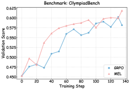
### Visual Description
\n
## Line Chart: Benchmark: OlympiadBench
### Overview
The image displays a line chart comparing the validation score performance of two models, labeled "GAPO" and "MEL," over the course of training steps on a benchmark called "OlympiadBench." The chart shows both models improving over time, with the MEL model consistently achieving a higher validation score after the initial training steps.
### Components/Axes
* **Chart Title:** "Benchmark: OlympiadBench" (centered at the top).
* **Y-Axis:** Labeled "Validation Score." The scale runs from 0.450 to 0.625, with major grid lines and labels at intervals of 0.025 (0.450, 0.475, 0.500, 0.525, 0.550, 0.575, 0.600, 0.625).
* **X-Axis:** Labeled "Training_Step." The scale runs from 0 to 140, with major grid lines and labels at intervals of 20 (0, 20, 40, 60, 80, 100, 120, 140).
* **Legend:** Located in the bottom-right corner of the chart area. It contains two entries:
* A blue line with a circle marker labeled "GAPO".
* A red line with a circle marker labeled "MEL".
* **Data Series:** Two lines plotted on the chart, corresponding to the legend entries.
### Detailed Analysis
**Data Series: GAPO (Blue Line)**
* **Trend:** The line shows an overall upward trend with notable volatility. It experiences a dip early in training before recovering and climbing, with several smaller fluctuations along the way.
* **Approximate Data Points (Training Step, Validation Score):**
* (0, ~0.450)
* (10, ~0.475)
* (20, ~0.465) - *Local minimum*
* (30, ~0.475)
* (40, ~0.500)
* (50, ~0.510)
* (60, ~0.540)
* (70, ~0.560)
* (80, ~0.555)
* (90, ~0.560)
* (100, ~0.575)
* (110, ~0.565)
* (120, ~0.580)
* (130, ~0.570)
* (140, ~0.575)
**Data Series: MEL (Red Line)**
* **Trend:** The line shows a strong, consistent upward trend with less volatility than the GAPO line. After an initial dip, it climbs steadily and maintains a clear performance lead over GAPO for the majority of the training process.
* **Approximate Data Points (Training Step, Validation Score):**
* (0, ~0.475)
* (10, ~0.500)
* (20, ~0.475) - *Local minimum, similar to GAPO*
* (30, ~0.525)
* (40, ~0.550)
* (50, ~0.565)
* (60, ~0.575)
* (70, ~0.585)
* (80, ~0.590)
* (90, ~0.595)
* (100, ~0.590)
* (110, ~0.600)
* (120, ~0.600)
* (130, ~0.605)
* (140, ~0.625) - *Highest point on the chart*
### Key Observations
1. **Performance Gap:** After training step 20, the MEL model (red) establishes and maintains a clear performance advantage over the GAPO model (blue). The gap is most pronounced between steps 40 and 100.
2. **Initial Dip:** Both models experience a performance dip around training step 20, suggesting a common challenge or phase in the early training process on this benchmark.
3. **Volatility vs. Stability:** The GAPO line is more volatile, with sharper peaks and valleys. The MEL line, while not perfectly smooth, demonstrates a more stable and consistent improvement trajectory.
4. **Final Convergence?:** Towards the end of the plotted training (steps 120-140), the GAPO line shows a slight recovery after a dip, while the MEL line continues its strong upward climb, reaching its peak at the final data point. The lines do not appear to converge.
### Interpretation
The data suggests that for the "OlympiadBench" benchmark, the MEL training method or model architecture is more effective and robust than GAPO. MEL not only achieves a higher final validation score (~0.625 vs. ~0.575) but also demonstrates more stable learning dynamics after an initial adjustment period.
The synchronized dip at step 20 is a critical investigative point. It could indicate a specific difficulty in the benchmark dataset encountered at that stage of training, a learning rate schedule effect, or a characteristic of the optimization landscape. The fact that both models recover but then diverge significantly implies that MEL is better equipped to overcome this hurdle and continue scaling its performance.
The chart does not show signs of overfitting (a declining validation score) for either model within the 140 steps, suggesting that performance might continue to improve with further training, particularly for MEL. The primary takeaway is the clear superiority of the MEL approach on this specific task, both in terms of absolute performance and learning stability.
</details>
<details>
<summary>x24.png Details</summary>
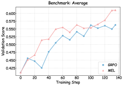
### Visual Description
## Line Chart: Benchmark: Average
### Overview
The image displays a line chart comparing the performance of two methods, labeled "GRPO" and "MEL," over the course of training. The chart plots a "Validation Score" against "Training Step," showing how each method's performance evolves. The overall trend for both methods is upward, indicating improvement with more training steps, but their trajectories and final performance levels differ.
### Components/Axes
* **Chart Title:** "Benchmark: Average" (centered at the top).
* **Y-Axis:**
* **Label:** "Validation Score" (rotated vertically on the left).
* **Scale:** Linear scale ranging from approximately 0.425 to 0.600.
* **Major Tick Marks:** Labeled at 0.425, 0.450, 0.475, 0.500, 0.525, 0.550, 0.575, 0.600.
* **X-Axis:**
* **Label:** "Training Step" (centered at the bottom).
* **Scale:** Linear scale from 0 to 140.
* **Major Tick Marks:** Labeled at 0, 20, 40, 60, 80, 100, 120, 140.
* **Legend:**
* **Position:** Bottom-right corner of the chart area.
* **Entries:**
1. **GRPO:** Represented by a blue line with circular markers.
2. **MEL:** Represented by a red line with circular markers.
* **Grid:** Light gray horizontal and vertical grid lines are present, aligning with the major tick marks on both axes.
### Detailed Analysis
**Data Series: GRPO (Blue Line)**
* **Trend:** The line shows an overall upward trend but with notable volatility. It begins with a sharp initial rise, experiences a significant dip, recovers, and then continues a generally increasing but fluctuating path.
* **Approximate Data Points:**
* Step 0: ~0.425
* Step 10: ~0.450
* Step 20: ~0.440 (local dip)
* Step 30: ~0.425 (lowest point after start)
* Step 40: ~0.475
* Step 50: ~0.500
* Step 60: ~0.525
* Step 70: ~0.510 (dip)
* Step 80: ~0.525
* Step 90: ~0.520 (dip)
* Step 100: ~0.550
* Step 110: ~0.560
* Step 120: ~0.550 (dip)
* Step 130: ~0.560
* Step 140: ~0.575
**Data Series: MEL (Red Line)**
* **Trend:** The line shows a strong, consistent upward trend with only minor fluctuations. It starts higher than GRPO and maintains a lead throughout, with the performance gap widening significantly in the later stages of training.
* **Approximate Data Points:**
* Step 0: ~0.450
* Step 10: ~0.450
* Step 20: ~0.475
* Step 30: ~0.510
* Step 40: ~0.525
* Step 50: ~0.550
* Step 60: ~0.550
* Step 70: ~0.560
* Step 80: ~0.550 (minor dip)
* Step 90: ~0.560
* Step 100: ~0.575
* Step 110: ~0.575
* Step 120: ~0.590
* Step 130: ~0.600
* Step 140: ~0.610 (highest point on chart)
### Key Observations
1. **Performance Gap:** The MEL method (red) consistently achieves a higher Validation Score than the GRPO method (blue) after the initial training steps (around step 10).
2. **Volatility vs. Stability:** The GRPO line exhibits more pronounced dips and recoveries (e.g., at steps 20, 70, 90, 120), suggesting less stable training. The MEL line is smoother, indicating more stable and reliable improvement.
3. **Divergence:** The performance gap between the two methods widens considerably after step 80. By step 140, MEL's score (~0.610) is approximately 0.035 points higher than GRPO's (~0.575).
4. **Final Trajectory:** At the final recorded step (140), the MEL line is still on a clear upward trajectory, while the GRPO line appears to be plateauing or rising more slowly.
### Interpretation
This chart demonstrates a comparative benchmark of two training methodologies. The data strongly suggests that the **MEL method is superior to the GRPO method** for this specific task, based on two key metrics:
* **Higher Final Performance:** MEL achieves a significantly higher validation score.
* **More Stable Learning:** MEL's learning curve is smoother and more consistent, which is often desirable in machine learning as it indicates robustness and predictability.
The widening gap in later training stages implies that MEL may have a better capacity for continued learning or generalization as training progresses. The volatility in the GRPO curve could indicate sensitivity to hyperparameters, batch composition, or other training instabilities. For a technical document, this chart provides clear empirical evidence favoring the adoption of the MEL approach over GRPO for the benchmarked task, assuming validation score is the primary success metric.
</details>
Figure 8: Performance evolution of GRPO and MEL on Qwen3-14B-Base across training steps on multiple benchmarks.
## Appendix B Retention Ratio of Meta-Experience
Through empirical validation via replay, MEL is able to collect high-quality meta-experiences. To examine the utilization of collected meta-experiences, Figure 9 reports the retention ratio of meta-experiences after empirical validation throughout training. We observe that the retention ratio consistently increases with model scale, indicating that larger models are more effective at abstracting high-quality knowledge into meta-experiences, thereby achieving higher retention.
<details>
<summary>x25.png Details</summary>
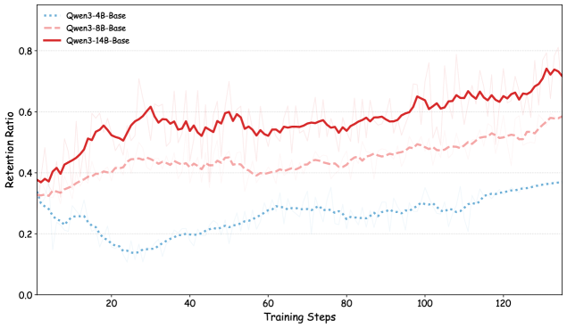
### Visual Description
## Line Chart: Retention Ratio vs. Training Steps for Qwen3 Models
### Overview
The image displays a line chart comparing the "Retention Ratio" of three different-sized base models from the Qwen3 series over the course of training. The chart plots performance across approximately 130 training steps, showing distinct trends for each model size.
### Components/Axes
* **Chart Type:** Multi-series line chart with a light grid background.
* **X-Axis:** Labeled "Training Steps". Major tick marks are present at intervals of 20, from 0 to 120. The axis extends slightly beyond 120, suggesting data up to approximately step 130.
* **Y-Axis:** Labeled "Retention Ratio". The scale ranges from 0.0 to 0.8, with major tick marks at 0.0, 0.2, 0.4, 0.6, and 0.8.
* **Legend:** Positioned in the top-left corner of the plot area. It contains three entries:
1. `Qwen3-4B-Base`: Represented by a blue dotted line.
2. `Qwen3-8B-Base`: Represented by a pink dashed line.
3. `Qwen3-14B-Base`: Represented by a red solid line.
* **Data Series:** Each model's performance is shown as a jagged line, indicating high-frequency measurement or inherent variance in the metric. Faint, lighter-colored lines of the same style appear behind each main line, likely representing raw or unsmoothed data.
### Detailed Analysis
**Trend Verification & Approximate Data Points:**
1. **Qwen3-14B-Base (Red Solid Line):**
* **Trend:** Shows a strong, generally upward trend with significant fluctuations. It is consistently the highest-performing series.
* **Key Points (Approximate):**
* Starts at ~0.38 at step 0.
* Rises to ~0.6 by step 30.
* Fluctuates between ~0.5 and ~0.6 from steps 40-80.
* Begins a more pronounced climb after step 80, reaching its peak of ~0.75 near step 130.
2. **Qwen3-8B-Base (Pink Dashed Line):**
* **Trend:** Shows a moderate, steady upward trend with less volatility than the 14B model. It maintains a middle position throughout.
* **Key Points (Approximate):**
* Starts at ~0.32 at step 0.
* Rises to ~0.45 by step 30.
* Plateaus and fluctuates around ~0.45 from steps 40-80.
* Resumes a gradual climb after step 80, ending at ~0.58 near step 130.
3. **Qwen3-4B-Base (Blue Dotted Line):**
* **Trend:** Exhibits a non-monotonic trend. It initially declines, reaches a trough, and then recovers with a gradual upward slope. It is consistently the lowest-performing series.
* **Key Points (Approximate):**
* Starts at ~0.30 at step 0.
* Declines to a minimum of ~0.15 around step 25.
* Begins a slow recovery, crossing ~0.25 by step 60.
* Continues a gradual, fluctuating ascent to end at ~0.38 near step 130.
### Key Observations
1. **Clear Model Size Hierarchy:** There is a strict and consistent performance hierarchy based on model parameter size: 14B > 8B > 4B. The lines do not cross after the initial steps.
2. **Divergent Early Behavior:** The smallest model (4B) experiences a significant performance drop in the first quarter of training (steps 0-25), while the larger models show immediate improvement.
3. **Concurrent Late-Stage Improvement:** All three models show their most sustained period of improvement in the final third of the chart (after step 80), though the rate of improvement is steepest for the 14B model.
4. **Volatility Correlates with Performance:** The highest-performing model (14B) also exhibits the most pronounced short-term fluctuations in its retention ratio.
### Interpretation
This chart demonstrates a clear positive correlation between model size (parameter count) and the "Retention Ratio" metric throughout the training process for the Qwen3 base models. The data suggests that larger models not only achieve a higher final retention score but also learn more efficiently from the outset, avoiding the performance dip seen in the 4B model.
The "Retention Ratio" likely measures how well the model retains information or capabilities during training, possibly in the context of continual learning or preventing catastrophic forgetting. The 4B model's initial dip could indicate a period of instability or significant parameter adjustment that temporarily harms this retention capability before a recovery phase.
The synchronized upward trend for all models after step 80 might point to a change in the training regime (e.g., a learning rate schedule adjustment) or a phase in the training data that is particularly conducive to improving this metric. The greater volatility in the 14B model's line could be a function of its higher capacity, making its performance more sensitive to individual training batches, or it could be an artifact of the measurement scale.
**Language Declaration:** All text within the image (labels, legend, axis titles) is in English.
</details>
Figure 9: Dynamics of the retention ratio of MEL across different model scales.
## Appendix C Prompt Template
We use the same prompt template for all models. Details of the prompts used for meta-experience construction and for empirical validation via replay are shown below.
Meta-Experience Prompt
You are a Meta-Cognitive Reasoning Analyst specializing in self-reflection, error root-cause analysis, and the extraction of generalizable heuristics. You are provided with multiple solution trajectories for the same problem. Note that the labels Correct or Incorrect apply to the final answer, but the reasoning process itself may contain twists and turns. Your task is to conduct a deep comparative autopsy of the thinking processes. You must identify the structural differences in cognition that led to success or failure, and synthesize these into abstract principles for future use. Core Analysis Requirements: 1.
Deep Dive into Correct Trajectories (Resilience & Robustness Analysis): •
Scenario A (Self-Correction): If you find the reasoning contains initial errors or uncertainties, look for moments of self-correction. What triggered the realization? What structural insight allowed the reasoning to pivot back to the right track? •
Scenario B (Flawless Execution): When every step of the reasoning is correct from the start, identify the Foundational “Immunity”. What specific definition, clear knowledge representation, or disciplined step-by-step verification prevented this Agent from falling into the traps that the Incorrect Agent fell into? •
Goal: Extract the specific logic validation technique or robust mental representation that saved the solution. 2.
Deep Dive into Incorrect Trajectories (Vulnerability Analysis): •
You must identify not only where the math/logic went wrong, but also why the reasoning drifted. •
Identify: The “Bifurcation Point” where a correct start turned into a hallucination or logic gap. •
Analyze: The latent cognitive defect (e.g., concept conflation, rigid mindset, overlooking edge cases, intuitive bias) that caused the error. •
Identify: What specific knowledge point or constraint was violated? 3.
Comparative Synthesis: •
Contrast the Solutions and Decision Boundaries. Why did the successful trajectory avoid the trap that the failed one fell into? •
What structural insight did the winner have that the loser missed? (e.g., The winner treated the problem as a geometric issue, while the loser got stuck in algebra). 4.
Strict Generalization Constraint: •
Forbidden: Do NOT mention the specific numbers, variables, or exact answer of the current problem in your “Heuristics” or “Reflective Summary”. •
Required: Convert specific lessons into abstract heuristics (e.g., instead of “The integral of $x^2$ is…”, use “When integrating polynomial functions…”). Formulate them as conditionally triggered rules (“If…Then…”, “When dealing with [Concept X]…I should…”). Output Format (Strict Adherence Required) 1. Failure Resolution Path & Error Pattern Recognition (Mandatory for incorrect samples) •
Failure Point: Identify the exact step where logic diverged. Did it start correctly? Where did the drift happen? •
Latent Cognitive Pattern: Reveal the deep-seated reasoning defect. Was it a bias? A missing prerequisite? A misunderstanding of the prompt’s intent? Do not list surface-level calculation errors. 2. Analysis of Success Factors (Mandatory for correct samples) •
Reasoning Pivot (If applicable): If the path involved self-correction, describe the moment of realization and the strategy used to fix it. •
Robustness Factor (If flawless): If the path was perfect, explain the fundamental concept or structural approach that effectively “immunized” the reasoning against common errors. •
Reason for Effectiveness: Why did this perspective work? What fundamental logic did it satisfy? 3. First-Person Reflective Summary (Mandatory) Write a meta-cognitive reflection from the first-person perspective (“I”). •
Review: Briefly review the thinking process differences. •
Insight: Discuss the specific knowledge point or cognitive habit that was critical. •
Action: Explain how you will restructure your approach to avoid the identified “Internal Reasoning Defects” in the future. Focus on the “How” of thinking, not the “What” of the answer. 4. Subject Heuristics (Internalized Experience) (Mandatory) •
[Pattern Name]: If [abstract condition] occurs, then [abstract action]… •
[Pattern Name]: When dealing with [concept type], I must strictly verify [constraint]… (Note: These must be applicable to *future* problems of a similar class, completely stripped of this problem’s specifics.) Here the question and the corresponding solutions. $<$ question $>$ {question} $<$ /question $>$ Solution 1: $<$ answer $>$ {error_ans} $<$ /answer $>$ $<$ judge $>$ Incorrect $<$ /judge $>$ Solution 2: $<$ answer $>$ {correct_ans} $<$ /answer $>$ $<$ judge $>$ Correct $<$ /judge $>$
Empirical Validation Prompt
Prior study has provided some internal reference information relevant to this question, including the key approaches, steps, and reasoning needed for a correct solution; the typical reasoning biases, logical flaws, or pitfalls that appear in incorrect solutions; and various heuristic insights on how to complete this problem more effectively. {experience} Now, please fully internalize this information as your own experience, then independently think through the problem in detail and produce a complete answer. Note: •
You must perform full, in-depth reasoning internally and arrive at the final answer while making full use of the information above. Answer the following question: {question}