# LLM-Based Scientific Equation Discovery via Physics-Informed Token-Regularized Policy Optimization
**Authors**: Boxiao Wang, Kai Li, Tianyi Liu, Chen Li, Junzhe Wang, Yifan Zhang, Jian Cheng
> 0009-0008-2970-7575 Institute of Automation, Chinese Academy of Sciences Beijing China
> Institute of Automation, Chinese Academy of Sciences Beijing China
> State Key Laboratory of Aerodynamics Mianyang, Sichuan China
> School of Mathematical Sciences, University of Chinese Academy of Sciences Beijing China
## Abstract
Symbolic regression aims to distill mathematical equations from observational data. Recent approaches have successfully leveraged Large Language Models (LLMs) to generate equation hypotheses, capitalizing on their vast pre-trained scientific priors. However, existing frameworks predominantly treat the LLM as a static generator, relying on prompt-level guidance to steer exploration. This paradigm fails to update the model’s internal representations based on search feedback, often yielding physically inconsistent or mathematically redundant expressions. In this work, we propose PiT-PO (Physics-informed Token-regularized Policy Optimization), a unified framework that evolves the LLM into an adaptive generator via reinforcement learning. Central to PiT-PO is a dual-constraint mechanism that rigorously enforces hierarchical physical validity while simultaneously applying fine-grained, token-level penalties to suppress redundant structures. Consequently, PiT-PO aligns LLM to produce equations that are both scientifically consistent and structurally parsimonious. Empirically, PiT-PO achieves state-of-the-art performance on standard benchmarks and successfully discovers novel turbulence models for challenging fluid dynamics problems. We also demonstrate that PiT-PO empowers small-scale models to outperform closed-source giants, democratizing access to high-performance scientific discovery.
conference: ; ;
## 1. Introduction
Symbolic Regression (SR) (Makke and Chawla, 2024b) stands as a cornerstone of data-driven scientific discovery, uniquely capable of distilling interpretable mathematical equations from observational data. Unlike black-box models that prioritize mere prediction, SR elucidates the fundamental mechanisms governing system behavior, proving instrumental in uncovering physical laws (Makke and Chawla, 2024a; Reuter et al., 2023), modeling chemical kinetics (Chen et al., 2025; Deng et al., 2023), and analyzing complex biological dynamics (Wahlquist et al., 2024; Shi et al., 2024).
However, the search for exact governing equations represents a formidable challenge, formally classified as an NP-hard problem (Virgolin and Pissis, 2022). To navigate this vast search space, algorithmic strategies have evolved from Genetic Programming (GP) (Schmidt and Lipson, 2009; Cranmer, 2023) and Reinforcement Learning (RL) (Petersen et al., 2021) to Transformer-based architectures that map numerical data directly to symbolic equations (Biggio et al., 2021; Kamienny et al., 2022; Zhang et al., 2025). Most recently, the advent of Large Language Models (LLMs) has introduced a new paradigm. Methods such as LLM-SR (Shojaee et al., 2025a) and LaSR (Grayeli et al., 2024) leverage the pre-trained scientific priors and in-context learning capabilities of LLMs to generate equation hypotheses. These approaches typically employ an evolutionary search paradigm, where candidates are evaluated, and high-performing solutions are fed back via prompt-level conditioning to steer subsequent generation.
Despite encouraging progress, existing LLM-based SR methods remain constrained by severe limitations. First, most approaches treat the LLM as a static generator, relying primarily on prompt-level, verbal guidance to steer the evolutionary search (Shojaee et al., 2025a; Grayeli et al., 2024). This “frozen” paradigm inherently neglects the opportunity to adapt and enhance the generative capability of the LLM itself based on evaluation signals, preventing the model from internalizing feedback and adjusting its generation strategies to the specific problem. Second, they typically operate in a physics-agnostic manner, prioritizing syntactic correctness over physical validity (Shojaee et al., 2025a; Grayeli et al., 2024). Without rigorous constraints, LLMs often generate equations that fit the data numerically but violate fundamental physical principles, rendering them prone to overfitting and practically unusable.
In this work, we propose to fundamentally shift the role of the LLM in SR from a static proposer to an adaptive generator. We establish a dynamic feedback loop in which evolutionary exploration and parametric learning reinforce each other: evolutionary search uncovers diverse candidate equations and generates informative evaluation signals, while parametric adaptation enables the LLM to consolidate effective symbolic patterns and guide subsequent exploration more efficiently. By employing in-search fine-tuning, i.e., updating the LLM parameters during the evolutionary search process, we move beyond purely verbal, prompt-level guidance and introduce numerical guidance that allows feedback to be directly internalized into the model parameters, progressively aligning LLM with the intrinsic properties of the target system.
To realize this vision, we introduce PiT-PO (Physics-informed Token-regularized Policy Optimization), a unified framework that bridges LLM-driven evolutionary exploration with rigorous verification. PiT-PO is built upon two technical components. 1) In-Search LLM Evolution. We implement the numerical guidance via reinforcement learning, which efficiently updates the LLM’s parameters during the search process. Instead of relying on static pre-trained knowledge, this in-search policy optimization enables LLM to dynamically align its generative distribution with the structural characteristics of the specific task, effectively transforming general scientific priors into domain-specific expertise on the fly. 2) Dual Constraints as Search Guidance. We enforce hierarchical physical constraints to ensure scientific validity, and uniquely, we incorporate a fine-grained regularization based on our proposed Support Exclusion Theorem. This theorem allows us to identify mathematically redundant terms and translate them into token-level penalties, effectively pruning the search space and guiding LLM toward physically meaningful and structurally parsimonious equations.
Comprehensive experimental results demonstrate that PiT-PO achieves state-of-the-art performance across standard SR benchmarks, including the LLM-SR Suite (Shojaee et al., 2025a) and LLM-SRBench (Shojaee et al., 2025b), and recovers the largest number of ground-truth equations among all evaluated methods. In addition to synthetic benchmarks, the effectiveness of PiT-PO is validated on an application-driven turbulence modeling task involving flow over periodic hills. PiT-PO improves upon traditional Reynolds-Averaged Navier-Stokes (RANS) approaches by producing anisotropic Reynolds stresses closer to Direct Numerical Simulation (DNS) references. The learned method shows enhanced physical consistency, with reduced non-physical extremes and better flow field predictions. Finally, PiT-PO maintains robust performance even when using resource-constrained small models, such as a quantized version of Llama-8B, and remains efficient under strict wall-clock time budgets, establishing a practical methodology for automated scientific discovery.
<details>
<summary>x1.png Details</summary>
### Visual Description
## Diagram: Process Flow for Physics-Informed Token-Regularized Policy Optimization
### Overview
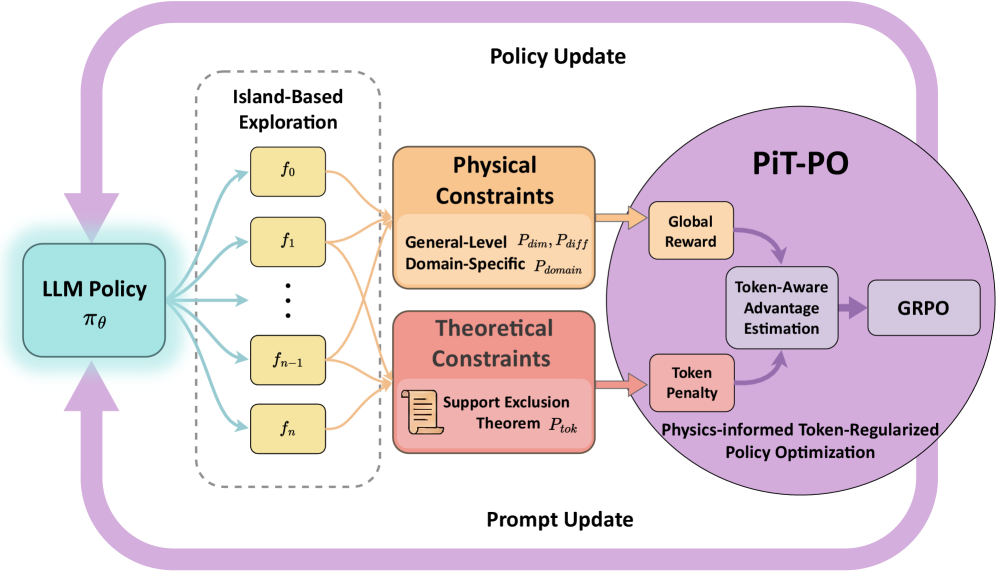
The diagram illustrates a cyclical process for optimizing a Language Model (LLM) policy through island-based exploration, constraint integration, and physics-informed token-regularized policy optimization (PiT-PO). Arrows indicate directional flow between components, emphasizing iterative updates.
---
### Components/Axes
1. **Left Section (Island-Based Exploration)**
- **Box**: "Island-Based Exploration"
- Sub-components: Functions `f₀`, `f₁`, ..., `fₙ` (representing exploration outputs).
- **Arrows**: Connect "LLM Policy" (`π_θ`) to exploration functions, indicating policy-driven exploration.
2. **Middle Section (Constraints)**
- **Box 1**: "Physical Constraints"
- Sub-components:
- General-Level: `P_dim`, `P_diff`
- Domain-Specific: `P_domain`
- **Box 2**: "Theoretical Constraints"
- Sub-component: "Support Exclusion Theorem" (`P_tok`).
- **Arrows**: Connect exploration outputs to constraints, showing constraint evaluation.
3. **Right Section (Policy Update)**
- **Circle**: "PiT-PO" (Physics-informed Token-Regularized Policy Optimization)
- Sub-components:
- "Token-Aware Advantage Estimation"
- "GRPO" (Gradient Regularized Policy Optimization)
- "Token Penalty"
- **Arrows**:
- From constraints to "Global Reward" and "Token Penalty."
- From "Token-Aware Advantage Estimation" to GRPO.
- From GRPO back to "LLM Policy" (`π_θ`), completing the loop.
---
### Detailed Analysis
- **LLM Policy (`π_θ`)**:
- Central node driving the process.
- Outputs exploration functions (`f₀` to `fₙ`) for island-based exploration.
- **Island-Based Exploration**:
- Generates diverse function outputs (`f₀` to `fₙ`) to explore policy behavior.
- **Physical Constraints**:
- Enforce general (`P_dim`, `P_diff`) and domain-specific (`P_domain`) rules.
- Ensure exploration outputs adhere to real-world physics.
- **Theoretical Constraints**:
- "Support Exclusion Theorem" (`P_tok`) filters invalid or redundant exploration paths.
- **PiT-PO System**:
- Integrates constraints into policy updates via:
1. **Token-Aware Advantage Estimation**: Evaluates policy performance with token-level awareness.
2. **GRPO**: Optimizes policy using gradient regularization.
3. **Token Penalty**: Penalizes deviations from physical/theoretical constraints.
- **Cyclical Flow**:
- Policy → Exploration → Constraints → Policy Update → Repeat.
---
### Key Observations
1. **Iterative Optimization**: The loop emphasizes continuous refinement of the LLM policy using constraint feedback.
2. **Constraint Integration**: Physical and theoretical constraints act as gatekeepers for valid exploration paths.
3. **Token-Aware Mechanisms**: Highlight the importance of token-level granularity in policy optimization.
4. **GRPO Role**: Serves as the final optimization step, balancing exploration and constraint adherence.
---
### Interpretation
This diagram represents a framework for training robust LLM policies in constrained environments. By combining island-based exploration (diverse function sampling) with physics and theoretical constraints, the system ensures policies remain grounded in real-world feasibility. The PiT-PO system further refines policies using token-aware advantage estimation and gradient regularization, preventing overfitting to exploration noise. The cyclical nature suggests a reinforcement learning approach where constraints dynamically shape policy updates, critical for applications like robotics or safety-critical systems.
</details>
Figure 1. The overall framework of PiT-PO. PiT-PO transforms the LLM from a static proposer into an adaptive generator via a closed-loop evolutionary process. The framework integrates dual-constraint evaluation—comprising physical constraints and theoretical constraints—to generate fine-grained token-level learning signals. These signals guide the LLM policy update via reinforcement learning, ensuring the discovery of parsimonious, physically consistent equations.
## 2. Preliminaries
### 2.1. Problem Setup
In SR, a dataset of input–output observations is given:
$$
D=\{(x_{i},y_{i})\}_{i=1}^{n},\;x_{i}\in\mathbb{R}^{d},\;y_{i}\in\mathbb{R}. \tag{1}
$$
The objective is to identify a compact and interpretable function $f\in\mathcal{F}$ such that $f(x_{i})\approx y_{i}$ for the observed samples, while retaining the ability to generalize to unseen inputs.
### 2.2. LLM-based SR Methods
Contemporary LLM-based approaches reformulate SR as a iterative program synthesis task. In this paradigm, typified by frameworks such as LLM-SR (Shojaee et al., 2025a), the discovery process is decoupled into two phases: structure proposal and parameter estimation. Specifically, the LLM functions as a symbolic generator, emitting functional skeletons with placeholders for learnable coefficients. A numerical optimizer (e.g., BFGS (Fletcher, 1987)) subsequently fits these constants to the observed data. To navigate the combinatorial search space, these methods employ an evolutionary-style feedback loop: high-fitness equations are maintained in a pool to serve as in-context examples, prompting the LLM to refine subsequent generations. Our work leverages this architecture as a backbone, but fundamentally redefines the LLM’s role from a static proposer to an adaptive generator.
### 2.3. Group Relative Policy Optimization
Group Relative Policy Optimization (GRPO) (Shao et al., 2024) is a RL algorithm tailored for optimizing LLMs on reasoning tasks, characterized by its efficient baseline estimation without the need for a separate value network. In the context of LLM-based SR, the generation process is modeled as a Markov Decision Process (MDP), where LLM functions as a policy $\pi_{\theta}$ that generates a sequence of tokens $o=(t_{1},\dots,t_{L})$ given a prompt $q$ . For each $q$ , GRPO samples a group of $G$ outputs $\{o_{1},\dots,o_{G}\}$ from the sampling policy $\pi_{\theta_{old}}$ . GRPO maximizes the following surrogate loss function:
$$
\mathcal{J}_{GRPO}(\theta)=\mathbb{E}_{q\sim P(Q),\{o_{i}\}\sim\pi_{\theta_{old}}}\left[\frac{1}{G}\sum_{i=1}^{G}\left(\frac{1}{L_{i}}\sum_{k=1}^{L_{i}}\mathcal{L}^{clip}_{i,k}(\theta)-\beta\mathbb{D}_{KL}(\pi_{\theta}||\pi_{ref})\right)\right], \tag{2}
$$
where $\pi_{ref}$ is the reference policy to prevent excessive deviation, and $\beta$ controls the KL-divergence penalty. The clipping term $\mathcal{L}^{clip}_{i,k}(\theta)$ ensures trust region updates:
$$
\mathcal{L}^{clip}_{i,k}(\theta)=\min\left(\frac{\pi_{\theta}(t_{i,k}|q,o_{i,<k})}{\pi_{\theta_{old}}(t_{i,k}|q,o_{i,<k})}\hat{A}_{i},\;\text{clip}\left(\frac{\pi_{\theta}(t_{i,k}|q,o_{i,<k})}{\pi_{\theta_{old}}(t_{i,k}|q,o_{i,<k})},1-\epsilon,1+\epsilon\right)\hat{A}_{i}\right). \tag{3}
$$
Here, $\epsilon$ is the clipping coefficient. A distinctive feature of GRPO lies in its advantage estimation, it computes the advantage $\hat{A}_{i}$ by standardizing the reward $R(o_{i})$ relative to the group:
$$
\hat{A}_{i}=\frac{R(o_{i})-\text{mean}(\{R(o_{j})\})}{\text{std}(\{R(o_{j})\})}. \tag{4}
$$
Consequently, every token within the sequence $o_{i}$ is assigned the exact same feedback signal. This coarse granularity treats valid and redundant terms indistinguishably, a limitation that our work addresses by introducing fine-grained, token-level regularization.
## 3. Method
We propose PiT-PO (Physics-informed Token-regularized Policy Optimization), a framework that evolves LLM into an adaptive, physics-aware generator. PiT-PO establishes a closed-loop evolutionary process driven by two synergistic mechanisms: (1) a dual-constraint evaluation system that rigorously assesses candidates through hierarchical physical verification and theorem-guided redundancy pruning; and (2) a novel policy optimization strategy that updates LLM using fine-grained, token-level feedback derived from these constraints. This combination effectively aligns the LLM with the intrinsic structure of the problem, guiding the LLM toward solutions that are not only numerically accurate but also structurally parsimonious and scientifically consistent.
### 3.1. Dual-Constraint Learning Signals
Navigating the combinatorial space of symbolic equations requires rigorous guidance. We employ a reward system driven by dual constraints: physical constraints delineate the scientifically valid region, while theoretical constraints drive the search toward simpler equations by identifying and pruning redundant terms.
#### 3.1.1. Hierarchical Physical Constraints.
To ensure scientific validity, we construct a hierarchical filter that categorizes constraints into two levels: general properties and domain-specific priors.
General-Level Constraints. We enforce fundamental physical properties applicable across scientific disciplines. To prune physically impossible structures (e.g., adding terms with mismatched units), we assign penalty-based rewards for Dimensional Homogeneity ( $P_{dim}$ ) and Differentiability ( $P_{diff}$ ). The former strictly penalizes equations with unit inconsistencies, while the latter enforces smoothness on the data-defined domain.
Domain-Specific Constraints. To tackle specialized tasks, we inject expert knowledge as inductive biases. We define the domain-specific penalty $P^{(j)}_{domain}$ to penalize candidate equations that violate the $j$ -th domain-specific constraint. Taking the turbulence modeling task (detailed in Appendix E.4) as a representative instantiation, we enforce four rigorous constraints: (1) Realizability (Pope, 2000), ensuring the Reynolds stress tensor has positive eigenvalues; (2) Boundary Condition Consistency (Monkewitz, 2021), requiring stresses to decay to zero at the wall; (3) Asymptotic Scaling (Tennekes and Lumley, 1972; WANG et al., 2019), enforcing the cubic relationship between stress and wall distance in the viscous sublayer; and (4) Energy Consistency (Pope, 2000; MOCHIZUKI and OSAKA, 2000), aligning predicted stress with turbulent kinetic energy production.
This hierarchical design effectively embeds physical consistency as a hard constraint in the reward function, prioritizing scientific validity over mere empirical fitting.
#### 3.1.2. Theorem-Guided Mathematical Constraints
While physical constraints ensure validity, they do not prevent mathematical redundancy. To rigorously distinguish between essential terms and redundant artifacts, we introduce the Support Exclusion Theorem.
Let $\mathcal{S}$ denote the full support set containing all candidate basis functions $\{\phi_{j}\}$ . The ground truth equation is $f^{*}=\sum_{j\in\mathcal{S}^{\prime}}a_{j}\phi_{j}$ , where $\mathcal{S}^{\prime}\subseteq\mathcal{S}$ is the true support set (i.e., the indices of basis functions that truly appear in the governing equation), and $\{a_{j}\}_{j\in\mathcal{S}^{\prime}}$ are the corresponding true coefficients. Consider a candidate equation $f=\sum_{j\in\mathcal{K}}b_{j}\phi_{j}$ , where $\mathcal{K}\subseteq\mathcal{S}$ represents the current support set (i.e., the selected terms in the skeleton), $\mathbf{b}=\{b_{j}\}_{j\in\mathcal{K}}$ are the optimized coefficients derived from the data. We define the empirical Gram matrix of these basis functions as $G\in\mathbb{R}^{|\mathcal{S}|\times|\mathcal{S}|}$ and the corresponding Projection Matrix as $T$ , where $T_{ij}:=G_{ji}/G_{ii}$ .
** Theorem 3.1 (Support Exclusion Theorem)**
*Assume the ground-truth support is finite and satisfies $|\mathcal{S}^{\prime}|\leq M$ , and let the true function coefficients be bounded by $A\leq|a_{j}|\leq B$ for all $j\in\mathcal{S}^{\prime}$ . A term $\phi_{i}$ ( $i\in\mathcal{K}$ ) is theoretically guaranteed to be a false discovery (not in the true support $\mathcal{S}^{\prime}$ ) if its fitted coefficient magnitude satisfies:
$$
|b_{i}|<A-\left(\underbrace{\sum_{j\in\mathcal{K},j\neq i}(B+|b_{j}|)|T_{ij}|}_{\text{Internal Interference}}+\underbrace{B\sum_{k=1}^{m}s_{(k)}}_{\text{External Interference}}\right). \tag{5}
$$
$s(k)$ denotes the $k$ -th largest value in $\{|T_{i\ell}|:\ell\in\mathcal{S}\setminus\mathcal{K}\}$ , and $m:=\min\!\big(M-1,\;|\mathcal{S}\setminus\mathcal{K}|\big)$ .*
Detailed definitions of all notations and the rigorous proof of Theorem 3.1 are provided in Appendix B. This theorem formalizes the intuition that coefficients of redundant terms (absent from the true support $\mathcal{S}^{\prime}$ ) have significantly smaller magnitudes than those of valid components.
Specifically, after fitting $\mathbf{b}$ , we compute the normalized coefficient ratio $\tau_{i}=|b_{i}|/(\sum_{j}|b_{j}|+\epsilon)$ . We introduce a threshold $\rho\in(0,1)$ to identify potentially redundant terms. Terms satisfying $\tau_{i}>\rho$ incur no penalty, while components with $\tau_{i}\leq\rho$ are considered redundant. To suppress these redundancies, we define a token penalty for each token in redundant term $i$ :
$$
P_{tok}=p\cdot\max\left(0,-\log\left(|b_{i}|+\epsilon\right)\right), \tag{6}
$$
where $p>0$ is a scaling coefficient. We use a logarithmic scale to impose stronger penalties on terms with smaller coefficients.
By integrating this penalty into the policy optimization, we guide the LLM to reduce the probability of generating redundant terms, thereby steering the optimization toward parsimonious equations.
### 3.2. Token-Aware Policy Update
Our proposed PiT-PO effectively operationalize the hierarchical constraints and theoretical insights derived in Section 3.1. Unlike standard GRPO that assign a uniform scalar reward to the entire generated sequence, our method transitions the learning process from coarse-grained sequence scoring to fine-grained token-level credit assignment. This ensures that the policy not only learns to generate physically valid equations but also explicitly suppresses theoretically redundant terms.
#### 3.2.1. Global Reward with Gated Constraints
The optimization is driven by a composite global reward, $R_{global}$ , which balances fitting accuracy, structural parsimony, and physical consistency. Formally, for a sampled equation $o_{i}$ , the rewards are defined as follows:
Fitting Accuracy ( $R_{fit}$ ). We use the normalized log-MSE to encourage precise data fitting:
$$
R_{fit}=-\alpha\log(\text{MSE}+\epsilon), \tag{7}
$$
where $MSE=\frac{1}{n}\sum_{i=1}^{n}(y_{i}-\hat{y}_{i})^{2}$ .
Complexity Penalty ( $P_{cplx}$ ). Adhering to Occam’s Razor, we penalize structural complexity based on the Abstract Syntax Tree (AST) (Neamtiu et al., 2005) node count:
$$
P_{cplx}=\lambda_{len}\cdot\text{Length}(\text{AST}). \tag{8}
$$
In PiT-PO, each equation generated by the LLM is represented as a Python function and parsed into an AST, where each node corresponds to a variable or operator. The total node count provides a meaningful estimate of structural complexity.
Gated Physical Penalty ( $P_{phy}$ ). Imposing strict physical constraints too early can hinder exploration, causing the model to discard potentially promising functional forms. We therefore activate physical penalties only after the candidate equation reaches a baseline fitting accuracy threshold ( $\delta_{gate}$ ). Specifically, we define
where $\mathbb{1}(\cdot)$ is the indicator function. This mechanism effectively creates a soft curriculum: it allows “free” exploration in the early stages and enforcing strict physical compliance only after the solution enters a plausible region.
The total reward $R_{global}$ is then formulated as:
$$
R_{global}(o_{i})=R_{fit}(o_{i})-P_{cplx}(o_{i})-P_{phy}(o_{i}). \tag{10}
$$
#### 3.2.2. Fine-Grained Advantage Estimation
Standard GRPO applies a uniform advantage across all tokens in a sequence. We refine this by synthesizing the global reward with the token-level penalty $P_{tok}$ (Equation 6). Specifically, we define the token-aware advantage $\hat{A}_{i,k}$ for the $k$ -th token in the $i$ -th sampled equation as:
$$
\hat{A}_{i,k}=\underbrace{\frac{R_{global}(o_{i})-\mu_{group}}{\sigma_{group}}}_{\text{Global Standardization}}-\underbrace{P_{i,k}}_{\text{Local Pruning}}. \tag{11}
$$
Here, the first term standardizes the global reward against the group statistics ( $\mu_{group},\sigma_{group}$ ), reinforcing equations that satisfy multi-objective criteria relative to their peers. The second term, $P_{i,k}$ , applies a targeted penalty to suppress redundancy. Specifically, we set $P_{i,k}=0$ if token $k$ belongs to a non-redundant term, and $P_{i,k}=P_{tok}$ otherwise. This ensures that penalties are applied exclusively to tokens contributing to mathematically redundant structures, while valid terms remain unaffected.
Substituting this token-aware advantage into the GRPO objective, the policy gradient update of our PiT-PO becomes:
$$
\nabla\mathcal{J}_{PiT-PO}\propto\sum_{i,k}\hat{A}_{i,k}\nabla\log\pi_{\theta}(t_{i,k}|o_{i,<k}). \tag{12}
$$
This creates a dual-pressure optimization landscape: global rewards guide the policy toward physically consistent and accurate equations, while local penalties surgically excise redundant terms. This ensures the final output aligns with the sparse, underlying physical laws rather than merely overfitting numerical data.
Input: Dataset $D=\{(x_{i},y_{i})\}_{i=1}^{n}$ ; LLM $\pi_{\theta}$ ; number of islands $N$ ; group size $G$ ; iterations $T$ .
Output: Best equation $o^{*}$ .
1
2 1ex
3 Initialize $o^{*}$ , $s^{*}$ , and buffers $\mathcal{B}_{j}\leftarrow\emptyset$ for $j=1,\dots,N$
4
5 for $t\leftarrow 1$ to $T$ do
// Stage 1: Island-Based Exploration
6 for $j\leftarrow 1$ to $N$ do
$q_{j}\leftarrow\textsc{BuildPrompt}(D,\mathcal{B}_{j})$
// in-context rule
$\{o_{i}\}_{i=1}^{G}\sim\pi_{\theta}(\cdot\mid q_{j})$
// sample a group
7 for $i\leftarrow 1$ to $G$ do
$(R_{i},\{P_{i,k}\})\leftarrow\textsc{DualConstraintEval}(o_{i},D)$
// $R_{i}=R_{\mathrm{global}}(o_{i})$
8 $\mathcal{B}_{j}\leftarrow\mathcal{B}_{j}\cup\{(q_{j},o_{i},R_{i},\{P_{i,k}\})\}$
9 if $R_{i}>s^{*}$ then
10 $o^{*}\leftarrow o_{i}$ ; $s^{*}\leftarrow R_{i}$
11
12
13
// Stage 2: In-Search LLM Evolution
14 $\theta\leftarrow\textsc{PiT-PO\_Update}(\theta,\{\mathcal{B}_{j}\}_{j=1}^{N},\pi_{{\theta}})$
// Stage 3: Hierarchical Selection
15 $\{\mathcal{B}_{j}\}_{j=1}^{N}\leftarrow\textsc{SelectAndReset}(\{\mathcal{B}_{j}\}_{j=1}^{N})$
16 return $o^{*}$
Algorithm 1 PiT-PO Overall Training Pipeline
### 3.3. Overall Training Pipeline
We orchestrate the PiT-PO framework through a closed-loop evolutionary RL cycle. As illustrated in Algorithm 1, the training process iterates through three synergistic phases:
Phase 1: Island-Based Exploration (Data Generation). To prevent premature convergence to local optima, a common pitfall in SR, we employ a standard multi-island topology ( $N$ islands) to structurally enforce search diversity (Cranmer, 2023; Romera-Paredes et al., 2024). Each island $j$ maintains an isolated experience buffer $\mathcal{B}_{j}$ , evolving its own lineage of equations. This information isolation allows distinct islands to cultivate diverse functional forms independently.
Phase 2: In-Search LLM Evolution (Policy Update). This phase transforms the collected data into parametric knowledge. We aggregate the trajectories from all $N$ islands into a global batch to perform policy optimization using PiT-PO. By minimizing the loss, the model explicitly lowers the probability of generating mathematically redundant tokens and physically inconsistent structures. To ensure computational efficiency during this iterative search, we implement the update using Low-Rank Adaptation (LoRA) (Hu et al., 2021).
Phase 3: Hierarchical Selection (Population Management). We apply standard survival-of-the-fittest mechanisms to maintain population quality. Local buffers $\mathcal{B}_{j}$ are updated by retaining only top-performing candidates, while underperforming islands are periodically reset with high-fitness seeds to escape local optima.
This cycle establishes a reciprocal reinforcement mechanism: the island-based exploration maintains search diversity, while policy update consolidates these findings into the model weights, progressively transforming the LLM into a domain-specialized scientific discoverer.
## 4. Experiments
### 4.1. Setup
Benchmarks. To provide a comprehensive evaluation of PiT-PO, we adopt two widely used benchmarks to compare against state-of-the-art baselines:
LLM-SR Suite (Shojaee et al., 2025a). This suite comprises four tasks spanning multiple scientific domains: Oscillation 1 & 2 (Nonlinear Oscillatory Systems) feature dissipative couplings and non-polynomial nonlinearities with explicit forcing, making recovery of the correct interaction terms from trajectory data non-trivial; E. coli Growth (Monod, 1949; Rosso et al., 1995) models multivariate population dynamics with strongly coupled, multiplicative effects from nutrients, temperature, and acidity; and Stress-Strain (Aakash et al., 2019) uses experimental measurements of Aluminum 6061-T651 and exhibits temperature-dependent, piecewise non-linear deformation behavior. Detailed information about these tasks is provided in Appendix D.1.
LLM-SRBench: (Shojaee et al., 2025b) To evaluate generalization beyond canonical forms, we adopt the comprehensive LLM-SRBench benchmark, which contains 239 tasks organized into two complementary subsets, LSR-Transform and LSR-Synth. LSR-Transform changes the prediction target to rewrite well-known physics equations into less common yet analytically equivalent forms, producing 111 transformed tasks. This design aims to reduce reliance on direct memorization of canonical templates and tests whether a method can recover the same physical law under non-trivial variable reparameterizations. Complementarily, LSR-Synth composes equations from both known scientific terms and synthetic but plausible terms to further assess discovery beyond memorized templates: candidate terms are proposed by an LLM under domain context, assembled into full equations, and then filtered through multiple checks, including numerical solvability, contextual novelty, and expert plausibility, yielding 128 synthetic tasks. Further details are given in Appendix D.2.
Baselines.
We compare PiT-PO against representative baselines spanning both classical and LLM-based SR methods. For the four tasks in the LLM-SR Suite, we include GPlearn, a genetic programming-based SR approach; PySR (Grayeli et al., 2024), which couples evolutionary search with symbolic simplification; uDSR (Landajuela et al., 2022), which replaces the RNN policy in DSR with a pretrained Transformer and employs neural-guided decoding; RAG-SR (Zhang et al., 2025), which incorporates structure retrieval to assist equation generation; and LLM-SR (Shojaee et al., 2025a). For the broader LLM-SRBench benchmark, we further compare against leading LLM-based SR methods, including SGA (Ma et al., 2024), which integrates LLM-driven hypothesis proposal with physics-informed parameter optimization in a bilevel search framework, and LaSR (Grayeli et al., 2024), which leverages abstract symbolic concepts distilled from prior equations to guide hybrid LLM–evolutionary generation.
Evaluation metrics. We evaluate methods using Accuracy to Tolerance and Normalized Mean Squared Error (NMSE). For a tolerance $\tau$ , we report $\mathrm{Acc}_{\mathrm{all}}(\tau)$ (Biggio et al., 2021) and $\mathrm{Acc}_{\mathrm{avg}}(\tau)$ based on relative error: $\mathrm{Acc}_{\mathrm{all}}(\tau)=\mathbbm{1}\!\bigl(\max_{1\leq i\leq N_{\mathrm{test}}}\bigl|\tfrac{\hat{y}_{i}-y_{i}}{y_{i}}\bigr|\leq\tau\bigr)$ and $\mathrm{Acc}_{\mathrm{avg}}(\tau)=\tfrac{1}{N_{\mathrm{test}}}\sum_{i=1}^{N_{\mathrm{test}}}\mathbbm{1}\!\bigl(\bigl|\tfrac{\hat{y}_{i}-y_{i}}{y_{i}}\bigr|\leq\tau\bigr)$ , where $\hat{y}_{i}$ and $y_{i}$ denote the predicted and ground-truth values at the $i$ -th test point, respectively. We additionally report $\mathrm{NMSE}=\frac{1}{N_{\mathrm{test}}}\sum_{i=1}^{N_{\mathrm{test}}}\frac{(\hat{y}_{i}-y_{i})^{2}}{\mathrm{Var}(y)}$ to assess overall numerical accuracy. We additionally adopt the Symbolic Accuracy (SA) metric (Shojaee et al., 2025b), which directly measures whether the discovered equation recovers the correct symbolic form (i.e., whether it is mathematically equivalent to the ground-truth equation up to fitted constants).
Hyperparameter Configurations. All experiments were run for 2,500 search iterations. To ensure a fair comparison, all hyperparameters related to LLM generation and search were kept consistent with the default configuration of LLM-SR. For the in-search policy optimization specific to PiT-PO, we use a learning rate of $1\times 10^{-6}$ , a group size of $G=4$ , and a multi-island setting of $N=4$ , resulting in an effective per-device batch size of $G\times N=16$ . The coefficient of the KL regularization term was set to 0.01, and the LoRA rank was set to $r=16$ . In addition, experiments were conducted on a single NVIDIA RTX 3090 using 4-bit quantized Llama-3.2-1B-Instruct, Llama-3.2-3B-Instruct, and Llama-3.1-8B-Instruct (Kassianik et al., 2025) to evaluate the training stability and performance transferability of PiT-PO across different parameter scales under constrained compute and memory budgets. More details are in Appendix A.
| GPlern uDSR PySR | 0.11 1.78 3.80 | 0.0972 0.0002 0.0003 | 0.05 0.36 7.02 | 0.2000 0.0856 0.0002 | 0.76 1.12 2.80 | 1.0023 0.5059 0.4068 | 28.43 59.15 70.60 | 0.3496 0.0639 0.0347 |
| --- | --- | --- | --- | --- | --- | --- | --- | --- |
| RAG-SR | 39.47 | 1.49e-6 | 0.43 | 0.0282 | 2.04 | 0.2754 | 76.28 | 0.0282 |
| LLM-SR (Mixtral) | 100.00 | 1.32e-11 | 99.98 | 1.18e-11 | 2.88 | 0.0596 | 71.44 | 0.0276 |
| LLM-SR (4o-mini) | 99.92 | 8.84e-12 | 99.97 | 8.70e-10 | 5.52 | 0.0453 | 85.33 | 0.0245 |
| LLM-SR (Llama-3.1-8B) | 59.58 | 1.17e-6 | 99.96 | 9.66e-10 | 4.86 | 0.0555 | 77.74 | 0.0246 |
| LLM-SR (Llama-3.2-3B) | 39.45 | 1.76e-6 | 66.34 | 6.99e-7 | 1.08 | 0.3671 | 74.78 | 0.0324 |
| LLM-SR (Llama-3.2-1B) | 3.28 | 4.47e-4 | 7.81 | 0.0002 | 1.70 | 0.5801 | 30.35 | 0.3801 |
| PiT-PO (Llama-3.1-8B) | 100.00 | 6.41e-31 | 99.99 | 2.11e-13 | 10.42 | 0.0090 | 84.45 | 0.0136 |
| PiT-PO (Llama-3.2-3B) | 100.00 | 7.58e-31 | 99.97 | 9.77e-10 | 7.01 | 0.0248 | 84.54 | 0.0156 |
| PiT-PO (Llama-3.2-1B) | 99.95 | 1.34e-11 | 99.97 | 1.70e-8 | 4.76 | 0.0240 | 76.91 | 0.1767 |
Table 1. Overall performance on LLM-SR Suite.
### 4.2. PiT-PO Demonstrates Superior Equation Discovery Capability
As evidenced in Table 1, PiT-PO establishes a new state-of-the-art on LLM-SR Suite. It consistently dominates baseline methods across all metrics, achieving the highest accuracy while maintaining the lowest NMSE in nearly all test cases. Crucially, when controlling for the LLM backbone, PiT-PO yields a substantial performance margin over LLM-SR, validating the effectiveness of our in-search policy optimization framework. Notably, PiT-PO is the only approach to successfully identify the exact ground-truth equation for the Oscillator 1. This structural precision extends to the larger-scale LLM-SRBench (Table 2), where PiT-PO achieves the highest symbolic accuracy across all categories. These results collectively demonstrate that PiT-PO not only fits data numerically but excels in uncovering the true underlying equations.
These quantitative gains are not accidental but stem from PiT-PO’s structural awareness. Analysis of the iterative trajectories of LLM-SR and PiT-PO in Appendix C.4 corroborates this conclusion: the iterations of LLM-SR remain persistently influenced by clearly incorrect terms, which violate physical meaning despite providing strong numerical fits, as well as by additional nuisance terms. Consequently, the search of LLM-SR often stagnates in a low-MSE regime without reaching the correct structure. In contrast, once PiT-PO enters the same regime, the dual constraints rapidly eliminate terms that improve fitting performance but are structurally incorrect. This behavior highlights the central advantage of the proposed dual-constraint learning signals, in which the physical constraints and token-level penalties provide data-driven signals for precise structural correction, guiding the LLM toward the true underlying equation rather than mere numerical overfitting.
<details>
<summary>x2.png Details</summary>
### Visual Description
## Chart Type: Multi-Chart Comparison of LLM-SR and PiT-PO Performance
### Overview
The image contains four sub-charts arranged in a 2x2 grid, comparing the performance of two methods (LLM-SR and PiT-PO) across four datasets: Oscillation 1, Oscillation 2, E. coli Growth, and Stress-Strain. Each chart plots Normalized Mean Squared Error (NMSE) on a logarithmic scale against iteration steps (0–2500). Shaded regions represent uncertainty intervals for each method.
### Components/Axes
- **X-axis**: "Iteration" (0–2500), linear scale.
- **Y-axis**: "NMSE (log scale)" ranging from 10⁻²⁵ to 10⁰.
- **Legends**:
- Blue line/shade: LLM-SR.
- Red line/shade: PiT-PO.
- **Sub-chart Titles**:
- Top-left: Oscillation 1
- Top-right: Oscillation 2
- Bottom-left: E. coli Growth
- Bottom-right: Stress-Strain
### Detailed Analysis
#### Oscillation 1
- **LLM-SR (Blue)**:
- Starts at ~10⁻¹, decreases stepwise to ~10⁻¹³ by iteration 625, then plateaus.
- Uncertainty (shaded blue) narrows significantly after iteration 625.
- **PiT-PO (Red)**:
- Begins at ~10⁻⁷, drops to ~10⁻¹³ by iteration 625, then plateaus.
- Uncertainty (shaded red) widens slightly after iteration 1250.
#### Oscillation 2
- **LLM-SR (Blue)**:
- Starts at ~10⁻², decreases to ~10⁻⁸ by iteration 625, then plateaus.
- Uncertainty narrows sharply after iteration 625.
- **PiT-PO (Red)**:
- Begins at ~10⁻⁵, drops to ~10⁻¹¹ by iteration 1250, then plateaus.
- Uncertainty widens after iteration 1250.
#### E. coli Growth
- **LLM-SR (Blue)**:
- Starts near 10⁰, decreases stepwise to ~10⁻¹ by iteration 625, then plateaus.
- Uncertainty narrows after iteration 625.
- **PiT-PO (Red)**:
- Begins near 10⁰, drops to ~10⁻² by iteration 1250, then plateaus.
- Uncertainty widens slightly after iteration 1250.
#### Stress-Strain
- **LLM-SR (Blue)**:
- Starts at ~10⁻¹, decreases to ~10⁻² by iteration 625, then plateaus.
- Uncertainty narrows after iteration 625.
- **PiT-PO (Red)**:
- Begins at ~10⁻¹, drops to ~10⁻² by iteration 1250, then plateaus.
- Uncertainty widens slightly after iteration 1250.
### Key Observations
1. **Performance Trends**:
- LLM-SR consistently shows higher initial NMSE but converges faster in most datasets (e.g., Oscillation 1, E. coli Growth).
- PiT-PO starts with lower NMSE in Oscillation 2 and Stress-Strain but plateaus at higher error levels.
2. **Uncertainty Patterns**:
- LLM-SR’s uncertainty decreases with iterations, suggesting improved reliability over time.
- PiT-PO’s uncertainty increases in later iterations (e.g., Oscillation 1, Stress-Strain), indicating potential instability.
3. **Convergence**:
- Both methods plateau by ~1875 iterations, but LLM-SR achieves lower final NMSE in most cases.
### Interpretation
The data suggests that **LLM-SR** is more effective at reducing error over time across most datasets, despite higher initial uncertainty. Its narrowing uncertainty intervals imply increasing confidence in predictions. **PiT-PO**, while starting with lower error in some cases (e.g., Oscillation 2), exhibits higher final NMSE and growing uncertainty, which may indicate limitations in handling complex or dynamic datasets. The divergence in performance highlights trade-offs between initial accuracy and long-term reliability, with LLM-SR favoring robustness and PiT-PO prioritizing early precision. Further investigation into dataset-specific factors (e.g., noise, nonlinearity) could clarify these trends.
</details>
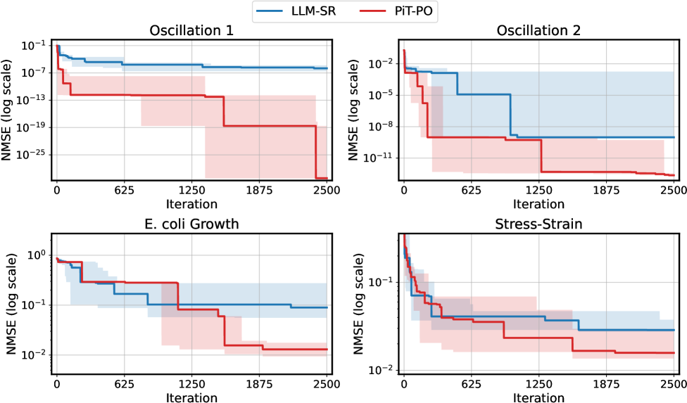
Figure 2. NMSE trajectories (log scale) over search iterations for LLM-SR and PiT-PO (Llama-3.1-8B) on LLM-SR Suite. Lines denote the median over seeds, and shaded regions indicate the min–max range.The remaining iteration curves for smaller backbones (3B and 1B) are deferred to Appendix C.1.
| Direct Prompting SGA LaSR | 3.61 2.70 5.41 | 1.801 0.909 45.94 | 0.3697 0.3519 0.0021 | 0.00 0.00 0.00 | 0.00 8.33 27.77 | 0.0644 0.0458 2.77e-4 | 0.00 0.00 4.16 | 0.00 0.00 16.66 | 0.5481 0.2416 2.73e-4 | 0.00 0.00 4.54 | 0.00 2.27 25.02 | 0.0459 0.1549 0.0018 | 0.00 0.00 8.21 | 0.00 12.12 64.22 | 0.0826 0.0435 7.44e-5 |
| --- | --- | --- | --- | --- | --- | --- | --- | --- | --- | --- | --- | --- | --- | --- | --- |
| LLM-SR | 30.63 | 38.55 | 0.0101 | 8.33 | 66.66 | 8.01e-6 | 25.30 | 58.33 | 1.04e-6 | 6.97 | 34.09 | 1.23e-4 | 4.10 | 88.12 | 1.15e-7 |
| PiT-PO | 34.23 | 46.84 | 0.0056 | 13.89 | 77.78 | 4.13e-7 | 29.17 | 70.83 | 9.37e-8 | 11.36 | 40.91 | 6.57e-5 | 12.00 | 92.00 | 1.18e-8 |
Table 2. Overall performance on LLM-SRBench (Llama-3.1-8B-Instruct).
### 4.3. PiT-PO Empowers Lightweight Backbones to Rival Large Models
As shown in Table 1, the performance of PiT-PO with the Llama-3.1-8B, Llama-3.2-3B, and Llama-3.2-1B backbones is competitive with, and often exceeds, the performance of LLM-SR that relies on substantially larger or proprietary models, including Mixtral 8 $\times$ 7B and 4o-mini.
These results indicate that PiT-PO effectively bridges the capability gap between lightweight open-source models and large-scale commercial systems. From a practical standpoint, this reduces the barrier to entry for scientific discovery: by delivering state-of-the-art performance on consumer-grade hardware (even maintaining competitiveness with a 1B backbone), PiT-PO eliminates the dependence on massive compute and closed-source APIs, thereby democratizing access to powerful SR tools.
<details>
<summary>x3.png Details</summary>
### Visual Description
## Bar Chart: NMSE Comparison Across Model Configurations
### Overview
The chart compares Normalized Mean Squared Error (NMSE) values across three model configurations ("w/o Phy", "w/o TokenReg", "PiT-PO") for two data types: In-Distribution (ID) and Out-Of-Distribution (OOD). The y-axis uses a logarithmic scale from 10⁻²⁹ to 10⁻¹¹.
### Components/Axes
- **X-axis**: Model configurations
- "w/o Phy" (no physics component)
- "w/o TokenReg" (no token regularization)
- "PiT-PO" (full model)
- **Y-axis**: NMSE values (log scale)
- **Legend**:
- ID (solid blue)
- OOD (striped blue)
- **Bar Colors**:
- ID: Solid blue
- OOD: Striped blue
### Detailed Analysis
1. **w/o Phy**
- ID: 7.60e-21
- OOD: 2.06e-10
2. **w/o TokenReg**
- ID: 2.77e-19
- OOD: 9.97e-11
3. **PiT-PO**
- ID: 6.40e-31
- OOD: 1.63e-30
### Key Observations
- OOD NMSE values are consistently **10⁻¹⁰ to 10⁻¹¹** higher than ID values in "w/o Phy" and "w/o TokenReg" configurations.
- In "PiT-PO", both ID and OOD NMSE values drop to **~10⁻³⁰**, with OOD slightly higher (1.63e-30 vs 6.40e-31).
- The largest performance gap between ID and OOD occurs in the "w/o Phy" configuration (2.06e-10 vs 7.60e-21).
### Interpretation
The data demonstrates:
1. **Model Robustness**: The full "PiT-PO" model achieves near-identical performance on ID and OOD data (~10⁻³⁰ NMSE), suggesting strong generalization.
2. **Component Sensitivity**: Removing physics ("w/o Phy") causes the largest ID-OOD performance gap (10¹¹ difference in NMSE), indicating physics components are critical for generalization.
3. **Regularization Impact**: Token regularization ("w/o TokenReg") reduces but doesn't eliminate the ID-OOD gap (10⁸ difference).
4. **Scale Significance**: All NMSE values are <10⁻¹⁰, suggesting the model operates in a highly precise regime.
The logarithmic scale emphasizes multiplicative differences rather than absolute values, highlighting the exponential performance disparities between configurations.
</details>
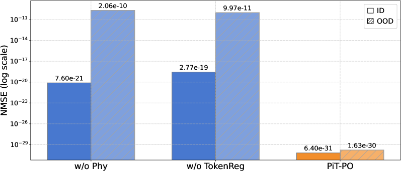
Figure 3. Ablation results of PiT-PO and its variants.
### 4.4. PiT-PO Enhances Search Efficiency and Breaks Stagnation
Figure 2 shows that PiT-PO achieves superior search efficiency in discovering accurate equations. In the early search stage, the red and blue curves are close across all four tasks: both methods primarily rely on the fitting signal (MSE) and therefore exhibit comparable per-iteration progress. As NMSE enters a lower regime, the trajectories consistently separate: PiT-PO exhibits abrupt step-wise drops while LLM-SR tends to plateau, yielding a clear red–blue gap in every subplot. Concretely, once the search reaches these lower-error regions, PiT-PO repeatedly exits stagnation and transitions to the next accuracy phase with orders-of-magnitude NMSE reductions (most prominently in Oscillation 1 and Oscillation 2, and also evident in E. coli Growth and Stress-Strain), whereas LLM-SR often remains trapped near its current error floor. This behavior confirms that the proposed dual-constraint mechanism effectively activates exactly when naive MSE feedback becomes insufficient. By penalizing physical inconsistencies and structural redundancy, PiT-PO forces the LLM to exit stagnation and transition toward the correct functional form.
While the in-search fine-tuning introduces a computational overhead, this cost is decisively outweighed by the substantial gains in performance. As detailed in Appendix C.2, PiT-PO maintains a significant performance edge even when evaluated under equivalent wall-clock time, demonstrating that the accelerated convergence speed effectively compensates for the additional training time.
### 4.5. Ablation Study
To rigorously validate the contribution of each algorithmic component, we conduct an ablation study across three settings: w/o Phy, which excludes the physics-consistency penalty $P_{\text{phy}}$ ; w/o TokenReg, which removes the redundancy-aware token-level regularization; and the full PiT-PO framework. As shown in Figure 3, removing any single component leads to a substantial deterioration of NMSE and a larger generalization gap between In-Distribution (ID) and Out-Of-Distribution (OOD) data. These empirical results underscore the necessity of the complete framework, demonstrating that the proposed dual constraints are indispensable for ensuring both search stability and robust generalization.
<details>
<summary>x4.png Details</summary>
### Visual Description
## Diagram: Flow Field with Boundary Conditions and Parameter Zones
### Overview
The diagram illustrates a flow field with normalized coordinates (x/H, y/H), where H is a characteristic length scale. It depicts regions with distinct boundary conditions ("solid wall," "cyclic") and parameter zones (α = 0.5, 0.8, 1.0). A highlighted area labeled "H" is marked in the bottom-right corner, and a flow direction arrow indicates the direction of movement.
### Components/Axes
- **Axes**:
- **x/H**: Horizontal axis, ranging from 0 to 9.
- **y/H**: Vertical axis, ranging from 0 to 3.
- **Regions**:
- **Solid wall**: Red-shaded regions on the left (x/H ≈ 0–1) and right (x/H ≈ 8–9).
- **Cyclic**: Teal-shaded region in the middle (x/H ≈ 1–6).
- **Cyclic cyclic**: Dark blue-shaded region on the far right (x/H ≈ 6–8).
- **Parameter Zones**:
- **α = 0.5**: Labeled at x/H ≈ 6.
- **α = 0.8**: Labeled at x/H ≈ 7.
- **α = 1.0**: Labeled at x/H ≈ 8.
- **Flow Direction**: Arrow pointing from left to right (center of the diagram).
- **Highlighted Area**: Yellow-shaded region labeled "H" at the bottom-right (x/H ≈ 8–9, y/H ≈ 0–1).
### Detailed Analysis
- **Boundary Conditions**:
- **Solid wall**: No-slip boundaries at x/H ≈ 0–1 and x/H ≈ 8–9.
- **Cyclic**: Periodic boundary conditions in the central region (x/H ≈ 1–6).
- **Cyclic cyclic**: Overlapping cyclic conditions in the transition zone (x/H ≈ 6–8).
- **Parameter Zones**:
- α increases from 0.5 to 1.0 as x/H increases, suggesting a gradient in a parameter (e.g., porosity, phase fraction, or turbulence intensity).
- **Highlighted Area (H)**:
- Positioned at the bottom-right corner (x/H ≈ 8–9, y/H ≈ 0–1), possibly indicating a region of interest (e.g., a boundary layer, separation zone, or transition area).
### Key Observations
1. **Flow Transition**: The flow moves from a "solid wall" region (no-slip) to a "cyclic" region (periodic), then to a "cyclic cyclic" zone, suggesting a complex interaction between boundary conditions.
2. **Parameter Gradient**: α increases monotonically from 0.5 to 1.0, indicating a systematic change in the parameter across the flow field.
3. **Highlighted Region (H)**: The yellow-shaded area "H" may represent a critical zone where flow behavior changes (e.g., turbulence onset, separation, or boundary layer development).
### Interpretation
This diagram likely represents a computational fluid dynamics (CFD) simulation or experimental setup with varying boundary conditions and material properties. The "solid wall" regions act as fixed boundaries, while the "cyclic" regions imply periodic or repeating flow patterns. The parameter α (e.g., porosity, phase fraction, or turbulence intensity) increases with x/H, suggesting a gradient in the medium or flow conditions. The highlighted "H" area could mark a region where a specific phenomenon occurs, such as flow separation, transition to turbulence, or a boundary layer development. The flow direction arrow confirms the left-to-right movement, aligning with the spatial progression of boundary conditions and parameter changes.
**Note**: The diagram does not include numerical data tables or explicit equations, so interpretations are based on spatial and label-based analysis.
</details>
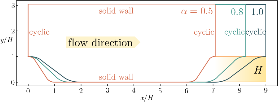
Figure 4. Schematic of the geometries for periodic hills.
### 4.6. Case Study: Turbulence Modeling
To validate the practical utility of PiT-PO in high-fidelity scientific discovery, we select the Flow over Periodic Hills (Xiao et al., 2020) (Figure 4) as a testbed. This problem is widely recognized in Computational Fluid Dynamics (CFD) (Pope, 2000) as a benchmark for Separated Turbulent Flows, presenting complex features such as strong adverse pressure gradients, massive flow detachment, and reattachment.
Problem Definition and Physics: The geometry consists of a sequence of polynomially shaped hills arranged periodically in the streamwise direction. The flow is driven by a constant body force at a bulk Reynolds number of $Re_{b}=5600$ (based on hill height $H$ and bulk velocity $U_{b}$ ). The domain height is fixed at $L_{y}/H=3.036$ , while the streamwise length $L_{x}$ varies with the slope factor $\alpha$ according to $L_{x}/H=3.858\alpha+5.142$ . Periodic boundary conditions are applied in the streamwise direction, with no-slip conditions on the walls.
The Scientific Challenge: The challenge lies in the Separation Bubble (Pope, 2000), a region where turbulence exhibits strong anisotropy due to streamline curvature. Traditional Linear Eddy Viscosity Models (LEVM) (Pope, 2000), such as the $k$ - $\omega$ SST model (Menter, 1994; Menter et al., 2003), rely on the Boussinesq hypothesis which assumes isotropic turbulence. Consequently, they systematically fail to predict key flow features, such as the separation bubble size and reattachment location.
Discovery Objective: Instead of fitting a simple curve, our goal is to discover a Non-linear Constitutive Relation for the Reynolds stress anisotropy tensor $a_{ij}$ and the dimensionless Reynolds stress anisotropy tensor $b_{ij}$ . By learning the Reynolds stress tensor $\tau_{ij}$ from high-fidelity Direct Numerical Simulation (DNS) (Pope, 2000) data, PiT-PO aims to formulate a symbolic correction term that captures the anisotropic physics missed by linear models.
Baselines: We follow standard turbulence modeling protocols and compare primarily against the standard $k$ - $\omega$ SST model of RANS. We also include LLM-SR and DSRRANS (Tang et al., 2023a), a strong SR-based turbulence modeling method specifically designed for turbulence tasks.
<details>
<summary>x5.png Details</summary>
### Visual Description
## Heatmap: Coefficient Variations Across Turbulence Models
### Overview
The image presents a 5x3 grid of heatmaps comparing normalized turbulence coefficients (a₁₁, a₂₂, a₃₃) across five turbulence modeling approaches: RANS, DSRANS, LLM-SR, PiT-PO, and DNS. Each panel visualizes spatial distributions of coefficients normalized by τₑ² (wall shear stress squared), with color gradients from blue (low values) to red (high values). The spatial domain is normalized by H (domain height) on both axes.
### Components/Axes
- **Rows**: Turbulence models (top to bottom):
1. RANS
2. DSRANS
3. LLM-SR
4. PiT-PO
5. DNS
- **Columns**: Coefficients (left to right):
1. a₁₁/τₑ² (streamwise component)
2. a₂₂/τₑ² (spanwise component)
3. a₃₃/τₑ² (normal component)
- **Axes**:
- X-axis: x/H (normalized streamwise position, 0–8)
- Y-axis: y/H (normalized wall-normal position, 0–2.5)
- **Legend**: Right-aligned colorbar (blue=low, red=high values)
### Detailed Analysis
- **RANS/DNS Panels**:
- Uniform coloration (blue to light red) across all coefficients.
- a₁₁/τₑ² (first column) shows minimal variation, suggesting steady streamwise behavior.
- a₃₃/τₑ² (third column) exhibits slight reddening near y/H=0.5, indicating localized normal stress.
- **LLM-SR/PiT-PO Panels**:
- Strong red regions in a₂₂/τₑ² (second column), particularly near y/H=1.5–2.0, suggesting dominant spanwise turbulence.
- a₃₃/τₑ² (third column) shows alternating red/blue bands, implying oscillatory normal stress.
- **DSRANS Panel**:
- Moderate red patches in a₁₁/τₑ² (first column) near x/H=4–6, indicating transient streamwise fluctuations.
### Key Observations
1. **DNS as Reference**:
- Most uniform distributions across all coefficients, aligning with direct numerical simulation's accuracy.
2. **LLM-SR/PiT-PO Anomalies**:
- a₂₂/τₑ² (spanwise) dominates in these models, with localized high-intensity regions absent in RANS/DSRANS.
3. **a₃₃/τₑ² Variability**:
- Normal component (third column) shows the most pronounced spatial heterogeneity, especially in LLM-SR/PiT-PO.
### Interpretation
The heatmaps reveal critical differences in how turbulence models capture anisotropic stress components. LLM-SR and PiT-PO exhibit enhanced sensitivity to spanwise (a₂₂) and normal (a₃₃) turbulence, likely due to advanced subgrid modeling. RANS/DSRANS, while computationally efficient, underresolve these components, showing smoother distributions. The DNS results validate the models' limitations, with LLM-SR/PiT-PO approaching but not fully replicating DNS's spatial complexity. The normalized coefficients suggest that wall-normal position (y/H) is a key driver of anisotropy, with high-y/H regions (near the domain top) showing stronger spanwise/normal coupling. This aligns with boundary layer transition physics, where turbulence becomes more three-dimensional away from the wall.
</details>
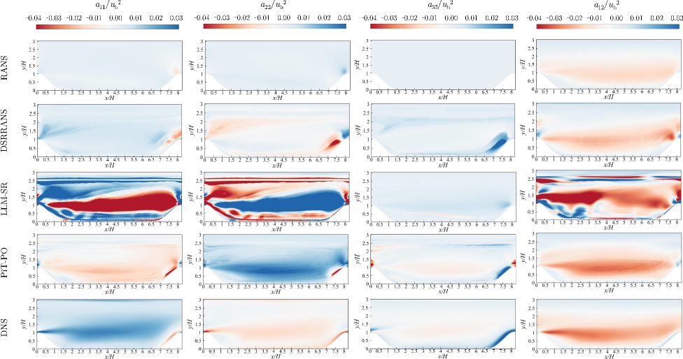
Figure 5. Comparison of the four anisotropic Reynolds stress components for periodic hill training flow using RANS, DSRRANS, LLM-SR, PiT-PO and DNS, respectively.
We cast turbulence closure modeling as a SR problem (Tang et al., 2023b) (see Appendix E for details). After obtaining the final symbolic equation, we embed it into a RANS solver of OpenFOAM (Weller et al., 1998) and run CFD simulations on the periodic-hill configuration. We compare the resulting Reynolds-stress components, mean-velocity fields, and skin-friction profiles against DNS references. Figures 5 – 7 visualize these quantities, enabling a direct assessment of physical fidelity and flow-field prediction quality.
Based on the comparative analysis of the anisotropic Reynolds stress contours (Figure 5), DSRRANS and PiT-PO show enhancement over the traditional RANS approach. Among them, PiT-PO performs the best: its contour matches the DNS reference most closely, with reduced error compared to DSRRANS and LLM-SR, demonstrating less severe non-physical extremes.
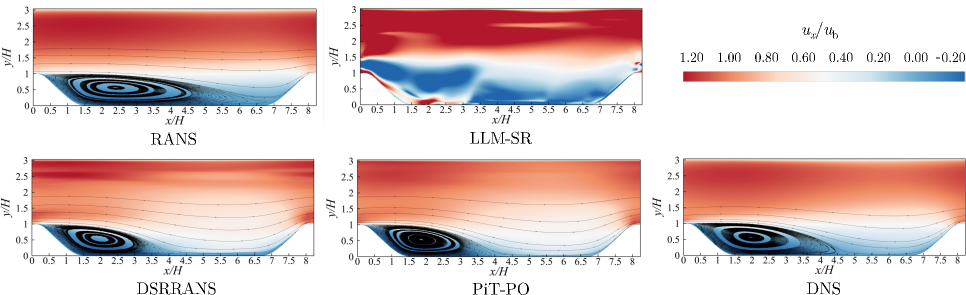
The stream-wise velocity contours illustrate the correction of the bubble size, a region of reversed flow that forms when fluid detaches from a surface. In Figure 6, PiT-PO most accurately represents the extent and shape of the recirculation zone, where fluid circulates within the separated region, closely consistent with the DNS data throughout the domain, particularly within the separation region and the recovery layer, where flow re-attaches to the surface.
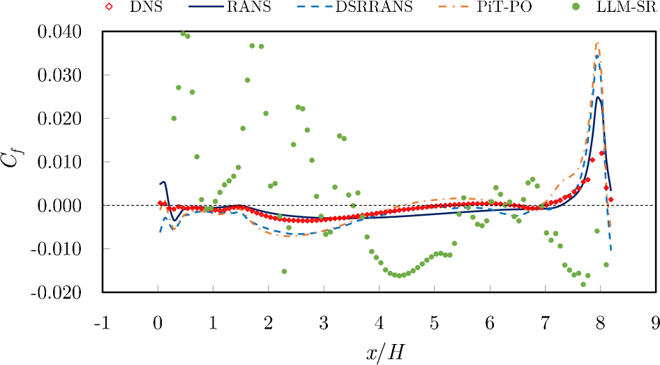
The skin friction coefficient (Figure 7), defined as the ratio of the wall stress to the dynamic pressure of the flow along the bottom wall, is a sensitive metric for predicting flow separation. The $k$ - $\omega$ SST model of RANS underestimates the magnitude of the skin friction and predicts a delayed reattachment location compared to the DNS. The learned model (PiT-PO) improves the prediction, aligning more closely with the DNS profile.
These results demonstrate that PiT-PO can generate symbolic equations tailored to turbulence modeling and that, under a posteriori CFD evaluation, the resulting predictions more closely match DNS references, which increases the practical value of LLM-based SR in real scientific and engineering workflows. With the proposed dual constraints,
PiT-PO provides targeted search and learning signals that enable the internalization of turbulence priors during equation discovery, thereby steering the model toward physically consistent and domain-relevant structures.
<details>
<summary>x6.png Details</summary>
### Visual Description
## Heatmap:Turbulence Model Velocity Profiles
### Overview
The image presents six comparative heatmaps visualizing velocity profiles (u_x/u_b) across normalized spatial coordinates (x/H, y/H) for different turbulence modeling approaches. Each heatmap represents a distinct computational method, with color gradients indicating velocity magnitude and direction relative to a reference velocity (u_b).
### Components/Axes
- **X-axis (x/H)**: Normalized horizontal position, ranging from 0.5 to 7.5.
- **Y-axis (y/H)**: Normalized vertical position, ranging from 0 to 3.
- **Color Bar (u_x/u_b)**:
- Scale: -0.20 (blue) to 1.20 (red), representing velocity ratios.
- Position: Right-aligned vertical bar.
- **Heatmap Labels**:
- Top row: RANS, LLM-SR.
- Bottom row: DSRRANS, PiT-PO, DNS.
- Note: A sixth heatmap is unlabeled in the provided image.
### Detailed Analysis
1. **RANS**:
- Dominant red hues in upper regions (y/H > 1.5), indicating high velocity.
- Central blue vortex near y/H = 0.5, suggesting localized flow reversal.
2. **LLM-SR**:
- Smooth gradient from red (top) to blue (bottom), with no distinct vortices.
- Velocity transitions appear more uniform compared to RANS.
3. **DSRRANS**:
- Similar to RANS but with a less pronounced vortex.
- Red regions extend slightly lower (y/H ≈ 1.0), indicating broader high-velocity zones.
4. **PiT-PO**:
- Clear vortex structure near y/H = 0.5, matching DNS in spatial resolution.
- Red-to-blue gradient is sharper, suggesting higher velocity contrast.
5. **DNS**:
- Most detailed flow features, including a well-defined vortex at y/H ≈ 0.5.
- Red regions dominate the upper half (y/H > 1.5), with precise velocity gradients.
### Key Observations
- **Vortex Presence**: DNS and PiT-PO exhibit distinct vortices, while RANS and LLM-SR show weaker or absent vortices.
- **Velocity Contrast**: DNS and PiT-PO display sharper red-to-blue transitions, indicating higher fidelity in capturing flow dynamics.
- **Model Fidelity**: DNS (ground truth) shows the most complex flow structure, while RANS and LLM-SR exhibit oversimplified gradients.
### Interpretation
The heatmaps demonstrate how turbulence modeling approaches approximate flow dynamics:
- **DNS** serves as the reference, capturing intricate vortex structures and precise velocity gradients.
- **PiT-PO** closely mimics DNS, suggesting it effectively resolves turbulent features.
- **RANS** and **LLM-SR** oversimplify flow behavior, likely due to turbulence modeling assumptions (e.g., Reynolds-averaged equations).
- **DSRRANS** bridges RANS and DNS, retaining some vortex details but with reduced accuracy.
The color bar confirms that red regions (u_x/u_b > 1.0) represent supercritical velocities, while blue regions (u_x/u_b < 0) indicate flow reversal. The absence of a sixth label in the image may indicate a missing model or a labeling error. These results highlight the trade-offs between computational cost and flow fidelity across turbulence modeling strategies.
</details>
Figure 6. Non-dimensional stream-wise velocity contours obtained by the learned model and the standard $k$ - $\omega$ SST model of RANS, compared with DNS data.
## 5. Related Work
Traditional SR has been studied through several lines, including genetic programming , reinforcement learning (Petersen et al., 2021), and transformer-based generation (Biggio* et al., 2021). Genetic programming (Koza, 1990) casts equation discovery as an evolutionary search over tree-structured programs, where candidate expressions are iteratively refined via mutation and crossover. Reinforcement learning-based SR, introduced by Petersen et al. (Petersen et al., 2021), has developed into a family of policy-optimization frameworks (Mundhenk et al., 2021; Landajuela et al., 2021; Crochepierre et al., 2022; Du et al., 2023) that formulate SR as a sequential decision-making process. More recently, transformer-based models (Valipour et al., 2021; Vastl et al., 2024; Kamienny et al., 2022; Li et al., 2023; Zhang et al., 2025) have been adopted for SR, using large-scale pretraining to map numerical data directly to equations. However, these methods typically fail to incorporate scientific prior knowledge.
Recent progress in natural language processing has further enabled LLM-based SR methods, including LLM-SR (Shojaee et al., 2025a), LaSR (Grayeli et al., 2024), ICSR (Merler et al., 2024), CoEvo (Guo et al., 2025), and SR-Scientist (Xia et al., 2025). LLM-SR exploits scientific priors that are implicitly captured by LLMs to propose plausible functional forms, followed by data-driven parameter estimation. LaSR augments SR with abstract concept generation to guide hypothesis formation, while ICSR reformulates training examples as in-context prompts to elicit function generation. However, a unifying limitation across these methods is their reliance on the LLM as a frozen generator, which precludes incorporating search feedback to update the generation strategy and consequently restricts their ability to adapt to complex problems.
While some recent works, such as SOAR (Pourcel et al., 2025) and CALM (Huang et al., 2025), have begun to explore adaptive in-search tuning, they primarily focus on algorithm discovery or combinatorial optimization problems, whereas our method is specifically tailored for SR. By integrating hierarchical physical constraints and theorem-guided token regularization, PiT-PO establishes an adaptive framework capable of discovering accurate and physically consistent equations.
<details>
<summary>x7.png Details</summary>
### Visual Description
## Line Chart: Coefficient of Friction (C_f) vs. Normalized Distance (x/H)
### Overview
The chart compares the performance of multiple turbulence modeling approaches in predicting the coefficient of friction (C_f) across a normalized distance (x/H). Data is presented as both continuous lines (model predictions) and discrete points (empirical measurements or DNS validation). The graph spans x/H from -1 to 9 and C_f from -0.02 to 0.04.
### Components/Axes
- **X-axis**: Normalized distance (x/H), ranging from -1 to 9 in increments of 1.
- **Y-axis**: Coefficient of friction (C_f), ranging from -0.02 to 0.04 in increments of 0.01.
- **Legend**: Located in the top-right corner, with five entries:
- **DNS**: Red diamonds (empirical/validation data)
- **RANS**: Solid blue line (Reynolds-Averaged Navier-Stokes)
- **DSRRANS**: Dashed blue line (Delayed RANS)
- **PiT-PO**: Dashed orange line (Pressure-Impulse Turbulence Model)
- **LLM-SR**: Green dots (Large Eddy Simulation - Subgrid Resolution)
### Detailed Analysis
1. **DNS (Red Diamonds)**:
- Scattered data points clustered around the RANS line.
- Notable deviations at x/H ≈ 0.5 (C_f ≈ -0.005) and x/H ≈ 7.5 (C_f ≈ 0.015).
- Outliers at x/H ≈ -0.5 (C_f ≈ 0.035) and x/H ≈ 8.5 (C_f ≈ -0.015).
2. **RANS (Solid Blue Line)**:
- Baseline model with a smooth trend.
- Initial dip to C_f ≈ -0.01 at x/H = 0, recovering to C_f ≈ 0.005 by x/H = 1.
- Remains near C_f ≈ 0 until x/H = 8, where it spikes to C_f ≈ 0.035.
3. **DSRRANS (Dashed Blue Line)**:
- Mirrors RANS but with delayed response.
- Dip to C_f ≈ -0.008 at x/H = 0, rising to C_f ≈ 0.003 by x/H = 1.
- Spikes to C_f ≈ 0.03 at x/H = 8, slightly lower than RANS.
4. **PiT-PO (Dashed Orange Line)**:
- Similar trend to RANS but with higher variability.
- Peaks at C_f ≈ 0.032 at x/H = 8, with a broader rise.
5. **LLM-SR (Green Dots)**:
- Highly dispersed data points.
- Central cluster between C_f ≈ 0.005 and 0.025 (x/H = 2–7).
- Outliers at x/H ≈ -0.5 (C_f ≈ 0.03) and x/H ≈ 8.5 (C_f ≈ -0.01).
### Key Observations
- **Sharp Spike at x/H = 8**: All models predict a sudden increase in C_f, suggesting a critical flow transition (e.g., boundary layer separation or turbulence intensification).
- **DNS-RANS Agreement**: Empirical data (DNS) closely follows RANS predictions, validating its accuracy in this regime.
- **LLM-SR Variability**: Green dots show significant scatter, indicating potential limitations in subgrid-scale modeling or data resolution.
- **DSRRANS vs. RANS**: Delayed response in DSRRANS aligns with its design for transient flows but underperforms RANS in peak prediction.
### Interpretation
The graph demonstrates that RANS remains the most reliable model for steady-state predictions in this flow configuration, while DNS serves as a robust validation benchmark. The sharp C_f increase at x/H = 8 highlights a critical flow feature (e.g., shockwave or separation point) that all models capture, albeit with varying accuracy. LLM-SR’s inconsistency suggests challenges in resolving small-scale turbulence, possibly due to insufficient grid resolution or model assumptions. The DSRRANS and PiT-PO lines indicate that modifications to standard RANS (e.g., delayed effects or pressure-impulse mechanisms) improve transient behavior but require refinement for peak accuracy. The outliers in DNS and LLM-SR data may reflect experimental noise or unmodeled physical phenomena.
</details>
Figure 7. Skin friction distribution along the bottom obtained by the learned model and the standard $k$ - $\omega$ SST model of RANS, compared with DNS data.
## 6. Conclusion
In this work, we introduced PiT-PO, a unified framework that fundamentally transforms LLMs from static equation proposers into adaptive, physics-aware generators for SR. By integrating in-search policy optimization with a novel dual-constraint evaluation mechanism, PiT-PO rigorously enforces hierarchical physical validity while leveraging theorem-guided, token-level penalties to eliminate structural redundancy. This synergistic design aligns generation with numerical fitness, scientific consistency, and parsimony, establishing new state-of-the-art performance on SR benchmarks. Beyond synthetic tasks, PiT-PO demonstrates significant practical utility in turbulence modeling, where the discovered symbolic corrections improve Reynolds stress and flow-field predictions. Notably, PiT-PO achieves these results using small open-source backbones, making it a practical and accessible tool for scientific communities with limited computational resources. Looking forward, we plan to extend PiT-PO to broader scientific and engineering domains by enriching the library of domain-specific constraints and validating it across more complex, real-world systems. Moreover, we anticipate that integrating PiT-PO with larger-scale multi-modal foundation models could further unlock its potential in processing heterogeneous scientific data.
## References
- (1)
- Aakash et al. (2019) B. S. Aakash, JohnPatrick Connors, and Michael D Shields. 2019. Stress-strain data for aluminum 6061-T651 from 9 lots at 6 temperatures under uniaxial and plane strain tension. Data in Brief 25 (Aug 2019), 104085. doi: 10.1016/j.dib.2019.104085
- Biggio et al. (2021) Luca Biggio, Tommaso Bendinelli, Alexander Neitz, Aurelien Lucchi, and Giambattista Parascandolo. 2021. Neural Symbolic Regression that Scales. arXiv:2106.06427 [cs.LG] https://arxiv.org/abs/2106.06427
- Biggio* et al. (2021) L. Biggio*, T. Bendinelli*, A. Neitz, A. Lucchi, and G. Parascandolo. 2021. Neural Symbolic Regression that Scales. In Proceedings of 38th International Conference on Machine Learning (ICML 2021) (Proceedings of Machine Learning Research, Vol. 139). PMLR, 936–945. https://proceedings.mlr.press/v139/biggio21a.html *equal contribution.
- Chen et al. (2025) Jindou Chen, Jidong Tian, Liang Wu, ChenXinWei, Xiaokang Yang, Yaohui Jin, and Yanyan Xu. 2025. KinFormer: Generalizable Dynamical Symbolic Regression for Catalytic Organic Reaction Kinetics. In International Conference on Representation Learning, Y. Yue, A. Garg, N. Peng, F. Sha, and R. Yu (Eds.), Vol. 2025. 67058–67080. https://proceedings.iclr.cc/paper_files/paper/2025/file/a76b693f36916a5ed84d6e5b39a0dc03-Paper-Conference.pdf
- Cranmer (2023) Miles Cranmer. 2023. Interpretable Machine Learning for Science with PySR and SymbolicRegression.jl. arXiv:2305.01582 [astro-ph.IM] https://arxiv.org/abs/2305.01582
- Crochepierre et al. (2022) Laure Crochepierre, Lydia Boudjeloud-Assala, and Vincent Barbesant. 2022. Interactive Reinforcement Learning for Symbolic Regression from Multi-Format Human-Preference Feedbacks. In IJCAI 2022- 31st International Joint Conference on Artificial Intelligence. Vienne, Austria. https://hal.science/hal-03695471
- Deng et al. (2023) Song Deng, Junjie Wang, Li Tao, Su Zhang, and Hongwei Sun. 2023. EV charging load forecasting model mining algorithm based on hybrid intelligence. Computers and Electrical Engineering 112 (2023), 109010. doi: 10.1016/j.compeleceng.2023.109010
- Du et al. (2023) Mengge Du, Yuntian Chen, and Dongxiao Zhang. 2023. DISCOVER: Deep identification of symbolically concise open-form PDEs via enhanced reinforcement-learning. arXiv:2210.02181 [cs.LG] https://arxiv.org/abs/2210.02181
- Fletcher (1987) Roger Fletcher. 1987. Practical Methods of Optimization (2nd ed.). John Wiley & Sons, Chichester, New York.
- Grayeli et al. (2024) Arya Grayeli, Atharva Sehgal, Omar Costilla-Reyes, Miles Cranmer, and Swarat Chaudhuri. 2024. Symbolic Regression with a Learned Concept Library. arXiv:2409.09359 [cs.LG] https://arxiv.org/abs/2409.09359
- Guo et al. (2025) Ping Guo, Qingfu Zhang, and Xi Lin. 2025. CoEvo: Continual Evolution of Symbolic Solutions Using Large Language Models. arXiv:2412.18890 [cs.AI] https://arxiv.org/abs/2412.18890
- Hu et al. (2021) Edward J. Hu, Yelong Shen, Phillip Wallis, Zeyuan Allen-Zhu, Yuanzhi Li, Shean Wang, Lu Wang, and Weizhu Chen. 2021. LoRA: Low-Rank Adaptation of Large Language Models. arXiv:2106.09685 [cs.CL] https://arxiv.org/abs/2106.09685
- Huang et al. (2025) Ziyao Huang, Weiwei Wu, Kui Wu, Jianping Wang, and Wei-Bin Lee. 2025. CALM: Co-evolution of Algorithms and Language Model for Automatic Heuristic Design. arXiv:2505.12285 [cs.NE] https://arxiv.org/abs/2505.12285
- Kamienny et al. (2022) Pierre-Alexandre Kamienny, Stéphane d’Ascoli, Guillaume Lample, and François Charton. 2022. End-to-end symbolic regression with transformers. arXiv:2204.10532 [cs.LG] https://arxiv.org/abs/2204.10532
- Kassianik et al. (2025) Paul Kassianik, Baturay Saglam, Alexander Chen, Blaine Nelson, Anu Vellore, Massimo Aufiero, Fraser Burch, Dhruv Kedia, Avi Zohary, Sajana Weerawardhena, Aman Priyanshu, Adam Swanda, Amy Chang, Hyrum Anderson, Kojin Oshiba, Omar Santos, Yaron Singer, and Amin Karbasi. 2025. Llama-3.1-FoundationAI-SecurityLLM-Base-8B Technical Report. arXiv:2504.21039 [cs.CR] https://arxiv.org/abs/2504.21039
- Koza (1990) J.R. Koza. 1990. Genetically breeding populations of computer programs to solve problems in artificial intelligence. In [1990] Proceedings of the 2nd International IEEE Conference on Tools for Artificial Intelligence. 819–827. doi: 10.1109/TAI.1990.130444
- Landajuela et al. (2022) Mikel Landajuela, Chak Shing Lee, Jiachen Yang, Ruben Glatt, Claudio P Santiago, Ignacio Aravena, Terrell Mundhenk, Garrett Mulcahy, and Brenden K Petersen. 2022. A Unified Framework for Deep Symbolic Regression. In Advances in Neural Information Processing Systems, S. Koyejo, S. Mohamed, A. Agarwal, D. Belgrave, K. Cho, and A. Oh (Eds.), Vol. 35. Curran Associates, Inc., 33985–33998. https://proceedings.neurips.cc/paper_files/paper/2022/file/dbca58f35bddc6e4003b2dd80e42f838-Paper-Conference.pdf
- Landajuela et al. (2021) Mikel Landajuela, Brenden K. Petersen, Soo K. Kim, Claudio P. Santiago, Ruben Glatt, T. Nathan Mundhenk, Jacob F. Pettit, and Daniel M. Faissol. 2021. Improving exploration in policy gradient search: Application to symbolic optimization. arXiv:2107.09158 [cs.LG] https://arxiv.org/abs/2107.09158
- Li et al. (2023) Wenqiang Li, Weijun Li, Linjun Sun, Min Wu, Lina Yu, Jingyi Liu, Yanjie Li, and Song Tian. 2023. Transformer-based model for symbolic regression via joint supervised learning. In International Conference on Learning Representations. https://api.semanticscholar.org/CorpusID:259298765
- Ma et al. (2024) Pingchuan Ma, Tsun-Hsuan Wang, Minghao Guo, Zhiqing Sun, Joshua B. Tenenbaum, Daniela Rus, Chuang Gan, and Wojciech Matusik. 2024. LLM and Simulation as Bilevel Optimizers: A New Paradigm to Advance Physical Scientific Discovery. In Proceedings of the 41st International Conference on Machine Learning (Proceedings of Machine Learning Research, Vol. 235), Ruslan Salakhutdinov, Zico Kolter, Katherine Heller, Adrian Weller, Nuria Oliver, Jonathan Scarlett, and Felix Berkenkamp (Eds.). PMLR, 33940–33962. https://proceedings.mlr.press/v235/ma24m.html
- Makke and Chawla (2024a) Nour Makke and Sanjay Chawla. 2024a. Data-driven discovery of Tsallis-like distribution using symbolic regression in high-energy physics. PNAS Nexus 3, 11 (10 2024), pgae467. arXiv:https://academic.oup.com/pnasnexus/article-pdf/3/11/pgae467/60816181/pgae467.pdf doi: 10.1093/pnasnexus/pgae467
- Makke and Chawla (2024b) Nour Makke and Sanjay Chawla. 2024b. Interpretable scientific discovery with symbolic regression: a review. Artificial Intelligence Review 57 (01 2024). doi: 10.1007/s10462-023-10622-0
- Menter (1994) Florian R Menter. 1994. Two-equation eddy-viscosity turbulence models for engineering applications. AIAA journal 32, 8 (1994), 1598–1605.
- Menter et al. (2003) Florian R Menter, Martin Kuntz, Robin Langtry, et al. 2003. Ten years of industrial experience with the SST turbulence model. Turbulence, heat and mass transfer 4, 1 (2003), 625–632.
- Merler et al. (2024) Matteo Merler, Katsiaryna Haitsiukevich, Nicola Dainese, and Pekka Marttinen. 2024. In-Context Symbolic Regression: Leveraging Large Language Models for Function Discovery. In Proceedings of the 62nd Annual Meeting of the Association for Computational Linguistics (Volume 4: Student Research Workshop). Association for Computational Linguistics, 589–606. doi: 10.18653/v1/2024.acl-srw.49
- MOCHIZUKI and OSAKA (2000) Shinsuke MOCHIZUKI and Hideo OSAKA. 2000. Management of a Stronger Wall Jet by a Pair of Streamwise Vortices. Reynolds Stress Tensor and Production Tenns. TRANSACTIONS OF THE JAPAN SOCIETY OF MECHANICAL ENGINEERS Series B 66, 646 (2000), 1309–1317. doi: 10.1299/kikaib.66.646_1309
- Monkewitz (2021) Peter A. Monkewitz. 2021. Asymptotics of streamwise Reynolds stress in wall turbulence. Journal of Fluid Mechanics 931 (Nov. 2021). doi: 10.1017/jfm.2021.924
- Monod (1949) Jacques Monod. 1949. THE GROWTH OF BACTERIAL CULTURES. Annual Review of Microbiology 3, Volume 3, 1949 (1949), 371–394. doi: 10.1146/annurev.mi.03.100149.002103
- Mundhenk et al. (2021) T. Nathan Mundhenk, Mikel Landajuela, Ruben Glatt, Claudio P. Santiago, Daniel M. Faissol, and Brenden K. Petersen. 2021. Symbolic Regression via Neural-Guided Genetic Programming Population Seeding. arXiv:2111.00053 [cs.NE] https://arxiv.org/abs/2111.00053
- Neamtiu et al. (2005) Iulian Neamtiu, Jeffrey S. Foster, and Michael Hicks. 2005. Understanding source code evolution using abstract syntax tree matching. In Proceedings of the 2005 International Workshop on Mining Software Repositories (St. Louis, Missouri) (MSR ’05). Association for Computing Machinery, New York, NY, USA, 1–5. doi: 10.1145/1083142.1083143
- Petersen et al. (2021) Brenden K. Petersen, Mikel Landajuela, T. Nathan Mundhenk, Claudio P. Santiago, Soo K. Kim, and Joanne T. Kim. 2021. Deep symbolic regression: Recovering mathematical expressions from data via risk-seeking policy gradients. arXiv:1912.04871 [cs.LG] https://arxiv.org/abs/1912.04871
- Pope (2000) Stephen B. Pope. 2000. Turbulent Flows. Cambridge University Press. doi: 10.1017/cbo9780511840531
- Pourcel et al. (2025) Julien Pourcel, Cédric Colas, and Pierre-Yves Oudeyer. 2025. Self-Improving Language Models for Evolutionary Program Synthesis: A Case Study on ARC-AGI. arXiv:2507.14172 [cs.LG] https://arxiv.org/abs/2507.14172
- Reuter et al. (2023) Julia Reuter, Hani Elmestikawy, Fabien Evrard, Sanaz Mostaghim, and Berend van Wachem. 2023. Graph Networks as Inductive Bias for Genetic Programming: Symbolic Models for Particle-Laden Flows. In Genetic Programming, Gisele Pappa, Mario Giacobini, and Zdenek Vasicek (Eds.). Springer Nature Switzerland, Cham, 36–51.
- Romera-Paredes et al. (2024) Bernardino Romera-Paredes, Mohammadamin Barekatain, Alexander Novikov, Matej Balog, M Pawan Kumar, Emilien Dupont, Francisco JR Ruiz, Jordan S Ellenberg, Pengming Wang, Omar Fawzi, et al. 2024. Mathematical discoveries from program search with large language models. Nature 625, 7995 (2024), 468–475.
- Rosso et al. (1995) L Rosso, J. R. Lobry, S Bajard, and J. P. Flandrois. 1995. Convenient Model To Describe the Combined Effects of Temperature and pH on Microbial Growth. Applied and Environmental Microbiology 61, 2 (Feb 1995), 610–6. doi: 10.1128/aem.61.2.610-616.1995
- Schmidt and Lipson (2009) Michael Schmidt and Hod Lipson. 2009. Distilling Free-Form Natural Laws from Experimental Data. Science 324, 5923 (2009), 81–85. arXiv:https://www.science.org/doi/pdf/10.1126/science.1165893 doi: 10.1126/science.1165893
- Shao et al. (2024) Zhihong Shao, Peiyi Wang, Qihao Zhu, Runxin Xu, Junxiao Song, Xiao Bi, Haowei Zhang, Mingchuan Zhang, Y. K. Li, Y. Wu, and Daya Guo. 2024. DeepSeekMath: Pushing the Limits of Mathematical Reasoning in Open Language Models. arXiv:2402.03300 [cs.CL] https://arxiv.org/abs/2402.03300
- Shi et al. (2024) Hao Shi, Weili Song, Xinting Zhang, Jiahe Shi, Cuicui Luo, Xiang Ao, Hamid Arian, and Luis Seco. 2024. AlphaForge: A Framework to Mine and Dynamically Combine Formulaic Alpha Factors. arXiv:2406.18394 [q-fin.CP] https://arxiv.org/abs/2406.18394
- Shojaee et al. (2025a) Parshin Shojaee, Kazem Meidani, Shashank Gupta, Amir Barati Farimani, and Chandan K Reddy. 2025a. LLM-SR: Scientific Equation Discovery via Programming with Large Language Models. arXiv:2404.18400 [cs.LG] https://arxiv.org/abs/2404.18400
- Shojaee et al. (2025b) Parshin Shojaee, Ngoc-Hieu Nguyen, Kazem Meidani, Amir Barati Farimani, Khoa D Doan, and Chandan K Reddy. 2025b. LLM-SRBench: A New Benchmark for Scientific Equation Discovery with Large Language Models. arXiv:2504.10415 [cs.CL] https://arxiv.org/abs/2504.10415
- Tang et al. (2023a) Hongwei Tang, Yan Wang, Tongguang Wang, and Linlin Tian. 2023a. Discovering explicit Reynolds-averaged turbulence closures for turbulent separated flows through deep learning-based symbolic regression with non-linear corrections. Physics of Fluids 35, 2 (2023), 025118. arXiv:https://doi.org/10.1063/5.0135638 doi: 10.1063/5.0135638
- Tang et al. (2023b) Hongwei Tang, Yan Wang, Tongguang Wang, and Linlin Tian. 2023b. Discovering explicit Reynolds-averaged turbulence closures for turbulent separated flows through deep learning-based symbolic regression with non-linear corrections. Physics of Fluids 35, 2 (Feb. 2023). doi: 10.1063/5.0135638
- Tennekes and Lumley (1972) Henk Tennekes and John L. Lumley. 1972. A First Course in Turbulence. The MIT Press. doi: 10.7551/mitpress/3014.001.0001
- Valipour et al. (2021) Mojtaba Valipour, Bowen You, Maysum Panju, and Ali Ghodsi. 2021. SymbolicGPT: A Generative Transformer Model for Symbolic Regression. arXiv:2106.14131 [cs.LG] https://arxiv.org/abs/2106.14131
- Vastl et al. (2024) Martin Vastl, Jonáš Kulhánek, Jiří Kubalík, Erik Derner, and Robert Babuška. 2024. SymFormer: End-to-End Symbolic Regression Using Transformer-Based Architecture. IEEE Access 12 (2024), 37840–37849. doi: 10.1109/ACCESS.2024.3374649
- Virgolin and Pissis (2022) Marco Virgolin and Solon P. Pissis. 2022. Symbolic Regression is NP-hard. arXiv:2207.01018 [cs.NE] https://arxiv.org/abs/2207.01018
- Wahlquist et al. (2024) Ylva Wahlquist, Jesper Sundell, and Kristian Soltesz. 2024. Learning pharmacometric covariate model structures with symbolic regression networks. Journal of Pharmacokinetics and Pharmacodynamics 51, 2 (2024), 155–167. doi: 10.1007/s10928-023-09887-3
- WANG et al. (2019) Wei WANG, Yang ZHANG, and Lili CHEN. 2019. An application of the shear stress transport low-Reynolds-number k-ε turbulence model on turbulent flows. ACTA AERODYNAMICA SINICA 37, 3 (2019), 419–425. doi: 10.7638/kqdlxxb-2016.0158
- Weller et al. (1998) H.G. Weller, Gavin Tabor, Hrvoje Jasak, and Christer Fureby. 1998. A Tensorial Approach to Computational Continuum Mechanics Using Object Orientated Techniques. Computers in Physics 12 (11 1998), 620–631. doi: 10.1063/1.168744
- Xia et al. (2025) Shijie Xia, Yuhan Sun, and Pengfei Liu. 2025. SR-Scientist: Scientific Equation Discovery With Agentic AI. arXiv:2510.11661 [cs.AI] https://arxiv.org/abs/2510.11661
- Xiao et al. (2020) Heng Xiao, Jin-Long Wu, Sylvain Laizet, and Lian Duan. 2020. Flows over periodic hills of parameterized geometries: A dataset for data-driven turbulence modeling from direct simulations. Computers & Fluids 200 (2020), 104431. doi: 10.1016/j.compfluid.2020.104431
- Zhang et al. (2025) Hengzhe Zhang, Qi Chen, Bing XUE, Wolfgang Banzhaf, and Mengjie Zhang. 2025. RAG-SR: Retrieval-Augmented Generation for Neural Symbolic Regression. In The Thirteenth International Conference on Learning Representations. https://openreview.net/forum?id=NdHka08uWn
| Fitting log-MSE scale | $\alpha$ | 1.0 | Scaling in $R_{\mathrm{fit}}=-\alpha\log(\mathrm{MSE}+\epsilon)$ . |
| --- | --- | --- | --- |
| Complexity penalty weight | $\lambda_{\mathrm{len}}$ | 5e-3 | Weight in $P_{\mathrm{cplx}}=\lambda_{\mathrm{len}}\cdot\mathrm{Length}(\mathrm{AST})$ . |
| Dimensional homogeneity penalty weight | $P_{\mathrm{dim}}$ | 1.0 | Penalty/reward weight for unit inconsistency (general-level constraint). |
| Differentiability penalty weight | $P_{\mathrm{diff}}$ | 0.5 | Penalty/reward weight for non-smoothness on the data-defined domain (general-level constraint). |
| Domain-specific constraint weight (j-th) | $P_{\mathrm{domain}}^{(j)}$ | 0.5 | Weight for the $j$ -th domain prior (e.g., realizability, wall BC, asymptotic scaling, energy consistency). |
| Gating threshold for physics constraints | $\delta_{\mathrm{gate}}$ | 1e-3 * MSE_{initial} | Activate physics penalties only after fitting reaches a sufficiently low-error regime. |
| Numerical stability constant in $\tau_{i}$ | $\epsilon$ | 1e-50 | Used in $\tau_{i}=\frac{|b_{i}|}{\sum_{j}|b_{j}|+\epsilon}$ to avoid division by zero. |
| Redundancy threshold | $\rho$ | 1e-2 | A term is considered redundant if $\tau_{i}\leq\rho$ . |
| Token penalty scale | $p$ | 0.5 | Scaling coefficient in $P_{\mathrm{tok}}=p\cdot\max(0,-\log(|b_{i}|+\epsilon))$ . |
Table 3. Hyperparameters for dual-constraint evaluation and token-level signal synthesis.
## Appendix A Additional Hyperparameters of PiT-PO
Table 3 lists the additional hyperparameters of PiT-PO, including (i) general-level physical penalties (dimensional homogeneity and differentiability), (ii) domain-specific constraint penalties, (iii) the gated activation threshold for physical constraints, and (iv) theorem-guided redundancy detection and token-level penalization.
## Appendix B Support Exclusion Theorem: Theory and Practice
### B.1. Preliminaries: Empirical Function Space and Orthogonality
** Definition B.1 (Basis functions / dictionary)**
*Let $\mathcal{X}\subseteq\mathbb{R}^{d}$ be the domain, and let $\{\phi_{j}:\mathcal{X}\to\mathbb{R}\}_{j\in\mathcal{S}}$ be a collection of candidate basis (dictionary) functions indexed by $\mathcal{S}$ . For any subset $\mathcal{K}\subseteq\mathcal{S}$ , denote the corresponding model subspace by
$$
\mathrm{span}\{\phi_{j}:j\in\mathcal{K}\}.
$$*
** Definition B.2 (Target functionf∗f^{*})**
*Assume the ground-truth target function admits a sparse expansion over the dictionary:
$$
f^{*}(x)=\sum_{j\in\mathcal{S}^{\prime}}a_{j}\,\phi_{j}(x),
$$
where $\mathcal{S}^{\prime}\subseteq\mathcal{S}$ is the true support set (indices of nonzero terms) and satisfies $|\mathcal{S}^{\prime}|\leq M$ . Moreover, the true coefficients are bounded as
$$
A\leq|a_{j}|\leq B,\qquad\forall j\in\mathcal{S}^{\prime}.
$$*
** Definition B.3 (Empirical inner product and empirical norm)**
*Given a finite dataset $D=\{x_{n}\}_{n=1}^{N}\subset\mathcal{X}$ , for any two functions $f,g:\mathcal{X}\to\mathbb{R}$ , define the empirical inner product by
$$
\langle f,g\rangle_{D}:=\frac{1}{N}\sum_{n=1}^{N}f(x_{n})\,g(x_{n}),
$$
and the induced empirical norm by
$$
\|f\|_{D}:=\sqrt{\langle f,f\rangle_{D}}.
$$
The empirical function space
$$
\mathcal{F}_{D}:=\{(f(x_{1}),\ldots,f(x_{N})):\ f:\mathcal{X}\to\mathbb{R}\}
$$
is a finite-dimensional inner-product space under $\langle\cdot,\cdot\rangle_{D}$ .*
** Definition B.4 (Empirical Orthogonality)**
*Two functions $f,g\in\mathcal{F}_{D}$ are empirically orthogonal if $\langle f,g\rangle_{D}=0$ .*
Convention. Unless stated otherwise, throughout this appendix we write $\langle\cdot,\cdot\rangle$ and $\|\cdot\|$ to mean the empirical inner product $\langle\cdot,\cdot\rangle_{D}$ and the empirical norm $\|\cdot\|_{D}$ .
### B.2. Proof of the Support Exclusion Theorem
** Theorem B.5 (Support Exclusion Theorem)**
*Let $\mathcal{K}\subseteq\mathcal{S}$ be a candidate skeleton (active set). Consider the empirical least-squares fit over $\mathcal{K}$ :
$$
b\in\arg\min_{\{b_{j}\}_{j\in\mathcal{K}}}\left\|f^{*}-\sum_{j\in\mathcal{K}}b_{j}\phi_{j}\right\|^{2}.
$$
Define the empirical Gram matrix $G\in\mathbb{R}^{|\mathcal{S}|\times|\mathcal{S}|}$ by
$$
G_{ij}:=\langle\phi_{i},\phi_{j}\rangle,\qquad i,j\in\mathcal{S},
$$
and assume $G_{ii}>0$ . For any $i\in\mathcal{S}$ , define
$$
T_{ij}:=\frac{G_{ji}}{G_{ii}},\qquad j\in\mathcal{S}.
$$
Further define the external-candidate vector
$$
u_{i}:=\big(|T_{i\ell}|\big)_{\ell\in\mathcal{S}\setminus\mathcal{K}}\in\mathbb{R}^{|\mathcal{S}\setminus\mathcal{K}|},
$$
and let $s(1)\geq s(2)\geq\cdots\geq s(|\mathcal{S}\setminus\mathcal{K}|)$ be the entries of $u_{i}$ sorted in non-increasing order. If for some $i\in\mathcal{K}$ ,
$$
|b_{i}|<A-\left(\underbrace{\sum_{j\in\mathcal{K},\,j\neq i}(B+|b_{j}|)\,|T_{ij}|}_{\textnormal{Internal Interference}}+\underbrace{B\sum_{k=1}^{|\mathcal{S}\setminus\mathcal{K}|}s(k)}_{\textnormal{External Interference}}\right),
$$
then $i\notin\mathcal{S}^{\prime}$ .*
* Proof*
Step 1: Empirical orthogonality (first-order optimality of least squares). Let
$$
g(x):=\sum_{j\in\mathcal{K}}b_{j}\phi_{j}(x),\qquad r(x):=f^{*}(x)-g(x).
$$
The objective is $\|r\|^{2}=\langle r,r\rangle$ . For any $i\in\mathcal{K}$ , the first-order optimality condition yields
$$
0=\frac{\partial}{\partial b_{i}}\|r\|^{2}=-2\langle r,\phi_{i}\rangle\quad\Longrightarrow\quad\langle r,\phi_{i}\rangle=0.
$$
Hence, the residual $r$ is empirically orthogonal to $\mathrm{span}\{\phi_{i}:i\in\mathcal{K}\}$ . Step 2: Set decomposition. Define three disjoint sets
$$
\mathcal{T}:=\mathcal{K}\cap\mathcal{S}^{\prime},\qquad\mathcal{F}:=\mathcal{K}\setminus\mathcal{S}^{\prime},\qquad\mathcal{R}:=\mathcal{S}^{\prime}\setminus\mathcal{K}.
$$
Then $\mathcal{K}=\mathcal{T}\cup\mathcal{F}$ and $\mathcal{S}^{\prime}=\mathcal{T}\cup\mathcal{R}$ . Expanding the residual gives
$$
r=\sum_{j\in\mathcal{T}}(a_{j}-b_{j})\phi_{j}+\sum_{j\in\mathcal{R}}a_{j}\phi_{j}-\sum_{j\in\mathcal{F}}b_{j}\phi_{j}.
$$ Step 3: An exact coefficient identity for $i\in\mathcal{T}$ . Fix any $i\in\mathcal{T}\subseteq\mathcal{K}$ . Using $\langle r,\phi_{i}\rangle=0$ and writing $G_{ji}=\langle\phi_{j},\phi_{i}\rangle$ , we obtain
$$
(a_{i}-b_{i})G_{ii}+\sum_{j\in\mathcal{T},\,j\neq i}(a_{j}-b_{j})G_{ji}+\sum_{j\in\mathcal{R}}a_{j}G_{ji}-\sum_{j\in\mathcal{F}}b_{j}G_{ji}=0.
$$
Dividing by $G_{ii}>0$ and using $T_{ij}=G_{ji}/G_{ii}$ yields
$$
a_{i}-b_{i}=-\sum_{j\in\mathcal{T},\,j\neq i}(a_{j}-b_{j})T_{ij}-\sum_{j\in\mathcal{R}}a_{j}T_{ij}+\sum_{j\in\mathcal{F}}b_{j}T_{ij}.
$$ Step 4: Upper bound via internal and external interference. Taking absolute values and applying the triangle inequality gives
$$
|a_{i}-b_{i}|\leq\sum_{j\in\mathcal{T},\,j\neq i}|a_{j}-b_{j}|\,|T_{ij}|+\sum_{j\in\mathcal{R}}|a_{j}|\,|T_{ij}|+\sum_{j\in\mathcal{F}}|b_{j}|\,|T_{ij}|.
$$
For $j\in\mathcal{T}\subseteq\mathcal{S}^{\prime}$ , we have $|a_{j}|\leq B$ and thus
$$
|a_{j}-b_{j}|\leq|a_{j}|+|b_{j}|\leq B+|b_{j}|.
$$
Therefore,
$$
|a_{i}-b_{i}|\leq\sum_{j\in\mathcal{T},\,j\neq i}(B+|b_{j}|)\,|T_{ij}|+\sum_{j\in\mathcal{F}}|b_{j}|\,|T_{ij}|+B\sum_{j\in\mathcal{R}}|T_{ij}|.
$$
Since $|b_{j}|\leq B+|b_{j}|$ for all $j\in\mathcal{F}$ , we further have
$$
\sum_{j\in\mathcal{F}}|b_{j}|\,|T_{ij}|\leq\sum_{j\in\mathcal{F}}(B+|b_{j}|)\,|T_{ij}|.
$$
Combining $\mathcal{T}\setminus\{i\}$ and $\mathcal{F}$ yields the internal-interference term:
$$
|a_{i}-b_{i}|\leq\underbrace{\sum_{j\in\mathcal{K},\,j\neq i}(B+|b_{j}|)\,|T_{ij}|}_{\textnormal{Internal Interference}}+B\sum_{j\in\mathcal{R}}|T_{ij}|.
$$
For the external term, note that $\mathcal{R}\subseteq\mathcal{S}\setminus\mathcal{K}$ , and the entries $\{|T_{i\ell}|\}_{\ell\in\mathcal{S}\setminus\mathcal{K}}$ sorted in non-increasing order are $s(1)\geq\cdots\geq s(|\mathcal{S}\setminus\mathcal{K}|)$ . Hence, for any subset $\mathcal{R}$ ,
$$
\sum_{j\in\mathcal{R}}|T_{ij}|\leq\sum_{k=1}^{|\mathcal{R}|}s(k).
$$
Assuming $|\mathcal{S}^{\prime}|\leq M$ and that the current support is partially correct, i.e., $\mathcal{K}\cap\mathcal{S}^{\prime}\neq\emptyset$ , we have $|\mathcal{R}|=|\mathcal{S}^{\prime}\setminus\mathcal{K}|\leq|\mathcal{S}^{\prime}|-1\leq M-1$ . Define $m:=\min\!\big(M-1,\ |\mathcal{S}\setminus\mathcal{K}|\big)$ . Since also $|\mathcal{R}|\leq|\mathcal{S}\setminus\mathcal{K}|$ , it follows that $|\mathcal{R}|\leq m$ , and thus
$$
\sum_{j\in\mathcal{R}}|T_{ij}|\leq\sum_{k=1}^{|\mathcal{R}|}s(k)\leq\sum_{k=1}^{m}s(k).
$$
Thus,
$$
|a_{i}-b_{i}|\leq\sum_{j\in\mathcal{K},\,j\neq i}(B+|b_{j}|)\,|T_{ij}|+B\sum_{k=1}^{m}s(k).
$$ Step 5: Lower bound when $i\in\mathcal{S}^{\prime}$ . If $i\in\mathcal{S}^{\prime}$ , then $|a_{i}|\geq A$ . By the reverse triangle inequality,
$$
|a_{i}-b_{i}|\geq\big||a_{i}|-|b_{i}|\big|\geq A-|b_{i}|.
$$ Step 6: Contradiction. Assume, for contradiction, that there exists $i\in\mathcal{K}\cap\mathcal{S}^{\prime}$ satisfying
$$
|b_{i}|<A-\left(\sum_{j\in\mathcal{K},\,j\neq i}(B+|b_{j}|)\,|T_{ij}|+B\sum_{k=1}^{m}s(k)\right).
$$
Rearranging yields
$$
A-|b_{i}|>\sum_{j\in\mathcal{K},\,j\neq i}(B+|b_{j}|)\,|T_{ij}|+B\sum_{k=1}^{m}s(k).
$$
However, Step 5 implies $|a_{i}-b_{i}|\geq A-|b_{i}|$ , while the bound above implies
$$
|a_{i}-b_{i}|\leq\sum_{j\in\mathcal{K},\,j\neq i}(B+|b_{j}|)\,|T_{ij}|+B\sum_{k=1}^{m}s(k),
$$
which is a contradiction. Therefore such an $i$ cannot belong to $\mathcal{S}^{\prime}$ , i.e., $i\notin\mathcal{S}^{\prime}$ . ∎
## Appendix C Supplementary Diagnostics and Analyses
### C.1. Remaining Iteration Curves on Smaller Backbones
In the main text, we report iteration curves for the 8B backbone. Here we provide the remaining curves for 3B and 1B (Figure 8), which corroborate the observations in Section 4.4.
<details>
<summary>x8.png Details</summary>
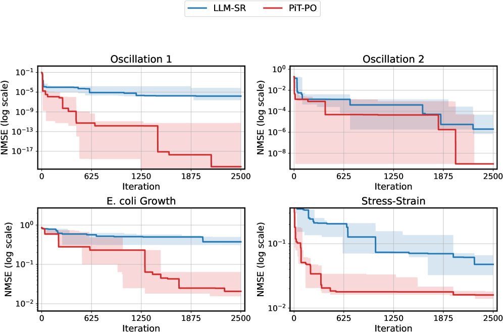
### Visual Description
## Line Chart: Comparative NMSE Performance Across Iterations
### Overview
The image contains four line charts arranged in a 2x2 grid, comparing the performance of two methods (LLM-SR and PiT-PO) across four datasets: Oscillation 1, Oscillation 2, E. coli Growth, and Stress-Strain. Each chart tracks the Normalized Mean Squared Error (NMSE) on a logarithmic scale against iteration count (0–2500). Shaded regions represent uncertainty bounds for each method.
### Components/Axes
- **X-axis**: Iteration (0–2500, linear scale)
- **Y-axis**: NMSE (log scale, 10⁻¹⁷ to 10⁰)
- **Legends**:
- Blue line/shade: LLM-SR
- Red line/shade: PiT-PO
- **Chart Titles**:
- Top-left: Oscillation 1
- Top-right: Oscillation 2
- Bottom-left: E. coli Growth
- Bottom-right: Stress-Strain
### Detailed Analysis
#### Oscillation 1
- **LLM-SR (Blue)**:
- Starts at ~10⁻¹ NMSE, drops sharply to ~10⁻⁵ by 625 iterations, then plateaus.
- Uncertainty (shaded blue) narrows significantly after 1250 iterations.
- **PiT-PO (Red)**:
- Begins at ~10⁻³ NMSE, decreases to ~10⁻⁹ by 1250 iterations, then stabilizes.
- Uncertainty (shaded red) remains broader than LLM-SR throughout.
#### Oscillation 2
- **LLM-SR (Blue)**:
- Initial NMSE ~10⁻², declines to ~10⁻⁴ by 625 iterations, then plateaus.
- Uncertainty reduces by ~50% after 1875 iterations.
- **PiT-PO (Red)**:
- Starts at ~10⁻⁴ NMSE, drops to ~10⁻⁶ by 1250 iterations, then stabilizes.
- Shaded red region shows consistent uncertainty reduction.
#### E. coli Growth
- **LLM-SR (Blue)**:
- Begins at ~10⁰ NMSE, decreases to ~10⁻¹ by 625 iterations, then plateaus.
- Uncertainty narrows by ~70% after 1250 iterations.
- **PiT-PO (Red)**:
- Starts at ~10⁻¹ NMSE, drops to ~10⁻² by 1250 iterations, then stabilizes.
- Shaded red region shows gradual uncertainty reduction.
#### Stress-Strain
- **LLM-SR (Blue)**:
- Initial NMSE ~10⁻¹, decreases to ~10⁻² by 625 iterations, then plateaus.
- Uncertainty reduces by ~60% after 1875 iterations.
- **PiT-PO (Red)**:
- Begins at ~10⁻² NMSE, drops to ~10⁻³ by 1250 iterations, then stabilizes.
- Shaded red region shows steady uncertainty reduction.
### Key Observations
1. **Performance Trends**:
- LLM-SR consistently achieves lower NMSE than PiT-PO across all datasets.
- Both methods show rapid improvement in early iterations (0–1250), with diminishing returns afterward.
2. **Uncertainty Patterns**:
- Shaded regions (confidence intervals) narrow for both methods as iterations increase, indicating improved model stability.
- LLM-SR’s uncertainty bounds are consistently tighter than PiT-PO’s.
3. **Dataset-Specific Behavior**:
- Oscillation 1 and Stress-Strain show the most dramatic NMSE reductions.
- E. coli Growth exhibits the slowest convergence for both methods.
### Interpretation
The data demonstrates that **LLM-SR outperforms PiT-PO** in all tested scenarios, achieving lower NMSE and tighter confidence intervals. The logarithmic scale highlights exponential improvements in early iterations, suggesting these methods are particularly effective for initial model calibration. The narrowing uncertainty bands imply that both approaches become more reliable with increased computational effort, but LLM-SR maintains a consistent advantage. This could indicate architectural or algorithmic efficiencies in LLM-SR that make it preferable for applications requiring high-precision predictions under iterative refinement.
</details>
(a) Llama-3B
<details>
<summary>x9.png Details</summary>
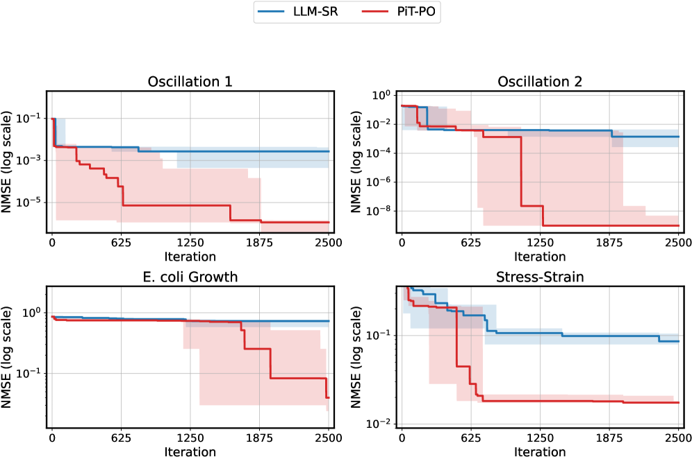
### Visual Description
## Line Graphs: NMSE Performance Across Tasks
### Overview
The image contains four line graphs arranged in a 2x2 grid, comparing the performance of two methods (LLM-SR and PiT-PO) across four tasks: Oscillation 1, Oscillation 2, E. coli Growth, and Stress-Strain. All graphs share identical axes labels and scales, with iterations (0–2500) on the x-axis and NMSE (log scale) on the y-axis. The legend identifies blue lines as LLM-SR and red lines as PiT-PO, with shaded regions representing uncertainty intervals.
---
### Components/Axes
- **X-axis**: Iteration (0–2500, linear scale).
- **Y-axis**: NMSE (log scale, 10⁻¹ to 10⁰).
- **Legend**:
- Blue: LLM-SR
- Red: PiT-PO
- **Shaded Regions**: Confidence intervals (wider at lower iterations, narrowing over time).
---
### Detailed Analysis
#### Oscillation 1
- **LLM-SR (Blue)**: Starts at ~10⁻¹, drops sharply to ~10⁻³ by iteration 625, then plateaus.
- **PiT-PO (Red)**: Starts at ~10⁻³, drops to ~10⁻⁵ by iteration 625, then plateaus.
- **Trend**: PiT-PO consistently outperforms LLM-SR after iteration 625. Both methods stabilize by iteration 1250.
#### Oscillation 2
- **LLM-SR (Blue)**: Starts at ~10⁻², drops to ~10⁻⁴ by iteration 625, then plateaus.
- **PiT-PO (Red)**: Starts at ~10⁻³, drops to ~10⁻⁵ by iteration 625, then plateaus.
- **Trend**: Similar to Oscillation 1, PiT-PO achieves lower NMSE earlier and maintains superiority.
#### E. coli Growth
- **LLM-SR (Blue)**: Starts near 10⁰, drops to ~10⁻¹ by iteration 625, then plateaus.
- **PiT-PO (Red)**: Starts near 10⁰, drops to ~10⁻¹ by iteration 625, then plateaus.
- **Trend**: Both methods converge at ~10⁻¹ by iteration 625, with PiT-PO showing slightly lower NMSE throughout.
#### Stress-Strain
- **LLM-SR (Blue)**: Starts at ~10⁻¹, drops to ~10⁻² by iteration 625, then plateaus.
- **PiT-PO (Red)**: Starts at ~10⁻², drops to ~10⁻³ by iteration 625, then plateaus.
- **Trend**: PiT-PO achieves lower NMSE earlier and maintains a consistent advantage.
---
### Key Observations
1. **Early Performance Drop**: All tasks show a sharp NMSE reduction (~1–2 orders of magnitude) around iteration 625 for both methods.
2. **Convergence**: By iteration 1250, NMSE values stabilize for both methods across all tasks.
3. **Method Comparison**: PiT-PO (red) consistently achieves lower NMSE than LLM-SR (blue) after iteration 625 in all tasks.
4. **Uncertainty**: Shaded regions (confidence intervals) are widest at early iterations, narrowing significantly by iteration 1250.
---
### Interpretation
The data demonstrates that **PiT-PO outperforms LLM-SR** in reducing NMSE across diverse tasks (oscillations, biological growth, mechanical stress). The early drop in NMSE (~iteration 625) suggests a critical adaptation phase where PiT-PO’s methodology (e.g., parameter tuning, model architecture) becomes more effective. The plateauing NMSE after iteration 1250 implies diminishing returns from further iterations. The narrowing confidence intervals indicate increasing model stability over time. These results highlight PiT-PO’s robustness in handling varied dynamical systems, with potential applications in predictive modeling where low NMSE is critical.
</details>
(b) Llama-1B
Figure 8. NMSE versus iteration on smaller backbones, consistent with the trends in the 8B setting.
<details>
<summary>x10.png Details</summary>
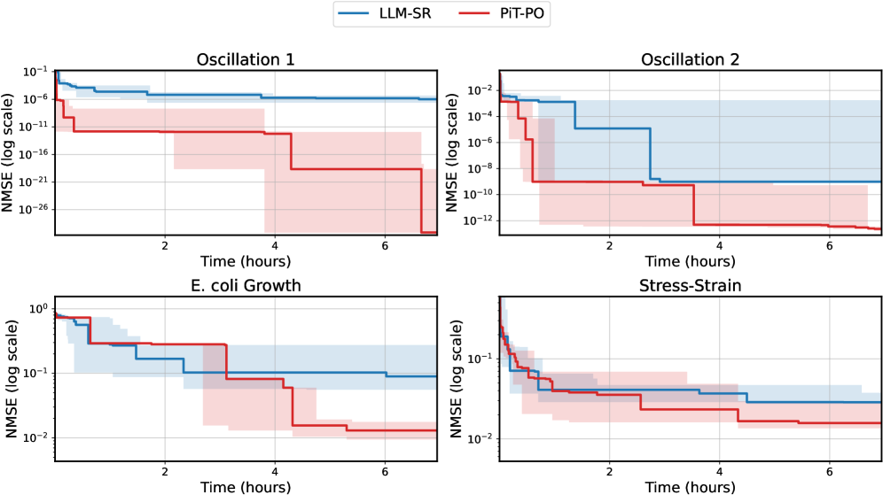
### Visual Description
## Line Chart: Comparative NMSE Performance Across Scenarios
### Overview
The image displays four line charts comparing the Normalized Mean Squared Error (NMSE) performance of two models (LLM-SR and PIT-PO) across four scenarios: Oscillation 1, Oscillation 2, E. coli Growth, and Stress-Strain. NMSE values are plotted on a logarithmic scale against time (hours). Both models show stepwise improvements in performance over time, with LLM-SR consistently outperforming PIT-PO.
### Components/Axes
- **X-axis**: Time (hours), ranging from 0 to 6 hours in all charts.
- **Y-axis**: NMSE (log scale), with varying ranges:
- Oscillation 1 & 2: 10⁻¹ to 10⁻²⁶
- E. coli Growth & Stress-Strain: 10⁰ to 10⁻²
- **Legend**: Located at the top center, with:
- **Blue line**: LLM-SR
- **Red line**: PIT-PO
- **Shaded regions**: Confidence intervals (error bounds) around each line.
### Detailed Analysis
#### Oscillation 1
- **LLM-SR (Blue)**:
- Starts at ~10⁻¹ at 0h.
- Drops sharply to ~10⁻⁶ at 2h.
- Remains stable at ~10⁻⁶ until 6h.
- **PIT-PO (Red)**:
- Starts at ~10⁻¹ at 0h.
- Drops to ~10⁻¹⁶ at 2h.
- Further decreases to ~10⁻²¹ at 4h.
- Reaches ~10⁻²⁶ at 6h.
- **Confidence Intervals**: Widen significantly at 2h and 4h for PIT-PO.
#### Oscillation 2
- **LLM-SR (Blue)**:
- Starts at ~10⁻¹ at 0h.
- Drops to ~10⁻⁴ at 2h.
- Remains stable at ~10⁻⁴ until 6h.
- **PIT-PO (Red)**:
- Starts at ~10⁻¹ at 0h.
- Drops to ~10⁻⁸ at 2h.
- Further decreases to ~10⁻¹⁰ at 4h.
- Reaches ~10⁻¹² at 6h.
- **Confidence Intervals**: Expand at 2h and 4h for PIT-PO.
#### E. coli Growth
- **LLM-SR (Blue)**:
- Starts at ~10⁰ at 0h.
- Drops to ~10⁻¹ at 2h.
- Remains stable at ~10⁻¹ until 6h.
- **PIT-PO (Red)**:
- Starts at ~10⁰ at 0h.
- Drops to ~10⁻² at 2h.
- Further decreases to ~10⁻³ at 4h.
- Reaches ~10⁻⁴ at 6h.
- **Confidence Intervals**: Narrower compared to oscillation scenarios.
#### Stress-Strain
- **LLM-SR (Blue)**:
- Starts at ~10⁻¹ at 0h.
- Drops to ~10⁻² at 2h.
- Remains stable at ~10⁻² until 6h.
- **PIT-PO (Red)**:
- Starts at ~10⁻¹ at 0h.
- Drops to ~10⁻³ at 2h.
- Further decreases to ~10⁻⁴ at 4h.
- Reaches ~10⁻⁵ at 6h.
- **Confidence Intervals**: Minimal expansion across time.
### Key Observations
1. **Performance Gap**: LLM-SR consistently achieves lower NMSE than PIT-PO in all scenarios.
2. **Stepwise Improvements**: Both models show abrupt performance gains at 2h and 4h, suggesting discrete optimization stages.
3. **Scale Variance**: Oscillation scenarios exhibit NMSE orders of magnitude lower than biological/mechanical systems.
4. **Confidence Uncertainty**: PIT-PO’s confidence intervals widen during performance drops, indicating higher variability in error estimation.
### Interpretation
The data demonstrates that LLM-SR outperforms PIT-PO across diverse applications, with the largest relative improvements in oscillation modeling (10⁻¹⁶ vs. 10⁻⁶ NMSE at 2h). The stepwise drops align with potential model retraining or data assimilation events. The logarithmic scale emphasizes the exponential decay in error for PIT-PO, though its wider confidence intervals suggest less reliable predictions despite lower NMSE. The biological/mechanical scenarios (E. coli, Stress-Strain) show higher baseline errors, implying greater complexity in modeling these systems. The consistent performance gap highlights LLM-SR’s robustness, while the confidence intervals caution against over-reliance on PIT-PO in high-stakes applications.
</details>
(a) Llama-3.1-8B
<details>
<summary>x11.png Details</summary>
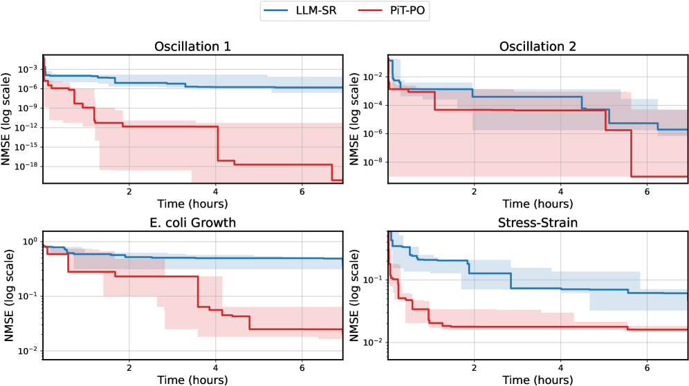
### Visual Description
## LineGraphs: NMSE Comparison of LLM-SR and PIT-PO Across Scenarios
### Overview
The image contains four line graphs comparing the performance of two methods, **LLM-SR** (blue) and **PIT-PO** (red), across four scenarios: **Oscillation 1**, **Oscillation 2**, **E. coli Growth**, and **Stress-Strain**. Each graph plots **Normalized Mean Squared Error (NMSE)** on a logarithmic scale against **Time (hours)**. Shaded regions around the lines represent confidence intervals (e.g., ±1σ or ±2σ).
---
### Components/Axes
- **X-axis**: Time (hours), ranging from 0 to 6 hours in all graphs.
- **Y-axis**: NMSE (log scale), spanning from 10⁻³ to 10⁻¹⁸ (Oscillation 1), 10⁻² to 10⁻⁸ (Oscillation 2), 10⁻¹ to 10⁻² (E. coli Growth), and 10⁻¹ to 10⁻² (Stress-Strain).
- **Legend**: Located in the top-right corner of the entire figure.
- **Blue**: LLM-SR
- **Red**: PIT-PO
- **Shading**:
- Blue shading for LLM-SR confidence intervals.
- Red shading for PIT-PO confidence intervals.
---
### Detailed Analysis
#### Oscillation 1
- **LLM-SR (Blue)**:
- Starts at ~10⁻³ NMSE at 0 hours.
- Drops stepwise to ~10⁻⁶ at 2 hours, ~10⁻¹² at 4 hours, and ~10⁻¹⁸ by 6 hours.
- Confidence interval narrows significantly over time.
- **PIT-PO (Red)**:
- Begins at ~10⁻⁶ NMSE, remaining relatively flat until 4 hours (~10⁻⁹).
- Sharp drop to ~10⁻¹⁵ at 6 hours.
- Confidence interval remains wide throughout.
#### Oscillation 2
- **LLM-SR (Blue)**:
- Starts at ~10⁻² NMSE, drops to ~10⁻⁴ at 2 hours, ~10⁻⁶ at 4 hours, and ~10⁻⁸ by 6 hours.
- Confidence interval tightens progressively.
- **PIT-PO (Red)**:
- Begins at ~10⁻⁴ NMSE, remains stable until 4 hours (~10⁻⁶).
- Sharp decline to ~10⁻⁸ at 6 hours.
- Confidence interval widens slightly after 4 hours.
#### E. coli Growth
- **LLM-SR (Blue)**:
- Starts at ~10⁻¹ NMSE, drops to ~10⁻² at 2 hours, ~10⁻³ at 4 hours, and ~10⁻⁴ by 6 hours.
- Confidence interval narrows steadily.
- **PIT-PO (Red)**:
- Begins at ~10⁻² NMSE, remains flat until 4 hours (~10⁻³).
- Sharp drop to ~10⁻⁴ at 6 hours.
- Confidence interval widens after 4 hours.
#### Stress-Strain
- **LLM-SR (Blue)**:
- Starts at ~10⁻¹ NMSE, drops to ~10⁻² at 2 hours, ~10⁻³ at 4 hours, and ~10⁻⁴ by 6 hours.
- Confidence interval tightens over time.
- **PIT-PO (Red)**:
- Begins at ~10⁻² NMSE, remains stable until 4 hours (~10⁻³).
- Sharp decline to ~10⁻⁴ at 6 hours.
- Confidence interval widens after 4 hours.
---
### Key Observations
1. **LLM-SR consistently outperforms PIT-PO** across all scenarios, achieving lower NMSE values.
2. **Stepwise drops** in NMSE for LLM-SR suggest adaptive adjustments to dynamic conditions (e.g., oscillations, stress events).
3. **PIT-PO shows delayed improvement**, with significant NMSE reductions only after 4–6 hours.
4. **Confidence intervals** for LLM-SR are narrower, indicating more reliable predictions compared to PIT-PO.
---
### Interpretation
- **Performance Implications**: LLM-SR’s lower NMSE and tighter confidence intervals suggest superior predictive accuracy and stability under varying conditions (oscillations, biological growth, mechanical stress).
- **Temporal Dynamics**: The stepwise NMSE reductions in LLM-SR may reflect event-driven model updates (e.g., detecting oscillations or stress thresholds), while PIT-PO’s delayed response hints at slower adaptation.
- **Robustness**: LLM-SR’s narrower confidence intervals imply better generalization, whereas PIT-PO’s wider intervals indicate higher uncertainty in predictions.
- **Scenario-Specific Behavior**:
- In **Oscillation 1/2**, LLM-SR’s rapid NMSE drops align with periodic event detection.
- In **E. coli Growth** and **Stress-Strain**, LLM-SR’s gradual improvements suggest effective handling of nonlinear dynamics.
This analysis underscores LLM-SR’s advantages in dynamic, real-time prediction tasks, while PIT-PO may require optimization for scenarios demanding rapid adaptation.
</details>
(b) Llama-3.2-3B
<details>
<summary>x12.png Details</summary>
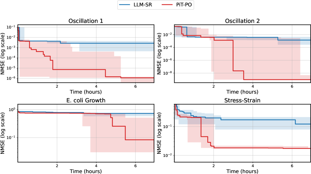
### Visual Description
## Chart Type: 2x2 Grid of Line Charts
### Overview
The image displays four line charts arranged in a 2x2 grid, comparing two models (LLM-SR and PIT-PO) across four scenarios: Oscillation 1, Oscillation 2, E. coli Growth, and Stress-Strain. Each chart plots Normalized Mean Squared Error (NMSE) on a logarithmic scale against time (hours). The legend is positioned in the top-right corner, with blue representing LLM-SR and red representing PIT-PO.
### Components/Axes
- **X-axis**: Time (hours), ranging from 0 to 6 hours.
- **Y-axis**: NMSE (log scale), ranging from 10⁻¹ to 10⁻⁸.
- **Legend**:
- Blue: LLM-SR
- Red: PIT-PO
- **Chart Titles**:
- Top-left: Oscillation 1
- Top-right: Oscillation 2
- Bottom-left: E. coli Growth
- Bottom-right: Stress-Strain
### Detailed Analysis
#### Oscillation 1
- **LLM-SR (Blue)**:
- Starts at ~10⁻¹ NMSE at 0h.
- Drops to ~10⁻³ at 2h, ~10⁻⁵ at 4h, and ~10⁻⁶ at 6h.
- Shaded blue region indicates uncertainty, narrowing as NMSE decreases.
- **PIT-PO (Red)**:
- Starts at ~10⁻² NMSE at 0h.
- Drops to ~10⁻⁴ at 2h, ~10⁻⁶ at 4h, and ~10⁻⁸ at 6h.
- Shaded red region shows larger uncertainty than LLM-SR.
#### Oscillation 2
- **LLM-SR (Blue)**:
- Starts at ~10⁻¹ NMSE at 0h.
- Drops to ~10⁻³ at 2h, ~10⁻⁵ at 4h, and ~10⁻⁶ at 6h.
- Shaded region remains consistent in width.
- **PIT-PO (Red)**:
- Starts at ~10⁻² NMSE at 0h.
- Sharp drop to ~10⁻⁴ at 2h, then stabilizes at ~10⁻⁶ by 4h.
- Shaded region narrows significantly after 2h.
#### E. coli Growth
- **LLM-SR (Blue)**:
- Starts at ~10⁰ NMSE at 0h.
- Drops to ~10⁻¹ at 2h, ~10⁻³ at 4h, and ~10⁻⁵ at 6h.
- Shaded region widens slightly after 4h.
- **PIT-PO (Red)**:
- Starts at ~10⁻¹ NMSE at 0h.
- Drops to ~10⁻³ at 2h, ~10⁻⁵ at 4h, and ~10⁻⁷ at 6h.
- Shaded region narrows steadily.
#### Stress-Strain
- **LLM-SR (Blue)**:
- Starts at ~10⁻¹ NMSE at 0h.
- Drops to ~10⁻² at 2h, ~10⁻⁴ at 4h, and ~10⁻⁶ at 6h.
- Shaded region remains narrow.
- **PIT-PO (Red)**:
- Starts at ~10⁻² NMSE at 0h.
- Drops to ~10⁻⁴ at 2h, ~10⁻⁶ at 4h, and ~10⁻⁸ at 6h.
- Shaded region narrows sharply after 2h.
### Key Observations
1. **Model Performance**:
- PIT-PO consistently achieves lower NMSE than LLM-SR across all scenarios.
- Both models show exponential decay in NMSE over time, but PIT-PO’s decline is steeper.
2. **Uncertainty**:
- Shaded regions (likely confidence intervals) are narrower for PIT-PO in most cases, suggesting higher prediction stability.
3. **Scenario-Specific Trends**:
- In Oscillation 2, PIT-PO’s NMSE stabilizes after 2h, while LLM-SR continues to decline.
- E. coli Growth and Stress-Strain show similar decay patterns but differ in baseline NMSE values.
### Interpretation
The data suggests that **PIT-PO outperforms LLM-SR** in all tested scenarios, with faster and more stable convergence to lower error rates. The logarithmic scale emphasizes the exponential improvement in accuracy over time. The shaded regions imply that PIT-PO’s predictions are less variable, which could be critical in applications requiring high reliability (e.g., real-time systems). The consistent trend across diverse scenarios (oscillations, biological growth, mechanical stress) indicates that PIT-PO’s methodology may generalize better than LLM-SR. Further investigation into the architectural or training differences between the models would clarify the source of this performance gap.
</details>
(c) Llama-3.2-1B
Figure 9. Wall-clock efficiency under a fixed 25,000-second budget.
### C.2. Time-Cost Analysis under a Fixed Wall-Clock Budget
To complement the iteration-based efficiency analysis in Section 4.4, we evaluate search efficiency under a strict wall-clock constraint. We fix the total runtime of each method to 25,000 seconds ( $\approx$ 6.9 hours) and track the best-so-far NMSE as a function of elapsed time (Figure 9). This protocol directly answers a practical question: given the same compute time, which method returns a more accurate recovered equation?
Across all three backbones (Llama-3.1-8B, Llama-3.2-3B, and Llama-3.2-1B), PiT-PO consistently yields lower NMSE trajectories than LLM-SR under the same 25,000-second budget. In line with the behavior discussed in Section 4.4, the curves exhibit a characteristic divergence in the low-error regime: LLM-SR often plateaus after an initial reduction, while PiT-PO continues to realize step-wise decreases over time, indicating more effective late-stage credit assignment and continued progress rather than stagnation.
The advantage is most pronounced on the two oscillator systems. For 8B and 3B, PiT-PO achieves rapid early improvements and maintains additional phase transitions later in the run, reaching substantially lower NMSE within the same wall-clock budget. For the 1B model, both methods converge more slowly overall, yet PiT-PO still more reliably escapes stagnation and attains markedly lower final NMSE, suggesting that the proposed in-search tuning remains effective even in the small-model regime.
Similar trends hold for the E. coli Growth and Stress–Strain tasks, where progress is typically more gradual. Under equal wall-clock time, PiT-PO achieves a lower final NMSE and exhibits clearer late-stage improvements, whereas LLM-SR tends to flatten earlier. Importantly, these gains are obtained without increasing runtime: despite the additional overhead introduced by in-search policy optimization, PiT-PO delivers consistently better return-on-compute within a fixed time budget, validating the practical efficiency of the proposed approach.
| LLM-SR (Llama-3.1-8B) LLM-SR (Llama-3.2-3B) LLM-SR (Llama-3.2-1B) | 0.0114 0.0191 0.1182 | 8.05e-10 5.56e-5 7.57e-3 | 0.1676 809.94 1888.5 | 0.1026 0.0264 0.2689 |
| --- | --- | --- | --- | --- |
| PiT-PO (Llama-3.1-8B) | 1.63e-30 | 1.36e-11 | 0.1163 | 0.0163 |
| PiT-PO (Llama-3.2-3B) | 2.63e-30 | 8.52e-10 | 0.0237 | 0.0144 |
| PiT-PO (Llama-3.2-1B) | 5.99e-5 | 8.58e-10 | 0.3462 | 0.0124 |
Table 4. OOD evaluation: NMSE on the OOD split.
### C.3. OOD Evaluation (NMSE ${}_{\text{OOD}}$ )
We report out-of-distribution performance using NMSE on the OOD split (NMSE ${}_{\text{OOD}}$ ), summarized in Table 4. Across all three backbones (8B/3B/1B) and all four tasks, PiT-PO achieves lower NMSE ${}_{\text{OOD}}$ than LLM-SR under the same setting. In particular, PiT-PO maintains extremely small OOD errors on the two oscillator systems, and yields substantially reduced OOD NMSE on E. coli growth and Stress–Strain, where LLM-SR exhibits noticeably larger errors. These results provide consistent evidence that the improvements observed in the main text persist under OOD evaluation.
### C.4. Equation Iterative Trajectories
<details>
<summary>x13.png Details</summary>
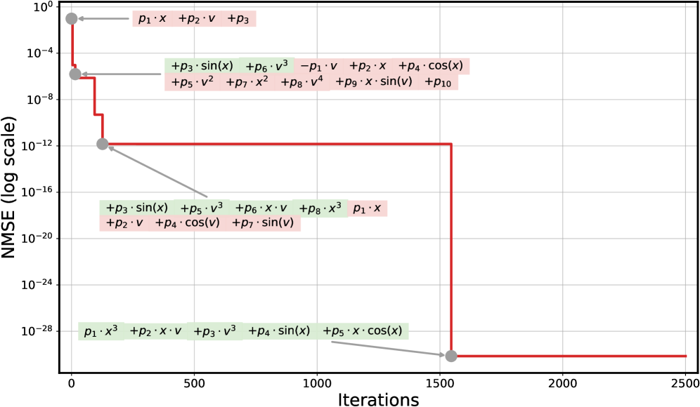
### Visual Description
## Line Graph: NMSE vs. Iterations
### Overview
The image is a line graph depicting the relationship between the Normalized Mean Squared Error (NMSE) and the number of iterations. The y-axis is logarithmic (ranging from 10⁻²⁸ to 10⁰), and the x-axis represents iterations (0 to 2500). Multiple data series are plotted, each associated with distinct mathematical expressions involving variables like `p1`, `p2`, `x`, `v`, and trigonometric functions (e.g., `sin(x)`, `cos(x)`). The graph shows exponential decay in NMSE as iterations increase, with distinct trends for different series.
---
### Components/Axes
- **Y-axis**: "NMSE (log scale)" with values from 10⁻²⁸ to 10⁰ (logarithmic scale).
- **X-axis**: "Iterations" with values from 0 to 2500.
- **Legend**: Located on the right side of the graph, with color-coded labels for each data series. Colors include red, gray, and green, each corresponding to specific mathematical expressions.
- **Data Series**:
- **Red Line**: `p1·x + p2·v + p3` (initial NMSE ~10⁰, drops to ~10⁻⁴).
- **Gray Lines**:
- `+p3·sin(x) + p6·v³ - p1·v + p2·x + p4·cos(x)` (NMSE ~10⁻⁴ to ~10⁻⁸).
- `+p5·v² + p7·x² + p8·v⁴ + p9·x·sin(v) + p10` (NMSE ~10⁻⁸ to ~10⁻¹²).
- `+p3·sin(x) + p5·v³ + p6·x·v + p8·x³ + p1·x` (NMSE ~10⁻¹² to ~10⁻¹⁶).
- `+p2·v + p4·cos(v) + p7·sin(v)` (NMSE ~10⁻¹⁶ to ~10⁻²⁰).
- **Green Lines**:
- `+p1·x³ + p2·x·v + p3·v³ + p4·sin(x) + p5·x·cos(x)` (NMSE ~10⁻²⁰ to ~10⁻²⁸).
---
### Detailed Analysis
1. **Red Line (`p1·x + p2·v + p3`)**:
- Starts at 10⁰ (iteration 0) and drops sharply to 10⁻⁴ by iteration 500.
- Remains flat at 10⁻⁴ until iteration 1500, then continues to decline slightly.
2. **Gray Lines**:
- **First Gray Line**:
- Starts at 10⁻⁴ (iteration 500) and drops to 10⁻⁸ by iteration 1000.
- Remains flat at 10⁻⁸ until iteration 1500.
- **Second Gray Line**:
- Starts at 10⁻⁸ (iteration 1000) and drops to 10⁻¹² by iteration 1500.
- **Third Gray Line**:
- Starts at 10⁻¹² (iteration 1500) and drops to 10⁻¹⁶ by iteration 2000.
- **Fourth Gray Line**:
- Starts at 10⁻¹⁶ (iteration 2000) and drops to 10⁻²⁰ by iteration 2500.
3. **Green Lines**:
- **First Green Line**:
- Starts at 10⁻²⁰ (iteration 2000) and drops to 10⁻²⁸ by iteration 2500.
---
### Key Observations
- **Exponential Decay**: All data series show a logarithmic decrease in NMSE as iterations increase, indicating rapid convergence.
- **Complexity vs. Performance**: Series with higher-order terms (e.g., `x³`, `v⁴`, `sin(x)`) achieve lower NMSE values, suggesting that more complex models improve accuracy faster.
- **Color Consistency**: The legend matches the colors of the data series (red, gray, green) accurately.
- **Flat Plateaus**: Some series exhibit flat regions (e.g., red line at 10⁻⁴), indicating periods of minimal improvement.
---
### Interpretation
The graph demonstrates that increasing the number of iterations significantly reduces NMSE, reflecting improved model performance. The use of complex mathematical expressions (e.g., trigonometric functions, higher powers) correlates with faster convergence, as these terms likely capture more nuanced patterns in the data. The red line (simplest model) shows the slowest improvement, while green lines (most complex) achieve the lowest NMSE. This suggests that model complexity and iteration count are critical factors in optimizing accuracy. The flat plateaus may indicate saturation points where further iterations yield diminishing returns.
</details>
(a) PiT-PO.
<details>
<summary>x14.png Details</summary>
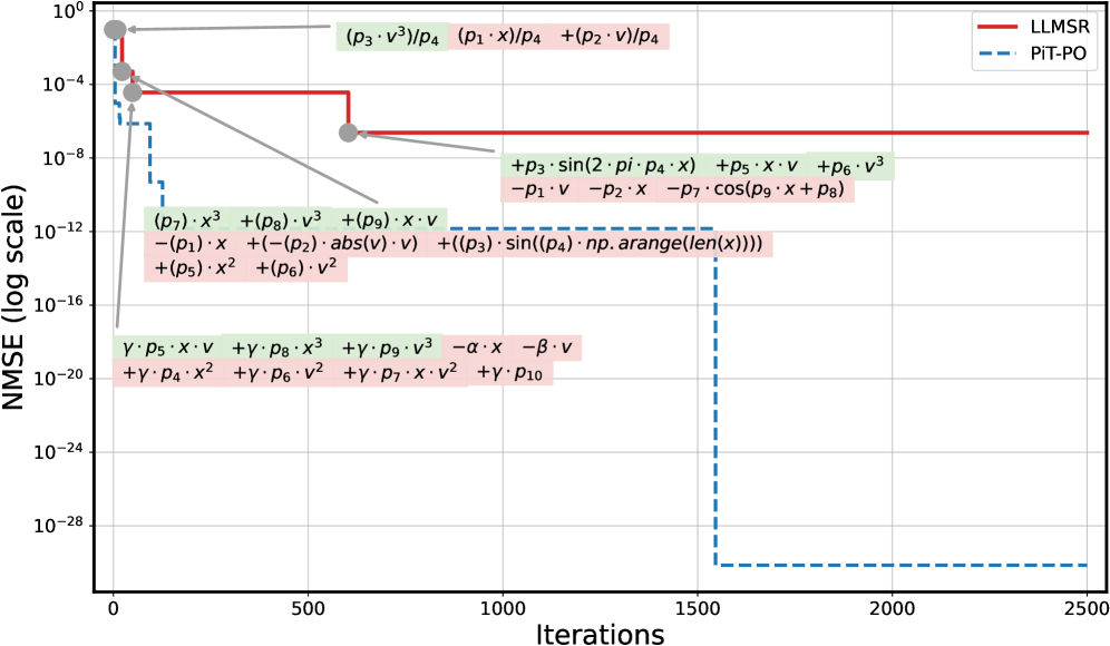
### Visual Description
## Line Graph: NMSE vs Iterations for LLMSR and PiT-PO Algorithms
### Overview
The image is a logarithmic-scale line graph comparing the Normalized Mean Squared Error (NMSE) performance of two algorithms, LLMSR (red solid line) and PiT-PO (blue dashed line), across 2500 iterations. The y-axis spans 10⁰ to 10⁻²⁸, while the x-axis ranges from 0 to 2500 iterations. Annotations with mathematical expressions are overlaid on the graph, pointing to specific data points and trends.
---
### Components/Axes
- **Y-Axis**: "NMSE (log scale)" with values: 10⁰, 10⁻⁴, 10⁻⁸, 10⁻¹², 10⁻¹⁶, 10⁻²⁰, 10⁻²⁴, 10⁻²⁸.
- **X-Axis**: "Iterations" with markers at 0, 500, 1000, 1500, 2000, 2500.
- **Legend**: Top-right corner, associating:
- Red solid line → LLMSR
- Blue dashed line → PiT-PO
- **Annotations**: Colored text boxes with equations (green, pink, gray) pointing to specific points on the lines.
---
### Detailed Analysis
1. **LLMSR (Red Line)**:
- Starts at ~10⁻⁴ NMSE at iteration 0.
- Drops sharply to ~10⁻⁸ by ~500 iterations.
- Remains flat at ~10⁻⁸ for the remainder of the iterations.
- Annotations:
- Green: `(p₃·v³)/p₄`, `(p₁·x)/p₄`, `(p₂·v)/p₄` (near initial drop).
- Pink: `-(p₁·x) + (-p₂·abs(v·v)) + (p₃·sin(p₄·np.arange(len(x))))` (near stabilization).
2. **PiT-PO (Blue Line)**:
- Starts at ~10⁻⁴ NMSE at iteration 0.
- Drops sharply to ~10⁻¹⁶ by ~500 iterations.
- Remains flat at ~10⁻¹⁶ for the remainder of the iterations.
- Annotations:
- Green: `p₃·sin(2·π·p₄·x) + p₅·x·v + p₆·v³` (near stabilization).
- Pink: `-p₁·v - p₂·x - p₇·cos(p₉·x + p₈)` (near stabilization).
- Gray: `γ·p₅·x·v + γ·p₈·x³ + γ·p₉·v³ - α·x - β·v` (initial drop).
---
### Key Observations
1. **Performance Gap**: PiT-PO achieves a significantly lower NMSE (~10⁻¹⁶) compared to LLMSR (~10⁻⁸) after ~500 iterations.
2. **Convergence Speed**: PiT-PO converges ~10⁸ times faster than LLMSR (10⁻¹⁶ vs. 10⁻⁸).
3. **Anomalies**:
- LLMSR shows a minor initial spike to ~10⁻² before dropping.
- PiT-PO’s drop is abrupt and sustained, suggesting rapid error reduction.
4. **Annotations**: Mathematical terms in annotations likely represent error components or algorithmic parameters (e.g., `sin(2πp₄x)` implies periodic adjustments in PiT-PO).
---
### Interpretation
- **Algorithm Efficacy**: PiT-PO outperforms LLMSR by orders of magnitude, indicating superior error minimization. The logarithmic scale emphasizes this disparity.
- **Convergence Dynamics**: PiT-PO’s rapid drop suggests it addresses error sources more effectively early in iterations, while LLMSR’s gradual decline may reflect slower adaptation.
- **Mathematical Insights**: Annotations reveal PiT-PO incorporates trigonometric and higher-order terms (e.g., `v³`), potentially capturing complex error patterns. LLMSR’s annotations focus on linear and absolute terms, hinting at simpler error modeling.
- **Practical Implications**: PiT-PO’s efficiency makes it preferable for applications requiring rapid, precise error correction, while LLMSR may suit scenarios with less stringent convergence needs.
---
### Spatial Grounding & Trend Verification
- **Legend**: Top-right, correctly aligned with line colors.
- **Trend Logic-Check**:
- Red line (LLMSR) slopes downward then plateaus, matching its annotations’ gradual terms.
- Blue line (PiT-PO) drops sharply, aligning with its complex trigonometric/higher-order annotations.
- **Component Isolation**:
- **Header**: Legend and axis labels.
- **Main Chart**: Two lines with annotations.
- **Footer**: No additional elements.
---
### Content Details
- **Data Points**:
- LLMSR: Initial ~10⁻⁴ → ~10⁻⁸ (500 iters) → flat.
- PiT-PO: Initial ~10⁻⁴ → ~10⁻¹⁶ (500 iters) → flat.
- **Annotations**:
- Green: Focus on periodic (`sin`) and cubic terms.
- Pink: Linear and cosine terms with phase shifts.
- Gray: Initial error components involving `γ`, `α`, and `β`.
---
### Final Notes
The graph underscores PiT-PO’s dominance in error reduction, likely due to its sophisticated error modeling (e.g., `sin(2πp₄x)`). LLMSR’s simpler approach results in higher residual error. The annotations provide clues about the algorithms’ internal mechanisms, with PiT-PO leveraging periodic adjustments and higher-order terms for precision.
</details>
(b) LLM-SR.
Figure 10. Iterative trajectories of PiT-PO and LLM-SR on Oscillator1 with Llama-3.1-8B-Instruct. The NMSE curves (log scale) report the best-so-far value over iterations. Annotated equation snapshots illustrate how the discovered structure evolves along the search trajectory. The green-shaded terms are correct, whereas the red-shaded terms are erroneous.
Figure 10 visualizes how symbolic structures evolve along the iterative search. For PiT-PO (Figure 10(a)), the trajectory reveals a clear process of progressively excluding spurious terms. Under the theorem-guided mathematical constraints and the token-aware policy update, tokens marked as redundant are assigned token-level penalties; as this penalty signal repeatedly accumulates across many sampled equations during optimization, such spurious components become progressively less preferred and are unlikely to reappear in later generations. As a result, the search does not merely fit numerically; instead, it repeatedly transitions to cleaner structures, and each step-wise NMSE drop aligns with the removal of nuisance terms and a move toward a more parsimonious functional form. This “error-term elimination” behavior effectively shrinks the search space and substantially strengthens the exploration capability.
In contrast, LLM-SR (Figure 10(b)) exhibits much weaker structural correction. Since its guidance is primarily prompt-level rather than parameter-level, terms that appear early—even if structurally incorrect—tend to persist and continue influencing subsequent proposals. Consequently, the search frequently enters a plateau where NMSE stops improving meaningfully: the method keeps revisiting or retaining earlier spurious components instead of systematically pruning them, indicating a stagnation regime with limited ability to reach the correct structure.
## Appendix D Datasets
### D.1. LLM-SR Suite
We use the LLM-SR Suite, which consists of four standard scientific equation discovery tasks spanning physics, biology, and materials science. The suite includes two nonlinear oscillator systems (Oscillation 1/2), an E. coli growth model (E. coli Growth), and a temperature-dependent stress–strain dataset (Stress–Strain). The first three tasks are dynamical systems and are simulated over a fixed time horizon, while the last task is a static constitutive relation evaluated on experimental measurements.
#### D.1.1. Oscillation 1 (Nonlinear Oscillator)
Nonlinear oscillators with dissipative and non-polynomial couplings provide a demanding test for recovering interacting terms from trajectories. We define the state as $x(t)$ and $v(t)=\dot{x}(t)$ , and simulate the following system:
| | $\displaystyle\dot{x}$ | $\displaystyle=v,$ | |
| --- | --- | --- | --- |
We set $F=0.8$ , $\alpha=0.5$ , $\beta=0.2$ , $\gamma=0.5$ , and $\omega=1.0$ , with initial conditions $x(0)=0.5$ , $v(0)=0.5$ , and simulate over $t\in[0,50]$ .
#### D.1.2. Oscillation 2 (Nonlinear Oscillator)
The second oscillator introduces explicit time forcing and an exponential nonlinearity, leading to a different coupling pattern between $x$ and $v$ :
| | $\displaystyle\dot{x}$ | $\displaystyle=v,$ | |
| --- | --- | --- | --- |
We use $F=0.3$ , $\alpha=0.5$ , $\beta=1.0$ , $\delta=5.0$ , $\gamma=0.5$ , and $\omega=1.0$ . The initial conditions and simulation window are the same as Oscillation 1: $x(0)=0.5$ , $v(0)=0.5$ , $t\in[0,50]$ .
#### D.1.3. E. coli Growth (Bacterial Growth)
This task models the growth rate of E. coli as a product of multiplicative factors capturing distinct physiological effects from population size, nutrient availability, temperature, and acidity:
$$
\frac{dB}{dt}=f_{B}(B)\cdot f_{S}(S)\cdot f_{T}(T)\cdot f_{\mathrm{pH}}(\mathrm{pH}),
$$
where $B$ is bacterial density, $S$ is nutrient concentration, $T$ is temperature, and $\mathrm{pH}$ denotes acidity. In our benchmark, the explicit functional form is:
This specification combines saturation kinetics, sharp temperature modulation, and a structured pH response, yielding a challenging multivariate nonlinear discovery setting.
#### D.1.4. Stress–Strain (Material Stress Behavior)
To assess performance on experimental measurements, we consider tensile stress–strain data for Aluminum 6061-T651 collected at multiple temperatures (from room temperature up to $300^{\circ}\text{C}$ ). While no single exact governing equation is provided, a commonly used phenomenological approximation for temperature-dependent hardening is:
$$
\sigma=\left(A+B\varepsilon^{n}\right)\left(1-\left(\frac{T-T_{r}}{T_{m}-T_{r}}\right)^{m}\right).
$$
where $\sigma$ is stress, $\varepsilon$ is strain, $T$ is temperature, $T_{r}$ is a reference temperature, and $T_{m}$ is the melting temperature. The coefficients $A$ , $B$ , $n$ , and $m$ are fitted from data for the given alloy.
### D.2. LLM-SRBench
We additionally report results on LLM-SRBench, a benchmark specifically constructed to evaluate data-driven scientific equation discovery with LLMs while reducing the risk of trivial memorization of canonical textbook formulas. It contains 239 problems spanning four scientific domains (chemistry, biology, physics, and material science), and each task is packaged with (i) a short scientific context describing variables and the target quantity and (ii) tabular numerical samples used for discovery.
Dataset composition
LLM-SRBench is organized into two complementary subsets.
(1) LSR-Transform. This subset converts well-known physics equations into less-common but analytically equivalent forms by changing the prediction target. Concretely, starting from the original equation, one input variable is chosen as a pivot and promoted to the new target; the equation is then symbolically solved (e.g., via SymPy) for that pivot variable, yielding an alternative representation of the same underlying physical law. Only transformations that admit an analytic solution are retained, and the original datapoints are filtered to satisfy the valid domain of the transformed expression (e.g., avoiding invalid denominators or square-root domains). Finally, a new natural-language problem statement is generated to match the transformed input–output specification. This pipeline produces 111 transformed problems.
(2) LSR-Synth. This subset is designed to test discovery beyond memorized templates by composing equations from both known scientific terms and synthetic (novel yet plausible) terms. Candidate known/synthetic terms are proposed with an LLM given the domain context, combined into full equations, and then filtered through multiple checks: numerical solvability (e.g., via standard ODE solvers for dynamical systems), novelty assessment in context (using an LLM-based novelty evaluator), and expert plausibility validation. After passing these filters, datapoints are generated for each approved equation, yielding 128 synthetic problems across the same four domains.
Symbolic Accuracy (SA)
Besides numeric fit metrics (e.g., $\mathrm{NMSE}$ and $\mathrm{Acc}_{all}(\tau)$ ), LLM-SRBench emphasizes symbolic correctness. Symbolic Accuracy (SA) is computed using an LLM-based equivalence judge (GPT-4o): given a predicted hypothesis and the ground-truth expression, the evaluator first normalizes both by removing extraneous text (e.g., comments) and replacing explicit numeric constants with placeholder parameters, then decides whether there exist parameter values that make the hypothesis mathematically equivalent to the ground truth. SA is the fraction (percentage) of problems judged equivalent under this protocol. The benchmark authors validated this evaluation by comparing against human judgments on 130 sampled problems and reported 94.6% agreement between GPT-4o and human evaluators.
## Appendix E Turbulence Task Setup: Periodic Hill Flow
### E.1. Dataset
We consider the periodic hill flow configuration with streamwise periodic boundary conditions and no-slip walls.
In this work, the features selected for the symbolic regression process are computed from the mean strain-rate ( $S$ ) and rotation-rate ( $R$ ) tensors. Following established practice, these tensors are normalized using local turbulence scales prior to invariant calculation to ensure well-conditioned inputs:
$$
\displaystyle S \displaystyle=\frac{1}{2}\,\frac{1}{\beta^{*}\omega}\Bigl[\nabla\boldsymbol{u}+(\nabla\boldsymbol{u})^{\mathsf{T}}\Bigr], \displaystyle R \displaystyle=\frac{1}{2}\,\frac{1}{\beta^{*}\omega}\Bigl[\nabla\boldsymbol{u}-(\nabla\boldsymbol{u})^{\mathsf{T}}\Bigr], \tag{13}
$$
where $(\cdot)^{\mathsf{T}}$ denotes matrix transposition. The invariants are then computed as $I_{1}=\mathrm{Tr}(S^{2})$ and $I_{2}=\mathrm{Tr}(R^{2})$ .
The dataset provides (i) two invariant features $(I_{1},I_{2})$ (stored in the Lambda columns), (ii) tensor bases $\{T^{m}\}_{m=1}^{3}$ (stored in the first three $3\times 3$ tensors in the Tensor columns), and (iii) the target anisotropy tensor field $b$ (and its nonlinear correction form used for training, denoted by $b^{\perp}$ ), together with auxiliary fields such as turbulent kinetic energy $k$ when needed by the evaluator.
#### E.1.1. Data Collection
DNS source.
The DNS data are obtained from the publicly available NASA turbulence modeling resource (Turbulence Modeling Resource / TMBWG) for periodic hills of parameterized geometries. https://tmbwg.github.io/turbmodels/Other_DNS_Data/parameterized_periodic_hills.html
RANS baseline generation (for non-DNS methods).
For all non-DNS methods, we compute baseline solutions using OpenFOAM with the same initial and boundary conditions as the DNS. Specifically, we employ the incompressible steady-state solver simpleFoam and apply the turbulence models considered in this paper (all belonging to RANS and its SST variants). The solver outputs, at each sampling point and converged iteration/time-step, the required physical quantities for subsequent post-processing.
DNS–RANS grid alignment and target construction.
To construct training targets consistent with the RANS discretization, we interpolate the DNS fields onto the RANS grid points. The interpolated DNS quantities are then post-processed in the CFD workflow (i.e., as offline preprocessing prior to training) to compute the Reynolds stress tensor, which is packaged into the dataset files as the supervision signal for training.
Feature & basis construction.
Following Pope’s tensor-basis expansion hypothesis, the Reynolds stress decomposition involves (i) tensor bases and (ii) scalar coefficient functions of invariant features. Since our final turbulence closure is embedded as a correction to the baseline kOmegaSST model, we use the physical fields produced by the baseline kOmegaSST computation for post-processing to obtain the input features and the tensor bases. These are stored in separate files (features and bases), while the learning target is defined to match the Reynolds-stress-related quantity described in Section E.2.
#### E.1.2. Pre-processing
We normalize the two invariant inputs prior to feeding them into the learned symbolic expressions:
$$
\tilde{I}=\tanh\!\left(\frac{I}{2.0}\right),\qquad\tilde{I}_{1}=\tanh\!\left(\frac{I_{1}}{2.0}\right),\quad\tilde{I}_{2}=\tanh\!\left(\frac{I_{2}}{2.0}\right), \tag{15}
$$
which maps the raw values into approximately $[-1,1]$ and improves numerical stability during parameter fitting.
### E.2. Casting Turbulence Closure as a Symbolic Regression Problem
Predicting scalar coefficients instead of tensor entries.
Rather than directly searching over tensor-valued symbolic forms, we let the LLM predict three scalar coefficient functions $(G^{1},G^{2},G^{3})$ , each parameterized as a symbolic expression of only two variables $(I_{1},I_{2})$ . The evaluator then reconstructs the predicted tensor via the (fixed) tensor bases:
$$
\hat{b}\;=\;G^{1}(I_{1},I_{2})\,T^{1}\;+\;G^{2}(I_{1},I_{2})\,T^{2}\;+\;G^{3}(I_{1},I_{2})\,T^{3}. \tag{16}
$$
This design compresses the LLM input variable dimension to two, significantly reducing the symbolic search space.
Scoring by MSE in the evaluator.
Given a candidate hypothesis, we compute the fitting score by the mean squared error between the target tensor and the reconstructed tensor. In the final evaluator, we additionally scale both prediction and target by the sample-wise $k$ before error aggregation:
$$
\hat{\tau}_{ij}(x_{n})=k(x_{n})\,\hat{b}_{ij}(x_{n}),\qquad\tau_{ij}(x_{n})=k(x_{n})\,b_{ij}(x_{n}), \tag{17}
$$
We compute the MSE only over a selected subset of tensor components. This is because the Reynolds-stress (and anisotropy) tensor is symmetric, so only six components are independent, and in the present periodic hill flow setting two off-plane shear components are typically several orders of magnitude smaller and are commonly neglected in practical turbulence modeling. Following this standard practice, we evaluate the error only on
$$
\Omega=\{(0,0),(0,1),(1,1),(2,2)\}, \tag{18}
$$
$$
\qquad\mathrm{MSE}=\frac{1}{|\Omega|}\sum_{(i,j)\in\Omega}\frac{1}{N}\sum_{n=1}^{N}\Bigl(\tau_{ij}(x_{n})-\hat{\tau}_{ij}(x_{n})\Bigr)^{2}. \tag{19}
$$
The resulting MSE is used as the numerical fitting score for the symbolic regression loop.
Prompt and fairness across methods.
We provide the same problem specification text (task description, variable definitions, and operator constraints) to both LLM-SR and PiT-PO to ensure a fair comparison. An example prompt is shown in Figure 11 – 13. In our current experiments, we also explicitly restrict the hypothesis space by asking the LLM to avoid trigonometric functions.
<details>
<summary>x15.png Details</summary>
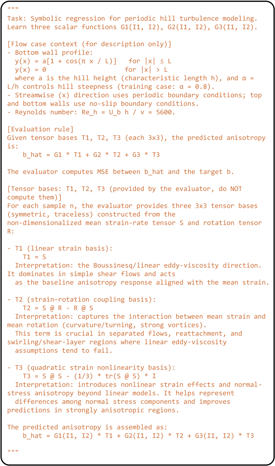
### Visual Description
## Screenshot: Technical Document on Symbolic Regression for Periodic Hill Turbulence Modeling
### Overview
The image displays a technical document outlining a symbolic regression framework for modeling periodic hill turbulence. It includes flow case context, evaluation rules, tensor basis definitions, and a final equation for predicted anisotropy.
### Components/Axes
- **Sections**:
1. **Task**: Symbolic regression for periodic hill turbulence modeling.
2. **Flow case context**: Describes bottom wall profile equations and boundary conditions.
3. **Evaluation rule**: Defines predicted anisotropy using tensor bases.
4. **Tensor bases**: Describes T1 (linear strain), T2 (strain-rotation coupling), and T3 (quadratic strain nonlinearity).
5. **Final equation**: Combines tensor bases with coefficients G1, G2, G3.
### Detailed Analysis
- **Flow case context**:
- Bottom wall profile:
- \( y(x) = a[1 + \cos(\pi x / L)] \) for \( |x| \leq L \)
- \( y(x) = 0 \) for \( |x| > L \)
- \( a \) = hill height (characteristic length \( h \)), \( \alpha = L/h \) controls steepness (training case: \( \alpha = 0.8 \)).
- Reynolds number: \( Re_h = 5600 \).
- Boundary conditions: No-slip at bottom wall, periodic at top wall.
- **Tensor bases**:
- **T1 (linear strain basis)**:
- \( T1 = S \) (Boussinesq/linear eddy-viscosity direction).
- Dominates in simple shear flows; baseline anisotropy aligned with mean strain.
- **T2 (strain-rotation coupling basis)**:
- \( T2 = S @ R - R @ S \) (interaction between mean strain and rotation).
- Critical in separated flows, reattachment, and swirling regions.
- **T3 (quadratic strain nonlinearity basis)**:
- \( T3 = S @ S - \frac{1}{3} \cdot \text{tr}(S @ S) \cdot I \).
- Captures nonlinear strain effects and normal-stress anisotropy.
- **Final equation**:
- Predicted anisotropy:
\[
b_{\text{hat}} = G1(II, I2) \cdot T1 + G2(II1, I2) \cdot T2 + G3(II1, I2) \cdot T3
\]
- Coefficients \( G1, G2, G3 \) are learned via symbolic regression.
### Key Observations
- The model uses symbolic regression to learn scalar functions \( G1, G2, G3 \) that weight tensor bases.
- Tensor bases are constructed from the non-dimensionalized mean strain-rate tensor \( S \) and rotation tensor \( R \).
- T2 and T3 address limitations of linear eddy-viscosity models in complex flow regions.
### Interpretation
This framework extends linear turbulence modeling by incorporating nonlinear and rotational effects through tensor bases. The symbolic regression approach allows data-driven optimization of coefficients \( G1, G2, G3 \), enabling the model to adapt to specific flow conditions (e.g., hill steepness \( \alpha \)). The inclusion of T2 and T3 suggests an emphasis on capturing anisotropic turbulence in regions with strong vortices or separation, where linear models fail. The Reynolds number \( Re_h = 5600 \) indicates a moderately turbulent flow regime.
</details>
Figure 11. Problem Specification.
<details>
<summary>x16.png Details</summary>
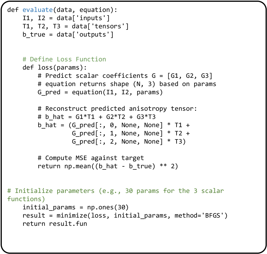
### Visual Description
## Python Code Snippet: Anisotropy Tensor Optimization Workflow
### Overview
The image contains a Python code snippet implementing an optimization workflow for predicting scalar coefficients of an anisotropy tensor. The code defines functions for evaluation, loss calculation, parameter initialization, and optimization using the BFGS method. Key elements include matrix operations, mean squared error (MSE) computation, and parameter minimization.
### Components/Axes
- **Functions**:
- `evaluate(data, equation)`: Processes input data and applies an equation to generate predictions.
- `loss(params)`: Computes the loss (MSE) between predicted and true anisotropy tensor values.
- **Variables**:
- `I1, I2`: Input data arrays.
- `T1, T2, T3`: Tensor data arrays.
- `b_true`: True output anisotropy tensor.
- `G_pred`: Predicted scalar coefficients (shape `(N, 3)`).
- `b_hat`: Reconstructed anisotropy tensor from predictions.
- **Optimization**:
- `initial_params`: Initialized parameters (30-dimensional array).
- `minimize(loss, initial_params, method='BFGS')`: Optimizes parameters to minimize loss.
### Detailed Analysis
1. **Data Extraction**:
- Inputs (`I1, I2`), tensors (`T1, T2, T3`), and true outputs (`b_true`) are extracted from `data`.
2. **Loss Function**:
- Predicts scalar coefficients `G = [G1, G2, G3]` using `equation(I1, I2, params)`.
- Reconstructs `b_hat` via matrix multiplication: `G_pred[:, 0] * T1 + G_pred[:, 1] * T2 + G_pred[:, 2] * T3`.
- Computes MSE: `np.mean((b_hat - b_true) ** 2)`.
3. **Parameter Initialization**:
- `initial_params = np.ones(30)`: Initializes 30 parameters (likely 10 per scalar function).
- `minimize` uses the BFGS algorithm to find optimal parameters.
### Key Observations
- The code assumes the `equation` function returns a tensor of shape `(N, 3)` based on input parameters.
- The loss function doubles the MSE (`** 2`), which may be a typo or intentional scaling.
- The BFGS method is used for optimization, a quasi-Newton algorithm suitable for smooth, differentiable loss landscapes.
### Interpretation
This code optimizes scalar coefficients (`G1, G2, G3`) to minimize the discrepancy between predicted and true anisotropy tensors. The workflow:
1. **Predicts** coefficients using an equation dependent on inputs and parameters.
2. **Reconstructs** the anisotropy tensor via linear combinations of input tensors.
3. **Optimizes** parameters to reduce MSE, leveraging gradient-based methods (BFGS).
The use of 30 parameters suggests a model with three scalar functions, each requiring 10 parameters (e.g., polynomial coefficients). The doubling of MSE (`** 2`) is ambiguous but could reflect a domain-specific requirement or error in implementation. The BFGS method ensures efficient convergence for smooth loss functions, critical for high-dimensional parameter spaces.
</details>
Figure 12. Evaluation and Optimization.
<details>
<summary>x17.png Details</summary>
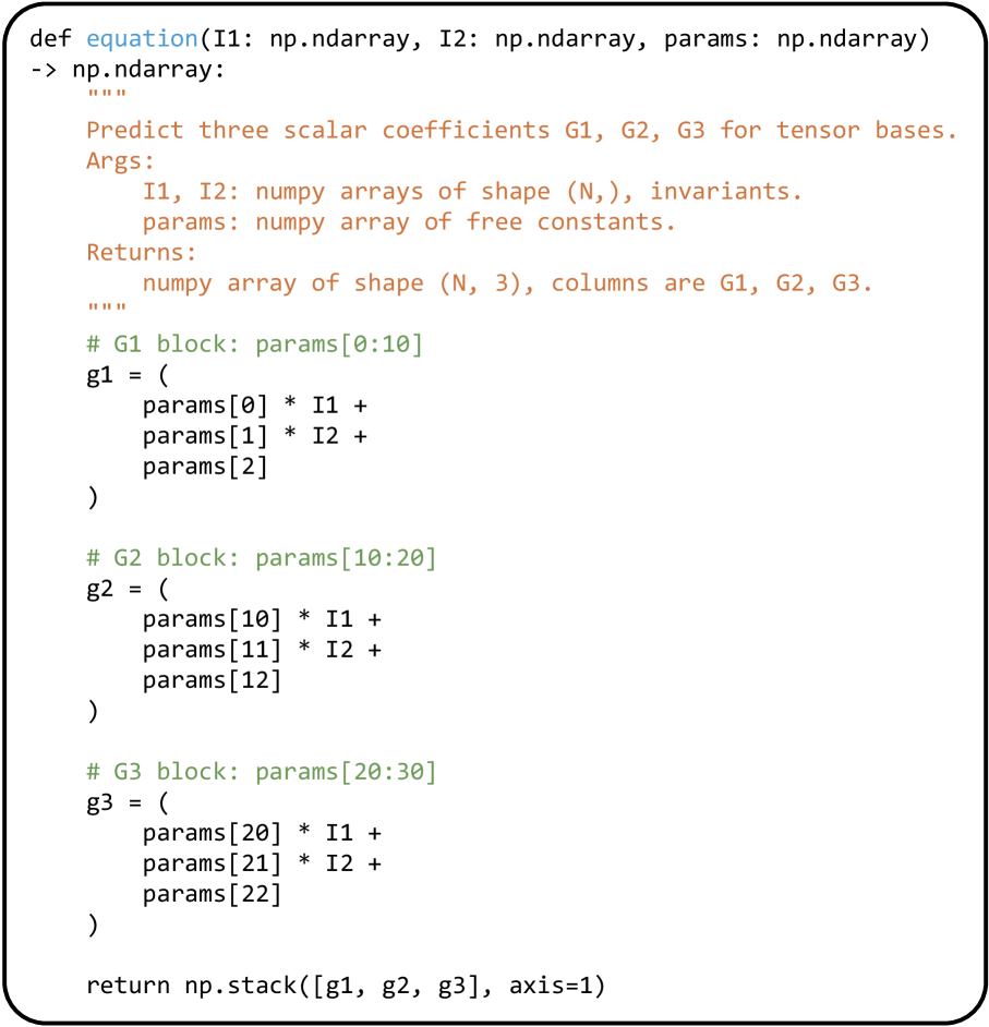
### Visual Description
## Python Function: `equation` for Tensor Coefficient Prediction
### Overview
The image shows a Python function definition for `equation`, which computes three scalar coefficients (G1, G2, G3) for tensor bases using input arrays and free parameters. The function uses NumPy operations to combine input arrays (`I1`, `I2`) with parameter slices (`params`) and returns a stacked array of coefficients.
---
### Components/Axes
- **Function Signature**:
`def equation(I1: np.ndarray, I2: np.ndarray, params: np.ndarray) -> np.ndarray:`
- **Parameters**:
- `I1`, `I2`: Numpy arrays of shape `(N,)` (invariants).
- `params`: Numpy array of free constants (shape `(30,)`).
- **Return**: Numpy array of shape `(N, 3)` with columns `[G1, G2, G3]`.
- **Code Structure**:
- **G1 Block**: Uses `params[0:10]` (indices 0–9).
- **G2 Block**: Uses `params[10:20]` (indices 10–19).
- **G3 Block**: Uses `params[20:30]` (indices 20–29).
---
### Detailed Analysis
1. **G1 Calculation**:
```python
g1 = (params[0] * I1 + params[1] * I2 + params[2])
```
- Combines the first three parameters with `I1` and `I2`, then adds a constant (`params[2]`).
2. **G2 Calculation**:
```python
g2 = (params[10] * I1 + params[11] * I2 + params[12])
```
- Uses parameters 10–12 similarly to G1.
3. **G3 Calculation**:
```python
g3 = (params[20] * I1 + params[21] * I2 + params[22])
```
- Uses parameters 20–22.
4. **Stacking**:
```python
return np.stack([g1, g2, g3], axis=1)
```
- Combines `g1`, `g2`, and `g3` into a 2D array where each row corresponds to an input index `N`, and columns represent G1, G2, G3.
---
### Key Observations
- **Parameter Slicing**: Each coefficient block (`G1`, `G2`, `G3`) uses a distinct 3-parameter subset of `params`.
- **Linear Combination**: Each coefficient is a linear combination of `I1`, `I2`, and a constant term.
- **Output Shape**: The final output has shape `(N, 3)`, ensuring one coefficient per input element.
---
### Interpretation
This function models tensor coefficients as linear combinations of input invariants (`I1`, `I2`) and free parameters. The parameter array `params` is partitioned into three blocks, each governing one coefficient. The design suggests a modular approach, allowing independent tuning of G1, G2, and G3 via separate parameter subsets. The use of `np.stack` ensures the output aligns with the input dimensionality, making it suitable for tensor-based applications like material science or physics simulations.
No numerical values or trends are present in the code itself, as it defines a computational framework rather than presenting empirical data.
</details>
Figure 13. Equation Program Example.
### E.3. Back to Turbulence Modeling
From discovered expressions to a deployable closure
After obtaining an explicit expression for the Reynolds-stress-related term from symbolic regression, we rewrite the discovered formula into an OpenFOAM-readable form.
Embedding into OpenFOAM
We embed the resulting closure into the existing kOmegaSST implementation by replacing the routine that evaluates the Reynolds stress (or its modeled contribution) with the discovered expression, thereby forming an optimized turbulence model within the RANS framework.
Verification against DNS
We then run RANS simulations with the modified model under the same configuration as the baseline and compare the resulting flow statistics against the DNS reference data. This completes the end-to-end turbulence modeling and validation pipeline considered in this work.
### E.4. Domain-Specific Constraints for Turbulence Modeling
To encode expert knowledge as inductive biases, we augment the reward with a domain-specific penalty term:
$$
P_{\text{domain}}\;=\;\sum_{j=1}^{4}w_{j}\,P_{\text{domain}}^{(j)}, \tag{20}
$$
where each $P_{\text{domain}}^{(j)}\geq 0$ quantifies violations of the $j$ -th turbulence constraint.
(1) Realizability.
A physically admissible Reynolds stress tensor must be symmetric and positive semi-definite (PSD), which implies that all eigenvalues are nonnegative. Non-realizable predictions are penalized by
$$
P_{\text{domain}}^{(1)}\;=\;\frac{1}{N}\sum_{n=1}^{N}\max\Bigl(0,\,-\lambda_{\min}(\tau(x_{n}))\Bigr), \tag{21}
$$
where $\lambda_{\min}(\cdot)$ denotes the smallest eigenvalue. This PSD requirement is a standard realizability condition for Reynolds stresses (Pope, 2000).
(2) Boundary-condition consistency.
At a no-slip wall, the Reynolds stress tensor must decay to zero. Accordingly, non-vanishing stresses in a near-wall band $\mathcal{W}=\{x:y(x)<y_{0}\}$ are penalized as
$$
P_{\text{domain}}^{(2)}\;=\;\frac{1}{|\mathcal{W}|}\sum_{x_{n}\in\mathcal{W}}\|\tau(x_{n})\|_{F}, \tag{22}
$$
where $y(x)$ is the wall distance field. In practice, $y(x)$ can be computed and exported using standard CFD post-processing tools (OpenFOAM wall-distance utilities such as wallDist and checkMesh-writeAllFields) (Monkewitz, 2021).
(3) Asymptotic scaling in the viscous sublayer.
Near-wall Taylor expansions under the no-slip constraint imply that $u^{\prime}=O(y)$ and, for incompressible flow, $v^{\prime}=O(y^{2})$ . Consequently, the Reynolds shear stress $-\overline{u^{\prime}v^{\prime}}$ exhibits cubic leading-order scaling, $O(y^{3})$ , in the viscous sublayer (Tennekes and Lumley, 1972). This constraint is enforced by evaluating the slope of $\log|\tau_{xy}^{+}|$ with respect to $\log(y^{+})$ over the viscous sublayer range $\mathcal{V}=\{x:y^{+}(x)\in[y_{1}^{+},y_{2}^{+}]\}$ :
$$
p\;=\;\mathrm{slope}\bigl(\log|\tau_{xy}^{+}|\;\text{vs}\;\log(y^{+})\bigr),\qquad P_{\text{domain}}^{(3)}\;=\;|p-3|. \tag{23}
$$
Here $y^{+}=y\,u_{\tau}/\nu$ is the wall unit, with friction velocity $u_{\tau}=\sqrt{\tau_{w}/\rho}$ . In CFD, $y^{+}$ and $\tau_{w}$ can be obtained through standard post-processing utilities (OpenFOAM yPlus and wallShearStress).
(4) Energy consistency.
Energy consistency is enforced by constraining the turbulent kinetic energy production implied by the predicted stress:
$$
P_{k}(x)\;=\;-\tau_{ij}(x)\,\frac{\partial U_{i}}{\partial x_{j}}(x), \tag{24}
$$
and penalizing mismatches with the reference production $P_{k}^{\text{ref}}$ (computed from DNS-aligned fields) via
$$
P_{\text{domain}}^{(4)}\;=\;\mathrm{MSE}\bigl(P_{k},\,P_{k}^{\text{ref}}\bigr). \tag{25}
$$
The definition in Eq. (24) is the standard production term in the TKE budget (Pope, 2000).
Efficient evaluation via elite-CFD refinement (multi-fidelity constraint scheduling).
Constraints (2)–(4) require additional CFD-derived fields (wall distance $y$ , wall shear stress $\tau_{w}$ and the associated $y^{+}$ , and mean velocity gradients $\nabla U$ ), which can be expensive to obtain at each candidate-evaluation step. To keep the symbolic regression loop efficient, we adopt a two-stage evaluation schedule.
Stage-A (inexpensive screening, applied to all candidates) evaluates the data-fitting score (MSE) together with realizability $P_{\text{domain}}^{(1)}$ using only the predicted stress tensor.
Stage-B (expensive physics checks, triggered by an improving best MSE) is activated when a candidate in the current batch achieves a new best MSE value relative to all previously evaluated candidates. In this case, the candidate is treated as an elite solution, and CFD-based post-processing is performed to obtain the required auxiliary fields, compute $P_{\text{domain}}^{(2)}$ – $P_{\text{domain}}^{(4)}$ , and conduct an additional online fine-tuning step using the full domain-specific penalty. All non-elite candidates are trained only with the realizability constraint, whereas elite candidates receive the full turbulence constraint suite after CFD evaluation. This design enables rigorous physics enforcement without incurring prohibitive CFD costs during exploration.