# Finding the Cracks: Improving LLMs Reasoning with Paraphrastic Probing and Consistency Verification
**Authors**: Weili Shi, Dongliang Guo, Lehan Yang, Tianlong Wang, Hanzhang Yuan, Sheng Li
Abstract
Large language models have demonstrated impressive performance across a variety of reasoning tasks. However, their problem-solving ability often declines on more complex tasks due to hallucinations and the accumulation of errors within these intermediate steps. Recent work has introduced the notion of critical tokens –tokens in the reasoning process that exert significant influence on subsequent steps. Prior studies suggest that replacing critical tokens can refine reasoning trajectories. Nonetheless, reliably identifying and exploiting critical tokens remains challenging. To address this, we propose the P araphrastic P robing and C onsistency V erification (PPCV) framework. PPCV operates in two stages. In the first stage, we roll out an initial reasoning path from the original question and then concatenate paraphrased versions of the question with this reasoning path. And we identify critical tokens based on mismatches between the predicted top-1 token and the expected token in the reasoning path. A criterion is employed to confirm the final critical token. In the second stage, we substitute critical tokens with candidate alternatives and roll out new reasoning paths for both the original and paraphrased questions. The final answer is determined by checking the consistency of outputs across these parallel reasoning processes. We evaluate PPCV on mainstream LLMs across multiple benchmarks. Extensive experiments demonstrate PPCV substantially enhances the reasoning performance of LLMs compared to baselines.
Machine Learning, ICML
<details>
<summary>images/compare_ct_sc_gsm8k.png Details</summary>
### Visual Description
## Line Chart: Pass@k(%) vs. Number of Sample k
### Overview
The image is a line chart comparing the performance of "critical tokens" and "self-consistency" methods as the number of samples (k) increases. The y-axis represents "pass@k(%)", indicating the percentage of successful attempts, while the x-axis represents the "number of sample k". The chart shows how the performance of each method changes with an increasing number of samples.
### Components/Axes
* **X-axis:** "number of sample k" with tick marks at 10, 20, 30, 40, and 50.
* **Y-axis:** "pass@k(%)" with tick marks at 70.0, 72.5, 75.0, 77.5, 80.0, 82.5, 85.0, 87.5, and 90.0.
* **Legend:** Located in the bottom-right corner.
* Red line with triangle markers: "critical tokens"
* Purple line with star markers: "self-consistency"
### Detailed Analysis
* **Critical Tokens (Red Line):** The line slopes upward, indicating an increase in "pass@k(%)" as the number of samples increases.
* At k=5, pass@k(%) ≈ 76.8%
* At k=15, pass@k(%) ≈ 85.3%
* At k=25, pass@k(%) ≈ 86.6%
* At k=35, pass@k(%) ≈ 87.7%
* At k=48, pass@k(%) ≈ 89.3%
* **Self-Consistency (Purple Line):** The line also slopes upward, indicating an increase in "pass@k(%)" as the number of samples increases, but at a slower rate compared to "critical tokens".
* At k=5, pass@k(%) ≈ 70.5%
* At k=10, pass@k(%) ≈ 76.8%
* At k=18, pass@k(%) ≈ 80.2%
* At k=25, pass@k(%) ≈ 82.8%
* At k=33, pass@k(%) ≈ 83.6%
* At k=48, pass@k(%) ≈ 84.6%
### Key Observations
* Both methods show improved performance with an increasing number of samples.
* The "critical tokens" method consistently outperforms the "self-consistency" method across all sample sizes shown.
* The rate of improvement for "critical tokens" appears to decrease as the number of samples increases, suggesting diminishing returns.
* The "self-consistency" method shows a more gradual and consistent improvement.
### Interpretation
The chart suggests that increasing the number of samples (k) generally improves the performance of both "critical tokens" and "self-consistency" methods, as measured by "pass@k(%)". However, the "critical tokens" method demonstrates superior performance compared to "self-consistency" across the tested range of sample sizes. The diminishing returns observed for "critical tokens" at higher sample sizes might indicate a point beyond which further increasing the number of samples yields minimal performance gains. The consistent improvement of "self-consistency" suggests it may be more stable or predictable with increasing sample sizes, although its overall performance remains lower.
</details>
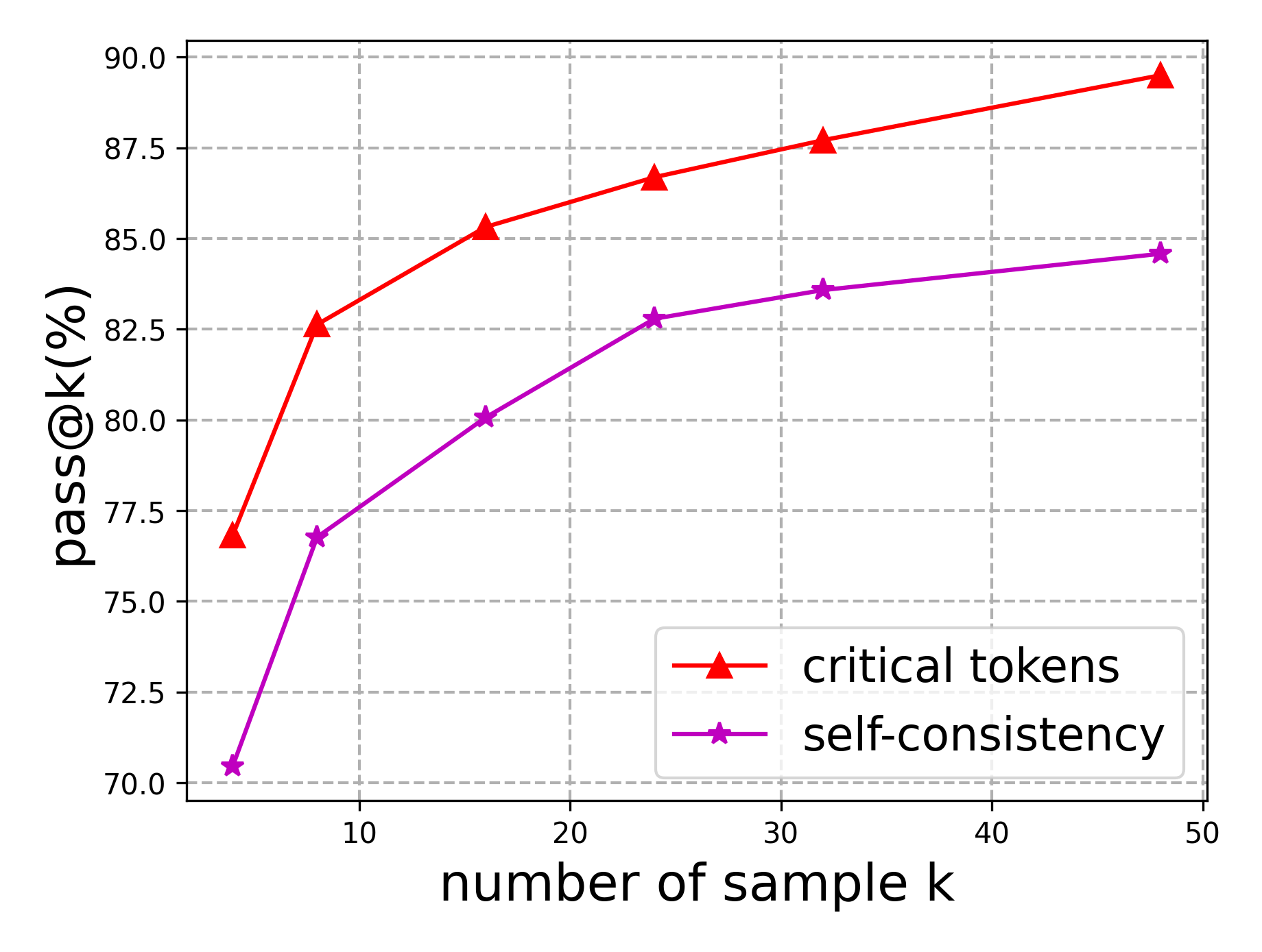
Figure 1: Comparison of the effects of critical tokens and Self-Consistency on the reasoning performance of LLMs, evaluated on samples from the GSM8K training data.
1 Introduction
The emergence of large language models (LLMs) (Brown et al., 2020; Grattafiori et al., 2024; Achiam et al., 2023; Yang et al., 2025a) has astonished the AI community with their remarkable capabilities across a wide range of reasoning tasks, including mathematical problem solving, programming, and planning. By generating intermediate reasoning steps through techniques such as chain-of-thought prompting (Wei et al., 2022; Kojima et al., 2022; Zhang et al., 2022; Sprague et al., 2025), LLMs can emulate human-like reasoning processes and achieve strong performance on diverse reasoning benchmarks. Despite their success, the problem-solving ability of LLMs often declines on complex reasoning tasks due to hallucinations and the accumulation of errors in intermediate steps (Lightman et al., 2023; Ling et al., 2023; Bubeck et al., 2023). To mitigate this issue, prior works (Wang et al., 2024; Yuan et al., 2025; Chen et al., 2024a; Chen and Li, 2024) have proposed the inference-time optimization paradigm, which evaluates and refines reasoning trajectories through self-correction by the LLM itself or with feedback from external verifiers such as process reward models (PRMs) (Uesato et al., 2022). However, existing studies (Yang et al., 2025b; Tyen et al., 2024; Stechly et al., 2025) suggest that LLMs struggle to reliably identify errors in their reasoning and often fail to correct previous outputs without external guidance. Moreover, obtaining high-quality, stepwise process supervision for training external verifiers is challenging and limits the practicality of these approaches (Feng et al., 2025).
<details>
<summary>images/para_example.png Details</summary>
### Visual Description
## Case Study: Effects of Question Paraphrasing
### Overview
The image presents a case study examining the effects of question paraphrasing on problem-solving. It compares the solution process for an original question and a paraphrased version of the same question. The problem involves calculating the number of rounds Jane played in a game, given her points earned and lost.
### Components/Axes
The image is divided into two main sections:
1. **Original Question:** Presents the initial problem statement and its step-by-step solution.
2. **Paraphrased Question:** Presents a reworded version of the problem and its corresponding solution.
Each section includes:
* **Question:** The problem statement.
* **Response:** A step-by-step breakdown of the solution.
* **Ground Truth Answer:** The correct answer to the problem (8).
* A checkmark or X indicating if the solution is correct.
### Detailed Analysis
**Original Question:**
* **Question:** "In a card game, you are awarded 10 points if you win one round. While playing, Jane ends up with 60 points. If she lost 20 points, then how many rounds did she play? (ground truth answer: 8)"
* **Response:**
* Step 1: "Determine the total points Jane earned by subtracting the points she lost from her final score. Total points earned = Final score - Points lost. Total points earned = 60 - 20. Total points earned = 40."
* Step 2: "Since Jane earns 10 points for each round she wins, we can find the number of rounds she played by dividing the total points earned by the points earned per round. Number of rounds = Total points earned / Points earned per round. Number of rounds = 40 / 10. Number of rounds = 4."
* Conclusion: "Therefore, Jane played 4 rounds." (Marked with an "X", indicating an incorrect answer)
**Paraphrased Question:**
* **Question:** "At a bridge competition, every game won grants the player 10 points. Unfortunately, Jane started with an advantage but ended up losing 20 points and scoring only 60 points. If she had won x rounds and lost none, what would be the value of x? (ground truth answer: 8)"
* **Response:**
* Step 1: "Understand the given information. Jane started with an advantage but ended up losing 20 points. She scored a total of 60 points. Every game won grants the player 10 points."
* Step 2: "Determine the total points Jane would have had if she hadn't lost any points. Since she lost 20 points, we need to add 20 to her total score to find out how many points she would have had if she hadn't lost any points. Total points without loss = 60 + 20 = 80 points."
* Step 3: "Calculate the number of games Jane won. Since every game won grants the player 10 points, we can divide the total points without loss by 10 to find the number of games she won. Number of games won = Total points without loss / 10 = 8. The number of games she won is equal to 8." (Marked with a checkmark, indicating a correct answer)
### Key Observations
* The original question's solution incorrectly calculates the total points earned by subtracting the points lost from the final score, leading to an incorrect number of rounds played (4).
* The paraphrased question's solution correctly calculates the total points without loss by adding the points lost to the final score, leading to the correct number of games won (8).
* The ground truth answer is 8 for both questions.
### Interpretation
The case study demonstrates that question paraphrasing can significantly impact problem-solving accuracy. The original question's wording may have led to a misunderstanding of how to calculate the total points earned, resulting in an incorrect solution. The paraphrased question, by explicitly stating that Jane started with an advantage and lost points, guided the solver to correctly calculate the total points without loss and arrive at the correct answer. This highlights the importance of clear and unambiguous question wording in problem-solving contexts.
</details>
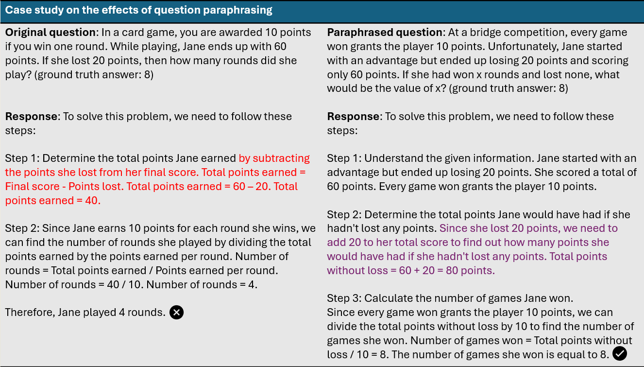
Figure 2: Case study illustrating that LLMs can refine intermediate incorrect reasoning segments (highlighted in red).
Recent work has introduced the concept of critical tokens (Lin et al., 2025), which play pivotal roles in intermediate reasoning steps and exert strong influence on subsequent reasoning and final outcomes. We evaluate the criticality of a token based on the average accuracy of sampling rollouts generated from the partial reasoning trajectories truncated at the token’s position. A token is identified as critical if it lies on an incorrect trajectory and satisfies the following conditions:
- The correctness score of rollouts initiated from the token is close to zero (e.g., below 5%);
- The correctness scores of rollouts initiated from subsequent tokens remain below a threshold (e.g., 10%).
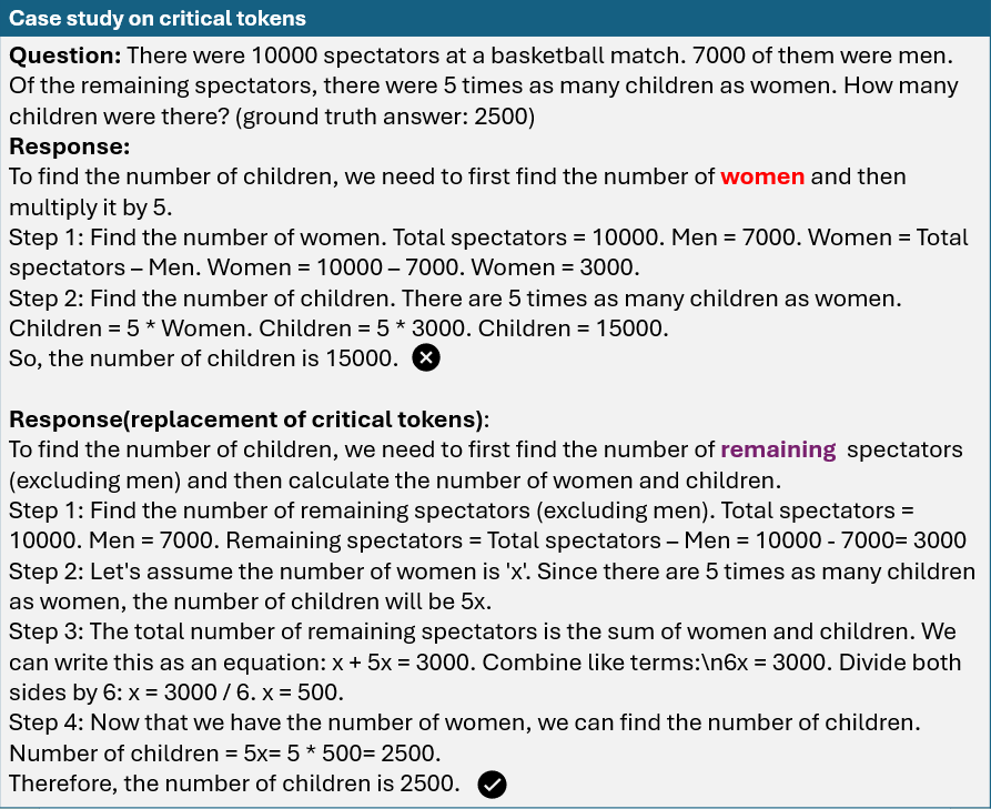
Prior studies suggest that critical tokens often diverge from human-annotated error tokens, yet they induce more sustained degradation in reasoning quality than other tokens. Moreover, as illustrated in Figure 3, replacing critical tokens in an incorrect reasoning trajectory with suitable candidate tokens can correct subsequent steps and lead to the right answer in new rollouts. To quantitatively assess the effectiveness of critical tokens, we conduct an empirical study using LLMs such as Llama-3.1-8B-Instruct (Grattafiori et al., 2024) on reasoning tasks. Specifically, we randomly sample 100 instances with incorrect reasoning steps from the GSM8K (Cobbe et al., 2021) training data. Following the criterion, we locate critical tokens through exhaustive search. We then truncate the reasoning path at the critical token, substitute it with alternative tokens, and roll out new reasoning paths. For example, as shown in Figure 3, the token “woman” is replaced with “remaining”. We evaluate performance using Pass@k and compare against Self-Consistency (Wang et al., 2023), which also samples multiple reasoning paths. As shown in Figure 1, critical token replacement provides a clear advantage in correcting errors compared to plain sampling. Nonetheless, reliably identifying and leveraging critical tokens for reasoning remains a nontrivial challenge.
<details>
<summary>images/critical_token_example.png Details</summary>
### Visual Description
## Textual Case Study: Critical Tokens
### Overview
The image presents a case study on critical tokens, posing a word problem about the number of children at a basketball match given the total number of spectators and the number of men. It provides two different responses to the problem, one incorrect and one correct, demonstrating the importance of correctly interpreting and applying the given information.
### Components/Axes
The image is structured as follows:
1. **Title:** "Case study on critical tokens"
2. **Question:** A word problem describing the scenario.
* Total spectators: 10000
* Number of men: 7000
* Relationship between children and women: 5 times as many children as women
* Question: How many children were there? (ground truth answer: 2500)
3. **Response:** An incorrect solution to the problem.
* Step 1: Calculates the number of women as 3000 (10000 - 7000).
* Step 2: Calculates the number of children as 15000 (5 * 3000).
* Conclusion: The number of children is 15000. (Marked with a red "X")
4. **Response (replacement of critical tokens):** A correct solution to the problem.
* Step 1: Calculates the number of remaining spectators (excluding men) as 3000 (10000 - 7000).
* Step 2: Assumes the number of women is 'x', therefore the number of children is '5x'.
* Step 3: Sets up the equation x + 5x = 3000, simplifies to 6x = 3000, and solves for x (x = 500).
* Step 4: Calculates the number of children as 2500 (5 * 500).
* Conclusion: The number of children is 2500. (Marked with a green checkmark)
### Detailed Analysis or ### Content Details
The word problem states:
* There were 10000 spectators at a basketball match.
* 7000 of them were men.
* Of the remaining spectators, there were 5 times as many children as women.
* The question is: How many children were there? (ground truth answer: 2500)
The first response incorrectly calculates the number of children by assuming that all the remaining spectators are women, and then multiplying that number by 5.
The second response correctly calculates the number of children by setting up an equation that accounts for both women and children among the remaining spectators.
### Key Observations
* The first response fails to account for the fact that the remaining spectators include both women and children.
* The second response correctly identifies that the remaining spectators consist of women and children and sets up an equation to solve for the number of women, then calculates the number of children.
* The "ground truth answer" provided in the question is 2500, which matches the correct solution.
### Interpretation
The case study highlights the importance of carefully reading and interpreting word problems. The incorrect response demonstrates a common mistake of overlooking crucial information and making incorrect assumptions. The correct response demonstrates the importance of setting up equations to accurately represent the relationships between different variables in the problem. The problem emphasizes the need for critical thinking and attention to detail when solving mathematical problems.
</details>
Figure 3: An example demonstrating how substitution of a critical token (red) with a candidate token (purple) modifies the reasoning path and produces the correct answer.
Recent studies (Zhou et al., 2024; Chen et al., 2024b), on surface form, the way questions, assumptions, and constraints are phrased, have revealed its subtle influence on the trajectory of intermediate reasoning steps, As shown in Figure 2. LLMs could adjust the intermediate steps under the paraphrased form of the question. This motivates us to explore the role of paraphrasing in the extraction and utilization of critical tokens for reasoning tasks. To this end, we propose the P araphrastic P robing and C onsistency V erification (PPCV) framework , a two-stage approach designed to leverage critical tokens to enhance the reasoning ability of LLMs. In the first stage, we probe critical tokens using paraphrased questions. Specifically, we first roll out the initial reasoning path from the original question, then concatenate paraphrased questions with this reasoning path. The resulting synthetic inputs are fed into the LLM to obtain token-level logits for each position in the reasoning path. Positions where the predicted top-1 token diverges from the expected token are flagged as potential pivotal points, as these positions are sensitive to paraphrased inputs and can trigger a pivot in the reasoning trajectory. Next, an empirical criterion is applied to determine the final critical token. In contrast to prior work (Lin et al., 2025), which depends on external models for identifying critical tokens with ambiguous criteria, our method introduces a self-contained mechanism that pinpoints critical tokens.
In the second stage, we leverage the extracted critical tokens to refine the initial reasoning path. Specifically, we select the top-K tokens (include critical token itself) at the critical token position and roll out new reasoning paths for both the original and paraphrased questions. Based on the empirical observation that trajectories leading to correct answers are robust to paraphrastic perturbations, we propose a paraphrase consistency mechanism. In contrast to Self-Consistency (Wang et al., 2023), which relies on majority voting, our method selects the final answer by comparing outputs from paraphrased and original questions and choosing the one with the most consistent matches. To address potential ties across multiple answers, we further introduce similarity-weighted paraphrase consistency, which incorporates similarity scores between paraphrased and original questions when computing consistency.
Compared with self-correction (Wu et al., 2024; Miao et al., 2024) and PRM-based methods (Wang et al., 2024; Yuan et al., 2025), our framework exploits critical tokens to refine reasoning trajectories without requiring step-level error detection by the LLM itself or auxiliary models. We evaluate our method on mainstream LLMs across mathematical and commonsense reasoning benchmarks, demonstrating consistent improvements in reasoning performance. The contributions of the paper is summarized as follows:
- We propose a novel two-stage framework, P araphrastic P robing and C onsistency V erification (PPCV) designed to extract and leverage critical tokens to enhance the reasoning performance of LLMs.
- We show that critical tokens can more effectively correct erroneous reasoning trajectories than traditional sampling methods like Self-Consistency. Furthermore, our approach successfully extracts these tokens through paraphrastic probing, achieving improved final results via paraphrase consistency.
- We evaluate our method on mainstream LLMs across various reasoning tasks, including math and logic reasoning. Experimental results show significant performance improvements over baseline methods.
2 Related Work
Inference-Time Optimization for LLM reasoning. With the advent of chain-of-thought (CoT) prompting, LLMs have demonstrated strong reasoning capabilities by producing intermediate steps during inference. This success has motivated a growing body of work (Wu et al., 2025; Snell et al., 2024) on augmenting reasoning trajectories at test time to further improve performance. Existing approaches can be broadly categorized into search-based methods (Bi et al., 2025; Yao et al., 2023; Hao et al., 2023; Xie et al., 2023; Besta et al., 2024), such as Tree-of-Thoughts (Yao et al., 2023), and sampling-based methods (Wang et al., 2023; Xu et al., 2025; Wan et al., 2025; Ma et al., 2025), such as Self-Consistency (Wang et al., 2023). However, due to intrinsic hallucinations (Bubeck et al., 2023), LLMs often generate erroneous intermediate steps, which can ultimately lead to incorrect answers, especially on complex problems. This limitation highlights the need for inference-time optimization of reasoning processes.
To address this issue, one line of research (Yin et al., 2024; Chen et al., 2024a; Ling et al., 2023; Wu et al., 2024; Miao et al., 2024; Madaan et al., 2023) designs instructional prompts that guide LLMs to detect and refine their own mistakes. Despite its appeal, prior work has shown that the effectiveness of self-correction is limited in practice. Another line of work (Wang et al., 2024; Yuan et al., 2025; He et al., 2024; Havrilla et al., 2024) introduces external verifiers, such as process reward models (Snell et al., 2024), to identify and filter out error-prone reasoning steps. These methods typically require high-quality training data for the verifier, with data scarcity often mitigated through strategies such as Monte Carlo Tree Search (Guan et al., 2025; Qi et al., 2025; Li, 2025; Zhang et al., 2024). In addition, a recent line of decoding-based approaches (Xu et al., 2025; Ma et al., 2025) seeks to improve reasoning by dynamically adjusting the next-token prediction based on future trajectory probing. In contrast, our method refines reasoning by directly leveraging critical tokens, without relying on stepwise verification or external verifiers. This design underscores both the utility and universality of our approach.
Paraphrasing for LLMs. A growing number of work (Zhou et al., 2024; Chen et al., 2024b) has examined the impact of a problem’s surface form on the reasoning ability of LLMs. Findings (Zhou et al., 2024; Chen et al., 2024b; Huang et al., 2025) suggest that even subtle modifications in phrasing can substantially affect both the reasoning process and the final outcome. Building on this observation, several methods (Yadav et al., 2024; Chen et al., 2024b) leverage beneficial paraphrasing to enhance LLM performance in tasks such as reasoning and intent classification. In addition, paraphrasing has been employed to assess model uncertainty (Gao et al., 2024; Tanneru et al., 2024), thereby enhancing the reliability and trustworthiness of LLM applications. In our work, we utilize paraphrasing as a principled tool to extract critical tokens and to aggregate answers.
<details>
<summary>x1.png Details</summary>
### Visual Description
## Diagram: Paraphrastic Probing and Consistency Verification
### Overview
The image presents a two-phase process for verifying answers to questions, using paraphrasing and consistency checks. Phase I focuses on paraphrasing the original question and generating an initial response, while Phase II verifies the consistency of the answer by considering alternative tokens and trajectories.
### Components/Axes
**Phase I: Paraphrastic Probing**
* **Step 1:** paraphrase the original question.
* Original Question: "A bakery produces 60 loaves of bread each day... How many loaves of bread are sold in the afternoon?"
* Paraphrased Question: "In a bustling bakery, daily production meets the demand for 60 freshly baked loaves... What is the number of loaves sold in the afternoon?"
* **Step 2:** generate the initial response.
* Question: "A bakery produces 60 loaves of bread each day... How many loaves of bread are sold in the afternoon?"
* Process: "To solve this problem, we will break it down into steps. Step 1: Calculate the number of loaves sold in... Therefore, the number of loaves of bread sold in the afternoon is 5."
* **Step 3:** Concatenate the paraphrased question with the initial answer. And obtain the probabilities for top-1 tokens and expected tokens at each position.
* Question: "In a bustling bakery, daily production meets the demand for 60 freshly baked loaves... What is the number of loaves sold in the afternoon?"
* Process: "To solve this problem, we will break it down into steps. Step 1: Calculate the number of loaves sold in... Therefore, the number of loaves of bread sold in the afternoon is 5."
* Top-1 tokens: p(To) = 0.89, p(solve) = 0.92, ..., p(the) = 0.71, p(total) = 0.60, ..., p(sold) = 0.85, p(the) = 0.68....
* Expected tokens: p(To) = 0.89, p(solve) = 0.92, ..., p(the) = 0.71, p(number) = 0.25, ..., p(sold) = 0.85, p(in) = 0.22.
* **Step 4:** Identify the critical token with the verifier Δ.
* Δ(number) = p(total) - p(number) = 0.60 - 0.25 = 0.35.
* Δ(in) = p(the) - p(in) = 0.68 - 0.22 = 0.46. 0.46 > 0.35.
* The token 'in' is the chosen critical token.
**Phase II: Consistency Verification**
* **Step 1:** Obtain the candidate tokens at the critical token position.
* Question: "A bakery produces 60 loaves of bread each day... How many loaves of bread are sold in the afternoon?"
* Process: "To solve this problem, we will break it down into steps. Step 1: Calculate the number of loaves sold in."
* Candidate tokens: 'during', 'the', ...
* **Step 2:** Truncate the initial answer and replace the critical token with the critical tokens.
* Process 1: "To solve this problem, we will break it down into steps. Step 1: Calculate the number of loaves sold during."
* Process 2: "To solve this problem, we will break it down into steps. Step 1: Calculate the number of loaves sold the."
* **Step 3:** Generate new trajectories from partial answers to both the original and paraphrased questions, and the same procedure is also applied to the initial answer.
* **(Original)** Question: "A bakery produces 60 loaves of bread each day ... How many loaves of bread are sold in the afternoon?"
* Process: "To solve this problem, we will break it down into steps. Step 1: Calculate the number of loaves sold in."
* Process: "To solve this problem... Calculate the number of loaves sold in the morning. The bakery produces 60 loaves of bread each day. Two-thirds of the loaves are sold in the morning... Therefore, the number of loaves of bread sold in the afternoon is 5."
* **(Original)** Question: "A bakery produces 60 loaves of bread each day ... How many loaves of bread are sold in the afternoon?"
* Process: "To solve this problem, we will break it down into steps. Step 1: Calculate the number of loaves sold the."
* Process: "To solve this problem,... Calculate the number of loaves sold the first half of the day (before noon). Two-thirds of 60 loaves are sold before noon.... Therefore, the number of loaves of bread sold in the afternoon is 10."
* **(Paraphrased)** Question: "In a bustling bakery, daily production meets the demand for 60 freshly baked loaves... What is the number of loaves sold in the afternoon?"
* Process: "To solve this problem, we will break it down into steps. Step 1: Calculate the number of loaves sold in."
* Process: "To solve this problem... Calculate the number of loaves sold in the morning. The bakery produces 60 loaves, and two-thirds of these loaves are sold in the morning. ...Therefore, the number of loaves of bread sold in the afternoon is 8."
* **(Paraphrased)** Question: "In a bustling bakery, daily production meets the demand for 60 freshly baked loaves... What is the number of loaves sold in the afternoon?"
* Process: "To solve this problem, we will break it down into steps. Step 1: Calculate the number of loaves sold the."
* Process: "To solve this problem,... Calculate the number of loaves sold the morning after the bakery opens. The bakery starts with 60 loaves. Therefore, the number of loaves of bread sold in the afternoon is 10."
* **Step 4:** Determine the final answer with consistency mechanism.
* "The answers derived from the second input are more consistent than that from the first input. Thus, the final answer is 10."
### Detailed Analysis or ### Content Details
The diagram outlines a process for verifying answers to questions, particularly focusing on mathematical word problems. It uses paraphrasing to generate alternative versions of the question and then checks the consistency of the answers obtained using different approaches. The probabilities of different tokens are used to identify critical tokens and evaluate the consistency of the answers.
### Key Observations
* Phase I focuses on generating paraphrases and an initial answer.
* Phase II focuses on verifying the consistency of the answer by considering alternative tokens and trajectories.
* The probabilities of different tokens are used to identify critical tokens and evaluate the consistency of the answers.
* The final answer is determined based on the consistency of the answers derived from different inputs.
### Interpretation
The diagram illustrates a method for improving the accuracy of answers to questions by using paraphrasing and consistency checks. This approach is particularly useful for mathematical word problems, where there may be multiple ways to arrive at the correct answer. By considering alternative tokens and trajectories, the system can identify and correct errors in the initial answer. The use of probabilities to identify critical tokens allows the system to focus on the most important parts of the question and answer, improving the efficiency of the verification process. The final answer is determined based on the consistency of the answers derived from different inputs, which helps to ensure that the answer is accurate and reliable.
</details>
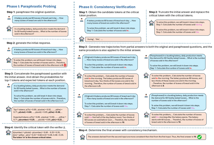
Figure 4: Illustration of the proposed paraphrastic probing and consistency verification (PPCV) framework. The framework comprises two stages: (i) probing critical tokens through paraphrased forms, and (ii) rolling out new reasoning steps with alternative tokens and selecting the final answer using the paraphrase consistency verification mechanism.
<details>
<summary>images/probe_illustration.png Details</summary>
### Visual Description
## Text Analysis: Case Study on Critical Tokens
### Overview
The image presents a case study focused on identifying and utilizing critical tokens in problem-solving. It includes an original question, a paraphrased question, and two different approaches to solving the problem. One approach highlights candidate critical tokens, while the other initializes responses from the critical token position.
### Components/Axes
The image is structured into the following sections:
1. **Title:** "Case study on the identification and effects of critical tokens"
2. **Original Question:** A word problem about Jane playing a card game.
3. **Paraphrased Question:** A similar word problem set in a bridge competition context.
4. **Response with highlighted candidate critical tokens:** A step-by-step solution to the problem, with certain words highlighted.
5. **New responses initialized from the critical token position:** An alternative step-by-step solution.
### Detailed Analysis or ### Content Details
**Original Question:**
* Problem: "In a card game, you are awarded 10 points if you win one round. While playing, Jane ends up with 60 points. If she lost 20 points, then how many rounds did she play?"
* Ground truth answer: 8
**Paraphrased Question:**
* Problem: "At a bridge competition, every game won grants the player 10 points. Unfortunately, Jane started with an advantage but ended up losing 20 points and scoring only 60 points. If she had won x rounds and lost none, what would be the value of x?"
* Ground truth answer: 8
**Response with highlighted candidate critical tokens:**
* Step 1: Determine [Understand] the total points Jane earned [scored] by [.] subtracting [winning] the points she lost from her [the] final score.
* Total points earned = Final score - [+] Points lost.
* Total points earned = 60 - 20.
* Total points earned = 40.
* Step 2: Since Jane earns 10 points for [per] each round she [won] wins, we can find the number of rounds she played by dividing the total points earned by the points earned per round.
* Number of rounds = Total points earned / Points earned per round.
* Number of rounds = 40 / 10.
* Number of rounds = 4.
* Conclusion: Therefore, Jane played 4 rounds. (Incorrect, marked with an "X")
**New responses initialized from the critical token position:**
* Step 1: Determine the total points Jane earned by winning games. Since Jane scored 60 points and lost 20 points, we can set up an equation to represent the situation.
* Total points = Points earned from winning + Points lost
* We know that Jane lost 20 points, so we can subtract this from the total points to find the points earned from winning.
* 60 = Points earned from winning - 20.
* Step 2: Solve for the points earned from winning.
* Add 20 to both sides of the equation to isolate the points earned from winning.
* 60 + 20 = Points earned from winning.
* 80 = Points earned from winning.
* Step 3: Determine the number of games won. Since Jane earns 10 points for each game won, we can divide the points earned from winning by 10 to find the number of games won.
* Number of games won = Points earned from winning / 10 = 8.
* (Correct, marked with a checkmark)
### Key Observations
* The "Response with highlighted candidate critical tokens" arrives at an incorrect answer (4 rounds) because it misinterprets the problem's initial conditions. It fails to account for the points lost.
* The "New responses initialized from the critical token position" correctly solves the problem by considering the points lost and working backward to find the points earned from winning.
* The highlighted words in the first solution are intended to represent "critical tokens," but their selection does not guarantee a correct solution.
### Interpretation
The case study illustrates the importance of correctly identifying and interpreting critical tokens in problem-solving. Highlighting keywords alone is insufficient; a deeper understanding of the problem's context and relationships between variables is necessary. The incorrect solution demonstrates how a superficial analysis of tokens can lead to flawed reasoning. The correct solution emphasizes a more holistic approach, starting from the final score and working backward to account for all relevant factors. The example highlights the potential pitfalls of relying solely on keyword identification without a thorough understanding of the underlying problem.
</details>
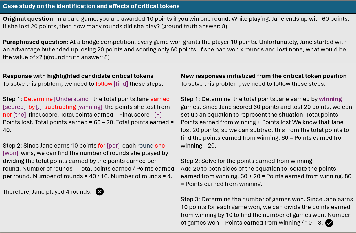
Figure 5: Case study illustrating the identification and effects of critical tokens identified by our method. Tokens highlighted in red indicate candidate critical tokens, whereas tokens highlighted in purple correspond to alternative tokens generated when conditioning on paraphrased questions.
3 Methodology
In this section, we present the two components of our framework in detail: paraphrastic probing and consistency verification. An detailed illustration of our framework is shown in Figure 4. We then discuss the proposed method and provide the complete algorithm.
3.1 Paraphrastic Probing
Previous findings (Zhou et al., 2024; Chen et al., 2024b; Huang et al., 2025) on the impact of a problem’s surface form suggest that the quality of intermediate reasoning steps is influenced not only by the underlying mathematical relationships and logic, but also by how the problem is expressed. Notably, LLMs are sometimes able to solve a paraphrased version of a problem that they fail to solve in its original form, highlighting the potential of paraphrasing to uncover pivotal tokens that are critical for successful reasoning. Motivated by this observation, we introduce paraphrastic probing to efficiently identify the critical token. Given the original question $q_{0}$ , we first prompt the LLM to generate multiple paraphrased forms, denoted as $q_{1},q_{2},...,q_{N}$ , where $N$ is the number of the paraphrased questions. We adopt Automatic Prompt Engineering (APE) (Zhou et al., 2022) to derive paraphrasing instructions that preserve semantic integrity and all numerical values, mathematical relationships, and core logical structures of the problem, while maximizing linguistic and contextual diversity. Additional details can be found in Appendix B. We then obtain the initial reasoning path $r^{q_{0}}_{0}$ for the original question using greedy decoding. This reasoning path is subsequently concatenated with each paraphrased question, and the resulting synthetic inputs are fed into the LLM to compute the token probability distribution at each position in $r^{q_{0}}_{0}$ . Specifically, the token probability distribution at $i$ th position conditioned on the paraphrased question $q_{n}$ is expressed as
$$
P_{i}^{q_{n}}=\text{LLM}(\tilde{a}_{i}|\mathcal{I},q_{n},r^{q_{0}}_{0,<i}), \tag{1}
$$
where $\mathcal{I}$ denotes the instruction prefix and $\tilde{a}_{i}$ represents the sampled token at $i$ th position. The token $\tilde{a}_{i}$ is regarded as a candidate critical token if predicted top-1 token does not match the expected token at the same position in $r^{q_{0}}_{0}$ , i.e.,
$$
\operatorname*{arg\,max}P_{i}^{q_{n}}\neq a_{i}, \tag{2}
$$
where $a_{i}$ denotes the token at the $i$ th position in $r^{q_{0}}_{0}$ .
<details>
<summary>images/condition_one_gsm8k.png Details</summary>
### Visual Description
## Bar Chart: Token Fraction vs. Average Accuracy
### Overview
The image is a bar chart comparing the fraction (percentage) of "critical tokens" and "random tokens" at two different average accuracy levels: "≤ 5%" and "> 5%". The chart includes error bars indicating the variability in the data.
### Components/Axes
* **X-axis:** "Average accuracy(%)" with two categories: "≤ 5%" and "> 5%".
* **Y-axis:** "Fraction(%)" with a scale from 0 to 70.
* **Legend:** Located at the top-right of the chart.
* "critical tokens" (represented by a teal bar)
* "random tokens" (represented by a light green bar)
* **Error Bars:** Black vertical lines extending above and below the top of each bar, indicating the range of uncertainty.
### Detailed Analysis
* **Category: ≤ 5% Average Accuracy**
* "critical tokens" (teal bar): Approximately 69% with an error range of +/- 3%.
* "random tokens" (light green bar): Approximately 32% with an error range of +/- 5%.
* **Category: > 5% Average Accuracy**
* "critical tokens" (teal bar): Approximately 31% with an error range of +/- 3%.
* "random tokens" (light green bar): Approximately 68% with an error range of +/- 5%.
### Key Observations
* At lower average accuracy (≤ 5%), the fraction of critical tokens is significantly higher than random tokens.
* At higher average accuracy (> 5%), the relationship reverses: the fraction of random tokens is significantly higher than critical tokens.
* The error bars suggest some variability in the data, but the overall trends are clear.
### Interpretation
The chart suggests an inverse relationship between the fraction of critical tokens and average accuracy. When the average accuracy is low (≤ 5%), critical tokens make up a larger proportion of the total tokens. Conversely, when the average accuracy is high (> 5%), random tokens become more prevalent. This could indicate that critical tokens are more important for achieving a baseline level of accuracy, while random tokens contribute more as accuracy increases. The error bars indicate that the observed differences are statistically significant, despite some variability in the data.
</details>
(a)
<details>
<summary>images/condition_two_gsm8k.png Details</summary>
### Visual Description
## Bar Chart: Fraction of Tokens vs. Average Accuracy
### Overview
The image is a bar chart comparing the fraction (%) of "critical tokens" and "random tokens" against two categories of average accuracy (≤ 10% and > 10%). Error bars are present on each bar, indicating variability.
### Components/Axes
* **X-axis:** Average accuracy (%), with two categories: "≤ 10%" and "> 10%".
* **Y-axis:** Fraction (%), ranging from 0 to 60. Axis markers are present at intervals of 10 (0, 10, 20, 30, 40, 50, 60).
* **Legend:** Located at the top-right of the chart.
* "critical tokens" (teal)
* "random tokens" (light green)
### Detailed Analysis
* **Category: ≤ 10% Average Accuracy**
* "critical tokens" (teal): Approximately 62% with an error bar extending from approximately 61% to 64%.
* "random tokens" (light green): Approximately 40% with an error bar extending from approximately 39% to 42%.
* **Category: > 10% Average Accuracy**
* "critical tokens" (teal): Approximately 37% with an error bar extending from approximately 36% to 38%.
* "random tokens" (light green): Approximately 60% with an error bar extending from approximately 59% to 62%.
### Key Observations
* For average accuracy ≤ 10%, "critical tokens" have a higher fraction than "random tokens".
* For average accuracy > 10%, "random tokens" have a higher fraction than "critical tokens".
* The fraction of "critical tokens" decreases as average accuracy increases.
* The fraction of "random tokens" increases as average accuracy increases.
### Interpretation
The chart suggests an inverse relationship between the fraction of "critical tokens" and "random tokens" and the average accuracy. When the average accuracy is low (≤ 10%), "critical tokens" are more prevalent. Conversely, when the average accuracy is high (> 10%), "random tokens" are more prevalent. This could indicate that "critical tokens" are more important for lower accuracy scenarios, while "random tokens" become more influential as accuracy improves. The error bars provide a sense of the variability in the data, suggesting that these trends are reasonably consistent.
</details>
(b)
<details>
<summary>images/compare_ct_rnd_gsm8k.png Details</summary>
### Visual Description
## Chart: Pass@k vs. Number of Samples
### Overview
The image is a line chart comparing the "pass@k(%)" metric for "critical tokens" and "random tokens" against the "number of sample k". The chart displays two lines, one red for "critical tokens" and one purple for "random tokens", with error bars indicating variability. The x-axis represents the number of samples, and the y-axis represents the pass@k percentage.
### Components/Axes
* **X-axis:** "number of sample k" with tick marks at 10, 20, 30, and 40.
* **Y-axis:** "pass@k(%)" with tick marks at 50, 55, 60, 65, 70, 75, 80, and 85.
* **Legend:** Located in the bottom-right corner, it identifies the red line as "critical tokens" and the purple line as "random tokens".
* **Gridlines:** Gray dashed lines are present for both x and y axes.
### Detailed Analysis
* **Critical Tokens (Red):** The red line represents the "pass@k(%)" for "critical tokens". The trend is generally upward, with a steeper increase initially, followed by a plateau.
* At k=5, pass@k(%) ≈ 71% ± 2%
* At k=15, pass@k(%) ≈ 82% ± 2%
* At k=30, pass@k(%) ≈ 85% ± 1%
* At k=45, pass@k(%) ≈ 86% ± 1%
* **Random Tokens (Purple):** The purple line represents the "pass@k(%)" for "random tokens". The trend is also upward, but less steep than the "critical tokens" line.
* At k=5, pass@k(%) ≈ 51% ± 3%
* At k=15, pass@k(%) ≈ 60% ± 3%
* At k=30, pass@k(%) ≈ 62% ± 3%
* At k=45, pass@k(%) ≈ 64% ± 3%
### Key Observations
* The "pass@k(%)" is consistently higher for "critical tokens" compared to "random tokens" across all values of k.
* The "pass@k(%)" for "critical tokens" increases rapidly initially, then plateaus.
* The "pass@k(%)" for "random tokens" increases more gradually.
* The error bars suggest more variability in the "random tokens" data, especially at lower values of k.
### Interpretation
The data suggests that using "critical tokens" leads to a significantly higher "pass@k(%)" compared to using "random tokens". This indicates that "critical tokens" are more effective in achieving the desired outcome, as measured by the "pass@k(%)" metric. The initial rapid increase in "pass@k(%)" for "critical tokens" suggests that a relatively small number of samples is sufficient to achieve a substantial improvement, while further increasing the number of samples provides diminishing returns. The higher variability in the "random tokens" data may indicate that the performance is more sensitive to the specific set of random tokens used.
</details>
(c)
<details>
<summary>images/density_gsm8k.png Details</summary>
### Visual Description
## Bar Chart: Consistency Score vs. Density
### Overview
The image is a bar chart comparing the density (%) of incorrect and correct answers against a "consistency score" ranging from 0 to 5. The chart uses two distinct colors to differentiate between incorrect (light green) and correct (light red) answers.
### Components/Axes
* **X-axis:** "consistency score" with markers at 0, 1, 2, 3, 4, and 5.
* **Y-axis:** "density(%)" ranging from 0.0 to 0.7, with markers at 0.0, 0.1, 0.2, 0.3, 0.4, 0.5, 0.6, and 0.7.
* **Legend (top-right):**
* Light Green: "w incorrect answers"
* Light Red: "w correct answers"
### Detailed Analysis
* **"w incorrect answers" (Light Green):**
* Consistency Score 0-1: Density approximately 0.68
* Consistency Score 1-2: Density approximately 0.17
* Consistency Score 2-3: Density approximately 0.00
* Consistency Score 3-4: Density approximately 0.00
* Consistency Score 4-5: Density approximately 0.00
* **"w correct answers" (Light Red):**
* Consistency Score 0-1: Density approximately 0.05
* Consistency Score 1-2: Density approximately 0.06
* Consistency Score 2-3: Density approximately 0.10
* Consistency Score 3-4: Density approximately 0.15
* Consistency Score 4-5: Density approximately 0.55
### Key Observations
* For low consistency scores (0-1), the density of incorrect answers is significantly higher than correct answers.
* As the consistency score increases, the density of correct answers increases, becoming dominant at scores 4-5.
* The density of incorrect answers decreases as the consistency score increases.
### Interpretation
The chart suggests a strong correlation between the consistency score and the correctness of answers. Low consistency scores are associated with a higher proportion of incorrect answers, while high consistency scores are associated with a higher proportion of correct answers. This indicates that the "consistency score" is a good predictor of answer accuracy. The data implies that a higher consistency score reflects a better understanding or knowledge, leading to more correct answers.
</details>
(d)
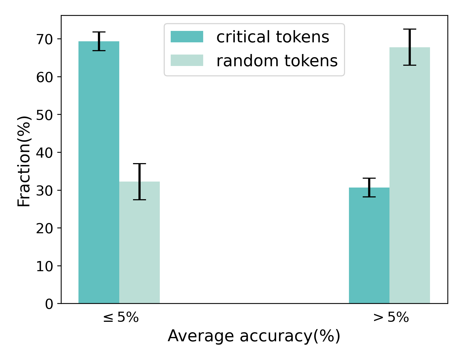
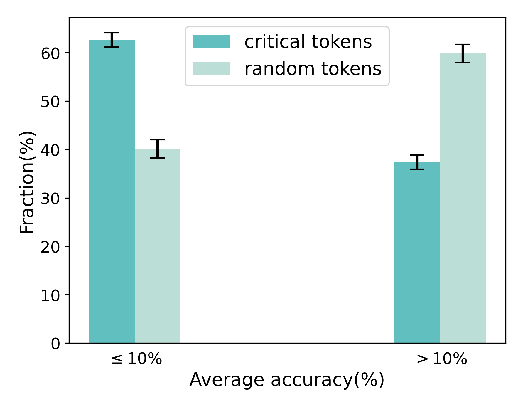
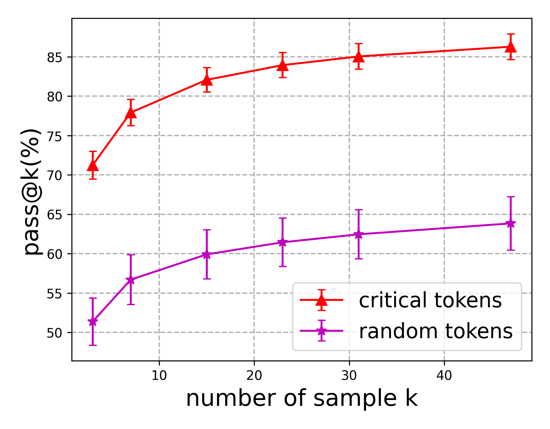
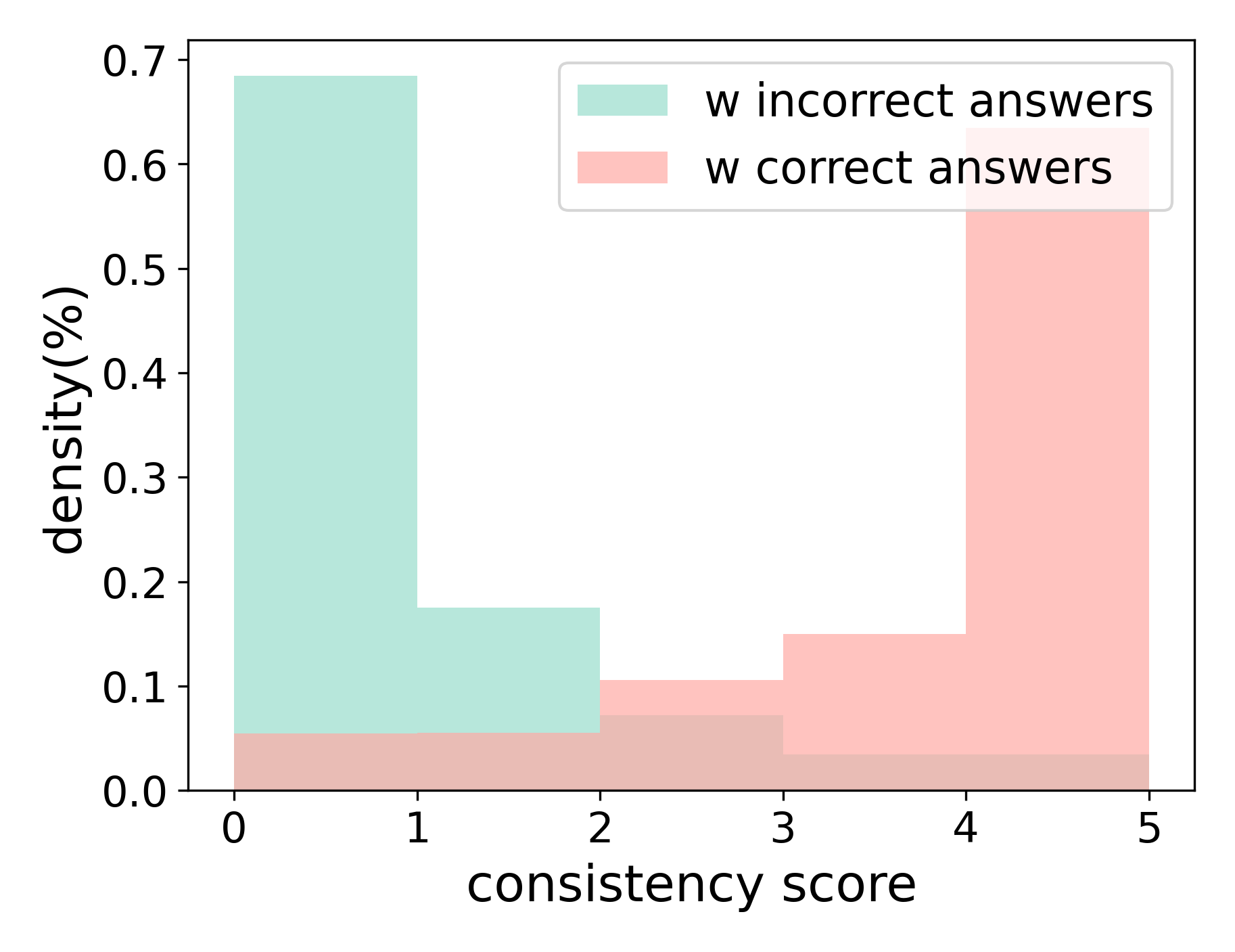
Figure 6: (a) Comparison of the fraction of tokens whose associated rollout correctness falls below or above 5%, for tokens extracted by our method versus randomly selected tokens. (b) Comparison of the fraction of the subsequent tokens whose associated rollout correctness falls below or above 10%, for tokens extracted by our method versus randomly selected tokens. (c) Comparison of the impact of extracted tokens by our method versus random tokens on LLM reasoning performance. (d) Comparison of the density distributions of consistency scores for rollouts with correct and incorrect answers.
To validate the effectiveness of our method in identifying critical tokens and to demonstrate the pivotal role these tokens play when extracted via paraphrastic probing, we conduct a case study illustrated in Figure 5. Because large language models can adjust their reasoning trajectories under the paraphrased form of the question, certain tokens in the original reasoning sequence produce different subsequent tokens when conditioned on paraphrased inputs. In this example, most candidate critical tokens are located within incorrect reasoning segments. Notably, when we identify “subtracting” as a critical token and replace it with an alternative token (i.e., “winning”), the resulting rollout corrects the erroneous reasoning steps and yields the correct final answer. This example highlights the impact of critical tokens and underscores the effectiveness of our method in identifying tokens that are pivotal to reasoning outcomes.
In addition, we conduct a quantitative analysis to examine the authenticity and impact of tokens extracted via paraphrastic probing, comparing them against randomly selected tokens. Specifically, we sample 100 instances with incorrect reasoning trajectories from the GSM8K (Cobbe et al., 2021) training sets. Following the paraphrastic probing pipeline, we identify candidate critical tokens in the early reasoning steps. In each run, we randomly sample 40% of the candidate critical tokens for evaluation and repeat the experiment independently 10 times. For comparison, we apply the same procedure to randomly selected tokens. All evaluations are conducted using Llama-3.1-8B-Instruct (Grattafiori et al., 2024). We first compute the average accuracy of rollouts generated from partial trajectories truncated at the position of the extracted tokens, and compare these results with those obtained from random-token truncation. As shown in Figure 6(a), a large proportion of the extracted tokens exhibit near-zero correctness, consistent with the first criterion of critical tokens. We further evaluate the average accuracy of rollouts initiated from subsequent tokens (5–10 tokens). The results in Figure 6(b) indicate that errors persist beyond the identified positions, supporting the second criterion that critical tokens induce sustained degradation in downstream reasoning. Finally, we substitute the extracted critical tokens with alternative tokens and roll out multiple new reasoning trajectories. As shown in Figure 6(c), replacing critical tokens leads to a significantly larger improvement in reasoning accuracy compared to substituting random tokens. These results further validate both the pivotal role of the identified critical tokens and the effectiveness of our paraphrastic probing method. Additional results can be found in Appendix A.
We introduce a heuristic verifier to select the final critical token from multiple candidates. For a candidate token $a_{i}$ and paraphrased question $q_{n}$ , the verification score is defined as
$$
\Delta_{q_{n}}(a_{i})=\max P^{q_{n}}_{i}-P^{q_{n}}_{i}(\tilde{a}_{i}=a_{i}). \tag{3}
$$
where $P^{q_{n}}_{i}$ denotes the predictive distribution at position $i$ on question $q_{n}$ . Intuitively, $\Delta$ measures how much the predicted top-1 token deviates from the expected token, indicating the token’s potential impact on the reasoning trajectory. For each extracted token $a_{i}$ ,we take the maximum score across paraphrases,
$$
\Delta(a_{i})=\max_{q_{n}}\Delta_{q_{n}}(a_{i}),\vskip-5.69054pt \tag{4}
$$
and select the final critical token as
$$
a_{c}=\operatorname*{arg\,max}_{i}\Delta(a_{i}).\vskip-5.69054pt \tag{5}
$$
3.2 Consistency Verification
After identifying the final critical token $a_{c}$ , we aim to refine the original reasoning path with alternative tokens and achieve final answer with paraphrase consistency mechanism. Specifically, we generate a set of alternative tokens $a^{0}_{c},a^{1}_{c},a^{2}_{c},...,a^{K-1}_{c}$ using the LLM conditioned on original question $q_{0}$ , where $a^{0}_{c}$ is the original token in $r^{q_{0}}_{0}$ and the remaining tokens are sampled via top-K sampling. The initial reasoning path is truncated at the position of critical token, and each alternative token is concatenated to form synthetic inputs $\tilde{r}_{c}^{0},\tilde{r}_{c}^{1},\tilde{r}_{c}^{2},...,\tilde{r}_{c}^{K-1}$ . We then roll out new reasoning trajectories for each synthetic input with respect to both the original and paraphrased questions using greedy decoding, denoted as $r^{q_{0}}_{k},r^{q_{1}}_{k},...,r^{q_{N}}_{k}$ for $k=0,1,2,...,K-1$ . Next, for the rollout with the $k$ th alternative token, we compare the answers obtained from the paraphrased forms with that from the original form and compute a consistency score $c_{k}=\sum_{n-1}^{N}\mathbb{I}(\Phi(r^{q_{0}}_{k})=\Phi(r^{q_{n}}_{k}))$ , where $\Phi(·)$ and $\mathbb{I}(·)$ denotes the function that extracts the final answer from a reasoning trajectory and the indicator function, respectively. The answer associated with the highest consistency score is then selected as the final prediction
$$
\text{ans}_{f}=\Phi(r^{q_{0}}_{k}),\text{where}\,k=\operatorname*{arg\,max}_{k}c_{k}.\vskip-11.38109pt \tag{6}
$$
To justify our paraphrase consistency mechanism, we investigate the impact of paraphrased forms on LLM reasoning. We sample instances from the GSM8K (Cobbe et al., 2021) and follow our pipeline to extract critical tokens. From each truncated reasoning trajectory, we roll out multiple reasoning paths by concatenating alternative tokens. For each original question, we generate five paraphrased variants and compute the consistency score for resulting rollouts. The evaluation is conducted on Llama-3.1-8B-Instruct (Grattafiori et al., 2024). We then analyze the distribution of consistency scores for rollouts that yield correct versus incorrect answers. As shown in Figure 6(d), more than 90% of rollouts with correct answers achieve a consistency score of at least 1, whereas this proportion drops to around 30% for rollouts with incorrect answers. This sharp contrast indicates that correct rollouts are more robust across paraphrased variants, motivating the design of our paraphrase consistency mechanism to exploit this property for improved final predictions.
To address potential collisions when multiple answers obtain the same maximum consistency score, we introduce similarity-weighted consistency verification. Inspired by weighted majority voting (Dogan and Birant, 2019), this approach adjusts the influence of each paraphrased form on the consistency score according to its similarity to the original form. Intuitively, paraphrased forms with lower similarity should exert greater weight, as they provide stronger evidence of robustness, whereas those closely resembling the original form contribute less. Concretely, we first extract embeddings for both the original and paraphrased questions and compute their similarity scores as $s_{n}=\text{sim}(q_{0},q_{n})$ , where $\text{sim}(·)$ denotes a similarity measure such as cosine similarity. We then derive weights via a softmax function $w_{n}=\text{softmax}(s_{n})=\frac{\exp(-\lambda s_{n})}{\sum_{n}\exp(-\lambda n)}$ , where $\lambda$ is the temperature scaling coefficient. Finally, the similarity-weighted consistency score is defined as $\tilde{c}_{k}=\sum_{n-1}^{N}w_{n}\mathbb{I}(\Phi(r^{q_{0}}_{k})=\Phi(r^{q_{n}}_{k}))$ . This ensures agreement with more diverse paraphrases contributes more strongly to the final decision.
Table 1: Comparison of our method with baseline approaches on Llama-3.1-8B-Instruct and Mistral-7B-Instruct-v0.2.
| Llama-3.1 Self-Consistency Tree-of-Thought | Chain-of-Thought 80.60 75.74 | 77.40 31.80 33.28 | 28.00 37.80 31.60 | 31.00 85.10 81.20 | 83.00 60.75 80.72 | 58.91 |
| --- | --- | --- | --- | --- | --- | --- |
| Guided Decoding | 75.51 | 32.45 | 31.20 | 81.70 | 81.74 | |
| Predictive Decoding | 81.43 | 40.26 | 34.00 | 85.90 | 84.56 | |
| Phi-Decoding | 86.58 | 39.88 | 38.20 | 84.50 | 85.41 | |
| PPCV (Ours) | 88.24 | 49.73 | 50.00 | 89.60 | 88.31 | |
| Mistral-7B | Chain-of-Thought | 46.45 | 26.91 | 12.20 | 62.40 | 41.42 |
| Self-Consistency | 50.38 | 28.65 | 14.20 | 66.70 | 44.54 | |
| Tree-of-Thought | 50.49 | 25.78 | 11.40 | 60.60 | 41.04 | |
| Guided Decoding | 50.79 | 27.07 | 14.00 | 62.90 | 39.51 | |
| Predictive Decoding | 55.67 | 27.07 | 14.40 | 62.10 | 47.87 | |
| Phi-Decoding | 56.60 | 28.43 | 13.40 | 63.20 | 60.24 | |
| PPCV (Ours) | 56.58 | 31.08 | 14.60 | 69.30 | 69.88 | |
Table 2: Comparison of our method with baseline approaches on Qwen3-32B (non-thinking mode).
| Qwen3-32B Guided Decoding Predictive Decoding | Chain-of-Thought 26.67 32.67 | 30.00 22.67 24.00 | 23.67 28.67 33.33 | 30.00 7.33 10.33 | 9.67 |
| --- | --- | --- | --- | --- | --- |
| Phi-Decoding | 33.60 | 24.33 | 36.67 | 10.67 | |
| PPCV (Ours) | 40.00 | 26.00 | 43.33 | 13.33 | |
3.3 Discussion
Our technical contributions differ from prior works in three distinct ways. First, prior works (Zhou et al., 2024; Chen et al., 2024b; Yadav et al., 2024) typically use paraphrasing merely to expand the solution space. In contrast, we introduce Paraphrastic Probing, a mechanism that uses paraphrasing to test the model’s internal confidence. By analyzing the discrepancy in token-level logits of the initial trajectory between the original and paraphrased questions, we can rigorously pinpoint the critical tokens that may lead to errors in the following steps.This transforms paraphrasing from a generation tool into a precise, token-level diagnostic tool. Second, prior works (Zhou et al., 2024; Chen et al., 2024b) typically rely on simple majority voting across multiple solutions. Our Paraphrase Consistency mechanism is technically distinct. It validates answers based on their robustness across semantic variations of the problem constraint. We further introduce a similarity-weighted consistency metric that weighs answers based on the linguistic diversity of the paraphrase, offering a more nuanced selection criterion than simple frequency counts. At last, a major technical limitation in current reasoning research is the reliance on external models or human-annotated error steps. Our method contributes a fully self-contained pipeline that identifies and corrects errors using the model’s own sensitivity to surface-form perturbations. More discussion on the impact of critical tokens on correct trajectory can be found in Appendix D.
Besides, although we select the top candidate for the primary experiments to maintain computational efficiency, the framework itself naturally extends to the multi–critical-token setting. For multiple critical tokens, we can generate alternative tokens for each identified position and apply paraphrase consistency across the new rollouts. This allows the model to refine multiple segments of its intermediate reasoning steps rather than only one. The details of the algorithm can be found in Appendix C.
Table 3: Comparison of model performance when using critical tokens versus random tokens.
| Chain-of-Thought random tokens critical tokens (Ours) | 77.40 82.08 88.24 | 28.00 40.29 49.73 | 31.00 42.12 50.00 | 83.00 84.77 89.60 | 58.91 75.68 88.31 |
| --- | --- | --- | --- | --- | --- |
Table 4: Comparison of our proposed paraphrase consistency against the majority voting.
| Chain-of-Thought majority voting paraphrase consistency (Ours) | 77.40 87.20 88.24 | 28.00 47.36 49.73 | 31.00 48.19 50.00 | 83.00 88.80 89.60 | 58.91 86.16 88.31 |
| --- | --- | --- | --- | --- | --- |
4 Experiments
In this section, we first describe the experimental setup, followed by the main results of our proposed method compared to the baselines. We also perform ablation study and computational cost analysis.
4.1 Setup
Datasets. To comprehensively assess our method, we evaluate it on seven benchmarks. Six focus on mathematical reasoning, including GSM8K (Cobbe et al., 2021), GSM-Hard (Gao et al., 2023), SVAMP (Patel et al., 2021), Math500 (Hendrycks et al., 2021), and the more challenging competition-level datasets AIME2024, AIME2025, BRUMO2025, and HMMT2025 (Balunović et al., 2025). In addition, we use ARC-Challenge (Clark et al., 2018) to evaluate knowledge reasoning ability of LLMs.
Baselines. In our experiments, we use Chain-of-Thought (CoT) (Wei et al., 2022), Self-Consistency (Wang et al., 2023), Tree-of-Thought (ToT) (Yao et al., 2023), Guided Decoding (Xie et al., 2023), Predictive Decoding (Ma et al., 2025), and Phi-Decoding (Xu et al., 2025) as baseline methods.
Metric. Following prior work, we adopt pass@k (k=1,4) as the primary evaluation metric.
Implementation Details. In our experiments, we adopt Llama-3.1-8B-Instruct (Grattafiori et al., 2024), Mistral-7B-Instruct-v0.2 (Jiang et al., 2023), Qwen-3-32B (Yang et al., 2025a) and DeepSeek-R1-Distill-Llama-70B as the target models. we employ the non-thinking mode for Qwen-3-32B. Throughout our method, we employ the same model for generating paraphrased problems, identifying critical tokens, and producing new rollouts. In the first stage, we generate 4 paraphrased variants for each problem in the math benchmarks and 3 variants for each problem in the ARC dataset. In the second stage, we select the top 10 tokens for new rollouts, with the temperature scaling coefficient $\lambda$ set to 2. For fair comparison, we ensure a comparable inference budget across methods. Specifically, we rollout 48 samples for Self-Consistency (Wang et al., 2023). For Predictive Decoding (Ma et al., 2025) and Phi-Decoding (Xu et al., 2025), we rollout 4-8 samples per foresight step, and each problem typically involves 5–8 foresight steps. We also adopt a zero-shot CoT prompt to elicit the new rollouts. For the baselines, we strictly follow their original settings, including temperature values, sampling strategies, and the number of few-shot examples. All experiments are conducted on NVIDIA A100 GPUs.
<details>
<summary>images/topk.png Details</summary>
### Visual Description
## Line Chart: Pass@1(%) vs. Number of Alternative Tokens
### Overview
The image is a line chart comparing the performance of two models, GSM8K and SVAMP, based on the "pass@1(%)" metric against the "number of alternative tokens." The chart displays two lines, one for each model, showing how the pass@1(%) score changes as the number of alternative tokens increases.
### Components/Axes
* **X-axis:** "number of alternative tokens" ranging from 3 to 10, with tick marks at each integer value.
* **Y-axis:** "pass@1(%)" ranging from 80 to 94, with tick marks at each even integer value.
* **Legend:** Located in the top-right corner, it identifies the two models:
* GSM8K (yellow-gold line with square markers)
* SVAMP (turquoise line with diamond markers)
* **Gridlines:** Dashed gray lines are present for both x and y axes.
### Detailed Analysis
* **GSM8K (Yellow-Gold Line):**
* Trend: Generally increasing, but plateaus after 7 tokens.
* Data Points:
* At 3 tokens: approximately 84.8%
* At 5 tokens: approximately 86.6%
* At 7 tokens: approximately 88.2%
* At 10 tokens: approximately 88.2%
* **SVAMP (Turquoise Line):**
* Trend: Consistently increasing.
* Data Points:
* At 3 tokens: approximately 87.0%
* At 5 tokens: approximately 87.4%
* At 7 tokens: approximately 88.2%
* At 10 tokens: approximately 89.6%
### Key Observations
* SVAMP consistently outperforms GSM8K across all tested numbers of alternative tokens.
* GSM8K's performance plateaus after 7 alternative tokens, while SVAMP continues to improve.
* Both models show improvement in pass@1(%) as the number of alternative tokens increases, up to a point.
### Interpretation
The chart suggests that increasing the number of alternative tokens generally improves the performance of both GSM8K and SVAMP models, as measured by the pass@1(%) metric. However, the effect is more pronounced for SVAMP, which shows a consistent upward trend, while GSM8K's performance plateaus. This could indicate that SVAMP is better able to leverage additional alternative tokens to improve its accuracy, or that GSM8K reaches a saturation point beyond which more tokens do not provide significant benefit. The data implies that SVAMP is the superior model for this particular task and metric, within the tested range of alternative tokens.
</details>
(a)
<details>
<summary>images/time.png Details</summary>
### Visual Description
## Bar Chart: Latency Comparison of Different Decoding Methods
### Overview
The image is a bar chart comparing the latency (in seconds) of different decoding methods across five datasets: GSM8K, GSMHard, Math500, SVAMP, and ARC. The chart displays the latency for Chain-of-Thought, Predictive Decoding, Phi-Decoding, and four variations of PPCV (T1, T2, T3, and T4).
### Components/Axes
* **Y-axis:** Latency (s), with a scale from 0 to 40 in increments of 5.
* **X-axis:** Datasets: GSM8K, GSMHard, Math500, SVAMP, ARC.
* **Legend (Top-Right):**
* Chain-of-Thought (Teal)
* Predictive Decoding (Light Blue)
* Phi-Decoding (Pale Pink)
* PPCV-T1 (Ours) (Light Pink)
* PPCV-T2 (Ours) (Orange)
* PPCV-T3 (Ours) (Yellow-Green)
* PPCV-T4 (Ours) (Salmon Pink)
### Detailed Analysis
**GSM8K Dataset:**
* Chain-of-Thought: ~2.2 s
* Predictive Decoding: ~15.5 s
* Phi-Decoding: ~13 s
* PPCV-T1: ~2.5 s
* PPCV-T2: ~4 s
* PPCV-T3: ~5 s
* PPCV-T4: ~18 s
**GSMHard Dataset:**
* Chain-of-Thought: ~3 s
* Predictive Decoding: ~26.5 s
* Phi-Decoding: ~23 s
* PPCV-T1: ~3 s
* PPCV-T2: ~6.5 s
* PPCV-T3: ~7 s
* PPCV-T4: ~23 s
**Math500 Dataset:**
* Chain-of-Thought: ~6.5 s
* Predictive Decoding: ~42 s
* Phi-Decoding: ~37.5 s
* PPCV-T1: ~2.5 s
* PPCV-T2: ~28 s
* PPCV-T3: ~10 s
* PPCV-T4: ~38 s
**SVAMP Dataset:**
* Chain-of-Thought: ~2 s
* Predictive Decoding: ~14 s
* Phi-Decoding: ~11 s
* PPCV-T1: ~2 s
* PPCV-T2: ~2 s
* PPCV-T3: ~3 s
* PPCV-T4: ~17 s
**ARC Dataset:**
* Chain-of-Thought: ~2.2 s
* Predictive Decoding: ~15.5 s
* Phi-Decoding: ~15 s
* PPCV-T1: ~2 s
* PPCV-T2: ~3 s
* PPCV-T3: ~3.5 s
* PPCV-T4: ~12.5 s
### Key Observations
* Predictive Decoding consistently exhibits the highest latency across all datasets.
* Chain-of-Thought generally has the lowest latency.
* PPCV-T1, T2, and T3 show relatively low latency compared to other methods.
* PPCV-T4 latency varies across datasets, sometimes being comparable to Phi-Decoding.
* Math500 shows the largest latency differences between Predictive Decoding and Chain-of-Thought.
### Interpretation
The bar chart illustrates the performance of different decoding methods in terms of latency across various datasets. Predictive Decoding and Phi-Decoding generally have higher latencies, suggesting they are more computationally intensive. Chain-of-Thought demonstrates the lowest latency, indicating it is the most efficient in terms of processing time. The PPCV variations show varying performance, with T1, T2, and T3 consistently exhibiting low latency, while T4's performance is more dataset-dependent. The Math500 dataset appears to be the most challenging, as it shows the largest latency values for Predictive Decoding and Phi-Decoding. The data suggests that the choice of decoding method significantly impacts latency, and the optimal method may vary depending on the specific dataset.
</details>
(b)
<details>
<summary>images/throughput.png Details</summary>
### Visual Description
## Bar Chart: Throughput Comparison of Different Decoding Methods
### Overview
The image is a bar chart comparing the throughput (in tokens/sec) of four different decoding methods: Chain-of-Thought, Predictive Decoding, Phi-Decoding, and PPCV (Ours). The chart displays the performance of these methods across five different tasks: GSM8K, GSMHard, Math500, SVAMP, and ARC.
### Components/Axes
* **X-axis:** Represents the different tasks: GSM8K, GSMHard, Math500, SVAMP, ARC.
* **Y-axis:** Represents the throughput in tokens/sec, ranging from 0 to 2000, with increments of 250.
* **Legend (Top-Right):**
* Chain-of-Thought (Teal)
* Predictive Decoding (Light Green)
* Phi-Decoding (Pale Pink)
* PPCV (Ours) (Light Red)
### Detailed Analysis
**GSM8K:**
* Chain-of-Thought: ~125 tokens/sec
* Predictive Decoding: ~700 tokens/sec
* Phi-Decoding: ~525 tokens/sec
* PPCV (Ours): ~1325 tokens/sec
**GSMHard:**
* Chain-of-Thought: ~125 tokens/sec
* Predictive Decoding: ~600 tokens/sec
* Phi-Decoding: ~450 tokens/sec
* PPCV (Ours): ~1725 tokens/sec
**Math500:**
* Chain-of-Thought: ~125 tokens/sec
* Predictive Decoding: ~800 tokens/sec
* Phi-Decoding: ~575 tokens/sec
* PPCV (Ours): ~2025 tokens/sec
**SVAMP:**
* Chain-of-Thought: ~110 tokens/sec
* Predictive Decoding: ~550 tokens/sec
* Phi-Decoding: ~400 tokens/sec
* PPCV (Ours): ~1500 tokens/sec
**ARC:**
* Chain-of-Thought: ~125 tokens/sec
* Predictive Decoding: ~775 tokens/sec
* Phi-Decoding: ~600 tokens/sec
* PPCV (Ours): ~1500 tokens/sec
### Key Observations
* PPCV (Ours) consistently achieves the highest throughput across all tasks.
* Chain-of-Thought consistently has the lowest throughput across all tasks.
* Predictive Decoding and Phi-Decoding have intermediate throughput values, with Predictive Decoding generally performing better than Phi-Decoding.
* The throughput of PPCV (Ours) is significantly higher than other methods, especially on Math500.
### Interpretation
The chart demonstrates that the PPCV (Ours) decoding method significantly outperforms Chain-of-Thought, Predictive Decoding, and Phi-Decoding in terms of throughput (tokens/sec) across the five tasks tested. This suggests that PPCV (Ours) is a more efficient decoding method for these types of tasks. The consistent low performance of Chain-of-Thought indicates it may be less suitable for tasks requiring high throughput. The performance differences between Predictive Decoding and Phi-Decoding suggest that Predictive Decoding is a more optimized approach compared to Phi-Decoding. The Math500 task seems to particularly benefit from the PPCV (Ours) method, indicating a potential synergy between the task's characteristics and the decoding method's strengths.
</details>
(c)
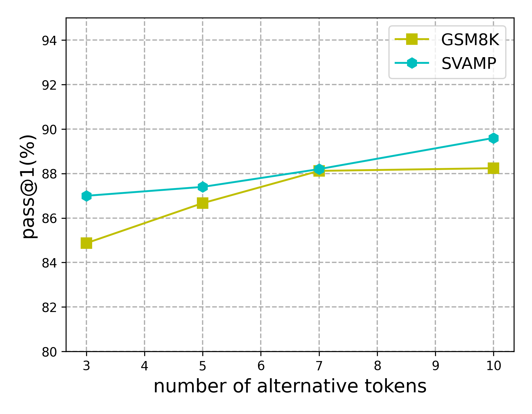
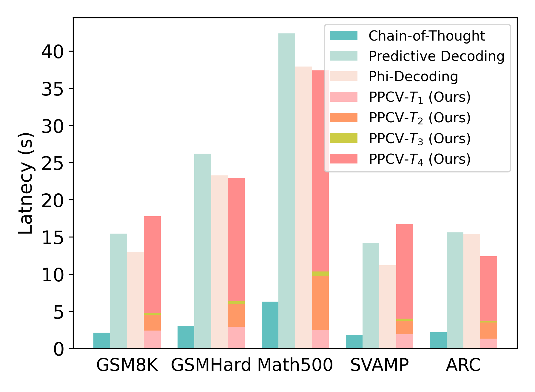
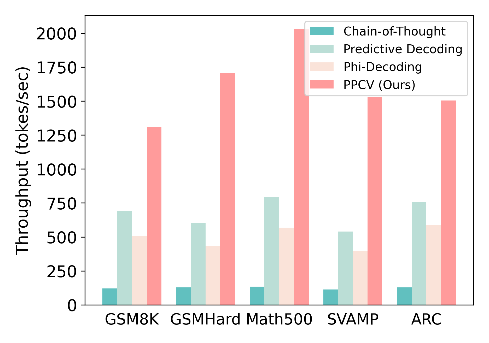
Figure 7: (a) The impact of number of sampled alternative tokens on the performance. (b) Latency comparison between the baselines and our method, measured as the average inference time per question (in seconds). $T_{1}$ , $T_{2}$ , $T_{3}$ , $T_{4}$ denote time for paraphrased question generation, initial answer generation, forward pass and new rollouts from truncated trajectories. (c) Throughput comparison between the baselines and our method, measured in output tokens per second.
4.2 Main Results
The main results are summarized in Table 1 and Table 2. The results indicate that Self-Consistency effectively improves the reasoning performance of LLMs compared to vanilla Chain-of-Thought prompting. For example, Llama-3.1-8B-Instruct (Grattafiori et al., 2024) achieves about 3% higher accuracy with Self-Consistency than with CoT. These findings suggest that augmenting reasoning during inference through sampling is an effective way to refine reasoning trajectories. Recent decoding-based methods, such as Predictive Decoding (Ma et al., 2025) and Phi-Decoding (Xu et al., 2025), also achieve strong results.Unlike prior works that rely on carefully designed prompts to self-correct errors in intermediate steps, these two methods modify the current step by probing future steps with pre-defined reward signals. Furthermore, our experimental results demonstrate that the proposed method consistently outperforms the baselines across most tasks, spanning both mathematical and knowledge reasoning, thereby highlighting its generalization ability across different reasoning settings. Notably, our method even surpasses the latest approaches such as Predictive Decoding (Ma et al., 2025) and Phi-Decoding (Xu et al., 2025). In particular, it achieves approximately 50.00% accuracy on the Math500 dataset (Hendrycks et al., 2021), exceeding these baselines considerably. The results on competition-level datasets further demonstrate the effectiveness of our method in enhancing the reasoning ability of LLMs. These results indicate that our method can effectively extract critical tokens that play a pivotal role in the final outcome and correct the reasoning trajectory by leveraging alternative tokens. Additional results can be found in Appendix E.
4.3 Ablation Study
In this section, we analyze the contribution of each stage individually. All the evaluations are conducted on Llama-3.1-8B-Instruct (Grattafiori et al., 2024).
Effectiveness of extracted critical tokens. To demonstrate the effectiveness of our extracted critical tokens, we conduct an evaluation in which the critical tokens are replaced with random tokens in the first stage, while keeping the second stage unchanged. This evaluation is performed across multiple benchmark datasets, with pass@1 as the metric. The results, shown in Table 3, reveal a substantial decline in performance. These findings highlight the pivotal role of critical tokens and indicate that our method can effectively identify and extract them. More ablation study on comparison with Paraphrased Majority Voting (PMV) can be found in Appendix F.
Effectiveness of paraphrase consistency. We also evaluate the effectiveness of our proposed paraphrase consistency and compare it with traditional majority voting. While keeping the first stage unchanged, instead of using paraphrased forms to generate new reasoning steps, we simply sample multiple new steps from alternative tokens conditioned on the original question and use majority voting to determine the final answer. The results, shown in Table 4, reveal a noticeable decline in performance, highlighting the importance of paraphrased forms in improving the intermediate reasoning steps.
Impact of number of sampled alternative tokens.We investigate the influence of the number of sampled alternative tokens in the second stage by selecting values of 3, 5, 7, and 10. The results, shown in Figure 7(a), demonstrate that performance improves as the number of alternative tokens increases. This suggests that exploring more reasoning steps with additional alternative tokens during inference can be beneficial for reasoning tasks.
5 Computational Cost Analysis
In this section we examine the composition of the latency in our method. The latency arises from four components: Paraphrased question generation ( $T_{1}$ ); initial answer generation ( $T_{2}$ ), equivalent to vanilla CoT; a forward pass for identifying critical tokens ( $T_{3}$ ), which does not generate new tokens and is computationally lightweight; rollouts of truncated trajectories using alternative tokens under both the original and paraphrased questions ( $T_{4}$ ), which constitutes the main source of overhead.
We evaluate all components on Llama-3.1-8B-Instruct using vLLM on NVIDIA A100 GPUs, with a maximum output length of 4096 tokens for each question. For our method, we use 4 paraphrased questions on math datasets and 3 on ARC, and select the top-10 candidate tokens as alternatives. The updated average latency results are reported in Figure 7(b). As expected, $T_{1}$ scales with the number of paraphrases, $T_{3}$ remains minimal, and $T_{4}$ dominates the total cost. Specifically, $T_{4}$ depends on the number of top-k alternative tokens, the number of paraphrased questions and the position of the critical token in the trajectory. Since the new rollouts from truncated trajectories for different alternative tokens and paraphrased questions are independent, $T_{4}$ can take advantage of vLLM’s parallelism. These rollouts can therefore be processed concurrently, improving overall efficiency. This is reflected in the higher throughput (tokens/sec) shown in Figure 7(c). And results of our method in latency comparable to baseline methods, even on challenging benchmarks such as Math500 and GSM-Hard where the critical token tends to occur in later reasoning steps. On the GSM8K and SVAMP benchmarks, our method, as well as baselines such as Predictive Decoding, would incur a approximately $6\text{–}8×$ latency overhead compared to vanilla Chain-of-Thought. More analysis on the trade-off between the latency and performance can be found in Appendix G.
6 Conclusion
In this study, inspired by beneficial impact of paraphrase forms on reasoning, we investigate the pivotal role of critical tokens in shaping the reasoning trajectory. To leverage these two factors, we propose the Paraphrastic Probing and Consistency Verification framework. Our framework consists of two stages: Paraphrastic Probing, which identifies and extracts critical tokens, and Consistency Verification, which adopts paraphrase forms to generate new reasoning trajectories with alternative tokens to reach the final answer. We evaluate our proposed framework with different LLMs and extensive evaluations across multiple benchmarks demonstrate the promising performance of our method.
Impact Statement
This paper presents work whose goal is to advance the field of machine learning. There are many potential societal consequences of our work, none of which we feel must be specifically highlighted here.
References
- J. Achiam, S. Adler, S. Agarwal, L. Ahmad, I. Akkaya, F. L. Aleman, D. Almeida, J. Altenschmidt, S. Altman, S. Anadkat, et al. (2023) Gpt-4 technical report. arXiv preprint. Cited by: §1.
- M. Balunović, J. Dekoninck, I. Petrov, N. Jovanović, and M. Vechev (2025) MathArena: evaluating llms on uncontaminated math competitions. SRI Lab, ETH Zurich. External Links: Link Cited by: §4.1.
- M. Besta, N. Blach, A. Kubicek, R. Gerstenberger, M. Podstawski, L. Gianinazzi, J. Gajda, T. Lehmann, H. Niewiadomski, P. Nyczyk, et al. (2024) Graph of thoughts: solving elaborate problems with large language models. In Proceedings of the AAAI conference on artificial intelligence, Vol. 38, pp. 17682–17690. Cited by: §2.
- Z. Bi, K. Han, C. Liu, Y. Tang, and Y. Wang (2025) Forest-of-thought: scaling test-time compute for enhancing llm reasoning. In Forty-second International Conference on Machine Learning, Cited by: §2.
- T. Brown, B. Mann, N. Ryder, M. Subbiah, J. D. Kaplan, P. Dhariwal, A. Neelakantan, P. Shyam, G. Sastry, A. Askell, et al. (2020) Language models are few-shot learners. Advances in neural information processing systems 33, pp. 1877–1901. Cited by: §1.
- S. Bubeck, V. Chandrasekaran, R. Eldan, J. Gehrke, E. Horvitz, E. Kamar, P. Lee, Y. T. Lee, Y. Li, S. Lundberg, et al. (2023) Sparks of artificial general intelligence: early experiments with gpt-4. arXiv preprint. Cited by: §1, §2.
- S. Chen, B. Li, and D. Niu (2024a) Boosting of thoughts: trial-and-error problem solving with large language models. In The Twelfth International Conference on Learning Representations, Cited by: §1, §2.
- S. Chen and B. Li (2024) Toward adaptive reasoning in large language models with thought rollback. In Forty-first International Conference on Machine Learning, Cited by: §1.
- W. Chen, W. Wang, Z. Chu, K. Ren, Z. Zheng, and Z. Lu (2024b) Self-para-consistency: improving reasoning tasks at low cost for large language models. In Findings of the Association for Computational Linguistics ACL 2024, pp. 14162–14167. Cited by: §1, §2, §3.1, §3.3.
- P. Clark, I. Cowhey, O. Etzioni, T. Khot, A. Sabharwal, C. Schoenick, and O. Tafjord (2018) Think you have solved question answering? try arc, the ai2 reasoning challenge. arXiv preprint arXiv:1803.05457. Cited by: §4.1.
- K. Cobbe, V. Kosaraju, M. Bavarian, M. Chen, H. Jun, L. Kaiser, M. Plappert, J. Tworek, J. Hilton, R. Nakano, et al. (2021) Training verifiers to solve math word problems. arXiv preprint. Cited by: §1, §3.1, §3.2, §4.1.
- A. Dogan and D. Birant (2019) A weighted majority voting ensemble approach for classification. In 2019 4th international conference on computer science and engineering (UBMK), pp. 1–6. Cited by: §3.2.
- S. Feng, X. Kong, S. Ma, A. Zhang, D. Yin, C. Wang, R. Pang, and Y. Yang (2025) Step-by-step reasoning for math problems via twisted sequential monte carlo. In The Thirteenth International Conference on Learning Representations, Cited by: §1.
- L. Gao, A. Madaan, S. Zhou, U. Alon, P. Liu, Y. Yang, J. Callan, and G. Neubig (2023) Pal: program-aided language models. In International Conference on Machine Learning, pp. 10764–10799. Cited by: §4.1.
- X. Gao, J. Zhang, L. Mouatadid, and K. Das (2024) SPUQ: perturbation-based uncertainty quantification for large language models. In Proceedings of the 18th Conference of the European Chapter of the Association for Computational Linguistics (Volume 1: Long Papers), pp. 2336–2346. Cited by: §2.
- A. Grattafiori, A. Dubey, A. Jauhri, A. Pandey, A. Kadian, A. Al-Dahle, A. Letman, A. Mathur, A. Schelten, A. Vaughan, et al. (2024) The llama 3 herd of models. arXiv preprint. Cited by: Appendix A, Appendix A, §1, §1, §3.1, §3.2, §4.1, §4.2, §4.3.
- X. Guan, L. L. Zhang, Y. Liu, N. Shang, Y. Sun, Y. Zhu, F. Yang, and M. Yang (2025) RStar-math: small llms can master math reasoning with self-evolved deep thinking. In Forty-second International Conference on Machine Learning, Cited by: §2.
- S. Hao, Y. Gu, H. Ma, J. Hong, Z. Wang, D. Z. Wang, and Z. Hu (2023) Reasoning with language model is planning with world model. In NeurIPS 2023 Workshop on Generalization in Planning, Cited by: §2.
- A. Havrilla, S. C. Raparthy, C. Nalmpantis, J. Dwivedi-Yu, M. Zhuravinskyi, E. Hambro, and R. Raileanu (2024) GLoRe: when, where, and how to improve llm reasoning via global and local refinements. In Forty-first International Conference on Machine Learning, Cited by: §2.
- M. He, Y. Shen, W. Zhang, Z. Tan, and W. Lu (2024) Advancing process verification for large language models via tree-based preference learning. In Proceedings of the 2024 Conference on Empirical Methods in Natural Language Processing, pp. 2086–2099. Cited by: §2.
- D. Hendrycks, C. Burns, S. Kadavath, A. Arora, S. Basart, E. Tang, D. Song, and J. Steinhardt (2021) Measuring mathematical problem solving with the math dataset. In Thirty-fifth Conference on Neural Information Processing Systems Datasets and Benchmarks Track (Round 2), Cited by: Appendix A, Appendix A, §4.1, §4.2.
- K. Huang, J. Guo, Z. Li, X. Ji, J. Ge, W. Li, Y. Guo, T. Cai, H. Yuan, R. Wang, et al. (2025) MATH-perturb: benchmarking llms’ math reasoning abilities against hard perturbations. In Forty-second International Conference on Machine Learning, Cited by: §2, §3.1.
- A. Q. Jiang, A. Sablayrolles, A. Mensch, C. Bamford, D. S. Chaplot, D. de Las Casas, F. Bressand, G. Lengyel, G. Lample, L. Saulnier, L. R. Lavaud, M. Lachaux, P. Stock, T. L. Scao, T. Lavril, T. Wang, and W. E. Sayed (2023) Mistral 7b. arXiv preprint arXiv:2310.06825. Cited by: §4.1.
- T. Kojima, S. S. Gu, M. Reid, Y. Matsuo, and Y. Iwasawa (2022) Large language models are zero-shot reasoners. Advances in neural information processing systems 35, pp. 22199–22213. Cited by: §1.
- Y. Li (2025) Policy guided tree search for enhanced llm reasoning. In Forty-second International Conference on Machine Learning, Cited by: §2.
- H. Lightman, V. Kosaraju, Y. Burda, H. Edwards, B. Baker, T. Lee, J. Leike, J. Schulman, I. Sutskever, and K. Cobbe (2023) Let’s verify step by step. In The Twelfth International Conference on Learning Representations, Cited by: §1.
- Z. Lin, T. Liang, J. Xu, Q. Liu, X. Wang, R. Luo, C. Shi, S. Li, Y. Yang, and Z. Tu (2025) Critical tokens matter: token-level contrastive estimation enhances llm’s reasoning capability. In Forty-second International Conference on Machine Learning, Cited by: §1, §1.
- Z. Ling, Y. Fang, X. Li, Z. Huang, M. Lee, R. Memisevic, and H. Su (2023) Deductive verification of chain-of-thought reasoning. Advances in Neural Information Processing Systems 36, pp. 36407–36433. Cited by: §1, §2.
- C. Ma, H. Zhao, J. Zhang, J. He, and L. Kong (2025) Non-myopic generation of language models for reasoning and planning. In The Thirteenth International Conference on Learning Representations, Cited by: §2, §2, §4.1, §4.1, §4.2.
- A. Madaan, N. Tandon, P. Gupta, S. Hallinan, L. Gao, S. Wiegreffe, U. Alon, N. Dziri, S. Prabhumoye, Y. Yang, et al. (2023) Self-refine: iterative refinement with self-feedback. Advances in Neural Information Processing Systems 36, pp. 46534–46594. Cited by: §2.
- N. Miao, Y. W. Teh, and T. Rainforth (2024) SelfCheck: using llms to zero-shot check their own step-by-step reasoning. In The Twelfth International Conference on Learning Representations, Cited by: §1, §2.
- A. Patel, S. Bhattamishra, and N. Goyal (2021) Are nlp models really able to solve simple math word problems?. In Proceedings of the 2021 Conference of the North American Chapter of the Association for Computational Linguistics: Human Language Technologies, pp. 2080–2094. Cited by: §4.1.
- Z. Qi, M. Mingyuan, J. Xu, L. L. Zhang, F. Yang, and M. Yang (2025) Mutual reasoning makes smaller llms stronger problem-solver. In The Thirteenth International Conference on Learning Representations, Cited by: §2.
- C. Snell, J. Lee, K. Xu, and A. Kumar (2024) Scaling llm test-time compute optimally can be more effective than scaling model parameters. arXiv preprint. Cited by: §2, §2.
- Z. R. Sprague, F. Yin, J. D. Rodriguez, D. Jiang, M. Wadhwa, P. Singhal, X. Zhao, X. Ye, K. Mahowald, and G. Durrett (2025) To cot or not to cot? chain-of-thought helps mainly on math and symbolic reasoning. In The Thirteenth International Conference on Learning Representations, Cited by: §1.
- K. Stechly, K. Valmeekam, and S. Kambhampati (2025) On the self-verification limitations of large language models on reasoning and planning tasks. In The Thirteenth International Conference on Learning Representations, Cited by: §1.
- S. H. Tanneru, C. Agarwal, and H. Lakkaraju (2024) Quantifying uncertainty in natural language explanations of large language models. In International Conference on Artificial Intelligence and Statistics, pp. 1072–1080. Cited by: §2.
- G. Tyen, H. Mansoor, V. Cărbune, Y. P. Chen, and T. Mak (2024) LLMs cannot find reasoning errors, but can correct them given the error location. In Findings of the Association for Computational Linguistics ACL 2024, pp. 13894–13908. Cited by: §1.
- J. Uesato, N. Kushman, R. Kumar, F. Song, N. Siegel, L. Wang, A. Creswell, G. Irving, and I. Higgins (2022) Solving math word problems with process-and outcome-based feedback. arXiv preprint. Cited by: §1.
- G. Wan, Y. Wu, J. Chen, and S. Li (2025) Reasoning aware self-consistency: leveraging reasoning paths for efficient llm sampling. In Proceedings of the 2025 Conference of the Nations of the Americas Chapter of the Association for Computational Linguistics: Human Language Technologies (Volume 1: Long Papers), pp. 3613–3635. Cited by: §2.
- P. Wang, L. Li, Z. Shao, R. Xu, D. Dai, Y. Li, D. Chen, Y. Wu, and Z. Sui (2024) Math-shepherd: verify and reinforce llms step-by-step without human annotations. In Proceedings of the 62nd Annual Meeting of the Association for Computational Linguistics (Volume 1: Long Papers), pp. 9426–9439. Cited by: §1, §1, §2.
- X. Wang, J. Wei, D. Schuurmans, Q. V. Le, E. H. Chi, S. Narang, A. Chowdhery, and D. Zhou (2023) Self-consistency improves chain of thought reasoning in language models. In The Eleventh International Conference on Learning Representations, Cited by: §1, §1, §2, §4.1, §4.1.
- J. Wei, X. Wang, D. Schuurmans, M. Bosma, F. Xia, E. Chi, Q. V. Le, D. Zhou, et al. (2022) Chain-of-thought prompting elicits reasoning in large language models. Advances in neural information processing systems 35, pp. 24824–24837. Cited by: Appendix D, §1, §4.1.
- Y. Wu, Z. Sun, S. Li, S. Welleck, and Y. Yang (2025) Inference scaling laws: an empirical analysis of compute-optimal inference for llm problem-solving. In The Thirteenth International Conference on Learning Representations, Cited by: §2.
- Z. Wu, Q. Zeng, Z. Zhang, Z. Tan, C. Shen, and M. Jiang (2024) Large language models can self-correct with key condition verification. In Proceedings of the 2024 Conference on Empirical Methods in Natural Language Processing, pp. 12846–12867. Cited by: §1, §2.
- Y. Xie, K. Kawaguchi, Y. Zhao, J. X. Zhao, M. Kan, J. He, and M. Xie (2023) Self-evaluation guided beam search for reasoning. Advances in Neural Information Processing Systems 36, pp. 41618–41650. Cited by: §2, §4.1.
- F. Xu, H. Yan, C. Ma, H. Zhao, J. Liu, Q. Lin, and Z. Wu (2025) Phi-decoding: adaptive foresight sampling for balanced inference-time exploration and exploitation. In Proceedings of the 63rd Annual Meeting of the Association for Computational Linguistics (Volume 1: Long Papers), pp. 13214–13227. Cited by: §2, §2, §4.1, §4.1, §4.2.
- V. Yadav, Z. Tang, and V. Srinivasan (2024) Pag-llm: paraphrase and aggregate with large language models for minimizing intent classification errors. In Proceedings of the 47th international ACM SIGIR conference on research and development in information retrieval, pp. 2569–2573. Cited by: §2, §3.3.
- A. Yang, A. Li, B. Yang, B. Zhang, B. Hui, B. Zheng, B. Yu, C. Gao, C. Huang, C. Lv, et al. (2025a) Qwen3 technical report. arXiv preprint. Cited by: §1, §4.1.
- L. Yang, Z. Yu, T. Zhang, M. Xu, J. E. Gonzalez, B. CUI, and S. YAN (2025b) SuperCorrect: advancing small llm reasoning with thought template distillation and self-correction. In The Thirteenth International Conference on Learning Representations, Cited by: §1.
- S. Yao, D. Yu, J. Zhao, I. Shafran, T. Griffiths, Y. Cao, and K. Narasimhan (2023) Tree of thoughts: deliberate problem solving with large language models. Advances in neural information processing systems 36, pp. 11809–11822. Cited by: §2, §4.1.
- Z. Yin, Q. Sun, Q. Guo, Z. Zeng, X. Li, J. Dai, Q. Cheng, X. Huang, and X. Qiu (2024) Reasoning in flux: enhancing large language models reasoning through uncertainty-aware adaptive guidance. In Proceedings of the 62nd Annual Meeting of the Association for Computational Linguistics (Volume 1: Long Papers), pp. 2401–2416. Cited by: §2.
- L. Yuan, W. Li, H. Chen, G. Cui, N. Ding, K. Zhang, B. Zhou, Z. Liu, and H. Peng (2025) Free process rewards without process labels. In Forty-second International Conference on Machine Learning, Cited by: §1, §1, §2.
- D. Zhang, S. Zhoubian, Z. Hu, Y. Yue, Y. Dong, and J. Tang (2024) Rest-mcts*: llm self-training via process reward guided tree search. Advances in Neural Information Processing Systems 37, pp. 64735–64772. Cited by: §2.
- Z. Zhang, A. Zhang, M. Li, and A. Smola (2022) Automatic chain of thought prompting in large language models. In The Eleventh International Conference on Learning Representations, Cited by: §1.
- Y. Zhou, A. I. Muresanu, Z. Han, K. Paster, S. Pitis, H. Chan, and J. Ba (2022) Large language models are human-level prompt engineers. In The eleventh international conference on learning representations, Cited by: Appendix B, §3.1.
- Y. Zhou, Y. Zhu, D. Antognini, Y. Kim, and Y. Zhang (2024) Paraphrase and solve: exploring and exploiting the impact of surface form on mathematical reasoning in large language models. In Proceedings of the 2024 Conference of the North American Chapter of the Association for Computational Linguistics: Human Language Technologies (Volume 1: Long Papers), pp. 2793–2804. Cited by: §1, §2, §3.1, §3.3.
Appendix A Empirical Study
<details>
<summary>images/condition_one_math.png Details</summary>
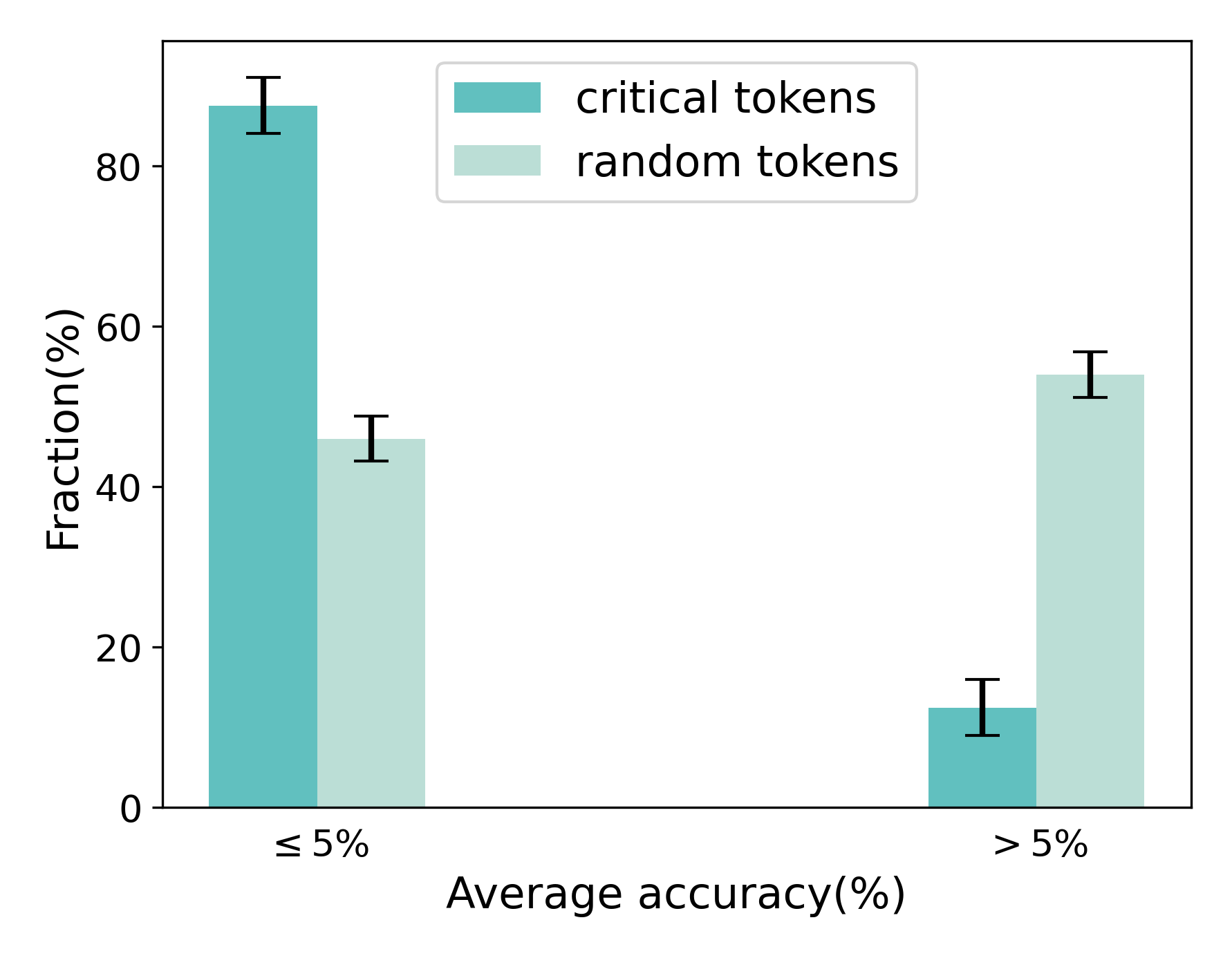
### Visual Description
## Bar Chart: Fraction of Critical and Random Tokens vs. Average Accuracy
### Overview
The image is a bar chart comparing the fraction (percentage) of "critical tokens" and "random tokens" at two different levels of average accuracy: "≤ 5%" and "> 5%". Error bars are included on each bar, indicating variability.
### Components/Axes
* **X-axis:** Average accuracy (%), with two categories: "≤ 5%" and "> 5%".
* **Y-axis:** Fraction (%), ranging from 0 to 80, with tick marks at 0, 20, 40, 60, and 80.
* **Legend:** Located at the top-right of the chart.
* "critical tokens" - Represented by a teal/cyan color.
* "random tokens" - Represented by a light green/mint color.
### Detailed Analysis
* **Average Accuracy ≤ 5%:**
* **Critical Tokens (Teal):** Fraction is approximately 87% with an error bar extending from approximately 84% to 90%.
* **Random Tokens (Light Green):** Fraction is approximately 46% with an error bar extending from approximately 43% to 49%.
* **Average Accuracy > 5%:**
* **Critical Tokens (Teal):** Fraction is approximately 13% with an error bar extending from approximately 10% to 16%.
* **Random Tokens (Light Green):** Fraction is approximately 54% with an error bar extending from approximately 51% to 57%.
### Key Observations
* For average accuracy ≤ 5%, critical tokens have a significantly higher fraction than random tokens.
* For average accuracy > 5%, random tokens have a significantly higher fraction than critical tokens.
* The fraction of critical tokens decreases dramatically as average accuracy increases from ≤ 5% to > 5%.
* The fraction of random tokens increases as average accuracy increases from ≤ 5% to > 5%.
### Interpretation
The chart suggests an inverse relationship between the fraction of critical tokens and the average accuracy. When the average accuracy is low (≤ 5%), critical tokens make up a large portion of the tokens. However, when the average accuracy is higher (> 5%), random tokens become more prevalent. This could indicate that models rely more on critical tokens when they are less accurate, and rely more on random tokens when they are more accurate. The error bars provide a visual representation of the variability in the data.
</details>
(a)
<details>
<summary>images/condition_two_math.png Details</summary>
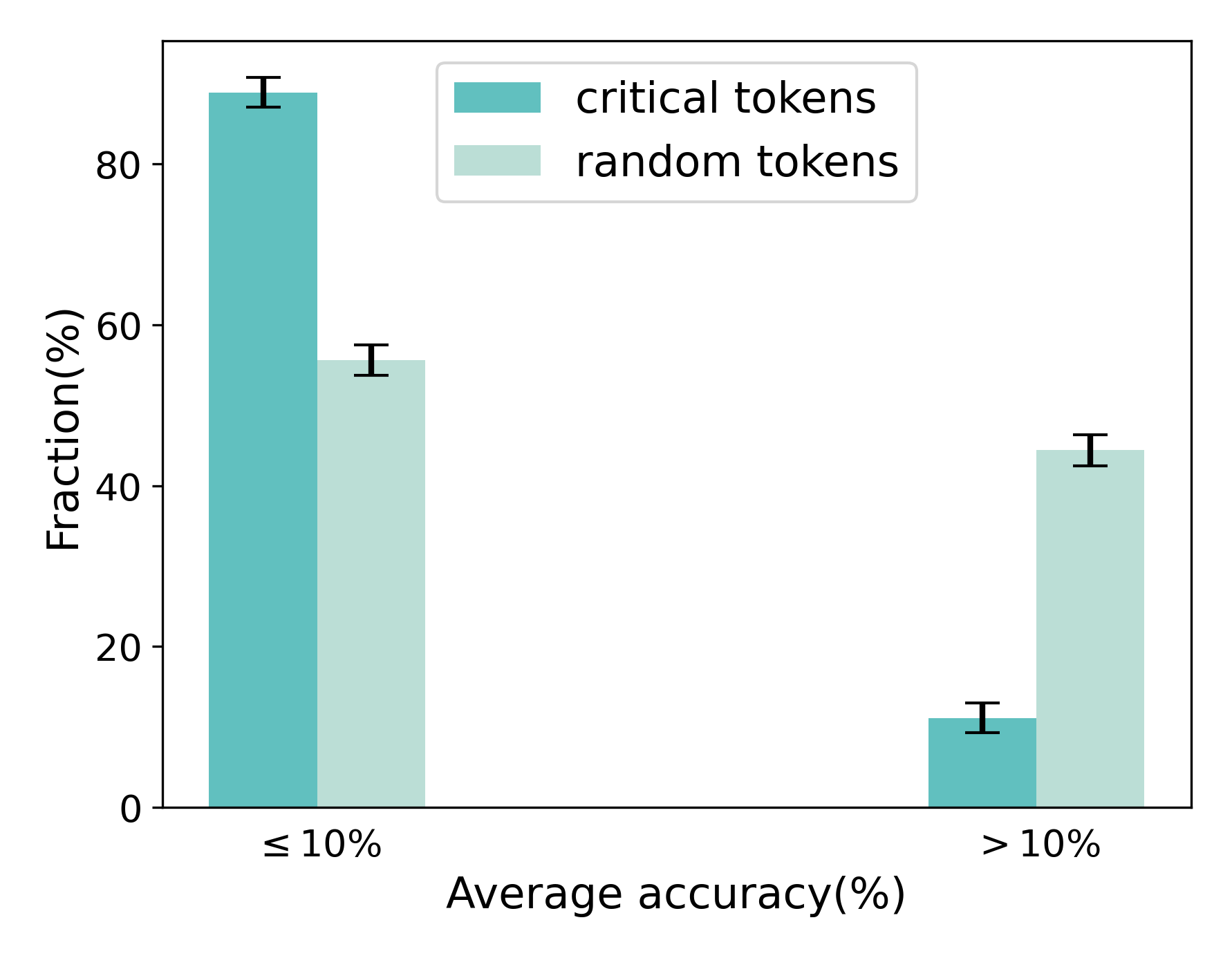
### Visual Description
## Bar Chart: Token Fraction vs. Average Accuracy
### Overview
The image is a bar chart comparing the fraction (percentage) of "critical tokens" and "random tokens" against two categories of average accuracy: "≤ 10%" and "> 10%". Error bars are included on each bar.
### Components/Axes
* **X-axis:** "Average accuracy(%)" with two categories: "≤ 10%" and "> 10%".
* **Y-axis:** "Fraction(%)" with a scale from 0 to 80 in increments of 20.
* **Legend:** Located at the top-right of the chart.
* "critical tokens" represented by a teal bar.
* "random tokens" represented by a light-green bar.
### Detailed Analysis
* **Category: ≤ 10% Average Accuracy**
* "critical tokens" (teal): Approximately 88% with an error bar range of approximately +/- 2%.
* "random tokens" (light-green): Approximately 55% with an error bar range of approximately +/- 3%.
* **Category: > 10% Average Accuracy**
* "critical tokens" (teal): Approximately 11% with an error bar range of approximately +/- 3%.
* "random tokens" (light-green): Approximately 44% with an error bar range of approximately +/- 3%.
### Key Observations
* For average accuracy ≤ 10%, "critical tokens" have a significantly higher fraction than "random tokens".
* For average accuracy > 10%, "random tokens" have a significantly higher fraction than "critical tokens".
* The fraction of "critical tokens" decreases sharply as average accuracy increases from ≤ 10% to > 10%.
* The fraction of "random tokens" decreases slightly as average accuracy increases from ≤ 10% to > 10%.
### Interpretation
The chart suggests that "critical tokens" are more prevalent when the average accuracy is low (≤ 10%), while "random tokens" become more prevalent when the average accuracy is higher (> 10%). This could indicate that the model relies more on "critical tokens" when it struggles to achieve high accuracy, and relies more on "random tokens" when it is more accurate. The error bars indicate the variability in the data, but the overall trends are clear.
</details>
(b)
<details>
<summary>images/compare_ct_rnd_math.png Details</summary>
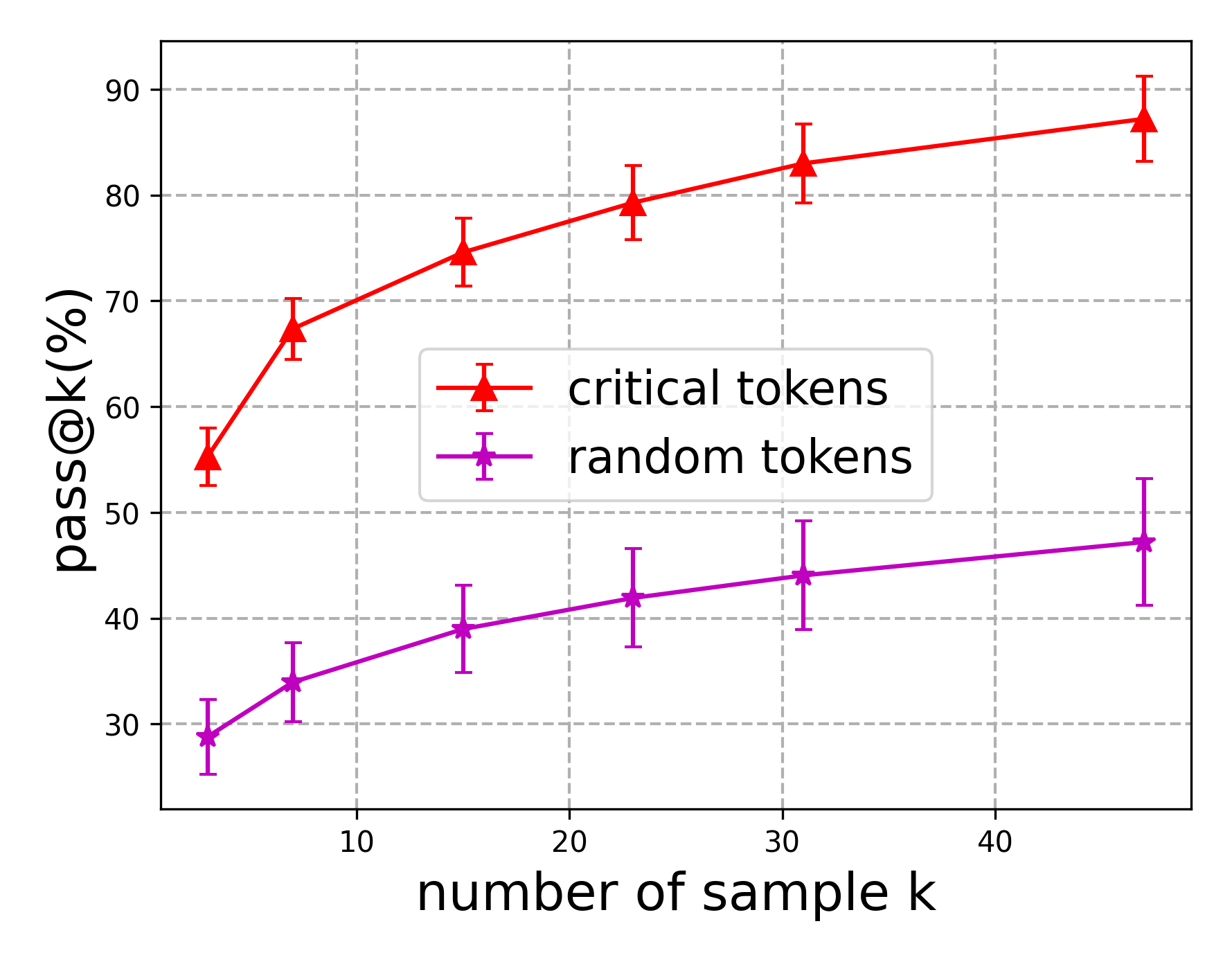
### Visual Description
## Line Chart: Pass@k(%) vs. Number of Sample k
### Overview
The image is a line chart comparing the performance of "critical tokens" and "random tokens" based on the "pass@k(%)" metric, as the "number of sample k" increases. The chart includes error bars for each data point, indicating variability.
### Components/Axes
* **X-axis:** "number of sample k" with tick marks at 10, 20, 30, and 40.
* **Y-axis:** "pass@k(%)" with tick marks at 30, 40, 50, 60, 70, 80, and 90.
* **Legend:** Located in the center of the chart.
* Red line with triangle markers: "critical tokens"
* Purple line with plus markers: "random tokens"
### Detailed Analysis
* **Critical Tokens (Red Line):** The line slopes upward, indicating an increase in "pass@k(%)" as the "number of sample k" increases.
* At k=5, pass@k(%) is approximately 57% (with an error range of +/- 3%).
* At k=15, pass@k(%) is approximately 75% (with an error range of +/- 3%).
* At k=25, pass@k(%) is approximately 80% (with an error range of +/- 3%).
* At k=30, pass@k(%) is approximately 83% (with an error range of +/- 3%).
* At k=45, pass@k(%) is approximately 87% (with an error range of +/- 4%).
* **Random Tokens (Purple Line):** The line also slopes upward, but at a shallower angle compared to the "critical tokens" line.
* At k=5, pass@k(%) is approximately 30% (with an error range of +/- 3%).
* At k=15, pass@k(%) is approximately 40% (with an error range of +/- 3%).
* At k=25, pass@k(%) is approximately 42% (with an error range of +/- 3%).
* At k=30, pass@k(%) is approximately 45% (with an error range of +/- 4%).
* At k=45, pass@k(%) is approximately 47% (with an error range of +/- 6%).
### Key Observations
* The "critical tokens" consistently outperform "random tokens" across all values of k.
* The performance gap between "critical tokens" and "random tokens" widens as k increases, but the rate of increase slows down for both.
* The error bars suggest that the variability in "pass@k(%)" is relatively consistent across different values of k for both token types.
### Interpretation
The data suggests that using "critical tokens" leads to a significantly higher "pass@k(%)" compared to using "random tokens." This indicates that "critical tokens" are more effective in achieving the desired outcome, whatever that may be. The increasing performance with higher k values suggests that increasing the number of samples improves the overall performance for both token types, but the effect is more pronounced for "critical tokens." The error bars provide a measure of confidence in these observations, suggesting that the observed differences are statistically significant. The flattening of the curves at higher k values might indicate a point of diminishing returns, where increasing the number of samples provides less and less improvement in performance.
</details>
(c)
<details>
<summary>images/density_math.png Details</summary>
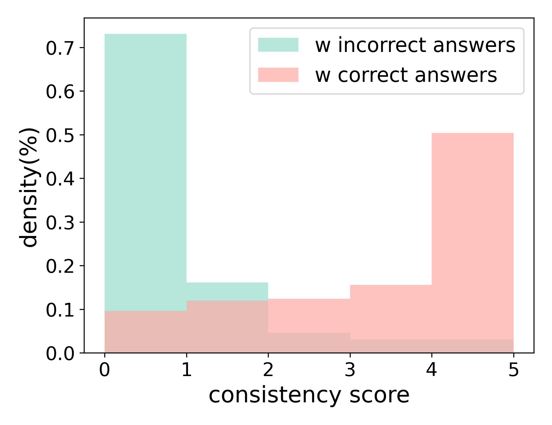
### Visual Description
## Histogram: Consistency Score vs. Density
### Overview
The image is a histogram comparing the density (%) of consistency scores for data associated with incorrect answers and correct answers. The x-axis represents the consistency score, ranging from 0 to 5. The y-axis represents the density (%), ranging from 0.0 to 0.7. The histogram uses two colors to differentiate between data associated with incorrect answers (light green) and correct answers (light red).
### Components/Axes
* **X-axis:** consistency score, with markers at 0, 1, 2, 3, 4, and 5.
* **Y-axis:** density(%), with markers at 0.0, 0.1, 0.2, 0.3, 0.4, 0.5, 0.6, and 0.7.
* **Legend (top-right):**
* Light Green: w incorrect answers
* Light Red: w correct answers
### Detailed Analysis
**Data for "w incorrect answers" (light green):**
* **Consistency Score 0-1:** Density is approximately 0.73.
* **Consistency Score 1-2:** Density is approximately 0.16.
* **Consistency Score 2-3:** Density is approximately 0.00.
* **Consistency Score 3-4:** Density is approximately 0.00.
* **Consistency Score 4-5:** Density is approximately 0.00.
**Data for "w correct answers" (light red):**
* **Consistency Score 0-1:** Density is approximately 0.10.
* **Consistency Score 1-2:** Density is approximately 0.13.
* **Consistency Score 2-3:** Density is approximately 0.13.
* **Consistency Score 3-4:** Density is approximately 0.16.
* **Consistency Score 4-5:** Density is approximately 0.51.
### Key Observations
* For incorrect answers, the highest density occurs at a consistency score between 0 and 1.
* For correct answers, the density increases with the consistency score, peaking between 4 and 5.
* The density of incorrect answers is significantly higher than correct answers at lower consistency scores (0-2).
* The density of correct answers is significantly higher than incorrect answers at higher consistency scores (4-5).
### Interpretation
The histogram suggests a strong correlation between consistency score and the correctness of answers. Lower consistency scores are more frequently associated with incorrect answers, while higher consistency scores are more frequently associated with correct answers. This indicates that a higher consistency score is a good predictor of answer accuracy. The data implies that the consistency score is a useful metric for evaluating the reliability or validity of the answers.
</details>
(d)
Figure 8: (a) Comparison of the fraction of tokens whose associated rollout correctness falls below or above 5%, for tokens extracted by our method versus randomly selected tokens. (b) Comparison of the fraction of the subsequent tokens whose associated rollout correctness falls below or above 10%, for tokens extracted by our method versus randomly selected tokens. (c) Comparison of the impact of extracted tokens by our method versus random tokens on LLM reasoning performance. (d) Comparison of the density distributions of consistency scores for rollouts with correct and incorrect answers. All the evaluations are conducted on Math500 dataset.
we follow the previous pipeline to conduct a quantitative analysis to examine the authenticity and impact of tokens extracted via paraphrastic probing, comparing them against randomly selected tokens. Specifically, we sample 100 instances with incorrect reasoning trajectories from the Math500 (Hendrycks et al., 2021) training sets. Following the paraphrastic probing pipeline, we identify candidate critical tokens in the early reasoning steps. In each run, we randomly sample 40% of the candidate critical tokens for evaluation and repeat the experiment independently 10 times. For comparison, we apply the same procedure to randomly selected tokens. All evaluations are conducted using Llama-3.1-8B-Instruct (Grattafiori et al., 2024). We first compute the average accuracy of rollouts generated from partial trajectories truncated at the position of the extracted tokens, and compare these results with those obtained from random-token truncation. As shown in Figure 8(a), we also obverse a large proportion of the extracted tokens exhibit near-zero correctness. We further evaluate the average accuracy of rollouts initiated from subsequent tokens (5–10 tokens). The results in Figure 8(b) also indicate that errors persist beyond the identified positions. Finally, we substitute the extracted critical tokens with alternative tokens and roll out multiple new reasoning trajectories. As shown in Figure 8(c), replacing critical tokens leads to a significantly larger improvement in reasoning accuracy compared to substituting random tokens.
To justify our paraphrase consistency mechanism on Math500 dataset (Hendrycks et al., 2021), we follow the same procedure. The evaluation is conducted on Llama-3.1-8B-Instruct (Grattafiori et al., 2024). We then analyze the distribution of consistency scores for rollouts that yield correct versus incorrect answers. As shown in Figure 8(d), majority of rollouts with correct answers achieve a consistency score of at least 1, whereas this proportion drops sharply for rollouts with incorrect answers.
Appendix B Automatic Prompt Engineering for Paraphrasing
The quality of paraphrased questions is crucial for our framework, as it directly affects both the identification of critical tokens and the stability of paraphrase-based consistency verification. To ensure high-quality paraphrasing, we adopt Automatic Prompt Engineering (APE) (Zhou et al., 2022) as an evaluation to optimize the paraphrasing instruction. This allows us to systematically control the quality of paraphrases rather than relying solely on manually written prompts. The APE procedure we employ consists of four steps:
- We create a small set of original questions paired with valid paraphrased variants. Using this exemplar set, the model generates multiple candidate instructions that could produce the paraphrased outputs from the original questions.
- Prompt each candidate instruction to the language model to generate paraphrases for the original problems and compare the mean solve rate change before and after paraphrasing.
- Choose the instruction that maximizes the mean solve rate change.
- Repeat the previous steps multiple times.
In our experiments, we initialize the paraphrasing instruction and iteratively refine it using APE with samples drawn from the GSM8K and Math500 training sets. With this approach, the refined paraphrasing prompt helps us reliably produce high-quality paraphrased questions.
Algorithm 1 PPCV Framework
0: LLM; original question $q_{0}$ ; number of paraphrased questions $N$ ; number of sampled alternative tokens $K$ ; temperature-scaling coefficient $\lambda$ .
0: Final answer $\text{ans}_{f}$ .
(Paraphrasing) Generate paraphrased variants $q_{1},q_{2},...,q_{N}$ from $q_{0}$ using the LLM.
(Initial reasoning) Obtain the initial reasoning path $r^{q_{0}}_{0}$ for $q_{0}$ .
(Token influence analysis) For each paraphrased question $q_{n}$ , compute the token distribution $P^{q_{n}}$ by concatenating $q_{n}$ with $r^{q_{0}}_{0}$ (Eq. 1).
(Candidate selection) Identify candidate critical token positions based on the mismatch between the top-1 predicted tokens and the expected tokens in $q_{0}$ (Eq. 2).
(Critical token verification) Select the final critical token $a_{c}$ using the criteria (Eqs. 3 – 5).
(Alternative token sampling) Sample $K$ alternative tokens $a_{c}^{0},a_{c}^{1},...,a_{c}^{K-1}$ (including $a_{c}^{0}=a_{c}$ ) using top- $K$ sampling on $q_{0}$ .
(Truncated rollouts) Truncate the initial reasoning path $r^{q_{0}}_{0}$ at position $a_{c}$ and form synthetic inputs $\tilde{r}_{c}^{0},\tilde{r}_{c}^{1},...,\tilde{r}_{c}^{K-1}$ by appending each alternative token.
for each synthetic input $\tilde{r}_{c}^{k}$ , $k=0,...,K-1$ do
Generate rollouts $r^{q_{0}}_{k},r^{q_{1}}_{k},...,r^{q_{N}}_{k}$ for the original and paraphrased questions using the LLM.
end for
(Consistency verification) Compute the final answer $\text{ans}_{f}$ using (similarity-weighted) paraphrase consistency (Eq. 6).
Appendix C Algorithm
The complete algorithm of our proposed PPCV framework is illustrated in Algo. 1.
Appendix D Discussion
<details>
<summary>images/critical_token_on_correct.png Details</summary>
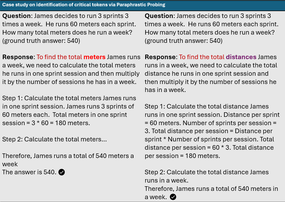
### Visual Description
## Text Comparison: Paraphrastic Probing Case Study
### Overview
The image presents a case study on the identification of critical tokens via paraphrastic probing. It shows two attempts to answer a word problem, with slight variations in the wording of the response and steps. Both attempts arrive at the correct answer.
### Components/Axes
The image is divided into two columns, each containing:
- A "Question" section, which is identical in both columns.
- A "Response" section, which contains a step-by-step solution to the question.
### Detailed Analysis or ### Content Details
**Left Column:**
* **Question:** James decides to run 3 sprints 3 times a week. He runs 60 meters each sprint. How many total meters does he run a week? (ground truth answer: 540)
* **Response:**
* To find the total meters James runs a week, we need to calculate the total meters he runs in one sprint session and then multiply it by the number of sessions he has in a week.
* Step 1: Calculate the total meters James runs in one sprint session. James runs 3 sprints of 60 meters each. Total meters in one sprint session = 3 * 60 = 180 meters.
* Step 2: Calculate the total meters...
* Therefore, James runs a total of 540 meters a week.
* The answer is 540. (followed by a checkmark symbol)
**Right Column:**
* **Question:** James decides to run 3 sprints 3 times a week. He runs 60 meters each sprint. How many total meters does he run a week? (ground truth answer: 540)
* **Response:**
* To find the total distances James runs in a week, we need to calculate the total distance he runs in one sprint session and then multiply it by the number of sessions he has in a week.
* Step 1: Calculate the total distance James runs in one sprint session. Distance per sprint = 60 meters. Number of sprints per session = 3. Total distance per session = Distance per sprint * Number of sprints per session. Total distance per session = 60 * 3. Total distance per session = 180 meters.
* Step 2: Calculate the total distance James runs in a week.
* Therefore, James runs a total of 540 meters in a week. (followed by a checkmark symbol)
### Key Observations
* The "Question" is identical in both columns.
* The "Response" sections differ slightly in wording. The left column uses "total meters," while the right column uses "total distances."
* Both solutions arrive at the correct answer of 540 meters.
* The right column provides a more detailed breakdown of the calculation in Step 1.
### Interpretation
The case study demonstrates how paraphrastic probing can be used to identify critical tokens in a text. By slightly altering the wording of the response (e.g., "total meters" vs. "total distances"), the study aims to assess the impact of these changes on the model's ability to arrive at the correct answer. In this instance, both paraphrased responses lead to the correct solution, suggesting that the model is robust to these minor variations. The more detailed breakdown in the right column's Step 1 might provide additional insight into the model's reasoning process.
</details>
Figure 9: Effect of the critical token on an initial reasoning path that yields the correct answer. Critical tokens are highlighted in bold red, and alternative tokens in bold purple.
We have shown that replacing critical tokens can correct intermediate reasoning paths and lead to the correct answer. In this section, we examine how our method influences reasoning paths that are already correct. First, we conduct a case study on an instance with a correct answer, where we follow our pipeline to identify the critical token and roll out new reasoning paths using alternative tokens. As illustrated in Figure 9, the new rollouts also yield the correct answer. Second, our pipeline incorporates both the initial reasoning path $r^{q_{0}}_{0}$ and its paraphrased variants $r^{q_{n}}_{0}$ for evaluation. The robustness of correct rollouts across paraphrased forms ensures high consistency scores, allowing them to stand out as the final answer. These findings suggest that our pipeline preserves the performance of LLMs on problems that can already be solved correctly by CoT (Wei et al., 2022).
Table 5: Comparison between our method and baselines with DeepSeek-R1-Distill-Llama-70B model on mathematical reasoning benchmarks using pass@1 accuracy.
| Chain-of-Thought Predictive Decoding Phi-Decoding | 56.67 60.00 64.00 | 38.00 40.66 46.67 | 43.33 44.66 48.00 | 30.00 30.66 31.33 |
| --- | --- | --- | --- | --- |
| PPCV (Ours) | 70.00 | 56.66 | 56.66 | 33.33 |
Table 6: Comparison of our method and the baseline approach on Llama-3.1-8B-Instruct, evaluated using pass@k (k=4).
| Phi-Decoding PPCV (Ours) | 92.15 93.83 | 53.57 61.41 | 52.60 59.39 | 91.19 94.48 | 90.73 94.24 |
| --- | --- | --- | --- | --- | --- |
Table 7: Comparison of our method and the baseline approach on Qwen3-32B, evaluated using pass@k (k=4).
| Phi-Decoding PPCV (Ours) | 41.61 49.71 | 30.19 34.28 | 45.09 51.42 | 13.11 19.28 |
| --- | --- | --- | --- | --- |
Table 8: The comparison of performance between Paraphrased Majority Voting (PMV) and our proposed PPCV using pass@1 accuracy.
| Chain-of-Thought PMV PPCV (Ours) | 77.40 83.55 88.24 | 28.00 33.16 49.73 | 31.00 40.60 50.00 | 83.00 87.70 89.60 | 58.91 61.63 88.31 |
| --- | --- | --- | --- | --- | --- |
Appendix E Main results
To further assess the effectiveness of our method, we evaluate it on a larger reasoning model such as DeepSeek-R1-Distill-Llama-70B. We apply our full pipeline and compare against all baselines across multiple mathematical reasoning benchmarks. The results, presented in Table 5, show that our method consistently outperforms the baselines. These improvements demonstrate that our approach remains effective for stronger reasoning models and generalizes well beyond the smaller models.
we also conduct additional experiments to report pass@k performance for both our method and the baselines. In these experiments, we use Phi-Decoding as the representative baseline and evaluate on two models: Llama-3.1-8B-Instruct and Qwen3-32B. We set k= 4 and generate 12 samples per question to obtain stable estimates of pass@4. The results across multiple benchmarks are presented in Table 6 and Table 7, respectively. Consistent with our main findings, our method achieves higher pass@k scores compared to the baseline methods, indicating that paraphrastic critical-token refinement continues to provide benefits in a multi-sample setting. These results further validate the robustness of our approach under stochastic sampling and demonstrate improved hit rates when multiple outputs are available.
Appendix F Ablation Study
We also perform a comparison against a Paraphrased Majority Voting (PMV) strategy is essential to demonstrate that the performance gains of our method are indeed derived from the critical token correction, rather than simply the benefit of having multiple paraphrased samples. Thus, we have performed the suggested additional experiment. We adopt Paraphrased Majority Voting (PMV) as the baseline. For a fair comparison, this approach uses the same total number of trajectories generated from the paraphrased questions as PPCV, and reaches the final answer using standard majority voting over the rollouts from the paraphrased questions. Specifically, we use four variants of each question, with 10 rollouts per variant. We compare the PMV baseline against our full PPCV method and ensure the same number of paraphrased questions as in our method. The results shown in Table 8 demonstrate that the performance yielded by PMV is significantly lower than that of our proposed PPCV method. This result confirms that simply rolling out trajectories from paraphrased questions and aggregating the answers is insufficient. The substantial performance gap between PMV and PPCV decisively highlights the necessity and effectiveness of our extracted critical tokens and the subsequent corrective reasoning step.
<details>
<summary>images/latency_trade_off.png Details</summary>
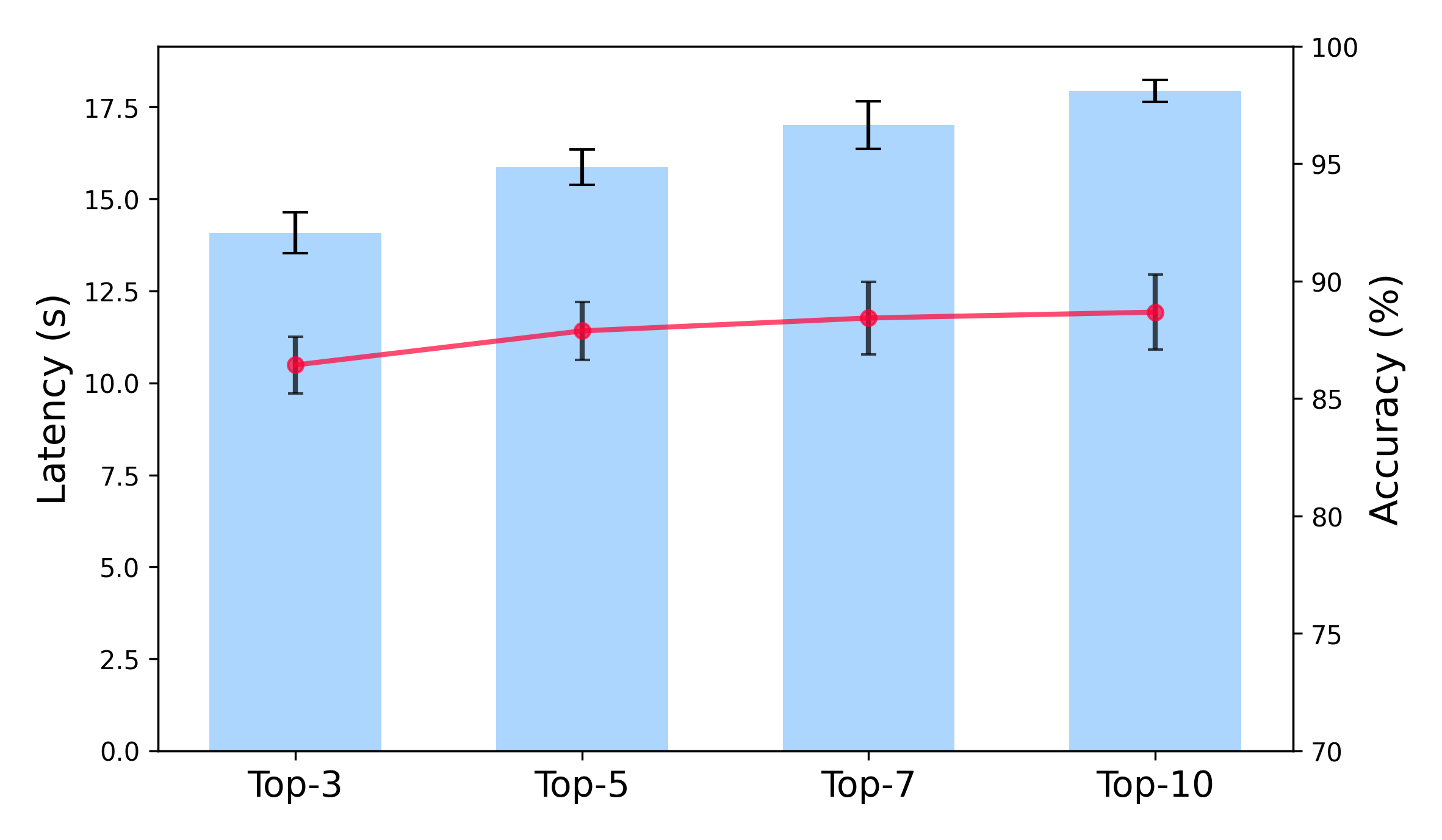
### Visual Description
## Combined Bar and Line Chart: Latency vs. Accuracy for Top-K Values
### Overview
The image is a combined bar and line chart comparing latency (in seconds) and accuracy (in percentage) for different "Top-K" values (Top-3, Top-5, Top-7, and Top-10). The latency is represented by light blue bars, while the accuracy is represented by a red line with circular markers. Error bars are present for both latency and accuracy.
### Components/Axes
* **X-axis:** Categorical axis labeled "Top-3", "Top-5", "Top-7", and "Top-10".
* **Left Y-axis:** Numerical axis labeled "Latency (s)", ranging from 0.0 to 17.5 in increments of 2.5.
* **Right Y-axis:** Numerical axis labeled "Accuracy (%)", ranging from 70 to 100 in increments of 5.
* **Latency Data:** Represented by light blue bars with black error bars.
* **Accuracy Data:** Represented by a red line with circular markers and black error bars.
### Detailed Analysis
* **Latency (Light Blue Bars):**
* Top-3: Approximately 14.0 s, with an error range of approximately +/- 0.7 s.
* Top-5: Approximately 16.0 s, with an error range of approximately +/- 0.6 s.
* Top-7: Approximately 17.0 s, with an error range of approximately +/- 0.7 s.
* Top-10: Approximately 18.0 s, with an error range of approximately +/- 0.6 s.
* **Trend:** The latency generally increases as the "Top-K" value increases.
* **Accuracy (Red Line):**
* Top-3: Approximately 87%, with an error range of approximately +/- 2%.
* Top-5: Approximately 88%, with an error range of approximately +/- 2%.
* Top-7: Approximately 89%, with an error range of approximately +/- 2%.
* Top-10: Approximately 89%, with an error range of approximately +/- 2%.
* **Trend:** The accuracy shows a slight increase from Top-3 to Top-7, then plateaus between Top-7 and Top-10.
### Key Observations
* Latency increases consistently with increasing "Top-K" values.
* Accuracy increases slightly from Top-3 to Top-7, then remains relatively stable.
* The error bars indicate the variability in both latency and accuracy.
### Interpretation
The chart suggests a trade-off between latency and accuracy when choosing the "Top-K" value. Increasing the "Top-K" value (e.g., from Top-3 to Top-10) leads to a higher accuracy, but also results in a higher latency. The choice of the optimal "Top-K" value would depend on the specific application and the relative importance of latency and accuracy. The relatively flat accuracy from Top-7 to Top-10 suggests that there may be diminishing returns in terms of accuracy beyond Top-7, while the latency continues to increase.
</details>
(a)
<details>
<summary>images/throughput_trade_off.png Details</summary>
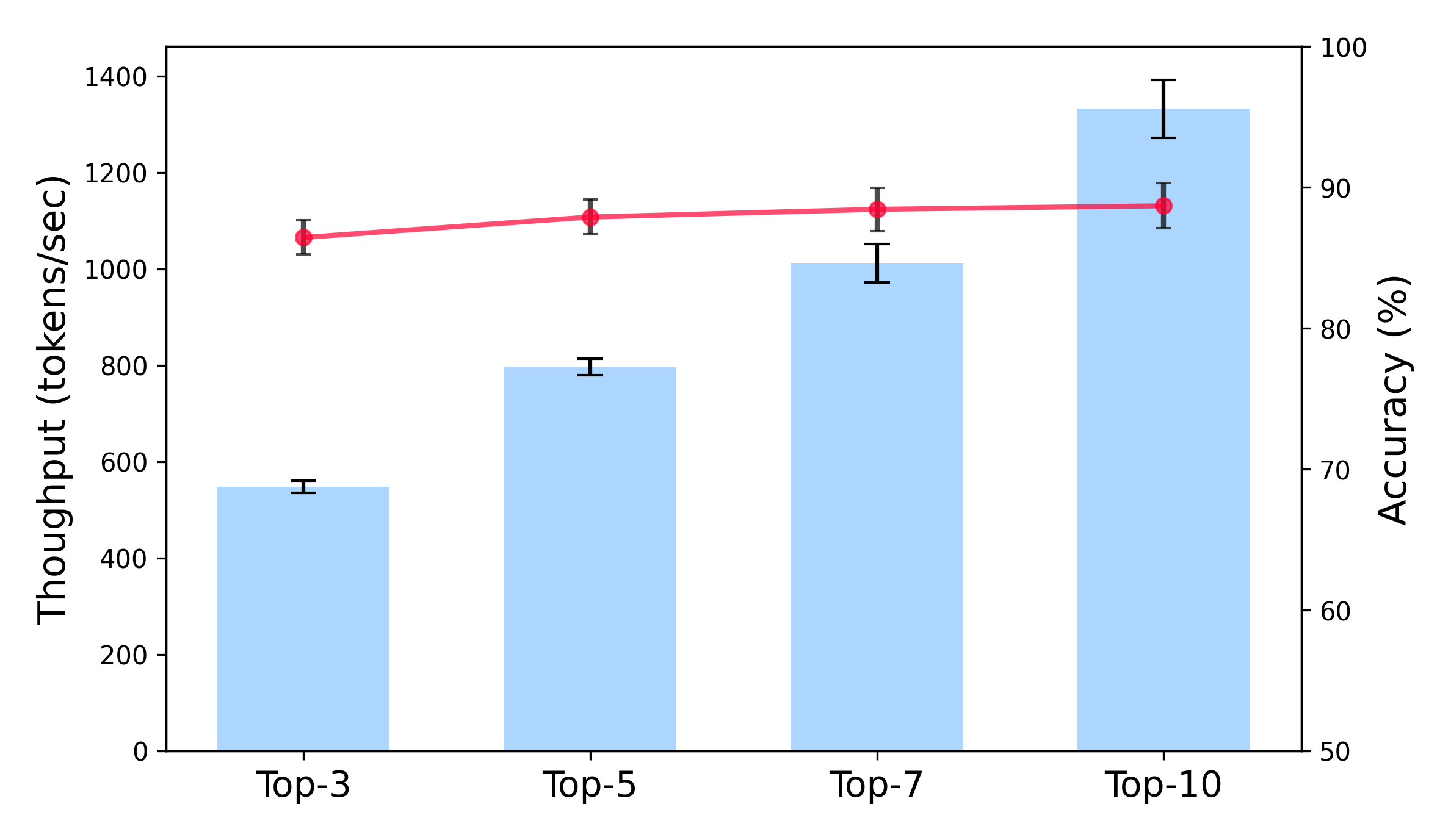
### Visual Description
## Dual-Axis Bar and Line Chart: Throughput vs. Accuracy for Top-K Values
### Overview
The image is a dual-axis chart comparing the throughput (tokens/sec) and accuracy (%) for different "Top-K" values (Top-3, Top-5, Top-7, Top-10). Throughput is represented by light blue bars, while accuracy is represented by a red line. Error bars are present on both the bars and the line.
### Components/Axes
* **X-axis:** Categorical, labeled "Top-3", "Top-5", "Top-7", and "Top-10".
* **Left Y-axis:** Numerical, labeled "Throughput (tokens/sec)". Scale ranges from 0 to 1400, with increments of 200.
* **Right Y-axis:** Numerical, labeled "Accuracy (%)". Scale ranges from 50 to 100, with increments of 10.
* **Data Series 1:** Throughput (tokens/sec), represented by light blue bars with black error bars.
* **Data Series 2:** Accuracy (%), represented by a red line with black error bars.
### Detailed Analysis
**Throughput (tokens/sec) - Light Blue Bars:**
* **Top-3:** Approximately 550 tokens/sec. Error bars extend roughly +/- 25 tokens/sec.
* **Top-5:** Approximately 800 tokens/sec. Error bars extend roughly +/- 25 tokens/sec.
* **Top-7:** Approximately 1025 tokens/sec. Error bars extend roughly +/- 75 tokens/sec.
* **Top-10:** Approximately 1325 tokens/sec. Error bars extend roughly +/- 75 tokens/sec.
The throughput shows a clear upward trend as the "Top-K" value increases.
**Accuracy (%) - Red Line:**
* **Top-3:** Approximately 87%. Error bars extend roughly +/- 1%.
* **Top-5:** Approximately 88%. Error bars extend roughly +/- 1%.
* **Top-7:** Approximately 89%. Error bars extend roughly +/- 1%.
* **Top-10:** Approximately 89%. Error bars extend roughly +/- 1%.
The accuracy shows a slight upward trend, but it plateaus after Top-7.
### Key Observations
* Throughput increases significantly as the "Top-K" value increases.
* Accuracy increases slightly, but the increase is much less pronounced than the increase in throughput.
* The error bars for throughput are larger for Top-7 and Top-10 compared to Top-3 and Top-5.
* The error bars for accuracy are relatively consistent across all "Top-K" values.
### Interpretation
The chart suggests that increasing the "Top-K" value leads to a substantial increase in throughput, but only a marginal increase in accuracy. This implies a trade-off: by considering more potential options ("Top-K"), the system can process more tokens per second, but the improvement in accuracy diminishes as K increases. The larger error bars for throughput at higher "Top-K" values might indicate increased variability or instability in the system's performance under those conditions. The plateau in accuracy suggests that there is a point of diminishing returns in increasing "Top-K" beyond a certain value (around Top-7 in this case).
</details>
(b)
Figure 10: Trade-off between performance and efficiency for our method under different numbers of top-k tokens (k = 3, 5, 7, 10), measured by latency (left) and throughput (right).
Appendix G Computational Cost Analysis
We also conduct a trade-off analysis between performance and efficiency by varying the number of alternative tokens considered at the critical position. Specifically, we test top-3, top-5, top-7, and top-10 alternatives using GSM8K, sampling 200 random questions and repeating the experiment five times to compute confidence intervals. The results are presented in Figure 10. We observe a clear trade-off. Reducing the number of alternative tokens lowers both latency and throughput, while causing a slight reduction in accuracy. This provides a practical mechanism for adjusting performance-efficiency trade-offs in real deployments. Depending on resource availability and target accuracy, practitioners can choose the appropriate number of alternative tokens.
G.1 Prompts
Prompts for reasoning (for math datasets) System: You are a specialized AI assistant designed to solve mathematical problems. User: Please solve the following problem step by step, and put your final answer within boxed{}. Each pack of dvds costs 76 dollars. If there is a discount of 25 dollars on each pack How much do you have to pay to buy each pack? Assistant: To find the price after the discount, we need to subtract the discount amount from the original price. Step 1: Identify the original price and the discount amount.Original price = $76. Discount amount = $25 Step 2: Subtract the discount amount from the original price. Price after discount = Original price - Discount amount. Price after discount = $76 - $25. Price after discount = $51 So, you have to pay $51 to buy each pack. boxed{$51}
Prompts for reasoning (for ARC dataset) System: You are a specialized AI assistant designed to solve complex reasoning problems. User: Your task is to carefully read the following question, apply logical reasoning, scientific knowledge, and commonsense inference, and arrive at the correct answer. Always explain your reasoning step by step in clear language. At the end of your response, output the final choice in the following format: The answer is: (option), where option is the correct option letter (A, B, C, D, etc.), enclosed in parentheses. A group of engineers wanted to know how different building designs would respond during an earthquake. They made several models of buildings and tested each for its ability to withstand earthquake conditions. Which will most likely result from testing different building designs? (A) buildings will be built faster (B) buildings will be made safer (C) building designs will look nicer (D) building materials will be cheaper? Assistant: We are given a scenario in which engineers are testing different building designs to see how well they withstand earthquake conditions. The goal is to determine which of the listed outcomes is most likely to result from such testing. Let 2019s evaluate each option in turn: (A) Buildings will be built faster. 2013 This is not directly related to how well a building withstands earthquakes. Earthquake resistance is about structural integrity, not construction speed. While a good design might simplify construction, the primary purpose of the test is not speed. So this is not the most likely result. (B) Buildings will be made safer 2013 This is directly aligned with the purpose of the experiment. Testing building designs under earthquake conditions helps identify which designs can better absorb or resist seismic forces. The goal is to improve safety during earthquakes. Therefore, this outcome is a direct and logical result of such testing. (C) Building designs will look nicer 2013 Aesthetics are not the focus of earthquake testing. While a design might be both safe and attractive, the test itself does not evaluate visual appeal. So this is not a likely result of the testing. (D) Building materials will be cheaper 2013 Cost of materials is not necessarily a result of testing for earthquake resistance. … The answer is: (B)
Prompts to paraphrase the question (for math datasets) System: You are a paraphrasing assistant specialized in math problems. Your task is to paraphrase a given math word problem. The core objective is to create a new, diverse expression of the problem while strictly preserving all numerical values, mathematical relationships, and the core logic required to solve it. User: Please create 5 paraphrased versions of the question below. Do NOT change any numbers or quantities. Maintain the exact mathematical operations and relationships. And vary the context and language. Please output paraphrased questions starting with a bracketed serial number like [1] [2] and ending with a new line. A robe takes 2 bolts of blue fiber and half that much white fiber. How many bolts in total does it take? Assistant: [1] Two bolts of blue fabric and one and a half times that amount of white fabric are required to make a robe. How many bolts in all are needed? [2] A robe is made from 2 bolts of blue yarn and an additional amount equal to half of that for white yarn. In total, how many bolts does it call for? [3] To create a robe, you’ll need 2 bolts of blue thread and another half-quantity of white thread. How many bolts of thread in total should you purchase? [4] For a single robe, the production process demands 2 bolts of blue fabric and 1.5 times as much white fabric. What is the total number of bolts required? [5] The manufacture of a robe necessitates the usage of 2 bolts of blue material and slightly less than double that quantity for white material. How many total bolts does this equate to?
Prompts to paraphrase the question (for ARC dataset) System: You are given a multiple-choice question from a reasoning benchmark. Your task is to generate multiple different paraphrased versions of the question. Each version must preserve the original meaning, answer choices, and scientific/commonsense accuracy. Guidelines: - Keep the question logically equivalent to the original. - Do not change the correct answer. - Do not add or remove details that would alter the difficulty. - Use different phrasing, sentence structures, or synonyms for each version. - Keep the multiple-choice options (A, B, C, D, etc.) unchanged. Example Input: A large gene has dozens of exons, of which the central ones code for folded triple helical repeats that connect the cytoskeleton with sarcolemma and extracellular space. Each exon usually codes for one folded triple alpha helix. The most common mutations of the gene are central exon deletions that create out-of-frame peptides and progressive degenerative organ waste. A solution is to deliver a Morpholino that recognizes the 5’ end of the out-of-frame exon in pre-mRNA. The molecule prevents binding of the spliceosome and creates exon skipping and in-frame joining. Several missing exons are well tolerated by an organism. Which structure below is not involved in the proposed therapy? (A) antisense (B) lariat (C) R-loops (D) polyA tail User: Please create 3 paraphrased versions of the question below. Only paraphrases the question and leaves the multiple-choice options untouched. Please output paraphrased questions starting with a bracketed serial number like [1] [2] and ending with a new line, An astronomer observes that a planet rotates faster after a meteorite impact. Which is the most likely effect of this increase in rotation? (A) Planetary density will decrease. (B) Planetary years will become longer. (C) Planetary days will become shorter. (D) Planetary gravity will become stronger. Assistant: [1] An astronomer notices that a planet’s rotational speed increases following a meteorite collision. What is the most probable consequence of this accelerated rotation? (A) Planetary density will decrease. (B) Planetary years will become longer. (C) Planetary days will become shorter. (D) Planetary gravity will become stronger. [2] After a meteorite strikes a planet, the astronomer observes an increase in its rotational velocity. What is the most likely outcome of this faster rotation? (A) Planetary density will decrease. (B) Planetary years will become longer. (C) Planetary days will become shorter. (D) Planetary gravity will become stronger. [3] A planet begins to rotate more quickly after experiencing a meteorite impact. Which of the following is most likely to result from this increased spin? (A) Planetary density will decrease. (B) Planetary years will become longer. (C) Planetary days will become shorter. (D) Planetary gravity will become stronger.
Appendix H Use of Large Language Models
In our work, we focus on improving large Malaguena models, and LLMs are used in our experimental evaluation. In addition, we employ LLMs to check grammatical errors and refine sentence structures.