2602.13583v1

# Differentiable Rule Induction from Raw Sequence Inputs > Corresponding author. ## Abstract Rule learning-based models are widely used in highly interpretable scenarios due to their transparent structures. Inductive logic programming (ILP), a form of machine learning, induces rules from facts while maintaining interpretability. Differentiable ILP models enhance this process by leveraging neural networks to improve robustness and scalability. However, most differentiable ILP methods rely on symbolic datasets, facing challenges when learning directly from raw data. Specifically, they struggle with explicit label leakage: The inability to map continuous inputs to symbolic variables without explicit supervision of input feature labels. In this work, we address this issue by integrating a self-supervised differentiable clustering model with a novel differentiable ILP model, enabling rule learning from raw data without explicit label leakage. The learned rules effectively describe raw data through its features. We demonstrate that our method intuitively and precisely learns generalized rules from time series and image data. ## 1 Introduction The deep learning models have obtained impressive performances on tabular classification, time series forecasting, image recognition, etc. While in highly trustworthy scenarios such as health care, finance, and policy-making process (Doshi-Velez and Kim, 2017), lacking explanations for decision-making prevents the applications of these complex deep learning models. However, the rule-learning models have interpretability intrinsically to explain the classification process. Inductive logic programming (ILP) is a form of logic-based machine learning that aims to learn logic programs for generalization and interpretability from training examples and background knowledge (Cropper et al., 2022). Traditional ILP methods design deterministic algorithms to induce rules from symbolic data to more generalized formal symbolic first-order languages (Quinlan, 1990; Blockeel and De Raedt, 1998). However, these symbolic ILP methods face robustness and scalability problems when learning from large-scale and ambiguous datasets (Evans et al., 2021; Hocquette et al., 2024). With the sake of robustness of neural networks, the neuro-symbolic ILP by combining neural networks and ILP methods can learn from noisy data (Evans and Grefenstette, 2018; Manhaeve et al., 2018; Gao et al., 2022a) and can be applied to large-scale datasets (Yang et al., 2017; Gao et al., 2024; Phua and Inoue, 2024). However, existing neuro-symbolic ILP methods are mainly learned from discrete symbolic data or fuzzy symbolic data that the likelihoods are generated from a pre-trained neural network module (Evans et al., 2021; Shindo et al., 2023). Learning logic programs from raw data is prevented because of the explicit label leakage problem, which is common in neuro-symbolic research (Topan et al., 2021): The leakage happens by introducing labels of ground objects for inducing rules (Evans and Grefenstette, 2018; Shindo et al., 2023). In fact, generating rules to describe objects in raw data without label information is necessary, especially when some objects are easily overlooked or lack labels yet are important for describing the data. In this study, we introduce Neural Rule Learner (NeurRL), a framework designed to learn logic programs directly from raw sequences, such as time series and flattened image data. Unlike prior approaches prone to explicit label leakage, where input feature labels are extracted using pre-trained supervised neural networks and then processed with differentiable ILP methods to induce rules trained with input labels, our method bypasses the need for supervised pre-trained networks to generate symbolic labels. Instead, we leverage a pre-trained clustering model in an unsupervised manner to discretize data into distinct features. Subsequently, a differentiable clustering module and a differentiable rule-learning module are jointly trained under supervision using raw input labels. This enables the discovery of rules that describe input classes based on feature distributions within the inputs. As a result, the model achieves efficient training in a fully differentiable pipeline while avoiding the explicit label leakage issue. The contributions of this study include: (1) We formally define the ILP learning task from raw inputs based on the interpretation transition setting of ILP. (2) We design a fully differentiable framework for learning symbolic rules from raw sequences, including a novel interpretable rule-learning module with multiple dense layers. (3) We validate the model’s effectiveness and interpretability on various time series and image datasets. ## 2 Related work Inductive logic programming (ILP), introduced by Muggleton and Feng (1990); Muggleton and De Raedt (1994), learns logic programs from symbolic positive and negative examples with background knowledge. Inoue et al. (2014) proposed learning from interpretation transitions, and Phua and Inoue (2021) applied ILP to Boolean networks. Manhaeve et al. (2018); Evans and Grefenstette (2018) adapted neural networks for differentiable and robust ILP, while Gao et al. (2022b) introduced a neural network-based ILP model for learning from interpretation transitions. This model was later extended for scalable learning from knowledge graphs (Gao et al., 2022a; 2024). Similarly, Liu et al. (2024) proposed a deep neural network for inducing mathematical functions. In our work, we present a novel neural network-based model for learning logic programs from raw numeric inputs. In the raw input domain, Evans and Grefenstette (2018) proposed $\partial$ ILP to learn rules from symbolic relational data, using a pre-trained neural network to map raw input data to symbolic labels. Unlike $\partial$ ILP, which enforces a strong language bias by predefining logic templates and limiting the number of atoms, NeurRL uses only predicate types as language bias. Similarly, Evans et al. (2021) used pre-trained networks to map sensory data to disjunctive sequences, followed by binary neural networks to learn rules. Shindo et al. (2023) introduced $\alpha$ ILP, leveraging object recognition models to convert images into symbolic atoms and employing top- $k$ searches to pre-generate clauses, with neural networks optimizing clause weights. Our approach avoids pre-trained large-scale neural networks for mapping raw inputs to symbolic representations. Instead, we propose a fully differentiable framework to learn rules from raw sequences. Additionally, unlike the memory-intensive rule candidate generation required by $\partial$ ILP and $\alpha$ ILP, NeurRL eliminates this step, enhancing scalability. Adapting autoencoder and clustering methods in the neuro-symbolic domain shows promise. Sansone and Manhaeve (2023) applies conventional clustering on input embeddings for deductive logic programming tasks. Misino et al. (2022) and Zhan et al. (2022) use autoencoders and embeddings to calculate probabilities for predefined symbols to complete deductive logic programming and program synthesis tasks. In our approach, we use an autoencoder to learn representations for sub-areas of raw inputs, followed by a differentiable clustering method to assign ground atoms to similar patterns. The differentiable rule-learning module then searches for rule embeddings with these atoms in a bottom-up manner (Cropper and Dumancic, 2022). Similarly, DIFFNAPS (Walter et al., 2024) also uses an autoencoder to build hidden features and explain raw inputs. Additionally, BotCL (Wang et al., 2023) uses attention-based features to explain the ground truth class. However, the logical connections between the features used in DIFFNAPS and BotCL to describe the ground truth class are unclear. In contrast, rule-based explainable models like NeurRL use feature conjunctions to describe the ground truth class. Azzolin et al. (2023) use a post-hoc rule-based explainable model to globally explain raw inputs from local explanations. In contrast, our model directly learns rules from raw inputs, and NeurRL’s performance is unaffected by other explainable models. Das et al. (1998) used clustering to split sequence data into subsequences and symbolize them for rule discovery. Our model combines clustering and rule-learning in a fully differentiable framework to discover rules from sequence and image data, with the rule-learning module providing gradient information to prevent cluster collapse (Sansone, 2023), where very different subsequences are assigned to the same clusters. He et al. (2018) viewed similar subsequences, called motifs, as potential rule bodies. Unlike their approach, we do not limit the number of body atoms in a rule. Wang et al. (2019) introduced SSSL, which uses shapelets as body atoms to learn rules and maximize information gain. Our model extends this by using raw data subsequences as rule body atoms and evaluating rule quality with precision and recall, a feature absent in SSSL. ## 3 Preliminaries ### 3.1 Logic Programs and Inductive Logic Programming A first-order language $\mathcal{L}=(D,F,C,V)$ (Lloyd, 1984) consists of predicates $D$ , function symbols $F$ , constants $C$ , and variables $V$ . A term is a constant, variable, or expression $f(t_{1},\dots,t_{n})$ with $f$ as an $n$ -ary function symbol. An atom is a formula $p(t_{1},\dots,t_{n})$ , where $p$ is an $n$ -ary predicate symbol. A ground atom (fact) has no variables. A literal is an atom or its negation; positive literals are atoms, and negative literals are their negations. A clause is a finite disjunction of literals, and a rule (definite clause) is a clause with one positive literal, e.g., $\alpha_{h}\lor\neg\alpha_{1}\lor\neg\alpha_{2}\lor\dots\lor\neg\alpha_{n}$ . A rule $r$ is written as: $\alpha_{h}\leftarrow\alpha_{1},\alpha_{2},\dots,\alpha_{n}$ , where $\alpha_{h}$ is the head ( $\textnormal{head}(r)$ ), and $\{\alpha_{1},\alpha_{2},\dots,\alpha_{n}\}$ is the body ( $\textnormal{body}(r)$ ), with each atom in the body called a body atom. A logic program $P$ is a set of rules. In first-order logic, a substitution is a finite set $\{v_{1}/t_{1},v_{2}/t_{2},\dots,v_{n}/t_{n}\}$ , where each $v_{i}$ is a variable, $t_{i}$ is a term distinct from $v_{i}$ , and $v_{1},v_{2},\dots,v_{n}$ are distinct (Lloyd, 1984). A ground substitution has all $t_{i}$ as ground terms. The ground instances of all rules in $P$ are denoted as $\textnormal{ground}(P)$ . The Herbrand base $B_{P}$ of a logic program $P$ is the set of all ground atoms with predicate symbols from $P$ , and an interpretation $I$ is a subset of $B_{P}$ containing the true ground atoms (Lloyd, 1984). Given $I$ , the immediate consequence operator $T_{P}\colon 2^{B_{P}}\to 2^{B_{P}}$ for a definite logic program $P$ is defined as: $T_{P}(I)=\{\text{head}(r)\mid r\in\textnormal{ground}(P),\textnormal{body}(r)\subseteq I\}$ (Apt et al., 1988). A logic program $P$ with $m$ rules sharing the same head atom $\alpha_{h}$ is called a same-head logic program. A same-head logic program with $n$ possible body atoms can be represented as a matrix $\mathbf{M}_{P}\in[0,1]^{m\times n}$ . Each element $a_{kj}$ in $\mathbf{M}_{P}$ is defined as follows (Gao et al., 2022a): If the $k$ -th rule is $\alpha_{h}\leftarrow\alpha_{j_{1}}\land\dots\land\alpha_{j_{p}}$ , then $a_{k{j_{i}}}=l_{i}$ , where $l_{i}\in(0,1)$ and $\sum_{s=1}^{p}l_{s}=1\ (1\leq i\leq p,\ 1<p,\ 1\leq j_{i}\leq n,\ 1\leq k\leq m)$ . If the $k$ -th rule is $\alpha_{h}\leftarrow\alpha_{j}$ , then $a_{kj}=1$ . Otherwise, $a_{kj}=0$ . Each row of $\mathbf{M}_{P}$ represents a rule in $P$ , and each column represents a body atom. An interpretation vector $\mathbf{v}_{I}\in\{0,1\}^{n}$ corresponds to an interpretation $I$ , where $\mathbf{v}_{I}[i]=1$ if the $i$ -th ground atom is true in $I$ , and $\mathbf{v}_{I}[i]=0$ otherwise. Given a logic program with $m$ rules and $n$ atoms, along with an interpretation vector $\mathbf{v}_{I}$ , the function $D_{P}:\{0,1\}^{n}\to\{0,1\}^{m}$ (Gao et al., 2024) calculate the Boolean value for the head atom of each rule in $P$ . It is defined as:: $$ \displaystyle D_{P}(\mathbf{v}_{I})=\theta(\mathbf{M}_{P}\mathbf{v}_{I}), \tag{1} $$ where the function $\theta$ is a threshold function: $\theta(x)=1$ if $x\geq 1$ , otherwise $\theta(x)=0$ . For a same-head logic program, the Boolean value of the head atom $v(\alpha_{h})$ is computed as $v(\alpha_{h})=\bigvee_{i=1}^{m}D_{P}(\mathbf{v}_{I})[i]$ . Additionally, Gao et al. (2024) replaces $\theta(x)$ with a differentiable threshold function and use fuzzy disjunction $\tilde{\bigvee}_{i=1}^{m}\mathbf{x}[i]=1-\prod_{i=1}^{m}\mathbf{x}[i]$ to calculate the Boolean value of the head atom in a same-head logic program with neural networks. Inductive logic programming (ILP) aims to induce logic programs from training examples and background knowledge (Muggleton et al., 2012). ILP learning settings include learning from entailments (Evans and Grefenstette, 2018), interpretations (De Raedt and Dehaspe, 1997), proofs (Passerini et al., 2006), and interpretation transitions (Inoue et al., 2014). In this paper, we focus on learning from interpretation transitions: Given a set $E\subseteq 2^{B_{P}}\times 2^{B_{P}}$ of interpretation pairs $(I,J)$ , the goal is to learn a logic program $P$ such that $T_{P}(I)=J$ for all $(I,J)\in E$ . ### 3.2 Sequence data and Differentiable Clustering Method A raw input consists of an instance $(\mathbf{x},\mathbf{y})$ , where $\mathbf{x}\in\mathbb{R}^{T_{1}\times T_{2}\times\dots\times T_{d}}$ represents real-valued observations with $d$ variables, $T_{i}$ indicates the length for $i$ -th variable, and $\mathbf{y}\in\{0,1,\dots,u-1\}$ is the class label, with $u$ classes. A sequence input is a type of raw input where $\mathbf{x}\in\mathbb{R}^{T_{1}}$ is an ordered sequence of real-valued observations (Wang et al., 2019). A subsequence $\mathbf{s}_{i}$ of length $l$ from sequence $\mathbf{x}=(x_{1},x_{2},\dots,x_{T})$ is a contiguous sequence $(x_{i},\dots,x_{i+l-1})$ (Das et al., 1998). All possible subsequence with length $l$ include $\mathbf{s}_{1}$ , …, $\mathbf{s}_{T-l+1}$ . Clustering can be used to discover new categories (Rokach and Maimon, 2005). In the paper, we adapt the differentiable $k$ -means method (Fard et al., 2020) to group raw data $\mathbf{x}\in\mathbf{X}$ . First, an autoencoder $A$ generates embeddings $\mathbf{h}_{\gamma}$ for $\mathbf{x}$ , where $\gamma$ represents the parameters. Then, we set $K$ clusters to discretize all raw data $\mathbf{x}$ . The representation of the $k$ -th cluster is $\mathbf{r}_{k}\in\mathbb{R}^{p}$ , with $p$ as the dimension, and $\mathcal{R}=\{\mathbf{r}_{1},\dots,\mathbf{r}_{K}\}$ as the set of all cluster representations. For any vector $\mathbf{y}\in\mathbb{R}^{p}$ , the function $c_{f}(\mathbf{y};\mathcal{R})$ returns the closest representation based on a fully differentiable distance function $f$ . Then, the differentiable $k$ -means problems are defined as follows: $$ \displaystyle\min_{\mathcal{R},\gamma}\sum_{\mathbf{x}\in\mathbf{X}}f(\mathbf{x},A(\mathbf{x};\gamma))+\lambda\sum_{k=1}^{K}f(\mathbf{h}_{\gamma}(\mathbf{x}),\mathbf{r}_{k})G_{k,f}(\mathbf{h}_{\gamma}(\mathbf{x}),\alpha;\mathcal{R}), \tag{2} $$ where the parameter $\lambda$ regulates the trade-off between seeking good representations for $\mathbf{x}$ and the representations that are useful for clustering. The weight function $G$ is a differentiable minimum function proposed by Jang et al. (2017): $$ \displaystyle G_{k,f}(\mathbf{h}_{\gamma}(\mathbf{x}),\alpha;\mathcal{R})=\frac{e^{-\alpha f(\mathbf{h}_{\gamma}(\mathbf{x}),\mathbf{r}_{k})}}{\sum_{k^{\prime}=1}^{K}e^{-\alpha f(\mathbf{h}_{\gamma}(\mathbf{x}),\mathbf{r}_{k^{\prime}})}}, \tag{3} $$ where $\alpha\in[0,+\infty)$ . A larger value of $\alpha$ causes the approximate minimum function to behave more like a discrete minimum function. Conversely, a smaller $\alpha$ results in a smoother training process We set $\alpha$ to 1000 in the whole experiments.. ## 4 Methods ### 4.1 Problem Statement and formalization In this subsection, we define the learning problem from raw inputs using the interpretation transition setting of ILP and describe the language bias of rules for sequence data. We apply a neuro-symbolic description method from Marconato et al. (2023) to describe a raw input: (i) assume the label $\mathbf{y}$ depends entirely on the state of $K$ symbolic concepts $B=(a_{1},a_{2},\dots,a_{K})$ , which capture high-level aspects of $\mathbf{x}$ , (ii) the concepts $B$ depend intricately on the sub-symbolic input $\mathbf{x}^{\prime}$ and are best extracted using deep learning, (iii) the relationship between $\mathbf{y}$ and $B$ can be specified by prior knowledge $\mathcal{B}$ , requiring reasoning during the forward computing of deep learning models. In this paper, we treat each subset of raw input as a constant and each concept as a ground atom. For example, in sequence data $\mathbf{x}\in\mathbf{X}$ , if a concept increases from the point 0 to 10, the corresponding ground atom is $\texttt{increase}(\mathbf{x}[0:10])$ . We define the body symbolization function $L_{b}$ to convert a continuous sequence $\mathbf{x}$ into discrete symbolic concepts, so that the set of all symbolic concepts $B$ across all raw inputs $\mathbf{X}$ holds $B=L_{b}(\mathbf{X})$ . For binary class raw inputs, we use target atom $h_{t}$ to represents the target class, where $h_{t}$ being true means the instance belongs to the positive class. Then, a head symbolization function $L_{h}$ maps an binary input $\mathbf{x}$ to a set of atoms: if the class of $\mathbf{x}$ is the target class $t$ , then $L_{h}(\mathbf{x})=\{h_{t}\}$ ; otherwise, $L_{h}(\mathbf{x})=\emptyset$ . Hence, a logic program $P$ describing binary class raw inputs consists of rules with the same head atom $h_{t}$ We can transfer multiple class raw inputs to the binary class by setting the class of interest as the target class and the other classes as the negative class.. We define the Herbrand base $B_{P}$ of a logic program as the set of all symbolic concepts $B$ in all raw inputs and the head atom $h_{t}$ . For a raw input $\mathbf{x}$ , $L_{b}(\mathbf{x})$ represents a set of symbolic concepts $I\subseteq B_{P}$ , which can be considered an interpretation. The task of inducing a logic program $P$ from raw inputs based on learning from interpretation transition is defined as follows: **Definition 1 (Learning from Binary Raw Input)** *Given a set of raw binary label inputs $\mathbf{X}$ , learn a same-head logic program $P$ , where $T_{P}(L_{b}(\mathbf{x}))=L_{h}(\mathbf{x})$ holds for all raw inputs $\mathbf{x}\in\mathbf{X}$ .* In the paper, we aim to learn rules to describe the target class with the body consisting of multiple sequence features. Each feature corresponds to a subsequence of the sequence data. Besides, each feature includes the pattern information and region information of the subsequence. Based on the pattern information, we further infer the mean value and tendency information of the subsequence. Using the region predicates, we can apply NeurRL to the dataset, where the temporal relationships between different patterns play a crucial role in distinguishing positive from negative examples. Specifically, we use the following rules to describe the sequence data with the target class: $$ \displaystyle h_{t}\leftarrow pattern_{i_{1}}(X_{j_{1}}),region_{k_{1}}(X_{j_{1}}),\dots,pattern_{i_{n_{1}}}(X_{j_{n_{2}}}),region_{k_{n_{3}}}(X_{j_{n_{2}}}), \tag{4} $$ where the predicate $\texttt{pattern}_{i}$ indicates the $i$ -th pattern in all finite patterns within all sequence data, the predicate $\texttt{region}_{k}$ indicates the $k$ -th region in all regions in a sequence, and the variable $X_{j}$ can be substituted by a subsequence of the sequence data. For example, $\texttt{pattern}_{1}(\mathbf{x}[0:5])$ and $\texttt{region}_{0}(\mathbf{x}[0:5])$ indicate that the subsequence $\mathbf{x}[0:5]$ matches the pattern with index one and belongs to the region with index zero, respectively. A pair of atoms, $\texttt{pattern}_{i}(X)\land\texttt{region}_{k}(X)$ , corresponds to a feature within the sequence data. In this pair, the variables are identical, with one predicate representing a pattern and the other representing a region. We infer the following information from the rules in format (4): In a sequence input $\mathbf{x}$ , if all pairs of ground patterns and regions atoms substituted by subsequences in $\mathbf{x}$ are true, then the sequence input $\mathbf{x}$ belongs to the target class represented by the head atom $h_{t}$ . ### 4.2 Differentiable symbolization process <details> <summary>x1.png Details</summary>  ### Visual Description \n ## Diagram: Deep Rule Learning Architecture ### Overview The image presents a diagram of a deep rule learning architecture. It illustrates the flow of data through an encoder-decoder structure, followed by differentiable k-means clustering and a deep rule learning module for prediction. The diagram includes labeled components, data flow arrows, and a legend explaining the different types of connections and losses. ### Components/Axes * **Title:** None explicitly given, but the diagram depicts a deep rule learning architecture. * **Sections:** The diagram is divided into two main sections: Encoder (left) and Decoder (right). * **Components:** * "All subsequences s of a series x" (brown box, top-left) * "Dense layer" (white boxes, top, repeated twice in both Encoder and Decoder) * "Embeddings z" (vertical gray box, center) * "Reconstructed subsequences s'" (brown box, top-right) * "Differentiable k-means" (below Embeddings) * "r1, r2, r3, r4" (labels for clusters in the k-means output) * "Deep rule learning module" (white box, right-center) * "Label of the series x" (light blue box, bottom) * "Logic programs P" (output of the deep rule learning module) * "Predicted label" (output of the deep rule learning module) * **Legend:** (bottom-left) * Blue arrow: "Differentiable path" * Light brown box: "Loss for autoencoder (supervised)" * Light blue box: "Loss for DeepFOL (supervised)" * Gray box: "Loss for differentiable k-means (unsupervised)" * **Arrows:** Blue arrows indicate the flow of data/computation. An orange arrow indicates "Extract" and a blue arrow indicates "Predict". ### Detailed Analysis or ### Content Details 1. **Encoder:** * Starts with "All subsequences s of a series x". * Passes through two "Dense layer" blocks. * Outputs "Embeddings z". 2. **Decoder:** * Receives "Embeddings z". * Passes through two "Dense layer" blocks. * Outputs "Reconstructed subsequences s'". 3. **Differentiable k-means:** * Receives "Embeddings z". * Clusters the data into four regions labeled "r1", "r2", "r3", and "r4". * Each region contains data points of a specific color: r1 (blue), r2 (purple), r3 (green), r4 (orange). * Outputs "vI" to the "Deep rule learning module". 4. **Deep rule learning module:** * Receives "vI" from the k-means clustering and "v(h)" from the "Label of the series x". * Extracts "Logic programs P" (orange arrow). * Predicts "Predicted label" (blue arrow). ### Key Observations * The architecture combines an autoencoder (encoder-decoder) with k-means clustering and a deep rule learning module. * The encoder and decoder both use two dense layers. * The k-means clustering step divides the data into four clusters. * The deep rule learning module takes input from both the k-means clustering and the label of the series. ### Interpretation The diagram illustrates a deep learning architecture designed for learning logical rules from sequential data. The encoder-decoder structure likely aims to extract meaningful features from the input series. The k-means clustering step then groups similar subsequences together, and the deep rule learning module learns logical rules based on these clusters and the series labels. This architecture could be used for tasks such as time series classification or anomaly detection, where understanding the underlying logical rules is important. The use of differentiable k-means allows for end-to-end training of the entire architecture. </details> (a) Learning pipeline. <details> <summary>x2.png Details</summary>  ### Visual Description ## Diagram: Fuzzy Disjunction Network ### Overview The image presents a diagram of a fuzzy disjunction network, illustrating the flow of information and the application of fuzzy logic operations. The network consists of four input nodes (a1, a2, a3, a4), two layers of intermediate nodes, and a final output node (h). The diagram shows the connections between nodes and the associated weights or values. ### Components/Axes * **Nodes:** Represented by circles. * Input Nodes: a1, a2, a3, a4 (bottom layer) * First Layer Nodes: a1 ∧ a2, a3, a3 ∧ a4 * Second Layer Nodes: a1 ∧ a2 ∧ a3, a3 ∧ a4 * Output Node: h * **Connections:** Represented by lines. * Orange lines indicate connections between input nodes and first-layer nodes, and between first-layer nodes and second-layer nodes. * Blue lines indicate connections between second-layer nodes and the output node. * **Weights/Values:** Numerical values associated with the connections and nodes. * **Labels:** * h ← (a1 ∧ a2 ∧ a3) ∨ (a3 ∧ a4) (top) * Fuzzy disjunction (right, top) * Second layer (right, middle) * M2 (right, middle) * First layer (right, middle) * M1 (right, bottom) * Input nodes (right, bottom) ### Detailed Analysis * **Input Nodes (Bottom Layer):** * a1 * a2 * a3 * a4 * **First Layer:** * Node: a1 ∧ a2. Connected to a1 with weight 0.58 and to a2 with weight 0.4. * Node: a3. Connected to a2 with weight 0.9. * Node: a3 ∧ a4. Connected to a3 with weight 0.45 and to a4 with weight 0.5. * **Second Layer:** * Node: a1 ∧ a2 ∧ a3. Receives input from a1 ∧ a2 with a value of 0.34, from a2 with a value of 0.23, and from a3 with a value of 0.36. * Node: a3 ∧ a4. Receives input from a3 with a value of 0.41 and from a4 with a value of 0.45. * **Output Node (Top):** * h. Represents the fuzzy disjunction of (a1 ∧ a2 ∧ a3) and (a3 ∧ a4). ### Key Observations * The diagram illustrates a hierarchical structure, with information flowing from the bottom (input nodes) to the top (output node). * The connections between nodes have associated weights, indicating the strength or importance of each connection. * The fuzzy logic operations (∧ and ∨) are used to combine the inputs at each layer. ### Interpretation The diagram represents a fuzzy logic system designed to evaluate the expression h ← (a1 ∧ a2 ∧ a3) ∨ (a3 ∧ a4). The input nodes (a1, a2, a3, a4) represent fuzzy variables, and the connections between nodes represent fuzzy implications. The weights associated with the connections represent the degree of membership or truth value of each implication. The fuzzy AND (∧) and OR (∨) operations are used to combine the fuzzy variables at each layer, ultimately producing a fuzzy output value for h. The diagram provides a visual representation of the fuzzy inference process, allowing for a better understanding of the system's behavior. </details> (b) Deep rule-learning module. Figure 1: The learning pipeline of NeurRL and the rule-learning module. In this subsection, we design a differentiable body symbolization function $\tilde{L}_{b}$ , inspired by differentiable $k$ -means (Fard et al., 2020), to transform numeric sequence data $\mathbf{x}$ into a fuzzy interpretation vector $\mathbf{v}_{I}\in[0,1]^{n}$ . This vector encodes fuzzy values of ground patterns and region atoms substituted by input subsequences. A higher value in $\mathbf{v}_{I}[i]$ indicates the $i$ -th atom in the interpretation $I$ is likely true. Using the head symbolization function $J=L_{h}(\mathbf{x})$ , we determine the target atom’s Boolean value $v(h_{t})$ , where $v(h_{t})=1$ if $J=\{h_{t}\}$ and $v(h_{t})=0$ if $J=\emptyset$ . Building on (Gao et al., 2024), we learn a logic program matrix $\mathbf{M}_{P}\in[0,1]^{m\times n}$ such that $\tilde{\bigvee}_{i=1}^{m}D_{P}(\mathbf{v}_{I})[i]=v(h_{t})$ holds. The rules in format (4) are then extracted from $\mathbf{M}_{P}$ , generalized from the most specific clause with all pattern and region predicates. 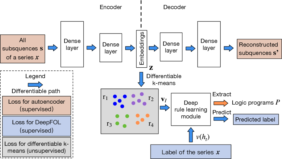The architecture of NeurRL is shown in Fig. 1(a). To learn a logic program $P$ from sequence data, each input sequence $\mathbf{x}$ is divided into shorter subsequences $\mathbf{s}$ of length $l$ with a unit step stride. An encoder maps subsequences $\mathbf{s}$ to an embedding space $\mathbf{z}$ , and a decoder reconstructs $\mathbf{s}^{\prime}$ from $\mathbf{z}$ We use fully connected layers as the encoder and decoder structures.. The differentiable $k$ -means algorithm described in Section 3.2 clusters embeddings $\mathbf{z}$ , grouping subsequences $\mathbf{s}$ with similar patterns into groups $\mathbf{r}$ . This yields fuzzy interpretation vectors $\mathbf{v}_{I}$ and Boolean target atom value $v(h_{t})$ for each sequence. Finally, the differentiable rule-learning module uses $\mathbf{v}_{I}$ as inputs and $v(h_{t})$ as labels to learn high-level rules describing the target class. Now, we describe the method to build the differentiable body symbolization function $\tilde{L}_{b}$ from sequence $\mathbf{x}$ to interpretation vector $\mathbf{v}_{I}$ as follows: Let $K$ be the maximum number of clusters based on the differentiable $k$ -means algorithm, each subsequence $\mathbf{s}$ with the length $l$ in $\mathbf{x}$ and the corresponding embedding $\mathbf{z}$ has a cluster index $c$ $(1\leq c\leq K)$ , and each sequence input $\mathbf{x}$ can be transferred into a vector of cluster indexes $\mathbf{c}\in\{0,1\}^{K\times(\left\lvert\mathbf{x}\right\rvert-l+1)}$ . Additionally, to incorporate temporal or spatial information into the predicates of the target rules, we divide the entire sequence data into $R$ equal regions. The region of a subsequence $\mathbf{s}$ is determined by the location of its first point, $\mathbf{s}[0]$ . For each subsequence $\mathbf{s}$ , we calculate its cluster index vector $\mathbf{c}_{s}\in[0,1]^{K}$ using the weight function $G_{k,f}$ as defined Eq. (2), where $\mathbf{c}_{s}[k]=G_{k,f}(\mathbf{h}_{\gamma}(\mathbf{s}),\alpha;\mathcal{R})$ ( $1\leq k\leq K$ and $\sum_{i=1}^{K}\mathbf{c}_{s}[i]=1$ ). A higher value in the $i$ -th element of $\mathbf{c}_{s}$ indicates that the subsequence $\mathbf{s}$ is more likely to be grouped into the $i$ -th cluster. Hence, we can transfer the sequence input $\mathbf{x}\in\mathbb{R}^{T}$ to cluster index tensor with the possibilities of cluster indexes of subsequences in all regions $\mathbf{c}_{x}\in[0,1]^{K\times l_{p}\times R}$ , where $l_{p}$ is the number of subsequence in one region of input sequence data $\lceil\left\lvert\mathbf{x}\right\rvert/R\rceil$ . To calculate the cluster index possibility of each region, we sum the likelihood of cluster index of all subsequence within one region in cluster index tensor $\mathbf{c}_{x}$ and apply softmax function to build region cluster matrix $\mathbf{c}_{p}\in\mathbb{R}^{K\times R}$ as follows: $$ \displaystyle\mathbf{c}[i,j]=\sum_{k=1}^{l_{p}}\mathbf{c}_{x}[i,k,j],\ \mathbf{c}_{p}[i,j]=\frac{e^{\mathbf{c}[i,j]}}{\sum_{i=1}^{K}e^{\mathbf{c}[i,j]}}. \tag{5} $$ Since the region cluster matrix $\mathbf{c}_{p}$ contains clusters index for each region. Besides, each cluster corresponds to a pattern. Hence, we flatten $\mathbf{c}_{p}$ into a fuzzy interpretation vector $\mathbf{v}_{I}$ , which serves as the input to the deep rule-learning module of NeurRL. ### 4.3 Differentiable rule-learning module In this section, we define the novel deep neural network-based rule-learning module denoted as $N_{R}$ to induce rules from fuzzy interpretation vectors. Based on the label of the sequence input $\mathbf{x}$ , we can determine the Boolean value of target atom $v(h_{t})$ . Then, using fuzzy interpretation vectors $\mathbf{v}_{I}$ as inputs and Boolean values of the head atom $v(h_{t})$ as labels $y$ , we build a novel neural network-based rule-learning module as follows: Firstly, each input node receives the fuzzy value of a pattern or region atom stored in $\mathbf{v}_{I}$ . Secondly, one output node in the final layer reflects the fuzzy values of the head atom. Then, the neural network consists of $k$ dense layers and one disjunction layer. Lastly, let the number of nodes in the $k$ -th dense layer be $m$ , then the forward computation process is formulated as follows: $$ \displaystyle\hat{y}=\tilde{\bigvee}_{i=1}^{m}\left(g_{k}\circ g_{k-1}\circ\dots\circ g_{1}(\mathbf{v}_{I})\right)[i], \tag{6} $$ where the $i$ -th dense layer is defined as: $$ \displaystyle g_{i}(\mathbf{x}_{i-1})=\frac{1}{1-d}\ \text{ReLU}\left({\mathbf{M}}_{i}\mathbf{x}_{i-1}-d\right), \tag{7} $$ with $d$ as the fixed bias In our experiments, we set the fixed bias as 0.5.. The matrix ${\mathbf{M}}_{i}$ is the softmax-activated of trainable weights $\tilde{\mathbf{M}}_{i}\in\mathbb{R}^{n_{\text{out}}\times n_{\text{in}}}$ in $i$ -th dense layer of the rule-learning module: $$ \displaystyle\mathbf{M}_{i}[j,k] \displaystyle=\frac{e^{\tilde{\mathbf{M}}_{i}[j,k]}}{\sum_{u=1}^{n_{\text{in}}}e^{\tilde{\mathbf{M}}_{i}[j,u]}}. \tag{8} $$ With the differentiable body symbolization function $\tilde{L}_{b}$ and $N_{R}$ , we now define a target function that integrates the autoencoder module, clustering module, and rule-learning module as follows: where $\gamma_{e}$ and $\gamma_{l}$ represent the trainable parameters in the encoder and rule-learning module, respectively. The loss function $f_{1}$ and $f_{2}$ are set to mean square error loss and cross-entropy loss correspondingly. The parameters $\lambda_{1}$ and $\lambda_{2}$ regulate the trade-off between finding the concentrated representations of subsequences, the representations of clusters for obtaining precise patterns, and the representations of rules to generalize the data In our experiments, we assigned equal weights to finding representations, identifying clusters, and discovering rules by setting $\lambda_{1}=\lambda_{2}=1$ .. Fig. 1(a) illustrates the loss functions defined in the target function (9). The supervised loss functions are applied to the autoencoder (highlighted in orange boxes) and the rule-learning module (highlighted in blue boxes), respectively. The unsupervised loss function is applied to the differentiable k-means method (highlighted in gray box). 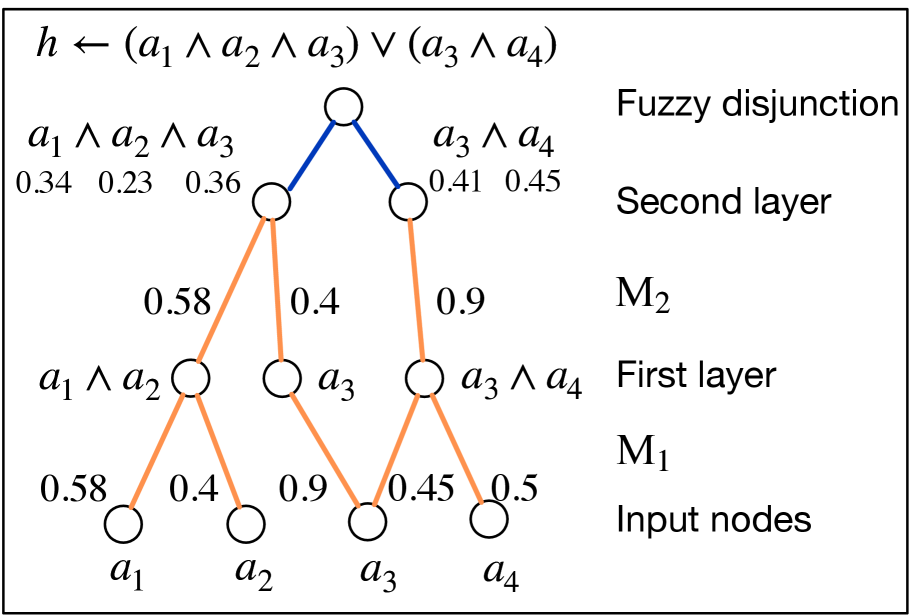We analyze the interpretability of the rule-learning module $N_{R}$ . In the logic program matrix $\mathbf{M}_{P}$ defined in Section 3.1, the sum of non-zero elements in each row, $\sum_{j=1}^{n}\mathbf{M}_{P}[i,j]$ , is normalized to one, matching the threshold in the function $\theta$ in Eq. (1). The conjunction of the atoms corresponding to non-zero elements in each row of $\mathbf{M}_{P}$ can serve as the body of a rule. Similarly, in the rule-learning module of NeurRL, the sum of the softmax-activated weights in each layer is also one. Due to the properties of the activation function $\text{ReLU}(x-d)/(1-d)$ in each node, a node activates only when the sum of the weights approaches one; otherwise, it deactivates. This behavior mimics the threshold function $\theta$ in Eq. (1). Similar to the logic program matrix $\mathbf{M}_{P}$ , the softmax-activated weights in each layer also have interpretability. When the fuzzy interpretation vector and Boolean value of the target atom fit the forward process in Eq. (6), the atoms corresponding to non-zero elements in each row of the $i$ -th dense softmax-activated weight matrix $\mathbf{M}_{i}$ form a conjunction. From a neural network perspective, the $j$ -th node in the $i$ -th dense layer, denoted as $n_{j}^{i}$ , represents a conjunction of atoms from the previous $(i-1)$ -th dense layer (input layer). The likelihood of these atoms appearing in the conjunction is determined by the softmax-activated weights $\mathbf{M}_{i}[j,:]$ connecting to node $n_{j}^{i}$ . In the final $k$ -th dense layer, the disjunction layer computes the probability of the target atom $h_{t}$ . The higher likelihood conjunctions, represented by the nodes in the final $k$ -th layer, form the body of the rule headed by $h_{t}$ . To interpret the rules headed by $h_{t}$ , we compute the product of all softmax-activated weights $\mathbf{M}_{i}$ as the program tensor: $\mathbf{M}_{P}=\prod_{i=1}^{k}\mathbf{M}_{i}$ , where $\mathbf{M}_{P}\in[0,1]^{m\times n}$ . The program tensor has the same interpretability as the program matrix, with high-value atoms in each row forming the rule body and the target atom as the rule head. The number of nodes in the last dense layer $m$ determines the number of learned rules in one learning epoch. Fig. 1(b) shows a neural network with two dense layers and one disjunction layer in blue. The weights in orange represent significant softmax-activated values, with input nodes as atoms and hidden nodes as conjunctions. Multiplying the softmax weights identifies the atoms forming the body of a rule headed by the target atom. We use the following method to extract rules from program tensor $\mathbf{M}_{P}$ : We set multiple thresholds $\tau\in[0,1]$ . When the value of the element in a row of $\mathbf{M}_{P}$ is larger than a threshold $\tau$ , then we regard the atom corresponding to these elements as the body atom in a rule with the format (4). We compute the precision and recall of the rules based on the discretized fuzzy interpretation vectors generated from the test dataset. The discretized fuzzy interpretation vector is derived as the flattened version of $\bar{\mathbf{c}}_{p}[i,j]=\mathbbm{1}(\mathbf{c}_{p}[i,j]=\max_{k}\mathbf{c}_{p}[k,j])$ , where $\max_{k}\mathbf{c}_{p}[k,j]$ represents the maximum value in the $j$ -th column of $\mathbf{c}_{p}$ . Then, we keep the high-precision rules as the output. The precision and recall of a rule are defined as: $\text{precision}={n_{\text{body $\land$ head}}}/{n_{\text{body}}}$ and $\text{recall}={n_{\text{body $\land$ head}}}/n_{\text{head}}$ , where $n_{\text{body $\land$ head}}$ denotes the number of discretized fuzzy interpretation vectors $\mathbf{v}_{I}$ that satisfy the rule body and have the target class as the label. Similarly, $n_{\text{body}}$ represents the number of discretized fuzzy interpretation vectors that satisfy the rule body, while $n_{\text{head}}$ refers to the number of instances with the target class. When obtaining rules in the format (4), we can highlight the subsequences satisfying the pattern and region predicates above on the raw inputs for more intuitive interpretability. To train the model, we first pre-train an autoencoder to obtain subsequence embeddings, then initialize the cluster embeddings using $k$ -means clustering (Lloyd, 1982) based on these embeddings. Finally, we jointly train the autoencoder, clustering model, and rule-learning model using the target function (9) to optimize the embeddings, clusters, and rules simultaneously. ## 5 Experimental results <details> <summary>x3.png Details</summary>  ### Visual Description ## Line Chart: Positive and Negative Values Over Time ### Overview The image is a line chart comparing "Positive" and "Negative" values over 15 time points (0 to 14). The chart displays two primary data series, one in blue representing "Positive" values and the other in orange representing "Negative" values. There is also a thicker red line that seems to represent a modified version of the "Positive" values between time points 5 and 9. The chart includes a grid for easier value estimation. The title indicates this chart relates to a pattern and region, with parameters p=1 and r=1. ### Components/Axes * **Title:** `h_p ← pattern_0(X) ∧ region_1(X) (p = 1, r = 1)` * **X-axis:** "Time points", labeled from 0 to 14 in increments of 2. * **Y-axis:** "Value", ranging from 0.0 to 1.0 in increments of 0.2. * **Legend:** Located on the right side of the chart. * Blue line: "Positive" * Orange line: "Negative" ### Detailed Analysis * **Positive (Blue) Line:** * Starts at approximately 0.0 at time point 0. * Increases to approximately 0.5 at time point 2. * Increases to approximately 0.95 at time point 4. * Remains at approximately 0.95 at time point 6. * Decreases to approximately 0.0 at time point 10. * Increases to approximately 0.95 at time point 14. * **Negative (Orange) Line:** * Starts at approximately 0.95 at time point 0. * Decreases to approximately 0.5 at time point 2. * Decreases to approximately 0.0 at time point 4. * Remains at approximately 0.0 at time point 6. * Increases to approximately 0.5 at time point 8. * Increases to approximately 0.95 at time point 10. * Decreases to approximately 0.0 at time point 14. * **Modified Positive (Red) Line:** * This line is only present between time points 5 and 9. * It starts at approximately 0.95 at time point 5. * Decreases to approximately 0.35 at time point 8. * Decreases to approximately 0.0 at time point 9. ### Key Observations * The "Positive" and "Negative" lines exhibit an inverse relationship, with one increasing as the other decreases. * The "Positive" line has a modified version (red line) between time points 5 and 9, which deviates from the original "Positive" line. * Both lines appear to oscillate between approximately 0.0 and 1.0. ### Interpretation The chart likely represents a scenario where two opposing factors, "Positive" and "Negative", influence a system over time. The inverse relationship suggests that as one factor becomes more dominant, the other weakens. The modified "Positive" line could indicate an intervention or a change in the system that temporarily alters the "Positive" value. The formula in the title suggests that the data is related to pattern recognition and regional analysis, possibly within a machine learning or data analysis context. The parameters p=1 and r=1 might represent specific settings or conditions within the analysis. </details> (a) The signals based on triangular pulse. <details> <summary>x4.png Details</summary>  ### Visual Description ## Line Chart: Pattern and Region Analysis ### Overview The image is a line chart comparing "Positive" and "Negative" values over time points. The chart visualizes the relationship between these two categories, showing their fluctuations and intersections across the time points. The chart also includes a formula at the top: "hp ← pattern0(X) ∧ region2(X) (p = 1, r = 1)". ### Components/Axes * **Title:** hp ← pattern0(X) ∧ region2(X) (p = 1, r = 1) * **X-axis:** "Time points" with markers at 0, 2, 4, 6, 8, 10, 12, and 14. * **Y-axis:** "Value" with markers at 0.0, 0.2, 0.4, 0.6, 0.8, and 1.0. * **Legend:** Located in the top-left corner. * "Positive" - represented by a blue line. * "Negative" - represented by an orange line. ### Detailed Analysis * **Positive (Blue Line):** * Trend: The line generally oscillates, showing a wave-like pattern. * Data Points: * Time point 0: Value ≈ 0.5 * Time point 2: Value ≈ 0.1 * Time point 6: Value ≈ 0.0 * Time point 10: Value ≈ 0.9 * Time point 14: Value ≈ 0.1 * **Negative (Orange Line):** * Trend: The line also oscillates, showing a wave-like pattern, but generally inverse to the "Positive" line. * Data Points: * Time point 0: Value ≈ 0.4 * Time point 2: Value ≈ 0.0 * Time point 6: Value ≈ 0.9 * Time point 10: Value ≈ 0.0 * Time point 14: Value ≈ 1.0 ### Key Observations * The "Positive" and "Negative" lines exhibit an inverse relationship, with one generally increasing when the other is decreasing. * Both lines show a periodic pattern, suggesting a cyclical behavior over time. * Around time point 10, the "Positive" line transitions to a darker red/purple color, and the "Negative" line continues as orange. ### Interpretation The chart visualizes the interplay between "Positive" and "Negative" values over time. The oscillating patterns suggest a dynamic relationship, possibly representing opposing forces or alternating states. The formula at the top indicates that these patterns are related to specific regions and patterns identified by the variables X, p, and r. The change in color of the "Positive" line around time point 10 could indicate a shift in the underlying process or a change in the data being represented. The data suggests a system where positive and negative attributes fluctuate in a somewhat predictable, inverse manner, potentially driven by underlying patterns and regional characteristics. </details> (b) The signals based on trigonometry function. Figure 2: The synthetic data and the learned rules. 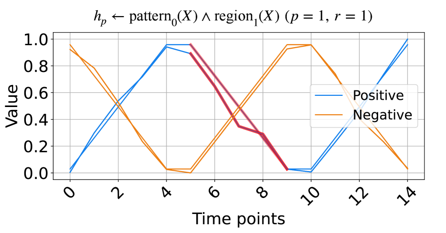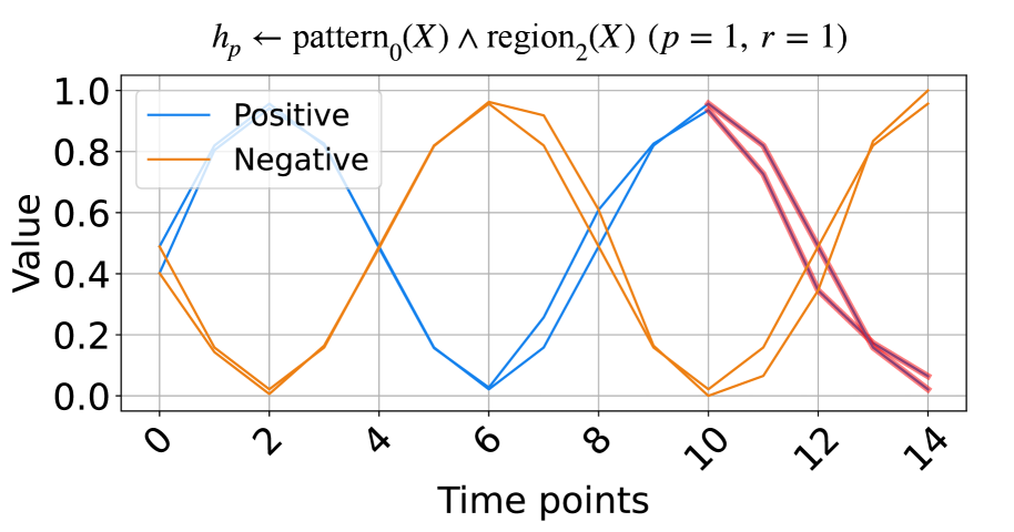### 5.1 Learning from synthetic data In this subsection, we evaluate the model on synthetic time series data based on triangular pulse signals and trigonometric signals. Each signal contains two key patterns, increasing and decreasing, with each pattern having a length of five units. To test NeurRL’s learning capability on a smaller dataset, we set the number of inputs in both the positive and negative classes to two for both the training and test datasets. In each class, the difference between two inputs at each time point is a random number drawn from a normal distribution with a mean of zero and a variance of 0.1. The positive test inputs are plotted in blue, and the negative test inputs in orange in Fig. 2. We set both the length of each region and the subsequence length to five units, and the number of clusters is set to three in this experiment. NeurRL is tasked with learning rules to describe the positive class, represented by the head atom $h_{p}$ . If the ground body atoms, substituted by subsequences of an input, hold true, the head atom $h_{p}$ is also true, indicating that the target class of the input is positive. The rules with 1.0 precision ( $p$ ) and 1.0 recall ( $r$ ) are shown in Fig. 2. The rule in Fig. 2(a) states that when $\texttt{pattern}_{0}$ (cluster index 0) appears in $\texttt{region}_{1}$ (from time points 5 to 9), the time series label is positive. Similarly, the rule in Fig. 2(b) indicates that when $\texttt{pattern}_{0}$ appears in $\texttt{region}_{2}$ (from time points 10 to 14), the label is positive. We highlight subsequences that satisfy the rule body in red in Fig. 2, inferring that the $\texttt{pattern}_{0}$ indicates decreasing. These red patterns perfectly distinguish positive from negative inputs. ### 5.2 Learning from UCR datasets <details> <summary>x5.png Details</summary>  ### Visual Description ## Line Chart: Positive and Negative Values Over Time ### Overview The image is a line chart displaying multiple time series data, differentiating between "Positive" and "Negative" values across "Time points". The chart includes a legend to distinguish between the two categories, and the plot shows fluctuations in value over time for each category. Some regions of the chart are highlighted with different colors (red and green) to emphasize specific patterns. 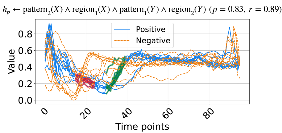### Components/Axes * **Title:** h\_p ← pattern₂(X) ∧ region₁(X) ∧ pattern₁(Y) ∧ region₂(Y) (p = 0.83, r = 0.89) * **X-axis:** * Label: Time points * Scale: 0 to 80, with major ticks at 0, 20, 40, 60, and 80. * **Y-axis:** * Label: Value * Scale: 0.0 to 0.8, with major ticks at 0.0, 0.2, 0.4, 0.6, and 0.8. * **Legend:** Located in the top-right of the chart. * Positive: Represented by solid blue lines. * Negative: Represented by dashed orange lines. * **Highlighted Regions:** * Red: Located around time points 15-25. * Green: Located around time points 30-40. ### Detailed Analysis * **Positive (Blue Lines):** * Trend: Initially high, decreases sharply until approximately time point 20, then gradually increases and stabilizes around a value of 0.5 between time points 40 and 80. There is a slight increase near time point 80. * Values: Starts around 0.7-0.9 at time point 0, drops to approximately 0.1-0.3 around time point 20, and stabilizes around 0.5 from time point 40 onwards. * **Negative (Dashed Orange Lines):** * Trend: Starts high, decreases to a minimum around time point 20, then increases and fluctuates around a value of 0.4-0.5 between time points 40 and 80. There is a peak near time point 80. * Values: Starts around 0.6-0.8 at time point 0, drops to approximately 0.2-0.3 around time point 20, and fluctuates around 0.4-0.5 from time point 40 onwards. * **Highlighted Regions:** * Red: The red region highlights a period where both positive and negative values are at their lowest. * Green: The green region highlights a period where both positive and negative values are increasing. ### Key Observations * The "Positive" and "Negative" values exhibit an inverse relationship initially, with both converging to similar values after time point 40. * The highlighted regions (red and green) indicate specific time intervals where the values undergo significant changes. * The title includes parameters p = 0.83 and r = 0.89, which likely represent statistical measures related to the data. ### Interpretation The chart visualizes the temporal dynamics of "Positive" and "Negative" values, possibly representing different attributes or categories within a system. The initial divergence and subsequent convergence of these values suggest a shift in their relationship over time. The highlighted regions likely correspond to critical events or transitions within the system. The parameters p and r in the title likely quantify the statistical significance and correlation of the observed patterns. The data suggests that the system undergoes a period of instability or change between time points 0 and 40, after which it reaches a more stable state. </details> (a) A rule from ECG dataset. <details> <summary>x6.png Details</summary>  ### Visual Description ## Line Chart: Pattern and Region Analysis ### Overview The image is a line chart comparing "Positive" and "Negative" data series over time. Multiple lines are plotted for each category, showing the variation within each group. The chart includes a title indicating the analysis is based on pattern and region, with associated probability (p) and correlation (r) values. 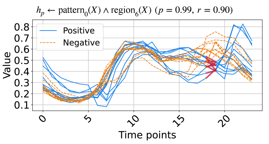### Components/Axes * **Title:** `h_p ← pattern_0(X) ∧ region_6(X) (p = 0.99, r = 0.90)` * **X-axis:** "Time points", ranging from 0 to 20 in increments of 5. * **Y-axis:** "Value", ranging from 0.1 to 0.8 in increments of 0.1. * **Legend:** Located in the top-left corner. * "Positive": Represented by solid blue lines. * "Negative": Represented by dashed orange lines. ### Detailed Analysis * **Positive (Blue Lines):** * General Trend: The "Positive" lines generally start around a value of 0.4-0.5, decrease to around 0.2 between time points 4 and 6, then increase to a peak between time points 10 and 12, reaching values between 0.6 and 0.7. After the peak, the lines generally decrease to values between 0.4 and 0.6 at time point 20. * Specific Values: At time point 0, the values range from approximately 0.4 to 0.5. At time point 10, the values peak between 0.6 and 0.7. At time point 20, the values range from approximately 0.4 to 0.6. * **Negative (Dashed Orange Lines):** * General Trend: The "Negative" lines start around a value of 0.2-0.5, decrease to around 0.2 between time points 4 and 6, then increase to a peak between time points 10 and 12, reaching values between 0.5 and 0.6. After the peak, the lines generally decrease to values between 0.3 and 0.7 at time point 20. * Specific Values: At time point 0, the values range from approximately 0.2 to 0.5. At time point 10, the values peak between 0.5 and 0.6. At time point 20, the values range from approximately 0.3 to 0.7. * **Highlighted Region:** There is a region highlighted in red around time point 19, where some of the "Positive" and "Negative" lines intersect or are in close proximity. ### Key Observations * Both "Positive" and "Negative" series show a similar trend: a decrease in value from time point 0 to around time point 5, followed by an increase to a peak around time point 10-12, and then a decrease towards time point 20. * The "Positive" series generally has higher values than the "Negative" series, especially around the peak at time points 10-12. * The highlighted region around time point 19 indicates an area of potential overlap or similarity between the "Positive" and "Negative" series. ### Interpretation The chart visualizes the behavior of "Positive" and "Negative" patterns over time, likely representing different classes or conditions. The similar trends suggest that both patterns are influenced by the same underlying factors, but the difference in magnitude indicates that the "Positive" pattern is generally stronger or more prevalent. The highlighted region could indicate a point where the two patterns are difficult to distinguish or where their effects converge. The values of p = 0.99 and r = 0.90 suggest a high probability and correlation associated with the pattern and region analysis, indicating a strong relationship between the variables being analyzed. </details> (b) A rule from ItalyPow.Dem. dataset. Figure 3: Selected rules from two UCR datasets. In this subsection, we experimentally demonstrate the effectiveness of NeurRL on 13 randomly selected datasets from UCR (Dau et al., 2019), as used by Wang et al. (2019). To evaluate NeurRL’s performance, we consider the classification accuracy from the rules extracted by the deep rule-learning module (denoted as NeurRL(R)) and the classification accuracy from the module itself (denoted as NeurRL(N)). The number of clusters in this experiment is set to five. The subsequence length and the number of regions vary for each task. We set the number of regions to approximately 10 for time series data. Additionally, the subsequence length is set to range from two to five, depending on the specific subtask. The baseline models include SSSL (Wang et al., 2019), Xu (Xu and Funaya, 2015), and BoW (Wang et al., 2013). SSSL uses regularized least squares, shapelet regularization, spectral analysis, and pseudo-labeling to auto-learn discriminative shapelets from time series data. Xu’s method constructs a graph to derive underlying structures of time series data in a semi-supervised way. BoW generates a bag-of-words representation for time series and uses SVM for classification. Statistical details, such as the number of classes (C.), inputs (I.), series length, and comparison results are shown in Tab. 1, with the best results in bold and second-best underlined. The NeurRL(N) achieves the most best results, with seven, and NeurRL(R) achieves five second-best results. Table 1: Classification accuracy on 13 binary UCR datasets with different models. | Coffee | 2 | 56 | 286 | 0.588 | 0.620 | 0.792 | 0.964 | 1.000 | | --- | --- | --- | --- | --- | --- | --- | --- | --- | | ECG | 2 | 200 | 96 | 0.819 | 0.955 | 0.793 | 0.820 | 0.880 | | Gun point | 2 | 200 | 150 | 0.729 | 0.925 | 0.824 | 0.760 | 0.873 | | ItalyPow.Dem. | 2 | 1096 | 24 | 0.772 | 0.813 | 0.941 | 0.926 | 0.923 | | Lighting2 | 2 | 121 | 637 | 0.698 | 0.721 | 0.813 | 0.689 | 0.748 | | CBF | 3 | 930 | 128 | 0.921 | 0.873 | 1.000 | 0.909 | 0.930 | | Face four | 4 | 112 | 350 | 0.833 | 0.744 | 0.851 | 0.914 | 0.964 | | Lighting7 | 7 | 143 | 319 | 0.511 | 0.677 | 0.796 | 0.737 | 0.878 | | OSU leaf | 6 | 442 | 427 | 0.642 | 0.685 | 0.835 | 0.844 | 0.849 | | Trace | 4 | 200 | 275 | 0.788 | 1.00 | 1.00 | 0.833 | 0.905 | | WordsSyn | 25 | 905 | 270 | 0.639 | 0.795 | 0.875 | 0.932 | 0.946 | | OliverOil | 4 | 60 | 570 | 0.639 | 0.766 | 0.776 | 0.768 | 0.866 | | StarLightCurves | 3 | 9236 | 2014 | 0.755 | 0.851 | 0.872 | 0.869 | 0.907 | | Mean accuracy | | | | 0.718 | 0.801 | 0.859 | 0.842 | 0.891 | The learned rules from the ECG and ItalyPow.Dem. datasets in the UCR archive are shown in Fig. 3. In Fig. 3(a), red highlights subsequences with the shape $\texttt{pattern}_{2}$ in the region $\texttt{region}_{1}$ , while green highlights subsequences with the shape $\texttt{pattern}_{1}$ in the region $\texttt{region}_{2}$ . The rule suggests that when data decreases between time points 15 to 25 and then increases between time points 30 to 40, the input likely belongs to the positive class. The precision and recall for this rule are 0.83 and 0.89, respectively. In Fig. 3(b), red highlights subsequences with the shape $\texttt{pattern}_{0}$ in the region $\texttt{region}_{6}$ . The rule indicates that a lower value around time points 18 to 19 suggests the input belongs to the positive class, with precision and recall of 0.99 and 0.90, respectively. <details> <summary>x7.png Details</summary>  ### Visual Description ## Image Analysis: Positive and Negative Class Examples ### Overview The image presents two examples of handwritten digits, one labeled as a "positive class" and the other as a "negative class." The positive class example (a digit '1') has colored horizontal lines overlaid on it. The negative class example (a digit '0') is shown without any overlays. The image also includes the notation "p = 1, r = 1" below the examples. ### Components/Axes * **Positive Class:** A handwritten digit '1' with colored horizontal lines overlaid. * **Negative Class:** A handwritten digit '0'. * **Labels:** "positive class", "negative class", "p = 1, r = 1" * **Colored Lines (Positive Class):** The digit '1' has several short, horizontal lines of different colors overlaid on it. The colors appear to be: * Red * Blue * Green * Teal * Purple * Yellow ### Detailed Analysis or ### Content Details * **Positive Class (Digit '1'):** The digit '1' is slightly slanted. The colored lines are positioned horizontally across the digit. * **Negative Class (Digit '0'):** The digit '0' is a closed loop. * **Text:** The text "positive class" is located below the digit '1'. The text "negative class" is located below the digit '0'. The text "p = 1, r = 1" is located below both examples, centered. ### Key Observations * The positive class example has colored lines overlaid, while the negative class example does not. * The notation "p = 1, r = 1" likely refers to parameters or values associated with the classification or data generation process. ### Interpretation The image illustrates the concept of positive and negative classes in a classification problem, likely related to digit recognition. The colored lines on the positive class example might represent features or attributes that are important for identifying the digit '1'. The "p = 1, r = 1" notation suggests specific parameter settings used in this example. The image highlights the distinction between a positive instance (digit '1') and a negative instance (digit '0') within the context of a machine learning or pattern recognition task. 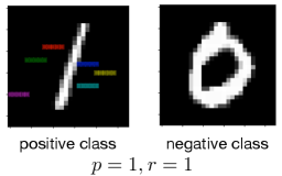</details> Figure 4: Learned rules from MNIST datasets. To demonstrate the benefits of the fully differentiable learning pipeline from raw sequence inputs to symbolic rules, we compare the accuracy and running times (in seconds) between NeurRL and its deep rule-learning module using the non-differentiable $k$ -means clustering algorithm (Lloyd, 1982). We use the same hyperparameter to split time series into subsequences for two methods. Results in Tab. 2 show that the differentiable pipeline significantly reduces running time without sacrificing rule accuracy in most cases. Table 2: Comparisons with non-differentiable $k$ -means clustering algorithm. | Coffee | 0.893 | 313 | 0.964 | 42 | | --- | --- | --- | --- | --- | | ECG | 0.810 | 224 | 0.820 | 65 | | Gun point | 0.807 | 102 | 0.740 | 35 | | ItalyPow.Dem. | 0.845 | 114 | 0.926 | 63 | | Lighting2 | 0.672 | 1166 | 0.689 | 120 | ### 5.3 Learning from images In this subsection, we ask the model to learn rules to describe and discriminate two classes of images from MNIST datasets. We divide the MNIST dataset into five independent datasets, where each dataset contains one positive class and one negative class. For two-dimensional image data, we first flatten the image data to one-dimensional sequence data. Then, the sequence data can be the input for the NeurRL model to learn the rules. The lengths of subsequence and region are both set to three. Besides, the number of clusters is set to five. After generating the highlighted patterns based on the rules, we recover the sequence data to the image for interpreting these learned rules. We present the rule for learning the digit one from the digit zero in Fig. 4, and the rules for learning other positive class from the negative class are shown in Fig. 6 in Appendix C. We present the rule with the precision larger than 0.9 and the highlight features (or areas) defined in the rules. Each highlight feature corresponds to a pair of region and pattern atoms in a learned rule. We can interpret rules like importance attention (Zhang et al., 2019), where the colored areas include highly discriminative information for describing positive inputs compared with negative inputs. For example, in Fig. 4, if the highlighted areas are in black at the same time, then the image class is one. Otherwise, the image class is zero. Compared with attention, we calculate the precision and recall to evaluate these highlight features quantitatively. 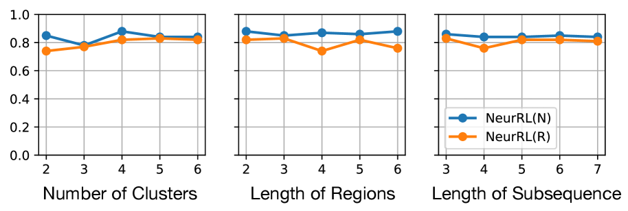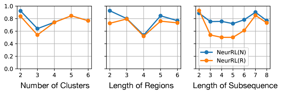### 5.4 Ablation study We conducted ablation studies using default hyperparameters, except for the one being explored. In this study, the number of clusters and regions influences the number of atoms in the learned rules, while the length of subsequences depends on the length of potential patterns. Hence, these three hyperparameters collectively describe the sensitivity of NeurRL. We present the accuracy of both NeurRL(N) and NeurRL(R) on the time series tasks ECG and ItalyPow.Dem. from the UCR archive. <details> <summary>x8.png Details</summary>  ### Visual Description ## Line Charts: NeurRL Performance vs. Parameters ### Overview The image presents three line charts comparing the performance of two algorithms, NeurRL(N) and NeurRL(R), across different parameter settings. The charts depict performance (y-axis) against "Number of Clusters", "Length of Regions", and "Length of Subsequence" (x-axis). ### Components/Axes * **Y-axis (all charts):** Performance, ranging from 0.0 to 1.0 in increments of 0.2. * **X-axis (left chart):** Number of Clusters, with values 2, 3, 4, 5, and 6. * **X-axis (middle chart):** Length of Regions, with values 2, 3, 4, 5, and 6. * **X-axis (right chart):** Length of Subsequence, with values 3, 4, 5, 6, and 7. * **Legend (bottom-right):** * Blue line: NeurRL(N) * Orange line: NeurRL(R) ### Detailed Analysis **Chart 1: Number of Clusters** * **NeurRL(N) (Blue):** The line starts at approximately 0.85 at 2 clusters, dips slightly to around 0.80 at 3 clusters, then rises to approximately 0.90 at 4 clusters, and decreases slightly to approximately 0.84 at 5 and 6 clusters. * (2, 0.85) * (3, 0.80) * (4, 0.90) * (5, 0.84) * (6, 0.84) * **NeurRL(R) (Orange):** The line starts at approximately 0.74 at 2 clusters, rises to approximately 0.78 at 3 clusters, then rises to approximately 0.83 at 4 clusters, and remains relatively stable at approximately 0.83 at 5 and 6 clusters. * (2, 0.74) * (3, 0.78) * (4, 0.83) * (5, 0.83) * (6, 0.83) **Chart 2: Length of Regions** * **NeurRL(N) (Blue):** The line starts at approximately 0.89 at length 2, dips slightly to around 0.87 at length 3, then rises to approximately 0.88 at length 4, and increases slightly to approximately 0.90 at lengths 5 and 6. * (2, 0.89) * (3, 0.87) * (4, 0.88) * (5, 0.90) * (6, 0.90) * **NeurRL(R) (Orange):** The line starts at approximately 0.83 at length 2, dips to approximately 0.74 at length 3, then rises to approximately 0.82 at length 4, and remains relatively stable at approximately 0.84 at lengths 5 and 6. * (2, 0.83) * (3, 0.74) * (4, 0.82) * (5, 0.84) * (6, 0.84) **Chart 3: Length of Subsequence** * **NeurRL(N) (Blue):** The line starts at approximately 0.88 at length 3, dips slightly to around 0.84 at length 4, then rises to approximately 0.87 at length 5, and increases slightly to approximately 0.90 at lengths 6 and 7. * (3, 0.88) * (4, 0.84) * (5, 0.87) * (6, 0.90) * (7, 0.90) * **NeurRL(R) (Orange):** The line starts at approximately 0.80 at length 3, rises to approximately 0.82 at length 4, then remains relatively stable at approximately 0.82 at lengths 5, 6 and 7. * (3, 0.80) * (4, 0.82) * (5, 0.82) * (6, 0.82) * (7, 0.82) ### Key Observations * NeurRL(N) generally outperforms NeurRL(R) across all parameter settings. * The performance of both algorithms is relatively stable across the tested parameter ranges. * NeurRL(R) shows a more pronounced dip in performance at lower values of "Length of Regions" (length 3). ### Interpretation The charts suggest that NeurRL(N) is a more robust algorithm than NeurRL(R) across the tested parameter ranges. While both algorithms exhibit relatively stable performance, NeurRL(N) consistently achieves higher performance scores. The dip in NeurRL(R)'s performance at a "Length of Regions" of 3 indicates that this parameter may be more sensitive for that algorithm. The data implies that NeurRL(N) is less sensitive to the specific parameter settings within the tested ranges, making it a potentially more reliable choice. Further investigation could explore the performance of these algorithms outside of these parameter ranges to identify optimal settings and potential limitations. </details> (a) On ECG dataset. <details> <summary>x9.png Details</summary>  ### Visual Description ## Line Charts: NeurRL Performance vs. Parameter Settings ### Overview The image presents three line charts comparing the performance of two algorithms, NeurRL(N) and NeurRL(R), across different parameter settings. The charts depict performance (y-axis) against "Number of Clusters", "Length of Regions", and "Length of Subsequence" (x-axis). ### Components/Axes * **Y-axis (all charts):** Performance, ranging from 0.0 to 1.0 in increments of 0.2. * **X-axis (left chart):** Number of Clusters, ranging from 2 to 6 in increments of 1. * **X-axis (middle chart):** Length of Regions, ranging from 2 to 6 in increments of 1. * **X-axis (right chart):** Length of Subsequence, ranging from 2 to 8 in increments of 1. * **Legend (bottom-right):** * Blue line with circle markers: NeurRL(N) * Orange line with circle markers: NeurRL(R) ### Detailed Analysis **Chart 1: Number of Clusters** * **NeurRL(N) (Blue):** Starts at approximately 0.9 at 2 clusters, decreases to approximately 0.65 at 3 clusters, increases to approximately 0.75 at 4 clusters, increases to approximately 0.85 at 5 clusters, and decreases slightly to approximately 0.8 at 6 clusters. * **NeurRL(R) (Orange):** Starts at approximately 0.85 at 2 clusters, decreases to approximately 0.55 at 3 clusters, increases to approximately 0.75 at 4 clusters, increases to approximately 0.85 at 5 clusters, and decreases to approximately 0.78 at 6 clusters. **Chart 2: Length of Regions** * **NeurRL(N) (Blue):** Starts at approximately 0.95 at length 2, decreases to approximately 0.8 at length 3, decreases to approximately 0.55 at length 4, increases to approximately 0.85 at length 5, and decreases slightly to approximately 0.8 at length 6. * **NeurRL(R) (Orange):** Starts at approximately 0.75 at length 2, increases slightly to approximately 0.8 at length 3, decreases to approximately 0.55 at length 4, increases to approximately 0.75 at length 5, and increases slightly to approximately 0.78 at length 6. **Chart 3: Length of Subsequence** * **NeurRL(N) (Blue):** Starts at approximately 0.95 at length 2, decreases to approximately 0.75 at length 3, remains relatively stable at approximately 0.75 at length 4, decreases slightly to approximately 0.72 at length 5, increases to approximately 0.78 at length 6, increases to approximately 0.92 at length 7, and decreases to approximately 0.8 at length 8. * **NeurRL(R) (Orange):** Starts at approximately 0.85 at length 2, decreases to approximately 0.52 at length 3, remains relatively stable at approximately 0.5 at length 4, increases to approximately 0.6 at length 5, increases to approximately 0.8 at length 6, increases to approximately 0.9 at length 7, and decreases to approximately 0.72 at length 8. ### Key Observations * Both algorithms show performance variation with changes in "Number of Clusters", "Length of Regions", and "Length of Subsequence". * NeurRL(N) generally outperforms NeurRL(R) across different parameter settings, especially for "Length of Subsequence". * Both algorithms show a performance dip at a "Length of Regions" of 4. * For "Length of Subsequence", both algorithms peak at a length of 7. ### Interpretation The charts suggest that the performance of NeurRL algorithms is sensitive to the choice of parameters like "Number of Clusters", "Length of Regions", and "Length of Subsequence". NeurRL(N) appears to be more robust to parameter changes compared to NeurRL(R). The performance dip at a "Length of Regions" of 4 might indicate a critical threshold or a less optimal configuration for both algorithms. The peak performance at a "Length of Subsequence" of 7 suggests an optimal subsequence length for the given problem. Further investigation is needed to understand the underlying reasons for these performance variations and to optimize the parameter settings for each algorithm. </details> (b) On ItalyPow.Dem. dataset. Figure 5: Results of ablation study. Hyperparameter values vs. accuracy. From Fig. 5, we observe that NeurRL’s sensitivity varies across tasks, and the subsequence length is a sensitive hyperparameter when the sequence length is small, as seen in the ItalyPow.Dem. dataset. Properly chosen hyperparameters can achieve high consistency in accuracy between rules and neural networks. Notably, increasing the number of clusters or length of regions does not reduce accuracy linearly. This suggests that the rule-learning module effectively adjusts clusters within the model. In addition, we conduct another ablation study in Tab. 3 of Appendix A to show that pre-training the autoencoder and clustering prevents cluster collapse (Sansone, 2023) and improves accuracy without increasing significant training time. ## 6 Conclusion Inductive logic programming (ILP) is a rule-based machine learning method that supporting data interpretability. Differentiable ILP offers advantages in scalability and robustness. However, label leakage remains a challenge when learning rules from raw data, as neuro-symbolic models require intermediate feature labels as input. In this paper, we propose a novel fully differentiable ILP model, Neural Rule Learner (NeurRL), which learns symbolic rules from raw sequences using a differentiable $k$ -means clustering module and a deep neural network-based rule-learning module. The differentiable $k$ -means clustering algorithm groups subcomponents of inputs based on the similarity of their embeddings, and the learned clusters are used as input for the rule-learning module to induce rules that describe the ground truth class of input based on its features. Compared to other rule-based models, NeurRL achieves comparable classification accuracy while offering interpretability through quantitative metrics. Future goals include variables representing entire inputs to explain handwritten digits without label leakage (Evans et al., 2021). Another focus is learning from incomplete data (e.g., healthcare applications) to address real-world challenges. #### Acknowledgments We express our gratitude to the anonymous Reviewers for their valuable feedback, which has contributed significantly to enhancing the clarity and presentation of our paper. We also thank Xingyao Wang, Yingzhi Xia, Yang Liu, Jasmine Ong, Justina Ma, Jonathan Tan, Yong Liu, and Rick Goh for their supporting. This work has been supported by AI Singapore under Grant AISG2TC2022006, Singapore. This work has been supported by the NII international internship program, JSPS KAKENHI Grant Number JP21H04905 and JST CREST Grant Number JPMJCR22D3, Japan. This work has also been supported by the National Key R&D Program of China under Grant 2021YFF1201102 and the National Natural Science Foundation of China under Grants 61972005 and 62172016. ## References - K. R. Apt, H. A. Blair, and A. Walker (1988) Towards a theory of declarative knowledge. In Foundations of Deductive Databases and Logic Programming, pp. 89–148. Cited by: §3.1. - S. Azzolin, A. Longa, P. Barbiero, P. Liò, and A. Passerini (2023) Global explainability of gnns via logic combination of learned concepts. In Proceedings of the 11th International Conference on Learning Representations, ICLR-23, Cited by: §2. - H. Blockeel and L. De Raedt (1998) Top-down induction of first-order logical decision trees. Artif. Intell. 101 (1-2), pp. 285–297. Cited by: §1. - A. Cropper, S. Dumancic, R. Evans, and S. H. Muggleton (2022) Inductive logic programming at 30. Mach. Learn. 111 (1), pp. 147–172. Cited by: §1. - A. Cropper and S. Dumancic (2022) Inductive logic programming at 30: A new introduction. J. Artif. Intell. Res. 74, pp. 765–850. Cited by: §2. - G. Das, K. Lin, H. Mannila, G. Renganathan, and P. Smyth (1998) Rule discovery from time series. In Proceedings of the Fourth International Conference on Knowledge Discovery and Data Mining (KDD-98), pp. 16–22. Cited by: §2, §3.2. - H. A. Dau, A. Bagnall, K. Kamgar, C. M. Yeh, Y. Zhu, S. Gharghabi, C. A. Ratanamahatana, and E. Keogh (2019) The UCR time series archive. IEEE/CAA Journal of Automatica Sinica 6 (6), pp. 1293–1305. Note: https://www.cs.ucr.edu/~eamonn/time_series_data_2018/ Cited by: §5.2. - L. De Raedt and L. Dehaspe (1997) Clausal discovery. Mach. Learn. 26 (2-3), pp. 99–146. Cited by: §3.1. - F. Doshi-Velez and B. Kim (2017) Towards a rigorous science of interpretable machine learning. arXiv preprint arXiv:1702.08608. Cited by: §1. - R. Evans, M. Bosnjak, L. Buesing, K. Ellis, D. P. Reichert, P. Kohli, and M. J. Sergot (2021) Making sense of raw input. Artif. Intell. 299, pp. 103521. Cited by: §1, §2, §6. - R. Evans and E. Grefenstette (2018) Learning explanatory rules from noisy data. J. Artif. Intell. Res. 61, pp. 1–64. Cited by: §1, §2, §2, §3.1. - M. M. Fard, T. Thonet, and É. Gaussier (2020) Deep k -means: jointly clustering with k -means and learning representations. Pattern Recognit. Lett. 138, pp. 185–192. Cited by: §3.2, §4.2. - K. Gao, K. Inoue, Y. Cao, and H. Wang (2022a) Learning first-order rules with differentiable logic program semantics. In Proceedings of the 31st International Joint Conference on Artificial Intelligence, IJCAI-22, pp. 3008–3014. Cited by: §1, §2, §3.1. - K. Gao, K. Inoue, Y. Cao, and H. Wang (2024) A differentiable first-order rule learner for inductive logic programming. Artif. Intell. 331, pp. 104108. Cited by: §1, §2, §3.1, §3.1, §4.2. - K. Gao, H. Wang, Y. Cao, and K. Inoue (2022b) Learning from interpretation transition using differentiable logic programming semantics. Mach. Learn. 111 (1), pp. 123–145. Cited by: §2. - Y. He, X. Chu, G. Peng, Y. Wang, Z. Jin, and X. Wang (2018) Mining rules from real-valued time series: A relative information-gain-based approach. In 2018 IEEE 42nd Annual Computer Software and Applications Conference, COMPSAC-18, pp. 388–397. Cited by: §2. - C. Hocquette, A. Niskanen, M. Järvisalo, and A. Cropper (2024) Learning MDL logic programs from noisy data. In Proceedings of the 39th Annual AAAI Conference on Artificial Intelligence, AAAI-24, pp. 10553–10561. Cited by: §1. - K. Inoue, T. Ribeiro, and C. Sakama (2014) Learning from interpretation transition. Mach. Learn. 94 (1), pp. 51–79. Cited by: §2, §3.1. - E. Jang, S. Gu, and B. Poole (2017) Categorical reparameterization with gumbel-softmax. In Proceedings of the 5th International Conference on Learning Representations, ICLR-17, Cited by: §3.2. - Z. Liu, Y. Wang, S. Vaidya, F. Ruehle, J. Halverson, M. Soljacic, T. Y. Hou, and M. Tegmark (2024) KAN: kolmogorov-arnold networks. CoRR abs/2404.19756. Cited by: §2. - J. W. Lloyd (1984) Foundations of logic programming, 1st edition. Springer. Cited by: §3.1, §3.1. - S. P. Lloyd (1982) Least squares quantization in PCM. IEEE Trans. Inf. Theory 28 (2), pp. 129–136. Cited by: §4.3, §5.2. - R. Manhaeve, S. Dumancic, A. Kimmig, T. Demeester, and L. D. Raedt (2018) DeepProbLog: neural probabilistic logic programming. In Advances in Neural Information Processing Systems 31: Annual Conference on Neural Information Processing Systems, NeurIPS-18, pp. 3753–3763. Cited by: §1, §2. - E. Marconato, G. Bontempo, E. Ficarra, S. Calderara, A. Passerini, and S. Teso (2023) Neuro-symbolic continual learning: knowledge, reasoning shortcuts and concept rehearsal. In Proceedings of the 40th International Conference on Machine Learning, ICML-23, Vol. 202, pp. 23915–23936. Cited by: §4.1. - E. Misino, G. Marra, and E. Sansone (2022) VAEL: bridging variational autoencoders and probabilistic logic programming. In Advances in Neural Information Processing Systems 35: Annual Conference on Neural Information Processing Systems, NeurIPS-22, Cited by: §2. - S. H. Muggleton and L. De Raedt (1994) Inductive logic programming: theory and methods. J. Log. Program. 19/20, pp. 629–679. Cited by: §2. - S. H. Muggleton and C. Feng (1990) Efficient induction of logic programs. In Algorithmic Learning Theory, First International Workshop, ALT-90, pp. 368–381. Cited by: §2. - S. H. Muggleton, L. D. Raedt, D. Poole, I. Bratko, P. A. Flach, K. Inoue, and A. Srinivasan (2012) ILP turns 20 - biography and future challenges. Mach. Learn. 86 (1), pp. 3–23. Cited by: §3.1. - A. Passerini, P. Frasconi, and L. D. Raedt (2006) Kernels on prolog proof trees: statistical learning in the ILP setting. J. Mach. Learn. Res. 7, pp. 307–342. Cited by: §3.1. - Y. J. Phua and K. Inoue (2021) Learning logic programs using neural networks by exploiting symbolic invariance. In Proceedings of the 30th international conference on Inductive Logic Programming, ILP-21, Lecture Notes in Computer Science, Vol. 13191, pp. 203–218. Cited by: §2. - Y. J. Phua and K. Inoue (2024) Variable assignment invariant neural networks for learning logic programs. In Proceedings of the 18th International Conference on Neural-Symbolic Learning and Reasoning, NeSy-24, Lecture Notes in Computer Science, Vol. 14979, pp. 47–61. Cited by: §1. - J. R. Quinlan (1990) Learning logical definitions from relations. Mach. Learn. 5, pp. 239–266. Cited by: §1. - L. Rokach and O. Maimon (2005) Clustering methods. In The Data Mining and Knowledge Discovery Handbook, pp. 321–352. Cited by: §3.2. - E. Sansone and R. Manhaeve (2023) Learning symbolic representations through joint generative and discriminative training. In Proceedings of the 11th International Conference on Learning Representations on Neurosymbolic Generative Models Workshops (NeSy-GeMs, ICLR-23), Cited by: §2. - E. Sansone (2023) The triad of failure modes and a possible way out. In Proceedings of the 37th Annual Conference on Neural Information Processing Systems on the 4th Workshop on Self-Supervised Learning: Theory and Practice (SSL, NeurIPS-23), Cited by: §2, §5.4. - H. Shindo, V. Pfanschilling, D. S. Dhami, and K. Kersting (2023) $\alpha$ ILP: thinking visual scenes as differentiable logic programs. Mach. Learn. 112 (5), pp. 1465–1497. Cited by: §1, §2. - S. Topan, D. Rolnick, and X. Si (2021) Techniques for symbol grounding with SATNet. In Advances in Neural Information Processing Systems 34: Annual Conference on Neural Information Processing Systems, NeurIPS-21, M. Ranzato, A. Beygelzimer, Y. N. Dauphin, P. Liang, and J. W. Vaughan (Eds.), pp. 20733–20744. Cited by: §1. - N. P. Walter, J. Fischer, and J. Vreeken (2024) Finding interpretable class-specific patterns through efficient neural search. In Proceedings of the 38th AAAI Conference on Artificial Intelligence, AAAI-24, Vol. 38, pp. 9062–9070. Cited by: §2. - B. Wang, L. Li, Y. Nakashima, and H. Nagahara (2023) Learning bottleneck concepts in image classification. In Proceedings of the 34th IEEE/CVF Conference on Computer Vision and Pattern Recognition, CVPR-23, pp. 10962–10971. Cited by: §2. - H. Wang, Q. Zhang, J. Wu, S. Pan, and Y. Chen (2019) Time series feature learning with labeled and unlabeled data. Pattern Recognit. 89, pp. 55–66. Cited by: §2, §3.2, §5.2, §5.2. - J. Wang, P. Liu, M. F. She, S. Nahavandi, and A. Z. Kouzani (2013) Bag-of-words representation for biomedical time series classification. Biomed. Signal Process. Control. 8 (6), pp. 634–644. Cited by: §5.2. - Z. Xu and K. Funaya (2015) Time series analysis with graph-based semi-supervised learning. In 2015 IEEE International Conference on Data Science and Advanced Analytics, DSAA-15, pp. 1–6. Cited by: §5.2. - F. Yang, Z. Yang, and W. W. Cohen (2017) Differentiable learning of logical rules for knowledge base reasoning. In Advances in Neural Information Processing Systems 30: Annual Conference on Neural Information Processing Systems, NIPS-17, pp. 2319–2328. Cited by: §1. - E. Zhan, J. J. Sun, A. Kennedy, Y. Yue, and S. Chaudhuri (2022) Unsupervised learning of neurosymbolic encoders. Trans. Mach. Learn. Res. 2022. Cited by: §2. - H. Zhang, I. J. Goodfellow, D. N. Metaxas, and A. Odena (2019) Self-attention generative adversarial networks. In Proceedings of the 36th International Conference on Machine Learning, ICML-19, Proceedings of Machine Learning Research, Vol. 97, pp. 7354–7363. Cited by: §5.3. ## Appendix A Ablation Study on pre-training In this section, we conduct experiments with and without pre-training the autoencoder and clustering model to investigate whether pre-training improves accuracy. The results, including accuracy and running time (in seconds), are presented in Tab. 3. Table 3: Ablation study: With vs. without pre-training autoencoder and clustering model. The first accuracy is achieved using NeurRL(N), while the second accuracy is obtained with NeurRL(R). | Coffee ECG ItalyPow.Dem. | 1.00, 0.96 0.88, 0.82 0.92, 0.93 | 42 65 63 | 0.83, 0.81 0.87, 0.64 0.75, 0.80 | 30 53 61 | | --- | --- | --- | --- | --- | | Gun Point | 0.87, 0.76 | 35 | 0.86, 0.43 | 31 | | Lighting2 | 0.75, 0.69 | 120 | 0.64, 0.60 | 63 | The experiment results indicate the pre-training autoencoder and clustering model can improve the accuracy of both NeurRL(N) and NeurRL(R) without increasing significant training time. ## Appendix B The link of the model The model and data can be found here: https://github.com/gaokun12/NeurRL ## Appendix C Classifying and Explaining MNIST data Each column in Fig. 6 corresponds to a learning task. There are six rules presented in Fig. 6 to describe the positive class from the negative class. 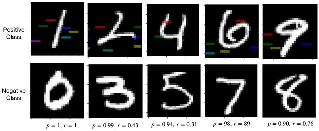<details> <summary>x10.png Details</summary>  ### Visual Description ## Image Classification: Digit Analysis ### Overview The image presents a visual comparison of handwritten digits classified as either "Positive Class" or "Negative Class." Each digit is displayed as a pixelated image on a black background. Above each digit in the "Positive Class" row, there are short, colored horizontal lines. Below each digit, the image includes "p" and "r" values, presumably representing probabilities or scores related to the classification. ### Components/Axes * **Rows:** Two rows labeled "Positive Class" (top) and "Negative Class" (bottom). * **Columns:** Five columns, each displaying a different digit. * **Digits (Positive Class):** 1, 2, 4, 6, 9 * **Digits (Negative Class):** 0, 3, 5, 7, 8 * **Colored Lines:** Short horizontal lines of varying colors (red, green, blue, yellow, cyan, purple) are located above each digit in the "Positive Class" row. The purpose of these lines is not explicitly stated, but they likely represent feature activations or some other form of visual explanation. * **p and r values:** Each digit has two values associated with it, labeled "p" and "r". ### Detailed Analysis or ### Content Details **Positive Class:** * **Digit 1:** p = 1, r = 1. Colored lines above the digit include purple, cyan, yellow, green, blue, and red. * **Digit 2:** p = 0.99, r = 0.43. Colored lines above the digit include cyan, yellow, green, blue, and red. * **Digit 4:** p = 0.94, r = 0.31. Colored lines above the digit include yellow, green, and red. * **Digit 6:** p = 98, r = 89. Colored lines above the digit include cyan, yellow, green, and red. * **Digit 9:** p = 0.90, r = 0.76. Colored lines above the digit include cyan, yellow, green, and red. **Negative Class:** * **Digit 0:** p = 1, r = 1 * **Digit 3:** p = 0.99, r = 0.43 * **Digit 5:** p = 0.94, r = 0.31 * **Digit 7:** p = 98, r = 89 * **Digit 8:** p = 0.90, r = 0.76 ### Key Observations * The "Positive Class" row contains digits 1, 2, 4, 6, and 9, while the "Negative Class" row contains digits 0, 3, 5, 7, and 8. * Each digit in the "Positive Class" row has associated colored lines above it. * Each digit, regardless of class, has "p" and "r" values associated with it. * The "p" values for the positive class are: 1, 0.99, 0.94, 98, 0.90 * The "r" values for the positive class are: 1, 0.43, 0.31, 89, 0.76 * The "p" values for the negative class are: 1, 0.99, 0.94, 98, 0.90 * The "r" values for the negative class are: 1, 0.43, 0.31, 89, 0.76 ### Interpretation The image likely illustrates the performance of a digit classification model. The "Positive Class" and "Negative Class" rows represent the model's predictions or classifications. The colored lines above the digits in the "Positive Class" row may represent feature activations or attention maps, indicating which parts of the image the model focused on when making its prediction. The "p" and "r" values likely represent the probability (p) and recall (r) scores for each digit, providing a quantitative measure of the model's confidence and accuracy. The fact that the p and r values are identical for the positive and negative classes suggests that the model is not performing well, or that the p and r values are not being used effectively. The high "p" value of 98 for digits 6 and 7 is anomalous and may indicate a scaling or formatting error. </details> Figure 6: Rules from MNIST datasets.