2602.13583v1

# Differentiable Rule Induction from Raw Sequence Inputs > Corresponding author. ## Abstract Rule learning-based models are widely used in highly interpretable scenarios due to their transparent structures. Inductive logic programming (ILP), a form of machine learning, induces rules from facts while maintaining interpretability. Differentiable ILP models enhance this process by leveraging neural networks to improve robustness and scalability. However, most differentiable ILP methods rely on symbolic datasets, facing challenges when learning directly from raw data. Specifically, they struggle with explicit label leakage: The inability to map continuous inputs to symbolic variables without explicit supervision of input feature labels. In this work, we address this issue by integrating a self-supervised differentiable clustering model with a novel differentiable ILP model, enabling rule learning from raw data without explicit label leakage. The learned rules effectively describe raw data through its features. We demonstrate that our method intuitively and precisely learns generalized rules from time series and image data. ## 1 Introduction The deep learning models have obtained impressive performances on tabular classification, time series forecasting, image recognition, etc. While in highly trustworthy scenarios such as health care, finance, and policy-making process (Doshi-Velez and Kim, 2017), lacking explanations for decision-making prevents the applications of these complex deep learning models. However, the rule-learning models have interpretability intrinsically to explain the classification process. Inductive logic programming (ILP) is a form of logic-based machine learning that aims to learn logic programs for generalization and interpretability from training examples and background knowledge (Cropper et al., 2022). Traditional ILP methods design deterministic algorithms to induce rules from symbolic data to more generalized formal symbolic first-order languages (Quinlan, 1990; Blockeel and De Raedt, 1998). However, these symbolic ILP methods face robustness and scalability problems when learning from large-scale and ambiguous datasets (Evans et al., 2021; Hocquette et al., 2024). With the sake of robustness of neural networks, the neuro-symbolic ILP by combining neural networks and ILP methods can learn from noisy data (Evans and Grefenstette, 2018; Manhaeve et al., 2018; Gao et al., 2022a) and can be applied to large-scale datasets (Yang et al., 2017; Gao et al., 2024; Phua and Inoue, 2024). However, existing neuro-symbolic ILP methods are mainly learned from discrete symbolic data or fuzzy symbolic data that the likelihoods are generated from a pre-trained neural network module (Evans et al., 2021; Shindo et al., 2023). Learning logic programs from raw data is prevented because of the explicit label leakage problem, which is common in neuro-symbolic research (Topan et al., 2021): The leakage happens by introducing labels of ground objects for inducing rules (Evans and Grefenstette, 2018; Shindo et al., 2023). In fact, generating rules to describe objects in raw data without label information is necessary, especially when some objects are easily overlooked or lack labels yet are important for describing the data. In this study, we introduce Neural Rule Learner (NeurRL), a framework designed to learn logic programs directly from raw sequences, such as time series and flattened image data. Unlike prior approaches prone to explicit label leakage, where input feature labels are extracted using pre-trained supervised neural networks and then processed with differentiable ILP methods to induce rules trained with input labels, our method bypasses the need for supervised pre-trained networks to generate symbolic labels. Instead, we leverage a pre-trained clustering model in an unsupervised manner to discretize data into distinct features. Subsequently, a differentiable clustering module and a differentiable rule-learning module are jointly trained under supervision using raw input labels. This enables the discovery of rules that describe input classes based on feature distributions within the inputs. As a result, the model achieves efficient training in a fully differentiable pipeline while avoiding the explicit label leakage issue. The contributions of this study include: (1) We formally define the ILP learning task from raw inputs based on the interpretation transition setting of ILP. (2) We design a fully differentiable framework for learning symbolic rules from raw sequences, including a novel interpretable rule-learning module with multiple dense layers. (3) We validate the model’s effectiveness and interpretability on various time series and image datasets. ## 2 Related work Inductive logic programming (ILP), introduced by Muggleton and Feng (1990); Muggleton and De Raedt (1994), learns logic programs from symbolic positive and negative examples with background knowledge. Inoue et al. (2014) proposed learning from interpretation transitions, and Phua and Inoue (2021) applied ILP to Boolean networks. Manhaeve et al. (2018); Evans and Grefenstette (2018) adapted neural networks for differentiable and robust ILP, while Gao et al. (2022b) introduced a neural network-based ILP model for learning from interpretation transitions. This model was later extended for scalable learning from knowledge graphs (Gao et al., 2022a; 2024). Similarly, Liu et al. (2024) proposed a deep neural network for inducing mathematical functions. In our work, we present a novel neural network-based model for learning logic programs from raw numeric inputs. In the raw input domain, Evans and Grefenstette (2018) proposed $\partial$ ILP to learn rules from symbolic relational data, using a pre-trained neural network to map raw input data to symbolic labels. Unlike $\partial$ ILP, which enforces a strong language bias by predefining logic templates and limiting the number of atoms, NeurRL uses only predicate types as language bias. Similarly, Evans et al. (2021) used pre-trained networks to map sensory data to disjunctive sequences, followed by binary neural networks to learn rules. Shindo et al. (2023) introduced $\alpha$ ILP, leveraging object recognition models to convert images into symbolic atoms and employing top- $k$ searches to pre-generate clauses, with neural networks optimizing clause weights. Our approach avoids pre-trained large-scale neural networks for mapping raw inputs to symbolic representations. Instead, we propose a fully differentiable framework to learn rules from raw sequences. Additionally, unlike the memory-intensive rule candidate generation required by $\partial$ ILP and $\alpha$ ILP, NeurRL eliminates this step, enhancing scalability. Adapting autoencoder and clustering methods in the neuro-symbolic domain shows promise. Sansone and Manhaeve (2023) applies conventional clustering on input embeddings for deductive logic programming tasks. Misino et al. (2022) and Zhan et al. (2022) use autoencoders and embeddings to calculate probabilities for predefined symbols to complete deductive logic programming and program synthesis tasks. In our approach, we use an autoencoder to learn representations for sub-areas of raw inputs, followed by a differentiable clustering method to assign ground atoms to similar patterns. The differentiable rule-learning module then searches for rule embeddings with these atoms in a bottom-up manner (Cropper and Dumancic, 2022). Similarly, DIFFNAPS (Walter et al., 2024) also uses an autoencoder to build hidden features and explain raw inputs. Additionally, BotCL (Wang et al., 2023) uses attention-based features to explain the ground truth class. However, the logical connections between the features used in DIFFNAPS and BotCL to describe the ground truth class are unclear. In contrast, rule-based explainable models like NeurRL use feature conjunctions to describe the ground truth class. Azzolin et al. (2023) use a post-hoc rule-based explainable model to globally explain raw inputs from local explanations. In contrast, our model directly learns rules from raw inputs, and NeurRL’s performance is unaffected by other explainable models. Das et al. (1998) used clustering to split sequence data into subsequences and symbolize them for rule discovery. Our model combines clustering and rule-learning in a fully differentiable framework to discover rules from sequence and image data, with the rule-learning module providing gradient information to prevent cluster collapse (Sansone, 2023), where very different subsequences are assigned to the same clusters. He et al. (2018) viewed similar subsequences, called motifs, as potential rule bodies. Unlike their approach, we do not limit the number of body atoms in a rule. Wang et al. (2019) introduced SSSL, which uses shapelets as body atoms to learn rules and maximize information gain. Our model extends this by using raw data subsequences as rule body atoms and evaluating rule quality with precision and recall, a feature absent in SSSL. ## 3 Preliminaries ### 3.1 Logic Programs and Inductive Logic Programming A first-order language $\mathcal{L}=(D,F,C,V)$ (Lloyd, 1984) consists of predicates $D$ , function symbols $F$ , constants $C$ , and variables $V$ . A term is a constant, variable, or expression $f(t_{1},\dots,t_{n})$ with $f$ as an $n$ -ary function symbol. An atom is a formula $p(t_{1},\dots,t_{n})$ , where $p$ is an $n$ -ary predicate symbol. A ground atom (fact) has no variables. A literal is an atom or its negation; positive literals are atoms, and negative literals are their negations. A clause is a finite disjunction of literals, and a rule (definite clause) is a clause with one positive literal, e.g., $\alpha_{h}\lor\neg\alpha_{1}\lor\neg\alpha_{2}\lor\dots\lor\neg\alpha_{n}$ . A rule $r$ is written as: $\alpha_{h}\leftarrow\alpha_{1},\alpha_{2},\dots,\alpha_{n}$ , where $\alpha_{h}$ is the head ( $\textnormal{head}(r)$ ), and $\{\alpha_{1},\alpha_{2},\dots,\alpha_{n}\}$ is the body ( $\textnormal{body}(r)$ ), with each atom in the body called a body atom. A logic program $P$ is a set of rules. In first-order logic, a substitution is a finite set $\{v_{1}/t_{1},v_{2}/t_{2},\dots,v_{n}/t_{n}\}$ , where each $v_{i}$ is a variable, $t_{i}$ is a term distinct from $v_{i}$ , and $v_{1},v_{2},\dots,v_{n}$ are distinct (Lloyd, 1984). A ground substitution has all $t_{i}$ as ground terms. The ground instances of all rules in $P$ are denoted as $\textnormal{ground}(P)$ . The Herbrand base $B_{P}$ of a logic program $P$ is the set of all ground atoms with predicate symbols from $P$ , and an interpretation $I$ is a subset of $B_{P}$ containing the true ground atoms (Lloyd, 1984). Given $I$ , the immediate consequence operator $T_{P}\colon 2^{B_{P}}\to 2^{B_{P}}$ for a definite logic program $P$ is defined as: $T_{P}(I)=\{\text{head}(r)\mid r\in\textnormal{ground}(P),\textnormal{body}(r)\subseteq I\}$ (Apt et al., 1988). A logic program $P$ with $m$ rules sharing the same head atom $\alpha_{h}$ is called a same-head logic program. A same-head logic program with $n$ possible body atoms can be represented as a matrix $\mathbf{M}_{P}\in[0,1]^{m\times n}$ . Each element $a_{kj}$ in $\mathbf{M}_{P}$ is defined as follows (Gao et al., 2022a): If the $k$ -th rule is $\alpha_{h}\leftarrow\alpha_{j_{1}}\land\dots\land\alpha_{j_{p}}$ , then $a_{k{j_{i}}}=l_{i}$ , where $l_{i}\in(0,1)$ and $\sum_{s=1}^{p}l_{s}=1\ (1\leq i\leq p,\ 1<p,\ 1\leq j_{i}\leq n,\ 1\leq k\leq m)$ . If the $k$ -th rule is $\alpha_{h}\leftarrow\alpha_{j}$ , then $a_{kj}=1$ . Otherwise, $a_{kj}=0$ . Each row of $\mathbf{M}_{P}$ represents a rule in $P$ , and each column represents a body atom. An interpretation vector $\mathbf{v}_{I}\in\{0,1\}^{n}$ corresponds to an interpretation $I$ , where $\mathbf{v}_{I}[i]=1$ if the $i$ -th ground atom is true in $I$ , and $\mathbf{v}_{I}[i]=0$ otherwise. Given a logic program with $m$ rules and $n$ atoms, along with an interpretation vector $\mathbf{v}_{I}$ , the function $D_{P}:\{0,1\}^{n}\to\{0,1\}^{m}$ (Gao et al., 2024) calculate the Boolean value for the head atom of each rule in $P$ . It is defined as:: $$ \displaystyle D_{P}(\mathbf{v}_{I})=\theta(\mathbf{M}_{P}\mathbf{v}_{I}), \tag{1} $$ where the function $\theta$ is a threshold function: $\theta(x)=1$ if $x\geq 1$ , otherwise $\theta(x)=0$ . For a same-head logic program, the Boolean value of the head atom $v(\alpha_{h})$ is computed as $v(\alpha_{h})=\bigvee_{i=1}^{m}D_{P}(\mathbf{v}_{I})[i]$ . Additionally, Gao et al. (2024) replaces $\theta(x)$ with a differentiable threshold function and use fuzzy disjunction $\tilde{\bigvee}_{i=1}^{m}\mathbf{x}[i]=1-\prod_{i=1}^{m}\mathbf{x}[i]$ to calculate the Boolean value of the head atom in a same-head logic program with neural networks. Inductive logic programming (ILP) aims to induce logic programs from training examples and background knowledge (Muggleton et al., 2012). ILP learning settings include learning from entailments (Evans and Grefenstette, 2018), interpretations (De Raedt and Dehaspe, 1997), proofs (Passerini et al., 2006), and interpretation transitions (Inoue et al., 2014). In this paper, we focus on learning from interpretation transitions: Given a set $E\subseteq 2^{B_{P}}\times 2^{B_{P}}$ of interpretation pairs $(I,J)$ , the goal is to learn a logic program $P$ such that $T_{P}(I)=J$ for all $(I,J)\in E$ . ### 3.2 Sequence data and Differentiable Clustering Method A raw input consists of an instance $(\mathbf{x},\mathbf{y})$ , where $\mathbf{x}\in\mathbb{R}^{T_{1}\times T_{2}\times\dots\times T_{d}}$ represents real-valued observations with $d$ variables, $T_{i}$ indicates the length for $i$ -th variable, and $\mathbf{y}\in\{0,1,\dots,u-1\}$ is the class label, with $u$ classes. A sequence input is a type of raw input where $\mathbf{x}\in\mathbb{R}^{T_{1}}$ is an ordered sequence of real-valued observations (Wang et al., 2019). A subsequence $\mathbf{s}_{i}$ of length $l$ from sequence $\mathbf{x}=(x_{1},x_{2},\dots,x_{T})$ is a contiguous sequence $(x_{i},\dots,x_{i+l-1})$ (Das et al., 1998). All possible subsequence with length $l$ include $\mathbf{s}_{1}$ , …, $\mathbf{s}_{T-l+1}$ . Clustering can be used to discover new categories (Rokach and Maimon, 2005). In the paper, we adapt the differentiable $k$ -means method (Fard et al., 2020) to group raw data $\mathbf{x}\in\mathbf{X}$ . First, an autoencoder $A$ generates embeddings $\mathbf{h}_{\gamma}$ for $\mathbf{x}$ , where $\gamma$ represents the parameters. Then, we set $K$ clusters to discretize all raw data $\mathbf{x}$ . The representation of the $k$ -th cluster is $\mathbf{r}_{k}\in\mathbb{R}^{p}$ , with $p$ as the dimension, and $\mathcal{R}=\{\mathbf{r}_{1},\dots,\mathbf{r}_{K}\}$ as the set of all cluster representations. For any vector $\mathbf{y}\in\mathbb{R}^{p}$ , the function $c_{f}(\mathbf{y};\mathcal{R})$ returns the closest representation based on a fully differentiable distance function $f$ . Then, the differentiable $k$ -means problems are defined as follows: $$ \displaystyle\min_{\mathcal{R},\gamma}\sum_{\mathbf{x}\in\mathbf{X}}f(\mathbf{x},A(\mathbf{x};\gamma))+\lambda\sum_{k=1}^{K}f(\mathbf{h}_{\gamma}(\mathbf{x}),\mathbf{r}_{k})G_{k,f}(\mathbf{h}_{\gamma}(\mathbf{x}),\alpha;\mathcal{R}), \tag{2} $$ where the parameter $\lambda$ regulates the trade-off between seeking good representations for $\mathbf{x}$ and the representations that are useful for clustering. The weight function $G$ is a differentiable minimum function proposed by Jang et al. (2017): $$ \displaystyle G_{k,f}(\mathbf{h}_{\gamma}(\mathbf{x}),\alpha;\mathcal{R})=\frac{e^{-\alpha f(\mathbf{h}_{\gamma}(\mathbf{x}),\mathbf{r}_{k})}}{\sum_{k^{\prime}=1}^{K}e^{-\alpha f(\mathbf{h}_{\gamma}(\mathbf{x}),\mathbf{r}_{k^{\prime}})}}, \tag{3} $$ where $\alpha\in[0,+\infty)$ . A larger value of $\alpha$ causes the approximate minimum function to behave more like a discrete minimum function. Conversely, a smaller $\alpha$ results in a smoother training process We set $\alpha$ to 1000 in the whole experiments.. ## 4 Methods ### 4.1 Problem Statement and formalization In this subsection, we define the learning problem from raw inputs using the interpretation transition setting of ILP and describe the language bias of rules for sequence data. We apply a neuro-symbolic description method from Marconato et al. (2023) to describe a raw input: (i) assume the label $\mathbf{y}$ depends entirely on the state of $K$ symbolic concepts $B=(a_{1},a_{2},\dots,a_{K})$ , which capture high-level aspects of $\mathbf{x}$ , (ii) the concepts $B$ depend intricately on the sub-symbolic input $\mathbf{x}^{\prime}$ and are best extracted using deep learning, (iii) the relationship between $\mathbf{y}$ and $B$ can be specified by prior knowledge $\mathcal{B}$ , requiring reasoning during the forward computing of deep learning models. In this paper, we treat each subset of raw input as a constant and each concept as a ground atom. For example, in sequence data $\mathbf{x}\in\mathbf{X}$ , if a concept increases from the point 0 to 10, the corresponding ground atom is $\texttt{increase}(\mathbf{x}[0:10])$ . We define the body symbolization function $L_{b}$ to convert a continuous sequence $\mathbf{x}$ into discrete symbolic concepts, so that the set of all symbolic concepts $B$ across all raw inputs $\mathbf{X}$ holds $B=L_{b}(\mathbf{X})$ . For binary class raw inputs, we use target atom $h_{t}$ to represents the target class, where $h_{t}$ being true means the instance belongs to the positive class. Then, a head symbolization function $L_{h}$ maps an binary input $\mathbf{x}$ to a set of atoms: if the class of $\mathbf{x}$ is the target class $t$ , then $L_{h}(\mathbf{x})=\{h_{t}\}$ ; otherwise, $L_{h}(\mathbf{x})=\emptyset$ . Hence, a logic program $P$ describing binary class raw inputs consists of rules with the same head atom $h_{t}$ We can transfer multiple class raw inputs to the binary class by setting the class of interest as the target class and the other classes as the negative class.. We define the Herbrand base $B_{P}$ of a logic program as the set of all symbolic concepts $B$ in all raw inputs and the head atom $h_{t}$ . For a raw input $\mathbf{x}$ , $L_{b}(\mathbf{x})$ represents a set of symbolic concepts $I\subseteq B_{P}$ , which can be considered an interpretation. The task of inducing a logic program $P$ from raw inputs based on learning from interpretation transition is defined as follows: **Definition 1 (Learning from Binary Raw Input)** *Given a set of raw binary label inputs $\mathbf{X}$ , learn a same-head logic program $P$ , where $T_{P}(L_{b}(\mathbf{x}))=L_{h}(\mathbf{x})$ holds for all raw inputs $\mathbf{x}\in\mathbf{X}$ .* In the paper, we aim to learn rules to describe the target class with the body consisting of multiple sequence features. Each feature corresponds to a subsequence of the sequence data. Besides, each feature includes the pattern information and region information of the subsequence. Based on the pattern information, we further infer the mean value and tendency information of the subsequence. Using the region predicates, we can apply NeurRL to the dataset, where the temporal relationships between different patterns play a crucial role in distinguishing positive from negative examples. Specifically, we use the following rules to describe the sequence data with the target class: $$ \displaystyle h_{t}\leftarrow pattern_{i_{1}}(X_{j_{1}}),region_{k_{1}}(X_{j_{1}}),\dots,pattern_{i_{n_{1}}}(X_{j_{n_{2}}}),region_{k_{n_{3}}}(X_{j_{n_{2}}}), \tag{4} $$ where the predicate $\texttt{pattern}_{i}$ indicates the $i$ -th pattern in all finite patterns within all sequence data, the predicate $\texttt{region}_{k}$ indicates the $k$ -th region in all regions in a sequence, and the variable $X_{j}$ can be substituted by a subsequence of the sequence data. For example, $\texttt{pattern}_{1}(\mathbf{x}[0:5])$ and $\texttt{region}_{0}(\mathbf{x}[0:5])$ indicate that the subsequence $\mathbf{x}[0:5]$ matches the pattern with index one and belongs to the region with index zero, respectively. A pair of atoms, $\texttt{pattern}_{i}(X)\land\texttt{region}_{k}(X)$ , corresponds to a feature within the sequence data. In this pair, the variables are identical, with one predicate representing a pattern and the other representing a region. We infer the following information from the rules in format (4): In a sequence input $\mathbf{x}$ , if all pairs of ground patterns and regions atoms substituted by subsequences in $\mathbf{x}$ are true, then the sequence input $\mathbf{x}$ belongs to the target class represented by the head atom $h_{t}$ . ### 4.2 Differentiable symbolization process <details> <summary>x1.png Details</summary>  ### Visual Description ## Diagram: Hybrid Autoencoder with Differentiable Clustering and Rule Learning Architecture ### Overview The image displays a technical architecture diagram for a machine learning model that combines an autoencoder with differentiable k-means clustering and a deep rule learning module. The system processes time-series data, learns compressed representations, clusters them, and then extracts interpretable logic programs for prediction. The diagram is divided into two primary sections: an **Encoder-Decoder Autoencoder** (top) and a **Rule Learning Pipeline** (bottom), connected via learned embeddings. ### Components/Axes The diagram is not a chart with axes but a flowchart with labeled components and directional arrows indicating data flow. **Primary Components:** 1. **Encoder:** Processes input data. 2. **Decoder:** Reconstructs the input from the learned representation. 3. **Differentiable k-means:** Clusters the learned embeddings. 4. **Deep rule learning module:** Learns logical rules from cluster assignments and labels. 5. **Legend:** Defines the meaning of colored boxes and arrows. **Legend (Located in the bottom-left corner, enclosed in a dashed box):** * **Blue Arrow:** Labeled "Differentiable path". * **Light Orange Box:** Labeled "Loss for autoencoder (supervised)". * **Light Blue Box:** Labeled "Loss for DeepFOL (supervised)". * **Light Gray Box:** Labeled "Loss for differentiable k-means (unsupervised)". ### Detailed Analysis **1. Encoder-Decoder (Autoencoder) Path:** * **Input (Top-Left):** A light orange box labeled "All subsequences **s** of a series **x**". * **Encoder Flow:** The input passes through a "Dense layer" (white box), then another "Dense layer" (white box), resulting in "Embeddings **z**" (a vertical white box). A dashed vertical line separates the Encoder and Decoder sections. * **Decoder Flow:** The "Embeddings **z**" pass through a "Dense layer" (white box), then another "Dense layer" (white box), leading to the output. * **Output (Top-Right):** A light orange box labeled "Reconstructed subsequences **s'**". * **Loss Connection:** The input and output boxes are colored light orange, corresponding to the "Loss for autoencoder (supervised)" in the legend. **2. Rule Learning Pipeline:** * **Input to Clustering:** A blue arrow labeled "Differentiable k-means" points downward from the "Embeddings **z**" box. * **Clustering Module:** A gray box contains four clusters of colored dots, labeled **r₁** (blue dots), **r₂** (purple dots), **r₃** (green dots), and **r₄** (orange dots). This represents the output of the differentiable k-means algorithm. * **Cluster Assignment Vector:** A blue arrow labeled "**v_I**" points from the clustering box to the next module. * **Deep Rule Learning Module:** A white box labeled "Deep rule learning module". * **Label Input:** A light blue box at the bottom labeled "Label of the series **x**" feeds into the rule learning module via an arrow labeled "**v(h_t)**". * **Outputs of Rule Learning:** * An orange arrow labeled "Extract" points to a light orange box labeled "Logic programs **P**". * A blue arrow labeled "Predict" points to a light blue box labeled "Predicted label". * **Loss Connections:** The "Label of the series **x**" and "Predicted label" boxes are light blue, corresponding to "Loss for DeepFOL (supervised)". The clustering box is light gray, corresponding to "Loss for differentiable k-means (unsupervised)". ### Key Observations 1. **Hybrid Supervised/Unsupervised Learning:** The architecture integrates three distinct loss functions: two supervised (autoencoder reconstruction and final prediction) and one unsupervised (clustering). 2. **End-to-End Differentiability:** The legend explicitly marks a "Differentiable path" (blue arrows), indicating the entire pipeline, including the k-means clustering, is designed to be trained with gradient-based optimization. 3. **Interpretability Focus:** The system's goal extends beyond prediction to extracting "Logic programs **P**", suggesting a focus on creating interpretable models from the learned clusters and rules. 4. **Data Flow Segmentation:** The diagram clearly separates the representation learning phase (autoencoder) from the symbolic rule extraction phase (rule learning module), with the embeddings **z** and cluster assignments **v_I** serving as the bridge. ### Interpretation This diagram illustrates a sophisticated machine learning framework designed for **interpretable time-series analysis**. The autoencoder first learns a compressed, latent representation (**z**) of input subsequences. This representation is then clustered in a differentiable manner, allowing the cluster assignments to be optimized jointly with the rest of the network. The core innovation appears to be the "Deep rule learning module," which takes these soft cluster assignments (**v_I**) and the true series label to learn human-readable logic programs (**P**). The architecture suggests a Peircean investigative approach: it moves from raw data (the series **x**) to a lawful, symbolic representation (the logic programs **P**). The "Predicted label" is a byproduct of this rule-based reasoning. The separation of losses indicates a multi-objective optimization: the model must reconstruct its input well (autoencoder loss), form meaningful clusters (k-means loss), and make accurate, rule-based predictions (DeepFOL loss). The ultimate value of this system lies in its potential to provide **explainable predictions** for time-series data by revealing the underlying logical rules it has discovered, moving beyond black-box predictions. </details> (a) Learning pipeline. <details> <summary>x2.png Details</summary>  ### Visual Description ## Diagram: Hierarchical Fuzzy Logic System ### Overview The image displays a hierarchical tree diagram representing a fuzzy logic inference system. It visually decomposes a complex logical rule into simpler, interconnected components across multiple layers. The system computes an output `h` based on four input variables (`a₁`, `a₂`, `a₃`, `a₄`) through a series of fuzzy conjunction (AND) and disjunction (OR) operations, with associated numerical values likely representing membership degrees or rule strengths. ### Components/Axes The diagram is structured vertically into distinct layers, labeled on the right side from bottom to top: * **Input nodes**: The base layer containing four nodes labeled `a₁`, `a₂`, `a₃`, and `a₄`. * **M₁**: A label for the first set of connections/weights from the input nodes to the first layer. * **First layer**: Contains three nodes representing intermediate fuzzy conjunctions: `a₁ ∧ a₂`, `a₃`, and `a₃ ∧ a₄`. * **M₂**: A label for the second set of connections/weights from the first layer to the second layer. * **Second layer**: Contains two nodes representing higher-level conjunctions: `a₁ ∧ a₂ ∧ a₃` and `a₃ ∧ a₄`. * **Fuzzy disjunction**: The top layer, represented by a single node that combines the outputs of the second layer using a logical OR (∨) operation. **Title/Header**: The overarching logical rule is stated at the top: `h ← (a₁ ∧ a₂ ∧ a₃) ∨ (a₃ ∧ a₄)`. **Connections & Color Coding**: * **Orange lines**: Connect nodes within the lower three layers (Input to First, First to Second). These represent the flow of fuzzy conjunction operations. * **Blue lines**: Connect the two nodes of the Second layer to the top Fuzzy disjunction node. This represents the final fuzzy disjunction (OR) operation. ### Detailed Analysis **1. Input Nodes (Bottom Layer):** * Nodes: `a₁`, `a₂`, `a₃`, `a₄`. * Associated numerical values (likely initial membership degrees or input strengths): * Near `a₁`: `0.58` * Near `a₂`: `0.4` * Near `a₃`: `0.9` * Between `a₃` and `a₄`: `0.45` and `0.5` (These values are positioned along the connections from `a₃` and `a₄` to the `a₃ ∧ a₄` node in the first layer). **2. First Layer (Fuzzy Conjunctions):** * **Node `a₁ ∧ a₂`**: Receives inputs from `a₁` (value `0.58`) and `a₂` (value `0.4`). * **Node `a₃`**: Receives input directly from `a₃` (value `0.9`). * **Node `a₃ ∧ a₄`**: Receives inputs from `a₃` (value `0.45`) and `a₄` (value `0.5`). **3. Second Layer (Higher-Order Conjunctions):** * **Node `a₁ ∧ a₂ ∧ a₃`**: Receives inputs from the `a₁ ∧ a₂` node (connection value `0.58`) and the `a₃` node (connection value `0.4`). * Output values listed below this node: `0.34`, `0.23`, `0.36`. * **Node `a₃ ∧ a₄`**: Receives input from the `a₃ ∧ a₄` node in the first layer (connection value `0.9`). * Output values listed below this node: `0.41`, `0.45`. **4. Top Layer (Fuzzy Disjunction):** * The single node combines the outputs from the two second-layer nodes via blue connection lines. * The logical operation performed here is the OR (∨) of `(a₁ ∧ a₂ ∧ a₃)` and `(a₃ ∧ a₄)` to produce the final output `h`. ### Key Observations 1. **Hierarchical Decomposition**: The diagram clearly breaks down the complex rule `h ← (a₁ ∧ a₂ ∧ a₃) ∨ (a₃ ∧ a₄)` into a computable network of simpler AND operations, culminating in a final OR operation. 2. **Dual Pathways**: There are two distinct pathways to activate the output `h`: * **Pathway 1**: Requires the conjunction of `a₁`, `a₂`, and `a₃`. * **Pathway 2**: Requires the conjunction of `a₃` and `a₄`. * Variable `a₃` is critical, as it is a necessary component in both pathways. 3. **Numerical Flow**: Numerical values are propagated and transformed through the network. The values at the input nodes (`0.58`, `0.4`, `0.9`, `0.45`, `0.5`) are processed through the conjunction nodes, resulting in different output values at the second layer (`0.34, 0.23, 0.36` and `0.41, 0.45`). 4. **Visual Encoding**: The use of orange lines for conjunctions and blue lines for the final disjunction provides a clear visual distinction between the types of logical operations being performed at different stages. ### Interpretation This diagram is a **fuzzy inference system** or a **fuzzy neural network** structure. It models a rule-based decision process where conditions are not simply true or false but have degrees of membership (represented by the numerical values). * **What it demonstrates**: The system shows how to evaluate a compound logical statement (`h`) by computing the truth value of its sub-expressions in a layered, modular fashion. Each node performs a fuzzy AND (typically modeled as a `min` operation) on its inputs, and the top node performs a fuzzy OR (typically a `max` operation). * **Relationship between elements**: The lower layers handle specific, granular conditions (`a₁ AND a₂`, `a₃ AND a₄`). These results are then combined into more general conditions (`a₁ AND a₂ AND a₃`). The top layer makes the final decision by checking if *any* of the high-level conditions is sufficiently true. * **Notable patterns/anomalies**: The presence of multiple numerical values under the second-layer nodes (`0.34, 0.23, 0.36` and `0.41, 0.45`) is interesting. They may represent: * The membership values for each input variable contributing to that node's output. * Different possible output strengths based on different fuzzy inference methods (e.g., product vs. minimum). * The values could also be weights (`M₁`, `M₂`) associated with the connections, though their placement suggests they are node outputs. * **Underlying Meaning**: This structure is used in control systems, decision-making algorithms, and AI to handle uncertainty and imprecise data. It translates human-like, linguistic rules (e.g., "If conditions A, B, and C are true, or if conditions C and D are true, then do H") into a mathematical framework that can process numerical inputs. The specific numerical values would determine the final strength of the output `h` for a given set of inputs `a₁-a₄`. </details> (b) Deep rule-learning module. Figure 1: The learning pipeline of NeurRL and the rule-learning module. In this subsection, we design a differentiable body symbolization function $\tilde{L}_{b}$ , inspired by differentiable $k$ -means (Fard et al., 2020), to transform numeric sequence data $\mathbf{x}$ into a fuzzy interpretation vector $\mathbf{v}_{I}\in[0,1]^{n}$ . This vector encodes fuzzy values of ground patterns and region atoms substituted by input subsequences. A higher value in $\mathbf{v}_{I}[i]$ indicates the $i$ -th atom in the interpretation $I$ is likely true. Using the head symbolization function $J=L_{h}(\mathbf{x})$ , we determine the target atom’s Boolean value $v(h_{t})$ , where $v(h_{t})=1$ if $J=\{h_{t}\}$ and $v(h_{t})=0$ if $J=\emptyset$ . Building on (Gao et al., 2024), we learn a logic program matrix $\mathbf{M}_{P}\in[0,1]^{m\times n}$ such that $\tilde{\bigvee}_{i=1}^{m}D_{P}(\mathbf{v}_{I})[i]=v(h_{t})$ holds. The rules in format (4) are then extracted from $\mathbf{M}_{P}$ , generalized from the most specific clause with all pattern and region predicates. 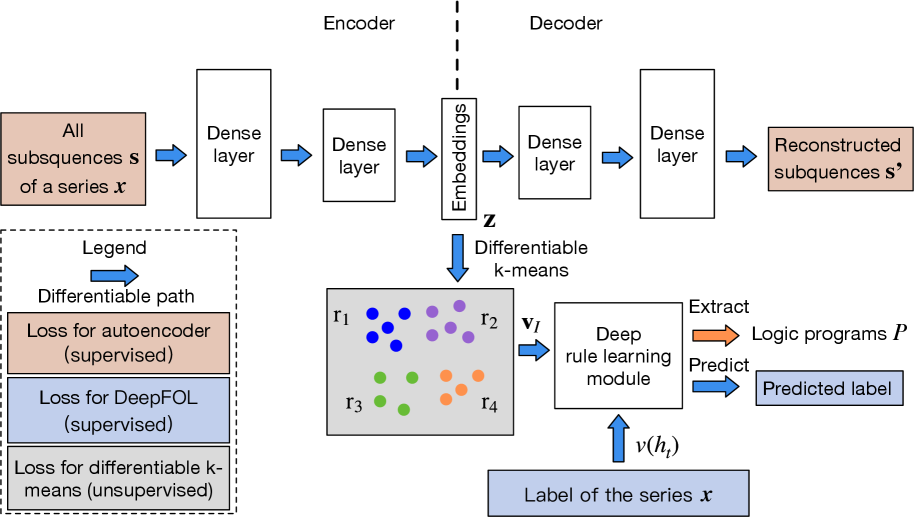The architecture of NeurRL is shown in Fig. 1(a). To learn a logic program $P$ from sequence data, each input sequence $\mathbf{x}$ is divided into shorter subsequences $\mathbf{s}$ of length $l$ with a unit step stride. An encoder maps subsequences $\mathbf{s}$ to an embedding space $\mathbf{z}$ , and a decoder reconstructs $\mathbf{s}^{\prime}$ from $\mathbf{z}$ We use fully connected layers as the encoder and decoder structures.. The differentiable $k$ -means algorithm described in Section 3.2 clusters embeddings $\mathbf{z}$ , grouping subsequences $\mathbf{s}$ with similar patterns into groups $\mathbf{r}$ . This yields fuzzy interpretation vectors $\mathbf{v}_{I}$ and Boolean target atom value $v(h_{t})$ for each sequence. Finally, the differentiable rule-learning module uses $\mathbf{v}_{I}$ as inputs and $v(h_{t})$ as labels to learn high-level rules describing the target class. Now, we describe the method to build the differentiable body symbolization function $\tilde{L}_{b}$ from sequence $\mathbf{x}$ to interpretation vector $\mathbf{v}_{I}$ as follows: Let $K$ be the maximum number of clusters based on the differentiable $k$ -means algorithm, each subsequence $\mathbf{s}$ with the length $l$ in $\mathbf{x}$ and the corresponding embedding $\mathbf{z}$ has a cluster index $c$ $(1\leq c\leq K)$ , and each sequence input $\mathbf{x}$ can be transferred into a vector of cluster indexes $\mathbf{c}\in\{0,1\}^{K\times(\left\lvert\mathbf{x}\right\rvert-l+1)}$ . Additionally, to incorporate temporal or spatial information into the predicates of the target rules, we divide the entire sequence data into $R$ equal regions. The region of a subsequence $\mathbf{s}$ is determined by the location of its first point, $\mathbf{s}[0]$ . For each subsequence $\mathbf{s}$ , we calculate its cluster index vector $\mathbf{c}_{s}\in[0,1]^{K}$ using the weight function $G_{k,f}$ as defined Eq. (2), where $\mathbf{c}_{s}[k]=G_{k,f}(\mathbf{h}_{\gamma}(\mathbf{s}),\alpha;\mathcal{R})$ ( $1\leq k\leq K$ and $\sum_{i=1}^{K}\mathbf{c}_{s}[i]=1$ ). A higher value in the $i$ -th element of $\mathbf{c}_{s}$ indicates that the subsequence $\mathbf{s}$ is more likely to be grouped into the $i$ -th cluster. Hence, we can transfer the sequence input $\mathbf{x}\in\mathbb{R}^{T}$ to cluster index tensor with the possibilities of cluster indexes of subsequences in all regions $\mathbf{c}_{x}\in[0,1]^{K\times l_{p}\times R}$ , where $l_{p}$ is the number of subsequence in one region of input sequence data $\lceil\left\lvert\mathbf{x}\right\rvert/R\rceil$ . To calculate the cluster index possibility of each region, we sum the likelihood of cluster index of all subsequence within one region in cluster index tensor $\mathbf{c}_{x}$ and apply softmax function to build region cluster matrix $\mathbf{c}_{p}\in\mathbb{R}^{K\times R}$ as follows: $$ \displaystyle\mathbf{c}[i,j]=\sum_{k=1}^{l_{p}}\mathbf{c}_{x}[i,k,j],\ \mathbf{c}_{p}[i,j]=\frac{e^{\mathbf{c}[i,j]}}{\sum_{i=1}^{K}e^{\mathbf{c}[i,j]}}. \tag{5} $$ Since the region cluster matrix $\mathbf{c}_{p}$ contains clusters index for each region. Besides, each cluster corresponds to a pattern. Hence, we flatten $\mathbf{c}_{p}$ into a fuzzy interpretation vector $\mathbf{v}_{I}$ , which serves as the input to the deep rule-learning module of NeurRL. ### 4.3 Differentiable rule-learning module In this section, we define the novel deep neural network-based rule-learning module denoted as $N_{R}$ to induce rules from fuzzy interpretation vectors. Based on the label of the sequence input $\mathbf{x}$ , we can determine the Boolean value of target atom $v(h_{t})$ . Then, using fuzzy interpretation vectors $\mathbf{v}_{I}$ as inputs and Boolean values of the head atom $v(h_{t})$ as labels $y$ , we build a novel neural network-based rule-learning module as follows: Firstly, each input node receives the fuzzy value of a pattern or region atom stored in $\mathbf{v}_{I}$ . Secondly, one output node in the final layer reflects the fuzzy values of the head atom. Then, the neural network consists of $k$ dense layers and one disjunction layer. Lastly, let the number of nodes in the $k$ -th dense layer be $m$ , then the forward computation process is formulated as follows: $$ \displaystyle\hat{y}=\tilde{\bigvee}_{i=1}^{m}\left(g_{k}\circ g_{k-1}\circ\dots\circ g_{1}(\mathbf{v}_{I})\right)[i], \tag{6} $$ where the $i$ -th dense layer is defined as: $$ \displaystyle g_{i}(\mathbf{x}_{i-1})=\frac{1}{1-d}\ \text{ReLU}\left({\mathbf{M}}_{i}\mathbf{x}_{i-1}-d\right), \tag{7} $$ with $d$ as the fixed bias In our experiments, we set the fixed bias as 0.5.. The matrix ${\mathbf{M}}_{i}$ is the softmax-activated of trainable weights $\tilde{\mathbf{M}}_{i}\in\mathbb{R}^{n_{\text{out}}\times n_{\text{in}}}$ in $i$ -th dense layer of the rule-learning module: $$ \displaystyle\mathbf{M}_{i}[j,k] \displaystyle=\frac{e^{\tilde{\mathbf{M}}_{i}[j,k]}}{\sum_{u=1}^{n_{\text{in}}}e^{\tilde{\mathbf{M}}_{i}[j,u]}}. \tag{8} $$ With the differentiable body symbolization function $\tilde{L}_{b}$ and $N_{R}$ , we now define a target function that integrates the autoencoder module, clustering module, and rule-learning module as follows: where $\gamma_{e}$ and $\gamma_{l}$ represent the trainable parameters in the encoder and rule-learning module, respectively. The loss function $f_{1}$ and $f_{2}$ are set to mean square error loss and cross-entropy loss correspondingly. The parameters $\lambda_{1}$ and $\lambda_{2}$ regulate the trade-off between finding the concentrated representations of subsequences, the representations of clusters for obtaining precise patterns, and the representations of rules to generalize the data In our experiments, we assigned equal weights to finding representations, identifying clusters, and discovering rules by setting $\lambda_{1}=\lambda_{2}=1$ .. Fig. 1(a) illustrates the loss functions defined in the target function (9). The supervised loss functions are applied to the autoencoder (highlighted in orange boxes) and the rule-learning module (highlighted in blue boxes), respectively. The unsupervised loss function is applied to the differentiable k-means method (highlighted in gray box). 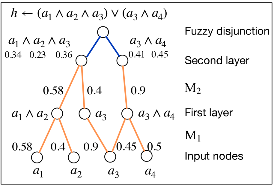We analyze the interpretability of the rule-learning module $N_{R}$ . In the logic program matrix $\mathbf{M}_{P}$ defined in Section 3.1, the sum of non-zero elements in each row, $\sum_{j=1}^{n}\mathbf{M}_{P}[i,j]$ , is normalized to one, matching the threshold in the function $\theta$ in Eq. (1). The conjunction of the atoms corresponding to non-zero elements in each row of $\mathbf{M}_{P}$ can serve as the body of a rule. Similarly, in the rule-learning module of NeurRL, the sum of the softmax-activated weights in each layer is also one. Due to the properties of the activation function $\text{ReLU}(x-d)/(1-d)$ in each node, a node activates only when the sum of the weights approaches one; otherwise, it deactivates. This behavior mimics the threshold function $\theta$ in Eq. (1). Similar to the logic program matrix $\mathbf{M}_{P}$ , the softmax-activated weights in each layer also have interpretability. When the fuzzy interpretation vector and Boolean value of the target atom fit the forward process in Eq. (6), the atoms corresponding to non-zero elements in each row of the $i$ -th dense softmax-activated weight matrix $\mathbf{M}_{i}$ form a conjunction. From a neural network perspective, the $j$ -th node in the $i$ -th dense layer, denoted as $n_{j}^{i}$ , represents a conjunction of atoms from the previous $(i-1)$ -th dense layer (input layer). The likelihood of these atoms appearing in the conjunction is determined by the softmax-activated weights $\mathbf{M}_{i}[j,:]$ connecting to node $n_{j}^{i}$ . In the final $k$ -th dense layer, the disjunction layer computes the probability of the target atom $h_{t}$ . The higher likelihood conjunctions, represented by the nodes in the final $k$ -th layer, form the body of the rule headed by $h_{t}$ . To interpret the rules headed by $h_{t}$ , we compute the product of all softmax-activated weights $\mathbf{M}_{i}$ as the program tensor: $\mathbf{M}_{P}=\prod_{i=1}^{k}\mathbf{M}_{i}$ , where $\mathbf{M}_{P}\in[0,1]^{m\times n}$ . The program tensor has the same interpretability as the program matrix, with high-value atoms in each row forming the rule body and the target atom as the rule head. The number of nodes in the last dense layer $m$ determines the number of learned rules in one learning epoch. Fig. 1(b) shows a neural network with two dense layers and one disjunction layer in blue. The weights in orange represent significant softmax-activated values, with input nodes as atoms and hidden nodes as conjunctions. Multiplying the softmax weights identifies the atoms forming the body of a rule headed by the target atom. We use the following method to extract rules from program tensor $\mathbf{M}_{P}$ : We set multiple thresholds $\tau\in[0,1]$ . When the value of the element in a row of $\mathbf{M}_{P}$ is larger than a threshold $\tau$ , then we regard the atom corresponding to these elements as the body atom in a rule with the format (4). We compute the precision and recall of the rules based on the discretized fuzzy interpretation vectors generated from the test dataset. The discretized fuzzy interpretation vector is derived as the flattened version of $\bar{\mathbf{c}}_{p}[i,j]=\mathbbm{1}(\mathbf{c}_{p}[i,j]=\max_{k}\mathbf{c}_{p}[k,j])$ , where $\max_{k}\mathbf{c}_{p}[k,j]$ represents the maximum value in the $j$ -th column of $\mathbf{c}_{p}$ . Then, we keep the high-precision rules as the output. The precision and recall of a rule are defined as: $\text{precision}={n_{\text{body $\land$ head}}}/{n_{\text{body}}}$ and $\text{recall}={n_{\text{body $\land$ head}}}/n_{\text{head}}$ , where $n_{\text{body $\land$ head}}$ denotes the number of discretized fuzzy interpretation vectors $\mathbf{v}_{I}$ that satisfy the rule body and have the target class as the label. Similarly, $n_{\text{body}}$ represents the number of discretized fuzzy interpretation vectors that satisfy the rule body, while $n_{\text{head}}$ refers to the number of instances with the target class. When obtaining rules in the format (4), we can highlight the subsequences satisfying the pattern and region predicates above on the raw inputs for more intuitive interpretability. To train the model, we first pre-train an autoencoder to obtain subsequence embeddings, then initialize the cluster embeddings using $k$ -means clustering (Lloyd, 1982) based on these embeddings. Finally, we jointly train the autoencoder, clustering model, and rule-learning model using the target function (9) to optimize the embeddings, clusters, and rules simultaneously. ## 5 Experimental results <details> <summary>x3.png Details</summary>  ### Visual Description \n ## Line Chart: Hypothesis Function Evaluation Over Time ### Overview The image displays a line chart plotting two data series, labeled "Positive" and "Negative," against a sequence of time points. The chart is titled with a mathematical expression suggesting it visualizes the output of a logical hypothesis function. The two series exhibit a clear inverse relationship over the observed period. ### Components/Axes * **Title:** Located at the top center. Text: `h_p ← pattern_0(X) ∧ region_1(X) (p = 1, r = 1)`. This is a logical expression where `∧` denotes "AND". It defines a hypothesis `h_p` as the conjunction of `pattern_0(X)` and `region_1(X)`, with parameters `p=1` and `r=1`. * **Y-Axis:** Labeled "Value" on the left side. Scale ranges from 0.0 to 1.0, with major tick marks at 0.0, 0.2, 0.4, 0.6, 0.8, and 1.0. * **X-Axis:** Labeled "Time points" at the bottom. Scale shows integer markers from 0 to 14, with labeled ticks at 0, 2, 4, 6, 8, 10, 12, and 14. * **Legend:** Positioned in the center-right area of the plot. It contains two entries: * A blue line segment labeled "Positive". * An orange line segment labeled "Negative". * **Data Series:** * **Positive (Blue Line):** A smooth, continuous line. * **Negative (Orange Line):** A smooth, continuous line. ### Detailed Analysis **Positive Series (Blue Line) Trend & Approximate Data Points:** The line starts near the minimum value, rises to a peak, falls to a trough, and then rises sharply again. * Time 0: Value ≈ 0.0 * Time 4: Value ≈ 0.95 (Peak) * Time 10: Value ≈ 0.05 (Trough) * Time 14: Value ≈ 1.0 (Final point, highest value) **Negative Series (Orange Line) Trend & Approximate Data Points:** The line starts near the maximum value, falls to a trough, rises to a peak, and then falls sharply again. Its movement is the inverse of the Positive series. * Time 0: Value ≈ 0.95 * Time 4: Value ≈ 0.05 (Trough) * Time 10: Value ≈ 0.95 (Peak) * Time 14: Value ≈ 0.05 (Final point) **Relationship:** The two lines are near-perfect mirror images of each other across the horizontal midline (Value ≈ 0.5). When one is high, the other is low. ### Key Observations 1. **Inverse Correlation:** The most prominent pattern is the strong inverse relationship between the "Positive" and "Negative" values. Their peaks and troughs align at the same time points (4, 10, 14) but with opposite magnitudes. 2. **Cyclic Behavior:** Both series exhibit a cyclic pattern over the 14 time points, completing roughly one full cycle (high-to-low-to-high for Positive, low-to-high-to-low for Negative). 3. **Symmetry:** The chart is highly symmetric. The value of one series at any given time point appears to be approximately `1 - (value of the other series)`. 4. **Mathematical Context:** The title indicates this is not arbitrary data but a visualization of a specific logical function (`pattern_0 AND region_1`) being evaluated over time or across samples (`X`). ### Interpretation This chart likely illustrates the output of a binary classifier or a logical rule applied to a dataset over time. The "Positive" and "Negative" labels probably refer to the confidence, probability, or activation level of two complementary conditions or classes. * **What the data suggests:** The function `h_p` produces outputs where the "Positive" and "Negative" components are mutually exclusive and exhaustive. When the condition for "Positive" is strongly met (value ~1), the condition for "Negative" is not met (value ~0), and vice versa. This is characteristic of a system modeling a clear dichotomy. * **How elements relate:** The title defines the rule, and the chart shows its dynamic application. The parameters `(p=1, r=1)` might control the sensitivity or scope of the `pattern` and `region` components of the rule. * **Notable anomalies:** There are no apparent outliers; the data follows a very clean, smooth, and intentional pattern. This suggests the chart is likely a theoretical demonstration or the result of a controlled simulation rather than noisy empirical data. * **Underlying meaning:** The visualization demonstrates the successful implementation of the logical conjunction (`∧`). The inverse relationship confirms that the two conditions (`pattern_0` and `region_1`) are being combined correctly to produce a single, decisive hypothesis output that flips between two states over the evaluated sequence. </details> (a) The signals based on triangular pulse. <details> <summary>x4.png Details</summary>  ### Visual Description \n ## Line Chart: Pattern and Region Logical Operation ### Overview The image displays a line chart plotting two primary data series ("Positive" and "Negative") over a series of time points. A third, unlabeled line in a pinkish-red color appears in the latter portion of the chart. The chart's title is a formal logical expression, suggesting it originates from a technical or academic context, likely related to pattern recognition, signal processing, or formal logic. ### Components/Axes * **Title:** `h_p ← pattern_0(X) ∧ region_2(X) (p = 1, r = 1)` * This is a logical assignment statement. `h_p` is assigned the result of a logical AND (`∧`) between `pattern_0(X)` and `region_2(X)`. Parameters `p` and `r` are both set to 1. * **Y-Axis:** * **Label:** "Value" * **Scale:** Linear, ranging from 0.0 to 1.0. * **Ticks:** 0.0, 0.2, 0.4, 0.6, 0.8, 1.0. * **X-Axis:** * **Label:** "Time points" * **Scale:** Linear, integer steps. * **Ticks:** 0, 2, 4, 6, 8, 10, 12, 14. * **Legend:** * **Position:** Top-left corner of the chart area. * **Entries:** * **Blue Line:** "Positive" * **Orange Line:** "Negative" * **Data Series:** 1. **Positive (Blue Line):** A continuous line. 2. **Negative (Orange Line):** A continuous line. 3. **Unlabeled (Pinkish-Red Line):** A line that appears to start at Time point 10 and continues to Time point 14. It is not identified in the legend. ### Detailed Analysis **Trend Verification & Data Point Extraction:** * **Positive (Blue) Series Trend:** The line exhibits a wave-like pattern with two peaks and a trough. It starts mid-range, rises to a peak, falls to a minimum, rises to a second peak, and then declines. * Time 0: ~0.5 * Time 2: ~0.95 (First Peak) * Time 6: ~0.05 (Trough) * Time 10: ~0.95 (Second Peak) * Time 14: ~0.1 * **Negative (Orange) Series Trend:** This line shows an inverse wave-like pattern relative to the Positive line. It starts lower, dips to a minimum, rises to a peak, falls to a minimum, and then rises sharply. * Time 0: ~0.4 * Time 2: ~0.0 (Minimum) * Time 6: ~0.95 (Peak) * Time 10: ~0.0 (Minimum) * Time 14: ~0.95 * **Unlabeled (Pinkish-Red) Series Trend:** This line appears to diverge from the Positive (Blue) line at its second peak. * Time 10: ~0.95 (appears to share the same point as the Blue line) * Time 12: ~0.4 * Time 14: ~0.05 **Spatial Grounding:** The legend is anchored in the top-left quadrant of the plot area. The two main data series (Blue/Positive and Orange/Negative) are present across the entire x-axis. The unlabeled Pinkish-Red line is confined to the rightmost segment of the chart, from x=10 to x=14. ### Key Observations 1. **Inverse Correlation:** The "Positive" and "Negative" series are strongly inversely correlated. When one is near its maximum (~1.0), the other is near its minimum (~0.0), and vice-versa. Their peaks and troughs are perfectly staggered. 2. **Symmetry:** The patterns are roughly symmetrical around the midpoint of the time axis (around Time point 7-8). 3. **Unlabeled Element:** The presence of the third, pinkish-red line is a significant anomaly. It is not defined in the legend, creating ambiguity. It visually splits from the Positive line at Time point 10 and follows a steep downward trajectory. 4. **Mathematical Context:** The title implies the plotted values represent the output (`h_p`) of a logical operation between a pattern detector and a region detector over time. The "Positive" and "Negative" labels may refer to the truth value or activation strength of this operation under different conditions. ### Interpretation This chart likely visualizes the output of a computational model or logical system over discrete time steps. The core insight is the demonstration of a perfect or near-perfect inverse relationship between two states or conditions labeled "Positive" and "Negative." This could represent: * The activation of two mutually exclusive rules or patterns. * The confidence scores for two opposing classifications. * The result of a logical function where one input (`pattern_0`) and another (`region_2`) oscillate in opposition. The unlabeled pinkish-red line is critical. Its divergence from the "Positive" line at Time point 10 suggests a **point of intervention, a fault, or the introduction of a new variable**. It may represent: * A "ground truth" or reference signal that the "Positive" line was following until t=10. * The output of a modified version of the system (e.g., with a different parameter `r`). * An error signal or a different logical operation taking precedence. The chart's primary message is not just the inverse relationship, but the **event at Time point 10** that causes a divergence, highlighting a change in the system's behavior or a comparison between two different system responses. The formal title grounds this in a framework of logical pattern-region conjunction, making it a technical diagnostic or result plot from a research experiment. </details> (b) The signals based on trigonometry function. Figure 2: The synthetic data and the learned rules. 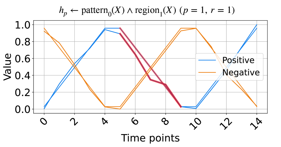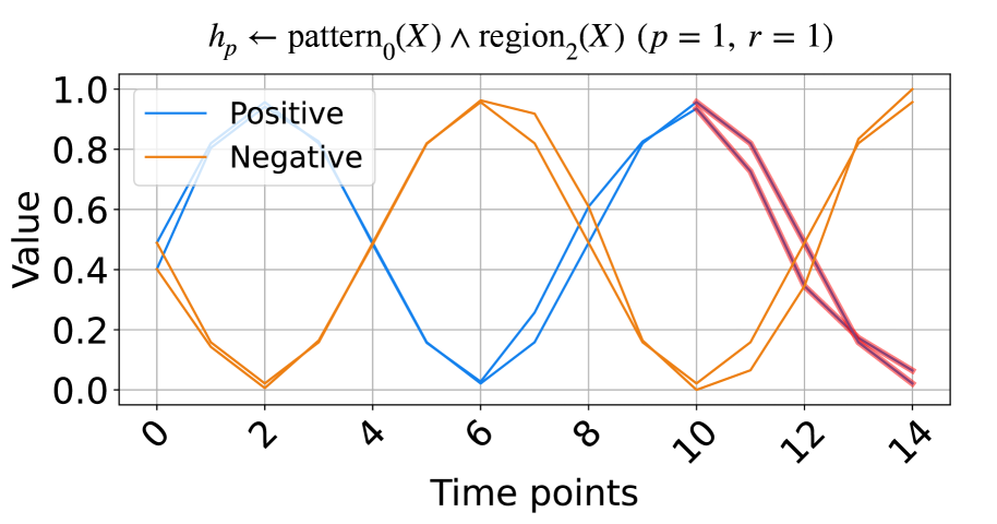### 5.1 Learning from synthetic data In this subsection, we evaluate the model on synthetic time series data based on triangular pulse signals and trigonometric signals. Each signal contains two key patterns, increasing and decreasing, with each pattern having a length of five units. To test NeurRL’s learning capability on a smaller dataset, we set the number of inputs in both the positive and negative classes to two for both the training and test datasets. In each class, the difference between two inputs at each time point is a random number drawn from a normal distribution with a mean of zero and a variance of 0.1. The positive test inputs are plotted in blue, and the negative test inputs in orange in Fig. 2. We set both the length of each region and the subsequence length to five units, and the number of clusters is set to three in this experiment. NeurRL is tasked with learning rules to describe the positive class, represented by the head atom $h_{p}$ . If the ground body atoms, substituted by subsequences of an input, hold true, the head atom $h_{p}$ is also true, indicating that the target class of the input is positive. The rules with 1.0 precision ( $p$ ) and 1.0 recall ( $r$ ) are shown in Fig. 2. The rule in Fig. 2(a) states that when $\texttt{pattern}_{0}$ (cluster index 0) appears in $\texttt{region}_{1}$ (from time points 5 to 9), the time series label is positive. Similarly, the rule in Fig. 2(b) indicates that when $\texttt{pattern}_{0}$ appears in $\texttt{region}_{2}$ (from time points 10 to 14), the label is positive. We highlight subsequences that satisfy the rule body in red in Fig. 2, inferring that the $\texttt{pattern}_{0}$ indicates decreasing. These red patterns perfectly distinguish positive from negative inputs. ### 5.2 Learning from UCR datasets <details> <summary>x5.png Details</summary>  ### Visual Description ## Line Chart: Pattern-Region Hypothesis Performance Over Time ### Overview The image displays a line chart plotting multiple time-series data series against a "Value" metric over "Time points." The chart is titled with a logical hypothesis expression and associated statistical performance metrics. It compares two primary categories, "Positive" and "Negative," each represented by multiple individual lines, suggesting multiple trials or samples per category. Two distinct clusters of data points, colored red and green, are overlaid on the main lines in the early-to-mid time range. ### Components/Axes * **Title/Header:** Located at the top center. Text: `hₚ ← pattern₂(X) ∧ region₁(X) ∧ pattern₁(Y) ∧ region₂(Y) (p = 0.83, r = 0.89)`. This appears to define a hypothesis (`hₚ`) as a logical conjunction of patterns and regions for variables X and Y, with a p-value of 0.83 and a correlation coefficient (r) of 0.89. * **Y-Axis:** Labeled "Value" (vertical text, left side). Scale ranges from 0.0 to 0.8 with major tick marks at 0.0, 0.2, 0.4, 0.6, and 0.8. * **X-Axis:** Labeled "Time points" (bottom center). Scale ranges from 0 to approximately 90, with major labeled tick marks at 0, 20, 40, 60, and 80. * **Legend:** Positioned in the top-center area of the plot, inside the axes. It contains two entries: * A solid blue line labeled "Positive". * A dashed orange line labeled "Negative". * **Data Series:** * **Positive (Solid Blue Lines):** Multiple (approximately 8-10) solid blue lines. They generally start at high values (0.6-0.8+) at Time point 0, show a sharp decline to a trough between Time points 15-25 (values ~0.1-0.3), then recover and stabilize in the 0.4-0.6 range for the remainder of the timeline, with a notable spike near Time point 90. * **Negative (Dashed Orange Lines):** Multiple (approximately 8-10) dashed orange lines. They exhibit higher volatility. Many start lower than the Positive lines, dip to very low values (near 0.0) around Time point 15, then rise sharply. They fluctuate significantly in the middle range (Time points 20-70) and show a dramatic, synchronized spike to high values (0.7-0.9) near Time point 90 before dropping again. * **Overlaid Clusters:** * **Red Cluster:** A dense grouping of red data points or short line segments located approximately between Time points 15-25 and Value 0.1-0.3. This cluster overlaps with the trough region of many lines. * **Green Cluster:** A dense grouping of green data points or short line segments located approximately between Time points 30-40 and Value 0.2-0.5. This cluster is positioned on the rising slope following the initial trough. ### Detailed Analysis * **Trend Verification - Positive (Blue) Series:** The general trend for the Positive series is a "U" or "check mark" shape: high initial value, a pronounced dip in the first quarter of the timeline, followed by a recovery and a relatively stable plateau with minor fluctuations, ending with a late spike. * **Trend Verification - Negative (Orange) Series:** The Negative series trend is more complex and volatile. It shows an initial decline to a deep minimum, a sharp rebound, a period of high variance and oscillation in the middle, culminating in a very sharp, collective peak near the end of the observed time range. * **Spatial Grounding of Clusters:** The red cluster is situated in the lower-left quadrant of the main data area, precisely where both Positive and Negative series reach their lowest values. The green cluster is positioned to the right of the red cluster, along the upward trajectory where values are increasing from the trough. * **Statistical Annotation:** The title provides key metrics: `p = 0.83` (suggesting a non-significant p-value if this is a statistical test) and `r = 0.89` (indicating a strong positive correlation). ### Key Observations 1. **Divergent Early Behavior:** Positive and Negative series show their most distinct separation in the initial phase (Time 0-15), with Positive starting much higher. 2. **Convergent Trough:** Both series converge to their lowest values in the Time 15-25 window, which is also where the red cluster is located. 3. **Mid-Chart Volatility:** The Negative series exhibits substantially more noise and fluctuation between Time points 20 and 70 compared to the smoother Positive series. 4. **Synchronized Late Spike:** A striking feature is the near-simultaneous sharp peak in almost all Negative series lines and some Positive lines around Time point 90. 5. **Cluster Significance:** The red and green clusters highlight specific temporal regions (early trough and subsequent rise) that are likely critical to the hypothesis being tested, as indicated by the title. ### Interpretation This chart visualizes the temporal dynamics of a model or system's output ("Value") under conditions hypothesized to be "Positive" or "Negative." The title suggests the chart evaluates a specific, complex hypothesis (`hₚ`) involving the conjunction of patterns and regions across two variables (X and Y). The data demonstrates that the "Positive" condition leads to a more stable and predictable recovery after an initial drop, while the "Negative" condition is associated with high instability and a dramatic, late-stage anomaly (the spike). The strong correlation (`r=0.89`) noted in the title may refer to the relationship between the hypothesized conditions and the observed value trajectories, despite the high p-value (`p=0.83`) which might indicate the observed pattern could occur by chance under a null hypothesis, or relates to a different statistical test. The red and green clusters likely mark algorithmically identified "regions of interest" (`region₁` and `region₂` from the title) where specific patterns (`pattern₁`, `pattern₂`) are detected. Their placement in the trough and recovery phases suggests these are the critical periods where the logical conditions of the hypothesis are most active or discriminative. The chart ultimately suggests that the defined hypothesis `hₚ` captures a meaningful temporal signature that differentiates the two conditions, particularly in the early dip and the mid-chart volatility, with the late spike being a notable, possibly anomalous, event. </details> (a) A rule from ECG dataset. <details> <summary>x6.png Details</summary>  ### Visual Description ## Line Chart: Pattern and Region Analysis Over Time ### Overview The image displays a line chart comparing two categories of data series—"Positive" and "Negative"—over a sequence of time points. The chart includes a mathematical title, a legend, labeled axes with grid lines, and multiple data lines for each category. A distinct red marker highlights a specific data point. ### Components/Axes * **Title (Top Center):** `$h_p \leftarrow \text{pattern}_0(X) \land \text{region}_6(X) \ (p = 0.99, r = 0.90)$` * This is a mathematical/logical expression. The notation suggests a hypothesis (`h_p`) is derived from the conjunction of `pattern_0(X)` and `region_6(X)`, with associated statistical values: a p-value (`p`) of 0.99 and a correlation coefficient (`r`) of 0.90. * **Legend (Top-Left Corner):** * **Positive:** Represented by a solid blue line. * **Negative:** Represented by a dashed orange line. * **Y-Axis (Left Side):** * **Label:** "Value" * **Scale:** Linear, ranging from 0.1 to 0.8. * **Major Tick Marks:** 0.1, 0.2, 0.3, 0.4, 0.5, 0.6, 0.7, 0.8. * **X-Axis (Bottom):** * **Label:** "Time points" * **Scale:** Linear, ranging from 0 to 20. * **Major Tick Marks:** 0, 5, 10, 15, 20. * **Data Series:** The chart contains multiple lines for each category (approximately 8-10 blue solid lines and 8-10 orange dashed lines), indicating multiple samples or trials for both "Positive" and "Negative" conditions. * **Highlighted Point (Approx. Coordinates: Time=18, Value=0.45):** A red, star-shaped marker is placed on one of the blue solid lines in the lower-right quadrant of the chart. ### Detailed Analysis **Trend Verification & Data Point Extraction:** * **General Trend for Both Series:** All lines begin in a cluster between Values 0.2 and 0.5 at Time point 0. They generally trend downward to a minimum around Time points 4-6 (Values ~0.1-0.25), then rise sharply to a peak or plateau between Time points 8-12 (Values ~0.5-0.7). After Time point 12, the series exhibit more volatility and divergence. * **"Positive" (Blue Solid Lines) Trend:** After the plateau (~Time 8-12), the blue lines show significant spread. Some lines dip around Time 14-16 (to ~0.3-0.4) before rising sharply again, with several reaching the highest values on the chart (peaking between 0.7 and 0.8+ near Time 20). The overall late-stage trend (Time 15-20) is upward for many blue lines, but with high variance. * **"Negative" (Orange Dashed Lines) Trend:** The orange lines also plateau around Time 8-12. Afterward, they remain more tightly clustered than the blue lines, generally fluctuating between Values 0.4 and 0.7 through Time point 20. Their late-stage trend is more horizontal or slightly declining compared to the rising blue lines. * **Key Data Points (Approximate):** * **Start (Time 0):** Blue lines range ~0.25-0.55. Orange lines range ~0.2-0.4. * **First Trough (Time ~5):** Blue lines range ~0.1-0.25. Orange lines range ~0.15-0.25. * **First Peak (Time ~10):** Blue lines cluster ~0.55-0.65. Orange lines cluster ~0.5-0.65. * **Divergence Zone (Time 15-20):** Blue lines spread widely from ~0.3 to >0.8. Orange lines are concentrated ~0.4-0.7. * **Highlighted Red Star:** Located at approximately Time point 18, Value 0.45, on a blue line that is in the lower portion of the blue cluster at that time. ### Key Observations 1. **High Correlation & Significance:** The title's `p = 0.99` and `r = 0.90` suggest the relationship between the pattern/region and the observed data is statistically very strong and highly correlated. 2. **Synchronized Early Behavior:** Both "Positive" and "Negative" series follow a very similar pattern of decline and recovery for the first half of the timeline (Time 0-12), suggesting a common underlying process or stimulus. 3. **Late-Stage Divergence:** The primary difference between the categories emerges after Time point 12-15. The "Positive" series exhibits greater volatility and a tendency for some samples to reach much higher values, while the "Negative" series remains more stable and bounded. 4. **Outlier/Event Marker:** The red star at (18, 0.45) singles out a specific data point on a "Positive" line. Its placement in a relatively low-value region for that time point, amidst rising blue lines, may indicate an anomaly, a critical event, or a point of interest for failure/analysis. ### Interpretation This chart likely visualizes the output of a model or experiment testing a hypothesis (`h_p`) related to a specific pattern (`pattern_0`) within a defined region (`region_6`) of input data `X`. The high `r` value (0.90) indicates that the model's predictions or the measured phenomenon strongly align with the actual data. The data suggests that the conditions labeled "Positive" and "Negative" are not distinctly different in their initial response (Time 0-12). The critical differentiating factor manifests in the later phase (Time >15), where the "Positive" condition allows for or triggers a much wider range of outcomes, including significantly higher "Value" scores. The "Negative" condition appears to constrain the system, preventing extreme high values. The red star likely marks a point of investigation—perhaps a sample that behaved unexpectedly (a "Positive" case that yielded a low value late in the sequence) or a timestamp where a specific intervention occurred. The overall narrative is of two processes that start similarly but bifurcate in their potential and stability over time, with the "Positive" class showing greater expressive range or susceptibility to high-value outcomes. </details> (b) A rule from ItalyPow.Dem. dataset. Figure 3: Selected rules from two UCR datasets. In this subsection, we experimentally demonstrate the effectiveness of NeurRL on 13 randomly selected datasets from UCR (Dau et al., 2019), as used by Wang et al. (2019). To evaluate NeurRL’s performance, we consider the classification accuracy from the rules extracted by the deep rule-learning module (denoted as NeurRL(R)) and the classification accuracy from the module itself (denoted as NeurRL(N)). The number of clusters in this experiment is set to five. The subsequence length and the number of regions vary for each task. We set the number of regions to approximately 10 for time series data. Additionally, the subsequence length is set to range from two to five, depending on the specific subtask. The baseline models include SSSL (Wang et al., 2019), Xu (Xu and Funaya, 2015), and BoW (Wang et al., 2013). SSSL uses regularized least squares, shapelet regularization, spectral analysis, and pseudo-labeling to auto-learn discriminative shapelets from time series data. Xu’s method constructs a graph to derive underlying structures of time series data in a semi-supervised way. BoW generates a bag-of-words representation for time series and uses SVM for classification. Statistical details, such as the number of classes (C.), inputs (I.), series length, and comparison results are shown in Tab. 1, with the best results in bold and second-best underlined. The NeurRL(N) achieves the most best results, with seven, and NeurRL(R) achieves five second-best results. Table 1: Classification accuracy on 13 binary UCR datasets with different models. | Coffee | 2 | 56 | 286 | 0.588 | 0.620 | 0.792 | 0.964 | 1.000 | | --- | --- | --- | --- | --- | --- | --- | --- | --- | | ECG | 2 | 200 | 96 | 0.819 | 0.955 | 0.793 | 0.820 | 0.880 | | Gun point | 2 | 200 | 150 | 0.729 | 0.925 | 0.824 | 0.760 | 0.873 | | ItalyPow.Dem. | 2 | 1096 | 24 | 0.772 | 0.813 | 0.941 | 0.926 | 0.923 | | Lighting2 | 2 | 121 | 637 | 0.698 | 0.721 | 0.813 | 0.689 | 0.748 | | CBF | 3 | 930 | 128 | 0.921 | 0.873 | 1.000 | 0.909 | 0.930 | | Face four | 4 | 112 | 350 | 0.833 | 0.744 | 0.851 | 0.914 | 0.964 | | Lighting7 | 7 | 143 | 319 | 0.511 | 0.677 | 0.796 | 0.737 | 0.878 | | OSU leaf | 6 | 442 | 427 | 0.642 | 0.685 | 0.835 | 0.844 | 0.849 | | Trace | 4 | 200 | 275 | 0.788 | 1.00 | 1.00 | 0.833 | 0.905 | | WordsSyn | 25 | 905 | 270 | 0.639 | 0.795 | 0.875 | 0.932 | 0.946 | | OliverOil | 4 | 60 | 570 | 0.639 | 0.766 | 0.776 | 0.768 | 0.866 | | StarLightCurves | 3 | 9236 | 2014 | 0.755 | 0.851 | 0.872 | 0.869 | 0.907 | | Mean accuracy | | | | 0.718 | 0.801 | 0.859 | 0.842 | 0.891 | 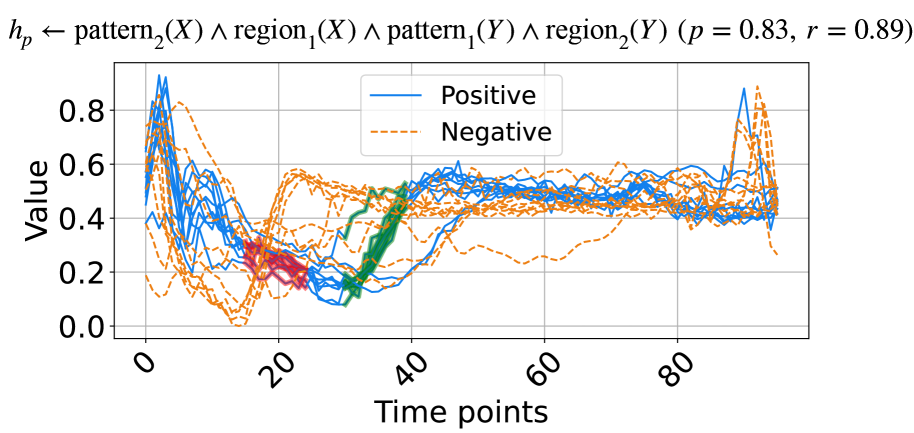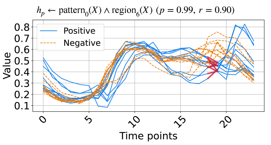The learned rules from the ECG and ItalyPow.Dem. datasets in the UCR archive are shown in Fig. 3. In Fig. 3(a), red highlights subsequences with the shape $\texttt{pattern}_{2}$ in the region $\texttt{region}_{1}$ , while green highlights subsequences with the shape $\texttt{pattern}_{1}$ in the region $\texttt{region}_{2}$ . The rule suggests that when data decreases between time points 15 to 25 and then increases between time points 30 to 40, the input likely belongs to the positive class. The precision and recall for this rule are 0.83 and 0.89, respectively. In Fig. 3(b), red highlights subsequences with the shape $\texttt{pattern}_{0}$ in the region $\texttt{region}_{6}$ . The rule indicates that a lower value around time points 18 to 19 suggests the input belongs to the positive class, with precision and recall of 0.99 and 0.90, respectively. <details> <summary>x7.png Details</summary>  ### Visual Description ## Diagram: Binary Classification Representation ### Overview The image is a conceptual diagram illustrating two distinct classes in a binary classification problem. It visually contrasts the spatial distribution of data points belonging to a "positive class" versus a "negative class." The diagram includes a performance metric at the bottom. ### Components/Axes The image is divided into two primary panels side-by-side on a black background, with a line of text centered below them. 1. **Left Panel (Positive Class):** * **Visual Element:** A thick, white diagonal line runs from the bottom-left to the top-right. Intersecting this line are several short, horizontal colored bars. * **Colors Observed (from top to bottom):** Red, Green, Blue, Purple. * **Label:** The text "positive class" is centered directly below this panel. 2. **Right Panel (Negative Class):** * **Visual Element:** A thick, white, irregular ring or oval shape with a black center. The shape is not a perfect circle and has a slightly jagged or pixelated edge. * **Label:** The text "negative class" is centered directly below this panel. 3. **Bottom Text:** * **Content:** The mathematical notation `p = 1, r = 1` is centered at the very bottom of the entire image, beneath both class labels. ### Detailed Analysis * **Positive Class Representation:** The data points (represented by colored bars) are arranged linearly along a clear diagonal decision boundary (the white line). This suggests a feature space where the positive class is linearly separable. The different colors (red, green, blue, purple) may represent different sub-categories, features, or instances within the positive class, but no legend is provided to define them. * **Negative Class Representation:** The data forms a continuous, ring-like cluster. This represents a non-linear distribution where the negative class occupies a region surrounding a central void. This is a classic example of data that is not linearly separable from a central point. * **Performance Metric:** The text `p = 1, r = 1` is standard notation for **Precision (p)** and **Recall (r)**. A value of 1 for both indicates perfect classification performance on a given dataset: no false positives (Precision = 1) and no false negatives (Recall = 1). ### Key Observations 1. **Contrasting Geometries:** The core visual message is the stark contrast between a linearly organized class (positive) and a non-linear, clustered class (negative). 2. **Perfect Scores:** The stated precision and recall of 1.0 imply that, for the data this diagram represents, a classifier has achieved flawless separation between these two geometrically distinct classes. 3. **Color Usage:** Colors are used only in the positive class panel, potentially to highlight individual data points or subgroups. The negative class is monochromatic (white). 4. **Spatial Layout:** The legend/labels are placed directly below their respective visual components. The performance metric is placed centrally at the bottom, acting as a summary for the entire classification result. ### Interpretation This diagram is a pedagogical or conceptual illustration, not a plot of empirical data. Its purpose is to visually communicate the idea of class separability in machine learning. * **What it demonstrates:** It shows that perfect classification (`p=1, r=1`) is achievable when two classes have fundamentally different and non-overlapping geometric structures in the feature space—one is a line, the other is a ring. * **Relationship between elements:** The left and right panels are direct counterparts, showing the two possible outcomes of a binary classifier. The bottom text (`p=1, r=1`) is the quantitative result of successfully distinguishing between the two visual patterns shown above. * **Underlying Message:** The image likely serves to explain a concept like the "kernel trick" in Support Vector Machines (SVMs) or the need for non-linear models. It visually argues that while a simple linear boundary (the white line) can define the positive class, a more complex, non-linear boundary is required to encapsulate the negative class (the ring). The perfect scores suggest that with the right model or feature transformation, such distinct patterns can be perfectly classified. 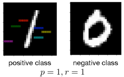</details> Figure 4: Learned rules from MNIST datasets. To demonstrate the benefits of the fully differentiable learning pipeline from raw sequence inputs to symbolic rules, we compare the accuracy and running times (in seconds) between NeurRL and its deep rule-learning module using the non-differentiable $k$ -means clustering algorithm (Lloyd, 1982). We use the same hyperparameter to split time series into subsequences for two methods. Results in Tab. 2 show that the differentiable pipeline significantly reduces running time without sacrificing rule accuracy in most cases. Table 2: Comparisons with non-differentiable $k$ -means clustering algorithm. | Coffee | 0.893 | 313 | 0.964 | 42 | | --- | --- | --- | --- | --- | | ECG | 0.810 | 224 | 0.820 | 65 | | Gun point | 0.807 | 102 | 0.740 | 35 | | ItalyPow.Dem. | 0.845 | 114 | 0.926 | 63 | | Lighting2 | 0.672 | 1166 | 0.689 | 120 | ### 5.3 Learning from images In this subsection, we ask the model to learn rules to describe and discriminate two classes of images from MNIST datasets. We divide the MNIST dataset into five independent datasets, where each dataset contains one positive class and one negative class. For two-dimensional image data, we first flatten the image data to one-dimensional sequence data. Then, the sequence data can be the input for the NeurRL model to learn the rules. The lengths of subsequence and region are both set to three. Besides, the number of clusters is set to five. After generating the highlighted patterns based on the rules, we recover the sequence data to the image for interpreting these learned rules. We present the rule for learning the digit one from the digit zero in Fig. 4, and the rules for learning other positive class from the negative class are shown in Fig. 6 in Appendix C. We present the rule with the precision larger than 0.9 and the highlight features (or areas) defined in the rules. Each highlight feature corresponds to a pair of region and pattern atoms in a learned rule. We can interpret rules like importance attention (Zhang et al., 2019), where the colored areas include highly discriminative information for describing positive inputs compared with negative inputs. For example, in Fig. 4, if the highlighted areas are in black at the same time, then the image class is one. Otherwise, the image class is zero. Compared with attention, we calculate the precision and recall to evaluate these highlight features quantitatively. ### 5.4 Ablation study We conducted ablation studies using default hyperparameters, except for the one being explored. In this study, the number of clusters and regions influences the number of atoms in the learned rules, while the length of subsequences depends on the length of potential patterns. Hence, these three hyperparameters collectively describe the sensitivity of NeurRL. We present the accuracy of both NeurRL(N) and NeurRL(R) on the time series tasks ECG and ItalyPow.Dem. from the UCR archive. 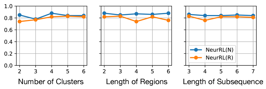<details> <summary>x8.png Details</summary>  ### Visual Description \n ## [Line Charts]: Performance Comparison of NeurRL(N) and NeurRL(R) Across Three Parameters ### Overview The image displays three horizontally arranged line charts comparing the performance of two methods, labeled "NeurRL(N)" and "NeurRL(R)". The charts share a common y-axis scale (0.0 to 1.0) but have different x-axes representing distinct parameters: "Number of Clusters", "Length of Regions", and "Length of Subsequence". A single legend is provided in the third chart. ### Components/Axes * **Y-Axis (All Charts):** Unlabeled, but scale ranges from 0.0 to 1.0 with major tick marks at 0.0, 0.2, 0.4, 0.6, 0.8, and 1.0. This likely represents a performance metric (e.g., accuracy, score). * **X-Axis (Left Chart):** "Number of Clusters". Ticks at integer values: 2, 3, 4, 5, 6. * **X-Axis (Middle Chart):** "Length of Regions". Ticks at integer values: 2, 3, 4, 5, 6. * **X-Axis (Right Chart):** "Length of Subsequence". Ticks at integer values: 3, 4, 5, 6, 7. * **Legend (Bottom-Right of Right Chart):** * Blue line with circle markers: `NeurRL(N)` * Orange line with circle markers: `NeurRL(R)` ### Detailed Analysis **Chart 1: Number of Clusters** * **NeurRL(N) (Blue):** Starts at ~0.85 (x=2), dips to ~0.78 (x=3), peaks at ~0.88 (x=4), then stabilizes around ~0.84 (x=5,6). Trend: Initial dip, peak at 4 clusters, then plateau. * **NeurRL(R) (Orange):** Starts lower at ~0.74 (x=2), rises to ~0.78 (x=3), peaks at ~0.82 (x=4), and plateaus around ~0.82 (x=5,6). Trend: Steady increase to a plateau. * **Comparison:** NeurRL(N) consistently scores higher than NeurRL(R) across all cluster numbers. The gap is narrowest at x=3 and widest at x=4. **Chart 2: Length of Regions** * **NeurRL(N) (Blue):** Starts high at ~0.88 (x=2), dips slightly to ~0.84 (x=3), rises to ~0.87 (x=4), dips to ~0.85 (x=5), and ends at ~0.87 (x=6). Trend: Relatively stable with minor fluctuations. * **NeurRL(R) (Orange):** Starts at ~0.82 (x=2), rises to ~0.84 (x=3), dips sharply to ~0.74 (x=4), recovers to ~0.82 (x=5), and dips again to ~0.76 (x=6). Trend: Volatile, with a significant dip at region length 4. * **Comparison:** NeurRL(N) maintains a clear and consistent performance advantage. The most notable feature is the large performance drop for NeurRL(R) at a region length of 4. **Chart 3: Length of Subsequence** * **NeurRL(N) (Blue):** Starts at ~0.85 (x=3), dips slightly to ~0.83 (x=4), rises to ~0.84 (x=5), peaks at ~0.85 (x=6), and ends at ~0.84 (x=7). Trend: Very stable, hovering around 0.84-0.85. * **NeurRL(R) (Orange):** Starts at ~0.82 (x=3), dips to ~0.76 (x=4), recovers to ~0.82 (x=5), and plateaus around ~0.81 (x=6,7). Trend: A distinct dip at subsequence length 4, followed by recovery and plateau. * **Comparison:** NeurRL(N) is again superior and more stable. Both methods show a performance dip at subsequence length 4, but the dip is much more severe for NeurRL(R). ### Key Observations 1. **Consistent Superiority:** The `NeurRL(N)` method (blue line) achieves a higher score than `NeurRL(R)` (orange line) at every data point across all three charts. 2. **Stability vs. Volatility:** `NeurRL(N)` exhibits relatively stable performance with minor fluctuations. `NeurRL(R)` is more volatile, showing significant performance drops at specific parameter values (Region Length=4, Subsequence Length=4). 3. **Critical Parameter Value:** The value "4" on the x-axis appears to be a critical point. In the middle and right charts, `NeurRL(R)` experiences its most significant performance degradation at this point. 4. **Plateauing Effect:** In the first chart (Number of Clusters), both methods show a plateau in performance after 4 clusters, suggesting diminishing returns or a performance ceiling for this parameter. ### Interpretation The data suggests that the `NeurRL(N)` method is both more effective (higher scores) and more robust (less sensitive to parameter changes) than `NeurRL(R)` for the task being measured. The consistent gap indicates a fundamental advantage in the `N` variant's design. The pronounced dips for `NeurRL(R)` at a value of 4 for both "Length of Regions" and "Length of Subsequence" are highly significant. This could indicate a specific weakness in the `R` method's algorithm when handling medium-length sequential or regional patterns. It might struggle with a particular scale of complexity that emerges at that length, whereas the `N` method handles it without issue. The plateau in the first chart implies that increasing the "Number of Clusters" beyond 4 does not meaningfully improve performance for either method. This is a practical insight for resource allocation, suggesting that using more than 4 clusters may be computationally wasteful for minimal gain. Overall, this technical comparison strongly favors the adoption of `NeurRL(N)` over `NeurRL(R)`, particularly in scenarios where the "Length of Regions" or "Length of Subsequence" parameters might be set to or near the value of 4. </details> (a) On ECG dataset. 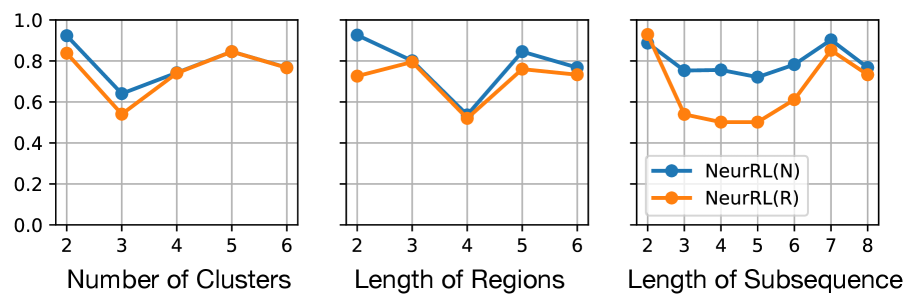<details> <summary>x9.png Details</summary>  ### Visual Description ## Line Charts: Performance Comparison of NeurRL(N) vs. NeurRL(R) ### Overview The image displays three horizontally arranged line charts comparing the performance (y-axis, 0.0 to 1.0) of two methods, **NeurRL(N)** (blue line) and **NeurRL(R)** (orange line), across three different independent variables. The charts share a common y-axis scale. A single legend is placed within the third chart. ### Components/Axes * **Y-Axis (Shared):** Vertical axis on the left of each chart. Scale ranges from **0.0 to 1.0** with major grid lines at intervals of **0.2** (0.0, 0.2, 0.4, 0.6, 0.8, 1.0). No explicit axis title is present, but the context suggests it represents a performance metric (e.g., accuracy, score). * **X-Axes (Individual):** 1. **Left Chart:** Titled **"Number of Clusters"**. Markers at integer values: **2, 3, 4, 5, 6**. 2. **Center Chart:** Titled **"Length of Regions"**. Markers at integer values: **2, 3, 4, 5, 6**. 3. **Right Chart:** Titled **"Length of Subsequence"**. Markers at integer values: **2, 3, 4, 5, 6, 7, 8**. * **Legend:** Located in the **bottom-right corner of the third (rightmost) chart**. It defines the two data series: * **Blue line with circle markers:** `NeurRL(N)` * **Orange line with circle markers:** `NeurRL(R)` ### Detailed Analysis **Chart 1: Number of Clusters** * **Trend - NeurRL(N) (Blue):** Starts high, dips sharply, then recovers and plateaus. * Points (approx.): (2, ~0.95), (3, ~0.65), (4, ~0.75), (5, ~0.85), (6, ~0.78). * **Trend - NeurRL(R) (Orange):** Follows a similar pattern but is consistently lower than NeurRL(N) after the first point. * Points (approx.): (2, ~0.85), (3, ~0.55), (4, ~0.75), (5, ~0.85), (6, ~0.78). * **Relationship:** Both methods show a significant performance drop at 3 clusters. They converge at 4 and 5 clusters, with NeurRL(N) maintaining a slight lead at 2 and 6 clusters. **Chart 2: Length of Regions** * **Trend - NeurRL(N) (Blue):** Starts high, dips, then recovers to a peak before a slight decline. * Points (approx.): (2, ~0.95), (3, ~0.80), (4, ~0.55), (5, ~0.85), (6, ~0.78). * **Trend - NeurRL(R) (Orange):** Shows a more stable, slightly arched trend, peaking at 3. * Points (approx.): (2, ~0.75), (3, ~0.80), (4, ~0.55), (5, ~0.78), (6, ~0.75). * **Relationship:** NeurRL(N) outperforms at region lengths 2, 5, and 6. They perform identically at length 4 (the lowest point for both). NeurRL(R) slightly outperforms at length 3. **Chart 3: Length of Subsequence** * **Trend - NeurRL(N) (Blue):** Exhibits a fluctuating but generally high performance, with a notable dip at length 5. * Points (approx.): (2, ~0.90), (3, ~0.78), (4, ~0.78), (5, ~0.72), (6, ~0.80), (7, ~0.90), (8, ~0.78). * **Trend - NeurRL(R) (Orange):** Starts very high, drops sharply, then gradually recovers before a final dip. * Points (approx.): (2, ~0.95), (3, ~0.55), (4, ~0.52), (5, ~0.52), (6, ~0.62), (7, ~0.88), (8, ~0.75). * **Relationship:** NeurRL(R) starts higher but is significantly outperformed by NeurRL(N) from length 3 through 6. They nearly converge at length 7 before both decline at length 8. ### Key Observations 1. **Consistent Superiority:** NeurRL(N) (blue) generally achieves higher or equal performance compared to NeurRL(R) (orange) across most data points in all three experiments. 2. **Common Vulnerability Points:** Both methods show pronounced performance dips at specific parameter values: **3 clusters**, **4 region length**, and **3-5 subsequence length**. 3. **Convergence Points:** The methods often converge in performance at certain values (e.g., 4-5 clusters, 4 region length, 7 subsequence length), suggesting these are operating points where the distinction between the methods diminishes. 4. **Variable Impact:** The "Length of Subsequence" parameter (right chart) induces the most volatile performance swings for both methods, particularly for NeurRL(R). ### Interpretation The data suggests that the **NeurRL(N)** variant is generally more robust and higher-performing than **NeurRL(R)** across a range of hyperparameters related to clustering, region segmentation, and subsequence analysis. The consistent dips indicate specific configurations where both models struggle, potentially revealing inherent challenges in the underlying task at those scales (e.g., a cluster count of 3 or a region length of 4 may represent a particularly ambiguous or complex problem structure). The dramatic drop and recovery in the "Length of Subsequence" chart for NeurRL(R) implies it is highly sensitive to this parameter, performing well only with very short or optimally long subsequences, while NeurRL(N) maintains more stable performance. This could indicate that NeurRL(N) has better generalization or a more effective inductive bias for sequential data. The charts collectively serve to justify the selection of NeurRL(N) over NeurRL(R) and to guide the tuning of the presented hyperparameters for optimal system performance. </details> (b) On ItalyPow.Dem. dataset. Figure 5: Results of ablation study. Hyperparameter values vs. accuracy. From Fig. 5, we observe that NeurRL’s sensitivity varies across tasks, and the subsequence length is a sensitive hyperparameter when the sequence length is small, as seen in the ItalyPow.Dem. dataset. Properly chosen hyperparameters can achieve high consistency in accuracy between rules and neural networks. Notably, increasing the number of clusters or length of regions does not reduce accuracy linearly. This suggests that the rule-learning module effectively adjusts clusters within the model. In addition, we conduct another ablation study in Tab. 3 of Appendix A to show that pre-training the autoencoder and clustering prevents cluster collapse (Sansone, 2023) and improves accuracy without increasing significant training time. ## 6 Conclusion Inductive logic programming (ILP) is a rule-based machine learning method that supporting data interpretability. Differentiable ILP offers advantages in scalability and robustness. However, label leakage remains a challenge when learning rules from raw data, as neuro-symbolic models require intermediate feature labels as input. In this paper, we propose a novel fully differentiable ILP model, Neural Rule Learner (NeurRL), which learns symbolic rules from raw sequences using a differentiable $k$ -means clustering module and a deep neural network-based rule-learning module. The differentiable $k$ -means clustering algorithm groups subcomponents of inputs based on the similarity of their embeddings, and the learned clusters are used as input for the rule-learning module to induce rules that describe the ground truth class of input based on its features. Compared to other rule-based models, NeurRL achieves comparable classification accuracy while offering interpretability through quantitative metrics. Future goals include variables representing entire inputs to explain handwritten digits without label leakage (Evans et al., 2021). Another focus is learning from incomplete data (e.g., healthcare applications) to address real-world challenges. #### Acknowledgments We express our gratitude to the anonymous Reviewers for their valuable feedback, which has contributed significantly to enhancing the clarity and presentation of our paper. We also thank Xingyao Wang, Yingzhi Xia, Yang Liu, Jasmine Ong, Justina Ma, Jonathan Tan, Yong Liu, and Rick Goh for their supporting. This work has been supported by AI Singapore under Grant AISG2TC2022006, Singapore. This work has been supported by the NII international internship program, JSPS KAKENHI Grant Number JP21H04905 and JST CREST Grant Number JPMJCR22D3, Japan. This work has also been supported by the National Key R&D Program of China under Grant 2021YFF1201102 and the National Natural Science Foundation of China under Grants 61972005 and 62172016. ## References - K. R. Apt, H. A. Blair, and A. Walker (1988) Towards a theory of declarative knowledge. In Foundations of Deductive Databases and Logic Programming, pp. 89–148. Cited by: §3.1. - S. Azzolin, A. Longa, P. Barbiero, P. Liò, and A. Passerini (2023) Global explainability of gnns via logic combination of learned concepts. In Proceedings of the 11th International Conference on Learning Representations, ICLR-23, Cited by: §2. - H. Blockeel and L. De Raedt (1998) Top-down induction of first-order logical decision trees. Artif. Intell. 101 (1-2), pp. 285–297. Cited by: §1. - A. Cropper, S. Dumancic, R. Evans, and S. H. Muggleton (2022) Inductive logic programming at 30. Mach. Learn. 111 (1), pp. 147–172. Cited by: §1. - A. Cropper and S. Dumancic (2022) Inductive logic programming at 30: A new introduction. J. Artif. Intell. Res. 74, pp. 765–850. Cited by: §2. - G. Das, K. Lin, H. Mannila, G. Renganathan, and P. Smyth (1998) Rule discovery from time series. In Proceedings of the Fourth International Conference on Knowledge Discovery and Data Mining (KDD-98), pp. 16–22. Cited by: §2, §3.2. - H. A. Dau, A. Bagnall, K. Kamgar, C. M. Yeh, Y. Zhu, S. Gharghabi, C. A. Ratanamahatana, and E. Keogh (2019) The UCR time series archive. IEEE/CAA Journal of Automatica Sinica 6 (6), pp. 1293–1305. Note: https://www.cs.ucr.edu/~eamonn/time_series_data_2018/ Cited by: §5.2. - L. De Raedt and L. Dehaspe (1997) Clausal discovery. Mach. Learn. 26 (2-3), pp. 99–146. Cited by: §3.1. - F. Doshi-Velez and B. Kim (2017) Towards a rigorous science of interpretable machine learning. arXiv preprint arXiv:1702.08608. Cited by: §1. - R. Evans, M. Bosnjak, L. Buesing, K. Ellis, D. P. Reichert, P. Kohli, and M. J. Sergot (2021) Making sense of raw input. Artif. Intell. 299, pp. 103521. Cited by: §1, §2, §6. - R. Evans and E. Grefenstette (2018) Learning explanatory rules from noisy data. J. Artif. Intell. Res. 61, pp. 1–64. Cited by: §1, §2, §2, §3.1. - M. M. Fard, T. Thonet, and É. Gaussier (2020) Deep k -means: jointly clustering with k -means and learning representations. Pattern Recognit. Lett. 138, pp. 185–192. Cited by: §3.2, §4.2. - K. Gao, K. Inoue, Y. Cao, and H. Wang (2022a) Learning first-order rules with differentiable logic program semantics. In Proceedings of the 31st International Joint Conference on Artificial Intelligence, IJCAI-22, pp. 3008–3014. Cited by: §1, §2, §3.1. - K. Gao, K. Inoue, Y. Cao, and H. Wang (2024) A differentiable first-order rule learner for inductive logic programming. Artif. Intell. 331, pp. 104108. Cited by: §1, §2, §3.1, §3.1, §4.2. - K. Gao, H. Wang, Y. Cao, and K. Inoue (2022b) Learning from interpretation transition using differentiable logic programming semantics. Mach. Learn. 111 (1), pp. 123–145. Cited by: §2. - Y. He, X. Chu, G. Peng, Y. Wang, Z. Jin, and X. Wang (2018) Mining rules from real-valued time series: A relative information-gain-based approach. In 2018 IEEE 42nd Annual Computer Software and Applications Conference, COMPSAC-18, pp. 388–397. Cited by: §2. - C. Hocquette, A. Niskanen, M. Järvisalo, and A. Cropper (2024) Learning MDL logic programs from noisy data. In Proceedings of the 39th Annual AAAI Conference on Artificial Intelligence, AAAI-24, pp. 10553–10561. Cited by: §1. - K. Inoue, T. Ribeiro, and C. Sakama (2014) Learning from interpretation transition. Mach. Learn. 94 (1), pp. 51–79. Cited by: §2, §3.1. - E. Jang, S. Gu, and B. Poole (2017) Categorical reparameterization with gumbel-softmax. In Proceedings of the 5th International Conference on Learning Representations, ICLR-17, Cited by: §3.2. - Z. Liu, Y. Wang, S. Vaidya, F. Ruehle, J. Halverson, M. Soljacic, T. Y. Hou, and M. Tegmark (2024) KAN: kolmogorov-arnold networks. CoRR abs/2404.19756. Cited by: §2. - J. W. Lloyd (1984) Foundations of logic programming, 1st edition. Springer. Cited by: §3.1, §3.1. - S. P. Lloyd (1982) Least squares quantization in PCM. IEEE Trans. Inf. Theory 28 (2), pp. 129–136. Cited by: §4.3, §5.2. - R. Manhaeve, S. Dumancic, A. Kimmig, T. Demeester, and L. D. Raedt (2018) DeepProbLog: neural probabilistic logic programming. In Advances in Neural Information Processing Systems 31: Annual Conference on Neural Information Processing Systems, NeurIPS-18, pp. 3753–3763. Cited by: §1, §2. - E. Marconato, G. Bontempo, E. Ficarra, S. Calderara, A. Passerini, and S. Teso (2023) Neuro-symbolic continual learning: knowledge, reasoning shortcuts and concept rehearsal. In Proceedings of the 40th International Conference on Machine Learning, ICML-23, Vol. 202, pp. 23915–23936. Cited by: §4.1. - E. Misino, G. Marra, and E. Sansone (2022) VAEL: bridging variational autoencoders and probabilistic logic programming. In Advances in Neural Information Processing Systems 35: Annual Conference on Neural Information Processing Systems, NeurIPS-22, Cited by: §2. - S. H. Muggleton and L. De Raedt (1994) Inductive logic programming: theory and methods. J. Log. Program. 19/20, pp. 629–679. Cited by: §2. - S. H. Muggleton and C. Feng (1990) Efficient induction of logic programs. In Algorithmic Learning Theory, First International Workshop, ALT-90, pp. 368–381. Cited by: §2. - S. H. Muggleton, L. D. Raedt, D. Poole, I. Bratko, P. A. Flach, K. Inoue, and A. Srinivasan (2012) ILP turns 20 - biography and future challenges. Mach. Learn. 86 (1), pp. 3–23. Cited by: §3.1. - A. Passerini, P. Frasconi, and L. D. Raedt (2006) Kernels on prolog proof trees: statistical learning in the ILP setting. J. Mach. Learn. Res. 7, pp. 307–342. Cited by: §3.1. - Y. J. Phua and K. Inoue (2021) Learning logic programs using neural networks by exploiting symbolic invariance. In Proceedings of the 30th international conference on Inductive Logic Programming, ILP-21, Lecture Notes in Computer Science, Vol. 13191, pp. 203–218. Cited by: §2. - Y. J. Phua and K. Inoue (2024) Variable assignment invariant neural networks for learning logic programs. In Proceedings of the 18th International Conference on Neural-Symbolic Learning and Reasoning, NeSy-24, Lecture Notes in Computer Science, Vol. 14979, pp. 47–61. Cited by: §1. - J. R. Quinlan (1990) Learning logical definitions from relations. Mach. Learn. 5, pp. 239–266. Cited by: §1. - L. Rokach and O. Maimon (2005) Clustering methods. In The Data Mining and Knowledge Discovery Handbook, pp. 321–352. Cited by: §3.2. - E. Sansone and R. Manhaeve (2023) Learning symbolic representations through joint generative and discriminative training. In Proceedings of the 11th International Conference on Learning Representations on Neurosymbolic Generative Models Workshops (NeSy-GeMs, ICLR-23), Cited by: §2. - E. Sansone (2023) The triad of failure modes and a possible way out. In Proceedings of the 37th Annual Conference on Neural Information Processing Systems on the 4th Workshop on Self-Supervised Learning: Theory and Practice (SSL, NeurIPS-23), Cited by: §2, §5.4. - H. Shindo, V. Pfanschilling, D. S. Dhami, and K. Kersting (2023) $\alpha$ ILP: thinking visual scenes as differentiable logic programs. Mach. Learn. 112 (5), pp. 1465–1497. Cited by: §1, §2. - S. Topan, D. Rolnick, and X. Si (2021) Techniques for symbol grounding with SATNet. In Advances in Neural Information Processing Systems 34: Annual Conference on Neural Information Processing Systems, NeurIPS-21, M. Ranzato, A. Beygelzimer, Y. N. Dauphin, P. Liang, and J. W. Vaughan (Eds.), pp. 20733–20744. Cited by: §1. - N. P. Walter, J. Fischer, and J. Vreeken (2024) Finding interpretable class-specific patterns through efficient neural search. In Proceedings of the 38th AAAI Conference on Artificial Intelligence, AAAI-24, Vol. 38, pp. 9062–9070. Cited by: §2. - B. Wang, L. Li, Y. Nakashima, and H. Nagahara (2023) Learning bottleneck concepts in image classification. In Proceedings of the 34th IEEE/CVF Conference on Computer Vision and Pattern Recognition, CVPR-23, pp. 10962–10971. Cited by: §2. - H. Wang, Q. Zhang, J. Wu, S. Pan, and Y. Chen (2019) Time series feature learning with labeled and unlabeled data. Pattern Recognit. 89, pp. 55–66. Cited by: §2, §3.2, §5.2, §5.2. - J. Wang, P. Liu, M. F. She, S. Nahavandi, and A. Z. Kouzani (2013) Bag-of-words representation for biomedical time series classification. Biomed. Signal Process. Control. 8 (6), pp. 634–644. Cited by: §5.2. - Z. Xu and K. Funaya (2015) Time series analysis with graph-based semi-supervised learning. In 2015 IEEE International Conference on Data Science and Advanced Analytics, DSAA-15, pp. 1–6. Cited by: §5.2. - F. Yang, Z. Yang, and W. W. Cohen (2017) Differentiable learning of logical rules for knowledge base reasoning. In Advances in Neural Information Processing Systems 30: Annual Conference on Neural Information Processing Systems, NIPS-17, pp. 2319–2328. Cited by: §1. - E. Zhan, J. J. Sun, A. Kennedy, Y. Yue, and S. Chaudhuri (2022) Unsupervised learning of neurosymbolic encoders. Trans. Mach. Learn. Res. 2022. Cited by: §2. - H. Zhang, I. J. Goodfellow, D. N. Metaxas, and A. Odena (2019) Self-attention generative adversarial networks. In Proceedings of the 36th International Conference on Machine Learning, ICML-19, Proceedings of Machine Learning Research, Vol. 97, pp. 7354–7363. Cited by: §5.3. ## Appendix A Ablation Study on pre-training In this section, we conduct experiments with and without pre-training the autoencoder and clustering model to investigate whether pre-training improves accuracy. The results, including accuracy and running time (in seconds), are presented in Tab. 3. Table 3: Ablation study: With vs. without pre-training autoencoder and clustering model. The first accuracy is achieved using NeurRL(N), while the second accuracy is obtained with NeurRL(R). | Coffee ECG ItalyPow.Dem. | 1.00, 0.96 0.88, 0.82 0.92, 0.93 | 42 65 63 | 0.83, 0.81 0.87, 0.64 0.75, 0.80 | 30 53 61 | | --- | --- | --- | --- | --- | | Gun Point | 0.87, 0.76 | 35 | 0.86, 0.43 | 31 | | Lighting2 | 0.75, 0.69 | 120 | 0.64, 0.60 | 63 | The experiment results indicate the pre-training autoencoder and clustering model can improve the accuracy of both NeurRL(N) and NeurRL(R) without increasing significant training time. ## Appendix B The link of the model The model and data can be found here: https://github.com/gaokun12/NeurRL ## Appendix C Classifying and Explaining MNIST data Each column in Fig. 6 corresponds to a learning task. There are six rules presented in Fig. 6 to describe the positive class from the negative class. 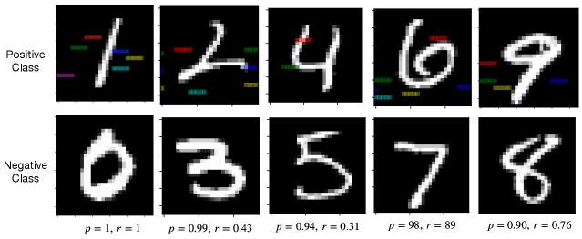<details> <summary>x10.png Details</summary>  ### Visual Description \n ## [Image Type]: Handwritten Digit Classification Grid ### Overview The image displays a 2x5 grid of grayscale handwritten digit images, likely from a dataset such as MNIST. The grid is organized into two rows labeled "Positive Class" and "Negative Class," each containing five distinct digits. Below each column of the grid, two statistical metrics, denoted as `p` and `r`, are provided. The positive class images feature overlaid colored horizontal lines, while the negative class images do not. ### Components/Axes * **Row Labels (Left Side):** * Top Row: "Positive Class" * Bottom Row: "Negative Class" * **Column Metrics (Bottom):** Five pairs of values are aligned beneath the five columns. * Column 1: `p = 1, r = 1` * Column 2: `p = 0.99, r = 0.43` * Column 3: `p = 0.94, r = 0.31` * Column 4: `p = 98, r = 89` (Note: This appears to be a formatting inconsistency; values are likely 0.98 and 0.89). * Column 5: `p = 0.90, r = 0.76` * **Image Content:** Each cell contains a white handwritten digit on a black background. * **Positive Class (Top Row, Left to Right):** Digits `1`, `2`, `4`, `6`, `9`. * **Negative Class (Bottom Row, Left to Right):** Digits `0`, `3`, `5`, `7`, `8`. * **Visual Annotations:** The five images in the "Positive Class" row have multiple short, colored horizontal lines (red, green, blue, yellow, cyan, magenta) overlaid on them. These lines are absent in the "Negative Class" row. ### Detailed Analysis The grid presents a comparative analysis of two classes of handwritten digits, with associated performance metrics. **Column-by-Column Breakdown:** 1. **Column 1:** * Positive: Digit `1`. Has colored line overlays. * Negative: Digit `0`. * Metrics: `p = 1, r = 1`. This indicates perfect precision and recall for this specific example or category. 2. **Column 2:** * Positive: Digit `2`. Has colored line overlays. * Negative: Digit `3`. * Metrics: `p = 0.99, r = 0.43`. Very high precision but low recall. 3. **Column 3:** * Positive: Digit `4`. Has colored line overlays. * Negative: Digit `5`. * Metrics: `p = 0.94, r = 0.31`. High precision, very low recall. 4. **Column 4:** * Positive: Digit `6`. Has colored line overlays. * Negative: Digit `7`. * Metrics: `p = 98, r = 89`. **Anomaly:** The values lack decimal points and are an order of magnitude different from others. Interpreted as `p = 0.98, r = 0.89` for consistency. This would indicate high precision and high recall. 5. **Column 5:** * Positive: Digit `9`. Has colored line overlays. * Negative: Digit `8`. * Metrics: `p = 0.90, r = 0.76`. Good precision and recall. **Visual Pattern:** The "Positive Class" images are all annotated with colored lines, suggesting these are the digits the model is focusing on or has correctly identified for a specific task. The "Negative Class" images are clean, representing counter-examples or misclassifications. ### Key Observations 1. **Metric Discrepancy:** The values in Column 4 (`p = 98, r = 89`) are presented as integers, unlike the decimal format (0.xx) used in all other columns. This is likely a typographical error in the source image. 2. **Performance Trend:** The `r` (recall) metric shows significant variation across the positive class examples, from a perfect 1.0 down to 0.31. The `p` (precision) metric remains consistently high (≥0.90) across all columns. 3. **Class Composition:** The positive class contains the digits {1, 2, 4, 6, 9}, while the negative class contains {0, 3, 5, 7, 8}. This is not a simple even/odd split. 4. **Annotation Specificity:** The colored line overlays are present only on the positive class images, indicating they are a visual marker for that class or for model attention/saliency. ### Interpretation This image appears to be a diagnostic or explanatory figure from a machine learning paper or report, likely evaluating a classifier for handwritten digits. * **What it Demonstrates:** The figure illustrates the model's performance on specific digit pairs. For each column, the top image is a "positive" example (perhaps correctly classified or from a target class), and the bottom is a "negative" example (incorrectly classified or from an opposing class). The `p` and `r` values likely represent **Precision** and **Recall** for the model's predictions related to that specific positive digit. * **Relationship Between Elements:** The colored lines on the positive class images are almost certainly **saliency maps** or **attention highlights**, showing which parts of the input image the model's decision was based on. Their absence on the negative class suggests those images were not processed in the same way or are shown for contrast. * **Notable Insights:** * The model achieves high precision across these examples, meaning when it predicts a digit belongs to the positive class, it is usually correct. * The recall is highly variable, indicating the model misses a significant portion of true positive instances for some digits (e.g., `4` and `2`), but performs well for others (e.g., `1` and `6`). * The pairing of digits (1 vs 0, 2 vs 3, etc.) might indicate the model is being tested on its ability to distinguish between visually similar digits, or these are simply representative samples from a larger evaluation set. * The anomaly in Column 4's formatting (`98` instead of `0.98`) is a critical detail for accurate data extraction and suggests a need for verification against the original source. </details> Figure 6: Rules from MNIST datasets.